PHYSICAL REVIEW E 85, 056410 (2012)

Dynamical-systems approach to relativistic nonlinear wave-particle interactionin collisionless plasmas

A. Osmane* and A. M. HamzaDepartment of Physics, University of New Brunswick, Fredericton, NB, E3B5A3, Canada

(Received 11 March 2012; published 18 May 2012)

In this report, we present a dynamical systems approach to study the exact nonlinear wave-particle interactionin relativistic regime. We give particular attention to the effect of wave obliquity on the dynamics of the orbitsby studying the specific cases of parallel (θ = 0) and perpendicular (θ = −π/2) propagations in comparison tothe general case of oblique propagation θ =]−π/2,0[. We found that the fixed points of the system correspondto Landau resonance and that the dynamics can evolve from trapping to surfatron acceleration for propagationangles obeying a Hopf bifurcations condition. Cyclotron-resonant particles are also studied by the constructionof a pseudo-potential structure in the Lorentz factor γ . We derived a condition for which Arnold diffusion resultsin relativistic stochastic acceleration. Hence, two general conclusions are drawn: (1) The propagation angle θ

can significantly alter the dynamics of the orbits at both Landau and cyclotron-resonances. (2) Considering theshort-time scales upon which the particles are accelerated, these two mechanisms for Landau and cyclotronresonant orbits could become potential candidates for problems of particle energization in collisionless space andcosmic plasmas.

DOI: 10.1103/PhysRevE.85.056410 PACS number(s): 94.05.Pt, 94.30.Xy

I. INTRODUCTION

The wave-particle interaction has long been considered adominant energy-momentum exchange mechanism in spaceand astrophysical plasmas. Beyond the dense and internalboundaries of stars and planetary magnetospheres, spaceand astrophysical plasmas are predominantly collisionlessand populated by distributions functions inconsistent withcollisional equilibrium conditions. These plasmas are alsobelieved to be turbulent systems described by a conventionalenergy cascade from large scales to small scales where dis-sipation takes place. While fluid theories provide satisfactorydescriptions of macroscopic quantities at large scales, they arenot equipped to explain the plasma physics at smaller kineticscales, and one needs to include nonlinear kinetic processes(wave-particle interactions and wave-wave interactions) fora correct description of these turbulent and collisionlessplasmas [1].

Studies of wave-particle interactions in space and astro-physical turbulent plasmas have commonly fallen under thescope of quasilinear theory [2,3]. Quasilinear theory departsfrom linear theory in conserving energy and momentumthrough the account of the wave-particle interaction, resultingin a diffusion process for an ensemble averaged distributionfunction solution to a Fokker-Planck equation. However,quasilinear theory is constrained by a number of severelimitations, making it inapplicable for plasmas containinglarge-amplitude quasimonochromatic electromagnetic and/orelectrostatic waves. Indeed, the first assumption for quasi-linear theory consists in constraining particle orbits to theirunperturbed components. A second assumption consists inassuming a wave spectrum sufficiently dense so that interfer-ence between modes is destroyed by phase-mixing. Hence,quasilinear theory is valid only when the bandwidth is broadenough to enable resonances to be maintained as particles are

*a.osmane@unb.ca

scattered, and nonlinear trapping effects by individual wavesare too weak to be taken into consideration.

Due to the inherent difficulties of strong turbulence theories,test-particle methods have become a favored tool for thestudy of wave-particle interaction beyond the constraints ofquasilinear theory. Numerous methods have been developed inthe context of the radiation belts alone, ranging from guiding-center approximation [4], to resonance-averaged Hamiltonian[5], gyroresonance averaged equations [6], and computersimulations, taking into account approximate and exact dipolarfields (see Ref. [7] and references therein). However, thegeneral case of oblique propagation has often been avoidedin favor of the more tractable case of parallel of propagation[8]. A strong case can be made for the neglect of obliquepropagation and nonlinear effects for small amplitude wavessince the appearance of a small parallel electric field cannottrap orbits [9]. However, if the electric-field component of thewave becomes sufficiently large, such that nonlinear effectscan be triggered, then a rich class of orbits can result, and theparallel approximation becomes invalid. It is in this sense thatwe are solving the equation of motion exactly.

Recent observations of the radiation belts suggest thatobliquely propagating waves with Poynting flux two ordersof magnitude larger than previously observed whistlers wavesare commonly generated in the radiation belts and appearcorrelated with relativistic electron microbursts [10]. Theselarge-amplitude waves can propagate at large propagationangles (θ � 70o) and possess amplitudes capable of energizingelectrons on time scales of the order of the milliseconds [11].If these large-amplitude waves are shown to be a commonobservational signature in the radiation belts, the conventionalmodels used to describe the wave-particle interaction using aquasilinear formalism will have to be revisited. It is not onlyinaccurate to assume that a particle will execute a random walkin pitch angle during the course of one bounce period, but asdemonstrated below, a particle can be irreversibly acceleratedto relativistic energies in less than one bounce period.

056410-11539-3755/2012/85(5)/056410(12) ©2012 American Physical Society

A. OSMANE AND A. M. HAMZA PHYSICAL REVIEW E 85, 056410 (2012)

In this report, we investigate the exact nonlinear wave-particle interaction in the relativistic regime. The inclusion ofrelativistic effects is a sine qua non condition for any attemptat solving the outstanding problems which have emerged inradiation belts dynamics as well as galactic cosmic rays. Ourgoal is to provide a general framework for the wave-particleinteraction by using a dynamical systems approach. Suchapproach, although lacking the level of self-consistency foundin numerical simulations, can facilitate the understanding ofcomplex systems such as cosmic and space plasmas and,therefore, provide for an intuitive as well as quantitative leapbetween theoretical models and simulations.

The report is written as follows. In Sec. II we derive thedynamical system as well as its fixed points and invariants.In Sec. III we treat the special cases of parallel and purelyperpendicular propagation. In Sec. IV we study the generalcase of oblique propagation for the cyclotron-resonance case aswell as the Landau resonance. Section V contains a discussionof the general framework for the understanding of the wave-particle interaction and the effect of oblique propagation incollisionless plasmas such as the radiation belts. In Sec. VI weconclude and discuss studies currently underway to addresslimitations of the dynamical system approach.

II. DYNAMICAL SYSTEM

A. Equation of motion for the general case

Our study begins with the equation of motion of a particle inan electromagnetic field, as described by the Lorentz equation.The equations of motion can be written as

dpdt

= e

[E(x,t) + p

mγc× B(x,t)

], (1)

for a particle of charge e, momentum p = mγ v, and rest massm. The Lorentz factor, γ , is defined in terms of the relativisticmomentum as follows:

γ =√

1 + p2

m2c2. (2)

The electromagnetic field configuration consists of a back-ground magnetic field B0 to which is superposed an electro-magnetic wave given by (δE,δB):

E(x,t) = δE(x,t) (3)

B(x,t) = B0 + δB(x,t) (4)

The electromagnetic wave vector k is chosen to point in the z

direction, obliquely to the background magnetic field lying inthe y-z plane:

k · B0 = kB0 cos(θ ) (5)δE = δEx x + δEy y

δB = δBx x + δBy y,(6)

with the wave magnetic field components written as

δBx = δB sin(kz − ωt)

δBy = δB cos(kz − ωt)(7)

and Faraday’s law, expressed in terms of the Fouriercomponents, providing for the components of the electricfield

ck × δE(k,ω) = ωδB(k,ω). (8)

We can, therefore, express the dynamical system in terms ofthe phase velocity vφ = ω/k, and the variables p� = mγv�;1 = eδB/mcγ ; 0 = eB0/mcγ , resulting in the followingcoupled ordinary differential equations:

px = py0 cos(θ ) + (p� − pz)1 cos(kz − ωt)

+pz0 sin(θ )

py = −px0 cos(θ ) + (pz − p�)1 sin(kz − ωt)

pz = −px0 sin(θ ) + px1 cos(kz − ωt)

−py1 sin(kz − ωt)

z = pzv�/p�. (9)

In the classical case, the dynamical system is composed offour equations, the three components of the velocity plusthe position coordinate along k. However, in the relativisticcase the expression for the Lorentz factor must be obeyed andconstitutes a constraint on the particle’s trajectory. We can keeptrack of this constraint by adding an equation in the expressionof a dynamical gyrofrequency:

0 = d

dt

(eB0

mcγ

)= −0

pc2

m2c4 + p2c2p

= −01p�

m2γ 2c2[px cos(kz − ωt) − py sin(kz − ωt)]. (10)

If we define the constant δ1 = 1/0, it is straightforwardto see that 1 = δ10, and similarly, since p� = p�(γ ), thetime evolution of this quantity can be written as:

p� = −mv�γ0

0. (11)

In order to simplify the dynamical system, we can eliminatethe explicit time dependence of the equations by making thefollowing mathematical transformation:

p′x = px, p′

y = py, p′z = γw(pz − pφ),

z′ = γw(z − vφt)

(12)

for the Lorentz factor:

γw = 1√1 − v2

�

c2

. (13)

056410-2

DYNAMICAL-SYSTEMS APPROACH TO RELATIVISTIC . . . PHYSICAL REVIEW E 85, 056410 (2012)

We can, therefore, write the equations of motion as follow:

p′x = 0p

′y cos(θ ) − 1p

′z cos(kz′/γw)/γw

+0(p′z/γw + pφ) sin(θ )

p′y = −0p

′x cos(θ ) + 1p

′z sin(kz′/γw)/γw

p′z/γw = −0p

′x sin(θ ) + 1p

′x cos(kz′/γw)

−1p′y sin(kz′/γw) − p�

z′ = p′zv�/p�. (14)

If we absorb the Lorentz factor γw into p′z and k, that is we

write p′z → p′

z/γw and k → k/γw, and write p� in terms of(p′

x,p′y,p

′z,z

′,0), we can express the dynamical system as:

p′x = 0p

′y cos(θ ) − 1p

′z cos(kz′) + 0(p′

z + pφ) sin(θ )

p′y = −0p

′x cos(θ ) + 1p

′z sin(kz′)

p′z = −0p

′x sin(θ ) + 1(

n2 − 1

n2)[p′

x cos(kz′) − p′y sin(kz′)]

z′ = p′zv�/p�, (15)

where the refractive index is represented as n2 = c2/v2�.

The magnitude of the momentum is now written as p′ =√p

′2x + p

′2y + (p

′z/γw)2; hence, the Lorentz contraction factor

also transforms from γ (p) → γ (p′). The dynamical systemfor the classical case can be recovered by setting γ = 1and 1/n2 → 0. Indeed, the equations are equivalent to theclassical case under the following transformations: p → u

and → /γ . Hence, the main difference lies in the timedependence of the Larmor frequencies and the extra term thatgoes as 1/n2 in the p′

z equation.

B. Representation in terms of (P , α, �, z′)

It is convenient to express the relativistic momentum inspherical coordinates, that is in terms of a magnitude p′ andphase angles (α,�). This can be achieved by introducing thefollowing scalar and vector variables:

p‖ = p‖b0

p⊥ = p0 × (p × p0) = p − p‖b0,(16)

where b0 = B0/B0. Using these definitions, we can rewrite themomentum p′ = (p′

x,p′y,p

′z) in terms of the pitch angle α and

the dynamical gyrophase �, both defined as

tan(α) = p′⊥

p′‖

tan(�) = p′⊥1

p′⊥2

= p′x

p′y cos(θ ) + p′

z sin(θ ). (17)

Hence, all three-momentum components in the wave frameare written as

p′x = p′ sin(α) cos(�)

p′y = p′ sin(α) sin(�) cos(θ ) − p′ cos(α) sin(θ )

p′z = p′ sin(α) sin(�) sin(θ ) + p′ cos(α) cos(θ ). (18)

Using the definition Eqs. (17) and the representation of themomentum in Eq. (18), we can proceed to write the dynamicalsystem Eq. (15) in terms of the normalized variables:

P = kp′

mω, δ1 = 1

0, δ2 = mωc

eB0, δ3 = 1

δ2γ,

(19)

n2 = c2

v2�

, Z = kz′, τ = ωt

and the function F (α,�,Z), as follows:

dP

dτ= sin(α) cos(�) sin(θ )/δ2 − δ1δ3P

n2[ sin(α) sin(�) sin(θ )+cos(α) cos(θ )]F (α,�,Z)

dα

dτ= 1

Pδ2cos(α) cos(�) sin(θ ) − δ1δ3

[cos2

(θ

2

)cos(� + Z) − sin2

(θ

2

)cos(� − Z)

]

+ δ1δ3

n2[ cos(θ ) sin(α) − cos(α) sin(�) sin(θ )]F (α,�,Z)

d�

dτ= −δ3 + sin(θ )

[δ1δ3 cos(Z) − sin(�)

δ2P sin(α)

]+ δ1δ3

tan(α)

[cos2

(θ

2

)sin(� + Z) + sin2

(θ

2

)sin(Z − �)

]

− δ1δ3

n2

cos(�) sin(θ )

sin(α)F (α,�,Z)

dZ

dτ= δ2δ3P [ sin(α) sin(�) sin(θ ) + cos(α) cos(θ )]

dδ3

dτ= −δ1δ2δ

33P

n2F (α,�,Z)

F (α,�,Z) = sin(α) sin2

(θ

2

)cos(� − Z) + sin(α) cos2

(θ

2

)cos(� + Z) + cos(α) sin(θ ) sin(Z). (20)

It is easy to observe that we can recover the classical regime by setting δ3 = γ /γ δ2 = 0 or F (α,�,Z) = 0. We now proceed tostudy some of the properties of the dynamical system.

056410-3

A. OSMANE AND A. M. HAMZA PHYSICAL REVIEW E 85, 056410 (2012)

C. Fixed points

A common first step in the study of dynamical systemsis to find and investigate the properties of fixed (stationary)points. The fixed points of the dynamical system Eq. (20) aredefined as the values in (P,α,�,Z,γ ), for which (P = α =� = Z = γ = 0). It can be demonstrated (see Appendix A)that the dynamical system, for −π/2 < θ < 0, possesses thefollowing values for the fixed points:

P = −γ tan(θ ); α = ±θ ± π

2;

� = ±π

2; Z = 0,π ; (21)

γ = 1√1 − v2

�

c2 (1 + tan2(θ )).

It is already evident from Eq. (21) that in the case ofparallel propagation (θ = 0), the only fixed point is that forthe trivial case P = 0. The fixed point for the relativisticregime appears, therefore, similar to the classical one forparallel and oblique propagation [12]. The fixed point for therelativistic regime will translate into properties found in thenonrelativistic regime, but also results in different types ofstructures in their vicinity. For nonzero propagation angles,fixed points identify volumes of phase-space composed ofphysically trapped orbits. The trapped orbits could give rise tokinetic distortions in the distribution functions, such as beamsand temperature anisotropies, as was revealed in the classicalnonrelativistic case [13]. However, because the relativisticequations possess a constraint in the form of the Lorentz factorγ , different effects are shown to arise.

D. Invariants

The dynamical system Eq. (20) also possesses a numberof invariants valid for the general case of oblique propa-gation. Knowledge of these invariants is used to constructpseudo-potential structures. In turn, these structures provideinformation on trapped and quasitrapped orbits.

1. First invariant: I1

Using Eqs. (19) to normalize Eq. (10), the equationdescribing the evolution of the gyrofrequency can be writtenas follows:

δ3 = −δ31

1 + n2

�2

�

�, (22)

for � = kp/mω. Hence, this equation has an exact solution,providing the following constant of the motion:

I1 = δ3

√�2 + n2. (23)

We can write this invariant in terms of the variables P,α,�,Z,

and δ3 as follows:

I1 =√

δ23P

2 + 2δ3Pz/δ2 + δ23n

2. (24)

The conservation of this quantity will indicate the degree towhich the constraint for the Lorentz factor Eq. (2) is respectedin a numerical scheme.

2. Second invariant: I2

A second general invariant can be found and expressed interms of the normalized variables as follows:

I2 = δ2(n2 − 1)γ cos(θ ) − δ2P cos(α) + δ1 sin(θ ) cos(Z).

(25)

This invariant underlies a fundamental property of obliquepropagation. One can indeed rewrite the invariant in the formE = mγc2 ∼ P‖, which means that one needs a change inthe parallel momentum to change the energy. This is a well-known statement resulting from the Maxwell-Lorentz invariantquantity E · B = 0, since a parallel component of the electricfield cannot be eliminated by any Lorentz translation, while thephysics in a frame with E‖ = 0, such as in the case of parallelpropagation, is no different, therefore, than the physics in aframe where E⊥ = E‖ = 0, for which energy is a constant ofthe motion.

III. SPECIAL CASES

A. Parallel propagation: θ = 0

The wave-particle interaction problem has overwhelminglybeen treated for the special case of parallel propagation. Eventhough we do not present any new result in this section, wefind it useful to briefly discuss the parallel case as a means ofcomparison to the general oblique case. Setting θ = 0 in Eq.(20), we recover the following dynamical system:

dP

dτ= −δ1δ3P

n2cos(α)F (α,�,Z)

dα

dτ= −δ1δ3 cos(� + Z) + δ1δ3

n2sin(α)F (α,�,Z)

d�

dτ= −δ3 + δ1δ3

tan(α)sin(� + Z)

dZ

dτ= δ2δ3P cos(α)

dδ3

dτ= −δ1δ2δ

33P

n2F (α,�,Z)

F (α,�,Z) = sin(α) cos(� + Z). (26)

In addition to the two invariants I1 and I2, Eqs. (26) alsopossesses the following constant of motion [27] for n2 �= 1:

[δ2P cos(α) − 1]2 = 2δ1δ2n2 − 1

n2P sin(α) sin(� + Z).

(27)

Moreover, the existence of physically trapped orbits for θ =0 requires that cos(α) = cos(� + Z) = 0; hence, α = � +Z = π/2. However, this conditions results in � �= 0. Asidefrom the trivial case of P = 0, no fixed point exists and theparallel propagation has the particular distinction, with respectto oblique propagation, to not possess solutions for which aparticle could be trapped in Z.

The parallel case has been studied in both the classicaland relativistic regime. The classical treatment covered byMatsumoto [14] and Hamza et al. [12], have shown that one canfind exact solutions in terms of elliptical integrals. Lutomirskiand Sudan [15] have studied the relativistic case showing thatsimilar solutions were also possible. Roberts and Buchsbaum

056410-4

DYNAMICAL-SYSTEMS APPROACH TO RELATIVISTIC . . . PHYSICAL REVIEW E 85, 056410 (2012)

[16] have also treated the relativistic case with a special focuson the case n2 = 1, for which a cyclotron-resonant particlewas shown to gain energy indefinitely, while for n2 �= 1, theparticle simply becomes phase trapped at cyclotron-resonancewith no net gain in energy on average. Using the invariant inEq. (27) as well as I1 and I2, those results can be expressed interms of a pseudopotential equation in the parallel componentof the momentum that we write as y = δ2P cos(α) = δ2P‖:

y2

2= −V (y; δ1,δ2,n

2,I2)

= δ21

2

[n2 − 1

n2

]2[n2 − 1

σ (y)2− 2

y

σ (y)− (y2 + n2δ2)

]

− 1

8σ (y)2(y − 1)4, (28)

for the function σ (y) = (n2 − 1)/(I2 + y). Solutions toEq. (28) for V (y; δ1,δ2,n

2,I2) < 0 are bound states of thesystem for as far as parallel momentum is concerned. However,this only holds for n2 �= 1. In the case of n2 = 1, we caneasily recover the unlimited acceleration found by Robertsand Buchsbaum [16] from the invariants of the motion. Settingθ = 0 and n2 = 1 for I2, one finds that P‖ is constant. Thatis, if a particle is at cyclotron-resonance, it will remain soforever (or until the wave damps) and gain energy indefinitely.It is demonstrated in the remainder of the report that unlimitedacceleration is also possible for oblique propagation and thatit underlies a specific property of the fixed points.

B. Perpendicular propagation: θ = −π/2

We now investigate the purely perpendicular case, as itstreatment will be useful to characterize the dynamics forpropagation angles that increase toward |π/2|. The dynamicalsystem is written in the following form:

dP

dτ= − sin(α) cos(�)

δ2

+ δ1δ3P

n2sin(α) sin(�)F (α,�,Z)

dα

dτ= − 1

δ2Pcos(α) cos(�) + δ1δ3 sin(�) sin(Z)

+ δ1δ3

n2cos(α) sin(�)F (α,�,Z)

d�

dτ= −δ3 − δ1δ3 cos(Z) + sin(�)

δ2P sin(α)

+ δ1δ3

tan(α)cos(� + Z) + δ1δ3 cos(�)

n2 sin(α)

× cos(� + Z)F (α,�,Z)

dZ

dτ= −δ2δ3P sin(α) sin(�)

dδ3

dτ= −δ1δ2δ

33P

n2F (α,�,Z)

F (α,�,Z) = sin(α) cos(�) cos(Z) − cos(α) sin(Z). (29)

Similar to the parallel case, the dynamical system Eq. (29)possesses its own set of invariants, written as

I4 = δ1 cos(Z) + δ2P cos(α)

I5 = δ2P cos(�) sin(α) + δ1 sin(Z) + Z + τ. (30)

With the fixed point analysis for this particular case showingthat no fixed points exist, i.e., a particle cannot be physicallytrapped, we make the assumption that the solution for Z takesthe form of a linear relationship in time: Z = Z0 + βτ , withZ0 as the initial condition and β as a constant. Replacingthe solution for Z in the invariant I5 results in the followingexpression:

I5 = δ2P cos(�) sin(α) + δ1 sin(Z0 + βτ ) + Z0 + βτ + τ.

(31)

It is, therefore, evident that for I5 = 0 to be true, the term (β +1)τ must be either zero, or compensated by the momentum inx, Px = P sin(α) cos(�), to grow to minus infinity as τ goesto infinity. In the absence of accessible Landau and cyclotronresonances, the latter solution does not appear acceptable. Wecan qualitatively demonstrate this assumption by noting thatfor τ δ1, the following approximation must be respected:

γ

tan(�) 1−β

δ2βτ . Hence, either (a) γ → ∞ or (b) � → 0. In

the first case, if γ → ∞, then P → ∞ as well. Hence, for I4

to be constant, stationary solutions giving Py = P cos(α) ∼constant are required. Such solutions would necessitate Py ∼0. Such constraint means that either Pz = 0 or Z = 0. Butboth solutions are unacceptable since they would imply theexistence of a fixed point, which has been demonstrated tonot exist for the special case of perpendicular propagation. Inthe second case, the requirement that � → 0 means that sinceδ3P v � c is bounded, Z → 0, which is in contradictionwith the evidence that Z must be linear in time because ofa zero parallel electric field. We are, therefore, left with theassumption that β ∼ −1, an assumption that can indeed beverified by numerical integration.

Without any loss of generality, we set Z0 = 0, resulting inthe solution Z = −τ . Using I4, we find the following solutionsfor P‖:

δ2P‖ = I4 − δ1 cos(τ ). (32)

Similarly, the solution for Px can be directly found from I5:

δ2Px = I5 + δ1 sin(τ ). (33)

Using those two solutions, we can find the exact differentialfor δ3:

dδ3

δ33

= − δ1

n2[I5 cos(τ ) + I4 sin(τ )]dτ. (34)

Hence, the following solutions for δ3:

1

δ23

− 1

δ23(0)

= 2δ1

n2[I5 sin(τ ) + I4 − I4 cos(τ )]. (35)

We can finally find the exact solution for the last variable interms of τ from the dynamical system equation in Z, that is:

δ2Pz =√

1

δ23(0)

+ 2δ1

n2[I5 sin(τ ) + I4 − I4 cos(τ )]. (36)

056410-5

A. OSMANE AND A. M. HAMZA PHYSICAL REVIEW E 85, 056410 (2012)

We have, therefore, derived exact solutions for the perpen-dicular case, based on the existence of two invariants andthe nonexistence of fixed points. Two limiting cases canbe deduced from these solutions. If the wave is sustainedfor long periods, such that the time of interaction with theparticles τint ∼ 1/εω for ε � 1, the perpendicular propagationresults in phase trapped orbits with no net gain of energy onaverage. In the opposite case, where the interaction would beshort-lived such that τint ∼ ε/ω, we can calculate the averageincrement in energy during the time of interaction. If wewrite Eq. (35) in terms of E = mγc2, and assume largeamplitude, low-frequency waves such that δ1/δ2 ∼ 1, then

E/E0 =√

1 + 2δ21/δ

22n

2γ 20 ∼ 1 + v2

�/c2 and a particle gains

energy of the order of �E/E ∼ v2�/c2 for every interaction.

Given a prescription in the probability of interaction P (v�,�t)with an electromagnetic wave of phase-speed v�, one couldbuild a map to describe the nonlinear interaction of a particlein a relativistic turbulent plasma composed of highly obliqueelectromagnetic waves. This qualitative analysis for purelyperpendicular wave applies for particles that do not belong toLandau or cyclotron resonance.

IV. CYCLOTRON AND LANDAU RESONANCES

A. Stochastic acceleration at cyclotron resonance:ω − k‖v‖ = ±s�0/γ

The most commonly studied problems of wave-particleinteractions have been addressed in the context of cyclotron-resonance. However, we demonstrate below that the caseof cyclotron-resonance contains further intricacies when thegeneral case of oblique propagation and nonlinear interactionis treated in the relativistic limit. In order to do so, we constructa pseudopotential function for a particle crossing resonances.

The resonance condition is written in terms of the normal-ized variables as:

γ sin2(θ ) − P cos(α) cos(θ ) = ±s/δ2. (37)

Using the resonance condition to replace the expression ofP cos(α) in I2, we find the following expression:

I2 cos(θ ) ∓ s = δ2γ [n2 cos2(θ ) − 1]

+ δ1 cos(Z) sin(θ ) cos(θ ). (38)

If γ and Z do not have singularities in their derivatives whenthe resonance condition is respected, the following relationshipmust be satisfied:

dγ

dτ= δ1 sin(θ ) cos(θ )

δ2[n2 cos2(θ ) − 1]sin(Z)

dZ

dτ. (39)

We can find an expression between Z and γ from the invariantI1. In order to do so, we write the invariant quantity in thefollowing form:

dZ

dτ− n2 − 1

2= −P 2 + n2

2γ 2

= − n2

2γ 2

[(P

n+ 1

)2

− 2P

n

]

− n2

2γ 2; if

P

n� 1. (40)

Hence, using Eq. (40) in addition to Eq. (38) we can replaceZ and sin(Z) and find a pseudopotential equation in γ of theform

γ 2

2+ V (γ ; δ1,δ2,θ ) = 0, (41)

for a pseudopotential written as:

V (γ ; δ1,δ2,θ ) = −1

2

[n2 − 1

2− n2

2γ 2

]2

×[(

δ1

δ2

sin(θ ) cos(θ )

n2 cos2(θ ) − 1

)2

−(

I2 cos(θ ) ∓ s

δ2n2 cos2(θ ) − δ2− γ

)2]

= −1

8

[β1 − β1 + 1

γ 2

]2[β2

2 − (β3 − γ )2

],

(42)

for the set of constants β1,β2,β3 defined as follows:

β1 = n2 − 1 (43)

β2 = δ1

δ2

sin(θ ) cos(θ )

n2 cos2(θ ) − 1(44)

β3 = I2 cos(θ ) ∓ s

δ2n2 cos2(θ ) − δ2. (45)

If we set the initial conditions Z0 = 0 and γ0 = 1, we can writeβ3 = β2 + 1. Taking the second derivative of Eq. (41), we findthe following expression:

γ = 1

4β2

1γ − 1

4β2β

21 + 1

2

β3β1(β1 + 1)

γ 2

+ 1

2

(β1 + 1)2 + (β2

3 − β22

)(β1 + 1)

γ 3

+ 3

4

β3(β1 + 1)2

γ 4− 1

2

(β2

2 − β23

)(β1 + 1)2

γ 5. (46)

This equation can be used to treat the cyclotron-resonancefor different limits. We hereafter focus on the relativistic lowenergy case for which γ = γ0 + δγ , with δγ � γ0. UsingNewton’s approximation to express γ −n γ −n

0 (1 − nδγ /γ0)and setting γ0 = 1, we find the following forced oscillatorequation:

¨δγ + �2δγ = �(β1,β2), (47)

for the frequency squared:

�2 = − 14β2

1 − β3β1(β1 + 1)

+ 32

[(β1 + 1)2 + (

β23 − β2

2

)(β1 + 1)

]+ 3β3(β1 + 1)2 − 5

2

[(β2

2 − β23

)(β1 + 1)2

], (48)

and the constant forcing term

� = − 14β2

1 (β3 − 1) + 14β3(β1 + 1)(β1 + 3)

+ 12

[(β1 + 12) + (

β23 − β2

2

)(β1 + 1)

]− 1

2

(β2

2 − β23

)(β1 + 1)2. (49)

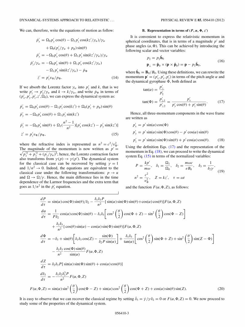
Figure 1 represents the dependence of � as a function ofθ for fixed values of δ1. It is clear that for the range of

056410-6

DYNAMICAL-SYSTEMS APPROACH TO RELATIVISTIC . . . PHYSICAL REVIEW E 85, 056410 (2012)

FIG. 1. (Color online) Squared frequency �2 as a function ofthe propagation angle θ for a relativistic particle in cyclotronresonance. Each curve represents a different value in the wave-amplitude parameter spanning 0.01 � δ1 � 1. The four bold (red)lines correspond, from top to bottom, to δ1 = (0.05,0.09,0.1,0.3).

chosen parameters (v�/c ∼ .70,δ2 = 1), the oscillations in δγ

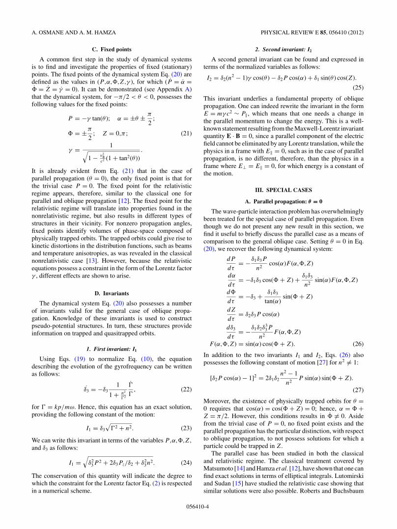
can evolve from harmonic solutions to hyperbolic solutionsas the amplitude of the wave increases. As a result of alarge-wave amplitude, that is δ1 growing, a wide range ofpropagation angles will result in hyperbolic perturbationsfor a relativistic particle in cyclotron resonance. Figure 2represents the transition from �2 > 0 to �2 < 0. As the waveamplitude increases, the particle transits from trapped-orbitsto quasitrapped orbits in phase-space. If the amplitude isfurther increased, the orbit becomes stochastic. Quasitrappedand stochastic orbits result from the wandering of the particlefrom one cyclotron harmonic to another. Hence, the particlegains energy stochastically. This result is an extension of the

FIG. 2. (Color online) (a) Pitch angle α vs. dynamical gyrophase� for �2 > 0. The particle is phase-trapped. (b) Pitch angle α vs.dynamical gyrophase � for �2 < 0. The particle is quasitrapped inphase-space. (c) Lorentz factor γ vs. Z for δ1 = (0.05,0.09,0.1,0.3).When �2 < 0, the orbit is unstable in γ and depart from theforced harmonic oscillation observed for �2 > 0. (d) Resonancecondition quantified by s(P,γ,α; θ,δ2) for the case of �2 < 0. Theparticle travels through multiple resonances as it gains energy throughrepeated kicks.

−80 −70 −60 −50 −40 −30 −20 −101.26

1.28

1.3

1.32

1.34

1.36

1.38

1.4

1.42

1.44

θ

n

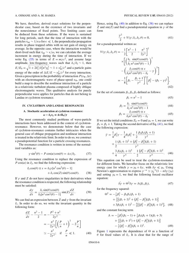
FIG. 3. (Color online) Arnold tongue in the parameter space(θ,n = c/v�), for δ1 = 0.3, δ2 = 1.

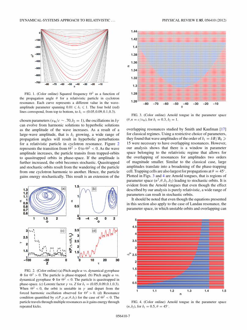
overlapping resonances studied by Smith and Kaufman [17]for classical regimes. Using a restrictive choice of parameters,they found that wave amplitudes of the order of δ1 = δB/B0 �15 were necessary to have overlapping resonances. However,our analysis shows that there is a window in parameterspace belonging to the relativistic regime that allows forthe overlapping of resonances for amplitudes two ordersof magnitude smaller. Similar to the classical case, largeamplitudes translate into a broadening of the phase-trappingcell. Trapping cells are also largest for propagations at θ = 45◦.Plotted in Figs. 3 and 4 are Arnold tongues, that is regions ofparameter space (n2,θ,δ1,δ2) leading to stochastic orbits. It isevident from the Arnold tongues that even though the effectdescribed by our analysis is purely relativistic, a wide range ofparameters can result in stochastic orbits.

It should be noted that even though the equations presentedin this section also apply to the case of Landau resonance, theparameter space, in which unstable orbits and overlapping can

1 1.1 1.2 1.3 1.4 1.5

0.5

1

1.5

2

2.5

3

3.5

4

4.5

5

n

δ 2

FIG. 4. (Color online) Arnold tongue in the parameter space(n,δ2), for δ1 = 0.5, θ = 45◦.

056410-7

A. OSMANE AND A. M. HAMZA PHYSICAL REVIEW E 85, 056410 (2012)

operate, belongs to velocities that must go beyond the speed oflight. Therefore, the aforementioned result applies specificallyto the case of cyclotron-resonances.

B. Hopf bifurcation at Landau resonance: ω = k‖v‖

A fundamental property of a given dynamical system can bededuced by investigating whether the phase-space density andvolume is conserved or not. That is, whether or not Liouville’stheorem applies [18]. The validity of Liouville’s theoremprovides the possibility to construct distribution functions andfollow their evolution in time. Nonconservation of phase-spacedensity, either locally or globally, stems from the existenceof either attractors or nonbounded orbits. Making use ofthe invariant I2, we compute the divergence of the flow inphase-space as follows:

1

V

dV

dt= �∇ · d�ξ

dt= ∂Px

∂Px

+ ∂Py

∂Py

+ ∂Pz

∂Pz

+ ∂Z

∂Z= − γ

γ, (50)

for the volume in phase-space V and the phase-space vectorcoordinate �ξ = (Px,Py,Pz,Z). Hence, Eq. (50) hints at theexistence of an attractor if the volume in phase-space shrinksas γ → ∞. In the case where the particle’s energy oscillatesback and forth such as for a volume of physically trappedorbits, we can consider Liouville’s theorem to apply. But itcan be shown that such an attractor does exist. A recentlypublished Letter has shown that the attractor arises from achange in parameters that results in the bifurcation of the orbitsaround the fixed points [19]. Indeed, the stability analysis inAppendix B demonstrates that to every fixed points, combinedvalues in (θ,n2), satisfying the condition n2 − 1 = tan2(θ ),correspond to a bifurcation in stability [28]. That is, an orbit,close to the fixed point will experience a transition from a(marginally) stable orbit to an unstable orbit. We observe thatwhen the condition in parameter space is respected, and fora large enough amplitude of the wave magnetic field, the

1 1.2 1.4 1.6 1.8 20.3

0.32

0.34

0.36

0.38

0.4

0.42

0.44

0.46

0.48

α

Φ

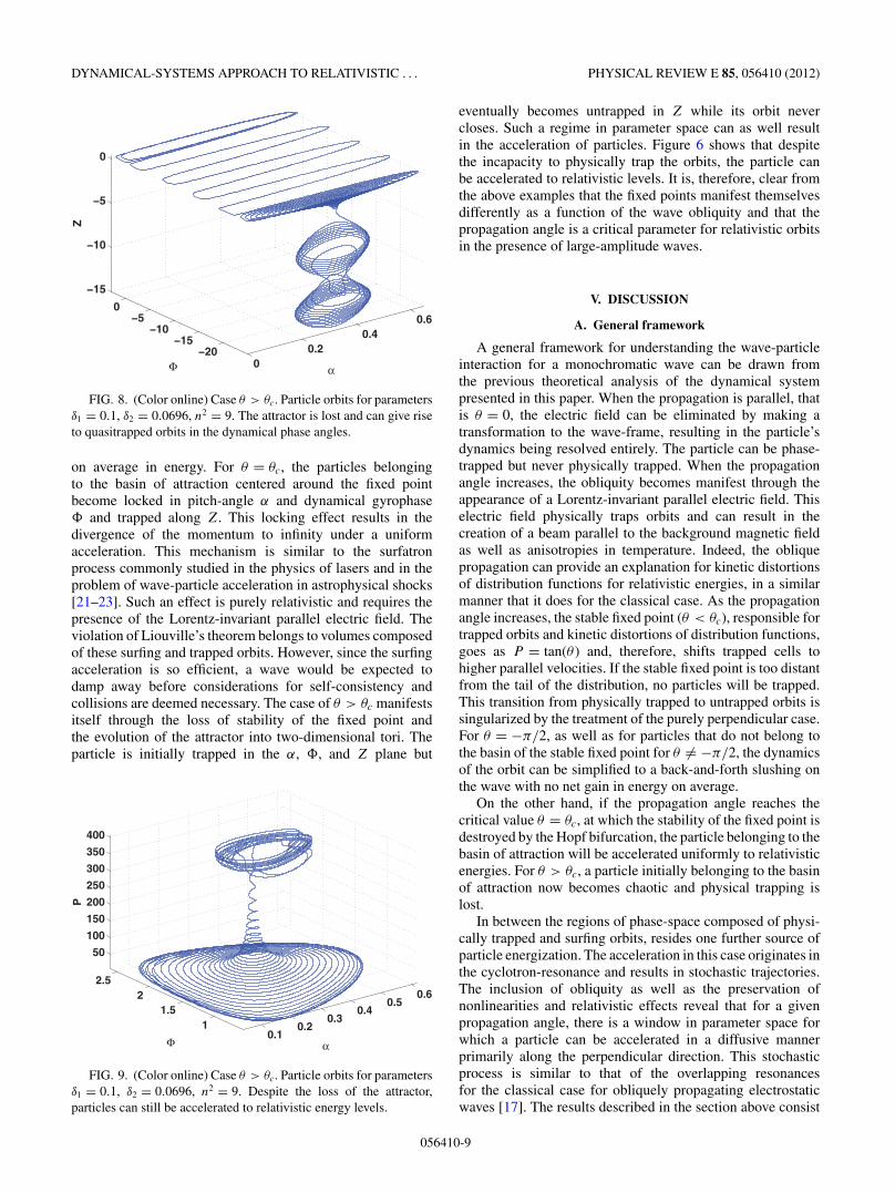
FIG. 5. (Color online) Case θ < θc = arctan√

n2 − 1. Particleorbit for parameters δ1 = 0.1, δ2 = 0.0696, n2 = 4, θ = θc − 1◦ andinitial conditions v′

x0 = 0, v′y0 = −v� tan(θ ) − 1.6v�, v′

z0 = −v�,Z0 = 0. The particle is physically and phase trapped. It bouncesback and forth in the potential well with no net gain in energy.

0.20.4

0.60.8

11.2

1.41.6

−1.8−1.6

−1.4−1.2

−1−0.8

−0.6−0.4

−0.2

05

10152025303540

αZ

P

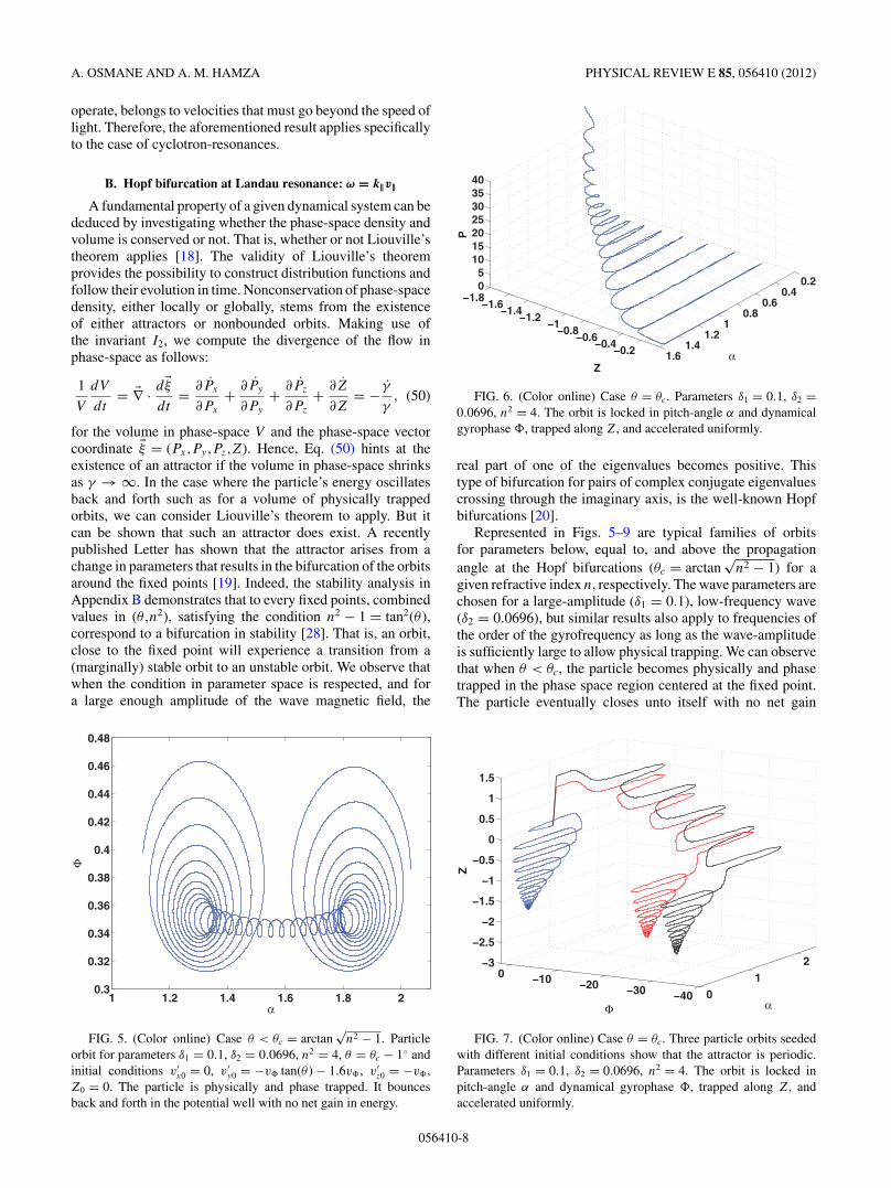
FIG. 6. (Color online) Case θ = θc. Parameters δ1 = 0.1, δ2 =0.0696, n2 = 4. The orbit is locked in pitch-angle α and dynamicalgyrophase �, trapped along Z, and accelerated uniformly.

real part of one of the eigenvalues becomes positive. Thistype of bifurcation for pairs of complex conjugate eigenvaluescrossing through the imaginary axis, is the well-known Hopfbifurcations [20].

Represented in Figs. 5–9 are typical families of orbitsfor parameters below, equal to, and above the propagationangle at the Hopf bifurcations (θc = arctan

√n2 − 1) for a

given refractive index n, respectively. The wave parameters arechosen for a large-amplitude (δ1 = 0.1), low-frequency wave(δ2 = 0.0696), but similar results also apply to frequencies ofthe order of the gyrofrequency as long as the wave-amplitudeis sufficiently large to allow physical trapping. We can observethat when θ < θc, the particle becomes physically and phasetrapped in the phase space region centered at the fixed point.The particle eventually closes unto itself with no net gain

01

2

−40−30−20−100−3

−2.5

−2

−1.5

−1

−0.5

0

0.5

1

1.5

αΦ

Z

FIG. 7. (Color online) Case θ = θc. Three particle orbits seededwith different initial conditions show that the attractor is periodic.Parameters δ1 = 0.1, δ2 = 0.0696, n2 = 4. The orbit is locked inpitch-angle α and dynamical gyrophase �, trapped along Z, andaccelerated uniformly.

056410-8

DYNAMICAL-SYSTEMS APPROACH TO RELATIVISTIC . . . PHYSICAL REVIEW E 85, 056410 (2012)

00.2

0.40.6

−20−15

−10−5

0

−15

−10

−5

0

αΦ

Z

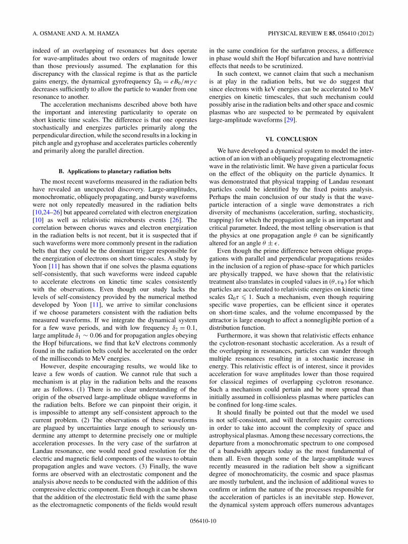
FIG. 8. (Color online) Case θ > θc. Particle orbits for parametersδ1 = 0.1, δ2 = 0.0696, n2 = 9. The attractor is lost and can give riseto quasitrapped orbits in the dynamical phase angles.

on average in energy. For θ = θc, the particles belongingto the basin of attraction centered around the fixed pointbecome locked in pitch-angle α and dynamical gyrophase� and trapped along Z. This locking effect results in thedivergence of the momentum to infinity under a uniformacceleration. This mechanism is similar to the surfatronprocess commonly studied in the physics of lasers and in theproblem of wave-particle acceleration in astrophysical shocks[21–23]. Such an effect is purely relativistic and requires thepresence of the Lorentz-invariant parallel electric field. Theviolation of Liouville’s theorem belongs to volumes composedof these surfing and trapped orbits. However, since the surfingacceleration is so efficient, a wave would be expected todamp away before considerations for self-consistency andcollisions are deemed necessary. The case of θ > θc manifestsitself through the loss of stability of the fixed point andthe evolution of the attractor into two-dimensional tori. Theparticle is initially trapped in the α, �, and Z plane but

0.10.2

0.30.4

0.50.6

11.5

22.5

50

100

150

200

250

300

350

400

αΦ

P

FIG. 9. (Color online) Case θ > θc. Particle orbits for parametersδ1 = 0.1, δ2 = 0.0696, n2 = 9. Despite the loss of the attractor,particles can still be accelerated to relativistic energy levels.

eventually becomes untrapped in Z while its orbit nevercloses. Such a regime in parameter space can as well resultin the acceleration of particles. Figure 6 shows that despitethe incapacity to physically trap the orbits, the particle canbe accelerated to relativistic levels. It is, therefore, clear fromthe above examples that the fixed points manifest themselvesdifferently as a function of the wave obliquity and that thepropagation angle is a critical parameter for relativistic orbitsin the presence of large-amplitude waves.

V. DISCUSSION

A. General framework

A general framework for understanding the wave-particleinteraction for a monochromatic wave can be drawn fromthe previous theoretical analysis of the dynamical systempresented in this paper. When the propagation is parallel, thatis θ = 0, the electric field can be eliminated by making atransformation to the wave-frame, resulting in the particle’sdynamics being resolved entirely. The particle can be phase-trapped but never physically trapped. When the propagationangle increases, the obliquity becomes manifest through theappearance of a Lorentz-invariant parallel electric field. Thiselectric field physically traps orbits and can result in thecreation of a beam parallel to the background magnetic fieldas well as anisotropies in temperature. Indeed, the obliquepropagation can provide an explanation for kinetic distortionsof distribution functions for relativistic energies, in a similarmanner that it does for the classical case. As the propagationangle increases, the stable fixed point (θ < θc), responsible fortrapped orbits and kinetic distortions of distribution functions,goes as P = tan(θ ) and, therefore, shifts trapped cells tohigher parallel velocities. If the stable fixed point is too distantfrom the tail of the distribution, no particles will be trapped.This transition from physically trapped to untrapped orbits issingularized by the treatment of the purely perpendicular case.For θ = −π/2, as well as for particles that do not belong tothe basin of the stable fixed point for θ �= −π/2, the dynamicsof the orbit can be simplified to a back-and-forth slushing onthe wave with no net gain in energy on average.

On the other hand, if the propagation angle reaches thecritical value θ = θc, at which the stability of the fixed point isdestroyed by the Hopf bifurcation, the particle belonging to thebasin of attraction will be accelerated uniformly to relativisticenergies. For θ > θc, a particle initially belonging to the basinof attraction now becomes chaotic and physical trapping islost.

In between the regions of phase-space composed of physi-cally trapped and surfing orbits, resides one further source ofparticle energization. The acceleration in this case originates inthe cyclotron-resonance and results in stochastic trajectories.The inclusion of obliquity as well as the preservation ofnonlinearities and relativistic effects reveal that for a givenpropagation angle, there is a window in parameter space forwhich a particle can be accelerated in a diffusive mannerprimarily along the perpendicular direction. This stochasticprocess is similar to that of the overlapping resonancesfor the classical case for obliquely propagating electrostaticwaves [17]. The results described in the section above consist

056410-9

A. OSMANE AND A. M. HAMZA PHYSICAL REVIEW E 85, 056410 (2012)

indeed of an overlapping of resonances but does operatefor wave-amplitudes about two orders of magnitude lowerthan those previously assumed. The explanation for thisdiscrepancy with the classical regime is that as the particlegains energy, the dynamical gyrofrequency 0 = eB0/mγ c

decreases sufficiently to allow the particle to wander from oneresonance to another.

The acceleration mechanisms described above both havethe important and interesting particularity to operate onshort kinetic time scales. The difference is that one operatesstochastically and energizes particles primarily along theperpendicular direction, while the second results in a locking inpitch angle and gyrophase and accelerates particles coherentlyand primarily along the parallel direction.

B. Applications to planetary radiation belts

The most recent waveforms measured in the radiation beltshave revealed an unexpected discovery. Large-amplitudes,monochromatic, obliquely propagating, and bursty waveformswere not only repeatedly measured in the radiation belts[10,24–26] but appeared correlated with electron energization[10] as well as relativistic microbursts events [26]. Thecorrelation between chorus waves and electron energizationin the radiation belts is not recent, but it is suspected that ifsuch waveforms were more commonly present in the radiationbelts that they could be the dominant trigger responsible forthe energization of electrons on short time-scales. A study byYoon [11] has shown that if one solves the plasma equationsself-consistently, that such waveforms were indeed capableto accelerate electrons on kinetic time scales consistentlywith the observations. Even though our study lacks thelevels of self-consistency provided by the numerical methoddeveloped by Yoon [11], we arrive to similar conclusionsif we choose parameters consistent with the radiation beltsmeasured waveforms. If we integrate the dynamical systemfor a few wave periods, and with low frequency δ2 = 0.1,large amplitude δ1 ∼ 0.06 and for propagation angles obeyingthe Hopf bifurcations, we find that keV electrons commonlyfound in the radiation belts could be accelerated on the orderof the milliseconds to MeV energies.

However, despite encouraging results, we would like toleave a few words of caution. We cannot rule that such amechanism is at play in the radiation belts and the reasonsare as follows. (1) There is no clear understanding of theorigin of the observed large-amplitude oblique waveforms inthe radiation belts. Before we can pinpoint their origin, itis impossible to attempt any self-consistent approach to thecurrent problem. (2) The observations of these waveformsare plagued by uncertainties large enough to seriously un-dermine any attempt to determine precisely one or multipleacceleration processes. In the very case of the surfatron atLandau resonance, one would need good resolution for theelectric and magnetic field components of the waves to obtainpropagation angles and wave vectors. (3) Finally, the waveforms are observed with an electrostatic component and theanalysis above needs to be conducted with the addition of thiscompressive electric component. Even though it can be shownthat the addition of the electrostatic field with the same phaseas the electromagnetic components of the fields would result

in the same condition for the surfatron process, a differencein phase would shift the Hopf bifurcation and have nontrivialeffects that needs to be scrutinized.

In such context, we cannot claim that such a mechanismis at play in the radiation belts, but we do suggest thatsince electrons with keV energies can be accelerated to MeVenergies on kinetic timescales, that such mechanism couldpossibly arise in the radiation belts and other space and cosmicplasmas who are suspected to be permeated by equivalentlarge-amplitude waveforms [29].

VI. CONCLUSION

We have developed a dynamical system to model the inter-action of an ion with an obliquely propagating electromagneticwave in the relativistic limit. We have given a particular focuson the effect of the obliquity on the particle dynamics. Itwas demonstrated that physical trapping of Landau resonantparticles could be identified by the fixed points analysis.Perhaps the main conclusion of our study is that the wave-particle interaction of a single wave demonstrates a richdiversity of mechanisms (acceleration, surfing, stochasticity,trapping) for which the propagation angle is an important andcritical parameter. Indeed, the most telling observation is thatthe physics at one propagation angle θ can be significantlyaltered for an angle θ ± ε.

Even though the prime difference between oblique propa-gations with parallel and perpendicular propagations residesin the inclusion of a region of phase-space for which particlesare physically trapped, we have shown that the relativistictreatment also translates in coupled values in (θ,v�) for whichparticles are accelerated to relativistic energies on kinetic timescales 0τ � 1. Such a mechanism, even though requiringspecific wave properties, can be efficient since it operateson short-time scales, and the volume encompassed by theattractor is large enough to affect a nonnegligible portion of adistribution function.

Furthermore, it was shown that relativistic effects enhancethe cyclotron-resonant stochastic acceleration. As a result ofthe overlapping in resonances, particles can wander throughmultiple resonances resulting in a stochastic increase inenergy. This relativistic effect is of interest, since it providesacceleration for wave amplitudes lower than those requiredfor classical regimes of overlapping cyclotron resonance.Such a mechanism could pertain and be more spread thaninitially assumed in collisionless plasmas where particles canbe confined for long-time scales.

It should finally be pointed out that the model we usedis not self-consistent, and will therefore require correctionsin order to take into account the complexity of space andastrophysical plasmas. Among these necessary corrections, thedeparture from a monochromatic spectrum to one composedof a bandwidth appears today as the most fundamental ofthem all. Even though some of the large-amplitude wavesrecently measured in the radiation belt show a significantdegree of monochromaticity, the cosmic and space plasmasare mostly turbulent, and the inclusion of additional waves toconfirm or infirm the nature of the processes responsible forthe acceleration of particles is an inevitable step. However,the dynamical system approach offers numerous advantages

056410-10

DYNAMICAL-SYSTEMS APPROACH TO RELATIVISTIC . . . PHYSICAL REVIEW E 85, 056410 (2012)

and the endeavors for greater self-consistency can be achievedaccordingly. Indeed, the dynamical system for the general case,once families of solutions have been found, can be used as abackground nonlinear solution to the wave-particle interaction,upon which corrections, such as addition of waves, changingpolarization, dispersion effects, inhomogeneous backgroundmagnetic field, etc., can all be treated as perturbations tothe family of solutions of the “nonlinear homogeneous”system. Such method could be investigated theoretically andnumerically, in a similar methodological fashion and withcomparable tools that Hamiltonian systems were constructedto investigate the impact of nonlinear perturbations.

ACKNOWLEDGMENTS

We thank K. Meziane and L. B. Wilson III for helpfuldiscussions. This work was supported by the Natural Sciencesand Engineering Research Council of Canada (NSERC). Oneof the authors, A.M.H., wishes to acknowledge CSA (CanadianSpace Agency) support. Computational facilities are providedby ACEnet, the regional high-performance computing consor-tium for universities in Atlantic Canada.

APPENDIX A: FIXED POINTS ANALYSIS

Fixed points of an n-dimensional dynamical system denotestationary solutions for all n variables. Fixed points are definedfor values of the variables for which the dynamical systemequations equal zero. In this particular case, fixed pointsrepresent orbits of physically trapped particles. In order tofind the fixed points, we proceed as follows. It is clear at firstthat in order to have γ = 0, one needs to have F (α,�,Z) = 0.Keeping this in mind, we first transform the dynamical systemas represented by Eqs. (20) into polynomial form by using thefollowing change of variables:

x = eiα; y = ei�; z = eiZ; (A1)

and writing the different trigonometric functions in terms of(x,y,z). For the time evolution of P , the equation in terms ofthe (x,y,z) variables result in

(eiα − e−iα)(ei� + e−i�) sin(θ ) = 0 (A2)(x − 1

x

)(y + 1

y

)= 0 (A3)

(x2 − 1)(y2 + 1) = 0, (A4)

since x,y,z �= 0. We apply the same procedure for theremaining three equations of motion and we find that for α = 0,the polynomial equation gives

sin(θ )(x2 + 1)(y2 + 1)/δ2

− δ1δ3Px[cos(θ )(z2 + 1)(y2 + 1) + (z2 − 1)(y2 − 1)] = 0,

(A5)

the polynomial equation for � is

−4P (x2 − 1)yz

+ sin(θ )[2δ1P (x2 − 1)(z2 + 1)y − 4x(y2 − 1)z/δ2δ3]

+ δ1P (x2 + 1)[(y2 + 1)(z2 − 1)

+ cos(θ )(y2 − 1)(z2 + 1)] = 0, (A6)

and the polynomial equation for Z resumes as

2 cos(θ )y(x2 + 1) − sin(θ )(x2 − 1)(y2 − 1) = 0. (A7)

Equation (A4) has the following solutions:

x = ±1; y = ±i. (A8)

We look at each solution starting with the case x = ±1.Replacing x in Eq. (A7) cancels the second term and resultsin the following constraint:

4 cos(θ )y = 0. (A9)

Since the solutions of this equation are

cos(θ ) = 0, y = 0, (A10)

neither of them is acceptable. We are interested in the caseof oblique propagation with θ �= π

2 , and by definition y �= 0.Hence, the case x = ±1 does not result in a fixed point for theoblique propagation.

We now look at the second solution, which satisfiesEq. (A4), y = ±i. We replace y in Eq. (A7) and find

±i cos(θ )(x2 + 1) + sin(θ )(x2 − 1) = 0 (A11)

x2[±i cos(θ ) + sin(θ )] = −[±i cos(θ ) − sin(θ )] (A12)

x2[±(eiθ + e−iθ ) − (eiθ − e−iθ )]

= −[±(eiθ + e−iθ ) + (eiθ − e−iθ )], (A13)

which results in

x2 = −e±2iθ ; x = ±ie±iθ . (A14)

To find the value of z, we replace the value of y in Eq. (A5),which results in the cancellation of the first two terms andgives the following result:

−2δ1Px(z2 − 1) = 0. (A15)

Since by definition x �= 0, and we are not interested with thetrivial case P = 0, the solution for this equation is

z = ±1. (A16)

The last step consists in finding the value of P for the fixedpoint, which can be done by replacing y = ±i and z = ±1 inEq. (A7).

−4P (±i)(±1)(x2 − 1) + 4P sin(θ )δ1(±i)(x2 − 1)

+8 sin(θ )(±1)x/δ2δ3 − 4δ1P cos(θ )(x2 + 1) = 0,(A17)

TABLE I. Fixed points in the (px,py,pz,Z,γ ) representation

px0 py0 pz0 Z0 γ0

0 −p� tan(θ ) p� 0 1√1− v2

�

c2 [1+tan2(θ)]

0 −p� tan(θ ) p� π 1√1− v2

�

c2 [1+tan2(θ)]

0 +p� tan(θ ) p� 0 1√1− v2

�

c2 [1+tan2(θ)]

0 +p� tan(θ ) p� π 1√1− v2

�

c2 [1+tan2(θ)]

056410-11

A. OSMANE AND A. M. HAMZA PHYSICAL REVIEW E 85, 056410 (2012)

which can be written as

−P = ±2ix

x2 − 1

sin(θ )

δ2δ3. (A18)

Replacing x with the use of Eq. (A14), we find

δ2δ3P = − tan(θ ). (A19)

Since P is always positive, the solution requires −π2 < θ < 0.

Transforming back x,y,z to the dynamical system variablesα,�,Z, we find that the fixed points are given by:

P = −γ tan(θ ); α = ±θ ± π

2;

� = ±π

2; Z = 0,π. (A20)

Using the values in Eqs. (A20) for F (α,�,Z) sets it equalto zero. Hence, Eqs. (A20) are the fixed point equations forthe dynamical system Eq. (20). We can also express the fixedpoints in terms of (px,py,pz,z

′,γ ) as demonstrated in Table I.

APPENDIX B: STABILITY ANALYSIS

The next fundamental step in dynamical system theory isto investigate the equilibrium of the fixed points. In order todo so, we apply a basic Lyapunov linear analysis that canbe found in any textbook on dynamical systems. The methodis summarized as follows. For a dynamical system x = F (x)possessing a fixed point x0 for which F (x0) = 0, one can makea Taylor expansion around the fixed point and keep the first-order terms. That is, writing the dynamical for the perturbationδx and the Jacobian J = ∂F

∂xi|x0 as d

dtδx = Jδx. We are left with

the task of solving an eigenvalue problem since we can writethe solution to the linearized equation as δx = ξie

λi t for theeigenvalues λi and eigenvectors ξi , assuming the eigenvalues

are not degenerate. If one eigenvalue λi > 0, the system islinearly unstable at x0, if not the system is linearly stable atx0. From the expression for γ0 in the previous Appendix, it isclear that a fixed point does not exist for all parameter valuesof θ and v�. Since γ � 1, the argument in the denominatorsquare root must obey the condition n2 � 1 + tan2(θ ). Hence,we write the Jacobian for the dynamical system as follows:⎛⎜⎜⎜⎜⎝

0 cos(θ)δ2γ0

∓δ1+sin(θ)δ2γ0

0

− cos(θ)δ2γ0

0 0 0(− sin(θ)δ1

± n2−1n2

)δ1

δ2γ00 0 ∓ δ1 tan(θ)

δ2

n2−1n2

0 0 1γ0

0

⎞⎟⎟⎟⎟⎠ ,

where the ± symbols denote the two values of the fixed pointsin Z = kz′. Solving the eigenvalue problem (J − λI)ξ = 0 wefind a biquadratic polynomial function in λ that can be writtenas χ (λ) = λ4 + η1λ

2 + η2 = 0, with the constant coefficientsη1 and η2 given by the following expressions:

η1 = δ1

δ2γ0

n2 − 1

n2tan(θ ) + cos2(θ )

δ22γ

20

− δ1

δ22γ

20

[−n2 − 1

n2± 2 sin(θ ) − sin2(θ )

δ1∓ sin(θ )

n2

]

η2 = δ1

δ22γ

20

n2 − 1

n2sin(θ ) cos(θ ). (B1)

A close look at the coefficients of Eqs. (7) shows that all foureigenvalues will cross the zero real axis when the condition

n2 − 1 = tan2(θ ) (B2)

is respected. That is, for parameter values corresponding toγ −1

0 = 0 and resulting in λ4 = 0.

[1] R. Kulsrud, Plasma Physics for Astrophysics (Princeton Univer-sity Press, New Jersey, 2005).

[2] C. F. Kennel and F. Engelmann, Phys. Fluids 9, 2377 (1966).[3] A. Roux and J. Solomon, Ann. Geophys. 26, 279 (1970).[4] Y. Omura and H. Matsumoto, J. Geophys. Res. 87, 4435 (1982).[5] J. M. Albert, Geophys. Res. Lett. 29, 1275 (2002).[6] J. Bortnik, R. M. Thorne, and U. S. Inan, Geophys. Res. Lett.

35, L21102 (2008).[7] D. Shklyar and H. Matsumoto, Surv. Geophys. 30, 55 (2009).[8] X. Tao and J. Bortnik, Nonlin. Proc. Geophys. 17, 599 (2010).[9] J. Albert, J. Geophys. Res. 115 (2010).

[10] L. B. Wilson III, C. A. Cattell, P. J. Kellogg, J. R. Wygant,K. Goetz, A. Breneman, and K. Kersten, Geophys. Res. Lett.38, L17107 (2011).

[11] P. H. Yoon, Geophys. Res. Lett. 38, L12105 (2011).[12] A. M. Hamza, K. Meziane, and C. Mazelle, J. Geophys. Res. A

111, 04104 (2006).[13] A. Osmane, A. M. Hamza, and K. Meziane, J. Geophys. Res. A

115, 05101 (2010).[14] H. Matsumoto, Space Sci. Rev. 42, 429 (1985).[15] R. F. Lutomirski and R. N. Sudan, Phys. Rev. 147, 156 (1966).[16] C. S. Roberts and S. J. Buchsbaum, Phys. Rev. 135, 381

(1964).[17] G. R. Smith and A. N. Kaufman, Phys. Fluids 21, 2230 (1978).

[18] O. Regev, Chaos and Complexity in Astrophysics (CambridgeUniversity Press, Cambridge, 2006).

[19] A. Osmane and A. M. Hamza, Phys. Plasmas 19, 030702 (2012).[20] J. Guckenheimer and P. Holmes, Nonlinear Oscillations, Dy-

namical Systems, and Bifurcations of Vector Fields, Vol. 42(1986).

[21] T. Katsouleas and J. M. Dawson, Phys. Rev. Lett. 51, 392 (1983).[22] H. Karimabadi et al., Phys. Fluids B 2, 606 (1990).[23] A. A. Chernikov, G. Schmidt, and A. I. Neishtadt, Phys. Rev.

Lett. 68, 1507 (1992).[24] C. Cattell et al., Geophys. Res. Lett. 35, L01105 (2008).[25] P. J. Kellogg et al., Geophys. Res. Lett. 37, L20106 (2010).[26] K. Kersten et al., Geophys. Res. Lett. 38, 8107 (2011).[27] This invariant is the relativistic equivalent found in previous

studies, i.e., Refs. [15] and [12].[28] The fixed point at Z = π is unstable. Hence, no physical trapping

is possible for θ < θc and no uniform acceleration can arise forθ = θc.

[29] The stochastic process for the cyclotron resonance case isunlikely to be relevant to the Earth’s radiation belts since theamplitudes and phase-speed of the waves are much larger thanthose observed but could be of interest in the context of cosmicrays where growing evidence of a structured spectrum suggestsmultiple acceleration mechanisms.

056410-12