Comput Mech (2009) 43:265–275DOI 10.1007/s00466-008-0304-0

ORIGINAL PAPER

Probabilistic modeling of a nonlinear dynamical systemused for producing voice

Edson Cataldo · Christian Soize · Rubens Sampaio ·Christophe Desceliers

Received: 4 April 2008 / Accepted: 20 May 2008 / Published online: 20 June 2008© Springer-Verlag 2008

Abstract This paper is devoted to the construction of astochastic nonlinear dynamical system for signal generationsuch as the production of voiced sounds. The dynamical sys-tem is highly nonlinear, and the output signal generated isvery sensitive to a few parameters of the system. In the con-text of the production of voiced sounds the measurementshave a significant variability. We then propose a statisticaltreatment of the experiments and we developed a proba-bility model of the sensitive parameters in order that thestochastic dynamical system has the capability to predictthe experiments in the probability distribution sense. Thecomputational nonlinear dynamical system is presented, theMaximum Entropy Principle is used to construct the proba-bility model and an experimental validation is shown.

Keywords Stochastic mechanics · Voice production ·Probabilistic modeling · Biomechanics · Acoustic

E. Cataldo (B)Applied Mathematics Department, Universidade FederalFluminense, Graduate Program in TelecommunicationsEngineering, Rua MárioSantos Braga, S/N, Centro,Niterói, RJ, CEP 24020-140, Brazile-mail: ecataldo@vm.uff.br

C. Soize · C. DesceliersLaboratoire de Mécanique, Université de Marne-la-Vallée,5, BdDescartes, 77454 Marne-la-Vallée, Francee-mail: soize@univ-mlv.fr

R. SampaioMechanical Engineering Department, PUC-Rio,Rua Marquês de SãoVicente, 225, Gávea, RJ,CEP 22453-900, Brazile-mail: rsampaio@mec.puc-rio.br

1 Introduction

This paper is devoted to the signal generation by a nonlineardynamical system modeling the voice production through amathematical-mechanical model. Of course, since the voiceproduction system is a very complex system the mechanicalmodel is simplified. In order to improve the predictions ofthe model, uncertainties present in the model must be takeninto account and such simplified mechanical model must bevalidated with experiments. We then propose a stochasticnonlinear dynamical model to produce voiced sounds andinformation such as the fundamental frequency of the sto-chastic output signal is extracted from the model. A proba-bilistic analysis of the fundamental frequency is performedand the results compared with experiments.

In this paper we use the two-mass model of the vocal foldsproposed by [1], referred henceforth as IF72, which has beenwidely used and the capability of this well-known model toreproduce the vocal folds vibrations has been successfullydemonstrated, even recently in modern applications [2].

The IF72 model has been used for producing [3] and study-ing voiced sounds in a deterministic way and it depends on theparameters used in the simulation [4]. However, the param-eters are uncertain and we take into account these uncertain-ties using a parametric probabilistic approach, which consistsin modeling each uncertain parameter by a random variableand a strategy is used to construct probability density func-tions associated to these random variables. In principle allthe parameters could be taken as uncertain but in this paperwe take only three, which are the neutral glottal area, thesubglottal pressure and the tension parameter, because thefundamental frequency mainly depends on these parameters,discussed, for example, in [5,6].

Since the fundamental frequency is a nonlinear mappingfrom the random variables modeling the three uncertain

123

266 Comput Mech (2009) 43:265–275

parameters, the probability density functions of theserandom variables are required. The probability density func-tions of these three uncertain parameters are then derivedusing the Maximum Entropy Principle. Such an approach isused because available experimental data sets are not suf-ficiently large to construct a good estimation of the prob-ability density function using nonparametric mathematicalstatistics.

Below we are interested in constructing the probabilitydensity function of the fundamental frequency of a voicesignal (see, for instance [5] and, in particular, [7] who dis-cuss distributional characteristics of perturbations and saythat different types of vocal perturbations may have differentdistributions).

Since the dynamical system producing the output stochas-tic signal is nonlinear, the stochastic solver used is based onthe Monte Carlo simulation method. Independent realiza-tions of the random variables modeling the uncertain param-eters are obtained with generators adapted to their probabilitydistributions which are constructed in the paper.

The paper is organized as follows. In Sect. 2 the equationsthat describe the deterministic problem (defined as the meanproblem) are formulated; the procedure for computing theoutput signal and, consequently, the fundamental frequencyis presented for the mean problem. In Sect. 3 the construc-tion of the probabilistic model of the uncertain parametersand the construction of the approximation of the stochasticproblem are presented. Section 4 is devoted to the calcula-tion of the statistics of the random fundamental frequencyand of its probability density function. A comparison of theresults with experimental data is in Sect. 5. Conclusions areoutlined in Sect. 6. The Appendix describes the functions andmatrices used in the model.

2 Equations for the mean model

The mechanical model depends on two sets of parameters.The first one is constituted of fixed parameters for whichuncertainties are not taken into account. The second is con-stituted of three uncertain parameters (introduced in Sect. 1)that will be modeled by random variables in Sect. 3. In thissection, all the parameters are considered deterministic andthe parameters of the second set are fixed at their mean values.

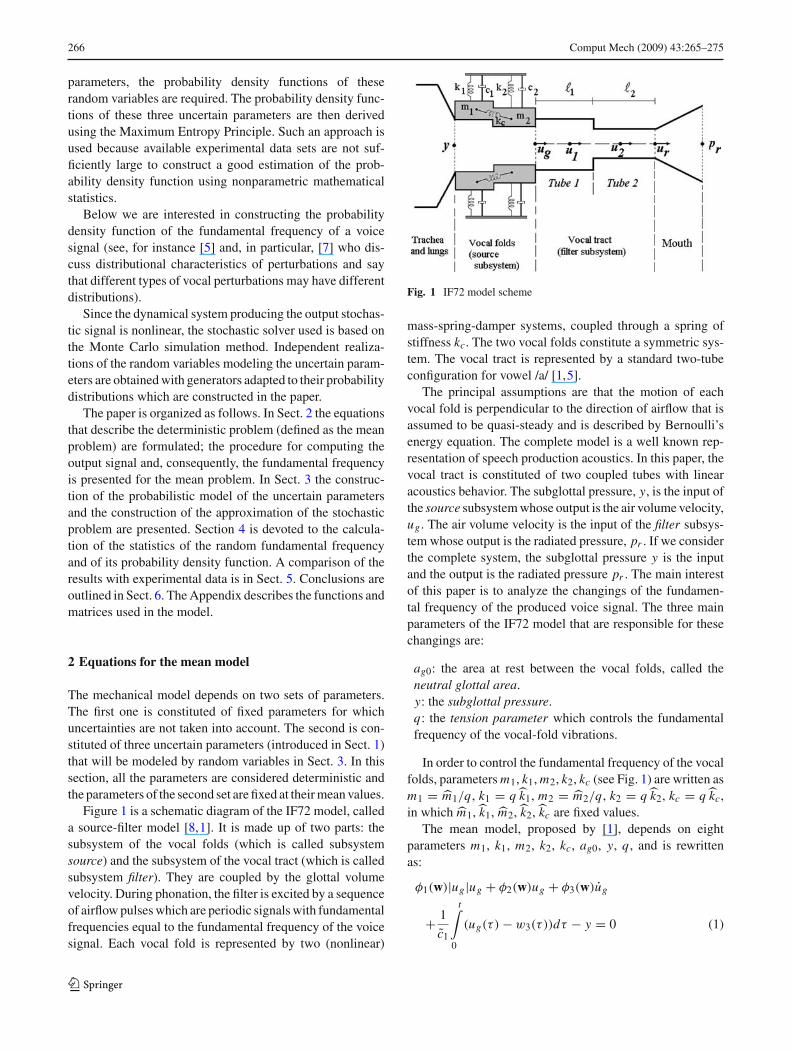
Figure 1 is a schematic diagram of the IF72 model, calleda source-filter model [8,1]. It is made up of two parts: thesubsystem of the vocal folds (which is called subsystemsource) and the subsystem of the vocal tract (which is calledsubsystem filter). They are coupled by the glottal volumevelocity. During phonation, the filter is excited by a sequenceof airflow pulses which are periodic signals with fundamentalfrequencies equal to the fundamental frequency of the voicesignal. Each vocal fold is represented by two (nonlinear)

Fig. 1 IF72 model scheme

mass-spring-damper systems, coupled through a spring ofstiffness kc. The two vocal folds constitute a symmetric sys-tem. The vocal tract is represented by a standard two-tubeconfiguration for vowel /a/ [1,5].

The principal assumptions are that the motion of eachvocal fold is perpendicular to the direction of airflow that isassumed to be quasi-steady and is described by Bernoulli’senergy equation. The complete model is a well known rep-resentation of speech production acoustics. In this paper, thevocal tract is constituted of two coupled tubes with linearacoustics behavior. The subglottal pressure, y, is the input ofthe source subsystem whose output is the air volume velocity,ug . The air volume velocity is the input of the filter subsys-tem whose output is the radiated pressure, pr . If we considerthe complete system, the subglottal pressure y is the inputand the output is the radiated pressure pr . The main interestof this paper is to analyze the changings of the fundamen-tal frequency of the produced voice signal. The three mainparameters of the IF72 model that are responsible for thesechangings are:

ag0: the area at rest between the vocal folds, called theneutral glottal area.y: the subglottal pressure.q: the tension parameter which controls the fundamentalfrequency of the vocal-fold vibrations.

In order to control the fundamental frequency of the vocalfolds, parameters m1, k1, m2, k2, kc (see Fig. 1) are written asm1 = m1/q, k1 = qk1, m2 = m2/q, k2 = qk2, kc = qkc,in which m1,k1, m2,k2,kc are fixed values.

The mean model, proposed by [1], depends on eightparameters m1, k1, m2, k2, kc, ag0, y, q, and is rewrittenas:

φ1(w)|ug|ug + φ2(w)ug + φ3(w)ug

+ 1

c1

t∫

0

(ug(τ ) − w3(τ ))dτ − y = 0 (1)

123

Comput Mech (2009) 43:265–275 267

and

[M]w + [C]w + [K ]w + h(w, w, ug, ug) = 0. (2)

in which w(t) = (w1(t), w2(t), w3(t), w4(t), w5(t)), withw1(t) = x1(t), w2(t) = x2(t), w3(t) = u1(t), w4(t) =u2(t), w5(t) = ur (t). The functions x1 and x2 are the dis-placements of the masses m1 and m2, the functions u1 andu2 describe the air volume velocity through the two tubesmodeling the vocal tract, and ur is the air volume velocitythrough the mouth. The function pr (output signal) is eval-uated by pr (t) = ur (t)rr , with rr = 128ρvs/9π3r2

2 , whereρ is the air mass density, vs is the sound velocity, and r2

is the radius of tube 2. Constant c1, functions φ1, φ2, φ3,(w, w, ug, ug) �→ h(w, w, ug, ug), and matrices [M], [C],[K ] are described in the Appendix.

We can note that Eq. 2 describes the vibration problem ineach of the two subsystems (vocal folds and vocal tract) andEq. 1 is the equation that couples the two subsystems.

2.1 Solver

In order to solve Eqs. (1) and (2), i.e. to find ug and w for agiven y, an implicit-time numerical method is proposed.

This algorithm uses (1) an implicit forward finite differ-ence method for Eq. (1) in which the integral is discretizedwith the method of left Riemann sum and (2) an uncondition-nally stable Newmark method for Eq. (2). Let �t be the sam-pling time and wi = w(i�t), wi = w(i�t), wi = w(i�t),ugi = ug(i�t) and ugi = ug(i�t). Then, for all i ≥ 1,Eqs. (1) and (2) yield

φ1(wi )|ugi |ugi + φ2(wi )ugi + φ3(wi )1

�t(ugi − ugi−1)

+ 1

c1�t

i−1∑

k=0

(ugk − w3k ) − y = 0 (3)

and

[A]wi + h(

wi , wi , ugi ,ugi − ugi−1

�t

)

= zi (4)

in which⎧

⎪

⎪

⎪

⎪

⎪

⎪

⎪

⎪

⎪

⎪

⎪

⎪

⎨

⎪

⎪

⎪

⎪

⎪

⎪

⎪

⎪

⎪

⎪

⎪

⎪

⎩

[A] = [K ] + a0[M] + a1[C]zi = [M](a0wi−1 + a2wi−1 + a3wi−1)

+[C](a1wi−1 + a4wi−1 + a5wi−1)

wi = a0(wi − wi−1) − a2wi−1 − a3wi−1

wi = wi−1 + a6wi−1 + a7wi

a0 = 1α�t2 , a1 = δ

α�t , a2 = 1α�t , a3 = α − 1

2

a4 = δα

− 1, a5 = δ2

(

δα

− 2)

, a6 = �t (1 − δ),

a7 = δ�t

(5)

with ug0 = 0, w0 = 0, w0 = 0, δ = 0.5 and α = 0.25.The method used to construct the approximation of

Eqs. (3) and (4) consists in finding ugi as the limit of the

sequence {uαgi

}, α ≥ 1, when α goes to infinity such that, forall α ≥ 1 and i ≥ 1, we have

φ1(wα−1i )|uα

gi|uα

gi+ φ2(w

α−1i )uα

gi+ φ3(w

α−1i )

+ 1

�t(uα

gi− ugi−1) + 1

c1�t

i−1∑

k=0

(ugk − w3k )−y =0, (6)

with w0i = wi−1 and u1

gi= ugi−1 . In Eq. (6), wα−1

i is the limit

of the sequence {wα−1,βi }, β ≥ 0, when β goes to infinity

and is such that, for all β ≥ 1, α ≥ 2 and i ≥ 1,

[A]wα−1,βi = zi − h

(

wα−1,β−1i , wα−1,β−1

i ,uα−1

gi− ugi−1

�t

)

,

(7)

with wα,0i = wα−1

i and wα,0i = wα−1

i .

For each time step i , index α of the iteration loop beingfixed, first Eq. (6) is solved to calculate uα

gi and, second,

Eq. (7) is solved to calculate wα−1i using an iteration loop

in β. Loop in α is performed until convergence is reached.Then, the next time step is computed.

As will be seen from the results, the methodology ofapproximation was well adapted to the problem.

2.2 Validation of the solver

Numerical tests of the algorithm have been performed and itwas verified that it is unconditionally stable. Below we pres-ent an example related to the output signal for a vowel /a/using data from [1]: d1 = 2.5 × 10−3 m, d2 = 5 × 10−4 m,y = 8, 000 Pa, ag0 = 5 × 10−6 m2, q = 1, m1 = 1.25 ×10−4 kg, m2 = 2.5 × 10−5 kg, k1 = 80 N/m, k2 = 8 N/m,kc = 25 N/m, ξ1 = 0.1 , ξ2 = 0.6 , ηk1 = ηk2 = 100,ηh1 = ηh2 = 500. The lengths considered for the two tubesare �1 = 8.9 × 10−2 m and �1 = 8.1 × 10−2 m, and theircorresponding radius are r1 = 0.56 × 10−2 m and r2 =1.49 × 10−2 m. The sampling time step used to set a goodaccuracy is �t = 1/45, 000 s. Figure 2 displays the timeresponse of the system for ug , x1, x2, and pr normalized topmax = maxt pr (t). The graphs agree with those publishedby [1].

2.3 Calculation of the output signal fundamental frequency

As we have explained in Sect. 1, the objectives of this paperare: (1) to make a probabilistic analysis of the fundamen-tal frequency f0 of the output signal pr and (2) to constructthe probability density function of f0. Let tmax be such thatpr (t) = 0, for t ≥ tmax. The Fourier transform of t �→pr (t), denoted by ω �→ pr (ω), is given by

pr (ω) =∫

Tpr (t)e

−iωt dt, (8)

123

268 Comput Mech (2009) 43:265–275

0 0.02 0.04 0.06 0.08 0.10

500

1000u

(×

10

m /s

)g

−9

3

0 0.02 0.04 0.06 0.08 0.1−0.1

0

0.1

disp

. (×

10

m))

−

2

0 0.02 0.04 0.06 0.08 0.1−1

0

1

p (

norm

)r

x1x2

Fig. 2 Simulation of a vowel /a/: Glottal volume velocity (ug) (top),displacements of the two masses (x1 and x2) (middle), and output signalnormalized (pr ) (bottom)

0 200 400 600 800 10000

0.2

0.4

0.6

0.8

1

Frequency(Hz)

Fig. 3 Normalized modulus of the Fourier transform of the outputsignal. The marker indicates the first peak that corresponds to the fun-damental frequency (in this case 160 Hz)

in which T = [0, tmax]. The fundamental frequency is thendefined as the frequency of the first peak in the graph ofω �→| pr (ω) |. Clearly, there are two mappings L and Msuch that the output signal pr at time t and the fundamentalfrequency f0 can be written as

pr (t) = L(t; ag0, y, q), (9)

f0 = M(ag0, y, q). (10)

For instance, Fig. 3 shows the modulus of the Fouriertransform | pr (ω)| normalized with respect to pmax = maxω |pr (ω) | associated with the time signal shown in Fig. 2, inwhich the first peak is marked. If output signal is not pro-duced, then f0 is taken as zero.

3 Stochastic modeling

The three main parameters responsible for the changing ofthe fundamental frequency will be considered as uncertainand random variables will be associated with them. It meansthat for each realization of the three random variables a dif-ferent output signal is produced, that is the output signal isa stochastic process. It is assumed that the stochastic pro-cess can locally be modeled as being stationary and ergodicstochastic process (see, for instance, [10]).

The probability density functions associated with therandom variables corresponding to the chosen uncertainparameters will be constructed using the Maximum EntropyPrinciple (see [11,12]) in the context of the Information the-ory introduced by [13].

This principle states: Out of all probability distributionsconsistent with a given set of available information, choosethe one that has maximum uncertainty (entropy).

The measure of uncertainty (entropy) used is given byEq. 11:

S(pX ) = −+∞∫

−∞pX (x)ln ( pX (x) ) dx . (11)

The goal is to maximize the entropy S, under the con-straints defined by the following available information

+∞∫

−∞pX (x)dx = 1, (12)

and

+∞∫

−∞pX (x)gi (x)dx = ai , i = 1, . . . , m, (13)

where the real numbers ai and the functions gi are given.See in the appendix more detail on the construction of the

probability density functions, using the Maximum EntropyPrinciple.

3.1 Probabilistic model of the uncertain parameters

As explained in Sect. 1, the three parameters ag0, y, and q aremodeled by random variables Ag0, Y , and Q. Consequently,parameters m1, k1, m2, k2, and kc become random variablesdenoted by M1, K1, M2, K2, and Kc defined by M1 = m1/Q,K1 = Qk1, M2 = m2/Q, K2 = Qk2, and Kc = Qkc. Theprobability models derived here are particular cases of thoseones described in [9]. Since no information is available con-cerning cross statistical informations between random vari-ables Ag0, Y , Q, the use of the Maximum Entropy Principleshows that these random variables are independent. The level

123

Comput Mech (2009) 43:265–275 269

of uncertainties will be controlled by the coefficients of var-iation δAg0 , δY and δQ of the random variables Ag0, Y andQ and will be defined as dispersion parameters of the prob-ability model.

3.1.1 Random variable Ag0

The parameter ag0 is modeled by a random variable Ag0

with values in R+ (due to physical restriction) and the mean

value Ag0 is known. Then the available information can bedefined as (1) the support of the probability density func-tion which is ]0,+∞[, (2) the mean value which is such thatE{Ag0} = Ag0, (3) the second-order moment which must befinite, E{A2

g0} < +∞. The probability density function pAg0

of Ag0 has then to verify the following constraint equations,

+∞∫

−∞pAg0(ag0) dag0 = 1, (14)

+∞∫

−∞ag0 pAg0(ag0) dag0 = Ag0, (15)

+∞∫

−∞a2

g0 pAg0(ag0) dag0 = c, (16)

in which c is a positive finite constant which is unknown. Theuse of the Maximum Entropy Principle yields:

pAg0(ag0) = 1]0,+∞[e−λ0−λ1ag0 −λ2(ag0 )2, (17)

where λ0, λ1 and λ2 are the solution of the three equationsdefined by Eq. 16. Since the constant c is unknown, we intro-duce a new parametrization expressing c as a function ofthe coefficient of variation δAg0 of the random variable Ag0

which is such that δA2g0

= E{A2g0}/A2

g0 − 1 which proves

that c = Ag02(

1 + δ2Ag0

)

.

3.1.2 Random variable Y

The parameter y is modeled by a random variable Y withvalues in R

+ (due to physical restriction) and the mean valueY is known. Then the available information is constituted of(1) the support of the probability density function which is]0,+∞[, (2) the mean value which is such that E{Y } = Y ,(3) the condition E{ln(Y )} = c1 with |c1| < +∞ whichimplies that zero is a repulsive value for the positive-val-ued random variable Y . The introduction of the last availableinformation is related to the need to have a minimum value ofY to produce an output signal [14]. The probability densityfunction pY of Y has then to verify the following constraint

equations:

+∞∫

−∞pY (y) dy = 1, (18)

+∞∫

−∞y pY (y) dy = Y , (19)

+∞∫

−∞ln(y) pY (y) dy = c1. (20)

Applying the Maximum Entropy Principle yields the follow-ing probability density function for Y ,

pY (y) = 1]0,+∞[(y)1

Y

(

1

δ2Y

) 1δ2Y

× 1

�(

1/δ2Y

)

(

y

Y

) 1δ2Y

−1

exp

(

− y

δ2Y Y

)

, (21)

in which δY = σY /Y is the coefficient of variation of therandom variable Y such that 0 ≤ δY < 1/

√2 and where σY

is the standard deviation of Y . In this equation α �→ �(α)

is the Gamma function defined by �(α) = ∫ +∞0 tα−1e−t dt .

From Eq. (21), it can be verified that Y is a second-orderrandom variable.

3.1.3 Random variable Q

The parameter q is modeled by a random variable Q withvalues in R

+ (due to physical restriction) and the mean valueQ is known. Since M1 = m1/Q has to be a second-orderrandom variable, it is necessary that E{M2

1 } < +∞ yield-ing E{1/Q2} < +∞. Then the available information isdefined by (1) the support of the probability density func-tion is ]0,+∞[, (2) the mean value is such that E{Q} = Qand (3) E{1/Q2} = c′

2 with c′2 < +∞. The third constraint

is taken into account by requiring that E{ln(Q)} = c2 with|c2| < +∞. So, the probability density function pQ of Q,whose support is ]0,+∞[, has to verify the following con-straint equations,

+∞∫

−∞pQ(q) dq = 1, (22)

+∞∫

−∞q pQ(q) dq = Q, (23)

+∞∫

−∞ln(q) pQ(q) dq = c2. (24)

123

270 Comput Mech (2009) 43:265–275

Applying the Maximum Entropy Principle yields again

pQ(q) = 1]0,+∞[(q)1

Q

(

1

δ2Q

) 1δ2

Q

× 1

�(

1/δ2Q

)

(

q

Q

) 1δ2

Q−1

exp

(

− q

δ2Q Q

)

, (25)

where the positive parameter δQ = σQ/Q is the coefficient

of variation of the random variable Q such that δQ < 1/√

2and where σQ is the standard deviation of Q. From Eq. (25),it can be verified that Q is a second-order random variableand that E{1/Q2} < +∞.

3.2 Uncertain mechanical system

The stochastic system is deduced from the deterministic onesubstituting ag0, y and q by the random variables Ag0, Y andQ. Consequently, according to Eq. (10), the random funda-mental frequency F0 is given by F0 = M(Ag0, Y, Q). How-ever, the nonlinear mapping M is not explicitly known and itis implicitly defined by Eqs. (1), (2), (8), and (10) substitutingag0, y and q by random variables Ag0, Y and Q.

3.3 Stochastic solver for the uncertain mechanical system

Equations (1), (2), (8), (10) defining the nonlinear mappingM have to be solved using their approximations defined byEqs. (3) to (7) and (8) substituting ag0, y and q by the ran-dom variables Ag0, Y and Q. The stochastic solver used isbased on the Monte Carlo method. First, independent real-izations X(θ) of the random variable X = (Ag0, Y, Q) areconstructed using the probability density functions definedby Eqs. (17), (21) and (25). For each realization X(θ), therealization F0(θ) of the random fundamental frequency F0

is given by

F0(θ) = M(Ag0(θ), Y (θ), Q(θ)), (26)

and is calculated solving deterministic Eqs. (3) to (7) and(8) substituting x = (ag0, y, q) by X (θ) = (Ag0(θ), Y (θ),

Q(θ)). The mean-square convergence of the random variableF0 is analyzed with respect to the number n of independentrealizations for the Monte Carlo method. The mathematicalstatistics are used to construct the estimation of (1) the meanvalue m F0 = E{F0}, (2) the variance σ 2

F0of the random var-

iable F0, (3) the confidence region of the random variable F0

and finally, (4) the probability density function pF0 .

3.3.1 Mean-square convergence analysis

The mean-square convergence analysis with respect toindependent realizations F0(θ1), . . . , F0(θn) of the random

1000 2000 3000 4000 50004.4

4.45

4.5

4.55

n

log

(C

onv(

n))

10

Fig. 4 Mean-square convergence of the Monte Carlo method withrespect to the number n of realizations

variable F0 is carried out studying the function n �→ Conv(n)

defined by

Conv(n) = 1

n

n∑

j=1

F0(θ j )2. (27)

This convergence analysis is performed for different valuesof δAg0 , δY , and δQ . For n ≥ 2, 000, the convergence isalways reached. Then, n = 2, 000 was used for all furtherestimations. For instance, Fig. 4 shows the graph of the func-tion n → log10(Conv(n)) for δAg0 = δY = δQ = 0.10.

3.3.2 Estimation of the mean value, variance, confidenceregion, and probability density function of F0

An estimation m F0 of the mean value m F0 = E{F0} and anestimation σF0

2 of the variance σ 2F0

of the random variableF0 are given by

m F0 = 1

n

n∑

j=1

F0(θ j ), (28)

σ 2F0

= 1

n − 1

n∑

j=1

(

F0(θ j ) − m F0

)2. (29)

The confidence region associated with a probability levelPc is constructed using quantiles [16]. Let FF0( f0) =P{F0 ≤ f0} be the cumulative distribution function of therandom variable F0. For 0 < p < 1, the pth quantile ofFF0 is defined as ζ(p) = Inf{ f : FF0( f ) ≥ p}. Then, theupper envelope f + and the lower envelope f − of the con-fidence interval are defined by f + = ζ((1 + Pc)/2) andf − = ζ((1 − Pc)/2) . Let f1 = F0(θ1), . . . , fn = F0(θn)

be n independent realizations of the random variable F0.Let ˜f1 < · · · < fn be the order statistics associated withf1, . . . , fn . Therefore, we have the following estimation:

123

Comput Mech (2009) 43:265–275 271

f + = ˜f j+ with j+ = fix(n(1 + Pc)/2) and f − = ˜f j−with j− = fix(n(1 − Pc)/2) in which fix(z) is the integerpart of the real number z.

The estimation of the probability density function pF0 ofthe random variable F0 is constructed as follows. Let M bethe number of intervals. Let I j = [ν j , ν j + �ν[ for j =1, . . . , M with ν1 = ˜f1 and �ν = (˜fM − ˜f1)/M . An esti-mation pF0 of the probability density function of F0 is givenby

pF0( f0) =M∑

j=1

1I j ( f0)n j

n�ν(30)

in which n j is the number of realizations in the interval I j .

4 Application to the production of voiced sounds

The application to the production of voiced sounds is donewith the data defined in Sect. 2.2. The mean values of theuncertain parameters used are Ag0 = 5 × 10−2 m2, Y =800 Pa, and Q = 1. It should be noted that the fundamentalfrequency f0 calculated with the deterministic model (ag0 =Ag0, y = Y , and q = Q) is f0 = 168.5 Hz.

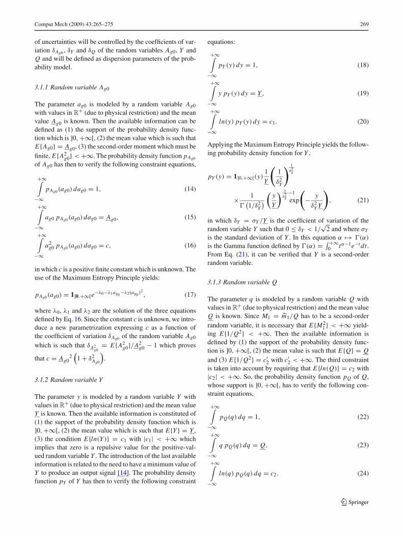
Figure 5 shows the confidence regions for the fundamen-tal frequency F0 with (1) δY = 0.01, δQ varying from 0.01up to 0.60 (top figure); (2) δQ = 0.01, δY varying from 0.01up to 0.60 (bottom figure). For both cases, ag0 was consid-ered fixed at 0.05 cm2. In each figure, the middle line is theestimation m F0 of the mean value defined by Eq. (28). Fig-ure 6 displays the probability density function of F0 for fivedifferent cases with respect to different values of δAg0 , δY ,δQ defined in the figures. For a realization θ , when no voicedsound is produced, the realization F0(θ) of the random fun-damental frequency F0 is taken as zero.

Figure 5 shows that the dispersion of the random funda-mental frequency and also the values of m F0 increase with thelevel of uncertainties. However, it should be noted that thisdispersion is much more important with respect to δQ thanwith respect to δY . In addition, the probabilistic approachwhich is proposed allows a quantification of uncertaintiespropagation through the model to be performed. Such a quan-tification can be analyzed constructing the probability densityfunction of F0 shown in Fig. 6.

It should be noted that the probabilistic approach of uncer-tainties is particularly well adapted to characterize (or to iden-tify) the probabilistic model of voice signals produced by agiven person taking into account the dispersion.

5 Experimental validation

In order to validate the development presented here exper-imental voice signals produced by one person have been

0 0.1 0.2 0.3 0.4 0.5 0.6 0.7

50

100

150

200

250

300

350

Dispersion parameter (δQ

)

Fund

amen

tal f

requ

ency

(Hz)

δY

= 0.01

0 0.1 0.2 0.3 0.4 0.5 0.6 0.7120140160180200220

Dispersion parameter (δY

)Fu

nd. f

req.

(H

z) δQ

= 0.01

Fig. 5 Confidence regions and mean values of the random fundamentalfrequency F0 versus the dispersion coefficient: δY = 0.01 and δQ varies(top figure); δQ = 0.01 and δY varies (bottom figure). The value of Ag0is maintained fixed

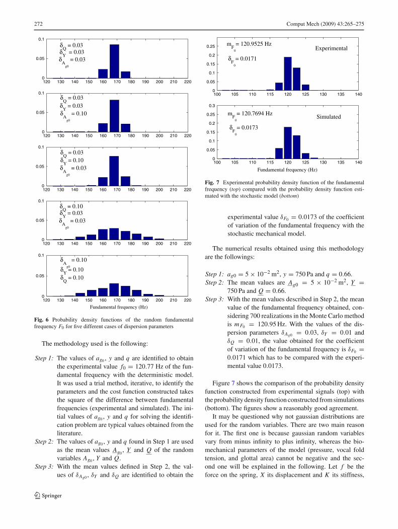
analyzed and their statistics have been compared withsimulations with the mechanical model with uncertaintiesdeveloped here. The measurements are made up of 675recorded voice signals corresponding to a sustained vowel/a/ from one person. The duration of each signal is 0.01 s.For each experimental signal the corresponding experimen-tal fundamental frequency is calculated. The mean value ofthe experimental fundamental frequency is m F0 = 120.77Hz and its coefficient of variation is δF0 = 0.0173. In addi-tion, the experimental probability density function is calcu-lated. The objective is to compare the probability densityfunction of the experimental fundamental frequency with theprobability density function constructed with the stochasticmechanical model.

Our goal is to solve an inverse problem in order to con-struct, from simulations, a probability density function sim-ilar to the experimental one. That is, we want to identify themean values Ag0, Y , Q, and also the coefficients of dispersionδAg0 , δY , δQ such that we can achieve the same experimentalmean value of the fundamental frequency m F0 = 120.77 Hzand also the same experimental coefficient of dispersion of

the fundamental frequency δF0 = m F0

δF0

= 0.0173. We want

also to compare the shapes of the distributions: experimentaland constructed.

123

272 Comput Mech (2009) 43:265–275

120 130 140 150 160 170 180 190 200 210 2200

0.05

0.1

δQ

= 0.03δ

Y = 0.03

δA

g0

= 0.03

120 130 140 150 160 170 180 190 200 210 2200

0.05

0.1δ

Q = 0.03

δY

= 0.03δ

Ag0

= 0.10

120 130 140 150 160 170 180 190 200 210 2200

0.05

0.1δ

Q = 0.03

δY

= 0.10δ

Ag0

= 0.03

120 130 140 150 160 170 180 190 200 210 2200

0.05

0.1δ

Q = 0.10

δY

= 0.03δ

Ag0

= 0.03

120 130 140 150 160 170 180 190 200 210 2200

0.05

0.1δ

Ag0

= 0.10

δY

= 0.10δ

Q = 0.10

Fundamental frequency (Hz)

Fig. 6 Probability density functions of the random fundamentalfrequency F0 for five different cases of dispersion parameters

The methodology used is the following:

Step 1: The values of ag0 , y and q are identified to obtainthe experimental value f0 = 120.77 Hz of the fun-damental frequency with the deterministic model.It was used a trial method, iterative, to identify theparameters and the cost function constructed takesthe square of the difference between fundamentalfrequencies (experimental and simulated). The ini-tial values of ag0 , y and q for solving the identifi-cation problem are typical values obtained from theliterature.

Step 2: The values of ag0 , y and q found in Step 1 are usedas the mean values Ag0

, Y and Q of the randomvariables Ag0 , Y and Q.

Step 3: With the mean values defined in Step 2, the val-ues of δAg0 , δY and δQ are identified to obtain the

100 105 110 115 120 125 130 135 1400

0.05

0.1

0.15

0.2

0.25 Experimentalm

F0

= 120.9525 Hz

δF

0

= 0.0171

100 105 110 115 120 125 130 135 1400

0.05

0.1

0.15

0.2

0.25

0.3

SimulatedmF

0

= 120.7694 Hz

δF

0

= 0.0173

Fundamental frequency (Hz)

Fig. 7 Experimental probability density function of the fundamentalfrequency (top) compared with the probability density function esti-mated with the stochastic model (bottom)

experimental value δF0 = 0.0173 of the coefficientof variation of the fundamental frequency with thestochastic mechanical model.

The numerical results obtained using this methodologyare the followings:

Step 1: ag0 = 5 × 10−2 m2, y = 750 Pa and q = 0.66.Step 2: The mean values are Ag0 = 5 × 10−2 m2, Y =

750 Pa and Q = 0.66.Step 3: With the mean values described in Step 2, the mean

value of the fundamental frequency obtained, con-sidering 700 realizations in the Monte Carlo methodis m F0 = 120.95 Hz. With the values of the dis-persion parameters δAg0 = 0.03, δY = 0.01 andδQ = 0.01, the value obtained for the coefficientof variation of the fundamental frequency is δF0 =0.0171 which has to be compared with the experi-mental value 0.0173.

Figure 7 shows the comparison of the probability densityfunction constructed from experimental signals (top) withthe probability density function constructed from simulations(bottom). The figures show a reasonably good agreement.

It may be questioned why not gaussian distributions areused for the random variables. There are two main reasonfor it. The first one is because gaussian random variablesvary from minus infinity to plus infinity, whereas the bio-mechanical parameters of the model (pressure, vocal foldtension, and glottal area) cannot be negative and the sec-ond one will be explained in the following. Let f be theforce on the spring, X its displacement and K its stiffness,

123

Comput Mech (2009) 43:265–275 273

so that X = f/K . Assume the force is deterministic, andthat both the stiffness and the displacement are random. Itis natural to consider the expected value of X finite; that is,E{X2} < +∞ ⇒ E{ f 2/K 2} < +∞ ⇒ E{1/K 2} < +∞,which is not true for a gaussian random variable. Then, prin-cipally the random variable Q cannot be taken as gaussian.

6 Conclusions

We have proposed a parametric probabilistic approach to takeinto account uncertainties in a nonlinear dynamical modelused to produce voiced sounds. The three parameters con-trolling the values of fundamental frequency of the producedvoice signal are modeled by random variables whose proba-bility distributions are constructed using the MaximumEntropy Principle, and they are not simply considered asgaussian, for example. A complete stochastic computationalmodel has been developed and an experimental validation ispresented in the statistical sense.

In the context of such a problem, the experimental outputsignal of the nonlinear dynamical system has a significantvariability which has to be analyzed in the context of theprobability theory. We have shown that it is possible to iden-tify a reasonable computational stochastic nonlinear dynam-ical model which allows experiments to be predicted in theprobability distribution sense. This kind of problem is nottrivial due to the high nonlinearities in the dynamical systemfor which a pertinent probability model must be constructed.

Acknowledgments This work was financed by the InternationalCooperation Project CAPES-COFECUB N.476/04, by CNPq(Conselho Nacional de Desenvolvimento Científico e Tecnológico) andby FAPERJ (Fundação Carlos Chagas Filho de Amparo à Pesquisa doEstado do Rio de Janeiro).

Appendix A: Functions and matrices introduced in Sect. 2

[M] =

⎡

⎢

⎢

⎢

⎢

⎢

⎢

⎢

⎣

m1 0 0 0 0

0 m2 0 0 0

0 0 �1 + �2 0 0

0 0 0 �2 + �r −�r

0 0 0 −�r �r

⎤

⎥

⎥

⎥

⎥

⎥

⎥

⎥

⎦

,

[C] =

⎡

⎢

⎢

⎢

⎢

⎢

⎢

⎢

⎣

c1 0 0 0 0

0 c2 0 0 0

0 0 r1 + r2 0 0

0 0 0 r2 0

0 0 0 0 rr

⎤

⎥

⎥

⎥

⎥

⎥

⎥

⎥

⎦

,

[K ] =

⎡

⎢

⎢

⎢

⎢

⎢

⎢

⎢

⎣

k1 + kc −kc 0 0 0

−kc k2 + kc 0 0 0

0 0 1c1

+ 1c2

− 1c2

0

0 0 − 1c2

1c2

0

0 0 0 0 0

⎤

⎥

⎥

⎥

⎥

⎥

⎥

⎥

⎦

,

h(w, w, ug, ug) =⎡

⎢

⎢

⎢

⎢

⎢

⎢

⎢

⎣

s1(w1) + t1(w1)w1 − f1(w1, ug, ug)

s2(w2) + t2(w2)w2 − f2(w1, w2, ug, ug)

− 1c1

ug

0

0

⎤

⎥

⎥

⎥

⎥

⎥

⎥

⎥

⎦

,

with �n = ρ�n2πr2

n, �r = 8ρ

3π2rn, rn = 2

rn

√

ρµω2 , ω =

√

k1m1

,

an = πr2n , cn = �nπr2

nρv2

c, and where �n is the length of the

nth tube, rn is the radius of the nth tube, and µ is the shearviscosity coefficient.

φ1(w) =(

0.19ρ

ag0 + 2�gw1+ 2�gw1

)

+ ρ

(ag0 + 2�gw2)2

×[

0.5 − ag0 + 2�gw2

a1

(

1 − ag0 + 2�gw2

a1

)]

,

φ2(w) =(

12µ�gd1

(ag0 + 2�gw1)3

+12�2g

d2

(ag0 + 2�gw2)3 + r1

)

,

φ3(w) =(

ρd1

ag0 + 2�gw1+ ρd2

ag0 + 2�gw2+ �1

)

s1(w1) =

⎧

⎪

⎪

⎪

⎪

⎪

⎨

⎪

⎪

⎪

⎪

⎪

⎩

k1ηk1w31, w1 > − ag0

2�g,

k1ηk1w31+

3k1

{

(

w1 + ag02�g

)

+ ηh1

(

w1 + ag02�g

)3}

,

w1 ≤ − ag02�g

,

s2(w2) =

⎧

⎪

⎪

⎪

⎪

⎪

⎨

⎪

⎪

⎪

⎪

⎪

⎩

k2ηk2w32, w2 > − ag0

2�g,

k2ηk2w32+

3k2

{

(

w2 + ag02�g

)

+ ηh2

(

w2 + ag02�g

)3}

,

w2 ≤ − ag02�g

,

t1(w1) ={

0, w1 > − ag02�g

,

2ξ√

m1k1, w1 ≤ − ag02�g

,

t2(w2) ={

0, w2 > − ag02�g

,

2ξ√

m2k2, w2 ≤ − ag02�g

,

123

274 Comput Mech (2009) 43:265–275

f1(w1, ug, ug) ={

�gd1 pm1(w1, ug, ug), w1 > − ag02�g

,

0, otherwise,

pm1(w1, ug, ug) = y − 1.37ρ

2

(

ug

ag0 + 2�gw1

)2

−1

2

(

12µ�gd1

(ag0 + 2�gw1)3

+ ρd1

ag0 + 2�gw1

)

ug

f2(w1, w2, ug, ug)

=

⎧

⎪

⎨

⎪

⎩

�gd2 pm2(w1, w2, ug, ug), w1>− Ag02�g

and w2>− ag02�g

,

�gd2 y, w1 > − ag02�g

, w2 ≤ − ag02�g

,

0, otherwise,

pm2(w1, w2, ug, ug) = pm1

−1

2

{(

12µ�gd1

(ag0 + 2�gw1)3

+12�2g

d2

(ag0 + 2�gw2)3

)

ug

}

+1

2

{(

ρd1

ag0 + 2�gw1+ ρd2

ag0 + 2�gw2

)

ug

}

−ρ

2u2

g

(

1

(ag0 + 2�gw2)2 − 1

(ag0 + 2�gw1)2

)

.

Appendix B: Maximum Entropy Principle

The Maximum Entropy Principle used to construct the prob-ability density functions consists in maximizing the entropyS, given by Eq. 31:

S(pX ) = −+∞∫

−∞pX (x)ln ( pX (x) ) dx (31)

under the constraints defined by the following, so-called,available information+∞∫

−∞pX (x)dx = 1, (32)

and+∞∫

−∞pX (x)gi (x)dx = ai , i = 1, . . . , m, (33)

where the real numbers ai and the functions gi are known.To solve the corresponding optimization problem, let

(λ0 − 1), λ1, λ2, . . . , λm be the 1 + m real lagrangian mul-tiplicators associated to the 1 + m constraints and let L(pX )

be given by:

L(pX ) = S(pX ) − (λ0 − 1)

⎧

⎨

⎩

+∞∫

−∞pX (x)dx − 1

⎫

⎬

⎭

−m∑

j=1

⟨

λ j ,

+∞∫

−∞g j (x)pX (x)dx − a j

⟩

, (34)

where 〈., .〉 is the internal product in R.One can write

L(pX ) = b −+∞∫

−∞h(x, pX (x))dx (35)

with

b = (λ0 − 1) +m∑

j=1

〈λ j , a j 〉, (36)

and

h(x, pX (x)) = pX (x)

⎧

⎨

⎩

�n(pX (x))

+(λ0 − 1) +m∑

j=1

〈λ j , g j (x)〉⎫

⎬

⎭

. (37)

Using Calculus of Variations, it can be proven that themaximum and minimum of L(pX ) verify the equation

∂

∂pX (x)h(x, pX (x)) = 0, (38)

which solution is

pX (x) = 1S(x) exp

⎛

⎝−λ0 −m∑

j=1

〈λ j , g j (x)〉⎞

⎠ , (39)

where 1S is the support of pX .This extremum is unique and it is a maximum because

∂2h(x, pX (x))

∂pX (x)2 = 1

pX (x)> 0. (40)

The corresponding 1+m lagrange multiplicators, (λ0−1),

λ1, λ2, . . . , λm , are evaluated using the Eqs. 32 and 33.More details and applications of the Maximum Entropy

Principle can be found in [15].

References

1. Ishizaka K, Flanagan JL (1972) Synthesis of voiced sounds from atwo-mass model of the vocal cords. Bell Syst Tech J 51:1233–1268

2. Zhang Y, Jiang J, Rahn III DA (2005) Studying vocal fold vibra-tions in Parkinson’s disease with a nonlinear model Chaos 033903:1–10

123

Comput Mech (2009) 43:265–275 275

3. Cataldo E, Leta FR, Lucero J, Nicolato L (2006) Synthesisof voiced sounds using low-dimensional models of the vocalcords and time-varying subglottal pressure. Mech Res Commun33:250–260

4. Lucero JC (1995) The minimum lung pressure to sustain vocal foldoscillation. J Acoust Soc Am 98:779–784

5. Titze I (1994) Principles of voice production. Prentice-Hall,Englewood Cliffs, NJ

6. Sciamarella D, Alessandro C (2004) On the acoustic sensitivity ofa symmetrical two-mass model of the vocal fols do the variation ofcontrol parameters. Acta Acustica United Acustica 90:746–761

7. Pinto N, Titze I (1990) Unification of perturbation measures inspeech signals. J Acoust Soc Am 87(3):1278–1289

8. Fant G (1960) The acoustic theory of speech production. Mouton,The Hague

9. Soize C (2001) Maximum entropy approach for modeling ran-dom uncertainties in transient elastodynamics. J Acoust Soc Am109:1979–1996

10. Schoengten J (2001) Stochastic models of Jitter. J Acoust Soc Am109:1631–1650

11. Jaynes E (1957) Information theory and statistical mechanics. PhysRev 106(4):620–630

12. Jaynes E (1957) Information theory and statistical mechanics II.Phys Rev 108:171–190

13. Shannon CE (1948) A mathematical theory of communication. BellSystem Tech J 27:379–423, 623–659

14. Baer T (1975) Investigation of phonation using excised larynges.Ph.D. thesis, Massachussetts Institute of Technology, Cambridge,MA

15. Kapur JN, Kesavan HK (1992) Entropy optimization principleswith applications. Academic Press, San Diego

16. Serfling R (1980) Approximation theorems of mathematical statis-tics. Wiley, New York

123