On non-autonomous dynamical systemsA. Anzaldo-Meneses Citation: Journal of Mathematical Physics 56, 042702 (2015); doi: 10.1063/1.4916893 View online: http://dx.doi.org/10.1063/1.4916893 View Table of Contents: http://scitation.aip.org/content/aip/journal/jmp/56/4?ver=pdfcov Published by the AIP Publishing Articles you may be interested in Ground state solutions for non-autonomous dynamical systems J. Math. Phys. 55, 101504 (2014); 10.1063/1.4897443 A stochastic perturbation theory for non-autonomous systems J. Math. Phys. 54, 123303 (2013); 10.1063/1.4848776 Unified formalism for higher order non-autonomous dynamical systems J. Math. Phys. 53, 032901 (2012); 10.1063/1.3692326 Simulation of quantum systems with the coupled channel method Am. J. Phys. 76, 493 (2008); 10.1119/1.2837813 Integrable and superintegrable systems with spin J. Math. Phys. 47, 103509 (2006); 10.1063/1.2360042

This article is copyrighted as indicated in the article. Reuse of AIP content is subject to the terms at: http://scitation.aip.org/termsconditions. Downloaded

to IP: 189.245.210.210 On: Fri, 10 Apr 2015 19:01:37

JOURNAL OF MATHEMATICAL PHYSICS 56, 042702 (2015)

On non-autonomous dynamical systemsA. Anzaldo-Menesesa)

Departamento de Ciencias Básicas, Universidad Autónoma Metropolitana,Distrito Federal 02200, México

(Received 6 March 2014; accepted 21 March 2015; published online 7 April 2015)

In usual realistic classical dynamical systems, the Hamiltonian depends explicitlyon time. In this work, a class of classical systems with time dependent nonlinearHamiltonians is analyzed. This type of problems allows to find invariants by afamily of Veronese maps. The motivation to develop this method results fromthe observation that the Poisson-Lie algebra of monomials in the coordinates andmomenta is clearly defined in terms of its brackets and leads naturally to an infinitelinear set of differential equations, under certain circumstances. To perform explicitanalytic and numerical calculations, two examples are presented to estimate thetrajectories, the first given by a nonlinear problem and the second by a quadraticHamiltonian with three time dependent parameters. In the nonlinear problem, theVeronese approach using jets is shown to be equivalent to a direct procedure usingelliptic functions identities, and linear invariants are constructed. For the secondexample, linear and quadratic invariants as well as stability conditions are given.Explicit solutions are also obtained for stepwise constant forces. For the quadraticHamiltonian, an appropriated set of coordinates relates the geometric setting to thatof the three dimensional manifold of central conic sections. It is shown further that thequantum mechanical problem of scattering in a superlattice leads to mathematicallyequivalent equations for the wave function, if the classical time is replaced by thespace coordinate along a superlattice. The mathematical method used to compute thetrajectories for stepwise constant parameters can be applied to both problems. It is thestandard method in quantum scattering calculations, as known for locally periodicsystems including a space dependent effective mass. C 2015 AIP Publishing LLC.[http://dx.doi.org/10.1063/1.4916893]

I. INTRODUCTION

Nonlinear, non-autonomous dynamical systems occur very often in real world. Of particularrelevance is the motion of electric charges in time varying electromagnetic fields, classically aswell as quantum mechanically. Of great interest is also the study of stability of general Hamilto-nian systems. However, due to the difficulty to analyze them mathematically or numerically, it isnecessary to introduce simplifications or approximations and to study the resulting linear quasi-timeindependent models. One of the main difficulties is that the Hamiltonian is time dependent andtherefore non-conserved. This fact makes it natural to search for invariants, which somehow help tounderstand or to describe the time variation of the Hamiltonian. The study of classical and quantumsystems with time dependent Hamiltonians from the algebraic point of view has a long tradition.1,2

The importance of canonical transformations of classical mechanics also for quantum mechanicalproblems was recognized early.3 Other standard approaches include adiabatic approximations, sud-den approximations, as well as time dependent perturbative methods.4 For particular Hamiltonians,the knowledge of symmetries is also very useful, for example, by applying Noether’s theorem or viacanonical transformations. In certain cases, ad hoc approaches can further lead to useful results.5

Alternative general methods to study analytically this problem are welcome but scarce. Here, a new

a)Electronic mail: answald@ymail.com

0022-2488/2015/56(4)/042702/20/$30.00 56, 042702-1 © 2015 AIP Publishing LLC

This article is copyrighted as indicated in the article. Reuse of AIP content is subject to the terms at: http://scitation.aip.org/termsconditions. Downloaded

to IP: 189.245.210.210 On: Fri, 10 Apr 2015 19:01:37

042702-2 A. Anzaldo-Meneses J. Math. Phys. 56, 042702 (2015)

simple method to study nonlinear, non-autonomous classical problems is proposed based on theintroduction of a set of coordinates, in general infinite, and leading to equivalent linear problems. Itis then suggested to formally solve the resulting linear problem and to use the initial conditions toconstruct invariants.

Two examples for flat metrics are given. In the first, using the proposed method, a nonlineartime dependent one dimensional case is solved in terms of elliptic functions. It is shown that theseries expansion of the addition theorem for elliptic functions corresponds to the expected infinitelinear combination in terms of a basis of nonlinear coordinates. Elliptic functions are common inmany solvable problems in modern classical mechanics since its beginnings.6 A linear invariantsurface is constructed explicitly. The second example is a harmonic oscillator with three timedependent parameters and its geometry is naturally described by introducing two sets of coordinatesin parameter space and in a space formed by ad-hoc quadratic coordinates defining a cone andconstructed from the two dimensional phase space coordinates. The Poisson algebra satisfied bythe quadratic coordinates is then a symplectic algebra and the trajectories are described in threespace. It is natural to see the trajectory in quadratic coordinates as lying on a “light” cone definedas the set of null-vectors. The “phase space” of quadratic coordinates together with the Minkowskimetric defines a Lorentz manifold. Following the standard procedures, the stability of the systemis resumed for periodically varying parameters. Mathieu equation is used as an example for laterreference. For the particular case of stepwise constant parameters, the system is integrated applyingtechniques from the quantum scattering theory of quasi-one-dimensional systems.7 It is shown, thatthe scattering amplitudes are good candidates to describe stability for locally periodic systems. Theexplicit results allow a simple calculation of some relevant quantities, which make the time behaviorof the system clearer as the number of steps increases.

In Sec. II, a general problem is given to show that several characteristics of the one-dimensionalcase are generic and therefore could also be helpful in other applications. A general method is pre-sented to study nonlinear time dependent Hamiltonians with non-flat metrics. In Sec. III, a nonlinearflat example is solved. In Sec. IV, a non-autonomous quadratic one dimensional Hamiltonian isconsidered, the stability conditions are studied, and the particular case of stepwise constant periodicparameters is integrated, where an analogy with quantum scattering is given. Section V contains theconclusions.

II. CERTAIN DYNAMICAL SYSTEMS

Consider a smoothly varying family of Riemannian metrics parametrized by time ⟨v,gw⟩ =i j gi j(x, t)viwi, with invertible symmetric metric matrix g, on a compact 2n-dimensional manifold.

Let be a non-autonomous dynamical system with a Hamiltonian defined in extended phase space(p, x, t) as

H =n

i, j=1

g−1i j (x, t)

pipj

2+

ni=1

ai(x, t)pi + V (x, t) = 12⟨p, g−1p⟩ + atp + V, (1)

where the g−1i j are the matrix elements of the inverse g−1 of g. The canonical equations are

x =(∂H∂pi

)= g−1p + a,

p = −(∂H∂xi

)= −1

2grad ⟨p, g−1p⟩ − grad atp − grad V,

or more explicitly

pi = −j,k

∂g−1jk

∂xi

pjpk2−j

∂a j

∂xipj −

∂V∂xi

.

Defining z = (xt,pt), the geodesic flow is obtained solving z = f (z, t), in general a nonlinear matrixdifferential equation with time dependent coefficients. Here, for given initial data, it shall be supposed

This article is copyrighted as indicated in the article. Reuse of AIP content is subject to the terms at: http://scitation.aip.org/termsconditions. Downloaded

to IP: 189.245.210.210 On: Fri, 10 Apr 2015 19:01:37

042702-3 A. Anzaldo-Meneses J. Math. Phys. 56, 042702 (2015)

that a solution exists and is unique in a certain domain, under the usual assumptions made in thecorresponding general Picard-Lindelöf existence and uniqueness theorems.

The sole existence and uniqueness of a solution do not say much about how to find it. A formalsolution of the equations of motion shall be now given using elementary arguments of algebraicgeometry. First, the possibility shall be assumed to represent by Laurent series (positive powerseries plus a number of negative powers) for all functions of the xi in the right hand side of theequations of motion in a certain region of phase space. Thus, all problems whose Hamiltonians arenot expressible through Laurent series are excluded from the present approach.

After expressing all functions of x by series, the time derivative of x and p is given by series,whose terms are products of powers of the xi, products of powers of the xi times momenta pj,and products of powers of the xi times second degree factors pjpk. All monomials present in thedifferential equation have the form xkp j, using a multi-index notation. So that xk is the vector(xk

1 , xk−11 x2, . . . , x

k11 xk2

2 · · · xknn , . . . , x

knn )t where all distinct sets of integers ki such that

ni=1 ki = k

are included, and p j is a vector where only positive integers ji are needed. Only positive powers ofthe momenta are needed, but positive and also negative powers of the coordinates shall be necessaryin general. Further, it is clear that the time derivative of the involved monomials shall again beexpressible in terms of the same kind of monomials. In general, quadratic or higher degree terms inthe momenta cannot be reduced to lower order, since the Hamiltonian is time dependent. But alsofor constant Hamiltonians, only in the one dimensional problem, it shall be possible to reduce allquadratic terms in the momentum to linear ones.

Let now gi be the Poisson-Weyl algebra satisfied by the monomials xℓi p

mi for ℓ ∈ Z and m ∈ N,

resulting from the corresponding Poisson-Heisenberg algebra {xi,pj} = δi, j, i, j = 1, . . . , n, fromwhich

{xℓi p

mi , x

uj pv

j } = δi j(ℓ v − u m)xℓ+u−1i pm+v−1

i ,

for ℓ,u ∈ Z and m, v ∈ N. In some cases, only the sub-algebras m, v = 0,1,2 are needed. In parti-cular,

{xℓi p

mi , x jpj} = δi j(ℓ − m)xℓ

i pmi ,

and for µ = 0,1,2,

{xℓi p

µi , x

2−ℓj p2−µ

j } = δi j(ℓ(2 − ℓ) − µ(2 − µ))xipi.

The general resulting algebra is infinite, but for flat metrics and quadratic potentials, only finitesub-algebras are needed. For flat metrics, the algebra generated by the elements {xk} and {x jp} willsuffice. In general, however, the associative algebra g generated by all products of elements of the giwill be necessary.

To integrate formally the equations of motion, it seems convenient to rewrite them as the firstorder time derivative of a vector ζ given by a time dependent transformation Λ (independent of thecoordinates and momenta) of the same vector. Hence, the main idea to get rid of the nonlinear termsin the equations of motion is to include them in the infinite vector ζ , avoiding to get a coordinatesdependent Λ. Define in consequence the vector ζ with entries xkp j, for j ∈ N and k ∈ Z, where thenotation explained in the last paragraphs is used. Thus, the whole vector looks like

(. . . , x−1n−1x−1

n , . . . , x−1n ,1,p1, . . . , x1, . . . ,p1x1, . . . ,p2

1, . . . , x21, . . . ,p1p2, . . .).

Let (x1, . . . , x2n) = (x1, . . . , xn,p1, . . . ,pn), a degree-d Veronese map νd : P2n → Pm is defined8

as [x1 : . . . : x2n] → [. . . : x I : . . .], where I ranges over a basis of monomials of degree d inx1, . . . , x2n. So I ∈ N2n, I = (i1, . . . , i2n), |I | = i1 + · · · + i2n = d, and x I = xi1

1 · · · xi2n2n . Therefore, m

= ♯{(i1, . . . , i2n : i1 + · · · + i2n = d} = (2n + d − 1)!/d!(2n − 1)!. Thus, up to reordering, the aboveidentification of powers as coordinates is a Veronese map for each fixed degree.

Note that the introduction of the elementary powers above leads directly to a particular setof algebraic invariants in terms of identities between symmetric functions in 2n variables. Forexample, for ζ1 = x1x2, ζ2 = x2

1, and ζ3 = x22, it follows that I = ζ2

1 − ζ2ζ3 is an obvious invariantwith I = 0 for all times.

This article is copyrighted as indicated in the article. Reuse of AIP content is subject to the terms at: http://scitation.aip.org/termsconditions. Downloaded

to IP: 189.245.210.210 On: Fri, 10 Apr 2015 19:01:37

042702-4 A. Anzaldo-Meneses J. Math. Phys. 56, 042702 (2015)

Since all components of ζ are mapped into some others by a time derivative, the followinginhomogeneous linear differential equation is satisfied:

ζ = Λζ + β, (2)

where Λ is a time dependent matrix and β is a time dependent vector and both are independent ofthe coordinates. In particular cases, the vector ζ , the matrix Λ, and the vector β can be taken asfinite dimensional. Basic linear differential equation (2) is in general defined in a Hilbert space andhas been studied in many branches of Physics in the past1 in very different situations. In certaincases, the matrix Λ can be expressed linearly as a finite sum Λ =

i λi(t)Xi, where the coefficients

λi are functions of time and the Xi’s generate a Lie algebra after successive computation of their Liebrackets, but this shall not be assumed here.

Since it is supposed that a solution z(t) = (p(t), x(t))t of the original problem exists and isunique, then there exists a linear transformation W (t, t0), such that z(t) = W (t, t0)z(t0). In the spacegenerated by the vectors ζ there will be, formally associated, a transformation, denoted here byW (t, t0), so that a formal solution is

ζ(t) = W (t, t0)ζ(t0) + α(t, t0), (3)

with W (t0, t0) = I and α(t0, t0) = 0. Only the 2n initial conditions ζi(t0) given directly as x1(t0), . . . ,xn(t0),p1(t0), . . . pn(t0) are algebraically independent, since all other depend algebraically on these.The linear map x(t),p(t) → x(t0),p(t0) is canonical and therefore the brackets satisfied by the ζi(t)are preserved, since they depend only on the x,p and the simple evaluation at t = t0 leaves themunaltered.

Direct substitution of (3) into (2) leads to

W = ΛW, α = Λα + β,

using the arbitrariness of the initial conditions. This means that the column vectors of W are alsosolutions of the homogeneous equations of motion (2), with simpler initial conditions. The solutionof the inhomogeneous equation can be written as

α(t, t0) = W (t, t0) t

t0

W−1(t ′, t0)β(t ′)dt ′ = t

t0

W−1(t ′, t)β(t ′)dt ′, (4)

where it is assumed, that the inverse W−1(t ′, t0) = W (t0, t ′) exists along the integration interval.Equation (3) leads to the constant vector

ζ(t0) = W−1(t, t0)(ζ(t) − α(t, t0)). (5)

For each ζi(t0), this identity allows to define the hyperplane

Pi = {ζ j | ζi(t0) −j

W−1i, j (t, t0)(ζ j(t) − α j(t, t0)) = 0}, (6)

with time dependent coefficients in a space with sets of coordinates ζ j, one set for each i, replacingthe original solutions ζ j(t). It is important to notice that for a fixed time, (5) is a single point in thespace (ζ1(t), ζ2(t), . . . , t), whereas (6) is a curve in the space (ζi1(t), ζi2(t), . . . , t). On each hyperplanePi, the set of solutions ζ j(t) with a set of initial conditions ζi(t0) is embedded. It is clear that, for afixed i, each hyperplane contains also solutions with the same initial ζi(t0) but with distinct ζ j(t0),for j , i, in general. The complete vector ζ(t) with initial solution ζ(t0) is at the intersection of allhyperplanes Pi.

General linear invariant vectors have the form

I = Mζ + C.

Using I = 0, it follows that

M = −MΛ, C = −M β.

Thus, since M = −M (dM−1/dt) M , for M invertible, M = W−1, as expected from (5).

This article is copyrighted as indicated in the article. Reuse of AIP content is subject to the terms at: http://scitation.aip.org/termsconditions. Downloaded

to IP: 189.245.210.210 On: Fri, 10 Apr 2015 19:01:37

042702-5 A. Anzaldo-Meneses J. Math. Phys. 56, 042702 (2015)

The constant entries of ζ(t0) or of I can also be used to construct more complicated invariants.For example, introduce a general function F(ζ1(t0), ζ2(t0), . . .) = 0 and express the ζi(t0) in termsof the ζi(t) to obtain first F(ζ1(t), ζ2(t), . . .) = 0. From this identity, define a new hypersurface afterreplacing the original ζi by new variables ζi satisfying the same equation. An additional way toobtain invariants is to propose a function G(p, x, t) and to integrate it over a certain time interval as

J = t0+T

t0

G(p, x, t)dt.

This quantity is a constant which can be expressed in terms of the initial conditions p0 and x0 afterinserting in the integrand the momenta and coordinates as functions of the initial conditions andtime as

J(p0, x0) = t0+T

t0

G(p0, x0, t)dt .

For example, for periodic systems the action variables provide such invariants as

Ji(p0, x0) =

pidxi =

pi(p0i, x0i, t)xi(p0i, x0i, t)dt . (7)

After reexpressing the initial conditions in terms of the variables pi and xi, these invariants couldthen be used to express the momenta as functions of the coordinates, the time, and the invariants,i.e. p = p(x, J, t). Explicit examples are given in Secs. III and IV, which include instructive newlinear and quadratic invariants for elementary Hamiltonians.

The search for invariants in classical mechanics has a long tradition since its origin in thework of Hamilton, Jacobi, Poincaré, and Cartan.6 Of particular relevance are the more recent worksby Lewis and Riesenfeld,2 where invariants are constructed by studying directly the time depen-dence of the coefficients of a quadratic invariant Ansatz. Those coefficients satisfy similar (albeitnonlinear) differential equations as the original equations of motion for a harmonic oscillator withtime dependent frequency, and the method has been applied to the quantum mechanical problemof a charge in time dependent magnetic fields. These works generated a fruitful series of similarstudies and generalizations to higher order invariants, including the application of Noether’s theo-rem and canonical transformations to obtain related results.3 The method presented here is different,since it does not introduce any new differential equations besides the original equations of motionand is based on the older literature, which stresses the importance of the initial conditions. Theproduced invariants and the explicit calculation for standard examples show its applicability. Fora quadratic one dimensional Hamiltonian, the relation between the direct Ansatz method and themethod of this work is given (see Sec. IV and (20)).

The method of this section is directly related with the Hamilton-Jacobi6 method, since thecanonical transformation from the original variables to their initial values can be accomplished bya generating function S(P, x, t) with P = p(t0), which maps the original Hamiltonian H(p, x, t) to anew vanishing one H ′, so that the Hamilton-Jacobi equation for S holds

H ′ = H(∂S∂x

, x, t) + ∂S∂t= 0.

Also,

pi =∂S∂xi

, Xi =∂S∂Pi

,

with X = x(t0). Notice here that these last two relations mean that the pi are certain functions of thexi and the initial momenta Pi or after solving these relations, when possible, that the constants Pi

are given as functions of the pi and the xi, say Pi = Pi(p, x, t). The corresponding Jacobian for thisstep should not vanish. Similarly, in principle also the constants Xi are certain functions of the piand xi, i.e., Xi = Xi(p, x, t). A procedure to construct invariants consists here in the substitution ofthe pi and the qi by new pi and qi and in the interpretation of the resulting relations, pi = pi(q,P)and Xi = Xi(p, x, t), as hypersurfaces in the space (p, x, t).The constants Pi and Qi could also be other convenient functions of the initial momenta andcoordinates. For example, action variables (7) could be used as transformed momenta.

This article is copyrighted as indicated in the article. Reuse of AIP content is subject to the terms at: http://scitation.aip.org/termsconditions. Downloaded

to IP: 189.245.210.210 On: Fri, 10 Apr 2015 19:01:37

042702-6 A. Anzaldo-Meneses J. Math. Phys. 56, 042702 (2015)

A more rigorous treatment should clarify under which circumstances the Hamiltonian allowsthe application of the presented method. Only one set of examples of invariants shall be given inSecs. III and IV to make plausible the validity of the method of this section, at least in certainconcrete cases.

III. SIMPLE NONLINEAR CASES

A class of time dependent Hamiltonians, which can be easily reduced to a time independentexpression, has the form

H =12⟨A−1p, g−1(Atx)A−1p⟩ + at(Atx)A−1p + V (Atx) + xt A

dA−1

dtp, (8)

where A is an invertible space independent but time dependent square matrix, a is a vector depend-ing on time only through Atx, and g−1 is a square matrix depending also on time only through Atx.The canonical generating function F(x,P) = xt AP leads to

X =∂F∂P= Atx, p =

∂F∂x= AP, P = A−1p,

and to a time independent Hamiltonian

H ′ = H +∂F∂t=

12⟨P, g−1(X)P⟩ + at(X)P + V (X),

or in the original coordinates

H ′ = H(p, x, t) − xt AdA−1

dtp.

Given the initial conditions x0 and p0, the numerical value for H ′ fixes an algebraic curve inextended phase space.

A. Integrable one dimensional flat metric

For flat metric, the one dimensional particular case of the last paragraph is

H =1

2A2 p2 + a(Ax)A−1p + V (Ax) + x AdA−1

dtp, (9)

where A is a time dependent function and a is a function depending on time only through Ax. Theabove canonical transformation F = AxP, X = Ax, P = p/A leads to a time independent Hamilto-nian

H ′ =12

P2 + a(X)P + V (X).A second canonical transformation with the generating function

F ′(u,P) = uP + u

u0

a(u)du

leads to

X =∂F ′

∂P= u, v =

∂F ′

∂u= P + a,

and to the simpler Hamiltonian

H ′′ = H ′ =12v2 + V (u) − 1

2a(u)2,

which defines a surface in the extended phase space. The equations of motion for the new coordi-nates are

u = v, v = −dVdu− a(u)da(u)

du.

This article is copyrighted as indicated in the article. Reuse of AIP content is subject to the terms at: http://scitation.aip.org/termsconditions. Downloaded

to IP: 189.245.210.210 On: Fri, 10 Apr 2015 19:01:37

042702-7 A. Anzaldo-Meneses J. Math. Phys. 56, 042702 (2015)

Thus, this problem can be integrated by quadratures as

t − t0 =

u(t)

u(t0)du

2H ′′ − 2V (u) + a(u)2 ,

valid under the assumption of a well behaved integrand.

B. A quartic potential

In this subsection, a detailed example of the Veronese map method is given, and linear andquadratic invariant surfaces are constructed, computed, and displayed.

Consider the nonlinear problem associated to the flat one dimensional Hamiltonian

H =p2

2A2 +b0

2A2x2 +

c4

A4x4 + (C + AA)xp,

with b0, c and C constant, and a time dependent function A. Thus, now

x =pA2 + (C +

AA)x, p = −b0A2x − cA4x3 − (C + A

A)p

and

x + 2A−1Ax + (b0 − 2A−2A2 − A−1A − C2 − 4A−1AC)x + A2cx3 = 0.

This equation with time dependent coefficients can be used to model dissipation.Via the canonical transformation F(x,P) = AxP, x = X/A, and p = AP, a time independent

Hamiltonian H ′ results

H ′ =12

P2 +b0

2X2 +

c4

X4 + CX P,

which is an elliptic curve. The canonical transformation F ′(X, v) = Xv − CX2/2, u = X , v = P +CX leads to

H ′′ = H ′ =12v2 +U(u),

with U(u) = 12 bu2 + c

4 u4 and b = b0 − C2. Further, higher powers in v can be reduced using

u = v, v2 = 2H ′′ − 2U(u), (10)

v = u = −bu − cu3, · · ·.

So that, for one dimensional problems, also with more general potentials, the reduction leads tovectors containing only powers of u and powers of u times v , respectively, times u.

Introduce now a vector χ with components χ0 = 1, χk = uk and χ−k = uk−1u, for k = 1,2 . . ..Thus,

χk = k χ−k, χ−k = 2(k − 1)H ′χk−2 − kbχk − (k + 1) c2χk+2 (11)

allow to write the linear infinite dimensional differential equation

χ = M χ, M = *,

0 M−M+ 0

+-,

where M± are constant infinite band matrices. For odd powers in u and even powers times u, defin-ing the column vector χodd = (χ+Todd, χ

−Todd)T , for χ±odd = (χ±1, χ±3, . . .)T , the equations of motion

are

χ+odd = m−χ−odd, χ−odd = m+χ+odd, or χ±odd = m∓m±χ±odd,

This article is copyrighted as indicated in the article. Reuse of AIP content is subject to the terms at: http://scitation.aip.org/termsconditions. Downloaded

to IP: 189.245.210.210 On: Fri, 10 Apr 2015 19:01:37

042702-8 A. Anzaldo-Meneses J. Math. Phys. 56, 042702 (2015)

with

m− = D, and m+ =

*......,

−b −c 0 . . .

4H ′ −3b −2c0 8H ′ −5b...

. . .

+//////-

= 4H ′a+ − ca− − bD,

where D = diag(1,3,5, . . .), a− is an upper diagonal matrix with upper first diagonal (1,2,3, . . .) anda+ = at

− is a lower diagonal matrix with lower first diagonal (1,2,3, . . .). Clearly the following threedimensional Lie algebra, essentially sl(2), results

[a−,a+] = D, [a−,D] = 2a−, [a+,D] = −2a+. (12)

For the harmonic oscillator with c = 0, only the first element of D and m+ will be necessary, makingthe problem elementary. The operators a± and D act naturally on infinite dimensional orthonormalcanonical basis vectors |k⟩ given as column vectors with a one in the (k + 1)-th row and zerootherwise. Here,

a−|k⟩ = k |k − 1⟩, a+|k⟩ = (k + 1)|k + 1⟩,D|k⟩ = (2k + 1)|k⟩,so that a− acts as an annihilation operator and a+ as a creation operator, whereas a+a− act as asquared number of state operator, since a+a−|k⟩ = k2|k⟩. Starting with the vacuum state |0⟩, anyother state can be reached |k⟩ = 1

k! ak+|0⟩. It seems that many more similitudes exist with the standard

creation and annihilation operators of the harmonic oscillator, which satisfy a nilpotent Heisenbergalgebra instead of (12).Equivalently for χTodd = (χ+Todd,m−χ

−Todd),

ddtχodd = O χodd, O = *

,

0 I

m−m+ 0+-.

Setting χ(t + t0) = exp(Ot) χodd(t0). Indeed, O2k+1 = (m−m+)kO and O2k = (m−m+)kI2×2 lead to

χodd(t + t0) =k≥0

( t2k+1

(2k + 1)!O +t2k

(2k)! I2×2

)(m−m+)k χodd(t0), (13)

or, symbolically,

χodd(t + t0) = *,

cosh(√m−m+ t) sinh(√m−m+ t)/√m−m+√m−m+ sinh(√m−m+ t) cosh(√m−m+ t)

+-χodd(t0).

Therefore, the computation of the exponential exp(Ot) is reduced to the calculation of the powersof m−m+, which can be obtained recursively. For the simplest case, corresponding to the harmonicoscillator with c = 0, this relation is just the well known addition formula for trigonometric func-tions.

To corroborate solution (13), reparametrize first (10) taking 2H ′′ = 1, 2δ = b, and ϵ = −c/2, toobtain

u2 = 1 − 2δu2 + ϵu4, (14)

which is one usual normal form for an elliptic curve. After Euler,9 the solution satisfies

u(t0 + t) = u(t0)u(t) + u(t0)u(t)1 − ϵu(t0)2u(t)2 .

To find the matrix W , introduce a solution y(t) of (14) with initial conditions y(0) = 0 and y(0) = 1,and the vector ξodd with elements ξk = yk, and ξ−k = yk−1 y , for k = 1,2, . . . . The Poisson algebrasatisfied by the vector elements is

{ξ±k, ξ± j} = 0, {ξk, ξ− j} = kξk+ j−2, {ξ−k, ξ− j} = (k − j)ξ− j−k+2,

for k, j = 1,2, . . ., and with ξ0 = 1. This is a semi-direct sum of an Abelian algebra and a Wittalgebra.

This article is copyrighted as indicated in the article. Reuse of AIP content is subject to the terms at: http://scitation.aip.org/termsconditions. Downloaded

to IP: 189.245.210.210 On: Fri, 10 Apr 2015 19:01:37

042702-9 A. Anzaldo-Meneses J. Math. Phys. 56, 042702 (2015)

After expanding formally the right hand side of the addition formula into power series, it followsthat

ξ1(t0 + t) =j≥0

ϵ j[ξ−2 j−1(t0)ξ2 j+1(t) + ξ2 j+1(t0)ξ−2 j−1(t)],

which has the desired form of a matrix product implicit in general solution (3). As a result, otherelements ξk satisfy addition formulas, for example,

ξ−1(t0 + t) =j≥0

ϵ j[ξ−2 j−1(t0)ξ2 j+1(t) + (2 j + 1)ξ−2 j−1(t0)ξ−2 j−1(t)],

where ξ−2 j−1 is given by (11). Higher powers can be obtained using higher derivatives, for example,y3 = −(2δy + y)/2ϵ . In general,

ξ±2k±1(t0 + t) =j≥0

(a±2k±1,2 j+1(t0)ξ2 j+1(t) + a±2k±1,−2 j−1(t0)ξ−2 j−1(t)

),

where a±k,± j depends linearly on the {ξ∓k′}. A W matrix such that ξodd(t0 + t) = W (t0)ξodd(t) can begiven as

W = *,

α β

γ δ+-,

with infinite blocks α = (a2k+1,2 j+1), β = (a2k+1,−2 j−1), γ = (a−2k−1,2 j+1), and δ = (a−2k−1,−2 j−1).They begin with

α =

*....,

ξ−1 ϵξ−3 · · ·a3,1 a3,3 · · ·...

.... . .

+////-

, β =

*....,

ξ1 ϵξ3 · · ·a3,−1 a3,−3 · · ·...

.... . .

+////-

,

γ =

*....,

ξ−1 ϵ ξ−3 · · ·a−3,1 a−3,3 · · ·...

.... . .

+////-

, δ =

*....,

ξ−1 3ϵξ−3 · · ·a−3,−1 a−3,−3 · · ·...

.... . .

+////-

,

where each function depends only on t0. By construction, ξodd(t0 + t) = Moddξodd, so that W =ModdW . Therefore, each column vector of W is a solution of the equations of motion with initialconditions given by W (0) = I. Since (14) and (10) are the same equations, for 2aH = 1, thenχodd(t0 + t) = W (t)χodd(t0) as well.

In particular, taking Eq. (14) to be that satisfied by the standard Jacobi elliptic function y(t) =sn(k, t), corresponding to 2δ = 1 + k2, and ϵ = k2,

u(t0 + t) = u(t0) y(t) + u(t0)y(t)1 − k2u(t0)2y2(t) . (15)

This is the desired solution for general initial conditions containing a linear combination of thecoordinates ξi at t0 with known time dependent coefficients.

To corroborate (13) for a particular matrix element, let us look at the coefficient of X0 corre-sponding to sn in addition formula (15), given as ξ−1, the first powers of the corresponding Taylorseries for the Jacobi function sn are

sn(t) = 1 − 12(1 + ϵ)t2 +

124

(1 + 14ϵ + ϵ2)t4 − 1720

(1 + 135ϵ + 135ϵ2 + ϵ3)t6 +O(t7).Compare this terms now with the first matrix element of cosh(√m−m+ t) in (13), that is,

(cosh(√m−m+ t))1,1 = *,

k≥0

t2k

(2k)! (m−m+)k+-1,1

,

This article is copyrighted as indicated in the article. Reuse of AIP content is subject to the terms at: http://scitation.aip.org/termsconditions. Downloaded

to IP: 189.245.210.210 On: Fri, 10 Apr 2015 19:01:37

042702-10 A. Anzaldo-Meneses J. Math. Phys. 56, 042702 (2015)

with

m−m+ =

*......,

−(1 + ϵ) 2ϵ 0 . . .

6 −9(1 + ϵ) 12ϵ0 20 −25(1 + ϵ)...

. . .

+//////-

.

So that (m−m+)1,1 = −(1 + ϵ) and (m−m+)211 = 1 + 14ϵ + ϵ2, (m−m+)311 = −1 − 135ϵ − 135ϵ2 − ϵ3,provide precisely the same first coefficients as in the Taylor expansion above.

Linear invariants can be given by taking the derivative of (15) to obtain

u0 y = (1 − k2u20y

2)u − 2k2u20yyu − u0 y ,

where u0 = u(t0) and u0 = u(t0). From the two independent equations, it follows that

(1 + k2u20y

2) yu − (1 − k2u20y

2)yu − u0( y2 − yy) = 0,

which is the equation of a straight line in the plane {u, v}, with v = u and time dependent coef-ficients. Since u0 = v0 is not present, the resulting surface in three space {u, v, t} comprises allsolutions with a fixed u0. In Fig. 1, the linear invariant surfaces generated by the straight lines areshown for initial condition u0 = 1 and the moduli k2 = 0, 0.4, and 0.8 from left to right. The twocurves correspond to trajectories with v0 = 1 (black) and −1 (red).

IV. THREE DIMENSIONAL PARAMETRIC SPACES

In this section, the one dimensional problem with a quadratic potential, friction, and parametricoscillations is studied. Such problem corresponds, for example, to a simple pendulum with verti-cal oscillations of its fixed point or subject to oscillating external fields or can be used to studyelectrons in time dependent electromagnetic fields.2,4 Many of the following results can be readilygeneralized to higher dimensional problems with quadratic Hamiltonians.Consider the time dependent Hamiltonian

H(x,p, t) = a1p2

2+ a2p x + a3

x2

2,

where a1, a2, and a3 are time dependent and do not necessarily allow to reduce the problem to a timeindependent Hamiltonian as above. In the important field of geometric phases, this Hamiltoniandeserved large interest.1 Linear terms in x and p could be added to the above Hamiltonian, withoutadding too much difficulties, but that case shall not be considered here. Essentially, the conic sec-tions described by the associated quadratic invariant would then include also parabolas, instead ofonly central conic sections as those below. Physically, the linear terms in the Hamiltonian lead toinhomogeneous motion equations corresponding to forced oscillators. Since particular solutions ofthe inhomogeneous equations in terms of the solution of the homogeneous equations (see (4)) canbe easily given, no relevant additional mathematical difficulties are involved.

FIG. 1. Invariant linear surfaces and trajectories for k2= 0, 0.4, and 0.8.

This article is copyrighted as indicated in the article. Reuse of AIP content is subject to the terms at: http://scitation.aip.org/termsconditions. Downloaded

to IP: 189.245.210.210 On: Fri, 10 Apr 2015 19:01:37

042702-11 A. Anzaldo-Meneses J. Math. Phys. 56, 042702 (2015)

The corresponding canonical equations are

η = *,

−a2 −a3

a1 a2

+-η, (16)

where η = (p, x)t. The equations of motion can be written as

η = (−a3 e− − a2e0 + a1e+)η,with the generators of sp1

e− = *,

0 10 0

+-, e0 = *

,

1 00 −1

+-, e+ = *

,

0 01 0

+-,

which satisfy {e±,e0} = ±2e± and {e−,e+} = e0. Since the functions ai are time dependent, thetrajectories are given by time dependent vector fields of sp1.It follows that

x =a1

a1x + (a2

2 − a1a3 +a1a2 − a1a2

a1)x. (17)

Introducing the functions u1 = a1/a1 and u2 = a22 − a1a3 + a2 − a1a2/a1, (17) is

x = u1x + u2x. (18)

For periodic parameters, this is a Hill equation with damping.The solution of (16) is given by a time dependent canonical transformation with

*,

px+-= *,

a bc d

+-*,

p0

x0

+-, (19)

and ad − bc = 1 for all time. The vectors (a,c) and (b,d) satisfy the same equation as (p, x) but withinitial conditions (a(t0),c(t0)) = (1,0) and (b(t0),d(t0)) = (0,1), respectively. The canonical transfor-mation from the initial values to the actual variables can be performed using a generating functionS(x,p0, t) with

p =∂S∂x=

p0

d+

bxd, x0 =

∂S∂p0=

xd− cp0

d.

Thus, up to an additive function of time,

S = −cp2

0

2d+

p0xd+

bx2

2d.

The resulting Hamiltonian H ′ vanishes, so that S satisfies the Hamilton-Jacobi equation,

a1

2

(∂S∂x

)2+ a2x

∂S∂x+

a3

2x2 +

∂S∂t= 0.

There are two linear invariants associated with this problem, say

Ii = Aip + Bix, i = 1,2.

Here, the functions of time Ai and Bi are obtained as in Sec. II using the initial conditions or bysetting Ii = 0 and finding the coefficients. Ai and Bi satisfy the same equations as x and p, butwith the simpler initial conditions A1(t0) = 1, B1(t0) = 0 and A2(t0) = 0 and B2(t0) = 1, according toI1 = p(t0), I2 = x(t0) and A1 = d,B1 = −b, A2 = −c, and B2 = a.

A quadratic invariant I can be constructed as

I = α1I21 + 2α2I1I2 + α3I2

2 = Ap2 + 2B xp + Cx2, (20)

where the αi are constant and

A = α1A21 + 2α2A1A2 + α3A2

2,

B = α1A1B1 + α3A2B2 + α2(A1B2 + A2B1),C = α1B2

1 + 2α2B1B2 + α3B22.

This article is copyrighted as indicated in the article. Reuse of AIP content is subject to the terms at: http://scitation.aip.org/termsconditions. Downloaded

to IP: 189.245.210.210 On: Fri, 10 Apr 2015 19:01:37

042702-12 A. Anzaldo-Meneses J. Math. Phys. 56, 042702 (2015)

FIG. 2. Invariant linear surface for Mathieu equation and embedded non-periodic trajectories for a non-periodic (left),respectively, a periodic (right) case.

Clearly, by the above definition, I = 0 and the equations satisfied by A,B, and C are more compli-cated as those for the Ai but are irrelevant in this approach. Here, it is preferred to let the originalequations of motion play throughout the central role. For periodic systems, a natural quadraticinvariant results from the action variable

J =

pdx

for a period T , for which

α1 =

T

0(a1a2 + a2ac)dt, α2 =

12

T

0(2a1ab + a2(ad + cb))dt,

α3 =

T

0(a1b2 + a2bd)dt .

An important example with time dependent frequency is Mathieu equation,10

x + (a − 2q cos(2t))x = 0, (21)

where a and q are fixed parameters. Invariant linear and quadratic surfaces are shown in Figs. 2and 3. Care must be taken, since the Mathieu functions are complex for certain regions of the (a,q)parametric real plane, and the non-normalized determinant can become complex or null.

The quadratic invariant determines a family of conic sections in parameter space. From (20),

AC − B2− = δ∆2,

with ∆ = A1B2 − A2B1 and δ = α1α3 − α22. This equation can be rewritten as

14(A + C)2 − B2 − 1

4(A − C)2 = δ∆2.

FIG. 3. Invariant quadratic surface for a harmonic oscillator (left) and for Mathieu equation (right) and embedded trajectories.

This article is copyrighted as indicated in the article. Reuse of AIP content is subject to the terms at: http://scitation.aip.org/termsconditions. Downloaded

to IP: 189.245.210.210 On: Fri, 10 Apr 2015 19:01:37

042702-13 A. Anzaldo-Meneses J. Math. Phys. 56, 042702 (2015)

FIG. 4. (a) From left to right, a double sheet hyperboloid, a cone, and a one sheet hyperboloid in parameter space. (b) Doublesheet hyperboloid (left) for a = 2, cone (center) for a = b2, and one sheet hyperboloid (right) for a = 2.5 in parameter spacewith parametric trajectories.

In phase space (p, x), setting I > 0 for simplicity, the relation for I is the equation of an ellipsewith variable semi-axes if AC − B2 = δ > 0. If AC − B2 = δ = 0, the curve degenerates into straightlines and if AC − B2 = δ < 0, it becomes a hyperbola.

Therefore, in parameter space (A + C,B, A − C), the invariant, for ∆ , 0, corresponds to a onesheet hyperboloid for δ < 0, to a two sheet hyperboloid for δ > 0, and to a cone for δ = 0, shown inFig. 4(a), with particular parametric curves for a harmonic oscillator. In Fig. 4(b), the surfaces areshown for Mathieu equation. A periodic solution is given for the cone and the characteristic valuea = b2. The hyperboloids display segments of non-periodic solutions, all with q = 1.

A clear advantage of I is that it depends on three parameters given in simple terms of the orig-inal three parameters of the equation of motion for x. Further, the invariant contains all three alge-braically independent second degree monomials in x and p. The just introduced three dimensionalparametric space allows to write the invariant as I = R · r , defining the vectors R = (2B, A,C)t andr = (px,p2, x2)t. The invariant I as well as the Hamiltonian is linear in terms of the coordinates r1,r2and r3. Thus, I describes moving planes in “quadratic phase space” {px,p2, x2}.

A simple manner to visualize the coordinates of r in R3 is to identify them as describ-ing a surface r2

1 = r2r3. The resulting surface is a cone with circular cross section shown inFig. 5(a), with solutions of Mathieu equation. This cone is easier to visualize using as coordinatesξ = (√2px, (p2 − x2)/√2, (p2 + x2)/√2)t, with ξ2

1 + ξ22 − ξ

23 = 0.

Alternative quadratic coordinates are (p2 − [a − 2q cos(2t)]x2,2

a − 2q cos(2t) px,p2

+ [a − 2q cos(2t)]x2), also defining a cone. In Fig. 5(b) the Hamiltonian for Mathieu equation isgiven as vertical coordinate with a linear phase space (p, x) as horizontal axes in the left picture witha periodic trajectory with q = 2 and characteristic value a = a1.5. In the right hand side of the samefigure, the cone defined by the alternative quadratic coordinates with the same periodic trajectory,for which the vertical axis is now the quadratic Hamiltonian.

This article is copyrighted as indicated in the article. Reuse of AIP content is subject to the terms at: http://scitation.aip.org/termsconditions. Downloaded

to IP: 189.245.210.210 On: Fri, 10 Apr 2015 19:01:37

042702-14 A. Anzaldo-Meneses J. Math. Phys. 56, 042702 (2015)

FIG. 5. (a) Cones in quadratic phase space, the left with a periodic trajectory, the right cone with part of a non-periodic one.(b) A trajectory, to the left for phase space in the horizontal plane and the Hamiltonian as vertical coordinate, to the right forquadratic space.

It follows also that

ξ = (2a2L1 + (a1 − a3)L2 − (a1 + a3)L3)ξ,with the generators of the algebra so(1,2)

[L1,L2] = ϵ L3, [L2,L3] = L1, [L3,L1] = L2,

and

L1 =*...,

0 0 00 0 −10 ϵ 0

+///-

, L2 =*...,

0 0 10 0 0−ϵ 0 0

+///-

, L3 =*...,

0 −1 01 0 00 0 0

+///-

, (22)

where ϵ = −1, associated to the group of isometries of the hyperbolic plane H2 = {x ∈ R3 | x23 −

x22 − x2

1 = 1}. The trajectories in quadratic phase space are then integral curves of time dependentvector fields given by elements of so(1,2). The inner product is now ⟨ξ,η⟩θ = ξ tgη = −ξ1η1 −ξ2η2 + ξ3η3, with the three dimensional Minkowski metric,

θ =*...,

−1 0 00 −1 00 0 1

+///-

,

and ξ is a null vector ⟨ξ, ξ⟩θ = ξ23 − ξ

22 − ξ

21 = 0. Thus, in Euclidean three space, the vectors ξ and

ξ = θξ are orthogonal, and therefore ξ is a normal vector to the light cone at ξ. The vector ξ isperpendicular to ξ, since

ξ = (2a2L1 + (a1 − a3)L2 + (a1 + a3)L3)ξ,where the generators are given now by (22), but with ϵ = 1, corresponding to so3, leading to a vectorproduct in R3.

This article is copyrighted as indicated in the article. Reuse of AIP content is subject to the terms at: http://scitation.aip.org/termsconditions. Downloaded

to IP: 189.245.210.210 On: Fri, 10 Apr 2015 19:01:37

042702-15 A. Anzaldo-Meneses J. Math. Phys. 56, 042702 (2015)

A. Stability

The standard method3 of Lyapunov is resumed in this section to study the stability of periodicsystems. This results shall be used as a guide for locally periodic systems, which are those systemswhose parameters are periodic only for a certain time interval.

Defining ξ = (x, x)t, it follows from (18) that

ξ = U(t)ξ, U(t) = *,

0 1u2 u1

+-, (23)

where u1(t) and u2(t) are such that ui(t) = ui(t + τ) for t ∈ (0,∞). Let, xi(t), i = 1,2 be two linearlyindependent solutions such that xi(0) = δi,1 and xi(0) = δi,2. Then, the fundamental matrix is

W (t) = *,

x1(t) x2(t)x1(t) x2(t)

+-,

with W (0) = I, the areal speed is given by Det W (t), and

ξ(t) = W (t)ξ(0).Note that this is in general a distinct relation as that for canonical transformations in phase spacecoordinates x and p (see (19)), for which its determinant is unity for all time. The Lyapunovconstant is given by

α = Tr W (τ) = x1(τ) + x2(τ).Lemma: The eigenvalues of the monodromy matrix W (τ) are

2λ± = −α ±α2 − 4β, with β = Det W (τ) > 0.

Proof: Notice that x1x2 − x2x1 = u2(x1x2 − x2x1), so that the Liouville formula results

Det W (t) = exp� t

0u1dt

�= exp(

t

0Tr U dt),

which leads to β > 0. Now, since W is a two by two matrix, it satisfies λ2 − αλ + β = 0. �

Starting from an initial condition ξ0, at time t0, after a time Nτ,

ξ(t0 + Nτ) = W N(τ) ξ(t0).Matrices like W are called transfer matrices in quantum scattering theory. Diagonalizing as Λ−1W(τ)Λ = D, with D = Diag(λ+,λ−) and writing ξ = Λξ, it follows

ξ(t0 + Nτ) = *,

λN+ 00 λ

N−

+-ξ(t0).

Using the above results, the next theorem holds.

Theorem: The system defined by (23) satisfies the following conditions.

I. If β > 1, the system is unstable.II. For 0 ≤ β ≤ 1, there are the following cases.

1. If 0 ≤ α2 < 4β, and(a) The system is asymptotically stable if 0 < β < 1.(b) Stable if β = 1.

2. If α2 > 4β,(a) The system is asymptotically stable if |α| < 1 + β.(b) There is a periodic solution if α = 1 + β, with period τ and the eigenvalues are

1 and β or if α = −1 − β, there is periodic solution with period 2τ and the eigen-values are −1 and β.

This article is copyrighted as indicated in the article. Reuse of AIP content is subject to the terms at: http://scitation.aip.org/termsconditions. Downloaded

to IP: 189.245.210.210 On: Fri, 10 Apr 2015 19:01:37

042702-16 A. Anzaldo-Meneses J. Math. Phys. 56, 042702 (2015)

(c) Unstable if |α| > 1 + β.3. If α2 = 4β,

(a) The system is asymptotically stable if 0 < β < 1.(b) The solution is periodic, if β = 1, with period τ if λ± = 1 or 2τ if λ± = −1.

Proof: I. follows, since for |β | = |λ+λ−| > 1, at least one eigenvalue has absolute value largerthan unit and its powers diverge for large N . II.1 follows, since for 0 ≤ β ≤ 1 and 0 ≤ α2 < 4β,the eigenvalues are complex conjugated, |λ±|2 = β. II.2 follows, since for 0 ≤ β ≤ 1 and α2 > 4β,the eigenvalues are real and the eigenvalue with the largest absolute value satisfies 2|λmax| =|α| + α2 − 4β. Notice that although β < 1, it can happen that one of the eigenvalues could havean absolute value larger than unit. II.3 is obtained since for α2 = 4β, the eigenvalues are real anddegenerated. �

Remember that4 a point x0 of a map W is Lyapunov stable (respectively, asymptotically stable)if for all ϵ > 0 exist δ > 0 such that if |x − x0| < δ, then |W nx −W nx0| < ϵ for all 0 < n < ∞(respectively W nx −W nx0 → 0, as n → ∞).

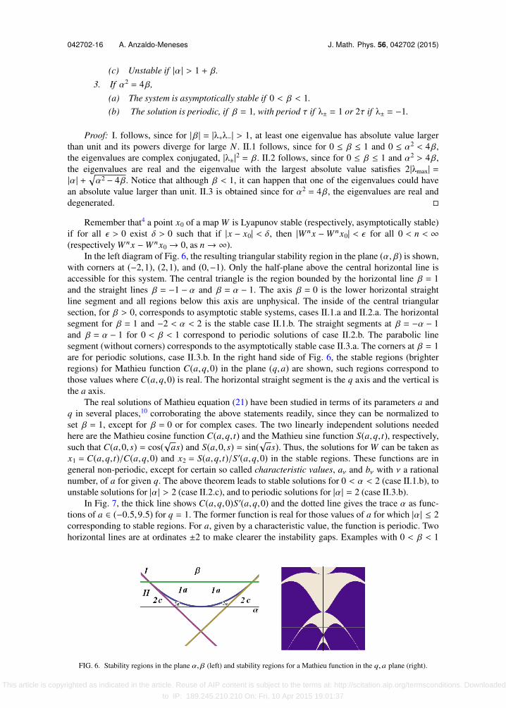
In the left diagram of Fig. 6, the resulting triangular stability region in the plane (α, β) is shown,with corners at (−2,1), (2,1), and (0,−1). Only the half-plane above the central horizontal line isaccessible for this system. The central triangle is the region bounded by the horizontal line β = 1and the straight lines β = −1 − α and β = α − 1. The axis β = 0 is the lower horizontal straightline segment and all regions below this axis are unphysical. The inside of the central triangularsection, for β > 0, corresponds to asymptotic stable systems, cases II.1.a and II.2.a. The horizontalsegment for β = 1 and −2 < α < 2 is the stable case II.1.b. The straight segments at β = −α − 1and β = α − 1 for 0 < β < 1 correspond to periodic solutions of case II.2.b. The parabolic linesegment (without corners) corresponds to the asymptotically stable case II.3.a. The corners at β = 1are for periodic solutions, case II.3.b. In the right hand side of Fig. 6, the stable regions (brighterregions) for Mathieu function C(a,q,0) in the plane (q,a) are shown, such regions correspond tothose values where C(a,q,0) is real. The horizontal straight segment is the q axis and the vertical isthe a axis.

The real solutions of Mathieu equation (21) have been studied in terms of its parameters a andq in several places,10 corroborating the above statements readily, since they can be normalized toset β = 1, except for β = 0 or for complex cases. The two linearly independent solutions neededhere are the Mathieu cosine function C(a,q, t) and the Mathieu sine function S(a,q, t), respectively,such that C(a,0, s) = cos(√as) and S(a,0, s) = sin(√as). Thus, the solutions for W can be taken asx1 = C(a,q, t)/C(a,q,0) and x2 = S(a,q, t)/S′(a,q,0) in the stable regions. These functions are ingeneral non-periodic, except for certain so called characteristic values, aν and bν with ν a rationalnumber, of a for given q. The above theorem leads to stable solutions for 0 < α < 2 (case II.1.b), tounstable solutions for |α| > 2 (case II.2.c), and to periodic solutions for |α| = 2 (case II.3.b).

In Fig. 7, the thick line shows C(a,q,0)S′(a,q,0) and the dotted line gives the trace α as func-tions of a ∈ (−0.5,9.5) for q = 1. The former function is real for those values of a for which |α| ≤ 2corresponding to stable regions. For a, given by a characteristic value, the function is periodic. Twohorizontal lines are at ordinates ±2 to make clearer the instability gaps. Examples with 0 < β < 1

FIG. 6. Stability regions in the plane α, β (left) and stability regions for a Mathieu function in the q,a plane (right).

This article is copyrighted as indicated in the article. Reuse of AIP content is subject to the terms at: http://scitation.aip.org/termsconditions. Downloaded

to IP: 189.245.210.210 On: Fri, 10 Apr 2015 19:01:37

042702-17 A. Anzaldo-Meneses J. Math. Phys. 56, 042702 (2015)

FIG. 7. The trace and C(a,q,0)S′(a,q,0) as functions of a.

leading to asymptotic stable regions can be constructed taking above a1 = exp(γt), a2 constant, anda3 = a30 exp(−γt) cos(ω0t) with γ,ω0, and a30 constant.

B. Stepwise constant oscillations

It is possible to do a more detailed analysis taking stepwise constant functions u1 and u2, sincethen, the differential equations are easily solvable in each section. The solutions of each section areconnected with those of their neighboring sections imposing continuity on the functions and theirfirst derivatives at each discontinuity border.

Set u1(t) = u1 j, u2(t) = u2 j, and xi(t) = x(t) for t ∈ (tMi+ j, tMi+ j+1), i = 1,2, . . . ,N , j = 1, . . . ,M . Only the case, ∆ = ti − ti−1 constant for all i shall be considered and the period is taken to beτ = M ∆. The equations are now

xi = u1 j xi + u2 jxi, for t ∈ (tMi+ j, tMi+ j+1).Forming the 2N-dimensional vector χ = (x, x)t, it satisfies

χ = Uj χ, for t ∈ [tMi+ j−1, tMi+ j),with

Uj = *,

0 1u2 j u1 j

+-.

The eigenvalues of these matrices are κ±j = −γ j ± ω j with

ω j =

γ2j + u2 j, γ j = −u1 j/2.

The solution can be written, for n > 0, as

χ(t0 + nτ) = W n χ(t0), with W = W1W2 · · ·WM, W j = exp(∆Uj).Thus, the matrix W is a transfer matrix, it translates the vector ξ from an initial value to its value attime M∆. Therefore, for non-degenerated eigenvalues,

W j =e−γ j∆

ω j

(sinh(∆ω j)Uj + {γ j sinh(∆ω j) − ω j cosh(∆ω j)}I

)or

W j =e−γ j∆

ω j

*,

γ js j − ω jcj s j(ω2

j − γ2j )s j −γ js j − ω jcj

+-,

with cj = cosh(∆ω j) y s j = sinh(∆ω j). This article is copyrighted as indicated in the article. Reuse of AIP content is subject to the terms at: http://scitation.aip.org/termsconditions. Downloaded

to IP: 189.245.210.210 On: Fri, 10 Apr 2015 19:01:37

042702-18 A. Anzaldo-Meneses J. Math. Phys. 56, 042702 (2015)

It is possible to express W n in terms of symmetric polynomials in the eigenvalues λ± of

W = *,

a bc d

+-

as

W n = pn W − pn−1 βI = *,

a pn − β pn−1 b pn

c pn d pn − β pn−1

+-,

with n = 1, . . . ,p0 = 0,p1 = 1, where

pn(λ+,λ−) = λn+ − λn−λ+ − λ−

is a symmetric polynomial, in the variables λ±, of degree n − 1, that satisfies

pn+1 = αpn − βpn−1.

As above, α = Tr W = λ+ + λ− and β = Det W = λ+λ−. If the eigenvalues are complex conjugated,then β = 1 and the polynomials are those of Chebyshev.

Clearly, the stability criteria of Sec. IV A can be used as a reference to analyze the behavior ofthe solutions. Following the statements of the stability theorem, the value of the determinant of Wand its trace can be used directly to classify the trajectories. It is also possible to apply the standardtechniques of quantum scattering theory for locally periodic systems7 with some modifications tostudy the classical problem. This analogy is explained in Sec. IV C.

C. Elementary scattering theory

For zero friction, u1 = 0, an analogous problem in one dimensional quantum scattering theorycorresponds, up to certain important physical constants, to take time as the spatial coordinate, say y ,the classical coordinate x as being the wave function ψ and the function u2 to be the potential energyV minus the total energy E. The Schrödinger equation is then

− ~2

2md2

dy2ψ(y) + V (y)ψ = Eψ.

The wave function and its derivative are given in terms of the eigenfunctions φ±, on both sides(V=0) of a succession of potential regions with V , 0. Here,

ξ(y ′) = *,

Aφ+(y ′) + Bφ−(y ′)iκ(Aφ+(y ′) − Bφ−(y ′))

+-,

for y ′ to the left of the scattering region and

χ(y) = *,

Cφ+(y) + Dφ−(y)iκ(Cφ+(y) − Dφ−(y))

+-= W χ(y ′),

for y to the right with κ =√

2mE/~. The constant coefficients A,B,C,D are the so called scatter-ing amplitudes. The scattering matrix S is now introduced relating the incoming waves with theoutcoming waves as

*,

Bφ−(y ′)Cφ+(y)

+-= S *

,

Aφ+(y ′)Dφ−(y)

+-= *,

r t ′

t r ′+-*,

Aφ+(y ′)Dφ−(y)

+-,

where r is the reflexion amplitude and t the transmission amplitude for a wave coming from theleft-hand side and where r ′ and t ′ correspond to the respective amplitudes for a wave coming fromthe right-hand side of the scattering region. The probabilities of transmission T or reflexion R aregiven by the squared absolute values of the corresponding amplitudes. The scattering amplitudescan thus be given in terms of the elements of W , for example,

t ′ = 2(a − ibκ + ic/κ + d)−1.

This article is copyrighted as indicated in the article. Reuse of AIP content is subject to the terms at: http://scitation.aip.org/termsconditions. Downloaded

to IP: 189.245.210.210 On: Fri, 10 Apr 2015 19:01:37

042702-19 A. Anzaldo-Meneses J. Math. Phys. 56, 042702 (2015)

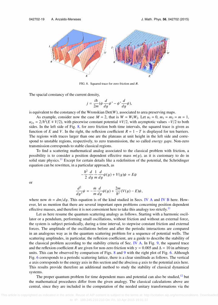
FIG. 8. Squared trace for zero friction and R.

The spacial constancy of the current density,

j =i~2m

(ψ ddy

ψ∗ − ψ∗ ddy

ψ),is equivalent to the constancy of the Wronskian Det(W ), associated to area preserving maps.

As example, consider now the case M = 2, that is W = W1W2. Let u1 = 0, m1 = m2 = m = 1,u2± = 2/~2(E ∓ V/2), with piecewise constant potential ∓V/2, with asymptotic values −V/2 to bothsides. In the left side of Fig. 8, for zero friction both time intervals, the squared trace is given asfunction of E and V . In the right, the reflexion coefficient R = 1 − T is displayed for ten barriers.The regions with traces larger than one are the plateaus at unit height in the left side and corre-spond to unstable regions, respectively, to zero transmission, the so called energy gaps. Non-zerotransmission corresponds to stable classical regions.

To find a scattering mathematical analog associated to the classical problem with friction, apossibility is to consider a position dependent effective mass m(y), as it is customary to do insolid state physics.11 Except for certain details like a redefinition of the potential, the Schrödingerequation can be rewritten, in a particular approach, as

−~2

2d

dy1m

ddy

ψ(y) + V (y)ψ = Eψ

ord2

dy2ψ = −mm

ddy

ψ(y) + 2m~2 (V (y) − E)ψ,

where now m = dm/dy . This equation is of the kind studied in Secs. IV A and IV B here. How-ever, let us mention that there are several important open problems concerning position dependenteffective masses, and therefore it is not convenient here to take this analogy too strictly.11

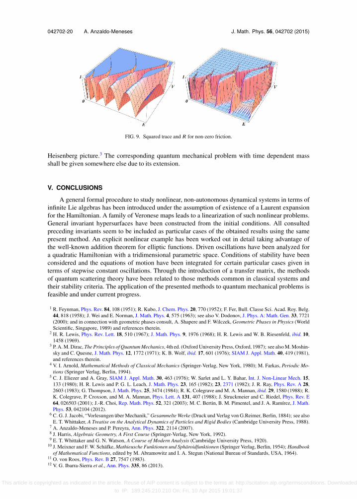
Let us here resume the quantum scattering analogy as follows. Starting with a harmonic oscil-lator or a pendulum, performing small oscillations, without friction and without an external force,the system is subject periodically, during a time interval, to stepwise constant friction and externalforces. The amplitude of the oscillations before and after the periodic interactions are comparedin an analogous way as in the quantum scattering problem for a sequence of potential wells. Thescattering amplitudes, in particular, the reflexion coefficient, are a guide to describe the stability ofthe classical problem according to the stability criteria of Sec. IV A. In Fig. 9, the squared traceand the reflexion coefficient R are given for non-zero friction with γ = 0.005 and ∆ = 10 in arbitraryunits. This can be observed by comparison of Figs. 8 and 9 with the right plot of Fig. 6. AlthoughFig. 6 corresponds to a periodic scattering lattice, there is a clear similitude as follows. The verticala axis corresponds to the energy axis in this section and the abscissa q axis to the potential axis here.This results provide therefore an additional method to study the stability of classical dynamicalsystems.

The proper quantum problem for time dependent mass and potential can also be studied,12 butthe mathematical procedures differ from the given analogy. The classical calculations above arecentral, since they are included in the computation of the needed unitary transformations via the

This article is copyrighted as indicated in the article. Reuse of AIP content is subject to the terms at: http://scitation.aip.org/termsconditions. Downloaded

to IP: 189.245.210.210 On: Fri, 10 Apr 2015 19:01:37

042702-20 A. Anzaldo-Meneses J. Math. Phys. 56, 042702 (2015)

FIG. 9. Squared trace and R for non-zero friction.

Heisenberg picture.3 The corresponding quantum mechanical problem with time dependent massshall be given somewhere else due to its extension.

V. CONCLUSIONS

A general formal procedure to study nonlinear, non-autonomous dynamical systems in terms ofinfinite Lie algebras has been introduced under the assumption of existence of a Laurent expansionfor the Hamiltonian. A family of Veronese maps leads to a linearization of such nonlinear problems.General invariant hypersurfaces have been constructed from the initial conditions. All consultedpreceding invariants seem to be included as particular cases of the obtained results using the samepresent method. An explicit nonlinear example has been worked out in detail taking advantage ofthe well-known addition theorem for elliptic functions. Driven oscillations have been analyzed fora quadratic Hamiltonian with a tridimensional parametric space. Conditions of stability have beenconsidered and the equations of motion have been integrated for certain particular cases given interms of stepwise constant oscillations. Through the introduction of a transfer matrix, the methodsof quantum scattering theory have been related to those methods common in classical systems andtheir stability criteria. The application of the presented methods to quantum mechanical problems isfeasible and under current progress.

1 R. Feynman, Phys. Rev. 84, 108 (1951); R. Kubo, J. Chem. Phys. 20, 770 (1952); F. Fer, Bull. Classe Sci. Acad. Roy. Belg.44, 818 (1958); J. Wei and E. Norman, J. Math. Phys. 4, 575 (1963); see also V. Dodonov, J. Phys. A: Math. Gen. 33, 7721(2000); and in connection with geometric phases consult, A. Shapere and F. Wilczek, Geometric Phases in Physics (WorldScientific, Singapore, 1989) and references therein.

2 H. R. Lewis, Phys. Rev. Lett. 18, 510 (1967); J. Math. Phys. 9, 1976 (1968); H. R. Lewis and W. B. Riesenfeld, ibid. 10,1458 (1969).

3 P. A. M. Dirac, The Principles of Quantum Mechanics, 4th ed. (Oxford University Press, Oxford, 1987); see also M. Moshin-sky and C. Quesne, J. Math. Phys. 12, 1772 (1971); K. B. Wolf, ibid. 17, 601 (1976); SIAM J. Appl. Math. 40, 419 (1981),and references therein.

4 V. I. Arnold, Mathematical Methods of Classical Mechanics (Springer-Verlag, New York, 1980); M. Farkas, Periodic Mo-tions (Springer Verlag, Berlin, 1994).

5 C. J. Eliezer and A. Gray, SIAM J. Appl. Math. 30, 463 (1976); W. Sarlet and L. Y. Bahar, Int. J. Non-Linear Mech. 15,133 (1980); H. R. Lewis and P. G. L. Leach, J. Math. Phys. 23, 165 (1982); 23, 2371 (1982); J. R. Ray, Phys. Rev. A 28,2603 (1983); G. Thompson, J. Math. Phys. 25, 3474 (1984); R. K. Colegrave and M. A. Mannan, ibid. 29, 1580 (1988); R.K. Colegrave, P. Croxson, and M. A. Mannan, Phys. Lett. A 131, 407 (1988); J. Struckmeier and C. Riedel, Phys. Rev. E64, 026503 (2001); J.-R. Choi, Rep. Math. Phys. 52, 321 (2003); M. C. Bertin, B. M. Pimentel, and J. A. Ramírez, J. Math.Phys. 53, 042104 (2012).

6 C. G. J. Jacobi, “Vorlesungen über Mechanik,” Gesammelte Werke (Druck und Verlag von G.Reimer, Berlin, 1884); see alsoE. T. Whittaker, A Treatise on the Analytical Dynamics of Particles and Rigid Bodies (Cambridge University Press, 1988).

7 A. Anzaldo-Meneses and P. Pereyra, Ann. Phys. 322, 2114 (2007).8 J. Harris, Algebraic Geometry, A First Course (Springer-Verlag, New York, 1992).9 E. T. Whittaker and G. N. Watson, A Course of Modern Analysis (Cambridge University Press, 1920).

10 J. Meixner and F. W. Schäfke, Mathieusche Funktionen und Sphäroidfunktionen (Springer Verlag, Berlin, 1954); Handbookof Mathematical Functions, edited by M. Abramowitz and I. A. Stegun (National Bureau of Standards, USA, 1964).

11 O. von Roos, Phys. Rev. B 27, 7547 (1983).12 V. G. Ibarra-Sierra et al., Ann. Phys. 335, 86 (2013).

This article is copyrighted as indicated in the article. Reuse of AIP content is subject to the terms at: http://scitation.aip.org/termsconditions. Downloaded

to IP: 189.245.210.210 On: Fri, 10 Apr 2015 19:01:37