DISCRETE AND CONTINUOUS doi:10.3934/dcdsb.2014.19.1783DYNAMICAL SYSTEMS SERIES BVolume 19, Number 6, August 2014 pp. 1783–1800

PERMANENCE AND EXTINCTION OF A NON-AUTONOMOUS

HIV-1 MODEL WITH TIME DELAYS

Xia Wang

School of Mathematics and Information SciencesShaanxi Normal University

Xi’an, 710062, China

College of Mathematics and Information ScienceXinyang Normal University

Xinyang, 464000, China

Shengqiang Liu1

The Academy of Fundamental and Interdisciplinary Science

Harbin Institute of Technology

3041#, 2 Yi-Kuang Street, Harbin, 150080, China

Libin Rong

Department of Mathematics and Statistics

Oakland UniversityRochester, MI 48309, USA

(Communicated by Yuan Lou)

Abstract. The environment of HIV-1 infection and treatment could be non-periodically time-varying. The purposes of this paper are to investigate the

effects of time-dependent coefficients on the dynamics of a non-autonomous

and non-periodic HIV-1 infection model with two delays, and to provide ex-plicit estimates of the lower and upper bounds of the viral load. We established

sufficient conditions for the permanence and extinction of the non-autonomoussystem based on two positive constants R∗ and R∗ (R∗ ≥ R∗) that could

be precisely expressed by the coefficients of the system: (i) If R∗ < 1, then

the infection-free steady state is globally attracting; (ii) if R∗ > 1, then thesystem is permanent. When the system is permanent, we further obtained

detailed estimates of both the lower and upper bounds of the viral load. The

results show that both R∗ and R∗ reduce to the basic reproduction ratio of thecorresponding autonomous model when all the coefficients become constants.

Numerical simulations have been performed to verify/extend our analytical re-

sults. We also provided some numerical results showing that both permanenceand extinction are possible when R∗ < 1 < R∗ holds.

1. Introduction. Mathematical modeling of virus infections such as human im-munodeficiency virus type 1 (HIV-1) has improved our understanding of the virusdynamics (see for example [6, 10, 11, 17, 18, 19, 20, 21, 22, 23, 24, 34]). Most ofthe HIV models have used constant coefficients for the infection rate, death rateof infected cells, viral production rate, viral clearance rate, and the effectiveness

2010 Mathematics Subject Classification. Primary: 34K11, 37N25; Secondary: 92D30.Key words and phrases. HIV-1 infection, non-autonomous system, virus dynamic, permanence

and extinction, antiretroviral therapy.1Corresponding author

1783

1784 XIA WANG, SHENGQIANG LIU AND LIBIN RONG

of antiretroviral therapy. However, the environment of HIV-1 infection and treat-ment may not be time-invariant. For example, the drug efficacy of antiretroviralagents can be oscillating because of dosing. No progeny virus is generated duringthe eclipse phase of the viral life cycle, after which the viral production rate in-creases [8]. A recent experiment in rhesus macaque monkeys infected with simianimmunodeficiency virus (SIV, which infects macaques and leads to a clinical im-munodeficiency syndrome similar to AIDS in HIV-infected humans) suggested thatthe infectivity of virus changes over time during infection [15]. A new model withtime-dependent infectivity was shown to fit the data significantly better than themodel with constant infectivity [31].

A number of non-autonomous epidemiological models [2, 7, 12, 13, 16, 28, 29, 30,33, 36] have been proposed to account for the effects of seasonal (or periodic) changessuch as contact rates [3, 4, 7], birth rates of populations, and periodic vaccinations[5]. In many of these non-autonomous epidemic models with (or without) delay,uniform persistence was either considered or studied by the persistence theory ofdiscrete dynamical systems. Recently, a few non-autonomous HIV-1 viral infectionmodels have been studied such as [1, 4, 9, 14, 25, 27, 32, 35], where time-varyingcoefficients (especially periodic coefficients) were used in within-host infection orepidemic HIV models. For example, Rong et al. [25] employed a two-strain modelto study the emergence of drug resistance during antiretroviral therapy. Lou etal. [14] extended the model by including impulsive antiretroviral drug effects toinvestigate emergence of drug resistance during the course of different treatmentprograms. In [35], Yang et al. considered an HIV model with periodic regimenand obtained threshold conditions for the extinction and uniform persistence ofthe disease using the basic reproduction ratio for a periodic system. These modelshave investigated how time-varying drug efficacy due to the drug dosing sched-ule affects the dynamics of HIV infection. In addition, Samanta [27] considereda non-autonomous stage-structured HIV/AIDS epidemic model, established suffi-cient conditions for the permanence and extinction of the disease, and provided anestimate for the eventual lower bound of infected persons.

Although within-host HIV-1 models including periodic drug effectiveness havebeen studied [1, 4, 14, 25, 32, 35], up to now, a general non-autonomous HIV-1model (not necessarily periodic) with time delays has not been considered. Sincethe popular techniques to address the periodic model, such as the basic reproduc-tion ratio derivation and the persistence theory of periodic epidemic systems, arenot applicable to the time-varying model of non-periodic type, analysis of sucha model is not trivial. So far, no criteria for the extinction and permanence ofthe non-autonomous within-host viral dynamic model have been proposed. Therelationship of the conditions for extinction or uniform persistence of the generalnon-autonomous delayed HIV model and the system with periodic drug effective-ness remains unclear. We also lack an explicit estimate of the viral load using loweror upper bounds of model parameters. Our study seems to be the first attemptto studying the dynamics of a general non-autonomous HIV-1 dynamics with timedelays, and to addressing the explicit estimates of the lower and upper bounds ofthe viral load when the system is permanent.

In this paper, using the oscillation theory for differential equations, we providesufficient conditions for the permanence and extinction of the non-autonomous sys-tem. These conditions are expressed in terms of two positive threshold values whichcan be explicitly estimated from the range of time-varying coefficients. The two

A NON-AUTONOMOUS HIV-1 MODEL WITH TWO DELAYS 1785

values will become the basic reproductive ratio of the corresponding autonomoussystem when all the coefficients become constants. We also obtain explicit estimateof the viral load using the lower and upper bounds of coefficients.

The paper is organized as follows. In the next section, we introduce our mainmodel, and give some Lemmas and definitions there. In section 3, we study thepermanence and extinction of the main model. In the following section, we performnumerical simulations to verify/extend our analytical results. At the end of thepaper, we give a brief summary of the results.

2. Model and preliminary results.

2.1. The non-autonomous model with delays. The general model given by thefollowing system of integro-differential equations was originally proposed by Nelsonand Perelson (see [19], Eq. (23)):

x(t) = λ− µx(t)− (1− nrt)kx(t)v(t),

y(t) = (1− nrt)k∫ ∞

0

G1(ξ)x(t− ξ)v(t− ξ)dξ − δy(t),

v(t) = (1− np)Nδ∫ ∞

0

G2(ξ)y(t− ξ)dξ − cv(t),

(1)

where x, y and v are the concentrations of uninfected target cells, infected cells, andfree virus, respectively. The positive constant λ is the rate at which new targetcells are generated. µ > 0, δ > 0 are the death rates of uninfected target cells andinfected cells, respectively. k > 0 denotes the constant rate at which uninfectedcells become infected cells by contacting with virus particles. N > 0 is the totalnumber of new virus particles produced by each infected cell during its life time1δ . So, the virus is produced at the rate δN . c ≥ 0 denotes the rate at which thevirus is cleared from the blood. The constants nrt, np ∈ [0, 1] are the efficaciesof reverse transcriptase inhibitors (RTs) and protease inhibitors (PIs), respectively.As mentioned in Nelson and Perelson [19], the two functions G1(ξ) and G2(ξ) aredelay kernels. If G1(ξ) = e−δ1τ1δ(ξ − τ1) and G2(ξ) = e−δτ2δ(ξ − τ2), where δ(·) isthe Dirac delta function, then system (1) reduces to

x(t) = λ− µx(t)− (1− nrt)kx(t)v(t),

y(t) = (1− nrt)ke−δ1τ1x(t− τ1)v(t− τ1)− δy(t),

v(t) = (1− np)Nδe−δτ2y(t− τ2)− cv(t),(2)

where τ1 can be regarded as the time needed for the infected cell to finish the reversetranscription (RT) after viral entry and τ2 is the time needed for the infected cell(that has finished RT) to go through the rest processes and produce new virions.Here, δ1 is the death rate of infected cells that have not finished RT, and it is lessthan δ because of low virion expression, and thus less immune attack during theearly stage of infection.

In this paper, we investigate a non-autonomous HIV-1 infection model with twotime delays as follows:

x(t) = λ(t)− µ(t)x(t)− (1− nrt(t))k(t)x(t)v(t),

y(t) = (1− nrt(t))k(t)e−∫ τ10 δ1(s)dsx(t− τ1)v(t− τ1)− δ(t)y(t),

v(t) = (1− np(t))N(t)δ(t)e−∫ τ20 δ(s)dsy(t− τ2)− c(t)v(t),

(3)

where functions λ(t), µ(t), k(t), δ(t), δ1(t), N(t), c(t), nrt(t) and np(t) correspond toparameters λ, µ, k, δ, δ1, N, c, nrt and np in model (2), respectively.

1786 XIA WANG, SHENGQIANG LIU AND LIBIN RONG

For convenience of notations, we set

β(t) = (1− nrt(t))k(t), β1(t) = β(t)e−∫ τ10 δ1(s)ds,

γ(t) = (1− np(t))N(t)δ(t)e−∫ τ20 δ(s)ds,

(4)

which simplify (3) to the following system: x(t) = λ(t)− µ(t)x(t)− β(t)x(t)v(t),y(t) = β1(t)x(t− τ1)v(t− τ1)− δ(t)y(t),v(t) = γ(t)y(t− τ2)− c(t)v(t).

(5)

2.2. Preliminary results of (5). In the following, we will introduce some as-sumptions and notations for system (5):

(H1) Functions λ(t), µ(t), β(t), β1(t), δ(t), δ1(t), γ(t), c(t) are positive continuousbounded and have positive lower bounds.

(H2) If f(t) is a continuous bounded function defined on [0,+∞), then we set

f l = lim inft→+∞

f(t), fu = lim supt→+∞

f(t).

The initial condition of (5) is given as

x(θ) = ϕ1(θ), y(θ) = ϕ2(θ), v(θ) = ϕ3(θ), −τ ≤ θ ≤ 0, ϕi(0) > 0, i = 1, 2, 3, (6)

where ϕ = (ϕ1, ϕ2, ϕ3)T such that ϕi(θ) ≥ 0 (i = 1, 2, 3) for all θ ∈ [−τ, 0], τ =max{τ1, τ2}, and C denotes the Banach space C([−τ, 0], R3) of continuous functionsmapping the interval [−τ, 0] into R3 and is equipped with the norm of an elementϕ in C by

‖ϕ‖ = sup−τ≤θ≤0

{|ϕ1(θ)|, |ϕ2(θ)|, |ϕ3(θ)|}.

In order to investigate the persistence and extinction for the system (5), weintroduce the following definition.

Definition 2.1. The system (5) is said to be permanent if there are positive con-

stants q, qi and L, Li(i = 1, 2) such that

q ≤ lim inft→+∞

x(t) ≤ lim supt→+∞

x(t) ≤ L,

q1 ≤ lim inft→+∞

y(t) ≤ lim supt→+∞

y(t) ≤ L1,

q2 ≤ lim inft→+∞

v(t) ≤ lim supt→+∞

v(t) ≤ L2,

hold for any solution (x(t), y(t), v(t)) of (5) with initial condition (6). Here q, qiand L, Li (i = 1, 2) are independent of (6).

Lemma 2.2. (see [36]) Consider the following non-autonomous linear equation

z(t) = λ(t)− µ(t)z(t). (7)

Suppose that assumptions (H1) and (H2) hold, then we have the following results:(1) Denote the ultimate limit of all the solutions of Eq. (7) with the initial valuez(0) > 0 by z∗(t). z∗(t) is bounded and globally uniformly attractive on R+ =(0,+∞).(2) There exist m,M > 0, such that m < lim inf

t→+∞z(t) ≤ lim sup

t→+∞z(t) < M.

(3) When Eq. (7) is ω-periodic, then Eq. (7) has a unique nonnegative ω-periodicsolution z∗(t) which is globally uniformly attractive.

A NON-AUTONOMOUS HIV-1 MODEL WITH TWO DELAYS 1787

(4) If µ(t) > 0 for all t ≥ 0 and

0 < lim inft→+∞

λ(t)

µ(t)≤ lim sup

t→+∞

λ(t)

µ(t)<∞,

then for any solution z(t) of Eq. (7) with the initial value z(0) > 0, we have(λ(t)

µ(t)

)l< lim inf

t→+∞z(t) ≤ lim sup

t→+∞z(t) <

(λ(t)

µ(t)

)u,

where (λ(t)

µ(t)

)l= lim inf

t→+∞

λ(t)

µ(t),(λ(t)

µ(t)

)u= lim sup

t→+∞

λ(t)

µ(t).

Lemma 2.3. The solution (x(t), y(t), v(t)) of system (5) with (6) is positive andbounded for all t ≥ 0.

Proof. Since the right hand side of system (5) is completely continuous, the solution(x(t), y(t), v(t)) of system (5) with initial condition (6) exists and is unique. Clearly,from system (5), we have

x(t) = x(0)e−∫ t0

(µ(s)+β(s)v(s))ds +

∫ t

0

λ(s)e∫ st

(µ(θ)+β(θ)v(θ))dθds,

y(t) = y(0)e−∫ t0δ(s)ds +

∫ t

0

β1(s)x(s− τ1)v(s− τ1)e∫ stδ(θ)dθds,

v(t) = v(0)e−∫ t0c(s)ds +

∫ t

0

γ(s)y(s− τ2)e∫ stc(θ)dθds.

(8)

It is evident that x(t) > 0 for all t ≥ 0 since x(0) > 0.Next, we will prove that y(t), v(t) > 0 for all t ≥ 0. If they are not true, then

there exists t0 > 0 such that

min{y(t), v(t)}t=t0 = 0 and min{y(t), v(t)}t∈[0,t0) > 0.

If y(t0) ≤ 0, by (8), we get

y(t0) = y(0)e−∫ t00 δ(s)ds +

∫ t0

0

β1(s)x(s− τ1)v(s− τ1)e∫ st0δ(θ)dθ

ds

≥ y(0)e−∫ t00 δ(s)ds > 0,

which leads to a contradiction. Thus, y(t) > 0, for all t ≥ 0.Similarly, by (8), v(t) > 0, for all t ≥ 0. Thus, we obtain x(t) > 0, y(t) >

0, v(t) > 0 for all t ≥ 0 since x(0), y(0), v(0) > 0.In the following, we will show that x(t) > 0, y(t) > 0, v(t) > 0 are bounded for

all t ≥ 0.

Let H(t) = x(t) +βl

βu1y(t + τ1) +

βlδl

2βu1 γuv(t + τ1 + τ2), and σ = min{µl, δ

l

2 , cl},

then we get

H(t) = λ(t)− µ(t)x(t) +( βlβu1

(β1(t+ τ1)− β(t)

)x(t)v(t)

+( βlδl

2βu1 γuγ(t+ τ1 + τ2)− βl

βu1δ(t+ τ1)

)y(t+ τ1)

1788 XIA WANG, SHENGQIANG LIU AND LIBIN RONG

− βlδl

2βu1 γuc(t+ τ1 + τ2)v(t+ τ1 + τ2)

≤ λ(t)− µlx(t)− βl

βu1· δ

l

2y(t+ τ1)− βlδlcl

2βu1 γuv(t+ τ1 + τ2)

≤ λu − σH(t),

which implies that

lim supt→+∞

H(t) ≤ λu

σ. (9)

Thus, we easily have that

lim supt→+∞

y(t) ≤ βu1 λu

βlσ

∆= L1, lim sup

t→+∞v(t) ≤ 2βu1 γ

uλu

βlδlσ

∆= L2,

where ∆ means “is defined as”. According to the first equation of system (5), we

have x(t) ≤ λu − µlx(t). By Lemma 2.2, we have lim supt→+∞

x(t) ≤ λu

µl∆= L. This

completes the proof of Lemma 2.3.

Lemma 2.4. For any monotonic increasing {tn}∞n=1 large enough, there exist c1 >0, c2 > 0 such that

y(tn − s) ≤ c1y(tn), v(tn − s) ≤ c2v(tn), 0 ≤ s ≤ τ, τ = max{τ1, τ2}.

Proof. According to the second equation of (5), we can obtain

y(t) ≥ −δ(t)y(t) ≥ −δuy(t).

Integrating the above inequality from tn − s to tn, we have

y(tn) ≥ y(tn − s)e−∫ tntn−s δ

udθ = e−δusy(tn − s) ≥ e−δ

uτy(tn − s).

So y(tn − s) ≤ eδuτy(tn)

∆= c1y(tn). Similarly, from the third equation of (5), we

can obtain v(t) ≥ −c(t)v(t) ≥ −cuv(t). Integrating this inequality from tn − s to

tn, we obtain v(tn − s) ≤ ecuτv(tn)

∆= c2v(tn).

Lemma 2.5. The solution (x(t), y(t), v(t)) of system (5) with initial condition (6)satisfies

lim inft→+∞

x(t) ≥

(λ(t)

µ(t) + 2β(t)βu1 γ

uλu

βlδlσ

)l∆= q.

Proof. By Lemma 2.3, H(t) ≥ βlδl

2βu1 γu v(t + τ1 + τ2). From (9), for any ε > 0, there

exists a large enough t0 > 0 such that

v(t) ≤ 2βu1 γ

uλu

βlδlσ+ ε, t ≥ t0.

Thus, from the first equation of system (5), when t ≥ t0, we have

x(t) ≥ λ(t)−[µ(t) + β(t)(2

βu1 γuλu

βlδlσ+ ε)

]x(t),

which implies that

lim inft→+∞

x(t) ≥

(λ(t)

µ(t) + 2β(t)βu1 γ

uλu

βlδlσ

)l∆= q. (10)

A NON-AUTONOMOUS HIV-1 MODEL WITH TWO DELAYS 1789

Next, we derive the conditions for the permanence and extinction of system (5).We define two functions as follows:

w(t) = y(t) +δu

γlv(t) +

∫ t

t−τ1β1(s+ τ1)x(s)v(s)ds+

δu

γl

∫ t

t−τ2γ(s+ τ2)y(s)ds, (11)

and

G(t) = y(t) +δl

γuv(t) +

∫ t

t−τ1β1(τ1 + ξ)x(ξ)v(ξ)dξ+

δl

γu

∫ t

t−τ2γ(τ2 + ξ)y(ξ)dξ. (12)

For these two functions, we have the following results.

Lemma 2.6. For any t large enough, we have

(i)

w(t) ≤ k1y(t) + k2v(t), (13)

where

k1 = 1 +δuγu

γlc1τ, k2 =

δu

γl+βu1 λ

u

µlc2τ.

(ii)

G(t) ≤ k′1y(t) + k′2v(t) ≤ w(t), (14)

where

k′1 = 1 + δlc1τ, k′2 =

δl

γu+βu1 λ

u

µlc2τ.

Proof. From (11) and Lemmas 2.3-2.5, we have

w(t) = y(t) +δu

γlv(t) +

∫ t

t−τ1β1(s+ τ1)x(s)v(s)ds+

δu

γl

∫ t

t−τ2γ(s+ τ2)y(s)ds

≤ y(t) +δu

γlγuc1τy(t) + (

δu

γl+ βu1

λu

µlc2τ)v(t)

∆= k1y(t) + k2v(t).

Similarly, from (12) and Lemmas 2.3-2.5, we have

G(t) ≤ k′1y(t) + k′2v(t) ≤ w(t).

3. Permanence and extinction.

3.1. Viral persistence. Denote

R∗ =βl1γ

lλl

δucuµu, R∗ =

βu1 γuλu

δlclµl. (15)

We have the following Theorems.

Theorem 3.1. Suppose that system (5) with initial condition (6) satisfies R∗ > 1,then the system (5) is permanent. More specifically we have the following results:

(I)

lim inft→+∞

y(t) ≥ q1, lim inft→+∞

v(t) ≥ q2, (16)

where

q1 =1

2

βl1q

δuγle−c

u(τ+2p)

γlk2c2 + k1cuq1, q2 =

1

2

γlq1e−cu(τ+2p)

γlk2c2 + k1cu

1790 XIA WANG, SHENGQIANG LIU AND LIBIN RONG

with positive constants

p =1

µu(R∗ + 1)ln

2R∗R∗ − 1

, q1 =1

2min{ c

lµu

γuβu(R∗ − 1),

δuµu

γlβu(R∗ − 1)} (17)

and c2, q, k1 and k2 are defined in Lemmas 2.4, 2.5 and 2.6, respectively.(II)

lim supt→+∞

y(t) ≤ L1, lim supt→+∞

v(t) ≤ L2, (18)

where L1, L2 are defined in Lemma 2.3.

We will use the following proposition in combination with Lemma 2.3 to completethe proof of this theorem.

Proposition 1. Assume that R∗ > 1, then for any positive solution (x(t), y(t), v(t))of system (5) with initial condition (6), we have lim inf

t→+∞y(t) ≥ q1, and lim inf

t→+∞v(t) ≥

q2, where q1 and q2 are defined in Theorem 3.1.

Proof. we prove it using four steps:

Step 1. We will prove that there exists q1 > 0 such that lim supt→+∞

y(t) ≥ q1 for any

solution of system (5). Suppose that it is not true, then we have lim supt→+∞

y(t) < q1.

From the third equation of system (5), we get v(t) ≤ γuq1− clv(t). By Lemma 2.2,

lim supt→+∞

v(t) < q1γu

cl.

Thus, from the first equation of system (5), we obtain

x(t) ≥ λl − (µu + βuq1γu

cl)x(t).

By Lemma 2.2 again, we have

lim inft→+∞

x(t) ≥ λl

µu + βuq1γu

cl

∆= h(q1).

According to the definition of w(t) in (11), we have

w(t) = β1(t)x(t− τ1)v(t− τ1)− δ(t)y(t) +δu

γl(γ(t)y(t− τ2)− c(t)v(t))

+β1(t+ τ1)x(t)v(t)− β1(t)x(t− τ1)v(t− τ1)

+δu

γl(γ(t+ τ2)y(t)− γ(t)y(t− τ2))

≥ [β1(t+ τ1)x(t)− δu

γlc(t)]v(t)

≥ [βl1h(q1)− δu

γlcu]v(t).

(19)

From (17), it follows that q1 ≤1

2

clµu

γuβu(R∗ − 1). Thus,

w(t) ≥( βl1λ

l

µu[1 + 12 (R∗ − 1)]

− δu

γlcu)v(t) =

δucu

γlR∗ − 1

R∗ + 1v(t) > 0, if R∗ > 1,

which means that w(t) is increasing. By Lemma 2.3, w(t) is positive bounded.There exists a constant w∗ > 0 such that w(t)→ w∗ as t→ +∞. This shows that

A NON-AUTONOMOUS HIV-1 MODEL WITH TWO DELAYS 1791

w(t) → 0 as t → +∞. Thus, v(t) → 0, and then y(t) → 0 as t → +∞. Hencew(t) → 0 as t → +∞. This generates a contradiction because w(t) > w(0) > 0.Thus, lim sup

t→+∞y(t) ≥ q1.

Step 2. We will show that there exists c0 = q1e−(τ+2p)cu > 0 such that w(t) ≥ c0.

From (11) and Step 1, we obtain that ∀ t0 ≥ 0, w(t) < q1 is impossible for allt ≥ t0. Hence, we will consider the following two possibilities:

(i) w(t) > q1 for all t large enough.(ii) w(t) oscillates about q1 for all t large enough.Obviously, we only need to consider the second case. Let t1 and t2 be sufficiently

large such that

w(t1) = w(t2) = q1, w(t) < q1, ∀t ∈ (t1, t2).

If t2 − t1 ≤ τ + 2p, where p is defined in Theorem 3.1, from (11), we have w(t) ≥δu

γlv(t). Thus,

v(t) ≤ q1γl

δu, ∀t ∈ (t1 + τ, t2).

From the first equation of system (5), we get

x(t) ≥ λl − (µu +βuγlq1

δu)x(t), ∀t ∈ (t1 + τ, t2). (20)

For any t ∈ (t1 + τ, t2), integrating the inequality (20) from t1 + τ to t, we have

x(t) ≥ x(t1 + τ) exp(−∫ t

t1+τ

(µu +βuγlq1

δu)ds)

+

∫ t

t1+τ

λl exp(−∫ t

s

(µu +βuγlq1

δu)dθ)ds

≥ λl

µu +βuγlq1

δu

(1− exp

(−(µu +

βuγlq1

δu)(t− t1 − τ)

)).

(21)

Thus, there exits

ε0 =λl

2µuR∗ − 1

R∗(R∗ + 1)> 0, (22)

such that

x(t) ≥ λl

µu +βuγlq1

δu

− ε0∆= x∆ ≥

λl

µu(R∗ + 1)

3R∗ + 1

2R∗, ∀t ∈ (t1 + τ + p, t2). (23)

From (11) and (19), we further obtain

w(t) ≥ (β1(t+ τ1)x(t)− δu

γlc(t))v(t) ≥ −δ

ucu

γlv(t) ≥ −cuw(t), ∀t ∈ (t1, t2). (24)

Noting that t2 − t1 ≤ τ + 2p, where p is defined in Theorem 3.1, we get

w(t) ≥ w(t1)e−

∫ tt1cuds

= q1e−(t−t1)cu ≥ q1e

−(τ+2p)cu ∆= c0. (25)

If t2 − t1 > τ + 2p and t ∈ [t1, t1 + τ + 2p], then w(t) ≥ c0 is valid. Whent ∈ [t1 + τ + 2p, t2], from (19) and (23), we have

w(t) ≥(βl1x∆ −

δu

γlcu)v(t) ≥ δu

γlcu

R∗ − 1

2(R∗ + 1)v(t) > 0, if R∗ > 1.

1792 XIA WANG, SHENGQIANG LIU AND LIBIN RONG

By the monotonicity of w(t) in t ∈ [t1 + τ + 2p, t2], we have

w(t) ≥ w(t1 + τ + 2p) ≥ c0, for all t ∈ [t1 + τ + 2p, t2].

Therefore, we have that if R∗ > 1, then there exists a positive constant c0 such thatw(t) ≥ c0 > 0 for all t large enough.

Step 3. We will show that

lim inft→+∞

v(t) ≥ q2, (26)

where

q2 =1

2

γlc0γlk2c2 + k1cu

=1

2

γlq1e−cu(τ+2p)

γlk2c2 + k1cu> 0,

and c2, k1 and k2 are defined in Lemmas 2.4 and 2.6.If (26) is not true, then we have lim inf

t→+∞v(t) < q2. By the definition of inferior

limit of v(t), we obtain that there exists a time-sequence {tn}∞n=1 such that

v(tn) ≤ q2, tn → +∞ as n→ +∞.

From Lemmas 2.3-2.6, we have

v(tn − s) ≤ c2v(tn), 0 ≤ s ≤ τ, and c0 ≤ w(tn) ≤ k1y(tn) + k2v(tn).

Thus,

y(tn − τ2) ≥ c0 − k2v(tn − τ2)

k1≥ c0 − k2c2v(tn)

k1.

From the third equation of system (5), we can obtain

v(tn) ≥ γ(tn)c0 − k2c2v(tn)

k1− c(tn)v(tn)

≥ γlc0k1− (cu +

γlk2c2k1

)v(tn)

≥ γlc0k1− (cu +

γlk2c2k1

)q2 >γlc02k1

> 0.

(27)

Next, we consider the following three cases.(i) If v(tn) oscillates about q2, obviously, there exists a subsequence {tnj} such

that tnj → +∞, as j →∞, and v(tnj ) = 0. This is a contradiction from v(tn) > 0.(ii) If v(tn) < q2 and v(tn) is uniformly ultimately increasing, by v(tn) > 0, there

exists Tn > 0 such that v(Tn) → v∗(constant) ≤ q2 as n → ∞. Thus, v(Tn) → 0.

Noting (27), we have limn→∞

v(Tn) >γlc02k1

> 0. This leads to a contradiction.

(iii) If v(tn) < q2 and v(tn) is not uniformly ultimately increasing, then for anyT > 0, there exists tT > T such that v(tT ) < 0 and v(tT ) < q2. This leads to acontradiction again.

Therefore, we have

lim inft→+∞

v(t) ≥ q2.

Step 4. Lastly, we will prove that lim inft→+∞

y(t) ≥ q1, where q1 is defined in the

following (28).By the second equation of system (5) and Lemma 2.5, we get

y(t) = β1(t)x(t− τ1)v(t− τ1)− δ(t)y(t) ≥ βl1qq2 − δuy(t).

A NON-AUTONOMOUS HIV-1 MODEL WITH TWO DELAYS 1793

According to Lemma 2.2, we have

lim inft→+∞

y(t) ≥ βl1qq2

δu=

1

2

βl1q

δuγle−c

u(τ+2p)

γlk2c2 + k1cuq1 = q1. (28)

Remark 1. From Lemma 2.3 and Proposition 1, we obtain

q ≤ lim inft→+∞

x(t) ≤ lim supt→+∞

x(t) ≤ L,

andq1 ≤ lim inf

t→+∞y(t) ≤ lim sup

t→+∞y(t) ≤ L1,

andq2 ≤ lim inf

t→+∞v(t) ≤ lim sup

t→+∞v(t) ≤ L2.

This completes the proof of Theorem 3.1.

3.2. Viral clearance. Next we provide the sufficient condition for the extinctionof both virus and infected cells for model (5).

Theorem 3.2. If R∗ < 1, then any positive solution (x(t), y(t), v(t)) of system(5) with (6) satisfies lim

t→+∞y(t) = 0, lim

t→+∞v(t) = 0, and lim

t→+∞|x(t) − z∗(t)| = 0,

where z∗(t) is the ultimate limit of all the solutions of Eq. (7) with the initial valuez(0) > 0.

Proof. From R∗ < 1, there exists a small ε > 0 such that

βu1 γu

δlcl

(λu

µl+ ε

)< 1.

By the definition of G(t) in (12), we obtain

G(t) ≤ β1(t+ τ1)x(t)v(t)− δl

γuc(t)v(t) ≤

(βu1 (

λu

µl+ ε)− δlcl

γu

)v(t)

=δlcl

γu

(βu1 γ

u

δlcl(λu

µl+ ε)− 1

)v(t)

≤ cl(βu1 γ

u

δlcl(λu

µl+ ε)− 1

)G(t).

Using R∗ < 1, we obtain G(t) < 0, and limt→+∞

G(t) = 0. Thus we have

limt→+∞

y(t) = 0, limt→+∞

v(t) = 0.

Next, we consider the globally attracting property of x(t). Let z(t) = x(t)−z∗(t),we have

˙z(t) = x(t)− z∗(t)= −µ(t)z(t)− β(t)x(t)v(t).

Thus we have

|z(t)| =

∣∣∣∣z(0)e−∫ t0µ(s)ds −

∫ t

0

β(s)x(s)v(s)e−∫ tsµ(θ)dθds

∣∣∣∣≤ |z(0)|e−

∫ t0µ(s)ds +

∫ t

0

β(s)x(s)v(s)e−∫ tsµ(θ)dθds

≤ |z(0)|e−∫ t0µ(s)ds +

βuλu

µl

∫ t

0

v(s)

eµl(t−s)ds.

(29)

1794 XIA WANG, SHENGQIANG LIU AND LIBIN RONG

From v(t) > 0, we know

A(t) =

∫ t

0

v(s)eµlsds (30)

is increasing with respect to t. Thus we obtain that A(t) has the property: eitherlim

t→+∞A(t) = A∗ (a positive constant), or lim

t→+∞A(t) = +∞, since lim

t→+∞v(t) = 0

and a simple calculation shows that

limt→+∞

βuλu

µl

∫ t0v(s)eµ

lsds

eµlt=βuλu

µllim

t→+∞

A(t)

eµlt= 0. (31)

Thus, we easily get limt→+∞

|z(t)| = 0, that is limt→+∞

|x(t)− z∗(t)| = 0.

Remark 2. If we assume that all coefficients λ(t), µ(t), β(t), β1(t), δ(t), γ(t) andc(t) are constant, then system (5) degenerates to the following autonomous system: x(t) = λ− µx(t)− βx(t)v(t)

y(t) = β1x(t− τ1)v(t− τ1)− δy(t)v(t) = γy(t− τ2)− cv(t).

(32)

Evidently, we have

R∗ = R∗ = R0 =β1

δ· λµ· γc,

where R0 is the basic reproduction number of system (32). From Theorem 3.1, weeasily find that the main results in Liu and Wang [11] are improved and extendedin the present paper when R0 < 1.

4. Numerical example and sensitivity test of R∗ and R∗. Consider the fol-lowing non-periodic time-varying HIV-1 system with delays:

x(t) = λ− µx(t)− (1− a(0.5 sin(b(t2 + t)) + s))kx(t)v(t),y(t) = (1− a(0.5 sin(b(t2 + t)) + s))ke−δ1τ1x(t− τ1)v(t− τ1)− δy(t),v(t) = Nδe−δτ2y(t− τ2)− cv(t),

(33)

where all parameters are defined in Table 1.From (15), we have

R∗ =(1− a(s+ 0.5))Nλe−δ1τ1e−δτ2

cµ,

and

R∗ =(1− a(s− 0.5))Nλe−δ1τ1e−δτ2

cµ.

We chose parameters λ = 10000 ml−1day−1, µ = 0.01 day−1, k = 0.00002ml day−1, a = 0.5, b = 3.5, s = 0.6, δ = 1 day−1, δ1 = 0.3 day−1, N = 20, c =23 day−1, τ1 = 0.25 day, τ2 = 1 day. By Theorem 3.1, we have R∗ ≈ 2.676 > 1.Thus, the system (33) is permanent (see FIG. 1).

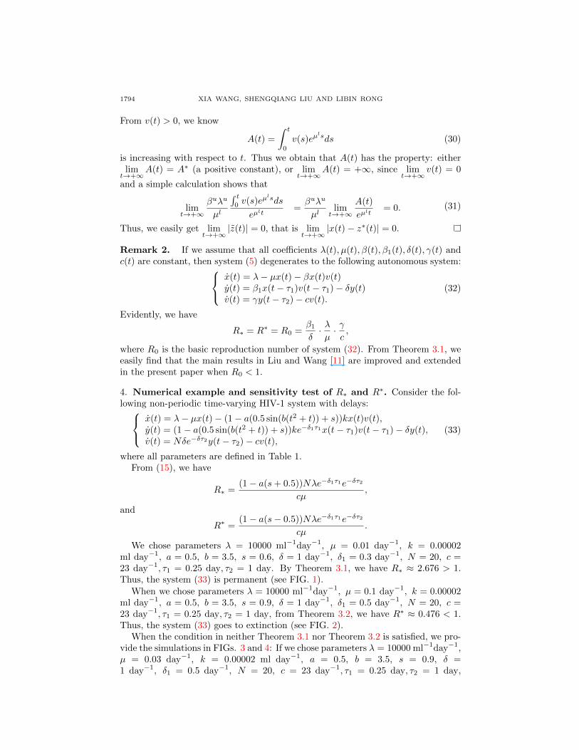
When we chose parameters λ = 10000 ml−1day−1, µ = 0.1 day−1, k = 0.00002ml day−1, a = 0.5, b = 3.5, s = 0.9, δ = 1 day−1, δ1 = 0.5 day−1, N = 20, c =23 day−1, τ1 = 0.25 day, τ2 = 1 day, from Theorem 3.2, we have R∗ ≈ 0.476 < 1.Thus, the system (33) goes to extinction (see FIG. 2).

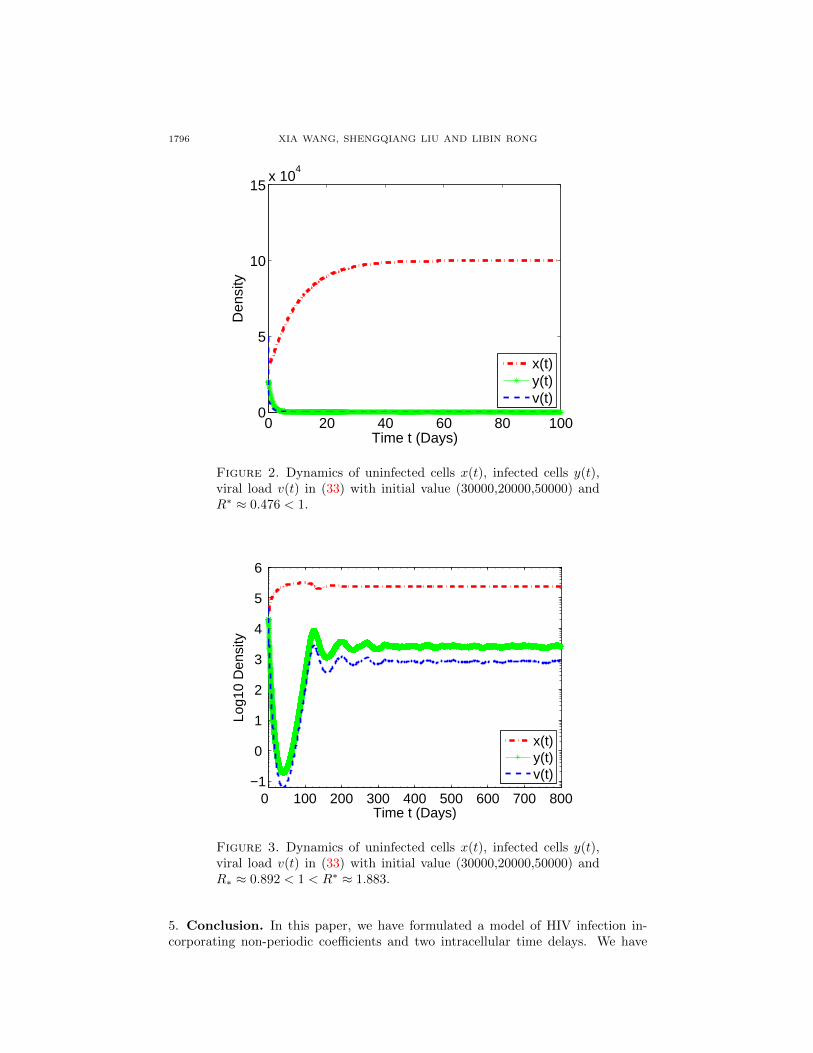
When the condition in neither Theorem 3.1 nor Theorem 3.2 is satisfied, we pro-vide the simulations in FIGs. 3 and 4: If we chose parameters λ = 10000 ml−1day−1,µ = 0.03 day−1, k = 0.00002 ml day−1, a = 0.5, b = 3.5, s = 0.9, δ =1 day−1, δ1 = 0.5 day−1, N = 20, c = 23 day−1, τ1 = 0.25 day, τ2 = 1 day,

A NON-AUTONOMOUS HIV-1 MODEL WITH TWO DELAYS 1795

Table 1. Parameter values in numerical simulations for system (33).

Parameters Base values Reference

λ : Recruitment rate of uninfected cells 104 cellsml−1day−1 [25]

µ : Death rate of uninfected cells 0.01 day−1 [25]

k : Infection rate 2 × 10−5 ml day−1 [23]δ : Death rate of infected cells that have finished RT 1 day−1 [25]

δ1 : Death rate of infected cells that have not finished RT 0.5 day−1 [25]

a : The constant used in time-varying drug efficacy 0.5 —s : The constant used in time-varying drug efficacy 0.6 or 0.9 —

b : The constant used in time-varying drug efficacy 3.5 —

N : Number of virion produced by an infected cell 20 —c : Clearance rate of free virus 23 day−1 [25]

τ1 : Time needed to complete RT 0.25 day [26]

τ2 : Time between RT and the release of new virions 1 day —

we have R∗ ≈ 0.892 < 1 < R∗ ≈ 1.883, and the system (33) is permanent (see FIG.3). If we let µ = 0.1 day−1, N = 50, and other parameters remain unchanged,then we have R∗ ≈ 0.669 < 1 < R∗ ≈ 1.412, and the system (33) goes to extinction(see FIG. 4). Thus, when R∗ < 1 < R∗, both viral persistence and extinction arepossible.

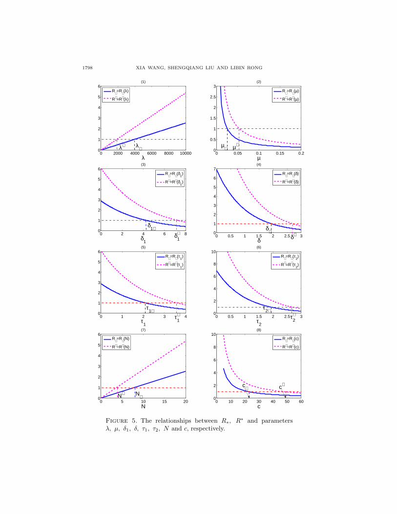
From the analysis we know that R∗, R∗ are important values that determines

whether the virus can be cleared. In FIG. 5, we plotted the change of R∗ (or R∗)as a function of one parameter (all the other parameters were fixed). We obtaineda threshold value for each parameter such that R∗ (or R∗) is 1. Specifically, whenλ < λ∗ (or λ < λ∗), or N < N∗ (or N < N∗), R∗ (or R∗) is less than 1. When µ(or δ1 or δ or τ1 or τ2 or c) is greater than its corresponding threshold value, R∗ (orR∗) is also less than 1.

0 200 400 600 8000

2

4

6

Time t (Days)

Log1

0 D

ensi

ty

x(t)y(t)v(t)

Figure 1. Dynamics of uninfected cells x(t), infected cells y(t),viral load v(t) in (33) with initial value (30000,20000,50000) andR∗ ≈ 2.676 > 1.

1796 XIA WANG, SHENGQIANG LIU AND LIBIN RONG

0 20 40 60 80 1000

5

10

15x 10

4

Time t (Days)

Den

sity

x(t)y(t)v(t)

Figure 2. Dynamics of uninfected cells x(t), infected cells y(t),viral load v(t) in (33) with initial value (30000,20000,50000) andR∗ ≈ 0.476 < 1.

0 100 200 300 400 500 600 700 800−1

0

1

2

3

4

5

6

Time t (Days)

Log1

0 D

ensi

ty

x(t)y(t)v(t)

Figure 3. Dynamics of uninfected cells x(t), infected cells y(t),viral load v(t) in (33) with initial value (30000,20000,50000) andR∗ ≈ 0.892 < 1 < R∗ ≈ 1.883.

5. Conclusion. In this paper, we have formulated a model of HIV infection in-corporating non-periodic coefficients and two intracellular time delays. We have

A NON-AUTONOMOUS HIV-1 MODEL WITH TWO DELAYS 1797

0 20 40 60 80 1000

5

10

15x 10

4

Time t (Days)

Den

sity

x(t)y(t)v(t)

Figure 4. Dynamics of uninfected cells x(t), infected cells y(t),viral load v(t) in (33) with initial value (30000,20000,50000) andR∗ ≈ 0.669 < 1 < R∗ ≈ 1.412.

developed a rigorous analysis of the model by applying the oscillation theory andthe comparison theory of differential equations.

Our analysis yields two positive constants R∗ and R∗ (see (15)), both of whichcan be explicitly expressed by the parameters of the system, to obtain conditionsfor the permanence and extinction of the virus. We derived a sufficient condition(R∗ > 1) for the permanence of this general system (see Theorem 3.1 and FIG.1), and a sufficient condition (R∗ < 1) for the clearance of the virus (see Theorem3.2 and FIG. 2). From these results, we can obtain the complicated effects of thetime-varying parameters on the sufficient conditions for the permanence and theextinction of the model.

When R∗ > 1 (i.e., the system is permanent), based on the explicitly parameter-

dependent values q2 and L2, we obtain estimates of the lower and upper bounds ofthe viral load and their dependence on the parameters. When all the coefficientsare constant, the two values R∗ and R∗ reduce to the basic reproductive number ofthe corresponding autonomous system (see Remark 2), and thus our work improvedsome existing results of HIV models including time delays [11].

We performed numerical simulations using non-periodic drug effectiveness. Thenumerical results confirmed our theoretical analysis. We also obtained the corre-sponding permanence threshold values for all the parameters (see FIG. 5). Thesevalues are important in determining whether the virus can be eradicated from in-fected individuals. Moreover, our simulations suggest the significant differences inthe sensitivities of R∗ and R∗ to the different coefficients of the model.

We remark that the dynamics of our model are still unclear for the case ofR∗ < 1 < R∗, in which the virus may be persistent (see FIG. 3) or cleared (seeFIG. 4) under this condition. It remains an interesting future problem for a non-autonomous HIV model.

1798 XIA WANG, SHENGQIANG LIU AND LIBIN RONG

0 2000 4000 6000 8000 100000

1

2

3

4

5

6

λ

(1)

R∗=R

∗(λ)

R∗ =R∗ (λ)

λ∗ λ∗0 0.05 0.1 0.15 0.2

0

0.5

1

1.5

2

2.5

3

µ

(2)

R∗=R

∗(µ)

R∗ =R∗ (µ)

µ∗µ∗

0 2 4 6 80

1

2

3

4

5

6

δ1

(3)

R∗=R

∗(δ

1)

R∗ =R∗ (δ1)

δ1∗

δ1∗

0 0.5 1 1.5 2 2.5 30

1

2

3

4

5

6

7

δ

(4)

R∗=R

∗(δ)

R∗ =R∗ (δ)

δ∗δ∗

0 1 2 3 40

1

2

3

4

5

6

τ1

(5)

R∗=R

∗(τ

1)

R∗ =R∗ (τ1)

τ1∗

τ1∗

0 0.5 1 1.5 2 2.5 30

2

4

6

8

10

τ2

(6)

R∗=R

∗(τ

2)

R∗ =R∗ (τ2)

τ2∗

τ2∗

0 5 10 15 200

1

2

3

4

5

6

N

(7)

R∗=R

∗(N)

R∗ =R∗ (N)

N∗N∗

0 10 20 30 40 50 600

2

4

6

8

10

c

(8)

R∗=R

∗(c)

R∗ =R∗ (c)

c∗c∗

Figure 5. The relationships between R∗, R∗ and parametersλ, µ, δ1, δ, τ1, τ2, N and c, respectively.

A NON-AUTONOMOUS HIV-1 MODEL WITH TWO DELAYS 1799

In the previous works, by using the methods of persistence theory, thresholddynamics for periodic HIV-1 models were established [14, 35]. However, the methodsused in these references are not applicable to our non-autonomous model (3) sincethe coefficients are not necessarily periodic. Our methods may be used in theanalysis of permanence and extinction for other general time-varying mathematicalmodels (with or without delay).

Acknowledgments. We thank two anonymous reviewers and the editor for theirhelpful suggestions and comments which led to improvement of our original man-uscript. XW is supported by the NNSF of China (No.11301453, 11171284) andprogram for Innovative Research Team (in Science and Technology) in University ofHenan Province (2010IRTSTHN006) and the Natural Science Foundation of HenanProvince (No.142300410198). SL is supported by the Fundamental Research Fundsfor the Central Universitys (Grant No. HIT. IBRSEM. A. 201401). LR is supportedby the NSF grant DMS-1122290 and Oakland University Research Excellence Fund.

REFERENCES

[1] C. Browne and S. Pilyugin, Periodic multidrug therapy in a within-host virus model, Bulletin

of Mathematical Biology, 74 (2012), 562–589.[2] K. Dietz, The incidence of infectious diseases under the influence of seasonal fluctuations,

in Mathematical Models in Medicine, Lecture Notes in Biomathematics 11 , Springer-Verlag,

New York, 11 (1976), 1–15.[3] S. Dowell, Seasonal variation in host susceptibility and cycles of certain infectious diseases,

Emerging Infectious Diseases, 7 (2001), 369–374.

[4] P. De Leenheer, Within-host virus models with periodic antiviral therapy, Bulletin of Math-ematical Biology, 71 (2009), 189–210.

[5] N. Grassly and C. Fraser, Seasonal infectious disease epidemiology, Proceedings of the Royal

Society B: Biological Sciences, 273 (2006), 2541–2550.[6] A. Herz, S. Bonhoeffer, R. Anderson, R. May and M. Nowak, Viral dynamics in vivo: Limita-

tions on estimates of intracellular delay and virus decay, Proceedings of the National Academy

of Sciences, 93 (1996), 7247–7251.[7] H. Hethcote, Asymptotic behavior in a deterministic epidemic model, Bulletin of Mathemat-

ical Biology, 36 (1973), 607–614.[8] D. Ho and Y. Huang, The HIV-1 vaccine race, Cell, 110 (2002), 135–138.

[9] Y. Huang, S. Rosenkranz and H. Wu, Modeling HIV dynamics and antiviral response with

consideration of time-varying drug exposures, adherence and phenotypic sensitivity, Mathe-matical Biosciences, 184 (2003), 165–186.

[10] T. Kepler and A. Perelson, Drug concentration heterogeneity facilitates the evolution of drug

resistance, Proceedings of the National Academy of Sciences, 95 (1998), 11514–11519.[11] S. Liu and L. Wang, Global stability of an HIV-1 model with distributed intracellular delays

and a combination therapy, Mathematical biosciences and engineering, 7 (2010), 675–685.

[12] Y. Lou and X.-Q. Zhao, Threshold dynamics in a time-delayed periodic SIS epidemic model,Discrete and Continuous Dynamical Systems. Series B, 12 (2009), 169–186.

[13] Y. Lou and X.-Q. Zhao, A climate-based malaria transmission model with structured vector

population, SIAM Journal on Applied Mathematics, 70 (2010), 2023–2044.[14] J. Lou, Y. Lou and J. Wu, Threshold virus dynamics with impulsive antiretroviral drug effects,

Journal of Mathematical Biology, 65 (2012), 623–652.[15] Z. Ma, M. Stone, M. Piatak, B. Schweighardt, N. L. Haigwood, D. Montefiori, J. D. Lifson,

M. Busch and C. J. Miller, High specific infectivity of plasma virus from the pre-ramp andramp up stages of acute simian immunodeficiency virus infection, Journal of Virology, 83(2009), 3288–3297.

[16] M. Martcheva, A non-autonomous multi-strain SIS epidemic model, Journal of Biological

Dynamics, 3 (2009), 235–251.[17] P. Nelson, J. Murray and A. Perelson, A model of HIV-1 pathogenesis that includes an

intracellular delay, Mathematical Biosciences, 163 (2000), 201–215.

1800 XIA WANG, SHENGQIANG LIU AND LIBIN RONG

[18] P. Nelson, J. Mittler and A. Perelson, Effect of drug efficacy and the eclipse phase of theviral life cycle on estimates of HIV-1 viral dynamic parameters, Journal of Acquired Immune

Deficiency Syndromes, 26 (2001), 405–412.

[19] P. Nelson and A. Perelson, Mathematical analysis of delay differential equation models ofHIV-1 infection, Mathematical Biosciences, 179 (2002), 73–94.

[20] M. A. Nowak and R. M. May, Virus Dynamics: Mathematical Principles of Immunology andVirology, Oxford University Press, Oxford, 2000.

[21] K. Pawelek, S. Liu, F. Pahlevani and L. Rong, A model of HIV-1 infection with two time

delays: Mathematical analysis and comparison with patient data, Mathematical Biosciences,Mathematical Biosciences, 235 (2012), 98–109.

[22] A. Perelson and P. Nelson, Mathematical analysis of HIV-I dynamics in vivo, SIAM Review,

41 (1999), 3–44.[23] A. Perelson, D. Kirschner and R. de Boer, Dynamics of HIV infection of CD4+ T cells,

Mathematical Biosciences, 114 (1993), 81–125.

[24] A. Perelson, A. Neumann, M. Markowitz, J. Leonard and D. Ho, HIV-1 dynamics in vivo:Virion clearance rate, infected cell life-span, and viral generation time, Science, 271 (1996),

1582–1586.

[25] L. Rong, Z. Feng and A. Perelson, Emergence of HIV-1 drug resistance during antiretroviraltreatment, Bulletin of Mathematical Biology, 69 (2007), 2027–2060.

[26] L. Rong, Z. Feng and A. Perelson, Mathematical Analysis of Age-Structured HIV-1 Dynamicswith Combination Antiretroviral Therapy, SIAM Journal on Applied Mathematics, 67 (2007),

731–756.

[27] G. Samanta, Permanence and extinction of a nonautonomous HIV/AIDS epidemic model withdistributed time delay, Nonlinear Analysis: Real World Applications, 12 (2011), 1163–1177.

[28] H. L. Smith, Multiple stable subharmonics for a periodic epidemic model, Journal of Mathe-

matical Biology, 17 (1983), 179–190.[29] H. Thieme, Uniform weak implies uniform strong persistence for non-autonomous semiflows,

Proceedings of the American Mathematical Society, 127 (1999), 2395–2403.

[30] H. Thieme, Uniform persistence and permanence for non-autonomous semiflows in populationbiology, Mathematical Biosciences, 166 (2000), 173–201.

[31] N. Vaidya, R. Ribeiro, C. Miller and A. Perelson, Viral dynamics during primary simian im-

munodeficiency virus infection: effect of time-dependent virus infectivity, Journal of Virology,84 (2010), 4302–4310.

[32] K. Wang, W. Wang and X. Liu, Viral infection model with periodic lytic immune response,Chaos Solitons & Fractals, 28 (2006), 90–99.

[33] W. Wang and X.-Q. Zhao, Threshold dynamics for compartmental epidemic models in periodic

environments, Journal of Dynamics and Differential Equations, 20 (2008), 699–717.[34] X. Wang and Y. Tao, Lyapunov function and global properties of virus dynamics with CTL

immune response, International Journal of Biomathematics, 1 (2008), 443–448.[35] Y. Yang, Y. Xiao and J. Wu, Pulse HIV vaccination: Feasibility for virus eradication and

optimal vaccination schedule, Bulletin of Mathematical Biology, 75 (2013), 725–751.

[36] T. Zhang and Z. Teng, On a nonautonomous SEIRS model in epidemiology, Bulletin of

Mathematical Biology, 69 (2007), 2537–2559.

Received May 2013; revised November 2013.

E-mail address: xywangxia@163.com

E-mail address: sqliu@hit.edu.cn

E-mail address: rong2@oakland.edu