Extinction thresholds for species in fractal landscapes

$: Extinction thresholds for species in fractal landscapes$
314

Conservation Biology, Pages 314–326Volume 13, No. 2, April 1999

Extinction Thresholds for Species in Fractal Landscapes

KIMBERLY A. WITH* AND ANTHONY W. KING†

*Department of Biological Sciences, Bowling Green State University, Bowling Green, OH 43403, U.S.A., email [email protected]†Environmental Sciences Division, Oak Ridge National Laboratory, Oak Ridge, TN 37831, U.S.A., email [email protected]

Abstract:

Predicting species’ responses to habitat loss and fragmentation is one of the greatest challenges fac-ing conservation biologists, particularly if extinction is a threshold phenomenon. Extinction thresholds areabrupt declines in the patch occupancy of a metapopulation across a narrow range of habitat loss. Metapop-ulation-type models have been used to predict extinction thresholds for endangered populations. These modelsoften make simplifying assumptions about the distribution of habitat (random) and the search for suitablehabitat sites (random dispersal). We relaxed these two assumptions in a modeling approach that combines ametapopulation model with neutral landscape models of fractal habitat distributions. Dispersal success forsuitable, unoccupied sites was higher on fractal landscapes for nearest-neighbor dispersers (moving throughadjacent cells of the landscape) than for dispersers searching at random (random distance and direction be-tween steps) on random landscapes. Consequently, species either did not suffer extinction thresholds or extinc-tion thresholds occurred later, at lower levels of habitat abundance, than predicted previously. The exception

is for species with limited demographic potential, owing to low reproductive output (

R

9

o

5

1.01), in which ex-tinction thresholds occurred sooner than on random landscapes in all but the most clumped fractal land-scapes (

H

5

1.0). Furthermore, the threshold was more precipitous for these species. Many species of conserva-tion concern have limited demographic potential, and these species may be at greater risk from habitat lossand fragmentation than previously suspected.

Umbrales de Extinción para Especies en Paisajes Fraccionados

Resumen:

La predicción de las respuestas de especies a la pérdida del hábitat y su fragmentación es uno delos retos más grandes a los que se enfrentan los biólogos conservacionistas, particularmente si la extinción esun fenómeno de umbrales. Los umbrales de extinción son declinaciones abruptas en la ocupación de parchede una metapoblación a lo largo de un rango somero de pérdida de hábitat. Los modelos de tipo metapobla-cional han sido usados para predecir umbrales de extinciones para poblaciones amenazadas. Estos modelosfrecuentemente simplifican las suposiciones sobre la distribución del hábitat (al azar) y la busqueda de sitiosde hábitat apropiado (dispersión al azar). Relajamos estas dos suposiciones en un modelo que combina unmodelo de metapoblación con modelos de paisaje neutral de distribuciones de hábitat fracturados. El éxito dedispersión para sitios disponibles y desocupados fue mayor en paisajes fracturados para dispersores del ve-cino más cercano (moviéndose a través de celdas en el paisaje), que para dispersores en busquedas al azaren paisajes aleatorios (distancia al azar y dirección entre pasos). Consecuentemente, las especies no sufrieronumbrales de extinción o los umbrales ocurrieron más tarde, a niveles aún mas bajos de abundancia del hábi-tat que los predecidos anteriormente. La excepción es para especies con potencial demográfico limitado, de-bido a un bajo rendimiento reproductivo (

R

9

o

5

1.01), en las cuales los umbrales de extinción ocurren mástemprano que en paisajes aleatorios, en todos los paisajes fraccionados excepto aquellos muy ramificados(

H

5

1.0). Más aún, los umbrales fueron más precipitados en estas especies. Muchas de las especies de impor-tancia en conservación tienen un potencial geográfico limitado y podrían estar en un riesgo mayor al previ-

amente supuesto, debido a la pérdida de hábitat y a la fragmentación.

Paper submitted December 8, 1997; revised manuscript accepted June 24, 1998.

Conservation BiologyVolume 13, No. 2, April 1999

With & King Extinction Thresholds in Fractal Landscapes

315

Introduction

Critical thresholds in species’ responses to habitat frag-mentation have serious implications for the conservationof biodiversity. In this context, a critical threshold is anabrupt, nonlinear change that occurs in some parameteracross a small range of habitat loss. Neutral landscapemodels, derived from percolation theory in the field oflandscape ecology (Gardner & O’Neill 1991; With 1997;With & King 1997), characterize habitat fragmentation asa threshold phenomenon. Above the threshold, habitatdestruction results in a simple loss of suitable habitat; theeffect of habitat loss on landscape structure is a quantita-tive one, a reduction in the proportion of habitat (

h

) onthe landscape (e.g., Andrén 1994; Bascompte & Solé1996). A qualitative change in landscape structure occursat the threshold: a small additional loss of habitat at thispoint produces a fragmented landscape in which habitatis dissected into many small, isolated patches. Furtherhabitat loss can lead to further fragmentation. The thresh-old at which landscapes become fragmented is defined bythe presence or absence of a continuous cluster of habitatthat spans the entire landscape (the

percolating cluster

).It is the disruption of the percolating cluster that pro-duces a threshold in landscape connectivity (With 1997).The level of habitat loss at which this threshold in land-scape connectivity occurs is determined by the pattern ofhabitat distribution and the dispersal capabilities of thespecies (With & Crist 1995; Pearson et al. 1996; With1997; With et al. 1997).

If habitat loss leads to a critical threshold in landscapeconnectivity—fragmentation—then the ecological conse-quences of habitat fragmentation may also exhibit thresh-old behavior. Consider that an abrupt decline in land-scape connectivity may interfere with dispersal success(Wiens et al. 1997; With & King, in press) such that for-merly widespread populations may suddenly becomefragmented into small, isolated patches (Andrén 1994;With & Crist 1995). This may in turn lead to an abrupt de-cline in patch occupancy and extinction of the popula-tion across the landscape (extinction thresholds; Lande1987; Kareiva & Wennergren 1995; Bascompte & Solé1996; Ritchie 1997). Because habitat fragmentation canhave nonlinear effects, it may be difficult to predict theconsequences of land-use change or habitat destructionfor biodiversity until the threshold is exceeded. Thus, crit-ical threshold phenomena have been identified as “a ma-jor unsolved problem facing conservationists” (Pulliam &Dunning 1997).

It is desirable to understand under what conditions ex-tinction thresholds occur as a result of habitat loss andfragmentation. Are extinction thresholds, for example,coincident with thresholds in landscape connectivity?One of the most useful applications of spatial models inconservation biology is to alert conservationists to thepotential consequences of habitat fragmentation (Wen-

nergren et al. 1995). We present a synthesis of metapop-ulation theory and percolation theory in which we cou-ple Lande’s (1987) demographic model of extinctionthresholds for territorial populations with neutral land-scape models. This modeling synthesis enables us to in-vestigate the relative effects of landscape pattern, habi-tat loss, and fragmentation on population persistence forspecies with different dispersal abilities and life-historytraits. We show how relaxing assumptions in Lande’soriginal model, concerning habitat distribution and thesearch behavior of individuals seeking suitable habitat,influences whether and under what conditions extinc-tion thresholds occur.

Extinction Thresholds of Territorial Populations

Lande (1987) extended Levins’s (1969) metapopulationmodel to quantify extinction thresholds—the minimumproportion of suitable habitat necessary for populationpersistence—for territorial species with different life-his-tory characteristics and dispersal abilities. In this model alandscape is divided into discrete territories of equal size.A proportion

h

of these territories is designated as suit-able for survival and reproduction, and territories are as-sumed to be distributed randomly across the landscape.The proportion of unsuitable territories is

u

5

1

2

h.

Each territory can be occupied by only one pair or re-productive female, and juveniles either inherit their na-tal territory with constant probability

e

or disperse andsearch up to

m

territories for a suitable, unoccupied site.Assuming random encounter with potential territories,the probability that a juvenile successfully finds a suit-able unoccupied territory is

(1)

where

p

is the proportion of suitable territories alreadyoccupied by adult females. At demographic equilibrium,the proportion of suitable, occupied territories is givenby the Euler-Lotka equation, which identifies the net life-time reproductive output (female offspring per female,

R

o

) with unity, or

(2)

where

R

9

o

is the net lifetime production of female off-spring per female, which depends on their finding a suit-able territory. The proportion of suitable territories oc-cupied by females at demographic equilibrium is then

(3)

where

(4)

1 1 e–( )– u ph+( )m,

1 1 e–( ) u p*h+( )m–[ ] R ′o 1,=

p* 1 1 k–( )/h–= if h 1 k,–>

or p* 0 if h 1 k–≤( ),=

k 1 1 R ′o⁄–( ) 1 e–( )⁄[ ] 1/m= .

316

Extinction Thresholds in Fractal Landscapes With & King


Lande referred to the composite parameter

k

as thedemographic potential of the population. It incorpo-rates both reproductive output

R

9

o

and dispersal ability

m

. The parameter

k

also gives the maximum occupancyof territories at equilibrium when the entire landscape issuitable (

h

5

1.0). The extinction threshold is at

h

5

1

2

k

, where

p

*

5

0 (Fig. 1). The population can persistonly when the proportion of suitable habitat or territo-ries is greater than 1

2

k

. Lande’s model also predicts thatspecies will not occupy all available habitat, even whenthe entire landscape is suitable; a proportion 1

2

k

ofthe sites will remain unoccupied when

h

5

1.0 (Fig. 1).The equilibrium occupancy of sites as a function of

habitat loss is of conservation interest. For example, aspecies with low demographic potential (e.g.,

k

5

0.20), either as a consequence of low reproductive ca-pacity or limited dispersal ability or both, cannot persistif suitable habitat is reduced below 80% (Fig. 1). A spe-cies with greater demographic potential (e.g.,

k

5

0.80),due to its higher reproductive output or better dispersalability, will occupy a greater proportion of suitable terri-tories (80% when

h

5

1.0) and will be able to persist atlower proportions of suitable habitat (Fig. 1). As habitatloss approaches the extinction threshold, however, arelatively small change in the amount of suitable habitatwill result in a disproportionately large decline in

p

*. Forexample, consider a species with

k

5

0.9. A change insuitable habitat from 90% to 80% would have relativelylittle impact on

p

*, whereas a similar amount of habitatloss from 20% to 10% would result in extinction of thepopulation (Fig. 1).

Dispersal Success in Fractal Landscapes

Lande’s model assumes that suitable territories are ran-domly distributed across the landscape. Random land-scape structure is a practical null model for assessing theecological consequences of habitat fragmentation (Gard-ner et al. 1987, 1993; With & King 1997), and Lande’smodel has been useful for predicting the effects of habi-tat destruction on endangered populations such as theNorthern Spotted Owl (

Strix occidentalis caurina

; Lande1988; Lamberson et al. 1992; Noon & McKelvey 1996).Habitats are often patchily distributed, however, and theassumption of random distribution may not be validwhen the model is applied to natural landscapes. Howdoes a clumped, nonrandom distribution of suitable hab-itat affect patch occupancy and extinction thresholdspredicted by Lande’s model?

Fractal algorithms are increasingly being used to gener-ate complex spatial patterns for habitat and other resourcedistributions (Milne 1992; Palmer 1992; With et al. 1997).A fractal distribution of habitat results in landscapes that arestatistically more clumped than a random landscape (Withet al. 1997; Fig. 2). The clumping of habitat is determinedby the fractal dimension

D

. To a get a sense of this, con-sider fractal landscape maps generated by the midpointdisplacement algorithm (Saupe 1988; Palmer 1992; Withet al. 1997). Although this fractal algorithm generates acontinuously varying surface of “elevation” or “topogra-phy,” it is possible to divide the surface to produce eitherbinary (two-state) landscapes (habitat versus nonhabitat)or heterogeneous landscapes comprised of more thanone habitat type (With et al. 1997). In Fig. 2, the continu-ously varying surface has been truncated at a selected “el-evation” to produce a binary landscape map with a pro-portion

h

of the landscape identified as habitat. Truncatedlandscapes generated from fractal surfaces with a high de-gree of spatial autocorrelation (

H

5

1.0) have extremelyclumped habitat distributions. At the opposite extreme,habitat is distributed as small, isolated patches for trun-cated landscapes generated from fractal distributions withlow spatial autocorrelation (

H

5

0.0; Fig. 2). Fractal land-scapes provide a means of systematically controlling boththe amount (

h

) and spatial contagion (

H

) of habitat. It istherefore possible to tease apart the effects of habitat lossper se from those of fragmentation (or changes in spatialdistribution) on population persistence. The terms

habi-tat

loss

and

fragmentation

are often used synonymously(e.g., Noon & McKelvey 1996). Habitat loss does not nec-essarily lead to fragmentation, however (Fahrig 1997). Weadopted the definition of fragmentation as a disruption inlandscape connectivity (a threshold phenomenon; Gard-ner et al. 1987, 1993; With 1997), as defined by percola-tion theory in the implementation of neutral landscapemodels. Fragmentation is thus a qualitative change in land-scape structure apart from a quantitative change in loss oftotal habitat area (Andrén 1994; Bascompte & Solé 1996).

Figure 1. The proportion of territories occupied at de-mographic equilibrium for species with different de-mographic potentials ( k) on random landscapes (af-ter Lande 1987). Extinction thresholds are given by the value of h where p* 5 0. Different curves corre-spond to species with different demographic poten-tials.


With & King Extinction Thresholds in Fractal Landscapes

317

Lande’s model also assumes that dispersing juvenilesrandomly encounter potential territories. This can occureither when suitable territories are randomly distributedacross the landscape or when dispersal is a randomwalk, random with respect to both direction and dis-tance at each step. If juvenile dispersal is truly randomand the dispersing individual can randomly sample theentire landscape, the assumption of random encounterwith potential territories holds regardless of the spatialdistribution of suitable habitat. Lande’s model thus ap-plies to both random and clumped (fractal) landscapes.The distribution of habitat does not affect the ability ofindividuals to locate suitable habitat; only the abun-dance of habitat,

h

, affects dispersal success under theassumption of random dispersal or encounter with suit-able habitat.

The assumption of random encounter is also a “good ap-proximation when suitable territories are evenly (ratherthan randomly) distributed,

if the root-mean-squared dis-persal distance of individuals is much larger than thedistance between suitable territories” (Lande 1987:625;emphasis ours). If, however, the scale at which juvenilessearch for suitable territories is fine relative to the scale ofthe landscape pattern, such as when the juvenile is con-strained to search in the neighborhood of its natal terri-tory, then the assumption of random encounter is neithervalid nor a good approximation when suitable habitat isclumped rather than randomly distributed. In this circum-stance a clumped distribution of habitat should increasedispersal success over that for a random distribution (e.g.,Doak 1989; Doak et al. 1992; Adler & Nuerenberger 1994;Lamberson et al. 1994). We therefore relaxed Lande’s as-sumption regarding dispersal behavior (effectively an as-sumption of random dispersal). We constrained dispersersto search in the neighborhood of their natal territory andredefined the scale at which individuals interact with thepatch structure of the landscape.

A challenge in developing this synthesis betweenmetapopulation theory and neutral landscape modelslies in defining dispersal success on a fractal landscapewithin the analytical framework of Lande’s model. In do-ing so we can investigate the consequences of our alter-native assumptions about habitat distribution and dis-persal behavior by direct comparison with the analyticalresults of Lande’s extinction threshold model. We havenot been able to derive a closed-form solution for dis-persal success (assuming fine-scale local dispersal) on abinary fractal landscape from a “first principle” consider-ation of the probability of encounter with suitable terri-tories. A closed-form solution may not exist. Instead, weapproximated the probability of dispersal success byfirst simulating dispersal success on fractal landscapesthat vary in habitat abundance (h) and spatial contagion(H). We then fit a mathematical function to describe therelationship between dispersal success and landscapestructure (h and H), which we can substitute for equa-tion 1, the probability that a juvenile finds a suitable un-occupied territory. This was then substituted in equa-tion 2, which we solved for p*, the expected proportionof territories occupied at demographic equilibrium in afractal landscape, to compare with the response curvesgenerated by Lande’s model (Fig. 1).

Description of Simulation Model

We simulated dispersal on fractal landscape maps gener-ated by the midpoint displacement algorithm, in whichwe varied habitat abundance, h, and spatial contagion(H; Fig. 2). Each map was a square lattice of 128 rowsand 128 columns. Cells were labeled as either suitable orunsuitable habitat; each cell represented a territory as inLande’s model. We represented landscapes as binaryhabitat maps—suitable versus unsuitable habitat—to re-

Figure 2. Fractal landscapes generated by midpoint displacement with different levels of spatial contagion or “clumping” (H). Habitat abundance ( h) is 50% in all maps.

318 Extinction Thresholds in Fractal Landscapes With & King


main consistent with Lande’s model, but it is possible togenerate heterogeneous landscape maps with habitatsof different quality or suitability (e.g., With et al. 1997).We generated fractal landscapes for 3 levels of conta-gion (H 5 0.0, 0.5, 1.0; Fig. 2) and 9 levels of habitatabundance (h 5 0.1, 0.2, ..., 0.9). Because the probabil-ity of successfully finding a territory is also a function ofp, the proportion of sites already occupied (equation 1),we included 10 levels of habitat occupancy ( p 5 0.0,0.1, ..., 0.9). Occupied cells were randomly distributedamong suitable habitat cells; the proportion of suitableunoccupied sites is thus (1 2 p)h. The simulations thusinvolved a factorial of 3 levels of H (landscape pattern),9 levels of h (habitat abundance), and 10 levels of p(prior occupancy), or 270 (3 3 9 3 10) different land-scape configurations.

Dispersal was initiated from a randomly selected natal(i.e., occupied) cell of suitable habitat. In these simula-tions we assumed that e, the probability of inheriting thematernal cell, was zero, so all juveniles were forced to dis-perse (obligate juvenile dispersal). Dispersal was modeledas a nearest-neighbor random lattice walk, in which thedisperser could move only into one of the four neighbor-ing grid cells (vertically and horizontally adjacent) at eachstep; the direction of movement (the cell to which thedisperser moved) was chosen randomly with equal (0.25)probability. Individuals were able to move through habi-tat as well as nonhabitat cells in their search for a suitableunoccupied territory. By constraining individuals to moveonly through adjacent cells, we tended to restrict dis-persal to the neighborhood of the natal territory. We des-ignated this dispersal behavior as nearest-neighbor dis-persal (NND) to distinguish it from the effectively randomor broader-scale dispersal of Lande’s model, which wedesignated as random dispersal (RD). Nearest-neighbordispersal effectively altered the scale of dispersal, suchthat the organism interacted with the spatial pattern ofthe landscape at a finer scale than in RD.

The edge of the landscape map was modeled as a re-flective barrier. Edge effects (Haefner et al. 1991) wereunlikely given the extremely large size of these land-scape grids (16,384 cells), the large number (n 5 1000)of individuals that were run independently on thesemaps, and the limited number of grid cells (m 5 50) dis-persers could search for a suitable unoccupied territory.Individuals were allowed to move until they encoun-tered an unoccupied cell of suitable habitat and werescored as a success or until they had made a total of m 550 steps without finding a territory and were scored as afailure and “died.” No other cost to dispersal was as-sessed in this version of the model, to keep it generaland consistent with Lande’s original formulation (butfor a treatment of continuous mortality during dispersalsee Carroll & Lamberson 1993). Dispersal success wasscored for a total of n 5 1000 independent individualsfor each landscape configuration (n 5 270). The proba-

bility of successfully finding a suitable territory was theproportion of dispersal trials (individuals) scored as asuccess on each landscape.

Comparison of Dispersal Success on Random and Fractal Landscapes

Nearest-neighbor dispersers generally had greater suc-cess in finding suitable habitat on fractal landscapes thandid random dispersers on random landscapes, especiallywhen dispersal was limited and habitat was rare (Fig. 3).The poorest nearest-neighbor dispersers (m 5 1) search-ing for rare habitat (h 5 0.1) in even the most frag-

Figure 3. Probability of successfully finding a suitable, unoccupied territory for nearest-neighbor dispersal on different fractal landscapes with different proportions of habitat ( h). Prior patch occupancy (p) is set to p 5 0 in this example so that the effects of landscape struc-ture ( h and H) on dispersal success are apparent. Solid lines are the dispersal success for random dis-persers on random landscapes derived from Lande’s (1987) model (equation 1 in text).


With & King Extinction Thresholds in Fractal Landscapes 319

mented fractal landscapes (H 5 0.0) were able to findsuitable habitat 50% of the time. By comparison, only10% of poor dispersers searching at random on a ran-dom landscape were successful. Dispersal success in-creased for nearest-neighbor dispersers with increasedclumping of suitable habitat. When suitable habitat wasrare (h 5 0.1), success rates increased to greater than80% for NND in highly clumped landscapes (0.5 # H #1.0; top panel, Fig. 3). The enhanced search success ofNND diminished as dispersal range (m) or habitat abun-dance (h) increased, however. When most of the land-scape was suitable (h $ 0.5), NND was more successfulthan RD for only the poorest dispersers (m , 5). Whenhabitat was abundant (h 5 0.9), success in locating suit-able habitat was 90% or more for even the poorest dis-persers (m 5 1) and was nearly absolute when m $ 2,regardless of the underlying pattern of habitat distribu-tion (Fig. 3).

Not surprisingly, the probability of successfully find-ing a suitable unoccupied territory increased with dis-persal range (m) and decreased as degree of habitat oc-cupancy p increased (Fig 4). There were, however,significant interactions between dispersal ability andprior occupancy, whereas the proportion of suitablehabitat had a smaller effect. When suitable habitat wascommon (h 5 0.9), poor dispersers (m 5 1) on nearlysaturated landscapes (p = 0.9) had only a 10% chance offinding a territory, compared to a 50% chance when thehabitat was half occupied or 90% when only 10% occu-pied (Fig. 4 for h 5 0.9). When habitat was rare (h 50.1) or covered half the landscape (h 5 0.5), the proba-bility of success for poor dispersers decreased to lessthan 50% when half the suitable habitat was occupied( p 5 0.5) and was 80% when only 10% was occupied( p 5 0.1; Fig. 4). These differences were ameliorated bythe dispersal range (m) of the species, however. Whenprior occupancy was low (0.1 # p # 0.5), the probabil-ity of successfully finding a territory was 100% whenm $ 10. Available territories were more difficult to findin heavily occupied landscapes ( p 5 0.9), as expected;success was not certain even for species with excep-tional dispersal abilities (m 5 50) unless habitat wasabundant (h 5 0.9; Fig. 4).

Extinction Thresholds on Fractal Landscapes

To incorporate dispersal success on fractal landscapes inLande’s analytical framework, we fitted the simulationresults (Figs. 3 & 4) with a mathematical function thatcould be substituted for equation 1 and applied in equa-tion 2. Dispersal success for NND on fractal landscapesis described by the equation

(5)

where e, p, and m are as in equation 1; h9 5 a 1 bh,

Pr(success) 1 1 ε–( ) 1([ h′ )– mβ1

ph( ′ )mβ2+ ],–=

where h is the abundance of habitat and a and b are fit-ted parameters that vary with the spatial contagion H ofthe landscape. The parameters b1 and b2 are also fitted;b1 varies with H, and b2 varies with both H and h. Themathematical form of this function was selected for itsrelative simplicity and consistency with the analyticalform of equation 1; this equation provided the best fitamong several other functions we generated.

Properly calibrated or parameterized (by choice of a,b, b1, and b2), equation 5 provided a good fit to the sim-ulation data, as shown by the comparisons between sim-ulated dispersal success for NND (symbols) on fractallandscapes and the curves generated by equation 5(lines) in Fig. 4. We selected this particular example be-cause it represents the poorest fit of the function to the

Figure 4. Comparison of dispersal success for nearest-neighbor dispersers (symbols) and the fit of the mathe-matical function (lines; equation 5 in text) at different levels of patch occupancy (p) on a fractal landscape ( H 5 0.5) with different proportions of habitat ( h).



simulations (e.g., compare curves for p 5 0.9 at h = 0.9).Even so, it aptly described the behavior of the simulationmodel. The fit improved at lower levels of p and h in thisexample (Fig. 4) and in all other landscape scenarios.

Substituting equation 5 for the Pr(success) term inequation 2, the proportion of suitable territories occu-pied at demographic equilibrium (p*) is given by

(6)

where

(7)

Compare equation 6 with equation 3 and equation 7 withequation 4. Lande presents p* as a function of h for differ-ent values of the composite parameter k (Fig. 1), whichcombines the life-history parameters R9o, m, and e in ameasure of what Lande termed the “demographic poten-tial” (equation 4). To compare our estimates of p* fromequation 6 with those of Lande’s model (equation 3), wedecomposed his composite variable k and made compari-sons for values of R9o, m, and e. If we assume that e 5 0.0(obligate juvenile dispersal), then we need only specify m(dispersal ability) and R9o (reproductive potential).

Model Results

Populations were generally able to persist across a greaterrange of habitat loss on fractal landscapes for nearest-neighbor dispersers than was predicted by Lande’s model(Table 1; Figs. 5–7). Extinction thresholds did not occurat all for species exhibiting modest reproductive poten-tials (R9o $ 1.10) in maximally clumped fractal landscapes(H 5 1.0; Figs. 6 & 7). These species persisted at or nearmaximum patch occupancy (k) across the entire range ofhabitat loss (h 5 0.1–1.0). It was only when the reproduc-tive potential was near replacement (R9o 5 1.01) thatpopulations went extinct on these clumped landscapes,but even then they persisted longer than random dispers-ers on random landscapes (Fig. 5). At the other extreme

p* k([ ′ 1( h′ )– mβ1

– )m

1β2------

] h ,⁄=

k ′ 1 1/R ′o–( )/ 1 e–( )[ ] .=

in extensively fragmented fractal landscapes (H 5 0.0),extinction thresholds occurred sooner for nearest-neigh-bor dispersers with limited-to-moderate reproductive po-tentials (1.01 # R9o # 1.10) than for random dispersers inrandom landscapes (Figs. 5 & 6). The only exception wasfor species that were good dispersers (m 5 20) and had amoderate reproductive potential (R9o 5 1.10), in whichthe extinction threshold occurred later than predicted forrandom dispersers on random landscapes (Fig. 6). Oncepopulations achieved a reproductive potential of R9o 51.25, thresholds either occurred later (m 5 1–7) or not atall (m 5 10–20) in even the most fragmented fractal land-scapes (H 5 0.0, Fig. 7).

Lande’s composite parameter, k, combines the life-history parameters R9o and m into a single index of de-mographic potential (equation 4). The behavior of Lande’smodel is controlled by the composite value of k. For ex-ample, a species with k 5 0.79 will always have an ex-tinction threshold at h 5 0.21 in Lande’s model, regard-less of the combination of R9o and m that contributes tothat particular k value. That is not the case for ourmodel. For example, if a species has an extremely lowreproductive output (R9o 5 1.01) but good dispersalabilities (m 5 20), such that k 5 0.79, populations onfractal landscapes are predicted to go extinct at 50%when H 5 0.0 and at 32% habitat when H 5 0.5 (Fig. 5).In contrast, populations with the same demographic po-tential (k 5 0.79) but with a slightly higher reproductiveoutput (R9o 5 1.10) and a correspondingly lower dis-persal range (m 5 10) are predicted to go extinct at h 50.28 only in highly fragmented fractal landscapes (H 50.0) and at h , 0.1 for less fragmented fractal landscapes(H $ 0.5; Fig. 6). If reproductive output is increased toR9o 5 1.25 and m reduced to 7 to maintain k 5 0.79(Fig. 7), then persistence is greater for nearest-neighbordispersers on fragmented fractal landscapes (H 5 0.0)than for random dispersers on random ones (H 5 0.0:h 5 0.11; random: h 5 0.21; Fig. 7).

In our model, the effects of reproductive output anddispersal ability on extinction thresholds were notequivalent. Reproductive output appeared to be more

Table 1. Summary of population responses to habitat loss in fractal landscapes that vary in spatial contagion (H) for species with different reproductive capacities (R9o) and dispersal abilities (m).*

R9o H 5 1.0 H 5 0.5 H 5 0.0

1.01 for all m: threshold occurs later (at lower values of h)

m 5 1–2: threshold occurs laterm 5 5–20: threshold occurs sooner

m 5 1: threshold occurs marginally laterm 5 2–20: threshold occurs much sooner

1.10 for all m: thresholds not evident; population persists at or near maximum patch occupancy (k)

m 5 1–2: threshold occurs laterm 5 5–20: thresholds not evident;

population persists at or near maximum patch occupancy

m 5 1: threshold occurs marginally laterm 5 2: threshold is the samem 5 5–10: threshold occurs soonerm 5 20: threshold occurs later

1.25 for all m: thresholds not evident; population persists at or near maximum patch occupancy

for all m: thresholds not evident; population persists at or near maximum patch occupancy

m 5 1–7: threshold occurs laterm 5 10–20: thresholds not evident; population

persists at or near maximum patch occupancy

*Comparisons are made between extinction threshold values obtained by our model and those of Lande’s (1987) model in which the habitatdistribution was assumed to be random.



important than dispersal ability in favoring populationpersistence. This is not true for Lande’s model, at leastfor R9o , 2.00. At R9o 5 1.01, extinction thresholds gen-erated from Lande’s model for random dispersers on ran-dom landscapes ranged from h 5 1.0 to h 5 0.2 as dis-persal increased from m 5 1 to m 5 20 (Random, Fig.8). As reproductive output increased from R9o 5 1.01 toR9o 5 2.00 (when m 5 1), the thresholds ranged fromh 5 1.0 to only h 5 0.5 (Random, Fig. 8). For popula-tions on fragmented fractal landscapes (H 5 0.0), extinc-tion thresholds ranged from h 5 0.98 to h 5 0.5 (for R9o 51.01) as a function of increasing dispersal, but rangedfrom h 5 0.98 to h 5 0.11 (at m 5 1) as reproductiveoutput increased (Fig. 8). The relative effect of increasedreproductive output on population persistence becameeven more pronounced in clumped fractal landscapes(H 5 0.5 2 1.0). In these landscapes, populations werepredicted to persist when h $ 0.1 for all species except

those with the lowest reproductive potential (e.g., R9o 51.01). In fractal landscapes with intermediate clumping(H 5 0.5), extinction thresholds ranged from h 5 0.94to h 5 0.33 (for R9o 5 1.01) as dispersal increased (Fig.8). Likewise, in clumped fractal landscapes (H 5 1.0) ex-tinction thresholds ranged from h 5 0.74 to h 5 0.12(for R9o 5 1.01) with increasing dispersal, but even asmall increase in R9o beyond 1.01 pushed the extinctionthresholds to h , 0.10; these species persisted at nearmaximum occupancy across a wide range of habitatabundance (Fig. 8).

Discussion

Predicting extinction risk for populations in the face ofwidespread habitat loss and fragmentation is one of themajor challenges facing conservation biologists. The po-

Figure 5. Equilibrium patch occupancy (p*) for populations with a net lifetime reproductive output R9o 5 1.01 and different dispersal abilities (m). “Random” indicates random dispersal on random landscapes (i.e., Lande’s model); nearest-neighbor dispersal is modeled on fractal landscapes with different levels of spatial contagion ( H) ( k, demographic potential).



tential for threshold responses, such as a precipitous de-cline in the regional persistence of a species owing to asmall loss of habitat near the threshold, makes this task allthe more urgent. The fear, however, is that it may be im-possible to develop general predictions of how species re-spond to scenarios of land-use change leading to habitatloss and fragmentation. As our model results demonstrate,species are predicted to exhibit a diverse array of re-sponses to habitat fragmentation depending upon thespecific combination of life-history traits and dispersal ca-pabilities. Nevertheless, some general patterns emerge.

Clumped habitat distributions enhance dispersal suc-cess for dispersers whose search is at finer scales thanthat of the overall landscape pattern (e.g., Doak et al.1992; Adler & Nuernberger 1994; this study). The criti-cal assumption that we modified in Lande’s (1987) ex-

tinction threshold model pertains to how individuals in-teract with landscape structure. This involved relaxingassumptions about both habitat distribution and dis-persal behavior. We generated fractal landscape pat-terns, which are perhaps more representative of naturalhabitat distributions than the random distribution usedin Lande’s model (Mandelbrot 1983). Fractal landscapescontain fewer, larger habitat patches with less edge thanrandom landscapes, and thus they maintain connectivityacross a greater range of habitat destruction (With et al.1997). In both models, juveniles initiate dispersal fromtheir natal territories, which by definition are in suitablehabitat. In our model, however, we constrained dispers-ers to move through adjacent cells in search of suitablehabitat, rather than effectively searching at randomthroughout the landscape as in Lande’s model. This

Figure 6. Equilibrium patch occupancy (p*) for populations with a net lifetime reproductive output R9o 5 1.10 and different dispersal abilities (m). “Random” indicates random dispersal on random landscapes (i.e., Lande’s model); nearest-neighbor dispersal is modeled on fractal landscapes with different levels of spatial contagion ( H) ( k, demographic potential).



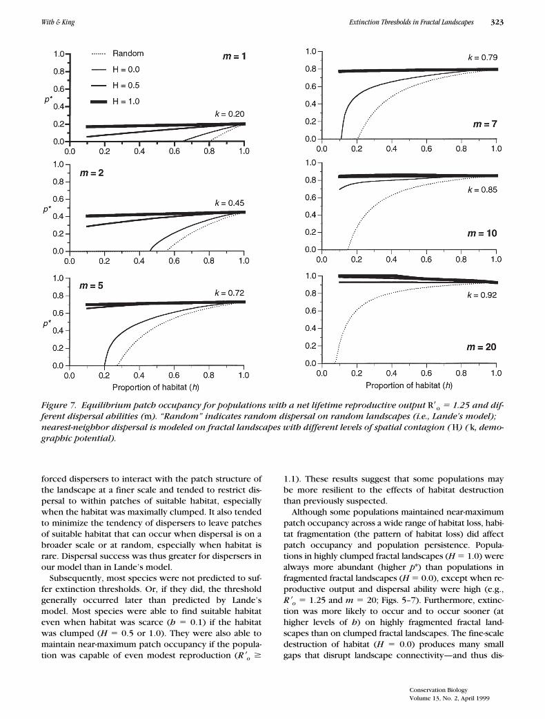
forced dispersers to interact with the patch structure ofthe landscape at a finer scale and tended to restrict dis-persal to within patches of suitable habitat, especiallywhen the habitat was maximally clumped. It also tendedto minimize the tendency of dispersers to leave patchesof suitable habitat that can occur when dispersal is on abroader scale or at random, especially when habitat israre. Dispersal success was thus greater for dispersers inour model than in Lande’s model.

Subsequently, most species were not predicted to suf-fer extinction thresholds. Or, if they did, the thresholdgenerally occurred later than predicted by Lande’smodel. Most species were able to find suitable habitateven when habitat was scarce (h 5 0.1) if the habitatwas clumped (H 5 0.5 or 1.0). They were also able tomaintain near-maximum patch occupancy if the popula-tion was capable of even modest reproduction (R9o $

1.1). These results suggest that some populations maybe more resilient to the effects of habitat destructionthan previously suspected.

Although some populations maintained near-maximumpatch occupancy across a wide range of habitat loss, habi-tat fragmentation (the pattern of habitat loss) did affectpatch occupancy and population persistence. Popula-tions in highly clumped fractal landscapes (H 5 1.0) werealways more abundant (higher p*) than populations infragmented fractal landscapes (H 5 0.0), except when re-productive output and dispersal ability were high (e.g.,R9o 5 1.25 and m 5 20; Figs. 5–7). Furthermore, extinc-tion was more likely to occur and to occur sooner (athigher levels of h) on highly fragmented fractal land-scapes than on clumped fractal landscapes. The fine-scaledestruction of habitat (H 5 0.0) produces many smallgaps that disrupt landscape connectivity—and thus dis-

Figure 7. Equilibrium patch occupancy for populations with a net lifetime reproductive output R9o 5 1.25 and dif-ferent dispersal abilities (m). “Random” indicates random dispersal on random landscapes (i.e., Lande’s model); nearest-neighbor dispersal is modeled on fractal landscapes with different levels of spatial contagion ( H) ( k, demo-graphic potential).



persal success and patch colonization—sooner than ifhabitat is destroyed at a coarser scale (H 5 1.0) so as toleave large, continuous patches of habitat (Pearson et al.1996). The impact of habitat loss and fragmentation mustbe assessed with respect to the scale of the habitat de-struction (e.g., change in spatial pattern) and the scale atwhich the organisms of concern interact with that pattern.

Just because a species does not exhibit an extinctionthreshold, however, does not mean that it is not affectedby habitat loss or fragmentation. A species that maintainsa maximum patch occupancy of 80% across the full rangeof habitat destruction will still occur in fewer patcheswhen habitat is scarce (h 5 0.1) than when the landscapeis totally suitable (h 5 1.0); occupying 80% of habitatpatches when the landscape is totally suitable is clearlypreferable to occupying 80% of the patches when only10% of the landscape is suitable. A reduction in the re-gional distribution of a species could render populationsmore susceptible to demographic and environmental sto-chastic events, produce Allee effects, reduce genetic vari-ability, and lead to an overall decline in population viabil-ity. Furthermore, habitat destruction may produce effectsthat are not apparent until years later (“extinction debt,”

Tilman et al. 1994). Our assessment of population persis-tence is thus based on only one measure—patch occu-pancy—and these other effects should also be consideredto render a full evaluation of population responses to hab-itat loss and fragmentation.

Nevertheless, species with limited reproductive po-tential (R9o 5 1.01) are predicted to go extinct soonerthan predicted by Lande’s model (Fig. 5). Many speciesof management concern have limited reproductive po-tential, which limits their ability to respond to environ-mental disturbance such as anthropogenic habitat frag-mentation. Moreover, the approach to the extinctionthreshold is often more precipitous for these species(Fig. 5). Thus, the effects of habitat fragmentation mayactually be far worse than previously suspected for spe-cies with limited demographic potential, which are of-ten the species of concern to conservation biologists.

In our model the dispersal and demographic compo-nents of the demographic potential (k) are not inter-changeable as in Lande’s model. Because dispersal suc-cess is high for nearest-neighbor dispersers on fractallandscapes, dispersal ability had little effect on extinc-tion thresholds (Fig. 8). Instead, reproductive capacity

Figure 8. Extinction thresholds as a function of dispersal ability (m) for species that differ in net lifetime reproduc-tive output ( R9o 5 1.01, 1.10, 1.25, and 2.00) in random and fractal landscapes. Fractal landscapes vary in spatial contagion ( H), ranging from highly fragmented ( H 5 0.0) to highly clumped ( H 5 1.0). The extinction threshold is defined as the proportion of habitat on the landscape ( h) at which equilibrium patch occupancy is zero (p* 5 0).



(R9o) was a more important determinant of populationpersistence. This suggests a reappraisal of applicationsbased on Lande’s (1987) model (e.g., Lande 1988; Noon& McKelvey 1996) in which dispersal ability has beenshown to have a profound effect on patch occupancyand population persistence. Maintaining connectivity inlandscapes with even minimal clumping (e.g., H 5 0.0)by construction of corridors may not be as important,for even poor dispersers, as enhancing reproductive out-put by management of high-quality habitats, establishingadditional nest sites, or supplementing food resources.

Implications for Conservation Biology

The coupling of metapopulation and neutral landscapemodels moves us closer to the “exciting scientific synthe-sis” between metapopulation theory and landscape ecol-ogy envisioned by Hanski and Gilpin (1991) by providinga generalized, spatially explicit framework for assessingspecies’ responses to habitat loss and fragmentation (alsosee Wiens 1997). Analytical metapopulation models havethe advantage of high generality and have provided theunderlying theoretical framework for understanding pop-ulation or community responses to fragmentation (e.g.,Hanski & Simberloff 1997). Their shortcoming, however,is that they cannot be easily applied to a specific land-scape to predict how land-use change or timber-harvestschedules will affect different species in that landscape(e.g., Hanski 1994). At the other end of the continuum are“spatially realistic” (Hanski & Simberloff 1997) or spatiallyexplicit (Dunning et al. 1995) population models thatcouple population simulation models with specific land-scape maps generated by geographic information systems(GIS) to predict the consequences of proposed or actualmanagement scenarios on target species (e.g., Liu et al.1995). These models are clearly important managementtools, but they lack the generality and discrete solutionsof spatially implicit metapopulation models. Furthermore,it will not be possible to develop spatially explicit modelsfor every species and landscape. Such models are gener-ally parameterized for only a single species in a givenlandscape and are not easily generalized even to otherspecies in the same system (e.g., Liu et al. 1995).

Thus, general demographic models coupled with neu-tral landscape models offer the best features of bothmodeling approaches: generality and the potential forapplication in spatially complex landscapes. This type ofmodeling approach can provide a baseline for under-standing how habitat loss and fragmentation are likely toaffect species with different life-history characteristicsand dispersal abilities. Furthermore, the grid structure ofneutral landscapes integrates well with raster landscapemaps generated by GIS, thereby facilitating comparisonsbetween theoretical expectations and management ap-plications in a given landscape.

The ultimate objective of a generalized, spatially ex-plicit extinction model is to generate hypotheses aboutthe persistence of species with different suites of life-his-tory characteristics and dispersal abilities in landscapessubjected to varying degrees of habitat loss and fragmen-tation. Nevertheless, predictions regarding extinctionthresholds must be interpreted carefully in the formula-tion of conservation policy. Predicted extinction thresh-olds may underestimate true thresholds if they fail to ac-commodate demographic or environmental stochasticityor immigration from outside the region (Lande 1988; Lam-berson et al. 1992; Pagel & Payne 1996; Noon et al. 1997).Our concern, then, is the use of theoretical models as pre-scriptions for conservation without regard to the underly-ing assumptions. Theoretical models are useful as nullmodels or for otherwise assessing how habitat fragmenta-tion might affect population persistence, but they areonly tools and should not be used uncritically to formu-late blanket conservation policies. We have illustratedhow changing model assumptions, such as the underlyinghabitat distribution and dispersal behavior, can funda-mentally alter predictions of extinction thresholds, andthis may have profound implications for the managementof biodiversity. The best application of theory in conser-vation is thus to inform research, generate hypotheses,and identify unforeseen threats, while recognizing thattheoretical generalizations should not be accepted asdogma or blindly implemented as policy (Doak & Mills1994; Dunning et al. 1995).

Acknowledgments

This research was supported by a Conservation and Resto-ration Biology grant to K.A.W. from the National ScienceFoundation (DEB-9532079). A.W.K. received support fromthe Strategic Environmental Research and DevelopmentProgram (SERDP) through military interagency purchaserequisition no. W74RDV53549127 and the Office ofHealth and Environmental Research of the U.S. Depart-ment of Energy under contract DE-AC05-96OR22464 withLockheed Martin Energy Research Corp., and NSF grantDEB-9532079. We thank R. H. Gardner for the use ofRULE, the FORTRAN program used to generate the neutrallandscape maps. Three anonymous reviewers and L. Fah-rig provided constructive comments on the manuscript.

Literature Cited

Adler, F., and B. Nuernberger. 1994. Persistence in patchy irregular land-scapes. Theoretical Population Biology 45:41–75.

Andrén, H. 1994. Effects of habitat fragmentation on birds and mammalsin landscapes with different proportions of suitable habitat: a review.Oikos 71:355–366.

Bascompte, J., and R. V. Solé. 1996. Habitat fragmentation and extinc-tion thresholds in spatially explicit models. Journal of Animal Ecol-ogy 65:465–473.



Carroll, J. E., and R. H. Lamberson. 1993. A continuous model for the dis-persal of territorial species, SIAM. Journal of Applied Mathematics53:205–218.

Doak, D. F. 1989. Spotted Owls and old growth logging in the Pacificnorthwest. Conservation Biology 3:389–396.

Doak, D. F., and L. S. Mills. 1994. A useful role for theory in conserva-tion. Ecology 75:615–626.

Doak, D. F., P. C. Marino, and P. M. Kareiva. 1992. Spatial scale mediatesthe influence of habitat fragmentation on dispersal success: implica-tions for conservation. Theoretical Population Biology 41:315–336.

Dunning, J. B., Jr., D. J. Steward, B. J. Danielson, B. R. Noon, T. L. Root, R.H. Lamberson, and E. E. Stevens. 1995. Spatially explicit populationmodels: current forms and future uses. Ecological Applications 5:3–11.

Fahrig, L. 1997. Relative effects of habitat loss and fragmentation onpopulation extinction. Journal of Wildlife Management 61:603–610.

Gardner, R. H., and R. V. O’Neill. 1991. Pattern, process, and predictabil-ity: the use of neutral landscape models for landscape analysis. Pages289–307 in M. G. Turner and R. H. Gardner, editors. Quantitativemethods in landscape ecology. Springer-Verlag, New York.

Gardner, R. H., B. T. Milne, M. G. Turner, and R. V. O’Neill. 1987. Neu-tral models for the analysis of broad-scale landscape pattern. Land-scape Ecology 1:19–28.

Gardner, R. H., R. V. O’Neill, and M. G. Turner. 1993. Ecological implica-tions of landscape fragmentation. Pages 209–226 in S. T. A. Pickett,and M. G. McDonnell, editors. Humans as components of ecosys-tems: subtle human effects and ecology of populated areas. Springer-Verlag, New York.

Haefner, J. W., G. C. Poole, P. V. Dunn, and R. T. Decker. 1991. Edge ef-fects in computer models of spatial contagion. Ecological Modelling56:221–244.

Hanski, I. 1994. A practical model of metapopulation dynamics. Journalof Animal Ecology 63:151–162.

Hanski, I., and M. E. Gilpin. 1991. Metapopulation dynamics: a brief his-tory and conceptual domain. Biological Journal of the Linnean Soci-ety 42:3–16.

Hanski, I., and D. Simberloff. 1997. The metapopulation approach, itshistory, conceptual domain, and application to conservation. Pages5–26 in I. A. Hanski, and M. E. Gilpin, editors. Metapopulation biol-ogy. Academic Press, San Diego.

Kareiva, P., and U. Wennergren. 1995. Connecting landscape patterns toecosystem and population processes. Nature 373:299–302.

Lamberson, R. H., R. McKelvey, B. R. Noon, and C. Voss. 1992. A dy-namic analysis of Northern Spotted Owl viability in a fragmented for-est landscape. Conservation Biology 6:505–512.

Lamberson, R. H., B. R. Noon, C. Voss, and K. S. McKelvey. 1994. Re-serve design for territorial species: the effects of patch size and spac-ing on the viability of the Northern Spotted Owl. Conservation Biol-ogy 8:185–195.

Lande, R. 1987. Extinction thresholds in demographic models of territo-rial populations. American Naturalist 130:624–635.

Lande, R. 1988. Demographic models of the Northern Spotted Owl(Strix occidentalis). Oecologia 75:601–607.

Levins, R. 1969. Some demographic and genetic consequences of envi-ronmental heterogeneity for biological control. Bulletin of the Ento-mological Society of America 15:237–240.

Liu, J. J. B. Dunning, Jr., and H. R. Pulliam. 1995. Potential effects of aforest management plan on Bachman’s Sparrows (Aimophila aesti-valis): linking a spatially explicit model with GIS. Conservation Biol-ogy 9:62–75.

Mandelbrot, B. B. 1983. The fractal geometry of nature. W. H. Freeman,New York.

Milne, B. T. 1992. Spatial aggregation and neutral models in fractal land-scapes. American Naturalist 139:32–57.

Noon, B. R., and K. S. McKelvey. 1996. A common framework for con-servation planning: linking individual and metapopulation models.Pages 139–165 in D. R. McCullough, editor. Metapopulations andwildlife conservation. Island Press, Washington, D.C.

Noon, B., K. McKelvey, and D. Murphy. 1997. Developing an analyticalcontext for multispecies conservation planning. Pages 43-59 inS. T. A. Pickett, R. S. Ostfeld, M. Shachak, and G. E. Likens, editors.The ecological basis of conservation. Chapman and Hall, New York.

Pagel, M., and R. J. H. Payne. 1996. How migration affects estimation ofthe extinction threshold. Oikos 76:323–329.

Palmer, M. W. 1992. The coexistence of species in fractal landscapes.American Naturalist 139:375–397.

Pearson, S. M., M. G. Turner, R. H. Gardner, and R. V. O’Neill. 1996. Anorganism-based perspective of habitat fragmentation. Pages 77–95 inR. C. Szaro and D. W. Johnston, editors. Biodiversity in managedlandscapes. Oxford University Press, New York.

Pulliam, H. R., and J. B. Dunning. 1997. Demographic processes: popula-tion dynamics on heterogeneous landscapes. Pages 203–232 in G. K.Meffe, C. R. Carroll, and contributors. Principles of conservation bi-ology. 2nd edition. Sinauer Associates, Sunderland, Massachusetts.

Ritchie, M. E. 1997. Populations in a landscape context: sources, sinksand metapopulations. Pages 160–184 in J. A. Bissonette, editor. Wild-life and landscape ecology. Springer-Verlag, New York.

Saupe, D. 1988. Algorithms for random fractals. Pages 71–113 in H.-O.Petigen and D. Saupe, editors. The science of fractal images.Springer-Verlag, New York.

Tilman, D., R. M. May, C. L. Lehman, and M. A. Nowak. 1994. Habitat de-struction and the extinction debt. Nature 371:65–66.

Wennergren, U., M. Ruckelshaus, and P. Kareiva. 1995. The promiseand limitation of spatial models in conservation biology. Oikos 74:349–356.

Wiens, J. A. 1997. Metapopulation dynamics and landscape ecology.Pages 5–26 in I. Hanski and M. Gilpin, editors. Metapopulation dy-namics. Academic Press, San Diego.

Wiens, J. A., R. L. Schooley, and R. D. Weeks Jr. 1997. Patchy landscapesand animal movements: do beetles percolate? Oikos 78:257–264.

With, K. A. 1997. The application of neutral landscape models in conser-vation biology. Conservation Biology 11: 1069-1080.

With, K. A., and T. O. Crist. 1995. Critical thresholds in species’ re-sponses to landscape structure. Ecology 76:2446–2459.

With, K. A., and A. W. King. 1997. The use and misuse of neutral land-scape models in ecology. Oikos 79:219–229.

With, K. A., and A. W. King. In press. Dispersal success in fractal land-scapes: a consequence of lacunarity thresholds. Landscape Ecology.

With, K. A., R. H. Gardner, and M. G. Turner. 1997. Landscape connec-tivity and population distributions in heterogeneous environments.Oikos 78:151–169

Extinction thresholds for species in fractal landscapes

Documents

Transcript of Extinction thresholds for species in fractal landscapes