Comput Mech (2010) 45:415–427DOI 10.1007/s00466-009-0462-8

ORIGINAL PAPER

Robust optimization of the rate of penetration of a drill-stringusing a stochastic nonlinear dynamical model

T. G. Ritto · Christian Soize · R. Sampaio

Received: 12 August 2009 / Accepted: 15 December 2009 / Published online: 5 January 2010© Springer-Verlag 2010

Abstract This work proposes a strategy for the robustoptimization of the nonlinear dynamics of a drill-string,which is a structure that rotates and digs into the rock tosearch for oil. The nonparametric probabilistic approach isemployed to model the uncertainties of the structure as wellas the uncertainties of the bit-rock interaction model. Thispaper is particularly concerned with the robust optimizationof the rate of penetration of the column, i.e., we aim to max-imize the mathematical expectation of the mean rate of pen-etration, respecting the integrity of the system. The variablesof the optimization problem are the rotational speed at thetop and the initial reaction force at the bit; they are consid-ered deterministic. The goal is to find the set of variables thatmaximizes the expected mean rate of penetration, respecting,vibration limits, stress limit and fatigue limit of the dynami-cal system.

Keywords Robust optimization · Stochastic optimization ·Drill-string nonlinear dynamics · Uncertainty modeling

1 Introduction

In a drilling operation, a drill-string is used to dig into therock in search of oil. This process induces a complex dynamic

T. G. Ritto (B) · R. SampaioDepartment of Mechanical Engineering, PUC-Rio, Rua Marquêsde São Vicente, 225, 22453-900 Rio de Janeiro, Brazile-mail: thiagoritto@gmail.com

R. Sampaioe-mail: rsampaio@puc-rio.br

T. G. Ritto · C. SoizeLaboratoire de Modélisation et Simulation Multi-Echelle, MSME,Université Paris-Est, FRE3160 CNRS, 5 bd Descartes,77454 Marne-la-Vallée, Francee-mail: christian.soize@univ-paris-est.fr

response of the column (drill-string) that should be con-trolled to avoid accidents [1]. In addition, a drill-string robustmodel should take into account uncertainties, which play animportant role in this problem. There are still many chal-lenges involving the complete understanding of the nonlineardynamics of a drill-string and the high cost of a drill-stringfailure justifies the interest in developing better numericalmodels. It should be noted that there are few works deal-ing with the stochastic nonlinear dynamics of a drill-string(see, [2,3]) and, at the best of the authors knowledge, this isthe first time that a robust optimization of the dynamics of adrill-string is investigated.

The aim of this paper is to propose an optimization pro-cedure for the nonlinear dynamics of a drill-string takeninto account the uncertainties inherent in the problem. Anoptimization procedure that considers uncertainties is calledrobust optimization and its application to dynamical systemsis quite recent [4–8]. In a drilling operation, the goal is todrill as fast as possible preserving the integrity of the system,i.e., avoiding failures. In the optimization strategy proposed,the objective function is the mean rate of penetration, andthe constraint of the problem is its integrity limits. For theintegrity limits of the structure, we use the Von Mises stress,the damage due to fatigue and a stick-slip stability factor.Fatigue is an important factor of failure in a drilling pro-cess [1,9]. The idea of this paper is to consider fatigue as aconstraint to the optimization analysis without taking intoaccount all the details (for fatigue analysis of a drill-string,see [10,11]). Thus, the analysis done here is more qualitativethan quantitative.

There are many aspects that should be taken into account ina drilling process concerning its dynamics [12]. Some authorshave proposed different models to represent the dynamics ofa drill-string as, for instance, [13–21]. The model used inthis paper takes into account the drive force at the top (as a

123

416 Comput Mech (2010) 45:415–427

constant rotational speed), the support force at the top (knownas weight-on-hook) and the bit-rock interaction. We considerthe axial and torsional displacements of the column and thediscretization is done by means of the Finite Element Method.

To model the uncertainties, the nonparametric probabilis-tic approach [24–27] is used because (1) only one parameteris necessary to control the uncertainty of each operator ofthe dynamical system and (2) it takes into account both sys-tem-parameter and model uncertainties (which is importantin this problem that uses simplified physical models).

The three parameters that are usually employed to controlthe drilling process are the rotational speed of the rotary table,the reaction force at the bottom (known as the weight-on-bit)and the fluid pump flow (less important, therefore neglectedin the analysis). The value of the weight-on-bit fbit fluctuates;hence it would be difficult to use fbit in the optimization pro-cedure. We propose then to use the initial reaction force at thebit fc, which is used to calculate the initial prestressed state.The drilling process is stopped after every 10 m of penetra-tion to assemble another tube. When the operation is goingto re-start, we can choose two parameters: the top speed andthe static reaction force at the bit fc (adjusting the support-ing force at the top). Then, the drilling process re-starts andthe value of the fbit (which was initially fc, when there wasno movement of the column) now fluctuates. Therefore, theoptimization variables used in the robust optimization prob-lem are the rotational speed at the top ωRPM and the initialreaction force at the bit fc.

This paper is organized as follows. The deterministicmodel is described in Sect. 2 and the probabilistic modelof uncertainties is presented in Sect. 3. In Sect. 4 the robustoptimization problem is presented, stating the objective func-tion and the constraints of the problem. The numerical resultsare shown in Sect. 5 and, finally, the concluding remarks aremade in Sect. 6.

2 Deterministic model

To derive the equations of motion, the extended HamiltonPrinciple is applied. Defining the potential � by

� =t2∫

t1

(U − T − W )dt, (1)

where U is the potential strain energy, T is the kinetic energyand W is the work done by the nonconservative forces andany force not accounted for in the potential energy. The firstvariation of � must vanish:

δ� =t2∫

t1

(δU − δT − δW )dt = 0. (2)

In order to focus the attention on the robust optimizationproblem (which is the objective of this paper), a simple non-linear dynamical model is introduced in neglecting the lateralvibrations which are then assumed to be sufficiently small.

2.1 Finite element discretization

The finite element model is constructed using two-node ele-ments with two degrees of freedom per node (axial and tor-sional). The finite element approximation of the displacementfields are then written as

u(ξ, t) = Nu(ξ)ue(t), θx(ξ, t) = Nθx(ξ)ue(t), (3)

where u is the axial displacement, θx is the rotation about thex-axis, ξ = x/ le is the element coordinate, N are the shapefunction

Nu = [(1 − ξ) 0 ξ 0],Nθx = [0 (1 − ξ) 0 ξ ], (4)

and

ue = [u1 θx1 u2 θx2]T , (5)

where exponent T means transposition.

2.2 Kinetic energy

The kinetic energy is written as

T = 1

2

L∫

0

(ρ Au2 + ρ Ip θ

2x

)dx, (6)

where the time derivative (d/dt) is denoted by a superposeddot, ρ is the mass density, A is the cross sectional area, Ip isthe cross sectional polar moment of inertia and L is the lengthof the column. The first variation of the kinetic energy, afterintegrating by parts in time, may be written as

δT = −L∫

0

(ρ Auδu + ρ Ip θxδθx

)dx, (7)

which yields the constant mass matrix [M]. The element massmatrix is written as:

[M](e) =1∫

0

[ρ A(NTu Nu + ρ Ip(NT

θxNθx)] ledξ. (8)

2.3 Strain energy

The strain energy is given by

U = 1

2

∫

V

εT S dV, (9)

123

Comput Mech (2010) 45:415–427 417

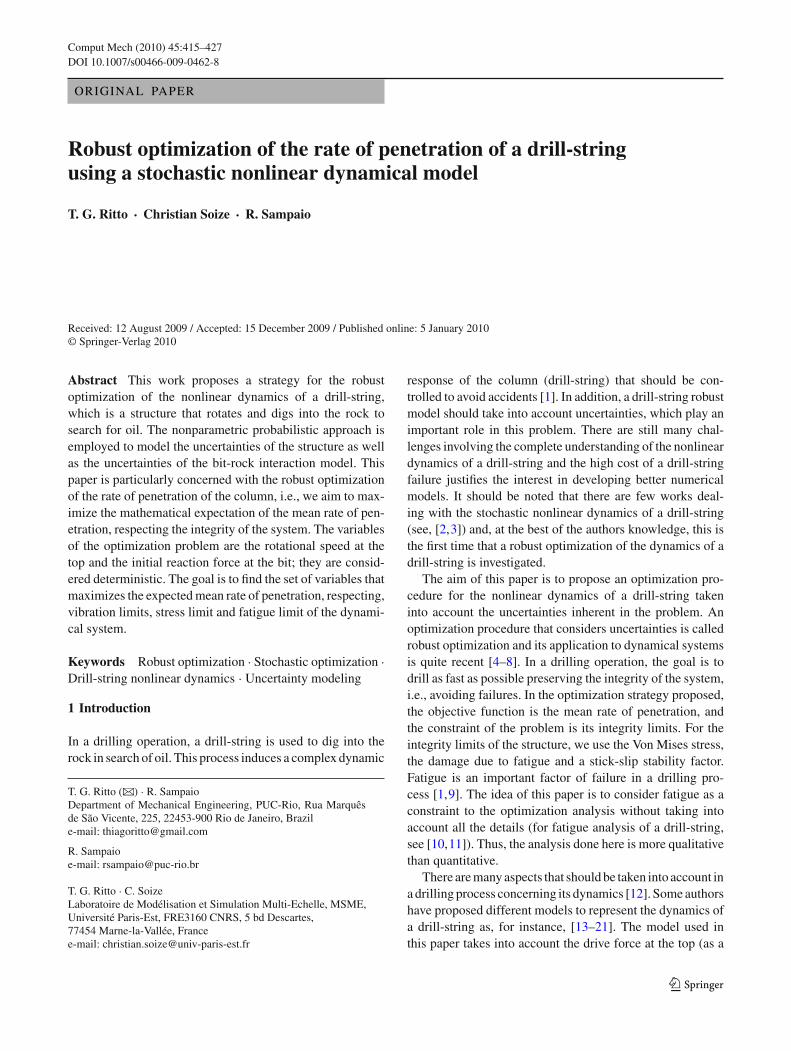
Fig. 1 Displacement field

where V is the domain of integration, ε = [εxx 2γxy 2γxz]T

is the vector of the Green-Lagrange strain tensor and S is thevector written in the Voigt notation of the second Piola-Kirch-hoff tensor. Substituting the constitutive equation S = [D]εand computing the first variation of the strain energy yield

δU =∫

V

δεT

⎡⎣ E 0 0

0 G 00 0 G

⎤⎦ ε dV . (10)

The position X of the reference configuration, the positionx of the deformed configuration, and the displacement fieldp, all written in the inertial frame of reference, are such that

p=⎡⎣ ux

uy

uz

⎤⎦=x−X=

⎡⎣ x + u

y cos(θx) − z sin(θx)

y sin(θx) + z cos(θx)

⎤⎦ −

⎡⎣x

yz

⎤⎦

(11)

then,

⎡⎣ ux

uy

uz

⎤⎦ =

⎡⎣ u

y cos(θx) − z sin(θx) − yy sin(θx) + z cos(θx) − z

⎤⎦ . (12)

Figure 1 shows that uy and uz are related to the torsion ofthe drill-string; the lateral displacements of the neutral lineof the column are zero (v = w = 0).

Finite strains are considered, thus the components of theGreen-Lagrange strain tensor are written as

εxx = ux,x + 1

2

(u2

x,x + u2y,x + u2

z,x

),

γxy = 1

2

(uy,x + ux,y + ux,xux,y + uy,xuy,y + uz,xuz,y

),

γxz = 1

2

(uz,x + ux,z + ux,xux,z + uy,xuy,z + uz,xuz,z

),

(13)

where ux,y = ∂ux/∂y and so on. Equation (10) may bewritten as

δU =∫

V

(E δεxx εxx+4G δγxy γxy+4G δγxz γxz)dV . (14)

The linear terms yield the stiffness matrix [K ] and thehigher order terms yield the geometric stiffness matrix [Kg].The element stiffness matrix is written as

[K ](e) =1∫

0

[E A

le

(N′T

u N′u

)+ G Ip

le

(N′T

θxN′

θx

)]dξ, (15)

where the space derivative (d/dξ ) is denoted by (′). The ele-ment geometric stiffness matrix is written as

[Kg](e) =1∫

0

[(N′T

u N′u

) (3E Au′ + 1.5E Au′2+0.5E Ipθ

′2x

)

+(

N′Tu N′

θx

) (E Ipθ

′x + E Ipθ

′xu′) (

N′Tθx

N′u

)

+ (E Ipθ

′x + E Ipθ

′xu′) +

(N′T

θxN′

θx

) (E Ipu′

+0.5 E Ipu′2 + 1.5E Ip4θ′2x + 3E I22θ

′2x

)] 1

ledξ,

(16)

where u′ = N′uue/ le, θ ′

x = N′θx

ue/ le, I22 = ∫A(y2z2)d A

and Ip4 = ∫A(y4 + z4)d A. It should be noted that u and θx

are the axial displacement and the angular rotation and con-sequently, there are no terms related to transverse vibrationin Eq. (16).

2.4 Bit-rock interaction model

The model used in this work for the bit-rock interaction isthe one developed in [30], which can be written as

ubit = −a1 − a2 fbit + a3ωbit,

tbit = − ubit

ωbita4 − a5,

(17)

where fbit is the axial force (also called weight-on-bit), tbit

is the torque about the x-axis, ubit is the axial speed of thebit (rate of penetration) and ωbit is the rotational speed of thebit. The positive constants a1, . . . , a5 depend on the bit androck characteristics as well as on the average weight-on-bit.Equation (17) is rewritten as

fbit = − ubit

a2 Z(ωbit)2 + a3ωbit

a2 Z(ωbit)− a1

a2,

tbit = − ubita4 Z(ωbit)2

ωbit− a5 Z(ωbit),

(18)

where e is the regularization parameter and Z is the regular-ization function.

123

418 Comput Mech (2010) 45:415–427

2.5 Gravity

The work done by gravity is written as

W =L∫

0

ρgAu dx, (19)

where g is the gravity acceleration. The variation of Eq. (19)gives

δW =L∫

0

ρgA δu dx, (20)

and the discretization by means of the finite element methodyields the force element vector

f (e)g =

1∫

0

NTu ρgA ledξ. (21)

2.6 Initial prestressed configuration

Before starting the rotation about the x-axis, the column isput down through the channel until it reaches the soil. At thispoint, the forces acting on the structure are: the reaction forceat the bit, the weight of the column and the supporting forceat the top. In this equilibrium configuration, the column isprestressed (see Fig. 2). Above the neutral point the structureis tensioned and below is compressed. As it can be seen inFig. 2, if the reaction force increases, the neutral point movesup, increasing the length of the compressed part.

To calculate the initial prestressed state, the column isclamped at the top and consequently,

uS = [K ]−1(fg + fc). (22)

Fig. 2 Initial prestressed configuration of the system

where fg is the force induced by the gravity, fc is the vec-tor related to the reaction force at the bit. Note that fc =[0 0 . . . − fc 0]T in which fc is the initial reaction force atthe bit.

To verify if an element is compressed or tensioned, the ele-ment axial displacements of uS is checked. If (u2 − u1) > 0the element is tensioned, if u2 = u1 there is no stress and if(u2 − u1) < 0 the element is compressed.

2.7 Final computational dynamical model

Small vibrations about the initial prestressed configurationdefined by uS are assumed. Therefore, the geometric stiff-ness matrix [Kg(uS)] is constant. Introducing u = u − uS,the computational dynamical model can then be written as

[M] u(t) + [C]u(t) + ([K ] + [Kg(uS)])u(t)

= g(t) + fbit(u),

u(0) = u0, u(0) = v0,

(23)

in which [M] and [K ] are the mass and stiffness matrices. Theproportional damping matrix [C] = α [M]+β [K ] (α and β

are positive constants) is added a posteriori in the computa-tional model. The constant α is strictly positive. This yieldsthat the damping matrix is positive definite although thereare two rigid body modes. Such a damping model is chosenbecause it is assumed that there is an additional external dis-sipations when the dynamical system move in the two rigidbody modes. The initial conditions are defined by u0 and v0.The force vector related to the bit-rock interaction is fbit andthe imposed rotation at the top (dirichlet boundary condition)is expressed by g.

2.8 Reduced computational model

To speed up the numerical simulations, the computationalmodel is reduced in projecting the nonlinear dynamical equa-tion on a subspace spanned by an appropriated basis. In thepresent paper, the basis used is made up of suitable normalmodes. The normal modes are constructed from the follow-ing generalized eigenvalue problem

([K ] + [Kg(uS)])φ = ω2[M]φ, (24)

where φi is the i th normal mode and ωi is the correspondingnatural frequency. The reduced model is written as

u(t) = [�] q(t),

[Mr ]q(t)+[Cr ]q(t)+[Kr ]q(t) = [�]T (g(t)+fbit([�] q)),

q(0) = q0, q(0) = v0, (25)

123

Comput Mech (2010) 45:415–427 419

in which q0 and v0 are the initial conditions and where [�]is the (m × n) real matrix composed by n normal modes and

[Mr ] = [�]T [M][�], [Cr ] = [�]T [C][�],[Kr ] = [�]T ([K ] + [Kg(uS)])[�] (26)

are the reduced matrices.

3 Probabilistic model of uncertainties

The nonparametric probabilistic approach is used to modelthe uncertainties in the computational model. First, theprobabilistic model for the structure is presented and thenthe probabilistic model for the bit-rock interaction model isdeveloped. Note that a probabilistic model that takes intoaccount both parameter and model uncertainties is necessaryto better represent the uncertainties of the problem analyzed.

3.1 Model uncertainties for the structure

The physical theory used to model the mechanical system(for instance, beam theory for the column) is a simplifica-tion of the real system. Therefore, it is necessary to take intoaccount model uncertainties induced by the model errors.One way to take into account model uncertainties is to use thenonparametric probabilistic approach [24,25,27] for whichapplications with experimental validation can be found in[31–33].

To construct the random reduced matrices, the ensemblesSE+0 and SE+ of random matrices defined in [25] are used.The first step is to decompose the matrices of the determin-istic model applying the Cholesky decomposition

[Mr ] = [L M ]T [L M ],[Cr ] = [LC ]T [LC ],[Kr ] = [L K ]T [L K ].

(27)

Matrices [Mr ], [Cr ], [Kr ], [L M ] and [LC ] have dimen-sion n ×n. The matrix [L K ] has dimension p ×n in which pis equal to (n − µrig) where µrig is the dimension of the nullspace of [Kr ] (note that µrig = 2 for the problem consid-ered). The nonparametric probabilistic approach consists insubstituting the matrices of the reduced deterministic modelby the following three independent random matrices

[Mr ] = [L M ]T [GM ][L M ],[Cr ] = [LC ]T [GC ][LC ],[Kr ] = [L K ]T [GK ][L K ],

(28)

in which [GM ], [GC ] and [GK ] are random matrices belong-ing to the ensemble SE+ defined in [25]. Matrices [GM ] and[GC ] have dimension n × n and matrix [GK ] has dimensionp×p. The probability distribution of [GA] (for A∈{M, C, K })

is completely defined and the generator of its independentrealizations is given in Appendix A.

The level of statistical fluctuations of random matrix [GA]is controlled by the dispersion parameter δA defined by

δA ={

1

pE{||[GA] − [I ]||2F }

} 12

, (29)

whereE{·}denotes the mathematical expectation and ||[A]||F

= (trace{[A][A]T })1/2 denotes the Frobenius norm. Conse-quently, the level of uncertainties for quantity A is controlledby dispersion parameter δA.

3.2 Model uncertainties for the bit-rock interaction

The probabilistic model introduced in [3] to take into accountuncertainties in the bit-rock interaction forces is briefly sum-marized. Again, the nonparametric probabilistic approachis used to model the uncertainties. It consists in modelingthe operator of the constitutive bit-rock interaction equationby a random operator. Let the generalized forces at the bitfbit(x(t)) and x(t) be such that

fbit(x(t)) =(

fbit(x(t))tbit(x(t))

)and x(t) =

(ubit(t)ωbit(t)

). (30)

The deterministic constitutive equations of the bit-rock inter-action can be written as

fbit(x(t)) = −[Ab(x(t))]x(t), (31)

in which

[Ab(x(t))]11 = a1

a2ubit(t)+ 1

a2 Z(ωbit(t))2

− a3ωbit(t)

a2 Z(ωbit(t))ubit(t),

[Ab(x(t))]22 = a4 Z(ωbit(t))2ubit(t)

ωbit(t)2 + a5 Z(ωbit(t))

ωbit(t),

[Ab(x(t))]12 = [Ab(x(t))]21 = 0.

(32)

For all x(t), [Ab(x(t))] is positive-definite. This matrix issubstituted by a random matrix [Ab(x(t))] with values in theset M

+2 (R) of all the positive-definite symmetric (2 × 2)

real matrices. Thus, the constitutive equation defined by Eq.(31) becomes a random constitutive equation which can bewritten as

Fbit(x(t)) = −[Ab(x(t))]x(t). (33)

The probability distribution of random variable [Ab(x(t))]is constructed for all fixed vector x(t). Using the Choleskydecomposition, the mean value of [Ab(x(t))] is written as

[Ab(x(t))] = [Lb(x(t))]T [Lb(x(t))]. (34)

The random matrix [Ab(x(t))] is defined by

[Ab(x(t))] = [Lb(x(t))]T [Gb][Lb(x(t))], (35)

123

420 Comput Mech (2010) 45:415–427

in which [Gb] belongs to the same ensemble that for [GA]defined in the last subsection for which the dispersion param-eter is defined by Eq. (29). It should be noted that, in theconstruction proposed, random matrix [Gb] neither dependson x nor on t .

3.3 Stochastic reduced computational model

The deterministic reduced computational model defined byEq. (25) is then replaced by the following stochastic reducedcomputational model

U(t) = [�] Q(t),

[Mr ]Q(t) + [Cr ]Q(t) + [Kr ]Q(t)

= [�]T {g(t) + Fbit([�] Q(t))},Q(0) = q0, Q(0) = v0,

(36)

where [Mr ], [Kr ] and [Cr ] are the random matrices definedby Eq. (28), Q is the stochastic process of the generalizedcoordinates, U is the stochastic process of the response ofthe system and Fbit is the random force related to the bit-rock interaction probabilistic model defined by Eq. (33).

4 Optimization problem

In this section, the objective function of the optimizationproblem is defined, the constraints related to the integritylimits of the mechanical system are presented and the robustoptimization is defined.

4.1 Objective function

The goal of the optimization problem is to find the set ofvalues s = (ωRPM, fc) that maximizes the expected meanrate of penetration (mean in time), respecting the integritylimits of the mechanical system. The objective function isdefined by

J (s) = E {R(s)}, (37)

where J is the mathematical expectation of the random meanrate R of penetration which is such that

R(s) = 1

t1 − t0

t1∫

t0

Ubit(s)dt, (38)

in which (t0, t1) is the time interval analyzed and Ubit isthe random rate of penetration. The constraints related to theintegrity limits of the mechanical system are discussed in thenext section.

4.2 Constraints of the problem (integrity limits)

Three constraints are proposed to represent the integrity ofthe mechanical system. The first one is the maximum stressvalue that the structure may resist. If the structure is submit-ted to a stress greater than the maximum admissible stress, itwill fail. The second constraint is the damage cumulated byfatigue. If the damage is greater than one, a crack will occur,what is not desired. The third constraint is a stick-slip factor,since we want to avoid torsional instability and stick-slip.

The first constraint is the maximum Von Mises stress σ

(see Appendix B) that must be below the ultimate stress σmax

of the material,

maxx,t

{σ(s, x, t)} ≤ σmax, (39)

where x = (x, y, z) belongs to the domain �c of the problem(the column). For the stochastic problem this constraint mustbe true with probability (1 − Prisk).

Prob

{max

x,t{S(s, x, t)} ≤ σmax

}≥ 1 − Prisk, (40)

where S is the random variable modeling the stress σ in pres-ence of uncertainties in the computational model and Prisk

represents the risk we are willing to take. The more conser-vative we are, the lower we set Prisk. The second constraintis the damage cumulated due to fatigue d that must be belowa given limit dmax.

maxx

{d(s, x)} ≤ dmax, (41)

where d is the cumulated damage related to pr meters of pen-etration. The damage d is computed for (t0, t1) (see Appen-dix C) and then, this damage is extrapolated to consider pr

meters of penetration,

d = d

(pr

pd

), (42)

where pd is how much it was drilled in (t0, t1). For the sto-chastic problem this constraint must be true with probability(1 − Prisk).

Prob{

maxx

{D(s, x)} ≤ dmax

}≥ 1 − Prisk. (43)

where D(s, x) is the random variable modeling d(s, x).Sometimes, in the field, engineers use a constraint relatedto the stick-slip instability. So, finally, the third constraint isthe stick-slip stability factor ss that must be below a givenlimit ssmax,

ss(s) ≤ ssmax. (44)

Factor ss is defined by

ss(s) = ωbmax(s) − ωbmin(s)ωbmax(s) + ωbmin(s)

. (45)

123

Comput Mech (2010) 45:415–427 421

where ωbmax is the maximum rotational speed of the bit andωbmin is the minimum rotational speed of the bit for a giventime period (t0, t1):

ωbmin(s) = mint∈(t0,t1)

{ωbit(s, t)},ωbmax(s) = max

t∈(t0,t1){ωbit(s, t)}. (46)

where ωbit is the rotational speed of the bit. As the amplitudeof the torsional vibrations increases, ss increases, augment-ing the risk of stick-slip (when ωbit = 0 and then the bitslips). This type of oscillations must be avoided. For the sto-chastic problem this constraint must be true with probability(1 − Prisk).

Prob {S(s) ≤ ssmax} ≥ 1 − Prisk, (47)

where S(s) is the random variable modeling ss(s).In the present analysis, the lateral displacement of the col-

umn is neglected. If lateral vibrations were taken into acc-ount, a constraint to the radial displacement r = √

v2 + w2

should be considered in which v and w would be the lateraldisplacements of the neutral line. For example, the columnshould have radial displacements below a given limitrmax, thus maxx,t {r(s, x, t)} ≤ rmax. For the stochasticproblem, this constraint should be true with probability(1− Prisk), hence we would have Prob

{maxx,t {R(s, x, t)} ≤

rmax} ≥ (1 − Prisk), where R would be the random variable

modeling r .

4.3 Robust optimization problem

The proposed robust optimization problem aims to maximizethe expected mean rate of penetration of the drill-string (seeSect. 4.1), respecting the integrity limits of the mechanicalsystem (see Sect. 4.2). It is written as

soptm = arg maxs ∈ C

J (s),

s.t. Prob

{max

j,t{S j (s, t)} ≤ σmax

}≥ 1 − Prisk,

Prob

{max

j{D j (s)} ≤ dmax

}≥ 1 − Prisk,

Prob {S(s) ≤ ssmax} ≥ 1 − Prisk,

(48)

where the admissible set C = {s = (ωRPM, fc) : ωmin ≤ωRPM ≤ ωmax, fmin ≤ fc ≤ fmax}. The index j representsthe points (x j , y j , z j ) chosen for the analysis.

This robust optimization problem is not convex and it doesnot exist any algorithm which allows the global optimum tobe surely reached with a finite number of operations. For suchan optimization problem, the objective is to improve a giveninitial solution with an appropriate algorithm and the level ofimprovement got is proportional to the CPU time spent. Sev-eral techniques can be used such as random search algorithms

[34] (for instance, Latin hypercube sampling type), geneticalgorithms [35], local search with random restart points, etc.).Presently, since the dimension of the parameter space is small(2 parameters), a trial approach (which surely allows the ini-tial solution to be improved) is used and is very efficient.The algorithm is then the following. A grid is generated inthe parameter space and the stochastic problem is solved foreach point of the grid. The points of the grid that do not satisfythe constraints of the optimization problem are eliminated.Then, the optimal point is chosen in the set of all the retainedpoints. The identified region containing this first optimumpoint can be reanalyzed introducing a new refine grid aroundthis point to improve the solution.

5 Application of the optimization problem

The data (geometry, material, etc.) used in the applicationare representative values of a drilling system, see Appen-dix D. The integrity limits are given by σmax = 650 MPa,dmax = 1 and ssmax = 1.20. The damage d and the max-imum stress value σ are calculated in the critical region ofthe drill-pipe, close to the drill-collar: x = 1,400 m andy = z = r0 cos (π/4) (where r0 is the outer radius of thedrill-pipe). The damage d is calculated using pr = 2,000 m,which means that we allow damage equals to one after 2,000m of penetration. The nonlinear dynamical system analyzedis sensitive to model uncertainties [3], therefore, the prob-abilistic model is fixed with δG = 0.005 and δM = δC =δK = 0.001. The drill-string is discretized with 120 finite ele-ments. For the construction of the reduced dynamical model,7 torsional modes, 4 axial modes and also the two rigid bodymodes of the structure (axial and torsional) are used. For thetime integration procedure, the implicit Newmark integra-tion scheme has been implemented with a predictor and a fixpoint procedure to equilibrate the system response at eachtime step. All the numerical results presented below corre-spond to the stationary response for which the transient partof the response induced by the initial conditions has vanished,(t0, t1) = (60, 100) s.

5.1 Deterministic response

Some deterministic responses are presented in this Section.Figure 3a shows the axial displacement of the bit and Fig.3b shows the rate of penetration for ωRPM = 100 RPM andfc = 100 kN. Figure 4 shows the rotational speed of the bitfor fc = 100 kN, comparing ωRPM = 80 RPM, ωRPM =120 RPM and ωRPM = 450 RPM. No stick phase is observed(when ωbit = 0), but there are significant oscillations on therotational speed of the bit (for ωRPM = 80 and 120 RPM)that can be dangerous for the system, since it might causestick-slip and crack initiation due to fatigue. The dynamic

123

422 Comput Mech (2010) 45:415–427

70 75 80 85 90 952

2.2

2.4

2.6

2.8

3

3.2

(a)

(b)

x 10−3 Axial displacement of the bit

time [s]

disp

lace

men

t [cm

]

70 75 80 85 90 95

1

2

3

4

5

x 10−3

Dynamic response, ROP

time [s]

spee

d of

the

bit [

m/s

]

Fig. 3 (a) axial displacement of the bit and (b) rate of penetration, forωRPM = 100 RPM and fc = 100 kN

70 75 80 85 90 95

0

100

200

300

400

500

Dynamic response ωbit

time [s]

rota

tiona

l spe

ed [R

PM

] ωRPM

=80 RPM

ωRPM

=120 RPM

ωRPM

=450 RPM

Fig. 4 Rotational speed of the bit for fc = 100 kN, comparing ωRPM= 80 RPM, ωRPM = 120 and ωRPM = 450 RPM

70 75 80 85 90 95

99

100

101

102

103

104

105

106

Force at the bit

time [s]

forc

e [k

N]

fc=100 kN

fc=105 kN

Fig. 5 Force at the bit for ωRPM = 100 RPM, comparing fc = 100and fc = 105 kN

70 75 80 85 90 95 100220

240

260

280

300

Von Mises stress

time [s]

σ VM

[MP

a]

Fig. 6 Von Misses stress for ωRPM = 100 and fc = 100 kN

response of the bit depends on the bit-rock interaction aswell as on the characteristics of the column (length, crosssectional area, material, etc). It should be noticed that forhigh top speeds (for example, ωRPM = 450 RPM, see Fig. 4),the torque at the bit is almost constant and the oscillations ofthe rotational speed of the bit are small. However, as a con-sequence, for high top speeds the lateral vibrations (whichare not considered in the analyzed model) will increase, whataugment the risk of lateral instability and impacts betweenthe column and the borehole. Figure 5 shows the force atthe bit for ωRPM = 100 RPM, comparing fc = 100 kN withfc = 105 kN. Note that the force at the bit fluctuates aboutthe value of fc. The last result presented is the Von Missesstress for fc = 100 kN and ωRPM = 100 RPM (see Fig. 6).

123

Comput Mech (2010) 45:415–427 423

In the next two sections the deterministic and the stochas-tic responses are going to be used to solve the deterministicand the robust optimization problem, respectively.

5.2 Results of the deterministic optimization problem

In this section, the deterministic optimization problem is ana-lyzed. For the deterministic problem, Eq. (48) is written as

soptm = arg maxs ∈ C

J det(s),

s.t. maxj,t

{σ j (s, t)} ≤ σmax,

maxj

{d j (s)} ≤ dmax,

ss(s) ≤ ssmax,

(49)

where the admissible set C = {s = (ωRPM, fc) : 80 RPM ≤ωRPM ≤ 120 RPM, 90 kN ≤ fc ≤ 110 kN} and

J det(s) = 1

t1 − t0

t1∫

t0

ubit(s) dt, (50)

where ubit is the deterministic rate of penetration.Figure 7 shows the variation of J det with ωRPM for some

values of fc which are 90, 95, 100, 105 and 110 kN. WhenωRPM and fc increase, J det also increases. Of course, thereare side effects: (1) the neutral point will move upwards,(2) the column will be more flexible and (3) the dynamicalresponse is more likely to be unstable.

To proceed with the optimization problem, we eliminatethe points (ωRPM, fc) that do not satisfy the integrity limitsof the system. For the points simulated, the maximum stressis always below the established limit of σmax = 650 MPa.Figure 8 shows ωRPM versus the value of the stick-slip factor

80 90 100 110 120

2.5

3

3.5

4

x 10−3

rotational speed at the top (RPM)

Jdet (

m/s

)

90kN95kN100kN105kN110kN

Fig. 7 Rotational speed at the top versus J det for different fc (90, 95,100, 105 and 110 kN)

80 90 100 110 120

0.95

1

1.05

1.1

1.15

1.2

1.25

1.3

1.35

rotational speed at the top (RPM)

stic

k sl

ip fa

ctor

90kN95kN100kN105kN110kNlimit

Fig. 8 Rotational speed at the top versus ss for different fc (90, 95,100, 105 and 110 kN). The dashed line shows the limit ssmax = 1.20

80 90 100 110 120

0.5

1

1.5

2

2.5

rotational speed at the top (RPM)

dam

age

90kN95kN100kN105kN110kNlimit

Fig. 9 Rotational speed at the top versus d for different fc (90, 95,100, 105 and 110 kN). The dashed line shows the limit dmax = 1

ss and Fig. 9 shows ωRPM versus the damage cumulated dueto fatigue d for some values of fc. It can be seen that somepoints present values greater than the established limits ofssmax = 1.20 and dmax = 1.

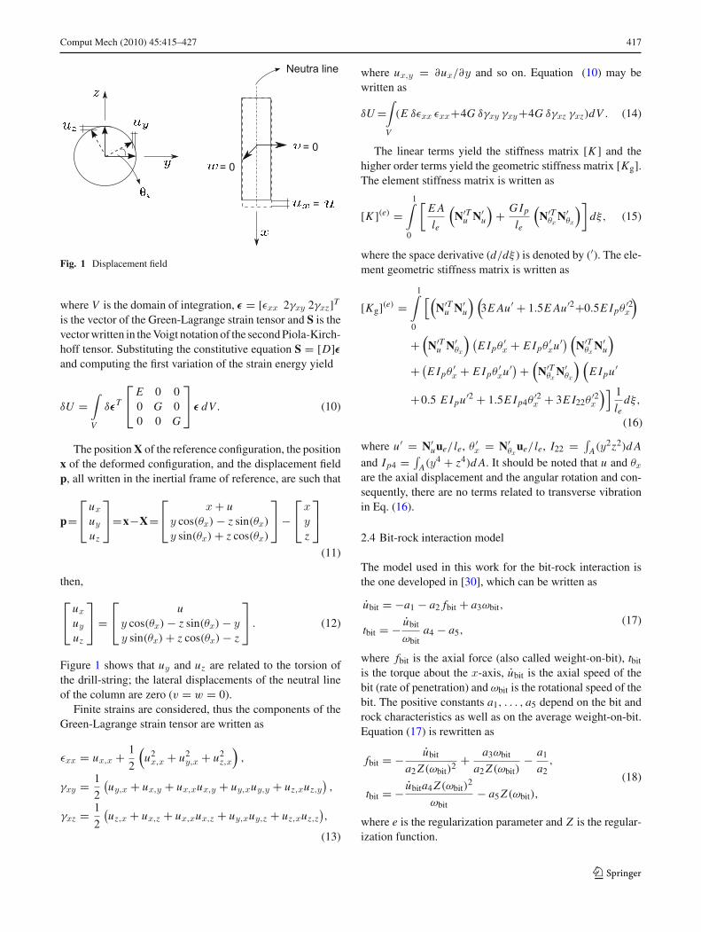
The points that do not respect the integrity limits of thesystem are eliminated. Figure 10 summarizes the analysis.The points that are crossed are the ones that do not respectthe constraint limits and the best point of the deterministicanalysis is identified: soptm = (ωRPM = 120 RPM, fc = 110kN), which gives J det

optm = 3.92 × 10−3 m/s ∼ 14.11 m/h.In the next section, the results of the robust optimization

problem are presented. It will be seen that the results arequite different from the ones presented in this section. Therobust analysis considers the 90% percentile of the stick-slip factor, for instance. Therefore, we expect more pointsto be eliminated in the robust analysis, for example points

123

424 Comput Mech (2010) 45:415–427

80 90 100 110 120

90

95

100

105

110

rotational speed at the top (RPM)

reac

tion

forc

e at

the

bit (

kN)

Best point

Fig. 10 Graphic showing the best point (ωRPM, fc) (circle); thecrossed points do not respect the integrity limits

50 100 150 200 250 300 350

4.363

4.3635

4.364

4.3645

4.365

4.3655

4.366

x 109

number of simulations

conv

Fig. 11 Convergence function

(ωRPM = 120 RPM, fc = 105 kN) and (ωRPM = 120 RPM,fc = 110 kN) (see Fig. 8), because they are already bearingthe limit in the deterministic analysis.

5.3 Results of the robust optimization problem

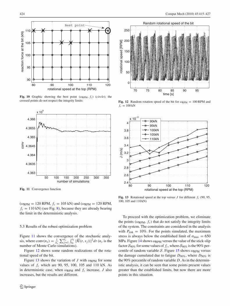
Figure 11 shows the convergence of the stochastic analy-sis, where conv(ns) = 1

ns

∑nsj=1

∫ t1t0

||U(t, s j )||2dt (ns is thenumber of Monte Carlo simulations).

Figure 12 shows some random realizations of the rota-tional speed of the bit.

Figure 13 shows the variation of J with ωRPM for somevalues of fc which are 90, 95, 100, 105 and 110 kN. Asin deterministic case, when ωRPM and fc increase, J alsoincreases, but the results are different.

70 75 80 85 90 95

0

50

100

150

200

250

Random rotational speed of the bit

rota

tiona

l spe

ed [R

PM

]

time [s]

Fig. 12 Random rotation speed of the bit for ωRPM = 100 RPM andfc = 100 kN

80 90 100 110 1202.4

2.6

2.8

3

3.2

3.4

3.6

3.8

4x 10

−3

rotational speed at the top (RPM)

J (m

/s)

90kN95kN100kN105kN110kN

Fig. 13 Rotational speed at the top versus J for different fc (90, 95,100, 105 and 110 kN)

To proceed with the optimization problem, we eliminatethe points (ωRPM, fc) that do not satisfy the integrity limitsof the system. The constraints are considered in the analysiswith Prisk = 10%. For the points simulated, the maximumstress is always below the established limit of σmax = 650MPa. Figure 14 shows ωRPM versus the value of the stick-slipfactor S90% for some values of fc, where S90% is the 90% per-centile of random variable S. Figure 15 shows ωRPM versusthe damage cumulated due to fatigue D90%, where D90% isthe 90% percentile of random variable D. As in the determin-istic analysis, it can be seen that some points present valuesgreater than the established limits, but now there are morepoints in this situation.

123

Comput Mech (2010) 45:415–427 425

80 90 100 110 120

1

1.1

1.2

1.3

1.4

1.5

rotational speed at the top (RPM)

stic

k sl

ip fa

ctor

, 90%

per

cent

ile

90kN95kN100kN105kN110kNlimit

Fig. 14 Rotational speed at the top versus S90% for different fc (90,95, 100, 105 and 110 kN). The dashed line shows the limit ssmax = 1.20

80 90 100 110 120

0.5

1

1.5

2

2.5

rotational speed at the top (RPM)

dam

age,

90%

per

cent

ile

90kN95kN100kN105kN110kNlimit

Fig. 15 Rotational speed at the top versus D90% for different fc (90,95, 100, 105 and 110 kN). The dashed line shows the limit dmax = 1

It can be seen (Figs. 14 and 15) that the constraints arenot respected for high values of ωRPM and fc. Note that wewould like to increase ωRPM and fc to have a higher J , but torespect the integrity limits these parameters are constrained.

The points that do not respect the integrity limits of thesystem are eliminated. Figure 16 summarizes the analysis.The points that are crossed are the ones that do not respectthe constraint limits and the best point of the robust analysisis identified: soptm = (ωRPM = 110 RPM, fc = 105 kN),which gives J optm = 3.54 × 10−3 m/s ∼ 12.76 m/h.

It can be concluded that the robust optimization generatesdifferent results comparing to the deterministic optimization.If uncertainties are important in the dynamical analysis, we

80 90 100 110 120

90

95

100

105

110

rotational speed at the top (RPM)

reac

tion

forc

e at

the

bit (

kN)

Best point

Fig. 16 Graphic showing the best point (ωRPM, fc) (circle)

should always proceed with the robust optimization problem,instead of the deterministic optimization problem.

6 Concluding remarks

This paper has proposed a methodology for the robust opti-mization of the nonlinear dynamics of a drill-string system.Applications of robust optimization in dynamical systemsare quite recent. This is the first time a robust optimiza-tion problem is proposed and investigated for the nonlin-ear dynamics of a drill-string system. It has been shownthat the robust analysis gives different results comparingto the deterministic optimization analysis. The aim of theproposed optimization problem is to maximize the expectedmean rate of penetration of the drill-string, respecting theintegrity limits. Three constraints have been proposed to rep-resent the integrity of the system: (1) the ultimate stress of thematerial, (2) the damage cumulated by fatigue (3) a stick-slipfactor.

Uncertainties are modeled using the nonparametricprobabilistic approach, which takes into account both sys-tem-parameter and model uncertainties. This feature of theprobabilistic approach used is important because a simplifiedmechanical model is employed in the analysis. The mass,damping and stiffness of the system, as well as the bit-rockinteraction forces are considered uncertain.

The parameters of the optimization problem, which arethe initial reaction force at the bit and the rotational speed atthe top, have been considered deterministic. The optimiza-tion problem is solved for two cases: the computational modeldoes not have any uncertainties and the computational modelhas uncertainties (robust optimization). For these two cases,the best combination of the two parameters has been foundand shows that the robust optimization must be used insteadof a non robust optimization.

123

426 Comput Mech (2010) 45:415–427

Appendix A: Algorithm for the realizationsof the random germ [GA]

The p × p random matrix [GA] can be written as [GA] =[LA]T [LA] in which [LA] is an upper triangular real randommatrix such that:

1. The random variables {[LA] j j ′, j ≤ j ′} are independents.2. For j < j ′ the real-valued random variable [LA] j j ′ =

σ Vj j ′ , in which σ = δ(p + 1)−1/2 and Vj j ′ is a real-valued gaussian random variable with zero mean and unitvariance.

3. For j = j ′ the real-valued random variable [LA] j j =σ(2Vj )

1/2. In which Vj is a real-valued gamma randomvariable whose probability density function is written as

pVj (v) = 1R+(v) 1

�(

p+12δ2 + 1− j

2

) vp+12δ2 − 1+ j

2 e−v ,

Appendix B: Stress calculation

The numerical simulations give the axial displacement u andthe section area rotation θx. With Eqs. (12) and (13), thedisplacement field and the strain are computed. Finally, thestress components are calculated doing

σxx = εxxE,

τxy = G(2γxy),

τxz = G(2γxz).

(51)

The Von Mises stress is computed as:

σ(t) =√

(k f σxx(t))2 + 3((k f τxy(t))2 + (k f τxz(t))2)), (52)

where k f is the stress concentration factor for fatigue. Thevalue of k f might vary a lot depending on several factors,such as the type of joint, tip radius, etc, [9]. In this work thevalue used is k f = 3.

Appendix C: Damage calculation

In this section we explain how the damage caused by fatigueis calculated. We use the Goodman-Wohler-Miner model.

(1) Goodman to calculate the equivalent alternate stress(σeq) that causes a crack initiation.

σa

σeq+ σm

σmax= 1 −→ σeq = σa

1 − σm

σmax

(53)

where σmax is the ultimate stress limit of the material,σa is the alternate Von Mises stress and σm is the meanVon Mises stress, calculated as:

σa = max {σ } − min {σ }2

,

σm = max {σ } + min {σ }2

. (54)

(2) Wohler (or σeq N ) to model the relationship between thestress (σeq) and the number of cycles (N ) that cause acrack initiation.

Nσ beq = c, (55)

where b and c are two positive constants that areobtained fitting experiments. We use c = 4.16 × 1011

and b = 3, [36]. Note that the stress value is writtenin MPa (b and c will have different values for differentunits).

(3) Miner to calculate the damage cumulation.

d = n

N= n

c(σeq)

b. (56)

where n is the number of cycles that the structure hasbeen subjected to.

Appendix D: Data used in the simulation

Ldp = 1,400 m (length of the drill pipe),Ldc = 200 m (length of the drill collar),Di = 0.095 m (inside diameter of the column),Dodp = 0.12 m (outside diameter of the drill pipe),Dodc = 0.15 m (outside diameter of the drill collar),E = 210 GPa (elasticity modulus of the drill stringmaterial),ρ = 7,850 kg/m3 (density of the drill string material),ν = 0.29 (poisson coefficient of the drill string mate-rial),g = 9.81 m/s2 (gravity acceleration),a1 = 3.429×10−3 m/s, (constants of the bit-rock inter-action model)a2 = 5.672 × 10−8 m/(N s),a3 = 1.374 × 10−4 m/rd,a4 = 9.537 × 106N rd,a5 = 1.475 × 103N m,e = 2 rd/s (regularization parameter).

123

Comput Mech (2010) 45:415–427 427

The damping matrix is constructed using [C] = α[M] +β([K ] + [Kg(uS)]) with α = 0.1 and β = 0.00008.

Acknowledgments The authors acknowledge the financial supportof the Brazilian agencies CNPQ, CAPES and FAPERJ, and the Frenchagency COFECUB (project CAPES-COFECUB 476/04).

References

1. Macdonald KA, Bjune JV (2007) Failure analysis of drillstrings.Eng Fail Anal 14:1641–1666

2. Spanos PD, Chevallier AM, Politis NP (2002) Nonlinear stochasticdrill-string vibrations. J Vib Acoust Trans ASME 124(4):512–518

3. Ritto TG, Soize C, Sampaio R (2009) Non-linear dynamics of adrill-string with uncertain model of the bit-rock interaction. Int JNon-Linear Mech 44(8):865–876

4. Ben-Tal A, Nemirovski A (2002) Robust optimization–methodol-ogy and applications. Math Programm 92(3):453–480

5. Zang C, Friswell MI, Mottershead JE (2005) A review of robustoptimal design and its application in dynamics. Comput Struct83(4/5):315–326

6. Capiez-Lernout E, Soize C (2008) Robust design optimizationin computational mechanics. J Appl Mech Trans ASME 75(2):021001-1–021001-11

7. Soize C, Capiez-Lernout E, Ohayon R (2008) Robust updating ofuncertain computational models using experimental modal analy-sis. Mech Syst Signal Process 22(8):1774–1792

8. Guedri M, Ghanmi S, Majed R, Bouhaddi N (2009) Robust toolsfor prediction of variability and optimization in structural dynam-ics. Mech Syst Signal Process 23(4):1123–1133

9. Vaisberg O, Vincke O, Perrin G, Sarda JP, Fay JB (2002) Fatigueof drillstring: state of the art. Oil Gas Sci Technol 57(1):7–37

10. Bertini L, Beghini M, Santus C, Baryshnikov A (2008) Resonanttest rigs for fatigue full scale testing of oil drill string connections.Int J Fatigue 30(6):978–988

11. Miscow GF, de Miranda PEV, Netto TA, Plácido JCR (2004)Techniques to characterize fatigue behaviour of full size drill pipesand small scale samples. Int J Fatigue 26:575–584

12. Spanos PD, Chevallier AM, Politis NP, Payne ML (2003) Oiland gas well drilling: a vibrations perspective. Shock Vib Digest35(2):85–103

13. Berlioz A, Der Hagopian J, Dufour R, Draoui E (1996) Dynamicbehavior of a drill-string: experimental investigation of lateralinstabilities. J Vib Accoustics 118(3):292–298

14. Christoforou AP, Yigit AS (1997) Dynamic modeling of rotat-ing drillstrings with borehole interactions. J Sound Vib 206(2):243–260

15. Christoforou AP, Yigit AS (2003) Fully coupled vibrations ofactively controlled drillstrings. J Sound Vib 267:1029–1045

16. Khulief YA, AL-Naser H (2005) Finite element dynamic analysisof drillstrings. Finite Elements Anal Des 41:1270–1288

17. Khulief YA, Al-Sulaiman FA, Bashmal S (2007) Vibration analy-sis of drillstrings with self excited stick-slip oscillations. J SoundVib 299:540–558

18. Sampaio R, Piovan MT, Lozano GV (2007) Coupled axial/tor-sional vibrations of drilling-strings by mean of nonlinear model.Mech Res Commun 34(5/6):497–502

19. Trindade MA, Wolter C, Sampaio R (2005) Karhunen–Loèvedecomposition of coupled axial/bending of beams subjected toimpacts. J Sound Vib 279:1015–1036

20. Tucker RW, Wang C (1999) An integrated model for drill-stringdynamics. J Sound Vib 224(1):123–165

21. Yigit AS, Christoforou AP (1996) Coupled axial and transversevibrations of oilwell drillstrings. J Sound Vib 195(4):617–627

22. Kotsonis SJ, Spanos PD (1997) Chaotic and random whirlingmotion of drillstrings. J Energy Resour Technol (Trans ASME)119(4):217–222

23. Spanos PD, Chevallier M (2000) Non linear stochastic drill–string vibrations. 8th ASCE specialty conference on probabilisticmechanics and structural reliability, South Bend, USA

24. Soize C (2000) A nonparametric model of random uncertities forreduced matrix models in structural dynamics. Probab Eng Mech15:277–294

25. Soize C (2005) Random matrix theory for modeling uncertaintiesin computational mechanics. Comput Methods Appl Mech Eng194(12–16):1333–1366

26. Soize C (2005) A comprehensive overview of a non-parametricprobabilistic approach of model uncertainties for predictive mod-els in structural dynamics. J Sound Vib 288(3):623–652

27. Soize C (2010) Generalized probabilistic approach of uncertaintiesin computational dynamics using random matrices and polynomialchaos decompositions. International Journal for Numerical Meth-ods in Engineering. Published on line 5 Aug 2009, doi:10.1002/nme.2712

28. Van de Vrande BL, Van Campen DH, de Kraker A (1999) Anapproximate analysis of dry-friction-induced stick-slip vibrationsby a smoothing procedure. Nonlinear Dyn 19:157–169

29. Van de Wouw N, Leine RI (2004) Attractivity of equilibrium setsof systems with dry friction. Nonlinear Dyn 35:19–39

30. Tucker RW, Wang C (2003) Torsional vibration control and coss-erat dynamics of a drill-rig assembly. Meccanica 38(1):143–159

31. Chen C, Duhamel D, Soize C (2006) Probabilistic approach formodel and data uncertainties and its experimental identification instructural dynamics: case of composite sandwich panels. J SoundVib 194(1/2):64–81

32. Duchereau J, Soize C (2006) Transient dynamics in structures withnonhomogeneous uncertainties induced by complex joints. MechSyst Signal Process 20:854–867

33. Durand JF, Soize C, Gagliardini L (2008) Structural-acoustic mod-eling of automotive vehicles in presence of uncertainties andexperimental identification and validation. J Acoust Soc Am124(3):1513–1525

34. Solis FJ, Wets RJ-B (1981) Minimization by random search tech-niques. Math Oper Res 6(1):19–30

35. Goldberg DE (1989) Genetic algorithms in search, optimization,and machine learning. Addison-Wesley, Reading

36. Netto TA, Lourenco MI, Botto A (2008) Fatigue performance ofpre-strained pipes with girth weld defects: full-scale experimentsand analysis. Int J Fatigue 30:767–778

123