Author's personal copy

International Journal of Non-Linear Mechanics 44 (2009) 865 -- 876

Contents lists available at ScienceDirect

International Journal of Non-LinearMechanics

journal homepage: www.e lsev ier .com/ locate /n lm

Non-linear dynamics of a drill-stringwith uncertainmodel of the bit–rock interaction

T.G. Rittoa,b, C. Soizeb,∗, R. Sampaioa

aPUC-Rio, Department of Mechanical Engineering, Rua Marquês de São Vicente, 225, Gávea, RJ 22453-900, BrazilbUniversité Paris-Est, Laboratoire de Modélisation et Simulation Multi Echelle, MSME FRE3160 CNRS, 5 bd Descartes, 77454 Marne-la-Vallée, France

A R T I C L E I N F O A B S T R A C T

Article history:Received 21 June 2008Received in revised form 5 June 2009Accepted 8 June 2009

Keywords:Drill-string dynamicsBit–rock probabilistic modelNon-linear stochastic dynamicsNon-parametric probabilistic approach

The drill-string dynamics is difficult to predict due to the non-linearities and uncertainties involved inthe problem. In this paper a stochastic computational model is proposed to model uncertainties in thebit–rock interaction model. To do so, a new strategy that uses the non-parametric probabilistic approachis developed to take into account model uncertainties in the bit–rock non-linear interaction model.The mean model considers the main forces applied to the column such as the bit–rock interaction, thefluid–structure interaction and the impact forces. The non-linear Timoshenko beam theory is used andthe non-linear dynamical equations are discretized by means of the finite element method.

© 2009 Elsevier Ltd. All rights reserved.

1. Introduction

Drill-strings are slender structures used to dig into the rock insearch of oil and their dynamics must be controlled to avoid failures[1]. A general vibration perspective of the oil and gas drilling processcan be found in [2]. We are particulary concerned with a verticaldrill-string that may reach some kilometers. When the drill-stringis that long, it turns out that the vibration control is harder for thefollowing reasons: the non-linearities are important, the sensorsmaynot work properly and uncertainties increase.

The drill-string is composed of thin tubes called drill-pipes thattogether measure some kilometers and some thicker tubes calleddrill collars that together have some hundred meters. The regioncomposed by the thicker tubes is called bottom-hole-assembly(BHA). Fig. 1 shows the general scheme of the system analyzed. Theforces taken into account are the motor torque (as a constant rota-tional speed at the top �x), the supporting force fhook, the torque tbitand force fbit at the bit, the weight of the column, the fluid forces,the impact and rubbing between the column and the borehole, theforces due to the stabilizer, and also the elastic and kinetic forcesdue to the deformation and to the motion of the structure.

There are some ways to model the non-linear dynamics of a drill-string, e.g. [3–10]. These models are able to quantify some effectsthat occur in a drilling operation (such as the stick-slip oscillations)but they cannot predict correctly the dynamical response of a realsystem. This is explained since, first, the above models are too simple

∗ Corresponding author.E-mail addresses: thiagoritto@gmail.com (T.G. Ritto),

christian.soize@univ-paris-est.fr (C. Soize), rsampaio@puc-rio.br (R. Sampaio).

0020-7462/$ - see front matter © 2009 Elsevier Ltd. All rights reserved.doi:10.1016/j.ijnonlinmec.2009.06.003

compared to the real system and, second, uncertainties are not takeninto account. Each author uses a different approach to the problem:[3,4] use a one-mode approximation to analyze the problem [8–10],use the Euler–Bernoulli beammodel with the finite element method,while [6,7] use the Cosserat theory.

A fluid–structure interaction that takes into account the drillingfluid that flows inside and outside the column is not considered inany of the above works. In the present paper, the fluid–structureinteraction model proposed in [11] is employed in the analysis.

To model the column, the Timoshenko beammodel is applied andthe finite element method is used to discretize the system. Moreover,finite strains are considered with no simplifications (what couplesaxial, torsional and lateral vibrations).

In a drilling operation there are many sources of uncertaintiessuch as material properties (column and drilling fluid), dimensions ofthe system (especially the borehole), fluid–structure interaction andbit–rock interaction. The uncertainty analysis of the present paperis focused on the bit–rock interaction because it seems to be one ofthe most important sources of uncertainties in this problem. Thereare few articles treating the stochastic problem of the drill-stringdynamics, specially we may cite [12,13]. In [12], stochastic lateralforces are analyzed at the bit, and in [13], a random weight-on-bit isanalyzed using a simple two degrees of freedom drill-string model.

The bit–rock interaction model used in the analysis is the onedeveloped in [7]. This model is able to reproduce the main phenom-ena and describes the penetration of the bit into the rock. Thus, itallows the analysis of the rate of penetration (ROP). Usually, the bitis assumed to be fixed [9,10] or an average rate of penetration isassumed [5,14].

The non-parametric probabilistic approach [15–17] is usedto model the uncertainties in the bit–rock interaction, which is

Author's personal copy

866 T.G. Ritto et al. / International Journal of Non-Linear Mechanics 44 (2009) 865 -- 876

Fig. 1. General scheme of the drill-string system.

represented by a non-linear operator. It should be noticed that a newstrategy is developed to take into account uncertainties for a localnon-linear operator.

The paper is organized as follows. In Section 2 the mean model ispresented then, in Section 3, the probabilistic model of the bit–rockinteraction model is developed. The results are shown in Section 4and the concluding remarks are made in Section 5.

2. Mean model

In this section the equations used to model the problem are pre-sented. The strategy used in this work is, in some respects, similar tothe one used in [9], but there are several important additional fea-tures, such as (1) impact and rubbing between the column and theborehole, (2) shear (Timoshenko beam model), (3) fluid–structureinteraction and (4) a bit–rock interaction model that allows thesimulation of the bit penetration.

To derive the equations of motion, the extended HamiltonPrinciple is applied. Defining the potential � by

� =∫ t2

t1(U − T − W)dt, (1)

where U is the potential strain energy, T is the kinetic energy andW is the work done by the non-conservative forces and any forcenot accounted in the potential energy. The first variation of � mustvanish:

�� =∫ t2

t1(�U − �T − �W)dt = 0. (2)

2.1. Finite element discretization

In the discretization by means of the finite element method atwo-node approximation with six degrees of freedom per node is

Fig. 2. Degrees of freedom of an element.

chosen (see Fig. 2). The nodal displacement is written as

ue = Nuue, ve = Nvue, we = Nwue, (3)

�xe = N�xue, �ye = N�y

ue, �ze = N�zue, (4)

where N is the shape function (see Appendix A), ue, ve and we arethe displacements in x, y and z directions, �xe, �ye and �ze are therotations about the x-, y- and z-axes (see Fig. 2).

The element coordinate is � = x/le and

ue = (u1 v1 �z1 w1 �y1 �x1 u2 v2 �z2 w2 �y2 �x2)T , (5)

where (·)T means transpose.The total Lagrangian formulation is used, the stress tensor is

the second Piola–Kirchhoff tensor and finite strains are considered(Green–Lagrange strain tensor). We are assuming axi-symmetryabout the x-axis, small lateral displacements (v and w) and smallrotations (�y and �z), and a linear stress–strain relationship.

2.2. Kinetic energy

The kinetic energy is written as

T = 12

∫ L

0(�AvTv + �xT [It]x)dx, (6)

where � is the mass density, A is the cross sectional area, L is thelength of the column, [It] is the cross sectional inertial matrix, vis the velocity vector and x the angular velocity vector. The threefollowing quantities v, [It] and x are written as

v =

⎛⎜⎝

u

v

w

⎞⎟⎠ , [It] =

⎛⎜⎝Ip 0 0

0 I 0

0 0 I

⎞⎟⎠ , x=

⎛⎜⎝

�x+�y�z

cos(�x)�y− sin(�x)�z

sin(�x)�y+ cos(�x)�z

⎞⎟⎠ , (7)

where the time derivative (d/dt) is denoted by a superposed dot.The angular velocity x is derived by first rotating the inertial frameabout the x-axis �x, then rotating the resulting frame about they-axis �y and, finally, rotating the resulting frame about the z-axis�z. It is written in the inertial frame and it is assumed small rotations�y and �z. Developing the expression of the kinetic energy yields

T = 12

∫ L

0[�A(u)2 + �A(v)2 + �A(w)2

+ �I(�y)2 + �I(�z)

2 + �Ip(�x)2 + 2�Ip(�x�y�z)]dx. (8)

The first three terms of Eq. (8) are related to the translational inertia,the next three terms are related to the rotational inertia and the last

Author's personal copy

T.G. Ritto et al. / International Journal of Non-Linear Mechanics 44 (2009) 865 -- 876 867

term is the coupling term. In rotor-dynamics analysis the couplingterm (2�Ip(�x�y�z)) yields the gyroscopic matrix which does not in-troduce a non-linearity into the system as �x ∼ cte (see, for instance,[18]). In our case this is not true, therefore, it yields a non-linear for-mulation. The first variation of the kinetic energy, after integratingby parts in time, may be written as

�T = −∫ L

0[�Au�u + �Av�v + �Aw�w + �I�y��y + �I�z��z

+ �Ip�x��x + (�Ip(−�y�z��x − �y�z��x + �x�z��y

− �x�y��z − �y�x��z))]dx. (9)

For convenience the energy is divided into two parts. The first one is

�T1 = −∫ L

0[�A(u�u + v�v + w�w) + �I(�y��y + �z��z)

+ �Ip�x��x]dx, (10)

which yields the constant mass matrix [M]. The second part is

�T2 = −∫ L

0[(�Ip(−�y�z��x − �y�z��x + �x�z��y

− �x�y��z − �y�x��z))]dx, (11)

which yields the vector fke that is incorporated in the non-linearforce vector fNL (see Eq. (31)). Note that this force couples the axial,torsional and lateral motions.

2.3. Strain energy

The strain energy is given by

U = 12

∫V�TSdV , (12)

where V is the domain of integration, � = (�xx 2xy 2xz)T is the

Green–Lagrange strain tensor and S is second Piola–Kirchhoff tensor(written in Voigt notation). Substituting S= [D]� and computing thefirst variation of the strain energy yields

�U =∫V��

T

⎛⎜⎝E 0 0

0 ksG 0

0 0 ksG

⎞⎟⎠�dV . (13)

The Timoshenko beam model (where the cross sectional arearemains plane but not necessarily perpendicular to the neutral line,i.e. shear effects are considered) is used because it is more generalthan the Euler–Bernoulli model, what gives more flexibility forthe applications. If there is no shear, the equations reduce to theEuler–Bernoulli model.

The components of the Green–Lagrange strain tensor may bewritten as

�xx = �ux�x

+ 12

(�ux�x

�ux�x

+ �uy�x

�uy�x

+ �uz�x

�uz�x

),

xy = 12

(�uy�x

+ �ux�y

+ �ux�x

�ux�y

+ �uy�x

�uy�y

+ �uz�x

�uz�y

),

xz = 12

(�uz�x

+ �ux�z

+ �ux�x

�ux�z

+ �uy�x

�uy�z

+ �uz�x

�uz�z

). (14)

The displacements written in the undeformed configuration are

ux = u − y�z + z�y,

uy = v + y(cos(�x) − 1) − z sin(�x),

uz = w + z(cos(�x) − 1) + y sin(�x), (15)

in which u, v and w are the displacements of the neutral line.Note that cos(�x) and sin(�x) have not been simplified in the aboveexpression. Eq. (13) may be written as

�U =∫V(E��xx�xx + 4ksG�xyxy + 4ksG�xzxz)dV . (16)

The linear terms yield the stiffnessmatrix [K] and the higher orderterms yield the geometric stiffness matrix [Kg] and the vector fsethat is incorporated in the non-linear force vector fNL (see Eq. (31)).Note that due to the finite strain formulation, the axial, torsional andlateral vibrations are all coupled.

2.4. Impact and rubbing

The forces generated by the impact and rubbing between thecolumn and the borehole are modeled by concentrated forces andtorques. The radial forces are modeled as an elastic force governedby the stiffness parameter kip (N/m) such that

Fr ip

{= 0 if (r − Rch − Ro)�0,

= − kip(r − Rch − Ro) if (r − Rch − Ro)>0,(17)

where r =√v2 + w2, Rch is the radius of the borehole and Ro is the

outer radius of the column. The rubbing between the column andthe borehole is simply modeled as a frictional torque governed bythe frictional coefficient ip and is such that

Txip

{= 0 if (r − Rch − Ro)�0,

= − ipFr ipRo sign(�x) if (r − Rch − Ro)>0,(18)

where ip is the frictional coefficient.

2.5. Fluid–structure interaction model

The drilling fluid (mud) is responsible for transporting the cut-tings (drilled solids) from the bottom to the top to avoid cloggingof the hole. It also plays an important role in cooling and stabilizingthe system [19]. The rheological properties of the mud are complex,see [20] for instance. There is no doubt that the drilling fluid influ-ences the dynamics of a drill-string, but solving the complete prob-lem would be extremely expensive computationally. There are someworks that are strictly concerned with the drilling fluid flow, e.g.[21–23]. We use a linear fluid–structure coupling model similar to[11,24]. In this simplified model there are the following hypotheses:

1. For the inside flow the fluid is taken as inviscid; for the outsideas viscous.

2. The flow induced by the rotational speed about the x-axis is notconsidered in this first analysis.

3. The pressure varies linearly with x.

The element matrices are presented in Eq. (19). These equationsare an extension and an adaptation of the model developed in [11]:

[Mf ](e) =

∫ 1

0(Mf + ��fAo)(NT

wNw + NTvNv)le d�,

[Kf ](e) =

∫ 1

0(−MfU

2i − Aipi + Aopo − ��fAoU2

o )(N′wTN′

w + N′vTN′

v)1le

d�

+∫ 1

0

(−Ai

�pi�x

+ Ao�po�x

)(NT

�yN�y

+ NT�zN�z

)le d�,

[Cf ](e) =

∫ 1

0(−2MfUi + 2��fAoUo)(NT

�yN�y

+ NT�zN�z

)le d�

+∫ 1

0

(12Cf�fDoUo + k

)(NT

wNw + NTvNv)le d�,

Author's personal copy

868 T.G. Ritto et al. / International Journal of Non-Linear Mechanics 44 (2009) 865 -- 876

f(e)f =∫ 1

0

(Mfg − Ai

�pi�x

− 12Cf�fDoU2

o

)NTule d�, (19)

in which, Mf is the fluid mass per unit length, �f is the density ofthe fluid, �= ((Dch/Do)

2 +1)/((Dch/Do)2 −1) (>1), Dch is the borehole

(channel) diameter, Di,Do are the inside and outside diameters of thecolumn, Ui,Uo are the inlet and outlet flow velocities, pi, po are thepressures inside and outside the drill-string, Ai,Ao are the inside andoutside cross sectional area of the column, Cf , k are the fluid viscousdamping coefficients.

As pointed out before, it is assumed that the inner and the outerpressures (pi and po) vary linearly with x

pi = (�fg)x + pcte, (20)

po =(�fg + Ffo

Ao

)x, (21)

where pcte is a constant pressure and Ffo is the frictional force dueto the external flow given by

Ffo = 12Cf�f

D2oU

2o

Dh. (22)

In the above equation, Dh is the hydraulic diameter (4Ach/Stot) andStot is the total wetted area per unit length (�Dch + �Do). Note thatthe reference pressure is po|x=0=0. Another assumption is that thereis no head loss when the fluid passes from the drill-pipe to the drill-collar (and vice versa). The head loss due to the change in velocityof the fluid at the bottom (it goes down and then up) is given by

h = 12g

(Ui − Uo)2. (23)

If the geometry and the fluid characteristics are given, only theinlet flow at x = 0 can be controlled as the fluid speed is calculatedusing the continuity equation and the pressures are calculated usingthe Bernoulli equation.

Examining Eq. (19), it can be noticed that the fluid mass matrixis the usual added mass that, in our case, represents a significantvalue. For example, using representative values, the added mass isapproximately 50% of the original mass, what changes the naturalfrequencies in about 20%.

The fluid stiffness matrix depends on the speed of the insideand outside flow as well as on the pressure and on the pressurederivatives. Analyzing the signs in the equation (Eq. (19)) it can benoticed that the outside pressure tends to stabilize the system whilethe inside pressure and the flow tends to destabilize the system.The term (−piAi + poA0) plays a major role on the stiffness of thesystem because, even though pi is close to po, in the drill collar region(at the bottom) A0 is around 10 times Ai what turns the system stifferat the bottom.

The fluid damping matrix depends on the flow velocity aswell as on the viscous parameters of the fluid which have notwell-established values. A detailed analysis of the damping is notaddressed in the present paper.

Finally, the fluid force vector ff is a constant axial force inducedby the fluid and it is the only fluid force in the axial direction.

2.6. Bit–rock interaction model

The model used in this work is the one developed in [7], whichcan be written as

ubit = −a1 − a2fbit + a3 bit,

tbit = −DOC a4 − a5,

DOC = ubit bit

, (24)

−500 0 500−1

−0.8

−0.6

−0.4

−0.2

0

0.2

0.4

0.6

0.8

1Regularization function

ωbit [RPM]

Z

e=2 rd/se=4 rd/se=6 rd/s

Fig. 3. Regularization function.

where fbit is the axial force (also called weight-on-bit), tbit is thetorque about the x-axis and a1, . . . , a5 are positive constants thatdepend on the bit and rock characteristics as well as on the averageweight-on-bit. Note that ubit ( = ROP) depends linearly on fbit andon bit (=�bit), and tbit depends linearly on the depth-of-cut (DOC).Note also that these forces couple the axial and torsional vibrations.Eq. (24) is rewritten as

fbit = − ubita2Z( bit)

2 + a3 bit

a2Z( bit)− a1

a2,

tbit = − ubita4Z( bit)2

bit− a5Z( bit), (25)

where Z( bit) is the regularization function:

Z( bit) = bit√( bit)

2 + e2. (26)

Z is such that tbit is continuous and when bit approaches zero,tbit and ubit vanish. The regularization function is plotted in Fig. 3.Fig. 4 shows how the torque varies with bit.

The models usually applied for the bit–rock interaction are basedon [14], see [5,9,10], for instance. In [9,10] the bit cannot move andthe torque at the bit is essentially given by

tbit = bitfbit

[tanh( bit) + �1 bit

1 + �2 2bit

], (27)

where bit is a factor that depends on the bit cutting characteristicsand �1, �2 are constants that depend on the rock properties. Fig. 5shows a comparison of the torque at the bit for the models givenby Eqs. (25) and (27). It shows that they are close to each otherfor fbit = −100kN (value used in the simulations), �1 = �2 = 1 andbit = 0.04 (data used in [10]).

The response of the system is calculated in the prestressed con-figuration, therefore the initial reaction force at the bit must be sub-tracted in the expression of fbit.

2.7. Boundary and initial conditions

As boundary conditions, the lateral displacements and therotations about the y- and z-axes are zero at the top. The lateral

Author's personal copy

T.G. Ritto et al. / International Journal of Non-Linear Mechanics 44 (2009) 865 -- 876 869

−50 0 50−8

−6

−4

−2

0

2

4

6

8

Bit−rock interaction model

ωbit [RPM]

t bit [

kN.m

]

fbit=100kN

fbit=200kNfbit=300kN

Fig. 4. Torque at the bit in function of bit .

−500 0 500−6

−4

−2

0

2

4

6

Bit−rock interaction model, fbit=−100kN

ωbit [RPM]

t bit [

kN.m

]

model usedother model

Fig. 5. Torque at the bit in function of bit .

displacements at the bit are also zero. A constant rotational speedabout the x-axis �x is imposed at the top.

To apply the boundary conditions above, the lines and rows corre-sponding to the mentioned degrees of freedom are eliminated fromthe full matrices and the forces corresponding to the imposed rota-tional speed at the top are considered in the right-hand side of theequation.

In drilling operations there are stabilizers in the BHA region thathelp to decrease the amplitude of lateral vibrations. Stabilizers areconsidered as elastic elements:

Fy|x=xstab = kstabv|x=xstab and Fz|x=xstab = kstabw|x=xstab , (28)

where xstab is the stabilizer location and kstab is the stabilizer stiff-ness.

As initial conditions, all the points movewith constant axial speedand constant rotational speed about the x-axis, and the column isdeflected laterally.

Fig. 6. Initial prestressed configuration of the system.

2.8. Initial prestressed configuration

Before starting the rotation about the x-axis, the column is putdown through the channel until it reaches the soil. At this pointthe forces acting on the structure are: the reaction force at the bit,the weight of the column, the supporting force at the top and aconstant fluid force. In this equilibrium configuration, the column isprestressed (see Fig. 6). There is tension above the neutral point andcompression below it.

The initial prestressed state is calculated by

uS = [K]−1(fg + fc + ff ). (29)

where fg is the gravity, fc is the reaction force at the bit and ff is thefluid axial force.

2.9. Final discretized system of equations

After assemblage and considering the prestressed configuration(Eq. (29)), the final discretized system is written as

([M] + [Mf ])u + ([C] + [Cf ])u + ([K] + [Kf ] + [Kg(uS)])u

= fNL(t,u, u, u), (30)

in which u = u − uS. The response u is represented in a subspaceVm ⊂ Rm, where m equals the number of degrees of freedom of thesystem. [M], [C] and [K] are the usual mass, damping and stiffnessmatrices, [Mf ], [Cf ] and [Kf ] are the fluid mass, damping and stiffnessmatrices, ff is the fluid force vector, [Kg(uS)] is the geometric stiff-ness matrix and fNL(t,u, u, u) is the non-linear force vector that iswritten as

fNL(t,u, u, u) = fke(u, u, u) + fse(u) + fip(u) + fbr(u) + g(t). (31)

where fke is composed by the quadratic terms of the kinetic energy(see Section 2.2), fse is composed by the quadratic and higher orderterms of the strain energy (see Section 2.3), fip is the force vector due

Author's personal copy

870 T.G. Ritto et al. / International Journal of Non-Linear Mechanics 44 (2009) 865 -- 876

to the impact and rubbing between the column and the borehole (seeSection 2.4), fbr is the force vector due to the bit–rock interactions(see Section 2.6) and g(t) is the force that corresponds to the Dirichletboundary condition (rotational speed imposed at the top).

2.10. Reduced model

Usually the final discretized FE system have big matrices(dimension m × m) and the dynamical analysis may be time con-suming, which is the case of the present analysis. One way toreduce the system is to project the non-linear dynamical equationon a subspace Vn, with n>m, in which Vn is spanned by analgebraic basis of Rn. In the present paper, the basis used for thereduction corresponds to the normal modes projection. The nor-mal modes are obtained from the following generalized eigenvalueproblem

([K] + [Kf ] + [Kg(uS)])/= 2([M] + [Mf ])/, (32)

where/i is the i-th normal mode and i is the i-th natural frequency.Using the representation

u = [�]q, (33)

and substituting it in Eq. (30) yields

([M] + [Mf ])[�]q + ([C] + [Cf ])[�]q + ([K] + [Kf ] + [Kg(uS)])[�]q

= fNL(t,u, u, u). (34)

where [�] is an (m × n) real matrix composed by n normal modes.Projecting Eq. (34) on the subspace spanned by these normal modesyields

[Mr]q(t) + [Cr]q(t) + [Kr]q(t) = [�]T fNL(t,u, u, u), (35)

where

[Mr] = [�]T ([M] + [Mf ])[�], [Cr] = [�]T ([C] + [Cf ])[�],

[Kr] = [�]T ([K] + [Kf ] + [Kg(uS)])[�] (36)

are the reduced matrices.

3. Probabilistic model for the uncertain bit–rock interactionmodel

The parametric probabilistic approach allows physical-parameteruncertainties to be modeled. It should be noted that the underlyingdeterministic model defined by Eq. (25) exhibits parameters a1, a2,a3, a4 and a5 which do not correspond to physical parameters. Con-sequently, it is difficult to construct an a priori probabilistic modelusing the parametric probabilistic approach. For instance, there isno available information concerning the statistical dependence ofthese parameters. Then, we propose to apply the non-parametricprobabilistic approach to model uncertainties [15] which consistsin modeling the operator of the constitutive equation (Eq. (25)) by arandom operator. Such an approach allows both system-parameteruncertainties and modeling errors to be globally taken into account.

The non-parametric probabilistic approach has been applied forlinear operators [17]. Recently it was extended [25] but the type ofproblem studied in the present paper is completely different from thegeometrically non-linear dynamical system studied in [25]. We are

dealing with a non-linear operator (related to a local non-linearity).Therefore, it requires a different methodology. Let fbit(x) and x besuch that

fbit(x) =(fbit(x)

tbit(x)

)and x =

(ubit bit

). (37)

In the fist step of the methodology proposed, we look for a sym-metric positive-definite matrix [Ab(x)] depending on x such that thevirtual power of the bit–rock interactions be written as

�Pbit(x) = 〈fbit(x),�x〉 = −〈[Ab(x)]x,�x〉, (38)

and such that force fbit(x) be given by

fbit(x) = ∇�x�Pbit(x), (39)

Eq. (25) can be rewritten as

fbit(x) = −[Ab(x)]x = −

⎛⎜⎜⎜⎝

a1a2

+ ubita2Z( bit)

2 − a3 bit

a2Z( bit)

a4Z( bit)2ubit

bit+ a5Z( bit)

⎞⎟⎟⎟⎠ . (40)

From Eqs. (38) to (40) it can be deduced that

[Ab(x)]11 = a1a2ubit

+ 1

a2Z( bit)2 − a3 bit

a2Z( bit)ubit,

[Ab(x)]22 = a4Z( bit)2ubit

2bit

+ a5Z( bit) bit

,

[Ab(x)]12 = [Ab(x)]21 = 0. (41)

It can be seen that for all x belonging to its admissible space C,[Ab(x)] is positive-definite.

The second step consists, for all deterministic vector x belongingto C, in modeling matrix [Ab(x)] by a random matrix [Ab(x)] withvalues in the set M+

2 (R) of all positive-definite symmetric (2 × 2)real matrices. Note that matrix [Ab(x)] should be written as [Ab(x(t))]which shows that {[Ab(x(t))], t >0} is a stochastic process with valuesin M+

2 (R). Thus, for all x in C, the constitutive equation definedby Eq. (40) becomes a random constitutive equation which can bewritten as

Fbit(x) = −[Ab(x)]x. (42)

The third step consists in constructing the probability distributionof random variable [Ab(x)] for all fixed vector x in C. The availableinformation is [17]:

1. random matrix [Ab(x)] is positive-definite almost surely,2. E{[Ab(x)]} = [Ab(x)],3. E{‖[Ab(x)]

−1‖2F } = c1, |c1|<+ ∞,

in which E{·} is the mathematical expectation, ‖ · ‖F denotes theFrobenius norm such that ‖[A]‖F = (tr{[A][A]T })1/2 and [Ab(x)] is thematrix of the mean model. Following the methodology of the non-parametric probabilistic approach and using the Cholesky decompo-sition, the mean value of [Ab(x)] is written as

[Ab(x)] = [Lb(x)]T [Lb(x)], (43)

and random matrix [Ab(x)] is defined by

[Ab(x)] = [Lb(x)]T [Gb][Lb(x)]. (44)

Author's personal copy

T.G. Ritto et al. / International Journal of Non-Linear Mechanics 44 (2009) 865 -- 876 871

Table 1Eigenfrequencies of the linearized system.

Rank Eigenfrequency (Hz) Type

1–2 0.0372 Lateral3–4 0.0744 Lateral5–6 0.1065 Lateral7–8 0.1117 Lateral9–10 0.1488 Lateral11–12 0.1860 Lateral13 0.2144 Torsional14–15 0.2160 Lateral16–17 0.2234 Lateral18–19 0.2605 Lateral...

.

.

....

76 1.1105 Torsional...

.

.

....

81 1.2018 Axial...

.

.

....

163–164 3.2671 Lateral165 4.6761 Axial

0 50 100 150 200 2508.056

8.057

8.058

8.059

8.06

8.061

8.062

8.063

x 109

number of simulations

conv

Fig. 7. Typical mean-square convergence curve.

In the above equation, [Gb] is a random matrix satisfying the follow-ing available information:

1. random matrix [Gb] is positive-definite almost surely,2. E{[Gb]} = [I],3. E{‖[Gb]

−1‖2F } = c2, |c2|<+ ∞,

in which [I] is the identity matrix. It should be noted that, in theconstruction proposed, random matrix [Gb] neither depends on xnor on t. Let the dispersion parameter � be such that

� = { 12E{‖[Gb] − [I]‖2F }}1/2. (45)

Taking into account the above available information and using theMaximum Entropy Principle [26–28] yield the following probabilitydensity function of [Gb] [17],

p[Gb]([Gb]) = 1M+2 (R)([Gb])CGb

det([Gb])3(1−�2)/2�2

× exp{− 3

2�2 tr([Gb])}, (46)

210 220 230 2400.5

1

1.5

2

2.5

3

x 10−3

time (s)

spee

d [m

/s]

Stochastic response, ROP

Mean modelMean of the Stoch. Model95% confidence limits

0.5 1 1.5 2

10−8

10−6

10−4

Frequency spectrum

frequency (Hz)

spee

d [m

/s]mean modelmean of the stoch model95% envelope

Fig. 8. Stochastic response for � = 0.001. ROP (a) and its frequency spectrum (b).

where det(·) is the determinant, tr(·) is the trace. The constant ofnormalization is written as

CGb=

(3

2�2

)3/(2�2)

(2�)1/2�(

3

2�2

)�(

3

2�2 − 12

) , (47)

where �(z) is the gamma function defined for z>0 by �(z) =∫ +∞0 tz−1e−t dt.

The random generator of independent realizations of randomma-trix [Gb] for which the probability density function defined by Eq.(46) is given in Appendix B. Deterministic equations (30) and (31)are rewritten as

LNL(u(t), u(t), u(t)) = fbr(u(t)), (48)

where LNL represents all the terms in Eqs. (30) and (31) except thebit forces fbr. The non-zero components of fbr are related to the axialand torsional degrees of freedom at the bit and are represented byfbit defined by Eq. (40). For stochastic modeling, fbit is replaced by

Author's personal copy

872 T.G. Ritto et al. / International Journal of Non-Linear Mechanics 44 (2009) 865 -- 876

210 220 230 240−1.03

−1.025

−1.02

−1.015

−1.01

−1.005

−1

−0.995

−0.99

x 105

time (s)

forc

e [N

]

Stochastic response, FOB

Mean modelMean of the Stoch. Model95% confidence limits

200 210 220 230 240−6200

−6000

−5800

−5600

−5400

−5200

−5000

−4800

time (s)

torq

ue [N

.m]

Stochastic response, TOB

Mean modelMean of the Stoch. Model95% confidence limits

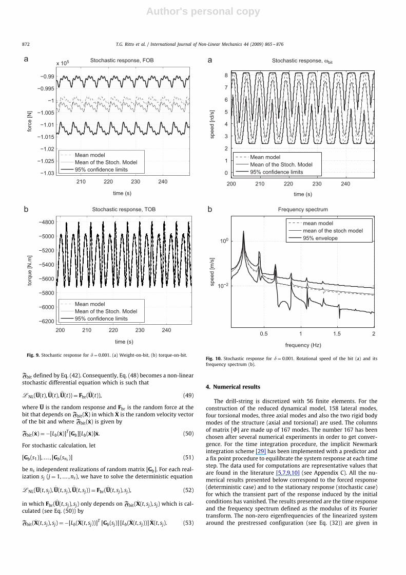
Fig. 9. Stochastic response for � = 0.001. (a) Weight-on-bit, (b) torque-on-bit.

Fbit defined by Eq. (42). Consequently, Eq. (48) becomes a non-linearstochastic differential equation which is such that

LNL(U(t), U(t), U(t)) = Fbr(U(t)), (49)

where U is the random response and Fbr is the random force at thebit that depends on Fbit(X) in which X is the random velocity vectorof the bit and where Fbit(x) is given by

Fbit(x) = −[Lb(x)]T [Gb][Lb(x)]x. (50)

For stochastic calculation, let

[Gb(s1)], . . . , [Gb(sns )] (51)

be ns independent realizations of random matrix [Gb]. For each real-ization sj (j = 1, . . . ,ns), we have to solve the deterministic equation

LNL(U(t, sj), U(t, sj), U(t, sj)) = Fbr(U(t, sj), sj), (52)

in which Fbr(U(t, sj), sj) only depends on Fbit(X(t, sj), sj) which is cal-culated (see Eq. (50)) by

Fbit(X(t, sj), sj) = −[Lb(X(t, sj))]T [Gb(sj)] [Lb(X(t, sj))] X(t, sj). (53)

200 210 220 230 240

0

1

2

3

4

5

6

7

8

time (s)

spee

d [rd

/s]

Stochastic response, ωbit

Mean modelMean of the Stoch. Model95% confidence limits

0.5 1 1.5 2

10−2

100

Frequency spectrum

frequency (Hz)

spee

d [m

/s]

mean modelmean of the stoch model95% envelope

Fig. 10. Stochastic response for � = 0.001. Rotational speed of the bit (a) and itsfrequency spectrum (b).

4. Numerical results

The drill-string is discretized with 56 finite elements. For theconstruction of the reduced dynamical model, 158 lateral modes,four torsional modes, three axial modes and also the two rigid bodymodes of the structure (axial and torsional) are used. The columnsof matrix [�] are made up of 167 modes. The number 167 has beenchosen after several numerical experiments in order to get conver-gence. For the time integration procedure, the implicit Newmarkintegration scheme [29] has been implemented with a predictor anda fix point procedure to equilibrate the system response at each timestep. The data used for computations are representative values thatare found in the literature [5,7,9,10] (see Appendix C). All the nu-merical results presented below correspond to the forced response(deterministic case) and to the stationary response (stochastic case)for which the transient part of the response induced by the initialconditions has vanished. The results presented are the time responseand the frequency spectrum defined as the modulus of its Fouriertransform. The non-zero eigenfrequencies of the linearized systemaround the prestressed configuration (see Eq. (32)) are given in

Author's personal copy

T.G. Ritto et al. / International Journal of Non-Linear Mechanics 44 (2009) 865 -- 876 873

210 220 230 240 250−0.06

−0.04

−0.02

0

0.02

0.04

0.06

0.08

0.1

time (s)

disp

lace

men

t [m

]

Stochastic response, x=700 m

boreholeMean modelMean of the Stoch. Model95% confidence limits

0.5 1 1.510−6

10−4

10−2

Frequency spectrum

frequency (Hz)

disp

lace

men

t [m

]

mean modelmean of the stoch model95% envelope

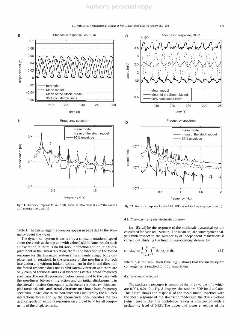
Fig. 11. Stochastic response for � = 0.001. Radial displacement at x= 700m (a) andits frequency spectrum (b).

Table 1. The lateral eigenfrequencies appear in pairs due to the sym-metry about the x-axis.

The dynamical system is excited by a constant rotational speedabout the x-axis at the top and with value 0.83Hz. Note that for suchan excitation, if there is no bit–rock interaction and no initial dis-placement in the lateral direction, there is no vibration in the forcedresponse for the linearized system (there is only a rigid body dis-placement in rotation). In the presence of the non-linear bit–rockinteraction and without initial displacement in the lateral direction,the forced response does not exhibit lateral vibration and there areonly coupled torsional and axial vibrations with a broad frequencyspectrum. The results presented below correspond to the case withthe non-linear bit–rock interaction and an initial displacement inthe lateral direction. Consequently, the forced response exhibits cou-pled torsional, axial and lateral vibrations on a broad band frequencyspectrum. In fact, due to the non-linearities induced by the bit–rockinteractions forces and by the geometrical non-linearities the fre-quency spectrum exhibits responses on a broad band for all compo-nents of the displacements.

210 220 230 240 250

0.5

1

1.5

2

2.5

3

3.5

x 10−3

time (s)

spee

d [m

/s]

Stochastic response, ROP

Mean modelMean of the Stoch. Model95% confidence limits

0.5 1 1.5 210−8

10−6

10−4

Frequency spectrum

frequency (Hz)

spee

d [m

/s]

mean modelmean of the stoch model95% envelope

Fig. 12. Stochastic response for � = 0.01. ROP (a) and its frequency spectrum (b).

4.1. Convergence of the stochastic solution

Let [U(t, sj)] be the response of the stochastic dynamical systemcalculated for each realization sj. Themean-square convergence anal-ysis with respect to the number ns of independent realizations iscarried out studying the function ns�conv(ns) defined by

conv(ns) = 1ns

ns∑j=1

∫ tf

0‖U(t, sj)‖2 dt, (54)

where tf is the simulation time. Fig. 7 shows that the mean-squareconvergence is reached for 150 simulations.

4.2. Stochastic response

The stochastic response is computed for three values of � whichare 0.001, 0.01, 0.1. Fig. 8 displays the random ROP for � = 0.001.This figure shows the response of the mean model together withthe mean response of the stochastic model and the 95% envelope(which means that the confidence region is constructed with aprobability level of 0.95). The upper and lower envelopes of the

Author's personal copy

874 T.G. Ritto et al. / International Journal of Non-Linear Mechanics 44 (2009) 865 -- 876

210 220 230 240

0

1

2

3

4

5

6

7

8

time (s)

spee

d [rd

/s]

Stochastic response, ωbit

Mean modelMean of the Stoch. Model95% confidence limits

0.5 1 1.5 2

10−4

10−2

100

Frequency spectrum

frequency (Hz)

spee

d [m

/s]

mean modelmean of the stoch model95% envelope

Fig. 13. Stochastic response for � = 0.01. Rotational speed of the bit bit (a) and itsfrequency spectrum (b).

confidence region are calculated using the method of quantiles[30].

Fig. 8(b) shows that the dispersion of the random ROP is alreadysignificant in the high part of the frequency band. However, thestochastic response in the low part of the frequency band is robustfor the level of uncertainties considered. Fig. 9 shows the randomweight-on-bit and torque-on-bit. It should be noted that, for eachtime t, the coefficients of variation of the random weight-on-bit andof the random torque-on-bit are small (∼ 5 × 10−3). Nevertheless,although this dispersion is small, it induces a significant dispersionon the stochastic response (∼ 0.15 for the coefficient of variation ofthe random ROP, for instance). Fig. 10 shows the random rotationalspeed of the bit and Fig. 11 shows the random radial displacementat x = 700m (middle point of the drill pipe). It can be seen that thelateral vibrations are also affected by the probabilistic model of thebit–rock interaction.

As � increases the stochastic response gets more uncertain withwider statistical envelopes. Fig. 12 shows the random ROP andFig. 13 shows the random rotational speed of the bit ( bit) for� = 0.01. Note that some other peaks appear in the frequency

200 210 220 230 240 250−0.06

−0.04

−0.02

0

0.02

0.04

0.06

0.08

time (s)

disp

lace

men

t [m

]

Stochastic response, x=700 m

boreholeMean modelMean of the Stoch. Model95% confidence limits

0.5 1 1.5 2

10−8

10−6

10−4

10−2

Frequency spectrum

frequency (Hz)

disp

lace

men

t [m

]

mean modelmean of the stoch model95% envelope

Fig. 14. Stochastic response for � = 0.01. Radial displacement at x = 700m and itsfrequency spectrum (b).

spectrum. Fig. 14 shows the random radial displacement. As shownin Fig. 14(a), there are some realizations where impacts occurbetween the column and the borehole.

Fig. 15 shows the random rotational speed of the bit for �=0.1. Itcan be noted that, for this level of uncertainty, the dispersion of thestochastic response is significant for all the frequency band analyzed.Fig. 16 shows some Monte Carlo realizations of the stochastic ROP.The arrows in Fig. 16 indicate that, for some realizations, the bit losescontact with the soil.

The probabilistic model proposed for the bit–rock interactionmodel allows us to simulate cases such as the bit losing contact withthe soil and the column impacting the borehole. The non-parametricprobabilistic approach permits both parameters and modeling errorsto be taken into account for the bit–rock interaction model.

5. Concluding remarks

A computational non-linear dynamical model taking into accountuncertainties has been developed to simulate the drill-string dynam-ics and it has been shown to be well suited to describe the prob-lem. A probabilistic model has been proposed to model uncertainties

Author's personal copy

T.G. Ritto et al. / International Journal of Non-Linear Mechanics 44 (2009) 865 -- 876 875

200 210 220 230 240−5

0

5

10

15

time (s)

spee

d [rd

/s]

Stochastic response, ωbit

Mean modelMean of the Stoch. Model95% confidence limits

0.5 1 1.5 210−6

10−4

10−2

100

Frequency spectrum

frequency (Hz)

spee

d [m

/s]

mean modelmean of the stoch model95% envelope

Fig. 15. Stochastic response for � = 0.1. Rotational speed of the bit bit (a) and itsfrequency spectrum (b).

in the bit–rock interaction model. Since the parameters of the meanmodel of the bit–rock interaction do not correspond to physicalparameters, these parameters are not adequate to the use of theparametric probabilistic approach. Then, the non-parametric prob-abilistic approach has been used. This corresponds to a completelynovel approach to take into account model uncertainties in a non-linear constitutive equation. Since the dynamical system is globallynon-linear, an adapted strategy has been developed to implement astochastic solver.

The non-linear Timoshenko beam model has been used and themain forces that affect the dynamics of the drill-string have beenconsidered such as the bit–rock interaction, the fluid–structureinteraction and the impact forces.

The parametric numerical analysis performed shows that thenon-linear dynamical responses of this type of mechanical system isvery sensitive to uncertainties in the bit–rock interaction model. Inaddition, these uncertainties play an important role in the couplingbetween the axial responses and the torsional one, and consequently,play a role in the lateral responses.

6 7 8 90

2

4

6

8

10

12

x 10−3

time [s]

Stochastic response, ROP

spee

d [m

/s]

For some realizations the bit loses contact with the soil

Fig. 16. Random ROP for � = 0.1.

Acknowledgments

The authors acknowledge the financial support of the Brazilianagencies CNPQ, CAPES and FAPERJ, and the French agency COFECUB(project CAPES-COFECUB 476/04).

Appendix A. Shape functions

Linear shape functions are used for the axial and torsional dis-placements and the shape functions for the lateral displacements arederived by calculating the static response of the beam [31,32]:

Nu = [(1 − �) 0 0 0 0 0 � 0 0 0 0 0],

Nv = [0 Nv1 Nv2 0 0 0 0 Nv3 Nv4 0 0 0],

Nw = [0 0 0 Nv1 − Nv2 0 0 0 0 Nv3 − Nv4 0],

N�x= [0 0 0 0 0 (1 − �) 0 0 0 0 0 �],

N�y= [0 0 0 − N�1 N�2 0 0 0 0 − N�3 N�4 0],

N�z= [0 N�1 N�2 0 0 0 0 N�3 N�4 0 0 0],

where

Nv1 = 11 + �

(1 − 3�2 + 2�3 + �(1 − �)),

Nv2 = le1 + �

(� − 2�2 + �3 + �

2(� − �2)

),

Nv3 = 11 + �

(3�2 − 2�3 + ��),

Nv4 = le1 + �

(−�2 + �3 + �

2(�2 − �)

),

N�1 = 1(1 + �)le

(−6� + 6�2),

N�2 = 11 + �

(1 − 4� + 3�2 + �(1 − �)),

N�3 = 1(1 + �)le

(6� − 6�2),

N�4 = 11 + �

(−2� + 3�2 + ��),

Author's personal copy

876 T.G. Ritto et al. / International Journal of Non-Linear Mechanics 44 (2009) 865 -- 876

in which � = 12EI/ksGAl2e , where E is the elasticity modulus, I is the

area moment of inertia (y–z plane), ks is shearing factor, G is theshear modulus, A is the cross sectional area and le is the length ofan element.

Appendix B. Algorithm for the realizations of the random germ[G]

Random matrix [G] can be written as [G] = [LG]T [LG] in which

[LG] is an upper triangular real random matrix such that:

1. The random variables {[LG]jj′ , j� j′} are independents.2. For j< j′ the real-valued random variable [LG]jj′ = �Vjj′ , in which

� = �3−1/2 and Vjj′ is a real-valued Gaussian random variable withzero mean and unit variance.

3. For j = j′ the real-valued random variable [LG]jj = �(2Vj)1/2. In

which Vj is a real-valued gamma random variable with probabilitydensity function written as

pVj(v) = 1R+ (v)

1

�(

3

2�2 + 1 − j2

)v3/2�2−(1+j)/2e−v.

Appendix C. Data used in the simulation

�x = 0.83Hz (rotational speed about the x-axis at the top),Ldp = 1400m (length of the drill pipe),Ldc = 200m (length of the drill collar),Dodp = 0.127m (outside diameter of the drill pipe),Dodc = 0.2286m (outside diameter of the drill collar),Didp = 0.095m (inside diameter of the drill pipe),Didc = 0.0762m (inside diameter of the drill collar),Dch = 0.3m (diameter of the borehole (channel)),xstab = 1400m (location of the stabilizer),kstab = 17.5MN/m (stiffness of the stabilizer per meter),E = 210GPa (elasticity modulus of the drill-string material),� = 7850kg/m3 (density of the drill-string material),� = 0.29 (Poisson coefficient of the drill-string material),ks = 6

7 (shearing correcting factor),kip = 1 × 108 N/m (stiffness per meter used for the impacts),ip = 0.0005 (frictional coefficient between the string and theborehole),uin = 1.5m/s (flow speed in the inlet),�f = 1200kg/m3 (density of the fluid),Cf = 0.0125 (fluid viscous damping coefficient),k = 0 (fluid viscous damping coefficient),g = 9.81m/s2 (gravity acceleration),a1=3.429×10−3 m/s (constant of the bit–rock interaction model),a2 = 5.672 × 10−8 m/(N s) (constant of the bit–rock interactionmodel),a3 = 1.374 × 10−4 m/rd (constant of the bit–rock interactionmodel),a4=9.537×106 N rd (constant of the bit–rock interaction model),a5 =1.475×103 Nm (constant of the bit–rock interaction model),e = 2 rd/s (regularization parameter).

The damping matrix is constructed using the relationship [C] =�([M]+ [Mf ])+ �([K]+ [Kf ]+ [Kg(uS)]) with � = 0.01 and � = 0.0003.

References

[1] K.A. Macdonald, J.V. Bjune, Failure analysis of drillstrings, Engineering FailureAnalysis 14 (2007) 1641–1666.

[2] P.D. Spanos, A.M. Chevallier, N.P. Politis, M.L. Payne, Oil and gas well drilling: avibrations perspective, The Shock and Vibration Digest 35 (2) (2003) 85–103.

[3] A. Yigit, A. Christoforou, Coupled axial and transverse vibrations of oilwelldrillstrings, Journal of Sound and Vibration 195 (4) (1996) 617–627.

[4] A.P. Christoforou, A.S. Yigit, Dynamic modeling of rotating drillstrings withborehole interactions, Journal of Sound and Vibration 206 (2) (1997) 243–260.

[5] A.P. Christoforou, A.S. Yigit, Fully vibrations of actively controlled drillstrings,Journal of Sound and Vibration 267 (2003) 1029–1045.

[6] R.W. Tucker, C. Wang, An integrated model for drill-string dynamics, Journalof Sound and Vibration 224 (1) (1999) 123–165.

[7] R.W. Tucker, C. Wang, Torsional vibration control and Cosserat dynamics of adrill-rig assembly, Meccanica 224 (1) (2003) 123–165.

[8] Y.A. Khulief, H. Al-Naser, Finite element dynamic analysis of drill-strings, FiniteElements in Analysis and Design 41 (2005) 1270–1288.

[9] Y.A. Khulief, F.A. Al-Sulaiman, S. Bashmal, Vibration analysis of drill-strings withself excited stick-slip oscillations, Journal of Sound and Vibration 299 (2007)540–558.

[10] R. Sampaio, M.T. Piovan, G.V. Lozano, Coupled axial/torsional vibrationsof drilling-strings by mean of nonlinear model, Mechanics ResearchCommunications 34 (5–6) (2007) 497–502.

[11] M.P. Paidoussis, T.P. Luu, S. Prabhakar, Dynamics of a long tubular cantileverconveying fluid downwards, which then flows upwards around the cantileveras a confined annular flow, Journal of Fluids and Structures 24 (11) (2007)111–128.

[12] P.D. Spanos, A.M. Chevallier, N.P. Politis, Nonlinear stochastic drill-stringvibrations, Journal of Vibration and Acoustics 124 (4) (2002) 512–518.

[13] S.J. Kotsonis, P.D. Spanos, Chaotic and random whirling motion of drillstrings,Journal of Energy Resources Technology (Transactions of the ASME) 119 (4)(1997) 217–222.

[14] P.D. Spanos, A.K. Sengupta, R.A. Cunningham, P.R. Paslay, Modeling of roller conebit lift-off dynamics in rotary drilling, Journal of Energy Resources Technology117 (3) (1995) 197–207.

[15] C. Soize, A nonparametric model of random uncertainties for reduced matrixmodels in structural dynamics, Probabilistic Engineering Mechanics 15 (2000)277–294.

[16] C. Soize, Maximum entropy approach for modeling random uncertainties intransient elastodynamics, Journal of the Acoustical Society of America 109 (5)(2001) 1979–1996.

[17] C. Soize, Random matrix theory for modeling uncertainties in computationalmechanics, Computer Methods in Applied Mechanics and Engineering 194(12–16) (2005) 1333–1366.

[18] D. Childs, Turbomachinery Rotordynamics: Phenomena, Modeling, and Analysis,Wiley-Interscience, 1993.

[19] ASME, Handbook: Drilling Fluids Processing, Elsevier Inc., Amsterdam, 2005.[20] P. Coussot, F. Bertrand, B. Herzhaft, Rheological Behavior of drilling muds,

characterization using MRI visualization, Oil and Gas Science and Technology59 (1) (2004) 23–29.

[21] M.P. Escudier, I.W. Gouldson, P.J. Oliveira, F.T. Pinho, Effects of inner cylinderrotation on laminar flow of a Newtonian fluid through an eccentric annulus,International Journal of Heat and Fluid Flow 21 (2000) 92–103.

[22] M.P. Escudier, P.J. Oliveira, F.T. Pinho, Fully developed laminar flow ofpurely viscous non-Newtonian liquids through annuli including the effects ofeccentricity and inner-cylinder rotation, International Journal of Heat and FluidFlow 23 (2002) 52–73.

[23] E.P.F. Pina, M.S. Carvalho, Three-dimensional flow of a Newtonian liquid throughan annular space with axially varying eccentricity, Journal of Fluids Engineering128 (2) (2006) 223–231.

[24] M.P. Paidoussis, Non-linear dynamics of a fluid-conveying cantilevered pipewith a small mass attached at the free end, International Journal of Non-LinearMechanics 33 (1) (1998) 15–32.

[25] M.P. Mignolet, C. Soize, Stochastic reduced order models for uncertaingeometrically nonlinear dynamical systems, Computer Methods in AppliedMechanics and Engineering 197 (45–48) (2008) 3951–3963.

[26] C.E. Shannon, A mathematical theory of communication, Bell System TechnicalJournal 27 (1948) 379–423 623–659.

[27] E. Jaynes, Information theory and statistical mechanics, The Physical Review106 (4) (1957) 1620–1630.

[28] E. Jaynes, Information theory and statistical mechanics II, The Physical Review108 (1957) 171–190.

[29] K.J. Bathe, Finite Element Procedures, Prentice-Hall Inc., Englewood Cliffs, NJ,1996.

[30] R.J. Serfling, Approximation Theorems of Mathematical Statistics, Wiley, NewYork, 1980.

[31] H.D. Nelson, A finite rotating shaft element using Timoshenko been theory,Journal of Mechanical Design 102 (1980) 793–803.

[32] A. Bazoune, Y.A. Khulief, Shape functions of the three-dimensional Timoshenkobeam element, Journal of Sound and Vibration 259 (2) (2002) 473–480.