
On the Density-Density Critical Indices�in Interacting Fermi Systems
46
On the density-density critical indices in interacting Fermi systems G. Benfatto V. Mastropietro Dipartimento di Matematica, Universit`a di Roma “Tor Vergata” 25 febbraio 2002 Abstract The behaviour of correlation functions of d = 1 interacting fermionic systems is determined by a small number of critical indices. We prove that one of them is exactly zero. As a consequence, the behavior of the Fourier transform of the density-density correlation at zero momen- tum is qualitatively unaffected by the interaction, contrary to what happens at ±2˜ p F , if ˜ p F is the Fermi momentum. The result is ob- tained by implementing Ward identities in a Renormalization Group approach. 1 Introduction and main results 1.1 Motivations and results If a ± x , x = −[ L−1 2 ],..., [ L 2 ], is a set of fermionic creation and annihilation operators, we consider the Hamiltonian H = [ L 2 ] x=−[ L−1 2 ] 1 2 (a + x+1 − a + x )(a − x+1 − a − x ) − μa + x a − x +λ(a + x a − x − 1 2 )(a + x+1 a − x+1 − 1 2 ) , (1) describing a system of spinless fermions in d = 1 with chemical potential μ, a nearest-neighbor interaction and periodic boundary conditions. The 1
Transcript of On the Density-Density Critical Indices�in Interacting Fermi Systems

On the density-density critical indices in
interacting Fermi systems
G. BenfattoV. Mastropietro
Dipartimento di Matematica, Universita di Roma “Tor Vergata”
25 febbraio 2002
Abstract
The behaviour of correlation functions of d = 1 interacting fermionic
systems is determined by a small number of critical indices. We prove
that one of them is exactly zero. As a consequence, the behavior of the
Fourier transform of the density-density correlation at zero momen-
tum is qualitatively unaffected by the interaction, contrary to what
happens at ±2pF , if pF is the Fermi momentum. The result is ob-
tained by implementing Ward identities in a Renormalization Group
approach.
1 Introduction and main results
1.1 Motivations and results
If a±x , x = −[L−12], ..., [L
2], is a set of fermionic creation and annihilation
operators, we consider the Hamiltonian
H =
[L2]
∑
x=−[L−12
]
1
2(a+x+1 − a+x )(a
−x+1 − a−x )− µa+x a
−x
+λ(a+x a−x − 1
2)(a+x+1a
−x+1 −
1
2)
, (1)
describing a system of spinless fermions in d = 1 with chemical potentialµ, a nearest-neighbor interaction and periodic boundary conditions. The
1

space-time density-density correlation function at temperature β−1 is givenby
ΩL,β(x) =< a+x a−x a
+0 a
−0 >L,β − < a+x a
−x >L,β< a+0 a
−0 >L,β, (2)
where x = (x, x0), a±x = eHx0a±x e
−Hx0 and < . >L,β= Tr[e−βH .]/Tr[e−βH ]denotes the expectation in the grand canonical ensemble. We shall use alsothe notation Ω(x) ≡ limL,β→∞ΩL,β(x).
If the fermions are non interacting (λ = 0), one can easily check that, if|x| ≥ 1, cos pF = 1− µ, v0 = sin pF > 0,
Ω(x) = cos(2pFx)Ωa0(x) + Ωb0(x) + Ωc0(x),
Ωa0(x) =1
2π2[x2 + (v0x0)2], (3)
Ωb0(x) =1
2π2[x2 + (v0x0)2]
x20 − (x/v0)2
x2 + (v0x0)2,
|Ωc0(x)| ≤1
1 + |x|2+ϑ ,
for some positive constant ϑ < 1.The interaction has two main effects: the period of the oscillating term
cos(2pFx)Ωa0(x) changes and the large distance asymptotic decay is modified
by critical indices. It was indeed proved in [BM] by a Renormalization Groupanalysis that, for λ small enough and |x| ≥ 1,
Ω(x) = cos(2pFx)Ωa(x) + Ωb(x) + Ωc(x),
Ωa(x) =1 + λB1(x)
2π2[x2 + (v∗0x0)2]1+ηa, (4)
Ωb(x) =1
2π2[x2 + (v∗0x0)2]1+ηb
x20 − (x/v∗0)2
x2 + (v∗0x0)2+ λB2(x)
,
|Bi(x)| ≤ C, |Ωc(x)| ≤ 1
1 + |x|2+ϑ ,
where C is a positive constant, ηa, ηb are critical indices expressed by con-vergent series in λ, v∗0 = v0 + δ∗ and pF (λ, pF ) = pF + λf(λ, pF ) with δ
∗, fanalytic in λ and |δ∗| ≤ C|λ|, |f(λ, pF )| ≤ C; note that f(λ, π
2) = 0, by
symmetry reasons.By an explicit computation of the lowest order of the convergent series
for ηa one obtains that ηa = −a1λ+O(λ2), where a1 > 0 is a non vanishingconstant. The lowest order contributions to ηb are instead vanishing, inagreement with the conjecture (see for instance [Sp]) that ηb is exactly zero.The aim of this paper is to prove such conjecture.
2

Theorem 1.1 There exists a positive constant λ0 such that, if |λ| ≤ λ0,the density-density correlation function (2) can be written as in (4) with thecritical index ηb identically vanishing.
The vanishing of the critical index ηb has many interesting consequences.For instance, see [BM], if λ = 0 the Fourier transform Ω(k) of Ω(x, 0) hasthree cusps, at k = 0 and k = ±2pF , i.e. ∂kΩ(k) has a first order discontinuityat k = 0 and k = ±2pF . The vanishing of ηb = 0 implies that Ω(k) hasstill a cusp at k = 0 even if λ 6= 0; in fact it was proved in [BM] that, ifηb = 0, the possible logarithmic singularity of ∂Ω(k) at k = 0 is changed bya parity cancellation into a first order discontinuity with jump 1+O(λ); thisis remarkable because, generally, the qualitative behaviour close to criticalpoints is deeply changed by the interaction; for instance ∂kΩ(k) at k = ±2pFin the λ 6= 0 case is continuous for λ < 0, while it diverges as |k− (±2pF )|2ηafor λ > 0.
Note finally that the model (1) is equivalent to the XXZ spin-chain withmagnetic field h = µ − 1, as one can show by a Schwinger-Dyson transfor-mation [LSM], with (2) representing the spin-spin correlation function alongthe third axis. Moreover our proof that ηb = 0 could be easily extended toa large class of models; for instance one can replace the nearest neighborinteraction with a non nearest neighbor one, or the lattice with a continuum,or to consider the anisotropic XY Z spin chain, see [BM]. We rememberfinally that there are remarkable relations, based on exact solutions, betweenproperties of quantum spin chains and bidimensional classical statistical me-chanics models; for instance the spin-spin correlation function of the XY Zspin chain is believed to be equal to the correlation between two verticalarrows in the same row in the eigth vertex model, see [B] and [JKM], if asuitable identification of the parameters is done. Hence our results could berelevant also for such problems. Another application is for models of vicinalsurfaces, see [Sp].
1.2 Remarks
In [BM] we derived a convergent expansion for the critical index ηb; eachorder is obtained by summing up a certain numbers of terms, and ηb = 0means that there is a cancellation at all orders between such terms. Whileone can easily check from such expansion that this is the case at the secondorder, to prove directly that such cancellation occurs at all orders looks to usessentially impossible. We proceed instead in a different way and our proofis conceptually divided in two main steps.
3

For the first step we refer to [BM], where the proof that ηb = 0 is re-duced to a special property (see (20) below) of the Schwinger functions of amodel (which we will call reference model), describing fermions with a linear“relativistic” dispersion relation and allowed momenta restricted by infraredand ultraviolet cut-offs. This result, which is resumed in Theorem 2.2 be-low, gives further ground to the remarkable observation of Tomonaga [T],according to which the model (1) is essentially equivalent, as far as the lowenergy behaviour is considered, to a system of interacting massless relativisticfermions.
In the second step we deduce such property of the reference model by us-ing a suitable Ward identity, which is obtained through a local gauge trans-formation. Usually in relativistic quantum field theory Ward identities arerelations between correlation functions; the Ward identity we find is insteada relation between correlation functions and some other extra terms, whichwe call ”correction” as they would be formally zero if the cut-offs were re-moved. The extra terms do not vanish when the infrared cut-off is removed.The property that we need is reduced to suitable bounds (see Theorems 2.1and 2.3), proved by using convergent expansions for all terms appearing inthe Ward identity.
We conclude the introduction with a technical note. With respect toprevious applications of Wilsonian Renormalization Group to d = 1 inter-acting fermionic theories, like [BG] or [BGPS], we are able here to rigorouslyimplement in this scheme the method of Ward identities (based on localgauge transformations) to produce non trivial results. In the physical liter-ature there are many claims on the vanishing of ηb, see for instance [DL],[ES], [DM], and our results convert such ideas into a rigorous proof. Fi-nally, note that there are many examples of QFT models in which WardIdentities are implemented in a mathematical way, perturbatively (see forinstance [FHRW], [KK]) or non perturbatively (see for instance [BFS] or[MSR]). However such works consider the application of Ward Identities torelativistic QFT; hence corrections to formal exact Ward Identities are pos-sibly found as a consequence of the cut-offs imposed to regularize the theory,but they are vanishing when the cut-offs are removed. The main noveltyof our paper is that we try to implement the method of Ward identities inthe not relativistic model (1), where there is no reason why a Ward Identityinvolving only correlation functions should be valid. The corrections are notvanishing and the technical problem is to get for such terms bounds goodenough to prove that ηb = 0.
4

2 Ward Identities
2.1 The reference model
The reference model is not Hamiltonian and is defined in terms of Grassmannvariables. Given the interval [0, L], the inverse temperature β and the (large)integer N , we introduce in Λ = [0, L] × [0, β] a lattice ΛN , whose sites aregiven by the space-time points x = (x, x0) = (na, n0a0), a = L/N , a0 = β/N ,n, n0 = 0, 1, . . . , N − 1. We also consider the set D of space-time momentak = (k, k0), with k = 2π
L(n+ 1
2) and k0 =
2πβ(n0 +
12), n, n0 = 0, 1, . . . , N − 1.
With each k ∈ D we associate four Grassmanian variables ψ[h,0]σk,ω , σ, ω ∈
+,−. The lattice ΛN is introduced only for technical reasons so that thenumber of Grassmann variables is finite, and eventually the limit N → ∞is taken (and it is trivial, see [BM], §2.1). If γ is a fixed number greaterthan 1 and h is a negative integer, we define the function [Ch,0]
−1(k) as astrictly positive smooth function acting as a cut-off for momenta |k| ≥ γ(ultraviolet region) and |k| ≤ γh−1 (infrared region) and having value 1 inthe intermediate region γh ≤ |k| ≤ 1. The infrared cut-off γh is not fixed,because we are interested in the dependence on h of the reference model. Theexact definition of [Ch,0]
−1(k) is the following one. We introduce a positivefunction χ0 ∈ C∞(R+) such that
χ0(t) =
1 if 0 ≤ t ≤ 1 ,0 if t ≥ γ0 , 1 < γ0 ≤ γ
(5)
and we define, for any integer j ≤ 0,
fj(k) = χ0(γ−j|k|)− χ0(γ
−j+1|k|) . (6)
Then we define [Ch,0(k)]−1 =
∑0j=h fj(k). If D = k ∈ D : [Ch,0(k)]
−1 6= 0,we define the functional integration
∫
Dψ[h,0] as the linear functional on the
Grassmann algebra generated by the variables ψ[h,0]σk,ω , such that, given a
monomial Q(ψ) in the variables ψ[h,0]σk,ω , its value is 0, except in the case
Q(ψ) =∏
k∈D,ω=± ψ[h,0]−k,ω ψ
[h,0]+k,ω , up to a permutation of the variables. In this
case the value of the functional is determined, by using the anticommutingproperties of the variables, by
∫
Dψ[h,0]Q(ψ) = 1 . We also define theGrassmanian field on the lattice ΛN as
ψ[h,0]σx,ω =
1
Lβ
∑
k∈Deiσkxψ
[h,0]σk,ω , x ∈ ΛN . (7)
Note that ψ[h,0]σx,ω is antiperiodic both in time and space variables.
5

The Schwinger functions of the reference model are
S(x1, σ1, ω1; ...;xs, σs, ωs) =
∫
P (dψ[h,0])e−V (ψ[h,0])∏si=1 ψ
[h,0]σixi,ωi
∫
P (dψ[h,0])e−V (ψ[h,0]), (8)
whereV (ψ[h,0]) = λ
∫
dx ψ[h,0]+x,+ ψ
[h,0]−x,+ ψ
[h,0]+x,− ψ
[h,0]−x,− , (9)
∫
dx is a shorthand for “a a0∑
x∈ΛN” and
P (dψ[h,0]) = N−1Dψ[h,0] · (10)
· exp
− 1
Lβ
∑
ω=±1
∑
k∈DCh,0(k)(−ik0 + ωk)ψ
[h,0]+k,ω ψ
[h,0]−k,ω
,
with N =∏
k∈D[(Lβ)−2(−k20 − k2)Ch,0(k)
2].
We also define the connected Schwinger functions as the functional deriva-tives of the Generating functional
W(φ, J) = log∫
P (dψ)e−V (ψ)+
∑
ω
∫
dx
[
Jx,ωψ[h,0]+x,ω ψ
[h,0]−x,ω +φ+x,ωψ
[h,0]−x,ω +ψ
[h,0]+x,ω φ−x,ω
]
(11)with respect to the external field variables φσx,ω and Jx,ω, x ∈ ΛN , ω = ±1.The variables φσx,ω are antiperiodic in x0 and x and anticommuting with
themselves and ψ[h,0]σx,ω , while the variables Jx,ω are periodic and commuting
with themselves and all the other variables. We shall need in particular thefollowing connected Schwinger functions:
G2,1ω (x;y, z) =
∂
∂Jx,ω
∂2
∂φ+y,ω∂φ
−z,ω
W(φ, J)|φ=J=0 , (12)
G2ω(y, z) =
∂2
∂φ+y,ω∂φ
−z,ω
W(φ, J)|φ=J=0 . (13)
They will be pictorially represented as in Fig. 1.We also need the Fourier transforms of G2,1
ω and G2ω, defined by
G2ω(x,y) =
1
(Lβ)
∑
k
e−ik(x−y)G2ω(k) , (14)
G2,1ω (x;y, z) =
1
(Lβ)2∑
k,p
eipxe−ikyei(k−p)zG2,1ω (p,k) , (15)
In §3 we prove the following bounds for the reference model with cut-offγh, which has to be of course larger than minπ/L, π/β (otherwise the setD is empty).
6

G2,1ω
x
y zω ω
ω ω
G2ω
z
y
ω
ω
Figure 1: Graphical representation of the connected Schwinger functions G2,1ω
and G2ω.
Theorem 2.1 There exists a positive constant λ0, independent of h, suchthat, if |λ| ≤ λ0, there exist two positive functions of λ, Z
(2)h and Zh, and
a positive constant C, independent of h, so that, uniformly in N,L, β largeenough, if k ∈ D is such that γh ≤ |k| ≤ γh+1
G2,1ω (2k,−k) = − Z
(2)h
Z2hDω(k)2
[1 +O(λ2)] , (16)
G2ω(k) =
1
ZhDω(k)[1 +O(λ2)] , (17)
Cλ2|h| ≤ logZ(2)h ≤ 2Cλ2|h| , C|h|λ2 ≤ logZh ≤ 2Cλ2|h| (18)
with Dω(k) = −ik0 + ωk. Moreover
limh→−∞
logZ
(2)h−1
Z(2)h
= η2(λ) , limh→−∞
logZh−1
Zh= η(λ) , (19)
with η(λ) = a2λ2 + O(λ3), and η2(λ) = a2λ
2 + O(λ3) where a2 is a positiveconstant.
The connection between the model (1) and the reference model is givenby the following theorem, which is proved in [BM] , even if it is not explicitlyformulated. To be more precise, in §5.5 of [BM] we show that the condition(20), equivalent to eq. (5.35) of [BM], implies the bound (5.38) of [BM],which is equivalent to say that ηb = 0.
Theorem 2.2 Under the same assumptions of Theorem 2.1, there exists aconstant C such that, if for all negative integer h the functions Zh, Z
(1)h in
(16), (17) verify
Cλ2 ≤ |Z(2)h
Zh− 1| ≤ 2Cλ2 , (20)
7

then in(4) ηb(λ) = 0.
Hence by Theorem 2.2 the proof of ηb = 0 is reduced to the verification of(20), to which the rest of this paper is devoted. Note that (20) is equivalent,by (18), to η(λ)− η2(λ) = 0 (in Theorem 2.1 it is only claimed that η(λ)−η2(λ) = O(λ3)).
2.2 Ward identities for the reference model
We have so far reduced the proof that ηb = 0 in the model (1) to the verifi-cation of (20) in the reference model. This result will be achieved by usingan identity relating G2
ω to G2,1, obtained by performing a local gauge trans-formation, together with equations (16), (17).
In order to derive such identity, we find convenient to introduce a cut-offfunction [Cε
h,0(k)]−1, where ε is a small positive parameter and limε→0+[C
εh,0(k)]
−1 =Ch,0(k)]
−1. The functions [Cεh,0(k)]
−1 and [Ch,0(k)]−1 are equivalent as far
as the scaling properties of the theory are concerned but the support of[Cε
h,0(k)]−1 is the set D instead of D. The definition (10) of the reference
model is easily extended to the case in which the cut-off is [Cεh,0(k)]
−1 in-stead of [Ch,0(k)]
−1, by substituting in the r.h.s. of (10), as well as in thedefinition of the integration
∫
Dψ[h,0], the set D with D. A reason why wefind this convenient is that a technically important role in the following isplayed by the gauge invariance of the integration
∫
Dψ[h,0], a property whichis lost if the Grassmann algebra is restricted to the variables ψk,ω with k ∈ D.
The exact definition of [Cεh,0(k)]
−1 is the following one. Given a positiveε << 1, we define
χεh,0(k) = [Cεh,0(k)]
−1 =0∑
j=h
f εj (k) , (21)
where f εj (k) = fj(k), if h+ 1 ≤ j ≤ −1, while f ε0 (k) and fεh(k) are obtained
by slightly modifying f0(k) and fh(k) in the following way. f ε0 (k) is a C∞
function of |k|, such that limε→0 fε0 = f0, f
ε0 (k) = f0(k) for γ−1 ≤ |k| ≤ 1,
f ε0 (k) > 0 for |k| ≥ 1 and, if |k| ≥ γ, 0 < f ε0 (k) ≤ εe−|k|. Analogously,f εh(k) is a C∞ function of |k|, such that limε→0 f
εh = fh, f
εh(k) = fh(k) for
γh ≤ |k| ≤ γh+1, f εh(k) > 0, if 0 < |k| ≤ γh, and if 0 < |k| ≤ γh−1,0 < f εh(k) ≤ ε exp(−|k|−1).
Hence, we first study the case ε > 0, for which a Ward identity canbe easily obtained, relating the Schwinger functions of interest for us, forwhich the limit ε→ 0 is trivial, and a “correction term”, which is apparentlysingular as ε → 0. However we prove that this term can be written as a
8
|k|
1
γhγh−1 γ1
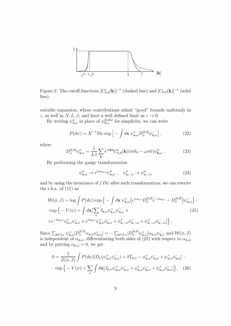
Figure 2: The cutoff functions [Cεh,0(k)]
−1 (dashed line) and [Ch,0(k)]−1 (solid
line).
suitable expansion, whose contributions admit “good” bounds uniformly inε, as well in N,L, β, and have a well defined limit as ε→ 0.
By writing ψσx,ω in place of ψ[h,0]σx,ω for simplicity, we can write
P (dψ) = N−1Dψ exp[
−∫
dx ψ+x,ωD
[h,0]ω ψ−
x,ω
]
, (22)
where
D[h,0]ω ψσx,ω =
1
Lβ
∑
k
eiσkxCεh,0(k)(iσk0 − ωσk)ψσk,ω . (23)
By performing the gauge transformation
ψσx,ω → eiσαx,ωψσx,ω , ψσx,−ω → ψσx,−ω (24)
and by using the invariance of∫
Dψ after such transformation, we can rewritethe r.h.s. of (11) as
W(φ, J) = log∫
P (dψ) exp
−∫
dx ψ+x,ω
(
eiαx,ωD[h,0]ω e−iαx,ω −D
[h,0]ω
)
ψ−x,ω
·
· exp
− V (ψ) +∫
dx[∑
ω
Jx,ωψ+x,ωψ
−x,ω + (25)
+e−iαx,ωφ+x,ωψ
−x,ω + eiαx,ωψ+
x,ωφ−x,ω + φ+
x,−ωψ−x,−ω + ψ+
x,−ωφ−x,−ω]
,
Since∑
x∈ΛNψ+x,ω[D
[h,0]ω αx,ωψ
−x,ω] = −∑x∈ΛN
[D[h,0]ω ψ+
x,ω]αx,ωψ−x,ω and W(φ, J)
is independent of αx,ω, differentiating both sides of (25) with respect to αx,ω
and by putting αx,ω = 0, we get
0 =1
Z(φ, J)
∫
P (dψ)[Dω(ψ+x,ωψ
−x,ω) + δTx,ω − φ+
x,ωψ−x,ω + ψ+
x,ωφ−x,ω] ·
· exp
− V (ψ) +∑
ω
∫
dx[Jx,ωψ+x,ωψ
−x,ω + φ+
x,ωψ−x,ω + ψ+
x,ωφ−x,ω]
, (26)
9

where Z(φ, J) = expW(φ, J), Dω is defined as D[h,0]ω , see (23), with 1 in
place of Cεh,0(k), so that, if Dω(p) = −ip0 + ωp
Dω(ψ+x,ωψ
−x,ω) =
1
(Lβ)2∑
p,k
Dω(p)e−ipxψ+
k,ωψ−k−p,ω . (27)
where p = (p, p0) is summed over momenta of the form (2πn/L, 2πm/β),with n,m integers Moreover
δTx,ω =1
(Lβ)2∑
k+ 6=k−
ei(k+−k−)xCε(k+,k−)ψ+
k+,ωψ−k−,ω , (28)
Cε(k+,k−) = [Cεh,0(k
−)− 1]Dω(k−)− [Cε
h,0(k+)− 1]Dω(k
+) , (29)
By differentiating the r.h.s. of (26) with respect to φ+y,ω and φ−
z,ω and thensetting the external fields equal to 0, we obtain, in terms of the Fouriertransform
−DωG2,1ω (x;y, z) = δ(x−y)G2
ω(x, z)−δ(x−z)G2ω(y,x)+∆2,1
ω (x;y, z) , (30)
where∆2,1ω (x;y, z) =< ψ−
y,ω;ψ+z,ω; δTx,ω >
T . (31)
If A1, . . . , An are functions of the field, we are using the symbol
< A1; . . . ;An >T=
∂n
∂λ1...∂λnlog
∫
P (dψ)e−V (ψ)+∑n
i=1λiAi
∣
∣
∣
λ=0. (32)
It is convenient to express the Ward identity (30) in terms of the Fouriertransforms of the connected Schwinger functions; ∆2,1
ω (p,k) is defined in asimilar way to G2,1
ω (p,k). In terms of the Fourier transform (30) can bewritten (see Fig. 3) as
Dω(p)G2,1ω (p,k) = G2
ω(k− p)− G2ω(k) + ∆2,1
ω (p,k) , (33)
If p 6= 0, (33) can be written in the form
G2,1ω (p,k) =
G2ω(k− p)−G2
ω(k)
Dω(p)+ H2,1
ω (k,p) , (34)
where H2,1ω (k,p) is the Fourier transform, defined in agreement with (15), of
H2,1ω (x;y, z) =
∂
∂Jx,ω
∂2
∂φ+y,ω∂φ
−z,ω
W∆(φ, J)|φ=J=0 , (35)
10

G2,1ω
Dω(p)
k q
p = k− q
=G2ω
q
q
− G2ω
k
k
+ ∆2,1ω
k q
p
Figure 3: Graphical representation of the identity (33).
with
W∆(φ, J) = log∫
P (dψ)e−V (ψ)+∑
ω
∫
dx[Jx,ωTx,ω+φ+x,ωψ
−x,ω+ψ
+x,ωφ
−x,ω ] , (36)
Tx,ω =1
(Lβ)2∑
k+ 6=k−
ei(k+−k−)x Cε(k+,k−)
Dω(k+ − k−)ψ+k+,ωψ
−k−,ω . (37)
Equation (34) is our Ward identity; it involves not only correlation func-tions but also the term H2,1
ω (k,p), which we can call the correction term asit would be formally zero in absence of cut-offs. Note that the definition (35)of the correction term H2,1
ω is similar to the definition (12) of G2,1ω , but the
two quantities have very different properties. In fact H2,1ω can be obtained by
substituting ψ+x,ωψ
−x,ω in (11) with Tx,ω, given by (37), which looks as a very
singular term as ε → 0. We are nevertheless able to express also H2,1ω (k,p)
by a convergent expansion, and we can prove in §4 the following bound.
Theorem 2.3 There exists a positive constant λ0, independent of h, suchthat, if |λ| ≤ λ0, then, uniformly in ε small enough and N,L, β large enough
Cγ−2hλ2Z
(2)h
(Zh)2≤ |H2,1
ω (2k,−k)| ≤ 2Cγ−2hλ2Z
(2)h
(Zh)2. (38)
Moreover, limε→0 H2,1ω does exist.
The above result (it was already claimed in [BM] referring for the proofto the present paper) says that H2,1
ω behaves, as h → −∞, exactly asG2,1ω (2k,−k), but its bound has an extra λ2 factor. This is just what we
need; if we insert (16), (17) and (38) in (33), we obtain (20) and hence, byTheorem 2.1 and 2.2, ηb = 0.
11

2.3 Remarks
In the physical literature Ward identities for interacting d = 1 fermions withcut-offs are usually derived by various formal arguments, see for example[DL], [ES], [MD], [S]. All arguments are essentially equivalent to expandingG2ω and G2,1
ω in Feynman graphs and then ”forget” the cut-off function. Infact, if we neglect the cut-offs, the propagator is simply Dω(k)
−1 and the“identity” G2,1
ω (p,k) = [G2ω(k−p)−G2
ω(k)]/D(p), from which ηb = 0 follows,is derived by the following obvious identity
Dω(p)−1[Dω(k)
−1 −Dω(k + p)−1] = Dω(k+ p)−1Dω(k)−1 , (39)
By taking consistently into account the cut-off function one gets, instead of(39), the identity
gω(k)− gω(k+ p)
Dω(p)= gω(k)gω(k+ p) + gω(k)gω(k + p)
Cε(k,k + p)
D(p), (40)
which allows in principle to check directly equation (34) at any order (veryeasily at order 0, which coincides with (34)). Our analysis shows then thatone can still derive from the Ward identities the vanishing of ηb in a rigorousway, by taking into account the presence of cut-offs. This however seems nottrue for other consequences of Ward identities for the model (1) claimed inthe literature, see [BM1].
Note also that, as ε→ 0, [Cεh,0(k)]
−1 becomes a compact support function,so Cε(k,k + p) becomes singular. However the singularity at ε = 0 of thefunction Cε(k,k + p) in the second addend of the r.h.s. in (40) is of coursecompensated by the cut-off functions appearing in the propagators. Henceone could “in principle” derive (34) directly using a compact support cut-off (i.e. using [Ch,0]
−1 instead of [Cεh,0]
−1), for instance by a Feynman graphanalysis using (40) at ε = 0, but such derivation would be surely much morelengthy.
3 Renormalization Group analysis
3.1 The effective potentials and the beta function
The results in Theorem 2.1 and 2.3 can be derived by expressing G2ω, G
2,1ω
and H2,1ω by a suitable multiscale expansion based on Renormalization group
ideas. In the following sections we will prove (16),(17),(38), referring to [BM]for the proof of many technical lemmas we will need.
12
We begin our analysis, for clarity reason, by studying the ”free energy”
of the model, which is the simplest quantity which can be studied by ourmethod; it is defined by
EL,β = − 1
Lβlog
∫
P (dψ[h,0])e−V (ψ[h,0]) . (41)
The functional integration in (41) can be performed iteratively by a slightmodification of the procedure described (for instance) in sec.(2.5)-(2.8) of[BM]. We prove by induction that, for any negative integer j, there are aconstant Ej , a positive function Zj(k) and a functional V(j) such that
∫
P (dψ[h,0])e−V (ψ[h,0]) =∫
PZj ,Cεh,j(dψ[h,j]) e−V(j)(
√Zjψ[h,j])−LβEj , (42)
with V(j)(0) = 0, Zj = maxk Zj(k),
PZj ,Cεh,j(dψ[h,j]) =
∏
k:Cεh,j
(k)>0
∏
ω=±1
dψ[h,j])+k,ω dψ
[h,j]−k,ω
Nj(k)·
· exp
− 1
Lβ
∑
k
Cεh,j(k)Zj(k)
∑
ω±1
ψ[h,j]+ω Dω(k)ψ
[h,j]−k,ω
, (43)
Cεh,j(k)
−1 =j∑
r=h
f εr (k) ≡ χh,j(k) (44)
and Nj(k) = (Lβ)−1Cεh,j(k)Zj(k)[−k20 − k2]1/2. Finally, V(j) which can be
written as
V(j)(ψ) =∞∑
n=1
1
(Lβ)2n∑
k1,...,k2nω1,...,ω2n
2n∏
i=1
ψσiki,ωiW
(j)2n,ω(k1, ...,k2n−1)δ
(
2n∑
i=1
σiki
)
,
(45)where σi = + for i = 1, . . . , n, σi = − for i = n + 1, . . . , 2n and ω =(ω1, . . . , ω2n).
Equation (42) is in fact true for j = 0, with
Z0(k) = 1, E0 = 0, V(0)(ψ) = V (ψ) . (46)
Assume then that it is true for j and we show that it holds also for j − 1.First of all, we split V(j) as LV(j) + RV(j), where R = 1 − L and L,
the localization operator, is a linear operator on functions of the form (45),
defined in the following way by its action on the kernels W(j)2n,ω.
13

1. If 2n = 4, then
LW (j)4,ω(k1,k2,k3) = W
(j)4,ω(k++, k++, k++) , (47)
where we used the definition
kηη′ =
(
ηπ
L, η′
π
β
)
, η, η′ = ± . (48)
Note that LW (j)4,ω(k1,k2,k3) = 0, if
∑4i=1 ωi 6= 0, by simple symmetry
considerations.
2. If 2n = 2 (in this case there is a non zero contribution only if ω1 = ω2)
LW (j)2,ω(k) =
1
4
∑
η,η′=±1
W(j)2,ω(kηη′)
1 + ηL
π+ η′
β
πk0
. (49)
In order to better understand this definition, note that, if L = β = ∞,
LW (j)2,ω(k) = W
(j)2,ω(0) + k
∂W(j)2,ω
∂k(0) + k0
∂W(j)2,ω
∂k0(0) . (50)
3. In all other cases
LW (j)2n,ω(k1, . . . ,k2n−1) = 0 . (51)
The above definitions are such that L2 = L, a property which plays animportant role in the analysis of [BM]. Moreover
LV(j)(ψ[h,j]) = zjF[h,j]ζ + ajF
[h,j]α + ljF
[h,j]λ , (52)
where zj , aj and lj are real numbers and
F [h,j]α =
∑
ω
ω
(Lβ)
∑
k:Cεh,j
(k)>0
kψ[h,j]+k,ω ψ
[h,j]−k,ω =
=∑
ω
iω∫
Λdxψ[h,j]+
x,ω ∂xψ[h,j]−x,ω , (53)
F[h,j]ζ =
∑
ω
1
(Lβ)
∑
k:Cεh,j
(k)>0
(−ik0)ψ[h,j]+k,ω ψ
[h,j]−k′,ω =
= −∑
ω
∫
Λdxψ[h,j]+
x,ω ∂0ψ[h,j]−x,ω , (54)
F[h,j]λ =
1
(Lβ)4∑
k1,...,k4:
Cεh,j
(ki)>0
ψ[h,j]+k1,+
ψ[h,j]−k2,+
ψ[h,j]+k3,− ψ
[h,j]−k4,− δ(k1 − k2 + k3 − k4) =
=∫
Λdxψ
[h,j]+x,+ ψ
[h,j]−x,+ ψ
[h,j]+x,− ψ
[h,j]−x,− . (55)
14

∂x and ∂0 are discrete derivatives defined so that the second equality in (53)and (54) is satisfied; if N = ∞ they are simply the partial derivative withrespect to x and x0. Note that LV(0) = V(0), hence l0 = λ, a0 = z0 = 0.There is no local term proportional to
∑
k ψ[h,j]+k,ω ψ
[h,j]−k,ω , because of the parity
properties of the propagator.We now renormalize PZj ,Cε
h,j(dψ[h,j]), by adding to it part of the quadratic
part of the r.h.s. of (52). We get
∫
PZj ,Cεh,j(dψ[h,j]) e−V(j)(
√Zjψ
[h,j]) =
= e−Lβtj∫
PZj−1,Cεh,j(dψ[h,j]) e−V(j)(
√Zjψ[h,j]) , (56)
whereZj−1(k) = Zj(k)[1 + χεh,j(k)zj ] , (57)
V(j)(√
Zjψ[h,j]) = V(j)(
√
Zjψ[h,j])− zjZj[F
[h,j]ζ + F [h,j]
α ] , (58)
and the factor exp(−Lβtj) in (56) takes into account the different normal-ization of the two functional integrals.
If j > h, the r.h.s of (56) can be written as
e−Lβtj∫
PZj−1,Cεh,j−1
(dψ[h,j−1])∫
PZj−1,f−1j(dψ(j)) e−V(j)(
√Zj [ψ
[h,j−1]+ψ(j)]) ,
(59)where PZj−1,f
−1j(dψ(j)) is the integration with propagator
g(j)ω (k) =1
Zj−1
fj(k)
Dω(k), (60)
with fj(k) = f εj (k)Zj−1[Zj−1(k)]−1. It is Zj−1(k) = Z0 +
∑0i=j Ziziχ
εh,i(k)
and, if j > h and fj(k) 6= 0, then Zj−1(k) = Zj + Zjzj [fεj−1(k) + f εi (k)], so
that the propagators for j > h do not depend of the infrared cut-off and wehave
fj(k) = f εj (k)Zj(1 + zj)
Zj + Zjzj [f εi−1(k) + f εi (k)]≤ f εj (k)(1 + zj) . (61)
This equation also implies that g(j)ω (k) is of size Z−1j−1γ
−j .All the dependence on the infrared cut-off is restricted to the integration
of the field of scale h, whose propagator (see (56) with j = h) is
g(h)(k) =f εh(k)
Zh−1(k)Dω(k)=
f εh(k)
Dω(k)
1
Z0 +∑0i=h Ziziχ
εh,i(k)
. (62)
15
The latter propagator g(h)(k) depends strongly on k near the cut-off; in fact,if fh(k) 6= 0 but fh+1(k) = 0, then
g(h)(k) =f εh(k)
Dω(k)
1
Z0 + (Zh−1 − Z0)fεh(k)
. (63)
However, g(j)(k) is of size Z−1j−1γ
−j even for j = h, because
Zh−1fεh(k)
Z0 + (Zh−1 − Z0)fεh(k)
≤ 2 . (64)
We now rescale the field so that
V(j)(√
Zjψ[h,j]) = V(j)(
√
Zj−1ψ[h,j]) ; (65)
it follows thatLV(j)(ψ[h,j]) = δjF
[h,j]α + λjF
[h,j]λ , (66)
where
δj =ZjZj−1
(aj − zj) , λj =
(
ZjZj−1
)2
lj . (67)
We call the pairs ~vj = (δj , λj) the running coupling constants on scale j. Asimple perturbative calculation shows that λ−1 = λ + O(λ2), a−1 = O(λ2),z−1 = O(λ2).
Finally
e−V(j−1)(√Zj−1ψ[h,j−1])−LβEj =
∫
PZj−1,f−1j(dψ(j)) e−V(j)(
√Zj−1[ψ[h,j−1]+ψ(j)]) ,
(68)
and V(j−1)(√
Zj−1ψ[h,j−1]) is of the form (45); moreover it satisfies the identity
(42), with Ej−1 = Ej + tj + Ej . This completes the iterative step.We finally define
e−LβEh =∫
PZh,f−1h(dψ(h)) e−V(h)(
√Zhψ
(h)) , (69)
so that
EL,β = Eh =−1∑
j=h
Ej +−1∑
j=h+1
tj . (70)
Note that the above procedure allows us to write, in particular, the run-ning coupling constants ~vj , 0 < j ≤ h, in terms of ~vj′, 0 ≥ j′ ≥ j + 1:
~vj = ~β(~vj+1, . . . , ~v0) , ~v0 = (λ, 0) . (71)
16

The function ~β(~vj+1, ..., ~v0) is called the Beta function. The fact that it iswell defined, for small values of λ, in the limit L, β → ∞, is a highly nontrivial result, see [BG, BGPS, BoM1, BM].
Finally note that Zh represents the wave function renormalization of thefermionic field, δj the renormalization of its velocity and λj is the effectivecoupling of the theory at scale j.
3.2 The tree expansion
One can write the effective potential on scale j, if h ≤ j < 0, as a sum ofterms, which is in fact a finite sum for finite values of N,L, β. Each term ofthis expansion is associated with a tree in the following way.
r v0
v
j j + 1 hv −1 0 +1
Figure 4: Example of a tree.
1. Let us consider the family of all trees which can be constructed byjoining a point r, the root, with an ordered set of n ≥ 1 points, theendpoints of the unlabeled tree (see Fig. 4), so that r is not a branchingpoint. n will be called the order of the unlabeled tree and the branchingpoints will be called the non trivial vertices. The unlabeled trees arepartially ordered from the root to the endpoints in the natural way; weshall use the symbol < to denote the partial order.
Two unlabeled trees are identified if they can be superposed by a suit-able continuous deformation, so that the endpoints with the same indexcoincide. It is then easy to see that the number of unlabeled trees withn end-points is bounded by 4n.
17

We shall consider also labeled trees (which we shall call simply trees inthe following); they are defined by associating certain labels with theunlabeled trees, as explained in the following items.
2. We associate a label j ≤ 0 with the root and we denote Tj,n the corre-sponding set of labeled trees with n endpoints. Moreover, we introducea family of vertical lines, labeled by an an integer taking values in [j, 1],and we represent any tree τ ∈ Tj,n so that, if v is an endpoint or a nontrivial vertex, it is contained in a vertical line with index hv > h, to becalled the scale of v, while the root is on the line with index j. Thereis the constraint that, if v is an endpoint, hv > j + 1.
The tree will intersect in general the vertical lines in set of pointsdifferent from the root, the endpoints and the non trivial vertices; thesepoints will be called trivial vertices. The set of the vertices of τ willbe the union of the endpoints, the trivial vertices and the non trivialvertices. Note that, if v1 and v2 are two vertices and v1 < v2, thenhv1 < hv2 .
Moreover, there is only one vertex immediately following the root,which will be denoted v0 and can not be an endpoint; its scale is j+1.
3. With each endpoint v of scale hv we associate one of the two localterms contributing to LV(hv)(ψ[h,hv−1]) in the r.h.s. of (66) and onespace-time point xv. We shall say that the endpoint is of type δ or λ,with an obvious correspondence with the two terms. Note that thereis no endpoint of type δ, if hv = +1.
Given a vertex v, which is not an endpoint, xv will denote the familyof all space-time points associated with one of the endpoints followingv.
Moreover, we impose the constraint that, if v is an endpoint, hv =hv′ + 1, if v′ is the non trivial vertex immediately preceding v.
4. If v is not an endpoint, the cluster Lv with frequency hv is the setof endpoints following the vertex v; if v is an endpoint, it is itself a(trivial) cluster. The tree provides an organization of endpoints into ahierarchy of clusters.
5. We introduce a field label f to distinguish the field variables appearingin the terms associated with the endpoints as in item 3); the set of fieldlabels associated with the endpoint v will be called Iv. Analogously, ifv is not an endpoint, we shall call Iv the set of field labels associatedwith the endpoints following the vertex v; x(f), σ(f) and ω(f) will
18

denote the space-time point, the σ index and the ω index, respectively,of the field variable with label f .
6. If the endpoint v is of type δ, one of the field variables belonging to Ivcarries also a derivative. In (53) this derivative acts on the field ψ−, but
we could also choose a representation of F[h,j]ζ such that the derivative
acts on the field ψ+. Which representation is used depends on detailedproperties of the different terms associated with the tree, which arediscussed in [BM], see Remark after eq. 3.40 there. Once this choice isdone, we can associate an integer m(f) ∈ 0, 1 to each field label f ,denoting the order of the derivative acting on the corresponding fieldvariable.
7. We associate with any vertex v of the tree a subset Pv of Iv, the exter-nal fields of v. These subsets must satisfy various constraints. First ofall, if v is not an endpoint and v1, . . . , vsv are the sv vertices immedi-ately following it, then Pv ⊂ ∪iPvi ; if v is an endpoint, Pv = Iv. Weshall denote Qvi the intersection of Pv and Pvi; this definition impliesthat Pv = ∪iQvi . The subsets Pvi\Qvi , whose union will be made, bydefinition, of the internal fields of v, have to be non empty, if sv > 1,that is if v is a non trivial vertex.
Given τ ∈ Tj,n, there are many possible choices of the subsets Pv,v ∈ τ , compatible with the previous constraints; let us call P one of thischoices. Given P, we consider the family GP of all connected Feynmangraphs, such that, for any v ∈ τ , the internal fields of v are pairedby propagators of scale hv, so that the following condition is satisfied:for any v ∈ τ , the subgraph built by the propagators associated withall vertices v′ ≥ v is connected. The sets Pv have, in this picture, therole of the external legs of the subgraph associated with v. The graphsbelonging to GP will be called compatible with P and we shall denotePτ the family of all choices of P such that GP is not empty.
As explained in detail in §3.2 of [BM], we can write, if h ≤ j ≤ −1,
V(j)(√
Zjψ[h,j]) + LβEj+1 = (72)
=∞∑
n=1
∑
τ∈Tj,n
∑
P∈Pτ
√
Zj|Pv0 |
∫
dxv0ψ[h,j](Pv0)K
(j+1)τ,P (xv0) ,
whereψ[h,j](Pv) =
∏
f∈Pv
ψ[h,j]σ(f)x(f),ω(f) (73)
19
and K(j+1)τ,P (xv0) is a suitable function, which is obtained by summing the
values of all the Feynman graphs compatible with P, see item 7) above, andapplying iteratively in the vertices of the tree, different from the endpointsand v0, the R-operation, starting from the vertices with higher scale. Notethat there is no derivative acting on the fields with label f ∈ Pv0 , even if thefield is associated with the endpoint of type δ; this result is achieved by usingthe freedom discussed in item 6) about the choice of the field with m(f) = 1.
In a similar way we get
Eh =∞∑
n=1
∑
τ∈Th−1,n
∑
P∈Pτ :Pv0=∅K
(h)τ,P(xv0) . (74)
3.3 The main bound
In order to control, uniformly in L and β, the various sums in (72), one hasto exploit in a careful way the R operation acting on the vertices of the tree,as explained in full detail in [BM], §3. The result of this analysis, whichapplies essentially unchanged to the model studied in this paper, is a generalbound which has a simple dimensional interpretation.
Let us see what happens if we erase the R operation in all the vertices ofthe tree. In this case one gets the dimensional bound
∫
dxv0 |K(j+1)τ,P (xv0)| ≤ Lβ (Cε)nγ−j(−2+|Pv0 |/2) ·
·∏
v not e.p
(ZhvZhv−1
)|Pv |2 γ−(−2+
|Pv |2
) , (75)
where C is a suitable constant and ε = maxj+1≤j′≤0 |~vj′|. Note that thegood dependence on n derives from the anticommuting properties of thefield variables.
The bound (75) allows us to associate a factor γ2−|Pv|/2 with any trivial ornon trivial vertex of the tree. This would allow us to control the sums overthe scale labels and Pτ , provided |Pv| were larger than 4 in all vertices, whichis however not true. The effect of the R operation is to improve the bound,so that there is a factor less than 1 associated even with the vertices where|Pv| is equal to 2 or 4. In order to explain how this works, we need a moredetailed discussion of the R operation. We shall do that below by using thesimpler expressions that one obtains in the (formal) limit L = β = ∞; thisis sufficient to explain the essential points and makes clearer the notation.
1) If 2n = 4, by (47) (with L = β = ∞),
L∫
dxW (x)4∏
i=1
ψ[h,j]σixi,ωi
=∫
dxW (x)4∏
i=1
ψ[h,j]σix4,ωi
] , (76)
20

where x = (x1, . . . ,x4) andW (x) is the Fourier transform of W(j)4,ω(k1,k2,k3).
Note that W (x) is translation invariant; hence ψ[h,j]σix4,ωi
in the r.h.s. of (76)
can be substituted with ψ[h,j]σixk ,ωi
, k = 1, 2, 3 and we have four equivalentrepresentations of the localization operation, which differ by the choice ofthe localization point.
If the localization point is chosen as in (76), we have
R∫
dxW (x)4∏
i=1
ψ[h,j]σixi,ωi
=∫
dxW (x)
[
4∏
i=1
ψ[h,j]σixi,ωi
−4∏
i=1
ψ[h,j]σix4,ωi
]
=
=∫
dxW (x)[
ψ[h,j]σ1x1,ω1
ψ[h,j]σ2x2,ω2
D1[h,j]σ3x3,x4,ω3
ψ[h,j]σ4x4,ω4
+ (77)
+ψ[h,j]σ1x1,ω1
D1[h,j]σ2x2,x4,ω2
ψ[h,j]σ3x4,ω3
ψ[h,j]σ4x4,ω4
+D1[h,j]σ1x1,x4,ω1
ψ[h,j]σ2x4,ω2
ψ[h,j]σ3x4,ω3
ψ[h,j]σ4x4,ω4
]
,
where (again if L = β = ∞)
D1[h,j]σy,x,ω = ψ[h,j]σ
y,ω − ψ[h,j]σx,ω . (78)
The field D1[h,j]σy,x,ω is dimensionally equivalent to the product of |y − x|
and the derivative of the field, so that the bound of its contraction withanother field variable on a scale j′ < j will produce a “gain” γ−(j−j′) withrespect to the contraction of ψ[h,j]σ
y,ω . On the other hand, each term in the
r.h.s. of (77) differs from the term which R acts on mainly because one ψ[h,j]
field is substituted with a D1[h,j] field and some of the other ψ[h,j] fields are“translated” in the localization point. All three terms share the propertythat the field whose x coordinate is equal to the localization point is notaffected by the action of R.
2) If 2n = 2, by (50),
R∫
dx1dx2W (x1 − x2)ψ[h,j]+x1,ω
ψ[h,j]−x2,ω
= (79)
=∫
dx1dx2W (x1 − x2)ψ[h,j]+x1,ω D2[h,j]−
x2,x1,ω =∫
dx1dx2W (x1 − x2)D2[h,j]+x1,x2,ωψ
[h,j]−x2,ω ,
where W (x) is the Fourier transform of W(j)2,ω,ω(k) and
D2[h,j]σy,x,ω = ψ[h,j]σ
y,ω − ψ[h,j]σx,ω − (y − x) · ∇ψ[h,j]σ
x,ω . (80)
As in item 1) above, we define the localization point as the x coordinateof the field which is left unchanged by L or R. We are free to choose it equalto x1 or x2. Hence the effect of R can be described as the replacement of aψ[h,j]σ field with a D2[h,j]σ field, with a gain in the bounds of a factor γ−2(j−j′).
21

By suitably using the definition of the R, it is shown in §3 of [BM] that
RV(j)(√
Zjψ[h,j]) = (81)
=∞∑
n=1
∑
τ∈Tj,n
∑
P∈Pτ
∑
α∈Aτ,P
√
Zj|Pv0 |
∫
dxv0Dαψ[h,j](Pv0)K
(j+1)τ,P,α (xv0) ,
where Aτ,P labels a finite set of different terms, of counting power Cn, and,for any α ∈ Aτ,P, Dα denotes an operator dimensionally equivalent to aderivative of order mα. The important property of (81) is that, see eq. 3.110of [BM],
∫
dxv0 |K(j+1)τ,P,α (xv0)| ≤ Lβ (Cε)nγ−j(−2+|Pv0 |/2+mα) ·
·∏
v not e.p
(ZhvZhv−1
)|Pv|/2γ−[−2+|Pv|/2+z(Pv)] , (82)
where mα ≥ z(Pv0) and
z(Pv) =
1 if |Pv| = 4 ,2 if |Pv| = 2 ,0 otherwise.
(83)
We now consider the action of L on V(j)(√
Zjψ[h,j]). We get an expansion
similar to (81), that we can write in the form
LV (j)(τ,√
Zjψ[h,j]) =
∞∑
n=1
∑
τ∈Tj,n[zj(τ)ZjF
[h,j]ζ + aj(τ)ZjF
[h,j]α + lj(τ)Z
2jF
[h,j]λ ] ,
(84)where (in the limit L = β = ∞)
zj(τ) =1
Lβ
∑
P∈Pτ ,α∈Aτ,PPv0=(f1,f2),ω(f1)=ω(f2)=+1
∫
dxv0 [x(f2)− x(f1)]K(j+1)τ,P,α (xv0) ,
aj(τ) =1
Lβ
∑
P∈Pτ ,α∈Aτ,PPv0=(f1,f2),ω(f1)=ω(f2)=+1
∫
dxv0 [x(f2)− x(f1)]K(j+1)τ,P,α (xv0) ,
lj(τ) =1
Lβ
∑
P∈Pτ ,α∈Aτ,P|Pv0 |=4,σ=(+,−,+,−),ω=(+1,−1,−1,+1)
∫
dxv0K(j+1)τ,P,α (xv0) . (85)
The constants zj , aj and lj, which characterize the local part of the ef-fective potential, can be obtained from (85) by summing over n ≥ 1 and
22

τ ∈ Tj,n. Finally, the constant Ej+1 appearing in the l.h.s. of (72) can bewritten in the form Ej+1 =
∑∞n=1
∑
τ∈Tj,n Ej+1(τ), with
Ej+1(τ) =1
Lβ
∑
P∈Pτ ,αPv0=∅
∫
dxv0K(j)τ,P,α(xv0) . (86)
All the kernels appearing in (85) and (86) satisfy the bound (82), withmα = 0
Note that, by the remark preceding (62), the effective potential is inde-pendent of the infrared cut-off for j > h. This means in particular that, ifwe add a superscript (h) to keep track of the infrared cut-off, ~v
(h)j = ~v−∞
j forj > h. On the other hand, in previous papers (see [BGPS], [GS], [BoM1],[BM]) it was shown, by using several properties of the exact solution of theLuttinger model (see [ML], [BGM]), that λ−∞
j = λ+O(λ2) and δ−∞j = O(λ2).
Moreover, since λh− λ−∞h = (λh− λ
(h)h+1)− (λ−∞
h − λ−∞h+1), the previous result
implies that λh = λ−∞h + O(λ2), since, by (82) and (85), both λh − λ
(h)h+1
and λ−∞h − λ−∞
h+1 are of order λ2. We can resume this results in the followingTheorem.
Theorem 3.1 There is a constant ε0, such that, if |λ| ≤ ε0, then, uniformlyin the infrared cut-off,
λj = λ+O(λ2) , δj = O(λ2) , h ≤ j ≤ −1 . (87)
3.4 The expansion for the Schwinger functions
The procedure described in sections (3.1)-(3.3) can be generalized to get anexpansion for the connected Schwinger functions of the model, in particularthose defined by (12) and (13). The main difference with respect to the “freeenergy” case is that the external fields Jx,ω and φx,ω have to be taken intoaccount.
We start from the generating function (11) and we perform iterativelythe integration of the ψ variables, to be defined iteratively in the followingway. After the fields ψ(0), ...ψ(j+1) have been integrated, we can write
eW(φ,J) = e−LβEj
∫
PZj ,Cεh,j(dψ[h,j])e−V(j)(
√Zjψ
[h,j])+B(j)(√Zjψ
[h,j],φ,J) , (88)
where B(j)(√
Zjψ, φ, J) denotes the sum over the terms containing at leastone φ or J field; we shall write it in the form
B(j)(√
Zjψ, φ, J) = B(j)φ (
√
Zjψ) + B(j)J (
√
Zjψ) +W(j)R (
√
Zjψ, φ, J) , (89)
23

where B(j)φ (ψ) and B(j)
J (ψ) denote the sums over all the terms containingonly one φ or J field, respectively. For j = 0, the comparison with (11)
shows that W(0)R = 0, B(0)
φ (ψ) =∑
ω
∫
dx[φ+x,ωψ
−x,ω + ψ+
x,ωφ−x,ω] and B(0)
J (ψ) =∑
ω
∫
dxJx,ωψ+x,ωψ
−x,ω.
In order to control the expansion of the connected Schwinger functions, we
have to extend the definition of the localization operation L to B(j)(√
Zjψ, φ, J).
First of all, we put LW (j)R = W
(j)R . Let us now consider B(j)
φ (√
Zjψ); we wantto show that, by a suitable choice of the localization procedure, it can bewritten in the form
B(j)φ (
√
Zjψ) =∑
ω
0∑
i=j+1
∫
dxdy[
φ+x,ωg
Q,(i)ω (x− y)
∂
∂ψ+yω
V(j)(√
Zjψ) +
+∂
∂ψ−y,ω
V(j)(√
Zjψ)gQ,(i)ω (y− x)φ−
x,ω
]
+ (90)
+1
√
Zj
1
Lβ
∑
ω,k
[
(√
Zjψ+k,ω)Q
(j+1)ω (k)φ−
k,ω + φ+k,ωQ
(j+1)ω (k)(
√
Zjψ−k,ω)
]
,
wheregQ,(i)ω (k) = g(i)ω (k)Q(i)
ω (k) (91)
and Q(j)ω (k) is defined inductively by the relations
Q(j)ω (k) = Q(j+1)
ω (k)− zjZjDω(k)0∑
i=j+1
gQ,(i)ω (k) , Q(0)ω (k) = 1 . (92)
In fact, the terms in the first two lines of (90) have a simple interpretationin terms of Feynman graphs; they are obtained by taking all the graphscontributing to V(j)(
√Zhψ) and, given a single graph, by adding a new space-
time-point x associated with a term φxψx and contracting the correspondentψ field with one of the external fields of the graph through a propagator∑0i=j+1 g
Q,(i)ω (x − y). Hence, it is very easy to see that (90) is satisfied for
j = −1. The fact that it is valid for any j follows from our choice to localize
B(j)φ (
√
Zjψ) by the following procedure: first of all we substitute in the r.h.s.
of (90) V(j) with LV(j)+RV(j), LV(j) being defined by (52); then we extractfrom LV(j) the terms proportional to zj , as in (58), which are absorbed inthe terms in the third line of (90). Finally we rescale the field ψ by (65) andperform the integration of the scale j field. It is then easy to check that (90)is satisfied for j = j + 1, if it is satisfied for j = j, together with (92).
Note that fj(k) = 0 for |k| < γj−1 or |k| > γj+1, so that
fh1(k)fh2(k) = 0 if |h1 − h2| > 1 . (93)
24

It follows that, if g(j)ω (k) 6= 0, by using also (62) and (92),
Q(j)ω (k) = 1− zjf
εj+1(k)
Zj
Zj(k). (94)
Hence, the propagator gQ,(i)ω (k) is equivalent to g(i)ω (k), as concerns the di-mensional bounds.
Finally let us consider B(j)J (
√
Zjψ). It is easy to see that the field J isequivalent, from the point of view of dimensional considerations, to two ψfields. Hence, the only terms which need a regularization are those of secondorder in ψ, which are indeed marginal. We shall use for them the definition
B(j,2)J (
√
Zjψ) =∑
ω,ω
∫
dxdydzBω,ω(x,y, z)Jx,ω(√
Zjψ+y,ω)(
√
Zjψ−z,ω) =
=1
(Lβ)2∑
ω,ω,k,p
Bω,ω(p,k)J(p)(√
Zjψ+p+k,ω)(
√
Zjψ−k,ω) . (95)
We write
B(j,2)J (
√
Zjψ) = LB(j,2)J (
√
Zjψ) +RB(j,2)J (
√
Zjψ) , (96)
where L is defined through its action on Bω(p,k) in the following way:
LBω,ω(p,k) =1
4
∑
η,η′=±1
Bω,ω(pη′ , kη,η′) , (97)
where kη,η′ is defined as in (48) and pη′ = (0, 2πη′/β). In the L = β = ∞ it
reduces simply to LBω,ω(p,k) = Bω,ω(0, 0).This definition apparently implies that we have to introduce two new
renormalization constants. However, this is not the case. One can showthat, in the L = β = ∞ limit
Bω,−ω(0, 0) = 0 , (98)
by using the symmetry property of the propagators
g(j)ω (k) = −iωg(j)ω (k∗) , k = (k, k0), k∗ = (−k0, k) . (99)
In fact, the contribution of order n in ε to Bω,−ω(p,k) can be written asa sum of connected Feynman graphs obtained by contracting 2n + 2 fieldsof type ω and 2n − 2 fields of type −ω, so that, by (99), Bω,−ω(p,k) =(−iω)n+1(iω)n−1Bω,−ω(p∗,k∗) = −Bω,−ω(p∗,k∗), which implies (98).
25
If L and β are finite, the identity (98) is not true anymore, but the cor-rections do not give rise to any divergence, as j → ∞, and go to zero, for anyfixed j, as L, β → ∞. In fact it is not hard to see, by comparing LBω,ω(p,k)with its limit as L, β → ∞ and using the properties of the multiscale expan-sion described above, that the corrections are of order γ−j maxL−1, β−1, asone can guess by dimensional arguments. In other words, one can say thatLBω,−ω behaves as an irrelevant term (hence no renormalization constant isassociated to it).
The previous considerations imply that we can write
LB(j,2)J (
√
Zjψ) =∑
ω
Z(2)j
Zj
∫
dxJx,ω(√
Zjψ+x,ω)(
√
Zjψ−x,ω) , (100)
which defines a new renormalization constant Z(2)j , the density renormaliza-
tion. It is easy to see, by proceeding as in §3.3, that RB(j,2)J (
√
Zjψ) can be
written as a sum of terms of the form (95), with one of the fields ψ replacedby a field D1 (see (78)). This allows us to improve the bounds in the usualway, see §3.3. The definition of R is extended to all the other contributions
to B(j)J (
√
Zjψ) as the identity.At the end of the iterative integration procedure, we get
W(ϕ, J) = −LβEL,β +∑
mφ+nJ≥1
S(h)
2mφ,nJ (φ, J) . (101)
We can expand the functional S(h)
2mφ,nJ (φ, J) and the various terms in ther.h.s. of (89) in terms of trees, as we did for the effective potential, bysuitably modifying the definitions given in §3.2.
1. First of all, we have to add two new types of endpoints, to be called oftype φ and J ; the first one is associated with the terms in the third lineof (90), the second one with the terms in the r.h.s. of (100). They willbe sometimes called special endpoints; as for the other endpoints, thescale of a special endpoint v is hv+1, if hv is the scale of the non trivialvertex immediately preceding v. Given v ∈ τ , we shall call nφv andnJv the number of endpoints of type φ and J belonging to the clusterLv, defined as in item 4) of §3.3, while nv will denote the number ofendpoints of type λ or δ, to be called normal. Analogously, given τ ,we shall call nφτ and nJτ the number of endpoint of type φ and J , whilenτ will denote the number of normal endpoints. Finally, Tj,n,nφ,nJ willdenote the set of trees with n normal endpoints, nφ endpoints of typeφ and nJ endpoints of type J .
26

2. The definition of the sets Pv (of the external fields in the vertex v) ismodified, in the sense that the set Pv includes both the field variablesof type ψ which are not yet contracted in the vertex v, to be callednormal external fields, and those which belong to an endpoint normalor of type J and are contracted with a field variable belonging to anendpoint of type φ through a propagator gQ,(hv), to be called specialexternal fields of v.
3. As explained above, we regularize the terms linear in φ by extractingfrom the effective potential, in the r.h.s. of (90), its local part, definedby (52). This implies that one of the ψ variables contracted in the prop-agator linked to the φ variable is treated as an external field variable,see item 2) above. However, in order to exploit the regularizing effectof the R operation on the terms with 2 or 4 external fields (see remarkafter (78)), we have to be sure that the field variable which “acquiresa derivative” is not yet contracted on the vertex scale. This can berealized by choosing the localization point as the space-time point ofthe special external field, that is the field which is contracted with theψ field of the type φ endpoint.
It is easy to see that
S(h)
2mφ,nJ (φ, J) =∞∑
n=0
−1∑
j0=h−1
∑
ω
∑
τ∈Tj0,n,2mφ,nJ
∑
P∈Pτ :|Pv0 |=2mφ
∫
dx2mφ∏
i=1
φσixi,ωi
nJ∏
r=1
Jx2mφ+r
,ω2mφ+r
S2mφ,nJ ,τ,ω(x) , (102)
where ω = ω = ω = ω = ω1, . . . , ω2mφ+nJ, x = x1, . . . ,x2mφ+nJ andσi = + if i is odd, σi = − if i is even.
The Schwinger functions are simply related to the kernels of the func-tionals S
(h)
2mφ,nJ (φ, J) and (102) allows us to get an expansion for them. For
example, G2ω(x1,x2) is equal to the sum over the terms in the r.h.s. of (102)
with mφ = 1, nJ = 0 and ω = (ω, ω), while G2,1ω (x;y, z) is obtained by se-
lecting the terms with mφ = 1, nJ = 1 and ω = (ω, ω, ω). Hence, a bound forthe Fourier transform of the Schwinger functions can be obtained by usingthe dimensional bound
∫
dx |S2mφ,nJ ,τ,ω(x)| ≤ Lβ (Cε)nγ−j0(−2+mφ+nJ)2mφ∏
i=1
γ−hi
(Zhi)1/2
·
·nJ∏
r=1
Z(2)
hr
Zhr
∏
v not e.p
(ZhvZhv−1
)|Pv|/2γ−dv , (103)
27

where hi is the scale of the propagator linking the i-th endpoint of type φ tothe tree, hr is the scale of the r-th endpoint of type J and
dv = −2 + |Pv|/2 + nJv + z(Pv) , (104)
with
z(Pv) =
z(Pv) if nφv ≤ 1 , nJv = 0 ,1 if nφv = 0 , nJv = 1 , |Pv| = 2 ,0 otherwise
(105)
The bound (103) can be easily obtained by the same arguments leadingto the bound (82), by taking into account the remarks in items 1)-3) above.Essentially one has to modify the bound (82) in the following way.
a) Insert a factor γ−hi(Zhi)−1/2 for each endpoint of type φ; this factor
bounds the product of the propagator linking the i-th endpoint of typeφ to the tree and the (Zhi)
1/2 renormalization constant of the corre-sponding special external field variable. We use here (60), (61) and(64).
b) Insert a factor Z(2)
hr/Zhr for each endpoint of type J .
c) Substitute the “regularization index” zv with zv, to take into account thatthe R operation is trivial in all the vertices with nφv + nJv > 1.
d) Insert a factor γnJv for each non trivial vertex v, to take into account that
any J variable is dimensionally equivalent to two ψ external fields,so that the dimension of any vertex v increases by one unit for anyendpoint of type J belonging to the cluster Lv.
The bound (103) is sufficient to get a bound for the Schwinger functionsFourier transforms, because, by translation invariance, the Fourier transformof S2mφ,nJ ,τ,ω(x) is bounded by (Lβ)−1
∫
dx|S2mφ,nJ ,τ,ω(x)|. We only haveto sum over τ the r.h.s. of (103) (without the Lβ factor), by using thetechniques described in detail in §5 of [BM]. The main point is to controlthe sums over the sets Pv and the scale indices hv, for fixed values of theexternal propagators scale indices hi, which are determined up to one unitby the external momenta. Hence, if all the “vertex dimensions” dv weregreater than 0, one would get a dimensional bound of the type
(Cε)nh∑
j0=h
γ−j0(−2+mφ+nJ )2mφ∏
i=1
γ−hi
(Zhi)1/2
nJ∏
r=1
Z(2)
hr
Zhr, (106)
28

where n is the minimal order in λ of the graphs contributing to the Schwingerfunction and h is an upper bound on the scale of the tree lower vertex v0,which depends on the external momenta.
However, it is not true that, given τ , dv > 0 for all non trivial v ∈ τ ; infact dv = 0, if |Pv| = 2 and nφv = nJv = 1 or nφv = 2, nJv = 0. This implies thatthe sum over the scale indices of some special paths on the tree can producea result different from the “trivial one”, leading to (106). Hence, in order toget the right bound, one has to analyze case by case the constraints on theendpoint scale indices, related with the support properties of the single scalepropagators and the fact that the φ and J momenta are fixed.
The result of this analysis, rather difficult to describe in general, will begiven only for the bound of the connected Schwinger functions appearing inTheorem 2.1. Moreover, we shall use the expansion (102) also to extractsome “dominant terms” and get an improved bound on the rest, as we shallsee below.
3.5 Proof of Theorem 2.1
The bounds (18) and the equations (19) are proved in [BM], Theorem 4.9;so it remains to prove (16) and (17).
By using (102), we can write, for any k
G(2)ω (k) =
0∑
j=h
gQ,(j)ω (k) +∞∑
n=1
−1∑
j0=h−1
∑
τ∈Tj0,n,2,0|Pv0 |=2
G2,τ (k) , (107)
where G2,τ = S2,0,τ,,τ,ω,ω. The choice of k implies that, given τ , the scale
of the external propagators has to be equal to h or h+ 1, hence G2,τ can bedifferent from 0 only if the index j0 in the r.h.s. of (107) (which is also thescale index of v0, the lower tree vertex) takes the value h or h + 1. In thiscase, by using the bound (103) and translation invariance, we get, by usingalso the fact that Zj/Zj−1 < 1 (see [BM], Theorem 4.9) and Theorem 3.1,
|G2,τ (k)| ≤1
Lβ
∫
dx1dx2|G2,τ (x1 − x2)| ≤ (Cε)nγ−hZ−1h
∏
v
γ−dv . (108)
The previous considerations also imply that the only vertices of τ with dv = 0have scale h or h+1, so that there is no problem in performing the sum overthe scale indices in the r.h.s. of (107). Moreover, by symmetry reasons,G2,τ = 0 if nτ = 1; hence the sum over all the trees with n ≥ 1 can bebounded by (Cε)2γ−hZ−1
h . Finally, the terms of order 0 in the r.h.s. of (107)
29

sum up to
1
Zh
fh+1(k) + fh(k)
Dω(k)[1 +O(ε2] =
1
ZhDω(k)[1 +O(ε2] , (109)
which easily implies (16).We finally prove (17). By using (102), we can write, if p = k1 − k2 and
k = k2,
G(2,1)ω (p,k) =
∞∑
n=0
−1∑
j0=h−1
∑
τ∈Tj0,n,2,1|Pv0 |=2
G2,1,τ (p,k) , (110)
where G2,1,τ = S2,1,τ,,τ,ω,ω,ω.The condition on k1 and k2 implies that, for any τ , the only vertices with
dv = 0 have scale h or h + 1. Hence, the sum over the trees with n normalendpoints of |G2,1,τ (p,k)| satisfies, by (103), the dimensional bound
∑
τ :nτ=n
|G2,1,τ (p,k)| ≤ (Cε)nγ−2h
Zh
Z(2)h
Zh. (111)
Moreover, by symmetry reasons, G2,1,τ (p,k) = 0, if nτ = 1, and
∑
τ :nτ=0
G2,1,τ (p,k) =Z
(2)h
ZhZh
1
ZhDω(k1)
1
ZhDω(k2)[1 +O(ε2] , (112)
since fh+1(ki) + fh(ki) = 1. Hence, we get (17).
4 The expansion for H2,1ω
4.1 Preliminary remark
In this section we have to find an expansion for correction term H2,1ω . The
definition of H2,1ω as a derivative of a functional integral, see (35-37), is ap-
parently very similar to the expression for G2,1ω given by (11-12). In fact, the
definition (11) of the generating function W(φ, J) differs from the definition(36) of W∆(φ, J) only because ψ+
x,ωψ−x,ω is replaced by Tx,ω. However, such
difference is not trivial at all, because of the singularity of C(k,k + p), asε → 0, and of D−1(p) at p = 0. Nevertheless, we are still able to prove thebound (29), which differs from the analogous bound for G2,1 by an extra λ2
factor.In order to get this result, we will define a multiscale expansion similar
to the previous ones, so getting a few terms of a new kind, for which the L
30
operation must be defined in a proper way. Correspondingly new renormal-ization constants will appear, which we can prove are strictly related to Z
(2)h ,
what is crucial to get (29).
4.2 Properties of Tx,ω
We begin our analysis by studying the quantity
∆(i,j)ω (k+,k−) =
C(k+,k−)
Dω(p)g(i)ω (k+)g(j)ω (k−) =
=1
Zi−1Zj−1
1
Dω(p)
f εi (k+)
Dω(k+)
[ f εj (k−)
χεh,0(k−)
− f εj (k−)]
− (113)
− f εj (k−)
Dω(k−)
[ f εi (k+)
χεh,0(k+)
− f εi (k+)]
,
where p = k+ − k−. The above quantity appears in the expansion for H2,1
when both the fields of Tx,ω are contracted. Note first that
∆(i,j)ω (k+,k−) = 0 , if 0 > i, j > h , (114)
since χεh,0(k±) = 1, if h < i, j < 0. We will see that this property plays a
crucial role; it says that, contrary to what happens for G2,1, at least one ofthe two fermionic lines connected to J must have scale 0 or h.
In the the cases in which ∆(i,j)ω (k+,k−) is not identically equal to 0, since
∆(i,j)ω (k+,k−) = ∆(j,i)
ω (k−,k+), we can restrict the analysis to the case i ≥ j.
1) If i = j = 0, by using (21), it is easy to see that the r.h.s. of (113) has awell defined limit as ε→ 0, given by
∆(0,0)ω (k+,k−) =
1
Dω(p)
[
f0(k+)
Dω(k+)u0(k
−)− f0(k−)
Dω(k−)u0(k
+)
]
, (115)
where u0(k) is a C∞ function such that
u0(k) =
0 if |k| ≤ 11− f0(k) if 1 ≤ |k| . (116)
We want to show that
∆(0,0)ω (k+,k−) =
p
Dω(p)S(0)ω (k+,k−) =
p0S(0)ω,0(k
+,k−) + pS(0)ω,1(k
+,k−)
Dω(p),
(117)
31

where S(0)ω,i(k
+,k−) are smooth functions such that
|∂m+
k+ ∂m−
k− S(0)ω,i(k
+,k−)| ≤ Cm++m− , (118)
if ∂mk denotes a generic derivative of order m with respect to the variables kand Cm is a suitable constant, depending on m.
The proof of (117) is trivial if p is bounded away from 0, for example|p| ≥ 1/2. It is sufficient to remark that ∆(0,0)
ω (k+,k−), by the compact
support properties of f0(k), is a smooth function and put S(0)ω,0 = −i∆(0,0)
ω ,
S(0)ω,1 = ω∆(0,0)
ω . If |p| ≤ 1/2, we can use the identity
∆(0,0)ω (k+,k−) = − f0(k
+)u0(k+)
Dω(k+)Dω(k−)+ (119)
+p
Dω(p)
∫ 1
0dt
k+ − tp
|k+ − tp|
[
f ′0(k
+ − tp)u0(k
+)
Dω(k−)− u′0(k
+ − tp)f0(k
+)
Dω(k+)
]
,
from which (118) follows.
2) If i = 0 and h ≤ j < 0, we get
∆(0,j)ω (k+,k−) = − 1
Zj−1
fj(k−)u0(k+)
Dω(p)Dω(k−)+ δj,h
1
Zh−1(k−)
f0(k+)uh(k
−)
Dω(p)Dω(k+),
(120)where
uh(k) =
0 if |k| ≥ γh
1− fh(k) if |k| ≤ γh. (121)
If j < −1, the first term in the r.h.s. of (120) vanishes for |p| ≤ 1−γ−1, sinceu0(k
+) 6= 0 implies that |k+| ≥ 1, so that |k−| = |k+ − p| ≥ 1− (1− γ−1) =γ−1 and, as a consequence, fj(k
−) = 0. Analogously, the second term in ther.h.s. of (120) vanishes for |p| ≤ 1− γ−1 − γh, since f0(k
+) 6= 0 implies that|k+| ≥ 1 − γ−1, so that |k−| ≥ γh and, as a consequence, uh(k
−) = 0. Onthe other hand, if j = −1, because f−1(k)u0(k) = 0, we can write
u0(k+)f−1(k
−) = −u0(k+) p∫ 1
0dt
k+ − tp
|k+ − tp| f′−1(k
+ − tp) . (122)
It follows that∆(0,j)ω (k+,k−) =
p
Dω(p)S(j)ω (k+,k−) , (123)
where S(j)ω,i(k
+,k−) are smooth functions such that
|∂m0
k+ ∂mj
k−S(j)ω,i(k
+,k−)| ≤ Cm0+mj
γ−j(1+mj)
Zj−1(k−), h ≤ j < 0 . (124)
32

3) If i = j = h we get
∆(h,h)ω (k+,k−) =
1
Dω(p)
1
Zh−1(k+)Zh−1(k−)·
·[
fh(k+)uh(k
−)
Dω(k+)− uh(k
+)fh(k−)
Dω(k−)
]
. (125)
Since this expression can appear only at the last integration step, it is notinvolved in any regularization procedure. Hence we only need its size forvalues of p of order γh or larger. It is easy to see that
|∆(h,h)ω (k+,k−)| ≤ C
M
γ−2h
Zh−1(k+)Zh−1(k−), if |p| ≥Mγh . (126)
4) If j = h < i < −1, we get
∆(i,h)ω (k+,k−) =
1
Zh−1(k−)Zi−1
fi(k+)uh(k
−)
Dω(p)Dω(k+), (127)
which satisfies the bound
|∆(i,h)ω (k+,k−)| ≤ C
M
γ−h−i
Zh−1(k−)Zi−1
, if |p| ≥Mγh . (128)
4.3 The multiscale expansion of the correction term
We are now ready to begin the description of the iterative integration proce-dure. As in §3.4, we can write
eW∆(φ,J) = e−LβEj
∫
PZj ,Cεh,j(dψ[h,j])e−V(j)(
√Zjψ[h,j])+K(j)(
√Zjψ[h,j],φ,J) , (129)
where K(j)(√
Zjψ, φ, J) denotes the sum over the terms containing at leastone φ or J field; we shall write it in the form
K(j)(√
Zjψ, φ, J) = B(j)φ (
√
Zjψ) +K(j)J (
√
Zjψ) + W(j)R (
√
Zjψ, φ, J) , (130)
where B(j)φ (ψ) and K
(j)J (ψ) denote the sums over the terms containing only
one φ or J field, respectively. Note that B(j)φ (ψ) it is the same function
appearing in (89) and the action of L on it is defined exactly as before.
As in §3.4, the only terms contributing to K(j)J (
√
Zjψ), for which thelocalization has to be defined different from the identity, are those of sec-ond order in ψ, which behave as marginal terms; we shall denote their sum
33
K(j,2)J (
√
Zjψ). For j = 0, K(0,2)J (
√Z0ψ) = K
(0)J (
√Z0ψ) =
∑
ω
∫
dxJx,ωT[h,0]x,ω
and we define the L operation on it as the identity, that is
LK(0,2)J (
√
Z0ψ[h,0]) = K
(0,2)J (
√
Z0ψ[h,0]) . (131)
Let us now analyze the structure of K(−1,2)J (
√Z−1ψ
[h,−1]), as it appearsafter integrating the ψ(0) field and rescaling ψ[h,−1]. We have
K(−1,2)J (ψ) =
1
Z−1
∑
ω
∫
dxJx,ω
Tx,ω +
∑
ω
∫
dydz[F(−1)2,ω,ω(x,y, z) + δω,ωF
(−1)1,ω (x,y, z)]ψ+
y,ωψ−z,ω
. (132)
F(−1)2,ω,ω denotes the sum over all Feynman graphs built by contracting both ψ
fields of Tx,ω (on scale 0) and by choosing equal to ω = ±1 the ω-index of
the two external ψ fields. F(−1)1,ω represents the sum over the graphs build by
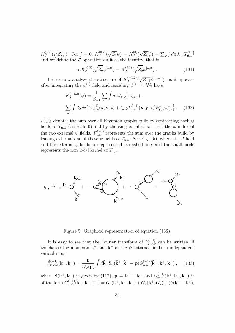
leaving external one of these ψ fields of Tx,ω. See Fig. (5), where the J fieldand the external ψ fields are represented as dashed lines and the small circlerepresents the non local kernel of Tx,ω.
K(−1,2)J = + + +
p
k+
k−
ω
ω
k+ω
ω
k+
k−
ω
ω
ω
ω
ω
ω
ω
ω
Figure 5: Graphical representation of equation (132).
It is easy to see that the Fourier transform of F(−1)2,ω,ω can be written, if
we choose the momenta k+ and k− of the ψ external fields as independentvariables, as
F(−1)2,ω,ω(k
+,k−) =p
Dω(p)
∫
dk+Sω(k+, k+ − p)G
(−1)ω,ω (k+,k+,k−) , (133)
where S(k+,k−) is given by (117), p = k+ − k− and G(−1)ω,ω (k+,k+,k−) is
of the form G(−1)ω,ω (k+,k+,k−) = G0(k
+,k+,k−) +G1(k+)G2(k
−)δ(k+ −k+),
34

where G0 represents a suitable sum over connected graphs with four externallines, while G1 and G2 represent suitable sums over connected graphs withtwo external lines. Note that all these three functions can be written, at ordern of perturbation theory, as sums of Cn terms, each term being representedas a truncated expectation of ψ monomials, which can then be expanded as asum over tree graphs of suitable determinants, thanks to the anticommutingproperties of the Grassmanian variables [Le], hence the argument in [BM] toavoid bad factorials in the bounds can be used.
G(−1)ω,ω has special symmetry properties, which it is very important to
exploit. Consider first the case ω = ω; then each term contributing to G(−1)ω,ω
is obtained by taking n interaction terms (each having two ψ fields of typeω and two of type −ω) and by building a graph with four external lines, twoof type ω and two of type ω. It follows that n ≥ 2 and that in the graphthere are (2n − 4)/2 propagators of type ω and (2n)/2 propagators of type−ω. By using the symmetry property of the propagators (99), one gets
G(−1)ω,ω (k+,k+,k−) = −G(−1)
ω,ω (k+∗,k+∗,k−∗) . (134)
In a similar way, one can check that
G(−1)ω,−ω(k
+,k+,k−) = G(−1)ω,−ω(k
+∗,k+∗,k−∗) , (135)
p · Sω(k+,k−) = −iωp∗ · Sω(k+∗,k−∗) . (136)
(133), (134), (135) and (136) imply that
F(−1)2,ω,ω(k
+,k−) =1
Dω(p)[p0A
(−1)ω,ω,0(k
+,k−) + pA(−1)ω,ω,1(k
+,k−)] , (137)
where A(−1)ω,ω,i(k
+,k−) are smooth functions verifying the condition
A(−1)ω,ω,1(k
+,k−) = iωA(−1)ω,ω,0(k
+∗,k−∗) . (138)
It follows that, if we define (in the L = β = ∞ limit, see the discussion after(97))
LF (−1)2,ω,ω(k
+,k−) =1
Dω(p)[p0A
(−1)ω,ω,0(0, 0) + pA
(−1)ω,ω,1(0, 0)] , (139)
thenLF (−1)
2,ω,ω(k+,k−) = Z
(3,+)−1 , (140)
LF (−1)2,ω,−ω(k
+,k−) = Z(3,−)−1
D−ω(p)
Dω(p), (141)
35

where Z(3,+)−1 = iA
(−1)ω,ω,0(0, 0) and Z
(3,−)−1 = iA
(−1)ω,−ω,0(0, 0) are constants, which
one can easily show to be real.The action of L on F−1
2,ω,ω was given above in momentum space; it ishowever very easy to write it in coordinate space. The support propertiesof the external propagator imply that |p| ≤ γ + γh, hence |p| ≤ γ2, if γh
is small enough, as we shall suppose (to simplify the notation). Then wecan freely multiply ∆(i,j)
ω (k+,k−) by χ0(γ−2|k+ −k−|). Hence, in space-time
coordinates, the contribution to K(−1,2)J (ψ) containing F
(−1)2,ω,ω can be written,
by using the representation (137) as
1
Z−1
∑
ω,ω
∫
dxJx,ω
∫
dx′Vω(x− x′)∫
dydzA(−1)ω,ω (x′,y, z)ψ+
y,ωψ−z,ω , (142)
where
Vω(x) =∫
dp
(2π)2
√
χ0(γ−2|p|)eipx p
Dω(p),
A(−1)ω,ω (x′,y, z) =
∫
dk+dk−
(2π)4
√
χ0(γ−2|k+ − k−|) · (143)
·eik+(x′−y)−ik−(x′−z)A(−1)ω,ω (k+,k−) .
It follows that the operation L can be described as the localization of theψ fields in the point x′ and that the corresponding R operation producesa term with ψ+
y,ωψ−z,ω − ψ+
x′,ωψ−x′,ω in place of ψ+
y,ωψ−z,ω. We can then apply
the argument following (78) to explain the regularization effect of R, since
A(−1)ω,ω,i(k
+,k−) are smooth functions.
If λ is small enough, the size of Z(3,+)−1 and Z
(3,−)−1 is determined by the
contributions of lower order in their expansions in power of λ. It is easy tosee that Z
(3,+)−1 is of order λ2 and that there is only one graph of that order
different from zero in its expansion, that on the left of Fig. 6, while Z(3,−)−1 is
of order λ and the only corresponding first order graph is represented on theright of the picture.
By an explicit calculation, one can check that the contributions to Z(3,+)−1
and Z(3,−)−1 of the two graphs are different from zero. Hence
Z(3,+)−1 = −c+λ2 < 0 , Z
(3,−)−1 =
λ
4π. (144)
We now consider the contribution to F(−1)1,ω (x,y, z) associated with the
third term in Fig. 5. Its Fourier transform can be written as
F(−1,+)1,ω (k+,k−) =
[Cεh,0(k
−)− 1]Dω(k−)g(0)ω (k+)− u0(k
+)
Dω(p)G(2)ω (k+) , (145)
36

ω
ω
ω
ω
−ω−ω
−ω
−ω
ω
ω
Figure 6: Terms of lower order contributing to Z(3,+)−1 and Z
(3,−)−1 .
where G(2)ω (k+) represents the sum over the connected Feynman graphs with
propagator g(0) and two external lines. Since, by symmetry reasons, G(2)ω (0) =
0, the simplest way to regularize F(−1,+)1,ω is to define
RF (−1,+)1,ω (k+,k−) =
[Cεh,0(k
−)− 1]Dω(k−)g(0)ω (k+)− u0(k
+)
Dω(p)·
·[G(2)ω (k+)−G(2)
ω (0)] , (146)
whose corresponding local part is vanishing. In other words the dimensionalgain is here obtained without the introduction of a renormalization constant.Note that there is a simple description of this operation in terms of a local-ization operation on the ψ fields, as in the remark following (141). A similar
procedure can be defined for the contribution to F(−1)1,ω (x,y, z) associated
with the fourth term in Fig. (5).We can summarize the previous discussion by defining
LK(−1,2)J (ψ) =
∑
ω
∫
dx
Jx,ω
Tx,ωZ−1
+Z
(3,+)−1
Z−1ψ+x,ωψ
−x,ω
+
Z(3,−)−1
Z−1J (−)x,ωψ
+x,−ωψ
−x,−ω
, (147)
where J (−)x,ω is the Fourier transform of
J (−)p,ω = Jp,ω
D−ω(p)
Dω(p). (148)
Equation (147) implies that the integration of the scale j = −1 has totake into account two new local terms, to be called of type Z+ and of typeZ−, similar to those introduced in §3.4 to analyze the Schwinger functions,
37

see (100). There is however an important difference in the term of type Z−,related with the fact that, in this term, we have absorbed in the external Jfield a bounded but not smooth function of p, in order to avoid that it isinvolved in the regularization operations.
We can now describe the general step, by defining the action of L onK
(j,2)J (ψ), which can be written, if j < −1, after rescaling ψ[h,j], as
K(j,2)J (ψ) =
1
Zj
∑
ω
∫
dx
Jx,ωTx,ω +∑
ω
∫
dydz[
Jx,ωF(j)Z+,ω,ω(x,y, z) +
+ J (−)x,ωF
(j)Z−,ω,ω(x,y, z) + Jx,ωF
(j)2,ω,ω(x,y, z) + (149)
+ δω,ωJx,ωF(j)1,ω(x,y, z)
]
ψ+y,ωψ
−z,ω
,
where F(j)Z±,ω,ω represents the sum over all graphs with one vertex of type
Z± and two ψ external fields of type ω, build by using propagators of scalei ∈ [j+1,−1], F
(j)2,ω,ω is the sum over the same kind of graphs with one vertex
Tx,ω, whose ψ fields are both contracted and F(j)1,ω is the sum over the graphs
with one vertex Tx,ω, such that one of its ψ fields is external.It is important to stress that, thanks to the identity (114), given a graph
contributing to F(j)2,ω,ω, at least one among the ψ fields belonging to Tx,ω is
contracted on scale 0, so that we can write
F(j)2,ω,ω(k
+,k−) =p
Dω(p)
0∑
i=j
∫
dk+S(i)ω (k+, k+ − p)G
(i)ω,ω(k
+,k+,k−) , (150)
where S(i)(k+,k−) is given by (117) for i = 0 and (123) for i < 0, if noderivative acts on S(i)(k+,k−) as a consequence of the regularization on ascale r such that j < r ≤ i, otherwise it is given by a suitable derivativeof S(i)(k+,k−). Moreover, G
(i)ω,ω(k
+,k+,k−) is a suitable smooth function,
which can be expressed as a sum over products of propagators g(i′), i′ ∈
[j + 1, 0], or their derivatives, integrated over suitable loop variables. Hencewe can extend to the case j < −1 the definition of L given for j = −1, forwhat concerns its action on all terms in the r.h.s. of (149) except F
(j)Z+,ω,ω
and F(j)Z−,ω,ω, for which we put (for L = β = ∞, see otherwise the discussion
after (99))
LF (j)Z±,ω,ω(k
+,k−) = F(j)Z±,ω,ω(0, 0) . (151)
Note that S(i)(k+,k−) is a smooth function, by our definition of RF (j)1,ω,
which generalizes (146). And, by the same argument leading to (98), we have
F(j)Z+,ω,−ω(0, 0) = F
(j)Z−,ω,ω(0, 0) = 0 . (152)
38

It follows that we can write
LK(j,2)J (ψ) =
∑
ω
∫
dx
Jx,ω
Tx,ωZj
+Z
(3,+)j
Zjψ+x,ωψ
−x,ω
+
Z(3,−)j
ZjJ (−)x,ωψ
+x,−ωψ
−x,−ω
, (153)
which defines the new renormalization constants Z(3,+)j and Z
(3,−)j , for j ∈
[h,−1].
4.4 The bounds
The previous considerations allow to define a tree expansion for H2,1ω , similar
to that used for G2,1ω in §3 and described in §3.4 after (103). The only
important difference is that we have now three different special endpointsassociated with the field J , corresponding to the three different terms in ther.h.s. of (153); we shall call these endpoints of type J and subtype T , Z+ andZ−, respectively.
There is of course a tree expansion also for the renormalization constantsZ
(3,+)j and Z
(3,−)j , involving trees with root at scale j−1, one endpoint of type
J , |Pv0 | = 2 and the operation L acting on v0. One can show in the usualway that, given a tree τ with n normal endpoints and the special endpointof subtype Z± and scale i + 1, its contribution Z(3,±)
τ to Z(3,±)j satisfies the
bound
|Z(3,±)τ | ≤ (Cε)n|Z(3,±)
i |∏
v∈τγ−dv , with dv ≥ 1, ∀v ∈ τ . (154)
A similar bound is satisfied if the special endpoint is of subtype T , without the|Z(3,±)
i | factor. However, in this case, the scale index of the special endpointhas to be equal to 1, because of the properties of the function ∆(i,j)
ω describedin §4.2. Therefore there is a path C in the tree connecting the special endpointwith v0 and we can extract from
∏
v∈τ γ−dv a small factor γ1/2 for each v ∈ C,
without loosing the summability properties of the bound; hence we write
|Z(3,±)τ | ≤ (Cε)nγj/2
∏
v∈Cγ−(dv− 1
2)∏
v∈τ\Cγ−dv , with dv ≥ 1, ∀v ∈ τ . (155)
Another important property, following from (151) and (152), is thatZ(3,+)τ = 0, if the special endpoint is of subtype Z−, and viceversa. Hence we
can write, if j ∈ [h+ 1,−1],
Z(3,±)j−1 = Z
(3,±)j +
−1∑
i=j
βj,iZ(3,±)i + β
(3,±)j , (156)
39

where βj,iZ(3,±)i is the sum over the contributions associated with trees whose
special endpoint is of subtype Z± and scale i + 1, while β(3,±)j is the sum
over the trees whose special endpoint is of subtype T . Note that βj,i is
equal for Z(3,+)j−1 and Z
(3,−)j−1 , by the symmetry of the interaction (9) under the
transformation ω → −ω.Let us now observe that the the trees contributing to β
(3,+)j have at least
two normal endpoints, since it is not possible to build a graph contributing toZ
(3,+)j with only one endpoint of type λ and the local part of the graphs with
one endpoint of type δ is equal to zero. This last property is of course truealso for Z
(3,−)j , but in this case it is possible to build a graph contributing
to it with one endpoint of type λ, see Fig. 6. However, the considerationsof §4.2, item 2), imply that this graph could give a contribution different
from zero to β(3,−)j only for j = −1, but also in this case a simple explicit
calculation implies that its value is zero.By using (155) and the previous remark, one can easily show that
|β(3,±)j | ≤ Cε2γj/2 . (157)
In a similar way one can prove that
|βj,i| ≤ Cε2γ−i−j2 . (158)
We want to compare the flow equation (156) with the flow equation of
the renormalization constant Z(2)j introduced in §3.4 to study the Schwinger
Functions, see (100). In this case the involved trees have one endpoint oftype J , which can have scale ≥ +1, while in the previous case the scale ofthe special endpoints of subtype Z± was ≥ 0. However, if the scale of thespecial endpoint is ≥ 0, the contribution of corresponding trees is equal toβj,iZ
(2)i , where βj,i is the same number appearing in (156). Hence we can
write, if j ∈ [h+ 1,−1],
Z(2)j−1 = Z
(2)j +
−1∑
i=j
βj,iZ(2)i + β
(2)j , (159)
where βj,iZ(2)i is the sum over the contributions to Z
(2)j associated with trees
whose special endpoint has scale i + 1 ≥ 0, while β(2)j is the sum over the
trees whose special endpoint has scale +1. By proceeding as in the proof of(157), one can show that
|β(2)j | ≤ Cε2γj/2 . (160)
As we shall see, the renormalization constants Z(3,±)j and Z
(2)j are diver-
gent as j → −∞, but Z(3,±)j /Z
(2)j is bounded and of order ε2, uniformly in
j.
40

Lemma 4.1 If ε ≤ 2|λ| and |λ| is small enough, there is a constant c0,independent of j and h, such that
c0λ2 ≤
∣
∣
∣
∣
∣
∣
Z(3,+)j
Z(2)j
∣
∣
∣
∣
∣
∣
≤ 2c0λ2 , c0|λ| ≤
∣
∣
∣
∣
∣
∣
Z(3,−)j
Z(2)j
∣
∣
∣
∣
∣
∣
≤ 2c0|λ| , j ∈ [h,−1] . (161)
Proof - Let us consider first Z(3,+)j . In order to control its dependence on
j, we have to analyze in a different way the regions j ∈ [j0,−1] and j < j0,with j0 chosen so that
γj0/2 = c1|λ|2 , (162)
for some constant c1. If j ≥ j0, we put Z(3,+)j = aj + bj , where aj is the
contribution of order λ2, while bj is the sum over the terms of order ≥ 3.The analysis of §4.2 implies that aj is obtained by applying the L operation tothe graph in the left of Fig. (6), with the two propagators of type ω on scale0 or −1 (by the remark after (121), the local part is zero, if this condition isnot satisfied) and the two propagators of type −ω on scale i ∈ [j + 1, 0]. Byan explicit calculation, we can show that
c2λ2 ≤ −aj ≤ 2c2λ
2 , uniformly in j . (163)
On the other hand, if we extract from both sides of (156) the terms of orderε2, we get
bj−1 = bj +−1∑
i=j
βj,iZ(3,+)i + βj , |βj| ≤ Cε3γj/2 , (164)
which allows very easily to prove the bound |bj | ≤ c3ε3(1 + c2ε)|j|, for some
constant c3, as far as c3ε(1 + c2ε)|j| ≤ c2/2, a condition which is certainlysatisfied for j ≥ j0, if ε is small enough, and allows also to prove, under thefurther hypothesis ε ≤ 2|λ|, that
c22ε2 ≤ |Z(3,+)
j | ≤ 5c22ε2 , j ∈ [j0,−1] . (165)
Moreover, by using (159), the fact that Z(2)0 = 1 and an explicit second order
calculation, one can show very easily by induction that there exists a positiveconstant c4 such that
γc4ε2 ≤ Z
(2)j−1
Z(2)j
≤ γ2c4ε2 ⇒ γc4ε
2|j| ≤ Z(2)j ≤ γ2c4ε
2|j| , j ∈ [h+ 1,−1] .
(166)
41

(165) and (166) immediately imply the first of the bounds (161), if j ≥ j0and |λ| ≥ ε/2 is so small that γCεj0 ≥ 1/2.
Let us now suppose that j < j0. Equation (156) can be rewritten in theform
Z(3,+)j−1 = Z
(3,+)j +
j0∑
i=j
βj,iZ(3,+)i + βj , βj =
−1∑
i=j0+1
βj,iZ(3,+)i + β3,+
j . (167)
By using (157), (158), (162) and (165), we get the bound
|βj| ≤ Cε4γ−(j0−j)/2 , (168)
which allows to prove by induction that there is a constant, which can ofcourse be chosen equal to the constant c4 of (166) if it is large enough, suchthat, if j ∈ [h+ 1, j0],
γc4ε2 ≤ Z
(3,+)j−1
Z(3,+)j
≤ γ2c4ε2 ⇒ c2
2ε2γc4ε
2(j0−j) ≤ Z(3,+)j ≤ 5c2
2ε2γ2c4ε
2(j0−j) .
(169)We want now to show that, if r < j0, there exists a constant c5 such that
∣
∣
∣
∣
∣
∣
Z(3,+)r−1
Z(3,+)r
− Z(2)r−1
Z(2)r
∣
∣
∣
∣
∣
∣
≤ c5ε2γ−(j0−r)/4 . (170)
Note that, by (159), (166), (167) and (169), if j < j0,
Z(3,+)j−1
Z(3,+)j
− Z(2)j−1
Z(2)j
=j0∑
i=j
βj,i
Z(3,+)i
Z(3,+)j
− Z(2)i
Z(2)j
+ ηj , (171)
with|ηj| ≤ Cε2γ−(j0−j)/2 ≤ c5
2ε2γ−(j0−j)/2 , (172)
if c5 is chosen large enough. Hence, the bound (170) follows immediatelyfrom (171), if r = j0; let us suppose that it is satisfied for r ∈ [j + 1, j0],j ≤ j0−1 and note that, if ε is small enough, by the first of (166) and (169),
|Z(3,+)r /Z
(3,+)r−1 − Z(2)
r /Z(2)r−1| ≤ |Z(3,+)
r−1 /Z(3,+)r − Z
(2)r−1/Z
(2)r |, since γc4ε
2> 1.
Hence, if i ∈ [j + 1, j0],∣
∣
∣
∣
∣
∣
Z(3,+)i
Z(3,+)j
− Z(2)i
Z(2)j
∣
∣
∣
∣
∣
∣
=
∣
∣
∣
∣
∣
∣
i∏
r=j+1
Z(3,±)r
Z(3,±)r−1
−i∏
r=j+1
Z(2)r
Z(2)r−1
∣
∣
∣
∣
∣
∣
≤ (173)
≤i∑
r=j+1
c5ε2γ−(j0−r)/4γ−c4ε
2(i−j−1) ≤ c5c6ε2(i− j)γ−(j0−i)/4 ,
42

for some constant c6. This bound, together with (158), (171) and (172),imply that there exists a constant c7 such that
∣
∣
∣
∣
∣
∣
Z(3,+)j−1
Z(3,+)j
− Z(2)j−1
Z(2)j
∣
∣
∣
∣
∣
∣
≤ c5ε2γ−(j0−j)/4[
1
2+ c7ε
2] , (174)
which implies (170) for r = j, if ε is small enough.By using (166), (169) and (170), we get, if i < j0
∣
∣
∣
∣
∣
∣
Z(3,+)i−1
Z(2)i−1
− Z(3,+)i
Z(2)i
∣
∣
∣
∣
∣
∣
≤∣
∣
∣
∣
∣
∣
Z(3,+)i−1
Z(3,+)i
− Z(2)i−1
Z(2)i
∣
∣
∣
∣
∣
∣
∣
∣
∣
∣
∣
∣
Z(3,+)i
Z(2)i−1
∣
∣
∣
∣
∣
∣
≤
Cε4γ−(j0−i)/4+c4ε2(j0−i) ≤ Cε4γ−(j0−j)/8 , (175)
so that∣
∣
∣
∣
∣
∣
Z(3,+)j
Z(2)j
− Z(3,+)j0
Z(2)j0
∣
∣
∣
∣
∣
∣
≤ Cε4j0∑
i=j+1
γ−(j0−j)/8 ≤ Cε4 , (176)
which implies (161) for Z(3,+)j /Z
(2)j , if ε ≤ 2|λ|.
The proof for Z(3,−)j /Z
(2)j is very similar. However, one can avoid the
different treatment of the regions j ≥ j0 and j < j0, since β(3,−)j /Z
(3,−)j is of
order ε, by the bound on the right of (143). This bound also justifies thepresence of ε in place of ε2.
Lemma 4.2 If k1 = −k2 = k and |k| = γh, then there exists a constant Csuch that
Cγ−2hεZ
(2)h
(Zh)2≤ |H2,1
ω (k1 − k2, k2)| ≤ 2Cγ−2hεZ
(2)h
(Zh)2. (177)
Proof - As explained at the beginning of §4.4, H2,1ω (p,k) admits an expan-
sion similar to that of G(2,1)ω (p,k), see (110). The main difference is that the
special endpoint of type J can be of three different subtypes, so that it isconvenient to write
H2,1ω (p,k) = H2,1
ω,Z+(p,k) + H2,1ω,Z−(p,k) + H2,1
ω,T (p,k) , (178)
where H2,1ω,Z± denotes the sum over the trees whose special endpoint is of
subtype Z±, while H2,1ω,T is the sum over the trees whose special endpoint is
of subtype T .Let us now suppose that p = k1 − k2 and k = k2, with |k| = γh. Then it
is obvious that the sum over the trees with n normal endpoints contributing
43

to H2,1ω,Z+(p,k) can be bounded as in the case of G(2,1)
ω (p,k), see (111), by
substituting Z(2)h with Z
(3,+)h . A similar argument can be used for H2,1
ω,Z−(p,k),but in this case one has to take into account the fact that the trivial treescontaining only one endpoint, the special one, does not contribute. Hencewe have
|H2,1ω,Z+(k1 − k2, k2)|+ |H2,1
ω,Z−(k1 − k2, k2)| ≤ Cγ−2h |Z(3,+)h |+ ε|Z(3,−)
h |(Zh)2
.
(179)Let us now consider H2,1
ω,T . The analysis of the previous sections (in par-ticular the bounds (126) and (128)) implies that a bound like (111) is still
valid for the sum over the trees with n normal endpoints, but now Z(2)h
has to be substituted with 1. Moreover, the contributions correspondingto the trivial trees without normal endpoints are given by ∆(h,h)
ω (k1, k2) +∆(h,h+1)ω (k1, k2) + ∆(h+1,h)
ω (k1, k2), because of the support properties of thepropagators. However, by (125) and (127), this quantity is exactly equal to0, so that
|H2,1ω,T (k1 − k2, k2)| ≤ Cγ−2h ε
(Zh)2. (180)
The bound (179) and (180), immediately imply the upper bound of Theo-rem 2.3. The lower bound follows from the explicit calculation of the leadingcontributions to H2,1
ω,Z+(p,k) and H2,1ω,Z−(p,k), which are both of order λ2;
one has essentially to check that they do not cancel out.
References
[B] R.J. Baxter: Exactly solvable models in statistical mechanics, page258. Academic Press, (1984).
[BFS] D. Brydges, J. Frohlich, E. Seiler: On the construction of quantizedgauge fields. III. The two-dimensional abelian Higgs model withoutcutoffs. Comm. Math. Phys. 79, 353–399 (1981).
[BG] G. Benfatto, G. Gallavotti: Perturbation Theory of the Fermi Sur-face in a Quantum Liquid. A General Quasiparticle Formalism andOne-Dimensional Systems. J. Stat. Phys. 59, 541–664 (1990).
[BGM] G. Benfatto, G. Gallavotti, V. Mastropietro: RenormalizationGroup and the Fermi Surface in the Luttinger Model. Phys. Rev. B45, 5468–5480, (1992).
44

[BGPS] G. Benfatto, G. Gallavotti, A. Procacci, B. Scoppola: Beta Func-tions and Schwinger Functions for a Many Fermions System in OneDimension. Comm. Math. Phys. 160, 93–171 (1994).
[BM] G. Benfatto, V. Mastropietro: Renormalization Group, hidden sym-metries and approximate Ward identities in the XY Z model. Toappear on Rev. Math. Phys., (2001).
[BM1] G. Benfatto, V. Mastropietro: Ward identities and local gauge in-variance in d = 1 interacting Fermi systems, preprint (2001).
[BoM1] F. Bonetto, V. Mastropietro: Beta Function and Anomaly of theFermi Surface for a d = 1 System of Interacting Fermions in aPeriodic Potential. Comm. Math. Phys. 172, 57–93 (1995).
[DL] I.E. Dzyaloshinky, A.I. Larkin: Soviet Phys. JETP 38, 202 (1974).
[ES] H.U. Everts, H. Schulz. Solid state Comm. 15, 1413 (1974).
[FHRW] J. Feldman, T. Hurd, L. Rosen, J. Wright: QED: a proof of renor-malizability. Lecture Notes in Physics 312, Springer-Verlag, Berlin(1988).
[G] G. Gallavotti: Renormalization theory and Ultraviolet Stability forScalar Fields via Renormalization Group methods. Rev. Mod. Phys.57, 471–562 (1985).
[GS] G. Gentile, B. Scoppola: Renormalization group and the ultravioletproblem in the Luttinger model. Commun. Math. Phys. 154, 153–179 (1993).
[KK] G. Keller, Ch. Kopper: Renormalizability Proof for QED Based onFlow Equations. Commun.Math.Phys. 176, 193–226 (1996).
[JKM] J.D. Johnson, S. Krinsky, B. McCoy: Vertical-Arrow CorrelationLength in the Eight-Vertex Model and the Low-Lying Excitationsof the X-Y-Z Hamiltonian. Phys.Rev. A. 8, 2526–2538 (1973).
[Le] A. Lesniewski: Effective action for the Yukawa 2 quantum fieldTheory. Commun. Math. Phys. 108, 437–467 (1987).
[LSM] E. Lieb, T. Schultz, D. Mattis: Two Soluble Models of an Antifer-romagnetic Chain. Ann. of Phys. 16, 407–466 (1961).
[MD] W. Metzner, C. Di Castro: Phys. Rev. B 47, 16107, (1993).
45

[ML] D. Mattis, E. Lieb: Exact solution of a many fermion system andits associated boson field. J. Math. Phys. 6, 304–312 (1965).
[MRS] J. Magnen, V. Rivasseau, R. Seneor: Construction of Yang-Mills(4)with an infrared cutoff. Commun. Math. Phys. 155, 325–384 (1993).
[S] Solyom, J: The Fermi gas model of one dimensional conductors.Adv. in Phys. 28, 201–303, (1978).
[Sp] H. Spohn: Bosonization, vicinal surfaces and Hydrodynamic fluc-tuation theory. Phys. Rev. E60, 6411–6420 (1999).
[T] S. Tomonaga: Remarks on Bloch’s method of sound waves appliedto many fermion problem, Progr. Theoret. Phys. 5, 349-374 (1950)
46