arX

iv:1

103.

1667

v1 [

cond

-mat

.mes

-hal

l] 8

Mar

201

1

Slow dynamics of interacting antiferromagnetic nanoparticles

Sunil K. Mishra and V. SubrahmanyamDepartment of Physics, Indian Institute of Technology Kanpur-208016, India

(Dated: March 10, 2011)

We study magnetic relaxation dynamics, memory and aging effects in interacting polydisperseantiferromagnetic NiO nanoparticles by solving a master equation using a two-state model. Weinvestigate the effects of interactions using dipolar, Nearest-Neighbour Short-Range (NNSR) andLong-Range Mean-Field (LRMF) interactions. The magnetic relaxation of the nanoparticles in atime-dependent magnetic field has been studied using LRMF interaction. The size-dependent effectsare suppressed in the ac-susceptibility, as the frequency is increased. We find that the memory dip,that quantifies the memory effect is about the same as that of non-interacting nanoparticles for theNNSR case. There is a stronger memory-dip for LRMF, and a weaker memory-dip for the dipolarinteractions. We have also shown a memory effect in the Zero-field-cooled magnetization for thedipolar case, a signature of glassy behaviour, from Monte-Carlo studies.

PACS numbers: 75.50.Ee, 75.50.Tt, 75.75.Fk, 75.75.Jn

I. INTRODUCTION

Magnetism in nanoparticles has received enormous at-tention in recent years due to its technological1–3 as wellas fundamental research aspects.4–32. Amid many stud-ies related to magnetic nanoparticles, the important con-cerns were related to the relaxation behaviour of the as-semblies of nanoparticles which has been addressed inthe recent times.7–12 The dynamics of an assembly ofnanoparticles at low temperatures has gained a lot of at-tention over the last few years. In a dilute system ofnanoparticles, the interparticle interaction is very smallas compared to the anisotropy energy of the individualparticles. These isolated particles follow the dynamics inaccordance with the Neel-Brownmodel,33 and the systemis known as superparamagnetic. The giant spin momentof the nanoparticles thermally fluctuates between theireasy directions at high temperatures. As the temperatureis lowered towards a blocking temperature, the relaxationtime becomes equal to the measuring time and the super-spin moments freeze along one of their easy directions. Asthe role of interparticle interaction becomes significant,the nanoparticles do not behave like individual particles;rather, their dynamics is governed by the collective be-haviour of the particles, like in a spin glass.7–12

In our recent work,34 we studied the slow dynamics ofNiO nanoparticles distributed sparsely so that particle-particle interactions could be neglected. However, in re-ality, interparticle interactions play a major role in de-scribing various interesting phenomena observed experi-mentally in a collection of nanoparticles. This leads usto include interactions among the particles in our study.If the interparticle interaction is too small, the dynam-ics of an assembly of nanoparticles is a result of the in-dividual nanoparticle dynamics. Increasing the particle-particle interaction, the behaviour of the system becomesmore complicated, even if we consider each nanoparticleas a single giant-spin. The dynamics of the assembly ofnanoparticles involves various degrees of freedom relatedto the individual particles coupled to each other with in-

terparticle interactions. In this paper, we will discussvarious interactions comparatively.

The main type of magnetic interactions that can playan important role in the assemblies of nanoparticles are:(i) long-range interactions (for example, dipolar interac-tions) among the particles, and (ii) short-range exchange-interactions arising due to the surface spins of the parti-cles which are in close contact. The dipolar interactionis a peculiar kind of interaction which may favour ferro-magnetic or antiferromagnetic alignment of the magneticmoments depending upon the geometry of the system.This interaction among the nanoparticles may give riseto a collective behaviour which may lead to a dynamicssimilar to that of a spin-glass. A resemblance from spinglass system owes to a random distribution of easy axes,which causes disorder and frustration of the magnetic in-teractions. The complex interplay between the disorderand frustration determines the state of the system and itsdynamical properties. These systems are widely knownas superspin glasses. This superspin glass phase hasbeen characterised by observations of a critical slowing-down,13 a divergence in the non-linear susceptibility,16

and aging and relaxation effects in the low-frequency acsusceptibility.17 The Monte Carlo simulations on the sys-tem of an assembly of nanoparticles show aging35 andmagnetic relaxation behaviour36 like in a spin glass. Foran interacting assembly of nanoparticles, the aging andmemory effects are the two aspects that have been stud-ied extensively in recent years, however, mostly in thecase of ferromagnetic particles.7–9,16,18–29

In this paper, we investigate the effects of interactionson a collection of a few antiferromagnetic nanoparticles,which has received relatively lesser attention. Recently,we have shown that for NiO nanoparticles, a combinedeffect of the surface-roughness effect and finite-size effectsin the core magnetization leads to size-dependent fluctu-ations in net magnetic-moment.37 These size-dependentfluctuations in the magnetization lead to a dynamicswhich is qualitatively different from that of ferromag-netic nanoparticles. We will study the dynamics of the

2

2 3 4 5R

i

0

0.001

0.002

0.003

0.004

0.005P

(Ri)

1 2 3 4 5R

i

0

500

1000

1500

2000

2500

3000

µ i

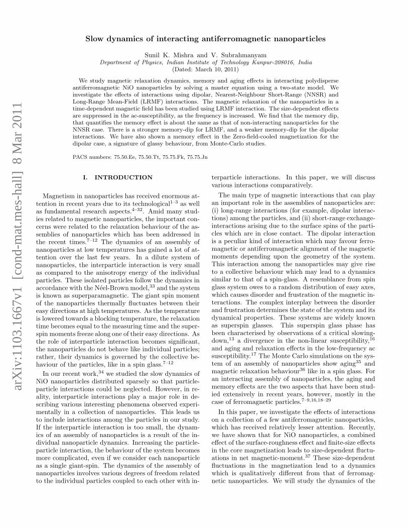
FIG. 1: A lognormal distribution of nanoparticles with sizesranging from 1.3a0-5.3a0, where a0 = 4.17A. The width of thedistribution is 0.6. The inset displays the magnetic momentvs the particle size for the same size range. The magneticmoment has a non-monotonic and oscillatory dependence onR.

system by analytically solving the master equation fora two-state model. We will invoke various interactionsand study the relaxation phenomena under these in-teractions comparatively. We will show the effect ofthe size-dependent magnetization fluctuations on thetime-dependent properties of an interacting assembly ofnanoparticles. We will also compare the dynamics withthat of the non-interacting case. We will discuss thememory effects in the FC as well as the ZFC magne-tization protocols. The organisation of this paper is asfollows. In Section II, we discuss the two-state model.We discuss the ZFC and FC magnetizations in SectionIII, and the ac-susceptibility study in Section IV. In Sec-tion V, we show the memory effect investigations. Theaging effect has been presented in Section VI. Finally,we summarise in Section VII.

II. RELAXATION PHENOMENA ANDVARIOUS INTERACTIONS

We assume a nanoparticle to be a giant spin in whichthe exchange interactions are so strong that all the spinsin the particle show a coherent rotation in unison. Hence,the dynamics of a system of nanoparticles can be eas-ily understood as the dynamics of a giant spin-moment.Here, we are dealing with antiferromagnetic nanoparti-cles, which display size dependent fluctuations in themagnetization as shown in the inset of the figure FIG.1. On the other hand, the net magnetic moment of fer-romagnetic nanoparticles shows a linear dependence onthe volume of the particles.23 As we study the dynamicsof antiferromagnetic nanoparticles, we might expect the

role of these size-dependent fluctuations in the magneti-zation to be manifested in the time-dependent propertiesof these antiferromagnetic nanoparticles. We use a simplemodel where the energy of each particle i is contributedby the anisotropy energy and the Zeeman energy. Now,in order to incorporate interactions in the present model,we add an interaction energy term Vij in the Hamilto-nian. Thus, the Hamiltonian is written as:

H = −∑

i

KVi −∑

i

~µi. ~H +∑

i

∑

j 6=i

Vij , (1)

and the energy of a particle is given by

Ei = −KVi − µiH +∑

j 6=i

Vij , (2)

where ~µi is the magnetic moment of the ith particle, µi =|~µi|, K is the anisotropy constant, and H is the appliedfield. Because of the interaction term Vij , the energyof the ith particle depends on the state of all the otherparticles. We assume each nanoparticle to be an isingspin, and the magnetic moment of each particle to be~µi = µisiz, with si = ±1. The various interactions usedin the present study are:

i) A Nearest-Neighbour Short-Range (NNSR) typeinteraction, which can be written as:

Vsrij = J sr

∑

<i,j>

µiµj , (3)

where the summation is taken over the nearest-neighbour sites. Here J sr is the NNSR interactionstrength.

ii) A long-Range, Mean-Field (LRMF) typeinteraction,38 which is given as:

V lrij =

J lr

2N(

N∑

i=1

µi)2

=J lr

2N

N∑

i=1

µ2i +

J lr

N

∑

j 6=i

µiµj , (4)

where N is the total number of nanoparticles andJ lr is interaction parameter. The above equationEq. (4) is scaled by N in order to insure that thetotal interaction-energy is proportional to N andnot N2.

iii) A long-range dipolar interaction, with the particlej separated by a distance rij from particle i, givenas:

Vdipolarij = α

∑

j 6=i

[

~µi ~µj

r3ij− 3 (~µi. ~rij) ( ~µj . ~rij)

r5ij

]

, (5)

where α = µ0µ2B/4πr

20 characterises the strength of

the dipolar interaction and r0 is the lattice param-eter of the lattice, where nanoparticles are placed.

3

Variations in r0 may result the nanoparticles to begetting closer or away from each other and hence,increasing or decreasing the effects of dipolar inter-actions.

Let us consider a model case of NNSR. Using the mean-field approximation, we can find a mean field felt by theith particle due to interactions with its neighbours. Wecan replace Eq. (3) by its mean-field form as:

VMFij = µi

∑

j 6=i

〈µj〉,

= µiHMFi , (6)

where HMFi is the mean field on the ith spin from all

the nearest neighbour spins. Thus, in this framework,each particle can be viewed under the influence of a localmagnetic-field:

Heffi = H +HMF

i . (7)

The effect of interactions on a nanoparticle can be in-corporated by replacing the external field by an effectivefield which may lead to a mean-field equation of stateand can be solved self-consistently. Hereafter, in all thecases of interactions, we will define an effective field Heff

i

on a nanoparticle i as the sum of the external field H anda locally-changing interaction-field i.e.,

Heffi = H +

1

µi

∑

j 6=

Vij . (8)

The above equation shows that the role of the interac-tions is to modify the energy barrier, which is solely dueto the anisotropy contributions of each particle in thenon-interacting case. For strong interactions, their effectsbecome dominant and the individual energy-barriers canno longer be considered to be the only relevant energy-scale. In this case, the relaxation is governed by a co-operative phenomenon of the system. The energy land-scape with a complex hierarchy of local minima is similarto that of a spin glass. We should note that in contrastwith the static energy barrier distribution arising onlyfrom the anisotropy contribution, the reversal of one par-ticle moment may change the energy barriers of the as-sembly, even in the weak-interaction limit. Therefore,the energy-barrier distribution gets modified as the mag-netization relaxes.By defining an effective field given by Eq. (8), we can

map an interacting assembly of nanoparticles as a collec-tion of non-interacting nanoparticles, where each particleexperiencesan effective field Heff

i which gets modified asthe temperature changes. In the absence of the magneticfield, the superparamagnetic relaxation-time for the ther-mal activation over the energy barrier KVi is given byτi = τ0 exp(KVi/kBT ), where τ0, the microscopic time,is of the order of 10−9 s. The anisotropy constant K hasa typical value of about 4× 10−1 J cm−3 for NiO.39

The occupation probabilities with the magnetic mo-ments parallel and antiparallel to the magnetic field di-rection are denoted by p1(t) and p2(t) = 1−p1(t), respec-tively. The magnetic moment of each particle is supposedto occupy one of the two available states with energies−KVi + µs

iHeffi or −KVi − µs

iHeffi , where µs

i is the satu-ration magnetic-moment of the ith particle. These prob-abilities satisfy a master equation, which is given by,

d

dtp1(t) = − 1

τip1(t) +

1

2τi

[

1 +µsiH

effi

T

]

. (9)

The magnetic moment of each particle of volume Vi canbe written as µi = [2p1 − 1]µs

i . as

d

dtµi = −µi

τi+

1

2τi

[

1 +(µs

i)2 Heff

i

T

]

. (10)

We can define magnetization of each particle as Mi ≡µi/Vi. Since Heff

i also contains a summation over all theother µj ’s interacting with the particle, the right-handside of the above equation can be written as the sumof the interaction term with jth particle and the termcontaining the magnetic field. Thus, we can write theEq. (10) as:

d

dtMi = A(i, j)Mj − a0i, (11)

Here A(i, j) represents the interaction term which isgiven below for each case separately, and a0i =− (µs

i)2H/ViτiT .

(i) For NNSR interaction, A(i, j) is given as:

A(i, j) =

{

− 1τi, if i = j;

Jsr(µsi)

2

ViτiTδ~r,~r+ǫ, if i 6= j

where ~r is the position vector of any site and ǫ isthe nearest-neighbour distance.

(ii) For LRMF interaction, we can write A(i, j) as

A(i, j) =

{

− 1τi

+ J lr

2N(µs

i)2

ViτiT, if i = j;

J lr

N(µs

i)2

ViτiT, if i 6= j.

(iii) For dipolar interaction we can write,

A(i, j) =

{ − 1τi, if i = j;

α(µsi)

2

ViτiT

(r2ij−3z2ij)

r5ij

, if i 6= j.

There are N equations of the form given by Eq. (11)for the system of N particles. We can write these Nequations in a matrix form as:

d

dtM = AM − a0, (12)

4

where A is a N × N matrix whose elements are givenby A(i, j), defined above, and M and a0 are vectors of

length N . The elements of M are the Mi’s, and those ofa0 are the a0i’s. Eq. (12) can be solved for the variousinteractions defined above. The formal solution of thematrix equation Eq. (12) takes the form:

M(t) = eAtC + ν, (13)

where ν = A−1a0, a time-independent solution of Eq.(13) and C = M(0)− ν, M(0) being the value of M att = 0. Thus we can write,

M(t) = eAtM(0) + (1− eAt)ν. (14)

The matrix A in the above equation Eq. (14) is a generalmatrix of order N × N . To evaluate eAt, we use theMATLAB function expm which implements a diagonalPade approximation of exponential of the matrix with ascaling and squaring technique.43,44

Pade approximation to an exponential of a matrix Bis written as:

eB ≈ Rpq(B) = [Dpq(B)]−1Npq(B) (15)

where the numerator term is given as

Npq(B) =p∑

j=0

(p+ q − j)!p!

(p+ q)!j!(p− j)!Bj (16)

and the denominator term is written as

Dpq(B) =q∑

j=0

(p+ q − j)!q!

(p+ q)!j!(q − j)!(−B)j (17)

Diagonal Pade approximants can be calculated by takingq = p in Eqs. (16) & (17). The index p depends upon thenorm of the matrix B. Using a backward-error analysis,p can be calculated.44 Unfortunately, the Pade approx-imants are accurate only near the origin. This problemcan be overcome by the scaling and squaring techniquewhich exploits,

eB =(

eB/2k)2k

. (18)

Firstly, a sufficiently large k is chosen such that B/2k isclose to the zero matrix. Then, a diagonal Pade approxi-mant is used to calculate exp(B/2k). Finally, the result issquared k times to obtain the approximation to eB. Wecan use Pade approximation with a scaling and squar-ing technique to calculate eAt in Eq. (14). However, thenorm of the matrix A, ‖A‖ ≈ 109, is too large in allthe three cases of interactions in Eqs. (3), (4) & (5), forN = 1000. The scaling and squaring method comes veryhandy to overcome this large value of the norm.44 In thiscase, the degree of the approximant is p = 13. The to-tal magnetic moment of the system of nanoparticles withvolume distribution P (Vi) is given by

M =1

N

N∑

i=1

Mi =

∫

MiP (Vi)dVi. (19)

The size-distribution plays a significant role in theoverall dynamics of the system of nanoparticles governedby equation (19). The exponential dependence of τ onthe particle size Vi assures that even a weak polydisper-sity may lead to a broad distribution of relaxation times,which gives rise to an interesting slow dynamics. Fora dc measurement, if relaxation time coincides with themeasurement time scale τm, we can define45 a criticalvolume VB as KVB = kBTBln(τm/τ0), where TB is re-ferred as blocking temperature. The critical volume VB

has a strong linear dependence on TB and weakly log-arithmic dependence on the observation time scale τm.If the volume of the particle Vi in a polydisperse sys-tem is less than VB, the super spin would have under-gone many rotations within the measurement time scalewith an average magnetic moment zero. These particlesare termed as superparamagnetic particles. On the otherhand if Vi > VB, the super spins can not completelyrotate within the measurement time window and showblocked or frozen behavior. However, the particles havingvolume Vi ≃ VB are in dynamically active regime. Thesystems of magnetic nanoparticles are in general polydis-perse. The shape and size of the particles are not well-known but the particle-size distribution is often foundto be lognormal.46 We consider the system consisting oflognormally-distributed and the volume Vi of each parti-cle is obtained from a lognormal distribution

P (Vi) =1

σVi

√2π

exp

[−(ln(Vi)− υ)2

2σ2

]

, (20)

where υ = ln(V ), V is the mean size and σ the width ofthe distribution. The distribution consists of 1000 par-ticles of sizes between R = 1.3a0 and R = 5.3a0, wherea0(= 4.17A) is the lattice parameter of NiO.39 The totalnumber of particles is deliberately chosen to be small inorder to simplify the numerical calculation, as well as toget some insight into the role of size-dependent fluctua-tions in the magnetization in the present study. In allthe cases, we use σ = 0.6 and υ = 3.57. For the dipolarcase, the nanoparticles are arranged in a 10 × 10 × 10simple-cubic box. We can solve Eqs. (14) and (19) forany heating/cooling process using any of the interactionsdiscussed above. A recipe to solve these equations for azero-field-cooled (ZFC) protocol is as follows. The sys-tem is cooled from a very high temperature to the lowesttemperature in the absence of any magnetic field. Theabsence of the field during cooling causes a complete de-magnetization of the nanoparticles. This condition is thesame as p1(0) = 1/2, or M(0) = 0 in Eq. (14). Now, aconstant field is applied and the system is heated uptoa high temperature. At each temperature change, weevolve the system using Eq. (14). Suppose we increasethe temperature from T to T + dT . Then, the magneti-zation at T + dT is given as:

MZFC(t, T + dT ) = eA(T+dT )tMZFC(0, T + dT )

+ (1− eA(T+dT )t)ν(T + dT ),

(21)

5

0 0.1 0.2 0.3 0.4Temperature (T/KV)

0

0.05

0.1

0.15

0.2

0.25

0.3M

agne

tizat

ion

J=0J=1.5×10−6

J=2.0×10−6

J=2.5×10−6

NNSR(a)

0 0.1 0.2 0.3 0.4Temperature (T/KV)

0

0.05

0.1

0.15

0.2

0.25

0.3

Mag

netiz

atio

n

J=0J=1.5×10−8

J=3.5×10−8

J=4.5×10−8

LRMF(b)

0 0.1 0.2 0.3 0.4Temperature (T/KV)

0

0.05

0.1

0.15

0.2

0.25

Mag

netiz

atio

n

α=0α=1.5×10−6

α=2.0×10−6

α=2.5×10−6

Dipolar(c)

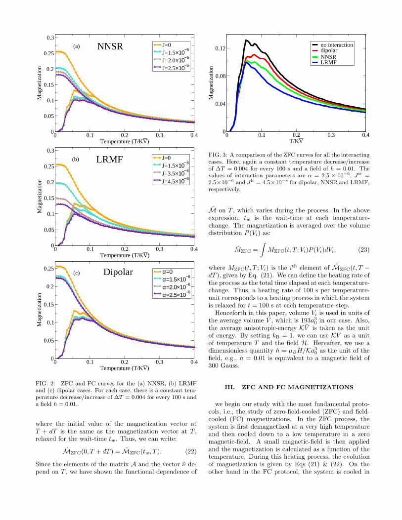
FIG. 2: ZFC and FC curves for the (a) NNSR, (b) LRMFand (c) dipolar cases. For each case, there is a constant tem-perature decrease/increase of ∆T = 0.004 for every 100 s anda field h = 0.01.

where the initial value of the magnetization vector atT + dT is the same as the magnetization vector at T ,relaxed for the wait-time tw. Thus, we can write:

MZFC(0, T + dT ) = MZFC(tw, T ). (22)

Since the elements of the matrix A and the vector ν de-pend on T , we have shown the functional dependence of

0 0.1 0.2 0.3 0.4T/KV

0

0.04

0.08

0.12

Mag

netiz

atio

n

no interactiondipolarNNSRLRMF

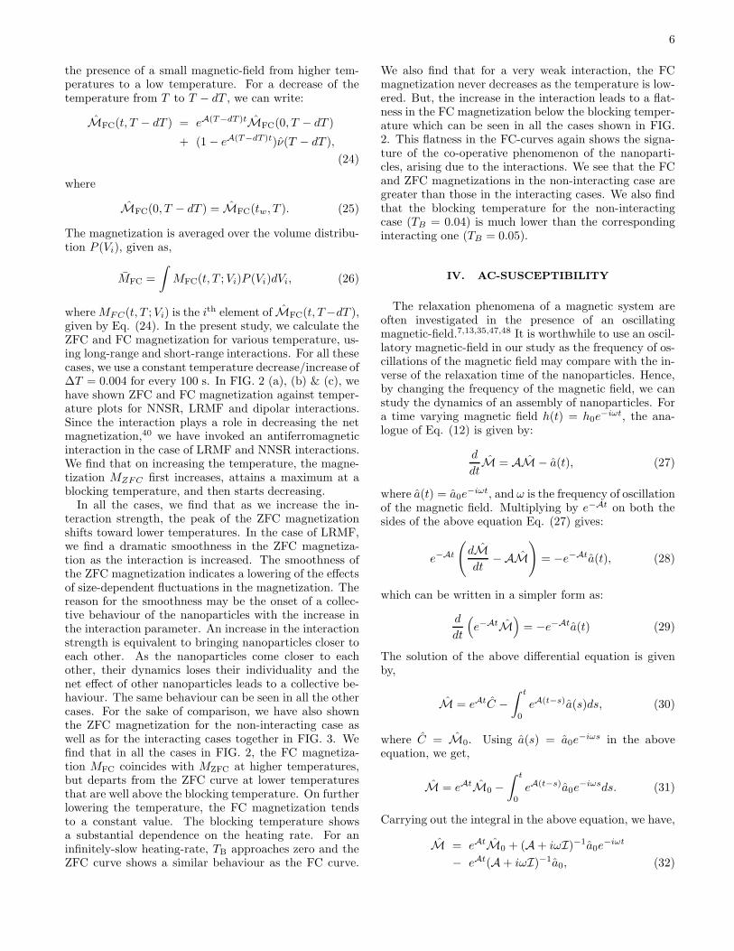
FIG. 3: A comparison of the ZFC curves for all the interactingcases. Here, again a constant temperature decrease/increaseof ∆T = 0.004 for every 100 s and a field of h = 0.01. Thevalues of interaction parameters are α = 2.5 × 10−6, Jsr =2.5×10−6 and J lr = 4.5×10−8 for dipolar, NNSR and LRMF,respectively.

M on T , which varies during the process. In the aboveexpression, tw is the wait-time at each temperature-change. The magnetization is averaged over the volumedistribution P (Vi) as:

MZFC =

∫

MZFC(t, T ;Vi)P (Vi)dVi, (23)

where MZFC(t, T ;Vi) is the ith element of MZFC(t, T −dT ), given by Eq. (21). We can define the heating rate ofthe process as the total time elapsed at each temperature-change. Thus, a heating rate of 100 s per temperature-unit corresponds to a heating process in which the systemis relaxed for t = 100 s at each temperature-step.Henceforth in this paper, volume Vi is used in units of

the average volume V , which is 193a30 in our case. Also,the average anisotropic-energy KV is taken as the unitof energy. By setting kB = 1, we can use KV as a unitof temperature T and the field H. Hereafter, we use adimensionless quantity h = µBH/Ka30 as the unit of thefield, e.g., h = 0.01 is equivalent to a magnetic field of300 Gauss.

III. ZFC AND FC MAGNETIZATIONS

we begin our study with the most fundamental proto-cols, i.e., the study of zero-field-cooled (ZFC) and field-cooled (FC) magnetizations. In the ZFC process, thesystem is first demagnetized at a very high temperatureand then cooled down to a low temperature in a zeromagnetic-field. A small magnetic-field is then appliedand the magnetization is calculated as a function of thetemperature. During this heating process, the evolutionof magnetization is given by Eqs (21) & (22). On theother hand in the FC protocol, the system is cooled in

6

the presence of a small magnetic-field from higher tem-peratures to a low temperature. For a decrease of thetemperature from T to T − dT , we can write:

MFC(t, T − dT ) = eA(T−dT )tMFC(0, T − dT )

+ (1− eA(T−dT )t)ν(T − dT ),

(24)

where

MFC(0, T − dT ) = MFC(tw, T ). (25)

The magnetization is averaged over the volume distribu-tion P (Vi), given as,

MFC =

∫

MFC(t, T ;Vi)P (Vi)dVi, (26)

whereMFC(t, T ;Vi) is the ith element of MFC(t, T−dT ),

given by Eq. (24). In the present study, we calculate theZFC and FC magnetization for various temperature, us-ing long-range and short-range interactions. For all thesecases, we use a constant temperature decrease/increase of∆T = 0.004 for every 100 s. In FIG. 2 (a), (b) & (c), wehave shown ZFC and FC magnetization against temper-ature plots for NNSR, LRMF and dipolar interactions.Since the interaction plays a role in decreasing the netmagnetization,40 we have invoked an antiferromagneticinteraction in the case of LRMF and NNSR interactions.We find that on increasing the temperature, the magne-tization MZFC first increases, attains a maximum at ablocking temperature, and then starts decreasing.In all the cases, we find that as we increase the in-

teraction strength, the peak of the ZFC magnetizationshifts toward lower temperatures. In the case of LRMF,we find a dramatic smoothness in the ZFC magnetiza-tion as the interaction is increased. The smoothness ofthe ZFC magnetization indicates a lowering of the effectsof size-dependent fluctuations in the magnetization. Thereason for the smoothness may be the onset of a collec-tive behaviour of the nanoparticles with the increase inthe interaction parameter. An increase in the interactionstrength is equivalent to bringing nanoparticles closer toeach other. As the nanoparticles come closer to eachother, their dynamics loses their individuality and thenet effect of other nanoparticles leads to a collective be-haviour. The same behaviour can be seen in all the othercases. For the sake of comparison, we have also shownthe ZFC magnetization for the non-interacting case aswell as for the interacting cases together in FIG. 3. Wefind that in all the cases in FIG. 2, the FC magnetiza-tion MFC coincides with MZFC at higher temperatures,but departs from the ZFC curve at lower temperaturesthat are well above the blocking temperature. On furtherlowering the temperature, the FC magnetization tendsto a constant value. The blocking temperature showsa substantial dependence on the heating rate. For aninfinitely-slow heating-rate, TB approaches zero and theZFC curve shows a similar behaviour as the FC curve.

We also find that for a very weak interaction, the FCmagnetization never decreases as the temperature is low-ered. But, the increase in the interaction leads to a flat-ness in the FC magnetization below the blocking temper-ature which can be seen in all the cases shown in FIG.2. This flatness in the FC-curves again shows the signa-ture of the co-operative phenomenon of the nanoparti-cles, arising due to the interactions. We see that the FCand ZFC magnetizations in the non-interacting case aregreater than those in the interacting cases. We also findthat the blocking temperature for the non-interactingcase (TB = 0.04) is much lower than the correspondinginteracting one (TB = 0.05).

IV. AC-SUSCEPTIBILITY

The relaxation phenomena of a magnetic system areoften investigated in the presence of an oscillatingmagnetic-field.7,13,35,47,48 It is worthwhile to use an oscil-latory magnetic-field in our study as the frequency of os-cillations of the magnetic field may compare with the in-verse of the relaxation time of the nanoparticles. Hence,by changing the frequency of the magnetic field, we canstudy the dynamics of an assembly of nanoparticles. Fora time varying magnetic field h(t) = h0e

−iωt, the ana-logue of Eq. (12) is given by:

d

dtM = AM − a(t), (27)

where a(t) = a0e−iωt, and ω is the frequency of oscillation

of the magnetic field. Multiplying by e−At on both thesides of the above equation Eq. (27) gives:

e−At

(

dMdt

−AM)

= −e−Ata(t), (28)

which can be written in a simpler form as:

d

dt

(

e−AtM)

= −e−Ata(t) (29)

The solution of the above differential equation is givenby,

M = eAtC −∫ t

0

eA(t−s)a(s)ds, (30)

where C = M0. Using a(s) = a0e−iωs in the above

equation, we get,

M = eAtM0 −∫ t

0

eA(t−s)a0e−iωsds. (31)

Carrying out the integral in the above equation, we have,

M = eAtM0 + (A+ iωI)−1a0e−iωt

− eAt(A+ iωI)−1a0, (32)

7

0.05 0.1 0.15 0.2 0.25

Temperature (T/KV)

0

2

4

6

8χ′

(ω)

no interactioninteracting (LRMF)

(a)

0.05 0.1 0.15 0.2 0.25

Temperature (T/KV)

0

2

4

6

8

χ″(ω

)

no interactioninteracting (LRMF)

(b)

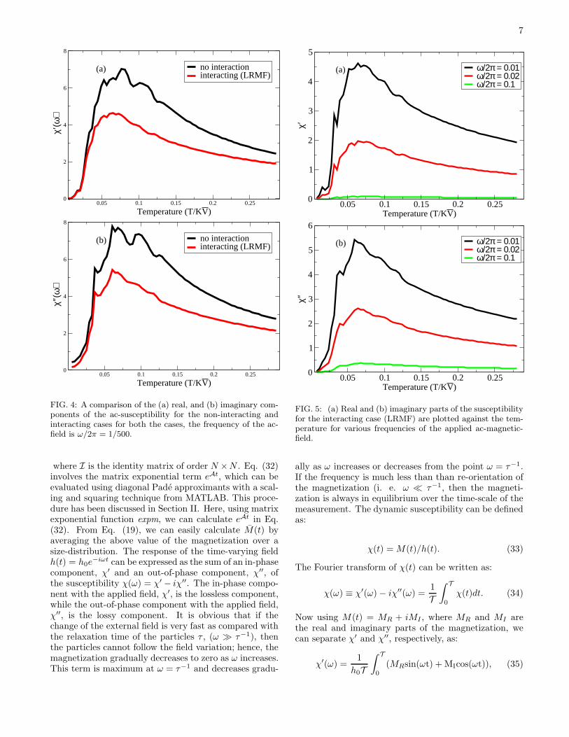
FIG. 4: A comparison of the (a) real, and (b) imaginary com-ponents of the ac-susceptibility for the non-interacting andinteracting cases for both the cases, the frequency of the ac-field is ω/2π = 1/500.

where I is the identity matrix of order N ×N . Eq. (32)involves the matrix exponential term eAt, which can beevaluated using diagonal Pade approximants with a scal-ing and squaring technique from MATLAB. This proce-dure has been discussed in Section II. Here, using matrixexponential function expm, we can calculate eAt in Eq.(32). From Eq. (19), we can easily calculate M(t) byaveraging the above value of the magnetization over asize-distribution. The response of the time-varying fieldh(t) = h0e

−iωt can be expressed as the sum of an in-phasecomponent, χ′ and an out-of-phase component, χ′′, ofthe susceptibility χ(ω) = χ′ − iχ′′. The in-phase compo-nent with the applied field, χ′, is the lossless component,while the out-of-phase component with the applied field,χ′′, is the lossy component. It is obvious that if thechange of the external field is very fast as compared withthe relaxation time of the particles τ , (ω ≫ τ−1), thenthe particles cannot follow the field variation; hence, themagnetization gradually decreases to zero as ω increases.This term is maximum at ω = τ−1 and decreases gradu-

0.05 0.1 0.15 0.2 0.25Temperature (T/KV)

0

1

2

3

4

5

χ′

ω/2π = 0.01ω/2π = 0.02

(a)

ω/2π = 0.1

0.05 0.1 0.15 0.2 0.25Temperature (T/KV)

0

1

2

3

4

5

6

χ″

ω/2π = 0.01ω/2π = 0.02

(b)

ω/2π = 0.1

FIG. 5: (a) Real and (b) imaginary parts of the susceptibilityfor the interacting case (LRMF) are plotted against the tem-perature for various frequencies of the applied ac-magnetic-field.

ally as ω increases or decreases from the point ω = τ−1.If the frequency is much less than than re-orientation ofthe magnetization (i. e. ω ≪ τ−1, then the magneti-zation is always in equilibrium over the time-scale of themeasurement. The dynamic susceptibility can be definedas:

χ(t) = M(t)/h(t). (33)

The Fourier transform of χ(t) can be written as:

χ(ω) ≡ χ′(ω)− iχ′′(ω) =1

T

∫ T

0

χ(t)dt. (34)

Now using M(t) = MR + iMI , where MR and MI arethe real and imaginary parts of the magnetization, wecan separate χ′ and χ′′, respectively, as:

χ′(ω) =1

h0T

∫ T

0

(MRsin(ωt) +MIcos(ωt)), (35)

8

and

χ′′(ω) =1

h0T

∫ T

0

(MRcos(ωt)−MIsin(ωt)). (36)

Using the above set of equations, we can calculate thereal and imaginary parts of the ac-susceptibility. Forthe ac-susceptibility calculations, the system is demagne-tized at the lowest temperature and an ac-magnetic-fieldof amplitude h0 = 0.01 and frequency ω/2π = 0.01 isapplied. The system is then heated upto a high temper-ature. At each temperature change, we evolve the systemfor T = 100 s and calculate χ′ and χ′′ using the above dy-namical equations. It has been experimentally observedthat ac-susceptibility measurements are sensitive to theinteraction effects13 and confirmed using Monte Carlosimulations.35 We also compare the effect of interactionsby considering the non-interacting and interacting casesindividually. We find that non-interacting case, which iswell described by the individual relaxation of particlesdiffers qualitatively from the interacting case, where theinteractions among the particles make the dynamics com-plex. The real and imaginary parts of ac-susceptibilityfor the non-interacting case as well as the interactingcase using LRMF interactions is shown in FIG. 4. Forboth the cases, the frequency of the ac-field is fixed toω/2π = 1/500. We find that the due to the interaction,the in-phase part as well as the out-of-phase part showreduction in the net value of the susceptibility. The ef-fect of size-dependent fluctuations can be observed in thein-phase and out-of-phase components of the susceptibil-ity. The effect of these size-dependent fluctuations aredisplayed in the non-interacting as well as the interact-ing cases, as ripples in the ac-susceptibility. But, it isinteresting to see that the ripples are smoothened in theinteracting cases. The correlated behaviour of nanopar-ticles is responsible for the averaging of the ripples in thiscase. The effects of interaction can also be seen as theshifting of the peaks of χ′ and χ′′ curves towards lowertemperatures.

We have also performed a detailed study of the fre-quency dependence of the real and imaginary parts ofthe susceptibility. In FIGs. 5 (a) and (b) we have showna frequency dependence of the susceptibility for the in-teracting case by plotting χ′ and χ′′ versus temperatureat various frequencies. We see that the increase in thefrequency causes a lowering in the magnitude of χ′ andχ′′. Again, we find that the ripples in the susceptibilitycomponents due to size-dependent fluctuations get sup-pressed with an increase in the frequency. We also seethat the peak in the χ′ and χ′′ curves slightly shifts to-wards higher temperatures as the frequency is increased.This frequency dependence shows that the particles be-come less responsive to the magnetic field as the fre-quency is increased. For a very large frequency the par-ticles may not flip due to the magnetic field which mayresult in zero-magnetization.

V. MEMORY EFFECTS

A. FC memory-effect

Sun et al19 have shown a memory-effect phenomenonin the dc-magnetization by a series of measurementson a permalloy Ni81Fe19 nanoparticle sample. Later,this memory effect was also been reported by Sasakiet al.23 and Tsoi et al.24 for the non-interacting orweakly-interacting superparamagnetic system of ferritinnanoparticles and Fe2O3 nanoparticles, respectively. Allof the studies were concerned only to the ferromagneticnanoparticles. Experiments on NiO nanoparticles byBisht and Rajeev49 also confirm a weak memory effectin these particles. Chakraverty et al.50 have investigatedthe effect of polydispersity and interactions among theparticles in an assembly of nickel ferrite nanoparticles em-bedded in a host non-magnetic SiO2 matrix. They foundthat either tuning the interparticle interaction or tailor-ing the particle-size distribution in a nano-sized magneticsystem leads to important applications in memory de-vices. In our recent study,34 we had also shown thememory effects for an assembly of non-interacting NiOantiferromagnetic nanoparticles by the analytical solu-tion of a two-state model. The protocol for the memoryeffect is as follows. Firstly, we cool the system from avery high temperature to Tbase = 0.005 with a probingfield of h = 0.01 switched on. The system is again heatedfrom Tbase to get the reference curves, which are shownas “Ref.” in FIG. 6. The dynamics of the system in thisprocess is the same as that given by Eqs. (24), (25) &(26) during the cooling process, and Eqs. (21), (22) &(23), during the heating process. During these processes,we allow 100 s to ellapse for every temperature step of∆T = 0.001. We again cool the system from TH to Tbase

but this time with a stop of 10000 s at T = 0.04. The fieldis cut off during the stop. At the stop, the magnetizationis given by,

Mcool(t, Tstop) = eA(Tstop)tMcool(0, Tstop), (37)

where

Mcool(0, Tstop) = Mcool(tw, Tstop). (38)

and

Mcool =

∫

Mcool(t, T ;Vi)P (Vi)dVi. (39)

After the pause, the field is again applied and the systemis again cooled upto the base temperature Tbase. Therecovered magnetization can be given as:

Mcool(t, Tstop − dT ) = eA(Tstop−dT )tMcool(0, Tstop − dT )

+ (1− eA(Tstop−dT )t)ν(Tstop − dT ),

(40)

where

Mcool(0, Tstop − dT ) = Mcool(tw, Tstop). (41)

9

0 0.05 0.1 0.15 0.2T/KV

0

0.05

0.1

0.15

0.2

0.25M

Ref.heatingcooling

no interactiondipolarNNSRLRMF

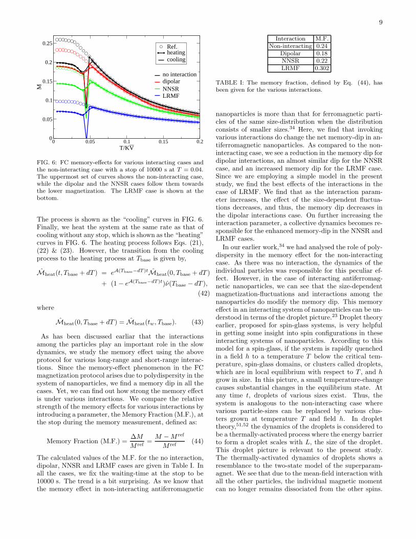
FIG. 6: FC memory-effects for various interacting cases andthe non-interacting case with a stop of 10000 s at T = 0.04.The uppermost set of curves shows the non-interacting case,while the dipolar and the NNSR cases follow them towardsthe lower magnetization. The LRMF case is shown at thebottom.

The process is shown as the “cooling” curves in FIG. 6.Finally, we heat the system at the same rate as that ofcooling without any stop, which is shown as the “heating”curves in FIG. 6. The heating process follows Eqs. (21),(22) & (23). However, the transition from the coolingprocess to the heating process at Tbase is given by,

Mheat(t, Tbase + dT ) = eA(Tbase−dT )tMheat(0, Tbase + dT )

+ (1− eA(Tbase−dT )t)ν(Tbase − dT ),

(42)

where

Mheat(0, Tbase + dT ) = Mheat(tw, Tbase). (43)

As has been discussed earliar that the interactionsamong the particles play an important role in the slowdynamics, we study the memory effect using the aboveprotocol for various long-range and short-range interac-tions. Since the memory-effect phenomenon in the FCmagnetization protocol arises due to polydispersity in thesystem of nanoparticles, we find a memory dip in all thecases. Yet, we can find out how strong the memory effectis under various interactions. We compare the relativestrength of the memory effects for various interactions byintroducing a parameter, the Memory Fraction (M.F.), atthe stop during the memory measurement, defined as:

Memory Fraction (M.F.) =∆M

M ref=

M −M ref

M ref(44)

The calculated values of the M.F. for the no interaction,dipolar, NNSR and LRMF cases are given in Table I. Inall the cases, we fix the waiting-time at the stop to be10000 s. The trend is a bit surprising. As we know thatthe memory effect in non-interacting antiferromagnetic

Interaction M.F.Non-interacting 0.24

Dipolar 0.18NNSR 0.22LRMF 0.302

TABLE I: The memory fraction, defined by Eq. (44), hasbeen given for the various interactions.

nanoparticles is more than that for ferromagnetic parti-cles of the same size-distribution when the distributionconsists of smaller sizes.34 Here, we find that invokingvarious interactions do change the net memory-dip in an-tiferromagnetic nanoparticles. As compared to the non-interacting case, we see a reduction in the memory dip fordipolar interactions, an almost similar dip for the NNSRcase, and an increased memory dip for the LRMF case.Since we are employing a simple model in the presentstudy, we find the best effects of the interactions in thecase of LRMF. We find that as the interaction param-eter increases, the effect of the size-dependent fluctua-tions decreases, and thus, the memory dip decreases inthe dipolar interactions case. On further increasing theinteraction parameter, a collective dynamics becomes re-sponsible for the enhanced memory-dip in the NNSR andLRMF cases.

In our earlier work,34 we had analysed the role of poly-dispersity in the memory effect for the non-interactingcase. As there was no interaction, the dynamics of theindividual particles was responsible for this peculiar ef-fect. However, in the case of interacting antiferromag-netic nanoparticles, we can see that the size-dependentmagnetization-fluctuations and interactions among thenanoparticles do modify the memory dip. This memoryeffect in an interacting system of nanoparticles can be un-derstood in terms of the droplet picture.23 Droplet theoryearlier, proposed for spin-glass systems, is very helpfulin getting some insight into spin configurations in theseinteracting systems of nanoparticles. According to thismodel for a spin-glass, if the system is rapidly quenchedin a field h to a temperature T below the critical tem-perature, spin-glass domains, or clusters called droplets,which are in local equilibrium with respect to T , and hgrow in size. In this picture, a small temperature-changecauses substantial changes in the equilibrium state. Atany time t, droplets of various sizes exist. Thus, thesystem is analogous to the non-interacting case wherevarious particle-sizes can be replaced by various clus-ters grown at temperature T and field h. In droplettheory,51,52 the dynamics of the droplets is considered tobe a thermally-activated process where the energy barrierto form a droplet scales with L, the size of the droplet.This droplet picture is relevant to the present study.The thermally-activated dynamics of droplets shows aresemblance to the two-state model of the superparam-agnet. We see that due to the mean-field interaction withall the other particles, the individual magnetic momentcan no longer remains dissociated from the other spins.

10

0.05 0.1 0.15 0.2 0.25 0.3

T/KV

-0.02

-0.01

0

M-M

Ref

0 0.1 0.2T/KV

0

0.2

0.4

0.6

0.8

M

MRef

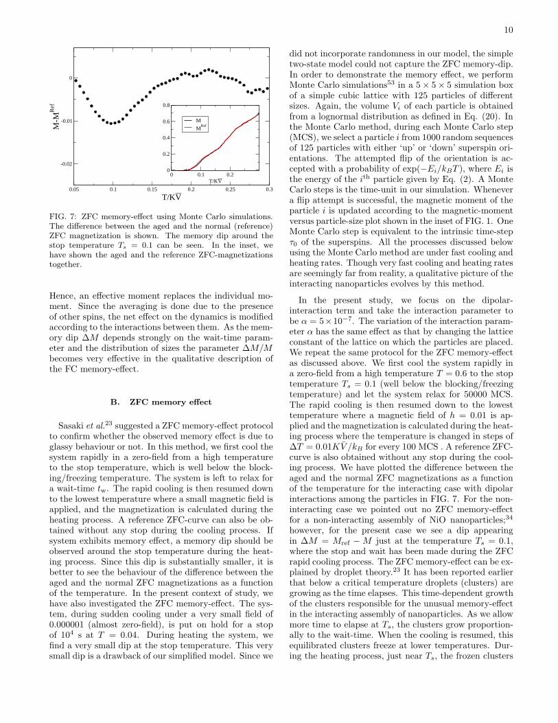
FIG. 7: ZFC memory-effect using Monte Carlo simulations.The difference between the aged and the normal (reference)ZFC magnetization is shown. The memory dip around thestop temperature Ts = 0.1 can be seen. In the inset, wehave shown the aged and the reference ZFC-magnetizationstogether.

Hence, an effective moment replaces the individual mo-ment. Since the averaging is done due to the presenceof other spins, the net effect on the dynamics is modifiedaccording to the interactions between them. As the mem-ory dip ∆M depends strongly on the wait-time param-eter and the distribution of sizes the parameter ∆M/Mbecomes very effective in the qualitative description ofthe FC memory-effect.

B. ZFC memory effect

Sasaki et al.23 suggested a ZFC memory-effect protocolto confirm whether the observed memory effect is due toglassy behaviour or not. In this method, we first cool thesystem rapidly in a zero-field from a high temperatureto the stop temperature, which is well below the block-ing/freezing temperature. The system is left to relax fora wait-time tw. The rapid cooling is then resumed downto the lowest temperature where a small magnetic field isapplied, and the magnetization is calculated during theheating process. A reference ZFC-curve can also be ob-tained without any stop during the cooling process. Ifsystem exhibits memory effect, a memory dip should beobserved around the stop temperature during the heat-ing process. Since this dip is substantially smaller, it isbetter to see the behaviour of the difference between theaged and the normal ZFC magnetizations as a functionof the temperature. In the present context of study, wehave also investigated the ZFC memory-effect. The sys-tem, during sudden cooling under a very small field of0.000001 (almost zero-field), is put on hold for a stopof 104 s at T = 0.04. During heating the system, wefind a very small dip at the stop temperature. This verysmall dip is a drawback of our simplified model. Since we

did not incorporate randomness in our model, the simpletwo-state model could not capture the ZFC memory-dip.In order to demonstrate the memory effect, we performMonte Carlo simulations53 in a 5× 5× 5 simulation boxof a simple cubic lattice with 125 particles of differentsizes. Again, the volume Vi of each particle is obtainedfrom a lognormal distribution as defined in Eq. (20). Inthe Monte Carlo method, during each Monte Carlo step(MCS), we select a particle i from 1000 random sequencesof 125 particles with either ‘up’ or ‘down’ superspin ori-entations. The attempted flip of the orientation is ac-cepted with a probability of exp(−Ei/kBT ), where Ei isthe energy of the ith particle given by Eq. (2). A MonteCarlo steps is the time-unit in our simulation. Whenevera flip attempt is successful, the magnetic moment of theparticle i is updated according to the magnetic-momentversus particle-size plot shown in the inset of FIG. 1. OneMonte Carlo step is equivalent to the intrinsic time-stepτ0 of the superspins. All the processes discussed belowusing the Monte Carlo method are under fast cooling andheating rates. Though very fast cooling and heating ratesare seemingly far from reality, a qualitative picture of theinteracting nanoparticles evolves by this method.

In the present study, we focus on the dipolar-interaction term and take the interaction parameter tobe α = 5×10−7. The variation of the interaction param-eter α has the same effect as that by changing the latticeconstant of the lattice on which the particles are placed.We repeat the same protocol for the ZFC memory-effectas discussed above. We first cool the system rapidly ina zero-field from a high temperature T = 0.6 to the stoptemperature Ts = 0.1 (well below the blocking/freezingtemperature) and let the system relax for 50000 MCS.The rapid cooling is then resumed down to the lowesttemperature where a magnetic field of h = 0.01 is ap-plied and the magnetization is calculated during the heat-ing process where the temperature is changed in steps of∆T = 0.01KV /kB for every 100 MCS . A reference ZFC-curve is also obtained without any stop during the cool-ing process. We have plotted the difference between theaged and the normal ZFC magnetizations as a functionof the temperature for the interacting case with dipolarinteractions among the particles in FIG. 7. For the non-interacting case we pointed out no ZFC memory-effectfor a non-interacting assembly of NiO nanoparticles;34

however, for the present case we see a dip appearingin ∆M = Mref − M just at the temperature Ts = 0.1,where the stop and wait has been made during the ZFCrapid cooling process. The ZFC memory-effect can be ex-plained by droplet theory.23 It has been reported earlierthat below a critical temperature droplets (clusters) aregrowing as the time elapses. This time-dependent growthof the clusters responsible for the unusual memory-effectin the interacting assembly of nanoparticles. As we allowmore time to elapse at Ts, the clusters grow proportion-ally to the wait-time. When the cooling is resumed, thisequilibrated clusters freeze at lower temperatures. Dur-ing the heating process, just near Ts, the frozen clusters

11

10 100 1000 10000t/τ0

0

0.05

0.1

0.15M

agne

tizat

ion

No interactionDipolarNNSRLRMF

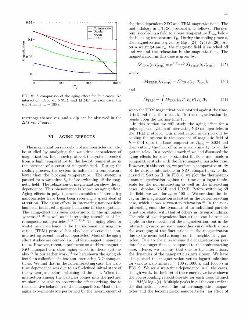
FIG. 8: A comparison of the aging effect for four cases: Nointeraction, Dipolar, NNSR, and LRMF. In each case, thewait-time is tw = 100 s.

rearrange themselves, and a dip can be observed in the∆M vs. T curve.

VI. AGING EFFECTS

The magnetization relaxation of nanoparticles can alsobe studied by analysing the wait-time dependence ofmagnetization. In one such protocol, the system is cooledfrom a high temperature to the lowest temperature inthe presence of a constant magnetic-field. During thecooling process, the system is halted at a temperaturelower than the blocking temperature. The system ispaused for a wait-time tw before switching off the mag-netic field. The relaxation of magnetization show the twdependence. This phenomenon is known as aging effect.Aging effects in polydispersed assemblies of interactingnanoparticles have been been receiving a great deal ofattention. The aging effects in interacting nanoparticleshas been indicated a glassy behaviour in these systems.The aging-effect has been well-studied in the spin-glasssystems,54–56 as well as in interacting assemblies of fer-romagnetic nanoparticles.9,18,20,23,24 The aging effect orwait-time dependence in the thermoremanant magneti-zation (TRM) protocol has also been observed in non-interacting assemblies of nanoparticles. Most of the agingeffect studies are centred around ferromagnetic nanopar-ticles. However, recent experiments on antiferromagneticNiO nanoparticles show aging effect in these systemsalso.49 In our earlier work,34 we had shown the aging ef-fect for a collection of a few non-interacting NiO nanopar-ticles. We find that in the non-interacting case, the wait-time dependence was due to an ill-defined initial state ofthe system just before switching off the field. When theinteraction among the particles comes into the picture,we should be able to observe the effects arising due tothe collective behaviour of the nanoparticles. Most of theaging experiments are performed by the measurement of

the time-dependent ZFC and TRM magnetizations. Themethodology in a TRM protocol is as follows. The sys-tem is cooled in a field to a base temperature Tbase belowthe blocking temperature TB. During the cooling process,the magnetization is given by Eqs. (24), (25) & (26). Af-ter a waiting-time tw, the magnetic field is switched offand we find the relaxation in the magnetization. Themagnetization in this case is given by,

MTRM(t, Tstop) = eA(Tstop)tMTRM(0, Tstop), (45)

where

MTRM(0, Tstop) = MTRM(tw, Tstop), (46)

and

MTRM =

∫

MTRM(t, T ;Vi)P (Vi)dVi. (47)

when the TRMmagnetization is plotted against the time,it is found that the relaxation in the magnetization de-pends upon the waiting-time tw.In this section we will study the aging effect for a

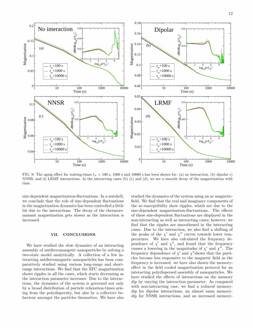
polydispersed system of interacting NiO nanoparticles inthe TRM protocol. Our investigation is carried out bycooling the system in the presence of magnetic field ofh = 0.01 upto the base temperature Tbase = 0.024 andthen cutting the field off after a wait-time tw to let thesystem relax. In a previous work,34 we had discussed theaging effects for various size-distributions and made acomparative study with the ferromagnetic particles case.However, in this section, we perform a comparative studyof the various interactions in NiO nanoparticles, as dis-cussed in Section II. In FIG. 8, we plot the thermorem-anant magnetization against the time on a logarithmic-scale for the non-interacting as well as the interactingcases: dipolar, NNSR and LRMF. Before switching offthe field, we wait for tw = 100 s. We see that the de-cay in the magnetization is fastest in the non-interactingcase, which shows a two-step relaxation.34 In the non-interacting case, the dynamics of an individual particleis not correlated with that of others in its surroundings.The role of size-dependent fluctuations can be seen asripples in the relaxation of the magnetization, but in theinteracting cases, we see a smoother curve which showsthe averaging of the fluctuations in the magnetizationdue to the mean field arising from the neighbouring par-ticles. Due to the interactions the magnetization per-sists for a longer time as compared to the noninteractingcase. Hence, we can say that due to the interactions,the dynamics of the nanoparticles gets slower. We havealso plotted the magnetization versus logarithmic-timefor various wait-times tw = 100 s, 1000 s, and 10000 s inFIG. 9. We see a wait-time dependence in all the cases,though weak. In the inset of these curves, we have shownthe corresponding relaxation-rate for each case, definedas −∂M/∂ log10(t). Multiple peaks in all the cases reflectthe distinction between the antiferromagnetic nanopar-ticles and the ferromagnetic nanoparticles: an effect of

12

1 10 100 1000 10000 Time (s)

0

0.05

0.1

0.15

0.2M

agne

tizat

ion

tw

=100 stw

=1000 s tw

=10000 s

0 2 4 6 8log

10(t/τ0)

0

0.02

0.04

0.06

-∂Μ

/∂lo

g 10(t

/τ0)

No interaction

(a)

1 10 100 1000 10000 Time (s)

0.06

0.08

0.1

0.12

0.14

0.16

0.18

Mag

netiz

atio

n

tw

=100 stw

=1000 s tw

=10000 s

0 2 4 6 8log

10(t/τ0)

0

0.01

0.02

-∂Μ

/∂lo

g 10(t

/τ0)

Dipolar

(b)

1 10 100 1000 10000Time (s)

0.04

0.06

0.08

0.1

Mag

netiz

atio

n

tw

=100 stw

=1000 s tw

=10000 s

0 2 4 6 8log

10(t/τ0)

0

0.01

0.02

-∂Μ

/∂lo

g 10(t

/τ0)

NNSR

(c)

1 10 100 1000 10000Time (s)

0

0.01

0.02

0.03

0.04

0.05

Mag

netiz

atio

n

tw

=100 stw

=1000 s tw

=10000 s

0 2 4 6 8log

10(t/τ0)

0

0.005

0.01

-∂Μ

/∂lo

g 10(t

/τ0)

LRMF

(d)

FIG. 9: The aging effect for waiting-times tw = 100 s, 1000 s and 10000 s has been shown for: (a) no interaction, (b) dipolar c)NNSR, and d) LRMF interactions. In the interacting cases (b) (c) and (d), we see a smooth decay of the magnetization withtime.

size-dependent magnetization-fluctuations. In a nutshell,we conclude that the role of size-dependent fluctuationsin the magnetization dynamics has been controlled a littlebit due to the interactions. The decay of the thermore-manant magnetization gets slower as the interaction isincreased.

VII. CONCLUSIONS

We have studied the slow dynamics of an interactingassembly of antiferromangetic nanoparticles by solving atwo-state model analytically. A collection of a few in-teracting antiferromagnetic nanoparticles has been com-paratively studied using various long-range and short-range interactions. We find that the ZFC magnetizationshows ripples in all the cases, which starts decreasing asthe interaction parameter increases. Due to the interac-tions, the dynamics of the system is governed not onlyby a broad distribution of particle relaxation-times aris-ing from the polydispersity, but also by a collective be-haviour amongst the particles themselves. We have also

studied the dynamics of the system using an ac magnetic-field. We find that the real and imaginary components ofthe ac-susceptibility show ripples, which are due to thesize-dependent magnetization-fluctuations. The effectsof these size-dependent fluctuations are displayed in thenon-interacting as well as interacting cases; however, wefind that the ripples are smoothened in the interactingcases. Due to the interaction, we also find a shifting ofthe peaks of the χ′ and χ′′ curves towards lower tem-peratures. We have also calculated the frequency de-pendence of χ′ and χ′′, and found that the frequencycauses a lowering in the magnitudes of χ′ and χ′′. Thefrequency dependence of χ′ and χ′′shows that the parti-cles become less responsive to the magnetic field as thefrequency is increased. we have also shown the memory-effect in the field cooled magnetization protocol for aninteracting polydispersed assembly of nanoparticles. Wehave studied the effects of interactions on the memorydip by varying the interaction parameter. As comparedwith non-interacting case, we find a reduced memory-dip for dipolar interactions, an almost same memory-dip for NNSR interactions, and an increased memory-

13

dip for LRMF interactions. Due to the limitations in ourmodel, we find the best effect of the interactions only inthe case of LRMF. We find that as the interaction pa-rameter increases, the effect of the size-dependent fluc-tuations decreases, and thus, the memory dip decreasesin the dipolar interactions cases. On further increasingthe interaction parameter, a collective dynamics becomesresponsible for the enhanced memory dip in the NNSRcase and LRMF cases. The memory effect and a weakaging effect have also been discussed for all the cases.For the non-interacting case, the size-dependent fluctua-tions play a role in the obtaining of a high memory frac-tion. As the interactions are incorporated, the memoryfraction decreases, but for the strong interaction cases,

the memory fraction increases. As the present modelcould not incorporate randomness and disorder, we haveperformed a Monte Carlo study considering the dipo-lar interactions among the particles. We find a memorydip in the ZFC magnetization, which indicates the im-portance of the interactions among the particles. TheZFC memory-effect is attributed only to the collectivedynamics of the nanoparticles. The system of interact-ing nanoparticles under various interactions also showsa wait-time dependence. The decay of thermoremanantmagnetization slows down as the interaction among thenanoparticles increases. We have done a comparativestudy of the aging effects in the no interaction, dipolar,NNSR and LRMF cases.

1 D. Weller and A. Moser, IEEE Trans. Magn. 35, 4423(1999).

2 H. J. Richter J. Phys. D 40, R149 (2007).3 C. C. Berry and A. S. G. Curtis, J. Phys. D 36, R198(2003).

4 Surface Effects in Magnetic Nanoparticles, edited byD. Fiorani (Springer, New York, 2005).

5 R. H. Kodama, S. A. Makhlouf, and A. E. Berkowitz, Phys.Rev. Lett. 79, 1393 (1997).

6 R. H. Kodama, A. E. Berkowitz, Phys. Rev. B 59, 6321(1999)

7 T. Jonsson, J. Mattsson, C. Djurberg, F. A. Khan,P. Nordblad, and P. Svedlindh Phys. Rev. Lett. 75, 4138(1995).

8 P. Jonsson, M. F. Hansen, and P. Nordblad, Phys. Rev. B61, 1261 (2000).

9 S. Sahoo, O. Petracic, Ch. Binek, W. Kleemann,J. B. Sousa, S. Cardoso, and P. P. Freitas, Phys. Rev. B65, 134406 (2002).

10 J. L. Dormann, R. Cherkaoui, L. Spinu, M. Nogues, F. Lu-cari, F. D’Orazio, A. Garcia, E. Tronc, and J. P. Jolivet,J. Magn. Magn. Mater. 187, L139 (1998).

11 X. Batlle and A. Labarta, J. Phys. D 35, R15 (2002).12 P. Jonsson, Adv. Chem. Phys. 128, 191 (2004).13 C. Djurberg, P. Svedlindh, P. Nordblad, M. F. Hansen,

F. Bødker, and S. Mørup, Phys. Rev. Lett. 79 5154 (1997).14 M. Bandyopadhyay and J. Bhattacharya, J. Phys.: Con-

dens. Matter 18, 11309 (2006).15 J. L. Garcia-Palacios, Adv. Chem. Phys. 112, 1 (2007).16 T. Jonsson, P. Svedlindh, and M. F. Hansen, Phys. Rev.

Lett. 81, 3976 (1998).17 H. Mamiya, I. Nakatani and T. Furubayashi, Phys. Rev.

Lett. 82, 4332 (1999).18 S. Sahoo, O. Petracic, W. Kleemann, P. Nordblad, S. Car-

doso, and P.P. Freitas, Phys. Rev. B 67, 214422 (2003).19 Y. Sun, M. B. Salamon, K. Garnier, and R. S. Averback,

Phys. Rev. Lett. 91, 167206 (2003).20 O. Petracic, X. Chen, S. Bedanta, W. Kleemann, S. Sahoo,

S. Cardoso, and P. P. Freitas, J. Magn. Magn. Mater. 300,192 (2006).

21 S. Sahoo, O. Petracic, Ch. Binek, W Kleemann, J B Sousa,S Cardoso and P. P. Freitas, J. Phys.: Condens. Matter 14,6729 (2002).

22 R. K. Zheng, G. Gu, and X. X. Zhang, Phys. Rev. Lett.

93, 139702 (2004).23 M. Sasaki, P. E. Jonsson, H. Takayama and H. Mamiya,

Phys. Rev. B 71, 104405 (2005).24 G. M. Tsoi, L. E. Wenger, U. Senaratne, R. J. Tackett,

E. C. Buc, R. Naik, P. P. Vaishnava, and V. Naik, Phys.Rev. B 72 014445 (2005).

25 M. Bandyopadhyay and S. Dattagupta, Phys. Rev. B 74,214410 (2006).

26 W. J. Wang, J. J. Deng, J. Lu, B. Q. Sun, and J. H. Zhao,Appl. Phys. Lett. 91, 202503 (2005), W. J. Wang,J. J. Deng, J. Lu, B. Q. Sun, X. G. Wu, and J. H. Zhao,J. Appl. Phys. 105, 053912 (2009).

27 J. Du, B. Zhang, R. K. Zheng and X. X. Zhang, Phys. Rev.B 75, 014415 (2007).

28 M. Suzuki, S. I. Fullem, I. S. Suzuki, L. Wang and Chuan-Jian Zhong, Phys. Rev. B 79 024418 (2009).

29 T. Zhang, X. G. Li, X. P. Wang, Q. F. Fang, and M.Dressel, Eur. Phys. J. B 74, 309 (2010).

30 E. Winkler, R. D. Zysler, M. Vasquez Mansilla, and D. Fio-rani, Phys. Rev. B 72, 132409 (2005).

31 S. A. Makhlouf, F. T. Parker, F. E. Spada andA. E. Berkowitz, J. Appl. Phys. 81, 5561 (1997).

32 S. D. Tiwari and K. P. Rajeev, Phys. Rev. B 72, 104433(2005).

33 L. Neel, Ann. Geophys. C.N.R.S. 5, 99 (1949) ;W. F. Brown, Jr., Phys. Rev. 130, 1677 (1963).

34 S. K. Mishra Eur. Phys. J .B 78, 65 (2010).35 J.-O. Andersson, C. Djurberg, T. Jonsson, P. Svedlindh,

and P. Nordblad, Phys. Rev. B 56,13983 (1997).36 M. Ulrich, J. Garcia-Otero, J. Rivas, and A. Bunde, Phys.

Rev. B 67, 024416 (2003).37 S. K. Mishra, V. Subrahmanyam, (to be published in Int.

J. Mod. Phys. B) arXiv:0806.1262v3. (2008).38 S. Gupta and D. Mukamel J. Stat. Mech. P08026 (2010).39 M. T. Hutchings and E. J. Samuelsen, Phys. Rev. B 6,

3447 (1972).40 J. Garcia-Otero, M. Porto, J. Rivas, and A. Bunde, Phys.

Rev. Lett. 84, 167 (2000).41 G. H. Golub, c. F. Van Loan: Matrix Computations 3th

edn. (John Hopkins Baltimore).42 N. J. Higham, SIAM J. Matrix Anal. Appl.,26(4) (2005),

pp. 1179-1193.43 G. H. Golub, c. F. Van Loan: Matrix Computations 3th

edn. (John Hopkins Baltimore).

14

44 N. J. Higham, SIAM J. Matrix Anal. Appl.,26(4) (2005),pp. 1179-1193.

45 C. P. Been and J. D. Livingston, J. Appl. Phys. 30, 4816(1966).

46 C. G. Granqvist and R. A. Buhrman J. Appl. Phys. 47,2200 (1976).

47 T. Jonsson, P. Nordblad, and P. Svedlindh Phys. Rev. B57, 497 (1998).

48 O. Petracic, A. Glatz and W. Kleemann Phys. Rev. B 70,214432 (2004).

49 V. Bisht and K. P. Rajeev, J. Phys.: Condens. Matter 22,016003 (2010).

50 S. Chakraverty, M. Bandyopadhyay, S. Chatter-jee, S. Dattagupta, A. Frydman, S. Sengupta, and

P. A. Sreeram, Phys. Rev. B 71, 054401 (2005).51 D. S. Fisher and D. A. Huse, Phys. Rev. B 38, 373 1988 .52 D. S. Fisher and D. A. Huse, Phys. Rev. B 38, 386 1988 .53 K. Binder and D. W. Heermann, Monte Carlo Simulations

in Statistical Physics, Springer Series in Solid State ScienceVol. 80 (Springer, Berlin, 1992), 2nd ed.

54 U. Nowak, R. W. Chantrell, and E. C. Kennedy, Phys.Rev. Lett. 84, 163 (2000), D. Hinzke and U. Nowak, Phys.Rev. B 61, 6734 (2000).

55 L. Lundgren, P. Svedlindh, P. Nordblad, and O. Beckman,Phys. Rev. Lett. 51, 911 (1983).

56 M. Ocio, M. Alba, and J. Hammann, J. Phys. (France)Lett. 46, L1101 (1985), ibid. Europhys. Lett. 2, 45 (1986).