ChemInform Abstract: Proton Coordination by Polyamine Compounds in Aqueous Solution
Upload
independentCategory
view
0download
0
3
Exchange Bias Effectof Ferro-/Antiferromagnetic Heterostructures
Florin Radu1 and Hartmut Zabel2
1BESSY GmbH, Albert-Einstein-Str. 15, 12489 Berlin, [email protected] fur Experimentalphysik/Festkorperphysik, Ruhr-Universitat Bochum,44780 Bochum, [email protected]
Abstract. The exchange bias effect, discovered more than fifty years ago, is afundamental interfacial property, which occurs between ferromagnetic and antifer-romagnetic materials. After intensive experimental and theoretical research overthe last ten years, a much clearer picture has emerged about this effect, which is ofimmense technical importance for magneto-electronic device applications. In this re-view we start with the discussion of numerical and analytical results of those modelswhich are based on the assumption of coherent rotation of the magnetization. Thebehavior of the ferromagnetic and antiferromagnetic spins during the magnetizationreversal, as well as the dependence of the critical fields on characteristic parameterssuch as exchange stiffness, magnetic anisotropy, interface disorder etc. are analyzedin detail and the most important models for exchange bias are reviewed. Finallyrecent experiments in the light of the presented models are discussed.
3.1 Fundamental Aspects of Exchange Bias: Introduction
The exchange bias (EB) effect was discovered 50 years ago by Meiklejohn andBean [1]. Meanwhile the EB effect has become an integral part of modernmagnetism with implications for basic research and for numerous device ap-plications. The EB effect was the first of its kind which relates to an interfaceeffect between two different classes of materials, here between a ferromagnetand an antiferromagnet. Later on the interlayer exchange coupling betweenferromagnets interleaved by paramagnet layers was discovered [2], and theproximity effect between ferromagnetic and superconducting layers was de-scribed [3, 4]. Recent reviews on these topics can be found in [5, 6, 7] and alsoin this book. The EB effect manifests itself in a shift of the hysteresis loopto negative or positive direction with respect to the applied field. Its originis related to the magnetic coupling across the common interface shared by aferromagnetic (F) and an antiferromagnetic (AF) layer. Extensive research isbeing carried out to unveil the details of this effect, which has resulted in more
F. Radu and H. Zabel: Exchange Bias Effect of Ferro-/Antiferromagnetic Heterostructures,
STMP 227, 97–184 (2007)
DOI 10.1007/978-3-540-73462-8 3 c© Springer-Verlag Berlin Heidelberg 2007

98 F. Radu and H. Zabel
then 600 publications in the last five years and since the last comprehensivereviews by Nogues and Schuller [8], Kiwi [9], Berkowitz [10], and Stamps [11].
An EB bilayer consists of two key elements, with rather different magneticand structural properties: the ferromagnetic layer and the antiferromagneticlayer. While the ferromagnetic layer can be studied in detail by using labo-ratory equipment like SQUID, MOKE and MFM, this is not the case for themagnetic interface and for the antiferromagnetic layer. The interface embed-ded in between the F and AF layer has low volume, therefore it is difficult toseparate its contribution from the F layer. Still, for the exchange bias effect theinterfacial magnetic properties are essential for understanding the effect. Forthis purpose polarized neutron scattering and soft-xray magnetic scatteringtechniques can reveal some of the key magnetic properties of the interface. TheAF layer has in principle no macroscopic magnetization, even so the magneticmoment of individual atoms is rather high. The magnetic properties of the AFmaterials are traditionally studied by neutron diffraction. In thin films, due tothe reduced AF volume available for scattering, this method is rather difficultto apply. Here, soft-xray magnetic scattering through the linear dichroism canreveal information about the magnetic properties of the AF layer, thereforeproviding useful insights into the origin of the EB effect.
From the application point of view the situation appears to be less com-plex. The effect is being used in spin valves with one pinned and one freeferromagnetic layer which are embedded in devices such as storage media,readout sensors, and magnetic random access memory(MRAM). Neverthe-less, robust, reliable and easy to control functional elements based on theexchange bias phenomenon require more understanding of the fundamentalsof the effect, which is further motivating research in this field.
Because of recent experimental verifications of the existence of interfaciallayers by several groups [12, 13, 14, 15, 16, 17, 18, 19, 20, 21, 22, 23], earliermodels of EB need to be revisited and eventually modified to take into accountthe effects, which are introduced by this layer.
Here we first review some of the basic models for exchange bias. We focuson numerical calculations and analytical treatment of those models whichare based on the Stoner-Wohlfarth model [24, 25]. This has the advantagethat analytical expressions can be derived and a numerical analysis can bemuch more efficiently performed as compared to micromagnetic simulations.It has, however, the disadvantage that only coherent magnetization reversalprocesses are described within this formalism. Nevertheless, for a large fractionof experimental situations the Stoner-Wolhfarth approach is adequate. Thebehavior of the F and AF spins during the magnetization reversal, as wellas the dependence of the critical fields on the parameters of the F and AFlayer are analyzed in detail. The Meiklejohn and Bean [1, 26, 27] model andthe Mauri model [28] are revisited and numerical and analytical expressionsare compared. We continue with describing the main features of the RandomField model (RF) of Malozemoff [29, 30, 31] and the Domain State (DS)model [32, 33, 34, 35, 36, 84, 38, 39]. Then, we review the Kim and Stamp

3 Exchange Bias Effect of Ferro-/Antiferromagnetic Heterostructures 99
approach [40], which focuses on a spring-like behavior of the AF layers andcoercivity enhancement. We continue with one of the most recent models forexchange bias, the Spin Glass (SG) model [41]. Assuming a realistic state of theinterface between the F and AF layers, the SG model describes well most of theimportant features of EB heterostructures, including azimuthal dependence ofexchange bias field and coercivity, AF and F thickness dependence, the inverselinear dependence on the lateral extension, and training effects. Finally we willdiscuss recent experiments in the light of the presented models. However, themain emphasis of this review is to describe the basic models in a systematicfashion and to compare them with recent experimental results.
3.2 Stoner-Wohlfarth Model
The term anisotropy refers to the orientation of the magnetic moments withrespect to given geometrical directions. In bulk materials the crystal axes arethe reference directions, while in thin films other reference systems becomeimportant. In order to account for the orientation of the magnetic momentsin magnetic materials, the minimum energy state is provided by analysisof the different contributing terms to the total magnetic energy: Zeemanterm, anisotropy terms, and exchange coupling terms. This evaluation is per-formed by minimization of the total magnetic energy with respect to variousparameters.
In the following we use the simplest possible expression for the total mag-netic energy for a ferromagnetic thin film and calculate the magnetic hysteresisloops. We assume that all spins are confined in the film plane and that thefilm has a uniaxial anisotropy. The response of the magnetization to an ap-plied magnetic field is then uniform. Therefore the spins will coherently rotateduring the variation of the external field. The direction of the magnetizationcan be described by only one parameter, namely the (θ − β) angle definingthe direction of the magnetization vector with respect to the applied field (seeFig. 3.1). Many complexities of the magnetization reversal are neglected inthis approach. Nevertheless, the Stoner-Wohlfarth (SW) model [24, 25, 42],named after the investigators who developed it for treating the magnetizationreversal of a small single domain, is used with considerable success for variousmagnetic thin films and heterostructures.
The total magnetic energy per unit volume of a ferromagnetic film within-plane uniaxial anisotropy reads:
EV (β) = −μ0HMF cos(θ − β) +KF sin2(β) , (3.1)
where the first term is the Zeeman energy contribution and the second term isthe magnetic crystalline anisotropy (MCA), here assumed to have an uniaxialsymmetry. The other parameters are: H for the applied field, MF for thesaturation magnetization of the ferromagnet, KF for the volume anisotropy

100 F. Radu and H. Zabel
H
MF
�
�
KF
Ferromagnetic film
Easy
ax
is
Hard axis
Fig. 3.1. Definition of angles and vectors used in Stoner-Wohlfarth type modelcalculations. The reference direction of the film is along the unidirectional anisotropy
constant of the ferromagnet, and θ for the orientation of the applied magneticfield with respect to the uniaxial anisotropy direction, and β the orientationof the magnetization vector during the magnetization reversal.
The minimization of the total magnetic energy with respect to the angleβ and the stability equation:
∂EV (β)∂β
= 0,∂2EV (β)∂β2 > 0 , (3.2)
leads to the following equations:
− μ0HMF sin(θ − β) +KF sin(2 β) = 0 (3.3)μ0HMF cos(β − θ) + 2KF cos(2 β) > 0. (3.4)
By solving (3.3) with the condition imposed by the (3.4) one obtains theangle β, which determines the longitudinal component (m|| = cos(β − θ))and the transverse component (m⊥ = sin(β − θ)) of the magnetization. Bothcomponents are plotted in Fig. 3.2 for different in-plane orientations (θ). Theevolution of the hysteresis loops for different angles θ between the appliedmagnetic field and the orientation of the uniaxial anisotropy is shown in theleft column of Fig. 3.2 and reflects the typical behavior of thin films within-plane uniaxial anisotropy. Along the easy axis the hysteresis loop is squareshaped and the transverse component is zero. When the applied field is per-pendicular to the anisotropy axis (hard axis), the hysteresis loop has a linearslope, whereas the transverse component is ovally shaped.
The expression for the coercive field can easily be inferred from (3.3):
Hc (θ) =2KF
μ0MF| cos θ| . (3.5)
For the hysteresis loops shown in Fig. 3.2, the coercive field follows in detailthe expression above. At the position of the easy axis (θ = 0, π) the coercive
3 Exchange Bias Effect of Ferro-/Antiferromagnetic Heterostructures 101
Fig. 3.2. The longitudinal (left column) and transverse (right column) componentsof the magnetization for a film with in-plane uniaxial anisotropy. The curves aregenerated by numerical evaluation of (3.3)
field is equal to the anisotropy field Ha = 2KF/μ0MF , whereas along thehard axis (θ = ±π/2) the coercive field is zero. Experimentally, this is an oftenencountered situation. For instance, polycrystalline magnetic films grown ona-plane sapphire substrates show such uniaxial and growth induced anisotropydue to steps at the substrate surface.
Aside from the coercive field dependence as a function of the azimuthalangle θ, another critical field can be recognized in Fig. 3.2. This is the fieldwhere the magnetization changes irreversibly (i.e. where the hysteresis opens).This irreversible switching field Hirr can be extracted by solving both (3.3)and (3.4). Expressing the applied magnetic field H by its components alongthe easy and hard axis directions: H = (Hx, Hy ) = (H cos θ, H sin θ ),the solution of the system of (3.3) and (3.4) gives: Hx = −Ha cos3 β andHy = +Ha cos3 β. Eliminating β from the previous two equations we obtainthe asteroid equation [43, 44, 42]:
|Hx|2/3 + |Hy|2/3 = H2/3a . (3.6)

102 F. Radu and H. Zabel
Now, introducing back into the equation above the expression for the fieldcomponents we obtain for the irreversible switching field the following expres-sion [42, 43, 44]:
Hirr
Ha=
1[(sin2 θ)2/3 + (cos2 θ)2/3]3/2
. (3.7)
This field is plotted in the right panel of Fig. 3.3. At the position ofthe easy axis (θ = 0, π) the irreversible field is equal to the anisotropyfield Ha, whereas at θ = π/4, 3π/4, the irreversible field is equal to halfof the anisotropy field (Hirr (π/4) = Ha/2). The irreversible switching fieldcan be experimentally extracted from the transverse components of themagnetization, whereas the coercive field is extracted from the longitudinalcomponent of the magnetization(see Fig. 3.2).
Figure 3.6 shows the so called asteroid curve which defines stability criteriafor the magnetization reversal (3.6). The asteroid method refers to an elegantgeometrical solution of (3.1) introduced by Slonczewski [43]. An extendedanalysis can be found in [44]. The field measured in units of Ha appears asa point in Fig. 3.4. Given a field P1 outside the asteroid curve, two solutionscan be found by drawing tangent lines to the critical curve. Only one is astable solution and is given by the tangent closest to the easy axis, orientingthe magnetization towards the field. For fields inside the asteroid curve (P2)four tangents leading to four solutions can be drawn. Two solutions are stableand the other two are unstable. The magnetization is stable oriented alongthe corresponding tangent [43, 44].
Fig. 3.3. a) The azimuthal dependence of the normalized coercive field of a ferro-magnetic film with uniaxial anisotropy. The curve is calculated with (3.5). b) Theazimuthal dependence of the normalized irreversible switching field of a ferromag-netic film with uniaxial anisotropy. The curve is calculated using (3.7)

3 Exchange Bias Effect of Ferro-/Antiferromagnetic Heterostructures 103
Fig. 3.4. The asteroid curve for a film with uniaxial anisotropy. Two situationsare depicted for finding a geometrical solution to the (3.6): a) The magnetic fieldrepresented as a point P1 lying outside the asteroid region exhibits one stable solu-tion (solid line with filled arrow) and one unstable one (solid line with open arrow).b) A magnetic field P2 within the asteroid curve exhibits four solutions (see thetangent lines): two of them are stable (solid line with filled arrow) and the othertwo are unstable (solid line with open arrow). The dotted line show tangents for theunstable solutions [42, 43, 44]
3.3 Discovery of the Exchange Bias Effect
The exchange bias (EB) effect, also known as unidirectional anisotropy, wasdiscovered in 1956 by Meiklejohn and Bean [1, 26, 27] when studying Co parti-cles embedded in their native antiferromagnetic oxide CoO. It was concludedfrom the beginning that the displacement of the hysteresis loop is broughtabout by the existence of an oxide layer surrounding the Co particles. Thisimplies that the magnetic interaction across their common interface is essen-tial in establishing the effect. Being recognized as an interfacial effect, thestudies of the EB effect have been performed mainly on thin films consistingof a ferromagnetic layer in contact with an antiferromagnetic one. Recently,however, the lithographically prepared structures as well as F and AF particlesare studied with renewed vigor.
104 F. Radu and H. Zabel
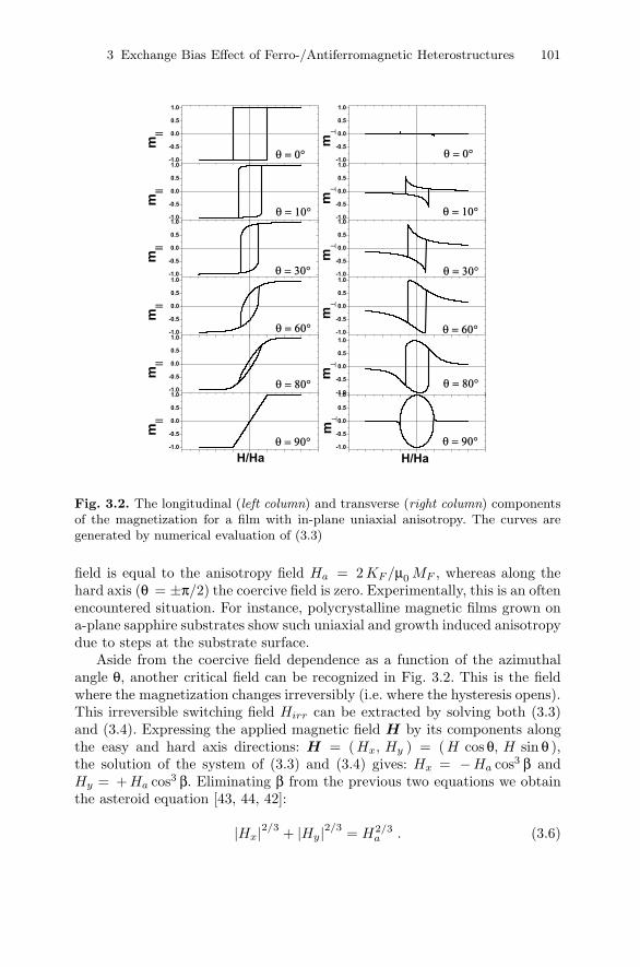
Fig. 3.5. a) Hysteresis loops of Co-CoO particles taken at 77◦K. The dashed lineshows the loop after cooling in zero field. The solid line is the hysteresis loop mea-sured after cooling the system in a field of 10 kOe. b) Torque curve for Co particlesat 300 K showing uniaxial anisotropy. b) Torque curve of Co-CoO particles taken at77◦K showing the unusual unidirectioal anisotropy. d) The torque magnetometer.The main component is a spring which measures the torque as a function of the θangle on a sample placed in a magnetic field. [1, 26]
In Fig. 3.5 the original figures from [1, 26] show the shift of a hystere-sis loop of Co-CoO particles. The system was cooled from room temperaturedown to 77 K through the Neel temperature of CoO (TN (CoO) = 291 K).The magnetization curve is shown in Fig. 3.5a) as a dashed line. It is sym-metrically centered around zero value of the applied field, which is the generalbehavior of ferromagnetic materials. When, however, the sample is cooled ina positive magnetic field, the hysteresis loop is displaced to negative values(see continuous line of Fig. 3.5a)). Such displacement did not disappear evenwhen extremely high applied fields of 70 000 Oe were used.
In order to get more insight into this unusual effect, the authors studiedthe anisotropy behavior by using a self-made torque magnetometer schemati-cally shown in Fig. 3.5d). It consists of a spring connected to a sample placedin an external magnetic field. Generally, torque magnetometry is an accu-rate method for measuring the magnetocrystalline anisotropy (MCA) of singlecrystal ferromagnets. The torque on a sample is measured as a function of theangle θ between certain crystallographic directions and the applied magneticfield. In strong external fields, when the magnetization of the sample is almostparallel to the applied field (saturation), the torque is equal to:
T = −∂E(θ)∂θ
,
where E(θ) is the MCA energy. In the case of Co, which has a hexagonal struc-ture, the torque about an axis perpendicular to the c-axis follows a sin(2θ)function as seen in Fig. 3.5b). The torque and the energy density can then bewritten as:
T = −K1 sin(2θ)

3 Exchange Bias Effect of Ferro-/Antiferromagnetic Heterostructures 105
EV =∫K1 sin(2θ) dθ = K1 sin2(θ) +K0 ,
where K1 is the MCA anisotropy and K0 is an integration constant. It isclearly seen from the energy expression that along the c-axis, at θ = 0 andθ = 180◦, the particles are in a stable equilibrium. This typical case of auniaxial anisotropy is seen for the Co particles at room temperature, wherethe CoO is in a paramagnetic state. At 77◦K, after field cooling, the CoO isin an antiferromagnetic state. Here, the torque curve of the Co-CoO systemlooks completely different as seen in Fig. 3.5c). The torque curve is a functionof sin(θ):
T = −Ku sin(θ) , (3.8)
hence,
EV =∫Ku sin(θ) dθ = −Ku cos(θ) +K0 . (3.9)
The energy function shows that the particles are in equilibrium for oneposition only, namely θ = 0. Rotating the sample to any angle, it tries toreturn to the original position. This direction is parallel to the field coolingdirection and such anisotropy was named unidirectional anisotropy.
Now, one can analyze whether the same unidirectional anisotropy observedby torque magnetometry is also responsible for the loop shift. In Fig. 3.1 areshown schematically the vectors involved in writing the energy per unit volumefor a ferromagnetic layer with uniaxial anisotropy having the magnetizationoriented opposite to the field. It reads:
EV = −μ0HMF cos(−β) +KF sin2(β) , (3.10)
where H is the external field, MF is the saturation magnetization of theferromagnet per unit volume, and KF is the MCA of the F layer. The twoterms entering in the formula above are the Zeeman interaction energy of theexternal field with the magnetization of the F layer and the MCA energy ofthe F layer, respectively. Now, writing the stability conditions and assumingthat the field is parallel to the easy axis, we find that the coercive field is:
Hc = 2KF/(μ0MF ) . (3.11)
Next step is to cool the system down in an external magnetic field and tointroduce in (3.10) the unidirectional anisotropy term. The expression for theenergy density then becomes:
EV = −μ0HMF cos(−β) +KF sin2(β) −Ku cos(β) . (3.12)
We notice that the solution is identical to the previous case (3.10) with thesubstitution of an effective field: H ′ = H+Ku/MF . This causes the hysteresisloop to be shifted by −Ku/(μ0MF ). Thus, Meiklejohn and Bean concludedthat the loop displacement is equivalent to the explanation for the unidirec-tional anisotropy.
106 F. Radu and H. Zabel
Besides the shift of the magnetization curve and the unidirectionalanisotropy, Meiklejohn and Bean have observed another effect when measur-ing the torque curves. Their experiments revealed an appreciable hysteresis ofthe torque (see Fig. 3.9 and Fig. 3.10 of [26] and Fig. 3.2 of [27] ), indicatingthat irreversible changes of the magnetic state of the sample take place whenrotating the sample in an external magnetic field. As the system did not dis-play any rotational anisotropy when the AF was in the paramagnetic state,this provided evidence for the coupling between the AF CoO shell and theF Co core. Such irreversible changes were suggested to take place in the AFlayer.
3.4 Ideal Model of the Exchange Bias: Phenomenology
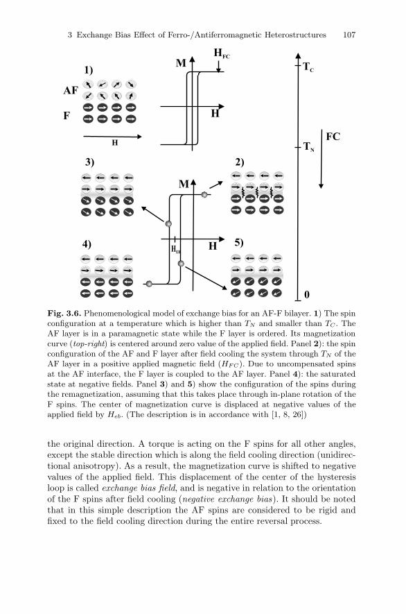
The macroscopic observation of the magnetization curve shift due to uni-directional anisotropy of a F/AF bilayer can qualitatively be understoodby analyzing the microscopic magnetic state of their common interface.Phenomenologically, the onset of exchange bias is depicted in Fig. 3.6.A ferromagnetic layer is in close contact to an antiferromagnetic one. Theircritical temperatures should satisfy the condition: TC > TN , where TC is theCurie temperature of the ferromagnetic layer and TN is the Neel temperatureof the antiferromagnetic layer. At a temperature which is higher than the Neeltemperature of the AF layer and lower than the Curie temperature of the fer-romagnet (TN < T < TC), the F spins align along the direction of the appliedfield, whereas the AF spins remain randomly oriented in a paramagnetic state(see Fig 3.6(1)). The hysteresis curve of the ferromagnet is centered aroundzero, not being affected by the proximity of the AF layer. Next, we saturatethe ferromagnet by applying a high enough external field HFC and then, with-out changing the magnitude or direction of the applied field, the temperatureis decreased to a finite value lower then TN (field cooling procedure).
After field cooling the system, due to exchange interaction at the interfacethe first monolayer of the AF layer will align parallel (or antiparallel) to theF spins. The next monolayer of the antiferromagnet will align antiparallel tothe previous layer as to complete AF order, and so on (see Fig 3.6(2)). Notethat the spins at the AF interface are uncompensated, leading to a finite netmagnetization of this monolayer. It is assumed that both the ferromagnet andthe antiferromagnet are in a single domain state and that they will remainin this single domain state during the magnetization reversal process. Whenreversing the field, the F spins will try to rotate in-plane to the opposite di-rection. Being coupled to the AF spins, it takes a bigger force and therefore astronger external field to overcome this coupling and to rotate the ferromag-netic spins. As a result, the first coercive field is higher than it used to be atT > TN , where the F/AF interaction is not yet active (Fig 3.6(3)). On theway back from negative saturation to positive field values (Fig 3.6(4)), the Fspins require a smaller external force in order to rotate back (Fig 3.6(5)) to
3 Exchange Bias Effect of Ferro-/Antiferromagnetic Heterostructures 107
AF
F
M
M
HFC
H TN
FC
TC
0
H
HHEB
1)
2)3)
4) 5)
Fig. 3.6. Phenomenological model of exchange bias for an AF-F bilayer. 1) The spinconfiguration at a temperature which is higher than TN and smaller than TC . TheAF layer is in a paramagnetic state while the F layer is ordered. Its magnetizationcurve (top-right) is centered around zero value of the applied field. Panel 2): the spinconfiguration of the AF and F layer after field cooling the system through TN of theAF layer in a positive applied magnetic field (HF C). Due to uncompensated spinsat the AF interface, the F layer is coupled to the AF layer. Panel 4): the saturatedstate at negative fields. Panel 3) and 5) show the configuration of the spins duringthe remagnetization, assuming that this takes place through in-plane rotation of theF spins. The center of magnetization curve is displaced at negative values of theapplied field by Heb. (The description is in accordance with [1, 8, 26])
the original direction. A torque is acting on the F spins for all other angles,except the stable direction which is along the field cooling direction (unidirec-tional anisotropy). As a result, the magnetization curve is shifted to negativevalues of the applied field. This displacement of the center of the hysteresisloop is called exchange bias field, and is negative in relation to the orientationof the F spins after field cooling (negative exchange bias). It should be notedthat in this simple description the AF spins are considered to be rigid andfixed to the field cooling direction during the entire reversal process.
108 F. Radu and H. Zabel
3.5 The Ideal Meiklejohn-Bean Model: QuantitativeAnalysis
Based on their observation about the rotational anisotropy, Meiklejohn andBean proposed a model to account for the magnitude of the hysteresis shift.The assumptions made are the following [1, 8, 42]:
• The F layer rotates rigidly, as a whole;• Both the F and AF are in a single domain state;• The AF/F interface is atomically smooth;• The AF layer is magnetically rigid, meaning that the AF spins remain
unchanged during the rotation of the F spins;• The spins of the AF interface are fully uncompensated: the interface layer
has a net magnetic moment;• The F and the AF layers are coupled by an exchange interaction across
the F/AF interface. The parameter assigned to this interaction is the in-terfacial exchange coupling energy per unit area Jeb;
• The AF layer has an in-plane uniaxial anisotropy.
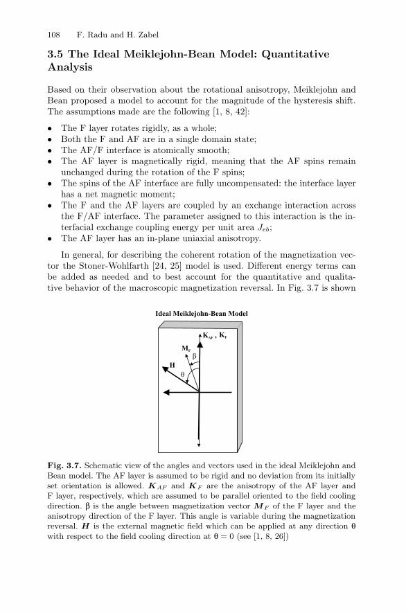
In general, for describing the coherent rotation of the magnetization vec-tor the Stoner-Wohlfarth [24, 25] model is used. Different energy terms canbe added as needed and to best account for the quantitative and qualita-tive behavior of the macroscopic magnetization reversal. In Fig. 3.7 is shown
H
MF
�
KFKAF ,
Ideal Meiklejohn-Bean Model
�
Fig. 3.7. Schematic view of the angles and vectors used in the ideal Meiklejohn andBean model. The AF layer is assumed to be rigid and no deviation from its initiallyset orientation is allowed. KAF and KF are the anisotropy of the AF layer andF layer, respectively, which are assumed to be parallel oriented to the field coolingdirection. β is the angle between magnetization vector MF of the F layer and theanisotropy direction of the F layer. This angle is variable during the magnetizationreversal. H is the external magnetic field which can be applied at any direction θwith respect to the field cooling direction at θ = 0 (see [1, 8, 26])

3 Exchange Bias Effect of Ferro-/Antiferromagnetic Heterostructures 109
schematically the geometry of the vectors involved in the ideal Meiklejohn andBean model. H is the applied magnetic field, which makes an angle θ withrespect to the field cooling direction denoted by θ = 0, KF and KAF are theuniaxial anisotropy directions of the F and the AF layer, respectively. Theyare assumed to be oriented parallel to the field cooling direction. MF is themagnetization orientation of the F spins during the magnetization reversal. Itis assumed that the AF spins are fixed to their orientation defined during thefield cooling procedure (rigid AF). In the analysis below the angle (θ = 0) forthe applied field is assumed to be parallel to the field cooling direction. Thiscondition refers to the direction along which the hysteresis loops is measured,whereas θ �= 0 is used for torque measurements or for measuring the azimuthaldependence of the exchange bias field.
Within this model the energy per unit area assuming coherent rotation ofthe magnetization, can be written as [1, 8, 11]:
EA = −μ0HMF tF cos(−β) +KF tF sin2(β) − Jeb cos(β) , (3.13)
where Jeb [J/m2] is the interfacial exchange energy per unit area, and MF isthe saturation magnetization of the ferromagnetic layer. The interfacial ex-change energy can be further expressed in terms of pair exchange interactions:Eint =
∑ij Ji jS
AFi SF
j , where the summation includes all interactions withinthe range of the exchange coupling [29, 31, 45, 46].
The stability condition ∂EA / ∂θ = 0 has two types of solutions: one isβ = cos−1[(Jeb − μ0HMF tF )/(2KF )] for μ0HMF tF − Jeb ≤ 2KF ; theother one is β = 0, π for μ0HMF tF − Jeb ≥ 2KF , corresponding to positiveand negative saturation, respectively. The coercive fields Hc1 and Hc2 areextracted from the stability equation above for β = 0, π:
Hc1 = −2KF tF + Jeb
μ0MF tF(3.14)
Hc2 =2KF tF − Jeb
μ0MF tF. (3.15)
Using the expressions above, the coercive field Hc of the loop and thedisplacement Heb can be calculated according to:
Hc =−Hc1 +Hc2
2and Heb =
Hc1 +Hc2
2(3.16)
which further gives:
Hc =2KF
μ0MF, (3.17)
andHeb = − Jeb
μ0MF tF. (3.18)
Equation (3.18) is the master formula of the EB effect. It gives the expectedcharacteristics of the hysteresis loop for an ideal case, in particular the linear

110 F. Radu and H. Zabel
dependence on the interfacial energy Jeb and the inverse dependence on theferromagnetic layer thickness tF . Therefore this equation serves as a guidelineto which experimental values are compared. In the next section we will discusssome predictions of the model above.
3.5.1 The Sign of the Exchange Bias
Equation (3.18) predicts that the sign of the exchange bias is negative. Al-most all hysteresis loops shown in the literature are shifted oppositely to thefield cooling direction. The positive or negative exchange coupling across theinterface produces the same (negative) sign of the exchange bias field. Thereare, however, exceptions. Positive exchange bias was observed for CoO/Co,FexZn1−xF2/Co and Cu1−xMnx/Co bilayers when the measuring temperaturewas close to the blocking temperature [14, 47, 48, 49, 50]. At low tempera-tures positive exchange bias was observed in Fe/FeF2 [163] and Fe/MnF2 [51]bilayers. Specific of the last two systems is the low anisotropy of the anti-ferromagnet and the antiferromagnetic type of coupling between the F andAF layers. It was proposed that, at high cooling fields, the interface layer ofthe antiferromagnet aligns ferromagnetically with the external applied fieldand therefore ferromagnetically with the F itself. As the preferred orientationbetween the interface spins of the F layer and AF layer is the antiparallel one(AF coupling), the EB becomes positive. Further theoretical and experimentaldetails of the positive exchange bias mechanism are presented in [52, 53, 54].In the original Meiklejohn and Bean model the interaction of the cooling fieldwith the AF spins is not taken into account. However this interaction canbe easily introduced in their model. The positive exchange bias could also beaccounted for in the M&B model by simply changing the sign of Jeb in (3.13)from negative to positive.
3.5.2 The Magnitude of the EB
Often the exchange coupling parameter Jeb is identified with the exchangeconstant of the AF layer (JAF ). For various calculations a value ranging fromJAF to JF was assumed. For CoO, JAF = 21.6K = 1.86 meV [55]. Using thisvalue, the expected exchange coupling constant Jeb of a CoO(111)/F layercan be estimated as [29, 56]:
Jeb = NJAF /A = 4mJ/m2 , (3.19)
where N = 4 is the number of Co2+ ions at the uncompensated CoO interfaceper unit area A=
√(3) a2, and a = 4.27 A is the CoO lattice parameter. With
this number we would expect for a 100 A thick Co layer, which shares aninterface with a CoO AF layer, an exchange bias of:
Heb [Oe] =Jeb [J/m2]
MF [kA/m] tF [A]1011 (3.20)

3 Exchange Bias Effect of Ferro-/Antiferromagnetic Heterostructures 111
Heb =0.004
1460× 1001011 = 2740 Oe .
This exchange bias field is by far bigger than experimentally observed. Sofar an ideal magnitude of the EB field as predicted by the equation (3.19)has not yet been observed, even so for some bilayers high EB fields weremeasured (see Table 3.1). We encounter here two problems: first, we do notknow how to evaluate the real coupling constant Jeb at the interfaces withvariable degrees of complexity, and the second, in reality interfaces are neveratomically smooth. The unknown interface was nicely labelled by Kiwi [9] as“a hard nut to crack”. Indeed, the features of the interfaces may be complexregarding the structure, the roughness, the magnetic properties, and domainstate of the AF and F layers.
In Table 3.1 are listed some EB data of systems with CoO as the AF layer.We focus on experimentally determined interfacial exchange coupling con-stants using Jeb = −Heb μ0MF tF . The observed exchange coupling constantis usually smaller then the expected value of 4 mJ/m2 for CoO/Co bilayersby a factor ranging from 3 to several orders of magnitude. One anomaly isseen for the multilayer system Co/CoO which is actually ∼3 times higher then
Table 3.1. Experimental values related to Co/CoO exchange bias systems. Thesymbols used in the table are: ebe-electron-beam evaporation, rsp-reactive sputter-ing, msp-magnetron sputtering, mbe-molecular beam epitaxy, F-ferromagnet, AF an-tiferromagnet, tAF -the thickness of the AF, tF -the thickness of the F, Heb-measuredexchange bias field, Hc-measured coercive field, TB-measured blocking temperature,Tmes-the measuring temperature, Jeb-the coupling energy extracted from the exper-imental value of exchange bias field (Jeb = −Heb (μ0MF tF ))
AF F tAF tF Heb Hc TB Tmes Jeb Ref[A] [A] [Oe] [Oe] [K] [K] [mJ/m2]
CoO (air) Co(rsp) 20 40 –3000 NA - 4.2 1.75 [57]CoO (air) Co(rsp) 25 27 –2321 3683 180 10 0.91 [14]CoO (air) Co(rsp) 25 56 –1073 1751 180 10 0.88 [14]CoO (air) Co(rsp) 25 87 –675 1315 180 10 0.86 [14]CoO (air) Co(rsp) 25 119 –557 901 180 10 0.97 [14]CoO (air) Co(rsp) 25 153 –443 789 180 10 0.99 [14]CoO (air) Co(rsp) 25 260 –251 427 180 10 0.95 [14]CoO (air) Co(rsp) 25 320 –202 346 180 10 0.94 [14]CoO (air) Co(rsp) 25 398 –174 290 180 10 1.00 [14]CoO (air) Co(msp) 33 139 –145 325 - 5 0.29 [58]CoO (air) Co(msp) 33 139 –50 NA - 30 0.1 [59]CoO (rsp) Co(rsp) 20 150 –25 295 - 20 0.055 [47][CoO (rsp) Co(rsp)]x25 70 37 –2500 5000 - 5 13.5! [60]CoO (in-situ) Co(ebe) 20 160 –220 330 180 10 0.51 [61]CoO(111)(mbe) Fe(110)(mbe) 200 150 –150 520 291 10 0.4 Sect.
[62, 63]
112 F. Radu and H. Zabel
the expected value of 4mJ/m2, and to our knowledge is the highest value ob-served experimentally [60]. Such a variation of the experimental values for theinterfacial exchange coupling constant is motivating further considerations ofthe mechanisms controlling the EB effect.
3.5.3 The 1/tF Dependence of the EB Field
Equation (3.18) predicts that the variation of the EB field is proportional tothe inverse thickness of the ferromagnet:
Heb ≈ 1tF
. (3.21)
This dependence was subject of a large number of experimental investigations[8], because it is associated with the interfacial nature of the exchange biaseffect. For the CoO/Co bilayers no deviation was observed [61], even for verylow thicknesses (2 nm) of the Co layer [14]. For other systems with thin Flayers of the order of several nanometers it was observed that the 1/tF lawis not closely obeyed [8]. It was suggested that the F layer is no longer lat-erally continuous [8]. Deviations from 1/tF dependence for the other extremewhen the F layer is very thick were observed as well [8]. For this regime itis assumed that for F layers thicker than the domain wall thickness (500 nmfor permalloy), the F spins may vary appreciably across the film upon themagnetization reversal [64].
3.5.4 Coercivity and Exchange Bias
According to (3.17) the coercivity of the magnetic layer is the same withand without exchange bias effect. This contradicts experimental observations.Usually an increase of the coercive field is observed.
3.6 Realistic Meiklejohn and Bean Model
In [26] a new degree of freedom for the AF spins was introduced: the AF is stillrigid, but it can slightly rotate during the magnetization reversal as a wholeas indicated in Fig. 3.8. This parameter was introduced in order to account forthe rotational hysteresis observed during the torque measurements. Allowingthe AF layer to rotate is not in contradiction to the rigid state of the AFlayer, because it is allowed only to rotate as a whole. Therefore, the fourth as-sumption of the ideal M&B model in Sect. 3.5 is removed. The new conditionfor the AF spins is: α �= 0. With this new assumption, the equation (3.13)reads [8, 27]:
3 Exchange Bias Effect of Ferro-/Antiferromagnetic Heterostructures 113
H
MAF
MF
��
�
KFKAF ,
Meiklejohn-Bean Model
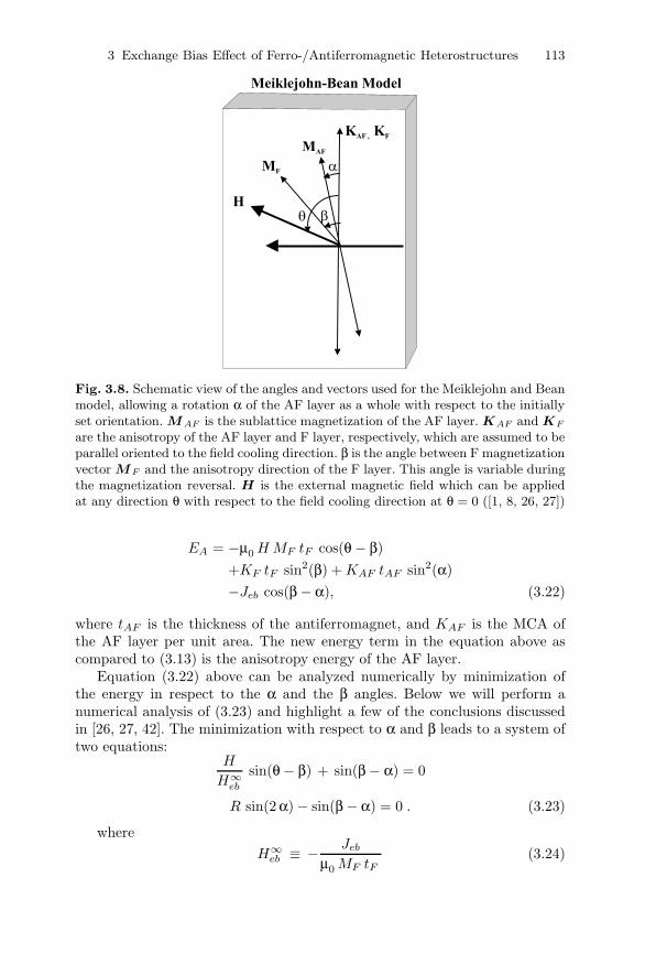
Fig. 3.8. Schematic view of the angles and vectors used for the Meiklejohn and Beanmodel, allowing a rotation α of the AF layer as a whole with respect to the initiallyset orientation. M AF is the sublattice magnetization of the AF layer. KAF and KF
are the anisotropy of the AF layer and F layer, respectively, which are assumed to beparallel oriented to the field cooling direction. β is the angle between F magnetizationvector MF and the anisotropy direction of the F layer. This angle is variable duringthe magnetization reversal. H is the external magnetic field which can be appliedat any direction θ with respect to the field cooling direction at θ = 0 ([1, 8, 26, 27])
EA = −μ0HMF tF cos(θ − β)+KF tF sin2(β) +KAF tAF sin2(α)−Jeb cos(β − α), (3.22)
where tAF is the thickness of the antiferromagnet, and KAF is the MCA ofthe AF layer per unit area. The new energy term in the equation above ascompared to (3.13) is the anisotropy energy of the AF layer.
Equation (3.22) above can be analyzed numerically by minimization ofthe energy in respect to the α and the β angles. Below we will perform anumerical analysis of (3.23) and highlight a few of the conclusions discussedin [26, 27, 42]. The minimization with respect to α and β leads to a system oftwo equations:
H
H∞eb
sin(θ − β) + sin(β − α) = 0
R sin(2 α) − sin(β − α) = 0 . (3.23)
whereH∞
eb ≡ − Jeb
μ0MF tF(3.24)

114 F. Radu and H. Zabel
is the value of the exchange bias field when the anisotropy of the AF is in-finitely large, and
R ≡ KAF tAF
Jeb, (3.25)
is the parameter defining the ratio between the AF anisotropy energy andthe interfacial exchange energy Jeb. As we will see further below, exchangebias is only observed, if the AF anisotropy energy is bigger than the exchangeenergy. The unknown variables α and β are numerically extracted as a functionof the applied field H . Note that for clarity reasons the anisotropy of theferromagnet was neglected (KF = 0) in the system of equation above. As aresult the coercivity, which will be discussed further below, is not related tothe F layer anymore, but to the AF layer alone. Also, in order to simplify thediscussion we consider first the case θ = 0, which corresponds to measuring ahysteresis loop parallel to the field cooling direction.
Numerical evaluation of the (3.23) yields the angles:
• α of the AF spins as a function of the applied field during the hysteresismeasurement
• β of the F spins which rotate coherently during their reversal
The β angle defines completely the hysteresis loop and at the same time thecoercive fields Hc1 and Hc2. These fields, in turn, define the coercive field Hc
and the exchange bias field Heb (see equation (3.16)). The α angle influencesthe shape of the hysteresis loops when the R-ratio has low values, as we willsee below. For high R values the rotation angle of the antiferromagnet is closeto zero, giving a maximum exchange bias field equal to H∞
eb .The properties of the EB system originate from the properties of the AF
layer, which are accounted for by one parameter, the R-ratio. We will considerthe effect of the R-ratio on the angels β and α which, as stated above, definethe macroscopic behavior and the critical fields of the EB systems.
Numerical simulations of (3.23) as a function of R-ratio are shown inFig. 3.9 and in Fig. 3.10. We distinguish three physically distinct regions [26,27, 42, 65]:
• I. R ≥ 1In this region the coercive field is zero and the exchange bias field is fi-nite, decreasing from the asymptotic value H∞
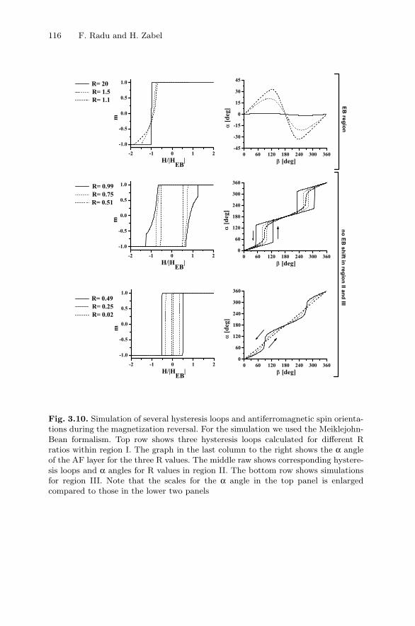
eb to the lowest finite valueat R = 1. The AF spins rotate reversibly during the complete reversalof the F spins. The α angle has a maximum value as a function of theR-ratio, ranging from approximatively zero for R = ∞ to α = 45◦ atR = 1. Notice that as the maximum angle of the AF spins increases, aslight decrease of the exchange bias field is observed. When the R-ratioapproaches the critical value of unity, the exchange bias has a minimum.In the phase diagram, only range I can cause a shift of the magnetizationcurve. Simulated hysteresis loops for three different values of the R-ratioare shown in Fig. 3.10. One notices that not only the size of the exchange

3 Exchange Bias Effect of Ferro-/Antiferromagnetic Heterostructures 115
Fig. 3.9. Left: The phase diagram of the exchange bias field and the coercive fieldsas a function of the Meiklejohn-Bean parameter R. Right: Typical behavior of theantiferromagnetic angle α for the three different regions of the phase diagram. Onlyregion I can lead to a shift of the hysteresis loop. In the other two regions a coercivityis observed but no exchange bias field
bias field decreases when the R-ratio approaches unity, but also the shapeof the hysteresis curve is changing. At high R-ratios the reversal is rathersharp, whereas for R-ratios close to unity it become more extended, almostresembling a spring-like behavior.
• II. 0.5 ≤ R < 1Characteristic for this region is that the AF spins are no more reversible.They follow the F spins and they change direction irreversibly, causinga coercive field at the expense of the exchange bias field, which becomeszero. Furthermore, depending on the field sweeping direction, there is ahysteresis-like behavior of the AF spin rotation. At a critical angle β ofthe F spin rotation, the AF spins cannot withstand the torque by thecoupling to the F spins and they jump in a discontinuous fashion to anotherangle (jump angle). The hysteresis loops corresponding to this region (seeFig. 3.10) are drastically different from the previous case. The coercivityshows a strong dependence as function of the R-ratio and they are notshifted at all. Moreover, the AF jump angles are clearly visible as kinks inthe hysteresis during the reversal.
• III. R < 0.5This region preserves the features of the previous one with one excep-tion, namely that the AF spins follow reversibly the F spins, withoutany jumps. Therefore, no hysteresis-like behavior of the α angle is seen.The exchange bias field is zero and the coercive field is finite, dependingon the R-ratio. The hysteresis loops shown in Fig. 3.10 are quite similarto a ferromagnet with uniaxial anisotropy. Within the Stoner-Wolhfarthmodel the resultant coercive field can be roughly approximated as [42]:Hc ≈ 2KAF tAF /(μ0MF tF ).
116 F. Radu and H. Zabel
Fig. 3.10. Simulation of several hysteresis loops and antiferromagnetic spin orienta-tions during the magnetization reversal. For the simulation we used the Meiklejohn-Bean formalism. Top row shows three hysteresis loops calculated for different Rratios within region I. The graph in the last column to the right shows the α angleof the AF layer for the three R values. The middle raw shows corresponding hystere-sis loops and α angles for R values in region II. The bottom row shows simulationsfor region III. Note that the scales for the α angle in the top panel is enlargedcompared to those in the lower two panels
3 Exchange Bias Effect of Ferro-/Antiferromagnetic Heterostructures 117
It is easy to recognize that allowing the AF to rotate as a whole leads toan impressively rich phase diagram of the EB systems as a function of the pa-rameters of the AF layer (and F layer). The R-ratio can be varied across thewhole range from zero to infinity by changing the thickness of the AF layer [8],by varying its anisotropy (dilution of the AF layers with non-magnetic impu-rities [32, 66, 67]), or by varying the interfacial exchange energy Jeb (low doseion bombardment [68, 69, 70]). Recently [71], an almost ideal M&B behaviorhas been observed in Ni80Fe20/Fe50Mn50 bilayers. At high thicknesses of theAF layer the hysteresis loop is shifted to negative values and the coercivityis almost zero, whereas for reduced AF thicknesses a strong increase of thecoercive field is observed together with a drastic decrease of exchange bias.
3.6.1 Analytical Expression of the Exchange Bias Field
First we calculate analytically the expression of the exchange bias field forθ = 0 and KF = 0. The exact analytical solution is obtained by solving thesystem of (3.23) for β = 0, which leads to:
Heb =
⎧⎪⎨⎪⎩H∞
eb
√1 − 1
4R2 R ≥ 1
0 R < 1. (3.26)
This equation retains the 1/tF dependence of the exchange bias field, but atthe same time provides new features. The most important one is an addi-tional term, which effectively lowers the exchange bias field when the R-ratioapproaches the critical value of one. The R-ratio has three terms. One of themincludes the thickness of the AF layer. The analytical expression for the ex-change bias field (3.26) predicts that there is a critical AF thickness tcr
AF belowwhich the exchange bias cannot exist. This is [72]:
tcrAF =
Jeb
KAF. (3.27)
Below this critical thickness the interfacial energy is transformed into coerciv-ity. Above the critical thickness the exchange bias increases as a function ofthe AF layer thickness, reaching the asymptotic (ideal) value H∞
eb when tAF
is infinite. Most recent observation of an AF critical thickness can be foundin [73].
A similar expression as (3.26) was derived by Binek et al. [127] using aseries expansion of (3.22) with respect to α=0 : Heb ≈ H∞
eb (1 − 18R2 ) for
1/R≥0. Note that close to the critical value of R=1, the α angle could reachhigh values up to 45◦. Therefore, the series expansion with respect to α=0 isa good approximation for R>5.
118 F. Radu and H. Zabel
3.6.2 Azimuthal Dependence of the Exchange Bias Field
In the following we consider the exchange bias field in region I, where itacquires non vanishing values. The coercive fields and the exchange bias fieldare extracted from the condition β = θ+π/2 for both Hc1 and Hc2. This givesHc1 = Hc2 = (−Jeb/μ0MF tF ) cos(α(R, θ + π/2) − θ), where α(R, θ + π/2)is the value of the rotation angle of the AF spins at the coercive field. Withthe notation: α0 ≡ α(R, θ + π/2), and using the expression 3.16, the angulardependence of the exchange bias field becomes:
Heb(θ) =−Jeb
μ0MF tFcos( α0 − θ) . (3.28)
The equation above can be also written as:
Heb(θ) = −KAF tAF
μ0MF tFsin(2 α0) . (3.29)
Interestingly, the exchange coupling parameter Jeb in (3.28) is missing in (3.29),leaving instead an explicit dependence of the exchange bias field on the pa-rameters of the antiferromagnet and the ferromagnet. The exchange couplingconstant and the θ angle are accounted for by the AF angle α0.
Equations (3.28) and (3.29) are the most general expressions for an ex-change bias field. They include both, the influence of the rotation of the AFlayer and the influence of the azimuthal orientation of the applied field. More-over, the anisotropy and the thickness of the AF layer are explicitly shownin (3.29). To illustrate their generality we consider below two special cases forthe (3.28):
• θ = 0In this case the hysteresis loop is measured along the field cooling direction(θ = 0) and (3.28) becomes equivalent to the (3.26).
• R → ∞When R is very large (R 1), α approximates zero, i.e. the rotation ofthe AF - layer becomes negligible. This is actually the original assumptionof the Meiklejohn and Bean model. Such a condition (R → ∞) is approx-imately satisfied for large thicknesses of the AF layer. Then the exchangebias field as function of θ can be written as [94, 127, 165]:
Hα=0eb (θ) =
−Jeb
μ0MF tFcos(θ) . (3.30)
In order to get more insight into the azimuthal dependence of the ex-change bias field, we show in Fig. 3.11 the normalized exchange bias fieldHeb(θ) /|H∞
eb (0)| as a function of the θ angle, according to (3.28) and (3.29),and for three different values of the R ratio (R = 1.1, R = 1.5, R = 20).The α0 angle (see Fig. 3.10) was obtained by numerically solving the system

3 Exchange Bias Effect of Ferro-/Antiferromagnetic Heterostructures 119
Fig. 3.11. Azimuthal dependence of exchange bias as a function of the θ angle. Thecurves are calculated by the (3.28) and (3.29)
of (3.23). For large values of R, the azimuthal dependence of the exchange biasfield follows closely a cos(θ) unidirectional dependence. When, however, theR-ratio takes small values but larger then unity, the azimuthal behavior of theEB field deviates from the ideal unidirectional characteristic. There are twodistinctive features: one is that at θ = 0 the exchange bias field is reduced, andthe other one is that the maximum of the exchange bias field is shifted fromzero towards negative azimuthal angle values. According to (3.28) this shiftangle is equal to α0. In other words, the exchange bias field is not maximumalong the field cooling direction. Another striking feature is that the shiftedmaximum of the exchange bias field with respect to the azimuthal angle θdoes not depend on thickness and anisotropy of the AF layer:
HMAXeb = − Jeb
μ0MF tF. (3.31)
Summarizing we may state that, within the Meiklejohn and Bean model,a reduced exchange bias field is observed along the field cooling directiondepending on the parameters of the AF layer (KAF and tAF ). However, forR ≥ 1 the maximum value for the exchange bias field which is reached at θ �= 0does not depend on the anisotropy constant (KAF ) and thickness (tAF ) of theAF layer. The azimuthal characteristic of the exchange bias allows to extractall three essential parameters defining the exchange bias field: Jeb,KAF and,tAF .
The condition for extracting the Hc1 and Hc2 from the same β angle hidesan important property of the magnetization reversal of the ferromagneticlayer. This will be described next.

120 F. Radu and H. Zabel
3.6.3 Magnetization Reversal
A distinct feature of exchange bias phenomena is the magnetization reversalmechanism. In Fig. 3.12 is shown the parallel component of the magnetizationm|| = cos(β) versus the perpendicular component m⊥ = sin(β) for severalR-ratios and for θ = 30◦. The geometrical conventions are the ones shownin Fig. 3.8. We see that for R < 1 the reversal of the F spins is symmetric,similar to typical ferromagnets with uniaxial anisotropy. Although the regions0.5 ≤ R < 1 and R < 0.5 exhibit different reversal modes of the AF spins (seeFig. 3.10), there is little difference with respect to the F spin rotation. Forboth regions 0.5 ≤ R < 1 and R < 0.5 the F spins do make a full rotation,similar to the uniaxial ferromagnets. At the steep reversal branches one wouldexpect magnetic domain formation.
When R ≥ 1 another reversal mechanism is observed. The ferromagneticspins first rotate towards the unidirectional axis as lowering the field frompositive to negative values, and then the rotation proceeds continuously untilthe negative saturation is reached. On the return path, when the field isswept from negative to positive values, the ferromagnetic spins follow thesame path towards the positive saturation. The rotation is continuous withoutany additional steps or jumps. A similar behavior was observed theoreticallywithin the domain state model [36, 39]. The magnetization reversal modes canbe accessed experimentally by using the Vector-MOKE technique [74, 75, 76,41] which allows to follow both the magnetization vector and its angle duringthe reversal process.
Fig. 3.12. Magnetization reversal for several values of the R ratio. The parallelcomponent of the magnetization vector m|| = cos(β) is plotted as a function of theperpendicular component of the magnetization m⊥ = sin(β). The reversal for R < 1resembles the typical reversal of ferromagnets with uniaxial anisotropy. For R ≥ 1the reversal proceeds along the same path for the increasing and decreasing branchof the hysteresis loop. The angle θ = 30◦ is chosen arbitrarily

3 Exchange Bias Effect of Ferro-/Antiferromagnetic Heterostructures 121
3.6.4 Rotational Hysteresis
We briefly discuss again the rotational hysteresis deduced from torque mea-surements [1, 26, 27], now in the light of the analysis provided above. Thetorque measurements were carried out in a strong applied magnetic field H.Therefore the applied field H and the magnetization MF can be assumed tobe parallel (β = θ). The torque is given by:
T = −∂E(θ)∂θ
= Jeb sin(θ − α(θ)).
This expression differs from (3.8) for the ideal model by the rotation of theAF spins through the α angle. However, this does not explain the energyloss during the torque measurements, as observed in the experiment (3.6(b)).The torque curve would only be a bit distorted but completely reversible.The integration of the energy curve predicts a rotational hysteresis Wrot = 0.In order to account for a finite rotational hysteresis, one can assume that afraction p of particles at the F-AF interface are uniaxially coupled behavingas in region II, whereas the remaining fraction (1 − p) of the F-AF particlesare coupled unidirectionally, having the ideal behavior as described in regimeI. As seen in Fig. 3.9(left), when the R-ratio of the uniaxial particle is in therange 0.5 ≤ R < 1, the AF spins will rotate irreversibly, showing hysteresis-like behavior due to α jumps indicated in the Fig. 3.9 (right). A rotationalhysteresis is not expected for unidirectional particles with R ≥ 1 because theAF structure changes reversibly with θ. With this assumption the uniaxialparticles will contribute to the energy loss during the torque measurements,while the unidirectional particles are responsible for the unidirectional featureof the torque curve. This argument was used by Meiklejohn and Bean [27]when studying the exchange bias in core-Co/shell-CoO. A fraction p = 0.5was inferred from the torque curves shown in Fig. 3.5.
3.7 Neel’s AF Domain Wall–Weak Coupling
Both concepts, the rigid AF spin state and rigidly rotating AF spins impose arestriction on the behavior of the antiferromagnetic spins, namely that the AForder is preserved during the magnetization reversal. Such restriction impliesthat the interfacial exchange coupling is found almost entirely in the hysteresisloop either as a loop shift or as coercivity. Experimentally, however, the size ofthe exchange bias does not agree with the expected value, being several ordersof magnitude lower then predicted. In order to cope with such loss of couplingenergy, one can assume that a partial domain wall develops in the AF layerduring the magnetization reversal. This concept was introduced by Neel [77, 9]when considering the coupling between a ferromagnet and a low anisotropyantiferromagnet. The AF partial domain wall will store an important fractionof the exchange coupling energy, lowering the shift of the hysteresis loop.

122 F. Radu and H. Zabel
Neel has calculated the magnetization orientation of each layer througha differential equation. The weak coupling is consistent with a partial AFdomain wall which is parallel to the interface (Neel domain wall). His modelpredicts that a minimum AF thickness is required to produce hysteresis shift.More importantly the partial domain wall concept forms the basis for furthermodels which incorporate either Neel wall or Bloch wall formation as a wayto reduce the observed magnitude of exchange bias.
3.8 Malozemoff Random Field Model
Malozemoff (1987) proposed a novel mechanism for exchange anisotropypostulating a random nature of exchange interactions at the F-AF inter-face [29, 30, 31]. He assumed that the chemical roughness or alloying at theinterface, which is present for any realistic bilayer system, causes lateral vari-ations of the exchange field acting on the F and AF layers. The resultantrandom field causes the AF to break up into magnetic domains due to theenergy minimization. By contrast with other theories, where the unidirec-tional anisotropy is treated either microscopically [78, 79, 80] or macroscopi-cally [1, 26, 28], the Malozemoff approach belongs to models on the mesoscopicscale for surface magnetism.
The general idea for estimating the exchange anisotropy is depicted inFig. 3.13, where a domain wall in an uniaxial ferromagnet is driven by anapplied in-plane magnetic field H [29]. Assuming that the interfacial energyin one domain (σ1) is different from the energy in the neighboring domain(σ2), then the exchange field can be estimated by the equilibrium conditionbetween the applied field pressure 2HMF tF and the effective pressure fromthe interfacial energy Δσ:
Heb =Δσ
2MF tF, (3.32)
where MF and tF are the magnetization and thickness of the ferromagnet.When the interface is treated as ideally “compensated”, then the exchangebias field is zero. On the other hand, if the AF/F interface is ideally uncom-pensated there is an interfacial energy difference Δσ = 2Ji/a
2, where Ji is
AF
F
Domain
WallM F
����
H
tF
tAF
Fig. 3.13. Schematic side view of a F/AF bilayer with a ferromagnetic wall drivenby an applied field H [29]
3 Exchange Bias Effect of Ferro-/Antiferromagnetic Heterostructures 123
b) c)
x x xxx x x x
UNCOMPENSATED COMPENSATED
�= - J/a2
�= + J/a2
�= 0 �= 0
a) d)
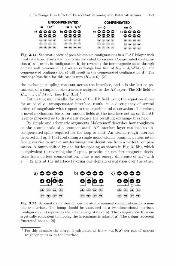
Fig. 3.14. Schematic view of possible atomic configurations in a F-AF bilayer withideal interfaces. Frustrated bonds are indicated by crosses. Compensated configura-tion a) will result in configuration b) by reversing the ferromagnetic spins throughdomain wall movement. It gives an exchange bias field of Heb = Ji/a2MF tF . Thecompensated configuration c) will result in the compensated configuration d). Theexchange bias field for this case is zero (Heb = 0). [29]
the exchange coupling constant across the interface, and a is the lattice pa-rameter of a simple cubic structure assigned to the AF layer. The EB field isHeb = Ji/a
2MF tF (see Fig. 3.14)1.Estimating numerically the size of the EB field using the equation above
for an ideally uncompensated interface, results in a discrepancy of severalorders of magnitude with respect to the experimental observation . Therefore,a novel mechanism based on random fields at the interface acting on the AFlayer is proposed as to drastically reduce the resulting exchange bias field.
By simple and schematic arguments Malozemoff describes how roughnesson the atomic scale of a “compensated” AF interface layer can lead to un-compensated spins required for the loop to shift. An atomic rough interfacedepicted in Fig. 3.15a) containing a single mono-atomic bump in a cubic inter-face gives rise to six net antiferromagnetic deviations from a perfect compen-sation. A bump shifted by one lattice spacing as shown in Fig. 3.15b), whichis equivalent to reversing the F spins, provides six net ferromagnetic devia-tions from perfect compensation. Thus a net energy difference of ziJi withzi = 12 acts at the interface favoring one domain orientation over the other.
x
xx
xx
x
a)
x x x
b) c)
Fig. 3.15. Schematic side view of possible atomic moment configurations for a non-planar interface. The bump should be visualized on a two-dimensional interface.Configuration c) represents the lower energy state of a). The configuration b) is en-ergetically equivalent to flipping the ferromagnetic spins of a). The x signs representfrustrated bonds. [29]
1 For this example the energy is calculated as Ekl = −JiSkSl per pair of nearestneighbor spins kl at the interface.

124 F. Radu and H. Zabel
Note that for an ideally uncompensated interface the energy difference is only8Ji when reversing the F spins. This implies that an atomic step roughnessat a compensated interface leads to a higher exchange bias field as comparedto the ideally compensated interface.
The estimates of this local field can be further refined assuming a moredetailed model. For example, by inverting the spin in the bump shown inFig. 3.15c, the interfacial energy difference is reduced by 5 × 2Ji at the costof generating one frustrated pair in the AF layer just under the bump. Thisfrustrated pair increases the energy difference by 2JA, where JA is the AFexchange constant. Thus the energy difference between the two domains be-comes 2Ji + 2JA or roughly 4J if Ji ≈ JA ≈ J . If one allows localized cantingof the spins, one expects the energy difference to be reduced somewhat further.
Each interface irregularity will give a local energy difference between do-mains whose sign depends on the particular location of the irregularity andwhose magnitude is on the average 2zJ , where z is a number of order unity.Furthermore, for an interface which is random on the atomic scale, the lo-cal unidirectional interface energy σl = ±zJ/a2 will also be random andits average σ in a region L2 will go down statistically as σ ≈ σl/
√N , where
N = L2/a2 is the number of sites projected onto the interface plane. Thereforethe effective AF-F exchange energy per unit area is given by:
Jeb ≈ 1√NJi ≈ 1
LJi,
where Ji is the exchange energy of a fully uncompensated AF-surface.Given a random field provided by the interface roughness and assuming a
region with a single domain of the ferromagnet, it is energetically favorablefor the AF to break up into magnetic domains, as shown schematically inFig. 3.16. A perpendicular domain wall is the most preferable situation. Thisperpendicular domain wall is permanently present in the AF layer. It should bedistinguished from a domain wall parallel to AF/F interface, which accordingto the Mauri model [28] develops temporarily during the rotation of the Flayer.
By further analyzing the stability of the magnetic domains in the presenceof random fields, a characteristic length L of the frozen-in AF domains andtheir characteristic height are obtained: L ≈ π
√AAF /KAF and h = L/2,
whereAAF is the exchange stiffness and h is the characteristic height of the AF
x xx
Fig. 3.16. Schematic view of a vertical domain wall in the AF layer. It appears asan energetically favorable state of F/AF systems with rough interfaces [29, 81]

3 Exchange Bias Effect of Ferro-/Antiferromagnetic Heterostructures 125
domains. Once these domains are fixed, flipping the ferromagnetic orientationcauses an energy change per unit area of Δσ = 4zJ/πaL, which further leadsto the following expression for the EB field [29]:
Heb =2 z
√AAFKAF
π2MF tF. (3.33)
Assuming a CoO/Co(100 A) film, the calculated exchange bias using the(3.33) is:
Heb =2 × 1
√0.0186×1.6×10−19[J]
4.27×10⁻¹⁰[m] 2.5 × 10⁷ [J/m3]
π2 × 1460 [kA/m] 100× 10−10× 10
= 580Oe. (3.34)
For the estimations above we used for the exchange stiffness the followingvalue: AAF = JAF /a, where a is the lattice parameter of CoO (a = 4.27A)and JAF = 1.86 meV is the exchange constant for CoO [55].
The characteristic length of the AF domains is for CoO:
L = π√AAF /KAF
= π ×√
0.0186 × 1.6 × 10−19[J ]4.27 × 10⁻¹⁰[m] × 2.5 × 10⁷ [J/m3]
= 16.6 A. (3.35)
The height of the AF domains is h = L/2 = 8.3 A. Comparing this valueto the experimental data on CoO(25A)/Co studied in [82], we notice thatthe calculated EB field agrees well with the value observed experimentally.For example, the exchange bias field for CoO(25 A)/Co(119 A) is 557 Oe andthe theoretical value calculated with (3.33) is 487 Oe. Also, the length andthe height of the AF domains have enough space to develop. The differencebetween theory and experiment is, however, that experimentally AF domainscan occur and vary size and orientation after the very first magnetizationreversal, whereas within the Malozemoff model the AF domains are assumedto develop during the field cooling procedure. Nevertheless, the agreementappears to be excellent.
3.9 Domain State Model
The Domain State model (DS) introduced by Nowak and coworkers [32, 33,35, 36, 83, 84, 38] is a microscopic model in which disorder is introduced viamagnetic dilution not only at the interface but also in the bulk of the AFlayer as in Fig. 3.17. The key element in the model is that the AF layer isa diluted Ising antiferromagnet in an external magnetic field (DAFF) whichexhibits a phase diagram like the one shown in Fig. 3.18 [35]. In zero field the
126 F. Radu and H. Zabel
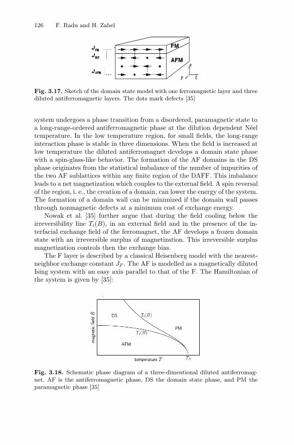
Fig. 3.17. Sketch of the domain state model with one ferromagnetic layer and threediluted antiferromagnetic layers. The dots mark defects [35]
system undergoes a phase transition from a disordered, paramagnetic state toa long-range-ordered antiferromagnetic phase at the dilution dependent Neeltemperature. In the low temperature region, for small fields, the long-rangeinteraction phase is stable in three dimensions. When the field is increased atlow temperature the diluted antiferromagnet develops a domain state phasewith a spin-glass-like behavior. The formation of the AF domains in the DSphase originates from the statistical imbalance of the number of impurities ofthe two AF sublattices within any finite region of the DAFF. This imbalanceleads to a net magnetization which couples to the external field. A spin reversalof the region, i. e., the creation of a domain, can lower the energy of the system.The formation of a domain wall can be minimized if the domain wall passesthrough nonmagnetic defects at a minimum cost of exchange energy.
Nowak et al. [35] further argue that during the field cooling below theirreversibility line Ti(B), in an external field and in the presence of the in-terfacial exchange field of the ferromagnet, the AF develops a frozen domainstate with an irreversible surplus of magnetization. This irreversible surplusmagnetization controls then the exchange bias.
The F layer is described by a classical Heisenberg model with the nearest-neighbor exchange constant JF . The AF is modelled as a magnetically dilutedIsing system with an easy axis parallel to that of the F. The Hamiltonian ofthe system is given by [35]:
Fig. 3.18. Schematic phase diagram of a three-dimentional diluted antiferromag-net. AF is the antiferromagnetic phase, DS the domain state phase, and PM theparamagnetic phase [35]

3 Exchange Bias Effect of Ferro-/Antiferromagnetic Heterostructures 127
H = −JF
∑<i,j>εF
Si.Sj −∑iεF
(dzS2iz + dxS
2ix + μBSi)
−JAF
∑<i,j>εAF
εiεjσiσj −∑iεAF
μBzεiσi
−JINT
∑<iεAF,jεF>
εiσiSjz , (3.36)
where the Si and σi are the classical spin vectors at the ith site of the Fand AF, respectively. The first line contains the energy contribution of theF, the second line describes the diluted AF layer, and the third line includesthe exchange coupling across the interface between F and DAFF, where it isassumed that the Ising spins in the topmost layer of the DAFF interact withthe z component of the Heisenberg spins of the F layer.
In order to obtain the hysteresis loop of the system, the Hamiltonianin (3.36) is treated by Monte Carlo simulations. Typical hysteresis loops areshown in Fig. 3.19 [84], where both the magnetization curve of the F layerand of the interface monolayer of the DAFF are shown. The coercive field ex-tracted from the hysteresis curve depends on the anisotropy of the F layer, butit is also influenced by the DAFF. It, actually, depends on the thickness andanisotropy of the DAFF layer. The coercive field decreases with the increasingthickness of the DAFF layer [84], which can be understood as follows: the inter-face magnetization tries to orient the F layer along its direction. The coercivefield has to overcome this barrier, and the higher the interface magnetizationof the DAFF, the stronger is the field required to reverse the F layer. The
Fig. 3.19. Simulated hysteresis loops within the domain state model. The tophysteresis belongs to the ferromagnetic layer and the bottom hysteresis belongs toan AF interface monolayer [84]

128 F. Radu and H. Zabel
interface magnetization decreases with increasing DAFF thickness due to acoarsening of the AF domains accompanied by smoother domain walls.
The strength of the exchange bias field can be estimated from the (3.36)using simple ground state arguments. Assuming that all spins in the F remainparallel during the field reversal and some net magnetization of the interfacelayer of the DAFF remains constant during the reversal of the F, a simplecalculation gives the usual estimate for the bias field [35]:
lμBeb = JINTmINT , (3.37)
where l is the number of the F layers and mINT is the interface magneti-zation of the AF per spin. Beb is the notation for the exchange bias fieldin [35] and is equivalent to Heb in this chapter. For an ideal uncompensatedinterface (mINT = 1) the exchange bias is too high, whereas for an ideallycompensated interface the exchange bias is zero. Within the DS model theinterface magnetization mINT < 1 is neither a constant nor is it a simplequantity [35]. Therefore, it is replaced by mIDS , which is a measure of theirreversible domain state magnetization of the DAFF interface layer and isresponsible for the EB field. With this, an estimate of exchange bias field forl = 9, JINT = −3.2 × 10⁻²²J , and μ = 1.7 μB gives a value of about 300 Oe.
The exchange bias field depends also on the bulk properties of the DAFFlayer as shown by Miltenyi et al. [32]. There the AF layer was diluted bysubstituting non-magnetic Mg in the bulk part and away from the interface.The representative results are shown in Fig. 3.20. It was shown experimentallythat the EB field depends strongly on the dilution of the AF layer. As afunction of concentration of the non-magnetic Mg impurities, the EB evolvesas following: at zero dilution the exchange bias has finite values, whereas byincreasing the Mg concentration, the EB field increases first, showing a broadpeak-like behavior, and then, when the dilution is further increased the EBfield decreases again. Simulations within the DS model showed an overallgood qualitative agreement. The peak-like behavior of the EB as a functionof the dilution is clearly seen in the simulations (see Fig. 3.20). However, itappears that at zero dilution, the DS gives vanishing exchange bias whereasexperimentally finite values are observed. The exchange bias is missing at lowdilutions because the domains in the AF cannot be formed as they would costtoo much energy to break the AF bonds. This discrepancy [35, 85] is thoughtto be explained by other imperfections, such as grain boundaries in the AFlayer which is similar to dilution and which can also reduce the domain-wallenergy, thus leading to domain formation and EB even without dilution of theAF bulk.
An important property of the kinetics of the DAFF is the slow relaxation ofthe remanent magnetization, i.e., the magnetization obtained after switchingoff the cooling field [35]. It is known that the remanent magnetization of theDS relaxes nonexponentially on extremely long-time scales after the field isswitched off or even within the applied field. In the DS model the EB is relatedto this remanent magnetization. This implies a decrease of EB due to slow

3 Exchange Bias Effect of Ferro-/Antiferromagnetic Heterostructures 129
Fig. 3.20. In the right side of the figure is shown the film structure used to studythe dilution influence on the exchange bias field. a) EB field as function of the Mgconcentration x in the Co1−xMgxO layer for several temperatures. b) EB field as afunction of different dilutions of the AF volume. [32]
relaxation of the AF domain state. The reason for the training effect can beunderstood within the DS model from Fig. 3.19 bottom panel, where it isshown that the hysteresis loop of the AF interface layer is not closed on theright hand side. This implies that the DS magnetization is lost partly duringthe hysteresis loop due to a rearrangement of the AF domain structure. Thisloss of magnetization clearly leads to a reduction of the EB.
The blocking temperature 2 within the DS model can be understood byconsidering the phase diagram of the DAFF shown in Fig. 3.17. The frozenDS of the AF layer occurs after field cooling the system below the irre-versibility temperature Ti(b). Within this interpretation, the blocking tem-perature corresponds to Ti(b). Since Ti(b) < TN , the blocking tempera-ture should be always below the Neel temperature and should be depen-dent on the strength of the interface exchange field. The simulations withinthe DS model shows that EB depends linearly on the temperature, as ob-served experimentally in some Co/CoO systems, but no reason is givenfor this behavior [35]. In [86] the blocking temperature of a DAFF sys-tem (Fe1−xZnxF2(110)/Fe/Ag with x=0.4) exhibits a significant enhancement
2 The blocking temperature of an exchange bias system is the temperature wherethe hysteresis loop acquires a negative or positive shift with respect to the fieldaxis. It is always lower then the Neel temperature of the AF layer.

130 F. Radu and H. Zabel
with respect to the global ordering temperature TN=46.9 K, of the bulk an-tiferromagnet Fe0.6Zn0.4F2.
Overall, it is believed that strong support for the DS model is given byexperimental observations where nonmagnetic impurities are added to the AFlayer in a systematic and controlled fashion [32, 87, 69, 88, 66, 85, 67]. Also,good agreement has been observed in [89], where the dependence of the EB asa function of AF thickness and temperature for IrMn/Co was analyzed. Theasymmetry of the magnetization reversal mechanisms [36, 39] is shown to bedependent on the angle between the easy axis of the F and DAFF layers. It wasfound that either identical or different F reversal mechanisms (domain wallmovement or coherent rotation) can occur as the relative orientation betweenthe anisotropy axis of the F and AF is varied. This is discussed in more detailin Sect. 3.12.4 and 3.14.1.
3.10 Mauri Model
The model of Mauri et al. [28] renounces the assumption of a rigid AF layerand proposes that the AF spins develop a domain wall parallel to the interface.The motivation to introduce such an hypothesis was to explore a possiblereduction of the exchange bias field resulting from the Meiklejohn and Beanmodel.
The assumptions of the Mauri model are:
• both the F and AF are in a single domain state;• the F layer rotates rigidly, as a whole;• the AF layer develops a domain wall parallel to the interface;• the AF interface layer is uncompensated (or fully compensated);• the AF layer has a uniaxial anisotropy;• the cooling field is oriented parallel to the uniaxial anisotropy of the AF
layer;• the AF and F spins rotate coherently, therefore the Stoner-Wohlfarth
model is used to describe the system.
Schematically the spin configuration within the Mauri model is shown inFig. 3.21. The F spins rotate coherently, when the applied magnetic field isswept as to measure the hysteresis loop. The first interfacial AF monolayeris oriented away from the F spins making an angle α with the field coolingdirection and with the anisotropy axis of the AF layer. The next AF monolay-ers are oriented away from the interfacial AF spins as to form a domain wallparallel to the interface. The spins of only one AF sublattice are depicted, thespins of the other sublattice being oppositely oriented for completing the AForder. At a distance ξ at the interface, a ferromagnetic layer of thickness tFfollows. Using the Stoner-Wohlfarth model, the total magnetic energy can bewritten as [28]:
3 Exchange Bias Effect of Ferro-/Antiferromagnetic Heterostructures 131
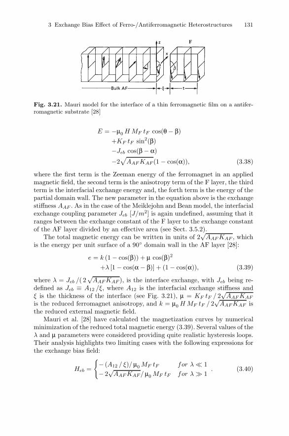
Fig. 3.21. Mauri model for the interface of a thin ferromagnetic film on a antifer-romagnetic substrate [28]
E = −μ0HMF tF cos(θ − β)+KF tF sin2(β)−Jeb cos(β − α)
−2√AAFKAF (1 − cos(α)), (3.38)
where the first term is the Zeeman energy of the ferromagnet in an appliedmagnetic field, the second term is the anisotropy term of the F layer, the thirdterm is the interfacial exchange energy and, the forth term is the energy of thepartial domain wall. The new parameter in the equation above is the exchangestiffness AAF . As in the case of the Meiklejohn and Bean model, the interfacialexchange coupling parameter Jeb [J/m2] is again undefined, assuming that itranges between the exchange constant of the F layer to the exchange constantof the AF layer divided by an effective area (see Sect. 3.5.2).
The total magnetic energy can be written in units of 2√AAFKAF , which
is the energy per unit surface of a 90◦ domain wall in the AF layer [28]:
e = k (1 − cos(β)) + μ cos(β)2
+λ [1 − cos(α − β)] + (1 − cos(α)), (3.39)
where λ = Jeb /( 2√AAFKAF ), is the interface exchange, with Jeb being re-
defined as Jeb ≡ A12 /ξ, where A12 is the interfacial exchange stiffness andξ is the thickness of the interface (see Fig. 3.21), μ = KF tF / 2
√AAFKAF
is the reduced ferromagnet anisotropy, and k = μ0HMF tF / 2√AAFKAF is
the reduced external magnetic field.Mauri et al. [28] have calculated the magnetization curves by numerical
minimization of the reduced total magnetic energy (3.39). Several values of theλ and μ parameters were considered providing quite realistic hysteresis loops.Their analysis highlights two limiting cases with the following expressions forthe exchange bias field:
Heb =
{− (A12 / ξ)/ μ0MF tF for λ� 1− 2
√AAFKAF/ μ0MF tF for λ 1
. (3.40)

132 F. Radu and H. Zabel
In the strong coupling limit λ � 1, the expression for the exchange biasfield is similar to the value given by the Meiklejohn and Bean model. Forthis situation, practically no important differences between the predictions ofthe two models exist. When the coupling is weak (λ 1), the Mauri modeldelivers a reduced exchange bias field which is practically independent of theinterfacial exchange energy. It depends on the domain wall energy and theparameters of the F layer. In either case the “1/tF ” dependence is preservedby the Mauri-model.
3.10.1 Analytical Expression of Exchange Bias Field
In order to compare the predictions of the Mauri model and the Meiklejohnand Bean approach, we reconsider the analysis of the free energy. Startingfrom the expression of the free energy (3.38), the minimization with respectto the α and β angles leads to the following system of equations:
⎧⎪⎨⎪⎩
H
− Jebμ0MF tF
sin(θ − β) + sin(β − α) = 0
2√
AAF KAF
Jebsin(α) − sin(β − α) = 0 .
(3.41)
Similar to the Meiklejohn and Bean model we define the parameters P ≡2√
AAF KAF
JebandH∞
eb ≡ − Jeb
μ0 MF tF. Also we set θ = 0, meaning that the applied
field is swept along the easy axis of the AF layer. Also, we do not take intoaccount the anisotropy of the ferromagnet (KF = 0), for two reasons. For onethe coercive fields of the exchange bias systems are usually much higher thenthe coercive field of the isolated F layer, and secondly it is easier to comparethe results of the Mauri model and the M&B model when the anisotropy ofthe F layer is disregarded. From inspection of the (3.41) and (3.23) one canclearly see that the first equations of the two systems are identical, while thesecond ones are different in two respects. The first difference is related to theterm P , which includes the domain wall energy instead of the AF anisotropyterm in the R ratio. The second difference is that instead of a sin(2 α) termin the second equation of (3.23), the Mauri model has a sin(α) term, whichinfluences strongly the phase diagram shown in Fig. 3.22.
The analytical expression for the exchange bias are obtained by solv-ing the system of (3.41). First step in solving the (3.41) is to extract theα angle (α = ± arccos(± P−cos(β)√
1+P 2−2 P cos(β))) from the second equation and to
introduce it in the first equation. Next we use the condition that at the coer-cive field β = −π/2 to obtain both coercive fields Hc1 = Hc2. Then, insertingthem into the general expressions of (3.16), the coercive field Hc is zero andthe exchange bias field becomes [11]:

3 Exchange Bias Effect of Ferro-/Antiferromagnetic Heterostructures 133
Fig. 3.22. Left: The phase diagram of the exchange bias field and the coercive fieldsgiven by the Mauri formalism. Right: Typical behavior of the antiferromagnetic angleα for the two different regions of the phase diagram. In both regions I and II a shiftof the hysteresis loop can exist. The coercive field is zero in both regimes
Heb = − Jeb
μ0MF tF
2√AAF KAF√
J2eb + 4AAF KAF
= − Jeb
μ0MF tF
P√1 + P 2
. (3.42)
This equation is plotted as a function of H/|HEB| and for different P valuesranging from P = 0 to P = 5. (compare Fig. 3.22 left panel). The behaviorof the EB field according to the (3.42) is monotonic with respect to the stiff-ness and anisotropy of the AF spins. At P 1 the exchange bias is equalto HP→∞
eb = − Jeb
μ0 MF tF, which is the well known expression given by M&B
model. When, however, the P -ratio approaches low values, the exchange biasdecreases, vanishing at P = 0, provided that the thickness of the AF layeris sufficiently thick to allow a 180◦ wall. With some analytical analysis ofthe (3.42) one can easily reach the limiting cases of weak coupling (P � 1)and strong coupling (P 1) discussed by Mauri et al. [28] (see (3.40)). InFig. 3.22 right column is shown the representative behavior of the α angle ofthe first interfacial AF monolayer as a function of the β orientation of the Fspins during the magnetization reversal and for two representative P values(see the discussion below).
In Fig. 3.23 the hysteresis loops (m|| = cos(β)) and the correspondingAF angle rotation during the magnetization reversal are plotted for severalP -ratios. They were obtained by solving numerically the system of (3.41). Forall the values of the P -ratio the magnetization curves are shifted to negativevalues of the applied magnetic field. We distinguish two different regions withrespect to the behavior of the α angle of the first AF monolayer. In the firstregion, for P ≥ 1 (region I), the AF monolayer in the proximity of the F layerbehaves similar to the Meiklejohn and Bean, namely the α angle deviates
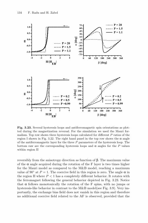
134 F. Radu and H. Zabel
Fig. 3.23. Several hysteresis loops and antiferromagnetic spin orientations as plot-ted during the magnetization reversal. For the simulation we used the Mauri for-malism. Top row shows three hysteresis loops calculated for different P ratios of theregion I shown in Fig. 3.22. The right hand panel in the top row shows the α angleof the antiferromagnetic layer for the three P parameters of the hysteresis loop. Thebottom raw are the corresponding hysteresis loops and α angles for the P valueswithin region II
reversibly from the anisotropy direction as function of β. The maximum valueof the α angle acquired during the rotation of the F layer is two times higherfor the Mauri model as compared to the M&B model, reaching a maximumvalue of 90◦ at P = 1. The coercive field in this region is zero. The angle α inthe region II where P < 1 has a completely different behavior. It rotates withthe ferromagnet following the general behavior depicted in Fig. 3.23. Noticethat α follows monotonically the rotation of the F spins, with no jumps orhysteresis-like behavior in contrast to the M&B model(see Fig. 3.9). Very im-portantly, the exchange bias field does not vanish in this region and thereforeno additional coercive field related to the AF is observed, provided that the
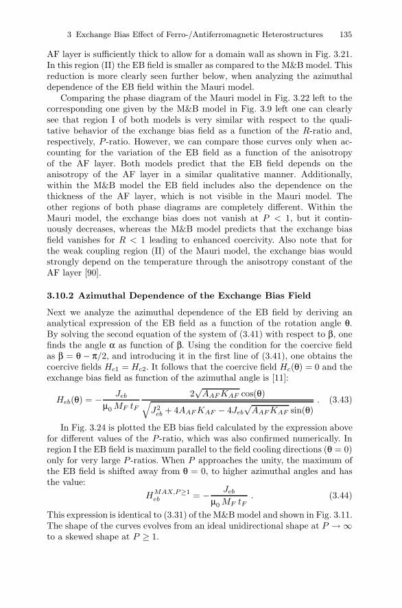
3 Exchange Bias Effect of Ferro-/Antiferromagnetic Heterostructures 135
AF layer is sufficiently thick to allow for a domain wall as shown in Fig. 3.21.In this region (II) the EB field is smaller as compared to the M&B model. Thisreduction is more clearly seen further below, when analyzing the azimuthaldependence of the EB field within the Mauri model.
Comparing the phase diagram of the Mauri model in Fig. 3.22 left to thecorresponding one given by the M&B model in Fig. 3.9 left one can clearlysee that region I of both models is very similar with respect to the quali-tative behavior of the exchange bias field as a function of the R-ratio and,respectively, P -ratio. However, we can compare those curves only when ac-counting for the variation of the EB field as a function of the anisotropyof the AF layer. Both models predict that the EB field depends on theanisotropy of the AF layer in a similar qualitative manner. Additionally,within the M&B model the EB field includes also the dependence on thethickness of the AF layer, which is not visible in the Mauri model. Theother regions of both phase diagrams are completely different. Within theMauri model, the exchange bias does not vanish at P < 1, but it contin-uously decreases, whereas the M&B model predicts that the exchange biasfield vanishes for R < 1 leading to enhanced coercivity. Also note that forthe weak coupling region (II) of the Mauri model, the exchange bias wouldstrongly depend on the temperature through the anisotropy constant of theAF layer [90].
3.10.2 Azimuthal Dependence of the Exchange Bias Field
Next we analyze the azimuthal dependence of the EB field by deriving ananalytical expression of the EB field as a function of the rotation angle θ.By solving the second equation of the system of (3.41) with respect to β, onefinds the angle α as function of β. Using the condition for the coercive fieldas β = θ − π/2, and introducing it in the first line of (3.41), one obtains thecoercive fields Hc1 = Hc2. It follows that the coercive field Hc(θ) = 0 and theexchange bias field as function of the azimuthal angle is [11]:
Heb(θ) = − Jeb
μ0MF tF
2√AAFKAF cos(θ)√
J2eb + 4AAFKAF − 4Jeb
√AAFKAF sin(θ)
. (3.43)
In Fig. 3.24 is plotted the EB bias field calculated by the expression abovefor different values of the P -ratio, which was also confirmed numerically. Inregion I the EB field is maximum parallel to the field cooling directions (θ = 0)only for very large P -ratios. When P approaches the unity, the maximum ofthe EB field is shifted away from θ = 0, to higher azimuthal angles and hasthe value:
HMAX,P≥1eb = − Jeb
μ0MF tF. (3.44)
This expression is identical to (3.31) of the M&B model and shown in Fig. 3.11.The shape of the curves evolves from an ideal unidirectional shape at P → ∞to a skewed shape at P ≥ 1.

136 F. Radu and H. Zabel
Fig. 3.24. Azimuthal dependence of exchange bias as a function of the θ angle. Thedotted line for P = 20 can be considered an “ideal” case. The curves are plottedaccording to (3.43)
In region II (Fig. 3.24 left) a drastic change as compared to region I is seenfor the maximum of the exchange bias field as a function of azimuthal angle.Its value decreases monotonically towards zero according to the following ex-pression:
HMAX,P<1eb = −P = −2
√AAF KAF
Jeb. (3.45)
In this region the shape of the curves is also skewed for P -ratios close to unity,but as P decreases towards zero, the curves acquire a more ideal unidirectionalbehavior. Similar to region I, the maximum EB value is shifted away from thefield cooling direction to higher azimuthal angles, whereas in M&B it is shiftedto lower azimuthal angles.
In the limit of strong R and P -ratios (R,P 1) the Mauri and M&Bmodels give similar results. The differences appear for the R and P -ratioswhich are close to but higher than one. This region (0 < R,P ≤ 5) can beexperimentally explored in order to decide in favor of one or the other model.In order to distinguish between the Mauri and the M&B model, the azimuthaldependence of the exchange bias offers an excellent tool because it is visiblydifferent for the two models (shift to higher or lower azimuthal angles).
The presence of the planar domain wall as described by Mauri et al. ap-pears to have been confirmed experimentally for first time in [16]. Althoughthe Co/NiO system studied by Scholl et al. did not exhibit a hysteresis loopshift, the rotation angle α of the AF planar wall was deduced as function offield. Also, a recent publication by Gornakov et al. [91] show experimentalresults that are similar to the characteristic curves for the α angle shown inFig. 3.22. An AF critical thickness which is often observed experimentally donot appear explicitly in the Mauri model. To account for the AF thickness
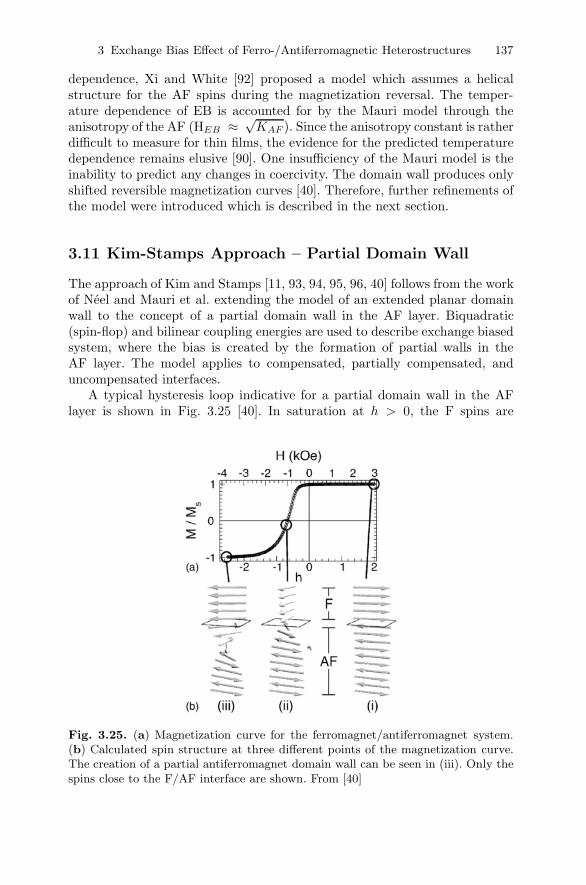
3 Exchange Bias Effect of Ferro-/Antiferromagnetic Heterostructures 137
dependence, Xi and White [92] proposed a model which assumes a helicalstructure for the AF spins during the magnetization reversal. The temper-ature dependence of EB is accounted for by the Mauri model through theanisotropy of the AF (HEB ≈ √
KAF ). Since the anisotropy constant is ratherdifficult to measure for thin films, the evidence for the predicted temperaturedependence remains elusive [90]. One insufficiency of the Mauri model is theinability to predict any changes in coercivity. The domain wall produces onlyshifted reversible magnetization curves [40]. Therefore, further refinements ofthe model were introduced which is described in the next section.
3.11 Kim-Stamps Approach – Partial Domain Wall
The approach of Kim and Stamps [11, 93, 94, 95, 96, 40] follows from the workof Neel and Mauri et al. extending the model of an extended planar domainwall to the concept of a partial domain wall in the AF layer. Biquadratic(spin-flop) and bilinear coupling energies are used to describe exchange biasedsystem, where the bias is created by the formation of partial walls in theAF layer. The model applies to compensated, partially compensated, anduncompensated interfaces.
A typical hysteresis loop indicative for a partial domain wall in the AFlayer is shown in Fig. 3.25 [40]. In saturation at h > 0, the F spins are
Fig. 3.25. (a) Magnetization curve for the ferromagnet/antiferromagnet system.(b) Calculated spin structure at three different points of the magnetization curve.The creation of a partial antiferromagnet domain wall can be seen in (iii). Only thespins close to the F/AF interface are shown. From [40]
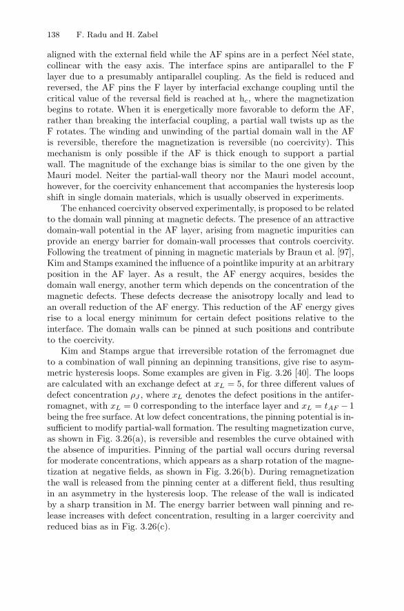
138 F. Radu and H. Zabel
aligned with the external field while the AF spins are in a perfect Neel state,collinear with the easy axis. The interface spins are antiparallel to the Flayer due to a presumably antiparallel coupling. As the field is reduced andreversed, the AF pins the F layer by interfacial exchange coupling until thecritical value of the reversal field is reached at hc, where the magnetizationbegins to rotate. When it is energetically more favorable to deform the AF,rather than breaking the interfacial coupling, a partial wall twists up as theF rotates. The winding and unwinding of the partial domain wall in the AFis reversible, therefore the magnetization is reversible (no coercivity). Thismechanism is only possible if the AF is thick enough to support a partialwall. The magnitude of the exchange bias is similar to the one given by theMauri model. Neiter the partial-wall theory nor the Mauri model account,however, for the coercivity enhancement that accompanies the hysteresis loopshift in single domain materials, which is usually observed in experiments.
The enhanced coercivity observed experimentally, is proposed to be relatedto the domain wall pinning at magnetic defects. The presence of an attractivedomain-wall potential in the AF layer, arising from magnetic impurities canprovide an energy barrier for domain-wall processes that controls coercivity.Following the treatment of pinning in magnetic materials by Braun et al. [97],Kim and Stamps examined the influence of a pointlike impurity at an arbitraryposition in the AF layer. As a result, the AF energy acquires, besides thedomain wall energy, another term which depends on the concentration of themagnetic defects. These defects decrease the anisotropy locally and lead toan overall reduction of the AF energy. This reduction of the AF energy givesrise to a local energy minimum for certain defect positions relative to theinterface. The domain walls can be pinned at such positions and contributeto the coercivity.
Kim and Stamps argue that irreversible rotation of the ferromagnet dueto a combination of wall pinning an depinning transitions, give rise to asym-metric hysteresis loops. Some examples are given in Fig. 3.26 [40]. The loopsare calculated with an exchange defect at xL = 5, for three different values ofdefect concentration ρJ , where xL denotes the defect positions in the antifer-romagnet, with xL = 0 corresponding to the interface layer and xL = tAF − 1being the free surface. At low defect concentrations, the pinning potential is in-sufficient to modify partial-wall formation. The resulting magnetization curve,as shown in Fig. 3.26(a), is reversible and resembles the curve obtained withthe absence of impurities. Pinning of the partial wall occurs during reversalfor moderate concentrations, which appears as a sharp rotation of the magne-tization at negative fields, as shown in Fig. 3.26(b). During remagnetizationthe wall is released from the pinning center at a different field, thus resultingin an asymmetry in the hysteresis loop. The release of the wall is indicatedby a sharp transition in M. The energy barrier between wall pinning and re-lease increases with defect concentration, resulting in a larger coercivity andreduced bias as in Fig. 3.26(c).

3 Exchange Bias Effect of Ferro-/Antiferromagnetic Heterostructures 139
Fig. 3.26. Defect-induced asymmetry in hysteresis loops. The hysteresis loopsare shown for a reduced exchange defect at xL = 5 for three concentrations: (a)ρJ = 0.15,. (b) ρJ = 0.45, and (c) ρJ = 0.75. The components of magnetizationparallel (M||) (dots) and perpendicular (M⊥) (open circles) to the field directionare shown. The arrows indicate the directions for reversal and remagnetization. Thespin configuration near the interface is shown for selected field values below thehysteresis curves [40]
Within this model, the asymmetry of the hysteresis loops is interpretedin terms of domain-wall pinning processes in the antiferromagnet. This ex-planation appears to be consistent with some recent work by Nikitenko et al.and Gornakov et al. on a NiFe/FeMn system [98, 91] who concluded that thepresence of an antiferromagnetic wall at the interface is necessary to explaintheir hysteresis measurements.
3.12 The Spin Glass Model of Exchange Bias
To overcame the theoretical difficulties in explaining interconnection betweenthe exchange bias and coercivity, in [41, 63] is considered a magnetic stateof the interface between F and AF layer which is magnetically disorderedbehaving similar to a spin glass system. The assumptions of the spin glass(SG) model are:
• the F/AF interface is a frustrated spin system (spin-glass like);• frozen-in uncompensated AF spins are responsible for the EB shift;• low anisotropy interfacial AF spins contribute to the coercivity.

140 F. Radu and H. Zabel
AF INT FKAF
Frozen-in AF Spins
Rotatable AF Spins
KAF
Training Effect
f Jeb
Jeb
Fig. 3.27. Schematic view of the SG Model. At the interface between the AF andthe F layer the AF anisotropy is assumed to be reduced leading to two types ofAF states after field cooling the system: frozen-in AF spins and rotatable AF spins.After reversing the magnetic field, the rotatable spins follows the F layer rotationmediating coercivity. The frozen-in spins remain largely unchanged in moderatefields. But some of them will also deviate from the original cooling state. This couldlead to training effects and also to an open loop in the right side of the hysteresisloop. At larger applied fields in the negative direction, the frustrated frozen-in spinscan further reverse leading to a slowly decreasing slope of the hysteresis loop. A morecomplex antiferromagnetic state consisting of frozen magnetic domains or/and AFgrains can be also reduced to the basic concepts depicted here
Within this model, the AF layer is assumed to contain, in a first approxi-mation, two types of AF states (see Fig. 3.27). One part has a large anisotropywith the orientation ruled by the AF spins and another part with a weakeranisotropy which allows some spins to rotate together with the F spins. Thisinterfacial part of the AF is a frustrated region (spin-glass-like) and gives riseto an increased coercivity. The presence of a low anisotropy AF region canbe rationalized as follows: the interface between the F and AF layer is neverperfect, therefore one may assume chemical intermixing, deviations from sto-ichiometry, structural inhomogeneities, low coordination, etc, at the interfaceto take place. This leads to the formation of a transition region from the pureAF state to a pure F state. On average, the anisotropy of such an interfacialregion is reduced. In addition, structural and magnetic roughness can providea weak AF interface region. Therefore, we assume that a fraction of the frus-trated interfacial spins do rotate almost in phase with the F spins and thatthey mediate enhanced coercivity. We describe them by an effective uniaxialanisotropy Keff
SG , because they are coupled to the presumably uniaxial AFlayer.

3 Exchange Bias Effect of Ferro-/Antiferromagnetic Heterostructures 141
Generally, one can visualize a spin glass system [37] as a collection ofspins which remains in a frozen disordered state even at low-temperatures.In order to achieve such a state, two ingredients are necessary: a) there mustbe a competition among the different interactions between the moments, inthe sense that no single configuration of the spins is uniquely favored by allinteractions (this is commonly called ‘frustration’); b) these interactions mustbe at least partially random. This partial random state will be introduced inthe M&B model as an effective uniaxial anisotropy.
Adding this effective anisotropy to the M&B model, the free energyreads [41]:
E = −μ0HMF tF cos(θ − β)+ KF tF sin2(β)+ KAF (tAF ) tAF sin2(α)
+ KeffSG sin2(β − γ) − Jeff
eb cos(β − α) , (3.46)
where, KeffSG is an effective uniaxial SG anisotropy related to the frustrated
AF spins with reduced anisotropy at the interface, Jeffeb is the reduced interfa-
cial exchange energy, and γ is the average angle of the effective SG anisotropy.KAF (tAF ) is the anisotropy constant of AF layer. To avoid further compli-cations for the numerical simulations, we neglect the thickness dependenceof the KAF anisotropy (KAF (tAF ) ≡ KAF ). We mention though, that thisdependence could become important for low AF thicknesses due to finite sizeeffects and due to structurally non-ideal very thin layers. From now on, theMCA anisotropy of the ferromagnetic layer (KF = 0) will also be neglectedas to highlight more clearly the influences of AF layer and the SG interfaceonto the general properties of the EB systems. Note that the Zeeman ener-gies of the ferromagnetic-like AF interfacial spins are neglected in the modelsince they are usually much smaller as compared to Zeeman energy of the Flayer. Nevertheless, they can be seen as a vertical shift of the hysteresis loop(frozen-in AF spins in Fig. 3.27) and as an additional contribution to the totalmagnetization (rotatable AF spins in Fig. 3.27).
The model is depicted schematically in Fig. 3.27. At the interface tworather distinct AF phases are assumed to occur in an EB system: the rotatableAF spins, depicted as open circles and frozen-in AF spins shown as filledcircles. After field cooling, a presumably collinear arrangement is depicted inthe right hand panel. After reversing the magnetic field, the rotatable AFspins follow the F layer rotation mediating coercivity. The frozen-in spinsremain largely unchanged in moderate fields. But some of them could alsodeviate from the original cooling state. Irreversible changes of the frustratedAF spins lead to training effects and also to an open loop in the right side ofthe hysteresis loop. At larger negative applied fields, the frustrated frozen-inspins could further reverse leading to a slowly decreasing slope of the hysteresisloop. A more complex antiferromagnetic state consisting of frozen magneticdomain state or/and AF grains can be also reduced to the basic two spin
142 F. Radu and H. Zabel
components depicted in Fig. 3.27. Basically, additional frozen-in spins canoccur in the AF layer extending to the interface and, therefore, leading toeven more interfacial disorder.
Next, we evaluate numerically the resulting hysteresis loops and azimuthaldependence of the exchange bias within the SG model. When the Keff
SG pa-rameter is zero, the system behaves ideally as described by the M&B modeldiscussed in Sect. 3.6: the coercive field is zero and the exchange bias is finite.In the other case, when the interface is disordered we relate the SG effectiveanisotropy to the available interfacial coupling energy as follows:
Keff = (1 − f)Jeb
Jeffeb = f Jeb , (3.47)
where Jeb is the total available exchange energy and f is a conversion factordescribing the fractional order at the interface, with f = 1 for a perfectinterface and f = 0 for perfect disorder. Some basic models to calculate theavailable exchange energy were discussed in the previous sections. For evenmore complicated situations when the AF consists of AF grains and/or AFdomains the exchange energy can be further estimated as described in [46].
With these notations we write the system of equations resulting from theminimization of the (3.46) with respect to the angles α and β:
h sin(θ − β) +(1 − f)f
sin(2 (β − γ)) + sin(β − α) = 0
R sin(2 α) − sin(β − α) = 0 , (3.48)
where,
h =H
− Jeffeb
μ0 MF tF
=H
− f Jeb
μ0 MF tF
,
is the reduced applied field and
R ≡ KAF tAF
Jeffeb
=KAF tAF
f Jeb,
is the R-ratio defining the strength of the AF layer.The system of equations above can easily be solved numerically, but it does
not provide simple analytical expressions for the exchange bias. Numericalevaluation provides the α and β angles as a function of the applied magneticfield H . The reduced longitudinal component of magnetization along the fieldaxis follows from m|| = cos(β − θ) and the transverse component from m⊥ =sin(β − θ).
With the assumptions made above the absolute value of the exchange biasfield is directly proportional to f . The parameter f can be called conversionfactor, as it describes the conversion of interfacial energy into coercivity. Forexample, in the M&B phase diagram in the region II and III corresponding

3 Exchange Bias Effect of Ferro-/Antiferromagnetic Heterostructures 143
to reduced R-ratios, the exchange bias field is zero and the coercive field isenhanced as a result of such a conversion of the interfacial energy into coercivefield.
The idea of reduced interfacial anisotropy at the interface can be tracedback to the the Neel weak ferromagnetism at the surface of AF particles.Neel [77] discussed the training effect as a tilting of the superficial magnetiza-tion of the AF domains. Later, Schlenker et al. [99] suggested that successivereversals of the F magnetization could lead to changes of the interface un-compensated AF magnetization and therefore provide means of going fromone ground state to another. Such multiple interface configurations are sim-ilar to a spin glass system. The spin-glass interface is further discussed byother authors [100, 101, 102, 103, 104, 105, 106, 107, 50]. Exchange bias hasbeen observed recently for spin-glass/F system [108]. The interfacial mag-netic disorder was observed through hysteresis loop widening below a criticaltemperature point [109]. Non-collinearity have been observed at the AF/F inremanence [110] and even in saturation [111, 60, 112]. The frozen spins atthe interface were also observed by MFM [113]. Using element specific tech-niques such as soft x-ray resonant magnetic dichroism (XMCD) and of x-rayresonant magnetic scattering (XRMS), both frozen and rotatable AF spinscan be studied [13, 114, 115, 116, 15, 117, 17, 19, 20]. The frozen-in spinsappear as a shift of the hysteresis loop along magnetization axis, whereas theAF rotatable spins exhibit a hysteresis loop. Moreover, an evidence for SGbehavior is recently reported in thin films [118] and AF nanoparticles [119].Therefore, we believe that there is enough experimental evidence to considerthe interface between the AF/F layer as a disordered state behaving similarto a spin-glass system.
3.12.1 Hysteresis Loops as a Function of the Conversion Factor f
If Fig. 3.28 we show simulations of several hysteresis loops as a function of theconversion factor f . We assume a strong antiferromagnet in contact with aferromagnet, where the interface has different degrees of disorder depicted inthe right column of Fig. 3.28. For the R ratio we assume the following value:R = KAF tAF
fJeb= 62.5/f which corresponds to a 100 A thick CoO antiferromag-
netic layer. The field cooling direction and the measuring field direction areparallel to the anisotropy axis of the AF. The anisotropy of the ferromagnetis neglected in the simulations below. For the interface we have chosen a SGanisotropy oriented 10 degrees away from the unidirectional anisotropy orien-tation (γ = 10◦). On the abscissa the reduced exchange bias field h = H/|H∞
eb |(H∞
eb ≡ − Jeffeb
μ0 MF tF) is plotted, which then can easily be compared to the M&B
model. With this assumption the system of (3.48) was solved numerically.The left column shows the longitudinal component of the magnetization
(parallel to the measuring field direction) (m|| = cos(β)) whereas the middlecolumn shows the transverse component of the magnetization (m⊥ = sin(β)).

144 F. Radu and H. Zabel
Fig. 3.28. Longitudinal (m|| = cos(β)) and transverse (m⊥ = sin(β)) componentsof the magnetization for a F(KF = 0)/AF(R = 62.5/f, γ = 10◦,θ = 0) bilayer fordifferent values of the conversion factor f (f = 80%, 60%, 20%). We observe, thatwhen the AF layer is strong (R � 1), the hysteresis loops are symmetric whenmeasured along the field cooling direction. The hysteresis loops are simulated bysolving numerically the (3.48). In the right column is schematically depicted thelayer structure, here the emphasis is given to the disorder state at the interface.The AF layer is depicted as consisting of magnetic domains which also contributeto interface disorder
We observe that with decreasing conversion factor f the exchange biasvanishes linearly. The reduction of the EB field is accompanied by an increasedcoercivity. The shape of the hysteresis loop is close to the results found inliterature. For instance the hysteresis loop with f = 60% is similar to thedata shown in [120, 61]. The hysteresis loop with f = 20% is similar tothe data shown in [14, 109]. The longitudinal and transverse componentsof the magnetization show that the reversal mechanism is symmetric. Thesymmetry is directly related to the strength of the AF layer, when no trainingeffect is involved. For the examples depicted in Fig. 3.28, the R-ratio is muchlarger than 1 (R 1), and therefore the hysteresis loops are symmetric whenmeasured along the field cooling direction and along the anisotropy axis of theAF layer. The asymmetry of the hysteresis loops is discussed further below.

3 Exchange Bias Effect of Ferro-/Antiferromagnetic Heterostructures 145
3.12.2 Phase Diagram of Exchange Bias and Coercive FieldWithin the Spin Glass Model
In this section we discuss the phase diagram for the exchange field and coer-cive field as a function of the R-value within the SG-model. The additionalparameter is the conversion factor f . In Fig. 3.29 phase diagrams are shownfor reduced exchange bias and reduced coercive fields as a function of theR-ratio for four different values of the conversion factor f . This allows usto compare directly the behavior of exchange bias fields as predicted in theSG model and the M&B model. The reduced exchange bias field plotted inFig. 3.29 (left panel) is defined:
heb =Heb
Jeffeb
μ0 MF tF
=Heb
f H∞eb
,
where the Heb is the absolute value of the exchange bias within the SG modeland the denominator term Jeb
μ0 MF tfis the exchange bias field within the ideal
M&B model.The reduced coercive field shown in Fig. 3.29 is defined:
hc =HSG
c
Jeffeb
μ0 MF tF
,
where HSGc is the absolute value of the coercive field within the SG model. It
has no relation to the coercive field of the M&B model because the coercive
Fig. 3.29. The dependence of the reduced exchange bias field heb and the reducedcoercive field hc as a function of the R-ratio for four different values of the conversionfactor f

146 F. Radu and H. Zabel
field within the M&B model is considered to be a constant when the exchangebias is finite.
3.12.3 Azimuthal Dependence of Exchange Bias and CoerciveField Within the Spin Glass Model
In this section, the azimuthal dependence of exchange bias and coercivefields within the SG model are discussed and compared with experimentalresults of polycrystalline Ir17Mn83(15nm)/Co70Fe30(30nm) exchange biassystem [41].
In Fig. 3.30 calculated magnetization components are plotted togetherwith the experimental data points, and in Fig. 3.31b the azimuthal dependenceof the coercive field and exchange bias field are plotted and compared tothe experimental data in Fig. 3.31a. The hysteresis loops were calculated bynumerical minimizing the expressions in (3.48). The parameters used in thesimulation f = 80%, R = 5.9/f, γ = 20◦ do best reproduce the experimentaldata. Furthermore, it is assumed that the AF layer has a uniaxial anisotropy.The MCA anisotropy of the F layer is neglected (KF = 0). Therefore, thecoercivity which appears in the simulations is not related to the F properties,but to the interfacial properties of the F/AF bilayer.
First we discuss the hysteresis loops shown in Fig. 3.30. The system iscooled down in a field oriented parallel to the AF anisotropy direction. Thehysteresis loops (solid lines) are simulated for different azimuthal angles θof the applied field in respect to the field cooling orientation. In Fig. 3.30representative hysteresis curves are shown for the longitudinal (m||) andtransverse (m⊥) magnetization. At θ = 0◦, the magnetization curves are sym-metric and shifted to negative fields. At θ = 180◦, the magnetization curvesare also symmetric but shifted to positive fields. At θ = 3◦, however, thelongitudinal hysteresis loop becomes asymmetric. The first reversal at Hc1 issharp and the reversal at Hc2 is more rounded. This asymmetry is also seen inthe transverse component of the magnetization. The F spins rotate asymmet-rically: the values of the β angle depend on the external field scan direction,being different for swaps from negative to positive saturation as compared withswaps from positive to negative saturation. As the azimuthal angle increases,the coercive field becomes zero. For instance, at θ = 20◦, 90◦ and 160◦ thereis almost no coercivity. Also, the transverse component of the magnetizationshows that the F spins do not follow a 360◦ path, but they rotate within the180◦ angular space.
In Fig. 3.31 the coercive field and the exchange bias field are extractedfrom the experimental and simulated hysteresis loops using (3.16). We dis-tinguish the following characteristics of the Hc and Heb: the unidirectionalbehavior (≈ cos(θ)) of the Heb as a function of the azimuthal angle is (seeFig. 3.11) clearly visible; additionally, the behavior of the Heb as a function ofthe azimuthal angle shows sharp modulations close to the orientation of theAF uniaxial anisotropy; the coercive field Hc has a peak-like behavior close
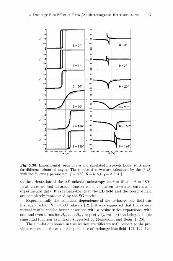
3 Exchange Bias Effect of Ferro-/Antiferromagnetic Heterostructures 147
Fig. 3.30. Experimental (open circles)and simulated hysteresis loops (black lines)for different azimuthal angles. The simulated curves are calculated by the (3.48)with the following parameters: f = 80%, R = 5.9/f, γ = 20◦ [41]
to the orientation of the AF uniaxial anisotropy, at θ = 0◦ and θ = 180◦.In all cases we find an astounding agreement between calculated curves andexperimental data. It is remarkable, that the EB field and the coercive fieldare completely reproduced by the SG model
Experimentally the azimuthal dependence of the exchange bias field wasfirst explored for NiFe/CoO bilayers [121]. It was suggested that the experi-mental results can be better described with a cosine series expansions, withodd and even terms for Heb and Hc , respectively, rather than being a simplesinusoidal function as initially suggested by Meiklejohn and Bean [1, 26].
The simulations shown in this section are different with respect to the pre-vious reports on the angular dependence of exchange bias field [121, 122, 123,

148 F. Radu and H. Zabel
Fig. 3.31. a) The experimental coercive field (open symbols ) and exchange bias(filled symbols) field as a function of the azimuthal angle θ.d) Simulated coercive field(dotted line) and exchange bias field (continuous line) as a function of the azimuthalangle [41]
124, 125]. One difference is that the MCA anisotropy of the F is supposed tobe negligible when compared with the coercive fields obtained experimentally,and the sharp features of the Heb are reproduced numerically rather thenbeing described by cosine series expansions. Recently, Camarero et al. [76]reports on very similar azimuthal dependent hysteresis loops as shown here.There, an elegant way based on asteroid curve is used to describe the intrinsicasymmetry of the hysteresis loops close to the 0◦ and 180◦ azimuthal angle. Aunidirectional anisotropy displaces the asteroid critical curve from the origin.Therefore, if the applied field is not parallel to the unidirectional anisotropy,the field sweep line does not pass through the symmetry center of the as-teroid critical curve leading to inequivalent switching fields and consequentlyasymmetric reversals [76].
3.12.4 Dependence of Exchange Bias Field on the Thicknessof the Antiferromagnetic Layer
After a short inspection of the phase diagram of EB and coercive field(Fig. 3.29) we notice that there is a critical value for the R-ratio at which

3 Exchange Bias Effect of Ferro-/Antiferromagnetic Heterostructures 149
the exchange bias vanishes and the coercive field is enhanced. This criticalvalue R=1 depends on four parameters: the anisotropy of the antiferromagnet,the interfacial exchange coupling parameter, the thickness of the ferromagnet,and the conversion factor. The conversion factor further depends on the AFdomain and/or AF grain size, if any.
In Fig. 3.32 the normalized exchange bias field is plotted as a function ofthe AF thickness and for several conversion factors. The anisotropy of the AFlayer (KAF ) and the Jeb parameter are assumed to be constant.We notice twomain characteristics of the EB field dependence on the AF thickness: whenf has high values close to unity, the EB field decreases with decreasing AFthickness. However, when f is reduced, a completely different behavior of theEB is observed. The EB field increases as the thickness of the AF decreases,developing a peak-like feature. This peak-like behavior for the EB field atcritical AF thickness is a result of enhanced coercivity which is accounted forby the f-factor. Also, an essential parameter is the α angle, which describesthe rotation of the AF spins during the magnetization reversal. The criticalthickness is preserved by the SG model, but it differs in magnitude as com-pared to the M&B model. Since some interfacial coupling energy is dissipatedas coercivity, the critical thickness within SG model is lower as compared tothe corresponding one given by the M&B model. The critical AF thicknesswithin the SG model follows from the condition R = 1:
Fig. 3.32. The normalized exchange bias heb/f = Heb/H∞eb as a function of the
tAF KAF /Jeb for different values of the conversion factor f . The anisotropy constantKAF and Jeb are assumed to be constant as the AF thickness is being varied foreach f . An asymmetric peak like behavior of the exchange bias field develops forhigh values of the conversion factor

150 F. Radu and H. Zabel
tSGAF,cr =
f Jeb
KAF= f tMB
AF,cr , (3.49)
where tSGAF,cr and tMB
AF,cr are the AF critical thickness predicted by the SG andM&B models, respectively.
Experimentally the R-ratio can be tuned by changing the thickness of theAF and keeping the other three parameters constant. As a result one observesa critical thickness of the AF layer for which the EB disappears [126, 72, 127,73, 128, 81, 89]. This AF critical thickness can be qualitatively understoodwithin the M & B model. When the hardness of the AF layer is reduced,the AF spins will rotate under the torque created by the F layer trough theinterfacial coupling constant. The shape of the EB as function of AF thick-ness, however, can be different from one system to another depending on theother three parameters. The most prominent experimental feature of the EBdependence on the AF thickness is the development of a peak close to the crit-ical thickness. Several proposals were made to describe the peculiar shapes ofEB field dependence on AF thickness. According to the Malozemoff model, achange in the AF domain size as function of AF thickness results in a changeof exchange bias magnitude. Other influences on the AF dependence of theEB and coercive field are of structural origin [126, 73, 18]. It has been shownby Kuch et al. [18] that at the microscopic level, the coupling between theAF an F layers depends on the atomic layer filling and on the morphology ofthe interface. The AF-F coupling was observed to vary by a factor of two be-tween filled and half-filled interface. Moreover, islands and vacancy islands atthe interface lead to a quite distinct coupling behavior. Therefore, structuralconfigurations are indeed contributing to the EB-dependence as function ofAF thickness.
The peak-like behavior of the EB field as function of the AF thickness isstrongly dependent on temperature. An almost complete set of curves, showinga monotonous development of the AF peak from high to low temperatures wasmeasured by Ali et al. [89]. The data is reproduced in Fig. 3.33 together withthe simulations based on DS model. Although the DS model does describewell some experimental observed features, some discrepancies still exists. Forinstance the development of the AF peak as well as the critical AF thicknessas function of temperature are more pronounced in the experimental data ascompared to the DS simulations.
The SG model, through the conversion factor f, appears to be ableto describe the evolution of the critical AF thickness(see Fig. 3.32 andFig. 3.33 (left)). Also the shape of the EB dependence on the AF thick-ness, from an almost ideal M&B type at T=290 K to a pronounced peakedcurve at T=2 K is qualitatively reproduced. Although not considered so far,the conversion factor seems to be temperature dependent. This can be un-derstood if we consider the basic assumption of the SG model, namely thefrustration at the interface. Temperature fluctuations acting on metastablespin states cause a variation of the SG anisotropy as function of tempera-

3 Exchange Bias Effect of Ferro-/Antiferromagnetic Heterostructures 151
Fig. 3.33. Left: IrMn thickness dependence of the exchange bias field Heb for anumber of temperatures. Lines between the points are a guide to the eye. Right:Prediction of the DS model for the AF thickness dependence of the exchange biasfield from the stability analysis of the interface AF domains at different tempera-tures. (from [89])
ture. We will not further speculate on the exact temperature dependence ofthe f-factor, but we mention that a numerical analysis for the EB dependen-cies shown in Fig. 3.33 would allow to untangle all the parameters in theR-ratio. The conversion factor is given by the shape of the EB curves, fJeb
can be extracted from the temperature dependence of the EB field at highAF thicknesses, and finally, the anisotropy constant will be deduced from thecritical AF thickness. Note also, that the SG model has the potential to evendescribe the different temperature dependent shapes of the EB field, namelylinear dependence versus more rounded shape: for an AF thickness close tothe critical region, the temperature dependence of the EB bias will be clearlysteeper (linear-like) as compared to the corresponding one at higher AF thick-nesses(more rounded).
3.12.5 The Blocking Temperature for Exchange Bias
Experimentally it is found that the temperature where the exchange bias effectfirst occurs is usually lower than the Neel temperature of the AF layer (TN ) [8].This lower temperature is called blocking temperature (TB). For thick AFlayers TB ≤ TN , whereas for thin AF layers TB � TN [8]. Furthermore,the coercive field increases starting just below TN (with some exceptions) incontrast to the EB field, which appears only below TB.
These three experimentally observed characteristic features can qualita-tively be explained within the M&B and SG models. In order to have a non-vanishing EB field in the region with R ≥ 1, the following condition has to bebe fulfilled:
KAF >fJeb
tAF= KAF,crit , (3.50)
152 F. Radu and H. Zabel
where KAF,crit is the critical AF anisotropy for the onset of the EB field. Fora fixed AF layer thickness, the condition above sets a critical value for the AFanisotropy for which the EB can exist. Considering that the AF anisotropy in-creases steadily below TN , for large AF layer thicknesses the condition of (3.50)is fulfilled just below TN , whereas for thinner AF layers this condition is ful-filled at a correspondingly lower temperature TB. It is clear from the phasediagrams in Fig. 3.29 and in Fig. 3.32 that there is a region of anisotropy0 < KAF < Kcrit
AF where the EB field is zero and the coercive field is enhanced.It follows that the enhancement of the coercive field should be observed abovethe blocking temperature and below the Neel temperature of the AF. Thissituation is indeed observed experimentally. For the case of CoO(25 A)/Colayers the coercive field increases starting from the TCoO
N = 291 K, whereasthe exchange bias field first appears below TB = 180 K [14].
Further possible causes for a reduced blocking temperature and for the be-havior of the EB and coercive fields as a function of temperature are discussedelsewhere: finite size effects [129], stoichiometry [130] or multiple phases [131],AF grains [132] and diluted AF [38].
3.13 Training Effect
The training effect refers to the dramatic change of the hysteresis loop whensweeping consecutively the applied magnetic field of a system which is in abiased state. The coercive fields and the resulting exchange bias field ver-sus n, where n is the nth measured hysteresis loop, displays a monotonicdependence [133, 134, 134, 99]. The absolute value of Hc1 and of the EB fielddecreases from an initial value at n = 1 to an equilibrium value at n = ∞.The absolute value of the coercive field Hc2, however, displays an oppositebehavior, i.e. it increases with n. These features of the training effect is re-ferred to as Type I by Zhang et al. [135]. The other case when both |Hc1|and |Hc2| decrease is called Type. II. In this section we deal only with theso-called Type I training effect. Several mechanisms were suggested as a pos-sible cause of the effect. While it is widely accepted that the training effect isrelated to the unstable state of the AF layer and/or F/AF interface preparedby field cooling procedure, it is not yet well established what mechanisms aredominantly contributing to the training effect.
Neel [77] discussed the training effect as a tilting of the superficial magne-tization of the AF domains. This would lead to a Type I training effect. Neelalso discussed that a creeping effect could lead to a Type II training effect.
Micromagnetic simulations within the DS model [32, 35] show that thehysteresis curve is not closed after a complete loop. The lost magnetizationis directly related to a partial loss of the superficial magnetization of the AFdomains, which further leads to a decreased exchange bias.

3 Exchange Bias Effect of Ferro-/Antiferromagnetic Heterostructures 153
Zhang et al. [136] suggested that the training effect can be explained by in-corporating into the Fulcomer and Charap’s model [137] positive and negativeexchange coupling between the grains constituting the AF layers.
In [138], the authors found direct evidence for the proportionality betweenthe exchange bias and the total saturation moment of the heterostructure.The findings were related to the prediction of the phenomenological M&Bapproach, where a linear dependence of the exchange bias on the AF interfacemagnetization is expected.
Binek [139] suggested that the phenomenological origin of the trainingeffect is a deviation of the AF interface magnetization from its equilibriumvalue. Analytical calculations in the framework of non-equilibrium thermody-namics leads to a recursive relation accounting for the dependence of the Heb
field on n.Hoffmann [140] argues that only biaxial AF symmetry can lead to training
effects, reproducing important features of the experimental data, while sim-ulation with uniaxial AF symmetry show no difference between the first andsecond hysteresis loops.
Experiments performed by PNR, AMR and Kerr Microscopy [111, 47,14, 141, 59, 112, 142, 143] also support the irreversible changes taking placeat the F/AF interface and in the AF layer. It has been observed that duringthe very first reversal at Hc1, interfacial magnetic domains are formed andthey do not disappear even in positive or negative “saturation”. The interfa-cial domains serve as seeds for the subsequent magnetization reversals. Theseferromagnetic domains at the interface have to be intimately related to theAF domain state [144]. Therefore, the irreversible changes of the AF domainstate are responsible for the training effect. Furthermore measurements havedetected out-of-plane magnetic moments [82, 59] hinting at the existence ofperpendicular domain walls in the AF layer, as originally suggested by Mal-ozemoff. Therefore, irreversible changes of the AF magnetic domains and ofthe interfacial domains during the hysteresis loops play an important role forthe training effect.
3.13.1 Interface Disorder and the Training Effect
In the following we analyze the AF domains and interface contributions to thetraining effect. We assume that a gradual increase of the interfacial disorder ofthe F/AF system leads to a training effect. Within the SG model, the magneticstate of the F/AF interface can be mimiced through a unidirectional inducedanisotropy Keff , which is allowed to have an average direction γ, where γ isrelated to the spin disorder of the interface. Also, we will consider the influenceof a progressive rotation of an AF domain anisotropy during the reversal. Bothsituations will be treated below.
In Fig. 3.34a) and b) we show first and second hysteresis loops (longitu-dinal and transverse components of magnetization) calculated with the helpof (3.48). In these calculations we set the conversion factor to f = 60% and
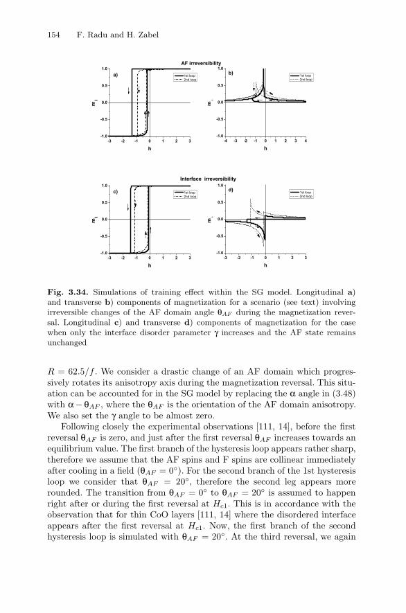
154 F. Radu and H. Zabel
Fig. 3.34. Simulations of training effect within the SG model. Longitudinal a)and transverse b) components of magnetization for a scenario (see text) involvingirreversible changes of the AF domain angle θAF during the magnetization rever-sal. Longitudinal c) and transverse d) components of magnetization for the casewhen only the interface disorder parameter γ increases and the AF state remainsunchanged
R = 62.5/f . We consider a drastic change of an AF domain which progres-sively rotates its anisotropy axis during the magnetization reversal. This situ-ation can be accounted for in the SG model by replacing the α angle in (3.48)with α− θAF , where the θAF is the orientation of the AF domain anisotropy.We also set the γ angle to be almost zero.
Following closely the experimental observations [111, 14], before the firstreversal θAF is zero, and just after the first reversal θAF increases towards anequilibrium value. The first branch of the hysteresis loop appears rather sharp,therefore we assume that the AF spins and F spins are collinear immediatelyafter cooling in a field (θAF = 0◦). For the second branch of the 1st hysteresisloop we consider that θAF = 20◦, therefore the second leg appears morerounded. The transition from θAF = 0◦ to θAF = 20◦ is assumed to happenright after or during the first reversal at Hc1. This is in accordance with theobservation that for thin CoO layers [111, 14] where the disordered interfaceappears after the first reversal at Hc1. Now, the first branch of the secondhysteresis loop is simulated with θAF = 20◦. At the third reversal, we again

3 Exchange Bias Effect of Ferro-/Antiferromagnetic Heterostructures 155
assume that the AF domain angle further increases. Therefore, the secondbranch of the hysteresis loop is simulated assuming a new value of θAF = 30◦.
The hysteresis loops bear all the features observed experimentally [99,136, 135, 58, 61, 111, 60, 138]. More strikingly, the transverse component ofmagnetization shows a small step increase at Hc1 and larger increase at Hc2,on the reverse path. These are typical features observed experimentally byPNR [111, 14], AMR [47, 143, 112] and MOKE [141]. Moreover, the trans-verse component at saturation behaves very close to recent observations ofBrems et al. [112] on Co/CoO bilayers and lithographically nanostructuredwires. After field cooling and before passing through the first magnetizationreversal in the descending field branch, the resistance in saturation (whichis proportional to the square of the orientation of transverse component ofmagnetization) reaches its maximum because all spins are oriented along thecooling field. After going through a complete hysteresis loop, the resistanceat saturation is reduced, indicating that spins in the F are rotated away fromthe cooling field. After reversing the field back to positive saturation the re-sistance does not recover its initial value. Moreover, the untrained state canbe partially reinduced by changing the orientation of the applied magneticfield [112] which can be interpreted as a further indication of AF domainrotation during the reversal.
Next, we consider only the interface disorder through a progressive changeof γ angles. In Fig. 3.34b) and c) we show first and second hysteresis loops cal-culated with the help of (3.48). In these calculations we consider that the AFis strong, R = 62.5/f . For the conversion factor we take a value of f = 60%.Also, we assume the average AF orientation to be parallel to the field coolingorientation (θAF = 0). Following closely the experimental observations, be-fore the first reversal γ is zero, while just after the first reversal, γ increasestowards an equilibrium value. The first branch of the hysteresis loop appearsrather sharp, therefore we assume that the AF spins and F spins are collinearimmediately after cooling in a field (γ = 0). For the second branch of the 1sthysteresis loop we consider that γ = 10◦, therefore the second leg appearsrather rounded. The transition from γ = 0 to γ = 10◦ is assumed to happenright after or during the first reversal at Hc1. The first branch of the secondhysteresis loop is simulated with γ = 10◦. At the third reversal, we again as-sume that the disorder of the interface increases. Therefore, the second branchof the hysteresis loop (and right after during during the reversal at Hc1 of thesecond loop) is simulated assuming a new value of γ = 20◦.
The simulations above implies a viscosity-like behavior to the disorderedinterface [145]. For example, when the F magnetization acquires an angle withrespect to the unidirectional anisotropy, the torque exerted on the interfacialspins will drag them away from the initial direction set by the field cooling.Reversing the magnetization back to positive directions the Keff spins willnot follow (completely), they remain close to this position (viscosity). This isbecause the maximum torque exerted by the F spins was already acting atnegative fields, while for positive fields it is much reduced. When measuring
156 F. Radu and H. Zabel
again the hysteresis loop, at negative coercive field, the Keff spins will rotateeven further and so on. Therefore, the angle of the Keff anisotropy and/orof the AF domains increases after each hysteresis loop, similar to a rachet,causing a decreased exchange bias field.
Comparing the hysteresis curves shown in Fig. 3.34a) with the ones inFig. 3.34c) one notices the same qualitative characteristics. This is not thecase for the transverse magnetization curve. The F spins rotate only on thepositive side for the first case, whereas for the second case the F magnetizationrotation covers the entire 360◦ angular range. The anisotropic magnetoresis-tance (AMR) and PNR hides the chirality of the ferromagnetic spin rotation asthey provide sin2(β) information, whereas MOKE is sensitive to the chiralityas it provides sin(β) information. Therefore, measuring both hysteresis com-ponents by MOKE, can help to distinguish between the dominant influenceon the training effect: AF domain (or/and grain) rotation versus SG interfaceinstability. The training effect is discussed furthermore in Sect. 3.13.2.
3.13.2 Empirical Expression for the Training Effect
The very first empirical expression for training [133, 134] effects suggested apower law dependence of the coercive fields and the exchange bias field as afunction of cycle index n:
Hneb = H∞
eb +k√n, (3.51)
where k is an experimental constant. This expression follows well the experi-mental dependence of the EB field for n ≥ 2, but when the very first point isincluded to the fit, then the agreement is poor.
Binek [139] has shown by using non-equilibrium thermodynamics that us-ing a recursive relation, the evolution of the EB field as a function of n, can bewell reproduced for all cycle indexes (n ≥ 1). The recursive expression reads:
Hn+1eb −Hn
eb = −γ (Hneb −H∞
eb )3 , (3.52)
where γ is a physical parameter which, for n 1, was directly related to thek parameter of (3.51). It was shown that a satisfactory agreement betweenthe (3.51) and (3.52) is achieved for n ≥ 3. Therefore the approach of Binekappears to provide the phenomenological origin of the hitherto unexplainedpower-law decay of the EB field with increasing loop index n > 1. The ana-lytic expression (3.52) was further tested for temperature dependent trainingeffect [146].
More recently the equation (3.52) has been further refined by extendingthe free energy expansion with a correction of the leading term. The newequation for training effect reads [147]:
Hn+1eb −Hn
eb = −γb (Hneb −H∞
eb )3 − γc (Hneb −H∞
eb )5 , (3.53)
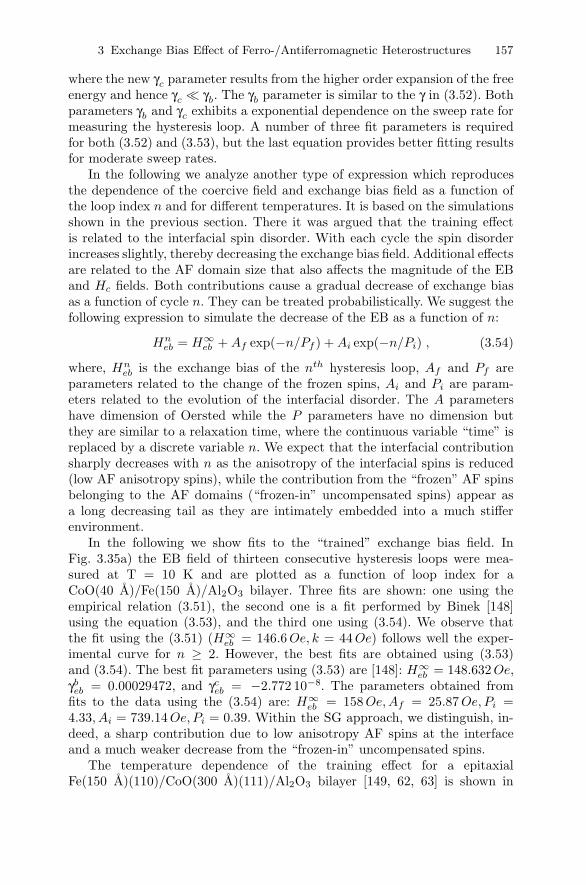
3 Exchange Bias Effect of Ferro-/Antiferromagnetic Heterostructures 157
where the new γc parameter results from the higher order expansion of the freeenergy and hence γc � γb. The γb parameter is similar to the γ in (3.52). Bothparameters γb and γc exhibits a exponential dependence on the sweep rate formeasuring the hysteresis loop. A number of three fit parameters is requiredfor both (3.52) and (3.53), but the last equation provides better fitting resultsfor moderate sweep rates.
In the following we analyze another type of expression which reproducesthe dependence of the coercive field and exchange bias field as a function ofthe loop index n and for different temperatures. It is based on the simulationsshown in the previous section. There it was argued that the training effectis related to the interfacial spin disorder. With each cycle the spin disorderincreases slightly, thereby decreasing the exchange bias field. Additional effectsare related to the AF domain size that also affects the magnitude of the EBand Hc fields. Both contributions cause a gradual decrease of exchange biasas a function of cycle n. They can be treated probabilistically. We suggest thefollowing expression to simulate the decrease of the EB as a function of n:
Hneb = H∞
eb +Af exp(−n/Pf ) +Ai exp(−n/Pi) , (3.54)
where, Hneb is the exchange bias of the nth hysteresis loop, Af and Pf are
parameters related to the change of the frozen spins, Ai and Pi are param-eters related to the evolution of the interfacial disorder. The A parametershave dimension of Oersted while the P parameters have no dimension butthey are similar to a relaxation time, where the continuous variable “time” isreplaced by a discrete variable n. We expect that the interfacial contributionsharply decreases with n as the anisotropy of the interfacial spins is reduced(low AF anisotropy spins), while the contribution from the “frozen” AF spinsbelonging to the AF domains (“frozen-in” uncompensated spins) appear asa long decreasing tail as they are intimately embedded into a much stifferenvironment.
In the following we show fits to the “trained” exchange bias field. InFig. 3.35a) the EB field of thirteen consecutive hysteresis loops were mea-sured at T = 10 K and are plotted as a function of loop index for aCoO(40 A)/Fe(150 A)/Al2O3 bilayer. Three fits are shown: one using theempirical relation (3.51), the second one is a fit performed by Binek [148]using the equation (3.53), and the third one using (3.54). We observe thatthe fit using the (3.51) (H∞
eb = 146.6Oe, k = 44Oe) follows well the exper-imental curve for n ≥ 2. However, the best fits are obtained using (3.53)and (3.54). The best fit parameters using (3.53) are [148]: H∞
eb = 148.632Oe,γbeb = 0.00029472, and γc
eb = −2.772 10−8. The parameters obtained fromfits to the data using the (3.54) are: H∞
eb = 158Oe,Af = 25.87Oe, Pi =4.33, Ai = 739.14Oe, Pi = 0.39. Within the SG approach, we distinguish, in-deed, a sharp contribution due to low anisotropy AF spins at the interfaceand a much weaker decrease from the “frozen-in” uncompensated spins.
The temperature dependence of the training effect for a epitaxialFe(150 A)(110)/CoO(300 A)(111)/Al2O3 bilayer [149, 62, 63] is shown in
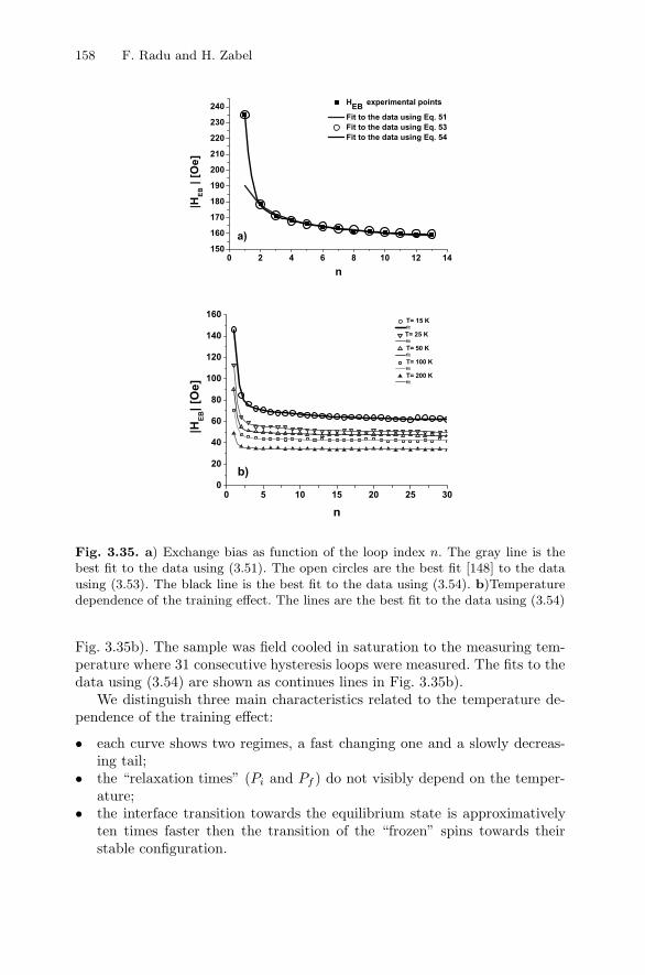
158 F. Radu and H. Zabel
Fig. 3.35. a) Exchange bias as function of the loop index n. The gray line is thebest fit to the data using (3.51). The open circles are the best fit [148] to the datausing (3.53). The black line is the best fit to the data using (3.54). b)Temperaturedependence of the training effect. The lines are the best fit to the data using (3.54)
Fig. 3.35b). The sample was field cooled in saturation to the measuring tem-perature where 31 consecutive hysteresis loops were measured. The fits to thedata using (3.54) are shown as continues lines in Fig. 3.35b).
We distinguish three main characteristics related to the temperature de-pendence of the training effect:
• each curve shows two regimes, a fast changing one and a slowly decreas-ing tail;
• the “relaxation times” (Pi and Pf ) do not visibly depend on the temper-ature;
• the interface transition towards the equilibrium state is approximativelyten times faster then the transition of the “frozen” spins towards theirstable configuration.

3 Exchange Bias Effect of Ferro-/Antiferromagnetic Heterostructures 159
3.14 Further Characteristics of EB-systems
3.14.1 Asymmetries of the Hysteresis Loop
A curios characteristic of EB systems is the often observed asymmetry be-tween the two branches of the hysteresis loop for descending and ascendingmagnetic fields. The hysteresis loop shape of an isolated ferromagnet is withno exceptions symmetric with respect to the field and magnetization axis.This is not the case for an exchange bias system, where the unidirectionalanisotropy and the stability of the AF can result in asymmetries of the hys-teresis loops and of the magnetization reversal modes. One can distinguishtwo different classes of the hysteresis loop asymmetries. One of them can beassigned to intrinsic properties of the EB systems which lacks training effects,and the another one is intimately related to irreversible changes of the AFdomain structure during the magnetization reversal.i) In the first category we encounter four different situations of asymmetryicmagnetization reversal all related to a stable interface without training effect:a) the first branch of the hysteresis loop is much extended compared to theascending branch (see Fig. 3.36). This asymmetric hysteresis loop was ob-served in FeNi/FeMn bilayers [98]. The underlying mechanism is related to aMauri type mechanism for exchange bias where a parallel domain wall (ex-change spring) is formed in the AF layer. The reversal is understood in termsof domain wall pinning in the antiferromagnet [98, 40, 91].
b) coherent rotation during the first reversal at Hc1, domain wall nucleationand propagation at Hc2 (see Fig. 3.37). Such asymmetric magnetization rever-sal has been observed by PNR in Fe/FeF2 and Fe/MnF2 systems [150]. Thisasymmetry depends on the relative orientation of the field cooling directionwith respect to the twin structure of the AF layer. The reversal asymmetrymentioned above takes place when the FC is parallel oriented with a directionbisecting the anisotropy axes of the two AF structural domains. When thefield cooling orientation is parallel to the anisotropy axes of one AF domain,
Fig. 3.36. a) Asymmetric hysteresis loop (a) of a NiFe/FeMn bilayer and schematicsof domain structure at different stages of magnetization reversal [98]

160 F. Radu and H. Zabel
Fig. 3.37. a) Asymmetric hysteresis loop (b) of a Fe/MnF2 bilayer and and thecorresponding neutron reflectivity curves: a) the PNR curves recorded at the firstcoercive field, Hc1 and c) the PNR curve recorded at Hc2. The lack of SF reflec-tivity at Hc2 suggests that the reversal proceeds by domain wall nucleation andpropagation, whereas at Hc1 the magnetization reverses by rotation [150, 90]
the reversal mechanism is symmetric, i.e. for both branches of the hysteresisloop magnetization rotation prevails.
c) sharp reversal on the descending branch and rounded reversal on theascending one (see Fig. 3.38). This asymmetry has recently been clarified bystudies of the azimuthal dependence of exchange bias in IrMn/F bilayers [76,41, 151]. It is an intrinsic property of the EB bilayer systems and it takes placewhenever the measuring external field is offset with respect to the field coolingorientation. By simply analyzing the geometrical asteroid solutions, it becomesobvious that the sweep line does not symmetrically cross the shifted asteroidwhen the field is not parallel to the unidirectional anisotropy. Actually, thisis a peculiar case of asymmetry which can be understood even within thephenomenological model for exchange bias [76] which assumes a rigid AF spinstructure. Within the SG and M&B model [41] such asymmetric reversalscan be simulated over a wide range of AF thicknesses and anisotropies. Also,
Fig. 3.38. Asymmetric hysteresis loop of a IrMn/CoFe bilayer along an offset θ = 3◦
angle [41]
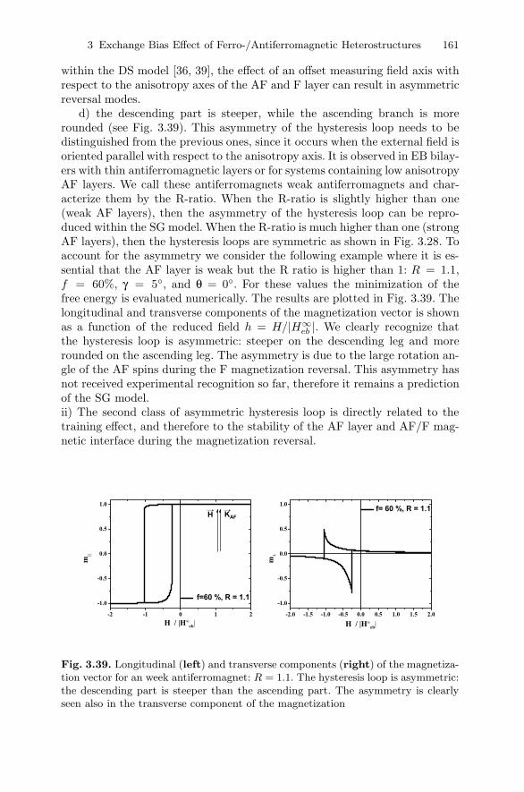
3 Exchange Bias Effect of Ferro-/Antiferromagnetic Heterostructures 161
within the DS model [36, 39], the effect of an offset measuring field axis withrespect to the anisotropy axes of the AF and F layer can result in asymmetricreversal modes.
d) the descending part is steeper, while the ascending branch is morerounded (see Fig. 3.39). This asymmetry of the hysteresis loop needs to bedistinguished from the previous ones, since it occurs when the external field isoriented parallel with respect to the anisotropy axis. It is observed in EB bilay-ers with thin antiferromagnetic layers or for systems containing low anisotropyAF layers. We call these antiferromagnets weak antiferromagnets and char-acterize them by the R-ratio. When the R-ratio is slightly higher than one(weak AF layers), then the asymmetry of the hysteresis loop can be repro-duced within the SG model. When the R-ratio is much higher than one (strongAF layers), then the hysteresis loops are symmetric as shown in Fig. 3.28. Toaccount for the asymmetry we consider the following example where it is es-sential that the AF layer is weak but the R ratio is higher than 1: R = 1.1,f = 60%, γ = 5◦, and θ = 0◦. For these values the minimization of thefree energy is evaluated numerically. The results are plotted in Fig. 3.39. Thelongitudinal and transverse components of the magnetization vector is shownas a function of the reduced field h = H/|H∞
eb |. We clearly recognize thatthe hysteresis loop is asymmetric: steeper on the descending leg and morerounded on the ascending leg. The asymmetry is due to the large rotation an-gle of the AF spins during the F magnetization reversal. This asymmetry hasnot received experimental recognition so far, therefore it remains a predictionof the SG model.ii) The second class of asymmetric hysteresis loop is directly related to thetraining effect, and therefore to the stability of the AF layer and AF/F mag-netic interface during the magnetization reversal.
Fig. 3.39. Longitudinal (left) and transverse components (right) of the magnetiza-tion vector for an week antiferromagnet: R = 1.1. The hysteresis loop is asymmetric:the descending part is steeper than the ascending part. The asymmetry is clearlyseen also in the transverse component of the magnetization
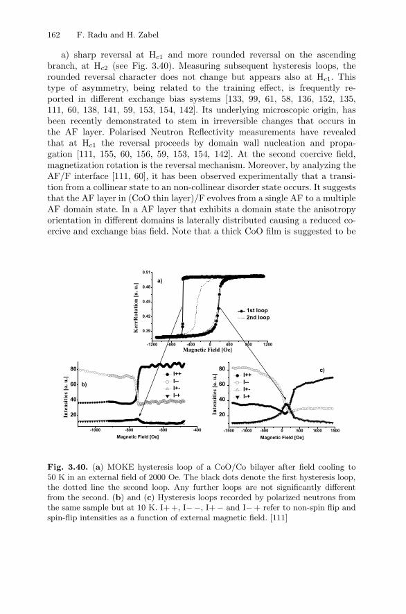
162 F. Radu and H. Zabel
a) sharp reversal at Hc1 and more rounded reversal on the ascendingbranch, at Hc2 (see Fig. 3.40). Measuring subsequent hysteresis loops, therounded reversal character does not change but appears also at Hc1. Thistype of asymmetry, being related to the training effect, is frequently re-ported in different exchange bias systems [133, 99, 61, 58, 136, 152, 135,111, 60, 138, 141, 59, 153, 154, 142]. Its underlying microscopic origin, hasbeen recently demonstrated to stem in irreversible changes that occurs inthe AF layer. Polarised Neutron Reflectivity measurements have revealedthat at Hc1 the reversal proceeds by domain wall nucleation and propa-gation [111, 155, 60, 156, 59, 153, 154, 142]. At the second coercive field,magnetization rotation is the reversal mechanism. Moreover, by analyzing theAF/F interface [111, 60], it has been observed experimentally that a transi-tion from a collinear state to an non-collinear disorder state occurs. It suggeststhat the AF layer in (CoO thin layer)/F evolves from a single AF to a multipleAF domain state. In a AF layer that exhibits a domain state the anisotropyorientation in different domains is laterally distributed causing a reduced co-ercive and exchange bias field. Note that a thick CoO film is suggested to be
Fig. 3.40. (a) MOKE hysteresis loop of a CoO/Co bilayer after field cooling to50 K in an external field of 2000 Oe. The black dots denote the first hysteresis loop,the dotted line the second loop. Any further loops are not significantly differentfrom the second. (b) and (c) Hysteresis loops recorded by polarized neutrons fromthe same sample but at 10 K. I++, I−−, I+− and I−+ refer to non-spin flip andspin-flip intensities as a function of external magnetic field. [111]

3 Exchange Bias Effect of Ferro-/Antiferromagnetic Heterostructures 163
already in a domain state [35] after field cooling, therefore one would expecta variation of the loop asymmetry (and training effect) with respect to thethickness of the AF layer.
3.14.2 Temperature Dependence of the Rotatable AF Spins(Coercivity)
We discuss here the temperature dependence of the interfacial properties.Experimentally this can best be studied by an element selective method[114, 115, 117, 17, 19] to distinguish between the hysteresis of the F and AFlayer. Element specific hysteresis loops have been studied for Fe/CoO [19],which highlights the behavior of the rotatable interfacial AF spins.
The exchange bias hysteresis loops measured at the L3 absorption edgesof Co (E=780 eV, closed symbols) and Fe (E=708.2 eV, open symbols) andfor different temperatures are shown in Fig. 3.41. After FC to 30 K, several
Fig. 3.41. The temperature dependence of the exchange biased hysteresis loopsmeasured at L3 absorption edges of Co (E=780 eV, closed symbols) and Fe (E=708.2eV, open symbols). Scattering angle is 2θ = 32◦ [19]
164 F. Radu and H. Zabel
hysteresis loops were measured in order to eliminate training effects. Subse-quentially the temperature was raised stepwise, from low to high T. For eachtemperature an element-specific hysteresis loop at the energies correspondingto Fe and CoO, respectively, was measured. The hysteresis loops of Fe as afunction of temperature show a typical behavior. At low temperatures an in-creased coercive field and a shift of the hysteresis loop is observed. As thetemperature is increased, the coercive field and the exchange bias decreaseuntil the blocking temperature is reached. Here, the exchange bias vanishesand the coercive field shows little changes as the temperature is further in-creased.
A ferromagnetic hysteresis loop corresponding to the CoO layer is observedfor all temperatures, following closely the hysteresis loop of Fe, with somenotable differences. It appears that the ferromagnetic components of CoOdevelop higher coercive fields than Fe below the blocking temperature. This isan essential indication that the AF rotatable spins mediate coercivity betweenthe AF layer and the F one, justifying the conversion factor introduced in theSG model. After careful analysis of the element specific reflectivity data [157,19], one can conclude that a positive exchange coupling across the Fe/CoOinterface. The ferromagnetic moment of CoO is present also above the Neeltemperature. Here, the AF layer is in a paramagnetic state, therefore thecoercive fields for the Fe and CoO rotatable spins are equal.
3.14.3 Vertical Shift of Magnetization Curves (Frozen AF Spins)
A vertical shift of magnetization has been observed frequently [53, 158, 138,66, 35, 159, 15, 85, 20, 160, 161, 160, 119, 162] and is considered to haveseveral origins related to the different mechanisms for exchange bias. Withinthe M&B model a AF monolayer in contact to the F layer is assumed to beuncompensated, but still being part of the AF lattice. At most one could ex-pect a contribution to the macroscopic or microscopic magnetization equal tothat of the net magnetization of an AF monolayer and this only by probingan AF layer consisting of an odd number of monolayers. The Mauri mech-anism for exchange bias is not likely to result in a vertical shift of the hys-teresis loop, since the AF interface is compensated. Within the SG, Mal-ozemoff, and DS models for EB, a small vertical shift is intrinsic. At theinterface between the AF and F layer, a number of frozen AF spins will beuncompensated due to the proximity of the F layer. Their orientation is ei-ther parallel or antiparallel oriented with respect to the F spins, depend-ing on the type of coupling (direct or indirect exchange). They contributeto the magnetization of the system. In case of an indirect exchange cou-pling mechanism, the hysteresis loop should be shifted downwards [163, 158],whereas in case of direct exchange coupling the magnetization curve shouldbe shifted upwards. The other part of the interface magnetization, namelythe rotatable AF spins, do not cause any shift since they rotate in phasewith the F layer. Within the DS model AF domains cause an additional

3 Exchange Bias Effect of Ferro-/Antiferromagnetic Heterostructures 165
shift to the macroscopic magnetization curve along the magnetization axis[35, 66, 85].
To demonstrate the shift of the magnetization we discuss a recent experi-ment by Ohldag et al. [20] using XMCD [164]. The evolution of the dichroicsignal as function of the magnetic field, providing the element specific hys-teresis loops, is shown Fig. 3.42.
The sample structure is Pd(2 nm)/Co(2.8 nm)/FeF2(68 nm)(110)/MgF2(110)/substrate and has been grown by via molecular beam epitaxy.The F layer is a polycrystalline Co whereas the AF layer is a FeF2(110)untwined single crystalline layer. The system exhibits a positive exchange biasat large cooling fields [163]. For weak cooling fields the exchange bias curve isshifted to negative fields, as usual for all EB systems. The microscopic originof the positive exchange bias is an antiferromagnetic coupling at the F/AFinterface [163]. Although, the mechanism was clearly demonstrated by mag-netometery measurements, the microscopic investigation of the AF interfaceprovides more detailed information.
The hysteresis loop of Co is typical and appears symmetric with respectto the magnetization axis (see Fig. 3.42). This is not the case for the AF in-terface magnetization which shows a twofold behavior: a) some interfacial AFspins are parallel oriented with respect to the F spins and both are rotatingalmost in phase; the AF hysteresis loop is shifted downwards with respectto the magnetization axis. This seems to be a direct proof of the preferredantiparallel coupling between the F Co and the AF Fe magnetization at theAF-F interface. The interfacial AF Fe moments are aligned during FC by theexchange interaction which acts as an effective field on the uncompensated
Fig. 3.42. Element-specific Co (black) and Fe (gray) hysteresis loops acquired atT= 15 K after field cooling in +200 Oe along the FeF2 [001] axis, parallel to the AFspin axis. The direction of the cooling field and the vertical shift of the Fe loop atT = 15 K is indicated by arrows. Reproduced from [20]

166 F. Radu and H. Zabel
spins, most likely confined to the interface [20]. An AF uncompensated mag-netization in FeF2 can also occur due to piezomagnetism, which is allowedby symmetry in rutile-type AF compounds and may be induced by stressesoccurring below the Neel temperature [165, 148].
These experimental observations can also be described by the SG model.During the field cooling procedure the frozen-in spins depicted in Fig. 3.27will be pointing opposite to the F spins as to fulfill the indirect exchangecondition at the F/AF interface. The rotatable ones remain unchanged inthe figure, being parallel aligned with the F spins. The orientation of thefrozen spins is governed by the exchange interaction at the F/AF interface,whereas the rotatable spins are aligned by the F layer and the external field.Upon reversal the rotatable spins will follow the ferromagnet whereas thefrozen spins remain pinned, leading to a shift downwards of the interfacialAF hysteresis loop. As the system described above does not exhibit trainingeffects, no irreversible changes occur during the magnetization reversal. Inhigh enough cooling fields, the frozen-in spins will align parallel to the coolingfield becoming also parallel with the rotatable AF and F spins. This willcause a positive shift of the hysteresis loop (positive exchange bias), since theorientation of the AF frozen spins is negative with respect to the couplingsign [163].
The experimental results described above could most likely be describedalso by the DS model and the Malozemoff model if magnetic domains in theAF layer will be confirmed.
A relative vertical shift of the magnetization related to training effects isdescribed by Hochstrat et al. [138] for a NiO(0001)/Fe(110) exchange biassystem. The antiferromagnet is a single crystal NiO whereas the ferromag-netic material is an Fe layer deposited under ultrahigh vacuum condition.Upon successive reversals of the F layer a decrease of the total magnetizationwas observed by SQUID magnetometery. The variation of the vertical shiftas a function of the hysteresis loop index n was correlated to a decrease ofthe AF magnetization. A linear correlation between the AF magnetization,deduced from the vertical shift, and the exchange bias field during trainingwas found, suggesting that the training effect may be related to a reduced AFmagnetization along the measuring field axis and as a function of the loopindex.
In Fig. 3.43 we show another situation where a vertical shift is visible inmacroscopic magnetization curves measured by SQUID magnetometery [166].The system is a polycrystalline CoO(2.5 nm)/Co(15 nm) bilayer grown bymagnetron sputtering [112]. The hysteresis loop at room temperature andalong the easy magnetization axis of the F layer is symmetric with respectto the magnetization axis and shows a low coercive field. Upon field coolingthe system through the Neel temperature t of the CoO layer (TN = 291 K)to the measuring temperature T=4.2 K the system is set in an exchangebias state. Then, a hysteresis loop is measured by sweeping the field from2000 Oe to –2000 Oe and back. By comparing this hysteresis loop with the

3 Exchange Bias Effect of Ferro-/Antiferromagnetic Heterostructures 167
Fig. 3.43. Hysteresis loops of CoO(25 A)/Co(180 A). The dashed line is the hys-teresis loop recorded at 300 K which is above the Neel temperature of the CoOlayer. After field cooling the system to 4.2 K, a hysteresis loop is recorded sweepingthe applied field from 9000 to –9000 Oe and back to 9000 Oe (black line, long loop).A second loop is measured under the same conditions as the previous one, but thefield range is shorter, namely between 2000 Oe to –2000 Oe and back to 2000 Oe.The cooling field was positive. A vertical shift of the hysteresis loop is clearly visiblefor the short loop, whereas the long loop appears to be centered with respect tomagnetization axis. [166]
one measured at room temperature one clearly observes a vertical shift upalong the magnetization axis. Moreover, this up-shift is due to the ferromag-netic Co spins which do not fully saturate at –2000 Oe. Previous studieshave shown that after the reversal at Hc1, the AF CoO layer breaks into AFdomains exhibiting an anisotropy distribution. Due to the strong coupling be-tween the F and the AF domains, the F layer cannot easily be saturated. Next,after repeating the field cooling procedure, another hysteresis loop was mea-sured by sweeping the external field to a much larger negative value, namelyto –9000 Oe. Now one observes that the hysteresis loop becomes more sym-metric with respect to the magnetization axis. The saturation field, where thehysteresis loops closes, is about –8000 Oe.
The example above shows that a vertical shift of magnetization can berelated to a non homogeneous state of the F layer due to non-collinearitiesat the AF/F interface. The relation to the training effect is clearly seen asdifferent coercive fields Hc2 depending on the strength of the applied fields.When a stronger field is applied in the negative direction, the exchangebias decreases due to a larger degree of irreversible changes into the AFlayer.

168 F. Radu and H. Zabel
A distinct class of vertical shifts is found in exchange bias systems where adiluted antiferromagnet [167, 66, 35, 85] acts as a pinning layer. As function ofdilution of a CoO layer by Mg impurities, as well as, partial oxygen pressureduring the deposition, the AF layer acquires an excess magnetization seen asa vertical shift of the hysteresis loop. This strongly supports the fact that thedomain state in the AF layer as well as the EB effect is caused and controlledby the defects [66, 85].
Vertical shifts in nanostructures and nanoparticles are often observed dueto uncompensated AF spins. For a detailed discussion we refer to recent re-views by Nogues et al. [161] and Iglesias et al. [160] and also recent papers onAF nanoparticles [119, 162].
3.15 Further Evidence for Spin-Glass Like BehaviorObserved in Finite Size Systems
Although nanoparticles are not covered in this review, we, nevertheless, dis-cuss two recent instances which in AF nanoparticles confirm the SG behavior.One is Co3O4 nanowires [119] and the other is CoO granular structure [118].
3.15.1 AF Nanoparticles
Nanoparticles of antiferromagnetic materials have been predicted by Neel [168]to have a small net magnetic moment due to an unequal number of spins onthe two sublattices as a result of the finite size [169]. Hysteresis loops ofAF nanoparticles have been observed and several suggestions were made toaccount for their weak ferromagnetism [169]. One important finite size effect ofAF magnetic nanoparticle is the breaking of a large number of exchange bondsfor surface atoms. This can have a particularly strong effect on ionic materials,since the exchange interactions are superexchange interactions. The deficit ofexchange bonds could lead to a spin disordered shell exhibiting spin-glass likebehavior. The last effect is demonstrated most recently by Salabas et al. [119]and discussed further below.
In Fig. 3.44 two hysteresis loops of Co3O4 nanoparticles (8 nm diameter)prepared by a nanocasting route are shown [119]. Both curves were measuredat T = 2 K after cooling the system in zero field (ZFC hysteresis loop) andin an external applied field of +4 T (FC hysteresis loop). Whereas the ZFCloop shows typical weak ferromagnetic properties specific to AF particles,after FC a completely different behavior is observed. The hysteresis loop isexchange biased, it is vertically shifted and shows training effect. Moreover,the temperature dependence (not shown) of the coercive field and exchangebias field increases with decreasing temperature, which is also a usual behaviorof EB systems. More strikingly the FC hysteresis loop does not close on theright side at positive fields. This open hysteresis loop is a direct indicationof a spin-glass like behavior, similar to the loops observed in pure spin glass

3 Exchange Bias Effect of Ferro-/Antiferromagnetic Heterostructures 169
Fig. 3.44. Field cooled and zero field cooled hysteresis loops of Co3O4 nanowires.From [119]
systems [37]. This behavior appears to support the SG model (Fig. 3.27),where a reduced anisotropy is assumed to occur at the F/AF interface. Bothfrozen-in spins and rotatable spins are directly seen in the FC hysteresis loop.Moreover, the irreversible changes of the surface AF spins are causing the openloop. A similar open loop is also predicted by the DS model. Within the DSmodel the hysteresis loop of the AF interface layer is not closed on the righthand side because the DS magnetization is lost partly during F reversal dueto a rearrangement of the AF domain structure. The AF particles, however,are supposed to be single AF domains, therefore irreversible changes are dueto surface effects rather than caused by AF domain kinetics. Certainly, atvery large cooling fields, the bulk structure of the AF particle should be alsoaffected. The spin-glass like behavior was also recently observed for cobaltferrite nanoparticles [162], for (Mn,Fe)2O3−t nanograins [170], and for a ε-Fe3NCrN nanocomposite system [171].
3.15.2 Extended Granular AF Film
Another direct experimental evidence of a spin-glass like behavior was ob-served by Gruyters [118] on CoO/Au multilayers, CoO/Cu/Fe trilayers, andCoO/Fe bilayers with granular structure. In Fig. 3.45a) the ZFC hysteresisloop of a CoO/Au multilayer and for different temperature is shown. Onenotices that the coercive field is enhanced at low temperatures, but no hys-teresis shift develops. The FC hysteresis loop (see Fig. 3.45b)), however, isalmost completely shifted to one side of the field axis. These observationsare explained by Gruyters as an effect of the uncompensated AF spins of thegranular film structure. The saturation magnetization of this granular CoOfilm is about 60–62 emu/gCoO which would result in an enormous amount ofuncompensated spins equivalent to 22% for the observed particles volume. Nostoichiometry influences are considered to contribute to this value. Althoughthe uncompensation level is unclear, the evidence of a spin-glass behavior

170 F. Radu and H. Zabel
Fig. 3.45. a) ZFC hysteresis loops of [CoO [x A]/Au (60 A)] multilayers. b) FChysteresis loop of a [CoO [20 A]/Au (60 A)] multilayer. c) ZFC and FC magnetizationcurves as a function of increasing temperature T in different fields for a [CoO [15A]/Au (60 A)] multilayer. d) Field dependence of Tirr raised to the 2/3 power fortwo different multilayers. ([118])
is well demonstrated. In Fig. 3.45c) ZFC and FC magnetization curves aremeasured as function of temperature and for different external fields. Twomain characteristic features are observed for these curves: an irreversibilitytemperature Tirr, where the ZFC and FC branches of MCoO(T) coalesce, anda pronounced peak due to superparamagnetic blocking in the ZFC magneti-zation. The direct evidence of a spin-glass behavior is the field dependenceof Tirr shown in Fig. 3.45d). The existence of critical lines spanned by thevariables temperature and magnetic field can be explained by mean-field the-ory. One of these lines has been predicted by de Almeida and Thouless forIsing spin systems [118]. The Tirr raised to 2/3 power as function of fieldexhibits a linear dependence in agreement with the predictions of Almeidaand Thouless.
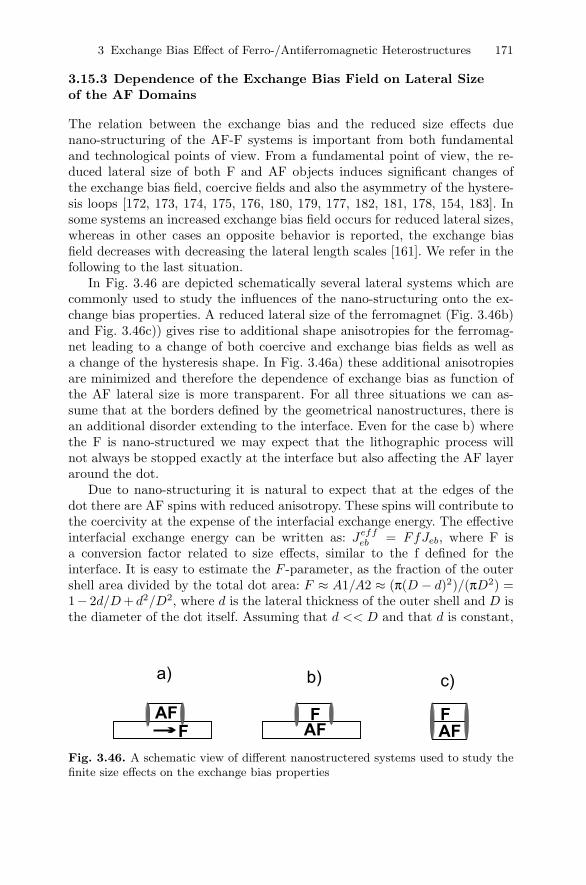
3 Exchange Bias Effect of Ferro-/Antiferromagnetic Heterostructures 171
3.15.3 Dependence of the Exchange Bias Field on Lateral Sizeof the AF Domains
The relation between the exchange bias and the reduced size effects duenano-structuring of the AF-F systems is important from both fundamentaland technological points of view. From a fundamental point of view, the re-duced lateral size of both F and AF objects induces significant changes ofthe exchange bias field, coercive fields and also the asymmetry of the hystere-sis loops [172, 173, 174, 175, 176, 180, 179, 177, 182, 181, 178, 154, 183]. Insome systems an increased exchange bias field occurs for reduced lateral sizes,whereas in other cases an opposite behavior is reported, the exchange biasfield decreases with decreasing the lateral length scales [161]. We refer in thefollowing to the last situation.
In Fig. 3.46 are depicted schematically several lateral systems which arecommonly used to study the influences of the nano-structuring onto the ex-change bias properties. A reduced lateral size of the ferromagnet (Fig. 3.46b)and Fig. 3.46c)) gives rise to additional shape anisotropies for the ferromag-net leading to a change of both coercive and exchange bias fields as well asa change of the hysteresis shape. In Fig. 3.46a) these additional anisotropiesare minimized and therefore the dependence of exchange bias as function ofthe AF lateral size is more transparent. For all three situations we can as-sume that at the borders defined by the geometrical nanostructures, there isan additional disorder extending to the interface. Even for the case b) wherethe F is nano-structured we may expect that the lithographic process willnot always be stopped exactly at the interface but also affecting the AF layeraround the dot.
Due to nano-structuring it is natural to expect that at the edges of thedot there are AF spins with reduced anisotropy. These spins will contribute tothe coercivity at the expense of the interfacial exchange energy. The effectiveinterfacial exchange energy can be written as: Jeff
eb = FfJeb, where F isa conversion factor related to size effects, similar to the f defined for theinterface. It is easy to estimate the F -parameter, as the fraction of the outershell area divided by the total dot area: F ≈ A1/A2 ≈ (π(D − d)2)/(πD2) =1− 2d/D+ d2/D2, where d is the lateral thickness of the outer shell and D isthe diameter of the dot itself. Assuming that d << D and that d is constant,
AF
F AF
F F
AF
a) b) c)
Fig. 3.46. A schematic view of different nanostructered systems used to study thefinite size effects on the exchange bias properties

172 F. Radu and H. Zabel
we obtain the general expression for the variation of the exchange bias fieldas D:
−Heb +HD→∞eb
HD→∞eb
≈ 1 − F ≈ 1D, (3.55)
where HD→∞eb is the exchange bias of an extended film. Within this simple
model the exchange bias field decreases as the lateral size of the AF structuredecreases. This 1/D dependence is often observed experimentally [161].
The general behavior of the hysteresis loops as a function of the f -parameter is depicted in Fig. 3.28. We see that for high f corresponding to alarge diameter AF dot, the coercive field is small and the exchange bias is high.When, however, the lateral size of a AF object becomes smaller, the f ratio de-creases leading to an increased coercive field and reduced exchange bias field.Transition from the top hysteresis to the bottom hysteresis of Fig. 3.28 areusually observed due to nanostructuring of the AF layers [172, 177, 178, 161].
3.16 Conclusions
The results presented in this chapter provides an overview of the physics ofa F/(Interface)/AF exchange bias systems. Fundamental properties of theunidirectional anisotropy are considered and discussed. The Meiklejohn andBean model as well as the Mauri model are considered in detail and compared,both analytically and numerically. The Neel approach, Malozemoff model,Domain State model and a model of Kim and Stamps are discussed as theyprovide novel and fundamental ideas on the EB phenomenon. The Spin Glassmodel is discussed in even more details. Further experimental results touchingthe fundamentals of exchange bias are described.
We distinguish several outcomes of our overview:
• The exchange bias is an interface effect, as clearly proven by the 1/tF
dependence. Deviations from this law were observed in the literature, butfundamentally this expression is clearly well established.
• The AF anisotropies in the bulk of the AF layer and at the interface toa soft ferromagnetic layer give rise to an impressively rich behavior ofthe magnetic properties: the hysteresis loops can be shifted along bothfield and magnetization axis and in both positive and negative directions,the azimuthal dependence of exchange bias exhibits non-intuitive behaviorsuch as a shift of its maximum with respect to the field cooling orientation,the hysteresis loops are asymmetrically shaped, etc. Some of the exchangebias characteristics mentioned above are not fully and consistently revealedexperimentally which leaves an open window for further quests.
• The analytical formulae for the exchange bias within the M&B modeldepends mainly on the properties of the AF layer, namely on its anisotropyand thickness.

3 Exchange Bias Effect of Ferro-/Antiferromagnetic Heterostructures 173
• The peak-like increase of the EB close to the critical thickness of the AFlayer can be reproduced by the SG model. This effect is also accounted forby the DS model.
• The azimuthal dependence of the exchange bias effect could help to dis-tinguish between two ideal mechanisms for exchange bias: Mauri versusM&B models.
• The SG model describes the conversion of coupling into coercivity.
List of acronyms
AMR Anisotropic Magneto-ResistanceFC Field CoolingZFC Zero Field CoolingEB Exchange BiasDS Domain State ModelSG Spin Glass ModelSW Stoner-Wohlfarth ModelM&B Meiklejohn and Bean ModelMCA Magneto-Crystalline AnisotropyMOKE Magneto-Optical Kerr EffectPNR Polarized Neutron ReflectivitySQUID Superconducting Quantum Interference DeviceAF AntiferromagnetF FerromagnetMFM Magnetic Force MicroscopyMRAM Magnetic Random Access MemoryDAFF Diluted Antiferromagnets in an External Magnetic FieldXMCD Soft X-ray Resonant Magnetic DichroismXRMS Soft X-ray Resonant Magnetic Scattering
Acknowledgments
We gratefully acknowledge support by the DFG Sonderforschungsbereich 491:Magnetic Heterostructures: spin structure and spin transport, and by BESSY.
We have benefitted from discussions with: Werner Keune, Wolfgang Klee-mann, Kurt Westerholt, Ulrich Nowak, Klaus D. Usadel, Christian Binek,Kristiaan Temst, Ivan K. Schuller, Robert L. Stamps.
References
1. W. H. Meiklejohn and C. P. Bean. New magnetig anisotropy. Phys. Rev.,102:1413, 1956.

174 F. Radu and H. Zabel
2. P. Grunberg, R. Schreiber, Y. Pang, M.B. Brodsky, and H. Sowers. Lay-ered magnetic structures: Evidence for antiferromagnetic coupling of Fe-layersacross Cr-interlayers. Phys. Rev. Lett., 57:2442, 1986.
3. N. R. Werthamer. Theory of the superconducting transition temperature andenergy gap function of superposed metal films. Phys. Rev., 132:2440, 1963.
4. Zoran Radovic, Marko Ledvij, Ljiljana Dobrosavljevic-Grujic, A. I. Buzdin,and John R. Clem. Transition temperatures of superconductor-ferromagnetsuperlattices. Phys. Rev. B., 44:759, 1991.
5. D. Burgler, S. O. Demokritov, P. Gurnberg, and M. T. Johnson. Interlayerexchange coupling in layered magnetic structures. in Handbook of MagneticMaterials K. H. J. Buschow, ed., Elsevier North-Holland, Amsterdam, 13, 2001.
6. F. S. Bergeret, A. F. Volkov, and K. B. Efetov. Odd triplet superconductivityand related phenomena in superconductor-ferromagnet structures. Rev. Mod.Phys., 77:1321, 2005.
7. A. I. Buzdin. Proximity effects in superconductor-ferromagnet heterostruc-tures. Rev. Mod. Phys., 77:935, 2005.
8. J. Nogues and I. K. Schuller. Exchange bias. J. Magn. Magn. Mater., 192:203,1999.
9. M. Kiwi. Exchange bias theory. J. Magn. Magn. Mater., 234:584–595, 2001.10. A. E. Berkowitz and K. Takano. Exchange anisotropy - a review. J. Magn.
Magn. Mater., 200:552, 1999.11. R. L. Stamps. Mechanisms for exchange bias. J. Phys. D:Appl. Phys., 33:R247,
2000.12. T. J. Regan, H. Ohldag, C. Stamm, F. Nolting, J. Luning, J. Stohr, and
R. L. White. Chemical effects at metal/oxide interfaces studied by x-ray-absorption spectroscopy. Phys. Rev. B., 64(21):214422, Nov 2001.
13. H. Ohldag, T. J. Regan, J. Stohr, A. Scholl, F. Nolting, J. Luning, C. Stamm,S. Anders, and R. L. White. Spectroscopic identification and direct imaging ofinterfacial magnetic spins. Phys. Rev. Lett., 87(24):247201, Nov 2001.
14. F. Radu, M. Etzkorn, R. Siebrecht, T. Schmitte, K. Westerholt, and H. Zabel.Interfacial domain formation during magnetization reversal in exchange-biasedCoO/Co bilayers. Phys. Rev. B., 67:134409, 2003.
15. H. Ohldag, A. Scholl, F. Nolting, E. Arenholz, S. Maat, A. T. Young, M. Carey,and J. Stohr. Correlation between exchange bias and pinned interfacial spins.Phys. Rev. Lett., 91(1):017203, 2003.
16. A. Scholl, M. Liberati, E. Arenholz, H. Ohldag, and J. Stohr. Creation of anantiferromagnetic exchange spring. Phys. Rev. Lett., 92:247201, 2004.
17. S. Roy, M. R. Fitzsimmons, S. Park, M. Dorn, O. Petracic, Igor V. Roshchin,Zhi-Pan Li, X. Batlle, R. Morales, A. Misra, X. Zhang, K. Chesnel, J. B.Kortright, S. K. Sinha, and Ivan K. Schuller. Depth profile of uncompensatedspins in an exchange bias system. Phys. Rev. Lett., 95(4):047201, 2005.
18. W. Kuch, F. Offi L. I. Chelaru, M. Kotsugi J. Wang, and J. Kirschner. Tuningthe magnetic coupling across ultrathin antiferromagnetic films by controllingatomic-scale roughness. Nature Materials, 5:128–133, 2006.
19. F. Radu, A. Nefedov, J. Grabis, G. Nowak, A. Bergmann, and H. Zabel. Softx-ray magnetic scattering studies on Fe/CoO exchange bias bilayers. J. Magn.Magn. Mater., 300:206, 2006.
20. Hendrik Ohldag, Hongtao Shi, Elke Arenholz, Joachim Stohr, and David Le-derman. Parallel versus antiparallel interfacial coupling in exchange biasedCo/FeF2. Phys. Rev. Lett., 96(2):027203, 2006.

3 Exchange Bias Effect of Ferro-/Antiferromagnetic Heterostructures 175
21. T. Hauet, J. A. Borchers, Ph. Mangin, Y. Henry, and S. Mangin. Trainingeffect in an exchange bias system: The role of interfacial domain walls. Phys.Rev. Lett., 96(6):067207, 2006.
22. C. Tusche, H. L. Meyerheim, F. U. Hillebrecht, and J. Kirschner. Evidencefor a mixed Co/NiO layer at the Co/NiO(001) interface from surface x-raydiffraction. Phys. Rev. B., 73(12):125401, 2006.
23. V. K. Valev, M. Gruyters, A. Kirilyuk, and Th. Rasing. Direct observation ofexchange bias related uncompensated spins at the CoO/Cu interface. Phys.Rev. Lett., 96(6):067206, 2006.
24. E. C. Stoner and E. P. Wohlfarth. Interpretation of high coercivity in ferro-magnetic materials. Nature, 160:650, 1947.
25. E. C. Stoner and E. P. Wohlfarth. A mechanism of magnetic hysteresis in het-erogeneous alloys. Philosophical Transactions of the Royal Society of London.Series A, Mathematical and Physical Sciences, 240(826):599–642, 1948.
26. W. H. Meiklejohn and C. P. Bean. New magnetig anisotropy. Phys. Rev.,105:904, 1957.
27. W. H. Meiklejohn. Exchange anisotropy - a review. J. Appl. Phys., 33:1328,1962.
28. D. Mauri, H. C. Siegmann, P. S. Bagus, and E. Kay. Simple model for thin fer-romagnetic films exchange coupled to an antiferromagnetic substrate. J. Appl.Phys., 62:3047, 1987.
29. A. P. Malozemoff. Random-field model of exchange anisotropy at roughferromagnetic-antiferromagnetic interfaces. Phys. Rev. B., 35:3679, 1987.
30. A. P. Malozemoff. Mechanisms of exchange anisotropy (invited). J. Appl.Phys., 63(8):3874–3879, 1988.
31. A. P. Malozemoff. Heisenberg-to-Ising crossover in a random-field model withuniaxial anisotropy. Phys. Rev. B., 37(13):7673–7679, 1988.
32. P. Miltenyi, M. Gierlings, J. Keller, B. Beschoten, G. Guntherodt, U. Nowak,and K. D. Usadel. Diluted antiferromagnets in exchange bias: Proof of thedomain state model. Phys. Rev. Lett., 84(18):4224–4227, 2000.
33. U. Nowak, A. Misra, and K. D. Usadel. Domain state model for exchange bias.J. Appl. Phys., 89(11):7269–7271, 2001.
34. U. Nowak, A. Misra, and K. D. Usadel. Modeling exchange bias microscopically.J. Magn. Magn. Mater., 240(1-3):243–247, 2002.
35. U. Nowak, K. D. Usadel, J. Keller, P. Miltenyi, B. Beschoten, andG. Guntherodt. Domain state model for exchange bias. I. Theory. Phys. Rev.B., 66:014430, 2002.
36. B. Beckmann, U. Nowak, and K. D. Usadel. Asymmetric reversal modes in fer-romagnetic/antiferromagnetic multilayers. Phys. Rev. Lett., 91:187201, 2003.
37. K. Binder. Spin glasses: Experimental facts, theoretical concepts, and openquestions. Rev. Mod. Phys., 58(4):801–976, October 1986.
38. G. Scholten, K. D. Usadel, and U. Nowak. Coercivity and exchange bias of fer-romagnetic/antiferromagnetic multilayers. Phys. Rev. B., 71(6):064413, 2005.
39. B. Beckmann, K. D. Usadel, and U. Nowak. Cooling-field dependence of asym-metric reversal modes for ferromagnetic/antiferromagnetic multilayers. Phys.Rev. B., 74(5):054431, 2006.
40. Joo-Von Kim and R. L. Stamps. Hysteresis from antiferromagnet domain-wallprocesses in exchange-biased systems: Magnetic defects and thermal effects.Phys. Rev. B., 71(9):094405, 2005.

176 F. Radu and H. Zabel
41. F. Radu, A. Westphalen, K. Theis-Brohl, and H. Zabel. Quantitative de-scription of the azimuthal dependence of the exchange bias effect. J. Phys.:Condens. Matter, 18:L29–L36, 2006.
42. R. Coehoorn. Exchange anisotropy, Stoner-Wolhfarth model. Lecture Notes,Eindhoven University of Technology, Eindhoven University of Technology,2000-2001.
43. J. C. Slonczewski. In: Research Memorandum RM 003.111.224, IBM ResearchCenter Poughkeepsie, unpublished, 1956.
44. Andre Thiaville. Extensions of the geometric solution of the two dimensionalcoherent magnetization rotation model. J. Magn. Magn. Mater., 182(1-2):5,1998.
45. N. J. Gokemeijer, T. Ambrose, and C. L. Chien. Long-range exchange biasacross a spacer layer. Phys. Rev. Lett., 79:4270, 1997.
46. Kentaro Takano, R. H. Kodama, A. E. Berkowitz, W. Cao, and G. Thomas.Interfacial uncompensated antiferromagnetic spins: Role in unidirectionalanisotropy in polycrystalline Ni81Fe19/CoO bilayers. Phys. Rev. Lett.,79(6):1130–1133, 1997.
47. T. Gredig, I. N. Krivorotov, P. Eames, and D. Dahlberg. Unidirectional coer-civity enhancement in exchange-biased Co/CoO. Appl. Phys. Lett., 81:1270,2002.
48. C. Prados, E. Pina, A. Hernando, and A. Montone. Reversal of exchange bias innanocrystalline antiferromagnetic-ferromagnetic bilayers. J. Phys.: Condens.Matter, 14:10063, 2002.
49. Hongtao Shi, Zhongyuan Liu, and David Lederman. Exchange bias of poly-crystalline co on single-crystalline FexZn1−xF2 thin films. Phys. Rev. B.,72(22):224417, 2005.
50. Mannan Ali, Patrick Adie, Christopher H. Marrows, Denis Greig,Bryan J. Hickey, and Robert L. Stamps. Exchange bias using a spin glass.Nature Materials, 6:70, 2007.
51. C. Leighton, J. Nogues, H. Suhl, and I. K. Schuller. Competing interfacialexchange and Zeeman energies in exchange biased bilayers. Phys. Rev. B.,60:12837, 1999.
52. T. M. Hong. Simple mechanism for a positive exchange bias. Phys. Rev. B.,58:97, 1998.
53. B. Kagerer, C. Binek, and W. Kleemann. Freezing field dependence ofthe exchange bias in uniaxial FeF2-CoPt heterosystems with perpendicularanisotropy. J. Magn. Magn. Mater., 217(1-3):139–146, 2000.
54. T. L. Kirk, O. Hellwig, and E. E. Fullerton. Coercivity mechanisms in positiveexchange-biased Co films and Co/Pt multilayers. Phys. Rev. B., 65:224426,2002.
55. M. D. Rechtin and B. L. Averbach. Long-range magnetic order in coo. Phys.Rev. B., 6:4294, 1972.
56. Peter Miltenyi. Mikroskopischer ursprung der austauschkopplung in ferromag-netischen/antiferromagnetischen schichten. PHD Thesis, Aachen, 2000.
57. B. H. Miller and E. Dan Dahlberg. Use of the anisotropic magnetoresistance tomeasure exchange anisotropy in Co/CoO bilayers. Appl. Phys. Lett., 69:3932,1996.
58. S. G. E. te Velthuis, A. Berger, G. P. Felcher, B. K. Hill, and E. Dan Dahlberg.Training effects and the microscopic magnetic structure of exchange biasedCo/CoO bilayers. J. Appl. Phys., 87:5046, 2000.

3 Exchange Bias Effect of Ferro-/Antiferromagnetic Heterostructures 177
59. U. Welp, S. G. E. te Velthuis, G. P. Felcher, T. Gredig, and E. D. Dahlberg. Do-main formation in exchange biased Co/CoO bilayers. J. Appl. Phys., 93:7726,2003.
60. F. Radu, M. Etzkorn, V. Leiner, T. Schmitte, A. Schreyer, K. Westerholt, andH. Zabel. Polarised neutron reflectometry study of Co/CoO exchange biasedmultilayers. Appl. Phys. A, 74:S1570, 2002.
61. M. Gruyters and D. Riegel. Strong exchange bias by a single layer of inde-pendent antiferromagnetic grains: The CoO/Co model system. Phys. Rev. B.,63:052401, 2000.
62. G. Nowak, A. Remhof, F. Radu, A. Nefedov, H.-W. Becker, and H. Zabel.Structural and magnetic properties of stoichiometric epitaxial CoO/Fe ex-change bias bilayers. Phys. Rev. B., 75:174405, 2007.
63. Florin Radu. Fundamental aspects of exchange bias effect. PhD thesis, Ruhr-University Bochum, 2005.
64. C. Tsang, N. Heiman, and K. Lee. Exchange induced unidirectional anisotropyat FeMn-Ni80Fe20 interfaces. J. Appl. Phys, 52:2471, 1981.
65. H. Fujiwara, C. Hou, M. Sun, and H. S. Cho. Effect of exchange coupling ofpolycrystalline antiferromagnetic layers on the magnetization behavior of softmagnetic layers. IEEE Transactions on Magnetics, 35(5):3082, 1999.
66. J. Keller, P. Miltenyi, B. Beschoten, G. Guntherodt, U. Nowak, and K. D.Usadel. Domain state model for exchange bias. ii. experiments. Phys. Rev. B.,66:014431, 2002.
67. Jung-Il Hong, Titus Leo, David J. Smith, and Ami E. Berkowitz. Enhancingexchange bias with diluted antiferromagnets. Phys. Rev. Lett., 96(11):117204,2006.
68. C. Chappert, H. Bernas, J. Ferre, V. Kottler, J. P. Jamet, Y. Chen, E. Cambril,T. Devolder, F. Rousseaux, V. Mathet, and H. Launois. Planar patternedmagnetic media obtained by ion irradiation. Science, 280:1919–1922, 1998.
69. A. Mougin, T. Mewes, M. Jung, D. Engel, A. Ehresmann, H. Schmoranzer,J. Fassbender, and B. Hillebrands. Local manipulation and reversal of theexchange bias field by ion irradiation in FeNi/FeMn double layers. Phys. Rev.B., 63:060409, 2001.
70. V. Hoink, M. D. Sacher, J. Schmalhorst, G. Reiss, D. Engel, D. Junk,and A. Ehresmann. Postannealing of magnetic tunnel junctions with ion-bombardment-modified exchange bias. Appl. Phys. Lett., 86(15):152102, 2005.
71. S. Urazhdin and C. L. Chien. Effects of antiferromagnetic spin rotation onthe anisotropy of ferromagnetic/antiferromagnetic bilayers. Phys. Rev. B.,71(22):220410, 2005.
72. D. Mauri, E. Kay, D. Scholl, and J. K. Howard. Novel method for determiningthe anisotropy constant of MnFe in a NiFe/MnFe sandwich. J. Appl. Phys.,62:2929, 1987.
73. J. T. Kohlhepp and W. J. M. de Jonge. Stabilization of metastable expandedface-centered-tetragonal manganese. Phys. Rev. Lett., 96(23):237201, 2006.
74. C. Daboo, R. J. Hicken, E. Gu, M. Gester, S. J. Gray, D. E. P. Eley, E. Ahmad,J. A. C. Bland, R. Ploessl, and J. N. Chapman. Anisotropy and orientationaldependence of magnetization reversal processes in epitaxial ferromagnetic thinfilms. Phys. Rev. B., 51(22):15964–15973, Jun 1995.
75. Till Schmitte. Bragg-moke and vector-moke investigations: Magnetic reversalof patterned microstripes. PhD thesis, Ruhr-University Bochum, 2002.

178 F. Radu and H. Zabel
76. Julio Camarero, Jordi Sort, Axel Hoffmann, Jose Miguel Garcıa-Martın,Bernard Dieny, Rodolfo Miranda, and Josep Nogues. Origin of the asymmet-ric magnetization reversal behavior in exchange-biased systems: Competinganisotropies. Phys. Rev. Lett., 95:057204, 2005.
77. L. Neel. Etude theorique du couplage ferro-antiferromagnetique dans lescouches minces. Ann. Phys. (Paris), 2:61, 1967.
78. N. C. Koon. Calculations of exchange bias in thin films with ferromag-netic/antiferromagnetic interfaces. Phys. Rev. Lett., 78:4865–4868, 1997.
79. T. C. Schulthess and W. H. Butler. Consequences of spin-flop coupling inexchange biased films. Phys. Rev. Lett., 81(20):4516–4519, 1998.
80. T. C. Schulthess and W. H. Butler. Coupling mechanisms in exchange biasedfilms. J. Appl. Phys., 85(8):5510–5515, 1999.
81. R. Coehoorn, J. T. Kohlhepp, R. M. Jungblut, A. Reinders, and M. J. Dekker.Mesoscopic magnetism and the phenomenon of exchange anisotropy: MBEgrown Cu(110)/Ni80Fe20/Fe50Mn50 bilayers with corrugated interfaces. Phys-ica B: Condensed Matter, 319(1-4):141–167, 2002.
82. F. Radu, A. Vorobiev, J. Major, H. Humblot, K. Westerholt, and H. Zabel.Spin-resolved off-specular neutron scattering from magnetic domain walls usingthe polarized 3He gas spin filter. Physica B, 335:63–67, 2003.
83. A. Misra, U. Nowak, and K. D. Usadel. Control of exchange bias by dilutingthe antiferromagnetic layer. J. Appl. Phys., 93(10):6593–6595, 2003.
84. A. Misra, U. Nowak, and K. D. Usadel. Structure of domains in an exchange-bias model. J. Appl. Phys., 95(3):1357–1363, 2004.
85. Cristian Papusoi, Jan Hauch, Marian Fecioru-Morariu, and GernotGuntherodt. Tuning the exchange bias of soft metallic antiferromagnets byinserting nonmagnetic defects. J. Appl. Phys., 99(12):123902, 2006.
86. Xi Chen, Ch. Binek, A. Hochstrat, and W. Kleemann. Dilution-induced en-hancement of the blocking temperature in exchange-bias heterosystems. Phys.Rev. B., 65(1):012415, Dec 2001.
87. T. Mewes, R. Lopusnik, J. Fassbender, B. Hillebrands, M. Jung, D. Engel,A. Ehresmann, and H. Schmoranzer. Suppression of exchange bias by ionirradiation. Appl. Phys. Lett., 76(8):1057–1059, 2000.
88. Hongtao Shi, David Lederman, and Eric E. Fullerton. Exchange bias inFex§Zn1−xF2/Co bilayers. J. Appl. Phys., 91(10):7763–7765, 2002.
89. M. Ali, C. H. Marrows, M. Al-Jawad, B. J. Hickey, A. Misra, U. Nowak, andK. D. Usadel. Antiferromagnetic layer thickness dependence of the IrMn/Coexchange-bias system. Phys. Rev. B., 68(21):214420, 2003.
90. M. R. Fitzsimmons, C. Leighton, A. Hoffmann, P. C. Yashar, J. Nogues, K. Liu,C. F. Majkrzak, J. A. Dura, H. Fritzsche, and I. K. Schuller. Influence ofinterfacial disorder and temperature on magnetization reversal in exchange-coupled bilayers. Phys. Rev. B., 64:104415, 2001.
91. V. S. Gornakov, Yu. P. Kabanov, O. A. Tikhomirov, V. I. Nikitenko,S. V. Urazhdin, F. Y. Yang, C. L. Chien, A. J. Shapiro, and R. D. Shull.Experimental study of the microscopic mechanisms of magnetization reversalin FeNi/FeMn exchange-biased ferromagnet/antiferromagnet polycrystallinebilayers using the magneto-optical indicator film technique. Phys. Rev. B.,73:184428, 2006.
92. Haiwen Xi and Robert M. White. Antiferromagnetic thickness dependence ofexchange biasing. Phys. Rev. B, 61(1):80–83, Jan 2000.

3 Exchange Bias Effect of Ferro-/Antiferromagnetic Heterostructures 179
93. R. L. Stamps. Dynamic magnetic hysteresis and anomalous viscosity in ex-change bias systems. Phys. Rev. B., 61(18):12174–12180, 2000.
94. Joo-Von Kim, R. L. Stamps, B. V. McGrath, and R. E. Camley. An-gular dependence and interfacial roughness in exchange-biased ferromag-netic/antiferromagnetic bilayers. Phys. Rev. B., 61(13):8888–8894, 2000.
95. Joo-Von Kim and R. L. Stamps. Defect-modified exchange bias. Appl. Phys.Lett., 79(17):2785–2787, 2001.
96. Joo-Von Kim and R. L. Stamps. Theory of long-wavelength spin waves inexchange biased bilayers. J. Appl. Phys., 89(11):7651–7653, 2001.
97. H.-B. Braun, J. Kyriakidiis, and D. Loss. Dynamic magnetic hysteresis andanomalous viscosity in exchange bias systems. Phys. Rev. B., 56:8129, 1997.
98. V. I. Nikitenko, V. S. Gornakov, A. J. Shapiro, R. D. Shull, K. Liu, S. M. Zhou,and C. L. Chien. Asymmetry in elementary events of magnetization reversalin a ferromagnetic/antiferromagnetic bilayer. Phys. Rev. Lett., 84:765, 2000.
99. C. Schlenker, S. S. P. Parkin, J. C. Scott, and K. Howard. Magnetic disorderin the exchange bias bilayered FeNi-FeMn system. J. Magn. Magn. Mater.,54-57:801, 1986.
100. W. Stoecklein, S. S. P. Parkin, and J. C. Scott. Ferromagnetic resonance studiesof exchange-biased permalloy thin films. Phys. Rev. B, 38(10):6847–6854, Oct1988.
101. R. P. Michel, A. Chaiken, C. T. Wang, and L. E. Johnson. Exchangeanisotropy in epitaxial and polycrystalline NiO/NiFe bilayers. Phys. Rev. B,58(13):8566–8573, Oct 1998.
102. Mark Rubinstein, Peter Lubitz, and Shu-Fan Cheng. Ferromagnetic-resonancefield shift in an exchange-biased CoO/Ni80Fe20 bilayer. J. Magn. Magn. Mater.,195:299–306, 1999.
103. Ilya N. Krivorotov, Hongwei Yan, E. Dan Dahlberg, and Andreas Stein. Ex-change bias in macroporous Co/CoO. J. Magn. Magn. Mater., 226-230:1800–1802, 2001.
104. H. Wang, T. Zhu, K. Zhao, W. N. Wang, C. S. Wang, Y. J. Wang, and W. S.Zhan. Surface spin glass and exchange bias in Fe3O4 nanoparticles compactedunder high pressure. Phys. Rev. B., 70(9):092409, 2004.
105. S. A. Koch, G. Palasantzas, T. Vystavel, J. Th. M. De Hosson, C. Binns, andS. Louch. Magnetic and structural properties of Co nanocluster thin films.Phys. Rev. B., 71(8):085410, 2005.
106. C. Martinez-Boubeta, K. Simeonidis, M. Angelakeris, N. Pazos-Perez, M. Gier-sig, A. Delimitis, L. Nalbandian, V. Alexandrakis, and D. Niarchos. Criticalradius for exchange bias in naturally oxidized Fe nanoparticles. Phys. Rev. B.,74(5):054430, 2006.
107. Li Pi, Shixiong Zhang, Shun Tan, and Yuheng Zhang. Exchange bias-likephenomenon in SrRuO3. Appl. Phys. Lett., 88:102502, 2006.
108. K. Westerholt, U. Geiersbach, and A. Bergmann. Exchange bias in[Co2MnGe/Au]n, [Co2MnGe/Cr]n and [Co2MnGe/Cu2MnAl]n multilayers. J.Magn. Magn. Mater., 257:239, 2003.
109. A. Berger, A. Inomata, J. S. Jiang, J. E. Pearson, and S. D. Bader. Exper-imental observation of disorder-driven hysteresis-loop criticality. Phys. Rev.Lett., 85(19):4176–4179, Nov 2000.
110. W. A. A. Macedo, B. Sahoo, V. Kuncser, J. Eisenmenger, I. Felner, J. Nogues,K. Liu, W. Keune, and I. K. Schuller. Changes in ferromagnetic spin structureinduced by exchange bias in Fe/MnF2 films. Phys. Rev. B., 70:224414, 2004.

180 F. Radu and H. Zabel
111. F. Radu, M. Etzkorn, T. Schmitte, R. Siebrecht, A. Schreyer, K. Westerholt,and H. Zabel. Asymmetric magnetization reversal on exchange bias CoO/Cobilayers. J. Magn. Magn. Mater., 240:251, 2002.
112. Steven Brems, Dieter Buntinx, Kristiaan Temst, Chris Van Haesendonck,Florin Radu, and Hartmut Zabel. Reversing the training effect in exchangebiased CoO/Co bilayers. Phys. Rev. Lett., 95:157202, 2005.
113. P. Kappenberger, S. Martin, Y. Pellmont, H. J. Hug, J. B. Kortright,O. Hellwig, and Eric E. Fullerton. Direct imaging and determination of theuncompensated spin density in exchange-biased CoO/CoPt multilayers. Phys.Rev. Lett., 91:267202, 2005.
114. C. Sanchez-Hanke and C. C. Kao. An element-sensitive hysteresis loop studyof an exchange-biased Co/NiO bilayer. J. Magn. Magn. Mater., 226-230:1803,2001.
115. O. Zaharko, P. M. Oppeneer, H. Grimmer, M. Horisberger, H.-Ch. Mertins,D. Abramsohn, F. Schafers, A. Bill, and H.-B. Braun. Exchange coupling inFe/NiO/Co film studied by soft x-ray resonant magnetic reflectivity. Phys.Rev. B., 66(13):134406, Oct 2002.
116. J. Camarero, Y. Pennec, J. Vogel, S. Pizzini, M. Cartier, F. Fettar, F. Ernult,A. Tagliaferri, N. B. Brookes, and B. Dieny. Field dependent exchange couplingin NiO/Co bilayers. Phys. Rev. B., 67(2):020413, 2003.
117. D. Engel, H. Schmoranzer, A. Ehresmann, H. C. Mertins, D. Abramsohn,and W. Gudat. Soft x-ray resonant magnetic reflection investigations ofFeMn/Co/Cu/Co spin valves modified by he-ion bombardment. J. Magn.Magn. Mater., 345:185–188, 2004.
118. M. Gruyters. Spin-glass-like behavior in CoO nanoparticles and the originof exchange bias in layered CoO/ferromagnet structures. Phys. Rev. Lett.,95(7):077204, 2005.
119. Elena-Lorena Salabas, Anja Rumplecker, Freddy Kleitz, Florin Radu, and FerdiSchuth. Exchange anisotropy in nanocasted Co3O4 nanowires. Nano Letters,6(12):2977–2981, 2006.
120. N. J. Gokemeijer, R. L. Penn, D. R. Veblen, and C. L. Chien. Exchangecoupling in epitaxial CoO/NiFe bilayers with compensated and uncompensatedinterfacial spin structures. Phys. Rev. B., 63:174422, 2001.
121. T. Ambrose, R. L. Sommer, and C. L. Chien. Angular dependence of exchangecoupling in ferromagnet/antiferromagnet bilayers. Phys. Rev. B., 56:83, 1997.
122. J. Geshev, L. G. Pereira, and J. E. Schmidt. Angular dependence of the ex-change bias obtained from magnetization and ferromagnetic resonance mea-surements in exchange-coupled bilayers. Phys. Rev. B., 64:184411, 2001.
123. T. Mewes, H. Nembach, M. Rickart, S. O. Demokritov, J. Fassbender, andB. Hillebrands. Angular dependence and phase diagrams of exchange-coupledepitaxial Ni81Fe19/Fe50Mn50(001) bilayers. Phys. Rev. B., 65(22):224423, Jun2002.
124. K. Steenbeck, R. Mattheis, and M. Diegel. Antiferromagnetic energy loss andexchange coupling of IrMn/CoFe films: experiments and simulations. J. Magn.Magn. Mater., 279:317, 2004.
125. Yong-Goo Yoo, Mun-Cheol Paeka, Seong-Gi Min, and Seong-Cho Yu. Angulardependence of exchange coupling in NiFe/spacer/IrMn trilayer structures. J.Magn. Magn. Mater., 290-291:198, 2005.

3 Exchange Bias Effect of Ferro-/Antiferromagnetic Heterostructures 181
126. R. Jungblut, R. Coehoorn, M. T. Johnson, J. aan de Stegge, and A. Reinders.Orientational dependence of the exchange biasing in molecular-beam-epitaxy-grown Ni80Fe20/Fe50Mn50 bilayers. J. Appl. Phys., 75:6659, 1994.
127. Ch. Binek, A. Hochstrat, and W. Kleemann. Exchange bias in a generalizedmeiklejohn-bean approach. J. Magn. Magn. Mater., 234:353, 2001.
128. T. Gredig, I. N. Krivorotov, and D. Dahlberg. Magnetization reversal in ex-change biased Co/CoO probed with anisotropic magnetoresistance. J. Appl.Phys., 91(10):7760, 2002.
129. D. Lederman, C.A. Ramos, V. Jaccarino, and J.L. Cardy. Finite-size scalingin FeF2/ZnF2 superlattices. Phys. Rev. B., 48:8365, 1993.
130. Y. Tsuchiya, K. Kosuge, S. Yamaguchi, and N. Nakayama. Exchangeanisotropy of CrNx/FeNy/CrNx trilayer thin films prepared by reactive sput-tering. Mater. Trans. JIM, 38:91, 1997.
131. M. Tsunoda, Y. Tsuchiya, M. Konoto, and M. Takahashi. Microstructure ofantiferromagnetic layer affecting on magnetic exchange coupling in trilayeredNi-Fe/25 at % Ni-Mn/Ni-Fe films. J. Magn. Magn. Mater., 171:29, 1997.
132. Jing guo Hu, Guojun Jin, An Hu, and Yu qiang Ma. Temperature dependenceof exchange bias and coercivity in ferromagnetic/antiferromagnetic bilayers.Eur. Phys. J. B, 40:265–271, 2004.
133. D. Paccard, C. Schlenker, O. Massenet, R. Montmory, and A. Yelon. A newproperty of ferromagnetic-antiferromagnetic coupling. Phys. Status Solidi,16:301, 1966.
134. C. Schlenker and D. Paccard. Couplages ferromagnetiques-antiferro-magnetiques: etude des contractions de cycles d′hysteresis a l′aide dun traceurde cycle tres basses frequences. J. Phys., 28:611, 1967.
135. K. Zhang, T. Zhao, and F. Fujiwara. Training effect in ferro(f)/antiferromagnetic (af) exchange coupled systems: Dependence on af thick-ness. J. Appl. Phys., 91:6902, 2002.
136. K. Zhang, T. Zhao, and F. Fujiwara. Training effect of exchange biased iron-oxide/ferromagnet systems. J. Appl. Phys., 89:6910, 2001.
137. E. Fulcomer and S. H. Charap. Temperature and frequency dependence ofexchange anisotropy effects in oxidized NiFe films. J. Appl. Phys., 43:4184,1972.
138. A. Hochstrat, Ch. Binek, and W. Kleemann. Training of the exchange-biaseffect in NiO/Fe heterostructures. Phys. Rev. B., 66:092409, 2002.
139. Christian Binek. Training of the exchange-bias effect: A simple analytic ap-proach. Phys. Rev. B., 70:014421, 2004.
140. A. Hoffmann. Symmetry driven irreversibilities at ferromagnetic-antiferromagnetic interfaces. Phys. Rev. Lett., 93:097203, 2004.
141. J. McCord, R. Mattheis, and R. Schafer. Kerr observations of asymmetricmagnetization reversal processes in CoFe/IrMn bilayer systems. J. Appl. Phys.,93:5491, 2003.
142. K. Temst, E. Popova, H. Loosvelt, M. J. Van Bael, S. Brems, Y. Bruynser-aede, C. Van Haesendonck, H. Fritzsche, M. Gierlings, L. H. A. Leunissen, andR. Jonckheere. The influence of finite size and shape anisotropy on exchangebias: A study of patterned Co/CoO nanostructures. J. Magn. Magn. Mater.,304:14–18, 2006.
143. T. Gredig, I. N. Krivorotov, and E. Dan Dahlberg. Temperature dependenceof magnetization reversal and angular torque in Co/CoO. Phys. Rev. B.,74:094431, 2006.

182 F. Radu and H. Zabel
144. F. Nolting, A. Scholl, J. Stohr, J. W. Seo, J. Fompeyrine, H. Siegwart,J.-P. Locquet, S. Anders, J. Luning, E. E. Fullerton, M. F. Toney, M. R. Schein-feink, and H. A. Padmore. Direct observation of the alignment of ferromagneticspins by antiferromagnetic spins. Nature, 405:767, 2000.
145. E. Fulcomer and S. H. Charap. Thermal fluctuation aftereffect model forsome systems with ferromagnetic-antiferromagnetic couplings. J. Appl. Phys.,43:4190, 1972.
146. Christian Binek, Xi He, and Srinivas Polisetty. Temperature dependence of thetraining effect in a Co/CoO exchange-bias layer. Phys. Rev. B., 72(5):054408,2005.
147. S. Sahoo, S. Polisetty, Ch. Binek, and A. Berger. Dynamic enhancement of theexchange bias training effect. J. Appl. Phys., 101(5):053902, 2007.
148. Christian Binek. private communication.149. G. Nowak. Diploma Thesis, Bochum, 2004.150. M. R. Fitzsimmons, P. Yashar, C. Leighton, Ivan K. Schuller, J. Nogues,
C. F. Majkrzak, and J. A. Dura. Asymmetric magnetization reversal inexchange-biased hysteresis loops. Phys. Rev. Lett., 84:3986, 2000.
151. J. McCord et al. unpublished.152. O. Hellwig, S. Maat, J. B. Kortright, and Eric E. Fullerton. Magnetic reversal
of perpendicularly-biased Co/Pt multilayers. Phys. Rev. B., 65(14):144418,2002.
153. K. Temst, M.J. Van Bael, J. Swerts, H. Loosvelt, E. Popova, D. Buntinx,J. Bekaert, C. Van Haesendonck, Y. Bruynseraede, R. Jonckheere, andH. Fritzsche. Polarized neutron reflectometry on lithographically patternedthin film structures. Superlattices and Microstructures, 34:87, 2003.
154. E. Girgis, R. D. Portugal, M. J. Van Bael, K. Temst, and C. Van Haesendonck.Asymmetric magnetization reversal in exchange-biased NiFe/CoO submicron-sized structures. J. Appl. Phys., 97(10):103911, 2005.
155. M. Gierlings, M.J. Prandolini, H. Fritzsche, M. Gruyters, and D. Riegel.Change and asymmetry of magnetization reversal for a Co/CoO exchange-biassystem. Phys. Rev. B., 74:092407, 2002.
156. W.-T. Lee, S. G. E. te Velthuis, G. P. Felcher, F. Klose, T. Gredig, andE. D. Dahlberg. Ferromagnetic domain distribution in thin films during mag-netization reversal. Phys. Rev. B., 65:224417, 2002.
157. J. W. Freeland, V. Chakarian, Y. U. Idzerda, S. Doherty, J. G. Zhu,J.-H. Park, and C.-C. Kao. Identifying layer switching in magneticmultilayers with x-ray resonant magnetic scattering. Appl. Phys. Lett.,71(2):276–278, 1997.
158. J. Nogues, C. Leighton, and Ivan K. Schuller. Correlation between antifer-romagnetic interface coupling and positive exchange bias. Phys. Rev. B.,61(2):1315–1317, 2000.
159. Z. Y. Liu. Exchange bias and vertical loop shifts in a Co(32 A)/NiO(10 A)/[Co(4 A)/Pt(6 A)]4 multilayer. Appl. Phys. Lett., 85(21):4971–4973, 2004.
160. Oscar Iglesias, Amilcar Labarta, and Xavier Batlle. Exhange bias phe-nomenolgy and models of core/shell naopartiles. arXiv:cond-mat/0607716,2006.

3 Exchange Bias Effect of Ferro-/Antiferromagnetic Heterostructures 183
161. J. Nogus, J. Sort, V. Langlais, V. Skumryev, S. Suriach, J. S. Muoz, andM.D. Barb. Exchange bias in nanostructures. Physics Reports, 422(3):65,2005.
162. A. Mumtaz, K. Maaz, B. Janjua, S. K. Hasanain, and Massimo F. Bertino.Exchange bias and vertical shift in CoFe2O4 nanoparticles. J. Magn. Magn.Mater., 313:266–272, 2007.
163. J. Nogues, D. Lederman, T. J. Moran, and Ivan K. Schuller. Positive exchangebias in FeF2-Fe bilayers. Phys. Rev. Lett., 76:4624, 1996.
164. J. Stohr. Nexafs spectroscopy, volume 25 of Springer Series in Surface Sciences.Springer, Heidelberg, 1992.
165. Christian Binek. Ising-type antiferromagnets. Springer Tracts in ModernPhysics, 196, 2003.
166. Steven Brems, Dieter Buntinx, Kristiaan Temst, Chris Van Haesendonck,Florin Radu, and Hartmut Zabel. unpublished, 2005.
167. P. Nordblad, J. Mattsson, and W. Kleemann. Low field excess magnetisationin Fe0.7Mg0.3Cl2. J. Magn. Magn. Mater., 140-144:1553–1554, 1995.
168. L. Neel. in: C. Dewitt, B. Dreyfus, P.D. de Gennes (Eds.), Low TemperaturePhysics. Gordon and Beach, New York, 1962.
169. R. H. Kodama. Magnetic nanoparticles. J. Magn. Magn. Mater., 200:359,1999.
170. E.C. Passamani, C. Larica, C. Marques, A.Y. Takeuchi, J.R. Proveti, andE. Favre-Nicolin. Large vertical loop shifts in mechanically synthesized(Mn,Fe)2O3−t nanograins. J. Magn. Magn. Mater., 314:21–20, 2007.
171. N. S. Gajbhiye and Sayan Bhattacharyya. Exchange bias and spin-glass-likeordering in ε-Fe3N-CrN nanocomposites. Japanese Journal of Applied Physics,46(3A):980–987, 2007.
172. M. Fraune, U. Rudiger, G. Guntherodt, S. Cardoso, and P. Freitas. Size depen-dence of the exchange bias field in NiO/Ni nanostructures. Appl. Phys. Lett.,77:3815–3817, 2000.
173. J. Yu, A. D. Kent, and S. S. P. Parkin. Exchange biasing in polycrystallinethin film microstructures. J. Appl. Phys., 87:5049, 2000.
174. K. Liu, S. M. Baker, M. Tuominen, T. P. Russell, and I. K. Schuller. Tailoringexchange bias with magnetic nanostructures. Phys. Rev. B., 63:060403, 2001.
175. Y. Shen, Y. Wu, H. Xie, K. Li, J. Qiu, , and Z. Guo. Exchange bias of patternedNiFe/IrMn film. J. Appl. Phys., 91:8001, 2002.
176. Z. B. Guo, K. B. Li, G. C. Han, Z. Y. Liu, P. Luo, and Y. H. Wu. Exchangebias in patterned FeMn/NiFe bilayers. J. Magn. Magn. Mater., 251:323, 2002.
177. V. Baltz, J. Sort, B. Rodmacq, B. Dieny, and S. Landis. Size effects on ex-change bias in sub 100 nm ferromagnetic antiferromagnetic dots deposited onprepatterned substrates. Appl. Phys. Lett., 84:4923, 2004.
178. Johannes Eisenmenger, Zhi-Pan Li, Waldemar A. A. Macedo, andIvan K. Schuller. Exchange bias and asymmetric reversal in nanostructureddot arrays. Phys. Rev. Lett., 94(5):057203, 2005.
179. E. Girgis, R. D. Portugal, H. Loosvelt, M. J. Van Bael, I. Gordon, M. Malfait,K. Temst, C. Van Haesendonck, L. H. A. Leunissen, and R. Jonckheere. En-hanced asymmetric magnetization reversal in nanoscale Co/CoO arrays: Com-petition between exchange bias and magnetostatic coupling. Phys. Rev. Lett.,91:187202, 2003.
184 F. Radu and H. Zabel
180. A. Hoffman, M. Grimsditch, J. E. Pearson, J. Nogues, W. A. A. Macedo, andI. K. Schuller. Tailoring the exchange bias via shape anisotropy in ferromag-netic/antiferromagnetic exchange-coupled systems. Phys. Rev. B., 67:220406,2003.
181. A. Paul, E. Kentzinger, U. Rucker, D. E. Burgler, and P. Gurnberg. Se-quence, symmetry, and magnetic fluctuations of the magnetization reversalin exchange-biased multilayers. Phys. Rev. B., 70:224410, 2004.
182. A. Scholl, F. Nolting, J. W. Seo, H. Ohldag, J. Stohr, S. Raoux, J.-P. Loc-quet, and J. Fompeyrine. Domain-size-dependent exchange bias in Co/LaFeO3.Appl. Phys. Lett., 85:174428, 2004.
183. K. Temst, E. Girgis, R. D. Portugal, H. Loosvelt, E. Popova, M.J. Van Bael,C. Van Haesendonck, H. Fritzsche, M. Gierlings, L. H.A. Leunissen, andR. Jonckheere. Magnetization and polarized neutron reflectivity experimentson patterned exchange bias structures. Eur. Phys. J. B, 45:261–266, 2005.
Copyright © 2022 FDOKUMEN


![ChemInform Abstract: Ecofriendly Synthesis of Thieno[2,3-b]pyridines Derivatives](https://static.fdokumen.com/doc/165x107/632083a318429976e4063ccf/cheminform-abstract-ecofriendly-synthesis-of-thieno23-bpyridines-derivatives.jpg)