arX

iv:c

ond-

mat

/040

4058

v1 [

cond

-mat

.sup

r-co

n] 2

Apr

200

4

Stability of π junction configurations in ferromagnet-superconductor heterostructures

Klaus Halterman∗

Sensor and Signal Sciences Division, Research Department,

Naval Air Warfare Center, China Lake, California 93555

Oriol T. Valls†

School of Physics and Astronomy and Minnesota Supercomputer Institute, Minneapolis, Minnesota 55455

(Dated: February 2, 2008)

We investigate the stability of possible order parameter configurations in clean layered heterostruc-tures of the SFS...FS type, where S is a superconductor and F a ferromagnet. We find that formost reasonable values of the geometric parameters (layer thicknesses and number) and of the ma-terial parameters (such as magnetic polarization, wavevector mismatch, and oxide barrier strength)several solutions of the self consistent microscopic equations can coexist, which differ in the arrange-ment of the sequence of “0” and “π” junction types (that is, with either same or opposite sign ofthe pair potential in adjacent S layers). The number of such coexisting self consistent solutionsincreases with the number of layers. Studying the relative stability of these configurations requiresan accurate computation of the small difference in the condensation free energies of these inhomo-geneous systems. We perform these calculations, starting with numerical self consistent solutions ofthe Bogoliubov-de Gennes equations. We present extensive results for the condensation free energiesof the different possible configurations, obtained by using efficient and accurate numerical methods,and discuss their relative stabilities. Results for the experimentally measurable density of states arealso given for different configurations and clear differences in the spectra are revealed. Comprehen-sive and systematic results as a function of the relevant parameters for systems consisting of threeand seven layers (one or three junctions) are given, and the generalization to larger number of layersis discussed.

PACS numbers: 74.50+r, 74.25.Fy, 74.80.Fp

I. INTRODUCTION

A remarkable manifestation of the macroscopic quan-tum nature of superconductivity is seen in the descriptionof the superconducting state by a complex order param-eter with an associated phase, φ, which is a macroscopicquantum variable. For composite materials comprisedof multiple superconductor (S) layers separated by non-superconducting materials, the phase difference ∆φ be-tween adjacent S layers becomes a very relevant quantity.For the case where a nonmagnetic normal metal is sand-wiched between two superconductors, it is straightfor-ward to see that the minimum free energy configurationcorresponds to that having a zero phase difference be-tween the S regions, in the absence of current. The situ-ation becomes substantially modified for superconductor-ferromagnet-superconductor (SFS) junctions, where thepresence of the magnetic (F ) layers leads to spin-splitAndreev1 states and to a spatially modulated2,3 orderparameter that can yield a phase difference of ∆φ = πbetween S layers. These are the so-called π junctions.Junctions of this type can occur also in more compli-cated layered heterostructures of the SFSFSF.. type,where the relative sign of the pair potential ∆(r) canchange between adjacent S layers.

Continual improvements in well controlled deposi-tion and fabrication techniques have helped increase theexperimental implementations of systems containing πjunctions.4,5,6,7,8,9,10,11,12,13 Possible applications to de-vices and to quantum computing, as well as purely sci-

entific interest, have stimulated further interest in thesedevices. The pursuit of the π state has consequentlygenerated ample supporting data for its existence andproperties: The observed nonmonotonic behavior in thecritical temperature was found to be consistent with theexistence of a π state.6 The domain structure in F is ex-pected to modify the critical temperature behavior how-ever, depending on the applied field.7 The ground stateof SFS junctions has been recently measured,8 and itwas found that 0 or π coupling existed, depending on thewidth dF of the F layer, in agreement with theoreticalexpectations. Similarly, damped oscillations in the criti-cal current IC as a function of dF suggested also a 0 toπ transition.9 The reported signature in the character-istic IC curves also indicated a crossover from the 0 toπ phase in going from higher to lower temperatures.10

Furthermore, the current phase relation was measured,12

demonstrating a re-entrant IC with temperature varia-tion.

A good understanding of the mechanism and robust-ness of the π state in general is imperative for the furtherscientific and practical development of this area. Theπ state in SFS structures was first investigated longago.14 In general, the exchange field in the ferromag-net shifts the different spin bands occupied by the corre-sponding particle and hole quasiparticles. This splittingdetermines the spatial periodicity of the pair amplitudein the F layer15 and can therefore induce a crossoverfrom the 0 state to the π state as the exchange field h0

varies,16 or as a function of dF . The Josephson critical

2

current was found to be nonzero at the 0 to π transition,as a result from higher harmonics in the current-phaserelationship.17 It was found that a coexistence of sta-ble and metastable states may arise in Josephson junc-tions, which was also attributed to the existence of higherharmonics.18 If the magnetization orientation is varied,the π state may disappear,19 in conjunction with theappearance of a triplet component to the order param-eter. A crossover between 0 and π states by varyingthe temperature was explained within the context of aAndreev bound state model that reproduced experimen-tal findings.20 In the ballistic limit a transition occurs ifthe parameters of the junction are close to the crossoverat zero temperature.21 An investigation into the groundstates of long (but finite) Josephson junctions revealeda critical geometrical length scale which separates half-integer and zero flux states.22 The lengths of the individ-ual junctions were also found to have important impli-cations, as a phase modulated state can occur through asecond order phase transition.23

Nevertheless, little work has been done that studiesthe stability of the π state for an SFS junction froma complete and systematic standpoint, as a function ofthe relevant parameters. This is a fortiori true for lay-ered systems involving more than one junction, each ofwhich can in principle exist in the 0 or the π state, orfor superlattices. There are several reasons for this. Theexistence or absence of π junction states is intimatelyconnected to the spatial behavior of ∆(r) and of the pairamplitude F (r) (which oscillates in the magnetic layers),and thus the precise form of these quantities must be cal-culated self-consistently, so that the resulting F (r) cor-responds to a minimum in the free energy. An assumed,non self consistent form for the pair potential, typicallya piecewise constant in the S layers, often deviates verysubstantially from the correct self consistent result, andtherefore may often lead to spurious conclusions. Indeed,the assumed form may in effect force the form of the fi-nal result, thereby clearly leading to misleading results.Self-consistent approaches, despite their obvious superi-ority, are too infrequently found in the literature primar-ily because of the computational expense inherent in thevariational or iterative methods necessary to achieve asolution. A second problem is that investigation the rela-tive stability of self-consistent states requires an accuratecalculation of their respective condensation energies, andthat, too, is not an easy problem.

In this paper, we approach in a fully self consistentmanner the question of the stability of states containingπ junctions in SFSF...S multilayer structures. As has al-ready been shown in trilayers,24 it can be the case that,for a given set of geometrical and material parameters,more than one self consistent solution exists, each witha particular spatial profile for ∆(r) involving a junctionof either the 0 or π type. It will be demonstrated be-low that this is in fact a very common situation in theseheterostructures: one can typically find several solutions,all with a negative condensation energy, i.e., they are all

stable with respect to the normal state. Thus a carefulanalysis is needed to determine whether each state is aglobal or local minimum of the condensation free energy.This determination is, as we shall see, very difficult tomake from numerical self-consistent results, because itrequires a very accurate computation of the free energiesof the possible superconducting states, from which thenormal state counterpart must then be subtracted. Thissubtraction of large quantities to obtain a much smallerone makes the problem numerically even more challeng-ing than that of achieving self-consistency, since althoughthe number of terms involved is the same, the numericalaccuracy required is much greater. Until now, this hasbeen seen as a prohibitive numerical obstacle. Removingthis obstacle involves a careful analysis and computationof the eigenstates for each state configuration, that is,the energy spectrum of the whole system.

The numerical method we will discuss and implementovercomes these difficulties, and therefore enables us todetermine the relative stability of the different states in-volved, as we shall see, for a variety of F/S multilayerstructure types, and broad range of parameters. Thecondensation energies for the several states found in afully self consistent manner, are accurately computed as afunction of the relevant parameters. The material param-eters we investigate include, interfacial scattering, Fermiwave vector mismatch, and magnetic exchange energy,while the geometrical parameters are the superconduc-tor and ferromagnet thicknesses, and total number oflayers. We will see that as the number of S layers in-creases, the number of possible stable junction configu-rations correspondingly increases. Our emphasis is onsystem sizes with S layers of order of the superconduct-ing coherence length ξ0, separated by nanoscale magneticlayers. In order to retain useful information that de-pends on details at the atomic length scale, it is neces-sary to go beyond the various quasiclassical approachesand use a microscopic set of equations that does not av-erage over spatial variations of the order of the Fermiwavelength. This is particularly significant in our mul-tiple layer geometry, where interfering trajectories cangive important contributions to the quasiparticle spectra,owing to the specular reflections at the boundaries, andnormal and Andreev reflections at the interfaces.25 Theinfluence of these microscopic phenomena is neglected inalternative approaches involving averaging over the mo-mentum space governing the quasiparticle paths. Thus,our starting point is fully microscopic the Bogoliubov de-Gennes (BdG) equations,26 which are a convenient andphysically insightful set of equations that govern inhomo-geneous superconducting systems. It is also appropriatefor the relatively small heterostructures we are interestedin, to consider the clean limit.

The outline of the paper is as follows. In Sec. II, wewrite down the relevant form of the real-space BdG equa-tions, and establish notation. After introducing an ap-propriate standing wave basis, we develop expressions forthe matrix elements needed in the numerical calculations

3

of the quasiparticle amplitudes and spectra. The itera-tive algorithm which embodies the self-consistency proce-dure is reviewed. We then explain how to use the self con-sistent pair amplitudes and quasiparticle spectra to cal-culate the free energy, as necessary to distinguish amongthe possible stable and metastable states. In Sec. III, weillustrate for several junction geometries the spatial de-pendence of the pair amplitude F (r), which is a directmeasure of the proximity effect and gives a physical un-derstanding of the various self consistent states we find.We display this quantity as a function of the importantphysical parameters. The stability of systems containingvarious numbers of π junctions is then clarified througha series of condensation energy calculations that againtake into consideration the material and geometrical pa-rameters mentioned above. Of importance experimen-tally is the local density of states (DOS), which we alsoillustrate for certain multilayer configurations. We finddiffering signatures for the possible configurations thatshould make them discernible in tunneling spectroscopyexperiments. To conclude, in Sec. IV we summarize theresults.

II. METHOD

A. Basic equations

In this section we briefly review the form that theBogoliubov-de Gennes (BdG) equations26 take for theS/F multilayered heterostructures we study. Additionaldetails can be found in Refs. 24,27,28. The BdG equa-tions are particularly appropriate for the investigation ofthe stability of layered configurations in which the pairamplitude may or may not change sign between adjacentsuperconducting layers. These are conventionally called“0” or “π” junction configurations respectively.

We consider three-dimensional slab-like heterostruc-tures translationally invariant in the x − y plane, withall spatial variations occurring in the z direction. Theheterostructure consists of superconducting, S, and fer-romagnetic, F , layers. Examples are depicted in Fig. 1.The corresponding coupled equations for the spin-up andspin-down quasiparticle amplitudes (u↓

n, v↑n) then read

[−1

2m

∂2

∂z2+ ε⊥ − EF (z) + U(z) − h0(z)]u↑

n(z) + ∆(z)v↓n(z) = ǫnu↑n(z) (1a)

−[−1

2m

∂2

∂z2+ ε⊥ − EF (z) + U(z) + h0(z)]v↓n(z) + ∆(z)u↑

n(z) = ǫnv↓n(z), (1b)

where ε⊥ is the kinetic energy term corresponding toquasiparticles with momenta transverse to the z direc-tion, ǫn are the energy eigenvalues, ∆(z) is the pair po-tential, and U(z) is the potential that accounts for scat-tering at each F/S interface. An additional set of equa-tions for u↓

n and v↑n can be readily written down fromsymmetry arguments, and thus is suppressed here forbrevity. The form of the ferromagnetic exchange en-ergy h0(z) is given by the Stoner model, and thereforetakes the constant value h0 in the F layers, and zero else-where. Other relevant material parameters are taken intoaccount through the variable bandwidth EF (z). Thisis taken to be EF (z) = EFS in the S layers, whilein the F layers one has EF (z) = EFM so that inthese regions the up and down bandwidths are respec-tively EF↑ = EFM + h0, and EF↓ = EFM − h0. Thedimensionless parameter I, defined as I ≡ h0/EFM ,

conveniently characterizes the magnets’ strength, withI = 1 corresponding to the half metallic limit. The ratioΛ ≡ EFM/EFS ≡ (kFM/kFS)2 describes the mismatchbetween Fermi wavevectors on the F and S sides, assum-ing parabolic bands with kFS denoting the Fermi wavevector in the S regions.

The spin-splitting effects of the exchange field coupledwith the pairing interaction in the S regions, results in anontrivial spatial dependence of the pair potential, whichis further compounded by the normal and Andreev scat-tering events that occur at the multiple S/F interfaces.When these complexities are taken into account, one gen-erally cannot assume any explicit form for ∆(z) a priori.Thus, when solving Eqs. (1), the pair potential must becalculated in a self consistent manner by an appropriatesum over states:

∆(z) =πg(z)N(0)

kFSd

∑

ǫn≤ωD

∫

dε⊥[

u↑n(z)v↓n(z) + u↓

n(z)v↑n(z)]

tanh(ǫn/2T ), (2)

where N(0) is the DOS per spin of the superconductor in the normal state, d is the total system size in the z

4

(a)

(b)

S S SF F F

S F F FS S S

dSdF

dS dF 2dS

S

FIG. 1: Examples of the two types of multilayer geometriesfor the heterostructures examined in this paper. The systemhas a total thickness d in the z direction, and the F layers havethickness dF . The general patterns shown hold for structureswith an arbitrary odd value of the number of layers, NL. Theseven layer case is displayed. In pattern (a) the thicknessesof each S layer is dS, while in (b) the two outer S layers havethickness dS, and the inner ones have thickness 2dS (see text).

direction, T is the temperature, ωD is the cutoff “Debye”energy of the pairing interaction, and g(z) is the effectivecoupling, which we take to be a constant g within thesuperconductor regions and zero elsewhere.

The presence of interfacial scattering is expected tomodify the proximity effect. We assume that every S/Finterface induces the same scattering potential, which wetake of a delta function form:

U(zl, z) = Hδ(z − zl) (3)

where zl is the location of the interface and H is thescattering parameter. It is convenient to use the dimen-sionless parameter HB ≡ mH/kFS to characterize theinterfacial scattering strength.

An appropriate choice of basis allows Eqs. (1) to betransformed into a finite 2N × 2N dimensional matrixeigenvalue problem in wave vector space:

[

H+ DD H−

]

Ψn = ǫn Ψn, (4)

where ΨTn = (u↑

n1, . . . , u↑nN , v↓n1, . . . , v

↓nN ), are the ex-

pansion coefficients associated with the set of orthonor-

mal basis vectors, u↑n(z) =

√

2/d∑N

q=1 u↑nq sin(kqz), and

v↓n(z) =√

2/d∑N

q=1 v↓nq sin(kqz). The longitudinal mo-

mentum index kq is quantized via kq = q/πd, where qis a positive integer. The label n encompasses the indexq and the value of ε⊥. The finite range of the pairinginteraction ωD, implies that N is finite. In our layeredgeometry submatrices corresponding to different valuesof ε⊥ are decoupled from each other, so one considersmatrices labeled by the q index, for each relevant valueof ε⊥. The matrix elements in Eq. (4) depend in generalon the geometry under consideration, and are given fortwo specific cases in the subsections below.

B. Identical superconducting layers

The first type of structure we consider is one consistingof alternating S and F layers, each of width dS and dF

respectively. This geometry is shown in Fig. 1(a) for theparticular case of NL = 7. For a given total number oflayers (superconducting plus magnetic) NL, we have inthis case for the interfacial scattering:

U(z) =

(NL−1)/2∑

i=1

[U(i(dS+dF ), z)+U((i(dS+dF )−dF )), z]

(5)where U(zl, z) is given in Eq. (3). The matrix elementsH+

qq′ and H−qq′ in Eq. (4) are compactly written for this

geometry as

H+qq =

k2q

2m+ ε⊥ +

2H

d

[

NL − 1

2− A(2q)

]

− EF↑

[

dF

d

(

NL − 1

2

)

+ B(2q)

]

− EFS

[

dS

d

(

NL + 1

2

)

− B(2q)

]

, (6a)

H+qq′ =

2H

d[A(q − q′) − A(q + q′)] + [EF↑ − EFS ][B(q − q′) − B(q + q′)], q 6= q′, (6b)

5

where,

A(q) = cos

(

dF πq

2d

) (NL−1)/2∑

i=1

cos[πq

2d(2dSi + dF (2i − 1))

]

, (7a)

B(q) =2 sin

(

dSπq2d

)

πq

(NL+1)/2∑

i=1

cos[πq

2d(dS(2i − 1) + 2dF (i − 1))

]

. (7b)

The matrix elements H−qq′ are similarly expressed in term of the coefficients A(q) and B(q),

H−qq = −

k2q

2m− ε⊥ −

2H

d

[

NL − 1

2− A(2q)

]

+ EF↓

[

dF

d

(

NL − 1

2

)

+ B(2q)

]

+ EFS

[

dS

d

(

NL + 1

2

)

− B(2q)

]

, (8a)

H−qq′ = −

2H

d[A(q − q′) − A(q + q′)] − [EF↓ − EFS ][B(q − q′) − B(q + q′)], q 6= q′. (8b)

The Dqq′ in the off-diagonal part of the left side ofEq. (4) arise from an integral over ∆(z), which scatters aquasiparticle of a given spin into a quasihole of oppositespin. One has:

Dqq′ =2

d

∫ d

0

dz sin(kqz)∆(z) sin(k′qz). (9)

It is straightforward to write also24,28 the self consistencyequation in terms of matrix elements.

C. Half-width superconducting outer layers

The previous subsection outlined the details needed toarrive at the matrix elements when the S layers are of

the same width dS . We are also interested in investi-gating structures where the inner S layers are twice asthick (2dS) as the outer ones (see Fig. 1(b)) while theF layers remain all of the same width. This case is ofinterest because, roughly speaking, the inner layers, be-ing between ferromagnets, should experience about twicethe pair-breaking effects of the exchange field than do theouter ones. Therefore, the results might depend on NL

more systematically, particularly for relatively small NL,if the witdth of the outer layers is halved. This has beenfound to be the case in some studies29 of the transitiontemperature in thin layered systems.

A slight modification to the previous results yields thefollowing form of the scattering potential U(z),

U(z) =

(NL−1)/2∑

i=1

[U((i(2dS + dF ) − dS), z) + U((i(2dS + dF ) − dS − dF ), z)] (10)

The matrix elements H+qq′ are now expressed as

H+qq′ =

2H

d[A(q − q′) − A(q + q′)] + [EF↑ − EFS ][B(q + q′) − B(q − q′)], q 6= q′ (11a)

H+qq =

k2q

2m+ ε⊥ +

2H

d

[

NL − 1

2− A(2q)

]

− EF↑

[

dF

d

(

NL − 1

2

)

− B(2q)

]

− EFS

[

dS

d(NL − 1) + B(2q)

]

, (11b)

where the coefficients A(q) and B(q) now read,

A(q) = cos

(

dF πq

2d

) (NL−1)/2∑

i=1

cos[πq

2d(2i − 1)(2dS + dF )

]

, B(q) =2A(q)

πqtan

(

dF πq

2d

)

. (12)

6

In a similar manner, The matrix elements H−qq′ are written as

H−qq = −

k2q

2m− ε⊥ −

2H

d

[

NL − 1

2− A(2q)

]

+ EF↓

[

dF

d

(

NL − 1

2

)

− B(2q)

]

+ EFS

[

dS

d(NL − 1) + B(2q)

]

, (13a)

H−qq′ = −

2H

d[A(q − q′) − A(q + q′)] − [EF↓ − EFS ][B(q + q′) − B(q − q′)], q 6= q′

(13b)

The matrix elements of D are as in the previous sub-section, and the self consistent equation can be similarlyrewritten.

D. Spectroscopy

Experimentally accessible information regarding thequasiparticle spectra is contained in the local density ofone particle excitations in the system. The local densityof states (LDOS) for each spin orientation is given by

Nσ(z, ǫ) = −∑

n

{

[uσn(z)]2f ′(ǫ−ǫn)+[vσ

n(z)]2f ′(ǫ+ǫn)}

.

(14)where σ =↑, ↓ and f ′(ǫ) = ∂f/∂ǫ is the derivative of theFermi function.

As discussed in the Introduction, the condensation freeenergies of the different self consistent solutions foundmust be compared24 in order to find the most stableconfiguration, as opposed to those that are metastable.While for homogeneous systems this quantity is found instandard textbooks,30,31. the case of an inhomogeneoussystem is more complicated. We will use the convenientexpression found in Ref. 32 for the free energy F :

F = −2T∑

n

ln[

2 cosh( ǫn

2T

)]

+

∫ d

0

dz|∆(z)|2

g, (15)

where the sum can be taken over states of energy lessthan ωD. For a uniform system the above expressionproperly reduces to the standard textbook result.31 Thecorresponding condensation free energy (or, at T = 0,the condensation energy) is obtained by subtracting thecorresponding normal state quantity, as discussed below.Thus, in principle, only the results for ∆(z) and the ex-citation spectra are needed to calculate the free energy.As pointed out in Ref. 24, a numerical computation ofthe condensation energies that is accurate enough to al-low comparison between states of different types requiresgreat care and accuracy. Details will be given in the nextsection.

III. RESULTS

As explained in the Introduction, the chief objective ofthis work is to study the relative stability of the differentstates that are obtained through self-consistent solutionof the BdG equations for this geometry. These solutionsdiffer in the nature of the junctions. Each junction be-tween two consecutive S layers can be of the “0” type(with the order parameter in both S layers having thesame phase) or of the “π” type (opposite phase). As thenumber of layers, and junctions, increases, the number oforder parameter (or junction) configurations which arein principle possible increases also. As we shall see, forany set of parameter values (geometrical and material)not all of the possible configurations are realized: somedo not correspond to free energy local minima. Amongthose that do, the one (except for accidental degenera-cies) which is the absolute stable minimum must be deter-mined, the other ones being metastable. We will discussthese stability questions as a function of the material andgeometrical properties, as represented by dimensionlessparameters as we shall now discuss.

A. General considerations

Three material parameters are found to be very im-portant: one is obviously the magnet strength I. We willvary this parameter in the range from zero to one, thatis, from nonmagnetic to half-metallic. The second is thewavevector mismatch characterized by Λ ≡ (kFM/kFS)2.The importance of this parameter can be understood byconsidering that, even in the non self consistent limit,the different amplitudes for ordinary and Andreev scat-tering depend strongly on the wavevectors involved, asit follows from elementary considerations. We will varyΛ in the range from unity (no mismatch) down to 1/10.We have not considered values larger than unity as theseare in practice infrequent. The third important dimen-sionless parameter is the barrier height HB defined belowEq. (3). This we will vary from zero to unity, at whichvalue the S layers become, as we shall see, close to beingdecoupled. We will keep the superconducting correlationlength fixed at kFSξ0 ≡ Ξ0 = 100. This quantity setsthe length scale for the superconductivity and therefore

7

can be kept fixed, recalling only that, to study the dS

dependence, one needs to consider the value of dS/ξ0.Finally the cutoff frequency ωD can be kept fixed (we setωD = 0.04EFS) since it sets the overall energy scale andwe are interested in relative shifts. The dimensionlesscoupling constant gN(0) can be derived from these quan-tities using standard relations. In this study we will focuson very low temperatures limit, fixing T to T = 0.01T 0

C

(where T 0C is the bulk transition value). The geometrical

parameters are obviously the number of layers NL, andthe thicknesses dF and dS . We will consider two exam-ples of the first: NL = 3 and NL = 7. For the largervalue we will study both of the geometries in panels (a)and (b) of Fig. 1. The thicknesses, usually expressed interms of the dimensionless quantities DS ≡ kFSdS andDF ≡ kFSdF , will be varied over rather extended ranges.

As we study the effect of each one of these parametersby varying it in the appropriate range, we will be hold-ing the others constant at a certain value. Unless other-wise indicated, the values of the parameters held constantwill take the “default” values I = 0.2, DS = 100 = Ξ0,DF = 10, Λ = 1, and HB = 0. One important derivedlength is (k↑ − k↓)

−1, where k↑ and k↓ are the Fermiwavevectors of the up and down magnetic bands. Asis well known15,27, this quantity determines the approx-imate spatial oscillations of the pair amplitude in themagnet. In terms of the quantities I and Λ we can de-fine:

Ξ2 ≡ kFS(k↑−k↓)−1 =

1

Λ1/2

1√

(1 + I) −√

(1 − I)(16)

At I = 0.2 and Λ = 1 one has Ξ2 = 4.97 increasingto 15.7 at Λ = 0.1. This motivates our default choiceDF = 10.

The numerical algorithm used in our self consistent cal-culations follows closely that of previous developed codesused in simpler geometries.24,28 There are however someextra complexities that arise for the larger multilayeredstructures studied here, and from the increased numberof self consistent states to be analyzed. As usual, onemust assume an initial particular form for the pair po-tential, to start the iteration process. This permits astraightforward diagonalization of the matrix given inEq. (4) for a given set of geometrical and material pa-rameters, for each value of the transverse energy ε⊥. Theinitial guess of ∆(z) is always chosen as a piecewise con-stant ±∆0, where ∆0 is the zero temperature bulk gap,and the signs depend on the possible configuration be-ing investigated (see below). Self consistency is deemedto have been achieved when the difference between twosuccessive ∆(z)’s is less than 10−5∆0 at every value ofz. The minimum number of ε⊥ variables needed for selfconsistency is around N⊥ = 500 different values of ε⊥. Inpractice however, use of a value close to this minimum isinsufficient to produce smooth results for the local DOS.Therefore, we first calculate ∆(z) self consistently us-ing N⊥ = 500, after which iteration is continued withN⊥ increased by a factor of ten. The computed spectra

then summed according to Eq. (14) are smooth and fur-ther increases in N⊥ produce no discernible change in theoutcome. This two-step procedure leads to considerablesavings in computer time. The convergence propertiesand net computational expense obviously depend also onthe dimension of the matrix to be diagonalized, dictatedby the number of basis functions, N , which scales lin-early with system size kFSd. Thus, the computationaltime then increases approximately as (kFSd)2, which canbe a formidable issue. For the largest structures consid-ered in this paper, the resultant matrix dimension is then2N × 2N ≃ 2000 × 2000 for each ε⊥.

The number of iterations needed for self consistencydepends on the initial guess. If the self consistent stateturns out to be composed of junctions of the same typesas the initial guess, as specified by the signs in the ±∆0,then forty or fifty iterations are usually sufficient. But acrucial point is that, as we shall see, not all of the initialjunction configurations lead to self consistent solutionsof the same type. Since the self-consistency condition isderived from a free energy minimization condition, thismeans that some of the initial guesses do not lead tominima in the free energy with the same junction config-uration as the initial guess, and thus that locally stablestates of that type do not exist, for the particular pa-rameter values studied. In this case, the number of iter-ations required to get a self consistent solution increasesdramatically, since the pair potential has to reconfigureitself into a much different profile. The number of itera-tions in those cases can exceed 400.

The computation of the condensation free energies ofthe self consistent states found is still a difficult task, evenafter the spectra are computed: considering for illustra-tion the T = 0 limit, recall30 that the bulk condensationenergy, given by

Eb0 = −(1/2)N(0)∆2

0 (17)

represents a fraction of the energy of the relevant elec-trons of order (∆/ωD)2, a quantity of order 10−2 orless. The condensation free energies of the inhomoge-neous states under discussion are usually much smaller(by about an order of magnitude as we shall see) thanthat of the bulk. Distinguishing among competing statesby comparing their often similar condensation free ener-gies, requires computing these individual condensationenergies to very high precision. This task is numeri-cally difficult. Here the advantages of the expressionfrom Ref. 32 which we use (see Eq. (15)) are obvious.Only the energies are explicitly needed in the sums andintegrals on the right side, the influence of the eigen-functions being only indirectly felt through the relativelysmooth function ∆(z). The required quantities are ob-tained with sufficient precision, as we shall demonstrate,from our numerical calculations. Some of the differentbut equivalent expressions found in the literature for thecondensation energies or free energies31,33, contain ex-plicit sums over eigenfunctions, which can lead to cumu-lative errors. Also, the approximate formula used for the

8

condensation energy of trilayers in Ref. 24, consisting inreplacing, in Eq. (17), the pair amplitude with its spatialaverage, while plausible, is difficult to validate in general,and becomes inaccurate for systems involving a largernumber of thinner layers, particularly with S widths oforder of ξ0.

Using this procedure, the task then becomes feasiblebut not trivial as it involves a sum over more than 106

terms. Also, to obtain the condensation energy one stillhas to subtract from the superconducting F the corre-sponding normal quantity FN . It is from subtractingthese larger quantities that the much smaller condensa-tion free energy is obtained. The normal state energyspectra used to evaluate FN are computed by takingD = 0 in Eq. (4), and diagonalizing the resulting ma-trix. The presence of interfacial scattering and mismatchin the Fermi wavevectors still introduces off-diagonal ma-trix elements. In performing the subtraction, care mustbe taken (as in fact is also the case in the bulk analyticcase) to include exactly the same number of states inboth calculations, rather than loosely using the same en-ergy cutoff: no states overall are created or lost by thephase transition. With all of these precautions, resultsof sufficient precision and smoothness are obtained. Re-sults obtained with alternative equivalent34 formulas areconsistent but noisier. We have verified that in the lim-iting case of large superconducting slabs our procedurereproduces the analytic bulk results.

B. Pair amplitude

We begin by presenting some results for the pair ampli-tude F (z), showing how this quantity varies as a functionof the interface scattering parameter HB and the Fermiwavevector mismatch Λ. This is best done by means ofthree dimensional plots. In the first of these, Fig. 2, weshow the pair amplitude (normalized to ∆0) for a threelayer SFS system, with DF = 10 and DS = 100, as afunction of position and of mismatch parameter Λ, atHB = 0. The top panel shows the results of attemptingto find a solution of the “0” type by starting the iterationprocess with an initial guess of that form. Clearly suchan attempt fails at small mismatch (Λ >

∼ 0.7) indicatingthat a solution of this type is then unstable. At largermismatch, a 0 state solution is found. Panel (b) showssolutions obtained by starting with an initial guess of the“π” type: a self consistent solution of this type is thenalways obtained (note that the Λ scales run in differentdirections in panels (a) and (b)). For Λ >

∼ 0.7, the solu-tions of course turn out to be the same as found in panel(a) in the same range. Thus, we see that for small mis-match there is only one self consistent solution, which isof the π type, while when the mismatch is large thereare two competing solutions and their relative stabilitybecomes an issue.

We now turn to seven layer SFSFSFS structures. Inclassifying the different possible configurations, it is con-

FIG. 2: (Color online). The pair amplitude F (Z), normalizedto ∆0, for a three layer SFS structure, plotted as a functionof Z ≡ kF Sz and of the mismatch parameter Λ, at HB = 0.The direction of the Λ scale is different in the top and bottompanels. The Z = 0 point is at the center of the structure. Wehave DS ≡ kF SdS = 100 and DF ≡ kF SdF = 10. Panel (a)corresponds to self consistent results obtained with an initialguess where the junction is of the “0” type and panel (b) witha “π” type. In the latter case, the solution found is alwaysof the π type, but in the former a solution of the 0 type isobtained only for large mismatch (small Λ). We have I = 0.2and T = 0.01T 0

c here. See text for discussion.

venient to establish a notation that envisions the sevenlayer geometry as consisting of three adjacent SFS junc-tions. Thus, up to a trivial reversal, we can then denoteas “000” the structure when adjacent S layers alwayshave the same sign of ∆(z), and as “πππ” the structurewhere successive S layers alternate in sign. There are alsotwo other distinct symmetric states: one in which ∆(z)has the same sign in the first two S layers, and in the lasttwo it has the opposite sign, (this is labeled as the “0π0”configuration), and the other corresponding to the twoouter S layers having the same sign for ∆(z), oppositeto that of the two inner S layers: these are referred toas “π0π” structures in this notation. We will focus ourstudy on these symmetric configurations. Asymmetricconfigurations corresponding in our notation to the π00,

9

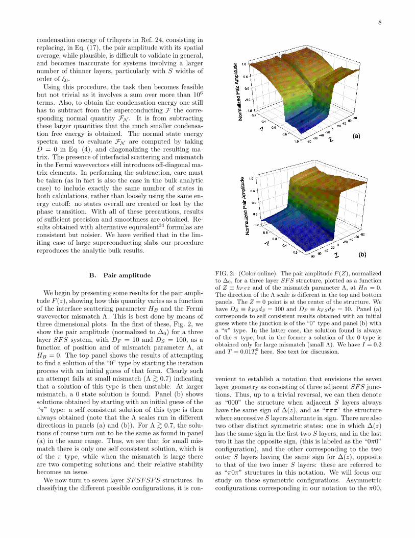
FIG. 3: (Color online). The normalized pair amplitude F (Z)for a seven layer SFSFSFS structure, plotted as in Fig. 2for the same parameter values. In panels (a) and (b), thethickness of all S layers is the same, while in panels (c) and (d)the thickness of the two inner S layers is doubled to 2DS = 200(see Fig. 1). Panels (a) and (c) correspond to an initial guessof the “000” type and panels (b) and (d) to a “πππ” type, (seetext). The configuration of the plotted self consistent resultscan be “000”, “πππ” or “π0π” as explained in the text.

and ππ0 states are not forbidden, but occur very rarelyand will be addressed only as need may arise. In Fig. 3we repeat the plots in Fig. 2 for seven layer structures.We include the cases in which all S layers are of the samethickness (top two panels) and the case where the thick-ness of the two inner S layers is doubled (bottom panels,see Fig. 1). In panels (a) and (c), the initial guess is ofthe 000 type, while in (b) and (d) it is of the πππ type.In the case of identical S layer widths, we see that a 000guess (Fig. 3(a)) yields a self consistent state of the same000 form only for larger mismatch, Λ <

∼ 0.5, while forsmaller mismatch the configuration obtained is clearly ofthe π0π form. Thus there is a value of Λ where two selfconsistent solutions cross over. However, a πππ guess(Fig. 3(b)) results in a self consistent πππ configurationfor the whole Λ range. Thus, there is a clear competitionbetween at least these three observed states, resultingfrom multiple minima of the free energy. Solutions ofthe 0π0 type are not displayed in this Figure but theywill be discussed below. In the two bottom panels we seethe same effects when the thickness of the inner S layersis doubled. As explained above, this describes a morebalanced situation, since the inner layers have magneticneighbors on both sides. It is evident from the figure thatthe pairing correlations are increased in the S layers. In

FIG. 4: (Color online). The pair amplitude F (Z) for a sevenlayer structure, plotted for the same parameter values andconventions as in the upper panels of Fig. 2, but as a functionof the dimensionless barrier height HB (at Λ = 1), ratherthan of the mismatch.

Fig. 3(c), there is also a noticeable shift in the crossoverpoint separating the 000 and π0π self consistent states,occurring now at smaller mismatch Λ ≈ 0.7. Again wefind the competition between the various states extendsthrough the entire range of Λ considered.

Next we consider in Fig. 4 the influence of the bar-rier height as represented by the dimensionless parame-ter HB . This figure is completely analogous to Fig. 3(a)and (b), except for the substitution of HB for Λ, which isset to unity (no mismatch). We find, by examining andcomparing the panels that two solutions of the πππ andπ0π type exist for small barrier heights (HB

<∼ 0.5), but

when HB becomes larger the πππ and 000 states thencompete. Another trend which one can clearly discern isthat the absolute values of F (Z) in the middle of the Slayers increase with HB. This makes sense, as at largerbarrier heights the layers become more isolated from eachother, and the proximity effects must in general weaken.

To conclude this discussion of F (z) we display in Fig. 5,the pair amplitude for the same three layer system as inFig. 2, as a function of position and of the magnetic ex-

10

FIG. 5: (Color online). The pair amplitude F (Z) for a threelayer structure, plotted for the same parameter values andconventions as in Fig. 2, but as a function of the dimensionlessmagnetic polarization I , at Λ = 1 and HB = 0.

change parameter I in its entire range, without a barrieror mismatch. Careful examination of the two panels re-veals a rather intricate situation: a solution of the π typeexists nearly in the entire I range (see Fig. 5(b)), the ex-ception being at very small I, where the magnetism be-comes weaker and, as one would expect, only the 0 statesolution is found. This requires small values of I, I <

∼ 0.1however. One can see that in a small neighborhood ofI ≈ 0.1, as the 0 state transitions to the π state, thepair amplitude is small throughout the structure. Thismay correspond to a marked dip in the transition tem-perature. At larger values of I, the two types of solutionscoexist, but there is a range around I = 0.2 where clearlythere is only one.

These results, which include for brevity only a verysmall subset of those obtained, are sufficient, we believe,to persuade the reader that although for some parame-ter values a unique self consistent solution exists, this iscomparatively rare, and that in general several solutionsof differing symmetry types can be found. These self con-sistent solutions correspond to local free energy minima:they are at least metastable. Furthermore, it is clear thatthe uniqueness or multiplicity of solutions depends in acomplicated way not only on the geometry, but also on

FIG. 6: (Color online). The normalized condensation freeenergy ∆E0 (see text) of a three layer SFS structure, plottedas a function of barrier height (top) and mismatch parameterΛ (bottom) for self consistent states of both the 0 and π types,as indicated. All other material parameters, geometrical val-ues, and temperature, are as in Fig. 2. The vertical arrowmarks the end, as either HB increases (top) or Λ increases(bottom), of the region of stability of the 0 state in this case.

the specific material parameter values.

C. Condensation Free Energy: Stability

One must, in view of the results in the previous sub-section, find a way to determine in each case the relativestability of each configuration and the global free energyminimum. This is achieved by computing the free energyof the several self consistent states, using the accuratenumerical procedures explained earlier in this Section.Results for this quantity, which at the low temperaturestudied is essentially the same as the condensation en-ergy, are given in the next figures below. The quantityplotted in these figures, which we call the normalized∆E0, is the condensation free energy (as calculated from

11

FIG. 7: (Color online). The normalized ∆E0 for a seven layerSFSFSFS structure plotted as a function of barrier height(top) and mismatch parameter Λ (bottom) for self consistentstates of the types indicated (see text for explanation). Ma-terial parameter and geometrical values are as in previousFigures, and all S layers are of the same thickness. The verti-cal arrows mark the end, as HB decreases (top) or Λ increases(bottom, see inset) of the region of stability of a certain state(see text).

Eq. (15) after normal state subtraction) normalized toN(0)∆2

0, which is twice the zero temperature bulk value(see Eq. 17). Therefore, at the low temperatures stud-ied, the bulk uniform value of the quantity plotted is veryclose to −(1/2).

In Figure 6 we plot ∆E0, defined and normalized asexplained, for a three layer SFS system. As in previousFigures, we have DS = 100, DF = 10 and I = 0.2. Re-sults for self consistent states of both the 0 and π typeare plotted as indicated. The top panel shows ∆E0 as afunction of the barrier thickness parameter HB at Λ = 1.The bottom panel plots the same quantity as a functionof mismatch Λ at zero barrier and should be viewed inconjunction with Fig. 2. Looking first at the top panel,one sees that the zero state is stable (has nonzero con-

FIG. 8: (Color online). Normalized ∆E0 for a seven layerSFSFSFS structure, as in Fig. 7, but for the case where thethickness of the two inner S layers is doubled.

densation energy) only for HB greater than about 0.31.An attempt to find a solution of the 0 type for HB justbelow its “critical” value by using a solution of that typepreviously found for a slightly higher HB as the startingguess, and iterating the self consistent process, leads aftermany iterations to a solution of the π type. This is indi-cated by the vertical arrow. At larger barrier heights,the two states become degenerate. This makes sensephysically: as the barriers become higher the proximityeffect becomes less important, and the S layers behavemore as independent superconducting slabs. The rela-tive phase is then immaterial. For even larger HB weexpect, from Eq. 17 and the geometry, the normalizedquantity plotted to trend, from above, toward a limit≈ −0.5(1 − DF /DS) = −0.45 and this is seen in the toppanel. One can also see that in the region of interest(barriers not too high), the absolute value of the conden-sation energy is substantially below that of the bulk. Inthe bottom panel similar trends can be seen: in the ab-sence of mismatch (Λ = 1) only the π state is found, and

12

FIG. 9: (Color online). The normalized ∆E0 for a three layerSFS system, as a function of the thickness dS of the S layers(given in units of ξ0) at fixed DF = 10, I = 0.2 and without abarrier or mismatch. Results for 0 and π self consistent statesare given as indicated.

its condensation energy exhibits a somewhat oscillatorybehavior as Λ decreases from unity. The 0 state does notappear until Λ is about 0.7 and attempts (by the proce-dure just described) to find it lead to a π solution uponiteration (arrow). This is in agreement with the results inFig. 2. For large mismatch the absolute value of ∆E0 in-creases, as the S slabs become more weakly coupled, witha trend toward the limiting value just discussed. A veryimportant difference between the top and bottom pan-els, however, is the crossing of the curves near Λ = 0.33in Fig. 6(b). This is in effect a first order phase transi-tion between the π and 0 configurations as the mismatchchanges.

The results of performing the same study for a sevenlayer system with four S layers can be seen in the nexttwo Figures. Figure 7 corresponds to the case where allthe S layers have the same thickness (DS = 100, and allother parameters also as in the previous figures), whilein Fig. 8 the thickness of the two inner S layers is dou-bled. Results for the four possible symmetric junctionconfigurations mentioned in conjunction with Fig. 3 aregiven, as indicated in the legends of Figs. 7 and 8. Threeof those configurations, 000, πππ and π0π have appearedamong the results in Figs. 3 and 4. The other configura-tion corresponds to the 0π0 sequence. We see that thereare some striking differences between these examples andthe three layer system. While in the latter case a configu-ration ceases to exist only when its condensation energytends to zero, now configurations can become unstableeven when, for nearby values of the relevant parameter,they still have a negative condensation energy. As thisoccurs, the vertical arrows in each panel indicate (an in-set is needed in one case for clarity) how the states trans-form into each other as one varies the parameters fromthe unstable to the stable region. Regardless of whether

FIG. 10: (Color online). The normalized ∆E0 for a threelayer SFS junction, as a function of the parameter I , forthree different S thicknesses (as labeled) and fixed DF = 10.Results for 0 and π self consistent states are given as indicated.

the inner layers are doubled or not, the tendency is forthe innermost junction to remain of the same type, whilethe two outer junctions flip. Comparing Fig. 7 and Fig. 8we see that the doubling of the inner layers has a clearquantitative effect without having any strong qualitativeinfluence. An important difference between the two casesis that in the first (all S layer widths equal) the two possi-ble states (π0π and πππ) at zero barrier and no mismatchare nearly degenerate, while in the other case, the πππconfiguration is favored. In the first case, the degener-acy is removed as the barrier height begins to increase,but Λ has a small effect in relative stability. In Fig. 8,bottom panel, the oscillatory effect of Λ near the no-mismatch limit is seen, as in the three layer case. Forlarge mismatch or barrier, the results become again de-generate and trend towards the appropriate limit. Weexpect these seven layer results to be at least qualita-tively representative of what occurs for larger values ofNL: thus, states of the types 000 · · ·000, ππ · · ·ππ, andπ00 · · · 00π (outer junctions one way and inner ones theother) should predominate for large NL.

It is at least of equal interest to study how the stabilitydepends on the geometry. We discuss this question in thenext four figures. First, in Fig. 9 we present results for

13

FIG. 11: (Color online). The normalized ∆E0 for a threelayer SFS system, as a function of dF , (rather than of I as inFig. 10) for four different S thicknesses (as labeled) and fixedI = 0.2, HB = 0, Λ = 1.

the condensation free energy of a three layer system asa function of dS/ξ0 at fixed DF = 10, I = 0.2, HB = 0,Λ = 1. We see that dS must be at least half a corre-lation length for superconductivity to be possible at allin this system. Convergence near that value is ratherslow, requiring approximately 200 iterations. The super-conducting state then begins occurring, for this value ofDF , in a π configuration only. When dS reaches ξ0, the πstate condensation energy reaches already an appreciablevalue that is consistent with that seen in the appropriatelimits of the panels in Fig. 6. The 0 state is still not at-tainable (again, consistent with Fig. 6) until dS reachesa somewhat larger value. The condensation energies ofthe two states converge slowly toward each other uponincreasing dS , but remain clearly non-degenerate well be-yond the range plotted. The small breaks in the 0 statecurve correspond to specific S widths that permit onlythe π state.

The behavior seen in Fig. 9 depends strongly on I.This dependence is displayed in Fig. 10 where we showthe normalized ∆E0 for the same system, as a function ofI, for three different values of dS . For the value I = 0.2,the results shown are consistent with Fig. 9, includingthe nonexistence of the 0 state at dS = ξ0. We nowsee, however, that it is not always the π state which isfavored, but that the difference in condensation energiesis an oscillatory function of I. This of course reflectsthat whether the 0 or the π state is preferred depends, allother things being equal, on the relation between DF and(k↑ − k↓)

−1, and this quantity (see Eq. (16)) depends onI. At intermediate values of I (centered around I = 0.5)the zero state is favored, and when I becomes very smallthe π state ceases to exist altogether (this can be seen alsoby examination of Fig. 5). As I → 0 the condensationenergy of the 0 state remains somewhat above the bulk

FIG. 12: (Color online). The normalized condensation freeenergy for a seven layer SFSFSFS system, as a functionof DF , for fixed I = 0.2, dS = ξ0, Λ = 1 and HB = 0.5.Results for the four possible symmetric self consistent statesare given, as indicated, for both the cases where all S layersare identical (top) and where the thickness of the inner onesis doubled (bottom). Lines are guides to the eye. Breaks (toppanel) indicate regions where a certain configuration is notfound.

value and, as one would expect, decreases slightly withincreasing dS . At larger values of I, the absolute values of∆E0 increase with dS and on the average decrease slowlywith I.

The oscillations in Fig. 10 as a function of I at con-stant dF can also be displayed by considering results as afunction of dF at constant I. We do so in Fig. 11 wherewe plot, for a three layer SFS system, ∆E0 as a functionof DF at constant I = 0.2 for four values of dS/ξ0. Onesees again that for this value of I the 0 state does notexist at dS = ξ0 and DF = 10 but that it appears atlarger values of dS/ξ0. The damped oscillatory behavioris quite evident. At larger values of dF the condensa-tion energies of the two states trend towards a commonvalue that increases in absolute value with dS . At a verysmall value of dF , which depends on dS , the π state be-gins to vanish, and the condensation free energy of the0 state tends then towards the bulk value. All of this isconsistent with simple physical arguments.

In Fig. 12 we extend the results of Fig. 11 to the sevenlayer system. In this case we consider only one value ofdS (dS = ξ0) but include a finite barrier thickness, HB =0.5. The finite barrier allows for the possibility of moredistinct states coexisting (see Figs. 7-8). We consider

14

both the cases where all S layers thicknesses are equal(top panel) and the case where the inner ones are doubled(bottom panel). All possible symmetric self consistentstates were studied, as indicated in the figure. In contrastwith the three layer example with no barrier, in the sevenlayer cases with HB = 0.5 all of the four symmetric states(000, πππ, π0π, 0π0) are at least metastable over a rangeof dF , even at dS = ξ0. In the top panel we see howeverthat only the 0π0 state is stable over the whole dF range.The πππ state reverts to the 0π0 state in the range 1.6 <

∼dF

<∼ 4.2, while the π0π state reverts to 000 state for

1.8 <∼ dF

<∼ 2.4. The 000 state is unstable for much of

the range for 6 <∼ dF

<∼ 12. It appears that in this range

the 000 state is sufficiently close to a crossover (see e.g.Fig. 7) that attempts to find it sometimes converge toan asymmetric π00 state, rather than the expected π0π.In these cases the number of iterations to convergence issubstantially increased, as the order parameter attemptsto readjust its profile. For the situation where the innerS layers are twice the width of the outer ones, we see(bottom panel) that all four symmetric configurations areeither stable or metastable for the whole dF range. Thisis consistent with Fig. 7, where at HB = 0.5 all four statesare present simultaneously. The condensation energy isof course lower than in the previous case, due to theincreased pairing correlations associated with the thickerS slabs. For both geometries oscillations arising from thescattering potential lead to deviations from the estimatedperiodicity determined by (k↑ − k↓)

−1. For sufficientlylarge dF the difference in energies becomes small. Onecan infer from these results than in superlattices withrealistic oxide barriers, where as the number of layersincreases a larger number of nontrivial possible statesarise, the number of local free energy minima that cancoexist will increase.

D. DOS

We conclude this section by presenting some resultsfor the DOS, as it can be experimentally measured. Theresults given are in all cases for the quantity Nσ(z, ǫ) de-fined in Eq. (14), summed over σ, and integrated overa distance of one coherence length from the edge of thesample. We normalize our results to the correspondingvalue for the normal state of the superconducting mate-rial, and the energies to the bulk value of the gap, ∆0.All parameters not otherwise mentioned are set to their“default” values outlined at the beginning of this section.

In the top panel of Fig. 13 we present results for anSFS trilayer, for two contrasting values of the mismatchparameter Λ. As usual, results labeled as “0” and “π”are for the case where the self consistent states plot-ted are of these types. The 0 and π state curves cor-responding to Λ = 0.67, where (see Fig. 6) the 0 state isbarely metastable, have clearly distinct signatures, witha smaller gap opening for the 0 state, and consequentlymore subgap quasiparticle states. Therefore, as can be

FIG. 13: (Color online). The normalized DOS (see text)for a SFS trilayer, plotted as a function of the energy (inunits of the bulk zero temperature gap). Results for both 0and π self consistent states are given, as indicated. In thetop panel, the DOS is shown at HB = 0 for two differentvalues of the mismatch parameter, Λ = 0.2, and 0.67, thelatter being a case for which the 0 state is nearly unstable(see Fig. 6). The bottom panel shows the DOS profile in theabsence of mismatch (Λ = 1), but with the interface scatteringparameter HB taking on the two values shown, chosen onsimilar criteria as the Λ values (see text).

seen in Fig. 2, when there is little mismatch the pair am-plitude is relatively large in the F layer. When thereis more mismatch the proximity effect weakens, the gapopens and large peaks form which progressively becomemore BCS-like as the mismatch increases (Λ decreases) toΛ = 0.2. This progression takes a different form for the 0and π states, as one can see by careful comparison of thecurves. In the bottom panel we demonstrate the effect ofthe barrier height. The results are displayed as in the toppanel, but with the dimensionless height HB taking theplace of the mismatch parameter. This Figure should beviewed in conjunction with the top panel of Fig. 6. Oneof the values of HB chosen (HB = 0.32) is again such thatthe 0 state is barely metastable, while for the other valuethe 0 and π states have similar condensation energies.For HB close to 0.31 there is a marked contrast betweenthe two plots, with the gap clearly opening wider, andcontaining more structure for the π state. At larger HB

the gap becomes larger in both cases, with the BCS-likepeaks increasing in height. Thus, as the barriers becomeslarger, one is dealing with nearly independent supercon-ducting slabs and the plots become more similar. Thelargest difference therefore, occurs, as for the mismatch,

15

FIG. 14: (Color online). The normalized local DOS for aseven layer system versus the dimensionless energy and mis-match parameter Λ. The panels are arranged as those inFig. 3: (a) and (b) show results obtained when all S layershave the same thickness, while in (c) and (d) that thicknessis doubled. Panels (a) and (c) correspond to starting the it-eration procedure with a 000 order parameter, while panels(b) and (d) are obtained by starting with a πππ junction, inwhich case the self-consistent solution is also always of thistype.

at the intermediate values more likely to be found exper-imentally.

It is also illustrative to display the DOS in a threedimensional format. Thus, in Fig. 14, the normalizedDOS is presented as a function of ǫ/∆0 and Λ for theseven layer structures previously discussed. This permitsa much more extensive range of Λ values to be exam-ined. The panel arrangement is the same as in Fig. 3: inthe top two panels, all S layers have the same thickness(dS = ξ0) while in the bottom ones the thickness of theinner ones is doubled. On the right column (panels (b)and (d)) the self-consistent results shown were obtainedby starting the iteration process with an initial guess ofthe πππ type, in which case, as one can see from Fig. 3and the bottom panels of Figs. 7 and 8, the solution isalso of the πππ type. The left column panels were ob-tained from an initial guess of the 000 type and thereforecorrespond, as one can see from Figs. 3, 7 and 8, to solu-tions of the 000 type for Λ <

∼ 0.5 (panel (a)) and Λ <∼ 0.7

(panel (c)), and to solutions of the 0π0 type otherwise.There is no overlap among the results in the four panels.One sees again that as mismatch increases the BCS likepeaks become more prominent and move out, trendingtowards their bulk positions, while the gap opens. Fur-thermore, the πππ results for the doubled dS inner layersare smoother and show clearly a broader gap throughout,due to the extended S geometry. The DOS behavior ob-

served here is entirely consistent with the condensationenergy results found.

IV. CONCLUSIONS

In summary, we have found self consistent solutions tothe microscopic BdG equations for SFS and SFSFSFSstructures, for a wide range of parameter values. Wehave shown that, in most cases, several such self consis-tent solutions coexist, with differing spatial dependenceof the pair potential ∆(r) and the pair amplitude F (r).Thus, there can be in general competing local minima ofthe free energy. Determining their relative stability re-quires the computation of their respective condensationfree energies, which we have done by using an efficient,accurate approach that does not involve the quasiparticleamplitudes directly, and requires only the eigenenergiesand the pair potential.

For SFS trilayers (single junctions), we found thatboth π and 0 junction states exist for a range of valuesof the relevant parameters. We have displayed resultsfor the pair amplitude, which give insight into the su-perconducting correlations, and for the condensation freeenergies of each configuration, to determine the true equi-librium state. We have shown that a transition (whichis in effect of first order in parameter space) can occurbetween the 0 and π states for a critical value of Λ. Thedifference in condensation energies between the two pos-sible states exhibits oscillations as a function of I. Thisbehavior is strongly dependent on the width of the S lay-ers. For dS equal to one coherence length ξ0, there existsa range of I in which either a 0 or π state survives, butnot both. Increasing the S width by about ξ0/2 restoresthe coexistence of both states.

Several interesting phenomena arise when one exploresthe geometrical parameters of trilayer structures. For afixed ferromagnet width dF , and parameters values thatlead to a π state, we found (see Fig. 9) that the π con-figuration remains the ground state of the system as dS

varies. The π state first appears at small dS (dS ≈ ξ0/2),and then its condensation energy declines monotonicallytowards the bulk limit. The metastable 0 state begins atlarger dS ≈ ξ0, and its condensation energy declines alsoslowly over the range of dS studied. The other relevantlength that was considered is dF . The condensation en-ergy is, for both states, an oscillatory function of dF . Theoscillations become better defined, and the possibility ofboth 0 and π states coexisting increases, at larger dS .As expected, we find that the condensation energy hasvery similar properties when either dF or I varies. Theperiod approximately agrees with the estimate given by(k↑−k↓)

−1, which governs the oscillations of the pair am-plitude and in general, of other single particle quantities.The results for the DOS reflect the crossover from a statewith populated subgap peaks to a nearly gapped BCS-like behavior as Λ is decreased or the barrier height HB

increased. Signatures that may help to experimentally

16

identify the 0 and π configurations were seen.As the number of layers increases, so does the number

of competing stable and metastable junction configura-tions. We considered two types of seven layers structures,and found that doubling the width of the inner S lay-ers (which are bounded on each side by ferromagnets),resulted typically in different quasiparticle spectra andpair amplitudes, compared to the situation when all Slayers have the same dS . For large mismatch or barrierstrength, the phase of the pair amplitude in each layeris independent, and configurations are nearly degener-ate, but as each of these parameters diminishes thereis a crossing over to a situation where the free energiesof each configuration are well-separated. At certain val-ues of Λ and HB, some configurations become unstable.These values are different depending on the type of sys-tem (single or double inner layers). For fixed I and dF

we found that if a state is stable at no mismatch andzero barrier, then it remains at least metastable over avery wide range of Λ and HB values. Our results showedthat self-consistency cannot be neglected as the numberof layers increases, due to the nontrivial and intricatespatial variations in F (r) that become possible.

For seven layers, we studied in detail the condensa-tion free energies of the four symmetric junction states,000, πππ, π0π and 0π0, in the previously introduced no-tation. We first investigated the stable states as a func-tion of Λ and HB . In contrast to the three layer system,we found that states could become unstable even whenthe condensation energy did not tend to zero for nearbyvalues of the relevant parameters. For double width in-ner layered structures, we found a greater spread in thefree energies between the four states, and the instabil-ity found in certain cases for the 000 and 0π0 states wasshifted in Λ and HB , in agreement with the pair ampli-tude results. It is reasonable to assume that these resultsare representative of what occurs for superlattices. Weagain found transitions upon varying Λ and the numberand sequence of the transitions is now more intricate (seeFigs. 7 and 8). The analysis of the geometrical propertiesrevealed that scattering at the interfaces modifies the ex-pected damped oscillatory behavior of the condensationenergy as a function of dF . In effect, the barriers intro-duce significant atomic scale oscillations that smear the

periodicity. This underlines the importance of a micro-scopic approach for the investigation of nanostrucutres.As with the Λ dependence, we also showed that the globalminima in the free energy is different for the two struc-tures as dF changes. The configuration of the groundstate of the system with S layers of uniform width wasmore variable in parameter space, compared to when theinner layers are doubled, (compare Figs. 7 and 8). Fi-nally, we calculated the DOS, to illustrate and comparethe differences in the spectra for the two different sevenlayer geometries. Of the two, the energy gap for the singleinner layer case, and πππ stable state, contains more sub-gap states, for the specific examples plotted (Figs. 13 and14) due to stronger pair breaking effects of the exchangefield. These states fill in increasingly with decreased mis-match.

Our results were obtained in the clean limit, which isappropriate for the relatively thin structures envisionedhere. Furthermore, as shown in Ref. 28 in conjunctionwith realistic comparison with experiments,35 the influ-ence of impurities can be taken into account by replac-ing the clean value of ξ0 with an effective one. A sep-arate important issue is that of the free energy barri-ers separating the different free energy minima we havefound, and hence to which degree are metastable stateslong lived. Our method cannot directly answer this ques-tion, but from the macroscopic symmetry differences inthe pair amplitude structure of the different states onewould have to conclude that the barriers are high andthe metastable states could be very long lived. We ex-pect that the transitions found here in parameter spaceat constant temperature will be reflected in actual firstorder phase transitions as a function of T . Such transi-tions would presumably be very hysteretic. We hope toexamine this question in the future.

Acknowledgments

The work of K. H. was supported in part by a grantof HPC time from the Arctic Region SupercomputingCenter and by ONR Independent Laboratory In-houseResearch funds.

∗ Electronic address: klaus.halterman@navy.mil† Electronic address: otvalls@umn.edu1 A.F. Andreev, Zh. Eksp. Teor. Fiz. 46, 1823 (1964) [Sov.

Phys. JETP 19 1228 (1964)].2 P. Fulde and A. Ferrell, Phys. Rev. 135, A550 (1964).3 A. Larkin and Y. Ovchinnikov, Sov. Phys. JETP 20, 762

(1965).4 O. Vavra, S. Gazi, J. Bydzovsky, J. Derer, E. Kovacova, Z.

Frait, M. Marysko, and I. Vavra, J. Magn. Mangn. Mater.240, 583 (2002);C. Surgers, T. Hoss, C. Schonenberger,and C. Strunk, ibid. 240, 598 (2002).

5 C. Bell, G. Burnell, C.W. Leung, E.J. Tarte, D.-J. Kang,and M.G. Blamire, Appl. Phys. Lett. 84, 1153 (2003).

6 J.S. Jiang, D. Davidovic, D.H. Reich, and C.L. Chien,Phys. Rev. Lett. 74, 314 (1995); Phys. Rev. B 54, 6119(1996).

7 M. Lange, M.J. Van Bael, and V.V. Moshchalkov, Phys.Rev. B 68, 174522 (2003).

8 W. Guichard, M. Aprili, O. Bourgeois, T. Kontos, J.Lesueur, and P. Gandit, Phys. Rev. Lett. 90, 167001(2003).

9 T. Kontos, M. Aprili, J. Lesueur, F. Genet, B. Stephanidis,

17

and R. Boursier, Phys. Rev. Lett. 89, 137007 (2002).10 V.V. Ryazanov, V.A. Oboznov, A.Y. Rusanov, A.V.

Veretennikov, A.A. Golubov, and J. Aarts, Phys. Rev.Lett. 86, 2427 (2001).

11 A.V. Veretennikov, V.V. Ryazanov, V.A. Oboznov, A.Y.Rusanov, V.A. Larkin, and J. Aarts, Physica B 284, 495(2000).

12 S.M. Frolov, D.J. Van Harlingen, V.A. Oboznov, V.V. Bol-ginov, and V.V. Ryazanov, cond-mat/0402434 (2004).

13 E. Goldobin, A. Sterck, T. Gaber, D. Koelle, and R.Kleiner, Phys. Rev. Lett. 92, 057005 (2004).

14 L.N. Bulaevskii, V.V. Kuzii, and A.A. Sobyanin, Pis’maZh. Eksp. Teor. Fiz. 25, 314 (1977) [JETP Lett. 25, 290(1977)].

15 E.A. Demler, G.B. Arnold, and M.R. Beasley, Phys. Rev.B 55,15 174 (1997).

16 A.I. Buzdin and M.Y. Kuprianov, Pis’ma Zh. Eksp. Teor.Fiz. 53, 308 (1991) [JETP Lett. 53, 321 (1991)].

17 N.M. Chtchelkatchev, W. Belzig, Y.V. Nazarov, and C.Bruder, JETP Lett. 74, 323 (2001).

18 Z. Radovic, L.D-Grujic, and B. Vujicic, Phys. Rev. B 63,214512 (2001).

19 F.S. Bergeret, A.F. Volkov, and K.B. Efetov, Phys. Rev.B 64, 134506 (2001).

20 H. Sellier, C. Baraduc, F. Lefloch, and R. Calemczuk,Phys. Rev. B 68, 054531 (2003).

21 Z. Radovic, N. Lazarides, and N. Flytzanis, Phys. Rev. B68, 014501 (2003).

22 A. Zenchuk and E. Goldobin, Phys. Rev. B 69, 024515(2004).

23 A. Buzdin, A.E. Koshelev, Phys. Rev. B 67, 220504 (2003).24 K. Halterman and O.T. Valls, Phys. Rev. B 69, 014517

(2004).25 M. Ozana and A. Shelankov, Phys. Rev. B 65, 014510

(2001).26 P.G. de Gennes, Superconductivity of Metals and Alloys

(Addison-Wesley, Reading, MA, 1989).27 K. Halterman and O.T. Valls, Phys. Rev. B 65, 014509

(2002).28 K. Halterman and O.T. Valls, Phys. Rev. B 66, 224516

(2002).29 Y.N. Proshin, Y.A. Izyumov, and M.G. Khusainov, Phys.

Rev. B 64, 064522 (2001).30 M. Tinkham, Introduction to Superconductivity, (Krieger,

Malabar FL) (1975).31 A. L. Fetter and J.D. Walecka, Quantum Theory of many-

particle systems, (McGraw-Hill, New York NY) (1971).32 I. Kosztin, S. Kos, M. Stone, and A.J. Leggett, Phys. Rev.

B 58, 9365 (1998).33 J.B. Ketterson and S.W. Song, Superconductivity, (Cam-

bridge University Press, Cambridge UK) (1999).34 The equivalence of different formulas is discussed by

C.W.J. Beenaker and H. van Houten, in Proceedings of In-

ternational Symposium on Nanostructures and Mesoscopic

systems, ed. by W.P. Kirk and M.A. Reed, Academic Press,New York, (1991).

35 N. Moussy, H. Courtois, and B. Pannetier, Europhys. Lett.55, 861, (2001).