VJEŽBA 2: MJERENJE TEMPERATURE 4. OPĆENITO O MJERENJU TEMPERATURE
Upload
khangminh22Category
view
0download
0
Oxygen Dynamics in the High-TemperatureSuperconductor LSCO+O
PhD Thesis in Physics by
Tim Tejsner
SupervisorLinda Udby, Niels Bohr Institute
Co-supervisorsMartin Boehm, Institut Laue-LangevinAndrea Piovano, Institut Laue-Langevin
This thesis has been submitted tothe PhD School of The Faculty of Science,
University of Copenhagen
December, 2019


Abstract
Understanding the mechanisms of high-temperature superconductivity in the cuprates remainsone of the great unsolved questions of condensed matter physics. Hole-doping the Mott-insulatorLa2CuO4 with various chemical species creates a superconductor with a transition temperature Tcthat depends heavily on the amount and type of doped species. While the amount of hole-dopingtypically dictates the phase diagram, there are certain situations where superconductivity can besuppressed or enhanced due to structural modifications caused by the dopant species. In thisthesis, I investigate these structural modifications and, in particular, related dynamics in order tobetter understand any possible relationship to superconductivity.
A particular interesting sample in this context is La2−xSrxCuO4+δ (LSCO+O), where dopingcan be performed with two distinct chemical species, Sr and O. Doping with Sr is ‘quenched’,meaning that Sr has a fixed, random distribution on La sites. On the other hand, doping with Ois performed after crystal growth using electrochemical methods. Oxygen dopants are ‘annealed’in the sense that they sit on interstitial sites and are mobile at room temperature. In addition,doping with O creates a superconductor with slightly better Tc that is equipped with a numberof unique phenomena such as electronic phase separation and complex superstructures. In thisthesis, various aspects of phonon dynamics in LSCO+O are investigated through a combinationof theoretical and experimental methods. Density functional theory and molecular dynamics isused to numerically estimate the phonon band structure and density of states. Inelastic neutronscattering is used to probe phonon dynamics and the two methods are compared.
Despite the fact that Density Functional Theory is known to struggle with the electronic struc-ture of the cuprates, excellent agreement between phonon dynamical simulations and experimentsare found. An analysis of this relationship reveals unique dynamics of octahedral tilt patterns dueto interstitial oxygen. We speculate that these tilt patterns may assist in relieving the inherentfrustration between magnetism and superconductivity in LSCO+O. Finally, anomalous featuresin the Cu-O bond stretching phonon of two different LSCO+O samples is observed with neutronscattering. This ‘phonon anomaly’ is suspected to be a signature of charge density fluctuations thatmight be important for superconductivity. While previously observed in Sr-doped La2−xSrxCuO4,this result rules out a phonon anomaly caused by structural mechanism related to the specificdopant type.
1

Resumé
Forståelsen af høj-temperatur superledning i kupraterne er stadig et uløst spørgsmål i faststoffysikken.Ved at huldope det Mott-insulatorende materiale La2CuO4 med forskellige kemiske arter, skabesen superleder med en overgangstemperatur Tc der afhænger kraftigt af typen og mængden afdenne kemiske ‘dopant’. Selvom mængden af huldoping typisk dikterer fasediagrammet, er dersituationer hvor superledning kan understrykkes eller forbedres på baggrund af strukturelle modi-fikationer forudsaget af den kemiske dopant. I denne afhandling undersøges disse strukturellemodifikationer, og især den relaterede dynamik, for bedre at forstå en eventuel relation til super-ledning.
En særligt interessant prøve i denne sammenhæng er La2−xSrxCuO4+δ (LSCO+O), hvor dop-ing kan udføres med to forskellige kemiske arter, Sr og O. Doping med Sr er ‘quenched’, hvilketbetyder at Sr har en fikseret, tilfældig distribution. På den anden side, udføres doping med O vedbrug af elektrokemiske metoder after krystallen er groet. Oxygen doping er derfor ‘annealet’ i denforstand at O sidder på interstitielle sites og er mobile ved stuetemperatur. Derudover skaber dop-ing med O en superleder med lidt bedre Tc der er udstyret med en række unikke fænomener somelektronisk faseseperation og komplekse superstrukturer. I denne afhandling undersøges diverseaspeketer af fonon-dynamik i LSCO+O gennem en komination af teoretiske og eksperimentellemetoder. Density Functional Theory og molekyledynamik bruges til at estimere fonon bånd-strukuter og density-of-states. Inelastisk neutron spredning bruges til at undersøge fonon dynamikeksperimentelt og de to metoder sammenlignes.
Selvom Density Functional Theory ikke kan beskrive den elektroniske struktur af kuprater,finder vi en fremragende overensstemmelse mellem simulering og eksperiment i kontekst af fonon-dynamik. En analyse af denne overensstemmelse afslører unik dynamik af octahedrale tilt-mønstresom konsekvens af interstitiel oxygen. Vi formoder at disse tilt-mønste kan assistere til at lindreden kendte frustration mellem magnetisme og superledning i LSCO+O. Afslutningsvis undersøgervi en såkaldt fonon-anomali relateret til en Cu-O vibration i to forskellige LSCO+O prøver vedhjælp af neutronspredning. Denne fonon-anomaly mistankes for at være relateret til ladningsfluk-tationer som igen mistænkes for at være vigtigt for superledning. Selvom denne anomali tidligereer observeret i Sr-dopet La2−xSrxCuO4, udelukker dette resultat en fonon-anomali forudsaget afstrukturelle mekanismer relatret til den specifikke dopant.
3


Contents
1 Introduction 71.1 Superconductivity . . . . . . . . . . . . . . . . . . . . . . . . . . . . . . . . . . . . 71.2 Cuprates . . . . . . . . . . . . . . . . . . . . . . . . . . . . . . . . . . . . . . . . . . 91.3 La214 . . . . . . . . . . . . . . . . . . . . . . . . . . . . . . . . . . . . . . . . . . . 151.4 LSCO+O . . . . . . . . . . . . . . . . . . . . . . . . . . . . . . . . . . . . . . . . . 171.5 Thesis objectives . . . . . . . . . . . . . . . . . . . . . . . . . . . . . . . . . . . . . 19
2 Methods 212.1 Neutron Scattering . . . . . . . . . . . . . . . . . . . . . . . . . . . . . . . . . . . . 212.2 Specific Scattering Methods . . . . . . . . . . . . . . . . . . . . . . . . . . . . . . . 252.3 Density Functional Theory . . . . . . . . . . . . . . . . . . . . . . . . . . . . . . . 292.4 Phonon Calculations . . . . . . . . . . . . . . . . . . . . . . . . . . . . . . . . . . . 332.5 Molecular Dynamics . . . . . . . . . . . . . . . . . . . . . . . . . . . . . . . . . . . 392.6 Comparing Simulation and Experiment . . . . . . . . . . . . . . . . . . . . . . . . 41
3 Phonon Calculations 453.1 Computational Details . . . . . . . . . . . . . . . . . . . . . . . . . . . . . . . . . . 453.2 Electronic and Structural Phases . . . . . . . . . . . . . . . . . . . . . . . . . . . . 473.3 Coordinate systems . . . . . . . . . . . . . . . . . . . . . . . . . . . . . . . . . . . . 483.4 Strategy . . . . . . . . . . . . . . . . . . . . . . . . . . . . . . . . . . . . . . . . . . 513.5 Benchmarking . . . . . . . . . . . . . . . . . . . . . . . . . . . . . . . . . . . . . . . 513.6 Geometry optimization . . . . . . . . . . . . . . . . . . . . . . . . . . . . . . . . . . 533.7 Phonons . . . . . . . . . . . . . . . . . . . . . . . . . . . . . . . . . . . . . . . . . . 573.8 Validation of simulations . . . . . . . . . . . . . . . . . . . . . . . . . . . . . . . . . 613.9 Summary . . . . . . . . . . . . . . . . . . . . . . . . . . . . . . . . . . . . . . . . . 62
4 Molecular Dynamics 634.1 Computational Details . . . . . . . . . . . . . . . . . . . . . . . . . . . . . . . . . . 634.2 Octahedral tilts . . . . . . . . . . . . . . . . . . . . . . . . . . . . . . . . . . . . . . 634.3 Structures with dopant ions . . . . . . . . . . . . . . . . . . . . . . . . . . . . . . . 644.4 Geometry Optimization . . . . . . . . . . . . . . . . . . . . . . . . . . . . . . . . . 654.5 Benchmarking . . . . . . . . . . . . . . . . . . . . . . . . . . . . . . . . . . . . . . . 674.6 DOS and PDF . . . . . . . . . . . . . . . . . . . . . . . . . . . . . . . . . . . . . . 684.7 Microscopic analysis . . . . . . . . . . . . . . . . . . . . . . . . . . . . . . . . . . . 694.8 Summary . . . . . . . . . . . . . . . . . . . . . . . . . . . . . . . . . . . . . . . . . 73
5 Local structure 775.1 Superstructures in single crystals . . . . . . . . . . . . . . . . . . . . . . . . . . . . 775.2 Real-space correlation in powders . . . . . . . . . . . . . . . . . . . . . . . . . . . . 795.3 Summary . . . . . . . . . . . . . . . . . . . . . . . . . . . . . . . . . . . . . . . . . 85
6 Low Energy Lattice Dynamics 876.1 Acoustic Phonons and Simulation Validation . . . . . . . . . . . . . . . . . . . . . 876.2 Structural instabilities . . . . . . . . . . . . . . . . . . . . . . . . . . . . . . . . . . 926.3 Low energy modes of superstructures . . . . . . . . . . . . . . . . . . . . . . . . . . 946.4 Summary . . . . . . . . . . . . . . . . . . . . . . . . . . . . . . . . . . . . . . . . . 96
5

6 CONTENTS
7 Phonon Density of States 977.1 Experiment . . . . . . . . . . . . . . . . . . . . . . . . . . . . . . . . . . . . . . . . 987.2 Results . . . . . . . . . . . . . . . . . . . . . . . . . . . . . . . . . . . . . . . . . . . 997.3 Comparison with Simulation . . . . . . . . . . . . . . . . . . . . . . . . . . . . . . 1017.4 Summary . . . . . . . . . . . . . . . . . . . . . . . . . . . . . . . . . . . . . . . . . 102
8 Phonon Anomalies 1058.1 Motivation . . . . . . . . . . . . . . . . . . . . . . . . . . . . . . . . . . . . . . . . 1058.2 Phonon Anomalies . . . . . . . . . . . . . . . . . . . . . . . . . . . . . . . . . . . . 1058.3 Experiment . . . . . . . . . . . . . . . . . . . . . . . . . . . . . . . . . . . . . . . . 1068.4 Phonon Anomaly and Magnetic Stripe Order . . . . . . . . . . . . . . . . . . . . . 1088.5 Discussion . . . . . . . . . . . . . . . . . . . . . . . . . . . . . . . . . . . . . . . . . 1098.6 Summary . . . . . . . . . . . . . . . . . . . . . . . . . . . . . . . . . . . . . . . . . 110
9 Electronic Structure 1139.1 Sample . . . . . . . . . . . . . . . . . . . . . . . . . . . . . . . . . . . . . . . . . . . 1139.2 Experiment . . . . . . . . . . . . . . . . . . . . . . . . . . . . . . . . . . . . . . . . 1149.3 Summary . . . . . . . . . . . . . . . . . . . . . . . . . . . . . . . . . . . . . . . . . 114
10 Conclusion 11710.1 Oxygen Interstitial Observables . . . . . . . . . . . . . . . . . . . . . . . . . . . . . 11810.2 Phonons and Stripes . . . . . . . . . . . . . . . . . . . . . . . . . . . . . . . . . . . 119
A PhononNeutron 121
B Low energy phonons, additional plots 123
C Phonon DOS, additional plots 131
Bibliography 133

Chapter 1
Introduction
In this thesis, I explore certain aspects of the so-called high-temperature superconductors. Whilethese materials were discovered fairly recently (1986), they have a rich history with hundreds ofthousands of citations and, to this day, a lively debate surrounding the microscopic nature of thismysterious macroscopic quantum state. The purpose of this chapter is to briefly state the ‘thestory so far’ in broad strokes, and then dive deeper into state-of-the-art research relevant for thework performed in this thesis.
1.1 Superconductivity
Superconductivity is a state of matter where a material is able to conduct electricity with zeroDC resistance below a certain critical temperature Tc. Since we, fortunately, live in a world wherethe ‘spherical cow in a vacuum’ model is a very crude approximation to reality, it is remarkableto find real materials where electrons can propagate without friction. In fact, experiments haveshown, that under the right conditions it is possible to keep a persistent superconducting currentrunning for 100000 years [1]!
Superconductivity was first discovered in 1911 by Heike Kamerlingh Onnes, essentially as aconsequence of being able to liquefy helium in 1908 and reach temperatures close to absolute zero(see ref. [2] and references therein for a breakdown of the experiments). His low-temperaturemeasurement of lead revealed a sudden drop in resistivity at 4.2K, as seen in the historic plot onfigure 1.1
Despite this remarkable experimental result, it would take 20 years for the next major milestoneto appear. In 1933 the Meissner effect was discovered [4], showing that superconducting materialswould completely resist an applied magnetic field by exhibiting perfect diamagnetism as sketched infigure 1.2. In 1935 this effect was phenomenologically explained by the London equations, showingthat the Meissner effect is due to superconducting currents on the surface of the material [5]. Fromtheir relatively simple set of equations, an observable length scale known as the penetration depth
Figure 1.1: Left: Kammerling Onnes (right) and his chief engineer (left) in their cryogenics lab.Right: Resistivity as a function of temperature in elemental Lead. Both images from ref. [2].
7

8 CHAPTER 1. INTRODUCTION
Figure 1.2: The Meissner effect. As a superconducting material is cooled below Tc, the appliedmagnetic field B is completely expelled due to superconducting currents on the surface. As aconsequence there is no magnetic flux inside the superconducting material, in contrast to the samesituation for ‘normal’ conductors. Figure from [3].
was definedλL =
√m
µ0nq2
where µ0 is the permeability of free space, n the number concentration of the superconducting car-riers, m the electron mass and q the electron charge. This length scale determines how an externalmagnetic field penetrates the superconductor through the relationship B(x) = B(0) exp(−x/λ). λis typically on the order of 20 nm to 100 nm [6].
Another roughly 20 years would pass until Landau’s work on phase transitions paved the wayto understanding the superconducting phase transition as a thermodynamic quantity through theGinzburg-Landau equations in 1950 [7]. I will not repeat the details here, but the idea is to make apolynomial expansion of the free energy as a function of a complex superconducting wavefunctionψ. As the material is cooled below Tc, ψ ‘chooses’ a phase and breaks gauge symmetry, analogousto how a ferromagnet choses a common direction for the magnetic moment at the magnetic phasetransition. This description predicts an new characteristic length scale of the superconductor calledthe coherence length ξ and recasts the penetration depth in terms of ψ:
ξ =
√h2
4m|α|λ =
√m
4µ0e2ψ20
,
where α is a phenomenological parameter of the polynomial expansion. The ratio of these paramet-ers, κ = λ/ξ, are used to classify superconductors into type-I (κ < 1/
√2) and type-II (κ > 1/
√2).
The significance of κ > 1/√2 can be understood as a threshold where the surface tension between
normal and superconducting phases becomes negative [8]. Intuitively, the coherence length ξdefines the shortest length within which the superconducting carrier concentration are allowedto change considerably. For elemental metals ξ can be on the nanometre to micrometre scale:1600 nm in Al and 83 nm in Pb [6]. In the cuprates (which will be discussed in detail in the nextsection), ξ is typically on the order of a few lattice spacings (1 nm in YBa2Cu3O7−δ [9]).
Based on Ginzburg-Landau theory, Abrikosov predicted the existence of vortices in Type-IIsuperconductors, which showed excellent agreement with the measured magnetization of severallead alloys [8]. These vortices can be pinned by defects and form a lattice that we have beenable to image using modern day microscopy techniques (see e.g. [10] for a recent example withbeautiful real-space images). The experimental evidence piled up [11, 12], and it quickly becameevident that Ginzburg-Landau theory is applicable to most known superconductors, including thecuprates and iron-based varieties.
Despite the descriptive power of Ginzburg-Landau theory, we are left with no recipe on how toconstruct, even theoretically, ‘better’ superconductors. In order to manipulate material properties,

1.2. CUPRATES 9
it is necessary to understand the microscopic properties that lead to macroscopic behaviour (e.g.how phonons influence thermal properties or how magnetic exchange influences magnetic proper-ties. Inspired by Ginzburg-Landau theory, rapid progress towards a microscopic theory was beingmade in the mid 1950s, culminating in the famous BCS theory formulated by Bardeen, Cooperand Schrieffer [13].
BCS theory is based on the assumption that an attractive interaction between electrons atthe Fermi level can result in so-called ‘cooper-pairs’, a bosonic quasi-particle consisting of anelectron pair with opposite momentum and spin. The bosonic nature of this quasi-particle can,at low temperatures, result in a Bose-Einstein condensate where a large fraction of these electronpairs occupy the lowest energy quantum state. This microscopic theory of superconductivitymade several testable predictions, such as the appearance of an energy gap with a temperature-dependent width ∆(T ) in the electronic density of states related to the critical temperature throughthe relationship
2∆(T = 0) = 3.5kBTc ,
where kB is the Boltzmann constant. A few years later electron tunnelling experiments confirmedthis prediction with reasonable accuracy [14, 15]. Additionally, Josephson predicted that super-conducting currents could tunnel across an insulating barrier [16], experimentally verified a fewyears later [17].
While BCS theory predicts an attractive interaction between electrons, the original paper[13] makes no assumption about the nature of this interaction. Some experiments, performeda few years prior, showed that Tc of Hg198 was higher when compared to that of natural Hg(avg. atomic weight of 200.6) [18, 19]. Since the chemistry of these materials can be assumedidentical, this experiment suggests a positive correlation between phonon frequencies and Tc, sincelighter elements have more energetic vibrations. Assuming an attractive potential due to latticevibrations, BCS theory could relate the attractive interaction to phonon frequencies and predict arelative relationship between isotopic mass and critical temperature [20]:
Tc ∝ 1√mion
,
where mion is the isotopic mass of the constituent ionic species. With BCS theory, supercon-ductivity in many elemental metals were believed to be ‘solved’ with the identification of phonon-mediated superconductivity. Unfortunately, this discovery also set a practical upper limit on Tc.In order to increase phonon frequencies, and thus critical temperatures, we need materials withlow mass atomic species, while still being crystalline. At ambient pressure this practical upperlimit is often quoted to be around 30K. A good demonstration of this principle is the case of H2Swhere researchers were able to reach a critical temperature of Tc = 200K by applying a pressureof 155GPa [21]. This material contains the light atomic species we require, but cannot crystallizeat ambient pressures so we can only reach high critical temperatures under extreme conditions. Adifferent example is the highly unusual case of MgB2, where coincidences add up to an unusuallyhigh electron-phonon coupling resulting in a critical temperature of Tc = 39K [22].
While this thesis is about cuprates, which cannot be described within the BCS framework, Ibelieve that the history of conventional superconductivity emphasizes exactly what is desired froma ‘solution’ to high-temperature superconductivity. It is also a fascinating story due to the factthat the tools to solve the problem were not even close to being developed when the phenomenonwas discovered. It took roughly 50 years for a satisfying conclusion and we have only been workingon the cuprates for roughly 30 years.
1.2 Cuprates
With this brief introduction to superconductivity, I will proceed with an introduction to cupratesuperconductivity. While the previous section contains research results and explanations generallyaccepted and agreed upon, it is difficult to capture an unbiased view of cuprate research. Assuch, the following will be somewhat narrowly focused. While this is a reasonable choice for thisintroduction, it is important to realize just how massive the field is and how impossible it is toknow every last detail.
Before we begin, I want to establish some of the nomenclature As the title of this thesis suggests,I am working on the so-called ‘high-temperature superconductors’. This definition essentially onlyconcerns itself with the value of the critical temperature (usually above the ‘BCS-limit’ of 30K),without saying anything about other physical properties. On the other hand Type-I and Type-II, as seen in the previous section, are rigidly defined with respect to their properties as defined

10 CHAPTER 1. INTRODUCTION
Table 1.1: list of common cuprate families. In the case of La-214, doping is performed by ex-changing La with Re = Sr, Ba or by the introduction of additional oxygen δ. In Y-123, doping isperformed by removing a small amount of oxygen δ. n is the number of CuO2 layers per ‘copperoxide block’ (see figure 1.3)
Chemical Formula Name Optimal Tc [K] References
La2−xRexCuO4+δ La-214 / LSCO 40 [23]YBa2Cu3O7−δ Y-123 / YBCO 93 [24]Bi2Sr2Can−1CunO2n+4 Bi-22(n-1)n 120 [25]Ti2Ba2Can−1CunO2n+4 Ti-22(n-1)n 127 [26–29]HgBa2Can−1CunO2n+2 Hg-12(n-1)n 133 [30, 31]
through Ginzburg-Landau Theory. Finally, ‘conventional superconductors’ are those that can bemicroscopically described with BCS theory, while ’unconventional superconductors’ cannot. Whilecuprates are relatively simple crystals, most of them have a variety of names and abbreviationsattached to them. Table 1.1 lists the most important ones along with their critical temperatures.
The discovery of LBCORoughly 30 years after BSC theory was nailed down, in 1986, Bednorz and Müller discovereda new type of superconductor while trying to manipulate the electronic properties of the anti-ferromagnetic insulator La2CuO4. By effectively removing a small number of electrons from thesystem by substitution of dopant species, they achieved a record Tc of 30K. Shortly after, in1987, the sister-compound YBa2Cu3O7−δ was discovered, shattering previous records and finallyachieving a critical temperature Tc = 93K that could be reached using liquid nitrogen [24].
While the increased critical temperatures are remarkable on their own, it quickly becameapparent that we were dealing with a completely new type of superconductivity which cannot beexplained with BCS theory. The normal state (T > Tc) of cuprate superconductors is as, if notmore, complex when compared to the superconducting state and the BCS assumption of beingmetallic in the normal state is generally not fulfilled. In addition, the BCS relationship betweenisotopic mass critical temperature (Tc ∝ m−0.5
ion ) is not fulfilled when performing O16/O18 isotopicsubstitution [32].
Similar to semiconductors, the properties of the cuprates are dramatically changed with theintroduction of dopant species. In general, we call the addition of electrons electron doping and theremoval of electrons hole doping. In the original paper, La2CuO4 was hole-doped by exchangingLa3+ with Ba2+. We define the amount of hole-doping (nh) as the fraction of holes added perCuO2 layer. The amount of electron doping (ne) is defined similarly. In general, the undopedcompounds nh = 0 are anti-ferromagnetic insulators and you need a small amount of doping tomake the materials superconducting. It it also possible to dope too much (typically nh > 0.25)and the materials become non-superconducting metals.
The fact that we need finite amounts of doping in order to make cuprates superconducting,makes them inherently inhomogeneous materials. This inhomogeneity may or may not be import-ant for cuprate superconductivity, but there is no denying that it exists. In fact, recent STMstudies on underdoped Bi2Sr2CaCu2O8+δ (nh = 0.06, Tc = 10K) have shown significant spatialinhomogeneities due to random distributions of defects [33].
StructureCuprate superconductors are characterized by a layered structure where CuO2 layers are separatedby so-called charge reservoirs (or spacer layers). In general, the conventional Bravais lattice is eithertetragonal or orthorhombic with the CuO2 layers in the a-b plane. A few examples of cupratecrystal structures is shown in figure 1.3. The different structures are generally characterized bythe number n of subsequent CuO2 layers. Interestingly, there appears to be a maximum Tcfor compounds with n = 3. It has been proposed that this maximum at n = 3 is due to abalance between Josephson tunneling between adjacent layers (tends to increase Tc and the chargeimbalance between outer and inner layers (tends to decrease Tc) [34].
Doping is performed either by substitution or addition of dopant species as indicated by table1.1. Doping thus necessarily changes the lattice either due to a difference in ionic radii of a

1.2. CUPRATES 11
Figure 1.3: A selection of cuprates and a schematic of their layered structure. Left: The structureof La2CuO4 (La-214) in the tetragonal coordinate system. Modified from [35]. Right: The layeredstructure of various cuprates with n = 1 and n = 2. For the naming scheme and chemical formulae,see table 1.1
substitutional dopant or a strain in the lattice because of an interstitial species. In the case ofsubstitutional doping of La2CuO4, the structural and electronic properties vary wildly (as we shallsee in section 1.3) depending on the dopant species (Ba, Sr).
Different members of the cuprate family have their own structural peculiarities. In single-layerLSCO, many structural properties are linked to the CuO6 octahedra which are not present instructures with n ≥ 2 and in YBCO, Cu-O chains form along the crystallographic b-axis. Despitethese specific structural properties of the various cuprates, they are all equipped with square CuO2
planes and have remarkably similar phase diagrams.
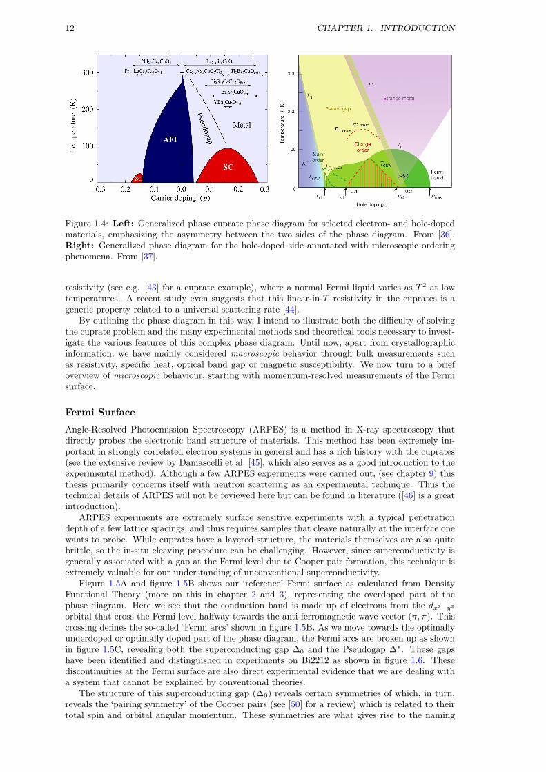
Phase diagramA general phase diagram for the cuprates is shown in figure 1.4 illustrating the many macroscopicand microscopic phases in the cuprates as a function of temperature and doping. First, figure 1.4(left) shows a asymmetry between hole and electron-doping. Since cuprates are superconductingfor a wider range of doping on the hole-doped side, most research focuses on this side of thephase diagram. Second, as shown in figure 1.4 (right), cuprates are only superconducting for anarrow range of hole doping typically between nh = 0.05 and nh = 0.25 with a maximum aroundnh = 0.15. This region is known as the ‘superconducting dome’.
I emphasize here the very different states of matter at the boundaries of the superconductingdome at T = 0: Over-doped cuprates are typically metals while underdoped cuprates are magneticinsulators. In some sense, superconductivity is optimized in a region between localized (magnet)and itinerant (metal) behavior – a region also containing poorly understood normal state (T > Tc)behavior such as the Pseudogap and strange metal phase.
The Pseudogap is a curious phenomena first observed in NMR measurements of YBCO [38]and later on in the c-axis resistivity [39] and specific heat [40]. The name comes from the factthat, by now, it is generally associated with the opening of a gap in the electronic density of states(see below). The difficulty in finding a microscopic origin of the phase transition at the Pseudogaptemperature T ∗ has attracted as much attention as the superconducting transition itself. Manyresearchers believe that the key to understanding the superconducting transition is directly relatedto the Pseudogap. One idea is that of ‘pre-formed pairs’, where Cooper pairs start forming at T ∗,but the macroscopic superconducting state fails to settle between T ∗ and Tc due to incoherentfluctuations in the phase of the pairing field [41, 42].
The strange metal phase is possibly the least understood part of the cuprate phase diagram[37]. A ‘strange’ metal is essentially a phase of matter where the theory of ‘normal’ metals (Fermiliquids) breaks down and is a phenomenon seen in a number of correlated electron systems, notjust the cuprates. A significant indicator of this behavior is a linear temperature-dependence of
12 CHAPTER 1. INTRODUCTION
Figure 1.4: Left: Generalized phase cuprate phase diagram for selected electron- and hole-dopedmaterials, emphasizing the asymmetry between the two sides of the phase diagram. From [36].Right: Generalized phase diagram for the hole-doped side annotated with microscopic orderingphenomena. From [37].
resistivity (see e.g. [43] for a cuprate example), where a normal Fermi liquid varies as T 2 at lowtemperatures. A recent study even suggests that this linear-in-T resistivity in the cuprates is ageneric property related to a universal scattering rate [44].
By outlining the phase diagram in this way, I intend to illustrate both the difficulty of solvingthe cuprate problem and the many experimental methods and theoretical tools necessary to invest-igate the various features of this complex phase diagram. Until now, apart from crystallographicinformation, we have mainly considered macroscopic behavior through bulk measurements suchas resistivity, specific heat, optical band gap or magnetic susceptibility. We now turn to a briefoverview of microscopic behaviour, starting with momentum-resolved measurements of the Fermisurface.
Fermi SurfaceAngle-Resolved Photoemission Spectroscopy (ARPES) is a method in X-ray spectroscopy thatdirectly probes the electronic band structure of materials. This method has been extremely im-portant in strongly correlated electron systems in general and has a rich history with the cuprates(see the extensive review by Damascelli et al. [45], which also serves as a good introduction to theexperimental method). Although a few ARPES experiments were carried out, (see chapter 9) thisthesis primarily concerns itself with neutron scattering as an experimental technique. Thus thetechnical details of ARPES will not be reviewed here but can be found in literature ([46] is a greatintroduction).
ARPES experiments are extremely surface sensitive experiments with a typical penetrationdepth of a few lattice spacings, and thus requires samples that cleave naturally at the interface onewants to probe. While cuprates have a layered structure, the materials themselves are also quitebrittle, so the in-situ cleaving procedure can be challenging. However, since superconductivity isgenerally associated with a gap at the Fermi level due to Cooper pair formation, this technique isextremely valuable for our understanding of unconventional superconductivity.
Figure 1.5A and figure 1.5B shows our ‘reference’ Fermi surface as calculated from DensityFunctional Theory (more on this in chapter 2 and 3), representing the overdoped part of thephase diagram. Here we see that the conduction band is made up of electrons from the dx2−y2
orbital that cross the Fermi level halfway towards the anti-ferromagnetic wave vector (π, π). Thiscrossing defines the so-called ‘Fermi arcs’ shown in figure 1.5B. As we move towards the optimallyunderdoped or optimally doped part of the phase diagram, the Fermi arcs are broken up as shownin figure 1.5C, revealing both the superconducting gap ∆0 and the Pseudogap ∆∗. These gapshave been identified and distinguished in experiments on Bi2212 as shown in figure 1.6. Thesediscontinuities at the Fermi surface are also direct experimental evidence that we are dealing witha system that cannot be explained by conventional theories.
The structure of this superconducting gap (∆0) reveals certain symmetries of which, in turn,reveals the ‘pairing symmetry’ of the Cooper pairs (see [50] for a review) which is related to theirtotal spin and orbital angular momentum. These symmetries are what gives rise to the naming

1.2. CUPRATES 13
Figure 1.5: Fermi surface of the cuprates with respect to the cupper oxide planes. A: Bandstructure of overdoped La2−xSrxCuO4, showing the Cu d orbitals along high-symmetry lines.calculated with Density Functional Theory. Modified from ref. [47]. B: The same band structure,this time represented in two dimensions, with the lines showing where the dx2−y2 band crosses theFermi surface. [45]. C: The gap structure of underdoped La2−xSrxCuO4, showing how the ‘arcs’in B are broken [48].
Figure 1.6: Experimental evidence of both the d-wave gap at T = 10K (below Tc and thePseudogap at T = 130K (just above Tc) in the trilayer (n = 3) cuprate Bi2223. The data istaken along the fermi arcs (figure 1.5B) and clearly show the momentum dependence of the twodistinct gaps. Figure from ref. [49].
scheme taken from electron orbitals, where s-wave superconductors have an isotropic gap and d-wave superconductors have a gap with momentum dependence ∆∗ = | cos kx − cos ky|/2, where(kx, ky) are wave vectors along the Fermi arcs (see ∆0 in figure 1.5C). Other symmetries have alsobeen found, such as p-wave in Sr2RuO4 [51] and f -wave in UPt3 [52].
While these observations of the electronic band structure and Fermi surface thus tells us a lotabout the nature of the superconducting pairing, it does not directly give us a mechanism for thepairing similar to how BCS theory and the isotope effect gave us Cooper pairs due to phonons.While theoreticians have been working tirelessly to construct models that can explain all thesebehaviours, no consensus have been reached at this point. For this reason, some experimentalistsare looking at microscopic correlations in order to uncover what the atoms and electrons are ‘doing’at the various phase transitions summarized in figure 1.4.
Microscopic correlationsWhen any type of phase transition happens in a material it, by definition, must be caused by amicroscopic phenomenon. Any satisfactory theory in condensed matter physics should be able toexplain macroscopic behavior starting from the constituent parts and experiment that can probemicroscopic behavior are often essential. Sometimes, as with the isotope effect in conventionalsuperconductors, we can infer the microscopic behavior in indirect ways, but often it is necessaryto probe the atomic length scales directly. The microscopic probe used in this thesis is neutronscattering, which is used to infer structure and dynamics through a scattering process between abeam of neutrons and a sample. Technical details of the method will be covered in chapter 2, but
14 CHAPTER 1. INTRODUCTION
A B
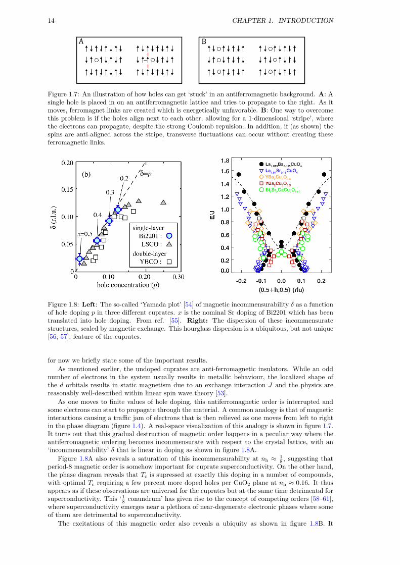
Figure 1.7: An illustration of how holes can get ‘stuck’ in an antiferromagnetic background. A: Asingle hole is placed in on an antiferromagnetic lattice and tries to propagate to the right. As itmoves, ferromagnet links are created which is energetically unfavorable. B: One way to overcomethis problem is if the holes align next to each other, allowing for a 1-dimensional ‘stripe’, wherethe electrons can propagate, despite the strong Coulomb repulsion. In addition, if (as shown) thespins are anti-aligned across the stripe, transverse fluctuations can occur without creating theseferromagnetic links.
Figure 1.8: Left: The so-called ‘Yamada plot’ [54] of magnetic incommensurability δ as a functionof hole doping p in three different cuprates. x is the nominal Sr doping of Bi2201 which has beentranslated into hole doping. From ref. [55]. Right: The dispersion of these incommensuratestructures, scaled by magnetic exchange. This hourglass dispersion is a ubiquitous, but not unique[56, 57], feature of the cuprates.
for now we briefly state some of the important results.As mentioned earlier, the undoped cuprates are anti-ferromagnetic insulators. While an odd
number of electrons in the system usually results in metallic behaviour, the localized shape ofthe d orbitals results in static magnetism due to an exchange interaction J and the physics arereasonably well-described within linear spin wave theory [53].
As one moves to finite values of hole doping, this antiferromagnetic order is interrupted andsome electrons can start to propagate through the material. A common analogy is that of magneticinteractions causing a traffic jam of electrons that is then relieved as one moves from left to rightin the phase diagram (figure 1.4). A real-space visualization of this analogy is shown in figure 1.7.It turns out that this gradual destruction of magnetic order happens in a peculiar way where theantiferromagnetic ordering becomes incommensurate with respect to the crystal lattice, with an‘incommensurability’ δ that is linear in doping as shown in figure 1.8A.
Figure 1.8A also reveals a saturation of this incommensurability at nh ≈ 18 , suggesting that
period-8 magnetic order is somehow important for cuprate superconductivity. On the other hand,the phase diagram reveals that Tc is supressed at exactly this doping in a number of compounds,with optimal Tc requiring a few percent more doped holes per CuO2 plane at nh ≈ 0.16. It thusappears as if these observations are universal for the cuprates but at the same time detrimental forsuperconductivity. This ‘ 18 conundrum’ has given rise to the concept of competing orders [58–61],where superconductivity emerges near a plethora of near-degenerate electronic phases where someof them are detrimental to superconductivity.
The excitations of this magnetic order also reveals a ubiquity as shown in figure 1.8B. It

1.3. LA214 15
turns out that the magnetic fluctuations from this incommensurate order has a highly unusual‘hourglass’-shape, where the ‘neck’ of the hourglass is scaled by the strength of the magneticexchange in the parent compound. Additionally, when static magnetic order disappears the fluc-tuations persist and become gapped. While this picture is appealing, some experimental resultsdeserve to be mentioned in this context. First, it was recently suggested that the magnetic orderand fluctuations are distinct phenomena due to a mismatch in wave vector [62]. Second, Kofu et al.found evidence of gapped excitations and static order in samples close to nh = 1
8 . Third, an hour-glass excitation spectrum was observed in cobalt-oxides with no stripe order or superconductivity[56, 57].
These observations, together with the d-wave structure of the Fermi surface, intuitively pointsto a picture where the behaviour of the dx2−y2 band alone is the key to understanding cupratesuperconductivity. One popular approach is one where pairing happens not due to an externalattractive potential, but through spin fluctuations of the electrons themselves [64]. While thesemodels are not without their problems (Anderson has argued that the idea of a bosonic glue mightnot even be appropriate [65]), they reproduce parts of the phase diagram quite well [66].
1.3 La214
I will now depart from general observations in the cuprates and focus on a particular class ofcuprates based on the parent compound La2CuO4 (see figure 1.3). Sometimes known as ‘La214’ orwith specific acronyms depending on the dopant species, these materials are single-layer cuprateswith a relatively simple crystal structure and a maximum critical temperature Tc ≈ 40K.
Crystal StructureLa214 generally exist with four different structural symmetries, ordered here from highest to lowestsymmetry:
• High-Temperature Tetragonal (HTT). Spacegroup 139 (I4/mmm)
• Low-Temperature Orthorhombic (LTO). Spacegroup 64 (Bmab)
• Low-Temperature Tetragonal (LTT). Spacegroup 138 (P42/ncm)
• Low-Temperature Less Orthorhombic (LTLO). Spacegroup 56 (Pccn)
which can all be described with reference to the structure shown in figure 1.9. Comparing withfigure 1.3, we see that this structure is enlarged and rotated by 45. The smaller structure is knownas the tetragonal coordinate system, and the larger is the orthorhombic coordinate system sincethey represent the conventional cell of the HTT and LTO phase, respectively. Unless otherwisespecified, we will generally use the orthorhombic coordinate system in this thesis.
The difference between the structural phases can be identified with respect to the tilting patternof the CuO6 octahedra. We define the rotation Q1 as a rotation along a (around b) and Q2 as arotation along b (around a) with respect to figure 1.9. The tilts Q1, Q2 along with the orthorhombicstrain η = b−a
b+a can fully describe the structural phase transitions [67].Since this thesis is focussed on specific structural aspects and phonon dynamics, this ‘relatively’
simple crystal structure is a particularly strong point for us. Since we want to model the full3-dimensional structure using computationally heavy simulation methods, it is advantageous toconsider the simplest system possible. In addition, since the lanthanum cuprates were the first so-called ’high-temperature superconductors‘ to be discovered, there is a massive amount of literatureon which to build our ideas from.
TwinningThe structural transition from HTT to LTT is associated with a process where the a and b directionsbecome inequivalent due to the orthorhombic strain. This strain is caused by a mismatch of theCu-O and La-O bond lengths due to their different thermal expansions. As the crystal is cooledthrough this HTT-LTO structural phase transition, the inequivalent directions of a and b areformed in domains separated by grain boundaries.
The result of this phenomenon is the formation of so-called ‘twin domains’, where both possiblechoices of the new a and b directions happen in different parts of the crystal. The unfortunateresult of twinning is that our measurements will see both twin domains simultaneously, making us

16 CHAPTER 1. INTRODUCTION
Figure 1.9: Crystal structure of La2CuO4. The Cu atoms are not shown in the structural schematic,where the octahedral coordination is emphasized. The inset shows 6 basal CuO2 planes, wherethe difference between the tetragonal and orthorhombic coordinate systems is emphasized.
Table 1.2: Atomic species which can be substituted into La2CuO4. La, Nd, Pr will not change thedoping. Ba, Sr will hole dope the system and Ce can be used for electron-doping. For Ce, the datais from ref. [69], all other species from ref. [70]. When doping with oxygen, the procedure is notsubstitutional, but rather the addition of an atomic species. Since the oxidation state of oxygen is2-, we expect the addition of two holes.
Dopant Oxidation State Ionic Radius [Å]
La 3+ 1.216Nd 3+ 1.163Pr 3+ 1.179Ba 2+ 1.47Sr 2+ 1.31Ce 3.84+ 0.998
unable to tell the difference between the a and b directions. In terms of scattering, it means thatany measurement will be a superposition of (hkl) and (khl). These effects will become importantin chapters 5 and 6. Further details about this phenomenon in La2−xSrxCuO4 can be found inref. [68].
Stripe OrderLa2CuO4 can be doped by substitution of La with various atomic species where some of themresults in hole doping (e.g. Ba, Sr), while others have been used to modify the structure withoutchanging the effective hole doping (e.g. Nd, Eu). Table 1.2 shows the ionic radius and oxidationstate (which determines hole doping) of the species that can be used to dope variants of La2CuO4.
It turns out that La214 cuprates have particularly pronounced physics with regards to beha-viour at nh = 1
8 . In La2−xBaxCuO4, superconductivity is almost completely supressed at nh = 18 ,
while in La2−xSrxCuO4 we only see a small plateau. In fact, by performing a combination of sub-stitutions it is possible to create materials such as La1.48Nd0.4Sr0.12CuO4 where superconductivityis completely supressed while being at an otherwise ‘optimal’ doping level. A common thread forLa2−xBaxCuO4 and La1.48Nd0.4Sr0.12CuO4 is that this suppression of Tc happens simultaneouslywith the tetragonal (LTT) phase. I note here that a tetragonal phase in itself does not inherentlyprohibit superconductivity since La2−xSrxCuO4 is tetragonal, but with HTT symmetry, at lowtemperatures for nh ≥ 0.2125 [71]. We thus appear to be in a situation where crystal symmetryhas a non-trivial relationship with superconductivity. For a thorough discussion of this particulartopic, see the review by Hücker [35].

1.4. LSCO+O 17
Figure 1.10: The stripe model in real (b) and reciprocal (a) space. Antiferromagnetic regions areseparated by lines of charge due to hole doping, creating a period-8 magnetic and period-4 chargestructure which can be observed by neutron scattering at the shown positions. From ref. [35].
It can thus be argued that La214 cuprates are the appropriate materials in which to examinethe significance of the nh = 1
8 phase and a lot of attention was given to these phenomena in theearly 1990s, culminating in the discovery of so-called ‘stripe order’ in non-superconducting LNSCO[72]. The stripe model is one where the magnetic period-8 order appears simultaneously with aperiod-4 charge order. These observations led to the stripe model as shown in figure 1.10, wherethe magnetic order is separated by one-dimensional ‘stripes’ of charge.
This model is appealing because it suggests that superconducting electrons are locally segreg-ated from the localized magnetic electrons. It also seems like a reasonable way to relieve thefrustration in the traffic jam analogy (figure 1.7). When discussing stripes, a distinction betweenspin stripes and charge stripes is typically made. While evidence mostly points to a picture wherecharge and spin stripes are simultaneous, charge stripes are much harder to detect and only seemto be associated with the nh = 1
8 phase [73–75] where spin stripe order is seen in a large part ofthe phase diagram 0.02 < nh < 0.13 [76].
The excitations associated with the spin stripes exhibit the universal hourglass dispersion aswe saw in figure 1.8 [77] and the relationship between stripe order and the associated excitationshave been extensively studied as summarized by figure 1.11. In short, the ordering temperature ofspin stripe order increases with doping up to nh ≈ 1
8 where the excitations become gapped. In theoptimally doped region of the phase diagram, the size of the gap Eg is roughly of the order kBTc,suggesting a direct connection between the magnetic excitation spectrum and superconductivity.
1.4 LSCO+O
Finally, we turn to the material studied in this thesis, La2−xSrxCuO4+δ (LSCO+O). In additionto the substitutional doping outlined above, La2CuO4 can be doped with additional oxygen usingelectrochemical methods [78], yielding La2CuO4+δ (LCO+O). These materials are sometimes calledover-stoichiometric or super-oxygenated and the additional oxygen can be combined with Sr-dopingyielding the ‘co-doped’ samples LSCO+O. Due to the electrochemical method of introducing theadditional oxygen, it can be difficult to control the amount of nominal doping, and we are oftenforced to use relatively imprecise or destructive methods such as titration (see e.g. MSc thesis byMariam Ahmad [79]) or Thermogravimetric Analysis (TGA) [80] in order to determine the dopingnh.
With that in mind, a comparison of LSCO and LCO+O is sketched in figure 1.12. A peculiarfeature of doping with oxygen is the fact that only certain superconducting phases seem to emerge(Tc ≈ 15, 30, 40K) and the amount of each phase can be tuned with oxygen content [81], pressure[82] or thermal treatment [83]. The white parts of the LCO+O phase diagram is the ‘miscibil-ity gap’, where phases co-exist. I emphasize here that LSCO+O has a slightly better Tc whencompared to LSCO.
Since the electrochemical doping procedure essentially pushes oxygen atoms into the lattice, we

18 CHAPTER 1. INTRODUCTION
Figure 1.11: Phase diagram of LSCO with respect to Tc and stripe order. Stripe I and II is static,magnetic stripe order and are distinguished by a 45 rotation in propagation direction. Trianglesindicate the gap size of the magnetic excitations in units of kB. From ref. [63].
Figure 1.12: Schematic phase diagram of La2CuO4 using different dopant species. When dopingwith Sr, we get the familiar phase diagram (see e.g. figure 1.4 and figure 1.11). When doping withoxygen, on the other hand, we get discrete phases separated by regions where these phases mix.This ‘miscibility gap’ is shown in white. From ref. [84].
know that the oxygen is equipped with some level of mobility within the lattice and this mobilityis likely the reason for this ‘discretization’ of Tc. Another way of thinking about this is in terms ofan ‘annealed disorder’ [84], where the oxygen can achieve an optimal inhomogeneity [85]. This isin contrast to the ‘quenched disorder’ [84] of LSCO where the positions of Sr ions are fixed duringthe solid state synthesis at elevated temperatures (T ≈ 1000 C).
This annealed disorder results in a number of structural phenomena. First, a structural correl-ation along the c-axis known as staging [86], shown in figure 1.13, is likely the result of the latticetrying to accommodate the interstitial oxygens. There is little reason to believe that staging hasanything to do with superconductivity since it appears in a very similar way in the isostructuralnon-superconducting nickelate La2NiO4 + δ [87] and no direct relation between the staging detailsand Tc was found in LSCO+O [88].
A more complex three dimensional ordering has been observed both by neutrons [88, 89] andby x-ray micro-diffraction [83, 85]. Since thermal treatments that modify the superconductingphases simultaneously removes some of these structural features [85], it has been suggested thatthese superstructures might be related to superconductivity through the ‘superstripes’ idea [90].
A peculiar feature of LSCO+O, is the fact that the superconducting and magnetic phasesof LSCO+O are distinct and separate. Magnetic susceptibility and muon-spin-rotation (µSR)measurements have revealed a linear relationship between the volumes of the two phases, suggestingthat they are separated in real space [91, 92]. In the context of the LSCO phase diagram, it is

1.5. THESIS OBJECTIVES 19
Figure 1.13: Illustration of staging in LCO+O. A: Crystal structure of La2CuO4, highlightingthe octahedra centred at the copper atom. B: Displacement pattern of these octahedra as viewedfrom the side. C: Staging pattern due to intercalated oxygen. By creating anti-phase boundariesthe structure accommodates the oxygen atoms in an energetically favourable way. The numberof CuO2 planes between the anti-phase boundaries determines the staging number (in this casestage-6). From ref. [84].
believed that these two phases is one with exactly nh = 18 (magnetic) and one with nh ≈ 0.16
(optimally superconducting). Whether this phase separation is unique to LSCO+O is hard to say– one could imagine a scenario where the annealed doping of LSCO+O allows these phases to‘grow’ in contrast to LSCO with only quenched doping from Sr [92].
Finally, LSCO+O (with one exception, see chapter 8) is equipped with static stripe orderdespite having a Tc reminiscent of optimally doped LSCO. In addition, the transition temperatureof this static order TN coincides with Tc [92], suggesting a unique and direct connection betweenthe two electronic phases in this compound.
LSCO+O is thus structurally and electronically distinct from LSCO, while still exhibiting theuniversal features of the cuprates in a consistent way. This system is important in the largercontext because, as we learned in this chapter, 1) the cuprates are fundamentally inhomogeneoussystems and 2) the fact that crystal structure clearly interacts with the superconducting stateand/or stripe order. Since LSCO+O is unique on these two counts, an investigation of this systemcan help us understand those unsolved issues.
1.5 Thesis objectives
The objective of this thesis is to investigate phonon dynamics of the LSCO+O system throughneutron scattering measurements and molecular simulations. The idea is to consider here thefull three dimensional lattice of the cuprates by trying to understand how the surrounding latticeinteracts with the CuO2 planes (which are usually studied). The strategy is to primarily focus onthe dynamical aspects of the lattice by measuring and simulating phonons in the system. Whilephonon-mediated superconductivity in the manner of conventional BCS theory is unlikely in thecuprates, a better understanding of the lattice dynamical effects in the cuprates, and possiblyindirect effects on superconductivity could be useful to the community as a whole.
In this context I will mention a few experimental result that emphasizes this motivation. Re-cently, a longitudinal study of several different cuprates suggested that the Cu-O distance to theapical oxygen (the oxygen atoms directly above and below the copper atoms) has an effect on thein-plane exchange interaction [93]. A different study on thin films showed a similar effect on thein-plane Cu-O distances [94]. Finally, a measurement of atomic pair distribution functions as afunction of doping in LSCO has shown that the distribution of in-plane Cu-O distances is broadestat optimal doping, suggesting that a phase separation picture might be relevant for LSCO [95].
Just as with stripes picture, the excitations are just as relevant as the static order. In the sameway, a study of phonons might reveal subtleties that we have not been able to discern from a purely

20 CHAPTER 1. INTRODUCTION
structural viewpoint. The goal of this thesis is thus to carefully evaluate the phonon spectrum ofLCO, LSCO, LCO+O and LSCO+O in theory and practice. This is done with various techniquesin neutron scattering and simulations with density functional theory (DFT). In a more concreteway, this thesis tries to answer the following research questions:
1. Can a relationship between specific dopant type (quenched/annealed) and the phonon spec-trum be established?
2. Is it possible to establish a relationship between superconductivity and the phonon spectrum?
3. To what extend can DFT-based simulation methods be used to explain observed changes inthe phonon spectrum?
OutlineIn chapter 2, the experimental and simulation methods used in this thesis are outlined. Subsequentchapters then deals with specific research projects pertaining to aspects of the research questionsoutlined above. In chapter 3, phonon calculations on La2CuO4 is performed in various structuraland electronic phases in order to obtain a ‘baseline’ for subsequent simulations. Chapter 4 usesthese results to perform molecular dynamics of structures with added dopants. The experimentalpart of this thesis starts in chapter 5, where we look at structural correlations and compare theseto observables from molecular dynamics. In chapter 6 investigates low energy phonon dynamics inorder to 1) validate our simulations, 2) look at structural instabilities and 3) investigate dynamicsrelated to the observed superstructures seen in chapter 5. In chapter 7 I look at phonon density ofstates measurements of powders with different dopants in order to directly answer question 2. fromabove. In chapter 8 I look at an anomaly detected in a specific high-energy phonon mode, possiblyconnected to stripes. In chapter 9 I report results from an electronic band structure measurementon an oxygen-doped sample. Finally, in chapter chapter 10, the thesis is briefly summarized anddiscussed.

Chapter 2
Methods
In this chapter, I give an overview of primarily neutron scattering and density functional theory.Since these two methods are central to the experimental and theoretical work performed in thisthesis, the objective here is to give the background necessary to understand the remaining chapters.In addition, I attempt to contextualize the reason for using these methods in the study of cupratesuperconductors.
2.1 Neutron Scattering
In this section, we give some of the key equations and concepts related to neutron scattering. Basicconcepts will not be dealt with in detail, since excellent literature already exists and does a muchbetter job than I would be capable of. See e.g. [96–98] for general theory and [99] for triple-axisspectroscopy. Rather, I will attempt to take a more practical approach with three primary goals:
1. Understand what types of problems can be solved with neutron scattering.
2. Understand the relationship between correlation functions and neutron scattering.
3. Emphasize the equations relevant for our experiments.
General TheoryIn neutron scattering, the idea is to illuminate a sample with a beam of neutrons and then recordthe scattered neutrons. In order to have enough neutrons for our experiments, they are usuallyproduced through nuclear fission in a reactor or by bombarding a target with high energy protonsin a so-called spallation source.
The neutron is a neutral, spin- 12 particle with a mass mn = 1.675× 10⁻²⁷ kg and a magneticmoment µn = −1.913µB. Just like any quantum object, the neutron exhibits particle-wave dualityand as it propagates through a medium we can conveniently characterize it by a wavevector k thathas a magnitude k = 2π
λ , where λ is the wavelength, and points in the direction of propagation.Given the wavevector k, along with the fact that typical neutrons for experiments can be treatedas non-relativistic particle, we can compute the neutron energy E = h2k2
2mnand its equivalent
temperature through E = kBT . In neutron scattering we often categorize experimental methodsbased on the temperature of the incident neutrons, as summarized in table 2.1.
In general, scattering experiments have optimal conditions when the wavelength of the probeis similar to the studied length scale. Similarly, when studying excitations, it is preferable that theenergy of the probe is similar to that of the excitations. This is exactly why neutron scattering is souseful for condensed matter since typical wavelengths matches interatomic distances (≈ 10−10 m)
Table 2.1: Approximate values of of energies, temperatures and wavelength for the three classific-ations of reactor sources. From [97].
Source Energy [meV] Temperature [K] Wavelength [Å]
cold 0.1-10 1-120 30-3thermal 5-100 60-1000 4-1hot 100-500 1000-6000 1-0.4
21

22 CHAPTER 2. METHODS
and typical energies matches elemental excitations of matter (≈ 10meV). In addition, since theneutron has a magnetic moment it can be used to study magnetic structure and excitations.
In order to describe the scattering experiment, we first need to understand how the neutroninteracts with the atomic species in our sample. The process is a neutron-nucleus scatteringprocess, where the potential of the nucleus is approximated by the Fermi pseudopotential
V (r) =2πh
mnbδ(r) , (2.1)
where b is called the nuclear scattering length and depends on the specific nuclear species involvedin the scattering process. The δ-function in the pseudopotential is an expression of the fact that weare using the Born approximation, which is essentially a statement that the nucleus can be thoughtof as a point-scatterer compared to the neutron. Since the wavelength of a typical thermal neutrons(≈ 10−10 m) is orders of magnitude larger than the range of nuclear forces (≈ 10−15 m), this isa reasonable assumption. For a single, free nuclei, the scattering will be isotropic and the totalscattering is σtot = 4πb2.
The general geometry of a scattering experiment is outlined in figure 2.1. An incident beamwith wave vector ki is scattered from the origin to a final wave vector kf at an azimuthal angle Θand a polar angle Φ into a solid angle Ω distance r away from the origin. From this geometry wedefine the differential scattering cross-section as
dσ
dΩ=
flux of neutrons into dΩ
incident flux of neutronsSince we can only measure the neutron flux, dσ/dΩ is our experimental observable, given thatwe have neutron detectors before and after the sample. Since the neutron flux tells us nothingabout the wave vectors or energy, additional constraints are necessary to get information aboutthe scattering process from the experiment. In elastic scattering, we assume that no energy isexchanged in the scattering process so that |kf| = |ki|. By fixing one of them (typically ki), theother is completely described by the geometry of figure 2.1 and we can measure dσ/dΩ as a functionof kf since the location of our detector, and thus Φ and Θ is known. In inelastic scattering, weneed to fix the lengths, and thus the energy, of both ki and kf. This defines the partial differentialcross-section:
d2σ
dΩdEf=
flux of neutrons into dΩ with energy between Ef and Ef + dEfincident neutron flux with energy Ei
,
where Ei is the energy of the incident neutron and Ef is the energy of the final neutron. With theobservables now defined, we can start to discuss how to actually extract useful information aboutthe atomic/microscopic details of a sample from a neutron scattering experiment. Knowing kiand kf, the coordinate system can be redefined with respect to our sample through the scatteringvector Q = ki − kf. In addition, we define the energy transfer as the amount of energy gained (orlost, for negative values) by the neutron in the scattering process hω = Ef − Ei.
The objective of neutron scattering theory (or really, any scattering theory), is then to finda sample-dependent function S(Q, ω) that can be related to the observable (partial) scatteringcross-section. In fact, as we shall see in the next section, it turns out that this scattering functionS(Q, ω) not only exists, but have an intimate relationship with microscopic correlation functionswhich can be derived from first principles.
This, somewhat abstract, introduction essentially covers most of what we need to know withregards to the neutron scattering process and coordinate systems. The rest of this section is thendedicated to 1) understanding what the scattering function S(Q, ω) actually represents and 2)outline some of practicalities involved in the neutron scattered methods used in this thesis.
Correlation FunctionsAfter setting up the coordinate system, we are now left with the much more complicated task ofconstructing models that can help us interpret the partial differential cross-section. As I previouslysuggested, information about our samples comes from the pattern of d2σ/dΩdEf as a function ofQ and ω, or equivalently: The angles Φ, Θ and neutron energies Ei, Ef. Intuitively, the reasonwe have any pattern at all is due to interference of the scattered waves. Since the scattering froma single nucleus is isotropic, any pattern in S(Q, ω) comes from the specific composition of, orcorrelations between, atomic species in our sample.
It turns out that this can be conveniently described through the mathematics of correlationfunctions, introduced by Van Hove in 1954 [100]. We start with the time-dependent pair-correlation

2.1. NEUTRON SCATTERING 23
Figure 2.1: Geometry of a scattering experiment. An incident beam of neutrons characterizedby the wave vector ki impinges on a sample at the origin. The neutron beam is scattered in thedirection of kf, defined by the two angles Φ and Θ. The neutrons are detected at a solid angle dΩat a distance r. From [98]
function for a system of identical particles G(r, t), which describes the probability of finding a pairof particles separated by the spatial vector r at time t. Similarly, the self time-dependent pair-correlation function Gs(r, t) describes the probability of finding the same particle at a distance rat a time t. These concepts can be defined mathematically defined through position operators:
G(r, t) =1
N
∑i =j
∫⟨δ(r′ −Rj(0))δ(r
′ + r −Ri(t))⟩dr′
Gs(r, t) =1
N
∑i
∫⟨δ(r′ −Ri(0))δ(r
′ + r −Ri(t))⟩dr′ ,
where i, j are particle indices and Ri(t) is the position operator for particle i at time t. Finallythe following functions can be obtained through Fourier transforms in time and space:
I(Q, t) =
∫G(r, t) exp(iQ · r)dr
Is(Q, t) =
∫Gs(r, t) exp(iQ · r)dr
S(Q, ω) =1
2πh
∫I(Q, t) exp(−iωt)dt
Si(Q, t) =1
2πh
∫Is(Q, t) exp(−iωt)dt ,
where I(Q, t) is known as the intermediate function, Is(Q, t) the self intermediate function, S(Q, ω)the scattering function and Si(Q, t) the incoherent scattering function. The connection to thepartial differential cross-section can now be stated succinctly as
d2σ
dΩdEf=
(d2σ
dΩdEf
)coh
+
(d2σ
dΩdEf
)inc
(2.2)
with
(d2σ
dΩdEf
)coh
=σcoh4π
kfkiNS(Q, ω)(
d2σ
dΩdEf
)inc
=σinc4π
kfkiNSi(Q, ω)

24 CHAPTER 2. METHODS
where
σcoh = 4πb2
σinc = 4π(b2 − b
2)
In the above equations, N is the number of particles in the scattering system, b is the nuclearscattering length as defined in equation (2.1) and the bars denote ensemble averages. The coherentcross-section σcoh is thus related to the average scattering length, while the incoherent cross-section σinc is related to the distribution of scattering lengths. These cross-sections are determinedexperimentally and are tabulated for most elements [101].
In a neutron scattering experiment we thus see a superposition of pair-correlations throughcoherent scattering and self-correlations through incoherent scattering. As an example involvingdynamics, phonons (correlated motion) are generally seen as coherent scattering while Brownianmotion (random motion) would show up as incoherent scattering.
It thus turns out that there is a direct relationship between the measured partial differentialcross-section in neutron scattering and microscopic correlation functions. In fact, many microscopictheories can be translated directly into a theoretical S(Q, ω) and compared 1-to-1 with experiment.One illustrative example, used in this thesis, is that of a molecular dynamics simulation where werecord the atomic positions as a function of time. From this trajectory it is trivial to compute aclassical version of G(r, t) and thus obtain predictions for neutron scattering experiments.
Even more generally, given a Hamiltonian (quantum or classical) and assuming a weak (linear)perturbation, it is possible to invoke linear response theory (see e.g. [102, chapter 3]). Importantly,linear response theory provides a link between the spontaneous fluctuations of a system and theresponse to an external perturbation. The object of interest in this context becomes the dynamicsusceptibility χ(Q, ω), which can be thought of as
χ(Q, ω) = χ′(Q, ω) + χ′′(Q, ω) =‘response’
‘force’ ,
where the real part χ′(Q, ω) describes a response in phase with the perturbation (reactive), whilethe imaginary part χ′′(Q, ω) describes an anti-phase response (dissipative). The real and imaginaryparts are linked through the Kramers-Kronig relation
χ′′(Q, ω) = − 1
πP∫ ∞
−∞
χ′(Q, ω′)
ω′ − ωdω′ ,
where P is the Cauchy principal value. Finally, the scattering function is related to the imaginarypart of the dynamic susceptibility through the fluctuation-dissipation theorem:
S(Q, ω) =1
1− ehωkBT
χ′′(Q, ω) . (2.3)
Since the real and imaginary parts of the susceptibility are uniquely connected through theKramers-Kronig relation, neutron scattering experiments can directly probe predictions of linearresponse theory. A particularly illustrative example in the context of this thesis is that of a dampedharmonic oscillator (DHO). Consider the classical system shown in figure 2.2, with the equationsof motion:
m⟨x(t)⟩+mw20⟨x(t)⟩ = −mγ⟨x(t)⟩ .
Assuming an impulsive perturbation (a δ-function displacement) and going through the mathem-atics of linear response theory (see [96] for details), we arrive at the dynamic susceptibility
χ[ω] =1
m
1
ω20 − ω2 + iγω
=1
m
ω20 − ω2
(ω20 − ω2)2 + γ2ω2
− i
m
γω
(ω20 − ω2)2 + γ2ω2
. (2.4)
From the last term we thus see that damped harmonic motion can be observed as a Lorentzianas a function of energy in a neutron scattering experiment, where the position ω0 denotes thefundamental frequency and the width γ is the damping constant. In fact, this expression is typicallyused as a fitting function when measuring phonons [103]. While rudimentary, the purpose of thisexample is to emphasize the intimate relationship between observables in neutron scattering andmicroscopic theories.

2.2. SPECIFIC SCATTERING METHODS 25
m(ω20x+ γv)∆x
v
0 2 4 6 8 10
−1
0
1
t
x(t)
Figure 2.2: Mechanical version of the damped harmonic oscillator. Left: A mass on a springmoving with velocity v under the influence of a restoring spring force (blue arrow) with forceconstant ω2
0 and a frictional force γ which is linear in velocity. Right: Position of the spring as afunction of time after applying a an impulsive perturbation, analogous to quickly pulling the massand letting go.
Resolution
When performing actual neutron scattering measurements, the incident and final wave vectors arenot completely defined by a single vector, but rather by some finite distribution. In fact, sinceneutrons are relatively sparse, it is not uncommon to relax this distribution in order to increasethe signal. This finite distribution of wave vectors will broaden the signal in both Q and ω. Sincethe optics of the instrument is responsible for this broadening, we call the effect instrumentalresolution.
To make matters more complex, the resolution is not a constant object, but rather varies asa function of both Q and ω. It is therefore important to understand the instrumental resolutionfor any particular measurement to make sure that, for example, a broad feature is due to thesample and not the instrument. In many cases, the resolution can be measured with respect toa standard and subtracted in the same way for every experiment. In some cases, such as thetriple-axis spectrometer, the experimental condition vary wildly between experiments and it mightbe beneficial to calculate the resolution beforehand.
The resolution is quantified by the resolution function R(Q, ω). which can be represented by a4 dimensional ellipsoid if we assume that the distribution of neutrons follow a normal distributionas they propagate through the instrument. The 4 major axes of this ellipsoid then represents theGaussian width σ in each direction. By projecting this ellipsoid onto the scattering plane, one cangain an intuitive understanding of how the resolution affects the experiment.
I will not go into further detail at this point, but rather refer to [99, Chapter 4] for a muchmore in-depth discussion of this topic in the context of triple-axis spectroscopy. Finally, the bestway to understand how resolution affects measurements is to play around with software that cansimulate and visualize the resolution ellipsoid in various conditions [104, 105].
2.2 Specific Scattering Methods
Departing from the abstract concepts of the preceding section, I will now outline specific neutronscattering techniques used in the experimental part of this thesis. Despite the significant powergenerated in a neutron reactor, the number of neutrons expelled from the source is typically smallwith respect to neutron experiments, especially when compared to X-ray synchrotron radiation.In addition, the neutrons have a wide distribution of wavelengths and propagate in all directions.Neutron facilities and instruments thus take advantage of various optical elements in order todefine the neutron beam.
Transporting the neutrons to the instruments is done with neutron guides, which are rectangulartubes where the insides are coated with mirrors that can cause total reflection of neutrons atsufficiently small angles (0.1to1). When neutrons reach the instrument, we have so-called awhite beam with a wide distribution of wavelengths, but most experiments needs a well-defined ki.Details about neutron instrumentation quickly becomes complex, so we stop the detailed discussionhere since it would divert from the purposes of this thesis.

26 CHAPTER 2. METHODS
Figure 2.3: Layout of the IN8 instrument at ILL [106]. Neutrons from the thermal source hitsone of the 3 optional monochromators (PG002, Cu200, Si111) and continues towards the samplewhere it is scattered towards the analyser that selects the final energy.
Triple-Axis SpectroscopyIn some way, the triple-axis spectrometer (TAS) is the easiest neutron scattering instrument tounderstand because it has a one-to-one correspondence with the geometry from figure 2.1. Figure2.3 shows the view from above of the TAS instrument IN8 at ILL. The triple-axis (or triple-angle)name comes from the fact that all the angles defined by the beam path can be adjusted by movingthe motors of the instrument. These angles then completely define ki, kf and we essentially havea two dimensional version of figure 2.1, known as the scattering plane.
Because the instrument is essentially two-dimensional, single crystal samples must be alignedwith a desired crystal plane in the scattering plane. With the sample in place, we can nowcompletely explore S(Q, ω) with the restriction that Q is restricted to the scattering plane. Thesample is placed on a rotating sample stick that, together with the scattering angle, allows usto access the two dimensions of Q. The energy transfer hω is controlled by monochromator andanalyser.
As one might have noticed, figure 2.3 features just a single detector. While other optionsexists (see chapter 6), this is typical for TAS instruments. As a consequence, measurementsare performed along pre-defined paths in (Q, ω) space step-by-step. The main purpose of TASinstruments is then generally to look at specific features in S(Q, ω) with high counting statisticsand tight resolution. Since inelastic scattering is orders of magnitude weaker than elastic scattering,spectroscopic measurements are usually the primary focus for TAS instruments.
In this thesis, most TAS measurements are of specific phonon branches. The 1-phonon cross-section gives an expression for the differential coherent cross section of phonons, indexed by thephonon band ν [97].
S(Q, ν, ω) =kfki
N
h
∑q
|F (Q, q, ν)|2(nqν + 1)δ(ω − ωqν)δ(Q− q −G) (2.5)
with
F (Q, q, ν) =∑j
√h
2mjωqνbj exp
(−1
2⟨|Q · u(j0)|2⟩
)exp[−i(Q− q) · r(j0)]Q · ej(q, ν)
where Q and ω are the wave vector and energy of our measurement. ν is a phonon band and qis the phonon wave vector. ωqν is the energy of phonon band ν at wave vector q and nqν is theBose factor at this energy. Atomic species are designated with index j, their mass is mj and theircoherent neutron cross-section is bj . u(j0) and r(j0) is the displacement and position of atom jin unit cell 0, respectively. Finally, G is any reciprocal lattice vector and ej(q, ν) is the phononeigenvector of atom j, band ν and wave vector q.
While this expression rests on some microscopic details that we might not have knowledge of,close inspection of equation (2.5) allows us to extract information from an experiment without

2.2. SPECIFIC SCATTERING METHODS 27
Figure 2.4: Layout of the IN4 instrument at ILL [107]. Neutrons are chopped into discrete packetsbefore hitting the monochomator and continuing towards the sample position. A Fermi chopperis used to make very short neutron pulses, such that their (Q,ω) can be determined from thetime-of-flight from the Fermi chopper to the detector,
any prior knowledge of the system. The δ-functions makes sure that we only see scattering at thephonon dispersion. In addition, the Q · ej(q, ν) term tells us that scattering is strongest when theeigenvector of the phonon mode is parallel to Q (and vanishes when perpendicular). This allows usto distinguish longitudinal and transverse phonons, since they vibrate parallel and perpendicularto Q, respectively. For an example of this, see figure 6.5 in chapter 6.
As it turns out, it is possible to obtain prior knowledge about the phonon spectrum throughmicroscopic simulations. These simulations give us direct access to eigenvectors and we can makea detailed analysis of equation (2.5). More information about this type of calculation is given insection 2.4.
One caveat with equation (2.5) is the fact that phonons can be broadened, on top of broadeningdue to resolution, such that the delta function in energy is replaced with a Lorentzian as we sawin equation (2.4) and (2.3). This is known as lifetime broadening and the Lorentzian width can beinterpreted as the reciprocal lifetime of the measured phonon.
Time-of-Flight Spectroscopy
In Time-of-Flight (ToF) spectroscopy, we take advantage of the fact that thermal neutrons move atspeeds that we can accurately determine experimentally (10meV neutrons has a speed of roughly1400m s−1). Figure 2.4 shows a schematic of the IN4c spectrometer at ILL. Neutrons from thereactor are chopped up into discrete packets using two rotating discs (background choppers) andthen monochromatized using a crystal monochromator. Before impinging on the sample, theneutrons pass through a ‘Fermi chopper’ which produces very short neutron pulses (10 µs to 50 µs).Neutrons are then detected radially in one of the many detectors. By recording the time-of-flightfrom the Fermi chopper to a specific detector, we can determine the energy transfer through thevelocity as determined from the flight time and Q from the angle to the detector where the neutronwas measured.
Time-of-Flight spectrometers thus perform many simultaneous measurements, but can in somesense be used to probe many of the same things as TAS instruments. The better choice depends,of course, on the sample and phenomena that you are using it to probe. In the case of this thesis,we used the IN4 spectrometer to measure the phonon density-of-states of powdered samples. Sincethe powder is rotationally averaged, the result of a measurement is a (Q, hω) map where Q isdefined as the length of Q. An example of such a dataset is shown in figure 7.2 in chapter 7. Byintegrating the full map onto the energy axis we obtain the experimental phonon density-of-states.
While equation 2.5 is still valid since most of our scattering is 1-phonon processes at lowtemperature, we use the confusingly named incoherent approximation. The physical reasoning isthat the rotational averaging due to the powder cancels out correlations between distinct atoms.

28 CHAPTER 2. METHODS
Figure 2.5: Schematic layout of the D4 instrument at ILL [109]. The neutron beam from the hotsource hits the monochromator and directed towards the sample position. The scattered neutronsare collected at the nine detectors each containing 64 cells. The detector bank can be moved duringthe experiment in order to cover the full Q-range.
Mathematically, it is due to factor ∑j
Q · ej(q, ν)
2
which in the incoherent approximation is replaced by [108]∑j
Q2 (ej(q, ν))2
essentially eliminating the cross terms. With this approximation, the 1-phonon incoherent cross-section becomes:
S(1)inc(Q,E) = exp
(−2W (Q)
) Q2
E⟨n+
1
2± 1
2⟩
[∑k
σscattk
2mkgk(E)
]
where gk(E) represents the phonon density of states. With this, much simpler, expression we cantransform our (Q,E) dataset into the phonon density of states, only supplying the mean-squareddisplacement and atomic composition. Similar to the phonon bands, the phonon density of statescan also be directly obtained from simulations methods. ToF spectroscopy on powders thus allowsus to investigate properties of the overall phonon spectra, in contrast to the distinct phonon bandsas measured by TAS spectroscopy.
Real-space diffractionThe last method I will cover here is a diffraction instrument focussed on obtaining real spacestructures. In terms of the correlation functions defined in section 2.1, we are interested in thetime-averaged value of G(r, t) which can be found as the Fourier transform of S(Q, ω = 0). Inorder to perform this Fourier transform, it is desired to measure at a wide range of Q in order toavoid artefacts related to the Fourier transformation pocedure itself.
Figure 2.5 shows the D4 diffractometer at ILL. Since diffraction assumes elastic scattering, theinstrument is equipped with a monochromator before the sample, but no energy analysis of thescattered neutrons is performed. Rather, the neutrons are directly measured at the radial detectors.In order to optimize the Q-range of the instrument, we want to minimize the wavelength (Bragg’slaw), so D4 is placed at a hot source so that we can get a large number of high-energy neutrons.For our particular experiment the monochromator selected neutrons with a wavelength λ = 0.35Å,corresponding to an energy of E = 668meV.
The object of interest in this case is the total pair distribution function G(r), which tellsyou the probability of finding two atoms separated by a distance r, weighted by the product of

2.3. DENSITY FUNCTIONAL THEORY 29
their coherent neutron scattering lengths b. As we shall see in section 2.6, these distributions canbe found from a molecular dynamics simulation. In order to compare with experiment we thenconsider
G(r) =1
b2
∑α=1,β≥α
cαcβbαbβ(gαβ(r)− 1) ,
where gαβ(r) is the partial radial distribution function which describes the probability of findinga particle with label β at a distance r away from a particle with label α. ci = Ni
N is the numberconcentration, bi is the coherent neutron cross section of species i, and
b2=
(∑α
bαcα
)2
.
In the research community working with pair distribution functions (PDF) there is a large numberof conventions regarding how to normalize and represent pair-correlation functions in theory andexperiment (see review by Keen [110]). The G(r) presented here is typically called the Total Pair-Distribution Function. Details about the definitions of gαβ(r) and G(r) and how to obtain themfrom molecular dynamics trajectories can be found in section 2.5
2.3 Density Functional Theory
We now turn to the computational framework used in this thesis, Density Functional Theory(DFT). Similar to the section on neutron scattering, this is a vast subject that is impossible tofully explore on a few pages, but I will once again try to outline the key concepts, advantagesand disadvantages. For more comprehensive material, I recommend the books by Giustino [111](introduction to the subject) and Martin [112, 113] (comprehensive reviews). The review paper byHoffmann [114] discusses what kinds of problems DFT can solve and is recommended for anyonecurious about DFT.
DFT is a computational method in quantum chemistry, where the objective is to compute themany-body Schrödinger equation for molecules and solids:−∑
i
∇2i
2−∑i
∑I
ZI
|ri −RI |+
1
2
∑i =j
1
|ri − rj |
Ψ = EΨ , (2.6)
where ri is the position of electron i and RI , ZI is the position, charge of nucleus I. As one mighthave noticed, the kinetic energy of nuclei and nuclei-nuclei interactions have been omitted. Thisis known as the clamped nuclei approximation, which assumes immobile nuclei. This results ina vanishing kinetic energy and a constant Coulomb repulsion which can be subtracted from theenergy on the right-hand-side of equation (2.6):
E = Etotal −1
2
∑I =J
ZIZJ
|RI −RJ |
These equations are written in the so-called Hartree units (see [111, chapter 2.3]), such that energiesare in units of Hartree energies (1Eh = 27.2114 eV), distances are in units of the Bohr radius a0and masses are in units of electron masses me. Since the nuclear coordinates are considered fixed,the many-body wavefunction Ψ in equation (2.6) is a function of electron positions
Ψ(r1, r2, . . . , rn)
While this object seems innocent at first glance, the many-body Schrödinger equation quicklybecomes a completely unmanageable object. Imagine that we want to calculate this object for asmall molecule such as Benzene (C6H6) containing 12 nuclei and 42 electrons. This wavefunctionexists in 42 ·3−3 = 123 dimensional cartesian space! If we want to store this object on a computerwith a modest precision of 10 grid points per coordinate, it would require 10156 complex numbersor 64 · 10156 bits (assuming single-precision floating points numbers of 32 bits). Lloyd estimatedthe total number of bits available for computation in the observable universe to be 1090 [115].Even with the entire universe at our disposal this object is completely unmanageable. In order toarrive at a reasonably manageable theory, we assume that electrons are independent such that themany-body wavefunction can be written as a product of single-electron wavefunctions:
Ψ(r1, r2, . . . , rn) −→ ϕ1(r1)ϕ2(r2) . . . ϕN (rN ) (2.7)

30 CHAPTER 2. METHODS
Where each of the wavefunctions ϕi are found as solutions to the single-electron Schrödingerequation [
−∇2
2−∑I
ZI
|r −RI |
]ϕi = ϵiϕi .
Using these definitions, the many-body Schrödinger equation becomes
∑i
[−∇2
2−∑I
ZI
|ri −RI |
]Ψ = EΨ , (2.8)
where E = ϵ1+ϵ2+ . . . ϵN , with the single-electron energies being ordered from smallest to largest.This corresponds to the situation usually taught in condensed matter physics where the lowestenergy configuration is found by filling up electronic orbitals starting from the lowest eigenvalue[6]. Inspection of equation 2.8 reveals that the independent electron approximation, as the nameimplies, has completely ignored the Coulomb repulsion between electrons. To rectify this fact, wemake a mean-field approximation, such that each electron feels an electrostatic ‘Hartree potential’:
∇2VH(r) = −4πn(r)
where the electron density is defined as the sum of single-electron densities:
n(r) =∑i
|ϕi(r)|2 . (2.9)
Starting with the many-body Schrödinger equation we have thus arrived at an approximate versionthat can be approached from a computational point of view. However, at this stage we haveignored exchange (equation (2.7) is not anti-symmetric with regards to a change of variables) andcorrelation (the mean field approximation used for the Hartree potential). As we shall see, DFTgives us a way to correct for both of these effects in a surprisingly accurate manner.
The Kohn-Sham equationsThe main idea behind DFT is expressed through the ‘Hohenberg-Kohn theorem’, which is thesimple but powerful statement that the total energy of a many-electron system is a functional ofthe electron density. In addition, the ‘Hohenberg–Kohn Variational Principle’ tells us that theground state density is the functional that minimizes the total energy. To quote the original paper[116]:
This paper deals with the ground state of an interacting electron gas in an externalpotential v(r). It is proved that there exists a universal functional of the density,F [n(r)], independent of v(r), such that the expression E =
∫v(r)n(r)dr+F [n(r)] has
as its minimum value the correct ground-state energy associated with v(r).
The theorem states the existence of the functional F [n(r)], but leaves us with no recipe on how toconstruct this functional. The ‘game’ in DFT thus consists of constructing functionals and test thecomputational results against experimental observations. Since the universal functional has notbeen found, hundreds of functionals [117] have been created with specific purposes in mind. Withthat being said, very good ‘universal’ functionals exist and most people stick to a small subset ofthis ‘functional zoo’. Returning the objective at hand, the idea of Kohn and Sham [118] was tosplit the contributions to the functional F [n(r)] into terms of kinetic and coulomb energy and anadditional term with ‘everything else’:
E =
∫Vn(r)n(r)dr + F [n(r)] (2.10)
F [n(r)] =∑i
∫ϕ∗i (r)
∇2
2ϕi(r)dr +
1
2
∫∫n(r)n(r′)
|r − r′|drdr′ + EXC[n(r)] . (2.11)
This expression thus lets us evaluate the total energy of our approximate many-body Schrödingerequation given a set of one-electron orbitals ϕi, the electronic density n(r) and the exchangecorrelation functional EXC[n(r)]. These are evaluated using the Kohn-Sham equations [118]:[
−1
2∇2 + Vtot(r)
]ϕi(r) = ϵiϕi(r) , (2.12)

2.3. DENSITY FUNCTIONAL THEORY 31
where
Vtot = Vn(r) + VH(r) + VXC(r) (2.13)
Vn(r) = −∑I
ZI
|r −RI |(2.14)
∇2VH(r) = −4πn(r) (2.15)
VXC =δEXC[n]
δn(r) . (2.16)
Where the last equation defines the exchange correlation potential. Methods to actually solveequation 2.12 numerically are outside the scope of this thesis and can be found in literature [112,part IV]. In general, this depends on the representation of our one-electron orbitals ϕ, also knownas the basis set. In this thesis, we make use of a basis set which is expanded in plane waves. Planewave DFT is particularly popular for computing crystalline materials, since we are guaranteedthat ϕ are cell-periodic (Bloch functions). The main disadvantage is that you need a large numberof plane waves to have a reasonable representation of electronic orbitals.
What we have done so far is to reduce the electronic structure problem into one that iscompletely described by the electronic density. In addition, the contributions to the equationshave been split up into well-understood terms (kinetic energy, nuclear-electron potential, mean-field Hartree potential) and the unknown exchange-correlation functional EXC. When the phrase‘choice of functional’ comes up in the context of DFT, one actually means the choice of exchange-correlation functional since everything else is fixed in the Kohn-Sham equations.
Exchange-Correlation FunctionalWith the large number of XC functionals in existence, it may seem a bit daunting to make areasonable choice. In fact, if we need to build new functionals for every peculiarity, is thereeven any merit to this method? It turns out that the simplest possible model for interactingelectrons, the homogeneous electron gas (HEG), gives a surprisingly good representation of realsystems where the distribution of electrons is inhomogenous. In fact, the original paper on theHohenberg-Kohn theorem was titled ‘Inhomogeneous Electron Gas’ [116].
The most basic functional to express the exchange-correlation functional is the so-called Local-Density Approximation (LDA) [119, 120], where parameters of the HEG was found using quantummonte carlo methods. For this reason, this functional is entirely non-empirical and built fromsimple principles, both desirable qualities in any theory. While successful in these respects, itquite significantly overestimates atomization energies [121].
The ‘local‘ in local-density approximation refers to the fact that EXC depends only on thelocal density. To improve on this, functionals based on the Generalized Gradient Approximation(GGA) also takes into account the gradient of the local density. Of these, especially the Perdew-Burke-Ernzerhof (PBE) functional has gained popularity due to its relatively simple derivationthat retains the important features of the LDA while incorporating non-locality and having abetter agreement with experiment.
It seems reasonable that adding more non-local components to the EXC will approve accuracy.Perdew and Schmidt suggested that the road to a universal potential should be constructed withrespect to the so-called Jacob’s Ladder [121] as shown in figure figure 2.6, where the lowest rungis the LDA and the second-lowest is the GGA. Successive improvements should be done in a waythat keeps the principles of the previous rungs intact, but include orbital contributions. In thecontext of this thesis, we stick to the second rung of Jacob’s ladder.
The Self-Consistent Field (SCF) CycleIn order to actually perform a DFT calculation, we need to evaluate the Kohn-Sham equations.The solution to (2.12) depends on the density and gives the one-electron orbitals ϕi, but at thesame time the density is defined with respect to the orbitals, equation (2.9). For this reason, theKohn-Sham equations are solved with the Self-Consistent Field method, where we keep performingthe calculations of equation (2.12) until the density of successive iterations agree within some pre-defined accuracy. This procedure is outlined schematically in figure 2.7.
The initial guess of the electron density is typically generated as a superposition of atomiccharge densities, but can also be supplied to the program from a previous run, significantly speedingup calculations on continuation jobs. Once again, there are many subtleties regarding the actual

32 CHAPTER 2. METHODS
Figure 2.6: Jacob’s Ladder of exchange-correlation potentials. At the lowest rung we only considerthe local density. At the second rung, we include the gradient of the density. At the third,we include the kinetic energy density for the occupied orbitals τ(r), in the so-called meta-GGAfunctionals [122]. At the fourth rung we find Hybrid functionals which includes exact exchangeand at the fifth we include both exact exchange and orbital contribtions. The original paper [121]‘only guarantees safety on the two lowest rungs’. From [121]
Figure 2.7: The self-consistent field (SCF) cycle used in most DFT calculations. Vn is a fixedquantity due to the clamped nuclei approximation and will not change during the SCF cycle. TheHartree VH and exchange-correlation VXC potentials are updated throughout the run due to achange in density and finally the orbitals and electronic density is computed. This is performeduntil the successive iterations agree on the density. Adapted from ref. [111].

2.4. PHONON CALCULATIONS 33
computation of the different steps in figure 2.7 which are outside the scope of this thesis. We willsee some of these concepts in the context of the actual calculations in chapter 3.
DFT+UDespite the success of DFT for many materials, it generally struggles with the so-called strongly-correlated electron systems. One prominent example of this problem is exactly the materialsstudied in this thesis – the cuprates. While DFT is able to include magnetism through inequi-valent spin-up and spin-down densities, LDA and GGA functionals generally fail to describe theanti-ferromagnetic ground state of La2CuO4. The strong correlations of the d-orbitals cannot bedescribed at the orbital-independent LDA and GGA level of theory.
DFT+U is an attempt to approximately treat strong correlations of specific orbitals by introdu-cing a non-local screened Coulomb potential. This screened Coulomb interaction U is only addedto a sub-system consisting of the ‘correlated orbitals’, while the remaining orbitals are treated asnormal. This results in occupied states of the correlated orbitals to be shifted by −U/2 whilethe unoccupied states are shifted by +U/2, essentially creating a gap with the size of U [123].However, as we shall see in chapter 3, the actual band gap is usually smaller since the interactionis only added to the d orbitals of Cu.
While DFT+U helps us with an accurate description of Mott insulators, it departs slightly fromthe spirit of ab-initio simulations since we are forced to input external parameters. A differentchoice could be to move up a rung on Jacob’s Ladder (figure 2.6), but this comes at a significantcomputational cost and exact exchange ignores the screened nature of U [123].
The Hellman-Feynman Theorem and Molecular ForcesUntil now, we have only been concerned with calculating the free energy E through computationsthrough the electronic density n and the electronic orbitals ϕi. Since we are interested in dynamics,we need some tools to manipulate the atomic positions, despite the fact that we are in the clampednuclei approximation. The Hellman-Feynman theorem [124]
∂E
∂x=
∫ϕ(r)∗
∂H
∂xϕ(r)dr
turns out to be extrordinarily helpful in this regards. Intuitively, the theorem states that anyderivative of the total energy can be obtained by evaluating a matrix element constructed fromthe derivative of the hamiltonian H. Since the atomic forces are simply derivatives of E withrespect to atomic postions RI , this derivative can be performed directly on the first term ofequation (2.10), since the second term is a function of electronic coordinates only. This results inthe remarkable fact that we can calculate the forces on every atom in our system from a singlegroundstate energy, significantly reducing the computational effort.
For our purposes, the obtained forces are then treated classically with Newton’s equations ofmotion. This will then be used to find equilibrium structures, phonon frequencies and to generatemolecular dynamics trajectories. Since phonons are of particular interest to the scope of this thesis,the next section outlines how to obtain phonon frequencies from DFT and in chapter 3 I will showthe result of such computations on La2CuO4 in various structural and electronic phases.
2.4 Phonon Calculations
In most textbooks (e.g. Kittel [6]), phonon calculations are exemplified by simple models in onedimension consisting of only one or two inequivalent atoms. While these models are useful forproviding basic results of lattice dynamical models, the extension to realistic models requires somelevel of abstraction in order to be useful. In particular, it is essential to cast the problem in termsof linear algebra. In this section, I will start from the (somewhat abstract) formalism used inpractice and work backwards towards a physical understanding. While software such as PHONON[125] and Phonopy [126] can be used without prior knowledge of the formalism, it is always usefulto have some insights about our frequently used ’black boxes‘. In order to calculate the phononspectrum for a given system in the harmonic approximation, we require the following objects:
1. Primitive unit cell and fractional atomic coordinates
2. Symmetry operations
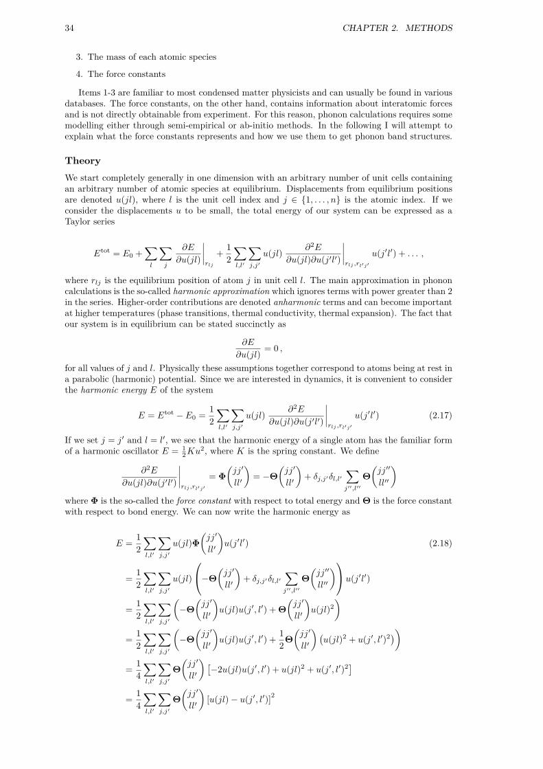
34 CHAPTER 2. METHODS
3. The mass of each atomic species
4. The force constants
Items 1-3 are familiar to most condensed matter physicists and can usually be found in variousdatabases. The force constants, on the other hand, contains information about interatomic forcesand is not directly obtainable from experiment. For this reason, phonon calculations requires somemodelling either through semi-empirical or ab-initio methods. In the following I will attempt toexplain what the force constants represents and how we use them to get phonon band structures.
TheoryWe start completely generally in one dimension with an arbitrary number of unit cells containingan arbitrary number of atomic species at equilibrium. Displacements from equilibrium positionsare denoted u(jl), where l is the unit cell index and j ∈ 1, . . . , n is the atomic index. If weconsider the displacements u to be small, the total energy of our system can be expressed as aTaylor series
Etot = E0 +∑l
∑j
∂E
∂u(jl)
∣∣∣∣rlj
+1
2
∑l,l′
∑j,j′
u(jl)∂2E
∂u(jl)∂u(j′l′)
∣∣∣∣rlj ,rl′j′
u(j′l′) + . . . ,
where rlj is the equilibrium position of atom j in unit cell l. The main approximation in phononcalculations is the so-called harmonic approximation which ignores terms with power greater than 2in the series. Higher-order contributions are denoted anharmonic terms and can become importantat higher temperatures (phase transitions, thermal conductivity, thermal expansion). The fact thatour system is in equilibrium can be stated succinctly as
∂E
∂u(jl)= 0 ,
for all values of j and l. Physically these assumptions together correspond to atoms being at rest ina parabolic (harmonic) potential. Since we are interested in dynamics, it is convenient to considerthe harmonic energy E of the system
E = Etot − E0 =1
2
∑l,l′
∑j,j′
u(jl)∂2E
∂u(jl)∂u(j′l′)
∣∣∣∣rlj ,rl′j′
u(j′l′) (2.17)
If we set j = j′ and l = l′, we see that the harmonic energy of a single atom has the familiar formof a harmonic oscillator E = 1
2Ku2, where K is the spring constant. We define
∂2E
∂u(jl)∂u(j′l′)
∣∣∣∣rlj ,rl′j′
= Φ
(jj′
ll′
)= −Θ
(jj′
ll′
)+ δj,j′δl,l′
∑j′′,l′′
Θ
(jj′′
ll′′
)where Φ is the so-called the force constant with respect to total energy and Θ is the force constantwith respect to bond energy. We can now write the harmonic energy as
E =1
2
∑l,l′
∑j,j′
u(jl)Φ
(jj′
ll′
)u(j′l′) (2.18)
=1
2
∑l,l′
∑j,j′
u(jl)
−Θ
(jj′
ll′
)+ δj,j′δl,l′
∑j′′,l′′
Θ
(jj′′
ll′′
)u(j′l′)
=1
2
∑l,l′
∑j,j′
(−Θ
(jj′
ll′
)u(jl)u(j′, l′) +Θ
(jj′
ll′
)u(jl)2
)
=1
2
∑l,l′
∑j,j′
(−Θ
(jj′
ll′
)u(jl)u(j′, l′) +
1
2Θ
(jj′
ll′
)(u(jl)2 + u(j′, l′)2
))
=1
4
∑l,l′
∑j,j′
Θ
(jj′
ll′
)[−2u(jl)u(j′, l′) + u(jl)2 + u(j′, l′)2
]=
1
4
∑l,l′
∑j,j′
Θ
(jj′
ll′
)[u(jl)− u(j′, l′)]
2

2.4. PHONON CALCULATIONS 35
u2,l-1 u1,l u2,l u1,l+1
a
m1 m1m1 m2 m2 m2
Figure 2.8: Diatomic chain. Two atomic species with masses m1 and m2 are connected by springs.The system is periodic with a unit ‘cell’ of length a. Displacements are denoted uj,l, where j is anatomic index, and l is a unit cell index.
and it becomes evident that the harmonic energy can be described with respect to atoms orbonds in mathematically equivalent ways. Since the bond-centered description does not includeindividual atomic displacements, it is necessary to add a self-term to Θ. As a visual aid to theseindex-heavy equations, Figure 2.8 illustrates the one-dimensional diatomic chain, which is oftenused in introductory texts. If we consider only nearest-neighbour interactions and identical springs,the bond-centered harmonic energy can be written
E =1
4Θ∑l
2 [u(1, l)− u(2, l)]2+
1
4Θ∑n
2 [u(2, l)− u(1, l + 1)]2
=1
2Θ∑l
[u(1, l)− u(2, l)]2+
1
2Θ∑n
[u(2, l)− u(1, l + 1)]2
where the factor of 2 comes from double-counting. The purpose of this example is to show thatthe (somewhat abstract) harmonic energy in equation (2.17) is equivalent to our intuitive under-standing of coupled harmonic oscillators. With this in mind, we can return to the matter at handand write the equation of motion for an atom j in cell l through Newtons second law F = ma:
mj u(jl, t) = − ∂E
∂u(jl)= −
∑l′
∑j′
Φ
(jj′
ll′
)u(j′l′, t) ,
where mj is the atomic mass of atom j. Solutions to this equation is given as a sum of travellingharmonic waves with wave vectors q and band indices ν ∈ 1, . . . , n
u(jl, t) =∑q,ν
u(j, q, ν) exp(iqr(jl)) exp(−iω(q, ν)t)
where ω(q, ν) is the frequency, r(jl) is the position of atom j in cell l, ω(q, ν) is the frequencyand the complex number u is called the displacement vector. If we insert these solutions into theequations of motion and just consider one band at one wave vector we obtain
mjω(q, ν)2u(j, q, ν) exp(iqr(jl)) = −
∑l′
∑j′
Φ
(jj′
ll′
)u(j′, q, ν) exp(iqr(j′l′))
mjω(q, ν)2u(j, q, ν) = −
∑l′
∑j′
Φ
(jj′
ll′
)u(j′, q, ν) exp(iq[r(j′l′)− r(jl)])
mjω(q, ν)2u(j, q, ν) = −
∑l′
∑j′
Φ
(jj′
0l′
)u(j′, q, ν) exp(iq[r(j′l′)− r(j0)]) , (2.19)
where the last equality is simply a change of origin in order to follow the convention of mostsoftware. The full account of phonon frequencies ω and displacements u can be found as solutionsto equation (2.19). At a given q and ν, the equations are indexed by j and we will have n equationswith n unknowns with respect to u(j, q, ν), where n is the number of atoms in the unit cell. Infact, equation (2.19) can be written as an eigenvalue equation:
D(q) · e(q, ν) = ω(q, ν)2 · e(q, ν) , (2.20)
where

36 CHAPTER 2. METHODS
e(q, ν) =
√m1u(1, q, ν)√m2u(2, q, ν)
...√mnu(n, q, ν)
and the elements of D(q) are given
D(jj′) =1
√mjmj′
∑l′
Φ
(jj′
0l′
)exp(iq[r(j′l′)− r(j0)]) . (2.21)
D(q) is known as the dynamical matrix and can be constructed solely from force constants.Furthermore, equation (2.21) reveals that the dynamical matrix is Hermitian so the eigenval-ues ω(q, ν)2 are real and the eigenvectors e(q, ν) are orthonormal. In addition, the eigenvalues andeigenvectors are trivially obtained numerically (e.g. numpy.linalg.eigh in the Python numpylibrary). In order to get the full dispersion, this diagonalization is performed for each of the nbands ν at the desired wave vectors in the first Brillouin Zone (FBZ).
The extension to 3 dimensions is done by treating the Cartesian components separately andconsidering q and r as vectors. The eigenvector then becomes a column vector of 3n components
e(q, ν) =
√m1ux(1, q, ν)√m1uy(1, q, ν)√m1uz(1, q, ν)√m2ux(2, q, ν)
...√mnuz(n, q, ν)
,
the number of bands increase to 3n and we get a 3n×3n dynamical matrix, where each component(2.21) is a 3× 3 block of the form
D(jj′) =
D(jj′)xx D(jj′)xy D(jj′)xz
D(jj′)yx D(jj′)yy D(jj′)yz
D(jj′)zx D(jj′)zy D(jj′)zz
where
D(jj′)αβ =1
√mjmj′
∑l′
Φ
(jj′
0l′
)αβ
exp(iq[r(j′l′)− r(j0)]) (2.22)
While the path was somewhat involved, it is useful to take a step back and consider the con-sequences of our outlined formalism. Everything we need to know about our phonon system canbe obtained from the dynamical matrix that, in turn, is constructed from force constants throughequation (2.22). Finally, all of these objects can be constructed in computationally trivial wayfrom force constants.
Practical considerationsAt this point, it is useful to consider how we construct elements of the dynamical matrix inpractice. Inspection of equation (2.22) contains a sum over all unit cells l′ and thus approachesan infinite sum. On the other hand, it is reasonable to assume that the dominant force constantsΦ are short range. The compromise is to use a finite supercell such that the second derivativesinvolved in calculating force constants outside this cell are minimized. While the reasonable size ofsuch a supercell obviously depends on the system and model, quantum contributions to the forceconstants generally vanish within a distance of roughly 10Å to 15Å. If the force constants can beobtained analytically from a semi-empirical potential, calculation is computationally simple andwe can use large supercells. However, since force constants are usually obtained from DFT, weare limited by computational resources and are usually restricted to supercells with a maximalinteratomic distance of roughly 5Å (e.g. a cubic system with a = 10Å).
Since the number of force constants needed is at least equal to the size of the dynamical matrix,the number of calculations to perform is at least 3n × 3n. Even for a fairly small system such asLCO in the I4/mmm space group (HTT, n = 7) the number of elements in the dynamical matrix is

2.4. PHONON CALCULATIONS 37
a
b
q=(0,0,0) q=(0.25,0.25,0) q=(0.5,0.5,0)
Figure 2.9: Cu-O bond stretching mode in La2CuO4 at three different values of q referring to theorthorhombic coordinate system (Bmab) as shown by the grey outline in the leftmost figure. Bluemarkers are oxygen and red markers are copper. The phase is set to ϕ = 3
4π in equation 2.23 inorder to get displacement vectors of equal length.
(3·7)2 = 441. In the finite displacement method, each force constant is the result of a self-consistentDFT calculation, so the computational effort appears prohibitively expensive at first glance. Forthis reason we use a numerical fitting of symmetry inequivalent force constants (see section 2.4).In the case of LCO in the I4/mmm space group the number of necessary displacements is reducedto only 7 (6 if we ignore magnetism), making the problem much more manageable.
Phonon eigenvectorsThe phonon dispersion is contained within the eigenvalues ω(q, ν)2. We can plot the bands ν alonghigh-symmetry lines in the FBZ by carefully choosing the values of q where the dynamical matrixis diagonalized. Similarly, we can sample the dispersion in a dense q-mesh in order to evaluate thephonon density of states. In addition, many thermodynamic properties can be calculated by onlyconsidering the eigenvalues.
The eigenvectors e(q, ν) are more subtle in nature. Each component of e(q, ν) is a complexnumber that describes the wave amplitude and phase of one atomic species j in one cartesiandirection α. In addition, the eigenvector is normalized and thus only describes relative atomicmotion. In order to visualize the collective displacement due to a phonon mode ν at q we candisplace all atoms j in unit cells l by
∆jl =A
√mj
Re [exp(iϕ)ej(q, ν) exp(i 2π q · r(jl)] (2.23)
where ej(q, ν) is the j’th component of e(q, ν) and A is an arbitrary amplitude. The phase ϕdescribes periodic motion of atoms. An animation can be produced by varying ϕ between 0 and2π.
In Phonopy the eigenvectors are always given with respect to the primitive unit cell and the 3Cartesian components are along the basis vectors of this primitive unit cell. If we want, for example,to visualize the bond-stretching mode in the HTT phase of LCO at q = ( 14 ,
14 , 0) in orthorhombic
notation, we look at atoms in primitive unit cells with origin (0,0,0), (1,0,1), (2,0,2) and (3,0,3)using the eigenvectors at q = (0.125,−0.125, 0.125). For this specific mode, the movement ofoxygen along the Cu-O bond dominates. Figure 2.9 shows this phonon mode at the zone center,halfway through the zone and at the zone boundary.
Imaginary modesIn contrast to real-world phonons, there is no guarantee that the energies obtained from equa-tion (2.20) are positive. Negative energies in a calculated phonon dispersion are called imaginarymodes and corresponds to a situation where the system gains energy by a displacement corres-ponding to the eigenvector of the imaginary mode. In other words, we are not at equilibriumwith respect to that particular phonon mode. While this is at odds with one of our assumptions,imaginary modes can reveal that a chosen symmetry might be unstable. In the case of La2CuO4,our calculations correctly predict unstable modes in the high-temperature tetragonal phase. Theinformation gathered from imaginary modes is of course limited by the fact that DFT calculationsare performed at T = 0K.

38 CHAPTER 2. METHODS
Obtaining Force Constants from DFTForce constants from DFT are found in a surprisingly simple way. In the previous sections wedefined the force constant with respect to total energy as
Φ
(jj′
ll′
)αβ
=∂2E
∂uα(jl)∂uβ(j′l′)= −∂Fβ(j
′l′)
∂uα(jl)
where Fβ(j′l′) is the force on atom (j′l′) in the direction β. Notice that everything is now labelled
by a Cartesian direction and these directions are treated individually. In practice the Cartesiandirections correspond to the unit cell vectors, but to reduce confusion we use the labels (x, y, z).We can approximate the derivative by performing a finite displacement ∆uα(jl) and simply takingthe numerical derivative
Φ
(jj′
ll′
)αβ
≈ −Fβ(j′l′;∆uα(jl))− Fβ(j
′l′)
∆uα(jl)(2.24)
where Fβ(j′l′;∆uα(jl)) is the force on atom (j′l′) in the direction β after performing the displace-
ment ∆uα(jl). At equilibrium we assume Fβ(j′l′) = 0 and we only need to calculate the forces
due to a finite displacement. In ab-initio methods, there is no reason to assume a particular shapeof the potential energy landscape and we can only expect the harmonic approximation to be validfor small finite displacements. For this reason, displacements have to be chosen large enough sothat we are not subject to numerical noise and small enough to avoid anharmonic contributions.In Phonopy the default value is 0.01Å, while PHONON uses 0.03Å.
As mentioned in section 2.4, we need a large number of force constants to construct the dy-namical matrix, even when dealing with small systems. For this reason, a numerical fitting offorces and displacements, known as the Parlinski-Li-Kawazoe method [125], is used to find forceconstants. We notice that equation (2.24) can be written as a matrix equation for one pair ofatoms (jl) and (j′l′):
F (j′l′) = −U(jl)P (jl; j′l′) ,
where
F (j′l′) = (Fx Fy Fz) ,
U(jl) = (∆ux(jl) ∆uy(jl) ∆uz(jl))
and
P (jl; j′l′) =
Φxx Φxy Φxz
Φyx Φyy Φyz
Φzx Φzy Φzz
If we perform m finite displacements, we get m simultaneous equations for each pair of atoms:
F1(j′l′)
F2(j′l′)
...Fm(j′l′)
= −
U1(jl)
U2(jl)...
Um(jl)
P (jl; j′l′) .
which can be solved by a Moore-Penrose pseudo-inverse matrix (in Numpy: numpy.linalg.pinv)given a sufficient number of displacements. Since U only depends on (jl), we can build up the fullforce constant matrix by iterating this procedure over (j′l′). The minimum number of displace-ments is equal to the number of non-equivalent atoms in the crystal primitive unit cell multipliedby a number of independent x,y,z coordinates in the site symmetry of a given atom [125]. Forthis reason, software such as Phonopy and PHONON determines the primitive unit cell, the supercellexpansion matrix and all the symmetry operations before generating displacements.

2.5. MOLECULAR DYNAMICS 39
2.5 Molecular Dynamics
The objective of a molecular dynamics simulations is to generate a trajectory of atomic positionsas a function of time. This method has a rich history in materials science since it can be use tostudy ensembles explictely. The general idea is to build a real space model containing particlesand their interactions and then integrate the Newtons equations of motion for this many-bodysystem. By analyzing the resulting trajectory, one can obtain information about thermodynamic,structural and (of course) dynamical properties.
In the context of this thesis, the forces for our simulation is obtained through a DFT calculation,so that every configuarion of atomic postions requires a self-consistent calculation. For this reason,the forces are obtained ab-initio and we only have to worry about integrating the equations ofmotion. This can be done very efficiently using the Verlet algorithm [127]:
ri(t+∆t) = −ri(t−∆t) + 2ri(t) + ai(t)∆t2 +O(∆t4)
where ri is the position of atom i, ai is the acceleration, ∆t is the time step. This equation caneasily be obtained by summing the Taylor expansions of ri(t + ∆t) and ri(t − ∆t). The timestep is a crucial choice for any MD simulation. On one hand, it is important to have a smallenough time step such that the dynamics are accurately described. On the other hand, if the totalsimulation time is too short, we might not probe a large enough part of phase space to make theensemble averages represenatative. In other words, short simulation times might trap you in alocal minimum of phase space.
MD simulations are, unlike DFT ground state calculations, generally performed at finite tem-peratures. Generally this temperature is initialized by giving every atom an initial velocity takenfrom the Boltzman distributon at the initial temperature. During the simulation, the temperat-ure can be controlled in different ways, depending on the thermodynamic ensemble one wishes tosimulate. While energy should be conserved, the Verlet algorithm might cause the total energy todrift, especially if the system is out of equilibrium. For this reason, it is usually desirable to havea thermostat that controls the temperature. For the simulations performed in this thesis, we usethe Nosé-Hover thermostat [128]. I will not repeat the details here, but the general idea of MDthermostats is to scale the velocities such that the temperature is kept constant.
After having performed a MD simulation, we want to be able to compare with experiment. Thetrajectories can be analyzed in a variety of ways, but there are a few basic observables that areeasy to compute in the case of crystalline materials: The phonon density of states and the pair-distribution function. In the following, I outline how these observables are obtained in practice.
VACF and gDOSIt turns out [129] that the phonon density of states can be found from the power spectrum of themass-weighted velocity autocorrelation function (VACF). The VACF is, as the name implies, anexpression of the correlation between velocites at different times. In liquids, the VACF will rapidlydecay to zero and in solids the VACF will fluctuate due to coherent vibrations around equilibriumpositions. The VACF for a single atomic species α is defined as
Cα(t) =1
3⟨vα(t0) · vα(t)⟩
By invoking ergodicity, the ensemble average can be replaced with a time average with respect tot0.
Cα(t) =1
3
1
T − t
T−t∑t0=0
vα(t0) · vα(t0 + t) =1
3
1
T − t
T−t∑t0=0
∑β=x,y,z
vαβ(t0)vαβ(t0 + t)
where T is the total simulation time and vαβ is the velocity of atom α in direction β. The totalVACF is defined as
C(t) =∑α
mαCα(t)
where mα is a weight depending on the atomic species and the terms of the sum are the partialVACFs. To get the mass-weighted VACF mα is equal to the atomic weight of species α divided

40 CHAPTER 2. METHODS
Figure 2.10: Visualization of the radial distribution function. Centered on an atom α (blue), wecount the number of atoms β (green) that can be found in a spherical shell at a distance r with awith dr. As shown in the text, this can be used to construct the radial distribution function g(r).Figure from [130].
by the average weight of atomic species. The density of states is obtained as the power spectrumof the mass-weighted velocity autocorrelation function:
DOS(ω) =∑α
σα1
2π
∫ +∞
−∞dt exp[−iωt]mαCα(t) ,
where the terms of the sum, once again, determines the partial density of states for atomic speciesα. To get the neutron-weighted DOS, we set σα equal to the coherent neutron cross-section ofspecies α. In practice both the VACF and DOS is found numerically by FFT methods. Theneutron-weighted phonon DOS obtained from simulations in this thesis are all evaluated using thetools created in appendix A.
Radial distribution functionThe radial distribution function is defined as
g(r) =ρ(r)
ρ,
where ρ(r) is the particle number density at a distance r from an arbitrary atomic origin andρ = N
V is the number density of the unit cell. A visual representation of this quantity is shown infigure 2.10. Formally this can be found from atomic positions
g(r) =1
Nρ
⟨N∑i
∑i=j
δ(r − rij)
⟩
where i and j are particle indices and rij is the distance between particle i and j. N is the totalnumber of particles and the brackets denote an ensemble average. Due to the delta function, thisexpression is not particularly useful when analysing MD trajectories of discrete particle positions.To overcome this, we define n(r,dr) as a function that counts the number of particles at a distancer within a spherical shell of thickness dr.
g(r) =2 ⟨n(r,dr)⟩NρVs(r,dr)
, (2.25)
where Vs(r,dr) ≈ 4πr2dr is the thickness of the spherical shell. Due to the ergodic hypothesis, theensemble average is replaced with a time average, so that
⟨n(r,dr)⟩ = 1
M
M∑k=1
nk(r,dr)

2.6. COMPARING SIMULATION AND EXPERIMENT 41
where M is the number of time steps. In practice nk is evaluated by creating a list of all particle-particle distances in the frame k and generating a histogram with bin size dr. The factor of twoin equation (2.25) comes from the fact that nk only counts each pair once.
The g(r) we just defined treats all particle pairs on an equal footing. In order to comparesimulations with neutron scattering data it is necessary to weigh distinct particle pairs by theproduct of their neutron cross sections. First, we define the partial radial distribution functiongαβ(r) as the probability of finding a particle with label β at a distance r away from a particlewith label α plus the probability of finding a particle with label α at a distance r away from aparticle with label β.
gαβ(r) =⟨nαβ(r,dr)⟩NαρβVs(r,dr)
+⟨nαβ(r,dr)⟩NβραVs(r,dr)
=2V
NαNβ
⟨nαβ(r,dr)⟩Vs(r,dr)
,
where Ni is the number and ρi is the density of particle species i. The reason to define it in ‘bothdirections’ is that nαβ is symmetric to exchange of particles. From the partial pair distributionfunctions, G(r) can be trivially computed and optionally weighted by neutron cross sections, aswe saw in section 2.1:
G(r) =1
b2
∑α=1,β≥α
cαcβbαbβ(gαβ(r)− 1) ,
Atomic distance histogramsIf our MD simulations fulfils the ergodic hypothesis, it is useful to look at various distributions thatcan be extracted from the simulation. While a lot of this information is contained in the radialdistribution function, the system studied in this thesis is not isotropic. In fact, the 2-dimensionalnature of the cuprates appears to be essential for the electronic properties. By generating histo-grams for certain atoms, we can ask a few pertinent questions such as:
• What is the distribution of Cu-Oeq distance?
• What is the distribution of Cu-Oap distance?
• What is the distribution of octahedral tilts (Q1, Q2)?
• What is the nature of Oint diffusion?
All of these questions are well-defined in the context of molecular dynamics trajectories, but itcan be tedious for large systems to label all the relevant atoms. To overcome this, we generatepairs of atomic species based on certain conditions. For example, if we want to find pairs of Cuand Oeq, we loop over all Cu-O pairs and only list the pairs where the distance vector is lessthan r = (2.1, 2.1, 1)Å. After building the pair-lists it is trivial to generate histograms of certaindistances.
Similarly, we can build the CuO6 octahedra by applying the same idea to both equatorial andapical oxygen atoms. We can identify the 6 corners of the octahedron simply by checking the signsof the 6 distance vectors (e.g. the ‘top’ apical oxygen will have a positive z component). Q1 andQ2 can then be computed and we can generate histograms of the octahedral tilts.
Finally, we can also use these pairs to generate symmetry operations in a fairly simple way.Since we know that the octahedra have alternating tilt patterns, we can check the tilt pattern atframe 1 and generate a list of the 4 different combinations of Q1 and Q2 ((+,+),(+,-),(-,+),(-,-)).Applying these symmetry operations to our calculations then lets us obtain a histogram of thesymmetry-adapted octahedral tilts.
2.6 Comparing Simulation and Experiment
Finally, we conclude this chapter by giving examples of how to compare the simulation methodswith neutron scattering experiments. As we saw in section 2.1, this thesis features 3 types ofneutron measurements.
1. Direct measurements of phonon bands with TAS spectroscopy

42 CHAPTER 2. METHODS
2. Phonon density of states on powders with time-of-flight methods.
3. PDF measurements of powders
All of these can be compared directly with simulations in various ways, but there are some subtletieson how to perform this comparison correctly. In this section we thus treat them one at a time.
Phonon bands with TAS
The master equation for phonon scattering can be found in [97] and directly relates the measureddifferential cross-section to the phonon band structure as we saw in section 2.2, equation (2.5)(repeated here for clarity)
S(Q, ν, ω) =kfki
N
h
∑q
|F (Q, q, ν)|2(nqν + 1)δ(ω − ωqν)δ(Q− q −G) (2.26)
F (Q, q, ν) =∑j
√h
2mjωqνbj exp
(−1
2⟨|Q · u(j0)|2⟩
)exp[−i(Q− q) · r(j0)]Q · ej(q, ν) (2.27)
Note that the equations have been rewritten slightly when compared to Squires [97] (similar towhat is presented on the Phonopy website [131]), such that S(Q, ν, ω) is defined separately foreach phonon band. In addition, the sum in the phonon structure factor runs over atomic indicesin unit cell 0, consistent with the definitions made earlier in this chapter.
By close inspection of equation (2.26) and (2.27), we realise that the information obtained by thecalculation of phonon band structures provides us with all the information necessary to constructS(Q, ν, ω). Since normalization on an absolute scale is usually not possible when performing aTAS experiment, the neutron-weighted band structures are shown with Nkf/ki = 1.
The δ-functions in equation (2.5) tells us that a neutron measurement will only have intensityif we measure at values of Q and ω that correspond to a point of the dispersion of band ν. Wethus reduce our calculations to sampling S(Q, ν, ω) at (q, ωqν). The only computationally heavypart then becomes the Debye-Waller factor
W =1
2
⟨|Q · u(j0)|2
⟩which has to be sampled at some finite grid in unit cell 0 in order to get a reasonable estimateof the ensemble average. In many cases we compare measurements to a phonon dispersion in thefirst BZ where W varies only slightly, so if we want to sample a large number of Q-points it canbe advantageous to simply omit the Debye-Waller factor. As of this writing, this is not possiblein Phonopy directly, so we have to live with someone heavy computations for now.
With these equations in mind, we can now plot the neutron-weighted phonon bands and com-pare them with TAS-measurements. We can represent the neutron weighted bands either bycolouring the band-structure lines according to intensity or by giving the dispersion curves a finiteGaussian width to replicate a finite instrument resolution and/or linewidth broadening. Figure2.11 shows examples of the two kinds of representations. By adding obtained neutron data tothese plots, we can then directly compare theory and experiment. We note here that a comparisonwith MD simulations is not possible since these simulations give no information about the discretephonon bands.
Phonon Density of States
The phonon density of states (DOS) is a simple projection of the phonon bands onto the energy axis.While this obviously reduces the amount of information due to the reduction of dimensionality,the phonon DOS is a useful object for a couple of reasons:
1. Often only powders are available for experiments and resolving bands can be difficult due tothe rotational averaging.
2. Many neutron scattering instruments are specifically designed for DOS measurements.
3. DOS can be obtained from molecular dynamics as well as band structure calculations.

2.6. COMPARING SIMULATION AND EXPERIMENT 43
Figure 2.11: Neutron weighted phonon band structure of La2CuO4 in the high-temperature tetra-gonal phase. On the left, the bands are shown as a line plot where the lines are colored accordingto neutron intensity. On the right the same simulation is shown, but the bands are given aGaussian width along the energy axis of σ = 0.5meV, giving a better idea of what the measuredneutron spectrum would look like. Additionally, this plot is produced with a minimum threshold ofneutron intensities in order to remove bands with very little intensity (the calculation will allwaysreturn a finite intensity).
The last point is particularly important in the case where we are working with defect structuressuch as oxygen interstitials. Here, the (local) symmetry is usually severely broken (often to P1symmetry) and a phonon calculation would be prohibitively expensive. As shown in section 2.5,the phonon DOS can be obtained, in the harmonic approximation, rather simply from a MDtrajectory.
To obtain the DOS from a band-structure calculation, we perform an integration over a com-mensurate grid in the 1st BZ and project the result onto the energy axis for each atomic species jin the following way:
gj(ω) =∑
n=x,y,z
1
N
∑q,ν
δ(ω − ωqν) |n · ej(q, ν)|2
g(ω) =∑j
gj(ω)
where n is the unit vector in the three cartesian directions. Comparing this equation with equation(2.5) we notice that we only need to weigh by mass and the neutron cross-section in order to go fromthe true density of states g(ω) to the neutron S(ω). If we performed a TAS experiment on a singlecrystal with perfect resolution at every relevant (q, ωqν) point, these definitions would be correctand we could perform the integration on our massive 4-dimensional dataset. However, due to thenature of typical DOS measurements, we need to invoke the so-called incoherent approximation anduse the incoherent 1-phonon partial differential cross-section when treating the data. In practicethis means using the total neutron cross sections (σtot) with the incoherent 1-phonon S(q, ω) asshown in section 2.2.
Pair-density function measurements
When performing neutron PDF measurements, it is possible to extract the normalized total neutronPDF (construction of partials require several measurements, see ref. [132]). As such, we should beable to compare directly with the PDF as extracted from molecular dynamics as shown in section2.5. PDF from phonon band structure calculations are in principle possible since we can extractthermal displacements, but it is currently not a feature in Phonopy, so this analysis has not beenperformed here.


Chapter 3
Phonon Calculations
In this chapter, results from ab-initio simulations are presented independent of experimental data.It turns out that a careful investigation of various phases of La2CuO4 presents us with valuable cluesregarding the average and local structure. While DFT is unable to capture the strongly correlatednature of the cuprates, it turns out to be a reasonable description with regards to intermolecularforces. The subsequent strategy is to carefully validate our simulations and establish a ‘one-electronbaseline’ for the studied systems. Experimental deviations from this baseline can then be analysedfor clues possibly pertaining to superconductivity or other phenomena not captured at the DFTlevel of theory.
One example of such a deviation is shown in Chapter 8, where we can detect potentially interest-ing physics by following how a certain phonon mode diverges from our otherwise robust simulationresults. In this chapter we perform DFT simulations based on the La2CuO4 parent compoundacross three structural and two electronic phases, all of which have been observed experimentally inthe lanthanum-based cuprates. We then calculate phonons within the ‘Frozen-Phonon’ approachand obtain the neutron-weighted phonon band structure. Since the computational requirementsof phonon calculations are heavily influenced by symmetries, we do not consider defects such asinterstitials in this chapter as this would make the computational effort unmanageable. To under-stand the dynamics due to dopant species, molecular dynamics simulations based on the results ofthis chapter are presented in Chapter 4.
3.1 Computational Details
The theory and principles behind Density Functional Theory (DFT) is presented in chapter 2,section 2.3. DFT simulations in this thesis are performed using the Vienna Ab-Initio SimulationPackage (VASP) [133–136] using Projector Augmented-Wave Pseudopotentials (PAW) [137, 138]to describe the atomic wavefunctions. While ab-initio loosely translates to ‘from the beginning’,There are several choices to be made with regards to computational parameters. First, we needto define the pseudo-potentials that describes the valence electrons of each atomic species in oursystem. For L(S)CO(+O), the relevant pseudo-potentials are listed in Table 3.1 along with theirelectronic configuration. For both La and O we used the recommended potentials, while for Cu weused a more accurate version where all 6 3p electrons are included (_pv is short for ‘p in valence’).The reason for this is simply because it was difficult to have the simulations converge with thestandard potential – not because we necessarily believe that the Cu 3p states are important forthe chemistry of our system. To run a simulation in VASP, or in any DFT software, the followinginformation (files) is required:
• Crystal lattice and atomic coordinates (POSCAR)
• Pseudopotential configuration (POTCAR)
• k-point mesh (KPOINTS)
• Computational parameters (INCAR)
The choice of crystal lattice and atomic positions are typically taken from experiment, but it isimportant to realize that the simulation might not ‘agree’ completely. This is especially importantif we want to calculate phonons through the evaluation of forces due to displacements away fromequilibrium positions. The pseudopotential configuration is usually taken from a database sincethe generation of consistent, transferable potentials is a difficult, time-consuming task. In fact,
45

46 CHAPTER 3. PHONON CALCULATIONS
the main selling point of VASP is their high-quality pseudopotentials. The k-point mesh definesthe number of k-points where the wavefunctions and density is evaluated and has a huge impacton computational effort (going from e.g. a 2 × 2 × 2 grid to a 4 × 4 × 4 takes 8 times as manyevaluations). Luckily, the amount of k-points needed for an accurate calculation usually convergesrapidly and we often check this convergence explicitly. Since the density of the k-point meshdepends on the system size, it is common to state the k-point density which is defined as thenumber of k-points per reciprocal atom (or simply #k-points × #atoms).
Finally, there is a large number of computational parameters that can be tweaked dependingon the desired type of calculation. The VASP INCAR file has more than 300 optional tags [139],but usually only a few needs to be tweaked depending on the desired type of simulation. For thesimulations performed in this thesis the following keywords are important:
• ENCUT: The plane-wave cut-off and thus the size of the basis set. Usually the default performswell, but for accurate forces, this needs to be increased. In the manual they recommend 1.3times the default cut-off, but there are cases where even this is insufficient [140].
• EDIFF: The threshold for the the self-consistent cycle to terminate. For accurate forces thisneeds to be increased.
• PREC: A tag that defines the ‘precision’ by setting new defaults for certain parameters. Igenerally increase this to ‘Accurate’ for all simulations. ‘Normal’ is the default.
• LREAL: A PAW pseudopotential specific tag which determines if an evaluation of a certainprojection operator is performed in real or reciprocal space. This operation is faster inreal space, but at the cost of accuracy. For phonons we want to perform the operation inreciprocal space.
• GGA: Sets the exchange-correlation functional (see section 2.3). Usually the default (PBE) isa good starting point, but experimentation is encouraged!
• ISPIN and MAGMOM: Turns on a spin-polarized calculation.
• IBRION and ISIF: How and when to update the ionic positions. This can be used to performmolecular dynamics and structural optimizations in different ways.
• ISMEAR and SIGMA: A tag that controls ‘fermi surface smearing’, which is important formetallic systems where we need to evaluate a discontinuous function at the fermi level dueto partial occupancies. This can be done in several ways, and it is usually good practice totest the convergence and performance of these methods.
• LDAU: Switches on LDA+U (see section 2.3) which can alleviate the intrinsic problem of DFTwhen dealing with localized d- and f-orbitals. This is needed in our simulations if we wantto describe the anti-ferromagnetic structure of La2CuO4.
• ISYM: Controls how VASP deals with space group symmetry.
The take-home message here is that phonon calculations generally needs increased precision withrespect to the recommended default values. When one is mainly concerned with the electronic bandstructure the dominant energies are typically on the order of eV, where typical phonon energies areon the order of meV, 3 orders of magnitude smaller. In addition, forces are evaluated as derivativesof the total energy (per the Hellmann-Feynmann Theorem, see section 2.4) so numerical noise isamplified. For molecular dynamics this precision is less crucial since the many time steps willaverage out this numerical noise.
Z Core (# electrons) Valence (# electrons)
La 57 1s22s22p63s23p63d104s24p64d10 (46) 5s25p65d16s2 (11)Sr_sv 38 1s22s22p63s23p63d10 (28) 4s24p65s2 (10)Cu_pv 29 1s22s22p63s2 (12) 3p63d104s1 (17)O 8 1s2 (2) 2s22p4 (6)
Table 3.1: PAW pseudopotential electronic configuration used in VASP calculations. Whilelanthanum is typically placed in the f-block on periodic tables it’s electronic configuration hasno f-electrons. This is fortunate since DFT (in)famously struggles with highly localized orbitals.

3.2. ELECTRONIC AND STRUCTURAL PHASES 47
Functional and Energy Cut-offAs we discussed in Section 2.3, a large number of functionals have been developed for DFT cal-culations. At the GGA level of theory 24 functionals are available in VASP and choosing one canseem like an daunting task at first glance. It is, however, important to realize that most functionalshave been created to treat a specific problem. This is an expression of the fact that, despite ourbest efforts, no universal functional exists currently. With that in mind, functionals with hightransferability do exist and the default PBE functional in VASP has been used to describe a widevariety of systems, emphasized by the 40000+ citations of the original paper [141].
While PBE is technically a semi-empirical functional, the only experimental parameter is de-rived from the uniform electron gas. The simplicity and transferability of this functional thusmakes it an excellent starting point for any DFT calculation. Generally one would start with PBEand then turn to other functionals if calculations fail to line up with empirical data. As we shallsee, we run into this exact problem when evaluating forces in our system and we have to changeour functional to PBESol (PBE revised for solids) in order to get a reasonable description of lowenergy phonons.
We run into a similar problem with the plane wave energy-cutoff when evaluating forces. Thedefault energy-cutoff is generally set by the element with the highest recommended cut-off, in ourcase oxygen at 400 eV. For accurate forces it is recommended to increase this by a factor of 1.3,but for phonon calculations, we see improvements all the way up to an 800 eV cut-off. The lessonhere is a cautionary tale – at times, the lack of precision in the calculation might not reveal itselfbefore having performed an expensive phonon calculation.
3.2 Electronic and Structural Phases
With an understanding of the functionality and limitations of DFT, and in particular VASP, wecan begin to formulate a strategy to investigate the La2CuO4 (LCO) system. From diffractionstudies, we know that LCO can exist in (at least) three structural phases depending on doping andtemperature (see section 1.3). While the electronic structure of superconducting cuprates cannotbe accurately described within DFT, undoped and overdoped La2CuO4 can be described as Mott-Insulator and Fermi-Liquid, respectively. Both of these electronic phases can be approximatelydescribed with DFT.
In order to say anything about the superconducting cuprates with DFT, we are thus limitedto a study of limiting cases in terms of the electronic structure. On the other hand, if we wantto study phonons through atomic forces, many-body theories will struggle with realistic systemsizes. Quantum Monte Carlo methods are making progress, but accurate forces are still a significantlimitation [142]. Since we are working with the knowledge that the exact behaviour of the electronsare poorly described in our theory, our simulations must be carefully evaluated against experimentsto ensure that our simulations are capturing the dominating contributions to atomic forces.
Electronic StructureSince ‘electronic structure’ is the output of a DFT calculation, one might object to the statementthat we want to investigate different electronic structures of La2CuO4. Without any additionalconstrains, DFT at the GGA level of theory generally results in a metallic state [143], wherethe observed antiferromagnetic (AFM) solution requires a non-local theory [144]. Since non-localtheories (beyond GGA) are computationally expensive, they become impractical for our purposes.Some authors have reported an AFM solution using certain GGA functionals [145], but I have notbeen able to reproduce this result in a consistent way. If a magnetic solution is found, the magneticmoment usually vanishes by small changes to the k-point mesh or energy cut-off, suggesting thatthe magnetic ground state is a local minimum.
A compromise developed specifically for correlated electron systems is the LDA+U (sometimescalled DFT+U or GGA+U) method [123] described in section 2.3. This ad-hoc method treats thestrong on-site Coulomb interaction of localized electrons with a Hubbard-like term parametrizedthrough an on-site repulsion U and an exchange parameter J . In the method by Dudarev et al.[146] these are reduced to one parameter Ueff = U − J . The LDA+U method was developedspecifically to treat Mott-Insulators [123], but has been used to calculate hole doped La2CuO4 andLa2NiO4 [123]. Some recent studies have even looked at stripe ordered phases of La2−xSrxCuO4
[147, 148]. In these studies, hole doping is done by removing electrons and adding a neutralizingbackground, rather than the introduction of actual dopant species. Since LDA+U comes at a much

48 CHAPTER 3. PHONON CALCULATIONS
Table 3.2: Crystal structures found in various lanthanum-based cuprates. All structural phases canbe parametrized with respect to LTLO, where Q1 and Q2 represent octahedral tilts as describedin the text and η = b−a
b+a is the orthorhombic strain.
Space Group (#) Name (shorthand) Tilts η
I4/mmm (139) High-Temperature Tetragonal (HTT) Q1 = Q2 = 0 = 0
Fmmm (69) Q1 = Q2 = 0 = 0
Bmab (64) Low-Temperature Orthorhombic (LTO) Q2 = 0, Q1 = 0 = 0
P42/ncm (138) Low-Temperature Tetragonal (LTT) Q1 = Q2 = 0 = 0
Pccn (56) Low-Temperature-Less-Orthorhombic (LTLO) Q1 = Q2 = 0 = 0
lower computational cost compared to e.g. hybrid functionals and since it was developed with thecuprates in mind, it becomes an obvious choice for our purposes.
Crystal Structure
The observed structural phases of lanthanum based cuprates fall into a moderate number of spacegroups as listed in Table 3.2 and introduced in section 1.3. All of the structural phases can bedescribed with reference to Figure 1.9 where we define Q1 as a rotation along a (around b) and Q2
as a rotation along b (around a). In addition, we define the orthorhombic strain as η = b−ab+a . In
our simulations we have chosen to focus on three structural phases
• HTT: The parent high-symmetry phase observed at high temperatures and/or overdopedsamples.
• LTO: The most common structural phase at low temperatures for relevant superconductingsamples.
• LTT: A lower symmetry phase than LTO observed in La2−xBaxCuO4 and La1.6−xNd0.4SrxCuO4.Appears to supress superconductivity with the notable exception of La1.88Ba0.12CuO4 (Tc ≈5K)
3.3 Coordinate systems
Having decided on the phases to investigate, we take a short detour to describe the coordinate sys-tems used in real and reciprocal space. Since we are dealing with several electronic and structuralphases, we need a common description to compare between phases. In real space, we use the Q1,Q2, η description from above and in reciprocal space we use the HTT Brillouin Zone.
Octahedral Tilts
In order to quantify the octahedral tilts for use in simulations, we use the coordinate systemsketched in Figure 3.1. All possible tilts can be described with reference to the lowest symmetryspace group (LTLO, Pccn). The octahedra are described with two in-plane oxygens (O1, O2) andone apical oxygen O3 and the Pccn space group is the only one with three inequivalent oxygenatoms. Due to symmetry constrains, a rotation of this octahedron will cause a displacements inthe c-direction of the in-plane oxygen and in the a, b direction of the apical oxygen (a reasonableapproximation at small angles). Following [67], we define Q1 as a rotation around the (010) axisand Q2 as a rotation around the (100) axis in orthorhombic notation. In more intuitive terms, Q1
‘tilts’ the octahedron along a, while Q2 ‘tilts’ along b.By inspection of Figure 3.1, a Q1 rotation will displace O3 in the x-direction and O1, O2 in
the negative z-direction. A Q2 rotation will displace O3 in the y-direction, O1 in the positivez-direction and O2 in the negative z-direction. If we want to express Q1 and Q2 as angles, thedisplacements become:

3.3. COORDINATE SYSTEMS 49
dy
dz
O2
O1
(100)o
(010)o
Figure 3.1: Left: Geometry of octahedral tilts in the with the c-axis vertical. Right: Illustrationof the two inequivalent in-plane oxygens. Q1 is a rotation around the (010) axis while Q2 is arotation around the (100) axis.
Ox3 = Oz
ap sin(Q1)c
a
Oy3 = Oz
ap sin(Q2)c
b
Oz1 =
1
4c[−a sin(Q1) + b sin(Q2)]
Oz2 =
1
4c[−a sin(Q1)− b sin(Q2)] ,
where Oij is the i-component of oxygen j in fractional coordinates. Since these equations uniquely
define displacements in terms of tilt angles, we can also find tilt angles from structural displace-ments from either the apical oxygen:
Q1 = sin−1
(Ox
3
Ozap
× a
c
)Q2 = sin−1
(Oy
3
Ozap
× b
c
),
or the equatorial oxygen:
Q1 = sin−1
(−2c
a× (Oz
1 + Oz2)
)Q2 = sin−1
(−4c
b× Oz
2 −a
b× sin(Q1)
).
To apply an orthorhombic strain η to a tetragonal structure with an in-plane lattice parameter a′,while keeping the volume constant (which is important when comparing DFT simulations due toPulay Stress, [149]), the following equations can be used to find the a and b lattice parameters:
a =a′
1 + η
b = (1 + η)a′ .
These equations can then be used to generate desired tilts and extract tilt angles from any givenstructure. Since every tilt is defined with respect to only 3 oxygen atoms, these equations requireat least Pccn symmetry which is preserved for geometry optimizations and phonon calculations.For lower symmetries (in e.g. MD simulations) we define a ‘symmetrized average tilt’ (see chapter4). Code to generate these structures and extract rotation angles from any structure can be foundin appendix A. This methodology can also be used with any software that can generate crystal

50 CHAPTER 3. PHONON CALCULATIONS
Figure 3.2: Brillouin Zones of the HTT, LTO and LTT phases (see Table 3.2). Modified from [152]
Γ X(π,0)
M(π,π)X(0,π)M(-π,π)
Figure 3.3: Left: BZ of a primitive tetragonal cell with high-symmetry lines. Right: The in-planeBZ with the same labels and the usual Γ-X-M -Γ path. If the large BZ is the crystallographic HTTphase, then the broken blue lines represent the LTO/LTT/LTLO BZ and we can consider the Γ-X-M2 -Γ path, since M becomes Γ for this (smaller) BZ. In literature the labels are often confused,while (π, π) and (π, 0) are universally agreed upon. In any band structure diagrams presentedhere, the labels in this figure is used.
structures from space group symmetry and fractional coordinates (e.g. ASE [150] and VESTA[151]). The same result can, of course, also be obtained by considering each of the space groupsindividually and then figuring out how to generate tilts and transform the lattice to a commoncoordinate system. If one is only interested in atomic coordinates, starting from Pccn is convenient.This way, atomic indices are also identical for all structures.
Reciprocal Space: Band StructuresBand structures are described with respect to the reciprocal lattice. Due to the enlargement of thereal-space crystal structure as we move through HTT → LTO → LTT, the Brillouin Zone (BZ)shrinks by the same amount. Similar to how it is useful to describe our real-space lattice withrespect to the Pccn coordinate system, it is useful to describe reciprocal space with respect to acommon coordinate system when comparing results. As we can see in Figure 3.2, the BZs of HTT,LTO and LTT have vastly different shapes, so it is difficult to superimpose results.
For this reason, we chose a primitive tetragonal BZ to describe the HTT phase (note that thisshape is different from the actual HTT BZ in figure 3.2) and then construct the smaller LTO andLTT BZZs with respect to this construction. The idea is sketched in Figure 3.3. This constructionalso helps emphasize the 2-dimensional nature of the cuprates. In all following simulations, theband labels in Figure 3.3 will be used, keeping in mind that the nature of high-symmetry pointscan change depending on the considered structural phase. One example is that the M point, whichis the zone boundary of HTT, becomes the zone centre of LTO and would thus usually be denotedΓ.
While this construction is useful for our intuitive understanding of the different phases, phononcalculations require k-vectors with respect to the primitive unit cell. For this reason, we need thetransformation matrices from our constructed coordinate system to the primitive HTT and LTO

3.4. STRATEGY 51
unit cells (the LTT transformation is the identity matrix). This conversion can be done with thefollowing matrices.
PAHTT =
0 0 12
12
12 0
12
12
12
PALTO =
12
12 0
0 0 112
12 0
these matrices can be used to generate k-points starting from the more ‘intuitive’ notation outlinedin Figure 3.3. For example, the X-point (( 12
120) with respect to our coordinate system) in the HTT
phase becomes ( 12120) · PAHTT = ( 14
1414 ).
3.4 Strategy
To find a connection between the structural phases, we start with the highest symmetry phase(HTT) using cell parameters and fractional positions approximated from literature [71]. The AFMstructure is based on La2CuO4 that has been modified in a way such that η = 0 and Q1 = Q2 = 0.The metallic structure is based on La1.775Sr0.225CuO4, which is tetragonal (HTT) at 10K.
The structure is then optimized and we calculate the electronic and phonon band structures.We then break the symmetry by applying a small rigid tilt Q2 = 5 along with small orthorhombicstrain η = 0.005, resulting in the LTO phase which we then optimize and finally perform thesame set of calculations. A HTT-LTT transformation is performed in a similar fashion withQ1 = Q2 = 5 and η = 0. This procedure is then performed in parallel for the anti-ferromagneticsolution using LDA+U and the metallic solution. The resulting band structures, density-of-statesand total energies are then analysed and validated against experimental data.
All calculations in this chapter is performed on La2CuO4 in the conventional orthorhombic unitcell, which corresponds to the primitive Pccn lattice that we use to generate the structures. Thiscell contains four formula units and is large enough to accommodate anti-ferromagnetism. SinceVASP can handle symmetry through the ISYM keyword, we don’t need an input cell correspondingto the primitive cell of the considered structural phase. Before starting any ‘production’ DFTcalculation, it is advantageous to benchmark certain computational parameters in order to get anidea of how well-behaved the SCF convergence is and what energy scales we can expect to probe.
3.5 Benchmarking
When performing DFT calculations in VASP there are a few parameters that have significantimpact on the precision of the calculation. Increasing the precision also results in significantlylonger computation time, so it is important to find a compromise.
Figure 3.4 shows a benchmark of AFM LCO with respect to the k-point mesh and smearingwidth σ. Since there are no states at the Fermi level, the smearing width converges rather quickly,and we can safely use a value of σ = 0.1 eV. The k-point density also converges rather quickly,and we achieve a precision of 0.1meV using a fairly coarse MP-grid of 8 × 8 × 4 (7168 k-pointsper reciprocal atom). In AFM LCO we also checked the effect on electronic structure due to theon-site repulsion U . The result is shown in Table 3.3 and the values of U = 8 eV, J = 0.8 eV arechosen based on the proximity to experimental evidence [153, 154] and previous theoretical studiesof the La2CuO4 system, where the values of U and J where found self-consistently [147, 155].
Table 3.3: LDA+U Benchmarking of the parameters U and J calculated with LDAUTYPE=4 in theHTT phase of La2CuO4. Experimentally the Cu moment is (0.48± 0.15)µB [153] and the opticalgap is ≈ 2 eV [154]. As a reasonable compromise we chose U = 8 eV and J = 0.8 eV, a set ofvalues also used in a previous study of the same system [147].
U [eV] J [eV] Moment [µB] Optical gap [eV]
4.0 0.4 0.330 0.3486.0 0.6 0.481 1.0168.0 0.8 0.588 1.68610.0 1.0 0.676 1.87712.0 1.2 0.755 2.042
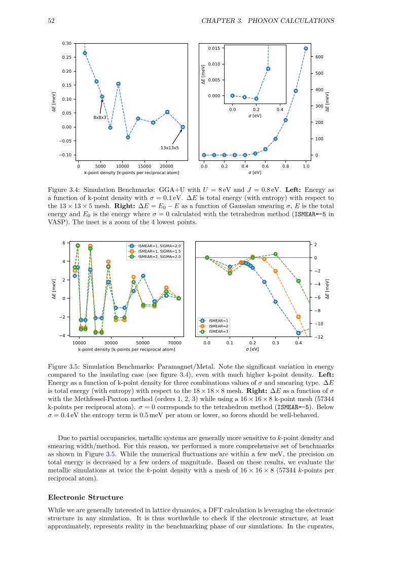
52 CHAPTER 3. PHONON CALCULATIONS
0 5000 10000 15000 20000k-point density [k-points per reciprocal atom]
0.10
0.05
0.00
0.05
0.10
0.15
0.20
0.25
0.30
E [m
eV]
8x8x3
13x13x5
0.0 0.2 0.4 0.6 0.8 1.0 [eV]
0
100
200
300
400
500
600
E [m
eV]
0.0 0.2 0.4 [eV]
0.000
0.005
0.010
0.015
E [m
eV]
Figure 3.4: Simulation Benchmarks: GGA+U with U = 8 eV and J = 0.8 eV. Left: Energy asa function of k-point density with σ = 0.1 eV. ∆E is total energy (with entropy) with respect tothe 13× 13× 5 mesh. Right: ∆E = E0 −E as a function of Gaussian smearing σ, E is the totalenergy and E0 is the energy where σ = 0 calculated with the tetrahedron method (ISMEAR=-5 inVASP). The inset is a zoom of the 4 lowest points.
10000 30000 50000 70000k-point density [k-points per reciprocal atom]
4
2
0
2
4
6
E [m
eV]
ISMEAR=1, SIGMA=2.0ISMEAR=1, SIGMA=1.5ISMEAR=2, SIGMA=2.0
0.0 0.1 0.2 0.3 0.4 [eV]
12
10
8
6
4
2
0
2
E [m
eV]
ISMEAR=1ISMEAR=2ISMEAR=3
Figure 3.5: Simulation Benchmarks: Paramagnet/Metal. Note the significant variation in energycompared to the insulating case (see figure 3.4), even with much higher k-point density. Left:Energy as a function of k-point density for three combinations values of σ and smearing type. ∆Eis total energy (with entropy) with respect to the 18× 18× 8 mesh. Right: ∆E as a function of σwith the Methfessel-Paxton method (orders 1, 2, 3) while using a 16× 16× 8 k-point mesh (57344k-points per reciprocal atom). σ = 0 corresponds to the tetrahedron method (ISMEAR=-5). Belowσ = 0.4 eV the entropy term is 0.5meV per atom or lower, so forces should be well-behaved.
Due to partial occupancies, metallic systems are generally more sensitive to k-point density andsmearing width/method. For this reason, we performed a more comprehensive set of benchmarksas shown in Figure 3.5. While the numerical fluctuations are within a few meV, the precision ontotal energy is decreased by a few orders of magnitude. Based on these results, we evaluate themetallic simulations at twice the k-point density with a mesh of 16 × 16 × 8 (57344 k-points perreciprocal atom).
Electronic StructureWhile we are generally interested in lattice dynamics, a DFT calculation is leveraging the electronicstructure in any simulation. It is thus worthwhile to check if the electronic structure, at leastapproximately, represents reality in the benchmarking phase of our simulations. In the cuprates,

3.6. GEOMETRY OPTIMIZATION 53
25 20 15 10 5 0 5Energy [eV]
0
250
500
750
1000
1250
1500
1750
DOS
PBESol
MetalAFM
25 20 15 10 5 0 5Energy [eV]
PBE
MetalAFM
Figure 3.6: Electronic density of states for HTT phase with two different functionals in a metallic(paramagnetic) and AFM (GGA+U) states. The two functionals appear to describe the systemidentically. The AFM state is shifted by −1 eV for comparative purposes (which is why the Fermilevel is in the middle of the gap).
it is well known that DFT is unable to explain the peculiarities in the superconducting phase.However, we can get fairly close in the limit of zero doping (AFM Mott Insulator) and over-doping(fermi liquid). Figure 3.6 compares the electronic density of states of the Mott Insulator and fermiliquid for our chosen functionals. We clearly see how the DFT+U opens a gap by pushing statesbelow the Fermi level. We also notice that, in terms of DOS, the functionals behave qualitativelysimilar.
To further illustrate this point, Figure 3.7 and 3.8 shows the electronic band structures colouredby atomic projections in the AFM and metallic state, respectively. We now notice that DFT+U ispushing the Cu states down by about 8 eV, as expected from the on-site repulsion U . Comparingour band structures to literature we have, as expected, a qualitative agreement in both the AFM[144] and metallic [47, 156] cases. The question of LDA+U being an appropriate model for theundoped AFM system is still not settled [45].
3.6 Geometry optimization
Having settled on a set of appropriate computational parameters, we can proceed with the originalgoal of optimizing the geometry of the various structural phases. Optimizing geometry in VASPcan be performed with 3 different algorithms controlled by the IBRION tag:
1. RM-DIIS
2. Conjugate Gradient (CG)
3. Damped molecular dynamics
All algorithms requires to set the POTIM tag which controls the step-size. Usually the default valueof 0.5 is reasonable. Damped molecular dynamics requires a damping factor in addition, set bythe SMASS tag. For this reason RM-DIIS and CG require less user intervention and are good firstchoices. While RM-DIIS is usually a good choice for systems close to equilibrium, it struggles withrigid unit modes such as octahedral tilts in perovskites. Since these tilts are at the centre of ourinvestigation, we use CG in all geometry optimizations.
The optimization routine is constrained by the point group symmetry as determined by VASP.The ISIF tag controls how the positions, cell shape and cell volume is updated during the optimiz-ation. It might seem obvious to simply optimize everything, but for complex problems convergencecan be problematic. In addition, changing the cell volume affects the plane-wave basis set. Intuit-ively, this can be understood through thinking of the plane waves as standing waves in our finite

54 CHAPTER 3. PHONON CALCULATIONS
Figure 3.7: GGA+U: AFM Electronic Band Structure of the Bmab LTO structure along the Γ-X-M -Γ path (HTT high symmetry lines). The upper and lower Hubbard bands are clearly visibleand are separated by 8 eV as expected.
Figure 3.8: Metallic Electronic Band Structure of the I4/mmm HTT structure. Path is throughthe high-symmetry points as defined in Figure 3.3 with respect to the conventional unit cell. TheΓ-Z path is shown to illustrate the 2-dimensional nature of the electronic structure (The dispersionis relatively flat).

3.6. GEOMETRY OPTIMIZATION 55
box. Changing the size of the box necessarily changes the plane waves. This is also true when con-sidering changes to the cell shape, but in a less significant way. These effects are known as ‘Pulaystress’ [149] and are important to keep in mind when performing geometry optimizations. Theeffect of this can be avoided by changing the size of the basis set through the energy cut-off or byavoiding volume relaxations all together. In practice, there are two primary strategies for gettingaccurate geometry optimizations in VASP. The first is a step-wise optimization of parameters inthe scheme
Coordinates → Coordinates/Shape → Coordinates/Shape/Volume,
where we are susceptible to significant Pulay stress only in the last step. The second is per-form successive coordinate+shape optimizations at a set of fixed volumes and fit the resultingvolume-energy curve to an equation-of-state (EOS). This avoids the most significant contributionto Pulay stress by never performing a volume optimization explicitly. While this method is morecomputationally expensive, it is more accurate and provides us with additional information aboutvolume-dependent behaviour such as the bulk modulus, tilt patterns and orthorhombic strain. Inpractice we use the exponential EOS formulated by Vinet et al. [157]:
E(V ) = E0 +2B0V0
(B′0 − 1)
2
×
2−
[5 + 3
(V
V0
) 13
(B′0 − 1)− 3B′
0
]exp
[−3
2(B′
0 − 1)
[(V
V0
) 13
− 1
]]
where V0 is the equilibrium volume, B0 is the bulk modulus and
B′0 =
(∂B0
∂P
)T
,
where P is pressure and T is temperature. There exists several alternative energy-volume EOSformulations in literature [158–160] designed for different conditions and materials. By testingseveral of these formulations on the same data, we get practically indistinguishable results, so thechoice of the Vinet formula is somewhat arbitrary. In practice, roughly 10 volumes ranging from±5% of the equilibrium are chosen, adding more volumes to fill out the graph if necessary. Whileperforming the fits, we extract information about the volume-dependent tilt angles and cell ratios.
Since forces are more susceptible to the energy cut-off, test were performed at the recommendedcut-off, 1.3 times the cut-off and 2 times the cut-off. While the latter seems extreme at first glance,our phonon calculations show that we iron out certain artefacts of low-energy modes by using alarge cut-off. A similar effect was seen in simulations of CsSnI3 [140], a perovskite with distortedoctahedra. As we shall see, the forces related to tilting octahedra is quite subtle in DFT.
Geometry of AFM LCOWe performed equation-of-state fits to AFM La2CuO4 in all three structural phases. Figure 3.9shows the Energy-Volume fits, Figure 3.10 shows the volume dependence of the cell ratios andFigure 3.11 shows how the angles in the LTO and LTT phases change as a function of volume.Contrary to experiment, the LTO phase is energetically unfavourable and the favoured phase isLTT. In the tetragonal phases, the optimal c/a ratio is reduced as a function of volume while theLTO phase has a maximum at optimal volume. The orthorhombicity in the LTO phase increases asa function of volume and tilts in the LTO and LTT phases increase wit increasing volume. Figure3.11 additionally reveals that the Q1 and Q2 are not completely rigid, consistent with experiment[71]. Intuitively, it is ‘easier’ to move the apical oxygen due to the interlayer region being lessdense. The observations on LTO are consistent with structural studies of LSCO under pressure[161], where both the orthorhombic strain and tilt angle are decreased with increasing pressure.
Geometry of metallic LCOThe same geometry optimization was performed in the metallic state of La2CuO4. EOS fits areshown in Figure 3.12, cell ratios are shown in Figure 3.13 and the LTO/LTT angles are shownin Figure 3.14. Qualitatively, we notice very similar behaviour to AFM LCO with regards tocell ratios and tilt angles, but for these calculations LTT and LTO are the preferred phases withvery similar total energies. This is inconsistent with, the electronically well-described, over-doped

56 CHAPTER 3. PHONON CALCULATIONS
340 360 380 400Volume [Å3]
206.5
206.0
205.5
205.0
204.5
204.0
203.5En
ergy
[eV]
HTT
340 360 380 400Volume [Å3]
LTO
340 360 380 400Volume [Å3]
LTT
Figure 3.9: Equation-of-state fits (AFM). Optimal volume of simulated structures are found byperforming optimization of fractional coordinates and cell shape at a series of fixed volumes. Theresulting Energy/Volume curve is then fit to a Vinet exponential equation of state [157]. This isdone for the HTT, LTO and LTT phases with the PBESol functional.
340 350 360 370 380 390Volume [Å3]
2.39
2.40
2.41
2.42
2.43
2.44
2.45
2.46
2.47
2.48
c/a
HTT c/ab/a
340 350 360 370 380 390Volume [Å3]
LTO
c/ab/a
340 350 360 370 380 390Volume [Å3]
LTT c/ab/a
1.00
1.01
1.02
1.03
1.04
1.05
b/a
Figure 3.10: Cell Ratios (AFM). During the equation-of-states fits from Figure 3.9, the cell shapeis modified, changing the b/a ratio (orthorhombicity) and c/a ratio (larger values correspond to acell that is elongated along c). Due to symmetry b/a = 1 for the HTT and LTT phases. Verticalline is the optimal volume from the fit.
350 355 360 365 370 375 380 385Volume [Å3]
3
4
5
6
7
8
angl
e [d
egre
es]
LTO
Q2(eq)Q2(ap)
350 355 360 365 370 375 380 385Volume [Å3]
LTT
Q1=Q2(eq)Q1=Q2(ap)
Figure 3.11: LTO/LTT Angles (AFM) During equation-of-state fits, we record the tilt angles forthe LTO and LTT phase. Here, they are plotted as a function of Volume. Note that for LTOQ1 = 0 and for LTT Q1 = Q2. However, the rotation angle is measured differently from theequatorial (eq) and apical (ap) oxygen. The difference in values can be thought of as ‘non-rigidity’of the rotation.

3.7. PHONONS 57
340 360 380 400Volume [Å3]
217.8
217.6
217.4
217.2
217.0
216.8
216.6
216.4
216.2
Ener
gy [e
V]
HTTm
340 360 380 400Volume [Å3]
LTOm
340 360 380 400Volume [Å3]
LTTm
Figure 3.12: Equation-of-state fits (Metal). Optimal volume of simulated metallic structures arefound by performing optimization of fractional coordinates and cell shape at a series of fixedvolumes. The resulting Energy/Volume curve is then fit to a Vinet exponential equation of state[157]. This is done for the HTT, LTO and LTT phases with the PBESol functional.
350 360 370 380 390Volume [Å3]
2.39
2.40
2.41
2.42
2.43
2.44
2.45
2.46
2.47
2.48
c/a
HTTm c/ab/a
350 360 370 380 390Volume [Å3]
LTOm
c/ab/a
350 360 370 380 390Volume [Å3]
LTTm c/ab/a
1.00
1.01
1.02
1.03
1.04
1.05
b/a
Figure 3.13: Cell ratios (Metal). During the equation-of-states fits from Figure 3.12, the cell shapeis modified, changing the b/a ratio (orthorhombicity) and c/a ratio (larger values correspond to acell that is elongated along c). Due to symmetry b/a = 1 for the HTT and LTT phases. Verticalline is the optimal volume from the fit.
phase where the structure is actually HTT at low temperatures [71]. Since the difference is roughly0.2 eV = 200meV and our uncertainty in energy is around 2meV (see Figure 3.5), it is hard toimagine a scenario where the discrepancy is due to numerical noise, especially since the calculationswere performed with a very dense k-point mesh of 16× 16× 8. It is, however, worth noting thatthe evaluation of forces is quite different between metallic and insulating solutions in plane waveDFT.
Summary of geometry optimizationA summary of all the geometry optimizations are shown in Table 3.4. Additional data fromsimulations with a different functional have been added to this table. We notice that the PBEfunctional finds a volume closer to experimental value, but phonon calculations show a moreconsistent behaviour of the PBESol functional.
3.7 Phonons
Phonons are calculated using the Phonopy software using the finite displacement (also known asthe direct method or the frozen phonon method). Details on the methodology is given in section2.4. Phonon calculations were performed on both metallic and AFM LCO in the HTT, LTO andLTT structural phases. We use the same computational parameters as in the preceding sections,but expand to a 2×2×1 supercell in order to compute phonon energies at finite values of q. Sincethe cell is expanded, we reduce the k-point mesh to 4× 4× 4 for both the metallic and magnetic

58 CHAPTER 3. PHONON CALCULATIONS
350 355 360 365 370 375 380 385 390Volume [Å3]
3
4
5
6
7
8
9an
gle
[deg
rees
]
LTOm
Q2(eq)Q2(ap)
355 360 365 370 375 380 385 390Volume [Å3]
LTTm
Q1=Q2(eq)Q1=Q2(ap)
Figure 3.14: LTO/LTT angles (Metal). During equation-of-state fits, we record the tilt angles forthe LTO and LTT phase. Here, they are plotted as a function of Volume. Note that for LTOQ1 = 0 and for LTT Q1 = Q2. However, the rotation angle is measured differently from theequatorial (eq) and apical (ap) oxygen. The difference in values can be thought of as ‘non-rigidity’of the rotation.
Table 3.4: Resulting structure due to EOS fits to various structural phases and functionals. Thetwo values given for Q1/Q2 are angles calculated from equatorial and apical oxygens, respectively.Interestingly, in terms of energy LTT < HTT < LTO, while the phonons are ‘more unstable’ forHTT than LTO (See Figures 3.16, 3.17, 3.18). For the metallic cases, we note the optimal geometryis similar to the magnetic case. While the energy is lower, it is not meaningful to compare totalenergies between GGA+U and GGA.
structure phase encut XC E0 V0 c/a η Q1 Q2
HTT afm 520 PBE -194.352 383.410 2.431 0.000 0.000 0.000HTT afm 800 PBE -194.494 383.297 2.430 0.000 0.000 0.000HTT afm 800 PBESol -206.390 367.310 2.443 0.000 0.000 0.000LTO afm 800 PBESol -205.476 370.500 2.437 1.465 0.000 5.786LTT afm 800 PBESol -206.565 372.282 2.410 0.000 4.612 4.612HTT metal 800 PBESol -217.546 368.774 2.456 0.000 0.000 0.000LTO metal 800 PBESol -217.735 373.793 2.430 1.795 0.000 6.421LTT metal 800 PBESol -217.735 373.948 2.428 0.000 4.528 4.528
solutions. While it would be preferable to perform the metallic simulation at a higher k-pointdensity, memory requirements became a problem when performing computations on a supercellwith P1 symmetry. While we can rely on most of the computational parameters chosen/obtainedin the preceding sections, we check the effect of functional choice and energy cut-off (ENCUT) onphonon bands since these are more susceptible to instabilities in forces. In Figure 3.15, we showthe phonon band structure in the AFM phase with ENCUT=520 and ENCUT=800. While the effect ofincreasing the plane wave cut-off is small, we see immediately that it fixes some instabilities at Γ.While we do expect instabilities at the M point in the HTT phase, the results could be improved.
For this reason, we keep the 800 eV cut-off and perform the same phonon calculation usingthe PBESol [162] functional. This functional has been successful for phonon calculations in otherperovskite systems with tilt disorder [140], so it is a likely candidate for improvement.
Band structuresFigure 3.16 shows phonon band structures in the HTT phase using both AFM and metallic elec-tronic structures. We immediately notice improvements on two fronts. First, the low-energy modesare ‘more stable’ and the low-energy optic modes have been moved up. In addition the unstablemodes are localized around M where we expect a structural phase transition. Second, the high-energy bond-stretching mode (Γ-X) has increased in energy and is much closer to experimentalvalues. In addition, we reproduce the softening of this mode at X due to doping.

3.7. PHONONS 59
X M20
0
20
40
60
80
Ener
gy [m
eV]
HTT (AFM) - PBE low prec
X M
HTT (AFM) - PBE high prec
Figure 3.15: Phonon band structure of LCO in the HTT phase using the PBE functional witha 520 eV (low prec) and 800 eV (high prec) plane wave cut-off. Both simulations are performedusing a magnetic electronic structure within the DFT+U formalism.
X M
0
20
40
60
80
Ener
gy [m
eV]
HTT (AFM)
X M
HTT (Metal)
Figure 3.16: Phonon band structure of LCO in the HTT phase using the PBESol functional and an800 eV plane-wave cut-off. The high-symmetry lines are with respect to the primitive tetragonalBZ (See Figure 3.3)
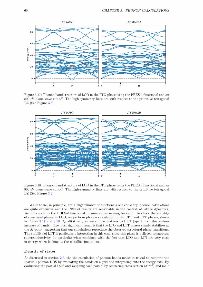
60 CHAPTER 3. PHONON CALCULATIONS
X M
0
20
40
60
80
Ener
gy [m
eV]
LTO (AFM)
X M
LTO (Metal)
Figure 3.17: Phonon band structure of LCO in the LTO phase using the PBESol functional and an800 eV plane-wave cut-off. The high-symmetry lines are with respect to the primitive tetragonalBZ (See Figure 3.3)
X M
0
20
40
60
80
Ener
gy [m
eV]
LTT (AFM)
X M
LTT (Metal)
Figure 3.18: Phonon band structure of LCO in the LTT phase using the PBESol functional and an800 eV plane-wave cut-off. The high-symmetry lines are with respect to the primitive tetragonalBZ (See Figure 3.3)
While there, in principle, are a huge number of functionals one could try, phonon calculationsare quite expensive and the PBESol results are reasonable in the context of lattice dynamics.We thus stick to the PBESol functional in simulations moving forward. To check the stabilityof structural phases in LCO, we perform phonon calculation in the LTO and LTT phases, shownin Figure 3.17 and 3.18. Qualitatively, we see similar features to HTT (apart from the obviousincrease of bands). The most significant result is that the LTO and LTT phases clearly stabilizes atthe M -point, suggesting that our simulations reproduce the observed structural phase transitions.The stability of LTT is particularly interesting in this case, since this phase is believed to suppresssuperconductivity. In particular when combined with the fact that LTO and LTT are very closein energy when looking at the metallic simulations.
Density of statesAs discussed in section 2.6, the the calculation of phonon bands makes it trivial to compute the(partial) phonon DOS by evaluating the bands on a grid and integrating onto the energy axis. Byevaluating the partial DOS and weighing each partial by scattering cross section (σtotal) and ionic

3.8. VALIDATION OF SIMULATIONS 61
0.00
0.05
0.10
0.15
DOS
HTT AFM CuLaO
LTO AFM LTT AFM
0 20 40 60 80Energy [meV]
0.00
0.05
0.10
0.15
DOS
HTT METAL
0 20 40 60 80Energy [meV]
LTO METAL
0 20 40 60 80Energy [meV]
LTT METAL
Figure 3.19: Neutron-weighted phonon density of states in the various structural and electronicphases of LCO. Both the partial and total density of states is shown in the plot.
mass, we obtain the generalized phonon DOS as seen by a time-of-flight neutron spectrometer inthe incoherent approximation.
Figure 3.19 shows the neutron weighted partial and total density of states due to the 6 dif-ferent phonon calculations we performed. The density of states was evaluated on a 48 × 48 × 48grid, integrated using the tetrahedron method and an applied Gaussian smearing of σ = 1meV(2.35meV FWHM). To get comparable values of g(ω), the plots are normalized to the BZ volume(4V BZ
HTT = 2V BZLTO = V BZ
LTT).Qualitatively, the main difference between the structural phases is a modification of the peak
at ≈ 30meV as you go to progressively lower symmetries. A quick inspection of the eigenvectorsof the HTT calculation reveals 4 modes in this energy-range (inspection performed at Γ):
1. 26.3meV: An in-plane oxygen mode where the oxygens move along c and the two diagonalsof the octahedra is out of phase.
2. 27.2meV: An apical oxygen mode where apical of the same ‘plane’ move together with thedirection alternating between each plane
3. 27.9meV: A mode where every oxygen-atom moves in-phase along c, keeping the rest of thelattice still.
4. 28.6meV: A lanthanum mode where the atoms move out of phase along c.
The metallic simulations mainly have the effect of generally pushing phonon energies down anda ‘smoothing’ of high-energy modes. Extrapolating from the HTT phase, this is directly linkedto the softening of the Cu-O bond-stretching mode at the zone boundary, as will be discussedin chapter 8. In addition, the two peaks at 50meV and 60meV have weight shifted towards thelatter. The mode at 50meV is a bond-stretching mode of the apical oxygen, while the mode at60meV involves vibration of all oxygen-atoms along the c axis, with in-plane and apical oxygenatoms being relatively out of phase.
3.8 Validation of simulations
Since LSCO is such an extensively studied system, there is data available in the literature tocompare our band structures. By inspection of the band structure plots in the previous section,it seems like a difficult task to actually separate the bands in a neutron scattering experiment.Luckily, there are a few modes that can be distinguished. Figure 3.20 compares our HTT bandphonons band structures along Γ-X with experimental data from a range of LSCO samples. Thehighlighted modes is the Cu-O half-breathing mode (≈ 80meV) and the apical oxygen stretchingmode (≈ 60meV). We will discuss this mode in detail in Chapter 8

62 CHAPTER 3. PHONON CALCULATIONS
X0
10
20
30
40
50
60
70
80
90
Ener
gy [m
eV]
LSCO 20%
LSCO 15%
Metal
X
LSCO 15%
LCO
AFM
Figure 3.20: Comparison of phonon band structures in the HTT structural phase along the Γ-Xpath with data from literature. Data for LSCO 15% taken from ref. [163], data for LSCO 20%and 0% taken from ref. [164]. Modes associated with data are highlighted in red.
Further validation of our simulations are performed in the experimental Chapters 6 and 7where we look at low-energy phonon modes and density-of-states measurements, respectively. Inaddition, some of the ideas developed here will be used in the investigation of simulations withO/Sr defects using ab-initio MD in the following chapter.
3.9 Summary
I summary, we performed ab-initio phonon calculations of La2CuO4 in 3 structural and two elec-tronic phases, using the PBESol functional and an increased plane wave energy cut-off in order tocorrectly stabilize low-energy phonons. We discover imaginary modes at the M point of the HTT,consistent with the observation of the HTT-LTO structural phase transition due to octahedraltilts. The relationship between the LTO and LTT phases are less consistent and we get differentresults for the metallic and AFM solutions. For the AFM case, LTT is the stable phase (and LTO is‘less stable’ compared to HTT), never seen in experiments on the undoped compound. In fact, theorthorhombic strain and octahedral tilt are both largest at zero doping [71]. For the metallic case,LTO and LTT are nearly degenerate (indistinguishable energies within our numerical precision),while experiments tells us that HTT is the stable phase at overdoing, at least for La2−xSrxCuO4.
Despite our results being inconsistent with regards to total energies and observed structuralphases, we proceed our investigations based on the computational parameters decided on through-out this chapter. There are two reasons for this. First, we have a remarkable agreement withphonons at both high (chapter 8 and Figure 3.20) and low (Chapter 6) energies. Second, we knowthat a one-electron theory such as DFT is unable to explain the correlated nature of the cupratesat optimal doping, so we settle on the best description possible in the edge cases and try to extra-polate from that. The electronic structure of the cuprates at intermediate doping is essentially anunsolved problem outside the scope of this thesis.
Chapter 4
Molecular Dynamics
Using the lessons learned in the previous chapter and after a reasonably successful validation ofsimulations (see section 3.8), we can use the computational parameters at a lower precision andperform Molecular Dynamics simulations in VASP. The purpose of this chapter is to discuss thecomputational details, outline the chosen defect structures and finally present how defects (inter-stitial or otherwise) modifies the structure and dynamics of the parent compound. While moleculardynamics simulations are unable to provide information about the phonon band structure directly,it is possible to extract the phonon DOS and other relevant dynamical information as outlined insection 2.5. In order to distinguish the simulations, we use a similar notation as in the previouschapter, but with the option to add dopants: [HTT/LTO/LTT][m]+[Sr/Oi], where omitting the[m] refers to the AFM electronic structure. For example, LTOm+Sr refers to a calculation startingfrom orthorhombic (Bmab) symmetry, in the metallic phase, with added Sr dopant.
4.1 Computational Details
Since Molecular Dynamics simulations require a large number of SCF cycles, it is necessary todrastically reduce the precision of our simulation. In general, the most drastic approximationcomes from only running the simulation at one k-point (Γ). Other parameters are benchmarkedby small test runs of a couple hundred steps and then evaluating the computational resources/timeavailable. In our case we end up with the following additional reductions in precision:
• Planewave cut-off at the default: 400 eV (ENCUT=400)
• Threshold for the SCF to stop reduced to 10−5 eV (EDIFF=1E-5)
• A faster algorithm for electronic minimization (ALGO=F)
• Projection operators calculated in real space (LREAL=A)
We keep the PREC tag set to ‘Accurate’, since changing to ‘Normal’ resulted in convergenceissues. In addition, we need to specify the temperature and type of ensemble (see section 2.5).For all simulations, we run at T = 300K (TEBEG=300) within the canonical (NVT) ensemble usingthe algorithm of Nosé with a Nosé-mass such that the temperature fluctuates with a frequency ofroughly 38THz (SMASS=1). In order to get reasonable statistics we run with a time step ∆t = 2 fs(POTIM=2) for a total of 21000 (NSW=21000) steps, corresponding to a simulation time of 42 ps. Forthe analysis, we discard the first 2 ps in order to let the system equilibrate.
For the initial structures where defects have been added, we perform a geometry optimization ofthe supercell in order to find a structural minimum from which to start the MD simulation. Due tothe reduced symmetry (compared to the phonon calculations in chapter 3) this is a fairly expensivecomputation, so we perform the optimization with the same parameters as the MD simulation,except that we increase the k-point mesh to 4× 4× 4 and the SCF threshold to 10−6 eV. Similarto the phonon calculations, we use the conjugate gradient algorithm for this minimization.
4.2 Octahedral tilts
In order to obtain octahedral tilts from MD simulations where symmetry is turned off, we areforced to define the octahedral tilts for each octahedra in the supercell. In fact, by writing whichoctahedra each oxygen atom (excluding interstitials) in our simulation belongs to, we can extract
63

64 CHAPTER 4. MOLECULAR DYNAMICS
b
a
c
b
O4
O3O2
O1
O6
O5
O1/O4 O2/O3
Q11 = sin−1
(Ox
6
Oz6
)Q2
1 = sin−1
(Ox
5
Oz5
)Q3
1 = sin−1
(Oz
1
2Ox1
+Oz
2
2Ox2
)Q4
1 = sin−1
(Oz
3
2Ox3
+Oz
4
2Ox4
)Figure 4.1: Finding octahedral tilts from arbitrary oxygen positions. Q2 angles can be found inan analogous way by replacing x with y and ‘pairing up’ O1 with O4 and O2 with O3.
the (Q1, Q2) tilt as seen from that oxygen. Since the tilts alternate, each tilt belongs to one offour symmetries with respect to (Q1, Q2): (+,+), (+,-), (-,+), (-,-). In practice, we analyse theinitial t = 0 structure with the following steps for each Cu atom in the supercell:
1. Record the position of the Cu atom
2. Find apical oxygens by searching for (Cu, O) pairs with a distance less than r = (1, 1, 2.7)Å
3. Find equatorial oxygens by searching for (Cu, O) pairs with a distance less than r =(2.1, 2.1, 1)Å
4. Determine the Q1, Q2 tilt as seen from each of the 6 oxygen atoms in the list.
5. Apply the symmetry operations.
6. Save the 4 (Q1, Q2) value pairs.
Step 4 is performed by first converting fractional coordinates to real-space coordinates and thenfinding angles as outlined in Figure 4.1. The symmetry operations in step 5 is a matrix with 8columns corresponding to the 8 tilt values and a number of rows equal to the number of octahedra– 16 in the case of our 2× 2× 1 supercell. Each element of the matrix is either +1 or -1, where -1will reverse the tilt direction and +1 will keep it as-is. The matrix can be generated by examiningthe output of the starting structure (which has the correct space group symmetry) and thenconstructing the matrix such that all (Q1, Q2) tilts agree. While the same result can be archivedby manually assigning the different atoms of our manageable supercell, this methodology allowsthe code to eventually be expanded to other systems, since we can set up arbitrary local coordinatesystems.
After having performed this analysis, we can apply the same operations to every time step andobtain statistics about the time-evolution of the octahedral tilts in our system. This is similar to thePositional Recurrence Maps (PRM) methodology [165] that has been used to extract informationabout the apical oxygen dynamics in Nd2NiO4+δ [166].
4.3 Structures with dopant ions
Since the introduction of dopant ions breaks the crystal symmetry, we cannot perform phononcalculations using the direct method without making an excessive amount of high-precision cal-culations. Our typical 2 × 2 × 1 supercell containing 112 ions with P1 symmetry would require112× 3 = 336 displacements just to describe phonon frequencies and eigenvectors at Γ. The worstcase phonon calculation (LTT with magnetism) in the preceding chapter required just 21 displace-ments. For this reason, we are essentially forced to use molecular dynamics. In the following, themodel for placing the initial dopants is outlined for Sr- and O-doped systems separately.
LCO+OWe start by considering the La2CuO4+δ System, which is simply LCO with added oxygen atoms atinterstitial sites. It is generally accepted that the oxygen enters in the middle of the rock-salt layer,the least dense area of the crystal structure. Figure 4.2 shows possible interstitial positions for theLTO (Bmab) and LTT (P42/ncm) phase, taken from a model proposed for the La2NiO4+δ system

4.4. GEOMETRY OPTIMIZATION 65
Figure 4.2: Illustration of interstitial oxygen in-plane (a-b) location with respect to the apicaloxygen displacements in the rock-salt layer. Open squares represent apical oxygens ‘hanging down’while closed squares represent apical oxygens ‘sticking up’. Interstitial oxygen are red circles andare shown on every possible interstitial site for clarity. Adapted from ref. [87].
[87]. Simulations in the defect phases are denoted by subscript ‘defect’. We ignore the HTT phasefor molecular dynamics since the symmetry is broken and the preliminary geometry optimizationwould tend to tilt the octahedra similar to the LTT phase. To represent a reasonable doping level,we consider the addition of a single interstitial. It is generally accepted that the oxidation stateis, at least approximately, O2−, such that each dopant adds two holes. In our 2× 2× 1 supercellwith 16 formula units, this corresponds to a doping of nh = 2
16 = 0.125.To see how the symmetry is broken, Table 4.1 shows the resulting space groups when inserting
an interstitial into various starting symmetries. As expected, the symmetry is lowered substantially,especially if the z-component of the interstitial is different from 1
4 . While the symmetry isn’treduced to P1, it is difficult to imagine that any of the space groups in Table 4.1 could be usedsolve the observed superstructures in LCO+O (see section 1.4). Diffraction studies point to theinterstitial being placed at either
(1414z)
with z close to 14 or on a general (xyz) position [167].
When modelling this position in diffraction studies, it is possible to keep the parent symmetryby assigning an occupation factor to the interstitial and thus keeping the symmetry of the parentphase. Since we are not afforded that luxury when building structures for molecular dynamics,defects will naturally break the symmetry of our parent phase. Table 4.1 should thus not be seenas proposed models, but rather as an illustration of our inability to model partial occupancies ina small real-space box.
LSCOIn the La2−xSrxCuO4 system, our current best guess is that the distribution of the doped Srspecies is completely random and homogeneous. Since randomness is difficult to implement in a(relatively) small system with periodic boundary conditions, we initially place them at a distanceof about half the box side in order to represent homogeneous doping. Replacing La3+ with Sr2+adds one hole, so we add two dopants in order to be at nh = 0.125 doping.
4.4 Geometry Optimization
We performed high-precision geometry optimizations of ionic positions only on these LCO+Odefect structures starting from the various relevant symmetries. The starting structures were theoptimized structures from chapter 3 with an interstitial inserted according to Table 4.1. Thedefect structures were created by reversing certain tilts according to Figure 4.2. For the geometryoptimization we kept the volume fixed at the value obtained from the parent structures without tiltdefects, substitutions or interstitials. Performing an equation-of-state geometry optimization forall structures as in section 3.6 is computationally expensive for the defect supercells, but Figure 4.3shows a EOS fit of the LTT structure with a limited number of points, revealing that the Volumedoes not change significantly due to the interstitial.
Table 4.2 shows the resulting total energies and (Q1, Q2) tilts for a variety of starting structuresincluding oxygen interstitials. A few trends emerge from this investigation. First, the defectstructures in Figure 4.2 has the effect of reducing the average tilt of the structure, if we keep thesymmetry operations from the non-defective phase. In the case of LTO the average tilts completelycancel out, while in the case of LTT they are cut in half. In addition, both the average and localtilts move towards the tilt pattern of the non-defective phase during optimization. In general,

66 CHAPTER 4. MOLECULAR DYNAMICS
Table 4.1: Space group symmetry due to the introduction of an interstitial oxygen in variousstructures all described in a 2 × 2 × 1 supercell of the Bmab (conventional) coordinate system.HTT, LTO and LTT are the usual phases as described in literature [35]. The structures labelleddefect is (1) in the LTO case: A stacking fault where the middle layer has its tilts reversed and (2)in the LTT case: A line along [110] with reversed tilts. Both are described in [87] and are designedin order to ‘make room’ for the interstitial oxygen (see Figure 4.2).
Phase Space Group Oxi Oy
i Ozi
HTT I4/mmm (139)HTT + Oi P-42m (111) 0.125 0.125 0.25HTT + Oi Cmm2 (35) 0.125 0.125 0.24LTO Bmab (64)LTO + Oi P2 (3) 0.125 0.125 0.25LTO + Oi P2 (3) 0.125 0.125 0.24LTOdefect Pmna (53)LTOdefect + Oi P2 (3) 0.875 0.375 0.25LTOdefect + Oi P2 (3) 0.875 0.375 0.24LTT P42/ncm (138)LTT + Oi P-4 (81) 0.375 0.125 0.25LTT + Oi P2 (3) 0.375 0.125 0.24LTTdefect Pmma (51)LTTdefect + Oi Cmm2 (35) 0.875 0.375 0.25LTTdefect + Oi Cmm2 (35) 0.875 0.375 0.24
1425 1450 1475 1500 1525 1550Volume [Å3]
830.0
829.5
829.0
828.5
Ener
gy [e
V]
databest-fit
Figure 4.3: Equation-of-state fit to La2CuO4.0625 starting from the LTT phase with one addedinterstitial oxygen in our supercell. The broken vertical line is the minimum of the fit, showingthat our starting volume was reasonable. Each minimization was performed without symmetrywhile relaxing both ionic positions and the cell shape. The orthorhombic strain due to the cellshape change was below η = 0.0004 for all volumes, suggesting that the tetragonal crystal shapeis a stable minimum.

4.5. BENCHMARKING 67
our simulations find that it costs more energy to reverse the tilts compared to the addition ofthe interstitial. This is inconsistent with the observation of staging (see section 1.4) and is likelyrelated to the limited size of our simulation. Since a well-defined energy minimum is important forthe initial configuration of the MD simulations, we stick with the parent, undistorted phases wheninvestigating LCO+O. Finally, we notice that the tilts tend towards an ‘LTT-like’ tilt-pattern inthe optimization of metallic LTO, while keeping a significant orthorhombic strain.
Table 4.3 shows the same optimizations performed on Sr-doped La2CuO4. The results here areas we expect from the small difference between the ionic radius of La3+ and Sr2+ (see table 1.2).We seem to be in a well-defined minimum and the average tilt is only modified slightly. Whilegeometry optimizations are only able to locate a local minimum, the results in Tables 4.2 and 4.3point toward the expected conclusion that interstitial oxygen has a more significant effect on theoctahedral tilt patterns compared to Sr doping. The nature of these effects cannot be obtainedfrom geometry optimizations alone, and we turn to molecular dynamics for the detailed analysisof structure and dynamics.
4.5 Benchmarking
Similar to our phonon calculations in the previous chapter, molecular dynamics simulations aretypically benchmarked in various ways. Depending on the type of ensemble and thermostat, eitherthe temperature or total energy is expected to be conserved. It is, however, possible for numericalnoise to cause these quantities to drift. In our case the Nosé thermostat controls temperaturethrough velocities, so it can be useful to plot the temperature as a function of simulation time tosee if the fluctuations are reasonable. The temperature can be calculated from the MD trajectoryby first computing the velocities through the Verlet algorithm (see section 2.5) and then evaluating
T =1
3kB(Nions − 1)
∑j
Mj |vj |2 ,
where Nions is the number of atoms, Mj is the mass of atom n and vj is the velocity of atom j.We divide by (Nions − 1) rather than Nions, since temperature is defined with respect to degreesof freedom and we can arbitrarily redefine our coordinate system with respect to a particular
Table 4.2: Oxygen interstitial phases, geometry optimization. Geometry optimization performedon ionic positions only. E0 corresponds to the energy after inserting the interstitial oxygen, butbefore geometry optimization. E1 is the total energy after optimization. The octahedral tilts(Q1, Q2) are similarly defined before and after the optimization.
E0 [eV] E1 [eV] (Q1, Q2)0 (Q1, Q2)1
HTT + Oi -827.27669 -829.76250 (0.00, 0.00) (1.00, 1.00)LTO + Oi -828.29890 -830.39658 (0.00, 5.79) (1.21, 5.92)LTOdefect + Oi -823.09516 -830.03588 (0.00, 0.00) (2.12, 4.48)LTT + Oi -828.04663 -830.08248 (4.61, 4.61) (3.77, 3.72)LTTdefect + Oi -826.03173 -829.94243 (2.31, 2.31) (2.80, 2.70)LTOm + Oi -872.73074 -876.56079 (0.00, 6.42) (3.76, 3.90)LTTm + Oi -872.35546 -876.56195 (4.53, 4.53) (3.85, 3.85)
Table 4.3: Sr doped phases, geometry optimization. E0 corresponds to the energy after replacingLa with Sr, but before geometry optimization. E1 is the total energy after optimization. Geometryoptimization performed on ionic positions only. The octahedral tilts are similarly defined beforeand after the optimization.
E0 [eV] E1 [eV] (Q1, Q2)0 (Q1, Q2)1
LTO + Sr -858.73485 -859.48650 (0.00, 5.79) (0.00, 5.38)LTOm + Sr -858.57712 -859.39905 (0.00, 6.42) (0.00, 5.69)LTT + Sr -858.68994 -859.49712 (4.61, 4.61) (3.87, 3.97)LTTm + Sr -858.57810 -859.40170 (4.53, 4.53) (3.98, 4.08)

68 CHAPTER 4. MOLECULAR DYNAMICS
0.0 2.5 5.0 7.5 10.0 12.5 15.0 17.5 20.0Time [ps]
150200250300350400450500
Tem
pera
ture
[K]
T= 299.86 ± 23.525 K
dt=1 fsdt=2 fs
0 20 40 60 80 100Energy [meV]
0.00
0.01
0.02
0.03
0.04
0.05
0.06
0.07
Phon
on D
OS [Å
2 /fs2 ]
dt=2 fs, M=10000dt=1 fs, M=9000
Figure 4.4: Benchmark of molecular dynamics, using LCO in the LTO phase with no dopant ionsor defects. Top: Temperature fluctuations for a simulation stitched together with the first 10 psusing a 1 fs time step and the last part of the simulation using a 2 fs time step. Bottom: Densityof States weighted by neutron-cross sections and broadened by a Gaussian with σ = 0.5meV(1.18meV FWHM) evaluated at the same two parts of the simulation.
atom. When considering the instantaneous temperature in this way, we expect the mean-squaredtemperature fluctuations to be [168]
⟨(∆T 2
)⟩=
2T 20
3Nions.
Four our simulation with Nions = 112 at T0 = 300K we thus expect temperatures fluctuationsof ±23.15K. Figure 4.4 is a summary of benchmarks performed on the LCO in the LTO phasewith no dopant ions or defects. Simulations were performed with two different time steps andthe difference in temperature fluctuations and the resulting phonon DOS was recorded. In termsof temperature fluctuations, there is little effect of going from 1 to 2 fs time steps, but there areslight modifications to the DOS, especially in the region around 30 meV. While this may be seenas problematic, it is important to realize that we are probing a relatively small number of steps,and it is unlikely that our simulation is completely ergodic. In other words, we may be probinga different area of phase space in the two simulations. It is unlikely that the time step resolutionitself is causing the effects on DOS, since an energy of 30meV = 7.3THz is probed by simulationtimes of roughly 137 fs. While higher precision is always desirable, we stick with a time step of2 fs in order to be able to probe dynamics for longer time scales in more systems. Now, almostby definition, different time steps do probe different dynamics. I emphasize that any comparisonbetween MD simulations is done at the same time step.
4.6 DOS and PDF
Molecular dynamics simulations have been performed with 7 starting configurations based ongeometry optimizations in Table 4.2 and 4.3 as well as references without dopant ions. Since thefull matrix of combinations now includes 3 structural phases, 2 dopant ions, 2 electronic phasesand 2 ‘defect’ phases, the total number of desired simulations is 20. In order to limit the scope and

4.7. MICROSCOPIC ANALYSIS 69
focus computational resources, we chose to focus on the LTO phase and end up with the followinglist of simulations:
1. LTT: LTT in AFM phase.
2. LTO: LTO in AFM phase.
3. LTO+Sr: LTO in AFM phase with added Sr dopants.
4. LTO+O: LTO in AFM phase with added O dopant.
5. LTOm: LTO in metallic phase.
6. LTOm+Sr: LTO in metallic phase with added Sr dopants.
7. LTOm+O: LTO in metallic phase with added O dopant
Our primary observables when comparing to experiment is the phonon density of states andpair-density-function. We start by considering the DOS of all simulations, calculated with themethod described in section 2.5 and the scripts developed in appendix A. Figure 4.5 shows theneutron-weighted phonon DOS for all 7 simulations. While the overall shape of the phonon DOSis mostly unchanged, there are some subtleties that we might consider for further analysis. For themagnetic simulations, we see a similar modification of modes at ≈ 30meV when comparing theLTO and LTT phases. Interestingly, the sharp dip in DOS at 30meV is seen in LTO+O as well.In fact, the LTT and LTO+O phases appear to share more qualitative features with each othercompared to the parent LTO phase. This is consistent with the initial geometry optimization ofLCO+O in table 4.2 moving towards a LTT-like tilt pattern. LTO+Sr, on the other hand, mostlyseem to broaden features rather than directly modify then.
For the metallic simulations, we see similar trends but in a much more smeared out fashion,possibly due to reduced accuracy of these simulations due to the fermi surface smearing (see figure3.5 in section 3.5). Similar to the observations in chapter 3, the main modification of the phononDOS compared to the magnetic simulations is related to the high energy modes.
In order to compare more directly these observations, Figure 4.6 shows a direct comparison ofDOS and PDF of our LTO, LTO+O and LTT simulations. This comparison clearly shows thatthe LTT and LTO+O share common features especially around 30meV (various c-axis modes, seesection 3.7 and 60meV (apical oxygen bond-stretching mode). The PDF in the same figure showonly very subtle deviations, most notably around 5.2Å where, once again, the LTT simulationshares features with LTO+O.
4.7 Microscopic analysis
In addition to observables for comparison with experiment, the purpose of molecular dynamicssimulations is to relate microscopic phenomena to these observables. For this reason, we willtry to extract relevant information from the simulation trajectory in order to understand what iscausing the changes in the phonon DOS and PDF. In the cuprates, there is much experimentalevidence of the fact that Cu-O distances and distributions are important for superconductivity [93–95]. Inspired by these results, Figure 4.7 show the distribution of Cu-Oequatorial and Cu-Oapicaldistances for selected simulations. In general, they follow a normal distribution showing that theharmonic approximation works well for our system, with the notable exception of the apical oxygendistance in LTO+O.
Table 4.4 summarizes these distances for all of the performed simulations. As expected from thealmost identical PDF across simulations, the mean Cu-Oequatorial distances does not seem to haveany discernible trends, but there is a slight widening of the distributions in the systems containingdopants. In some sense this is expected since we have created different local environments by theintroduction of impurity dopants. The same trend can be seen in the Cu-Oapical distanced, buthere we additionally have an shortening of the mean distance due to the introduction of oxygen(notice also that this shortening is identical to the LTT distance in magnetic case). For Sr-dopingthere is an elongation in the magnetic simulation but a shortening in the metallic simulation. Itis, however, important to note that these differences are extremely subtle and may just be due tonumerical peculiarities.
Using the definitions of octahedral tilts described in section 4.2, Figure 4.8 shows a histogramof (Q1, Q2) tilts from all of our performed MD simulations on a logarithmic scale. Similar toobservations from DOS and PDF, the tilt patterns of LTO+O are LTT-like, while the Sr-doped

70 CHAPTER 4. MOLECULAR DYNAMICS
Figure 4.5: Neutron-weighed density-of-states for all molecular dynamics simulations performedin this chapter. The filled grey area is the total DOS and the lines are the partial atomic DOS.The initial conditions for the MD simulation is annotated on each plot according to the notationoutlined in the beginning of this chapter. The density-of-states was obtained through the powerspectrum of the velocity autocorrelation function (see section 2.5). The power spectrum wassmoothed by a Gaussian kernel with width σ = 0.5meV (1.18meV FWHM).
Table 4.4: Cu-O Distances distance statistics for all MD simulations performed in this chapter.Columns 2 and 3 show the mean distance and standard deviation for the Cu-O equatorial distance.Column 3 is the R2 value of a linear regression assuming a normal distribution. Columns 4-6 showthe same values for the Cu-O apical distance.
name ⟨Oeq⟩ [Å] σ (Oeq) [Å] R2 (Oeq) ⟨Oap⟩ [Å] σ (Oap) [Å] R2 (Oap)
LTO 1.898 0.0455 0.9972 2.421 0.113 0.9989LTO+O 1.902 0.0464 0.9972 2.406 0.127 0.9608LTO+Sr 1.898 0.0507 0.9947 2.438 0.146 0.9995LTOm 1.909 0.0514 0.9951 2.462 0.140 0.9997LTOm+O 1.908 0.0532 0.9934 2.440 0.156 0.9992LTOm+Sr 1.905 0.0523 0.9947 2.451 0.151 0.9992LTT 1.907 0.0461 0.9971 2.406 0.109 0.9992

4.7. MICROSCOPIC ANALYSIS 71
0 20 40 60 80 100Energy [meV]
0.00
0.02
0.04
0.06
0.08
DOS
[Å2 /f
s2 ]
LTOLTO+OLTT
2 4 6 8 10r [Å]
0.5
0.0
0.5
1.0
1.5
2.0
LTOLTO+OLTT
Figure 4.6: Top: Total DOS for selected MD simulations. In general, differences are subtle, butwe see some surprising similarities between the LTO+O and LTT simulation, indicating LTT-likebehavior due to the interstitial (see text). Bottom: PDF of the same simulations, showing almostidentical spectra for the 3 simulations. At roughly 5.2Å there is a small modification where, onceagain, LTO+O and LTT simulations show similarities.
1.7 1.8 1.9 2.0 2.1
LTOOeq
1.8 1.9 2.0 2.1 2.2
LTTOeq
1.7 1.8 1.9 2.0 2.1
LTO+OOeq
2.0 2.2 2.4 2.6 2.8 3.0distance [Å]
LTOOap
2.0 2.2 2.4 2.6 2.8distance [Å]
LTTOap
2.0 2.2 2.4 2.6 2.8 3.0 3.2distance [Å]
LTO+OOap
Figure 4.7: Distance histograms of Cu-O distances with respect to the equatorial oxygen (Oeq)and apical oxygen (Oap) in the three simulations we compared in Figure 4.6. The data wasgenerated by recording all appropriate distances at every time step of the simulation. The y-axisis normalized to unity and the broken line is a Gaussian function with expected value and variancecalculated from the data. The histograms are normalized to unity.
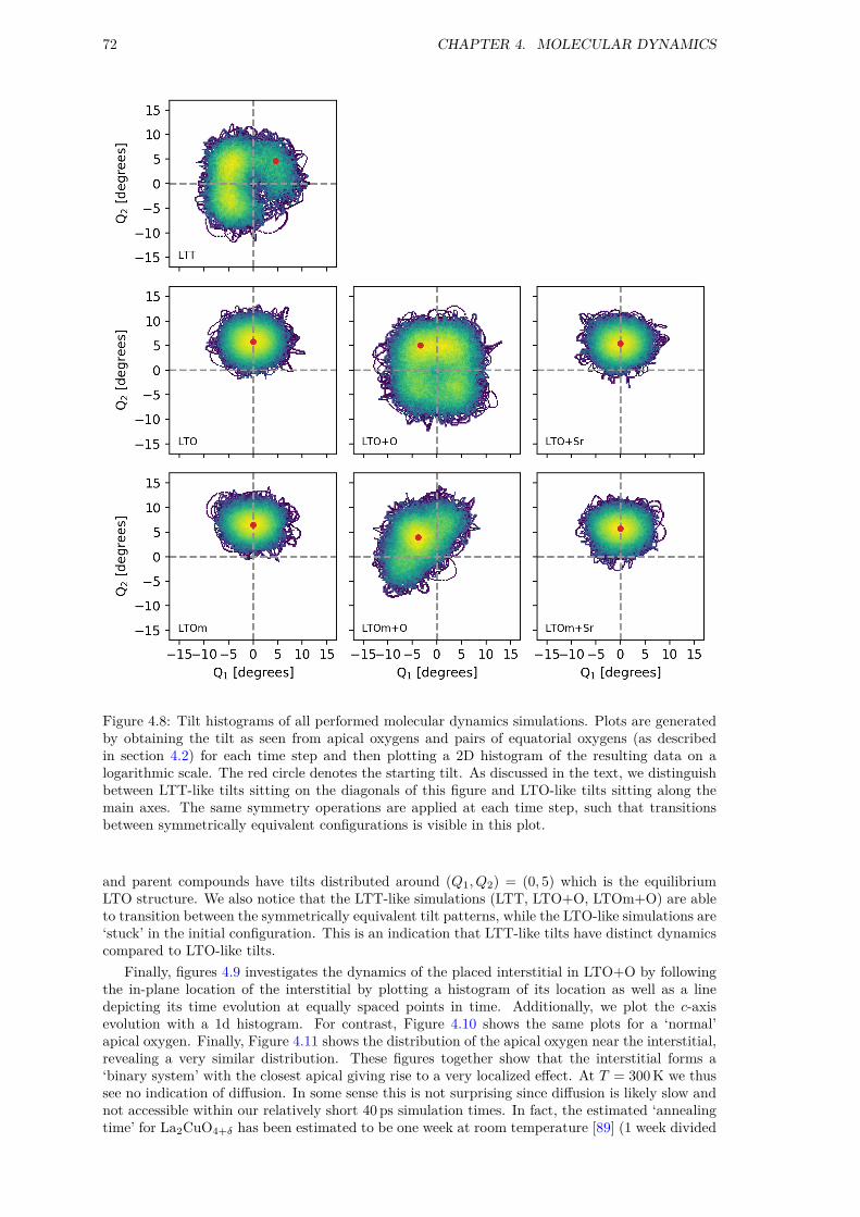
72 CHAPTER 4. MOLECULAR DYNAMICS
Figure 4.8: Tilt histograms of all performed molecular dynamics simulations. Plots are generatedby obtaining the tilt as seen from apical oxygens and pairs of equatorial oxygens (as describedin section 4.2) for each time step and then plotting a 2D histogram of the resulting data on alogarithmic scale. The red circle denotes the starting tilt. As discussed in the text, we distinguishbetween LTT-like tilts sitting on the diagonals of this figure and LTO-like tilts sitting along themain axes. The same symmetry operations are applied at each time step, such that transitionsbetween symmetrically equivalent configurations is visible in this plot.
and parent compounds have tilts distributed around (Q1, Q2) = (0, 5) which is the equilibriumLTO structure. We also notice that the LTT-like simulations (LTT, LTO+O, LTOm+O) are ableto transition between the symmetrically equivalent tilt patterns, while the LTO-like simulations are‘stuck’ in the initial configuration. This is an indication that LTT-like tilts have distinct dynamicscompared to LTO-like tilts.
Finally, figures 4.9 investigates the dynamics of the placed interstitial in LTO+O by followingthe in-plane location of the interstitial by plotting a histogram of its location as well as a linedepicting its time evolution at equally spaced points in time. Additionally, we plot the c-axisevolution with a 1d histogram. For contrast, Figure 4.10 shows the same plots for a ‘normal’apical oxygen. Finally, Figure 4.11 shows the distribution of the apical oxygen near the interstitial,revealing a very similar distribution. These figures together show that the interstitial forms a‘binary system’ with the closest apical giving rise to a very localized effect. At T = 300K we thussee no indication of diffusion. In some sense this is not surprising since diffusion is likely slow andnot accessible within our relatively short 40 ps simulation times. In fact, the estimated ‘annealingtime’ for La2CuO4+δ has been estimated to be one week at room temperature [89] (1 week divided

4.8. SUMMARY 73
0.25 0.50 0.75h [r.l.u]
0.0
0.1
0.2
0.3
0.4
0.5
k [r.
l.u]
A B
0.25 0.30 0.35Oi z-component [r.l.u]
C
startOap
Figure 4.9: Distribution of the interstitial oxygen in LTO+O. (A): In-plane distribution of theinterstitial. Circles denote apical oxygens ‘sticking up’, while crosses denote apical oxygen ‘hangingdown’ (similar to Figure 4.2). (B): Zoomed-in version of (A) with the line marking the time-evolution of the interstitial sampled at isochronal points. C: c-coordinate distribution of theinterstitial with the initial and average position marked in red and orange, respectively.
0.25 0.50 0.75h [r.l.u]
0.0
0.1
0.2
0.3
0.4
0.5
k [r.
l.u]
A B
0.25 0.30 0.35Oi z-component [r.l.u]
C
Figure 4.10: Distribution of a normal apical oxygen in LTO+O. (A): In-plane distribution of theapical. Circles denote apical oxygens ‘sticking up’, while crosses denote apical oxygen ‘hangingdown’ (similar to Figure 4.2). (B): Zoomed-in version of (A) with the line marking the time-evolution of the interstitial sampled at isochronal points. C: c-coordinate distribution of theapical.
by 40 ps is roughly 1016).
4.8 Summary
The main take-home message from chapter is the fact that interstitials seem to have a very subtleeffect on structure but a more significant effect on dynamics. In particular, an observable such asPDF will se barely any difference between our simulations but high-quality DOS measurementsshould be able to see subtle differences due to dopants.
If we can obtain a reasonable validation of these simulations, the microscopic analysis revealsvery clearly that oxygen interstitial phases move towards LTT-like tilt dynamics. Since the averagestructure of LCO+O at accessible temperatures is LTO, a possible explanation is that this tendencytoward LTT-like tilts can result in the observed superstructures (and/or staging) [83, 88] if we had

74 CHAPTER 4. MOLECULAR DYNAMICS
0.25 0.50 0.75h [r.l.u]
0.0
0.1
0.2
0.3
0.4
0.5k
[r.l.u
]
A B
0.25 0.30 0.35Oi z-component [r.l.u]
C
Oap
Figure 4.11: Distribution of an apical oxygen in LTO+O near the interstitial. (A): In-plane distri-bution of the apical. Circles denote apical oxygens ‘sticking up’, while crosses denote apical oxygen‘hanging down’ (similar to Figure 4.2). (B): Zoomed-in version of (A) with the line marking thetime-evolution of the interstitial sampled at isochronal points. C: c-coordinate distribution of theapical, with the average position marked in orange.
access to bigger simulation boxes and longer simulation times. It might be valuable to examinethis more closely with real-space methods such as reverse monte-carlo (RMC) or by performingclassical MD based on the results obtained in this chapter.
Before moving on to experimental comparisons, Figure 4.12 shows a comparison of phononDOS as calculated from the previous chapter and the one obtained from molecular dynamics here.While there is a definite distinction between the spectra, it is important to realize that they areobtained by very different methods, while being based on the same computational background. Inaddition, molecular dynamics are not constrained by symmetry.
A direct comparison between molecular dynamics and phonon calculations should thus only beperformed with extreme caution. For this reason, we mainly use the phonon calculations to identifythe kinds of bands that correspond to certain features in the phonon DOS. When analyzing therole of dopants, simulations will all be done in the context of molecular dynamics (e.g. figure 4.6).In the experimental chapters I will leverage the phonon band structure calculations in context oftriple-axis measurements of single crystals. Molecular dynamics simulations, on the other hand,will be used in the context of PDF and inelastic time-of-flight measurements of powdered samples.
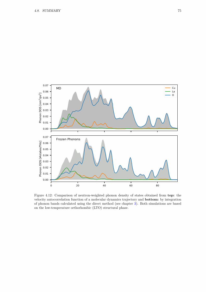
4.8. SUMMARY 75
0.00
0.01
0.02
0.03
0.04
0.05
0.06
0.07
Phon
on D
OS [n
m2 /p
s2 ]
MD CuLaO
0 20 40 60 80
0.00
0.01
0.02
0.03
0.04
0.05
0.06
0.07
Phon
on D
OS [#
stat
es/T
Hz] Frozen Phonons
Figure 4.12: Comparison of neutron-weighted phonon density of states obtained from top: thevelocity autocorrelation function of a molecular dynamics trajectory and bottom: by integrationof phonon bands calculated using the direct method (see chapter 3). Both simulations are basedon the low-temperature orthorhombic (LTO) structural phase.


Chapter 5
Local structure
In this chapter, we look at structural correlations in La2−xSrxCuO4+δ (LSCO+O) containing oxy-gen interstitials. As discussed in section 1.4, LSCO+O is known to form complex superstructuresthat shows up in single-crystal diffraction. To recap, ‘staging’ [84, 88] was discovered early onand appears unrelated to superconductivity. On the other hand, novel superstructures, known as‘Local Lattice Distortions’ (LLD) and ‘Oxygen Interstitials’ (Oi), are suggested to have a connec-tion with superconductivity [169]. In fact, it appears that these two orderings are anti-correlatedin real space, forming ‘puddles’ on µm scale [85].
The data shown in this chapter is a collection of experiments performed on three differentinstruments: IN8 [106], ThALES and D4 [109] at Institut Laue-Langevin in Grenoble, France. Inthe first part, we explore some of the superstructures mentioned above in two single crystals ofLSCO+O: La2CuO4+δ (Tc = 43K) and La1.94Sr0.06CuO4+δ (Tc = 37.5K). In the second part,we perform a diffraction experiment on powders of LSCO+O with the purpose of looking at realspace correlation through pair-distribution-function (PDF) analysis.
5.1 Superstructures in single crystals
While superstructures in LSCO+O have been extensively studied in the past, it is always usefulto check if your samples comply with previous observations. The measurements shown here weremostly performed as a reference for some of the work shown in chapter 6, but I present it heresince it has relevance for structural correlations and can help us with the analysis of the PDF datain the following section. Superstructures in LCO+O are generally observed at Q2 = (0, 0.21, 0.29)and Q3 = (0.09, 0.24, 0.50) [170] and should thus mainly be observable in the a-c (or equivalentlyb-c due to twinning) plane.
When using certain Triple-Axis spectrometers (IN8, IN20, ThALES) at the ILL, we have theoption of a secondary spectrometer (everything after the sample) called FlatCone [171] where wecan probe a large part of reciprocal space simultaneously. In particular, the FlatCone analysersystem is built in such a way that you probe a large part of the scattering plane at a constant energytransfer hω. In the following we are interested in structural correlations, so we are measuring athω = 0. In chapter 6 we will investigate finite energy transfers in detail.
Figure 5.1 shows the result of such a measurement of La2CuO4+δ on the thermal TAS IN8,performed in the a-b plane using the orthorhombic coordinate system (see section 1.4). Thecoverage of our measurement is such that we see the (200), (020) and (220) fundamental Braggpeaks. Some satellite peaks are visible at roughly Q = (0.2,±0.05, 0) as marked on the zoomed-inright-hand-side of the figure. Satellite peaks with zero l-component was previously observed byour group [172], but the nature of these peaks are currently unknown. We can, however, makethe simple observation that this peak corresponds to a real-space structural periodicity with acharacteristic length scale d1 ≈ 26Å in the a-b plane.
Figure 5.2 shows the same type of measurement, but this time of La1.94Sr0.06CuO4+δ on the coldtriple-axis spectrometer ThALES. While similar features are visible, the satellites seen in figure 5.1are smeared out, suggesting that the tiny amount of Sr in this sample causes a significant amountof disorder which shows up as diffuse satellites.
Finally, in figure 5.3, we show a measurement of La2CuO4+δ in the a-c plane also performedon ThALES. This measurement is entirely consistent with superstructures known from literature[170], and we can clearly index the peaks as Q2 = (0.19, 0, 0.31) (even showing 2nd and 3rd orderreflections) and Q3 = (0.25, 0, 0.5). I note here that, because of twinning, we can not distinguish
77

78 CHAPTER 5. LOCAL STRUCTURE
Figure 5.1: Reciprocal space map of single crystal La2CuO4+δ, measured in the a-b plane withthe unconventional Bmab orthorhombic coordinate system. Left: Full map, showing mainly thefundamental Bragg peaks. Circular arcs are powder lines from Al. Right: Zoomed-in view of theare marked in red. We notice satellite peaks around (220) at Q = (0.2,±0.05, 0) (|Q| = 0.241Å−1).
Figure 5.2: Reciprocal space map of single crystal La1.94Sr0.06CuO4+δ, measured in the a-b planewith the unconventional Bmab orthorhombic coordinate system. Left: Full map, showing mainlythe fundamental Bragg peaks. Circular arcs are powder lines from Al. Right: Zoomed-in view ofthe are marked in red, showing diffuse scattering. The marks are at identical locations to figure5.1 as a reference for comparison.
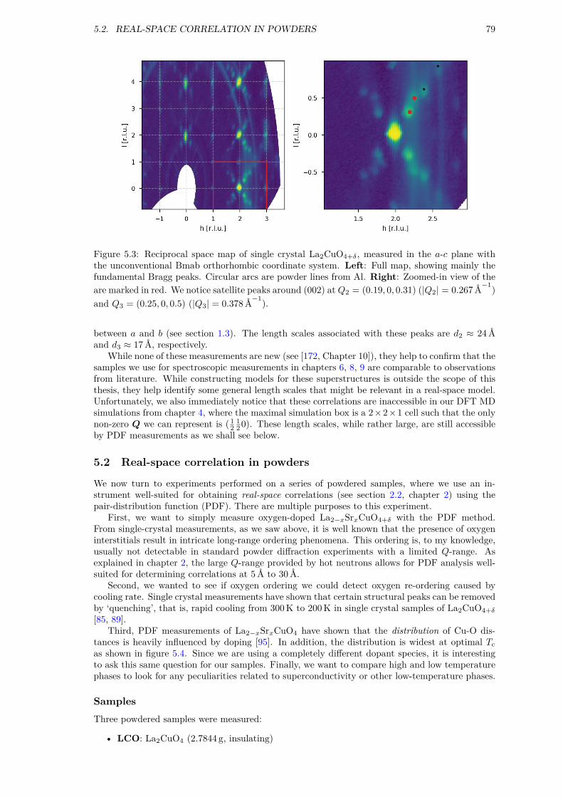
5.2. REAL-SPACE CORRELATION IN POWDERS 79
Figure 5.3: Reciprocal space map of single crystal La2CuO4+δ, measured in the a-c plane withthe unconventional Bmab orthorhombic coordinate system. Left: Full map, showing mainly thefundamental Bragg peaks. Circular arcs are powder lines from Al. Right: Zoomed-in view of theare marked in red. We notice satellite peaks around (002) at Q2 = (0.19, 0, 0.31) (|Q2| = 0.267Å−1)and Q3 = (0.25, 0, 0.5) (|Q3| = 0.378Å−1).
between a and b (see section 1.3). The length scales associated with these peaks are d2 ≈ 24Åand d3 ≈ 17Å, respectively.
While none of these measurements are new (see [172, Chapter 10]), they help to confirm that thesamples we use for spectroscopic measurements in chapters 6, 8, 9 are comparable to observationsfrom literature. While constructing models for these superstructures is outside the scope of thisthesis, they help identify some general length scales that might be relevant in a real-space model.Unfortunately, we also immediately notice that these correlations are inaccessible in our DFT MDsimulations from chapter 4, where the maximal simulation box is a 2×2×1 cell such that the onlynon-zero Q we can represent is ( 12
120). These length scales, while rather large, are still accessible
by PDF measurements as we shall see below.
5.2 Real-space correlation in powders
We now turn to experiments performed on a series of powdered samples, where we use an in-strument well-suited for obtaining real-space correlations (see section 2.2, chapter 2) using thepair-distribution function (PDF). There are multiple purposes to this experiment.
First, we want to simply measure oxygen-doped La2−xSrxCuO4+δ with the PDF method.From single-crystal measurements, as we saw above, it is well known that the presence of oxygeninterstitials result in intricate long-range ordering phenomena. This ordering is, to my knowledge,usually not detectable in standard powder diffraction experiments with a limited Q-range. Asexplained in chapter 2, the large Q-range provided by hot neutrons allows for PDF analysis well-suited for determining correlations at 5Å to 30Å.
Second, we wanted to see if oxygen ordering we could detect oxygen re-ordering caused bycooling rate. Single crystal measurements have shown that certain structural peaks can be removedby ‘quenching’, that is, rapid cooling from 300K to 200K in single crystal samples of La2CuO4+δ
[85, 89].Third, PDF measurements of La2−xSrxCuO4 have shown that the distribution of Cu-O dis-
tances is heavily influenced by doping [95]. In addition, the distribution is widest at optimal Tcas shown in figure 5.4. Since we are using a completely different dopant species, it is interestingto ask this same question for our samples. Finally, we want to compare high and low temperaturephases to look for any peculiarities related to superconductivity or other low-temperature phases.
SamplesThree powdered samples were measured:
• LCO: La2CuO4 (2.7844 g, insulating)

80 CHAPTER 5. LOCAL STRUCTURE
Figure 5.4: Relationship between strontium content x in La2−xSrxCuO4 (LSCO) and the width ofthe Cu-O equatorial bond distribution σ. For reference, LSCO is superconducting from x = 0.05to x = 0.25 and reaches the largest Tc at x = 0.15. Figure from [95]
• LCO+O: La2CuO4.05 (0.7403 g, Tc ≈ 40K)
• LSCO3+O: La1.97Sr0.03CuO4.05 (3.3612 g, Tc ≈ 40K)
Measurements were performed at the Disordered materials diffractometer D4 at Institut Laue-Langevin in Grenoble, France. Reduction and transformation of data was performed at the instru-ment with software specifically built for D4. All steps of the data treatment is saved, but we willmainly use the fully reduced and normalized datasets in both Q- and r-space. When comparingsubtle differences between spectra (such as the same sample after different cooling procedures),we might construct a difference curve from the raw data since the background subtractions willcancel out.
ExperimentTable 5.1 contains a list of the measurements performed in the order which they were performed.The quenching was performed by submerging the 300K sample in liquid nitrogen and then trans-ferring to the 100K cryostat. Annealing was performed by heating the cryostat to 350K for aboutan hour which is known to disorder the oxygen [85]. The reason we performed the quenching beforethe annealing was due to time constraints. Each acquisition was approximately 2 hours.
In summary we have a total of three samples to compare at 300K. For the oxygen-dopedsamples we can additionally look at the low temperature phase as well as the difference between‘quenched’ and ‘annealed’ doping.
ResultsWe start with the second objective of figuring out if there is any difference due to cooling procedure.Figure 5.5 shows the difference between cooling procedures for the two oxygen-doped samples. Ingeneral there are no systematic differences apart from the slight decline of the difference curvefor the LCO+O sample. This is likely due to a small amount of hydrogen in the cryostat as aconsequence of the quenching procedure. The preliminary conclusion is that there is no differencebetween quenched and annealed measurements to a high degree of certainty. This is somewhatsurprising since it is well known that certain structural peaks can be removed from quenching insingle crystals [85]. We cannot conclude if our result is due to the sample being a powder or dueto rotational averaging. Since we detect no difference in the spectra, we can use the annealed 15Kdata and initial 300K data for the remaining analysis.
In Figure 5.6 we compare the three samples at 300K in both real and reciprocal space. Whilethe differences are quite small, the difference curves (green) seem to be larger between parent/oxy-genated compounds compared to the two oxygenated compounds. This is consistent with a picture

5.2. REAL-SPACE CORRELATION IN POWDERS 81
index sample temperature state
0 LCO 300 initial1 LCO+O 300 initial2 LCO+O 100 quenched3 LCO+O 15 quenched4 LCO+O 300 quenched5 LCO+O 350 annealing6 LCO+O 300 annealed7 LCO+O 100 annealed8 LCO+O 15 annealed9 LCO+O 300 annealed10 LSCO3+O 300 initial11 LSCO3+O 100 quenched12 LSCO3+O 15 quenched13 LSCO3+O 350 annealing14 LSCO3+O 15 annealed
Table 5.1: List of measurements performed at D4 in chronological order. ‘Quenched’ refers to therapid cooling as described in the text, and annealing refers to keeping the sample at 350K forroughly 30 minutes.
0.250.500.751.001.251.501.75
d/d
[bar
ns/s
tr/at
om] LCO+O quenched
LCO+O annealedLSCO3+O quenchedLSCO3+O annealed
0 5 10 15 20q [Å 1]
0
250
Inte
nsity
[a.u
]
quenched - annealed
0 5 10 15 20q [Å 1]
quenched - annealed
Figure 5.5: Difference between quenched and annealed cooling procedures for LCO+O andLSCO3+O samples. The topmost plots are comparisons of the reduced and corrected dσ/dωin absolute units, while the difference curves are extracted from the raw q data.

82 CHAPTER 5. LOCAL STRUCTURE
0 5 10 15 20q [Å 1]
0
1
2
d/d
[bar
ns/s
tr/at
om]
LCOLCO+O
0 5 10 15 20q [Å 1]
LCO+OLSCO3+O
0 10 20 30 40r [Å]
1
0
1
2
[bar
ns/Å
2 ]
0 10 20 30 40r [Å]
Figure 5.6: Comparison of the three different samples at 300K in both real and reciprocal space.On the left we compare LCO with LCO+O in order to see if there is an effect of oxygen. On theright we look at LCO+O versus LSCO3+O to have a similar comparison between two differentoxygen-doped samples.
0 5 10 15 20q [Å 1]
0
1
2
d/d
[bar
ns/s
tr/at
om]
LCO+O 300KLCO+O 15K
0 5 10 15 20q [Å 1]
LSCO3+O 300KLSCO3+O 15K
0 10 20 30 40r [Å]
1012
[bar
ns/Å
2 ]
0 10 20 30 40r [Å]
Figure 5.7: Temperature dependence of 300K and 15K for LCO+O and LSCO3+O in both realand reciprocal space.
where oxygen distorts the lattice in a meaningful way, while the effect of a small amount of stron-tium is negligible. Figure 5.7 shows the high- and low-temperature data for the two oxygen-dopedsamples. At first glance there seems to be nothing out of the ordinary, peaks are shifting slightlydue to thermal expansion (this is particularly easy to spot in the real-space data).

5.2. REAL-SPACE CORRELATION IN POWDERS 83
2
1
0
1
2
[bar
ns/Å
2 ]
LCO+O, T=300K LSCO3+O, T=300K
1.5 2.0 2.5r [Å]
2
1
0
1
2
[bar
ns/Å
2 ]
LCO+O, T=15K
1.5 2.0 2.5r [Å]
LSCO3+O, T=15K
1.5 2.0 2.5r [Å]
LCO, T=300K
Figure 5.8: Cu-O distance Gaussian fits. For each of the five temperature/sample combinations(figure text), the short range PDF is shown along with a Gaussian fit of the first peak. In orderto compare between the fits, the constant background has been fixed to −1.2 bÅ−2
Sample Temperature [K] Cu-O mean distance Cu-O sigma
LCO 300 1.9010 ± 0.0003 0.0941 ± 0.0003LCO+O 300 1.9005 ± 0.0012 0.1112 ± 0.0014LSCO3+O 300 1.8995 ± 0.0003 0.0989 ± 0.0004LCO+O 15 1.8983 ± 0.0009 0.1096 ± 0.0010LSCO3+O 15 1.8944 ± 0.0003 0.0951 ± 0.0004
Table 5.2: Cu-O distances in all samples at all available temperatures as extracted from the fits infigure 5.8.
Analysis
Without performing detailed modelling, we can take a look at the first peak in the real-space datawhich corresponds to the Cu-O in-plane bond. This bond-length is suspected to be importantfor superconductivity by controlling the Coulomb interaction (the Hubbard-U) [94]. Previously,as mentioned above, measurements on La2−xSrxCuO4 have shown that the width of the Cu-O bond-length distribution is largest at optimal doping x = 0.15 and qualitatively tracks thesuperconducting dome [95]. We fit the first peak of all relevant datasets to a single Gaussian asshown in Figure 5.8 and report the fitting parameters in Table 5.2.
Comparing to La2−xSrxCuO4, our samples have roughly the same peak position at r = 1.9Å.At 300K LCO has a smaller width compared to LCO+O and LSCO3+O. At 15K the widths areslightly smaller as one would expect from the reduced temperatures. Our measurements are thusconsistent with the observations of [95], that the Cu-O bond-length tracks Tc , but with an entirelydifferent dopant species. Interestingly, the sample with a small amount of Sr has a slightly smallerσ, indicating that the addition of Sr restricts the Cu-O bond lengths.
In figure 5.9, we take a closer look at the PDF from the three samples obtained at 300K. As wementioned earlier, any differences between the plots are quite subtle, but our initial analysis thatthere is a ‘larger’ difference between LCO and LCO+O when compared to the difference betweenLCO+O and LSCO3+O seems to be correct. Marked in figure 5.9 are regions where there is aqualitative difference between the curves. That is, we don’t just see sharpening/broadening, butthe shape of the peaks are noticeably different. In addition, I marked the possible correlationlengths identified in the previous section.
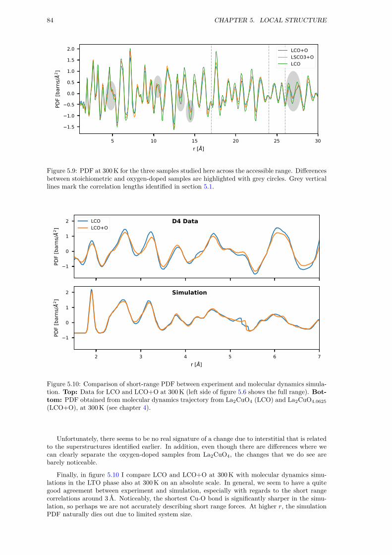
84 CHAPTER 5. LOCAL STRUCTURE
5 10 15 20 25 30r [Å]
1.5
1.0
0.5
0.0
0.5
1.0
1.5
2.0PD
F [b
arns
/Å2 ]
LCO+OLSCO3+OLCO
Figure 5.9: PDF at 300K for the three samples studied here across the accessible range. Differencesbetween stoichiometric and oxygen-doped samples are highlighted with grey circles. Grey verticallines mark the correlation lengths identified in section 5.1.
1
0
1
2
[bar
ns/Å
2 ]
D4 DataLCOLCO+O
2 3 4 5 6 7r [Å]
1
0
1
2
[bar
ns/Å
2 ]
Simulation
Figure 5.10: Comparison of short-range PDF between experiment and molecular dynamics simula-tion. Top: Data for LCO and LCO+O at 300K (left side of figure 5.6 shows the full range). Bot-tom: PDF obtained from molecular dynamics trajectory from La2CuO4 (LCO) and La2CuO4.0625
(LCO+O), at 300K (see chapter 4).
Unfortunately, there seems to be no real signature of a change due to interstitial that is relatedto the superstructures identified earlier. In addition, even though there are differences where wecan clearly separate the oxygen-doped samples from La2CuO4, the changes that we do see arebarely noticeable.
Finally, in figure 5.10 I compare LCO and LCO+O at 300K with molecular dynamics simu-lations in the LTO phase also at 300K on an absolute scale. In general, we seem to have a quitegood agreement between experiment and simulation, especially with regards to the short rangecorrelations around 3Å. Noticeably, the shortest Cu-O bond is significantly sharper in the simu-lation, so perhaps we are not accurately describing short range forces. At higher r, the simulationPDF naturally dies out due to limited system size.

5.3. SUMMARY 85
5.3 Summary
In this chapter, we performed experiments with the intention of gaining a further understandingof the various superstructures present in LSCO+O. Through single-crystal measurements we in-dependently confirmed the existence of the superstructures reported by various groups [170] andadditionally observed in-plane satellites only seen by us [172].
We performed high-quality PDF measurements of 3 powdered samples with and without in-terstitial oxygen, confirming subtle differences due to interstitials. A direct connection to thesuperstructures observed in single crystals could, however, not be made. If this is a consequence ofsuperstructures not being visible in the rotationally averaged diffraction pattern or if the powdersare different with regards to superstructure signatures, is hard to say. Our measurements appearsconsistent with the observation of Božin et al. [95] and have an increased distribution of in-planeCu-O distances in superconducting samples, slightly more so in LCO+O compared to LSCO3+O.
Finally, the MD simulations performed in chapter 4 are consistent with the shape of the meas-ured PDF, especially in the 2Å to 4Å range. In order to properly describe the differences we seeat higher correlation lengths, some real space modelling and/or reverse monte-carlo fitting of thePDF would be required to properly analyse the data. The work performed in this chapter couldthus be used as a first step for constructing real-space models of non-stoichiometric oxides.


Chapter 6
Low Energy Lattice Dynamics
In this chapter we investigate the lattice dynamics of La1.94Sr0.06CuO4+δ as observed by neutronscattering with the intention of comparing with simulations performed in chapter 3. Similar tothe elastic reciprocal space maps done with the FlatCone analyser in the previous chapter, wenow look at the same maps with finite energy transfers. These are compared to experiment byconstructing neutron-weighted band structures and 2D (Qx, Qy) maps from simulation data.
We also look at soft phonons related to the LTO-LTT transition in La2CuO4+δ. These phon-ons have shown interesting behavior in La2−xSrxCuO4, and we are interested in how this picturechanges when working with oxygen-doped samples. Finally, we look at the superstructures dis-cussed in the previous chapter and search for possibly related dynamics.
6.1 Acoustic Phonons and Simulation Validation
We start by considering measurements performed on IN8 at ILL, using the FlatCone secondaryspectrometer as described in section 5.1. By measuring a large region of Q while changing theenergy transfer hω, we can build up a three-dimensional data-set of low energy phonon dispersions.The sample is a single crystal La1.94Sr0.06CuO4+δ (Tc = 37.5K) aligned in the a-b plane. Theelastic signal was shown in the previous chapter, figure 5.2. The spectroscopic measurements wereperformed from 1meV to 16meV in steps of 1meV.
Figure 6.1 shows representative data at 3meV, 9meV and 12meV in the top row. The bottomrow shows simulations results of La2CuO4 in the Low-Temperature Orthorhombic structural phase(see figure 3.17 for the phonon band structure along high-symmetry lines). As shown in section2.4, phonon band structure calculations result in a data structure where we can obtain phononeigenvectors at arbitrary reciprocal wave vectors Q. By combining this fact with the coherentone-phonon dynamic structure factor (equation (2.5), we can evaluate the neutron intensity at anypoint in reciprocal space due to phonon scattering.
Technically, the output from a phonon calculation gives you the band structure as a list ofenergies, corresponding to the number of bands, at every value of Q. This means that theyare δ-functions in 4-dimensional (Q, hω) space and we need to give them a finite width in orderto produce plots as in figure 6.1. This is done by evaluating the phonons as Gaussian along theenergy-axis with a width σ. Details about this implementation and the production of 2-dimensionalphonon colorplots are described in appendix A.
Now, as we can see in figure 6.1, there is a nice qualitative correspondence between theory andexperiment. I emphasize here that the experimental and simulation data is shown without anyscaling in energy. In order to quantify our experimental data, one dimensional spectra have beenextracted by interpolation along the annotated directions in figure 6.1 using the nplot software[173]. Transverse polarization of phonon modes are annotated by ‘T’, while longitudinal motionsare annotated with ‘L’. Due to the polarization factor Q ·e (see equation (2.5)), different directionsin Q distinguish different polarization components. At the fundamental Bragg peak position(400), the steeper acoustic phonon modes with longitudinal polarization along the [100] directionare visible as inner shell, while the outer acoustic modes along [010] have transverse character(figure 6.1 top middle). At (220) essentially longitudinal acoustic modes (parallel to [110]) andtransverse longitudinal modes (parallel to [1-10]) are visible. In addition, we noticed a smallamount of spectral weight at 7meV to 10meV at the (310) position.
Figures 6.2 and 6.3 shows the peak positions as a function of energy along the transverse andlongitudinal directions, respectively along with a naive fit to the shape of a monoatomic phonondispersion [6]. Details about the peak finding feature and plots of the data is shown in appendix
87

88 CHAPTER 6. LOW ENERGY LATTICE DYNAMICS
Figure 6.1: FlatCone data of La2CuO4+δ in the a-b plane at three energies and simulation dataof La2CuO4 at the same energies. Top: Raw data at 6meV, 9meV and 12meV annotated withcut directions in the leftmost figure. In addition, the middle figure highlights a small amount ofspectral weight observed in a narrow range of energies near (310). Bottom: Simulation data atenergies corresponding to the top row. Details about the simulation data is given in the text.
1.50 1.75 2.00 2.25 2.50k [r.l.u]
0
2
4
6
8
10
12
14
16
Ener
gy [m
eV]
0.50 0.25 0.00 0.25 0.50h [r.l.u]
0
2
4
6
8
10
12
14
16
Ener
gy [m
eV]
Figure 6.2: transverse flatcone dispersions at 220 (left) and 400 (right). Fit is a simple acousticphonon dispersion for monoatomic systems: ω =
√4C/M | sin(π(q− q0))|, where M is the mass C
is the spring constant and q0 is an offset to adjust for possible misalignment of the sample. q is inreciprocal lattice units.

6.1. ACOUSTIC PHONONS AND SIMULATION VALIDATION 89
1.50 1.75 2.00 2.25 2.50h [r.l.u]
0
2
4
6
8
10
12
14
16En
ergy
[meV
]
3.50 3.75 4.00 4.25 4.50k [r.l.u]
0
2
4
6
8
10
12
14
16
Ener
gy [m
eV]
Figure 6.3: Longitudinal flatcone dispersions at 220 (left) and 400 (right). Fit is a simple acousticphonon dispersion for monoatomic systems: ω =
√4C/M | sin(π(q− q0))|, where M is the mass C
is the spring constant and q0 is an offset to adjust for possible misalignment of the sample. q is inreciprocal lattice units.
10
15
20
25
30
35
Inte
nsity
[cnt
s/m
on]
7 meV 8 meV
0.0 0.5 1.0 1.5 2.0k [r.l.u.]
10
15
20
25
30
35
Inte
nsity
[cnt
s/m
on]
9 meV
0.0 0.5 1.0 1.5 2.0k [r.l.u.]
10 meV
x 0.7
Figure 6.4: 310T flatcone raw data. The dispersion appears quite flat: δk = 0.06, 0.12, 0.25, 0.35for the 4 energies shown, with the last one (10meV) being a very rough estimate from visualinspection. The direction is (400)-(220).
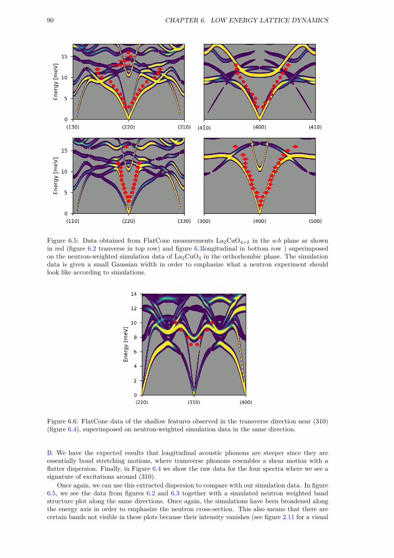
90 CHAPTER 6. LOW ENERGY LATTICE DYNAMICS
Figure 6.5: Data obtained from FlatCone measurements La2CuO4+δ in the a-b plane ar shownin red (figure 6.2 tranverse in top row) and figure 6.3longitudinal in bottom row ) superimposedon the neutron-weighted simulation data of La2CuO4 in the orthorhombic phase. The simulationdata is given a small Gaussian width in order to emphasize what a neutron experiment shouldlook like according to simulations.
Figure 6.6: FlatCone data of the shallow features observed in the transverse direction near (310)(figure 6.4), superimposed on neutron-weighted simulation data in the same direction.
B. We have the expected results that longitudinal acoustic phonons are steeper since they areessentially bond stretching motions, where transverse phonons resembles a shear motion with aflatter dispersion. Finally, in Figure 6.4 we show the raw data for the four spectra where we see asignature of excitations around (310).
Once again, we can use this extracted dispersion to compare with our simulation data. In figure6.5, we see the data from figures 6.2 and 6.3 together with a simulated neutron weighted bandstructure plot along the same directions. Once again, the simulations have been broadened alongthe energy axis in order to emphasize the neutron cross-section. This also means that there arecertain bands not visible in these plots because their intensity vanishes (see figure 2.11 for a visual

6.1. ACOUSTIC PHONONS AND SIMULATION VALIDATION 91
Figure 6.7: Simulation data in the a-b plane of La2CuO4 at 9 meV in the low-temperature or-thorhombic phase. The first two images show the effect of exchanging the a and b directions whengenerating the plot and the last shows the superposition of the two.
Figure 6.8: Simulation data in the a-b plane at 9meV from the six different phonon calculationsperformed in chapter 3.
explanation of this point). As indicated by the two dimensional color plot in figure 6.1, we haveexcellent agreement between measurement and simulation. I mention here that that it was onlypossible to fit the steeply dispersive acoustic phonons as shown in appendix B. Since FlatConemeasurements are constant energy scans, flat modes are difficult to extract unambiguously. Wherefitting was not possible, the peaks were assigned from visual inspection.
As the attentive reader might have noticed, we performed simulations of several different ver-sions of La2CuO4 in chapter 3. The comparison shown here is the low-temperature orthorhombicstructural phase in the insulating state with static magnetism. This was chosen using through avisual inspection of the different simulations. The remaining five plots are shown in appendix B.
In addition, the bottom row of figure 6.1 was generated taking twinning (see section 1.3) intoaccount. Since a and b directions in the low-temperature orthorhombic phase are close in length,twinning essentially makes the two directions indistinguishable. To show how this affects thedynamics, figure 6.7 gives a visual indication of this superposition at 9meV. While the HK0/KH0planes have a similar overall shape, it becomes clear that the superposition has the strongestresemblance to our data.
For the sake of completeness, figure 6.8 shows all six simulations from chapter 3 at 9meV.Once again, it seems likely that the ‘LTO AFM’ simulation is the best representation of the

92 CHAPTER 6. LOW ENERGY LATTICE DYNAMICS
Figure 6.9: Soft phonons in La2−xSrxCuO4. Left: Schematic of the phonons related to struc-tural phase transitions, with HTT being high-temperature tetragonal, LTO low-temperature or-thorhombic and LTT low-temperature tetragonal. Decreasing the temperature across the struc-tural phase transition temperature Ts, the X-point phonon becomes soft and finally splits into Γand Z-point phonon branches. If the Z-point phonon softens completely, the LTT phase is realized.Right: Measurements of the Z-point phonon in La1.95Sr0.05CuO4 and La1.85Sr0.15CuO4, showinga softening of this mode where the phonon energy ω0 decreases with decreasing temperature. Thissoftening is associated with a sharpening of the linewidth γ.
sample chosen for this experiment, La1.94Sr0.06CuO4+δ.While they may not be groundbreaking in terms of scientific impact, I believe that these
comparisons confidently shows that our simulations can be trusted to some degree with regardsto lattice dynamics. In addition, I hope that the tools (appendix A) developed to generate theseplots can be helpful for neutron scatterers in the future. To end this section, I direct the readerto a video at https://youtu.be/LC-qV3CjqBM which illustrates the dispersive features of the 2Dcolorplots in this section by moving through the energy axis which may be instructive for thereader to predict what may be observed at constant neutron energy measurements besides theones explicitly plotted in this thesis.
6.2 Structural instabilities
In this section, we investigate a peculiarity with regards to the low-temperature orthorhombicphase in La2−xSrxCuO4. In the mid 2000s, it was discovered that this material is unstable to-wards a low-temperature tetragonal phase. This shows up as the softening of a phonon at (104) andthe temperature-dependence has been measured in optimally doped La1.85Sr0.15CuO4 and insu-lating La1.95Sr0.05CuO4, summarized in figure 6.9. Back then, it was suggested that the softeningabruptly stops at Tc for the optimally doped sample, essentially preventing the tetragonal phasefrom emerging – or at least stopping the instability in its tracks.
These ideas are consistent with the idea that lanthanum cuprates near x = 18 have their
Tc suppressed due to the proximity of this tetragonal phase. This is particularly apparent inLa2−xBaxCuO4 where the tetragonal phase appears and Tc drops to a few Kelvin [35].
We set out to do a similar experiment on the cold Triple-Axis ThALES at ILL. The sample is asingle crystal La2CuO4+δ aligned in the a-c plane. Measurements were constant-Q scans, and thetemperature dependence is shown in figure 6.10 and the summary of the fits are shown in 6.11.
We immediately notice that our experiment stands out when compared to La2−xSrxCuO4.First, the energy dependence resembles that of La1.85Sr0.15CuO4, but shifted up by roughly 1meVand our linewidth increases with decreasing temperature. In this case, the Sr-doped samples areunusual, since soft phonons is usually accompanied by an increased linewidth. I stress here thatwe performed these experiments with an extremely tight energy resolution (roughly 0.1meV, seefigure 6.12), so the broadening is definitely unique to this system.
I foresee two scenarios causing this broadening. Either it is the expected broadening that istypically observed with soft phonons or it is caused by a splitting or distribution of modes at this

6.2. STRUCTURAL INSTABILITIES 93
60
80
100
Inte
nsity
[cnt
s/m
in] T=100K T=80K T=60K
406080
100120
Inte
nsity
[cnt
s/m
in] T=50K T=45K T=40K
20
40
60
80
100
Inte
nsity
[cnt
s/m
in] T=35K
1 2 3 4 5Energy [meV]
T=30K
1 2 3 4 5Energy [meV]
T=20K
1 2 3 4 5Energy [meV]
20
40
60
Inte
nsity
[cnt
s/m
in] T=10K
Figure 6.10: Measurements of the Z-point phonon in La2CuO4+δ. At each temperature an energyscan from 0.5meV to 5.5meV is performed, clearly showing the phonon at ≈ 2.5meV. The strongBragg tail comes from the fact that we are measuring (104) and (014) simultaneously as a resultof twinning. (104) is Z in the orthorhombic phase, while (014) is Γ. The data is fitted to a sum oftwo Gaussian functions, describing the Bragg tail and phonon plus a constant background. Theuse of a Gasussian rather than Lorentzian for the phonon is phenological, since it described thedata much better.

94 CHAPTER 6. LOW ENERGY LATTICE DYNAMICS
0 20 40 60 80 100Temperature [K]
2.2
2.4
2.6
2.8
3.0Ph
onon
Ene
rgy
[meV
]LCO+Ox=0.05
0 20 40 60 80 100Temperature [K]
0.0
0.5
1.0
1.5
2.0
2.5
Phon
on L
inew
idth
[meV
]
LCO+Ox=0.05x=0.15
1.2
1.3
1.4
1.5
1.6
1.7
x=0.15
Figure 6.11: Temperature dependence of the Z-point phonon in La2CuO4+δ compared toLa2−xSrxCuO4 with x = 0.05 (insulating) [174] and x = 0.15 (Tc = 37K) [175]. Left: Phononenergy as a function of temperature. The left energy axis correpsonds to the x = 0.15 data.Right: Phonon linewidth as a function of temperature, with the width measured as Full-WidthHalf-Maximum in meV.
0.4 0.2 0.0 0.2 0.4Energy [meV]
0.00
0.01
0.02
0.03
0.04
0.05
0.06
Inte
nsity
[CNT
S/M
1]
= 0.0434Q=(0.8,0,3.8)
Figure 6.12: Energy resolution of ThALES in the conditions used to measure soft phonons. Anenergy scan at an arbitrary Q = (0.8, 0, 3, 8) close to the (104) peak we are interested in revealsan energy resolution with a σ = 0.04meV Gaussian with corresponding to 0.10meV Full-WidthHalf-Maximum.
energy. Since we know that the interstitial oxygen in La2CuO4+δ is spatially inhomogeneous, itwould not be surprising to have spatially separated regions with different ‘spring constants’ forthis phonon modes. In particular, we know that this mode is related to octahedral tilts which areaffected by the interstitial near the apex of the CuO6 octahedra. While not conclusive, this pointsto abnormal behavior which would be in favor of the second scenario.
6.3 Low energy modes of superstructures
Finally, we take a look at the superstructures observed in chapter 5 and use the Triple-Axis Spectro-meter ThALES to look for a dynamic signature of these satellites. It is well known that structuralpeaks, per Goldstone’s theorem, should have acoustic modes emerging from their position.
We start by looking at these dynamics with the FlatCone analyser as shown in figure 6.13. We,once again, clearly see the elastic scattering from the superstructures, but as we move up in energy,we only see the acoustic phonon emerging from the Bragg peak. It should however be noted thatsince the FlatCone analyser measures at a fixed energy, it can be difficult to detect flat modes.
For this reason, we switched to a single detector and made detailed measurements along theline shown in figure 6.13. The result is shown in figure 6.14, revealing that we do not observe anyphonon-like signature, despite very strong satellite reflections (roughly 20000 neutron counts per

6.3. LOW ENERGY MODES OF SUPERSTRUCTURES 95
Figure 6.13: FlatCone data of La2CuO4+δ in the a-b plane in the elastic condition (top left) andat 1meV, 2meV, 3meV and 4meV as indicated by the figures. In general, the energy-dependantfeatures show no signature of superstructures, and we only see the acoustic phonon from the (200)Bragg peak.
Figure 6.14: Data collected with a single-detector setup, designed to search for fundamental excit-ations from the satellite peaks as shown in figure 6.13, which also shows the direction where thisdata was obtained. The red and white markers indicate features visible in the individual scans,see appendix B for details. Due to the linear shape of these features, it seems likely that these areartifacts of the experiment.

96 CHAPTER 6. LOW ENERGY LATTICE DYNAMICS
2.00 1.95 1.90QH [rlu]
0.0
QL [r
lu] (-200) A
B
0.25 0.00 0.25Energy [meV]
0.00
0.02
0.04
0.06
0.08
0.10A
x0 = 0.04= 0.026
0.25 0.00 0.25Energy [meV]
0.0
0.5
1.0
1.5
2.0
2.5
3.0
Inte
nsity
[CNT
S/M
1]
Bx0 = 0.02
= 0.033
Figure 6.15: Resolution in the experiment where we look for dynamics associated with super-structures. Left: Schematic of reciprocal space where we measured the energy-resolution of theinstrument. I remark here that the superstructures are seen in the direction of B. Subfigures Aand B, shows the raw data with a Gaussian fit at the two locations corresponding to the schematic.Since we are measuring close to the elastic Bragg peak, the increased intensity at B suggests thatour resolution ellipsoid has points along the (200)-B direction.
second). We even confirmed that we were in the best conditions possible with regards to resolutionas shown in figure 6.15.
I do not currently have a satisfying explanation for these observations and I would be cau-tious about insisting that the excitations simply do not exist. Since we have no idea about thepolarization fo these modes, I would suggest additional experiments at different Q values. Inparticular, I note that our measurements were performed around l = 0. For the phonos associatedwith CuO6 tilt patterns in section 6.2, a finite l-component is necessary in order to get phononintensity. Since we believe that the superstructures are associated with tilt patterns, we might bein a similar situation.
6.4 Summary
In this chapter, a few experiments concerning low-energy phonons were bundled together in orderto help us better understand the dynamic nature of octahedral tilts in oxygen doped La2CuO4.We have shown that our simulations are highly reproducible in experiment, suggesting that we canexpand our models to include interstitals through molecular dynamics in the next chapter.
We also observed unusual behavior in La2CuO4+δ when trying to investigate soft phonons re-lated to a structural instability. The behavior is significantly different from that of La2−xSrxCuO4,but we still see a correlation between this phonon and Tc. It was suggested that this behaviorcould be associated with a distribution of domains, each with different ‘tilt dynamics’.
Finally, we found no evidence of dynamics related to the well-known superstructures in La2CuO4+δ,which is highly unusual if we expect the dynamics to behave like acoustic phonons. We interpretthis lack of intensity as either a consequence of the measurement conditions with respect to themode eigenvectors or as an extremely flat dispersion. Since these superstructures are associatedwith a long-range modulation, the dynamics are not likely to be very energetic.

Chapter 7
Phonon Density of States
In this chapter, we take a closer look at the phonon Density-of-States (DOS) in a series of insulatingand superconducting samples with different dopant species. In the previous chapter, we lookedat certain low-energy phonon branches which could be properly separated and measured due tothe sparse nature of bands from 0meV to 10meV. This was due to the fact that the neutrondifferential cross-section ‘sees’ preferentially vibrations parallel to the neutron wave vector due tothe Q · ej factor in equation (2.5). At higher energies, the phonon bands are heavily entangled(in the literal sense) making it difficult to separate different contributions to a measured spectrumwhere we have a finite resolution.
As a reminder, figure 7.1 shows the neutron-weighted bands in La2CuO4 with orthorhombicsymmetry. At energies from 10meV to 40meV we have a lot of intensity originating from multiplebands. Even if we took the data in all these directions, which would be a very laborious task,comparing experiment and simulation would be much harder compared to the analysis performedin chapter 6. On the right-hand side of figure 7.1 we see the neutron-weighted DOS, which is foundby essentially summing up the three dimensional band structure onto the energy axis.
The advantage of using the phonon DOS, is that we can obtain a ‘dynamical fingerprint’ ofa specific sample and consequently compare different samples, temperatures or other parametersof interest. In addition, the phonon DOS can be obtained experimentally by measuring powderswith a Time-of-Flight (ToF) spectrometer as we covered in section 2.2, chapter 2.
Figure 7.1: Neutron weighted phonon bands and DOS computed for La2CuO4 in the orthorhombic(LTO) crystal structure and magnetic, insulating electronic structure. Left: Band structure shownwith neutron intensity where the energy axis have been given a Gaussian width of 0.3meV Full-Width Half-Maximum (FWHM). The white lines shows the δ-function dispersion and thus revealcertain bands invisible to neutrons. Right: Phonon DOS obtained by integration of the firstBrillouin Zone on a 20× 20× 20 grid and broadening the spectra with a Gaussian width of 1meVFWHM. Certain Features that we observe in experiments are marked with grey horizontal lines.See discussion in the text, figure 7.4 and table 7.4.
97

98 CHAPTER 7. PHONON DENSITY OF STATES
Table 7.1: Samples used in the experiment, along with a naming scheme used in this chapter,the composition and the superconducting transition temperature as obtained from susceptibilitymeasurements. For additional details about these powdered samples see the MSc thesis by Ahmad[79].
Name Composition Tc
LCO La2CuO4 -LCOO La2CuO4.05 ≈ 40K
LSCO3 La1.97Sr0.03CuO4 -LSCOO3 La1.97Sr0.03CuO4+δ ≈ 40K
Table 7.2: Overview of incident energies and corresponding monochromators used in the experi-ments on IN4C.
λ [Å] Monochromator k [Å−1] E [meV] Sapphire Filter
1.6 PG004 3.93 31.95 IN1.1 PG004 5.71 67.61 IN0.85 Cu220 7.39 113.22 OUT
Figure 7.2: A: S(Q, ω) map of LSCO3 at 10K with λ = 1.6Å incident wavelength. Data hasnormalized by the Bose factor. B: Sample mounted in cadmium frame.
7.1 Experiment
We performed inelastic neutron time-of-flight experiments on a series of La2−xSrxCuO4+δ powderedsamples in order to better understand the relationship between mobile (O) and static (Sr) dopantssimilar to the objectives outlined for Pair-Distribution Function analysis in chapter 5. The samplesused here are listed in table 7.1 and are identical to the ones as used in 5 [79]. The naming schemeof table 7.1 will be used throughout this chapter.
Experiments were performed at the thermal neutron time-of-flight spectrometer IN4c at InstitutLaue-Langevin in Grenoble, France. In order to see excitations in the 5meV to 100meV range,each sample/temperature was measured at three different incident neutron wavelengths as shownin Table 7.2. Sample was mounted in a cadmium frame as shown in Figure 7.2B. Each of the 4samples was measured for 3.5-4 hours per temperature/wavelength combination.
The raw time-of-flight data was reduced to S(Q, ω) using the Mantid [176] software and themeasured background was corrected by subtracting measurements of a sample of polycrystallinevanadium from our data. Due to the isotropic nature of the powder, we only consider the magnitudeof Q and the resulting data can be viewed in two dimensions as shown in Figure 7.2A. Obtainingthe density-of-states is done in Mantid with the ComputeIncoherentDOS [177] algorithm, using the

7.2. RESULTS 99
Table 7.3: Q and E-ranges used in the computation of DOS. For all spectra a mean squareddisplacement of ⟨u2⟩ = 0.015Å2 was used.
λ [Å] Qmin [Å−1] Qmax [Å−1] Emin [meV] Emax [meV] ∆E [meV]
1.6 2.0 7.0 4.0 26.0 0.21.1 3.0 10.0 7.0 59.0 0.40.85 4.0 12.0 15.0 98.0 1.0
0 10 20 30 40 50 60 70 80 90Energy [meV]
0.0005
0.0010
0.0015
0.0020
0.0025
0.0030
0.0035
0.0040
DOS
LSCO3 = 1.6 Å= 1.1 Å= 0.85 Å
Figure 7.3: Visualization of the data ‘stitching’ procedure. Our spectra are obtained at lowtemperatures and we thus only consider neutron energy loss, meaning that the maximal energyof the spectrum is limited by the incoming neutron energy. For this reason, a full spectrum isobtained from three separate measurements and are put together as shown. The energies wheredata is stitched together is determined by a visual inspection such that we minimize artifactscreated by this procedure.
following expression for the one-phonon incoherent scattering function (see section 2.2 for details):
S(1)inc(Q,E) = exp
(−2W (Q)
) Q2
E⟨n+
1
2± 1
2⟩
[∑k
σscattk
2mkgk(E)
],
where W = Q2⟨u2⟩/2 with ⟨u2⟩ being the average mean-squared displacement. n is the Bosefactor and E is the energy transfer. Finally, the term in brackets is the neutron-weighted densityof states with k running over the different elements in our sample. The calculated DOS is given inmilibarns/steredians per formula unit per meV. The mean squared displacement is set to ⟨u2⟩ =0.015Å2, which is a good compromise between qualitatively describing our data and the actualvalues of ⟨u2⟩ as obtained from experiments [178] and simulations.
In order to get meaningful results from this procedure, reduction of the raw data is usuallyrequired. Generally, one chooses a range of Q and E to sum over along with a binning of E (whichis measured through time-of-flight and thus on a continuos scale). Since the measured (Q,E)space is different between incident energies, the integration ranges are chosen for each of the threeconfigurations independently (see Table 7.2). The parameters used for our data reduction areshown in Table 7.3.
7.2 Results
In order to visualize our spectra, we start by stitching the different wavelengths together. Sincethe energy resolution of the instrument decreases with increasing incoming energy Ei we stitchtogether data from the different wavelengths, such that the λ = 1.6Å data describes low energiesup to ≈ 24meV, λ = 1.1Å data describes intermediate energies up to ≈ 43meV and λ = 0.85Ådata describes high energy data.

100 CHAPTER 7. PHONON DENSITY OF STATES
0.0015
0.0025
0.0035DO
SLCO LSCO3
0 20 40 60 80Energy [meV]
0.0015
0.0025
0.0035
DOS
LCOO
0 20 40 60 80Energy [meV]
LSCOO3
Figure 7.4: DOS of all measured samples (see table 7.1 for naming scheme) at 10K. Data wasreduced with Mantid and stitched together from several measurements as described in the text.
Table 7.4: Peaks in the phonon DOS at 10K of samples considered in this chapter, obtainedthrough visual inspection of figure 7.4 (grey vertical lines).
Sample E1 E2 E3 E4 E5 E6 E7 E8 E9
LCO 10.2 12.8 - 18.9 - 27.5 38.2 56.4 80.0LCOO 11.5 - - 18.4 - 28.9 38.5 55.4 79.5LSCO3 10.7 13.6 16.5 18.9 22.9 28.8 39.1 56.4 83.5LSCOO3 11.6 - - 18.8 23.2 28.9 38.8 56.5 79.5
Data is stitched together by choosing some cut-off energies such that no features are introducedwhen we combine the data. The data for λ = 1.1Å and λ = 0.85Å is then scaled such that we geta continuous spectrum across the full range. For this reason, the absolute values of the DOS is onlyrepresentative for the λ = 1.6Å data. Figure 7.3 shows the result of such a concatenation of data.In addition, vertical lines have been added to show qualitative ‘peak’ features of the spectrum.
Applying this procedure to all 4 samples, figure 7.4 shows the phonon DOS for all samples at10K. Since no noticeable temperature dependance was found, apart from a tendency to smoothout features, spectra at 60K and 300K are not shown here, but can be found in appendix C.Vertical lines in the plots mark peaked features in the spectra and are obtained from a visualinspection. These features are mainly a convenient way to quantify certain differences betweensamples.
Table 7.4 shows these features in a list of peak-energies Ek, indicating that we can generallyidentify four separate high-energy peaks at ≈ 28meV, 39meV, 56meV and 80meV which aregeneral similar between our samples. Comparison with figure 7.1 shows that these features arequalitatively consistent with the calculated spectrum and that the two highest energy featuresoriginate from distinct bands. Features below 30meV are much more subtle and will have to beanalyzed based on changes in the shape of our measured DOS.
Comparing between samples with and without interstitial oxygen, our visual inspection revealstwo distinct features. First, we see a subtle modification of the high-energy mode at ≈ 80meV,where it seems that spectral weight is moved to lower energies. This is consistent with softeningof the Cu-O bond-stretching mode which we will return to in the next chapter. Second, thereis a general smoothing of features below 30meV when introducing interstitial oxygen into thesample. Intuitively, one would expect a smoother DOS with increased disorder, so this observationis, at least qualitatively, consistent with what we would expect. On the other hand, we also see aslight sharpening of features when comparing Sr-doped LSCO3 with the parent compound LCO,

7.3. COMPARISON WITH SIMULATION 101
0 10 20 30 40Energy [meV]
0.0015
0.0020
0.0025
0.0030
0.0035
0.0040
Phon
on D
OS 1
2
43 5
6
IN4 Data
LSCO3LSCOO3
0 10 20 30 40Energy [meV]
0.001
0.002
0.003
0.004
0.005
0.006
1
2 4
35
6
Simulation
LCOLCO+O
Figure 7.5: Left: Phonon DOS data for LSCO3 and LSCOO3 at 10K. Features are numberedand dissimilarities between the samples are highlighted Right: Simulations from LCO AFM andLCO+O AFM (see chapter 4 for details) with the same highlighted features as from the data.The simulation data is smoothed by a width that depends on the energy such that FWHM =1.4 + 0.024E, with E being the energy in meV.
inconsistent with the intuitive notion of disorder-induced smoothing of the spectra. On the otherhand, it does seem consistent with the sharper distribution of Cu-O in-plane distances that weobserved in the previous chapter (see table 5.2). LCO has a peculiar broad feature at high energies(65meV to 85meV), that is unique to that sample and cannot be explained by the logic we usedso far.
7.3 Comparison with Simulation
Since the high energy features are either very similar between samples (28meV, 39meV and56meV) or considered separately in the next chapter (80meV), the following analysis will befocussed on the low-energy part of the phonon DOS. Since the differences between spectra arequite subtle, we consider the effects of oxygen-doping of LSCO3 first, since we are free of thepeculiar features of the LCO sample.
Figure 7.5 shows a comparison of LSCO3 and LSCOO3 in the low-energy regime below 40meValongside a comparison of phonon DOS obtained by molecular dynamics for LCO and LCO+O.Since the Sr content is very low in this sample (x = 0.03), it is reasonable to assume that it is,at least, approximately similar to LCO with x = 0. While we had reasonable success in chapter6 when comparing band structures directly, the correspondence between spectra are not quiteas convincing in this case. We recover general features as shown in the figure, but the spectralweight and absolute energies deviate slightly from the experimental spectrum (notice the differentenergy-axes between experiment and simulation).
While the agreement is not perfect, we can still assign the features with some confidence asshown in the labeled features in figure 7.5. In both the experiment and simulation we see thedouble-peak at (1) merging, the peak at (2) disappearing and a modification of spectral weightto higher energies at (4) when adding oxygen to the sample. Features at (3), (5) and (6) stayroughly the same.
Figure 7.6 shows the same idea, but this time for the effect of Sr-doping. We note here that thesimulation has roughly four times the doping (x = 0.125) of the experimental sample (x = 0.03).The minimal possible doping (one substitution) in our simulation cell would be x = 0.0625. Itappears as if the addition of strontium has a similar effect to that of oxygen, but with a smallermagnitude – there is an overall smoothing of the spectrum due to the introduction of disorder.Interestingly, we reproduce the ‘dip’ at ≈ 30meV in our simulation. One thing that we cannotexplain in these measurements, is the very sharp features of LSCO3 when compared to LCO,especially at ≈ 20meV.
For the sake of completeness, figure 7.7 shows the experimental phonon DOS as a function of thetwo dopants (oxygen, strontium), where it becomes clear that the modification of spectral weight

102 CHAPTER 7. PHONON DENSITY OF STATES
0 10 20 30 40Energy [meV]
0.0015
0.0020
0.0025
0.0030
0.0035
0.0040Ph
onon
DOS
IN4 Data
LCOLSCO3
0 10 20 30 40Energy [meV]
0.001
0.002
0.003
0.004
0.005
0.006
Simulation
LCOLSCO
Figure 7.6: Left: Phonon DOS data for LCO and LSCO3 at 10K. Right: Simulations from LCOAFM and LCO+Sr AFM (see chapter 4 for details). The simulation data is smoothed by a widththat depends on the energy such that FWHM = 1.4 + 0.024E, with E being the energy in meV.
0 5 10 15 20 25 30 35 40Energy [meV]
0.0020
0.0025
0.0030
0.0035
0.0040
Phon
on D
OS
LCOLCOO
0 5 10 15 20 25 30 35 40Energy [meV]
LCOLSCO3
Figure 7.7: Dopant dependence of measured phonon DOS. Left: Effect of oxygen through acomparison of LCO and LCOO. Notice in particular the modification at low energies. Right:Effect of strontium through a comparison of LCO and LSCO3. While the LSCO3 spectra is muchsharper, low energy features are similar in energy when compared to the effect of oxygen.
at low energies (≈ 5meV to 15meV) are more dramatic in the case of oxygen. A correspondingcomparison of the simulations can be found in figure 4.5, chapter 4.
7.4 Summary
In this chapter we measured several samples of La2CuO4 with different dopant species in orderto shed light on the effect of specific types of chemical disorder on the phonon density of states.While it is possible to discern certain features in the experimental spectra related to the dopantspecies, differences are in general quite subtle.
With that in mind, we have been able to identify features at low energies which are qualitativelyreproduced by our molecular dynamics simulations. At higher energies we only see a modificationof the topmost phonon band which will be discussed in the following chapter.
It thus appears, despite the significantly reduced simulation precision, that our molecular dy-namics simulations can be used to identify a microscopic origin of the modified phonon DOS. Theanalysis of molecular dynamics simulations concluded that the inclusion of interstitial oxygen spe-cies resulted in local ‘LTT-like tilts’ despite the structure being LTO. In fact, it is quite remarkablethat the structure of these samples are almost identical in our diffraction experiments (the data

7.4. SUMMARY 103
in chapter 5 is from the same samples), but we clearly see a signature of the dopant species in thedynamics.
While our simulations reproduce the general features of the phonon spectrum, there are stilla few unexplained phenomena. The addition of oxygen seem relatively well-understood throughthe comparison with simulations; features around 10meV and 20meV are broadened due to theinterstitial. The effect of Sr-doping, on the other hand, is difficult to explain as a purely structuralphenomena. It appears as if the LSCO3 sample is sharpening features quite substantially, oppositeto the effect we see from simulations. From an intuitive, structural perspective, one would alsoexpect disorder to broaden features when compared to the stoichiometric compound. While theLSCO3 sample is insulating, it lies in the underdoped region where the magnetic properties aresimilar to samples with x ≤ 0.125 [76].
To summarize, it appears that our simulations can explain features in the phonon dos due tooxygen doping, but not due to a small amount of strontium doping. One way to think aboutthis is a scenario where the effect of oxygen dopants is dominated by phenomena which we canexplain in a semi-classical way without having to consider the complex electronic structure. Sincestrontium-doping barely modifies the structure, it is possible that the sharpening of the phononDOS is mostly due to electronic correlations. This is also somewhat consistent with the factthat structural correlations due to interstitials take over, once again, when comparing LSCO3 andLSCOO3 (figure 7.5).

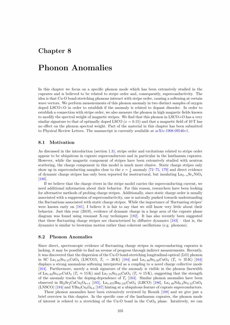
Chapter 8
Phonon Anomalies
In this chapter we focus on a specific phonon mode which has been extensively studied in thecuprates and is believed to be related to stripe order and, consequently, superconductivity. Theidea is that Cu-O bond-stretching phonons interact with stripe order, causing a softening at certainwave vectors. We perform measurements of this phonon anomaly in two distinct samples of oxygendoped LSCO+O in order to establish if the anomaly is related to dopant disorder. In order toestablish a connection with stripe order, we also measure the phonon in high magnetic fields knownto modify the spectral weight of magnetic stripes. We find that this phonon in LSCO+O has a verysimilar signature to that of optimally doped LSCO (x = 0.15) and that a magnetic field of 10T hasno effect on the phonon spectral weight. Part of the material in this chapter has been submittedto Physical Review Letters. The manuscript is currently available at arXiv:1908.09546v1.
8.1 Motivation
As discussed in the introduction (section 1.3), stripe order and excitations related to stripe orderappear to be ubiquitous in cuprate superconductors and in particular in the lanthanum cuprates.However, while the magnetic component of stripes have been extensively studied with neutronscattering, the charge component in this model is much more elusive. Static charge stripes onlyshow up in superconducting samples close to the x = 1
8 anomaly [72–75, 179] and direct evidenceof dynamic charge stripes has only been reported for isostructural, but insulating La2−xSrxNiO4
[180].If we believe that the charge rivers in the stripe model carries the superconducting current, we
need additional information about their behavior. For this reason, researchers have been lookingfor alternative methods of probing charge stripes. Additionally, since static charge order is usuallyassociated with a suppression of superconductivity, one is naturally pushed towards understandingthe fluctuations associated with static charge stripes. While the importance of ‘fluctuating stripes’were known early on [181], I believe it is fair to say that we still know very little about theirbehavior. Just this year (2019), evidence of dynamic charge in a large area of the cuprate phasediagram was found using resonant X-ray techniques [182]. It has also recently been suggestedthat these fluctuating charge stripes are characterized by diffusive dynamics [183] – that is, thedynamics is similar to brownian motion rather than coherent oscillations (e.g. phonons).
8.2 Phonon Anomalies
Since direct, spectroscopic evidence of fluctuating charge stripes in superconducting cuprates islacking, it may be possible to find an avenue of progress through indirect measurements. Recently,it was discovered that the dispersion of the Cu-O bond-stretching longitudinal-optical (LO) phononin SC La1.85Sr0.15CuO4 (LSCO15, Tc = 38K) [184] and La1.80Sr0.20CuO4 (Tc ≈ 35K) [164]displays a strong anomalous softening interpreted as a coupling to a novel charge collective mode[164]. Furthermore, merely a weak signature of the anomaly is visible in the phonon linewidthof La1.93Sr0.07CuO4 (Tc ≈ 15K) and La1.75Sr0.25CuO4 (Tc ≈ 15K), suggesting that the strengthof the anomaly tracks the doping-dependence of Tc [164]. Similar phonon anomalies have beenobserved in Bi2Sr2CaCu2O8+δ [185], La1.875Ba0.125CuO4 (LBCO) [186], La1.48Nd0.4Sr0.12CuO4
(LNSCO) [184] and YBa2Cu3O6.6 [187] hinting at a ubiquitous feature of cuprate superconductors.These phonon anomalies have been extensively reviewed by Reznik [188] and we give just a
brief overview in this chapter. In the specific case of the lanthanum cuprates, the phonon modeof interest is related to a stretching of the Cu-O bond in the CuO2 plane. Intuitively, we can
105

106 CHAPTER 8. PHONON ANOMALIES
‘Static’ lowering of energy
charge oscilation (out-of-phase)
charge oscilation (in-phase)
Figure 8.1: Possible scenarios of the phonon anomaly. In the first two scenarios, only the movementof the oxygen atoms are shown and the bars represent charge stripe dynamics with the propagationas shown. In these cases the charge oscillation can be either in-phase (shown top rown) or out-of-phase (shown in middle row) with the phonon [189]. In the last scenario (shown in the bottomrow) open circles represent Cu atoms with magnetic ordering and closed circles are charge stripesrunning perpendicular to the chain. The static charge order then lowers the energy of the phonon[186].
already see why this phonon mode might be interesting to look at since the vibrational frequenciescould be modified by charge modulations in the CuO2 plane. In addition, phonon anomalies havebeen observed at exactly the charge ordering wave vector Qco =
(14140)
in the Bmab orthorhombiccoordinate system (see section 1.3).
Figure 8.1 shows a sketch of possible scenarios involving a chain of Cu atoms (circles) separatedby oxygen atoms with a certain displacement pattern (arrows). In one scenario [189], the chargestripes are fluctuating and the phonon ‘resonates’ with this fluctuation, essentially lowering itsenergy. In the second scenario [186], static charge order changes the forces between certain Cu-Opairs, an effect that is also minimized at Qco as shown in the figure. A third possibility is onewhere the phonon anomaly is found in the perpendicular direction to the one shown in figure 8.1.In this case the phonon would resonate with the modulation ‘within’ the charge stripe. Since thesoftening happens close to Qco it seems more likely that one of the first two cases are responsible,but it has technically not been settled.
8.3 Experiment
We measured the phonon dispersion highlighted in figure 3.20 in two oxygenated single crystalsamples: La2CuO4+δ and La1.94Sr0.06CuO4+δ at the triple-axis spectrometer IN8 at ILL. Measur-ing this phonon dispersion turned out to be more difficult than anticipated, and several attemptswere spent in order to reach optimal conditions where we could actually observe the phonon dis-persion with relative success.
After our initial attempts, we realized that our signal was contaminated by so-called spuriousscattering. While not immediately apparent to us, we identified this ‘spurion’ as accidental Braggscattering from the analyzer [99]. This means that we are in the unfortunate situations where theanalyser is at angle where the sample scatters strongly from a structural Bragg peak. While the‘job’ of the analyser is to select a desired final energy, Bragg scattering is so strong that the signalat the detector will be contaminated by incoherent, scattering from the analyser crystals.
Figure 8.2 shows the geometry of this accidental Bragg scattering in reciprocal space. From thissketch we see that the spurious scattering comes from the (8,4,0) reflection. In order to quantifywhere we would observe this scattering in our measurements, we can make a simulation where weevaluate the strength of the spurion at the desired values of (Q, ω). This is done by constructingthe geometry as in 8.2 (top) and then defining the spurious strength through the distance to (8,4,0).The result of such a simulation is shown in figure 8.2 (bottom), and we clearly see that this signalintersects the expected phonon dispersion.
Two measures were taken to avoid this spurious scattering. First, by using the goniometersinstalled on IN8 we can effectively rotate the sample around the [110] axis, which has no affecton our measurements in the [hh0] direction, but does move further away from the condition forspurious scattering since (8,4,0) will be out of the scattering plane. Second, we installed a position-sensitive detector (PSD) with the hope that the spurious scattering is spatially separated fromthe phonon scattering. It turns out that the spurious scattering indeed can be separated from thephonon as shown in Figure 8.3. Unfortunately, this background subtraction procedure is associatedwith a large increase in error bars as shown in the figure.

8.3. EXPERIMENT 107
0 2 4 6 8 10h [r.l.u.]
0
1
2
3
4
5
k [r.
l.u.]
qkikfqkikf
4.5 4.6 4.7 4.8 4.9 5.0(hh0) [r.l.u.]
68
70
72
74
76
78
80
82
84
Ener
gy [m
eV]
Figure 8.2: Left: Scattering triangle responsible for the A-type spurious scattering (broken lines)at Q = (4.7, 4.7, 0). Green points represent Bragg peaks in the (h,k)-plane. The (8,4,0) Braggrefection is responsible for the spurious scattering. Right: Simulated effect of the (8,4,0) reflectionon a Q-hω map assuming a Gaussian spurious signal depending on distances in Q. Broken linerepresents a ‘normal’ sinosoidal dispersion in this region as described in the text.
BG Phonon BG
65.0 67.5 70.0 72.5 75.0 77.5 80.0 82.5 85.0 [meV]
50
100
150
200
250
300
Inte
nsity
[a.u
.]
fitdataraw data
Figure 8.3: Illustration of the data reduction performed using the PSD. Left: Summed rawdata from an energy scan at Q = (4.65, 4.65, 0). The dashed lines denote the regions of interest(ROI) used in the data reduction. The geometry of the instrument ensures that the desiredphonon scattering will occur in the ‘Phonon’ ROI. Right: Corresponding raw (diamonds) andreduced/normalized (circles) data. The raw data is obtained by only considering the ‘Phonon’ROI, while the reduced data is obtained by subtracting the intensity from the two ‘BG’ ROIs. Thesolid line is a fit to a DHO lineshape as described in the text.
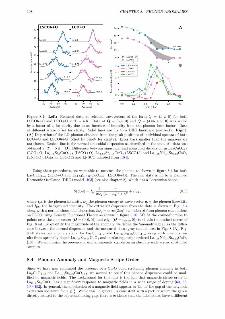
108 CHAPTER 8. PHONON ANOMALIES
60 70 80 90 [meV]
10
20
30
40
50
60
70
80
90In
tens
ity [a
rb. u
nits
]
h=4.5
h=4.7
h=4.75
h=4.85
h=5.0
LSCO6+O
60 70 80 90 [meV]
h=4.5
h=4.7
h=4.75
h=4.85
h=5.0
LCO+O
70
75
80
85
90
[meV
]
+5 meV
A
LSCO6+OLCO+O
0.0 0.1 0.2 0.3 0.4 0.5(hh0) [r.l.u.]
1
0
1
2
3
4
5
Anom
aly
Sign
al [m
eV]
BLSCO6+OLCO+OLSCO15LNSCO
Figure 8.4: Left: Reduced data at selected wavevectors of the form Q = (h, h, 0) for bothLSCO6+O and LCO+O at T = 5K. Data at Q = (5, 5, 0) and Q = (4.85, 4.85, 0) was scaledby a factor of 1
2 for clarity due to an increase of intensity from the phonon form factor. Dataat different h are offset for clarity. Solid lines are fits to a DHO lineshape (see text). Right:(A) Dispersion of the LO phonon obtained from the peak positions of individual spectra of bothLCO+O and LSCO6+O (offset by 5meV for clarity). Error bars smaller than the markers arenot shown. Dashed line is the normal sinusoidal dispersion as described in the text. All data wasobtained at T = 5K. (B): Difference between sinusoidal and measured dispersion in La2CuO4+δ
(LCO+O) La2−xSrxCuO4+δ (LSCO+O), La1.85Sr0.15CuO4 (LSCO15) and La1.48Nd0.4Sr0.12CuO4
(LNSCO). Data for LSCO15 and LNSCO adapted from [184].
Using these procedures, we were able to measure the phonon as shown in figure 8.4 for bothLa2CuO4+δ (LCO+O)and La1.94Sr0.06CuO4+δ (LSCO6+O). The raw data is fit to a DampedHarmonic Oscillator (DHO) model [103] (see also chapter 2), which has a Lorentzian shape:
S(q, ω) = Iph1
πωq
γ
(ω − ωq)2 + γ2+ IBG , (8.1)
where Iph is the phonon intensity, ωq the phonon energy at wave vector q, γ the phonon linewidthand IBG the background intensity. The extracted dispersion from the data is shown in Fig. 8.4along with a normal sinusoidal dispersion, hωq = α cos(2πq)+β, inferred from phonon calculationson LSCO using Density Functional Theory as shown in figure 3.20. We fit the cosine-function topoints near the zone center (Q = (0, 0, 0)) and edge (Q = ( 12 ,
12 , 0)) to obtain the dashed curves of
Fig. 8.4A. To quantify the magnitude of the anomaly, we define the ‘anomaly signal’ as the differ-ence between the normal dispersion and the measured data (gray shaded area in Fig. 8.4A). Fig.8.4B shows our anomaly signal for La2CuO4+δ and La1.94Sr0.06CuO4+δ along with previous res-ults from optimally doped La1.85Sr0.15CuO4 and insulating, stripe-ordered La1.48Nd0.4Sr0.12CuO4
[184]. We emphasize the presence of similar anomaly signals on an absolute scale across all studiedsamples.
8.4 Phonon Anomaly and Magnetic Stripe Order
Since we have now confirmed the presence of a Cu-O bond stretching phonon anomaly in bothLa2CuO4+δ and La1.94Sr0.06CuO4+δ, we wanted to see if this phonon dispersion could be mod-ified by magnetic fields. The background for this idea is the fact that magnetic stripe order inLa2−xSrxCuO4 has a significant response to magnetic fields in a wide range of doping [60, 63,190–192]. In general, the application of a magnetic field appears to ‘fill in’ the gap of the magneticexcitation spectrum for x ≥ 1
8 . While this, in general, is consistent with a picture where the gap isdirectly related to the superconducting gap, there is evidence that the filled states have a different

8.5. DISCUSSION 109
0.4 0.2 0.0 0.2 0.4k [r.l.u]
2.00
2.25
2.50
2.75
3.00
3.25
3.50
3.75
Inte
nsity
[arb
. uni
ts]
4 6 8 10 12 14 [meV]
0.0
0.5
1.0
1.5
2.0
′′ P(n+
1)
0T, 5K10T, 5K3T, 5K
Figure 8.5: Magnetic fluctuations in La1.94Sr0.06CuO4+δ. Left: Example spectrum obtained as aconstant-energy scan in the k direction with h = 0.125. Solid line is a fit to the functional formoutlined in ref. [194]. Right: Amplitude of the magnetic excitations, as extracted from the fittingprocedure, in at a variety of fields and temperatures as a function of energy transfer.
60 65 70 75 80 85 90 [meV]
2
3
4
5
6
7
8
Inte
nsity
[arb
. uni
ts]
h=4.75
h=4.5
0T10T
Figure 8.6: Comparison of representative constant-Q (h,h,0) scans of La1.94Sr0.06CuO4+δ in zero-field and with an applied field of 10T. All measurements performed at T = 5K
origin [63]. Since one could write books about the spin excitation spectrum in La2−xSrxCuO4, Iwill keep the discussion somewhat limited and refer to the excellent review by Tranquada [193].
Returning to the objective at hand, our idea was to both measure the spin excitation spectrumand anomalous phonons in the same experimental conditions in order to directly probe any cor-relation (or lack thereof) between the two phenomena. These measurements were only performedfor the La1.94Sr0.06CuO4+δ sample. Figure 8.5A shows the amplitude of the magnetic fluctuationsas a function of energy transfer and figure 8.5B shows an example of the neutron scattering dataused to extract this amplitude. The figure clearly shows that La1.94Sr0.06CuO4+δ has gappedexcitations which are filled in with the application of a magnetic field (or raising the temperatureabove Tc). This is in contrast to other oxygen-doped samples (e.g. La2CuO4+δ [62]) where theexcitations are not gapped.
In figure 8.6 we have measured the phonon at a ‘normal’ and anomalous wavevector at T = 5Kwith and without an applied field of 10T. From this measurement it is thus clear that a field of10T has no effect on the bond stretching phonon at anomalous wave vectors.
8.5 Discussion
To begin the discussion of our results, we remark that softening and/or broadening of phononmodes is generally a signature of an incipient structural or electronic instability. Typical examplesinclude structural phase transitions, Q-dependence of the electron-phonon matrix element, Fermi

110 CHAPTER 8. PHONON ANOMALIES
surface nesting and electronic correlations [188]. In order to determine the origin of a given phononanomaly, it is therefore important to carefully exhaust alternatives before making statements aboutthe connection to novel phases such as dynamic charge stripes [188].
The phonon anomaly appears in vicinity of the wave vector Qco = ( 14 ,14 , 0), consistent with
charge stripe ordering as illustrated in Fig. 8.1. Measurements of LNSCO [195], LSCO15 [184] andLBCO [184] have shown a suppression of the anomaly as one moves away from the bond-stretchingdirection [195], supporting a one-dimensional stripe-like picture. Additionally, the phonon anomalyin LSCO15 and LBCO has almost no temperature dependence apart from a slightly sharper peakshape when heating from 10K to 300K [184, 186]. These phenomena rule out anharmonicity andstructural inhomogeneity as mechanisms for the phonon anomaly in these systems.
A combination of inelastic X-ray and ARPES measurements on overdoped LSCO (x = 0.2and x = 0.3) have shown that the phonon anomaly wavevector is inconsistent with Fermi surfacenesting [164, 196], contradicting the idea of a phonon softening due to a Kohn anomaly. A different,possibly Q-dependent, electron-phonon coupling could still be responsible for the phonon anomaly.Such an effect would renormalize the electronic quasiparticle dispersion (the so-called ‘ARPES kink’[197]) at energies similar to the phonon softening. The ARPES kink has been observed in LSCOx = 0.2 and x = 0.3, but since of these two dopings only LSCO x = 0.2 shows anomalous phonons,the two phenomena appear to not be connected [164].
Thus, all previous studies are unable to explain the phonon anomaly through conventionalmeans and any coupling to stripe order is likely dynamic. One possible scenario is a couplingof the Cu-O bond-stretching phonon with steeply dispersing charge fluctuations. Kaneshita etal. performed calculations based on the Hubbard model of this scenario, predicting anomalousphonon dispersions due to both transverse (meandering) and longitudinal (compression) coherentstripe fluctuations [189] (see Fig. 8.1 for a sketch of the transverse mode). We emphasize thatthe observed phonon anomaly reported here (see Fig. 8.4) and in LBCO/LSCO [184, 186] isremarkably similar to the calculation by Kaneshita et al. (see Fig. 5 in [189]).
Despite differences in the magnetic excitation spectra as recorded by neutron scattering (in-cluding low and zero energy transfers), the three materials LCO+O, LSCO6+O and LSCO15 haveremarkably similar in-plane Cu-O bond-stretching dispersions (Fig. 8.4). Furthermore, staticcharge order at zero field has been observed in a different sample of LCO+O [198] and in LNSCO[179] but so far not in LSCO6+O nor in LSCO15. These observations together indicate that thereis no direct connection between static stripes (spin and charge) and the phonon anomaly. In or-der to further confirm this point, we performed scans of LSCO6+O at selected wave vectors ina H = 10T magnetic field which is known to induce a considerable volume of stripe-like mag-netic order in this particular sample [199]. While static charge order has not been observed inLSCO6+O, measurements on LSCO (x = 0.12) have shown that static charge and spin stripesrespond identically to magnetic fields [73].
Figure 8.6 contains data at two wave vectors with and without an applied magnetic field of 10T,clearly showing the absence of any detectable field effect on the in-plane Cu-O bond-stretchingphonon at Q = ( 14 ,
14 , 0). These measurements were performed simultaneously with measurements
of the low-energy magnetic fluctuations as shown in figure 8.5, confirming a significant increasein the magnetic spectral weight towards lower energies consistent with the appearance of field-induced stripe-order [199]. Thus, the appearance of static magnetic stripe order does not affectthe phonon anomaly in LSCO6+O. A similar insensitivity of the phonon anomaly to an appliedmagnetic field has been observed in underdoped (Tc = 66K) YBa2CuO6.6 [200].
8.6 Summary
In this chapter, I showed that the phonon anomaly is a robust feature in optimally doped as wellas stripe-ordered cuprates which is independent of the structural details related to the dopingprocess. Since it is equally well-formed in stripe-ordered and optimally doped systems, where thelatter show no static magnetic order, the anomaly is surprisingly insensitive to low-energy magneticcharacteristics. This is further confirmed by the absence of a magnetic field effect of the chargedynamics in which is known to introduce static magnetic stripe-order in the same LSCO6+Osample.
The phonon anomaly is strongest in the doping region around optimal Tc (0.125 ≤ nh ≤ 0.20)(LSCO15, LNSCO [184], LBCO [186], LSCO6+O, LCO+O), regardless of the presence of staticcharge order (LNSCO [72], LBCO [201]), suppression of bulk superconductivity (LNSCO [179]) ordopant disorder (LCO+O, LSCO6+O). In addition, the phonon anomaly is unaffected by magnetic

8.6. SUMMARY 111
fields (LSCO6+O, YBa2CuO6.6 [200]) and temperature (LBCO, LSCO15) [184]). Thus it appearsto be an intrinsic, robust signature of doped cuprates near optimal doping.
If fluctuating stripes are the fundamental degrees of freedom relevant for the cuprates, it isappealing to draw a connection to Pair-Density-Wave superconductors [202]. In this system, thefundamental degrees of freedom are transverse charge fluctuations in an ‘electronic liquid crystal’phase without long range order [203]. In this scenario, the phonon anomaly in materials withoutstatic stripe order is due to a matching of the phonon wavevector with, otherwise undetectable,short-range transverse stripe correlations. The x = 1
8 anomaly then corresponds to the specialcase where stripes exhibit long-range order.
To summarize, we measured the in-plane Cu-O bond-stretching phonon in LSCO6+O andLCO+O and provided evidence for significant anomalous behavior. Since one sample (LCO+O)exhibits charge order [198] while the other (LSCO6+O) does not [199], and since the samplesalso have different magnetic spectra with distinct field dependencies [62, 199] we conclude thatthe phonon anomaly has no direct, trivial relationship to either magnetic or charge static order.In addition, the unique structural characteristics of oxygen-doped samples rule out a connectionbetween the specific dopant species and the phonon anomaly. We proceed to conclude that thephonon anomaly is a signature of transverse charge stripe fluctuations, which is a common char-acteristic of the cuprate family and appears to be a pre-requisite to optimal superconductivity inthese systems.


Chapter 9
Electronic Structure
In this brief chapter, we take a look at the Fermi surface as measured by Angle-Resolved Pho-toemission Spectroscopy (ARPES) on a sample of La2CuO4+δ. Tha majority of the experimentalwork was performed with assistance from Johan Chang’s group at the Laboratory for QuantumMatter Research (LQMR) in Zürich, Switzerland. I mention in particular Masafumi Horio, whohelped me prepare the samples and did all of the data analysis. I was present at the measurements,but success would not have been possible without the expertise of the LQMR group.
While the analysis presented here is very preliminary, I include it because it is, to my knowledge,the first ARPES experiment performed on an oxygen doped La2CuO4+δ sample. Since thesesamples are known to phase separate electronically [92], we expect a superposition of a magnetic‘ 18 ’ phase and an optimally superconducting phase. It is possible that we could see some of thisbehavior in an ARPES experiment.
The fermi surface evolution of La2−xSrxCuO4 is shown in figure 9.1, indicating how the brokenFermi arcs at
(π2 ,
π2
)become connected at optimal doping. Since La2CuO4+δ is phase separated,
we would expect to see signatures of either x = 0.1, x = 0.15 or both. The naive expectationwould be a superposition of the two, removing any signature of the 1
8 phase. In this context, I alsomention the fact that La1.48Nd0.4Sr0.12CuO4 (stripe ordered, insulating) and La1.85Sr0.15CuO4
(optimally doped, Tc = 37K) have curiously similar Fermi surfaces despite being electronicallydistinct [205].
9.1 Sample
The sample is a small piece (≈ 1 cm3) of La2CuO4+δ, carefully cut with the c-axis vertical. Beforecutting the sample, we characterized it with a Laue camera and magnetization measurements asshown in figure 9.2. When performing ARPES experiments, you need an atomically flat surface.Since La2CuO4 is a very brittle material, the only way to do this is by gluing on a small pin,knocking it off and hoping that the sample breaks in an atomically sharp way. Luckily, the 2-dimensional nature of the cuprates also translate to their structural integrity, so they are likelyto cleave naturally at the CuO2 interface. Before going to the ARPES experiment, the procedurewas tested in the lab as shown in figure 9.3.
Figure 9.1: Fermi surface evolution of under- (x = 0.1), optimally- (x = 0.15) and overdoped(x = 0.22) La2−xSrxCuO4. From ref. [204].
113

114 CHAPTER 9. ELECTRONIC STRUCTURE
10 20 30 40 50T [K]
0.8
0.6
0.4
0.2
0.0
[em
u c
m3
Oe
1 ]
Figure 9.2: Left: Laue diffraction pattern of the La2CuO4+δ sample, aligned with the c axis ver-tical. Right: Vibrating Sample Magnetometry (VSM) performed on a Quantum Design MPMS.Normalization performed through χ = 4π µ(1−N)
V Happ, where µ is the measured signal, V is the volume,
Happ is the applied field and N is the demagnetization factor. Vertical line marks the onsetsuperconducting transition temperature Tc = 41K
Figure 9.3: Cleaving procedure. 1: The sample is mounted using Torr Seal Low Pressure Epoxy.2: A stainless steel pin (L = 6mm, d = 1mm) is glued to the top of the sample and subsequently3: knocked off with a regular screwdriver.
9.2 Experiment
ARPES experiments were carried out on the La2CuO4+δ sample at the Surface/Interface Spectro-scopy (SIS) beamline at the Swiss Light Source. The sample was cleaved in situ at ≈ 20K underultra high vacuum (≤ 5× 10⁻¹¹ Torr) by employing the top-post technique as shown in figure 9.3.Cleaving in vacuum is essentially the same procedure as our ambient test-case, made possible witha screwdriver that we can control from outside the vacuum chamber. Ultraviolet ARPES spectrawere recorded using a SCIENTA R4000 electron analyser with horizontal slit setting. All the datawere recorded at the cleaving temperature. Figure 9.4 shows the Fermi surface map at T = 22Krecorded using circularly polarized 160 eV phonons. Detailed cut along the nodal direction withcircularly polarized light is shown in Figure 9.5. A comparison of different photon polarizationsalong with data from La1.77Sr0.23CuO4 is shown in Figure 9.6.
9.3 Summary
The area of the Fermi surface as shown in Figure 9.4 corresponds to a carrier (hole) dopingnh = 0.16 and a hopping parameter t′
t ≈ −0.14, according to analysis performed by MasafumiHorio from the LMQR group. It turns out that the measured spectra as e.g. the cut shown in Figure9.5 are very similar to what was observed by the LMQR group in overdoped La1.77Sr0.23CuO4
[156]. There is thus no indication of ‘ 18 -physics’ which is generally characterized by the formation

9.3. SUMMARY 115
Figure 9.4: Fermi surface of at 22K represented as raw and symmetrized data. kx and ky are intetragonal (I4/mmm) units. The cut indicates the nodal direction as used in subsequent measure-ments of the band structure.
Figure 9.5: Cut along the nodal direction (see Figure 9.4) with 160 eV circularly polarized photons.The subtracted background is defined by the minimum Momentum Distribution Curve (MDC)intensity at each binding energy.
of Fermi arcs. We cannot however rule out that such arcs are not observed due to an unfavorablesuperposition of photoemission from the 1/8 phase and optimally doped phase in our sample.
By using different polarizations of light (linear horizontal and linear vertical) Figure 9.6 showsthat we can separate the dx2−y2 band from the dz2 band. In the same figure, data from overdopedLa1.77Sr0.23CuO4 [156] is shown. The band structure is very similar except that the dz2 band ismoved down by about 0.2 eV. This could be due to an elongation of the c-axis, but while oxygen-doped samples are elongated when compared to the parent compound, La2CuO4+δ has a similar(or even smaller) c-axis when compared to La1.77Sr0.23CuO4.
Thus there must be another explanation for the decreased energy of the dz band further awayfrom the Fermi energy. Maybe the coupling along c is weakened by oxygen-doping and this infact enhancing Tc for oxygen doped samples? There is some evidence that relieving Josephsonfrustration along c gives 2D superconductivity with Tc = 40K [206].

116 CHAPTER 9. ELECTRONIC STRUCTURE
Figure 9.6: Cut along the nodal direction (see Figure 9.4) with 160 eV photons using differentpolarizations. Left: Linear horizontal polarization, showing clearly the dz2 band dispersing fromroughly -−1 eV to −1.5 eV. Right: Linear vertical polarization, showing the steeply dispersingdx2−y2 band. Center: Comparison with data of La1.77Sr0.23CuO4 from ref. [156], showing similarfeatures to our sample.

Chapter 10
Conclusion
In this chapter, I will attempt to condense the thesis as a whole in order to discuss what was learnedthrough the process of the various experimental and theoretical exercises. In a broad sense, theobjective of this thesis is to investigate the effects of chemical disorder through different dopantspecies in La2CuO4 as introduced in chapter 1 with the methods presented in chapter 2. This wasprimarily done through DFT simulations being compared to a neutron scattering experiment. Thechallenge with this objective is that we know that the exact electronic structure of the cuprates,at the relevant doping levels, is an unsolved problem in condensed matter. DFT, in particular, hasnot been very successful in the underdoped part of the phase diagram and many-body methodsare usually necessary to explain phenomena such as stripe order and fermi arcs.
Figure 10.1 attempts to visualize this problem by showing how superconductivity is squeezedbetween localized electrons giving rise to antiferromagnetic order and a fermi liquid with itinerantelectrons and a continuous Fermi surface. The solution to this problem was to simply consider thetwo cases available to us and perform the calculations with this drawback in mind. In some sense,we are trying to figure out how well this level of theory can explain experimental observations.Exactly for this reason, I think a crucial part of this thesis is a careful evaluation of theory withexperiment – essentially we need to know ‘how wrong’ the theory is.
Now, we are certainly not the first to consider La2CuO4 within a one-electron theory. SinceDFT was well-established when the high-temperature superconductors were discovered, this meth-odology was applied right away (see review by Pickett [143]). Various levels of theory have appliedto La2CuO4, including pure Hartree-Fock [207], and semi-local potentials [144]. Correlated phe-nomena, such as stripes [147] and broken up Fermi arcs [208, 209] have even been calculated within
Figure 10.1: Schematic of the electronic structure as a function of hole doping nh. As one movesfrom left to right, nh increases. On the left we have the undoped compound where there is a gapin electronic density of states due to the antiferromagnetic ground state. As doping is increased,the strong antiferromagnetic interactions are disrupted and novel phenomena such as stripe orderand broken Fermi arcs emerge [37]. Finally, on the right, the hole doping is sufficient such that thematerial becomes a normal metal and the strong correlations are destroyed. The electronic bandstructures are calculated and presented in chapter 3.
117

118 CHAPTER 10. CONCLUSION
DFT, albeit with ad-hoc methods such as DFT+U.In this thesis, I make no attempt to contribute to this discussion. Rather, I prioritize getting
accurate inter-atomic forces such that we get the best possible representation of the phonon spec-trum. We thus stick to the generally accepted GGA level of theory. As we saw in chapter 3, someexperimentation lead us to the PBESol functional and a significantly increased plane-wave cutoffin order to get reasonable acoustic phonons.
Within this framework, it was possible to get a good description of the unstable modes re-lated to the structural phase transitions observed in La2CuO4. However, it turns out that thelow-temperature tetragonal (LTT) phase is the ‘most stable’ structural phase both with respectto total energy and unstable phonons. Since this LTT phase is known to be suppressing supercon-ductivity, our calculations are consistent with a picture where superconductivity competes withthis structural phase and thus prevents the structural phase transition. In this context, I remarkthat the isostructural, non-superconducting compound La2NiO4 is LTT at low temperatures [87].
While more experimentation with structural phases, functionals and computational parametersis always desireable, I decided to move on with the relatively successful description of phonondynamics in La2CuO4 within DFT. In chapter 4, we use these simulations to approach the actualobjective of treating doped La2CuO4 as a defect structure with molecular dynamics. Our analysisof the trajectories show that oxygen interstitials tend towards a LTT-like structure, while undopedand strontium-doped compounds stay LTO-like. While our simulation box and total simulationtime is somewhat limited, these results is a good indication of distinct dynamics associated withinterstitials. Importantly, these distinct dynamics are associated with a modification of the phonondensity-of-states which can be observed experimentally.
10.1 Oxygen Interstitial Observables
A large part of this thesis has been dedicated to finding signatures of oxygen interstitials. Asmentioned in the introduction, these materials appear to optimize the superconducting transitiontemperature Tc and it is suspected that the mobile, interstitial nature might be important forthe elevated Tc. As we also show in chapter 5, the ‘annealed doping’ [84] associated with inter-stitial oxygen is mainly observed in diffraction experiments. Remarkably, our high-quality PDFmeasurement shows almost no signature of oxygen interstitials. The superstructures observedin single-crystal measurements are so strong that this absence must be due to either rotationalaveraging or because powdered samples simply don’t have these superstructures.
However, the dynamics of the same powdered samples (measured in chapter 7) does have asignature of oxygen interstitials through a broadening of the phonon DOS in the 10meV to 25meVrange. We can qualitatively identify this broadening, through our simulations, as a signature ofoxygen disorder. In the case of strontium-doping, on the other hand, we see a sharpening of featureswhich cannot be explained through our simulations. It is possible that the electronic structure ofthe LSCO x = 0.03 sample modifies the phonon spectrum in a novel way, but more experimentsare required to understand the observations. The fact that we can identify the features in thismanner suggests that our model captures some of the dynamics associated with interstitials. This,in extension, is evidence for LTT-like tilts in La2CuO4+δ in a sample that is always observed tobe structurally LTO.
This intimate relationship to an incipient tetragonal phase is also observed in our measurementsof soft phonons in chapter 6. While none of these measurements are conclusive on their own, takentogether they point to LTT-like behavior being important in La2CuO4+δ (LCO+O). To brieflyrecap, I have found that LCO+O features
1. LTT-like tilt dynamics.
2. Instability towards LTT which is stabilized at Tc.
3. Phase separation into distinct nh = 18 and optimally superconducting phases [91, 92].
Allowing myself to speculate wildly, this is consistent with a scenario where La2CuO4+δ is able tooptimize the relationship between a stripe phase and a superconducting phase by leveraging LTT-like tilts. In this way, the annealed oxygen order, optimally superconducting phase can be ‘close’to the static stripe phase without actually being pinned by LTT symmetry. This is consistent witha situation where ‘stripe degrees of freedom’ are necessary for superconductivity, but where weneed to be sufficiently far away from static order. Essentially, one could think of a situation wherethe mobile dopants in La2CuO4+δ self-organize in a way that optimizes the conditions for these
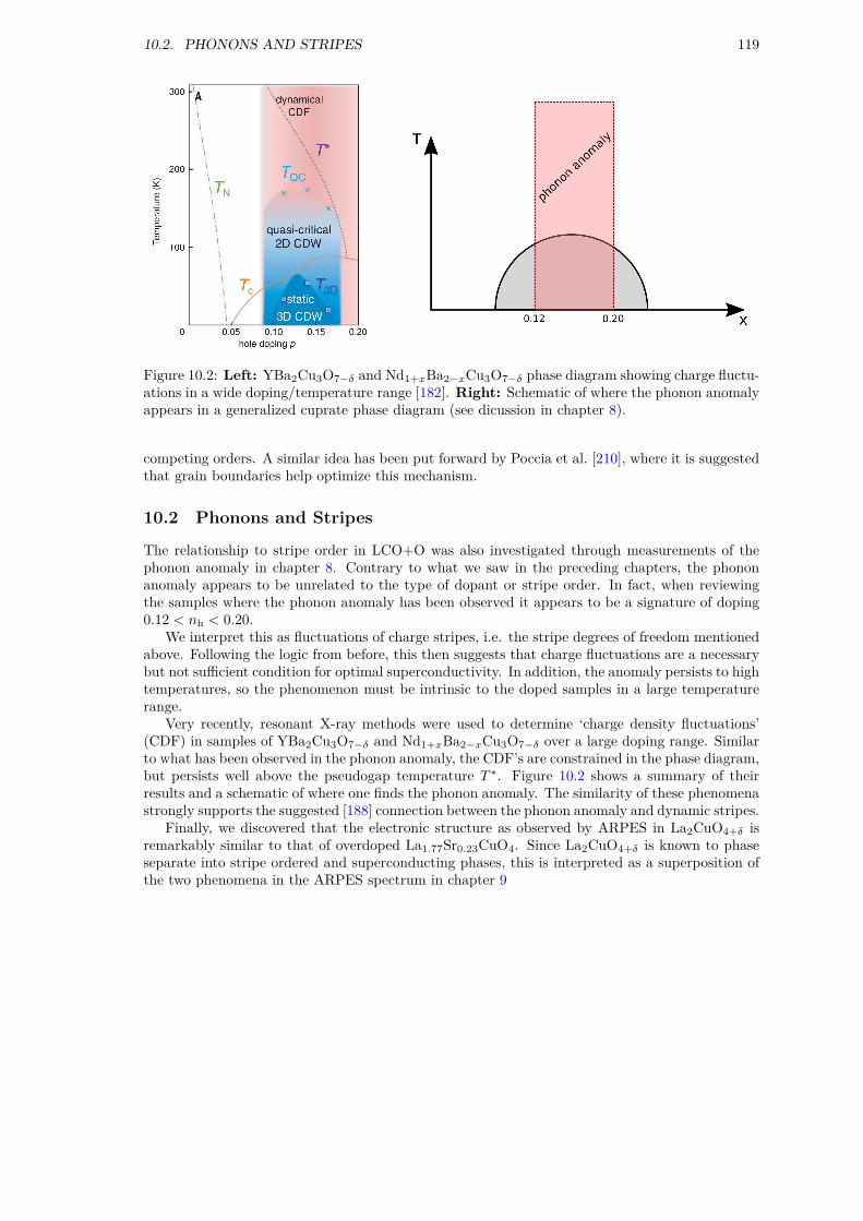
10.2. PHONONS AND STRIPES 119
Figure 10.2: Left: YBa2Cu3O7−δ and Nd1+xBa2−xCu3O7−δ phase diagram showing charge fluctu-ations in a wide doping/temperature range [182]. Right: Schematic of where the phonon anomalyappears in a generalized cuprate phase diagram (see dicussion in chapter 8).
competing orders. A similar idea has been put forward by Poccia et al. [210], where it is suggestedthat grain boundaries help optimize this mechanism.
10.2 Phonons and Stripes
The relationship to stripe order in LCO+O was also investigated through measurements of thephonon anomaly in chapter 8. Contrary to what we saw in the preceding chapters, the phononanomaly appears to be unrelated to the type of dopant or stripe order. In fact, when reviewingthe samples where the phonon anomaly has been observed it appears to be a signature of doping0.12 < nh < 0.20.
We interpret this as fluctuations of charge stripes, i.e. the stripe degrees of freedom mentionedabove. Following the logic from before, this then suggests that charge fluctuations are a necessarybut not sufficient condition for optimal superconductivity. In addition, the anomaly persists to hightemperatures, so the phenomenon must be intrinsic to the doped samples in a large temperaturerange.
Very recently, resonant X-ray methods were used to determine ‘charge density fluctuations’(CDF) in samples of YBa2Cu3O7−δ and Nd1+xBa2−xCu3O7−δ over a large doping range. Similarto what has been observed in the phonon anomaly, the CDF’s are constrained in the phase diagram,but persists well above the pseudogap temperature T ∗. Figure 10.2 shows a summary of theirresults and a schematic of where one finds the phonon anomaly. The similarity of these phenomenastrongly supports the suggested [188] connection between the phonon anomaly and dynamic stripes.
Finally, we discovered that the electronic structure as observed by ARPES in La2CuO4+δ isremarkably similar to that of overdoped La1.77Sr0.23CuO4. Since La2CuO4+δ is known to phaseseparate into stripe ordered and superconducting phases, this is interpreted as a superposition ofthe two phenomena in the ARPES spectrum in chapter 9


Appendix A
PhononNeutron
During the thesis, a selection of Python classes were developed with the intention of generalizingsome of the tasks required to get the correct neutron weights out of simulations. While softwaresuch as MDANSE [211] does a good job with respect to molecular dynamics, I wanted somethingfocussed on analyzing phonons specifically from different levels of theory (MD and ‘Frozen Phon-ons’). The code be found at https://github.com/tejsner/phonon_neutron and features twomodules
1. md_tools.py
2. phonopy_tools.py
md_tools.pyThis module is used to perform various task on molecular dynamics trajectories as obtained fromVASP. VASP trajectories are saved in XDATCAR files, which can be analysed, for example, in thefollowing way:
1 from md_tools import VaspMD2 md_data = VaspMD('XDATCAR', dt=1)3 md_data.compute_velocity()4 md_data.compute_temperature()5 md_data.compute_pdf()6 md_data.compute_dos(sigma=0.5)
Line 1 simply imports the module, line 2 reads the VASP trajectory and lines 3-6 computesvelocity, temperature, the pair distribution function and the phonon density of states with aGaussian smearing width of σ = 0.5meV. Everything is now saved in the md_data object, andcan be plotted, for example, using matplotlib in the following way:
1 import matplotlib.pytplot as plt2 # temperature3 plt.figure()4 plt.plot(md_data.vtime , md_data.temperature)5 # PDF6 plt.figure()7 plt.plot(md_data.pdf_x , md_data.pdf)8 # DOS9 plt.figure()
10 plt.plot(md_data.omega , md_data.dos)
Many additional features are present in this module and can be found by inspecting the code. Acurrent limitation is that it only contains neutron cross sections for the atomic species used in thisthesis (La, Sr, Cu, O), but it is a fairly simple procedure to add scattering lengths at the top ofmd_tools.py.
121

122 APPENDIX A. PHONONNEUTRON
phonopy_tools.pyThis module contains a number of helper functions used to manipulate output from a Phonopy[126, 131] calculation. In particular, I wanted easy access to neutron-weighted band structureplotted in different ways as shown throughout this thesis (in particular chapter 6). In order forthe code to load Phonopy data, we require two files
1. phonopy_disp.yaml: Contains information about the input structure and phonon calcula-tion.
2. FORCE_SETS: Contains the force constants obtained from DFT calculations.
With those files, neutron weighted band structure plots can be generated in the following way
1 from phonopy_tools import PhonopyNeutron2 import matplotlib.pyplot as plt3 f, ax = plt.subplots()4 ph_data = PhonopyNeutron('phonopy_disp.yaml', 'FORCE_SETS')5 ph_data.set_path([[0,0,0],[0.5,0.5,0],[1,0,0],[0,0,0]])6 ph_data.set_labels(['$\Gamma$', 'X', 'M', '$\Gamma$'])7 ph_data.compute_bands()8 ph_data.compute_neutron_bands()9 ph_data.plot_neutron_bands(ax, plotype='lines', sigma=0.2)
Line 1 imports the module, and line 4 imports the Phonopy data. In order to get the bandstructure, it is necessary to set the path in reciprocal space that you want to plot as shown inline 5. The coordinates are here with respect to the input cell, so not necessarily the primitivecell. Line 5 simply labels these paths, line 6 and 7 computes the bands and line 8 plots them. Adifferent option is to plot in 2 dimensions of Q at a selected energy as we also saw in chapter 6.An example of how to get this plot is:
1 from phonopy_tools import PhonopyNeutron , get_xy_colormap2 import matplotlib.pyplot as plt3 ph_data = PhonopyNeutron('phonopy_disp.yaml', 'FORCE_SETS')4 cmap_data = lco.get_sqw_xy([1,5,-1,3], 100, 100)5 x, y, I = get_xy_colormap(cmap_data , 9, sigma=1)6 plt.pcolor(x, y, I)
We load the modules in line 1, and the Phonopy data in line 3. In line 4, we generate the S(Q, ω)in a grid where Qx ranges from 1 to 5 and Qy ranges from -1 to 3 with a grid size of 100 in eachdirection. The evaluation of this can be quite slow, so start with a small grid size. Finally, theget_xy_colormap() function uses this data to generate a colormap at a certain energy with somefixed resolution σ (in meV).

Appendix B
Low energy phonons, additional plots
This appendix contains the plot and fits used to compare low energy phonons with simulation datain chapter 6. Figures B.1, B.2, B.3 and B.4 is data obtained from interpolation of FlatCone datain various directions. Figures B.5, B.6, B.7, B.8 and B.9 show the comparison of this data withsimulations in various structural and electonic phases.
123

124 APPENDIX B. LOW ENERGY PHONONS, ADDITIONAL PLOTS
0
500
1000
1500
2000
Inte
nsity
[cts
/mon
] 3 meV
0
250
500
750
1000 4 meV
0
200
400
600
Inte
nsity
[cts
/mon
] 5 meV
0
200
4006 meV
100
200
3007 meV
100
200
Inte
nsity
[cts
/mon
] 8 meV
50
100
150
200 9 meV
50
100
150 10 meV
50
75
100
125
Inte
nsity
[cts
/mon
] 11 meV
40
60
80 12 meV
40
50
60 13 meV
1.0 0.5 0.0 0.5 1.0h [r.l.u.]
40
50
60
Inte
nsity
[cts
/mon
] 14 meV
1.0 0.5 0.0 0.5 1.0h [r.l.u.]
40
50
6015 meV
1.0 0.5 0.0 0.5 1.0h [r.l.u.]
40
50
60
70 16 meV
Figure B.1: Interpolated data from FlatCone measurements of La1.94Sr0.06CuO4+δ taken aroundthe (400) peak in the transverse direction. Fits are two Gaussians.

125
0
500
1000
1500
Inte
nsity
[cts
/mon
] 3 meV
0
200
400
600
800 4 meV
0
200
400
Inte
nsity
[cts
/mon
] 5 meV
0
100
200
300
400 6 meV
50
100
150
2007 meV
50
100
150
Inte
nsity
[cts
/mon
] 8 meV
25
50
75
1009 meV
20
40
6010 meV
20
30
40
Inte
nsity
[cts
/mon
] 11 meV
15
20
25
12 meV
14
16
18
20
22 13 meV
1.0 1.5 2.0 2.5 3.0k [r.l.u.]
15
20
25
Inte
nsity
[cts
/mon
] 14 meV
1.0 1.5 2.0 2.5 3.0k [r.l.u.]
15
20
2515 meV
1.0 1.5 2.0 2.5 3.0k [r.l.u.]
15
20
25
30 16 meV
Figure B.2: Interpolated data from FlatCone measurements of La1.94Sr0.06CuO4+δ taken aroundthe (200) peak in the transverse direction. Fits are two Gaussians.

126 APPENDIX B. LOW ENERGY PHONONS, ADDITIONAL PLOTS
0
1000
2000
3000
4000
Inte
nsity
[cts
/mon
] 2 meV
0
500
1000
15003 meV
0
200
400
600
800 4 meV4 meV
0
200
400
Inte
nsity
[cts
/mon
] 5 meV5 meV
0
100
200
300 6 meV6 meV
50
100
150
200 7 meV7 meV
50
100
150
Inte
nsity
[cts
/mon
] 8 meV8 meV8 meV8 meV
50
100
9 meV9 meV9 meV9 meV
20
40
60
80
100 10 meV10 meV10 meV10 meV
20
40
60
80
Inte
nsity
[cts
/mon
] 11 meV11 meV11 meV
20
40
60
80 12 meV12 meV12 meV12 meV
20
40
6013 meV13 meV13 meV13 meV
3 4 5h [r.l.u.]
20
40
60
Inte
nsity
[cts
/mon
] 14 meV14 meV14 meV14 meV14 meV
3 4 5h [r.l.u.]
30
40
50
60
7015 meV15 meV15 meV15 meV
3 4 5h [r.l.u.]
20
40
60 16 meV16 meV16 meV16 meV16 meV
Figure B.3: Interpolated data from FlatCone measurements of La1.94Sr0.06CuO4+δ taken aroundthe (400) peak in the longitudinal direction.

127
0
250
500
750
1000
Inte
nsity
[cts
/mon
] 3 meV3 meV3 meV
0
200
4004 meV4 meV4 meV4 meV4 meV
0
100
200
300
Inte
nsity
[cts
/mon
] 5 meV5 meV5 meV5 meV5 meV
0
50
100
150
2006 meV6 meV6 meV6 meV6 meV
50
1007 meV7 meV7 meV
20
40
60
80
100
Inte
nsity
[cts
/mon
] 8 meV8 meV8 meV8 meV
20
40
60
80 9 meV9 meV9 meV
20
40
60 10 meV10 meV10 meV10 meV
20
40
60
Inte
nsity
[cts
/mon
] 11 meV11 meV11 meV11 meV
20
30
40
50 12 meV12 meV12 meV12 meV
20
30
4013 meV13 meV13 meV13 meV
1.5 2.0 2.5 3.0h [r.l.u.]
20
30
40
50
Inte
nsity
[cts
/mon
] 14 meV14 meV14 meV14 meV
1.5 2.0 2.5 3.0h [r.l.u.]
20
30
40
50 15 meV15 meV15 meV15 meV
1.5 2.0 2.5 3.0h [r.l.u.]
20
30
40
5016 meV16 meV16 meV16 meV16 meV
Figure B.4: Interpolated data from FlatCone measurements of La1.94Sr0.06CuO4+δ taken aroundthe (220) peak in the longitudinal direction.

128 APPENDIX B. LOW ENERGY PHONONS, ADDITIONAL PLOTS
Figure B.5: Red datapoints are measured by neutron spectroscopy using a Flatcone analyser andlines are neutron weighted simulation data. HTT AFM simulation data.
Figure B.6: Flatcone dispersion and neutron weighted simulation data. LTT AFM simulationdata.

129
Figure B.7: Flatcone dispersion and neutron weighted simulation data. LTT AFM simulationdata.
Figure B.8: Flatcone dispersion and neutron weighted simulation data. LTO metal simulationdata.

130 APPENDIX B. LOW ENERGY PHONONS, ADDITIONAL PLOTS
Figure B.9: Flatcone dispersion and neutron weighted simulation data. LTT Metal simulationdata.

Appendix C
Phonon DOS, additional plots
This appendix contains additional temperatures of the density of states measurements performedin chapter 7. Figure C.1 contains data for 60K and C.2 contains data for 300K
0.0015
0.0025
0.0035
DOS
LCO LSCO3
0 20 40 60 80Energy [meV]
0.0015
0.0025
0.0035
DOS
LCO+O
0 20 40 60 80Energy [meV]
LSCO3+O
Figure C.1: Phonon density of states of all four samples at at 60K
131

132 APPENDIX C. PHONON DOS, ADDITIONAL PLOTS
0.0015
0.0025
0.0035
DOS
LCO LSCO3
0 20 40 60 80Energy [meV]
0.0015
0.0025
0.0035
DOS
LCO+O
0 20 40 60 80Energy [meV]
LSCO3+O
Figure C.2: Phonon density of states of all four samples at at 300K

Bibliography
[1] J. File and R. G. Mills, Phys. Rev. Lett. 10, 93–96 (1963).[2] D. van Delft and P. Kes, Physics Today 63, 38–43 (2010).[3] File:efektmeisnera.svg, https://commons.wikimedia.org/wiki/File:EfektMeisnera.
svg (visited on 06/12/2019).[4] W. Meissner and R. Ochsenfeld, Naturwissenschaften 21, 787–788 (1933).[5] F. London and H. London, Proceedings of the Royal Society of London. Series A, Mathem-
atical and Physical Sciences 149, 71–88 (1935).[6] C. Kittel, Introduction to solid state physics, 8th ed. (Wiley, 2005).[7] V. L. Ginzburg and L. D. Landau, ‘On the Theory of Superconductivity’, in On Supercon-
ductivity and Superfluidity: A Scientific Autobiography, edited by V. L. Ginzburg (Springer,Berlin, Heidelberg, 2009), pp. 113–137.
[8] A. A. Abrikosov, Journal of Physics and Chemistry of Solids 2, 199–208 (1957).[9] K. Tomimoto, I. Terasaki, A. I. Rykov, T. Mimura and S. Tajima, Phys. Rev. B 60, 114–117
(1999).[10] F. S. Wells, A. V. Pan, X. R. Wang, S. A. Fedoseev and H. Hilgenkamp, Scientific Reports
5, 8677 (2015).[11] R. Doll and M. Näbauer, Phys. Rev. Lett. 7, 51–52 (1961).[12] B. S. Deaver and W. M. Fairbank, Phys. Rev. Lett. 7, 43–46 (1961).[13] J. Bardeen, L. N. Cooper and J. R. Schrieffer, Phys. Rev. 108, 1175–1204 (1957).[14] I. Giaever, Phys. Rev. Lett. 5, 147–148 (1960).[15] I. Giaever, Phys. Rev. Lett. 5, 464–466 (1960).[16] B. D. Josephson, Physics Letters 1, 251–253 (1962).[17] R. C. Jaklevic, J. Lambe, J. E. Mercereau and A. H. Silver, Phys. Rev. 140, A1628–A1637
(1965).[18] E. Maxwell, Phys. Rev. 78, 477 (1950).[19] C. A. Reynolds, B. Serin, W. H. Wright and L. B. Nesbitt, Phys. Rev. 78, 487–487 (1950).[20] J. de Launay, Phys. Rev. 93, 661–665 (1954).[21] A. P. Drozdov, M. I. Eremets, I. A. Troyan, V. Ksenofontov and S. I. Shylin, Nature 525,
73–76 (2015).[22] J. Nagamatsu, N. Nakagawa, T. Muranaka, Y. Zenitani and J. Akimitsu, Nature 410, 63–
64 (2001).[23] J. G. Bednorz and K. A. Müller, en, Z. Physik B - Condensed Matter 64, 189–193 (1986).[24] M. K. Wu, J. R. Ashburn, C. J. Torng, P. H. Hor, R. L. Meng, L. Gao, Z. J. Huang, Y. Q.
Wang and C. W. Chu, Phys. Rev. Lett. 58, 908–910 (1987).[25] R. M. Hazen, C. T. Prewitt, R. J. Angel, N. L. Ross, L. W. Finger, C. G. Hadidiacos,
D. R. Veblen, P. J. Heaney, P. H. Hor, R. L. Meng, Y. Y. Sun, Y. Q. Wang, Y. Y. Xue,Z. J. Huang, L. Gao, J. Bechtold and C. W. Chu, Phys. Rev. Lett. 60, 1174–1177 (1988).
[26] Z. Z. Sheng, A. M. Hermann, A. El Ali, C. Almasan, J. Estrada, T. Datta and R. J. Matson,Phys. Rev. Lett. 60, 937–940 (1988).
[27] R. M. Hazen, L. W. Finger, R. J. Angel, C. T. Prewitt, N. L. Ross, C. G. Hadidiacos, P. J.Heaney, D. R. Veblen, Z. Z. Sheng, A. El Ali and A. M. Hermann, Phys. Rev. Lett. 60,1657–1660 (1988).
133

134 BIBLIOGRAPHY
[28] S. S. P. Parkin, V. Y. Lee, E. M. Engler, A. I. Nazzal, T. C. Huang, G. Gorman, R. Savoyand R. Beyers, Phys. Rev. Lett. 60, 2539–2542 (1988).
[29] T. Kaneko, H. Yamauchi and S. Tanaka, en, Physica C: Superconductivity 178, 377–382(1991).
[30] S. N. Putilin, E. V. Antipov, O. Chmaissem and M. Marezio, en, Nature 362, 226–228(1993).
[31] A. Schilling, M. Cantoni, J. D. Guo and H. R. Ott, en, Nature 363, 56–58 (1993).[32] Suryadijaya, T. Sasagawa and H. Takagi, Physica C: Superconductivity, Proceedings of the
17th International Symposium on Superconductivity (ISS 2004) 426-431, 402–406 (2005).[33] W. Ruan, X. Li, C. Hu, Z. Hao, H. Li, P. Cai, X. Zhou, D.-H. Lee and Y. Wang, Nature
Physics 14, 1178 (2018).[34] S. Chakravarty, H.-Y. Kee and K. Völker, en, Nature 428, 53–55 (2004).[35] M. Hücker, Physica C: Superconductivity, Stripes and Electronic Liquid Crystals in Strongly
Correlated Materials 481, 3–14 (2012).[36] D. C. Peets, J. D. F. Mottershead, B. Wu, I. S. Elfimov, R. Liang, W. N. Hardy, D. A.
Bonn, M. Raudsepp, N. J. C. Ingle and A. Damascelli, New J. Phys. 9, 28–28 (2007).[37] B. Keimer, S. A. Kivelson, M. R. Norman, S. Uchida and J. Zaanen, Nature 518, 179–186
(2015).[38] H. Alloul, T. Ohno and P. Mendels, Phys. Rev. Lett. 63, 1700–1703 (1989).[39] C. C. Homes, T. Timusk, R. Liang, D. A. Bonn and W. N. Hardy, Phys. Rev. Lett. 71,
1645–1648 (1993).[40] J. W. Loram, K. A. Mirza, J. R. Cooper and W. Y. Liang, Phys. Rev. Lett. 71, 1740–1743
(1993).[41] V. J. Emery and S. A. Kivelson, Nature 374, 434–437 (1995).[42] P. Curty and H. Beck, Phys. Rev. Lett. 91, 257002 (2003).[43] S. Martin, A. T. Fiory, R. M. Fleming, L. F. Schneemeyer and J. V. Waszczak, Phys. Rev.
B 41, 846–849 (1990).[44] A. Legros, S. Benhabib, W. Tabis, F. Laliberté, M. Dion, M. Lizaire, B. Vignolle, D. Vign-
olles, H. Raffy, Z. Z. Li, P. Auban-Senzier, N. Doiron-Leyraud, P. Fournier, D. Colson, L.Taillefer and C. Proust, Nature Physics, 1 (2018).
[45] A. Damascelli, Z. Hussain and Z.-X. Shen, Rev. Mod. Phys. 75, 473–541 (2003).[46] J. Osterwalder, ‘Electron Based Methods: 3.2.2 Photoelectron Spectroscopy and Diffrac-
tion’, in Surface and Interface Science (John Wiley & Sons, Ltd, 2014), pp. 151–214.[47] C. E. Matt, D. Sutter, A. M. Cook, Y. Sassa, M. Månsson, O. Tjernberg, L. Das, M. Horio,
D. Destraz, C. G. Fatuzzo, K. Hauser, M. Shi, M. Kobayashi, V. N. Strocov, T. Schmitt,P. Dudin, M. Hoesch, S. Pyon, T. Takayama, H. Takagi, O. J. Lipscombe, S. M. Hayden,T. Kurosawa, N. Momono, M. Oda, T. Neupert and J. Chang, Nature Communications 9,972 (2018).
[48] T. Yoshida, M. Hashimoto, I. M. Vishik, Z.-X. Shen and A. Fujimori, J. Phys. Soc. Jpn.81, 011006 (2011).
[49] D. L. Feng, A. Damascelli, K. M. Shen, N. Motoyama, D. H. Lu, H. Eisaki, K. Shimizu, J.-i.Shimoyama, K. Kishio, N. Kaneko, M. Greven, G. D. Gu, X. J. Zhou, C. Kim, F. Ronning,N. P. Armitage and Z.-X Shen, Phys. Rev. Lett. 88, 107001 (2002).
[50] C. C. Tsuei and J. R. Kirtley, Rev. Mod. Phys. 72, 969–1016 (2000).[51] A. P. Mackenzie and Y. Maeno, Rev. Mod. Phys. 75, 657–712 (2003).[52] R. Joynt and L. Taillefer, Rev. Mod. Phys. 74, 235–294 (2002).[53] N. S. Headings, S. M. Hayden, R. Coldea and T. G. Perring, Phys. Rev. Lett. 105, 247001
(2010).[54] K. Yamada, C. H. Lee, K. Kurahashi, J. Wada, S. Wakimoto, S. Ueki, H. Kimura, Y. Endoh,
S. Hosoya, G. Shirane, R. J. Birgeneau, M. Greven, M. A. Kastner and Y. J. Kim, Phys.Rev. B 57, 6165–6172 (1998).

BIBLIOGRAPHY 135
[55] M. Enoki, M. Fujita, T. Nishizaki, S. Iikubo, D. K. Singh, S. Chang, J. M. Tranquada andK. Yamada, Phys. Rev. Lett. 110, 017004 (2013).
[56] Y. Drees, D. Lamago, A. Piovano and A. C. Komarek, en, Nature Communications 4, 2449(2013).
[57] Y. Drees, Z. W. Li, A. Ricci, M. Rotter, W. Schmidt, D. Lamago, O. Sobolev, U. Rütt,O. Gutowski, M. Sprung, A. Piovano, J. P. Castellan and A. C. Komarek, en, NatureCommunications 5, 5731 (2014).
[58] E. Demler, S. Sachdev and Y. Zhang, Phys. Rev. Lett. 87, 067202 (2001).[59] Y. Zhang, E. Demler and S. Sachdev, Phys. Rev. B 66, 094501 (2002).[60] J. Chang, C. Niedermayer, R. Gilardi, N. B. Christensen, H. M. Rønnow, D. F. McMorrow,
M. Ay, J. Stahn, O. Sobolev, A. Hiess, S. Pailhes, C. Baines, N. Momono, M. Oda, M. Idoand J. Mesot, Phys. Rev. B 78, 104525 (2008).
[61] R. J. Birgeneau, C. Stock, J. M. Tranquada and K. Yamada, J. Phys. Soc. Jpn. 75, 111003(2006).
[62] H. Jacobsen, S. L. Holm, M.-E. Lăcătuşu, A. T. Rømer, M. Bertelsen, M. Boehm, R. Toft-Petersen, J.-C. Grivel, S. B. Emery, L. Udby, B. O. Wells and K. Lefmann, Phys. Rev. Lett.120, 037003 (2018).
[63] M. Kofu, S.-H. Lee, M. Fujita, H.-J. Kang, H. Eisaki and K. Yamada, Phys. Rev. Lett. 102,047001 (2009).
[64] D. J. Scalapino, Rev. Mod. Phys. 84, 1383–1417 (2012).[65] P. W. Anderson, en, Science 316, 1705–1707 (2007).[66] N. E. Bickers, D. J. Scalapino and S. R. White, Phys. Rev. Lett. 62, 961–964 (1989).[67] J. D. Axe, A. H. Moudden, D. Hohlwein, D. E. Cox, K. M. Mohanty, A. R. Moodenbaugh
and Y. Xu, Phys. Rev. Lett. 62, 2751–2754 (1989).[68] M. Braden, G. Heger, P. Schweiss, Z. Fisk, K. Gamayunov, I. Tanaka and H. Kojima,
Physica C: Superconductivity 191, 455–468 (1992).[69] T. C. Huang, E. Moran, A. I. Nazzal, J. B. Torrance and P. W. Wang, en, Physica C:
Superconductivity 159, 625–628 (1989).[70] R. D. Shannon, en, Acta Cryst A 32, 751–767 (1976).[71] P. G. Radaelli, D. G. Hinks, A. W. Mitchell, B. A. Hunter, J. L. Wagner, B. Dabrowski,
K. G. Vandervoort, H. K. Viswanathan and J. D. Jorgensen, Phys. Rev. B 49, 4163–4175(1994).
[72] J. M. Tranquada, B. J. Sternlieb, J. D. Axe, Y. Nakamura and S. Uchida, Nature 375,561–563 (1995).
[73] N. B. Christensen, J. Chang, J. Larsen, M. Fujita, M. Oda, M. Ido, N. Momono, E. M.Forgan, A. T. Holmes, J. Mesot, M. Huecker and M. v Zimmermann, arXiv:1404.3192[cond-mat] (2014).
[74] T. P. Croft, C. Lester, M. S. Senn, A. Bombardi and S. M. Hayden, Phys. Rev. B 89,224513 (2014).
[75] V. Thampy, M. P. M. Dean, N. B. Christensen, L. Steinke, Z. Islam, M. Oda, M. Ido, N.Momono, S. B. Wilkins and J. P. Hill, Phys. Rev. B 90, 100510 (2014).
[76] M. H. Julien, Physica B: Condensed Matter, Proceedings of the 23rd International Confer-ence on Low Temperature Physics 329-333, 693–696 (2003).
[77] J. M. Tranquada, H. Woo, T. G. Perring, H. Goka, G. D. Gu, G. Xu, M. Fujita and K.Yamada, en, Nature 429, 534–538 (2004).
[78] P. Blakeslee, R. J. Birgeneau, F. C. Chou, R. Christianson, M. A. Kastner, Y. S. Lee andB. O. Wells, Phys. Rev. B 57, 13915–13921 (1998).
[79] M. Ahmad, ‘Property investigation of the high Tc superconductors La2CuO4+y and La2−xSrxCuO4+y’,MA thesis (University of Copenhagen, 2019).
[80] M. Karppinen, L. Niinistö and H. Yamauchi, en, Journal of Thermal Analysis 48, 1123–1141 (1997).
[81] L. H. Liu, G. C. Che, J. Zhao and Z. X. Zhao, Physica C: Superconductivity 425, 37–43(2005).

136 BIBLIOGRAPHY
[82] B. Lorenz, Z. G. Li, T. Honma and P.-H. Hor, Phys. Rev. B 65, 144522 (2002).[83] M. Fratini, N. Poccia, A. Ricci, G. Campi, M. Burghammer, G. Aeppli and A. Bianconi,
en, Nature 466, 841–844 (2010).[84] B. O. Wells, Y. S. Lee, M. A. Kastner, R. J. Christianson, R. J. Birgeneau, K. Yamada,
Y. Endoh and G. Shirane, en, Science 277, 1067–1071 (1997).[85] N. Poccia, A. Ricci, G. Campi, M. Fratini, A. Puri, D. D. Gioacchino, A. Marcelli, M.
Reynolds, M. Burghammer, N. L. Saini, G. Aeppli and A. Bianconi, PNAS 109, 15685–15690 (2012).
[86] B. O. Wells, R. J. Birgeneau, F. C. Chou, Y. Endoh, D. C. Johnston, M. A. Kastner, Y. S.Lee, G. Shirane, J. M. Tranquada and K. Yamada, en, Zeitschrift für Physik B CondensedMatter 100, 535–545 (1996).
[87] J. M. Tranquada, Y. Kong, J. E. Lorenzo, D. J. Buttrey, D. E. Rice and V. Sachan, Phys.Rev. B 50, 6340–6351 (1994).
[88] P. J. Ray, N. H. Andersen, T. B. S. Jensen, H. E. Mohottala, C. Niedermayer, K. Lefmann,B. O. Wells, M. v. Zimmermann and L. Udby, Phys. Rev. B 96, 174106 (2017).
[89] Y. S. Lee, F. C. Chou, A. Tewary, M. A. Kastner, S. H. Lee and R. J. Birgeneau, Phys.Rev. B 69, 020502 (2004).
[90] A. Bianconi, International Journal of Modern Physics B 14, 3289–3297 (2000).[91] H. E. Mohottala, B. O. Wells, J. I. Budnick, W. A. Hines, C. Niedermayer, L. Udby, C.
Bernhard, A. R. Moodenbaugh and F.-C. Chou, Nature Materials 5, 377–382 (2006).[92] L. Udby, J. Larsen, N. B. Christensen, M. Boehm, C. Niedermayer, H. E. Mohottala, T. B. S.
Jensen, R. Toft-Petersen, F. C. Chou, N. H. Andersen, K. Lefmann and B. O. Wells, Phys.Rev. Lett. 111, 227001 (2013).
[93] Y. Y. Peng, G. Dellea, M. Minola, M. Conni, A. Amorese, D. Di Castro, G. M. De Luca,K. Kummer, M. Salluzzo, X. Sun, X. J. Zhou, G. Balestrino, M. Le Tacon, B. Keimer, L.Braicovich, N. B. Brookes and G. Ghiringhelli, Nature Physics 13, 1201–1206 (2017).
[94] O. Ivashko, M. Horio, W. Wan, N. B. Christensen, D. E. McNally, E. Paris, Y. Tseng, N. E.Shaik, H. M. Rønnow, H. I. Wei, C. Adamo, C. Lichtensteiger, M. Gibert, M. R. Beasley,K. M. Shen, J. M. Tomczak, T. Schmitt and J. Chang, Nature Communications 10, 786(2019).
[95] E. S. Božin, G. H. Kwei, H. Takagi and S. J. L. Billinge, Phys. Rev. Lett. 84, 5856–5859(2000).
[96] S. W. Lovesey, Theory of Neutron Scattering from Condensed Matter, en (Clarendon Press,1984).
[97] G. L. Squires, Introduction to the Theory of Thermal Neutron Scattering, en (CambridgeUniversity Press, Mar. 2012).
[98] H. Schober, Journal of Neutron Research 17, 109–357 (2014).[99] G. Shirane, S. M. Shapiro and J. M. Tranquada, Neutron Scattering with a Triple-Axis
Spectrometer: Basic Techniques (Cambridge University Press, Feb. 2002).[100] L. Van Hove, Phys. Rev. 95, 249–262 (1954).[101] Neutron scattering lengths and cross sections, https://www.ncnr.nist.gov/resources/
n-lengths/ (visited on 21/11/2019).[102] J. Jensen and A. R. Mackintosh, Rare earth magnetism: structures and excitations, en
(Clarendon Press, Aug. 1991).[103] B. Fåk and B. Dorner, Physica B: Condensed Matter, Proceedings of the First European
Conference on Neutron Scattering 234-236, 1107–1108 (1997).[104] T. Weber, R. Georgii and P. Böni, SoftwareX 5, 121–126 (2016).[105] J. Šaroun and J. Kulda, Physica B: Condensed Matter, Proceedings of the First European
Conference on Neutron Scattering 234-236, 1102–1104 (1997).[106] Thermal neutron three-axis spectrometer in8, https://www.ill.eu/users/instruments/
instruments-list/in8/description/instrument-layout/ (visited on 22/11/2019).[107] Thermal neutron time-of-flight spectrometer in4c, https://www.ill.eu/users/instruments/
instruments-list/in4c/description/instrument-layout/ (visited on 22/11/2019).

BIBLIOGRAPHY 137
[108] J. M. Carpenter and D. L. Price, Phys. Rev. Lett. 54, 441–443 (1985).[109] Disordered materials diffractometer, https://www.ill.eu/users/instruments/instruments-
list/d4/description/instrument-layout/ (visited on 22/11/2019).[110] D. A. Keen, en, J Appl Cryst 34, 172–177 (2001).[111] F. Giustino, Materials Modelling using Density Functional Theory: Properties and Predic-
tions, en (OUP Oxford, May 2014).[112] R. M. Martin, Electronic Structure: Basic Theory and Practical Methods, en (Cambridge
University Press, Apr. 2004).[113] R. M. Martin, L. Reining and D. M. Ceperley, Interacting Electrons, en (Cambridge Uni-
versity Press, June 2016).[114] R. Hoffmann, en, Angewandte Chemie International Edition in English 26, 846–878 (1987).[115] S. Lloyd, Phys. Rev. Lett. 88, 237901 (2002).[116] P. Hohenberg and W. Kohn, Phys. Rev. 136, B864–B871 (1964).[117] N. Mardirossian and M. Head-Gordon, Molecular Physics 115, 2315–2372 (2017).[118] W. Kohn and L. J. Sham, Phys. Rev. 140, A1133–A1138 (1965).[119] D. M. Ceperley and B. J. Alder, Phys. Rev. Lett. 45, 566–569 (1980).[120] J. P. Perdew and A. Zunger, Phys. Rev. B 23, 5048–5079 (1981).[121] J. P. Perdew and K. Schmidt, AIP Conference Proceedings 577, 1–20 (2001).[122] J. Tao, J. P. Perdew, V. N. Staroverov and G. E. Scuseria, Phys. Rev. Lett. 91, 146401
(2003).[123] V. I. Anisimov, F. Aryasetiawan and A. I. Lichtenstein, J. Phys.: Condens. Matter 9, 767
(1997).[124] R. P. Feynman, Phys. Rev. 56, 340–343 (1939).[125] K. Parlinski, Z. Q. Li and Y. Kawazoe, Phys. Rev. Lett. 78, 4063–4066 (1997).[126] A. Togo and I. Tanaka, Scripta Materialia 108, 1–5 (2015).[127] L. Verlet, Phys. Rev. 159, 98–103 (1967).[128] S. Nosé, J. Chem. Phys. 81, 511–519 (1984).[129] M. T. Dove, Introduction to Lattice Dynamics, en (Cambridge University Press, Oct. 1993).[130] The radial distribution functions: definitions, http://isaacs.sourceforge.net/phys/
rdfs.html (visited on 07/12/2019).[131] Phonopy website, https://atztogo.github.io/phonopy/ (visited on 25/11/2019).[132] H. E. Fischer, A. C. Barnes and P. S. Salmon, en, Rep. Prog. Phys. 69, 233–299 (2005).[133] G. Kresse and J. Hafner, Phys. Rev. B 47, 558–561 (1993).[134] G. Kresse and J. Hafner, Phys. Rev. B 49, 14251–14269 (1994).[135] G. Kresse and J. Furthmüller, Phys. Rev. B 54, 11169–11186 (1996).[136] G. Kresse and J. Furthmüller, Computational Materials Science 6, 15–50 (1996).[137] P. E. Blöchl, Phys. Rev. B 50, 17953–17979 (1994).[138] G. Kresse and D. Joubert, Phys. Rev. B 59, 1758–1775 (1999).[139] The VASP Manual - Vaspwiki, https://cms.mpi.univie.ac.at/wiki/index.php/The_
VASP_Manual (visited on 14/11/2019).[140] E. L. da Silva, J. M. Skelton, S. C. Parker and A. Walsh, Phys. Rev. B 91, 144107 (2015).[141] J. P. Perdew, K. Burke and M. Ernzerhof, Phys. Rev. Lett. 77, 3865–3868 (1996).[142] L. K. Wagner and D. M. Ceperley, Rep. Prog. Phys. 79, 094501 (2016).[143] W. E. Pickett, Rev. Mod. Phys. 61, 433–512 (1989).[144] C. Lane, J. W. Furness, I. G. Buda, Y. Zhang, R. S. Markiewicz, B. Barbiellini, J. Sun and
A. Bansil, Phys. Rev. B 98, 125140 (2018).[145] F. Giustino, M. L. Cohen and S. G. Louie, Nature 452, 975–978 (2008).[146] S. L. Dudarev, G. A. Botton, S. Y. Savrasov, C. J. Humphreys and A. P. Sutton, Phys.
Rev. B 57, 1505–1509 (1998).

138 BIBLIOGRAPHY
[147] V. I. Anisimov, M. A. Korotin, A. S. Mylnikova, A. V. Kozhevnikov, D. M. Korotin andJ. Lorenzana, Phys. Rev. B 70, 172501 (2004).
[148] S. Pesant and M. Côté, Phys. Rev. B 84, 085104 (2011).[149] Energy vs volume Volume relaxations and Pulay stress - Vaspwiki, https://cms.mpi.
univie.ac.at/wiki/index.php/Energy_vs_volume_Volume_relaxations_and_Pulay_stress (visited on 14/11/2019).
[150] A. H. Larsen, J. J. Jørgen Mortensen, J. Blomqvist, I. E. Castelli, R. Christensen, M. Dułak,J. Friis, M. N. Groves, B. Hammer, C. Hargus, E. D. Hermes, P. C. Jennings, P. BjerreJensen, J. Kermode, J. R. Kitchin, E. L. Kolsbjerg, J. Kubal, K. Kaasbjerg, S. Lysgaard,J. Bergmann Maronsson, T. Maxson, T. Olsen, L. Pastewka, A. Peterson, C. Rostgaard,J. Schiøtz, O. Schütt, M. Strange, K. S. Thygesen, T. Vegge, L. Vilhelmsen, M. Walter,Z. Zeng and K. W. Jacobsen, J Phys Condens Matter 29, 273002 (2017).
[151] K. Momma and F. Izumi, J Appl Cryst 41, 653–658 (2008).[152] Y. Hinuma, G. Pizzi, Y. Kumagai, F. Oba and I. Tanaka, Computational Materials Science
128, 140–184 (2017).[153] D. Vaknin, S. K. Sinha, D. E. Moncton, D. C. Johnston, J. M. Newsam, C. R. Safinya and
H. E. King, Phys. Rev. Lett. 58, 2802–2805 (1987).[154] S. Uchida, T. Ido, H. Takagi, T. Arima, Y. Tokura and S. Tajima, Phys. Rev. B 43, 7942–
7954 (1991).[155] V. I. Anisimov and O. Gunnarsson, Phys. Rev. B 43, 7570–7574 (1991).[156] M. Horio, C. E. Matt, K. Kramer, D. Sutter, A. M. Cook, Y. Sassa, K. Hauser, M. Månsson,
N. C. Plumb, M. Shi, O. J. Lipscombe, S. M. Hayden, T. Neupert and J. Chang, NatureCommunications 9, 3252 (2018).
[157] P. Vinet, J. R. Smith, J. Ferrante and J. H. Rose, Phys. Rev. B 35, 1945–1953 (1987).[158] F. D. Murnaghan, PNAS 30, 244–247 (1944).[159] F. Birch, Phys. Rev. 71, 809–824 (1947).[160] J. P Poirier and A Tarantola, Physics of the Earth and Planetary Interiors 109, 1–8 (1998).[161] H. Takahashi, H. Shaked, B. A. Hunter, P. G. Radaelli, R. L. Hitterman, D. G. Hinks and
J. D. Jorgensen, Phys. Rev. B 50, 3221–3229 (1994).[162] G. I. Csonka, J. P. Perdew, A. Ruzsinszky, P. H. T. Philipsen, S. Lebègue, J. Paier, O. A.
Vydrov and J. G. Ángyán, Phys. Rev. B 79, 155107 (2009).[163] R. J. McQueeney, Y. Petrov, T. Egami, M. Yethiraj, G. Shirane and Y. Endoh, Phys. Rev.
Lett. 82, 628–631 (1999).[164] S. R. Park, T. Fukuda, A. Hamann, D. Lamago, L. Pintschovius, M. Fujita, K. Yamada
and D. Reznik, Phys. Rev. B 89, 020506 (2014).[165] A. Piovano, A. Perrichon, M. Boehm, M. R. Johnson and W. Paulus, en, Phys. Chem.
Chem. Phys. 18, 17398–17403 (2016).[166] A. Perrichon, A. Piovano, M. Boehm, M. Zbiri, M. Johnson, H. Schober, M. Ceretti and
W. Paulus, J. Phys. Chem. C 119, 1557–1564 (2015).[167] C. Rial, E. Morán, M. A. Alario-Franco, U. Amador and N. H. Andersen, Physica C:
Superconductivity 278, 122–134 (1997).[168] J. Hickman and Y. Mishin, Phys. Rev. B 94, 184311 (2016).[169] N. Poccia, M. Fratini, A. Ricci, G. Campi, L. Barba, A. Vittorini-Orgeas, G. Bianconi, G.
Aeppli and A. Bianconi, en, Nature Mater 10, 733–736 (2011).[170] F. V. Kusmartsev, D. Di Castro, G. Bianconi and A. Bianconi, en, Physics Letters A 275,
118–123 (2000).[171] Flatcone, https://www.ill.eu/users/instruments/instruments- list/flatcone/
(visited on 27/11/2019).[172] P. J. Ray, ‘Master’s thesis: Structural investigation of La(2-x)Sr(x)CuO(4+y) - Following
staging as a function of temperature’, MA thesis (University of Copenhagen, 2016).[173] Nplot, https://github.com/nplot/nplot (visited on 28/11/2019).

BIBLIOGRAPHY 139
[174] S. Wakimoto, S. Lee, P. M. Gehring, R. J. Birgeneau and G. Shirane, J. Phys. Soc. Jpn.73, 3413–3417 (2004).
[175] C.-H. Lee, K. Yamada, M. Arai, S. Wakimoto, S. Hosoya and Y. Endoh, Physica C: Super-conductivity and its Applications 257, 264–270 (1996).
[176] O. Arnold, J. C. Bilheux, J. M. Borreguero, A. Buts, S. I. Campbell, L. Chapon, M. Doucet,N. Draper, R. Ferraz Leal, M. A. Gigg, V. E. Lynch, A. Markvardsen, D. J. Mikkelson, R. L.Mikkelson, R. Miller, K. Palmen, P. Parker, G. Passos, T. G. Perring, P. F. Peterson, S.Ren, M. A. Reuter, A. T. Savici, J. W. Taylor, R. J. Taylor, R. Tolchenov, W. Zhou and J.Zikovsky, Nuclear Instruments and Methods in Physics Research Section A: Accelerators,Spectrometers, Detectors and Associated Equipment 764, 156–166 (2014).
[177] Computeincoherentdos v1, https://docs.mantidproject.org/v3.11.0/algorithms/ComputeIncoherentDOS-v1.html (visited on 30/11/2019).
[178] P. S. Häfliger, S. Gerber, R. Pramod, V. I. Schnells, B. dalla Piazza, R. Chati, V. Pom-jakushin, K. Conder, E. Pomjakushina, L. Le Dreau, N. B. Christensen, O. F. Syljuåsen,B. Normand and H. M. Rønnow, Phys. Rev. B 89, 085113 (2014).
[179] J. M. Tranquada, J. D. Axe, N. Ichikawa, Y. Nakamura, S. Uchida and B. Nachumi, Phys.Rev. B 54, 7489–7499 (1996).
[180] S. Anissimova, D. Parshall, G. D. Gu, K. Marty, M. D. Lumsden, S. Chi, J. A. Fernandez-Baca, D. L. Abernathy, D. Lamago, J. M. Tranquada and D. Reznik, en, Nature Commu-nications 5, 3467 (2014).
[181] S. A. Kivelson, I. P. Bindloss, E. Fradkin, V. Oganesyan, J. M. Tranquada, A. Kapitulnikand C. Howald, Rev. Mod. Phys. 75, 1201–1241 (2003).
[182] R. Arpaia, S. Caprara, R. Fumagalli, G. D. Vecchi, Y. Y. Peng, E. Andersson, D. Betto,G. M. D. Luca, N. B. Brookes, F. Lombardi, M. Salluzzo, L. Braicovich, C. D. Castro, M.Grilli and G. Ghiringhelli, en, Science 365, 906–910 (2019).
[183] M. Mitrano, S. Lee, A. A. Husain, L. Delacretaz, M. Zhu, G. d. l. P. Munoz, S. X.-L. Sun,Y. I. Joe, A. H. Reid, S. F. Wandel, G. Coslovich, W. Schlotter, T. van Driel, J. Schneeloch,G. D. Gu, S. Hartnoll, N. Goldenfeld and P. Abbamonte, en, Science Advances 5, eaax3346(2019).
[184] D. Reznik, L. Pintschovius, M. Fujita, K. Yamada, G. D. Gu and J. M. Tranquada, en, JLow Temp Phys 147, 353–364 (2007).
[185] L. Chaix, G. Ghiringhelli, Y. Y. Peng, M. Hashimoto, B. Moritz, K. Kummer, N. B. Brookes,Y. He, S. Chen, S. Ishida, Y. Yoshida, H. Eisaki, M. Salluzzo, L. Braicovich, Z.-X. Shen,T. P. Devereaux and W.-S. Lee, en, Nature Physics 13, 952–956 (2017).
[186] D. Reznik, L. Pintschovius, M. Ito, S. Iikubo, M. Sato, H. Goka, M. Fujita, K. Yamada,G. D. Gu and J. M. Tranquada, Nature 440, 1170–1173 (2006).
[187] M. Le Tacon, A. Bosak, S. M. Souliou, G. Dellea, T. Loew, R. Heid, K.-P. Bohnen, G.Ghiringhelli, M. Krisch and B. Keimer, en, Nature Physics 10, 52–58 (2014).
[188] D. Reznik, Physica C: Superconductivity, Stripes and Electronic Liquid Crystals in StronglyCorrelated Materials 481, 75–92 (2012).
[189] E. Kaneshita, M. Ichioka and K. Machida, Phys. Rev. Lett. 88, 115501 (2002).[190] A. T. Rømer, J. Chang, N. B. Christensen, B. M. Andersen, K. Lefmann, L. Mähler, J.
Gavilano, R. Gilardi, C. Niedermayer, H. M. Rønnow, A. Schneidewind, P. Link, M. Oda,M. Ido, N. Momono and J. Mesot, Phys. Rev. B 87, 144513 (2013).
[191] J. M. Tranquada, C. H. Lee, K. Yamada, Y. S. Lee, L. P. Regnault and H. M. Rønnow,Phys. Rev. B 69, 174507 (2004).
[192] B. Lake, G. Aeppli, K. N. Clausen, D. F. McMorrow, K. Lefmann, N. E. Hussey, N.Mangkorntong, M. Nohara, H. Takagi, T. E. Mason and A. Schröder, en, Science 291,1759–1762 (2001).
[193] J. M. Tranquada, AIP Conference Proceedings 1550, 114–187 (2013).[194] G. Aeppli, T. E. Mason, S. M. Hayden, H. A. Mook and J. Kulda, en, Science 278, 1432–
1435 (1997).[195] D. Reznik, T. Fukuda, D. Lamago, A. Q. R. Baron, S. Tsutsui, M. Fujita and K. Yamada,
Journal of Physics and Chemistry of Solids, SNS2007 69, 3103–3107 (2008).

140 BIBLIOGRAPHY
[196] S. R. Park, Y. Cao, Q. Wang, M. Fujita, K. Yamada, S.-K. Mo, D. S. Dessau and D. Reznik,Phys. Rev. B 88, 220503 (2013).
[197] D. R. Garcia and A Lanzara, Advances in Condensed Matter Physics 2010 (2010).[198] Z. Zhang, R. Sutarto, F. He, F. C. Chou, L. Udby, S. L. Holm, Z. H. Zhu, W. A. Hines,
J. I. Budnick and B. O. Wells, Phys. Rev. Lett. 121, 067602 (2018).[199] S. Holm-Dahlin, J. Larsen, H. Jacobsen, A. T. Rømer, A.-E. Ţuţueanu, M. Ahmad, J.-C.
Grivel, T. Goko, R. Scheuermann, M. v Zimmermann, M. Boehm, P. Steffens, K. Conder,C. Niedermayer, K. S. Pedersen, N. B. Christensen, S. B. Emery, B. O Wells, K. Lefmannand L. Udby, Manuscript in preparation (2019).
[200] D. Reznik, D. Parshall, S. R. Park, J. W. Lynn and T. Wolf, en, J Supercond Nov Magn29, 643–644 (2016).
[201] M. Fujita, H. Goka, K. Yamada, J. M. Tranquada and L. P. Regnault, Phys. Rev. B 70,104517 (2004).
[202] E. Fradkin, S. A. Kivelson and J. M. Tranquada, Rev. Mod. Phys. 87, 457–482 (2015).[203] S. A. Kivelson, E. Fradkin and V. J. Emery, en, Nature 393, 550–553 (1998).[204] A. Ino, C. Kim, M. Nakamura, T. Yoshida, T. Mizokawa, A. Fujimori, Z.-X. Shen, T.
Kakeshita, H. Eisaki and S. Uchida, Phys. Rev. B 65, 094504 (2002).[205] X. J. Zhou, T. Yoshida, S. A. Kellar, P. V. Bogdanov, E. D. Lu, A. Lanzara, M. Nakamura,
T. Noda, T. Kakeshita, H. Eisaki, S. Uchida, A. Fujimori, Z. Hussain and Z.-X. Shen, Phys.Rev. Lett. 86, 5578–5581 (2001).
[206] Q. Li, M. Hücker, G. D. Gu, A. M. Tsvelik and J. M. Tranquada, Phys. Rev. Lett. 99,067001 (2007).
[207] Y.-S. Su, T. A. Kaplan, S. D. Mahanti and J. F. Harrison, Phys. Rev. B 59, 10521–10529(1999).
[208] P. Lazić and D. K. Sunko, en, EPL 112, 37011 (2015).[209] P. Lazić, D. Pelc, M. Požek, V. Despoja and D. K. Sunko, en, J Supercond Nov Magn 28,
1299–1303 (2015).[210] N. Poccia, A. Ricci, G. Campi and A. Bianconi, en, Supercond. Sci. Technol. 30, 035016
(2017).[211] G. Goret, B. Aoun and E. Pellegrini, J. Chem. Inf. Model. 57, 1–5 (2017).
Copyright © 2022 FDOKUMEN