arX

iv:c

ond-

mat

/010

7232

v1 [

cond

-mat

.sup

r-co

n] 1

1 Ju

l 200

1

Proximity effects at ferromagnet-superconductor interfaces

Klaus Halterman† and Oriol T. Valls∗

School of Physics and Astronomy and Minnesota Supercomputer Institute

University of Minnesota

Minneapolis, Minnesota 55455-0149

(February 1, 2008)

We study proximity effects at ferromagnet superconductor interfaces by self-consistent numericalsolution of the Bogoliubov-de Gennes equations for the continuum, without any approximations.Our procedures allow us to study systems with long superconducting coherence lengths. We obtainresults for the pair potential, the pair amplitude, and the local density of states. We use theseresults to extract the relevant proximity lengths. We find that the superconducting correlations inthe ferromagnet exhibit a damped oscillatory behavior that is reflected in both the pair amplitudeand the local density of states. The characteristic length scale of these oscillations is approximatelyinversely proportional to the exchange field, and is independent of the superconducting coherencelength in the range studied. We find the superconducting coherence length to be nearly independentof the ferromagnetic polarization.

74.50.+r, 74.25.Fy, 74.80.Fp

I. INTRODUCTION

In recent years, technological advances in materialsgrowth and fabrication techniques have made it possibleto create heterostructures including high quality ferro-magnet/superconductor (F/S) interfaces. These systemshave great intrinsic scientific importance and potentialdevice applications, including quantum computers andmagnetic information storage1–3. This has led to re-newed interest in proximity effects involving magneticand superconducting compounds. Understanding howproximity effects modify electronic properties near F/Sinterfaces is constantly becoming more important as therapid growth of nanofabrication technology continues.

The juxtaposition of a ferromagnet and a supercon-ductor can result4 in a spatial variation of magneticand superconducting correlations in both materials. Theleakage of superconducting correlations into the non-superconducting material is an example of the supercon-ducting proximity effect. Similarly, the spin polarizationmay extend into the superconductor and modify its prop-erties, creating a magnetic proximity effect.

In general, if one is interested in a microscopic solutionof the F/S proximity effect problem valid at all lengthscales, one must solve the appropriate equations, e.g. theGor’kov5, or Bogoliubov-de Gennes6 (BdG) equations ina self-consistent manner and with as few approximationsas possible. In practice, approximations are often madein the basic equations. Further, in many cases a sim-ple form for the pair potential ∆(r) is assumed, usu-ally a constant in the superconductor region, and zeroelsewhere is used. Such crude non self-consistent treat-ments have been widely applied because of their simplic-ity. However they are valid typically only for length scalesmuch longer than the superconducting coherence length,which characterizes the depletion of the pair potentialin the superconductor near the interface, or in the case

where the non-superconductor is very thin.7 The super-conducting proximity effect is linked to the phenomenonof Andreev reflection8. This is the process where at theinterface, an electron is reflected as a hole, transmitting aCooper pair into the superconductor and vice versa. Theinhomogeneity in ∆(r) creates a potential well for quasi-particles, causing electon-hole scattering, and subsequentbound states below the maximum value of ∆(r).

There are several quantities that can be studied, the-oretically or experimentally, in the context of character-izing proximity effects. The traditional description4 ofthe superconducting proximity effect is through a char-acteristic proximity length which can be associated withthe behavior of the pair amplitude, F (r), the probabil-ity amplitude to find a Cooper pair at point r. Thisquantity does not vanish identically inside the non-superconductor. This is in contrast to the pair poten-tial ∆(r), which is of limited use, since it is zero insidethe non-superconducting material unless it is arbitrarilyassumed that a small nonvanishing pairing interactionexists there. An additional important quantity, which isnow experimentally accessible thanks to improved STMtechnology9 which allow local spectroscopy to be per-formed, is the local density of states (DOS). This quan-tity reflects the one-particle energy spectrum, and there-fore one aspect of the proximity effect.

For a nonmagnetic normal metal in contact with a su-perconductor, the proximity effect has been much studiedand well understood for many years.4 For clean systems,if the non self-consistent step function for the pair poten-tial is used, solutions to the microscopic equations are rel-atively easy to obtain.10–13 Other approaches involve firstsimplifying the basic equations. One can, for example, in-tegrate out the energy variable in the Gor’kov equations.The resultant (quasiclassical) Eilenberger14 equationshave the advantage of being first order, and thereforeeasier to solve. They can be extended to systems of ar-

1

bitrary impurity concentration.15 Results that calculatethe pair potential self-consistently are more sparse. TheEilenberger equations have been solved numerically,16

and the DOS was calculated, with comparisons made be-tween self-consistent and non-self-consistent results. Forsystems in which the electron mean free path is muchshorter than the superconducting coherence length, whenthe Eilenberger equations can be reduced to the sim-pler Usadel equations17, a calculation of the DOS18 hasbeen performed. Numerical approaches which do not re-quire simplifying the starting equations are possible, al-though rare. Numerical self consistent solutions of thefull Gor’kov equations in heterogeneous systems havebeen obtained,19,20 and from these the density of statesand pair potential of normal metal-superconductor bilay-ers and multilayers were calculated.20

When the normal metal is replaced by a ferromag-net, the theoretical situation is much less satisfactory.The presence of the exchange field in the ferromagnetmakes the overall physical and mathematical pictureof the proximity effect in F/S systems quite differentfrom its non-magnetic counterpart. Since on the mag-netic side Fermi surface quasiparticles with different spinshave different wavevectors, numerical solution becomesmuch more difficult, as matrices in wavevector space be-come more complicated, and approximate diagonaliza-tion methods such as those employed in Refs. ( 19,20)cannot be used. The only existing microscopic numericalself-consistent calculations21,22 addressing the proximityeffect at an F/S interface, are based on an extended Hub-bard model in real space. This is adequate only when thecoherence length is very short, and the material param-eters used21 were unrealistic. Analytic work is similarlyhampered. The traditional4 way out is to conjecture adependence of the proximity length on the exchange field,but the underlying assumption, while plausible, has neverbeen proved and has been recently labeled23 as being justad hoc. Physically, the spin imbalance in F results in amodified Andreev process, since the electron and holeoccupy opposite spin bands.24 The exchange field causesthe quasiparticles comprising a singlet Cooper pair tohave different wavevectors, so that the pair amplitudein the ferromagnet becomes spatially modulated.25 Suchoscillations were first investigated long ago by Fulde andFerrell26 and Larkin and Ovchinnikov.27 The resultingoscillations in F (r) induce oscillations (about the nor-mal state value) in the local density of states (DOS) asa function of distance from the interface. These oscil-lations have been studied theoretically28 (but non self-consistently) by using the Eilenberger equations, andgood agreement was found with experiment.29 The Us-adel equations revealed similar behavior.30 Quasiclassicalapproaches are clearly no substitute for a microscopicanalysis which is required to study the case when thecorrelation length is not small.

Thus, the theoretical situation for the F/S interfaceproblem is unsatisfactory. In this paper, we attack thisproblem by obtaining numerical, fully self-consistent so-

lutions for the continuum BdG equations for a ferromag-net in contact with an s-wave superconductor. Our nu-merical iterative methods overcome the technical difficul-ties associated with the different Fermi wavevectors, al-luded to above, and allow us to focus on the case of longersuperconducting coherence lengths in the clean limit. Weare able also to allow for different bandwidths in the twomaterials (Fermi wavevector mismatch31). The full BdGequations that are our starting point provide a rigorous,microscopic method for studying inhomogeneous super-conductors and their interfacial properties, and have theadvantage that their solution provides the quasiparticleamplitudes and excitation energies. The resulting wavefunctions and energies are used to compute physicallyrelevant quantities. We extract the relevant lengths fromanalysis of F (r) and investigate the local DOS as a func-tion of position on both sides of the F/S interface. Ourresults put the entire theory of the F/S proximity effecton firmer grounds, confirm some of the features previ-ously obtained approximately, and uncover new ones.

This paper is organized as follows. In Sec. II, weintroduce the spin-dependent BdG equations, and themethods we employ to extract the pair potential, the pairamplitude, and the local DOS. In Sec. III we discuss thephysical parameters we will use and present the results.Finally in Sec. IV, we summarize the results and discussfuture work.

II. METHOD

In this section we present the basic equations we usefor a system containing a ferromagnet/superconductor(F/S) interface and the methods we employ for their self-consistent solution. After self-consistency for the pairpotential is achieved, we can then calculate other phys-ically relevant quantities such as the pair condensationamplitude and the local DOS.

The system we consider is semi-infinite and uniform inthe x, y directions and confined to the region 0 < z < d,with the F/S interface located at z = d′ and the super-conductor in the region z > d′. We will take here d and d′

larger than the other relevant lengths in the problem inorder to study the interface between two bulk materials.

We begin with a brief review of the starting equationsin order to clarify our notation and conventions, includingspin and choice of parameters. For a spatially inhomoge-neous system, a complete description of the quasiparticleexcitation spectrum along with the quasiparticle ampli-tudes is given by the BdG equations6. In the absence ofan applied magnetic field, the system is described, usingthe usual second quantized form, by an effective meanfield Hamiltonian,

Heff =∑

σ,σ′

∫d3r

{ψ†

σ(r)H0(r)ψσ(r) + ψ†σ(r)hσσ′ (r)ψσ′ (r)

+1

2ησσ′ [∆(r)ψ†

σ(r)ψ†σ′ (r) + ∆∗(r)ψσ(r)ψσ′ (r)]

}, (1)

2

where ∆(r) is the pair potential, to be calculated self-consistently, greek indices denote spin, η = iσy (the σ’s

are the usual Pauli matrices), and h(r) = −h0σzΘ(d′−z)is the magnetic exchange matrix. The step function inthis term reflects the assumption that the exchange fieldarises from the electronic structure in the F side. Thesingle-particle Hamiltonian is given by,

H0(r) = − 1

2m∇2 + U0(r) − µ. (2)

Here µ is the chemical potential, U0 is the spin indepen-dent mean field term, and we have set h = kB = 1.

The BdG equations are derived by setting up the diag-onalization of the effective Hamiltonian via a Bogoliubovtransformation, which in our notation is written as

ψ↑(r) =∑

n

[un↑(r)γn − v∗n↑(r)γ†n], (3a)

ψ↓(r) =∑

n

[un↓(r)γn + v∗n↓(r)γ†n], (3b)

where γ and γ† are Bogoliubov quasiparticle annihila-tion and creation operators respectively, and n labelsthe relevant quantum numbers. The quasiparticle am-plitudes unα and vnα are to be determined by requir-ing that Eqs.(3) diagonalize Eq.(1). The resulting6 BdGequations read,

(H0 + hσσ)unσ +∑

σ′

ρσσ′∆(r)vnσ′ (r) = ǫnunσ(r),

(4a)

−(H0 + hσσ)vnσ +∑

σ′

ρσσ′∆∗(r)unσ′(r) = ǫnvnσ(r),

(4b)

where ρ ≡ σx, and the ǫn are the quasiparticle en-ergy eigenvalues measured with respect to the chem-ical potential. Equations (4) must be supplementedby the self consistency condition for the pair potential,

∆(r) = g(r)〈ψ↑(r)ψ↓(r)〉, which in terms of the quasipar-ticle amplitudes reads,

∆(r) =g(r)

2

∑

σ,σ′

ρσσ′

∑

n

′

unσ(r)v∗nσ′ (r) tanh(ǫn/2T ), (5)

where g(r) is the effective superconducting coupling. Wetake this quantity to be a constant in the superconduc-tor, and to vanish outside of it. This is analogous to

the assumption made for h. Our method does not re-quire that a small nonzero value of g be assumed inthe non-superconducting side. The prime on the sumin (5) reflects that the sum is only over eigenstates with|ǫn| ≤ ωD, where ωD is the cutoff (Debye) energy. Thenormalization condition for the quasiparticle amplitudesin our geometry is,

∑

σ

∫ d

0

d3r[|unσ(r)|2 + |vnσ(r)|2] = 1. (6)

The Hamiltonian is translationally invariant in anyplane parallel to the interface, therefore the componentof the wavevector perpendicular to the z direction, k⊥,is a good quantum number. We can then write

unσ(r) = uσn(z)eik⊥·r, (7a)

vnσ(r) = vσn(z)eik⊥·r, (7b)

where k⊥ = (kx, ky, 0). Eqs.(4) then become one dimen-sional BdG equations,

[− 1

2m

∂2

∂z2+ ε⊥ + hσσ(z) − µ

]uσ

n(z)

+∑

σ′

ρσσ′∆(z)vσn(z) = ǫnu

σn(z), (8a)

−[− 1

2m

∂2

∂z2+ ε⊥ + hσσ(z) − µ

]vσ

n(z)

+∑

σ′

ρσσ′∆(z)uσn(z) = ǫnv

σn(z), (8b)

where ε⊥ is the transverse kinetic energy, and we haveabsorbed the mean field term by a shift in the zero of theenergies. One can assume ∆(z) to be real without loss ofgenerality.

We can now solve Eq. (8) by expanding the quasipar-ticle amplitudes in terms of a complete set of functionsφm(z),

uσn(z) =

N∑

m=1

uσnmφm(z), (9a)

vσn(z) =

N∑

m=1

vσnmφm(z). (9b)

A set of functions appropriate for our setup and geometryis that of the normalized free particle wavefunctions of aone-dimensional box,

φm(z) =

√2

dsin(kmz), km =

mπ

d. (10)

If there was only one Fermi wavevector in the problem,the upper limit in the sum, N , would be determined bythat wavevector and ωD in the usual way.19 But since thisis not the case some care is required. The appropriatecutoff for this problem is given by

N = [(kFXd/π)√

1 + ωD/µ], (11)

where kFX is the largest Fermi wavevector in either the Sor F side (see below) and the brackets denote the integervalue of the expression they enclose. In a similar way, wecan also expand the pair potential,

∆(z) =N∑

q=1

∆qφq(z). (12)

3

After inserting these expansions into Eqs.(8) and makinguse of the orthogonality of the chosen basis, we obtain thefollowing equations for the the matrix elements,

[ k2q

2m+ ε⊥

]uσ

nq −∑

q′

[(EFM − hσσ)Fqq′ + EFSSqq′

]uσ

nq′

+∑

σ′

∑

p,p′

ρσσ′∆pJpp′q vσnp′ = ǫnu

σnq (13a)

−[ k2

q

2m+ ε⊥

]vσ

nq +∑

q′

[(EFM − hσσ)Fqq′ + EFSSqq′

]vσ

nq′

+∑

σ′

∑

p,p′

ρσσ′∆pJpp′q uσnp′ = ǫnv

σnq. (13b)

In writing each term in Eq. (13) we have taken careto measure the chemical potential from the same origin(bottom of the same band) as the corresponding ener-gies. Because of the magnetic polarization and possibledifferences in carrier densities between the ferromagnetand superconductor, there are up to three different Fermiwavevectors involved in the problem, the two correspond-ing to spin up and and spin down on the F side, andone in the superconductor. On the F side we have in-troduced EFM through k2

F↑/2m ≡ EF↑ ≡ EFM + h0,

k2F↓/2m ≡ EF↓ ≡ EFM − h0. On the S side, we have

k2FS/2m = EFS , where EFS is the appropriate band-

width. It has been shown,31 that Fermi wavevector mis-match in F/S tunneling junction spectroscopy leads tonontrivial differences in the conductance spectrum. Thematrix elements in (13) are given by,

Fqq′ = Cq′−q(d′) − Cq′+q(d

′), (14a)

Sqq′ = δqq′ − Fqq′ , (14b)

Jpp′q = − 1√2d

[Eq+p′−p(d) − Eq+p′−p(0) + Ep+p′−q(d)

− Ep+p′−q(0) + Ep+q−p′ (d) − Ep+q−p′ (0)

− Ep+p′+q(d) + Ep+p′+q(0)], (14c)

where we have defined Cm(z) ≡ sin(kmz)/(πm),Em(z) ≡ cos(kmz)/(πm), for m 6= 0, and E0(z) ≡ 1.The self-consistency condition now reads,

∆q =g

2

∑

p,p′

Kpp′q

∑

σ,σ′

∑

n

′

ρσσ′uσnpv

σ′

np′ tanh(ǫn/2T ), (15)

where the quantum numbers n include ε⊥ and a longitu-dinal index m, the sum being limited by the restrictionmentioned below Eq.(5), and we have,

Kpp′q = − 1√2d

[Eq+p′−p(d) − Eq+p′−p(d

′) + Ep+p′−q(d)

− Ep+p′−q(d′) + Ep+q−p′(d) − Ep+q−p′(d′)

− Ep+p′+q(d) + Ep+p′+q(d′)

]. (16)

Finally, the normalization condition, Eq.(6), in terms ofthe expansion coefficients, is

∑

σ

∑

m

[|uσnm|2 + |vσ

nm|2] = 1. (17)

It is very difficult to solve Eqs.(13) numerically as theystand, for large sizes. The required effort can be con-siderably reduced by solving for u↑nq, v

↓nq only, allowing

for both positive and negative energies. The solutionsfor u↓nq, v

↑nq are then obtained via the transformation:

u↑nq → v↑nq, v↓nq → −u↓nq, ǫn → −ǫn. This simplifica-

tion follows from the form of the exchange matrix, be-low Eq.(1). Formally, the exchange field breaks the ro-tational invariance in spin space,32 however, there are nospin flip effects, so that the four equations (13) split intotwo equivalent sets of equations.

For any fixed ε⊥ we can now cast Eqs. (13) as a 2N ×2N matrix eigenvalue problem,

H+ D

D H−

Ψn = ǫn Ψn, (18)

where Ψn is the column vector corresponding to ΨTn =

(u↑n1, . . . , u↑nN , v

↓n1, . . . , v

↓nN ). The matrix elements are

H+

qq′ = [k2

q

2m+ ε⊥]δqq′ − EF↑Fqq′ − EFSSqq′ , (19a)

H−qq′ = −[

k2q

2m+ ε⊥]δqq′ + EF↓Fqq′ + EFSSqq′ , (19b)

Dqq′ =∑

p

∆pJpqq′ . (19c)

The basic method of self consistent solution of Eqs.(18) and (15) works as follows: we first choose an initialtrial form for the ∆p. We then find, by numerical di-agonalization, all the eigenvectors and eigenvalues of thematrix in Eq.(18), for every value of ε⊥ consistent withthe energy cutoff (see Eq. (11)). The formally continu-ous variable ε⊥ is discretized for numerical purposes. Thecalculated eigenvectors and eigenvalues are then summedaccording to Eq.(15), and a new pair potential is found.This new pair potential is then substituted33 into theentire set of eigenvalue equations, and a new set of eigen-values and eigenvectors is obtained, from which in turn anew pair potential is constructed. The whole process isrepeated until convergence is obtained, that is, until themaximum relative change in the pair potential betweensuccessive iterations is sufficiently small (see below). Asan initial guess for the pair potential one can use, in thefirst instance, a step function of the bulk value, ∆0, inthe superconductor. The initial ∆p are then obtainedby inverting (12). After self-consistent results for ∆p forone set of parameter values have been obtained, those re-sults can be used as the initial guess for a case involvinga nearby set of parameter values. This process reducesthe number of required iterations considerably. The finalself-consistent result is insensitive to the initial choice.By using these methods, it is then possible, as we shall

4

see, to obtain results even when the coherence length islong.

This general procedure immediately yields the self con-sistent results for the pair potential. As mentioned in theintroduction, this quantity gives valuable information re-garding superconducting correlations on the S side only ,since it vanishes on the F side where g(r) = 0. Insightinto the superconducting correlations on the F side, andthe extraction of the proximity effect in the ferromag-net, is most easily obtained by considering4,34 the pairamplitude,

F (r) = ∆(r)/g(r), (20)

which has a finite value on both sides of the interface.One can also study proximity effects through anotherquantity which is directly related to observation. Thisis the local density of states (DOS), given by35

N(z, ǫ) =∑

σ

∑

n

′[u2

nσ(z)δ(ǫ− ǫn) + v2nσ(z)δ(ǫ+ ǫn)].

(21)

In the next section we will first consider the relevantset of dimensionless parameters in the problem, and howwe implement the general procedures discussed above fora wide range of the values of these parameters. We thendiscuss our results, and investigate the length scales rel-evant to the variation of the pair potential, the pair am-plitude and the DOS.

III. RESULTS

Before discussing our numerical techniques and resultsfor the model outlined in the previous section, we haveto introduce a convenient set of dimensionless parame-ters for the problem. First, there are two dimensionlessratios arising from the three material parameters EFS ,EFM and h0. We choose the ratio I ≡ h0/EFM as thedimensionless exchange field parameter we will vary tostudy different degrees of polarization for the F side. Ivaries between I = 0 when one has a normal (nonmag-netic) metal and I = 1, the half-metallic limit. In thiswork we choose the second ratio so that EF↑/EFS = 1 atthe value of I under consideration. Next, we have to con-sider the superconducting parameters. We have chosento present here results for T = 0, postponing the studyof temperature effects for future work. We then need tospecify the dimensionless Debye frequency ω ≡ ωD/EFS

and the dimensionless length scale kFSξ0, where ξ0 is theusual zero-temperature coherence length related to otherquantities by the BCS relation, kFSξ0 = (2/π)(EFS/∆0).Throughout, we will keep the relatively unimportant pa-rameter ω fixed at 0.1, and present results for two differ-ent values of kFSξ0, 50 and 200. Thus, our method canhandle coherence lengths two orders of magnitude larger

than what has been achieved through the use21 of tightbinding methods.

We also have to consider the purely computational pa-rameters. These are determined by the overall size of thesystem, measured in terms of kFSd, and the ratio d′/d.Our two choices of ξ0 demand different system sizes, sincethe length scale over which the pair potential reaches itsbulk value in S is determined (see below) by ξ0. Thus, weneed d≫ ξ0 in order to study an interface between bulksystems. Thus, we take kFSd = 1000, d′/d = 600/1000,for kFSξ0 = 50, and kFSd = 1700, d′/d = 750/1700 forkFSξ0 = 200. These slab widths allow us to investigatefully the bulk proximity effects that occur on both sidesof the interface.

The computational work required is chiefly determinedby the system size. As outlined in the previous section,we must numerically diagonalize the Hamiltonian matrixand calculate the eigenenergies and eigenvectors for eachε⊥. Each value of ε⊥ requires diagonalizing a matrixof size 2N × 2N , where N is defined in Eq. (11). Forthe large values of d required by our assumed values ofξ0 this matrix size exceeds 1100. The number of dis-cretized transverse energies, N⊥, must be chosen largeenough so that the results are not affected by it. The re-quired value depends on the quantity being studied. For∆(z), and F (z), a value of N⊥ = 500 was found to besufficient even for the longer coherence length. For thelocal DOS, we used N⊥ = 1000 in both cases. Thesediagonalizations must be performed at each step in theiteration process described below Eq.(19). The basic di-agonalization process employed a procedure whereby thesymmetric matrix, Eq.(18), is transformed into tridiago-nal form, and then the eigenvalues and eigenvectors arecomputed by the QL36 algorithm. The iteration processwas concluded when the maximum relative error betweensuccessive iterations of the pair potential at any pointwas less than 10−3. A smaller relative error would re-quire more computation time, but we verified that noappreciable difference in the results ensued. A numberof checks were performed, including reproducing the cor-rect wavefunctions and energies for the limiting case of asingle semi-infinite superconductor, ferromagnet or nor-mal metal, and also verifying that in the limit of anentirely superconducting sample the correct finite sizeoscillations37,38 of the pair potential were obtained, withthe correct ξ0 dependence.19

A. Pair potential

We begin by presenting in Fig.1 our self consistent re-sults for the pair potential, ∆(z) (normalized to the bulkvalue ∆0), which we plot as a function of the dimension-less variable Z ≡ kFSz. In the four panels of the leftcolumn we show results for kFSξ0 = 50 for four evenlyspaced values of I ranging from zero to unity. In thecorresponding panels in the right column we have results

5

FIG. 1. The self consistent pair potential ∆(z), normalizedto the bulk value ∆0, is plotted as a function of dimensionlessdistance Z ≡ kF Sz. The left column is for kF ξ0 = 50, with theF/S interface at Z = 600. The right column is for kF ξ0 = 200,the interface is then at Z = 750. In both cases results for thesame four exchange fields (indicated by the labels) are shown.

for kFSξ0 = 200 at the same values of the exchange field.The pair potential always vanishes on the F side sincewe assumed g(r) = 0 in that region. All of the panelsshow that on the S side, the normalized pair potentialrises near the interface and then eventually reaches itsbulk value over a length scale determined by the coher-ence length ξ0. Comparing the top panels in each col-umn, where I = 0, with the others in the figure, wherethe exchange field can be large, we see that for all fourvalues of I and a given value of ξ0, the characteristic de-pletion near the interface is nearly independent of I. Itcan be concluded therefore, that the magnitude of theexchange field has little effect on ∆(z) and that the ef-fective coherence length in the superconducting side ofthe F/S interface is only an extremely weak function ofthe strength of the ferromagnetic exchange field. Similarfindings were obtained in Ref. 21, in the short ξ0 limit.The general shape of the curves is the same for bothvalues of ξ0, indicating that the effect of this quantityis merely a rescaling of the relevant length which gov-erns the interface depletion. Near the surface-vacuumboundary in S, the pair potential exhibits atomic scale(a distance of order 1/kFS) oscillations as seen in previ-ous work19, as a result of pair-breaking by the surface.

FIG. 2. The pair amplitude F (z) (defined in Eq.(20)), nor-malized to its bulk value in the superconductor, plotted as afunction of dimensionless distance Z ≡ kF Sz. Results are forthe same coherence lengths and exchange fields as in Fig.1,and with the same panel arrangements.

B. Pair amplitude

The above study of ∆(z) illustrates the detail, andquality of the results. However, since ∆(z) vanishes inthe F side, this quantity cannot be used to study su-perconducting proximity effects in the magnet. For thispurpose we now turn our attention to the pair amplitudeF (z), a quantity that directly reflects4 the superconduct-ing correlations in both F and S. The main panels in Fig-ure 2, which repeat the arrangement of Fig. 1, show eightsets of results for F (z), four for each of our two valuesof kFSξ0, for the same values of I as in Fig.1. We havenormalized F (z) to its bulk value in the superconductor.In the S region the curves are the same as those for thecorresponding ∆(z), seen above in Fig. 1.

Turning our attention to the F side of the interface (z <d′) in Fig.2, we first look at the normal metal limit (I =0) in the top panels. We see that as expected4,38 F (z)decays only extremely slowly in the normal region at T =0. In effect, there is no mechanism to disrupt the Cooperpairs from drifting across the interface38, therefore thedecay is very slow and occurs over a length scale thatis much larger than ξ0. The most rapid change occursnear the interface, where F (z) decays very quickly beforeflattening out.

In the remaining panels of Fig.2 the effects of a finiteexchange field are seen. The situation is now very dif-

6

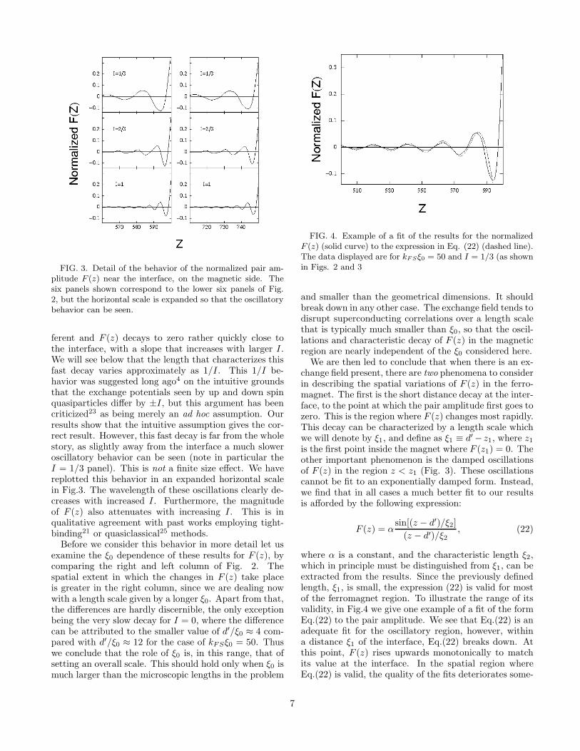
FIG. 3. Detail of the behavior of the normalized pair am-plitude F (z) near the interface, on the magnetic side. Thesix panels shown correspond to the lower six panels of Fig.2, but the horizontal scale is expanded so that the oscillatorybehavior can be seen.

ferent and F (z) decays to zero rather quickly close tothe interface, with a slope that increases with larger I.We will see below that the length that characterizes thisfast decay varies approximately as 1/I. This 1/I be-havior was suggested long ago4 on the intuitive groundsthat the exchange potentials seen by up and down spinquasiparticles differ by ±I, but this argument has beencriticized23 as being merely an ad hoc assumption. Ourresults show that the intuitive assumption gives the cor-rect result. However, this fast decay is far from the wholestory, as slightly away from the interface a much sloweroscillatory behavior can be seen (note in particular theI = 1/3 panel). This is not a finite size effect. We havereplotted this behavior in an expanded horizontal scalein Fig.3. The wavelength of these oscillations clearly de-creases with increased I. Furthermore, the magnitudeof F (z) also attenuates with increasing I. This is inqualitative agreement with past works employing tight-binding21 or quasiclassical25 methods.

Before we consider this behavior in more detail let usexamine the ξ0 dependence of these results for F (z), bycomparing the right and left column of Fig. 2. Thespatial extent in which the changes in F (z) take placeis greater in the right column, since we are dealing nowwith a length scale given by a longer ξ0. Apart from that,the differences are hardly discernible, the only exceptionbeing the very slow decay for I = 0, where the differencecan be attributed to the smaller value of d′/ξ0 ≈ 4 com-pared with d′/ξ0 ≈ 12 for the case of kFSξ0 = 50. Thuswe conclude that the role of ξ0 is, in this range, that ofsetting an overall scale. This should hold only when ξ0 ismuch larger than the microscopic lengths in the problem

FIG. 4. Example of a fit of the results for the normalizedF (z) (solid curve) to the expression in Eq. (22) (dashed line).The data displayed are for kF Sξ0 = 50 and I = 1/3 (as shownin Figs. 2 and 3

and smaller than the geometrical dimensions. It shouldbreak down in any other case. The exchange field tends todisrupt superconducting correlations over a length scalethat is typically much smaller than ξ0, so that the oscil-lations and characteristic decay of F (z) in the magneticregion are nearly independent of the ξ0 considered here.

We are then led to conclude that when there is an ex-change field present, there are two phenomena to considerin describing the spatial variations of F (z) in the ferro-magnet. The first is the short distance decay at the inter-face, to the point at which the pair amplitude first goes tozero. This is the region where F (z) changes most rapidly.This decay can be characterized by a length scale whichwe will denote by ξ1, and define as ξ1 ≡ d′− z1, where z1is the first point inside the magnet where F (z1) = 0. Theother important phenomenon is the damped oscillationsof F (z) in the region z < z1 (Fig. 3). These oscillationscannot be fit to an exponentially damped form. Instead,we find that in all cases a much better fit to our resultsis afforded by the following expression:

F (z) = αsin[(z − d′)/ξ2]

(z − d′)/ξ2, (22)

where α is a constant, and the characteristic length ξ2,which in principle must be distinguished from ξ1, can beextracted from the results. Since the previously definedlength, ξ1, is small, the expression (22) is valid for mostof the ferromagnet region. To illustrate the range of itsvalidity, in Fig.4 we give one example of a fit of the formEq.(22) to the pair amplitude. We see that Eq.(22) is anadequate fit for the oscillatory region, however, withina distance ξ1 of the interface, Eq.(22) breaks down. Atthis point, F (z) rises upwards monotonically to matchits value at the interface. In the spatial region whereEq.(22) is valid, the quality of the fits deteriorates some-

7

what for larger exchange fields (0.4 <∼ I < 1) becausethe spatial modulation of F (z) slightly deviates from thesimple periodic sine curve given by Eq.(22). This smalldiscrepancy can be glimpsed in the lower panels of Fig.3.The spatial structure becomes slightly nonperiodic, butoverall the functional form given by Eq.(22) is still satis-factory.

The oscillatory behavior of the pair amplitude as givenby (22) is physically the result25 of the exchange field,which creates electron and hole excitations in oppo-site spin bands. The pair amplitude involves productsof these particle and hole quasiparticle amplitudes (seeEq.(5)). The superposition of these wavefunctions thencreates oscillations on a length scale set by the differencebetween the spin up and spin down wavevectors in theferromagnet. One then expects25 a decay of the form(22) with ξ2 ≈ (kF↑ − kF↓)

−1. We can then write:

ξ2 ≈[√

2m(EFM + h0) −√

2m(EFM − h0)]−1

= k−1

FS

√1 + I√

1 + I −√

1 − I, (23)

where in the last step we have used, as previously men-tioned, EF↑/EFS = 1. For small I, Eq.(23) can be sim-plified to kFSξ2 ≈ 1/I, showing that ξ2 is then inverselyproportional to the exchange field. At larger values ofI there are deviations, but these are small since in theI = 1 limit both Eq. (23) and the approximate expres-sion coincide. These oscillations are also related to thoseresponsible for oscillatory coupling in structures involv-ing magnetic layers and superconducting spacers,39 andthe nonmonotonic behavior in the critical temperature,Tc, versus the F-layer thickness in S/F/S junctions.32 Inparticular, the sign change in the pair amplitude has thesame physical origin as the so called “π phase” that existsin F/S multilayers,40,41 and the nonmonotonic variationof the Josephson current with exchange field.42

Having introduced the two length scales ξ1 and ξ2 char-acterizing the superconducting proximity effect in themagnetic region, it is useful to compare their magnitudeand behavior as functions of I. The result of doing thisis shown in Fig.5. Data at additional values of I, notdisplayed in previous Figures, is included. For compari-son, Eq.(23) is shown as the solid curve. We find that ξ2follows very closely the expected theoretical expression,and that the other length, ξ1(I) ≈ ξ2(I). This is be-cause, as mentioned above, the expression4 kFSξ1 = 1/Inearly coincides numerically with the more complicatedresult for ξ2 as given above. Thus it turns out that thefast decay and the spatial period of the oscillations arecharacterized by lengths that are virtually identical.

C. Local density of states

To further investigate the F/S proximity effects, wefocus now on another experimentally accessible quantity,

FIG. 5. Exchange field, I , dependence of the lengthsξi, i = 1, 2, defined in the text. The circles are ξ1, and thesquares represent ξ2. The curve is the expression in Eq.(23).The results plotted are for kF Sξ0 = 50 but these quantitiesare nearly independent of ξ0.

the local DOS. Advances in STM technology9 have madeit possible to perform localized spectroscopic measure-ments with atomic scale resolution. We therefore presentnow the local DOS as a function of energy and position,as calculated from Eq.(21) and the self-consistent spec-tra. All results below are normalized to the normal-stateDOS in the S side and convolved with a Gaussian of width0.01∆0, to eliminate the spectrum discretization result-ing from the finite size of the computational sample. Wefocus only on results for positive energies, since those fornegative ones can be obtained by symmetry. We plot theresults in terms of the normalized energy variable ε/∆0.The locations chosen are given by the dimensionless po-sition measured relative to the interface in terms of thequantity Z ′ ≡ kFS(z − d′). Thus, a positive value of Z ′

denotes a location within the superconductor.We consider first the limit where the exchange field I

is zero. In Fig.6, we show the DOS for four different posi-tions at each of the two values kFSξ0 = 50 (left column)and kFSξ0 = 200 (right column). The three top rowsin Fig.6 show the DOS on the S side. For the shortercoherence length results for the locations Z ′ = 50, 100,and 200 are shown. These are multiples of the coherencelength, and the same multiples are shown in the rightcolumn. Several pronounced peaks are visible inside thegap, due to a finite number of bound states existing forε/∆0 < 1. These states were predicted long ago in anon self-consistent treatment by de Gennes and Saint-James11. These peaks diminish at greater distances in-side the superconductor. On the corresponding panels inthe right column, we see that the number of de GennesSaint-James peaks have been reduced. This is becausethe number of bound states depends upon the coherencelength ξ0, as well as on the superconductor and normalmetal widths10. In general, the number of such peaks de-

8

FIG. 6. Normalized local DOS (see Eq.(21)), plotted versusthe dimensionless energy ε/∆0 at I = 0 for kF Sξ0 = 50 (leftcolumn) and kF Sξ0 = 200 (right column). The values of thedimensionless quantity Z′

≡ kF S(z − d′) shown by the labelsare positions relative to the interface. Each position displayedis a multiple of the coherence length: from top to bottomthe rows correspond to Z′ = ξ0, Z′ = 2ξ0, Z′ = 4ξ0, andZ′ = −2ξ0.

creases as ξ0/d′ increases. The patterns seen at ε/∆0 > 1

are discussed below.On the normal metal side, we see on the bottom panels

of Fig.6, that there is no evidence of a gap, but a patternof jagged peaks appears in the DOS for ε/∆0

<∼ 1. Atlarger energies, interference patterns are seen, similar tothose in the S side. At longer coherence lengths thispattern is more coarse. This coarseness (which is alsoseen in subsequent figures) arises from the finite value ofN⊥. If this quantity is increased, the pattern becomessmoother and more regular, as in the left column. Theremaining regular oscillations ultimately vanish as d andd′ tend to infinity. We have chosen to display only oneposition in the F side for I = 0 since the overall behavioris nearly identical for all points in the normal metal. Thisis in agreement with our observation in connection withthe I = 0 panels in Fig.2, that the pair amplitude has avery slow rate of change.

We now turn to the case of a finite exchange field. Fig-

FIG. 7. Normalized local DOS for I = 1/3 at four positionsin the ferromagnetic side, near the interface. The left columncorresponds to kF Sξ0 = 50 and the right one to kF Sξ0 = 200.Z′ is defined as in the previous Figure.

ure 7 shows the DOS for kFSξ0 = 50 (left column), andkFSξ0 = 200 (right column) at I = 1/3 for four posi-tions very near the interface, within the magnetic mate-rial. This is done to illustrate how changes in the localDOS with distance are correlated with the rapid changein F (z) near the interface. Consider first the distanceZ ′ = −5 (top panels). This corresponds to the locationwhere F (z) has its more prominent minimum (see Fig.3). There is a weak minimum for the DOS at ε/∆0 = 0,which is more prominent at the smaller ξ0, and with in-creasing energy the DOS rises, until about ε/∆0 ≈ 1 atwhich point a peak occurs. For energies larger than ∆0

the DOS quickly settles down to its normal state value,unity in our normalization. At Z ′ = −4, as F (z) be-gins to rise, we see, focusing on the range of energiesless than ∆0, that the minimum of the DOS has begunto shift away from zero. At Z ′ = −3, in the next row ofpanels, the DOS has now a marked minimum at finite en-ergies within the gap, at ε/∆0 ≈ 0.6. The next position(last row) in Fig.7 shows a clear minimum of the DOS atenergies just below the gap. By comparing the top andbottom rows of Fig.7, we see that (for ε/∆0

<∼ 1) whatwere once dips and peaks in the DOS have now reversedroles. Fig.5 shows that the length characterizing the fast

9

FIG. 8. Local DOS at three positions inside the supercon-ductor, for I = 1/3 and kF Sξ0 = 50. The curves showncorrespond to (from top to bottom at small energy) Z′ = 50,Z′ = 100, and Z′ = 200. These are the same values as in thetop three panels of the left column of Fig. 6.

rise of F (z) is kFSξ1 ≈ 3.5 at I = 1/3. The DOS startsthe reversal process, as the interface is approached, ataround Z ′ ≈ −3.5, as seen in Fig. 7. The similarity be-tween right and left columns in this Figure reflects thatthe length scale ξ1, defining the inversion point, is thesame in both cases. The behavior of the DOS at largervalues of |Z ′| is qualitatively similar, but as the oscilla-tions die down it becomes much less discernible.

We show also (see Fig.8) the local DOS for three dif-ferent positions in the superconductor side for the sameI = 1/3 and the shorter ξ0. The de Gennes-Saint Jamespeaks are now gone, with just a hint of small structurefor ε/∆0 < 1 remaining at Z ′ = 50. This structure startsto become washed out at a distance of about 2ξ0 from theinterface. Finally, at Z ′ = 200, the DOS is of the familiarBCS form, with a well defined gap and pronounced peakat ε/∆0 = 1. In what follows, we focus only on the fer-romagnetic region, since the overall behavior of the DOSin S at larger values of I is quite similar to that seen inFig.8.

In Fig.9, we show the DOS for I = 2/3. As in Fig.7,we consider four spatial positions for each value of ξ0,however the range is now closer to the interface, sincethe larger exchange field reduces the spatial extent ofthe superconducting correlations and the length ξ1. Be-ginning at Z ′ = −4, Fig.9 (top) illustrates the formationof a small dip at low energies, and a continual rise up toε/∆0 ≈ 1, after which we recover the bulk DOS limit fora ferromagnet with this polarization. With our normal-ization, this value is smaller than unity. This is due to thedecrease in the number of spin down states with increas-ing exchange field. In Fig.9 (second row), the minimumin the DOS has moved, while the peak still remains atε/∆0 ≈ 1. At Z ′ = −2, (third row) the DOS is already

FIG. 9. Normalized local DOS for I = 2/3. The panelarrangement is the same as in Fig. 7.

rising upwards at low energies. The previous dip in theDOS has shifted to a higher energy, while a peak formsaround zero energy. We again find consistency with theξ1 values given in Fig.5, where for I = 2/3, kFSξ1 ≈ 2.2.Thus, as in the previous case, a reversal of the DOS be-havior occurs in the ξ1 range. The bottom panel of Fig. 9shows the DOS at Z ′ = −1. We see that the zero energymaximum has increased slightly from the previous rowand the minimum has shifted to energy ∆0. Again, thisqualitative behavior is independent of ξ0 reflecting theindependence of ξ1 from ξ0. Thus, we see here the samebehavior we found for I = 1/3 the only change being thedifferent value of ξ1.

We finally consider in Fig.10 the DOS for a fully polar-ized (half metallic) ferromagnet (I = 1.0). The locationsZ ′ are the same as in Fig.9. The structure of the DOSat energies below the gap for all positions has becomesmoother. Because of the large exchange field, the rever-sal of the occupation of states occurs over a length scaleξ1 which is now small (see Fig.3). Based on the previousfit in Fig.5, we find this point to be Z ′ ≈ 1.7. Again,we find consistency between the pair amplitude and theDOS. Note that as one moves away from the interface,the DOS tends to 1/2 at higher energies. This is due tothe total absence of the down band in this half metallic

10

FIG. 10. Normalized local DOS for a fully polarized ferro-magnet (I = 1.0). Again, results for kF Sξ0 = 50 are in theleft column, and those for kF Sξ0 = 200 in the right column,and positions with respect to the interface are indicated.

limit. These remarks apply to both values of ξ0.The above pertains to the proximity effect in the F

side. We now investigate further whether the presenceof the ferromagnet has any effect on the superconduct-ing correlations. That any effect is small is shown al-ready by Fig. 2. The influence of the magnet on Swill be reflected in a nonzero value of the difference inthe density of states for spin-up and spin-down electrons,δN ≡ N↑−N↓, where N↑ andN↓ are the spin up and spindown terms in Eq.(21) respectively. One might view thisas a self consistent determination of an effective parame-ter I(z) which may extend into the superconductor. Wefocus here only on the case of a half metallic ferromagnet(I = 1), and for illustration take kFSξ0 = 50. Figure 11shows that there is in fact a small proximity effect intothe superconductor, since very close to the interface theeffective polarization is nonzero. This effect is howevershort ranged, and we see that it nearly dies out beforeZ ′ = 5. At very small exchange fields (of order of thesuperconducting gap), we have found also a longer rangeproximity effect in the superconductor, similar to thatfound for dirty systems.43

FIG. 11. Leakage of magnetism into the superconductor:the quantity plotted difference between spin up and spin downvalues of the local DOS, δN ≡ N↑−N↓, normalized as in pre-vious Figures. This quantity is displayed at several positionsjust inside the superconductor. All results shown in this Fig-ure are for kF Sξ0 = 50. The values of Z′ are indicated in thepanels.

IV. CONCLUSIONS

We have introduced in this paper numerical techniquesto accurately and self-consistently solve the continuumBdG equations. We have shown how one can use thesemethods to perform a detailed study of F/S interfacialproperties. Our procedures allow us to consider super-conducting and magnetic proximity effects in a bulk sys-tem containing an F/S interface, even when the super-conducting coherence length is orders of magnitude largerthan the interparticle distance. In this work, we haveused these techniques to investigate the proximity effectsfor a clean F/S system. We have extracted the relevantcharacteristic lengths through a careful analysis of thepair potential and the pair amplitude, and we have shownhow, near the interface, the behavior of the pair ampli-tude correlates with that of the local DOS. Our workextends well beyond previous numerical computations inthe tight-binding case, valid only for very short values ofξ0, and beyond theoretical work limited by quasiclassicalapproximations or restricted to regimes where the meanfree path or ξ0 are very short.

On the S side we have found, near the interface, adepletion of both the pair potential and the pair ampli-tude. This depletion extends over a length scale deter-mined essentially by ξ0, and hence nearly independent ofthe exchange field I. For the bulk heterostructures weconsidered, the effect of varying ξ0 in the range studied

11

(kFSξ0 = 50 to kFSξ0 = 200) was an effective rescaling ofthe characteristic length that determines this depletion.In the F region, for finite values of the exchange field, thepair amplitude exhibited a sharp monotonic decline nearthe interface, followed by damped oscillations. The fastdecay was found to take place over a length scale ξ1 ap-proximately inversely proportional to I, independent ofthe ξ0, according the the expression4 kFSξ1 ≈ 1/I. Theoscillatory part of the spatial variation of the pair ampli-tude could be fit to a simple sine function with an ampli-tude decaying as the inverse of distance from the inter-face. We found that the spatial period of the oscillationsis determined by the length difference ξ2 = (kF↑−kF↓)

−1

(the inverse of the difference between spin up and spindown Fermi wavevectors) provided that I is not too large.This is in reasonable agreement with previous theoreticalexpectations25. We have presented extensive results forthe local DOS, as a function of position and energy, asobtained via the self-consistent quasiparticle amplitudesand energies. The periodic sign change in the pair am-plitude is found to be correlated with oscillations in thelocal DOS relative to its normal state values. Finally,we verified also from the local DOS that the effect ofthe exchange field on superconducting correlations in Sis minimal (although nonzero): the difference in the lo-cal DOS of spin up and spin down quasiparticles vanishesexcept very close to the interface, at least for I ≥ 1/3.

Clearly, the powerful methods and techniques for theself-consistent solution of the BdG equations presentedhere open new vistas and possibilities for use in the studyof many other aspects of the F/S interface and similarproblems. A thorough investigation of the physical quan-tities and characteristic lengths studied in this paper, in-corporating other parameter regimes and the effects offinite temperature is needed, and it can be straightfor-wardly carried out. Interface scattering, and supercon-ductors with nodes in the pair potential (unconventionalpair potentials), can be also easily considered. Spin-flipeffects, and disorder in both F and S materials can also beincorporated. By suitably changing the boundary con-ditions, self consistent solutions of the tunneling spec-troscopy problem in the long ξ0 regime will be obtain-able. Our numerical methods are particularly suitable tothe study of mesoscopic structures involving F/S multi-layers of differing thickness, where size effects may comeinto play. The study of tunneling phenomena in non-equilibrium situations is also feasible by extension of ourmethod to the time-dependent BdG equations.

ACKNOWLEDGMENTS

We thank P. Kraus and A.M. Goldman for many con-versations concerning this problem. This work was sup-ported in part by the Petroleum Research Fund, admin-istered by the ACS.

† Electronic address: khalter@physics.umn.edu∗ Electronic address: otvalls@tc.umn.edu1 G. Blatter, V.B. Geshkenbein, and L.B. Ioffe, Phys. Rev.B 63, 174511 (2001)

2 S. Oh, D. Youm, and M.R. Beasley, Appl. Phys. Lett. 16,2376 (1997)

3 L.R. Tagirov, Phys. Rev. Lett. 83, 2058 (1999)4 G. Deutscher and P.G. de Gennes, in Superconductivity,edited by R.D. Parks (Marcel Dekker, New York, 1969), p.1005.

5 A.L. Fetter and J.D. Walecka, Quantum Theory of Many

Particle Systems (McGraw-Hill, New York, 1971).6 P.G. de Gennes, Superconductivity of Metals and Alloys

(Addison-Wesley, Reading, MA, 1989).7 G.B. Arnold, Phys. Rev. B 18, 1076 (1978)8 A.F. Andreev, Zh. Eksp. Teor. Fiz. 46, 1823 (1964) [Sov.Phys. JETP 19, 1228 (1964)].

9 N. Moussy, H Courtois, and B. Pannetier, Rev. Sci. In-strum.,72, 128 (2001).

10 M.P. Zaitlin, Phys. Rev. B 25, 5729 (1982).11 P.G. de Gennes and D. St.-James, Phys. Lett. 4, 151

(1963).12 W.L. McMillan, Phys. Rev. B 175, 559 (1968).13 O. Entin-Wohlman and T. Bar-Sagi, Phys. Rev. B 18, 3174

(1978).14 G. Eilenberger, Z. Phys. 214, 195 (1968).15 S. Pilgram, W. Belzig, and C. Bruder, Phys. Rev. B 62,

12462 (2000).16 G. Kieselmann, Phys. Rev. B 35, 6762 (1987).17 K.D. Usadel, Phys. Rev. Lett. 25, 507 (1970).18 W. Belzig, C. Bruder, and G. Schon, Phys. Rev. B 54, 9443

(1996).19 B.P. Stojkovic, and O.T. Valls, Phys. Rev. B 47, 5922

(1993).20 B.P. Stojkovic, and O.T. Valls, Phys. Rev. B 50, 3374

(1994).21 J-X Zhu and C.S. Ting, Phys. Rev. B 61, 1456 (2000).22 K. Kuboki, Journal Phys. Soc. Japan 68, 3150 (1999).23 M.D. Lawrence and N. Giordano J. Phys. Cond. Matt. 11

1089 (1998).24 M.J.M de Jong, and C.W.J. Beenakker, Phys. Rev. Lett.

9, 1657 (1995).25 E.A. Demler, G.B. Arnold, and M.R. Beasley, Phys. Rev.

B 55,15 174 (1997).26 P. Fulde and A. Ferrell, Phys. Rev. 135, A550 (1964).27 A. Larkin and Y. Ovchinnikov, Sov. Phys. JETP 20, 762

(1965).28 M. Zareyan, W. Belzig, and Y.V. Nazarov, Phys. Rev. Lett.

86,308 (2001).29 T. Kontos, M. Aprili, J. Lesueur, and X. Grison, Phys.

Rev. Lett. 86,304 (2001).30 A. Buzdin, Phys. Rev. B 62,11 377 (2000).31 I. Zutic and O.T. Valls, Phys. Rev. B 61, 1555 (2000)32 Z. Radovic et al, Phys. Rev. B 44, 759 (1991)33 In some cases it is more efficient to modify the result of the

12

previous iteration before using it as the next input.34 P.G. De Gennes, Rev. Mod. Phys. 36, 225 (1964).35 See e.g. F. Gygi and M. Schluter, Phys. Rev. B 41,822

(1990).36 The implementation of the subroutine was that in the IBM

Engineering and Scientific Subroutine Library (ESSL).37 C.J. Thompson and J.M. Blatt, Phys. Lett. 5, 6 (1963).38 D.S. Falk, Phys. Rev. 132, 1576 (1963).39 O. Sipr and B.L. Gyorffy, J. Phys.: Condens. Matter 7,5239

(1995).40 A.V. Andreev, A.I. Buzdin, and R.M. Osgood III, Phys.

Rev. B 43, 10124 (1991).41 I. Baladie, A. Buzdin, N. Ryzhanova, and A. Vedyayev,

Phys. Rev. B 63,54518 (2001).42 V. Prokic, A.I. Buzdin, and L. Dobrosavljevic-Grujic,

Phys. Rev. B 59,587 (1999).43 R. Fazio and C. Lucheroni, Europhys. Lett. 45, 707 (1999).

13