PhD Thesis - Ayman Alserafi - 2020 - Proximity Mining
189
T BI I D C Dataset Proximity Mining for Supporting Schema Matching and Data Lake Governance Ph.D. Dissertation Ayman Alserafi
-
Upload
khangminh22 -
Category
Documents
-
view
3 -
download
0
Transcript of PhD Thesis - Ayman Alserafi - 2020 - Proximity Mining

T BII
D C
Dataset Proximity Miningfor Supporting Schema
Matching and Data LakeGovernance
Ph.D. DissertationAyman Alserafi

Dataset proximity mining for supporting schema
matching and data lake governance
Ayman Alserafi
ADVERTIMENT La consulta d’aquesta tesi queda condicionada a l’acceptació de les següents condicions d'ús: La difusió d’aquesta tesi per mitjà del repositori institucional UPCommons (http://upcommons.upc.edu/tesis) i el repositori cooperatiu TDX ( h t t p : / / w w w . t d x . c a t / ) ha estat autoritzada pels titulars dels drets de propietat intel·lectual únicament per a usos privats emmarcats en activitats d’investigació i docència. No s’autoritza la seva reproducció amb finalitats de lucre ni la seva difusió i posada a disposició des d’un lloc aliè al servei UPCommons o TDX. No s’autoritza la presentació del seu contingut en una finestra o marc aliè a UPCommons (framing). Aquesta reserva de drets afecta tant al resum de presentació de la tesi com als seus continguts. En la utilització o cita de parts de la tesi és obligat indicar el nom de la persona autora. ADVERTENCIA La consulta de esta tesis queda condicionada a la aceptación de las siguientes condiciones de uso: La difusión de esta tesis por medio del repositorio institucional UPCommons (http://upcommons.upc.edu/tesis) y el repositorio cooperativo TDR (http://www.tdx.cat/?locale- attribute=es) ha sido autorizada por los titulares de los derechos de propiedad intelectual únicamente para usos privados enmarcados en actividades de investigación y docencia. No se autoriza su reproducción con finalidades de lucro ni su difusión y puesta a disposición desde un sitio ajeno al servicio UPCommons No se autoriza la presentación de su contenido en una ventana o marco ajeno a UPCommons (framing). Esta reserva de derechos afecta tanto al resumen de presentación de la tesis como a sus contenidos. En la utilización o cita de partes de la tesis es obligado indicar el nombre de la persona autora. WARNING On having consulted this thesis you’re accepting the following use conditions: Spreading this thesis by the institutional repository UPCommons (http://upcommons.upc.edu/tesis) and the cooperative repository TDX (http://www.tdx.cat/?locale- attribute=en) has been authorized by the titular of the intellectual property rights only for private uses placed in investigation and teaching activities. Reproduction with lucrative aims is not authorized neither its spreading nor availability from a site foreign to the UPCommons service. Introducing its content in a window or frame foreign to the UPCommons service is not authorized (framing). These rights affect to the presentation summary of the thesis as well as to its contents. In the using or citation of parts of the thesis it’s obliged to indicate the name of the author.


T BII
D C
Dataset Proximity Miningfor Supporting Schema
Matching and Data LakeGovernance
Ph.D. DissertationAyman Alserafi
Supervisors:Prof. Alberto AbellóProf. Oscar RomeroProf. Toon Calders
Dissertation submitted on November, 2020
A thesis submitted to Barcelona School of Informatics at Universitat Politèc-nica de Catalunya, BarcelonaTech (UPC) and the Faculty of Engineering atUniversité Libre De Bruxelles (ULB), in partial fulfilment of the requirementswithin the scope of the IT4BI-DC programme for the joint Ph.D. degree incomputer science. The thesis is not submitted to any other organization at thesame time.


Thesis title: Dataset Proximity Mining for Supporting SchemaMatching and Data Lake Governance
Thesis submitted: November, 2020
PhD Supervisors: Prof. Alberto AbellóUniversitat Politècnica de Catalunya, BarcelonaTech,SpainProf. Oscar RomeroUniversitat Politècnica de Catalunya, BarcelonaTech,SpainProf. Toon CaldersUniversité Libre de Bruxelles, Brussels, Belgium andUniversiteit Antwerpen, Antwerp, Belgium
PhD Committee: Prof. Wolfgang LehnerTechnische Universität Dresden, GermanyProf. Patrick MarcelUniversité de Tours, FranceProf. Jose Francisco Aldana MontesUniversidad de Málaga, Spain
PhD Series: Barcelona School of Informatics, Universitat Politèc-nica de Catalunya, BarcelonaTech
Doctoral Programme: The Erasmus Mundus Joint Doctorate in Informa-tion Technologies for Business Intelligence - Doc-toral College (IT4BI-DC)
© Copyright by Ayman Alserafi. Author has obtained the right to include thepublished and accepted articles in the thesis, with a condition that they arecited, DOI pointers and/or copyright/credits are placed prominently in thereferences.
Printed in Spain, 2020

Abstract
A task is only as difficult as one perceives it. Everything can bedissected into its smaller simpler parts. If a task seemsunattainable, break it into smaller pieces and it will seemsimpler and more interesting to achieve or study.
With the huge growth in the amount of data generated by informationsystems, it is common practice today to store datasets in their raw formats(i.e., without any data preprocessing or transformations) in large-scale datarepositories called Data Lakes (DLs). Such repositories store datasets fromheterogeneous subject-areas (covering many business topics) and with manydifferent schemata. Therefore, it is a challenge for data scientists using the DLfor data analysis to find relevant datasets for their analysis tasks without anysupport or data governance. The goal is to be able to extract metadata andinformation about datasets stored in the DL to support the data scientist infinding relevant sources. This shapes the main goal of this thesis, where weexplore different techniques of data profiling, holistic schema matching andanalysis recommendation to support the data scientist. We propose a novelframework based on supervised machine learning to automatically extractmetadata describing datasets, including computation of their similarities anddata overlaps using holistic schema matching techniques. We use the extractedrelationships between datasets in automatically categorizing them to supportthe data scientist in finding relevant datasets with intersection between theirdata. This is done via a novel metadata-driven technique called proximitymining which consumes the extracted metadata via automated data miningalgorithms in order to detect related datasets and to propose relevant cate-gories for them. We focus on flat (tabular) datasets organised as rows of datainstances and columns of attributes describing the instances. Our proposedframework uses the following four main techniques: (1) Instance-based schemamatching for detecting relevant data items between heterogeneous datasets, (2)Dataset level metadata extraction and proximity mining for detecting related
v

datasets, (3) Attribute level metadata extraction and proximity mining fordetecting related datasets, and finally, (4) Automatic dataset categorization viasupervised k-Nearest-Neighbour (kNN) techniques. We implement our pro-posed algorithms via a prototype that shows the feasibility of this framework.We apply the prototype in an experiment on a real-world DL scenario to provethe feasibility, effectiveness and efficiency of our approach, whereby we wereable to achieve high recall rates and efficiency gains while improving the com-putational space and time consumption by two orders of magnitude via ourproposed early-pruning and pre-filtering techniques in comparison to classicalinstance-based schema matching techniques. This proves the effectiveness ofour proposed automatic methods in the early-pruning and pre-filtering tasksfor holistic schema matching and the automatic dataset categorisation, whilealso demonstrating improvements over human-based data analysis for thesame tasks.
Keywords: Data Lake Governance, Dataset Similarity Mining, Holistic SchemaMatching, Metadata Management, Supervised Machine Learning

Resum
Amb l’enorme creixement de la quantitat de dades generades pels sistemesd’informació, és habitual avui en dia emmagatzemar conjunts de dades en elsseus formats bruts (és a dir, sense cap preprocessament de dades ni transforma-cions) en dipòsits de dades a gran escala anomenats Data Lakes (DL). Aquestsdipòsits emmagatzemen conjunts de dades d’àrees temàtiques heterogènies(que abasten molts temes empresarials) i amb molts esquemes diferents. Pertant, és un repte per als científics de dades que utilitzin la DL per a l’anàliside dades trobar conjunts de dades rellevants per a les seves tasques d’anàlisisense cap suport ni govern de dades. L’objectiu és poder extreure metadades iinformació sobre conjunts de dades emmagatzemats a la DL per donar suportal científic en trobar fonts rellevants. Aquest és l’objectiu principal d’aquestatesi, on explorem diferents tècniques de perfilació de dades, concordançad’esquemes holístics i recomanació d’anàlisi per donar suport al científic.Proposem un nou marc basat en l’aprenentatge automatitzat supervisat perextreure automàticament metadades que descriuen conjunts de dades, incloentel càlcul de les seves similituds i coincidències de dades mitjançant tècniquesde concordança d’esquemes holístics. Utilitzem les relacions extretes entreconjunts de dades per categoritzar-les automàticament per donar suport alcientífic del fet de trobar conjunts de dades rellevants amb la intersecció entreles seves dades. Això es fa mitjançant una nova tècnica basada en metadadesanomenada mineria de proximitat que consumeix els metadades extrets mit-jançant algoritmes automatitzats de mineria de dades per tal de detectarconjunts de dades relacionats i proposar-ne categories rellevants. Ens centremen conjunts de dades plans (tabulars) organitzats com a files d’instànciesde dades i columnes d’atributs que descriuen les instàncies. El nostre marcproposat utilitza les quatre tècniques principals següents: (1) Esquema deconcordança basat en instàncies per detectar ítems rellevants de dades en-tre conjunts de dades heterogènies, (2) Extracció de metadades de nivell dedades i mineria de proximitat per detectar conjunts de dades relacionats, (3)Extracció de metadades a nivell de atribut i mineria de proximitat per detectarconjunts de dades relacionats i, finalment, (4) Categorització de conjunts dedades automàtica mitjançant tècniques supervisades per k-Nearest-Neighbour
vii

(kNN). Posem en pràctica els nostres algorismes proposats mitjançant unprototip que mostra la viabilitat d’aquest marc. El prototip s’experimenta enun escenari DL real del món per demostrar la viabilitat, l’eficàcia i l’eficiènciadel nostre enfocament, de manera que hem pogut aconseguir elevades taxesde record i guanys d’eficiència alhora que millorem el consum computacionald’espai i temps mitjançant dues ordres de magnitud mitjançant el nostre esvan proposar tècniques de poda anticipada i pre-filtratge en comparació ambtècniques de concordança d’esquemes basades en instàncies clàssiques. Aixòdemostra l’efectivitat dels nostres mètodes automàtics proposats en les tasquesde poda inicial i pre-filtratge per a la coincidència d’esquemes holístics i laclassificació automàtica del conjunt de dades, tot demostrant també milloresen l’anàlisi de dades basades en humans per a les mateixes tasques.

Résumé
Avec l’énorme croissance de la quantité de données générées par les systèmesd’information, il est courant aujourd’hui de stocker des ensembles de don-nées (datasets) dans leurs formats bruts (c’est-à-dire sans prétraitement nitransformation de données) dans des référentiels de données à grande échelleappelés Data Lakes (DL). Ces référentiels stockent des ensembles de donnéesprovenant de domaines hétérogènes (couvrant de nombreux sujets commerci-aux) et avec de nombreux schémas différents. Par conséquent, il est difficilepour les data-scientists utilisant les DL pour l’analyse des données de trouverdes datasets pertinents pour leurs tâches d’analyse sans aucun support ni gou-vernance des données. L’objectif est de pouvoir extraire des métadonnées etdes informations sur les datasets stockés dans le DL pour aider le data-scientistà trouver des sources pertinentes. Cela constitue l’objectif principal de cettethèse, où nous explorons différentes techniques de profilage de données, decorrespondance holistique de schéma et de recommandation d’analyse poursoutenir le data-scientist. Nous proposons une nouvelle approche basée surl’intelligence artificielle, spécifiquement l’apprentissage automatique super-visé, pour extraire automatiquement les métadonnées décrivant les datasets,calculer automatiquement les similitudes et les chevauchements de donnéesentre ces ensembles en utilisant des techniques de correspondance holistiquede schéma. Les relations entre datasets ainsi extraites sont utilisées pour caté-goriser automatiquement les datasets, afin d’aider le data-scientist à trouverdes datasets pertinents avec intersection entre leurs données. Cela est fait viaune nouvelle technique basée sur les métadonnées appelée proximity mining,qui consomme les métadonnées extraites via des algorithmes de data miningautomatisés afin de détecter des datasets connexes et de leur proposer descatégories pertinentes. Nous nous concentrons sur des datasets plats (tabu-laires) organisés en rangées d’instances de données et en colonnes d’attributsdécrivant les instances. L’approche proposée utilise les quatres principalestechniques suivantes: (1) Correspondance de schéma basée sur l’instance pourdétecter les éléments de données pertinents entre des datasets hétérogènes, (2)Extraction de métadonnées au niveau du dataset et proximity mining pourdétecter les datasets connexes, (3) Extraction de métadonnées au niveau des
ix
attributs et proximity mining pour détecter des datasets connexes, et enfin,(4) catégorisation automatique des datasets via des techniques superviséesk-Nearest-Neighbour (kNN). Nous implémentons les algorithmes proposésvia un prototype qui montre la faisabilité de cette approche. Nous appliquonsce prototype à une scénario DL du monde réel pour prouver la faisabilité,l’efficacité et l’efficience de notre approche, nous permettant d’atteindre destaux de rappel élevés et des gains d’efficacité, tout en diminuant le coût enespace et en temps de deux ordres de grandeur, via nos techniques proposéesd’élagage précoce et de pré-filtrage, comparé aux techniques classiques decorrespondance de schémas basées sur les instances. Cela prouve l’efficacitédes méthodes automatiques proposées dans les tâches d’élagage précoce et depré-filtrage pour la correspondance de schéma holistique et la cartegorisationautomatique des datasets, tout en démontrant des améliorations par rapportà l’analyse de données basée sur l’humain pour les mêmes tâches.

Acknowledgements
We don’t work in isolation, but rather in stronger, more efficient and successful groups. [...]Karma does take place, and we reap what we sow! Thus, treat others like you’d like to be treated.
This thesis would not have been possible if it was not for the supportof many people who helped me along the journey in many positive ways.Firstly, I would like to thank my thesis supervisors for their huge effortswith my thesis and all our fruitful discussions. I have learned a lot fromthem in many useful ways. They taught me to achieve professional rigorousresearch, to keep expanding my knowledge and to never give up along the(rocky!) path till the finish line. I would also like to thank my family fortheir continuous support during the most difficult times. They deserve allthe sincere appreciation in the world. All the grateful appreciation to mysincere friends (you know yourselves!) who helped me adapt with all the newexperiences and for always being there when I need them (especially duringthe low times). Without them I would not have been able to finish this PhDproject. I would like to thank all my colleagues from IT4BI-DC, UPC, and ULBwho made it an amazing work environment for learning and collaboratingtogether. I learned something useful from each and everyone of this bigresearch group (and academic family). I’m also really thankful for all theassistance by the technical support staff at the ULB and UPC labs. This thesiswould not have been possible without the grateful funding and contributionsby the European Commission via the research grant that supported me tocomplete my thesis and my international research stays. I am also thankfulfor my country, the cradle of ancient civilisations, for making me who I amand for engraving in me all the good values which support me in my life. Ittaught me the love for all of humanity, and the respect for all our beautifuldiversity. Finally, I would like to end this with a dedication by wishing allthe prosperity for the nations and peoples of Europe, Africa, my homeland,and the whole world. May God bless them all and their future generations ofscientists and engineers. With our continuous collaboration we will achieve abetter world and future for everyone and the whole of humanity!
27th of March, 2020
xi

Contents
Abstract v
Resum vii
Résumé ix
Acknowledgements xiList of Figures . . . . . . . . . . . . . . . . . . . . . . . . . . . . . . . . xvList of Tables . . . . . . . . . . . . . . . . . . . . . . . . . . . . . . . . . xviii
Abbreviations xx
Thesis Details xxi
1 Introduction 11 Motivation . . . . . . . . . . . . . . . . . . . . . . . . . . . . . . . 12 Background and State-of-the-art . . . . . . . . . . . . . . . . . . 2
2.1 Data Lakes and Tabular Datasets . . . . . . . . . . . . . . 22.2 Data Lake Governance . . . . . . . . . . . . . . . . . . . . 3
3 Techniques and Challenges . . . . . . . . . . . . . . . . . . . . . 103.1 Schema Matching . . . . . . . . . . . . . . . . . . . . . . . 113.2 Dataset Similarity Computation . . . . . . . . . . . . . . 143.3 Similarity Models Learning . . . . . . . . . . . . . . . . . 15
4 Thesis Objectives and Research Questions . . . . . . . . . . . . . 185 Thesis Overview . . . . . . . . . . . . . . . . . . . . . . . . . . . 20
5.1 Proximity Mining Framework . . . . . . . . . . . . . . . 205.2 DL Categorization . . . . . . . . . . . . . . . . . . . . . . 235.3 Metadata Query Interface . . . . . . . . . . . . . . . . . . 25
6 Thesis Contributions . . . . . . . . . . . . . . . . . . . . . . . . . 257 Structure of the Thesis . . . . . . . . . . . . . . . . . . . . . . . . 27
7.1 Chapter 2: Instance-level value-based schema matchingfor mining proximity between datasets . . . . . . . . . . 28
xii

Contents
7.2 Chapter 3: Dataset-level content metadata based prox-imity mining . . . . . . . . . . . . . . . . . . . . . . . . . 28
7.3 Chapter 4: Attribute-level content metadata based prox-imity mining for pre-filtering schema matching . . . . . 28
7.4 Chapter 5: Automatic categorization of datasets usingproximity mining . . . . . . . . . . . . . . . . . . . . . . . 29
7.5 Chapter 6: Prox-mine tool for browsing DLs using prox-imity mining . . . . . . . . . . . . . . . . . . . . . . . . . 29
2 Instance-level value-based schema matching for computing datasetsimilarity 311 Introduction . . . . . . . . . . . . . . . . . . . . . . . . . . . . . . 332 Related Work . . . . . . . . . . . . . . . . . . . . . . . . . . . . . 353 Motivational Case-Study . . . . . . . . . . . . . . . . . . . . . . . 364 A Framework for Content Metadata Management . . . . . . . . 375 The CM4DL Prototype . . . . . . . . . . . . . . . . . . . . . . . . 39
5.1 Prototype Architecture . . . . . . . . . . . . . . . . . . . . 405.2 Ontology Alignment Component . . . . . . . . . . . . . 415.3 Dataset Comparison Algorithm . . . . . . . . . . . . . . 43
6 Experiments and Results . . . . . . . . . . . . . . . . . . . . . . . 457 Discussion . . . . . . . . . . . . . . . . . . . . . . . . . . . . . . . 488 Conclusion and Future Work . . . . . . . . . . . . . . . . . . . . 49
3 Dataset-level content metadata based proximity mining for comput-ing dataset similarity 511 Introduction . . . . . . . . . . . . . . . . . . . . . . . . . . . . . . 532 Problem Statement . . . . . . . . . . . . . . . . . . . . . . . . . . 543 Related Work . . . . . . . . . . . . . . . . . . . . . . . . . . . . . 554 The DS-Prox Approach . . . . . . . . . . . . . . . . . . . . . . . . 56
4.1 The Meta-Features Distance Measures . . . . . . . . . . . 574.2 The Approach . . . . . . . . . . . . . . . . . . . . . . . . . 58
5 Experimental Evaluation . . . . . . . . . . . . . . . . . . . . . . . 615.1 Datasets . . . . . . . . . . . . . . . . . . . . . . . . . . . . 615.2 Experimental Setup . . . . . . . . . . . . . . . . . . . . . 625.3 Results . . . . . . . . . . . . . . . . . . . . . . . . . . . . . 635.4 Discussion . . . . . . . . . . . . . . . . . . . . . . . . . . . 64
6 Conclusion and Future Work . . . . . . . . . . . . . . . . . . . . 66
4 Attribute-level content metadata based proximity mining for pre-filtering schema matching 681 Introduction . . . . . . . . . . . . . . . . . . . . . . . . . . . . . . 702 Related Work . . . . . . . . . . . . . . . . . . . . . . . . . . . . . 723 Preliminaries . . . . . . . . . . . . . . . . . . . . . . . . . . . . . . 75
xiii

Contents
4 Approach: Metadata-based Proximity Mining for Pre-filteringSchema Matching . . . . . . . . . . . . . . . . . . . . . . . . . . . 794.1 Proximity Metrics: Meta-features Distances . . . . . . . 794.2 Supervised Proximity Mining . . . . . . . . . . . . . . . . 814.3 Pre-filtering Dataset Pairs for Schema Matching . . . . . 88
5 Experimental Evaluation . . . . . . . . . . . . . . . . . . . . . . . 885.1 Datasets . . . . . . . . . . . . . . . . . . . . . . . . . . . . 895.2 Evaluation Metrics . . . . . . . . . . . . . . . . . . . . . . 925.3 Experiment 1: Attribute-level Models . . . . . . . . . . . 945.4 Experiment 2: Dataset-level Models . . . . . . . . . . . . 955.5 Experiment 3: Computational Performance Evaluation . 1035.6 Generalisability . . . . . . . . . . . . . . . . . . . . . . . . 105
6 Conclusion . . . . . . . . . . . . . . . . . . . . . . . . . . . . . . . 105
5 Automatic categorization of datasets using proximity mining 1071 Introduction . . . . . . . . . . . . . . . . . . . . . . . . . . . . . . 1092 Preliminaries . . . . . . . . . . . . . . . . . . . . . . . . . . . . . . 111
2.1 Proximity Mining: Meta-features Metrics and Models . 1133 DS-kNN: a Proximity Mining Based k-Nearest-Neighbour Al-
gorithm for Categorizing Datasets . . . . . . . . . . . . . . . . . 1154 Experimental Evaluation . . . . . . . . . . . . . . . . . . . . . . . 117
4.1 Dataset: OpenML DL Ground-truth . . . . . . . . . . . . 1174.2 Experimental Setup . . . . . . . . . . . . . . . . . . . . . 1184.3 Results . . . . . . . . . . . . . . . . . . . . . . . . . . . . . 1214.4 Validation Experiment . . . . . . . . . . . . . . . . . . . . 131
5 Related Work . . . . . . . . . . . . . . . . . . . . . . . . . . . . . 1336 Conclusion . . . . . . . . . . . . . . . . . . . . . . . . . . . . . . . 134
6 Prox-mine tool for browsing DLs using proximity mining 1351 Introduction . . . . . . . . . . . . . . . . . . . . . . . . . . . . . . 1362 Data Lake Index . . . . . . . . . . . . . . . . . . . . . . . . . . . . 1373 Similarity Search . . . . . . . . . . . . . . . . . . . . . . . . . . . 1374 Dataset Categorization . . . . . . . . . . . . . . . . . . . . . . . . 1385 Dataset Matching . . . . . . . . . . . . . . . . . . . . . . . . . . . 140
5.1 New Dataset Matching . . . . . . . . . . . . . . . . . . . 1416 Proximity Graph . . . . . . . . . . . . . . . . . . . . . . . . . . . 143
7 Conclusions and Future Directions 1481 Conclusions . . . . . . . . . . . . . . . . . . . . . . . . . . . . . . 1492 Future Directions . . . . . . . . . . . . . . . . . . . . . . . . . . . 150
Bibliography 152References . . . . . . . . . . . . . . . . . . . . . . . . . . . . . . . . . . 152
xiv

List of Figures
List of Figures
1.1 A flat structured dataset consisting of tabular data organised asattributes and instances . . . . . . . . . . . . . . . . . . . . . . . 3
1.2 DL governance classification and tasks . . . . . . . . . . . . . . 41.3 An example of schema matching and dataset similarity compu-
tation . . . . . . . . . . . . . . . . . . . . . . . . . . . . . . . . . . 111.4 Classification of schema matching techniques . . . . . . . . . . 131.5 Example of a decision tree model for classification of related
dataset pairs . . . . . . . . . . . . . . . . . . . . . . . . . . . . . . 171.6 An ensemble of decision trees for classification . . . . . . . . . . 181.7 Overview of the proposed proxmity mining framework . . . . 211.8 The proximity mining metadata management process . . . . . . 221.9 A proximity graph showing topic-wise groupings of interlinked
datasets in the DL with their similarity scores . . . . . . . . . . 241.10 DL content metadata management and analysis process . . . . 25
2.1 The Metadata Management BPMN Process Model . . . . . . . . 372.2 The EXP01 Metadata Exploitation Sub-Process Model . . . . . . 382.3 CM4DL System Architecture . . . . . . . . . . . . . . . . . . . . 402.4 Performance analysis of CM4DL in the OpenML experiments . 47
3.1 Similarity relationships between two pairs of datasets . . . . . . 553.2 DS-Prox: supervised machine learning . . . . . . . . . . . . . . 583.3 DS-Prox cut-off thresholds tuning . . . . . . . . . . . . . . . . . 603.4 Recall-efficiency plots (left column) and recall-precision plots
(right column) for experiments 1,2,3 and 4 in each row . . . . . 67
4.1 The stratified holistic schema matching approach at differentlevels of granularity. . . . . . . . . . . . . . . . . . . . . . . . . . 71
4.2 The dependencies of components in the metadata-based prox-imity mining approach for pre-filtering schema matching. . . . 76
4.3 Final output of our approach consisting of similarity relation-ships between two pairs of datasets. . . . . . . . . . . . . . . . . 78
4.4 An overview of the process to build the supervised ensemblemodels in our proposed datasets proximity mining approachusing previously manually annotated dataset pairs. . . . . . . . 82
4.5 Proximity Mining: supervised machine learning for predictingrelated data objects. . . . . . . . . . . . . . . . . . . . . . . . . . . 83
4.6 Different normal distributions for assigning weights to rankedattribute linkages. . . . . . . . . . . . . . . . . . . . . . . . . . . . 86
xv
List of Figures
4.7 An overview of the process to apply the learnt supervisedmodels in our approach for pre-filtering previously unseendataset pairs independent of the build process. . . . . . . . . . . 87
4.8 A 10-fold cross-validation experimental setup consisting ofalternating folds in training and test roles. Image adaptedfrom the book: Raschka S (2015) Python Machine Learning. 1stEdition. Packt Publishing, Birmingham, UK. . . . . . . . . . . . 97
4.9 Classification accuracy from 10-fold cross-validation of datasetpairs pre-filtering models. . . . . . . . . . . . . . . . . . . . . . . 98
4.10 Kappa statistic from 10-fold cross-validation of dataset pairspre-filtering models. . . . . . . . . . . . . . . . . . . . . . . . . . 98
4.11 ROC statistic from 10-fold cross-validation of dataset pairs pre-filtering models. . . . . . . . . . . . . . . . . . . . . . . . . . . . . 98
4.12 Recall against efficiency gain for the different supervised models.1004.13 Recall against precision for the different supervised models. . . 1004.14 Recall against efficiency gain for the different metric types. . . 1004.15 Recall against precision for the different metric types. . . . . . . 100
5.1 A visualisation of the output from DS-kNN data lake (DL) cate-gorization. A proximity graph shows the datasets as nodes andthe proximity scores as edges between nodes. Fig.(a) completeDL and Fig. (b) a zoomed-in view highlighted by the red boxin (a) . . . . . . . . . . . . . . . . . . . . . . . . . . . . . . . . . . 110
5.2 The data lake categorization scenario using k-NN proximitymining . . . . . . . . . . . . . . . . . . . . . . . . . . . . . . . . . 113
5.3 Performance of DS-kNN using k=1, different models, differentground-truths, and different category sizes . . . . . . . . . . . . 122
5.4 Performance of DS-kNN using k=3, different models, differentground-truths, and different category sizes . . . . . . . . . . . . 123
5.5 Performance of DS-kNN using k=5, different models, differentground-truths, and different category sizes . . . . . . . . . . . . 124
5.6 Performance of DS-kNN using k=7, different models, differentground-truths, and different category sizes . . . . . . . . . . . . 125
6.1 The input screen for the similarity search component of Prox-mine1386.2 The output screen for the similarity search component of Prox-
mine . . . . . . . . . . . . . . . . . . . . . . . . . . . . . . . . . . 1386.3 The input screen for the dataset categorization component of
Prox-mine . . . . . . . . . . . . . . . . . . . . . . . . . . . . . . . 1396.4 The output screens for the dataset categorization component of
Prox-mine. . . . . . . . . . . . . . . . . . . . . . . . . . . . . . . . 1406.5 The input screen for the dataset matching component of Prox-
mine . . . . . . . . . . . . . . . . . . . . . . . . . . . . . . . . . . 141
xvi

List of Figures
6.6 The output screens for the dataset matching component ofProx-mine. . . . . . . . . . . . . . . . . . . . . . . . . . . . . . . . 142
6.7 The input screen for the new dataset matching component ofProx-mine . . . . . . . . . . . . . . . . . . . . . . . . . . . . . . . 143
6.8 The output screen for the new dataset matching component ofProx-mine . . . . . . . . . . . . . . . . . . . . . . . . . . . . . . . 144
6.9 The input screen for the proximity graph component of Prox-mine1456.10 An overview of the output proximity graph component of
Prox-mine, where (a) gives a zoomed-out view and (b) gives azoomed-in view . . . . . . . . . . . . . . . . . . . . . . . . . . . . 145
6.11 The search and filtration panel of the output proximity graphcomponent of Prox-mine, where (a) gives a view of the categoryselector in the left-panel and (b) gives the result of applying thefiltration step . . . . . . . . . . . . . . . . . . . . . . . . . . . . . 146
6.12 The selection of a specific dataset node in the proximity graphand the relationships information panel shown on the right side 147
xvii
List of Tables
List of Tables
1.1 Current types of metadata tools for data lakes . . . . . . . . . . 7
2.1 Description of OpenML datasets . . . . . . . . . . . . . . . . . . 362.2 Example Cross-dataset Relationships . . . . . . . . . . . . . . . 432.3 Results of Manual Annotation . . . . . . . . . . . . . . . . . . . . 47
3.1 DS-Prox meta-features . . . . . . . . . . . . . . . . . . . . . . . . 573.2 A description of the OpenML samples collected . . . . . . . . . 623.3 An example of pairs of datasets from the all-topics sample from
OpenML . . . . . . . . . . . . . . . . . . . . . . . . . . . . . . . . 623.4 A description of the experiments conducted . . . . . . . . . . . 63
4.1 Schema matching techniques state-of-the-art comparison . . . . 754.2 Schema matching pre-filtering functions . . . . . . . . . . . . . . 764.3 Attribute level content meta-features . . . . . . . . . . . . . . . . 804.4 Description of the OML01 datasets . . . . . . . . . . . . . . . . . 904.5 Example Cross-dataset Attribute Relationships from OML01 . . 914.6 Description of the OML02 datasets . . . . . . . . . . . . . . . . . 924.7 An example of pairs of datasets from the OML02 sample from
OpenML . . . . . . . . . . . . . . . . . . . . . . . . . . . . . . . . 924.8 The significance of the Kappa statistic . . . . . . . . . . . . . . . 934.9 The significance of the ROC statistic . . . . . . . . . . . . . . . . 934.10 Performance evaluation of attribute pairs proximity models . . 954.11 Spearman rank correlation for the different meta-features. We
aggregate minimum (Min.), average (Avg.), maximum (Max.),& standard deviation (Std. Dev.) for different meta-feature types. 99
4.12 The standard deviation of each evaluation measure for 10-foldcross-validation of each dataset pairs pre-filtering model, wherecd “ 0.5 . . . . . . . . . . . . . . . . . . . . . . . . . . . . . . . . . 101
4.13 The computational performance of our approach vs. the PARISimplementation in terms of time and storage space . . . . . . . 104
5.1 A description of the OpenML categorized datasets collected.Datasets are categorized by subject and by entity for the 203 dssample, or by entity for the 118 ds sample. . . . . . . . . . . . . 119
5.2 The evaluation of DS-kNN for the minimum category size of1+ with the different model types and ground-truth types. Foreach setting, we only show here the best performing parametersbased on F1-scores. . . . . . . . . . . . . . . . . . . . . . . . . . . 127
xviii

List of Tables
5.3 The evaluation of DS-kNN for the minimum category size of3+ with the different model types and ground-truth types. Foreach setting, we only show here the best performing parametersbased on F1-scores. . . . . . . . . . . . . . . . . . . . . . . . . . . 128
5.4 The evaluation of DS-kNN for the minimum category size of5+ with the different model types and ground-truth types. Foreach setting, we only show here the best performing parametersbased on F1-scores. . . . . . . . . . . . . . . . . . . . . . . . . . . 129
5.5 The evaluation of DS-kNN for the minimum category size of8+ with the different model types and ground-truth types. Foreach setting, we only show here the best performing parametersbased on F1-scores. . . . . . . . . . . . . . . . . . . . . . . . . . . 130
5.6 The evaluation of top performant DS-kNN settings for theminimum category sizes of 1+, 3+ and 8+ with the 118 dsvalidation sample. . . . . . . . . . . . . . . . . . . . . . . . . . . . 132
5.7 The evaluation of specific DS-kNN settings which met specificcriteria with the 203 ds sample. We re-validate them with the118 ds sample. . . . . . . . . . . . . . . . . . . . . . . . . . . . . . 132
xix

Abbreviations
Standardisation is the pinnacle of global human development.
BD: Big Data
BI: Business Intelligence
CSV: Comma-Separated Values
DB: Database
DL: Data Lake
DM: Data Mining
DS: Dataset
DW: Data Warehousing
ETL: Extract, Transform and Load
GUI: Graphical User Interface
HTML: Hypertext Markup Language
k-NN: k-Nearest-Neighbour
Prox: Proximity
xx

Thesis Details
Thesis Title: Dataset Proximity Mining for Supporting Schema Matchingand Data Lake Governance
Ph.D. Student: Ayman AlserafiSupervisors: Prof. Alberto Abelló, Universitat Politècnica de Catalunya,
BarcelonaTech, Spain (UPC supervisor)Prof. Oscar Romero, Universitat Politècnica de Catalunya,BarcelonaTech, Spain (UPC supervisor)Prof. Toon Calders, Université Libre de Bruxelles, Brussels,Belgium (ULB supervisor)
The main body of this thesis consists of the following papers:
[1] Towards information profiling: data lake content metadata manage-ment. Ayman Alserafi, Alberto Abelló, Oscar Romero, Toon Calders.International Conference on Data Mining Workshop (ICDMW) on DataIntegration and Applications (2016).
[2] DS-Prox: Dataset Proximity Mining for Governing the Data Lake. AymanAlserafi, Toon Calders, Alberto Abelló, Oscar Romero. InternationalConference on Similarity Search and Applications (SISAP) (2017).
[3] Keeping the Data Lake in Form: Proximity Mining for Pre-filteringSchema Matching. Ayman Alserafi, Alberto Abelló, Oscar Romero, ToonCalders. ACM Transactions on Information Systems (TOIS) 38(3): 26(2020).
[4] Keeping the Data Lake in Form: DS-kNN Datasets Categorization UsingProximity Mining. Ayman Alserafi, Alberto Abelló, Oscar Romero,Toon Calders. International Conference on Model and Data Engineering(MEDI) (2019).
xxi

Thesis Details
[5] Prox-Mine: a Tool for Governing the Data Lake using Proximity Mining.Ayman Alserafi, Alberto Abelló, Oscar Romero, Toon Calders. Undersubmission (2020).
This thesis has been submitted for assessment in partial fulfillment of the PhDdegree. The thesis is based on the published or under-submission scientificpapers which are listed above.
xxii
Chapter 1
Introduction
To start with, don’t just share a problem, present the solutionas well!
1 Motivation
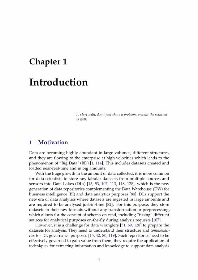
Data are becoming highly abundant in large volumes, different structures,and they are flowing to the enterprise at high velocities which leads to thephenomenon of “Big Data" (BD) [1, 114]. This includes datasets created andloaded near-real-time and in big amounts.
With the huge growth in the amount of data collected, it is more commonfor data scientists to store raw tabular datasets from multiple sources andsensors into Data Lakes (DLs) [13, 53, 107, 113, 118, 128], which is the newgeneration of data repositories complementing the Data Warehouse (DW) forbusiness intelligence (BI) and data analytics purposes [80]. DLs support thenew era of data analytics where datasets are ingested in large amounts andare required to be analysed just-in-time [82]. For this purpose, they storedatasets in their raw formats without any transformation or preprocessing,which allows for the concept of schema-on-read, including “fusing” differentsources for analytical purposes on-the-fly during analysis requests [107].
However, it is a challenge for data wranglers [51, 69, 128] to prepare thedatasets for analysis. They need to understand their structure and commonali-ties for DL governance purposes [15, 42, 80, 119]. Such repositories need to beeffectively governed to gain value from them; they require the application oftechniques for extracting information and knowledge to support data analysis
1

2. Background and State-of-the-art
and to prevent them from becoming an unusable data swamp [4] (a DL reposi-tory which is not well governed, does not maintain appropriate data qualitymeasures, and which stores data without associated metadata, decreasingtheir utility [13]). This involves the organised and automated extraction ofmetadata describing the structure of data stored [132], which is the main focusof this thesis. The main challenge for DL governance is related to informationdiscovery [95]: identifying related datasets that could be analysed together aswell as duplicated information to avoid repeating analysis efforts.
DLs should provide a standard access interface to support all its consumers[54, 91], including analysis by non-technical-savvy users who are interested inanalysing these data [13, 30, 92, 128]. Such access should support those dataconsumers in finding the required data in the large amounts of informationstored inside the DL for analytical purposes [132]. Currently, data preprocess-ing, including the crucial step of information discovery, consumes 70% of timespent in data analytics projects [128], which clearly needs to be decreased.To handle this challenge, this thesis proposes an integrated framework forextracting metadata describing the datasets stored in DLs and relationshipsbetween those datasets. Thus, we propose using Data Mining (DM) techniquesto effectively and efficiently extract similarity between datasets. Currently,there is a lack of such techniques for finding data patterns and similaritybetween datasets [2, 40, 84, 99, 105]. This is the focus of this thesis.
2 Background and State-of-the-art
In this section, we introduce the preliminaries and the main concepts relatedto DLs and their governance. We describe here the state-of-the-art of metadataextraction and management for governing DLs. We present an overview of theapproaches used, including the short-comings faced which we aim to solve inthe thesis.
2.1 Data Lakes and Tabular Datasets
DLs are large repositories of raw data coming from multiple data sourceswhich cover a wide-range of heterogeneous topics of interest [4, 82, 107]. Wefocus on DLs having datasets storing data in flat tabular formats as shown inFigure 1.1. These are organised as attributes and instances, such as commaseparated values (CSV) files, hypertext markup language (HTML) web tables,spreadsheets, HDFS tables in Hadoop1, etc. Such datasets are common in DLstoday [28, 42, 47].
These datasets have instances describing real-world entities, where eachis expressed as a set of attributes describing the properties of the entity. We
1https://hadoop.apache.org
2

2. Background and State-of-the-art
Att1 Att2 Att3
Value 1a 0.25 Value 3a
Value 1b 55.6 Value 3b
Value 1c 27.9 Value 3c
Value 1d 73.1 Value 3d
Attributes
Instances
Figure 1.1: A flat structured dataset consisting of tabular data organised as attributes andinstances
formally define a dataset D as a set of instances D “ tI1, I2, ...Inu. The datasethas a set of attributes S “ tA1, A2, ...Amu, where each attribute Ai has a fixedtype, and every instance has a value of the right type for each attribute. Wedistinguish between two types of attributes: continuous numeric attributeswith real numbers like ‘Att2’ in Figure 1.1, and categorical nominal attributeswith discrete values like ‘Att1’ and ‘Att3’.
2.2 Data Lake Governance
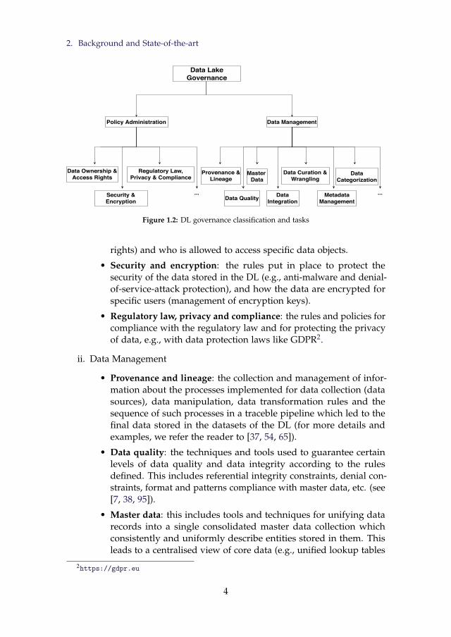
DL governance is concerned with management of the data stored appropriatelyso that they are easy to find, understand, utilise and administer in a timelymanner [12, 53, 106, 113, 118]. This makes the DL more accessible (searchable),data-driven, compliant to regulations, etc. It can be seen from two perspectivesas seen in the classification in Figure 1.2: (i) Policy administration and (ii)Data management. The first is about enacting procedures, managing peopleand responsibilities, implementing regulations, etc., while the latter is aboutthe technical implementation of protocols and technologies that help managethe data stored as an asset for supporting users in analysing them. Figure 1.2shows some of the main tasks required for each type of DL governance (thisis only a partial list of the most important tasks mainly based on [106] andour adapted / expanded classification from it).
We describe the different tasks of DL governance as follows:
i. Policy Administration
• Data ownership and access rights: the policies of data stewardshiprelated to the procedures and regulations for data sources allowedto be ingested in the DL, the persons responsible for managingspecific datasets and their metadata descriptions, and polices re-garding how the data should be used (read, write and delete access
3
2. Background and State-of-the-art
Data LakeGovernance
Policy Administration Data Management
Security &Encryption
Data Ownership &Access Rights
...
Provenance &Lineage
Data Quality MetadataManagement
DataCategorization
Data Curation &Wrangling
...
Master Data
Regulatory Law,Privacy & Compliance
DataIntegration
Figure 1.2: DL governance classification and tasks
rights) and who is allowed to access specific data objects.
• Security and encryption: the rules put in place to protect thesecurity of the data stored in the DL (e.g., anti-malware and denial-of-service-attack protection), and how the data are encrypted forspecific users (management of encryption keys).
• Regulatory law, privacy and compliance: the rules and policies forcompliance with the regulatory law and for protecting the privacyof data, e.g., with data protection laws like GDPR2.
ii. Data Management
• Provenance and lineage: the collection and management of infor-mation about the processes implemented for data collection (datasources), data manipulation, data transformation rules and thesequence of such processes in a traceble pipeline which led to thefinal data stored in the datasets of the DL (for more details andexamples, we refer the reader to [37, 54, 65]).
• Data quality: the techniques and tools used to guarantee certainlevels of data quality and data integrity according to the rulesdefined. This includes referential integrity constraints, denial con-straints, format and patterns compliance with master data, etc. (see[7, 38, 95]).
• Master data: this includes tools and techniques for unifying datarecords into a single consolidated master data collection whichconsistently and uniformly describe entities stored in them. Thisleads to a centralised view of core data (e.g., unified lookup tables
2https://gdpr.eu
4

2. Background and State-of-the-art
for entities and their identifiers), and is commonly called MasterData Management [92].
• Data integration: this involves combining and mapping differentdatasets together so that they can be used to answer analyticalqueries. It tackles overall, high-level and generic data requirements.For details see [14, 67, 93]. Other tasks include entity resolutionand deduplication [112, 56], and extract, transform and load (ETL)for creating a consolidated global schema or views over the data[63, 68, 97, 129].
• Data curation and wrangling: this includes the processes forpreparing data for BI and analytics, for structuring the data intomachine processable formats and schemata, and also using themetadata describing datasets to identify commonalities betweenthem, commonly called schema matching (see Section 3.1). These arecommonly tasks targeting a specific analytical goal. The reader canfind more details in [125, 128].
• Metadata Management: this is a transversal task serving all theother governance tasks. The datasets inside the DL need to bedescribed to include information about what they store (i.e., withsemantic definitions and data profiling statistics), how they arestored (e.g., data formats and schema definitions), where are theystored, how they are related to one another, etc. This is all con-sidered metadata, and the management of them in a centralisedrepository is the main task of concern here. For a detailed discus-sion of the types of metadata needed for DLs, the reader can check[25, 53, 54, 58, 108, 113, 119, 118, 122, 132]. As this is a core topicfor this thesis, we further describe specific metadata which need tobe collected and managed later in this section.
• Data categorization: we introduce this data management conceptfor DLs as the task involving the identification of information over-laps between datasets and data catalogues to understand what dataare owned in the DL. Such catalogues describe how the datasets areclassified into specific subject areas (topics). This is similar to dataclassification [106] as it also tags datasets with a category from acatalogue, however, for the purpose of this thesis, it is a data-drivenand automatic task rather than a manual data-tagging task. This isalso closely related to text-document categorization [19, 55], but itcategorizes tabular datasets as described in Section 2.1 rather thanfree-text documents. We describe this further in Sections 2.2 and5.2. Also see [16] and Chapter 5 for details.
5

2. Background and State-of-the-art
Data categorization is the data-driven task of automatically classifyingdatasets into pre-defined topics-of-interest (i.e., business domains) based onthe overlap between data stored in them and the common information theystore (i.e., dataset similarity).
In this thesis, we focus on the data management perspective and whenwe refer to our proposed approaches for DL governance we mean metadatamanagement for data categorization in specific, which we describe further inthis section.
Metadata Management for Data Categorization
There is currently a need for DL governance by collecting and managingmetadata about ingested datasets [14, 94, 95, 107, 119] to prevent the DL frombecoming a data swamp. In addition, proper DL governance should providean interactive data exploration interface that supports analysing relationshipsbetween datasets.
It is important to govern the data ingested into the DL and to be ableto describe the data with metadata [95, 119]. The current tools supportingmetadata collection in a DL environment (examples given below) usuallyinclude automatic and manual techniques for generating metadata. As canbe seen in Table 1.1, the tools are either automatically generating metadataabout data provenance or manually generating some data content descriptionsusing user tagging. Examples of such tools which are able to integrate withHadoop and which were available for us to survey include Apache Atlas3
(open-source tool), Teradata Loom4 (free non-commercial use), DataRPM5
(proprietary tool), Waterline6 (proprietary tool), Zaloni7 (proprietary tool),and Podium Data8 (proprietary tool). Other examples of tools which were notavailable at hand but which claim to support some metadata managementtasks for DLs include: Collibra9 (proprietary tool), Palantir10 (proprietarytool), and PoolParty Suite11 (proprietary tool).
Apache Atlas is mainly for general metadata management and it does notuse any DM techniques. It handles mainly the data provenance metadata for
3http://atlas.incubator.apache.org4http://loom.teradata.com5http://datarpm.com6http://www.waterlinedata.com/data-catalog-details7https://resources.zaloni.com/webinars/zaloni-bedrock-and-mica-20-minute-
demonstration8https://www.podiumdata.com/product/podium-platform9https://www.collibra.com/data-governance
10https://www.palantir.com11https://www.poolparty.biz/
6

2. Background and State-of-the-art
Technique Metadata Type Description
Automatic
Empty textFile-level metadata(e.g. filename, creationdate, source)
Empty textThe automatic processingof files ingested in the DLto collect provenancemetadata like file source,data creation and updatedate and time, dataownership, etc.
Manual User tagging of data
Empty textThis includes the usertagging the ingested datawith business taxonomies.The user tagging isexecuted using conditionalrules defined by the userdepending on the type ofdata source, e.g., tag alldata files loaded from thefinancial module of theenterprise system as“Financial". Anotherpossibility is the uservisually exploring the filesfrom each new data sourceand individually taggingthe instances seen by theuser.
Table 1.1: Current types of metadata tools for data lakes
the DL rather than data categorization. The Waterline data management toolcomplements Apache Atlas by adding capabilities for simple data profiling ofdatasets ingested in the DL (e.g., the top values per field, number of uniquevalues, etc.), which they call “Data Fingerprinting”. They only implementsimple data profiling techniques which does not include DM or cross-datasetsprofiling. Teradata Loom is mainly for data lineage and provenance man-agement of files and data manipulations / ingestion job tasks. It does somesimple statistical calculations on the input data using an automatic technologyfor data profiling called “Activescan”12, but only at the column level. Finally,DataRPM claims to have an automatic data curation platform (i.e., for data
12http://blogs.teradata.com/data-points/overview-of-teradata-loom-technology
7

2. Background and State-of-the-art
discovery and data preparation for analytics, whose details about data cu-ration can be found in [128]), but with little description, no case-study andno published research papers. After investigating this tool it was found thatit is more focused on natural language processing, similar to IBM Watson13.Although they claim that they can automatically curate data sources in theDL using machine learning14, there is little evidence in online material orpublished research about their techniques. This might be because the companydeveloping the tool is a relatively new start-up.
Other tools also include Apache Falcon15 (designed for the Hortonworksdistribution of Hadoop) and the Cloudera Navigator16 (designed for theCloudera Hadoop distribution). Both tools handle two of the most populardistributions of Hadoop. Concerning the support provided for handlingmetadata and data governance, those tools are mainly focused on DL oper-ations metadata like data provenance and lineage, in addition to manuallyuser-generated data catalogues. Both tools are targeting in newer versionsthe gradual addition of more exploratory content analytics and metadata,however, at the current time such support is very primitive and does notinclude advanced techniques like schema matching [24], ontology alignment[14, 126] or data mining [99].
The Waterline Data for Hadoop17 seems to be the closest solution availableto our envisioned metadata-based DL governance solution in this thesis. Thetool supports exploratory analysis and profiling of data ingested in the DL.However, it is currently lacking in the following aspects described in theresearch literature:
• Data and schema profiling [98, 115, 123]
• Schema and ontology matching [14, 24, 126]
• Machine learning and DM techniques for finding data patterns andsimilarity [2, 40, 84, 99, 105]
• Ontology integration (semantic metadata) [2, 3, 94, 132]
Tools implementing some of the above techniques for automatic profilingof datasets and metadata collection exist in the research literature. This in-cludes semantic RDF profiling tools [2], ontology mapping tools like ODIN[94], platforms for BD analysis like Metanome and Stratosphere data pro-filer [8, 102], metadata visualization tools for BD like [46, 57, 70], and dataprovenance metadata capture and management like [65]. Other research inves-tigated specific research problems for metadata management like: automatic
13http://www.ibm.com/smarterplanet/us/en/ibmwatson/what-is-watson.html14http://www.kdnuggets.com/2014/06/data-lakes-vs-data-warehouses.html15https://falcon.apache.org16https://www.cloudera.com/products/cloudera-navigator.html17http://www.waterlinedata.com/prod
8

2. Background and State-of-the-art
key and dependency detection [98], schema matching and evolution [120],entity resolution and matching [120], schema mining from semi-structureddata [10, 23, 105], ontology mining [3], etc. Those independent techniques stillneed to be directed and integrated in a coherent framework for profiling datain the DL and managing metadata about the content of the files [128]. Wemainly propose in this thesis an automated metadata management frameworkin Section 5.1 that augments many of those techniques in a novel approachwe call proximity mining, including: data and schema profiling, schema match-ing (see Section 3.1), and machine learning & DM techniques for similaritycomputations between datasets (see Section 3.3).
Most of the research literature [98] also demonstrates the shortcomings andgaps of current data profiling techniques for automatic metadata managementover the DL. The current shortcomings of the tools in research and industryindicate a lack of automatic data categorization capabilities which can besummarised in the list below:
1. Efficiently collect cross-dataset metadata like relationships between themusing automatic techniques.
2. Automatically categorize datasets into pre-defined topics of interest.
3. Provide better presentation and querying interfaces of metadata discov-ered from the DL which can make the data more accessible for BI.
As can be seen from the above list and Table 1.1, there is a need to have anautomatic process to generate the tagging (commonly called annotation [5]) ofdata content ingested in the DL using more efficient techniques compared tothe manual visual scanning of the files. This includes automatic techniquesfor data profiling and analysis of similarity of data content and relationshipsbetween datasets ingested in the DL, which is the main purpose of this thesis.
It is currently a challenge to create an analytical environment where thereis an integrated, subject-oriented view of the DL which is similar to that inthe data warehouse [64]. This poses the need for annotation of the datasets tofacilitate finding the relationships between them [30], which includes collectionof metadata about the informational content of the datasets in the DL [58].
We propose to govern the DL by means of cross-dataset metadata collec-tion and management so it does not become a disconnected group of datasilos where datasets can not be used together in meaningful analysis. This isdone by automating the data cataloguing tasks which include finding relateddatasets and categorizing datasets into topical domains. Thus, we handle DLgovernance from metadata management and dataset categorization perspec-tives, where we aim to support the users in understanding what datasets theyown, how they are related to one another, and to support automatic datasetcategorization. This should ultimately support data analytics over these data.
9

3. Techniques and Challenges
We aim to automatically and efficiently collect two types of metadata: con-tent metadata based on data profiling statistics and cross-dataset relationshipsusing DM (see Section 3.3) and schema matching (see Section 3.1). Tradi-tional data profiling and schema extraction involves analysing raw data forextracting metadata about the structural patterns and statistical distributionof datasets [98]. There is currently a need for higher-level profiling, whichinvolves the analysis of data and schemas [58, 116] using DM techniques[23, 87, 105]. This contributes to the computation of cross-dataset relationshipsto support information discovery and interpretation, in addition to automatictopical categorization of datasets, which are specific research challenges of DLgovernance we tackle.
Metadata querying and visualization
Metadata collected about the datasets in the DL should be presented to theusers using querying and visualisation interfaces. Some examples of suchqueryable metadata Graphical User Interface (GUI) include: [14] providesa query engine using SPARQL over metadata stored in an RDF repository,[34] provides a dataset search query engine over DLs, [54] provides keywordsearch over the dataset names and storage location paths, and [33] provides aquery language to query the indexes of attributes found in datasets to retrieverelevant ones. The goal is to retrieve datasets related to a specific subject-areaand all their datasets found in the enormous amount of data. We considerthat related datasets are those matched and found using the indexed metadatastored in the repository. This should support in describing and extractingsimilar data elements from data repositories, in order to reuse these data,mash-up the data for more plausible business problems and questions, and tobe able to handle this data discovery process [125].
We aim to provide solutions to the current shortcomings of such metadatadiscovery approaches for DLs. This includes the need for generic datasetmetadata handling which does not assume specific subject-areas (businessdomains) or availability of pre-defined metadata like mapping to a globalontology similar to the work in [14, 79, 96], context TF-IDF similarity ofwords around a web table found on the same webpage like [133], or specificpre-defined rules and patterns for data stored in the attributes like [134].
3 Techniques and Challenges
In order to support the DL governance tasks of automatic metadata collection& management and dataset categorization, we utilise different techniquesincluding schema matching, dataset similarity computation and supervisedmachine learning. We explain in this section those techniques, their currentshort-comings and their challenges which we tackle.
10

3. Techniques and Challenges
3.1 Schema Matching
The datasets in the DL usually cover a wide range of heterogeneous topicsmaking it difficult for the data scientist to identify overlapping attributes. Datawranglers must be able to find those datasets which have related data to beused together in data analysis tasks [82, 89], commonly referred to as schemamatching [24]. This supports in the automatic collection of metadata aboutcross-dataset relationships.
D2: census_data D3: health_data
A6: type {f,m,o} A11: gender {fem,mal,oth}
A7: age { 0<A2<100} A12: Ethnicity {EA,EB,EC,ED,EE,EF}
Sim(D2,D3) = 0.5D1: 1992_city_data
A1: salary {25k<A1<600k}
A2: age { 20<A2<97}
Sim(D1,D2) = 0.7
A7: age { 0<A2<100}
A13: age { 30<A3<60} A8: race {01,02,03,04,05,06}
{EA,EB,EC,ED,EE,EF}
A9: House_size { 0<A4<16} A14: Temp { 35<A4<42}
A10: sal { 50k<A5<300k} A15: H_rate { 40<A5<160}
A2: age { 20<A2<97}
A3: family_Size { 2<A3<11}
A4: identity {w,m,t,u}
A5: house_type {h,t,v,s,p,l} . . .
. . .
. . .
Figure 1.3: An example of schema matching and dataset similarity computation
We show an example for schema matching in Figure 1.3 with threedatasets and their attributes (each numbered starting with ‘A’), namely“1992_city_data”, “census_data” and “health_data”, where each dataset has5 attributes. Attributes can be numerical like ‘A1’, ‘A7’, etc. which havethe ranges shown. On the other hand, the attributes can be nominal like‘A4’, ‘A12’, etc. where we show the distinct values for each attribute. Thegoal of schema matching is to be able to find attributes between differentschemata (datasets) which store similar data. This is shown by the attributesconnected by arrows in the figure. Those attributes have similar values (andpossibly similar names as well), which should be automatically found usingschema matching techniques. Further, we label a similarity score we call ‘Sim’between dataset pairs, which is a real number in the range of r0, 1s describingthe overall dataset pair similarity (this is explained in Section 3.2).
Schema matching usually requires Cartesian product comparisons of at-tributes, entities and their values for calculating their similarity [73], with theaim of finding connection strengths between similar concepts from differentpairs of datasets [27, 35, 83, 104]. The large-scale application of such a task toBD repositories is referred to as holistic schema matching [18, 89, 104, 110, 133],where the goal is to match multiple datasets together considering them allin the matching task. With thousands of datasets and millions of attributesstored, there is a need for efficient similar attributes search, filtering schemamatching comparison tasks, commonly called early-pruning [24], as simple
11

3. Techniques and Challenges
brute-force similarity search of all pairs of attributes from different datasetsbecomes infeasible [54]. Alternatively, comparisons can be computed fasterusing parallel computing techniques like the MapReduce framework [133].
It is a challenge for data wranglers using the DL to efficiently processthe datasets to detect their common features, as schema matching tasks aregenerally expensive (involving huge amounts of string comparisons andmathematical calculations) [14, 24, 27, 60, 71]. In this thesis, we propose noveltechniques to reduce those comparisons using pre-filtering techniques thatreduce the number of comparisons. With the rise of DLs, previous researchlike [43] and [24] recommended using early-pruning steps to facilitate thetask using schema matching pre-filtering. Here, only datasets detected to be ofrelevant similarity are recommended for further fine-grained schema matchingtasks, and dissimilar ones should be filtered out from further comparisons.Such previous research like [24, 43] mentioned the need for early-pruningsteps but did not provide detailed solutions for this challenge. We explorethis with extensive details in Chapter 4.
Holistic schema matching techniques [110] seek to detect relationshipsbetween different schemata stored in a data repository. This can include rela-tionships between instances, which is called instance-based schema matchingand which is closely related to entity-resolution [24, 133], and also relation-ships between attributes (fields storing common information in structureddata), which is commonly called attribute-based schema matching. We focusin this thesis on the latter case within the environment of DLs. The goalof using those techniques in the DL is to detect relationships between theattributes inside different datasets. The output patterns from holistic schemamatching include multiple observations like: (i) Highly-similar and duplicatepairs of datasets (having similar schemata and data), and (ii) Outlier datasetswhich have no similarity with any other dataset in the DL (i.e., no similar at-tributes in the DL). The main challenges concerning this include the efficiency,scalability and handling the variety of topics found.
Current schema matching techniques are mainly based on Jaccard simi-larity of exact value matches and overlaps between attributes from datasets[33, 96, 101]. Those techniques fall short when values are coded differentlybetween different datasets and with the unavailability of extra semantic map-pings to ontologies or word embeddings like [96]. For example, in Figure 1.3we can see attribute “identity” (‘A4’) with the values “w”, “m”, “t” and “u” v.s.attribute “type” (‘A6’) with the values “f”, “m” and “o”. Both contain similarinformation but with different representations and attribute names whichclassical schema matching can not detect. This is also the same issue for (‘A8’)and (‘A12’) with different attribute names and value coding. Other challengesfor state-of-the-art schema matching include normalised v.s. non-normalisednumeric attributes, encrypted values v.s. non-encrypted values, etc. In thisthesis, we develop approximate matching techniques based on statistical
12

3. Techniques and Challenges
metadata, which do not necessarily require exact value overlaps betweendatasets.
SchemaMatching
Instance-based
Metadata-based
Valuematching
Stringcomparisons
Numericalcomparisons
Dataset-levelmatching
Attribute-levelmatching
Name stringscomparisons
Content statisticscomparisons
Name stringscomparisons
Content statisticscomparisons
Figure 1.4: Classification of schema matching techniques
Leading from the above discussion, for this thesis, we classify schemamatching as shown in Figure 1.4. Here, we can see on the left side the classicalschema matching techniques which seek to match values from instances in thedatasets. This is done using string comparisons of the values (and names ofattributes) or numerical comparisons for numerical attributes. This will havegood result with matching attributes like (‘A1’) and (‘A10’) from Figure 1.3 asthey have similar overlapping numerical values and similar attribute names.
On the other hand, we propose a new type of schema matching which wecall metadata-based schema matching.
Metadata-based schema matching pre-filtering techniques extract meta-data collected about the overall profiles of datasets or statistics about at-tributes for alleviating schema matching comparison tasks. The metadatais used to pre-filter dissimilar pairs of datasets to reduce the number ofcomparisons from the Cartesian product of value strings matching frominstances to a lower number of comparisons over the overall attributes’ anddatasets’ metadata.
For this purpose, we collect descriptive statistics about the attributes anddatasets to use them in the comparison task, which includes comparison ofname strings (e.g., using the edit distance [86]) and comparison of the statisticscollected about the content of the attributes (e.g., we can collect the number ofdistinct values for attributes and compare this when matching attribute pairs).We can collect such statistics at two levels: the dataset-level (e.g., the averagenumber of distinct values from all attributes in the dataset) or the attribute-level (e.g., the distinct number of values for each independent attribute, then
13

3. Techniques and Challenges
aggregating this to the dataset-level by averaging all the matching output foreach independent attribute). For example, in Figure 1.3, dataset D1 has anaverage of 4.5 distinct values for nominal attributes (3 for ‘A4’ and 6 for ‘A5’)while dataset D2 has an average of 3 distinct values for nominal attributes (2for ‘A6’ and 4 for ‘A9’).
Attribute-level comparisons are obviously at a more detailed level ofgranularity than the dataset-level. For example, in Figure 1.3, if we considerthe distinct values for each attribute to find the similarity between datasetD2 and D3 , we will find that they both have matching nominal attributes:‘A6’ and ‘A11’ with 3 distinct values each, and ‘A8’ with ‘A12’ with 6 distinctvalues each. Therefore, if we consider individual attributes they will have 100%matching nominal attributes, considering only ‘number of distinct values’.Such metadata-based schema matching is further explained in Chapters 3and 4, where the former investigates dataset-level matching and the latterinvestigates attribute-level matching.
Locality Sensitive Hashing
Locality sensitive hashing (LSH) [31, 44] is a family of techniques for groupingtogether objects of high probability of similarity18. Objects assigned to thesame block are further compared using more expensive computational tech-niques [117], like schema matching tasks involving string comparison of valuesand statistical computations of similarity from data profiles of attributes.
The challenge is to find an adequate LSH algorithm with a relevant simi-larity function and a list of features to use to compute an approximation ofthe similarity between objects inside the datasets [28, 33] to support schemamatching. For example, in [44] they propose LSH based on the MinHashalgorithm for entity resolution in ontologies using term frequencies. We applysimilar LSH techniques in this thesis when implementing instance-based valuematching in Chapter 2.
3.2 Dataset Similarity Computation
As low-level instance-based schema matching is computationally expensive,there is a need for a filtering strategy that computes similarities of datasets in acheaper way so that schema matching is conducted only in similar cases. Thisis done by applying a pre-filtering task before schema matching (i.e., early-pruning), where there needs to be dataset similarity computation techniquesthat can assign an estimation of the overall similarity score between datasets.This can be seen in Figure 1.3, where we give a similarity score betweendatasets using the connecting arrows between the dataset names. For example,
18Contrary to the classical hashing goals for database partitioning, where the goal is to putsimilar objects into different groups.
14

3. Techniques and Challenges
datasets D1 and D2 have an overall similarity of 0.7 (on a range of r0, 1s, i.e.,70% similarity) considering the attributes they store and the overlaps betweenthem.
Most similarity comptuation algorithms utilise attribute names stringcomparisons when computing dataset similarity [28, 33, 35, 36, 59, 79, 88,100, 104, 117, 133]. This becomes problematic in real-world scenarios whenattributes are not properly named or are named using generically generatedcodes [27, 96].
The current state-of-the-art mainly includes expensive computations thatinvolve string-matching of values found in attributes. The shortcoming of suchtechniques is that they can only match exact values of strings and can thereforenot produce approximate similarity computations which compare the overallsimilarity of attributes even if the values are coded differently. For example,[28, 33, 96, 101, 117, 133] aim to index and find similar attributes based on theexact values they store, mainly using Jaccard similarity computations like in[28, 96, 101, 117]. Other research like [60, 59, 96] use semantic based dictionarysearch of synonyms over values to improve the matching process. In [59], theyalso use extra query log metadata to find related attributes commonly usedtogether in search queries. Extra schema metadata like common primary keysbetween datasets can also be used as an indicator for dataset similarity [54].
Other techniques like [134] assume that datasets have attributes storingvalues according to a specific format or template (sequence of codes) which arepre-defined by the data analyst. Values are defined according to convertiblevalues using conversion rules (e.g., measurements in inches and feet). Thosetechniques are restricted to only matching those attributes which store thosespecific values defined by the format rules, therefore limiting the generalis-ability of their application with different domains and heterogeneous topicsof interest. We tackle those challenges and shortcomings in our proposedproximity mining approach introduced in the next section and Section 5.1.
3.3 Similarity Models Learning
We propose a novel approach (see Section 5.1) that learns similarity modelswhich are capable of detecting similar and dissimilar datasets to support theapproximation of dataset similarity computation and the early-pruning taskof holistic schema matching. This is done using supervised machine learning.
Supervised machine learning is a group of classical techniques used inartificial intelligence and data mining for automatically learning models fromdata examples to support future estimation, classification or prediction ofsimilar cases. This has been discussed extensively in textbooks like [127]and [32]. The main idea is to be able to make a computer (machine) learnfrom training examples to classify, predict, or estimate a dependent variable(the output, also called target variable) for new examples (commonly called
15

3. Techniques and Challenges
unseen instances) based on similarity to previous already seen instances withknown classification or values for the dependent variable (commonly calledtraining instances). This similarity needs to be measured according to a setof features that describe information about the instances. In contrast withsupervised machine learning, there is also unsupervised machine learning. Insuch learning problems, the instances do not have a predefined classificationor value for a dependent variable, rather, one common goal is to use thefeatures describing such instances to segment them into groups of highlysimilar instances (commonly called clustering) so we can automatically detectif there is meaningful grouping which can classify the instances into classes(i.e., the goal is to define the classification classes for instances which we donot already know in advance). This type of unsupervised learning does notrequire any training data (i.e., no pre-advanced annotated examples needed).
Supervised machine learning algorithms create models which are capableof getting an input set of features about unseen instances, to apply a groupof functions that check the similarity of those instances against previouslyseen instances based on those features, and to output a classification (if theoutput is binary or categorical) or estimation (if the output is a continuousnumber) for the dependent variable. The model created could be a decisiontree, a probabilistic statistical model, a mathematical regression, etc.
We give an example of a supervised learning model in Figure 1.5. Thismodel should be the resulting output from running a learning algorithmwith some training instances. The figure shows the outcome consisting ofa decision tree where the parent (top) node has an input of a previouslyunseen instance. In this toy example, we use the topic of this thesis, where weconsider input descriptions for a pair of datasets, which we call Dy and Dz,in order to decide if they are related to each other or not. The input featurescould include a percentage of the difference between the attribute names andattribute values from both datasets. Each node in the tree is a decision whichtakes as input one of those features and decides which branch of the tree totake based on the condition in the node. The leaf nodes (lowest children in thetree visualised as shaded boxes) give the output classification by the decisiontree. In this example, the output is binary: ‘0’ for not related and ‘1’ for relateddatasets. For example, if more than 80% of the attributes have similar namesthen they are considered to be related (as they are ă 20% different), whileif they have more than 50% difference in the attribute names and more than25% in their values, then they are considered not to be related. Decision treesare one type of supervised models for classification, but other types exist asdiscussed earlier (e.g., naive Bayes probabilistic approaches, lazy learners19
like k-nearest neighbour (k-NN), logistic regression for binary classification,
19They are called lazy learners because they do not create a model in advance, rather, theycheck unseen instances against all previously stored examples of classified instances in a databasein order to recommend a classification based on the most similar instances found.
16

3. Techniques and Challenges
New datasetpair
[Dy,Dz]
Yes
Yes
No
Attribute names difference
< 20%
Related(1)
Yes No
Attribute valuesdifference
< 40%
Related(1)
Not Related(0)
No
Attribute names difference
< 50%
Yes No
Attribute valuesdifference
< 25%
Related(1)
Not Related(0)
Figure 1.5: Example of a decision tree model for classification of related dataset pairs
linear regression for real-value estimation, etc.).To create a better performing machine learning model capable of more
accurately classifying new instances, it is common to create a grouping ofindependent models from multiple algorithms to create a single model com-bining them to give a single output. The combination can be a weightedaggregation or combination of the output from the independent models. Thisis illustrated in Figure 1.6, where we give an example of a decision tree ensem-ble consisting of multiple decision trees (from 1 to n). The output is combinedusing a weighted function (with weights ‘W’) to give a single classification asa final output. Common ensemble algorithms include boosting techniqueslike AdaBoost [49], decision tree ensembles like RandomForest [29], etc.
One of the common pitfalls of supervised machine learning is the dilemmaof overfitting, where there is a trade-off between highly accurate models andoverfitting of those models. Overfitting has a negative connotation as it meansthat the models are highly matching the exact cases in the training instances,to the extent that even the noise in such instances (i.e., instances which aremisclassified, erroneous, exceptional, etc.) are incorporated in the models.
17

4. Thesis Objectives and Research Questions
W1
W2
Wn
Decision Tree 1 Decision Tree 2 Decision Tree n
...
FinalClassification
Figure 1.6: An ensemble of decision trees for classification
This makes such overfitted models not generalisable to other instances fromanother sample not seen in the training, leading to lower performance andaccuracy when applied to them. This problem is commonly avoided by: doingcross-validation evaluation of models and optimising the performance forall runs of the validation process, removing noise from the input data (forexample by data cleansing), removing irrelevant or correlated features used inthe training of the models, selecting more relevant features for training, using abigger data sample, using a supervised learning algorithm which intrinsicallyleads to less bias and variance like RandomForest ensemble learners, etc.
We aim to develop a similarity technique for dataset pairs based on a setof meta-features we collect to describe them, and then applying supervisedmachine learning algorithms (including ensemble techniques) to create accu-rate models which can support the similarity computation task. The mainchallenge is finding adequate features and a generalisable approach to handlesuch similarity computations accurately and efficiently. We use supervisedmachine learning techniques to compute dataset similarity in Chapters 3 and4.
4 Thesis Objectives and Research Questions
The goal of this thesis is to implement an effective framework that can fillthe research gaps presented in the previous discussion. This includes thefollowing objectives:
18

4. Thesis Objectives and Research Questions
• Objective A: Formulate techniques that can efficiently and effectivelycompute approximation of dataset similarity.
• Objective B: Develop a framework based on approximate dataset similar-ity techniques that can support DL governance, mainly cross-dataset rela-tionships metadata management, holistic schema matching pre-filteringand automatic dataset categorization.
• Objective C: Validate our proposed framework in a real-world DL envi-ronment.
For Objective A, we formulate techniques which are able to approximateoverall dataset similarity based on metadata we collect from them, includingattribute profiles. In order to compute dataset similarity, we utilise supervisedmachine learning algorithms (e.g., RandomForest ensemble learners [29]).Such algorithms are able to learn from training examples to distinguishbetween different classification categories, where in this thesis we aim todifferentiate between similar and dissimilar dataset pairs based on the overlapbetween their data. We propose an approach that uses those techniquesto effectively and efficiently compute such similarity using the metadataextracted.
Then, for Objective B, we exploit the output dataset similarity computationsin specific DL governance tasks. This includes supporting the early-pruninggoal for holistic schema matching, in addition to supporting dataset topicalclassification using automatic categorization techniques. The thesis defines aframework for extracting the schema metadata from flat tabular datasets usingclassical techniques, in addition to experimentation with novel techniquesthat can successfully tackle extraction of cross-datasets relationships, whichinclude computation of attribute similarity between different datasets.
Finally, for Objective C, we validate our proposed framework and itsutilised techniques on a real-world DL called OpenML20 in our experiments[131], which has a large amount of datasets intended for analytics fromdifferent subject areas. OpenML is a web-based data repository that allows toupload different datasets used in DM experiments. OpenML stores datasetsin the ARFF tabular format which consists of diverse raw data loaded withoutany specific integration schema. This allows us to evaluate our approach in areal-life setting where datasets come from heterogeneous domains.
The above objectives can be translated into specific research questions asfollows:
• Dataset Similarity Computation
– Research Question RQ1: How can we use instance-based schemamatching techniques for computing dataset similarity?
20https://www.openml.org
19

5. Thesis Overview
– Research Question RQ2: How can we use schema and data pro-files in computing proximity between structured datasets usingsupervised machine learning techniques?
• Metadata Exploitation for Governing DLs
– Research Question RQ3: How can we use proximity scores be-tween datasets to pre-filter schema matching comparisons for earlypruning purposes?
– Research Question RQ4: How can we use proximity scores be-tween datasets to automatically and correctly categorize datasetsinto pre-existing categories of interest?
– Research Question RQ5: How can the content metadata be used tobrowse the DL and to support the users in finding relevant datasetswith overlapping data?
5 Thesis Overview
In this section we present an overview of the thesis, including the proposedproximity mining framework, the DL categorization challenge and how wetackle it, and finally the metadata query interface.
5.1 Proximity Mining Framework
We formulate a framework that caters for the current shortcoming of a for-malized metadata management process in the DL, with the goal of ingestingflat tabular datasets, extracting metadata describing them, using the metadatato find relationships, and finally categorising them in order to support gov-ernance. This is visualised in Figure 1.7, where we see at the bottom a set ofdatasets. First, we ingest them into the DL, parsing them to check that theyhave no errors and extract their schema, which includes description of theattributes found, their names and data types. All metadata extracted is storedin a database (stored as “schema metadata”), where each dataset is annotatedwith its corresponding schema description.
In the data digestion stage, we profile the datasets to extract distributionsand statistics about their attributes, which are stored as “dataset contentmetadata”. Then, we apply the proposed proximity mining techniques toextract relationships between different datasets, including similar schema (andduplicate schema with very high similarity), and we store this as cross-schemarelationships.
20

5. Thesis Overview
Ingest Data1Parse
Dataset
3Data
Profiling
Digest Data
2Extract
Schema
4Proximity
Mining
ExploitMetadata
Data LakeCategorization
SchemaMatching
Pre-filtering
DataLake
Browse DataLake
DatasetContent
Metadata
Cross-SchemaRelationshipsMetadata
Schema annotation
(A)Profile
annotation
(B)Cross-Profile
Relationships annotation
SchemaMetadata
Figure 1.7: Overview of the proposed proxmity mining framework
We define proximity mining as a data mining process for the extraction ofcross-dataset similarity using metadata-based supervised machine learningmodels.
Our proposed framework integrates DM techniques in the DL for enablinganalytical discovery of cross-dataset content relationships. We introduce inChapters 3 and 4 a novel supervised machine learning technique for com-puting cross-dataset similarity, which makes the basis of proximity mining.We mainly adapt the classical techniques of DM to the new environment ofthe DL and BD. This includes application of DM to discover similar datasetprofiles and related attributes between them.
Finally, the extracted metadata are exploited in the top-most stage, wherethe user (commonly a data wrangler [51, 69, 128]) is able to browse the DLfor finding relevant datasets with overlapping data. In addition, they are ableto categorize the datasets ingested based on the most similar ones alreadyexisting, and applying pre-filtering steps to prune unnecessary comparisonsof dataset pairs before running schema matching techniques. We use DM tech-niques for the pre-filtering task in Chapter 4 and the automatic categorizationof datasets in Chapter 5.
DM techniques (especially, supervised machine learning) are utilised inthe thesis to extract useful metadata about the content of the datasets and
21

5. Thesis Overview
metadata about the relationships between them. This includes data profilesand relevant information for the data scientist. Therefore, this thesis uses thecontributions of the DM field and applies it in the data management contextto achieve our thesis objectives. Examples of such application of DM include:
• Using supervised machine learning DM techniques to compute proxim-ities between datasets and to detect patterns in their metadata for theschema matching process.
• Using nearest-neighbour techniques with the metadata to automaticallyfind topical categories of datasets in the DL.
• Finding outliers which constitute abnormal data content which is notrelated to other datasets in the DL.
We model our approach as a 3-stages framework where each higher stagedoes less data analysis and gives more concise (summarised) information.The lowest ingestion stage has to scan the complete raw dataset files to checktheir correctness and extract their schema, the digestion stage only has to scanattributes to extract data profiles and proximity metrics, and finally the higheststage of exploitation only scans metadata without going through the raw datainside each dataset.
The proposed framework can be applied in the context of BI inside largebusiness organizations with huge amounts of data or in the context of gov-ernment administrations requiring a coherent framework of DL governance.Our framework also helps the data consumers understand the informationowned in the DL in a quick and easy fashion. As a result, organizations candiscover new analytical opportunities for BI and improve the time-to-value ofanalysing the DL.
Metadata Process Overview V6.4_thesis
Prox
imit
y M
inin
g M
etad
ata
Man
agem
ent
Dig
est
Dat
a
DigestData
DIG01 (Ch3)Profile the datasets
DIG04 (Ch2/3/4)Compute dataset-level
proximity
DIG02 (Ch4)Profile the attributesinside the datasets
DIG03 (Ch4)Find top matching
attributes
Expl
oit
Met
adat
a
ExploitMetadata
Datasets annotated
EXP04 (Ch6)Browse DL proximity
graph
EXP03 (Ch5)Categorize datasets
using proximitymining output
EXP01 (Ch3)Find duplicate andrelated schema in
datatsets
EXP02 (Ch4)Filter the dataset pairs to
be compared usingproximity mining
Inge
stD
ata
IngestData
ING01 (Ch2)Extract
schema fromdatasetsAnalyse DL
ING02 (Ch2)Sample the datasets'instances for profiling
Figure 1.8: The proximity mining metadata management process
22

5. Thesis Overview
In order to implement the proposed proximity mining framework inFigure 1.7, we instantiate it using prototypical implementations which use thetechniques described earlier in this chapter (Section 3). This is visualised inFigure 1.8 as a BPMN process where each activity starts with an identifierfor the activity (e.g., ‘ING01’), followed by the chapter number(s) where thecomponent is described in parentheses, and a description. The process isorganised into the three stages from Figure 1.7. In ingestion, the schema isextracted in ING01 and a random sample of the instances is collected in ING02for passing it to the next level of digesting the data.
Digestion starts with the dataset content metadata extraction using dataprofiling techniques. The datasets are profiled in DIG01 based on the sam-pled instances from the previous activity. In DIG01, we compute high-levelsummary statistics that describe the whole dataset. In DIG02, we computefiner-grained statistics about each individual attribute inside the datasets.
Then, we compute the cross-schema relationships metadata by matchingattributes between different datasets, where their data profiles (and theirattributes) are compared in DIG03 in order to find related attributes withsimilar data profiles and mapping each attribute to its top matching attributefrom the other datasets. The output from this activity is fed to the proximitymining models in DIG04 in order to compute overall dataset-level similarityscores.
Once the datasets are profiled and cross-schema relationships are com-puted, the metadata generated are stored in a repository and are utilised fordifferent tasks and applications. In EXP01, dataset pairs with high proximityscores are marked as related schema if they exceed a specific similarity thresh-old, or duplicated schema if the dataset pair is highly similar. Based on theoutput from EXP01, we aim in activity EXP02 to support the early-pruningtask for holistic schema matching by pre-filtering dissimilar dataset pairs witha low similarity score from any further comparisons. We also aim in EXP03 tocategorize datasets with unknown topics into a recommended topic groupingbased on the most similar datasets found in the DL. Finally, in EXP04, all themetadata collected are provided to the DL user in order to browse the datasetsin the DL by topics or by finding dataset pairs with highly similar schemata(possible overlapping data). This can be presented as a proximity graph wherenodes represent datasets and edges represent the proximity scores betweenthose datasets. We describe how we present the proximity graph and theoutput of exploitation in the following sub-sections.
5.2 DL Categorization
One of the tasks of DL Governance is effective data categorization. This meansfinding the subject areas in the datasets and classifying them accordingly. Thissupports data discovery which includes finding related datasets [10, 95] that
23

5. Thesis Overview
can be analysed together, duplicate datasets for data quality checks [56], andoutlier datasets [74].
2
5
4
3
1
16
18
1915 17
14
9
10
8
713
6 11
12
Topic 1
Topic 2
Topic 3
20s=0.1
s=0.97
s=0.33
s=0.89
s=0.15
s=0.29
s=0.19s=0.99
s=0.90
s=0.86
s=0.27
s=0.22
s=0.50
s=0.96
s=0.99
s=0.09
s=0.89
s=0.73
s=0.47
s=0.73s=0.29
s=0.67
s=0.07
s=0.33
s=0.82
Figure 1.9: A proximity graph showing topic-wise groupings of interlinked datasets in the DLwith their similarity scores
We seek to detect topic-wise categories of datasets in the DL describingsimilar real-life subject areas and business domains. This includes groupingsof highly related datasets with similar data components stored inside them,as depicted in the proximity graph in Figure 1.9. Here we show groupings ofdatasets into topic-wise clusters. Each numbered node is a dataset and theedges connecting them show a similarity score, where 1 means most similarand 0 means most dissimilar. The goal is to be able to maintain such groupingsover the DL, where each topical cluster consists of interlinked datasets thatare similar to each other.
We tackle this challenge by first extracting metadata describing the contentof the datasets in the DL in order to implement this categorization. We usethe relationships detected between pairs of datasets to find their proximity(similarities). Then, we use a measure of proximity between datasets usingthose detected relationships within the categorization algorithm, and finallywe allocate datasets to the topics existing in the DL based on their most similarcluster found in the DL or indicating that a dataset is an outlier that does notbelong to any such topic if no highly similar datasets are found [10, 105].
We allocate Chapter 5 to discuss the concept of automatic dataset catego-rization into pre-existing topics-of-interest where we are able to group datasetscontaining data about the same topic into the same grouping. This is a firststep toward fully automatic dataset categorisation for governing diverse DLs.
24
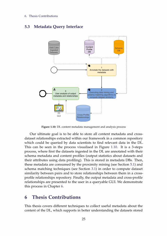
6. Thesis Contributions
5.3 Metadata Query Interface
Data LakeIngestedDatasets
1Annotate the datasets with
metadata
SchemaDB
2Executing data mining and
schema matching algorithms tocompute dataset similarity
Cross-ProfileRelationships
3User analysis of output
metadata and relationships
GUI
ContentProfile
DB
Figure 1.10: DL content metadata management and analysis process
Our ultimate goal is to be able to store all content metadata and cross-dataset relationships extracted within our framework in a common repositorywhich could be queried by data scientists to find relevant data in the DL.This can be seen in the process visualised in Figure 1.10. It is a 3-stepsprocess, where first the datasets ingested in the DL are annotated with theirschema metadata and content profiles (output statistics about datasets andtheir attributes using data profiling). This is stored in metadata DBs. Then,these metadata are consumed by the proximity mining (see Section 5.1) andschema matching techniques (see Section 3.1) in order to compute datasetsimilarity between pairs and to store relationships between them in a cross-profile relationships repository. Finally, the output metadata and cross-profilerelationships are presented to the user in a queryable GUI. We demonstratethis process in Chapter 6.
6 Thesis Contributions
This thesis covers different techniques to collect useful metadata about thecontent of the DL, which supports in better understanding the datasets stored
25

6. Thesis Contributions
and their relationships, including automatic algorithms for that collection. Theresearch undertaken is expected to contribute to multiple fields, but mainly tothe data management community. The outcome directly contributes to datamanagement by creating new knowledge about managing metadata, which in-cludes techniques to efficiently and effectively gather them to support holisticschema matching, information discovery and information summarisation.
Thus, the thesis formalises the DL metadata management process forgovernance purposes, experimenting with some schema matching techniquesfor detecting relationships, and using DM techniques to compute proximitybetween pairs of datasets. This includes reviewing the different techniquespreviously utilised in the research literature and adapting/improving thosetechniques in a holistic process to answer the research questions in Section4. In addition, we experiment with the data ingestion process of metadataextraction, which allows for the utilisation of schema matching and ontologyalignment techniques, like those in [126], to successfully compute similarityand cross-schema relationships between datasets. A novel DM-based approachto compute data profile similarity to find duplicates and relationships is alsoevaluated for the early-pruning step of holistic schema matching, makingsome new development and advancement for this topic.
For information discovery, the techniques proposed help discover dataprofiles and relationships between datasets to support identification of do-mains within the DL and identification of related datasets. As for informationsummarisation, the techniques investigated support producing statistical sum-maries and patterns from the data which efficiently describe their content.Finally, data schemas are extracted to maintain knowledge about datasetstructures and how they can be used together to improve data utilisation.In addition, the output metadata are managed to enhance integration andquerying for analytical discovery, which helps in the utility of the DL.
We implement and experiment with new proximity mining techniques(we describe them in Section 5.1) and prove their capabilities in accuratelyand efficiently computing similarities between heterogeneous schemata. Wepropose generic techniques that do not assume any specific topic or businessdomains, and improve the performance of the schema matching pre-filteringtask, outperforming the state-of-the-art instance-based schema matching tech-niques. In our proposed techniques, we use metadata-based approximationwhen matching datasets and their attributes instead of the current state-of-the-art involving exact-value string-matching techniques. This helps in findingrelated attributes and datasets where the data are coded or named differentlybetween datasets. Thus, we handle the shortcomings of current techniquesfor dataset similarity computation (see Section 3.2) by developing a proximitymining based approach in Chapters 3 and 4 which achieves the following:
• Extract automatic metadata about the data content stored in datasets at
26

7. Structure of the Thesis
the attribute- and dataset- levels.
• Propose similarity approximation techniques which do not depend onexact value matching and name based string-matching only.
• Propose generic approaches which do not assume the existence of anyspecific attribute value formats, conversion rules, topic domains, orthe existence of pre-defined metadata describing the datasets and theirattributes like ontology mappings.
This thesis examines multiple directions of research in data management,where the main contributions include answering the RQs in Section 4 asfollows:
1. rRQ1s Develop an approach for dataset similarity computation usinginstance-level schema matching between datasets.
2. rRQ2s Formulate a supervised machine learning technique to find prox-imity between heterogeneous datasets covering diverse topics.
3. rRQ2s Develop an approximate metadata-based schema matching ap-proach where the goal is not to depend solely on syntactic string-basedmatching but also on data profiles.
4. rRQ3s Experiment with techniques for schema matching early-pruningand introduce the concept of pre-filtering using proximity mining.
5. rRQ3, RQ4s Propose a framework that utilises proximity mining in DLgovernance, mainly for dataset categorisation and schema matchingpre-filtering.
6. rRQ5s Develop a GUI to query and use the output from our work tohelp in discovering the datasets stored in the DL and their relationships.
7 Structure of the Thesis
We aim to conduct the following tasks: (i) Framework conceptualisation andformalisation for the holistic proximity mining and metadata management inthe DL, (ii) Prototyping with instance-based techniques for matching datasets,(iii) Implementing efficient and effective proximity mining techniques forearly-pruning within holistic schema matching, (iv) Efficient pre-filteringschema matching implementation, and (v) Effective categorization techniquesfor segmenting the DL.
The thesis is organised as follows:
27

7. Structure of the Thesis
7.1 Chapter 2: Instance-level value-based schema matchingfor mining proximity between datasets
This chapter focuses on Objectives A and C and tackles Research QuestionRQ1. The goal is to apply instance-level value-based schema matching tech-niques to find related attributes between datasets and to compute overalldataset-level similarity. This includes the implementation of dataset similaritycomputation based on probabilistic value-based string matching techniques[126]. The computed relationships are aggregated to give overall dataset-level proximity scores between datasets. We experiment with different stringmatching techniques and different instance sampling sizes, where we test ourproposed approach on a sample from a real-world DL to prove its effectiveness.The experiment includes comparison of performance of our proposed auto-mated approach against human-based analysis, where our approach was ableto achieve a better performance when compared to humans. The approachwas found to be effective as a first step towards fully automated metadatacollection and management framework fro DLs. However, some shortcomingswere found, including the expensive computations required for the schemamatching task which need to improve by using a more efficient approach.This is achieved in Chapters 3 and 4 using higher-level approximate schemamatching pre-filtering techniques.
The chapter incorporates the tasks ING01, ING02, DIG03 and DIG04 fromFigure 1.8. As this approach handles the raw dataset and does not use anycontent-based metadata, it does not need to implement tasks DIG01-02.
7.2 Chapter 3: Dataset-level content metadata based proxim-ity mining
This chapter focuses on Objectives A and C and tackles research questionRQ2. We introduce the concept of proximity mining where we collect high-level,overall dataset content metadata using data profiling techniques, and we usethese metadata in supervised machine learning techniques for computingcross-dataset proximity (similarities) and duplicate schemata. We experimentour proposed techniques on a real-world DL, where we are able to detectrelated and duplicated datasets using high recall rates and efficiency gains.This includes tasks DIG01, DIG04 and EXP01 from Figure 1.8.
7.3 Chapter 4: Attribute-level content metadata based prox-imity mining for pre-filtering schema matching
This chapter focuses on Objectives A, B, and C and tackles research questionRQ3. We aim to improve the proximity mining techniques from Chapter 3by computing finer-granularity proximity scores between attributes and then
28
7. Structure of the Thesis
computing overall dataset-level proximities by aggregating the individualproximity scores between the top-matching attributes for a dataset pair. Wedemonstrate an application of our proposed techniques by pre-filtering schemamatching comparisons effectively and efficiently. Here, we are able to filterirrelevant dataset pairs with a low proximity score from further detailedvalue-based schema matching at the instance-level. We compare our approachagainst the state-of-the-art instance-based matching techniques and prove thatour proposed approach is more efficient and effective in detecting relateddatasets. This supports the goal of early-pruning, where we reduce theamount of comparisons for schema matching. This includes tasks DIG02,DIG03, DIG04 and EXP02 from Figure 1.8.
7.4 Chapter 5: Automatic categorization of datasets using prox-imity mining
This chapter focuses on Objectives B and C and tackles research questionRQ4. The goal is to identify a category of a dataset based on the most similardatasets already existing inside the DL. We devise a k-nearest-neighbourbased approach to handle this task, where we find the top-k most similardatasets depending on the extracted cross-dataset relationships metadataand we allocate the most common category among those datasets as theappropriate category. We experiment using a real-world DL sample and findthat our approach is highly effective in terms of recall and precision. Thisincludes task EXP03 from Figure 1.8.
7.5 Chapter 6: Prox-mine tool for browsing DLs using prox-imity mining
This chapter focuses on Objective C and tackles research question RQ5. Here,we integrate the different components and techniques of our approach intoa single prototype to demonstrate the value of proximity mining techniquesin a real-world setting. We implement a prototype that can handle datasetingestion, digestion and metadata exploitation for browsing the DL. Thisincludes tasks EXP04 from Figure 1.8, in order to support the DL user in thefollowing tasks:
• Find related and duplicated datasets.
• Identify the category of a new dataset based on the most similar datasetsexisting in the DL.
• Identify the top-matching attribute candidates between a dataset pairfor detailed schema matching.
29

7. Structure of the Thesis
• Browse the DL based on a proximity graph visualisation that showsthe relationships between datasets inside the DL using their computedproximity scores.
30

Chapter 2
Instance-level value-basedschema matching forcomputing dataset similarity
Everything starts as an experimental prototype underdevelopment, then it keeps changing, learning, evolving, andadapting over time. Everything that gets measured eventuallygets managed. One never stops learning!
This chapter has been published as a paper in the proceedings of the 16thInternational Conference on Data Mining Workshops (ICDMW) (2016) [15].The layout of the paper has been revisedDOI: https://doi.org/10.1109/ICDMW.2016.0033
IEEE copyright / credit notice:© 2016 IEEE. Reprinted with permission from Ayman Alserafi, Alberto Abelló,Oscar Romero, Toon Calders. Towards Information Profiling: Data LakeContent Metadata Management, ICDM workshops, 2016.
31

Abstract
There is currently a burst of Big Data (BD) processed and stored in huge raw datarepositories, commonly called Data Lakes (DL). These BD require new techniquesof data integration and schema alignment in order to make the data usable by itsconsumers and to discover the relationships linking their content. This can be providedby metadata services which discover and describe their content. However, there iscurrently a lack of a systematic approach for such kind of metadata discovery andmanagement. Thus, we propose a framework for the profiling of informational contentstored in the DL, which we call information profiling. The profiles are stored as meta-data to support data analysis. We formally define a metadata management processwhich identifies the key activities required to effectively handle this. We demonstratethe alternative techniques and performance of our process using a prototype imple-mentation handling a real-life case-study from the OpenML DL, which showcases thevalue and feasibility of our approach.
32

1. Introduction
1 Introduction
There is currently a huge growth in the amount, variety, and velocity of dataingested in analytical data repositories. Such data are commonly called BigData (BD). Data repositories storing such BD in their original raw-format arecommonly called Data Lakes (DL) [128]. DL are characterised by having alarge amount of data covering different subjects, which need to be analysed bynon-experts in IT commonly called data enthusiasts [91]. To support the dataenthusiast in analysing the data in the DL, there must be a data governanceprocess which describes the content using metadata. Such process shoulddescribe the informational content of the data ingested using the least intrusivetechniques. The metadata can then be exploited by the data enthusiast todiscover relationships between datasets, duplicated data, and outliers whichhave no other datasets related to them.
In this chapter, we investigate the appropriate process and techniquesrequired to manage the metadata about the informational content of the DL.We specifically focus on addressing the challenges of variety and variability ofBD ingested in the DL. The metadata discovered supports data consumers infinding the required data in the large amounts of information stored insidethe DL for analytical purposes [132]. Currently, information discovery toidentify, locate, integrate and reengineer data consumes 70% of time spentin data analytics project [128], which clearly needs to be decreased. Tohandle this challenge, this chapter proposes (i) a systematic process for theschema annotation of data ingested in the DL and (ii) the systematic extraction,management and exploitation of metadata about the datasets’ content and theirrelationship by means of existing schema matching and ontology alignmenttechniques [13, 24, 126].
The proposed process allows for the automation of data governance tasksfor the DL. To our knowledge, the proposed framework is the first holisticapproach which integrates automated techniques for supporting analyticaldiscovery of cross-DL content relationships, which we call information profiles asexplained below. This should cater for the current shortcoming of a formalizedmetadata management process to prevent the DL from becoming a data swamp;that is a DL that is not well governed and can not maintain appropriatedata quality. Data swamps store data without metadata describing them,decreasing their utility [13].
Information Profiling. Traditional schema extraction and data profilinginvolves analysing raw data for detecting structural patterns and statisticaldistributions [98]. There is currently a need for higher-level profiling whichinvolves analysing information about the approximate schema & instancesrelationships between different datasets instead of just single datasets [58],
33

1. Introduction
which we specifically define as Information Profiling. This involves theanalysis of metadata and schema [58, 116] extracted from the raw datausing ontology alignment techniques [24, 126]. Such techniques exploit 1.schema metadata and 2. data profile metadata to match different attributesfrom different datasets, generating the information profile. A schemaprofile describes the schema of datasets, e.g. how many attributes, theirdata types, and the names of the attributes [1]. The data profiles considereddescribe the values of the dataset, i.e. the single-attribute statistics of values[98]. Information profiles, the 3rd type of content metadata, exploits thepatterns from data profiles and data schemas [132]. For example, annotatingattributes which can be linked based on approximate similarity of datadistributions and data types.
Content Metadata. Content metadata is the representation of all typesof profiles in the DL. Of our interest is augmenting metadata describingthe informational content of datasets as first-class citizens, in order tosupport exploratory navigation of the DL. This involves representing theschema and profiles of data ingested in semantic-enabled standards likeRDF (https://www.w3.org/RDF), which is a recommendation of the W3Cfor representing metadata. It is important to have metadata in semantically-enabled formats, because it supports information profiling using schemamatching and ontology alignment techniques like [24, 126].
Contributions. The main contribution here is an end-to-end content metadatamanagement process which provides a systematic approach for data governance.We identify the key tasks and activities for content metadata managementin the DL for alignment purposes [76]. We focus on detecting three types ofrelationships: duplicate datasets, related datasets (i.e. “joinable" data attributesbetween datasets), and outlier datasets. This includes (i) identification ofwhat content metadata must be collected for detecting relationships betweendatasets. In addition, (ii) identification of methods to collect such metadata toannotate the datasets. Finally, (iii) we prove the feasibility of our approachusing a prototype applied to a real-life case-study. With the challenge of newformats of raw data flowing inside the DL and the high variability of suchdata, the answer to these challenges is non-trivial. Difficulties here includeeffective techniques for sampling the data to improve efficiency, applyingthe right matching techniques and efficiently using them for convergence.We propose a framework catering for those challenges which considers theschema, data, and information profile metadata managed.
34

2. Related Work
For the remainder of the chapter: we review related work in Section 2;we demonstrate our approach using a motivational case-study in Section 3;we propose a framework & process for managing such metadata in Section4; we showcase a prototype implementing our approach in Section 5; wefollow with results from experimenting with the prototype on the DL fromthe motivational example in Section 6; and we conclude the chapter with adiscussion of the metadata management approach and recommendations forfuture research in Sections 7 and 8.
2 Related Work
There is currently missing a holistic approach of informational content meta-data management to support the data enthusiast [128, 91]. The DL alsoneeds to have accompanying metadata to prevent it from becoming a dataswamp [13]. Currently, data profiling and annotation is of great importancefor research in DL architectures and is currently a hot topic for research[132, 105, 92]. Some techniques and approaches were previously investigated,but are mainly focused on relational content metadata [98, 1], free-text meta-data [92], or data provenance metadata [128, 65]. Most of the current researchefforts are suggesting the need for a governed metadata management processfor integrating different varieties of BD [58, 92, 30]. This is currently handledby manual inspection of the data in the DL which consumes a lot of time andresults in a big analytical latency [30]. Our proposed framework handles thismetadata using automatic techniques.
Many research efforts are targeting extraction of schema and content metadata.Those provide an overview of techniques, algorithms and approaches toextract schemas, matching schemas, and finding patterns in the data contentof data files [92, 130]. There is also research to detect cross-data relationshipswhich aim at detecting similar data files with similar informational concepts[30, 90].
Ontology alignment and schema matching techniques which are basedon finding similarity between data schemas and instances of data can alsobe utilised to integrate datasets [24]. This can be achieved by extractingthe schema and ontology from the data and then applying the matchingtechniques [130].
The current shortcoming of research about managing metadata in the DL isthat the available techniques are not formally defined as a systematic processfor data governance, it is still applicable only to relational data warehouses,and does not handle the automatic annotation of informational content ofdatasets in the DL. We cover this gap by proposing an automatic contentmetadata management process. The ontology alignment techniques were alsoclassically applied to discover similarity between two large ontologies [126],
35

3. Motivational Case-Study
Table 2.1: Description of OpenML datasets
Domain Datasets IDs DatasetsVehicles 21,455,967,1092 car,cars,cars,CrashBusiness 223,549,841 Stock,strikes,stockSports 214 baskballHealth 13,15,37 breast-cancer,breast-w,diabetesOthers 48,50,61,969 tae,tic-tac-toe,Iris,Iris
but have not been sufficiently applied before to duplicate detection, outlierdetection and cross-datasets relationships extraction on multiple discretedatasets.
3 Motivational Case-Study
In order to demonstrate the feasibility and value of our systematic approach forcontent metadata discovery, we implement a prototype called Content Metadatafor Data Lakes (CM4DL). This prototype is tested with a real-life example of aDL called OpenML1. OpenML is a web-based data repository which allowsdata scientists to contribute different datasets which can be used in datamining experiments [131]. The OpenML platform supports loading differenttypes of data which are stored in the WEKA2 format (i.e. ARFF). OpenMLstores datasets which represent diverse data domains, and can be considered aDL because it involves raw data loaded without a specific integration schemaand which represent diverse subject-areas intended for analytics. A subset ofthis DL involving 15 datasets categorized into 5 subject-areas were used inour experiments and can be seen in Table 2.1 (it uses the OpenML dataset-ID,which can be used for retrieving the data using the OpenML API3. The datasetnames from OpenML are given in the last column).
OpenML provides pre-computed data profiles for each dataset as JSONfiles (retrievable by the API too), which we have parsed in our prototype andused to compare the datasets with each other. This includes the statisticaldistribution of numerical attributes and the value frequency distribution ofnominal attributes [131]. The datasets will be used in our experiments asinput datasets. They will be automatically annotated to describe their content(attributes and instances). Each dataset consists of a number of attributes foreach instance. Each instance of a dataset shares the same attributes.
1http://www.openml.org2http://www.cs.waikato.ac.nz/ml/weka3http://www.openml.org/guide
36

4. A Framework for Content Metadata Management
x “ rdpd´ 1q{2s ˚m2 (2.1)
The number of attributes is 10 per dataset on average. In order to compareall attributes together from those datasets, there needs to be about 10500comparisons according to Equation 2.1. This approximates the number ofcomparisons x in terms of d number of datasets and m number of attributes,not comparing a dataset to itself or to other datasets twice. This is verydifficult for a human to achieve and will require a huge effort (as will bedescribed in the experiments in Section 6). Therefore, it is important tohave an automatic process which is capable of efficiently executing thosecomparisons and capturing the important informational relationships betweenthe datasets. Challenges which arise include efficiently handling the largevarieties of datasets in OpenML. The automated process handling this isdescribed in the next Section.
4 A Framework for Content Metadata Management
In this section, we propose a framework for the automatic management ofmetadata about the DL. The goal is a cross-datasets relationships aware DLwhich can be navigated easily. This framework integrates the different schemamatching and ontology alignment techniques for the purpose of informationprofiling. Metadata annotation can be efficient and does not heavily affectprocessing times of datasets in the DL as shown in related experiments like[92, 65] and in our experiments in Section 6.
Metadata Process Overview V5.6 - SML Publication
Met
adat
a M
anag
emen
t En
gine
Dig
est
Dat
a DIG02Sample the datafor information
profiling
DIG01Profile the
data &schema
DIG03Execute informationprofiling algorithms Metadata
Repository
Expl
oit
Met
adat
a
Dataset annotated
EXP01Analyze relationships
between datasets
Inge
stD
ata ING01
Readprovenance
metadataNew dataset
ING02Parse theingesteddataset
ING03Extract
schema fromdataset
Figure 2.1: The Metadata Management BPMN Process Model
37

4. A Framework for Content Metadata Management
EXP01 V5.4 SML PUB
DatasetProfiles Metadata
EXP01-1Analyze if related
datasets with similarmetadata profiles exist
EXP01 Analyze relationships between datasets
EXP01-2Analyze if
dataset is anoutlier
EXP01-3Annotatedataset as
outlier
EXP01-4Annotate cross-profile
relationships with othermatching profiles
Cross-ProfileMetadata
no
yes
yes
no
Figure 2.2: The EXP01 Metadata Exploitation Sub-Process Model
The framework involves 3 main phases. The first phase is data ingestionwhich includes discovering the new data by its provenance metadata, parsingthe data, extracting the schemas from the data (similar to [130]), and storingthe data in the DL with its annotated schema metadata. The second phase isdata digestion which means analysing the data flowing to the DL to discoverinformational concepts and data features. This phase includes data profiling,schema profiling and ontology alignment to extract information profiles (i.e.extraction of all content metadata artefacts). The datasets are annotated withtheir profiles in the metadata repository. The third phase includes metadataexploitation like discovering relationships between datasets. This involves in-formation profiling which exploits the content metadata from the data digestionprocess to detect and annotate the relationships of a dataset with other relateddatasets which can be analysed together [132]. Those are called cross-datasetrelationship metadata.
The framework is implemented by a structured metadata managementprocess, which can be seen in Figure 2.1. This facilitates systematically col-lecting and maintaining the metadata throughout the lifetime of the DL. Todefine the activities for this framework, we present a BPMN process model.Each activity in the BPMN model is described below by the technique alongwith its computational complexity, and description of what is achieved.Start & data ingestion. The dataset annotation process starts when a signalarrives to the metadata engine, indicating that a new dataset is uploadedto the DL. In ING01, the dataset is located using its provenance metadatain Op1q time. Then it is parsed in ING02 to verify its structural correctnessin Opnq time, where n is number of instances. The dataset is then analysedin activity ING03 to extract and annotate the schema semantics in Opmqtime, where m is the number of attributes. This is done using RDF ontology
38

5. The CM4DL Prototype
extraction techniques like in [130]. The generated metadata are stored in asemantic-aware metadata repository (i.e. RDF Triplestore4).Data digestion. The dataset is then digested to extract the content metadata.This starts by DIG01 which creates the data profile and schema profile usingsimple statistical techniques and profiling algorithms similar to [98]. This isdone in Opnq time. The following activity DIG02 samples the data instancesto improve the efficiency of the information profiling algorithms in the nextactivity, which is completed in Op1q time. In DIG03, the dataset and its profilesare compared to other datasets and their profiles using ontology alignmenttechniques, which requires Opm2q in worst case scenario [76]. We proposean algorithm to reduce this complexity in Section 5. There should be certaincut-off thresholds of schema similarity (like [92, 130, 90]) and data profilesimilarity [105] to indicate whether to align two datasets together, in order todecrease the number of comparisons made in this activity. Ontology alignmentis used to extract metadata about the relationships with other datasets. Theexisting alignment techniques we utilize first hash and index the values fromthe data instances like [124], then use an alignment algorithm like [126] tomatch the attributes from the datasets. The dataset is analysed to extract itsinformation profile and then goes to the exploitation phase of the framework.Metadata exploitation. This starts in the EXP01 subprocess which detectsrelationships with other datasets using the content metadata stored in theMetadata Repository. This can be seen in Figure 2.2. This includes EXP01-1which checks if similar attributes in other datasets exist by comparing thesimilarity stored between datasets’ attributes against a specific threshold.If the similarity of attributes exceeds the threshold then related datasetsexists, and the flow follows with EXP01-4 which annotates the cross-profilerelationships and stores this as the Cross-Profile Metadata. We also discoverduplicate datasets in EXP01-4. Those are datasets with the same profilesincluding the same schema structure, with the same number of attributes, andsimilar data profile (i.e. overlapping value frequency distributions). Otherwise,if there is no related datasets detected in EXP01-1, the dataset is checked inEXP01-2 to see whether it is an outlier [1]. The dataset is an outlier if it has nomatching attributes with other datasets found in the metadata repository, andis annotated as an outlier in EXP01-3.
The remainder of this chapter discusses an instantiation of this processand experimental results from its implementation.
5 The CM4DL Prototype
In order to instantiate the BPMN model in Figures 2.1 & 2.2 and to prove itsfeasibility, we implement a prototype called Content Metadata For Data Lakes
4https://www.w3.org/wiki/LargeTripleStores
39

5. The CM4DL Prototype
Figure 2.3: CM4DL System Architecture
(CM4DL in short). The prototype consists of multiple components and thesystem architecture can be seen in Figure 2.3. The prototype is based on aJava implementation. Tools and APIs which are developed by 3rd-parties, butwhich are utilised are shown using a different symbol as seen in the legend.
5.1 Prototype Architecture
The prototype consists of three main layers, in addition to the DL datasetfiles. The DL files containing the datasets are first read along with theiraccompanying JSON metadata from OpenML (using the OpenML Java-basedAPI library). This retrieves the ARFF datasets and JSON metadata objectsfrom the OpenML library and stores it on the local server machine. In thedata ingestion engine layer, a Java data parser component is utilised. Thedata parser reads the ARFF files using the WEKA Java API and converts thedatasets to CSV files. This conversion is based on mapping the ARFF attributesto CSV columns. The parser utilises the JSON metadata files provided by theOpenML API which describe each attribute and its data-type. This providesus with pre-computed data-profiles describing the dataset and each attributein the dataset. For numeric attributes, the metadata includes min, max, mean,and standard deviation. For nominal and string attributes, it provides the fullfrequency distribution of values.
The next layer is the main component for content metadata management,which is called Content Metadata Middleware. It is responsible for firstconverting the datasets from OpenML to RDF schemas. This is done using theschema extractor which loads the CSV files into a Jena TDB RDF triplestore.
40

5. The CM4DL Prototype
Those files are sampled for a specific number of instances, and are thenparsed using the Jena RDF library for Java5. The output leads to a mappingof each ingested dataset with an RDF N-triple ontology representing theschema and its sampled instances. Each dataset is represented as an RDFclass and each attribute as an RDF property. Finally, a metadata annotator usesthe generated ontology mappings to discover relationships between datasetsconsisting of similar attributes. This matching task is done using the ontologyalignment engine in the last layer which detects schema- and instance- basedrelationships between datasets, and returns them to the metadata annotatorto be stored in the Metadata Repository.
Each component in the system architecture of the prototype implementsand automates activities from the BPMN process in Figure. 2.1. The JavaData Parser handles the activities ING01 and ING02. The schema extractor inthe middleware layer handles activity ING03. The data and schema profileis ingested in the OpenML JSON metadata and JSON parser which providethe profile metadata for the middleware. The metadata annotator in themiddleware is able to exploit this profile metadata and the schema metadata todetect duplicates using profile querying and ontology alignment respectively.This handles activity DIG03. To detect relationships between datasets, EXP01is implemented in the ontology alignment layer to detect related datasetsand their related attributes by analysing the information profiles extracted inDIG03.
5.2 Ontology Alignment Component
In the CM4DL prototype, we utilize the existing ontology alignment enginesto facilitate our approach. The field of ontology alignment is very developedand to understand the basic techniques of such tools you can refer to thefollowing references: [24, 126, 124]. In order to select an appropriate tool forour task, we evaluated the research literature for a tool which supports thefollowing:
• Schema- and instance- based ontology alignment: the tool needs to analyseboth the schema (attribute types and dependencies) and the instances (valuesfor the attribute) to check for similarity. [24] compares such techniques.
• Indexing and hashing techniques (like the MinHash algorithm [124]): thisis essential to speed-up the comparison of the datasets and to make thismore efficient.
• Different techniques of instance-based similarity: the tool should imple-ment different techniques for comparing values of instances like different
5https://jena.apache.org
41

5. The CM4DL Prototype
string-comparison techniques (e.g., normalised identities [126], shingling-MinHash distances [124], etc.). The different similarity comparison tech-niques can yield different effectiveness with different types of data. Therefore,it is important to study different comparison techniques for effectiveness andefficiency in our task.
• Open-source Java API: the tool must expose an open-source API which isintegrable within our developed prototype.
From the short-listed tools, according to the above criteria, we identifiedCOMA++ [24] and PARIS probabilistic ontology alignment [126] as possiblecandidates. We selected PARIS because of its simplicity in integration witha Java-based API and being cited for having high effectiveness with large-scale ontology alignment when compared against other tools and benchmarks(see [76]). PARIS aligns ontologies [126] by finding RDF subclasses which inour case indicates the similarity of datasets, and RDF subproperties indicatingsimilarity of attributes in the datasets. Similarity is given as a percentage;higher values means more similar.
The ontology alignment tool is capable of reading two ontologies anddetecting the degree of similarity between the two ontologies based on theschema and instances in the ontology [126]. The ontology must be definedin N-Triples6 RDF representation. The metadata annotator component cansend any two datasets in N-Triples format and then the tool will return thesimilarity of classes (i.e. datasets) from both ontologies (coefficient between0 and 1) along with similarity between both datasets attributes (modelled asRDF properties). The similarity is based on comparing instances (modelled asRDF concepts) using string matching techniques. In PARIS [126], there are twotechniques provided, which we have used in our prototype: the identity-basedexact match [126] and the shingling-based MinHash approximate matching[124]. For the identity-based approach the attribute values are normalized byremoving punctuation marks and converting the characters to lower-case. Thenormalized text are then compared for exact matches. This works best fornumeric attributes with exact values. The shingling-based approach comparesn-grams of text (i.e. specific number of character sequences) and is bettersuited for approximate matching of strings.
Relationships detected in this layer include examples like those in Table2.2 which are based on the OpenML datasets used in the experiments. Thetable compares attributes from two datasets by showing their relationship.Each dataset is described by its OpenML ID and dataset name. The attributename from each dataset is then given. Finally a relationship is listed as either:related, duplicate, or outlier. The relationship related is used to identify similarattributes which can be used to “link" the datasets together. The relationships
6https://www.w3.org/TR/n-triples
42

5. The CM4DL Prototype
Table 2.2: Example Cross-dataset Relationships
No. Dataset 1 Dataset 2 Attribute 1 Attribute 2 Relationship1 37 (diabetes) 214 (baskball) age age related2 455 (cars) 549 (strikes) model.year year related3 455 (cars) 967 (cars) all all duplicate4 455 (cars) 1092 (Crash) name model related5 455 (cars) 1092 (Crash) weight Wt related7 50 (tic-tac-toe) N/A all N/A outlier
are identified by analysing the similarity of the actual value distribution of theattributes as exhibited by the instances of data in the dataset [126]. Relatedattributes should have an overlapping distribution of values which can beused to link the attributes together. The ontology alignment algorithms shouldbe capable to detect that attributes like those in relationships no. 2, 4, and5 are related. Although the attributes have different names in the schema,their values are overlapping and hold similar character- or numeric- values.Therefore, it is important to use ontology alignment which is instance-basedto detect such relationships.
In addition, when all attributes are related with attributes of anotherdataset we call this relationship a duplicate relation. This means the datasetscontain similar informational content in all their attributes. This can be seenfor example in Table 2.2 row 3. Detecting duplicates can help in data cleansingand de-duplication by eliminating or merging them to maintain high dataquality in the DL with less redundancy. It is based on taking a cut-off thresholdof similarity generated by the ontology alignment tool to indicate if datasetsare duplicates (e.g. taking 0.8 for similarity of all attributes). Finally, an outlieris a dataset which has no related attributes in any of the other datasets in thedata lake. For outliers, all attributes of a dataset have no matching attributesin any other dataset.
5.3 Dataset Comparison Algorithm
In order to match the datasets we use Algorithm 1. It automates the infor-mation profiling activity DIG03 in Figure 2.1, however, note that the BPMNdescribes the handling of each separate dataset while the algorithm describesthe overall collective handling of datasets. The matching algorithm is basedon the ontology alignment similarity measure [126] and the average data andschema profile similarity. The profile similarity is calculated as the average ofthe difference between the normalized profile features from each dataset. Thelist of profile features used includes: the number of attributes in the dataset,number and percentage of numerical/binary/symbolic attributes, the numberof classes for the target variable, the size and percentage of the majority and
43

5. The CM4DL Prototype
Algorithm 1: DatasetSimilarityMatchingInput: DLNTripleFiles, Pro f ileMetadata, Pro f ileThreshold, RelationThreshold, DuplicateThresholdOutput: Duplicates, Relationships, Outliersbegin
1 D Ð pDLNTripleFiles, Pro f ileMetadataq2 Duplicates, Relationships, Outliers Ð tu
3 foreach d P D do4 P Ð Dztdu5 foreach p P P do6 psimilarity Ð AvgPro f ileSimilaritypd, pq7 if psimilarity ą Pro f ileThreshold then8 Sem Ð parisSimilaritypd, pq9 foreach r P Sem do
10 if sprq ą RelationThreshold then11 Relationships Ð RelationshipsYtru
12 End If
13 if @a1 P Attributespdq,Da2 P Attributesppq^ pd, a1, p, a2, sq P Sem^ s ąDuplicateThreshold then
14 Duplicates Ð DuplicatesYtpd, pqu
15 End If
16 D Ð Dztdu
17 D Ð pDLNTripleFiles, Pro f ileMetadataq18 foreach d P D do19 if Epd, a, d2, a2, sq P Relationships then20 Outliers Ð OutliersYtdu
21 End If
22 return Duplicates, Relationships, Outliers
minority classes of the target variable, the number of instances in the dataset,percentage of instances with missing values, and the dimensionality measure.This subset of features were selected because they are the most frequentlyoccurring in the OpenML JSON metadata.
The algorithm consists of input DL N-Triple files (DLNTriples), the JSONmetadata features (ProfileMetadata), and the thresholds for matching datasetson the basis of profile metadata (ProfileThreshold), or thresholds for matchingattributes in the ontology alignment tool as related (RelationThreshold) orduplicates (DuplicateThreshold). The output of the algorithm is 3 sets consistingof discovered relationships. If two datasets d1 and d2 are duplicates of eachother they are added to the Duplicates set as a tuple pd1, d2q, if they are notrelated to any other dataset then they are added to the Outliers set as a tupleof the dataset identifier pdxq and if they are related to other datasets then theexact attributes from both datasets a1 and a2 with relationships (similaritymeasure s between 0 and 1) between them are added to the Relationships set asa tuple ‘r’ of pd1, a1, d2, a2, sq.
The algorithm loops (Lines 3-16) on each dataset (and its accompanyingprofile) and compares it with each of the other datasets (in set ‘P’ from Line4) based on the similarity of their data and schema profiles psimilarity. If
44

6. Experiments and Results
the psimilarity is bigger than the assigned threshold in the input then theontology similarity is computed within the inner-loop of Lines 5-15 whichcompares each dataset with each of the other datasets not checked beforeby the algorithm. This filtration If-statement (Line 7) is used to prevent non-necessary expensive comparisons with ontology alignment tools for datasetswith disjoint profiles. To prevent any filtration in this step, we can set theProfileThreshold to 0. The psimilarity is calculated as the average similarityof all data-profile and schema-profile metadata features in ProfileMetadatafor both datasets in AvgProfileSimilarity(d1, d2). In Line 8 we compute theontology similarity parisSimilarity [126] between each attribute of the datasetand attributes of the other datasets not checked by the algorithm before(we guarantee not double checking datasets by removing them from thecomparison list of ‘D’ at the end of the loop in Line 16). The set Sem in Line 8contains relationships tuples ‘r’. In Line 13, if all the attributes between bothdatasets have relationships with similarity exceeding the DuplicateThreshold,then we add the datasets to the Duplicates set. In Lines 18-21, if the datasetis not related to any other dataset (i.e. does not have any member tuple inthe Relationships set), then we add it to the Outliers set in Line 20. To makethe algorithm more efficient we take samples of instances for comparison inthe N-Triples of each dataset element of ‘D’. The worst-case complexity of thealgorithm is given in Equation 2.1.
6 Experiments and Results
In this section, we describe the results of executing the prototype on theOpenML DL. To compare the automated approach and algorithm with themanual approach, we conduct an experiment with OpenML data. Our goal isto test the feasibility and effectiveness of our automated approach as comparedto manual human checks. For the sample data of 15 datasets related todifferent domains as described in Table 2.1, we present these data to 5 human-experts to analyse the relationships (like those listed in Table 2.2) and thencompare this to our automated approach. The human participants consistedof postgraduate pharmacists representing data enthusiasts. We have alsoindependently analysed the datasets in 6 hours and have created a gold-standard of relationships, duplicates, and outliers for evaluating the manualand automatic approaches against. Such relationships detection includesanalysis of two main types of attributes described below:
• Numeric attributes: Those include attributes represented as integers or realnumbered values. They have a data profile involving statistical value distri-butions like mean, min, max, and standard deviations. An example wouldbe the attributes in row no. 5 in Table 2.2 showing the continuous numericvalue of the weight of cars in kilograms (e.g., 3000).
45

6. Experiments and Results
• Nominal and String attributes: Those include attributes having discretevalues of nominal numbers or strings of characters. Their data profile mainlyinvolves frequency distributions of their distinct values. An example would bethe attributes in row no. 4 in Table 2.2 showing the name of the car models inthe dataset in character strings. For example, the strings “volkswagen_type_3"and “Volkswagen". Although the values are represented in different stringsof characters, they still hold the same information about Volkswagen cars andshould be detected in the experiments as similar values.
For the automated CM4DL implementation, the thresholds used withAlgorithm 1 were 0.5 or 0.0 for ProfileThreshold, 0.5 for RelationThreshold and0.75 for DuplicatesThreshold. All experiments were executed on an i7-5500UQuad-core CPU, 8GB of memory and 64-Bit Windows 7 machine. We examineusing the following alternatives:
• Different sampling sizes: we execute random sampling on the data instancesto speed-up the ontology alignment task. We test using samples of sizes 100,500, and 700 instances.
• Different iteration counts until convergence: In order to align the ontologies,the techniques used are usually iterative in nature and require multipleiterations until convergence [126]. The iterative nature allows for refinementof the matching results [76]. We test different number of iterations until westop the alignment task. We test using 3,5,7, and 10 iterations.
• Different similarity detection approaches: We test two alternative approachesfor similarity detection between attributes: the identity-based and the shingling-based matching. We also combine both approaches to detect relationships byrunning them both on the data and merging the output.
• Different profile similarity thresholds: We examine using the average profilesimilarity between datasets as a filtering technique to eliminate comparisonsusing ontology alignment. This involves eliminating datasets having a profilesimilarity below a threshold. We test two thresholds: 0.5 and 0. For the laterthreshold, it means we do not filter any comparisons.
We compare the overall standard precision, recall and F1 measures [86]for the relationships detected. For the human-experts, their results are sum-marized in Table 2.3. As can be seen, it takes considerable effort and time tomanually compare the datasets. It took on average more than 2 hours and upto 4 hours to annotate the datasets by a human. The precision average is alsoconsiderably low at 57.5% (with a min of 20.5% and max of 91.3%). For therecall, it was also at a low average of 61.1%. The overall F1 mean is at 55.6%which shows a need for improvement by automated techniques.
The graphs in Figure 2.4 show the assessment of the F1 measure andcomputational efficiency (timing) of executing the automated algorithm on
46

6. Experiments and Results
Table 2.3: Results of Manual Annotation
Participant Time Taken Precision Recall F11 0.66 hours 91.3 55.3 68.92 4 hours 66.0 92.1 76.93 3 hours 20.5 42.1 27.64 2.66 hours 28.8 60.5 39.05 1.5 hours 80.8 55.3 65.6
(a)
40
55
70
85
100
3 5 7 10
F1 M
easu
re
No. of Iterations
0.5 - 100 -identity+shingling
0.5 - 500 -identity+shingling
0.5 - 700 -identity+shingling
no - 100 -identity+shingling
no - 500 -identity+shingling
no - 700 -identity+shingling
(b)
55
65
75
85
95
105
115
125
135
145
155
3 5 7 10
Tim
e (s
)
No. of Iterations
0.5 - 100 -identity+shingling
0.5 - 500 -identity+shingling
0.5 - 700 -identity+shingling
no - 100 -identity+shingling
no - 500 -identity+shingling
no - 700 -identity+shingling
Figure 2.4: Performance analysis of CM4DL in the OpenML experiments
the experiment data. The time durations include the following: loading thedatasets along with the JSON metadata to the triplestore, the tasks of thecontent metadata middleware in parsing the data and converting them intoRDF N-Triples, and the ontology alignment execution time between all thedatasets in the experimental setting. We test and compare for different numberof iterations for the ontology alignment and matching execution, differentsampling and different threshold of data profile similarity filtration. Graph(a) shows the F1 for the combined identity-similarity and shingling-similarityinstance-matching techniques, and graph (b) shows the corresponding execu-tion time of the Algorithm 1. Each line in the graphs represent the followingas indicated in the legend: ProfileThreshold for Algorithm 1-sampling size-similarity technique. ProfileThreshold was tested at 0.5 and without any limit(as indicated by ‘no’).
From the graphs in Figure 2.4, it can be seen that the automatic approachyields good F1 scores between 82% and 91% for sample sizes between 500and 700 instances. Generally, sampling negatively impacts the F1 score ofthe algorithm, however it has a bigger effect on smaller sample sizes like 100instances which yielded F1 between 46% and 50%. Filtering the data profilesbefore comparisons proved to be effective in improving computational timeswhile not severely impacting the F1 score. For a sample of 700 instances, wecan still achieve 87% F1 (just 3% downgrading from comparing all datasets)while considerably saving computation time from 151s to 92s. It was noted,as expected, that more iterations of the ontology alignment algorithm yields
47

7. Discussion
more time for computations. However, there is no big downgrades from usingless iterations, while it can considerably save processing time.
We only demonstrate the results from the combined approach in the graphsof Figure 2.4. However, it must be noted that the identity-similarity matchingoutperformed the shingling-similarity matching in all experiments. Shinglinghad an F1 score between 35% and 49% while taking more computation timebetween 63s and 82s for no filtering and 40s to 50s for filtering the dataprofiles. On the other hand, identity had an F1 score between 86% and 89%for sample sizes between 500 and 700 instances. For 100 instances samples,the effectiveness deteriorated sharply between 50% and 55%.
7 Discussion
As can be seen in the results, the automated techniques outperforms humansubjects in both effectiveness (in terms of F1 measure) and efficiency (in termsof time for computation). By interviewing the human subjects, it was notedthat they mainly focus on analysing nominal attributes without delving intonumerical attributes analysis. In some subjects, there were almost no relationsmade within numeric attributes in the whole exercise, although they wereinstructed to do so. The automated techniques are more adept at comparingnumeric features. On the flip side, humans are good at analysing nominalattributes as they can understand the semantic meanings behind them, whichis difficult for a machine, e.g., for relationship no. 2 in Table 2.2, it is obviousfor humans that a year ‘1975’ is similar to ‘75’ but the automated algorithmsconsidering shingling-sizes of 3 or 4 can not easily detect this relationships (aswas experienced in our experiments). Also, the general feedback from humansubjects expresses that they feel reluctant when making correlations betweendata. Such data enthusiasts simply do not want to spend considerable time totake the same systematic approach as a machine.
The results show that sampling can considerably minimize the algorithm’sexecution duration while not severely impacting the performance of thealgorithm. It was observed, as expected, that smaller sample sizes negativelyimpact effectiveness measured by F1. However, this impact becomes sharpwith very small sample sizes only. For slight sampling variations in largersample sizes, the F1 measure is not severely impacted. The results indicatethat higher number of iterations for the alignment algorithms can yield betterresults, however, a more optimal number of less iterations can be selectedwithout severely impacting the effectiveness of the algorithms. The efficiencygains from less iterations and more sampling can save considerable time.Sampling the data profiles from the datasets before comparison using ontologyalignment techniques also saves sufficient computational time while not havingconsiderable negative impact on the F1 score.
48

8. Conclusion and Future Work
Duplicates were overall really well detected in all experiments applyingthe identity-based matching algorithm. Relationships in numeric attributeswere better detected using identity-based matching, and for string attributesthey were better detected using shingling-based matching. Combining bothmatching approaches led to the highest overall F1 score.
Shingling matching techniques generally have a low recall and precisionbut are good in detecting approximate relationships for string-based attributes.Shingling adds considerable errors especially in numeric attributes whichreduces the precision. Identity-based techniques have high recall and precisionbut miss the cases of quasi-similarity string matching. Identity techniqueshave a high rate of recall and can easily detect duplicated datasets. It istherefore advisable to use multiple techniques in ontology alignment betweendatasets to improve the effectiveness in detecting the relationships betweenthem.
The automated end-to-end process saves the huge manual effort requiredto analyse the datasets and annotating the metadata to the datasets. Theautomation results in some tens of seconds for metadata extraction and man-agement instead of the multiple hours required by manual human inspection.
8 Conclusion and Future Work
We have presented our content metadata management framework which fa-cilitates alignment in DL. We have demonstrated our approach within theOpenML DL environment. Our experiments shows the feasibility of our auto-matic approach in detecting relationships between the datasets. The resultsshow that filtering the datasets for comparison, using sampling techniques,and using different ontology matching techniques can improve the efficiencyof the approach while still achieving good effectiveness. We have also demon-strated the types of content metadata to collect for: schema, data profiles, andinformation profiles. This content metadata was used in a structured processto detect relationships between datasets, in order to facilitate the navigationand analysis of the DL.
For the future, we will examine the utilization of different supervisedlearning techniques to find the optimum similarity thresholds and weightingsof the similarity measures to use in our algorithm. We will also investigatehow to dynamically select the sample size based on a measure of heterogeneityof the datasets being compared together. We also acknowledge that we canimprove the efficiency of the algorithm by creating a 3rd reference integrationontology after each ingestion to decrease the number of comparisons by thealgorithm to this single-integrated ontology. To improve the efficiency ofour algorithm we are planning to parallelize the computations in a parallel-computing framework like MapReduce.
49

8. Conclusion and Future Work
Acknowledgements. This research has been funded by the European Com-mission through the Erasmus Mundus Joint Doctorate (IT4BI-DC).
50

Chapter 3
Dataset-level contentmetadata based proximitymining for computing datasetsimilarity
A simpler solution with less knots and more abstraction can bebetter than a complex entangled monster stuck in the details!
This chapter has been published as a paper in the proceedings of theInternational Conference on Similarity Search and Applications (SISAP) (2017)[18].The layout of the paper has been revisedDOI: https://doi.org/10.1007/978-3-319-68474-1_20
Springer copyright / credit notice:© 2017 Springer, Cham. Reprinted with permission from Ayman Alserafi,Toon Calders, Alberto Abelló, Oscar Romero. DS-Prox: Dataset ProximityMining for Governing the Data Lake, SISAP, 2017.
51

Abstract
With the arrival of Data Lakes (DL) there is an increasing need for efficient datasetclassification to support data analysis and information retrieval. Our goal is to usemeta-features describing datasets to detect whether they are similar. We utilise anovel proximity mining approach to assess the similarity of datasets. The proximityscores are used as an efficient first step, where pairs of datasets with high proximityare selected for further time-consuming schema matching and deduplication. Theproposed approach helps in early-pruning unnecessary computations, thus improvingthe efficiency of similar-schema search. We evaluate our approach in experimentsusing the OpenML online DL, which shows significant efficiency gains above 25%compared to matching without early-pruning, and recall rates reaching higher than90% under certain scenarios.
52

1. Introduction
1 Introduction
Data Lakes (DL) [4] are huge data repositories covering a wide range ofheterogeneous topics and business domains. Such repositories need to beeffectively governed to gain value from them; they require the applicationof data governance techniques for extracting information and knowledge tosupport data analysis and to prevent them from becoming an unusable dataswamp [4]. This involves the organised and automated extraction of metadatadescribing the structure of information stored [132], which is the main focusof this chapter.
The main challenge for data governance posed by DLs is related to in-formation retrieval: identify related datasets to be analysed together as wellas duplicated information to avoid repeating analysis efforts. To handle thischallenge it was previously proposed in [15] (see Chapter 2) to utilise schemamatching techniques which can identify similarities between attributes ofdifferent datasets. Most techniques proposed by the research community [24]are designed for 1-to-1 schema matching applications that do not scale up tolarge-scale applications like DLs prone to gather thousands of datasets.
To facilitate such holistic schema matching and to deal with the sheer sizeof the DL, [24] proposed to utilise the strategy of early pruning which limitsthe number of comparisons of pairs of datasets. We apply this approach inthis chapter by proposing a technique which approximates the proximities ofpairs of datasets using similarity-comparisons of their meta-features. Morespecifically, we use a supervised machine learning approach to model topic-wise related classification of datasets. We then utilise this model in assigningproximities between new datasets and those already in the DL, and thenpredicting whether those pairs should be compared using schema matching(i.e., have related information) or not. We implement this technique in thedatasets-proximity (DS-Prox) approach presented in this chapter. Our focusis on early-pruning of unnecessary dataset comparisons prior to applyingstate-of-the-art schema matching and deduplication (the interested reader isreferred to [24, 110] for more details on such techniques).
Our contributions include the following: 1. a novel proximity miningapproach for calculating the similarity of datasets (Section 4), 2. applying ournew technique to the problem of early-pruning in holistic schema matchingand deduplication within different scenarios for maintaining the DL (Sections2, 3), and finally, 3. testing the proposed proximity mining approach on areal-world DL to demonstrate its effectiveness and efficiency in early-pruning(Section 5).
The chapter is organised as follows: we present a description of theproblem in Section 2, we present related work in Section 3, we present ourproposed dataset proximity mining approach in Section 4, we experimentally
53

2. Problem Statement
evaluate our approach on a real-world DL in Section 5 and finally we concludeand present future work in Section 6.
2 Problem Statement
Our goal is to automate information profiling, defined in Chapter 2, whichaims at efficiently finding relationships between datasets in large heteroge-neous repositories of flat data (i.e., tabular data like CSV, web tables, spread-sheets, etc.). Those repositories usually include datasets uploaded multipletimes with the same data but with different transformed attributes. We focuson two types of attributes: continuous numeric attributes and categorical nom-inal attributes, and two types of relationships for pairs of datasets rD1, D2s:
RelpD1, D2q: Related pairs of datasets describe similar real-world objects orconcepts from the same domain of interest. These datasets store similar in-formation in (some of) their attributes. Typically, the information containedin such attributes partially overlap. An example would be a pair of datasetsdescribing different human diseases, like one for diabetes patients andanother for hypertension patients. The datasets will have similar attributes(partially) overlapping their information like the patient’s age, gender, andsome common lab tests like blood samples.
DuppD1, D2q: Duplicate pairs of datasets describe the same concepts. Theyconvey the same information in most of their attributes, but such informationcan be stored using differences in data. For example, two attributes candescribe the weight of an object but one is normalised between 0 and 1 andthe other holds the raw data in kilograms. Both attributes are identified tobe representing similar information although their data are not identical.
Examples. We scrutinise the relationship between two pairs of datasets inFigure 3.1. Each dataset has a set of attributes. An arrow links similarattributes between two datasets. For example, attributes ‘A1’ from D2 andD3 are nominal attributes with two unique values, making them similar. Anumeric attribute like ‘A2’ in D2 holds similar data as attributes ‘A3’ and ‘A4’from D3, as expressed by the intersecting numeric ranges. In our approachwe extract meta-features from the datasets (for this example, the numberof distinct values and means respectively) to assess the similarity betweenattributes of a given pair of datasets. The Rel and Dup properties are then
54

3. Related Work
used to express datasets similarities. For example, DuppD1, D2q returns ‘1’because they have similar information in most attributes (even though ‘A5’ and‘A3’ do not match). Based on these two properties, our proposed approachwill indicate whether two datasets are possibly related (e.g., RelpD2, D3q =‘1’)and should be considered for further scrutinising by schema matching, or ifthey are possibly duplicated (e.g., DuppD1, D2q =‘1’) and should be consideredfor deduplication efforts.
D2: census_data D3: health_data
A1: type {f,m} A1: gender {female,male}
A2: age { 0<A2<100}
A3: age { 30<A3<60} A3: race {01,02,03,04}
A2: Ethnicity {AS,AF,ER,LT}
A4: Household { 0<A4<16} A4: Temp { 35<A4<42}
A5: income { 50k<A5<300k} A5: H_rate { 40<A5<160}
Rel(D2,D3) = 1Dup(D2,D3) = 0D1: 1992_city_data
A1: salary {25k<A1<600k}
A2: age { 20<A2<97}
A3: family_Size { 2<A3<11}
A4: identity {w,m,t}
A5: house_type {h,t,v,s,p,l} ...
Rel(D1,D2) = 1Dup(D1,D2) = 1
. . .
. . .
Figure 3.1: Similarity relationships between two pairs of datasets
Scenarios. We aim at governing the DL by maintaining the Rel and Dup rela-tionships between the datasets it contains. We consider two typical scenarios.In scenario (a), we want to dredge a data swamp which we don’t know anyrelationships for, thus, for all pairs in the DL we need to find if they are relatedor duplicated. In scenario (b), we have an existing DL for which we knowall relationships between the datasets. However, given the dynamic natureof DLs new datasets are frequently ingested. Thus, we need to compare thisdataset against the datasets already in the DL to find its relationships withthem.
3 Related Work
As described in [132], metadata describing the information stored in datasetsneed to be collected to effectively govern BD repositories. Such metadata areusually automatically collected across multiple datasets using data profilingtechniques like schema matching [98], which seeks to identify schematicoverlaps between datasets. This involves detecting related objects (instances orattributes) and matching instances between two different schemata [24]. Themain line of research in this field is focused around improving the efficiencyof matching techniques for two very large schemata. In our research, however,we focus on matching attributes between multiple large amounts of schemata,closely related to the field of holistic schema matching [24, 110]. A morerestrictive case of schema matching involves deduplication [110]; finding highlyoverlapping instances [39]. Similar to our special requirements for schema
55
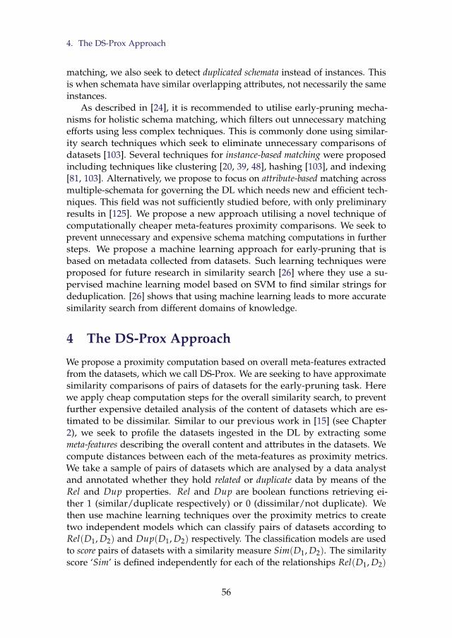
4. The DS-Prox Approach
matching, we also seek to detect duplicated schemata instead of instances. Thisis when schemata have similar overlapping attributes, not necessarily the sameinstances.
As described in [24], it is recommended to utilise early-pruning mecha-nisms for holistic schema matching, which filters out unnecessary matchingefforts using less complex techniques. This is commonly done using similar-ity search techniques which seek to eliminate unnecessary comparisons ofdatasets [103]. Several techniques for instance-based matching were proposedincluding techniques like clustering [20, 39, 48], hashing [103], and indexing[81, 103]. Alternatively, we propose to focus on attribute-based matching acrossmultiple-schemata for governing the DL which needs new and efficient tech-niques. This field was not sufficiently studied before, with only preliminaryresults in [125]. We propose a new approach utilising a novel technique ofcomputationally cheaper meta-features proximity comparisons. We seek toprevent unnecessary and expensive schema matching computations in furthersteps. We propose a machine learning approach for early-pruning that isbased on metadata collected from datasets. Such learning techniques wereproposed for future research in similarity search [26] where they use a su-pervised machine learning model based on SVM to find similar strings fordeduplication. [26] shows that using machine learning leads to more accuratesimilarity search from different domains of knowledge.
4 The DS-Prox Approach
We propose a proximity computation based on overall meta-features extractedfrom the datasets, which we call DS-Prox. We are seeking to have approximatesimilarity comparisons of pairs of datasets for the early-pruning task. Herewe apply cheap computation steps for the overall similarity search, to preventfurther expensive detailed analysis of the content of datasets which are es-timated to be dissimilar. Similar to our previous work in [15] (see Chapter2), we seek to profile the datasets ingested in the DL by extracting somemeta-features describing the overall content and attributes in the datasets. Wecompute distances between each of the meta-features as proximity metrics.We take a sample of pairs of datasets which are analysed by a data analystand annotated whether they hold related or duplicate data by means of theRel and Dup properties. Rel and Dup are boolean functions retrieving ei-ther 1 (similar/duplicate respectively) or 0 (dissimilar/not duplicate). Wethen use machine learning techniques over the proximity metrics to createtwo independent models which can classify pairs of datasets according toRelpD1, D2q and DuppD1, D2q respectively. The classification models are usedto score pairs of datasets with a similarity measure SimpD1, D2q. The similarityscore ‘Sim’ is defined independently for each of the relationships RelpD1, D2q
56

4. The DS-Prox Approach
and DuppD1, D2q as a number between 0 and 1, where 0 means dissimilar and1 means most similar: SimpD1, D2q P r0, 1s.
4.1 The Meta-Features Distance Measures
Table 3.1: DS-Prox meta-features
Type Meta-feature Description
GeneralNumber of Instances The number of instances in the datasetNumber of Attributes The number of attributes in the datasetDimensionality The ratio of number of attributes to number
of instances
Attributes by Type Number per Type The number of attributes per type (Nominalor Numerical)
Percentage per Type The percentage of attributes per type (Nomi-nal or Numerical)
Nominal AttributesAverage Number of Values The average number of distinct values per
nominal attributeStandard Deviation of Numberof Values
The standard deviation in the number of dis-tinct values per nominal attribute
Minimum/Maximum Numberof Values
The minimum and maximum number of dis-tinct values per nominal attribute
Numeric AttributesAverage Numeric Mean The average of the means of all numeric at-
tributesStandard Deviation of the Nu-meric Mean
The standard deviation of the means of thenumeric attributes
Minimum/Maximum NumericMean
The minimum and maximum mean of nu-meric attributes
Missing Values
Missing Attribute Count The number of attributes with missing valuesMissing Attribute Percentage The percentage of attributes with missing val-
uesMinimum/Maximum Numberof Missing Values
The minimum and maximum number of in-stances with missing values per attribute
Minimum/Maximum MissingValues Percentage
The minimum and maximum percentage ofinstances with missing values per attribute
Mean Number of Missing Val-ues
The mean number of missing values fromeach attribute
Mean Percentage of Missing Val-ues
The mean percentage of missing values fromeach attribute
For each dataset in the DL, we extract meta-features using data profilingtechniques. This includes general statistics about the dataset and its attributesas described in Table 3.1. Our purpose for those meta-features is to describe thegeneral structure and content of the datasets for an approximate comparisonusing our proximity metric and classification models. We compute distancesfor each meta-feature mi from Table 3.1 between each pair of datasets rD1, D2s
using equation 3.1 which gives the relative difference as a number between 0and 1. Those distances we feed to the supervised machine learning algorithmin our approach.
distmi pD1, D2q “maxtmipD1q, mipD2qu´mintmipD1q, mipD2qu
maxtmipD1q, mipD2qu(3.1)
57

4. The DS-Prox Approach
4.2 The Approach
The approach proposed for early-pruning depends on classical machine learn-ing which is divided into two phases: Supervised Learning Phase and Scoringand Classification Phase. In the first phase, which can be seen in Figure 3.2,we build a classification model for each of the properties Rel and Dup usingsupervised learning techniques. First, for each dataset we extract its meta-features from Table 3.1 which returns its data profile (In Figure 3.2 we seea sample of two meta-features: number of attributes ‘nAttr’, and number ofinstances ‘nIns’). Then, for each dataset, we generate all pairs with each of theother datasets and compute the distances between their meta-features usingEquation 3.1. We also present the pairs of datasets to a human-annotator whomanually decides whether they satisfy (assign ‘1’) or not satisfy (assign ‘0’)RelpD1, D2q and DuppD1, D2q. Any pair annotated as a match for DuppD1, D2q
must also be annotated as a match for RelpD1, D2q (i.e., all duplicate pairs ofdatasets are also related). We feed both the annotated pairs of datasets withtheir distances as training examples to a learner which creates two classifiers:Mrel and Mdup.
Figure 3.2: DS-Prox: supervised machine learning
In the second phase, we apply the classifiers to the scenarios discussed inSection 2, to score each new pair of previously unseen datasets. In scenario (a),we have a setting where there are two DLs. DL1 has a group of datasets whichhave previously known annotations of all their RelpD1, D2q and DuppD1, D2q
relationships between all pairs of datasets. On the other hand, DL2 is withoutany annotations of such relationships and is therefore a data swamp we wouldlike to dredge. Therefore, we need to learn the models for RelpD1, D2q andDuppD1, D2q from DL1 and apply them to DL2 which has different datasets.In scenario (b), we have an existing DL for which we know all relationships
58

4. The DS-Prox Approach
between the datasets. We need to deal with a new dataset as it arrives in thisDL. We learn the models from the DL, and we apply them to each new datasetDi ingested within the same DL. The models should identify all datasets inthe DL which are related or duplicate of Di.
When applying the classifiers, we compute for each pair of datasets thesimilarity score of SimrelpD1, D2q and SimduppD1, D2q using the classifiers ex-tracted in the previous phase. The Sim score is the positive-class distributionvalue generated by each classifier. The predicted distribution-value achievedfor the ‘true’ class from each classifier is checked against a minimum thresholdto indicate whether the pair of datasets are overall related or duplicates. In ourapproach, pairs of datasets are evaluated first if they match the DuppD1, D2q
relationship (indicating that it also matches RelpD1, D2q). If it fails this dupli-cate test, then we evaluate if the pair still satisfies RelpD1, D2q. The outputclassifiers can classify in the future any new pairs of datasets as either relatedor duplicate according to two matching approaches: 1-to-1 matching or clustermatching.
1-to-1 matching: all pairs satisfying RelpD1, D2q and DuppD1, D2q need tobe selected for further schema matching and deduplication. The calculationsare performed under the assumption that each and every pair of matchingdatasets should be correctly identified using our models.
Cluster-based matching: It is common to use clustering based approachesfor the matching process [20, 24, 48]. Groups of datasets with close proximityare segmented into clusters. In our case, the relationship Rel can be usedto cluster the datasets in the DL, after all relationships are discovered. Wetherefore relax our requirements for the second phase so that a new datasetshould match with any single dataset in the same cluster in order to considerit a positive match. Therefore, if a dataset matches one or more dataset(s)from a cluster, we consider all pairs of datasets in this cluster as positivelymatching pairs (even if the classifier did not indicate a positive match forsome of those pairs separately). The rationale behind this approach is thatin a real holistic schema matching setting, a new dataset ingested should becompared to all the datasets in a cluster it matches to. Clustering can takeplace after schema matching identifies the relationships between datasets(which is outside the scope of this chapter, but the reader can refer to [20, 48]for such clustering in instance-based matching).
We illustrate our general approach with a toy example in Figure 3.3. Sup-pose we have two meta-features nIns and nAttr for each dataset. To classify
59

4. The DS-Prox Approach
a pair rpnIns1, nAttr1q , pnIns2, nAttr2qs we compute the relative differences.In Figure 3.3(a) we have plotted p∆nIns, ∆nAttrq for all pairs in the trainingdata. ‘+’ indicates a matching pair, ‘-’ a non-matching pair. Based on this datawe learn a classifier, for instance a separating hyperplane as shown in Figure3.3(a) by the red line. Here, for simplification, we show pairs of datasetsplotted based on the distances of only two meta-features (nIns and nAttr).The actual approach would consider all meta-features in Table 3.1.
(a) (b)
Figure 3.3: DS-Prox cut-off thresholds tuning
Most classification models produce a score instead of a binary output.In the example of the separating hyperplane the obtained distance to thehyperplane can be used as a score. This score can be compared againstdifferent cut-off thresholds to decide on the final classification ‘+’ or ‘-’. Thethreshold can be chosen to lead to different results, as seen in Figure 3.3(b). Ifwe choose the cut-off threshold ‘C1’ we restrict the classifier to return less pairsof high proximity (i.e., low distance), leading to lower recall but less work.Alternatively, if we alter the cut-off threshold to ‘C2’, we relax the classifierto return pairs of lower proximity. This leads to more pairs (i.e., more work)returned by the classifier as positive matches and higher recall of positivecases, but, with more pairs marked incorrectly as matching. Therefore, thecut-off threshold can be tweaked by the data scientist according to practicalrequirements in order to increase recall at the expense of more work or viceversa. This is the trade-off which we seek to optimise in our experiments whenselecting different thresholds. We can use different thresholds ‘crel’ and ‘cdup’for each of the classifiers evaluated. This means that we consider a positivematch if the classifier scores a new pair of datasets with a score greater thanthe threshold as in Equations (3.2) and (3.3).
RelpD1, D2q “
#
1, SimrelpD1, D2q ą crel
0, otherwise(3.2) DuppD1, D2q “
#
1, SimduppD1, D2q ą cdup
0, otherwise(3.3)
60

5. Experimental Evaluation
The complexity of our approach is quadratic in the number of datasets,however, it applies the cheapest computational steps for early-pruning (justcomputing distances in Equation 3.1 and the classifier scoring model on eachpair). This way, we save unnecessary expensive schema matching processingin later steps.
5 Experimental Evaluation
We tested an implementation of the DS-Prox approach on OpenML1, whichcan be considered an online DL. It consists of different datasets coveringheterogeneous topics, each having a name and a description.
5.1 Datasets
The main challenge is to create the ground-truth which we use to evaluate ourapproach. To achieve this, we created an experimental environment where weextracted the following independent sets of datasets from OpenML:
• Restricted-topics sample: First, we extract some datasets by topic us-ing 11 keywords-search over OpenML, e.g., “Disease", “Cars",“Flights",“Sports", etc. This restricted sample consists of 130 datasets and weconsider them to be similar if they belong to the same topic.
• All-topics sample: This is an independent set of other datasets collectedfrom OpenML. To collect this sample, we scraped the OpenML repositoryto extract all datasets not included in the restricted-topics sample andhaving a description of more than 500 characters. Out of the 514 datasetsretrieved we selected 213 with descriptive descriptions (i.e., excludingdatasets whose descriptions do not allow to interpret its content and toassign a topic).
Therefore, we created two new groups of datasets from OpenML for ourexperiments, each having its own independent set of datasets without anyoverlap. Having two independent sets strengthens our results and allowsus to generalise our conclusions. A domain expert and one of the authorscollaborated to manually label the pairs of datasets with the same topic asduplicated and / or related. The interested reader can download the twoannotated datasets from GitHub2. The details of each sample is summarisedin Table 3.2, which lists the number of datasets, the number of topics, toptopics by the number of datasets, and the number of related and duplicatedpairs per sample.
1http://www.openml.org2https://github.com/AymanUPC/datasets_proximity_openml
61

5. Experimental Evaluation
Table 3.2: A description of the OpenML samples collected
Sample Datasets Topics Top Topics RelpD1, D2q DuppD1, D2q
Restricted-topics
130 29 Diseases (45), Health (31), Cars(13), Academic Courses (6),Sports (5)
1205 72
All-topics 213 79 computer software defects (17),citizens census data (12), digithandwriting recognition (12),Diseases (11)
570 128
Table 3.3: An example of pairs of datasets from the all-topics sample from OpenML
No. DID 1 Dataset 1 DID 2 Dataset 2 Topic Relationship1 23 cmc 179 adult Census Data related2 14 mfeat-
fourier1038 gina_agnostic Digit Handwriting
Recognitionrelated
3 55 hepatitis 171 primary-tumor
Disease related
4 189 kin8nm 308 puma32H Robot Motion Sensing duplicate5 1514 micro-
mass1515 micro-mass Mass Spectrometry
Dataduplicate
Some of the pairs from the all-topics sample can be seen in Table 3.3.Dataset with ID 23 should match all datasets falling under the topic of ‘censusdata’ like dataset 179. Both datasets have data about citizens from a populationcensus. In rows 4 and 5 we can see examples of duplicated datasets, whichhave highly intersecting data in their attributes. Duplicate pairs in row 4have the same number of instances, but described with different number ofattributes, which are overlapping. The duplicate pairs in row 5 have identicalnumber of attributes, yet, the attributes are transformed using pre-processingtechniques and there are different number of instances between both datasets,so in essence the second dataset is a transformed and cleaned version of thefirst. We aim to detect such kind of scenarios using our DS-Prox approach.
5.2 Experimental Setup
In order to evaluate our approach, we create an experimental setup wherewe have two sets of datasets for each experiment: 1. Training set and 2. Testset. The training set is used in the supervised learning phase to create theclassification models. The classification models are then evaluated using thetest set. We use the restricted-topics sample as a training set, and we use boththe restricted-topics and the all-topics samples in the scoring phase as test setsto evaluate our approach. We describe how we used those samples to createthe training and test sets within our experiments for the two scenarios fromSection 2:
• Scenario (a) from Section 2: We evaluate our approach by using therestricted-topics sample as the training set and the all-topics sample asthe test set. In this case the testing set is an independent collection ofdatasets. We evaluate both of the 1-to-1 matching and cluster matching
62

5. Experimental Evaluation
approaches for RelpD1, D2q. We also evaluate the 1-to-1 matching withDuppD1, D2q.
• Scenario (b) from Section 2: We evaluate our approach using a leave-one-out (LOO) variant evaluation method and the restricted-topics sample.Here we remove a dataset and all its pairs from the original trainingset and we use those pairs for evaluation of the output classifiers as aseparate test set. We also remove all duplicate pairs of this dataset fromthe training set to guarantee independence between the training andevaluation environments. We repeat this for every dataset in the inputtraining set. We use the 1-to-1 matching approach in our evaluation.
To execute our experiments, we profile the datasets to extract their meta-features. We use the training set of annotated datasets with the WEKA3
tool to create the classification models using different supervised techniques:Bayesian (Bayesian Network with K2 search, Naïve Bayes) , Regression (Log-itBoost) , Support Vector Machines (Sequential Minimal Optimization) , andDecision Trees (Random Forest). We also use Ensemble Learners [45]: Ad-aBoost (with Decision Stump classifier), Classification Via Regression (withM5 Tree classifier), and Random Subspace (with Regression Tree classifier).We tested different techniques because it was suggested by [45] that someindividual techniques can outperform the ensemble learners in classificationproblems. We evaluate the classifiers with 10 different cut-off thresholds for‘crel’ and ‘cdup’ from Equations (3.2) and (3.3), in order to cover a wide rangeof values. We benchmark the techniques against the decision table technique[72] which simply assigns the majority class based on matching the featuresto a table of learned examples.
5.3 Results
Table 3.4: A description of the experiments conducted
Experiment Graphs in Figure3.4 Matching Approach Scenario Relationship1 row 1: (a) and (b) 1-To-1 (b) RelpD1, D2q
2 row 2: (c) and (d) 1-To-1 (a) RelpD1, D2q
3 row 3: (e) and (f) Cluster-based (a) RelpD1, D2q
4 row 4: (g) and (h) 1-To-1 (a) DuppD1, D2q
We evaluate the effectiveness of our approach using the recall, precision,and efficiency-gain measurements, as described in Equations (3.4),(3.5) and(3.6) respectively. Here, TP means true-positives which are the pairs ofdatasets correctly classified by the classifier. FN are false negatives, FPare false-positives, TN are true-negatives, and N indicates the total number
3https://weka.wikispaces.com/Use+WEKA+in+your+Java+code
63

5. Experimental Evaluation
of possible pairs of datasets. The efficiency gain measures the amount ofreduction in work required, in terms of number of pairs of datasets eliminatedby the classifier.
recall “TP
TP` FN(3.4)
precision “TP
TP` FP(3.5) e f f iciency´ gain “
TN` FNN
(3.6)
We change the cut-off thresholds, and we aim to maximize this as much aspossible while maintaining the highest recall possible. The effectiveness of ourapproach is evaluated by recall and precision. By applying our approach withthe different scenarios and relationships, we conduct 4 sets of experiments asin Table 3.4. The results are depicted in the graphs in Figure 3.4.
The measures shown in the graphs are all averages from all datasetsinvolved in the test sets for a specific data mining technique and a certaincut-off threshold for the proximity score (darker points have higher cut-offvalues). The common measure for all graphs, which is the recall plotted on they-axis, is highlighted by having some of its main values labelled on each graph.Graphs (a) and (b) are the same graphs as (c) and (d) respectively but for the1-to-1 matching approach applied with the different scenarios. We select forthe experiments certain target results, which are minimum expected values foreach measure. All area above those values are shaded as follows: Min. recall:0.75 for 1-to-1 matching & 0.9 for cluster matching, Min. efficiency gain: 0.33for 1-to-1 matching & 0.25 for cluster matching, Min. precision: 0.25 for allapproaches. This means that we were targeting at least 75% recall rate for1-to-1 matching and 90% recall rate for the cluster based matching (whichimproves our previous results in [15] described in Chapter 2). We aimed for atleast 25% efficiency gains with the cluster matching approach, which exceedsthose achieved in [20]. However, we acknowledge that their approach appliedto instances-matching within the same dataset, not cross-schema attribute-matching as in our case. For experiment 4 for DuppD1, D2q, we aim for amin. recall of 0.9, min. efficiency gain of 0.75, and min. precision of 0.33.In real-world applications, the data scientist can choose different minimumthresholds for each measure according to practical requirements.
5.4 Discussion
General trend. From the results depicted in Figure 3.4, the optimum techniqueand cut-off threshold is the one in the top-right quadrant of each graph,optimising both measures plotted. The recall-precision and recall-efficiencyplots follow the general trend expected which indicate the trade-off betweenboth measures in each plot, yet, more optimised solutions are possible forbalancing recall-efficiency, as seen by the classifiers performing in the top-rightquadrant. As the cut-off thresholds increase, there is a drop in recall againstan increasing efficiency gain. Still, the top mining techniques and thresholdscan be used to achieve high efficiency gain and recall. This is discussed for
64

5. Experimental Evaluation
each property below. As the precision rates are generally low, we concludethat our approach can only be used as an early-pruning step, and should befollowed by other more expensive and more detailed matching steps. Yet, agood compromise can still achieve high recall and efficiency gains; efficiencygains up to 0.5 for Rel and 0.8 for Dup. Such efficiency gains can make animportant difference for computationally-expensive applications of holisticschema matching in the DL environment.Rel evaluation. The recall-efficiency plots indicated that it was possible toachieve an optimum technique and threshold in the top-right quadrant, whichrepresent the compromise of not sharply losing recall with higher efficiencygain. For example, from Figure 3.4 (e) for experiment 3, using the AdaBoosttechnique at a threshold of 0.5 can lead to 0.42 efficiency gains while stillmaintaining 0.95 recall. If a recall of 1.0 is required, then this can be achievedby the cut-off threshold of 0.3 for the same technique, but only 0.13 efficiencygain is achieved. The data scientist will have to decide if this efficiency gainis sufficient and whether a recall rate of 100% is critical in their application,else, a 0.05 drop in recall should be allowed to achieve much higher efficiencygain using the techniques and thresholds in the top quadrant. For the 1-to-1matching in Figure 3.4 (c), we can achieve 0.75 recall and 0.35 efficiency gain.There is a drop in recall, as would be expected, because the classifier hasmore challenges in matching all possible ‘related’ datasets, while in the clustermatching approach, a single match to a dataset in a cluster acts like a pivotwhich results in matching all the required related datasets in the same cluster.The cluster-matching approach shows an improved performance over the1-to-1 matching approach, therefore it is recommended to use DS-Prox withthe clustering-based approach.Dup evaluation. For the results in Figure 3.4 (g) and (h), the top performingtechniques were Random subspace and Random Forest at 0.2 cut-off thresh-olds. This achieved about 0.97 recall and 0.76-0.8 efficiency gain. The baselinemethod was not able to differentiate at different cut-off thresholds, and hadbest recall of 0.65, except for the lowest cut-off of 0.1 where it achieved a jumpto 0.94 recall. Since the recall was very high for our target efficiency gainusing the 1-to-1 approach, the cluster-based approach did not yield any betterresults.Baseline comparisons. Different techniques can yield better results than thebaseline for several of our experiments. There is not one single techniquewhich is best, yet, ensemble learners tend to perform better than their counter-parts. However, simple techniques like logistic regression and Naïve Bayescan still have good performance as seen in the graph (e) top-right quadrant.The baseline technique was never in the top-quadrant of graph (e) and manytechniques outperformed it. In the 1-to-1 matching in graphs (a) and (c),the baseline classifier was comparable with the other techniques. The toptechniques include the iterative optimiser in graph (c) with 0.75 recall and
65

6. Conclusion and Future Work
0.35 efficiency gain. Nearly 1.0 recall was possible using the same classifierat a lower threshold, yet with only 0.09 efficiency gain. For experiment 1,Random Forest and Random Subspace outperformed the baseline with 0.3cut-off thresholds.Generalizability. Although our approach is generic and does not apply to aspecific domain only, we note that we do not claim that the classifiers for onetype of data or of a certain domain will have the same guaranteed effectivenesswhen applied in another setting. The approach might need to be adjusted andretrained within other settings. Albeit, our results from experiments 2 and3 show a positive indicator of the possibility to train the model on specificdomains, independent of those used in the test set (or real-world setting),and still be effective. We think that this needs further experimentation in thefuture.
6 Conclusion and Future Work
This chapter presented a novel approach of similarity search within a DL basedon a proximity mining technique for early-pruning in holistic dataset schemamatching and deduplication applications. The approach uses supervised ma-chine learning techniques based on meta-features describing semi-structureddatasets. Experiments on a real-life DL demonstrate the effectiveness in achiev-ing high recall rates and efficiency gains. Proposed techniques support datagovernance in the DL by identifying relationships between datasets. Thedrawback of our approach, however, is that it needs some manual effort toannotate training examples for the classifiers. In the future, we will test thegeneralizability of applying the same classifier to different data sources. Weplan to experiment with more detailed meta-features which might lead toimproved results. We will also test our approach on other kinds of semi-structured data (like RDF or XML).
Acknowledgements. This research has been funded by the European Com-mission through the Erasmus Mundus Joint Doctorate (IT4BI-DC).
66

6. Conclusion and Future Work
0.00.1 0.2 0.3 0.4 0.5 0.6 0.7 0.8 0.9 1.0
Efficiency Gain
0.0
0.1
0.2
0.3
0.4
0.5
0.6
0.7
0.8
0.9
1.0Positive Class Recall
0.7794
0.8981 0.8162
0.0860
0.9020
0.7532
0.3760
0.7144
0.7781
0.6410
0.4835
1-to-1 Recall-Efficiency
Cut-Off Threshold0.10.20.30.40.50.60.70.750.80.85
AlgorithmAdaBoostM1BayesNetClassificationViaRegressionDecisionTableIterativeClassifierOptimizerNaiveBayesRandomForestRandomSubSpaceSimpleLogisticSMO
Baseline_highlightFALSETRUE
Sum of Overall Efficiency Gain vs. sum of Overall Positive Class Recall. Color shows details about Cut-Off Threshold. Size shows detailsabout Baseline_highlight. Shape shows details about Algorithm. The marks are labeled by sum of Overall Positive Class Recall. The datais filtered on included_algorithm, which keeps Yes. (a)
0.0 0.1 0.2 0.3 0.4 0.5 0.6 0.7 0.8 0.9
Positive Class Precision
0.0
0.1
0.2
0.3
0.4
0.5
0.6
0.7
0.8
0.9
1.0
Positive Class Recall
0.49240.3973
0.1919
0.8162
0.3076
0.0860
0.8674
0.3760
0.2305
0.1925
0.6410
0.4835
0.2232 0.2027
0.3267
0.2930
1-to-1 Recall-Precision
AlgorithmAdaBoostM1BayesNetClassificationViaRegressionDecisionTableIterativeClassifierOptimizerNaiveBayesRandomForestRandomSubSpaceSimpleLogisticSMO
Baseline_highlightFALSETRUE
Cut-Off Threshold0.10.20.30.40.50.60.70.750.80.85
Sum of Overall Positive Class Precision vs. sum of Overall Positive Class Recall. Color shows details about Cut-Off Threshold. Size showsdetails about Baseline_highlight. Shape shows details about Algorithm. The marks are labeled by sum of Overall Positive Class Recall. Thedata is filtered on included_algorithm, which keeps Yes. The view is filtered on Baseline_highlight, which keeps FALSE and TRUE.(b)
0.0 0.1 0.2 0.3 0.4 0.5 0.6 0.7 0.8 0.9 1.0
Efficiency Gain
0.0
0.1
0.2
0.3
0.4
0.5
0.6
0.7
0.8
0.9
1.0
Positive Class Recall
0.9083
0.5818
0.9939
0.9203
0.7541
0.9743
0.8785
0.6123
0.4760
0.72590.7127
0.6819
0.5269
0.4113
0.4256
0.2626
0.7747
0.1761
Ovr. Recall V2
Cut-Off Threshold0.10.20.30.40.50.60.70.750.80.85
AlgorithmAdaBoostM1BayesNetClassificationViaRegressionDecisionTableIterativeClassifierOptimizerNaiveBayesRandomForestRandomSubSpaceSimpleLogisticSMO
Baseline_highlightFALSETRUE
Average of Overall Efficiency Gain vs. average of Overall Positive Class Recall. Color shows details about Cut-Off Threshold. Sizeshows details about Baseline_highlight. Shape shows details about Algorithm. The marks are labeled by average of Overall PositiveClass Recall. The data is filtered on Subject Area, Singleton_Subject and included_algorithm. The Subject Area filter keeps 79 of 79members. The Singleton_Subject filter keeps FALSE. The included_algorithm filter keeps Yes.(c)
0.00.1 0.2 0.3 0.4 0.5 0.6 0.7 0.8 0.9 1.0
Positive Class Precision
0.0
0.1
0.2
0.3
0.4
0.5
0.6
0.7
0.8
0.9
1.0
Positive Class Recall
0.26880.1800
0.05420.13880.1141
0.8007
0.5269
0.1232
0.1513
0.0835
Ovr. Precision V2
Cut-Off Threshold0.10.20.30.40.50.60.70.750.80.85
AlgorithmAdaBoostM1BayesNetClassificationViaRegressionDecisionTableIterativeClassifierOptimizerNaiveBayesRandomForestRandomSubSpaceSimpleLogisticSMO
Baseline_highlightFALSETRUE
Average of Overall Positive Class Precision vs. average of Overall Positive Class Recall. Color shows details about Cut-OffThreshold. Size shows details about Baseline_highlight. Shape shows details about Algorithm. The marks are labeled by averageof Overall Positive Class Recall. The data is filtered on Singleton_Subject and included_algorithm. The Singleton_Subject filterkeeps FALSE. The included_algorithm filter keeps Yes.
(d)
0.0 0.1 0.2 0.3 0.4 0.5 0.6 0.7 0.8 0.9 1.0
Efficiency Gain
0.15
0.20
0.25
0.30
0.35
0.40
0.45
0.50
0.55
0.60
0.65
0.70
0.75
0.80
0.85
0.90
0.95
1.00
1.05
Positive Class Recall
0.8253
0.6988
0.9699
0.8313
0.7289
0.5181
1.0000
0.9458
0.1747
0.6807
0.4639
0.3735
0.8916
0.9639
0.8614
0.5964
Alg. Eff Gain V2
Cut-Off Threshold0.10.20.30.40.50.60.70.750.80.85
AlgorithmAdaBoostM1BayesNetClassificationViaRegressionDecisionTableIterativeClassifierOptimizerNaiveBayesRandomForestRandomSubSpaceSimpleLogisticSMO
Baseline_highlightFALSETRUE
Average of Efficiency Gain vs. average of Positive Class Recall. Color shows details about Cut-Off Threshold. Size shows details aboutBaseline_highlight. Shape shows details about Algorithm. The marks are labeled by average of Positive Class Recall. The data is filtered onSingleton_Subject, Subject Area and included_algorithm. The Singleton_Subject filter keeps FALSE. The Subject Area filter keeps 79 of 79members. The included_algorithm filter keeps Yes. (e)
0.00.1 0.2 0.3 0.4 0.5 0.6 0.7 0.8 0.9 1.0
Positive Class Precision
0.1
0.2
0.3
0.4
0.5
0.6
0.7
0.8
0.9
1.0
Positive Class Recall
0.6988
0.83130.7590
0.7289
0.5181
0.1747
0.5783
0.4639
0.3735
0.7711
0.7108
0.61450.5964
0.6867
0.5783
Alg. Precision
Cut-Off Threshold0.10.20.30.40.50.60.70.750.80.85
Baseline_highlightFALSETRUE
AlgorithmAdaBoostM1BayesNetClassificationViaRegressionDecisionTableIterativeClassifierOptimizerNaiveBayesRandomForestRandomSubSpaceSimpleLogisticSMO
Average of Positive Class Precision vs. average of Positive Class Recall. Color shows details about Cut-Off Threshold. Size showsdetails about Baseline_highlight. Shape shows details about Algorithm. The marks are labeled by average of Positive Class Recall.The data is filtered on Singleton_Subject and included_algorithm. The Singleton_Subject filter keeps FALSE. Theincluded_algorithm filter keeps Yes. (f)
0.550.600.650.700.750.800.850.900.951.001.05
Efficiency Gain
0.60
0.65
0.70
0.75
0.80
0.85
0.90
0.95
1.00
Positive Class Recall
0.9385
0.8213
0.9741 0.9684
0.9144
0.7392
0.8204
0.84300.8374
0.9661
0.7799
0.8833
0.7753
0.6440
0.8443
0.7266
0.7033
Eff. Gain Corrected V2
AlgorithmAdaBoostM1
BayesNet
ClassificationViaRegression
DecisionTable
IterativeClassifierOptimizer
NaiveBayes
RandomForest
RandomSubSpace
SimpleLogistic
SMO
Cut-Off Threshold0.1
0.2
0.3
0.4
0.5
0.6
0.7
0.75
0.8
0.85
Baseline_highlightFALSE
TRUE
Average of Efficiency Gain vs. average of Recall. Color shows details about Cut-Off Threshold. Size shows details about Baseline_highlight. Shape shows details aboutAlgorithm. The marks are labeled by average of Recall. The data is filtered on Precision, Positive_Dataset and included_algorithm. The Precision filter ranges from 0 to 1.The Positive_Dataset filter keeps Y. The included_algorithm filter keeps Yes. (g)
0.00.1 0.2 0.3 0.4 0.5 0.6 0.7 0.8 0.9 1.0
Positive Class Precision
0.60
0.65
0.70
0.75
0.80
0.85
0.90
0.95
1.00
Positive Class Recall
0.9385
0.7295
0.8213
0.66450.6807
0.7220
0.7875
0.9144
0.7392
0.8626
0.9684
0.7253
0.8204
0.9155
0.83080.8374
0.80760.7942
0.7799
0.7446
0.7823
0.6440
0.7576
0.8443
0.7033
Precision Corrected
Cut-Off Threshold0.1
0.2
0.3
0.4
0.5
0.6
0.7
0.75
0.8
0.85
AlgorithmAdaBoostM1
BayesNet
ClassificationViaRegression
DecisionTable
IterativeClassifierOptimizer
NaiveBayes
RandomForest
RandomSubSpace
SimpleLogistic
SMO
Baseline_highlightFALSE
TRUE
Average of Precision vs. average of Recall. Color shows details about Cut-Off Threshold. Size shows details about Baseline_highlight. Shape shows details aboutAlgorithm. The marks are labeled by average of Recall. The data is filtered on Precision, Positive_Dataset and included_algorithm. The Precision filter ranges from 0 to 1.The Positive_Dataset filter keeps Y. The included_algorithm filter keeps Yes. (h)
Figure 3.4: Recall-efficiency plots (left column) and recall-precision plots (right column) forexperiments 1,2,3 and 4 in each row
67

Chapter 4
Attribute-level contentmetadata based proximitymining for pre-filteringschema matching
Everything is continuously changing and to be successful, onemust embrace change and swiftly adapt to it. Improvement is alifetime journey.
This chapter has been published as a paper in the ACM Transactions onInformation Systems (TOIS) (2020) [17].The layout of the paper has been revisedDOI: https://doi.org/10.1145/3388870
ACM copyright / credit notice:© 2020 ACM. Reprinted with permission from Ayman Alserafi, Alberto Abelló,Oscar Romero, Toon Calders. Keeping the Data Lake in Form: ProximityMining for Pre-Filtering Schema Matching, TOIS, 2020.
68

Abstract
Data Lakes (DLs) are large repositories of raw datasets from disparate sources. As moredatasets are ingested into a DL, there is an increasing need for efficient techniques toprofile them and to detect the relationships among their schemata, commonly known asholistic schema matching. Schema matching detects similarity between the informationstored in the datasets to support information discovery and retrieval. Currently, thisis computationally expensive with the volume of state-of-the-art DLs. To handle thischallenge, we propose a novel early-pruning approach to improve efficiency, where wecollect different types of content metadata and schema metadata about the datasets,and then use this metadata in early-pruning steps to pre-filter the schema matchingcomparisons. This involves computing proximities between datasets based on theirmetadata, discovering their relationships based on overall proximities and proposingsimilar dataset pairs for schema matching. We improve the effectiveness of this taskby introducing a supervised mining approach for effectively detecting similar datasetswhich are proposed for further schema matching. We conduct extensive experimentson a real-world DL which proves the success of our approach in effectively detectingsimilar datasets for schema matching, with recall rates of more than 85% and efficiencyimprovements above 70%. We empirically show the computational cost saving inspace and time by applying our approach in comparison to instance-based schemamatching techniques.
69

1. Introduction
1 Introduction
Today, it is more and more common for data scientists to use Data Lakes (DLs)to store heterogeneous datasets coming from different sources in their rawformat [128]. Such data repositories support the new era of data analyticswhere datasets are ingested in large amounts and are required to be analysedjust-in-time [82]. However, it is a challenge for data wranglers [51, 69, 128]preparing the datasets for analysis to understand their structure and common-alities for DL governance purposes [15]. They must extract those datasetswhich have related data to be used together in data analysis tasks [82, 89].This is commonly referred to as schema matching, where the aim is to findconnection strengths between similar concepts from different pairs of datasets[27, 35, 83, 104]. When applied on large-scale heterogeneous repositories likeDLs, it becomes a case of holistic schema matching [18, 89, 104, 110].
Holistic schema matching: The large-scale application of schema matchingto BD repositories like DLs, where the goal is to match multiple datasetstogether considering them all in the matching task.
We focus on DLs having datasets storing data in flat tabular formats. Flatdatasets are organised as attributes and instances, such as tabular data, commaseparated values (CSV) files, hypertext markup language (HTML) tables, etc.(see Section 3). It is a challenge with such DLs to efficiently process the datasetsto detect their common features, as schema matching tasks are generallyexpensive (involving huge amounts of string comparisons and mathematicalcalculations) [24, 27, 71]. In this chapter, we propose novel techniques toreduce those comparisons using pre-filtering techniques that generate lesscomparisons. To illustrate this, consider the different types of comparisons inFigure 4.1. Traditionally, schema matching makes many comparisons of datavalues of instances from different datasets (see the instance-based matchingbox). With the rise of DLs, previous research [18, 43, 24] recommended usingearly-pruning steps to facilitate the task using schema matching pre-filtering.
Schema matching pre-filtering means that only dataset pairs detected tobe of relevant similarity are recommended for further fine-grained schemamatching tasks, and dissimilar ones are filtered out from further compar-isons. This supports the goal of early-pruning of the number of requiredcomparisons in order to improve the efficiency of schema matching inlarge-scale environments like DLs.
70
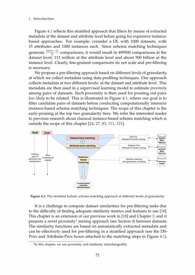
1. Introduction
Figure 4.1 reflects this stratified approach that filters by means of extractedmetadata at the dataset and attribute level before going for expensive instance-based approaches. For example, consider a DL with 1000 datasets, with15 attributes and 1000 instances each. Since schema matching techniquesgenerate n˚pn´1q
2 comparisons, it would result in 499500 comparisons at thedataset level, 113 million at the attribute level and about 500 billion at theinstance level. Clearly, fine-grained comparisons do not scale and pre-filteringis necessary.
We propose a pre-filtering approach based on different levels of granularity,at which we collect metadata using data profiling techniques. Our approachcollects metadata at two different levels: at the dataset and attribute level. Thismetadata are then used in a supervised learning model to estimate proximityamong pairs of datasets. Such proximity is then used for pruning out pairsless likely to be related. This is illustrated in Figure 4.1, where our goal is tofilter candidate pairs of datasets before conducting computationally intensiveinstance-based schema matching techniques. The scope of this chapter is theearly-pruning at the top two granularity tiers. We refer the interested readerto previous research about classical instance-based schema matching which isoutside the scope of this chapter [24, 27, 83, 111, 121].
Dataset-level matching
Attribute-level matching
Instance-based
matching
Content-basedmetadata
(Relationships)
Filteringpairs to
generate lesscomparisons
Morecomparisons
needed
DS-Prox(Dataset Proximity mining) Dataset
Meta-features
Attribute-Prox(Attribute Proximity mining) Attribute
Meta-features
Schema matching(string/semantic similarity) Attribute
Values
Goal Cost
Figure 4.1: The stratified holistic schema matching approach at different levels of granularity.
It is a challenge to compute dataset similarities for pre-filtering tasks dueto the difficulty of finding adequate similarity metrics and features to use [18].This chapter is an extension of our previous work in [18] and Chapter 3, and itpresents a novel proximity1 mining approach (see Section 4) between datasets.The similarity functions are based on automatically extracted metadata andcan be effectively used for pre-filtering in a stratified approach (see the DS-Prox and Attribute-Prox boxes attached to the matching steps in Figure 4.1).
1In this chapter, we use proximity and similarity interchangeably.
71

2. Related Work
To our knowledge, no other approach uses automatically extracted metadatafor this purpose.
To show the feasibility of our approach, we assess its performance by usingit on a real-world DL. Our approach was able to filter the number of fine-grained comparisons by about 75% while maintaining a recall rate of at least85% after filtration. Our early-pruning approach also saves computationalcosts in terms of space and time requirements by at least 2 orders of magnitudecompared to instance-based matching.
Contributions. We present an approach for pre-filtering schema matchingtasks. We propose techniques for detecting similar schemata based on meta-data at different levels of granularity. This supports in early-pruning of theraw-data instance-based schema matching tasks. We present an expandedand cross-validated experiment for the DS-Prox technique from our previouswork in [18] (see Chapter 3) and comparisons against combining it with ournew proposed attribute-level proximity metrics to find the most appropriatemetrics to assign similarities between pairs of datasets. We demonstrate adetailed analysis of the different proximity metrics based on different typesof meta-features (name-based and content-based). Our improvements out-perform our previous work in terms of effectiveness measures like recall andlift-scores.
The chapter is organised as follows: Section 2 presents the related work,Section 3 introduces the main concepts in our research, Section 4 presents ourproximity mining based approach for early-pruning tasks of holistic schemamatching, Section 5 presents our experimental evaluation, and finally, weconclude in Section 6.
2 Related Work
State-of-the-art schema matching techniques either use schema-level metadata(mainly names and data types of schema components) [35, 36, 100, 104] orinstance-level values of data objects [27, 35, 43, 52, 83, 100, 126]. Some othersuse a hybrid approach utilising schema metadata and data instances [24, 109].At the schema-level, these techniques usually use the syntactic similarity of thenames of the schema components for the matching task. At the instance-level,values are usually compared using Jaccard similarity of intersecting exactvalues [89]. This can also be achieved by first matching duplicate instancesand finding the correspondences between their schema components [27].Further, these algorithms can be domain-specific or generic [83].
Schema matching is a computationally intensive task that requires largeamounts of comparisons [15, 18, 24] because they typically generate a Carte-sian product between the values to be compared. Moreover, other approachesalso exploit the semantic or linguistic similarity of values, which requires fur-
72

2. Related Work
ther computations to translate data values (finding synonyms and hypernyms)or to map them to ontologies [83].
The current focus of the schema matching research community is to imple-ment efficient holistic schema matching that improves performance by reduc-ing the number of actual comparisons to conduct [89]. To handle this challenge,multiple techniques were proposed. For example, several approaches useclustering techniques as a pre-filter of datasets to match [9, 22, 104]. Onlydatasets falling in the same cluster are matched, or datasets from one clusterare only matched against representative datasets from other clusters. Thisis similar to the concept of “blocking” for record linkage [124], where itemshaving equal data values in some or all of their attributes are placed in thesame bucket for comparison. The work in [124] focuses on matching instancesof data (rows in tabular data) rather than attributes in schemata (columns intabular data). We propose in this chapter a supervised learning technique thatcan classify dataset pairs (schemata) for a decision whether they are related(should be compared) or not related, rather than unsupervised techniques likeblocking and clustering. In addition, we tackle the similar schemata searchproblem (i.e., schema matching) rather than similar records search (i.e., recordlinkage or entity resolution).
In [104], they cluster the schemata and attributes of datasets based onTF-IDF similarity scores of their textual descriptions. In [9], they exploitthe structural properties of semi-structured XML documents, i.e., data ele-ments embeddings and hierarchies, to cluster the datasets before applyinginstance-based schema matching. In [22], they use the textual descriptionsand keywords of the datasets to cluster them using TF-IDF and WordNet. Inthis chapter, we do not consider textual descriptions of datasets, which couldbe misleading or missing, but rely on metadata that can be automaticallyextracted from any dataset. Metadata describing datasets, their schemata,and the information stored in them can be collected using data profilingtechniques [1, 15, 75, 82, 98]. Different types of metadata can also describethe information inside datasets at different levels of granularity, e.g., overalldataset level [18] (see Chapter 3) or attribute descriptions like we propose inthis chapter.
The pre-filtering of dataset pairs which are less-likely to have interrelateddata before performing schema-matching is called early-pruning [15, 43, 24],and it was implemented in previous research on semi-structured datasets,like XML, by finding the similarity of hierarchical structures between nameddata objects [9]. Other works have investigated schema matching with semi-structured datasets like XML [83, 100] and JSON [52]. In the web of data,previous research like [41] investigated recommendation of RDF datasets inthe semantic web using pre-defined annotations such as the sameAs property.In this chapter, we consider flat datasets without such a hierarchy of embeddeddata objects and without pre-defined semantic linkages.
73

2. Related Work
To facilitate the early-pruning tasks for schema matching, we can applythe same approaches and concepts from collaborative filtering and adapt themto the holistic schema matching problem [6, 62]. The goal is to use profilinginformation for comparison and recommendation, which was applied tomultimedia in [6] and semi-structured documents in [52]. Content-basedmetadata was also used to predict schema labels [36]. They use minimumand maximum values for numeric attributes, and exact values for nominalattributes, including the format of values. We propose to apply similartechniques but at the dataset granularity level. Accordingly, we adapt suchtechniques and find the appropriate similarity metrics for tabular datasets.
Another line of research aims at optimising the schema matching processby using computational improvements [43, 109]. This can be done usingpartitioning techniques that parallelise the schema matching comparison task[109]. Another approach uses efficient string matching comparisons. Suchtechniques are very useful in the case when schema components are properlynamed in the datasets. However, such techniques fail when the componentsare not properly named (e.g., internal conventionalism, like sequential IDnumbering of the components). In [43], they introduce intelligent indexingtechniques based on value-based signatures.
Schema matching can also be automated using data mining techniques[35, 36, 52]. In [35], they use hybrid name-based and value-based classificationmodels to match dataset attributes to a mediated integration schema. Theirapproach is focused on one-to-one mediation between two schemata, whileour approach targets all datasets in a DL by holistic schema matching usingcoarser meta-features. In [36], they use content-based meta-features in multi-value classification models to match schema labels of attributes across datasets.Decision trees were also used to profile semi-structured documents beforeschema matching [52]. In this chapter, we also use data mining classificationmodels, however the goal differs from [35], [36] and [52] as it tackles the early-pruning and pre-filtering task rather than instance-based schema matching.
We summarise the state-of-the-art in Table 4.1. This table gives a com-parison of the most relevant techniques discussed with our approach basedon the main features discussed in this section. As a result, we can see thatwe propose an approach based not only on string matching, but also oncontent metadata matching involving statistics and profiles of data stored inthe datasets. Content metadata are matched based on approximate similaritiesand not just exact value-matches at the instance-level [82, 89]. We focus onproposing novel early-pruning techniques that use supervised learning to pre-filter irrelevant dataset pairs and to detect likely-to-be similar pairs. Finally,the table shows that our technique makes a novel contribution to the schemamatching pre-filtering problem that is not achieved by other state-of-the-arttechniques.
74

3. Preliminaries
Table 4.1: Schema matching techniques state-of-the-art comparison
COMA++[109]
PARIS[126]
LOD DataLinking[22]
XMLSemantic-basedMatching[71]
OntologyClustering[9]
ProximityMining[thiswork]
Type ofData
Tabular,semi-structured,SemanticOWL
RDF SemanticRDF
Semi-structuredXML
Semi-structured,SemanticOWL
Tabular
Instance-based
X X X X ˆ ˆ
Metadataused
Attribute-levelschemanames
ˆ Ontologymap-pings, RDFschemanames,Textual de-scriptions
Attribute-levelschemanames andstructuralmetadata
Attribute-levelstructuralmetadata
Dataset-levelcontentand name,Attribute-levelcontentand name
Data Min-ing based
ˆ ˆ Clustering ˆ Clustering Supervisedlearning
ApproximateMatching
ˆ ˆ X ˆ X X
3 Preliminaries
We consider DLs with datasets having tabular schemas that are structured asattributes and instances like Figure 1.1 as described in Section 2.1. We focus ontwo types of attributes: numeric attributes (consisting of real numbers) andnominal attributes (consisting of discrete categorical values). We differentiatebetween those two types of attributes, similar to previous research like [35, 36,100], because we collect different profiling metadata for them. The resultingstatistics collected are called content meta-features, and are as follows:
• Nominal attributes: frequency distributions of their distinct values.
• Numeric attributes: aggregated statistical value distributions like mean,min, max, and standard deviations.
For pairs of datasets and attributes, we compute the functions in Table 4.2and describe them in the rest of this section.
We aim at finding the relationship between a pair of datasets RelpDy, Dzq.We determine such relationship directly using dataset-level meta-features andby computing the relationships between their pairs of attributes pAi, Ajq, beingAi from Dy and Aj from Dz, as could be seen in Figure 4.2. The figure showsan overview of our proposed proximity mining approach.
The goals of the approach is to use efficient and effective techniques toaccurately predict RelpDy, Dzq for the pre-filtering task. As could be seen inFigure 4.2, this can be done using metadata and similarity collected at thedataset level (right-side) or by using the attribute level SimpAi, Ajq to predict
75

3. Preliminaries
Table 4.2: Schema matching pre-filtering functions
Relationship Function Type Output Object Type DescriptionRelpAi , Ajq Binary Z P t0, 1u Attribute
pairRelated attributes storingdata about the same real-lifeconcept which contain over-lapping information in theirvalues. 1 means positivelyrelated and 0 means not.
SimpAi , Ajq Continuous R P r0, 1s Attributepair
A value R to measure theattribute similarity in therange [0,1].
RelpDy , Dzq Binary Z P t0, 1u Dataset pair Related datasets which con-tain information about thesame real-life object. 1means positively related and0 means not.
SimpDy , Dzq Continuous R P r0, 1s Dataset pair A value R to measure thedataset similarity in therange [0,1].
Attribute-levelProximity
Dataset-levelProximity
Attribute ContentMeta-features Attributes Names Dataset Content
Meta-features Datasets Names
Levenshteindistance
Pmcomputation
Sim(Ai,Aj)
Agg
Levenshteindistance
Pmcomputation
Mcls-ds
Mcls-num-attr /Mcls-nom-attr
Sim(Dy,Dz)
Rel(Ai,Aj) Rel(Dy,Dz)
Figure 4.2: The dependencies of components in the metadata-based proximity mining approachfor pre-filtering schema matching.
it (left-side). The figure shows the steps required for combining attribute-levelsimilarity with the dataset-level similarity to predict RelpDy, Dzq. Here, weonly use SimpAi, Ajq as an auxiliary step that supports us in the main taskof predicting RelpDy, Dzq. This is possible because the attribute metadata areof finer granularity which can be aggregated to a single similarity score atthe dataset-level with an aggregation function Agg like averaging SimpAi, Ajq
76

3. Preliminaries
scores. When predicting RelpDy, Dzq, typically the dataset pair will have infor-mation contained in some of their attributes which are partially overlapping,satisfying RelpAi, Ajq, where DAi P Dy ^ Aj P Dz ùñ RelpAi, Ajq “ 1. Anexample would be a pair of datasets describing different human diseases,(e.g., diabetes and hypertension). The datasets will have similar attributes(partially) overlapping their information like the patient’s age, gender, andsome common lab tests like blood samples.
The intermediate output leading to RelpAi, Ajq and RelpDy, Dzq in our pro-posed proximity-based approach, seen in Figure 4.2, is a similarity scoreconsisting of a real number in the range of r0, 1s, which we indicate usingSimpAi, Ajq and SimpDy, Dzq respectively.
The similarity scores are computed based on proximity models we con-struct using ensemble supervised learning techniques [127], which we denoteas Mcls´ds for models handling dataset-level metadata and Mcls´num´attr orMcls´nom´attr for models handling attribute-level metadata (depending on theattribute type, numerical or nominal respectively). The models take as inputthe distance between the meta-features describing content of each object pair,whether dataset pair or attribute pair for SimpDy, Dzq and SimpAi, Ajq respec-tively, and we call the distance in a specific meta-feature ‘m’ a proximity metricwhich is denoted as PD
m pDy, Dzq for dataset pairs or PAm pAi, Ajq for attribute
pairs. The names of objects can also be compared using Levenshtein stringdistance comparison [86] to generate a distance score. The output from themodels is a score we compute using the positive class distribution (see Section4.2).
We convert the intermediate similarity scores to the final output consistingof a boolean value for the binary relationships using Equations (4.1) and(4.2). The sim score computed for each relationship type is checked against aminimum threshold in the range of r0, 1s to indicate whether the pair involvedis overall related ‘1’ or unrelated ‘0’, and therefore whether they should beproposed for expensive schema matching or otherwise filtered out. Usingcut-off thresholds of similarity rankings for the collaborative filtering taskand schema matching is a common practice [43, 62, 82]. We can use differentthresholds ‘cd’ and ‘ca’ for each of the relationship evaluated at the datasetlevel and attribute level respectively. This means that we only consider a pairsimilar if their similarity score is greater than the threshold as in Equations(4.1) and (4.2).
RelpDy , Dzq “
#
1, SimpDy , Dzq ą cd
0, otherwise(4.1) RelpAi , Ajq “
#
1, SimpAi , Ajq ą ca
0, otherwise(4.2)
To summarise Figure 4.2, the hierarchy to compute the final output is: Relis based on Sim similarity scores, which in turn are based on Pm proximitymetrics of meta-features. To convert from Pm to Sim we use an ensemble
77

3. Preliminaries
supervised model Mcls which takes the Pm proximity metrics as input. Theoutput Sim is compared against a minimum threshold, and those passingthe threshold are positive cases for Rel to be considered for further detailedschema matching.
D2: census_data D3: health_data
A6: type {f,m} A11: gender {female,male}
A7: age { 0<A2<100}
A13: age { 30<A3<60} A8: race {01,02,03,04}
A12: Ethnicity {AS,AF,ER,LT}
A9: Household { 0<A4<16} A14: Temp { 35<A4<42}
A10: income { 50k<A5<300k} A15: H_rate { 40<A5<160}
Rel(D2,D3) = 1D1: 1992_city_data
A1: salary {25k<A1<600k}
A2: age { 20<A2<97}
A3: family_Size { 2<A3<11}
A4: identity {w,m,t}
A5: house_type {h,t,v,s,p,l} . . .
Rel(D1,D2) = 1
. . .
. . .
Rel(A6,A11) = 1Rel(A1,A10) = 1
Figure 4.3: Final output of our approach consisting of similarity relationships between two pairsof datasets.
Examples. Consider the relationships between the three datasets in Figure4.3 which presents the final output of our approach. Each dataset has a set ofattributes. An arrow links attributes having similar data profiles. We labelthis as a RelpAi, Ajq “ 1. For example, attributes ‘A6’ and ‘A11’ from D2and D3 are nominal attributes with two unique values which we included asa meta-feature called ‘number of unique values’. The proximity metric is thedistance (difference) in the meta-feature of number of unique values, which inthis case PA
m “ 0, because they are identical (i.e., 2´ 2 “ 0), thus making theattribute pair similar (in this case, by their number of distinct values). If weconsider this proximity metric of ‘number of unique values’ alongside othercollected content-based meta-features using an ensemble supervised learningmodel Mcls, we can compute a SimpA6, A11q score based on the positive-classdistribution (see Section 4.2). This can lead to SimpA6, A11q “ 0.95 and if weuse a threshold of ca “ 0.75 then the final output for RelpA6, A11q “ 1. Anumeric attribute like ‘A7’ in D2 holds similar data as attributes ‘A13’ and‘A14’ from D3, as expressed by the intersecting numeric ranges. For suchnumeric attributes we can consider a meta-feature like ‘mean value’. On theother hand, attributes ‘A1’ and ‘A7’ have different data profiles (differentnumeric ranges) and therefore are not labelled with an arrow and do notsatisfy the RelpA1, A7q relationship, as they will have large differences intheir meta-features, leading to high proximity metric and a low similarityscores. In those examples, we collect attribute level meta-features from thedatasets (in this case, the number of distinct values for nominal attributes andmeans for numeric attributes) to assess the similarity between attributes of agiven pair of datasets. In our approach, we compute the similarity betweenattributes SimpAi, Ajq using real number proximity metrics in the range ofr0, 1s and we use it to predict RelpDy, Dzq instead of using the binary output
78
4. Approach: Metadata-based Proximity Mining for Pre-filtering Schema Matching
of RelpAi, Ajq. We should aggregate the individual attribute pairs’ similaritieswith an aggregation function agg to obtain a single value proximity metric forthe overall dataset level similarity. We discuss this in the description of ourapproach in Section 4.
Furthermore, we extract higher-granularity dataset level meta-features(e.g., ‘number of attributes per attribute type’) from the datasets for the taskof directly computing the SimpDy, Dzq similarity relationships. For example,RelpD2, D3q returns ‘1’ in the case we use ca “ 0.67 because they have 2nominal and 3 numeric attributes each, so overall they can have SimpD2, D3q “
0.7 passing the minimum threshold. Based on RelpD2, D3q =‘1’, our approachindicates that these two datasets are possibly related and should be consideredfor further scrutinising by schema matching.
4 Approach: Metadata-based Proximity Mining forPre-filtering Schema Matching
Our goal is to effectively apply early-pruning for holistic schema matchingin a DL setting. Such pre-filtering is based on novel proximity mining tech-niques. Those techniques evaluate similarity among pairs of datasets usingautomatically extracted meta-features and utilising a data-mining ensemblesupervised model to select highly similar pairs. We apply this using the strat-ified approach (Figure 4.1). An overview of the approach is summarised inFigure 4.2, which shows the steps required to compute the schema matchingpre-filtering functions from Table 4.2. We explain how we build and applythose models in this section.
In the remaining subsections, we describe the details of our approachas follows: profile the datasets to extract the meta-features and pair-wiseproximity metrics in Subsection 4.1, use supervised proximity mining to buildthe ensemble models for RelpAi, Ajq and RelpDy, Dzq in Subsection 4.2, thenapply the models on new pairs of attributes and datasets in the DL to computetheir SimpAi, Ajq and SimpDy, Dzq scores in Subsection 15, and finally usingthe SimpDy, Dzq to predict RelpDy, Dzq for pairs of datasets and applying thepre-filtering step for schema matching in Subsection 4.3.
4.1 Proximity Metrics: Meta-features Distances
Our approach gathers metadata at two levels of granularity: at the I. datasetlevel and II. attribute level. Further, at each of these levels, we gather A.content-based meta-features with profiling statistics and B. name-based meta-features with the naming of datasets and their attributes. The name-basedtechniques are the most commonly used metadata in previous research [52,
79

4. Approach: Metadata-based Proximity Mining for Pre-filtering Schema Matching
111, 121]. We propose other content-based meta-features at the two levels ofgranularity as follows:
• Dataset level (DS-Prox): We collect overall meta-features summarisingthe dataset content: overall statistics concerning all the attributes col-lectively, the attribute types found and the overall number of instances.The meta-features used are described in our previous work [18] (seeChapter 3 Section 4.1), which include a detailed list of meta-features thatproved to be effective in predicting related datasets for schema matchingpre-filtering, e.g., number of instances, number of attributes per attributetype, dimensionality, number of missing values, etc.
• Attribute level (Attribute-Prox): The set of meta-features used for bothtypes of attributes, nominal and numeric, is described in Table 4.3.For each attribute Ai in dataset D, we profile it based on its type bycomputing the appropriate features.
Table 4.3: Attribute level content meta-features
Attribute Type Meta-feature DescriptionAll distinct_values_cnt The number of distinct valuesAll distinct_values_pct The percentage of the distinct values from number of instancesAll missing_values_pct The percentage of missing values from number of instancesNominal val_size_avg The average number of strings in values from the attributeNominal val_size_min The minimum number of strings in values from the attributeNominal val_size_max The maximum number of strings in values from the attributeNominal val_size_std The standard deviation of number of strings in values from the attributeNominal val_pct_median The median percentage of instances per each value of the attributeNominal val_pct_min The minimum percentage of instances per each value of the attributeNominal val_pct_max The maximum percentage of instances per each value of the attributeNominal val_pct_std The standard deviation of the percentage of instances per each value of the attributeNumeric mean The mean numeric value of the attributeNumeric std The standard deviation of the numeric value of the attributeNumeric min_val The minimum numeric value of the attributeNumeric max_val The maximum numeric value of the attributeNumeric range_val The numeric range of the values of the attributeNumeric co_of_var The numeric coefficient of variance of the attribute
Equation 4.3 shows the proximity metric computed for a pair of attributes(or datasets), denoted as Oi, Oj. Using the meta-features described, wecompute the z-score distance for each meta-feature m. The result is a realnumber, Pm. The z-score is a normalisation where we use the mean ‘µ’ andstandard deviation ‘σ’ of each meta-feature considering its value from alldatasets in the DL. A value of 0 is the most similar, while larger negative orpositive number means more different. The z-score is used to standardise thecomparisons of attributes in a holistic manner that considers all datasets andattributes in the DL. Most pairs of attributes and dataset will have a valuefalling in the range of r´3, 3s.
Pm “ zscore_distancepOi , Ojq “
ˇ
ˇ
ˇ
ˇ
mpOiq´ µ
σ´
mpOjq´ µ
σ
ˇ
ˇ
ˇ
ˇ
(4.3)
80

4. Approach: Metadata-based Proximity Mining for Pre-filtering Schema Matching
For the name-based metadata we compute the proximity metric Pm with aLevenshtein string comparison function [86], as in Equation 4.4.
Pm “ levenshtein_distancepnamepOiq, namepOjqq (4.4)
4.2 Supervised Proximity Mining
After the different proximity metrics of meta-features are generated by pro-filing the datasets, a representative sample (an adequate sample size shouldbe similar to the sample in our experiments in Section 5) of dataset and at-tribute pairs should be selected by a human annotator and should be labelledwhether they satisfy RelpDy, Azq and RelpAi, Ajq respectively. The dataset andattribute pairs with their proximity metrics and labels are fed to a supervisedlearning algorithm to create a proximity scoring model. We propose super-vised ensemble models based on different dataset level and attribute levelproximity metrics for computing overall similarity between pairs of datasets.The models decide on the number of attributes to consider in order to evaluatea pair of datasets as ‘related’ by using different aggregation functions agg forthe attribute level metrics, giving different weights to a different number ofattribute linkages of different similarity ranks. This will be explained in detailin this section.
Our approach builds supervised ensemble models Mcls´ds for RelpDy, Dzq,and Mcls´nom´attr & Mcls´num´attr for RelpAi, Ajqwhether the attribute type isnominal or numerical respectively. Model-based learning for pre-filtering hasbeen applied before in the collaborative filtering field [6]. In such scenarios,item pairs are recommended or filtered out using model-based learningalgorithms where a learnt model is used to assign the similarities and rankingsof item pairs based on previously annotated examples. We give details of howwe learn the models and how we use them in our approach in the subsectionsbelow.
Building the models from annotated samples
An overview process for building the supervised models in our approachcan be seen in Figure 4.4. In the build phase, we take the pairs of datasetsand profile them by computing their dataset level and attribute level meta-features, followed by computing the proximity metrics for those extractedfeatures. We take different dataset pair samples for building the attributelevel models and the dataset level models as seen in the split into samplesOML01 and OML02 (how to build such samples is given in Section 5.1). Thepairs in sample OML01 should be already annotated to indicate whethertheir attributes match (i.e., RelpAi, Ajq for attribute level models) or whetherthe datasets are relevant for schema matching or not in sample OML02 (i.e.,RelpDy, Dzq for dataset level models). Initially, we start with the attribute level
81

4. Approach: Metadata-based Proximity Mining for Pre-filtering Schema Matching
Pairsof DS
DataLake
Profile Attribute-level Meta-
features
Build Dataset-level Classification Model
Mcls_ds
DS PairsTrainingSample
Aggregate attribute-level proximity to
dataset-levelAgg
Attribute PairsTrainingSample
SampleOML01
SampleOML02
Profile Attribute-level Meta-
features
Apply Attribute-levelProximity Model
Sim(Ai,Aj)Profile Dataset-level
Meta-features
Attribute-levelprofiling
Dataset-levelprofiling
Build Attribute-level Classification Models
Mcls_num_attrMcls_nom_attr
EvaluateAttribute-level
ClassifiersRel(Ai,Aj)
EvaluateDataset-level
ClassifierRel(Dy,Dz)
Computeattribute-levelmeta-feature
proximity metricsPm
Computeattribute-levelmeta-feature
proximity metricsPm
Compute Dataset-level meta-featureproximity metrics
Pm
Figure 4.4: An overview of the process to build the supervised ensemble models in our proposeddatasets proximity mining approach using previously manually annotated dataset pairs.
supervised learning procedure as it is only an auxiliary subcomponent usedfor the dataset level, where an aggregation step is used to compute datasetlevel proximities. First, we divide the pairs into training and test sets, we traina supervised learning ensemble model for each attribute type (nominal andnumeric types) using the training sample, and we test the performance of themodel on the test set (evaluation distinguished by dotted lines and circles inthe figure). We conduct this test to guarantee that the models generated areaccurate in detecting RelpAi, Ajq. Similarly, we do the same with the datasetlevel supervised models which generate RelpDy, Dzq. We use the datasetlevel proximity metrics and the attribute level aggregated proximity metricstogether to train a supervised model using a training sub-sample of datasetpairs from OML02. Finally, we evaluate the generated dataset level supervisedmodels to guarantee their accuracy in detecting RelpDy, Dzq.
Supervised learning. To build the models, we use classical supervisedlearning to create the proximity models. The meta-features are used as inputto the models as seen in Figure 4.5, where an object could be an attributefor attribute-level models or a dataset for dataset-level models. First, foreach object we extract its meta-features (i.e., ‘m1’, ‘m2’, ...). Then, for eachobject, we generate all pairs with each of the other objects and compute theproximity metrics between their meta-features using either Equation 4.3 forcontent-based meta-features or Equation 4.4 for the name-based comparison.We then take a sample of pairs of objects which are analysed by a dataanalyst; a human-annotator who manually decides whether the pairs ofobjects satisfy (assign ‘1’) or not (assign ‘0’) the Rel properties (see Section3). This can be achieved by simply labelling the objects with their respectivesubject-areas and those falling under the same one are annotated as positivelymatching ‘1’, otherwise all others are labelled with ‘0’ (see Section 5.1). Wethen use supervised learning techniques and 10-fold cross-validation overthe proximity metrics to create two types of independent models which canclassify pairs of datasets or pairs of attributes according to RelpDy, Dzq andRelpAi, Ajq respectively. This is the final output consisting of the two auxiliary
82

4. Approach: Metadata-based Proximity Mining for Pre-filtering Schema Matching
OB 1
ObjectOB 1
ObjectOB 2
ObjectOB n...
Extract Meta-Features
Profile 1 Profile 2 Profile n
m1
m2
...
10
320
m1
m2
...
22
1200
m1
m2
...
20
550
Annotate Pairs
Rel(1,2) = '1'
OB n
OB n
OB 2
OB 2
OB 1
OB 1
Rel(1,n) = '0'
Rel(2,n) = '1'
Compute distancesper pair
m1 = 0.55m2 = 0.73
OB n
OB n
OB 2
OB 2
OB 1...
m1 = 0.50m2 = 0.42...m1 = 0.09m2 = 0.54...
Generate Training SetTuples
Run Ensemble LearningAlgorithm
OB 1
OB 1
OB 2
OB 2
OB n
OB n
Rel(ob1,ob2)Classifier
0.55
0.50
0.09
m1 m2
0.73
0.42
0.54
...
...
...
...
Rel
+
-
+
Mcls
Extract Meta-Features
Extract Meta-Features
Figure 4.5: Proximity Mining: supervised machine learning for predicting related data objects.
supervised models Mcls´nom´attr, Mcls´num´attr for RelpAi, Ajq and the maindataset level model Mcls´ds for RelpDy, Dzq. The positive-class distributionfrom the generated models is used to score new pairs of objects (unseen inthe training process) with a similarity score SimpDy, Dzq using Mcls´ds, andSimpAi, Ajq using Mcls´nom´attr or Mcls´num´attr.
We use a random forest ensemble algorithm [29, 127] to train the super-vised models in predicting related attribute and dataset pairs as it is one ofthe most successful supervised learning techniques. The algorithm generatesa similarity score based on the positive-class distribution (i.e., the predictedprobability of the positive-class based on weighted averages of votes for thepositive class from all the sub-models in the ensemble model) to generate ascore in r0, 1s for Sim. For example, if Random Forest generates 1000 decisiontrees, and for a pair of datasets rDy, Dzs we get 900 trees vote positive forRelpDy, Dzq then we get 900
1000 “ 0.9 for SimpDy, Dzq score.We feed the supervised learning algorithm the normalised proximity
metrics of the meta-features for pairs of datasets rDy, Dzs. For attribute levelmeta-features, we feed the Mcls´ds model with all the different aggregationsof the meta-features after computing their normalised proximity metrics (i.e.,after applying Equation 4.7, which we describe later in this section).
Attribute-level proximity. To compute the overall proximity of datasetsusing their attribute level meta-features we use Algorithm 2, which firstcompares in Lines 5-10 the proximity metrics from the meta-features of eachattribute of a specific type against all other attributes of the same type in theother dataset using Mcls´nom´attr for nominal attributes and Mcls´num´attr fornumeric attributes. The algorithm then finds top matching attribute pairs in
83
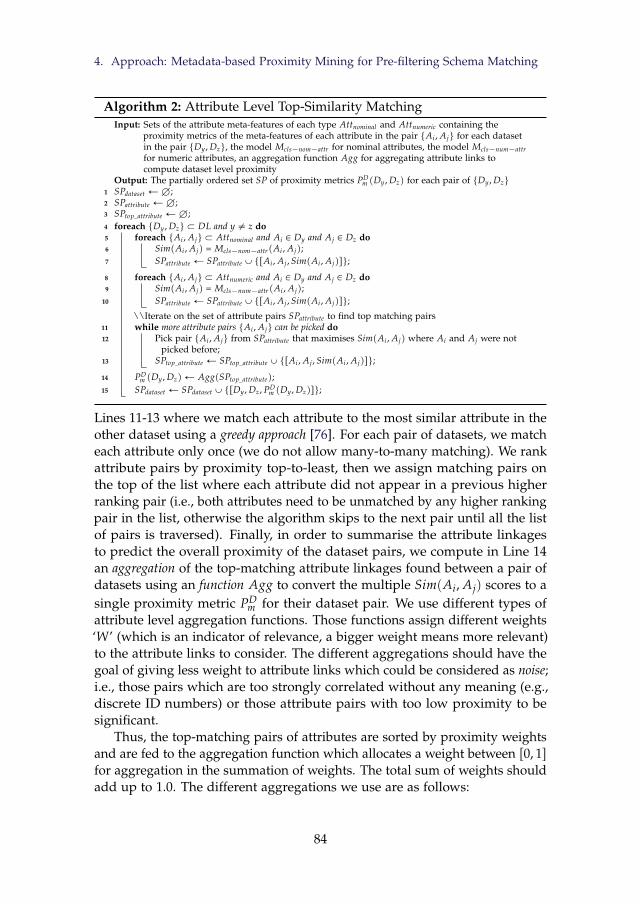
4. Approach: Metadata-based Proximity Mining for Pre-filtering Schema Matching
Algorithm 2: Attribute Level Top-Similarity MatchingInput: Sets of the attribute meta-features of each type Attnominal and Attnumeric containing the
proximity metrics of the meta-features of each attribute in the pair tAi , Aju for each datasetin the pair tDy , Dzu, the model Mcls´nom´attr for nominal attributes, the model Mcls´num´attrfor numeric attributes, an aggregation function Agg for aggregating attribute links tocompute dataset level proximity
Output: The partially ordered set SP of proximity metrics PDm pDy , Dzq for each pair of tDy , Dzu
1 SPdataset ÐH;2 SPattribute ÐH;3 SPtop_attribute ÐH;4 foreach tDy , Dzu Ă DL and y ‰ z do5 foreach tAi , Aju Ă Attnominal and Ai P Dy and Aj P Dz do6 SimpAi , Ajq = Mcls´nom´attrpAi , Ajq;7 SPattribute Ð SPattribute YtrAi , Aj , SimpAi , Ajqsu;
8 foreach tAi , Aju Ă Attnumeric and Ai P Dy and Aj P Dz do9 SimpAi , Ajq = Mcls´num´attrpAi , Ajq;
10 SPattribute Ð SPattribute YtrAi , Aj , SimpAi , Ajqsu;
\\Iterate on the set of attribute pairs SPattribute to find top matching pairs11 while more attribute pairs tAi , Aju can be picked do12 Pick pair tAi , Aju from SPattribute that maximises SimpAi , Ajq where Ai and Aj were not
picked before;13 SPtop_attribute Ð SPtop_attribute YtrAi , Aj , SimpAi , Ajqsu;
14 PDm pDy , Dzq Ð AggpSPtop_attributeq;
15 SPdataset Ð SPdataset YtrDy , Dz , PDm pDy , Dzqsu;
Lines 11-13 where we match each attribute to the most similar attribute in theother dataset using a greedy approach [76]. For each pair of datasets, we matcheach attribute only once (we do not allow many-to-many matching). We rankattribute pairs by proximity top-to-least, then we assign matching pairs onthe top of the list where each attribute did not appear in a previous higherranking pair (i.e., both attributes need to be unmatched by any higher rankingpair in the list, otherwise the algorithm skips to the next pair until all the listof pairs is traversed). Finally, in order to summarise the attribute linkagesto predict the overall proximity of the dataset pairs, we compute in Line 14an aggregation of the top-matching attribute linkages found between a pair ofdatasets using an function Agg to convert the multiple SimpAi, Ajq scores to asingle proximity metric PD
m for their dataset pair. We use different types ofattribute level aggregation functions. Those functions assign different weights‘W’ (which is an indicator of relevance, a bigger weight means more relevant)to the attribute links to consider. The different aggregations should have thegoal of giving less weight to attribute links which could be considered as noise;i.e., those pairs which are too strongly correlated without any meaning (e.g.,discrete ID numbers) or those attribute pairs with too low proximity to besignificant.
Thus, the top-matching pairs of attributes are sorted by proximity weightsand are fed to the aggregation function which allocates a weight between r0, 1sfor aggregation in the summation of weights. The total sum of weights shouldadd up to 1.0. The different aggregations we use are as follows:
84

4. Approach: Metadata-based Proximity Mining for Pre-filtering Schema Matching
• Minimum: we allocate all the weight (i.e., W “ 1.0) to the single attributepair link with the minimum similarity, and we consider this as the overallproximity between the dataset pair. Therefore, all top-matching attributepair links need to have a high similarity score to result into a highproximity for a dataset pair.
• Maximum: we allocate all the weight (i.e., W “ 1.0) to the single attributepair link with the maximum similarity, and we consider this as the overallproximity between the dataset pair. Therefore, only one top-matchingattribute pair link needs to have a high similarity score to result into ahigh proximity for a dataset pair.
• Euclidean: a Euclidean aggregation of the similarities Sim of all matchingpairs of attributes without any weighting as in Equation 4.5. Here weconsider all the attribute pair links in the aggregation and we assignequal weights to all the links.
PDm “
g
f
f
e
nÿ
i“1,j“2
rSimpAi , Ajqs2 (4.5)
• Average: a standard averaging aggregation of the pairs of attributeswithout any weighting, where all attribute links are equally weighted inthe average.
• Weighted function: a normal distribution function to assign differentproximity weights W for all attribute linkages found, and then summingup all the weighted similarities as the overall proximity as in Equation4.6.
PDm “
nÿ
i“1,j“2
rWi ˚ SimpAi , Ajqs (4.6)
This is visualised in Figure 4.6. Here the weight 0.0 ď W ď 1.0 foreach top-matching attribute linkage is assigned based on ordering thelinkages top-to-least in terms of their similarity scores, and the weightallocated varies according to a normal distribution. We use differentp-parameters (probability of success) of t0.1, 0.25, 0.5, 0.75, 0.9u, wherea parameter of 0.5 leads to a standard normal distribution of weightsallocated for the sorted pairs of attributes. A lower parameter valueleads to skewness to the left, allocating more weight to highly relatedpairs, and a higher parameter leads to skewness to the right, allocatinghigher weights to pairs with lower ranked relationships. This meansthat with lower p we expect similar datasets to have a few very similarattributes and a higher p value means we expect most of the attributesto be strongly similar.
85

4. Approach: Metadata-based Proximity Mining for Pre-filtering Schema Matching
Ass
igne
d W
eigh
t
Rank of Top Matching Attribute Pairs
p = 0.75
p = 0.50
p = 0.25
p = 0.90
p = 0.10
Figure 4.6: Different normal distributions for assigning weights to ranked attribute linkages.
As can be seen from their descriptions, each aggregation leads to a differentmeaning of similarity based on the number of attribute linkages to considerand which attribute linkages are considered more important (having higherweights assigned). All the dataset proximity metrics generated by the differentaggregations listed above are finally normalised using Equation 4.7. Theproximity metric PD
m for two datasets Dy and Dz is computed by multiplyingthe number of matching attributes found (N), and divided by the minimumnumber of attributes of both datasets (Minp|Attry|, |Attrz|q). This is done toprevent an inaccurate similarity score for two datasets having few very similarattributes of a single type, and many other attributes of different types. Forexample, if dataset D1 has 1 nominal attribute and 10 numeric attributesand D2 just has 8 nominal attributes, then if the single nominal attribute inD1 is highly similar to a nominal attribute in D2 (e.g., SimpA1, A2q “ 0.9)then the overall outcome without normalisation will be a high proximitymetric between both datasets although they have many disjoint attributetypes. The resulting proximity metric after normalisation for the datasetswould be calculated as follows: P1Dm “ 0.9 ˚ 1
9 “ 0.1, so overall they willhave a low proximity compensating for all the unmatched attributes withoutcorresponding types.
P1Dm “ PDm ˚
NMinp|Attry|, |Attrz|q
(4.7)
Applying the models on the DL
In the second phase, after building the ensemble models, we apply themto each new pair of previously unseen datasets to achieve a measure ofthe similarity score. When applying the models, we compute for each pairof datasets the similarity score of SimpDy, Dzq and for each attribute pairSimpAi, Ajq using the supervised models extracted in the previous phase. TheSim score is the positive-class distribution value generated by each ensemblemodel [127]. For the attribute level scoring, we complete the proximity mining
86
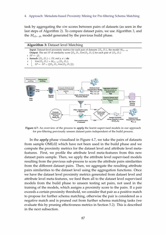
4. Approach: Metadata-based Proximity Mining for Pre-filtering Schema Matching
task by aggregating the sim scores between pairs of datasets (as seen in thelast steps of Algorithm 2). To compare dataset pairs, we use Algorithm 3, andthe Mcls´ds model generated by the previous build phase.
Algorithm 3: Dataset level MatchingInput: Dataset-level proximity metrics for each pair of datasets tDy , Dzu, the model Mcls´dsOutput: The set SP of similarity score rDy , Dz , SimpDy , Dzqs for each pair of tDy , Dzu
1 SP ÐH;2 foreach tDy , Dzu Ă DL and y ‰ z do3 SimpDy , Dzq = Mcls´dspDy , Dzq;4 SP Ð SPYtrDy , Dz , SimpDy , Dzqsu;
Pairsof DS
DataLake
Dataset-level Classification Model
Mcls_ds
Assign Proximityusing classifier's score
Sim(Dy,Dz)
Aggregate attribute-level proximity to
dataset-levelAgg
DS PairsTestingSample
Filter negative pairs of datasets
Attribute-level Classification Model
Mcls_num_attrMcls_nom_attr
NO
YES
Check passthreshold
Cd?
Evaluate Dataset-level
PruningRel(Dy,Dz)
Pass positive pairsof datasets
SampleOML02
Apply Attribute-levelProximity Model Compute Dataset level
meta-feature proximitymetricsPm
Attribute-levelprofiling
Dataset-levelprofiling
Compute Attribute levelmeta-feature proximity
metricsPm
Figure 4.7: An overview of the process to apply the learnt supervised models in our approachfor pre-filtering previously unseen dataset pairs independent of the build process.
In the apply phase visualised in Figure 4.7, we take the pairs of datasetsfrom sample OML02 which have not been used in the build phase and wecompute the proximity metrics for the dataset level and attribute level meta-features. First, we profile the attribute level meta-features from this newdataset pairs sample. Then, we apply the attribute level supervised modelsresulting from the previous sub-process to score the attribute pairs similaritiesfrom the different dataset pairs. Then, we aggregate the resulting attributepairs similarities to the dataset level using the aggregation functions. Oncewe have the dataset level proximity metrics generated from dataset level andattribute level meta-features, we feed them all to the dataset level supervisedmodels from the build phase to unseen testing set pairs, not used in thetraining of the models, which assigns a proximity score to the pairs. If a pairexceeds a certain proximity threshold, we consider that pair as a positive matchto propose for further schema matching, otherwise the pair is considered as anegative match and is pruned out from further schema matching tasks (weevaluate this by pruning effectiveness metrics in Section 5.2). This is describedin the next subsection.
87

5. Experimental Evaluation
4.3 Pre-filtering Dataset Pairs for Schema Matching
For the final step of pre-filtering pairs of datasets before applying detailedinstance-based schema matching, we check whether the pairs of datasets areoverall related or not, and therefore whether they should be filtered out orproposed for expensive schema matching. We analyses the final SimpDy, Dzq
score generated by the model Mcls´ds for each dataset pair in the DL to decidewhether they satisfy the RelpDy, Dzq or not. We consider the relationship ofeach dataset with each of the other datasets existing in the DL. Each datasetmust pass the similarity threshold cd with each individual dataset to beproposed for detailed schema matching (as in Equation 4.1).
If we choose a high cut-off threshold we restrict the supervised modelto return less pairs of high proximity, leading to lower recall but also lesscomparisons, thus helping to reduce the computational time at the expenseof possibly missing some misclassified pairs. Alternatively, if we choose alower cut-off threshold, we relax our model to return pairs of lower proximity.This leads to more pairs (i.e., more work for further schema matching tasks)yielding positive matches and higher recall of positive cases, but, with morepairs marked incorrectly as matching. We propose how to select an appropriatethreshold that optimises this trade-off empirically in Section 5.
The complexity of our approach is quadratic in the number of objects(attributes or datasets) compared, and therefore runs in polynomial time,however, it applies the cheapest computational steps for early-pruning (justcomputing distances in Equations 4.3 and 4.4 and applying the model toscore each pair). This way, we save unnecessary expensive schema matchingprocessing per each value instance of the attributes in later steps, reducing thecomputational workload at the detailed granularity schema matching level bypre-filtering the matching tasks. We demonstrate this empirically in Section5.5.
5 Experimental Evaluation
In this section, we present the experiments which evaluate our approach byusing a prototype implementation. We evaluate the following components ofour approach in predicting RelpDy, Dzq for pre-filtering schema matching:
• Proximity metrics: we evaluate the different individual dataset leveland aggregated attribute level meta-features.
• Supervised models: we also evaluate the ensemble supervised models,which consume the proximity metrics, in the pre-filtering task.
In addition, we evaluate the sub-components of our approach which in-clude the attribute level models Mcls´nom´attr and Mcls´num´attr in predicting
88

5. Experimental Evaluation
RelpAi, Ajq. We test the attribute level model in experiment 1, the datasetlevel pruning effectiveness against the ground-truth in experiment 2, and thecomputational performance in experiment 3.
In experiments 2 and 3, we compare the performance of our proposedproximity mining models against traditional instance-based schema matchingtechniques we proposed in Chapter 2. Those are the most expensive tech-niques which compare values from instances in the datasets to for computingschema similarity. We benchmark our results against a naïve averaging of at-tribute similarity from a prototype called Probabilistic Alignment of Relations,Instances, and Schema (PARIS), which is one of the most cited schema match-ing tools [126]. PARIS was found to be best performing with large datasetswhen compared against other tools [76] and does not need collection of extrametadata (see Table 4.1). PARIS does exact value-string matching based onvalue-frequency inverse functionality [126]. We implement a prototype in [15](see Chapter 2) which compares pairs of attributes from different datasetsusing PARIS and generates an overall score for SimpDy, Dzq by averagingSimpAi, Ajq generated by PARIS from the top-matching attribute-pairs (similarto Algorithm 2, where PARIS replaces the supervised models). It convertstabular datasets to RDF triples, and executes a probabilistic matching algo-rithm for identifying overlapping instances and attributes. We selected PARISbecause of its simplicity and ease of integration with Java-based APIs and itshigh performance in previous research [76]. We parametrised the prototypewith the top performing settings from experiments in [15] (see Chapter 2)sampling 700 instances per dataset, 10 iterations comparisons, with identityand shingling value strings matching. This will be a baseline pre-filteringheuristic approach we shall compare against in the experiments.
The rest of this section describes the datasets used in the experiments,the evaluation metrics used and the different experiments implemented. Wepresent the results from our experiments and discuss their implications.
5.1 Datasets
We use the OpenML DL2 in our experiments [131], which has more than 20,000datasets intended for analytics from different subject areas. OpenML is a web-based data repository that allows data scientists to upload different datasets,which can be used in data mining experiments. OpenML stores datasets inthe ARFF tabular format which consist of diverse raw data loaded withoutany specific integration schema. This allows us to evaluate our approach in areal-life setting where datasets come from heterogeneous domains.
We use two subsets of manually annotated datasets from OpenML asour ground-truth (gold standard) for our experiments. Those two subsets
2https://www.openml.org
89

5. Experimental Evaluation
have been generated using two different independent processes, and thereforeprovide independently generated ground truths that do not overlap. As theresearch community is lacking appropriate benchmarking gold standards forapproximate (non-equijoins) dataset and attribute similarity search [89], wepublished those datasets online to support in future benchmarking tasks3. Theexperimental datasets are described as follows:
• OML01 - The attribute level annotated 15 DS: consists of 15 datasetsfrom different domains as described in Table 4.4. The total number ofattributes is 126 (61 nominal and 65 numeric), and the average numberof attributes per dataset is 8. There is a total of 3468 pairs of attributes tobe matched (1575 nominal pairs and 1892 numeric pairs). All the pairsof attributes in this subset were manually scrutinised by 5 annotatorsconsisting of post-graduates with an average age of 28, where 4 arepharmacists and 1 is a computer scientist. They checked the attributesin the datasets and annotated all the pairs of attributes from differentdatasets with related data, RelpAi, Ajq. It took on average 3 hours byeach annotator to complete the task. Annotators assign a single valuefrom t0, 1u, where ‘1’ means a related attribute, and the majority vote istaken for each pair, where the average Kappa coefficient for the inter-rater agreement is 0.59, the maximum is 0.80 and the minimum 0.37.Annotators were given the following to judge if the attribute pair isrelated: attribute name, OpenML dataset description, top 10 values, andthe mean and standard deviation for numeric attributes. We didn’t giveinstructions on how to use the provided information to judge, but wedescribed that “related attributes should store data related to similarreal-world properties, e.g., car prices, specific body size measurementslike height, etc., and should contain similar data”. Examples of the an-notations can be seen in Table 4.5. There are only 56 positively matchingpairs (19 nominal and 37 numeric). This subset is used in training theattribute level models for computing the similarity between attributesfrom different datasets and predicting related attributes, RelpAi, Ajq.
Table 4.4: Description of the OML01 datasets
Domain Datasets IDs DatasetsVehicles 21,455,967,1092 car,cars,cars,CrashBusiness 223,549,841 Stock,strikes,stockSports 214 baskballHealth 13,15,37 breast-cancer,breast-w,diabetesOthers 48,50,61,969 tae,tic-tac-toe,Iris,Iris
• OML02 - The dataset level annotated 203 DS: consists of 203 datasetsdifferent from those in the OML01 subset. To collect this sample, we
3https://github.com/AymanUPC/all_prox_openml
90
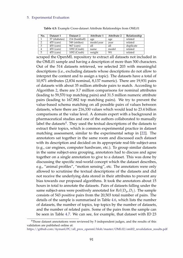
5. Experimental Evaluation
Table 4.5: Example Cross-dataset Attribute Relationships from OML01
No. Dataset 1 Dataset 2 Attribute 1 Attribute 2 Relationship1 37 (diabetes) 214 (baskball) age age related2 455 (cars) 549 (strikes) model.year year related3 455 (cars) 967 (cars) all all duplicate4 455 (cars) 1092 (Crash) name model related5 455 (cars) 1092 (Crash) weight Wt related
scraped the OpenML repository to extract all datasets not included inthe OML01 sample and having a description of more than 500 characters.Out of the 514 datasets retrieved, we selected 203 with meaningfuldescriptions (i.e., excluding datasets whose descriptions do not allow tointerpret the content and to assign a topic). The datasets have a total of10,971 attributes (2,834 nominal, 8,137 numeric). There are 19,931 pairsof datasets with about 35 million attribute pairs to match. According toAlgorithm 2, there are 3.7 million comparisons for nominal attributes(leading to 59,570 top matching pairs) and 31.5 million numeric attributepairs (leading to 167,882 top matching pairs). We try to prevent thevalue-based schema matching on all possible pairs of values betweendatasets, where there are 216,330 values which would lead to 23.4 billioncomparisons at the value level. A domain expert with a background inpharmaceutical studies and one of the authors collaborated to manuallylabel the datasets4. They used the textual descriptions of the datasets toextract their topics, which is common experimental practice in datasetmatching assessment, similar to the experimental setup in [22]. Theannotators sat together in the same room and discussed each datasetwith its description and decided on its appropriate real-life subject-area(e.g., car engines, computer hardware, etc.). To group similar datasetsin the same subject-area grouping, annotators had to discuss and agreetogether on a single annotation to give to a dataset. This was done bydiscussing the specific real-world concept which the dataset describes,e.g., “animal profiles”, “motion sensing”, etc. The annotators were onlyallowed to scrutinise the textual descriptions of the datasets and didnot receive the underlying data stored in their attributes to prevent anybias towards our proposed algorithms. It took the annotators about 15hours in total to annotate the datasets. Pairs of datasets falling under thesame subject-area were positively annotated for RelpDy, Dzq. The sampleconsists of 543 positive pairs from the 20,503 total number of pairs. Thedetails of the sample is summarised in Table 4.6, which lists the numberof datasets, the number of topics, top topics by the number of datasets,and the number of related pairs. Some of the pairs from the sample canbe seen in Table 4.7. We can see, for example, that dataset with ID 23
4Those dataset annotations were reviewed by 5 independent judges, and the results of thisvalidation are published online at:https://github.com/AymanUPC/all_prox_openml/blob/master/OML02/oml02_revalidation_results.pdf
91

5. Experimental Evaluation
should match all datasets falling under the topic of ‘census data’ likedataset 179. Both datasets have data about citizens from a populationcensus. In row 4, we can see an example of duplicated datasets havinghighly intersecting data in their attributes. Duplicate pairs like those inrow 4 have the same number of instances, but described with differentnumber of attributes, which are overlapping. We consider all duplicatepairs of datasets as related pairs. We aim to detect and recommend suchkind of similar dataset pairs as those in Table 4.7 for schema matchingusing our proximity mining approach.
Table 4.6: Description of the OML02 datasets
Datasets Topics Top Topics RelpDy, Dzq
203 74 computer software defects (16), healthmeasurements (13), digit handwritingrecognition (12), robot motion sensing(11), plant and fungi measurements (9),citizens census data (8), diseases (8)
543
Table 4.7: An example of pairs of datasets from the OML02 sample from OpenML
No. DID 1 Dataset 1 DID 2 Dataset 2 Topic Relationship1 23 cmc 179 adult Census Data related2 14 mfeat-
fourier1038 gina_agnosticDigit Handwriting
Recognitionrelated
3 55 hepatitis 171 primary-tumor
Disease related
4 189 kin8nm 308 puma32H Robot Motion Sensing duplicate
5.2 Evaluation Metrics
We use different evaluation metrics to assess the effectiveness of our approach.We use the traditional recommendation and information retrieval evaluationmetrics similar to other research [62, 86], including precision, recall and ROCmeasurements. For the supervised models, we use traditional data miningclassification effectiveness metrics [127]. We evaluate the computational costsof our approach vs. traditional schema matching for baseline comparison.Those metrics are categorised per the experiment types and granularities:
• Classification effectiveness
– Granularity: Attribute level RelpAi, Ajq and Dataset level RelpDy, Dzq
– Models evaluated: Mcls´nom´attr, Mcls´num´attr, Mcls´ds
– Classification measures: Classification accuracy, Recall, Precision,ROC, Kappa
92
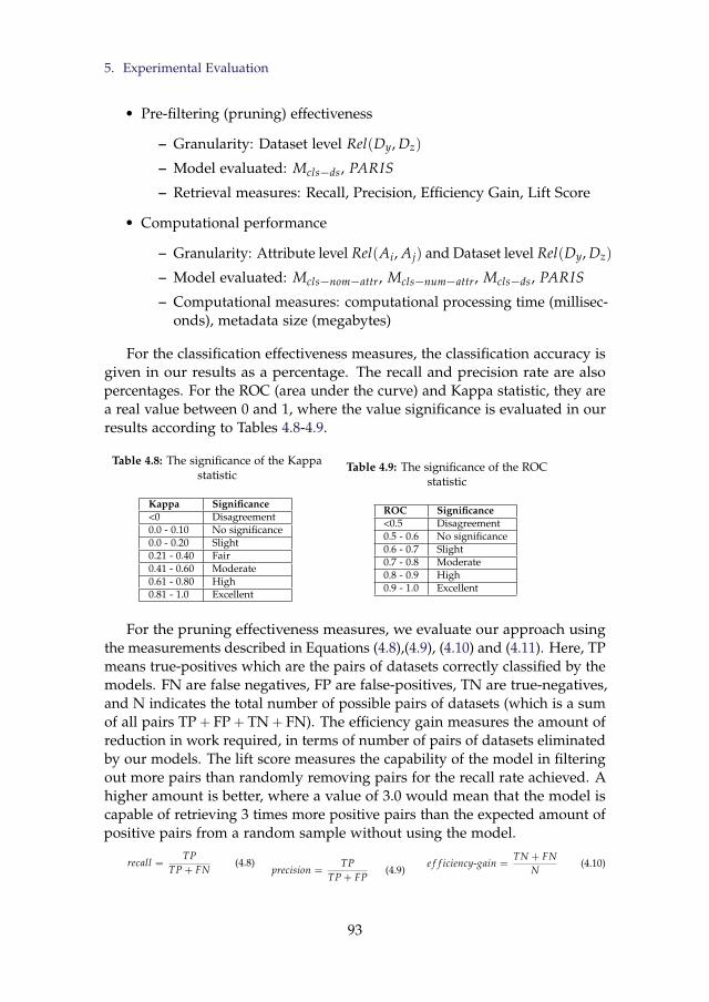
5. Experimental Evaluation
• Pre-filtering (pruning) effectiveness
– Granularity: Dataset level RelpDy, Dzq
– Model evaluated: Mcls´ds, PARIS
– Retrieval measures: Recall, Precision, Efficiency Gain, Lift Score
• Computational performance
– Granularity: Attribute level RelpAi, Ajq and Dataset level RelpDy, Dzq
– Model evaluated: Mcls´nom´attr, Mcls´num´attr, Mcls´ds, PARIS
– Computational measures: computational processing time (millisec-onds), metadata size (megabytes)
For the classification effectiveness measures, the classification accuracy isgiven in our results as a percentage. The recall and precision rate are alsopercentages. For the ROC (area under the curve) and Kappa statistic, they area real value between 0 and 1, where the value significance is evaluated in ourresults according to Tables 4.8-4.9.
Table 4.8: The significance of the Kappastatistic
Kappa Significance<0 Disagreement0.0 - 0.10 No significance0.0 - 0.20 Slight0.21 - 0.40 Fair0.41 - 0.60 Moderate0.61 - 0.80 High0.81 - 1.0 Excellent
Table 4.9: The significance of the ROCstatistic
ROC Significance<0.5 Disagreement0.5 - 0.6 No significance0.6 - 0.7 Slight0.7 - 0.8 Moderate0.8 - 0.9 High0.9 - 1.0 Excellent
For the pruning effectiveness measures, we evaluate our approach usingthe measurements described in Equations (4.8),(4.9), (4.10) and (4.11). Here, TPmeans true-positives which are the pairs of datasets correctly classified by themodels. FN are false negatives, FP are false-positives, TN are true-negatives,and N indicates the total number of possible pairs of datasets (which is a sumof all pairs TP` FP` TN` FN). The efficiency gain measures the amount ofreduction in work required, in terms of number of pairs of datasets eliminatedby our models. The lift score measures the capability of the model in filteringout more pairs than randomly removing pairs for the recall rate achieved. Ahigher amount is better, where a value of 3.0 would mean that the model iscapable of retrieving 3 times more positive pairs than the expected amount ofpositive pairs from a random sample without using the model.
recall “TP
TP` FN(4.8)
precision “TP
TP` FP(4.9)
e f f iciency-gain “TN` FN
N(4.10)
93

5. Experimental Evaluation
li f t-score “recall
p1.0´ e f f iciency-gainq(4.11)
5.3 Experiment 1: Attribute-level Models
Our goal in this experiment is to evaluate the supervised models we buildfor detecting the relationship between related attributes RelpAi, Ajq usingattribute level content meta-features as follows:
• Dataset: OML01
• Evaluation metrics: Classification effectiveness
• Relationship evaluated: RelpAi, Ajq
• Input: the attribute level meta-features matching for pairs of attributes.
• Output: a supervised model to predict related attributes per type.
• Goal: select the most appropriate models for predicting related attributesby evaluating their effectiveness for each type (nominal or numerical).
• Description: we take two subsets of attribute pairs and their meta-features, depending on the attribute type: nominal attributes and nu-meric attributes. The subsets are annotated by a human to decidewhether RelpAi, Ajq is 1 or 0. We build a proximity model using asupervised learning algorithm.
Experimental Setup
we evaluate the model using the leave-one-out approach (where we excludeone pair from training in each run, and use it to test the output model,therefore having a cross-validation where the number of folds is equal tothe number of pairs). As the number of positive pairs to negative pairsare imbalanced, we create a balanced training set for each type, nominal ornumeric, which consists of all the positive pairs of attribute matches andan equal number of negative unmatching pairs. To make the training setrepresentative of all the different negative cases, we cluster the negative casesusing the Expectation Maximisation (EM) algorithm [127] and we select arepresentative sample of negative cases from each cluster.
Results
The attribute level models were evaluated for both nominal attribute pairsand numeric attribute pairs. We evaluate the Mcls´nom´attr and Mcls´num´attr
94

5. Experimental Evaluation
models which assign the SimpAi, Ajq for attribute pairs. As could be seen inTable 4.10, we created two supervised models; one for each type of attributepairs. Both models achieved excellent ROC performance and highly significantresults on the Kappa statistic (see Tables 4.8-4.9 results significance). Themodels had good accuracy, recall, and precision rates. This is importantbecause the dataset pairs pre-filtering step depends on this attribute proximitystep, so we have to achieve a good performance at this level to minimiseaccumulation of errors for the following tasks.
Table 4.10: Performance evaluation of attribute pairs proximity models
Model ROC Kappa Accuracy Positive Recall Positive PrecisionNominal 0.957 0.65 82.5% 89.5% 77.3%Numeric 0.915 0.7 84.8% 89.2% 80.5%
5.4 Experiment 2: Dataset-level Models
In this experiment, we evaluate the effectiveness of the dataset level modelsin pre-filtering dataset pairs for further schema matching. Our goal is toevaluate how good is our approach in retrieving related datasets RelpDy, Dzq
and filtering out unrelated datasets from the schema matching process. Weevaluate the effectiveness of correctly proposing related datasets for schemamatching using the different types of models we describe later in this section.The evaluation is as follows:
• Dataset: OML02
• Evaluation metrics: Classification effectiveness, Pre-filtering effective-ness
• Relationship evaluated: RelpDy, Dzq
• Input: Pairs of datasets with different types of meta-features matching[dataset level names, dataset level content meta-features, attribute levelnames, attribute level meta-features, all meta-features].
• Output: a supervised model Mcls´ds to predict related datasets basedon proximity mining and PARIS baseline.
• Goal: select the best proximity model to predict related datasets and theproximity threshold cd to use with that model.
• Description: we take annotated pairs of datasets and their meta-features’normalised metrics. The pairs are annotated by a human annotator todecide whether RelpDy, Dzq is 1 or 0. We build a proximity model usinga supervised learning algorithm.
95

5. Experimental Evaluation
We create different types of dataset pairs ensemble models to scoreSimpDy, Dzq by using different combination of meta-feature types. We createdifferent models depending on the meta-feature type(s) used as input (namelythose are dataset content meta-features, dataset name similarity, attributecontent meta-features, and attribute name similarity). We can combine themeta-feature types used to build the model or use each type separately to leadto the following model types depending on which meta-features are used:
• DS-Prox-Content: uses the dataset level content meta-features, withoutconsidering the dataset name distance.
• DS-Prox-Name: uses the dataset name Levenshtein distance as the onlypredictor of dataset pairs similarity.
• Attribute-Prox-Content: uses the attribute level content meta-features,not considering the attribute name meta-features.
• Attribute-Prox-Name: uses the attribute level name meta-features only,not considering the attribute content meta-features.
• Name-Prox: uses dataset level and attribute level name-based meta-features only.
• Content-Prox: uses dataset level and attribute level content-based meta-features only.
• All-Prox: uses all the dataset level and attribute level meta-features,including both name-based and content-based meta-features.
We differentiate between the meta-feature types in our experiments so wecan test if a specific subset of meta-features is better in predicting RelpDy, Dzq
or whether it is necessary to use all of them together to build an effective prox-imity mining model for the pre-filtering task. We also investigate if there is adifference in performance with regards to the types of meta-features extracted:classical name-based meta-features vs. the newly proposed content-basedmeta-features, and whether using both types together in combination leadsto better results. We also separate the types so we can distinguish if purelycontent-based meta-features can be used as an alternative to name-basedmeta-features, especially in the case when the datasets and their attributes arenot properly named. The most comprehensive of all models is the All-Proxmodel which uses all the possible meta-features we collect from the dataprofiling step. The DS-Prox-Name is the most generic of all models as it justconsiders a single meta-feature at the most abstract-level, therefore it will beused as our baseline for our performance comparisons in the experiments.
96

5. Experimental Evaluation
Training Set
F1 F2 F3 F4 F5 F6 F7 F8 F9 F10
F1 F2 F3 F4 F5 F6 F7 F8 F9 F10
F1 F2 F3 F4 F5 F6 F7 F9F8 F10
. . .F8F2 F3 F4 F5 F6 F7 F9F1 F10
Test foldTraining folds
E1
E2
E3
E10
Eavg =10
Iteration 1
Iteration 2
Iteration 3
Iteration 10
f = 1
10Ef
1
Figure 4.8: A 10-fold cross-validation experimental setup consisting of alternating folds intraining and test roles. Image adapted from the book: Raschka S (2015) Python Machine
Learning. 1st Edition. Packt Publishing, Birmingham, UK.
Experimental Setup
To evaluate our approach and models, we consider in our experiments a10-fold cross-validation experimental setup using different subsets of datasetsfrom a real-world DL, as visualised in Figure 4.8. The purpose of a cross-validation setup is to select the best supervised model for the pre-filtering taskby evaluating the different models on test-sets separate from the training-sets,which is commonly used in recommendation assessment experiments [6, 62]and schema matching tasks [35]. Such an experimental setup increases thevalidity and generalisability of our experiments and approach. This is onlyachieved if the training set is representative of the cases found in the real-lifepopulation.
We make sure that the folds do not include intersecting dataset pairs. Wecreate a balanced training set with all the positive cases and an equal numberof negative cases similar to experiment 1. As the number of negative casesis much higher in the OML02 subset too, we also follow the clustering ofnegative cases approach to select a representative sample from each cluster(see Section 5.3). As seen in Figure 4.8, we iterate 10 times using an alternatingfold as the test set, and the remaining folds as the training set. We evaluate themodels in accurately predicting RelpDy, Dzq with 9 different cut-off thresholdsin r0.1-0.9s for ‘cd’ from Equation (4.1) in order to cover a wide range ofvalues. Finally, we evaluate the performance of each model by averagingthe evaluation metrics (‘E’) from all 10 iterations. We also compute standarddeviations in performance between different folds to evaluate the stability andconsistency of the models evaluated. For the PARIS baseline implementation,it does not need to train any models, so we simply run it on all pairs ofdatasets and compare its results to our approach.
97

5. Experimental Evaluation
Results
Classification effectiveness. First, we created the models for the dataset pairswhich assign SimpDy, Dzq and check if they satisfy RelpDy, Dzq by passing theminimum threshold. We evaluated the classification effectiveness measuresfor each proximity model after the 10-fold cross-validation. The results aresummarised in Figures 4.9-4.11. The figures show a plot of results (from 10folds) and interquartile ranges of accuracy, kappa statistic and ROC statisticfor each model type. The distribution between folds can also be seen to assessthe stability of the models. For our comparison, we use the name-basedmodels, which are common in previous research, as our baseline comparison.As could be seen, all models were stable with very close values for the differ-ent evaluation metrics, indicating the versatility of our approach. However,still the All-Prox and Attribute-Prox models consistently had slightly betterstability (lower deviations) than Name-Prox and other models. It can be seenfrom the results that the All-Prox and Attribute-Prox models are consistentlyperforming better than the name-based model in terms of accuracy, ROC andKappa statistic. This indicates that our proposed content-based and name-based combined meta-features models perform best with schema matchingpre-filtering.
Model Type
7172 73 74 75 76 77 78 79 80 8182
Classification Accuracy
All-ProxAttribute-ProxName-Prox
Content-ProxDS-Prox
78.1875.51
74.2973.72
73.29
Figure 4.9: Classification accuracy from 10-foldcross-validation of dataset pairs pre-filtering
models.
Model Type
0.440.460.480.500.520.540.560.580.600.62
Kappa Statistic
All-ProxAttribute-ProxName-Prox
Content-ProxDS-Prox
0.560.510.490.47
0.47
Figure 4.10: Kappa statistic from 10-foldcross-validation of dataset pairs pre-filtering
models.Model Type
0.800.810.820.830.840.850.860.870.88
Roc Score
All-ProxAttribute-ProxName-Prox
Content-ProxDS-Prox
0.860.83
0.810.810.81
Figure 4.11: ROC statistic from 10-foldcross-validation of dataset pairs pre-filtering
models.
The different models used for the schema matching pre-filtering taskachieve different results because the meta-features used in the different modelsare not correlated, therefore contain different information about the datasetsleading to the different performance of each model. We evaluated the Spear-man rank correlation [62] between the different types of meta-features, whichis presented in Table 4.11. The Spearman rank correlation ranks the dataset
98

5. Experimental Evaluation
Table 4.11: Spearman rank correlation for the different meta-features. We aggregate minimum(Min.), average (Avg.), maximum (Max.), & standard deviation (Std. Dev.) for different
meta-feature types.
Type 1 Type 2 Min. Correlation Avg. Correlation Max. Correlation Std. Dev. CorrelationAttribute Name Attribute Content -0.12 -0.01 0.19 0.04Attribute Name Dataset Content 0.02 0.04 0.10 0.02Attribute Name Dataset Name 0.06 0.07 0.13 0.02Dataset Content Attribute Content -0.01 0.09 0.15 0.04Dataset Content Dataset Name -0.02 0.00 0.02 0.02Dataset Name Attribute Content 0.00 0.01 0.04 0.01
pairs according to the proximity metrics of the meta-features. If the datasetpairs have the same identical rankings between two different meta-featuresthen we get a perfect correlation. If the rankings produced in descendingorder by the two proximity metrics are different (e.g., a dataset pair can beranked in the 100th position by one meta-feature and in the 9th position bythe other, which have a difference of 81 ranks) then we get a lower correla-tion, with completely uncorrelated meta-features. We evaluated the average,standard deviation, minimum, and maximum of the correlation between themeta-features falling under the different types of meta-features. Recall thateach type will have multiple meta-features (see Section 4.1), like attributecontent will include all the meta-features in Table 4.3 with all their differentproximity metrics according to the aggregations described in Section 4.2. Wecalculate the correlation between each individual meta-feature pair and wecalculate aggregates per type. As can be seen in Table 4.11, all the correlationvalues are low.
Pre-filtering effectiveness. We compare the effectiveness of our approachagainst the baseline implementation of PARIS. We change the cut-off thresh-olds for Equation 4.1, and we aim to maximize the efficiency-gain while main-taining the highest recall for all candidate dataset pairs satisfying RelpDy, Dzq.The effectiveness is also evaluated by lift scores. The results from our approachand from the ‘baseline’ PARIS prototype are presented in Figures 4.12-4.15.Figures 4.12-4.13 show the results for the different supervised models andPARIS, and Figures 4.14-4.15 show the results of the same evaluation met-rics but for the individual meta-features in our approach, where we use theindividual proximity metrics of the meta-features directly as an indicator ofRelpDy, Dzq without using any supervised learning models. We evaluate thedataset level meta-features from Section 4.1. The graphs show the averageperformance for all the individual metrics per specific type. We use a differentminimum threshold with each proximity model or meta-feature in Figures4.12-4.15 leading to the different plotted results per model or meta-feature.The aim of comparing both models and individual metrics is to be able todetect if the proposed supervised proximity models perform any better thansimply using single independent metrics for the pre-filtering task.
For each evaluation of the models or the individual metrics, we evaluatethe efficiency gain against recall first. We set a minimum target recall of 80%
99

5. Experimental Evaluation
0 10 20 30 40 50 60 70 80 90100Avg. Recall
010
20
30
40
50
60
70
80
90
100Avg. Efficiency Gain 3.1
2.3
2.9
5.6
1.7
1.9
2.4
4.5
1.6
10.83.3
1.31.2
4.5 24.6
4.9
5.5
7.614.8
1.3DS-Prox
Name-Prox
Content-Prox
Attribute-Prox
All-Prox
Baseline
Figure 4.12: Recall against efficiency gain forthe different supervised models.
0 10 20 30 40 50 60 70 80 90100
Avg. Recall
010
20
30
40
50
60
70
80
90
100
Avg. Precision
10.8
5.6
4.5
14.3
24.6
7.6
73.8
3.13.4
2.1
1.9
29.8
3.3
14.8
2.4
5.5
1.74.9
4.5
1.3
All-Prox
Attribute-Prox
Content-Prox
Name-Prox
DS-Prox
Baseline
Figure 4.13: Recall against precision for thedifferent supervised models.
0 10 20 30 40 50 60 70 80 90 100
Avg. Recall
0
10
20
30
40
50
60
70
80
90
100
Avg. Efficiency Gain
1.57
1.84
2.21
2.77
3.19
3.73
4.02
1.21
1.011.07
1.11
1.26
1.40
1.64
1.80
2.15
3.37
8.19
1.26
1.69
1.95
2.36
7.06
6.71
1.27
9.3829.1438.28
Sheet 4
Attribute- Name- Prox
Attribte-Content
DS-Content
DS-Name
Average of Recall vs. average of Efficiency Gain. Color shows details about Sim Measure Grouped. Shape shows details about Sim Measure Grouped. Themarks are labeled by average of Lift Score. Details are shown for Threshold. The data is filtered on Eval Type and Sim Measure. The Eval Type filter keepsentity. The Sim Measure filter has multiple members selected.
Figure 4.14: Recall against efficiency gain forthe different metric types.
0 10 20 30 40 50 60 70 80 90 100
Avg. Recall
0
10
20
30
40
50
60
70
80
90
100
Avg. Precision
3.194.026.57
1.11 1.011.213.37
8.19
14.26
22.11
6.63
8.81
12.69
15.54
17.06
18.40
10.41
11.68
1.69
14.96
1.952.362.74
6.71
8.70
23.93
29.14
32.37
32.51
34.2335.03
38.28
Sheet 5
Attribute Name Prox
Attribute-Content
DS-Content
DS-Name
Average of Recall vs. average of Precision. Color shows details about Sim Measure Grouped. Shape shows details about Sim Measure Grouped. The marksare labeled by average of Lift Score. Details are shown for Threshold. The data is filtered on Eval Type and Sim Measure. The Eval Type filter keeps entity.The Sim Measure filter has multiple members selected.
Figure 4.15: Recall against precision for thedifferent metric types.
and a minimum target efficiency gain of 60% (i.e., filtering out at least 60%of the pairs of datasets while still proposing 80% of the true positive pairs),which are the grey shaded areas in the graphs. The minimum thresholds canbe selected differently according to the requirements of the data analyst. Goodperforming models or proximity metrics are those that fall in this shaded area.The numbers annotated to some of the points in the graphs indicate the liftscore (higher values are better). Similarly, we compare the precision againstthe recall in the second graphs for each evaluation (models or metrics). Wealso annotate some selected lift scores for some points in the graph.
When comparing our new proposed proximity models with the proximitymodel (DS-Prox) from our previous work [18] (described in Chapter 3), it
100

5. Experimental Evaluation
can be seen that our Attribute-Prox model and the All-Prox model performconsistently better. This is expected because we are collecting finer granularitymetadata to describe the datasets which makes it easier in the supervisedlearning task to differentiate between positive pairs and negative pairs. Al-though our new proposed techniques outperform our previous work in theDS-Prox model in terms of recall rates and lift scores, it comes at the price of amore computationally expensive algorithm (Algorithm 2). The complexity ofthe dataset level Algorithm 3 is Oprn ˚ pn´ 1qs{2q while the complexity of theattribute level Algorithm 2 is Oprn ˚ pn´ 1q ˚ a2s{2q where ‘n’ is the number ofdatasets and ‘a’ is the number of attributes in each dataset (we can use theaverage number of attributes per dataset as an approximation for ‘a’ whenestimating the number of computations required).
If we would compare the content meta-features only model (Content-Prox)with the name meta-features only model (Name-Prox), we would see that bothmodels perform equally the same in the pre-filtering task, although combiningthem in the All-prox model leads to the best results capturing the similarityof difficult pairs that can not be retrieved by any single type individually.Therefore, it is possible to solely depend on content-based proximity modelsas a replacement of name-based proximity models to achieve similar results.This will be important in the cases of DLs which are not well maintained anddo not have properly named datasets and attributes. We investigate in detailthe performance of the All-Prox proximity model based on its true positives,false positives and false negative pairs in the Appendix5, where we present theexact cases, we discuss the reasons of discrepancies and we give a comparativeanalysis of the underlying proximity metrics which led to those cases.
For each of the pruning effectiveness evaluation metrics listed above, wecompute the average and standard deviation of the measure between thedifferent folds of evaluation for our approach. The average is plotted in thegraphs in Figures 4.12-4.15, and the standard deviations of each model forthe threshold 0.5 (we chose the mean threshold) are given in Table 4.12. Thestandard deviation indicates the stability of our proposed metrics and modelswith different subsets of datasets. We aim for a low standard deviation toprove the high adaptability of our approach.
Table 4.12: The standard deviation of each evaluation measure for 10-fold cross-validation ofeach dataset pairs pre-filtering model, where cd “ 0.5
Proximity SD Recall SD Efficiency Gain SD Precision SD Lift ScoreAll-Prox 5.4 0.61 0.58 0.32Attribute-Prox 6.5 1.0 0.7 0.24Content-Prox 6.8 1.0 0.38 0.35DS-Prox 7.86 0.85 0.29 0.28Name-Prox 6.3 1.1 0.47 0.24
5The appendix could be found online at https://aymanupc.github.io/all_prox_openml
101

5. Experimental Evaluation
Dataset Pairs Pre-filtering Meta-features
First, we assess if the supervised learning models perform better than a sim-pler approach based on the sub-components they are dependant on, which arethe individual meta-features used in the models. The supervised models usemultiple features in combination to score the similarity of pairs of datasets.Here, we assess the individual features as a baseline to compare against,and whether simply using a proximity metric of an individual meta-featurewithout any models can lead to any good result. We aggregated an averagefor the pruning evaluation metrics per each type of meta-feature. The resultscomparing recall against efficiency gain is given in Figure 4.14. In our experi-ments, no single meta-feature was able to individually predict related pairsof datasets to achieve optimum recall and efficiency gain, as can be seen bythe lack of any plotted result in the top-right box. As seen in Figure 4.15, thepre-filtering task using the meta-features can not have a precision better than10% for the higher recall rates.
We note here that the different types of meta-features are able to modeldifferent information about the datasets and their attributes as seen by the lowcorrelations in Table 4.11. That is the main reason we used the combinationof different types of meta-features in our proximity models which are able tocombine the meta-features to give better results.
Dataset Pairs Pre-filtering Efficiency Gain Vs. Recall
We also evaluated the different supervised proximity models by testing theirpre-filtering performance with different proximity thresholds. As can beseen in Figure 4.12, all of the proximity models were able to optimise recalland efficiency gain to achieve results in the top-right shaded area, comparedto the baseline PARIS implementation that was not successful. This showsthe value of approximate proximity matching and the supervised modelsin our approach compared to exact instance-based string matching in thebaseline. The best performing models were the All-Prox and Attribute-Proxmodels which achieved better results than DS-Prox from our previous work[18] (described in Chapter 3) and better results than Name-Prox which aremore common in other previous research. This means that combining bothname-based meta-features and content-based meta-feature in a supervisedmodel achieves best results in the schema matching pre-filtering task. Forexample, a good result can be achieved using the All-Prox model (combiningall meta-feature types) with a threshold of 0.4 which achieves a recall rateof 85%, an efficiency gain of 73% and a lift score of 3.14. This means thatthe model is able to effectively propose most of the pairs of datasets forschema matching with the least effort possible (only proposing 27% of pairsfor comparison), while achieving this with a performance that is three timesbetter than naive random selection of dataset pairs for schema matching (as
102

5. Experimental Evaluation
expressed by the lift score of 3.14 achieved by the All-Prox model).
Dataset Pairs Pre-filtering Precision Vs. Recall
As seen in Figure 4.13, the precision of the proximity models improvedthe performance of the schema matching pre-filtering as seen by the higherprecision rates compared to the individual meta-features in Figure 4.15. Bycombining the meta-features in a supervised model we were able to achievehigher precision rates with the same recall rates, for example, a precisionof 17% with a recall rate of 75% using the All-Prox model. This is betterthan the best achievable precision with the individual meta-features, whichcan achieve a precision of 4% with the same recall rate for the attribute levelmeta-feature type. However, we acknowledge that the precision rates are lowfor all types of models and meta-features. We can therefore conclude that ourproposed proximity mining approach can only be used as an initial schemamatching pre-filter which is able to prune unnecessary schema matchingcomparisons from further steps. Our approach can not be used for the finalschema matching task because it will produce false positives. Therefore,dataset pairs should be further scrutinised with more comparisons to assesstheir schema similarity (as seen in Figure 4.1 bottom instance-based matchinglayer). Such comparisons use instance-based matching similar to our previouswork [15] (described in Chapter 2).
5.5 Experiment 3: Computational Performance Evaluation
In this experiment, we evaluate the computational performance in terms oftime and storage space consumption as follows:
• Dataset: OML02
• Evaluation metrics: Computational performance
• Relationship evaluated: all
• Input: All the pairs of datasets from OML02, a model (Mcls´ds) and thePARIS schema matching prototype.
• Output: attribute-level and dataset-level metadata.
• Goal: test the comparable computational costs of running the differentcomponents of our proximity mining approach vs. traditional instance-based schema matching techniques. We show the value of pre-filteringby means of computational costs saving.
• Description: we take all the annotated pairs from OML02 and we do acomplete run which collects the required meta-features and metrics, and
103

5. Experimental Evaluation
Table 4.13: The computational performance of our approach vs. the PARIS implementation interms of time and storage space
Task Timing Average Time StorageSpace
Dataset Profiling 263,019ms (4:23 minutes) 1,295ms per dataset 31.25MBNumeric Attribute Matching 1,184,000ms (19:44 min-
utes)0.04ms per attribute pair In mem-
oryNominal Attribute Matching 160,000ms (2:40 minutes) 0.04ms per attribute pair In mem-
oryNumeric Attribute Top Match-ing
3,250,000ms (54:10 min-utes)
0.1ms per attribute pair
208ms per dataset pair(15,576 dataset pairs)
7MB
Nominal Attribute Top Match-ing
313,000ms (5:13 minutes) 0.08ms per attribute pair
19ms per dataset pair(16,290 dataset pairs)
2.33MB
Dataset-level All Aggregationsof Attribute Similarities
500,000ms (8:20 minutes) 25ms per dataset pair(19,931 dataset pairs)
35MB
Dataset-level Name Matching 202ms (0 minutes) 0.01ms per dataset pair(20,503 pairs)
Partof TopMatchingmetadata
Dataset-level Content Matching 5,100ms (5.1 seconds) 0.25ms per dataset pair(20,503 pairs)
3.25MB
Attribute-level Name Matching,top pairs computation, and ag-gregation
1,018,663ms (16:58 min-utes)
0.03ms per attribute pair(35,283,824 attribute pair)
51ms per dataset pair(19,931 dataset pair)
12.5MB
Apply the proximity models onthe dataset pairs to score theirsimilarities
1,665ms (1.66 seconds) 0.08ms per dataset pair(20,503 dataset pair)
8.5MB
PARIS Alignment Implementa-tion
743,077,431ms (12,384:37minutes)
36,241ms per dataset pair(0:36 minutes per datasetpair)
15,450MB(15.1GB)
we run the algorithms to compute SimpDy, Dzq. We measure the amountof time and storage space it takes to process the pairs.
We ran the experiments for our approach using a computer running onLinux Debian, 8GB main memory, a dual-core Intel i7 processor running at2.4GHz and 4MB cache, Java v8 for the implementation of our algorithms,and Postgres database v9.5.12 for the metadata storage and management. Forthe PARIS baseline implementation, we used a server with more resources asrecommended by the developers. The server runs on Linux Debian, Java v8,24GB of memory and a quad-core processor at 2.4 GhZ and 4MB cache. Wepresent the results below.
Results
We compare the computational performance by evaluating the amount of timeand storage space for running our approach and the PARIS-based implemen-tation with the DL sample OML02. The results can be seen in Table 4.13. Welist the tasks from our approach and compare to the baseline in the last row.
104

6. Conclusion
We compute the time for each task, the average time it takes, and the storagespace used. For the attribute matching, we keep the output in memory anddo not materialise it. We only materialise top-matching attribute pairs.
Based on the results in Table 4.13, our approach needs a total of 112minutes and 100MB storage space for the OML02 DL sample datasets of atotal size of 2.1GB (i.e., 5% metadata space overhead). This is at least 2 ordersof magnitude less than the time and space consumption of the baseline PARISimplementation. The most expensive steps in our approach were those for thenumeric matching tasks as they were much greater in amount than nominalattributes. Still, our approach is more efficient in terms of computationalperformance and pre-filtering effectiveness as shown by our results.
5.6 Generalisability
In our experiments, we have used the OpenML DL to create a 10-fold cross-validation experimental setup. OpenML stores datasets representing hetero-geneous subject-areas. Thus, we expect our proposed techniques to achievesimilar results with different heterogeneous DLs. We tested our approach withdifferent heterogeneous DL subsets covering randomly selected subject-areasin each cross-validation fold. This further improves the generalisability ofour results as the results achieved proved to be stable between the differentcross-validation folds. Therefore, our approach is recommended in the early-pruning and schema matching pre-filtering task in a DL environment withheterogeneous subject-areas. Under different settings, the data scientist shouldfirst test the performance of our approach on a test sample and then selectthe best performing cut-off thresholds accordingly. It is also crucial that thetraining samples selected for creating the supervised models are representa-tive of the specific DL setting they are used for. We also note, that althoughour experiments were done over binary approximation for the RelpDy, Dzq
function in the ground truth due to the difficulty to find a ground truth with asimilarity continuum, still our approach can be useful in dataset pairs rankingproblems using the SimpDy, Dzq continuous function.
6 Conclusion
We have presented in this chapter a novel approach for pre-filtering schemamatching using metadata-based proximity mining algorithms. The approachis able to detect related dataset pairs containing similar data by analysing theirmetadata and using a supervised learning model to compute their proximityscore. Those pairs exceeding a minimum threshold are proposed for more de-tailed, more expensive schema matching at the value-based granularity-level.Our approach was found to be highly effective in this early-pruning task,
105

6. Conclusion
whereby dissimilar datasets were effectively filtered out and datasets withsimilar data were effectively detected in a real-life DL setting. Our approachachieves high lift scores and efficiency gain in the pre-filtering task, whilemaintaining a high recall rate. For future research, we will investigate thedifferent techniques to improve the scalability of our approach by improvingattribute level matching selectivity. We also want to investigate the possibilityof detailed semantic schema matching at the attribute level. We will also in-vestigate our proximity mining approach in effectively clustering the datasetsinto meaningful groupings of similarity.
Acknowledgements. This research has been partially funded by the Euro-pean Commission through the Erasmus Mundus Joint Doctorate (IT4BI-DC).
106

Chapter 5
Automatic categorization ofdatasets using proximitymining
Birds that are alike attract each other, flock together, and groupup.
— Old proverb
This chapter is an extended version of the work published as a paperin the proceedings of the 9th International Conference on Model and DataEngineering (MEDI) (2019) [16].The layout of the paper has been revised and the content has been extendedDOI: https://doi.org/10.1007/978-3-030-32065-2_3
Springer copyright / credit notice:© 2019 Springer, Cham. Reprinted with permission from Ayman Alserafi,Alberto Abelló, Oscar Romero, Toon Calders. Keeping the Data Lake in Form:DS-kNN Datasets Categorization Using Proximity Mining, MEDI, 2019.
107
Abstract
Given the recent growth in the number of datasets stored in data repositories, there hasbeen a trend of using Data Lakes (DLs) to store such data. DLs store datasets in theirraw formats without any transformation or preprocessing, with accessibility availableusing schema-on-read. This makes it difficult for analysts to find datasets that canbe crossed and that belong to the same topic. To support them in this DL governancechallenge, we propose in this chapter an automatic algorithm for categorizing datasetsin the DL into pre-defined topic-wise categories of interest. We utilise a k-NN approachfor this task which uses a proximity score for computing similarities of datasets basedon metadata we collect. We test our algorithm on a real-life DL with a known ground-truth categorization. Our approach is successful in detecting the correct categories fordatasets and outliers with a precision of more than 90% and recall rates exceeding90% in specific settings.
108

1. Introduction
1 Introduction
Today, a lot of data is generated covering different heterogeneous topics anddomains. Those data are frequently stored as tabular datasets which describedifferent entities (in the rows) with information about them stored as attributes(in the columns). A collection of such raw datasets which are stored in theiroriginal schema without preprocessing or transformations is called a DataLake (DL) [128]. Over its lifetime, a DL becomes very diverse and can coverdifferent topics, making it difficult to find and retrieve relevant datasets foranalysis. Therefore, it is a challenge for the users to govern the DL by detectingthe groupings and underlying structures of similar datasets covering relevanttopics for analytics [15, 18, 85].
Automatic dataset categorization is concerned with the classification ofdatasets ingested in the data lake into topic-wise groupings based on theirmost-similar counterparts already existing in the DL. We use a lazy super-vised machine learning approach.
To tackle this challenge, we propose an automated algorithm called DS-kNN to detect such groupings using k-nearest-neighbour (k-NN). The algo-rithm relies on collecting relevant metadata about the datasets when they areingested, then we compute proximity models of dataset similarities based onsupervised machine learning, and apply those models on new datasets to com-pute their similarity scores with datasets stored in the DL. Once we computedthe similarities, we apply a k-NN algorithm to categorize the ingested datasetsinto the groupings already present in the DL or to classify them as outliers. Anexample of the expected results can be seen in Figure 5.1. Here, we visualisethe DL as a proximity graph having datasets as nodes and edges connecting thenodes showing the similarity scores (R P r0, 1s) computed using the proximitymodel. Datasets in the same category (cluster) are shown in the same colour.We only show edges between datasets in the same category. In Figure 5.1 (a)we show an example of a complete DL proximity graph and in (b) we zoom-inon the specific part highlighted with a box for showing more details.
This chapter is an extended version based on our work in [16]. The maincontributions of this chapter are:
1. We propose a kNN-based proximity mining algorithm for finding thecorrect categories for datasets based on existing categories in the DL.The improvement includes a new technique for finding top-k closestneighbours to propose a category for a dataset, where we search for thecategory having the highest aggregate total of similarity scores from the
109

1. Introduction
anneal
kr-vs-kp
letter
liver-disorders
lymph
mfeat-factors
mfeat-fourier
mfeat-karhunen
bridges
mfeat-morphological
bridges
mfeat-pixel
mfeat-zernike
cmc
mushroom
colic
optdigits
credit-approval
page-blocks
pendigits
postoperative-patient-data
segment
sonar
glass
haberman
spambase
hepatitis
vote
ionosphere
covertypeelectricity
molecular-biology_promoters
primary-tumor
shuttle-landing-control
adult
covertype
abalone
baseball
wine
kin8nm
autoMpgcpu_act
lowbwt
sleep
detroit
longleydiabetes_numeric
elevators
echoMonths
breastTumor
puma8NH
cpu_small
machine_cpu
fishcatch
flags
wine_quality
isolet
ozone_level
vowel
puma32H
spectrometer
us_crime
bridges
bridges
hayes-roth
white-clover
poker
JapaneseVowels
ipums_la_99-small
ipums_la_98-smallipums_la_97-small
irish
profb
cjs
fl2000
prnn_viruses
iq_brain_size
colleges_aaup
dj30-1985-2003
newton_hema
wind_correlationswind
tecator
space_ga
sleep
plasma_retinol
cps_85_wages
houses
colleges_usnews
socmob
pollution
transplant
detroit
mnist_784
cpu
cpu_small
kdd_el_nino-small
kdd_coil_1
kdd_coil_2
kdd_coil_3
delta_elevators
cpu_act
kdd_coil_4
kdd_coil_5
kdd_coil_6
kdd_coil_7
rmftsa_ladata
rmftsa_sleepdata
rmftsa_ctoarrivals
ESL
LEV
ERA
ESL
sylva_agnostic
ada_prior
gina_agnostic
sylva_prior
gina_prior
eye_movements
kc1-top5
pc4
pc3
cocomo_numeric
jm1
mc2
mc1
ar1
kc2
ar6
kc3
kc1-binary
kc1
pc2
kc1-numeric
mw1
datatrieve
USCrime
MercuryinBass
SMSABrainsize
Acorns
Cereals
FacultySalaries
ICU
pubexpendat
EgyptianSkulls
KDDCup09_appetency
KDDCup09_upselling
adult-census electricity_prices_ICON
bank-marketing
banknote-authentication
blogger
blood-transfusion-service-center
breast-tissuecardiotocography
dresses-sales
eeg-eye-state
energy-efficiency
gas-drift
gas-drift-different-concentrations
har
kr-vs-k
ldpa
ozone-level-8hr
phoneme
planning-relaxqualitative-bankruptcy
wall-robot-navigation
seeds
seismic-bumpssemeion
skin-segmentation
spoken-arabic-digit
steel-plates-fault
tamilnadu-electricity
walking-activity
wdbc
wholesale-customers
robot-failures-lp1
robot-failures-lp2
robot-failures-lp3
robot-failures-lp4
robot-failures-lp5
vertebra-column
vertebra-column
wall-robot-navigation
wall-robot-navigation
abalone
poker-hand
adult
covertype
creditcard
Amazon_employee_access
higgs
PhishingWebsites
GeographicalOriginalofMusic
BuzzinsocialmediaTomsHardware
Buzzinsocialmedia_Twitter
BachChoralHarmony
SpokenArabicDigit
Physical_Activity_Recognition_Dataset_Using_Smartphone_Sensors
LoanDefaultPrediction
0.51
0.63
0.46
0.52
0.20
0.46
0.39
0.29
0.29
0.57
0.28
0.28
0.28
0.20
0.20
0.57
0.29
0.20
0.51
0.28 0.40
0.57
0.51
0.57
0.78
0.63
0.78
0.510.510.40 0.63
0.63
0.78
0.63
0.63
0.78
0.63
0.63
0.63
0.63
0.63
0.75
0.75
0.80
0.75
0.86
0.63
0.40
0.28
0.28
0.28
0.28
0.29
0.39
0.160.65
0.75
0.75
0.75
0.63
0.52
0.39
0.39
0.39
0.39
0.57
0.39
0.160.75
0.75
0.75
0.78
0.40
0.39
0.39
0.39
0.39
0.57
0.39
0.10
0.75
0.78
0.63
0.63
0.66
0.65
0.63
0.63
0.63
0.63
0.29
0.52
0.39
0.29
0.29
0.63
0.78
0.51
0.75
0.63
0.52
0.63
0.63
0.39
0.63
0.29
0.57
0.160.51
0.78
0.57
0.57
0.57
0.57
0.39
0.39
0.28
0.52
0.29
0.51
0.28
0.280.28
0.85
0.85
0.39
0.85
0.29
0.630.29
0.29
0.39
0.29
0.63
0.63
0.63
0.39
0.63
0.39
0.63
0.39
0.63
0.39
0.51
0.51
0.51
0.20
0.51
0.57
0.39
0.20
0.63
0.40
0.630.57
0.57
0.46
0.46
0.28
0.29
0.46
0.63
0.63
0.78
0.63
0.63
0.63
0.63
0.63
0.78
0.69
0.69
0.51
0.63
0.69
0.78
0.28
0.39
0.57
0.63
0.57
0.78
0.28
0.78
0.57
0.63
0.78
0.78
0.51
0.78
0.78
0.39
0.39
0.28
0.63
0.180.29
0.52
0.52
0.23
0.75
0.63
0.63
0.63
0.63
0.63
0.29
0.52
0.22
0.29
0.58
0.290.29
0.52
0.29
0.57
0.63
0.29
0.780.20
0.29
0.78
0.86
0.450.46
0.69
0.78
0.38
0.78
0.290.29
0.52
0.70
0.40
0.57
0.86
0.86
0.570.29
0.16
0.16
0.29
0.29
0.57
0.57
0.86
0.39
0.39
0.86
0.86
0.39 0.78
0.39
0.78
0.28
0.51
0.63
0.51
0.780.780.69 0.63
0.780.70
0.52
0.28
0.860.63
0.39
0.58
0.290.29
0.29
0.29
0.69
0.29
0.63
0.460.57
0.39
0.38
0.220.39
0.28
0.39
0.28
0.20
0.39
0.28
0.390.390.20 0.39
0.51
0.78
0.51
0.78
0.78
0.51
0.78
0.78
0.86
0.570.29
0.16
0.16
0.29
0.58
0.57
0.57
0.29
0.29
0.86
0.86
0.86
0.29
0.39
0.57
0.52
0.69
0.50
0.46
0.290.39
0.39
0.54
0.51
0.390.28
0.51
0.570.29
0.20
0.20
0.29
0.58
0.57
0.57
0.280.28
0.75
0.630.51
0.28
0.570.57
0.63
0.63
0.29
0.39
0.39
0.390.39
0.39
0.29
0.29
0.40
0.40
0.40
0.39
0.26
0.86
0.390.46
0.78
0.510.51
0.39
0.39
0.68
0.39
0.29
0.680.52
0.52
0.68
0.58
0.57
0.39
0.39
0.39
0.39
0.29
0.390.29
0.29
0.39
0.29
0.39
0.39
0.29
0.39
0.29
0.390.52
0.63
0.39
0.29
0.78
0.29
0.78
0.20
0.390.29
0.57
0.29
0.29
0.57
0.57
0.78
0.46
0.29
0.63
0.78
0.28
0.40
0.63
0.78
0.690.690.69 0.63
0.39
0.28
0.29
0.39
0.78
0.57
0.39
0.57
0.280.280.20 0.39
0.46
0.46
0.29
0.57
0.39
0.29
0.28
0.51
0.63
0.78
0.780.780.69 0.63
0.29
0.57
0.39
0.390.39
0.28
0.29
0.290.39
0.52
0.570.20
0.29
0.57
0.57
0.29
0.630.29
0.29
0.63
0.63
0.290.39
0.28
0.29
0.29
0.57
0.39
0.28
0.280.280.20 0.39
0.63
0.69
0.69
0.51
0.63
0.69
0.29
0.39
0.86
0.28
0.86
0.860.86
0.86
0.86
0.86
0.57
0.860.86
0.86
0.86
0.86
0.57
0.86
0.86
0.86
0.86
0.57
0.86
0.86
0.86
0.57
0.86
0.86
0.570.86
0.57
0.57
0.52
0.69
0.510.510.51 0.52
0.78
0.86
0.29
0.57
0.78
0.86
0.28
0.69
0.20
0.29
0.78
0.78
0.86
0.40
0.63
0.50
0.28
0.69
0.40
0.63
0.50
0.52
0.400.20
0.40
0.690.69
0.630.46
0.78
0.69
0.51
0.57
0.51
0.78 0.86
0.20
0.40
0.86
0.51
0.28
0.78
0.510.78
0.78
0.78
0.51
0.78
0.51
0.78 0.69
0.78
0.51
0.69
0.78
0.51
0.510.78
0.78
0.78
0.51
0.78
0.51
0.78 0.69
0.51
0.51
0.69
0.78
0.51
0.40
0.63
0.40
0.51
0.51
0.78
0.51 0.63
0.40
0.69
0.63
0.51
0.78
0.46
0.78
0.20
0.69
0.20
0.46 0.46
0.51
0.28
0.46
0.69
0.40
0.46
0.51
0.57
0.51
0.78 0.78
0.20
0.40
0.78
0.51
0.280.69
0.78
0.46
0.69 0.69
0.78
0.78
0.69
0.69
0.51
0.28
0.78
0.78 0.51
0.46
0.69
0.51
0.78
0.57
0.28
0.57 0.57
0.78
0.28
0.57
0.78
0.51
0.78 0.51
0.46
0.69
0.51
0.78
0.57
0.78
0.57
0.78
0.78
0.78
0.28
0.20
0.40
0.86
0.51
0.28
0.57
0.20
0.78
0.78
0.40
0.78
0.57
0.51
0.28
0.51
0.63
0.20
0.20
0.63
0.520.630.52 0.63
0.38
0.29
0.780.780.40 0.63
0.29
0.29
0.86
0.39
0.39
0.78
0.52
0.40
0.780.78 0.63
0.78 0.63
0.39
0.52
0.86
0.520.16
0.33
0.28
0.51
0.29
0.39
0.52
0.39
0.79
0.40
0.40
0.79
0.69
0.86
0.86
0.33
0.57
0.57
0.51
0.51
0.51
0.51
0.78
0.78
0.33
0.52
0.86
0.78
0.51
0.33
0.33
0.78
0.51
0.33
0.33
0.78
0.33
0.52
0.79
0.79
0.86
0.86
0.29
0.46
0.20
(a)
anneal
kr-vs-kp
letter
liver-disorders
lymph
mfeat-factors
mfeat-fourier
mfeat-karhunen
bridges
mfeat-morphological
bridges
mfeat-pixel
mfeat-zernike
cmc
mushroom
colic
optdigits
credit-approval
page-blocks
pendigits
postoperative-patient-data
segment
sonar
glass
haberman
spambase
hepatitis
vote
ionosphere
covertypeelectricity
molecular-biology_promoters
primary-tumor
shuttle-landing-control
adult
covertype
abalone
baseball
wine
kin8nm
autoMpgcpu_act
lowbwt
sleep
detroit
longleydiabetes_numeric
elevators
echoMonths
breastTumor
puma8NH
cpu_small
machine_cpu
fishcatch
flags
wine_quality
isolet
ozone_level
vowel
puma32H
spectrometer
us_crime
bridges
bridges
hayes-roth
white-clover
poker
JapaneseVowels
ipums_la_99-small
ipums_la_98-smallipums_la_97-small
irish
profb
cjs
fl2000
prnn_viruses
iq_brain_size
colleges_aaup
dj30-1985-2003
newton_hema
wind_correlationswind
tecator
space_ga
sleep
plasma_retinol
cps_85_wages
houses
colleges_usnews
socmob
pollution
transplant
detroit
mnist_784
cpu
cpu_small
kdd_el_nino-small
kdd_coil_1
kdd_coil_2
kdd_coil_3
delta_elevators
cpu_act
kdd_coil_4
kdd_coil_5
kdd_coil_6
kdd_coil_7
rmftsa_ladata
rmftsa_sleepdata
rmftsa_ctoarrivals
ESL
LEV
ERA
ESL
sylva_agnostic
ada_prior
gina_agnostic
sylva_prior
gina_prior
eye_movements
kc1-top5
pc4
pc3cocomo_numeric
jm1
mc2
mc1
ar1
kc2ar6
kc3
kc1-binary
kc1
pc2
kc1-numeric
mw1
datatrieve
USCrime
MercuryinBass
SMSABrainsize
Acorns
Cereals
FacultySalaries
ICU
pubexpendat
EgyptianSkulls
KDDCup09_appetency
KDDCup09_upselling
adult-census electricity_prices_ICON
bank-marketing
banknote-authentication
blogger
blood-transfusion-service-center
breast-tissuecardiotocography
dresses-sales
eeg-eye-state
energy-efficiency
gas-drift
gas-drift-different-concentrations
har
kr-vs-k
ldpa
ozone-level-8hr
phoneme
planning-relaxqualitative-bankruptcy
wall-robot-navigation
seeds
seismic-bumpssemeion
skin-segmentation
spoken-arabic-digit
steel-plates-fault
tamilnadu-electricity
walking-activity
wdbc
wholesale-customers
robot-failures-lp1
robot-failures-lp2
robot-failures-lp3
robot-failures-lp4
robot-failures-lp5
vertebra-column
vertebra-column
wall-robot-navigation
wall-robot-navigation
abalone
poker-hand
adult
covertype
creditcard
Amazon_employee_access
higgs
PhishingWebsites
GeographicalOriginalofMusic
BuzzinsocialmediaTomsHardware
Buzzinsocialmedia_Twitter
BachChoralHarmony
SpokenArabicDigit
Physical_Activity_Recognition_Dataset_Using_Smartphone_Sensors
LoanDefaultPrediction
0.51
0.63
0.46
0.520.20
0.46
0.390.29
0.29
0.57
0.28
0.28
0.28
0.200.20
0.57
0.29
0.20
0.51
0.28 0.40
0.57
0.51
0.57
0.78
0.63
0.78
0.510.51 0.40 0.63
0.63
0.78
0.63
0.63
0.78
0.63
0.63
0.63
0.63
0.63
0.75
0.75
0.800.75
0.86
0.63
0.40
0.28
0.28
0.280.28
0.29
0.39
0.160.65
0.750.75
0.75
0.63
0.52
0.39
0.39
0.390.39
0.57
0.39
0.160.750.75
0.75
0.78
0.40
0.39
0.39
0.390.39
0.57
0.39
0.10
0.75
0.78
0.63
0.63
0.66
0.65
0.63
0.63
0.63
0.63
0.290.52
0.39
0.29
0.29
0.63
0.78
0.51
0.75
0.63
0.52
0.63
0.63
0.390.63
0.29
0.57
0.160.51
0.78
0.57
0.57
0.570.57
0.39
0.39
0.28
0.52
0.29
0.51
0.28
0.280.28
0.85
0.85
0.39
0.85
0.29
0.630.29
0.29
0.39
0.29
0.63
0.63
0.63
0.39
0.63
0.39
0.63
0.39
0.63
0.39
0.51
0.51
0.51
0.200.51
0.57
0.39
0.20
0.630.40
0.630.57
0.57
0.460.46
0.28
0.29
0.46
0.63
0.63
0.78
0.63
0.63
0.63
0.63
0.63
0.78
0.690.69
0.51
0.63
0.69
0.780.28
0.39
0.57
0.63
0.57
0.78
0.28
0.78
0.57
0.63
0.78
0.78
0.51
0.78
0.78
0.39
0.39
0.28
0.63
0.180.29
0.52
0.52
0.23
0.75
0.63
0.63
0.63
0.63
0.63
0.29
0.52
0.22
0.29
0.58
0.290.29
0.52
0.29
0.57
0.63
0.29
0.780.20
0.29
0.78
0.86
0.450.46
0.69
0.78
0.38
0.78
0.290.29
0.520.70
0.40
0.57
0.86
0.860.570.29
0.16
0.16
0.29
0.290.57
0.57
0.86
0.39
0.39
0.86
0.86
0.39 0.78
0.39
0.78
0.28
0.51
0.63
0.51
0.780.78 0.69 0.63
0.780.70
0.52
0.28
0.860.63
0.39
0.58
0.290.29
0.29
0.29
0.69
0.29
0.63
0.460.57
0.39
0.38
0.220.39
0.28
0.39
0.28
0.20
0.39
0.28
0.390.39 0.20 0.39
0.51
0.78
0.51
0.78
0.78
0.51
0.78
0.78
0.860.570.29
0.16
0.16
0.29
0.580.57
0.57
0.29
0.29
0.86
0.86
0.86
0.29
0.39
0.570.52
0.69
0.50
0.46
0.290.39
0.39
0.54
0.51
0.390.28
0.51
0.570.29
0.20
0.20
0.29
0.580.57
0.57
0.280.28
0.75
0.630.51
0.28
0.570.57
0.63
0.63
0.29
0.39
0.39
0.390.39
0.39
0.29
0.29
0.40
0.40
0.40
0.39
0.26
0.86
0.390.46
0.78
0.510.51
0.39
0.39
0.68
0.39
0.29
0.680.52
0.52
0.68
0.58
0.57
0.39
0.39
0.39
0.39
0.29
0.390.29
0.29
0.39
0.29
0.39
0.39
0.29
0.39
0.29
0.390.52
0.63
0.39
0.29
0.78
0.29
0.78
0.20
0.390.29
0.57
0.29
0.29
0.57
0.57
0.78
0.46
0.29
0.63
0.78
0.28
0.40
0.63
0.78
0.690.69 0.69 0.63
0.39
0.28
0.29
0.39
0.78
0.57
0.39
0.57
0.280.28 0.20 0.39
0.46
0.46
0.29
0.57
0.39
0.29
0.28
0.51
0.63
0.78
0.780.78 0.69 0.63
0.29
0.57
0.39
0.390.39
0.28
0.29
0.290.39
0.52
0.570.20
0.29
0.57
0.57
0.29
0.630.29
0.29
0.63
0.63
0.290.39
0.28
0.29
0.29
0.57
0.39
0.28
0.280.28 0.20 0.39
0.63
0.690.69
0.51
0.63
0.69
0.29
0.39
0.86
0.28
0.86
0.860.86
0.86
0.860.86
0.57
0.860.86
0.86
0.860.86
0.57
0.86
0.86
0.860.86
0.57
0.86
0.860.86
0.57
0.860.86
0.570.86
0.57
0.57
0.52
0.69
0.510.51 0.51 0.52
0.78
0.86
0.29
0.57
0.78
0.86
0.28
0.69
0.20
0.29
0.78
0.78
0.86
0.40
0.63
0.50
0.28
0.69
0.40
0.63
0.50
0.52
0.400.20
0.40
0.690.690.63
0.46
0.78
0.690.51
0.57
0.51
0.78 0.86
0.20
0.40
0.86
0.510.28
0.780.51
0.78
0.78
0.780.51
0.78
0.51
0.78 0.69
0.78
0.51
0.69
0.780.51
0.510.78
0.78
0.780.51
0.78
0.51
0.78 0.69
0.51
0.51
0.69
0.780.51
0.40
0.63
0.400.51
0.51
0.78
0.51 0.63
0.40
0.69
0.63
0.510.78
0.46
0.780.20
0.69
0.20
0.46 0.46
0.51
0.28
0.46
0.690.40
0.460.51
0.57
0.51
0.78 0.78
0.20
0.40
0.78
0.510.280.69
0.78
0.46
0.69 0.69
0.78
0.78
0.69
0.690.51
0.28
0.78
0.78 0.51
0.46
0.69
0.51
0.780.57
0.28
0.57 0.57
0.78
0.28
0.57
0.780.51
0.78 0.51
0.46
0.69
0.51
0.780.57
0.78
0.57
0.78
0.78
0.780.28
0.20
0.40
0.86
0.510.28
0.57
0.20
0.780.78
0.40
0.780.57
0.510.28
0.51
0.63
0.20
0.20
0.63
0.520.63 0.52 0.63
0.38
0.29
0.780.78 0.40 0.63
0.29
0.29
0.86
0.39
0.39
0.78
0.52
0.40
0.78 0.78 0.63
0.78 0.63
0.39
0.52
0.86
0.520.16
0.33
0.28
0.51
0.29
0.39
0.52
0.39
0.79
0.40
0.40
0.79
0.690.86
0.86
0.33
0.57
0.57
0.51
0.51
0.51
0.51
0.78
0.780.33
0.52
0.86
0.78
0.510.33
0.33
0.78
0.510.33
0.33
0.780.33
0.52
0.79
0.79
0.86
0.86
0.29
0.46
0.20
(b)
Figure 5.1: A visualisation of the output from DS-kNN data lake (DL) categorization. Aproximity graph shows the datasets as nodes and the proximity scores as edges between nodes.
Fig.(a) complete DL and Fig. (b) a zoomed-in view highlighted by the red box in (a)
110

2. Preliminaries
top-k nearest neighbours instead of the category with the majority ofdatasets in top-k.
2. We use different proximity mining models from Chapters 3 and 4 forassigning the similarity scores between dataset pairs including modelswhich consider dataset-names together with dataset content, modelswhich consider an ensemble of multiple dataset content meta-features,and models which use different aggregate proximity metrics from at-tribute comparisons. In addition, we also test models which combine allof these together.
3. We evaluate the algorithm in an expanded and improved experimentin a real-world setting to prove its effectiveness in assigning correctcategories to new datasets ingested in the DL. This includes testingdifferent k-values in full experimentation, treating all outliers (a datasetforming a category all by itself) as a single ‘Outlier’ category to preventthe macro-averaging evaluation metrics from being skewed towardsoutliers, and testing different category sizes against outliers as well(in addition to non-outlier datasets). This helps in evaluating if thealgorithm is capable of equally finding the correct categories as well asdetecting outliers without any matching categories in the DL.
4. We experimentally test the effect of different DL settings on the per-formance of our approach using different size categories and differentannotated ground-truths. This includes a new validation experimentof the top performing DS-kNN parameters using a new ground-truthsample of datasets we collect.
In the rest of this chapter, we define the DL and the scenario we considerin Section 2, we present the DS-kNN algorithm in Section 3, then we test thealgorithm on a real-life DL and we experiment with our algorithm in Section4, we present related work in Section 5, and we conclude in Section 6.
2 Preliminaries
We consider a DL consisting of tabular datasets. Those are large heterogeneousrepositories of flat structured data (i.e., CSV, web tables, spreadsheets, etc.).Such datasets are structured as groups of instances describing real-worldentities, where each instance is expressed as a set of attributes describing theproperties of the entity. We formally define a dataset D as a set of instancesD “ tI1, I2, ...Inu. The dataset has a set of attributes S “ tA1, A2, ...Amu, whereeach attribute Ai has a fixed type, and every instance has a value of theright type for each attribute. We focus on two types of attributes: continuous
111

2. Preliminaries
numeric attributes with real numbers and categorical nominal attributes withdiscrete values.
For each dataset, we collect different statistics about their content whichwe call content meta-features:
• Nominal attributes: their data profile mainly involves frequency distri-butions of their distinct values.
• Numeric attributes: their data profile mainly involves aggregated statis-tics like mean, min, max, and standard deviations.
We compute similarity scores between pairs of datasets rDa, Dbs, as follows:
• SimpDa, Dbq: an estimation (R P r0, 1s) of the similarity based on thecomparison of the content meta-features we collect about the datasets andtheir attributes. Typically, the information contained in highly similardatasets would overlap. An example would be a pair of datasets havingsimilar numeric values and distribution of values, or nominal attributeshaving the same number of values. Alternatively, it could be based onname string-similarity between datasets and their respective attributes.
Scenario. We aim at governing the DL by incrementally maintaining theclusters of datasets defined for them. We consider the scenario where weinitially have an existing DL for which we know all clusters of datasets basedon their categories. However, given the dynamic nature of DLs, new datasetsare frequently ingested. Thus, we need to compare these new datasets againstthe datasets already in the DL to find their similarity with them, and then tofind their most appropriate category based on the similar datasets found inthe DL, or to assign them to a separate category as an outlier.
This shapes the main problem for this chapter: given a collection of datasetsin a DL and a newly ingested dataset, find all pairs of highly similar datasets,and based on their categories, assign a new category for the new dataset, or ifno highly similar datasets are found then indicate that the dataset is an outlier.To compute the similarity between the datasets, we use a proximity model,which we call MDS´Prox. We discuss how we create this model in Subsection2.1.
The scenario discussed is visualized in Figure 5.2. Consider that there isa DL having a group of datasets (white circles) which have annotations ofall their SimpDa, Dbq relationships between pairs (as seen by the lines linkingthe datasets). Groups of datasets with linkages are segmented into categories(seen by the encompassing black circles). Those categories are the groupingsof the subject-areas or domains-of-knowledge we have in the DL. We needto automatically use this DL and its known annotations to create a modelMDS´Prox which can automatically annotate relationships of a new dataset Diwith SimpDi, Dbq similarity scores. Therefore, we want to learn a model from
112

2. Preliminaries
Data Lake
newD?
M
i
DS-Prox
C5C4C3C2C1
0.9 0.70.5
Figure 5.2: The data lake categorization scenario using k-NN proximity mining
the DL and apply it to estimate the similarity between a new dataset and allother datasets already in the DL, in order to find the top-k nearest neighbours.
Based on the similarity scores from the nearest neighbours we assign acategory to Di. The highlighted edges between the new dataset Di and somenodes in the DL are those having the highest similarity scores computedby the model (in this case, we give an arbitrary example where we usetop-3 nearest-neighbours). The numbers labelled on those edges are thecomputed SimpDi, Dbq scores. In our proposed approach, each of those topnearest neighbours passing a similarity threshold (i.e., minimum similarityscore) suggests its category as the correct one for Di, and the category withthe highest total SimpDi, Dbq similarity scores should be proposed to the user,or if no such similar datasets are found (i.e., no dataset has a similarity scoreabove the threshold) then Di is marked as an outlier without any relevantcategory found. In the case of tied categories among the proposed ones fromthe top-k similar datasets, then all of them are proposed to Di. In the examplein Figure 5.2, category ‘C1’ would be proposed as the final category as it hasan aggregated sum of similarity scores of (0.9` 0.7 “ 1.6), as compared toonly 0.5 for category ‘C3’.
To learn the MDS´Prox model, we use supervised machine learning asdescribed in Subsection 2.1.
2.1 Proximity Mining: Meta-features Metrics and Models
For all the datasets in the DL, we collect two metadata types: A.Content-based and B. Name-based meta-features. The name-based techniques are themost commonly used metadata in previous research [52, 85, 111, 121]. In ourDS-kNN approach, we also use our proposed content-based meta-featurescomplementing the name-based metadata when computing similarity scores
113

2. Preliminaries
(see Chapters 3 and 4). Such content meta-features include data profilingstatistics about the content of the datasets. Thus, we use two types of metadatafor similarity computations:
• Name-based metadata: the naming of datasets and their attributes.
• Content-based metadata: profiling statistics about the data stored in thedatasets. The collected meta-features (described in Table 4.3) includestatistics concerning all attributes collectively, the attribute types foundand the overall number of instances, in addition to attribue-level ag-gregated meta-features in Table 3.1. Those form a concise list of meta-features that have been proved in our work [18] (see Chapter 3 Section4.1) to be effective in predicting related datasets with similar schemataand stored information. Our purpose for those meta-features is todescribe the general structure and content of the datasets for an approxi-mate comparison using our proximity mining classification models.
For content meta-features, we construct the MDS´Prox model using theproximity mining approach from Chapters 3 and 4. First, we compute allproximity metrics for each meta-feature mi between each pair of datasetsrDa, Dbs. We compute this for all dataset pairs rDa, Dbs in the training sample.
For the attribute-names, we compute the proximity metrics between theattribute pairs from the different datasets and then compute an aggregationthat generates a single value for dataset pairs rDa, Dbs using: minimumdistance, maximum distance, and average. Note that to compute distancesfrom name-based metadata (instead of content-based meta-features), we usethe Levenshtein distance as a standard string comparison metric [86].
Once we have the metadata collected and their distances computed, we feedthem to a supervised machine learning algorithm to produce a classificationmodel which identifies those dataset pairs in the same assigned category. Thiscreates the proximity mining model to compute similarity scores. For thisinitial training sample of datasets we have in the DL, a data analyst shouldhave incrementally assigned a category cluster to each dataset based on theirtopics. The target variable for those classifiers is a binary value whether thedatasets in the pair belong to the same category or not.
We use the two top performing ensemble learning algorithms from chapter3 to learn the model, which are the boosting machine learning algorithmsAdaBoost by [49] and LogitBoost by [50]. We also use the top performingRandom Forest [29] ‘All-Prox’ model from chapter 4 which we call here ‘All-Ensemble’ model. Those algorithms were compared in our previous work toother algorithms and were found to be the best in finding related schemata.The positive-class distribution produced by the ensemble model is used as thesimilarity score SimpDa, Dbq [127].
114

3. DS-kNN: a Proximity Mining Based k-Nearest-Neighbour Algorithm forCategorizing Datasets
Finally, we apply the learnt MDS´Prox model on pairs of one new ingesteddataset and each existing datasets in the DL to generate the similarity scores.We compare the score against a minimum threshold like in Equation 5.1.Only pairs passing the threshold are considered as candidate top-k nearestneighbours to a dataset in our DS-kNN algorithm (we discuss this in detail inSection 3).
ToppDa , Dbq “
#
1, SimpDa , Dbq ą crel
0, otherwise(5.1)
3 DS-kNN: a Proximity Mining Based k-Nearest-Neighbour Algorithm for Categorizing Datasets
Algorithm 4: DS-kNN Categorization of a dataset ingested in a DataLake
Input: A new ingested dataset Da , each existing dataset Db in the data lake DL, Dataset-levelmeta-features distance metrics MF for each pair of datasets tDa , Dbu, the category CatDb foreach existing dataset in the DL, the classification model Mds´prox , algorithmic parameters:the number k of nearest neighbours, and the similarity score threshold crel
Output: The set SP of the ingested dataset and its similarity scores SimpDa , Dbq and category CatDbfor each pair tDa , Dbu passing crel , the set SP-Top of top matching k datasets and theircategories, the assigned category for the new dataset CatDa
1 SP ÐH;2 SP-Top ÐH;3 foreach tDa , Dbu Ă DL and a ‰ b do4 rDa , Db , SimpDa , Dbqs = Mds´proxpMFtDa ,Dbu
q;5 if SimpDa , Dbq ą crel then6 SP Ð SPYtrDa , Db , SimpDa , Dbq, CatDb su;
7 SP-Top = Top-k_Nearest_Neighbours(SP, k); \\Retrieve the subset of the highest ranking k-pairsby similarity score
8 CatDa “ Top-categorypSP-Topq; \\Get category with highest sum of similarity scores from Top-k9 if (CatDa “ NULL) then
10 CatDa “1 Outlier1;
We propose an algorithm for computing the categories of an ingesteddataset as described in the scenario in Section 2. After learning the classi-fication model MDS´Prox, we apply the classifier to each new pair rDa, Dbs
where Da is any new ingested dataset and Db is each of the existing datasetsin the DL, in order to obtain the similarity score SimpDa, Dbq with all datasetsin the DL. Then, we apply k-NN in our proposed DS-kNN Algorithm 4 tocompute the category for the new dataset. k-NN was already successful insimilar categorization problems, like free-text document categorization [55],image categorization [78], etc. We also select k-NN as our supervised classi-fication technique rather than other classification methods like Naïve Bayes
115

3. DS-kNN: a Proximity Mining Based k-Nearest-Neighbour Algorithm forCategorizing Datasets
and decision trees previously used with other applications like text documentclassification [19], as we preferred a generic lazy learning approach that doesnot need to be trained a priori for a specific list of pre-defined categories.Rather, k-NN facilitates categorization of datasets without retraining when theDL is dynamically growing with continuous addition of datasets belongingto new categories. Other techniques will require retraining whenever a newcategory is added to the DL.
First, our algorithm applies in Lines 3-6 the MDS´Prox model on all thedataset pairs for the new dataset Da to compute their similarity scores, andthose passing the minimum threshold are stored in the set SP. To improveefficiency, a heap data structure could be used to store the datasets with theirsimilarity scores for quick search and retrieval of top-k nearest-neighbours.The next step in Line 7 involves finding those top-k nearest-neighbours whichare existing datasets in the DL with the highest similarity scores to Da. Finally,we assign a category to the new dataset in Line 8 based on the categorywith the highest aggregated sum of similarity scores from the top-k nearestneighbours. If no top-k nearest neighbours that satisfy the given minimalsimilarity are found in Lines 9-10 then the dataset is marked as an ‘outlier’with no proposed category.
The algorithm has the following parameters as input:
• The number of neighbours (k): the top-k number of nearest neighbourswhich our algorithm uses to predict the new category for an ingesteddataset.
• The proximity model (Mds´prox): this is the proximity mining modelcreated using our approach described in Section 2. We use differentmodels depending on the metadata, i.e., content-based, dataset-namebased or attribute-name based.
• The similarity threshold (crel): the minimum allowed similarity scoreto consider a dataset pair as candidate nearest neighbour. This thresholdhelps in detecting outliers as it eliminates noise by preventing anydataset with a low similarity score from being proposed in the top-knearest neighbours and proposing its category incorrectly.
Different similarity thresholds lead to a different performance of the al-gorithm. A higher threshold prevents suggesting irrelevant categories byeliminating dataset pairs with a similarity score below the threshold, thereforehelping in improving the capability of the algorithm in detecting outliers(without any suggested categories in the DL). On the other hand, a lowerthreshold allows more dataset pairs with a lower similarity score to suggesttheir categories therefore preventing the algorithm from missing any relevantcategory for a new dataset. As a consequence of this trade-off, we test multiplethreshold values in our experiments to discover the best one to use. We also
116

4. Experimental Evaluation
note that generally a lower value for the parameter k makes the algorithmmore susceptible to outliers and overfitting, while a higher value leads tounderfitting. An optimum value that also tackles this trade-off needs to beempirically discovered too.
Different proximity models MDS´Prox are expected to lead to a differentperformance of the algorithm as different meta-feature comparisons betweendatasets will always lead to different similarity scores between them, depend-ing on what is being compared. For example, if we only consider attributenames in the model, then datasets with common values stored in their at-tributes yet having different naming will lead to a low similarity score, andvice versa. Combining both proximity metrics together might lead to a betterestimation of similarity. Therefore, we need to discover which proximitymodels are more effective with the DS-kNN algorithm and are more accuratein dataset categorization.
The complexity of our algorithm is quadratic in the number of objectscompared (attributes or datasets), and therefore runs in polynomial time. Foreach dataset, we first run some data profiling to analyse the schema and tocollect the meta-features in Table 3.1, which run in linear time in the numberof datasets. The comparison of the dataset pairs using Mds´prox is the stepleading to the overall quadratic complexity of the algorithm, however, wenote that this step is very cheap to compute as it involves computing theproximity metrics and feeding them to the scoring model Mds´prox which onaverage takes less than 0.01 millisecond to apply on a single dataset pair inthe experiments (on a single quad-core server running on Linux and 8GB ofRAM).
4 Experimental Evaluation
We test our proposed categorization algorithm on a real-life DL. We describethe datasets used, the experimental setup and our results with a detaileddiscussion of the performance of DS-kNN.
4.1 Dataset: OpenML DL Ground-truth
We created a ground-truth based on manual annotations of two samples ofdatasets from a real-life DL called OpenML1. It consists of different datasetscovering heterogeneous topics, each having a name and a description. Anexample of the categories found in the ground-truth are summarised in Figure5.1.
Firstly, we collect a set of 118 datasets from OpenML by topic using 11keywords-search over the dataset descriptions, e.g., “Disease”, “Cars”,“Flights”,
1http://www.openml.org
117

4. Experimental Evaluation
“Sports”, etc. A domain expert and one of the authors collaborated to manuallylabel the datasets with their topic. They assigned a topic to each dataset as itscategory based on the specific entity described by the instances inside it (i.e.,the item or object being described in the rows of the tabular data). For example,if each instance describes some health measurements related to patients, theyassigned the dataset to a “patient health measurements” category, etc. Theannotators examined the textual descriptions of the datasets which includeinformation about how the data was collected and an English description ofthe content stored in the datasets. We use this sample of annotated datasets inSection 4.4 as the validation set used to evaluate the top performing DS-kNNparameters on them.
We also collected another independent sample of datasets from OpenML touse them in the training of the proximity models and parametric trials of DS-kNN in Section 4.3. We scraped OpenML to extract another set of datasets notincluded in the above sample and that have a textual description of more than500 characters. The descriptions helped the manual annotators in decidingon the assigned topic for each dataset. Out of the 514 datasets retrieved,we selected 203 with meaningful descriptions (i.e., excluding datasets whosedescriptions do not allow to interpret its content and to assign a topic). Both ofthe annotators collaborated to manually label the datasets with their topic. Thedatasets were labelled by both their broad subject (e.g., ‘social demographics’)and the more specific entity described by the instances stored in them (e.g.,‘citizens census data’)2.
Table 5.1 shows the number of datasets per category assigned based ontopic grouping type and each sample. We only show the top 10 categoriesfound by size for each grouping. The total number of categories is also givenand the number of categories bigger than a specific size (i.e., with at leastthis number of members, for example 8+ means a category with at least 8member datasets), and the number of outliers (datasets with their own specificcategory without any other members). As can be seen in the table, the datasetsin the DL we use in the experiments cover heterogeneous topics and differentcategory sizes.
4.2 Experimental Setup
Our goal is to test the performance of the DS-kNN algorithm in correctlyproposing the category to datasets. We compare the performance of the DS-Prox content-based models when applied in DS-kNN against the baselinemodels of dataset-names and attribute-names, which are the commonly usedmetadata in previous work [52, 85, 111, 121] (see Section 5). We implementDS-kNN based on those different models in Java using a PostgreSQL database
2The interested reader can download the two annotated datasets from GitHub athttps://github.com/AymanUPC/ds-knn
118

4. Experimental Evaluation
Table 5.1: A description of the OpenML categorized datasets collected. Datasets are categorizedby subject and by entity for the 203 ds sample, or by entity for the 118 ds sample.
Sample CategoryType
No. ofCategories
Categories by Type Categories by Size Outliers
203 ds Subject 53 Computer Software (17), So-cial Demographics (17), ImageRecognition (16), Health (14),Robot (11), Disease (11), Natu-ral Water (8), Ecology (8), Com-puter Hardware (6), MotionSensing (5)
8+ members (8),5+ members (14),3+ members (25)
21
203 ds Entity 77 Computer Software defects (16),Citizens Census Data (12), DigitHandwriting Recognition (12),Diseases (11), Robot MotionMeasurements (11), Health Mea-surements (10), Chemical Con-tamination (8), Plantation Mea-surements (8), CPU Perfor-mance Data (6), Animal Profile(5)
8+ members (8),5+ members (12),3+ members (21)
47
118 ds Entity 35 Diseases (46), Plants (13), Cars(10), Citizen Census Data (4),University Faculty Evaluations(4), Stock Prices (3), EmployeeHR Records (2), Pollution Mea-sures (2), Food Nutritional Facts(2), Baseball Player (2)
8+ members (3),5+ members (3),3+ members (6)
18
as its backend for storing the metadata, and we feed it with the datasetsfrom the OpenML DL. We test the algorithm using different values for k Pt1, 3, 5, 7u. To test the generalizability and adaptability of DS-kNN underdifferent DL settings, we also conduct trials with the algorithm under thefollowing different settings which affect the ground-truth used in the trainingand testing of Mds´prox:
• Different category sizes: we test DS-kNN with all the datasets (includ-ing outliers where category size is just 1 dataset) and with categoriesthat at least contain the following number of members (3,5,8). We testdifferent sizes of categories to check if the algorithm is affected by them.We test all the datasets in the sample from different category sizes (in-cluding those in smaller categories), but we only consider top-k nearestneighbours from the categories of the sizes specified by this parame-ter. This way, we also consider outliers if they are not assigned to anycategory in the required sizes.
• Different ground-truth types: We test the algorithm with (1) the broadsubject-based categories from the 203 ds sample (Section 4.3), (2) themore detailed entity-based categories from the 203 ds sample (Section
119

4. Experimental Evaluation
4.3), and (3) we validate the top performing models on the 118 dsentity-based sample (Section 4.4).
For each DL setting, we compare the performance of the DS-kNN algorithmusing the following input parameters:
• k: the number of top ranking nearest neighbours considered for com-puting the assigned category for a dataset. We use the following values:1,3,5,7.
• Different models (Mds´prox): we test the different models generated bydifferent metadata, which are (1) Dataset Name, (2) Attribute Name(minimum, maximum and average aggregations) and (3) DS-Prox Con-tent. We also test ensemble models which combine all those differenttypes of meta-features in ‘All-Prox’.
• Different similarity thresholds: we use different thresholds for SimpDa, Dbq
including (0.0, 0.1, 0.2, 0.3, 0.4, 0.5, 0.6, 0.7, 0.8, 0.9).
For the ensemble models, we train a Random Forest based supervisedlearning model [29, 127] using the same setup in our previous work [18, 17](see Chapters 3 and 4). The difference is the input which consist of all thedistance metrics generated for all the types of meta-features. We also train themodels on a subset based on the type of meta-features used, which leads tothe following set of models:
• Combined all-ensemble (‘All-Prox’): uses all the meta-features togetherincluding dataset name distance, attribute name distances (minimum,maximum and average), the dataset content meta-features from Table3.1, and the attribute content meta-features from Table 4.3. This is themost comprehensive model.
• Name-based: uses only the name based meta-features from the datasetname and the attribute names.
• DS-Prox-and-Dataset-Name: uses both the dataset-name metadata andthe DS-Prox content-based meta-features (see Table 3.1) to train a singleensemble model.
We test the different combinations of the above parameters and settingswhich resulted in the execution of a total of 2880 independent trials for thedifferent settings (category sizes and ground-truth types) and algorithmicparameters (k, Mds´prox, similarity threshold). We utilise a leave-one-outexperimental setup to test our categorization algorithm in each trial, as seenby the example in Figure 5.2, so for each experimental trial we train the modelunder the same settings and with the same parameters 203 times, where for
120

4. Experimental Evaluation
each run we keep a single dataset out from the training of the model andtreat it as the new test dataset. We apply the proximity model on the testdataset with all dataset pairs found in the DL, and we run our algorithm tocompute its allocated category or to mark it as an outlier. Similarly, for the 118datasets validation sample, we test the top performing models 118 times. Weapply Algorithm 4 on the test dataset and we find the top categories it shouldbe allocated to. The goal is to maximise the number of correctly assignedcategories based on top-k nearest neighbours.
To evaluate the effectiveness, we consider our algorithm as an example ofa multi-class classification problem. We evaluate whether each dataset getsassigned the correct category based on top-k nearest neighbours. We computethe number of correctly annotated categories and outliers by measuring recall,precision and F1-scores which are commonly used for evaluation in similarsettings [9, 11, 85]. We compute the F1 score as the harmonic mean of therecall and the precision [86]. The evaluation metrics are described in Equations(5.2),(5.3) and (5.4) respectively. Here, TP means true-positives which are thedatasets correctly classified to their category. FN are false negatives, andFP are false positives. We compute the evaluation metrics per category andaverage the final scores from all categories to achieve macro-averaging scores[86]. For example, consider we have in the ground-truth two categories C1and C2 consisting of 10 datasets each. C1 had 9 TPs and 1 FP (i.e. a datasetfrom a different category incorrectly assigned to it by DS-kNN) while C2 had8 TPs and 2 FPs, therefore they will have a precision of 0.9 and 0.8 respectively.Therefore, the macro-precision will be 0.8`0.9
2 “ 0.85.
recall “TP
TP` FN(5.2)
precision “TP
TP` FP(5.3)
F1–score “ 2ˆpRecallˆ PrecisionqRecall` Precision
(5.4)
4.3 Results
We present the precision-recall curves from our experiments for k “ 1 inFigure 5.3, k “ 3 in Figure 5.4, k “ 5 in Figure 5.5 and k “ 7 in Figure 5.6. Eachgraph plots the macro-averaging performance resulting from leave-one-outcross-validation of a specific model for a specific ground-truth type fromthe 203 ds sample and different category sizes (which are labelled above thechart). For all our results we use percentages for the performance metrics.Here, we plot recall against precision for each of the different model typesused in DS-kNN and the different minimum category sizes we use in theexperiment. The numbers annotated on the points indicate the similarity
121

4. Experimental Evaluation
0% 20% 40% 60% 80% 100%
Recall
10%
20%
30%
40%
50%
60%
70%
80%
90%
100%
Precision
0.90.9
0.90.8 0.7
0.4
0.4
0.3
0.10
Attribute-Name-based, Entity, Size = 1+
ClassifierAttribute-name-average
Attribute-name-max
Attribute-name-min
Similarity Threshold0
0.1
0.2
0.3
0.4
0.5
0.6
0.7
0.8
0.9
ClassifierAttribute-name-average
Attribute-name-max
Attribute-name-min
(a)
0% 20% 40% 60% 80% 100%
Recall
10%
20%
30%
40%
50%
60%
70%
80%
90%
100%
Precision
0.9
0.90.8
0.7
0.70.6
0.50.4
0.3
0.1
Name-based, Entity, Size = 1+
ClassifierDataset-name
Name-based-all
Similarity Threshold0
0.1
0.2
0.3
0.4
0.5
0.6
0.7
0.8
0.9
ClassifierDataset-name
Name-based-all
(b)
0% 20% 40% 60% 80% 100%
Recall
10%
20%
30%
40%
50%
60%
70%
80%
90%
100%
Precision
0.9
0.8
0.9
0.9
0.4
DS-Prox, Entity, Size = 1+
ClassifierDS-Prox-AdaBoost
DS-Prox-Dataset-Name
DS-Prox-LogitBoost
ClassifierDS-Prox-AdaBoost
DS-Prox-Dataset-Name
DS-Prox-LogitBoost
Similarity Threshold0
0.1
0.2
0.3
0.4
0.5
0.6
0.7
0.8
0.9
(c)
0% 20% 40% 60% 80% 100%
Recall
10%
20%
30%
40%
50%
60%
70%
80%
90%
100%
Precision
0.9
0.8
0.7
All-ensemble, Entity, Size = 1+
ClassifierAll-Prox
Similarity Threshold0
0.1
0.2
0.3
0.4
0.5
0.6
0.7
0.8
0.9
ClassifierAll-Prox
(d)
0% 20% 40% 60% 80% 100%
Recall
10%
20%
30%
40%
50%
60%
70%
80%
90%
100%
Precision
0.90.9 0.7
0.7
0.60.6
0.40.3
0.3
0.2
0
Attribute-Name-based, Entity, Size = 1+
ClassifierAttribute-name-average
Attribute-name-max
Attribute-name-min
Similarity Threshold0
0.1
0.2
0.3
0.4
0.5
0.6
0.7
0.8
0.9
ClassifierAttribute-name-average
Attribute-name-max
Attribute-name-min
(e)
0% 20% 40% 60% 80% 100%
Recall
10%
20%
30%
40%
50%
60%
70%
80%
90%
100%
Precision
0.4
0.9
0.9
0.8
0.8
0.70.6
0.50.4
0.3
0.1
Name-based, Subject, Size = 1+
(f)
0% 20% 40% 60% 80% 100%
Recall
10%
20%
30%
40%
50%
60%
70%
80%
90%
100%
Precision
0.5
0.80.7
0.9
0.8
0.9
0.9
0.8
DS-Prox, Subject, Size = 1+
(g)
0% 20% 40% 60% 80% 100%
Recall
10%
20%
30%
40%
50%
60%
70%
80%
90%
100%
Precision
0.5
0.9
0.8
All-ensemble, Subject, Size = 1+
(h)
0% 20% 40% 60% 80% 100%
Recall
10%
20%
30%
40%
50%
60%
70%
80%
90%
100%
Precision
0.9
0.5
0.4
0.3
0.1
Attribute-Name-based, Entity, Size = 8+
ClassifierAttribute-name-average
Attribute-name-max
Attribute-name-min
Similarity Threshold0
0.1
0.2
0.3
0.4
0.5
0.6
0.7
0.8
0.9
ClassifierAttribute-name-average
Attribute-name-max
Attribute-name-min
(i)
0% 20% 40% 60% 80% 100%
Recall
10%
20%
30%
40%
50%
60%
70%
80%
90%
100%
Precision
0.9
0.9
0.8
0.8
0.7
0.60.4
0.3
0.1
Name-based, Entity, Size = 8+
ClassifierDataset-name
Name-based-all
ClassifierDataset-name
Name-based-all
Similarity Threshold0
0.1
0.2
0.3
0.4
0.5
0.6
0.7
0.8
0.9
(j)
0% 20% 40% 60% 80% 100%
Recall
10%
20%
30%
40%
50%
60%
70%
80%
90%
100%
Precision
0.9
0.8
0.9
0.9
0.70.8
0.8
DS-Prox, Entity, Size = 8+
ClassifierDS-Prox-AdaBoost
DS-Prox-Dataset-Name
DS-Prox-LogitBoost
Similarity Threshold0
0.1
0.2
0.3
0.4
0.5
0.6
0.7
0.8
0.9
ClassifierDS-Prox-AdaBoost
DS-Prox-Dataset-Name
DS-Prox-LogitBoost
(k)
0% 20% 40% 60% 80% 100%
Recall
10%
20%
30%
40%
50%
60%
70%
80%
90%
100%
Precision
0.9
0.8
0.7
All-ensemble, Entity, Size = 8+
ClassifierAll-Prox
Similarity Threshold0
0.1
0.2
0.3
0.4
0.5
0.6
0.7
0.8
0.9
ClassifierAll-Prox
(l)
0% 20% 40% 60% 80% 100%
Recall
10%
20%
30%
40%
50%
60%
70%
80%
90%
100%
Precision
0.9
0.5
0.4
0.3
0.1
Attribute-Name-based, Entity, Size = 8+
ClassifierAttribute-name-average
Attribute-name-max
Attribute-name-min
Similarity Threshold0
0.1
0.2
0.3
0.4
0.5
0.6
0.7
0.8
0.9
ClassifierAttribute-name-average
Attribute-name-max
Attribute-name-min
(m)
0% 20% 40% 60% 80% 100%
Recall
10%
20%
30%
40%
50%
60%
70%
80%
90%
100%
Precision
0.9
0.9 0.8
0.7
0.60.4
0.30.2
Name-based, Subject, Size = 8+
(n)
0% 20% 40% 60% 80% 100%
Recall
10%
20%
30%
40%
50%
60%
70%
80%
90%
100%
Precision
0.8
0.9
0.8
0.9
0.9
0.7
0.8
DS-Prox, Subject, Size = 8+
(o)
0% 20% 40% 60% 80% 100%
Recall
10%
20%
30%
40%
50%
60%
70%
80%
90%
100%
Precision
0.6
0.9
0.8
0.7
All-ensemble, Subject, Size = 8+
(p)10%
20%
30%
40%
50%
60%
70%
80%
90%
100%
Precision
0.9
0.9
0.8
0.9
0.9
0.9
0.90.9
0.8 0.8
0.8
0.8
0.7
0.7
0.70.5
0.40.4
0.3
All-Prox
Attribute-name-average
Attribute-name-max
Attribute-name-min
Dataset-name
DS-Prox-AdaBoost
DS-Prox-Dataset-Name
DS-Prox-LogitBoost
Name-based-all
All -Ensemble Attribute-name-average Attribute-name-max Attribute-name-min Dataset-name
DS-Prox-Adaboost DS-Prox-and-Dataset-Name DS-Prox-LogitBoost Name-based-all
Figure 5.3: Performance of DS-kNN using k=1, different models, different ground-truths, anddifferent category sizes
122

4. Experimental Evaluation
0% 20% 40% 60% 80% 100%
Recall
10%
20%
30%
40%
50%
60%
70%
80%
90%
100%
Precision
0.3
0.20.8
0.7
0.3
0.90.9
0.9
0.8
0.5
0.40.1
0
Attribute-Name-based, Entity, Size = 1+
(a)
0% 20% 40% 60% 80% 100%
Recall
10%
20%
30%
40%
50%
60%
70%
80%
90%
100%
Precision
0.9
0.90.8
0.70.6
0.50.4
0.3
0.2
Name-based, Entity, Size = 1+
(b)
0% 20% 40% 60% 80% 100%
Recall
10%
20%
30%
40%
50%
60%
70%
80%
90%
100%
Precision
0.9
0.8
0.9
0.9
0.8
0.6
0.40.2
DS-Prox, Entity, Size = 1+
(c)
0% 20% 40% 60% 80% 100%
Recall
10%
20%
30%
40%
50%
60%
70%
80%
90%
100%
Precision
0.5
0.9
0.8
All-ensemble, Entity, Size = 1+
(d)
0% 20% 40% 60% 80% 100%
Recall
10%
20%
30%
40%
50%
60%
70%
80%
90%
100%
Precision
0.6
0.9
0.90.9
0.6
0.2
0.2
0.1
Attribute-Name-based, Subject, Size = 1+
(e)
0% 20% 40% 60% 80% 100%
Recall
10%
20%
30%
40%
50%
60%
70%
80%
90%
100%
Precision
0.9
0.90.8
0.70.6
0.50.4
0.3
0.20.1
Name-based, Subject, Size = 1+
(f)
0% 20% 40% 60% 80% 100%
Recall
10%
20%
30%
40%
50%
60%
70%
80%
90%
100%
Precision
0.9
0.8
0.9
0.9
0.8
0.1
DS-Prox, Subject, Size = 1+
(g)
0% 20% 40% 60% 80% 100%
Recall
10%
20%
30%
40%
50%
60%
70%
80%
90%
100%
Precision
0.7
0.5
0.9
0.8
All-ensemble, Subject, Size = 1+
(h)
0% 20% 40% 60% 80% 100%
Recall
10%
20%
30%
40%
50%
60%
70%
80%
90%
100%
Precision
0.80.9 0.8
0.1
0.9
0.90.8
0.50.4
0.4
0.3
0
Attribute-Name-based, Entity, Size = 8+
(i)
0% 20% 40% 60% 80% 100%
Recall
10%
20%
30%
40%
50%
60%
70%
80%
90%
100%
Precision
0.9
0.9
0.8
0.8
0.7
0.6 0.4
0.2
Name-based, Entity, Size = 8+
(j)
0% 20% 40% 60% 80% 100%
Recall
10%
20%
30%
40%
50%
60%
70%
80%
90%
100%
Precision
0.9
0.8
0.9
0.9
0.70.8
0.8 0.6
DS-Prox, Entity, Size = 8+
(k)
0% 20% 40% 60% 80% 100%
Recall
10%
20%
30%
40%
50%
60%
70%
80%
90%
100%
Precision
0.9
0.8
0.7
All-ensemble, Entity, Size = 8+
(l)
0% 20% 40% 60% 80% 100%
Recall
10%
20%
30%
40%
50%
60%
70%
80%
90%
100%
Precision
0.9
0.90.8
0.5
0.4
0.4
0.30.30.2
0.1
0
Attribute-Name-based, Subject, Size = 8+
(m)
0% 20% 40% 60% 80% 100%
Recall
10%
20%
30%
40%
50%
60%
70%
80%
90%
100%
Precision
0.9
0.9
0.8
0.8
0.7
0.6 0.4
0.3
0.20
Name-based, Subject, Size = 8+
(n)
0% 20% 40% 60% 80% 100%
Recall
10%
20%
30%
40%
50%
60%
70%
80%
90%
100%
Precision
0.9
0.8
0.9
0.9
0.7
0.8 0.7
DS-Prox, Subject, Size = 8+
(o)
0% 20% 40% 60% 80% 100%
Recall
10%
20%
30%
40%
50%
60%
70%
80%
90%
100%
Precision
0.5
0.9
0.8
0.7
All-ensemble, Subject, Size = 8+
(p)10%
20%
30%
40%
50%
60%
70%
80%
90%
100%
Precision
0.9
0.9
0.8
0.9
0.9
0.9
0.90.9
0.8 0.8
0.8
0.8
0.7
0.7
0.70.5
0.40.4
0.3
All-Prox
Attribute-name-average
Attribute-name-max
Attribute-name-min
Dataset-name
DS-Prox-AdaBoost
DS-Prox-Dataset-Name
DS-Prox-LogitBoost
Name-based-all
All -Ensemble Attribute-name-average Attribute-name-max Attribute-name-min Dataset-name
DS-Prox-Adaboost DS-Prox-and-Dataset-Name DS-Prox-LogitBoost Name-based-all
Figure 5.4: Performance of DS-kNN using k=3, different models, different ground-truths, anddifferent category sizes
123
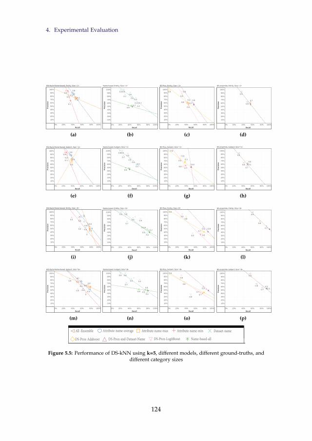
4. Experimental Evaluation
0% 20% 40% 60% 80% 100%
Recall
10%
20%
30%
40%
50%
60%
70%
80%
90%
100%
Precision
0.90.9
0.8
0.3
0.1
0.1
0
Attribute-Name-based, Entity, Size = 1+
ClassifierAttribute-name-average
Attribute-name-max
Attribute-name-min
Similarity Threshold0
0.1
0.2
0.3
0.4
0.5
0.6
0.7
0.8
0.9
ClassifierAttribute-name-average
Attribute-name-max
Attribute-name-min
(a)
0% 20% 40% 60% 80% 100%
Recall
10%
20%
30%
40%
50%
60%
70%
80%
90%
100%
Precision
0.9
0.90.8
0.7
0.70.6
0.50.4
0.3
0.2
0.1
Name-based, Entity, Size = 1+Similarity Threshold
0
0.1
0.2
0.3
0.4
0.5
0.6
0.7
0.8
0.9
ClassifierDataset-name
Name-based-all
ClassifierDataset-name
Name-based-all
(b)
0% 20% 40% 60% 80% 100%
Recall
10%
20%
30%
40%
50%
60%
70%
80%
90%
100%
Precision
0.9
0.8
0.9
0.9
0.8
0.5
0.2
0.1
DS-Prox, Entity, Size = 1+Similarity Threshold
0
0.1
0.2
0.3
0.4
0.5
0.6
0.7
0.8
0.9
ClassifierDS-Prox-AdaBoost
DS-Prox-Dataset-Name
DS-Prox-LogitBoost
ClassifierDS-Prox-AdaBoost
DS-Prox-Dataset-Name
DS-Prox-LogitBoost
(c)
0% 20% 40% 60% 80% 100%
Recall
10%
20%
30%
40%
50%
60%
70%
80%
90%
100%
Precision
0.9
0.8
0.7
All-ensemble, Entity, Size = 1+
ClassifierAll-Prox
Similarity Threshold0
0.1
0.2
0.3
0.4
0.5
0.6
0.7
0.8
0.9
ClassifierAll-Prox
(d)
0% 20% 40% 60% 80% 100%
Recall
10%
20%
30%
40%
50%
60%
70%
80%
90%
100%
Precision
0.90.9
0.6
0.20.1
Attribute-Name-based, Subject, Size = 1+
(e)
0% 20% 40% 60% 80% 100%
Recall
10%
20%
30%
40%
50%
60%
70%
80%
90%
100%
Precision
0.9
0.90.8
0.70.6
0.50.4
0.20.1
Name-based, Subject, Size = 1+
(f)
0% 20% 40% 60% 80% 100%
Recall
10%
20%
30%
40%
50%
60%
70%
80%
90%
100%
Precision
0.3
0.9
0.8
0.9
0.9
0.80.7
DS-Prox, Subject, Size = 1+
(g)
0% 20% 40% 60% 80% 100%
Recall
10%
20%
30%
40%
50%
60%
70%
80%
90%
100%
Precision
0.50.1
0.9
0.8
0.7
All-ensemble, Subject, Size = 1+
(h)
0% 20% 40% 60% 80% 100%
Recall
10%
20%
30%
40%
50%
60%
70%
80%
90%
100%
Precision
0.9
0.90.8
0.4
0.4
0.30.3
0
Attribute-Name-based, Entity, Size = 8+Similarity Threshold
0
0.1
0.2
0.3
0.4
0.5
0.6
0.7
0.8
0.9
ClassifierAttribute-name-average
Attribute-name-max
Attribute-name-min
ClassifierAttribute-name-average
Attribute-name-max
Attribute-name-min
(i)
0% 20% 40% 60% 80% 100%
Recall
10%
20%
30%
40%
50%
60%
70%
80%
90%
100%
Precision
0.9
0.9 0.8
0.7
0.7
0.6 0.4
0.30.1
Name-based, Entity, Size = 8+
ClassifierDataset-name
Name-based-all
Similarity Threshold0
0.1
0.2
0.3
0.4
0.5
0.6
0.7
0.8
0.9
ClassifierDataset-name
Name-based-all
(j)
0% 20% 40% 60% 80% 100%
Recall
10%
20%
30%
40%
50%
60%
70%
80%
90%
100%
Precision
0.9
0.8
0.9
0.9
0.70.8
0.8 0.6
DS-Prox, Entity, Size = 8+Similarity Threshold
0
0.1
0.2
0.3
0.4
0.5
0.6
0.7
0.8
0.9
ClassifierDS-Prox-AdaBoost
DS-Prox-Dataset-Name
DS-Prox-LogitBoost
ClassifierDS-Prox-AdaBoost
DS-Prox-Dataset-Name
DS-Prox-LogitBoost
(k)
0% 20% 40% 60% 80% 100%
Recall
10%
20%
30%
40%
50%
60%
70%
80%
90%
100%
Precision
0.9
0.8
0.7
All-ensemble, Entity, Size = 8+
ClassifierAll-Prox
Similarity Threshold0
0.1
0.2
0.3
0.4
0.5
0.6
0.7
0.8
0.9
ClassifierAll-Prox
(l)
0% 20% 40% 60% 80% 100%
Recall
10%
20%
30%
40%
50%
60%
70%
80%
90%
100%
Precision
0.9
0.90.8
0.5
0.4
0.4
0.30.3
0
Attribute-Name-based, Subject, Size = 8+
(m)
0% 20% 40% 60% 80% 100%
Recall
10%
20%
30%
40%
50%
60%
70%
80%
90%
100%
Precision
0.9
0.9
0.8
0.8
0.7
0.6 0.4
0.30.1
Name-based, Subject, Size = 8+
(n)
0% 20% 40% 60% 80% 100%
Recall
10%
20%
30%
40%
50%
60%
70%
80%
90%
100%
Precision
0.9
0.8
0.9
0.9
0.7
0.80.7
DS-Prox, Subject, Size = 8+
(o)
0% 20% 40% 60% 80% 100%
Recall
10%
20%
30%
40%
50%
60%
70%
80%
90%
100%
Precision
0.50.1
0.9
0.8
0.7
All-ensemble, Subject, Size = 8+
(p)10%
20%
30%
40%
50%
60%
70%
80%
90%
100%
Precision
0.9
0.9
0.8
0.9
0.9
0.9
0.90.9
0.8 0.8
0.8
0.8
0.7
0.7
0.70.5
0.40.4
0.3
All-Prox
Attribute-name-average
Attribute-name-max
Attribute-name-min
Dataset-name
DS-Prox-AdaBoost
DS-Prox-Dataset-Name
DS-Prox-LogitBoost
Name-based-all
All -Ensemble Attribute-name-average Attribute-name-max Attribute-name-min Dataset-name
DS-Prox-Adaboost DS-Prox-and-Dataset-Name DS-Prox-LogitBoost Name-based-all
Figure 5.5: Performance of DS-kNN using k=5, different models, different ground-truths, anddifferent category sizes
124

4. Experimental Evaluation
0% 20% 40% 60% 80% 100%
Recall
10%
20%
30%
40%
50%
60%
70%
80%
90%
100%
Precision
0.6
0.5
0.4
0.4
0.20
Attribute-Name-based, Entity, Size = 1+
(a)
0% 20% 40% 60% 80% 100%
Recall
10%
20%
30%
40%
50%
60%
70%
80%
90%
100%
Precision
0.8
0.9
0.9
0.8
0.70.6
0.5
0.4
0.3
0.10
Name-based, Entity, Size = 1+
(b)
0% 20% 40% 60% 80% 100%
Recall
10%
20%
30%
40%
50%
60%
70%
80%
90%
100%
Precision
0.30.9
0.8
0.9
0.9
0.8
0.8
DS-Prox, Entity, Size = 1+
(c)
0% 20% 40% 60% 80% 100%
Recall
10%
20%
30%
40%
50%
60%
70%
80%
90%
100%
Precision 0.6
0.5
0.9
0.8
0.7
All-ensemble, Entity, Size = 1+
(d)
0% 20% 40% 60% 80% 100%
Recall
10%
20%
30%
40%
50%
60%
70%
80%
90%
100%
Precision
0.80.6
0.5
0.40
Attribute-Name-based, Subject, Size = 1+
(e)
0% 20% 40% 60% 80% 100%
Recall
10%
20%
30%
40%
50%
60%
70%
80%
90%
100%
Precision
0.9
0.8
0.8
0.70.6
0.50.4
0.3
0.10
Name-based, Subject, Size = 1+
(f)
0% 20% 40% 60% 80% 100%
Recall
10%
20%
30%
40%
50%
60%
70%
80%
90%
100%
Precision
0.9
0.8
0.9
0.9
0.70.8
0.6
0.1
DS-Prox, Subject, Size = 1+
(g)
0% 20% 40% 60% 80% 100%
Recall
10%
20%
30%
40%
50%
60%
70%
80%
90%
100%
Precision
0.50.9
0.8
0.7
0.6
All-ensemble, Subject, Size = 1+
(h)
0% 20% 40% 60% 80% 100%
Recall
10%
20%
30%
40%
50%
60%
70%
80%
90%
100%
Precision
0.9
0.90.8
0.50.4
0.4
0.30.20.10
Attribute-Name-based, Entity, Size = 8+
(i)
0% 20% 40% 60% 80% 100%
Recall
10%
20%
30%
40%
50%
60%
70%
80%
90%
100%
Precision
0.9
0.9
0.8
0.8
0.7
0.7
0.6 0.4
0.30.1
Name-based, Entity, Size = 8+
(j)
0% 20% 40% 60% 80% 100%
Recall
10%
20%
30%
40%
50%
60%
70%
80%
90%
100%
Precision
0.9
0.8
0.9
0.9
0.70.8
0.8
DS-Prox, Entity, Size = 8+
(k)
0% 20% 40% 60% 80% 100%
Recall
10%
20%
30%
40%
50%
60%
70%
80%
90%
100%
Precision
0.6
0.4
0.9
0.8
0.7
All-ensemble, Entity, Size = 8+
(l)
0% 20% 40% 60% 80% 100%
Recall
10%
20%
30%
40%
50%
60%
70%
80%
90%
100%
Precision
0.9
0.9
0.7
0.5
0.5
0.4
0.4
0.3 0.20.20
Attribute-Name-based, Subject, Size = 8+
(m)
0% 20% 40% 60% 80% 100%
Recall
10%
20%
30%
40%
50%
60%
70%
80%
90%
100%
Precision
0.9
0.9
0.8
0.8
0.70.7
0.6 0.4
0.30
Name-based, Subject, Size = 8+
(n)
0% 20% 40% 60% 80% 100%
Recall
10%
20%
30%
40%
50%
60%
70%
80%
90%
100%
Precision
0.9
0.8
0.9
0.9
0.7
0.80.7
DS-Prox, Subject, Size = 8+
(o)
0% 20% 40% 60% 80% 100%
Recall
10%
20%
30%
40%
50%
60%
70%
80%
90%
100%
Precision
0.2
0.9
0.8
0.7
All-ensemble, Subject, Size = 8+
(p)10%
20%
30%
40%
50%
60%
70%
80%
90%
100%
Precision
0.9
0.9
0.8
0.9
0.9
0.9
0.90.9
0.8 0.8
0.8
0.8
0.7
0.7
0.70.5
0.40.4
0.3
All-Prox
Attribute-name-average
Attribute-name-max
Attribute-name-min
Dataset-name
DS-Prox-AdaBoost
DS-Prox-Dataset-Name
DS-Prox-LogitBoost
Name-based-all
All -Ensemble Attribute-name-average Attribute-name-max Attribute-name-min Dataset-name
DS-Prox-Adaboost DS-Prox-and-Dataset-Name DS-Prox-LogitBoost Name-based-all
Figure 5.6: Performance of DS-kNN using k=7, different models, different ground-truths, anddifferent category sizes
125

4. Experimental Evaluation
threshold (also indicated by the size of the points, where bigger size indicatesa higher similarity threshold). We show the results for the non-restricted(category size “ 1+) which includes outliers, and only the biggest categorysizes (category size “ 8+). Each model type has a different symbol and colour.For attribute-name based models in the first column, we show the results usingthe average, minimum and maximum aggregations. In the second column, weshow the results of the dataset-name based model and also the combinationof all the attribute-name based aggregations with the dataset name in a singleensemble model we call name-based-all. In the third column, we present thecontent-based DS-Prox models, where we include the AdaBoost-based modeland the LogitBoost-based model in addition to the model that combines themeta-features from Table 3.1 and the dataset-name within a single RandomForest model (we call it DS-Prox-and-Dataset-Name). Finally, we present in thefourth column the model showing the combination of all meta-features into asingle ensemble model we call All-Ensemble. We also present in Tables 5.2 -5.5 the evaluation metrics for the top performing parameters for DS-kNN (interms of F1-scores) for each category size for the different ground-truth typesand for each model type. We highlight the top 3 performing model types foreach category size and ground truth type.
As could be seen from the results, DS-kNN performs comparatively wellwith the attribute-name and the DS-Prox content-based models for categorysize 1+, while combining all the meta-features in a single ensemble modelperforms the best. There is a trade-off between the similarity threshold usedand recall, the higher the threshold the lower the recall and the higher theprecision, and vice versa. However, there is an optimum similarity thresholdthat can perform better than all others, e.g., the All-Ensemble model with athreshold of 0.9 in Figure 5.6d.
For larger category sizes the DS-Prox content models and the All-Ensembleare better in assigning the correct categories. For example, in Figure 5.3l, All-Ensemble leads to a precision of about 70% and recall of about 80% forcategory sizes of at least 8 members and the entity-based ground-truth, whileattribute-name model can only achieve in Figure 5.3i a maximum recall of onlyabout 70% with a precision of about 60%. Dataset-name based model performsa similar recall and slightly better precision. The results also indicate that thechoice of the similarity threshold can affect the performance of DS-kNN.
In general, DS-kNN performs better with bigger category sizes than smallercategory sizes as it becomes easier for the algorithm to find relevant top-knearest neighbours. However, it is still good in detecting outliers and othercategories as seen in Table 5.2 for the performance for ‘min. category size’ “ 1,for example a recall of 75% and precision of 95% for dataset-name basedmodel. The dataset-name model performs better in detecting outliers as seenfrom this result. The DS-kNN algorithm performed equally good with bothground-truth types under the same settings and with the same parameters,
126

4. Experimental Evaluation
Table 5.2: The evaluation of DS-kNN for the minimum category size of 1+ with the differentmodel types and ground-truth types. For each setting, we only show here the best performing
parameters based on F1-scores.
Model Type GroundTruthType
Min. Cate-gory Size
k SimilarityThresh-old
Recall Precision F1-score
Dataset Name entity 1 7 0.6 74.7% 95.2% 83.7%All-Ensemble entity 1 7 0.9 71.0% 94.7% 81.2%DS-Prox Logit-Boost
entity 1 7 0.9 66.8% 92.3% 77.5%
DS-Prox AdaBoost entity 1 7 0.9 61.0% 100.0% 75.8%Attribute NameMin.
entity 1 7 0.7 55.9% 98.5% 71.3%
Attribute NameAvg.
entity 1 7 0.9 56.6% 94.6% 70.8%
Attribute NameMax.
entity 1 5 0.1 48.0% 75.5% 58.7%
DS-Prox-and-Dataset-Name
entity 1 5 0.9 53.2% 61.4% 57.0%
Name-based-all entity 1 3 0.3 44.9% 56.0% 49.8%Dataset Name subject 1 7 0.6 58.0% 93.1% 71.4%All-Ensemble subject 1 7 0.9 52.4% 92.3% 66.8%Attribute NameAvg.
subject 1 7 0.8 51.7% 92.8% 66.4%
DS-Prox Logit-Boost
subject 1 7 0.9 52.8% 88.8% 66.3%
Attribute NameMin.
subject 1 7 0.4 47.9% 95.8% 63.9%
DS-Prox AdaBoost subject 1 7 0.8 44.6% 83.1% 58.1%DS-Prox-and-Dataset-Name
subject 1 5 0.9 49.7% 59.1% 54.0%
Attribute NameMax.
subject 1 5 0.4 38.3% 77.4% 51.3%
Name-based-all subject 1 5 0.7 40.2% 48.0% 43.7%
127

4. Experimental Evaluation
Table 5.3: The evaluation of DS-kNN for the minimum category size of 3+ with the differentmodel types and ground-truth types. For each setting, we only show here the best performing
parameters based on F1-scores.
Model Type GroundTruthType
Min. Cate-gory Size
k SimilarityThresh-old
Recall Precision F1-score
Attribute NameAvg.
entity 3 7 0.3 59.3% 75.3% 66.3%
Attribute NameMax.
entity 3 5 0 54.0% 76.0% 63.2%
All-Ensemble entity 3 7 0.8 53.6% 66.5% 59.4%DS-Prox-and-Dataset-Name
entity 3 7 0.7 62.9% 55.1% 58.7%
Dataset Name entity 3 3 0.4 49.9% 70.1% 58.3%Attribute NameMin.
entity 3 7 0 51.0% 63.6% 56.6%
DS-Prox Logit-Boost
entity 3 5 0 49.3% 55.7% 52.3%
Name-based-all entity 3 7 0.6 56.6% 45.6% 50.5%DS-Prox AdaBoost entity 3 3 0.1 49.0% 50.7% 49.8%Attribute NameAvg.
subject 3 7 0.1 53.1% 78.8% 63.4%
Attribute NameMax.
subject 3 7 0 45.7% 82.3% 58.8%
All-Ensemble subject 3 7 0.5 56.6% 61.0% 58.7%DS-Prox-and-Dataset-Name
subject 3 7 0.7 57.6% 57.8% 57.7%
Dataset Name subject 3 5 0.2 58.8% 53.3% 55.9%Name-based-all subject 3 7 0.7 49.4% 54.4% 51.8%Attribute NameMin.
subject 3 5 0.2 38.4% 78.6% 51.6%
DS-Prox AdaBoost subject 3 5 0.4 40.7% 69.2% 51.2%DS-Prox Logit-Boost
subject 3 5 0.3 41.5% 61.7% 49.6%
128

4. Experimental Evaluation
Table 5.4: The evaluation of DS-kNN for the minimum category size of 5+ with the differentmodel types and ground-truth types. For each setting, we only show here the best performing
parameters based on F1-scores.
Model Type GroundTruthType
Min. Cate-gory Size
k SimilarityThresh-old
Recall Precision F1-score
Attribute NameAvg.
entity 5 7 0.8 57.4% 93.2% 71.0%
Attribute NameMax.
entity 5 5 0.9 69.2% 69.9% 69.6%
All-Ensemble entity 5 3 0.9 51.5% 99.5% 67.9%Dataset Name entity 5 5 0.4 59.6% 77.8% 67.5%Attribute NameMin.
entity 5 1 0.5 51.8% 90.8% 65.9%
DS-Prox-and-Dataset-Name
entity 5 5 0.9 69.6% 61.1% 65.1%
Name-based-all entity 5 5 0.8 68.4% 48.1% 56.5%DS-Prox AdaBoost entity 5 5 0.5 63.7% 46.6% 53.8%DS-Prox Logit-Boost
entity 5 3 0.9 35.5% 95.1% 51.7%
Attribute NameAvg.
subject 5 7 0.1 66.2% 66.4% 66.3%
Attribute NameMax.
subject 5 5 0.4 59.8% 72.9% 65.7%
All-Ensemble subject 5 7 0.6 72.0% 59.1% 65.0%DS-Prox-and-Dataset-Name
subject 5 7 0 72.5% 57.7% 64.2%
Dataset Name subject 5 5 0.4 55.7% 72.1% 62.9%Attribute NameMin.
subject 5 1 0.5 47.6% 92.2% 62.8%
Name-based-all subject 5 7 0 66.7% 46.8% 55.0%DS-Prox AdaBoost subject 5 5 0.4 50.3% 53.6% 51.9%DS-Prox Logit-Boost
subject 5 5 0.7 54.9% 45.7% 49.9%
129

4. Experimental Evaluation
Table 5.5: The evaluation of DS-kNN for the minimum category size of 8+ with the differentmodel types and ground-truth types. For each setting, we only show here the best performing
parameters based on F1-scores.
Model Type GroundTruthType
Min. Cate-gory Size
k SimilarityThresh-old
Recall Precision F1-score
All-Ensemble entity 8 5 0.9 59.7% 99.2% 74.6%Attribute NameAvg.
entity 8 7 0.7 64.6% 87.9% 74.5%
Dataset Name entity 8 7 0.4 64.0% 80.2% 71.2%Attribute NameMax.
entity 8 5 0.9 73.0% 64.0% 68.2%
Attribute NameMin.
entity 8 7 0.5 55.1% 85.0% 66.9%
DS-Prox entity 8 5 0.9 76.9% 55.9% 64.7%Name-based-all entity 8 7 0.8 79.8% 50.2% 61.6%DS-Prox AdaBoost entity 8 7 0.7 73.4% 43.8% 54.8%DS-Prox Logit-Boost
entity 8 7 0.7 71.4% 36.6% 48.4%
All-Ensemble subject 8 7 0.9 54.8% 99.2% 70.6%Attribute NameAvg.
subject 8 7 0.7 58.8% 88.0% 70.5%
Dataset Name subject 8 7 0.4 62.1% 81.0% 70.3%DS-Prox-and-Dataset-Name
subject 8 5 0.9 76.9% 61.2% 68.1%
Attribute NameMax.
subject 8 5 0.4 78.4% 60.0% 68.0%
Name-based-all subject 8 7 0.7 81.2% 52.4% 63.7%Attribute NameMin.
subject 8 1 0.5 50.8% 85.1% 63.6%
DS-Prox AdaBoost subject 8 7 0.4 79.3% 44.6% 57.1%DS-Prox Logit-Boost
subject 8 7 0.6 78.8% 42.0% 54.8%
130

4. Experimental Evaluation
yet slightly better with the more specific entity-based ground-truth with smallcategory sizes and outliers. This indicates the adaptability of DS-kNN todifferent DL settings and properties.
In general, DS-kNN and All-Ensemble models perform better with biggercategory sizes. For example, they can achieve 90% recall and more than 50%precision for k “ 5 and a similarity threshold of 0.6 in Fig 5.5p and the subject-based ground-truth. This is comparatively similar with the entity-basedground-truth for k “ 3 and a similarity threshold of also 0.6 in Figure 5.4lwhich achieves a recall of 97% with a precision of more than 50%. However,the All-Ensemble model is still average in detecting outliers when combinedwith other categories as seen for the performance for ‘min. category size’ “ 1,for example a recall and precision of about 60% in Figure 5.5d, while thename-based model performs nearly the same in Figure 5.5b. The dataset-namemodel also performs similarly in detecting outliers as seen from the result inFigure 5.5c. The DS-kNN and All-Ensemble models perform equally goodwith both ground-truth types under the same settings and with the sameparameters, yet slightly better with the more specific entity-based ground-truth with small category sizes and outliers.
Similarly, combining the DS-Prox-and-Dataset-Name leads to a compara-tively good result like the All-Ensemble model as could be seen in Figure 5.5kand Figure 5.5o where a recall of about 90% is achieved with a precision above40%. Therefore, the combination of content-based meta-features with name-based meta-features lead to optimum results that can equally detect outliersand accurately assign a relevant category for bigger category sizes. To achievehigher recall rates, the DS-kNN algorithm generally works better when theDL contains bigger categories and by using bigger values for ‘k’. With smallercategory sizes and more outliers we need to use a higher similarity thresholdand vice versa.
4.4 Validation Experiment
In order to re-validate our results and to check the generalisability of theresults, we test the highlighted top performing DS-kNN settings from Tables5.2, 5.3, and 5.5 on the 118 ds sample in Table 5.1. As the sample onlyhas entity-based granularity of annotations, we only test the top performantmodels for the entity-based ground truth. We also only consider the modelsfor category size 8+ as the 118 ds sample only includes categories with size3+ or 8+ (i.e., 5+ and 8+ category sizes have the same categories as seen inTable 5.1). We execute the same leave-one-out experimental setup as describedpreviously, and we evaluate the recall, precision and F1-scores which aresummarised in Table 5.6. We also test on the 118 ds sample some specificDS-kNN settings which met specific criteria in our experiments on the 203 dssample, for example, at least 90% recall. Those are presented in Table 5.7.
131
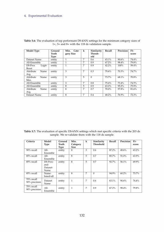
4. Experimental Evaluation
Table 5.6: The evaluation of top performant DS-kNN settings for the minimum category sizes of1+, 3+ and 8+ with the 118 ds validation sample.
Model Type GroundTruthType
Min. Cate-gory Size
k SimilarityThresh-old
Recall Precision F1-score
Dataset Name entity 1 7 0.6 63.1% 90.6% 74.4%All-Ensemble entity 1 7 0.9 67.2% 98.4% 79.8%DS-Prox Logit-Boost
entity 1 7 0.9 42.2% 100% 59.4%
Attribute NameAvg.
entity 3 7 0.3 79.6% 70.3% 74.7%
Attribute NameMax.
entity 3 5 0 73.7% 68.1% 70.8%
All-Ensemble entity 3 7 0.8 75.6% 73.4% 74.5%All-Ensemble entity 8 5 0.9 63.2% 95.2% 75.9%Attribute NameAvg.
entity 8 7 0.7 70.0% 97.8% 81.6%
Dataset Name entity 8 7 0.4 68.2% 76.9% 72.3%
Table 5.7: The evaluation of specific DS-kNN settings which met specific criteria with the 203 dssample. We re-validate them with the 118 ds sample.
Criteria ModelType
GroundTruthType
Min.CategorySize
k SimilarityThreshold
Recall Precision F1-score
90% recall All-Ensemble
entity 8 3 0.6 87.2% 49.6% 63.2%
85% recall All-Ensemble
entity 8 5 0.7 85.7% 51.0% 63.9%
85% recall DS-Prox-and-Dataset-Name
entity 8 5 0.7 92.7% 56.1% 69.9%
85% recall Name-based-all
entity 8 7 0 94.9% 60.2% 73.7%
70% recall90% precision Dataset
Nameentity 1 7 0.6 63.1% 90.6% 74.4%
70% recall90% precision All-
Ensembleentity 1 7 0.9 67.2% 98.4% 79.8%
132
5. Related Work
As could be seen in the results in Tables 5.6 and 5.7, we were able to achievesimilar or better results with the 118 ds validation sample by applying thesame top performing DS-kNN settings from Tables 5.2, 5.3 and 5.5 and someDS-kNN settings meeting specific criteria. This indicates the generalisabilityof our results and the capability of our algorithm in replicating similar resultswith other DL samples.
5 Related Work
Categorization of datasets from heterogeneous domains is an emerging re-search topic, and relevant previous research include the work by [85], wherethey utilise the attribute names to cluster the datasets into categories usinga probabilistic model. Datasets are assigned to different categories usingdifferent probabilities. They tackle the multi-label classification of datasetsand retrieval of datasets from relevant domains by querying systems. Ourapproach improves this by using a machine-learning based approximate prox-imity mining technique instead of the Jaccard similarity of exact values. Wealso use content-based metadata for categorizing and not only name-basedmetadata. This is important for DLs where datasets are not well maintainedwith meaningful attribute names.
Clustering could also be applied to other types of semi-structured datasetslike ontologies [9] and XML documents [11, 77], etc. In [9], they proposean algorithm to cluster instances from different ontologies based on theirstructural properties in the ontology graphs. Their goal is to facilitate ontologymatching rather than domains discovery. Similarly, in [11, 77] they cluster thesemi-structured documents based on their structure similarity and linguisticmatchers.
Clustering free-text without any structure is also possible. For example,[21] aim to cluster short text messages by computing TF-IDF word similaritybetween free-text documents. Classical text document classification can alsouse multi-class supervised learning based on the extracted keywords in thedocument [19]. Similarly, [55] categorizes free-text documents using a k-NNbased algorithm by first extracting TF-IDF weighted labels and feeding themto the algorithm. Another specific application would be clustering streamingdata where a sliding window algorithm could be used [61], where they alsouse k-NN when finding relevant clusters for a given data instance ingested ina stream of data points. k-NN was also used with image categorization basedon extracted features describing the images [78].
133

6. Conclusion
6 Conclusion
We proposed DS-kNN, a categorization algorithm for classifying datasetsinto pre-defined topic-wise groups. Our algorithm can be applied in a DLenvironment to support users in automatically finding relevant datasets foranalysis. Our algorithm uses extracted metadata from datasets to computetheir similarities to other datasets in the DL using a proximity mining modeland name strings comparisons. Those similarity scores are fed to DS-kNNto decide on the most relevant category for a dataset based on its top-k near-est neighbours. Our algorithm was effective in categorizing the datasets ina real-world DL and detecting outliers. In the future, we will seek to im-prove our algorithm with semantic analysis of values found in the attributes tocomplement the syntactical comparisons we compute in the proximity models.
Acknowledgements. This research has been partially funded by the Euro-pean Commission through the Erasmus Mundus Joint Doctorate (IT4BI-DC).
134

Chapter 6
Prox-mine tool for browsingDLs using proximity mining
A picture is worth a thousand words and is bettermarketing for an idea than just plain words.
Abstract
We present Prox-mine, a tool for browsing DLs using proximity mining. Prox-mineintegrates all the different components of this thesis and presents it in a coherentprototype. It supports the collection of descriptive statistics about tabular datasets andtheir attributes, calculation of overall dataset similarity scores between dataset pairsusing the collected statistics and the proximity models in Chapter 4, categorization ofdatasets into pre-existing categories defined in the DL using the computed similaritiesbetween datasets and a k-Nearest-Neighbour algorithm described in Chapter 5, inaddition to construction of proximity graph visualisations which summarise the overallstructure of the DL by showing datasets and their categories as nodes and relationships(similarities) modelled as edges.
The tool can be used to support the DL users in extracting useful metadatainvolving descriptive statistics about the content of the datasets stored, can help datawranglers and curators in finding relevant datasets by querying similar datasets inthe data lake given an input query dataset, and can also provide schema matchingsupport by showing the overlap of similar attributes and their data / names betweendataset pairs (using name-based and content-based analysis techniques as described inChapter 4).
135

1. Introduction
1 Introduction
We present a prototype integrating the different components of this thesis.We call the tool Prox-Mine, where the goal is to support data wranglers andcurators in finding relevant datasets by querying similar datasets in the DLgiven an input query dataset, and can also provide schema matching supportby showing the overlap of similar attributes and their data / names betweendataset pairs (using name-based and content-based analysis techniques asdescribed in Chapter 4).
Prox-mine supports the collection of descriptive statistics about tabulardatasets and their attributes, calculation of overall dataset similarity scoresbetween dataset pairs using the collected statistics and the proximity modelsin Chapter 4, categorization of datasets into pre-existing categories definedin the DL using the computed similarities between datasets and a k-Nearest-Neighbour algorithm described in Chapter 5, in addition to constructionof proximity graph visualisations which summarise the overall structure ofthe DL by showing datasets and their categories as nodes and relationships(similarities) modelled as edges.
Prox-mine is organised into the following components:
• Data Lake Index: an index of the datasets stored in the DL and theirground-truth categories.
• Similarity Search: supports searching for similar datasets to a querydataset based on the different proximity models and a minimum simi-larity threshold.
• Dataset Categorization: applies the DS-kNN algorithm from Chapter 5to facilitate the automatic recommendation of categories for a datasetbased on the most proposed category by the most similar datasets in theDL.
• Dataset Matching: applies the proximity models over a pair of datasetsin order to compute their overall similarity and the most similar attributepairs between them.
• Proximity Graph: constructs a graph visualisation to show the relation-ships between datasets based on their computed similarities using thedifferent proximity models and different minimum thresholds.
We describe each of the components above in the rest of this chapter. Thetool is hosted on a web server1 and is implemented as a Java-based web
1A live version of Prox-mine can be accessed at the following link: http://dtim.essi.upc.edu:8080/proxmine using the credentials of username:"proxmine" and password "12345". Thesource code for the tool is provided at: https://github.com/AymanUPC/proxmine, and moredetails can be found at the tool’s main page: https://www.essi.upc.edu/dtim/tools/proxmine
136
2. Data Lake Index
application. The tool implements a demonstration of the above componentsover the OpenML OML02 sample used in our experiments in Chapter 4. Allproximity models used in the demonstration are based on the same cross-validation experimental setup described in Chapter 4, where we make surethat the datasets we apply the models on were not used in the training steps.In addition to this overview, the tool provides tooltip help and support too byhovering over the input and output fields and titles when using it.
2 Data Lake Index
In this component, an overview of all the datasets stored in the DL is presented.This includes the following for each dataset:
• Dataset: the filename of the dataset
• Dataset Name: the name of the dataset
• Dataset Description: a link to the webpage with the textual descriptionand statistical metadata describing the dataset and its attributes.
• No. of Attributes: the number of attributes in the dataset
• No. of Instances: the number of instances in the dataset
• Ground-truth Category: the annotated ground-truth category assignedto the dataset based on manual inspection of it and its description (seeChapter 5.1 for more details about this annotation).
We also provide a list of all the ground-truth categories and the number ofdatasets which belong to those categories.
3 Similarity Search
This component allows searching for similar datasets to a query dataset (asshown in Figure 6.1) based on the different proximity models and a minimumsimilarity threshold. The proximity models are those described in Chapter 4and the minimum threshold should be a real-number in the range r0, 1s, forexample 0.75.
The output can be seen in Figure 6.2. This includes a description of theinput dataset used in the query. Then a table with the output similar datasetsis given, ordered by the similarity score computed by the proximity model, indescending order of similarity.
137

4. Dataset Categorization
Figure 6.1: The input screen for the similarity search component of Prox-mine
Figure 6.2: The output screen for the similarity search component of Prox-mine
4 Dataset Categorization
This component allows recommending a category for a query dataset basedon the most similar datasets found in the DL. This implements the DS-kNNalgorithm described in Chapter 5. The input required, as seen in Figure 6.3,
138

4. Dataset Categorization
Figure 6.3: The input screen for the dataset categorization component of Prox-mine
includes the query dataset, the proximity model, the number of k-nearest-neighbours to use for the recommendation (i.e., how many datasets fromthe top similar ones should recommend their category for the dataset), theminimum category size as described in Chapter 4 (i.e., only categories havingthis number of datasets or above can be recommended), and the minimumsimilarity threshold as a real-number in the range r0, 1s.
The output can be seen in Figure 6.4. This includes first a description ofthe input dataset used in the query. This table also includes an extra columncalled ‘Is Outlier?’ which indicates if the dataset belongs to a category inthe ground-truth of size 1, i.e., a category which only includes the querydataset and no other dataset stored in the DL. Then a table with the outputrecommended categories found using the DS-kNN algorithm is given orderedby the number of recommendations in descending order. Each of the mostsimilar k nearest-neighbours recommends its category for the dataset, andthe aggregate count is given for each category here. An indication whetherthe recommended category is the correct one is also given in the column‘Is Correct Category?’. Finally, a table is given showing a drill-down of thek-nearest-neighbours found which led to the recommended categories. Here
139

5. Dataset Matching
(a)
(b)
Figure 6.4: The output screens for the dataset categorization component of Prox-mine.
each of the top-k datasets is described in descending order of similarity scores.
5 Dataset Matching
This component allows the application of the proximity models over a pairof datasets in order to compute their overall similarity and the most simi-lar attribute pairs between them using the models trained for numeric andnominal attributes over the OML01 sample described in Chapter 5.1. This isdone using the input screen in Figure 6.5 where 2 datasets can be selectedalong with a minimum similarity threshold in the range r0.5, 1s. We restrict
140

5. Dataset Matching
Figure 6.5: The input screen for the dataset matching component of Prox-mine
the input to this threshold range as attribute matches with a similarity scorebelow this threshold could be considered as irrelevant and not strong enoughto be significant, distracting the user when analysing the output by presentingtoo many attribute pair matches.
The output can be seen in Figure 6.6. This includes first a descriptionof both input datasets and their ground-truth categories. This is followedby a table giving all the overall dataset similarity scores based on all typesof proximity models described in Chapter 4. Then the matching attributesare presented in two separate tables, where the first table is based on asimilarity score computed using the content-based similarity models andwhere the second table is based on similarity computed using Levenshteindistances of the attribute names. Each table shows attribute pair matchessorted by descending order of the similarity scores computed. We indicatethe attribute types compared, and a description of each attribute matched inthe pair, one attribute from each dataset. For the ‘Values’ column, we give theunique distinct values found for nominal attributes separated by pipes, andfor numeric attributes we give the range of values (minimum - maximum)and the mean value.
5.1 New Dataset Matching
Another component for matching datasets include the new dataset matchingcomponent, where the input screen can be seen in Figure 6.7. The user is ableto select a new CSV dataset file from the filesystem (stored on their computer)as the input of the matching process. The dataset is matched against another
141

5. Dataset Matching
(a)
(b)
Figure 6.6: The output screens for the dataset matching component of Prox-mine.
dataset available in the DL sample. A minimum similarity threshold in therange r0, 1s should also be selected.
The output can be seen in Figure 6.8. It also includes a description of theinput datasets, the output content-based similarity scores of attribute matchingand name-based similarity scores as well using the Levenshtein distances ofthe attribute names. The overall similarity score for the dataset pair is givenabove the matching output tables for content-based and name-based matching.Here, the content-based and name-based proximity is aggregated using theattribute-level models and algorithms in Chapter 4 to give a single approximatesimilarity score for the dataset pair.
142

6. Proximity Graph
Figure 6.7: The input screen for the new dataset matching component of Prox-mine
6 Proximity Graph
In this component, we construct a graph visualisation to visualise the rela-tionships between datasets based on their computed similarities using thedifferent proximity models and different minimum thresholds. We call thisa proximity graph, which was introduced in Chapter 5. The graph showsindividual datasets as nodes and edges showing relationships between datasetpairs (where an edge is drawn between dataset pairs having a similarity scoresabove the minimum threshold). The purpose of this is to be able to see all thedatasets in the DL and an overview of the relationships between them in avisually intuitive and interactive manner.
For the input screen seen in Figure 6.9, the user should select whichproximity model to use when constructing the relationships (similarities)between datasets and the minimum similarity threshold in t0.5, 0.75u. Thisway we allow to build proximity graphs with at least average similarity strengthor other graphs only showing strong relationships (in the case of selecting 0.75).The shape of the graph will differ based on the filtered relationships satisfyingthe minimum similarity threshold, as we use a force-directed graph structuringalgorithm [66] which depends on the relationship strengths between thenodes (the datasets) to group them and to position them accordingly. Moreinteresting proximity graphs can be achieved with higher minimum similaritythresholds, as this way only very similar datasets (usually having similarcategories in the ground-truth and the same colour for the nodes) are groupedtogether in a more coherent manner.
The overview of the output proximity graph can be seen in Figure 6.10.
143

6. Proximity Graph
Figure 6.8: The output screen for the new dataset matching component of Prox-mine
This is an interactive graph visualisation, where the graph is shown in themiddle. On the left-side, there is a graph search and category-filtration selector,and at the bottom there are three buttons to zoom-in, zoom-out or to return todefault view. When the graph is zoomed-in, the nodes show the names of thedatasets as their labels. The colours of the nodes represent the ground-truthcategory they belong to, therefore datasets in the same category have the samecolour.
The user can interact with the graph by zooming in and out and togglingthe view with the cursor to move the view to a different part of the graph. Inaddition, the user can search for a specific dataset node using the search barin the left panel, as seen in Figure 6.11. The datasets can also be filtered toonly highlight those belonging to a specific ground-truth category by selectingthe category from the drop-down group selector menu. The result of filtration
144

6. Proximity Graph
Figure 6.9: The input screen for the proximity graph component of Prox-mine
(a)
(b)
Figure 6.10: An overview of the output proximity graph component of Prox-mine, where (a)gives a zoomed-out view and (b) gives a zoomed-in view
by category is given in Figure 6.11b, where a only the datasets belonging to
145

6. Proximity Graph
(a)
(b)
Figure 6.11: The search and filtration panel of the output proximity graph component ofProx-mine, where (a) gives a view of the category selector in the left-panel and (b) gives the
result of applying the filtration step
the specific category are shown and a list showing those datasets is given inthe information pane on the right.
When a specific node is clicked and selected, only the datasets having arelationship with a similarity score above the minimum similarity thresholdare shown, as could be seen in Figure 6.12. The description of the selecteddataset and the connections (edges) list is given in the information pane onthe right side. This includes a list of all connected (related) datasets and thesimilarity scores for each related dataset. Hovering over a specific dataset inthe connections information pane highlights the dataset in the main proximitygraph view and shows its name label. To exit back to the full proximity graph,the user should click the ‘X’ symbol at the top of the information pane on theright side.
146

6. Proximity Graph
Figure 6.12: The selection of a specific dataset node in the proximity graph and the relationshipsinformation panel shown on the right side
147

Chapter 7
Conclusions and FutureDirections
Positivity leads to positive energy and success, negativity onthe other hand leads to negative energy and dismay.
Abstract
In this chapter, we summarise the outcome and results of this thesis, presented inChapters 2´ 6. Additionally, we present several interesting future directions arisingfrom this thesis work.
148

1. Conclusions
1 Conclusions
Everything must eventually come to an end. [...] Ctrl+S [...]Alt+F4 [...] Ctrl+Alt+Delete.
We have presented a novel metadata-based framework for computingdataset proximity using data profiling and supervised machine learningtechniques. The output from this framework is a metadata repository whichcan support in DL governance efforts, whereby datasets are automaticallyprofiled, matched against other datasets in the DL and categorised into topicaldomains in order to support information discovery and analytical tasks overthe DL.
We proposed novel approaches for computing approximate dataset similaritywhere dataset pairs contain overlapping attribute pairs based on contentstatistics summarising the information stored in the attributes (instead of exactvalues matching where attribute names should be identical and their valuesshould be coded using the same string patterns). This makes it possible toprovide estimation of overall dataset similarity to support early-pruning tasksof holistic schema matching and automatic dataset categorization based onmost similar datasets already categorized. The developed approach and itstechniques are novel solutions for those research challenges.
To implement this approach, we presented in Chapter 2 an overview ofexact value-based matching techniques for the dataset similarity computationchallenge. We were able to demonstrate the feasibility of this approach usinga real-world DL sample and we summarised the shortcomings of such value-based techniques; mainly: 1. high computational costs for the comparisonsand 2. inability to detect all related attributes due to the differences in theway values are coded or stored.
To tackle the shortcoming from the value-based approaches in Chapter2, we developed a novel technique called proximity mining in Chapter 3 forcomputing approximate dataset similarity based on schema and content meta-data we extract from the datasets. We utilise supervised machine learningtechniques to learn models which can detect similar and duplicate schematastored in the DL. The effectiveness and efficiency of the approach was evalu-ated on an expanded real-world DL sample, where we were able to achievehigh recall and efficiency gain.
We improve the proximity mining techniques using finer-grained attribute-level metadata in Chapter 4. Here, we collect finer grained metadata summaris-ing the content of each attribute in the datasets, we propose a greedy algorithmfor finding top-matching attribute pairs between different datasets, and we
149

2. Future Directions
utilise supervised machine learning models to compute overall dataset simi-larity between dataset pairs in the DL. The approach uses different metadata,mainly schema metadata consisting of attribute names and types in additionto content metadata consisting of data profiles for the different attributes.We test our proposed approach against both techniques from Chapter 2 andChapter 3 and we discover that the improved technique can achieve betterperformance in terms of effectiveness and efficiency gains. This was proven tobe useful for the holistic schema matching early-pruning task, whereby datasetpairs having an overall similarity score exceeding a minimum threshold areproposed for further, more detailed schema matching, and those which arebelow the similarity threshold are pre-filtered from any further scrutinization.
In Chapter 5, we use the output dataset similarity cross-dataset relation-ships to automatically categorise newly ingested datasets in the DL to topicsof interest already existing or to detect that the ingested dataset is an outlierwhich has no similar datasets stored in the DL. This is done using a k-nearest-neighbour algorithm which uses the computed proximity between datasets infinding the top-k most similar datasets in the DL and to propose their topicsas candidates for the newly ingested dataset.
Finally, in Chapter 6, we demonstrate a prototype which uses the outputfrom Chapters 3 and 4 in finding related dataset pairs, their overlapping at-tributes and to automatically categorize datasets based on those most similardatasets. We develop a simple web application which is able to store annota-tions of datasets stored in the DL using a metadata repository (a DB) and tovisualise the output from our approach using a querying interface to supportdata wranglers and DL uses in information discovery and DL exploration.
This thesis is a first step towards fully automated DL governance forsupporting information discovery and DL segmentation. We were able todemonstrate techniques which are able to effectively and efficiently computeoverall dataset similarity in an approximate manner. The proposed techniqueswere found to be more effective than state-of-the-art value-based schemamatching techniques and human-based manual analysis.
2 Future Directions
What is partially left should never be completely abandoned.
This thesis opens multiple research directions for future work. Firstly, thesame techniques can be adopted for other dataset types like semi-structuredand unstructured datasets. This can support the different variety of datasetsstored in the DL. In addition, the techniques proposed can be augmented
150

2. Future Directions
with semantic matching where datasets, their attributes and their valuescan be mapped to a knowledge base to support the computation of theirsimilarity. This can be useful for datasets storing different content but whichare modelling the same topics of interest.
The framework can also incorporate human-in-the-loop techniques ina pay-as-you-go approach whereby the data wrangler can interfere in thematching process to improve the supervised learning models and to help themodels when they are not accurately detecting similar attribute and datasetpairs. This can be done by manually correcting false positives and falsenegatives, and incorporating this in the training process of the models. Thiscan be seen as an incremental learning process.
Finally, the output of this thesis can be used for other applications likedataset search ranking engines, data integration tasks where joinable datasetsare detected, and de-duplication tasks where highly similar schemata areintegrated into a single dataset.
151

Bibliography
Standing on the shoulders of giants, a person’s legacycontinues via the knowledge and work passed on to theirstudents and to others.
References
[1] Z. Abedjan, L. Golab, and F. Naumann. Profiling relational data: asurvey. The VLDB Journal, 24(4):557–581, 2015.
[2] Z. Abedjan, T. Gruetze, A. Jentzsch, and F. Naumann. Profiling and min-ing RDF data with ProLOD++. In Proceedings - International Conferenceon Data Engineering, pages 1198–1201, 2014.
[3] Z. Abedjan and F. Naumann. Improving RDF Data Through AssociationRule Mining. Datenbank-Spektrum, 13(2):111, 2013.
[4] A. Abelló. Big Data Design. In Proceedings of ACM DOLAP, pages 35–38,2015.
[5] A. Abelló, J. Darmont, L. Etcheverry, M. Golfarelli, J. N. Mazón, F. Nau-mann, T. B. Pedersen, S. Rizzi, J. Trujillo, P. Vassiliadis, and G. Vossen.Fusion cubes: Towards self-service business intelligence. InternationalJournal of Data Warehousing and Mining, 9(2):66–88, 2013.
[6] G. Adomavicius, R. Sankaranarayanan, S. Sen, and A. Tuzhilin. In-corporating contextual information in recommender systems using amultidimensional approach. ACM Transactions on Information Systems(TOIS), 23(1):103–145, 2005.
[7] J. Akoka, L. Berti-Équille, O. Boucelma, M. Bouzeghoub, I. Comyn-Wattiau, M. Cosquer, V. Goasdoué-Thion, Z. Kedad, S. Nugier, V. Peralta,and S. S. Cherfi. A framework for quality evaluation in data integrationsystems. In 9th International Conference on Entreprise Information Systems(ICEIS), pages 170–175, 2007.
[8] A. Alexandrov, R. Bergmann, S. Ewen, J.-C. Freytag, F. Hueske, A. Heise,O. Kao, M. Leich, U. Leser, V. Markl, F. Naumann, M. Peters, A. Rhein-länder, M. J. Sax, S. Schelter, M. Höger, K. Tzoumas, and D. Warneke.The Stratosphere platform for big data analytics. The VLDB Journal,23(6):939–964, 2014.
152

References
[9] A. Algergawy, S. Massmann, and E. Rahm. A Clustering-Based Ap-proach for Large-Scale Ontology Matching. In East European Conferenceon Advances in Databases and Information Systems (ADBIS), pages 415–428.Springer, 2011.
[10] A. Algergawy, M. Mesiti, R. Nayak, and G. Saake. XML data clustering:An overview. ACM Computing Surveys (CSUR), 43(4):25, 2011.
[11] A. Algergawy, E. Schallehn, and G. Saake. A schema matching-basedapproach to XML schema clustering. In Proceedings of the InternationalConference on Information Integration and Web-based Applications & Services,pages 131–136. ACM, 2008.
[12] I. Alhassan, D. Sammon, and M. Daly. Data governance activities: ananalysis of the literature. Journal of Decision Systems, 25:64–75, 2016.
[13] H. Alrehamy and C. Walker. Personal Data Lake With Data Gravity Pull.In IEEE Fifth International Conference on Big Data and Cloud Computing(BDCloud), pages 160–167, 2015.
[14] H. Alrehamy and C. Walker. SemLinker: automating big data integrationfor casual users. Journal of Big Data, 5(1), 2018.
[15] A. Alserafi, A. Abelló, O. Romero, and T. Calders. Towards InformationProfiling: Data Lake Content Metadata Management. In DINA Workshop,ICDM, pages 178–185. IEEE, 2016.
[16] A. Alserafi, A. Abelló, O. Romero, and T. Calders. Keeping the datalake in form: Ds-knn datasets categorization using proximity mining.In International Conference on Model and Data Engineering, volume 11815of Lecture Notes in Computer Science, pages 35–49. Springer, 2019.
[17] A. Alserafi, A. Abelló, O. Romero, and T. Calders. Keeping the datalake in form: Proximity mining for pre-filtering schema matching. ACMTransactions on Information Systems (TOIS), 38(3: 26):1–30, 2020.
[18] A. Alserafi, T. Calders, A. Abelló, and O. Romero. DS-prox: Datasetproximity mining for governing the data lake. In International Conferenceon Similarity Search and Applications, volume 10609 LNCS, pages 284–299.Springer, 2017.
[19] M.-L. Antonie and O. R. Zaiane. Text document categorization by termassociation. In 2002 IEEE International Conference on Data Mining, 2002.Proceedings., pages 19–26. IEEE, 2002.
[20] L. G. Ares, N. R. Brisaboa, A. Ordoñez, and O. Pedreira. EfficientSimilarity Search in Metric Spaces with Cluster Reduction. In SISAP,pages 70–84. Springer, 2012.
153

References
[21] E. Baralis, T. Cerquitelli, S. Chiusano, L. Grimaudo, and X. Xiao. Analysisof twitter data using a multiple-level clustering strategy. In InternationalConference on Model and Data Engineering, pages 13–24. Springer, 2013.
[22] M. Ben Ellefi, Z. Bellahsene, S. Dietze, and K. Todorov. Dataset Recom-mendation for Data Linking: An Intensional Approach. In Proceedingsof the International Semantic Web Conference: The Semantic Web. LatestAdvances and New Domains, volume 9678, pages 36–51. Springer, 2016.
[23] R. Berlanga and V. Nebot. XML Mining for Semantic Web. In XML DataMining: Models, Methods, and Applications, pages 317 – 342. IGI Global,2011.
[24] P. A. Bernstein, J. Madhavan, and E. Rahm. Generic Schema Matching ,Ten Years Later. Proceedings of the VLDB Endowment, 4(11):695–701, 2011.
[25] B. Bilalli, A. Abelló, T. Aluja-Banet, and R. Wrembel. Towards intelligentdata analysis: The metadata challenge. In IoTBD, pages 331–338, 2016.
[26] M. Bilenko and R. J. Mooney. Adaptive Duplicate Detection UsingLearnable String Similarity Measures. In ACM SIGKDD, pages 39–48,2003.
[27] A. Bilke and F. Naumann. Schema Matching using Duplicates. InProceedings of the 21st International Conference on Data Engineering, pages69–80. IEEE, 2005.
[28] A. Bogatu, A. A. A. Fernandes, N. W. Paton, and N. Konstantinou.Dataset Discovery in Data Lakes. In 2020 IEEE 36th International Confer-ence on Data Engineering (ICDE), pages 709–720. IEEE, apr 2020.
[29] L. Breiman. Random Forests. Machine Learning, 45(1):5–32, 2001.
[30] S. Bykau, N. Kiyavitskaya, C. Tsinaraki, and Y. Velegrakis. Bridgingthe gap between heterogeneous and semantically diverse content ofdifferent disciplines. In IEEE 2010 Workshops on Database and ExpertSystems Applications (DEXA), pages 305–309, 2010.
[31] T. Calders. Three big data tools for a data scientist’s toolbox. In EuropeanBusiness Intelligence and Big Data Summer School, pages 112–133. Springer,2017.
[32] T. Calders and B. Custers. What Is Data Mining and How Does ItWork? In Discrimination and Privacy in the Information Society, Studiesin Applied Philosophy, Epistemology and Rational Ethics, volume 3, pages27–42. Springer Berlin Heidelberg, 2013.
154

References
[33] R. Castro Fernandez, Z. Abedjan, F. Koko, G. Yuan, S. Madden, andM. Stonebraker. Aurum: A Data Discovery System. In 2018 IEEE 34thInternational Conference on Data Engineering (ICDE), pages 1001–1012.IEEE, apr 2018.
[34] A. Chapman, E. Simperl, E. Kacprzak, P. Groth, L. Koesten, G. Konstan-tinidis, and L.-d. Ibáñez. Dataset search : a survey. The VLDB Journal,29(1):251–272, 2020.
[35] C. Chen, A. Halevy, and W.-c. Tan. BigGorilla : An Open-SourceEcosystem for Data Preparation and Integration. IEEE Data EngineeringBulletin, 41(2):10–22, 2018.
[36] Z. Chen, H. Jia, J. Heflin, and B. D. Davison. Generating Schema Labelsthrough Dataset Content Analysis. In Companion of the The Web Conference2018 on The Web Conference 2018 - WWW ’18, pages 1515–1522, 2018.
[37] J. Cheney, S. Chong, N. Foster, M. Seltzer, and S. Vansummeren. Prove-nance: a future history. In Proceedings of the 24th ACM SIGPLAN con-ference companion on Object oriented programming systems languages andapplications, pages 957–964, 2009.
[38] X. Chu, I. F. Ilyas, and P. Papotti. Discovering denial constraints. Pro-ceedings of the VLDB Endowment, 6(13):1498–1509, 2013.
[39] J. A. C. Cruz, S. E. Garza, and S. E. Schaeffer. Entity Recognition forDuplicate Filtering. In SISAP, pages 253–264. Springer, 2014.
[40] M. D’Aquin and N. Jay. Interpreting data mining results with linked datafor learning analytics: motivation, case study and directions. In LAK ’13Proceedings of the Third International Conference on Learning Analytics andKnowledge, pages 155 – 164. ACM, 2013.
[41] H. R. de Oliveira, A. T. Tavares, and B. F. Lóscio. Feedback-based dataset recommendation for building linked data applications. In Proceedingsof the 8th International Conference on Semantic Systems - I-SEMANTICS ’12,page 49. ACM, 2012.
[42] D. Deng, R. Castro, F. Ziawasch, A. Sibo, A. Elmagarmid, I. F. Ilyas,S. Madden, M. Ouzzani, and N. Tang. The Data Civilizer System. In 8thBiennial Conference on Innovative Data Systems Research (CIDR ‘17), 2017.
[43] D. Deng, A. Kim, S. Madden, and M. Stonebraker. SilkMoth: An EfficientMethod for Finding Related Sets with Maximum Matching Constraints.Proceedings of the VLDB Endowment, 10(10):1082–1093, 2017.
155
References
[44] S. Duan, A. Fokoue, O. Hassanzadeh, A. Kementsietsidis, K. Srinivas,and M. J. Ward. Instance-based matching of large ontologies usinglocality-sensitive hashing. In International Semantic Web Conference, pages49–64. Springer, 2012.
[45] S. Džeroski and B. Ženko. Is Combining Classifiers with Stacking Betterthan Selecting the Best One ? Machine learning, 54(3):255–273, 2004.
[46] J. Ellis and M. J. Ward. Exploring Big Data with Helix : Finding Needlesin a Big Haystack. ACM SIGMOD Record, 43(4):43–54, 2015.
[47] R. C. Fernandez, Z. Abedjan, S. Madden, and M. Stonebraker. TowardsLarge-Scale Data Discovery. In Proceedings of the International Workshopon Exploratory Search in Databases and the Web - ExploreDB, pages 3–5.ACM, 2016.
[48] K. Figueroa and R. Paredes. List of Clustered Permutations for ProximitySearching. In SISAP, pages 50–58. Springer, 2013.
[49] Y. Freund and R. E. Schapire. A decision-theoretic generalization ofon-line learning and an application to boosting. J. Comput. Syst. Sci.,55(1):119–139, 1997.
[50] J. Friedman, T. Hastie, R. Tibshirani, et al. Additive logistic regression:a statistical view of boosting (with discussion and a rejoinder by theauthors). The annals of statistics, 28(2):337–407, 2000.
[51] T. Furche, G. Gottlob, L. Libkin, G. Orsi, and N. W. Paton. Data wran-gling for big data: Challenges and opportunities. In EDBT, volume 16,pages 473–478, 2016.
[52] E. Gallinucci, M. Golfarelli, and S. Rizzi. Schema profiling of document-oriented databases. Information Systems, 75:13–25, 2018.
[53] C. Giebler, C. Gröger, E. Hoos, H. Schwarz, and B. Mitschang. Leverag-ing the Data Lake: Current State and Challenges. In C. Ordonez, I.-Y.Song, G. Anderst-Kotsis, A. M. Tjoa, and I. Khalil, editors, Big Data Ana-lytics and Knowledge Discovery (DaWaK), volume 11708 of Lecture Notesin Computer Science, pages 250–265, Cham, 2019. Springer InternationalPublishing.
[54] A. Halevy, F. Korn, N. F. Noy, C. Olston, N. Polyzotis, S. Roy, and S. E.Whang. Goods : Organizing Google’s Datasets. In Proceedings of theICMD, ACM, pages 795–806, 2016.
[55] E.-H. S. Han, G. Karypis, and V. Kumar. Text categorization using weightadjusted k-nearest neighbor classification. In Pacific-asia conference onknowledge discovery and data mining, pages 53–65. Springer, 2001.
156
References
[56] O. Hassanzadeh, F. Chiang, H. C. Lee, and R. J. Miller. Framework forevaluating clustering algorithms in duplicate detection. Proceedings ofthe VLDB Endowment, 2(1):1282–1293, 2009.
[57] O. Hassanzadeh, S. Duan, A. Fokoue, A. Kementsietsidis, K. Srinivas,and M. J. Ward. Helix : Online Enterprise Data Analytics. In WWW’11 Proceedings of the 20th international conference companion on World wideweb, pages 225–228, 2011.
[58] R. Hauch, A. Miller, and R. Cardwell. Information Intelligence : Meta-data for Information Discovery , Access , and Integration. In Proceedingsof the 2005 ACM SIGMOD international conference on Management of data,pages 793–798, 2005.
[59] Y. He, K. Chakrabarti, T. Cheng, and T. Tylenda. Automatic Discovery ofAttribute Synonyms Using Query Logs and Table Corpora. In Proceedingsof the 25th International Conference on World Wide Web - WWW ’16, pages1429–1439, New York, New York, USA, 2016. ACM.
[60] Y. He, K. Ganjam, and X. Chu. SEMA-JOIN: joining semantically-relatedtables using big table corpora. Proceedings of the VLDB Endowment,8(12):1358–1369, aug 2015.
[61] H. Hentech, M. S. Gouider, and A. Farhat. Clustering heterogeneousdata streams with uncertainty over sliding window. In InternationalConference on Model and Data Engineering, pages 162–175. Springer, 2013.
[62] J. Herlocker, J. A. Konstan, L. G. Terveen, and J. T. Riedel. EvaluatingCollaborative Filtering Recommender Systems. ACM Transactions onInformation Systems (TOIS), 22(1):5–53, 2004.
[63] M. Hewasinghage, J. Varga, A. Abelló, and E. Zimányi. Managingpolyglot systems metadata with hypergraphs. In International Conferenceon Conceptual Modeling, pages 463–478. Springer, 2018.
[64] W. H. Inmon, C. Imhoff, and R. Sousa. Corporate information factory. JohnWiley & Sons, 2002.
[65] M. Interlandi, K. Shah, S. D. Tetali, M. A. Gulzar, S. Yoo, M. Kim,T. Millstein, and T. Condie. Titian: Data Provenance Support in Spark.Proc. VLDB Endow., 9(3):216–227, 2015.
[66] M. Jacomy, T. Venturini, S. Heymann, and M. Bastian. ForceAtlas2, acontinuous graph layout algorithm for handy network visualizationdesigned for the Gephi software. PLoS ONE, 9(6):1–12, 2014.
157

References
[67] S. R. Jeffery, M. J. Franklin, and A. Y. Halevy. Pay-as-you-go userfeedback for dataspace systems. In Proceedings of the ACM SIGMODinternational conference on Management of data - SIGMOD ’08, page 847,2008.
[68] P. Jovanovic, O. Romero, A. Simitsis, and A. Abelló. Integrating etlprocesses from information requirements. In International Conference onData Warehousing and Knowledge Discovery, pages 65–80. Springer, 2012.
[69] S. Kandel, J. Heer, C. Plaisant, J. Kennedy, F. Van Ham, N. H. Riche,C. Weaver, B. Lee, D. Brodbeck, and P. Buono. Research directionsin data wrangling: Visualizations and transformations for usable andcredible data. Information Visualization, 10(4):271–288, 2011.
[70] S. Kandel, R. Parikh, and A. Paepcke. Profiler: Integrated statisticalanalysis and visualization for data quality assessment. In AVI ’12Proceedings of the International Working Conference on Advanced VisualInterfaces, pages 547–554, 2012.
[71] J. Kim, Y. Peng, N. Ivezic, and J. Shin. An Optimization Approach forSemantic-based XML Schema Matching. International Journal of Trade,Economics and Finance, 2(1):78 – 86, 2011.
[72] R. Kohavi. The Power of Decision Tables. In ECML, pages 174–189, 1995.
[73] H. Köpcke and E. Rahm. Frameworks for entity matching: A comparison.Data & Knowledge Engineering, 69(2):197–210, 2010.
[74] S. Krishna and S. Bhavani. An efficient approach for text clustering basedon frequent itemsets. European Journal of Scientific Research, 42(3):385–396,2010.
[75] S. Kruse, T. Papenbrock, H. Harmouch, and F. Naumann. Data Anam-nesis : Admitting Raw Data into an Organization. Bulletin of the IEEEComputer Society Technical Committee on Data Engineering, pages 8–20,2016.
[76] S. Lacoste-Julien, K. Palla, A. Davies, G. Kasneci, T. Graepel, andZ. Ghahramani. SiGMa: Simple Greedy Matching for Aligning LargeKnowledge Bases. In Proceedings of the 19th ACM SIGKDD internationalconference, pages 572–580, 2013.
[77] M. L. Lee, L. H. Yang, W. Hsu, and X. Yang. Xclust: clustering XMLschemas for effective integration. In Proceedings of the international con-ference on Information and knowledge management, pages 292–299. ACM,2002.
158

References
[78] T. M. Lehmann, M. O. Güld, T. Deselaers, D. Keysers, H. Schubert,K. Spitzer, H. Ney, and B. B. Wein. Automatic categorization of medicalimages for content-based retrieval and data mining. Computerized MedicalImaging and Graphics, 29(2-3):143–155, 2005.
[79] O. Lehmberg and C. Bizer. Stitching web tables for improving matchingquality. Proceedings of the VLDB Endowment, 10(11):1502–1513, aug 2017.
[80] M. R. Llave. Data lakes in business intelligence : reporting from thetrenches. Procedia Computer Science, 138:516–524, 2018.
[81] J. Lokoc, P. Cech, J. Novak, and T. Skopal. Cut-Region : A CompactBuilding Block for Hierarchical Metric Indexing. In SISAP, pages 85–100.Springer, 2012.
[82] A. Maccioni and R. Torlone. KAYAK: A Framework for Just-in-TimeData Preparation in a Data Lake. In International Conference on AdvancedInformation Systems Engineering, pages 474–489. Springer InternationalPublishing, 2018.
[83] J. Madhavan, P. a. Bernstein, and E. Rahm. Generic Schema Matchingwith Cupid. VLDB, 1:49–58, 2001.
[84] H. Mahgoub, N. Ismail, and F. Torkey. A Text Mining Technique Us-ing Association Rules Extraction. International Journal of ComputationalIntelligence, 4(1):21–28, 2008.
[85] H. A. Mahmoud and A. Aboulnaga. Schema clustering and retrieval formulti-domain pay-as-you-go data integration systems. In Proceedings ofthe ACM SIGMOD International Conference on Management of data, pages411–422. ACM, 2010.
[86] C. D. Manning, P. Raghavan, and H. Schütze. An Introduction to Informa-tion Retrieval. Cambridge University Press, USA, 2009.
[87] M. Mazuran, E. Quintarelli, and L. Tanca. Data Mining for XML Query-Answering Support. IEEE Transactions on Knowledge and Data Engineering,24(8):1393–1407, 2012.
[88] V. M. Megler, D. Maier, and S. Member. Are Data Sets Like Documents?: Evaluating Similarity-Based Ranked Search over Scientific Data. IEEETransactions on Knowledge and Data Engineering, 27(1):32–45, 2015.
[89] J. Miller. Open Data Integration. PVLDB, 11(12):2130–2139, 2018.
[90] S. Moawed, A. Algergawy, A. Sarhan, A. Eldosouky, and G. Saake.A Latent Semantic Indexing-Based Approach to Determine SimilarClusters in Large-scale. New Trends in Databases and Information Systems,pages 267–276, 2014.
159
References
[91] K. Morton, M. Balazinska, D. Grossman, and J. Mackinlay. Supportthe Data Enthusiast : Challenges for Next-Generation Data-AnalysisSystems. Proceedings of the VLDB Endowment, 7(6):453–456, 2014.
[92] K. Murthy, P. M. Deshpande, A. Dey, M. Mohania, and D. P. Jennifer.Exploiting Evidence from Unstructured Data to Enhance Master DataManagement. Proceedings of the VLDB Endowment, 5(12):1862–1873, 2012.
[93] S. Nadal, A. Abelló, O. Romero, S. Vansummeren, and P. Vassiliadis.MDM: Governing evolution in big data ecosystems. Advances in DatabaseTechnology - EDBT, 2018-March:682–685, 2018.
[94] S. Nadal, K. Rabbani, O. Romero, and S. Tadesse. ODIN: A dataspacemanagement system. In Proceedings of the ISWC 2019 Satellite Tracks(Posters & Demonstrations, Industry, and Outrageous Ideas) co-located with18th International Semantic Web Conference, volume 2456 of CEUR Work-shop Proceedings, pages 185–188. CEUR-WS.org, 2019.
[95] F. Nargesian, E. Zhu, R. J. Miller, K. Q. Pu, and P. C. Arocena. Data lakemanagement: challenges and opportunities. Proceedings of the VLDBEndowment, 12(12):1986–1989, aug 2019.
[96] F. Nargesian, E. Zhu, K. Q. Pu, and R. J. Miller. Table union search onopen data. Proceedings of the VLDB Endowment, 11(7):813–825, 2018.
[97] R. P. D. Nath, K. Hose, T. B. Pedersen, and O. Romero. Setl: A pro-grammable semantic extract-transform-load framework for semanticdata warehouses. Information Systems, 68:17–43, 2017.
[98] F. Naumann. Data profiling revisited. ACM SIGMOD Record, 42(4):40–49,2014.
[99] V. Nebot and R. Berlanga. Finding association rules in semantic webdata. Knowledge-Based Systems, 25(1):51–62, 2012.
[100] A. Oliveira, G. Tessarolli, G. Ghiotto, B. Pinto, F. Campello, M. Marques,C. Oliveira, I. Rodrigues, M. Kalinowski, U. Souza, L. Murta, andV. Braganholo. An efficient similarity-based approach for comparingXML documents. Information Systems, 78:40–57, 2018.
[101] M. Ota, H. Müller, J. Freire, and D. Srivastava. Data-driven domaindiscovery for structured datasets. Proceedings of the VLDB Endowment,13(7):953–967, mar 2020.
[102] T. Papenbrock and F. Naumann. Data Profiling with Metanome. Pro-ceedings of the VLDB Endowment - Proceedings of the 41st InternationalConference on Very Large Data Bases, 8(12):1860–1863, 2015.
160

References
[103] M. Patella and P. Ciaccia. Approximate similarity search : A multi-faceted problem. Journal of Discrete Algorithms, 7(1):36–48, 2009.
[104] J. Pei, J. Hong, and D. Bell. A novel clustering-based approach to schemamatching. In Proceedings of the international conference on Advances inInformation Systems, pages 60–69. Springer, 2006.
[105] M. Piernik, D. Brzezinski, and T. Morzy. Clustering XML documents bypatterns. Knowledge and Information Systems, 46(1):185–212, 2016.
[106] B. Quinto. Big Data Governance and Management. In Next-GenerationBig Data, pages 495–506. Apress, Berkeley, CA, 2018.
[107] C. Quix and R. Hai. Data Lake. Encyclopedia of Big Data Technologies,pages 552–559, 2019.
[108] C. Quix, R. Hai, and I. Vatov. GEMMS: A Generic and ExtensibleMetadata Management System for Data Lakes. In Proceedings of theCAiSE’16 Forum at the International Conference on Advanced InformationSystems Engineering, pages 129–136, 2016.
[109] E. Rahm. Towards large-scale schema and ontology matching. In Schemamatching and mapping, pages 3–27. Springer Berlin Heidelberg, 2011.
[110] E. Rahm. The Case for Holistic Data Integration. In ADBIS, pages 11–27,2016.
[111] E. Rahm and P. A. Bernstein. A survey of approaches to automaticschema matching. VLDB Journal, 10(4):334–350, 2001.
[112] B. Ranjbar-sahraei, J. Efremova, H. Rahmani, T. Calders, K. Tuyls, andG. Weiss. HiDER: Query-Driven Entity Resolution for Historical Data.Machine Learning and Knowledge Discovery in Databases, 9286:281–284,2015.
[113] F. Ravat and Y. Zhao. Data lakes: Trends and perspectives. In S. Hart-mann, J. Küng, S. Chakravarthy, G. Anderst-Kotsis, A. M. Tjoa, andI. Khalil, editors, International Conference on Database and Expert SystemsApplications (DEXA), volume 11706 of Lecture Notes in Computer Science,pages 304–313, Cham, 2019. Springer International Publishing.
[114] S. Sakr and A. Y. Zomaya, editors. Encyclopedia of Big Data Technologies.Springer, 2019.
[115] A. B. Salem, F. Boufares, and S. Correia. Semantic Recognition of aData Structure in Big-Data. Journal of Computer and Communications,02(09):93–102, 2014.
161
References
[116] V. Santos, F. A. Baião, and A. Tanaka. An architecture to support infor-mation sources discovery through semantic search. In IEEE InternationalConference on Information Reuse and Integration (IRI), pages 276–282, 2011.
[117] A. Sarma, L. Fang, N. Gupta, A. Halevy, H. Lee, F. Wu, R. Xin, andC. Yu. Finding related tables. In Proceedings of the 2012 internationalconference on Management of Data - SIGMOD ’12, pages 817–828, NewYork, New York, USA, 2012. ACM Press.
[118] P. Sawadogo and J. Darmont. On data lake architectures and metadatamanagement. Journal of Intelligent Information Systems, jun 2020.
[119] P. Sawadogo, É. Scholly, C. Favre, É. Ferey, S. Loudcher, and J. Dar-mont. Metadata Systems for Data Lakes: Models and Features. InT. Welzer, J. Eder, V. Podgorelec, R. Wrembel, M. Ivanovic, J. Gamper,M. Morzy, T. Tzouramanis, J. Darmont, and A. Kamišalic Latific, editors,New Trends in Databases and Information Systems ADBIS, volume 1064of Communications in Computer and Information Science, pages 405–416,Cham, 2019. Springer International Publishing.
[120] S. Scherzinger, M. Klettke, and U. Störl. Managing Schema Evolution inNoSQL Data Stores. In Proceedings of the 14th International Symposium onDatabase Programming Languages, 2013.
[121] P. Shvaiko. A Survey of Schema-based Matching Approaches. Journalon Data Semantics, 3730:146–171, 2005.
[122] K. Smith, L. Seligman, A. Rosenthal, C. Kurcz, M. Greer, C. Macheret,M. Sexton, and A. Eckstein. "Big Metadata": The Need for PrincipledMetadata Management in Big Data Ecosystems. In DanaC’14 Proceedingsof Workshop on Data Analytics in the Cloud, pages 13:1—-13:4, 2014.
[123] B. Spahiu, C. Xie, A. Rula, A. Maurino, and H. Cai. Profiling SimilarityLinks in Linked Open Data. In Proceedings of the 7th International Work-shop on Data Engineering meets the Semantic Web (DESWeb), ICDE, pages103–108, 2016.
[124] R. Steorts, S. Ventura, M. Sadinle, and S. Fienberg. A Comparison ofBlocking Methods for Record Linkage. In International Conference onPrivacy in Statistical Databases, pages 253–268, 2014.
[125] M. Stonebraker, D. Bruckner, I. F. Ilyas, G. Beskales, M. Cherniack, S. B.Zdonik, A. Pagan, and S. Xu. Data Curation at Scale: The Data TamerSystem. In 6th Biennial Conference on Innovative Data Systems Research(CIDR), 2013.
162

[126] F. M. Suchanek, S. Abiteboul, and P. Senellart. PARIS : ProbabilisticAlignment of Relations , Instances , and Schema. Proceedings of the VLDBEndowment, 5(3):157–168, 2011.
[127] P.-N. Tan, M. Steinbach, and V. Kumar. Introduction to data mining.Pearson Education, 2006.
[128] I. Terrizzano, P. Schwarz, M. Roth, and J. E. Colino. Data Wrangling:The Challenging Journey from the Wild to the Lake. In 7th BiennialConference on Innovative Data Systems Research CIDR’15, 2015.
[129] V. Theodorou, A. Abelló, M. Thiele, and W. Lehner. A frameworkfor user-centered declarative etl. In Proceedings of the 17th internationalworkshop on data warehousing and OLAP, pages 67–70, 2014.
[130] R. Touma, O. Romero, and P. Jovanovic. Supporting Data IntegrationTasks with Semi-Automatic Ontology Construction. In Proceedings of theACM Eighteenth International Workshop on Data Warehousing and OLAP ,DOLAP ’15, pages 89–98, 2015.
[131] J. Vanschoren, J. N. van Rijn, B. Bischl, and L. Torgo. OpenML: net-worked science in machine learning. ACM SIGKDD Explorations Newslet-ter, 15(2):49–60, 2014.
[132] J. Varga, O. Romero, and T. B. Pedersen. Towards Next GenerationBI Systems : The Analytical Metadata Challenge. Data Warehousingand Knowledge Discovery - Lecture Notes in Computer Science, 8646:89–101,2014.
[133] M. Yakout, K. Ganjam, K. Chakrabarti, and S. Chaudhuri. InfoGather:entity augmentation and attribute discovery by holistic matching withweb tables. In Proceedings of the 2012 international conference on Manage-ment of Data - SIGMOD ’12, pages 97–108, New York, New York, USA,2012. ACM Press.
[134] M. Zhang and K. Chakrabarti. InfoGather+: semantic matching andannotation of numeric and time-varying attributes in web tables. InProceedings of the 2013 international conference on Management of data -SIGMOD ’13, pages 145–156, New York, New York, USA, 2013. ACM.
163


Dataset Proximity Mining forSupporting Schema Matching and
Data Lake Governance
The goal of this thesis is to extract metadata and information about datasetsstored in the Data Lake (DL) to support the data scientist in finding relevantsources. We explore different techniques of data profiling, holistic schemamatching and analysis recommendation to support the data scientist. We pro-pose a novel framework based on supervised machine learning to automaticallyextract metadata describing datasets, including computation of their similari-ties and data overlaps using holistic schema matching techniques. We use theextracted relationships between datasets in automatically categorizing them tosupport the data scientist in finding relevant datasets with intersection betweentheir data. This is done via a novel metadata-driven technique called proximitymining which consumes the extracted metadata via automated data mining al-gorithms in order to detect related datasets and to propose relevant categoriesfor them. We focus on flat (tabular) datasets organised as rows of data instancesand columns of attributes describing the instances. We implement our pro-posed algorithms via a prototype that shows the feasibility of this framework.We apply the prototype in an experiment on a real-world DL scenario to provethe effectiveness and efficiency of our approach. We were able to achieve highrecall rates and efficiency gains while improving the computational space andtime consumption by two orders of magnitude via our proposed early-pruningand pre-filtering techniques in comparison to classical instance-based schemamatching techniques. This proves the effectiveness of our proposed automaticmethods, while also demonstrating improvements over human-based data anal-ysis for the same tasks.
Keywords: Data Lake Governance, Dataset Similarity Mining, Holistic Schema Matching,Metadata Management, Supervised Machine Learning
A PhD thesis byAyman AlSerafi