
LightFoot PhD - CORE
504
Estimation of the Lightning Performance of Transmission Lines with Focus on Mitigation of Flashovers Volume 1 of 2 Fabian Matthias Koehler Submitted for the degree of Doctor of Philosophy Heriot-Watt University School of Engineering & Physical Sciences Institute of Mechanical, Process and Energy Engineering August 2018 The copyright in this thesis is owned by the author. Any quotation from the thesis or use of any of the information contained in it must acknowledge this thesis as the source of the quotation or information.
-
Upload
khangminh22 -
Category
Documents
-
view
2 -
download
0
Transcript of LightFoot PhD - CORE

Estimation of the Lightning Performance of
Transmission Lines with Focus on Mitigation of
Flashovers
Volume 1 of 2
Fabian Matthias Koehler
Submitted for the degree of Doctor of Philosophy
Heriot-Watt University
School of Engineering & Physical Sciences
Institute of Mechanical, Process and Energy Engineering
August 2018
The copyright in this thesis is owned by the author. Any quotation from the thesis or use
of any of the information contained in it must acknowledge this thesis as the source of the
quotation or information.

i
ABSTRACT
The growth of transmission networks into remote areas due to renewable generation
features new challenges with regard to the lightning protection of transmission systems.
Up to now, standard transmission line designs kept outages resulting from lightning
strokes to reasonable limits with minor impacts on the power grid stability. However, due
to emerging problematic earthing conditions at towers, topographically exposed
transmission towers and varying lightning activity, such as encountered at the 400 kV
Beauly-Denny transmission line in Scotland, the assessment of the lightning performance
of transmission lines in operation and in planning emerges as an important aspect in
system planning and operations.
Therefore, a fresh approach is taken to the assessment of the lightning performance of
transmission lines in planning and construction, as well as possible lightning performance
improvements in more detail, based on the current UK/Scottish and Southern Energy
400 kV tower design and overhead line arrangements. The approach employs electro-
magnetic transient simulations where a novel mathematical description for positive,
negative and negative subsequent lightning strokes, which are all scalable with stroke
current, is applied. Furtermore, a novel tower foot earthing system model which combines
soil ionisation and soil frequency-dependent effect is used. Novel lightning stroke
distribution data for Scotland as well as novel cap-and-pin insulators with arcing horn
flashover data derived from laboratory experiments are applied. For overhead lines,
transmission towers, and flashover mitigation methods describing their physical
behaviour in lightning stroke conditions state-of-the-art models are utilised. The
investigation features a variety of tower and overhead line arrangements, soil conditions
and earthing designs, as well as the evaluation of various measures to improve the
performance. Results show that the lightning performance of a transmission line is less
dependent on the tower earthing conditions, but more dependent on the degree of
lightning activity and stroke amplitude distribution. The assessment of flashover
mitigation methods shows that cost-effective and maintenance free solutions, such as
underbuilt wires can effectively replace a costly improvement of the tower earthing
system. However, in locations where challenging earthing conditions prevail, tower line
arresters or counterpoise are the only options to maintain an effective lightning protection.

ii
ACKNOWLEDGEMENTS
Thanks go to Scottish and Southern Electricity Networks, Perth, Scotland (SSEN) under
the OFGEM Network Innovation Allowance (NIA_SHET_0011) for the funding of the
PhD and my supervisor Jonathan Swingler for the support during my PhD.
Special thanks go to the High Voltage Laboratory of the University of Manchester for the
support of the experiments.

iii
ACADEMIC REGISTRY Research Thesis Submission
Name: Fabian Matthias Koehler
School: School of Engineering and Physical Science
Version: (i.e. First,
Resubmission, Final) First Degree Sought: PhD in Electrical Engineering
Declaration In accordance with the appropriate regulations I hereby submit my thesis and I declare that:
1) the thesis embodies the results of my own work and has been composed by myself 2) where appropriate, I have made acknowledgement of the work of others and have made
reference to work carried out in collaboration with other persons 3) the thesis is the correct version of the thesis for submission and is the same version as
any electronic versions submitted*. 4) my thesis for the award referred to, deposited in the Heriot-Watt University Library, should
be made available for loan or photocopying and be available via the Institutional Repository, subject to such conditions as the Librarian may require
5) I understand that as a student of the University I am required to abide by the Regulations of the University and to conform to its discipline.
6) I confirm that the thesis has been verified against plagiarism via an approved plagiarism detection application e.g. Turnitin.
* Please note that it is the responsibility of the candidate to ensure that the correct version
of the thesis is submitted.
Signature of Candidate:
Date:
Submission
Submitted By (name in capitals):
Signature of Individual Submitting:
Date Submitted:
For Completion in the Student Service Centre (SSC)
Received in the SSC by (name in
capitals):
CHAPTER 1 Method of Submission
(Handed in to SSC; posted through internal/external mail):
CHAPTER 2 E-thesis Submitted (mandatory for final theses)
Signature:
Date:

iv
TABLE OF CONTENTS
VOLUME 1
CHAPTER 1 : INTRODUCTION ................................................................................. 1
1.1 : MOTIVATION ................................................................................................... 1
1.2 : OBJECTIVES ..................................................................................................... 1
1.3 : SOFTWARE ....................................................................................................... 3
1.4 : SAMPLE DATA ................................................................................................. 3
1.5 : STRUCTURE ...................................................................................................... 3
CHAPTER 2 : THE LIGHTNING FLASH ................................................................. 6
2.1 : THE PHYSICS OF LIGHTNING ....................................................................... 6
2.2 : THE ENGINEERING APPROACH TO LIGHTNING ................................... 12
2.2.1 : NEGATIVE DOWNWARD FLASH WAVESHAPES ........................ 13
2.2.2 : NEGATIVE DOWNWARD FLASH PEAK CURRENTS .................. 15
2.2.3 : NEGATIVE DOWNWARD FLASH PEAK CURRENT
CORRELATED PARAMETERS ......................................................... 18
2.2.4 : POSITIVE DOWNWARD FLASH WAVESHAPES .......................... 23
2.2.5 : POSITIVE DOWNWARD FLASH PEAK CURRENTS ..................... 24
2.2.6 : POSITIVE DOWNWARD FLASH PEAK CURRENT
CORRELATED PARAMETERS ......................................................... 26
2.2.7 : REGIONAL LIGHTNING DATA ........................................................ 27
2.3 : MODELLING OF LIGHTNING STROKES ................................................... 32
2.3.1 : EQUIVALENT CIRCUIT FOR LIGHTNING STROKE
SOURCES ............................................................................................. 33
2.3.2 : HEIDLER-FUNCTION MODEL.......................................................... 35

v
2.3.3 : CIGRE-MODEL .................................................................................... 40
2.3.4 : IMPROVED DOUBLE-EXPONENTIAL-FUNCTION MODEL
FOR NEGATIVE FIRST STROKE WAVESHAPES .......................... 44
2.3.5 : IMPROVED DOUBLE-EXPONENTIAL-FUNCTION MODEL
FOR NEGATIVE SUBSEQUENT STROKE WAVESHAPES ........... 50
2.3.6 : IMPROVED DOUBLE-EXPONENTIAL-FUNCTION MODEL
FOR POSITIVE STROKE WAVESHAPES ........................................ 52
2.4 : SUMMARY AND CONCLUSION ON LIGHTNING .................................... 54
CHAPTER 3 : THE TRANSMISSION LINE ............................................................ 59
3.1 : TRANSMISSION LINE THEORY .................................................................. 59
3.1.1 : TRAVELLING WAVES ....................................................................... 59
3.1.2 : SKIN-EFFECT ...................................................................................... 61
3.1.3 : INFLUENCE OF CURRENT EARTH-RETURN ................................ 62
3.1.4 : CORONA-EFFECT ............................................................................... 67
3.2 : MODELLING OF TRANSMISSION LINES .................................................. 77
3.2.1 : TRANSMISSION LINE CHARACTERISTICS .................................. 77
3.2.2 : LOSSLESS LINE MODEL ................................................................... 80
3.2.3 : FREQUENCY-DEPENDENT LINE MODEL ..................................... 81
3.2.4 : FREQUENCY-DEPENDENT LINE MODEL WITH CORONA-
EFFECT ................................................................................................. 81
3.2.5 : VERIFICATION OF TRANSMISSION LINE MODELS ................... 84
3.3 : SUMMARY AND CONCLUSION ON TRANSMISSION LINES ................ 87
CHAPTER 4 : THE TRANSMISSION LINE INSULATOR ................................... 89
4.1 : BREAKDOWN PROCESS OF THE AIR GAP ............................................... 89
4.2 : AIR GAP BREAKDOWN CRITERIA ............................................................. 90
4.3 : AIR GAP FLASHOVER MODELS ................................................................. 91

vi
4.3.1 : VOLTAGE-THRESHOLD MODEL .................................................... 92
4.3.2 : VOLTAGE-TIME CURVE MODEL .................................................... 92
4.3.3 : INTEGRATION METHODS ................................................................ 92
4.3.4 : LEADER-PROGRESSION MODEL .................................................... 93
4.4 : MODELLING OF THE LEADER PROGRESSION AND ELECTRIC
ARC .................................................................................................................. 95
4.5 : VERIFICATION OF THE LEADER PROGRESSION MODEL .................... 99
4.5.1 : LABORATORY INVESTIGATION OF THE BREAKDOWN
PROCESS .............................................................................................. 99
4.5.2 : IMPULSE GENERATOR SOFTWARE MODEL ............................. 105
4.5.3 : FITTING OF SOFTWARE MODEL TO MEASUREMENT
DATA .................................................................................................. 107
4.6 : SUMMARY AND CONCLUSION ON INSULATORS ............................... 117
CHAPTER 5 : THE TRANSMISSION TOWER .................................................... 119
5.1 : DETERMINATION OF TOWER SURGE RESPONSE ............................... 119
5.2 : CHARACTERISTICS OF TOWER SURGE RESPONSE ............................ 120
5.3 : MODELLING OF TRANSMISSION TOWERS ........................................... 121
5.3.1 : DISCUSSION ON MODEL APPLICATION ..................................... 121
5.3.2 : SURGE IMPEDANCE MODELS....................................................... 123
5.3.3 : DISTRIBUTED TOWER SURGE IMPEDANCE MODEL .............. 126
5.4 : SUMMARY AND CONCLUSION ON TRANSMISSION TOWERS ......... 129
CHAPTER 6 : TOWER EARTHING SYSTEMS ................................................... 132
6.1 : ELECTRICAL BEHAVIOUR OF TOWER EARTHING SYSTEMS .......... 132
6.1.1 : PROPAGATION AND ATTENUATION EFFECTS OF
ELECTRODES .................................................................................... 133

vii
6.1.2 : LOW-CURRENT IMPULSE RESPONSE OF EARTHING
SYSTEMS ........................................................................................... 134
6.1.3 : HIGH-CURRENT IMPULSE RESPONSE OF GROUNDING
SYSTEMS ........................................................................................... 136
6.2 : APPLICATION RANGE OF EARTHING SYSTEM MODELS .................. 137
6.3 : MODELLING OF TOWER EARTHING SYSTEMS ................................... 141
6.3.1 : RESISTANCE MODELS .................................................................... 142
6.3.2 : R-C-CIRCUIT MODEL ...................................................................... 150
6.3.3 : TRANSMISSION LINE MODELS .................................................... 156
6.4 : SUMMARY AND CONCLUSION ON TOWER EARTHING
SYSTEMS ....................................................................................................... 159
CHAPTER 7 : LIGHTNING PERFORMANCE IMPROVEMENT
MEASURES ................................................................................................................ 163
7.1 : TRANSMISSION LINE ARRESTER ............................................................ 164
7.1.1 : SURGE ARRESTER CHARACTERISTICS ..................................... 164
7.1.2 : MODELLING OF TOWER LINE ARRESTERS............................... 165
7.2 : SHIELD WIRES ............................................................................................. 169
7.2.1 : UNDERBUILT WIRES ...................................................................... 169
7.2.2 : GUY WIRES ....................................................................................... 170
7.3 : IMPROVED EARTHING ............................................................................... 172
7.4 : SUMMARY AND CONCLUSION ON LIGHTNING
PERFORMANCE IMPROVEMENT MEASURES ...................................... 173
CHAPTER 8 : SIMULATION METHODOLOGY OF LIGHTNING
STROKES TO TRANSMISSION LINES ................................................................ 176
8.1 : PRECONSIDERATIONS ............................................................................... 176
8.1.1 : POWER-FREQUENCY SOURCE VOLTAGE ................................. 176

viii
8.1.2 : LIGHTNING ATTACHMENT TO TRANSMISSION LINES .......... 180
8.1.3 : CALCULATION OF FLASHOVER RATES ..................................... 187
8.2 : MONTE-CARLO SIMULATION PROCEDURE ......................................... 190
8.3 : SIMULATION SCENARIOS ......................................................................... 194
8.3.1 : BASE SCENARIOS ............................................................................ 195
8.3.2 : MITIGATION METHOD SCENARIOS ............................................ 196
8.4 : THE COMPLETE SIMULATION MODEL .................................................. 197
8.4.1 : MODEL OVERVIEW ......................................................................... 198
8.4.2 : LIGHTNING STROKE MODEL ........................................................ 201
8.4.3 : TRANSMISSION LINE SPAN MODEL ........................................... 201
8.4.4 : CAP-AND PIN INSULATOR STRING WITH ARCING
HORNS ................................................................................................ 201
8.4.5 : TOWER MODELS .............................................................................. 202
8.4.6 : EARTHING SYSTEM MODELS ....................................................... 202
8.4.7 : ARRESTER MODEL .......................................................................... 203
8.4.8 : REMARKS ON SAFETY MARGINS IN THE COMPLETE
MODEL ............................................................................................... 204
CHAPTER 9 : SIMULATION RESULTS AND EVALUATION .......................... 206
9.1 : CRITICAL CURRENT DETERMINATION METHOD ............................... 207
9.1.1 : SIMULATION RESULTS OF BASE SCENARIOS .......................... 207
9.1.2 : EVALUATION OF FLASHOVER RATES CALCULATED
FROM CRITICAL CURRENTS OF BASE SCENARIOS ................ 214
9.1.3 : SIMULATION RESULTS OF FLASHOVER MITIGATION
SCENARIOS ....................................................................................... 223

ix
9.1.4 : EVALUATION OF FLASHOVER RATES CALCULATED
FROM CRITICAL CURRENTS OF MITIGATION
SCENARIOS ....................................................................................... 227
9.2 : MONTE-CARLO METHOD .......................................................................... 231
9.2.1 : SIMULATION RESULTS OF BASE SCENARIOS .......................... 231
9.2.2 : EVALUATION OF FLASHOVER RATES CALCULATED
FROM FLASHOVER RATIOS FOR BASE SCENARIOS ............... 235
9.2.3 : SIMULATION RESULTS OF FLASHOVER MITIGATION
SCENARIOS ....................................................................................... 242
9.2.4 : EVALUATION OF FLASHOVER RATES CALCULATED
FROM FLASHOVER RATIOS FOR MITIGATION
SCENARIOS ....................................................................................... 244
9.3 : SUMMARY AND CONCLUSIONS ON THE EVALUATION OF
SIMULATION RESULTS ............................................................................. 246
CHAPTER 10 : DISCUSSION .................................................................................. 249
10.1 : NOVELTY OF THIS WORK ....................................................................... 249
10.2 : MAIN FINDINGS ......................................................................................... 251
10.3 : RECOMMENDATIONS WITH REGARD TO THE TOWER
EARTHING DESIGN .................................................................................... 254
10.4 : RECOMMENDATIONS FOR LIGHTNING PROTECTION WITH
REGARD TO TRANSMISSION LINE DESIGN ......................................... 256
CHAPTER 11 : CONCLUSION ................................................................................ 260
VOLUME 2
REFERENCES ............................................................................................................ 263
APPENDIX A : THE LIGHTNING .......................................................................... 286

x
: EVALUATION OF ANALYTICAL DESCRIPTION OF LIGHTNING
WAVESHAPES .............................................................................................. 286
: LIGHTNING LOCATION SYSTEM DATABASE RESULTS FOR
400 KV LINE ROUTE ................................................................................... 290
APPENDIX B : THE TRANSMISSION LINE ........................................................ 295
B.1 : COMPARISON OF FREQUENCY-DEPENDENT SOIL MODELS ........... 295
B.2 : CURVE FITTING OF FREQUENCY-DEPENDENT SOIL MODELS ....... 301
B.3 : TOWER DATA .............................................................................................. 307
B.4 : INSULATOR DATA ..................................................................................... 309
B.5 : CONDUCTOR DATA ................................................................................... 310
B.6 :: MATHEMATICAL DERIVATION OF CORONA MODEL ...................... 312
B.7 : TIDD-LINE DATA ........................................................................................ 315
: VERIFICATION OF FREQUENCY-DEPENDENCY OF
TRANSMISSION LINE MODELS ............................................................... 315
: VERIFICATION OF TRANSMISSION LINE CORONA MODEL ............ 317
APPENDIX C : THE TRANSMISSION LINE INSULATORS ............................. 319
C.1 : IMPULSE GENERATOR CIRCUITS ........................................................... 319
C.2 : MOTOYAMA MODEL NUMERICAL IMPLEMENTATION ................... 322
: VERIFICATION OF THE LEADER-PROGRESSION-MODEL ................ 323
C.4 : RESULTS OF FLASHOVER TESTS FOR POSITIVE POLARITY ........... 324
C.5 : RESULTS OF FLASHOVER TESTS FOR NEGATIVE POLARITY ......... 385
APPENDIX D : TOWER EARTHING SYSTEMS ................................................. 438
: VERIFICATION OF NIXON’S IONISATION MODEL ............................. 438
: VERIFICATION OF SEKIOKA’S FREQUENCY-DEPENDENT
MODEL .......................................................................................................... 440

xi
: DERIVATION OF THE FOUR RODS NIXON IONIZATION
MODEL .......................................................................................................... 441
: VERIFICATION OF EARTH WIRE MODEL ............................................. 445
: VERIFICATION OF COUNTERPOISE MODEL ........................................ 446
APPENDIX E : VERIFICATION OF THE ARRESTER MODEL ...................... 448
APPENDIX F : DATA FOR SIMULATIONS ......................................................... 449
: TOWER DATA .............................................................................................. 449
: DEVELOPMENT OF AN IMPROVED EGM PROCEDURE ...................... 455
APPENDIX G : SIMULATION RESULTS ............................................................. 457
: CRITICAL CURRENT DETERMINATION METHOD .............................. 457
: MONTE-CARLO METHOD ......................................................................... 470

xii
ABBREVIATIONS
AC Alternating Current
BFOR Back-Flashover Rate
BS British Standard
CCSC Custom Current Source and Conductance Interface
CIGRE Conseil International des Grands Réseaux Électriques
DC Direct Current
DSO Distribution System Operator
EAT EATechnology
EGM Electro-Geometric Model
EMF Electromagnetic Field
EMT Electro-Magnetic Transient
FEM Finite Element Method
FOR Flashover Rate
FTDT Finite Difference Time Domain
GEQ Equivalent Conductance Electric Interface
GMR Geometric Mean Radius
HV High Voltage
HWU Heriot-Watt University
IEC International Electrotechnical Commission
IEEE Institute of Electrical and Electronics Engineers
LCP Line Constant Program
LFOR Line Flashover Rate
LPM Leader Progression Model
LV Low Voltage
MCOV Maximum Continuous Operating Voltage
Mom Method of Moments
SFFOR Shielding Failure Flashover Rate
SSE Scottish and Southern Energy
TEM Transversal Electromagnetic Mode
TL Transmission Line
TLA Tower Line Arrester
TSO Transmission System Operator

: INTRODUCTION
xiii
UK United Kingdom
UoM University of Manchester

xiv
LIST OF PUBLICATIONS
Peer-Reviewed Journals:
F. Koehler and J. Swingler, “Simplified Analytical Representation of Lightning Strike
Waveshapes,” in IEEE Transactions on Electromagnetic Compatibility, vol. 58, no. 1,
2016.
F. Koehler, J. Swingler, and V. Peesapati, “Breakdown Process Experiments of Cap-and-
Pin Insulators and their EMT Leader-Progression Model Implementation,” in IET
Generation, Transmission & Distribution, 2017.
F. Koehler, J. Swingler, “Practical Model for Tower Earthing Systems in Lightning
Simulations,” in Electric Power Systems Research, 2018.
Conference Proceedings:
F. Koehler and J. Swingler, “An Evaluation Procedure for Lightning Strike Distributions
on Transmission Lines,” in International Conference on Lightning Protection, 2016.
F. Koehler and J. Swingler, “Unconventional Flashover Mitigation Measures to Improve
the Lightning Performance of Transmission Lines,” in International Conference on
Resilience of Transmission and Distribution Networks, 2017.
F. Koehler, J. Swingler, “Analysis of Flashover Mitigation Measures to Improve the
Lightning Performance of Transmission Lines,” in International Universities Power
Engineering Conference, 2018.

1
CHAPTER 1: INTRODUCTION
1.1: MOTIVATION
In general the lightning performance of transmission lines played a secondary role for
TSOs and DSOs in day-to-day network operation and transmission line planning in the
last decades, although lightning strokes to overhead transmission lines are a major cause
for overhead transmission line outages. International statistics show that the unexpected
switch-off of transmission lines caused by lightning attributes to approximately 65% of
total outages [1]–[3]. However, standard transmission line designs kept outages resulting
from lightning strikes to reasonable limits with minor impacts on the power grid stability,
but this is subject to change now and in the coming decades. The three main reasons for
that are, first, the expected increase in lightning activity as a result of global warming and
prospective increase in lightning strokes to transmission lines [4], [5]. Second, the
reduction of power grid stability due to the decrease of conventional power generation
and transmission in favour of converter-based renewable generation and transmission and
resulting increase in sensitivity of the power grid to lightning strokes. Third, the growth
of transmission networks into remote areas due to renewable generation, which feature
challenging earthing conditions, topographically exposed transmission towers and
varying lightning activity. As a result the importance of the lightning performance of
transmission lines in operation and in planning is underestimated. Therefore a re-
evaluation of existing transmission lines and possible lightning performance
improvements and a more-detailed evaluation of the lightning performance of
transmission lines in planning and construction with up-to-date methods and tools is
necessary.
1.2: OBJECTIVES
The overall objective of this thesis is to investigate the current UK/SSE 400 kV tower
design and practice of overhead line arrangements with regard to the lightning
performance of a whole transmission line taking into consideration varying lightning
activity and low to high soil resistivity. Furthermore, various measures to improve the
line performance are evaluated, for both measures compatible with lines in operation as
well as future lines to provide guidance to design engineers.

CHAPTER 1: INTRODUCTION
2
To achieve this goal, the lightning performance of a whole transmission line is assessed
with the so-called line flashover rate (LFOR), consisting of back-flashover rate (BFOR)
and shielding failure flashover rate (SFFOR). The process of the occurrence of a back-
flashover is described with the attachment of a lightning stroke to the uppermost wire on
a transmission line tower, called shield wire. This wire is connected to ground via the
tower structure and tower earthing system. The primary purpose of this wire is to provide
the least resistance path to earth for lightning strokes to an overhead line, thus attracting
the lightning and shielding the phase conductors. This maintains an undisturbed operation
of the AC system, namely the phase conductors insulated from the tower steel structure
through insulator strings. When a tower cannot be sufficiently earthed and the footing
resistance is high, e.g. where a tower is built into rock and the soil resistivity is high, the
voltage across the insulators may exceed the insulators threshold voltage due to ground
potential rise at the tower and voltage wave reflection at the tower foot during lightning
stroke conditions. As a result a conducting path between the tower structure (earth) and
phase conductors is established, which is called back-flashover. This can result in a short-
circuit of the AC system, potentially causing damage to the conductors and insulators in
case of high earth fault currents, with the risk of conductor or insulator failure and power
outages depending on the time duration of the back-flashover [1], [6], [7]. A shielding
failure flashover is the lightning stroke attachment to a phase wire and following flashover
of the insulator to the earthed tower structure.
To determine the flashover rate for BFOR and SSFOR with reasonable accuracy related
to the real process, computer simulations are utilized. To perform simulations, a
simulation model of a transmission line in an electromagnetic transient (EMT) program
has to be built, which necessitates a review and development of models of lightning
strokes, lines, towers, tower earthing networks, insulators, and arresters, based on state-
of-the-art literature and obtained data from field measurements and laboratory
experiments.
To perform an evaluation of the various methods to reduce the flashover rate (FOR),
simulations have to be conducted for a variety of tower arrangements, soil conditions and
earthing designs. Finally a comparison of the different FOR reduction methods with
regard to cost-effectiveness, practicality and soil characteristics has to be made to help
overhead line design engineers with decision-making in the planning process.

CHAPTER 1: INTRODUCTION
3
1.3: SOFTWARE
Computer-based lightning stroke simulations to transmission lines are normally
performed with an electromagnetic transient program. In this piece of work the EMT
program PSCAD/EMTDC is used, which is a renowned power systems computer aided
design program, used throughout the power systems industry for lightning overvoltage
calculations. The program offers a wide range of models, but also enables programming
of custom models. For further information on this program it is referred to [8], [9].
1.4: SAMPLE DATA
Throughout this piece of work, data from a 400 kV transmission line with high tower
footing resistance and cap-and-pin glass insulators built through the Scottish Low- and
Highlands is taken as an example to fulfill the mentioned objectives and demonstrate the
applicability of this work in an industrial context.
1.5: STRUCTURE
The structure of this thesis is informed by the different models needed for the simulation
of lightning strokes to transmission lines and evaluation of flashover of insulator strings,
which is as follows:
CHAPTER 1: Introduction
specifies the boundaries of this thesis and gives a brief introduction to the
issues at hand
CHAPTER 2: The Lightning Flash
deals with the formation of lightning, the engineering approach to describe
lightning strokes, obtain suitable local data of lightning distributions,
where novel data for Scotland is presented, and the modelling of negative
and positive lightning return strokes, where a novel mathematical
description of these is described
CHAPTER 3: The Transmission Line
discusses the behaviour of a transmission line under lightning stroke
conditions and investigates the different transmission line models used to
simulate the effects encountered at high frequencies

CHAPTER 1: INTRODUCTION
4
CHAPTER 4: The Transmission Line Insulator
explains the flashover process over the arcing horns of an insulator,
different models to simulate this process and shows how models can be
validated and improved through measurements, which is demonstrated
with novel data of cap-and-pin insulators with arcing horns and the
derivation of parameter sets for the EMT simulation
CHAPTER 5: The Transmission Tower
investigates various ways of describing the impulse response of
transmission towers and compares tower models for the simulation of
lightning strokes
CHAPTER 6: Tower Earthing Systems
describes the general behaviour of earthing systems of transmission line
towers and the application range of earthing models available in the
literature followed by modelling of selected tower earthing systems, which
includes a novel model of tower footing with ionization and frequency-
dependent effects of soil
CHAPTER 7: Lightning Performance Improvement Measures
investigates several mitigation methods to reduce the number of flash-
overs of insulators, including modelling of arresters and earthing
improvements
CHAPTER 8: Simulation Methodology of Lightning Strokes to Transmission Lines
presents the simulation methodology and addresses issues not discussed in
the previous chapters needed for the full simulation model and deals with
the deployment of individual models for the simulations followed by the
proposed scenarios
CHAPTER 9: Simulation Results and Evaluation
summarizes novel results and evaluations of the simulations of various
400 kV tower configurations and lightning stroke distributions for
Scotland for two methods to determine the line flashover rates
CHAPTER 10: Discussion
presents the contribution and novelty in the field and main findings of this
work as well as recommendations for a general procedure to evaluate the
lightning performance of a transmission line and specifically for the
deployment of the investigated mitigation methods

CHAPTER 1: INTRODUCTION
5
CHAPTER 11: Conclusion
summarizes the work and highlights the most important findings

6
CHAPTER 2: THE LIGHTNING FLASH
In the process of developing software models of a lightning stroke, first the formation of
lightning is explained in this chapter, followed by the engineering approach to lightning,
derived models for simulation of lightning and their mathematical description.
2.1: THE PHYSICS OF LIGHTNING
Up to now there is no conclusive full understanding of how the charge distribution leading
to lightning inside thunderclouds is generated [7]. One hypothesis, derived from cloud
electric field measurements, suggests that the charge transfer process may involve
hydrometeors, more specifically the collision between falling or stationary soft hail
particles and upward moving small crystals of ice in the cloud at a temperature range of
-10°C to -20°C [10], [11]. An idealized prevalent charge structure in a thundercloud is
illustrated in figure 2-1.
+
+
+ ++
+
+
+
+++
+
++
+ +
+ +
++
+
++
+
+
+
+++
+
+
+
+
++
+
+
+
+
++
+ +
++
++
+
+
+
+
+
+
+
++
+
+
+
+
-
-
- -
--
-
-- -
-
-
-
-
-
-
--
-
-- - -
-
-- -
--
-
---
--
- - -
-
-- - -
-
-- - -
-
-- - - -
-- - -
-
---
-
+
+
+ ++
+
+
+
+++
+
++
+ +
+ +
++
+
++
+
+
+
+++
+
+
+
+
++
+
+
+
+
++
+ +
++
++
+
+
+
+
+
+
+
++
+
+
+
+
-
-
- -
--
-
-- -
-
-
-
-
-
-
--
-
-- - -
-
-- -
--
-
---
--
- - -
-
-- - -
-
-- - -
-
-- - - -
-- - -
-
---
-
LP
N
P
1
2
3
4
56
7
Figure 2-1: Charge structure of two isolated simplified thunderclouds, adapted from [4]
A mature thundercloud comprises a mainly positive charge region (P) in its upper levels,
a mainly negative charge region (N) in its lower levels and a lower positive charge region

CHAPTER 2: THE LIGHTNING FLASH
7
(LP) at the clouds underside. It has to be noticed that the charge structure of a
thundercloud is actually more complex and can also be very different from the illustrated
tripole model as it varies from storm to storm, for instance the negative charge region
may be at the upper level and positive charge region at lower level. [10]
In some small regions, where the potential between the main charge regions, or the so-
called electric field strength, is high enough, a fraction of the drifting electrons will have
enough energy and velocity for collision ionization of air particles, starting with a “seed”
electron. The “seed” electron may be supplied by high-energy cosmic ray particles, ultra-
violet light or simply by collision between the rapidly rising air molecules and the slower
ice crystals. This ionization process leads to the generation of additional electrons, which
may also ionize air, hence continuing the process alongside with the increase of the
ionization rate. However, the process has to compete with the loss of electrons due to
attachment. If the ionization rate increases rapidly enough to surpass the attachment rate
at the conventional breakdown field, an avalanche of electrons is formed. If the number
of electrons at the tip exceeds a value of 𝑁𝑒 ≈ 106… 108 the electric field at the front of
the avalanche is locally enhanced in comparison to the surrounding base electric field 𝐸0
as a result of the separation of slower positive and faster negative charge carriers. This
electric field leads to an increased ionization and photoionization, which generates “seed”
electrons for leading and lagging secondary avalanches, as illustrated in figure 2-2 [12].
E0-
+
+
-
+-
+-
+-
Figure 2-2: Illustrative description of streamer mechanism

CHAPTER 2: THE LIGHTNING FLASH
8
This multitude of avalanches then forms a conducting path, which is called a “streamer”.
Through the leading secondary avalanches in front of the negative streamer and the
enhanced electric field, the streamer is able to propagate into lower electric field ambient.
When a streamer propagates through a strong base electrical field, the charge at the tip
may become large enough to lead to multiple streamers forming a network of streamer
branches. The current flow in these branches may be high enough to heat the surrounding
air and subsequently increase the current flow in a continually repeating process
constricting the current along a narrow hot channel, which is called “leader”. These highly
conductive leaders themselves produce large electric fields at their tips, which further
results in the propagation of streamers in front of them and allow the delivery of current
and heat to the leader [10], [13]. Observations show that the propagation of negative
leaders is performed in a stepwise fashion. To enable the leader to move forward, a newly
formed “space leader” in front of the old leader has to connect to the old leader channel
out of the preceding corona streamer. In the initial moment the leaders connect, a potential
equalisation occurs, triggering the propagation of a burst of streamers in front of the space
leader tip and repeat the described cycle. When the leader connects to a charge region of
opposite polarity a lightning is initiated as a result potential equalization of the two charge
regions. A number of possible lightning discharge locations is marked in figure 2-1, which
are (1) intra-cloud positive, (2) cloud-to-ground negative, (3) cloud-to-air positive, (4)
inter-cloud, (5) intra-cloud negative, (6) cloud-to-ground positive, (7) cloud-to-air
negative.
The attachment process of the most typical negative cloud-to-ground lightning leader may
be described as follows (see also figure 2-3, (a) to (d)) although this process is not
comprehensively understood up to now [14]. In the literature the common understanding
is that the attachment process of the downward leader to ground starts with the initiation
of an upward leader of opposite polarity from ground in response to the downward leader.
In the break-through phase, the up- and downward streamer zones ahead of the leaders
form a common streamer zone, where the leaders or plasma channels connect. The
channel’s connection causes high currents to flow into the ground and produces a
luminous light of the channel at the ground. The channel current and luminosity propagate
continuously up the channel, which is called “first return stroke”. However the movement
of electrons is always down the channel, representing the main component of current,
injected into the ground or ground connected objects [4].

CHAPTER 2: THE LIGHTNING FLASH
9
- - -- -- - - -
- --- - -- --
- - -- --
--
--
--
-
-
++++++++++++++++
+
+
+
++
+
+
+
++
+
+
+
++ +
+
+
++
+
+
+
++
+
+
+
++
- - -- -- - - -
- --- - -- --
- - -- --
--
--
--
-
-
---+
++
++++++++++++++++
+
+
+
+
++
+
+
+
++
+
+
+
++ +
+
+
++
+
+
+
++
+
+
+
++
a) Downward stepped leader propagation b) Upward leader propagation
- - -- -- - - -
- --- - -- --
- - -- --
--
--
--
-
-
---
+++++++
++ ++ +
+
+
+
+
+
+
+
++
+
+
+
++
+
+
+
++ +
+
+
++
+
+
+
++
+
+
+
++
- - -- -- - - --- - -
- --
++++++
++
+
+
+
++
+
+
+
+
+
+
+
++
+
+
+
++
+
+
+
++ +
+
+
++
+
+
+
++
+
+
+
++
c) First return-stroke initialization d) First return-stroke
- - -- -- --
-
--- -
- --
++++++
++
+
-
-
-
+
+
+
++
+
+
+
++
+
+
+
++ +
+
+
++
+
+
+
++
+
+
+
++
- - -- -- --
-
--- -
- --
++++++
++
+
-
-
-
+
+
+
++
+
+
+
++
+
+
+
++ +
+
+
++
+
+
+
++
+
+
+
++
+
e) Dart leader initialization f) Second (subsequent) return-stroke
Figure 2-3: Development of a negative cloud-to-ground flash, adapted from [10]

CHAPTER 2: THE LIGHTNING FLASH
10
If the lightning flash ends after the first stroke, then it is called a single lightning flash.
However in most of the cases a flash contains more than one stroke, so-called “subsequent
strokes”. If another negative charge region in the cloud connects via the described
streamer-leader process to the previous stroke channel as depicted in figure 2-3 (e) a
subsequent stroke is initiated. This conducting path of the previous stroke channel,
basically consisting of ionized air, only remains for a short time interval of about 100 ms
after cessation of the current of the previous stroke [10]. In contrast to the first stroke, the
leader propagates continuously along the defunct previous return-stroke channel, called
dart leader, followed by the return-stroke (see figure 2-3 (f)).
The lightning charge brought to ground can be divided into three modes of charge transfer
[15]–[17], illustrated in figure 2-4. First, the return stroke (figure 2-4 (a)), second the
continuing current (figure 2-4 (b)) and third the M-component (figure 2-4 (c)) [17].
Continuing currents may be seen as a quasi-stationary arc between the cloud charge
region and the ground and amount to hundreds of amperes with duration of up to hundreds
of milliseconds. M-components can be viewed as surges in the continuing current, and
may be originated from the superposition of propagating waves in the lightning channel.
[18]
Cu
rre
nt
Time
(a)
(b)
(c)
-
Figure 2-4: Modes of charge transfer of a negative cloud-to-ground lightning stroke
The above explained negative cloud-to-ground lightning flash is not the only type, since
four types of flashes can be distinguished as shown in figure 2-5 [19].

CHAPTER 2: THE LIGHTNING FLASH
11
- - -- -- - - -
- --- - -- --
- - -- --
--
--
--
-
-
++++++++++++++++
+
+
+
++
+
+
+
++
+
+
+
++ +
+
+
++
+
+
+
++
+
+
+
++
- - -- -- - - -
- --- - -- --
- - -- --
++++++++++++++++
+
+
+
++
+
+
+
++
+
+
+
++ +
+
+
++
+
+
+
++
+
+
+
++
+
+
+
+
+
a) Downward lightning negatively-charged leader b) Upward lightning positively-charged leader
- - -- -- - - -
-- - -- --
- --
+++++++++++
+
+
+
++
+
+
+
++
+
+
+
++ +
+
+
++
+
+
+
++
+
+
+
++
+++
+
+
++
+
+
++
+
+
+
+
+
+
- - - -
- - -- -- - - -
-- - -- --
- --
+++++++++++
+
+
+
++
+
+
+
++
+
+
+
++ +
+
+
++
+
+
+
++
+
+
+
++
+++
+
+
++
+
+
- - - --
-
-
--
c) Downward lightning positively-charged leader d) Upward lightning negatively-charged leader
Figure 2-5: Types of cloud-to-ground lightning flashes, adapted from [19]
As already mentioned the most common is the downward lightning negatively-charged
leader (figure 2-5 (a)), which accounts for approximately 90% and more of the global
lightning flashes and less than 10% are downward lightning positively-charged leaders
(figure 2-5 (c)). It is assumed that upward lightning only occurs from tall objects or
objects on mountain tops [19]. As cloud-to-ground lightning strokes pose the greatest
thread to transmission lines and apparatus due to high current crests, wavefront steepness
and charge transfer, investigations on lightning strokes are concentrated on these stroke
types [20]. Since this thesis aims to evaluate the flashover behaviour of the overhead line
insulators during a lightning stroke, the previous mentioned continuing currents and M-
components are not considered further.

CHAPTER 2: THE LIGHTNING FLASH
12
2.2: THE ENGINEERING APPROACH TO LIGHTNING
After giving a short description of the lightning stroke mechanism, the engineering
approach to lightning in the context of electric power systems is presented in this section.
The main goal of the engineering approach is to examine the important characteristics of
a lightning cloud-to-ground return-stroke at its point of connection to an object and find
a suitable mathematical description of the lightning flash to study the impact of lightning
on electrical equipment, in this case transmission lines [7].
The major groundwork for the lightning current impulse characteristics was conducted
by Berger, who performed measurements at a pylon at the top of Mt. San Salvatore
(Switzerland). From the manually evaluated 1296 recorded flashes of first and subsequent
strokes Berger et. al. produced a first summary of impulse parameters, statistical
distribution and correlations amongst various parameters [21]. Anderson and Eriksson re-
examined the later digitalized flash data to find a better representation of front wave
shapes of lightning flashes alongside with additional correlations and parameter
distributions [22], [23]. Berger’s, Anderson and Eriksson’s as well as work from others
was discussed in the CIGRE Working Group 33.01 for Lightning and consolidated in a
“Guide to Procedures for estimating the Lightning Performance of Transmission
Lines”[24]. Up to now, this guide remains a fundamental reference for parameters for
lightning investigations, where Berger’s data is the main source. More recently, an update
on the subject was released by CIGRE Working Group C4.407, “Lightning Parameters
for Engineering Applications”, which evaluates recent direct current measurements from
towers and rocket-triggered lightning, as well as the old data, to give recommendations
on their applicability on engineering applications [18], [25]–[31]. All over the world,
direct current measurements as well as electric field measurements of lightning flashes
are still ongoing, as the overall consensus of researchers is that more data is needed to
improve the understanding and modelling parameters of lightning.
The most important parameters to assess the severity of lightning strokes to power lines
and apparatus are the lightning return-stroke current and the charge delivered by the
lightning flash. The return-stroke current is described by its peak and waveshape, in which
the waveshape is specified by the front time, defined as the time from zero to peak, and
the subsequent tail time, specified as the decay from crest to half value. [32]

CHAPTER 2: THE LIGHTNING FLASH
13
2.2.1: NEGATIVE DOWNWARD FLASH WAVESHAPES
As most lightning strokes are negative downward flashes, and thus there is a significant
number of direct current measurement data available, the analysis of these features the
most reliable waveshapes and parameters. A typical current waveshape of a negative
downward first stroke is shown in figure 2-6.
Figure 2-6: Typical current oscillogram of a negative downward stroke, crest current 139 kA
[26]
Negative downward first strokes are characterized by a slow concave rise, followed by a
steep rise to its crest value. An idealized wave form of a negative impulse, describing the
defined parameters by Anderson [23] is depicted in figure 2-7.
S30
t [μs]
I [kA]
I90
I30
II = I100
IF
T30
tf
IF/2
th
t [ms]
Sm
S10
T10 I10
0
Figure 2-7: Definition of impulse-front parameters for a negative downward stroke, adapted
from [23]

CHAPTER 2: THE LIGHTNING FLASH
14
Here the 90% (𝐼90) amplitude on the wavefront is used to define most of the parameters,
which are:
𝑡𝑓: the wavefront duration, expressed as the interval between the virtual 0
to the intersection of the straight line connecting 10% (𝐼10) and 90%
(𝐼90) amplitude intercept on the wavefront
𝑇10: the wavefront duration, expressed as the interval between the 10% (𝐼10)
and 90% (𝐼90) amplitude intercept on the wavefront
𝑇30: the wavefront duration, expressed as the interval between the 30% (𝐼10)
and 90% (𝐼90) amplitude intercept on the wavefront
𝑆10: the average current steepness or rate of rise of current between the 10%
(𝐼10) and 90% (𝐼90) amplitude intercepts
𝑆30: the average current steepness or rate of rise of current between the 30%
(𝐼30) and 90% (𝐼90) amplitude intercepts
𝑆m: the maximum rate of rise of current on the wavefront
𝐼𝐼: initial/first peak of current
𝐼𝐹: crest (second) peak of current
Additionally the following parameters are of importance for later use:
𝑡ℎ: time interval from 2 kA on wave front to 50% of crest value (𝐼𝐹) on the
wavetail
𝑡m =𝐼F
𝑆m: minimum equivalent front or time-to-crest
𝑡𝑑: equivalent front time, either 𝑡d10 =𝑇10
0.8 or 𝑡d30 =
𝑇30
0.6
In contrast to negative first downward strokes, negative downward subsequent strokes are
characterized by a steep rise to the crest value and do not feature the slow concave rise,
as depicted in figure 8-18. This is attributed to the already existing conducting path to
earth formed by the first stroke.

CHAPTER 2: THE LIGHTNING FLASH
15
Time [µs]C
urr
en
t [k
A]
Figure 2-8: Typical triggered lightning return-stroke current waveform, similar to subsequent
stroke [33]
An idealized waveshape of a subsequent negative downward stroke is illustrated in figure
2-9, following the recommendation in [24] to neglect 𝑆30 or 𝑡d30.
I [kA]
t [μs]
IF
0.9 I
Sm
tf
0.1 I
Figure 2-9: Definition of impulse-front parameters for a subsequent negative downward stroke
2.2.2: NEGATIVE DOWNWARD FLASH PEAK CURRENTS
As lightning is random in its nature, flash parameters must be expressed in probabilistic
terms extracted from data measured in the field. Therefore parameters of a flash are
described with a log normal distribution with the probability density function,
𝑓(𝑥) =1
√2𝜋𝛽𝑥 𝑒−1
2(𝑙𝑛(
𝑥𝑀)
𝛽)
2
. (2.1)
Where M is the median and 𝛽 is the log standard deviation, where median means that
50% of the observations are above a certain value x. The median value can be calculated
from the geometric mean of n values in formula (2.2) and the log standard deviation from
the geometric standard deviation in formula (2.3).

CHAPTER 2: THE LIGHTNING FLASH
16
𝑀 = 𝑒1
𝑛∑ 𝑙𝑛𝑛𝑖=1 (𝑥𝑖) = 𝑒𝜇 = 𝐺𝑀 (2.2)
𝛽 = √∑ (ln(𝑥𝑖)−𝜇)
2𝑛𝑖=1
(𝑛−1) (2.3)
In [18], a summary of return-stroke peak currents for first strokes is provided, which
shows that distributions from all over the world can differ very much. Furthermore, it is
mentioned that local distributions of return-stroke peak currents can be significantly
different from regional or global distributions. In table 2-1 recommended parameters from
[24] for the log normal distribution of the final crest current and division into shielding
failure (stroke to phase wire) and backflash over (stroke to ground wire) domain for first
negative downward strokes are listed. It has to be noted, that the authors from [18] argue
that these parameters inherit some less accurate indirect measurements of “questionable
quality”, but […]“since these “global” distributions have been widely used in lightning
protection studies and are not much different (within 20% for currents up to 40 kA and
within 40% for currents up to 90 kA for the CIGRE distribution) from that based on direct
measurements only”[…][18] (Berger et al.’s distribution [21]), they still recommend their
use. For subsequent strokes, parameters from [21] are recommend by [18], which are
based on direct current measurements only.
Table 2-1: Current parameters of log-normal distribution for negative downward strokes,
adapted from [21], [24]
Parameter
First Stroke Subsequent Stroke
𝑀 𝛽 𝑀 𝛽
𝐼𝐹, final crest in kA [24] 31.1 0.484 12.3 0.530
Shielding Failure 𝐼𝐹 < 20 kA [24] 61 1.33 - -
Backflash 𝐼𝐹 > 20 kA [24] 33.3 0.605 - -
𝐼𝐹, final crest in kA [21] 30 0.6102 12 0.6102
From equation (2.4) and (2.5) the probability of a peak current exceeding a certain value
can be calculated with the parameters from table 2-1. 𝜙(𝑧) is the cumulative distribution
function of the standard normal distribution.
𝑃(𝑋 < 𝑥) = ∫1
√2𝜋𝛽𝑥
∞
𝑥 𝑒−1
2(𝑙𝑛(
𝑥𝑀)
𝛽)
2
𝑑𝑥. (2.4)

CHAPTER 2: THE LIGHTNING FLASH
17
𝑃(𝑋 > 𝑥) = 1 − 𝜙(𝑧) with 𝑧 =𝑙𝑛(
𝑥
𝑀)
𝛽 (2.5)
A summary of probability limits is presented in table 2-2. The corresponding cumulative
statistical distribution of negative downward flash peak currents of first and subsequent
strokes with parameters from table 2-2 is plotted in figure 2-10 for percent of cases
exceeding abscissa values. Relationship of first and subsequent strokes are derived from
stroke counts in different locations around the world, which show an average of 3 to 5
negative cloud-to-ground strokes per flash [29], [34], [35], whereas the geometric mean
interstroke interval, which is usually measured between the peaks of current, is
approximately 60 ms [15], [36]. Typically subsequent strokes are 2 to 3 times smaller
than first strokes. However it is reported in literature, that one third of subsequent strokes
contains a stroke with a 200% increase in crest value in comparison to first strokes [18].
Table 2-2: Selected probabilities of log-normal distributions for negative downward strokes,
adapted from [21], [24]
Distribution P(I > 50 kA)
in %
P(I > 100 kA)
in %
P(I > 200 kA)
in %
Berger, first stroke
(𝑀 = 30 kA, 𝛽 = 0.61) 20.1 2.4 0.09
CIGRE, first stroke
(𝑀 = 31.1 kA, 𝛽 = 0.484) 16.3 0.8 0.0006
CIGRE, first stroke, domains
(𝑀 = 61 kA, 𝛽 = 1.33 for 𝐼 <20 kA and 𝑀 = 33.3 kA, 𝛽 =0.605 for 𝐼 > 20 kA)
25.1 3.4 0.15
Berger, subsequent stroke
(𝑀 = 12 kA, 𝛽 = 0.61) 0.1 - -
CIGRE, subsequent stroke
(𝑀 = 12.3 kA, 𝛽 = 0.53) 0.4 - -

CHAPTER 2: THE LIGHTNING FLASH
18
Figure 2-10: Cumulative statistical distribution of peak currents for first and subsequent
negative downward strokes exceeding abscissa values for log normal distributions in
table 2-2
From table 2-2 it can be concluded that the two-part CIGRE distribution is the most
conservative for lightning over-voltage calculations with regard to the probability of
maximum stroke currents.
2.2.3: NEGATIVE DOWNWARD FLASH PEAK CURRENT
CORRELATED PARAMETERS
To obtain correlations amongst various parameters from measurement data, a regression
analysis can be performed assuming linear regression of the form
𝑦𝑚𝑐 = 𝑎 ∙ 𝑥𝑏 or ln 𝑦𝑚𝑐 = 𝑎 + 𝑏 ∙ ln 𝑥 (2.6)
with the peak current amplitudes as the independent variables. From the correlation
parameter 𝜌𝐶, the cumulative distribution median 𝑀 (denoted with index m) and the log
standard deviation in the form 𝜎𝑙𝑛 =𝛽
ln10 , conditional distributions of parameters in the
form 𝑦|𝑥 can be calculated with equation (2.7) to (2.9).
ln 𝑎 = ln 𝑦𝑚 − 𝜌𝐶𝜎ln𝑦
𝜎ln 𝑥ln 𝑥𝑚 (2.7)
𝑏 = 𝜌𝐶𝜎ln𝑦
𝜎ln𝑥 (2.8)

CHAPTER 2: THE LIGHTNING FLASH
19
𝜎ln𝑦|𝑥 = 𝜎ln𝑦√1 − 𝜌𝐶2 (2.9)
Various regression analysis of direct current measurements of natural and rocket-
triggered lightning has indicated, that there exists
• no correlation between first and subsequent stroke peak current amplitudes [23],
• a significant correlation between 𝑆𝑚, 𝑆30 and peak current amplitude 𝐼𝐹 [23], [25],
[26], [28], [37],
• a weak correlation between first and subsequent stroke peak current amplitudes 𝐼𝐹
[18], [21],
• no correlation between peak current amplitude and rise-time (rocket-triggered
lightning) [25], [26], [30], [37], [38]
• a significant correlation between charge transfer up to 100 µs for first strokes,
50 µs for subsequent strokes and their respective current peak amplitude [39].
However, obtained correlations through regression analysis differ in their value, which
may be related to different measurement methods and settings and regional and seasonal
variations of lightning discharges [18]. In [18] concerns are brought forward, that
Berger’s data, which is the main source for lightning parameters in [24], underestimates
the maximum current steepness due to the measurement method. This is supported by
measurements on 500 kV transmission line towers in Japan [25]. In table 6-3, a summary
of derived distribution parameters for the maximum steepness 𝑆m, 𝑆30 and 𝑆10 is
provided. Although the index “F” is denoted to the overall current crest value, the
distribution of first peak values 𝐼100 is used to calculate the derived distributions.
Generally, the rate of rise as well as correlation derived from tower measurements in [25]
is higher than those from Anderson and CIGRE, mostly derived from Berger’s
measurements.

CHAPTER 2: THE LIGHTNING FLASH
20
Table 2-3: Summarized derived distribution parameters of rate of rise of first negative
downward strokes, (1) 3 kA ≤ I ≤ 20 kA, (2) I > 20 kA
𝑆𝑚|𝐼𝐹 in kA
μs ρ𝐶 𝑆30|𝐼𝐹 in
𝑘𝐴
𝜇𝑠 ρ𝐶 𝑆10|𝐼𝐹 in
𝑘𝐴
𝜇𝑠 ρ𝐶
Anderson
[23] 3.9 ∙ 𝐼𝐹
0.55 0.423 3.2 ∙ 𝐼𝐹0.25 0.185 1.24 ∙ 𝐼𝐹
0.42 0.3
CIGRE
[24]
12 ∙ 𝐼𝐹0.171 (1)
6.5 ∙ 𝐼𝐹0.376 (2)
0.43 0.565 ∙ 𝐼𝐹
0.812 (1) 1.1 ∙ 𝐼𝐹
0.589 (2) 0.19 1.24 ∙ 𝐼𝐹
0.42 0.3
Takami
[25] 1.27 ∙ 𝐼𝐹
0.81 0.846 0.72 ∙ 𝐼𝐹0.75 0.787 0.372 ∙ 𝐼𝐹
0.827 0.83
In comparison to the above, the degree of correlation of rise time and peak value is vice
versa for the derived distribution parameters 𝑡30 and 𝑡10, listed in table 2-4. As a result of
the higher steepness value of 𝑆30 in [25], the rise time 𝑡30 is lower than in [23] and [24].
However, when 𝑡10-values are compared, the rise time in [25] is longer than in [23] and
[24].
Table 2-4: Summarized derived distribution parameters of rise time of first negative
downward strokes, (1) 3 kA ≤ I ≤ 20 kA, (2) I > 20 kA
𝑡30|𝐼𝐹 in 𝜇𝑠 ρ𝐶 𝑡10|𝐼𝐹 in 𝜇𝑠 ρ𝐶
Anderson [23] 0.526 ∙ 𝐼𝐹0.444 0.47 0.855 ∙ 𝐼𝐹
0.5 0.4
CIGRE [24] 1.77 ∙ 𝐼𝐹
0.188 (1) 0.906 ∙ 𝐼𝐹
0.411 (2) 0.45 2.209 ∙ 𝐼𝐹
0.173 0.4
Takami [25] 1.98 ∙ 𝐼𝐹0.143 0.223 2.39 ∙ 𝐼𝐹
0.209 0.345
The global variation of parameters can also be seen in the half-time value in table 2-5,
where data from Berger (Switzerland) [21], CIGRE (mostly Switzerland and Africa) [24]
and Visacro (Brazil) [30] are compared.
Table 2-5: Summarized half-time t h (trigger value to half –peak on wavetail) of first negative
downward strokes
Percent of cases exceeding tabulated values in µs
95% 50% 5%
Berger [21] 30 75 200
CIGRE [24] 30 77.5 200
Visacro [30] 19.7 53.5 145.2

CHAPTER 2: THE LIGHTNING FLASH
21
Another important parameter is the charge brought to ground through the return-stroke.
For first strokes information about charge transfer is limited to the measurement data from
Berger, summarized in table 2-6. There, it is distinguished between the flash charge,
which is the total charge transferred by a flash, the impulse charge, which is the charge
transported by the rapidly changing part of the stroke (normally up to 2 ms excluding
continuing currents) and the stroke charge, which is the total charge of a stroke (impulse
charge together with any charge transported by continuing currents) [21].
Table 2-6: Summarized derived distribution parameters of charge of first negative downward
strokes
𝑄|𝐼𝐹 in C 𝛽 ρ𝐶
Impulse Charge first 100 µs [39] 0.061 ∙ 𝐼𝐹 - 0.94
Impulse Charge [21] 0.918 ∙ 𝐼𝐹1.14 0.578 0.77
Stroke Charge [21] 0.22 ∙ 𝐼𝐹0.929 0.737 0.61
Flash Charge [21] 0.35 ∙ 𝐼𝐹0.9 0.856 0.54
From the correlation parameter ρ𝐶 in table 2-6, it can be concluded that the correlation is
weakened with increasing time span, since 𝑄 = ∫ 𝐼(𝑡) 𝑑𝑡. This may be explained with the
variation in wavetail time and continuing current along with the likelihood of subsequent
strokes.
The regression analysis results for subsequent strokes are shown in the following. A
summary of steepness parameters is given in table 2-7.
Table 2-7: Summarized derived distribution parameters of rate of rise of subsequent negative
downward strokes
𝑆𝑚|𝐼𝐹 in kA
μs ρ𝐶 𝑆30|𝐼𝐹 in
𝑘𝐴
𝜇𝑠 ρ𝐶 𝑆10|𝐼𝐹 in
𝑘𝐴
𝜇𝑠 ρ𝐶
Anderson
[23] 3.8 ∙ 𝐼𝐹
0.93 0.56 6.9 ∙ 𝐼𝐹0.42 0.23 3.85 ∙ 𝐼𝐹
0.55 0.31
CIGRE
[24] 4.17 ∙ 𝐼𝐹
0.93 0.56 7.1 ∙ 𝐼𝐹0.42 0.23 3.85 ∙ 𝐼𝐹
0.55 0.31
Visacro
[30] 7.57 ∙ 𝐼𝐹
0.49 0.383 7.88 ∙ 𝐼𝐹0.41 0.309 7.19 ∙ 𝐼𝐹
0.35 0.239
The correlation between steepness and current peak of negative subsequent strokes
features partly the same properties. For steepness parameters S10 and S30 the results are

CHAPTER 2: THE LIGHTNING FLASH
22
very similar, but differ much for steepness parameter Sm, where the maximum
steepness from Visacro [30] is only half the steepness from CIGRE [24] and Anderson
[23].
As already mentioned, there exists no remarkable correlation between rise time and
current crest value [23], [24].
The half-time values in table 2-8 of subsequent strokes are smaller than of first strokes
due to the faster rise to the current crest value. The same variability, with regard to
different measurement methods and settings, and regional and seasonal variations, as for
first strokes can also be encountered in subsequent strokes.
Table 2-8: Summarized half-time t h (trigger value to half –peak on wavetail) of subsequent
negative downward strokes
Percent of cases exceeding tabulated values th in µs
95% 50% 5%
Berger [21] 6.5 32 140
CIGRE [24] 6.5 30.2 140
Visacro [30] 2.2 16.4 122.3
Negative downward lightning charge measurements are not limited to direct current
measurements only, but can also be obtained by triggered-lightning [33], [38]. Therefore
a great number of measurement data is available to supplement the data from Berger [21].
A summary of derived parameters is listed in table 2-9.
Table 2-9: Summarized derived distribution parameters of charge of subsequent negative
downward strokes
𝑄|𝐼𝐹 in C 𝛽 ρ𝐶
Impulse Charge first 50 µs [39] 0.028 ∙ 𝐼𝐹 - -
Impulse Charge first 50 µs [40] 0.027 ∙ 𝐼𝐹 - 0.92
Impulse Charge [21] 0.081 ∙ 𝐼𝐹.988 0.632 0.69
Stroke Charge [21] 0.156 ∙ 𝐼𝐹0.883 1.131 0.43
Variable Charge up to 1 ms [40] 0.0068 ∙ 𝑡0.39 ∙ 𝐼𝐹 - 0.99 – 0.7
As already discussed for first strokes, the correlation between charge and crest current
amplitude is weakened with increasing time span of current integration. Therefore a

CHAPTER 2: THE LIGHTNING FLASH
23
prediction of total charge within the time span of 60 ms until a subsequent stroke occurs
may inherit greater uncertainty. Also the associated continuing current of a stroke may
amount an eligible charge, depending on the time span, as depicted in figure 2-11. There,
the dependency of the duration of continuing current on peak current is plotted for 248
negative and 9 positive strokes. From the plot, it can be derived that peak currents greater
20 kA feature a continuing current duration less than 40 ms and peak currents smaller
20 kA a continuing current duration up to 350 ms.
Figure 2-11: Peak current versus continuing current duration [41]
With regard to the number of negative subsequent strokes following a first negative
stroke, [18], [35] give summaries of counts of strokes per flash and percentage of single
strokes in various locations of the world. The percentage of single strokes ranges from
13% to 21%, in which the value of 39% from Berger [21] is excluded due to the note in
[18], that Berger’s value is highly overestimated. Furthermore, the average number of
strokes per flash is in the range of 3 to 6.
2.2.4: POSITIVE DOWNWARD FLASH WAVESHAPES
Positive lightning strokes to ground globally attribute less than 10% to the total number
of lightning flashes [24]. Up to now the main source for positive flashes are Berger’s 26
direct current measurements, where separation of up- and downward flashes is not clear
[19]. Due to the limited number of direct current measurements, derived parameters have
to be dealt with caution [18]. Therefore nowadays, data from electric field measurement
stations is used to improve the knowledge about positive lightning strokes [42], [43].

CHAPTER 2: THE LIGHTNING FLASH
24
A typical current waveshape of a positive first stroke is shown in figure 2-12.
Figure 2-12: Typical current oscillogram of four positive downward strokes, normalized crest
current [21]
Positive strokes do not feature an acceptable mean common waveshape, as depicted in
the four examples in figure 2-12 [21]. Therefore waveforms and stroke parameters have
either to be assumed or adapted from direct current or electric field measurements.
2.2.5: POSITIVE DOWNWARD FLASH PEAK CURRENTS
From Berger’s data, the log-normal distribution for positive strokes is listed in table 2-10,
alongside with the probability curve in figure 2-13 and selected calculated probabilities
for peak currents in table 2-11.
Table 2-10: Current parameters of log-normal distribution for positive strokes, adapted from
[21]
Parameter
First Stroke
𝑀 𝛽
𝐼𝐹, final crest in kA [21] 35 1.195

CHAPTER 2: THE LIGHTNING FLASH
25
Figure 2-13: Cumulative statistical distribution of peak currents for positive strokes exceeding
abscissa values for log normal distributions in table 2-10
Table 2-11: Selected probabilities of log-normal distributions for positive strokes, adapted from
[21]
Distribution P(I > 50 kA)
in %
P(I > 100 kA)
in %
P(I > 200 kA)
in %
P(I > 550 kA)
in %
Berger, first stroke
(𝑀 = 35 kA,
𝛽 = 1.195)
38.2 18.9 7.2 1.0
As can be derived from the probability of log-normal distributions for positive strokes,
positive strokes feature the highest lightning currents. In [44], positive strokes to
measurement towers in Japan are reported with peak current amplitudes up to 340 kA,
alongside with the highest charge transfer to ground (up to 400 Coulomb). Also positive
strokes are mostly of single stroke nature for a stroke objects, because positive strokes
generally feature separate channels to ground for subsequent strokes. Additionally,
positive strokes tend to be followed by continuing currents, lasting from tens to hundreds
of milliseconds with currents up to tens of kilo-amperes (Japanese winter season) [42],
[45].

CHAPTER 2: THE LIGHTNING FLASH
26
2.2.6: POSITIVE DOWNWARD FLASH PEAK CURRENT
CORRELATED PARAMETERS
Although there does not exist an acceptable mean common waveshape for positive
strokes, correlations between peak current and other parameters can still be investigated.
The regression analysis indicates that there exists
• a strong correlation between peak currents and impulse charge and action integral
[18],
• no correlation between peak current and front time [18],
• a weak correlation between peak current and maximum rate of rise [18].
Using the correlation parameters, median and standard deviation parameter distributions
for steepness, charge and half-time can be calculated, as shown in table 2-12.
Table 2-12: Summarized derived distribution parameters correlated to peak current of positive
strokes, adapted from [21], [31]
𝑆𝑚|𝐼𝐹 in 𝑘𝐴
𝜇𝑠 ρ𝐶
𝑄𝑆𝑡𝑟𝑜𝑘𝑒 in
C ρ𝐶
𝑄𝐼𝑚𝑝𝑢𝑙𝑠𝑒 in
C ρ𝐶 𝑡ℎ|𝐼𝐹 in 𝜇𝑠 ρ𝐶
0.242∙ 𝐼𝐹0.645
0.49 15.3 ∙ 𝐼𝐹0.465 0.62 0.709 ∙ 𝐼𝐹
0.876 0.77 85.97∙ 𝐼𝐹0.277
0.68
As already derived for negative strokes, the correlation of charge and peak current is also
weakened for positive strokes with increasing time span.
Further parameters of positive lightning are listed in table 2-13, obtained from other direct
current measurements.
Table 2-13: Summarized parameters of log-normal distribution for positive strokes derived
from other direct current measurements [46]
First Stroke 𝑀 𝛽
𝑆𝑎𝑣𝑒𝑟𝑎𝑔𝑒 in 𝜇𝑠 0.2 2.378
𝑇𝑓𝑟𝑜𝑛𝑡 in 𝜇𝑠 178 2.06
𝑇𝑡𝑎𝑖𝑙 in 𝜇𝑠 596 1.89
From the amount of available data and the distribution of positive stroke continuing
currents in figure 2-11, it can be seen that there are not enough parameters to describe a

CHAPTER 2: THE LIGHTNING FLASH
27
standard waveform for positive lightning strokes. Furthermore, front time parameters and
stroke current distributions vary regionally and seasonally [46]. Therefore the description
of positive stroke waveforms remains difficult. In [47] a proposal for a median (50%-
values) and severe (1%-values) positive lightning stroke is given composed from various
measurement sources. Although these parameters may be applied to model a positive
lightning stroke, the composition of data from various sources - keeping in mind the
seasonal and regional variation of parameters – may lead to an overestimation of worst-
case condition. Furthermore a set of data ranging from 3 kA to 250 kA is normally needed
for evaluation of the lightning performance of a transmission line to calculate the back-
flashover rate, rather than medium and worst-case parameters.
2.2.7: REGIONAL LIGHTNING DATA
The acquired data demonstrates that lightning stroke parameters vary regionally, but also
topographically. CIGRE recommends that local data is used, if it is available, to adjust
lightning stroke parameters [18] and thus increase the accuracy of the overall evaluation
of overvoltages and back-flashover risk of transmission lines. For the United Kingdom,
EA Technology (EAT) [48] maintains a lightning location sensor network with 8 stations
in the UK. Their database of measured electromagnetic fields originated from lightning
strokes contains recorded events since 1995, which can be utilized to derive the local
lightning stroke current distribution, lightning stroke density and the stroke polarity
distribution.
As a transmission line may be of hundreds of kilometers length and thus the terrain
features various topographical and regional variations with regard to lightning attraction
and lightning activity, a great number of data sets of lightning distribution along a
transmission line are needed. However the electric field-to-current (E-I) conversion needs
to be considered, which may contain some inaccuracy. To account for this inaccuracy of
the E-I-unit conversion, a safety factor may be multiplied to the resulting current
probability density function, e.g. the U.S. National Lightning Detection network features
an absolute error of 10-20% for negative strokes [49].
The EA Technology database is only provided in 10 kA steps, meaning if a stroke is in
the range of 10 kA to 20 kA, a value of 20 kA is stored. To account for these inaccuracies
and add a safety margin, the database value is taken into account at its highest value in
the category, e.g. the stroke is in the 10 kA to 20 kA range, a 20 kA value is assumed.
The location accuracy can be in a radius from 0 m up to 99900 m. Furthermore, the data

CHAPTER 2: THE LIGHTNING FLASH
28
is restricted to the highest current in a flash and does not record the first stroke current
value, or any subsequent stroke value apart from the stroke multiplicity. Nevertheless
these data can be used for the determination of the stroke current range applied in the
simulations, the final estimation of the flashover risk of the line, distribution of stroke
polarity and stroke multiplicity.
To be able to compare results from the last section to the sample line route of the 400 kV
line through the Scottish Highlands and Scotland as a whole, first the average
distributions for central Scotland are investigated. With a developed sorting algorithm,
the database (1995 to 2016) is scanned for strokes within the area of 55.9° to 57.7° latitude
and -6° to -2.3° longitude, which is an area of 45070 km2. Only values with a location
error of 99900 m are excluded. The processed results are summarized in table 2-14 and
table 2-15.
Table 2-14: Summarized results of EAT LLS database (1995-2016) query for flashes in central
Scotland, probability distributions
𝑀/µ 𝜎
Negative Current (log-normal distribution) 13.47 0.456
Positive Current (log-normal distribution) 25.23 0.9848
Unknown Polarity Current (log-normal
distribution) 13.06 0.5051
Negative Stroke Multiplicity (normal distribution) 1.241 1.127
Positive Stroke Multiplicity (normal distribution) 1.0671 1.0399
Unknown Stroke Multiplicity (normal distribution) 1.2633 1.1333
Table 2-15: Summarized results of EAT LLS database (1995-2016) query for flashes in central
Scotland, flash counts
No. Flash Density in
flashes/km2/year
Negative Flashes 20533 0.0414
Positive Flashes 8178 0.0165
Unknown Polarity Flashes 10018 0.0202
Negative Strokes, Multiplicity Count 25477 -
Positive Stroke, Multiplicity Count 8727 -
Unknown Stroke, Multiplicity Count 12656 -

CHAPTER 2: THE LIGHTNING FLASH
29
The results already show that the recommendation to use local lightning data is justified.
In comparison to data provided in the previous section, the negative and positive current
distribution is much lower than the CIGRE distribution, although a safety margin is
considered. Also the stroke multiplicity is lower than in other areas of the world. In
comparison to the stroke multiplicity for negative strokes mentioned in literature, which
is 3 to 5 subsequent strokes, in most of the cases only a single stroke occurs, but at certain
locations, one subsequent stroke is very likely. The multiplicity of positive strokes is in
accordance with the literature, as the occurrence of a subsequent stroke is unlikely. The
neglect of strokes of positive polarity does not hold for the stroke count in central
Scotland, where 53% are negative, 21% are positive and 26% are unknown polarity
strokes. Since the EAT LLS tends to count intra-cloud strokes or bipolar strokes as
unknown, unknown polarity is excluded. This results in a share of 71.6% for negative and
28.4% for positive downward strokes.
To evaluate the lightning stroke current distribution along a line route, the collection area
to be inputted into the developed sorting algorithm needs to be defined. In figure 2-14,
the definition of the collection area alongside the principle of how to decide if a stroke
location is within the collection area are illustrated. The distance 𝑑 from the straight line
through two adjacent tower centres marks one outer boundary, the perpendicular line
through the tower centre the other boundary. The maximum distance 𝑑 can either be
calculated with the electro-geometric model, discussed in section 8.1.2, which is
dependent on the tower geometry or with a simplified approach based on the maximum
stroke current. This approach is based on equation (2.5) and the attachment distance of
the shield wire 𝑑 = 8 ∙ I0.65, which is dependent on the stroke current, where the
likelihood of a maximum current is evaluated. First, with the likelihood that 95% of
strokes are below a value 𝐼 with 𝑃(𝑥 < 𝑋) and the maximum median stroke current in
table 2-14, the maximum current results in 131 kA. The associated distance from the line
span then is 190 m. In comparison to this approximate calculation, the EGM calculation
in section 8.1.2 results in a maximum attachment distance for the maximum tower height
of 146 m.
With the known distance 𝑑 and 𝑎, and the coordinates of each stroke location in the EAT
database, a criterion for the stroke collection area is readily calculated with triangle
geometry, as written in (2.10).
(𝑏𝑚𝑎𝑥 = √𝑑2 + 𝑎2 ∧ 𝑐𝑚𝑎𝑥 = 𝑑) ∨ (𝑏𝑚𝑎𝑥 = 𝑑 ∧ 𝑐𝑚𝑎𝑥 = √𝑑2 + 𝑎2) (2.10)

CHAPTER 2: THE LIGHTNING FLASH
30
a
bc
Tower Tower
Lightning Stroke
Collection Area
d
Figure 2-14: Calculation of lightning stroke collection area
An initial screening of the 400 kV Scottish transmission line data revealed that no strokes
with 𝑑 = 146 m or 𝑑 = 190 m search could be found with the described algorithm.
Therefore it is decided to use a standard 1 km band in this thesis and query the EAT
database on lightning strokes with a custom-written Matlab program. Thereby, the data
from 1995 to 2016 is used to increase the number of available measurements and only
exclude strokes with an estimated error radius of 99900 m. In figure 2-15 to figure 2-18
an excerpt of the results in appendix A.2 of the evaluation are presented.
Figure 2-15: Evaluation of lightning location system query for 400 kV line route through the
Scottish Highlands, number of negative strokes

CHAPTER 2: THE LIGHTNING FLASH
31
Figure 2-16: Evaluation of lightning location system query for 400 kV line route through the
Scottish Highlands, number of positive strokes
Figure 2-17: Evaluation of lightning location system query for 400 kV line route through the
Scottish Highlands, negative stroke current

CHAPTER 2: THE LIGHTNING FLASH
32
Figure 2-18: Evaluation of lightning location system query for 400 kV line route through the
Scottish Highlands, positive stroke current
This evaluation of a 400 kV line route through the Scottish Highlands reveals that
generally the lightning stroke density is very low, as parts of the line route feature no or
just a single recorded stroke. Due to the small number of samples, the calculation of the
median stroke current amplitude of negative and positive strokes reflects the value of
single strokes rather than a median. With regard to the stroke multiplicity, the evaluation
results match with those from the evaluation of central Scotland. The flash density,
although not directly calculated, is much higher than the average for central Scotland
where strokes are recorded. Due to the low number of samples, the flash density derived
from the line route has to be considered with care when employed in the evaluation of
strokes transmission line. In general standards recommend a number of 400 samples for
a reliable estimation [50].
2.3: MODELLING OF LIGHTNING STROKES
Engineering software models of lightning strokes, which can be implemented as
equivalent circuits into electromagnetic transient programs (EMT software), can be
divided into lightning-induced effect models and direct-stroke effect models [51].
Lightning-induced models feature the distribution of current along the lightning channel
to compute electric and magnetic fields, which induce voltage into conductors, such as

CHAPTER 2: THE LIGHTNING FLASH
33
overhead lines. As this piece of work deals solely with the effects of direct strokes to
transmission lines, lightning-induced effect models are not considered further. To
implement a direct stroke lightning source model, first the equivalent circuit of such a
model needs to be determined, followed by the mathematical description of the various
waveforms described in the last sections. Then, with selected lightning stroke parameters
from section 2.2.3 and 2.2.6, various mathematical models can be developed to describe
the standardized waveshape of the first negative strokes and the waveshape of subsequent
negative and positive strokes. This includes the CIGRE mathematical model for negative
first strokes for the determination of lightning performance of transmission lines and new
improved mathematical models developed for negative first and subsequent and positive
strokes. Furthermore, a universal mathematical model, found in the literature is
investigated.
2.3.1: EQUIVALENT CIRCUIT FOR LIGHTNING STROKE
SOURCES
The purpose of direct-stroke models is to inject a specified current over time into a
network node, whereas electromagnetic coupling effects are neglected. Therefore a
Thevenin- or Norton-equivalent circuit-approach can be applied [18], [51]. However, due
to the easier application in simulation software Norton-equivalents are preferred, as
illustrated in figure 2-19.
ZObjZCh
IGr
-+
ILi
Figure 2-19: Equivalent circuit of an engineering model of a lightning stroke
A Norton-equivalent circuit features an ideal current source, in figure 2-19 𝐼𝐿𝑖 in parallel
to an impedance 𝑍𝐶ℎ, which represents the wave impedance of the lightning channel. The
resulting current, injected into the stroke object, represented by the lumped impedance
𝑍𝑂𝑏𝑗, is 𝐼𝐺𝑟, calculated with formula (2.11).

CHAPTER 2: THE LIGHTNING FLASH
34
𝐼𝐺𝑟 = 𝐼𝑆𝐶𝑍𝐶ℎ
𝑍𝐶ℎ+𝑍𝑂𝑏𝑗 (2.11)
Theoretical considerations and practical measurements show that the lightning channel
surge impedance is in the range of 900 Ω to 3000 Ω and assumed substantially larger than
the surge impedance of the stroke object [18], [24], [52], [53]. Therefore the lightning-
channel impedance in the Norton-equivalent circuit approach may be neglected. This also
ensures to maintain a conservative approach for calculation of overvoltages, which is
illustrated in the following example and figure 2-20.
The stroke object’s impedance network, in this case an overhead line or overhead line
tower in figure 2-20(a), can be represented as a simplified equivalent circuit in figure
2-20(b) neglecting additional towers. At the stroke point, for instance the overhead line
earth wire as illustrated in figure 2-20(a), the injected current 𝐼𝐺𝑟 is divided equally
between the earth wire ends connected to the towers. Therefore the impedance 𝑍𝑂𝑏𝑗 seen
from the lightning stroke is a parallel circuit of earth wires 𝑍𝐸𝑎𝑟𝑡ℎ𝑊𝑖𝑟𝑒 and tower
impedances 𝑍𝑇𝑜𝑤𝑒𝑟. Assuming that the lightning channel impedance is 3000 Ω and the
earth wire impedance and tower impedance are 400 Ω, the equivalent impedance seen by
the lightning stroke calculates to 400 Ω resulting in the injection of approximately 88%
of the stroke current at the stroke point. When additional towers and lines are added to
the simplified equivalent circuit, the equivalent impedance will further decrease resulting
in a further increase of the injected stroke current.
0.5 IEarthWire 0.5 IEarthWire
IGr
a) Simplified illustration of an overhead line tower with conductors

CHAPTER 2: THE LIGHTNING FLASH
35
ZCh
-+
IGr
ZEarthWire
ZTower
ZEarthWire
0.5 IEarthWire 0.5 IEarthWire
ZTower
b) Simplified single-phase equivalent circuit of stroke object
Figure 2-20: Simplified equivalent network of a stroke object
The resulting simplified Norton-equivalent circuit with infinite channel impedance can
be applied to simulate a lightning stroke to a shielding or phase wire of a transmission
line.
To generate waveshapes of lightning strokes, which are injected by the discussed Norton-
equivalent circuit, mathematical models of the waveform generation are needed,
discussed on the next sub-section.
2.3.2: HEIDLER-FUNCTION MODEL
The Heidler function was originally introduced to overcome mathematical problems
when calculating lightning-induced voltages using a channel-base lightning current
model with a lightning electromagnetic pulse (LEMP). Existing analytical functions, such
as double-exponential functions, had problems with the elimination of the discontinuity
of the current derivatives at the time 𝑡 = 0 [54]. Therefore Heidler introduced a channel-
base current function in equation (2.12), which overcame these drawbacks [55] and which
also provided more flexibility in waveshape creation than the double-exponential
function.
𝑖(𝑡) =I0
𝜂∙ x(t) ∙ y(t) =
I0
𝜂 [
(𝑡
𝜏1)𝑛
(1+(𝑡
𝜏1)𝑛)] 𝑒−𝑡
𝜏2 (2.12)

CHAPTER 2: THE LIGHTNING FLASH
36
The power function in equation (2.12) controls the rise and the exponential function the
decay, where 𝐼0 is the peak current, 𝜂 the correction factor of the current peak, 𝑛 a current
steepness factor and 𝜏1 and 𝜏2 the current rise and decay time constants. An example of
a lightning impulse waveshape with parameters from [54] is depicted in figure 2-21.
a) Rise and decay function curve progression b) Resulting waveshape of 13 kA lightning
impulse
Figure 2-21: Example of Heidler-function waveform for 13 kA with = 0.84, n = 5, 1 = 0.27 µs
and 2 = 3.5 µs
The 𝑥(𝑡)- and 𝑦(𝑡)-functions can be decoupled by the application of a relatively high
exponent 𝑛, illustrated in figure 2-21 (a) [20]. However this results in a very fast transition
from wavefront to wavetail (see figure 2-21 (b)). Therefore a lower exponent 𝑛 may
provide a smoother change [20]. The exponent 𝑛 also controls the current level where the
maximum steepness occurs, which can be varied between the 0 %- and 50%-current levels
(𝑛 → ∞). In the example waveshape in figure 2-21 (b) the maximum steepness occurs
nearly at the current half-peak value with 𝑛 = 5.
Due to these limitations, the sum of two Heidler-functions was applied in [56] to better
represent the lightning current waveshape of a negative subsequent stroke. In [57], this
approach was developed further using six and seven Heidler-functions to synthesize
typical single- and more-realistic double-peak lightning current waveforms (equation
(2.13) and (2.14)).
𝑖(𝑡) = ∑I0𝑘
𝜂𝑘 [
(𝑡
𝜏1𝑘)𝑛𝑘
(1+(𝑡
𝜏1𝑘)𝑛𝑘)] 𝑒
−𝑡
𝜏2𝑘𝑚𝑘=1 (2.13)
𝜂𝑘 = 𝑒−[(
𝜏1𝑘𝜏2𝑘)∙(𝑛∙𝜏2𝑘𝜏1𝑘
)
1𝑛𝑘]
|| (𝑡𝐼𝑚𝑎𝑥,𝑘
𝜏1𝑘)𝑛𝑘≫ 1 (2.14)

CHAPTER 2: THE LIGHTNING FLASH
37
Despite the flexibility to produce various waveshapes, the main drawback of summing 𝑚
Heidler functions is the determination of 4 ∙ 𝑚 parameters, 𝐼0, 𝑛, 𝜏1 and 𝜏2.
Examples of resulting waveshapes created from 𝑚 Heidler functions are shown in figure
2-22 with parameters in table 2-16 to

CHAPTER 2: THE LIGHTNING FLASH
38
table 2-20. Parameters were derived through visual inspection of the waveform with an
educated guess of starting parameters [32].
a) Resulting waveshape of a negative continuing
current (one Heidler function)
b) Resulting waveshape of a negative subsequent
stroke current (two Heidler
functions)
c) Resulting waveshape of a negative first stroke
current (six Heidler functions)
d) Resulting waveshape of a negative double-peak
first stroke current (seven Heidler
functions)
e) Resulting waveshape of a positive first stroke current (four Heidler functions)
Figure 2-22: Examples of m Heidler function waveforms, parameters from [47], [57]
Table 2-16: Calculated values of Heidler function parameters for a medium negative continuing
current [47]
𝑘 I0𝑘 in kA 𝑛𝑘 𝜏1𝑘 in µs 𝜏2𝑘 in µs
1 0.20 9 4 70

CHAPTER 2: THE LIGHTNING FLASH
39
Table 2-17: Calculated values of Heidler function parameters for a medium negative subsequent
stroke current [57]
𝑘 I0𝑘 in kA 𝑛𝑘 𝜏1𝑘 in µs 𝜏2𝑘 in µs
1 10.7 2 0.25 2.5
2 6.5 2 2.1 230
Table 2-18: Calculated values of Heidler function parameters for a medium negative first stroke
current [47]
𝑘 I0𝑘 in kA 𝑛𝑘 𝜏1𝑘 in µs 𝜏2𝑘 in µs
1 3 2 4 20
2 3 3 4 20
3 3 9 4 20
4 3 11 4 20
5 20 85 4.5 23
6 15 2 20 240
Table 2-19: Calculated values of Heidler function parameters for a medium double-peak
negative first stroke current [57]
𝑘 I0𝑘 in kA 𝑛𝑘 𝜏1𝑘 in µs 𝜏2𝑘 in µs
1 3 2 3 76
2 4.5 3 3.5 25
3 3 5 5.2 20
4 3.8 7 6 60
5 13.6 44 6.6 60
6 11 2 10 600
7 5.7 15 11.7 48.5

CHAPTER 2: THE LIGHTNING FLASH
40
Table 2-20: Calculated values of Heidler function parameters for a medium positive first stroke
current [47]
𝑘 I0𝑘 in kA 𝑛𝑘 𝜏1𝑘 in µs 𝜏2𝑘 in µs
1 20 116 6 50
2 5 3 9 20
3 6 2.5 8 30
4 7 4 6 30
Up to now, the determination of parameters is a manual iterative process, as described in
[57] and recorded lightning current waveshapes are necessary for parameter
determination. However, the patterns of increasing steepness parameter 𝑛𝑘 and 𝜏1𝑘 for
the first negative strokes alongside with the requirements of first and second time
derivation of the Heidler functions may serve as a starting point for an automated iterative
determination of parameters as described in [58]. Furthermore, as pointed out in [20] a
simplified Heidler-function, in equation (2.11) can be employed, which is capable to
represent a subsequent stroke with one parameter set.
𝐼(𝑡) =𝐼𝐹
𝜂
𝑎(𝑡
𝑇)𝑘+(
𝑡
𝑇)𝑛
(1+(𝑡
𝑇)𝑛)∙ 𝑒−
𝑡
𝜏 (2.15)
As discussed before, the maximum steepness 𝑆𝑚 is placed at 0.9𝐼𝐹, which can be achieved
with a fixed parameter 𝑛 = 60 according to [20]. Since the peak correction factor 𝜂 and
𝑎 are close to 1, they are set to a fixed value of 1. However, a more simplified iterative
process is still required to determine the parameters.
2.3.3: CIGRE-MODEL
The mathematical model of the lightning stroke waveshape to calculate the lightning
performance of equipment proposed by CIGRE [24] is based on a piece-wise formula for
the front (0 to 0.9 𝐼𝐹) and the wavetail (0.9 𝐼𝐹 ongoing). CIGRE does not take into account
subsequent negative and positive strokes and hence only a model for the first negative
strokes is proposed. Thereby the following requirements should be fulfilled by the model:
• Reach the specified current amplitude
• Feature the highest steepness 𝑆𝑚 at 0.9 𝐼𝐹
• Feature the correct average steepness 𝑆30 for first strokes

CHAPTER 2: THE LIGHTNING FLASH
41
• Feature a steady transition from wavefront to wavetail formula
• Describe the current wavetail
The resulting wave shape for a first stroke as a combination of both parts is depicted in
figure 2-23.
I [kA]
t [µs]
Icrest
0.9 I
0.3 I
S30
Sm
tf
0.1 I
S10
Figure 2-23: CIGRE lightning current impulse wave shape for a first stroke [24]
The front is described with a linear and potential functions in equation (2.1) (see figure
2-24) with input parameters in equation (2.16) to (2.21). In this model it is assumed that
the maximum steepness is reached at 0.9 𝐼𝐹 at a time 𝑡𝑛 dependent on the exponent 𝑛.
𝐼(𝑡) = 𝐴 ∙ 𝑡 + 𝐵 ∙ 𝑡𝑛 (2.16)
𝑆𝑁 = 𝑆𝑚 ∙𝑡𝑓
𝐼𝐹 (2.17)
𝑡𝑛 = 0.6 ∙ 𝑡𝑓 [3 𝑆𝑁
2
1+𝑆𝑁2 ] (2.18)
𝑛 = 1 + 2(𝑆𝑁 − 1) (2 +1
𝑆𝑁) (2.19)
𝐴 =1
𝑛−1(0.9
𝐼𝐹
𝑡𝑛∙ 𝑛 − 𝑆𝑚|𝐼𝐹) (2.20)
𝐵 =1
𝑡𝑛𝑛(𝑛−1)
(𝑆𝑚|𝐼𝐹 ∙ 𝑡𝑛 − 0.9 𝐼𝐹) (2.21)

CHAPTER 2: THE LIGHTNING FLASH
42
a) Linear part of front equation b) Power function part of front equation
Figure 2-24: Curve progression of front equation summands, CIGRE (1991) model
The wavetail is described with a double exponential function in equation (2.22) (see
figure 2-25) with input parameters in equation (2.23) to (2.26). The first exponential
function describes the decay, the second exponential function ensures the smooth
transition from the wavefront to the wavetail and to reach the current peak amplitude.
𝐼(𝑡) = 𝐶 ∙ 𝑒−𝑡−𝑡𝑛𝑡1 − 𝐷 ∙ 𝑒
−𝑡−𝑡𝑛𝑡2 (2.22)
𝑡1 =(𝑡ℎ−𝑡𝑛)
ln2 (2.23)
𝑡2 =0.1 𝐼𝐹
𝑆𝑚 (2.24)
𝐶 =𝑡1𝑡2
𝑡1−𝑡2(𝑆𝑚 + 0.9
𝐼𝐹
𝑡2) (2.25)
𝐷 =𝑡1𝑡2
𝑡1−𝑡2(𝑆𝑚 + 0.9
𝐼𝐹
𝑡1) (2.26)
a) Peak part of wavetail equation b) Decay part of wavetail equation
Figure 2-25: Curve progression of wavetail equation summands, CIGRE (1991) model

CHAPTER 2: THE LIGHTNING FLASH
43
A complete waveform for three different peak current amplitudes is depicted in figure
2-26. According to recommendations in [24], the probability distribution for current
amplitude and median values for maximum steepness 𝑆𝑚|𝐼𝐹, 𝑡𝑑30|𝐼𝐹 (recalculated to 𝑆30)
and half-time medium value 𝑡ℎ = 75 𝜇𝑠 are used as input parameters for curve
generation, taken from table 2-1, table 2-3 and table 2-4.
Figure 2-26: Curve progression of combined wavefront and wavetail, CIGRE (1991) model
From the 200 kA current waveform in figure 2-26 it can be seen that the maximum current
amplitude of 200 kA is not reached. Therefore an analysis of the wavetail equation is
performed to investigate the deviation from the specified crest value. The maximum value
is determined with a goal-seek function and the deviation is expressed by
𝑑𝑒𝑣 = 1 −𝐼𝑚𝑎𝑥(𝑡)
𝐼𝐹 . (2.27)
The results of the analysis (see figure 2-27) using shielding and backflash domain
parameters from table 2-1 show an exponential increase of deviation. The deviation
originates from the assumption in equation (2.24), that the current crest amplitude is
reached after one time constant.

CHAPTER 2: THE LIGHTNING FLASH
44
Figure 2-27: Wavetail formula deviation from specified crest value, CIGRE (1991) model
For the later simulations the deviation from the specified crest may have an influence on
occurring overvoltages through the injecting of less current, resulting in an
underestimation of overvoltages and probability of insulator back-flashover risk.
Therefore an improved model is developed in the next section to minimize the deviation.
2.3.4: IMPROVED DOUBLE-EXPONENTIAL-FUNCTION MODEL
FOR NEGATIVE FIRST STROKE WAVESHAPES
As shown in the previous section, the CIGRE model is based on a fixed half-time value
𝑡ℎ and features an increasing deviation from the specified crest value with increasing
current amplitude. As outlined in the objectives in chapter 1.2, the application of tower
line arresters is investigated in the later simulation, thus the charge brought to ground or
energy stored in the arrester is important. To include the charge as an input parameter in
the mathematical description rather than using 𝑡ℎ and to improve the performance with
respect to the current crest amplitude, a new approach is taken in this thesis, but still
following the basic assumptions and requirements from [24]. To enable an evaluation of
the loss of accuracy due to simplifications in the different analytical models of lightning
stroke waveshapes, the exact numerical solution of variables is calculated as a reference.

CHAPTER 2: THE LIGHTNING FLASH
45
For negative first stroke waveshapes, the wavefront, can be described with a linear and
an exponential function in equation (2.28) with the exponential function depending on
the parameter n.
𝐼(𝑡) = 𝐴 ∙ 𝑡 + 𝐵 ∙ 𝑒𝑛∙𝑡 − 𝐵 (2.28)
To obtain the unknown parameters A, B and n analytically, conditions for steepness and
current values are applied and simplified, summarized in equation (2.29) to (2.32).
0.9 𝐼𝐹 − 𝐴 ∙ 𝑡90 − 𝐵 ∙ 𝑒𝑛∙𝑡90 + 𝐵 = 0 (2.29)
𝑆𝑚 − 𝐴 − 𝑛 ∙ 𝐵 ∙ 𝑒𝑛∙𝑡90 = 0 (2.30)
𝑆30 =0.9𝐼𝐹−0.3𝐼𝐹
𝑡90−𝑡30 𝑦𝑖𝑒𝑙𝑑𝑠→ 𝑡90 − 𝑡30 −
0.6𝐼𝐹
𝑆30= 0 (2.31)
0.3 𝐼𝐹 − 𝐴 ∙ 𝑡30 − 𝐵 ∙ 𝑒𝑛∙𝑡30 + 𝐵 = 0 (2.32)
With the assumption that 𝐴 has a linear correlation to the average steepness 𝑆30,
𝐴 = 𝑝 ∙ 𝑆30, (2.33)
the parameters for the wavefront can be derived, listed in equations (2.34) to (2.36).
𝑛 =𝑆𝑁−𝑝
1−𝑝∙𝑆30
0.6𝐼𝐹 (2.34)
𝑡90 =0.9𝐼𝐹
𝐴−1
𝑛(𝑆𝑚
𝐴− 1) (2.35)
𝐵 = (1 − 𝑝) ∙ 0.6𝐼𝐹 ∙ 𝑒−𝑛∙𝑡90 (2.36)
To determine a value for the parameter p, equation (2.29) is subtracted from equation
(2.32) and equation (2.31) is applied to obtain
𝑛 ∙0.6 𝐼𝐹
𝑆30⏟ 𝑥
∙1−𝑝
𝑆𝑁−𝑝⏟𝑦
= 1 − 𝑒−𝑛∙
0.6 𝐼𝐹𝑆30
𝑦𝑖𝑒𝑙𝑑𝑠→ 𝑒−𝑥 + 𝑥 ∙ 𝑦 − 1 = 0 . (2.37)
From equation (2.37), it can be assumed that for small values of 𝑥, 𝑦 is approximately
1/𝑥. To investigate if equation (2.37) meets this condition, a sensitivity analysis is
performed for the 𝑝 and 𝑦 value, calculated either from 𝑦 =1−𝑝
𝑆𝑁−𝑝 or 𝑦 =
1−𝑒−𝑥
𝑥 to

CHAPTER 2: THE LIGHTNING FLASH
46
determine the deviation. Using CIGRE parameters, the results of this analysis are
displayed in figure 2-28 and show that the deviation decreases with increasing 𝑝. Hence
the assumption that 𝐴 has a linear correlation to the average steepness 𝑆30 for values of
𝑝 > 0.5 features a minor error (below 8%) for crest current amplitudes smaller 200 kA.
In comparison to this, the CIGRE (1991) model features a variable 𝑝, which is in the
range of 0.29 ≤ 𝑝 ≤ 0.36.
Figure 2-28: Results of sensitivity analysis for p-value of linear part of wavefront formula,
improved double exponential model
In contrast to the CIGRE parameters of negative first strokes, the correlation between the
maximum crest value 𝐼𝐹 and the average steepness 𝑆10 for measured parameters in [25]
(see table 6-3) is strong. Therefore the assumption in equation (2.33) that the first part of
the wavefront equation is solely dependent on 𝑆30 is not needed to calculate the unknown
variables in the wavefront equation (2.28). With equation (2.38) and (2.39) a fourth
equation can be formulated.
𝑆10 =0.9𝐼𝐹−0.1𝐼𝐹
𝑡90−𝑡100 𝑦𝑖𝑒𝑙𝑑𝑠→ 𝑡90 − 𝑡10 −
0.8𝐼𝐹
𝑆10= 0 (2.38)
0.1 𝐼𝐹 − 𝐴 ∙ 𝑡10 − 𝐵 ∙ 𝑒𝑛∙𝑡10 + 𝐵 = 0 (2.39)
With some simplification of these nonlinear equations, the variables can be determined
with formula (2.40) to (2.43).

CHAPTER 2: THE LIGHTNING FLASH
47
𝐴 = (1
4
𝑆10−3
𝑆30
) (2.40)
𝐵 = (0.9 𝐼𝐹 − 𝐴 ∙ 𝑡90) ∙ 𝑒−𝑛∙𝑡90 (2.41)
𝑡90 = (1.2
𝑆10−0.3
𝑆30) 𝐼𝐹 (2.42)
𝑛 =𝑆𝑚−𝐴
0.9 𝐼𝐹−𝐴∙𝑡90 (2.43)
To evaluate the accuracy of the simplified analytical formulas for the front variables, an
analysis of the deviation from the numerical calculation of variables is performed. For the
CIGRE and Japan input parameters, the evaluation results for each variable in dependency
of the stroke current for different values of parameter p are depicted in appendix A.1.
Furthermore, a comparison of the deviation with Japan parameters using the additional
steepness 𝑆10 to determine the variable 𝐴 is included.
These results show that the deviation using CIGRE parameter is increased with increasing
crest current, but decreased for Japan parameters. Although the overall deviations of
analytically calculated variables from the numerical ones for the wavefront are
remarkable, the impact of their combined deviation on the whole waveform needs to be
determined first together with the wavetail formulation.
The wavetail formula in equation (2.44) is the same as in the CIGRE (1991) model, but
it is rewritten for ease of derivation.
𝐼(𝑡) = 𝐶 ∙ 𝑒−𝑡−𝑡90𝜏1 − 𝐷 ∙ 𝑒
−𝑡−𝑡90𝜏2 (2.44)
To obtain equations for the unknown parameters 𝐶, 𝐷, 𝜏1 and 𝜏2, boundary conditions in
equation (2.45) to (2.49) are applied.
0.9 𝐼𝐹 − 𝐶 + 𝐷 = 0 (2.45)
𝑆𝑚 +1
𝜏1𝐶 −
1
𝜏2𝐷 = 0 (2.46)
𝐼𝐹 − 𝐶 ∙ 𝑒−𝑡100−𝑡90
𝜏1 + 𝐷 ∙ 𝑒−𝑡100−𝑡90
𝜏2 = 0 (2.47)
−1
𝜏1𝐶 ∙ 𝑒
−𝑡100−𝑡90
𝜏1 +1
𝜏2𝐷 ∙ 𝑒
−𝑡100−𝑡90
𝜏2 = 0 (2.48)

CHAPTER 2: THE LIGHTNING FLASH
48
𝑄 =1
2𝐴𝑡90
2 +𝐵
𝑛(𝑒𝑛𝑡90 − 𝑡90) + 𝜏1𝐶 (1 − 𝑒
−𝑡𝑒𝑛𝑑−𝑡90
𝜏1 ) − 𝜏2𝐷 (1 − 𝑒−𝑡𝑒𝑛𝑑−𝑡90
𝜏2 ) (2.49)
With some simplifications and an assumption for 𝜏2, the variables 𝐶, 𝜏1, and 𝐷 can be
determined analytically in formula (2.50) to (2.53).
𝜏2 =0.1 𝐼𝐹
𝑆𝑚 (2.50)
C = 0.5 Q ∙ (1
𝜏2−√(
1
𝜏2)2
− 40𝑆𝑚
𝑄) (2.51)
𝜏1 ≈𝑄
𝐶 (2.52)
𝐷 = 𝐶 − 0.9 𝐼𝐹 (2.53)
As already performed for the wavefront variables, an analysis of the deviation from the
numerical solution is conducted. The results of this evaluation are depicted in appendix
A.1 for both CIGRE and Japan input parameters. In comparison to the remarkable
deviation of the wavefront variables, the wavetail variables feature a very small deviation
from their numerical counterparts.
The resulting waveshape using the improved double exponential formula with both
CIGRE and Japan parameters for a crest current of 200 kA is plotted in figure 2-29 and
in figure 2-30. The matching numerically calculated waveshapes are plotted in black.
The deviation between numerically and analytically calculated waveshapes decreases
with increasing p for both input parameter sets. In comparison with the CIGRE
formulation of the waveshape in section 2.3.3, the deviation from the specified crest value
decreases to -0.8% at 200 kA for the CIGRE parameters, for Japan parameters with
steepness parameter 𝑆10 this deviation decreases further to -0.5%. The waveshape with
𝑝 = 0.5 for the variable solution of 𝐴 approximates the waveshape using steepness
parameter 𝑆10 with increasing crest current. In summary, the combination of analytically
calculated variables for wavefront and wavetail produces a waveshape, which is very
close to one with numerically calculated variables.

CHAPTER 2: THE LIGHTNING FLASH
49
Figure 2-29: 200 kA current waveshapes of negative first strokes in dependency of parameter p,
CIGRE parameters for negative first strokes
Figure 2-30: 200 kA current waveshapes of negative first strokes in dependency of parameter p,
Japan parameters for negative first strokes

CHAPTER 2: THE LIGHTNING FLASH
50
2.3.5: IMPROVED DOUBLE-EXPONENTIAL-FUNCTION MODEL
FOR NEGATIVE SUBSEQUENT STROKE WAVESHAPES
With the improved double-exponential function for the peak and wavetail, a mathematical
description for negative subsequent strokes can be formulated, following the guidelines
from [24]. Unlike first negative strokes, subsequent strokes feature only a fast rise to the
peak value as illustrated in figure 2-9.
Therefore a new mathematical function for the wavefront with a fast rise from zero to
0.9 𝐼𝐹 has to be applied. An adapted wavefront, shown in equation (2.54), from the
negative first stroke front is used for this purpose, additionally to the improved double-
exponential function for peak and wavetail.
𝐼(𝑡) = 𝐵 ∙ 𝑒𝑛∙𝑡 − 𝐵 (2.54)
As there exists only a weak correlation between the peak current and the rise-time 𝑆30,
the average steepness 𝑆10 alongside with the correlation between peak current and
maximum steepness 𝑆𝑚 are applied as input parameter. With the requirements of current
and steepness value at 0.9 𝐼𝐹 and 0.1 𝐼𝐹, the wavefront equation parameters can be
determined in equation (2.55) to (2.58).
0.9 𝐼𝐹 − 𝐵 (𝑒𝑛∙𝑡90 − 1) = 0 (2.55)
𝑆𝑚 − 𝐵 (𝑒𝑛∙𝑡90 − 1) = 0 (2.56)
0.1 𝐼𝐹 − 𝐵 (𝑒𝑛∙𝑡10 − 1) = 0 (2.57)
𝑆10 −0.8 𝐼𝐹
𝑡90−𝑡10= 0 (2.58)
The equations can be simplified to obtain an analytical solution, as written in formula
(2.59) and (2.60).
𝑛 =𝑆𝑚
0.9 𝐼𝐹 (2.59)
𝐵 = 0.9 𝐼𝐹𝑒−
𝑆𝑚𝑆10∙0.9 (2.60)
As already performed for negative first strokes, an evaluation of the deviation from
numerical results is performed for the wavefront variables. The results are presented in
figure 2-31, which show a decreasing deviation with increasing crest current.

CHAPTER 2: THE LIGHTNING FLASH
51
a) Variable B b) Variable n
Figure 2-31: Deviation of analytical wavefront variable calculation from numerical solution in
dependency of parameter p, CIGRE parameters for negative subsequent strokes
Together with the analytical wavetail formulation for negative first strokes, the complete
waveform for negative subsequent can be described. The resulting waveshape for two
different values of 𝐼𝐹 is shown in figure 2-32, which shows a minor deviation for small
crest currents only. In comparison to negative first strokes, the total charge brought to
ground is small. Therefore an integration time of 100 µs to obtain the charge value is
sufficient, which results in a deviation of 0.1% for 100 kA crest current in comparison to
the numerically obtained result.
Figure 2-32: 12 kA and 30 kA current waveshapes of negative subsequent strokes, CIGRE
parameters for negative subsequent strokes

CHAPTER 2: THE LIGHTNING FLASH
52
2.3.6: IMPROVED DOUBLE-EXPONENTIAL-FUNCTION MODEL
FOR POSITIVE STROKE WAVESHAPES
As already explained in section 2.2.4, there currently exists no standardized waveshape
for positive lightning strokes and thus modelling of waveforms is based on recorded
waveshapes and available data. As only the maximum steepness parameter is available
for calculation of the rise time, a similar approach as for calculation of the front of
negative subsequent strokes is applied as shown in figure 2-33. Recorded waveshapes
feature the maximum steepness in the range of 30% to 70% of [21], [27], [31], [43], [46],
therefore a value of 0.6 𝐼𝐹 for the maximum steepness 𝑆𝑚 is chosen.
The wavefront can be described with a single power function in equation (2.61).
𝐼(𝑡) = 𝐵 ∙ 𝑡𝑛 (2.61)
However an assumption for the time 𝑡60, which specifies the transition point to the
wavetail, has to be made, as illustrated in figure 2-33 and written in equation (2.62) in
dependency of the parameter 𝑟.
𝑡60 =𝐼𝐹
𝑆𝑚(0.1+0.5∙𝑟
𝑟) (2.62)
I [kA]
t [µs]
Icrest
0.6 I
Sm
t60
Sm
r Sm
0.6 IF
0.1 IF
t0.6IF
Figure 2-33: Illustration of a positive stroke waveshape and assumed rise-time

CHAPTER 2: THE LIGHTNING FLASH
53
As a result the wavefront parameters can be calculated without using a numerical solution,
as performed in equation (2.63) to (2.66).
0.6 𝐼𝐹 − 𝐵 ∙ 𝑡60𝑛 = 0 (2.63)
𝑆𝑚 − 𝑛 ∙ 𝐵 ∙ 𝑡𝑛−1 = 0 (2.64)
𝑛 =𝑆𝑚∙𝑡60
0.6 𝐼𝐹 (2.65)
𝐵 =0.6 𝐼𝐹
𝑡60𝑛 (2.66)
The parameter r can be chosen in a range of 0.1 to 0.5 to achieve a waveform similar to
measurements. In the following 𝑟 = 0.25 is chosen to achieve a sufficient rise time to
0.6 𝐼𝐹.
The wavetail may be described with the double exponential function applied for negative
strokes using the stroke charge as input. However, due to the missing specification of
integration time for charge calculation, rather the half-time th, also featuring a better
correlation, is applied to calculate the variables.
From the following conditions in equation (2.67) to (2.71) the parameters 𝐶, 𝐷, 𝜏1 and 𝜏2
can be calculated.
0.6 𝐼𝐹 − 𝐶 + 𝐷 = 0 (2.67)
𝑆𝑚 +1
𝜏1𝐶 −
1
𝜏2𝐷 = 0 (2.68)
1.0 𝐼𝐹 − 𝐶 ∙ 𝑒−𝑡100−𝑡60
𝜏1 + 𝐷 ∙ 𝑒−𝑡100−𝑡60
𝜏2 = 0 (2.69)
𝑆𝑚 +1
𝜏1𝐶 ∙ 𝑒
−𝑡100−𝑡60
𝜏1 −1
𝜏2𝐷 ∙ 𝑒
−𝑡100−𝑡60
𝜏1 = 0 (2.70)
0.5 𝐼𝐹 − 𝐶 ∙ 𝑒−𝑡ℎ−𝑡60𝜏1 + 𝐷 ∙ 𝑒
−𝑡ℎ−𝑡60𝜏2 = 0 (2.71)
With some simplifications, the variables can be calculated analytically, as shown in
formula (2.72) to (2.75).
𝜏2 ≈0.465 𝐼𝐹
𝑆𝑚 (2.72)
𝜏1 = −𝑡ℎ−𝑡60−5 𝜏2
𝑙𝑛(0.5)−𝑙𝑛(1−0.6 𝑒−3) (2.73)

CHAPTER 2: THE LIGHTNING FLASH
54
C = 0.5 𝐼𝐹 𝑒𝑡ℎ−𝑡60𝜏1 (2.74)
𝐷 = 𝐶 − 0.6 𝐼𝐹 (2.75)
The resulting waveshapes for three different values of 𝐼𝐹 are shown figure 2-34. The
numerically calculated waveshapes are in black, but overlay with the analytically
calculated waveshapes.
Figure 2-34: 35 kA, 75 kA and 135 kA current waveshapes of positive strokes, Berger parameters
for positive strokes
2.4: SUMMARY AND CONCLUSION ON LIGHTNING
In this chapter, first the physical formation of lightning and the development of cloud-to-
ground lightning channels are explained, where the important return-stroke types for the
assessment of the lightning performance of a transmission line are downward negative
first and subsequent stroke and downward positive stroke. Since the major portion of
charge is transferred to ground within the first hundreds of microseconds, continuing
currents and M-components are neglected.
Second, the engineering approach to lightning flashes is examined. This approach
includes the measurement and evaluation of negative and positive cloud-to-ground direct
lightning strokes to find the dominant characteristics of a lightning cloud-to-ground
return-stroke at its point of connection to an object and derive suitable mathematical

CHAPTER 2: THE LIGHTNING FLASH
55
descriptions for engineering applications. Since lightning is random in its nature, a
probabilistic approach to extract lightning parameters and common properties of
waveshapes is taken.
Most recorded direct lightning stroke measurements are of negative cloud-to-ground
nature and thus a standardized waveshape as well as an extensive evaluation of data is
found in the literature. In this evaluation, correlations between various lightning stroke
parameters are investigated and it is concluded that the fixed parameter, on which all other
parameters, like steepness or charge transfer, are dependent on is the crest current. Unlike
for negative strokes, there exist only limited direct current measurements on positive
lightning strokes, which impede the extraction of standardized waveshapes and profound
evaluation of parameter correlations. In the process of gathering parameters of lightning
return-stroke waveforms in the literature, it is found that historical data of negative first
strokes underestimate the maximum steepness of the wavefront and more up-to-date data
has to be used as substitution. To account for the variation of negative lightning stroke
parameters and their different correlation to crest current value in the literature, only
parameters with good correlation or suggested parameters from standards are applied. For
positive strokes the limited available data from the literature is used, alongside with
recorded waveshapes, even though it is known that these data inherit some uncertainties.
Third, the determination of polarity and current distribution of return-strokes is
investigated. The common approach in the literature to the evaluation of lightning
protection of overhead transmission lines and substations suggests the neglect of positive
flashes, because their global contribution to all cloud-to-ground strokes is less than 10%.
However, it is suggested that local data is used as far as possible, because measured data
found in literature shows variations, which may be attributed to the measurement devices
used or to topographical, regional and seasonal variations. Nowadays lightning stroke
data is either obtained from direct current or electric field measurement systems.
Although direct current measurements feature a higher accuracy than electric field
measurements, due to the electric field to current conversion, direct current measurement
data is limited to specific locations and measurement equipment often located in exposed
positions to attract lightning.
Following the suggestion to use local lightning data, available local data from two
different lightning location systems, is sourced for an evaluation. To obtain return-stroke
polarity and current amplitude distributions, a calculation and evaluation software is
developed in Matlab, which accesses the database and searches for recorded strokes

CHAPTER 2: THE LIGHTNING FLASH
56
within a specified area. The selected local available data from electric field measurements
(EAT system) is evaluated with regard to stroke amplitude, polarity distribution and
multiplicity of strokes for the whole of Scottish Mainland. The evaluation revealed that
the median current amplitude is much lower than the global CIGRE distribution, 13.5 kA
in comparison to 31 kA for negative strokes, and 25 kA in comparison to 35 kA for
positive strokes. The percentage of positive strokes is approximately 30%, which shows
that positive strokes cannot be disregarded. With regard to multiplicity, since only the
number of strokes within a flash are recorded, the average number of strokes per flash is
1.24 for negative strokes and 1.06 for positive strokes. From this number it can be
concluded that only a minor number of positive strokes are accompanied by a subsequent
stroke and can therefore be neglected.
To produce more accurate stroke distributions, the programmed Matlab algorithm is used
to search for strokes in a band along the line route of the 400 kV transmission line through
the Scottish Highlands. The evaluation revealed that due to the low number of samples
along the line route, either the search band for strokes along the transmission line route
needs to be extended or average data from the evaluation in table 2-14 and
table 2-15 utilized. However, as mentioned in [59], lightning hot spot locations at
mountain tops have a greater influence on an extended search band than on the average
of a bigger area. Furthermore, the variation along the line route and small sample size
leads to a possible overestimation of the flash density, when compared to the average
data. Therefore the average data in table 2-14 and
table 2-15 should be used for the evaluation of a transmission line.
Finally, modelling of a lightning stroke for simulations is discussed. Generally a lightning
stroke model consists of its equivalent circuit and the lightning stroke waveshape
generation. In a simple example, it is shown that the lightning channel surge impedance
can be neglected and thus the equivalent circuit is reduced to a current source only. For
the generation of a specific lightning stroke waveform, a mathematical description is
necessary. A review of mathematical descriptions of lightning stroke in the literature
reveals, that in general two mathematical functions are utilized to represent the lightning
stroke waveform, the so-called Heidler and double-exponential function.
A review of these functions and their application for the description of negative and
positive strokes is performed with respect to the utilization of available waveshape
parameters, which are solely dependent on the current amplitude. From the review it is
concluded, that a sum of Heidler functions can be used to describe various waveshapes,

CHAPTER 2: THE LIGHTNING FLASH
57
which makes it a very flexible function in contrast to the waveshape description with
double-exponential functions. However, the determination of variables remains difficult,
because for each Heidler function four variables have to be determined. E.g., for a first
negative stroke six Heidler functions are needed and thus 24 equations are required to
determine the 24 variables, in comparison to only four equations for the double-
exponential function. Therefore, the application of the Heidler function found in the
literature is limited to the description of recorded waveshapes, unless many assumptions
for missing equations are made to determine the unknown variables. For the later
lightning stroke simulations and estimation of the back-flashover risk of insulators a
variation of the lightning stroke crest current dependent on the local lightning stroke
current probability function is necessary. As there is no data available to manually
produce waveshapes for a broad range of crest currents with the Heidler model, it is
concluded that this function is not suitable for the task at hand.
The review of double-exponential functions shows that only recommendations for first
negative strokes by CIGRE are available, but determination of parameters is a
straightforward procedure. However the first negative stroke model proposed by CIGRE
features an increasing deviation from the specified lightning stroke crest value and does
not take the energy or charge brought to ground into account. Furthermore the initial
steepness of the lightning stroke is not taken into account. Therefore a more accurate
double-exponential function for first and subsequent negative and positive return-strokes
is developed. In this respect the standardized waveform for negative first and subsequent
strokes is taken as a reference. For positive strokes, the mathematical description is
oriented towards recorded waveforms. Depending on the assumptions for the peak and
wavetail formula of the improved double-exponential function for first negative strokes,
the deviation from the specified crest value can be reduced to less than 0.8% for lightning
stroke peak currents up to 200 kA in contrast to 1.4% of the CIGRE model without taking
the initial steepness parameter into account. In case the initial steepness of the waveform
is considered, the deviation decreases to -0.5% at 200 kA.
Furthermore a mathematical description for negative subsequent strokes as well as
positive strokes is developed, using a combination of either a single exponential or single
power function for the wavefront, and the improved double-exponential function for peak
and wavetail. For all developed analytical formulations of waveshapes, an analysis of the
deviation from their numerically generated counterpart is performed, which shows that
the deviation is depending on the assumptions and simplifications in the analytical
formulation. However, in general, there is a good agreement between both analytically

CHAPTER 2: THE LIGHTNING FLASH
58
and numerically generated waveshapes, even being identical for certain parameters. At
last it has to be mentioned, that the developed mathematical functions are solely
dependent on the input of the lightning stroke current amplitude, and therefore enable a
direct variation of the lightning stroke crest current and waveform generation dependent
on the local lightning stroke current probability function.

59
CHAPTER 3: THE TRANSMISSION LINE
To estimate the impact of a lightning stroke to an overhead transmission line, the
appropriate representation is an essential requirement, because its line characteristics and
occurring phenomena determine the resulting surge voltage on the transmission line [24].
Generally, two types of time-domain models for the representation of a transmission line
exist, first, the lumped parameter model, e.g. the -circuit model, and second the
distributed parameter model, e.g. the travelling wave model. Depending on the time span
of interest and the line length, a suitable line model has to be selected to describe the
transmission line behaviour [60]. As lightning strokes are in the range of hundreds of
kilohertz, and therefore are categorized as fast front transients, they can be sufficiently
described with a distributed parameter or travelling wave model [24], [60], [61].
Within this chapter a brief overview of the different transmission line models and the
theory behind them associated with the occurring phenomena during lightning stroke
conditions is presented. Furthermore, the implementation into the used software PSCAD
is discussed and a comparison of models applying the lightning stroke models from
chapter 2.3 is performed.
3.1: TRANSMISSION LINE THEORY
3.1.1: TRAVELLING WAVES
The charge transfer during the lightning stroke initiates an electromagnetic surge in the
struck conductor, which propagates along the line [62]. This behaviour can be described
with the telegrapher’s equation in the frequency domain derived from the Maxwell
equations to determine the voltage and current magnitude along the transmission line. The
equivalent circuit of a differential section of a single-phase transmission is illustrated in
figure 3-1 alongside with the telegrapher’s equation in equation (3.1) and (3.2). Further
examples of different equivalent circuits are found in [7], [63].

CHAPTER 3: THE TRANSMISSION LINE
60
C dxG dx
L dxR dx
V
I
dx
Figure 3-1: Equivalent circuit of a differential section of a single-conductor transmission line
𝑑2𝑉(𝜔)
𝑑𝑥2− (𝑅(𝜔) + 𝑗𝜔𝐿(𝜔))(𝐺(𝜔) + 𝑗𝜔𝐶(𝜔)) ∙ 𝑉(𝜔) = 0 (3.1)
𝑑2𝐼(𝜔)
𝑑𝑥2− (𝑅(𝜔) + 𝑗𝜔𝐿(𝜔))(𝐺(𝜔) + 𝑗𝜔𝐶(𝜔)) ∙ 𝐼(𝜔) = 0 (3.2)
In transmission line theory, a possible solution for these equations is found in the form of
𝑉 = 𝑉𝑅 cosh 𝛾𝑥 − 𝐼𝑅𝑍𝑤(𝜔) sinh 𝛾𝑥 (3.3)
𝐼 = 𝐼𝑅 cosh 𝛾𝑥 − 𝑉𝑅𝑌𝑤(𝜔) sinh 𝛾𝑥 (3.4)
with 𝑉 = 𝑉𝑅, 𝐼 = 𝐼𝑅 at 𝑥 = 0, 𝑉 = 𝑉𝑆, 𝐼 = 𝐼𝑠 at 𝑥 = 𝑥1.
Thereby 𝑍𝑤(𝜔) =1
𝑌𝑤(𝜔)= √
𝑅(𝜔)+𝑗𝜔𝐿(𝜔)
𝐺(𝜔)+𝑗𝜔𝐶(𝜔) is called the wave impedance of the
transmission line and 𝑣(𝜔) =1
𝛾(𝜔)= √(𝑅(𝜔) + 𝑗𝜔𝐿(𝜔))(𝐺(𝜔) + 𝑗𝜔𝐶)(𝜔) the
propagation speed.
At points of discontinuity, such as a junction of different conductor types, one part of the
wave is reflected and the other part is transmitted onwards [63]. This is illustrated in
figure 3-2, where a surge is reflected at 𝑡 = 𝑡2. The reflected and transmitted wave can
be expressed with the reflection factor and transmission factor 𝑇 in formula (3.5) and
(3.6).
Γ =𝑍𝑤2−𝑍𝑤1
𝑍𝑤2+𝑍𝑤1 (3.5)
T =2𝑍𝑤2
𝑍𝑤2+𝑍𝑤1 (3.6)

CHAPTER 3: THE TRANSMISSION LINE
61
Zw1 Zw2
T· v
T· i · v
· i
v
i t = t1
t = t2
Figure 3-2: Example of wave propagation for an equivalent circuit of wave impedances with
discontinuity
From this example it can be concluded that the reflection of waves leads to either a
decrease or increase of amplitude due to superposition at various junction points.
3.1.2: SKIN-EFFECT
The skin effect describes the increase of a conductor’s resistance as a result of the increase
in frequency of the alternating current. Its origin can be explained with the distribution of
current inside of a conductor as illustrated in figure 3-3.
I
H
Ie
Figure 3-3: Illustration of eddy currents in a conductor
As a result of the flow of an alternating current (denoted 𝐼 in figure 3-3) in a conductor,
an alternating magnetic field (denoted 𝐻) inside and outside of the conductor is produced.
Further, the change of the magnetic field creates an opposing electric field, also called the
“back emf”, which leads to eddy currents inside the conductor (denoted 𝐼𝑒). As more
magnetic flux lines enclose the centre of the conductor, the eddy current density in the
centre is higher than near the surface of the conductor. This leads to a displacement of
current in the centre of the conductor and intensifies the current density near the conductor

CHAPTER 3: THE TRANSMISSION LINE
62
surface. As a result the conductor’s resistance is effectively increased, but its inductance
is slightly decreased [64].
The transmission line metal conductor has a very high conductivity (see equation (3.7))
and the absolute penetration depth of the conductor can be simplified, according to
equation (3.8) [62], [65].
𝜎 ≫ 𝜔|휀| (3.7)
δ = √2
𝜔𝜇𝜎 (3.8)
For calculation of the transmission lines conductors internal resistance and reactance, the
skin effect can be included in the geometric mean radius (GMR) of a hollow conductor
[66]–[68]. In conjunction with this, the GMR calculation of stranded conductors is
normally included to derive an equivalent for the GMR of a hollow conductor [69].
Together with the description of the earth-return in the next section, the frequency-
dependent self- and mutual impedance of a transmission line multi-conductor system can
be calculated.
3.1.3: INFLUENCE OF CURRENT EARTH-RETURN
The behaviour of multiconductor systems, such as 3-phase transmission lines, can be
described with a complex symmetrical matrix system in the form of equation (3.9) and
(3.10) [70], [71] as an extension of the equations in section 3.1.1.
𝑑2[𝑉(𝜔)]
𝑑𝑥2= [𝑍𝑤(𝜔)][𝑌𝑤(𝜔)] ∙ [𝑉(𝜔)] (3.9)
𝑑2[𝐼(𝜔)]
𝑑𝑥2= [𝑌𝑤(𝜔)][𝑍𝑤(𝜔)] ∙ [𝐼(𝜔)] = 0 (3.10)
Calculation of series impedances can be performed using either the well-established
Carson-formulas [72], which contain infinite integrals with complex arguments or the
Deri-Semlyen-formulas [73], where the concept of the “complex ground return plane” is
applied. This concept introduces a superconducting current return plane (plane ideal
ground) at the complex depth 𝐷’, which is equal to the complex penetration depth for
plane waves, as illustrated in figure 3-4. The complex plane represents the mirroring
surface for conductor images i’ and j’ at height -ℎ𝑖 and -ℎ𝑗 over real ground to derive
formula for self and mutual impedances with ground return.

CHAPTER 3: THE TRANSMISSION LINE
63
hi
real ground
ideal ground
hj
D’=p
ij
i’j’
hi’
hi’hj’
Dij
dij
Figure 3-4: Example for the complex ground plane model, adapted from [74]
The complex depth 𝐷’ in formula (3.11) is derived from the Maxwell equations and
simplified with the assumption that the displacement current can be neglected, which is
also applied in the Carson formulas.
D′ =1
√𝑗𝜔𝜇0(𝜎+𝑗𝜔 )≅
1
√𝑗𝜔𝜇0𝜎 (3.11)
The series impedance matrix is comprised of
𝑍𝑤,𝑖𝑗(𝜔) = 𝑅𝑖𝑗(𝜔) + 𝑗𝜔𝐿𝑖𝑗(𝜔) = 𝑍𝑤,𝑖=𝑗(𝜔) + 𝑍𝑤,𝑖≠𝑗(𝜔) , (3.12)
where the diagonal element (𝑖 = 𝑗) is the series self-impedance formed by the loop of the
conductor 𝑖 and the ground return, and where the off-diagonal element (𝑖 ≠ 𝑗) is the
series mutual impedance between conductors 𝑖 and 𝑗 [67].
The series self-impedance for a hollow conductor, taking the skin-effect penetration depth
into account, is written in equation (3.13), where 𝑟0 and 𝑟1 are the inner and outer radius
of the conductor and 𝐼𝑘(𝑥) and 𝐾𝑘(𝑥) are the modified Bessel functions of first and
second kind.
𝑍𝑤,𝑖=𝑗(𝜔) = 𝑗𝜔𝜇0𝜇
2𝜋 𝑟1 𝑚∙𝐼0(𝑚𝑟1)∙𝐾1(𝑚𝑟0)+𝐼1(𝑚𝑟0)∙𝐾0(𝑚𝑟1)
𝐼1(𝑚𝑟1)∙𝐾1(𝑚𝑟0)−𝐼1(𝑚𝑟0)∙𝐾1(𝑚𝑟1) , 𝑚 = √𝑗𝜔𝜇0𝜇𝜎 (3.13)
The mutual impedance between conductors (and conductor images) in equation (3.14)
includes the complex penetration depth 𝐷’ due to ℎ𝑖′ = ℎ𝑖 + 𝐷’.

CHAPTER 3: THE TRANSMISSION LINE
64
𝑍𝑤,𝑖≠𝑗(𝜔) = 𝑗𝜔𝜇0
2𝜋 ln𝐷𝑖𝑗
𝑑𝑖𝑗 (3.14)
For aerial conductors, the admittance is normally calculated under the assumption, that
the conductance is neglectable due to air being a lossless medium. The capacitance to
ground (𝑖 = 𝑗) and mutual capacitance between conductors (𝑖 ≠ 𝑗) in equation (3.15)
then can be calculated from geometrical dimensions [67].
𝑌𝑤,𝑖𝑗(𝜔)−1 =
1
𝑗𝜔𝐶𝑖𝑗(𝜔)=
1
𝑗𝜔2𝜋 0ln𝐷𝑖𝑗
𝑑𝑖𝑗 (3.15)
For both of the mentioned earth-return formulas, a constant electric ground conductivity
and permittivity is assumed. However, in reality electric conductivity as well as
permittivity are highly frequency-dependent [75], [76]. For frequencies in the range of
kHz to MHz, which are considered in lightning studies, a significant difference between
the simplified and the original complex depth 𝐷’ (see formula (3.11)) exists [77]–[79].
The inclusion of a frequency-dependent electric ground conductivity and permittivity
alters the waveshape of lightning strokes mainly as a result of a lower transmission line
resistance at higher frequencies in comparison to the Carson or Deri-Semlyen approach
[80]–[82]. It is recommended to include the frequency-dependency of the ground return
path to improve the modelling of transmission lines during lightning stroke conditions,
especially for high resistive soils [83]–[85].
There exist several methods of including the frequency-dependency of ground return in
transmission line models summarized in a comparison of models in [80], [86]. All these
methods propose formulas for the determination of the term in equation (3.16) as part of
the penetration depth 𝐷’.
𝜎 + 𝜔휀′′ + 𝑗𝜔휀′ = 𝜎 + 𝑗𝜔휀 (3.16)
In the following, it is focused on the three most recent and relevant approaches by
Visacro/Alipio [87], Alipio [88] and Portela [78], [81], which all are based on
measurements, although using different measurement approaches. However they all
feature the separation of equation (3.16) into a low-frequency part at 100 Hz and an
additional real and imaginary part for higher frequencies as generally formulated in
equation (3.17) and (3.18) [89].

CHAPTER 3: THE TRANSMISSION LINE
65
𝜎 + 𝑗𝜔휀 = 𝜎0 +𝐾𝜎𝜔𝛼 + 𝑗𝐾 𝜔𝛼 (3.17)
𝐾 =𝐾𝜎
2𝜋tan (
𝜋
2𝛼) (3.18)
𝜎 + 𝑗𝜔휀 = 𝐾𝜎 [1 + 𝑗 tan (𝜋
2𝛼)]𝜔𝛼 (3.19)
Visacro’s measurements are focused on the lightning response of grounding electrodes
and field measurements performed in the frequency interval of 100 Hz to 4 MHz to obtain
a formula for the frequency-dependency of soil.
In Alipio’s approach, using Visacro’s measurement data, this is developed further to take
the dispersion of real soil into account. This originates from the fact that measurement of
different types of soil can lead to the same low-frequency resistivity 𝜎0 due to the
combination of factors, such as soil moisture, compactness and grain size of material.
Portela performed lab measurements on various soil blocks in the frequency interval of
100 Hz to 2 MHz. As real soil samples of the same site showed a dispersion of
measurement results, the soil main electrical parameters are obtained through a statistical
distribution.[78]
In table 3-1 these different formulations of the average frequency-dependency of soil are
summarized. Visacro recommends using the low-frequency value of soil conductivity and
permittivity up to a frequency of 10 kHz, as values do not change very much up to this
frequency. However, this recommendation can be disregarded for lightning stroke
applications, because the frequency range of concern is much higher.

CHAPTER 3: THE TRANSMISSION LINE
66
Table 3-1: Summary of frequency-dependent soil formulations
Visacro [77]
𝜎 = 𝜎0 + 1.5 ∙ 10−2.19 𝜎0
0.27 (𝑓−100Hz
106)0.65
(3.20)
𝜔휀 = 𝜔휀0(7.6 ∙ 103 ∙ 𝑓−0.4 + 1.3) (3.21)
Alipio [88]
𝜎 = 𝜎0 + 𝜎00.27 ∙ 1.26 ∙ 10−2.19 ∙ (
𝑓
1 MHz)0.54
(3.22)
𝜔휀 = 12 𝜔0 + tan (𝜋
20.54) ∙ 𝜎0
0.27 ∙ 1.26 ∙ 10−2.19 ∙ (𝑓
1 MHz)0.54
(3.23)
Portela [78]
𝜎 = 𝜎0 + 9.33444 ∙ 10−8𝜔0.705519 (3.24)
𝜎 + 𝑗𝜔휀 = 9.33444 ∙ 10−8𝜔0.705519 tan (𝜋
20.705519) (3.25)
In appendix B.1 a comparison of the different formulas for average values in table 3-1
and selected soil measurement results from [77], [78], [81]–[83], [87]–[90] is performed
to investigate the consistency of these formulas.
From the plots comparison in appendix B.1 the following can be derived:
• the frequency-dependency of soil is significant above frequencies of 10 kHz,
especially the change from resistive to inductive behaviour, seen in the phase angle
• phase angle values from different formulation of frequency-dependency of soil
tend to the same value in the MHz range
• for low-conductive soils the change in the phase angle is much higher than for
high-conductive soils
• the frequency-dependency of soil using Portela’s average formulation is higher
than Visacro’s and Alipio’s formulation
• Portela’s average formulation differs more from specific measurement results than
Visacro’s and Alipio’s

CHAPTER 3: THE TRANSMISSION LINE
67
• Alipio’s formulation tends to have a slower linear rise in the phase angle change,
in comparison to the faster rise in Visacro’s and Portela’s formulation
Overall the trend of increasing conductivity and change to inductive behaviour of soil
with increasing frequency is present in all formulations. The difference in the
formulations can be attributed to the different measurement methods used to obtain
parameters, different soil samples, soil moisture content [91], evaluation techniques and
approximations made. As already suggested by Alipio [88], by taking the dispersion of
measurement results into account, different parameters for optimistic, average and
conservative frequency-dependent soil behaviour are used. This approach can be
generalized to utilize Portela’s formula for optimistic and Visacro’s or Alipio’s formula
for average frequency-dependent soil behaviour.
The simulation software PSCADs earth-return model features only the Portela
formulation of frequency-dependent ground return as an input parameter. Therefore the
Visacro and Alipio formulations have to be recalculated to be inputted in a variation of
Portela’s formula (3.26) in case these are applied.
𝜎 + 𝑗𝜔휀 = 𝐾 [cot (𝜋
2𝛼) + 𝑗] (
𝜔
2𝜋∙106)𝛼
(3.26)
In appendix B.2 the results of a comparison of the performed curve-fitting to the Portela
formulation in equation (3.19) and original curve progression for different soil
conductivities is presented. The resulting parameters are summarized in table 3-2.
Table 3-2: Summary of average frequency-dependent soil parameters in Portela formulation
Model K
Portela 0.0117094 0.705519
Visacro (1.3 ∙ 10−2.19 𝜎00.05)/𝑡𝑎𝑛 (
𝜋
2𝛼) 0.65
Alipio (1.3 ∙ 10−2.19 𝜎00.13)/𝑡𝑎𝑛 (
𝜋
2𝛼) 0.65
3.1.4: CORONA-EFFECT
In non-uniform electric fields, emitted from stranded transmission line conductors, an
increase in voltage causes the ionization of the surrounding air, which leads to a discharge
in air at points with the highest electric field density [92]. This discharge is called corona
discharge, or just corona with regard to transmission lines. Corona on transmission lines

CHAPTER 3: THE TRANSMISSION LINE
68
features two effects. First, the ionized air surrounding the conductor causes an increase
of the effective size of the conductor at a certain corona inception voltage, which also
increases the capacitance of the conductor. And secondly, corona produces a considerable
resistive loss due to its discharge process [93].
Derived from these effects, corona leads to significant attenuation of a lightning surge
travelling on a transmission line and distortion and delay of the wavefront of the surge,
respectively [92], [94]–[97]. Both effects are dependent on the properties of the conductor
bundle, the wavefront steepness and polarity, as shown in field tests [92], [94]–[96], [98]–
[103].
With respect to the surge voltages generated by a lightning stroke to a transmission line
and the possible flashover of insulators, the corona effect leads to a decrease of
overvoltages and flashover number [100], [102], [104]–[114].
The losses are dependent on the voltage surge applied to the conductor [94] and therefore
loss formulas for half- or full cycle measurements as proposed in [100], [115] are not
considered. However the losses can be described with the quadratic law of corona loss by
Peek [116]. For the frequency range of a lightning surge, the corona attenuation loss can
be simplified described with equation (3.27) as performed in [107], [113].
𝑖(𝑡) = k𝑅 ∙(𝑣(𝑡)−𝑣𝑐)
2
𝑣(𝑡) (3.27)
Where, k𝑅 is a constant, depending on the conductor radius 𝑟, height above ground ℎ and
the corona loss constant 𝜎𝐺 in formula (3.28). For a single conductor 𝜎𝐺 = 1 ∙ 107
according to [117].
k𝑅 = 𝜎𝐺 ∙ √𝑟
2ℎ∙ 10−11
𝑆
𝑚 (3.28)
The corona behaviour with regard to the line capacitance can generally be described with
the charge-voltage (q-v)-response of a conductor exemplarily illustrated in figure 3-5. Up
to the corona inception voltage Vi, the conductors capacitance is equal to its geometric
capacitance C. Although Vi can readily be calculated through Peek’s Law [96] for various
conductor sizes and bundle configurations for slow front surges, the corona inception
voltage is dependent on the wavefront steepness, especially in the range of lightning [94],
[98], [99], [118]. The main cause for this is a time delay until the corona starts, which

CHAPTER 3: THE TRANSMISSION LINE
69
originates from the generation of free electrons to start the ionization process of air around
the conductor. Therefore, to improve the calculation of the corona inception voltage,
which is dependent on the rise-time and corona polarity, a 𝑑𝑞
𝑑𝑡- or
𝑑𝑣
𝑑𝑡-component or time
delay can be added to Vi to increase the inception voltage to Vc [98], [99], [118]–[120].
Above Vc the voltage-dependent dynamic corona capacitance 𝑑𝑞
𝑑𝑢 is added. At the voltage
decay of the wavefront, which normally features a small steepness, the conductor’s
capacitance can again be represented by its geometric capacitance.
q
VVi
C
Vc
qi
qc
du
dq
Figure 3-5: Typical q-V characteristic for a line conductor, adapted from [95]
Generally the modelling of the corona phenomenon can be divided into macroscopic
models, which reproduce a measured or calculated q-V-curve [98], [100], [102], [107],
[119], [121], or microscopic models, such as space-charge models [120], [122]. Despite
the older piecewise models [97], [123], [124] and other approaches [102], [105], [109],
[115], [118], [125]–[127], the Skilling/ Umoto model [104], [107], [108], [112], [113],
Gary model [106], [110]–[112] and Siliciu-model [100], [123] and their variations [102],
[108], [127] are mostly used in electromagnetic transient simulations for transmission
lines in corona.
Derived from the literature above, it is concluded that a state-of-the-art corona model
features a dynamic voltage-dependent corona capacitance as well as a dynamic corona
inception voltage with a set of polarity parameters, which covers the range of slow to fast
front transients due to the range of steepness of lightning strokes, such as positive slow
front lightning strokes or negative fast-front subsequent lightning strokes. As
measurements of q-V- curves and corona losses of the conductors used in this piece of
work (see appendix B.5) are not available a generic corona model is needed.

CHAPTER 3: THE TRANSMISSION LINE
70
In this respect, a comparison of the requirements above and prevalent used corona models
shows, that the Skilling/Umoto model features no separate parameter sets for positive and
negative polarity and the model input constants, such as the corona attenuation constant
𝜎𝐶, have to be extracted from measurements. The Siliciu model is based on a fitting
method to a measured q-V curve. In contrast to the mentioned restrictions of these two
models, the Garry model [98] features a set of parameters for both single and bundled
conductors and polarities respectively. Furthermore it is not dependent on a measured q-
V-curve and allows the modelling of a continuous corona capacitance after reaching the
maximum voltage and continuous changes between positive and negative corona. Due to
these facts, it is decided to implement the Garry model and thus is investigated in more
detail in the following section.
To derive the additional corona capacitance 𝐶𝑐,𝑎𝑑𝑑 Gary’s formulation of charge 𝑄𝑐 in
equation (3.29) [98], [99] is rewritten to get the additional charge 𝑄𝑐,𝑎𝑑𝑑. The additional
corona capacitance 𝐶𝑐,𝑎𝑑𝑑 is then derived from equation (3.31) [95] in equation (3.32),
which is based on [110] in case a differential capacitance is described.
𝑄𝐶 =
𝐶0𝑉
𝐶0𝑉𝑖 ∙ (𝑉
𝑉𝑖)𝐵
𝐶0𝑉𝑖 ∙ (𝑉𝑚
𝑉𝑖)𝐵
− 𝐶0(𝑉𝑚 − 𝑉)
𝑉 ≤ 𝑉𝑖 ,𝑑𝑉
𝑑𝑡> 0
𝑉𝑖 ≤ 𝑉,𝑑𝑉
𝑑𝑡> 0
0 ≤ 𝑉 ≤ 𝑉𝑚𝑎𝑥 ,𝑑𝑉
𝑑𝑡< 0
(3.29)
𝑄𝑐,𝑎𝑑𝑑 =
0
𝐶0𝑉𝑖 ∙ (𝑉
𝑉𝑖)𝐵
− 𝐶0𝑉
𝐶0𝑉𝑖 ∙ (𝑉𝑚
𝑉𝑖)𝐵
− 𝐶0(𝑉𝑚 − 𝑉) − 𝐶0𝑉
𝑉 ≤ 𝑉𝑖 ,𝑑𝑉
𝑑𝑡> 0
𝑉𝑖 ≤ 𝑉,𝑑𝑉
𝑑𝑡> 0
0 ≤ 𝑉 ≤ 𝑉𝑚𝑎𝑥 ,𝑑𝑉
𝑑𝑡< 0
(3.30)
𝐶𝑐,𝑎𝑑𝑑 =𝑑𝑄𝐶,𝑎𝑑𝑑
𝑑𝑉 (3.31)
𝐶𝑐,𝑎𝑑𝑑 =
0
𝐶0 (𝐵 (𝑉
𝑉𝑖)𝐵−1
− 1)
0
𝑉 ≤ 𝑉𝑖 ,𝑑𝑉
𝑑𝑡> 0
𝑉𝑖 ≤ 𝑉,𝑑𝑉
𝑑𝑡> 0
0 ≤ 𝑉 ≤ 𝑉𝑚𝑎𝑥 ,𝑑𝑉
𝑑𝑡< 0
(3.32)
The geometric capacitance of the line 𝐶0 can be estimated with formula (3.33) in
dependency of the conductor radius 𝑟 and conductor height ℎ above ground [7].
𝐶0 =10−9
18 𝑙𝑛2ℎ
𝑟
[𝐹
𝑚] (3.33)

CHAPTER 3: THE TRANSMISSION LINE
71
Parameter B is obtained from Gary’s measurements [98], [99] and is dependent on the
conductor diameter d or bundle arrangement with 𝑛 (2 to 4) conductors in a bundle,
reproduced in table 3-3. Another set of formulas for parameter B is proposed in [106],
[110], summarized in table 3-4.
Table 3-3: Parameter B for corona model in dependency of polarity according to [98], [99]
Conductor type Positive polarity Negative polarity
Single conductor (d in m) 2.63 ∙ 𝑑0.153 1.121 + 3.4 𝑑
Bundle conductor (n in pu) 1.3 + 0.03 ∙ 𝑛 0.95 ∙ 𝑛0.2
Table 3-4: Parameter B for corona model in dependency of polarity according to [106], [110]
Conductor type Positive polarity Negative polarity
Single conductor (r in cm) 0.22 ∙ 𝑟 + 1.2 0.07 ∙ 𝑟 + 1.12
Bundle conductor (n in pu) 1.52 − 0.15 ∙ ln 𝑛 1.28 − 0.08 ∙ ln 𝑛
In figure 3-6 and figure 3-7 the results of a comparison of parameter B values from Gary
[98], [99] and Naredo/Khadir [106], [110] is performed.
Figure 3-6: Comparison of corona model parameter B values, single conductor

CHAPTER 3: THE TRANSMISSION LINE
72
Figure 3-7: Comparison of corona model parameter B values, bundled conductor
The evaluation shows that both parameter formulations match in a reasonable conductor
radius range for single conductors and negative corona bundled conductors. For the
positive corona bundled conductor Gary’s formulation leads to an increased corona
capacitance in comparison to Naredo/Khadir’s formulation. In this respect, the decision
is made to use Gary’s original corona formulation with corresponding parameters.
The corona inception voltage Vi can be calculated from equation (3.34) and the critical
electric field.
𝑉0 =2πε0𝑟𝐸0
𝐶0 (3.34)
For the critical electric field there exists some experimentally obtained formula with the
three well-known ones by CIGRE [24], equation (3.35), Peek [116], equation (3.36) and
Skilling [128], equation (3.37), where 𝑚 is the surface roughness factor of the conductor
(0.82 according to [96]), 𝛿 is the air density factor (usually set to 1) and 𝑟 is the conductor
radius in cm.
𝐸0,𝐶𝐼𝐺𝑅𝐸 = 23 ∙ (1 +1.22
(2𝑟)0.37) [
𝑘𝑉
𝑐𝑚] (3.35)
𝐸0,𝑃𝑒𝑒𝑘 = 30 ∙ m ∙ δ0.67 (1 +
0.3
√𝛿𝑟) [
𝑘𝑉
𝑐𝑚] (3.36)

CHAPTER 3: THE TRANSMISSION LINE
73
𝐸0,𝑆𝑘𝑖𝑙𝑙𝑖𝑛𝑔 = 23 ∙ m ∙ δ0.67 (1 +
0.3
√𝑟) [
𝑘𝑉
𝑐𝑚] (3.37)
The discrepancy between the CIGRE formula and Peek and Skilling formula is quite
distinctive. In [106] it is shown that a lower inception voltage, obtained from a lower
critical electrical field leads to a higher reduction of steepness of the waveform. In [105]
the proposal is given to apply the CIGRE formula for positive and the Peek formula for
negative corona, since the positive inception voltage is higher than for negative corona,
which is adopted here. Furthermore the inception voltage also depends on the maximum
voltage and rise-time of the surge voltage generating corona [94], [98], [99].
Measurement data with regard to the dependency of inception voltage Vi on the wavefront
steepness (or maximum surge voltage and front time τ) is limited to references [94], [95],
[99] and a general formulation based on voltage steepness 𝑑𝑉
𝑑𝑡 for corona modelling is not
available. Therefore, based on the above mentioned references for an approximately
matching conductor size for the earth wire (see appendix B.5), a corona inception
formulation depending on voltage steepness 𝑑𝑉
𝑑𝑡 is proposed. All data is referenced to the
peek formulation with δ = 1 and m = 0.82.
For various waveforms the positive and negative corona inception voltage dependent on
the square-root of maximum voltage divided by rise-time is extracted from the mentioned
references and plotted in figure 3-8 and figure 3-9. There, the maximum voltage of
interest is limited by the breakdown voltage of insulators, discussed in the next chapter.

CHAPTER 3: THE TRANSMISSION LINE
74
Figure 3-8: Dependency of inception voltage on maximum voltage and rise-time τ for positive
polarity, adapted from [94], [95], [99]
Figure 3-9: Dependency of inception voltage on maximum voltage and rise-time τ for negative
polarity, adapted from [94], [95], [99]
Apart from variations in the measurements, the following can be derived from figure 3-8
and figure 3-9 and its literature sources:
• the influence of maximum voltage and rise-time is limited to surges with rise-times
up to approximately 75 µs for both positive and negative corona

CHAPTER 3: THE TRANSMISSION LINE
75
• the inception voltage is higher for negative polarity due to the slower ionization
process started by ions
• above the nominal inception voltage V0 the increase of inception voltage in
dependency of the maximum voltage is linear
• above the nominal inception voltage V0 the increase of inception voltage in
dependency of the rise-time is logarithmic
Through adaption of measurement data and a regression analysis, a formula for the
inception voltage 𝑉𝑖
𝑉0 for positive and negative corona is derived for this work, which fits
the above described behaviour. This is illustrated in figure 3-10 and figure 3-11, where
the data points extracted from [94], [95], [99] are transformed into continuous lines
through regression analysis. The dashed lines are derived from matching data points with
the same maximum voltage and represent the change of 𝑑𝑉
𝑑𝑡.
Figure 3-10: Regression analysis of the dependency of inception voltage on maximum voltage and
rise-time τ for positive polarity, dashed lines: maximum voltage fixed, continuous
line: rise-time fixed

CHAPTER 3: THE TRANSMISSION LINE
76
Figure 3-11: Regression analysis of the dependency of inception voltage on maximum voltage and
rise-time τ for negative polarity, dashed lines: maximum voltage fixed, continuous
line: rise-time fixed
The best fit to the data is obtained with formula (3.38) for positive and (3.39) for negative
corona, respectively. However, the lack of measurement data in the region of 10 µs to
75 µs for negative as well as for the whole range for positive corona does not permit a
more accurate fitting.
𝑉𝑖+
𝑉0=
1
𝑉𝑑𝑦𝑛 = 0.01 ∙ 𝑉0.4569𝑙𝑛 (
𝑑𝑉
𝑑𝑡) , 0 < 𝑉 ≤ 𝑉𝑑𝑦𝑛, 𝑉 > 𝑉𝑑𝑦𝑛
(3.38)
𝑉𝑖−
𝑉0=
1
𝑉𝑑𝑦𝑛 = 0.017 ∙ 𝑉0.4346𝑙𝑛 (
𝑑𝑉
𝑑𝑡)
, 0 < 𝑉 ≤ 𝑉𝑑𝑦𝑛, 𝑉 > 𝑉𝑑𝑦𝑛
(3.39)
With these formulas a separate calculation of electric field strength for negative and
positive corona as mentioned earlier is not necessary and the base critical electric field
strength can be calculated from the Peek formula (3.36).
With the mathematical description of both positive and negative corona effect, a
simulation model can be constructed, which features a dynamic corona inception voltage
and corona capacitance.

CHAPTER 3: THE TRANSMISSION LINE
77
3.2: MODELLING OF TRANSMISSION LINES
As already briefly explained in the introduction to this chapter, various line models can
be applied to simulate the transmission line behaviour during lightning stroke conditions.
Transmission line models have been improved over the last two decades by many authors
to incorporate the different effects as discussed in the previous section, but generally no
transmission line model exists, which is suitable for all frequency ranges and phenomena
associated with steady-state, slow, fast and very-fast transients. Models have to be
adapted for a specific range of frequencies and effects to simulate the dominant behaviour
of the transmission line. The basis for each line model is the R-L-C parameters calculation
from the line geometry and materials’ electrical characteristics. Therefore, the electrical
characteristics of a line are briefly discussed, followed by the presentation of different
models and their utilization in an example network to show the impact of each physical
effect on the voltage waveform, originated from a lightning stroke.
3.2.1: TRANSMISSION LINE CHARACTERISTICS
As shown in the section 3.1, the calculation of the impedance and admittance matrix of a
multiphase system is complex. Therefore simulation programs feature a separate or built-
in tool to calculate these matrices for a single frequency or a range of frequencies for
input to a transmission line model. These tools generally feature some simplifications,
such as the already discussed simplifications for stranded conductor, skin-effect and
frequency-dependent earth-return and line sag. In this section, the influences of the line
characteristics themselves are discussed to improve the understanding of input parameters
to the transmission line models.
With the findings from section 3.1, the transmission line characteristics of the considered
400 kV transmission line with data from appendix B.3 to B.5 can be calculated. This is
performed using the Line Constant Program (LCP) from PSCAD for low and high soil
conductivity, calculation of R-L-C data for each frequency, with either Carson earth
return or frequency-dependent earth-return formulation. The input of the line sag is
assumed to be 15 m for the phase wires and 10 m for the shielding wire.
In figure 3-12 and figure 3-13, the series and shunt line characteristics of one circuit of
the double-circuit line for the frequency range from 1 kHz to 2 MHz for soil resistivity
ρ=20000 Ωm and ρ=100 Ωm are depicted.

CHAPTER 3: THE TRANSMISSION LINE
78
a) Resistance, earth-return with Carson formula b) Resistance, frequency-dependent earth-return
c) Inductance, earth-return with Carson formula d) Inductance, frequency-dependent earth-return
e) Capacitance, earth-return with Carson
formula
f) Capacitance, frequency-dependent earth-
return
Figure 3-12: Series and shunt line characteristics of the considered 400 kV transmission line, low
conductive soil ρ=20000 Ωm

CHAPTER 3: THE TRANSMISSION LINE
79
a) Resistance, earth-return with Carson formula b) Resistance, frequency-dependent earth-return
c) Inductance, earth-return with Carson formula d) Inductance, frequency-dependent earth-return
e) Capacitance, earth-return with Carson
formula
f) Capacitance, frequency-dependent earth-
return
Figure 3-13: Series and shunt line characteristics of the considered 400 kV transmission line,
high conductive soil ρ=100 Ωm
A comparison of the frequency-response characteristics of series impedance and shunt
admittance with and without frequency-dependent earth-return shows that:
• for low conductive soil the line resistance and inductance with frequency-
dependent earth-return in the frequency range starting from 10 kHz are reduced in
comparison to those with Carson earth-return
• for high conductive soil the effect of frequency-dependent earth-return on line
resistance and inductance is minimal

CHAPTER 3: THE TRANSMISSION LINE
80
• the shunt-capacitance is not influenced by the earth-return, only by height
• for low conductive soil the line resistance and inductance with frequency-
dependent earth-return tends to the behaviour of the line resistance and inductance
for high-conductive soil
In both figure 3-12 and figure 3-13, the influence of the conductor height and thus the
importance of reasonable assumptions for the conductor sag input can be observed. The
shunt capacitance for the ground wire is smaller with increasing height of the conductor
above ground, as calculated in equation (3.15). There, 𝐷𝑖𝑗 includes the absolute value of
penetration depth with height above ground in the denominator. For resistance and
inductance the earth-return equation (3.14) has to be looked at. The distance of a
conductor from its mirror image 𝐷𝑖𝑗 is complex in this case and therefore includes a
complex earth-return, which is frequency-dependent. Although not depicted in the
resistance plots, for small frequencies the conductor resistance is bigger with conductor
height above ground due to 𝐷𝑖𝑗 in the enumerator. However, due to the frequency-
dependency of the imaginary part of 𝐷′ for both Carson and frequency-dependent
formulation of ground return, the increase of resistance with frequency for greater
conductor height above ground is lower. Since the inductance contains the real part of 𝐷′
in the enumerator, the biggest inductance is calculated with greatest height above ground
of a conductor.
After the discussion of the input data, the different models used in simulations are
explained, followed by an example, which shows the effect mentioned in the preceding
paragraph.
3.2.2: LOSSLESS LINE MODEL
The lossless line or Bergeron line model, first described in [129], can be used for fast-and
very fast-front transients, such as lightning, to model the travelling wave phenomenon on
transmission lines. The model is based on the internal current sources, characteristic line
impedance and time delay to model the propagation of waves at the port connections,
as shown in the equivalent circuit in figure 3-14.

CHAPTER 3: THE TRANSMISSION LINE
81
Z
Ik(t- )
vk(t)
Ik,m(t)
Z
Im(t- )
vm(t)
Im,k(t)
Figure 3-14: Equivalent Circuit of Lossless Line or Bergeron Line Model
The Bergeron model is a single-frequency model, as the characteristic impedance is
calculated at a single frequency. Although nowadays, variations of the Bergeron model
include single-frequency loss approximations, while the original model features no
resistances, frequency-dependent effects, important for the attenuation of travelling
waves cannot be included. Therefore this model is depreciated in simulations of
transmission lines, however still in use for the simulation of vertical conductors (see
chapter 5). The model is readily available in PSCAD/EMTDC and enables fixed damping
resistances at the line terminals.
3.2.3: FREQUENCY-DEPENDENT LINE MODEL
The frequency-dependent line model is an elaborated model, which takes travelling waves
as well as the skin-effect into account. The model is based on the calculation of R-L-C
values for a range of frequencies, as shown in section 3.2.1. These values are transformed
into the propagation and characteristic admittance matrix and a rational function
approximation fitting algorithm in the frequency domain used to enable frequency-
dependent behaviour of the line [130]–[132]. The fitting algorithm is embedded in the
LCP of PSCAD/EMTDC and furthermore offers the input of pre-calculated R-L-C
parameters, if necessary.
3.2.4: FREQUENCY-DEPENDENT LINE MODEL WITH CORONA-
EFFECT
The frequency-dependent line model with corona effect is a combination of the already
available frequency-dependent line model and a dynamic resistance and capacitance to
ground according to the description in subsection 3.1.4. The implementation of a variable
network element is not a straightforward procedure and necessitates background

CHAPTER 3: THE TRANSMISSION LINE
82
knowledge of the EMT program structure. The mathematical basics for time
discretization and computer implementation of differential equations for capacitances and
inductances can be found in [67], [133], [134].
In detail, time-dependent elements, such as inductors and capacitors are represented either
by a Thevenin- or Norton-equivalent circuit. The latter is used PSCAD/EMTDC, as
illustrated in figure 3-15.
1/Y
I1
-+
C1
V
Figure 3-15: Representation of lumped elements in digital computer simulations
For the representation of these elements, the current 𝐶1 and slope Y are needed to calculate
the new current 𝐼1 for the next time-step in equation (3.40).
𝐼1 = Y ∙ V1 + 𝐶1, (3.40)
To implement a dynamic capacitance for the corona effect with its mathematical
description a custom switched type model needs to be created in the EMTDC Fortran
section, where calculations are performed in between time-steps of the simulation. The
so-called ‘GEQ’-interface is utilized to interface with the electric network solution, which
enables the direct implementation of the Norton-equivalent on a single-phase basis.
EMTDC offers either a direct call of its so called ‘Equivalent Conductance (GEQ)
Electric Interface’, where a re-triangularization of the conductance matrix at
discontinuities has to be performed manually within the code or its ‘Custom Current
Source and Conductance Interface (CCSC)’, which is a user-friendly interface routine of
the GEQ. Furthermore, a pre-built variable resistance/inductance/capacitance model is
available, but it is not capable of injecting any current and features a one-time-step delay
between the control signal transfer and the electric circuit.
For the corona losses, either the conductance 𝑌 and current 𝐶1 can be calculated from the
derivation of (3.27) with the trapezoidal rule and the “history” current as

CHAPTER 3: THE TRANSMISSION LINE
83
𝑌 = 𝑘𝑅 − 𝑘𝑅𝑉2
𝑉𝑐𝑜2 , (3.41)
𝐶1 = 𝐶0 (3.42)
to utilize the CCSC or direct GEQ interface or the pre-built variable resistance block can
be utilized.
For the corona dynamic capacitance, the differential equation in formula (3.32) for the
additional capacitance to ground needs to be transformed into a linear equation with the
trapezoidal rule. Since this process is not straight-forward first the linearization of a
constant capacitance is investigated.
For a constant capacitance the differential equation in (3.43) is transformed into a linear
equation with the trapezoidal rule.
𝑑𝑣
𝑑𝑡=
𝑖
𝐶 (3.43)
The variables 𝑌 and 𝐶1 for the Norton equivalent circuit can then be determined from
𝑌 =2𝐶
∆𝑡 , (3.44)
𝐶1 = −2Y ∙ V0 − 𝐶0 . (3.45)
To linearize a variable capacitance, a differential equation has to be linearized. With the
first terms of the Taylor series the dynamic capacitance in equation (3.46) can be
approximated as a linear equation and 𝑌 and 𝐶1 determined, as shown in appendix B.6.
𝑑𝑣
𝑑𝑡=
𝑖
𝐶∙[𝐵(𝑉
𝑉𝑖)𝐵−1
−1]
. (3.46)
In case a fixed capacitance for each time-step is modelled, the formula in (3.30) needs to
solved for a static charge.
The implementation of a capacitance with discontinuities, as in the above case, faces some
challenges with regard to numerical stability of the simulation. To avoid numerical
instabilities in the change of capacitance, especially at corona inception, where the
additional line capacitance jumps from 0 to a value of 𝐶0 ∙ (𝐵 − 1), and reach of
maximum voltage, strategies including damping of capacitors, such as recommended in

CHAPTER 3: THE TRANSMISSION LINE
84
[67], [105] can be employed. However, in the case of capacitance the ‘GEQ’-interface
features an additional voltage source, which can be used to charge the capacitance to the
value of inception voltage at the switch-on of corona.
With the above formula and the formulation of the dynamic inception voltage the corona
loss shunt resistance and capacitance is implemented in the corona model with pre-built
variable resistance/inductance/capacitance model. Since the corona loss shunt resistance
and capacitance cannot be incorporated into the frequency-dependent line model, it is
distributed along the line, at each end of a split 10 m frequency-dependent line model.
3.2.5: VERIFICATION OF TRANSMISSION LINE MODELS
After the presentation and brief explanation of the transmission line models, the different
physical effects explained in section 3.1 are shown in an example simulation. Furthermore
the example simulation is used to verify the model, which is accomplished through a
comparison with simulation results from another EMT software in [135].
The example network consists of a 1200 m LV single phase transmission line with shield
wire (8.4 m and 7.2 m height, solid copper conductor, radius 5 mm) and nodes every
300 m to measure the shield wire voltage, as depicted in figure 3-16. The transmission
line is terminated with its wave impedance of 480 Ω at the injection end. A lightning
stroke waveshape with 1 A amplitude, 30% to 90% rise time td30=0.2 µs and 21 µs time
to half value is injected at the earth wire at one end of the line section to produce the
voltage wave. Line-to-earth voltage is measured at nodes ‘C’ and ‘E’.
ZTerm-+
TL Model TL ModelBA TL Model TL ModelDC E
Figure 3-16: Example network of a transmission line (TL) section
The transmission line input parameters are calculated from the above mentioned
geometry and conductor data with the internal PSCAD LCP. To show the influence of
the frequency-dependent earth-return (see section 3.1.3), a comparison with the Carson
earth-return calculation at 0.001 S/m and 0.0001 S/m ground conductivity is made for the
frequency-dependent line model, which can be compared to the simulation results in [135]
for verification purpose. Additionally the simulations are conducted with the depreciated

CHAPTER 3: THE TRANSMISSION LINE
85
Bergeron model for parameters calculated at f = 1 MHz with the Carson earth-return
calculation to show the travelling wave phenomena.
The results of the simulations for node voltages ‘C’ and ‘E’ are plotted in appendix B.8
for soil resistivity 1000 Ωm and 10000 Ωm, respectively. A visual comparison of results
with those from [135] in appendix B.8 shows a very good agreement for both frequency-
dependent line models with Carsons and frequency-dependent (Portela) formulation of
the earth-return. Furthermore, results show the travelling wave effect due to the total
reflection of waves at point ‘E’ alongside the and skin-effect due to the damping effect of
the frequency-dependent resistance along the line. In contrast to the frequency-dependent
line model, the Bergeron model features no damping and reflections occur even at the
node terminations. The lower voltage encountered at the Bergeron line model is explained
with the fixed resistance calculation at 1 MHz, which is overestimated in this case due to
the total front and tail time longer than 1 µs. Furthermore, the inclusion of the frequency-
dependent earth-return in the frequency-dependent line model reduces the crest voltage
and dampens travelling waves.
For the verification of the corona model together with the frequency-dependent line
model, the so-called Tidd-Line corona measurement results [101], [136], [137] are
utilized. The necessary input data for the Tidd-Line is summarized in appendix B.7. Since
no information about the used impulse generator and its internal construction is available,
a simple voltage source is used to inject a 1700 kV 1.0/6.0 µs waveform, derived from
the plots in [136]. The simulation results of the corona effect are plotted in appendix B.9.
As can be seen from the comparison of simulation results in appendix B.9, some
deviations in the resulting crest voltage and occurring travelling waves are present. The
main cause for this is the simplification of the generation of impregnated voltage and
corona model simplifications. However when the voltage delays at the measurement
points are compared, a reasonable agreement with the measurement can be found.
Due to the extensive calculation time of the simulation and neglect of corona in various
studies, the effect of corona on a common span length of 200 m is assessed for the
example 400 kV line’s shield wire at standard height in this work (data from appendix
F.1). To avoid travelling waves and surge reflections at the tower footing, the 200 m line
is terminated with its surge impedance on both ends, as illustrated in figure 3-17. To

CHAPTER 3: THE TRANSMISSION LINE
86
evaluate the influence of corona, a 30 kA first and 12 kA subsequent stroke is injected
half-way and a comparison conducted between a line model with and without corona.
ZTerm -+
BA CTL Model with CoronaTL Model with Corona TL Model with Corona TL Model with Corona
ZTerm
30m70m 30m 70m
Figure 3-17: Simulation circuit for corona evaluation of a 200 m standard tower span, single
shield wire configuration
The simulation results for a first and subsequent negative stroke for the simulation circuit
in figure 3-17 are plotted in figure 3-18 and figure 3-19 for the stroke point (node A) and
30 m (node B) and 100 m away (node C).
Figure 3-18: Simulation results for a 30 kA first negative stroke for corona evaluation

CHAPTER 3: THE TRANSMISSION LINE
87
Figure 3-19: Simulation results for a 12 kA subsequent negative stroke for corona evaluation
The results clearly show that corona has an effect on the waveshape, more pronounced at
the voltage peak, but overall it is a marginal one, even at 100 m (node C) from the
injection point.
In summary, the corona effect has an influence on the wavefront of a voltage surge
generated by a lightning stroke, but its influence is dependent on the line length. The
effect of corona on the line voltage is marginal in close proximity to the stroke point, but
is increased with increasing travelling time and line length, respectively.
3.3: SUMMARY AND CONCLUSION ON TRANSMISSION
LINES
In this chapter the occurring physical effects of a transmission line during a lightning
stroke and their modelling in a transient simulation are discussed and investigated.
The physical effects of travelling waves, line conductor skin-effect, current earth-return
and corona play a decisive role in the simulation of surge voltages originating from a
lightning stroke to a transmission line. Travelling waves produce reflections at points of
changing surge impedance, which lead to additional maxima and minima of voltage along
the line. The skin-effect increases the line conductor resistance due to eddy currents,
which reduce the effective conductor size and consequentially increase the damping of
fast surges. The inclusion of current earth-return with its soil frequency-dependency

CHAPTER 3: THE TRANSMISSION LINE
88
additionally reduces the voltage surge on the line due to its inductive behaviour at higher
frequencies. The corona effect can be described as the inclusion of an additional
capacitance above an inception voltage, which adds an additional delay effect to a voltage
surge along the transmission line. For the corona effect, a dynamic calculation method
for the corona inception voltage is developed, based on available corona measurements
from the literature, which takes into account the influence of the rise-time of the surge
voltage on the corona inception voltage. This improvement helps to increase the corona
inception voltage for fast rise-times, mostly encountered at subsequent lightning strokes,
and thus delay the start of corona, rather than taking into account a fixed inception voltage
for all surge voltage rise-times. As a result, the surge voltages are higher for faster rise-
times, leading to a better accuracy in modelling the physical effect of corona.
With a simple example transmission line network, the frequency-dependent model with
Carson and frequency-dependent earth-return is verified against simulations in another
EMT program, found in the literature. The simulation results show, that the earth-return
has an effect on voltages at low-conductive soils depending on the applied transmission
line model. For the corona effect, a comparison to measured results is made for model
verification purpose, which shows good agreement between the simulated voltage results
and the measurements found in the literature. Due to the extensive increase in simulation
time when taking corona into account, an investigation into the influence on voltage
surges generated by a first and subsequent negative stroke is performed. Results clearly
show that corona has a neglectable influence in close proximity to the lightning current
injection point. Therefore, the corona effect can be neglected in the simulations of
lightning strokes to transmission lines, also because voltage surges generated in close
proximity to insulators generate the highest amplitudes and increase the likelihood of a
flashover, which is the main interest of this work. In contrast to that, the effect of corona
should not be neglected, when surge voltages in substation generated by lightning strokes
are investigated, because the effect of corona is increased with increasing line length and
travelling time, respectively.
In conclusion to the full simulation model of this work, a frequency-dependent model
with frequency-dependent earth-return is applied in the modelling of a transmission line,
which includes all relevant physical effects.

89
CHAPTER 4: THE TRANSMISSION LINE
INSULATOR
The breakdown charactersitic of the transmission line insulator string or its coordinated
gap (arcing horn) is a key parameter in estimating the back-flashover rate of the
transmission line under lightning stroke conditions. Thereby, the dielectric strength of air
together with the electrode configuration of the insulated gap between the insulator ends
or the arcing horn, if mounted, determines the breakdown characteristic.
In the following, the breakdown process of the air gap as well as the different breakdown
criteria based on practical measurements are explained. This is followed by explanation
of different methods and models of the breakdown process utilized in EMT simulations,
limited to the application of cap-and-pin glass insulators with arcing horns, as used in the
400 kV transmission line example of this work. Based on the review of the models and
reported recommendations in the literature, one model is chosen for the implementation
into PSCAD/EMTDC and verified with laboratory measurements.
4.1: BREAKDOWN PROCESS OF THE AIR GAP
The breakdown process of the air gap has been investigated since the early days of electric
power transmission. [138]. The physical breakdown process of the arc gap or insulator
consists of several stages, which sum up to the breakdown time 𝑇𝐵, as shown in equation
(4.1) and illustrated in figure 4-1. [139]–[143]
𝑇𝐵 = 𝑇𝑃 + 𝑇𝑆 + 𝑇𝐼 + 𝑇𝐿 + 𝑇𝐺 (4.1)

CHAPTER 4: THE TRANSMISSION LINE INSULATOR
90
a) Voltage waveform across the air gap b) Current waveform through the air gap
c) Negative rod-rod gap breakdown d) Positive rod-rod gap breakdown
Figure 4-1: Schematic breakdown process [139]
The breakdown process consists of the streamer inception time 𝑇𝑃, streamer development
time 𝑇𝑆, ionization propagation time 𝑇𝐼, leader development time 𝑇𝐿 and air heating time
𝑇𝐺 as shown in figure 4-1 c) and d) and follows the same physical breakdown process as
already mentioned in section 2.1. The applied voltage across the air gap in figure 4-1 a),
with its virtual zero at the zero crossing of the straight line from 30% to 90% of the
wavefront, results in the pre-discharge current in figure 4-1 b), starting from the end of
𝑇𝑆 to the beginning of 𝑇𝐺 [144]. For negative lightning impulse the streamers S and
ionization waves W and leader L move forward equally across the gap of length D, with
X the leader length until the breakdown B.D. occurs at the attachment point in the gap
midpoint. For positive lightning impulse, the streamer starts first from the electrode and
nearly bridges the whole gap before the attachment occurs near the anode. Thereby the
velocity of the attachment process of the leaders is dependent on the applied voltage
across the gap above the minimum flashover voltage [142], [145].
4.2: AIR GAP BREAKDOWN CRITERIA
In practical applications of testing the dielectric strength of apparatus under lightning
impulses, the crest value of voltage producing a flashover in 50% of its application, called
𝑉50 and the voltage-time curve, which relates the maximum voltage reached at breakdown

CHAPTER 4: THE TRANSMISSION LINE INSULATOR
91
to the time to breakdown as illustrated in figure 4-2, are criteria for the breakdown [146].
This is normally performed with the standard lightning waveshape for testing, called
1.2/50 µs, with a rise time of 1.2 µs to the peak and a tail time of 50 µs to the half-value
[147].
Figure 4-2: Volt-time curves for standard lightning impulses, rod-rod gap 1 m – 6 m [146]
However lightning strokes produce a rather non-standard short tail voltage across the
insulator or arcing horn due to reflections at towers, various tower footing resistances and
span length [24], [139], [146], [148]–[152]. Furthermore, it is found that the breakdown
process is dependent on the gap geometry, applied voltage surge waveshape and polarity
[139]–[143], [145], [148], [149]. Therefore the critical flashover voltage 𝑉50 as well as
volt-time curve are only accurate for a given gap configuration and voltage surge
waveshape [145], [153]. Consequentially, their application as breakdown criterions for
the air gap under lightning stress is limited, but can be used to validate the description of
the physical breakdown process [154].
4.3: AIR GAP FLASHOVER MODELS
In the literature several flashover models of the air gap can be found for the determination
of the flashover criterion, which are all related to parameters obtained from testing or the
physical breakdown process as described in the preceding sections. In the following,
different models are presented and their advantages and disadvantages discussed to

CHAPTER 4: THE TRANSMISSION LINE INSULATOR
92
enable an informed decision on the model to be implemented in PSCAD/EMTDC for the
later simulations of a lightning stroke to a transmission line.
4.3.1: VOLTAGE-THRESHOLD MODEL
In the voltage-threshold model the flashover criterion is solely based on the 𝑉50-value of
the coordinated gap. The flashover occurs, when the voltage exceeds the threshold voltage
𝑉50, as shown in equation (4.2) [155].
V𝐹𝑙𝑎𝑠ℎ𝑜𝑣𝑒𝑟 ≥ 𝑉50 → 𝑓𝑙𝑎𝑠ℎ𝑜𝑣𝑒𝑟V𝐹𝑙𝑎𝑠ℎ𝑜𝑣𝑒𝑟 < 𝑉50 → 𝑛𝑜 𝑓𝑙𝑎𝑠ℎ𝑜𝑣𝑒𝑟
(4.2)
Albeit the straightforward implementation of this criterion into a transient simulation and
readily available flashover parameter 𝑉50, this criterion does not feature any
representation of the physical breakdown process, voltage-breakdown time dependency
nor is it recommended by the relevant standard [153].
4.3.2: VOLTAGE-TIME CURVE MODEL
The voltage-time curve model uses an empirical voltage-time equation to determine the
flashover voltage. The criterion for flashover is the same as in equation (4.2). For
example, in [156] the flashover voltage is determined with formula (4.3), where 𝐿 is the
length of the insulator or arc gap in m. Time 𝑡 in µs starts at the moment the surge arrives
at the coordinated gap, which is often modelled with a threshold voltage trigger.
V𝐹𝑙𝑎𝑠ℎ𝑜𝑣𝑒𝑟(𝑘𝑉) = 400 ∙ 𝐿 +710∙𝐿
𝑡0.75 (4.3)
Although the model considers the volt-time curve of the arc gap or insulator, its relation
to the physical process of the breakdown is weak and its application is limited to the
applied waveform, as discussed in section 4.2. The determination of a suitable definition
for the volt-time curve for non-standard waveforms, as encountered at the insulator or arc
gap terminals during a lightning stroke is difficult. [24].
4.3.3: INTEGRATION METHODS
The integration method, also called severity index- or disruptive effect-method, applies
an area criterion to determine the breakdown of the air gap. This method utilizes a

CHAPTER 4: THE TRANSMISSION LINE INSULATOR
93
threshold voltage 𝑉0, which must be exceeded to start the integration at time 𝑡0 in equation
(4.4). When the volt-time area is greater than the defined area 𝐴 the breakdown of the arc
gap occurs, as illustrated in figure 4-3.
𝐴 = ∫ (𝑉(𝑡) − 𝑉0)𝑛𝑡𝑐
𝑡0𝑑𝑡 (4.4)
Umax
t
A AU∞
Figure 4-3: Equal-Area Criterion for voltage-time characteristics
The constants 𝑉0 and 𝑛 are determined based on a fit to a given voltage-time curve. In
[148] different values for these constants are given for various gap configurations, where
𝑉0 varies in the range of 90% of 𝑉50 [24]. A special case is 𝑛 = 1, which is called the
equal-area law by Kind [157] and produces a good fit to measured voltage-time curves
[148], [158], but 𝑉0 is not related to 𝑉50. CIGRE [24], [146], [154], IEEE [156] and IEC
[153] recommend the general integration method for modelling the flashover of an air
gap, but also report restriction of its application to air gaps smaller than 1.2 m. It’s main
disadvantage is the relation to specific geometries and waveshapes, since a parameter set
is adjusted to fit a specific measured volt-time curve [24].
4.3.4: LEADER-PROGRESSION MODEL
The leader progression model (LPM) is based on a simplified description of the
breakdown process in equation (4.1), where the streamer onset time 𝑇𝑃 is included into
the streamer development time 𝑇𝑆 and the ionization propagation time 𝑇𝐼and air heating
time 𝑇𝐺 are neglected due to their short time span [139]–[141], [144], [159]. The
breakdown process of the air gap can be described with equation (4.5), whereas 𝑇𝑆 is

CHAPTER 4: THE TRANSMISSION LINE INSULATOR
94
expressed as the breakdown onset criterion and 𝑇𝐿 as a function of leader velocity and
gap length, also called leader progression.
𝑇𝐵 = 𝑇𝑆 + 𝑇𝐿 (4.5)
In [143] a summary of the formulas for the calculation of the streamer and leader
development times for various gap configurations longer than 1 m can be found,
determined by laboratory experiments. Due to the LPMs general application to air gaps
and good agreement with measurements, CIGRE [24], [146], [154], IEEE [156] and IEC
[153] recommend its usage, whereas IEC recommends their usage for long air gaps only
[153]. Furthermore in [159] a LPM for short air gaps and transmission line arresters with
air gaps (TLA) is described, which shows good agreement with the measured volt-time
curves.
Although the older model by Pigini [140], mentioned in both CIGRE [24], [146], [154]
and IEC [153] is still in use, the LPM model by Motoyama [139] has become popular in
the last decade [143], [160]–[165] due to its independence of 𝑉50, eliminating the
probability element and the inclusion of the pre-discharge current into the model
equivalent circuit [166]. Furthermore, the model is not as conservative with regard to the
breakdown, as other models [167].
Due to these advantages, it is concluded to implement Motoyamas LPM into
PSCAD/EMTDC. However, as already mentioned in section 4.2, lightning impulses
feature a short tail, which is represented in Motoyama’s experiments with a decay time to
half of 3.2 µs to 3.7 µs (1.2 µs to 1.4 µs front time). This range of waveshapes, as well as
testing of rod-rod-gaps without influence of the insulators might limit the model’s
application with regard to the long wavefront of positive lightning strokes and high
current negative strokes (see section 2.2). Therefore a verification of Motoyama’s model
with other double-exponential waveshapes with a wavefront in the range of 1.2 µs to 5 µs
and a wavetail in the rage of 5 µs to 10 µs benefits the models validity and possible fine-
tuning of the model parameters for the cap-pin-insulators with arcing horns.

CHAPTER 4: THE TRANSMISSION LINE INSULATOR
95
4.4: MODELLING OF THE LEADER PROGRESSION AND
ELECTRIC ARC
Prior to the model validation and adjustment of model parameters by measurements, the
modelling and implementation of the LPM and electric arc into PSCAD/EMTDC
including a verification of the implementation is performed.
The LPM is based on the description in [139] and [163], which also enable modelling of
the leader development or pre-discharge current.
In the model the proposed leader onset condition is
1
𝑇𝑆∫ 𝑉(𝑡)𝑇𝑆
0′dt > 𝑉𝐴𝑉𝐸 . (4.6)
The polarity-dependent average applied voltage 𝑉𝐴𝑉𝐸 for rod-rod gap configurations is
calculated as a function of the gap length 𝐷.
𝑉+𝐴𝑉𝐸𝑉−𝐴𝑉𝐸
>k1+ ∙ 𝐷 + k2+ (𝑘𝑉)k1− ∙ 𝐷 + k2− (𝑘𝑉)
(4.7)
The numerical equivalent of the integral 𝐼𝑛𝑡, presuming a trapezoidal integration of
voltage V, is split in two parts, where indices 1 represents the current and 0 the previous
time step
𝐼𝑛𝑡1 =1
2(𝑉1 + 𝑉0)∆t + 𝐼𝑛𝑡0 (4.8)
𝑉𝐴𝑉𝐸 =𝐼𝑛𝑡1
𝑡−𝑡0 (4.9)
The integration start time 𝑡0 can be realized with either a threshold voltage criterion or an
area criterion. With regard to the start-up procedure in EMTDC and inclusion of power-
frequency voltage for the overall transient simulation, the area criterion in (4.10) is more
suitable for these cases. However for test scenarios, such as impulse generator simulations
the threshold voltage criterion produces exact starting times of integration.
1
2(𝑉1 + 𝑉0)∆t > ∫ cos𝜔𝑡
∆𝑡
0dt =
√2
√3𝑉𝐿−𝐿 sin𝜔∆𝑡 (4.10)

CHAPTER 4: THE TRANSMISSION LINE INSULATOR
96
The following leader development process is described with the average leader velocity
𝑣 in m/s and average leader length 𝑥𝐿 in m alongside with the linear relationship of leader
velocity to the pre-discharge current 𝑖 in A in (4.11) to (4.13).
𝑣 = 𝐾11 ∙ [
𝑉(𝑡)
𝐷−2𝑥𝐿− 𝐸0] 0 ≤ 𝑥𝐿 <
𝐷
4
𝐾12 ∙ [𝑉(𝑡)
𝐷−2𝑥𝐿− 𝐸 (𝑥 =
𝐷
4)] + 𝑣(𝑥 =
𝐷
4)
𝐷
4≤ 𝑥𝐿 <
𝐷
2
(4.11)
𝑥𝐿 = ∫ v𝑑𝑡 (4.12)
𝑖 = 2𝐾0𝑣 (4.13)
The above formula for velocity is directly implemented, followed by the numerical
equivalent of the leader length calculation in (4.14).
𝑥1 =1
2(𝑣1 + 𝑣0)∆t + 𝑥0 (4.14)
The relationship between the average electric field and the leader development velocity
is illustrated in figure 4-4.
v
EE0+E0- E+(x=D/4)E-(x=D/4)
v+(x=D/4)K12
-K12
K11+-K11-
v-(x=D/4)
Figure 4-4: Relationship between average electric field and leader development velocity,
adapted from [139]
The breakdown occurs when the leader bridges the gap length 𝐷 in equation (4.15).
𝐷 ≤ 2𝑥𝐿 (4.15)
The breakdown process is terminated if the applied voltage 𝑉(𝑡) becomes smaller than
the minimum voltage 𝑉𝑚𝑖𝑛 in (4.16), equivalent to the condition that the leader velocity
becomes 0.

CHAPTER 4: THE TRANSMISSION LINE INSULATOR
97
𝑉(𝑡) < 𝑉𝑚𝑖𝑛 = 𝐸0 ∙ (𝐷 − 2𝑥𝐿) or 𝑣 < 0 (4.16)
For the EMTDC implementation the stop criterion is checked before a new leader length
calculation is performed.
For a positive 3 m rod-rod gap LPM Motoyama [139] calculated optimum parameters to
fit the measurements. Ametani refined these and added suggestions for negative rod-rod
gap parameters, based on Motoyamas work [163]. A summary of these parameters is
found in table 4-1 and table 4-2.
Table 4-1: Summary of leader onset parameters
k1 (kV/m) k2 (kV)
Motoyama [139], positive
polarity, air gap 400 50
Motoyama [139], negative
polarity, air gap 460 150
Wang [143], positive polarity,
porcelain insulator 430 190
Wang [143], negative polarity,
porcelain insulator 490 90
Table 4-2: Summary of leader progression model parameters
E0 (kV/m) K0 (µC/m) K11 (m2/V∙s) K12 (m
2/V∙s)
Motoyama [139],
positive polarity 750 410 2.5 0.42
Ametani [163]
Positive polarity 𝑉(𝑇𝑆)/𝐷 410 3.5 0.4
Ametani [163]
Negative polarity 𝑉(𝑇𝑆)/𝐷 410 7.0 0.4
Wang [143],
positive polarity 580* 500* 2.9*
Wang [143],
negative polarity 640* 500* 2.5*
* parameters must be halved to be inputted directly into Motoyama LPM
The electric circuit part of the LPM is consistently implemented as a variable resistance
into EMT simulations [139], [143], [159]–[165], [168]. However the representation of
the electric arc - after the breakdown has occurred - varies. In the relevant standards [24],
[146], [153] the arc is modeled as a constant inductance of 1µH/m gap length. Other

CHAPTER 4: THE TRANSMISSION LINE INSULATOR
98
simulation models apply a time-dependent resistance [165], [168], decreasing from 1 kΩ
to 1 Ω in 0.1 µs and to 0.1 Ω in 1 s, based on [169] or use a fixed resistance of 0.1 Ω
[161].
For the verification the electric circuit implementation of the LPM including the leader
development current in PSCAD/EMTDC is performed using the ‘GEQ’ interface based
on the Dommel Norton-equivalent, already mentioned in section 3.2.4. The conductance
and history current are implemented as a function of the leader development process as
following in equation (4.17), derived in appendix C.2:
𝐺 = 0, 𝐼 = 0, before leader development
𝐺 =2𝐾0𝐾1
𝐷−2𝑥, 𝐼 = −2𝐾0𝐾1𝐸, during leader development
𝐺 = 1𝐸20, 𝐼 = 0, after breakdown
(4.17)
Until the streamer criterion is fulfilled, the LPM is a sole high resistance, which changes
to a variable resistance during the leader development and a constant low resistance after
the breakdown.
The validation of the LPM software implementation is performed by comparison of the
leader development current waveshape of the model and the reference [163], where the
short tail voltage surge is generated with a simplified test circuit. The test circuit is built
in PSCAD and the insulator model set to 3 m length. The results of the short-tail voltage
surge flashover test of the insulator are depicted appendix C.3 alongside the results from
Ametani [163]. The curve progression of the leader development currents show a very
close match.
Additionally, simulations with the mentioned electric arc implementations are shown in
figure 4-5. For both the inductive arc and time dependent resistance description a
discontinuity at point of the transition from the LPM current/conductance to fixed
inductance/ time-dependent conductance exists, which has to be dealt with, when
implementing these models instead of a pure resistance model.

CHAPTER 4: THE TRANSMISSION LINE INSULATOR
99
a) Voltage progression after breakdown b) Current progression after breakdown
Figure 4-5: Simulation results of electric arc implementation in PSCAD
4.5: VERIFICATION OF THE LEADER PROGRESSION
MODEL
The adjustment of the insulator breakdown software model is accomplished by
comparison of the voltage-time curve obtained from the simulation model and the
experimentally obtained voltage-time curves, as performed by many other researchers
[143][151][163]. However, in comparison to these references, tuning of parameters of the
software implementation of the LPM is performed with a distributed circuit of the impulse
generator in PSCAD/EMTDC including parasitic capacitances and inductances, matching
the waveshape of the recorded measurements, because the real impulse generator circuit
affects the experimental measured results [160]. Furthermore, to produce a generalized
set of parameters for cap-and-pin insulators, which are dependent on the number of discs
and arc gap length a generalized formula for the measured V-t-curves needs to be
determined.
4.5.1: LABORATORY INVESTIGATION OF THE BREAKDOWN
PROCESS
To validate the Motoyama model for cap-and-pin insulators with arcing horns, the critical
flashover voltage 𝑉50 and the volt-time curve for various insulator configurations is
measured at the Heriot-Watt University (HWU) and University of Manchester (UoM)
high voltage laboratories.
To obtain the actual measurement results at HWU, some preliminary and subsequent
work is necessary to ensure that results are reliable, considering the requirements stated
in [170], [171]. This includes the determination of the transfer function from the high

CHAPTER 4: THE TRANSMISSION LINE INSULATOR
100
voltage divider input to the control room low voltage oscilloscope output as well as the
proof of linearity with a sphere gap according to BS EN 60052 [172]. Furthermore post
processing of measurements with the transfer function, ambient temperature and pressure
correction and filtering of the signal is performed to obtain the HV output signal. At the
UoM facilities, impulse generator control as well as measurement and measurement
correction is fully automated and accredited, which does not require further actions with
respect to processing work.
The transfer function of the measurement track of the HWU impulse generator can be
obtained analytically as well as experimentally according to [171], [173], using the
frequency- or step-response method. Since the measurement equipment and step-response
generator for an experimental determination are not available, the transfer function is
determined analytically. This can be performed by calculating the capacitive and resistive
voltage dividers of the electric equivalent circuit of the measurement track to obtain the
transfer function 𝐻(𝑠) in the Laplace-domain as shown in equation (4.18).
𝐻(𝑠) =ℒ𝑉𝐿𝑉(𝑡)
ℒ𝑉𝐻𝑉(𝑡) (4.18)
For determination of the transfer function 𝐻(𝑠) the short cable connection from the
capacitive voltage divider into the control room at HWU is neglected, since this represents
predominantly travel time delay, which does not affect the signal itself [173]. The result
of the analytical transfer function calculation, found in appendix C.1 together with the
impulse generator single line diagram, is presented in equation (4.19).
𝐻(𝑠) =𝐾
1+𝑠𝑇2+𝑠2𝑇1=
4.442∙10−4
1+𝑠∙47.579∙10−9+𝑠2∙2.9587∙10−16 (4.19)
From the time constant values it can be deducted, that the effect of parasitic inductance
is by far negligible and the transfer function can be treated as a standard proportional-
delay function, which means the measurement signal at the low-voltage side is damped
and divided down. Due to the small value of time constant 𝑇1 it is practical to only
multiply the LV signal with the amplification to obtain the HV signal of the measurement
for a comparison with the impulse generator software model.
In figure 4-6 and figure 4-7 the recorded raw data at the LV side of a waveform generated
with the HWU 800 kV impulse generator and its processed counterpart are shown, which
provide an impression of the degree of post-processing.

CHAPTER 4: THE TRANSMISSION LINE INSULATOR
101
Figure 4-6: Example of raw output at LV side of impulse generator
Figure 4-7: Example of processed output at HV side of impulse generator
The determination of the 50% flashover voltage for both positive and negative polarity at
HWU and UoM is performed with the up-and-down method according to BS EN 60060-
1 [170] with 10 or more flashover samples. A summary of the resulting calculated 50%
flashover voltages as a function of number of discs or spacing between arcing horns is
plotted in figure 4-8.

CHAPTER 4: THE TRANSMISSION LINE INSULATOR
102
Figure 4-8: Results of the 50% flashover voltages of cap-and-pin insulator discs with 800 kV
impulse generator
Overall the relationship between 50% flashover voltages and number of discs points out
to be a linear function as already observed for longer gaps in [139]. However additional
tests with 10 or more discs at higher voltages are necessary to confirm this relationship
and compare it to already published results. As expected 𝑉50% for positive polarity is
lower than for negative polarity [7].
For determination of the voltage-time-curves of each of the insulator string/arcing horns
arrangements, 𝑉50% is taken as a start voltage. The impulse generator voltage is then
increased step-wise for each sample. The detailed recordings for both positive and
negative polarity can be found in appendix C.4 and C.5. These recordings are digitally
processed to calculate the time from waveform start, defined as the x-axis zero crossing
of a straight line between 30% and 90% of the peak voltage, to breakdown. Since the
breakdown process features a delay until the voltage crosses zero, illustrated in figure 4-9
a 𝑑𝑉/𝑑𝑡 criterion is applied to determine the end of the breakdown process as shown in
figure 4-10.

CHAPTER 4: THE TRANSMISSION LINE INSULATOR
103
Figure 4-9: Recorded sample of a positive flashover
Figure 4-10: dV/dt calculation of recorded sample of a positive flashover
The resulting V-t-curves for both positive and negative polarity are then plotted in figure
4-11 and figure 4-12. These results for V-t-curves generally align with those in tests with
air gaps [139]. However, due to the greater obtained size of samples, curve-fitting of the
samples to generate functions for each insulator/arcing horn arrangement for further
utilization in the software modelling of the flashover phenomenon is necessary.

CHAPTER 4: THE TRANSMISSION LINE INSULATOR
104
Additionally a curve-fitting algorithm is applied to the data, which reveals that a power
function fits the samples for each insulator/disc arrangement.
Figure 4-11: Voltage-time curve for positive polarity with curve-fitting
Figure 4-12: Voltage-time curve for negative polarity with curve-fitting

CHAPTER 4: THE TRANSMISSION LINE INSULATOR
105
4.5.2: IMPULSE GENERATOR SOFTWARE MODEL
To allow testing and parametrization of the Motoyama model constants with the obtained
voltage-time curves from laboratory tests, first a software model of the impulse generator
is needed. The tests are performed with an impulse generator at HWU and UoM as
illustrated in appendix C.1.
The general behaviour which has to be implemented into an EMT simulation is explained
with a single-circuit equivalent as shown in figure 4-13 in the following.
RfRc
Ci Rt
Lf
Cd
LHV
CTVDC
Figure 4-13: Single-equivalent circuit diagram of a single-stage impulse generator
The stage capacitors 𝐶𝑖 are slowly charged through the charging resistors 𝑅𝑐and then the
spark gap triggered to form an RC-circuit with the front and tail resistors 𝑅𝑓 and 𝑅𝑡, which
generates the desired waveform at the high voltage output. The voltage curve at the test
object with capacitance 𝐶𝑡 is measured at the voltage divider with capacitance 𝐶𝑑. [12],
[147], [174].
Due to the dimensions of an impulse generator with several stages, the inductances of the
earth return loops of the connection to the voltage divider 𝐿𝑑 and test object 𝐿𝐻𝑉 as well
as parasitic earth capacitances cannot be disregarded.
Therefore RLC values for the EMT implementation of the impulse generator are taken
from the manual and where not available calculated according to [174] or by means of an
iterative process by comparing EMT simulation and laboratory waveform sample outputs.
The results of this process are illustrated in figure 4-14 for the impulse generator at HWU,
where several measured recorded and simulated waveforms are compared and in figure
4-15 for the impulse generator at UoM.

CHAPTER 4: THE TRANSMISSION LINE INSULATOR
106
Figure 4-14: Comparison of software model and measurements, 800 kV impulse generator at
HWU
Figure 4-15: Comparison of software model and measurements, 2000 kV impulse generator at
UoM
In comparison to the simulated 1.2/50 µs waveform for the impulse generator at HWU,
the measured recorded waveform of the impulse generator features an oscillation
superimposed on the wavefront, which is intensified with increasing voltage output.
These oscillations stem from the breakdown of the spark gaps of each stage and associated

CHAPTER 4: THE TRANSMISSION LINE INSULATOR
107
transients due to the discharge of each stage RLC circuit. However these oscillations do
not influence investigations of the breakdown process of insulators with arcing horns,
since the earliest breakdown of arcing horns occurs near the crest of the wavefront. For
the measurement at UoM these oscillations are marginal due to a tuned measurement
system and measurement and simulations agree well. Therefore the software model of the
impulse generator is valid for investigations of the breakdown process of insulators.
4.5.3: FITTING OF SOFTWARE MODEL TO MEASUREMENT
DATA
In general, the LPM parameters are directly determined with measured current and leader
velocity, see [139], [143] and a set of various waveforms. As reported in [139], [140],
[143] short-tail waveshapes, as encountered during a lightning strike at the insulator, lead
to a higher voltage withstand capability than the 1.2/50 µs standard waveshape. However,
for most impulse generators, resistor kits are only available for standard waveshapes, such
as 250/2500 µs for switching and 1.2/50 µs for lightning impulse, which restrict testing
to these waveshapes. Nevertheless, in [139] it is reported, that obtained LPM parameters
from short-tail impulses also fit the breakdown characteristics of standard lightning
impulses. This leads to the conclusion that LPM parameters obtained with a 1.2/50 µs
waveshape represent a worst-case for the breakdown behaviour of the tested insulator/
arcing horn arrangement, which adds a safety margin in the assessment of the lightning
performance. Therefore, it is decided to conduct a parameter study and determine
parameters based on the best fit to the V-t-curve measurements.
At first, the parameter set from Motoyama in table 4-1 is compared to the measured V-t-
curves to identify the differences for a start point of the parameter study. To record both
the voltage at breakdown and time to breakdown, an implementation of the dV/dt-
criterion, explained in section 4.5.1 is implemented to align the evaluation procedure of
simulation and measurement.
In figure 4-16 to figure 4-19 the V-t-curves resulting from simulations with the 800 kV
and 2000 kV impulse generator at HWU and UoM are plotted together with the V-t-
curves resulting from the experiments.

CHAPTER 4: THE TRANSMISSION LINE INSULATOR
108
Figure 4-16: Voltage-time curve comparison of measurements and simulation for positive
polarity, 800 kV impulse generator HWU, Motoyama parameters
Figure 4-17: Voltage-time curve comparison of measurements and simulation for negative
polarity, 800 kV impulse generator HWU, Motoyama parameters

CHAPTER 4: THE TRANSMISSION LINE INSULATOR
109
Figure 4-18: Voltage-time curve comparison of measurements and simulation for positive
polarity, 2000 kV impulse generator UoM, Motoyama parameters
Figure 4-19: Voltage-time curve comparison of measurements and simulation for negative
polarity, 2000 kV impulse generator UoM, Motoyama parameters
A comparison of the V-t-curves shows, that the Motoyama parameters underestimate the
real performance of the cap-and-pin glass insulators with arcing horns and need to be
adjusted. Wang’s parameters [143] lead to no flashovers in all cases. In this respect, a
systematic approach to determine the influence of each parameter in the LPM on the

CHAPTER 4: THE TRANSMISSION LINE INSULATOR
110
simulated V-t-curve is taken. The result of this approach is depicted in figure 4-20, which
reveals that each parameter from equations (4.7),(4.11) and (4.13) features a dominant
influence on a property of the V-t-curve, and a minor influence on the whole shape of the
V-t-curve. B
rea
kd
ow
n V
olta
ge
[kV
]
Breakdown Time [µs]
K11,K12¯
Bre
akd
ow
n V
olta
ge
[kV
]
Breakdown Time [µs]
K0 ¯
a) Main influence of parameter K11 and K12 b) Main influence of parameter K0
Bre
akd
ow
n V
olta
ge
[kV
]
Breakdown Time [µs]
k1,k2¯
c) Main influence of parameter k1 and k2
Figure 4-20: Influence of LPM parameters on V-t-curve
The velocity parameters 𝐾11 and 𝐾12 shift the V-t-curve to longer breakdown times in
case of decreasing their values, but also stretch the curve to longer breakdown times. The
charge parameter 𝐾0, which mainly determines the pre-discharge current, decreases the
slope of the V-t-curve, but also the maximum peak voltage, when it is decreased.
Parameters 𝑘1 and 𝑘2 shift the curve to lower breakdown voltages, but also compress the
V-t-curve to lower breakdown time values when decreased.
Furthermore, it is found that there exists a range of parameter sets to fit the measured V-
t-curve, which demands for further criteria for curve fitting. Since the information
available is limited to the measured voltage and breakdown measurements, only the
criterion of maximum voltage is available. Concluding from the influence of parameter

CHAPTER 4: THE TRANSMISSION LINE INSULATOR
111
𝐾0 on the peak voltage in the previous paragraph, the maximum voltage - breakdown time
(Vmax-t) –Curve is utilized in addition to the V-t-curve for a parameter fitting of the LPM.
For a first parameter determination, the numbers of variables to be adjusted is reduced in
setting parameter 𝐾12 = 𝐾11. A manual adjustment can readily be performed in the
following steps:
• Adjust 𝑘1 and 𝑘2 to get an approximate fit for the horizontal line of the V-t-curve
• Adjust 𝐾11 to shift the V-t-curve vertically
• Adjust 𝐾0 to get a fit for the upper part of the V-t-curve
• Iterate above step until a reasonable fit is achieved
In figure 4-21 and figure 4-23 a reasonable fit for the measured positive and negative V-
t-curve is found with parameters K12=K11=0.7 m2/V∙s, K0=100 µC/m, k1=350 kV/m,
k2=190 kV and K12=K11=0.85 m2/V∙s, K0=100 µC/m, k1=350 kV/m, k2=190 kV,
respectively. The importance of the inclusion of the Vmax-t-curve is highlighted in figure
4-22 and figure 4-24, where measured and simulated curves do not match. In this case
however, no further improvements are possible.
Figure 4-21: Voltage-time curve comparison of measurements and simulation for positive
polarity, 2000 kV impulse generator UoM, K12=K11=0.7 m2/V∙s, K0=100 µC/m,
k1=350 kV/m, k2=190 kV

CHAPTER 4: THE TRANSMISSION LINE INSULATOR
112
Figure 4-22: Maximum Voltage-time curve comparison of measurements and simulation for
positive polarity, 2000 kV impulse generator UoM, K12=K11=0.7 m2/V∙s,
K0=100 µC/m, k1=350 kV/m, k2=190 kV
Figure 4-23: Voltage-time curve comparison of measurements and simulation for negative
polarity, 2000 kV impulse generator UoM, K12=K11=0.65 m2/V∙s, K0=100 µC/m,
k1=440 kV/m, k2=150 kV

CHAPTER 4: THE TRANSMISSION LINE INSULATOR
113
Figure 4-24: Maximum Voltage-time curve comparison of measurements and simulation for
negative polarity, 2000 kV impulse generator UoM, K12=K11=0.65 m2/V∙s,
K0=100 µC/m, k1=440 kV/m, k2=150 kV
To improve the fit to the measured V-t- and Vmax-t-curve the variable K12K11 is taken
into consideration in the simulations and the previously described procedure repeated. In
figure 4-25 to figure 4-28 the results of the curve-fitting procedure are plotted for both
positive and negative polarity with parameter values of K11=0.85 m2/V∙s, K12=
0.05 m2/V∙s, K0=100 µC/m, k1=350 kV/m, k2=190 kV and K11=0.7 m2/V∙s, K12=
0.05 m2/V∙s, K0=100 µC/m, k1=440 kV/m, k2=150 kV.

CHAPTER 4: THE TRANSMISSION LINE INSULATOR
114
Figure 4-25: Voltage-time curve comparison of measurements and simulation for positive
polarity, 2000 kV impulse generator UoM, K11=0.85 m2/V∙s, K12= 0.05m2/V∙s,
K0=100 µC/m, k1=350 kV/m, k2=190 kV
Figure 4-26: Maximum voltage-time curve comparison of measurements and simulation for
positive polarity, 2000 kV impulse generator UoM, K11=0.85 m2/V∙s, K12= 0.05m2/V∙s,
K0=100 µC/m, k1=350 kV/m, k2=190 kV

CHAPTER 4: THE TRANSMISSION LINE INSULATOR
115
Figure 4-27: Voltage-time curve comparison of measurements and simulation for negative
polarity, 2000 kV impulse generator UoM, K11=0.7 m2/V∙s, K12= 0.05m2/V∙s,
K0=100 µC/m, k1=440 kV/m, k2=150 kV
Figure 4-28: Maximum Voltage-time curve comparison of measurements and simulation for
negative polarity, 2000 kV impulse generator UoM, K11=0.7 m2/V∙s, K12= 0.05m2/V∙s,
K0=100 µC/m, k1=440 kV/m, k2=150 kV
With respect to the LPM parameters, determined with the curve-fitting procedure, a
comparison of table 4-1 and table 4-2 (Wang’s measurements) to table 4-3 and table 4-4
shows similarities to the parameters determined for a porcelain insulator without arcing

CHAPTER 4: THE TRANSMISSION LINE INSULATOR
116
horns. However due to the arcing horns, the leader onset voltage is lower. The charge
value K0 and velocity parameter K11 is in the same range as in Wang’s measurements
[143]. The parameters determined through curve-fitting as well as Wang’s parameters
both show, that the cap-and-pin insulators alter the arc gap behaviour in comparison to
Motoyama’s measurements of an air gap. Furthermore, the inclusion of the velocity
parameter K12 only effects lower breakdown voltages in the curve-fitting procedure.
Table 4-3: Summary of leader onset parameters from curve-fitting procedure
k1 (kV/m) k2 (kV)
Positive polarity K12=K11 350 190
Positive polarity K12K11 350 190
Negative polarity K12=K11 440 150
Negative polarity K12K11 440 150
Table 4-4: Summary of leader progression model parameters from curve-fitting procedure
E0 (kV/m) K0 (µC/m) K11 (m2/V∙s) K12 (m
2/V∙s)
Positive polarity
K12=K11 𝑉(𝑇𝑆)/𝐷 100 0.7 -
Positive polarity
K12K11 𝑉(𝑇𝑆)/𝐷 100 0.85 0.05
Negative polarity
K12=K11 𝑉(𝑇𝑆)/𝐷 100 0.65 -
Negative polarity
K12K11 𝑉(𝑇𝑆)/𝐷 100 0.7 0.05
Although a reasonable fit for both the breakdown voltage-time-curve and maximum
voltage-time-curve can be found, deviations from the measured curves still exist. The
main problem of curve-fitting is that no definite criterion for the breakdown can be
determined. The dV/dt-criterion used may be the best option to determine the breakdown
time, but due to the pre-discharge current, where no fast cut-off of voltage in the plots
exists, the determination of breakdown voltage leaves some degree of freedom as seen in
figure 4-9. Furthermore, inductive effects during the breakdown process and the electric
arc itself cannot be modelled in detail, which adds some further inaccuracy to the
determination of the LPM parameters, when velocity and current measurement during the
breakdown process are not available. However, as reported in [139], [140], [143] short-
tail waveshapes as encountered during a lightning stroke at the insulator with arcing horns

CHAPTER 4: THE TRANSMISSION LINE INSULATOR
117
have higher breakdown voltage than the 1.2/50µs waveshape, applied in this work, which
adds some safety margin. Although breakdown experiments are conducted only for arcing
horn length up to 1.70 m, the equidistant shift of the V-t-curves in dependency of the
number of insulator discs, justifies the LPM parameter usage for longer arcing horn
length, in this work the full 400 kV cap-and-pin insulators with arcing horns.
4.6: SUMMARY AND CONCLUSION ON INSULATORS
In this chapter the breakdown process of air gaps with respect to HV insulators is
investigated and the physical process of streamer and leader propagation leading to an
electric connection between the electrodes explained. Several models for this process are
available in the literature, which range from simple voltage-threshold models using the
50% flashover voltage value as a criterion for breakdown, over voltage-time-curve and
integration methods, which use a mathematical description of measured V-t-curves as a
breakdown criterion, to physical models of the leader progression.
It is decided to utilize Motoyamas leader progression model and implement it via the
PSCAD/EMTDC Fortran code alongside its verification with standard parameters. Since
model parameters are only available for pure air gaps, a comparison of the behaviour of
the cap-and-pin insulators with arcing horns is necessary. Therefore laboratory flashover
tests at the high voltage laboratory at HWU with a 800 kV and at UoM with a 2000 kV
impulse generator are performed to determine both the 50% flashover voltage as well as
the voltage-time-curve of various length of cap-and-pin insulators with arcing horns. The
conducted tests show, that the performance is depending on the test setup, but the general
behaviour of the insulators with arcing horns is the same.
To compare the behaviour of the Motoyama LPM with standard parameters for air gaps
and the measured behaviour of the insulator with arcing horns, a software model of the
impulse generators is built. The impulse generators voltage output of measured 1.2/50µs
curves is compared to the simulated ones to verify the impulse generator software models.
Then, the simulation of the breakdown tests of the insulators with arcing horns is
performed with standard Motoyama parameters. The comparison of measured and
simulated voltage-time-curves with 0.99 m to 1.69 m arcing gap shows, that the
simulation with standard parameters underestimates the real performance of the insulators
and an adjustment of the parameters is necessary. As only measurements of the voltage
are available, it is decided to iteratively determine the LPM parameters to fit to the
measurements. In this iterative process of curve-fitting it is found, that additionally to the

CHAPTER 4: THE TRANSMISSION LINE INSULATOR
118
breakdown voltage – breakdown time- curve the maximum voltage – breakdown time
curve can be used for a better curve fitting procedure. Although parameter sets for both
positive and negative polarity leading to a relatively good fit to the measured V-t-curves
are determined, it is known that the real flashover performance may be even better due to
short-tail impulses encountered at insulators during a lightning stroke, in contrast to the
relatively long 50 µs tail in the applied V-t-curve-fitting procedure. However, this
introduces a safety margin for the simulations and later evaluation of the flashover rate.
Finally it has to be mentioned, that no arc model after breakdown is applied, because for
the later evaluation of the flashover rate the voltages and currents after breakdown bring
no benefit. Also, the flashover might be affected by transient electromagnetic coupling
between the lightning channel, tower and phase conductor, which cannot be included in
an EMT simulation [175], which leads to a steeper rise and amplitude of voltages after
the back-flashover [161].

119
CHAPTER 5: THE TRANSMISSION TOWER
In the subject of a transmission line tower struck by lightning, the terms of tower surge
response or impulse characteristic are used, which both basically describe the approach
of the determination of the behaviour of a transmission tower excited with an impulse
current.
In the following, the different methods to determine the surge impedance are discussed,
as this is the basis for the subsequent characterization of the surge response as well as the
tower modelling.
5.1: DETERMINATION OF TOWER SURGE RESPONSE
The determination of the tower surge response contains the propagation velocity,
attenuation and characteristic surge impedance of a transmission tower. Approaches to
quantify these parameters can be categorized in theoretical, experimental and simulation.
Theoretical investigations are based on a simplified geometry of a transmission tower,
such as a cone or cylinder. There, the surge impedance can readily be calculated from
electromagnetic field [176]–[180], or circuit/transmission line theory [181]–[183]. Due
to their simplicity this calculation method is included in relevant standards [24], [153],
[154], [156], also because a good safety margin for the determination of the lightning
performance is included.
Experimental investigations of the surge response of transmission towers are performed
on actual towers [184]–[189] and scaled models [190], [191]. The surge impedance and
travel time is either determined with the “direct method”, where current is injected into
the tower top and voltage and current measured or the time-domain reflectometry method
for scale models. For the inclusion in an EMT simulation, the experimental setup is built
in the software and values determined iteratively to match the actual measurement
records.
In the last decade the determination of the surge response of transmission towers based
on finite element or finite difference time domain (FTDT) simulation [161], [183], [192]–
[198] has become popular, which is a numerical electromagnetic method to solve the

CHAPTER 5: THE TRANSMISSION TOWER
120
electric field equations directly. Whereby the surge response results from measurements
and FTDT calculation agree well [192]–[194], [196]–[198], which makes the FTDT
method an efficient and economic approach to determine the surge impedance of a
transmission tower.
5.2: CHARACTERISTICS OF TOWER SURGE RESPONSE
The findings of all of these approaches are summarized in the following and outline the
principle characteristics of the tower surge response.
• The surge impedance is a function of tower height [176], [181], [187], [188]
• The surge impedance is dependent on the angle of current injection at the tower
top due to the mutual coupling effects of tower and injection wire (or lightning
channel) [186]–[188], [198] and is greater for a vertical return-stroke (direct hit
of tower) than for a horizontal return stroke (span hit of earth wire) [178], [186].
In a comparison of a FTDT simulation and an actual tower measurement it is
shown that the surge impedance difference of horizontal to vertical current
injection is approximately 30% [196]. However in [186] it is mentioned that the
influence of angle of current injection derived from experiments on an actual
tower with earth wires has a minor influence on the archorn voltages.
• The surge impedance decreases over time, which is caused by the reflections at
the tower top [187], [188], [199].
• The cross bracing /slanted bars add capacitance and decrease the surge impedance
in comparison to a simplified geometric structure [177], [187], [188], [198].
• The surge impedance is frequency-dependent [163], [183], [200]. However in
[181] it is shown that the attenuation constant 𝛼 of the propagation constant Γ =
𝛼 + 𝑗𝛽 is heavily frequency-dependent under the assumption that 𝜔𝐿 ≫ 𝑅. As a
result the attenuation 𝛼 is directly proportional to resistance 𝑅 and the surge
impedance is independent of frequency.
• Experimental results on actual towers show that the surge velocity in a tower is
around 90% of the speed of light [164], [184], [185], [187], [196]. In comparison
to a cone model of the tower, there the propagation is assumed to be equal to the
speed of light, the cross-arms increase the total travel time by augmenting the
average path length taken by the return stroke [177], [198], [199].

CHAPTER 5: THE TRANSMISSION TOWER
121
5.3: MODELLING OF TRANSMISSION TOWERS
5.3.1: DISCUSSION ON MODEL APPLICATION
As can be seen in the previous two sections, each method for determining the surge
characteristics of a transmission tower features its pros and cons. In this context, a
discussion of the various models for the evaluation of the lightning performance of a
whole transmission line with an EMT simulation and their limitations with regard to the
real characteristics, as pointed out in the previous section, is necessary.
A critical review on the experimental determination is found in [200], which states the
problems of the definition of surge impedance with regard to the excitation waveform as
well as various definitions of experimentally obtained voltage-current ratios.
Additionally, the experimental results cannot be generalized to a form that fits various
tower heights and tower configurations [184]. In this respect, the well-known EMT
software model of a 500 kV multistory tower [185], [201], [202] needs to be mentioned
as an example (see figure 5-1), which is derived from a comparison of experimental and
simulation results through a trial-and-error analysis. The model incorporates the
attenuation change of the reflected waves at tower base, which is accomplished with R-L
parallel circuits and is valid for direct hits of the tower. The surge propagation is assumed
to be speed of light. Another study shows that the model shows a good agreement with
FTDT simulations of the transient behaviour until the back-flashover occurs [161].
However the model is restricted to the use of fixed resistance or inductance tower footing
models [165], [168], [202]. In [164], [184], [203] it is reported that the model is not
suitable for smaller towers and needs to be modified and aligned to measurements for
other tower structures. In this respect, the same arguments are valid for FTDT simulations
of towers, because simulations are performed for a single tower only due to their
complexity and the voltage-current-ratio used to calculate the surge impedance.

CHAPTER 5: THE TRANSMISSION TOWER
122
h3
h4
h2
h1 ZT1, h1
R1 L1
ZT2, h2
R2 L2
ZT3, h3
R3 L3
ZT4, h4
R4 L4
Rf
Figure 5-1: Multistory transmission tower model, adapted from [202]
Analytical formulas to calculate the surge impedance often use simplifications, such as
perfectly conducting earth, surge velocity equal to the speed of light or neglect of
attenuation and are based on simplified geometries of the tower [204]. These
simplifications may be justified for some tower configurations, e.g. low and medium
tower heights, where the attenuation and height-dependent effects do not contribute
significantly [184]. However analytical non-uniform multistory tower models show good
agreement with experimental results throughout [181], [183], [185], [204] and are widely
adaptable to cover various tower heights and geometries [181].
Finally, the restrictions of the simulation point of view need to be discussed. In [200] it
is stated that it is generally advised to obtain an understanding of the limits of the applied
tower simulation model to avoid unrealistic results. Furthermore it has to be noted that
EMT simulations are based on the transversal electromagnetic (TEM) mode, which limits
the description of the real behaviour of a tower during a lightning stroke. In [161] it is
shown through a comparison of an EMF FTDT and EMT simulation that the TEM mode
is sufficient to describe the transients until a flashover occurs. However due to actual
dynamic electromagnetic fields initiated at the instant of flashover, which includes non-
TEM coupling, the simulation results differ after the flashover. As a result multiple
flashovers cannot be estimated accurately.

CHAPTER 5: THE TRANSMISSION TOWER
123
The conclusion to the discussion above, keeping in mind the main goal of this work to
determine the lightning performance of a whole transmission line in an EMT simulation,
is that only the analytical formula for multistory tower models offer the required
flexibility for various tower heights and configurations. Although, it is possible to differ
between horizontal and vertical current injection with different formulas, only vertical
stroke tower models are taken into account, since the stroke angle has a minor influence
on the archorn voltages. Although analytical formulas have proven their accuracy, a
random sampling with FTDT measurements may further justify their application.
5.3.2: SURGE IMPEDANCE MODELS
As already mentioned in the previous section, simplified formulas for the determination
of the tower surge impedance can be applied. These formulas are based on the assumption
that earth is a perfect conductor and propagation velocity is speed of light and are either
valid for horizontal or vertical current injection at the tower top [176], [177], [199].
Furthermore, the formula used has to fit the tower geometry to achieve a good estimation
of the average surge impedance, as illustrated in figure 5-2.
r
r3
r2
r1
h2
h1
h
Figure 5-2: Comparison of conical and cylindrical approximations of steel-lattice towers,
adapted from [188]
For vertical current injection – direct stroke to a tower – a double-circuit steel lattice tower
can be reduced to a cone shape and the surge impedance calculated with formula (5.1) in
accordance with measurements in [176], but not taking cross-arms into account. There

CHAPTER 5: THE TRANSMISSION TOWER
124
the surge impedance is independent of waveform, but dependent on the tower base radius
𝑟 and height ℎ.
𝑍𝑐𝑜𝑛𝑒,𝑣𝑒𝑟𝑡𝑖𝑐𝑎𝑙 = 60 ∙ ln (√2√𝑟2+ℎ2
𝑟) (5.1)
For a cylindrical tower shape formula (5.2) with the same assumptions [176] provides an
estimation of the surge impedance.
𝑍𝑐𝑦𝑙𝑖𝑛𝑑𝑒𝑟,𝑣𝑒𝑟𝑡𝑖𝑐𝑎𝑙 = 60 ∙ ln (√22ℎ
𝑟) − 60 (5.2)
For horizontal current injection to the towers simplified as a cone formula (5.3) from
[177] and for a cylinder in formula (5.4) can be used to calculate the surge impedance.
𝑍𝑐𝑜𝑛𝑒,ℎ𝑜𝑟𝑖𝑧𝑜𝑛𝑡𝑎𝑙 = 60 ∙ ln [cot (tan−1(
𝑟
ℎ)
2)] (5.3)
𝑍𝑐𝑦𝑙𝑖𝑛𝑑𝑒𝑟,ℎ𝑜𝑟𝑖𝑧𝑜𝑛𝑡𝑎𝑙 = 60 ∙ ln [cot (tan−1(
𝑟
ℎ)
2)] − 60 (5.4)
Furthermore, CIGRE/IEEE [24] recommends formula (5.5) for a wasted tower shape with
a weighted radius 𝑟𝑎𝑣𝑔, as illustrated in figure 5-2 for horizontal current injection
according to [177].
𝑍𝐶𝐼𝐺𝑅𝐸 = 60 ∙ ln (cot (0.5 ∙ tan−1 (
𝑟𝑎𝑣𝑔
ℎ))) (5.5)
𝑟𝑎𝑣𝑔 =𝑟1ℎ1+𝑟2ℎ+𝑟3ℎ2
ℎ (5.6)
Furthermore, in [181] a formula for vertical conductors from [205] is applied, known as
‘Jordan’s formula’, written in (5.7).
𝑍𝐽𝑜𝑟𝑑𝑎𝑛 = 60 ∙ ln (ℎ
𝑟) − 60 (5.7)
For all the formula above the equivalent radius for a square is needed, which can be
calculated from the geometrical mean radius of the square in formula (5.8), where 𝑟 is the
radius of conductors forming the square and 𝑑, the distance between adjacent conductors.

CHAPTER 5: THE TRANSMISSION TOWER
125
𝑟𝑒𝑞,𝑠𝑞𝑢𝑎𝑟𝑒 = √√2 ∙ 𝑟 ∙ 𝑑34
(5.8)
For L-shaped sections with thickness much smaller than length, such as the steel-lattice
main supports, the geometric mean radius can be approximated with two lines in 90
degree angle in formula (5.9) [6].
𝑟𝑒𝑞,𝐿 = 0.692d (5.9)
To obtain average radii for cylinders, formula (5.10) is applied, as suggested in [181].
𝑟𝑒𝑞,𝑎𝑣𝑔,𝑐𝑦𝑙𝑖𝑛𝑑𝑒𝑟 = √1 ∙ 2 ∙ … ∙ 𝑛𝑛−1
(5.10)
To estimate the travel time and propagation velocity of a tower including the tower cross-
arm delay effects, a calculation method based on tower capacitance and surface area from
[177] can be utilized. However, the set of formulae is highly dependent on the surge
impedance value calculated from the formulae above and may result in unrealistic
propagation velocities. Since the surge impedance is slightly reduced when taking cross-
arms into account as mentioned in section 5.2, the decrease in propagation velocity can
be neglected [24]. As pointed out in [24], [177], [199] cross-arms can be included and
treated as short horizontal transmission lines.
In figure 5-3 a comparison of the various formulae above is presented for the 400 kV
suspension tower in appendix B.3 with variation of tower height and tower base edge
length.
Figure 5-3: Comparison of tower surge impedance formula

CHAPTER 5: THE TRANSMISSION TOWER
126
The plotted curves show that the relationship between average tower surge impedance
and height is approximately linear over a broad range, but also that there is no consistency
in the different formulas. In this respect it has to be mentioned that the formulas are based
on average impedances in the form of equation (5.11), which can lead to variations
dependent on tower geometry, such an extensive tower base paired with a thin top
structure.
𝑍𝑎𝑣𝑔 =1
ℎ∫ 𝑍(ℎ)𝑑ℎℎ
0 (5.11)
A comparison of measurements to the formulae from above in [181] shows that the
CIGRE as well as the horizontal cone formula show a pronounced deviation from
measurement results. Furthermore, measurements in [178], [186] show that the
impedance for vertical current injection is higher than for horizontal current injection,
which further supports the results in [181]. However, this behaviour of tower surge
impedance in dependency of the angle of current injection is shown in the cylinder
formula and Jordan’s formula, which also give much lower values for tower surge
impedance. To get a further improvement of the calculation of tower surge impedance,
the tower structure can be represented with a distributed surge impedance model, which
is an improved version of equation (5.11) [181].
5.3.3: DISTRIBUTED TOWER SURGE IMPEDANCE MODEL
To improve the tower representation in the evaluation of the lightning performance of a
transmission line, the tower and the tower cross-arms respectively have to be represented
with a distributed line model [179]. Ametani et al. present a method of calculating the
surge impedances of tower parts, which includes the penetration depth of soil and shows
a good approximation of a range of tower sizes, but lacks the frequency-dependent
behaviour [181]. However, since the frequency-dependent effect of a tower has a minor
effect when the tower grounding system is modelled as a variable resistance or inductive
branch [164], which will be discussed in the next chapter, the frequency-dependent effect
can be neglected.
Ametani et al. represent the tower with a set of cylinders, either for each leg or merged
into a single stack of cylinders, as shown in figure 5-4 [181]. Through an evaluation of
the influence of the penetration depth of soil, it is shown that the calculations can be
performed with sufficient accuracy taking into account a perfectly conducting ground.

CHAPTER 5: THE TRANSMISSION TOWER
127
For a four leg model in figure 5-4, (a), the mutual impedances have to be taken into
account (see equation (5.12)).
𝑍𝑆 =Z11+2∙𝑍12+Z13
4 (5.12)
The general formula for self and mutual surge impedance is written in equation (5.13)
and (5.14), whereas in the self-impedance case and for the cylinder representation in
figure 5-4, (b), 𝑑 = 𝑟 and the case of the bottom of the conductor on the earth surface
𝑋 = ℎ.
𝑍𝑖𝑗 = 60 ∙ P𝑖𝑗 (5.13)
𝑃𝑖𝑗 = ln [(√𝑑2+𝑋2+𝑋)∙(√𝑑2+4(ℎ−𝑋)2+2(ℎ−𝑋))
𝑑∙(√𝑑2+(2ℎ−𝑋)2)+(2ℎ−𝑋)] +
ℎ
𝑋∙ ln [
(√𝑑2+(2ℎ−𝑋)2+(2ℎ−𝑋))2
√𝑑2+4ℎ2+2ℎ∙
(√𝑑2 + 4(ℎ − 𝑋)2 + 2(ℎ − 𝑋))] +1
2𝑋(2𝑑 + √𝑑2 + 4ℎ2 +√𝑑2 + 4(ℎ − 𝑋)2 −
2√𝑑2 + 𝑋2 − 2√𝑑2 + (2ℎ − 𝑋)2) (5.14)
a) Two stair/ four leg model b) Four stair/ equivalent cylinder model
Figure 5-4: Multistair transmission tower models [181]
For the 400 kV suspension and tension tower in appendix B.3 with variation of tower
height and tower base edge length an evaluation of the distributed line impedances is

CHAPTER 5: THE TRANSMISSION TOWER
128
performed in figure 5-5 and figure 5-6. Thereby the towers are cut into a number of
sections and the calculated impedance is compared to assess the variation of surge
impedance with the number of stairs and tower height. In this respect, certain calculation
methods are applied for the equivalent radii of the cylinders (see equation (5.8) to (5.10)).
Figure 5-5: Results of suspension tower impedance calculation
Figure 5-6: Results of tension tower impedance calculation

CHAPTER 5: THE TRANSMISSION TOWER
129
The results for both the suspension and tension tower align with the results obtained in
[181] related to the comparison of a single cylinder 𝑍𝐶1, top and bottom cylinder 𝑍𝐶2,𝑡𝑜𝑝
and 𝑍𝐶2,𝑏𝑜𝑡𝑡𝑜𝑚for upper and lower tower section and the four cylinders 𝑍𝐶4,1 to 𝑍𝐶4,4 for
the tower with cross-arms. In addition to the findings in [181], the investigated
dependency of surge impedance with tower height for the two tower configurations shows
a more pronounced dependency for the single and bottom cylinder approximations
(𝑍𝐶1,𝑍𝐶2,𝑏𝑜𝑡𝑡𝑜𝑚, 𝑍𝐶4,4), which originates from the increasing edge length with tower
height. Since the tower structure top part of the investigated suspension and tension tower
remains unchanged, only a minor variation of the surge impedance with tower height is
observed for the four cylinder approximation, which ranges from 0.7% for 𝑍𝐶4,1 to 2.3%
for 𝑍𝐶4,3 for the suspension tower and 1% for 𝑍𝐶4,1 to 4.7% for 𝑍𝐶4,3 for the tension
tower. Therefore and with regard to the modelling of a whole transmission line it is
practical to fix 𝑍𝐶4,1 to 𝑍𝐶4,3 to medium values for the four cylinder approximation. Since
the variation of surge impedance of the bottom tower structure decreases with increasing
tower height, as seen at 𝑍𝐶4,4 for both suspension and tension tower, a further sectioning
of the bottom part 𝑍𝐶4,4 into a fixed part 𝑍𝐶5,4 and a variable part 𝑍𝐶5,5 is investigated. It
is found that the variation of 𝑍𝐶5,4 with tower height is in the range of up to 17.3% for
suspension and 16.5% tension tower, similar to 𝑍𝐶4,4, and the variation of 𝑍𝐶5,5 is even
more pronounced due to its short length and wide footing radius. This leads to the
conclusion that a four cylinder tower with three fixed and one height-dependent variable
impedance is sufficient for practical tower modelling.
5.4: SUMMARY AND CONCLUSION ON TRANSMISSION
TOWERS
In this chapter a literature review on the methods of determination of the transmission
tower surge impedance, tower surge response characteristics and tower modelling has
been conducted. The tower surge response can either be determined through experimental
tests on towers, EMF simulation, such as FTDT methods or analytically from simplified
tower structures.
The tower surge characteristics obtained from these methods are tower height dependent,
whereas the surge impedance is independent of the frequency. Various effects, such as
the tower meshed structure lead to an increased travelling distance from the tower top to

CHAPTER 5: THE TRANSMISSION TOWER
130
ground, which is equivalent to a decrease in surge velocity, which is found to be in the
region of 90% speed of light. For very high towers (h > 100 m) the attenuation of
travelling waves cannot be neglected, but is insignificant for small and medium tower
structures.
When modelling transmission towers in EMT simulations, application restrictions
originating from the determination method of the surge response have to be considered.
Models developed from measurements and FTDT simulations are found to be only valid
for the measured tower configuration, but may feature the measured transfer function
from top of the tower to ground including attenuation. In contrast to that analytically
derived models consist of calculated surge impedance and fixed surge velocity and
therefore lack attenuation. Since attenuation is only noticeable at very high towers,
analytical derived non-uniform multistory tower models show good agreement with
various measurements and are adaptable to various tower heights and geometries.
An investigation on analytical tower modelling with formulas for vertical and horizontal
current injection shows a broad variation of the calculated surge impedance values, in
which the tower impedance for vertical current injection is higher than for horizontal
current injection. Since formulas for vertical current injection lead to higher overvoltages
due to the higher tower impedance and the fact that the injection angle has a minor
influence on the archorn voltages, it is concluded to use formulas for vertical current
injection for tower modelling. A further investigation on an analytically derived non-
uniform multistory tower model with partitioning of the transmission towers in appendix
B.3 in two to five cylinder parts shows, that the tension and suspension tower structure
can be modelled with three fixed upper and one lower end tower height-dependent surge
impedance.
Derived from the performed literature review and investigation on the analytical
multistory tower model it is concluded that modelling of the suspension and tension tower
can be performed with the analytically derived multistory tower models for suspension
and tension tower without further verification. The surge velocity is fixed to 90% of the
speed of light to take into account the extended lightning surge path length due to slants
and cross-arms. Due to the limited tower height below 100 m and investigations with
grounding electrode models in the simulations, attenuation and distortion, in form of R-
L-circuits in between surge impedance models, are not considered. With regard to the
application of the multistory tower model in the later EMT simulation it is concluded to

CHAPTER 5: THE TRANSMISSION TOWER
131
deploy one tower lower end height-dependent surge impedance in combination with three
fixed surge impedances as a practical solution.

132
CHAPTER 6: TOWER EARTHING SYSTEMS
In this chapter, the fundamental physical behaviour of a tower earthing system in the
transient time domain is presented, followed by the boundaries of current verification
measurements and the models for simulation.
6.1: ELECTRICAL BEHAVIOUR OF TOWER EARTHING
SYSTEMS
The earthing system of a transmission line tower, also called tower footing, generally
comprises an earth electrode, such as rods, ring networks or strips connected to the tower
foot, and the surrounding soil, backfill and possible enhanced compounds [1]. The
grounding system performance is often associated with its power-frequency “tower
footing resistance”, obtained from low-frequency earth measurements [206].
Requirements for the limit of footing resistance are employed to keep the power-
frequency ground potential rise (GPR) and step-voltage during line faults below
hazardous limits [207], but the footing resistance is also utilized as a limit value with
respect to the lightning protection in international standards [208]. The electrical
behaviour of earthing systems has been studied since the early days of high voltage power
transmission (see references [77], [87], [209]–[229] and references therein), both for
power frequency as well as lightning transients. As is known for decades, the earthing
system behaviour with respect to lightning is rather represented with an impedance for
both the earthing electrode and soil [230], which demands for different requirements for
the earthing system performance with respect to fast front transients [208]. Various
studies ([189], [231]–[235]) show that the representation of the tower footing as an
impedance including physical effects in the transient time domain has a major effect on
the 𝐵𝐹𝑂𝑅 of insulators and the lightning performance of a transmission line, respectively.
Although there is a broad consensus on the general behaviour, a rigorous analysis of
current distribution to earth remains difficult because the soil under the earth surface is
by no means homogeneous [207] and soil properties vary due to environmental impacts
[236]–[239].

CHAPTER 6: TOWER EARTHING SYSTEMS
133
6.1.1: PROPAGATION AND ATTENUATION EFFECTS OF
ELECTRODES
In general the electrical behaviour of the tower earthing system is dependent on the soil-
penetrating current waveform and current density [216]. Researchers found that the
earthing system, especially long buried conductors and rods, feature travelling wave
behaviour and are subject to rise-time dependent damping effects [183], [189], [207],
[209], [216], [224], [225], [230], [240]–[244] with a fast decrease of velocity in earth
[207]. Due to the current dispersion to earth, the current and voltage wave is highly
attenuated along its propagation path [216], [245], as illustrated in figure 6-1.
Figure 6-1: Attenuation of current and voltage wave along a buried wire, adapted from [216]
In this context, the concept of effective length of impulse impedance 𝐿𝑒𝑓𝑓 from [246] has
to be mentioned, which is connected to the attenuation. With the decreasing dispersion of
current to soil along the propagation path of the electrode, the impulse impedance 𝑍𝑃 =𝑉
𝐼
decreases with electrode length, as depicted in figure 6-2 for various soil resistivity and
also with shorter front times of current waveshapes. At the point where no more current
is impressed into the soil the impulse impedance remains constant, which represents the
effective length. An extension of the electrode length still reduces the power-frequency
resistance of the earthing system, but has no effect on impulse currents [216].
Figure 6-2: Definition of the effective length from impulsive impedance curves, adapted from
[216]

CHAPTER 6: TOWER EARTHING SYSTEMS
134
6.1.2: LOW-CURRENT IMPULSE RESPONSE OF EARTHING
SYSTEMS
With respect to the current density impregnated to earth, it has to be distinguished
between a low-current and high-current impulse response [210]. With the example of a
hemisphere ground electrode in figure 6-3, the electrical behaviour of an earthing system
with regard to the above mentioned separation of effects is explained. Thereby it is
assumed that the soil surrounding the electrode is homogenous.
I
σr2
r1
Figure 6-3: Sphere ground electrode
For the low-current response of soil, various researchers found that soil is heavily
frequency-dependent [77], [87], [91], [212], [214], [216], [218], [221], [222], [224],
[225], [227]–[229], as already mentioned in chapter 3.1.3. To show the frequency-
dependency of the example in figure 6-3, measurement curve-fitted formulas for soil
resistivity and permittivity from [225] in formula (6.1) and (6.2) are utilized.
𝜌 = 𝜌0𝜌𝑟 = 𝜌01 + [1.2 ∙ 10−6 ∙ 𝜌0
0.73] ∙ [(𝑓 − 100)0.65]−1 (6.1)
휀𝑟 = 7.6 ∙ 103𝑓−0.4 + 1.3 (6.2)
The impedance of the sphere electrode is calculated with equation (6.3) and (6.4).
𝜎 =1
𝜌+ 𝑗𝜔휀0휀𝑟 (6.3)
𝑍 =1
2𝜋𝜎(1
𝑟1−1
𝑥) (6.4)
In figure 6-4 and figure 6-5 the impedance, represented as the commonly used impulse
coefficient and the corresponding phase angle are plotted for the sphere electrode.
The graphs show that for power-frequency the reactive effects are negligible and the soil
can be treated with a constant potential approach [216]. With increasing frequency the

CHAPTER 6: TOWER EARTHING SYSTEMS
135
contribution of capacitance to the impedance becomes more distinct. For high soil
resistivity this is even more pronounced, as can be seen from the impulse coefficient.
Figure 6-4: Impulse coefficients of various soils
Figure 6-5: Impulse coefficient angle of various soils
Several studies show that the frequency-dependency of soil has a major influence on the
back-flashover rate of insulators and therefore should be included in simulations [232]–
[235].

CHAPTER 6: TOWER EARTHING SYSTEMS
136
6.1.3: HIGH-CURRENT IMPULSE RESPONSE OF GROUNDING
SYSTEMS
When a current is discharged into a grounding system and the resulting field strength at
the electrode surface exceeds the critical breakdown field strength of the surrounding soil,
an ionization process in soil takes place [189], [207], [209], [211], [213], [215], [217],
[223], [226], [228], [247]–[249], as depicted in figure 6-6. This process is preceded by a
thermal process, there soil particles are heated up through the 𝐼2𝑅 losses and as a
consequence moisture evaporated, leaving voids in soil. The thermal process varies with
soil moisture and is not present for dry materials [217]. The thermal process is followed
by an air breakdown process in the voids, leaving ionized paths in soil [215].
The ionization process starts at the sphere electrode surface, where the current density is
the highest and streamers propagate in the direction away from the electrode until the
electric field strength drops below the breakdown value [211]. The ionized zones in soil
around the electrode decrease the grounding system’s surge impedance [189], [207] and
effectively increase the electrode’s radius [249]. For high soil resistivity the ionization
process is more pronounced than for low soil resistivity [216]. Furthermore, the intensity
of the ionization effect is dependent on the type of electrode used for earthing a
transmission tower. In [250], performed measurements show that long horizontal buried
electrodes feature a smaller ionization effect than short horizontal electrodes, in which
the ionization effect is predominant at the injection point.
Active Electrode
Soil Particles
Voids
Figure 6-6: Ionization process for a sphere electrode, adapted from [215]
The determination of a generalized approach for the breakdown electric field strength
remains difficult [219] as it is dependent on soil properties, whereas investigation results

CHAPTER 6: TOWER EARTHING SYSTEMS
137
range from 200 to 1700 kV/m [211]. However several researchers [211], [213], [251]
suggest the application of a value in the range of 300 kV/m to 400 kV/m, which is the
recommendation by CIGRE [249].
Several studies show that the lightning performance of a tower and the outage rate of a
transmission line, respectively, is very sensitive to the ionization process [169], [223].
Therefore this effect should also be included in simulations of lightning strokes to
transmission lines.
6.2: APPLICATION RANGE OF EARTHING SYSTEM
MODELS
With regard to the difficulties of finding a consistent theory and description of all the
above effects of travelling wave, frequency-dependency of soil and ionization effects, it
is necessary to evaluate the application range of earthing system models based on
available measurement data and determine areas subject to further research. Therefore an
overview of more recent performed measurements and test-setups is given in the
following.
Measurements on soil ionization can be divided into laboratory-scale and large scale tests,
whereas most tests are focused on rods and hemispheres in a sandy soil mix. A summary
in table 6-1 provides a list of the electrode types and low-frequency (DC or up to 100 Hz)
soil resistivity.

CHAPTER 6: TOWER EARTHING SYSTEMS
138
Table 6-1: Summary of soil ionization tests
Reference Waveshape
Current/
Voltage
Range
Electrode Type
Soil low-
frequency
resistivity
[210] 6-16/18-54 µs 1 kA -
20 kA
rod arrangements
hemisphere
sparking
connection to
ground
50 Ωm –
3100 Ωm
[247] - -
rod arrangements
hemisphere
horizontal wires in
soil
50 Ωm –
2000 Ωm
[211] - 0.1 kA -
27 kA
rod arrangements
hemisphere
rock footing
100 Ωm –
1000 Ωm
[213] up to 40 kA rods 200 Ωm –
1000 Ωm
[215] - up to 5 kA hemisphere -
[220], [223],
[252]
various, such
as 4.5/13 μs
8.2/36 μs
up to 9kA
horizontal buried
wire
tower footing
200 Ωm
[226] 1.2/50 μs up to 50 kV 2 to 4 rods
interconnected 780 Ωm
In this respect, the tests on a tower foot, discussed in [220], [223], [252] have to be
highlighted as the only test-setup for a tower base. The description and layout of the test-
setup is illustrated in figure 6-7. For the injection of impulse currents an impulse generator
rated 20 kJ, 20 kA is utilized. Connection to the tower base is made through a overhead
line consisting of a bundle of two 30 m-long insulated copper wires, supported by 1.7 m-
high wood poles. The current return electrode consists of a 60 m- diameter ring buried at
a depth of 0.3 m and connected to eight 16mm-diameter rods, driven to a depth of 2.4 m.
In contrast to other test setups such as in [226], which use a single rod as return electrode
(see figure 6-8), the ring offers a more even collection.

CHAPTER 6: TOWER EARTHING SYSTEMS
139
a) Elevated view
b) Plan view
Figure 6-7: Low- and high-current impulse measurement test setup of a 275 kV tower [252]
Figure 6-8: Low- and high-current impulse measurement test setup of 2 to 4 rod configurations
[226]

CHAPTER 6: TOWER EARTHING SYSTEMS
140
Although there are many references on low-current injection measurements of grounding
systems, an approach to determine the frequency-dependency of an earthing system is
provided in [242], [244] using various impulses, such as 8.2/36 µs or 4.9/13 µs for vertical
rods ranging between l.2 m and 4.8 m length, and horizontal electrodes of up to 88 m long
buried 30 cm below ground surface, and the already mentioned 275 kV tower footing
with the test setup in figure 6-9.
Figure 6-9: Low-current impulse measurement test setup [242]
A systematic approach to determine the formulas for the frequency-dependency of soil is
provided in [77], [218], [224], [225], [234], [243], where a 0.6 kV low-current impulse
generator was used to inject 0.1/10 µs, 0.2/100 µs and 20/10000 µs current waveforms on
a buried hemispheric electrode in sequence. Tests are performed on different soils ranging
from 50 Ωm to 9100 Ωm DC resistance. The current return electrode is composed of four
interconnected 70 cm- long rods, placed 30 m away, as shown in figure 6-10.
Figure 6-10: Low-current impulse measurement test setup [87]
With regard to the suite of towers and soil resistivity investigated in this work, such as
encountered at the 400 kV sample line in the Scottish Highlands, where a vast number of

CHAPTER 6: TOWER EARTHING SYSTEMS
141
towers feature a measured low-frequency soil resistivity of 2000 Ωm to 11000 Ωm, the
systematic approach in [77], [218], [224], [225], [234], [243] matches the application
range. However in the matter of soil ionization, which is distinctive for high soil
resistivity, the application range is limited to values up to 3100 Ωm and rod earthing
systems. As the utilization of rods in rocky soil is too expensive, either copper strips or
short rock footings are normally selected. The literature review reveals that there exist no
measurements up to date for these kinds of electrodes in high soil resistivity, which can
verify earthing system transient simulation models in this range. In comparison to lower
resistive soils, where the assumption of a uniform ionized area surrounding the electrode
is still justifiable, ionization paths are presumably confined to cracks in rock or loose
areas in rocky soil. Consequentially the extrapolation of ionization measurement results
and application of associated developed simulation models would lead to great
uncertainties in the prediction of flashovers on a transmission line.
In this context, further measurements on this application range would be necessary to gain
knowledge and confidence that modelling assumptions still hold or have to be changed
respectively. These measurements may be performed with a similar test setup as shown
in figure 6-7 with various current magnitudes and waveshapes. However practical
challenges arise with regard to the reference potential electrode to be placed in low-soil
resistivity as well as the configuration of the current return electrode in outdoor tests on
a tower base.
6.3: MODELLING OF TOWER EARTHING SYSTEMS
To simulate the behaviour of an earthing system subject to lightning impulses as outlined
in chapter 6.1, models available in the literature are either based on electromagnetic field
theory [253]–[258], such as finite element methods (FEM) and Method of Moments
(MoM), transmission line (TL) [259]–[262] or circuit theory [215], [245], [258], [262]–
[275]. Although EMF-based methods are the most accurate, computation time and
complexity hinders the fast and simple simulation of a whole transmission line [264], but
they are often used to verify circuit approaches or derive parameters for circuit elements,
such as the pi-circuit based on EMF simulation results fitting in [263], [266], [270], [271],
[276].
In general, modelling is dependent on the earthing systems electrode configuration, the
soil resistivity and impulse front time, in which travelling wave and attenuation effects,
also associated with an electrodes effective length, are pronounced for long buried

CHAPTER 6: TOWER EARTHING SYSTEMS
142
horizontal electrodes, in contrast to short vertical electrodes. The capacitive frequency-
dependent effect dominates at high soil resistivity, in contrast to inductive effects at low
soil resistivity, whereas the overall frequency-dependent effect is more pronounced at
short impulses. Soil ionization is only considered at high currents and higher soil-
resistivity respectively. [264]
As in this work an EMT circuit approach is taken, only transmission and circuit approach
models are applied. Due to the complexity of models, soil ionization models and
frequency-dependent soil models are separated in most simulation models, either as a
variable resistance or voltage/current source [269], [271], [275]. Although sole ionization
models based on R-L-C circuits, such as in [215], [272] feature a closer fit to some
measurements, the overall performance differs only slightly from variable resistance
models [265], [272]. Therefore only variable resistance models compatible to be included
into circuits for frequency-dependency are considered.
6.3.1: RESISTANCE MODELS
In the majority of studies performed to determine the lightning performance of a
transmission line a simple resistance model or variable resistance model is used [24], [50],
[61], [154], [164], [165], [168], [179], [277]–[285]. This originates from the fact that in
practice transmission codes state tower footing requirements (combined soil and
electrode) as a resistance at power frequency resistance. Using formulas, such as from
[286], the combined resistance of a tower earthing system and soil resistivity taken from
measurements can be calculated. Furthermore this type of model leads to conservative
results due to the underestimation of the performance of the earthing system [258].
A commonly used variable resistance model, such as proposed by Weck and adopted by
CIGRE [24], takes into account the soil ionization effect in equation (6.5) and (6.6), where
𝑅0 is the normal tower footing resistance, 𝐼 is the instantaneous current through the
resistance and 𝐸𝑐 the breakdown electric field value.
𝑅𝐹 =𝑅0
√1+𝐼
𝐼𝑐
(6.5)
𝐼𝑐 =𝐸𝑐𝜌
2𝜋𝑅02 (6.6)

CHAPTER 6: TOWER EARTHING SYSTEMS
143
The model is developed for earthing rods and not meant to be for extensive earthing
networks of more than 30m [249]. The determination of a generalized approach for the
breakdown electric field strength remains difficult. In [247], various measurements are
summarized and re-evaluated, which leads to a resistivity-dependent breakdown electric
field strength ranging from 400 kV/m for 10 Ωm to 1750 kV/m for 10000 Ωm. For (1) an
average of 1000 kV/m or the resistivity-dependent breakdown electric field strength from
[247] is proposed. In [211] an investigation into previous experiments reported
breakdown electric field strength is performed, which concludes to apply a value in the
range of 300 kV/m to 400 kV/m. Other researchers [213], [251] confirm a value in the
range of 300 kV/m to 400 kV/m, which is also the recommendation by CIGRE [249].
Another variable resistance model for a single rod, mentioned in [287], is based on
Korsuncev similarity method with the dimensionless factors in (6.7) and (6.8).
Π1 =𝑠𝑅0
𝜌 (6.7)
Π2 =𝜌𝐼
𝐸𝑐𝑠2 (6.8)
There, s is the distance between the centre and the outermost point of the metallic
structure in m, 𝑅0 is the footing resistance in Ω, ρ is the soil resistivity in Ωm, 𝐼 is the
instantaneous current in kA and 𝐸𝑐 is the breakdown electric field strength. It is shown
that a rod shaped electrode can be modelled as a hemispherical electrode shape with
reasonable accuracy in (6.9), where 𝐴 is the electrode surface area in m2.
Π10 = 0.4517 +
1
2𝜋𝑙𝑛 (
𝑠2
𝐴) (6.9)
Furthermore, above a critical distance, the ionized zone can be simplified with a sphere
electrode shape, where the correlation between Π1 and Π2 in the range of 0.3 to 10 for Π2
in (6.10) can be applied.
Π1 = 0.2631 ∙ Π2−0.3082 (6.10)
The initial resistive behaviour can then be established with (6.7) and (6.9) until Π1 in
(6.10) is greater than Π10 in (6.9). For a four rod arrangement, the total resistance can
calculated with equations provided in [210], [286] for input in with (6.7). The resulting

CHAPTER 6: TOWER EARTHING SYSTEMS
144
variable footing resistance as well as the derived critical current are calculated with (6.11)
and (6.12), dependent on a previously calculated total footing resistance 𝑅0.
𝑅𝐹 = 0.2631𝜌
𝑠(𝜌𝐼
𝐸𝑐𝑙2)−0.3082
(6.11)
I𝐶 =𝐸𝑐𝑠
2
𝜌(
Π1
0.2631)
1
−0.3082 (6.12)
A more elaborate soil ionization model for rods is based on the simplified physical
description of the formation of the ionization zone in the form of conductive shells around
the rod, as illustrated in figure 6-11, originally published by Liew et al. [210] and later
adapted and simplified by Nixon [288] or changed to be purely based on physical
constants by Cooray et al. [240].
Figure 6-11: Illustration of ionization and de-ionization zones of a rod electrode [288]

CHAPTER 6: TOWER EARTHING SYSTEMS
145
In general the following assumptions are made, excerpted from [288]:
• The soil surrounding the driven rod is homogeneous and isotropic with resistivity
𝜌𝑠𝑜𝑖𝑙.
• An injected impulse current 𝐼 results in equipotential surfaces that can be
approximated by a cylindrical and hemispherical portion, as shown in figure 6-11.
• The current density, 𝐽, in the soil at a radial distance, 𝑟, from the center of the
driven rod can be approximated by equation (6.13).
𝐽 =𝐼
2π(𝑟2+𝑟𝑙𝑟𝑜𝑑) (6.13)
• Breakdown by ionization occurs in the soil where the current density exceeds a
critical value of current density, 𝐽𝑐, given by equation (6.14).
𝐽𝑐 =𝐸𝑐
𝜌𝑠𝑜𝑖𝑙 (6.14)
• The regions of ionization and de-ionisation are assumed to be uniform as shown
in figure 6-11 and the resistivity in these regions is time-varying.
Due to the more realistic waveshapes used by Nixon [288] to validate his model (3.5-
5/10-14 µs) at 5/29 kA, in contrast to 15/25µs at 11 kA by Cooray et al. [240], there is
good agreement with original results from Liew et al. [210] for soil resistivities in the
range of 50 Ωm to 3100 Ωm and available EMT validated model in [288], this model is
chosen for implementation into PSCAD/EMTDC as an advanced variable resistance soil
ionization model. The mathematical description of a shell with thickness 𝑎 in equation
(6.15) together with the various soil resistivities of each region in the following enables
the calculation of a total variable resistance in
𝑑𝑅 = 𝜌
2𝜋𝑙𝑟𝑜𝑑(1
𝑟−
1
𝑎+𝑙𝑟𝑜𝑑) (6.15)
Region 1: Ionisation occurs for 𝐽 ≥ 𝐽𝑐 and 𝑟𝑟𝑜𝑑 < 𝑟 ≤ 𝑟𝑖 with 𝑡𝑖 the onset time of
ionization and 𝜏𝑖 the ionization constant with the soil resistivity in equation (6.16).
𝜌𝑖 = 𝜌𝑠𝑜𝑖𝑙 ∙ 𝑒−𝑡𝑖𝜏𝑖 (6.16)

CHAPTER 6: TOWER EARTHING SYSTEMS
146
Region 2: De-ionization occurs for 𝐽 < 𝐽𝑐 and 𝑟𝑖 < 𝑟 ≤ 𝑟𝑑 with 𝑡𝑑 the de-ionisation onset
time, 𝜏𝑑 the de-ionization constant and 𝜌𝑚 the soil resistivity at the onset of de-ionization
in equation (6.16). The corresponding formula for the soil resistivity in equation (6.17)
is:
𝜌𝑑 = 𝜌𝑚 + (𝜌𝑠𝑜𝑖𝑙 − 𝜌𝑚) (1 − 𝑒−𝑡𝑑𝜏𝑑 ) (1 −
𝐽
𝐽𝑐) (6.17)
Region 3: The soil resistivity features no ionization effect at 𝐽 < 𝐽𝑐 and 𝑟 > 𝑟𝑑 and
therefore soil resistivity is 𝜌𝑠𝑜𝑖𝑙.
The total resistance can then be expressed as during the ionization process:
𝑅 = ∫ 𝑑𝑅∞
𝑟𝑟𝑜𝑑=
𝜌𝑖
2𝜋𝑙𝑟𝑜𝑑ln𝑟𝑖(𝑟𝑟𝑜𝑑+𝑙𝑟𝑜𝑑)
𝑟𝑟𝑜𝑑(𝑟𝑖+𝑙𝑟𝑜𝑑)+
𝜌𝑑
2𝜋𝑙𝑟𝑜𝑑ln𝑟𝑑(𝑟𝑖+𝑙𝑟𝑜𝑑)
𝑟𝑖(𝑟𝑑+𝑙𝑟𝑜𝑑)+
𝜌𝑠𝑜𝑖𝑙
2𝜋𝑙𝑟𝑜𝑑ln𝑟𝑑+𝑙𝑟𝑜𝑑
𝑟𝑑 (6.18)
In case no ionization exists, the steady-state resistance is given by equation (6.19).
𝑅 =𝜌𝑠𝑜𝑖𝑙
2𝜋𝑙𝑟𝑜𝑑ln𝑟𝑟𝑜𝑑+𝑙𝑟𝑜𝑑
𝑟𝑟𝑜𝑑 (6.19)
In contrast to the two previously presented current-dependent ionization models, this
model features an additional time- or waveshape-dependency.
To validate the PSCAD/EMTDC implementation of Nixon’s model and investigate the
difference to the CIGRE soil ionization model, simulations of Nixon’s test circuit is
performed for the described rod geometry and model parameters given in table 6-2.
Table 6-2: Parameter values for rod ionisation model [288]
Soil parameters:
𝜌 in Ωm 139
𝐸0 in kV/m 300
𝜏𝑖 in µs 2.0
𝜏𝑑 in µs 4.5
Electrode Parameters
𝑟𝑟𝑜𝑑 in mm 7.95
𝑙𝑟𝑜𝑑 in mm 2667

CHAPTER 6: TOWER EARTHING SYSTEMS
147
Nixon verified his model with two applied current waveforms, as depicted in appendix
D.1. The resulting resistance of the model and, for comparison, the CIGRE model is
plotted in appendix D.1.
A comparison of Nixon’s simulation results in appendix D.1 show, that only marginal
differences to the PSCAD/EMTDC implementation exist with are attributed to the
differences in the generated waveform. Furthermore, a comparison of CIGRE and Nixon
model resistance calculation reveals that the CIGRE models initial resistance decrease is
more progressive than in Nixon’s model. However, the overall resistance reduction is
more pronounced in Nixon’s model afterwards. Both the behaviour for the lower increase
and slower decrease in resistance afterwards are a result of the modelling of the ionization
and de-ionization process.
To model a whole tower foot with four rods, first the power-frequency resistance of this
arrangement needs to be calculated and a mathematical description and model for the
ionization zones developed. The initial resistance of a four rod in a square arrangement
can be calculated with(6.20) to (6.23) [286], where 𝑅𝐹,𝑠 is the resistance of a single rod
in (6.21) and 𝑅𝐹,𝑚1 and 𝑅𝐹,𝑚2 are the mutual resistances, where 𝑙 is the length of a rod in
m and 𝑑 is the distance of rods in a square.
𝑅𝐹 =1
4𝑅𝐹,𝑠 + 𝑅𝐹,𝑚1 + 𝑅𝐹,𝑚2 (6.20)
𝑅𝐹,𝑠 =𝜌
2𝜋𝑙(ln (
4𝑙
𝑟𝑟𝑜𝑑) − 1) (6.21)
𝑅𝐹,𝑚1 =𝜌
4𝜋𝑙(ln (
2𝑙+√𝑑2+4𝑙2
𝑑) +
𝑑
2𝑙−√𝑑2+4𝑙2
2𝑙) (6.22)
𝑅𝐹,𝑚2 =𝜌
8𝜋𝑙(ln(
2𝑙+√(√2𝑑)2+4𝑙2
(√2𝑑))+
(√2𝑑)
2𝑙−√(√2𝑑)
2+4𝑙2
2𝑙) (6.23)
Another way to calculate the footing resistance is proposed in [210] in (6.24), based on
an area criterion in (6.25), which gives similar results as in (6.20) [210].
𝑅𝐹 =1
4∫
𝜌
𝐴1+𝐴2
∞
𝑟0𝑑𝑟 (6.24)

CHAPTER 6: TOWER EARTHING SYSTEMS
148
𝐴1 = 2𝜋𝑟𝑙 𝐴2 = 2𝜋𝑟2 𝑟0 < 𝑟 ≤ 𝑑/2
𝐴1 = (2𝜋 − 4𝜃)𝑟𝑙 𝐴2 = 2𝜋𝑟2 cos 𝜃 𝑑/2 < 𝑟 ≤ √2𝑑/2
𝐴1 = (3
2𝜋 − 2𝜃) 𝑟𝑙 𝐴2 = 2𝜋𝑟
2 cos 𝜃 + 𝑟2𝜃(sin 𝜃 − cos 𝜃)√2𝑑
2< 𝑟 ≤ ∞
(6.25)
Both the formulas to calculate the footing resistance show that it can be distinguished
between the self-resistance of each rod and the mutual resistance. When ionization takes
place, each rod can be modelled as a single rod with regard to the ionization, thus (6.18)
replaces (6.21) in the total resistance. From measurements of a four rod arrangement
[213], it is known, that the mutual resistance is only reduced slightly. Therefore, it is
concluded as a worst-case approximation that the mutual impedance remains constant.
However for the ionization radius the mathematical description in [210] has to be adapted
and extended with a dynamic ionization radius for implementation into PSCAD/EMTDC,
because ionization zones merge at an ionization radius of quarter the distance of tower
feet, as illustrated in figure 6-12.
d
20.5 d/2
Figure 6-12: Soil ionization radius for four rods in parallel, adapted from [210]
To determine the ionization radius equation (6.26) needs to be solved for the three cases
of the ionized area of each rod in equation (6.25), where 𝜃 = cos−1𝑑
2𝑟.
𝐽𝑖𝑜𝑛 =𝐼
𝐴
𝑦𝑖𝑒𝑙𝑑𝑠→ 𝐽𝑖𝑜𝑛 =
𝐼
4∙𝐴𝑟𝑜𝑑
𝑦𝑖𝑒𝑙𝑑𝑠→ 𝐽𝑖𝑜𝑛 =
𝐼
4∙(𝐴1+𝐴2) (6.26)

CHAPTER 6: TOWER EARTHING SYSTEMS
149
Up to 𝑑/2 , where 𝑑 is the distance between tower feet, the ionization radius is calculated
for each rod separately. At 𝑑/2 the ionization areas merge and thus the ionization area
needs to be adjusted. From √2𝑑/2 onwards the total ionization area only expands at the
outer borders until infinity.
To calculate the radius for the expansion of the ionized area, equation (6.26) needs to be
solved for the radius 𝑟 with the three cases in equation (6.25). For the case of 𝑟0 < 𝑟 ≤
𝑑/2, the radius can easily be determined solving the 2nd order equation.
𝑟1 =1
2(−𝑙 + √𝑙2 +
𝐼
2𝜋𝐽𝑖𝑜𝑛). (6.27)
For 𝑑/2 < 𝑟 ≤ √2𝑑/2 the resulting equation cannot be solved in a straightforward way
due to the arccosine description of the angle . Therefore the expression 𝜃 =
cos−1(𝑑 2𝑟⁄ ) needs to be approximated and linearized. It is found that a good fit to the
original description can be found with a linearization of points at 𝑑/2 and √2𝑑/2 in
appendix D.
Furthermore, for 𝑟 > √2𝑑/2 a linearization of the equation to solve for radius 𝑟 is
necessary. From a numerical viewpoint, the development of a linearization including ∞
is not possible. Therefore, the starting values of angle are applied and the distance 𝑑 is
used for a second point for linearization.
A graphical illustration of the equivalent ionization radii comprised of the cylinder and
sphere parts is shown in figure 6-13. The illustration shows the effect of the merge of the
four different ionization zones, as from the intersection of radius 𝑟1 and 𝑟2 nearly no
increase of the radius is achieved. At a point where all four ionization zones fully merged
into one, the increase is approximately equivalent to the increase of a bigger single rod.

CHAPTER 6: TOWER EARTHING SYSTEMS
150
Figure 6-13: Soil ionization surface area vs radius for four rods in parallel, d=8 m, rrod=0.1 m,
lrod=3 m, ρsoil=10000 Ωm and Ec=400 kV/m
6.3.2: R-C-CIRCUIT MODEL
In [275] modelling of the frequency-dependency of soil for rod geometries with an R-C-
circuit is performed. The R-C-circuit, depicted in figure 6-14 is based on the impulse
response, calculated from a low-frequency electrode resistance. The circuit comprises an
R-C-element for low- and high-frequency-response of soil as well as a resistance for the
initial impulse response. The travelling wave phenomenon is neglected due to the short
length of rods, but the initial surge response is included.
Figure 6-14: Equivalent RC-circuit for frequency-dependent low-current earthing system
modelling

CHAPTER 6: TOWER EARTHING SYSTEMS
151
The calculation of the circuits parameters is readily performed with the geometry factor
for rods in [286], using solely the soil low-frequency resistivity and rod geometry values.
First, the steady-state parameters including the surge impedance are calculated in (6.28)
to (6.32).
𝐾 =1
2𝜋𝑙ln2𝑙
𝑟 (6.28)
𝑅0 = ρK (6.29)
𝐶0 = εK−1 (6.30)
𝐿0 = μ0𝑙2𝐾 (6.31)
𝑍0 = √𝐿0
𝐶0 (6.32)
The impulse resistance is calculated according to [273], [275] for the case of the sending
end voltage neglecting damping for short rod arrangements in (6.33).
𝑅𝑖 = 3𝑍0 ∙ (exp (−𝑍0
𝑅0))2
(6.33)
The high-frequency circuit is calculated with equation (6.34) to (6.36) at 𝑓ℎ = 100 kHz
due to the range of rise-times of lightning stroke current in the microsecond range using
the frequency-dependent soil formulas from equation (6.1) (6.2) to determine soil
resistivity 𝜌𝑟(𝑓ℎ) and permittivity 휀𝑟(𝑓ℎ).
𝜏ℎ = 𝜌0𝜌𝑟(𝑓ℎ)휀0휀𝑟(𝑓ℎ) (6.34)
𝑅ℎ = 𝑅0 ∙ 𝜌𝑟(𝑓ℎ) − 𝑅𝑖 (6.35)
𝐶ℎ =𝜏ℎ
𝑅ℎ (6.36)
The low-frequency circuit is calculated with equation (6.37) to (6.39) at 𝑓𝑙 = 100 Hz, the
lowest possible value for equation in (6.1) and (6.2) for determination of 𝜌𝑟(𝑓𝑙) and
휀𝑟(𝑓𝑙).
𝜏𝑙 = 𝜌0휀0휀𝑟(𝑓𝑙) (6.37)
𝑅𝑙 = 𝑅0 − 𝑅𝑖 − 𝑅ℎ (6.38)

CHAPTER 6: TOWER EARTHING SYSTEMS
152
𝐶𝑙 =𝜏𝑙
𝑅𝑙 (6.39)
In figure 6-15, the step response for a rod with 𝑙 = 1.5 m and 𝑟 = 0.007 m and 𝑍0 =
75 Ω for three different soil resistivities, 143 Ωm, 495 Ωm and 949 Ωm from [275] shows
a good agreement with measured values.
Figure 6-15: Calculated step-response from equivalent RC-circuit for frequency-dependent soil
low-current rod earthing system [275]
The author of [275] mentions that soil ionization, as described in equation (6.5) and (6.6)
can be included in the initial surge resistance 𝑅𝑖. However, the presented ionization
models in section 6.3.1 are all based on the calculation of the steady-state resistance,
rather than the surge resistance. Therefore, a decrease of 𝑅𝑖 will not result in the same
degree of voltage reduction as a decrease of the steady-state resistance 𝑅0. To incorporate
soil ionization into the R-C-circuit model, a dynamic calculation and variable resistance
and capacitance elements have to be included in PSCAD/EMTDC in a custom model with
Fortran code.
For the verification of the described frequency-dependent circuit in combination with the
Nixon ionization model in the low current impulse range, measurement results of an
earthing rod in [213] are utilized. The corresponding simulation parameters are
summarized in table 6-3.

CHAPTER 6: TOWER EARTHING SYSTEMS
153
For the generation of lightning impulses, the current generator circuit used in the
measurements is modelled according to [289]. The simulation results for a single rod in
160 Ωm soil subject to lightning impulses with current amplitudes of 0.51 kA/
0.81 kA/1.13 kA are depicted in appendix D.2.
Table 6-3: Soil and electrode parameters in Sekiok’s lab experiements [213]
Soil parameters:
𝜌 in Ωm 160
𝐸0 in kV/m 300
𝜏𝑖 in µs 2.0
𝜏𝑑 in µs 4.5
Electrode Parameters
𝑟𝑟𝑜𝑑 in mm 7
𝑙𝑟𝑜𝑑 in mm 1500
A comparison of the PSCAD/EMTDC simulation results to the reference [213] in
appendix D.2 shows a good agreement. Therefore, it can be concluded, that the adjusted
frequency-dependent model in combination with the Nixon ionization model can be used
to model both soil ionization and frequency-dependent behaviour of single rods.
Furthermore, this represents a further verification of the Nixon ionization model with
measurements.
Although measurements of the ionization and frequency-dependent behaviour of four
rods in a square in [213] are conducted, the soil resistivity is too low to result in a merging
of the ionization zones. Therefore, only verification on the basis of similarity to the
CIGRE and similarity approach model can be accomplished and the overall influence on
resulting voltage assessed. The simulation results for a negative first and subsequent
stroke [47], applied to the developed model of merging ionization zones of a practical
tower footing configuration are shown in figure 6-16 and figure 6-17.

CHAPTER 6: TOWER EARTHING SYSTEMS
154
a) Current waveform, first stroke b) Resistance progression, first stroke
c) Current waveform, subsequent stroke d) Resistance progression, subsequent stroke
Figure 6-16: Simulation results of median strokes to frequency-dependent model with ionization
for four rods in parallel, rrod=0.1 m, lrod=3 m, d=8 m, ρ=10000 Ωm

CHAPTER 6: TOWER EARTHING SYSTEMS
155
a) Current waveform, first stroke b) Resistance progression, first stroke
c) Current waveform, subsequent stroke d) Resistance progression, subsequent stroke
Figure 6-17: Simulation results of severe strokes to frequency-dependent model with ionization
for four rods in parallel, rrod=0.1 m, lrod=3 m, d=8 m, ρ=10000 Ωm
The comparison of progression of resistance for CIGRE, similarity approach and the
developed model for a negative first stroke shows a very similar behavior. For the
negative subsequent stroke the time delay in the Nixon model is more dominant, leading
to a slower reduction in resistance over time. However the minimum resistance value is
very similar to the other models. Furthermore, the resistance progression of the similarity
approach and the developed model converge with increasing current, as seen in the case
of severe strokes in figure 6-17. The reason for this is that with increasing current the
merging of ionization zones forms a hemispherical area, which is both taken into account
in the similarity approach and the developed model. For subsequent strokes the minimum
resistance value during ionization is also very similar for all three models, but due to the
incorporated time delay in the developed ionization model, the reduction of resistance is
slower and thus overvoltages at insulators are consequentially higher. In conclusion, the
developed model offers a more conservative approach to the grounding system behavior
than the CIGRE and similarity approach model.

CHAPTER 6: TOWER EARTHING SYSTEMS
156
6.3.3: TRANSMISSION LINE MODELS
Modelling of an earthing system with transmission line models to include the travelling
wave phenomena for long buried electrodes is achieved by calculation of the surge
impedance and admittance matrix and propagation constant respectively. For the
calculation of G-L-C parameters [260]–[262] or direct calculation of impedance,
admittance and propagation [259] various formulas are available, but their
implementation into an EMT model is difficult due the general simplification of ground
admittance to curve-fitting procedures. Furthermore, an implementation of these formulas
into EMT line model calculation programs is still missing and calculations have to be
performed externally [259], [267]. In this respect, PSCAD/EMTDC offers an input of
impedance and admittance in form of a text file, which is utilized to create a transmission
model.
In [259], formulas for the calculation of the surge impedance and admittance without soil
frequency-dependency are compared, which are valid for buried wires. A simplified but
efficient formula is chosen for calculations as written in (6.40) to (6.43), with 𝑅𝑎𝑏 the
radius, 𝑑 the depth and 𝑎 the horizontal distance of the buried wire in case mutual
coupling of wires is calculated.
𝛾𝑔 = √jω𝜇0(𝜎𝑔 + 𝑗𝜔휀𝑔) (6.40)
𝜎𝑔 = 𝜎0𝜎𝑠 , 휀𝑔 = 휀0휀𝑠 (6.41)
𝑍 =jω𝜇0
2𝜋ln (
1+𝛾𝑔𝑅𝑎𝑏
𝛾𝑔𝑅𝑎𝑏) + (
2𝑒−2𝑑|𝛾𝑔|
4+𝛾𝑔2𝑅𝑎𝑏2) (6.42)
𝑌 =𝛾𝑔2
𝑍 (6.43)
𝑍𝑚 =jω𝜇0
2𝜋ln (
1+𝛾𝑔𝑎
𝛾𝑔𝑎) + (
2𝑒−2𝑑|𝛾𝑔|
4+𝛾𝑔2𝑎2) (6.44)
𝑌𝑚 =𝛾𝑔2
𝑍𝑚 (6.45)
Soil frequency-dependency can be considered with formulas for 𝜎𝑠 and 휀𝑠 in [82] (see
section 3.1.3).
To validate the transmission line model, a comparison of measurements presented in
[290] with simulations in PSCAD/EMTDC is performed. The horizontal electrode to be

CHAPTER 6: TOWER EARTHING SYSTEMS
157
simulated is made of a 15 m long 116 mm2 copper wire buried 0.6 m in soil with 70 Ωm
and is subject to an impulse with 35 A and 0.6 µs rise time to crest value.
Since no information about the test setup is available, a current source, generating the
current to be injected into the electrode, is directly connected to the transmission line
model of the buried electrode. Equation (6.42) and (6.43) alongside the frequency-
dependent parameters of soil are used in a Matlab script to calculate the magnitude of
impedance and admittance, plotted in figure 6-18 and figure 6-19. These values are
inputted into the curve-fitting algorithm of the PSCAD/EMTDC LCP through an
undocumented interface to generate a transmission line model.
Figure 6-18: Magnitude of impedance and admittance response of 15 m long, 116 mm2 copper
wire, 0.6 m buried in 70 Ωm soil

CHAPTER 6: TOWER EARTHING SYSTEMS
158
Figure 6-19: Magnitude of impedance and admittance phase response (rad) of 15 m long,
116 mm2 copper wire, 0.6 m buried in 70 Ωm soil
The simulation results of the injected current and resulting voltage at the beginning of the
15 m buried wire are plotted in appendix D.4. A comparison of the measurements and the
PSCAD/EMTDC counterpart in appendix D.4 show an overall good agreement.
However, since no information about the test setup is available and the PSCAD/EMTDC
model is simplified and therefore overlaying travelling waves are missing in the
PSCAD/ETMDC simulations.
To simulate more complex earthing arrangements, such as counterpoise, illustrated in
figure 6-20, mutual coupling needs to be taken into account. Since the transmission line
input data can only be fed into one line model without coupling in PSCAD/EMTDC, the
earthing arrangement has to be consolidated into one transmission line model, which
includes coupling. In [262], [267] a method to merge self-and mutual coupling impedance
of the counterpoise arrangement in figure 6-20 is described, resulting in equation (6.46)
for the calculation of the total impedance.
𝑍𝑡𝑜𝑡𝑎𝑙 =Z+𝑍𝑚
4 (6.46)

CHAPTER 6: TOWER EARTHING SYSTEMS
159
a
l
Figure 6-20: Counterpoise earthing arrangement of a transmission tower
To verify the developed procedure of calculation of impedance and admittance matrix of
buried wires and modelling of a frequency-dependent transmission line model of buried
wires with frequency-dependent soil parameters, a comparison with results in [262] is
performed. There, the injection of a subsequent stroke with 12 kA amplitude into a
counterpoise with electrodes of radius 2.5 mm, buried in the depth of 0.5 m, length 30 m
and distance 30 m in 2400 Ωm soil is simulated. However, the calculation of matrix
values in [262] is not taking frequency-dependent soil parameters into account. In
appendix D.5 the original transient response to a first and subsequent stroke is depicted
for a comparison to the PSCAD/EMTDC model, where soil-frequency dependency is
excluded in the Matlab calculation.
The comparison of voltage responses in appendix D.5 shows a perfect match of results
for first and subsequent strokes, which proves that the PSCAD/EMTDC implementation
alongside the calculation of impedance and admittance is correct. However, since no
frequency-dependent soil is taken into account in [262], a comparison to the inclusion of
frequency-dependent soil can be made. The results clearly show that the frequency-
dependent phenomenon of soil reduces voltages, being more pronounced for faster
impulses, such as subsequent strokes, where the initial voltage rise is halved in
comparison to the exclusion of the phenomenon.
6.4: SUMMARY AND CONCLUSION ON TOWER
EARTHING SYSTEMS
In this chapter the physical behaviour of tower earthing systems subject to lightning
strokes alongside the application range of earthing system models and modelling of

CHAPTER 6: TOWER EARTHING SYSTEMS
160
electrode arrangements are discussed. In this respect modelling is focused on practical
earthing systems to be deployed in medium to high soil resistivities.
The earthing system behaviour with respect to lightning is depending on the type of
electrode and waveform and maximum amplitude of injected current. When high currents
penetrate the soil, ionization of the soil surrounding the electrode occurs, which reduces
the overall earthing system resistance. This behaviour is more pronounced for short
earthing rods and higher soil resistivities, where a higher current density is present. At
low currents, the soil features a distinctive frequency-dependency, leading to a rather
capacitive behaviour of the earthing system at fast impulses. This phenomenon is
generally associated with long buried wires, such as counterpoise due to the lower
resistance even at higher soil resistivities. Furthermore the travelling wave phenomenon
and rise-time dependent damping effects are pronounced in this case.
To determine the application range of models with regard to the described physical
effects, a review of more recent measurements is performed, which reveals that soil
models are available in the range up to 9100 Ωm. However measurements of buried wires
and rod earthing arrangements are only available up to 2000 Ωm and 3100 Ωm
respectively. With regard to the assessment of the example transmission line in this work,
where the soil resistivity ranges from 2000 Ωm to 11000 Ωm, some uncertainties in the
prediction of flashovers on a transmission line exist when extrapolating results, especially
for soil ionization in high resistive soils. However, it has to be noted that in practice the
type of tower earthing is dependent on the local nature of soil and part of the tower
foundations, such as concrete steel reinforcements or solid steel rods. To achieve a certain
level of low-frequency tower earthing resistance, the earthing system area has to increase
with increasing soil resistivity. Therefore, from a technical point of view, rod type
earthing systems are employed at lower soil resistivities and earthing strips, such as
counterpoise or ring networks at higher soil resistivities to cover a wider area. Thereby it
is assumed that with increasing soil resistivity the density of soil increases (from gravel
over rocky soil to solid rock). However from a cost and environmental point of view,
covering a wider area with an earthing system is not favorable and the earthing system is
normally limited to the tower foundation.
Since only practical earthing arrangements are considered, the literature review of current
EMT transmission and circuit approach models is focused on rod and buried wire

CHAPTER 6: TOWER EARTHING SYSTEMS
161
arrangements. The review revealed that circuit and transmission models are either
adjusted to match EMF simulation or measurement results, or lack ionization effect,
frequency-dependent soil effect or travelling wave and attenuation phenomena.
Therefore, starting from the simplified resistance model of a tower earthing system, the
above mentioned effects are introduced by extending the model circuit. The fixed
resistance model using the 50 Hz measured earthing resistance, often used in simulations
to achieve worst case conditions is first extended to a variable resistance model to include
ionization effect. Ionization is taken into account either by the general CIGRE model,
which reduces the resistance in dependency of the current or the so-called Nixon model,
which is a physical model of ionization, taking into account ionization delay and de-
ionization area surrounding the electrode. A comparison with measurements of an
earthing rod subject to high currents is made, which shows that the Nixon model produces
a good match to the measurements. The CIGRE model initially shows a faster reduction
of footing resistance than the Nixon model. Although the Nixon model is therefore more
conservative, the comparison to measurements and the inclusion of the physical delay of
ionization leads to a more realistic behaviour. Next, a more advanced model of a double
R-C-circuit to take the frequency-dependency of soil into account is investigated and
combined with both the CIGRE and Nixon ionization model. Unlike the author’s
recommendation to include ionization in an additional resistance to ground, which does
lead to an underestimation of ionization, the model is refined by using three variable
resistances. A comparison of results with rod earthing system measurements shows a clear
improvement of the model and a good agreement with measurement results. To model a
complete tower base, the Nixon ionization model is extended to four rods, which demands
for a new mathematical description of the radius. To implement the extended model, a
linearization of the radius description is developed, which is readily implemented in the
EMT simulation software. Furthermore, a more general R-L-C model for buried wires is
investigated, which takes ionization effects with the CIGRE model into account. Its
application range is however limited to soil resistivities of less than 1000 Ωm and wire
length of 30 m and does not take attenuation and travelling wave effects into account.
Based on the assumption that the frequency-dependent effect determines the pre-
dominant behaviour of buried wires, a procedure is developed to model a buried wire with
a transmission line model including frequency-dependent soil effects. The procedure is
verified with measurements and EMF simulation results for a single buried wire as well
as a counterpoise arrangement found in the literature. In this respect, the inclusion of the

CHAPTER 6: TOWER EARTHING SYSTEMS
162
frequency-dependent soil effect for long buried electrodes shows its importance in
reducing the voltages at the current injection point.
For practical earthing arrangements of tower grounding the improved double RC for short
rods and tower foot anchor points and the transmission line model for counterpoise can
then be applied for the later simulations. Finally it has to be noted, that a considerable
degree of simplifications is unavoidable when modelling practical earthing system. This
stems from the complexity of the different types of tower foundations and their steel
reinforcement structure, which resembles an integrated earthing system. When modelling
these earthing systems, it is concentrated on the conductive steel part of the foundation
and the surrounding soil, which introduces a safety margin in the simulations.

163
CHAPTER 7: LIGHTNING PERFORMANCE
IMPROVEMENT MEASURES
Apart from the general protection of a transmission line against overvoltages caused by
lightning, such as shield wires, minimum standard length of insulators and standard
design of grounding systems, there exist several additional mitigation measures to
improve the lightning performance of a transmission line taking the standard transmission
line design as a basis. These measures are generally taken when the local lightning stroke
density is exceptionally high, there exist local unfavorable grounding conditions or high
soil resistivity, respectively, or there is a high demand of reliability of the line. Therefore
measures can be divided into standard measures and advanced measures. Standard
measures to improve the lightning performance of a line include
• the up-rating of the insulator BIL by increase of the insulator length,
• improvement of the tower grounding system, additional earthing rods or tower
foot bonding to decrease the tower footing impedance,
• increase of the shield wire diameter to decrease its resistance and consequentially
reduce the voltage at the insulator.
As outlined in the IEEE standard [50], other tested measures, here called advanced
measures, include
• the deployment of transmission line arresters (TLAs),
• additional underbuilt shield wires,
• guy wires on transmission towers,
• ground wires on separate structures,
• unbalanced insulation on double-circuit lines and
• active air terminals as well as
• counterpoise arrangements.
Furthermore, an improved grounding system with counterpoise as an advanced guy
wire method is proposed in [291]. In case longer parts of the line route feature a low
lightning stroke performance, deviation from the standard transmission line design,
e.g. two shielding wire tower or low-profile tower design, can also be considered.

CHAPTER 7: LIGHTNING PERFORMANCE IMPROVEMENT MEASURES
164
In this chapter, some advanced measures to improve the lightning performance of a
transmission line are investigated alongside their modelling in an EMT simulation, which
are feasible in practical applications.
7.1: TRANSMISSION LINE ARRESTER
The deployment of transmission line arresters on towers is one method to prevent back-
flashovers and improve the lightning performance of transmission lines [277], [292],
[293]. Transmission line arresters are made of metal oxide discs and can be paired with
an air gap to prevent any continuous current. They are installed in parallel to an insulator
and provide a controlled conducting path at high voltages, thus decreasing the voltage
across the insulator and prevent a flashover. In this work it is solely focused on metal
oxide arresters without air gap, whose characteristics are explained in the next subsection,
followed by the EMT modelling.
7.1.1: SURGE ARRESTER CHARACTERISTICS
The characteristics of a surge arrester can be explained with its voltage-current curve,
derived from measurements, as depicted in figure 7-1. The curve can be divided into three
regions according to [7]:
• In the maximum continuous operating voltage (MCOV) region, normally in the
power-frequency region, where only a small capacitive current (< 1mA) flows
through the arrester,
• The transient overvoltage and switching surge region, where a primarily resistive
current between 1 mA and 1 to 2 kA flows through the arrester, where special care
with regard to heating and energy dissipation has to be taken,
• And the lightning surge region, where currents reach values up to 100 kA.

CHAPTER 7: LIGHTNING PERFORMANCE IMPROVEMENT MEASURES
165
Figure 7-1: Typical voltage-current curve of a 550 kV arrester, adapted from [294]
In general, arresters are type tested according to [170], [295] with three different current
waveshapes 30/60 µs for switching and 8/20 µs and 1/2 µs for lightning alongside the
continuing current and current amplitudes of 2.5 kA, 5 kA, 10 kA, 20 kA and 40 kA.
Datasheets often refer to the maximum residual voltage at 500 A 30/60 µs, 1 kA 30/60
µs, 2 kA 30/60 µs, 5 kA 8/20 µs, 10 kA 8/20 µs, 10 kA 1/2 µs, 20 kA 8/20 µs and 40 kA
8/20 µs to construct a V-I-curve. From these characteristics the conclusion is drawn that
metal oxide surge arresters are frequency-dependent devices, where the voltage across
the arrester is both a function of current magnitude and rate of rise.
7.1.2: MODELLING OF TOWER LINE ARRESTERS
Since the behaviour of a surge arrester is frequency-dependent, various models have been
proposed, depending on the available input data [296]–[299]. In the following the two
most prominent and applied models in the literature for high voltage application are
discussed [297], [299]–[302], which use datasheets and measurement results as input
data.
An IEEE working group made an in-depth investigation on modelling of arresters in [296]
and has proposed to model the frequency-dependent behaviour with two R-L-circuits and
two variable resistances, as shown in figure 7-2, which is valid in the range of time-to-
crest of 5 µs to 40 µs, when parameters are determined correctly.

CHAPTER 7: LIGHTNING PERFORMANCE IMPROVEMENT MEASURES
166
R0
L0
C A0 A1
R1
L1
Figure 7-2: Frequency-dependent arrester model [296]
The parameters in figure 7-2 are chosen dependent on the overall arrester height 𝑑 and
number parallel columns of metal oxide discs 𝑛, in which 𝑅1 and 𝐿1 comprise the filter
between the two variable resistances in equation (7.1) and (7.2). It is noted that the model
does not include the influence of the connection leads inductive effect and stray
capacitance effect, which should be modelled separately [302].
𝐿1 = 15𝑑
𝑛 [𝜇𝐻] (7.1)
𝑅1 = 65𝑑
𝑛 [Ω] (7.2)
In [300] an optimization of the parameters is made, which concludes that a value of 𝐿1 =
5 𝑑/𝑛 fits better the measurements results. The terminal capacitance of the arrester is
calculated with (7.3) and 𝐿0 and 𝑅0 represent the magnetic fields in the vicinity of the
arrester and numerical damping measures, respectively.
𝐶 = 100𝑛
𝑑 [pF] (7.3)
𝐿0 = 0.2𝑑
𝑛 [𝜇𝐻] (7.4)
𝑅0 = 100𝑑
𝑛 [Ω] (7.5)
𝐴1 and 𝐴0 can be estimated using the volt-time curve, e.g. 30/60 µs values for 𝐴1 and
8/20 µs values for 𝐴0.
The authors of [296] state that these values not always lead to the best match of the
measured behaviour and value 𝐿1 has the biggest impact on it. Therefore they recommend
the following procedure:

CHAPTER 7: LIGHTNING PERFORMANCE IMPROVEMENT MEASURES
167
1. Determine parameters with formula (7.1) to (7.5) and 𝐴1 and 𝐴0 according to the
volt-time curve
2. Adjust characteristics of 𝐴1 and 𝐴0 to get a better approximation of the discharge
voltages associated with the switching surge currents (300/1000 µs)
3. Adjust 𝐿1 to get a better approximation of the discharge voltages associated with
the lightning surge currents 8/20 µs
Although accurate modelling of the arrester behaviour can be achieved with the procedure
above, it is a time-consuming and complex method to determine the above stated
parameters. Therefore a simplified version of the circuit in figure 7-2 is proposed in [298],
which is based on the requirements, that the manufacturers datasheet is available, no
iterative process to determine the parameters is used and the model behaves as the real
device in the simulations. The model is valid in a time range from 1 µs to 30 µs.
The frequency-dependent model from [296] in figure 7-3 is simplified in that the
capacitance is eliminated due to its negligible effects and the two resistances are
eliminated and replaced with one at the terminals to damp out numerical effects.
R
L0
A0 A1
L1
Figure 7-3: Simplified frequency-dependent arrester model [298]
The resistance of the model is chosen in the range of 1 MΩ to prevent any numerical
oscillations. However in [300], it is found that a value in the range of 1 kΩ gives better
overall results, but care has to be taken with numerical oscillations. Similar to the
calculation in [296], the parameters 𝐴1 and 𝐴0 are taken from the normalized curve in
figure 7-4, in which the parameters are multiplied with the maximum residual voltage of
the 8/20µs waveshape at 10 kA.

CHAPTER 7: LIGHTNING PERFORMANCE IMPROVEMENT MEASURES
168
Figure 7-4: Static characteristics of the non-linear elements with the voltage in p.u. referred to
the residual voltage Vr of 8/20µs waveshape at 10 kA [298]
The inductances 𝐿0 and 𝐿1 are calculated with formula (7.6) and (7.7), where 𝑉𝑛 is the
arrester rated voltage, 𝑉𝑟1/𝑇2 is the residual voltage at the 10 kA fast front current and
𝑉𝑟8/20 is the residual voltage at 10 kA current surge with the 8/20 µs waveshape.
𝐿1 =1
4∙𝑉𝑟1/𝑇2−𝑉𝑟8/20
𝑉𝑟8/20∙ 𝑉𝑛 [𝜇𝐻] (7.6)
𝐿0 =1
12∙𝑉𝑟1/𝑇2−𝑉𝑟8/20
𝑉𝑟8/20∙ 𝑉𝑛 [𝜇𝐻] (7.7)
The authors of [298] state, that a comparison with various arrester measurements shows
good agreement, but the curves in figure 7-4 may be adjusted for a better accuracy.
For the simulations to determine the lightning stroke performance of the line, one model
needs to be selected based on the available input data. Since the model in [298] is solely
based on the electrical parameters of the arrester, rather than a measured V-I-curve paired
with an iterative process in [296], the simplified arrester model is chosen and verified
with an EMT implementation and comparison with the results from [298].
For the comparison the data provided in the appendix of [298] is used and inputted into
the arrester model created in PSCAC/EMTDC. For the generation of the 8/20 µs
waveshape a single Heidler-function model as described in subsection 2.3.2 is employed.

CHAPTER 7: LIGHTNING PERFORMANCE IMPROVEMENT MEASURES
169
The simulation results from [298] and the PSCAD simulation from this work are depicted
in APPENDIX E.
A comparison of results shows that the crest amplitude of both simulations matches within
a 0.1 kV margin. However, the curve progressions in the PSCAD simulation deviate
slightly from that in [298]. This is due to the inputted current waveshape in the PSCAD
simulation. Although in both the reference and the PSCAD simulation an 8/20 µs
waveshape is applied, there exists a certain degree of freedom in the steepness and slope.
As the differences are traceable and explainable, the model itself can be acknowledged as
verified.
7.2: SHIELD WIRES
Another method to improve the lightning performance of a transmission line is the
installation of additional shield wires of some kind other than the installation of additional
shield wires on top of the towers. As mentioned in [50], these are underbuilt wires or guy
wires located at the tower. In the following, these methods are explained in more detail,
both investigating their advantages as well as modelling of these methods.
7.2.1: UNDERBUILT WIRES
The idea behind underbuilt wires is to install additional metallic wires below the phase
conductors, maintaining clearance, connected to the tower and adjacent towers, as
illustrated in figure 7-5. These wires reduce the overvoltages encountered during a
lightning stroke due to their coupling effect to the phase wires and divert the stroke
current, which would otherwise flow into the grounding system.
Shield Wire
Underbuilt Wire
Figure 7-5: Example of underbuilt wires

CHAPTER 7: LIGHTNING PERFORMANCE IMPROVEMENT MEASURES
170
Although publications on this type of technique are rare, the authors of [303] and previous
work in the references within, perform a study on their effectiveness. The technique is
recommended when the reduction of tower footing resistance is not readily achievable
and the installation of surge arresters to prevent flashovers is excluded. The results of
their investigation show that the effectiveness of the underbuilt wires to reduce
overvoltages increases with increasing grounding resistance, up to 44% at a grounding
resistance of 80 Ω at a 230 kV tower. The effect can furthermore increase when adjacent
towers feature a lower grounding resistance. Similar results are obtained for a medium
voltage line in [304]. In [305] the installation of additional underbuilt wires in between
the phase wires at a multi-circuit 500/220 kV line is discussed, in which the most effective
configuration is the installation of two underbuilt wires at the top and bottom traverse.
Modelling of underbuilt wires is accomplished in the same way as normal transmission
line modelling in chapter 3 and no limitations exist. Therefore no further investigation
into modelling of these is necessary.
7.2.2: GUY WIRES
As mentioned in [50], another method of improving the lightning performance of
transmission lines is the installation of guy wires at the tower below the phase wires, as
illustrated in figure 7-6. Although figure 7-6 shows an advanced version of this technique,
where the guy wires are connected to counterpoise or an aerial cable and further
connected to buried electrodes, the basic idea behind this method is the diversion of
lightning current to ground, preferably to locations with lower soil resistivity, rather than
the sole penetration of the tower foot. Therefore, it is often combined with additional
earthing measures.

CHAPTER 7: LIGHTNING PERFORMANCE IMPROVEMENT MEASURES
171
Figure 7-6: Example of a false guy wire configuration [306]
Also for this technique, reported experience in the literature is rare. A study in [306] is
performed to investigate the improvement of the lightning performance of a 230 kV
transmission line, where the lightning performance is dominated by some hot spots, such
as single towers placed on rocky hill tops, which feature a high soil resistivity although
long counterpoise is already installed. The authors mention that installation of arresters is
not possible in this case due to the remote location and resulting high efforts for
maintenance work. The results of their study show that overvoltages at the insulators
could be reduced to 40% of their original value without guy wires and buried electrodes
at the end of the counterpoise. The paper further reports the implementation of this
technique at 26 critical towers and a reduction of outages from 7 outages per year to 0.
Modelling of this technique including the long counterpoise and buried electrodes has its
challenges, as already reported in section 6.3. The guy wires can be modelled with
calculation methods described in section 5.3 for vertical conductors. Buried electrodes
can be modelled as concentrated hemispherical electrodes, as discussed in section 6.3, but
the travelling wave and lossy line effects of counterpoise buried in soil can only be
roughly estimated as outlined in section 6.3.3.

CHAPTER 7: LIGHTNING PERFORMANCE IMPROVEMENT MEASURES
172
7.3: IMPROVED EARTHING
In general earthing of transmission line towers is accomplished by encasing the tower feet
into concrete, rock anchors or other means. Any additional measure, such as driven
ground rods, ring or line electrodes and counterpoise can be seen as an improved
grounding measure. However, as discussed in section 6.1, the effectiveness of the
grounding system for lightning is different from those for power-frequency and
associated ground potential rise. Therefore, favorable measures to increase the
effectiveness can be contradictory for lightning and power frequency. As in this work the
focus is on transmission lines passing through areas with high soil resistivity, only
effective techniques such as counterpoise or line electrodes are discussed in the following.
As discussed in section 6.1, long electrodes or counterpoise feature a maximum effective
length dependent on the soil resistance, in which the transient impedance drops until a
maximum length is reached, in comparison to a further decrease of the power-frequency
resistance. A graphical representation of the effective length in dependency of the soil
resistivity based on a 1.2/50 µs lightning impulse, adapted from [216], is illustrated in
figure 7-7.
Figure 7-7: Effective length of a long buried wire in dependency of the soil resistivity, adapted
from [216]
To overcome this issue, the authors of [291] propose an arrangement as illustrated in
figure 7-8, which uses a line on wooden poles on each side of the tower to distribute the

CHAPTER 7: LIGHTNING PERFORMANCE IMPROVEMENT MEASURES
173
lightning current to an additional counterpoise system. The simulated results of this
230 kV tower arrangement show that a reduction in the impedance of 30% in the range
of 0.5 µs to 1.5 µs at 5000 Ωm soil resistivity.
Figure 7-8: Counterpoise arrangement to overcome the effective length issue [291]
Furthermore, when the effective length is longer than the span length due to high soil
resistivity, a continuous line electrode, either aerial or buried can be connected at the
towers foot. In [306] a reduction of 40% of overvoltages of continuous counterpoise is
reported for a 230 kV line, which shows the effectiveness of this technique.
With respect to modelling of the additional counterpoise, the same method as discussed
in section 6.3 can be applied. The additional overhead transmission line is modelled with
standard methods through the CLP in PSCAD/EMTDC. The short connection of the
wooden pole is either neglected or modelled with tower surge impedance formulas in
subsection 5.3.2.
7.4: SUMMARY AND CONCLUSION ON LIGHTNING
PERFORMANCE IMPROVEMENT MEASURES
In this chapter various measures to improve the lightning performance of a transmission
line are presented and discussed. Furthermore, modelling of improvement measures,
which are not covered by the previous chapters is presented.
In summary the advantages and disadvantages of the mentioned lightning performance
improvement measures are tabulated in table 7-1 to provide a basis for selection of

CHAPTER 7: LIGHTNING PERFORMANCE IMPROVEMENT MEASURES
174
measures to be applied in the later following simulations for comparison of improvement
measures.
Table 7-1: Summary of advantages and disadvantages of lightning performance improvement
measures
Measure Advantage Disadvantage
Increase of insulator length Higher insulation level Taller towers due to
clearance
Unbalanced insulator
length on double circuit
tower
Higher insulation level for
one circuit, reduce
likelihood of double-circuit
flashovers
Taller towers due to
clearance
Double shield wires Improve shielding of phase
wires
Increased attraction of
lightning
Tower line arresters Conducting path to reduce
insulator overvoltages
Increase failure rate at high
winds and ice loading
Underbuilt shield wires Improved dispersion of
lightning currents to
ground
Higher mechanical tower
strength needed
Guy Wires Improved dispersion of
lightning currents to
ground
Increase failure rate at high
winds and ice loading
Ground Wires on separate
structure
Improved dispersion of
lightning currents to
ground
Increased footprint of line
route
Counterpoise Improved dispersion of
lightning currents to
ground
Increased footprint of
tower foot
Guy wires and
counterpoise
Improved dispersion of
lightning currents to
ground
Increased footprint of
tower foot and failure rate
at high winds and ice
loading
In addition to the above technical disadvantages, other factors, such as environmental and
economic impact of an improvement measure must to be considered. In many cases these

CHAPTER 7: LIGHTNING PERFORMANCE IMPROVEMENT MEASURES
175
carry more weight in the selection of a lightning performance improvement measure than
the sole technical impact.
Scotlands strong commitment to preserve the landscape and environment, the visual
impact of overhead lines and the extend of groundwork undertaken limits the application
of certain lightning improvement measures. This involves tower height as well as tower
visibility. Therefore, guy wires, ground wires on separate structures, increased insulator
length, combinations of guy wires with counterpoise or improved earthing are not pursued
further. Although counterpoise involves more groundwork and cannot be laid openly on
rock due to health and safety reasons, it is not as intrusive to the landscape due to its
laying depth of 0.5 m compared to a tower foot mini-pile or shoe foundation. The
additional visibility effect of one additional wire - underbuilt or double-shield wires - as
well as tower line arresters is generally deemed acceptable. In conclusion, counterpoise,
tower line arresters, underbuilt and double shield wires are applied in the following
simulations to investigate their impact on the lightning performance of transmission lines.

176
CHAPTER 8: SIMULATION METHODOLOGY
OF LIGHTNING STROKES TO
TRANSMISSION LINES
8.1: PRECONSIDERATIONS
For the composition of a complete simulation model, conduction of simulations and the
subsequent evaluation of the lightning performance of a transmission line, some
modelling aspects, not addressed in the previous chapters, have to be investigated and
discussed. This involves the power-frequency voltage on the line, lightning stroke
attachment locations, line flashover rate calculation and simulation procedure.
8.1.1: POWER-FREQUENCY SOURCE VOLTAGE
Although the inclusion of system voltage prior to a lightning stroke is not necessarily
needed due to the small voltage amplitude in comparison to the lightning stroke surge
voltage, it is implemented in most of the conducted lightning simulations [153], [164],
[278], [307], [308]. The power-frequency voltage, which adds or subtracts to the insulator
withstand voltage during a lightning stroke to a shielding wire or to the surge voltage
caused by a direct stroke to a phase wire may have an impact on the flash-over of
insulators. To improve the accuracy of the back-flashover rate estimation, the power-
frequency voltage needs to be included in the lightning stroke equivalent circuit. As the
lightning stroke steep rise and half-time only lasts for some micro-seconds, a constant DC
power-frequency voltage may be applied. In [24] it is proposed to use an average value
of power-frequency voltage, such as 0.827 times the line-to-earth crest value for a single-
circuit horizontally-configured line, 0.551 times for a double-circuit vertically-configured
line or a general conservative factor of 0.83, rather than considering a variation of
instantaneous values. The probability distribution of voltage is assumed uniform.
For the inclusion of power-frequency into the lightning stroke simulation model, one has
to distinguish between shielding and phase wire lightning strokes.

CHAPTER 8: SIMULATION METHODOLOGY OF LIGHTNING STROKES TO TRANSMISSION
LINES
177
For a phase wire lightning stroke the voltage source may be placed at one end of the line,
as depicted in figure 8-1. The line has to be terminated with its wave-impedance to
prevent any wave-reflection and thus resulting in the application of two times the power-
frequency voltage to generate one time power frequency voltage at the line. For three-
phase circuits the voltage source has to be connected to each phase separately taking into
account the 120° phase shift. The current source for the lightning stroke is placed in front
of the surge impedance termination.
IDC
+-2UDC ZObj
-+
ILi
ZObj
Figure 8-1: Single-phase equivalent circuit of an engineering model of a lightning stroke to a
phase wire
However, the application of a voltage source at the overhead line end inherits some
disadvantages, depending on the overhead transmission line model used (see chapter 3)
and the aim of the simulation.
When a lossless line model is applied the resistive losses of the line are disregarded and
the above described approach may be applied. For other line models, which take into
account the lines resistance, a second source may be placed at the other end of the line to
maintain power-frequency voltage. This is illustrated in figure 8-2, where a simplified
single-phase equivalent circuit of a lightning stroke to a phase wire is sketched.
ΔUIns ΔUIns
ZOHL ZOHL
+-
-+
ILi
ZOHLZOHL
+-UDC UDC
ZOHL ZOHL
Figure 8-2: Simplified single-phase equivalent circuit of a lightning stroke to a phase wire
Here, the overhead line parts between two towers are represented with the lumped
impedance 𝑍OHL, insulator strings as switches and towers as earthed objects. The DC

CHAPTER 8: SIMULATION METHODOLOGY OF LIGHTNING STROKES TO TRANSMISSION
LINES
178
voltage source at each line end provides the power-frequency voltage resulting in a
voltage Δ𝑈𝐼𝑛𝑠 = 𝑈𝐷𝐶 − n ∙ Δ𝑈𝑂𝐻𝐿 across the insulator strings before the lightning stroke
is initiated. The voltage source amplitude may be adjusted to amount for the resistive line
losses.
For lightning strokes to a shielding wire the same approach may be adopted with an
extended impedance network, as drawn in figure 8-3. Additionally to the phase wire in
figure 8-2, the shielding (earth) wire and tower impedance are added to the simplified
equivalent circuit of a lightning stroke to a shielding wire in figure 8-3.
-+
ΔUInsZOHL ZOHL
ZTower
ZEarthWireZEarthWire ILi
+-
ZOHL
ZOHL
+-
Figure 8-3: Simplified single-phase equivalent circuit of a lightning stroke to a shielding wire
Although the application of a single voltage source may be sufficient in some cases to
ensure a conservative approach for the calculation of back-flashover of insulators or
where a substation approach is modelled and only one voltage source can be placed at the
line end, the more sophisticated power-frequency source model with two voltage sources
can be implemented in computational simulations as shown above, especially where a
whole line is investigated.
An example of a power frequency voltage source model implementation is shown in
figure 8-4. The DC voltage source is placed behind a resistance - matching the wave
impedance of the connected transmission line – and can be connected at the transmission
line termination.
Figure 8-4: Power-frequency block in PSCAD

CHAPTER 8: SIMULATION METHODOLOGY OF LIGHTNING STROKES TO TRANSMISSION
LINES
179
In figure 8-5, a simple example of the implementation of both the lightning stroke
waveshape and power-frequency block with two source voltages are illustrated. The
blocks are connected to a simplified network of resistances to show their application in
the later lightning stroke simulations. A power-frequency voltage of 132 kV is applied,
as seen in the small voltage offset at the measurement points in figure 8-6, before the
lightning stroke is initiated.
Figure 8-5: Lightning stroke waveshape and power-frequency block in PSCAD
Figure 8-6: Example curve progression of a negative first stroke simulation with power-
frequency voltage, peak current 35 kA, lighting initiation at 20 µs
As expected, the lightning stroke current is equally divided, measuring 17.5 kA on both
measurement signals ‘I_Ins’ and ‘I_Ins2’, because of the equal distribution of resistances

CHAPTER 8: SIMULATION METHODOLOGY OF LIGHTNING STROKES TO TRANSMISSION
LINES
180
on both sides of the stroke point. Therefore the line-to-earth voltage at one lines end
(measurement point ‘V_ins’) is 14132 kV. At the stroke point the lightning stroke faces
a resistance of 400 Ω and thus a line-to-earth voltage of 28132 kV is measured at
‘V_ins2’.
8.1.2: LIGHTNING ATTACHMENT TO TRANSMISSION LINES
For the simulations of lightning strokes to transmission lines as well as in the evaluation
process to determine the outage rate, the lightning stroke attachment to the transmission
line is of major importance. As already explained in section 2.1 and 2.2, the lightning
stroke attachment has a probabilistic element with respect to the stroke location, which is
either a direct hit to the tower or within the span. Concerning the occurrence of a back-
flashover, the highest insulation strength is at mid-span, the lowest at the tower and
insulators respectively. As shown in [24] there exists the possibility of flashovers within
the span, but they are insignificant to those at the towers. Therefore, only flashovers at
the transmission line insulators are taken into consideration in the simulations.
With regard to the stroke location, a direct hit to the tower represents the worst-case
scenario, but the sole consideration of this stroke location consequently leads to an
increased back-flashover rate of the whole line in the evaluation [7] due to the confined
number of stroke locations. Therefore it is recommended to correct the BFOR with a
factor of 0.6 [24]. However measurements of strokes to real lines, such as in table 6-3,
show that approximately 65% of lightning strokes hit the span when taking towers with
one earth wire into consideration [149], [309].
Table 8-1: Lightning stroke attachment number distribution [149]
Ground Wire Number
Impact Point 0 1 2 3
Tower [%] 55 35 20 10
Span [%] 45 65 80 90
Therefore, to include this distribution of stroke locations, it is decided to consider two
strokes within the span, additionally to a direct hit to the tower. This increases the number
of strokes to the line in the later evaluation and hence reduces the BFOR, similar to the
factor correction, mentioned above. However, this approach is more accurate due to the

CHAPTER 8: SIMULATION METHODOLOGY OF LIGHTNING STROKES TO TRANSMISSION
LINES
181
inclusion of the real lines parameters, setting, topographical location, local lightning
stroke distribution, etc., rather than the general reduction of the 𝐵𝐹𝑂𝑅.
To evaluate whether a lightning stroke hits the shielding wire or phase wire, different
lightning stroke attachment models, such as the electro-geometric model (EGM),
Eriksson’s, statistical or generic model are generally used [310]. Furthermore, research is
performed to apply leader-progression models [311], but these are dependent on leader
velocity and charge. Since both IEEE [282] and CIGRE [24] working groups recommend
the EGM, it is used in this work for differentiation of the attachment to shield or phase
wire.
The EGM is based solely on the stroke current amplitude in equation (8.1), in which
several publications discuss the input parameters 𝐴 and 𝑏. A summary of these is given
in [310]. In this work, the IEEE recommendation 𝐴 = 8 and 𝑏 = 0.65 for both shielding
to phase as well as phase to earth is applied.
𝑟 = A ∙ I𝑏 (8.1)
The EGM is based on a vertical lightning stroke attachment, which means that the
attachment process of the downward leader and the upward leader is assumed to be a
straight line.
In figure 8-7, the results of a shielding analysis of the minimum and maximum setups of
the span data in appendix F.1 is performed.
a) Minimum conductor height setup b) Maximum conductor height setup
Figure 8-7: Shielding analysis with electro-geometric model of example 400 kV transmission
lines

CHAPTER 8: SIMULATION METHODOLOGY OF LIGHTNING STROKES TO TRANSMISSION
LINES
182
The graphs show the unshielded area of each phase conductor, created by the
perpendicular line, composed of the interception points of circles with radius 𝑟 in equation
(8.1) of ground wire and phase wire, and the interception point of the circles with radius
𝑟 in equation (8.1) of phase wire and ground with height of radius 𝑟. This means that
lightning strokes up to the distance 𝑑𝑐𝑟𝑖𝑡 (conductor position to interception point of circle
of ground wire and ground) or a specific current 𝐼𝑐𝑟𝑖𝑡, calculated with equation (8.1), hit
the top line wire. In the example for minimum and maximum conductor height the critical
distance or current is 91 m and 146 m, 42 kA and 87 kA respectively. It has to be
mentioned that these critical current values are much higher than normally encountered
in 400 kV transmission lines due to the single shielding wire [24]. In case the tower
arrangement in appendix F.1 is changed to a dual shielding wire arrangement 5 m apart
from the center at the same height, as depicted in figure 8-8, the critical distance is reduced
to 51 m and 82 m and 17 kA and 36 kA, respectively.
a) Minimum conductor height setup b) Maximum conductor height setup
Figure 8-8: Shielding analysis with electro-geometric model of example 400 kV transmission
lines with dual shield wire, 5 m from centre
With respect to the simulation of lightning strokes to a transmission line the above
described approach and shielding analysis of the span conclude to simulate only strokes
to the ground/shield wire and the top line wire. The range of currents considered for the
simulation of strokes to the phase wire ranges from the lowest value 3 kA to the critical
current calculated in the shielding analysis and from 3 kA to the 99.9% limit of the
probability distribution of the stroke current.

CHAPTER 8: SIMULATION METHODOLOGY OF LIGHTNING STROKES TO TRANSMISSION
LINES
183
However, due to experience with the above described approach and comparison with real
shielding failure rates of transmission lines, already reported in 1969 [309], the simple
assumption that all leaders are vertical is replaced with the inclusion of the lightning
stroke attachment angle, measured from the vertical, as a probability function [279],
[312], [313]. The probability of the attachment angle distribution in (8.2) assumes that no
leader approaches from below the horizontal, in which the authors of [309] suggest
parameters 𝑚 = 2 and 𝐾2 =2
𝜋 as a result of visual observations.
𝑝(Ψ) = 0,
𝐾𝑚 cos𝑚Ψ
0,,
Ψ < −π/2−π/2 ≤ Ψ ≤ π/2
π/2 < Ψ (8.2)
Therefore the probability of stroke angles in the plane area sums up to 1, as plotted in
figure 8-9 for the above mentioned parameters applied to equation (8.3), which means
that the probability of a stroke to a shielding wire is much more likely than for a phase
wire.
𝑃(Ψ) = ∫ 𝐾𝑚 cos𝑚Ψ
𝜋/2
−𝜋/2𝑑Ψ = 1 (8.3)
Figure 8-9: Probability density function of stroke angle
In comparison to the standard EGM shielding analysis with regard to the simulations, the
range of currents considered for the simulation of strokes now includes a second

CHAPTER 8: SIMULATION METHODOLOGY OF LIGHTNING STROKES TO TRANSMISSION
LINES
184
probability element, namely the attachment angle . The impact of this element is shown
in figure 8-10, where it is now distinguished between lightning attachment to earth, shield
wire and three phase wires, rather than the sole consideration of strokes to shield wire and
top phase wire. As a result, the critical distance between conductor position and
interception point of the perpendicular line with the line-ground curve is reduced, which
also reduces the current injection amplitude in the simulation.
a) Minimum conductor height setup b) Maximum conductor height setup
Figure 8-10: Shielding analysis with electro-geometric model with attachment angle of example
400 kV transmission lines
The change to a dual shielding wire arrangement 5 m apart from the center at the same
height as shown before reduces the critical are of the top phase wire, as depicted in figure
8-11.

CHAPTER 8: SIMULATION METHODOLOGY OF LIGHTNING STROKES TO TRANSMISSION
LINES
185
a) Minimum conductor height setup b) Maximum conductor height setup
Figure 8-11: Shielding analysis with electro-geometric model with attachment angle of example
400 kV transmission lines with dual shield wire, 5 m from centre
To distinguish which conductor is hit by the lightning stroke in the EMT simulations, an
evaluation procedure has to be employed, taking stroke amplitude and angle into
consideration. In the literature, a method for a single line tower geometry is proposed,
taking into account a horizontal conductor arrangement, one shield wire and one phase
wire respectively [279], [312]. However, as shown in figure 8-10, all three phases need
to be included in such a method. Therefore a new calculation procedure for this tower
arrangement is developed.
First, the coordinates for the stroke point are defined, as depicted in figure 8-12 and
equations (8.4) and (8.5).
𝑦𝑆𝑃 = 𝑟𝑔 (8.4)
𝑥𝑆𝑃 =𝑦𝑆𝑃
tan(𝜋
2−Ψ)
(8.5)

CHAPTER 8: SIMULATION METHODOLOGY OF LIGHTNING STROKES TO TRANSMISSION
LINES
186
y
x
(xsp,ysp)
(xsw,ysw)
(xL1,yL1)
(xL2,yL2)
(xL3,yL3)
/2 -
y = rG
Figure 8-12: Definition of shielding angle and coordinate definition of developed EGM procedure
Then, the attachment area of each conductor is calculated with the interception points of
each conductor attachment radius and ground attachment height and conductor
attachment radi, as shown in in the four examples for the maximum conductor height
setup of the example 400 kV transmission line span with various stroke currents and
leader attachment angles in figure 8-12. At last the distances between the stroke point and
the areas are compared to determine the conductor the lightning stroke attaches to. A full
description of the procedure can be found in appendix F.2.

CHAPTER 8: SIMULATION METHODOLOGY OF LIGHTNING STROKES TO TRANSMISSION
LINES
187
a) Lightning attachment to phase wire L3 b) Lightning attachment to phase wire L2
c) Lightning attachment to ground d) Lightning attachment to shield wire
Figure 8-13: New shielding analysis procedure with electro-geometric model with attachment
angle of example 400 kV transmission lines, maximum conductor height setup
8.1.3: CALCULATION OF FLASHOVER RATES
In the general case, a measure for the assessment of the lightning performance of a
transmission line is the lightning flashover rate, abbreviated LFOR in flashes per 100
kilometer per year. As already pointed out, in subsection 8.1.2, there exist three
possibilities of stroke termination, ground, shield wire or phase wire. For the calculation
of the LFOR it is therefore distinguished between the shielding failure flashover rate
(SFFOR), which is the flashover of a line insulator caused by a lightning stroke to a phase

CHAPTER 8: SIMULATION METHODOLOGY OF LIGHTNING STROKES TO TRANSMISSION
LINES
188
wire, and the back-flashover rate (BFOR), which is a flashover due to a stroke to the
shielding wire or transmission line tower [7], [24].
The calculation of the SFFOR is related to the exposed area of the phase conductor and
therefore a result of the application of the EGM, discussed in subsection 8.1.2 and the
stroke current distribution in section 2.2. The SFFOR is a limitation of the case of the
shielding failure rate (SFR) in equation (8.6), which is the measure of strokes to a phase
wire.
𝑆𝐹𝑅 = 2𝑁𝐺𝐿 ∫ 𝐷𝐶𝑓(𝐼)𝐼𝑚
3𝑑𝐼 (8.6)
The SFR (related to the line length 𝐿 in flashes per 100 km-year) is calculated from 𝑁𝐺 ,
the ground flash density in units of flashes per 100 square km-year, 𝐿 ∙ 2𝐷𝐶 , the exposed
area of the phase conductor, which may collect a flash and 𝑃(𝐼) = ∫ 𝑓(𝐼)𝑑𝐼, the
probability of a current that will occur. The product 𝐿 ∙ 2𝐷𝐶 consists of the length of the
line 𝐿 multiplied with the exposed unshielded horizontal distance 𝐷𝐶 on both sides of the
span (see figure 8-14). Since 𝐷𝐶 decreases with increasing current (see section 8.1.2) until
distances 𝑟𝑐 of the shielding wire, phase wire and 𝑟𝑐 of the lightning ground attachment
radius meet, a maximum shielding failure current 𝐼𝑚 can be calculated. Therefore the
distance 𝐷𝐶 is part of the integral calculation together with the stroke current probability
function. The lowest value of current to occur is set to 3 kA, derived from the CIGRE
distribution of current, see section 2.2 for stroke current distributions.[7]
Figure 8-14: The geometric model, definitions of angles and distances [7]

CHAPTER 8: SIMULATION METHODOLOGY OF LIGHTNING STROKES TO TRANSMISSION
LINES
189
The SFFOR is a limitation of this minimum or critical current at and above a flashover
occurs, as written in equation (8.7).
𝑆𝐹𝐹𝑂𝑅 = 2𝑁𝐺𝐿 ∫ 𝐷𝐶𝑓(𝐼)𝐼𝑚
𝐼𝑐𝑑𝐼 (8.7)
The calculation of the BFOR follows this method of a critical current, as seen in equation
(8.9) for the probability of a stroke current at 𝐼𝑐 or above leading to a flashover multiplied
with the collection area 2𝐷𝑔′𝐿.
𝐷𝑔′ = 𝐷𝑔 +
1
2𝑆𝑔 (8.8)
𝐵𝐹𝑂𝑅 = 2𝐿𝑁𝐺 ∫ 𝐷𝑔′𝑓(𝐼)𝑑𝐼
∞
I𝑐 (8.9)
The resulting flashover rate then is a simple addition of the SFFOR and BFOR in equation
(8.10).
𝐿𝐹𝑂𝑅 = SFFOR + BFOR (8.10)
With respect to a simulation approach, the stroke current 𝐼𝑐 needs to be determined to
calculate the LFOR. In this case, the stroke current needs to be increased from the
minimum value until a breakdown of the insulator arc gap is present. However, in the
literature no differentiation between positive, negative first and negative subsequent
strokes is made, because historically only negative first strokes are investigated. This is
overcome in the simulation approach with a Monte-Carlo procedure, explained in the next
section. There, the calculation of SFFOR and BFOR per 1 km of the line can be simplified
to equation (8.11) and (8.12), where 𝑁𝐺 is the ground flash density in flashes/
100km2/year and d is the maximum width of impact area, which is considered separately
for strokes to each phase and shield wire. 𝐹𝑃/𝑁 and 𝐹𝐺/𝑁 respectively are the ratios of
simulations, which lead to a flashover divided by the total number of simulations.
𝑆𝐹𝐹𝑂𝑅 = 𝑁𝐺 ∙ 100 ∙ 𝑑 ∙𝐹𝑃
𝑁 (8.11)
𝐵𝐹𝑅 = 𝑁𝐺 ∙ 100 ∙ 𝑑 ∙𝐹𝐺
𝑁 (8.12)

CHAPTER 8: SIMULATION METHODOLOGY OF LIGHTNING STROKES TO TRANSMISSION
LINES
190
In contrast to the standard approach, where the critical current is determined, the Monte-
Carlo method allows the variation of stroke polarity among others, because only the
flashover itself is taken as a criterion rather than the stroke current.
In contrast to [314], where a fixed width 𝑑, based on the highest current value leading to
a flashover, is applied, a new procedure adapted from the standard calculation with critical
currents in equation (8.7) and (8.9) is applied. Since the lightning attachment angle is
taken into account in the Monte-Carlo method, it is derived from the standard calculation
method that the distance 𝑑 is different for each phase. This is furthermore justified,
because the attachment area (see figure 8-13) is smaller for the lower phase wires.
Therefore, for each phase the highest current leading to a flashover in the simulation is
taken and the distance 𝑑 calculated with the EGM for each phase and the shield wire
respectively. This leads to smaller distances 𝑑𝑃𝑊 for phase wires in comparison to the
distance 𝑑𝑆𝑊 for the shield wire.
8.2: MONTE-CARLO SIMULATION PROCEDURE
As the phenomenon of lightning strokes with respect to waveshape, stroke location and
attachment to a transmission line features a random behaviour, it can only be described
with a probabilistic approach as pointed out in the previous section to calculate the LFOR.
Therefore many researchers applied a Monte-Carlo procedure to estimate the lightning
performance of a transmission line [279]–[281], [284], [314]–[317]. In this work
subsequent strokes are considered as well, due to a major impact on the flashover rate
[318], [319].
In a Monte-Carlo procedure, probability distributions are used to generate random values
within their limits. In computer applications either a maximum number of generated
values or a stop criterion based on a comparison of the generated density functions to
their theoretical functions is applied.
For the simulations of lightning strokes to a transmission line the following distributions
are included, although authors in [279]–[281], [284], [314]–[317] use variations or
exclude certain distributions:
• Current amplitude 𝐼𝐹, log-normal distribution (see section 2.2)
• Stroke polarity and subsequent strokes, uniform distribution (see subsection 2.2.7)
• Attachment angle Ψ, quasi normal distribution (see subsection 8.1.2)
• Power frequency voltage, uniform distribution (see subsection 8.1.1)

CHAPTER 8: SIMULATION METHODOLOGY OF LIGHTNING STROKES TO TRANSMISSION
LINES
191
• Location within the span, uniform distribution (see subsection 8.1.2)
In contrast to other authors, no explicit variation of the steepnesses of waveshapes is
performed, but is included as a dependency of the current amplitude 𝐼𝐹 for each stroke
type.
In the literature, implementations of the Monte-Carlo procedure into an EMT program
are limited to ATP/EMTP or their derivatives, which use a combination of Matlab random
parameter generation, EGM calculation, simulation in EMT and evaluation in Matlab
[283], [314], [316], [320], as illustrated in figure 8-15.
Figure 8-15: Example of Monte-Carlo method implementation in a Matlab – EMTP procedure
[314]
However due to the program capability of PSCAD/EMTDC, used in this work, the
simulation control can be programmed within PSCAD, which calls Matlab scripts to
enable outsourcing of calculations. Therefore, the generation of random values,
construction of the EGM model and stroke termination calculation is performed in a
Matlab script and called from a PSCAD/EMTDC control simulation. Furthermore this
enables the run of simulations in parallel and batch mode to speed up simulations. The

CHAPTER 8: SIMULATION METHODOLOGY OF LIGHTNING STROKES TO TRANSMISSION
LINES
192
evaluation of the BFOR and SFFOR as well as the convergence check of probability
distributions for the randomly generated simulation input values is conducted similar to
the random value generation as a Matlab script. A schematic overview of the simulation
procedure developed in this study is shown in figure 8-16.
Start
PSCAD Control Simulation
PSCAD Simulation
Matlab Script
Random parameter generation
EGM model calculation
Stroke Point Determination
Line AttachmentYESNO
End
BFOR & SFFOR Calculation
Matlab Script
ConvergenceCheck
YES
NO
YESNO
Gamble for subsequent stroke
Subsequent stroke
YES
NO
Prev. negative first stroke
Figure 8-16: Schematic overview of simulation procedure in PSCAD/EMTDC
First, a Matlab script is called and the stored randomly generated parameters are checked
on the existence of a first negative stroke in the last simulation. If this is the case a random
generator is used to “gamble” for the occurrence of a negative subsequent stroke. The
Matlab script furthermore checks with an EGM calculation if a stroke hits the shield wire,
phase wire or ground. In case the calculation result is no attachment, the control
simulation is called again. Otherwise a PSCAD simulation is called with the randomly
generated parameters. At the end of the PSCAD simulation an evaluation script is called
from the control simulation to calculate the back-flashover rate and shielding failure
flashover rate. To generate a stop signal, a convergence check is programmed in the

CHAPTER 8: SIMULATION METHODOLOGY OF LIGHTNING STROKES TO TRANSMISSION
LINES
193
parameter generation procedure, which is conducted through the calculation of the
respective distribution from the generated values. For power frequency angle, polarity
and location the discrete normal distributions of natural numbers can be calculated using
(8.13) and (8.14), where 𝑛 is the number of values.
𝜇 =𝑛+1
2 (8.13)
𝜎 = √𝑛2−1
12 (8.14)
For the logarithmic standard deviation of the stroke current, based on a row of values, the
median 𝑀 is calculation with the geometric mean 𝐺𝑀 and the logarithmic standard
deviation with the geometric standard deviation 𝐺𝑆𝐷 in (8.15) and (8.16).
𝑀 = 𝑒𝜇 = 𝐺𝑀(𝑋) = 𝑒(1
𝑛∑ 𝑙𝑛(𝑎𝑖)𝑛𝑖=1 )
(8.15)
𝜎 = ln(𝐺𝑆𝐷(𝑋)) =√∑ (𝑙𝑛(
𝑎𝑖𝜇))
2𝑛𝑖=1
𝑛 (8.16)
The attachment angle distribution is approximated with a normal distribution and thus the
random sample mean and deviation is calculated in (8.17) and (8.18).
𝜇 =1
𝑛∑ 𝑎𝑖𝑛𝑖=1 (8.17)
𝜎 = √1
𝑛∑ (𝑎𝑖 − 𝜇)2𝑛𝑖=1 (8.18)
The associated criteria for convergence of distributions paired with the allowance of a
deviation of ±5% are input parameter dependent [314], [315]. For the power frequency
angle a range of 1 to 360 degree is chosen, which results in the mean and deviation of
𝜇 = 180.5 and 𝜎 = 103.92. To reflect the percentage of strokes to be positive or
negative, the polarity is randomly varied in the range of 1 and 100 in percent, which
results in 𝜇 = 50.5 and 𝜎 = 28.87. The stroke location is randomly varied between 1 and
15, derived from 3 possible stroke locations (in front of tower, tower, behind tower)
multiplied with the number of towers simulated, in this case 5, which calculates to 𝜇 = 8
and 𝜎 = 4.32. For the stroke current, the inputted median and log-normal deviation is

CHAPTER 8: SIMULATION METHODOLOGY OF LIGHTNING STROKES TO TRANSMISSION
LINES
194
used. Since the attachment angle is approximated as a uniform distribution, 𝜇 = 0 and
𝜎 = 0.57 are applied.
Once the criteria are met, a full simulation stop is programmed, writing out results to text
files including the number of simulations and number of simulations resulting in back-
flashovers and shielding failure flashover.
8.3: SIMULATION SCENARIOS
To investigate several mitigation methods for improving the lightning performance of a
transmission line and fulfill the goal of determination of suitable techniques in
dependency of the soil resistivity, several scenarios are simulated. A summary of general
variations is provided in figure 8-17.
Current Distribution
CIGRE LLS SCOTLAND
Span Width 200 m 350 m 500 m
Tower Height 46 m (Min) 49 m (Std) 70 m (Max)
Soil Resistivity 100 Ωm 500 Ωm 1000 Ωm 2500 Ωm 5000 Ωm 10000 Ωm
Figure 8-17: Summary of general simulation variations
To cover worst-case scenarios and with regard to the variation of lightning activity, as
discussed in subsection 2.2.7, additionally to the current distributions of peak currents of
lightning strokes obtained through the LLS evaluation, the CIGRE current distribution is
taken into account. To cover variations of tower and line configurations, the standard
400 kV tower design is considered with minimum, standard and maximum tower height
and three span lengths for a range of soil resistivities, informed by the soil measurements
of the sample line in section 1.4. With regard to a criterion for the effectiveness of a
flashover mitigation method, either the critical current value or the ratio of flashovers to
the total number of strokes can be applied, as outlined in subsection 8.1.3. Therefore, an
evaluation is carried out for simulations of lightning strokes to a single tower as part of a
span with regard to the critical current as well as simulations of lightning strokes to a
1 km span with the Monte Carlo method with regard to the ratio of number of flashovers
to total simulations.

CHAPTER 8: SIMULATION METHODOLOGY OF LIGHTNING STROKES TO TRANSMISSION
LINES
195
8.3.1: BASE SCENARIOS
First of all, base scenarios have to be established to enable a comparison to any lightning
performance improvement method. To investigate improvements in modelling the tower
foot or earthing system respectively, the simple tower footing resistance (see chapter 6)
is applied for all base cases. In practice, various methods to fix the towers to ground are
used, such as shallow pad and column foundations, rock anchor foundations, mini-pile or
pile-cap foundations. However, the most commonly used foundations on the sample line
in this work have a similar geometry in that each tower leg foundation a steel-reinforced
core with length between 1 and 4 m and an average thickness of 200 mm or equivalent.
To cover this majority of cases for the 400 kV tower earthing arrangements, it is decided
to use a range of rod length from 1 m to 4 m with a 200 mm diameter rod and 6 m to 8m
foot distance arrangements. For the calculation of the low-frequency tower footing
resistance for rods equation (6.19) is applied. For the base cases this results in a range of
5 Ω to 455 Ω for the tower footing resistance, which matches the range of measured
footing resistances of the sample line.
As the stroke current amplitude is linearly increased in the simulations of lightning strokes
to a single tower as part of a span, no lightning stroke distributions are needed for these
cases. For the simulations with the Monte-Carlo method, a summary of the different
parameters varied in the base cases is given below in table 8-2.
Table 8-2: Summary of simulation base scenarios, stroke current distributions
Negative First Stroke Peak
Current Distribution
Negative Subsequent Stroke Peak
Current Distribution
Positive Stroke Peak Current Distribution
Multiplicity of Negative Stroke
Distribution
Percentage of Positive
Strokes
M [kA] σ M
[kA] σ M [kA] σ M [kA] σ
CIGRE 31 0.484 12.4 0.53 35 1.195 1.241 1.127 10
LLS Scotland
13.5 0.456 12.4 0.53 25.2 0.985 1.241 1.127 29
To investigate the improvements in tower earthing modelling, the fixed footing resistance
is replaced with the frequency-dependent rod model with ionization effects, described in
subsection 6.3.2. In these cases, the impedance of the four rods is calculated from the
frequency-dependent soil resistivity.

CHAPTER 8: SIMULATION METHODOLOGY OF LIGHTNING STROKES TO TRANSMISSION
LINES
196
8.3.2: MITIGATION METHOD SCENARIOS
To assess the effectiveness of any mitigation method, simulations of lightning strokes to
a single tower as part of a span with regard to the critical current as well as simulations
of lightning strokes to a 1 km span with the Monte Carlo method are performed. However,
cases where the simulation results of base scenarios already show a sufficient lightning
performance are excluded.
As outlined in section 7.4, the following mitigation methods are investigated:
• Underbuilt shield wire
• Double shield wire on tower
• Counterpoise earthing
• Transmission line arresters
For simulations of an underbuilt shield wire, an identical shield wire is placed at the lower
end of the bottom traverse, because it is recommended in [303] to achieve a minimum
distance to the phase wires and top shield wire.
For the double shield wire arrangement, a Y-tower shape is chosen and the top part of the
towers replaced to achieve a location at 5 m from the center line of the towers at the same
height of the normal tower design (see appendix F.1).
With regard to counterpoise earthing, although, there exist several counterpoise layouts,
the predominantly used H-design in figure 6-20 is applied, where the length of the wires
is set to the effective length in dependency of the soil resistivity in figure 7-7.
For transmission line arresters, it is known that placement on all phases reduces the
SFFOR and BFOR to zero. However from an economical viewpoint a reduction of the
number of arresters is preferable. In [321] a similar tower configuration with one shield
wire is investigated with a variety of arrester placements on the tower. The results of a
literature investigation show that placement of an arrester at the top phase improves the
SFFOR and BFOR significantly. In case two arresters per system are employed, the mid
phase should be protected to mainly decrease shielding failures. In conclusion to the
simulations in this work, the configuration with two arresters at top and mid phase per
system is investigated due to the results in the electro-geometric model evaluation of

CHAPTER 8: SIMULATION METHODOLOGY OF LIGHTNING STROKES TO TRANSMISSION
LINES
197
lightning attachment to phase wires, which reveals a significant exposure of the top and
mid phase.
8.4: THE COMPLETE SIMULATION MODEL
To assess the line flashover rate of the scenarios set out in section 8.3 a full simulation
model is built in PSCAD/EMTDC with the models for lightning strokes, lines, insulators,
towers and earthing systems as presented and discussed in the previous chapter 2 to
chapter 7 and the pre-considerations in section 8.1 and the Monte-Carlo-procedure in
section 8.2. For both the simulations of lightning strokes to a single tower as part of a
span and the simulations of lightning strokes to a 1 km span with the Monte Carlo method,
the same simulation model is utilized with the exception of the control workspace and
automation of simulations. In the sections, supported by the input data summary flowchart
in figure 8-18, the complete simulation model is explained.

CHAPTER 8: SIMULATION METHODOLOGY OF LIGHTNING STROKES TO TRANSMISSION
LINES
198
Tower Footing
Resistance ModelRF (ρ,L,r,d) (Ω )4-Rod Ionisation & Frequency-Dependent ModelE0 = 300 (kV/m)τi= 2.0 µsτd= 4.5 µsCounterpoise ModelZF (ρ,L,r,d,f) (Ω )
Soil Resistivity ρElectrode Length LElectrode Radius r
Electrode Distance d
Tower Model
4-Stair Cylinder ModelZC1, ZC2, ZC3, ZC4
v = 0.9·c (m/s)
Tower Geometry
Leader-Progression Model
Leader Onset Parametersk1+ = 350 kV/mk2+ = 190 kVk1- = 440 kV/mk2- = 150 kVLeader Progression ParametersE0 = V(TS)/D (kV/m)K0 = 100 µC/mK11+ = 0.85 m2/VsK11- = 0.7 m2/VsK12 = 0.05 m2/Vs
Insulator Length D
Voltage Source
Simulation Model
Lightning Source
Transmission Line
Insulator
Tower
Earthing System
Lightning Stroke
First Negative StrokeSm = 1.27·IF
0.81 (kA/µs)S30 = 0.72·IF
0.75 (kA/µs)S10 = 0.372·IF
0.827 (kA/µs)t30 = 1.98·IF
0.143 (µs)t10 = 2.39·IF
0.209 (µs)QF = 0.061·IF (C)Subsequent Negative StrokeSm = 4.17·IF
0.93 (kA/µs)S30 = 7.1·IF
0.42 (kA/µs)S10 = 3.85·IF
0.55 (kA/µs)QF = 0.027·IF (C)Positive StrokeSm = 0.242·IF
0.645 (kA/µs)Q = 0.709·IF
0.876 (C)
Stroke Current IF
Power-Frequency Voltage
+0.83· V (kV) VSource = 0· V (kV) -0.83· V (kV)
Max. System Voltage V
Frequency-Dependent Line Model
Frequency-Dependent Soil ModelKε = 0.0117094α = 0.705519
Tower GeometryConductor Data
50Hz Soil Conductivity
Figure 8-18: Summary flowchart of model input data
8.4.1: MODEL OVERVIEW
In reality the span length and height as well as the soil resistivity and possible lightning
attachment points vary along a line route. However, to derive more general conclusions
for various tower heights and soil resistivities as summarized in section 8.3, the
investigation of an idealized line route piece is performed. In total, three idealized pieces
of a whole transmission line, consisting of either two tension and three suspension towers
with a span length of 200 m as illustrated in figure 8-19, two tension and one suspension

CHAPTER 8: SIMULATION METHODOLOGY OF LIGHTNING STROKES TO TRANSMISSION
LINES
199
tower with a span length of 350 m as illustrated in figure 8-20, which is the average span
length of the 400 kV sample line, or three tension towers with a span length of 500 m,
depicted in figure 8-21 for maximum tower height are investigated. Possible lightning
attachment locations are put on each connection of the line to the towers or insulator HV
sides and 30 m away from each side of the tower, marked with red dots. This is derived
from table 8-1, where approximately 33% of lightning strokes hit the transmission towers
when one shield wire is employed. To compare results for the 350 m and 500 m span, a
reduced number of attachment points is considered as for the 200 m span. The simulations
regarding the critical current are conducted with stroke locations at the mid suspension
tower.
200m
30m
Figure 8-19: Complete simulation model, main transmission line, span width 200 m
350m
30m
Figure 8-20: Complete simulation model, main transmission line, span width 350 m
500m
30m
Figure 8-21: Complete simulation model, main transmission line, span width 500 m
The line is terminated on both ends with another three suspension tower spans with 200 m
span length or one suspension tower for 350 m and one tension tower for 500 m span
length, respectively, and a terminating PI-circuit with matching surge impedances and
DC voltage sources to impregnate the power-frequency voltage as explained in subsection
8.1.1, depicted in figure 8-22, figure 8-23 or figure 8-24.

CHAPTER 8: SIMULATION METHODOLOGY OF LIGHTNING STROKES TO TRANSMISSION
LINES
200
200m
Pi-circuit
Figure 8-22: Complete simulation model termination, span width 200 m
350m
Pi-circuit
Figure 8-23: Complete simulation model termination, span width 350 m
500m
Pi-circuit
Figure 8-24: Complete simulation model termination, span width 500 m
The main reason behind that arrangement is to enable travelling waves to have an effect
on the tension towers insulator voltages and provide a more realistic voltage distribution
at the tower footings. Furthermore, due to the frequency-dependency of the line model, it
is impossible to terminate the line with the exact surge impedance to avoid reflections at
the Pi-circuit termination. The travel time delay of the additional three suspension tower
spans with 200 span widths, suspension with 350 m or one tension tower with 500 m span
width ensures that any reflections at the Pi-circuit are delayed and damped out before
arriving at the tension tower insulator. In simulations with the Monte-Carlo Method,

CHAPTER 8: SIMULATION METHODOLOGY OF LIGHTNING STROKES TO TRANSMISSION
LINES
201
additionally the power-frequency voltage in form of a DC voltage, as discussed in
subsection 8.1.1, is implemented.
8.4.2: LIGHTNING STROKE MODEL
For the injection of the lightning current stroke waveform, the current source model
described in subsection 2.3.1 is applied. The connection to the specific lightning
attachment point is made through a set of switches in PSCAD/EMTDC. For the
generation of the waveform shape, the improved double exponential description in
subsection 2.3.4 to 2.3.6 for negative first, negative subsequent and positive stroke is
implemented. For the description of negative first strokes the parameter sets from Takami
(Japanese parameter set) in table 2-3 and table 2-4 and the impulse charge for the first
100 µs in table 2-6 is used. For negative subsequent strokes the parameter set from
CIGRE in table 2-7 and the impulse charge parameter for the first 50 µs in table 2-9 is
implemented. For positive stroke parameters the set from Berger provided in table 2-12
is inputted in the mathematical description.
8.4.3: TRANSMISSION LINE SPAN MODEL
To model a transmission line span, taking the lightning attachment locations into account,
four connected 7-port frequency-dependent line models with frequency-dependent earth-
return, as concluded in section 3.3, are utilized. The necessary input data to the LCP is
taken from the conductor data sheets in appendix B.4 and B.5 and the necessary heights
and sag from appendix F.1 for the minimum, standard and maximum tower height of the
sample 400 kV line. To include the frequency-dependent earth-return, experimental
frequency-dependent soil data from Portela in table 3-2 is applied.
With regard to the flashover mitigation methods described in section 7.2 and 7.3, where
underbuilt shield wires and guy wires have to be modelled, the available shield wire data
from appendix B.4 is applied.
8.4.4: CAP-AND PIN INSULATOR STRING WITH ARCING
HORNS
As outlined in chapter 4, the Motoyama leader progression model in combination with
the parameter set from table 4-3 and table 4-4, determined from flashover tests, is used to
model the cap-and-pin insulator strings with arcing horns. The arc gap length is taken

CHAPTER 8: SIMULATION METHODOLOGY OF LIGHTNING STROKES TO TRANSMISSION
LINES
202
from appendix B.4 and is equal for both tension and suspension strings. However, due to
the double insulator string arrangement for tension strings on a tension tower, some
simplifications have to be made. Although, a double string still contains one set of arcing
horns, two sets of strings are mounted on a tension tower, electrically connected in
parallel. Since the pre-discharge current of an arc gap reduces the applied voltage, it can
be deducted, that two parallel arc gaps encounter both a lower voltage across the gap due
to two possible paths for the pre-discharge current to flow. Under this assumption, the
double string arrangement of a tension tower is modelled as a single string featuring an
additional safety margin for the assessment of the flashover rates.
8.4.5: TOWER MODELS
For modelling of tension and suspension towers, the distributed line tower model in
subsection 5.3.3 alongside the according surge impedance calculation is applied,
following the conclusion in section 5.4 to reduce surge velocity to 90% of the speed of
light to take into account the towers slanted structure. The calculated values for the three
tower heights are summarized in appendix F.1. Furthermore it has to be noted, that as a
result of the calculation and modelling process to model each tower story as a single
cylinder, only one electrical connection at the tower foot is available to connect an
earthing system model, instead of modelling all four tower feet.
8.4.6: EARTHING SYSTEM MODELS
With regard to the modelling of the typical earthing systems used for 400 kV towers of
the sample line and further for the mitigation methods to be investigated, a decision on
applicable models based on the earthing arrangements geometry is made.
In general, a standard tower footing consists of four foundations, which comprise some
sort of rod shape electrode. Therefore, the simple resistance model, applicable to rod and
hemispherical electrode shapes is applied, which comprises a noticeable safety margin.
Therefore, also the developed improved earthing modelling with ionization and
frequency-dependent effects in subsection 6.3.2 is applied for a whole tower foundation.
For an advanced earthing method, the counterpoise earthing strip model from section 6.3
is utilized.
Due to the single node restriction imposed by the tower model, superposition is employed
for modelling earthing systems connected to each foot of the tower. This principle is
described for the four rod and counterpoise models in subsection 6.3.1 and 6.3.3. For all

CHAPTER 8: SIMULATION METHODOLOGY OF LIGHTNING STROKES TO TRANSMISSION
LINES
203
base scenario simulations, an equivalent rod model with 4 m length and 0.2 m thickness
for each tower foundation is assumed. In dependency of the soil resistivity, this leads to
a low-frequency footing resistance in the range of measured values of the sample line,
summarized in table 8-3.
Table 8-3: Equivalent resistance for 4 parallel 4 m long 0.2 m thick rod in square distance of
8 m
ρ in Ωm 100 500 1000 2500 5000 10000
R in Ω 4.5 22.75 45.5 113.75 227.5 455
For counterpoise, data from the example in subsection 6.3.3 is used. This is a 2.5 mm
copper wire buried 0.5 m in soil. To form a counterpoise as in figure 6-20, two wires are
run in parallel at a distance 22 m apart on each side of the tower in the direction of the
line route. The length of the counterpoise wires is set to the effective length in dependency
of the soil resistivity, derived from figure 7-7, summarized for the investigated soil
resistivities in table 8-4.
Table 8-4: Effective length of counterpoise in dependency of the soil resistivity
ρ in Ωm 100 500 1000 2500 5000 10000
L in m 10 24 34 57 83 121
8.4.7: ARRESTER MODEL
The tower line arresters are modelled with the simplified arrester model in subsection
7.1.2, taking only the residual voltage value at 1/2 µs/10kA and 8/20 µs / 10 kA into
account, since the scale parameters for arresters in [298] are employed to create the V-I-
curve. The continuous operating voltage 𝑉𝐶 of the arresters should be at least 5 % higher
than the maximum power frequency line-to-earth voltage 𝑉𝐻/√3 of the system. With a
maximum system voltage of 420 kV, values close to 𝑉𝐶 are chosen, summarized in table
6-3. The stray inductances of the arrester are calculated according to equation (7.6) and
(7.7).

CHAPTER 8: SIMULATION METHODOLOGY OF LIGHTNING STROKES TO TRANSMISSION
LINES
204
Table 8-5: Tower line arrester data
𝑉𝐶 [kV] 267
𝑈𝑅(1/2µs, 10kA) [kV] 932
𝑈𝑅(8/20µs, 10kA) [kV] 855
8.4.8: REMARKS ON SAFETY MARGINS IN THE COMPLETE
MODEL
As already outlined in the summary and conclusion of chapter 2 to chapter 7, modelling
and simulation of lightning strokes to transmissions lines necessitates a certain degree of
simplification. This is ascribed partly to the kind of simulation approach, namely the
electromagnetic transient approach, which features no natural electromagnetic coupling
between modelled elements, but mainly to the derivation of EMT models from a limited
number of measurements and general simplifications when modelling physical behaviour
of apparatus. In this respect, the engineering approach to employ safety margins, where
uncertainties in the modelling exist, is applied.
In the following, a list of major simplifications is provided:
Lightning Stroke Model:
• Neglect of lightning channel impedance leads to higher injected currents
• Lightning stroke waveforms based on limited amount of measurements, especially
for positive strokes
• Lightning stroke waveform shape solely dependent on stroke current amplitude
Transmission Line Model:
• Neglect of corona phenomenon, however influence is negligible
• Current earth-return frequency-dependent soil model based on averaged soil
measurements
• Simplification and worst-case approximation of conductor sagging

CHAPTER 8: SIMULATION METHODOLOGY OF LIGHTNING STROKES TO TRANSMISSION
LINES
205
Insulator with Arcing Horns Model:
• Leader progression model based on tests with 1.2/50 µs waveshape, but lightning
strokes generally feature shorter tails, which leads to a better flashover
performance in reality
• Neglect of changing environmental conditions, such as rain, air pressure and
humidity
Transmission Line Towers:
• Attenuation and distortion of travelling waves due to slanted structure of pylons
are neglected
• Tower feet are summarized in one connection to grounding system
• Electromagnetic coupling of lightning channel and tower are neglected
Tower Earthing System:
• Simplification of foundations modelled as single rods, worst-case assumption
• Ionization parameters independent of soil properties
• Horizontal wire (counterpoise) soil ionization neglected
• Frequency-dependent soil model based on averaged soil measurements
Monte-Carlo-Method:
• Electro-geometric model to decide attachment to shield/phase wire based solely on
stroke current amplitude
• Division of strokes to span and tower based on limited measurement data

206
CHAPTER 9: SIMULATION RESULTS AND
EVALUATION
This chapter presents the simulation results and evaluation of the lightning performance
of a transmission line, either with the critical current 𝐼𝑐, used in CIGRE [24] or the ratio
of simulations leading to a flashover to the total number of simulations 𝐹/𝑁 in the Monte-
Carlo procedure in section 8.2. Therefore, as discussed in section 8.3, simulation
scenarios, simulations are performed to determine the current for shield and phase wires,
at and above a flashover occurs, called the critical current 𝐼𝑐, as well as simulations using
the Monte-Carlo method to take into account the randomness of lightning. Since both
these values, which are dependent on the transmission system and line route layout, are a
main input to the flashover ratio calculation, they are also criteria for measuring the
general performance of a transmission line system and thus a measure for any flashover
mitigation method.
In the following, first the simulation results for critical current determination, both for
base cases and flashover mitigation cases are presented, followed by the associated
evaluation of the flashover rates. Second, the results for the flashover ratio 𝐹/𝑁,
determined with Monte-Carlo method simulations and the evaluation of flashover ratios
are discussed. At last, a comparison of both critical current determination and the Monte-
Carlo method results is conducted and conclusions drawn on the advantages and
disadvantages of each mitigation method.
With regard to acceptable design limits for 𝑆𝐹𝐹𝑂𝑅 and 𝐵𝐹𝑂𝑅, [7] recommends a value
of 0.05 flashovers/ 100km-year for the 𝑆𝐹𝐹𝑂𝑅 for the critical current determination
method and attachment calculation with the EGM. For 𝐵𝐹𝑂𝑅 design limits, no explicit
recommendations are found, but since the 𝐵𝐹𝑂𝑅 is dependent on the lightning flash
density as well as tower earthing conditions, transmission and distribution system
operators use values between 0.2 to 4 flashovers/ 100km-year [7], [279], [315] based on
operation experience.

CHAPTER 9: SIMULATION RESULTS AND EVALUATION
207
9.1: CRITICAL CURRENT DETERMINATION METHOD
9.1.1: SIMULATION RESULTS OF BASE SCENARIOS
The critical current values are obtained from simulations with a variety of soil resistivities
(100 Ωm to 10000 Ωm), tower height (minimum ‘MIN’, standard ‘STD’ and maximum
‘MAX’) and span length of the transmission system (200 m to 500 m). Direct hits to the
tower and phase wires with positive and first negative and negative subsequent lightning
strikes are simulated and the stroke current amplitude increased in each simulation until
a flashover occurs.
A summary of critical current results for base cases, stroke to shield wire, with a simple
resistance representation of the tower earthing system, as well as an earthing rod model
representation with frequency-dependent and soil ionization behaviour is given in figure
9-1 to figure 9-6. Tables of simulation results are provided in appendix G.1. For all cases
the maximum simulated current is 1003 kA.
Figure 9-1: Results of critical current determination for shield wire, positive stroke polarity,
base scenarios with simple resistance tower earthing representation

CHAPTER 9: SIMULATION RESULTS AND EVALUATION
208
Figure 9-2: Results of critical current determination for shield wire, negative stroke polarity,
base scenarios with simple resistance tower earthing representation
Figure 9-3: Results of critical current determination for shield wire, negative subsequent stroke
polarity, base scenarios with simple resistance tower earthing representation

CHAPTER 9: SIMULATION RESULTS AND EVALUATION
209
Figure 9-4: Results of critical current determination for shield wire, positive stroke polarity,
base scenarios with improved tower earthing model representation
Figure 9-5: Results of critical current determination for shield wire, negative stroke polarity,
base scenarios with improved tower earthing model representation

CHAPTER 9: SIMULATION RESULTS AND EVALUATION
210
Figure 9-6: Results of critical current determination for shield wire, negative subsequent stroke
polarity, base scenarios with improved tower earthing model representation
In general the simulation results with respect to back-flashovers show that:
• The critical current decreases with increasing soil resistivity,
• the critical current decreases with increasing span length,
• the tower height of the sample transmission line suite has a minor influence on the
critical current independent of the stroke polarity and
• overall highest critical currents are seen at positive strokes, followed by first
negative and subsequent negative strokes.
A comparison of the resistive and improved earthing system model shows that the effect
of the variable impedance and foremost the ionization effect has a major impact on critical
currents. The ionization effect is especially pronounced for strokes of negative polarity
when the span length is increased to 500 m due to the smaller number of earthing points,
which leads to a higher current density and a further increase of ionization effect and
lower resistance respectively.
Following the determination of critical currents for hits to the shield wire, a summary of
the results for direct hits to the upper phase wire is presented in figure 9-7 to figure 9-12
for base scenarios with simple resistance tower earthing and improved tower earthing
representation. The whole simulation results are provided in appendix G.1.

CHAPTER 9: SIMULATION RESULTS AND EVALUATION
211
Figure 9-7: Results of critical current determination for top phase wire, positive stroke polarity,
base scenarios with simple resistance tower earthing representation
Figure 9-8: Results of critical current determination for top phase wire, negative stroke
polarity, base scenarios with simple resistance tower earthing representation

CHAPTER 9: SIMULATION RESULTS AND EVALUATION
212
Figure 9-9: Results of critical current determination for top phase wire, subsequent negative
stroke polarity, base scenarios with simple resistance tower earthing representation
Figure 9-10: Results of critical current determination for top phase wire, positive stroke polarity,
base scenarios with improved tower earthing model representation

CHAPTER 9: SIMULATION RESULTS AND EVALUATION
213
Figure 9-11: Results of critical current determination for top phase wire, negative stroke
polarity, base scenarios with improved tower earthing model representation
Figure 9-12: Results of critical current determination for top phase wire, subsequent negative
stroke polarity, base scenarios with improved tower earthing model representation

CHAPTER 9: SIMULATION RESULTS AND EVALUATION
214
The simulation results for direct strokes to the phase wires reveal that
• critical current values for different phases, tower heights, span length and soil
resistivities differ only marginally (in the range of 3 kA) for negative polarity with
an average of 9 kA,
• critical current values for negative first and subsequent strokes do not differ within
the resolution of the parameter,
• critical current values for positive strokes are slightly decreasing with increasing
soil resistivity, but decreasing with increasing tower height in the range of 20 to
40 kA and
• improving the tower earthing model does not change the critical current results.
9.1.2: EVALUATION OF FLASHOVER RATES CALCULATED
FROM CRITICAL CURRENTS OF BASE SCENARIOS
The calculation of flashover rates based on the critical current assumes that only vertical
first strokes occur and the attachment angle is not taken into consideration. To calculate
the 𝑆𝐹𝐹𝑂𝑅 with equation (8.7), the critical distance 𝐷𝐶 for strokes to the top phase wire
as well as 𝐷𝑔′ in formula (8.9) for the 𝐵𝐹𝑂𝑅 need to be determined. Furthermore, to
compare results for the various scenarios investigated, some simplifications in equation
(8.7) and (8.8) are made in equation (9.1) and (9.2). The equations are divided by the line
length 𝐿, multiplied by 100 and the ground flash density is recalculated to flashes per
square-km per year. The 𝑆𝐹𝐹𝑂𝑅 and 𝐵𝐹𝑂𝑅 are therefore expressed in flashes per 100
km per year. In general, strokes within the span have to be taken into consideration as
well. In [7], it is found that due to the attenuation of surges along the transmission line,
the actual 𝐵𝐹𝑂𝑅 can be calculated from the 𝐵𝐹𝑂𝑅 determined with critical currents from
direct hits to the tower by a multiplication of the factor 0.6. Although it is not explicitly
written in [7], the same argument is valid for the 𝑆𝐹𝐹𝑂𝑅. Therefore the same factor is
applied as well.
𝑆𝐹𝐹𝑂𝑅 = 0.6 ∙ 2𝑁𝐺 ∫ 𝐷𝐶𝑓(𝐼)𝐼𝑚
𝐼𝑐𝑑𝐼 (9.1)
𝐵𝐹𝑂𝑅 = 0.6 ∙ 2𝑁𝐺 ∫ 𝐷𝑔′𝑓(𝐼)𝑑𝐼
∞
I𝑐 (9.2)
To consider both stroke polarities, the line flashover rate is calculated from a sum of
𝑆𝐹𝐹𝑂𝑅 and 𝐵𝐹𝑅s of each polarity and their ground flash densities from

CHAPTER 9: SIMULATION RESULTS AND EVALUATION
215
table 2-15 respectively. As already noted, subsequent strokes are neglected in this type of
calculation. The maximum current for an attachment to the shield wire 𝐼𝑚 and distances
𝐷𝐶 and 𝐷𝑔′ are calculated with the EGM in section 8.1.2. The associated probability of the
stroke currents is calculated with both the CIGRE and LLS Scotland distribution in table
2-14 and
table 2-15. The ground flash density 𝑁𝐺 is based on the LLS Scotland data. The resulting
flashover rate calculation results are illustrated in figure 9-13 to figure 9-24.
Figure 9-13: Line flashover rate from critical current determination, base scenarios with simple
resistance tower earthing representation, CIGRE stroke distribution

CHAPTER 9: SIMULATION RESULTS AND EVALUATION
216
Figure 9-14: Shielding failure flashover rate from critical current determination, base scenarios
with simple resistance tower earthing representation, CIGRE stroke distribution
Figure 9-15: Back-flashover rate from critical current determination, base scenarios with simple
resistance tower earthing representation, CIGRE stroke distribution

CHAPTER 9: SIMULATION RESULTS AND EVALUATION
217
Figure 9-16: Line flashover rate from critical current determination, base scenarios with simple
resistance tower earthing representation, LLS Scotland stroke distribution
Figure 9-17: Shielding failure flashover rate from critical current determination, base scenarios
with simple resistance tower earthing representation, LLS Scotland stroke
distribution

CHAPTER 9: SIMULATION RESULTS AND EVALUATION
218
Figure 9-18: Back-flashover rate from critical current determination, base scenarios with simple
resistance tower earthing representation, LLS Scotland stroke distribution
Figure 9-19: Line flashover rate from critical current determination, base scenarios with
improved tower earthing model representation, CIGRE stroke distribution

CHAPTER 9: SIMULATION RESULTS AND EVALUATION
219
Figure 9-20: Shielding failure flashover rate from critical current determination, base scenarios
with improved tower earthing model representation, CIGRE stroke distribution
Figure 9-21: Back-flashover rate from critical current determination, base scenarios with
improved tower earthing model representation, CIGRE stroke distribution

CHAPTER 9: SIMULATION RESULTS AND EVALUATION
220
Figure 9-22: Line flashover rate from critical current determination, base scenarios with
improved tower earthing model representation, LLS Scotland stroke distribution
Figure 9-23: Shielding failure flashover rate from critical current determination, base scenarios
with improved tower earthing model representation, LLS Scotland stroke
distribution

CHAPTER 9: SIMULATION RESULTS AND EVALUATION
221
Figure 9-24: Back-flashover rate from critical current determination, base scenarios with
improved tower earthing model representation, LLS Scotland stroke distribution
The evaluation of simulation results for the critical current determination and flashover
ratio calculation clearly shows the impact of different stroke current distributions as well
as an improved earthing.
• The 𝐵𝐹𝑂𝑅 dominates the 𝐿𝐹𝑂𝑅, with a maximum of 0.4 flashes per 100 km-year
at a line span of 500 m and maximum tower height for CIGRE stroke distribution,
basic scenarios and simple tower footing resistance.
• The flashover and back-flashover ratio increases equally with the increase in
critical currents for increasing span length and soil resistivities.
• The 𝑆𝐹𝐹𝑂𝑅 is solely dependent on the tower geometry and height, respectively,
where the EGM shows an bigger exposed area of the top shield wire at higher tower
height and has a rather constant value for variation of span length and soil
resistivity, approximately 0.07 flashes per 100 km-year.
• For the LLS Scotland distribution, a decrease in the 𝐿𝐹𝑂𝑅, 𝐵𝐹𝑂𝑅 and 𝑆𝐹𝐹𝑂𝑅 is
present, which is a result of the lower median values of the stroke distribution with
the worst-case for maximum tower height and maximum span length being 0.14
flashovers per 100 km-year for the 𝐿𝐹𝑂𝑅 the worst-case value.

CHAPTER 9: SIMULATION RESULTS AND EVALUATION
222
• However, due to these lower median values, the 𝑆𝐹𝐹𝑂𝑅 increases for minimum
and standard tower height and furthermore is the dominant factor of the 𝐿𝐹𝑂𝑅 for
lower tower footing resistances and soil resistivities, respectively.
• For higher values of tower footing resistance, the 𝐵𝐹𝑂𝑅 increases to equal values
of flashover ratio related to the 𝑆𝐹𝐹𝑂𝑅.
• The inclusion of the frequency- and soil ionization dependent impedance as an
earthing system with regard to the CIGRE stroke distribution leads to a significant
drop of 𝐿𝐹𝑂𝑅 (worst-case of 0.1 flashovers per 100 km-year), and 𝐵𝐹𝑂𝑅 in all
scenarios,
• but the 𝑆𝐹𝐹𝑂𝑅 remains at the same level as for the basic scenario with simple
tower footing resistance due to the fact that the shielding failure calculation is
independent of the earthing system.
• For all variations of span length, tower height and soil resistivity, the 𝐵𝐹𝑂𝑅
features lower values than the 𝑆𝐹𝐹𝑂𝑅.
• For the LLS Scotland distribution, the 𝐵𝐹𝑂𝑅 is furthermore decreased to
insignificant values and the 𝐿𝐹𝑂𝑅 (worst-case of 0.06 flashovers per 100 km-year)
is clearly dominated by the 𝑆𝐹𝐹𝑂𝑅.
• With regards to the suggested 𝑆𝐹𝐹𝑂𝑅 and 𝐵𝐹𝑂𝑅 limits in the beginning of this
chapter, the calculation for all scenarios with the LLS Scotland stroke distribution
and furthermore with improved earthing show that a limit of approximately 0.1
flashovers per 100 km-year can be maintained for all cases.
• For the base cases with the CIGRE stroke distribution, this is achieved for
scenarios with a soil resistivity up to 1000 Ωm or 46Ω tower footing resistance
respectively.
In conclusion to the selection of scenarios to be simulated with flashover mitigation
methods, the evaluation of the base scenarios shows, that the tower height has a minor
influence on simulation results, in which worst-case scenarios are for maximum tower
height. Therefore, only the maximum tower height needs to be investigated for mitigation
scenarios. The improved tower earthing model, especially the soil ionization, leads to far
better results than the simple resistance model. However, due to the variety of tower
foundations in the practical case and unknown behaviour of the intensity of soil
ionization, these cases are not investigated further. In the evaluation, it has to be kept in

CHAPTER 9: SIMULATION RESULTS AND EVALUATION
223
mind that the effectiveness of the tower earthing is better than that of a solely resistive
representation of the earthing system.
9.1.3: SIMULATION RESULTS OF FLASHOVER MITIGATION
SCENARIOS
For the chosen mitigation methods, arresters installed at top and mid phase of each
system, double shield wire, counterpoise and underbuilt wire, the simulation of the critical
current are performed in the same way as for the base scenarios, but limited to the simple
resistive earthing system representation concluded from the base scenarios. A summary
of the results for positive, negative and negative subsequent strokes to one shield wire
and the top phase wire are given in figure 9-25 to figure 9-30.
Figure 9-25: Results of critical current determination for shield wire, positive stroke polarity,
mitigation scenarios with simple resistance tower earthing representation (AR:
arresters, Y: double shield wire, CP: counterpoise, UW: underbuilt wire)

CHAPTER 9: SIMULATION RESULTS AND EVALUATION
224
Figure 9-26: Results of critical current determination for shield wire, negative stroke polarity,
mitigation scenarios with simple resistance tower earthing representation (AR:
arresters, Y: double shield wire, CP: counterpoise, UW: underbuilt wire)
Figure 9-27: Results of critical current determination for shield wire, negative subsequent stroke
polarity, mitigation scenarios with simple resistance tower earthing representation
(AR: arresters, Y: double shield wire, CP: counterpoise, UW: underbuilt wire)

CHAPTER 9: SIMULATION RESULTS AND EVALUATION
225
Figure 9-28: Results of critical current determination for top phase wire, positive stroke polarity,
mitigation scenarios with simple resistance tower earthing representation (AR:
arresters, Y: double shield wire, CP: counterpoise, UW: underbuilt wire)
Figure 9-29: Results of critical current determination for top phase wire, negative stroke
polarity, mitigation scenarios with simple resistance tower earthing representation
(AR: arresters, Y: double shield wire, CP: counterpoise, UW: underbuilt wire)

CHAPTER 9: SIMULATION RESULTS AND EVALUATION
226
Figure 9-30: Results of critical current determination for top phase wire, negative subsequent
stroke polarity, mitigation scenarios with simple resistance tower earthing
representation (AR: arresters, Y: double shield wire, CP: counterpoise, UW:
underbuilt wire)
In comparison to the base scenario results for the critical current determination for the
shield wire, all mitigation methods increase the critical current for hits to the shield wire.
The effectiveness, however, varies. The highest critical currents are achieved with
counterpoise for all stroke polarities, where the length of the buried wires is increased
with soil resistivity, maintaining a rather constant critical current for all soil resistivities,
which is in the range of 1000 Ωm or 46Ω footing resistance respectively. Second in
effectiveness of increasing the critical current is the application of arresters. Due to the
lack of arrester on the bottom phase wire, the critical current decreases with increasing
soil resistivity, but critical current values are more than doubled in comparison to the base
scenario simulations. The flashover mitigation methods of double shield wire and
underbuilt wire approximately feature the same performance, where the critical current
values are nearly doubled in comparison to the base scenario simulations.
With regard to hits to the top shield wire, the critical currents remain the same as in the
base scenarios, expect for the arrester mitigation method, where critical currents increase
to values similar to results for the shield wire. Therefore, arresters are the sole mitigation
method to improve the critical current of a phase wire.

CHAPTER 9: SIMULATION RESULTS AND EVALUATION
227
9.1.4: EVALUATION OF FLASHOVER RATES CALCULATED
FROM CRITICAL CURRENTS OF MITIGATION SCENARIOS
The associated flashover rates for the different mitigation methods, calculated from the
determined critical currents for the CIGRE and the LLS Scotland distribution are
illustrated in figure 9-31 to figure 9-36. Tabulated results are summarized in appendix
G.1.
Figure 9-31: Line flashover rate from critical current determination, mitigation scenarios with
simple resistance tower earthing representation, CIGRE stroke distribution (AR:
arresters, Y: double shield wire, CP: counterpoise, UW: underbuilt wire)

CHAPTER 9: SIMULATION RESULTS AND EVALUATION
228
Figure 9-32: Shielding failure flashover rate from critical current determination, mitigation
scenarios with simple resistance tower earthing representation, CIGRE stroke
distribution (AR: arresters, Y: double shield wire, CP: counterpoise, UW:
underbuilt wire)
Figure 9-33: Back-flashover rate from critical current determination, mitigation scenarios with
simple resistance tower earthing representation, CIGRE stroke distribution (AR:
arresters, Y: double shield wire, CP: counterpoise, UW: underbuilt wire)

CHAPTER 9: SIMULATION RESULTS AND EVALUATION
229
Figure 9-34: Line flashover rate from critical current determination, mitigation scenarios with
simple resistance tower earthing representation, LLS Scotland stroke distribution
(AR: arresters, Y: double shield wire, CP: counterpoise, UW: underbuilt wire)
Figure 9-35: Shielding failure flashover rate from critical current determination, mitigation
scenarios with simple resistance tower earthing representation, LLS Scotland stroke
distribution (AR: arresters, Y: double shield wire, CP: counterpoise, UW:
underbuilt wire)

CHAPTER 9: SIMULATION RESULTS AND EVALUATION
230
Figure 9-36: Back-flashover rate from critical current determination, mitigation scenarios with
simple resistance tower earthing representation, LLS Scotland stroke distribution
(AR: arresters, Y: double shield wire, CP: counterpoise, UW: underbuilt wire)
Overall, all the investigated flashover mitigation methods for the CIGRE stroke
distribution show a significant decrease of the 𝐿𝐹𝑂𝑅, with arresters and double-shield
wires also reducing the 𝑆𝐹𝐹𝑂𝑅. With regard to the effectiveness, arresters decrease both
the 𝑆𝐹𝐹𝑂𝑅 and 𝐵𝐹𝑂𝑅, and thus are the most effective method with a worst-case 𝐿𝐹𝑂𝑅
of 0.08 flashes per 100 km-year. Since the counterpoise length is adjusted with soil
resistivity, the 𝐵𝐹𝑂𝑅 and 𝐿𝐹𝑂𝑅 respectively are dramatically reduced, making it the
second best option with a 𝐿𝐹𝑂𝑅 0.12 flashes per 100 km-year. For double shield wires
and underbuilt wires similar values of 𝐿𝐹𝑂𝑅 can be achieved, in the worst-case halving
the values from the base scenario to an 𝐿𝐹𝑂𝑅 of 0.22 flashes per 100 km-year. However,
the underbuilt wire features a better 𝐵𝐹𝑂𝑅 performance than the double shield wire due
to the smaller lightning attraction area formed by the shield wire. As previously
mentioned, values smaller than 0.05 flashes per 100 km-year are rounded to 0. Therefore
the 𝑆𝐹𝐹𝑂𝑅 for the double shield wire configuration is zero, although a neglectable value
of 𝑆𝐹𝐹𝑂𝑅 is calculated.
Results for the LLS Scotland stroke distribution show a further drop of flashover values
for all mitigation methods. Due to the lower median currents and resulting reduction of
back-flashover possibilities, the 𝑆𝐹𝐹𝑂𝑅 reduction becomes the dominant factor for
decreasing the 𝐿𝐹𝑂𝑅. Therefore the order of effectiveness changes, with arresters and
double shield wire being first and second choice. Due to the same 𝑆𝐹𝐹𝑂𝑅 performance

CHAPTER 9: SIMULATION RESULTS AND EVALUATION
231
of counterpoise and underbuilt wire, the greater reduction in 𝐵𝐹𝑂𝑅 for the counterpoise,
leads to lower 𝐿𝐹𝑂𝑅 values than for the underbuilt wire. However, the worst-case 𝐿𝐹𝑂𝑅
for the underbuilt wire mitigation method is still below 0.1 flashes per 100 km-year.
9.2: MONTE-CARLO METHOD
9.2.1: SIMULATION RESULTS OF BASE SCENARIOS
The ratio of simulations leading to a flashover to the total number of simulations 𝐹/𝑁
obtained with the Monte-Carlo procedure are determined for varying soil resistivity,
tower height, span length and lightning stroke distribution (CIGRE and LLS Scotland) of
a 1 km piece of a transmission line route. In contrast to fixed stroke locations at the tower
in the critical current determination, power-frequency voltage and the randomness of
lightning is taken into account with several randomized factors, such as stroke polarity,
current amplitude, lightning stroke attachment angle, stroke location, etc. (see section
8.2). The whole simulation results are provided in a tabulated form in appendix G.2, in
which a summary of results for base cases with a simple resistance representation of the
tower earthing system, as well as an earthing rod model representation with frequency-
dependent and soil ionization behaviour is given in figure 9-37 to figure 9-42. The results
are rounded to one digit, which results in ratios below 0.05% to be 0%.

CHAPTER 9: SIMULATION RESULTS AND EVALUATION
232
Figure 9-37: Results of shielding failure flashover ratio F/N determination with Monte-Carlo
method, CIGRE lightning stroke distributions, base scenarios with simple resistance
tower earthing representation
Figure 9-38: Results of back-flashover ratio F/N determination with Monte-Carlo method,
CIGRE lightning stroke distributions, base scenarios with simple resistance tower
earthing representation

CHAPTER 9: SIMULATION RESULTS AND EVALUATION
233
Figure 9-39: Results of shielding failure flashover ratio F/N determination with Monte-Carlo
method, LLS Scotland lightning stroke distributions, base scenarios with simple
resistance tower earthing representation
Figure 9-40: Results of back-flashover ratio F/N determination with Monte-Carlo method, LLS
Scotland lightning stroke distributions, base scenarios with simple resistance tower
earthing representation

CHAPTER 9: SIMULATION RESULTS AND EVALUATION
234
Figure 9-41: Results of shielding failure flashover ratio F/N determination with Monte-Carlo
method, CIGRE lightning stroke distributions, base scenarios with improved tower
earthing model representation
Figure 9-42: Results of back-flashover ratio F/N determination with Monte-Carlo method,
CIGRE lightning stroke distributions, base scenarios with improved tower earthing
model representation

CHAPTER 9: SIMULATION RESULTS AND EVALUATION
235
Generally the simulation results for the base scenarios can be summarized as follows:
• The shielding failure flashover ratio and back-flashover ratio increase with
increasing tower height,
• the back-flashover ratio increase with increasing span length and increasing soil
resistivity,
• the shielding failure flashover ratio is independent of the soil resitivity,
• the back-flashover ratio features negligible values for soil resistivities up to
1000 Ωm,
• lightning stroke distributions have a major impact on the line flashover ratio,
shielding failure flashover ratio and back-flashover ratio when the CIGRE and LLS
Scotland distribution are compared,
• the lower median values of the LLS Scotland distribution lead to a significant
reduction of back-flashover ratio, but shielding failure flashover ratios are
increased,
• improved modeling of the earthing system leads a neglectable back-flashover ratio
for all soil resistivities.
The simulation results for the base scenarios with improved earthing, considering
frequency-dependency and soil ionization, show that the back-flashover ratio is below
0.05%, thus approximately 0. In the case for maximum tower height and 350 m span
length, CIGRE lightning stroke distribution, some statistical outliers lead to the increased
flashover ratio of 0.3%.
9.2.2: EVALUATION OF FLASHOVER RATES CALCULATED
FROM FLASHOVER RATIOS FOR BASE SCENARIOS
With the ratio of simulations leading to a flashover to the total number of simulations
𝐹/𝑁 in the Monte-Carlo procedure the flashover rates can be determined according to
formula (8.11) and (8.12). However, a decision on the width 𝑑, which is the band or
corridor along a line route where lightning may hit the line has to be made. In the
literature, either a fixed width in the range of 400 m to 1 km or a variable width dependent
on the maximum stroke current peak value leading to a flashover generated in the Monte-
Carlo simulation is taken into account [279], [314], [322]. To align with the standard
calculation method for critical current determination, the corridor is determined on the

CHAPTER 9: SIMULATION RESULTS AND EVALUATION
236
basis of 𝐷𝑔′ , calculated separately for shield wire failure and back-flashover failure,
dependent on the maximum current in the simulation leading to a flashover. Since each
phase wire features its own lightning attraction area, the maximum stroke current peak
value leading to a shielding failure for a respective phase is determined to calculate 𝐷𝑔′
for each phase seperately. Therefore the shielding failure flashover rate consists of a sum
of each phases’ shielding failure flashover rate.
The resulting flashover rates are illustrated in figure 9-43 to figure 9-51 for both the
CIGRE and LLS Scotland stroke distribution and with simple resistance and impedance
tower earthing representation for the variations of tower height and span length.
Figure 9-43: Line flashover rate from Monte-Carlo method, base scenarios with simple resistance
tower earthing representation, CIGRE stroke distribution

CHAPTER 9: SIMULATION RESULTS AND EVALUATION
237
Figure 9-44: Shielding failure flashover rate from Monte-Carlo method, base scenarios with
simple resistance tower earthing representation, CIGRE stroke distribution
Figure 9-45: Back- flashover rate from Monte-Carlo method, base scenarios with simple
resistance tower earthing representation, CIGRE stroke distribution

CHAPTER 9: SIMULATION RESULTS AND EVALUATION
238
Figure 9-46: Line flashover rate from Monte-Carlo method, base scenarios with simple resistance
tower earthing representation, LLS Scotland stroke distribution
Figure 9-47: Shielding failure flashover rate from Monte-Carlo method, base scenarios with
simple resistance tower earthing representation, LLS Scotland stroke distribution

CHAPTER 9: SIMULATION RESULTS AND EVALUATION
239
Figure 9-48: Back- flashover rate from Monte-Carlo method, base scenarios with simple
resistance tower earthing representation, LLS Scotland stroke distribution
Figure 9-49: Line flashover rate from Monte-Carlo method, base scenarios with impedance
tower earthing representation, CIGRE stroke distribution

CHAPTER 9: SIMULATION RESULTS AND EVALUATION
240
Figure 9-50: Shielding failure flashover rate from Monte-Carlo method, base scenarios with
impedance tower earthing representation, CIGRE stroke distribution
Figure 9-51: Back- flashover rate from Monte-Carlo method, base scenarios with impedance
tower earthing representation, CIGRE stroke distribution

CHAPTER 9: SIMULATION RESULTS AND EVALUATION
241
In general, the results of the flashover rate calculations can be summarized in the
following points:
• The shielding failure flashover rate and back-flashover ratio increase with
increasing tower height,
• the back-flashover rate increase with increasing span length and increasing soil
resistivity,
• the shielding failure flashover rate is independent of the soil resitivity,
• the back-flashover rate features neglectable values for soil resistivities up to
1000 Ωm for both CIGRE and LLS Scotland distribution with the simple resistive
earthing model,
• lightning stroke distributions have a major impact on the back-flashover rate when
the CIGRE and LLS Scotland distribution are compared,
• the lower median values of the LLS Scotland distribution lead to a significant
reduction of back-flashover rate,
• improved modeling of the earthing system leads a neglectable back-flashover ratio
for all soil resistivities.
The most remarkable evaluation results is, that both, the calculation results for the 𝐿𝐹𝑂𝑅
with CIGRE and LLS Scotland distribution show a sharp increase in flashover rate values
above 1000 Ωm or 46 Ω footing resistance respectively, with originates from a significant
increase in the 𝐵𝐹𝑂𝑅 above this value. However at and below this tower footing
resistance value, the 𝐿𝐹𝑂𝑅 is dominated by the 𝑆𝐹𝐹𝑂𝑅 with 0.6 flashes per 100 km-year,
with negligible 𝐵𝐹𝑂𝑅 values (below 0.1 flashes per 100 km-year. It also has to be noted
that the existing variations in the flashover rate results are caused by the varying
maximum current leading to a flashover in each simulation set.
Furthermore, the evaluation of the flashover rates with regard to the stroke current
distribution shows, that a decrease in the median current (LLS Scotland) does not lead to
an increase in the 𝑆𝐹𝐹𝑂𝑅, which remains at 0.6 flashes per 100 km-year. This is due to
the calculation procedure of the 𝑆𝐹𝐹𝑂𝑅. At a lower median current, the likelihood of a
shielding failure is increased, but due to the lower maximum stroke current values, the
resulting exposed lightning attachment area is decreased, which leads to a nullification of
these effects.

CHAPTER 9: SIMULATION RESULTS AND EVALUATION
242
With regard to the magnitude of flashover rates, these are in the same range as values
reported in the literature for 400 kV lines [279]. At maximum tower height and span
length of 500 m for the CIGRE stroke distribution a 𝐿𝐹𝑂𝑅 worst-case value of 2.5 flashes
per 100 km-year is reached, which is mainly to a 𝐵𝐹𝑂𝑅 of 2.0 flashes per 100 km-year.
For the LLS Scotland distribution these values are significantly reduced to 0.8 flashes per
100 km-year for the 𝐿𝐹𝑂𝑅 and 0.26 flashes per 100 km-year for the 𝐵𝐹𝑂𝑅.
At last, from the evaluation it is deducted that mitigation methods are investigated for the
base scenario with simple resistive tower footing representation and CIGRE stroke
distribution as a worst-case.
9.2.3: SIMULATION RESULTS OF FLASHOVER MITIGATION
SCENARIOS
The simulations for the mitigation methods arresters, double shield wire, counterpoise
and underbuilt wire are conducted with the Monte-Carlo method to determine the
flashover ratios 𝐹/𝑁. The results of the simulations are presented in figure 9-52 and figure
9-53, with a tabulated summary in appendix G.2.
Figure 9-52: Results of shielding failure flashover ratio F/N determination with Monte-Carlo
method, CIGRE lightning stroke distributions, mitigation scenarios with simple
resistance tower earthing representation (AR: arresters, Y: double shield wire, CP:
counterpoise, UW: underbuilt wire)

CHAPTER 9: SIMULATION RESULTS AND EVALUATION
243
Figure 9-53: Results of back-flashover ratio F/N determination with Monte-Carlo method,
CIGRE lightning stroke distributions, mitigation scenarios with simple resistance
tower earthing representation (AR: arresters, Y: double shield wire, CP:
counterpoise, UW: underbuilt wire)
The results of the back-flashover ratios for the mitigation methods show a similar picture
as the base scenarios, as the flashover ratios feature a steep increase above the soil
resistivity of 1000 Ωm or 46 Ω tower footing resistance, respectively. For arresters as
well as counterpoise, the ratio is zero for back-flashovers. It is however remarkable that
the flashover ratios from the simulations of a double shield wire tower configuration are
higher than for an underbuilt wire. This can however be explained with the greater
attraction area of a double shield wire configuration. Furthermore, the positive effect of a
double shield wire arrangement on the 𝑆𝐹𝐹𝑂𝑅 can be seen then comparing the ratios to
the underbuilt wire and base scenario cases with CIGRE stroke distribution. Due to the
possibility of strokes to the unprotected bottom phase, the shielding failure ratio for
arresters is not zero. Another notable result is the back-flashover ratio of the underbuilt
wire mitigation method, which nearly halves the back-flashover ratio in comparison to
the base scenario.

CHAPTER 9: SIMULATION RESULTS AND EVALUATION
244
9.2.4: EVALUATION OF FLASHOVER RATES CALCULATED
FROM FLASHOVER RATIOS FOR MITIGATION SCENARIOS
The resulting flashover rates, calculated from the results in the last subsection for the
mitigation scenarios, are illustrated in figure 9-54 to figure 9-56. Detailed values are
tabulated in appendix G.2.
Figure 9-54: Line flashover rate from Monte-Carlo method, mitigation scenarios with simple
resistance tower earthing representation, CIGRE stroke distribution (AR: arresters,
Y: double shield wire, CP: counterpoise, UW: underbuilt wire)

CHAPTER 9: SIMULATION RESULTS AND EVALUATION
245
Figure 9-55: Shielding failure flashover rate from Monte-Carlo method, mitigation scenarios
with simple resistance tower earthing representation, CIGRE stroke distribution
(AR: arresters, Y: double shield wire, CP: counterpoise, UW: underbuilt wire)
Figure 9-56: Back-flashover rate from Monte-Carlo method, mitigation scenarios with simple
resistance tower earthing representation, CIGRE stroke distribution (AR: arresters,
Y: double shield wire, CP: counterpoise, UW: underbuilt wire)
The results of the flashover rates match the results of the flashover ratios in the last
subsection and partly of the results for the base scenarios in the following:

CHAPTER 9: SIMULATION RESULTS AND EVALUATION
246
• Below 1000 Ωm or 46 Ω tower footing resistance, respectively, the 𝐵𝐹𝑂𝑅 is
neglectable for all mitigation methods,
• for arresters as well as counterpoise, the 𝐵𝐹𝑂𝑅 is zero for all soil resistivities,
• for double shield wire and underbuilt wire the 𝐵𝐹𝑂𝑅 is halved in comparison to
the base scenarios,
• for the 𝑆𝐹𝐹𝑂𝑅, only arresters and double shield wires decrease the flashover rate,
• for a reduction of the 𝐿𝐹𝑂𝑅, the most effective method is arresters, followed by
counterpoise and
• for the reduction of the 𝐵𝐹𝑂𝑅, the most effective method is counterpoise followed
by arresters, underbuilt wires and double shield wire.
A notable results with regard to the reduction of the 𝐵𝐹𝑂𝑅 is the flashover mitigation
performance of the underbuilt wire, as a cost-effective method. Up to a tower footing
impedance of 114 Ω features a maximum rate of 0.2 flashes per 100 km-year for the
worst-case, which is at the lower end of design criterion.
In worst-case earthing conditions, only arresters and counterpoise reduce the 𝐵𝐹𝑂𝑅 to
acceptable limits. However from a practical point of view, a counterpoise configuration
with 120 m long earthing strips on each side of the tower in the 10000 Ωm case in rocky
soil is hardly achievable. Therefore only arresters are a practical flashover mitigation
method at these earthing conditions.
9.3: SUMMARY AND CONCLUSIONS ON THE
EVALUATION OF SIMULATION RESULTS
In this chapter the evaluation of the simulation results is conducted, based on the
simulations of various scenarios, summarized in section 8.3. To ensure simulation results
are valid and trustworthy, two different methods to obtain the 𝐿𝐹𝑂𝑅 are applied.
In the critical current determination method, the minimum or critical current at and above
a flashover occurs is determined for direct hits to the tower shield and top phase wire, and
𝐿𝐹𝑂𝑅 calculated with the probability and stroke distance at and above the critical current.
In the Monte-Carlo method, the randomness of lightning is taken into account and stroke
locations to the span and all phase wires included. The 𝐿𝐹𝑂𝑅 is then calculated based on
the ratio of simulations where a flashover occurs to the total number of simulations, in

CHAPTER 9: SIMULATION RESULTS AND EVALUATION
247
which the stroke distance in the flashover rate is calculated from the highest current
leading to a flashover for each phase in the simulation.
With regard to recommended design values for 𝑆𝐹𝐹𝑂𝑅 and 𝐵𝐹𝑂𝑅, for the critical current
determination method, recommendations for the 𝑆𝐹𝐹𝑂𝑅 found in the literature state a
design limit of 0.05 flashes per 100 km-year [7]. For the 𝐵𝐹𝑂𝑅 only values from TSO’s
experience exist, which are between 0.2 to 4 flashovers/ 100km-year [7], [279], [315].
Furthermore, these values depend on tower design, lightning activity and the necessary
reliability of a line. Therefore, recommendations for values are derived from the
following results of all scenarios.
The most important results from both methods with regard to the base scenarios are:
• The lightning stroke distribution applied in the calculation of the flashover rates
has a major influence on results,
• In which the lower median current in the LLS Scotland distribution leads to a
significant reduction in the 𝐵𝐹𝑂𝑅 in comparison the CIGRE distribution, where
worst-case values for 10000 Ωm/455 Ω soil resistivity/footing resistance,
maximum tower height and 500 m span length are 0.33 to 0.08 flashes per 100 km-
year for current determination and 2.0 to 0.25 flashes per 100 km-year for the
Monte-Carlo method.
• The 𝑆𝐹𝐹𝑂𝑅 is solely dependent on tower geometry and thus tower height, with
minor influence of the lightning stroke distribution, where the worst-case is
0.074 flashes per 100 km-year and 0.064 flashes per 100 km-year for CIGRE and
LLS Scotland distribution, respectively for the current determination method and
0.074 flashes per 100 km-year for the Monte-Carlo method.
• Up to 1000 Ωm/46 Ω soil resistivity/footing resistance, the 𝐵𝐹𝑂𝑅 features
neglectable values, 0.05 flashes per 100 km-year and 0.01 flashes per 100 km-year
for CIGRE and LLS Scotland distribution for the current determination method
and 0.11 flashes per 100 km-year and 0.01 flashes per 100 km-year for the Monte-
Carlo method, respectively.
• Inclusion of the physical effects of the tower earthing system and representation as
impedance with frequency-dependency and ionization effect leads to neglectable
values of the 𝐵𝐹𝑂𝑅.
The most important results with regard to the flashover mitigation scenarios are:

CHAPTER 9: SIMULATION RESULTS AND EVALUATION
248
• All flashover mitigation methods reduce the 𝐿𝐹𝑂𝑅 and 𝐵𝐹𝑂𝑅, however only
arresters and double shield wires reduce the 𝑆𝐹𝐹𝑂𝑅,
• where the order of effectiveness is arresters, counterpoise, double shield wires and
underbuilt wires for 𝐿𝐹𝑂𝑅, and
• arresters, counterpoise, underbuilt wires and double shield wires for 𝐵𝐹𝑂𝑅 for the
CIGRE stroke distribution.
• Double shield wires reduce the 𝑆𝐹𝐹𝑂𝑅, but this comes at the cost of an increased
𝐵𝐹𝑂𝑅 due to the greater lightning attraction radius.
There also exist major differences in the method used to obtain the flashover rates. The
critical current determination method is solely based on the EGM and only takes into
account first strokes as well as a single value, the critical current, for the calculation of
flashover rates. The Monte-Carlo method includes the randomness of lighting, which is
various stroke locations, attachment angle and as the most significant difference, all three
phase wire locations. Therefore, the flashover rate results differ significantly in their
values. However, the general conclusion drawn above are the same for both methods.
With regard to a comparison of calculated flashover rate values to values from experience,
the Monte-Carlo method offers a better fit.
As previously mentioned, flashover rate limits are normally based on operational
experience. Since the Monte-Carlo results show a constant value of approximately
0.6 flashes per 100 km-year for the 𝑆𝐹𝐹𝑂𝑅 based on the current UK/SSE 400 kV tower
design with the flash density for Scotland, this can be regarded as a design limit. For the
𝐵𝐹𝑂𝑅, results from both the critical current and Monte-Carlo method show that a value
of 0.1 flashes per 100 km-year is achievable up to 46 Ω tower footing resistance, which
is also below the lower end of reported values in the literature. Therefore this value can
be taken as a design limit for the 𝐵𝐹𝑂𝑅, although values of 0.2 flashes per 100 km-year
would be acceptable. These values are then applied to the following recommendations.

249
CHAPTER 10: DISCUSSION
As it is the intention of this thesis to provide recommendations and guidance to design
engineers for the lightning protection of transmission lines based on state-of-the art and
developed novel methods and models, first the novelty of this work is discussed with a
comparison to general practice in the assessment of the lightning protection of
transmission lines. Second, the most important findings for modelling of lightning strokes
to a transmission line are presented, followed by the discussion on the simulation and
evaluation of simulation results. Since the thesis aims to demonstrate the applicability of
this work in an industrial context, finally recommendations are developed for the current
UK/SSE 400 kV tower design and OHL arrangements with lightning data from Scotland.
Since the assessment of the lightning performance of a transmission line is based on the
line flashover rate are dependent on the lightning flash density, recommendations have
limited applicability in areas with different lightning density. However, recommendations
based on the calculated flashover ratios are generally applicable, because they are not
dependent on the lightning flash density, but solely on the overhead line properties.
10.1: NOVELTY OF THIS WORK
To evaluate the lightning performance of a transmission line with updated data, methods,
and simulations models, the following novel advancements are accomplished:
CHAPTER 2: The Lightning Flash
Valid standards and technical brochures [24], [153], [282] base the evaluation on the
assumption that positive lightning strokes are neglected due to the low probability of
occurrence. Furthermore, a general lightning stroke distribution comprised of data sets
from various locations (CIGRE distribution) is applied. Although [18] recommends to
apply local data for the evaluation of lightning strokes to transmission lines, no data for
Scotland is available in the public domain nor any recommendations on their reliability
and sample size.
Therefore, in section 2.2.7: Regional Lightning Data, through a developed tool to query
a LLS database, novel data for lightning stroke density and log-normal return-stroke
amplitude and multiplicity for Scotland is obtained [59], which is the first data set

CHAPTER 10: DISCUSSION
250
available for Scotland in the public domain. Furthermore, recommendations on the
applicability with regard to sample size and area are developed.
Furthermore it has to be noted that valid standards and technical brochures neglected
negative subsequent and positive strokes or models for them are only available for a fixed
waveshape and amplitude, e.g. in [47]. However the novel data set for Scotland
necessitates scalable waveforms for both negative and positive strokes, in section 2.3.4 to
2.3.6 a novel mathematical model for the generation of first and subsequent negative and
first positive strokes is developed, which features the advantage of utilizing initial
steepness of first strokes as well as scalability of first and subsequent negative and first
positive strokes with current amplitude [323].
CHAPTER 4: The Transmission Line Insulator
Various investigations into the assessment of the lightning performance [143], [160]–
[165] are conducted using the LPM model by Motoyama [139], who provides a set of
parameters for air gaps.
However, as in this work the flashover behaviour of cap-and-pin insulators with arcing
horns is assessed, and no data for this type of string arrangement is available in the
literature, laboratory investigations are performed to determine the real flashover
performance and compare the results with the LPM model and parameters by Motoyama.
In this respect, novel data in the form of V-t-curves and 50% flashover voltages for a
1.2/50 µs waveshape are generated, which represent a worst-case approximation for
lightning return-stroke waveshapes with shorter tail. For the EMT implementation of the
measured V-t-curves, a curve-fitting procedure is developed to generate a novel worst-
case LPM parameter set for cap-and-pin insulators with arcing horns [324].
CHAPTER 6: Tower Earthing Systems
Available earthing system simulation models in the literature for EMT simulations are
often based on measurements or accurate finite element methods (FEM) and Method of
Moments (MoM) of a specific electrode geometry and therefore lack an ease of
implementation in form of circuit models or differing electrode geometry. Additionally,
due to the complexity of models, soil ionization models and frequency-dependent soil
models are separated in most simulation models.
As a result of these restrictions, a novel circuit model of a tower footing based on a four-
rod in a square arrangement with variable geometry is developed, which features soil

CHAPTER 10: DISCUSSION
251
ionization as well as frequency dependency [325]. The model takes into account the
merging of ionization zones of the four rods which is especially important at very high
soil resistivities or high injected currents, as well as the time delay of forming of the
ionization area, which has an impact on the resulting voltages with regard to subsequent
strokes.
CHAPTER 9: Simulation Results and Evaluation
Various studies of the assessment of the lightning performance of transmission lines are
available, either conducted with the ‘classic’ critical current or the Monte-Carlo method.
However, as conducted in this work, a more detailed assessment, taking the specific
flashover behaviour of cap-and-pin insulators with arcing horns into account as well as
actual lightning data from Scotland is made. The novelty in this case lies in the BFOR
and SFFOR data, specific for Scottish 400 kV transmission lines, published for the first
time in the literature [326], [327] and in a more usable form for other lightning densities
in the determined critical currents 𝐼𝑐 and the ratio of simulations leading to a flashover to
the total number of simulations 𝐹/𝑁. The later can be used to calculate the 𝐿𝐹𝑂𝑅 for
other flash densities.
10.2: MAIN FINDINGS
CHAPTER 2: The Lightning Flash
The most important piece of information for the assessment of the lightning performance
of a transmission line is lightning data. As is evident from the evaluation of the lightning
location data, there exist remarkable differences in resulting lightning parameter
distributions and flash density dependent on the investigated area. It is found that the
percentage of positive strokes is approximately 30%, which shows that positive strokes
cannot be disregarded. Furthermore the median current amplitude is much lower than the
global CIGRE distribution, 13.5 kA in comparison to 31 kA for negative strokes, and
25 kA in comparison to 35 kA for positive strokes. The average number of strokes per
flash is 1.24 for negative strokes and 1.06 for positive strokes, which leads to the
conclusion that positive subsequent strokes can be neglected.
With regard to the selection of an appropriate search area for lightning strokes to be
considered in an evaluation, it is found that the search area is dependent on the sample
size available in a LLS database, but also on topographical circumstances. The conducted
research shows that the lightning activity in Scotland is very low and therefore the number

CHAPTER 10: DISCUSSION
252
of samples is generally poor. However it is also discovered that lightning hot-spot regions
exist, which feature a high number of samples, but also deviating lightning stroke
probability and density compared to a wider search area. Consequentially, investigations
of small areas, such as a line corridor, feature greater uncertainties with regard to the
information value. Therefore, it is concluded to use average values based on 100 square-
kilometer search grids rather than 1 km broad line corridors for Scotland.
CHAPTER 3: The Transmission Line
The physical effects of skin effect, travelling wave, current earth-return and corona effect
of a transmission line under lightning stroke conditions all reduce the generated surge
voltages on a transmission line. Therefore their inclusion is essential in modelling of a
transmission line subject to lightning surges. In the literature, as well as in standards and
technical reports [24], [164], [314], [316] it is common practice to neglect corona and the
frequency-dependent current earth return. Consequentially, the resulting surge voltages
are higher leading to a worst-case approximation with a safety margin.
As in this work, it is the aim to improve the modelling, an assessment of the current earth-
return and corona effect is performed. Results show, that the current earth-return should
be included, especially for higher soil resistivities. For the corona effect, for the
commonly simulated first negative strokes, the dynamic corona inception does not
influence the results, especially for higher lightning stroke currents due to the higher rise-
time. However for negative subsequent strokes, which also lead to back-flashovers [319],
[328], it is found that the dynamic corona inception voltage plays an important role.
CHAPTER 4: The Transmission Line Insulator
The flashover process of insulators with or without arcing horns has a major impact on
the overall results when evaluating the lightning performance of a transmission line.
Various models for the flashover criterion are found in the literature, in which the physical
model of leader progression is recommended by standards and technical reports [24],
[146], [153], [154], [156] due to its general application to air gaps. A comparison of the
measured V-t-curve of cap-and-pin insulators with arcing horns and the one produced
with LPM parameters from an air gap reveals that the parameter set for the air gap from
the literature underestimates the flashover performance of cap-and-pin insulators with
arcing horns. Therefore a new set of LPM parameters, specific for cap-and-pin insulators
has to be applied to get closer to the real flashover performance.

CHAPTER 10: DISCUSSION
253
CHAPTER 6: Tower Earthing Systems
The tower earthing system and the soil resistivity also have a major impact on the
lightning performance of a transmission line, where soil ionization is the dominant effect
for short electrode configurations and frequency-dependency of soil and travelling waves
are the two main effects for long electrode configurations to be considered for lightning
return-stroke currents. It is found that measurements are limited to soil resistivities in the
range of 3100 Ωm and therefore uncertainties exist in the earthing system behaviour
above this value. Therefore in many studies, a conservative approach to the modeling of
the earthing system is taken, in which a simple fixed low-frequency resistance is applied,
which does not include any of the above effects. In case these effects are included,
especially in conjunction with high soil resistivities, the resulting voltages at the tower
footing are highly decreased. As a result of the development of a novel tower footing
model for four rods in a square, it is found that the merging of ionization zones of each
rod does not decrease the total tower footing resistance as much and leads to higher
footing voltages, especially at higher currents and soil resistivities. Additionally, the
inclusion of the ionization delay with regard to subsequent strokes results in higher
voltages at the tower footing as well. In conclusion to this, both these features have to be
included in the modeling of tower earthing systems with respect to the lightning
phenomena to ensure a conservative modelling approach.
CHAPTER 9: Simulation Results and Evaluation
The simulation results for both the critical current and Monte-Carlo method reveal that
up to a footing resistance of 46 Ω the back-flashover rate is negligible and furthermore
that there is a high risk of shielding failures due to the standard tower design with one
shield wire. The investigation into flashover mitigation methods shows that arresters and
counterpoise are the most effective methods to decrease the back-flashover rate. However
underbuilt wires can also reduce the back-flashover to acceptable values with the
advantage of lower installation and maintenance cost. A tower design with two shield
wires would reduce the shielding failure flashover rate, but also leads to an increase of
the back-flashover rate due to the bigger attraction area of the two shield wires. From a
comparison of the two methods to determine the flashover rates it is concluded that the
critical current determination method underestimates the real flashover performance
when comparing results with those found in the literature. From the wealth of simulation
results and the evaluation recommendations are developed, which are outlined in the
following sections.

CHAPTER 10: DISCUSSION
254
10.3: RECOMMENDATIONS WITH REGARD TO THE
TOWER EARTHING DESIGN
Recommendations for the design of a transmission tower earthing system are twofold,
because the design is generally focused on the reduction of the ground potential rise
encountered during transmission line faults on a power-frequency basis, which is
associated with the low-frequency tower footing resistance. However, the earthing system
also needs to be designed to sufficiently disperse lightning stroke currents into the ground
to avoid back-flashovers of insulators. In this respect, the physical phenomena in soil
associated with the fast lightning surges demand for a different, sometimes contradictory
design of the earthing system at challenging soil resistivities, because the earthing
behaviour has the nature of an impedance [206][329][330][331] [332][333].
Due to the findings of the investigated 400 kV transmission line scenarios with lightning
data for Scotland, it is concluded that the general requirement of a 10 Ω low frequency
tower footing resistance or the goal to reduce the resistance as far as possible, neglecting
the actual lightning activity and associated phenomena in soil, is too conservative.
Instead, a requirement for the line flashover rate or back-flashover rate, taking into
account lightning activity and soil properties should be employed. In this respect
investigations employing the lightning activity for Scotland show, that a tower footing
resistance of approximately 50 Ω still maintains an appropriate lightning protection of the
transmission line with a 𝐵𝐹𝑂𝑅 of 0.1 flashes per 100 km-year.
Furthermore, at high soil resistivities and stroke currents in the kilo-ampere range,
frequency-dependency of soil and soil ionization are important factors in enhancing the
dispersion of currents into ground. Although the degree of ionization on actual tower
footing foundations cannot be quantified due to the complexity of actual pile, anchor or
block foundations, it leads to a decrease of the resistive part of the earthing impedance
during lightning conditions, especially at high soil resistivities. To improve the situation
further, concrete as a backfill material for rod electrode arrangements increases this effect
due to its earthing enhancement properties [238]. Therefore, the mentioned low-
frequency tower footing value of 50 Ω effectively comprises additional safety margins
due to the neglect of soil frequency-dependency and ionization effect.
In cases where long buried electrodes, such as counterpoise, are employed, the concept
of potential equalization does not apply to fast lightning surges [216]. Due to damping
and attenuation effects of high-frequency surges, the potential rise is more concentrated

CHAPTER 10: DISCUSSION
255
at the stroke current injection point and thus not equal along the electrode. In practice this
means, that an increase in electrode length decreases the low-frequency tower footing
resistance, but does not decrease the high-frequency impedance any further when
reaching the effective electrode length for lightning protection. An initial estimation of
the effective length with regard to the soil resistivity is provided in figure 10-1 (for details
see section 7.3).
Figure 10-1: Effective length of a long buried wire in dependency of the soil resistivity, adapted
from [216]

CHAPTER 10: DISCUSSION
256
10.4: RECOMMENDATIONS FOR LIGHTNING
PROTECTION WITH REGARD TO TRANSMISSION
LINE DESIGN
The guidelines for engineers on the design and policies regarding lightning protection for
transmission lines in Scotland are provided, deduced from the investigations of several
scenarios of transmission line layouts and earthing conditions.
As already discussed in the evaluation of simulation results, specifically the shielding
failure analysis, the tower design with a single shield wire contains a noticeable risk of
shielding failures. In the literature a value of 0.05 flashes per 100 km-year is
recommended using the critical current method with the electro-geometric lightning
attachment model, which is exceeded with the standard tower design at maximum tower
height. The only option to reduce the shielding failure flashover rate apart from arresters
is the use of double shield wires. However, as shown in the evaluation, this comes at the
expense of an increased back-flashover rate due to the greater attraction area and the fact
that soil resistivity and tower earthing system improvements do not affect the shielding
failure rate. Therefore in the case of standard tower design with a single shield wire it is
recommended to keep the tower height along the line to a minimum as long as clearance
to ground is maintained without shortening the insulator length at any point along the line.
With regard to the back-flashover rate, the evaluation clearly revealed that the lightning
stroke distribution as well as the tower footing impedance is a design input parameter for
the transmission line design. Generally a sufficient lightning protection against back-
flashovers can be achieved in cases where soil resistivities are small, but also where the
lightning activity and lightning flash density is low. The results with the CIGRE stroke
distribution with 31 kA median negative current and LLS Scotland stroke distribution
with 13.5 kA negative current and the LLS Scotland lightning flash density clearly show
that the back-flashover rate remains reasonably low up to values of 46 Ω tower footing
resistance in the worst-case scenarios, which equals a 𝐵𝐹𝑂𝑅 of 0.1 flashes per 100 km-
year. Furthermore, back-flashover rate values for the LLS Scotland stroke distribution are
marginal, in worst-cases 0.25 flashes per 100 km-year. As a result, back-flashover
mitigation methods, such as arresters, counterpoise or underbuilt wires only have to be

CHAPTER 10: DISCUSSION
257
employed at high tower footing resistances and higher lightning stroke distributions or
flash densities.
Overall, the back-flashover rate remains reasonably low at low soil resistivities and tower
footing resistances, but also at low lightning stroke current distributions and flash
densities. Deduced from the simulation results and a back-flashover rate limit of
0.2 flashes per 100 km-year, the following Flashover Mitigation Selection Scheme
(FMSS) for future transmission line design is proposed in figure 10-2.
LLS Data & Footing Resistance
CIGRE Stroke Distribution
LLS Scotland Stroke Distribution
Rf £ 50Ω
50Ω<Rf £
115Ω
No Flashover Mitigation
Underbuilt Wires
115Ω<Rf £
250Ω
Counterpoise
Rf > 250Ω
Arresters
Rf £ 115Ω
No Flashover Mitigation
Rf > 115Ω
Underbuilt Wires
Exposed Tower
Counterpoise
Arresters
Exposed Tower
Figure 10-2: Flashover mitigation selection scheme (FFMS) based on lightning flash density for
Scotland and BFOR=0.2 flashes/100km-year
The scheme takes into account the lightning stroke current and flash density distribution
as well as the tower footing resistance to categorize the application of flashover mitigation
methods. For exposed tower locations, such as on mountain ridges, arresters are favoured
over counterpoise due to installation cost. It has to be noted, that a further safety margin
is included, because the more accurate representation of the tower earthing system as
impedance with ionization effect is not taken into account. Additionally, values for LLS

CHAPTER 10: DISCUSSION
258
Scotland distribution above 115 Ω are only slightly above the set limit of
0.2 flashes/100km-year.
Once the lightning flash density and stroke current distributions are obtained from a
lightning location system or known for an area and the expected tower footing resistance
is calculated from soil measurements or measured, the scheme can be applied to charts as
in figure 10-3 for the sample 400 kV line route through the Scottish Highlands.
Figure 10-3: Excerpt of measured tower footing resistance of 400 kV line route through the
Scottish Highlands
Using the scheme in figure 10-2 for the LLS Scotland stroke distribution, three tower
locations (54, 90 and 110) are identified where flashover mitigation methods must be
employed. For other locations in the range of 115 Ω to 250 Ω an underbuilt wire may be
employed. However, due to the fact that the tower locations left and right of these
identified locations feature a much lower footing resistance, an underbuilt wire needs not
to be employed necessarily, also because soil frequency-dependency and ionization
effects are not taken into account.
In this respect, although the proposed scheme offers an initial recommendation on the line
route design with regard to the lightning protection on the safe side, an assessment of the
lightning protection of critical sections of a transmission line using the simulation

CHAPTER 10: DISCUSSION
259
approach taken in this work could determine the lightning performance more accurately
and possibly avoid mitigation methods and reduce cost.

260
CHAPTER 11: CONCLUSION
Since it is the overall objective of this work to investigate the current UK/SSE 400 kV
tower design and overhead line arrangements with regard to the lightning performance of
a whole transmission line, it is chosen to use an electro-magnetic transient simulation
approach as a state-of-the-art technique. This enables the investigation of a variety of
tower and overhead line arrangements, soil conditions and earthing designs, as well as
the evaluation of various measures to improve the lightning performance of a
transmission line. To undertake this approach, detailed lightning data needs to be sourced
and transmission line equipment models for the lightning, overhead line, insulators,
transmission towers, earthing systems and flashover mitigation methods describing their
physical behaviour in lightning stroke conditions need to be developed.
For the lightning an extensive literature review of the physics and characteristics
alongside available lightning stroke waveshape data is performed to describe both
positive and negative flashes.
Lightning data is sourced from a lightning location system to evaluate the frequency of
occurrence for each span of a transmission line as well as whole areas, in this work
Scotland. The evaluation of LLS data shows that the stroke amplitude distributions and
local flash density for Scotland is by far less than the global average and strokes with
positive polarity cannot be neglected. For a line route through the Scottish Low- and
Highlands, the evaluation reveals that the stroke amplitude distributions and local flash
density are by far overestimated due to the low sample size. Therefore stroke amplitude
distributions and local flash density for a bigger area should be used for the assessment
of the lightning protection of overhead lines. Furthermore the accuracy and reliability of
LLS data is dependent on the number of measurement stations for lightning stroke
localization. Consequentially the LLS with the most measurement stations in the
considered area should be utilized in any evaluation of lightning data.
To incorporate the different types of lightning stroke waveshapes into the simulation, a
mathematical description of positive, negative first and negative subsequent strokes is
developed due to a lack of mathematical description considering new available
waveshape parameters in the literature.

CHAPTER 11: CONCLUSION
261
For modelling of transmission lines, the physical effects of travelling waves, skin-effect,
current earth return and corona effect occurring during a lightning stroke attachment to
the line are reviewed. It is found that all these effects reduce the overvoltages generated
by a lightning stroke to a transmission line, in which the frequency-dependency of soil
has an effect not be neglected for high-resistive soils. As available transmission line
models in the used EMT software already include the effects of travelling waves,
frequency-dependency of conductor and current earth return, only an analysis of the
relevant input data, processing of data and model verification with available data and
measurements in the literature is performed. The analysis reveals that the input data of
conductor height over ground as well as the sagging of conductors has a relevant influence
on the surge impedance inputted into transmission line models and assumptions, such as
an average height for the whole line, can lead to great deviations from the real line
impedance. As the effect of corona is not included in the available transmission line
models, a literature review on available measurements and corona models is performed.
The review shows, that the corona inception voltage for very fast rise times of lightning
generated overvoltages is underestimated, which can be coped with a dynamic inception
voltage. Using available measurements, formulas for positive and negative dynamic
corona inception voltage are developed and implemented in the available mathematical
description of the corona effect. Following the implementation of the corona effect and
verification with available measurements, an evaluation of its impact on the lightning
waveshapes and generated overvoltages is performed. The results show, that corona can
be neglected for strokes in the vicinity of the towers and thus in the simulations.
For transmission line insulators with arcing horns a literature review on the breakdown
criterion of the arcing horns, the physical process and the associated models is performed.
From the literature review of models, a physical streamer-leader progression model is
selected, which is based on air-gap breakdown measurements. To verify the physical
model and assess the capacitive influence of the cap-and-pin insulators, laboratory
breakdown test on cap-and-pin insulator strings with arcing horns are performed and
compared to a transient simulation model of the impulse generator in combination with
the streamer-leader progression model in order to determine the insulator/arcing-horn
model parameters. Measurement results at Heriot-Watt and University of Manchester
show that the resulting voltage-time-curves of cap-and-pin insulators with arcing horns
perform better than a standard rod-rod arrangement found in the literature. Therefore the

CHAPTER 11: CONCLUSION
262
parameter inputs of the physical model are adjusted to fit the measurements and ensure a
more realistic breakdown process in the simulations.
For the transmission line tower a literature review on the impulse-response is conducted
alongside the various approaches on modelling. It is discovered that a general model from
measurements for a variety of tower geometries cannot be deduced. However theoretical
approaches, especially distributed-line approaches show good agreement to
measurements and a variety of tower geometries. An evaluation of the dependency of a
chosen distributed-line model on tower height shows that except for the tower base
impedance, fixed impedances for each section independent of tower height can be
applied.
For the tower earthing system a literature review on the basic physical effects of impulse
currents on earthing systems and available measurements is performed. It is found that
the effects of travelling waves, soil ionization and frequency- dependency all play an
important role but their significance is dependent on the type of earthing system and soil-
resistivity. Furthermore it is discovered that low-frequency soil resistivity measurements
cannot be used to quantify the real earthing system capability with regard to lightning.
For lightning, the earthing system has to be described with its impedance at high
frequencies, also taking into account low- and high-current waveshapes. Although
measurements for average soil resistivity are widely available, a blank spot with regard
to the soil ionization at high soil resistivity is discovered.
The literature review of tower earthing models reveals that there are currently no circuit
models available, which take into account the soil ionization and frequency-dependent
effect of soil. Therefore, for the two most common earthing systems, earthing rods and
earthing strips, models are developed and validated with measurements available in the
literature. For earthing rods, an ionization model for single rods taking into account the
ionization delay is combined with a circuit model for the frequency-dependency of soil,
both found in the literature are taken and a new model developed for the typical four
tower feet rod arrangement. For horizontal wires used in counterpoise, a calculation
procedure for wires in soil is adapted, which takes the frequency-dependency into
account, and an interface created to implement the resulting transmission line model into
the EMT software. Finally, a verification of the models is performed with available
measurements in the literature.

CHAPTER 11: CONCLUSION
263
With the obtained models a complete simulation model of a lightning stroke to a
transmission line is created and various scenarios are investigated. This includes various
soil resistivities, tower heights, span length, global and Scottish local lightning stroke
distribution, representation of the earthing system as resistance and impedance including
soil ionization as well as flashover mitigation methods of arresters, double shield wire,
counterpoise and underbuilt wire. The line flashover rate of each scenario is determined
with two different methods. In the critical current method, the minimum or critical current
above which flashovers occur is determined with simulations and the flashover rates
calculated using the probability of a lightning stroke exceeding a stroke current value.
This method only takes vertical strokes to the shield and top phase wire into account. The
current state-of-the-art Monte-Carlo method randomly generates stroke parameters and
stroke locations to determine the ratio of number of simulations leading to a flashover to
the total number of simulations. This method takes also strokes with an angle to the
horizontal into account, enabling an attachment of lightning to the mid and bottom phase
wire.
The evaluation of these simulations reveals that a reasonable lightning protection with the
standard tower design is maintained for tower footing resistances up to approximately
50 Ω. Above this value, mitigation methods have to be employed to keep the back-
flashover rate within reasonable limits, depending on the lightning stroke current
distribution and soil resistivity or tower footing resistance, respectively. In this respect, a
flashover mitigation selection scheme for 400 kV lines in Scotland is developed. In detail,
underbuilt wires are suitable for high soil resistivities in the range up to 115 Ω tower
footing resistance. Above that, only arresters and counterpoise with increasing copper
strip length are an effective method.

Estimation of the Lightning Performance of
Transmission Lines with Focus on Mitigation of
Flashovers
Volume 2 of 2
Fabian Matthias Koehler
Submitted for the degree of Doctor of Philosophy
Heriot-Watt University
School of Engineering & Physical Sciences
Institute of Mechanical, Process and Energy Engineering
August 2018
The copyright in this thesis is owned by the author. Any quotation from the thesis or use
of any of the information contained in it must acknowledge this thesis as the source of the
quotation or information.

i
ABSTRACT
The growth of transmission networks into remote areas due to renewable generation
features new challenges with regard to the lightning protection of transmission systems.
Up to now, standard transmission line designs kept outages resulting from lightning
strokes to reasonable limits with minor impacts on the power grid stability. However, due
to emerging problematic earthing conditions at towers, topographically exposed
transmission towers and varying lightning activity, such as encountered at the 400 kV
Beauly-Denny transmission line in Scotland, the assessment of the lightning performance
of transmission lines in operation and in planning emerges as an important aspect in
system planning and operations.
Therefore, a fresh approach is taken to the assessment of the lightning performance of
transmission lines in planning and construction, as well as possible lightning performance
improvements in more detail, based on the current UK/Scottish and Southern Energy
400 kV tower design and overhead line arrangements. The approach employs electro-
magnetic transient simulations where a novel mathematical description for positive,
negative and negative subsequent lightning strokes, which are all scalable with stroke
current, is applied. Furtermore, a novel tower foot earthing system model which combines
soil ionisation and soil frequency-dependent effect is used. Novel lightning stroke
distribution data for Scotland as well as novel cap-and-pin insulators with arcing horn
flashover data derived from laboratory experiments are applied. For overhead lines,
transmission towers, and flashover mitigation methods describing their physical
behaviour in lightning stroke conditions state-of-the-art models are utilised. The
investigation features a variety of tower and overhead line arrangements, soil conditions
and earthing designs, as well as the evaluation of various measures to improve the
performance. Results show that the lightning performance of a transmission line is less
dependent on the tower earthing conditions, but more dependent on the degree of
lightning activity and stroke amplitude distribution. The assessment of flashover
mitigation methods shows that cost-effective and maintenance free solutions, such as
underbuilt wires can effectively replace a costly improvement of the tower earthing
system. However, in locations where challenging earthing conditions prevail, tower line
arresters or counterpoise are the only options to maintain an effective lightning protection.

ii
TABLE OF CONTENTS
VOLUME 1
CHAPTER 1 : INTRODUCTION ................................................................................. 1
1.1 : MOTIVATION ................................................................................................... 1
1.2 : OBJECTIVES ..................................................................................................... 1
1.3 : SOFTWARE ....................................................................................................... 3
1.4 : SAMPLE DATA ................................................................................................. 3
1.5 : STRUCTURE ...................................................................................................... 3
CHAPTER 2 : THE LIGHTNING FLASH ................................................................. 6
2.1 : THE PHYSICS OF LIGHTNING ....................................................................... 6
2.2 : THE ENGINEERING APPROACH TO LIGHTNING ................................... 12
2.2.1 : NEGATIVE DOWNWARD FLASH WAVESHAPES ........................ 13
2.2.2 : NEGATIVE DOWNWARD FLASH PEAK CURRENTS .................. 15
2.2.3 : NEGATIVE DOWNWARD FLASH PEAK CURRENT
CORRELATED PARAMETERS ......................................................... 18
2.2.4 : POSITIVE DOWNWARD FLASH WAVESHAPES .......................... 23
2.2.5 : POSITIVE DOWNWARD FLASH PEAK CURRENTS ..................... 24
2.2.6 : POSITIVE DOWNWARD FLASH PEAK CURRENT
CORRELATED PARAMETERS ......................................................... 26
2.2.7 : REGIONAL LIGHTNING DATA ........................................................ 27
2.3 : MODELLING OF LIGHTNING STROKES ................................................... 32
2.3.1 : EQUIVALENT CIRCUIT FOR LIGHTNING STROKE
SOURCES ............................................................................................. 33
2.3.2 : HEIDLER-FUNCTION MODEL.......................................................... 35

iii
2.3.3 : CIGRE-MODEL .................................................................................... 40
2.3.4 : IMPROVED DOUBLE-EXPONENTIAL-FUNCTION MODEL
FOR NEGATIVE FIRST STROKE WAVESHAPES .......................... 44
2.3.5 : IMPROVED DOUBLE-EXPONENTIAL-FUNCTION MODEL
FOR NEGATIVE SUBSEQUENT STROKE WAVESHAPES ........... 50
2.3.6 : IMPROVED DOUBLE-EXPONENTIAL-FUNCTION MODEL
FOR POSITIVE STROKE WAVESHAPES ........................................ 52
2.4 : SUMMARY AND CONCLUSION ON LIGHTNING .................................... 54
CHAPTER 3 : THE TRANSMISSION LINE ............................................................ 59
3.1 : TRANSMISSION LINE THEORY .................................................................. 59
3.1.1 : TRAVELLING WAVES ....................................................................... 59
3.1.2 : SKIN-EFFECT ...................................................................................... 61
3.1.3 : INFLUENCE OF CURRENT EARTH-RETURN ................................ 62
3.1.4 : CORONA-EFFECT ............................................................................... 67
3.2 : MODELLING OF TRANSMISSION LINES .................................................. 77
3.2.1 : TRANSMISSION LINE CHARACTERISTICS .................................. 77
3.2.2 : LOSSLESS LINE MODEL ................................................................... 80
3.2.3 : FREQUENCY-DEPENDENT LINE MODEL ..................................... 81
3.2.4 : FREQUENCY-DEPENDENT LINE MODEL WITH CORONA-
EFFECT ................................................................................................. 81
3.2.5 : VERIFICATION OF TRANSMISSION LINE MODELS ................... 84
3.3 : SUMMARY AND CONCLUSION ON TRANSMISSION LINES ................ 87
CHAPTER 4 : THE TRANSMISSION LINE INSULATOR ................................... 89
4.1 : BREAKDOWN PROCESS OF THE AIR GAP ............................................... 89
4.2 : AIR GAP BREAKDOWN CRITERIA ............................................................. 90
4.3 : AIR GAP FLASHOVER MODELS ................................................................. 91

iv
4.3.1 : VOLTAGE-THRESHOLD MODEL .................................................... 92
4.3.2 : VOLTAGE-TIME CURVE MODEL .................................................... 92
4.3.3 : INTEGRATION METHODS ................................................................ 92
4.3.4 : LEADER-PROGRESSION MODEL .................................................... 93
4.4 : MODELLING OF THE LEADER PROGRESSION AND ELECTRIC
ARC .................................................................................................................. 95
4.5 : VERIFICATION OF THE LEADER PROGRESSION MODEL .................... 99
4.5.1 : LABORATORY INVESTIGATION OF THE BREAKDOWN
PROCESS .............................................................................................. 99
4.5.2 : IMPULSE GENERATOR SOFTWARE MODEL ............................. 105
4.5.3 : FITTING OF SOFTWARE MODEL TO MEASUREMENT
DATA .................................................................................................. 107
4.6 : SUMMARY AND CONCLUSION ON INSULATORS ............................... 117
CHAPTER 5 : THE TRANSMISSION TOWER .................................................... 119
5.1 : DETERMINATION OF TOWER SURGE RESPONSE ............................... 119
5.2 : CHARACTERISTICS OF TOWER SURGE RESPONSE ............................ 120
5.3 : MODELLING OF TRANSMISSION TOWERS ........................................... 121
5.3.1 : DISCUSSION ON MODEL APPLICATION ..................................... 121
5.3.2 : SURGE IMPEDANCE MODELS....................................................... 123
5.3.3 : DISTRIBUTED TOWER SURGE IMPEDANCE MODEL .............. 126
5.4 : SUMMARY AND CONCLUSION ON TRANSMISSION TOWERS ......... 129
CHAPTER 6 : TOWER EARTHING SYSTEMS ................................................... 132
6.1 : ELECTRICAL BEHAVIOUR OF TOWER EARTHING SYSTEMS .......... 132
6.1.1 : PROPAGATION AND ATTENUATION EFFECTS OF
ELECTRODES .................................................................................... 133

v
6.1.2 : LOW-CURRENT IMPULSE RESPONSE OF EARTHING
SYSTEMS ........................................................................................... 134
6.1.3 : HIGH-CURRENT IMPULSE RESPONSE OF GROUNDING
SYSTEMS ........................................................................................... 136
6.2 : APPLICATION RANGE OF EARTHING SYSTEM MODELS .................. 137
6.3 : MODELLING OF TOWER EARTHING SYSTEMS ................................... 141
6.3.1 : RESISTANCE MODELS .................................................................... 142
6.3.2 : R-C-CIRCUIT MODEL ...................................................................... 150
6.3.3 : TRANSMISSION LINE MODELS .................................................... 156
6.4 : SUMMARY AND CONCLUSION ON TOWER EARTHING
SYSTEMS ....................................................................................................... 159
CHAPTER 7 : LIGHTNING PERFORMANCE IMPROVEMENT
MEASURES ................................................................................................................ 163
7.1 : TRANSMISSION LINE ARRESTER ............................................................ 164
7.1.1 : SURGE ARRESTER CHARACTERISTICS ..................................... 164
7.1.2 : MODELLING OF TOWER LINE ARRESTERS............................... 165
7.2 : SHIELD WIRES ............................................................................................. 169
7.2.1 : UNDERBUILT WIRES ...................................................................... 169
7.2.2 : GUY WIRES ....................................................................................... 170
7.3 : IMPROVED EARTHING ............................................................................... 172
7.4 : SUMMARY AND CONCLUSION ON LIGHTNING
PERFORMANCE IMPROVEMENT MEASURES ...................................... 173
CHAPTER 8 : SIMULATION METHODOLOGY OF LIGHTNING
STROKES TO TRANSMISSION LINES ................................................................ 176
8.1 : PRECONSIDERATIONS ............................................................................... 176
8.1.1 : POWER-FREQUENCY SOURCE VOLTAGE ................................. 176

vi
8.1.2 : LIGHTNING ATTACHMENT TO TRANSMISSION LINES .......... 180
8.1.3 : CALCULATION OF FLASHOVER RATES ..................................... 187
8.2 : MONTE-CARLO SIMULATION PROCEDURE ......................................... 190
8.3 : SIMULATION SCENARIOS ......................................................................... 194
8.3.1 : BASE SCENARIOS ............................................................................ 195
8.3.2 : MITIGATION METHOD SCENARIOS ............................................ 196
8.4 : THE COMPLETE SIMULATION MODEL .................................................. 197
8.4.1 : MODEL OVERVIEW ......................................................................... 198
8.4.2 : LIGHTNING STROKE MODEL ........................................................ 201
8.4.3 : TRANSMISSION LINE SPAN MODEL ........................................... 201
8.4.4 : CAP-AND PIN INSULATOR STRING WITH ARCING
HORNS ................................................................................................ 201
8.4.5 : TOWER MODELS .............................................................................. 202
8.4.6 : EARTHING SYSTEM MODELS ....................................................... 202
8.4.7 : ARRESTER MODEL .......................................................................... 203
8.4.8 : REMARKS ON SAFETY MARGINS IN THE COMPLETE
MODEL ............................................................................................... 204
CHAPTER 9 : SIMULATION RESULTS AND EVALUATION .......................... 206
9.1 : CRITICAL CURRENT DETERMINATION METHOD ............................... 207
9.1.1 : SIMULATION RESULTS OF BASE SCENARIOS .......................... 207
9.1.2 : EVALUATION OF FLASHOVER RATES CALCULATED
FROM CRITICAL CURRENTS OF BASE SCENARIOS ................ 214
9.1.3 : SIMULATION RESULTS OF FLASHOVER MITIGATION
SCENARIOS ....................................................................................... 223

vii
9.1.4 : EVALUATION OF FLASHOVER RATES CALCULATED
FROM CRITICAL CURRENTS OF MITIGATION
SCENARIOS ....................................................................................... 227
9.2 : MONTE-CARLO METHOD .......................................................................... 231
9.2.1 : SIMULATION RESULTS OF BASE SCENARIOS .......................... 231
9.2.2 : EVALUATION OF FLASHOVER RATES CALCULATED
FROM FLASHOVER RATIOS FOR BASE SCENARIOS ............... 235
9.2.3 : SIMULATION RESULTS OF FLASHOVER MITIGATION
SCENARIOS ....................................................................................... 242
9.2.4 : EVALUATION OF FLASHOVER RATES CALCULATED
FROM FLASHOVER RATIOS FOR MITIGATION
SCENARIOS ....................................................................................... 244
9.3 : SUMMARY AND CONCLUSIONS ON THE EVALUATION OF
SIMULATION RESULTS ............................................................................. 246
CHAPTER 10 : DISCUSSION .................................................................................. 249
10.1 : NOVELTY OF THIS WORK ....................................................................... 249
10.2 : MAIN FINDINGS ......................................................................................... 251
10.3 : RECOMMENDATIONS WITH REGARD TO THE TOWER
EARTHING DESIGN .................................................................................... 254
10.4 : RECOMMENDATIONS FOR LIGHTNING PROTECTION WITH
REGARD TO TRANSMISSION LINE DESIGN ......................................... 256
CHAPTER 11 : CONCLUSION ................................................................................ 260
VOLUME 2
REFERENCES ............................................................................................................ 263
APPENDIX A : THE LIGHTNING .......................................................................... 286

viii
: EVALUATION OF ANALYTICAL DESCRIPTION OF LIGHTNING
WAVESHAPES .............................................................................................. 286
: LIGHTNING LOCATION SYSTEM DATABASE RESULTS FOR
400 KV LINE ROUTE ................................................................................... 290
APPENDIX B : THE TRANSMISSION LINE ........................................................ 295
B.1 : COMPARISON OF FREQUENCY-DEPENDENT SOIL MODELS ........... 295
B.2 : CURVE FITTING OF FREQUENCY-DEPENDENT SOIL MODELS ....... 301
B.3 : TOWER DATA .............................................................................................. 307
B.4 : INSULATOR DATA ..................................................................................... 309
B.5 : CONDUCTOR DATA ................................................................................... 310
B.6 :: MATHEMATICAL DERIVATION OF CORONA MODEL ...................... 312
B.7 : TIDD-LINE DATA ........................................................................................ 315
: VERIFICATION OF FREQUENCY-DEPENDENCY OF
TRANSMISSION LINE MODELS ............................................................... 315
: VERIFICATION OF TRANSMISSION LINE CORONA MODEL ............ 317
APPENDIX C : THE TRANSMISSION LINE INSULATORS ............................. 319
C.1 : IMPULSE GENERATOR CIRCUITS ........................................................... 319
C.2 : MOTOYAMA MODEL NUMERICAL IMPLEMENTATION ................... 322
: VERIFICATION OF THE LEADER-PROGRESSION-MODEL ................ 323
C.4 : RESULTS OF FLASHOVER TESTS FOR POSITIVE POLARITY ........... 324
C.5 : RESULTS OF FLASHOVER TESTS FOR NEGATIVE POLARITY ......... 385
APPENDIX D : TOWER EARTHING SYSTEMS ................................................. 438
: VERIFICATION OF NIXON’S IONISATION MODEL ............................. 438
: VERIFICATION OF SEKIOKA’S FREQUENCY-DEPENDENT
MODEL .......................................................................................................... 440

ix
: DERIVATION OF THE FOUR RODS NIXON IONIZATION
MODEL .......................................................................................................... 441
: VERIFICATION OF EARTH WIRE MODEL ............................................. 445
: VERIFICATION OF COUNTERPOISE MODEL ........................................ 446
APPENDIX E : VERIFICATION OF THE ARRESTER MODEL ...................... 448
APPENDIX F : DATA FOR SIMULATIONS ......................................................... 449
: TOWER DATA .............................................................................................. 449
: DEVELOPMENT OF AN IMPROVED EGM PROCEDURE ...................... 455
APPENDIX G : SIMULATION RESULTS ............................................................. 457
: CRITICAL CURRENT DETERMINATION METHOD .............................. 457
: MONTE-CARLO METHOD ......................................................................... 470

263
REFERENCES
[1] F. Kießling, P. Nefzger, and U. Kaintzyk, Freileitungen: Planung, Berechnung,
Ausführung. Springer-Verlag Berlin Heidelberg GmbH, 2001.
[2] European Network of Transmission System Operators for Electricity (ENTSO-
E), “Nordic Grid Disturbance Statistics 2012.” 2013.
[3] A. A. Chowdhury, L. Bertling, and B. P. Glover, “Causal and seasonal analysis
of bulk transmission line forced outages using the MAPP outage database,” in
2006 9th International Conference on Probabilistic Methods Applied to Power
Systems, PMAPS, June 11, 2006 - June 15, 2006, 2006.
[4] C. G. Price and D. Rind, “Possible implications of global climate change on
global lightning distributions and frequencies,” Journal of Geophysical Research,
vol. 99. pp. 10823–10831, 1994.
[5] D. M. Romps, J. T. Seeley, D. Vollaro, and J. Molinari, “Projected increase in
lightning strikes in the United States due to global warming,” Science, vol. 346,
no. 621, pp. 851–853, 2014.
[6] D. Oeding and B. Oswald, Elektrische Kraftwerke und Netze. Springer-Verlag
Berlin Heidelberg, 2011.
[7] A. R. Hileman, Insulation Coordination for Power Systems. Taylor & Francis,
1999.
[8] Manitoba HVDC Research Centre, “PSCAD User’s Guide.” 2010.
[9] Manitoba HVDC Research Centre, “EMTDC User’s Guide.” 2010.
[10] J. R. Dwyer and M. A. Uman, “The physics of lightning,” Physics Reports, vol.
534, no. 4, pp. 147–241, 2014.
[11] D. R. Poelman, “On the Science of Lightning : An Overview,” Royal
Meteorological Institute of Belgium, 2010.
[12] A. Küchler, Hochspannungstechnik. Berlin, Heidelberg: Springer Berlin
Heidelberg, 2009.
[13] P. D. Hinrichsen, “Hochspannungstechnik: Der elektrische Durchschlag von
Gasen,” Darmstadt, 2010.
[14] V. Rakov, “The Physics of Lightning,” Surveys in Geophysics, vol. 34, no. 6, pp.
701–729, 2013.
[15] V. Rakov and M. Uman, “Long continuing current in negative lightning ground
flashes,” Journal of Geophysical Research, vol. 95, no. D5, p. 5455, 1990.
[16] V. Rakov, “Transient response of a tall object to lightning,” IEEE Transactions
on Electromagnetic Compatibility, vol. 43, no. 4, pp. 654–661, 2001.
[17] L. Z. S. Campos, M. M. F. Saba, O. Pinto, and M. G. Ballarotti, “Waveshapes of
continuing currents and properties of M-components in natural negative cloud-to-
ground lightning from high-speed video observations,” Atmospheric Research,
vol. 84, no. 4, pp. 302–310, Jun. 2007.
[18] CIGRE Working Group C4.407, “Lightning Parameters for Engineering

REFERENCES
264
Applications,” 2013.
[19] K. Berger, “Blitzstrom-Parameter von Aufwärtsblitzen,” Bulletin SEV/VSE, vol.
69, pp. 353–369, 1978.
[20] F. Heidler and J. Cvetic, “A Class of Analytical Functions to Study the Lightning
Effects Associated With the Current Front,” ETEP, vol. 12, no. 2, pp. 141–150,
2002.
[21] K. Berger, “Parameters of Lightning Flashes,” ELECTRA, vol. 41, 1975.
[22] R. Anderson and A. Eriksson, “A summary of lightning parameters for
engineering applications,” ELECTRA, vol. 69, 1980.
[23] R. B. Anderson, “Summary of lightning parameters for engineering
applications,” International Conference on Large High Voltage Electric Systems,
vol. 2, no. Paper 33-0, 1980.
[24] CIGRE Working Group 33.01, “Guide to procedures for estimating the lightning
performance of transmission lines,” 1991.
[25] J. Takami, S. Okabe, and A. O. Sites, “Observational Results of Lightning
Current on Transmission Towers,” IEEE Transactions on Power Delivery, vol.
22, no. 1, pp. 547–556, 2007.
[26] T. Narita, T. Yamada, a. Mochizuki, E. Zaima, and M. Ishii, “Observation of
current waveshapes of lightning strokes on transmission towers,” IEEE
Transactions on Power Delivery, vol. 15, no. 1, pp. 429–435, 2000.
[27] F. Heidler, M. Manhardt, and K. Stimper, “Upward positive lightning measured
at the Peissenberg Tower, Germany,” 2013 International Symposium on
Lightning Protection (XII SIPDA), pp. 82–90, Oct. 2013.
[28] R. Fisher, G. Schnetzer, R. Thottappillil, V. Rakov, M. Uman, and J. Goldberg,
“Parameters of triggered-lightning flashes in Florida and Alabama,” Journal of
Geophysical Research, vol. 98, no. D12, p. 22887, 1993.
[29] V. Cooray and H. Pérez, “Some features of lightning flashes observed in
Sweden,” Journal of Geophysical Research, vol. 99, no. D5, p. 10683, 1994.
[30] S. Visacro, A. J. Soares, M. Schroeder, L. Cherchiglia, and V. J. de Sousa,
“Statistical analysis of lightning current parameters: Measurements at Morro do
Cachimbo Station,” Journal of Geophysical Research, vol. 109, no. D1, p.
D01105, 2004.
[31] K. Berger and E. Garabagnati, “Lightning current parameters,” International
Union of Radio Scienctist Conference, 1984.
[32] Lightning and Insulator Subcommitee of the T&D Commitee, “Parameters of
Lightning Strokes : A Review,” IEEE Transactions on Power Delivery, vol. 20,
no. 1, pp. 346–358, 2005.
[33] J. Schoene, M. Uman, V. Rakov, K. Rambo, J. Jerauld, C. Mata, A. Mata, D.
Jordan, and G. Schnetzer, “Characterization of return-stroke currents in rocket-
triggered lightning,” Journal of Geophysical Research, vol. 114, no. D3, p.
D03106, Feb. 2009.
[34] V. Rakov and M. Uman, “Some properties of negative cloud-to-ground lightning
flashes versus stroke order,” Journal of Geophysical Research, vol. 95, no. D5, p.
5447, 1990.

REFERENCES
265
[35] M. G. Ballarotti, C. Medeiros, M. M. F. Saba, W. Schulz, and O. Pinto,
“Frequency distributions of some parameters of negative downward lightning
flashes based on accurate-stroke-count studies,” Journal of Geophysical
Research: Atmospheres, vol. 117, no. D6, p. D06112, 2012.
[36] A. C. V Saraiva, M. M. F. Saba, O. Pinto, K. L. Cummins, E. P. Krider, and L. Z.
S. Campos, “A comparative study of negative cloud-to-ground lightning
characteristics in São Paulo (Brazil) and Arizona (United States) based on high-
speed video observations,” Journal of Geophysical Research: Atmospheres, vol.
115, no. D11, p. D11102, 2010.
[37] C. Leteinturier, J. H. Hamelin, S. Member, and A. Eybert-berard,
“Submicrosecond Characteristics of Lightning Return-Stroke Currents,” IEEE
Transactions on Electromagnetic Compatibility, vol. 33, no. 4, 1991.
[38] J. Yang, X. Qie, G. Zhang, Q. Zhang, G. Feng, Y. Zhao, and R. Jiang,
“Characteristics of channel base currents and close magnetic fields in triggered
flashes in SHATLE,” Journal of Geophysical Research: Atmospheres, vol. 115,
no. D23, p. D23102, 2010.
[39] V. Cooray, V. Rakov, and N. Theethayi, “The lightning striking distance—
Revisited,” Journal of Electrostatics, vol. 65, no. 5–6, pp. 296–306, 2007.
[40] J. Schoene, M. Uman, and V. Rakov, “Return stroke peak current versus charge
transfer in rocket-triggered lightning,” Journal of Geophysical Research, vol.
115, no. D12, p. D12107, Jun. 2010.
[41] M. M. F. Saba, O. Pinto, and M. G. Ballarotti, “Relation between lightning return
stroke peak current and following continuing current,” Geophysical Research
Letters, vol. 33, no. 23, p. L23807, Dec. 2006.
[42] A. Nag and V. Rakov, “Positive lightning: An overview, new observations, and
inferences,” Journal of Geophysical Research, vol. 117, no. D8, p. D08109, Apr.
2012.
[43] A. Nag and V. Rakov, “Parameters of Electric Field Waveforms Produced by
Positive Lightning Return Strokes,” IEEE Transactions on Electromagnetic
Compatibility, vol. 56, no. 4, pp. 932–939, Aug. 2014.
[44] T. Gakuin, “Electrical characteristics of winter lightning,” Journal of
Atmospheric and Terrestrial Physics, vol. 57, no. 5, pp. 449–458, 1995.
[45] V. Rakov, “A Review of Positive and Bipolar Lightning Discharges,” Bulletin of
the American Meteorological Society, vol. 84, no. 6, pp. 767–776, Jun. 2003.
[46] K. Miyakc, T. Suzuki, K. Shinjou, and K. Miyake, “Characteristics of winter
lightning current on Japan Sea coast,” IEEE Transactions on Power Delivery,
vol. 7, no. 3, pp. 1450–1457, 1992.
[47] W. Gamerota, J. Elism, M. Uman, and V. Rakov, “Current Waveforms for
Lightning Simulation,” IEEE Transactions on Electromagnetic Compatibility,
vol. 54, no. 4, pp. 880–888, 2012.
[48] M. Lees, “Lightning activity in the UK,” IEE Half-day Colloquium on Lightning
Protection of Wind Turbines, pp. 2–4, 1997.
[49] V. Rakov, A. Borghetti, C. Bouquegneau, W. Chisholm, V. Cooray, K.
Cummins, G. Diendorfer, F. Heidler, M. Ishii, C. Nucci, A. Piantini, O. Pinto, X.
Qie, F. Rachidi, M. Saba, T. Shindo, W. Schulz, S. Visacro, and W. Zischank,

REFERENCES
266
“CIGRE Technical Brochure on Lightning Parameters for Engineering
Applications,” pp. 373–377, 2013.
[50] Transmission and Distribution Committee of the IEEE Power Engineering
Society, IEEE Std 1243-1997: IEEE Guide For Improving The lightning
Performance of Transmission Lines. 1997, pp. 1–44.
[51] A. Greenwood, Electrical transients in power systems. John Wiley & Sons, Ltd,
1991.
[52] C. F. Wagner and A. Hileman, “Surge impedance and its application to the
Lightning Stroke,” Transactions of the American Institute of Electrical
Engineers. Part III: Power Apparatus and Systems, no. 2, pp. 1011–1020, 1961.
[53] K. Cummins, “A Review of Lightning Information for Power Systems Analysis,”
pp. 1072–1076.
[54] F. Heidler, J. M. Cvetic, and B. V. Stanic, “Calculation of lightning current
parameters,” IEEE Transactions on Power Delivery, vol. 14, no. 2, pp. 399–404,
Apr. 1999.
[55] F. Heidler, “Analytische Blitzstromfunktion zur LEMP-berechnung,” Proc. 18th
Int. Conf. Lightning Protection, 1985.
[56] C. A. Nucci, F. Rachidi, and V. Michel, “Lightning-Induced Voltages on
Overhead Lines,” IEEE Transactions on Electromagnetic Compatibility, vol. 35,
no. 9204745, 1993.
[57] A. De Conti and S. Visacro, “Analytical Representation of Single- and Double-
Peaked Lightning Current Waveforms,” IEEE Transactions on Electromagnetic
Compatibility, vol. 49, no. 2, pp. 448–451, May 2007.
[58] D. Lovrić, S. Vujević, and T. Modrić, “On the estimation of Heidler function
parameters for reproduction of various standardized and recorded lightning
current waveshapes,” International Transactions on Electrical Energy Systems,
2013.
[59] F. Koehler and J. Swingler, “An Evaluation Procedure for Lightning Strike
Distributions on Transmission Lines,” in International Conference on Lightning
Protection, 2016.
[60] B. Gustavsen, J. A. Martinez, D. Durbak, B. Johnson, J. Mahseredjian, B. Mork,
and R. Walling, “Parameter determination for modeling system transients - Part I:
Overhead Lines,” IEEE Transactions on Power Delivery, vol. 20, no. 3, pp.
2045–2050, 2005.
[61] A. F. Imece, D. W. Durbak, H. Elahi, S. Kolluri, D. Mader, T. E. Mcdermott, A.
Morched, A. M. Mousa, R. Natarajan, L. Rugeles, and E. Tarasiewicz,
“MODELING GUIDELINES FOR FAST FRONT TRANSIENTS - Report
Prepared by the Fast Front Transients Task Force of the IEEE Modeling and
Analysis of System Transients Working Group.”
[62] E. Jordan and K. Balmain, Electromagnetic waves and radiating systems.
Prentice Hall Professional, 1968.
[63] L. V. Bewley, “Traveling Waves on Transmission Systems,” Transactions of the
American Institute of Electrical Engineers, vol. 50, pp. 532–550, 1931.
[64] H. W. Johnson and M. Graham, High-speed Signal Propagation: Advanced
Black Magic. Prentice Hall Professional, 2003.

REFERENCES
267
[65] F. E. Gardiol, Lossy Transmission Lines. Artech House, 1987.
[66] A. S. Meliopoulos, “Power System Grounding and Transients-An Introduction,”
Mar & Dekker, Inc., New York and Basel, 1988.
[67] H. W. Dommel, Electromagnetic Transients Program Theory Book. Microtran
Power System Analysis Corporation, 1986.
[68] G. Herold, Elektrische Energieversorgung II.: Parameter elektrischer
Stromkreise, Leitungen, Transformatoren. J. Schlembach, 2008.
[69] L. Grigsby, Electric Power Generation, Transmission and Distribution. CRC
Press, 2012.
[70] J. Martinez-Velasco, Power System Transients: Parameter Determination. CRC
Press, 2009.
[71] C. Paul, Analysis of Multiconductor Transmission Lines. Wiley-IEEE Press,
2008.
[72] J. R. Carson, “Wave Propagation in Overhead Wires with Ground Return,” Bell
System Technical Journal, vol. 5, pp. 539–554, 1926.
[73] A. Deri, G. Tevan, A. Semlyen, and A. Castanheira, “The Complex Ground
Return Plane a Simplified Model for Homogeneous and Multi-Layer Earth
Return,” IEEE Transactions on Power Apparatus and Systems, vol. PAS-100, no.
8, pp. 3686–3693, 1981.
[74] C. Medeiros Portela, M. Cristina Tavares, and J. Pissolato Filho, “Accurate
representation of soil behaviour for transient studies,” IEE Proceedings -
Generation, Transmission and Distribution, vol. 150, no. 6, p. 736, 2003.
[75] C. Portela, “Frequency and transient behavior of grounding systems. I. Physical
and methodological aspects,” IEEE 1997 International Symposium on
Electromagnetic Compatibility, 1997.
[76] C. Portela, “Frequency and transient behavior of grounding systems. II. Practical
application examples,” IEEE 1997 International Symposium on Electromagnetic
Compatibility, pp. 385–390, 1997.
[77] R. Alipio and S. Visacro, “Frequency dependence of soil parameters: Effect on
the lightning response of grounding electrodes,” IEEE Transactions on
Electromagnetic Compatibility, vol. 55, no. 2, pp. 132–139, 2013.
[78] C. Portela, “Measurement and modeling of soil electromagnetic behavior,” 1999
IEEE International Symposium on Electromagnetic Compatability, vol. 2, pp.
1004–1009, 1999.
[79] Z. Li, J. He, and B. Zhang, “The influence of frequency dependent soil
parameters on transmission line,” International Conference on Lightning
Protection, pp. 1010–1013, 2014.
[80] R. Moura, M. Schroeder, P. Menezes, L. Nascimento, and A. Lobato, “Influence
of the Soil and Frequency Effects to Evaluate Atmospheric Overvoltages in
Overhead Transmission Lines – Part I : The Influence of the Soil in the
Transmission Lines Parameters,” in XV International Conference on Atmospheric
Electricity, 2014, no. June, pp. 15–20.
[81] A. de Lima and C. Portela, “Inclusion of frequency-dependent soil parameters in
transmission-line modeling,” IEEE Transactions on Power Delivery, vol. 22, no.

REFERENCES
268
1, pp. 492–499, 2007.
[82] S. Visacro, F. H. Silveira, S. Xavier, and H. B. Ferreira, “Frequency dependence
of soil parameters: The influence on the lightning performance of transmission
lines,” International Conference on Lightning Protection, pp. 1–4, Sep. 2012.
[83] S. Visacro, F. H. Silveira, and R. Alípio, “How the Lightning Performance of
Electrical Power Systems is affected by the Frequency Dependence of Soil
Parameters,” in International Conference on Lightning Protection, 2014, pp.
1267–1271.
[84] A. Semlyen, “Accuracy limits in the computed transients on overhead lines due
to inaccurate ground return modeling,” IEEE Transactions on Power Delivery,
vol. 17, no. 3, pp. 872–878, 2002.
[85] Z. Li and B. Zhang, “Influence of frequency characteristics of soil parameters on
ground-return transmission line parameters,” Electric Power Systems Research,
vol. 139, pp. 127–132, 2016.
[86] R. Moura, M. Schroeder, P. Menezes, L. Nascimento, and A. Lobato, “Influence
of the Soil and Frequency Effects to Evaluate Atmospheric Overvoltages in
Overhead Transmission Line - Part II : The Influence of the Soil in
Atmospheric,” XV International Conference on Atmospheric Electricity, no. June,
pp. 15–20, 2014.
[87] S. Visacro, R. Alipio, M. H. Murta Vale, and C. Pereira, “The response of
grounding electrodes to lightning currents: The effect of frequency-dependent
soil resistivity and permittivity,” IEEE Transactions on Electromagnetic
Compatibility, vol. 53, no. 2, pp. 401–406, 2011.
[88] R. Alipio, “A New Model for the Frequency Dependence of Soil Parameters,” in
International Conference on Lightning Protection, 2014, pp. 1432–1436.
[89] R. Alipio and S. Visacro, “Modeling the Frequency Dependence of Electrical
Parameters of Soil,” IEEE Transactions on Electromagnetic Compatibility, vol.
56, no. 5, pp. 1163–1171, 2014.
[90] C. M. Portela, J. B. Gertrudes, M. C. Tavares, and J. Pissolato, “Earth
conductivity and permittivity data measurements: Influence in transmission line
transient performance,” Electric Power Systems Research, vol. 76, pp. 907–915,
2006.
[91] S. Wang, Z. Li, J. Zhang, J. Wang, L. Cheng, T. Yuan, and B. Zhu,
“Experimental study on frequency-dependent properties of soil electrical
parameters,” Electric Power Systems Research, vol. 139, pp. 116–120, 2016.
[92] R. Davis, R. W. E. Cook, and W. G. Standring, “The surge corona discharge,”
Proceedings of the IEE Part C: Monographs, vol. 108, no. 13, p. 230, 1961.
[93] J. Lucas, “High voltage engineering,” Colombo, Open University of Sri. Lanka,
2001.
[94] P. Maruvada, “Corona characteristics of conductor bundles under impulse
voltages,” IEEE Transactions on Power Apparatus and Systems, vol. 96, no. 1,
1977.
[95] C. Gary, G. Dragan, and D. Critescu, “Attenuation of Traveling Waves caused by
Corona,” CIGRE Technical Brochure, 1978.
[96] G. V Podporkin and A. Sivaev, “Lightning impulse corona characteristics of

REFERENCES
269
conductors and bundles,” IEEE Transactions on Power Delivery, vol. 12, no. 4,
pp. 1842–1847, 1997.
[97] L. Ganesan and M. J. Thomas, “Studies on the influence of corona on
overvoltage surges,” Electric Power Systems Research, vol. 53, no. 2, pp. 97–
103, 2000.
[98] C. Gary, G. Dragan, and I. Langu, “Impulse corona discharge energy around the
conductors,” Industry Applications Society Annual Meeting, pp. 2–4, 1990.
[99] C. Gary, G. Drǎgan, and I. Lungu, “Several physical characteristics of impulse-
corona discharge around conductors. Part 2: Onset voltage and delay time of
corona discharge,” IEE Proceedings Physical Science, pp. 191–196, 1989.
[100] P. S. Maruvada, D. H. Nguyen, and H. Hamadani-Zadeh, “Studies on Modeling
Corona Attenuation of Dynamic Overvoltages,” IEEE Power Engineering
Review, vol. 9, no. 4, pp. 106–106, 1989.
[101] C. Wagner and B. Lloyd, “Effects of corona on traveling waves,” Electrical
Engineering, 1955.
[102] P. Yang, S. M. Chen, and J. He, “Lightning Impulse Corona Characteristic of
1000-kV UHV Transmission Lines and Its Influences on Lightning Overvoltage
Analysis Results,” IEEE Transactions on Power Delivery, vol. 28, no. 4, pp.
2518–2525, 2013.
[103] J. He, X. Zhang, P. Yang, S. Chen, and R. Zeng, “Attenuation and deformation
characteristics of lightning impulse corona traveling along bundled transmission
lines,” Electric Power Systems Research, vol. 118, pp. 29–36, 2015.
[104] S. Astinfeshan, A. Gholami, and M. Mohajeri, “Analysis of corona effect on
lightning performance of HV overhead transmission line using ATP/EMTP,”
ICEE 2012 - 20th Iranian Conference on Electrical Engineering, pp. 485–488,
2012.
[105] T. J. Gallagher and I. M. Dudurych, “Model of corona for an EMTP study of
surge propagation along HV transmission lines,” IEE Proceedings-Generation,
Transmission and Distribution, pp. 61–66, 2004.
[106] M. A. Kadir and W. Ahmad, “The Importance of Corona Effect in Lightning
Surge Propagation Studies,” Journal of Applied Sciences, vol. 8, 2008.
[107] K. C. Lee, “Non-Linear Corona Models in an Electromagnetic Transient Program
(EMTP),” IEEE Transactions on Power Apparatus and Systems, vol. 0, no. 9, pp.
2936–2942, 1983.
[108] J. M. Li and Y. Zhang, “Improvement on the Corona Model of Ultra High
Voltage Alternating Current Transmission Lines,” in Proceedings of 2013 IEEE
International Conference on Applied Superconductivity and Electromagnetic
Devices, 2013, pp. 69–75.
[109] Y. Lu, D. Sui, and J. Xu, “Study on the Lightning Withstand Ability of
Transmission Line Considering Surge Corona,” in Sixth International Conference
on Electromagnetic Field Problems and Applications (ICEF), 2012.
[110] J. Naredo, A. Soudack, and J. Marti, “Simulation of transients on transmission
lines with corona via the method of characteristics,” IEE Proceedings-
Generation, Transmission and Distribution, p. 7619, 1995.
[111] M. Davila, J. L. Naredo, M. P. Moreno, R. J. Gutierrez, and Z. P. Gomez,

REFERENCES
270
“Analyzing transients on multiconductor lines with corona,” 2004 IEEE/PES
Transmission and Distribution Conference and Exposition Latin America IEEE,
pp. 236–242, 2004.
[112] M. A. De Freitas, S. Kurokawa, and J. Pissolato Filho, “Corona effect in
frequency dependent transmission line models,” 2008 IEEE/PES Transmission
and Distribution Conference and Exposition: Latin America, pp. 1–7, 2008.
[113] M. S. Mamis, “Computation of electromagnetic transients on transmission lines
with nonlinear components,” IEE Proceedings - Generation, Transmission and
Distribution, vol. 150, no. 2, p. 200, 2003.
[114] T. H. Thang, Y. Baba, N. Nagaoka, A. Ametani, J. Takami, S. Okabe, and V.
Rakov, “FDTD simulation of lightning surges on overhead wires in the presence
of corona discharge,” IEEE Transactions on Electromagnetic Compatibility, vol.
54, no. 6, pp. 1234–1243, 2012.
[115] H. Kudyan and C. H-Shih, “A Nonlinear Circuit Model for Transmission Lines in
Corona,” IEEE Transactions on Power Apparatus and Systems, vol. PAS-100,
no. 3, pp. 1420–1430, 1981.
[116] F. W. Peek, “The Law of Corona and the Dielectric Strength of Air I-IV,”
Transactions of the American Institute of Electrical Engineers, Jul. 1911.
[117] K. Lee, “Non-Linear Corona Models in an Electromagnetic Transient Program,”
Power Apparatus and Systems, IEEE Transactions on, vol. 0, no. 9, pp. 2936–
2942, 1983.
[118] A. Semlyca and H. Wei-Gang, “Corona Modelling for the Calculation of
Transients on Transmission Lines,” IEEE Transactions on Power Delivery, vol.
1, no. 3, pp. 228–239, 1986.
[119] M. Mihailescu-Suliciu and I. Suliciu, “A Rate Type Constitutive Equation for the
Description of the Corona Effect,” IEEE Transactions on Power Apparatus and
Systems, vol. PAS-100, no. 8, 1981.
[120] C. de Jesus and M. T. C. de Barros, “Modelling of corona dynamics for surge
propagation studies,” IEEE Transactions on Power Delivery, vol. 9, no. 3, pp.
1564–1569, 1994.
[121] X. Li, O. P. Malik, and Z. Zhao, “A practical mathematical Model of Corona for
Calculation of Transients on Transmission Lines,” IEEE Transactions on Power
Delivery, vol. 4, no. 2, pp. 1145–1152, 1989.
[122] M. Al-Tai, H. Elayyan, D. German, A. Haddad, N. Harid, and R. T. Waters, “The
simulation of surge corona on transmission lines,” Power Delivery, IEEE
Transactions on, vol. 4, no. 2, pp. 1360–1368, 1989.
[123] J. Carnairo, J. R. Marti, H. W. Dommel, and H. M. Barros, “An Efficient
Procedure for the Implementation of Corona Models in Electromagnetic
Transient Programs,” IEEE Transactions on Power Delivery, vol. 9, 1994.
[124] S. Carneiro and J. R. Marti, “Evaluation of corona and line models in
electromagnetic transients simulations,” IEEE Transactions on Power Delivery,
vol. 6, no. 1, pp. 334–342, 1991.
[125] T. Noda, N. Nose, N. Nagaoka, and A. Ametani, “A Wave-Front-Time
Dependent Corona Model for Transmission-Line Surge Calculations,” Electrical
Engineering in Japan, vol. 129, no. 1, pp. 29–38, 1999.

REFERENCES
271
[126] A. Semlyen and W.-G. Huang, “Computation of Electro-Magnetic Transients on
Three-Phase Transmission Lines with Corona and Frequency-Dependent
Parameters,” IEEE Transactions on Power Delivery, vol. 2, no. 3, pp. 887–898,
1987.
[127] J. Wang and X. Wang, “Lightning transient simulation of transmission lines
considering the effects of frequency dependent and impulse corona,” 2011
International Conference on Electrical and Control Engineering, ICECE 2011 -
Proceedings, pp. 696–699, 2011.
[128] H. H. Skilling and P. de K. Dykes, “Distortion of Traveling Waves by Corona,”
Transactions of the American Institute of Electrical Engineers, vol. 56, no. 7, pp.
850–857, 1937.
[129] L. Bergeron, “Water hammer in hydraulics and wave surges in electricity,” 1961.
[130] B. Gustavsen and A. Semlyen, “Rational approximation of frequency domain
responses by vector fitting,” IEEE Transactions on Power Delivery, 1999.
[131] A. Morched, B. Gustavsen, and M. Tartibi, “A universal model for accurate
calculation of electromagnetic transients on overhead lines and underground
cables,” IEEE Transactions on Power Delivery, vol. 14, no. 3, pp. 1032–1037,
1999.
[132] B. Gustavsen, “Computer code for rational approximation of frequency
dependent admittance matrices,” IEEE Transactions on Power Delivery, vol. 17,
no. 4, pp. 1093–1098, 2002.
[133] A. M. Miri, Ausgleichsvorgänge in Elektroenergiesystemen: Mathematische
Einführung, elektromagnetische und elektromechanische Vorgänge. Springer-
Verlag, 2013.
[134] H. W. Dommel, “Berechnung elektromagnetischer Ausgleichsvorgaenge in
elektrischen Netzen mit Digitalrechnern,” Bulletin SEV/VSE, vol. 60, pp. 538–
548, 1969.
[135] A. De Conti and R. Alipio, “Lightning Transients on Branched Distribution Lines
Considering Frequency-Dependent Ground Parameters,” in International
Conference on Lightning Protection, 2016.
[136] C. F. Wagner, I. W. Gross, and B. L. Lloyd, “High-Voltage Impulse Tests on
Transmission Lines,” Transactions of the American Institute of Electrical
Engineers. Part III: Power Apparatus and Systems, vol. 73, no. 1, pp. 196–210,
1954.
[137] C. F. Wagner, A. Wagner, E. L. Peterson, and I. W. Gross, “Corona
Considerations on High-Voltage Lines and Design Features of Tidd 500-Kv Test
Lines,” Transactions of the American Institute of Electrical Engineers, vol. 66,
no. 1, pp. 1583–1591, 1947.
[138] W. Chisholm, “New challenges in lightning impulse flashover modeling of air
gaps and insulators,” IEEE Electrical Insulation Magazine, vol. 26, no. 2, pp. 14–
25, 2010.
[139] H. Motoyama, “Experimental study and analysis of breakdown characteristics of
long air gaps with short tail lightning impulse,” IEEE Transactions on Power
Delivery, vol. 11, no. 2, pp. 972–979, 1996.
[140] A. Pigini and G. Rizzi, “Performance of large air gaps under lightning

REFERENCES
272
overvoltages: experimental study and analysis of accuracy predetermination
methods,” IEEE Transactions on Power Delivery, 1989.
[141] T. Shindo and T. Suzuki, “A new calculation method of breakdown voltage-time
characteristics of long air gaps,” IEEE Transactions on Power Apparatus and
Systems, 1985.
[142] T. Suzuki and K. Miyake, “Experimental study of breakdown voltage-time
characteristics of large air gaps with lightning impulses,” IEEE Transactions on
Power Apparatus and Systems, vol. 96, 1977.
[143] X. Wang, Z. Yu, and J. He, “Breakdown Process Experiments of 110- to 500-kV
Insulator Strings Under Short Tail Lightning Impulse,” IEEE Transactions on
Power Delivery, vol. 29, no. 5, pp. 2394–2401, 2014.
[144] T. Shindo, Y. Aoshima, I. Kishizima, and T. Harada, “A study of predischarge
current characteristics of long air gaps,” IEEE Transactions on Power Apparatus
and Systems, vol. 78, no. 11, pp. 3262–3268, 1985.
[145] C. Wagner and A. Hileman, “Mechanism of breakdown of laboratory gaps,”
Transactions of the American Institute of Electrical Engineers - Power
Apparatus and Systems, Part III, vol. 80, pp. 604–618, 1961.
[146] CIGRE Working Group 33.07, “Guidelines for the evaluation of the dielectric
strength of external insulation,” 1992.
[147] W. Hauschild and E. Lemke, High-Voltage Test and Measuring Techniques.
Springer-Verlag, 2014.
[148] R. Caldwell and M. Darveniza, “Experimental and analytical studies of the effect
of non-standard waveshapes on the impulse strength of external insulation,”
IEEE Transactions on Power Apparatus and Systems, vol. 4, 1973.
[149] C. Gary, R. Garabedian, Z. Zhang, D. Cristescu, and R. Enache, “Breakdown
characteristics of insulator strings stressed by short tail waves,” IEE Proceedings
Physical Science, vol. 133, no. 8, 1986.
[150] A. Inoue and S. I. Kanao, “Observation and analysis of multiple-phase grounding
faults caused by lightning,” IEEE Transactions on Power Delivery, vol. 11, no. 1,
pp. 353–358, 1996.
[151] M. Kadir, M. Ahmad, and J. Jasni, “Effect of the Non-Standard Lightning
Current and Waveshape on Lightning Surge Analysis,” Asian Journal of Applied
Science, 2008.
[152] Y. Matsumoto, O. Sakuma, K. Shinjo, M. Saiki, T. Wakai, T. Sakai, H.
Nagasaka, H. Motoyama, and M. Ishii, “Measurement of lightning surges on test
transmission line equipped with arresters struck by natural and triggered
lightning,” IEEE Transactions on Power Delivery, vol. 11, no. 2, pp. 996–1002,
1996.
[153] IEC/TR 60071-4: 2004, “Insulation co-ordination - Part 4: Computational guide
to insulation co-ordination and modelling of electrical networks,” 2004.
[154] CIGRE Working Group 33.02, “Guidelines for Representation of Network
Elements when Calculating Transients,” 1990.
[155] I. Cotton, A. Kadir, and M. Abidin, “A randomised leader progression model for
backflashover studies,” European Transactions on Electrical Power, vol. 18, pp.
709–724, 2008.

REFERENCES
273
[156] IEEE Task Force on Fast Front Transients, “Modeling guidelines for fast front
transients,” IEEE Transactions on Power Delivery, vol. 11, no. 1, pp. 493–506,
1996.
[157] D. Kind, “Die Aufbaufläche bei Stoßbeanspruchung technischer
Elektrodenanordnungen in Luft,” Ph.D. Dissertation TU München. 1957.
[158] M. Darveniza and A. Vlastos, “Generalized integration method for predicting
impulse volt-time characteristics for non-standard wave shapes - a theoretical
basis.,” IEEE Transactions on Electrical Insulation, vol. 23, no. 3, pp. 373–381,
1988.
[159] T. Ueda, S. Neo, and T. Funabashi, “Flashover model for arcing horns and
transmission line arresters,” International Conference on Power Systems
Transients, 1995.
[160] Z. Datsios and P. Mikropoulos, “Implementation of leader development models
in ATP-EMTP Using a type-94 circuit component,” International Conference on
Lightning Protection, 2014.
[161] T. Mozumi, Y. Baba, M. Ishii, N. Nagaoka, and A. Ametani, “Numerical
electromagnetic field analysis of archorn voltages during a back-flashover on a
500-kV twin-circuit line,” IEEE Transactions on Power Delivery, vol. 18, no. 1,
pp. 207–213, 2003.
[162] T. Pham and S. Boggs, “Flashover model of arcing horn in transient simulation,”
Conference Record of IEEE International Symposium on Electrical Insulation,
pp. 8–11, 2010.
[163] A. Ametani, N. Nagaoka, K. Ueno, and T. Funabashi, “Investigation of flashover
phases in a lightning surge by new archorn and tower models,” IEEE/PES
Transmission and Distribution Conference and Exhibition, vol. 2, pp. 0–5, 2002.
[164] A. Ametani and T. Kawamura, “A method of a lightning surge analysis
recommended in Japan using EMTP,” IEEE Transactions on Power Delivery,
vol. 20, no. 2 I, pp. 867–875, 2005.
[165] M. Kizilcay, “Mitigation of Back-Flashovers for 110-kV Lines at Multi-Circuit
Overhead Line Towers,” Proceedings of the International Conference on Power
Systems Transients, 2009.
[166] Z. G. Datsios and P. N. Mikropoulos, “Modeling of lightning impulse behavior of
long air gaps and insulators including predischarge current: Implications on
insulation coordination of overhead transmission lines and substations,” Electric
Power Systems Research, vol. 139, pp. 37–46, 2015.
[167] Z. G. Datsios, P. N. Mikropoulos, and T. E. Tsovilis, “Estimation of the
minimum shielding failure flashover current for first and subsequent lightning
strokes to overhead transmission lines,” Electric Power Systems Research, vol.
113, pp. 141–150, 2014.
[168] M. Kizilcay and C. Neumann, “Backflashover Analysis for 110-kV Lines at
Multi-Circuit Overhead Line Towers,” International Conference on Power
Systems Transients, pp. 4–9, 2007.
[169] M. Fernandes, M. C. de Barros, and M. Ameida, “Statistical Study of the
Lightning Overvoltages at a Gas Insulated Station Transformer,” International
Conference on Power Systems Transients, 1995.

REFERENCES
274
[170] BS EN 60060-1, High-voltage test techniques – Part 1: General definitions and
test requirements. 2010, p. 154.
[171] BS EN 60060-2, High-voltage test techniques Part 2 : Measuring systems. 2011.
[172] BS EN 60052, Voltage measurement by means of standard air gaps, vol. 3. 2002.
[173] A. Schwab, Hochspannungsmesstechnik - Messgeraete und Messverfahren.
Springer Berlin Heidelberg, 2011.
[174] M. Naidu and V. Kamaraju, High Voltage Engineering. McGraw-Hill, 2013.
[175] CIGRE Working Group C4.501, “Guideline for Numerical Electromagnetic
Analysis Method and its Application to Surge Phenomena,” vol. 543. 2013.
[176] M. Sargent and M. Darveniza, “Tower Surge Impedance,” IEEE Transactions on
Power Apparatus and Systems, vol. PAS-88, no. 5, pp. 680–687, May 1969.
[177] W. A. Chisholm, Y. L. Chow, and K. D. Srivastava, “Travel Time of
Transmission Towers,” IEEE Transactions on Power Apparatus and Systems,
vol. PAS-104, no. 10, pp. 2922–2928, 1985.
[178] H. Motoyama and H. Matsubara, “Analytical and experimental study on surge
response of transmission tower,” IEEE Transactions on Power Delivery, vol. 15,
no. 2, pp. 812–819, 2000.
[179] Z. Lu and D. Li, “The lightning protection performance of back striking for
double-circuit transmission line based on the distributed transmission line tower
model,” in 2011 7th Asia-Pacific International Conference on Lightning,
APL2011, 2011, no. 2, pp. 500–503.
[180] C. F. Wagner and A. R. Hileman, “A New Approach to Calculation of Lightning
Performance of Transmission Lines-II,” Transactions of the American Institute of
Electrical Engineers. Part III: Power Apparatus and Systems, vol. 78, no. 4, pp.
996–1020, Dec. 1959.
[181] A. Ametani, Y. Kasa, J. Sawada, A. Mochizuki, and T. Yamada, “Frequency-
dependent impedance of vertical conductors and a multiconductor tower model,”
IEE Proceedings - Generation, Transmission and Distribution, vol. 141, no. 4, p.
339, 1994.
[182] J. A. Gutiérrez, R. P. Moreno, J. L. Naredo, J. L. Bermúdez, M. Paolone, C. a.
Nucci, and F. Rachidi, “Nonuniform transmission tower model for lightning
transient studies,” IEEE Transactions on Power Delivery, vol. 19, no. 2, pp. 490–
496, 2004.
[183] N. Harid, H. Griffiths, and A. Haddad, “A New Frequency-Dependent Surge
Impedance Calculation Method for High-Voltage Towers,” IEEE Transactions
on Power Delivery, vol. 21, no. 3, pp. 1430–1437, 2006.
[184] T. Ueda and T. Ito, “A comparison between two tower models for lightning surge
analysis of 77 kV system,” in International Conference on Power System
Technology, 2000, vol. 1, pp. 433–437.
[185] T. Yamada, a. Mochizuki, J. Sawada, E. Zaima, T. Kawamura, a. Ametani, M.
Ishii, and S. Kato, “Experimental evaluation of a UHV tower model for lightning
surge analysis,” IEEE Transactions on Power Delivery, vol. 10, no. 1, pp. 393–
402, 1995.
[186] H. Motoyama, Y. Kinoshita, and K. Nonaka, “Experimental Study on Lightning

REFERENCES
275
Surge Response of 500kV Transmission Tower with Overhead Lines,” IEEE
Transactions on Power Delivery, vol. 23, no. 4, pp. 2488–2495, 2008.
[187] G. Breuer and A. Schultz, “Field studies of the surge response of a 345-kV
transmission tower and ground wire,” Transactions of the American Institute of
Electrical Engineers. Part III: Power Apparatus and Systems, vol. 3, no. 76, pp.
1392–1396, 1957.
[188] M. Kawai, “Studies of the Surge Response on a Transmission Line Tower,” in
IEEE Summer General Meeting and Nuclear Radiation Effects Conference, 1964,
no. 63–1041, pp. 30–34.
[189] R. Davis and J. E. M. Johnston, “The Surge Characteristics of Tower and Tower-
Footing,” Journal of the Institution of Electrical Engineers-Part II: Power
Engineering, vol. 88, no. 5, 1941.
[190] J. Takami, T. Tsuboi, K. Yamamoto, S. Okabe, and Y. Baba, “Lightning surge
characteristics on inclined incoming line to substation based on reduced-scale
model experiment,” IEEE Transactions on Dielectrics and Electrical Insulation,
vol. 20, no. 3, pp. 739–746, 2013.
[191] J. L. Bermudez, J. A. Gutiérrez, W. A. Chisholm, F. Rachidi, and M. Paolone, “A
Reduced-Scale Model to Evaluate the Response of Tall Towers Hit by
Lightning,” International Symposium on Power Quality (SICEL), 2001.
[192] Y. Ikeda, N. Nagaoka, Y. Baba, and A. Ametani, “A frequency dependent circuit
model of a wind turbine tower using transient response calculated by FDTD,”
International Conference on Lightning Protection, vol. 113, pp. 1–6, 2012.
[193] T. Noda, “A Numerical Simulation of Transient Electromagnetic Fields for
Obtaining the Step Response of a Transmission Tower Using the FDTD
Method,” IEEE Transactions on Power Delivery, vol. 23, no. 2, pp. 1262–1263,
2008.
[194] T. X. Cao, T. Pham, and S. Boggs, “Computation of Tower Surge Impedance in
Transmission,” in 2013 Electrical Insulation Conference, 2013, pp. 77–80.
[195] A. Tatematsu, “Development of a Surge Simulation Code VSTL REV Based on
the 3D FDTD Method,” in IEEE International Symposium on Electromagnetic
Compatibility (EMC), 2015, pp. 1111–1116.
[196] H. Motoyama, Y. Kinoshita, K. Nonaka, and Y. Baba, “Experimental and
analytical studies on lightning surge response of 500-kV transmission tower,”
IEEE Transactions on Power Delivery, vol. 24, no. 4, pp. 2232–2239, 2009.
[197] J. Takami, T. Tsuboi, K. Yamamoto, S. Okabe, Y. Baba, and A. Ametani,
“Lightning surge response of a double-circuit transmission tower with incoming
lines to a substation through FDTD simulation,” IEEE Transactions on
Dielectrics and Electrical Insulation, vol. 21, no. 1, pp. 96–104, 2014.
[198] Y. Baba and M. Ishii, “Numerical electromagnetic field analysis of tower surge
response,” IEEE Transactions on Power Delivery, vol. 12, no. 1, pp. 483–488,
1997.
[199] W. A. Chisholm, Y. L. Chow, and K. D. Srivastava, “Lightning Surge Response
of Transmission Towers,” Power Engineering Review, IEEE, vol. PER-3, no. 9,
pp. 56–57, 1983.
[200] L. Grcev and F. Rachidi, “On tower impedances for transient analysis,” IEEE

REFERENCES
276
Transactions on Power Delivery, vol. 19, no. 3, pp. 1238-- 44, 2004.
[201] H. Motoyama, K. Shinjo, Y. Matsumoto, and N. Itamoto, “Observation and
analysis of multiphase back flashover on the Okushishiku Test Transmission
Line caused by winter lightning,” IEEE Transactions on Power Delivery, vol. 13,
no. 4, pp. 1391–1398, 1998.
[202] M. Ishii, T. Kawamura, and T. Kouno, “Multistory transmission tower model for
lightning surge analysis,” IEEE Transactions on Power Delivery, vol. 6, no. 3,
pp. 1327–1335, 1991.
[203] A. Ametani, N. Nagaoka, T. Funabashi, and N. Inoue, “Tower Structure Effect on
a Back-Flashover Phase,” in International Conference on Power Systems
Transients (IPST’05), 2005, no. IPST05-190.
[204] R. Gutiérrez, P. Moreno, L. Guardado, and J. L. Naredo, “Comparison of
transmission tower models for evaluating lightning performance,” in 2003 IEEE
Bologna PowerTech - Conference Proceedings, 2003, vol. 4, pp. 339–344.
[205] C. Jordan, “Lightning computations for transmission lines with overhead ground
wires,” General Electric Review, 1934.
[206] S. C. Lim, C. Gomes, and M. Z. A. Ab Kadir, “Electrical earthing in troubled
environment,” International Journal of Electrical Power & Energy Systems, vol.
47, pp. 117–128, 2013.
[207] R. Ruedenberg, “Grounding principles and practice I—Fundamental
considerations on ground currents,” Electrical Engineering, vol. 64, no. 1, pp. 1–
13, 1945.
[208] S. C. Lim, M. Z. Abidin Ab Kadir, C. Gomes, and J. Jasni, “Ambiguity of
grounding specifications: IEC 62305 revisited,” International Conference on
Lightning Protection, 2012.
[209] L. V. Bewley, “Test and theory of counterpoise,” Transactions of the American
Institute of Electrical Engineers, vol. 53, no. 8, pp. 1163–1172, 1934.
[210] A. C. Liew and M. Darveniza, “Dynamic model of impulse characteristics of
concentrated earths,” Proceedings of the Institution of Electrical Engineers, vol.
121, no. 2, p. 123, 1974.
[211] A. M. Mousa, “The soil ionization gradient associated with discharge of high
currents into concentrated electrodes,” IEEE Transactions on Power Delivery,
vol. 9, no. 3, pp. 1669–1677, 1994.
[212] S. Goo, K. Park, and J. Yoon, “Direct Measurement of Frequency Domain
Impedance Characteristics of Grounding System,” in Power System Technology,
2002, pp. 2218–2221.
[213] S. Sekioka, T. Sonoda, and a. Ametani, “Experimental Study of Current-
Dependent Grounding Resistance of Rod Electrode,” IEEE Transactions on
Power Delivery, vol. 20, no. 2, pp. 1569–1576, 2005.
[214] H. Motoyama, “Experimental and analytical studies on lightning surge
characteristics of a buried bare wire,” Electrical Engineering in Japan, vol. 126,
no. 3, p. 556--561+9, 2006.
[215] N. Mohamad Nor, A. Haddad, and H. Griffiths, “Characterization of ionization
phenomena in soils under fast impulses,” IEEE Transactions on Power Delivery,
vol. 21, no. 1, pp. 353–361, 2006.

REFERENCES
277
[216] S. Visacro, “A comprehensive approach to the grounding response to lightning
currents,” IEEE Transactions on Power Delivery, vol. 22, no. 1, pp. 381–386,
2007.
[217] N. Mohamad Nor and A. M. Ramli, “Electrical properties of dry soil under high
impulse currents,” Journal of Electrostatics, vol. 65, no. 8, pp. 500–505, 2007.
[218] S. Visacro and R. G, “Response of Grounding Electrodes to Impulsive Currents :
An experimental Evaluation,” IEEE Transactions on Electromagnetic
Compatibility, vol. 51, no. 1, pp. 161–164, 2009.
[219] F. Asimakopoulou, I. F. Gonos, and A. Stathopulos, “Experimental Investigation
on Soil Ionization,” in International Symposium on High Voltage Engineering,
2009, pp. 1–5.
[220] A. Haddad, H. Griffiths, M. Ahmeda, and N. Harid, “Experimental investigation
of the impulse characteristics of practical ground electrode systems,” High
Voltage Engineering and Application ICHVE 2010 International Conference on,
pp. 469–472, 2010.
[221] M. S. Castro, E. G. da Costa, R. C. S. Freire, E. C. T. Macedo, M. a. O.
Rodrigues, and L. V. Gomes, “Experimental impulse response of grounding
systems,” 2012 IEEE International Power Modulator and High Voltage
Conference (IPMHVC), pp. 148–151, 2012.
[222] G. Karnas, G. Maslowski, R. Ziemba, and S. Wyderka, “Influence of different
multilayer soil models on grounding system resistance,” International
Conference on Lightning Protection, pp. 1–4, 2012.
[223] N. Harid, H. Griffiths, N. Ullah, M. Ahmeda, and A. Haddad, “Experimental
investigation of impulse characteristics of transmission line tower footings,”
Journal of Lightning Research, pp. 36–44, 2012.
[224] S. Visacro, M. B. Guimarães, and L. S. Araujo, “Experimental impulse response
of grounding grids,” Electric Power Systems Research, vol. 94, pp. 92–98, 2013.
[225] R. Alipio and S. Visacro, “Frequency dependence of soil parameters: Effect on
the lightning response of grounding electrodes,” IEEE Transactions on
Electromagnetic Compatibility, vol. 55, no. 1, pp. 132–139, 2013.
[226] N. Mohamad Nor, S. Abdullah, R. Rajab, and K. Ramar, “Field tests:
Performances of practical earthing systems under lightning impulses,”
International Journal of Electrical Power & Energy Systems, vol. 45, no. 1, pp.
223–228, 2013.
[227] D. Guo, D. Clark, D. Lathi, N. Harid, H. Griffiths, A. Ainsley, and A. Haddad,
“Controlled Large-Scale Tests of Practical Grounding Electrodes 2014;Part I:
Test Facility and Measurement of Site Parameters,” IEEE Transactions on Power
Delivery, vol. 29, no. 3, pp. 1231–1239, 2014.
[228] D. Guo, D. Clark, D. Lathi, N. Harid, H. Griffiths, A. Ainsley, and A. Haddad,
“Controlled Large-Scale Tests of Practical Grounding Electrodes 2014;Part II:
Comparison of Analytical and Numerical Predictions With Experimental
Results,” IEEE Transactions on Power Delivery, vol. 29, no. 3, pp. 1231–1239,
2014.
[229] S. Mousa, N. Harid, H. Griffiths, and a. Haddad, “Experimental investigation of
high frequency and transient performance of earth rod systems,” Electric Power
Systems Research, vol. 113, pp. 196–203, 2014.

REFERENCES
278
[230] E. D. Sunde, “Surge Characteristics of a Buried Bare Wire,” Electrical
Engineering, vol. 59, no. 12, pp. 987–991, 1940.
[231] P. Yadee and S. Premrudeepreechacharn, “Analysis of Tower Footing Resistance
Effected Back Flashover Across Insulator in a Transmission System,”
International Conference on Power Systems Transients, 2007.
[232] F. M. Gatta, A. Geri, S. Lauria, and M. Maccioni, “Effect of corona and non-
linear tower grounding system modelling on backflashover simulation,”
International Conference on Lightning Protection, pp. 220–225, 2014.
[233] S. Visacro and F. H. Silveira, “Lightning performance of grounding of overhead
power distribution lines,” International Conference on Lightning Protection, vol.
134, no. 2, pp. 91–94, 2014.
[234] S. Visacro, R. Alipio, C. Pereira, M. Guimaraes, and M. A. O. Schroeder,
“Lightning Response of Grounding Grids: Simulated and Experimental Results,”
IEEE Transactions on Electromagnetic Compatibility, vol. 57, no. 1, pp. 121–
127, 2015.
[235] S. Visacro and F. H. Silveira, “The Impact of the Frequency Dependence of Soil
Parameters on the Lightning Performance of Transmission Lines,” IEEE
Transactions on Electromagnetic Compatibility, vol. 57, no. 3, pp. 434–441,
2015.
[236] N. M. Guimarães, L. Araujo, R. V. Castro, L. F. D. Santos, M. H. Murta Vale,
and S. Visacro, “Impulse response of grounding grids: Experimental versus
simulated results,” International Conference on Lightning Protection, pp. 6–9,
2012.
[237] A. Samouëlian, I. Cousin, A. Tabbagh, A. Bruand, and G. Richard, “Electrical
resistivity survey in soil science: a review,” Soil and Tillage Research, vol. 83,
no. 2, pp. 173–193, 2005.
[238] V. P. Androvitsaneas, I. F. Gonos, and I. A. Stathopulos, “Experimental study on
transient impedance of grounding rods encased in ground enhancing
compounds,” Electric Power Systems Research, vol. 139, pp. 109–115, 2016.
[239] V. L. Coelho, A. Piantini, H. A. D. Almaguer, R. A. Coelho, W. D. C.
Boaventura, and J. O. S. Paulino, “The influence of seasonal soil moisture on the
behavior of soil resistivity and power distribution grounding systems,” Electric
Power Systems Research, vol. 118, pp. 76–82, 2015.
[240] V. Cooray, M. Zitnik, M. Manyahi, R. Montano, M. Rahman, and Y. Liu,
“Physical model of surge-current characteristics of buried vertical rods in the
presence of soil ionisation,” Journal of Electrostatics, vol. 60, no. 2–4, pp. 193–
202, 2004.
[241] Y. Liu, N. Theethayi, and R. Thottappillil, “An engineering model for transient
analysis of grounding system under lightning strikes: Nonuniform transmission-
line approach,” IEEE Transactions on Power Delivery, vol. 20, no. 2, pp. 722–
730, 2005.
[242] N. Harid, D. Clark, S. Mousa, H. Griffiths, and A. Haddad, “Impulse
characterization of ground electrodes,” International Conference on Lightning
Protection, no. 3, pp. 1418–1423, 2014.
[243] R. Alipio and S. Visacro, “Impulse Efficiency of Grounding Electrodes: Effect of
Frequency-Dependent Soil Parameters,” IEEE Transactions on Power Delivery,

REFERENCES
279
vol. 29, no. 2, pp. 716–723, 2014.
[244] N. Harid, H. Griffiths, S. Mousa, S. Robson, D. Clark, and A. Haddad, “On the
Analysis of Impulse Test Results on Grounding Systems,” IEEE Transactions on
Industry Applications, vol. 9994, no. c, pp. 1–1, 2015.
[245] J. H. Choi and B. H. Lee, “An analysis of conventional grounding impedance
based on the impulsive current distribution of a horizontal electrode,” Electric
Power Systems Research, vol. 85, pp. 30–37, 2012.
[246] B. R. Gupta and B. Thapar, “Impulse Impedance of Grounding Grids,” IEEE
Transactions on Power Apparatus and Systems, vol. PAS-99, no. 6, pp. 2357–
2362, 1980.
[247] E. E. Oettle, “A new general estimation curve for predicting the impulse
impedance of concentrated earth electrodes,” IEEE Transactions on Power
Delivery, vol. 3, no. 4, pp. 2020–2029, 1988.
[248] Stojkovic Z., “The soil ionozation influence on the lightning performance of
transmission lines,” Electrical Engineering, vol. 82, pp. 49–58, 1999.
[249] A. Geri, “Behaviour of grounding systems excited by high impulse currents: the
model and its validation,” IEEE Transactions on Power Delivery, vol. 14, no. 3,
pp. 1008–1017, 1999.
[250] K. Otani, Y. Baba, N. Nagaoka, A. Ametani, and N. Itamoto, “FDTD surge
analysis of grounding electrodes considering soil ionization,” Electric Power
Systems Research, vol. 113, pp. 171–179, 2014.
[251] R. E. de Souza, F. H. Silveira, and S. Visacro, “The effect of soil ionization on
the lightning performance of transmission lines,” International Conference on
Lightning Protection, pp. 1307–1311, 2014.
[252] N. Harid, N. Ullah, M. Ahmeda, H. Griffiths, and N. Grid, “Experimental
Evaluation of Potential Rise and Step and Touch Voltages At High Voltage
Towers Under Lightning Impulses,” no. 1, pp. 1–6, 2009.
[253] L. D. Grcev and F. Dawalibi, “An electromagnetic model for transients in
grounding systems,” IEEE Transactions on Power Delivery, vol. 5, no. 4, pp.
1773–1781, 1990.
[254] L. D. Grcev, “Computer analysis of transient voltages in large grounding
systems,” IEEE Transactions on Power Delivery, vol. 11, no. 2, pp. 815–823,
1996.
[255] K. Tanabe and A. Asakawa, “Computer analysis of transient performance of
grounding grid element based on the finite-difference time-domain method,”
International Symposium on Electromagnetic Compatibility, vol. 1, p. 209–212
Vol.1, 2003.
[256] R. Xiong, B. Chen, C. Gao, Y. Yi, and W. Yang, “FDTD calculation model for
the transient analyses of grounding systems,” IEEE Transactions on
Electromagnetic Compatibility, vol. 56, no. 5, pp. 1155–1162, 2014.
[257] J. Wu, B. Zhang, J. He, R. Zeng, and S. Member, “A Comprehensive Approach
for Transient Performance of Grounding System in the Time Domain,” IEEE
Transactions on Electromagnetic Compatibility, vol. 57, no. 2, pp. 250–256,
2015.
[258] J. Wu, J. He, B. Zhang, and R. Zeng, “Influence of grounding impedance model

REFERENCES
280
on lightning protection analysis of transmission system,” Electric Power Systems
Research, vol. 139, no. JANUARY, pp. 133–138, 2016.
[259] N. Theethayi, R. Thottappillil, M. Paolone, C. A. Nucci, and F. Rachidi,
“External impedance and admittance of buried horizontal wires for transient
studies using transmission line analysis,” IEEE Transactions on Dielectrics and
Electrical Insulation, vol. 14, no. 3, pp. 751–761, 2007.
[260] A. P. C. Magalhães, C. Ufrj, C. Ufrj, M. Teresa, and C. De Barros, “Full-Wave
Modelling of a Counterpoise,” International Conference on Lightning Protection,
no. 1, 2016.
[261] R. Alipio, R. M. Costa, and R. N. Dias, “Grounding Modeling Using
Transmission Line Theory : Extension to Arrangements Composed of Multiple
Electrodes,” International Conference on Lightning Protection, 2016.
[262] J. Paulino, W. Boaventura, A. Lima, and M. Guimaraes, “Transient voltage
response of ground electrodes in the time-domain,” in International Conference
on Lightning Protection, 2012, vol. 2, pp. 1–6.
[263] F. M. Gatta, A. Geri, S. Launa, and M. Maccioni, “Equivalent lumped parameter
Pi-network of typical grounding systems for linear and non-linear transient
analysis,” 2009 IEEE Bucharest PowerTech, no. JUNE, pp. 1–6, 2009.
[264] L. Grcev, “Time- and frequency-dependent lightning surge characteristics of
grounding electrodes,” IEEE Transactions on Power Delivery, vol. 24, no. 4, pp.
2186–2196, 2009.
[265] E. P. Nicolopoulou, F. E. Asimakopoulou, I. F. Gonos, and I. a. Stathopulos,
“Comparison of circuit models for the simulation of soil ionization,”
International Conference on Lightning Protection, no. 1, pp. 1–6, 2012.
[266] F. M. Gatta, A. Geri, S. Lauria, and M. Maccioni, “Simplified HV tower
grounding system model for backflashover simulation,” Electric Power Systems
Research, vol. 85, pp. 16–23, 2012.
[267] A. B. Lima, J. O. S. Paulino, W. Do Couto Boaventura, and M. F. Guimarães, “A
simplified method for calculating the tower grounding impedance by means of
pspice,” in International Conference on Lightning Protection, 2012, no. 1, pp. 0–
3.
[268] G. Celli, E. Ghiani, and F. Pilo, “Behaviour of grounding systems: A quasi-static
EMTP model and its validation,” Electric Power Systems Research, vol. 85, pp.
24–29, 2012.
[269] M. Mokhtari, Z. Abdul-Malek, and Z. Salam, “An Improved Circuit-Based
Model of a Grounding Electrode by Considering the Current Rate of Rise and
Soil Ionization Factors,” IEEE Transactions on Power Delivery, vol. PP, no. 99,
pp. 1–1, 2014.
[270] F. M. Gatta, A. Geri, S. Lauria, M. Maccioni, and A. Santarpia, “An ATP-EMTP
Monte Carlo procedure for backflashover rate evaluation: A comparison with the
CIGRE method,” Electric Power Systems Research, vol. 113, pp. 134–140, 2014.
[271] F. M. Gatta, A. Geri, S. Lauria, and M. Maccioni, “Generalized pi-circuit tower
grounding model for direct lightning response simulation,” Electric Power
Systems Research, vol. 116, pp. 330–337, 2014.
[272] E. P. Nicolopoulou, F. E. Asimakopoulou, I. F. Gonos, and I. A. Stathopulos,

REFERENCES
281
“Comparison of equivalent circuit models for the simulation of soil ionization,”
Electric Power Systems Research, vol. 113, pp. 180–187, 2014.
[273] S. Sekioka, M. I. Lorentzou, and N. D. Hatziargyriou, “Approximate formulas for
terminal voltages on the grounding conductor,” IEEE Transactions on
Electromagnetic Compatibility, vol. 56, no. 2, pp. 444–453, 2014.
[274] R. A. Correa Altafim, L. Goncalves, R. A. Pisani Altafim, R. C. Creppe, and A.
Piantini, “One-port nonlinear electric circuit for simulating grounding systems
under impulse current,” Electric Power Systems Research, vol. 130, pp. 259–265,
2016.
[275] S. Sekioka, “Discussion of Current Dependent Grounding Resistance using an
Equivalent Circuit Considering Frequency-dependent Soil Parameters,” in
International Conference on Lightning Protection, 2016.
[276] P. Yutthagowith, “A Modified Pi-Shaped Circuit-Based Model of Grounding
Electrodes,” in International Conference on Lightning Protection, 2016.
[277] S. Bedoui, A. Bayadi, and A. M. Haddad, “Analysis of Lightning Protection with
Transmission Line Arrester Using ATP / EMTP : Case of an HV 220kV Double
Circuit Line,” in UPEC 2010, 2010.
[278] L. Colla, F. M. Gatta, A. Geri, and S. Lauria, “Lightning Overvoltages in HV-
EHV ‘ Mixed ’ Overhead-Cable Lines,” in International Conference on Power
System Transients, 2007, pp. 1–6.
[279] N. Filipe, C. Cardoso, J. Mendes, D. Duarte, L. Perro, and M. M. Fernandes, “A
methodology for estimating transmission lines lightning performance using a
statistical approach,” in International Conference on Lightning Protection, 2016.
[280] I. F. Gonos, L. Ekonomou, F. V Topalis, and I. A. Stathopulos, “Probability of
backflashover in transmission lines due to lightning strokes using Monte-Carlo
simulation,” Electrical Power and Energy Systems, vol. 25, pp. 107–111, 2003.
[281] R. Holt and T. T. Nguyen, “Monte Carlo estimation of the rates of lightning
strikes on power lines,” Electric Power Systems Research, vol. 49, no. 3, pp.
201–210, 1999.
[282] IEEE Standards Assocation, “IEEE Guide for Improving the Lightning
Performance of Electric Power Overhead Distribution Lines,” 2010.
[283] J. A. Martinez and F. Castro-Aranda, “Lightning Performance Analysis of
Overhead Transmission Lines Using the EMTP,” IEEE Transactions on Power
Delivery, vol. 20, no. 3, pp. 2200–2210, 2005.
[284] P. Sarajcev, “Monte Carlo method for estimating backflashover rates on high
voltage transmission lines,” Electric Power Systems Research, vol. 119, pp. 247–
257, 2015.
[285] C. Teixeira and J. Pinto, “Back-flashover analysis of overhead transmission lines
for different tower and lightning models,” in Universities Power Engineering
Conference, 2004, no. I, pp. 238–241.
[286] H. B. Dwight, “Calculation of Resistances to Ground,” Electrical Engineering,
no. December, 1936.
[287] W. A. Chisholm and W. Janischewskyj, “Lightning surge response of ground
electrodes,” IEEE Transactions on Power Delivery, vol. 4, no. 2, pp. 1329–1337,
1989.

REFERENCES
282
[288] K. J. Nixon, “The Lightning Transient Behaviour of a Driven Rod Earth
Electrode in Multi-Layer Soil - PhD Thesis,” University of the Witwatersrand,
Johannesburg, 2006.
[289] S.Sekioka, T. Hara, and A. Ametani, “Development of a nonlinear model of a
concrete pole grounding resistance,” in International Conference on Power
Systems Transients (IPST’05), 1995.
[290] L. Grcev, “Impulse efficiency of ground electrodes,” IEEE Transactions on
Power Delivery, vol. 24, no. 1, pp. 441–451, 2009.
[291] A. B. Lima, J. O. S. Paulino, W. C. Boaventura, C. E. F. Caetano, and E. N.
Cardoso, “Transmission line grounding arrangement that overcomes the effective
length issue,” in International Conference on Lightning Protection, 2016.
[292] C. A. Christodoulou, L. Ekonomou, G. P. Fotis, I. F. Gonos, and I. A.
Stathopulos, “Assessment of surge arrester failure rate and application studies in
Hellenic high voltage transmission lines,” Electric Power Systems Research, vol.
80, no. 2, pp. 176–183, 2010.
[293] N. H. N. Hassan, A. H. A. Bakar, H. Mokhlis, and H. A. Illias, “Analysis of
arrester energy for 132kV overhead transmission line due to back flashover and
shielding failure,” 2012 IEEE International Conference on Power and Energy,
vol. 1, no. December, pp. 683–688, 2012.
[294] Siemens, “Line surge arresters for increased system reliability.” 2014.
[295] British Standards Association, BS EN 60099-4: Surge arresters. 2014.
[296] IEEE Working Group 3.4.11, “Modeling of Metal Oxide Surge Arresters,” IEEE
Transactions on Power Delivery, vol. 7, no. 1, pp. 302–309, 1992.
[297] F. Fernandez and R. Diaz, “Metal oxide surge arrester model for fast transient
simulations,” The International Conference on Power System Transients, vol. 1,
pp. 0–4, 2001.
[298] M. Giannettoni and P. Pinceti, “A simplified model for zinc oxide surge
arresters,” IEEE Transactions on Power Delivery, vol. 14, no. 2, pp. 393–398,
1999.
[299] N. Triruttanapiruk and P. Yutthagowith, “A simple surge arrester model extracted
from experimental results,” International Conference on Lightning Protection,
pp. 1616–1620, 2014.
[300] G. D. Peppas, I. A. Naxakis, C. T. Vitsas, and E. C. Pyrgioti, “Surge arresters
models for fast transients,” International Conference on Lightning Protection,
no. 2, 2012.
[301] S. Dau, “Modelling of metal oxide surge arresters as elements of overvoltage
protection systems,” International Conference on Lightning Protection, pp. 0–4,
2012.
[302] P. M. Miguel, “Comparison of surge arrester models,” IEEE Transactions on
Power Delivery, vol. 29, no. 1, pp. 21–28, 2014.
[303] S. Visacro, F. H. Silveira, and A. De Conti, “The use of underbuilt wires to
improve the lightning performance of transmission lines,” IEEE Transactions on
Power Delivery, vol. 27, no. 1, pp. 205–213, 2012.
[304] T. Thanasaksiri, “Improving the lightning performance of overhead distribution

REFERENCES
283
lines,” IEEE Region Conference TENCON, vol. C, pp. 1–6, 2004.
[305] W. Xi, Z. Li, and J. He, “Improving the lightning protection effect of multi-
circuit tower by installing coupling ground wire,” Electric Power Systems
Research, vol. 113, pp. 213–219, 2014.
[306] S. Visacro, A. S. Jr, R. Oliveira, M. Felipe, A. Silva, and M. H. M. Vale, “Non-
Conventionnal Measures for Improvement of Lightning Performance of
Transmission Lines,” in International Conference on Lightning Protection, 2004.
[307] N. Malcolm and R. K. Aggarwal, “An Analysis of Reducing Back Flashover
Faults with Surge Arresters on 69 / 138 kV Double Circuit Transmission Lines
Due to Direct Lightning Strikes on the Shield Wires,” pp. 1–6.
[308] H. Schmitt and W. Winter, “Simulation of Lightning Overvoltages in Electrical
Power Systems,” International Conference on Power Systems Transients, p. 6,
2001.
[309] G. W. Brown and E. R. Whitehead, “Field and Analytical Studies of
Transmission Line Shielding : Part II,” IEEE Transactions on Power Apparatus
and Systems, no. 5, pp. 617–626, 1969.
[310] P. N. Mikropoulos, T. E. Tsovilis, and S. Member, “Lightning Attachment
Models and Maximum Shielding Failure Current : Application to Transmission
Lines,” IEEE Bucharest Power Tech Conference, pp. 1–8, 2009.
[311] X. Wang, Z. Yu, X. Peng, and Z. Li, “Comparison of numerical analysis models
for shielding failure of transmission lines,” Electric Power Systems Research,
vol. 94, pp. 71–78, 2013.
[312] A. Shafaei, A. Gholami, and R. Shariatinasab, “Probabilistic evaluation of
lightning performance of overhead transmission lines, considering non-vertical
strokes,” Scientia Iranica, vol. 19, no. 3, pp. 812–819, 2012.
[313] J. Plesch, T. Hoehn, and S. Pack, “Modelling and analysis of different
representations for high voltage tower structures,” in International Conference on
Lightning Protection, 2014, pp. 446–450.
[314] R. Shariatinasab, J. Gholinezhad, K. Sheshyekani, and M. R. Alemi, “The effect
of wide band modeling of tower-footing grounding system on the lightning
performance of transmission lines: A probabilistic evaluation,” Electric Power
Systems Research, vol. 141, pp. 1–10, 2016.
[315] R. Shariatinasab and J. G. Safar, “Probabilistic evaluation of lightning
performance of overhead distribution lines using Monte Carlo method,” in
Proceedings of 17th Conference on Electrical Power Distribution Networks
(EPDC), 2012, pp. 1–7.
[316] F. M. Gatta, A. Geri, S. Lauria, M. Maccioni, and A. Santarpia, “An ATP-EMTP
Monte Carlo Procedure for Backflashover Rate Evaluation,” in International
Conference on Lightning Protection, 2012, no. 1.
[317] J. G. Anderson, “Monte Carlo Computer Calculation of Transmission-Line
Lightning Performance,” Transactions of the American Institute of Electrical
Engineers. Part III: Power Apparatus and Systems, vol. 80, no. August, 1961.
[318] A. Jiang, Z. Fu, B. Huang, G. Wang, and R. Li, “Backflashover rate of
quadruple-circuit transmission lines due to first and subsequent return strokes,”
Electric Power Systems Research, vol. 139, pp. 47–51, 2015.

REFERENCES
284
[319] F. H. Silveira, S. Visacro, and A. De Conti, “Lightning Performance of 138-kV
Transmission Lines: The Relevance of Subsequent Strokes,” IEEE Transactions
on Electromagnetic Compatibility, vol. 55, no. 6, pp. 1195–1200, Dec. 2013.
[320] J. Martínez-Velasco and F. Castro-Aranda, “Emtp Implementation of a Monte
Carlo Method for Lightning Performance Analysis of Transmission Lines,”
Ingeniare. Revista chilena de ingeniería, vol. 16, pp. 169–180, 2008.
[321] J. A. Martinez and F. Castro-Aranda, “Lightning flashover rate of an overhead
transmission line protected by surge arresters,” 2007 IEEE Power Engineering
Society General Meeting, PES, pp. 1–6, 2007.
[322] J. Gholinezhad, “The Effect of High Frequency Model of Tower- Footing
Grounding Systems on the Back Flashover Rate of Transmission lines,”
International Conference on Lightning Protection, no. 1, 2016.
[323] F. Koehler and J. Swingler, “Simplified Analytical Representation of Lightning
Strike Waveshapes,” IEEE Transactions on Electromagnetic Compatibility, vol.
58, no. 1, 2016.
[324] F. Koehler, J. Swingler, and V. Peesapati, “Breakdown Process Experiments of
Cap-and-Pin Insulators and their EMT Leader-Progression Model
Implementation,” IET Generation, Transmission & Distribution, 2017.
[325] F. Koehler and J. Swingler, “Practical Model for Tower Earthing Systems in
Lightning Simulations,” Electric Power Systems Research, 2018.
[326] F. Koehler and J. Swingler, “Unconventional Flashover Mitigation Measures to
Improve the Lightning Performance of Transmission Lines,” in International
Conference on Resilience of Transmission and Distribution Networks, 2017.
[327] F. Koehler and J. Swingler, “Analysis of Flashover Mitigation Measures to
Improve the Lightning Performance of Transmission Line,” in Universities
Power Engineering Conference, 2018.
[328] F. H. Silveira, S. Visacro, A. De Conti, and C. R. De Mesquita, “Backflashovers
of Transmission Lines Due to Subsequent Lightning Strokes,” IEEE
Transactions on Electromagnetic Compatibility, vol. 54, no. 2, pp. 316–322, Apr.
2012.
[329] A. Rahman, A. Marican, and M. Z. Kadir, “Optimised transmission tower
earthing: Experience in design and operation,” International Conference on
Lightning Protection, pp. 1600–1603, 2014.
[330] S. Visacro and F. H. Silveira, “Lightning Performance of Transmission Lines:
Methodology to Design Grounding Electrodes to Ensure an Expected Outage
Rate,” IEEE Transactions on Power Delivery, vol. 30, no. 1, pp. 1–1, 2014.
[331] J. Liu and Q. Chen, “Optimized design of earthing network with power frequency
earthing resistance substituted by effective utilization ratio of earthing network
area in the event of lightning strike,” International Conference on Lightning
Protection, pp. 192–196, 2014.
[332] F. Zhang, A. Chang, Y. Yang, B. Cao, S. Wei, W. Zhou, and S. Yang, “The
simulation research on the impulse characteristics of the grounding electrode in
the layered soil,” International Conference on Lightning Protection, pp. 1625–
1628, 2014.
[333] V. P. Androvitsaneas, I. F. Gonos, and I. a. Stathopulos, “Transient impedance of

REFERENCES
285
grounding rods encased in ground enhancing compounds,” International
Conference on Lightning Protection, pp. 359–363, 2014.

286
APPENDIX A: THE LIGHTNING
: EVALUATION OF ANALYTICAL DESCRIPTION OF
LIGHTNING WAVESHAPES
a) Variable B b) Variable n
c) Variable t90
Figure A-1: Deviation of analytical wavefront variable calculation from numerical solution in
dependency of parameter p, CIGRE parameters for negative first strokes

APPENDIX A: THE LIGHTNING
287
a) Variable A b) Variable B
c) Variable n d) Variable t90
Figure A-2: Deviation of analytical wavefront variable calculation from numerical solution in
dependency of parameter p, Japan parameters for negative first strokes

APPENDIX A: THE LIGHTNING
288
a) Variable C b) Variable τ1
c) Variable D d) Variable τ2
e) Charge Q over 2 ms
Figure A-3: Deviation of analytical wavetail variable calculation from numerical solution,
CIGRE parameters for negative first strokes

APPENDIX A: THE LIGHTNING
289
a) Variable C b) Variable τ1
c) Variable D d) Variable τ2
e) Charge Q over 2 ms
Figure A-4: Deviation of analytical wavetail variable calculation from numerical solution,
CIGRE parameters for negative first strokes

APPENDIX A: THE LIGHTNING
290
: LIGHTNING LOCATION SYSTEM DATABASE
RESULTS FOR 400 KV LINE ROUTE
Figure A-5: Evaluation of lightning location system query for 400 kV line route through the
Scottish Highlands, number of negative strokes
Figure A-6: Evaluation of lightning location system query for 400 kV line route through the
Scottish Highlands, number of positive strokes

APPENDIX A: THE LIGHTNING
291
Figure A-7: Evaluation of lightning location system query for 400 kV line route through the
Scottish Highlands, number of unknown polarity strokes
Figure A-8: Evaluation of lightning location system query for 400 kV line route through the
Scottish Highlands, negative stroke current

APPENDIX A: THE LIGHTNING
292
Figure A-9: Evaluation of lightning location system query for 400 kV line route through the
Scottish Highlands, positive stroke current
Figure A-10: Evaluation of lightning location system query for 400 kV line route through the
Scottish Highlands, unknown polarity stroke current

APPENDIX A: THE LIGHTNING
293
Figure A-11: Evaluation of lightning location system query for 400 kV line route through the
Scottish Highlands, negative multiplicity
Figure A-12: Evaluation of lightning location system query for 400 kV line route through the
Scottish Highlands, positive multiplicity

APPENDIX A: THE LIGHTNING
294
Figure A-13: Evaluation of lightning location system query for 400 kV line route through the
Scottish Highlands, unknown polarity multiplicity

295
APPENDIX B: THE TRANSMISSION LINE
B.1: COMPARISON OF FREQUENCY-DEPENDENT SOIL
MODELS
a) Conductivity b) Permittivity
c) Absolute conductivity Abs(+j) d) Phase angle (+j)
Figure B-1: Comparison of frequency-dependent soil models for 0=0.0017 S/m

APPENDIX B: THE TRANSMISSION LINE
296
a) Conductivity b) Permittivity
c) Absolute conductivity Abs(+j) d) Phase angle (+j)
Figure B-2: Comparison of frequency-dependent soil models for 0=0.00005 S/m

APPENDIX B: THE TRANSMISSION LINE
297
a) Conductivity b) Permittivity
c) Absolute conductivity Abs(+j) d) Phase angle (+j)
Figure B-3: Comparison of frequency-dependent soil models for 0=0.00008416 S/m

APPENDIX B: THE TRANSMISSION LINE
298
a) Conductivity b) Permittivity
c) Absolute conductivity Abs(+j) d) Phase angle (+j)
Figure B-4: Comparison of frequency-dependent soil models for 0=0.000229 S/m

APPENDIX B: THE TRANSMISSION LINE
299
a) Conductivity b) Permittivity
c) Absolute conductivity Abs(+j) d) Phase angle (+j)
Figure B-5: Comparison of frequency-dependent soil models for 0=0.000459 S/m

APPENDIX B: THE TRANSMISSION LINE
300
a) Conductivity b) Permittivity
c) Absolute conductivity Abs(+j) d) Phase angle (+j)
Figure B-6: Comparison of frequency-dependent soil models for 0=0.00332 S/m

APPENDIX B: THE TRANSMISSION LINE
301
B.2: CURVE FITTING OF FREQUENCY-DEPENDENT
SOIL MODELS
a) Conductivity b) Permittivity
c) Absolute conductivity Abs(+j) d) Phase angle (+j)
Figure B-7: Curve fitting of Visacro frequency-dependent soil model, 0=0.002 S/m

APPENDIX B: THE TRANSMISSION LINE
302
a) Conductivity b) Permittivity
c) Absolute conductivity Abs(+j) d) Phase angle (+j)
Figure B-8: Curve fitting of Visacro frequency-dependent soil model, 0=0.0002 S/m

APPENDIX B: THE TRANSMISSION LINE
303
a) Conductivity b) Permittivity
c) Absolute conductivity Abs(+j) d) Phase angle (+j)
Figure B-9: Curve fitting of Visacro frequency-dependent soil model, 0=0.0000667 S/m

APPENDIX B: THE TRANSMISSION LINE
304
a) Conductivity b) Permittivity
c) Absolute conductivity Abs(+j) d) Phase angle (+j)
Figure B-10: Curve fitting of Alipio frequency-dependent soil model, 0=0.002 S/m

APPENDIX B: THE TRANSMISSION LINE
305
a) Conductivity b) Permittivity
c) Absolute conductivity Abs(+j) d) Phase angle (+j)
Figure B-11: Curve fitting of Alipio frequency-dependent soil model, 0=0.0002 S/m

APPENDIX B: THE TRANSMISSION LINE
306
a) Conductivity b) Permittivity
c) Absolute conductivity Abs(+j) d) Phase angle (+j)
Figure B-12: Curve fitting of Alipio frequency-dependent soil model, 0=0.000067 S/m

APPENDIX B: THE TRANSMISSION LINE
307
B.3: TOWER DATA
Figure B-13: 400 kV tension tower data
MAX EXT 18m

APPENDIX B: THE TRANSMISSION LINE
308
Figure B-14: 400 kV suspension tower data
MAX EXT 18m

APPENDIX B: THE TRANSMISSION LINE
309
B.4: INSULATOR DATA
Full insulator string with arcing horns: 21 discs@ 195mm spacing, arc gap 2800mm
Figure B-15: 400 kV insulator data

APPENDIX B: THE TRANSMISSION LINE
310
B.5: CONDUCTOR DATA
Figure B-16: 400 kV phase conductor data

APPENDIX B: THE TRANSMISSION LINE
311
Figure B-17: 400 kV earth conductor data

APPENDIX B: THE TRANSMISSION LINE
312
B.6:: MATHEMATICAL DERIVATION OF CORONA
MODEL
𝑑𝑣
𝑑𝑡=
𝑖
𝐶 ∙ [(𝑣𝑉𝑖)𝐵−1
− 1]
Taylor-Series with termination after second term:
𝑉1 − 𝑉0∆𝑡
= f(𝑣, 𝑖)|𝑣=𝑉0,𝑖=𝐼0 +df
dv|𝑣=𝑉0,𝑖=𝐼0
∙ (𝑉1 − 𝑉0) +df
di|𝑣=𝑉0,𝑖=𝐼0
∙ (𝐼1 − 𝐼0)
f(𝑣, 𝑖)|𝑣=𝑉0,𝑖=𝐼0 =𝐼0
𝐶 ∙ [(𝑉0𝑉𝑖)𝐵−1
− 1]
df
d𝑣|𝑣=𝑉0,𝑖=𝐼0
= −𝐼0 ∙ 𝐶 ∙ (
𝑉0𝑉𝑖)𝐵−2
∙ (𝐵 − 1) ∙1𝑉𝑖
𝐶 ∙ [(𝑉0𝑉𝑖)𝐵−1
− 1]
2 = −𝐼0 ∙ (
𝑉0𝑉𝑖)𝐵−2
∙ (𝐵 − 1) ∙1𝑉𝑖
𝐶 [(𝑉0𝑉𝑖)𝐵−1
− 1]
2
df
d𝑖|𝑣=𝑉0,𝑖=𝐼0
=1
𝐶 ∙ [(𝑉0𝑉𝑖)𝐵−1
− 1]
𝑉1 − 𝑉0∆𝑡
=𝐼0
𝐶 ∙ [(𝑉0𝑉𝑖)𝐵−1
− 1]
−𝐼0 ∙ (
𝑉0𝑉𝑖)𝐵−2
∙ (𝐵 − 1) ∙1𝑉𝑖
𝐶 ∙ [(𝑉0𝑉𝑖)𝐵−1
− 1]
2(𝑉1 − 𝑉0) +
1
𝐶 ∙ [(𝑉0𝑉𝑖)𝐵−1
− 1]
(𝐼1 − 𝐼0)
𝑉1 − 𝑉0∆𝑡
=𝐼0
𝐶 ∙ [(𝑉0𝑉𝑖)𝐵−1
− 1]
−𝐼0 ∙ (
𝑉0𝑉𝑖)𝐵−2
∙ (𝐵 − 1) ∙1𝑉𝑖
𝐶 ∙ [(𝑉0𝑉𝑖)𝐵−1
− 1]
2 ∙ 𝑉1 +𝐼0 ∙ (
𝑉0𝑉𝑖)𝐵−2
∙ (𝐵 − 1) ∙1𝑉𝑖
𝐶 ∙ [(𝑉0𝑉𝑖)𝐵−1
− 1]
2 ∙ 𝑉0
+𝐼1
𝐶 ∙ [(𝑉0𝑉𝑖)𝐵−1
− 1]
−𝐼0
𝐶 ∙ [(𝑉0𝑉𝑖)𝐵−1
− 1]
𝑉1 − 𝑉0∆𝑡
= −𝐼0 ∙ (
𝑉0𝑉𝑖)𝐵−2
∙ (𝐵 − 1) ∙1𝑉𝑖
𝐶 ∙ [(𝑉0𝑉𝑖)𝐵−1
− 1]
2 ∙ 𝑉1 +𝐼0 ∙ (
𝑉0𝑉𝑖)𝐵−2
∙ (𝐵 − 1) ∙1𝑉𝑖
𝐶 ∙ [(𝑉0𝑉𝑖)𝐵−1
− 1]
2 ∙ 𝑉0 +1
𝐶 ∙ [(𝑉0𝑉𝑖)𝐵−1
− 1]
∙ 𝐼1

APPENDIX B: THE TRANSMISSION LINE
313
Substitution of constants:
𝐶𝐾 = 𝐶 ∙ [(𝑉0𝑉𝑖)𝐵−1
− 1]
1
𝑉𝐾=(𝑉0𝑉𝑖)𝐵−2
∙ (𝐵 − 1) ∙1𝑉𝑖
[(𝑉0𝑉𝑖)𝐵−1
− 1]
𝑉1 − 𝑉0∆𝑡
= −𝐼0𝐶𝐾∙1
𝑉𝐾∙ 𝑉1 +
𝐼0𝐶𝐾∙1
𝑉𝐾∙ 𝑉0 +
1
𝐶𝐾𝐼1
𝑉1 − 𝑉0 = −∆𝑡
𝐶𝐾𝐼0 ∙
1
𝑉𝐾∙ 𝑉1 +
∆𝑡
𝐶𝐾𝐼0 ∙
1
𝑉𝐾∙ 𝑉0 +
∆𝑡
𝐶𝐾𝐼1
Substitution of next-time-step variables:
𝑉1 =𝐼1 − 𝑐1𝑌
𝐼0 = 𝑉0𝑌 + 𝑐0
𝑉1 − 𝑉0 = −∆𝑡
𝐶𝐾𝐼0 ∙
1
𝑉𝐾∙ 𝑉1 +
∆𝑡
𝐶𝐾𝐼1 +
∆𝑡
𝐶𝐾𝐼0 ∙𝑉0𝑉𝐾
𝐼1 − 𝑐1𝑌
− 𝑉0 = −∆𝑡
𝐶𝐾(𝑉0𝑌 + 𝑐0) ∙
1
𝑉𝐾∙𝐼1 − 𝑐1𝑌
+∆𝑡
𝐶𝐾(𝑉0𝑌 + 𝑐0) ∙
1
𝑉𝐾∙ 𝑉0 +
∆𝑡
𝐶𝐾𝐼1
𝐼1𝑌−𝑐1𝑌− 𝑉0 = −
∆𝑡
𝐶𝐾(𝑉0𝑌 + 𝑐0) ∙
1
𝑉𝐾∙𝐼1𝑌+∆𝑡
𝐶𝐾(𝑉0𝑌 + 𝑐0) ∙
1
𝑉𝐾∙𝑐1𝑌+∆𝑡
𝐶𝐾𝑉0𝑌 ∙
1
𝑉𝐾∙ 𝑉0 +
∆𝑡
𝐶𝐾𝑐0 ∙
1
𝑉𝐾∙ 𝑉0
+∆𝑡
𝐶𝐾𝐼1
𝐼1𝑌⏟−𝑐1𝑌− 𝑉0 = −
∆𝑡
𝐶𝐾𝑉0𝑌 ∙
1
𝑉𝐾∙𝐼1𝑌⏟ −∆𝑡
𝐶𝐾𝑐0 ∙
1
𝑉𝐾∙𝐼1𝑌⏟ +∆𝑡
𝐶𝐾𝑉0𝑌 ∙
1
𝑉𝐾∙𝑐1𝑌+∆𝑡
𝐶𝐾𝑐0 ∙
1
𝑉𝐾∙𝑐1𝑌+∆𝑡
𝐶𝐾𝑉0𝑌 ∙
1
𝑉𝐾∙ 𝑉0
+∆𝑡
𝐶𝐾𝑐0 ∙
1
𝑉𝐾∙ 𝑉0+
∆𝑡
𝐶𝐾𝐼1
⏟
𝐼1𝑌+∆𝑡
𝐶𝐾𝑉0 ∙
𝐼1𝑉𝐾+∆𝑡
𝐶𝐾𝑐0 ∙
1
𝑉𝐾∙𝐼1𝑌−∆𝑡
𝐶𝐾𝐼1
⏟ =0
=∆𝑡
𝐶𝐾𝑉0𝑐1𝑉𝐾+∆𝑡
𝐶𝐾𝑐0 ∙
1
𝑉𝐾∙𝑐1𝑌+∆𝑡
𝐶𝐾𝑉0𝑌 ∙
1
𝑉𝐾∙ 𝑉0 +
∆𝑡
𝐶𝐾𝑐0 ∙
1
𝑉𝐾∙ 𝑉0 +
𝑐1𝑌+ 𝑉0
Condition:

APPENDIX B: THE TRANSMISSION LINE
314
1
𝑌+∆𝑡
𝐶𝐾𝑉0 ∙
1
𝑉𝐾+∆𝑡
𝐶𝐾𝑐0 ∙
1
𝑉𝐾∙1
𝑌−∆𝑡
𝐶𝐾= 0
1
𝑌+∆𝑡
𝐶𝐾𝑐0 ∙
1
𝑉𝐾∙1
𝑌= −
∆𝑡
𝐶𝐾𝑉0 ∙
1
𝑉𝐾+∆𝑡
𝐶𝐾
1
𝑌(1 +
∆𝑡
𝐶𝐾𝑐0 ∙
1
𝑉𝐾) = −
∆𝑡
𝐶𝐾𝑉0 ∙
1
𝑉𝐾+∆𝑡
𝐶𝐾
Y =(1 +
∆𝑡𝐶𝐾𝑐0 ∙
1𝑉𝐾)
−∆𝑡𝐶𝐾𝑉0 ∙
1𝑉𝐾+∆𝑡𝐶𝐾
=(𝐶𝐾∆𝑡 +
𝑐0𝑉𝐾)
−𝑉0𝑉𝐾+ 1
= −(𝐶𝐾∆𝑡 +
𝑐0𝑉𝐾)
𝑉0𝑉𝐾− 1
0 =∆𝑡
𝐶𝐾𝑉0𝑐1𝑉𝐾⏟ +∆𝑡
𝐶𝐾𝑐0 ∙
1
𝑉𝐾∙𝑐1𝑌⏟ +∆𝑡
𝐶𝐾𝑉0𝑌 ∙
1
𝑉𝐾∙ 𝑉0 +
∆𝑡
𝐶𝐾𝑐0 ∙
1
𝑉𝐾∙ 𝑉0 +
𝑐1𝑌⏟+ 𝑉0
−∆𝑡
𝐶𝐾𝑉0𝑌 ∙
1
𝑉𝐾∙ 𝑉0 −
∆𝑡
𝐶𝐾𝑐0 ∙
1
𝑉𝐾∙ 𝑉0 − 𝑉0 =
∆𝑡
𝐶𝐾𝑉0𝑐1𝑉𝐾+∆𝑡
𝐶𝐾𝑐0 ∙
1
𝑉𝐾∙𝑐1𝑌+𝑐1𝑌
−∆𝑡
𝐶𝐾𝑉0𝑌 ∙
1
𝑉𝐾∙ 𝑉0 −
∆𝑡
𝐶𝐾𝑐0 ∙
1
𝑉𝐾∙ 𝑉0 − 𝑉0 = 𝑐1 (
∆𝑡
𝐶𝐾
𝑉0𝑉𝐾+∆𝑡
𝐶𝐾𝑐0 ∙
1
𝑉𝐾∙1
𝑌+1
𝑌)
−(∆𝑡
𝐶𝐾𝑉0𝑌 ∙
1
𝑉𝐾∙ 𝑉0 +
∆𝑡
𝐶𝐾𝑐0 ∙
1
𝑉𝐾∙ 𝑉0 + 𝑉0) = 𝑐1 (
∆𝑡
𝐶𝐾
𝑉0𝑉𝐾+∆𝑡
𝐶𝐾𝑐0 ∙
1
𝑉𝐾∙1
𝑌+1
𝑌)
−(∆𝑡
𝐶𝐾
𝑉0𝑉𝐾∙ 𝑉0𝑌 +
∆𝑡
𝐶𝐾𝑐0 ∙
1
𝑉𝐾∙ 𝑉0 + 𝑉0) = 𝑐1 (
∆𝑡
𝐶𝐾
𝑉0𝑉𝐾+∆𝑡
𝐶𝐾𝑐0 ∙
1
𝑉𝐾∙1
𝑌+1
𝑌)
−𝑉0𝑌 (∆𝑡
𝐶𝐾
𝑉0𝑉𝐾+∆𝑡
𝐶𝐾𝑐0 ∙
1
𝑉𝐾∙𝑉0𝑉0𝑌
+𝑉0𝑉0𝑌
) = 𝑐1 (∆𝑡
𝐶𝐾
𝑉0𝑉𝐾+∆𝑡
𝐶𝐾𝑐0 ∙
1
𝑉𝐾∙1
𝑌+1
𝑌)
−𝑉0𝑌 (∆𝑡
𝐶𝐾
𝑉0𝑉𝐾+∆𝑡
𝐶𝐾𝑐0 ∙
1
𝑉𝐾∙1
𝑌+1
𝑌) = 𝑐1 (
∆𝑡
𝐶𝐾
𝑉0𝑉𝐾+∆𝑡
𝐶𝐾𝑐0 ∙
1
𝑉𝐾∙1
𝑌+1
𝑌)
𝑐1 = −𝑉0𝑌

APPENDIX B: THE TRANSMISSION LINE
315
B.7: TIDD-LINE DATA
26.2m at tower insulator
15.2m at max. sag
ACSR d=23.54mm
0 m 2222 m620 m 1280 m
Measurement Points
: VERIFICATION OF FREQUENCY-DEPENDENCY
OF TRANSMISSION LINE MODELS
Figure B-18: Simulation results of transmission line models, soil resistance 1000 Ωm, measured
voltage at nodes C (top picture) and node E (bottom picture)

APPENDIX B: THE TRANSMISSION LINE
316
Figure B-19: Simulation results of transmission line models from [135], soil resistance 1000 Ωm,
measured voltage at nodes C (top picture) and node E (bottom picture)
Figure B-20: Simulation results of transmission line models, soil resistance 10000 Ωm, measured
voltage at nodes C (top picture) and node E (bottom picture)

APPENDIX B: THE TRANSMISSION LINE
317
Figure B-21: Simulation results of transmission line models from [135], soil resistance 10000 Ωm,
measured voltage at nodes C (top picture) and node E (bottom picture)
: VERIFICATION OF TRANSMISSION LINE CORONA
MODEL
Figure B-22: Tidd-Line measurement results for single ACSR conductor at various measurement
points [136]

APPENDIX B: THE TRANSMISSION LINE
318
Figure B-23: Tidd-Line PSCAD/EMTDC simulation results for single ACSR conductor at
various measurement points with corona model

319
APPENDIX C: THE TRANSMISSION LINE
INSULATORS
C.1: IMPULSE GENERATOR CIRCUITS
Rf+jLfRc
Ci
Rt+jLt
Cd
Ld
CM
VDC
0-100 kV
Ri
LHVRf2
Rw
Rd
Zw
8 Stages
Lf2
Ri = 538 kΩ Ci = 0.36 µFRc = 77.2 kΩRf = 120/4 Ω
Rt = 200 Ω Rf2 = 700 ΩRd= 119 Ω
Cd = 400 pFCM = 0.9 µF
Lf = 1.5 µH/4Lt = 0.26 µHLf2 = 7.7 µHLd = 0.74 µHLHV = 16 µHRW = 60 Ω Rm = 1 MΩ
VMEASRm
Figure C-1: 8-stage 800 kV impulse generator circuit with parasitic inductances at HWU HV lab
Transfer function (neglecting Zw):
𝑉𝑀𝐸𝐴𝑆𝑉𝑀
=𝑅𝑀
𝑅𝑀 + 𝑅𝑊
𝑍𝑀 =1
𝑠𝐶𝑀 𝑍𝑑 = 𝑅𝑑 + 𝑠𝐿𝑑 +
1
𝑠𝐶𝑑
𝑉𝑀𝑉𝐻𝑉
=𝑍𝑀
𝑍𝑀 + 𝑍𝑑
𝑉𝑀𝐸𝐴𝑆𝑉𝐻𝑉
=𝑅𝑀
𝑅𝑀 + 𝑅𝑊∙𝑍𝑀 + 𝑍𝑑𝑍𝑀

APPENDIX C: THE TRANSMISSION LINE INSULATORS
320
𝑉𝑀𝑉𝐻𝑉
=
1𝑠𝐶𝑀
1𝑠𝐶𝑀
+ 𝑅𝑑 + 𝑠𝐿𝑑 +1𝑠𝐶𝑑
=1
1 + 𝑠𝐶𝑀𝑅𝑑 + 𝑠2𝐿𝑑𝐶𝑀 +𝐶𝑀𝐶𝑑
=
1
1 +𝐶𝑀𝐶𝑑
1 + 𝑠𝐶𝑀𝑅𝑑
1 +𝐶𝑀𝐶𝑑
+ 𝑠2𝐿𝑑𝐶𝑀
1 +𝐶𝑀𝐶𝑑
𝐻(𝑠) =𝑉𝑀𝐸𝐴𝑆𝑉𝐻𝑉
=𝐾
1 + 𝑠𝑇2 + 𝑠2𝑇1
𝐾 =𝑅𝑀
𝑅𝑀 + 𝑅𝑊∙
1
1 +𝐶𝑀𝐶𝑑
𝑇1 =𝐿𝑑𝐶𝑀
1 +𝐶𝑀𝐶𝑑
𝑇2 =𝐶𝑀𝑅𝑑
1 +𝐶𝑀𝐶𝑑
Neglecting Ld:
𝑉𝑀𝑉𝐻𝑉
=
1𝑠𝐶𝑀
1𝑠𝐶𝑀
+ 𝑅𝑑 +1𝑠𝐶𝑑
=1
1 + 𝑠𝐶𝑀𝑅𝑑 +𝐶𝑀𝐶𝑑
=
1
1 +𝐶𝑀𝐶𝑑
1 + 𝑠𝐶𝑀𝑅𝑑
1 +𝐶𝑀𝐶𝑑
𝑉𝑀𝐸𝐴𝑆𝑉𝐻𝑉
=𝑅𝑀
𝑅𝑀 + 𝑅𝑊∙
1
1 +𝐶𝑀𝐶𝑑
1 + 𝑠𝐶𝑀𝑅𝑑
1 +𝐶𝑀𝐶𝑑
𝐻(𝑠) =𝑉𝑀𝐸𝐴𝑆𝑉𝐻𝑉
=𝐾
1 + 𝑠𝑇
𝐾 =𝑅𝑀
𝑅𝑀 + 𝑅𝑊∙
1
1 +𝐶𝑀𝐶𝑑
𝑇 =𝐶𝑀𝑅𝑑
1 +𝐶𝑀𝐶𝑑

APPENDIX C: THE TRANSMISSION LINE INSULATORS
321
Rf
Rc
Ci
Rt
Cd
Ld
VDC
0-200 kV
Ri
LHV LDL
Ri = 500 kΩ Ci = 1.5 µF
Rc = 500 kΩ Rf = 46 ΩRt = 92 ΩRp = 2 MΩRd = 400 ΩCd = 525 pF
LDL = 15.33 µHLd = 2.68 µHLHV = 20.0 µH
Rp
Ci
10 stages
Rd
Figure C-2: 10-stage 2000 kV impulse generator circuit at UoM HV lab

APPENDIX C: THE TRANSMISSION LINE INSULATORS
322
C.2: MOTOYAMA MODEL NUMERICAL
IMPLEMENTATION
𝐼𝐿 = 2𝐾0 ∙ 𝑣𝐿 = 2𝐾0𝐾1 (𝑉(𝑡)
𝐷 − 𝑥𝐿− 𝐸) =
2𝐾0𝐾1𝐷 − 𝑥𝐿
𝑉(𝑡) − 2𝐾0𝐾1𝐸
𝐼1 = 𝐺 ∙ 𝑉1 + 𝐼0𝑦𝑖𝑒𝑙𝑑𝑠→ 𝐺 =
2𝐾0𝐾1𝐷 − 𝑥𝐿
, 𝐼0 = −2𝐾0𝐾1𝐸
𝐼1 + 𝐼02
=2𝐾0𝐾1𝐷 − 𝑥𝐿
𝑉1 + 𝑉02
− 2𝐾0𝐾1𝐸
𝐼1 + 𝐼0 =2𝐾0𝐾1𝐷 − 𝑥𝐿
𝑉1 +2𝐾0𝐾1𝐷 − 𝑥𝐿
𝑉0 − 4𝐾0𝐾1𝐸
𝐼1 + 𝐼0 =2𝐾0𝐾1𝐷 − 𝑥𝐿
𝐼1 − 𝑐1𝑌
+2𝐾0𝐾1𝐷 − 𝑥𝐿
𝐼0 − 𝑐0𝑌
− 4𝐾0𝐾1𝐸
𝐼1 −2𝐾0𝐾1𝐷 − 𝑥𝐿
𝐼1𝑌⏟
0
= −2𝐾0𝐾1𝐷 − 𝑥𝐿
𝑐1𝑌+2𝐾0𝐾1𝐷 − 𝑥𝐿
𝐼0 − 𝑐0𝑌
− 4𝐾0𝐾1𝐸 − 𝐼0
𝐼1 (1 −2𝐾0𝐾1𝐷 − 𝑥𝐿
1
𝑌) = 0
𝑌 =2𝐾0𝐾1𝐷 − 𝑥𝐿
0 = −2𝐾0𝐾1𝐷 − 𝑥𝐿
𝑐1𝑌+2𝐾0𝐾1𝐷 − 𝑥𝐿
𝐼0 − 𝑐0𝑌
− 4𝐾0𝐾1𝐸 − 𝐼0
0 = −𝑐1 + 𝐼0 − 𝑐0 − 4𝐾0𝐾1𝐸 − 𝐼0
𝑐1 = −𝑐0 − 4𝐾0𝐾1𝐸
For resistance 𝑐1 = 𝑐0:
2𝑐1 = −4𝐾0𝐾1𝐸
𝑐1 = −2𝐾0𝐾1𝐸
For 𝐸 = 𝐸0 and 𝐾1 = 𝐾11 𝑥𝐿1 > 𝑥𝐿0 > 0 𝑦𝑖𝑒𝑙𝑑𝑠→ 𝑌1 > 𝑌0 > 0, 𝑐1 < 0
Transition from 𝐾1 = 𝐾11 to 𝐾1 = 𝐾12 𝑦𝑖𝑒𝑙𝑑𝑠→ 𝑣1 = 𝑣0
𝑣1 = 𝑣0 + 𝐾12 (𝑉
𝐷 − 2𝑥− 𝐸1)
𝑦𝑖𝑒𝑙𝑑𝑠→ 𝑣1 = 𝐾12 (
𝑉
𝐷 − 2𝑥− (𝐸1 −
𝑣0𝐾12))

APPENDIX C: THE TRANSMISSION LINE INSULATORS
323
: VERIFICATION OF THE LEADER-PROGRESSION-
MODEL
a) Short-tail voltage surge b) Leader development current
c) Leader velocity d) Leader length
Figure C-3: Simulation results of the insulator LPM implementation in PSCAD
Figure C-4: Experimental and simulation results of the insulator of flashover from [163]

APPENDIX C: THE TRANSMISSION LINE INSULATORS
324
C.4: RESULTS OF FLASHOVER TESTS FOR POSITIVE
POLARITY

APPENDIX C: THE TRANSMISSION LINE INSULATORS
325

APPENDIX C: THE TRANSMISSION LINE INSULATORS
326

APPENDIX C: THE TRANSMISSION LINE INSULATORS
327

APPENDIX C: THE TRANSMISSION LINE INSULATORS
328

APPENDIX C: THE TRANSMISSION LINE INSULATORS
329

APPENDIX C: THE TRANSMISSION LINE INSULATORS
330

APPENDIX C: THE TRANSMISSION LINE INSULATORS
331

APPENDIX C: THE TRANSMISSION LINE INSULATORS
332

APPENDIX C: THE TRANSMISSION LINE INSULATORS
333

APPENDIX C: THE TRANSMISSION LINE INSULATORS
334

APPENDIX C: THE TRANSMISSION LINE INSULATORS
335

APPENDIX C: THE TRANSMISSION LINE INSULATORS
336

APPENDIX C: THE TRANSMISSION LINE INSULATORS
337

APPENDIX C: THE TRANSMISSION LINE INSULATORS
338

APPENDIX C: THE TRANSMISSION LINE INSULATORS
339

APPENDIX C: THE TRANSMISSION LINE INSULATORS
340

APPENDIX C: THE TRANSMISSION LINE INSULATORS
341

APPENDIX C: THE TRANSMISSION LINE INSULATORS
342

APPENDIX C: THE TRANSMISSION LINE INSULATORS
343

APPENDIX C: THE TRANSMISSION LINE INSULATORS
344

APPENDIX C: THE TRANSMISSION LINE INSULATORS
345

APPENDIX C: THE TRANSMISSION LINE INSULATORS
346

APPENDIX C: THE TRANSMISSION LINE INSULATORS
347

APPENDIX C: THE TRANSMISSION LINE INSULATORS
348

APPENDIX C: THE TRANSMISSION LINE INSULATORS
349

APPENDIX C: THE TRANSMISSION LINE INSULATORS
350

APPENDIX C: THE TRANSMISSION LINE INSULATORS
351

APPENDIX C: THE TRANSMISSION LINE INSULATORS
352

APPENDIX C: THE TRANSMISSION LINE INSULATORS
353

APPENDIX C: THE TRANSMISSION LINE INSULATORS
354

APPENDIX C: THE TRANSMISSION LINE INSULATORS
355

APPENDIX C: THE TRANSMISSION LINE INSULATORS
356

APPENDIX C: THE TRANSMISSION LINE INSULATORS
357

APPENDIX C: THE TRANSMISSION LINE INSULATORS
358

APPENDIX C: THE TRANSMISSION LINE INSULATORS
359

APPENDIX C: THE TRANSMISSION LINE INSULATORS
360

APPENDIX C: THE TRANSMISSION LINE INSULATORS
361

APPENDIX C: THE TRANSMISSION LINE INSULATORS
362

APPENDIX C: THE TRANSMISSION LINE INSULATORS
363

APPENDIX C: THE TRANSMISSION LINE INSULATORS
364

APPENDIX C: THE TRANSMISSION LINE INSULATORS
365

APPENDIX C: THE TRANSMISSION LINE INSULATORS
366

APPENDIX C: THE TRANSMISSION LINE INSULATORS
367

APPENDIX C: THE TRANSMISSION LINE INSULATORS
368

APPENDIX C: THE TRANSMISSION LINE INSULATORS
369

APPENDIX C: THE TRANSMISSION LINE INSULATORS
370

APPENDIX C: THE TRANSMISSION LINE INSULATORS
371

APPENDIX C: THE TRANSMISSION LINE INSULATORS
372

APPENDIX C: THE TRANSMISSION LINE INSULATORS
373

APPENDIX C: THE TRANSMISSION LINE INSULATORS
374

APPENDIX C: THE TRANSMISSION LINE INSULATORS
375

APPENDIX C: THE TRANSMISSION LINE INSULATORS
376

APPENDIX C: THE TRANSMISSION LINE INSULATORS
377

APPENDIX C: THE TRANSMISSION LINE INSULATORS
378

APPENDIX C: THE TRANSMISSION LINE INSULATORS
379

APPENDIX C: THE TRANSMISSION LINE INSULATORS
380

APPENDIX C: THE TRANSMISSION LINE INSULATORS
381

APPENDIX C: THE TRANSMISSION LINE INSULATORS
382

APPENDIX C: THE TRANSMISSION LINE INSULATORS
383

APPENDIX C: THE TRANSMISSION LINE INSULATORS
384

APPENDIX C: THE TRANSMISSION LINE INSULATORS
385
C.5: RESULTS OF FLASHOVER TESTS FOR NEGATIVE
POLARITY

APPENDIX C: THE TRANSMISSION LINE INSULATORS
386

APPENDIX C: THE TRANSMISSION LINE INSULATORS
387

APPENDIX C: THE TRANSMISSION LINE INSULATORS
388
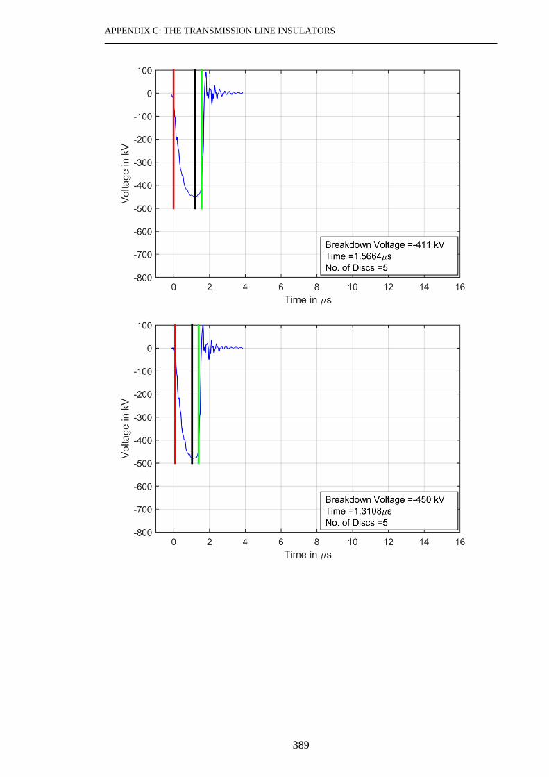
APPENDIX C: THE TRANSMISSION LINE INSULATORS
389

APPENDIX C: THE TRANSMISSION LINE INSULATORS
390

APPENDIX C: THE TRANSMISSION LINE INSULATORS
391

APPENDIX C: THE TRANSMISSION LINE INSULATORS
392

APPENDIX C: THE TRANSMISSION LINE INSULATORS
393

APPENDIX C: THE TRANSMISSION LINE INSULATORS
394

APPENDIX C: THE TRANSMISSION LINE INSULATORS
395

APPENDIX C: THE TRANSMISSION LINE INSULATORS
396

APPENDIX C: THE TRANSMISSION LINE INSULATORS
397

APPENDIX C: THE TRANSMISSION LINE INSULATORS
398

APPENDIX C: THE TRANSMISSION LINE INSULATORS
399

APPENDIX C: THE TRANSMISSION LINE INSULATORS
400

APPENDIX C: THE TRANSMISSION LINE INSULATORS
401

APPENDIX C: THE TRANSMISSION LINE INSULATORS
402

APPENDIX C: THE TRANSMISSION LINE INSULATORS
403

APPENDIX C: THE TRANSMISSION LINE INSULATORS
404

APPENDIX C: THE TRANSMISSION LINE INSULATORS
405

APPENDIX C: THE TRANSMISSION LINE INSULATORS
406

APPENDIX C: THE TRANSMISSION LINE INSULATORS
407

APPENDIX C: THE TRANSMISSION LINE INSULATORS
408

APPENDIX C: THE TRANSMISSION LINE INSULATORS
409

APPENDIX C: THE TRANSMISSION LINE INSULATORS
410

APPENDIX C: THE TRANSMISSION LINE INSULATORS
411

APPENDIX C: THE TRANSMISSION LINE INSULATORS
412

APPENDIX C: THE TRANSMISSION LINE INSULATORS
413

APPENDIX C: THE TRANSMISSION LINE INSULATORS
414

APPENDIX C: THE TRANSMISSION LINE INSULATORS
415

APPENDIX C: THE TRANSMISSION LINE INSULATORS
416

APPENDIX C: THE TRANSMISSION LINE INSULATORS
417

APPENDIX C: THE TRANSMISSION LINE INSULATORS
418

APPENDIX C: THE TRANSMISSION LINE INSULATORS
419

APPENDIX C: THE TRANSMISSION LINE INSULATORS
420

APPENDIX C: THE TRANSMISSION LINE INSULATORS
421

APPENDIX C: THE TRANSMISSION LINE INSULATORS
422

APPENDIX C: THE TRANSMISSION LINE INSULATORS
423

APPENDIX C: THE TRANSMISSION LINE INSULATORS
424

APPENDIX C: THE TRANSMISSION LINE INSULATORS
425

APPENDIX C: THE TRANSMISSION LINE INSULATORS
426

APPENDIX C: THE TRANSMISSION LINE INSULATORS
427

APPENDIX C: THE TRANSMISSION LINE INSULATORS
428

APPENDIX C: THE TRANSMISSION LINE INSULATORS
429

APPENDIX C: THE TRANSMISSION LINE INSULATORS
430

APPENDIX C: THE TRANSMISSION LINE INSULATORS
431

APPENDIX C: THE TRANSMISSION LINE INSULATORS
432

APPENDIX C: THE TRANSMISSION LINE INSULATORS
433

APPENDIX C: THE TRANSMISSION LINE INSULATORS
434

APPENDIX C: THE TRANSMISSION LINE INSULATORS
435

APPENDIX C: THE TRANSMISSION LINE INSULATORS
436

APPENDIX C: THE TRANSMISSION LINE INSULATORS
437

APPENDIX D: TOWER EARTHING SYSTEMS
438
APPENDIX D: TOWER EARTHING SYSTEMS
: VERIFICATION OF NIXON’S IONISATION MODEL
a) Current waveforms used in lab investigation in [288], implemented in PSCAD/EMTDC
b) Simulation results from PSCAD/ETMDC of soil ionisation models according to Nixon [288] and
CIGRE [24] for a single rod
Figure D-1: Simulation results of soil ionisation models according to Nixon [288]

APPENDIX D: TOWER EARTHING SYSTEMS
439
a) Current and voltage waveforms used in lab investigation from [288]
b) Current waveform and resistance from [288]
Figure D-2: Experimental and simulation results of soil ionisation models from [288]

APPENDIX D: TOWER EARTHING SYSTEMS
440
: VERIFICATION OF SEKIOKA’S FREQUENCY-
DEPENDENT MODEL
a) Current progression b) Resulting voltages
Figure D-3: Simulation results of frequency-dependent model according to Sekioka [213] and
Nixon ionization model [288], lightning impulse to single rod in 160 Ωm soil
a) Current progression b) Resulting voltages
Figure D-4: Measured results of voltages and applied currents, lightning impulse to single rod in
160 Ωm soil, from [213]

APPENDIX D: TOWER EARTHING SYSTEMS
441
: DERIVATION OF THE FOUR RODS NIXON
IONIZATION MODEL
𝐴1 = 2𝜋𝑟𝑙 𝐴2 = 2𝜋𝑟2 𝑟0 < 𝑟 ≤ 𝑑/2
𝐴1 = (2𝜋 − 4𝜃)𝑟𝑙 𝐴2 = 2𝜋𝑟2 cos 𝜃 𝑑/2 < 𝑟 ≤ √2𝑑/2
𝐴1 = (3
2𝜋 − 2𝜃) 𝑟𝑙 𝐴2 = 2𝜋𝑟
2 cos 𝜃 + 𝑟2𝜃(sin 𝜃 − cos 𝜃)√2𝑑
2< 𝑟 ≤ ∞
𝐽𝑖𝑜𝑛 =𝐼
4(𝐴1 + 𝐴2)
Case 1:
(𝐴1 + 𝐴2) −𝐼
4𝐽𝑖𝑜𝑛= 0
𝑟𝑙 + 𝑟2 −𝐼
8𝜋𝐽𝑖𝑜𝑛= 0
𝑟 =1
2(−𝑙 + √𝑙2 +
𝐼
2𝜋𝐽𝑖𝑜𝑛)
Crossing to next radius @ 𝑟 = 𝑑/2, determine 𝐼
𝑟𝑙 + 𝑟2 −𝐼
8𝜋𝐽𝑖𝑜𝑛= 0
𝑑
2𝑙 + (
𝑑
2)2
−𝐼
8𝜋𝐽𝑖𝑜𝑛= 0
2𝑑𝑙 + 𝑑2 −𝐼
2𝜋𝐽𝑖𝑜𝑛= 0
2𝜋𝐽𝑖𝑜𝑛(𝑑2 + 2𝑑𝑙) = 𝐼
Case 2:
(2𝜋 − 4𝜃)𝑟𝑙 + 2𝜋𝑟2 cos 𝜃 −𝐼
4𝐽𝑖𝑜𝑛= 0
2𝜋𝑟𝑙 − 4𝑟𝑙 cos−1𝑑
2𝑟 + 2𝜋𝑟2 cos 𝜃 −
𝐼
4𝐽𝑖𝑜𝑛= 0
2𝜋𝑟𝑙 − 4𝑟𝑙 cos−1𝑑
2𝑟 + 𝜋𝑟𝑑 −
𝐼
4𝐽𝑖𝑜𝑛= 0
Crossing to next radius @ 𝑟 = √2𝑑/2, determine 𝐼
𝜋√2𝑑𝑙 −𝜋𝑙√2𝑑
2 +𝜋√2𝑑2
2=
𝐼
4𝐽𝑖𝑜𝑛
2√2𝑑𝑙 − √2𝑑𝑙 + √2𝑑2 =𝐼
2𝜋𝐽𝑖𝑜𝑛
2√2𝜋𝐽𝑖𝑜𝑛(𝑑𝑙 + 𝑑2) = 𝐼

APPENDIX D: TOWER EARTHING SYSTEMS
442
Determination of formulation for radius 𝑟 for transition between Case 1 and 3:
𝑚 =2√2𝜋𝐽𝑖𝑜𝑛(𝑑𝑙 + 𝑑
2) − 2𝜋𝐽𝑖𝑜𝑛(𝑑2 + 2𝑑𝑙)
√2𝑑2 −
𝑑2
𝑚 =4𝜋𝐽𝑖𝑜𝑛 (√2(𝑑𝑙 + 𝑑
2) − (𝑑2 + 2𝑑𝑙))
√2𝑑 − 𝑑
𝑚 =4𝜋𝐽𝑖𝑜𝑛(√2𝑙 + √2𝑑 − 𝑑 − 2𝑙)
√2 − 1
𝑚 =4𝜋𝐽𝑖𝑜𝑛 (𝑙(√2 − 2) + 𝑑(√2 − 1))
√2 − 1
𝑡 = 2𝜋𝐽𝑖𝑜𝑛(𝑑2 + 2𝑑𝑙) −
4𝜋𝐽𝑖𝑜𝑛 (𝑙(√2 − 2) + 𝑑(√2 − 1))
√2 − 1
𝑑
2
𝑡 = 2𝜋𝐽𝑖𝑜𝑛𝑑2 + 2𝜋𝐽𝑖𝑜𝑛2𝑑𝑙 −
2𝜋𝐽𝑖𝑜𝑛𝑑 (𝑙(√2 − 2) + 𝑑(√2 − 1))
√2 − 1
𝑡 = 2𝜋𝐽𝑖𝑜𝑛𝑑2 + 2𝜋𝐽𝑖𝑜𝑛2𝑑𝑙 − 2𝜋𝐽𝑖𝑜𝑛
𝑑𝑙(√2 − 2)
√2 − 1− 2𝜋𝐽𝑖𝑜𝑛𝑑
2
𝑡 = 2𝜋𝐽𝑖𝑜𝑛𝑑𝑙 (2 −(√2 − 2)
√2 − 1)
Test at d/2:
𝑓(𝑟) =4𝜋𝐽𝑖𝑜𝑛 (𝑙(√2 − 2) + 𝑑(√2 − 1))
√2 − 1∙𝑑
2+ 2𝜋𝐽𝑖𝑜𝑛𝑑𝑙 (2 −
(√2 − 2)
√2 − 1)
𝑓(𝑟) =2𝜋𝐽𝑖𝑜𝑛𝑑 (𝑙(√2 − 2) + 𝑑(√2 − 1))
√2 − 1+ 4𝜋𝐽𝑖𝑜𝑛𝑑𝑙 − 2𝜋𝐽𝑖𝑜𝑛𝑑𝑙
(√2 − 2)
√2 − 1
𝑓(𝑟) = 2𝜋𝐽𝑖𝑜𝑛𝑑𝑙(√2 − 2)
√2 − 1+ 2𝜋𝐽𝑖𝑜𝑛𝑑
2 + 4𝜋𝐽𝑖𝑜𝑛𝑑𝑙 − 2𝜋𝐽𝑖𝑜𝑛𝑑𝑙(√2 − 2)
√2 − 1
𝐼(𝑟) = 2𝜋𝐽𝑖𝑜𝑛𝑑2 + 4𝜋𝐽𝑖𝑜𝑛𝑑𝑙
𝐼(𝑟) = 2𝜋𝐽𝑖𝑜𝑛(𝑑2 + 2𝑑𝑙)
Quadratic Law:
𝐼(𝑟) = 𝑎(𝑟 − 𝑟0)2 + 𝐼0
𝐼(𝑟) = 𝑎(𝑟 − 𝑑/2)2 + 2𝜋𝐽𝑖𝑜𝑛(𝑑2 + 2𝑑𝑙)
2√2𝜋𝐽𝑖𝑜𝑛(𝑑𝑙 + 𝑑2) = 𝑎(√2𝑑/2 − 𝑑/2)
2+ 2𝜋𝐽𝑖𝑜𝑛(𝑑
2 + 2𝑑𝑙)
𝑎 =2√2𝜋𝐽𝑖𝑜𝑛(𝑑𝑙 + 𝑑
2) − 2𝜋𝐽𝑖𝑜𝑛(𝑑2 + 2𝑑𝑙)
(√2𝑑/2 − 𝑑/2)2

APPENDIX D: TOWER EARTHING SYSTEMS
443
𝐼(𝑟) = 𝑎(𝑟 − 𝑟0)2 + 𝐼0
𝐼(𝑟) − 𝐼0𝑎
= (𝑟 − 𝑟0)2
0 = 𝑟2 − 2𝑟𝑟0 + 𝑟02 −
𝐼(𝑟) − 𝐼0𝑎
𝑟 = 0.5(2𝑟0 +√4𝑟02 − 4(𝑟02 −𝐼(𝑟) − 𝐼0𝑎
))
√𝐼(𝑟) − 𝐼0𝑎
+ 𝑟0 = 𝑟
Result for determination of radius r for Case 2:
𝐼 =4𝜋𝐽𝑖𝑜𝑛 (𝑙(√2 − 2) + 𝑑(√2 − 1))
√2 − 1𝑟 + 2𝜋𝐽𝑖𝑜𝑛𝑑𝑙 (2 −
(√2 − 2)
√2 − 1)
𝐼(√2 − 1) − 2𝜋𝐽𝑖𝑜𝑛𝑑𝑙 (2 −(√2 − 2)
√2 − 1) (√2 − 1)
= 4𝜋𝐽𝑖𝑜𝑛 (𝑙(√2 − 2) + 𝑑(√2 − 1)) 𝑟
𝐼(√2 − 1) − 2𝜋𝐽𝑖𝑜𝑛𝑑𝑙 (2 −(√2 − 2)
√2 − 1) (√2 − 1)
4𝜋𝐽𝑖𝑜𝑛 (𝑙(√2 − 2) + 𝑑(√2 − 1))= 𝑟
𝑟 =𝐼(√2 − 1) − 2𝜋𝐽𝑖𝑜𝑛𝑑𝑙 (2(√2 − 1) − (√2 − 2))
4𝜋𝐽𝑖𝑜𝑛 (𝑙(√2 − 2) + 𝑑(√2 − 1))
𝑟 =𝐼(√2 − 1) − 2𝜋𝐽𝑖𝑜𝑛𝑑𝑙(2√2 − 2 − √2 + 2)
4𝜋𝐽𝑖𝑜𝑛 (𝑙(√2 − 2) + 𝑑(√2 − 1))
𝑟 =
𝐼𝜋𝐽𝑖𝑜𝑛
(√2 − 1) − 𝑑𝑙√2
4 (𝑙(√2 − 2) + 𝑑(√2 − 1))
Case 3 @ 𝑟 = √2𝑑/2 to determine current:
(3
2𝜋 − 2𝜃) 𝑟𝑙 + 2𝜋𝑟2 cos 𝜃 + 𝑟2𝜃(sin 𝜃 − cos 𝜃) −
𝐼
4𝐽𝑖𝑜𝑛= 0
((3
2𝜋 − 2
𝜋
4)√2𝑑
2𝑙 + 𝜋
√2𝑑
2𝑑) −
𝐼
4𝐽𝑖𝑜𝑛= 0

APPENDIX D: TOWER EARTHING SYSTEMS
444
(𝜋√2
2𝑑𝑙 + 𝜋
√2
2𝑑2) =
𝐼
4𝐽𝑖𝑜𝑛
2√2𝜋𝐽𝑖𝑜𝑛(𝑑𝑙 + 𝑑2) = 𝐼
Case 3 @ 𝑟 = 𝑑 to determine current:
4𝐽𝑖𝑜𝑛 ((3
2𝜋 − 2
𝜋
3)𝑑𝑙 + 𝜋𝑑2 + 𝑑2
𝜋
3(√3
2−1
2)) = 𝐼
4𝜋𝐽𝑖𝑜𝑛 (5
6𝑑𝑙 + 𝑑2 + 𝑑2
1
3(√3
2−1
2)) = 𝐼
𝑚 =
4𝜋𝐽𝑖𝑜𝑛 (56𝑑𝑙 + 𝑑
2 + 𝑑213(√32 −
12)) − 2√2𝜋𝐽𝑖𝑜𝑛
(𝑑𝑙 + 𝑑2)
𝑑 −√22𝑑
𝑚 =
4𝜋𝐽𝑖𝑜𝑛 (56 𝑙 + 𝑑 + 𝑑
13(√32 −
12)) − 2√2𝜋𝐽𝑖𝑜𝑛
(𝑙 + 𝑑)
1 −√22
𝑡 = 4𝜋𝐽𝑖𝑜𝑛 (5
6𝑑𝑙 + 𝑑2 + 𝑑2
1
3(√3
2−1
2))
−
4𝜋𝐽𝑖𝑜𝑛 (56 𝑙 + 𝑑 + 𝑑
13(√32 −
12)) − 2√2𝜋𝐽𝑖𝑜𝑛
(𝑙 + 𝑑)
1 −√22
𝑑
𝑡 = 4𝜋𝐽𝑖𝑜𝑛 (5
6𝑑𝑙 + 𝑑2 + 𝑑2
1
3(√3
2−1
2))
−
4𝜋𝐽𝑖𝑜𝑛 (56𝑑𝑙 + 𝑑
2 + 𝑑213(√32 −
12)) − 2√2𝜋𝐽𝑖𝑜𝑛𝑑
(𝑙 + 𝑑)
1 −√22
𝑟 =𝐼 − 𝑡
𝑚

APPENDIX D: TOWER EARTHING SYSTEMS
445
: VERIFICATION OF EARTH WIRE MODEL
Figure D-5: PSCAD/EMTDC simulation of transient voltages to remote ground at the beginning
point of 15 long horizontal wire
Figure D-6: Measurement and simulation of transient voltages to remote ground at the
beginning point of 15 m long horizontal wire from [290]

APPENDIX D: TOWER EARTHING SYSTEMS
446
: VERIFICATION OF COUNTERPOISE MODEL
Figure D-7: Waveforms of injected current into counterpoise, PSCAD/EMTDC simulation
Figure D-8: Transient response of a typical transmission tower ground arrangement in a soil of
2400 Ωm, PSCAD/EMTDC simulation

APPENDIX D: TOWER EARTHING SYSTEMS
447
Figure D-9: Transient and resistive response of a typical transmission tower ground
arrangement in a soil of 2400 Ωm [262]

APPENDIX E: VERIFICATION OF THE ARRESTER MODEL
448
APPENDIX E: VERIFICATION OF THE
ARRESTER MODEL

449
APPENDIX F: DATA FOR SIMULATIONS
: TOWER DATA
L = 6.3m, Zw= 108 Ω
L = 9.4m, Zw= 116 Ω
L = 8.1m, Zw= 97 Ω
Lmin = 22.32m, Zw,min=94 Ω Lstd = 25.32m, Zw,std= 99 ΩLmax = 46.32m, Zw,max= 124 Ω
L = 7.4mZw,min= 300 Ω Zw,std= 305 ΩZw,max= 329 Ω
L = 10.55mZw,min= 289 Ω Zw,std= 295 ΩZw,max= 324 Ω
L = 8.55mZw,min= 267 Ω Zw,std= 275 ΩZw,max= 311 Ω
Figure F-1: 400 kV suspension tower dimensions

REFERENCES
450
Figure F-2: 400 kV suspension tower line heights
L = 8m, Zw= 108 Ω
L = 9.4m, Zw= 116 Ω
L = 8.1m, Zw= 97 Ω
Lmin = 22.32m, Zw,min=94 Ω Lstd = 25.32m, Zw,std= 99 ΩLmax = 46.32m, Zw,max= 124 Ω
L = 7.4mZw,min= 300 Ω Zw,std= 305 ΩZw,max= 329 Ω
L = 10.55mZw,min= 289 Ω Zw,std= 295 ΩZw,max= 324 Ω
L = 8.55mZw,min= 267 Ω Zw,std= 275 ΩZw,max= 311 Ω
D Suspension Double Shield Wire
Figure F-3: 400 kV suspension double shield wire tower dimensions

REFERENCES
451
L = 11.65m, Zw= 142 Ω
L = 9.0m, Zw= 105 Ω
L = 8.25m, Zw= 88 Ω
Lmin = 16.92m, Zw,min=70 Ω Lstd = 19.92m, Zw,std= 76 ΩLmax = 37.92m, Zw,max= 100 Ω
L = 8.0mZw,min= 293 Ω Zw,std= 298 ΩZw,max= 321 Ω
L = 11.15mZw,min= 278 Ω Zw,std= 284 ΩZw,max= 314 Ω
L = 9.15mZw,min= 252 Ω Zw,std= 262 ΩZw,max= 300 Ω
Figure F-4: 400 kV tension tower dimensions

REFERENCES
452
0.5m
L3,min = 16.92mL3,STD = 19.92mL3,max = 37.92m
L2,min = 25.17mL2,STD = 28.17mL2,max = 46.17m
L1,min = 34.17mL1,STD = 37.17mL1,max = 55.17m
LGW,min = 45.82mLGW,STD = 48.82mLGW,max = 66.82m
Figure F-5: 400 kV tension tower line heights

REFERENCES
453
L = 12.7m, Zw= 142 Ω
L = 9.0m, Zw= 105 Ω
L = 8.25m, Zw= 88 Ω
Lmin = 16.92m, Zw,min=70 Ω Lstd = 19.92m, Zw,std= 76 ΩLmax = 37.92m, Zw,max= 100 Ω
L = 8.0mZw,min= 293 Ω Zw,std= 298 ΩZw,max= 321 Ω
L = 11.15mZw,min= 278 Ω Zw,std= 284 ΩZw,max= 314 Ω
L = 9.15mZw,min= 252 Ω Zw,std= 262 ΩZw,max= 300 Ω
D10 Tension Double Shield Wire
Figure F-6: 400 kV tension double shield wire tower dimensions
Sag calculation for ground wire according to Error! Reference source not found.:
𝑆 = 200 m / 350 m / 500 m assumed
𝑚 = 1782 𝑘𝑔/𝑘𝑚, from ground wire datasheet
𝑤 = 𝑚 ∙ 𝑔 [𝑁
𝑚] =
1782
1000
𝑘𝑔
𝑚∙ 9.81
𝑚
𝑠2= 17.48142
𝑁
𝑚
𝐻 = 20% ∙ 𝐻𝑚𝑎𝑥 = 0.2 ∙ 300𝑘𝑁 = 60𝑘𝑁
sag ≈𝑤 (
𝑆
2)2
2 𝐻=𝑤 𝑆2
8 𝐻= 1.46 m / 4.46 m / 9.1 m
Sag calculation for phase wire Q&Q according to Error! Reference source not found.:
𝑆 = 200 m / 350 m / 500 m assumed

REFERENCES
454
𝑚 = 2348 𝑘𝑔/𝑘𝑚, from phase wire datasheet, 2 in a bundle
𝑤 = 𝑚 ∙ 𝑔 [𝑁
𝑚] =
2 ∙ 2348
1000
𝑘𝑔
𝑚∙ 9.81
𝑚
𝑠2= 46.06776
𝑁
𝑚
𝐻 = 15% ∙ 𝐻𝑚𝑎𝑥 = 0.15 ∙ 300𝑘𝑁 = 45𝑘𝑁
sag ≈𝑤 (
𝑆
2)2
2 𝐻=𝑤 𝑆2
8 𝐻= 5.12 m / 15.65 m / 32 m
𝑦 = 𝑦𝐺𝑊 + 𝑟𝐺𝑊 sin𝜑𝐺𝑊 = 𝑦𝐿𝑊 + 𝑟𝐿𝑊 sin𝜑𝐿𝑊
𝑥 = 𝑥𝐺𝑊 + 𝑟𝐺𝑊 cos𝜑𝐺𝑊 = 𝑥𝐿𝑊 + 𝑟𝐿𝑊 cos 𝜑𝐿𝑊
𝑥𝐺𝑊 − 𝑥𝐿𝑊 + 𝑟𝐺𝑊 cos𝜑𝐺𝑊 = 𝑟𝐿𝑊 cos𝜑𝐿𝑊

REFERENCES
455
: DEVELOPMENT OF AN IMPROVED EGM
PROCEDURE
Calculation of leader attachment coordinates:
Current and attachment angle are given
𝑟 = 8 ∙ I0.65 from CIGRE, index 𝑔 for ground, index 𝑠𝑤 for shield wire, index 𝐿𝑥 for
phase conductor
1. Determine coordinates of stroke point:
𝑦𝑆𝑃 = 𝑟𝑔
𝑥𝑆𝑃 =𝑦𝑆𝑃
tan (𝜋2 − Ψ)
2. Determine distance between (𝑥𝑆𝑃, 𝑦𝑆𝑃) and (𝑥𝑆𝑊/𝐿𝑊, 𝑦𝑆𝑊/𝐿𝑊)
|(𝑥𝑆𝑃, 𝑦𝑆𝑃)(𝑥𝑆𝑊/𝐿𝑊, 𝑦𝑆𝑊/𝐿𝑊) | = √(𝑥𝑆𝑃 − 𝑥𝑆𝑊/𝐿𝑊)
2+ (𝑦𝑆𝑃 − 𝑦𝑆𝑊/𝐿𝑊)
2
3. Determine distance between circles and stroke point
𝑑𝑆𝑊/𝐿𝑊 = |(𝑥𝑆𝑃 , 𝑦𝑆𝑃)(𝑥𝑆𝑊/𝐿𝑊, 𝑦𝑆𝑊/𝐿𝑊) | − 𝑟𝑆𝑊/𝐿𝑊
4. Determine perpendicular lines of shield wire/line wire and line wire/line wire
𝑥𝑃𝐿 =𝑥𝑆𝑊/𝐿𝑊1 + 𝑥𝐿𝑊2
2
𝑦𝑃𝐿 =𝑦𝑆𝑊/𝐿𝑊1 + 𝑦𝐿𝑊2
2
𝑚𝑃𝐿 = −𝑥𝐿𝑊2 − 𝑥𝑆𝑊/𝐿𝑊1
𝑦𝐿𝑊2 − 𝑦𝑆𝑊/𝐿𝑊1
𝑡𝑃𝐿 = 𝑦𝑃𝐿 −𝑚𝑃𝐿 ∙ 𝑥𝑃𝐿
5. Determine shortest distance point between perpendicular line and stroke point
𝑚𝑃𝐿 ∙ 𝑚𝑆𝑃 = −1𝑦𝑖𝑒𝑙𝑑𝑠→ 𝑚𝑆𝑃 = −
1
𝑚𝑃𝐿
𝑡𝑆𝑃 = 𝑦𝑆𝑃 −𝑚𝑆𝑃 ∙ 𝑥𝑆𝑃
𝑥𝑆𝑃/𝑃𝐿 =𝑡𝑃𝐿 − 𝑡𝑆𝑃𝑚𝑆𝑃 −𝑚𝑃𝐿
𝑦𝑆𝑃/𝑃𝐿 = 𝑚𝑃𝐿 ∙ 𝑥𝑆𝑃/𝑃𝐿 + 𝑡𝑃𝐿
6. Determine whether point is above or below perpendicular line
𝑦 = 𝑚𝑃𝐿 ∙ 𝑥𝑆𝑃/𝑃𝐿 + 𝑡𝑃𝐿
𝑦 ≥ 𝑦𝑆𝑃/𝑃𝐿𝑦𝑖𝑒𝑙𝑑𝑠→ (𝑥𝑆𝑃/𝑃𝐿 , 𝑦𝑆𝑃/𝑃𝐿) 𝑏𝑒𝑙𝑜𝑤 𝑜𝑟 𝑜𝑛 𝑝𝑒𝑟𝑝𝑒𝑛𝑑𝑖𝑐𝑢𝑙𝑎𝑟 𝑙𝑖𝑛𝑒
𝑦 < 𝑦𝑆𝑃/𝑃𝐿𝑦𝑖𝑒𝑙𝑑𝑠→ (𝑥𝑆𝑃/𝑃𝐿 , 𝑦𝑆𝑃/𝑃𝐿) 𝑎𝑏𝑜𝑣𝑒 𝑝𝑒𝑟𝑝𝑒𝑛𝑑𝑖𝑐𝑢𝑙𝑎𝑟 𝑙𝑖𝑛𝑒

REFERENCES
456
𝑑𝑆𝑃/𝑃𝐿 = 𝑦𝑆𝑃/𝑃𝐿 − 𝑦
7. Conditions to determine which conductor or earth is hit
Ground hit: 𝑑𝑆𝑊 > 0 𝐴𝑁𝐷 𝑑𝐿𝑊1 > 0 𝐴𝑁𝐷 𝑑𝐿𝑊2 > 0 𝐴𝑁𝐷 𝑑𝐿𝑊3 > 0
Shielding wire hit: 𝑑𝑆𝑊 ≤ 0 𝐴𝑁𝐷 𝑑𝐿1, 𝑆𝑃/𝑃𝐿 > 0 𝐴𝑁𝐷 𝑑𝐿2, 𝑆𝑃/𝑃𝐿 >
0 𝐴𝑁𝐷 𝑑𝐿3, 𝑆𝑃/𝑃𝐿 > 0
Line wire 1 hit:
𝑑𝐿𝑊1 ≤ 0 𝐴𝑁𝐷 𝑑𝐿1, 𝑆𝑃/𝑃𝐿 ≤ 0 𝐴𝑁𝐷 𝑑𝐿2, 𝑆𝑃/𝑃𝐿 > 0 𝐴𝑁𝐷 𝑑𝐿3, 𝑆𝑃/𝑃𝐿 > 0
Line wire 2 hit:
𝑑𝐿𝑊2 ≤ 0 𝐴𝑁𝐷 𝑑𝐿1, 𝑆𝑃/𝑃𝐿 ≤ 0 𝐴𝑁𝐷 𝑑𝐿2, 𝑆𝑃/𝑃𝐿 ≤ 0 𝐴𝑁𝐷 𝑑𝐿3, 𝑆𝑃/𝑃𝐿 > 0
Line wire 3 hit:
𝑑𝐿𝑊3 ≤ 0 𝐴𝑁𝐷 𝑑𝐿1, 𝑆𝑃/𝑃𝐿 ≤ 0 𝐴𝑁𝐷 𝑑𝐿2, 𝑆𝑃/𝑃𝐿 ≤ 0 𝐴𝑁𝐷 𝑑𝐿3, 𝑆𝑃/𝑃𝐿 ≤ 0

REFERENCES
457
APPENDIX G: SIMULATION RESULTS
: CRITICAL CURRENT DETERMINATION METHOD

REFERENCES
458
Table G-1: Critical Currents for base scenario with simple resistance, shield wire
Positive Stroke Polarity
Tower
Height MIN STD MAX
Soil Resistivity
Span
Length
Footing
Resistance
200m 350m 200m 350m 200m 350m 500m
100Ωm 4.5Ω 1003 1003 1003 876 1003 921 1003
500Ωm 23Ω 444 339 446 276 458 277 296
1000Ωm 46Ω 299 222 300 197 306 191 193
2500Ωm 114Ω 181 126 182 145 189 130 111
5000Ωm 228Ω 119 82 120 81 125 85 73
10000Ωm 455Ω 77 53 77 54 81 56 48
Negative Stroke Polarity
Tower Height MIN STD MAX
Soil Resistivity
Span
Length
Footing
Resistance
200m 350m 200m 350m 200m 350m 500m
100Ωm 4.5Ω 613 657 563 650 670 631 748
500Ωm 23Ω 240 214 241 211 250 218 220
1000Ωm 46Ω 147 126 148 126 154 130 126
2500Ωm 114Ω 83 68 84 70 87 71 65
5000Ωm 228Ω 58 47 59 47 60 49 44
10000Ωm 455Ω 44 35 44 35 45 36 32
Negative Subsequent Stroke Polarity
Tower Height MIN STD MAX
Soil Resistivity
Span
Length
Footing
Resistance
200m 350m 200m 350m 200m 350m 500m
100Ωm 4.5Ω 470 466 460 455 418 414 583
500Ωm 23Ω 333 330 329 293 314 308 383
1000Ωm 46Ω 209 196 211 198 215 193 221
2500Ωm 114Ω 110 77 111 79 118 95 69
5000Ωm 228Ω 58 45 58 45 63 48 37
10000Ωm 455Ω 42 29 43 29 44 30 26

REFERENCES
459
Table G-2: Critical Currents for base scenario with impedance, shield wire
Positive Stroke Polarity
Tower
Height MIN STD MAX
Soil Resistivity
Span
Length
Footing
Resistance
200m 350m 200m 350m 200m 350m 500m
100Ωm 4.5Ω 1003 1003 1003 1003 1003 1003 1003
500Ωm 23Ω 1003 1003 1003 1003 1003 1003 1003
1000Ωm 46Ω 1003 1003 1003 1003 1003 1003 1003
2500Ωm 114Ω 706 495 1003 509 709 609 610
5000Ωm 228Ω 519 455 502 355 547 505 366
10000Ωm 455Ω 434 311 485 335 465 346 295
Negative Stroke Polarity
Tower Height MIN STD MAX
Soil Resistivity
Span
Length
Footing
Resistance
200m 350m 200m 350m 200m 350m 500m
100Ωm 4.5Ω 1003 1003 1003 896 1003 1003 1003
500Ωm 23Ω 623 709 837 705 600 574 1003
1000Ωm 46Ω 505 729 631 732 494 516 757
2500Ωm 114Ω 533 436 533 437 546 447 461
5000Ωm 228Ω 322 300 322 301 327 312 309
10000Ωm 455Ω 167 150 175 155 186 174 187
Negative Subsequent Stroke Polarity
Tower Height MIN STD MAX
Soil Resistivity
Span
Length
Footing
Resistance
200m 350m 200m 350m 200m 350m 500m
100Ωm 4.5Ω 504 483 474 474 430 427 606
500Ωm 23Ω 443 437 433 429 398 395 552
1000Ωm 46Ω 406 405 399 388 370 367 434
2500Ωm 114Ω 291 285 288 285 278 275 331
5000Ωm 228Ω 185 177 186 178 191 183 195
10000Ωm 455Ω 143 135 144 135 149 142 147

REFERENCES
460
Table G-3: Critical Currents for base scenario with simple resistance, top phase wire
Positive Stroke Polarity
Tower
Height MIN STD MAX
Soil Resistivity
Span
Length
Footing
Resistance
200m 350m 200m 350m 200m 350m 500m
100Ωm 4.5Ω 27 35 25 35 20 25 15
500Ωm 23Ω 22 28 21 26 18 22 14
1000Ωm 46Ω 21 26 21 25 18 22 14
2500Ωm 114Ω 21 25 20 24 18 21 14
5000Ωm 228Ω 20 24 20 25 18 21 14
10000Ωm 455Ω 20 24 20 25 18 20 14
Negative Stroke Polarity
Tower Height MIN STD MAX
Soil Resistivity
Span
Length
Footing
Resistance
200m 350m 200m 350m 200m 350m 500m
100Ωm 4.5Ω 9 10 12 14 14 9 8
500Ωm 23Ω 15 9 15 9 9 9 11
1000Ωm 46Ω 15 9 15 9 14 9 11
2500Ωm 114Ω 15 9 15 9 14 9 11
5000Ωm 228Ω 15 9 15 9 9 9 8
10000Ωm 455Ω 15 9 15 9 9 9 8
Negative Subsequent Stroke Polarity
Tower Height MIN STD MAX
Soil Resistivity
Span
Length
Footing
Resistance
200m 350m 200m 350m 200m 350m 500m
100Ωm 4.5Ω 9 9 11 8 10 8 9
500Ωm 23Ω 11 8 11 8 10 8 9
1000Ωm 46Ω 11 8 10 8 10 8 9
2500Ωm 114Ω 11 8 9 8 10 8 9
5000Ωm 228Ω 11 8 9 8 10 8 9
10000Ωm 455Ω 11 8 9 8 10 8 9

REFERENCES
461
Table G-4: Critical Currents for base scenario with impedance, top phase wire
Positive Stroke Polarity
Tower
Height MIN STD MAX
Soil Resistivity
Span
Length
Footing
Resistance
200m 350m 200m 350m 200m 350m 500m
100Ωm 4.5Ω 27 35 0 25 35 0 20
500Ωm 23Ω 22 28 0 21 27 0 18
1000Ωm 46Ω 21 26 0 21 25 0 19
2500Ωm 114Ω 21 25 0 20 24 0 18
5000Ωm 228Ω 20 24 0 20 24 0 18
10000Ωm 455Ω 20 25 0 20 25 0 18
Negative Stroke Polarity
Tower Height MIN STD MAX
Soil Resistivity
Span
Length
Footing
Resistance
200m 350m 200m 350m 200m 350m 500m
100Ωm 4.5Ω 15 10 0 15 9 0 9
500Ωm 23Ω 15 9 0 15 9 0 9
1000Ωm 46Ω 15 9 0 15 9 0 9
2500Ωm 114Ω 15 9 0 15 9 0 9
5000Ωm 228Ω 15 9 0 15 9 0 14
10000Ωm 455Ω 15 9 0 9 9 0 9
Negative Subsequent Stroke Polarity
Tower Height MIN STD MAX
Soil Resistivity
Span
Length
Footing
Resistance
200m 350m 200m 350m 200m 350m 500m
100Ωm 4.5Ω 9 9 0 11 8 0 10
500Ωm 23Ω 11 8 0 11 8 0 10
1000Ωm 46Ω 11 8 0 10 8 0 10
2500Ωm 114Ω 11 8 0 9 8 0 10
5000Ωm 228Ω 11 8 0 9 8 0 10
10000Ωm 455Ω 9 8 0 9 8 0 10

REFERENCES
462
Table G-5: Flashover rates for base scenario with simple resistance and CIGRE distribution
derived from critical current determination simulations
LFOR
Tower
Height MIN STD MAX
Soil Resistivity
Span
Length
Footing
Resistance
200m 350m 200m 350m 200m 350m 500m
10000Ωm 455Ω 0.22432 0.3112 0.23369 0.31924 0.27697 0.35855 0.40252
5000Ωm 228Ω 0.13794 0.20634 0.14393 0.2162 0.19089 0.25239 0.29082
2500Ωm 114Ω 0.073905 0.11377 0.082532 0.11199 0.12829 0.16537 0.18741
1000Ωm 46Ω 0.038398 0.053658 0.047585 0.068765 0.09667 0.1185 0.12096
500Ωm 23Ω 0.025644 0.035335 0.035122 0.052221 0.086879 0.10079 0.101
100Ωm 4.5Ω 0.012652 0.011527 0.02129 0.022397 0.069145 0.073342 0.073787
SFFOR
Tower Height MIN STD MAX
Soil Resistivity
Span
Length
Footing
Resistance
200m 350m 200m 350m 200m 350m 500m
10000Ωm 455Ω 0.010964 0.013219 0.020332 0.022321 0.072421 0.07161 0.074199
5000Ωm 228Ω 0.010964 0.013219 0.020332 0.022321 0.072421 0.071209 0.074199
2500Ωm 114Ω 0.010693 0.013015 0.020332 0.022563 0.069956 0.071209 0.073507
1000Ωm 46Ω 0.010693 0.012826 0.020027 0.022321 0.069956 0.070812 0.073507
500Ωm 23Ω 0.010439 0.012494 0.020027 0.022095 0.072421 0.070812 0.073507
100Ωm 4.5Ω 0.012652 0.011527 0.02129 0.018249 0.069145 0.069654 0.073787
BFOR
Tower Height MIN STD MAX
Soil Resistivity
Span
Length
Footing
Resistance
200m 350m 200m 350m 200m 350m 500m
10000Ωm 455Ω 0.21335 0.29798 0.21335 0.29692 0.20455 0.28694 0.32832
5000Ωm 228Ω 0.12697 0.19313 0.1236 0.19388 0.11847 0.18118 0.21662
2500Ωm 114Ω 0.063213 0.10075 0.0622 0.089423 0.05833 0.094165 0.1139
1000Ωm 46Ω 0.027705 0.040832 0.027557 0.046444 0.026714 0.047684 0.047448
500Ωm 23Ω 0.015205 0.022842 0.015095 0.030126 0.014458 0.029976 0.027489
100Ωm 4.5Ω 0 0 0 0.004149 0 0.003688 0
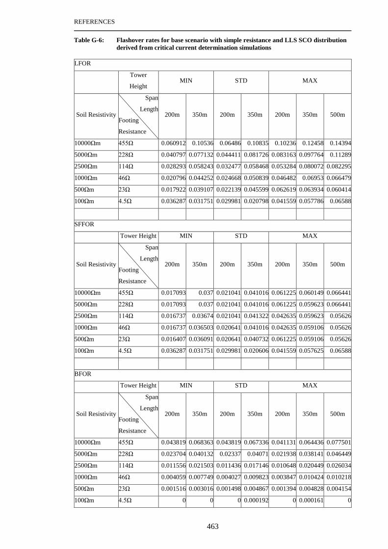
REFERENCES
463
Table G-6: Flashover rates for base scenario with simple resistance and LLS SCO distribution
derived from critical current determination simulations
LFOR
Tower
Height MIN STD MAX
Soil Resistivity
Span
Length
Footing
Resistance
200m 350m 200m 350m 200m 350m 500m
10000Ωm 455Ω 0.060912 0.10536 0.06486 0.10835 0.10236 0.12458 0.14394
5000Ωm 228Ω 0.040797 0.077132 0.044411 0.081726 0.083163 0.097764 0.11289
2500Ωm 114Ω 0.028293 0.058243 0.032477 0.058468 0.053284 0.080072 0.082295
1000Ωm 46Ω 0.020796 0.044252 0.024668 0.050839 0.046482 0.06953 0.066479
500Ωm 23Ω 0.017922 0.039107 0.022139 0.045599 0.062619 0.063934 0.060414
100Ωm 4.5Ω 0.036287 0.031751 0.029981 0.020798 0.041559 0.057786 0.06588
SFFOR
Tower Height MIN STD MAX
Soil Resistivity
Span
Length
Footing
Resistance
200m 350m 200m 350m 200m 350m 500m
10000Ωm 455Ω 0.017093 0.037 0.021041 0.041016 0.061225 0.060149 0.066441
5000Ωm 228Ω 0.017093 0.037 0.021041 0.041016 0.061225 0.059623 0.066441
2500Ωm 114Ω 0.016737 0.03674 0.021041 0.041322 0.042635 0.059623 0.05626
1000Ωm 46Ω 0.016737 0.036503 0.020641 0.041016 0.042635 0.059106 0.05626
500Ωm 23Ω 0.016407 0.036091 0.020641 0.040732 0.061225 0.059106 0.05626
100Ωm 4.5Ω 0.036287 0.031751 0.029981 0.020606 0.041559 0.057625 0.06588
BFOR
Tower Height MIN STD MAX
Soil Resistivity
Span
Length
Footing
Resistance
200m 350m 200m 350m 200m 350m 500m
10000Ωm 455Ω 0.043819 0.068363 0.043819 0.067336 0.041131 0.064436 0.077501
5000Ωm 228Ω 0.023704 0.040132 0.02337 0.04071 0.021938 0.038141 0.046449
2500Ωm 114Ω 0.011556 0.021503 0.011436 0.017146 0.010648 0.020449 0.026034
1000Ωm 46Ω 0.004059 0.007749 0.004027 0.009823 0.003847 0.010424 0.010218
500Ωm 23Ω 0.001516 0.003016 0.001498 0.004867 0.001394 0.004828 0.004154
100Ωm 4.5Ω 0 0 0 0.000192 0 0.000161 0

REFERENCES
464
Table G-7: Flashover rates for base scenario with impedance and CIGRE distribution derived
from critical current determination simulations
LFOR
Tower
Height MIN STD MAX
Soil Resistivity
Span
Length
Footing
Resistance
200m 350m 200m 350m 200m 350m 500m
10000Ωm 455Ω 0.026971 0.039246 0.037016 0.045938 0.086631 0.09355 0.1012
5000Ωm 228Ω 0.022684 0.027824 0.03274 0.043914 0.080649 0.083491 0.093931
2500Ωm 114Ω 0.017297 0.025719 0.020332 0.03468 0.078969 0.080006 0.082278
1000Ωm 46Ω 0.010693 0.012826 0.020027 0.022321 0.072014 0.070812 0.073507
500Ωm 23Ω 0.010439 0.012494 0.020027 0.021884 0.072421 0.070812 0.073507
100Ωm 4.5Ω 0.009414 0.011527 0.018967 0.020679 0.07161 0.069654 0.073787
SFFOR
Tower Height MIN STD MAX
Soil Resistivity
Span
Length
Footing
Resistance
200m 350m 200m 350m 200m 350m 500m
10000Ωm 455Ω 0.010964 0.013015 0.023686 0.022321 0.072421 0.071209 0.073507
5000Ωm 228Ω 0.010964 0.013219 0.020332 0.022563 0.069956 0.071209 0.073507
2500Ωm 114Ω 0.010693 0.013015 0.020332 0.022563 0.072421 0.071209 0.073507
1000Ωm 46Ω 0.010693 0.012826 0.020027 0.022321 0.072014 0.070812 0.073507
500Ωm 23Ω 0.010439 0.012494 0.020027 0.021884 0.072421 0.070812 0.073507
100Ωm 4.5Ω 0.009414 0.011527 0.018967 0.020679 0.07161 0.069654 0.073787
BFOR
Tower Height MIN STD MAX
Soil Resistivity
Span
Length
Footing
Resistance
200m 350m 200m 350m 200m 350m 500m
10000Ωm 455Ω 0.016007 0.026231 0.013329 0.023617 0.014211 0.022341 0.027693
5000Ωm 228Ω 0.01172 0.014605 0.012407 0.021351 0.010693 0.012283 0.020424
2500Ωm 114Ω 0.006604 0.012704 0 0.012117 0.006548 0.008797 0.00877
1000Ωm 46Ω 0 0 0 0 0 0 0
500Ωm 23Ω 0 0 0 0 0 0 0
100Ωm 4.5Ω 0 0 0 0 0 0 0

REFERENCES
465
Table G-8: Flashover rates for base scenario with impedance and LLS SCO distribution
derived from critical current determination simulations
LFOR
Tower
Height MIN STD MAX
Soil Resistivity
Span
Length
Footing
Resistance
200m 350m 200m 350m 200m 350m 500m
10000Ωm 455Ω 0.018704 0.040444 0.043971 0.04412 0.062563 0.062493 0.060446
5000Ωm 228Ω 0.018079 0.038419 0.022124 0.044016 0.043483 0.060688 0.058758
2500Ωm 114Ω 0.017129 0.037866 0.021041 0.042363 0.061612 0.060241 0.056875
1000Ωm 46Ω 0.016737 0.036503 0.020641 0.041016 0.060683 0.059106 0.05626
500Ωm 23Ω 0.016407 0.036091 0.020641 0.040469 0.061225 0.059106 0.05626
100Ωm 4.5Ω 0.015106 0.031751 0.019278 0.039024 0.060149 0.057625 0.06588
SFFOR
Tower Height MIN STD MAX
Soil Resistivity
Span
Length
Footing
Resistance
200m 350m 200m 350m 200m 350m 500m
10000Ωm 455Ω 0.017093 0.03674 0.042779 0.041016 0.061225 0.059623 0.05626
5000Ωm 228Ω 0.017093 0.037 0.021041 0.041322 0.042635 0.059623 0.05626
2500Ωm 114Ω 0.016737 0.03674 0.021041 0.041322 0.061225 0.059623 0.05626
1000Ωm 46Ω 0.016737 0.036503 0.020641 0.041016 0.060683 0.059106 0.05626
500Ωm 23Ω 0.016407 0.036091 0.020641 0.040469 0.061225 0.059106 0.05626
100Ωm 4.5Ω 0.015106 0.031751 0.019278 0.039024 0.060149 0.057625 0.06588
BFOR
Tower Height MIN STD MAX
Soil Resistivity
Span
Length
Footing
Resistance
200m 350m 200m 350m 200m 350m 500m
10000Ωm 455Ω 0.001611 0.003704 0.001192 0.003104 0.001338 0.00287 0.004186
5000Ωm 228Ω 0.000986 0.001419 0.001083 0.002695 0.000848 0.001065 0.002498
2500Ωm 114Ω 0.000392 0.001126 0 0.001042 0.000387 0.000618 0.000615
1000Ωm 46Ω 0 0 0 0 0 0 0
500Ωm 23Ω 0 0 0 0 0 0 0
100Ωm 4.5Ω 0 0 0 0 0 0 0

REFERENCES
466
Table G-9: Critical Currents for mitigation scenario with simple resistance, shield wire
Positive Stroke Polarity
Tower Height MIN STD MAX
Soil
Resistivity
Span
Length
Footing
Resistance
200m 350m 500m 200m 350m 500m 200m 350m 500m
100Ωm 4.5Ω 1003 1003 1003 1003 1003 1003 1003 1003 1003
500Ωm 23Ω 1003 695 571 695 501 413 719 545 454
1000Ωm 46Ω 637 469 395 467 326 272 572 418 354
2500Ωm 114Ω 394 292 240 268 183 157 442 317 266
5000Ωm 228Ω 275 212 175 174 121 104 366 260 216
10000Ωm 455Ω 201 164 134 115 84 71 316 224 185
Negative Stroke Polarity
Tower Height MIN STD MAX
Soil
Resistivity
Span
Length
Footing
Resistance
200m 350m 500m 200m 350m 500m 200m 350m 500m
100Ωm 4.5Ω 1003 1003 1003 861 787 751 708 660 710
500Ωm 23Ω 409 363 352 306 265 247 486 448 473
1000Ωm 46Ω 265 229 216 196 163 150 274 370 306
2500Ωm 114Ω 164 138 128 116 93 83 344 310 313
5000Ωm 228Ω 123 104 96 83 67 59 206 292 293
10000Ωm 455Ω 99 85 80 64 52 46 188 282 283
Negative Subsequent Stroke Polarity
Tower Height MIN STD MAX
Soil
Resistivity
Span
Length
Footing
Resistance
200m 350m 500m 200m 350m 500m 200m 350m 500m
100Ωm 4.5Ω 1003 1003 1003 518 514 514 407 403 563
500Ωm 23Ω 857 846 1003 396 388 387 385 361 384
1000Ωm 46Ω 539 527 288 262 247 246 348 290 276
2500Ωm 114Ω 336 319 321 154 136 131 334 241 262
5000Ωm 228Ω 261 217 246 100 68 58 330 303 198
10000Ωm 455Ω 208 205 165 70 51 39 327 324 325

REFERENCES
467
Table G-10: Critical Currents for mitigation scenario with simple resistance, top phase wire
Positive Stroke Polarity
Tower Height MIN STD MAX
Soil
Resistivity
Span
Length
Footing
Resistance
200m 350m 500m 200m 350m 500m 200m 350m 500m
100Ωm 4.5Ω 1003 1003 1003 1003 1003 1003 1003 1003 1003
500Ωm 23Ω 1003 695 571 695 501 413 719 545 454
1000Ωm 46Ω 637 469 395 467 326 272 572 418 354
2500Ωm 114Ω 394 292 240 268 183 157 442 317 266
5000Ωm 228Ω 275 212 175 174 121 104 366 260 216
10000Ωm 455Ω 201 164 134 115 84 71 316 224 185
Negative Stroke Polarity
Tower Height MIN STD MAX
Soil
Resistivity
Span
Length
Footing
Resistance
200m 350m 500m 200m 350m 500m 200m 350m 500m
100Ωm 4.5Ω 1003 1003 1003 861 787 751 708 660 710
500Ωm 23Ω 409 363 352 306 265 247 486 448 473
1000Ωm 46Ω 265 229 216 196 163 150 274 370 306
2500Ωm 114Ω 164 138 128 116 93 83 344 310 313
5000Ωm 228Ω 123 104 96 83 67 59 206 292 293
10000Ωm 455Ω 99 85 80 64 52 46 188 282 283
Negative Subsequent Stroke Polarity
Tower Height MIN STD MAX
Soil
Resistivity
Span
Length
Footing
Resistance
200m 350m 500m 200m 350m 500m 200m 350m 500m
100Ωm 4.5Ω 1003 1003 1003 518 514 514 407 403 563
500Ωm 23Ω 857 846 1003 396 388 387 385 361 384
1000Ωm 46Ω 539 527 288 262 247 246 348 290 276
2500Ωm 114Ω 336 319 321 154 136 131 334 241 262
5000Ωm 228Ω 261 217 246 100 68 58 330 303 198
10000Ωm 455Ω 208 205 165 70 51 39 327 324 325

REFERENCES
468
Table G-11: Flashover rates for mitigation scenario with simple resistance and CIGRE
distribution derived from critical current determination simulations
LFOR
Tower Height MIN STD MAX
Soil
Resistivity
Span
Length
Footing
Resistance
200m 350m 500m 200m 350m 500m 200m 350m 500m
10000Ωm 455Ω 0.049878 0.066641 0.081668 0.12523 0.18929 0.23391 0.097671 0.10963 0.12145
5000Ωm 228Ω 0.032089 0.046003 0.057762 0.068779 0.1154 0.1475 0.092896 0.099815 0.11453
2500Ωm 114Ω 0.018588 0.028878 0.037249 0.032065 0.059517 0.076272 0.087721 0.095848 0.10559
1000Ωm 46Ω 0.008088 0.01392 0.018264 0.008862 0.021448 0.030116 0.082296 0.087129 0.094945
500Ωm 23Ω 0 0.006816 0.009902 0.00033 0.007421 0.013495 0.078785 0.081573 0.088308
100Ωm 4.5Ω 0 0 0 0 0 0 0.07161 0.069654 0.073787
SFFOR
Tower Height MIN STD MAX
Soil
Resistivity
Span
Length
Footing
Resistance
200m 350m 500m 200m 350m 500m 200m 350m 500m
10000Ωm 455Ω 0 0 0 0 0 0 0.072421 0.070812 0.073507
5000Ωm 228Ω 0 0 0 0 0 0 0.072421 0.06737 0.074066
2500Ωm 114Ω 0 0 0 0 0 0 0.072421 0.070812 0.074066
1000Ωm 46Ω 0 0 0 0 0 0 0.072421 0.07042 0.073507
500Ωm 23Ω 0 0 0 0 0 0 0.072421 0.070812 0.073653
100Ωm 4.5Ω 0 0 0 0 0 0 0.07161 0.069654 0.073787
BFOR
Tower Height MIN STD MAX
Soil
Resistivity
Span
Length
Footing
Resistance
200m 350m 500m 200m 350m 500m 200m 350m 500m
10000Ωm 455Ω 0.049996 0.066937 0.082056 0.13284 0.19645 0.2404 0.02525 0.038814 0.047944
5000Ωm 228Ω 0.032089 0.046093 0.057947 0.076387 0.12248 0.15404 0.020475 0.032445 0.040468
2500Ωm 114Ω 0.018588 0.028878 0.037249 0.039755 0.066671 0.082812 0.015301 0.025036 0.031529
1000Ωm 46Ω 0.008088 0.01392 0.018264 0.016552 0.028676 0.036657 0.009875 0.016709 0.021438
500Ωm 23Ω 0 0.006816 0.009902 0.00802 0.014649 0.020036 0.006364 0.010761 0.014655
100Ωm 4.5Ω 0 0 0 0 0 0 0 0 0

REFERENCES
469
Table G-12: Flashover rates for mitigation scenario with simple resistance and LLS Scotland
distribution derived from critical current determination simulations
LFOR
Tower Height MIN STD MAX
Soil
Resistivity
Span
Length
Footing
Resistance
200m 350m 500m 200m 350m 500m 200m 350m 500m
10000Ωm 455Ω 0.00945 0.01382 0.01944 0.03123 0.05180 0.06323 0.06479 0.06671 0.06733
5000Ωm 228Ω 0.00491 0.00851 0.01228 0.01677 0.03379 0.04056 0.06372 0.04256 0.07164
2500Ωm 114Ω 0.00207 0.00429 0.00659 0.00817 0.02010 0.02439 0.06276 0.06265 0.06873
1000Ωm 46Ω 0.00054 0.00131 0.00206 0.00362 0.01061 0.01277 0.06197 0.06038 0.05897
500Ωm 23Ω 0.00000 0.00041 0.00075 0.00255 0.00799 0.00902 0.06160 0.05996 0.06432
100Ωm 4.5Ω 0.00000 0.00000 0.00000 0.00701 0.00654 0.00674 0.06015 0.05763 0.06588
SFFOR
Tower Height MIN STD MAX
Soil
Resistivity
Span
Length
Footing
Resistance
200m 350m 500m 200m 350m 500m 200m 350m 500m
10000Ωm 455Ω 0.00000 0.00000 0.00000 0.00217 0.00681 0.00769 0.06123 0.05911 0.05626
5000Ωm 228Ω 0.00000 0.00000 0.00000 0.00217 0.00691 0.00686 0.06123 0.03701 0.06345
2500Ωm 114Ω 0.00000 0.00000 0.00000 0.00206 0.00681 0.00686 0.06123 0.05911 0.06345
1000Ωm 46Ω 0.00000 0.00000 0.00000 0.00206 0.00671 0.00686 0.06123 0.05860 0.05626
500Ωm 23Ω 0.00000 0.00000 0.00000 0.00206 0.00671 0.00686 0.06123 0.05911 0.06289
100Ωm 4.5Ω 0.00000 0.00000 0.00000 0.00701 0.00654 0.00674 0.06015 0.05763 0.06588
BFOR
Tower Height MIN STD MAX
Soil
Resistivity
Span
Length
Footing
Resistance
200m 350m 500m 200m 350m 500m 200m 350m 500m
10000Ωm 455Ω 0.00945 0.01382 0.01944 0.02906 0.04499 0.05554 0.00357 0.00761 0.01107
5000Ωm 228Ω 0.00491 0.00851 0.01228 0.01460 0.02688 0.03370 0.00250 0.00555 0.00819
2500Ωm 114Ω 0.00207 0.00429 0.00659 0.00611 0.01329 0.01753 0.00153 0.00354 0.00528
1000Ωm 46Ω 0.00054 0.00131 0.00206 0.00156 0.00390 0.00591 0.00074 0.00178 0.00271
500Ωm 23Ω 0.00000 0.00041 0.00075 0.00048 0.00128 0.00216 0.00037 0.00086 0.00143
100Ωm 4.5Ω 0.00000 0.00000 0.00000 0.00000 0.00000 0.00000 0.00000 0.00000 0.00000

REFERENCES
470
: MONTE-CARLO METHOD
Table G-13: Flashover ratios for base scenario with footing resistance and CIGRE distribution
derived from Monte-Carlo simulations
N/F SFFO
Tower Height MIN STD MAX
Soil Resistivity
Span
Length
Footing
Resistance
200m 350m 200m 350m 200m 350m 500m
10000Ωm 455Ω 26.7 27.3 30.8 27.2 55.7 54.6 55.3
5000Ωm 228Ω 23.9 24.4 30.5 29.8 55.5 54.4 55.5
2500Ωm 114Ω 26.8 24.8 30.5 27.4 55.3 54.6 55.9
1000Ωm 46Ω 26.9 25.2 25.141 27.5 55.5 54.9 55.7
500Ωm 23Ω 26.9 25 27.2 26.6 55.9 54.8 55.9
100Ωm 4.5Ω 26.3 26.544 29.9 24.8 55.9 54.4 55.4
N/F BFO
Tower Height MIN STD MAX
Soil Resistivity
Span
Length
Footing
Resistance
200m 350m 200m 350m 200m 350m 500m
10000Ωm 455Ω 21.7 30.9 21.6 30.8 18 22.5 24.1
5000Ωm 228Ω 3.9 8.4 8.7 19.9 7 17 19.7
2500Ωm 114Ω 3.3 2.7 3.3 9.9 2.7 5.1 6.7
1000Ωm 46Ω 0 0.3 0 0.7 0.3 0.6 1.3
500Ωm 23Ω 0 0 0 0.1 0 0.1 0.2
100Ωm 4.5Ω 0 0 0 0 0 0 0

REFERENCES
471
Table G-14: Flashover ratios for base scenario with footing resistance and LLS SCO distribution
derived from Monte-Carlo simulations
N/F SFFO
Tower Height MIN STD MAX
Soil Resistivity
Span
Length
Footing
Resistance
200m 350m 200m 350m 200m 350m 500m
10000Ωm 455Ω 31.7 30.6 39.337 33.1 58.797 57.7 59.9
5000Ωm 228Ω 29.358 30 35.7 38 55.3 57.6 58
2500Ωm 114Ω 31.75 27.9 35.7 37.9 55.5 57.3 60.2
1000Ωm 46Ω 30.446 28.3 29.9 36 55.355 58.5 60
500Ωm 23Ω 28.8 28.4 29.6 37.3 53.914 57.8 60
100Ωm 4.5Ω 27.965 28.778 35 35.3 57.238 57.4 60
N/F BFO
Tower Height MIN STD MAX
Soil Resistivity
Span
Length
Footing
Resistance
200m 350m 200m 350m 200m 350m 500m
10000Ωm 455Ω 5.2 11.3 3.1056 10.1 3.5635 6.6 7.5
5000Ωm 228Ω 2.3591 5.4 2 5.4 2.7 3.8 4.5
2500Ωm 114Ω 1.2746 1.6 0.7 1.6 0.3 1.3 2.2
1000Ωm 46Ω 0 0.9 0 0.3 0.11274 0.5 0
500Ωm 23Ω 0 0 0 0 0 0 0
100Ωm 4.5Ω 0 0 0 0 0 0 0

REFERENCES
472
Table G-15: Flashover ratios for base scenario with footing impedance and CIGRE distribution
derived from Monte-Carlo simulations
N/F SFFO
Tower Height MIN STD MAX
Soil Resistivity
Span
Length
Footing
Resistance
200m 350m 200m 350m 200m 350m 500m
10000Ωm 455Ω 27.2 26.4 0 27.6 26.5 0 56.8
5000Ωm 228Ω 26.8 26.4 0 27.6 26 0 56.8
2500Ωm 114Ω 26.8 26.1 0 27.6 26 0 56.6
1000Ωm 46Ω 26.8 26.1 0 27.6 26.3 0 56.7
500Ωm 23Ω 26.3 26.1 0 27 26.3 0 56.1
100Ωm 4.5Ω 26.3 26.1 0 27 26.3 0 55.3
N/F BFO
Tower Height MIN STD MAX
Soil Resistivity
Span
Length
Footing
Resistance
200m 350m 200m 350m 200m 350m 500m
10000Ωm 455Ω 0.1 0.1 0 0 0.1 0 0
5000Ωm 228Ω 0 0.1 0 0 0.1 0 0
2500Ωm 114Ω 0 0 0 0 0.1 0 0
1000Ωm 46Ω 0 0 0 0 0 0 0
500Ωm 23Ω 0 0 0 0 0 0 0
100Ωm 4.5Ω 0 0 0 0 0 0 0

REFERENCES
473
Table G-16: Flashover rates for base scenario with footing resistance and CIGRE distribution
derived from Monte-Carlo simulations
LFOR
Tower Height MIN STD MAX
Soil Resistivity
Span
Length
Footing
Resistance
200m 350m 200m 350m 200m 350m 500m
10000Ωm 455Ω 1.9996 2.7675 2.0378 2.4972 2.0436 2.4024 2.539
5000Ωm 228Ω 0.52548 0.90824 0.9858 1.8938 1.1452 1.9524 2.1814
2500Ωm 114Ω 0.50031 0.44655 0.54586 0.83211 0.79329 0.98407 1.1244
1000Ωm 46Ω 0.23158 0.25485 0.23056 0.29611 0.59921 0.61944 0.68285
500Ωm 23Ω 0.23158 0.22948 0.24985 0.24326 0.57739 0.57201 0.59625
100Ωm 4.5Ω 0.22739 0.23992 0.27166 0.22468 0.57739 0.5667 0.57462
SFFOR
Tower Height MIN STD MAX
Soil Resistivity
Span
Length
Footing
Resistance
200m 350m 200m 350m 200m 350m 500m
10000Ωm 455Ω 0.23049 0.24825 0.27682 0.24302 0.57607 0.56802 0.57423
5000Ωm 228Ω 0.20752 0.22341 0.27651 0.27137 0.57449 0.56643 0.57528
2500Ωm 114Ω 0.23126 0.22643 0.27682 0.23917 0.57317 0.56828 0.57819
1000Ωm 46Ω 0.23158 0.23039 0.23056 0.24488 0.57475 0.57053 0.57687
500Ωm 23Ω 0.23158 0.22948 0.24985 0.23006 0.57739 0.5696 0.57995
100Ωm 4.5Ω 0.22739 0.23992 0.27166 0.22468 0.57739 0.5667 0.57462
BFOR
Tower Height MIN STD MAX
Soil Resistivity
Span
Length
Footing
Resistance
200m 350m 200m 350m 200m 350m 500m
10000Ωm 455Ω 1.7692 2.5192 1.761 2.2542 1.4675 1.8344 1.9648
5000Ωm 228Ω 0.31796 0.68483 0.70929 1.6224 0.57069 1.386 1.6061
2500Ωm 114Ω 0.26904 0.22013 0.26904 0.59294 0.22013 0.41579 0.54624
1000Ωm 46Ω 0 0.024458 0 0.051232 0.024458 0.048917 0.10599
500Ωm 23Ω 0 0 0 0.013193 0 0.002412 0.016306
100Ωm 4.5Ω 0 0 0 0 0 0 0

REFERENCES
474
Table G-17: Flashover rates for base scenario with footing resistance and LLS SCO distribution
derived from Monte-Carlo simulations
LFOR
Tower Height MIN STD MAX
Soil Resistivity
Span
Length
Footing
Resistance
200m 350m 200m 350m 200m 350m 500m
10000Ωm 455Ω 0.62542 1.0463 0.4048 0.60898 0.64174 0.74872 0.79941
5000Ωm 228Ω 0.37669 0.59801 0.36004 0.59801 0.79329 0.65462 0.79024
2500Ωm 114Ω 0.30941 0.29491 0.30348 0.29491 0.59921 0.56851 0.62413
1000Ωm 46Ω 0.237 0.26534 0.24028 0.32165 0.57637 0.55201 0.55023
500Ωm 23Ω 0.23099 0.22908 0.26058 0.31472 0.56193 0.53074 0.55023
100Ωm 4.5Ω 0.23705 0.23632 0.27847 0.30008 0.51267 0.52779 0.54996
SFFOR
Tower Height MIN STD MAX
Soil Resistivity
Span
Length
Footing
Resistance
200m 350m 200m 350m 200m 350m 500m
10000Ωm 455Ω 0.26071 0.25371 0.31869 0.28046 0.52335 0.52944 0.55023
5000Ωm 228Ω 0.25194 0.29433 0.29538 0.29433 0.57317 0.52837 0.53252
2500Ωm 114Ω 0.26214 0.23556 0.28368 0.23556 0.57475 0.52532 0.55103
1000Ωm 46Ω 0.237 0.22925 0.24028 0.3079 0.5723 0.5354 0.55023
500Ωm 23Ω 0.23099 0.22908 0.26058 0.31472 0.56193 0.53074 0.55023
100Ωm 4.5Ω 0.23705 0.23632 0.27847 0.30008 0.51267 0.52779 0.54996
BFOR
Tower Height MIN STD MAX
Soil Resistivity
Span
Length
Footing
Resistance
200m 350m 200m 350m 200m 350m 500m
10000Ωm 455Ω 0.36471 0.79255 0.086112 0.32852 0.11839 0.21928 0.24918
5000Ωm 228Ω 0.12476 0.30368 0.064661 0.30368 0.22013 0.12625 0.25772
2500Ωm 114Ω 0.047277 0.059346 0.019801 0.059346 0.024458 0.043192 0.073094
1000Ωm 46Ω 0 0.036084 0 0.013747 0.004064 0.016612 0
500Ωm 23Ω 0 0 0 0 0 0 0
100Ωm 4.5Ω 0 0 0 0 0 0 0

REFERENCES
475
Table G-18: Flashover rates for base scenario with footing impedance and CIGRE distribution
derived from Monte-Carlo simulations
LFOR
Tower Height MIN STD MAX
Soil Resistivity
Span
Length
Footing
Resistance
200m 350m 200m 350m 200m 350m 500m
10000Ωm 455Ω 0.23624 0.23052 0.24822 0.23052 0.58386 0.58605 0.58605
5000Ωm 228Ω 0.23126 0.23052 0.24822 0.22599 0.58386 0.58386 0.58386
2500Ωm 114Ω 0.23126 0.22537 0.24885 0.22599 0.58281 0.58281 0.58281
1000Ωm 46Ω 0.23126 0.22537 0.24885 0.22685 0.5832 0.5832 0.5832
500Ωm 23Ω 0.22739 0.22537 0.244 0.22685 0.57924 0.57924 0.57924
100Ωm 4.5Ω 0.22739 0.22537 0.244 0.22685 0.57396 0.57396 0.57396
SFFOR
Tower Height MIN STD MAX
Soil Resistivity
Span
Length
Footing
Resistance
200m 350m 200m 350m 200m 350m 500m
10000Ωm 455Ω 0.23383 0.22825 0.24822 0.22825 0.58386 0.58122 0.58122
5000Ωm 228Ω 0.23126 0.22825 0.24822 0.22483 0.58386 0.58386 0.58386
2500Ωm 114Ω 0.23126 0.22537 0.24885 0.22483 0.58281 0.58281 0.58281
1000Ωm 46Ω 0.23126 0.22537 0.24885 0.22685 0.5832 0.5832 0.5832
500Ωm 23Ω 0.22739 0.22537 0.244 0.22685 0.57924 0.57924 0.57924
100Ωm 4.5Ω 0.22739 0.22537 0.244 0.22685 0.57396 0.57396 0.57396
BFOR
Tower Height MIN STD MAX
Soil Resistivity
Span
Length
Footing
Resistance
200m 350m 200m 350m 200m 350m 500m
10000Ωm 455Ω 0.002412 0.002271 0 0.002271 0 0.004825 0.004825
5000Ωm 228Ω 0 0.002271 0 0.00116 0 0 0
2500Ωm 114Ω 0 0 0 0.00116 0 0 0
1000Ωm 46Ω 0 0 0 0 0 0 0
500Ωm 23Ω 0 0 0 0 0 0 0
100Ωm 4.5Ω 0 0 0 0 0 0 0

REFERENCES
476
Table G-19: Flashover ratios for mitigation scenario with simple resistance and CIGRE
distribution derived from Monte-Carlo simulations
F/N SFFO
Tower
Height AR Y CP UW
Soil
Resistivity
Span
Length
Footing
Resistance
200m 350m 500m 200m 350m 500m 200m 350m 500m 200m 350m 500m
10000Ωm 455Ω 12.7 12.3 12.8 43.2 41.4 43.3 56.4 54.8 56.7 55.8 54.8 55.7
5000Ωm 228Ω 12.9 10.8 12.8 43.8 43.7 44.5 56.6 56.6 56.6 56.2 53.9 55.6
2500Ωm 114Ω 12.8 11.4 13.1 41.2 40.5 43.3 56.4 56.4 56.4 56.1 55.2 56
1000Ωm 46Ω 13.3 12.8 12.8 44.6 43.3 44.2 56.3 56.3 56.3 56.2 54.8 56
500Ωm 23Ω 13.2 13.2 12.8 43.2 45.8 43.4 56.5 56.5 56.5 56.3 54.6 56
100Ωm 4.5Ω 12.7 13.2 12.8 45.8 43.6 43.8 56.2 54.5 54.5 56.1 55 55.6
F/N BFO
Tower
Height AR Y CP UW
Soil
Resistivity
Span
Length
Footing
Resistance
200m 350m 500m 200m 350m 500m 200m 350m 500m 200m 350m 500m
10000Ωm 455Ω 2.3 3.6 4.9 7.3 17.4 20.7 0 0.2 0.3 4.4 5.2 13.2
5000Ωm 228Ω 1.1 1.7 2.6 2.4 6.9 9.3 0 0 0.3 2 1.8 5.5
2500Ωm 114Ω 0.2 0.3 1 0.9 2.8 2.7 0 0 0 0.5 0.5 2.4
1000Ωm 46Ω 0 0 0.1 0 0.3 0 0 0 0 0 0 0.4
500Ωm 23Ω 0 0 0 0 0 0 0 0 0 0 0 0
100Ωm 4.5Ω 0 0 0 0 0 0 0 0 0 0 0 0

REFERENCES
477
Table G-20: Flashover rates for mitigation scenario with simple resistance and CIGRE
distribution derived from Monte-Carlo simulations
LFOR
Tower
Height AR Y CP UW
Soil
Resistiv
ity
Span
Length
Footing
Resistan
ce
200m 350m 500m 200m 350m 500m 200m 350m 500m 200m 350m 500m
10000Ω
m 455Ω
0.2739
7
0.3773
2 0.4866
0.9216
1 1.1595
1.696
2
0.580
96
0.5861
7
0.6079
2
0.9351
9
0.9900
4 1.653
5000Ω
m 228Ω
0.1774
6
0.1786
6
0.2990
9
0.7058
3
0.9955
2
0.930
84
0.582
28
0.5822
8 0.607
0.7421
6
0.6949
9 1.0243
2500Ω
m 114Ω
0.0983
56
0.0914
81
0.1706
2
0.4436
9
0.4812
6
0.489
23
0.580
96
0.5809
6
0.5809
6
0.6192
1
0.6107
7
0.7745
1
1000Ω
m 46Ω
0.0904
16
0.0877
63
0.0927
36
0.4015
3
0.3970
7
0.403
4
0.580
3 0.5803 0.5803
0.5791
1
0.5671
1
0.6114
6
500Ωm 23Ω 0.0897
56
0.0861
58
0.0871
16
0.3955
1
0.4002
2
0.382
4
0.578
96
0.5789
6
0.5789
6
0.5797
7
0.5657
9
0.5788
5
100Ωm 4.5Ω 0.0864
56
0.0861
58
0.0871
16
0.3978
1
0.3912
8
0.381
11
0.583
94
0.5673
6
0.5673
6
0.5787
1
0.5686
9
0.5759
4
SFFOR
Tower
Height AR Y CP UW
Soil
Resistiv
ity
Span
Length
Footing
Resistan
ce
200m 350m 500m 200m 350m 500m 200m 350m 500m 200m 350m 500m
10000Ω
m 455Ω
0.0864
56
0.0838
16
0.0871
16
0.3831
1
0.3713
4
0.388
95
0.580
96
0.5698
7
0.5834
7
0.5764
7
0.5660
9
0.5768
7
5000Ω
m 228Ω
0.0877
76
0.0746
69
0.0871
16 0.3878
0.3749
7
0.397
85
0.582
28
0.5822
8
0.5825
4
0.5791
1
0.5632
5
0.5759
4
2500Ω
m 114Ω
0.0871
16
0.0790
56
0.0890
96 0.3649
0.3642
6
0.386
72
0.580
96
0.5809
6
0.5809
6
0.5784
5
0.5700
1
0.5788
5
1000Ω
m 46Ω
0.0904
16
0.0877
63
0.0871
16
0.4015
3
0.3840
8
0.403
4
0.580
3 0.5803 0.5803
0.5791
1
0.5671
1
0.5788
5
500Ωm 23Ω
0.0897
56
0.0861
58
0.0871
16
0.3955
1
0.4002
2
0.382
4
0.578
96
0.5789
6
0.5789
6
0.5797
7
0.5657
9
0.5788
5
100Ωm 4.5Ω
0.0864
56
0.0861
58
0.0871
16
0.3978
1
0.3912
8
0.381
11
0.583
94
0.5673
6
0.5673
6
0.5787
1
0.5686
9
0.5759
4

REFERENCES
478
BFOR
Tower
Height AR Y CP UW
Soil
Resistiv
ity
Span
Length
Footing
Resistan
ce
200m 350m 500m 200m 350m 500m 200m 350m 500m 200m 350m 500m
10000Ω
m 455Ω
0.1875
1 0.2935
0.3994
9 0.5385
0.7881
7
1.307
2 0
0.0163
06
0.0244
58
0.3587
2
0.4239
4 1.0762
5000Ω
m 228Ω
0.0896
81
0.1039
9
0.2119
7
0.3180
3
0.6205
5 0.533 0 0
0.0244
58
0.1630
6
0.1317
4 0.4484
2500Ω
m 114Ω
0.0112
4
0.0124
25
0.0815
28
0.0787
83 0.117
0.102
52 0 0 0
0.0407
64
0.0407
64
0.1956
7
1000Ω
m 46Ω
0 0
0.0056
2 0
0.0129
94 0 0 0 0 0 0
0.0326
11
500Ωm 23Ω 0 0 0 0 0 0 0 0 0 0 0 0
100Ωm 4.5Ω 0 0 0 0 0 0 0 0 0 0 0 0