
PhD Thesis
199
ANNÉE 2013 THÈSE / UNIVERSITÉ DE RENNES 1 sous le sceau de l’Université Européenne de Bretagne pour le grade de DOCTEUR DE L’UNIVERSITÉ DE RENNES 1 Mention : Informatique Ecole doctorale Matisse présentée par Christophe Lino Préparée à l’unité de recherche UMR 6074 - IRISA Institut de Recherche en Informatique et Systèmes Aléatoires ISTIC - UFR Informatique et électronique Virtual Camera Control using Dynamic Spatial Partitions Contrôle de caméra virtuelle à base de partitions spatiales dynamiques Thèse soutenue à Rennes le 3 Octobre 2013 devant le jury composé de : Éric MARCHAND Professeur, Université de Rennes 1 / Président Daniel COHEN-OR Professor, Tel Aviv University / Rapporteur Michael YOUNG Professor, North Carolina State University / Rapporteur Rémi RONFARD Chargé de Recherche HDR, INRIA / Examinateur Kadi BOUATOUCH Professeur, Université de Rennes 1 / Directeur de thèse Marc CHRISTIE Maître de Conférences, Université de Rennes 1 / Co-directeur de thèse
-
Upload
khangminh22 -
Category
Documents
-
view
0 -
download
0
Transcript of PhD Thesis

ANNÉE 2013
THÈSE / UNIVERSITÉ DE RENNES 1
sous le sceau de l’Université Européenne de Bretagne
pour le grade de
DOCTEUR DE L’UNIVERSITÉ DE RENNES 1 Mention : Informatique
Ecole doctorale Matisse
présentée par
Christophe Lino Préparée à l’unité de recherche UMR 6074 - IRISA
Institut de Recherche en Informatique et Systèmes Aléatoires ISTIC - UFR Informatique et électronique
Virtual Camera Control using Dynamic Spatial Partitions Contrôle de caméra virtuelle à base de partitions spatiales dynamiques
Thèse soutenue à Rennes le 3 Octobre 2013
devant le jury composé de :
Éric MARCHAND Professeur, Université de Rennes 1 /
Président
Daniel COHEN-OR Professor, Tel Aviv University / Rapporteur
Michael YOUNG Professor, North Carolina State University / Rapporteur
Rémi RONFARD Chargé de Recherche HDR, INRIA / Examinateur
Kadi BOUATOUCH Professeur, Université de Rennes 1 / Directeur de thèse
Marc CHRISTIE Maître de Conférences, Université de Rennes 1 / Co-directeur de thèse


Acknowledgments
I first thank my two advisers Pr Kadi Bouatouch and Dr Marc Christie for all thethings they taught me during this thesis and even before, for being the first to trust inmy capacity for doing a good PhD thesis as well as for their every day cheerfulness. Ithas provided me with ideal working conditions which I really appreciated. I particularlythank Marc for his patience and for all the things he has done in order for this thesis tobegin and also to be completed. He has always been supportive (from any point of view)in good and even more in difficult moments. And he has been a really great adviserwith a clear vision of the field and with constructive remarks, which has helped meachieve my full potential throughout the last three years. It has been a great pleasureto work with Marc and I look forward to working with him again.
I kindly thank all members of the jury for their constructive remarks, which helpedme to improve this manuscript. I particularly thank Éric Marchand for accepting tochair the jury; as well as Daniel Cohen-Or and Michael Young, for having accepted thecharge of reviewing this thesis.
I thank all the people who collaborated to the different works and projects whichare presented and discussed hereafter. I thank Marc Christie (again) and FabriceLamarche for their co-supervision of my Master thesis, which has made me inexorablyattracted to motion planning and particularly virtual camera control problems and isat the origin of this PhD thesis. I thank Patrick Olivier for proof reading some ofthe papers, and for welcoming me on many occasions in the Culture Lab Newcastle. Ithank Guy Schofield for the instructive and constructive discussions we had about realcinematography. I thank William Bares, Roberto Ranon, Rémi Ronfard and MathieuChollet for the constructive discussions we had on various aspects of real/virtual filmediting, and for their participation in some common works presented in this thesis. Ithank Arnav Jhala for welcoming me at the University of California Santa Cruz andfor the instructive discussions we have had about narrative and cinematic discourse.
I thank the permanent and non-permanent members of the historical (and evenlegendary) Bunraku research team; and particularly of the Mimetic team, for all therelevant remarks they made me before, during and after the writing of this thesis. Ithank my successive roommates, and particularly Steve for the studious atmosphere ofthe room as well as for all the interesting discussions we had on a variety of topics. Ithank all the nice people I had the privilege to meet during my time at IRISA, for thefriendly atmosphere both in the corridors and during the numerous coffee breaks wehad together.
Je remercie ma famille, et en particulier mes parents pour tout le soutiens qu’ilsm’ont apporté tout au long de ces (longues) années d’études. Enfin, je remercie Aurélie
C

Acknowledgments
qui a vécu avec moi les bons et les moins bons moments de cette thèse, et qui a contribuépour une large part à sa réussite. Je la remercie pour tout le soutiens qu’elle m’a apportédurant ces trois années, et plus généralement pour tout ce qu’elle représente pour moidepuis toujours.
D

Résumé en français
Avec les avancées des techniques de rendu, le réalisme des environnements virtuelsne cesse de s’améliorer. Il est donc important que ces progrès s’accompagnent d’unemeilleure présentation de leur contenu. Une caméra virtuelle peut-être vue comme unefenêtre à travers laquelle le contenu d’un environnement virtuel est présenté à un uti-lisateur. Une configuration de caméra (i.e. une position fixée et une orientation fixéede la caméra) permet de fournir une vue (i.e. une image) montrant une partie d’unenvironnement ; en fournissant un flux d’images sur cet environnement, on peut alorsaider un utilisateur à se construire une représentation mentale du contenu de l’envi-ronnement (i.e. se faire une idée de l’agencement spatial et temporel des éléments quile composent, tels que l’existence d’un objet dans l’environnement ou sa position à unmoment donné). Il est alors essentiel de bien choisir les points de vue que l’on va utiliserpour présenter un environnement. Le contrôle d’une caméra virtuelle est un composantessentiel dans un grand nombre d’applications, telles que la visualisation de données, lanavigation dans les environnements virtuels (un musée virtuel par exemple), la narra-tion virtuelle (e.g. un film d’animation) ou encore les jeux vidéos. Il existe trois aspectsessentiels lorsque l’on contrôle une caméra virtuelle, qui sont : le choix des points devue, le choix des mouvements de camera et le montage (i.e. décider du moment et de lamanière d’effectuer une coupure entre les points de vue ou d’effectuer un mouvementde caméra). La nature du contrôle d’une caméra virtuelle peut varier selon les besoins,d’un contrôle semi-automatisé tel que dans les applications interactives, à un contrôlecomplètement automatisé. On peut cependant identifier trois problèmes transverses : (i)la composition à l’écran (i.e. la disposition des éléments à l’écran), (ii) la planificationde trajectoires de caméra et (iii) le montage.
Le contrôle de caméra virtuelle consiste en la recherche, à chaque pas de temps, dumeilleur point de vue (par rapport à un ensemble de propriétés) dans un espace à 7degrés de liberté. Par conséquent, on peut le voir comme une sous-classe de problèmesde planification de mouvements. Ce genre de techniques est généralement utilisé pourrechercher, dans un espace de grande dimension, un mouvement ou une trajectoire(d’un bras articulé par exemple) qui évite de rentrer en collision avec les obstaclesde l’environnement. Toutefois, le contrôle d’une caméra virtuelle ne se résume passimplement à trouver une suite discrète de configurations telle qu’il n’y ait pas decollision avec des éléments de l’environnement ; cela nécessite en supplément que cettesuite de points de vue satisfasse un certain nombre de contraintes, qui peuvent êtreliées à l’agencement des éléments à l’écran (par exemple maintenir un angle de vue oumaintenir la visibilité de sujets clés) ou bien à la trajectoire de la caméra (par exemplemaintenir une certaine continuité entre les points de vue successifs).
i

Résumé en français
Des chercheurs se sont intéressé aux trois problèmes principaux que nous avonsmentionnés, et ont proposé des techniques qui vont d’un contrôle complètement ma-nuel jusqu’à un contrôle complètement automatisé des degrés de liberté de la caméra.À partir de l’étude de la littérature, nous effectuons dans cette thèse trois observations.Premièrement, il n’existe aucun modèle générique prenant en compte les trois aspectsdu contrôle d’une caméra virtuelle (la composition visuelle, la planification de trajec-toires et le montage). En effet, les travaux de recherche se sont généralement focaliséssur un seul, voire deux de ces aspects. En outre, la composition, la planification de tra-jectoires et le montage impliquent une bonne gestion de la visibilité, problème qui a étéassez peu étudié dans le domaine. La prise en compte simultanée de ces quatre aspectsconstitue pourtant une base qui semble indispensable pour construire des applicationsgraphiques plus évoluées (e.g. pour la narration virtuelle ou les jeux vidéo). De plus,les techniques existantes manquent d’expressivité ; elle n’offrent qu’une prise en comptelimitée des styles/genres cinématographiques, et s’intéressent assez peu à fournir desmoyens de les mettre en œuvre. Deuxièmement, nous pensons qu’il est nécessaire quel’utilisateur puisse interagir avec ces différents aspects. Bien que les techniques automa-tisées permettent d’obtenir de bons résultats, le résultat attendu par un réalisateur estsouvent plus subtil et ne peut pas forcément être modélisé. Les technique automatiséesexistantes ne fournissent pas de réelle assistance aux utilisateurs dans la constructiond’une séquence cinématographique. Enfin, la composition visuelle est un élément centraldans le placement d’une caméra. Les problèmes de composition évolués sont générale-ment modélisés comme une fonction d’objectif, construite comme une agglomérationde fonctions de qualité liées chacune à une contrainte que l’on désire satisfaire (e.g. laposition à l’écran, la taille projetée ou encore la visibilité de certains éléments de lascène) ; les chercheurs utilisent ensuite des techniques d’optimisation numérique pourchercher un point de vue qui maximise cette fonction d’objectif. Cependant, agréger unensemble de fonctions de qualité réduit la capacité à guider le processus de résolution àtravers l’espace de recherche, ce qui conduit à l’exploration de larges zones de l’espacede recherche pour lesquels il n’existe aucune solution. Ce problème très spécifique decomposition visuelle est ainsi transformé en un processus de recherche générique pourlequel il est difficile de proposer des heuristiques générales permettant d’accélérer larecherche.
À partie des ces trois considérations, nous avons identifié trois axes de recherche :vers un système de cinématographie complètement intégré, c’est à dire qui per-mette de prendre en compte le calcul de points de vue, la planification de trajec-toires, les aspects liés au montage et à la visibilité de manière interactive, touten prenant en considération un certain nombre d’éléments de style cinématogra-phique ;vers une approche interactive qui assiste l’utilisateur dans son processus deconstruction d’un film, et qui lui permette d’avoir un certain degré de contrôle surle montage final, par la proposition d’une approche hybride combinant des calculsautomatisées avec une interaction plus directe de l’utilisateur ;vers une approche efficace du problème de composition visuelle.
Nous détaillons ci-dessous les contributions de la thèse, qui répondent à ces trois
ii

Résumé en français
axes de recherche.
Résumé de nos contributions
Un moteur cinématographique pour les environnements 3D interactifs
Nous proposons une approche unificatrice du problème de cinématographie inter-active, découlant sur un moteur cinématographique complètement intégré appelé Ci-neSys. CineSys gère les points de vue, le montage et la planification de trajectoiredans un contexte temps-réel (ou temps-interactif). Nous présentons un modèle expres-sif de montage, qui s’attaque à la complexité intrinsèque de problèmes très classiquestels que la détermination de visibilité et la planification de trajectoires – qui sont despré-requis au contrôle temps-réel d’une caméra virtuelle – ainsi qu’à des problème deplus haut niveau liés au maintien d’une certaine continuité dans la succession de planscinématographiques. Notre moteur de cinématographie encode des idiomes cinémato-graphiques et des règles dites de ”continuity-editing”, afin de produire des montages etdes trajectoires de caméra appropriés à partir d’un ensemble d’événements narratifs etd’indicateurs de style. Nous présentons le concept de Volumes Directeur, une partitionspatiale novatrice sur laquelle repose notre modèle de montage. Ces Volumes Directeursfournissent une caractérisation des régions de visibilité (avec visibilité totale, visibilitépartielle ou occultation totale) ainsi que des points de vues stéréotypiques (les VolumesSémantiques). CineSys raisonne ensuite sur ces Volumes Directeurs afin d’identifierquand et comment les transitions entre plans (mouvements de caméra ou coupures)doivent être effectuées. Ce raisonnement sémantique et géométrique repose sur unemise en œvre basée filtrage de conventions cinématographiques. Notre processus de rai-sonnement est de plus suffisamment expressif pour offrir la possibilité d’implémenterune variété de styles cinématographique. Nous démontrons l’expressivité de notre mo-dèle en faisant varier un certains nombre d’indicateurs stylistiques, tels que la visibilitédes sujets, le rythme de coupures (ou pacing), la dynamicité de la camera, ou encorela dimension narrative. L’expressivité de notre modèle est en contraste très net avecles approches existantes qui sont soit de nature procédurales, soit ne permettent pasdes calculs interactifs, soit ne prennent pas réellement en considération la visibilité dessujets clés.
Prise en compte de la participation d’un réalisateur dans le processus demontage
Nous présentons un cadre théorique novateur pour la cinématographie virtuelle etle montage qui ajoute une évaluation de la qualité des plans, des coupures et du rythmedes coupures. Nous proposons ensuite deux approches basées classement au problème demontage d’un film, qui se basent à la fois sur notre moteur de cinématographie CineSyset sur les métriques d’évaluation que nous avons proposée, pour aider un réalisateurdans son processus créatif. Nous présentons une stratégie de recherche performante dela meilleure suite de plans parmi un grand nombre de candidats générés par les idiomes
iii
Résumé en français
traditionnellement utilisés, et qui permet à l’utilisateur d’avoir une certaine maîtrise dumontage final. Nous permettons de plus l’application d’un rythme de coupures reposantsur un modèle fondé de durées de plans. Nous présentons ensuite un système interactifd’aide au montage, qui amène un processus novateur de création d’un film, basé sur lacollaboration interactive de la créativité d’un réalisateur et du potentiel de calcul d’unsystème automatisé. Ce processus de création permet une exploration rapide d’un grandnombre de possibilités de montage, et une prévisualisation rapide de films d’animationgénérés par ordinateur.
Une approche efficace du contrôle d’une caméra virtuelle : l’Espace ToriqueNous présentons une approche efficace et innovante du problème de placement d’une
caméra virtuelle ayant le potentiel de remplacer un certain nombre de techniques pré-cédentes de contrôle de caméra, et qui laisse entrevoir de grandes possibilités d’intégra-tion de techniques de composition visuelles plus évoluées dans un nombre importantd’application d’infographie. dans un premier temps, nous présentons un modèle para-métrique assez simple (la Variété Torique) qui résout le problème de positionnementexact de deux sujets à l’écran. Nous utilisons ensuite ce concept pour nous attaquer àdes problèmes liés à la tâche de positionner une caméra virtuelle afin de satisfaire desspécifications de positionnement d’éléments à l’écran. En particulier, nous proposonsla toute première méthode de résolution du problème du “vaisseau spatial” de Blinn[Bli88] utilisant une formulation purement algébrique plutôt qu’un processus itératif.De même, nous montrons comment formuler des problèmes de composition simples, gé-néralement gérés en 6D, comme une recherche dans un espace 2D sur la surface d’unevariété Dans un second temps, nous effectuons une extension de notre modèle en unespace 3D (l’Espace Torique) dans lequel nous intégrons la plupart des propriétés vi-suelles classique qui sont utilisées dans la littérature [RCU10]. Nous exprimons la taillede sujets clés (ou distance à la caméra), l’angle de vue (ou “vantage angle”) et unedescription plus souples du positionnement des sujets à l’écran comme des ensemblesde solutions en 2D dans l’Espace Torique. Nous détaillons la résolution théorique de lacombinaison d’un nombre indéterminé de tels ensembles de solutions, alors que cettecombinaison s’évère très difficile (voire impossible) à opérer dans l’espace classique desconfigurations de caméra en 6D. Nous montrons de plus comment les règles de mon-tage (“continuity-editing”) peuvent être exprimées facilement comme un ensemble decontraintes (e.g. distance, angle de vue) puis combinés avec les autres contraintes da,sl’Espace Torique. Nous présentons enfin une technique efficace qui génère un ensemblede points de vues représentatifs de la solution globale d’un problème de composition, eteffectue une estimation intelligente de la visibilité afin de sélectionner le meilleur pointde vue de cet ensemble. Du fait de la réduction de l’espace de recherche inhérente ànotre Espace Torique, le bénéfice en temps de calcul donne un avantage sérieux à notreapproche.
iv

Contents
Acknowledgments C
Résumé en français i
Contents vii
List of Figures xi
List of Tables xiii
1 Introduction 1
Publications 6
2 State of the Art 71 Cinematographic Background . . . . . . . . . . . . . . . . . . . . . . . . . 7
1.1 Shots . . . . . . . . . . . . . . . . . . . . . . . . . . . . . . . . . . 81.2 Camera motions . . . . . . . . . . . . . . . . . . . . . . . . . . . . 91.3 Editing . . . . . . . . . . . . . . . . . . . . . . . . . . . . . . . . . 111.4 From Real Cinematography to Virtual Cinematography . . . . . . . 12
2 Interactive Control . . . . . . . . . . . . . . . . . . . . . . . . . . . . . . . 132.1 Direct and Assisted Control . . . . . . . . . . . . . . . . . . . . . . 132.2 Physical Controllers . . . . . . . . . . . . . . . . . . . . . . . . . . 142.3 Through-The-Lens Control . . . . . . . . . . . . . . . . . . . . . . 152.4 From Interaction to Automation . . . . . . . . . . . . . . . . . . . 17
3 Automated Camera Composition . . . . . . . . . . . . . . . . . . . . . . . 173.1 Direct algebra-based Approaches . . . . . . . . . . . . . . . . . . . 173.2 Constraint-based Approaches . . . . . . . . . . . . . . . . . . . . . 183.3 Optimization-based Approaches . . . . . . . . . . . . . . . . . . . . 203.4 Constrained-optimization Approaches . . . . . . . . . . . . . . . . . 213.5 Hybrid Approaches . . . . . . . . . . . . . . . . . . . . . . . . . . 22
4 Automated Camera Planning . . . . . . . . . . . . . . . . . . . . . . . . . 234.1 Procedural Camera Movements . . . . . . . . . . . . . . . . . . . . 234.2 Reactive Approaches . . . . . . . . . . . . . . . . . . . . . . . . . 244.3 Constraint-based Approaches . . . . . . . . . . . . . . . . . . . . . 244.4 Optimization-based Approaches . . . . . . . . . . . . . . . . . . . . 25
v

Contents
5 Automated Editing . . . . . . . . . . . . . . . . . . . . . . . . . . . . . . 306 Visibility/Occlusion Handling . . . . . . . . . . . . . . . . . . . . . . . . . 347 Conclusion . . . . . . . . . . . . . . . . . . . . . . . . . . . . . . . . . . . 38
3 A Cinematic Engine for Interactive 3D Environments 411 Contributions . . . . . . . . . . . . . . . . . . . . . . . . . . . . . . . . . 422 Overview . . . . . . . . . . . . . . . . . . . . . . . . . . . . . . . . . . . . 423 Computing Director Volumes . . . . . . . . . . . . . . . . . . . . . . . . . 44
3.1 Semantic Volumes . . . . . . . . . . . . . . . . . . . . . . . . . . . 463.2 Visibility Volumes . . . . . . . . . . . . . . . . . . . . . . . . . . . 483.3 Director Volumes . . . . . . . . . . . . . . . . . . . . . . . . . . . 51
4 Reasoning over Director Volumes . . . . . . . . . . . . . . . . . . . . . . . 514.1 Filtering operator . . . . . . . . . . . . . . . . . . . . . . . . . . . 534.2 Continuity editing filters . . . . . . . . . . . . . . . . . . . . . . . . 534.3 Style filters . . . . . . . . . . . . . . . . . . . . . . . . . . . . . . . 554.4 Selection operator . . . . . . . . . . . . . . . . . . . . . . . . . . . 564.5 Failures in available Director Volumes . . . . . . . . . . . . . . . . 57
5 Enforcing Screen Composition . . . . . . . . . . . . . . . . . . . . . . . . 576 Performing cuts or continuous transitions . . . . . . . . . . . . . . . . . . 59
6.1 Controlling cuts with Pacing and Dynamicity . . . . . . . . . . . . 606.2 Performing continuous transitions by path-planning . . . . . . . . . 61
7 Results . . . . . . . . . . . . . . . . . . . . . . . . . . . . . . . . . . . . . 667.1 Pacing . . . . . . . . . . . . . . . . . . . . . . . . . . . . . . . . . 677.2 Degree of Visibility . . . . . . . . . . . . . . . . . . . . . . . . . . 677.3 Camera Dynamicity . . . . . . . . . . . . . . . . . . . . . . . . . . 707.4 Narrative Dimension . . . . . . . . . . . . . . . . . . . . . . . . . . 737.5 Limitations . . . . . . . . . . . . . . . . . . . . . . . . . . . . . . . 777.6 Discussion and Comparison . . . . . . . . . . . . . . . . . . . . . . 78
8 Conclusion . . . . . . . . . . . . . . . . . . . . . . . . . . . . . . . . . . . 81
4 Integrating Director’s Inputs into the Editing Process 831 Contributions . . . . . . . . . . . . . . . . . . . . . . . . . . . . . . . . . 832 Film grammar rules . . . . . . . . . . . . . . . . . . . . . . . . . . . . . . 84
2.1 Shot composition . . . . . . . . . . . . . . . . . . . . . . . . . . . 852.2 Relevance of a shot . . . . . . . . . . . . . . . . . . . . . . . . . . 862.3 Shot transitions . . . . . . . . . . . . . . . . . . . . . . . . . . . . 872.4 Relevance of a transition . . . . . . . . . . . . . . . . . . . . . . . 932.5 Pace in transitions . . . . . . . . . . . . . . . . . . . . . . . . . . . 94
3 An automated approach to constructing a well-edited movie . . . . . . . . 953.1 Overview . . . . . . . . . . . . . . . . . . . . . . . . . . . . . . . . 953.2 Computing takes . . . . . . . . . . . . . . . . . . . . . . . . . . . 963.3 Editing graph . . . . . . . . . . . . . . . . . . . . . . . . . . . . . 963.4 A best-first search for film editing . . . . . . . . . . . . . . . . . . 973.5 Feature weights selection . . . . . . . . . . . . . . . . . . . . . . . 1013.6 Experimental results . . . . . . . . . . . . . . . . . . . . . . . . . . 102
vi

Contents
4 The Director’s Lens . . . . . . . . . . . . . . . . . . . . . . . . . . . . . . 1044.1 Overview . . . . . . . . . . . . . . . . . . . . . . . . . . . . . . . . 1044.2 Computing suggestions . . . . . . . . . . . . . . . . . . . . . . . . 1054.3 Ranking suggestions . . . . . . . . . . . . . . . . . . . . . . . . . . 1064.4 Learning from the user inputs . . . . . . . . . . . . . . . . . . . . . 1074.5 The Director’s Lens system . . . . . . . . . . . . . . . . . . . . . . 1084.6 Results . . . . . . . . . . . . . . . . . . . . . . . . . . . . . . . . . 112
5 Discussion and Conclusion . . . . . . . . . . . . . . . . . . . . . . . . . . 115
5 An Efficient Approach to Virtual Camera Control: The Toric Space 1171 Contributions . . . . . . . . . . . . . . . . . . . . . . . . . . . . . . . . . 1182 Reducing search space in virtual camera composition . . . . . . . . . . . . 1183 Tackling exact on-screen positioning of two subjects: The Toric Manifold . 119
3.1 Solution in 2D . . . . . . . . . . . . . . . . . . . . . . . . . . . . . 1193.2 Solution in 3D . . . . . . . . . . . . . . . . . . . . . . . . . . . . . 1213.3 Application #1: Solution of Blinn’s spacecraft problem . . . . . . . 1233.4 Application #2: Solution for three or more subjects . . . . . . . . . 126
4 Tackling more evolved on-screen composition problems: The Toric Space . 1295 Expressing classical visual constraints in the Toric Space . . . . . . . . . . 130
5.1 On-screen positioning . . . . . . . . . . . . . . . . . . . . . . . . . 1315.2 Projected Size . . . . . . . . . . . . . . . . . . . . . . . . . . . . . 1335.3 Distance . . . . . . . . . . . . . . . . . . . . . . . . . . . . . . . . 1355.4 Vantage angle . . . . . . . . . . . . . . . . . . . . . . . . . . . . . 137
6 Combining Constraints . . . . . . . . . . . . . . . . . . . . . . . . . . . . 1457 Satisfaction of constraints . . . . . . . . . . . . . . . . . . . . . . . . . . . 146
7.1 Measuring the satisfaction of a distance constraint . . . . . . . . . 1467.2 Measuring the satisfaction of a vantage constraint . . . . . . . . . . 147
8 Results . . . . . . . . . . . . . . . . . . . . . . . . . . . . . . . . . . . . . 1488.1 Specification #1: static application of constraints . . . . . . . . . . 1498.2 Specification #2: visual composition enforcement . . . . . . . . . . 1518.3 Specification #3: editing . . . . . . . . . . . . . . . . . . . . . . . 1528.4 Performances . . . . . . . . . . . . . . . . . . . . . . . . . . . . . 154
9 Discussion . . . . . . . . . . . . . . . . . . . . . . . . . . . . . . . . . . . 15610 Conclusion . . . . . . . . . . . . . . . . . . . . . . . . . . . . . . . . . . . 160
6 Conclusion 161
Bibliography 174
Abstract 176
vii


List of Figures
2.1 Rule of thirds . . . . . . . . . . . . . . . . . . . . . . . . . . . . . . . . . 92.2 Framing heights . . . . . . . . . . . . . . . . . . . . . . . . . . . . . . . . 102.3 Shot angles . . . . . . . . . . . . . . . . . . . . . . . . . . . . . . . . . . 102.4 180◦ rule . . . . . . . . . . . . . . . . . . . . . . . . . . . . . . . . . . . . 132.5 Physical controller for virtual cameras . . . . . . . . . . . . . . . . . . . . 152.6 A simple camera model based on Euler angles . . . . . . . . . . . . . . . . 162.7 Blinn’s composition problem . . . . . . . . . . . . . . . . . . . . . . . . . 172.8 Evaluate-and-split approach . . . . . . . . . . . . . . . . . . . . . . . . . . 182.9 Hierarchical application of constraints . . . . . . . . . . . . . . . . . . . . 192.10 Semantic partitioning [CN05] . . . . . . . . . . . . . . . . . . . . . . . . . 232.11 Artificial potential field . . . . . . . . . . . . . . . . . . . . . . . . . . . . 262.12 Heat map illustrating an analysis of viewpoint quality w.r.t. limbs visibility
[ACoYL08] . . . . . . . . . . . . . . . . . . . . . . . . . . . . . . . . . . . 272.13 Cell decomposition and path planning . . . . . . . . . . . . . . . . . . . . 272.14 Rapidly-exploring Random Trees (RRT) . . . . . . . . . . . . . . . . . . . 282.15 Probabilistic Roadmap Method (PRM) . . . . . . . . . . . . . . . . . . . . 292.16 Corridor Map Method (CMM) . . . . . . . . . . . . . . . . . . . . . . . . 302.17 Film idioms as finite state machines [HCS96] . . . . . . . . . . . . . . . . 312.18 Film tree [CAH+96] . . . . . . . . . . . . . . . . . . . . . . . . . . . . . . 312.19 Intercut PRM [LC08] . . . . . . . . . . . . . . . . . . . . . . . . . . . . . 332.20 Hierarchical lines of action [KC08] . . . . . . . . . . . . . . . . . . . . . . 332.21 Staging [ER07] . . . . . . . . . . . . . . . . . . . . . . . . . . . . . . . . . 342.22 Potential Visibility Regions (PVR) [HHS01] . . . . . . . . . . . . . . . . . 362.23 Occlusion anticipation . . . . . . . . . . . . . . . . . . . . . . . . . . . . . 372.24 Sphere-to-sphere visibility [OSTG09] . . . . . . . . . . . . . . . . . . . . . 382.25 Proactive camera movement [OSTG09] . . . . . . . . . . . . . . . . . . . . 382.26 Visibility computation inside a camera volume [CON08a] . . . . . . . . . . 39
3.1 Overview of CineSys . . . . . . . . . . . . . . . . . . . . . . . . . . . . . . 453.2 Construction of an a-BSP data structure . . . . . . . . . . . . . . . . . . . 463.3 Design of Semantic Volumes . . . . . . . . . . . . . . . . . . . . . . . . . 473.4 Visibility computation principle . . . . . . . . . . . . . . . . . . . . . . . . 493.5 Visibility propagation . . . . . . . . . . . . . . . . . . . . . . . . . . . . . 503.6 Combining visibility information . . . . . . . . . . . . . . . . . . . . . . . . 523.7 Computing Director Volumes . . . . . . . . . . . . . . . . . . . . . . . . . 523.8 Reasoning over Director Volumes . . . . . . . . . . . . . . . . . . . . . . . 54
ix

List of Figures
3.9 Local search optimization inside a Director Volume . . . . . . . . . . . . . 593.10 Evaluation of a camera configuration w.r.t. frame composition . . . . . . . 603.11 Construction of the sampling-based roadmap . . . . . . . . . . . . . . . . . 623.12 Sampling method . . . . . . . . . . . . . . . . . . . . . . . . . . . . . . . 633.13 Computation of camera paths in the roadmap . . . . . . . . . . . . . . . . 653.14 Results: fast pacing . . . . . . . . . . . . . . . . . . . . . . . . . . . . . . 683.15 Results: slow pacing . . . . . . . . . . . . . . . . . . . . . . . . . . . . . . 683.16 Results: enforcing full visibility . . . . . . . . . . . . . . . . . . . . . . . . 693.17 Results: enforcing full occlusion . . . . . . . . . . . . . . . . . . . . . . . . 693.18 Results: enforcing partial visibility . . . . . . . . . . . . . . . . . . . . . . 703.19 Results: no dynamicity . . . . . . . . . . . . . . . . . . . . . . . . . . . . 713.20 Results: dynamicity on orientation . . . . . . . . . . . . . . . . . . . . . . 723.21 Results: dynamicity on orientation and position . . . . . . . . . . . . . . . 723.22 Results: full dynamicity . . . . . . . . . . . . . . . . . . . . . . . . . . . . 733.23 Results: influence of affinity . . . . . . . . . . . . . . . . . . . . . . . . . . 753.24 Results: influence of dominance . . . . . . . . . . . . . . . . . . . . . . . . 763.25 Results: default narrative dimension . . . . . . . . . . . . . . . . . . . . . 773.26 Results: affinity between Syme and Smith . . . . . . . . . . . . . . . . . . 773.27 Results: dominance of Syme . . . . . . . . . . . . . . . . . . . . . . . . . 773.28 Results: isolation of Syme . . . . . . . . . . . . . . . . . . . . . . . . . . . 78
4.1 Visibility scores . . . . . . . . . . . . . . . . . . . . . . . . . . . . . . . . 854.2 Action scores . . . . . . . . . . . . . . . . . . . . . . . . . . . . . . . . . . 864.3 Screen continuity scores . . . . . . . . . . . . . . . . . . . . . . . . . . . . 884.4 Gaze continuity scores . . . . . . . . . . . . . . . . . . . . . . . . . . . . . 894.5 Motion continuity scores . . . . . . . . . . . . . . . . . . . . . . . . . . . 904.6 Left-to-right ordering scores . . . . . . . . . . . . . . . . . . . . . . . . . . 914.7 Jump-cut scores . . . . . . . . . . . . . . . . . . . . . . . . . . . . . . . . 914.8 Size continuity scores . . . . . . . . . . . . . . . . . . . . . . . . . . . . . 924.9 Line of action scores . . . . . . . . . . . . . . . . . . . . . . . . . . . . . . 934.10 Editing graph . . . . . . . . . . . . . . . . . . . . . . . . . . . . . . . . . 974.11 Observation window . . . . . . . . . . . . . . . . . . . . . . . . . . . . . . 984.12 Bi-directional search . . . . . . . . . . . . . . . . . . . . . . . . . . . . . . 1014.13 Results on shots . . . . . . . . . . . . . . . . . . . . . . . . . . . . . . . . 1024.14 Results on edits . . . . . . . . . . . . . . . . . . . . . . . . . . . . . . . . 1034.15 Automated computation of suggestions . . . . . . . . . . . . . . . . . . . . 1054.16 Our hand-held virtual camera device . . . . . . . . . . . . . . . . . . . . . 1094.17 Explore Suggestions mode . . . . . . . . . . . . . . . . . . . . . . . . . . . 1104.18 Explore Suggestions mode (expanded with filtering) . . . . . . . . . . . . . 1114.19 Manual Control / Movie Playing mode . . . . . . . . . . . . . . . . . . . . 1124.20 Suggestions satisfying continuity rules . . . . . . . . . . . . . . . . . . . . 113
5.1 Heat map representing the quality of on-screen composition for two subjects 1195.2 Range of solutions for the exact composition of two subjects . . . . . . . . 1205.3 Example of 3D solution set for 2 subjects . . . . . . . . . . . . . . . . . . 121
x

List of Figures
5.4 Method used to solve a distance-to-B constraint . . . . . . . . . . . . . . . 1245.5 Resolution of Blinn’s spacecraft problem . . . . . . . . . . . . . . . . . . . 1255.6 Example solution of Blinn’s spacecraft problem . . . . . . . . . . . . . . . 1265.7 Three-subject on-screen positiong: heat map . . . . . . . . . . . . . . . . . 1285.8 Two solutions of the exact on-screen positioning of three subjects . . . . . 1285.9 Toric manifold . . . . . . . . . . . . . . . . . . . . . . . . . . . . . . . . . 1295.10 Representation of our Toric Space . . . . . . . . . . . . . . . . . . . . . . 1305.11 Relationship between β, β′ and θ . . . . . . . . . . . . . . . . . . . . . . . 1315.12 Soft two-subject on-screen positioning . . . . . . . . . . . . . . . . . . . . 1325.13 Computation of the camera orientation for a given camera position . . . . . 1345.14 Illustration of the resolution of a strict distance constraint in the plane (θ, α) 1375.15 Solution set corresponding to a camera in a range of distance to both subjects1385.16 Computation of the vantage function in the space (β, ϕ) (ellipse) . . . . . . 1395.17 Solution range of a vantage angle . . . . . . . . . . . . . . . . . . . . . . . 1445.18 Intersection of the solution sets for both a vantage angle . . . . . . . . . . 1455.19 Satisfaction of camera positions w.r.t. a range of distance . . . . . . . . . . 1475.20 Satisfaction of camera positions w.r.t. a vantage constraint . . . . . . . . . 1485.21 Results: static application of constraints . . . . . . . . . . . . . . . . . . . 1505.22 Results: constraints enforcement through a static camera in the Toric Space 1535.23 Results: constraints enforcement through a dynamic camera in the Toric
Space . . . . . . . . . . . . . . . . . . . . . . . . . . . . . . . . . . . . . . 1535.24 Results: constraints enforcement through a static camera + editing in the
Toric Space . . . . . . . . . . . . . . . . . . . . . . . . . . . . . . . . . . 1555.25 Results: constraints enforcement through a dynamic camera + editing in
the Toric Space . . . . . . . . . . . . . . . . . . . . . . . . . . . . . . . . 155
xi


List of Tables
3.1 Comparison with main contributions in the domain . . . . . . . . . . . . . 80
5.1 Performances: static application of constraints . . . . . . . . . . . . . . . . 1515.2 Comparison of performances of constraints enforcement techniques, for a
sampling density 5×5×5 . . . . . . . . . . . . . . . . . . . . . . . . . . . 1575.3 Comparison of performances of constraints enforcement techniques, for a
sampling density 10×10×10 . . . . . . . . . . . . . . . . . . . . . . . . . 1575.4 Comparison of performances of constraints enforcement techniques, for a
sampling density 15×15×15 . . . . . . . . . . . . . . . . . . . . . . . . . 1585.5 Comparison of performances of constraints enforcement techniques, for a
sampling density 20×20×20 . . . . . . . . . . . . . . . . . . . . . . . . . 158
xiii


1Introduction
With the advances in rendering, the realism of virtual environments is continuouslyincreasing. It is therefore necessary to relate such progress to better presentation oftheir contents. A virtual camera is a window through which such content can be pre-sented to a viewer. A single camera viewpoint provides a view (i.e. a single image)conveying a subpart of an environment; the flow of images then assists a viewer in theconstruction of a mental representation (spatial and/or temporal layout) of this envi-ronment. It is therefore necessary to carefully select viewpoints on these environments.Virtual camera control is an essential component for a large range of applications, suchas data visualization, virtual navigation (in a museum for instance), virtual storytellingor 3D games. The three essential aspects of virtual camera control are the choice ofthe viewpoint, the choice of the camera motions and the editing (i.e. deciding whenand where to perform cuts between viewpoints or motions). The nature of virtual cam-era control can vary w.r.t. needs, from semi-automated control such as in interactiveapplications, to fully automated approaches. However, one can identify three transver-sal issues: (i) the on-screen composition (i.e. visual arrangement of elements on thescreen), (ii) the planning of camera paths and (iii) the editing.
Virtual camera control consists in searching, at each time step, for the best cameraviewpoint (w.r.t. a set of properties) in a 7 dof s (degrees of freedom) search space.Consequently, it can be viewed as a sub-class of Motion Planning issues. Such tech-niques are generally used to search for a motion or path (of an articulated arm forinstance) with no collision with obstacles of an environment in high dimensions. How-ever, controlling a camera cannot be summarized as the search for a discrete series ofconfigurations with no collision; it also requires the sequence of camera viewpoints tosatisfy a set of constraints on the on-screen layout of elements (e.g. maintain a viewangle or the visibility of key subjects) or on the camera path (e.g. enforce coherencybetween successive camera viewpoints).
Researchers tackled the three main issues we have mentioned, and proposed a num-ber of techniques ranging from manual control to fully automated control of cameraparameters. From the literature, three observations can be made. Firstly, there is nogeneral model accounting for the three aspects (visual composition, path planning andediting). Indeed, researchers generally focused on one or two of these aspects only. Incomplement, composition, planning and editing need to deal with visibility, which hasbeen under-addressed in the field. The consideration of these four aspects togetheris a crucial basis to build more evolved computer graphics applications (e.g. in vir-tual storytelling or 3D games). Furthermore, existing techniques lack expressiveness,
1

Introduction
i.e. they provide limited account of cinematographic styles/genres and means to en-force them. Secondly, we believe there is a necessity to let the user interact. Thoughautomated techniques provide good results, the result intended by the user is generallymore subtle and cannot be easily expressed. Existing automated techniques do notreally provide assistance to users in the task of constructing a movie. Lastly, the visualcomposition is a central element of camera placement. Evolved composition problemare commonly modeled as an objective function constructed as the agglomeration ofquality functions related to each desired visual property (e.g. on-screen position, sizeor visibility of scene elements); researchers then use optimization-based techniques tofind a camera that maximizes this objective function. Aggregating quality functionsfor all properties together however reduces the capacities to guide the solving processthrough the search space, therefore leading to techniques which explore large areas ofthe search space without solutions. The specific problem of composition is transformedinto a general search process for which it is difficult to propose efficient and generalheuristics.
In this thesis, we investigate the control of a virtual camera in the context of virtualcinematography in interactive 3D environments. The thesis is organized as follows. In afirst part, we present our motivations, as well as a state of the art of existing techniques.
In a second part, we present a unifying approach to the problem of interactive cin-ematography. Our approach handles viewpoint computation, editing and planning ina real-time context. We address the innate complexity of well understood problemssuch as visibility determination and path planning required in real-time camera con-trol, while tackling higher-level issues related to continuity between successive shotsin an expressive editing model. Our model relies on a spatial partitioning, the Direc-tor Volumes, on which we reason to identify how, when and where shot transitionsshould be performed. This reasoning relies on a filtering-based encoding of cinematicconventions together with the possibility to implement different directorial styles. Theexpressiveness of our model stands in stark contrast to existing approaches that areeither procedural in character, non-interactive or do not account for proper visibilityof key subjects.
In a third part, we introduce a novel framework for virtual cinematography andediting which adds a quantitative evaluation of the key editing components. We furtherpropose two ranking-based approaches to editing a movie, that build upon the proposedevaluation metrics to assist a filmmaker in his creative process. We introduce an efficientsearch strategy for finding the best sequence of shots from a large number of candidatesgenerated from traditional film idioms, while providing the user with some control onthe final edit. We further enable enforcing the pace in cuts by relying on a well-foundedmodel of shot durations. We then present an interactive assistant (The Director’s Lens)whose result is a novel workflow based on interactive collaboration of human creativitywith automated intelligence. This workflow enables efficient exploration of a wide rangeof cinematographic possibilities, and rapid production of computer-generated animatedmovies.
In a fourth part, we introduce a parametric model (the Toric Manifold) to solve arange of problems that occur in the task of positioning a virtual camera given exact on-
2

screen specifications. Our model solves Blinn’s spacecraft problem [Bli88] by using analgebraic formulation rather than an iterative process. It casts simple camera optimiza-tion problems mostly conducted in 6D into searches inside a 2D space on a manifoldsurface. We further extend this model as a 3D space (the Toric Space) in which weintegrate most of the classical visual properties employed in the literature [RCU10].Because of the reduction in the search space inherent to our Toric Space, the benefitsin terms of computational cost greatly favors our approach.
We finally conclude by presenting the limitations of our work, the improvementsthat could be made and proposing some interesting perspectives.
3


Publications
[ACS+11] R. Abdullah, M. Christie, G. Schofield, C. Lino, and P. Olivier. AdvancedComposition in Virtual Camera Control. In Smart graphics, volume 6815of Lecture Notes in Computer Science, pages 13–24. Springer Berlin Hei-delberg, 2011. 21
[BLCR13] W. Bares, C. Lino, M. Christie, and R. Ranon. Methods, System andSoftware Program for Shooting and Editing a Film Comprising at least OneImage of a 3D Computer-generated Animation. US Patent n°20130135315,May 2013.
[CLR12] M. Christie, C. Lino, and R. Ronfard. Film Editing for Third PersonGames and Machinima. In Workshop on Intelligent Cinematography andEditing, Raleigh NC, USA, 2012.
[HLCO10] H. N. Ha, C. Lino, M. Christie, and P. Olivier. An Interactive Interfacefor Lighting-by-example. In Smart graphics, volume 6133 of Lecture Notesin Computer Science, pages 244–252. Springer-Verlag Heidelberg, 2010.
[LC12] C. Lino and M. Christie. Efficient Composition for Virtual Camera Con-trol. In 2012 ACM SIGGRAPH/Eurographics Symposium on ComputerAnimation, pages 65–70, Lausanne, Switzerland, 2012.
[LCCR11a] C. Lino, M. Chollet, M. Christie, and R. Ronfard. Automated CameraPlanner for Film Editing Using Key Shots. In 2011 ACM SIGGRAPH/ Eurographics Symposium on Computer Animation (Poster), Vancouver,Canada, 2011.
[LCCR11b] C. Lino, M. Chollet, M. Christie, and R. Ronfard. Computational Modelof Film Editing for Interactive Storytelling. In Interactive Storytelling(Poster), volume 7069 of Lecture Notes in Computer Science, pages 305–308. Springer Berlin Heidelberg, 2011.
[LCL+10] C. Lino, M. Christie, F. Lamarche, G. Schofield, and P. Olivier. A Real-time Cinematography System for Interactive 3D Environments. In 2010ACM SIGGRAPH / Eurographics Symposium on Computer Animation,pages 139–148, Madrid, Spain, 2010.
[LCLO09] C. Lino, M. Christie, F. Lamarche, and P. Olivier. A Real-time Cinematog-raphy System for 3D Environments. In 22es Journées de l’AssociationFrancophone d’Informatique Graphique (AFIG), pages 213–220, Arles,France, 2009.
[LCRB11a] C. Lino, M. Christie, R. Ranon, and W. Bares. A Smart Assistant forShooting Virtual Cinematography with Motion-tracked Cameras. In 19th
5

Publications
ACM International Conference on Multimedia (Demo), pages 831–832,Scottsdale Arizona, USA, 2011.
[LCRB11b] C. Lino, Marc Christie, Roberto Ranon, and William Bares. The Direc-tor’s Lens: An Intelligent Assistant for Virtual Cinematography. In 19thACM International Conference on Multimedia, pages 323–332, ScottsdaleArizona, USA, 2011.
6

2State of the Art
Virtual camera control encompasses viewpoint computation, path planning andediting. Virtual camera control is a key element in many computer graphics applicationssuch as scientific visualization, virtual exploration of 3D worlds, proximal inspectionof objects, video games or virtual storytelling. A wide range of techniques have beenproposed, from direct and assisted interactive camera control to fully automated cameracontrol techniques.
This state of the art is divided as follows. Firstly, we describe the cinematographicbackground about the use of real-world cameras in Section 1. Secondly, we describeinteractive camera control techniques in Section 2. Thirdly, we describe automatedcamera control techniques (viewpoint computation, path planning and editing) in Sec-tions 3 to 5. Fourthly, we discuss about a transverse issue in virtual camera control,the occlusion avoidance, in Section 6. Finally, we conclude on lacks of existing cameracontrol techniques, before detailing the contributions of the thesis in Section 7.
1 Cinematographic BackgroundAn overview of the use of real-world cameras can be found in some reference books
on photography and cinematography practice [Ari76, Mas65, Kat91]. In addition tocamera placement, cinematography involves a number of issues such as shot compo-sition, lighting and staging (how actors and scene elements are arranged), as well asthe implementation of filmmaker’s communicative goals. In movies, camera placement,lighting and staging are highly interdependent. However, in other situations such asin documentaries or news reports, the operator generally has no or a limited controlover staging and lighting. In this state of this art, we will review cinematic cameraplacement with this in mind. Indeed, in computer graphics applications (e.g. computergames) real-time camera control is very similar to documentaries; one must generallypresent scene elements to a viewer without direct modification of the elements them-selves [CON08a].
When taking a close look at the structure of a movie, one can view it as a sequenceof scenes. A scene can, in turn, be decomposed as a sequence of shots, separated withcuts. Finally, a shot can be viewed as a continuous series of frames, and may containcamera motions. In the following, we will focus on the cinematic knowledge at the scenelevel. This knowledge can be classified into three categories: the shots, the cameramotions, and the editing. The construction of a movie is both a creative and technical
7

State of the Art
craft, through which a director communicates his vision to the audience; shots, cameramotions, and editing play a key role in the communication of the director’s message.Real cinematographers have thus been elaborating a “visual” grammar of movie makingfor more than a century. How a director uses this grammar then determines his capacityto properly convey his vision. Indeed, two different directors, through the use of theirown style, would convey two different visions of the same narrative elements; whichwould potentially result in the construction of two different stories.
1.1 Shots
A shot is a key unit which provides information to the viewer. Each shot representsa unique way to frame one or more narrative element(s). The composition of theseelements (i.e. their spatial arrangement within the frame) is very important. Commonrules of composition [Tho98] encompass the content of the frame (what the key elementsare and what their degree of visibility is), the visual aspect of key elements, as well asthe arrangement and visual balance of elements. We here review a range of significantcomposition rules:
Head-room Head-room specifically refers to how much or how little space exists be-tween the top of an actor’s head and the top edge of the recorded frame.
Look-room The look-room is the empty area that helps balance out a frame where,for instance, the weight of an element occupies the left of the frame and the weightof the empty space occupies the right of the frame. Here, the word “weight” reallyimplies a visual mass whether it is an actual object, such as a head, or an emptyspace, such as the void filling the right of the frame.
Rule of thirds The rule of thirds is a composition rule that helps in building a well-balanced framing. The frame is equally divided into thirds, both vertically andhorizontally. Key elements are then to be placed along a line (called power line) orat the intersection of two lines (called power point). See Figure 2.1 for illustration.
Shot size There is a variety of common shot sizes classified according to the proportionof a subject that is included in the frame. This rule is commonly associatedwith the framing of a character (see Figure 2.2). For instance, a close up shotwould frame a character from the shoulders, a medium shot from the hips, a fullshot would include his whole body, whereas a long shot would be filmed from adistance.
Camera angles Horizontal camera angles are stereotypical positions around one (ormore) subject(s). For a one-character shot, horizontal angles can be representedas degrees of a circle (see Figure 2.3a). The 3/4 front, for instance, is the mostcommon view angle in fictional movies; it provides a clear view of facial expres-sions, or hand gestures. In a two-character shot, the over-the-shoulder (or OTS,shot above and behind the shoulder of one character shooting the other charac-ter) is very often used in dialogue scenes. The sense of proximity conveyed bysuch a shot is used, for example, to establish affinity between the viewer and thecharacter.
8

Cinematographic Background
The vertical angles (see Figure 2.3b) have strong meanings. Literature distin-guishes three main vertical angles: high angle (taken from above), low angle(taken from below), or neutral angle (taken from the subject’s height). A highangle often conveys the feeling that what is on screen is smaller, weaker, or cur-rently in a less powerful or compromised position. A low angle usually generatesthe reverse feeling. The subject seen from below appears larger, more significant,more powerful and physically higher in the film space.
(a) (b)
Figure 2.1 – The rule of thirds. (a) The frame is equally divided into thirds, bothvertically and horizontally. Key elements are placed along a line (power line) or at theintersection of two lines (power point). (b) Example of framing, extracted from TheGreat Dictator.
1.2 Camera motionsShots can contain be created using camera motions. Camera motions are used
to change the viewer’s perspective. Classical camera motions can be divided into 3categories: (1) the mounted camera creates the motion, (2) the camera and operatormove together and (3) only the camera lens moves. We hereafter review some wellestablished camera motions.
1.2.1 Mounted camera motions
This category is characterized by a camera motion with no physical motion of theoperator. This is commonly performed by mounting the camera on a tripod, for asmooth effect.Pan (or panoramic) The camera is turned horizontally left or right. Pan is used to
follow a subject or to show the distance between two subjects. Pan shots are alsoused for descriptive purposes.
Tilt The camera is turned up or down without raising its position. Like panning, itis used to follow a subject or to show the top and bottom of a stationary object.With a tilt, one can also reveal size of a subject.
9

State of the Art
Figure 2.2 – Framing heights describe the proportion of a subject that is included inthe frame.
(a) (b)
Figure 2.3 – Shot angles: (a) the different horizontal camera angles, (b) the differentvertical camera angles.
Pedestal The camera is physically moved up or down (in terms of position), withoutchanging its orientation.
1.2.2 Camera and operator motions
This category is characterized by a physical motion of both the operator and thecamera. Some of them may be performed by mounting the camera on a tripod.
Dolly The camera is set on tracks or wheels and moved toward or back from a subject.It can be used to follow a subject smoothly.
10

Cinematographic Background
Crane or Boom This works and looks similar to a construction crane. It is used forhigh sweeping shots or to follow the action of a subject. It provides a bird’s eyeview, that may be used for example in street scenes so one can shoot from abovethe crowd and the traffic, then move down to the level of individual subjects.
Hand held The camera is held without a tripod, which leads to a shaking motion tothe camera. It may introduce more spontaneity in the unfolding action (e.g. indocumentaries), or introduce a feeling of discomfort.
1.2.3 Camera lens motions
This category is characterized by a change in intrinsic parameters of the cameraonly (i.e. the field of view angle). There is no physical motion of the operator, and nochange of the extrinsic camera parameters (i.e. position and orientation).
Zoom The field of view is narrowed or widened, in order to zoom in or out. It is used tobring subjects at a distance closer to the lens, or to show size and perspective. Italso changes the perception of depth. Zooming in brings the subject closer, withless visible area around the subject and distant objects are compressed. Zoomingout shows more of the subject and make surrounding areas visible.
Rack Focus Depth of field determines the range of depth at which elements are infocus (i.e. appear sharp). Elements before and behind are out of focus (i.e. appearblurred). In a rack focus, the focal length is changed so that the depth of fieldchanges. Elements at a the initial depth of field become more and more blurred,while elements at the final depth of field appear more and more clearly. Rackfocus makes a transition similar to an edit by constructing two distinct shots.It is often used in dramas, changing focus from one character’s face to anotherduring a conversation or a tensed moment.
Simple camera motions can be combined to construct more complex camera mo-tions.
1.3 EditingThe process of editing – the timing and assembly of shots into a continuous flow of
images – is a crucial step in constructing a coherent cinematographic sequence. Somegeneral rules can be extracted from the literature. For instance, a new shot shouldprovide new information which progresses the story, and each cut should be motivated.
1.3.1 Continuity Editing
In order not to get the audience disoriented, editing should not break continuity.Here are some of the basic continuity rules listed in the literature.
Continuity of screen direction To help maintain lines of attention from shot toshot, the concept of 180 degree line or line of interest (LOI ) was introduced. TheLOI is an imaginary line, commonly established as the sight line of the subject ina one-character shot, or the line passing through both subjects for a two-character
11

State of the Art
shot. When editing two shots, one must ensure that the camera does not “crossthe line” (i.e. ensure that the two shots are taken from the same side of this line).Indeed, crossing the LOI would reverse the established directions of left and rightand lead to disorientation in the audience. Note that, when it is the intendedeffect, cinematographers can voluntarily introduce such a cut.
Continuity of motion If during a shot a subject walks out left of the frame, thesubject’s leftward motion dictates that in the new shot it should enter from theright of the frame. This enforces the direction of leftward motion within the film’sspace.
Jump Cut Because each shot or view of the action is supposed to show new infor-mation to the audience, it also makes sense that one should edit shots with asignificant difference in their visual composition. This will avoid what is knownas a jump cut – two shots with similar framing of the same subject, causinga visual jump in either space or time. This rule is commonly implemented byproviding a minimum change in the view angle (usually 30 degrees) and/or aminimum change in the size of a subject.
1.3.2 Idioms
Given prototypical situations (i.e. simple actions performed by the actors, such asdialogue scenes, walking scenes or door passing), there are typical camera placements(called idioms) to convey them (see [Ari76] for a cookbook of idioms). For instance, indialogue scenes, a classical idiom is to alternate between an OTS shot of one characterand an OTS shot of the other character (also known as shot / reverse shot). Usually,each shot shows the speaker from front, and a cut is made when a change of speaker oc-curs. One can also introduce reaction shots (i.e. shots on the listener, to see his reactionto the speaker’s words). For a given situation, however, the number of possible idiomsand how they are constructed are only limited by the creativity of cinematographers.
1.3.3 Pacing
Pacing is the rhythm at which transitions (cuts or camera motions) occur. Pacinghas a strong impact on the emotional response from the audience. For instance, inhighly dramatic moments, the story’s tension may be conveyed through fast-pacedcuts; while a romantic scene would rely on slow-paced cuts.
1.4 From Real Cinematography to Virtual Cinematography
Through this section, we have shown that real cinematography supplies filmmakerswith a range of practical tools and rules (on camera placement, camera motions andediting) which both furnish a framework for creating consistent movies and means toexpress their creativity. Virtual camera control can also benefit from such cinematicelements. This however requires to be capable of (i) modeling these elements and (ii)providing the user with means to re-use them to fully express his creativity in 3Denvironments. In the following sections, we review techniques that have been proposed
12

Interactive Control
Figure 2.4 – 180◦ rule. To enforce space continuity, a cut between two camera view-points must never cross the line of interest, drawn between the two subjects. The currentviewpoint is drawn in black. A cut to a green camera would enforce space continuity,while a cut to the red camera would break space continuity.
to control a virtual camera, and pay particular attention to how these elements havebeen accounted for.
2 Interactive Control
The interactive control of a camera is the process through which a user interactivelymodifies (directly or indirectly) camera parameters. Explored techniques can be cat-egorized into three classes: direct control techniques, assisted control techniques and“through-the-lens” control techniques.
2.1 Direct and Assisted Control
Direct control of a virtual camera requires dexterity from the user. It is howeverproblematic to deal simultaneously with all seven degrees of freedom (dof ). Researchersinvestigated means to facilitate this control; they provided mappings of the dof s of aninput device (commonly a mouse) into camera parameters. Such mappings are referredto as camera control metaphors, and have mainly been designed for applications suchas proximal inspection of objects or exploration of 3D worlds.
As stated in [CON08a], Ware and Osborne [WO90] reviewed the possible mappings,and categorized a broad range of approaches:
eyeball in hand: the camera is directly manipulated as if it were in the user’shand, encompassing rotational and translational movement. User input modifiesthe values of the position and orientation of the camera directly.world in hand: the camera is fixed and constrained to point at a fixed locationin the world, while the world is rotated and translated by the user’s input. User
13

State of the Art
input modifies the values of the position and orientation of the world (relative tothe camera) directly.flying vehicle: the camera can be treated as an airplane. User input modifies therotational and translational velocities directly.walking metaphor : the camera moves in the environment while maintaining aconstant distance (height) from a ground plane [HW97][Bro86].
Drucker et al. [DGZ92] proposed Cinema, a general system for camera movement. Cin-ema was designed to address the problem of combining metaphors (eyeball in hand,scene in hand and flying vehicle) for direct interactive viewpoint control. Cinema alsoprovides a framework in which the user can develop new control metaphors through aprocedural interface. Zeleznik in [ZF99] demonstrated the utility of this approach byproposing smooth transitions between multiple interaction modes with simple gestureson a single 2-dimensional input device. Chen et al. [CMS88] reviewed the possible map-pings of 3D rotations using 2D input devices. Notably, Shoemake [Sho92] introducedthe concept of the arcball, a virtual ball that contains the object to be manipulated.His solution relies on quaternions to stabilize the computation and avoid Euler sin-gularities (i.e. gimbal lock) while rotating around an object. Shoemake’s techniquesonly considers the position parameters. The camera is oriented toward the central keysubject. Jung et al. [JPK98] suggested a helicopter metaphor, as a mapping functionin which transitions are eased by using a set of planes to represent the camera’s 6 dof s.Transitions between planes can then be specified with a 2-dimensional input device.
Presented metaphors does not account for physical properties of cameras. To getcloser to a real camera’s behavior, Turner et al. [TBG91] explored the application ofa physical model to camera motion control. User inputs are treated as forces actingon a weighted mass (the camera). Friction and inertia are then incorporated to dampdegrees of freedom. Turner et al. ’s approach easily extend to manage any new setof forces and has inspired approaches that rely on vector fields to guide the cameraparameters.
Direct camera control metaphors lack avoidance of occlusions of key elementsand collisions with the scene elements. To overcome these issues, researchers pro-posed techniques to assist the user in interacting with the camera parameters. Khanet al. [KKS+05] proposed an assisted interaction technique for proximal object inspec-tion that automatically avoids collisions with scene objects and local environments. Thehovercam tries to maintain the camera at both a fixed distance around the object and(relatively) normal to the surface, following a hovercraft metaphor. Thus the cameraeasily turns around corners and pans along flat surfaces, while avoiding both collisionsand occlusions. A similar approach has been proposed by Burtnyk et al. [BKF+02],in which the camera is constrained to a surface defined around the object to explore(as in [HW97]). The surfaces are designed to constrain the camera to yield interest-ing viewpoints of the object that will guarantee a certain level of quality in the user’sexploration, and automated transitions are constructed between the edges of differentsurfaces in the scene.
Such camera control metaphors enable full control over the camera placement andmotions. These tasks however remain tedious and are not intuitive w.r.t. cinemato-graphic practice.
14

Interactive Control
2.2 Physical Controllers
In the purpose of getting closer to the look, feel, and way of working of real moviecameras, physical or tangible human input controllers have been proposed. Thesephysical controllers typically include a combination of a portable display, hand-heldmotion sensors, buttons, and joysticks. Physical input controllers enable filmmakers tointuitively operate virtual cameras in computer graphics applications. Filmmakers canthen rapidly preview and record complex camera motions by simply moving, turning,and aiming the physical controller as if it were a real camera.
Though physical controllers enable fine and intuitive control of the camera place-ment and of camera motions w.r.t. cinematic tasks, the operator needs to manuallyset a scale factor between the physical controller motion and the motion mapped tothe virtual camera; this enables handling motions at different scales, from fine cam-era motions to large fly-by movements. Setting the camera so as to match a givencomposition of scene elements moreover remains tedious, and involves the operator tophysically explore the space of camera placements.
Figure 2.5 – Physical controller for virtual cameras (here the NaturalPoint InsightVCS). Real-time virtual camera tracking replicates the organic cinematographer’s expe-rience with fidelity.
2.3 Through-The-Lens Control
Gleicher and Witkin [GW92] introduced the paradigm of “Through The Lens” Cam-era Control. This paradigm relies on the handling of the camera parameters throughdirect manipulations on the visual composition of a shot. The mathematical relationbetween an object in the 3D scene and its projection on the 2D screen is howeverstrongly non-linear. If we consider a Euler-based camera model (see Figure 2.6) forwhich the parameters are q = [xc, yc, zc, ϕc, θc, ψc, φc, ac]T , then the projection is givenby Equation 2.1. This relation is expressed as a 4×4 uniform matrixM(q) representingthe transformation from the world coordinates (x, y, z) of a 3D point to its on-screencoordinates (x′, y′). This transformation is the combination of three consecutive oper-ations: a translation T (xc, yc, zc), a rotation R(ϕc, θc, ψc) and a perspective projection
15

State of the Art
P (φc, ac). This transformation can be put into equations as follows:
x′
y′
z′
1
= P (φc, ac) ·R(ϕc, θc, ψc) ·T (xc, yc, zc) ·
x
y
z
1
= M(q) ·
x
y
z
1(2.1)
with z′ = −1 (depth of the camera plane). The strong non-linearity of this relationmakes it difficult to invert (i.e. to decide where to position the camera and how toorient it given both the world and screen positions of the object).
φϕ
θ
ψ
X
Y
Z
Figure 2.6 – A simple camera model based on a position (x, y, z), set in a global Carte-sian coordinate system (−→X,−→Y ,−→Z ), and three Euler angles: pan (θ), tilt (ϕ) and roll (ψ).The camera also has two intrinsic parameters: a field of view φ – which defines the zoomfactor –, and an aspect ratio a (generally fixed) – which defines the ratio width/heightof the screen.
Gleicher and Witkin proposed a technique that allows a user to control a camerathrough a direct manipulation of on-screen positions of elements (m points). Newcamera parameters are recomputed to match the user’s desired positions. The differencebetween the actual and desired on-screen positions is then treated as a velocity. Theyexpressed the relationship between the velocity (h) of the m displaced points on thescreen and the velocity (q) of the camera parameters through a Jacobian matrix Jrepresenting the derived perspective transformation. As detailed in [CON08a], Gleicherand Witkin presented this as a non-linear optimization problem in which a quadraticenergy function is minimized. This problem is then converted into a Lagrange equation,and solved. When the problem is over-constrained (i.e. the number of control points, m,is higher than the number of degrees of freedom), the complexity of the Lagrange processis O(m3). The formulation of this problem has then been improved and extended by
16

Automated Camera Composition
Kung et al. [KKH95], reducing the complexity to O(m).This technique enables an easy control of shot composition rules such as the rule of
thirds, the head-room and the look-room. The handling of shot size and view angles isalso possible, with some restrictions. For instance, the proposed method hardly handleslong shots – because points are mixed up from a certain distance –, or back views –where one or more points are occluded. Controlling the camera motions through theon-screen motion of projection points is moreover a tedious task.
2.4 From Interaction to Automation
On one hand, the interactive control of cinematic aspects is a tedious, and time con-suming task; especially as we think of dynamic scenes. Indeed, it is extremely difficultto manually handle shot composition, camera motions and editing at the same time,while minimizing occlusion of key subjects. On the other hand, cinematic knowledge ismade of well established rules; these rules can be formalized. The research communitythus focused on such formalizations and on the automation of camera positioning tasks,to tackle the automated composition of shots, planning of camera motions and editing.In the following sections we review the automated camera control techniques that havebeen proposed to tackle each of these three tasks.
3 Automated Camera CompositionGiven the difficulty of manually arranging the composition of shots, researchers have
proposed automated camera composition techniques. Given a number of constraintson the composition (i.e. visual properties to be satisfied), camera dof s are computedautomatically. The main problem here is to find where to position and how to orienta camera so that such visual properties are satisfied. Camera composition techniquescan be categorized into three classes of approach: direct algebra-based approaches,constraint-based approaches and optimization-based approaches.
3.1 Direct Algebra-based Approaches
The very first automated camera composition system has been proposed by Blinn[Bli88], who developed a framework for configuring a camera so that a probe and aplanet appear on screen at given exact coordinates.
Blinn’s expressed his spacecraft problem in terms of vector algebra for which bothan iterative approximation and a closed form solution can be found. Blinn’s approachrequires the world coordinates of the objects f and a (see Figure 2.7), their desiredposition on the screen (x′f , y′f ) and (x′a, y′a), the up-vector −→U , as well as the camera’sfield of view. The closed form solution computes the parameters of the translationmatrix T and rotation matrix R of the transformation from world space to view space(Equation 2.1). Blinn’s numerical solution has the advantage of producing an approx-imate result even where the specified properties have no algebraic solution. Two main
17

State of the Art
U
V
X
Y
Z
(x′f , y′f )
(x′a, y′a)
f (xf , yf , zf )
a (xa, ya, za)
Figure 2.7 – Blinn’s algebraic approach to camera control: two points on the screen, thefield of view and an up-vector allow direct computation of the camera position [Bli88].
drawbacks can however be highlighted. As for most vector algebra approaches, the so-lution is prone to singularities. Blinn’s technique is moreover restricted to this simplecomposition problem; it cannot extend to more evolved composition problems.
To implement cinematic knowledge related to visual composition, there is a needto resolve more complex problems involving a combination of both visual properties(e.g. on-screen position or projected size of subjects) and properties on the camera(e.g. distance or view angle w.r.t. subjects). With this in mind, researchers then pro-posed a range of declarative approaches. They take a set of properties as input, thenrely on constraint-based and/or optimization-based techniques to compute the cameraparameters that best satisfy those properties.
3.2 Constraint-based Approaches
Constraint satisfaction problem (CSP) frameworks enable modeling a large rangeof constraints in a declarative manner, and propose reliable techniques to solve them.
For instance, interval arithmetic-based solvers compute the whole set of solutionsas interval boxes through an evaluate-and-split dynamic programming process, as pre-sented in Figure 2.8. Each unknown in the problem is considered as an bounded intervalrepresenting the domain within which to conduct the search. All the computations aretherefore casted into operations on intervals. For a better insight of the use of intervalarithmetic in computer graphics, see [Sny92].
Bares et al. [BMBT00] designed a graphical interface to efficiently define sophisti-cated camera compositions by creating storyboard frames. The storyboard frames arethen automatically encoded into an extensive set of camera constraints capturing theirkey visual composition properties. They account for visual composition properties suchas the size and position of a subject appearing in a camera shot. A recursive heuris-tic constraint solver then analyzes the camera space to determine camera parameterswhich produce a shot close to the given storyboard frame.
However, applicable constraints are numerous, and imposing conflicting constraintsprevents solving the entire problem. Such conflicts can appear between two constraints,or in the combination of three or more constraints for example. Consequently, there isa necessity of a trade-off in the resolution of constraints and/or of a relaxation value
18

Automated Camera Composition
Figure 2.8 – Evaluate-and-split approach to solve f(x) ≤ 0 with interval arithmetic.White boxes contain solutions configurations only, dark boxes contain configurationsthat do not satisfy the relation, and gray boxes contain both solution configurations andconfigurations that do not satisfy the relation.
on each constraint (e.g. an acceptable interval of values).Hierarchical constraint approaches are able to relax some of the constraints to pro-
vide an approximate solution to the problem. Bares et al. [BZRL98] proposed Con-straintCam, a partial constraint satisfaction system for camera control. Inconsisten-cies are identified by manually constructing a pair graph of incompatible constraints.If the system fails to satisfy all the constraints of the original problem, it relaxes weakconstraints; and if necessary, decomposes a single shot problem to create a set of cam-era placements that can be composed in multiple viewports [BL99]. ConstraintCamuses a restricted set of cinematographic properties (viewing angle, viewing distance andocclusion avoidance) and the constraint satisfaction procedure is applied to relativelysmall problems (i.e. involving two objects). Halper et al. [HHS01] proposed an incre-mental solving process based on successive improvements of a current configuration (seeFigure 2.9). Their system accounts for various properties, including relative elevation,size, visibility and screen position. The solving process then incrementally satisfies theset of screen constraints at each frame, relaxing subsets as required.
One of the main drawbacks of constraint-based approaches is their lack in detectingand effectively resolving inconsistencies in over-constrained problems. Such approachesare thus hardly usable when no optimal solution exist. This has lead researchers totake an active interest in optimization-based techniques.
3.3 Optimization-based Approaches
Pure optimization techniques express shot properties to verify as a set of objectivefunctions fi(q) (one for each property) to maximize. Each objective function is ex-pressed from both a description of the problem and one or more metrics evaluating thesatisfaction of the property. A global fitness function F is then defined as the aggre-gation of objective functions fi(q). Finally, an optimization solver performs a search
19

State of the Art
Figure 2.9 – Hierarchical application of constraints [HHS01].
in the 7D space of possible camera configurations Q. This optimization process canformulated as
maximize F (f1(q), f2(q), . . . , fn(q)) s.t. q ∈ Q
where fi : Q→ R is the objective function of property i to maximize, and F is generallya linear combination of scalar weighted functions:
F (f1(q), f2(q), . . . , fn(q)) =n∑i=1
wi · fi(q)
where wi is the weight of property i. Note that the metric provided for a given visualproperty is not necessarily accurate. Ranon et al. [RCU10] proposed a rendering-basedtechnique that provides, through pixel counts, a rather accurate approximation of theactual satisfaction of commonly used visual properties or a combination of them.
Classical optimization techniques range from deterministic approaches (such asgradient-based) to non-deterministic approaches such as population-based algorithms(e.g. genetic algorithms), probabilistic methods (Monte Carlo) or stochastic local searchmethods (Artificial Potential Fields).
Discrete approaches tackle the exploration of this 7-dof continuous search space byconsidering a regular discretization on each dof. In [BTM00], Bares et al. proposedto use an exhaustive search by covering the search space by a 50 × 50 × 50 grid ofcamera positions, every 15◦ angle for orientation and 10 possible values for the field ofview. They further reduced the computational cost of their technique by (i) narrowingthe discretization to feasible regions of the search space (built from the intersectionof individual regions related to each composition property) and (ii) reducing the gridresolution at each step. The time complexity of such an exhaustive search is however
20

Automated Camera Composition
O(n7), which is the worst case possible. The grid structure will moreover never findthe optimal solution if it is not located exactly on the grid.
To scan the configuration space in a more continuous way, researchers explored theuse of population-based algorithms. Olivier et al. [OHPL99] proposed CamPlan, acamera planning subsystem for polygonal graphics. They used a large set of propertiesincluding explicit spatial relationships between objects, partial/total occlusion and sizeof objects. CamPlan uses a polygonal representation of the scene elements. The fitnessfunction is a linear-weighted combination of the fulfillment of the shot properties. Theseven parameters of the camera are encoded in the allele. A population of cameras isthen randomly distributed in the search space. Each individual of this population isevaluated w.r.t. the set of objective functions. The top 90% of the population survivesto the next generation, and the selection is made by binary tournament. The remaining10% is re-generated by random crossover and/or mutation. This was extended for adynamic camera by optimizing the control points of a quadratic spline (with a fixedlook-at point and known start and end positions) [HO00]. The computation timeCamPlan requires is however uneven and strongly dependends on the inital populationof cameras.
More recently, Ranon et al. [DER08] proposed to use a Particle Swarm Optimiza-tion (PSO) technique, which exhibits better performances. PSO is a population-basedmethod for global optimization, which is inspired by the social behavior that un-derlies the motions of insects or flocks of birds. They approximated subjects by abounded sphere and accounted for constraints such as subject view angle, subject inclu-sion/exclusion, subject distance, subject projection size, subject occlusion, and subjecton-screen position (as frames), as well as constraints on the camera position. Eachparticle is represented by a position, and a velocity. At the beginning of the search,the particles’ position and orientation are chosen randomly. The search is then per-formed as an iterative process, which at step n modifies the velocity and position ofeach particle on the basis of the values at step n − 1. During the search, the particlebest visited positions are memorized. Abdullah [ACS+11] used a similar technique, butused low-resolution renderings for the evaluation of properties’ satisfaction. This hasthe advantage of providing more precise results, at the cost of a higher computationtime.
In some cases, multiple solutions with approximately the same value of fitness mayexist. Preuss and Burelli [PBY12] proposed the application of niching and restart evo-lutionary algorithms to the problem of diversity of shot generation in virtual cameracomposition. Their technique simultaneously identifies multiple valid camera configu-rations. Though effective, their method does not evaluate accurately how different arethe shots generated by two solutions. For such purposes, Vázquez et al. [VFSH03] ex-plored the use of viewpoint entropy as a metric to maximize the quantity of informationin a minimal set of views.
The main drawbacks of population-based approaches are their computational cost,and their non-deterministic behavior.
More generally, optimization-based approaches suffer from the difficulty of modelingobjective functions for each property, and aggregating multiple properties into a single
21

State of the Art
fitness function. These two difficulties lead to a tedious tuning process.
3.4 Constrained-optimization Approaches
On one hand, pure optimization techniques enable computing of a possibly goodsolution, i.e. in which each property is satisfied to some degree. In the worst case, thispartial satisfaction can however lead to unnatural solutions in which either one functiondominates, or both are poorly satisfied. On the other hand, pure complete constraint-based techniques compute the whole set of solutions, but are often computationallyexpensive. Furthermore, pure constraint-based systems are not suitable in case ofan over-constrained problems, i.e. they cannot provide an approximate solution forsuch problems. A compromise can be found in the use of constrained-optimizationapproaches. In such approaches, the camera control problem is expressed as a set ofproperties to enforce (constraints) and a set of properties to optimize (through a fitnessfunction to maximize).
Drucker and Zeltzer [DZ95] proposed the specification of behaviors for virtual cam-eras as task-level goals (objective functions) and constraints on the camera parameters.The main drawback of their technique is that constraint functions and fitness functionsmust be continuously differentiable, thus limiting their approach to smooth functionssubject to smooth constraints; this conditions are often difficult to guarantee.
3.5 Hybrid Approaches
Constraint-based and optimization-based approaches directly tackle the whole 7-dofproblem, and consider the whole scene as search space. To find a good representative,the complexity of their solving process is then O(n7) with n large. A possible way toreduce this complexity is to consider the whole problem as made of sub-problems oflower complexity. Sub-problems can then be solved incrementally by using (for each)either a constraint-based or an optimization-based approach.
Researchers proposed to firstly reduce the search space, by creating geometricvolumes (only based on camera positions), to build models of the feasible space[BMBT00, PO03]. Classical stochastic search (as in [PO03]), or heuristic search (as in[BMBT00]) can then be applied within the resulting volumes. Christie and Normand[CN05] proposed the notion of Semantic Volumes, which can be considered as an ex-tension of visual aspects [KV79] and is closely related to viewpoint space partitioning[PD90]. Semantic Volumes are 3D volumes that categorize possible solutions w.r.t. theircinematic properties (see Figure 2.10). Their approach relies on (i) a space partitioningprocess derived from a study of possible camera locations w.r.t. the subjects in thescene, and (ii) on local search numerical techniques inside volumes to compute goodrepresentatives of each volume. [BDER08] used a similar process to compute feasiblecamera volumes from some of the properties. The search inside volumes is then car-ried out with PSO. The visual properties they adopted, as well as the solving process,are however not meant for dynamic scenes with temporary occlusions, which requiresproperties expressed over more than just the current point in time.
22

Automated Camera Planning
(a) (b)
Figure 2.10 – Semantic partitioning [CN05]: (a) encoding of camera distances, (b)encoding of relative camera angles.
In this section we have focused on the problem of automatically setting the cameraso as to compose static shots (i.e. a given frame of a shot). One may now want tocreate dynamic shots, i.e. containing camera motions. In the next section we willreview techniques proposed to automate the planning of camera motions.
4 Automated Camera Planning
A dynamic shot can be viewed as a discrete series of images (e.g. 25, 30, or 60images per second). In terms of camera placement, it then corresponds to a discretesequence of camera configurations; one configuration for each frame. These sequenceshave to fulfill a set of requirements, such as enforce visual composition, avoid collisionwith scene elements or mimic the behavior of a real camera.
4.1 Procedural Camera Movements
Early attempts to build cinematic-like camera motions focused on a direct deriva-tion of cinematic conventions. Palamidese [Pal96] proposed a camera motion metaphorbased on film grammar. She used a camera operator, that incorporates camera motionrules derived from accepted conventions in filming practice. Her camera operator canuse a set of basic techniques and concepts such as framing, tracking, panning, zoomingand shooting to build complex camera actions. Bares et al. [BZRL98] developed a cin-ematic task modeling framework for automated real-time task-sensitive camera control.Cinematic task models dynamically map the intentional structure of users’ activitiesto visual structures that continuously portrays the most relevant actions and subjectsin the environment. By exploiting cinematic task models, a cinematography interface
23

State of the Art
to 3D learning environments can dynamically plan camera positions, view directions,and camera movements that help users perform their tasks.
Though procedural techniques allow to mimic cinematic camera movements, theygenerally account for single subject situations. They moreover poorly account for issuesrelated to complex scenes, such as occlusions or collisions. Indeed, they consider eithera fully static environment or a single dynamic subject traveling in a static environ-ment. Camera movements are modeled as splines; they does not account for collisionsand occlusions along the camera path, or use a cut to overcome this problem. As aconsequence, there is a need for techniques capable of automatically planning camerapaths in complex dynamic environments, while avoiding collisions and occlusions.
Camera planning is the process of planning a path between a source and a targetcamera configuration, while enforcing properties along the path (e.g. maintaining com-position properties, avoiding collisions or occlusions, avoiding jerkiness of the camera).This problem is a sub-class of motion planning problems. Motion planning techniqueshave mainly been inspired from robotics [Lat91] and have been re-explored in com-puter graphics [LaV06]. Approaches can be categorized into three main classes: purelyreactive approaches, constraint-based approaches, and optimization-based approaches.
4.2 Reactive Approaches
Reactive approaches consists in re-computing a camera configuration to respondto changes in the image properties without resorting to any search process. Such ap-proaches are generally based on techniques from the robotics community. For instance,visual servoing approaches [ECR92] involve the specification of a task (usually posi-tioning or subject tracking) as the regulation of a set of visual features in an image. In[CM01], Courty and Marchand proposed a visual servoing approach integrating con-straints on a camera trajectory to address a range of non-trivial computer animationproblems. In a way similar to [GW92], a Jacobian matrix expresses the interactionbetween the motion of the points on the screen and the motion of the camera.
Visual servoing approaches are computationally efficient. Consequently, they aresuitable for highly dynamic environments such as in computer games. It is howeverdifficult to determine beforehand which camera dof will be instantiated by the maintask. Furthermore, such approaches often lead to sudden modifications of the cameraspeed and direction; they thus require to use an additional process to smooth thecamera path.
4.3 Constraint-based Approaches
Similarly to Section 3.2, constraint-based planning techniques are based on the dec-laration of constraints on the visual features and on the camera path, then rely on anumerical resolution process. Jardillier et al. [JL98] proposed a method in which thepath of the camera is created by declaring a set of properties on the desired shot includ-ing the vantage angle, framing and size of objects. They used pure interval methods
24

Automated Camera Planning
to compute camera paths, which yields sequences of images that satisfy temporally in-dexed image properties. The path is further modeled by using a parameterized function(of degree 3) for each dof of the camera. Christie et al. [CLGL02] proposed a rangeof improvements, from the inclusion of more expressive camera path constraints to theintegration of propagation techniques in the solving process. They model the camerapath as a set of primitive camera movements (hypertubes), which are then sequentiallylinked together. These primitives include travelings, panoramics, arcings and any com-position of these primitives. Their interval-based approach guarantees the satisfactionof properties all through the shot. Each primitive is then treated as a separate, butrelated, constraint satisfaction problem. The problem is processed sequentially, byconstraining the end of hypertube i to join the beginning of hypertube i+ 1.
Constraint-based planning techniques allow implementing cinematic-like cameramotions. They however do not account for issues related to the geometry of the envi-ronment, such as collisions with the scene or occlusions of key subjects. Moreover, asfor the camera composition, pure constraint-based approaches fail to find an acceptablesolution when not all constraints can be satisfied. To account for this problem, onemay use optimization-based approaches, which allow providing sub-optimal solutionsfor the camera path.
4.4 Optimization-based Approaches
Optimization-based planning techniques are based on the construction of a rep-resentation of the environment, then on a search (global or local) in this structure.Representations of environments can be categorized into three classes: Cell Decompo-sitions [TS91], Artificial Potential Fields [Kha86], and Sampling-based Roadmaps.
4.4.1 Artificial Potential Fields
Potential fields come from theoretical physics and the study of the interaction ofcharged particles in electrostatic fields. A path-planning problem can be modeled byconsidering both the obstacles and the camera as similarly charged particles. Thesolving process is based on a series of local motions following the steepest descent[Kha86]. A field function F is defined as the sum of attractive potentials (the targets)and repulsive potentials (the obstacles). For efficiency, repulsive potentials attachedto obstacles are usually set to zero outside a given distance from the obstacle (seeFigure 2.11). The gradient of the field function F at position pv then gives the directionof the next motion:
M(p) = −∇F (p)
For example, [HKB+97] and [CKL+98] presented a technique that avoids collisions forguided navigation in the human colon. The surfaces of the colon and the center lineof the colon are resp. modeled with repulsive and attractive fields. Burelli and Jhala[BJ09] moreover proposed to control both the camera motion and the visual composi-tion by casting frame constraints into force fields. They employed Artificial PotentialFields to move the camera and solve frame composition tasks. Obstacle avoidance is
25

State of the Art
modeled using repulsive forces and frame composition is obtained by translating frameconstraints into forces affecting both the position and the look-at point of the camera.
Figure 2.11 – Artificial potential field. A field function is defined as the sum of at-tractive potentials (goals) and repulsive potentials (obstacles). The gradient of the fieldfunction then gives the direction of the next move.
Dedicated to the specific task of creating overviews of human motions (e.g. frommocap data), Assa et al. [ACoYL08] casted the problem of camera control as an en-ergy minimization process guided by the conjunction of external forces (describing theviewpoint quality at each location and time) and internal forces (enforcing smoothnesson the generated path). Internal forces are composed of a number of criteria based onthe motion analysis of a single character including widest aspect descriptor (an approx-imation of the largest projection of the character) and limb visibility (see Figure 2.12).Other criteria such as motion direction and facing the character are included. As aresult, the system generates a sequence of camera paths (with edits) using an optimiza-tion process on a potential field defined by the aggregation of forces. Interestingly theauthors provide means to detect the best moment to perform cuts between shots (as athreshold on path quality and shot duration). While purely based on character motionanalysis and viewpoint quality heuristics, the process generates meaningful overviews ofhuman motions without integrating semantic aspects and notions of continuity betweenshots (other than line of motion).
The low cost of implementation and evaluation of potential fields make them a can-didate for applications in real-time contexts. The efficiency of the method is, however,overshadowed by its limitations with respect to the management of local minima. Italso has difficulties incorporating highly dynamic environments. Some authors howeverproposed some extensions. Beckhaus [Bec02] relies on dynamic potential fields to man-age dynamic environments by discretizing the search space, and therefore only locallyre-computing the potentials. In [BY10], a process similar to [BJ09] is used to find thebest camera configuration, and a stochastic population-based global search is employedto avoid premature convergences to local minima.
26
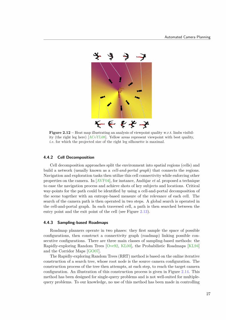
Automated Camera Planning
Figure 2.12 – Heat map illustrating an analysis of viewpoint quality w.r.t. limbs visibil-ity (the right leg here) [ACoYL08]. Yellow areas represent viewpoint with best quality,i.e. for which the projected size of the right leg silhouette is maximal.
4.4.2 Cell Decomposition
Cell decomposition approaches split the environment into spatial regions (cells) andbuild a network (usually known as a cell-and-portal graph) that connects the regions.Navigation and exploration tasks then utilize this cell connectivity while enforcing otherproperties on the camera. In [AVF04], for instance, Andùjar et al. proposed a techniqueto ease the navigation process and achieve shots of key subjects and locations. Criticalway-points for the path could be identified by using a cell-and-portal decomposition ofthe scene together with an entropy-based measure of the relevance of each cell. Thesearch of the camera path is then operated in two steps. A global search is operated inthe cell-and-portal graph. In each traversed cell, a path is then searched between theentry point and the exit point of the cell (see Figure 2.13).
4.4.3 Sampling-based Roadmaps
Roadmap planners operate in two phases: they first sample the space of possibleconfigurations, then construct a connectivity graph (roadmap) linking possible con-secutive configurations. There are three main classes of sampling-based methods: theRapidly-exploring Random Trees [Ove92, KL00], the Probabilistic Roadmaps [KL94]and the Corridor Maps [GO07].
The Rapidly-exploring Random Trees (RRT) method is based on the online iterativeconstruction of a search tree, whose root node is the source camera configuration. Theconstruction process of the tree then attempts, at each step, to reach the target cameraconfiguration. An illustration of this construction process is given in Figure 2.14. Thismethod has been designed for single-query problems and is not well-suited for multiple-query problems. To our knowledge, no use of this method has been made in controlling
27

State of the Art
Figure 2.13 – Cell decomposition and path planning. A cell-and-portal model parti-tions the search space and the relevance of each cell is evaluated with an entropy-basedmeasure. A path is built by ordering and connecting the most interesting cells [AVF04].
a virtual camera.
Figure 2.14 – The Rapidly-exploring Random Trees (RRT) [Ove92, KL00] are basedon the inline iterative construction of a search tree. Its root node is the source cameraconfiguration, and it tries, at each step, to reach the target configuration.
The Probabilistic Roadmap Method (PRM) is based on the offline construction ofa (static) roadmap, by randomly sampling the space of camera configurations. Sam-pled camera configurations that are selected (i.e. outside any obstacle) are denotedas nodes in the roadmap. The construction process then connects each pair of possi-ble consecutive configurations by a straight line segment (denoted as an edge in theroadmap). The criteria to create an edge in the roadmap is that the related segmentis free from collision with the geometry of the environment. A search of a path canfinally be operated, by adding the source and target configurations to the roadmap,then applying a search algorithm (an A* or IDA* for instance) to find an acceptablepath in the roadmap (see Figure 2.15a). Probabilistic roadmap approaches have beenused to compute collision-free paths to correct a user’s input, as described in [LT00].
The main issue of PRMs is their lack to produce natural-looking paths (i.e. enforcingcontinuity in the camera path). Indeed, the planned paths are broken lines. They areC0 continuous. Additional smoothing techniques are necessary on these paths. In
28

Automated Camera Planning
(a) (b)
Figure 2.15 – The Probabilistic Roadmap Method consists in building a connectivitygraph between randomly sampled configurations then building a path between an initialand a final configuration. (a) The computed path from a source to a target configuration(in red). (b) The planned path can be smoothed by using circular blends [NO04].
[LT00], Li and Ting used a global roadmap. During the interactive navigation process,a set of possible paths are then selected according to the current configuration and theuser’s input, from which the shortest and smoothest one is chosen. Nieuwenhuisen andOvermars [NO04] also proposed a technique to improve the computed path. They usedcircular blends between the edges that meet at a node, and replaced parts of the pathby a circle arc lying in the plane spanned by the two edges. By this process, the pathis made C1 continuous (see Figure 2.15b).
Another issue of PRMs is their lack of flexibility. The search is restricted to thesampled configurations and segments linking them only. They consequently can notaccount for dynamic obstacles. In their real-time camera planning system, Li andCheng [LC08] used a roadmap update strategy similar to the one called Lazy PRM,proposed in [BK00]. The validity of a node or a link is checked only when the node orthe link is under consideration during the search. They then used an “anytime” search(i.e. a search operated within a given time budget) to build camera paths.
To overcome these two lacks, Geraerts and Overmars [GO07] also proposed another approach: the Corridor Map Method (CMM). The CMM is based on a two phaseprocess. First, in an offline phase, a system of collision-free corridors is created for thestatic obstacles of the environment. Then, in a query phase, paths are planned insidethe corridors while avoiding dynamic obstacles. In [Ger09], Geraerts used the CMMto plan camera motions. Their technique tackles, in real-time, the trade-off betweengood motions (trajectories that are collision-free and keep the target in clear view),and frame coherence (i.e. the view changes smoothly such that the viewer does not getdisoriented).
In the last two sections, we have focused on automatically computing camera place-ments and sequences of camera placements to build shots. It is now necessary to take
29

State of the Art
Figure 2.16 – The Corridor Map Method (CMM) [GO07] is based on a system ofcollision-free corridors. Corridors are created for static obstacles. Paths are the plannedinside the corridors while avoiding dynamic obstacles.
a look at editing shots together, i.e. constructing proper sequences of shots, so as tosatisfy cinematographers’ communicative goals. In the next section, we will reviewtechniques proposed to automate the editing and storytelling process.
5 Automated Editing
The cinematic expertise w.r.t. editing is built upon a wide range of empiricalrules, which are used differently by cinematographers (e.g. timing, preferred shots,preferred camera movements). Researchers have investigated means to encode thisknowledge. We here review proposed editing approaches, ordered from purely proce-dural approaches to more expressive approaches.
He et al. [HCS96] proposed the first cinematography system, namely The VirtualCinematographer. The authors encoded cinematographic expertise (film idioms) assmall hierarchically-organized finite state machines (see Figure 2.17). Though theirsystem runs in real-time, it is fully procedural and thus lacks expressiveness. Indeed, novariation is possible in the directorial style. To each prototypical situation correspondsa single idiom (i.e. a single finite state machine) which is hard coded in the system.The execution of such state machines is obviously deterministic.
To overcome this lack of expressiveness, researchers proposed high-level declarativelanguages for encoding film idioms, and structured a film being generated as a film tree –a AND/OR graph (see Figure 2.18). Christianson et al. [CAH+96] proposed a languageto declare film idioms as procedural sequences of shots. Their system then operatesin two steps. It first expands the film tree until it has compiled detailed solutions foreach idiom. A heuristic evaluator then selects appropriate candidate frames for eachscene. Amerson et al. [AKY05] abstractly defined film idioms as weighted constraints,and in case of an over-constrained problem, used a procedural model for the relaxation
30

Automated Editing
(a) idiom choosing (b) idiom 2Talk
Figure 2.17 – Cinematic expertise (i.e. film idioms) is encoded as hierarchically orga-nized finite state machines [HCS96].
of constraints. Friedman and Feldman [FF04] split film idioms into shots (defaultviewpoints, list of viewpoints, preferred viewpoints) and cut rules (minimum change inangle, do not cross the line of interest). They then used a non-monotonic reasoningprocess to output the sequence of shots. A good property of their approach is that itenables emergent behaviors to appear, i.e. in case of conflicts between rules, shots canbe introduced without being explicitly specified.
Figure 2.18 – Film tree [CAH+96]. a movie is organized into a hierarchical structure.
Although such idiom-based systems enable expressing cinematic knowledge for sim-ple situations (e.g. discussions between 2 or 3 actors), they fail to be expressive enoughto take the users’ communicative goals into account, and necessitate the explicit defi-nition of idioms for each possible situation. To reach a higher level of expressiveness,it is necessary to provide editing rules that are more generic, and to propose models ofusers’ communicative goals.
The earlier attempt to account for user’s communicative goals is UCam [BL97].Users can describe their visualization preferences by using a Cinematographic Specifi-cation Language (CSL). UCam constructs a cinematographic user model consisting inprobabilistic micro-level camera planning directives (e.g. shot type, camera orientation,minimum shot durations). A camera planner then interprets this model to compute
31

State of the Art
executable directives for shot type, viewing angle, viewing elevation, transitions (cut,tracking, panning), shot duration, and panning/tracking speeds in real-time. Theirapproach works extremely well in real-time, but still lacks expressiveness. Indeed, theiruser model is restricted to eight possible directorial styles, as a combination of threefeatures: a viewpoint style (informational or dramatic), a camera pacing (slow or fast)and a transition style (gradual or jump).
More recently, significant advances have been made in improving the expressivenessof virtual cinematography systems. In their real-time navigation system, Li and Cheng[LC08] also integrated editing rules in their local PRM. They implemented two cut rules(LOI and minimum change in angle) in a simple way. The nodes of the local PRM aresplit into regions (see Figure 2.19). A cut is then possible between two regions lyingon the same side of the LOI, and which are not adjacent. Their technique is howeverlimited to tracking a single subject; the PRM being locally defined around a singlesubject. In what could be seen as an extension of [ACoYL08] to multiple characters[YLL12], Yeh et al. proposed to automatically extract social events from the jointanalysis of multiple character motions (e.g. related to trajectories and similarities indistance and direction of character motions). Events are then processed, analyzed forspatio-temporal correlation and ranked so as to generate a motion clip segmentation.The motion clip segmentation is used as a basis to express an optimization problem onthe camera parameters for each motion clip (actually long motion clips can be separatedinto segments solved individually). Following the lines of [ACoYL08], the optimizationprocess is guided by internal, external and continuity forces shaping a potential field.Continuity forces integrate the 180-degree rule as well as the jump-cut rule. Automatedediting of different viewpoints has further been addressed in an approach similar to[YLL12]. The objective is to properly convey motions of multiple humans in a real-time context [AWCO10] (while [YLL12] reported overall computation time between 1and 3 minutes). The authors consider a set of virtual cameras animated in real-timethat shoot multiple-character motions and offer means, not to control the cameras butto appropriately select viewpoints that maximize a measure of correlation between themotion of the characters in the scene, and the projected motion of the characters onthe screen. The hypothesis is that a strong correlation is a good indicator of viewpointquality. The approach uses a correlation analysis based on a optimized implementationof CCA (Canonical Correlation Analysis). The motion capture data is viewed as asequence of joint rotation vectors (the animation stream) and the projected data isa rendering of the 3D scene (the view stream). At each time step, the correlation iscomputed for a number of camera viewpoints and camera paths (the computation oftheir trajectories is either performed randomly or uses basic heuristics such as three-quarter views or over the shoulder cameras), and the best one is selected. In orderto perform cuts between viewpoint an interesting measurement of quality erosion isproposed. The measurement defines a maximum shot duration (3 seconds) coupledwith a quality erosion based on the evolution of the quality of the current view incomparison with the best view of the sequence. Furthermore, continuity in edits areguaranteed by filtering the viewpoints which do not respect the jump-cut rule or the 180degree rule, before correlations are computed. The necessity to compute and analyze theprojected view for each camera limits the number of cameras that are simultaneously
32

Automated Editing
considered. Their technique is further limited in the number of subjects consideredwhen performing cuts; the jump cut and 180 degree rules being only applicable toeither a single subject or a pair of subjects. Kardan and Casanova proposed a methodfor defining hierarchical lines of actions [KC08], and identified relevant first principlesof cinematography for using these lines of actions. Their approach is more flexibleand powerful than previous techniques because it naturally generalizes to any numberof subjects. They also provided an explicit enumeration of heuristics for continuityediting and stylistic rules resulting in various possible edits [KC09]. Their approach is,however, only suitable for static scenes.
Figure 2.19 – Intercut PRM [LC08]. The local PRM is augmented with editing infor-mation. Nodes are categorized into regions of space. Cut rules (180◦rule and minimumchange in angle) are then implemented by cuts between two regions on the same side ofthe line of interest and which are not adjacent.
Figure 2.20 – Hierarchical lines of action are built by grouping actors [KC08]. The lineof interest relative to a pair of subject is then the line of action built for their respectivegroups. This enables filming dialogues whith more than two or three subjects, whileenforcing space continuity.
To get closer to how real movies are built, the additional control of the staginghas also been explored. Elson and Riedl [ER07] proposed Cambot, a system to as-sist users in machinima production. They defined three different levels (or facets) ofcinematic knowledge (see Figure 2.21): the stage (area of space that is assumed to
33

State of the Art
be free of occlusion and obstruction), the blocking (geometric placement of subjectsw.r.t. the center point of a stage), and the shot (position, rotation, and focal length ofa virtual camera w.r.t. the center point of a stage). These modular and reusable facetsof cinematic knowledge enable the coordination between positions and movements ofthe camera and the actors. Cambot then relies on a dynamic programming algorithmto search for the best sequence of shots. Cambot also considers a few directorial styleparameters, such as pacing (slow or fast), viewpoint preferences and intensity.
(a) (b)
Figure 2.21 – Coordination of positions and movements of camera and actors [ER07].(a) relationships between the different facets of cinematic knowledge; blockings and shotsare defined w.r.t. to the center point of a stage; (b) a stage is associated with a blockingand shot.
As introduced in Section 1, every shot provides information (about narrative el-ements). Cuts may also provide information, i.e. links between narrative elements;these links can be intentional or unintentional. However presented approaches still lackconsidering the viewer’s comprehension of the complete sequence of shots and cuts.Jhala and Young [JY10] proposed Darshak, that uses cognitive models of narrativecomprehension to automatically construct cinematic discourse of a story in a 3D en-vironment. Dramatic situation patterns are realized through abstract communicativeoperators; these operators represent operations on a viewer’s beliefs about the storyand its telling. Darshak then relies on a hierarchical partial-order causal link (POCL)planning algorithm to generate story events and directives for filming them.
On one hand, recent approaches have enabled modeling, with some flexibility, bothclassical cinematic knowledge and aspects of directorial style, and to compute accept-able sequences of shots. On the other hand, two issues remain: (1) it is still difficult toexpress a specific style (or genre), and (2) there are so many possible combinations ofshots and transitions that it is difficult to properly evaluate them.
34

Visibility/Occlusion Handling
6 Visibility/Occlusion HandlingVisibility is a transverse issue in controlling a virtual camera. Visibility computa-
tion received much attention in computer graphics; for a complete survey on visibility,see [COCS+03]. Paradoxically, it has been under-addressed in the virtual camera con-trol domain. In most existing approaches (e.g. virtual exploration, computer games orvirtual storytelling), the visibility of subjects is computed by using raycast-based tech-niques on an abstraction of subjects (commonly bounding boxes). There are howeverbetter ways of tackling visibility issues related to virtual camera control. We here firstreview the main visibility concerns when controlling a virtual camera, then review themost significant visibility computation techniques proposed to tackle these issues.
In a camera control context, we identified four issues in handling visibility:
Static vs. Dynamic One question is whether the scene is purely static, or containsdynamic elements (occluders/occludees). For the static part of the environment,the visibility information can be pre-computed. For the dynamic part, the visibil-ity information must be computed on-the-fly, with real-time constraints imposedby interactive applications.
Accurate vs. Approximate vs. Inaccurate The visibility computation techniquescan be categorized into three main classes, w.r.t. the level of accuracy of theresult: the techniques providing an accurate visibility information (i.e. a precisedegree of visibility, as a real value between 0 and 1), the techniques providing anapproximate visibility information (as an approximate degree of visibility, suchas visible/partially visible/occluded), and the techniques providing an inaccuratevisibility information (as a boolean result such as visible/occluded).
Adapted to path planning vs. Adapted to viewpoint planning The potentialof a camera control approach is often dependent on the capabilities of the visi-bility computation technique it uses. In order to compute unoccluded viewpoints(e.g. for checking the visibility/occlusion from the current camera viewpoint, orfor planning a cut to a new camera viewpoint), the visibility process must com-pute the visibility/occlusion of key subjects from discrete points of space. Inthe same way, to plan a path between two given camera viewpoints, the visibil-ity process must compute the visibility/occlusion of key subjects along possiblesequences of intermediate camera viewpoints.
Anticipation In a range of applications (e.g. reactive approaches), the visibility pro-cess must be capable of anticipating future occlusions of key subjects. In otherwords, it must provide a good prediction of their visibility over time. This maythen serve for instance to predict a change in the camera position in reaction topast and/or current changes in the scene.
We will now focus on relevant contributions on visibility handling for camera control.Halper et al. [HHS01] proposed handling occlusion avoidance by using Potential
Visibility Regions (PVR). They imposed constraints on the camera movements as aset of geometric constraints using polygons (spheres). Polygons are shaded w.r.t. their
35

State of the Art
preference (a brighter color meaning a higher preference). To find the best positionthat satisfies visibility requirements, a visibility map is created. This visibility maponly considers the depth information from potential occluders. The potential visibilitygeometry is then rendered to the buffer from most desirable to least desirable regions.The result is an image buffer, whereby the brightest colors that first pass the depthtest are visible. The brightest color in the image buffer, therefore, denotes the mostdesirable position for the camera to move to (see Figure 2.22). They also tackled theproblem of occlusion anticipation. Their method uses approximative calculations forfuture scene and object state based on past trajectory and acceleration information,and solve the camera for that predicted state. The current camera path is adaptedso that the camera will be at this predicted position at the predicted time t. Anestimated camera position is finally computed for the next frame along this path (seeFigure 2.23). Halper et al. ’s approach is however only suited for planning camera pathslocally (i.e. step by step). If no solution exists in the rendering, their method will failfinding an unoccluded position (even if one exists), and planning a global camera pathto this unoccluded position.
To enable computing collision-free and occlusion-free camera paths in arbitrary envi-ronments, Oskam et al. [OSTG09] proposed to augment a roadmap graph with visibilityinformation, what they call a visibility-aware roadmap structure. Their method relieson the precomputation of a coarse representation of the scene (with a grid of bound-ing spheres), the creation of a roadmap by connecting overlapping spheres (throughcircular portals), and an estimate of pair-wise visibility between all spheres by usinga Monte-Carlo ray tracing algorithm (see Figure 2.24). Their system executes a pathplanning algorithm using the precomputed roadmap values to find a coarse path. Thispath is then refined using a sequence of occlusion maps computed on-the-fly. Theirglobal planning strategy on the visibility-aware roadmap enables both large-scale cam-era transitions and a local third-person camera module following a player and avoidingobstructed viewpoints. The data structure itself adapts at run-time to dynamic occlud-ers of the environment. Dynamic occluders are handled by performing an on-the-flyupdate of the roadmap information. Moving objects are approximated by one or morebounding spheres. When searching a path in the roadmap, all the connections betweentwo circular portals that touch the bounding spheres are marked as being occupied.This prevents the camera from colliding with the moving object. To anticipate futureocclusions of the player, they also proposed a risk prediction method. They extendedan algorithm inspired by the work of Bandyopadhyay et al. [BLAH06]. Their predic-tion algorithm uses the visibility-aware roadmap to find a path to the sphere closestto the player and which is not visible from the camera’s current position. This pathrepresents the highest risk of escape. The camera’s current position is then rotated toa new vantage so that this escape route is in view. An illustration of their method isgiven in Figure 2.25. Their technique is however limited to single-point focus targets.
Christie et al. [CON08b] presented an approach to the real-time evaluation of thevisibility of multiple target objects. The visibility of both targets is simultaneouslycomputed for a large sample of points. This involves to perform a low resolutionprojection from points on pairs of target objects onto a plane parallel to the pair andbehind the camera (see Figure 2.26). The combination of the depth buffers for these
36

Visibility/Occlusion Handling
(a)
(b)
Figure 2.22 – Potential Visibility Regions [HHS01]. (a) sample use of rendering camerasolution regions; selection is based first on highest color, then on closest angle. (b) Thecamera solution region is warped according to motion characteristics of the camera. Inthis case, selected regions are favored in the direction of motion, and the algorithmreturns the point to the right even though its angle of change is greater than that of thepoint to the left.
two projections then enables creating visibility volumes around the camera, with thejoint visibility information on the pair of objects. They also provided an extension ofthis pair-wise computation for three or more target objects. To mitigate over-reactivecamera behavior, visibility results are aggregated in a temporal window. They moreoveraddressed the problem of idealization of the target objects geometry. To this end, theyused a stochastic approximation of the physical extent of target objects by selectingprojection points randomly from the visible surface of the target object. A differentprojection point is used at each frame, so the aggregation of visibility information alongthe time provide a good approximation of the degree of visibility of the target object.
37

State of the Art
Figure 2.23 – Altering the camera path to adapt to a predicted occlusion [HHS01].
Figure 2.24 – Sphere-to-sphere visibility [OSTG09]. Based on an initial geometry ofthe environment, a spatial discretization is computed. A roadmap is then built from theoverlap regions. Finally, for each pair of spheres, a visibility probability is computedwith a Monte-Carlo raytracing algorithm.
7 Conclusion
From the literature study, we detailed a number of methods dedicated to controllinga virtual camera in 3D environments. We highlighted that the research community ismoving towards models of cinematic knowledge that are more and more expressive.There are however some important issues to tackle.
38

Conclusion
Figure 2.25 – Proactive camera movement [OSTG09]: the algorithm finds the closestsphere (indicated in orange) that has reduced visibility from the original camera position.After detecting a high escape risk, the camera’s viewing direction is aligned toward thissphere. Spheres with reduced visibility from the original camera position are shown indarker shades of gray.
Figure 2.26 – Computation of the visibility inside a camera volume by using the depthbuffer [CON08a]. The scene is rendered from each target back towards the actual positionof the camera. The visibility information for all target objects is then composed as avisibility volume.
In this thesis, we identified three research axes:1. Existing automated approaches generally focus on one or two cinematic aspects
only: visual composition, tracking of targets (camera planning), cinematography(editing, with no account for the visibility of subjects). These techniques also lackexpressiveness, i.e. they provide limited account of styles or genres. Furthermore,the handling of visibility appears as an essential aspect in controlling a camera,but has been under addressed in the field. In Chapter 3, we propose the first fullyintegrated cinematic engine, which handles both viewpoint computation, planningand editing, while accounting for visibility and proposing means to control someelements of style.
2. On one hand, fully automated cinematography approaches pose the problem oftuning a large set of high-level parameters to account for each single aspect (visual
39

State of the Art
properties, properties on the camera path, editing properties, visibility proper-ties). Furthermore, not all elements of directorial style can be modeled. Thoughautomated approaches provide good results, the result intended by a user is gen-erally more subtle and cannot be easily expressed. Indeed, one may use metricsto approximate a given directorial style (e.g. statistics of shot preferences, or shotduration), but we will never be capable of reproducing exactly the creative processof a given editor (e.g. build a “Spielberg-like” movie). This therefore raises thenecessity to let the user interact in the editing process. On the other hand, someinteractive control techniques enable finely controlling cinematic aspects (visualcomposition and camera motions) within a single shot, but lack the handling ofthe aspects related to editing. In Chapter 4, we propose a hybrid approach thatbuild upon an evaluation of the different cinematic aspects, and combines an au-tomated control of modeled cinematic aspects with direct interaction of an editorin the editing process.
3. The central element in controlling a camera is the visual composition. A largerange of computer graphics applications rely on the computation of viewpointsover 3D scenes that need to display a number of characteristic composition proper-ties. Such problems are generally casted as non-linear optimization problems in a7 degree-of-freedom search space. Given the size of the search space and the com-putational cost in the evaluation of composition properties (typically the visibilityof subjects), this optimization process is a time-consuming task and hampers theuse of evolved composition techniques in most applications. In Chapter 5, we in-troduce the Toric Space, a novel and efficient approach to virtual camera control.Based on a simple parametric model of the space of camera configurations, theToric Space has the intrinsic advantage to reduce the search space, and most ofclassical visual properties can be easily expressed and combined in this space.
40

3A Cinematic Engine for Interactive3D Environments
Related publications: This chapter presents a unifying approach to a fully auto-mated cinematic engine. As described in the state of the art, current contributionsin the field generally focus on individual aspects of cinematography: (i) on-screencomposition [BMBT00], (2) visibility and path-planning [OSTG09] or (iii) editing[CAH+96, ER07, AWCO10]. They moreover suffer from a limited integration of di-rectorial style and visibility enforcement. In this chapter, we propose CineSys, a fullyautomated cinematic engine for interactive environments accounting for both viewpointcomputation, viewpoint planning and editing.
The provision of a fully automated camera control system is complex as it raisesfour important challenges:
First, such a system needs to be underpinned by a narrative model that bothstructures the way the actions are organized, and allows to reason on their rela-tive importance and presentation. Following Chatman’s bipartite model [Cha80],interactive narratives have two levels: (1) the story, i.e. the chronologic account ofevents over time; and (2) the discourse, i.e. the way in which events are organizedand presented to the spectator.Second, the system should provide the user with well-composed viewpoints ofkey subjects in the scene following established conventions in the literature, whilemaintaining the visibility of these subjects in fully interactive 3D environments.For example, the simultaneous computation of the visibility of multiple subjects ina dynamic environment requires both an efficient solution and a good estimationof the visibility for a large range of viewpoints.Third, the system must address the innate complexity of planning path betweenviewpoints. For example, selecting appropriate tracking shots (sequences of view-points to follows an event) involves planning a camera’s motion in a dynamicenvironment whilst simultaneously taking account of the visibility of scene ele-ments from viewpoints along the spatio-temporal path.Last, a critical issue is related to the challenge of operationalizing editing rules andconventions in a sufficiently expressive model of automated editing. Such rules areoften expressed as a set of idioms (i.e. a typical set of camera configurations that,when assembled, bring to the screen the viewer’s understanding of the spatial andcausal relations pertained to a specific action). While current implementationsstrongly rely on these pragmatic representations to model camera editing systems,there is a clear necessity and demand to perform a shift toward more expressive
41

A Cinematic Engine for Interactive 3D Environments
representations that augment the range of possible variations in the montage. Tothis end, another essential task consists in identifying some of the parametersand devices (i.e. indicators) that underpin directorial style, such as pacing, dy-namicity, preferred views and enforcement of specific cinematic conventions. Asa consequence, the challenge consists in the design of a model expressive enoughto control such indicators and to yield a range of variations in results.
1 Contributions
We propose a fully automated system that allows the construction of a movie froma specified sequence of low-level narrative events (e.g. subjects’ actions and motions, orestablishing subjects in the scene). In essence, our approach contributes to the domainon the following points:
Real-time integrated system Our model proposes an integrated approach thatcharacterizes full and partial visibility of key subjects, performs camera planningbetween viewpoints, and enforces continuity editing rules in real-time.
Expressiveness Our cinematic engine introduces the notion of Director Volumes asa spatial characterization of viewpoint regions around key subjects. DirectorVolumes encode the empirical knowledge from practice and literature on camerastaging (e.g. Internal, External, Parallel) as well as classical shot sizes (e.g. close,medium, long). Additionally, knowledge related to continuity editing and styleis encoded by filtering operators over the Director volumes (line-of-interest, line-of-action, thirty-degree angle, preferred viewpoints). At last, our engine enforceson-the-screen composition that selects the best camera configuration from theresulting volumes using a local search optimization technique and following well-known composition rules.
Variation in directorial style CineSys moreover provides means to express notablevariations in directorial style in a real-time context by controlling indicators suchas pacing, camera dynamicity and composition. High-level narrative dimensionssuch as isolation, dominance and affinity between key subjects can furthermorebe enforced.
This chapter is organized as follows. First, we present an overview of our approach(Section 2), before detailing the construction of Director Volumes (Section 3) and themechanics of the reasoning process for editing (Section 4). Second, we present resultson a 3D replica of the canteen scene in Michael Radford’s 1984 movie (Section 7),in which we demonstrate variations in the application of directorial styles (pacing,dynamicity), together with variations in the visibility degree of subjects and in thenarrative dimensions. Finally, we compare our model to the state of the art in virtualcinematography on a set of important features.
42

Overview
2 OverviewOur cinematic engine takes as input a flow of narrative events (which are not known
beforehand). Our system computes appropriate viewpoints on these narrative events.A camera viewpoint is a camera placement defined at a symbolic level w.r.t. to a con-figuration of subjects, as the combination of a shot size (e.g. medium close-up, long)and a view angle (e.g. internal, external, parallel). Viewpoints are computed by select-ing specific regions referred to as Director Volumes that capture information both onvisibility and on stereotypical viewpoints. We then rely on filtering-based techniques toreason over Director Volumes and from a large set of possible camera configurations toselect the appropriate candidate camera configuration (a camera configuration is a cam-era placement defined at a numerical level). In this filtering process, cinematographicrules are expressed as constraints (applied on with constraint-based filtering processes)and cinematographic style is expressed as preferences to choose where to position thecamera, how to plan paths between viewpoints, and when to perform cuts. The outputof our system is a movie which conveys these narrative events according to some cine-matic rules and directorial style parameters. A movie is defined as a sequence of shotsseparated by cuts, where shots are continuous sequences of camera configurations. Wefurthermore propose the notion of an action shot as a continuous sequence of cameraconfigurations that conveys a given narrative event. A shot is then described as a se-quence of (one or more) action shots separated by continuous transitions (i.e. cameramotions).
At runtime, our system first selects the most relevant event (or set of events) andchooses the best viewpoint to convey this event by filtering the Director Volumes accord-ing to (i) the visibility of key-subjects, (i) the coherency in the sequence of viewpoints,(iii) and a characterization of style. A transition planner then determines appropriateviewpoint transitions, either by using a cut or a path-planning process between view-points. specifically, our system follows a five-step process to compute viewpoints andtransitions (see Figure 3.1):
1. Selecting narrative events. Whenever a new transition is enabled, the systemselects at run-time an event among all those occurring during the same timestep. We here consider that relevance of an event is computed by an externalprocess (e.g. a narrative engine) that distinguishes the relative importance ofevents running in parallel. This step selects the most relevant event; and in caseof failure in the following steps, re-iterate by selecting another event, consideredby decreasing order of relevance.
2. Computing Director Volumes. This stage turns a selected event into areaswhich can potentially portray the event (we refer to them as Director Volumes),by composing areas of characteristic viewpoints with an analysis of the full andpartial visibility of key subjects involved in the event.
3. Reasoning over Director Volumes. The selection of appropriate Director Vol-umes among all available is performed by applying two filtering processes, thena selection operator. Continuity filters typically enforce classical continuity rules
43

A Cinematic Engine for Interactive 3D Environments
between shots when performing a cut. They prune inconsistent regions in theset of Director Volumes (for example those that would make the camera cross aline-of-action). Style Filters then annotate Director Volumes w.r.t. elements ofdirectorial style (e.g. preferred viewpoints, enforcement of a narrative dimension).A Selection Operator finally selects one (or a set of) Director Volume(s) from allavailable, by using a ranking over remaining volumes.
4. Computing frame composition. A numerical optimization process is performedin each selected Director Volume to compute the best camera configuration interms of on-screen composition (exact locations of key subjects on the screen).
5. Computing transitions. Whenever it appears necessary to switch between Di-rector Volumes (e.g. end of event, new event, subject(s) occluded, pace in transi-tions), the system selects an appropriate transition (either a cut or a continuouscamera motion). For camera motions, we first build a roadmap over the DirectorVolumes. We then rely on an incremental Dijkstra search process to plan anappropriate path between the current camera configuration and a set of targetDirector Volumes (that may evolve as the scene evolves). When the camera entersa target Director Volume, we compute an appropriate camera configuration insidethe volume, as described above, and moves the camera toward this configuration.
In the sequel we detail the major steps of our computational process, namely com-puting Director Volumes, reasoning over Director Volumes and performing transitions.
3 Computing Director Volumes
At the core of our approach stands a spatial representation: the Director Volumes.A Director Volume aggregates camera configurations that give rise to a “cinemato-graphically” equivalent viewpoint in terms of information conveyed to the user (i.e. itssemantic w.r.t. a narrative event to convey), and in terms of visibility of key subjects.The Director Volumes are computed through a three-step process:
A first characterization process captures the semantic of viewpoints through aspatial representation of regions around key subjects. These regions representstereotypical viewpoints, and we refer to them as Semantic Volumes [CN05].A second characterization process captures visibility information on key subjectsthrough a spatial representation of regions of full visibility, partial visibility andfull occlusion of each key subject. We refer to these regions as Visibility Volumes.An intersection operator then augments the Semantic Volumes with visibilityinformation. This intersection operator takes as input the previously computedspatial representations and outputs a new spatial representation of regions (theDirector Volumes) that can potentially portray the narrative event.
To implement these spatial representations of regions (or volumes), we rely onBSP data-structures. We use annotated Binary Space Partitions (a-BSPs), which areclassical BSPs augmented with information on the nodes and leaves. These structuresare dynamically and procedurally processed w.r.t. the configuration of key subjects, foreach frame, and allows to efficiently characterize and partition the environment into
44

Computing Director Volumes
Figure 3.1 – Overview of our real-time cinematic engine CineSys. First, a relevantnarrative event is selected from a flow of unfolding events. This narrative event isthen turned into Director Volumes (all regions of space from which the narrative eventcan be portrayed). Editing is performed by reasoning over Director Volumes to selectone or more target volume(s), given continuity rules, and style rules. A target cameraconfiguration is then computed by using a local optimization process inside selectedvolumes, given composition rules. Finally a transition between the previous and newcamera configuration is computed (as a cut or as a continuous transition).
such sets of viewpoints (see Figure 3.2). Each node is represented by an intermediate(convex) cell and a stabbing line. Nodes are further annotated with information onsub-cells’ connectivity, which is updated as new intermediate cells are drawn. Each leafthen corresponds to a categorized cell (or volume), annotated with relevant information(e.g. viewpoint semantic, subjects’ visibility). The intersection operator then operateby merging the a-BSP structures associated with both Semantic Volumes and VisibilityVolumes, to create a new a-BSP structure corresponding to Director Volumes.
45

A Cinematic Engine for Interactive 3D Environments
This a-BSP representation enables (i) an on-the-fly cell subdivision process, throughthe use of a description of intermediate cells in each node; and (ii) a reduction of thesearch complexity when characterizing a given camera configuration in the environment(binary tree search of complexity O(logn), for a BSP with n leaves).
(a) Cell splitting
(b) a-BSP data structure over the cell
Figure 3.2 – Construction of an annotated Binary Space Partition (a-BSP) data struc-ture. The a-BSP is procedurally processed through a top-down injection of stabbinglines. Each node (dotted box) is represented by an intermediate convex cell (in black)and a stabbing line. Nodes are also annotated with information on sub-cells’ connectiv-ity (colored segments separating two sub-cells), which is updated as new intermediatecells are drawn. Each leaf (at the bottom) corresponds to a categorized cell (or volume),annotated with relevant information (e.g. viewpoint semantic, subjects’ visibility).
3.1 Semantic VolumesThe first step consists in translating the selected narrative event into Semantic
Volumes. Semantic Volumes are a formalization of the cinematic knowledge in terms ofcamera staging. In our approach, each narrative event is associated with a collection ofstereotypical viewpoints that convey the event according to established cinematographicconventions. A narrative event is modeled by a semantic tag (the performed action,e.g. “A speaks to B”, where participating subjects are abstracted), a start and end time,
46

Computing Director Volumes
(a)
(b)
Figure 3.3 – Design of Semantic Volumes (a) for a single subject action, and (b) for aclassical interaction between two key subjects (adapted from [Ari76]). Each blue circlerepresents a key subject.
as well as the participating subjects (abstracted as “A”, “B”, “C”, etc. in the semantictag). Typically an event such as “Symes speaks to Smith” can be portrayed througha large collection of viewpoints described in the literature (Internal, External, Apex,Subjective) together with a range of distances (Close-Up, Medium Shot, Long Shot,Extreme Long Shot) [Ari76]. Do note that for such an event, the utterance of a keysubject may be portrayed either by framing the talking key subject, the listening keysubject, or both (the choice is a matter of continuity and directorial style). By defaulteach narrative event is portrayed by all possible viewpoints, though some events mayrequire a specific subset of viewpoints (e.g. “Symes looks at Smith” obviously requiresthat the camera should not be located behind Syme).
In the task of precisely designing the Semantic volumes that encodes cinemato-graphic knowledge, we followed an experimental process that consists in positioning
47

A Cinematic Engine for Interactive 3D Environments
and evaluating camera configurations in a 3D modeler for key configurations of sub-jects (single subject, two subjects facing, two subjects not facing). This process wasguided by empirical evidence in literature and a professional experienced modeler (GuySchofield, Newcastle University). As a result we characterized the spatial extents ofviewpoint regions for key configurations of subjects. Resulting Semantic Volumes aredisplayed in Figure 3.3. Additionally, we studied the evolution of these Semantic Vol-umes w.r.t. the distance between the key subjects and the orientations of the keysubjects. In cases where the subjects are too close to each other, areas of SubjectiveShots are removed. In a similar way, as the distance between key subjects increases,the range of typical shot sizes is extended for Internal Shots (Close-Up, Close Shot,Medium Shot, Long Shot).
To represent Semantic Volumes, we rely on a single a-BSP data-structure. Thisstructure is dynamically and procedurally processed w.r.t. the configuration of the keysubjects (e.g. single subject, two subjects). First, the root cell of this a-BSP is set to abounding cell of all Semantic Volumes. Second, the regions of space corresponding tothe different shot sizes and view angles are modeled with bounding cells, and stereotyp-ical viewpoints (Semantic Volumes) are described with set operations on these regions(e.g. union, intersection, difference). Third, edges of these bounding cells are succes-sively injected into the a-BSP structure. Last, final leaves are categorized w.r.t. theirinclusion in the Semantic Volumes as described above.
Some sub-regions of space cannot however be selected as candidates since key sub-jects are fully or partially occluded. To efficiently compute the visibility informationthat we then store in the regions, a topological level of representation of the geometryis employed.
3.2 Visibility Volumes
The second step consists in computing and characterizing the visibility of key sub-jects. Real-time visibility computation is a prohibitively expensive process. We addressthis constraint by reducing the practical complexity through two assumptions on thegeometric properties of the environment. Firstly, we estimate the visibility of a keysubject (here, a character) by using a 2D convex hull of the projection of its geome-try onto the floor. Secondly, we restrict the setting to static 3D indoor environmentswhich we represent as a 2D cell-and-portal (C&P) structure [TS91]. Cells representrooms and portals represent doorways and connections between cells. Further, hardvisibility constraints are related to the portal extremities (e.g. walls or doorways); eachboundary between a wall and a doorway supports a stabbing line representing a sep-aration between visibility and occlusion. By assuming that the indoor environmentresides on plane (i.e. distinct floors) we extract a 2.5D topological C&P representation.All geometric elements in the scene above a specified height (here 1.5m) are treatedas occluders. The visibility process is therefore restricted to dynamic targets in staticenvironments.
To characterize partial visibility, we extend classical cell-and-portal visibility prop-agation techniques [TS91] to handle from-region visibility where subjects are approxi-
48

Computing Director Volumes
(a) (b)
Figure 3.4 – From a portal vertex p, two stabbing lines are defined w.r.t. a key subject(blue circle). (a) By combining both stabbing lines, a categorization into three regions(full occlusion, partial visibility and full visibility) is obtained. 2D visibility of a keysubject corresponds to a segment s (visibility segment) linking its extreme points. (b)From a viewpoint with partial visibility, we approximate the visibility degree of the keysubject by first computing the length of the non-occluded portion of segment s, thencalculating the relative proportion which remains visible.
mated as convex cells [COCS+03]. We base our visibility analysis on the use of stabbinglines to compute a dynamic categorization of the full and partial visibility of a key sub-ject. First, we identify the current topological cell in which the key subject is located,and list all adjacent topological cells (i.e. which can be reached through a single por-tal). Second, for a portal vertex p, two stabbing lines are defined such that each line istangential to, but on opposite sides of, the convex hull of the key subject (Figure 3.4).Each stabbing line therefore defines a point of contact (or extreme point) e on theconvex hull of the key subject. The stabbing line tangential to such a point e separatestwo regions: the region from where e is visible, and the region from where e is occluded.As the key subject is fully included between stabbing lines, the visibility categorizationof the whole key subject is then performed by combining the visibility categorizationof each stabbing line. This categorization follows a two-step process:
1. A visibility prism (or v-prism) is defined as the triangle between the portal vertexp and the two extreme points of the key subject. The segment s joining bothextreme points is then viewed as the abstraction of the 2D visible aspect of thekey subject at point p.
2. A reversed prism (or r-prism) is computed as the point reflection of the v-prism
49

A Cinematic Engine for Interactive 3D Environments
w.r.t. point p. This r-prism defines the partial visibility region generated by thevertex p. Three regions are then defined: a region from where the key subject isfully occluded, a region from where the key subject is fully visible, and an inter-mediate region from where the key subject is partially visible (r-prism). Further,for any camera viewpoint v inside the r-prism, we estimate the visibility degreeof the key subject as follows. We first create a frustum F , defined as a trianglebetween v and s, which is used to detect the occluding scene elements. We thencombine all portions segment s that are occluded by at least one scene element.We finally calculate the visible degree as the remaining proportion of s whichremains visible.
This process is further repeated for all portals connected to the current topolog-ical cell in which the key subject is located (see Figure 3.5). Areas of full visibility,partial visibility and full occlusion are then propagated through the cell-and-portalrepresentation in a way similar to [TS91].
An a-BSP representation is used for each topological cell to represent the regionsof full visibility, partial visibility, and full occlusion (i.e. the Visibility Volumes) in thiscell. The root cell of such an a-BSP is first set to the associated topological cell itself.The r-prisms are then propagated (and eventually reduced) incrementally to adjacenttopological cells through portals (see Figure 3.5). The propagation of r-prisms in atopological cell is processed by using a three-step process. First, we inject stabbinglines associated with each r-prism into the a-BSP of the topological cell. Second, wecategorize the leaves of the a-BSP included in at least one r-prism as “partially visible”.Last, to categorize remaining leaves as either “fully visible” or “fully occluded”, we relyon the information held by stabbing lines (i.e. w.r.t. visibility/occlusion of associatedextreme points of the convex hull of the key subject).
3.3 Director VolumesIn the previous sections, we have computed volumes corresponding to semantic
information on stereotypical viewpoints around key subjects, and volumes correspond-ing to visibility information on key subjects. The last step consists in combining thisinformation to characterize sets of “cinematographically” equivalent viewpoints (theDirector Volumes) in terms of both semantic and visibility of key subjects. The inter-section operator uses the compatibility between both BSP structures to fusion them,and create an a-BSP representation of Director Volumes per topological cell. Thisintersection operator can be formalized as follows.
First, we refer to the a-BSP characterizing Semantic Volumes around key subjectsas S.Second, we refer to the a-BSP characterizing visibility of key subject k in topo-logical cell j as Vjk.Last, we refer to the a-BSP characterizing Director Volumes around key subjectsin topological cell j as Dj , procedurally computed as
Dj =(⋂
k
Vjk
)∩ S
50

Reasoning over Director Volumes
(a) (b)
(c) (d)
Figure 3.5 – Visibility propagation using the cell-and-portal representation. Eachvisibility prism issued from a vertex of a portal is propagated through the portals of theadjacent cells. The process is repeated inside each cell until all cells are explored.
The successive steps of this intersection process are illustrated in Figures 3.6 and 3.7.We finally categorize all leaves of Dj by collecting (i) the visibility information asso-ciated with each subject k by using a binary tree search in Vjk and (ii) the semanticinformation on stereotypical viewpoints by using a binary tree search in S.
This process provides a good basis to reason on camera Director Volumes to eitherperform a cut, move in the environment, or maintain the camera position. In thefollowing we will present our editing method, providing the camera paths and cutsgiven as input to the dynamic resolution of non-occluded camera positions.
4 Reasoning over Director Volumes
Once the space of viewpoints has been characterized in terms of Director Volumes,the next step consists in selecting the best candidate volume(s) following continuityrules and directorial style.
To enforce elements of continuity and style in an expressive way, we propose tomodel rules as a two step generic process that operates over a set of Director Volumes.Our editing model considers a set of Director Volumes as input. We then sequen-tially apply a filtering operator over Director Volumes, then a selection operator overremaining volumes. The filtering operator is responsible for (i) pruning inappropri-ate viewpoints in Director Volumes and (ii) annotating remaining Director Volumeswith information that will be used by the selection operator. The selection operator isthen responsible for evaluating and ranking remaining Director Volumes (through a fit-
51

A Cinematic Engine for Interactive 3D Environments
Figure 3.6 – Combination of visibility information for a two-subject configuration (sub-jects are displays with a yellow area). The left-most image displays the Visibility Volumesof the left-most subject. The right-most image displays the combination of both visibil-ity information. This combination consists in building a new set of Visibility Volumes,informed with both visibility information, and is operated through an intersection ofvisibility a-BSPs of both subjects. In this image, black areas represents regions whereboth subjects are fully occluded while white areas represent regions where both subjectsare fully visible.
Figure 3.7 – Computation of Director Volumes for a two-subject configuration. From atopological analysis of the scene (top-left image), we compute two a-BSP representationsaround subjects: a representation of full/partial visibility regions (top-right image, seeFigure 3.6), and a representation of semantic regions (bottom-left image, see Figure 3.3).We then combine both representations to build Director Volumes around subjects, bysimply intersecting the visibility a-BSP with the semantic a-BSP.
52

Reasoning over Director Volumes
ness function accounting for annotations), and returning a sub-set of Director Volumes(which maximize the fitness value). The process is detailed in Figure 3.8.
4.1 Filtering operatorThe first reasoning step consists in applying the filtering operator, which is built as
a sequential application of filters over Director Volumes. A filter is defined in a genericmanner, as an operator that takes as input a set of (annotated) Director Volumes, andreturns a – possibly empty – new set of (annotated) Director Volumes. Each filterimplements either a continuity rule or a style rule. Filters can therefore be definedrecursively, i.e. a filter can be constructed as a sequential or parallel application ofsub-filters.
Filters can be categorized into three classes in accordance to their reasoning levelover Director Volumes: the geometric filters, the semantic filters and the annotationfilters.Geometric filters reason on the geometry of Director Volumes. They can split Direc-
tor Volumes to prune inappropriate geometric areas from these Director Volumes(e.g. remove all viewpoints that subtend an angle lower than 30 degrees to a givensubject from Director Volumes).
Semantic filters reason on the semantic aspects of Director Volumes. They eitheraccept or prune entire Director Volumes according to constraints established ata semantic level (e.g. remove all Director Volumes which are Close Shots).
Annotation filters can reason on the specific properties of each Director Volume.They can add, remove or edit the annotations associated with each DirectorVolume. A typical example is the fitness property. Each Director Volume has afitness (e.g. representing a degree of preference of this Director Volume) and rulescan add values (annotations) to the fitness property.
Our filtering operator is defined as the combination of two filtering processes. First,continuity editing filters remove inappropriate viewpoints in Director Volumes that donot match editing continuity rules (e.g. crossing the line-of-interest or crossing the line-of-action). Second, directorial style filters prune inappropriate viewpoints w.r.t. thecurrent directorial style, then annotate Director Volumes according to style preferences.Style preferences model for example the preferred set of viewpoints from which to shoota narrative event or a scene.
In this approach, we pose as the hypothesis that continuity in editing prevails overstyle. Indeed, we believe that violation in continuity is far more noticeable for theviewer than violation in style. For this purpose, as filters are applied in sequence, wefirst process the Director Volumes with continuity filters before style filters.
4.2 Continuity editing filtersContinuity ensures compliance with cinematographic conventions and enforces the
maintenance of the spatio-temporal context when the camera switches between twoviewpoints. Conventions are well established in relation to the key subjects’ motions,
53

A Cinematic Engine for Interactive 3D Environments
Figure 3.8 – Reasoning over Director Volumes. The selection of a sub-set of DirectorVolume is a two-step process. First, we apply a filtering operator on the set of DirectorVolumes. At this step, we sequentially apply (1) continuity editing filters, and (2) direc-torial style filters. We then apply a selection operator on remaining Director Volumes,to evaluate (w.r.t. a fitness function), rank, then select the sub-set of Director Volumeswith best fitness value(s).
spatial locations, line-of-interest and actions. We describe some continuity rules andthe way to model them as filters in our editing model:
Line-of-action continuity. Between two shots that portray the same key subject,coherency must be maintained in the apparent direction of motion of this keysubject. A line-of-action (LOA) is modeled as a geometric filter. All the view-points located on the opposite side w.r.t. the direction of motion of the subjectare removed from Director Volumes. For this purpose, we inject the line of actionof the subject into the a-BSP representation (i.e. along the direction of motionof the subject) and we compute the intersection of the resulting half plane withthe current set of Director Volumes.
54

Reasoning over Director Volumes
Line-of-interest continuity. In narrative events that involve two or more key sub-jects, once the side of the line-of-interest (LOI) has been chosen, it should notbe crossed, unless using an Extreme Long Shot (that re-establishes the key sub-jects in relation to the environment) or a continuous transition. The relative sidew.r.t. the LOI is directly encoded in the Semantic Volumes structure, which isrecomputed at each frame. The line-of-intersect is modeled as a semantic filter;all Director Volumes on the opposite side of the LOI, but Extreme Long Shots,are then discarded.
Matching between lines of interest. This LOI is, for a character, represented byhis gaze direction. If a key subject (character) watches an item which does notappear in the frame, the corresponding viewpoints should convey the fact that hiseyes are directed toward the place where user thinks the item is. Therefore, allthe Director Volumes for which the direction of the characters gaze is not visibleneed to be removed. This is implemented by a geometric filter; in the a-BSP, weinsert a new couple of half-lines representing a 60◦ wedge around the character’sgaze. All viewpoints out of the wedge are then discarded.
Change in angle or size. Between two shots that portray the same key subject,there should be at least a thirty-degree difference in orientation, or a notabledifference in size of portrayed subjects. This rule is implemented by applyingto sub-filters in parallel. First, a geometric filter that, in each Director Volume,removes all viewpoints that subtend an angle lower than 30◦ to the subject; tothis end, we inject two new half-lines in the a-BSP. Second, a semantic filterthat prunes Director Volumes which are less than two units different in size (ina graduation that ranges in Close-Up, Close Shot, Medium Shot, Long Shot andExtreme Long Shot). Last, we build the union of the two resulting sets of DirectorVolumes.
4.3 Style filters
Style in Director Volumes is defined as a number of preferences as to which view-points should be considered first for the next shot. Style is encoded as a secondaryfiltering process that ranks the Director Volumes according to different style param-eters. In our approach, we consider three style parameters, modeled as annotationfilters:
Preferred viewpoints. Moviemakers generally shoot a scene with a restricted set ofviewpoints (among all the possible ones). Obviously this sub-set is different fromone scene to another and such a variation underlines the narrative discourse outthrough the whole movie. We offer the possibility to indicate the viewpoints thatshould be used in priority, together with the viewpoints that should be avoided. Ascalar value ranging from -1 to +1 is attached to each Director Volume, indicatingits degree of preference (+1 to give preference, and -1 to avoid). In case of nopreference, all Director Volumes have the same value for this parameter. Note thatwe do not account for preferred transitions between viewpoints, but that such apreference would be easy to implement with our model. Indeed, to get closer from
55
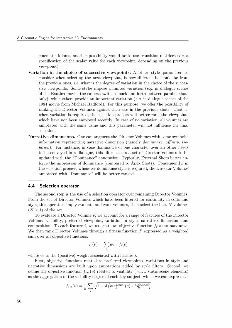
A Cinematic Engine for Interactive 3D Environments
cinematic idioms, another possibility would be to use transition matrices (i.e. aspecification of the scalar value for each viewpoint, depending on the previousviewpoint).
Variation in the choice of successive viewpoints. Another style parameter toconsider when selecting the next viewpoint, is how different it should be fromthe previous ones, i.e. what is the degree of variation in the choice of the succes-sive viewpoints. Some styles impose a limited variation (e.g. in dialogue scenesof the Exotica movie, the camera switches back and forth between parallel shotsonly), while others provide an important variation (e.g. in dialogue scenes of the1984 movie from Michael Radford). For this purpose, we offer the possibility ofranking the Director Volumes against their use in the previous shots. That is,when variation is required, the selection process will better rank the viewpointswhich have not been employed recently. In case of no variation, all volumes areannotated with the same value and this parameter will not influence the finalselection.
Narrative dimensions. One can augment the Director Volumes with some symbolicinformation representing narrative dimension (namely dominance, affinity, iso-lation). For instance, in case dominance of one character over an other needsto be conveyed in a dialogue, this filter selects a set of Director Volumes to beupdated with the “Dominance” annotation. Typically, External Shots better en-force the impression of dominance (compared to Apex Shots). Consequently, inthe selection process, whenever dominance style is required, the Director Volumesannotated with “Dominance” will be better ranked.
4.4 Selection operatorThe second step is the use of a selection operator over remaining Director Volumes.
From the set of Director Volumes which have been filtered for continuity in edits andstyle, this operator simply evaluate and rank volumes, then select the best N volumes(N ≥ 1) of the set.
To evaluate a Director Volume v, we account for a range of features of the DirectorVolume: visibility, preferred viewpoint, variation in style, narrative dimension, andcomposition. To each feature i, we associate an objective function fi(v) to maximize.We then rank Director Volumes through a fitness function F expressed as a weightedsum over all objective functions:
F (v) =∑i
wi · fi(v)
where wi is the (positive) weight associated with feature i.First, objective functions related to preferred viewpoints, variations in style and
narrative dimensions are built upon annotations added by style filters. Second, wedefine the objective function fvis(v) related to visibility (w.r.t. static scene elements)as the aggregation of the visibility degree of each key subject, which we can express as:
fvis(v) = 1k
∑k
√1− δ�visactualk (v), visdesiredk
�56

Enforcing Screen Composition
In this formula, visactualk (v) represents the actual visibility degree of key subject k fromvolume v and visdesiredk represents its desired visibility degree (as an interval). Thefunction δ represents a distance between them, returning a value ranging from 0 (theactual visibility degree belong to the desired interval) to 1 (the maximum distancevalue). The use of a square root in fvis will therefore favor balancing the distanceto the desired visibility degree for both key subjects. Third, the objective functionrelated to composition is defined as follows. We here assume that we have computedthe composition error εk of each key subject k for a single camera configuration inthe volume v – the computation of this error is described later (see Section 5). Thisobjective function is then expressed as
fcomp(v) = 1k
∑k
È1− εk(v)
where the error εk ranges from 0 (no error) to 1 (maximum error). Note that, similarlyto visibility, the use of a square root will balance the error in composition for each keysubject.
We finally select, among all available, the N Director Volumes of highest fitnessvalue(s). Note that in case the number of available volumes is lower or equal to N , weselect all those volumes without resorting to the fitness function.
4.5 Failures in available Director VolumesFailures occur when filtering operators prune all possible Director Volumes (before
applying Style filters). We handle such failures in two ways. First, in our design, Ex-treme Long Shots are not impacted by continuity rules; such viewpoints are generallyused to (re-)establish the relation between a key subject and his environment, and film-makers classically use this device. Second, continuous transitions are applied to violatecontinuity rules (e.g. crossing the line-of-interest) as long as the spatial continuity ismaintained.
5 Enforcing Screen CompositionThe next step consists in selecting an appropriate camera configuration inside a
selected Director Volume and enforcing some composition rules (e.g. the rule of thirdsand balance in the image). By definition each Semantic Volume encompasses someimplicit elements of composition (number of key subjects and relative positions of thesubjects on the screen). For example, an Apex Shot should portray two key subjectsrespectively on the left and on the right of the screen; and a Parallel Shot shouldportray a single key subject on one half of the frame, looking toward the other half ofthe frame. Our approach expresses the composition through the specification of theposition of key subjects on the screen. When key subjects are characters, we actuallyabstract characters by using their eyes or head location (depending on the shot size).
To enforce composition, we first associate with each Semantic Volume some con-straints on the composition for one, two or more key subjects on the screen. Since
57

A Cinematic Engine for Interactive 3D Environments
the volumes already encompass a notion of size (Close Shot to Long Shot), we do notmodel the size of the key subjects on the screen as a constraint. We build an objectivefunction to optimize as follows. For a given camera position inside the Director Volume,we compute the camera orientation algebraically. For each subject k, the compositionerror εk is defined as the Euclidean distance between the desired and actual on-screenpositions of the subject (the eyes or head for a character). The objective function fc(p)to minimize is then defined as
fc(p) = 1k
∑k
εk(p)
where p represents a camera position. The on-screen positioning constraints can there-fore be modified to enforce some specific narrative dimensions (e.g. dominance of onecharacter over another can be expressed by constraining his eye-line to be higher onscreen than the eye-line of the dominated character). The Results section details theimplementation of narrative dimensions with our system and displays the impact oncomposition.
At this step, the handling of dynamic occluders could be included by adding an newcomponent visdynk (p), related to the visibility of each key subject for dynamic occluders,to the objective function. Simple techniques such as ray-casts or depth rendering canbe integrated with little overhead.
We then rely on a local search optimization technique to compute the best cameraconfiguration inside a Director Volume. We start with a uniformly distributed set ofcandidate positions pi, i ∈ {1, n} inside a Director Volume. For each position pi, wethen use the following algorithm
1. We randomly sample m candidate positions qji around pi.
2. We discard all samples which lie outside the volume.
3. Among others, the best neighbor, i.e. with lowest composition error fc(qji ), isreferred to as qbesti .
4. If fc(qbesti ) < fc(pi), then we use qbesti as new candidate position and we reiteratethe process.
5. If not, no improvement has been made and we stop the process.
We also consider two additional stopping conditions. First, we use a threshold on thenumber of iterations, ensuring the termination of the algorithm. Second, we use athreshold on the composition error. When fc(pi) get under this threshold, the processis also stopped. Finally, among all candidate camera positions p computed in DirectorVolumes, we select the one with minimum value of fc(p).
58

Performing cuts or continuous transitions
See Figure 3.9 for an overview of the algorithm, and Figure 3.10 for an illustrationof the on-screen positioning optimization. The specification of the framing for thisexample is further provided hereafter:
Viewpoint "OTS-B"configuration 2-subjecttype Externalsize Medium Close-upside BFraming
Subject -0.33 -0.33Subject +0.33 +0.33
Figure 3.9 – A local search optimization is performed inside a Director Volume tosearch the viewpoint providing the best composition on the screen. The search processstarts from a set of uniformly distributed viewpoints inside the 2.5D volume. Then,for each viewpoint, a number of neighbor candidates are generated and evaluated withregard to composition. The best neighbor is chosen as the current configuration and theprocess iterates on a new set of neighbors.
6 Performing cuts or continuous transitions
Our system constantly reasons as to whether tomaintain the current position of the camera,perform a cut,make a continuous transition to another viewpoint,react to a new narrative event that has occurred.
These choices depend on: (i) the current and incoming narrative events (and their likelyduration), (ii) the current viewpoint, (iii) the past viewpoint, (iv) continuity and styleparameters.
59

A Cinematic Engine for Interactive 3D Environments
(a) (b)+
Figure 3.10 – The evaluation of a camera configuration w.r.t. frame composition isexpressed as the Euclidian distances between on-screen actual positions (red) and desiredpositions (green) of characters eyes. The solving process seeks for minimizing thesedistances using a local search optimization process.
6.1 Controlling cuts with Pacing and Dynamicity
In our approach we introduce two indicators of directorial style that control transi-tions: pacing and dynamicity.
6.1.1 Pacing
As described in literature, cuts are motivated either by directorial style or by neces-sity. When a matter of necessity, transitions may be performed at any moment in themovie. Such transitions are motivated by the occlusion of a key subject, or by a keysubject leaving the frame. When a matter of style, transitions are driven by the pacing,a specific indicator which represents the rate at which transitions are performed. Ourpacing is modeled with three values [dnew : [dmin; dmax]], where dnew is the minimumduration before making a transition to convey a (new) more relevant narrative eventand [dmin; dmax] is the interval of duration in which a transition is allowed to still conveythe same narrative event. The probability of making a transition within these boundsis driven by a Gaussian (the closer to dmin the less probable, the closer to dmax themore probable). Transitions will occur either due to pacing, or due to the onset of anarrative event of higher relevance.
6.1.2 Dynamicity
Changes in viewpoints may be realized through continuous transitions (i.e. camerapaths). Such changes are typically a matter of directorial style, which we model throughthe dynamicity indicator. In our implementation, dynamicity ranges from static shotsto panoramics, travellings or free camera motions. Interestingly, continuous transitions
60

Performing cuts or continuous transitions
may allow the director to break continuity rules, for example by crossing the line-of-interest or a line-of-action. Thus in cases where no Director Volume is applicable afterfiltering on continuity, we allow the camera to continuously move to any visible DirectorVolume.
The possibility our system offers to control the camera dynamicity encompasses boththe camera motions performed inside a Director Volume (none, panoramic, travelling)and the transitions between action shots (cuts or camera paths). Our cinematic engineoffers four possible levels of dynamicity:1. No Dynamicity (static shots): No camera motion is allowed inside an action shot,
and action shots are always separated by cuts (i.e. each shot is made of a singleaction shot);
2. Panning: Camera motions are restricted to pans inside an action shot;3. Travelling & Panning: Travelling camera motions are also allowed inside action
shots;4. Full Dynamicity (long take): All motions are allowed, and action shots are sepa-
rated by continuous transitions instead of cuts (i.e. a single shot is built to conveystory events).
Examples illustrating some variations in Pacing and Dynamicity are presented inthe Results section.
6.2 Performing continuous transitions by path-planning
To enforce continuous transitions between viewpoints, it is necessary to first builda roadmap of the environment and second, from this roadmap, perform path planningrequests between the camera current configuration and the desired location in theselected Director Volume.
6.2.1 Building a roadmap of the environment
Connectivity graphs of the scene can be defined at multiple levels:Topological cell-and-portal graph By construction, the topological cell-and-portal
decomposition offers a connectivity graph that avoids obstacles. At this levelof connectivity, one could be used to plan coarse paths at the cell level as in[AVF04]. At this level, we could consider a cell-to-cell path length and potentiallypreferences in cells to go through, or to avoid.
Connectivity between Visibility Volumes Each topological cell contains an a-BSP decomposition into Visibility Volumes. On could then build a connectivitygraph by interconnecting all adjacent cells inside a-BSPs and between a-BSPs indifferent cells. At this level of connectivity, one would be enabled to plan pathsinside a topological cell; it would also adds the possibility to reason about thevisibility (of one or more subjects) along the path.
61

A Cinematic Engine for Interactive 3D Environments
Figure 3.11 – The roadmap is built in multiple steps: (a) a first roadmap is builtfrom the cell-and-portal topological representation, (b) topological cells are split by thea-BSP representation of Director Volumes which in turn (c) forms a coarse roadmapby interconnecting all adjacent partitions inside a-BSPs and between a-BSPs, (d) theroadmap is then refined by sampling the edges shared between the partitions to providesmoother paths in the planning process.
Connectivity between Director Volumes Each topological cell also contains an a-BSP decomposition into Director Volumes. As well as for Visibility Volumes, onecould build a connectivity graph upon Director Volumes. At this level of connec-tivity, one could further reason about preferences in viewpoints to go through orto avoid.
Sampling-based roadmap We here propose a 4th level of connectivity, by construct-
62

Performing cuts or continuous transitions
(a) (b)
Figure 3.12 – Refinement of the connectivity inside a Director Volume. Walls arehere represented as thick black edges. We refine connectivity through the volume bysampling way points (black dots) on accessible edges (in red) with a given density δ. Wecreate a roadmap node to represent each way point. We then create a roadmap edgeto represent a link (in blue) between each pair of way point located on two differentedges. This sampling-based connectivity enables exploring more accurately the differentpossible camera paths inside a volume, thus enhancing the quality of the global camerapath.
ing a finer roadmap on top of Director Volumes’ connectivity. The connectivitygraph built for Director Volumes is refined by using a two step-process. First,instead of considering a camera path as just a sequence of Director Volumes, wepropose to further explore the different possible ways to go through a volume.We then uniformly sample way-points on each connection edge, with a samplingdensity δ; we further set the minimum number of samples on a connection edgeto 1, so as to guarantee the connectivity between two adjacent volumes. Eachsample way-point is then used as a node in the roadmap. Second, inside a givenDirector Volume, we create roadmap edges between all pairs of way-point nodeslocated on distinct connection edges. This sampling process has the advantageof providing a finer sampling of possible paths inside volumes, thus allowing toreason more accurately on the global path properties.
The different levels of connectivity are illustrated in Figure 3.11, and a focus onour sampling process inside volumes is illustrated in Figure 3.12. The sampling-basedroadmap is therefore recomputed on demand each time the scene evolves (i.e. when akey subject moves or new narrative events occur which demand the re-computation ofthe Director Volumes).
In contrast to existing sampling-based roadmap methods, our roadmap has twomain advantages. First, our roadmap is augmented with both semantic and visibilityinformation, what enables reasoning about a range of properties along computed camerapaths (e.g. minimize the path length, keep the camera at a certain distance from akey subject, enforce visibility along the path, avoid/prefer sub-sets of scene areas orviewpoints). Second, our roadmap is computed dynamically (the roadmap is updated asthe Director Volumes evolve), what enables recomputing paths dynamically to accountfor changes in the key subjects’ configuration (e.g. in case of subjects motions in the
63

A Cinematic Engine for Interactive 3D Environments
scene).
6.2.2 Computing Camera Paths
For a matter of simplicity, practically, we plan paths over the complete sampling-based roadmap built on top of Director Volumes. Theoretically, however, it would bepossible to design a more efficient path planning process taking advantage of the multi-level connectivity, and using an incremental planning algorithm from low resolutionto high resolution connectivity graphs. This would particularly avoid building thecomplete roadmap; only the traversed cells/volumes would then need to be consideredfor sampling.
Our roadmap can be formalized as a vector 〈N,E,AN , AE〉, where N the set ofnodes, E is the set of edges, AN is the set of node annotations (e.g. position, distanceto subjects), and AE is the set of edge annotations (e.g. length, traversed VisibilityVolume(s) and Semantic Volume). A camera path t can then be described in two ways:
as a sequence of edges: t = {e1, e2, . . . , em}, with ei ∈ E;as a sequence of nodes: t = {n0, n1, n2, . . . , nm}, where n0 and nm are resp. theinitial and target camera configurations, and ni ∈ N, 0 < i < n is the node sharedby edges ei and ei+1.
The task of planning a path between two Director Volumes is then expressed as aclassical optimization process. The cost C (to minimize) of the path t is given by
C(t) =∑e∈t
∑i
wi ·Ci(e) +∑n∈t
∑j
wj ·Cj(n)
Ci and wi are resp. the cost function (to minimize) and weight associated with edgefeature i (e.g. path length, occlusions of key subjects); similarly, Cj and wj are resp. thecost function (to minimize) and weight associated with node feature j.
In our implementation, we have considered two important features: the visibility ofkey subjects along the path and the length of the path. We have thus built our costfunction C as a weighted sum of the path length and visibility of key subjects:
C(t) =∑e ∈ t
�wvis ·Cvis(e) + wlen ·C len(e)
�In this formula, C len(e) is set to |e| > 0, the length of edge e. In the same way, Cvis(e)is the cost associated with visibility along edge e. By default, we express Cvis as aweighted sum of the visibility of each key subject k
Cvis(s) =∑k
wk ·Cvisk (e)
where wk is the weight associated with the visibility of subject k, and with
Cvisk (e) =√δ�visactualk (e), visdesiredk
�Here the function δ is defined in the same way as in Section 4.4. The square root inCvisk (e), together with the weights wk allows both balancing the visibility degree of
64

Performing cuts or continuous transitions
Figure 3.13 – We build upon the roadmap to compute paths between Director Volumes.Since the roadmap is built from the Director Volumes a-BSPs, each cell (and thereforeeach node of the roadmap holds the information of the Director Volumes (visibility, typeof viewpoint). Therefore the search for a path in the roadmap may contain evolvedsearch criteria such as finding paths with maximum visibility of targets, or finding pathswhich avoid certain shots (e.g. long shots).
subjects, and potentially favoring the maintenance of visibility on some subjects to thedetriment of others. By tuning the two weights wvis and wlen, such a representationallows favoring paths with (for each key subject) little, no or many occlusions on theway.
Our search is performed with a Dijkstra process that handles multiple target vol-umes and stops as soon as a solution path is found. We then use classical smoothing
65

A Cinematic Engine for Interactive 3D Environments
techniques to improve the computed path.
7 Results
This section details the application of our virtual cinematography system to thecanteen scene from Michael Radford’s 1984 movie, by exploring different ways of filmingthe same set of narrative events occurring in the same environment. The degrees ofvariation in the directorial style that we explore are related to low-level style parameterssuch as camera dynamicity, visibility of characters, and pacing. We then demonstratethe editing possibilities of our system with high-level narrative dimensions (dominance,affinity and isolation of characters) that influence the main components of our system.
To generate results, we provided our system with an annotated screenplay. Thisscreenplay specifies a set of narrative events (possibly overlapping in time) as theyoccur in a sequence of scenes by specifying, for each one, the starting and ending times,the involved subjects/objects (if any), a relevance value, and a textual description ofthe event. Events may be attached to a character or an object (e.g. "Parsons walks tothe table"), or describe any general event (e.g. "Characters are entering the canteen").In addition, the screenplay includes the names of particular 3D model parts for thesubjects, which are required to perform appropriate screen composition in computingviewpoints (e.g. for a character, body part, head part and eyes parts). All 3D models,XML representations of narrative events and cinematic idioms, together with resultingvideos are available at www.cameracontrol.org/1984-Canteen-scene.
In the context of the current application, our system however assumes that eventsare not known in advance; events are instead only considered in the system when theyoccur. An excerpt of the annotated screenplay for the canteen scene from MichaelRadford’s 1984 is provided below
Screenplay "1984"Scene "Canteen"
Location "Canteen"Subject "Smith" Character
body "SmithBody"head "SmithHead"leftEye "SmithLeftEye"rightEye "SmithRightEye"
Subject "Syme" Character...
Event "A pours gin"relevance 5begin 0 end 4Character "Smith"
Event "A drinks gin"relevance 5begin 4 end 12
66

Results
Character "Smith"Event "A turns"
relevance 3begin 10 end 18Character "Smith"
Event "A speaks to B"relevance 9begin 18 end 21Character "Smith"Character "Syme"
...End Screenplay
7.1 PacingThe pacing influences the duration of each shot, i.e. the interval of time in which
the system is allowed to make a cut or perform a camera movement. We recall that thepacing is defined as an input to the system declared as three values [d0 : [d1; d2]], whered0 is the minimum duration before making a cut to convey a new event, and [d1; d2] isthe interval of shot duration in which a cut is allowed to still convey the same event.Here, we display two simple examples of variations in editing by changing the pacingparameter in the 1984 canteen scene. For each of them, three snapshots of the systemare taken at three different dates (88s, 90s and 93s).
Example #1: Fast pacing (pacing=[2 : [4; 6]]) In the first example, three cutsare performed (see Figure 3.14), respectively after 3 seconds, 2 seconds, and 3 seconds.
Example #2: Slow pacing (pacing=[4 : [6; 8]]) In this second example, only onecut is performed (see Figure 3.15). Snapshots were taken at the same time steps as inExample #1 (88s, 90s and 93s). All three snapshots occur in the same shot (no cut),whereas in the same case in Example #1, three cuts were performed.
7.2 Degree of VisibilityAnother style parameter that we illustrate here is the degree of visibility that is
desired for a key subject and how it influences the editing. Our system considers asinput an interval of allowed visibility of key subjects in a continuous range between0 and 1. Value 0 stands for no visibility, while value 1 stands for full visibility. Thisinterval influences the editing process in (1) the choice of the viewpoints (the systemneeds to select viewpoints which ensure that the degree of visibility can be maintained),and (2) the critical moments to perform cuts (when the degree of visibility cannot bemaintained any more). Here we display three results on the same narrative event “Symeturns around pillars”, with three different ranges for the desired degree of visibility: fullvisibility (interval [1; 1]), full occlusion (interval [0; 0]) and partial visibility of Syme(interval [0.25; 0.75]).
67

A Cinematic Engine for Interactive 3D Environments
Figure 3.14 – Example #1: fast pacing. Pacing parameters are set to [2 : [4; 6]].Therefore cuts to convey a new narrative event may be performed after 2 seconds of thesame shot, and cuts to convey the same narrative event should be performed within theinterval of 4 to 6 seconds. Snapshots 1, 2 and 3 were taken respectively at time steps88, 90 and 93 seconds. Here three cuts of the same narrative event (Parson walking tothe table) were performed.
Figure 3.15 – Example #2: slow pacing. Pacing parameters are set to [4 : [6; 8]].Therefore cuts to convey a new narrative event may be performed after 4 seconds of thesame shot, and cuts to convey the same narrative event should be performed within theinterval of 6 to 8 seconds. As a result, there are only two shots. Snapshots were takenrespectively at time steps 88, 90 and 93 seconds (compare to Example #1, where threecuts were performed during this same interval).
Example #3: Full Visibility In this example, the degree of visibility is constrainedto interval [1; 1] (maintain full visibility of the subject). As displayed in Figure 3.16, assoon as the character is occluded by a pillar, the system performs a cut to an unoccludedview by selecting a Director Volume where visibility is equal to 1.
68

Results
Figure 3.16 – Example #3: enforcing a full visibility. In our editing model, as soonas the visibility constraint is violated, the system performs a cut. In this example, thevisibility is set to full visibility (interval [1; 1]). Therefore as soon as the character isoccluded by a pillar, the system automatically cuts to a new viewpoint.
Example #4: Full Occlusion In this example, we constraint the visibility to inter-val [0; 0] which stands for no visibility. As displayed in Figure 3.17, as soon as a partof the character starts to be visible, the system performs a cut to an occluded view byselecting a Director Volume where visibility is equal to zero.
Figure 3.17 – Example #4: enforcing a full occlusion. In this example, the visibility isset to no visibility (interval [0; 0]). Therefore as soon as a part of the character is visible,the system automatically cuts to a new viewpoint where the character is occluded. Onshots 2, 4 and 6 parts of the character which start to be visible are highlighted with ared circle, just before the system cuts to another viewpoint (time 0.9s, 4.3s and 6.1s).
Example #5: Partial Visibility In this example, the degree of visibility is con-strained to interval [0.25; 0.75], which stands for partial visibility of the key subject. Asdisplayed in Figure 3.18, as soon as the character is either strongly visible or strongly
69

A Cinematic Engine for Interactive 3D Environments
occluded, the system performs a cut to a more appropriate view by selecting adequateDirector Volumes with visibility inside the specified range.
Figure 3.18 – Example #5: enforcing a partial visibility. In this example, the visibilityis set to partial visibility (interval [0.25; 0.75]). Therefore as soon as the character iseither strongly occluded (visibility < 0.25), or strongly visible (visibility > 0.75), thesystem automatically cuts to a new viewpoint where the partial visibility is satisfied.See how the different shots display the character as only partially visible.
7.3 Camera DynamicityIn this result section, we describe how the camera dynamicity parameter impacts
the editing and the generation of camera movements computed by the system. Thecamera dynamicity influences our system in (1) allowing specific camera movements(panning, travelling, etc.) and (2) the choice of the next viewpoint when performing acut, due to changes in view angle and/or character size between the beginning and theend of a shot. Four level of dynamicity are proposed in our system:
No dynamicity: only static camera positions are computed;Dynamicity on orientation: panning motions are allowed for the camera;Dynamicity on orientation and position: travelling and panning motions are al-lowed (together with compositions of travellings and pannings);Full dynamicity: all camera motions are allowed. Furthermore all the transitionsbetween shots need to be continuous transitions instead of cuts (this generates along-take shot).
In the system, camera movements on position (i.e. travellings) are enabled by usingthe roadmap to plan a linear motion of the camera. A continuous transition consistsin planning a camera path from the starting Director Volume to the Director Volumechosen as candidate. A panning consists in re-orientating the camera to maintain thesatisfaction of the frame composition.
Example #6: No Dynamicity This level of dynamicity disallows any cameramovement. The editing is then only made of cuts between static viewpoints. Fig-
70

Results
ure 3.19 illustrates some results.
Figure 3.19 – Example #6: no dynamicity. In this example, the dynamicity of thecamera is set to “no dynamicity”, which means that only static shots are computed.The editing process therefore cuts according to the pacing constraints, the visibility ofcharacters and the occurrence of new events. For example, the cut from shot #1 to shot#2 is due to the new event “Parsons walks to the table”, the cut from shot #2 to shot#3 is due to the visibility of Parsons (he leaves the screen, see second snapshot), thecuts from shots #3 to #4 is due to visibility once again, while the last cut (#4 to #5)is due to the pacing parameter.
Example #7: Dynamicity on Orientation This level of dynamicity enables thecamera to perform panning shots. The editing process then selects either static shotsor panning shots depending on the nature of events occurring in the scene. In oursystem, events are tagged by the user with camera dynamicity features; i.e. for eachevent, the user specifies whether it may be shot with a static shot, or a dynamic shot(panning, travelling, full dynamic). This represents a matter of style, and differentdirectorial styles will obviously tag the events in a different way. In our Example #7,the event “Symes eats” is tagged with “static shot”, while the event “Parsons walks tothe table” is tagged with “dynamic shot”. Figure 3.20 details some results: shot #1is a static shot, shot #2 is a panning shot and a cut is performed at time=90s due topacing constraints. Shots #3 and #4 are panning shots too.
Example #8: Dynamicity on Orientation and Position This level of dynamic-ity enables the camera to perform both panning and travelling motions. In a way similarto Dynamicity on Position, our system uses the tags associated with the events to knowwhether a dynamic motion of the camera is possible. Travelling motions are computedby relying on the underlying roadmap (i.e. searching for close-to-linear paths). Snap-shots have been taken at the same time steps than Example #7, which provides a nicebasis for comparison: snapshots 1 and 2 are quite similar, while snapshots 3, 4, 5 and6 display some variation since a travelling motion is used. Cuts 2 and 3 are performeddue to pacing constraints only (see Figure 3.21).
71

A Cinematic Engine for Interactive 3D Environments
Figure 3.20 – Example #7: dynamicity on orientation. In this example, the dynamicityof the camera is set to “orientation”, which means that the camera can perform staticshots or panning shots. The editing process therefore cuts according to the pacingconstraints, the visibility of characters and the occurrence of new events. Shot #1 is astatic shot, while all others are panning shots. The second and third cuts occur due topacing constraints.
Figure 3.21 – Example #8: dynamicity on orientation and position. In this example,the dynamicity of the camera is set to “orientation and position”, which means thatthe camera can perform static shots, panning shots, travelling shots or a mix betweenpanning and travelling. The editing process therefore cuts according to the pacing con-straints, the visibility of characters and the occurrence of new events. Shot #1 is a staticshot, while all others are mixing panning and travelling shots. The second and thirdcuts occur due to pacing constraints. All snapshots are taken at the same time stepsthan Example #7, which provides a basis to compare the results.
Example #9: Full Dynamicity (Orientation, Position, Continuous Transi-tion) This level of dynamicity enables full dynamicity; i.e. the camera moves freely inthe environment, and no cuts are performed between the viewpoints. Such a parametergenerates long-takes. All transitions between viewpoints are continuous transitions us-
72

Results
ing the path planning process from the roadmap. When a new event occurs (e.g. hereParsons walking to the table), the camera performs a long movement and rotates tograb a view of Parsons, then the camera follows him continuously until he reaches thetable (see Figure 3.22).
Figure 3.22 – Example #9: full dynamicity. In this example, the dynamicity of thecamera is set to “full dynamicity”, which means that the camera can perform any motion,and performs path planning between viewpoints conveying different events. Only oneshot is produced with this system (a long take).
7.4 Narrative Dimension
In this section, we selected three narrative dimensions which could be manipulatedto affect a viewer’s perception of inter-character relationships in the scene: (1) isolation,(2) dominance of one character over another and (3) characters’ affinity for each other.The manipulation of these dimensions substantially changes the dramatic outcomes ofa section of the narrative, independently of dialogue and other characters’ actions.
We here detail the mechanisms by which we enforce dominance, affinity and isolationwithin our cinematography system and present our results with the 1984 Canteen scene.The narrative dimension influences our system in (1) specifying preferences on the setof characters that appear on screen and in (2) applying a specific frame composition ofthis set of characters.
The enforcement of these dimensions produces fairly different results in terms ofediting, viewpoint selection and composition. For each dimension, three snapshots ofthe system were taken at exactly the same time steps (19s, 41s and 50s), and clearlydemonstrates the variation (see Figures 3.26 to 3.28).
In order to implement these narrative dimensions, we extended the virtual cinematicengine in four ways:
narrative dimensions influence the selection of the next narrative events to convey.For example, by selecting a different protagonist in the story, only the narrativeevents related to this protagonist (and his interactions) will be considered.
73

A Cinematic Engine for Interactive 3D Environments
each Semantic Volume is annotated beforehand with the appropriate dimensionsit can convey (e.g. Apex shots better convey affinity, external shots better conveyaffinity and dominance, parallel shots better convey isolation). Each SemanticVolume may be annotated by multiple dimensions.a specific filter (called DimensionFilter) is added in the style filtering queue. Itsrole is to remove from the list of Director Volumes, all Volumes (i.e. viewpoints)which do not enforce a specified dimension.constraints on the screen composition are different from one dimension to another. For example, in an External shot, the dominant character will have hiseyes constrained to a higher location on the screen than the dominated character.Similarly, for isolation, the characters body, head or eyes (depending on the sizeof the shot) will be constrained on the far left or far right side of the screen.
Figures 3.23 and 3.24 illustrate how these narrative dimensions influence the differ-ent components of our cinematography system on an example with multiple narrativeevents. As displayed in these figures, the narrative dimensions mainly control the styleparameters which in turn control the choice of appropriate Director Volumes, edit-ing and screen composition. The narrative dimensions first influence the selection ofappropriate narrative events in the story (e.g. selecting events related to the main pro-tagonist). To each narrative event is associated a range of viewpoints. In a second step,this range of viewpoints is narrowed down by selecting preferred viewpoints (DirectorVolumes) associated with each narrative dimension. For example, affinity is betterconveyed using apex shots or over-the-shoulder shots, rather than using parallel shots.Third, narrative dimensions influence the selection of the next best Director Volume tocut to, given previous camera locations and preferred shots (Resulting shots in the Fig-ure). Finally, such dimensions influence the composition of key subjects on the screen,inside each Director Volume.
Example #10: Default Narrative Dimension For this narrative dimension,there is no preference as to which characters have to be framed: the DimensionFilterthus eliminates no viewpoint. Moreover, the frame composition is balanced: i.e. withregard to the rule of thirds, the eyes of both characters are placed on the top thirdhorizontal line (see Figure 3.25).
Example #11: Affinity between Syme and Smith To convey affinity betweenboth characters, the system will prefer shots with a balanced frame composition onSyme and Smith, and with regard to the rule of thirds, the eyes of both charactersare placed on the top horizontal line. Specifically, the system will favor apex shotsor external shots through the DimensionFilter which will only keep Apex or Externalshots (see Figure 3.26).
Example #12: Dominance of Syme To illustrate the dominance of Syme overSmith, the system will optimize the viewpoints where the eyes of Syme can be placedhigher than eyes of Smith on screen: with regards to the rule of thirds, the eyes ofSyme are placed on the top horizontal line, and the eyes of Smith are placed on the
74

Results
Figure 3.23 – Influence of the “affinity” narrative dimension on main components ofCineSys. It influences both the selection of narrative events in the story (e.g. selectingevents related to the main protagonist), the selection of preferred viewpoints (DirectorVolumes) and the composition of key subjects on the screen, inside each Director Volume.Affinity is better conveyed using apex shots or over-the-shoulder shots, rather than usingparallel shots, and positioning subjects at the same height on the screen.
bottom horizontal line. In terms of shots, the system the system will prefer externalshots: the DimensionFilter will only keep external shots (see Figure 3.27).
Example #13: Isolation of Syme To display the isolation of a character, oursystem favors shots where this character is alone. In this example, all along the dialogbetween Syme and Smith, the DimensionFilter will eliminate all viewpoints but internal
75

A Cinematic Engine for Interactive 3D Environments
Figure 3.24 – Influence of the “dominance” narrative dimension on main components ofCineSys. It influences both the selection of narrative events in the story (e.g. selectingevents related to the main protagonist), the selection of preferred viewpoints (DirectorVolumes) and the composition of key subjects on the screen, inside each Director Volume.Dominance is better conveyed using over-the-shoulder shots, and positioning the eyes ofthe dominant subject higher than the ones of the dominated subject on the screen.
shots on Syme, parallel shots on Syme and subjective shots on Syme. Moreover, theframe composition shows Syme spatially isolated on screen (composition is expressedwith the rule of the fifths, and character Syme is constrained to the rightmost verticalline (see Figure 3.28).
76

Results
Figure 3.25 – Example #10: shots illustrating the “default” narrative dimension (nospecific narrative dimension is enforced). All viewpoints are available to the process andcompositions are balance according to the rule of the thirds. Shots were respectivelytaken at time steps 19s, 41s and 50s (see Figures 37, 38 and 40 for a comparison).
Figure 3.26 – Example #11: shots illustrating the “affinity” narrative dimension.Only external shots and apex shots will be selected by the DimensionFilter process.The composition is a balanced composition in both apex and external views. Shotswere respectively taken at time steps 19s, 41s and 50s (see Figures 36, 38 and 39 for acomparison).
Figure 3.27 – Example #12: shots illustrating the “dominance” narrative dimension.Only external shots will be selected by the DimensionFilter process. The compositionprocess computes shots where the character Syme (right character) is always higher onthe screen than Smith (left character). Shots were respectively taken at time steps 19s,41s and 50s (see Figures 36, 37 and 39 for a comparison).
7.5 Limitations
A limitation of our approach lies in that the visibility computation for static oc-cluders is performed in 2D. Though the 2D cells are extruded to 2D1
2 (by consideringthe respective ceiling heights) and composition is computed in full 3D, the propagationof visibility between cells fundamentally relies on a 2D process. Therefore, in envi-ronments with multiple levels, inter-level visibility will not be computed although thiscould potentially be addressed by pre-computing inter-cell visibility for cells on differentlevels using ray casting techniques (in a way similar to [OSTG09]). Additionally visi-
77
A Cinematic Engine for Interactive 3D Environments
Figure 3.28 – Example #13: Shots illustrating the “isolation” narrative dimension.Only shots with one character on the screen are kept by the DimensionFilter. Thecomposition process computes shots where the character Syme is always on the rightmost part of the screen. Shots were respectively taken at time steps 19s, 41s and 50s(see Figures 3.25 to 3.27 for a comparison).
bility of key subjects w.r.t. dynamic occluders can be handled by including ray-castingor depth rendering techniques in the screen-composition process.
7.6 Discussion and Comparison
To compare our contribution to the state of the art, we selected a number of prop-erties a virtual cinematography system should display in a real-time context.
Interactive/Dynamic. First of all, such a system needs to be fully interactive,that is, enjoying the possibility to react to interactive events occurring in theenvironment. Events may be new actions, new characters entering the scene, newdialogues or any narrative events that influences the unfolding of the story. Thedynamic aspect requires re-computing camera locations for characters motionswhich are not known in advance.Shot coherency. As empirical rules guide the way shots should be organized in acoherent way to convey a piece of a story, a virtual cinematography system needsto encode such knowledge. The key relies in the expressiveness of approaches toencode such coherency.Composition. The composition property represents the capacity of a system tohandle screen composition and variation in screen composition. Composition isan essential component of cinematography, not only from the perspective of aes-thetics (modeling aesthetics in images represents an impossible challenge), butmore basically for understanding spatial relations between characters (a characteron the left of the screen and looking right is implicitly interacting with a subjecton his right) and causal relations. The range of composition properties and theexpressiveness of the underlying computational process is a key property of anyvirtual cinematography system.Style. The style property represents the capacity of a cinematography system toprovide a range of directorial styles, or some degree of variation in a style. Whilecharacterizing and enforcing style may represent a challenging task, a number ofdevices and parameters can be used to enforce variation.Path-planning. The path-planning property represents the ability of performingcomplex camera motions in environments. Nonetheless, path-planning is a key-
78

Results
component to represent simple motions such as travellings and trackings, togetherwith more complex motions such as those encountered with hand-held cameras.Cinematic discourse. This last property characterizes the ability of a cameracontrol system to deliver a coherent construction of viewpoints over a set of events,thereby conveying a coherent narration of the events.
Table 3.1 provides a comparison of major scientific contributions in the domain ofautomated camera control. As displayed in the table, our approach satisfies most of theproperties required in an interactive storytelling system and stands in stark contrast.The closest contribution to our work (Elson & Rield [ER07]) is not a reactive approach(the system runs offline) and therefore cannot handle interactivity, does not handlecomposition on the screen (all shots are pre-computed path sequences) and does notoffer path-planning capacities for complex camera motions.
79

ACinem
aticEngine
forInteractive3D
Environments
Paper Technique Interactive /Dynamic Coherency Composition Style Path
Planning Visibility Staging CinematicDiscourse
He et al.[HCS96]
Finite StateMachine Yes Limited No No No No No No
Christiansonet al. [CAH+96] Tree Model No Limited No No No No No No
Jhala & Young[JY05] Tree Model No Yes Pre-
computed No No No Yes Yes
Elson & Riedl[ER07]
Pre-setIdioms No Yes Pre-
computed Yes Pre-computed No Yes Limited
Li & Cheng[LC08]
ProbabilisticRoadmaps Yes Limited No No Yes No No No
Assaet al. [AWCO10] Correlation Yes No No No No Yes No No
Yehet al. [YLL12] Optimization No Yes No No Yes Yes No No
Our approach DirectorVolumes Yes Yes Yes Yes Yes Yes No Limited
Table 3.1 – Comparing our cinematography system to main contributions in the domain. This table compares 7 properties of maincinematography systems proposed in the computer science literature, together with the techniques that we implemented. The “Staging”parameter characterizes the ability of the system to automate the staging of characters in the scene. The “Interactive/Dynamic”parameter represents the ability to react to interactive events occurring in the environment. “Coherency” stands for the capacity toenforce some degree of coherency in a sequence of shots. “Composition” is related to the possibilities the system have in changingthe composition in shots. “Style” stands for the ability to perform some variations in the directorial style. Only Elson07 and ourapproach offer this possibility. “Path-planning” indicates whether the system is able to perform some camera motions inside theenvironment. Finally “cinematic discourse” represents the possibility of maintaining a cinematic discourse over a number of events.All in all, our approach fulfills most of the properties desired in a virtual cinematography system, and clearly represents a improvementin comparison to previous approaches.
80

Conclusion
8 ConclusionIn this chapter we have presented a unifying approach to the problem of interactive
cinematography. The approach indeed handles viewpoint, editing and planning in areal-time context. We address the innate complexity of well understood problems suchas visibility determination and path planning required in real-time camera control,while tackling higher-level issues related to continuity between successive shots in anexpressive editing model. Our real-time cinematic engine encodes cinematographicidioms and continuity-editing rules to produce appropriate edits and camera pathsfrom a set of narrative events and style indicators. The model relies on a spatialpartitioning, the Director Volumes, providing a characterization into visibility regions(with full visibility, partial visibility or full occlusion) and characteristic viewpoints (theSemantic Volumes). We reason on these Director Volumes to identify how, when andwhere shot transitions should be performed. This semantic and geometric reasoningrelies on a filtering-based encoding of cinematic conventions together with the possibilityto implement different directorial styles. The expressiveness of our model stands in starkcontrast to existing approaches that are either procedural in character, non-interactiveor do not account for proper visibility of key subjects.
On one hand, as we stated earlier, not all elements of directorial style can bemodeled. Further, the few elements of style we have considered are insufficient toexpress more complex directorial guidelines and more subtle compositions or edits. Onthe other hand, we have proposed a working automated model for efficiently tacklingkey components of film editing (particularly the composition of shots and editing rules,according to a given directorial style). There is a real interest in using this model as atool to assist a cinematographer in his creative process. In the next chapter, we buildupon CineSys to propose an approach of film editing which (i) accounts for the qualityof the edit and (ii) provides directors with a novel and efficient workflow.
81


4Integrating Director’s Inputs intothe Editing Process
This chapter presents two approaches to the problem of editing an animated moviethat add a measure of the quality of the edit, and provide assistance to a cinematog-rapher in his creative task. In existing approaches, the choice of shots and cuts is ledeither by (i) the application of a restricted number of deterministic and manually pre-encoded films idioms (one has to declare one idiom for each situation) or (ii) by relyingon continuity editing rules. These techniques are restricted to computing cinematically“acceptable” sequences of shots and transitions. Further, it appears tedious for a userto generate a sequence s/he consider satisfying, due to a lack in providing a real controlon the final edit. The user has to tune a set of parameters for which the impact theywill have in terms of final edit are not obvious. Particularly, the user has no control onthe moments of cuts, which is a key element in the art of building a good movie; andhas no mean to keep some part(s) of the movie, which s/he finds satisfactory, and makechanges on some other part(s) (one has to make changes on the system parameters,then regenerate the entire movie).
In this chapter, we propose the first computational model dedicated to the qualita-tive evaluation of an edit. We then propose to build upon CineSys, together with thisevaluation model, to assist a director in his creative process of constructing a movies/he finds satisfactory.
Note that Sections 2 and 3 stem from a joint work with Mathieu Chollet andRémi Ronfard from INRIA Grenoble (France), and that Section 4 stems from a jointwork with William Bares from Millsaps College (USA) and Roberto Ranon from theUniversity of Udine (Italy).
1 ContributionsQuality measurement of film edits. We present the first computational model
dedicated to evaluating the quality of an edit. In particular, we propose scores forshots, cuts and pacing (rhythm at which cuts are performed), independently of thefilm idioms used to generate them. The score for a shot is based on the Hitchcockprinciple of showing action from the best angle [ST85], the score for a cut betweenshots is based on the working practices of film and television [Tho93, Tho98] andthe score for pacing relies on a well-founded model to account for shots duration.
83

Integrating Director’s Inputs into the Editing Process
Efficient automated construction of well-edited movies. We introduce an effi-cient search strategy for finding the best sequence of shots from a large numberof candidates generated by traditional film idioms. By building upon our qualitymetrics, our approach enables separating correct from incorrect shot sequences.In contrast to related work, we account for a precise enforcement of pacing andstudy in detail the best moment to perform a cut, by precisely examining all pos-sible edit points. We further provide the user with more control on the final edit,through a specification of key shots as constraints during the search (i.e. shotsthe user wants to maintain in the sequence).
Novel workflow for film preview. We propose a novel workflow based on the inter-active collaboration of human creativity with automated intelligence that enablesefficient exploration of a wide range of cinematic possibilities, and rapid produc-tion of a film preview. This workflow is the first to combine the creative intel-ligence and skill of filmmakers with the computational power of an automatedcinematic engine.
Learning from examples. The approaches we propose learn editing preferences fromexamples of human experts. In particular, we introduce a novel modeling offilm idioms, through transition matrices, and our work constitutes the first efforttoward learning cinematic idioms from live human camera work, instead of tryingto pre-encode a limited number of situations.
This chapter is organized as follows. We firstly present our quality measurement offilm edits (Section 2). We secondly present the search algorithm we propose to auto-matically explore the possible sequences of shots and find the best film edit (Section 3).We thirdly present The Director’s Lens (Section 4), our intelligent and interactive as-sistant for film preview, that builds upon CineSys. We finally discuss the limitationsof our ranking-based approach and conclude on future research.
2 Film grammar rules
Evaluating the score of an entire sequence for a movie is built up from the scoresof its shots and transitions. We make the assumption that a cost function can becomputed for each fragment and cut in the sequence. We define a fragment as a pieceof a shot of duration ∆t, that we can express as a couple 〈i, t〉 where i denotes theshot index, and t the time. The cost per shot fragment is evaluated as a weighted sumof all violations of the rules of frame composition. And similarly, the cost of a cut isevaluated as a weighted sum of all violations of the rules of continuity editing. Thecost associated with shot i at time t is then given by CS(i, t), and the cost associatedwith a transition from shot i to shot j at time t is given by CT (i, j, t), expressed as
CS(i, t) =∑k
wSk ·CSk (i, t) CT (i, j, t) =∑l
wTl ·CTl (i, j, t)
where wk and wl are weights associated with each rule.
84

Film grammar rules
We furthermore consider a third key component of a movie: the pace in transitions.We assume that the cost of an entire sequence of shots (i.e. a movie, which we denoteas m) w.r.t. pace can be computed as a sum of a cost on the duration of each shot:
CP (m) =n∑s=0
CPDur(e(s)− b(s))
where b(s) and e(s) are resp. the beginning and end time of shot s.We finally build the cost function C of an entire sequence of shots as the weighted
sum of the costs taken on these three key components:
C(m) = WS ·
n∑s=0
e(s)∑
t=b(s)CS(s, t)
+W T ·
[n−1∑s=0
CT (s, s+ 1, e(s))]
+WP ·CP (m)
where WS , W T and WP are the weights associated with resp. the scores of shots, thescores of transitions and the score of the pace in transitions.
In the next sections, we detail the key features and rules we consider in this evalu-ation. These features and rules can be categorized into five classes: shot composition,continuity editing rules, relevance of a shot, relevance of a transition, and pace intransitions.
2.1 Shot compositionWe evaluate the composition of a shot fragment according to (i) a score on visibility
of subjects and (ii) a score on the composition of subjects on the screen.Before detailing the components of CS(i, t), we first introduce some useful notations.
Firstly, we will use K to represent the set of subjects that are within the frame in afragment f = 〈i, t〉. Secondly, we denote the on-screen location of eyes (middle of botheyes) and the projected size of subject k in fragment f resp. as ek(f) and sk(f). Finally,we introduce two vectors computed in the 2D screen space of a fragment f : the gazedirection and the motion of a subject k (resp. gk(f) and mk(f)).
2.1.1 Visibility
CSV is = 0.538 CSV is = 0.340 CSV is = 0Figure 4.1 – Visibility scores. Left: Poor. Middle: Better. Right: Best.
85

Integrating Director’s Inputs into the Editing Process
A good shot should maximize the visibility of the actions performed by the protag-onists. To account for this feature, we express a visibility cost CSV is which measuresthe occlusion degree of the projected bounding box of each protagonist
CSV is(f) =∑a
∑
i∈prtg(a)j 6=i
occlusion(boxi, boxj)
where prtg(a) are protagonists of action a, boxi represents the projection of the bound-ing boxes of actor i on the screen in fragment f , and occlusion(box1, box2) representthe quantity of box1 that is occluded by box2. This occlusion is measured by using theoverlap of projections of both bounding boxes. Figure 4.1 displays three shots with in-creasing visibility scores in a scene with two subjects. Shots with poor visibility scorestypically show subjects coming too close together, or hiding each other.
2.1.2 Look room
Following common practice, we favor shot composition where each key subject k isgiven enough screen space relative to the image frame, especially in the direction inwhich (s)he is looking. We compute this score as
CSLook(f) =∑k∈K
[ ek(f) + λ (sk(f)) · gk(f) ]
where λ is a scalar function of the subject’s on-screen size sk.
2.2 Relevance of a shot
CSAction = 0.8 CSAction = 0.3 CSAction = 0.2
CSAction = 0.7 CSAction = 0.5 CSAction = 0.2Figure 4.2 – Action scores. Top: Action Drink. Bottom: Action Pour. Left: Poor.Middle: Better. Left: Best.
86

Film grammar rules
Relevance of a viewpoint is measured by exploring its capacity to enhance a viewer’scomprehension of the unfolding narrative events. Each event has a relevance value thatencodes its importance for the story (e.g. representing whether the event is a foregroundaction, an establishing action, or a background action). Viewpoints that depict morerelevant events, from relevant viewpoints enforce the comprehension of the story andwill have a higher quality. We choose to evaluate the relevance of a shot with an“Action” term, which measures the amount of the scene events which is missed in ashot fragment f = 〈i, t〉
CSRel(f) = CSAction(f)
To this end, we define a cost table AS [a, s, p] which specifies the effectiveness of a shotsize s and a profile angle p conveying an action type a. This effectiveness is expressedas a cost ranging from 0 (most effective) to 1 (least effective). For example, one canprefer framing a subject speaking using a medium close-up from a front view.
The computation of the Action term over fragment f is expressed with a weightedsum over all actions a occurring during this fragment. The weighting is expressed bythe importance imp(n) of an event at time t in the scene (the closer to 0, the moreimportant). a = type(n) represents the type of the event, while size(n, f) and pr(n, f)represents resp. the shot size and profile angle of the viewpoint in fragment f w.r.t. themain subject of narrative event n
CSAction(f) =∑n
imp(n) ·AS [type(n), size(n, f), pr(n, f)]
With a suitable choice of the AS [a, s, p] coefficients, the Action term can serve toenforce the Hitchcock principle, which states that the screen size of subjects shouldbe proportional to their importance in the scene [ST85]. In our implementation, wetabulate the values in AS [a, s, p] with four action types: facial actions (speak, listen,watch, turn, nod), hand actions (lift, pour, drink, eat), feet actions (walk, sit down,stand up) and no action (idle). In the 3 cases, AS [a, s, p] stores preferences for shotsshowing the face, hands and feet with the largest possible screen size. For idle actions,AS [‘idle’, s, p] stores preferences for shots showing the subjects with the least possiblescreen size. Because screen size is a limited resource, minimizing CSAction has the effectof allocating screen space according to the importance of actions. Figure 4.2 illustratesthe preferences for shot sizes and profile angles for the special case of two hand actions:pour and drink.
2.3 Shot transitions
A transition between consecutive shots always causes discontinuity. The art of theeditor is to choose minimally intrusive transitions by selecting appropriate shots andmoments for cutting. A complete theory of what makes a cut intrusive is not currentlyavailable, although there has been work in film aesthetics [Ond02, BC11] and cognitivepsychology [DV90, Smi05, ZM10] on the subject. For our purpose, we have founduseful to compute the cost of a cut as the sum of terms measuring typical grammaticalerrors according to the classical style of continuity editing (continuities in the screen
87

Integrating Director’s Inputs into the Editing Process
positions, gaze directions and motion directions of subjects). Continuity editing isthe dominant style of editing in western cinematography and especially mainstreamHollywood movie-making. The primary goal of continuity editing is to hide the cuts asmuch as possible by avoiding all causes of screen discontinuities between shots. Suchdiscontinuities result in ungrammatical shot transitions. Ungrammatical cuts can alsobe obtained when the screen positions, orientations and sizes of actors are so similarthat the viewer may be tricked to believe that the subjects are jumping around thescreen. Such jump cuts can be prevented by ensuring that the screen sizes and profileangles of subjects change significantly between successive shots.
Before detailing the components of CT (i, j, t), we introduce some additional nota-tions. First, in the following, we evaluate a cut performed from a fragment f1 = 〈i, t〉to another fragment f2 = 〈j, t+ ∆t〉. We then use Ki to represent the set of subjectsthat are within the frame in fragment fi. Finally, we use the Kroneker symbol andrefer to it as δ(x, y). For the record, the Kroneker symbol is defined as
δ(x, y) ={
1, if x 6= y
0, if x = y
2.3.1 Screen continuity
CTScreen = 0.596
CTScreen = 0Figure 4.3 – Screen continuity scores. Left: cutting from left to right has the leftmostcharacter jumping to the screen center resulting in a poor cut. Right: keeping the centercharacter in the same screen location produces a smooth cut.
The score of screen continuity in transitions prevents subjects who appear in twosuccessive shots to jump around the screen. Because the subject’s eyes are the mostimportant center of attention, we favor transitions which maintain the subject’s eyesat the same screen location. We weight this term with the screen size of actors, sothat continuity in the foreground receives a larger reward than in the background. As
88

Film grammar rules
a result, screen continuity is enforced by minimizing
CTScreen(i, j, t) =∑
k∈K1∩K2
savgk ·φ(‖ek (f1)− ek (f2)‖)
where φ is a non-linear function of the change in on-screen location (in terms of distance)such as a sigmoid or threshold function. Each term in the sum is further weighted withthe average on-screen size savgk of the subject in the two fragments
savgk = sk (f1) + sk (f2)2
Figure 4.3 displays two examples of screen continuity score.
2.3.2 Gaze continuity
CTGaze = 1
CTGaze = 0Figure 4.4 – Gaze continuity scores. Left: the gaze direction of the main characterchanges between the left and right images, resulting in a poor cut. Right: keeping thegaze directions consistent results in a better cut.
Another important focus of attention when watching a movie is the gaze directionof subjects. We propose a cost function that penalizes viewpoint changes that causeapparent reversals in the subjects’ gaze directions. This cost is expressed as
CTGaze(i, j, t) =∑
k∈K1∩K2
savgk · δ ( sign [gxk (f1)] , sign [gxk (f2)] )
where gxk(f) is the x component of gk(f). Figure 4.4 displays two examples of gazecontinuity scores.
2.3.3 Motion continuity
Motion direction of subjects in two successive shots represents another focus ofattention. The corresponding transition score penalizes viewpoint changes that cause
89

Integrating Director’s Inputs into the Editing Process
CTMotion = 1
CTMotion = 0Figure 4.5 – Motion continuity scores. Left: the main character’s head is orienteddifferently in left and right shots, resulting in a poor cut. Right: keeping the headorientations consistent results in a better cut.
apparent reversals in the subjects’ motions. This score is expressed as
CTMotion =∑
k∈K1∩K2
savgk · δ ( sign [mxk (f1)] , sign [mx
k (f2)] )
where mxk(f) is the x component of mk(f). Figure 4.5 displays two examples of motion
continuity scores.
2.3.4 Left-to-right ordering
The left to right ordering of subjects is another important factor for ensuring screencontinuity. Subjects whose relative screen location are reversed appear to be jumpingaround, which attracts attention to the cut. We penalize such situations with thefollowing penalty cost
CTOrder =∑
k,k′∈K1∩K2
savgk,k′ · δ ( sign [exk (f1)− exk′(f1)] , sign [exk (f2)− exk′(f2)] )
where exk(f) is the x component of ek(f). Unlike previous cases, each term is hereweighted with savgk,k′ , the minimum value of the average screen size of subjects k and k′
savgk,k′ = min(savgk , savgk′
)
This gives more importance to changes in the relative screen locations of two subjects inthe foreground, who are both the focus of attention. Figure 4.6 displays two examplesof left-to-right ordering score.
90

Film grammar rules
CTOrder = 1
CTOrder = 0Figure 4.6 – Left-to-right ordering scores. Left: the foremost character moves from therightmost position to the leftmost position, resulting in a poor cut. Right: keeping therelative ordering of all characters results in a better cut.
CTJump = 1
CTJump = 0Figure 4.7 – Jump-cut scores. Transitions with insufficient change in size or orientationw.r.t. actors do not make good cuts (left) while transitions with significant changes makegood cuts (right).
2.3.5 Change-in-angle-or-size
An editor should always avoid putting together two shots which are too similar toeach other. In other terms, a cut should be avoided between two viewpoints when thereis not sufficient change in either the apparent size or the profile angle of at least onesubject. Such a cut would be interpreted as a sudden change in the subject’s pose, also
91

Integrating Director’s Inputs into the Editing Process
known as a jump cut. We penalize this type of transitions by the following cost
CTJump =∑
k∈K1∩K2
savgk · δ′ (|sk (f1)− sk (f2)| ,∆sk) · δ′ (|θk (f1)− θk (f2)| , α)
where θk(f) is the profile angle of actor k in fragment f , α is the minimum acceptedchange in profile angle, and ∆sk is the minimum accepted change in the apparent size.Further, we here introduce δ′, a modified version of the Kronecker symbol, which wedefine as
δ′(x, y) ={
1, if x < y
0, if x ≥ yWe thus favor transitions where a significant change in appearance occurs for eachsubject on the screen; and we favor changes occurring on foreground subjects ratherthan background subjects. Transitions with no change for all subjects receive thehighest penalty (see Figure 4.7).
CTSize = 1
CTSize = 0Figure 4.8 – Size continuity scores. Left: cutting directly from medium close-up tolong shot results in a poor cut (the change in shot range is too strong). Right: cuttingto a medium shot results in a smooth cut.
We also penalize excessive changes in shot sizes, i.e. between a Long Shot and aClose-up, because they make it more difficult for the viewer to recognize correspon-dences between subjects in the two shots. This is enforced with the simple cost term
CTSize =∑
k∈K1∩K2
φ (|sk (f1)− sk (f2)|)
where φ is a non-linear function of the size difference, such as a sigmoid or thresholdfunction (see Figure 4.8).
2.3.6 Action line continuity
In addition to preserving the continuity of subjects between successive shots, itis equally important to preserve the direction of the line of action between subjects
92

Film grammar rules
CTLoA = 0
CTLoA = 1Figure 4.9 – Line of action scores. In the left-most image, the gaze direction of themain subject defines the line of action. The right-most image shows the second subject.Top: the gaze direction of subjects are opposite, conveying that they are looking at eachother. The action line is maintained. Bottom: the gaze direction is the same for bothsubject, breaking the action line. The camera has crossed the line, resulting in a poorcut.
(usually the world line between their eyes or heads). Thus, when cutting between twosubjects A and B, the direction of the line (AB) should be preserved; even if the twosubjects are not simultaneously visible on the screen. This typical case occurs whensubjects are looking at each other: the cut is good when gaze directions cross eachother in the successive shots, which we express as
CTLoA =∑
k∈K1−K2k′∈K2−K1
savgk,k′ · δ ( sign [exk (f1)− exk′ (f1)] , sign [exk (f2)− exk′ (f2)] )
where exk(f) is x component of ek(f). Note that we also project the eyes of off-screensubjects, without clipping to the image frame. As a result, the lines between all subjectsmust retain their relative orientations when projected to the screen plane. Figure 4.9displays two examples of score according to action line continuity.
2.4 Relevance of a transitionRelevance of a transition is measured by exploring its capacity to enhance a viewer’s
comprehension of successive narrative events and causal links between them. We chooseto evaluate the relevance of a transition with two elements: an “Action” term, and a“View” term. The Action term measures the effectiveness in enforcing a continuityin the story, through the use of a cut between two narrative events n1 and n2. TheView term measures the effectiveness in providing an acceptable link between these twoevents, through the use of a cut between a first viewpoint conveying n1 and a secondviewpoint conveying n2.
93

Integrating Director’s Inputs into the Editing Process
To this end, we define two cost tables: AT (a1, a2) (where ai = type(ni)) andV T (s1, p1, s2, p2 | a1, a2). AT specifies the effectiveness in cutting between two eventsn1 and n2 w.r.t. their (causal) links in the story. V T specifies the effectiveness of atransition between two viewpoints (each characterized by a shot size si and a profileangle pi), knowing the two narrative events and their existing links in the story. Eacheffectiveness is expressed as a cost ranging from 0 (most effective) to 1 (least effective).For example, within in a dialog, a cut to a viewpoint that still convey the dialog maybe preferred to a cut to another event that has no link with the dialog. Similarly, whena change in speaker occurs in the dialog, a cut from a OTS shot on the first subjectspeaking and an OTS shot on the second subject speaking will probably be preferred,rather than cutting to a viewpoint where the new speaker is not framed.
We expressed this relevance cost as the product of two costs CTAction and CTV iew,intended to evaluate the effectiveness resp. on the Action term and on the View term
CTRel(i, j, t) = CTAction(i, j, t) ·CTV iew(i, j, t)
withCTAction(i, j, t) = [imp(n1) + imp(n2)] ·AT [ a1, a2 ]CTV iew(i, j, t) = V T [ size (n1, f1) , pr (n1, f1) , size (n2, f2) , pr (n2, f2) | a1, a2 ]
where imp(n) denotes the relative importance of narrative event n in the story.The values in tables P TAction and P TV iew can be left under the control of the user, or
be inferred from example movie scenes.
2.5 Pace in transitionsIn his book History of Film Style and Technology [Sal03], Barry Salt asserts that
shot durations in movies generally follow log-normal distributions – similar to sentencelengths in natural language – and proposes to use the parameters of the log-normaldistribution as a signature of film editing styles.
Remember the 2-parameter log-normal distribution for a variable X can be ex-pressed as a function of its scale parameter m and shape parameter ∑. The scaleparameter m is related to the mean µ of logX by the simple relation µ = logm. Theshape parameter is simply the standard deviation σ of logX. The resulting distributionis asymmetric and unimodal.
Because shot durations are such an important element of film editing style, weintroduce a duration cost per shot, measuring the deviation from a log-normal law
CPDur(d) = (ln(d)− µ)2
2σ2
where d is the duration of the shot to evaluate.The values for µ and σ can be left under the control of the user, be inferred from
the pacing of actions, or be inferred from example movie scenes.
In this section, we have introduced a computational model for evaluating an entirefilm edit w.r.t. film grammar. We have studied different key features and rules to
94

An automated approach to constructing a well-edited movie
consider, and provided evaluation metrics for them. In the next section, we present anapproach to film editing that take full advantage of our quality measurement and buildupon CineSys to automate the task of editing a grammatically correct movie, whileproviding a filmmaker with direct control on the final edit.
3 An automated approach to constructing a well-edited movie
In this section, we propose a general computational framework which provides theuser with an interactive process to generate a cinematic editing of a 3D animation.Based on the previously presented quality metrics for shots and transitions, we firstcast film editing as selecting a path in time through a collection of takes (a take is acontinuous sequence of images from a given camera) and precisely deciding when tocut in and out the takes. We then propose an algorithm suitable for on-line editingwhich uses an efficient best-first search technique. The algorithm relies on short-termanticipation to improve quality in cuts and produce movies consistent with the rules ofcinematography and editing. The user can further specify “key shots” to constrain thesearch. In contrast to previous work, our method precisely examines all possible editpoints and relies on a well-founded model to account for shot duration.
The section is organized as follows. After presenting an overview of our system, wedetail how we generate takes, and report on the search process we propose for exploringthe possible sequences of shots. We then present a collection of results before discussingthe limitations of the system.
3.1 Overview
The generation process is decomposed into three major steps.In a first step, we procedurally compute a collection of takes from the eventsoccurring in the 3D animation (the collection of takes is large enough to makethe search problem strongly combinatorial by generating many different cameraconfigurations – 80 in average per narrative event). All takes are cut into fragmentsof duration ∆t and individually evaluated to establish their fragment quality.In a second step, we construct a graph (which we refer to as the editing graph),in which a node represents a fragment of a take i at time t, and an arc representseither a cut-arc or a shot-arc. A cut-arc represents a cut from a take i at time tto a take j 6= i at timet + ∆t. A shot-arc represents continuity (i.e. no cut) in atake i between time t and time t+ 2∆t.In a last step, a search process is performed through this graph to compute atraversal of the animation sequence.
To integrate the user in the process of designing a sequence, constraints can beadded, e.g. enforcing camera positions at specific times in the editing graph (we refer tothese constrained shots as key shots). In this case, our system computes all intermediateshots that match the key shots ensuring both continuity rules and appropriate pacing.All variations in cinematic style are possible through the specification of numerous
95

Integrating Director’s Inputs into the Editing Process
parameters (pacing, preferred viewpoints for each type of event, preferred transitions,...).
3.2 Computing takesThe first step consists in generating takes. We build upon our cinematic engine
to procedurally compute, for each narrative event in the story, the set of possibleviewpoints around subjects. A take is then associated with each computed viewpoint– we here assume that takes are “static” (i.e. no camera motion) –, and the take ismade available for the duration of the event. We further extend this duration by usinga look-ahead of 1s before the beginning and after the end of the event, to allow thedirector anticipating an event or making a short pause after conveying an event.
Sometimes, subjects involved in the event are moving so much that it is impossibleto keep them within the frame during the entire duration of the take (typically, in feetactions). In such a case, we split the interval of time in which the event occurs into aset of sub-intervals of duration at least 1s. We then apply the same generation processas previously, with a look-ahead on each sub-interval.
We have generated a set of takes conveying the events of the story. We can nowuse these takes to reason on possible sequences of shots and cuts.
3.3 Editing graphRemember that a movie can be viewed as a sequence of shot fragments of duration
∆t (time step). Our editing problem can be cast into the choice, at each time step, ofthe best take fragment to use w.r.t. the fragments that have been chosen at previoustime steps.
The construction of our editing graph is operated in two steps. We first split thetakes we have computed into fragments of duration ∆t. We then construct an orientedgraph (the editing graph) over all take fragments, which we will use as a way to explorethe possible sequences of shots, cuts, and moments of cut. Our editing graph canbe formalized as follows. Each node n of the graph corresponds to a take fragment(n = 〈i, t〉, where i is the take index, and t the beginning time of the take fragment).We then use two different types of arc in this graph: shot-arcs and cut-arcs. A shot-arcas corresponds to a continuity (i.e. no cut) in the take i from time t to time t + 2∆t,which we can formalized as the transition
as = 〈i, t〉 → 〈i, t+ ∆t〉
A cut-arc ac corresponds to a cut from a take i to a take j (i 6= j) at time t+∆t, whichwe can formalized as the transition
ac = 〈i, t〉 → 〈j, t+ ∆t〉
At each time step t, we create a graph node 〈i, t〉 for each available take. We thencreate a shot-arc between all pairs of node 〈i, t〉 and 〈i, t+ ∆t〉 when such nodes areavailable; and we create a cut-arc between all pairs of node 〈i, t〉 and 〈j, t+ ∆t〉 (i 6= j)
96

An automated approach to constructing a well-edited movie
when such nodes are available. We further introduce two ’neutral’ nodes (of cost 0): aninitial node S (start) and and a final node E (end). Node S is linked to each availablenode at time 0 with a ’neutral’ arc (of cost 0). Similarly, each available node at timetend (end time of the story) is linked to node E with a cut-arc. Figure 4.10 illustratesthe construction of the editing graph. The editing problem is then cast into a searchof the best path from node S to node E, of which cost is computed as a sum of nodecosts and arc costs. The cost of a node corresponds to CS , the cost of shot-arc is 0 andthe cost of a cut-arc corresponds to CT together with the cost of pace on the (current)shot duration CPDur.
Figure 4.10 – Editing graph. Nodes (black dots) represent available take fragments.Shot-arcs (in red) represent continuity in a take (i.e. no cut). Cut-arcs (in blue) representa cut from a take to another. The black squares (S and E) represent resp. the initialnode (start) and final node (end). They are linked to the takes available resp. at thebeginning and at the end of the story. The construction of a movie is then operated bysearching the best path from node S to node E in the editing graph.
We discuss the way the user can constrain the search, and how constraints are takeninto consideration in the editing graph, in Section 3.4.2.
3.4 A best-first search for film editingThe computation of an optimal sequence of shots consists in searching for the path
of least cost in our editing graph. Algorithms to solve these classes of problems (dy-namic programming, A*-based algorithms) remain computationally complex in prac-tice. Additionally, the problem we address displays a very large collection of solutionswhich yield similar costs (e.g. consider the case of symmetric viewpoints around a sub-ject), and for which an optimal computation seems unnecessary. We thus propose asub-optimal best-first search with anticipation through the editing graph.
97

Integrating Director’s Inputs into the Editing Process
Figure 4.11 – Searching for the optimal transition in the observation window to decidewhether to cut or stay in the shot. Each green/blue rectange represents a fragmentof a shot. On the top image, the current optimal shot sequence is drawn in red andrecommends to cut at time t. A scanning process over the observation window (windowin light blue) is performed to seek for a possible better moment. On the bottom image,a sequence with a better cost is found (displayed in red). The observation window isthen shifted ahead one fragment in time and the process starts over.
3.4.1 Best-first search with anticipation
Given that the quality of the overall sequence strongly depends on the output of thissearch process, we propose to enhance the search by proposing an informed best-firstsearch. This informed search uses a sliding observation window over the next fragments
98

An automated approach to constructing a well-edited movie
to locally reason on the best moment for a transition.At a given depth in the search process (i.e. advancement in time over the fragments),
a critical decision needs to be made whether to stay within the current take or toperform a transition to another take. To inform this decision, we rely on this observationwindow over the next w fragments. We study within this window the best transition tobe performed, given the knowledge of the takes to come. If the best transition occursimmediately, the cut is performed. If the best transition occurs later in the observationwindow, we shift the window a fragment ahead and start the process over.
To compute the best moment for a transition inside the observation window we usean incremental scanning process. The process is illustrated in Figure 4.11. Given thecurrent take is i, for a given time t in the observation window and for each take j 6= i,we compute the cost CCut of a possible transition from shot i to shot j, and we compareit to the cost CStay of staying in the current take for the next w fragments.
CCut(i, j, tc) = WS ·
tc∑tw=0
CS(i, t+ tw) +w∆t∑tw=tc
CS(j, t+ tw)
+W T ·CT (i, j, t+ tc) +WP ·
�CPDur(dw + tc) + CPDur(w∆t− tc)
�and
CStay(i) = WS ·
w∆t∑tw=0
CS(i, t+ tw)
+WP ·CPDur(dw + w∆t)
where t is the current time (i.e. the beginning time of the observation window), tc is thetime of the cut within the observation window and dw is the duration of the currentshot at time t (i.e. the duration already spend in that shot before the observationwindow). Further, for a shot for which (i) the end time is not yet known (i.e. occursafter the end of the observation window) and (ii) the duration d is still lower than themode (i.e. ln(d) < µ), we set CPDur(d) to 0. This is to avoid penalizing such shots, asthe cut will occur later (and we do not know at which time yet). Indeed, in such a casewe cannot yet state that the shot duration will not be close to the mode, which wouldcorrespond to the lowest cost of pace (i.e. 0).
Theoretically, to decide whether to operate a cut within w time steps or not, we needto scan the entire observation window. This is the worst case, using a search algorithmwith complexity O(nw2) (considering n takes and w time steps in the observationwindow). If the cost of staying in the current take i have the minimal cost, we have
CStay(i) ≤ minj,tc
CCut(i, j, tc)
In this case, we extend the duration of current shot by ∆t and we shift the observationwindow a fragment ahead. Another case is when there exists a take j such thatC
Cut(i, j, 0) = minkCCut(i, k, 0)
CCut(i, j, 0) < CStay(i)
In such a case we need to know whether to cut at the current time t to take j, orto wait for a better moment. To implement this, the process explores the successive
99

Integrating Director’s Inputs into the Editing Process
fragments at tc = ∆t, tc = 2∆t, .. tc = w∆t in the observation window until a costlower than CCut(i, j, 0) is found. On one hand, if no better cut is found later in thewindow, the current time t represents the best moment for a transition and a cut isperformed toward shot j. On the other hand, if any better cut is found later in thewindow, we know that the best moment for cutting (no matter which) occurs later;the observation window can then be shifted a fragment ahead. And so it is for theinitial case (continuing with the current take). We also know that the best moment forcutting (no matter which) occurs later as soon as
CStay(i) ≤ minjCCut(i, j, 0)
This has two main advantages. First, we can evaluate cut moments with more antici-pation on what occurs after the cut. Second, this provide a significant improvement tothe search complexity. In most cases, our scanning process have a complexity close toO(n); and the worst case only occurs when a cut is necessary.
We fixed the size of the observation window to the mod m of the log normal law(m = logµ): w = m/∆t. Indeed, the evaluation over the window only considersone possible transition between takes, which optimally occurs every m seconds. Anywindow size larger than the mod would provide an erroneous estimation (consideringone cut when two may occur) and any size smaller would not fully consider the cost ofthe pacing over the next shot.
3.4.2 User Constraints: Key Shots
The process we describe enables a user to specify any number of key shots in thesequence. Each key shot is expressed as the specification of the take to use duringa selected interval of time. One may also specify a given part of an edit, s/he findssatisfying, as a sequence of key shots. Key shots thus represent constrained shots whichneed to be integrated as mandatory nodes in the editing graph. These constraintsare implemented by modifying the topology of the editing graph. We first create anintermediate ’neutral’ node Ki (similar to nodes S and E) to represent each key shot iin the editing graph. Each node immediately before a key shot i is then only linked toKi, by a cut-arc. In a symmetric way, only Ki is linked to each node immediately afterthe key shot, by a cut-arc. This enables recomputing some parts of the edit only, bysearching the editing graph (in parallel) between each pair of neutral node (i.e. fromnode E to K1, from a node Ki to a node Ki+1 and from node Kn to node E).
3.4.3 Bidirectional search
The presented algorithm provides a good support for constructing correct movies.There however remain a significant issue on the last shot, which may be of poor qualitydue to pace. Indeed, our search algorithm may lead to a last shot with very shortduration, as all nodes (take fragments) at the end of the movie are forced to cut to thefinal node E.
To improve the quality of the process, we propose to run a second best-first searchprocess, in reverse order between all pairs of neutral nodes. We then build a new graph
100

An automated approach to constructing a well-edited movie
Figure 4.12 – Searching for the optimal transition between forward and reverse searchesin the editing graph. Forward search may lead to an ending sequence of average qualitydue to constraint imposed by the user on the last shot. A reverse process is then per-formed from the last key shot to the first one. And in a final stage, we create a newediting graph with all possible transitions, and compute the optimal transition betweenboth paths.
only composed of the forward and backward paths, together with all possible transitionsbetween the take fragments composing the paths (see Figure 4.12). Finally the optimaltransition between the two paths (the transition of minimal cost for the whole graph)is computed using a simple graph traversal algorithm (given the topology, the numberof alternatives to evaluate is M the number of time steps).
This interactive process offers both the flexibility of fully automated computationand the ability to let the user integrate his own shots.
3.5 Feature weights selection
Putting everything together, we now build the cost function for an arbitrary se-quence of key shots, as a weighted sum of all its features. We choose the weights witha linear discriminant analysis (LDA) of shots and cuts labeled as ’grammatical’ and’ungrammatical’. LDA finds linear combinations of the cost features that minimize theoverlap of the transformed distributions [DHD00]. We separately set the weights witha first LDA for the shot terms using shot examples, then for the cut terms using cutexamples. Finally, we arbitrarily set the relative weights WS , W T and WP to 2, 1 and1, resp. representing the weighting of CS , CT and CPDur.
101

Integrating Director’s Inputs into the Editing Process
3.6 Experimental resultsWe have generated experimental results by using our system on the 1984 animation
content and annotated scene. The duration of the animation is 3 minutes, with over70 actions occurring with overlaps. Currently, the duration ∆t of a fragment is set to250ms (i.e. cuts between shots may occur every 250ms). For each action occurringin the scene, we generate between 50 shots (single-subject actions) and 80 shots (two-subject actions), corresponding to classical cinematic viewpoints.
Figure 4.13 – Two images illustrating the on-going actions (bottom part), the costs(middle part) and selected shot (top part). The left shot clearly displays the action (thecharacter is speaking), and respects head-rooom and look-room. The right shot displaysthe actor eating and guarantees a good visibility even if another character is in the frame.
Figure 4.13 displays two shots at different moments in a generated movie withdetails on the current action and values of all cost functions. We now allow the userto constrain the first shot of the movie by selecting a key shot. The system thereforecomputes a sequence which respects all continuity rules. Figure 4.14 compares thefirst shots with and without the key shot constraint. For the three-minute sequencein 1984, the fully automatic method takes 15 seconds; generating key shots manuallyfrom a gallery of candidate cameras and automatically recomputing the remaining shotsmakes it possible to edit the entire scene in less than five minutes.
In this section, we have introduced a novel framework for virtual cinematographyand editing which, in contrast to previous approaches, considers an evaluation of thequality of the movie edit. Experimental results demonstrate that our approach isefficient in separating correct from incorrect shot sequences. Furthermore, we haveintroduced an efficient search strategy for finding the best sequence of shots from alarge number of candidates generated by traditional film idioms.
102

An automated approach to constructing a well-edited movie
Figure 4.14 – Two different edits computed without a key shot at the beginning (top),and with a key shot at the beginning (first shot from the bottom row is user-constrained).
One of the limitations of our system resides in the learning phase. The system re-quires a substantial amount of correct and incorrect examples. In this task, it is howeverpossible to provide the system with real movies, in which frames would be annotatedwith information used in our evaluation metrics (e.g. subjects’ eyes location, gaze di-rection or size) – this would for instance enable approximating a given directorial style–, even if such an annotation remains tedious. Further, even in case of manually cre-ated edits, the learning phase provides a significant improvement compared to previoussystems. Indeed, our system can be parameterized through an explicit specification ofwhat leads to a “correct” or “incorrect” result, whereas existing approaches necessitatethe user to manually tune sets of parameters which are not directly related to the resultquality. In our system, the contribution lies in the fact that the user interacts with ahigh-level parameterization of the system, and do not need to be concerned about thelow-level parameters of the system (i.e. feature weights).
A second limitation is in our evaluation of pace. Inherently, the log-normal distri-bution of shot durations is the (involuntary) result of a filmmaker’s creative process,which is further strongly linked to the flow of events. Using such an output as aninput of an editing system, when applied to a completely different flow of events, maylead to an edit that seems unnatural. This raises an open question, about the bestmoments for cutting. Relevance of the transitions timing strongly depends both on theflow of narrative events, on their unfolding and on existing causal relations betweenthem. In particular, the extraction of critical moments for entering or leaving takes isan interesting and open problem.
A third limitation of our system is that the user control on the final edit remainslimited and appears tedious. Indeed, one has to explore takes on multiple features: thetime, the number of subjects (e.g. single-subject events, two-subjects events, . . . ), aswell as the shot type and shot size. In this task, the user is missing the provision of aclear visualization of the events timeline so as to decide when to cut, as well as a meanto compare a take with one another so as to decide where to cut to. Our approach ishowever the first automated editing technique that gives a user a real opportunity tointeract with the final edit directly.
A last limitation of our technique is that it does not account for dynamic shots,i.e. camera paths inside takes. Indeed, it is difficult to explore every possibility ofa moment to initiate and terminate a camera motion, as well as every possibility ofan initial and final camera configuration. Similarly, evaluating the quality of each
103

Integrating Director’s Inputs into the Editing Process
camera configuration on each camera path would lead to an exponential computationalcomplexity.
More generally, an important research issue is the discovery of film idioms and stylesfrom examples. For instance learning pace parameters from a user created edit is aninteresting problem; and more particularly in the case where shot durations of this editdo not follow a log-normal distribution.
In the next section, we present an intelligent assistant which provides the user witha more efficient workflow for creating a film edit and which enables learning cinematicidioms from user live camerawork.
4 The Director’s Lens: an intelligent assistant for interactivepreview
In in this section, we build upon the limitations of our previous technique, to-gether with a more general analysis of automated camera control techniques. We heremake two findings: it is difficult to (i) integrate all composition feature in the processof positioning a camera and (ii) create camera paths that mimic cinematic cameramotions (particularly when considering complex scenes, with occlusions and dynamicscene elements). In this section, we propose to combine automated control techniquesand manual control techniques. We here present the Director’s Lens, an intelligentinteractive assistant for crafting virtual cinematography using a motion-tracked hand-held device that can be aimed like a real camera. Our Director’s Lens system buildsupon CineSys to compute, at the request of the filmmaker, a set of suitable cameraplacements (or suggestions) for starting a new shot. These suggestions represent se-mantically and cinematically distinct choices for visualizing the current narrative. Incomputing suggestions, the system considers established cinema conventions of conti-nuity and composition along with the filmmaker’s previous selected suggestions. His orher manually crafted camera compositions are also considered, by a machine learningcomponent that adapts shot editing preferences from user-created camera edits.
4.1 Overview
The core of our Director’s Lens system relies on the automated generation of a largerange of suggested cameras and on the ranking of these suggestions according to thelast frame of the current shot.
As the user requests a list of suggestions (at time in the movie we denote ts), oursystem performs a three-step computation:
from the screenplay the system selects the list of all narrative events overlappingtime ts or occurring within a second after time ts (this enables to suggest a shotwhich anticipates an event);for each selected event, the set of key subjects (characters, objects, buildings)is extracted and our cinematic engine generates a wide collection of viewpointsensuring both a complete coverage of the key subjects and events, as well as
104

The Director’s Lens
significant difference between viewpoints (see detailed description in next Section).Each viewpoint represents a suggested starting point for a shot;each suggestion is then ranked by considering the enforcement of cinematic con-tinuity rules between the current viewpoint and the suggested viewpoint, thequality of the composition in the shot (how elements are spatially organized onthe screen), the relevance of the suggestion with relation to the action type andthe quality of the transition between the current shot and the suggestion.
Figure 4.15 – The automated computation of suggestions. Each selected action in thescreenplay leads to the computation of a set of spatial partitions (each partitioned arearepresents a typical shot of the action). Suggestions are computed and ranked for eacharea.
4.2 Computing suggestions
The first step consists in generating, for a given set of events occurring at time ts, arange of viewpoints around participating subjects of these events. To that purpose, webuild upon our space partitioning into Director Volumes. For each volume, our processgenerates three suggestions: a high-angle shot, a low-angle shot, and a medium angleshot; and for each of these suggestions, a default screen composition is computed byenforcing the rule of the thirds (key subjects are spatially arranged on the screen toappear at the intersection of power lines [Ari76]).
105

Integrating Director’s Inputs into the Editing Process
4.3 Ranking suggestionsOnce a set of suggestions is computed (for a two-subject configuration, over 240
shots are generated and for a one-subject configuration, 120 shots are generated), oursystem performs a quality ranking process, whose result is used when displaying thesuggestions to the user (see Section 4.5).
The quality Q(s) > 0 of a suggestion s is defined as a weighted sum of qualitiesassessing specific features of s:
Q(s) = wSComp ·QSComp(s) + wTCont ·QTCont(s) + wSRel ·QSRel(s) + wTRel ·QTRel(s)
withQTCont(s) = wTLOI ·QTLOI(s) + wTChange ·QTChange(s)
where wi are weights associated with each feature. In these formulas, QTCont measuresthe enforcement of continuity rules in the cut from current shot to suggestion s. QTLOIthen measures compliance with line-of-interest rule and QTChange the compliance withthe change-in-angle-or-size rule. QSComp represents the satisfaction of composition rules,QSRel represents the relevance of the suggestion s with relation to the relevance of thecurrent event, and QTRel represents the relevance of the transition between the currentviewpoint and the suggestion s. All the QSi (s) and QTj (s) functions return positive realvalues. We have implemented some of these quality functions by relying on either thecapacities of filters supplied by our cinematic engine (QTCont), or the evaluation functionwe have presented in Section 2 (QSComp(s)).
We hereafter detail how we build each of these quality functions.
4.3.1 Respecting continuity in the cut
First, filters associated with continuity editing rules (the line-of-interest filter andthe change-in-size/change-in-angle filters) are switched to “annotation” mode. If avolume violate a rule associated with a given filter, this filter will tag it with a specificannotation. Then, the resulting suggestions are then evaluated w.r.t. these annotations:
QTX(s) ={
1, if s respects the rule X0, if s violates the rule X
4.3.2 Respecting classical composition rules
We first use the visibility filter supplied by our cinematic engine to prune suggestionswhere a key subject is occluded by a static element of the scene. We then use the twovisual composition features (visibility and look-room) defined in Section 2, to rank theremaining suggestions as follows
QSComp(s) = φ�CS(s)�
withCS(s) = wSV is ·CSV is(s) + wSLook ·CSLook(s)
106

The Director’s Lens
where the feature costs CSi are computed similarly as in Section 2.1, and wi denotes theweight associated with feature i. In the top formula, φ represents a non-linear qualityfunction, such as a sigmoid or threshold function; φ(s) returns a value ranging from 0(highest value of CS(s)) to 1 (lowest value of CS(s)).
4.3.3 Relevance of a suggestion w.r.t. current event
Relevance of a suggestion is measured by exploring the capacity of the viewpoint toenhance a viewer’s comprehension of the unfolding actions. Each action has a relevancevalue that encodes its importance for the story (e.g. representing whether the action isa foreground action, an establishing action, or a background action). Viewpoints thatdepict more relevant actions, from relevant viewpoints enforce the comprehension ofthe story and will have a higher quality. To evaluate this feature, we use the “action”term defined in Section 2, to rank suggestions as follows
QSRel = φ�CSAction(s)
�where the feature cost CSAction is computed similarly as in Section 2.2. As previously,φ represents a non-linear quality function, such as a sigmoid or threshold function;φ(s) returns a value ranging from 0 (highest value of CSAction(s)) to 1 (lowest value ofCSaction(s)).
4.3.4 Relevance of transitions between viewpoints
We here measure the quality in transitions (i.e. cuts) by using transition matricesaccounting for both the "Action" and "View" terms described in Section 2.4. We modela transition matrix as a stochastic matrix describing the transitions of a Markov chain.We encode our transitions with a right stochastic matrix, i.e. a square matrix where eachrow consists of nonnegative real numbers summing to 1. Each value tij of the matrixT (i being the row index, and j the column index) corresponds to the probability ofperforming a cut from viewpoint (i.e. Semantic Volume) i to viewpoint j. We use threedifferent matrices depending on whether the transition is performed inside the sameaction (TS), between related actions (TR), or between unrelated actions (TU ). Thequality of the transition is given by an affine function y = ax + b, where a > 0, b > 0and x is equal to the value tkij related to the transition in the corresponding matrix Tk.The values in the matrices therefore represent user preferences in performing cuts. Inour approach, the values in these matrices are updated by a learning process describedin Section 4.4.
4.4 Learning from the user inputsWe rely on a simple reinforcement learning technique to update the probabilities in
the transition matrices, using the cuts already performed by the user. Three distincttransition matrices are encoded depending on whether the transition is performed:1. during the same event (matrix TS): the two consecutive shots are conveying
the same action;
107

Integrating Director’s Inputs into the Editing Process
2. between related events (matrix TR): the two consecutive shots are conveyingtwo different actions, but the actions have a causal link (e.g. in case of dialog,the first action being “Syme speaks Smith” and the second one “Smith answersto Syme” for instance). A causal link is established when the two actions sharethe same key subjects;
3. between unrelated events (matrix TU): the two consecutive shots are con-veying two different actions, and there is no causal link between them;
These transition matrices actually define preferences in using some transitions be-tween viewpoints over others. A viewpoint is identified by its type (orientation tosubject) and its size (Extreme Long to Extreme Close-up). Our system learns the tran-sition matrices from the user inputs, by analyzing the successive choices in viewpointsperformed by the user. The learning process operates as follows. Each time the userselects a suggestion as the new camera viewpoint, we first determine the transitionmatrix Tk to consider by analyzing whether (1) the successive conveyed events are thesame, (2) the events are different but causally linked or (3) the events are different andhave no causal link. Then all the values tkij of the row i of the corresponding matrixTk (where i is the viewpoint used in the last frame of the current shot), are updated inthe following way. We first introduce a matrix Pk, representing the number of use ofeach transition, in which all values pkij are initially set to 1. We then assume that thecurrent viewpoint at time ts is i. When a viewpoint of type n is selected as the startof a new shot, the value pkin is increased by 1. The values tkij are then re-computed asthe number of use of such a transition compared to the number of transitions alreadyoperated from viewpoint i
tkij =pkijcutski
, with cutski =∑x
pkix
The probabilities in the matrices influence the quality of a suggestion by rankingpreferred cuts higher (the quality of transition QTRel(s) is expressed as a function of tkij).
4.5 The Director’s Lens systemWe now describe the interface and user interactions with the Director’s Lens system.
To demonstrate the system, we use as example a reconstruction from a sequence ofMichael Radford’s 1984 movie, together with a set of 70 actions which describe indetails the events occurring over the scene. The scene is composed of 5 key subjects(Syme, Parsons, Julia, Smith and an anonymous member of the party).
In the following, we detail user inputs devices we use and the different possibleinteractions enabled between a user and our system.
4.5.1 User input devices
The Director’s Lens system features a 7-inch HD LCD touch-screen mounted to acustom-built dual handgrip rig (see Figure 4.16) that can be paired with either a 3dofor 6dof motion sensor.
108

The Director’s Lens
When used with a 3dof sensor (rotation controls camera aim direction), thetwo thumb sticks control camera position, and buttons adjust lens zoom, move-ment/zoom speed, and record/playback functions.When paired with an optical 6dof tracking system, a rigid cluster of reflectivemarkers is fixed to the device and one of the thumb sticks is configured to increaseor decrease lens zoom angle.
The spatial configuration (position/orientation) read by the tracking sensor is synchro-nized with the spatial configuration of the virtual camera in the system, so that (besidesa distance scaling factor that can be adjusted) movements of the motion-tracked devicewill correspond to analogous movements of the virtual camera in the 3D scene.
The system can also be used with just a desktop or notebook computer and a mouse.In this mode, the preferred workflow is primarily one of clicking to select a suggestedcamera placement for each shot to very rapidly compose a virtual 3D movie made withshots featuring static cameras.
Figure 4.16 – Our hand-held virtual camera device with custom-built dual handgriprig and button controls, a 7-inch LCD touch-screen.
4.5.2 User interfaces and interaction
The user’s interaction with Director’s Lens is divided into two interface modes: (i)explore suggestions (Figure 4.17) and (ii) manual control/movie playing (Figure 4.19).
Interface #1: explore suggestions The explore suggestions interface (Figure 4.17)displays the suggestions for beginning a new shot from any instant in the recordedmovie. The suggestions are presented as small movie frames, arranged in a grid whoserows and columns correspond to visual composition properties of the suggested cam-eras. More specifically, the horizontal axis from left-to-right varies by decreasing shotsize (or distance) in order of Extreme Long, Long, Medium, Close-up, and ExtremeClose-up. The vertical axis from top-to-bottom presents suggestions from a variety ofcamera heights in order of High angle, Medium angle, and Low angle. For example,Figure 4.17 shows the suggestions that are proposed to transition from a shot depictingthe event “Syme eats” to a new shot where two parallel events occur: “Syme eats”(which continues from the previous shot) and “Smith speaks to Syme” (the last frameof the previous shot is shown in the reel at the bottom left). Notice, for example,
109

Integrating Director’s Inputs into the Editing Process
that all suggestions in the top row are viewed by cameras positioned above the virtualactors.
When more than one suggestion is generated for each shot size and camera angle,the system displays a stack of frames in that grid position, where the top one is themost highly ranked (of all the suggestions in the stack). If the user wishes to browsea stack (s)he can expand the actually displayed suggestions for a grid column or rowby clicking on the corresponding column/row heading. For example, Figure 4.18 showsthe suggestions grid expanded to display all suggestions for Medium size / Mediumangle shots.
When the suggestions do not refer to the first instant in the movie (i.e. there areprevious shots), the system allows the user to visually filter the presented suggestions onthe basis of respect of cinematography rules, namely the line-of-interest, and minimumchange-in-angle-or-size with respect to the previous shot’s last frame. For example, inFigure 4.17 we have selected to display only suggestions that respect the line-of-interestrule (i.e. the camera is on the same side of the line-of-interest as in the last frame ofthe previous shot), while Figure 4.18 displays only suggestions where the camera hasat least a 30◦ difference in orientation w.r.t. the key subject (with respect to the lastframe of the previous shot).
The user selects a suggestion by touching its icon in the grid. The larger imageframed in the reel at the bottom left represents the previous shot to assist the userin choosing or modifying a suggestion to best follow its predecessor, and shows thecurrently selected suggestion to its right. The user finally confirms his or her choiceand goes to the camera control/movie playing interface.
Previous ShotLast Frame
Number of suggestions with
Extreme Long Shot, High Angle
CinematographicFilters
Suggestions with Close-Up Shot Length
Suggestions with Low
Camera Angle
Currently selected suggestion
Figure 4.17 – Screenshot of the interface in Explore Suggestions mode. In this ex-ample, we filter suggestions w.r.t. the line-of-intersect rule (only suggestions that respectthis rule are displayed).
110
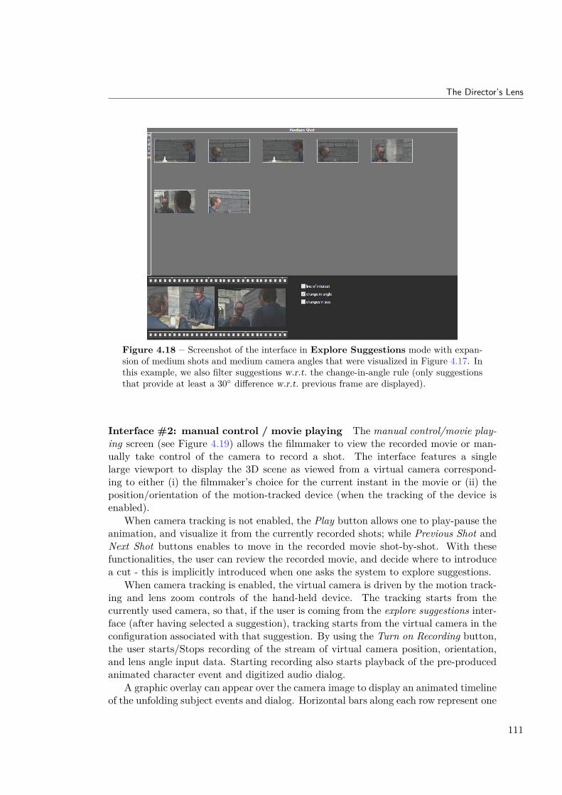
The Director’s Lens
Figure 4.18 – Screenshot of the interface in Explore Suggestions mode with expan-sion of medium shots and medium camera angles that were visualized in Figure 4.17. Inthis example, we also filter suggestions w.r.t. the change-in-angle rule (only suggestionsthat provide at least a 30◦ difference w.r.t. previous frame are displayed).
Interface #2: manual control / movie playing The manual control/movie play-ing screen (see Figure 4.19) allows the filmmaker to view the recorded movie or man-ually take control of the camera to record a shot. The interface features a singlelarge viewport to display the 3D scene as viewed from a virtual camera correspond-ing to either (i) the filmmaker’s choice for the current instant in the movie or (ii) theposition/orientation of the motion-tracked device (when the tracking of the device isenabled).
When camera tracking is not enabled, the Play button allows one to play-pause theanimation, and visualize it from the currently recorded shots; while Previous Shot andNext Shot buttons enables to move in the recorded movie shot-by-shot. With thesefunctionalities, the user can review the recorded movie, and decide where to introducea cut - this is implicitly introduced when one asks the system to explore suggestions.
When camera tracking is enabled, the virtual camera is driven by the motion track-ing and lens zoom controls of the hand-held device. The tracking starts from thecurrently used camera, so that, if the user is coming from the explore suggestions inter-face (after having selected a suggestion), tracking starts from the virtual camera in theconfiguration associated with that suggestion. By using the Turn on Recording button,the user starts/Stops recording of the stream of virtual camera position, orientation,and lens angle input data. Starting recording also starts playback of the pre-producedanimated character event and digitized audio dialog.
A graphic overlay can appear over the camera image to display an animated timelineof the unfolding subject events and dialog. Horizontal bars along each row represent one
111

Integrating Director’s Inputs into the Editing Process
Switch to Suggestions
Interface
Browse recorded shots animated timeline of
screenplay events
start / stop camera
recording
play / pause animation
toggle camera control
Lens zoom
Figure 4.19 – Screenshot of the interface in Manual Control / Movie Playingmode. The overlay horizontal bars show an animated timeline of screenplay events andtheir duration, together with an indication of the camera angle and framing that iscurrently being used in the movie.
subject’s event or dialog. The length of each bar represents the duration of that event.Bars scroll by as the animation plays to indicate the passage of time. This allows thefilmmaker to move the camera at the precise time in anticipation of an upcoming eventor spoken dialog in the screenplay. The overlay also displays the framing properties(e.g. Medium, Low, etc.) of the current camera view.
Figure 4.20 demonstrates an example in which the system suggests shots whichmatch the composition of the user’s previous shot. In this scene, Smith pours gin whileseated facing Syme. The user has composed a shot (shown in the right image in thefigure) in which Smith fills the rightmost third of the frame, gazing to the left andthe camera is located to his left-hand side. Consequently, when we click to enable theline-of-interest filter, the system generates suggestions in which no viewpoints violatethe line-of-interest by placing the camera on Smith’s right-hand side. Furthermore, allviewpoints display Smith on the right-most third of the frame. Also note suggestedcompositions leave more room ahead of Smith’s face, as did the user’s composition.
4.6 Results
Our system is coded in C++ and uses the OGRE real-time rendering engine, and acustom-written abstraction layer to interface to a variety of button and joystick inputdevices and motion trackers. In our tests we used 6dof rigid body reflective markerswith an A.R.T. optical tracker with 16 cameras covering a workspace of 4× 8 meters.The application runs on a computer whose video output is routed over an HDMI cableto the small LCD touch screen. The largest computational cost of the cinematic engineis in finding visibility and Director Volumes, which depend on the geometric complexityof the scene and the variations in position of the key subjects. In the pictured example,the computation of suggestions takes around a second on a Intel Core i7 2.13 GHz
112

The Director’s Lens
Figure 4.20 – Given user’s composition for the current shot (shown in the left image),the system suggests shots (right image) which satisfy continuity rules of editing.
notebook, which is acceptable since this computation is not required to happen inreal-time.
4.6.1 Applicability to Other Scenarios
The examples shown here feature mostly dialog events involving two or three char-acters, and also generic events (e.g. “Parsons walks to the table”) for which propersuggestions are computed. In general, the system can model any event where onecharacter or object, or group of objects (e.g. , cars driving, architectural elements) isinvolved, and propose suggestions to properly frame it using different angles and shotlengths. Note that for many situations (e.g. shooting of architecture, or crowds) thereare not many cinematographic conventions other than using establishing shots first,and then closer shots. However, in general, the cinematography knowledge the systemuses can be expanded by designing additional Director Volumes for specific cases orusing the automatically learned tables of transitions. For situations that involve, in thesame instant, more than three characters, the system could be extended by employingthe method of hierarchical lines of action [KC08].
Scenes involving very fast action can be a bit problematic as the system mightgenerate suggestions that are good for the considered instant, and decrease in qualityafter a short delay, for example because the framed character moves away or is coveredby some moving objects. This kind of situation would require the system either toconsider animations occurring in an interval of time, instead of an instant, or to suggestcamera movements, instead of just starting frames. However, this would be of muchgreater computational cost than deriving suggestions for single instants. In these cases,however, the filmmaker can at worst ignore the suggestions and deal with the situation
113

Integrating Director’s Inputs into the Editing Process
by taking manual control.Finally, the system computes all suggestions using a single fixed lens field of view.
However, the user can quickly adjust the field of view by manual control. The system’ssearch algorithm can be extended by taking into account variations on lens angle. Inpractice, the set of lens angles to consider would be limited to model the cinematographypractice of using a small number of user-selected “prime” or standard lenses.
4.6.2 User Feedback
While we do not currently have results from formal and extensive user evaluations,a few videographers have tried the system, reporting great satisfaction in using it.
In general, users found the system workflow refreshing compared to mouse-basedsolutions, were very willing to try it, and could rapidly use it to produce results. Inour tests, after a very brief introduction to the system, users familiar with cameraworkcould shoot a 3 minutes video of the 1984 scene in around 10-15 minutes, includingtaking decisions on camera angles and cuts. For comparison, producing a video for thesame animation sequence took an expert user a few hours of work using 3DS Max. Thereason for the huge difference in time comes from the fact that with typical animationsoftware tools one is forced to a workflow where cameras have to be manually positionedand animated, and then the shot can be watched, and often one has to go back andforth between cameras modifications and testing the result. Furthermore, there’s thecomplexity of manually keeping track of timings and motion curves, making sure thatedits occur in the correct place and time.
While the use of a motion-tracked virtual camera is surely pivotal in reducing theamount of time needed, we can hypothesize that suggestions also played a role, as ingeneral users needed to make very small movements to refine the suggestions and findtheir ideal starting camera positions. Moreover, from our feedback with professionalsin the development of motion-tracked virtual cameras, we know that having to walkaround in the tracked space to explore angles and distances is perceived as a real issue.Finally, users more experienced in real camerawork appreciated on-screen informationoverlays of character actions and their timing while shooting.
The interface for browsing suggestions by shot size and height was considered easyto learn and effective for a videographer, and the possibility of quickly visualizing manyalternatives was very appreciated, though not all users agreed with each suggestion.This is expected since the perceived quality of a suggestion is a subjective factor,which changes from one videographer to another. However, users’ attitude towards thecinematography engine work was positive, mainly because the system does not forceone to any shooting or editing style, and suggestions can be ignored. However, manytimes, they caused the videographer to consider solutions he had not thought about,thus enhancing creative thinking and exploration.
While a few experiments have been done in combining human expertise with au-tomatic camera planners, we believe this work is the first attempt at innovating theshooting process of CG animations, by providing intelligent and adaptive support increating shots. In the shooting of CG movies, video game cinematic scenes and ma-
114

Discussion and Conclusion
chinima, the system has the potential of making the process much easier and quickerthan current methods. From our early tests, unlike existing automated systems whichrely on pre-coded cinematic knowledge to cover all anticipated scenarios, our interac-tive approach proves effective even if no suggested viewpoint is "perfect" in the user’screative judgment.
5 Discussion and ConclusionIn this chapter, we have introduced a novel framework for virtual cinematography
and editing which adds a cost-driven evaluation of the key editing components. Wehave further proposed two ranking-based approaches to editing a movie, that buildupon the proposed evaluation metrics to assist a filmmaker in his creative process. Wehave introduced an efficient search strategy for finding the best sequence of shots froma large number of candidates generated from traditional film idioms, while providingthe user with some control on the final edit. We further enable enforcing the pace incuts by relying on a well-founded model of shot durations. We have then presented aninteractive assistant whose result is a novel workflow based on interactive collabora-tion of human creativity with automated intelligence. This workflow enables efficientexploration of a wide range of cinematographic possibilities, and rapid production ofcomputer-generated animated movies.
In the last chapters, we have relied on the concept of Director Volumes that pro-vide a good support in representing and solving viewpoints corresponding to a givensub-set of visual composition elements. This space representation is however prone tosome issues: (1) volumes remain expensive to compute, (2) they do not allow mod-eling all composition features, thus necessitating to re-evaluate computed viewpointsw.r.t. other features and (3) enforcing composition features while moving the camera is,as in most existing approaches, difficult to implement with this model. More generally,due to computational cost, all existing automated camera control techniques reduce thesearch of a camera configuration by first searching the camera position, then comput-ing algebraically an orientation corresponding to this camera position. Because of thisreduction, it is really difficult to find a camera configuration satisfying all compositionfeatures; and particularly the exact position of subjects on the screen, as this featureis strongly dependent of the camera orientation.
In the next chapter, we propose and investigate a novel and robust space repre-sentation which, in contrast to existing approaches, allows taking the whole cameraconfiguration (position and orientation) into consideration when searching for a solu-tion camera configuration.
115

5An Efficient Approach to VirtualCamera Control: The Toric Space
As presented in our state of the art, a large range of computer graphics applicationsrely on the computation of viewpoints over 3D scenes that need to display a number ofcharacteristic composition properties (e.g. the on-screen position, size, vantage angle orvisibility of key subjects). Simplified versions have been tackled with straightforwardvector algebra approaches (e.g. within an iterative technique [Bli88]) that compute anapproximate solution. More expressive versions are generally casted as non-linear op-timization problems in a 7 degree-of-freedom search space, i.e. computing the cameraposition, orientation and field of view, given a number of composition properties ex-pressed and aggregated in a single viewpoint quality function which is then maximized.Given the size of the search space and the computational cost in the evaluation of com-position properties (typically the visibility of subjects), this optimization process is atime-consuming task and hampers the use of evolved composition techniques in mostapplications.
An analysis of the problem and current solutions reveals a central issue. Aggregatingquality functions for all the properties reduces the capacities to guide the solving processthrough the search space, therefore leading to techniques which explore large areas ofthe search space without solutions. The specific problem of viewpoint computation istransformed into a general search process for which it is difficult to propose efficientand general heuristics. In the context of a dynamic scene, one generally re-executes thissearch process at each time step. The use of optimization-based approaches thereforelead to variations in the output camera viewpoint, which causes camera stability issues.
In this chapter, we introduce a novel and efficient approach to virtual camera con-trol. Based on a simple parametric model of the camera configurations space, we reducethe search space and consider both the camera position and orientation in the search.We first address an important visual property in virtual camera composition: the speci-fication of exact on-screen coordinates at which key subjects should project. We expressthe solution space for each couple of subjects as a 2D manifold surface. We demon-strate how to use this manifold surface to solve Blinn’s spacecraft problem [Bli88] witha straightforward algebraic approach, and extend the solution to three subjects. Wesecondly extend this parametric model as a novel 3D search space, in which most ofclassical visual properties can be easily expressed. The result is a robust and efficientapproach which finds a wide range of applications in virtual camera control and moregenerally in computer graphics.
117

An Efficient Approach to Virtual Camera Control: The Toric Space
1 ContributionsThe key contributions of this chapter are the following:
The Toric Manifold We provide a novel way to express, in a 2D manifold represen-tation, the solution space of the exact on-screen positioning of two subjects. Wethen provide an algebraic formulation using this manifold which is the first tosolve Blinn’s spacecraft problem [Bli88] without resorting to an iterative tech-nique. We further provide an expression of the on-screen positioning of three ormore targets as a search in a 2D space rather than in a 6D space (as performedin most of the literature).
The Toric Space We provide of a novel 3D search space (that we refer to as ToricSpace), as an extension of the Toric Manifold concept, in which most of classicalvisual properties can be expressed and combined. We show how to computealgebraic solutions, or a good approximation, to expressive composition problems(e.g. on-screen position, vantage angle, distance or projected size of subjects) inthe Toric Space. Furthermore, an inherent properties of our Toric Space is theprovision of a mean to dynamically enforce a set of visual properties on movingsubjects and to perform live editing. Particularly, our work provides the firstmodel that enables expressing, in a simple way, continuity editing rules in 3D.
Combination of expressive visual properties We propose an efficient algorithmto combine a set of expressive visual properties and compute a representative setof solution viewpoints in the Toric Space. As an extension, our algorithm providesa mean to detect potential issues in the application of visual constraints (e.g. aconflict between two or more constraints).
The chapter is organized as follows. Firstly, we show how the exact on-screenpositioning of two subjects can be expressed in a 2D manifold. We show how Blinn’sspacecraft problem [Bli88] can be solved by using this manifold, and how to extend tothree (or more) subjects. Secondly, we show how this model can be extended to a 3Dsearch space so as to tackle more expressive composition problems. We provide theexpression of a range of classical visual properties in this space then show how to tacklethe combination of constraints for a range of applications.
2 Reducing search space in virtual camera compositionBy focusing on the problem of composing two subjects on the screen, our objective
is to show that large regions of the search space can be discarded. For this purpose,we illustrate the quality of the on-screen positioning of two subjects as a 2D heat map.Figure 5.1 presents a 2D topview of a scene comprizing two subjects. Regions aroundthe subjects are colored w.r.t. viewpoint quality (expressed as the distance between thedesired and actual on-screen positions of subjects), from dark red (highest quality) todark blue (lowest quality) through yellow and green (intermediate quality). Note howthe region with highest quality is restricted to a small continuous portion of the whole
118

Tackling exact on-screen positioning of two subjects: The Toric Manifold
search space. In the following section we show that the entire solution set for the exacton-screen positioning problem can be determined with simple mathematical concepts,and that this model serves as a cornerstone for the resolution of more complex cameracomposition problems.
Figure 5.1 – Heat map representing the quality of on-screen composition for two sub-jects (white points) for a region of camera configurations (topview of a the 3D scene).Each colored point represents a camera configuration. Dark red areas are regions ofgood quality viewpoints (i.e. good compositions) while dark blue areas are regions ofbad quality viewpoints. Green regions represent average quality viewpoints. Note thatthe best viewpoints are very local to a given curve around the subjects.
Definition. Let two vectors −→u and −→v . We denote the oriented angle between −→u and−→v asØ�(−→u ,−→v ), and the non-oriented angle between −→u and −→v as
∣∣∣∣Ø�(−→u ,−→v )∣∣∣∣.
3 Tackling exact on-screen positioning of two subjects:The Toric Manifold
In this section, we show that the range of solutions for the exact composition oftwo subjects on the screen is a 2D manifold shaped as a spindle torus (we will referto it as Toric Manifold) and that the manifold can be explored using two meaningfulparameters θ and ϕ (see Figure 5.3). We then use this formulation to easily solveBlinn’s spacecraft problem [Bli88], and show how to generalize the approach to threeand more subjects.
3.1 Solution in 2DWe first provide an intuition of our model by studying the 2-subject on-screen
positioning problem in 2D (i.e. in the plane). In this case the screen dimension is 1D.
119

An Efficient Approach to Virtual Camera Control: The Toric Space
The goal is to find a 2D camera position P such that two subjects of world positions Aand B (A 6= B) project respectively at normalized screen positions pA, pB ∈ [−1; +1],knowing the camera field of view φ. We here assume that A is the left-most subject(i.e. pA < pB).
Theorem. (Inscribed Angle Theorem) The set of points P satisfying Ú�(−−→PB,−→PA) = α
is equal to the arcøAB (excluding A and B) of a circle C of center O passing through
A and B, such that Ú�(−−→OB,−→OA) = 2α (see Figure 5.2). The arcøAB then goes from A toB in the counterclockwise direction, and the radius r of C is equal to AB
2 sinα .
Figure 5.2 – The range of solutions for the exact composition of two subjects A and Bon the screen is displayed in red. The set of points satisfying a given angle α is exactly
the arc÷AB of the inscribed circle centered on O. MoreoverÚ�(−−→OB,−→OA) = 2α.
In our case, α is easily expressed from the on-screen distance between A and B andthe fixed field of view φ. We introduce two points in the camera coordinate system,projecting respectively at pA and pB on the screen:
pcamA
�pAS
; 1�
and pcamB
�pBS
; 1�, with S = tan(φ)
The solution of our 2D problem is then the arcøAB corresponding to α = Û�(−−→pcamB ,−−→pcamA )
To compute the direction vector −→f of our 2D camera, we also know to haveÙ�(−→PA,−→f ) = φ
2 · pA and Ù�(−−→PB;−→f ) = φ
2 · pB
By using the same theorem we know that the line of direction −→f and passing through
P intersects the circle C at a point F such thatÛ�(−−→OB,−−→OF ) = φ· pB, and is tangent to Cwhen points P and F coincide. The camera orientation is thus algebraically determinedfrom the camera position (see Figure 5.2).
120

Tackling exact on-screen positioning of two subjects: The Toric Manifold
As a conclusion, in 2D, the range of solutions to an exact on-screen positioningof two subjects is described with a single angular parameter θ ∈ ]0 ; 2(π − α)[. θ
represents the angle (−−→OP,−−→OB), P being the position of the camera.
3.2 Solution in 3DWe now consider the same composition problem in 3D. The screen dimension is now
2D, and the goal is to find a 3D camera position P such that the two subjects A and B(A 6= B) project respectively at normalized screen positions pA (xA; yA) , pB (xB; yB) ∈[−1; +1]2, knowing the camera field of view φ and its aspect ratio a. Note that φ hererepresents the field of view on the x axis (representing the left-to-right direction on thescreen). We also assume that A is the left-most key subject (i.e. either xA < xB, orxA = xB and yA 6= yB).
(a) (b)
Figure 5.3 – Example of 3D solution set for 2 subjects. Subjects A and B are dis-played resp. in red and green. (a) View of the solution set (a two-dimension para-metric space (θ, ϕ)), for the on-screen projections of A and B, resp. pA (−0.33;−0.33)and pB (+0.33; +0.33). (b) The result obtained from the viewpoint parameterized withθ = π − α
2 and ϕ = π
6 .
As previously, we introduce two points described in the camera coordinate system,projecting respectively at pA and pB on the screen:
pcamAxASx
; yASy
; 1 pcamBxBSx
; yBSy
; 1
with Sx = tan(φ) and Sy = 1a
· tan(φ).Remember the previous section. By considering a plane P defined by the two points
A and B, together with a third point C (not lying on the line (AB)), the solution of
our 3D problem on plane P is a 2D arc AB corresponding to α = (−−→pcamB ,−−→pcamA )
121

An Efficient Approach to Virtual Camera Control: The Toric Space
We therefore have the solution of our problem for an arbitrary plane. Let’s nowconsider that point C is the center of the inscribed circle in P, that we previously calledO. And let point I be the middle of segment AB. Note that, from the definition ofthe solution in 2D, we know to have OI = AB
2 tanα . We build a plane Q, defined by thepoint I and the normal vector −→n = −−→AB. The set of possible positions for O is thenthe circle CO of center I and radius AB
2 tanα defined in the plane Q. This, together withthe solution of our problem in an arbitrary plane containing A and B, defines a uniquesolution set for the camera position. This solution set is a 2-parameter manifold Mshaped like a spindle torus, that we refer to as Toric Manifold (see Figure 5.3).
We now show how to compute the camera orientation that satisfies the composition,assuming a camera position P ∈ M. We first construct an initial camera orientation(quaternion) qi from an orthonormal frame made of three unit vectors: a forward (look-at) vector −→fi , a right vector −→ri , and an up vector −→ui . They are given by
−→ui = −−→PB ×−→PA scaled to unit length
−→fi =
� −−→PB∥∥∥−−→PB∥∥∥ +
−→PA∥∥∥−→PA∥∥∥�
scaled to unit length
−→ri = −→fi ×−→ui
Note that −→ui is normal to the supporting plane P, and that −→fi and −→ri belong to P.The quaternion qi here represents a “default” composition of A and B
(i.e. yA = yB = 0 and xA = −xB). We then compute the rotation (quaternion) qc suchthat, when applied to qi, points A and B project at the appropriate locations on thescreen (i.e. pcamA and pcamB ). qc is computed in a way similar to qi, by replacing −→PA by−−→pcamA and −−→PB by −−→pcamB in the formulas, then computing an orthonormal frame made ofunit vectors fc, rc and uc. The solution camera orientation q is finally given by
q = qi · (qc)−1 (5.1)
Note that qi and qc are algebraically determined from respectively the camera position,and the desired on-screen composition.
As a conclusion, in 3D, the range of solutions (6D camera configurations) to theexact on-screen positioning of two subjects is described with two angular parametersθ ∈ ]0 ; 2(π − α)[ and ϕ ∈ ]− π ; +π]. ϕ represents the angle (in the circle CO) defin-ing the point O; thus defining the supporting plane P. As previously, θ then represents
the angleÛ�(−−→OP,−−→OB) in this plane.In other words, to each 2D point on our Toric Manifold corresponds a unique 6D
camera configuration (position and orientation) satisfying this exact 2-subject on-screenpositioning. The world (Cartesian) coordinates of a given viewpoint P (θ, ϕ) of our Toricmanifold can then be computed in the following way. First, we define the referenceposition O0, that we consider as the center of the inscribed circle for ϕ = 0, such that
122

Tackling exact on-screen positioning of two subjects: The Toric Manifold
−−→IO0 has a z component equal to 0. Second, we compute the vector −→n0 normal to thecorresponding supporting plane P0
−→n0 = −−→O0A×−−→O0B scaled to unit length
Third, we build two quaternions qθ and qϕ as the rotations resp. of θ radians aroundthe axis −→n0 and of ϕ radians around the axis −−→AB scaled to unit length. The positionof P (θ, ϕ) on the manifold is then given by
−→P = −→I + qϕ ·−−→IP0 (5.2)
with P0(θ, 0) (belonging to P0) such that−−→IP0 = −−→IO0 + qθ ·−−→O0B
In the following sections, we show how our model is applied to the resolution ofexact composition problems.
3.3 Application #1: Solution of Blinn’s spacecraft problemThe problem presented by Blinn [Bli88] is similar to the following. Where to put
the camera and how to set its orientation knowing (i) the result on-screen positions oftwo key subjects A and B, (ii) the distance d between the camera and the subject Band (iii) a given vector (a non-null vector −→v starting from B) that must appear verticaland pointing “up” on the screen? An illustration of this problem is given in Figure 5.6.To our knowledge, we here propose the first general technique to compute the exactsolution (or range of solutions) to this on-screen composition problem.
On-screen positioning constraint We can already state that the solution of Blinn’sproblem belongs to a 2D manifold as defined in Section 3.2.
Distance constraint We here make the assumption that α is lower than π/2; wedo not consider wide angle views, but the solution(s) for α ≥ π/2 can be computedwith a similar resolution. By using the analytic solution of the on-screen positioningproblem in 2D (Section 3.1), the distance constraint is quite simple to resolve. Indeed,let’s define a point B′ as the symmetric point to B w.r.t. the center point O of theinscribed circle. We will use the properties between angles and edges in the triangleBPB′ which is rectangle in P . Let’s then define the angle β as
β =Û�(−−→BP,
−−→BB′) = 1
2Û�(−−→OP,
−−→OB′) = cos−1
�d
2r
�Then we can state that there are 0, 1 or 2 solutions to this distance problem:
no solution if d = 0 or d > 2ra single solution if d ∈ ]0 ; AB]: θ = π − 2β
123

An Efficient Approach to Virtual Camera Control: The Toric Space
Figure 5.4 – Illustration of the method used to solve a distance-to-B constraint. Thedistance BP (P being the camera position) is d meters. The segment BB′ is a di-ameter of the inscribed circle of radius r. The angle β = cos−1 d
2r corresponds to
(−−→BP,−−→BB′) = 1
2(−−→OP,−−→OB′). The solution for (−−→OP,−−→OB) is then θ = π ± 2β, with the
restriction that P must lie on the arc AB (in red).
a single solution if d = 2r: θ = πtwo solutions if d ∈ ]AB ; 2r[: θ = π ± 2β
The resolution method is illustrated in Figure 5.4. Each solution θn in 2D works in 3Dsince they are not dependent of the value of the parameter ϕ (vertical angle). Such asolution to the distance constraint can therefore be viewed as a circle Cn lying on theToric Manifold; this circle is such that every point of the circle is at a distance d to B,i.e. this is the set of points P (θ, ϕ) such that θ = θn on the manifold.
“Up” vector constraint In the following, we will assume that the position of thecamera satisfying all the composition constraints is P . As stated above, P belongs toa circle Cn defined by the parameter θ = θn (solution to the distance constraint). Wethen search for the appropriate value of ϕ (if one value exists) such that P (θn, ϕ) issolution to this last constraint.
Let us consider −→u the up vector of the camera (computed from the quaternion q
described in equation Equation 5.1) at position P , and −→w the vector representing −−→PB.Solving Blinn’s problem corresponds to finding a position P on the circle Cn such thatthe two following constraints are satisfied.1. the vector −→v must appear vertical on the screen. This involves that −→u , −→w and−→v are coplanar.
2. −→v must point “up” on the screen. This implies −→u ·−→v > 0.From Equation 5.2, we know that the camera configuration (i.e. its position and
orientation) is defined as a rotation of a reference configuration, in which the camera
124

Tackling exact on-screen positioning of two subjects: The Toric Manifold
position is Pn,0(θn, 0) belonging to the circle Cn, by an angle of ϕ radians around theaxis −−→AB. Our problem is then similar to finding the rotation of ϕ radians around theaxis −−→BA = −−−→AB (scaled to unit length) to apply to the vector −→v such that it appearsvertical and points “up” on the screen when the camera position is set to Pn,0. Insteadof searching the camera position P on the circle Cn, we build a circle C representing therange of possible positions for the extremity of the vector −→v , and look for a positionon C such that the previous property is satisfied.
Before solving this dual problem, let us define three new vectors: −−→un,0 the up vectorof the camera when at Pn,0, −−→wn,0 the vector −−−→Pn,0B, and −→v0 the vector −→v rotated by anangle of ϕ radians around −−→BA (i.e. the solution vector). We then solve the problem asfollows.
We first define a plane P by the point P0,n and a normal vector −→n = −−→u0,n ×−−→w0,n(scaled to unit length). By definition, B belongs to P. We then define a half-planePH ⊂ P delimited by the line L of direction −−→wn,0 passing through Pn,0. The pointsbelonging to PH are located in the direction of −−→un,0. This half-plane defines the set ofvectors starting from B that appear vertical and pointing “up” on the screen when thecamera is positioned at Pn,0.
We then define an other plane Q by a normal vector −→t = −−→AB (scaled to unitlength) and a point F given by −→F = −→B +−→t · |−→v |· cos(π − γ), where γ = (−→t ,−→v )(NB: F belongs to the line (AB)). We then define the circle C as the circle of center Fand radius r′ = |−→v |· sin(π − γ) in the plane Q.
Figure 5.5 – Resolution of Blinn’s spacecraft problem. The vector (in black) startingfrom B must appear vertical and pointing “up” on screen. Subjects A and B are drawnresp. in red and green. The camera position P is a solution to the distance constraint(see Figure 5.4), corresponding to a given value θ = θn, and located at a given verticalangle (ϕ0 = 0) of the manifold. The red circle represents the appearance of −→v dependingon the vertical angle ϕ applied to the viewpoint P . The half-plane (in blue) representsthe set of vectors starting from B that appear vertical and pointing “up” on screen (−→u isthe up vector of the camera when at P , and −→w represents −−→PB). The solution of Blinn’sproblem is given by the intersection (E′) of the half-plane and the circle, and provides amean to compute the rotation ϕ to apply.
125

An Efficient Approach to Virtual Camera Control: The Toric Space
Figure 5.6 – Example solution of Blinn’s spacecraft problem. Subjects A and B aredrawn respectively in red and green. The camera must satisfy desired exact on-screenpositions of A and B, and be d meters away from subject B. An additional constraintis that the vector (in black) starting from B must appear vertical and pointing “up” onscreen.
The solution value of ϕ is finally given by using the intersection(s) of the half-planePH and the circle C. In other words, we compute the solution in a 3-step process:1. we compute the intersection I of PH with Q (none, a half-line or the half-planePH itself);
2. we compute the intersection(s) E′ of I with the circle C in the plane Q;3. the vertical angle ϕ that is solution to our problem is then given by ϕ =Û�
(−−→FE′,
−−→FE).
Figure 5.5 provides an illustration of this geometric resolution, and Figure 5.6 providesan example of solution computed with this method.
By using our method, the overall Blinn’s spacecraft problem (on-screen positioning,distance and “up” vector constraints) is solved algebraically in about 0.01ms per frame.
3.4 Application #2: Solution for three or more subjectsWe now take an interest in the problem of finding a camera configuration satisfying
the exact on-screen positioning of three or more subjects (abstracted as points).This could be viewed as a PnP (perspective n-points) problem. PnP problems
estimate the position (and sometimes the orientation) of an image sensor given theobtained on-screen projection of a well known pattern composed by n points. Forinstance, some techniques have been proposed that use analytic resolutions for problemsinvolving a given number of points (e.g. P3P or P4P problems) [FB81, Hor87, HCLL89,DRLR89] or an iterative resolution for the more general PnP problem [DD95]. However,in PnP problems, one make the strong assumption that at least one solution cameraconfiguration exist. Moreover, such resolutions generally extend the formulation ofFischler and Bolles [FB81] which involves the resolution of a non-linear system. This
126

Tackling exact on-screen positioning of two subjects: The Toric Manifold
requires a lot of computations and thus prevents such resolution techniques from beingusable in interactive applications.
In opposition to PnP problems, we here start from a desired (but not necessarilyfeasible) on-screen positioning of independent 3d world points (i.e. subjects). As aconsequence, there is no guarantee (at least for more than three subjects) that an exactsolution camera configuration exist. Moreover, in our case we do not need the overallon-screen positioning to be exact. Actually, in a cinematic context, there are commonlyone or two main subjects which the director wants to position precisely on the screenand a set of secondary subjects that can be positioned in an more flexible way. Inorder to account for these two preconditions, in the following, we propose a novel andefficient method based on our manifold concept to estimate a camera viewpoint for the“cinematic” on-screen positioning of three or more subjects.
Notice that the on-screen positioning approach we have presented for two subjects isalso extensible to three or more subjects. Indeed, let consider the case of three subjectswith world positions A, B, C (different from each other). As stated earlier, the solutionset for each pair of subjects is a 2D manifold. Consequently, the camera configurationP satisfying this 3-subject composition must verify two conditions:
the camera position P must be at the intersection of three manifoldsM,M′ andM′′ respectively defined by couples (A,B), (B,C) and (A,C);the camera orientation corresponding to P must match for this three manifolds.
This defines three angles α, α′ and α′′ corresponding to resp. M, M′ and M′′.Similarly, we define three quaternions q, q′ and q′′ as the orientations (defined as unitquaternions) at a given 3D point P , as defined respectively onM,M′ andM′′. If forinstance P belongs toM, then it verifies the following manifold equation:Ú�(−−→PB,−→PA)− α = 0 (5.3)
We here propose an algorithm which searches, on the surface of one manifold M,the configuration which maximizes the viewpoint quality (defined as a distance to theother manifolds). Typically the on-screen position of two subjects is fixed, and weoptimize the on-screen position of the third subject. The cost function to minimize isthen
dminθ,ϕ
�∣∣∣∣∣Û�(−−→PC,−−→PB)− α′∣∣∣∣∣+
∣∣∣∣∣Ú�(−−→PC,−→PA)− α′′∣∣∣∣∣+ ∣∣∣1− ⟨q′, q′′⟩2∣∣∣�
where 〈q′, q′′〉 denotes an inner product of q′ and q′′, providing a measure of the anglebetween them ranging from −1 (opposite orientations) to +1 (same orientation). Thiscost function is illustrated with a heat map in Figure 5.7. The solutions of an example3-subject composition problem are displayed in Figure 5.8.
The main advantage of this technique is that it can easily extend to more thanthree subjects. Though the composition may not be strictly satisfied, it enables fixingthe on-screen position of two (main) subjects, then optimizing the position of othersubjects.
127

An Efficient Approach to Virtual Camera Control: The Toric Space
We used this method on both a 3-subject and a 4-subject on-screen positioningproblem. In our test, we approximated the 3-subject exact composition in about 0.10msper frame and we minimized the 4-subject composition error in about 0.42ms per frame.
(a) (b)
Figure 5.7 – Heat map drawn on one of the manifolds. The cost function representsthe sum of the distance to the two other manifolds. Red: points close to both othermanifolds (drawn in blue and green), thus verifying the on-screen positioning of the 3subjects. Blue: points farest to both other manifolds. Green: intermediate-distancepoints. (a) 3D view of the manifolds and of the heat map; (b) view of the heat mapwhen the manifold is unfolded.
(a) (b)
Figure 5.8 – Two solutions of the exact on-screen positioning of three subjects A (red),B (green) and C (blue). Their respective on-screen positions are pA(−0.50; +0.25),pB(−0.25; +0.50) and pC(+0.25; +0.50). These solutions correspond to the intersectionof three solution set (described in Figure 5.7), each solving the exact on-screen positioningof two of the subjects.
In this section, we investigated the algebraic solution to the exact two-subject on-screen positioning problem. We showed that it corresponds to a 2D manifold surface.We showed how, by using this manifold, to solve Blinn’s spacecraft problem without
128

Tackling more evolved on-screen composition problems: The Toric Space
resorting to an iterative algorithm; and how the on-screen positioning problem for threeor more subject can be cast into a search in 2D. In the next section, we investigatemore expressive composition problems in which a degree of relaxation on constraints isnecessary so as not to restrict to much the possibility of finding an overall solution tothe problem (by avoiding conflicts between constraints as much as possible).
4 Tackling more evolved on-screen composition problems:The Toric Space
In this section, we extend the concept of Toric Manifold to a 3-dimensional searchspace (α, θ, ϕ) that we will refer to as Toric Space. This space represents the set of ToricManifolds that may be generated around a pair of subjects (A,B). The parameter α isthe manifold generator (which depends on both the field of view and the aspect ratio ofthe camera), and the pair (θ, ϕ) represents a unique position on a given manifold. In thefollowing we will show that a number of classical constraints related to virtual cameracomposition are easier to manipulate in our Toric Space (3 angular parameters) than inthe classical 6D camera space (3 Cartesian coordinates and 3 Euler angles). Illustrationof Toric Manifold and Toric Space are given resp. in Figure 5.9 and Figure 5.10.
Figure 5.9 – Toric Manifold. To a given on-screen positioning of two subjects (red angreen boxes) corresponds a unique angle α that generates such a manifold. Any point ofthis 2D manifold then represents a 6D camera configuration (position and orientation)satisfying this exact on-screen positioning.
Note that imposing conflicting constraints can prevent from finding an appropri-ate camera configuration, satisfying a set of exact visual features. Consequently, wehereafter consider composition problems in which there is a degree of relaxation in theapplication of constraints. In our approach the relaxation is represented as a range ofaccepted values for each feature.
In the next section, we compute solutions to constraints that are independent ofthe geometry of both the surrounding environment and of subjects (e.g. vantage an-gle, distance, on-screen positioning), together with good approximations to constraintssuch as visibility or projected size of subjects. We will then show how, by using in-terval analysis techniques, such computations in the Toric Space greatly improve the
129

An Efficient Approach to Virtual Camera Control: The Toric Space
Figure 5.10 – Representation of our Toric Space (3D extension of the Toric Manifoldconcept) in an orthogonal coordinate system. Here, there are however two singularities:(1) the two planes ϕ = ±π (top/bottom) are actually indistinguishable, and (2) the threeplanes θ = 0, α = 0, and α = π− θ2 (sides) represent the set of forbidden configurations.
placement of a virtual camera in a range of computer graphics applications.
5 Expressing classical visual constraints in the Toric SpaceWe here show how we express visual constraints in the Toric Space as 2D solution
sets. In our process, two planes of the Toric Space appear useful: the plane (θ, α) andthe plane (θ, ϕ). Note that a 2d solution set in the plane (θ, α) do not depend on thevalue of ϕ. Conversely, a solution set in the plane (θ, ϕ) will strongly dependent of thevalue of α. Indeed, there is a straightforward relationship between the parameter αand the maximum value the parameter θ can take:
0 < θ < 2(π − α)
We here introduce two additional angular parameters: β, β′ ∈ [0, π] (see Figure 5.11).β represents the angle between the vector −−→AB and a vector −→a whose origin is A anddestination is P . In the same way, β′ represents the angle between the vector −−→BA anda vector −→b whose origin is B and destination is P . As illustrated in Figure 5.11, in2D, iff (β + β′) ∈ ]0, π[ then the line passing through A and of direction −→a and theline passing through B and of direction −→b intersect on the manifold generated by theangle α = π − (β + β′). Moreover the coordinate θ corresponding to the intersectionpoint on this manifold is given by (inscribed angle theorem)
θ = 2β = 2(π − α− β′) (5.4)
For practical reasons, we will then first solve a number of constraints related to respec-tively A or B in a virtual plane (β∗, ϕ), where β∗ represents resp. β or β′. Second, wewill extend the resulting solution into the plane (θ, ϕ) by using the Equation 5.4, thencombine the computed solutions for both A and B (an example of such combination isillustrated in Figure 5.18).
130

Expressing classical visual constraints in the Toric Space
Figure 5.11 – There is a straightforward relationship between the parameter α and theparameter θ (0 < θ < 2(π − α)). In the same way, if we consider one line passing throughA and of direction a vector −→a (making an angle β with −−→AB), and one line passing throughB and of direction a vector −→b (making an angle β′ with −−→BA), then iff (β + β′) ∈ ]0, π[then these two lines intersect on the manifold generated by the angle α = π − (β + β′).Furthermore, the coordinate θ of this intersection is given by θ = 2β = 2(π − α− β′).
5.1 On-screen positioningWe here consider a more flexible positioning constraint for both subjects. We want
each subject (A and B) to project in a known convex shape expressed in the screen-space, that we will refer to them resp. as sA and sB (see Figure 5.13c). We thenlook for a set of camera configurations (position and orientation) that satisfies thisconstraint. For practical reasons, in the following, we will handle the camera positionand orientation separately.
Camera position At this point, we first use a scanning algorithm on both shapes.We sample points on both shapes, then compute the angle α (with our previous method,presented in Section 3.2) for every couple of a point on sA and a point on sB. Since sAand sB are convex shapes, this allows computing a range rα = [αmin, αmax] of possibleangles α satisfying the constraint of having one subject projecting inside sA and theother subject projecting inside sB. The solution of the relaxed 2-subject on-screenpositioning problem therefore corresponds to a horizontal strip in the plane (θ, α), asshown in Figure 5.12.
Camera orientation We here consider the camera position is set to PT (α, θ, ϕ),computed so as to satisfy the previous condition (α ∈ rα). For a given angle α ∈ rα,
131

An Efficient Approach to Virtual Camera Control: The Toric Space
Figure 5.12 – The on-screen positioning of two subjects inside convex shapes corre-sponds to a horizontal strip α ∈ [αmin, αmax] in the plane (θ, α).
there are however an infinite number of orientations, satisfying the on-screen positioningof A and B or not. We here propose a 3-step method to compute an appropriate cameraorientation.
Step 1: we compute a first orientation q1 that guarantees the satisfaction of theon-screen positioning constraint. We first consider two pairs of points Pmin(pmin
A , pminB )
and Pmax(pmaxA , pmax
B ). They correspond to the points of sA and sB that respectivelygenerate the angles αmin and αmax. We then define two points, pCA and pCB, as thebarycenter of resp. sA and sB. We finally use a dichotomy algorithm to search forappropriate on-screen positions pA and pB in resp. sA and sB. We consider Pmin
as minimum value, Pmax as maximum value and Pi(pCA, PCB ) as initial value. Thedichotomous process is stopped when the angle get close enough to the subject valueα. An example of computed orientation is given in Figure 5.13a.
Step 2: we compute the orientation q that minimizes the roll angle of the camera.To this end, we first construct a “default” orientation qd (i.e. such that pA = −pB)from an orthonormal frame, made of three unit vectors −→r (right vector), −→f (forwardvector) and −→u (up vector). −→f (xf , yf , zf ) is computed as follows:
−→f =
−−−→PWA∥∥∥−−−→PWA
∥∥∥+−−−→PWB∥∥∥−−−→PWB
∥∥∥scaled to unit length
where PW is the world position corresponding to PT . We then define a vector−→f ′ (xf , yf , 0) as the projection of −→f along the z direction. The right vector is then de-fined as −→r = qr ·
−→f ′ , where qr is the rotation of −pi
2 radians around the axis −→z (0, 0, 1);and the up vector is defined as −→u = −→r × −→f . We secondly compute the rotation toapply so as to have the camera viewpoint centered on the barycenter of shapes sA andsB. We define two points, PO(0, 0) the origin of the screen and pM (xM , yM ) the middle
132

Expressing classical visual constraints in the Toric Space
point between pCA and pCB. We construct two 3d points in the camera coordinate system:p3O and p3
M , representing points that project resp. at pO and pM on the screen.
p3O(0, 0, 1) and p3
M
�xMSx
,yMSy
, 1�
scaled to unit length
We then define qm as the rotation of angle∣∣∣∣(−→p3
O,−→p3M )∣∣∣∣ around the axis −→m =
−→p3M×−→p3O. The
orientation q2 of the camera is then built as q2 = qd · qm. An example of computedorientation is given in Figure 5.13b. Note that this orientation does not necessarilyguarantee that A and B project resp. in sA and sB.
Step 3: we combine the two previously computed orientation, so as to get a cameraorientation q that guarantees A and B to project in sA and sB, while minimizing theroll angle of the camera. To do so, we use a dichotomous process between q1 andq2 (through the use of the “Slerp” function to compute an interpolated orientation).The dichotomous process is stopped when the current positions pA and pB belong toresp. sA and sB. An example of computed orientation is given in Figure 5.13c.
The advantages of our method are fourfold: (i) it provides a fast orientation com-putation, (ii) a unique solution orientation can be computed for any position in thesolution set – in particular, our computation algorithm prevents camera jerkiness –,(iii) the computed orientation minimizes the camera roll angle and (iv) it preservescontinuity of the camera orientation in the space of possible camera positions.
5.2 Projected SizeWe here consider a constraint on the projected size (size in terms of ratio of the
screen area) of a subject, as an interval of accepted sizes [smin, smax]. We then searchthe set of camera configurations for which the projected size of the subject belongs tothis interval. Note that the solution set of a projected size is one of the most complicatedto solve. Indeed, such a solution set is strongly dependent of the shape of the subject.Consequently, to our knowledge, previous work has mainly focused on sampling-basedmethods in a 6D search space. We here propose to compute an approximated solutionset, through a 2-step computation. To do so, we first make a strong assumption: weconsider that the subject is abstracted as a bounding sphere S of a given radius r.
5.2.1 Naive resolution
We here assume the camera is set at a given position and is oriented so that thesubject is centered at the origin of the screen. The projection of the sphere S on thescreen corresponds to an ellipse of parameters a and b, computed as follows:
a = r·Sxd
and b = r·Syd
where d represents the distance between the camera and the subject. The projectedsize of the subject (i.e. the area of the ellipse in terms of frame ratio, the frame being
133

An Efficient Approach to Virtual Camera Control: The Toric Space
(a)
(b)
(c)
Figure 5.13 – Computation of the camera orientation for a given camera position.The on-screen positioning of the two subjects is here expressed as two convex areas(red and green ellipses) of the screen. (a) step 1: we compute a first orientation thatguarantees that the center of each subject projects in the proper area; (b) step 2: wecompute algebraically the orientation that minimizes the roll angle of the camera (ψ = 0,see Figure 2.6); (c) step 3: by using a dichotomy between these two orientations, wecompute the final camera orientation that satisfies the on-screen positioning constraintwhile minimizing the roll angle of the camera.
of area 4) is then given by
4s = π· r2 ·Sx ·Syd2
Starting from this formula, we then compute the reverse solution, which provides thedistance d at which to position the camera depending on the projected size of theabstracted subject
d = r
Êπ·Sx ·Sy
4s
134

Expressing classical visual constraints in the Toric Space
To consider the range of projected size [smin, smax], one must then consider thecorresponding approximate range of distance [dmin, dmax], where the distances dminand dmax correspond resp. to projected sizes smax and smin. This calculation providesa naive resolution of the interval [dmin, dmax]. With this interval, we can reduce therange of possible values for the parameter θ; this can further be applied for bothsubjects. The projected size is however dependent of on-screen position of the subject.
5.2.2 A more accurate approximation
We here consider that the subject projects at position p(x, y) on the screen (forinstance a position belonging to sA or sB). The projection of the sphere on the cam-era plane (i.e. before applying the projection component) corresponds to an ellipse ofparameters a and b, computed as follows:
a = sin γ cos γ| cos2 λ− sin2 γ|
and b = sin γÈ| cos2 λ− sin2 γ|
with cosλ =
�Ìx2
S2x
+ y2
S2y
+ 1
�−1
and γ = atan�r
d
�The projected size of the subject is then given by s = (π· a· b)÷ 4
Sx ·Sywhere the
left-most part represents the area of the ellipse, and the right-most part represents thearea of the rectangle representing the frame limits on the camera plane.
The distance d at which to position the camera can then be solved by using adichotomous search. We start the search from a close neighborhood of the value com-puted with the naive resolution process, and we stop the search when the error on thesize gets under a given threshold ε.
We have proposed a method to convert a range [smin, smax] of projected size intoan approximate range [dmin, dmax] of distance at which to place the camera. In thefollowing section, we investigate the resolution of a distance constraint, which we couldthen use for computing an appropriate camera configuration.
5.3 Distance
We here consider a constraint on the distance between the camera and a subject,as an interval of accepted distance. We then search for the set of camera positions,expressed in the Toric Space, that are at an acceptable distance from the subject. Wesolve such a constraint in the plane (θ, α). We first show how to solve a single strictdistance constraint (i.e. to a single subject). We then show how to compute the solutionset corresponding to a range of distance between the camera and a single subject, thento a (possibly different) range of distance for both subjects.
135

An Efficient Approach to Virtual Camera Control: The Toric Space
5.3.1 Single distance
Distance to A. Let first consider a strict distance constraint dA to A. We have,∀θ ∈ ]0, 2π[,
α = acos
�dA −AB· cos(θ/2)È
d2A +AB2 − 2 ·AB· dA · cos(θ/2)
�(5.5)
See Figure 5.14a for illustration and Figure 5.15a for an example (red curve).
Distance to B. Let now consider the strict distance constraint dB to B. There aretwo cases to consider here: dB ≤ AB and dB > AB.
Case dB ≤ AB: we have, ∀θ ∈�0, 2 asin
�dBAB
��,
α = π
2 ± acos�AB
dB· sin�θ
2
��(5.6)
Note that in the particular case dB = AB, the upper bound of θ (i.e. π) will beexcluded.
Case dB > AB: we have, ∀θ ∈ ]0, 2π[,
α = π
2 − acos�AB
dB· sin�θ
2
��(5.7)
See Figure 5.14b for illustration and Figure 5.15b for an example (green curve).
5.3.2 Range of distance
Range of distance to A. Let consider a range of distance rA = [dAmin, dAmax]. The
solution set is the interval
IAα (θ) = [αAmax(θ), αAmin(θ)]\{0, π}
where αAmin(θ) (resp. αAmax(θ)) is determined by injecting dAmin (resp. dAmax) in Equa-tion 5.5.
Range of distance to B. Let consider a range of distance rB = [dBmin, dBmax]. The
solution set is the interval
IBα (θ) = IBα,max(θ)− IBα,min(θ)
where IBα,min(θ) (resp. IBα,max(θ)) is determined by injecting dBmin (resp. dBmax) in theEquation 5.6 or 5.7.
As a conclusion, when constraining the camera by the two ranges of distance rAand rB, the solution is then the interval
Iα(θ) = IAα (θ) ∩ IBα (θ)
136

Expressing classical visual constraints in the Toric Space
(a)
(b)
Figure 5.14 – Illustration of the resolution of a strict distance constraint in the plane(θ, α). We express the solution value(s) of α for a given value of the angle θ. (a)Resolution of a strict distance dA to subject A. (b) Resolution of a strict distance dB tosubject B.
5.4 Vantage angle
The vantage angle constraint corresponds to a relative angle w.r.t. to a given subject.For instance, if we want to see a car from front with a high angle, this constraint canbe expressed as a direction vector from the car. More generally, a vantage angle canbe represented as a half-line of origin the subject (A or B) and direction vector −→v .To relax this constraint, we here further consider a range of accepted directions in theform of a maximum deviation to this reference direction; we represent such a constraintas a vantage cone, of directrix −→v and half-angle γ (the maximum accepted deviation).The solutions then belong to this cone. We hereafter show how to express, in theToric Space, the set of camera positions that satisfy a single vantage angle constraint
137

An Efficient Approach to Virtual Camera Control: The Toric Space
(a) Distance to A (b) Distance to B
(c) Solution to both distance constraints (A and B)
Figure 5.15 – Solution set corresponding to a camera in a range of distance to Aand/or B. (a) Solution camera positions for a distance to A in [5, 10] (white area);red curves correspond to the bounding values of the interval of distance. (b) Solutioncamera positions for a distance to B in [4, 8] (white area); green curves correspond tothe bounding values of the interval of distance. (c) Solution camera positions for thesatisfaction of both ranges of distance to resp. A and B.
(w.r.t. either A or B). We then show how to solve the set of camera positions satisfyingmultiple vantage constraints (w.r.t. to both A and B) in the Toric Space.
5.4.1 Resolution for one subject
We here focus on a single vantage angle constraint. For generalization purposes,we will refer to the concerned key subject (either A or B) as K, and to the other keysubject as K ′; the set of camera positions satisfying the vantage angle, with maximumdeviation γ, is the then set of points inside a vantage cone of apex K, direction −→vand half-angle γ. Note that the directrix −→v can be parameterized as a couple (λ, ϕv),where λ is the angle between vectors −→v and
−−→KK ′ (λ ∈ [0, π]) and ϕv represents the
plane supporting −→v .In this section, we show how to solve the set of camera positions satisfying such a
vantage angle constraint algebraically in the Toric Space; and more particularly in theplane (β∗, ϕ) – β∗ represents either β or β′ (see Figure 5.11).
138

Expressing classical visual constraints in the Toric Space
Let first introduce three planes whose normal vector −→n =−−→KK ′
KK ′:
Pβ∗<π/2, Pβ∗=π/2 and Pβ∗>π/2
They are built such that Pβ∗<π/2 contains the point K + −→n , Pβ∗=π/2 contains thepoint K itself, and Pβ∗>π/2 contains the point K −−→n . That is, a vector −→a (resp. −→b )intersect with them iff β∗ is respectively lower than, equal to or greater than π
2 .Remember that the intersection of a cone and a plane is a conic; it can be either an
ellipse (a particular case is the circle), a parabola, or a hyperbola. As a consequence, wehere propose to use equations of conics to compute either the range of possible valuesfor ϕ in function of the value β∗, or the range of possible values for β∗ in function ofthe value ϕ.
Figure 5.16 – Computation of the vantage function in the space (β, ϕ) in the case ofan ellipse. We intersect the ellipse with a circle of radius r = tan(β) = tan(θ/2), thencalculate the corresponding values of ϕ as ϕ = ± atan(y/x). This process is basicallythe same in case of a parabola or hyperbola.
In a first step, we will assume γ ∈ 0, π2 . We will also assume that −→v belongs tothe half-plane ϕv = 0. We will consider the general case afterwards. Here is the detailof resulting conics in function of λ and γ:
Pβ∗<π/2 Pβ∗=π/2 Pβ∗>π/2
λ = 0 circle ∅ ∅
0 < λ ≤ π/2 λ+ γ < π/2 ellipse ∅ ∅λ+ γ = π/2 parabola single line ∅
0 < λ ≤ π/2 λ+ γ > π/2 hyperbola two lines hyperbolaπ/2 ≤ λ < π λ− γ < π/2
π/2 ≤ λ < πλ− γ = π/2 ∅ single line parabolaλ− γ > π/2 ∅ ∅ ellipse
λ = π ∅ ∅ circle
139

An Efficient Approach to Virtual Camera Control: The Toric Space
Note that the second half of this table is obtained by symmetry with the first half,by replacing both λ by π−λ and β∗ by π−β∗ in the different cases. In the following wewill only consider the first half of the table and solve each case separately. We hereafterdetail the two possible resolutions of the vantage angle. In any case, one will only useone of them, depending on the need.
Resolution 1: ϕ in function of β∗ To express the frontier of the vantage cone inthe Toric Space, as a function Iϕ(β∗) – the interval of possible values of ϕ such thatany point (β∗, ϕ) belong to the cone – we will compute the intersection(s) I(x, y) ofthe given conic section C with a circle C′ of center (0, 0) and radius r, with r = tan β∗.The equation of C′ is given by x2 + y2 = r2
We will then resolve the maximum angle ϕ as
ϕ ∈�− atan
�y
x
�,+ atan
�y
x
��In the following cases, the range of values of β∗ that need a resolution is given byβ∗inf = max(λ− γ , γ − λ) and β∗sup = min(λ+ γ , 2π − (λ+ γ)).
Moreover, here are the solution ranges Iϕ when β∗ /∈ [β∗inf , β∗sup]:β∗ < β∗inf β∗ > β∗sup
λ− γ < 0 [−π; +π]λ− γ ≥ 0 ∅λ+ γ ≤ π ∅λ+ γ > π [−π; +π]
Resolution 2: β∗ in function of ϕ To express the frontier of the vantage cone inthe Toric Space, as a function Iβ∗(ϕ) – the interval of possible values of β∗ such thatany point (β∗, ϕ) belong to the cone – we will compute the intersection(s) I(x, y) of thegiven conic section C with a half-line L of origin (0, 0) and direction −→d (cosϕ, sinϕ).
When ϕ 6= ±π2 , the equation of L is
y = tanϕ·x, with sign(x) = sign (cosϕ)
When ϕ = ±π2 , L is defined as(x, y) s.t. x = 0 and
y ∈ R+ if sinϕ > 0
y ∈ R− if sinϕ < 0
We then compute the bounds of the corresponding range of β∗ as
β∗ = atan(È
x2 + y2)
An illustration of these two resolutions is given, for the ellipse, in Figure 5.16. Wewill now focus on each case of conic section separately and proper solutions for them.
140

Expressing classical visual constraints in the Toric Space
5.4.2 Ellipse
The conic section (ellipse) C is defined by its center C(xc, 0), its major radius a andits minor radius b, defined as follows
a = sin γ· cos γ| cos2 λ− sin2 γ|
b = sin γÈ| cos2 λ− sin2 γ|
xc = sinλ· cosλcos2 λ− sin2 γ
The equation of C is here (x− xc)2
a2 + y2
b2= 1
Resolution 1: Iϕ(β∗) The intersections I(x, y) are computed by solving the followingsystem Ax
2 +Bx+ C = 0
y =√r2 − x2
with A = b2 − a2, B = −2b2xc, C = b2x2c + a2(r2 − b2).
Resolution 2: Iβ∗(ϕ)
Case ϕ 6= ±π2 . The intersections I(x, y) are computed by solving the following system
Ax2 +Bx+ C = 0
y = tanϕ·x
with A = b2 + a2 tan2 ϕ, B = −2b2xc, C = b2(x2c − a2).
Case ϕ = ±π2 . The solution intersection I(x, y) is given by
x = 0
y = sinϕ· b
a
Èa2 − x2
c
Moreover, when γ ≤ λ, the extreme values of ϕ are reached when∆ = B2 − 4AC = 0, i.e.
Iϕ ⊆
− atan
�√b2
x2c − a2
�; + atan
�√b2
x2c − a2
�Otherwise (γ > λ), Iϕ ⊆ [−π; +π].
141

An Efficient Approach to Virtual Camera Control: The Toric Space
5.4.3 Circle
When λ = 0, the conic section (circle) C is here a special case of ellipse. The radiusof C is then r′ = a = b = tan γ, and its center is C(0, 0). In this case, the only possibleintersection between C and C′ is when r = r′. In the same way, the intersection betweenC and L is always I(tan γ· cosϕ, tan γ· sinϕ). Thus, the solution to both resolutionsis trivial: it corresponds to the line of equation β∗ = γ, for all ϕ ∈ [−π; +π].
5.4.4 Parabola
The conic section (parabola) C is defined by its vertex V (h, 0), and its focal lengthf defined as follows
h = tanλ− cotλ2
f = cotλ2
The equation of C is here y2 = 4f(x− h)
Resolution 1: Iϕ(β∗) The intersections I(x, y) are computed by solving the followingsystem Ax
2 +Bx+ C = 0
y =√r2 − x2
with A = −1, B = −4f , C = 4fh+ r2.The intersection with the intermediate plane will moreover be a single line. It
corresponds to the angle β∗ = π
2 , and the associated range Iϕ is {0}.
Resolution 2: Iβ∗(ϕ)Case ϕ 6= ±π2 . The intersections I(x, y) are computed by solving the following systemAx
2 +Bx+ C = 0
y = tanϕ·x
with A = tan2 ϕ, B = −4f , C = 4fh.Case ϕ = ±π2 . The solution intersection I(x, y) is given byx = 0
y = sinϕ· 2√−fh
Moreover, when γ ≤ λ, the extreme values of ϕ are reached when∆ = B2 − 4AC = 0, i.e.
Iϕ ⊆[− atan
(Êf
h
); + atan
(Êf
h
)]
142

Expressing classical visual constraints in the Toric Space
Otherwise (γ > λ), Iϕ ⊆ [−π; +π].
5.4.5 Hyperbola
The conic section (hyperbola) C is defined by its vertex V (xv, 0), its major radiusa, and its minor radius b, defined as follows
a = sin γ· cos γ| cos2 λ− sin2 γ|
b = sin γÈ| cos2 λ− sin2 γ|
xv = sinλ· cosλcos2 λ− sin2 γ
The equation of C is here (x− xv)2
a2 − y2
b2= 1
Resolution 1: Iϕ(β∗) The intersections I(x, y) are computed by solving the followingsystem Ax
2 +Bx+ C = 0
y =√r2 − x2
with A = b2 + a2, B = −2b2xv, C = b2x2v − a2(r2 + b2).
Resolution 2: Iβ∗(ϕ)
Case ϕ 6= ±π2 . The intersections I(x, y) are computed by solving the following systemAx2 +Bx+ C = 0
y = tanϕ·x
with A = b2 − a2 tan2 ϕ, B = −2b2xv, C = b2(x2v − a2).
Case ϕ = ±π2 . The solution intersection I(x, y) is given byx = 0
y = sinϕ· b
a
Èx2v − a2
Moreover, when γ ≤ λ, the extreme values of ϕ are reached when∆ = B2 − 4AC = 0, i.e.
Iϕ ⊆
− atan
�√b2
a2 − x2v
�; + atan
�√b2
a2 − x2v
�Otherwise (γ > λ), Iϕ ⊆ [−π; +π].
143

An Efficient Approach to Virtual Camera Control: The Toric Space
5.4.6 Generalization
In the general case (i.e. ϕv 6= 0), these resolutions will serve as a basis to computethe actual solution. Indeed, the remaining operation is to shift the resulting range Iϕfrom ϕv upward. The actual solution with this offset is then obtained by replacing ϕby ϕ− ϕv in the resolutions above.
Note that, in the particular case of γ = π
2 , the cone bounds will represent a plane
and the solution set will then be a half-space. We furthermore study the case γ > π
2 .In this case, the solution will then be given by considering the exclusion of the conewhose axis is opposite to the vantage vector and such that its half-angle γ′ and γ arecomplementary angles (they sum to π). This cone is then parameterized as λ′ = π−λ,γ′ = π − γ and ϕv′ = π − ϕv.
Examples of solutions for various vantage angles are given in Figure 5.17.
(a) γ ≤ π/6 (b) γ ≤ π/3 (c) γ ≤ 5π/6
Figure 5.17 – Solution range of a vantage angle, for a given direction vector anddifferent values of the half-angle γ of the vantage cone. In the examples, the directionvector of the vantage cone is parameterized by λ = π
4 and ϕv = 0. In each case, thewhite area represent the set of couples (β∗, ϕ) satisfying the vantage angle.
5.4.7 Intersection for both A and B
We here consider the combination of two vantage angle constraints: one relativeto A and one relative to B. Its solution is located at the intersection of both vantagecones. In order to find the set of camera positions satisfying both constraints, lets takea look at a section of the Toric Space at a given height ϕ ∈ IAϕ ∩ IBϕ . We compute theranges Iβ(ϕ) w.r.t. A and Iβ′(ϕ) w.r.t. B. We then build the functions that projectthe ranges of solution for A and B in the plane (θ, α), i.e. depending on the value ofα. To do so, we use the Equation 5.4. Resulting functions are of the form
θAi (α) = 2βiθBj (α) = 2(π − α− β′j)
where θAi (α) and θBj (α) are relative to respectively the range of vantage angle of A andB. The intersection of two such functions is then the point at which these functions
144

Combining Constraints
are equal, i.e.θi,j = θi, and αi,j = π − βi − β′j
The solution of such a combination of vantage constraints is then, for a given value ϕ,a set of parallelograms in the plane (θ, α), as illustrated in Figure 5.18; and the entiresolution is given by the integration of such intersections for all possible values of ϕ.
Figure 5.18 – Intersection, for a section at a given height ϕ, of the solution sets forboth a vantage angle w.r.t. A and a vantage angle w.r.t. B. The set of solution couples(θ, α) for each section corresponds to a set of parallelograms (in yellow).
6 Combining ConstraintsWe hereafter detail the general process we propose to solve the entire set of con-
straints. Our process is made of three consecutive steps, and enables computing therange of overall solutions in terms of positions (α, θ, ϕ).
Step 1 We compute the interval Iϕ = IAϕ ∩ IBϕ range of ϕ, for which there ispotentially an intersection of both vantage angles. By default IXϕ is set to [−π; +π].
Step 2 For all ϕ ∈ Iϕ, we compute the ranges (i.e. one or more intervals) IAθ (ϕ)and IBθ (ϕ) corresponding to the ranges of values of θ such that (θ, ϕ) is solution to thevantage angle of resp. A and B. We then define the range Iθ(ϕ), for which there ispotentially a solution to the intersection, as Iθ(ϕ) = IAθ (ϕ) (see Figure 5.18).
Step 3 For all θ ∈ Iθ(ϕ), we compute:IV ANTα (θ, ϕ), the range of values of α corresponding to the satisfaction of vantageangles for both subjects.IDISTα (θ), the interval of values of α corresponding to the satisfaction of distanceconstraints for both subjects.IOSPα , the interval of values of α corresponding to the satisfaction of the on-screenpositioning of both subjects.
145

An Efficient Approach to Virtual Camera Control: The Toric Space
We then compute the interval Iα(θ, ϕ) corresponding to the satisfaction of all con-straints as
Iα(θ, ϕ) = IV ANTα (θ, ϕ) ∩ IDISTα (θ) ∩ IOSPα
This provides a general mean to solve the range of solution coordinates (α, θ, ϕ). Inaddition, it provides a mean to check, at each step, issues in the application of con-straints (e.g. unsolvable constraints, or conflicts between two or more constraints) bysimply intersecting their solution intervals w.r.t. α, θ or ϕ.
An obvious way to compute the range of solutions would be to rely on intervalanalysis techniques and interval-based constraint solving. Such techniques provide anapproximation of the inner and outer limits of the solution as boxes (in the solution,out of the solution and on the frontier of the solution). However, the computationalcost of these techniques, coupled with the necessity to carefully control each step ofthe solving process led us to favor a progressive sampling technique. This efficientsampling-based technique computes a representative set of solution viewpoints. To doso, at each step, we use a sampling density (resp. dϕ, dθ and dα) and perform a regularsampling of the solution intervals Iϕ, Iθ(ϕ) and Iα(θ, ϕ). Therefore, we sample ϕ atstep 1 which provides a range of intervals on θ (step 2), which we sample to computea range of intervals on α (step 3), which we then sample to evaluate visibility. Eachstep filters inconsistent intervals on the parameters. We then introduce a fourth step,needed to handle the visibility constraint on subjects.
Step 4 For all α ∈ Iα(θ, ϕ) we compute the camera viewpoint (position andorientation) in world coordinates, then evaluate the visibility of each subject by usinga ray casting technique over an object-oriented bounding box representing the subject(we cast rays to the 8 corners and the center of the bounding box). We finally eitheraccept or discard the camera viewpoint depending on its satisfaction of the visibilityconstraint for each of the subjects.
7 Satisfaction of constraintsWe here consider the case where there is no overall solution to a given composition
problem. In such a case, one could then imagine to use an optimization-based techniqueguided by the algebraic solution of each single property in the Toric Space. As for theon-screen positioning constraint, the satisfaction can be trivially measured by using thesolution interval rα. We therefore study the two other properties we have previouslyintroduced (the distance and vantage angle constraints), and show how to measuretheir satisfaction in the Toric Space.
7.1 Measuring the satisfaction of a distance constraintLets take a look at how we can evaluate, for a given camera position P (α, θ, ϕ), the
satisfaction of a distance constraint. The actual distances to A (dA) and to B (dB) are
dA = AB
sin(α) · sin�α+ θ
2
�, and dB = AB
sin(α) · sin�θ
2
�146

Satisfaction of constraints
We can then evaluate the satisfaction of the different distance constraints by asimple comparison between the actual distance(s) and the desired range(s) of distance.An illustration of this satisfaction measurement is given in the form of a heat map inFigure 5.19.
Figure 5.19 – Heat map representing the satisfaction of camera positions w.r.t. a rangeof distance to A and a range of distance to B. Dark red: highest quality (solutionpositions); dark Blue: lowest quality.
7.2 Measuring the satisfaction of a vantage constraint
Lets now take a look at how we can evaluate, for a given camera position P (α, θ, ϕ)defined in the Toric Space, the satisfaction of a vantage constraint.
Firstly, we define two vectors −→c , representing the axis of the cone; and −→v , repre-senting the vector −→TV . Moreover, by using the equation Equation 5.4, the coordinatesof −→c and −→v in the plane (β∗, ϕ) can be computed as respectively (β∗C , ϕC) and (β∗V , ϕV ).
Secondly, to compute the angle between −→v and the axis −→c , we use the three pro-jection planes Pβ∗<π/2, Pβ∗=π/2 and Pβ∗>π/2. They serve as basis to express, in anorthonormal frame local to T , the coordinates of the intersection I(x, y, z) of one vector(−→c or −→v ) with one of these planes. Here is the way we compute the coordinates of thisintersection point, accordingly to the value of β∗:
β∗ < π/2 β∗ = π/2 β∗ > π/2x tan(β∗) · cos(ϕ) cos(ϕ) tan(π − β∗) · cos(ϕ)y tan(β∗) · sin(ϕ) sin(ϕ) tan(π − β∗) · sin(ϕ)z −1 0 +1
Finally, we compute the angle γ′ as the non-oriented angle between −→c and −→v . Thesatisfaction of a vantage angle constraint can then be computed by a simple comparisonbetween γ′ and the desired range of vantage angle. An illustration of this satisfactionmeasurement is given in the form of a heat map in Figure 5.20.
147

An Efficient Approach to Virtual Camera Control: The Toric Space
Figure 5.20 – Heat map representing the distance to the vantage cone for each pointof the plane (β∗, ϕ). Here, the direction vector of the vantage cone is parameterized byλ = π
4 and ϕ = 0 and the half-angle γ is equal to π/6. Dark red: highest quality ; darkblue: lowest quality.
8 ResultsWe illustrate the key features of our model by exploring three different specifications:
(i) applying, in a static scene, a set of visual constraints on a two-subject configura-tion, (ii) enforcing constraints on two moving subjects and (iii) using our model forcinematic purposes, i.e. editing a sequence of shots while enforcing a number of pre-ferred framings on the two-subject configuration. For the materials, we rely on a fullyanimated 3D environment of a city, in which two cars are racing together. The city is astatic geometry (e.g. buildings, bridges), and contains dynamic occluders (e.g. buses).Another particularity is that the scene also contains some occluders in which the carsget into (e.g. tunnels, trailers) during the race; this constitutes a challenge w.r.t. thesearch of a non-occluded viewpoint.
We cast Semantic Volumes specification into a set of constraints that our modelsolves: vantage angles, distances, on-screen positions of key subjects. In our tests, wehave used two different framings:Composition #1: Over-the-shoulder of A; A must be at a distance between 4 and 8,
and B must be at a distance greater than 5; the visibility of both subject must bewithin [0.25, 1.00]; A is positioned at (0.00,−0.33) on the screen (within a radiusof 0.15), and B is positioned at (0.00,+0.33) on the screen (within a radius of0.15).
Composition #2: Over-the-shoulder of B; A must be at a distance greater than 5,and B must be at a distance between 4 and 8; the visibility of both subjectmust be within [0.25, 1.00]; A is positioned at (0.00,+0.33) on the screen (within
148

Results
a radius of 0.15), and B is positioned at (0.00,−0.33) on the screen (within aradius of 0.15).
All tests have been run at a frame rate of 30fps on the same sequence of the ani-mation, of duration 93s.
8.1 Specification #1: static application of constraints
In this example, we consider all frames of the animation separately. At each timestep, we apply the composition to the two-subject configuration, without consideringthe previous/next time step. We then perform the two phases of the solution computa-tion: (i) the sampling phase of candidate configurations, and (ii) the ray cast phase (tocheck the visibility feature) on these candidates. We here make the assumption thatthe evaluation of visibility is the bottleneck of the pipeline. We therefore propose atechnique to reduce, as much as possible, the computation time necessary in this phaseto select the best candidate viewpoint.
For the purpose of comparison, we launched a random ray cast in our scene, using108 rays for which origin and target points are taken randomly in a bounding box ofthe whole environment. In our implementation, the ray casts are performed by usingthe C++ library bullet. In our scene, the mean cost per ray cast ranges from around7. 10−4 ms in regions with weak visibility constraints to 1. 10−2 ms in regions withstrong visibility constraints. In our tests, we sampled 9 points on the surface of eachsubject, corresponding to the 8 corners and the center of its bounding box; we thenused 18 ray casts per candidate viewpoint. In the worst case, this computation couldtherefore cost up to 0.18 ms per candidate. To reduce cost in the worst case, we insteaduse a “smart” selection process of the best candidate. We first rank sample candidateswith their satisfaction of constraints (or quality, by using a distance to the optimalvalue of each constraint). We sort samples w.r.t. their ranking QOthers w.r.t. visualconstraints (but visibility), then consider candidates in order of decreasing quality. Wefinally introduce a maximal value QV ismax corresponding to the evaluation of subject’svisibility (i.e. QV is(i) ≤ QV ismax). We then stop our iterative selection process as soonas the current candidate verifies
Qbest ≥ QOthers(i) +QV ismax
where i is the index of the current candidate, and Qbest is the best overall ranking(integrating the visibility quality) after iterating on the i− 1 best ranked candidates.
We launched our viewpoint computation algorithm on both composition #1 and#2, and used four different sampling densities on the three parameters dϕ, dθ and dα(5×5×5, 10×10×10, 15×15×15 and 20×20×20). Figure 5.21 illustrates an example ofthe evolution of parameters α, θ and ϕ, as well as the satisfaction of constraints overtime. Table 5.1 further aggregates the performances of our computation algorithmaccording to the sampling density used. We compute and evaluate an average of 3208viewpoints corresponding to a given composition in about 122ms (with a samplingdensity of 20×20×20). Four observations can further be made. First, one can observethat the number of cameras sampled increases proportionally to the sampling density,
149

An Efficient Approach to Virtual Camera Control: The Toric Space
and that it goes with an improvement in the number of successful frames (i.e. framesfor which a solution to the overall composition problem has been found). Second, themean computation time per camera is further improved through the use of a highersampling resolution; in our tests this improvement however reaches a threshold fordensities higher than 15×15×15. This result might be explained by a balance betweenthe cost of computing intervals Iϕ, Iθ (which remains expensive) and Iα and the costof computing more samples in these intervals (which in comparison is quite negligible,but necessitate the computation of more intervals in the next step). Third, as forthe visibility computations, we can observe that the number of cameras tested forvisibility is rather low (above 15%). An improvement in the ratio of cameras tested isfurther observed when increasing the sampling density. These two results demonstratesthat our regular interval-based sampling technique effectively computes a set of cameraviewpoints that properly represents the solution set of the overall composition problem,whether it be for low or high sampling resolutions. Indeed, if sampled cameras weretoo close to each other, they would have a similar ranking and one could not discard somany cameras. Last, interactive computation performances can reasonably be reachedby using a budget between 800 and 950 cameras. In our tests, this could be implementedthrough the use of a sampling density between 12 and 13 samples on each interval(i.e. using the resolution 12×12×12 or 13×13×13).
ϕ
θ
α
Time
visibilityvantagesdistances
vantages∩distancesvantages∩framingdistances∩framing vantages∩distances∩framing
Figure 5.21 – Illustration of the evolution of the parameters α, θ and ϕ (black curves),as well as the satisfaction of constraints over time, for an example of static application ofconstraints. Colored areas corresponds to failures. The color legend explains failures inthe application or combination of constraints. In this example, only the visibility causedfailures.
150

Results
5×5×5 10×10×10 15×15×15 20×20×20# frames 2792 2792 2792 2792
# successful frames 2369.5 2498 2519 2539.5(84.87%) (89.47%) (90.22%) (90.96%)
# cameras sampled 54 414 1301 3208Sampling (ms) 0.15 0.63 1.13 2.36Mean time 0.0030 0.0017 0.0009 0.0008per sampled camera (ms)
# cameras tested 7.5 48.5 143 342(13.9%) (11.7%) (10.9%) (10.6%)
Ray cast (ms) 2.52 17.36 46.71 119.58Standard deviation (ms) 5.97 50.12 141.47 373.46Mean time 0.0428 0.0399 0.0340 0.0348per sampled camera (ms)Total (ms) 2.67 17.99 47.84 121.94Mean time 0.0458 0.0416 0.0349 0.0356per sampled camera (ms)Table 5.1 – Performances of the two consecutive phases of the solutions computation:(i) sampling candidate camera configurations and (ii) evaluating their visibility oversubjects (through a ray casting technique). We here use four different sampling densitieson the three parameters dϕ, dθ and dα (5×5×5, 10×10×10, 15×15×15 and 20×20×20).The number of successful frames here corresponds to frames for which a solution to theoverall composition problem has been found.
8.2 Specification #2: visual composition enforcement
Since the Toric Space is defined relative to the subjects, the camera will movealong the subject. Therefore, a coordinate (α, θ, ϕ) computed at time t may preservethe satisfaction of all or a part of constraints at time t + ∆t, even if the subjectshave moved in the world. The camera position computed in the Toric Space thereforeserves as a mean to automatically re-compute an appropriate world camera positionand orientation from the subjects new world positions.
We hereafter compare two possible ways of enforcing the constraints: using eithera static camera or a dynamic camera in the Toric Space.
8.2.1 Enforcement of constraints through a static camera in the Toric Space
In this example, we compute a unique camera position (α, θ, ϕ) satisfying a givencomposition in the Toric Space at time t = 0. This position is then used to enforce
151

An Efficient Approach to Virtual Camera Control: The Toric Space
the constraints satisfaction, during the whole sequence, while the two cars are moving.Only the camera orientation is recomputed at each time step. Figure 5.22 illustratesan example of evolution of the parameters α, θ and ϕ, as well as the satisfaction ofconstraints over time.
8.2.2 Enforcement of constraints through a dynamic camera in the Toric Space
In addition to previous enforcement, in this example, we maintain the camera posi-tion (α, θ, ϕ) as much as possible and compute a new camera position (α′, θ′, ϕ′), in theneighborhood of the current camera configuration, when necessary. This new positionis then used to enforce the constraints satisaction on the moving cars. One advantageof our Toric Space is that, by simply using a linear interpolation between these twoconfigurations in the Toric Space, the camera can be moved in a natural way. Fig-ure 5.23 illustrates an example of the evolution of parameters α, θ and ϕ, as well asthe satisfaction of the constraints over time.
8.3 Specification #3: editing
The Toric Space also offers the possibility to implement classical continuity editingrules [Tho93] when constraints are not satisfied. We here detail how we express suchrules by using the constraints we have introduced beforehand. We then compare thesame constraints enforcement methods as previously, with the possibility to cut toanother viewpoint.
8.3.1 Continuity rules
We here express the continuity rules through previously presented constraints. Thisenables defining rules in 3D, whereas previous techniques only focused on applyingediting rules in 2D [HCS96, CAH+96, JY05, ER07, LC08]. We then combine these newconstraints with others, by simply intersecting their solution ranges with Iϕ, Iθ(ϕ) andIα(θ, ϕ) in the appropriate step (as described in Section 6). In the following, we assumethat the current camera configuration is C(αc, θc, ϕc).
Line of interest continuity: 180◦ rule. We have built our toric coordinate systemso that the 180◦ rule is quite simple to implement.
I180ϕ =
[−π2 ,+
π2 ] if ϕc ∈ [−π
2 ,+π2 ]
[−π,−π2 ] ∪ [+π
2 ,+π] if ϕc /∈ [−π2 ,+
π2 ]
Line of action continuity. To enforce the line of action of a subject, we simplyremove the half-space located either on his/her left side or on his/her right side de-pending on the case. To do so, we proceed as follows. Let −→r be the right vector ofa subject T (can be either A or B). If the non-oriented angle between −→v and −→TC islower than π
2 , then we apply a new vantage angle on T parameterized by the direction
152

Results
ϕ
θ
α
Time
visibilityvantagesdistances
vantages∩distancesvantages∩framingdistances∩framing vantages∩distances∩framing
Figure 5.22 – Illustration of the evolution of parameters α, θ and ϕ (black curves),as well as the satisfaction of constraints over time, for an example of enforcement ofconstraints through a static camera in the Toric Space. The red bar represent the initialcut, and colored areas corresponds to failures. The color legend explains failures in theapplication or combination of constraints.
ϕ
θ
α
TimeFigure 5.23 – Illustration of the evolution of the parameters α, θ and ϕ (black curves),as well as the satisfaction of constraints over time, for an example of enforcement ofconstraints through a dynamic camera in the Toric Space. The red bar represent theinitial cut, and colored areas corresponds to failures. The color legend explains failuresin the application or combination of constraints.
153

An Efficient Approach to Virtual Camera Control: The Toric Space
vector −→v and of half-angle γ = π2 . Otherwise, we apply a new vantage angle on T
parameterized by the opposite direction vector (−−→v ) and of half-angle γ = π2 .
Minimum change in angle: 30◦ rule. We construct:a new vantage angle w.r.t. A parameterized by λ = θc
2 , ϕ = ϕc and γ = π
6 .
a new vantage angle w.r.t. B parameterized by λ = π−α− θc2 , ϕ = ϕc and γ = π
6 .The intersection of these two vantage angles then describes the region of space in whicha camera would not satisfy the minimum change in angle.
Minimum change in size. We first compute the projected size of both subjectsthen construct a constraint on their projected size so that there is at most a 20% sizedifference between two consecutive shots for both subjects. This intersection of distanceconstraint on both subjects then describes the region of space in which a camera wouldnot satisfy the minimum change in size.
The intersection of the two described regions (minimum change in angle and dis-tance) then describes the region of space in which a camera would not satisfy theminimum change in angle; this region is removed from the search.
8.3.2 Enforcement of constraints through a static camera + editing in the ToricSpace
In this example, we compute a unique camera position (α, θ, ϕ) for each shot. Thisposition is used to enforce the constraints satisfaction during the whole shot and a cutis performed when necessary (e.g. unsatisfied constraint, visibility issue). Figure 5.24illustrates an example of evolution of the parameters α, θ and ϕ, as well as the satis-faction of constraints over time.
8.3.3 Enforcement of constraints through a dynamic camera + editing in the ToricSpace
In this example, we maintain the camera position (α, θ, ϕ) as much as possibleand compute a new camera position (α′, θ′, ϕ′), in the neighborhood of the currentcamera configuration, when necessary. As previously, we use a linear interpolation inToric Space to describe the camera motions. We then perform a cut when no solutionconfiguration can be found locally. Figure 5.25 illustrates an example of evolution ofthe parameters α, θ and ϕ, as well as the satisfaction of constraints over time.
8.4 Performances
We here compare the performances of the previous constraints enforcement meth-ods, with four different sampling densities on the three parameters dϕ, dθ and dα(5×5×5, 10×10×10, 15×15×15 and 20×20×20). The results of our tests are shown inTables 5.2 to 5.5. We can interpret these results as follows.
154

Results
ϕ
θ
α
Time
visibilityvantagesdistances
vantages∩distancesvantages∩framingdistances∩framing vantages∩distances∩framing
Figure 5.24 – Illustration of the evolution of the parameters α, θ and ϕ (black curves),as well as the satisfaction of constraints over time, for an example of enforcement ofconstraints through a static camera + editing in the Toric Space. The red bars representcuts, and colored areas corresponds to failures. The color legend explains failures in theapplication or combination of constraints.
ϕ
θ
α
TimeFigure 5.25 – Illustration of the evolution of the parameters α, θ and ϕ (black curves),as well as the satisfaction of constraints over time, for an example of enforcement ofconstraints through a dynamic camera + editing in the Toric Space. The red barsrepresent cuts, and colored areas corresponds to failures. The color legend explainsfailures in the application or combination of constraints.
155

An Efficient Approach to Virtual Camera Control: The Toric Space
The use of a static camera in the Toric Space all along the sequence already enablesto have near 50% of the frames in which all constrainst are satisfied, at a very low cost;its cost is near to 0 (the 1ms computation time per frame shown integrates the test ofconstraints satisfaction). The use of a dynamic camera in the Toric Space significantlyimproves the quality of the sequence of viewpoints, but at cost of computation timedue to re-computation of a solution viewpoint occurring more often (i.e. as soon asthe current viewpoint does not satisfy all the constraints). Furthermore, increasing thesampling density provides a real improvement in the number of successful frames. Itfurther leads to less occlusions of subjects, but above all leads to significant reductionof the duration of occlusions (up to a 17% redution). Editing seems a better choiceto reach both a lower computation time and an improvement in the quality of thesequence of viewpoints. Using cuts between static cameras in the Toric Space providesa real improvement in the number of successful frames w.r.t. just using a single staticcamera for the full sequence (up to a 60% improvement). In our tests, it further enablesreaching interactive computation performances even at highest resolution (20×20×20).Though, in some cases, editing may lead to more occlusions of subjects, the possibilityto perform cuts when necessary enables reducing the mean duration of these occlusions.In a logical manner, increasing the sampling density also enables reducing the numberof occlusions. When the sampling density becomes too important, one can howeverobserve a rise in both the number of occlusions and their mean duration. In our test,the best results for cuts between static cameras are obtained by using an intermediatesampling density (10×10×10). Using dynamic cameras, instead of a static camera, inthe Toric Space for each shot is a mean to reduce the number of cuts necessary (up to60%), and to reduce both the number and mean duration of occlusions. This appearsmore clearly at high resolutions (15×15×15 and 20×20×20). The computation timeis however close to three times higher. As a conclusion, it clearly appears that bothediting, camera motions in Toric space and the use of a higher sampling resolutionyield improvements in the quality of the viewpoints, but each at the cost of a highercomputation time. Results of combinations of these three features are mitigated. Onerneeds to consider a trade-off between the use of camera motions in Toric Space, theuse of cuts and the sampling resolution associated with each. One good compromiseseems to be the use of a dynamic camera with cuts when necessary, while using anintermediate sampling density, for instance 15×15×15. In our tests, these settingsprovide the best results in terms of number and mean duration of occlusions, whileproviding interactive computation performances (about 27fps in average).
9 Discussion
Though our approach is efficient, some aspects can be improved.
Projected size We here used a double approximation during the resolution: (i) asubject is assimilated to a sphere and (ii) a given subject size is approximated to aunique distance to the sphere, whatever the view angle. Theoretically, the approxima-tion could benefit from the use of an aspect graph of the subject geometry, that would
156

Discussion
5×5×5Type SC DC SC + Editing DC + Editing# frames 2792 2792 2792 2792# cuts 1 1 25.5 12.5# successful frames 1388.5 (49.7%) 2398 (86.9%) 1940 (69.5%) 1931 (69.2%)# occlusions of A 29 24.5 35 25
duration (s) mean 0.44 0.38 0.34 0.26(std dev.) (0.83) (0.83) (0.58) (0.31)
# occlusions of B 28.5 29.5 38 33
duration (s) mean 0.44 0.33 0.37 0.30(std dev.) (0.84) (0.67) (0.57) (0.32)
# occlusions of both 23.5 22.5 30.5 22
duration (s) mean 0.46 0.35 0.37 0.27(std dev.) (0.90) (0.75) (0.62) (0.33)
Time per frame (ms) 1.021 4.922 2.053 2.360
Table 5.2 – Comparison of performances of constraints enforcement techniques, for asampling density 5×5×5 (dϕ, dθ and dα). SC: single camera; DC: dynamic camera.
10×10×10Type SC DC SC + Editing DC + Editing# frames 2792 2792 2792 2792# cuts 1 1 37 15.5# successful frames 1322.5 (47.4%) 2529.5 (91.6%) 2320 (83.1%) 2265 (81.1%)# occlusions of A 32 20 24.5 25
duration (s) mean 0.43 0.36 0.29 0.35(std dev.) (0.85) (0.66) (0.39) (0.64)
# occlusions of B 34.5 23.5 36.5 30
duration (s) mean 0.40 0.31 0.30 0.31(std dev.) (0.83) (0.61) (0.39) (0.59)
# occlusions of both 28.5 16.5 24 23
duration (s) mean 0.41 0.33 0.30 0.31(std dev.) (0.90) (0.71) (0.40) (0.66)
Time per frame (ms) 0.984 20.416 3.906 14.320
Table 5.3 – Comparison of performances of constraints enforcement techniques, for asampling density 10×10×10 (dϕ, dθ and dα). SC: single camera; DC: dynamic camera.
157

An Efficient Approach to Virtual Camera Control: The Toric Space
15×15×15Type SC DC SC + Editing DC + Editing# frames 2792 2792 2792 2792# cuts 1 1 32 14# successful frames 1322 (47.3%) 2551.5 (91.4%) 2244.5 (80.4%) 2459 (88.1%)# occlusions of A 30.5 19.5 28.5 19
duration (s) mean 0.45 0.34 0.41 0.19(std dev.) (0.84) (0.63) (0.80) (0.23)
# occlusions of B 32 24 32 29
duration (s) mean 0.42 0.29 0.38 0.25(std dev.) (0.83) (0.57) (0.76) (0.27)
# occlusions of both 26 17 24 18
duration (s) mean 0.45 0.29 0.43 0.19(std dev.) (0.90) (0.66) (0.86) (0.24)
Time per frame (ms) 0.952 42.732 13.157 36.925
Table 5.4 – Comparison of performances of constraints enforcement techniques, for asampling density 15×15×15 (dϕ, dθ and dα). SC: single camera; DC: dynamic camera.
20×20×20Type SC DC SC + Editing DC + Editing# frames 2792 2792 2792 2792# cuts 1 1 40 15# successful frames 1331.5 (47.7%) 2575 (92.2%) 2269 (81.3%) 2334.5 (83.6%)# occlusions of A 31.5 23 28.5 24.5
duration (s) mean 0.43 0.28 0.39 0.30(std dev.) (0.88) (0.51) (0.75) (0.56)
# occlusions of B 33 25 33.5 29
duration (s) mean 0.42 0.26 0.35 0.27(std dev.) (0.87) (0.49) (0.70) (0.51)
# occlusions of both 28 18.5 24 21
duration (s) mean 0.42 0.24 0.39 0.26(std dev.) (0.93) (0.54) (0.80) (0.57)
Time per frame (ms) 1.083 97.044 31.419 87.722
Table 5.5 – Comparison of performances of constraints enforcement techniques, for asampling density 20×20×20 (dϕ, dθ and dα). SC: single camera; DC: dynamic camera.
158

Discussion
(potentially) lead to a more precise computation. This could however be at the cost ofa less generic technique. Another problematic of such a resolution would be the timenecessary to compute the solution set, and to combine this solution set to the solutionsets of other constraints.
Visibility Ray cast techniques provide very local visibility information (point to pointcheck), while computationally expensive. A possibility offered by the Toric Space wouldbe to express the subject’s visibility as a spheric depth map around the subject, thencast this depth map onto the plane (β∗, ϕ). The remaining problem with such a com-putation is related to (i) how to compute the spheric depth map, (ii) how to map thedepth map information onto a 2D manifold surface (iii) how to explore this informationand (iv) how to overall reach a low computational cost for each step.
Anticipation To further improve results, we could use the inherent properties of theToric Space to predict potential occlusions of subjects or that a given visual constraintwill no longer be satisfied from the current viewpoint in the Toric Space at time t+∆t.From a predicted state of the world (positions and orientation of each relevant sceneelement, and particularly key subjects) at time t+ ∆t, one could compute the cameraviewpoint (world position and orientation) corresponding to a given position in theToric Space (current position or target position in case of camera motions or cuts).This camera viewpoint, together with the predicted state of the scene at time t + ∆t,would provide a good mean to test the constraints satisfaction at time t+ ∆t. It couldtherefore assist our system in the decision of initiating a new camera motion or a newcut to prevent future issues, then in the computation of a target camera viewpoint(potentially statisfying all constraints at time t+ δt) to which move or cut to.
Over-constrained problem In case of an over-constrained problem (i.e. if there isat least one conflict in the application of constraints), two trails could be investigated.
Trail #1 The algebraic solutions we have provided can serve as a good startingpoint to the use of an optimization-based method. Initial samples could then be takenfrom solution sets of each constraints, and a cost-minimization process (using the satis-faction measures we provided could finally be operated so as to quickly converge towardan approximate solution.
Trail #2 A set of partial solution S′ (i.e. satisfying a solvable sub-set of con-straints) could be computed. This solution set could then used as the starting pointto the application of an optimization-based technique, by sampling S′ then operatinga cost-minimization on these samples through the use of the satisfaction functions weprovided for each constraint. One problematic would here be the provision of techniquesfor constructing optimal solvable sub-sets of constraints.
More generally, these two trails lead to a central problematic closely related toproposing good sampling heuristics and optimization techniques that adapt to the shapeof the solution sets.
159

An Efficient Approach to Virtual Camera Control: The Toric Space
10 ConclusionIn this chapter, we have introduced a parametric model (the Toric Manifold) to
solve a range of problems that occur in the task of positioning a virtual camera givenexact on-screen specifications. Our model solves Blinn’s spacecraft problem [Bli88] byusing an algebraic formulation rather than an iterative process. It casts simple cameraoptimization problems mostly conducted in 6D into searches inside a 2D space on amanifold surface. Though the solution for two subjects appears easy to formulate withvector algebra, it has not been reported before and the model serves as an expressiveway on which to build more evolved techniques.
We extended our model as a 3D space (the Toric Space) in which we integratedmost of the classical visual properties employed in the literature [RCU10]. The size ofkey subjects (or distance to camera), vantage angle and a softer on-screen positioningof subjects are expressed as 2D solution sets in the Toric Space. We have detailedthe theoretical resolution of the combination of any number or such solution sets (notethat this combination is difficult, if not impossible, to perform in the classical 6Dcamera space). We have presented an efficient technique to perform this combination tocompute a representative set of solutions viewpoints, and a “smart” visibility estimationto compute the best candidate camera. Because of the reduction in the search spaceinherent to our Toric Space, the benefits in terms of computational cost greatly favorsour approach.
The techniques presented in this chapter have the potential to replace a numberof previous formulations related to camera control with a simpler and more efficientapproach, and opens great possibilities to include more evolved on-screen compositiontechniques in a large range of applications in computer graphics.
One interesting problem to investigate would be the planning of cinematic cameramotions in Toric Space, in static scenes as well as in dynamic scenes. This howevergive rise to problematics related to planning a global path in this space, while enforcinga range of visual constraints. In the same way, another interesting problem is aboutthe planning of a camera motion from a two-subject configuration to a single-subjectconfiguration, or to another two-subject configuration.
Our Toric Space could also be used to position lights, as light placement and cameraplacement have quite similar constraints. There however raises the problem related toexpressing the set of constraints pertaining to light placement (expected visual effect)into either constraints similar to the ones we introduced earlier (e.g. distance, vantageangle), or as constraints that can be integrated in the Toric Space. To go further, in acinematic context, the Toric Space could then serve as a good basis for controlling thestaging (character placement), the camera and the lights simultaneously, as all threesteps are closely linked to each other.
160

6Conclusion
This thesis has focused on virtual camera control in interactive and non-interactive3D environments. After identifying key issues, we have presented three contributionsthat are now summarized. We then conclude this manuscript by proposing perspectivesfor future research in the field.
In this thesis, we introduced the motivations and issues of controlling a virtualcamera in 3D environments. We presented a state of the art of existing camera controltechniques, ranging from purely manual to fully automated control of camera param-eters. We highlighted that the research community is oriented toward a control thatis more and more automated and models of cinematic knowledge that are more andmore expressive. We identified three essential aspects in controlling a virtual camera:the viewpoint computation, the planning of camera motions and the editing. We iden-tified another essential element, the handling of key subjects’ visibility, which has beenunder-addressed in the field. We then identified three limitations in existing automatedtechniques. First, they generally focus on one or two of the aspects: visual composition(viewpoint computation), tracking of targets (viewpoint computation and planning),cinematography (editing, with no account for the visibility of subjects). The fourelements (viewpoint, planning, editing and visibility) considered simultaneously arehowever an essential basis for constructing more evolved camera control and virtualcinematography techniques. Existing techniques further lack expressiveness, i.e. theydo not provide means to address the modeling of directorial style and genre. Second,there is an interest in supporting the user’s creativity when building a cinematographicsequence, by weaving automated computation steps and user interactivity. This aspecthas only very partially been addressed in the literature. There exist interactive tech-niques enabling a finer control of some cinematic aspects (visual layout of elements onthe screen, “cinematic-like” camera motions) but suffer from a tedious handling of theediting aspect. Third, the central element in controlling a camera is the visual com-position (i.e. on-screen layout of key elements). Composition problems are generallycasted into non-linear optimization problems in a 7 degree-of-freedom search space.Given the size of the search space and the computational cost in the evaluation of com-position properties (typically the visibility of subjects), this optimization process is atime-consuming task and hampers the use of evolved composition techniques in mostapplications.
From these considerations, we identified three research axes:towards a fully integrated cinematography system, i.e. which handles viewpointcomputation, planning, editing and the visibility of subjects interactively, whileaccounting for elements of cinematographic style;
161

Conclusion
towards an interactive approach which assists the user in the task of constructinga movie, while having a degree of control on the final edit, through a hybridapproach which combines automated computation with direct user interaction;towards an efficient approach to the virtual camera composition problem.
Summary of our contributions
A cinematic engine for interactive 3D environments
We have proposed a unifying approach to the problem of interactive cinematogra-phy, as a fully integrated cinematic engine (CineSys) which handles viewpoint, editingand planning in a real-time context. We have introduced an expressive editing model,which addresses the innate complexity of problems such as visibility determination andpath planning required in real-time camera control, and tackles higher-level issues re-lated to continuity between successive shots. Our real-time cinematic engine encodescinematographic idioms and continuity-editing rules to produce appropriate edits andcamera paths from a set of narrative events and style indicators. We have introduceda novel spatial partitioning, the Director Volumes, on which our model relies. DirectorVolumes provide a characterization into visibility regions (with full visibility, partialvisibility or full occlusion) and stereotypical viewpoints (the Semantic Volumes). Ourcinematic engine then reason on these Director Volumes to identify how, when andwhere shot transitions should be performed. This semantic and geometric reasoningrelies on a filtering-based encoding of cinematic conventions. Our reasoning processis further expressive enough to offer the possibility to implement different directorialstyles. We have demonstrated the expressiveness of our model on a range of style in-dicators (visibility of subjects, pacing, camera dynamicity, narrative dimension). Theexpressiveness of our model stands in stark contrast to existing approaches that areeither procedural in character, non-interactive or do not account for proper visibilityof key subjects.
Integrating director’s input into the editing process
We have introduced a novel framework for virtual cinematography and editing whichadds an evaluation of the quality of shots, cuts and pacing. We have further proposedtwo ranking-based approaches to editing a movie, that build upon CineSys and pro-posed evaluation metrics to assist a filmmaker in his creative process. We have intro-duced an efficient search strategy for finding the best sequence of shots from a largenumber of candidates generated from traditional film idioms, while providing the userwith some control on the final edit. We have further enabled enforcing the pace incuts by relying on a well-founded model of shot durations. We have then presented aninteractive assistant whose result is a novel workflow based on interactive collabora-tion of human creativity with automated intelligence. This workflow enables efficientexploration of a wide range of cinematographic possibilities, and rapid production ofcomputer-generated animated movies.
162

An efficient approach to Virtual Camera Control: the Toric Space
We have introduced a novel and efficient approach to virtual camera control whichhas the potential to replace a number of previous formulations related to camera controland opens great possibilities to include more evolved on-screen composition techniquesin a large range of applications in computer graphics.
First, we have introduced a simple parametric model (the Toric Manifold) whichsolves a two-subject exact on-screen positioning problem. We then used this conceptto tackle a range of problems that occur in the task of positioning a virtual cameragiven exact on-screen specifications. Noticeably, we have proposed the first method tosolve Blinn’s spacecraft problem [Bli88] by using an algebraic formulation rather thanan iterative process. As well, we have shown how to cast simple camera optimizationproblems mostly conducted in 6D into searches inside a 2D space on a manifold surface.
Second, we have extended our model as a 3D space (the Toric Space) in whichwe have integrated most of the classical visual properties expressed in the litera-ture [RCU10]. We have expressed the size of key subjects (or distance to camera),vantage angle and a softer on-screen positioning of subjects as 2D solution sets in theToric Space. We have detailed the theoretical resolution of the combination of any num-ber or such solution sets, where such combination is really difficult (if not impossible)to perform in the classical 6D camera space. We have further shown how continuityediting rules can be easily expressed as a set of constraints (e.g. distance, vantage) andcombined with other constraints in Toric Space. We have finally presented an efficienttechnique to compute a representative set of solutions viewpoints, and a “smart” vis-ibility estimation to compute the best candidate viewpoint. Because of the reductionin the search space inherent in our Toric Space, the benefits in terms of computationalcost greatly favors our approach.
Perspectives
In this thesis, we attempted to overcome limitations of existing camera control ap-proaches in the placement of a virtual camera in 3D environments. However, virtualcamera control is a very complex problem which is not limited to the aspects we ad-dressed in the thesis. We here enumerate four points of interest which shape the futureof our research in the field.
Learning from real input data
From a user-created edit one can extract indicators on the user style and preferences.Extracting indicators could then serve to better approximate a given directorial style.In this thesis, we already extracted a simple indicator from user input: the preferencein transitions from one shot to the following shot, as transition matrices. Learninga directorial style is however more complicated, as it raises questions such as whatindicator(s) do we learn, and from which input data? For instance, in case of shot
163

Conclusion
preference, one further needs to differentiate the various causes of a given preference fora shot over another: which composition criterias causes this choice? which link has thischoice with other composition criteria? which link has this choice with previous/nextshot(s)? Learning such indicators also raises the question about the influence oneindicator may have on another, or about the influence of the set of narrative events onthe indicator values (e.g. the pacing is strongly dependent of the scheduling of events).This learning process finally raises the question about how to re-apply such indicatorsas an input to an automated system. All these issues must be addressed if we want toproperly learn elements of directorial style, and be capable of successfully re-applyingthis style to a different set of narrative events.
Visual compositionThe aesthetic of a visual composition is more complex than just the geometric visual
constraints which are commonly studied in the field (e.g. on-screen position, distance,vantage angle). For instance, the consideration of more subtle features, such as visualbalance, weight or convergence lines represents a step in the provision of more expressivecomposition techniques, which could further greatly improve the quality of computedviewpoints.
Study of camera parameters linked to human visionTo go further in computing more qualitative viewpoints, one should also take an
interest in additional camera parameters, such as stereoscopy and depth of field, whichcause a modification in the visual perception of depth in images. Stereoscopy providesa depth information through the use of two separate images (i.e. two slightly differentcamera viewpoints, one for the left eye and one for the right eye) reproducing theparallax effect. The depth of field is basically an intrinsic consequence of camera lenses,which results in a sharp region (around the focus point) and a blurred region in theimage. Note that for the depth of field parameter, one camera viewpoint can result indifferent images (depending on the focus point), and could then potentially serve asa new mean to perform a transition, by changing the focal point instead of changingthe camera viewpoint. The study of these two parameters could further, throughexperiments, provide interesting information on the impact such depth perceptionsmay have on other visual features.
Narrative discourseThe narrative discourse addresses the scheduling of narrative events to convey, as
well as the camera shots and cuts, so as to fulfill communicative goals (e.g. conveythat Bill has been shot and that John is the murderer, but without showing the gun).This is a challenging problem which raises issues such as determining the potentialcognitive state of a viewer, at each time step, depending on the sequence of shots andon the information contained in each shot; and finding a scheduling of narrative events(with or without time ellipses) and associated camera placements that make the viewer
164

follow a given cognitive path (as a sequence of changes in cognitive states). Note thateach cognitive path may represent either a different way to tell the same story or totell a completely different story (e.g. Bill survived, the murderer has not been foundor we did not see who has been shot). In that sense, the integration of narrativediscourse with evolved cinematographic techniques represents a key step in reachingmore expressiveness in cinematography applications.
165


Bibliography
[ACoYL08] J. Assa, D. Cohen-or, I.-C. Yeh, and T. Lee. Motion Overview of HumanActions. ACM Transactions on Graphics (TOG) - Proceedings of ACMSIGGRAPH Asia 2008, 27(5), December 2008. ix, 25, 27, 32
[ACS+11] R. Abdullah, M. Christie, G. Schofield, C. Lino, and P. Olivier. AdvancedComposition in Virtual Camera Control. In Smart Graphics, volume 6815of Lecture Notes in Computer Science, pages 13–24. Springer Berlin Hei-delberg, 2011. 21, 19
[AKY05] D. Amerson, S. Kime, and R. M. Young. Real-time Cinematic CameraControl for Interactive Narratives. In 2005 ACM SIGCHI InternationalConference on Advances in Computer Entertainment Technology, pages369–369, Stanford, CA, 2005. 30, 28
[Ari76] D. Arijon. Grammar of the Film Language. Hastings House Publishers,1976. 7, 12, 47, 105, 5, 10, 45, 103
[AVF04] C. Andújar, P. Vázquez, and M. Fairén. Way-Finder: Guided ToursThrough Complex Walkthrough Models. Computer Graphics Forum,23(3):499–508, Septembre 2004. 26, 27, 61, 25, 59
[AWCO10] J. Assa, L. Wolf, and D. Cohen-Or. The Virtual Director: a Correlation-Based Online Viewing of Human Motion. Computer Graphics Forum,29(2):595–604, January 2010. 32, 41, 80, 39
[BC11] T. Berliner and D. J. Cohen. The Illusion of Continuity: Active Perceptionand the Classical Editing System. Journal of Film and Video, 63(1):44–63,Spring 2011 2011. 87, 85
[BDER08] P. Burelli, L. Di Gaspero, A. Ermetici, and R. Ranon. Virtual CameraComposition with Particle Swarm Optimization. In Smart Graphics, vol-ume 5166 of Lecture Notes In Computer Science, pages 130–141. SpringerBerlin Heidelberg, 2008. 22, 21
[Bec02] S. Beckhaus. Dynamic Potential Fields for Guided Exploration in VirtualEnvironments. PhD thesis, Fakultät für Informatik, University of Magde-burg, September 2002. 26, 24
[BJ09] P. Burelli and A. Jhala. Dynamic Artificial Potential Fields for Au-tonomous Camera Control. In 5th Conference on Artificial Intelligenceand Interactive Digital Entertainment, Palo Alto, California, USA, 2009.25, 26, 24
167

Bibliography
[BK00] R. Bohlin and L. E. Kavraki. Path Planning using Lazy PRM. In IEEEInternational Conference on Robotics and Automation, volume 1, pages521–528, San Francisco, CA, 2000. 29
[BKF+02] N. Burtnyk, A. Khan, G. Fitzmaurice, R. Balakrishnan, and G. Kurten-bach. StyleCam: Interactive Stylized 3D Navigation using Integrated Spa-tial and Temporal Controls. In 15th annual ACM Symposium on User In-terface Software and Technology, pages 101–110, Toronto, Canada, 2002.14, 12
[BL97] W. H. Bares and J. C. Lester. Cinematographic User Models for Auto-mated Realtime Camera Control in Dynamic 3D Environments. In 6thInternational Conference on User Modeling, pages 215–226, 1997. 31, 29
[BL99] W. H. Bares and J. C. Lester. Intelligent Multi-shot Visualization Inter-faces for Dynamic 3D Worlds. In International Conference on IntelligentUser Interfaces, pages 119–126, Los Angeles, CA, USA, 1999. 19, 17
[BLAH06] T. Bandyopadhyay, Y. Li, M. H.. Jr Ang, and D. Hsu. A Greedy Strat-egy for Tracking a Locally Predictable Target among Obstacles. In IEEEInternational Conference on Robotics and Automation, pages 2342–2347,Orlando, FL, USA, 2006. 37, 34
[Bli88] J. Blinn. Where Am I? What Am I Looking At? IEEE Computer Graphicsand Applications, 8(4):76–81, July 1988. iv, 3, 17, 117, 118, 119, 123, 160,163, 15, 16, 115, 116, 121, 157, 161
[BMBT00] W. H. Bares, S. McDermott, C. Boudreaux, and S. Thainimit. Virtual 3DCamera Composition from Frame Constraints. In Eighth ACM Interna-tional Conference on Multimedia, pages 177–186, 2000. 18, 22, 41, 16, 21,39
[Bro86] F. P. Brooks. Walkthrough—A Dynamic Graphics System for SimulatingVirtual Buildings. In Workshop on Interactive 3D graphics, pages 9–21,1986. 14, 12
[BTM00] W. H Bares, S. Thainimit, and S. Mcdermott. A Model for Constraint-Based Camera Planning. In AAAI Spring Symposium on Smart Graphics,pages 84–91, 2000. 20, 19
[BY10] P. Burelli and G. N. Yannakakis. Global Search for Occlusion Minimi-sation in Virtual Camera Control. In IEEE Congress on EvolutionaryComputation, pages 1–8, Barcelona, Spain, 2010. 26, 24
[BZRL98] W. H. Bares, L. S. Zettlemoyer, D. W. Rodriguez, and J. C. Lester. Task-Sensitive Cinematography Interfaces for Interactive 3D Learning Environ-ments. In International Conference on Intelligent User Interfaces, pages81–88, San Francisco, CA, USA, 1998. 19, 23, 17, 22
[CAH+96] D. B. Christianson, S. E. Anderson, L.-W. He, D. H. Salesin, D. S. Weld,and M. F. Cohen. Declarative camera Control for Automatic Cinematog-raphy. In AAAI’96 Proceedings of the Thirteenth National Conference onArtificial Intelligencec, volume 1, pages 148–155, 1996. ix, 30, 31, 41, 80,152, 28, 29, 39, 78, 151
168

Bibliography
[Cha80] S. B. Chatman. Story and Discourse: Narrative Structure in Fiction andFilm. Cornell University Press, 1980. 41
[CKL+98] R. C. H. Chiou, A. E. Kaufman, Z. Liang, L. Hong, and M. Achniotou.Interactive Path Planning for Virtual Endoscopy. In IEEE Nuclear ScienceSymposium, volume 3, pages 2069 – 2072. Toronto, Canada, 1998. 25, 24
[CLGL02] M. Christie, E. Languénou, L. Granvilliers, and E. Languénou. ModelingCamera Control with Constrained Hypertubes. In Principles and Practiceof Constraint Programming, volume 2470 of Lecture Notes in ComputerScience, pages 618–632. Springer Berlin Heidelberg, 2002. 24, 23
[CM01] N. Courty and E. Marchand. Computer Animation: A new Applicationfor Image-based Visual Servoing. In IEEE International Conference onRobotics and Automation, volume 1, pages 223–228, 2001. 24, 22
[CMS88] M. Chen, S. J. Mountford, and A. Sellen. A Study in Interactive 3-D Ro-tation using 2-D Control Devices. ACM SIGGRAPH Computer Graphics,22(4):121–129, August 1988. 14, 12
[CN05] M. Christie and J.-M. Normand. A semantic Space Partitioning Approachto Virtual Camera Composition. Computer Graphics Forum, 24(3):247–256, September 2005. ix, 22, 23, 44, 21, 42
[COCS+03] D. Cohen-Or, Y. L. Chrysanthou, C. T. Silva, F. Durand, and Y. Chrysan-thou. A Survey of Visibility for Walkthrough Applications. IEEE Trans-actions on Visualization and Computer Graphics, 9(3):412–431, July 2003.34, 48, 31, 46
[CON08a] M. Christie, P. Olivier, and J.-M. Normand. Camera Control in ComputerGraphics. Computer Graphics Forum, 27(8):2197–2218, December 2008.ix, 7, 13, 16, 39, 5, 34, 36
[CON08b] M. Christie, P. Olivier, and J.-M. Normand. Occlusion-free Camera Con-trol. Technical Report RR-6640, INRIA, 2008. 37
[DD95] D. Dementhon and L. Davis. Model-Based Object Pose in 25 Lines ofCodes. International Journal of Computer Vision, 15(1-2):123–141, 1995.126
[DER08] L. Di Gaspero, A. Ermetici, and R. Ranon. Swarming in a Virtual World:A PSO Approach to Virtual Camera Composition. In Ant Colony Opti-mization and Swarm Intelligence, volume 5217 of Lecture Notes in Com-puter Science, pages 155–166. Springer Berlin Heidelberg, 2008. 21, 19
[DGZ92] S. M. Drucker, T. A.. Galyean, and D. Zeltzer. CINEMA: A System forProcedural Camera Movements. In 1992 Symposium on Interactive 3DGraphics, pages 67–70, 1992. 14, 12
[DHD00] R.O. Duda, P.E. Hart, and Stork D.G. Pattern Classification (2nd ed.).Wiley Interscience, 2000. 101, 99
[DRLR89] M. Dhome, M. Richetin, J.-T. Lapresté, and G. Rives. Determinationof the Attitude of 3D Objects from a Single Perspective View. IEEETransactions on Pattern Analysis and Machine Intelligence, 11(12):1265–1278, December 1989. 126
169

Bibliography
[DV90] G. D’Ydewalle and M. Vanderbeeken. Perceptual and Cognitive Processingof Editing Rules in Film. 1990. 87, 85
[DZ95] S. M. Drucker and D. Zeltzer. CamDroid: A System for Implementing In-telligent Camera Control. In 1995 Symposium on Interactive 3D Graphics,pages 139–144, 1995. 22, 20
[ECR92] B. Espiau, F. Chaumette, and P. Rives. A New Approach to VisualServoing in Roboticsh. IEEE Transactions on Robotics and Automation,8(3):313–326, June 1992. 24, 22
[ER07] D. K. Elson and M. O. Riedl. A Lightweight Intelligent Virtual Cinematog-raphy System for Machinima Production. In 3rd Annual Conference onArtificial Intelligence and Interactive Digital Entertainment, pages 8–13,2007. ix, 33, 34, 41, 79, 80, 152, 29, 31, 39, 77, 78, 151
[FB81] N. Fischler and R. C. Bolles. Random Sample Consensus: A Paradigmfor Model Fitting with Application to Image Analysis and AutomatedCartography. Communication of the ACM, 24(6):381–395, June 1981. 126
[FF04] D. A. Friedman and Y. A. Feldman. Knowledge-based Cinematographyand its Applications. In 16th European Conference on Artificial Intelli-gence, pages 256–260, Amstredam, The Netherlands, 2004. 30, 28
[Ger09] R. Geraerts. Camera Planning in Virtual Environments using the CorridorMap Method. In Motion in Games, volume 5884 of Lecture Notes inComputer Science, pages 194 – 206. Springer Berlin Heidelberg, 2009. 29,27
[GO07] R. Geraerts and M. H. Overmars. The Corridor Map Method: A GeneralFramework for Real-time High-quality Path Planning. Computer Anima-tion and Virtual Worlds, 18(2):107–119, May 2007. 28, 29, 30, 25, 27
[GW92] M. Gleicher and A. Witkin. Through-the-lens Camera Control. ACMSIGGRAPH Computer Graphics, 26(2):331–340, July 1992. 15, 24, 13
[HCLL89] R. Horaud, B. Conio, O. Leboulleux, and B. Lacolle. An Analytic Solutionfor the Perspective 4-points Problem. Computer Vision, Graphics andImage Processing, 47(1):33–44, July 1989. 126
[HCS96] L. W. He, M. F. Cohen, and D. H. Salesin. The Virtual Cinematographer:A Paradigm for Automatic Real-time Camera Control and Directingh. InSIGGRAPH ’96 Proceedings of the 23rd Annual Conference on ComputerGraphics and Interactive Techniques, pages 217–224, 1996. ix, 30, 31, 80,152, 28, 78, 151
[HHS01] N. Halper, R. Helbing, and T. Strothotte. A Camera Engine for Com-puter Games: Managing the Trade-Off Between Constraint Satisfactionand Frame Coherence. In Computer Graphics Forum, volume 20, pages174–183, September 2001. ix, 19, 35, 36, 37, 17, 18, 32, 33, 34
[HKB+97] L. Hong, A. Kaufman, D. Bartz, S. Muraki, and T. He. Virtual Voyage:Interactive Navigation in the Human Colon. In SIGGRAPH ’97 Proceed-ings of the 24th Annual Conference on Computer Graphics and InteractiveTechniques, pages 27–34, 1997. 25, 24
170

Bibliography
[HO00] N. Halper and P. Olivier. CamPlan: A Camera Planning Agent. In SmartGraphics AAAI Spring Symposium, pages 92–100, 2000. 21, 19
[Hor87] R. Horaud. New Methods for Matching 3D Objects with Single PerspectiveViews. IEEE Transactions on Pattern Analysis and Machine Intelligence,9(3):401–412, May 1987. 126
[HW97] A. J. Hanson and E. A. Wernert. Constrained 3D Navigation with 2DControllersk. In 8th Conference on Visualization, pages 175–182„ 1997.14, 12
[JL98] F. Jardillier and E. Languénou. Screen-Space Constraints for Cam-era Movements: The Virtual Cameraman. Computer Graphics Forum,17(3):175–186, September 1998. 24, 23
[JPK98] M.R. Jung, D. Paik, and D. Kim. A Camera Control Interface Based onthe Visualization of Subspaces of the 6D Motion Space of the Camera.In 6th Pacific Conference on Computer Graphics and Applications, pages198–206, 1998. 14, 12
[JY05] A. Jhala and R. M. Young. A Discourse Planning Approach to CinematicCamera Control for Narratives in Virtual Environments. In AAAI’05 Pro-ceedings of the 20th National Conference on Artificial Intelligence, vol-ume 1, pages 307–312, 2005. 80, 152, 78, 151
[JY10] A. Jhala and M. Young. Cinematic Visual Discourse: Representation,Generation, and Evaluation. IEEE Transactions on Computational Intel-ligence and AI in Games, 2(2):69–81, June 2010. 34, 30
[Kat91] S. D. Katz. Film Directing Shot by Shot: Visualizing from Concept toScreen. Michael Wiese Productions, 1991. 7, 5
[KC08] K. Kardan and H. Casanova. Virtual Cinematography of Group Scenesusing Hierarchical Lines of Actions. In 2008 ACM SIGGRAPH Symposiumon Video Games, pages 171–178, 2008. ix, 32, 33, 113, 29, 30, 111
[KC09] K. Kardan and H. Casanova. Heuristics for Continuity Editing of Cine-matic Computer Graphics Scenes. In 2009 ACM SIGGRAPH Symposiumon Video Games, pages 63–69, 2009. 33, 29
[Kha86] O. Khatib. Real-time Obstacle Avoidance for Manipulators and MobileRobots. IEEE International Journal of Robotics and Automation, 2:500 –505, 1986. 25, 23, 24
[KKH95] M. H. Kyung, M. S. Kim, and S. Hong. Through-the-lens Camera Controlwith a Simple Jacobian Matrix. In Graphics Interface, pages 117–178,1995. 16, 15
[KKS+05] A. Khan, B. Komalo, J. Stam, G. Fitzmaurice, and G. Kurtenbach. Hover-Cam : Interactive 3D Navigation for Proximal Object Inspection. In 2005Symposium on Interactive 3D Graphics and Games, pages 73–80, 2005. 14,12
[KL94] L. Kavraki and J. C. Latombe. Randomized Preprocessing of Configurationfor Fast Path Planning. In IEEE International Conference on Robotics andAutomation, volume 3, pages 2138–2145, San Diego, CA, 1994. 28, 25
171

Bibliography
[KL00] J. J. Kuffner Jr. and S. M. LaValle. RRT-Connect: An Efficient Approachto Single-Query Path Planning. In IEEE International Conference onRobotics and Automation, volume 2, pages 995–1001, San Francisco, CA,2000. 28, 25, 26
[KV79] J. J. Koenderink and A. J. Van Doorn. The Internal Representation ofSolid Shape with Respect to Vision. Biological Cybernetics, 32(4):211–216, January 1979. 22, 21
[Lat91] J.-C. Latombe. Robot Motion Planning. Kluwer Editions, 1991. 24, 22[LaV06] S. M. LaValle. Planning Algorithms. Cambridge University Press, Cam-
bridge, 2006. 24, 22[LC08] T.-Y. Li and C. C. Cheng. Real-Time Camera Planning for Navigation in
Virtual Environments. In Smart Graphics, volume 5166 of Lecture Notesin Computer Science, pages 118–129. Springer Berlin Heidelberg, 2008. ix,29, 32, 33, 80, 152, 27, 30, 78, 151
[LT00] T.-Y. Li and H.-K. Ting. An Intelligent User Interface with Motion Plan-ning for 3D Navigation. In IEEE Virtual Reality, pages 177–184, 2000. 28,26
[Mas65] J. Mascelli. The Five C’s of Cinematography: Motion Picture FilmingTechniques. Cine/Grafic Publications, Hollywood, 1965. 7, 5
[NO04] D. Nieuwenhuisen and M. H. Overmars. Motion Planning for CameraMovements. IEEE International Conference on Robotics and Automation,4:3870 – 3876, 2004. 28, 29, 26, 27
[OHPL99] P. Olivier, N. Halper, J. H. Pickering, and P. Luna. Visual Compositionas Optimisation. In AISB Symposium on on AI and Creativity in Enter-tainment and Virsual Art, pages 22–30, 1999. 20, 19
[Ond02] M. Ondaatje. The Conversations: Walter Murch and the Art of EditingFilm. Knopf, 2002. 87, 85
[OSTG09] T. Oskam, R. W. Sumner, N. Thuerey, and M. Gross. Visibility Tran-sition Planning for Dynamic Camera Control. In 2009 ACM SIG-GRAPH/Eurographics Symposium on Computer Animation, pages 55–65,2009. ix, 36, 38, 41, 77, 33, 35, 39, 76
[Ove92] M. H. Overmars. A Random Approach to Motion Planning. Technicalreport RUU-CS-92-32, Dept. Comput. Sci., Utrecht University, 1992. 28,25, 26
[Pal96] P. Palamidese. A Camera Motion Metaphor Based on Film Grammar.The Journal of Visualization and Computer Animation, 7(2):61–78, April1996. 23, 22
[PBY12] M. Preuss, P. Burelli, and G. Yannakakis. Diversified Virtual CameraComposition. In Applications of Evolutionary Computation, volume 7248of Lecture Notes in Computer Science, pages 265–274. Springer Berlin Hei-delberg, 2012. 21, 19
172

Bibliography
[PD90] H. Plantinga and C. R. Dyer. Visibility, Occlusion, and the Aspect Graph.International Journal of Computer Vision, 5(2):137–160, November 1990.22, 21
[PO03] J. Pickering and P. Olivier. Declarative Camera Planning Roles and Re-quirements. In Smart Graphics, volume 2733 of Lecture Notes in ComputerScience, pages 182–191. Springer Berlin Heidelberg, 2003. 22, 21
[RCU10] R. Ranon, M. Christie, and T. Urli. Accurately Measuring the Satisfactionof Visual Properties in Virtual Camera Control. In Smart Graphics, volume6133 of Lecture Notes in Computer Science, pages 91–102. Springer BerlinHeidelberg, 2010. iv, 3, 20, 160, 163, 18, 157, 161
[Sal03] B. Salt. Film Style and Technology: History and Analysis (2nd edition).Starword, 2003. 94, 92
[Sho92] K. Shoemake. Arcball: a User Interface for Specifying Three-dimensionalOrientation using a Mouse. In Graphics Interface, pages 151 – 156, 1992.14, 12
[Smi05] T. J. Smith. An Attentional Theory of Continuity Editing. PhD thesis,University of Edinburgh, 2005. 87, 85
[Sny92] J. M. Snyder. Interval Analysis for Computer Graphics. ACM SIGGRAPHComputer Graphics, 26(2):121–130, July 1992. 18, 16
[ST85] H. G. Scott and F. Truffaut. Hitchcock-Truffaut (Revised Edition). Simonand Schuster, 1985. 83, 87, 81, 85
[TBG91] R. Turner, F. Balaguer, and E. Gobbetti. Physically-based InteractiveCamera Motion Control using 3D Input Devices, chapter 2. SpringerJapan, 1991. 14, 12
[Tho93] R. Thompson. Grammar of the Edit. Focal Press, 1993. 83, 152, 81, 149[Tho98] R. Thompson. Grammar of the Shot. Focal Press, 1998. 8, 83, 6, 81[TS91] S. J. Teller and C. H. Séquin. Visibility Preprocessing for Interactive
Walkthroughs. ACM SIGGRAPH Computer Graphics, 25(4):61–70, July1991. 25, 48, 50, 23, 46
[VFSH03] P.-P. Vàzquez, M. Feixas, M. Sbert, and W. Heidrich. Automatic ViewSelection Using Viewpoint Entropy and its Application to Image-BasedModelling. Computer Graphics Forum, 22(4):689–700, December 2003.21, 20
[WO90] C. Ware and S. Osborne. Exploration and Virtual Camera Control inVirtual Three Dimensional Environments. ACM SIGGRAPH ComputerGraphics, 24(2):175–183, March 1990. 13, 11
[YLL12] I.-C. Yeh, W. C. Lin, and T. Y. Lee. Social-Event-Driven Camera Controlfor Multicharacter Animations. IEEE Transactions on Visualization andComputer Graphics, 18(9):1496–1510, September 2012. 32, 80
[ZF99] R. Zeleznik and A. Forsberg. UniCam—2D Gestural Camera Controls for3D Environments. In 1999 Symposium on Interactive 3D Graphics, pages169–173, 1999. 14, 12
173

Bibliography
[ZM10] J. M. Zacks and J. P. Magliano. Art and the Senses, chapter Film, Nar-rative, and Cognitive Neuroscience. Oxford University Press., 2010. 87,85
174

Bibliography
175

RésuméLe contrôle de caméra virtuelle est aujourd’hui un composant essentiel dans beau-
coup d’applications d’infographie. Malgré cette importance, les approches actuellesrestent limitées en terme d’expressivité, d’interactivité et de performances. Typique-ment, les éléments de style ou de genre cinématographique sont difficiles à modéliser età simuler dû à l’incapacité des systèmes actuels de calculer simultanément des pointsde vues, des trajectoires et d’effectuer le montage. Deuxièmement, elles n’explorent pasassez le potentiel créatif offert par le couplage potentiel d’un humain et d’un systèmeintelligent pour assister les utilisateurs dans une tâche complexe de construction deséquences cinématographiques. Enfin, la plupart des approches existantes se basentsur des techniques d’optimisation dans un espace de recherche 6D, qui s’avèrent coû-teuses et donc inadaptées à un contexte interactif. Dans cette thèse, nous proposonstout d’abord un cadre unique intégrant les quatre aspects clés de la cinématographie(le calcul de point de vue, la planification de trajectoires, le montage et la visibilité).Ce cadre expressif permet de simuler certaines dimensions de style cinématographique.Nous proposons ensuite une méthodologie permettant de combiner les capacités d’unsystème automatique avec une interaction utilisateur. Enfin, nous présentons un mod-èle de contrôle de caméra efficace qui réduit l’espace de recherche de 6D à 3D. Cemodèle a le potentiel pour remplacer un certain nombre de formulations existantes.
Mots-clés : contrôle de caméra, cinématographie virtuelle, interaction.
AbstractVirtual camera control is nowadays an essential component in many computer
graphics applications. Despite its importance, current approaches remain limited intheir expressiveness, interactive nature and performances. Typically, elements of direc-torial style and genre cannot be easily modeled nor simulated due to the lack of simul-taneous control in viewpoint computation, camera path planning and editing. Second,there is a lack in exploring the creative potential behind the coupling of a human withan intelligent system to assist users in the complex task of designing cinematographicsequences. Finally, most techniques are based on computationally expensive optimiza-tion techniques performed in a 6D search space, which prevents their application toreal-time contexts. In this thesis, we first propose a unifying approach which handlesfour key aspects of cinematography (viewpoint computation, camera path planning,editing and visibility computation) in an expressive model which accounts for some ele-ments of directorial style. We then propose a workflow allowing to combine automatedintelligence with user interaction. We finally present a novel and efficient approachto virtual camera control which reduces the search space from 6D to 3D and has thepotential to replace a number of existing formulations.
Keywords: camera control, virtual cinematography, interaction.

ACM ClassificationCategories and Subject Descriptors (according to ACM CCS):I.3.6 [Computer Graphics]: Methodology and Techniques–Interaction Techniques;I.3.7 [Computer Graphics]: Three-Dimensional Graphics and Realism–Animation;H.5.1 [Information Systems]: Multimedia Information Systems–Animations, Video
General Terms: Algorithms, Human Factors


VU : VU : Le Directeur de Thèse Le Responsable de l'École Doctorale (Nom et Prénom)
VU pour autorisation de soutenance
Rennes, le
Le Président de l'Université de Rennes 1
Guy CATHELINEAU
VU après soutenance pour autorisation de publication :
Le Président de Jury, (Nom et Prénom)