The circumstellar environment of evolved starsas traced by molecules and dustThe diagnostic power of Herschel

Robin LOMBAERT

Jury:Prof. Dr. C. Waelkens, chair (KU Leuven)Prof. Dr. L. Decin, supervisor (KU Leuven, University of Amsterdam)Prof. Dr. A. de Koter, cosupervisor (University of Amsterdam, KU Leuven)Prof. Dr. H. Van Winckel (KU Leuven)Dr. S. Lhermitte (KU Leuven)Dr. T. Verhoelst (Belgian Institute for Space Aeronomy)Dr. J. Yates (University College London)

Dissertation presented in partialfulfillment of the requirements forthe degree of Doctor in Science

December 2013

AcknowledgementsThis research work was based on financial support from the Fund for Scientific ResearchFlanders (FWO) under grant number ZKB5757-04-W01, from the Department ofPhysics and Astronomy of the KULeuven, and from the Belgian Federal Science PolicyO�ce via the PRODEX Program of ESA under grant number C90371. PACS — aninstrument with major contributions in this research work — has been developed by aconsortium of institutes led by MPE (Germany) and including UVIE (Austria); KUL,CSL, IMEC (Belgium); CEA, OAMP (France); MPIA (Germany); IFSI, OAP/AOT,OAA/CAISMI, LENS, SISSA (Italy); IAC (Spain). This development has beensupported by the funding agencies BMVIT (Austria), ESA-PRODEX (Belgium),CEA/CNES (France), DLR (Germany), ASI (Italy), and CICT/MCT (Spain). For thecomputations we used the infrastructure of the VSC (Flemish Supercomputer Center)funded by the Hercules Foundation and the Flemish Government — department EWI.

Cover illustrationThe mystic Universe dwarfs us and our little planet, yet we struggle to understand it.Will we ever fully grasp how unique we truly are? Even so, the night skies will nevercease to amaze us. I would like to express my gratitude to the anonymous artist of theoriginal artwork, and to J. Debosscher for editing the metaphorical illustration.

© KU Leuven — Faculty of ScienceGeel Huis, Kasteelpark Arenberg 11, 3001 Heverlee (Belgium)

Alle rechten voorbehouden. Niets uit deze uitgave mag worden vermenigvuldigd en/ofopenbaar gemaakt worden door middel van druk, fotokopie, microfilm, elektronischof op welke andere wijze ook zonder voorafgaande schriftelijke toestemming van deuitgever.

All rights reserved. No part of the publication may be reproduced in any form byprint, photoprint, microfilm or any other means without written permission from thepublisher.

D/2013/10.705/97ISBN 978-90-8649-683-9

Acknowledgements

Here I am. At the end of the road. My own personal road of conquering a covetedPhD degree. My own personal achievement. That’s the perception of how it feels now,near the very end: I did it! I made it! However, perception is not necessarily close tothe truth. Attaining a PhD actually feels like one of the most di�cult things I have everdone. Saying that this is my own achievement, in a way, is true. But I would simply nothave been able to finish the journey alone. Two weeks before the final, public defenseof my work, I’ve decided to sit down and think about who helped me reach the end ofthe road in one way or another. The list is long. And I’m not writing an abstract for it.

Leen, thank you so much, for so many moments during the past four years. Yourpassion for your science, your honesty and straightforward attitude in all aspects ofyour work and personal life, your thoughtfulness of other people’s personal situation;all of those characteristics I’ve gotten to know over the years. You’ve been dedicated tobeing my guide on the long road, and without the regular pointers to the right direction,I would have gotten lost a long time ago. Your approach to science and scientificsupervision always matched well with what I thought being a scientist would be like.You’ve taught me what it is like to be on track to build an academic career. If anyone isresponsible for turning me into a passionate scientist, it can be no one else but you. Isincerely hope that this PhD is not our last project together!

Alex, when I came to Amsterdam in February 2009 to write the second part of myMaster thesis, I had no idea what I’d gotten myself into. I truly believe my arrivalthe first day in your o�ce was the moment where I realized I’d be seeing you a lotmore in the future. Your approach to tackling problems and questions is very thorough,something which I admired and wanted to learn for myself. Whenever all of us sattogether discussing our science, there was bound to be a moment where we talkedabout the existential and philosophical nature of being a scientist. I truly loved thosemoments. Thank you for always being supportive and teaching me how to be criticalof my own work. Leen and Alex, you’ve complemented each other in a way that madeyour supervision an amazing experience.

i

ii ACKNOWLEDGEMENTS

So it took four years to write a PhD thesis. And in the end, I got to defend it in frontof a jury consisting of brilliant scientists who have contributed to improving my work.Thank you Christo↵el, Hans, Jeremy, Tijl, and Stef, for your great feedback. Also abig thank you to all those who coauthored the scientific papers with me. The cool thingabout science? All the collaborations and the team work that are needed to share ourscientific findings with the rest of the world.

With that, I want to express my gratitude to Christo↵el, for his more than significantcontribution to making the IvS what it is today. Additionally, you believe in my workand have ensured that I may continue to do what I do for another year at the IvS, givingme plenty of time to plan my future after finishing this thesis. A big thank you, also, toHans, for reminding me time and time again I have to fulfill my duty in the form ofobserving runs on La Palma. I’ve enjoyed those runs a lot, though, and I am gratefulI’ve been given the chance to experience them. I’d be a liar if I’d say a significant partof my passion for astronomy did not originate at the Roque de los Muchachos.

Some words of thanks to all those people who’ve contributed to discussions about mywork. Specifically, Sacha H. for the data he provided; Bram A., Tijl, Allard Jan, PieterD., Bart and Roald for some of the small scientific discussions; Pieter D., Kristof andJoris D. for the Python support; Wim D., Bram V. and Rik for the endless systemsupport and making sure we can actually do our science; Katrijn and Anne for allthe administrative assistance. And finally, a big thank you to Pierre for relentlesslyanswering my PACS-data-reduction questions.

And before I move on to the list of people that a↵ected me in less scientific ways, Iwant to thank the person that essentially picked me up and put me on the road to aresearch career, albeit indirectly. I don’t know if you remember our little conversation,Conny, but I sure do. It was somewhere halfway the first semester in the academic yearof 2006–2007, after a lecture of stellar structure and evolution. I dealt with the di�cultquestion of which Master to follow in the coming two years. I wanted to become ahigh-school teacher, and wasn’t sure if an Astronomy & Astrophysics Master would bethe right thing to choose. We had a short discussion and I posed that very question. Idon’t remember your exact answer, but it convinced me Astronomy & Astrophysicswas the way to go. We were all very wrong back then, though. I didn’t become ahigh-school teacher after all.

I was one of a few that started back in 2009. All of us finished up this year. I wouldsay, a job well done, Steven, Péter, Ben, Michel and Paul. We all made it in one piece.Especially to you, Paul: thank you for the endless support. And you’re welcome forreceiving some of it as well. We were the two at the end of the year — you dubbed usthe December twins, didn’t you? It was rough near the very end, but we’ve reached apoint where no one will ever take away all the good times we’ve had at the institute.Some shots of a godly liquor (see, e.g., middle panel in Fig. 1), a pizza or wok dishordered for the late nights (together with Devika, Timothy and Enrico), the co↵ees and

ACKNOWLEDGEMENTS iii

soups, and the sharing of a heater during the cold weekends. It was hard sometimes,but I enjoyed many of those moments. Thanks for that. And thank you also to all thosewho shared a schnapps with us over the last year!

When I started out in 2009, I was one of two work horses in our small research group.Elvire, you’ve taught me many things. Not just in science, but also in how to approachthe science, how to approach the politics and how to approach the pressures that comewith writing a PhD. You’ve also taught me it’s never a good idea to consider giving up,and that the most important thing is to allow yourself some time to catch up if thingsbecome too hard to deal with. I still remember sitting outside de Moete with you andMatthias, thinking things I thought I shouldn’t have thought, but in the end provedto be the right things to have thought. Matthias, to you as well: thank you. You areone of the big reasons I have become a lot more passionate about my research work. Ivalue the many scientific and nonscientific discussions we’ve had, and in all honesty, Icannot wait to work with both of you again. Thank you also for organizing the AGBminiworkshops. Now those did loads of sorts of good for motivation! And as a part ofthose miniworkshops, the many scientific discussions between all of us and with Leenand Alex, a word of thanks also to you, Theo. It was good to work together, and we’lldo more of that in the future, surely.

I did not write this thesis from home. Well, in a way, I did. Because the IvS really feelslike my second home. I even spent the night here, a few times. Unwillingly, but still.I’ve made friends for life here, and I’d feel horrible to have to leave this place at somepoint in the future. I know I’ll always be welcomed back, though, and that is whatmakes a great environment to work in. Thank you to everyone at the IvS, for all thegood times, all the scientific and less scientific discussions. Thank you for the sociallife outside the institute.

Social activities outside the IvS especially include the skiing holidays. So to the skigroup, including Tijl, Bart, Wim, Sara, Jonas, Kristof, Péter, Katrina, Rik, Valentina,Judith and Alejandra, thanks for the amazing times on the slopes. Hopefully, more willcome in the next few years!

A big cheers to my o�ce mates over the years, Bram A., Wolfgang, Pieter G., KennethD.S., Allard Jan, Ben, Steven, Thomas, Bram B., Valentina and Jonathan. You’ve putup with my undying need to dwell in dark surroundings with at most the light of asmall desk lamp. I’ve known people who’ve forsaken me for my vampiric ways, butyou’ve put up with it. You were probably annoyed by my loud music, or my nervousways. But, let me assure you, I am grateful for having seen your faces every day weshared an o�ce. It was fun, at times very useful, and even inspiring.

To the lunch bunch, both during the high-standard gastronomy at the Alma restaurantand during the lunch breaks in the co↵ee room. To the co↵ee break fanatics, both early,

iv ACKNOWLEDGEMENTS

Figure 1: The drinks.

afternoon and the 6-pm co↵ee. I don’t have to name any of you explicitly; you knowwho you are! Thanks for the cosy times!

Thank you Konstanze for being the incredibly nice person that you are. The sachertorteis absolutely amazing too! Thank you Ehsan and Hoda for being such a positive energyat the institute. I must say the concept of t’aarof intrigues me. Thank you Judith for thegood-spirited laughs and smiles you’ve shared with us. I still have your Granada shotglass on my desk! Jonathan, I must admit, your skill with equations amazes me. Cheersfor the many scientific discussions in between work and programming. I hope we canhave many more of those the next year. Thank you Jonas for the friendship and thehelp with the genius cover picture. Cheers Roy for being one of us late nighters. Wardand Rutger, I hope I can give you the support I once received from Elvire. Cheers forthe good times on the road to and from Bonn. Joris V. and Martina, I frankly just likeboth of you. Thanks for the nights out, the good laughs, and the interesting chemistryyou two have together. Alejandra, cheers for your big e↵orts in helping to make theinstitute the amazing place it is. Michel and Marleen, only seven words for you: julliekrijgen een kindje!!! Oh my god!!! Valentina, we too have had our fair share of beersand chats. Thank you loads and loads for those! Wim D. and Sara, I sincerely hopewe will have more schnapps together on the skiing slopes in the future. If it is not thenext year, then the year after! Bart, thank you for the many cocktails and the culinarytips about the use of liquid nitrogen. To just about everyone: thank you for the sharedfriendship, the shared beers, the shared fun inside and outside the institute!

Devika, you started out at the IvS just when I was headed for a crazy roller-coaster ridethat lasted for about eight months. You’ve been super supportive when I was finalizingmy thesis. Thank you for that. Remember, I still owe you a glass of the good stu↵ (see,e.g., left panel in Fig. 1)! Paul asked me the other day, yet again: What does the foxsay?

Steven, I must say, one of the greatest, and likely craziest, things I’ve done duringmy PhD was driving a van to La Palma. I still don’t know how you managed to win

ACKNOWLEDGEMENTS v

the sjoelbak contest on the ferry. In any case, I loved our discussions about anythingranging from science to life to the philosophical and sociological impact of Apple.

And Ben, thank you for all the magical times. No need to say more.

To Pieter G., Pieter N., Nadia, Valery, Ilse, David (I keep calling you half anastronomer): thank you for coming back time and time again after you’ve left theIvS as Masters in Astronomy & Astrophysics. And the drinks and the food and all thestu↵ we’ve shared together with Steven, Michel and Péter. Friendships made in thepast can be maintained, we are all proof of that!

Trouwens, over eeuwenoude vriendschappen gesproken. Kenneth, we hebben hethoogtepunt van de magie nog niet bereikt (lekker cryptisch). Britt, mijn steunen toeverlaat in donkere tijden, dat er nog veel tripels mogen vloeien (zie, e.g.,rechterpaneel in Fig. 1). Eef, ik wacht nog altijd op een uitnodiging voor diehousewarming! Ellen en Vincent, jullie gaan nu toch serieus niet nog een keer verhuizenbinnen dit en een jaar, eh?! Ilse V.G., ik heb zin in een spelleke Time’s up! (who amI kidding) Katleen, Dieter en Els, binnekort nog ’es een pokerke doen: altijd fermplezant! Veerle, zonder jouw motiverende en gedreven zin in het leven zou ik misschiennooit aan mijn doctoraat begonnen zijn. Dankjewel voor de leuke herinneringen.

Bij deze ook een gigantische merci aan Euridike voor het onveilig maken van ijshotels,de hete ko�e bij Kofi Anan (zo blijft die plek in mijn geheugen gegrift), en dechou↵e’kes! En een nog gigantischere merci aan de persoon die de nobelprijs verdientvoor speciale wereldvrede vanwege de oneindige steun van in ’t begin tot op ’t einde.Wat zou ik zonder u beginnen, Ilse?

Bovendien mag ik al acht jaar deel uit maken van een ongelooflijk initiatief: een weekjeskiles geven aan een groep superenthousiaste kinderen uit de middenschool in Asse.Samen met de andere moni’s en begeleiders geven we hen, en daardoor onszelf, eenonvergetelijke ervaring. Elk jaar is dat een weekje waar ik niet denk aan wetenschap.Een weekje rust, weg van alle stress en alle drukte. Ik hoop dat dit initiatief nog lang zalblijven doorgaan! Bedankt jullie allemaal! En zeker een pluim voor mijn toegeweidebegeleider die erin slaagt mijn onmogelijke en onconventionele methoden uit te staan!

In all fairness, I can’t forget the crazy people I’ve met through more digital ways. Liam,Ieva, Shish, Jen, Cedric, Vexx, Fluid, Shale, Freddie, Mosphe, Babossa and many more:cheers for all the good times and all the good laughs. Oh my god, oh my god, oh mygod, it’s a trampoline! It’s a trampoline! I’ll still bother you in the future, for somegood ole fun times.

En dan is er nog m’n familie, niet het minst essentieel in alles wat ik heb kunnenbereiken. Mama (+ de doe-het-zelver Johnny), papa (+ de bezige bij Ann en dekinderen) en zuske Farah (+ liefste zoet/vent Gorikske VédéVé): Merci voor alle steun.Merci voor de skivakanties. Merci voor de zondagen en de lunches en de dinners. Merci

vi ACKNOWLEDGEMENTS

om mijn niet-communicatieve neigingen uit te staan, en te accepteren dat het soms tochwel nogal druk was met die thesis. Ook een gigantische dankjewel aan Peter Jef, Cindy,Annita, Mark en Pascale voor de leuke momenten op ’t Fort, en natuurlijk hetzelfdeaan Ine, Caro, Bram, Pär, Fran en Ellen voor het onveilig maken van ongeveer alles!Dankjewel Mady en Jef, en Lies en Anika voor de weinige maar plezante afspraken!Als laatste, een gigantische, dikke merci aan meter voor alle moeite die je dag in dag uitdoet voor iedereen in de familie. Ik zou zeggen, merci ook voor de strijk. Maar, meter,jij doet veel meer dan dat! Dankjewel om een constante thuis te voorzien doorheen delaatste 27 jaar!

So the road was long, very long. It was bumpy, with a lot of turns that hid what camenext. There were ups. There were downs. I still wonder how I overcame some of them.The answer is rather obvious: all the people mentioned above, and those I have notmentioned explicitly, all of you have contributed in a way to help me reach the end ofthe road. However, the finish line was out of sight at some point, and without threespecific, very special people I would have never found it again. I fell, they picked meup, and then carried me for a little while. They showed me where the finish line lay. Ireached it by myself, but I didn’t do it alone. Ilse, Kenneth, and Ben, thank you forbeing my dedicated listener and personal life coach, my sea of endless rest, and myeye-opener. I’ll be forever grateful for what you’ve done for me.

And so, to end, a simple, short thank you to everyone.

Leuven, December 2013.

Summary

Low-to-intermediate mass stars end their life on the asymptotic giant branch (AGB),an evolutionary phase in which the star sheds most of its mantle into the circumstellarenvironment through a stellar wind. This stellar wind expands at relatively lowvelocities and enriches the interstellar medium with elements newly made in thestellar interior. The physical processes controlling the gas and dust chemistry in theoutflow, as well as the driving mechanism of the wind itself, are poorly understood andconstitute the broader context of this thesis work.

In a first chapter, we consider the thermodynamics of the high-density wind of theoxygen-rich star OH 127.8+0.0, using observations obtained with the PACS instrumentonboard the Herschel Space Telescope. Being one of the most abundant molecules,water vapor can be dominant in the energy balance of the inner wind of these types ofstars, but to date, its cooling contribution is poorly understood. We aim to improve theconstraints on water properties by careful combination of both dust and gas radiative-transfer models. This unified treatment is needed due to the high sensitivity of waterexcitation to dust properties. A combination of three types of diagnostics reveals apositive radial gradient of the dust-to-gas ratio in OH 127.8+0.0.

The second chapter deals with the dust chemistry of carbon-rich winds. The 30-µm dustemission feature is commonly identified as due to magnesium sulfide (MgS). However,the lack of short-wavelength measurements of the optical properties of this dust speciesprohibits the determination of the temperature profile of MgS, and hence its featurestrength and shape, questioning whether this species is responsible for the 30-µmfeature. By considering the very optically thick wind of the extreme carbon star LL Peg,this problem can be circumvented because in this case the short-wavelength opticalproperties are not important for the radial temperature distribution. We attribute the30-µm feature to MgS, but require that the dust species is embedded in a heterogeneouscomposite grain structure together with carbonaceous compounds.

The final chapter considers the circumstellar gas chemistry of carbon-rich AGBstars. The recent discovery of warm water vapor in carbon-rich winds challenges

vii

viii SUMMARY

our understanding of chemical processes ongoing in the wind. Two mechanismsfor producing warm water were proposed: water formation induced by interstellarultraviolet photons penetrating into the inner region of a clumpy wind, and waterformation induced by shocks passing through the atmospheric and inner-wind moleculargas. A sample of eighteen carbon-rich AGB stars has been observed with the HerschelSpace Telescope and o↵ers insights into the dependence of water properties on thestellar and circumstellar conditions. We suggest that both proposed water formationmechanisms must be at work to account for the following findings: 1) warm water ispresent in all observed carbon stars; 2) water formation e�ciency decreases with highercircumstellar column density; 3) water properties strongly depend on the variabilitycharacteristics of the AGB stars; and 4) a positive water abundance gradient is presentup to at most ⇠ 50 R? in individual stars.

Samenvatting

Sterren van lage tot middelgrote massa komen dicht bij het eind van hun leven op deasymptotische reuzentak (AGB, als afkorting van asymptotic giant branch). De AGB iseen evolutiefase tijdens welke de ster het merendeel van zijn mantel uitstoot naar zijnnabije omgeving onder de vorm van een sterrenwind. Deze wind zet uit met een relatieflage uitstroomsnelheid en verrijkt het interstellair medium met chemische elementendie zijn gesynthetiseerd in het binnenste van de ster. Deze thesis kadert in het beterbegrijpen van de fysische processen die zowel het verloop van de stof- en gaschemieals het drijvingsmechanisme van de sterrenwind bepalen.

In een eerste hoofdstuk gaan we in op de thermodynamica van de sterrenwind vanOH 127.8+0.0, een zuurstofrijke ster die een zeer hoog massaverlies vertoont. Hierbijwordt gebruik gemaakt van waarnemingen met het PACS instrument dat onderdeeluitmaakt van de ruimtetelescoop Herschel. Als één van de meest voorkomendemoleculen in een zuurstofrijke sterrenwind, kan water in zijn gasvorm een belangrijkebijdrage leveren aan de energiebalans. Echter, tot vandaag wordt het afkoelen van dewind vanwege de aanwezigheid van waterdamp niet goed begrepen. Wij hebben alsdoel om voorwaarden op te leggen aan de eigenschappen van waterdamp in de winddoor een doordachte combinatie van stralingstransportmodellen voor zowel stof als gas.Deze verenigde aanpak is noodzakelijk vanwege de gevoeligheid van de moleculaireexcitatie van waterdamp aan de eigenschappen van het aanwezige stof. Een combinatievan drie verschillende methoden laat ons toe een positieve, radiële gradiënt van destof-over-gas verhouding waar te nemen in de sterrenwind van OH 127.8+0.0.

Het tweede hoofdstuk behandelt de stofchemie van koolstofrijke sterren. Doorgaanswordt gedacht dat de emissieband rond 30 µm wordt veroorzaakt door magnesium-sulfide (MgS). De optische eigenschappen van deze stofsoort zijn echter niet gekendop korte golflengte. Bijgevolg kan het temperatuursprofiel van MgS moeilijk wordenbepaald, wat van groot belang is om de sterkte en de vorm van de emissieband tekennen. Dit probleem kan omzeild worden bij de studie van de extreme koolstofsterLL Peg omdat, dankzij de hoge optische diepte in diens sterrenwind, de optischeeigenschappen op korte golflengte niet van belang zijn voor de temperatuursverdeling

ix

x SAMENVATTING

van MgS. Wij bevestigen MgS als identificatie van de 30-µm band in deze bron, maarstellen als voorwaarde dat deze stofsoort voorkomt in heterogene stofdeeltjes die onderandere ook koolstof bevatten.

Het laatste hoofdstuk gaat over de gaschemie in de winden van koolstofrijke AGBsterren. De recente ontdekking van warme waterdamp in koolstofrijke sterrenwindenblijkt een uitdaging voor ons begrip van de chemische processen die daar aan de gangzijn. Twee mechanismen om warme waterdamp aan te maken werden voorgesteld.Het eerste mechanisme maakt watervorming mogelijk dankzij het binnendringenvan ultraviolette straling uit het interstellair midden in de binnenste regionen vaneen niet-homogene sterrenwind met macroscopische klonters. Het tweede gaat uitvan de schokken (veroorzaakt door stertrillingen) die doorheen de steratmosfeer enhet moleculaire gas in het binnenste van de sterrenwind lopen. Met behulp vanHerschel waarnemingen van een steekproef van achttien koolstofrijke AGB sterren,hebben we belankgrijke inzichten kunnen verwerven over hoe de eigenschappenvan waterdamp in zulke omgevingen afhangen van de eigenschappen van de steren diens wind. Wij stellen vast dat vier voorwaarden moeten worden opgelegd aande vooropgestelde watervormingsmechanismen: 1) er is warme waterdamp aanwezigin alle waargenomen koolstofrijke sterren; 2) de e�ciëntie van de watervormingneemt af bij hogere kolomdichtheid van de sterrenwind; 3) de eigenschappen vanwaterdamp in deze omgevingen hangen sterk af van de regelmaat waarmee AGBsterren trillingen ondergaan; en 4) binnen de wind van individuele sterren bevindt erzich een positieve radiële gradient in de waterabondantie tot maximum ongeveer vijftigsterstralen weg van het steroppervlak. Op basis van deze bevindingen suggereren wijdat beide mechanismen complementair zijn en dat watervorming in de koolstofrijkesterrenwinden afhangt van interstellaire ultraviolette straling, én van schokchemie dichttegen het steroppervlak.

Contents

Acknowledgements i

Summary vii

Samenvatting ix

Contents xi

List of Figures xvii

List of Tables xxi

1 Introduction 1

1.1 Stellar evolution . . . . . . . . . . . . . . . . . . . . . . . . . . . . . 2

1.1.1 Pre-AGB evolution . . . . . . . . . . . . . . . . . . . . . . . 2

1.1.2 On the AGB and beyond . . . . . . . . . . . . . . . . . . . . 5

1.1.3 Chemical evolution: Nucleosynthesis in AGB stars . . . . . . 7

1.1.3.1 Mixing processes: convective transport . . . . . . . 7

1.1.3.2 The initial composition . . . . . . . . . . . . . . . 7

1.1.3.3 The third dredge-up . . . . . . . . . . . . . . . . . 9

1.1.3.4 Hot-bottom burning . . . . . . . . . . . . . . . . . 10

xi

xii CONTENTS

1.2 AGB characteristics . . . . . . . . . . . . . . . . . . . . . . . . . . . 11

1.2.1 Pulsational variability . . . . . . . . . . . . . . . . . . . . . 13

1.2.2 Mass loss . . . . . . . . . . . . . . . . . . . . . . . . . . . . 16

1.2.2.1 The mass-loss mechanism . . . . . . . . . . . . . . 18

1.2.2.2 Evolutionary aspects of mass loss . . . . . . . . . . 19

1.3 The circumstellar envelope . . . . . . . . . . . . . . . . . . . . . . . 19

1.3.1 The four envelope realms . . . . . . . . . . . . . . . . . . . . 20

1.3.2 Gas particles . . . . . . . . . . . . . . . . . . . . . . . . . . 21

1.3.2.1 Molecule formation . . . . . . . . . . . . . . . . . 22

1.3.2.2 Line emission . . . . . . . . . . . . . . . . . . . . 24

1.3.3 Solid-state particles . . . . . . . . . . . . . . . . . . . . . . . 28

1.3.3.1 Dust formation . . . . . . . . . . . . . . . . . . . . 29

1.3.3.2 Infrared spectral features . . . . . . . . . . . . . . 31

1.3.4 Thermodynamics . . . . . . . . . . . . . . . . . . . . . . . . 34

1.3.4.1 Wind acceleration . . . . . . . . . . . . . . . . . . 34

1.3.4.2 Energy balance . . . . . . . . . . . . . . . . . . . 36

1.4 Star gazing in the infrared . . . . . . . . . . . . . . . . . . . . . . . . 39

1.4.1 The Herschel era . . . . . . . . . . . . . . . . . . . . . . . . 40

1.4.2 What the future holds . . . . . . . . . . . . . . . . . . . . . . 42

1.5 Confronting observations with theory: radiative transfer . . . . . . . . 45

1.5.1 Thermal-emission modeling with MCMax . . . . . . . . . . . 45

1.5.2 Molecular-emission modeling with GASTRoNOoM . . . . . 46

1.5.3 Improving model assumptions with ComboCode . . . . . . . 48

1.6 Questions answered and answers questioned . . . . . . . . . . . . . . 52

2 Water excitation in dusty AGB envelopes 55

2.1 Introduction . . . . . . . . . . . . . . . . . . . . . . . . . . . . . . . 58

CONTENTS xiii

2.2 Target selection and data reduction . . . . . . . . . . . . . . . . . . . 59

2.2.1 The OH/IR star OH 127.8+0.0 . . . . . . . . . . . . . . . . . 59

2.2.2 PACS . . . . . . . . . . . . . . . . . . . . . . . . . . . . . . 60

2.2.3 HIFI . . . . . . . . . . . . . . . . . . . . . . . . . . . . . . . 61

2.2.4 Ground-based data . . . . . . . . . . . . . . . . . . . . . . . 62

2.2.5 Spectral energy distribution . . . . . . . . . . . . . . . . . . 63

2.3 Methodology . . . . . . . . . . . . . . . . . . . . . . . . . . . . . . 64

2.3.1 Line radiative transfer with GASTRoNOoM . . . . . . . . . . 64

2.3.2 Continuum radiative transfer with MCMax . . . . . . . . . . 65

2.3.3 The five-step modeling approach . . . . . . . . . . . . . . . . 66

2.3.4 Incorporating gas diagnostics into the dust modeling . . . . . 67

2.3.5 Incorporating dust diagnostics into the gas modeling . . . . . 68

2.3.5.1 Dust temperature and the inner-shell radius . . . . . 68

2.3.5.2 Dust extinction e�ciencies . . . . . . . . . . . . . 69

2.3.5.3 The dust-to-gas ratio . . . . . . . . . . . . . . . . . 69

2.3.6 Advantages of combined dust and gas modeling . . . . . . . . 70

2.3.6.1 The condensation radius . . . . . . . . . . . . . . . 71

2.3.6.2 The dust opacity law . . . . . . . . . . . . . . . . . 74

2.3.6.3 The dust-to-gas ratio . . . . . . . . . . . . . . . . . 74

2.4 Case study: the OH/IR star OH 127.8+0.0 . . . . . . . . . . . . . . . 75

2.4.1 Thermal dust emission . . . . . . . . . . . . . . . . . . . . . 75

2.4.2 Molecular emission . . . . . . . . . . . . . . . . . . . . . . . 78

2.4.2.1 CO emission . . . . . . . . . . . . . . . . . . . . . 81

2.4.2.2 Validity of CO model results . . . . . . . . . . . . 82

2.4.2.3 H2O emission . . . . . . . . . . . . . . . . . . . . 84

2.4.2.4 Validity of H2O model results . . . . . . . . . . . . 85

2.4.2.5 The H2O vapor-ice connection . . . . . . . . . . . 90

xiv CONTENTS

2.4.3 Discussion: The dust-to-gas ratio . . . . . . . . . . . . . . . 92

2.5 Conclusions . . . . . . . . . . . . . . . . . . . . . . . . . . . . . . . 95

3 Composite grains in the carbon-rich AGB star LL Peg 97

3.1 Introduction . . . . . . . . . . . . . . . . . . . . . . . . . . . . . . . 99

3.2 Data . . . . . . . . . . . . . . . . . . . . . . . . . . . . . . . . . . . 99

3.3 Modeling the thermal energy distribution . . . . . . . . . . . . . . . 101

3.4 The 30-µm feature: resolving the mass problem . . . . . . . . . . . . 102

3.5 Discussion . . . . . . . . . . . . . . . . . . . . . . . . . . . . . . . . 104

3.5.1 Homogeneous versus composite grains . . . . . . . . . . . . 104

3.5.2 Particle shape and size . . . . . . . . . . . . . . . . . . . . . 105

3.5.3 Diversity of the 30-µm-feature shape in AGB outflows . . . . 107

3.6 Conclusions . . . . . . . . . . . . . . . . . . . . . . . . . . . . . . . 107

3.7 Prospects: the elusive 30-µm feature . . . . . . . . . . . . . . . . . . 108

4 Constraining H2O formation in carbon-rich AGB winds 111

4.1 Introduction . . . . . . . . . . . . . . . . . . . . . . . . . . . . . . . 114

4.2 Data . . . . . . . . . . . . . . . . . . . . . . . . . . . . . . . . . . . 115

4.2.1 Target selection and observation strategy . . . . . . . . . . . 115

4.2.2 Data reduction . . . . . . . . . . . . . . . . . . . . . . . . . 118

4.2.3 Line strengths . . . . . . . . . . . . . . . . . . . . . . . . . . 119

4.2.4 Stellar and circumstellar properties . . . . . . . . . . . . . . 119

4.3 Trend analysis . . . . . . . . . . . . . . . . . . . . . . . . . . . . . . 122

4.3.1 The observed CO line strength as an H2 density tracer . . . . 123

4.3.2 The H2O/CO line-strength ratio versus Mg . . . . . . . . . . 125

4.3.3 Least-squares-fitting approach . . . . . . . . . . . . . . . . . 127

4.4 Sample-wide H2O abundance . . . . . . . . . . . . . . . . . . . . . . 129

4.4.1 The model grid . . . . . . . . . . . . . . . . . . . . . . . . . 130

CONTENTS xv

4.4.2 CO line strengths . . . . . . . . . . . . . . . . . . . . . . . . 131

4.4.3 H2O/CO line-strength ratios . . . . . . . . . . . . . . . . . . 133

4.5 H2O abundance gradients within single sources . . . . . . . . . . . . 139

4.5.1 Molecular line contribution regions . . . . . . . . . . . . . . 139

4.5.2 H2O/H2O line-strength ratios . . . . . . . . . . . . . . . . . . 141

4.6 Discussion . . . . . . . . . . . . . . . . . . . . . . . . . . . . . . . . 145

4.6.1 Fischer-Tropsch catalysis . . . . . . . . . . . . . . . . . . . . 145

4.6.2 Shock-induced NLTE chemistry . . . . . . . . . . . . . . . . 146

4.6.3 UV photodissociation in the inner envelope . . . . . . . . . . 147

4.7 Conclusions . . . . . . . . . . . . . . . . . . . . . . . . . . . . . . . 148

5 Conclusions 151

6 Prospects 153

6.1 OH/IR stars: key to solving mass-loss evolution and wind driving . . 153

6.2 Lessons from H2O in carbon stars . . . . . . . . . . . . . . . . . . . 156

6.3 The promise of ALMA . . . . . . . . . . . . . . . . . . . . . . . . . 158

A Line strengths of OH 127.8+0.0 159

B Radial profiles of the 70-µm and 160-µm far-infrared broadbandemission 165

C PACS observations of carbon-rich AGB stars 169

Bibliography 225

Curriculum vitae 237

List of publications 241

List of Figures

1.1 The Hertzsprung-Russell diagram . . . . . . . . . . . . . . . . . . . 3

1.2 Evolutionary tracks of low and intermediate mass stars . . . . . . . . 4

1.3 Internal structure of an AGB star . . . . . . . . . . . . . . . . . . . . 6

1.4 Schematic representation of two consecutive thermal pulses . . . . . . 8

1.5 The evolution of the C/O ratio . . . . . . . . . . . . . . . . . . . . . 9

1.6 Spectra of AGB atmospheres . . . . . . . . . . . . . . . . . . . . . . 12

1.7 Mira light curves in di↵erent bandpasses . . . . . . . . . . . . . . . . 13

1.8 Spectral energy distribution of carbon AGB stars . . . . . . . . . . . 14

1.9 Period-luminosity diagram for long-period variables in the LMC . . . 15

1.10 Mass-loss rate as a function of period . . . . . . . . . . . . . . . . . 17

1.11 Mass-loss mechanism: pulsations and radiation pressure on dust . . . 17

1.12 Structure of the circumstellar envelope . . . . . . . . . . . . . . . . . 20

1.13 Molecular abundances from shock-induced NLTE carbon-rich chemistry 23

1.14 The vibrational excitation modes of H2O . . . . . . . . . . . . . . . . 26

1.15 The low-J CO ladder . . . . . . . . . . . . . . . . . . . . . . . . . . 26

1.16 CO and HCN lines in the PACS spectrum of LL Peg . . . . . . . . . . 27

1.17 Spectrally resolved line profiles . . . . . . . . . . . . . . . . . . . . . 28

1.18 Pressure-temperature diagram for dust condensation models . . . . . 30

1.19 Dust opacity profiles . . . . . . . . . . . . . . . . . . . . . . . . . . 32

xvii

xviii LIST OF FIGURES

1.20 Velocity profile of the M-type AGB star IK Tau . . . . . . . . . . . . 35

1.21 The gas kinetic-temperature profile of the M-type AGB star IK Tau . . 37

1.22 Gas cooling and heating contributions in IK Tau . . . . . . . . . . . . 38

1.23 Observing an AGB stellar wind . . . . . . . . . . . . . . . . . . . . . 40

1.24 The Herschel Space Telescope . . . . . . . . . . . . . . . . . . . . . 41

1.25 The Atacama Large Millimeter/submillimeter Array . . . . . . . . . . 43

1.26 CO J = 3 � 2 emission from the carbon-rich AGB star R Scl . . . . . 44

1.27 Schematic representation of our modeling approach . . . . . . . . . . 49

2.1 Ground-based JCMT observations of OH 127.8+0.0 . . . . . . . . . . 62

2.2 Dust extinction e�ciencies . . . . . . . . . . . . . . . . . . . . . . . 72

2.3 E↵ect of dust on high mass-loss-rate line-profile predictions . . . . . 73

2.4 E↵ect of dust on low mass-loss-rate line-profile predictions . . . . . . 73

2.5 Dust temperature profile of the circumstellar envelope of OH 127.8+0.0 78

2.6 The 3.1-µm ice absorption feature in OH 127.8+0.0 . . . . . . . . . . 79

2.7 Spectral energy distribution of OH 127.8+0.0 . . . . . . . . . . . . . 79

2.8 Spectrally resolved CO observations of OH 127.8+0.0 . . . . . . . . 80

2.9 Dust-to-gas ratio versus H2O vapor abundance . . . . . . . . . . . . . 85

2.10 OH 127.8+0.0 PACS spectrum: band B2A . . . . . . . . . . . . . . . 86

2.11 OH 127.8+0.0 PACS spectrum: band B2B . . . . . . . . . . . . . . . 87

2.12 OH 127.8+0.0 PACS spectrum: band R1A . . . . . . . . . . . . . . . 88

2.13 OH 127.8+0.0 PACS spectrum: band R1B . . . . . . . . . . . . . . . 89

2.14 Molecular abundance profiles in OH 127.8+0.0 . . . . . . . . . . . . 91

2.15 Dust-to-gas ratio versus radial distance for OH 127.8+0.0 . . . . . . . 94

3.1 Spectral energy distribution of LL Peg . . . . . . . . . . . . . . . . . 100

3.2 Dust temperature profile of the circumstellar envelope of LL Peg . . . 100

3.3 30-µm feature in LL Peg . . . . . . . . . . . . . . . . . . . . . . . . 104

LIST OF FIGURES xix

3.4 30-µm feature in selected carbon-rich stars . . . . . . . . . . . . . . . 106

4.1 CO J = 15 � 14 line strengths versus Mg . . . . . . . . . . . . . . . . 124

4.2 H2O/CO line-strength ratios versus Mg . . . . . . . . . . . . . . . . . 125

4.3 H2O/CO line-strength ratios versus P . . . . . . . . . . . . . . . . . 128

4.4 CO line strengths versus m probing the temperature profile . . . . . . 132

4.5 CO J = 15 � 14 line strengths versus m probing nCO/nH2 and 31,g . . 134

4.6 CO J = 15 � 14 line strengths versus m probing T? and L? . . . . . . 135

4.7 H2O/CO line-strength ratios versus m and nH2O/nH2 . . . . . . . . . . 137

4.8 H2O/CO line-strength ratios versus m and nH2O/nH2 probing 31,g and 138

4.9 Line contribution regions of selected H2O and CO transitions versus m 140

4.10 H2O/H2O line-strength ratios versus H2O/CO line-strength ratios . . . 142

6.1 Dependence of shock-induced H2O formation on SiO formation . . . 157

B.1 PACS radial emission profiles of Vesta, LL Peg and R Scl . . . . . . . 167

C.1 RW LMi PACS spectrum: band B2A . . . . . . . . . . . . . . . . . . 170

C.2 RW LMi PACS spectrum: band B2B . . . . . . . . . . . . . . . . . . 171

C.3 RW LMi PACS spectrum: band R1A . . . . . . . . . . . . . . . . . . 172

C.4 RW LMi PACS spectrum: band R1B . . . . . . . . . . . . . . . . . . 173

C.5 V Hya PACS spectrum: band B2A . . . . . . . . . . . . . . . . . . . 174

C.6 V Hya PACS spectrum: band B2B . . . . . . . . . . . . . . . . . . . 175

C.7 V Hya PACS spectrum: band R1A . . . . . . . . . . . . . . . . . . . 176

C.8 V Hya PACS spectrum: band R1B . . . . . . . . . . . . . . . . . . . 177

C.9 II Lup PACS spectrum: band B2A . . . . . . . . . . . . . . . . . . . 178

C.10 II Lup PACS spectrum: band B2B . . . . . . . . . . . . . . . . . . . 179

C.11 II Lup PACS spectrum: band R1A . . . . . . . . . . . . . . . . . . . 180

C.12 II Lup PACS spectrum: band R1B . . . . . . . . . . . . . . . . . . . 181

xx LIST OF FIGURES

C.13 V Cyg PACS spectrum: band B2A . . . . . . . . . . . . . . . . . . . 182

C.14 V Cyg PACS spectrum: band B2B . . . . . . . . . . . . . . . . . . . 183

C.15 V Cyg PACS spectrum: band R1A . . . . . . . . . . . . . . . . . . . 184

C.16 V Cyg PACS spectrum: band R1B . . . . . . . . . . . . . . . . . . . 185

C.17 LL Peg PACS spectrum: band B2A . . . . . . . . . . . . . . . . . . . 186

C.18 LL Peg PACS spectrum: band B2B . . . . . . . . . . . . . . . . . . . 187

C.19 LL Peg PACS spectrum: band R1A . . . . . . . . . . . . . . . . . . . 188

C.20 LL Peg PACS spectrum: band R1B . . . . . . . . . . . . . . . . . . . 189

C.21 LP And PACS spectrum: band B2A . . . . . . . . . . . . . . . . . . 190

C.22 LP And PACS spectrum: band B2B . . . . . . . . . . . . . . . . . . 191

C.23 LP And PACS spectrum: band R1A . . . . . . . . . . . . . . . . . . 192

C.24 LP And PACS spectrum: band R1B . . . . . . . . . . . . . . . . . . 193

C.25 V384 Per PACS line scans . . . . . . . . . . . . . . . . . . . . . . . 194

C.26 S Aur PACS line scans . . . . . . . . . . . . . . . . . . . . . . . . . 195

C.27 R Lep PACS line scans . . . . . . . . . . . . . . . . . . . . . . . . . 196

C.28 W Ori PACS line scans . . . . . . . . . . . . . . . . . . . . . . . . . 197

C.29 U Hya PACS line scans . . . . . . . . . . . . . . . . . . . . . . . . . 198

C.30 QZ Mus PACS line scans . . . . . . . . . . . . . . . . . . . . . . . . 199

C.31 Y CVn PACS line scans . . . . . . . . . . . . . . . . . . . . . . . . . 200

C.32 AFGL 4202 PACS line scans . . . . . . . . . . . . . . . . . . . . . . 201

C.33 V821 Her PACS line scans . . . . . . . . . . . . . . . . . . . . . . . 202

C.34 V1417 Aql PACS line scans . . . . . . . . . . . . . . . . . . . . . . 203

C.35 S Cep PACS line scans . . . . . . . . . . . . . . . . . . . . . . . . . 204

C.36 RV Cyg PACS line scans . . . . . . . . . . . . . . . . . . . . . . . . 205

C.37 LL Peg PACS line scans . . . . . . . . . . . . . . . . . . . . . . . . 206

List of Tables

2.1 Overview of stellar and circumstellar parameters of OH 127.8+0.0 . . 60

2.2 Modeling results for OH 127.8+0.0 . . . . . . . . . . . . . . . . . . 77

2.3 Dust composition of the circumstellar envelope of OH 127.8+0.0 . . . 77

2.4 Best-fit CO model parameters for OH 127.8+0.0 . . . . . . . . . . . 82

3.1 Properties of typical carbon-rich dust species in LL Peg . . . . . . . . 103

4.1 Settings of the MESS and OT2 observations . . . . . . . . . . . . . . 116

4.2 Properties of sample of carbon-rich AGB stars observed with Herschel 120

4.3 Properties of selected CO rotational transitions . . . . . . . . . . . . 123

4.4 Properties of selected H2O rotational transitions and results trend analysis126

4.5 Parameters of theoretical model grid . . . . . . . . . . . . . . . . . . 131

4.6 Overview of H2O formation mechanisms . . . . . . . . . . . . . . . 144

A.1 PACS line strengths of OH 127.8+0.0 . . . . . . . . . . . . . . . . . 160

B.1 FWHM of PACS photometric data of carbon-rich stars . . . . . . . . 166

C.1 CO and H2O line strengths in PACS spectra of RW LMi, V Hya andII Lup . . . . . . . . . . . . . . . . . . . . . . . . . . . . . . . . . . 207

C.2 CO and H2O line strengths in PACS spectra of V Cyg, LL Peg andLP And . . . . . . . . . . . . . . . . . . . . . . . . . . . . . . . . . 213

xxi

xxii LIST OF TABLES

C.3 CO and H2O line strengths in PACS line scans of QZ Mus, V821 Herand V1417 Aql . . . . . . . . . . . . . . . . . . . . . . . . . . . . . 217

C.4 CO and H2O line strengths in PACS line scans of S Cep, RV Cyg andLL Peg . . . . . . . . . . . . . . . . . . . . . . . . . . . . . . . . . 218

C.5 CO and H2O line strengths in PACS line scans of V384 Per, R Lep andW Ori . . . . . . . . . . . . . . . . . . . . . . . . . . . . . . . . . . 219

C.6 CO and H2O line strengths in PACS line scans of S Aur, U Hya, Y CVnand AFGL 4202 . . . . . . . . . . . . . . . . . . . . . . . . . . . . . 220

C.7 Strengths of unidentified lines in PACS line scans of QZ Mus,V821 Her, V1417 Aql, S Cep and RV Cyg . . . . . . . . . . . . . . . 221

C.8 Strengths of unidentified lines in PACS line scans of V384 Per, R Lep,W Ori, S Aur and U Hya . . . . . . . . . . . . . . . . . . . . . . . . 222

C.9 Strengths of unidentified lines in PACS line scans of LL Peg, Y CVnand AFGL 4202 . . . . . . . . . . . . . . . . . . . . . . . . . . . . . 223

Chapter 1

Introduction

At the end of their life, more than 90% of the stars evolve through an asymptotic-giant-branch (AGB) phase (Decin 2012). This phase is dominated by a strong stellarwind, which creates an extended circumstellar envelope (CSE). These envelopes areunique chemical laboratories in which, to date, more than 70 di↵erent molecules andseveral di↵erent dust species have been detected (Cernicharo et al. 2000; He et al. 2008;Olofsson 2008). The stellar wind injects the material into the interstellar medium (ISM),thereby enriching the ISM with elements synthesized in the hot stellar core. Eventhough the winds of evolved stars are important contributors to the interstellar chemicalbudget — up to ⇠85% of the interstellar gas and up to ⇠35% of the interstellar dustoriginate in these stellar winds (Tielens 2005) — many questions remain concerningthe physical and chemical processes in these outflows. In this thesis, we focus onlow-to-intermediate mass stars (LIMS), which develop a strong stellar wind in the AGBphase. Important questions include:

• At what rate do AGB stars lose material and which process is responsible forthis mass-loss process?

• What is the chemical distribution of gas particles (notably CO and H2O) asa function of radius in AGB winds and which physical processes control thisdistribution?

• How much solid-state material forms in the AGB outflow and what is its chemicalcomposition?

• What is the interaction between solid-state particles and molecules in the stellarwind of AGB stars?

1

2 INTRODUCTION

In this first chapter, we introduce the framework of stellar evolution in which the AGBphase is important. We present an overview of the internal structure of an AGB star andhow it connects to the circumstellar environment. The main focus of this chapter lies onthe chemical and physical properties of the stellar wind. Owing to the cool temperaturestypical of AGB stars (between 2000 and 3500 K), infrared (IR) observations with spacetelescopes predominantly drive this research. This thesis relies for an important parton the data obtained with the Herschel Space Telescope. We therefore describe theobservatory and its instruments in some detail. Observations must be confronted withtheory by making use of model predictions, which is discussed briefly in this chapteras well. Finally, we explain which aspects of the questions above are addressed in thisresearch work.

1.1 Stellar evolution

Stellar evolution constitutes the general framework in which stars are traced from theirbirth up to their death, and beyond. Here, we give a short overview of the life of a starand point out where the AGB phase fits into this framework. We then consider thechemical evolution of the star during the AGB phase. This section is based on chapter 2by Lattanzio & Wood in Habing & Olofsson (2003).

1.1.1 Pre-AGB evolution

The Hertzsprung-Russell (HR) diagram is the most used tool to visualize and interpretstellar evolution. Essentially, stars are classified according to their stellar e↵ectivetemperature and stellar luminosity or brightness, and are placed in the HR diagram,as shown in Fig. 1.1. Most stars can be found on the Main Sequence (MS), i.e. theclustering of stars along the diagonal going from bright and hot in the top left of the HRdiagram, down to dim and cool in the bottom right. Stars spend the bulk of their lifetimeon the MS converting hydrogen into helium through thermonuclear fusion in the stellarinterior, after which they move o↵ the MS, typically toward lower temperatures. Thelocation of a star on the MS is chiefly determined by its initial mass. More massivestars are hotter and brighter. Because they are more luminous and thus burn hydrogenat a higher rate, the massive stars take less time to exhaust the supply of hydrogen intheir core, causing them to move away from the MS considerably faster than low-massstars. As such, the initial mass primarily determines the evolutionary progress as wellas the lifetime of the star. Fig. 1.2 shows theoretically calculated evolutionary tracks ofa low-mass and an intermediate-mass star in the HR diagram, which can be used as aguideline for what follows.

STELLAR EVOLUTION 3

Figure 1.1: A schematic representation of the Hertzsprung-Russell diagram, showingthe stellar luminosity compared to the stellar e↵ective temperature. Credit: ESO.

Once the supply of core hydrogen is depleted, only gravitational energy is available tothe star through contraction. After an initial overall contraction, it is the contractionof the core that causes an expansion of the mantle1 leading to a decrease in surfacetemperature. The star moves o↵ the MS to cooler regions in the HR diagram, endingup on the red giant branch (RGB, see Fig. 1.2) where the star brightens significantly.The increasing core density causes the temperature in the core to rise, eventuallyreaching values high enough for helium to ignite and to produce carbon and oxygen,while hydrogen is burning in a shell around the core. This process continues until

1In the literature, the term envelope is often used to describe the region between the stellar core and thestellar atmosphere. However, we prefer the term mantle to avoid confusion between the stellar envelope andthe circumstellar envelope.

4 INTRODUCTION

Figure 1.2: The evolutionary track of low (a) and intermediate (b) mass stars(M? ⇠ 1 M� and M? ⇠ 5 M�, respectively) in the HR diagram. In both cases,the star has arrived on the zero-age main sequence (ZAMS) at the start of the branch,evolves through the RGB and AGB phases and ends up as a post-AGB star. Severalimportant events are indicated, see Sect. 1.1. Credit: Busso et al. (1999).

STELLAR EVOLUTION 5

the supply of core helium is exhausted. At this point, a distinction must be madebetween high-mass stars (M? & 8 M�, where M� is the mass of the Sun) and LIMS(with initial-mass range2 being between 0.8 M� and 8 M�). After the helium supplyis exhausted, more massive stars will again undergo core contraction until conditionsare favorable for carbon and oxygen to ignite and form heavier elements. These starswill continue to produce heavier elements all the way up to iron, at which point nuclearburning becomes endothermic, only leaving core contraction as a source of energy. Theiron core su↵ers gravitational collapse, blowing away the stellar mantle and causing asupernova explosion.

1.1.2 On the AGB and beyond

LIMS do not reach core temperatures and densities high enough to ignite carbon andoxygen. In this mass regime the carbon-oxygen core has become electron degenerate,which precludes further compression and provides su�cient cooling through neutrinoemission. When the core exhausts its helium supply, energy production continuesprimarily through nuclear burning in a helium shell around the core. The star now findsitself on the early AGB (E-AGB, see Fig. 1.2). The helium-burning shell will remainactive for a short while, steadily going through its helium supply, until temperaturesdrop to too low values to sustain nuclear burning. At this stage, the hydrogen-burningshell maintains the energy output of the star. Newly produced helium is added tothe underlying helium shell, where the density and temperature steadily increase tothe point where helium can reignite. This reignition happens violently in a flash-like event during which the energy output increases temporarily by several orders ofmagnitude. The helium-burning shell spends most of the available helium in a shortperiod, and returns to a dormant state. After this so-called first thermal pulse, thehydrogen-burning shell reactivates and the star moves onto the thermally pulsing AGB(TP-AGB). The cycle of intermittent slow hydrogen burning and fast helium burningcontinues throughout the TP-AGB phase and drives the evolution on the AGB, steadilyincreasing the size and brightness of the star, until the mantle runs out of hydrogen.

The stellar structure of LIMS that have arrived on the TP-AGB can be subdivided intothree major components (shown in Fig. 1.3). The electron-degenerate carbon-oxygencore lies at the center with its mass increasing after each thermal pulse. Around thecore, several layers stack on top of each other: the helium-burning shell at the base,an inactive helium-intershell zone, the hydrogen-burning shell, and finally an inactivelayer of hydrogen. The third major component is the stellar mantle (indicated as theconvective envelope in Fig. 1.3).

2The lower boundary of the mass range of stars that go through the AGB phase is uncertain. Stars with amass down to ⇠ 0.5 M� may also go through the AGB phase, but they have not yet had the time to do thisgiven the current age of the Universe. The initial metallicity of the star also a↵ects this lower boundary.

6 INTRODUCTION

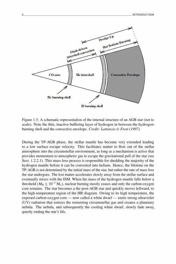
Figure 1.3: A schematic representation of the internal structure of an AGB star (not toscale). Note the thin, inactive bu↵ering layer of hydrogen in between the hydrogen-burning shell and the convective envelope. Credit: Lattanzio & Frost (1997).

During the TP-AGB phase, the stellar mantle has become very extended leadingto a low surface escape velocity. This facilitates matter to flow out of the stellaratmosphere into the circumstellar environment, as long as a mechanism is active thatprovides momentum to atmospheric gas to escape the gravitational pull of the star (seeSect. 1.2.2.1). This mass-loss process is responsible for shedding the majority of thehydrogen mantle before it can be converted into helium. Hence, the lifetime on theTP-AGB is not determined by the initial mass of the star, but rather the rate of mass lossthe star undergoes. The lost matter accelerates slowly away from the stellar surface andeventually mixes with the ISM. When the mass of the hydrogen mantle falls below athreshold (MH . 10�3 M�), nuclear burning mostly ceases and only the carbon-oxygencore remains. The star becomes a the post-AGB star and quickly moves leftward, tothe high-temperature region of the HR diagram. Owing to its high temperature, theexposed carbon-oxygen core — now called a white dwarf — emits strong ultraviolet(UV) radiation that ionizes the remaining circumstellar gas and creates a planetarynebula. The nebula, and subsequently the cooling white dwarf, slowly fade away,quietly ending the star’s life.

STELLAR EVOLUTION 7

1.1.3 Chemical evolution: Nucleosynthesis in AGB stars

The chemistry of a star does not remain constant throughout its life, because of thenucleosynthetic conversion of hydrogen into heavier elements in the stellar interior. Thenewly formed elements are brought to the surface via convective or chemical transportmechanisms, and as such change the chemical composition of the atmospheric layersof the star.

1.1.3.1 Mixing processes: convective transport

Most mixing occurs through convective motions. Whether a part of a stellar interioris convective or not, depends on the energy balance within that region. In normalconditions, energy is transported outward through radiation, but if the medium becomestoo opaque, convection becomes a more e�cient mechanism to transport the energy.As shown in Fig. 1.3, the stellar mantle of an AGB star is convective, implying thatany chemically enriched material inserted into the mantle will also a↵ect the chemicalcomposition of the stellar atmosphere.

However, the helium-intershell zone on top of the carbon-oxygen core is not convective,preventing direct mixing of helium-burning products. Moreover, AGB stars of mass. 5 M� have a radiative layer in between the hydrogen-burning shell and the mantle,such that mixing of hydrogen-burning products is also prohibited. The actual chemicalenrichment of the stellar mantle is thought to occur through dredge-ups. During theseevents, convective bubbles reach down into active nuclear-burning regions and mix thenewly produced elements with material from the stellar mantle.

Chemical enrichment of the mantle through these dredge-ups is complemented bydeep-mixing (or cool-bottom processing) between the convective mantle and theradiative layer above the hydrogen-burning shell (see, e.g., Stancli↵e & Lattanzio 2011and references therein). This extra mixing could be facilitated by, e.g., convectiveovershooting, rotational shear, thermohaline processes, or internal gravity waves.

1.1.3.2 The initial composition

The initial composition of the star depends on the abundance patterns of the gas cloudsin the region in which the star was formed. In our Galaxy, as well as the SmallMagellanic Cloud (SMC) and the Large Magellanic Cloud (LMC), the primordialcomposition contains more oxygen than carbon, such that every star entering theTP-AGB phase is oxygen-rich.

Before the star reaches the TP-AGB, nucleosynthetic processes have slightly alteredthe primordial composition. A first dredge-up (FDU) occurs just after the MS, at the

8 INTRODUCTION

Figure 1.4: A schematic representation of two consecutive thermal pulses in a TP-AGBstar. The mass coordinate is given with respect to the time. The thick solid line marksthe edge of the convective mantle and shows where convective mantle dips into deeperlayers during the dredge-up. The dashed line indicates the hydrogen-burning shell.The thin solid line denotes the helium-burning shell. The region in between these twoshells harbors the inactive helium-intershell zone, which becomes convective duringthe thermal pulse. Note that the convective thermal pulse does not reach all the way tothe hydrogen-burning shell. The grayed areas indicate where proton capture leads to13C production and where the s-process synthesizes elements heavier than iron throughslow neutron capture. Region A in the hydrogen-burning shell and region B in thehelium-intershell zone are mixed with the convective mantle during the dredge-up.Credit: adapted from Busso et al. (1999).

start of the RGB phase (see in Fig. 1.2), which mixes material of the mantle witha region that has undergone partial hydrogen burning. A second dredge-up (SDU)a↵ects intermediate-mass stars (M? & 4 M�) after core-helium exhaustion (see panel bin Fig. 1.2), as the helium-burning shell is being established. During the SDU, theconvective envelope reaches down into a region that has burned all hydrogen.

STELLAR EVOLUTION 9

Figure 1.5: The modeled evolution of the surface C/O ratio of AGB stars of 4, 5, and 6M� and metallicities of Z = 0.004 (typical for the SMC), Z = 0.008 (typical for theLMC), and Z = 0.02 (Solar composition). Credit: chapter 2 by Lattanzio &Wood inHabing & Olofsson (2003).

1.1.3.3 The third dredge-up

Once the star has started the cycles of intermittent hydrogen and helium shell burning,a third-dredge-up (TDU) event can happen during a thermal pulse. In Fig. 1.4, threeregions relevant for this process are shown: the convective mantle, the helium-intershellzone, and the carbon-oxygen core. Just below the convective mantle, the hydrogen-burning shell is active between consecutive thermal pulses, called the interpulse period.When a thermal pulse occurs, the hydrogen-burning shell goes inactive due to a decreasein temperature. The steep increase in energy production associated with the helium-shell flash causes the helium-intershell zone to become convective and helium-burningproducts to be dredged up into the intershell zone. In the relaxation period after theshell flash, the convective mantle can penetrate the intershell and mix burning products(from regions A and B in Fig. 1.4) with material from the mantle. This dredge-upceases when the hydrogen-burning shell reignites, leading the AGB star into the nextinterpulse period.

10 INTRODUCTION

The triple-alpha reaction predominantly produces 12C from 4He nuclei in the helium-burning shell, leading to the injection of 12C into the mantle by the TDU. Because16O production is thought to be negligible, this implies that the oxygen-rich initialcomposition of the AGB star can evolve into a carbon-rich composition. Fig. 1.5 showsthe surface carbon-to-oxygen abundance (C/O) ratio in terms of lifetime on the AGB aspredicted by nucleosynthetic models for several initial masses and metallicities. Everychange in C/O ratio corresponds to the e↵ect of one dredge-up episode. For low-massstars (M? . 4 M�), a monotonous increase of the C/O ratio is predicted, turning thechemistry of the star from oxygen-rich to carbon-rich after a given number of TDUs.This change in low-mass stars becomes steeper for lower-metallicity models owing toa lower initial oxygen abundance, while 12C-production is thought to remain the same,regardless of metallicity.

Not only the 12C abundance of the mantle is a↵ected by the dredge-ups. The abundanceof the 13C isotope as well as several other elements, including N, O, F, Mg, or theirisotopes, can be enhanced or reduced significantly. By measuring isotopic ratios,i.e. the abundance ratio of two isotopes of the same element, in observed spectraof circumstellar molecules (see, e.g., Decin 2012) one can pinpoint which nuclearand mixing processes have occurred in a stellar interior. This helps to constrain theevolutionary stage of an AGB star (see, e.g., Herwig 2005 for an overview). Lastly,in AGB stars the s-process is thought to be responsible for the synthesis of elementsbeyond iron, e.g. zirconium and barium. Iron-peak elements capture neutrons releasedin the radiative helium-intershell zone (see the grayed areas in Fig. 1.4) via either the13C(↵,n)16O or the 22Ne(↵,n)25Mg reaction. The neutron capture is usually followedby beta decay, such that neutron nucleosynthesis follows the stability valley (Herwig2005).

1.1.3.4 Hot-bottom burning

The primary pathway to form of 4He in shell burning is the CNO-cycle wheresubsequent proton capture by carbon, nitrogen and/or oxygen nuclei produces helium.This process critically depends on a high temperature, which is not attained in theconvective mantle of low-mass stars (M? . 5 M�). In case of intermediate-mass stars(5 M� . M? . 8 M�), however, the thin radiative layer of hydrogen present betweenthe convective mantle and the hydrogen-burning region disappears. Here, the base ofthe convective mantle dips into the hydrogen-burning shell and reaches temperatureshigh enough to allow the CNO-cycle to operate. This process is commonly calledhot-bottom burning (HBB).

Apart from the production of helium nuclei, the CNO-cycle also converts 12C into 14Nduring the process, e↵ectively counterbalancing 12C injection into the convective mantleby the TDU. Fig. 1.5 illustrates this e↵ect for a 6 M� star of Solar metallicity: rather

AGB CHARACTERISTICS 11

than an increase in C/O ratio, a decrease is expected until the point where the mantlemass becomes too small to support HBB. The middle column in Fig. 1.5 shows that thetransition point between both regimes lies at ⇠5 M�. At lower metallicities HBB doesnot preclude the evolution from an oxygen-rich to a carbon-rich atmosphere, but onlydelays it. Because of their high initial oxygen abundance, metal-rich intermediate-massstars will not become carbon-rich as their stay on the TP-AGB does not exceed a fewtimes 105 years.

If a source of protons is available in the helium intershell (such as during the TDU,indicated by p in the grayed area in Fig. 1.4), the reaction 12C(p,�)13C can occur. Inmetal-rich stars, this reaction causes the 12C/13C isotopic ratio to decrease to low valuesof ⇠ 5–20 by dredging up hydrogen-burning products during the FDU and the SDU.The TDU, however, inserts more 12C as part of the helium-burning products, therebyagain increasing the 12C/13C isotopic ratio. Because it ensures a constant source ofprotons, HBB precludes this e↵ect and leads to an e�cient conversion of 12C into14N as well as to an equilibrium value for the 12C/13C isotopic ratio of ⇠ 5–10. Acombination of several isotopic ratios, including 12C/13C but also, e.g., 16O/17O and16O/18O, can serve as a tracer for the occurrence of HBB in the stellar interior, and,hence, can constrain the initial mass of the star (see, e.g., De Beck et al. 2010 andreferences therein).

1.2 AGB characteristics

Having placed AGB stars in the framework of stellar evolution, we now turn to theirobservational characteristics. This section is based on Lamers & Cassinelli (1999),chapter 2 by Lattanzio & Wood and chapter 4 by Gustafsson & Höfner in Habing &Olofsson (2003), and Wood (2010). In addition to being cool and luminous giants,three distinct observational characteristics stand out.

1. Spectroscopy of AGB atmospheres points out three major spectral types: M-typespectra are dominated by oxygen-rich chemistry with bands of the TiO moleculein the optical as the trademark, carbon compounds such as C2 and CN litter thespectra of carbon stars (bottom panel in Fig. 1.6), and the S-type stars show amultitude of fingerprints typical of s-process elements, such as zirconium oxide(ZrO) bands, as well as other signatures, such as vanadium oxide (VO) bands.The classification is more detailed than this (including MS-type stars showinga mainly oxygen-rich chemistry, with some s-process elements as well; see toppanel in Fig. 1.6), but these three specific classes reveal the mechanism causingthe di↵erent spectral signatures: it is the carbon-to-oxygen abundance (C/O)ratio that determines the type of chemistry of an AGB atmosphere (Russell 1934;Gilman 1969; Beck et al. 1992). The S-type stars can be considered as transitional

12 INTRODUCTION

Figure 1.6: Spectra of an MS-type star (top panel) and a carbon star (bottom panel)in the LMC. Trademark molecular bands are indicated for each. Credit: chapter 2 byLattanzio & Wood in Habing & Olofsson (2003).

objects between oxygen-rich and carbon-rich stars, having a C/O ratio ⇠ 1. Thesedi↵erent spectral types are related to the chemical evolution of the stellar interior,discussed in Sect. 1.1.3.

2. Time series of photometric observations indicate varying brightness, eitherwith or without clear periodicity, and the amplitude is the largest at shortwavelengths (see Fig. 1.7). Based on the regularity and amplitude of thesebrightness variations a classification arose: Miras show a single period withlarge variations in the V-band (�mV > 2.5 mag), semiregular variables (SRVs)exhibit varying degrees of periodicity along with smaller variations in the V-band(�mV < 2.5 mag), and the light curves of irregular variables reveal no periodicityat all. We discuss variability of AGB stars in Sect. 1.2.1.

3. The spectral energy distribution (SED) contains the signature of the CSE presentaround many AGB stars (see Fig. 1.8). The circumstellar dust particles cansignificantly redden the stellar spectrum, which peaks around 2 µm for typicale↵ective temperatures of 2000–3000 K. In extreme cases, dust can obscure thecentral object entirely, in which case the strong IR emission is the only way todetect these objects. Oxygen-rich, high-mass-loss OH/IR stars are only detected

AGB CHARACTERISTICS 13

Figure 1.7: Light curves of the Mira RR Sco in di↵erent bandpasses, ordered fromsmallest wavelengths at the bottom to highest wavelengths at the top. Credit: chapter 2by Lattanzio & Wood in Habing & Olofsson (2003).

by the presence of hydroxyl (OH) masers in combination with a highly reddenedspectrum peaking between 20 and 40 µm. We discuss the mass-loss processresponsible for this stellar wind in Sect. 1.2.2 and continue in Sect. 1.3 with thechemical and thermodynamic characteristics of the CSE.

1.2.1 Pulsational variability

The empirical classification of AGB long-period variables (LPVs) is based on theregularity and amplitude of the sinusoidal variations in their light curve. One of themost outstanding properties of LPVs concerns the strong correlation between theaverage brightness and the period of the brightness variations of the order of a few

14 INTRODUCTION

101

� (µm)

103

104

105

F�

(Jy)

Figure 1.8: The distance-scaled SEDs of four carbon AGB stars as observed withthe ISO telescope. The dust content of the wind gradually increases from W Ori(blue) through V384 Per (green) and CW Leo (yellow) to LL Peg (red), displaying aprogressively reddened stellar spectrum. The stellar spectrum of W Ori is still clearlyvisible at short wavelengths up to ⇠ 8 µm (e.g. the atmospheric molecular absorptionbands at 3 and 4-6 µm), while the stellar spectrum of LL Peg is not visible anymoreand the 11-µm dust feature is in absorption.

hundred days. Fig. 1.9 compares both properties for a large sample of LPVs in the LMC.In this diagram, the observed quantities cluster in distinct sequences first identified byWood et al. (1999). Studies have attempted to identify the origin of such systematics,but so far have not been able to provide a complete explanation. The Miras clustertogether toward the high-end luminosity tail of sequence C (not shown explicitly inFig. 1.9). The SRVs can be found towards the low-end luminosities of sequence C,and on sequences A, B, C’ and F. Lastly, the carbon-rich sources tend toward higherluminosities.

Most of the detected variability in AGB stars originates from stellar pulsation modesdynamically driven in the stellar mantle, each mode having a characteristic period andamplitude of variation. Stellar pulsation can be driven by a -mechanism, in whichan opaque layer of material in the stellar atmosphere expands due to the radiationpressure. The decrease in temperature during expansion makes the layer transparentto radiation, allowing it to contract and become opaque again. However, this requirestransport of energy to be radiative, which is not the case in the fully convective AGBmantle. Hence, a classical -mechanism is highly unlikely to operate. The pulsationsare instead driven by heat from the partial hydrogen and helium ionization zone (Ostlie

AGB CHARACTERISTICS 15

Figure 1.9: Period-luminosity diagram for LPVs in the LMC. The quantity WJK on thevertical axis is the reddening-free Weisenheit index that corrects the KS-band magnitudefor interstellar and circumstellar reddening (Soszynski & Wood 2013). The coloredpoints are Miras and SRVs (oxygen-rich in blue and carbon-rich in red), while the graypoints are small-amplitude red giants detected in the OGLE project (OSARGs). Credit:Soszynski & Wood (2013).

& Cox 1986). The e↵ects of convection on pulsation have been considered in nonlinearpulsation models, but results are far from conclusive (e.g. the recent work by Xiong& Deng 2013, see also Keller & Wood 2006, and Aerts et al. 2010 and referencestherein). Linear pulsation models with an approximate treatment of convection succeedin explaining the observed properties of at least the Miras, and o↵er some ideas aboutthe less regular pulsators. Miras by far are the most regular, and models confidentlyidentify them as fundamental-mode pulsators on sequence C. Sequences A, B and C’appear to be associated with first-, second- or third-overtone pulsators. Identification ofthe AGB stars on these sequences in terms of SRV types remains di�cult (e.g. Mosseret al. 2013). SRVs of type a (SRa) show periodic light curves with some modulation,and are expected to be dominated by a single pulsation mode, and thus show one

16 INTRODUCTION

dominant period. SRVs of type b (SRb) appear to be unstable in more than onepulsation mode, and as a consequence show multiple periods. For instance, stars withthe primary period on sequence F also show secondary variations with a period thatwould place them somewhere between sequences C and D. Hence, these stars could beSRb objects, but this is not yet conclusive (Soszynski & Wood 2013).

The major issue with pulsation models is the lack of a proper treatment of time-dependent convection, which is essential to understand the dynamics of the mantle. Alot of theoretical work remains to be done in terms of fluid dynamics to describeconvection. Luckily, a lot of useful empirical relations between the period andluminosity of AGB stars have been published over the years, especially for objects inthe Magellanic clouds, for which the distances are well known. From these empiricalrelations, luminosity predictions lead to distance estimates for AGB stars in our ownGalaxy, where distance determination proves more di�cult. We apply the period-luminosity (PL) relations published by Whitelock et al. (1991) and Groenewegen &Whitelock (1996) in Chapters 2 and 3, respectively, to estimate luminosities. We makeuse of the PL-relations published by Whitelock et al. (2006), Whitelock et al. (2008),and Bergeat & Chevallier (2005) in Chapter 4 to ensure homogeneity between objectsin a larger sample.

1.2.2 Mass loss

The mass-loss process triggering the onset of the stellar wind has a large impact onthe late stages of stellar evolution because the rate at which mass is lost is muchhigher than the rate at which hydrogen is burned. Mass loss strips a major part of themantle o↵ the star, which e↵ectively ends the AGB phase, making mass loss one of thepriorities in understanding AGB evolution. Characteristics of mass loss in the AGBphase include: 1) the creation of a slow stellar wind with terminal gas velocities around10–20 km s�1, 2) a broad range of mass-loss rates spanning four orders of magnitudefrom 10�8 up to 10�4 M�/yr, 3) a strong correlation between period and mass-lossrate (see Fig. 1.11 for the LMC and SMC, as well as Fig. 14 in De Beck et al. 2010for Galactic sources), 4) a tendency toward a lower mass-loss rate for stars with lessregular pulsations (Whitelock et al. 2000; Yesilyaprak & Aslan 2004; De Beck et al.2010), 5) no noticeable dependence of mass-loss rate on spectral type (Ramstedt et al.2006; De Beck et al. 2010). In this section, we focus on the mechanism causing themass loss, which must be able to explain all these characteristics. We then highlightthe relation between mass loss and evolution on the AGB.

AGB CHARACTERISTICS 17

Figure 1.10: The mass-loss rate of AGB stars in the SMC (triangles) and the LMC(hexagons) compared to the pulsational period (in days). Credit: Wood et al. (2007).

Figure 1.11: The e↵ect on mass loss of pulsations and radiation pressure on dust. Theradius with respect to pulsation cycle of several packets of material are shown. On theleft: only pulsations are included in the model, leading to an insignificant mass-lossrate. On the right: same as on the left, but now radiation pressure on dust grains isincluded in the model, which results in a substantial mass-loss rate and the developmentof a stellar wind. Credit: Bowen (1988).

18 INTRODUCTION

1.2.2.1 The mass-loss mechanism

Mass loss from these low surface-gravity red giants requires a mechanism that allowsmatter to gain momentum and overcome the gravitational pull of the central star.Early modeling showed that mass loss may occur when a given set of conditions isfulfilled. Bowen (1988) presented one of the first advanced studies on the nature ofthe mass-loss mechanism. His calculations showed that a combination of pulsationsand the radiation pressure exerted on dust particles (Kwok 1975) can drive a stellarwind from AGB stars (see Fig. 1.11). Large-amplitude pulsations lift material to greatheights in the stellar atmosphere and reduce the temperatures enough to facilitatethe condensation of dust grains a few stellar radii away from the stellar surface. Asradiation pressure pushes these dust grains radially outward, they transfer momentum tothe gas particles and basically drag them along. Bowen’s results cemented the conceptof a pulsation-enhanced dust-driven stellar wind firmly in place as the most generallyaccepted mass-loss mechanism. Despite this success, several key assumptions wentinto the work by Bowen (1988). Especially the imposed boundary conditions stillcannot be explained through a unified, self-consistent model.

As previously discussed, pulsation models fail to explain the observed variabilitytypes with su�cient confidence, owing to the poor description of convection currentlyavailable. Bowen artificially induces pulsations by placing a piston at the base ofthe AGB atmosphere, which pushes the molecular layers up and down with givenperiodicity and amplitude. With this he explained that fundamental-mode pulsatorscan drive stronger stellar winds than first-overtone pulsators. The strong correlationbetween mass-loss rate and pulsation period shown in Fig. 1.10 also followed naturallyfrom these models. A more consistent treatment of pulsating atmospheres has beenincluded in mass-loss-mechanism studies by, e.g., Höfner & Dorfi (1997) and Höfneret al. (1998), but to date, no model has been able to include the stellar convectiveinterior from where pulsations are driven.

The second prerequisite for driving the wind is the presence of dust su�ciently closeto the stellar surface; the existence of which Bowen simply assumes. Though, the rapidformation of opaque dust grains in the inner wind has posed large problems for anoxygen-based chemistry in the AGB atmosphere. While the high opacity of amorphouscarbon allows e�cient wind driving, no opaque oxygen-rich equivalent is available,unless iron is included in the dust species. However, iron-rich silicates and oxides heatup too much close to the stellar surface, causing them to sublimate before they candrive a wind. Iron-poor silicates and oxides are too transparent to drive a wind up tothe observed mass-loss rates through absorption of radiation (Woitke 2006). Recently,studies have suggested that scattering of stellar light on large dust grains may initiatewind driving (Höfner 2008, 2012). Even though these large grains have indeed beendetected (Norris et al. 2012), the mechanism by which the first seed nuclei form soclose to the star in su�ciently high amounts remains a mystery, especially in the case

THE CIRCUMSTELLAR ENVELOPE 19

of oxygen-rich dust species. A more detailed introduction on dust formation is given inSect. 1.3.3.1.

1.2.2.2 Evolutionary aspects of mass loss

How to link the mass-loss rate to the evolutionary stage on the AGB is a widelydiscussed problem, to which a definitive answer has not yet been formulated. Becausethe wind-driving mechanism primarily depends on the interaction between stellarradiation and dust particles, a change in luminosity should a↵ect the mass-loss rate.Observationally, Figs. 1.9 and 1.10 readily show this, considering that the periodcorrelates with both the luminosity and the mass-loss rate, especially for high pulsationperiods associated with the most evolved stars on the TP-AGB. Evolutionary mass-lossmodels show a similar result (Iben & Renzini 1983; Bowen 1988; Vassiliadis & Wood1993; Willson 2000). As the star climbs the AGB in the HR diagram, the mass-lossrate increases along with the luminosity, in agreement with observations of Galacticand LMC sources. Near the end of the AGB phase, the star su↵ers a superwind phase(Renzini 1981; Iben & Renzini 1983), during which the mass-loss rate increases toextremely high values (> 10�5 M�/yr) implying that this phase cannot last longerthan a few times 104–105 years, depending on the initial mass. The cause of such asuperwind phase is not yet understood.

OH/IR stars and extreme carbon stars, respectively, represent the oxygen-rich andcarbon-rich equivalent of AGB stars undergoing a superwind. Carbon stars with ahigh mass-loss rate have indeed been observed, and it has been shown that this phaselasts up to ⇠ 104 years (Volk et al. 2000). Recent results pose a new problem forthe oxygen-rich equivalent: the observed high mass-loss rate in OH/IR stars has onlybeen reached during the last several hundred up to a few thousand years (Justtanont &Tielens 1992; Delfosse et al. 1997; Justtanont et al. 2006, 2013; de Vries et al. 2013).This is substantially shorter than the necessary ⇠ 104 years for a star with mass > 5 M�to shed its whole hydrogen mantle. For these stars to lose enough mass on the AGB,they would have to go through several such high, but short, mass-loss-rate episodes.Consequently, several shells of increased density should be visible around evolvedoxygen-rich stars. However, to date, no such shells have been observed (Cox et al.2012). de Vries et al. (2013) speculate that OH/IR stars may move on to even highermass-loss rates and become an as of yet unrecognized type of object.

1.3 The circumstellar envelope

The strong IR emission observed in the SEDs of many AGB stars points toward anextended circumstellar component created by a stellar wind. The CSE formed through

20 INTRODUCTION

Figure 1.12: Schematic structure of the circumstellar envelope (not to scale). The fourmajor regions are indicated and typical distances are given at the top. Credit: L. Decin.

mass loss o↵ers the unique opportunity to study several aspects of AGB evolutionindirectly. Because the circumstellar chemistry reflects the atmospheric chemicalcomposition, studying the molecular content yields insight in the chemical evolutionof an AGB star. By measuring column densities in the CSE, the mass-loss rate canbe determined and the mass-loss process can be studied. The velocity and densitystructure with respect to the distance from the stellar surface provides a fingerprint forthe mass-loss history up to a few times 104 years.

Section 1.3.1 gives an overview of the di↵erent circumstellar regions and importantongoing chemical processes. The literature references for this section are chapter 5 byMillar and chapter 7 by Olofsson in Habing & Olofsson (2003), Decin et al. (2006),Min (2009), De Beck (2011), Decin (2012) and Speck (2012).

1.3.1 The four envelope realms

The CSE of an AGB star can be subdivided in four major regions, the dimensions ofwhich depend on the average circumstellar column density (see Fig. 1.12). Typically, a

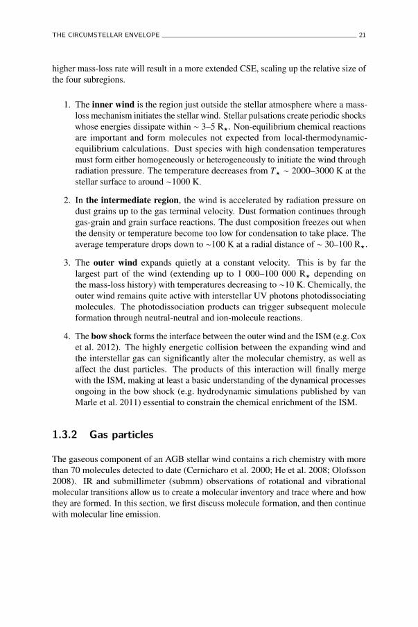
THE CIRCUMSTELLAR ENVELOPE 21

higher mass-loss rate will result in a more extended CSE, scaling up the relative size ofthe four subregions.

1. The inner wind is the region just outside the stellar atmosphere where a mass-loss mechanism initiates the stellar wind. Stellar pulsations create periodic shockswhose energies dissipate within ⇠ 3–5 R?. Non-equilibrium chemical reactionsare important and form molecules not expected from local-thermodynamic-equilibrium calculations. Dust species with high condensation temperaturesmust form either homogeneously or heterogeneously to initiate the wind throughradiation pressure. The temperature decreases from T? ⇠ 2000–3000 K at thestellar surface to around ⇠1000 K.

2. In the intermediate region, the wind is accelerated by radiation pressure ondust grains up to the gas terminal velocity. Dust formation continues throughgas-grain and grain surface reactions. The dust composition freezes out whenthe density or temperature become too low for condensation to take place. Theaverage temperature drops down to ⇠100 K at a radial distance of ⇠ 30–100 R?.

3. The outer wind expands quietly at a constant velocity. This is by far thelargest part of the wind (extending up to 1 000–100 000 R? depending onthe mass-loss history) with temperatures decreasing to ⇠10 K. Chemically, theouter wind remains quite active with interstellar UV photons photodissociatingmolecules. The photodissociation products can trigger subsequent moleculeformation through neutral-neutral and ion-molecule reactions.

4. The bow shock forms the interface between the outer wind and the ISM (e.g. Coxet al. 2012). The highly energetic collision between the expanding wind andthe interstellar gas can significantly alter the molecular chemistry, as well asa↵ect the dust particles. The products of this interaction will finally mergewith the ISM, making at least a basic understanding of the dynamical processesongoing in the bow shock (e.g. hydrodynamic simulations published by vanMarle et al. 2011) essential to constrain the chemical enrichment of the ISM.

1.3.2 Gas particles

The gaseous component of an AGB stellar wind contains a rich chemistry with morethan 70 molecules detected to date (Cernicharo et al. 2000; He et al. 2008; Olofsson2008). IR and submillimeter (submm) observations of rotational and vibrationalmolecular transitions allow us to create a molecular inventory and trace where and howthey are formed. In this section, we first discuss molecule formation, and then continuewith molecular line emission.

22 INTRODUCTION

1.3.2.1 Molecule formation

In describing the chemistry of molecules, an often used concept is that ofthermodynamic equilibrium (TE). A system in TE experiences no exchange of matteror energy with its environment (i.e. the temperature and pressure are constant, and theradiative input equals the radiative output), does not go through a phase change (e.g. nocondensation or sublimation takes place) and does not have unbalanced potentials(e.g. chemical reactions are in equilibrium). If any of these properties change in spaceor time, but do so slowly such that TE is valid at any given time in some limited region,the system is said to be in local thermodynamic equilibrium (LTE). LTE significantlysimplifies modeling the chemistry of a system. Any e↵ects that push a system o↵balance, will result in a situation of nonlocal thermodynamic equilibrium (NLTE).

The large extension of AGB atmospheres leads to temperatures so low that moleculescan form. The atmospheric densities and temperatures are still high enough for thesystem to be approximately in LTE. In LTE, the most stable molecules are molecularhydrogen (H2) and carbon monoxide (CO), and subsequent chemistry is driven byeither oxygen or carbon, whichever is most abundant. As discussed in Sect. 1.1.3, threespectral types are common among AGB stars: M-type spectra are dominated by oxygenchemistry, spectra of carbon stars show carbon-rich fingerprints, and S-type spectraare considered to be transitional between the previous two types. These spectral typesthus translate into a dominant chemistry in the stellar wind. For a few decades, LTEchemistry was assumed to be the norm for AGB winds as well (e.g. Tsuji 1973).

Observations of AGB stars showed in the early 90’s that LTE abundances do not hold forstellar winds (e.g. the detection of SiO in carbon stars by Bujarrabal et al. 1994, and thedetection of CO2 in M-type stars by Justtanont et al. 1998). Non-equilibrium chemicalprocesses cause the formation of these molecules and a↵ect the LTE abundancescalculated for AGB atmospheres. We review some chemical processes ordered in termsof the region where they are relevant.

Shock-induced chemistry. The atmospheric pulsations responsible for the mass-lossprocess periodically compress and heat material in the outer atmosphere and the innerwind. The shocks insert enough energy to break up molecules formed in the atmosphere,and liberate atomic elements for subsequent chemical reactions. Breaking up CO canprovide free carbon or oxygen in an environment otherwise dominated by the mostabundant of the two. After several studies dedicated to the e↵ect of shock-inducedchemistry (e.g. Duari et al. 1999 for M-type stars, Willacy & Cherchne↵ 1998 for carbonstars), it was shown both theoretically (Cherchne↵ 2006) and observationally (Decinet al. 2008) that a homogeneous set of parent molecules can be defined irrespective ofthe C/O ratio. These parent species form in the inner wind and are inserted into theintermediate and outer wind, where they are then subject to other chemical processes.Fig. 1.13 shows the shock-induced chemistry predictions for the abundance profiles of

THE CIRCUMSTELLAR ENVELOPE 23

Figure 1.13: Abundances of the prevalent molecules as a function of radius fromshock-induced NLTE chemistry in the carbon-rich star CW Leo. Abundances at 1 R?

are those derived from LTE chemistry in the atmosphere. Credit: Cherchne↵ (2012).

the parent species in the case of the high mass-loss carbon star CW Leo (Cherchne↵2012). Molecules such as CO and N2 are not a↵ected much by the shocks, but H2O,SiO and SiS have significantly increased abundances when compared to their LTEestimates (at a radius of 1 R?).

Gas-grain interaction. The presence of both molecules and dust grains implies thatinteraction between the two is possible as long as densities are high enough for themto collide frequently. The intermediate wind provides these conditions, as long as themass-loss rate is high and the expansion velocity low. Molecules can stick to dustgrains, where they interact with each other to form new molecules, or to facilitate dustmantle growth (see Sect. 1.3.3.1). For example, in Fischer-Tropsch catalysis iron ornickel grains act as catalysts for the formation of hydrocarbons or water molecules(Latter & Charnley 1996; Kress 1997), involving reactions which would otherwisehave too large activation energies in the gas phase.

UV photodissociation. The interstellar UV radiation field provides high-energyphotons to break molecules in the outer wind. The products from such photodissociationinclude very reactive gas particles that can go on to produce new molecules throughneutral-neutral or neutral-ion reactions. How deep UV radiation can penetrate the winddepends on the presence of dust, which blocks part of the incoming radiation, and the

24 INTRODUCTION

self-shielding e↵ect of some common molecules. Especially H2 and CO are e�cientat self-shielding, because they are mainly dissociated by line absorption and theirabundances are high. Assuming a spherical, smooth wind, the photodissociation radiusfor each molecule is directly proportional to the mass-loss rate (e.g. Mamon et al. 1988for CO, or Groenewegen 1994 for H2O). However, various observations (e.g. Mauron& Huggins 1999, Mauron & Huggins 2006, Decin et al. 2011) have revealed that AGBwinds tend to be far from spherically symmetric or smooth. Large-scale structure canmanifest in the form of arcs with a high density contrast. Small-scale structure canoccur as matter clumps together, creating a low-density interclump medium. This canhave a significant impact on the e�ciency of UV photodissociation and circumstellarchemistry. For instance, Decin et al. (2010a) and Agúndez et al. (2010) have shownthat UV radiation can penetrate the intermediate and even the inner envelope if thestellar wind is clumpy, increasing the chemical complexity in these regions.

1.3.2.2 Line emission

Molecules are part of the dynamical circumstellar environment and are subject tocountless interactions with other molecules, photons and dust grains. In theseinteractions, energy can be transferred to a molecule by exciting it to higher-energyquantum states.

Electronic excitation. Absorption of optical or UV photons raises electrons to ahigher-energy orbital in a molecule. Because AGB stars emit most of their stellar lightin the near-IR, and gas and dust particles in the stellar wind radiate at even longerwavelengths, electronic transitions are likely not important in AGB winds.

Vibrational excitation. Absorption of IR photons causes two nuclei of a moleculeto oscillate with respect to their center of mass. Diatomic molecules have only onemode of vibration, while more complex molecules can have multiple modes. Forexample, an H2O molecule has three modes of vibration: bending of the two hydrogen-oxygen bonds, and symmetric and asymmetric stretching of these bonds (see Fig. 1.14).Vibrational states are quantified by their vibrational quantum number ⌫.

Rotational excitation. Absorption of a small packet of energy can cause a moleculewith a permanent dipole moment to make an end-over-end rotational motion. Thetorque exerted by the irradiating electromagnetic field maintains this motion, e↵ectivelyplacing the molecule in a higher rotational state. For example, the CO moleculerequires progressively larger packets of energy to be excited to higher modes ofrotation, resulting in a ladder of increasingly energetic rotational states within eachvibrational state. The CO ladder is shown in Fig. 1.15 for 12CO and its isotopologue3

3Isotopologues are molecules that contain the same elements but one or more of them are of a di↵erentisotope.

THE CIRCUMSTELLAR ENVELOPE 25

13CO, indicating the energy of each level. Rotational states are quantified by therotational quantum number J, which is associated with the total angular momentum ofthe molecule. For nonlinear molecules, a simple scheme such as the CO ladder cannotbe used because their rotational spectrum becomes extremely complex with ordersof magnitude more possible states. For example, H2O is an asymmetric molecule inwhich the angular momentum has two additional degrees of freedom compared to CO,given by the projections of the angular momentum, Ka and Kc. A rotational state ofH2O is fully quantified by the three quantum numbers JKa,Kc .

Transitions between these di↵erent states obey a given set of quantum-mechanicalselection rules. For the CO molecule, rotational transitions within a vibrational statemust follow the selection rule �J = ±1. Each of these transitions increases or decreasesthe rotational energy of the molecule in discrete packages. If a photon is absorbed oremitted during the transition from one state to another, the photon will have a specificfrequency appropriate for the energy di↵erence between the two levels. The transitionfrequencies are indicated in Fig. 1.15 for the CO transitions up to J = 10 � 9.

Both radiative processes and collisions with predominantly H2 set the excitationdistribution of molecules. The stellar spectrum, thermal emission of dust particles, andcosmic rays form the most important sources of radiation that interact with gas particles.Which of the excitation mechanisms dominate, depends on the thermodynamicproperties of the wind, the spectroscopic properties of the molecule and the strengthsof the radiation fields. Microturbulent motions of the gas particles in addition to theradial gas expansion velocity broaden the frequency windows in which radiation caninteract with molecules. The gas kinetic temperature (see Sect. 1.3.4.2) in a givenregion often di↵ers considerably from the average excitation temperature of moleculesin that region. Therefore, molecular excitation in AGB winds reflects a condition ofNLTE, in which a nonlocal e↵ect, such as absorption of radiation from a di↵erentregion in the wind, keeps the molecular level populations from being thermalizedthrough collisions. Numerical radiative-transfer modeling is required to determinethe distribution of excited states among molecules in every part of the stellar wind.Methods used to tackle this problem include Monte Carlo approaches (e.g. Schöier& Olofsson 2001), multilevel approximate Newton-Raphson operators (e.g. Decinet al. 2006, see also Sect. 1.5) or accelerated lambda-iteration methods (e.g. Maerckeret al. 2008).

The level population distribution of a molecule and the thermodynamic structure ofthe wind determine the strength and shape of the molecular emission lines. Thisinformation constrains the thermodynamic, chemical and kinematic structure of thestellar wind, from which the mass-loss rate can be estimated. Whether the intrinsicline profile can be discerned in observations, depends on the spectral resolution of theinstrument. Fig. 1.16 shows spectrally unresolved emission lines of CO and HCN in thespectrum of LL Peg observed with the PACS instrument onboard the Herschel SpaceTelescope (see Sect. 1.4). Potential line confusion in such a spectrum can complicate

26 INTRODUCTION

Figure 1.14: The vibrational excitation modes of H2O: symmetric stretching(⌫1), bending (⌫2), and asymmetric stretching (⌫3). Credit: S. Scherer(http://backreaction.blogspot.be/).

Figure 1.15: The low-J ladder up to J = 10 � 9 for 12CO and 13CO. The horizontalaxis gives the upper J-level. The vertical axis gives the upper-level energy. For eachtransition, the frequency and the Einstein-A coe�cient of the emitted photon are listed.Credit: Yildiz (2013).

THE CIRCUMSTELLAR ENVELOPE 27

140 145 150 155 160 165

0

5

10

15

20

25

30

35F

�(J

y)J =

16 � 15

J = 17 � 16J = 18 � 17

J = 24 � 23

J = 23 � 22 J = 22 � 21 J = 21 � 20

165 170 175 180 185 190

� (µm)

0

5

10

15

20

25

30

35

F�

(Jy)

J = 14 � 13J = 15 � 14J = 20 � 19 J = 19 � 18

J = 18 � 17

Figure 1.16: An excerpt of the continuum-subtracted PACS spectrum of the carbon-richAGB star LL Peg. The red vertical bars indicate ground-state CO lines. The solidblack and dashed black vertical bars indicate HCN lines in the ground state and thevibrational ⌫2 = 1 state, respectively.

line identification and hamper the estimation of the strength of the emission of eachcontributing transition (e.g. the blend between a CO line and an HCN line at ⇠ 153 µmin Fig. 1.16). Notwithstanding these complications, the broad spectral coverage andthe high sensitivity of the PACS spectrometer provide a unique opportunity to observecountless mid-IR and far-IR molecular emission lines, including the entire CO ladderfrom J = 14 � 13 up to J = 47 � 46.

Spectrally resolved observations are often less sensitive, but o↵er spectral informationthat is key to constraining the kinematic structure of the wind. Fig. 1.17 shows afew examples of simple line shapes that are common in AGB winds, with the majordi↵erences originating from the spatial resolving power of the telescope and whetherthe wind is transparent (i.e. optically thin) or opaque (i.e. optically thick) in a givenline. The width of these emission lines is directly related to the gas expansion velocityin the region where the lines are formed, information which can be used to trace thevelocity profile of the wind (see Fig. 1.20 and Sect 1.3.4.1). Significantly more complexline profiles may appear depending on the kinematics of the envelope, for instancein the inner wind or when asymmetric outflows occur (e.g. Knapp et al. 1997, Sahaiet al. 2003, and Sahai et al. 2009 for the carbon star V Hya).

28 INTRODUCTION

Figure 1.17: Observed spectrally resolved line profiles of molecular emission:a) optically thin, spatially unresolved emission, b) optically thick, spatially unresolvedemission, c) optically thin, spatially resolved emission, d) optically thick, spatiallyresolved emission. Credit: adapted from chapter 7 by Olofsson in Habing & Olofsson(2003).

1.3.3 Solid-state particles

The presence of solid-state particles is evident from the strong IR component in theSEDs of AGB stars. The amount of dust in the stellar wind determines the degree ofcircumstellar reddening of the stellar spectrum (e.g. Fig. 1.8). By comparing the IRspectral structure with laboratory measurements, the dust composition can be inferred.This composition can be used to constrain dust formation models which in turn yieldimportant clues to help understand the mass-loss mechanism on the AGB. Even thoughdust formation models profit from laboratory measurements of dust optical propertiesas well as formation experiments, many questions remain. First, we give a shortoverview of important dust formation processes, followed by an introduction to IRspectral features and their identification.

THE CIRCUMSTELLAR ENVELOPE 29

1.3.3.1 Dust formation

Two dust formation mechanisms in AGB stellar winds have received ample attentionover the years. The first concerns the thermodynamic-equilibrium condensation fromgas-phase particles into solid-state particles (e.g. Lodders & Fegley 1999). The secondis the formation of seed nuclei followed by mantle growth (e.g. Gail & Sedlmayr 1999).The latter mechanism occurs in TE, as long as the density is high enough to supportgas-grain reactions. If dust temperatures drop to low enough values, water ice mantlescan form on top of already existing grains in the wind (Dijkstra et al. 2003a, 2006).The dominant formation mechanism for a given dust species strongly depends on theproperties of the precursor seed nuclei or molecules (e.g. their chemical compositionand vapor pressure) and on the properties of the resulting dust grains (e.g. theircondensation temperature, particle shape and optical constants). The dust condensationsequence in AGB winds is generally studied through theoretical models (e.g. thereview by Speck 2012), or through laboratory experiments (e.g. the review by Poschet al. 2006). Important constraints are provided by IR spectroscopy of AGB stars (seenext Sect. 1.3.3.2) and presolar grains in meteorites thought to be condensed fromAGB stars (e.g. Clayton & Nittler 2004).

A useful tool to study the stability of dust grains is the pressure-temperature (P-T)diagram, shown in Fig. 1.18 for typical carbon-rich and oxygen-rich dust species(Speck et al. 2008, 2009). Such diagrams indicate at which conditions a dust speciesis stable. As the gas in the inner wind expands, it cools down, reaching temperatureswhere dust particles such as aluminum oxide (or corundum, Al2O3) or titanium oxide(TiO2, not shown in Fig. 1.18) in oxygen-rich environments (Gail & Sedlmayr 1998),and amorphous carbon, silicon carbide (SiC) or titanium carbide (TiC, not shown inFig. 1.18) in carbon-rich environments (Lodders & Fegley 1999) can exist. Since noprecursor seed nuclei could have formed at higher temperatures, these species must formby direct condensation from the gas phase. Therefore, precursor molecules must beavailable in the cooling gas in su�ciently high quantities for these species to form. Thisseems to rule out corundum as one of the earliest condensing oxygen-rich dust species,because the Al2O3 molecule is not abundant above the condensation temperature⇠ 1400 K, and the nucleation rate of corundum is low at lower temperatures.

As the temperature decreases in the P-T diagram, chemically more complexdust species appear. Especially oxygen-rich species such as silicates (includingolivines, (MgxFe1�x)2SiO4, and pyroxenes, MgxFe1�xSiO3, both of which the Mg-richendmember is shown in Fig. 1.18) do not have equivalent gas-phase precursor moleculesas opposed to, e.g., TiO2. For these species to condense from gas phase, increasinglycomplex reaction schemes are needed (see, e.g., Goumans & Bromley 2012). Gail &Sedlmayr (1999) show that silicates may form more e�ciently through mantle growthon top of seed nuclei. The most abundant species that can condense from gas phaseat high temperatures is TiO2, but it seems unlikely that this species alone can provide

30 INTRODUCTION

Figure 1.18: Temperature-pressure diagram for dust condensation models in the innerwind of AGB stars. The top panel is for carbon-rich stars; the bottom panel is foroxygen-rich stars. The solid and long-dashed lines indicate for which temperature andpressure a given dust species is stable based on TE calculations. The light-gray dottedlines indicate the P-T paths of the gas for several mass-loss rates (in M�/yr). Credit:Speck (2012).

THE CIRCUMSTELLAR ENVELOPE 31

enough seed nuclei to facilitate silicate condensation. The most likely candidate tosupply seed nuclei would be the very abundant, reactive SiO molecule, especiallyconsidering that silicates contain many SiO compounds. This was originally ruledout because SiO condensation from gas phase starts only at ⇠ 600 K, too late in thecondensation sequence to serve as a seed nucleus (Nuth & Donn 1982; Gail & Sedlmayr1986). Recent laboratory measurements and modeling e↵orts have shown, however,that the condensation temperature may be considerably higher than previously thought(Nuth & Ferguson 2006; Gail et al. 2013; Wetzel et al. 2013). This example shows theneed for continued e↵orts to perform accurate laboratory measurements to understanddust condensation sequences in AGB environments.

An important consequence of the two suggested dust formation pathways, is theexistence of homogeneous and heterogeneous dust grains, respectively. Especially incarbon-rich stellar winds, it is not clear whether direct condensation or mantle growthon seed nuclei causes dust formation. In principle, both amorphous carbon (or thecrystalline form graphite) and SiC have equivalent gas-phase molecules and should beable to form directly from gas-phase condensation. However, presolar grains in theMurchison meteorite (Bernatowicz et al. 1996) clearly indicate a composite structure,often with TiC at the center and a mantle of graphite. SiC was found in only onegrain, suggesting SiC formed after the carbonaceous material, in agreement with TEcalculations such as shown in Fig. 1.18. Conclusions pertaining presolar grains must betreated with care, because they are a↵ected by unpredictable selection e↵ects (e.g. whathappened to AGB dust grains in the ISM before entering the proto-Solar cloud?).Nevertheless, presolar grains suggest that carbon-rich dust forms in heterogeneousgrains, rather than in homogeneous grains.

1.3.3.2 Infrared spectral features

To identify which dust species contribute to the IR spectral features observed inAGB winds, the optical properties of the dust grains must be computed. Vibrational,stretching and bending modes between atoms in the lattice of a material lead toresonance bands where the material will interact with incoming radiation moree�ciently. These wavelength-dependent resonances are specific for the compositionof a material and can be measured in the laboratory. However, the precise spectrallocation of a resonance also depends on several grain properties (e.g. the review byMin 2009).

Grain size. In the Rayleigh limit, the grain size is significantly smaller than thewavelength of incoming radiation and interaction with radiation depends on theresonances as measured in the laboratory. If the size of a dust grain is comparable tothe wavelength of incoming radiation, the spectral signature becomes less pronouncedand the resonances are suppressed.

32 INTRODUCTION

100 101 102

� (µm)

100

101

102

103

104

��

(cm

2 /g)

100 101 102

� (µm)100

101

102

103

104

��

(cm

2 /g)

Figure 1.19: Dust opacity profiles typical for carbon-rich (top) and oxygen-rich(bottom) environments. The carbon-rich dust species include amorphous carbon inred (Jäger et al. 1998b), metallic iron in yellow (Henning & Stognienko 1996), siliconcarbide in green (Pitman et al. 2008), and magnesium sulfide in blue (Begemannet al. 1994). The vertical dashed lines indicate where the silicon carbide featuredominates; this interval can be directly compared to the vertical dashed lines in Fig. 1.8.The oxygen-rich dust species include amorphous olivine in red (Jäger et al. 2003),crystalline olivine (called forsterite, Suto et al. 2006) in yellow, corundum in green(Koike et al. 1995), and crystalline water ice in blue (Warren 1984).

THE CIRCUMSTELLAR ENVELOPE 33

Grain shape. Simple grain shapes, such as homogeneous, spherical grains, typicallycause strong and narrow resonances, while highly irregular shapes broaden the spectralfeatures and shift them to redder wavelengths.

Particle structure. Single dust grains of the same or di↵erent composition can sticktogether in an aggregate structure. Open, flu↵y aggregates have optical propertiessimilar to those of the constituent grains. Compact aggregates show optical propertiestypical of much larger grains than those of the single grains. Coating of one materialon top of another also strongly a↵ects the optical properties, and more so if this coatingis highly symmetrical (e.g. mantles around spherical precursor grains introduce sharpspectral resonances).

By making assumptions about the grain size distribution, the grain shapes and theparticle structure, the absorption and scattering cross sections of a population of dustgrains can be computed based on the material-specific optical constants measured in thelaboratory. The strong and narrow features predicted for spherical particles were oftenshown to be unrealistic when compared with spectral features observed in stellar winds,suggesting that the dust grains in these winds are more irregularly shaped. Computingoptical properties of irregularly shaped grains is computationally intensive and too timeconsuming. An alternative, statistical approach searches for an ensemble of dust grainsof simple shapes that represents the optical properties of a population of irregularlyshaped grains. Commonly used grain shape models are the continuous distributionof ellipsoids (CDE, Bohren & Hu↵man 1983) and the distribution of hollow spheres(DHS, Min et al. 2003, Min et al. 2005).

Fig. 1.19 shows the dust opacity profiles of typical carbon-rich and oxygen-rich dustspecies calculated for a CDE. Both amorphous carbon and metallic iron have a high,smooth opacity profile without strong resonances, which makes it more di�cult todistinguish between the two. Silicon carbide is mostly transparent to radiation exceptin the strong resonance at ⇠ 11 µm. The vertical lines in Fig. 1.8 and the top panelof Fig. 1.19 compare the same wavelength window, indicating the match betweenthe resonance feature in the opacity profile and the spectral feature in the observedSEDs. Because of the well-ordered lattice structure of crystalline olivine, as opposedto amorphous olivine, the extinction behavior of the former is much more complex.The specific narrow features of crystals can be distinguished in spectra of the highmass-loss OH/IR stars (e.g. Sylvester et al. 1999). Many more dust species than thoseshown in Fig. 1.19 have been identified in AGB stellar winds. We refer to the reviewby Waters (2004) for an overview.

By placing an amount of dust of a given composition in a smooth density distributiontypical of an AGB wind, the emergent SED can be calculated by considering thethermal energy balance of the dust. Common methods to calculate continuum radiativetransfer include solving the integral equation of the spectral energy density (Ivezic &Elitzur 1997) and the Monte Carlo-based approach (Bjorkman & Wood 2001, Min

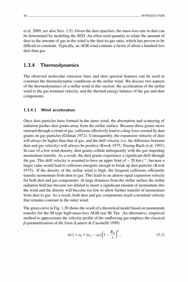
34 INTRODUCTION

et al. 2009, see also Sect. 1.5). Given the dust opacities, the mass-loss rate in dust canbe determined by modeling the SED. An often used quantity to relate the amount ofdust to the amount of gas in the wind is the dust-to-gas ratio, which has proven to bedi�cult to constrain. Typically, an AGB wind contains a factor of about a hundred lessdust than gas.

1.3.4 Thermodynamics

The observed molecular emission lines and dust spectral features can be used toconstrain the thermodynamic conditions in the stellar wind. We discuss two aspectsof the thermodynamics of a stellar wind in this section: the acceleration of the stellarwind to the gas terminal velocity, and the thermal energy balance of the gas and dustcomponents.

1.3.4.1 Wind acceleration

Once dust particles have formed in the inner wind, the absorption and scattering ofradiation pushes dust grains away from the stellar surface. Because these grains moveoutward through a cloud of gas, collisions e↵ectively lead to a drag force exerted by dustgrains on gas particles (Gilman 1972). Consequently, the expansion velocity of dustwill always be higher than that of gas, and the drift velocity (i.e. the di↵erence betweendust and gas velocity) will always be positive (Kwok 1975; Truong-Bach et al. 1991).In case of a low wind density, dust grains collide infrequently with the gas impedingmomentum transfer. As a result, the dust grains experience a significant drift throughthe gas. This drift velocity is assumed to have an upper limit of ⇠ 20 km s�1, because alarger value would lead to collisions energetic enough to break up dust particles (Kwok1975). If the density of the stellar wind is high, the frequent collisions e�cientlytransfer momentum from dust to gas. This leads to an almost equal expansion velocityfor both dust and gas components. At large distances from the stellar surface the stellarradiation field has become too diluted to insert a significant amount of momentum intothe wind and the density will become too low to allow further transfer of momentumfrom dust to gas. As a result, both dust and gas components reach a terminal velocitythat remains constant in the outer wind.

The green curve in Fig. 1.20 shows the result of a theoretical model based on momentumtransfer for the M-type high-mass-loss AGB-star IK Tau. An alternative, empiricalmethod to approximate the velocity profile of the outflowing gas employs the classical�-parametrization of the form (Lamers & Cassinelli 1999)

3(r) ' 30 + (31 � 30)✓1 � R?

r

◆�, (1.1)

THE CIRCUMSTELLAR ENVELOPE 35

Figure 1.20: Velocity profile of the M-type AGB star IK Tau. Diamonds show expansionvelocities derived from SiO, H2O or OH maser emission, as well as from the ground-based CO J = 1 � 0 emission line. The triangles show the expansion velocity derivedfrom HIFI data, with the formation region of the emission line being indicated as ahorizontal bar and the uncertainty on the measured velocity as a vertical bar. The solidgreen, dashed blue and dotted red curves give the modeling results for the momentumequation, a power law with � = 1 and a power law with � = 1.8, respectively. Thevertical dashed line marks the inner radius of the wind where dust formation is ongoing.Credit: Decin et al. (2010c).

where 30 is the velocity at the dust condensation radius, 31 the terminal gas velocity, and� quantifies the wind acceleration. The dashed blue and dotted red curves in Fig. 1.20show the velocity profiles for � = 1 and � = 1.8, respectively. These laws indicate aslower wind acceleration than what is predicted from momentum-transfer calculations.The theoretical velocities can be compared with measurements, by considering, e.g.,the width of molecular line profiles of CO, H2O, SiO, etc. These emission lines areformed in di↵erent parts of the stellar wind, allowing to trace the radial dependence ofthe velocity. Based on this comparison, the stellar wind of IK Tau favors the sloweracceleration approximated by a � = 1 parametrization (Decin et al. 2010c). Similarresults have been found for other oxygen-rich AGB stars. Schöier et al. (2006) found� = 0.2 for the carbon-rich AGB star CW Leo, which implies a more e�cient windacceleration, and can be explained by the higher opacity in the near-IR of carbon dustgrains (see, e.g., the carbon and olivine opacity profiles in Fig. 1.19). Such a low �approximates a momentum-transfer model well.

As mentioned in Sect. 1.2.2.1, the onset of the mass-loss process in oxygen-rich starsis poorly understood. Accelerating the stellar wind to the terminal velocity fast enoughalso proves to be a problem. Several issues may contribute to this discrepancy, but

36 INTRODUCTION

the degree to which remains unclear. Because radiation pressure on dust grains is themain process in driving the stellar wind, the wavelength-dependent opacities of thedust particles must be well constrained. Unfortunately, these are model dependent, asthe properties of the ensemble of grains need to be specified. The formation sequenceof oxygen-rich dust species is also not yet well understood. An important furtherassumption of momentum-transfer models is that of full momentum coupling betweengas and dust, which means that all dust particles interact with gas particles, regardlessof size or shape (Kwok 1975). MacGregor & Stencel (1992) find that silicate grainswith initial size smaller than ⇠ 0.05 µm decouple from the gas near the condensationradius, depending on the mass-loss rate. This may also slow down wind accelerationconsiderably. As a conclusion, wind acceleration models reproduce observed velocityprofiles reasonably well, but there is still room for improvement for oxygen-rich winds.

1.3.4.2 Energy balance

As dust grains absorb photons from the central star, they heat up. Collisions with gasparticles transfer some of this heat into the gas, but most of the heat is emitted asthermal radiation. The temperature of the dust grains is determined then by the balancebetween incoming radiation at relatively short wavelengths and reemission at relativelylong wavelengths, resulting in the reddening e↵ect of the stellar spectrum. More dustimplies that more radiation is processed, and leads to stronger emission in the IR (seeFig. 1.8).

The kinetic temperature of the gas depends on multiple cooling and heating terms (seeDecin et al. 2006 for an in-depth overview). Collisions with dust particles constitutethe main source of heating. Additional contributions include incident cosmic rays, andheat exchange between dust and gas particles. In the outer envelope, photoelectricheating becomes important as well, in which interstellar UV photons eject electronsfrom the dust grains. Cooling contributions primarily include adiabatic expansionand collisional excitation of the rotational levels of molecules followed by radiativedeexcitation. The most important coolants are CO and H2O (in oxygen-rich winds) orHCN (in carbon-rich winds), owing to their high abundance, high dissociation energyand substantial dipole moment. Vibrational excitation of H2, finally, also contributes tothe cooling in the inner wind. Fig. 1.21 shows the predicted gas kinetic-temperatureprofile for the M-type AGB star IK Tau taking into account the above discussed heatingand cooling e↵ects (albeit with an approximate cooling contribution from H2O). Thecooling and heating rates from the major contributors are given in Fig. 1.22.

Determining the energy balance for AGB winds is computationally intensive. Especiallythe radiative cooling by CO, H2O and HCN depends on the excitation analysis of thesemolecules. For CO, this has been included consistently in earlier studies by Crosas &Menten (1997) and Schöier & Olofsson (2001), but including H2O is di�cult owing

THE CIRCUMSTELLAR ENVELOPE 37

Figure 1.21: The gas kinetic-temperature profile of the M-type AGB star IK Tau asderived from the 12CO and HCN rotational line transitions. The heating and coolingterms taken into account are shown in Fig. 1.22. The dashed line shows a power lawof the form T (r) = T (r0) (r0/r)0.6 with T (r0) = 100 K (Willacy & Millar 1997). Thedotted vertical line corresponds to the inner radius of the dust shell. Credit: Decin et al.(2010b).

to the higher optical depth and the more complex spectroscopy. Radiative cooling ofH2O was included in the energy balance by Decin et al. (2006) through the three-levelapproximation, which essentially replaces the level populations of a molecule by onlytwo rotational levels and one vibrationally excited rotational level (Goldreich & Scoville1976). These first attempts indicate that H2O cooling significantly contributes to theenergy balance in the inner wind (see Fig. 1.22). Including full excitation analysis forH2O cooling leads to even larger cooling contributions from H2O. In fact, this has leadto excessive H2O cooling in the inner envelope to the point where temperatures becomeunphysical (Decin & Maercker, priv. comm.). To date, no solution has been found forthis issue. As a consequence, the interpretation of mass-loss rates and abundances inan absolute sense must be done carefully, because the e↵ect of consistent H2O coolingon derived values remains unclear (Maercker & Danilovich, priv. comm.).

To circumvent the poorly constrained H2O cooling contribution, an alternative approachis to approximate the gas kinetic-temperature profile with a power law of the form

Tg(r) = T?

rR?

!�✏,

38 INTRODUCTION

Figure 1.22: The cooling (top) and heating (bottom) rates contributing to the energybalance in the M-type AGB star IK Tau. The corresponding gas kinetic-temperatureprofile is shown in Fig. 1.21. H2O vibrational cooling is negligible and H2O rotationalcooling is calculated in a three-level approximation. Credit: Decin et al. (2010b).

STAR GAZING IN THE INFRARED 39

where r is the distance to the center of the star. The gas kinetic-temperature profilefor IK Tau can be reasonably approximated with a power law, as shown in Fig. 1.21.Because at high densities collisions dominate CO excitation, CO emission lines probethe temperature throughout the envelope well for high mass-loss-rate sources, suchas IK Tau. By constraining the temperature law empirically from CO lines coveringdi↵erent rotational quantum numbers and hence excitation regimes, mass-loss rates andabundances can be derived more reliably. This in turn helps to constrain the problematicH2O cooling.

1.4 Star gazing in the infrared

The cool surfaces of AGB stars and their cold stellar winds emit most radiation at IR,submm and radio wavelengths. When observing from the surface of the Earth, theatmospheric transparency is an important aspect to consider. For radio observations ofthe cold outer wind, a broad window at & 1 mm is accessible, but submm observationsdown to ⇠200 µm can only be done from dry locations at high altitude. Examplesinclude the Atacama Pathfinder Experiment (APEX, 0.2 mm . � . 1.5 mm) in LaSilla, Chile; the James Clerk Maxwell Telescope (JCMT, 0.44 mm . � . 1.4 mm)at Mauna Kea, Hawaï; the 30 meter telescope of the Institut de RadioastronomieMillimétrique (IRAM, 1 mm . � . 3.75 mm) at Pico Veleta, Spain; and the Very LargeArray (VLA, 7 mm . � . 4000 mm) at the Plains of San Agustin, USA.

The work presented in this thesis mainly deals with IR observations (2 µm . � .200 µm). Unfortunately, only specific IR bands are accessible from Earth’s surface,for instance in the near- and mid-IR (e.g. the Very Large Telescope — VLT — andthe Very Large Telescope Interferometer — VLTI — at Paranal, Chile). However, thefull IR spectral window is essential when studying cold environments, such as thoseof evolved stars (see Fig. 1.23) and disks around young stars. Especially emissionfrom water vapor, which ironically is the culprit of the atmosphere’s high opacity inthe IR, is essential to understand the thermodynamics of these environments. In a way,water provides a double-sided motivation to go to space: circumventing telluric water,and detecting cosmic water. A few space observatories have provided a wealth ofdata already, including the Infrared Astronomical Satellite (IRAS), the Infrared SpaceTelescope (ISO) and the Spitzer Space Telescope. For the remainder of this section, wefocus on future missions in the IR and submm domain, and most importantly on thestate-of-the-art far-IR and submm space observatory: Herschel (Pilbratt et al. 2010).

40 INTRODUCTION

Figure 1.23: Overview of past and present telescopes used for observing AGB stellarwinds. The typical size of the di↵erent regions in the AGB outflow puts strongconstraints on the type of instrument and/or telescope that can be used. A full, detailedobserving campaign to image an entire AGB stellar wind in all of its aspects wouldrequire a large number of telescopes. Credit: L. Decin.

1.4.1 The Herschel era

The first real water hunter, ESA’s Herschel Space Telescope was launched on May 9,2009 reaching its final destination after about sixty days4. Herschel is a Cassegrain-design telescope with a primary mirror of 3.5 m in diameter, to date the largest mirroron a space mission. As an IR observatory, the instruments onboard Herschel mustbe cooled to about 2 K to limit the background radiation from the telescope itself.The telescope was located in a Lissajous orbit around the L2 Lagrange point of theSun-Earth system to avoid as much background IR contamination from Earth and theMoon and utilized a large single-sided radiation shield to block radiation from the Sun(see Fig. 1.24). Herschel’s three instruments together cover a wavelength range from55 µm to 671 µm. We briefly discuss these three instruments.

4General information presented here on the Herschel Space Telescope is primarily taken from ESA’spublic web pages.

STAR GAZING IN THE INFRARED 41

Figure 1.24: The Herschel Space Telescope in an artist’s impression, pictured in the L2Lagrange point of the Sun-Earth system. Credit: ESA.

Photodetector Array Camera and Spectrometer (PACS). This imaging photometerand medium-resolution grating spectrometer o↵ers two modes of observation (Poglitschet al. 2010). In photometry mode, PACS images a field of view (FOV) of1.75 ⇥ 3.5 arcminutes simultaneously in two bands centered around 70 µm, 100 µmor 160 µm. The detectors for this mode are two bolometer arrays. In spectroscopymode, PACS covers the wavelength range from 55 µm to 210 µm with an FOV of47 ⇥ 47 arcseconds, spatially resolved into 5 ⇥ 5 pixels. With a resolving power between1000 and 4000 depending on wavelength, PACS leaps far ahead of the long-wavelengthspectrometer onboard Herschel’s predecessor, ISO. Even though the resolution isnot high enough to resolve the kinematics of AGB winds, the high sensitivity of theinstrument still provides an unprecedented opportunity to trace hundreds of molecularemission lines in the far-IR. PACS truly shines when constraining chemistry andthermodynamics in various cosmic environments.

42 INTRODUCTION

Spectral and Photometric Imaging Receiver (SPIRE). Like PACS, SPIRE o↵erstwo modes of observation as a three-band imaging photometer and an imagingFourier-transform spectrometer (Gri�n et al. 2010). The photometer has an FOV of4 ⇥ 8 arcminutes in three bands simultaneously centered around 250 µm, 350 µm and500 µm. In addition to point-source photometry, two mapping modes are supported aswell. The spectrometer gives access to the wavelength range between 194 and 671 µmand runs in continuous-scan mode with an adjustable spectral resolution between 50and 1000, depending on wavelength. The SPIRE spectrometer has a circular FOV2.6 arcminutes across.

Heterodyne Instrument for the Far Infrared (HIFI). As a high-resolution hetero-dyne spectrometer, HIFI translates the frequency range of the incoming signal to alower frequency by mixing it with a very stable monochromatic signal generated by alocal oscillator (de Graauw et al. 2010). This ensures very high sensitivity ideal fordetecting line emission at radio wavelengths. The largest perk of HIFI is its superiorresolution, which can go down to 0.13 MHz or ⇠ 100 m/s, providing the means totrace kinematics in detail. Five bands using superconductor-insulator-superconductormixers are available from 480 to 1250 GHz, and two bands are located in the 1410to 1910 GHz range using hot-electron-bolometer mixers, the full frequency rangecorresponding to the wavelength interval from 157 to 625 µm.

The telescope operated for as long as it had helium fuel to cool the instruments.On April 29, 2013, Herschel reached end-of-helium, evidenced by a steady rise ininstrumental temperature to the ambient value of ⇠ 80 K. This marked the end ofthe Herschel mission, which amassed over 35000 scientific observations containingmore than 25000 hours of science data. The observatory was finally propelled intoa long-term stable parking orbit around the Sun. On June 17, 2013, the mission waso�cially at an end as the final command to the telescope to shut down systems wasgiven.

1.4.2 What the future holds

Astronomy and astrophysics is a research field that is driven strongly by the advancesin observational techniques. Thanks to the monumental e↵orts of countless forefrontastronomy researchers and the ingenuity of space engineers, new missions both onthe ground and in space are being planned decades in advance. We list some of thehighlight telescopes currently in the early-operations phase or the planning phase.

Atacama Large Millimeter/submillimeter Array (ALMA) at Chajnantor, Chile.At an altitude of 5000 meters above sea level, ALMA makes use of the thin, dry air ofnorthern Chile’s Atacama desert to overcome the atmospheric opaqueness imposed bywater vapor (see Fig. 1.25). In its maximum setup, the ALMA interferometer comprises

STAR GAZING IN THE INFRARED 43

Figure 1.25: A view of the Atacama Large Millimeter/submillimeter Array atChajnantor, Chile. Credit: Stéphane Guisard/ESO.

66 antennas and provides an amazing spatial resolving power of ⇠ 0.1 arcsecondsand a sensitivity much higher than other submm or radio telescopes such as JCMTor IRAM. ALMA is able to resolve the circumstellar density structures, and has ledto groundbreaking results on the carbon AGB star R Scl (see Fig. 1.26, Maerckeret al. 2012). The image shows that the region in an AGB stellar wind where a givenmolecular emission line forms is well constrained with ALMA observations. This canhelp lift degeneracies in the modeling of wind acceleration and energy balance.

Stratospheric Observatory for Infrared Astronomy (SOFIA). Being the first of itskind, SOFIA is an airborne observatory that is designed for infrared astronomy in thestratosphere at an altitude of 12 kilometers (Young et al. 2012). The major advantageof SOFIA is the possibility of extended, more detailed studies of Galactic AGB stars inthe IR to sample dust chemistry. Space telescopes focus primarily on high-impact, high-yield studies owing to their typically shorter life span, making long-term observationcampaigns di�cult. SOFIA will be able to fill the niche of more extended observationswell. The aircraft has been in operation for routine science flights since December2010, and will reach its full capability in 2014 with about a hundred flights per year.

Gaia. Though strictly not an IR or submm observatory, Gaia will contribute to allastronomical fields of research by measuring an accurate distance to millions of stars.The AGB research field su↵ers from large uncertainties in distance determination, andGaia will remedy this for a sizable fraction of the Galactic AGB population. Someof the reddest, coldest AGB winds may not be accessible with Gaia, but even then,observations of less obscured AGB stars will allow better calibration of the PL-relationsdiscussed in Sect. 1.2.1. Gaia is currently scheduled for launch in December 2013.

James Webb Space Telescope (JWST). The first space observatory to accessthe near-IR and mid-IR wavelength regions since the Spitzer telescope, and at a

44 INTRODUCTION

Figure 1.26: CO J = 3 � 2 emission from the carbon-rich AGB star R Scl at the stellarvelocity as observed with the ALMA observatory. The emission pattern is an almostperfect spiral with small deviations on the order of ±1.5 km s�1. A binary companionlies at the basis of this large-scale density modulation. Credit: Maercker et al. (2012).

significantly improved resolution, JWST will contribute to accurate spectroscopy ofAGB atmospheres and dusty winds. The high sensitivity of the MIRI instrumentonboard JWST will give access to observations of extragalactic AGB stars beyondthe SMC and LMC at a significantly larger e�ciency. Such observations will providefundamental constraints on AGB-star dust production (Meixner 2011). The launch ofJWST is currently planned for 2018.

Space Infrared Telescope for Cosmology and Astrophysics (SPICA). Dubbed thenext-generation infrared space telescope, SPICA will have a mirror similar to thatof Herschel, but cooled to temperatures even closer to absolute zero (Goicoechea &Nakagawa 2011). The resulting increase in sensitivity will give instruments on SPICAaccess to infrared sources with a brightness two orders of magnitude weaker thanHerschel. One of the primary instruments onboard SPICA will be the European-builtSAFARI, an imaging spectrometer between 30 and 200 µm, making it Herschel’s

CONFRONTING OBSERVATIONS WITH THEORY: RADIATIVE TRANSFER 45

successor in the hunt for cosmic water. The European participation in SPICA will beproposed as the fourth medium-class mission in ESA’s cosmic vision program (launchopportunity in 2026).

1.5 Confronting observations with theory:radiative transfer

To confront observations with the theory of AGB stellar winds discussed in Sect. 1.3,we calculate theoretical models and determine the goodness-of-fit using straightforwardstatistical methods. Radiative transfer is an essential aspect in calculating these models.It is often treated di↵erently for the dust and gas components, because the former ismore akin to a continuum process with a weaker wavelength dependence, and the latteroccurs through highly wavelength-dependent line absorption and emission. Studies ofAGB winds often focus on either the dusty or the gaseous component of the CSE whileadopting a simplified treatment of the other component. Such simplifications can havea severe impact on the final results owing to the high degree of interaction between dustand gas in the stellar wind (e.g. Ramstedt et al. 2008). In addition, radiative-transfercalculations are intricately coupled with the thermodynamics of the wind, depend onmany stellar and circumstellar parameters and can be very time consuming.

In this thesis, we approach the radiative-transfer problem with two state-of-the-artnumerical codes specialized in one of the components: IR thermal emission ismodeled with the MCMax code (Min et al. 2009) and molecular emission lines withthe GASTRoNOoM code (Decin et al. 2006, 2010b). In addition, we have writtenthe interface ComboCode between MCMax and GASTRoNOoM. This allows moreconsistency between the continuum and line radiative-transfer models, increases thee�ciency and flexibility in terms of calculation time, and provides interaction with asupercomputer cluster. In what follows, we describe some model assumptions of thenumerical codes used in this thesis, and show how the new interface lifts some of theseassumptions.

1.5.1 Thermal-emission modeling with MCMax

The continuum radiative-transfer code MCMax is based on a Monte Carlo method thatsends out photon packets from a central source through a user-defined density structure.Because of the nature of the Monte Carlo approach, no iteration or convergencecriterion is required to arrive at a solution. The number of photon packets sent throughthe envelope determines the Monte Carlo noise on the emergent SED. The codeself-consistently calculates the dust temperature structure of the CSE by enforcing

46 INTRODUCTION

radiative equilibrium through continuous absorption and reemission of the photonpackets (Bjorkman & Wood 2001). As such, energy conservation is ensured becauseevery photon packet that originates from the central source will eventually escape theCSE after having interacted through scattering, or absorption and reemission with acertain amount of dust particles. Once the temperature structure of the CSE is known,a Monte Carlo ray-tracing method computes a spectrum, an image or visibilities. Whenconfronting the radiative-transfer models with observations, the best solution can bedetermined by a statistical method such as a �2-minimization routine. However, eventhough the computed optical depth represents the stellar wind well, this ’best’ solutionis not unique, owing to the degeneracy introduced by the dust extinction properties.

Dust properties. The dust composition, grain shape, grain structure, and grain sizedistribution are input parameters for the dust extinction properties that are used for theradiative-transfer model (see, e.g., Fig. 1.19). An iterative method provides the optionto estimate the dust condensation radius based on the local temperature and pressure inthe wind (i.e. Fig. 1.18). This does not take into account the dust formation mechanism,such as coating on seed grains or chaotic growth of flu↵y structures. Instead, eachindividual dust species is assumed to condense instantaneously at the radius where itscondensation temperature is reached. The temperature structure of the included dustspecies can be calculated independently of each other, or as if they were in thermalcontact. In a recent version of the code, the option to include temperature-dependentdust opacities was added, but is not used in this thesis.

Wind structure. In principle, MCMax is a 2D radiative-transfer code, but we assumethat density variations can only exist in the radial direction. A large-scale densitystructure such as a dusty disk or a small-scale structure such as a clumpy medium havenot been considered in this thesis. MCMax does not allow for a consistent momentum-transfer calculation between dust and gas, as the gaseous component of the CSE is nottaken into account at all.

1.5.2 Molecular-emission modeling with GASTRoNOoM

The GASTRoNOoM code consists of three major components. The first partsimultaneously calculates the momentum transfer from dust to gas and the energybalance in the wind. The convergence criterion depends on the requested gas terminalexpansion velocity, which is reached in the model by iteratively adapting the dust-to-gas ratio that goes into the momentum transfer. The code is applicable to gasterminal velocities in excess of 5 km s�1 and mass-loss rates larger than 3⇥10�7 M�/yr(Decin et al. 2006). The second component calculates the actual line radiative transferthrough an iterative method based on the multilevel approximate Newton-Raphsonoperator (Schönberg & Hempe 1986). A convergence criterion must be defined in termsof the smallest allowed di↵erence in calculated level populations between di↵erent

CONFRONTING OBSERVATIONS WITH THEORY: RADIATIVE TRANSFER 47

iterative steps. Typically, convergence can be reached within 10–20 iterations for windsaround cool giants (Schönberg & Hempe 1986). Finally, the emission line profiles arecomputed by ray tracing using formal integration (Schönberg 1988). For spectrallyresolved line profiles, the goodness-of-fit with observations is determined through theloglikelihood statistical method (see Decin et al. 2007, and references therein), which isespecially sensitive to the line-profile shape. For spectrally unresolved lines, we applya �2-minimization routine to the comparison of the predicted and observed integratedline strengths.

Dust properties. When calculating the thermodynamics and the radiative transfer,dust is taken into account as spherical particles in a grain size distribution typical ofthe ISM (Mathis et al. 1977). The dust temperature follows a power law of the formTd(r) = T?(R?/2r)2/5 (chapter 7 by Olofsson in Habing & Olofsson 2003). The dustis composed of silicate grains with a specific density of 3.3 g/cm3 (Draine & Lee1984). The optical properties of the silicate grains are those typical for OH/IR sources(Justtanont & Tielens 1992), because the code was originally applied to oxygen-richwinds. To simulate the momentum transfer from dust to gas, the radiative force on thedust grains is equated with the gas drag force, from which the grain-size-dependentdrift velocity can be calculated (Kwok 1975; Truong-Bach et al. 1991). The momentumcoupling between dust and gas is complete and photon scattering is not taken intoaccount. The dust is assumed to condense instantaneously at the inner radius withdust properties that remain the same throughout the wind. The dust-to-gas ratio alsoremains constant as a function of radius, but can be adapted between the first andsecond component of GASTRoNOoM.

Wind structure. GASTRoNOoM is a 1D radiative-transfer code, in which the H2density structure is assumed to be smooth (i.e. no clumpy medium). The velocityprofile determined from momentum transfer and the requested mass-loss rate definethe density structure of the wind through the equation of mass conservation (Goldreich& Scoville 1976; Tielens 1983). Usually, the mass-loss rate is taken constant, buttime-dependent mass loss can be introduced in the form of sinusoidal variations ora given number of discontinuities. Other large-scale structures such as a gaseousdisk or polar outflows are not considered. When determining the energy balancethe heating and cooling terms described in Sect. 1.3.4.2 are taken into account. Atdistances smaller than the inner radius, the gas velocity and temperature profiles areapproximated by a power law as described in Sects. 1.3.4.1 and 1.3.4.2, respectively.The radial dependence of the molecular abundances is user defined and is taken relativeto the H2 number density. For CO and H2O, the photodissociation radius is based onthe formalism of Mamon et al. (1988) and the analytic formula of Groenewegen (1994),respectively. The outer radius of the wind is taken where the CO abundance dropsbelow 1% of its value at the stellar photosphere.

Molecular excitation. The radiative-transfer calculation takes into account excitationby collisions with H2 and by incident radiation from dust grains, the stellar photosphere

48 INTRODUCTION

and the cosmic background. Each molecule is treated individually, so any additionalpumping through resonances with transitions in other molecules is not included. Masingis not taken into account. Lastly, the stellar spectrum can be taken as either a black bodyor a MARCS atmosphere model of 3000 K, but no time variability is included. Theappendix of Decin et al. (2010b) gives a detailed description of the collision rates andthe molecular line lists used in GASTRoNOoM. The line lists include the frequenciesand Einstein-A coe�cients of the transitions, and the rotational and vibrational energylevels.

1.5.3 Improving model assumptions with ComboCode

To lift some of the assumptions, we follow a five-step approach, in which we couple theresults of both radiative-transfer models. Fig. 1.27 shows a schematic representation ofhow both radiative-transfer models interact with each other. On the left, the MCMaxMonte Carlo radiative-transfer module and the ray-tracing method is shown, and onthe right, the three components of GASTRoNOoM are given. The Roman numeralsindicate the five steps in our approach.

I. The initial dust radiative-transfer model is calculated with MCMax and providesdust information for the next step.

II. The simultaneous calculation of the energy balance and the momentum transferin GASTRoNOoM leads to a gas kinetic-temperature profile, a gas velocity profileand a drift velocity profile.

III. The MCMax radiative-transfer model is recalculated, from which the dustobservables can be computed by ray tracing. These include spectra, imagesor visibilities depending on the type of observations with which the dust model iscompared.

IV. The energy balance and momentum transfer are recalculated in GASTRoNOoM.

V. Using GASTRoNOoM, the line radiative-transfer models for individual moleculesare computed next to arrive at level populations appropriate for the thermodynamicstructure from the previous step. These results are then used to compute the finalemission line profiles for the requested molecular transitions by ray tracing. Ifrequired, these line profiles are then convolved with the beam profile of thetelescope with which an emission line was observed.

The yellow markers in Fig. 1.27 indicate where model assumptions are improved withmore consistent properties. We summarize them here.

CONFRONTING OBSERVATIONS WITH THEORY: RADIATIVE TRANSFER 49

Figu

re1.

27:A

sche

mat

icre

pres

enta

tion

ofth

em

odel

ing

appr

oach

used

inth

isth

esis

.Ind

icat

edar

eth

etw

ora

diat

ive-

trans

fer

code

sM

CM

axan

dG

ASTR

oNO

oM,a

ndho

wth

eyar

eco

nnec

ted

acco

rdin

gto

the

five-

step

appr

oach

(Rom

annu

mer

als)

pres

ente

din

Sect

ions

1.5.

3an

d2.

3.3.

The

lette

rsin

dica

tew

here

we

use

the

inte

rfac

eC

ombo

Cod

eto

adop

tcon

sist

enti

nput

from

the

prev

ious

step

into

the

next

step

.The

abbr

evia

tion

RTst

ands

forr

adia

tive

tran

sfer

,Tfo

rthe

tem

pera

ture

profi

le,

fort

hedu

stab

sorp

tion

coe�

cien

tsan

dR i

fort

hein

nerr

adiu

sof

the

stel

larw

ind.

50 INTRODUCTION

a. The dust properties in the simultaneous computation of the energy balanceand the momentum transfer in GASTRoNOoM are improved. Previously, thedust temperature profile was approximated by a power law, the dust absorptioncoe�cients were assumed to be those of oxygen-rich silicates typical for OH/IRstars, and the inner-shell radius was a free parameter. These are now includedconsistently using the dust temperature profile and dust absorption coe�cientsderived from the MCMax model, and equating the inner-shell radius to the dustcondensation radius calculated with MCMax.

b. The drift-velocity profile from the momentum-transfer calculation in GASTRoNOoMprovides a consistent dust velocity profile, which improves the density structure inthe MCMax radiative-transfer model. Previously, the dust expansion velocity wasassumed to be equal to the gas terminal velocity and constant throughout the wind.

c. The dust properties in the simultaneous computation of the energy balance andthe momentum transfer in GASTRoNOoM are updated with the results from theprevious step.

d. The dust-to-gas ratio in the line radiative-transfer module of GASTRoNOoM waspreviously taken to be the dust-to-gas ratio as estimated from the momentum-transfer iteration. This value is now replaced by one consistent with the MCMaxradiative-transfer model.

Assuming a set of dust properties and a spherically symmetric density distribution, thedust mass-loss rate calculated with MCMax is accurate to within a factor of two for ahigh drift velocity, and accurate to within ⇠30% for a low drift velocity. The e↵ect ofchanging the dust properties depends heavily on the thermodynamic structure of thestellar wind and must be considered on a case-by-case basis. The dust models remaindegenerate with respect to the dust properties. The main contribution of the improvedkinematics is the inclusion of the drift velocity, meaning that the dust expansion velocityis not automatically equated to the gas expansion velocity. This can have a significantimpact on the estimated dust mass-loss rate by up to a factor of two. We therebyreduce the uncertainty on the calculated dust mass-loss rate to 20–30%, given theaforementioned assumptions. Including a gradual increase to the terminal velocity inthe dust radiative-transfer model is not expected to a↵ect the uncertainty on the dustmass-loss rate for winds with a high optical depth. This is less clear for winds with alow optical depth where thermal emission originating in the acceleration zone can havea significant impact on the shape of the SED.

The the gas mass-loss rate is estimated to be accurate to within a factor of two upto three and depends heavily on the uncertainties on the collision rates and on theproperties of the molecular transitions. Moreover, some assumptions such as sphericalsymmetry may have a considerable e↵ect as well. Most importantly, ComboCodelifts some assumptions concerning the dust properties in GASTRoNOoM, improving

CONFRONTING OBSERVATIONS WITH THEORY: RADIATIVE TRANSFER 51

the credibility of the gas mass-loss-rate estimates. The estimated uncertainty on thegas mass-loss rate remains the same because it is still dominated by the molecularproperties and by other assumptions. However, the uncertainty on the abundanceestimates for molecules whose excitation strongly depends on the dust properties in thewind is reduced significantly. Finally, the nonuniqueness of the dust radiative-transfermodels with MCMax may a↵ect the line radiative-transfer models with GASTRoNOoM,but the extent of that has not yet been tested. Generally, if the optical depth of the dustin the wind is approximated well by the MCMax model — independent of the dustextinction properties used to calculate this model — the dust properties in steps a. andc. in Fig. 1.27 are a good approximation. We therefore expect that the GASTRoNOoMmodel is relatively independent of the nonuniqueness of the dust model. As such, ourfive-step approach is robust with the benefit of improved consistency between dust andgas.

Chapter 2 provides an in-depth discussion of how these changes for improvedconsistency are implemented and which advantages are tied to such a comprehensiveapproach.

52 INTRODUCTION

1.6 Questions answered and answers questioned

Because thermodynamics and chemistry in AGB stellar winds are closely connected,it is not straightforward to focus on either one alone. The broad spectrum of subjectsaddressed in this thesis attests to that aspect of AGB research. In the followingsections, we overview the three main chapters of this thesis and place them in context.Chapter 2 zooms in on the circumstellar thermodynamics of a high mass-loss OH/IRstar. Chapters 3 and 4 focus on circumstellar dust and gas chemistry, respectively, incarbon-rich environments.

Chapter 2: The importance of dust for H2O excitation. The complexity of thero-vibrational molecular structure of H2O, multiple excitation mechanisms and severalsaturation e↵ects make H2O di�cult to model (Maercker et al. 2008, 2009; Decinet al. 2010c). Until recently, a lack of H2O observations impeded progress of in-depthH2O modeling, but the launch of the Herschel Space Observatory provided the uniqueopportunity to trace H2O emission from the stellar wind of evolved stars in more detail.In Chapter 2, we consider the PACS spectrum of the OH/IR star OH 127.8+0.0, whichcontains a rich H2O emission spectrum. We show that dust properties strongly a↵ectH2O emission, highlighting the importance of a consistent treatment between dust andgas. We apply three di↵erent methods to determine the dust-to-gas ratio directly, witheach method tracing a di↵erent region of the wind. The recent onset of the superwinddetected for most — if not all — OH/IR stars in independent studies (see Sect. 1.2.2.2),also appears in OH 127.8+0.0 from our modeling of the CO transitions observed withJCMT, the IRAM 30m telescope and the HIFI instrument onboard Herschel.

Chapter highlight:

For the first time, the radial dependence of the dust-to-gas ratio could be studied. Wefind a tentative positive gradient in the dust-to-gas ratio in the wind of OH 127.8+0.0.

Chapter 3: Observational constraints for composite grains in AGB winds. Astrong, broad spectral band is located around 30 µm in the SED of carbon-rich stars(see Fig. 1.8, and Sect. 1.3.3.1). Due to the similarity in shape, the feature was originallyattributed to magnesium sulfide (MgS, Goebel & Moseley1985). Subsequent studiesconfirmed this identification, though a few major issues arose. The 30-µm featureappears with various shapes and strengths in di↵erent carbon stars, which cannot beeasily reconciled with the spectral properties of MgS. However, an in-depth studyof MgS as a carrier of the 30-µm feature is di�cult owing to the lack of laboratorymeasurements of optical properties at � < 10 µm. Recently, Zhang et al. (2009)

QUESTIONS ANSWERED AND ANSWERS QUESTIONED 53

showed that an amount of MgS substantially exceeding the expected atmospheric sulfurabundance is needed to explain the strong 30-µm feature in the post-AGB carbon starHD 56126. We argue against this conclusion by suggesting to place MgS dust incomposite grains with carbon and SiC. As a result, the average temperature of MgSdust is significantly higher and a much stronger emission feature appears, solving theissue reported by Zhang et al. (2009).

Chapter highlight:

MgS as a carrier of the 30-µm feature requires carbon grains to form in a compositestructure.

Chapter 4: The H2O formation mechanism in carbon-rich AGB stars. Thedetection of warm H2O emission from carbon stars has sparked speculation aboutthe H2O formation mechanism. The first proposed mechanism concerns the penetrationof UV photons from the interstellar radiation field into the inner regions of the wind(see Sect. 1.3.2.1). Cherchne↵ (2011) o↵ered a second solution by shock-inducednon-equilibrium chemistry: she updated the reaction rates involving H2O and SiO inshock-induced chemistry and found that H2O can be produced in much larger amountsthan previously suggested (Cherchne↵ 2006). However, the relevant reaction ratesremain poorly constrained. Nevertheless, both formation mechanisms are promising.An extended survey of carbon stars with the PACS instrument onboard Herschel was setup to look for H2O emission in a sample of stars covering a broad range of circumstellarproperties. Chapter 4 presents an in-depth analysis of the detected H2O lines in 18carbon stars with the goal of constraining the H2O formation mechanism. We find thatH2O is present in all carbon stars, that the H2O abundance anti-correlates with thecircumstellar column densities and that SRb sources do not follow this trend.

Chapter highlight:

Based on a sample of 18 sources, we suggest that both deep-envelope penetration ofinterstellar UV photons and shock-induced non-equilibrium chemistry are responsible

for H2O formation in carbon-rich AGB stars.

Chapter 2

Water excitation in dustyAGB envelopes

This chapter was originally published as:

H2O vapor excitation in dusty AGB envelopes:A PACS view of OH 127.8+0.0

R. Lombaert, L. Decin, A. de Koter, J.A.D.L. Blommaert,P. Royer, E. De Beck, B.L. de Vries, T. Khouri, M. Min

Astronomy & Astrophysics, Vol. 554, A142, 2013

55

56 WATER EXCITATION IN DUSTY AGB ENVELOPES

ABSTRACT

Context: AGB stars lose a large percentage of their mass in a dust-driven wind.This creates a circumstellar envelope, which can be studied through thermal dustemission and molecular emission lines. In the case of high mass-loss rates, this studyis complicated by the high optical depths and the intricate coupling between gas anddust radiative-transfer characteristics. An important aspect of the physics of gas-dustinteractions is the strong influence of dust on the excitation of several molecules,including H2O.

Aims: The dust and gas content of the envelope surrounding the high mass-loss rateOH/IR star OH 127.8+0.0, as traced by Herschel observations, is studied, with a focuson the H2O content and the dust-to-gas ratio. We report detecting a large number ofH2O vapor emission lines up to J = 9 in the Herschel data, for which we present themeasured line strengths.

Methods: The treatments of both gas and dust species are combined using twonumerical radiative-transfer codes. The method is illustrated for both low and highmass-loss-rate sources. Specifically, we discuss di↵erent ways of assessing the dust-to-gas ratio: 1) from the dust thermal emission spectrum and the CO molecular-gasline strengths, 2) from the momentum transfer from dust to gas and the measured gasterminal velocity, and 3) from the determination of the required amount of dust toreproduce H2O lines for a given H2O vapor abundance. These three diagnostics probedi↵erent zones of the outflow, for the first time allowing an investigation of a possibleradial dependence of the dust-to-gas ratio.

Results: We modeled the infrared continuum and the CO and H2O emission lines inOH 127.8+0.0 simultaneously. We find a dust mass-loss rate of (0.5±0.1)⇥10�6 M�/yrand an H2O ice fraction of 16%± 2% with a crystalline-to-amorphous ratio of 0.8± 0.2.The gas temperature structure is modeled with a power law, leading to a constantgas mass-loss rate between 2 ⇥ 10�5 M�/yr and 1 ⇥ 10�4 M�/yr, depending on thetemperature profile. In addition, a change in mass-loss rate is needed to explain theJ = 1 � 0 and J = 2 � 1 CO lines formed in the outer wind, where the older mass-lossrate is estimated to be 1 ⇥ 10�7 M�/yr. The dust-to-gas ratio found with method 1) is0.01, accurate to within a factor of three; method 2) yields a lower limit of 0.0005; andmethod 3) results in an upper limit of 0.005. The H2O ice fraction leads to a minimumrequired H2O vapor abundance with respect to H2 of (1.7 ± 0.2) ⇥ 10�4. Finally, wereport detecting 1612-MHz OH maser pumping channels in the far-infrared at 79.1 µm,98.7 µm, and 162.9 µm.

WATER EXCITATION IN DUSTY AGB ENVELOPES 57

Conclusions: Abundance predictions for a stellar atmosphere in local thermodynamicequilibrium yield a twice higher H2O vapor abundance (⇠3 ⇥ 10�4), suggesting a50 % freeze-out. This is considerably higher than current freeze-out predictions.Regarding the dust-to-gas ratio, methods 2) and 3) probe a deeper part of the envelope,while method 1) is sensitive to the outermost regions. The latter diagnostic yields asignificantly higher dust-to-gas ratio than do the two other probes. We o↵er severalpotential explanations for this behavior: a clumpy outflow, a variable mass loss, or acontinued dust growth.

AUTHOR CONTRIBUTIONS

R. Lombaert has done the computing, analysis and methodology. The manuscript waswritten by R. Lombaert, with assistance from L. Decin and A. de Koter. R. Lombaert,L. Decin, A. de Koter and M. Min were involved in creating the concept of the combinedradiative-transfer modeling presented in the study. R. Lombaert, L. Decin, A. de Koter,J.A.D.L. Blommaert, T. Khouri, E. De Beck and B.L. de Vries were involved in thescientific discussions. The PACS data reduction was done by J.A.D.L. Blommaertand P. Royer, the HIFI data reduction by T. Khouri, and the IRAM and JCMT datareduction by E. De Beck. The dust extinction properties were calculated by B.L. deVries and M. Min.

58 WATER EXCITATION IN DUSTY AGB ENVELOPES

2.1 Introduction

Stars ascending the asymptotic giant branch (AGB) are cool and luminous, and theyshow pulsations with large periods and amplitudes. Their low e↵ective temperatureallows molecules and dust particles to form, with the dust playing an important rolein driving the stellar wind these stars exhibit (Kwok 1975). As such, AGB stars areimportant galactic factories of interstellar gas and dust, contributing significantly tothe interstellar mass budget (Whittet 1992; Tielens 2005). More than 70 molecularspecies have thus far been detected in AGB stars (Olofsson 2008). Of these, carbonmonoxide (CO) is one of the most abundant circumstellar molecules after molecularhydrogen (H2), locking up either all carbon atoms or all oxygen atoms, whichever isthe least abundant. When carbon is more abundant (i.e. the carbon-to-oxygen numberabundance ratio nC/nO > 1; defining carbon stars), the molecules and dust species willtypically be carbon-based. When oxygen is more abundant (i.e. nC/nO < 1; M-type),the circumstellar envelope (CSE) will consist mainly of oxygen-based molecules anddust species (Russell 1934; Gilman 1969; Beck et al. 1992).

As the star ascends the AGB, the mass loss increases gradually, eventually leadingto the final phase, which is suggested to be a superwind (Renzini 1981). If the AGBstar has not yet transitioned into a carbon star when it reaches the superwind phase,it is generally known as an OH/IR star, a name that stems from the presence ofstrong hydroxyl (OH) masers and infrared (IR) dust emission. For OH/IR stars, thecomparison of mass-loss rates determined from the emission of low-excitation COrotational transitions and those determined from the IR continuum emission appear toindicate surprisingly high dust-to-gas ratios > 0.01 (Heske et al. 1990; Justtanont &Tielens 1992; Delfosse et al. 1997). As IR dust emission originates in regions closer tothe stellar surface than low-excitation CO emission, therefore tracing a more recenthistory of the mass-loss behavior, these high dust-to-gas ratios may be spurious and inreality be a manifestation of the recent onset of a superwind (Justtanont & Tielens 1992;Delfosse et al. 1997).

Water (H2O) vapor has been detected in CSEs of all chemical types, albeit withsignificantly higher relative abundances with respect to H2 in M-type AGB stars(nH2O/nH2 ⇠ 10�4; Cherchne↵ 2006; Maercker et al. 2008; Decin et al. 2010c). Inthese stars, H2O vapor plays an important role in the energy balance because it is oneof the dominant coolants in the innermost regions of the envelope thanks to its largenumber of far-IR transitions (Truong-Bach et al. 1999). It is, however, di�cult todetermine H2O vapor abundances accurately from H2O vapor emission, owing to, e.g.,a complex ro-vibrational molecular structure, multiple excitation mechanisms, andsaturation e↵ects (Maercker et al. 2008, 2009; Decin et al. 2010c).

Hitherto, a lack of H2O observations has been hampering a detailed analysis of theH2O excitation and abundance. Some H2O masers and vibrationally excited H2O lines

TARGET SELECTION AND DATA REDUCTION 59

have been detected from the ground (Menten & Melnick 1989; Menten et al. 2006;see Maercker et al. 2008 for a summary). A detailed survey of multiple H2O vaporemission lines, however, requires observations made from space. Until recently, onlya few space missions have detected circumstellar H2O emission in the far-IR. TheInfrared Space Observatory (ISO, Kessler et al. 1996) found a rich H2O spectrum formultiple objects, though the spectral resolution was too low to detect anything but thestrongest emission lines (Truong-Bach et al. 1999; Barlow et al. 1996; Neufeld et al.1996).

The recently launched Herschel Space Observatory (Pilbratt et al. 2010), allows for abreakthrough in the study of H2O in AGB sources. OH 127.8+0.0 is the first high mass-loss OH/IR star observed with the Photodetecting Array Camera and Spectrometer(PACS, Poglitsch et al. 2010) onboard Herschel. High-J CO emission has also beendetected in observations made by the Heterodyne Instrument for the Far-Infrared(HIFI, de Graauw et al. 2010). We aim for a comprehensive study of the physics ofH2O in OH 127.8+0.0 by introducing a combined modeling of the gaseous and thesolid-state components of the outflow. We determine the gas mass-loss rate, the radialabundance profile of H2O vapor, the location of H2O ice formation, and the H2O-icecharacteristics, i.e. the ratio of amorphous to crystalline ice particles. We also addressthe dust-to-gas ratio using three di↵erent diagnostics. The first uses the thermal IRcontinuum of the dust, the second establishes the amount of dust needed to acceleratethe outflow to the observed terminal gas velocity, and the third is based on the impactof dust emission on the strength of H2O lines for a given H2O vapor abundance. Thesethree diagnostics probe di↵erent zones of the circumstellar envelope, for the first timeallowing an investigation of a possible radial dependence of the dust-to-gas ratio.

2.2 Target selection and data reduction

2.2.1 The OH/IR star OH 127.8+0.0

OH 127.8+0.0, also known as V669 Cas, is a high mass-loss-rate AGB star with arelatively simple geometry. VLA maser maps of this object show an almost sphericalstructure (Bowers & Johnston 1990). The maps hint at possible clumpiness in thegaseous component of the CSE. Estimates for the distance to this source vary from 1.8kpc to 7 kpc, corresponding to a luminosity range from 6 ⇥ 103 L� to 2.6 ⇥ 105 L�(Herman & Habing 1985; Engels et al. 1986; Bowers & Johnston 1990; Heskeet al. 1990; van Langevelde et al. 1990; Kemper et al. 2002). We follow Suh &Kim (2002), who take the pulsational phase into account while modeling the spectralenergy distribution (SED). They find a luminosity of L?,max = 3.6 ⇥ 104 L� at lightmaximum, L?,min = 1.0 ⇥ 104 L� at light minimum, and an average luminosity ofL?,avg = 2.7 ⇥ 104 L�. The last agrees with the period-luminosity relations derived by

60 WATER EXCITATION IN DUSTY AGB ENVELOPES

Table 2.1: Overview of some stellar and circumstellar parameters of OH 127.8+0.0.The distance to the star is denoted as d?, the stellar luminosity as L?, the CO abundanceas nCO/nH2 , the pulsational period as P, the stellar velocity with respect to the localstandard of rest as 3LSR, the stochastic velocity in the outflow as 3stoch, and the gasterminal velocity as 31,g.

Input parametersd? 2.1 kpc P 1573 daysL? 1.0 ⇥ 104 L� 3LSR -55.0 km s�1

nCO/nH2 2.0 ⇥ 10�4 31,g 12.5 km s�1

3stoch 1.5 km s�1

Whitelock et al. (1991), taking the pulsational period equal to P = 1537 ± 17.7 days(Suh & Kim 2002). Since the IR ISO Short Wavelength Spectrometer (SWS; de Graauwet al. 1996) data (observed in January 1998), as well as the PACS data (January 2010)were taken at light minimum, we take L? = 1.0 ⇥ 104 L�. This value corresponds toa distance of d? = 2.1 kpc. We assume a CO abundance of nCO/nH2 = 2.0 ⇥ 10�4

(Decin et al. 2010b). The gas terminal velocity 31,g = 12.5 km s�1 is determinedwell by the width of the low-excitation transitions of CO (see Fig. 2.1), and is usedas the primary constraint on the gas velocity field. The velocity of the system withrespect to the local standard of rest is 3LSR = �55.0 km s�1 (De Beck et al. 2010). Thestochastic velocity of the gas in the wind is taken to be 3stoch = 1.5 km s�1 (Skinner et al.1999). The stellar and circumstellar parameters for OH 127.8+0.0 are summarized inTable 2.1.

The CSE has been modeled by several authors who report high gas mass-loss rates ofMg ⇠ 10�5–10�4 M�/yr (Netzer & Knapp 1987; Bowers & Johnston 1990; Justtanont& Tielens 1992; Loup et al. 1993; Suh & Kim 2002; De Beck et al. 2010). Owing tothe high mass-loss rate, the density in the CSE is high enough for H2O ice to freezeout, shown by a strong absorption band around 3.1 µm (Omont et al. 1990; Justtanont& Tielens 1992; Sylvester et al. 1999).

2.2.2 PACS

We combined three PACS observations of OH 127.8+0.0 with six Herschel observationidentifiers (obsids, 1342189956 up to 1342189961) taken in January 2010. The firstobservation was performed with the standard Astronomical Observing Template (AOT)for SED. The two others were originally obtained as part of the AOT fine-tuning

TARGET SELECTION AND DATA REDUCTION 61

campaign. The corresponding observing modes are identical to the standard one,except that alternative chopping patterns were used. All observations were reducedwith the appropriate interactive pipeline in HIPE 8.0.1, with calibration set 32. Theabsolute flux calibration is based on the calibration block (i.e. the initial part of theobservation, performed on internal calibration sources) and is accurate to about 20%.We have rebinned the data with an oversampling factor of 2, i.e. a Nyquist samplingwith respect to the native instrumental resolution. Consistency checks between thepipeline products of the observations made with the three chopping patterns showexcellent agreement, well within the calibration uncertainty. Since OH 127.8+0.0 is apoint source, the spectrum is extracted from the central spaxel and then point-sourcecorrected in all bands. We list the integrated line strengths of detected emission linesin Table A.1 included in the appendix. The line strengths were measured by fitting aGaussian on top of a continuum to the lines. The reported uncertainties include thefitting uncertainty and the absolute-flux-calibration uncertainty of 20%. Measured linestrengths are flagged as line blends if they fulfill at least one of two criteria: 1) the fullwidth at half maximum (FWHM) of the fitted Gaussian is larger than the FWHM of thePACS spectral resolution by at least 30%, 2) multiple H2O transitions have a centralwavelength within the FWHM of the fitted central wavelength of the emission line.Other molecules are not taken into account. We caution the reader that the reportedline strengths not flagged as line blends may still be a↵ected by emission from othermolecules or H2O transitions not included in our modeling.

2.2.3 HIFI

OH 127.8+0.0 was observed with the HIFI instrument in the HIFI Single Point AOTwith dual-beam switching. The observed rotationally excited lines in the vibrationalground state include the J = 5 � 4 (obsid 1342201529, observed in July 2010) andJ = 9�8 (obsid 1342213357, observed in January 2011) transitions. These observationswere made in the framework of the SUCCESS Herschel Guaranteed Time program(Teyssier et al., in prep.). The data were retrieved from the Herschel Science Archive1

and reduced with the standard pipeline for HIFI observations in HIPE 8.1. The level2 pipeline products were then reduced further by first applying baseline subtraction,followed by the conversion to main-beam temperature with main-beam e�cienciestaken from the HIFI Observers’ Manual (version 2.4, section 5.5.2.4), and finally bytaking the mean of vertical and horizontal polarizations. The J = 5 � 4 line wasrebinned to a resolution of 1.3 km s�1 and the J = 9 � 8 line to a resolution of 2.2km s�1. The absolute-flux-calibration uncertainty of HIFI is estimated to be ⇠ 10%according to the HIFI Observers’ Manual (version 2.4, section 5.7). However, owing tothe low signal-to-noise of ⇠ 4–5 in the observed lines, we adopt a more conservativecalibration uncertainty of 20%.

1http://herschel.esac.esa.int/Science_Archive.shtml

62 WATER EXCITATION IN DUSTY AGB ENVELOPES

Figure 2.1: Ground-based JCMT observations of OH 127.8+0.0. The left panel showsthe CO J = 2 � 1 observation in red, whereas the CO J = 3 � 2 is shown in the rightpanel. The dashed green curve gives a line profile fit including a soft-parabola and aGaussian function. The solid blue curve indicates only the soft-parabola component,which represents the emission coming from the CSE of OH 127.8+0.0. The Gaussiancomponent reproduces the interstellar absorption.

2.2.4 Ground-based data

Data for several rotationally excited lines of CO in the vibrational ground state wereobtained with the ground-based James Clerk Maxwell Telescope (JCMT) and theground-based 30m telescope operated by the Institut de Radioastronomie Millimétrique(IRAM). The JCMT observations include the J = 2 � 1 (observed in September 2002),J = 3 � 2 (July 2000), J = 4 � 3 (April 2000) and J = 6 � 5 (November 2002)transitions. The first three JCMT transitions were published by Kemper et al. (2003),and the J = 6� 5 transition was presented by De Beck et al. (2010). Heske et al. (1990)published the IRAM observations including the J = 1 � 0 (June 1987) and J = 2 � 1(February 1988) transitions. We refer to these publications for the technical detailsconcerning the data reduction. In this study, the J = 4 � 3 transition is not taken intoaccount. Considering that the line formation regions of the J = 3 � 2 and the J = 4 � 3lines largely overlap, one can expect consistent line-integrated fluxes for the two lineswhen observed with the same telescope. No emission in the J = 4 � 3 observationis significantly detected, while a line-integrated flux well above the 3� noise levelof the JCMT observation is estimated from the J = 3 � 2, as well as from the otherobservations. This discrepancy can be caused by certain model assumptions, e.g., wedo not consider that the CO J = 4 level may be depopulated by pumping via a moleculeother than CO and therefore result in a significantly decreased expected J = 4 � 3emission; or by an observational issue, e.g., suboptimal pointing of the telescope. Thecause of the discrepancy is not clear, so that it is safer to exclude the observation fromthe study.

Strong CO emission at the JCMT o↵-source reference position contaminates the on-source J = 2 � 1 and J = 3 � 2 JCMT observations after background subtraction.As shown in Fig. 2.1, the lines can be fitted with an analytical function equal to the

TARGET SELECTION AND DATA REDUCTION 63

sum of a soft-parabola function representing the emission profile (following De Becket al. 2010) and a Gaussian function for the negative flux contribution. The Gaussiancomponent in the fit to both observations is centered on ⇠ 50 km s�1 and has a width of⇠ 1 km s�1, which is a typical value for the turbulent velocity in the interstellar medium(Redfield & Linsky 2008), assuming the CO emission in the o↵-source observationhas an interstellar origin. For the CO J = 2 � 1 and J = 3 � 2 JCMT observations,we use an absolute-flux-calibration uncertainty of 30% (Kemper et al. 2003). The COJ = 6 � 5 has a low signal-to-noise ratio and is therefore treated as an upper limit withan absolute-flux-calibration uncertainty of 40%. From the soft-parabola component ofthe J = 3 � 2 observation, which both has a high signal-to-noise and su↵ers less fromthe o↵-source contamination than the J = 2 � 1 line, we derive a gas terminal velocity31,g ⇠ 12.5 km s�1. For the IRAM observations, we use the line profiles publishedby Heske et al. (1990), who performed a careful background subtraction to avoid ano↵-source CO contribution. We assume an absolute-flux-calibration uncertainty of 20%for the IRAM data, taking the uncertainty involved with the background subtractioninto account (Heske et al. 1990).

2.2.5 Spectral energy distribution

The SED (see Sect. 2.4.1) is constructed from data obtained by the ISO-SWS and LongWavelength Spectrometer (LWS; Clegg et al. 1996; Swinyard et al. 1996) instruments,as well as from PACS data. The ISO-SWS data were retrieved from the Sloan et al.(2003) database. The ISO-LWS data were taken from the ISO Data Archive2 andrescaled to the calibrated ISO-SWS data. The ISO-LWS data are not background-subtracted, whereas the PACS data are, suggesting that more flux at long wavelengthsis expected in the ISO-LWS data owing to the location of OH 127.8+0.0 in the galacticplane. In addition, the PACS photometric data at 70 µm and 160 µm (not shown here)coincide with the PACS spectrum. The uncertainty on the absolute flux calibration ofthe PACS photometric data is below 15% (Groenewegen et al. 2011). Taking theseconsiderations into account, the ISO and PACS data agree well. The ISO-SWS andPACS data were all taken at the light-minimum pulsational phase, so we assumethe same stellar luminosity for both data sets and refer to the work of Suh & Kim(2002) for pulsationally dependent IR continuum modeling including photometric data.Because OH 127.8+0.0 lies in the galactic plane, we corrected for interstellar reddeningfollowing the extinction law of Chiar & Tielens (2006), with an extinction correctionfactor in the K-band of AK = 0.24 mag (Arenou et al. 1992).

2http://iso.esac.esa.int/iso/ida/

64 WATER EXCITATION IN DUSTY AGB ENVELOPES

2.3 Methodology

To get a full, consistent understanding of the entire CSE, information from both gasand dust diagnostics should be coupled. Kinematical, thermodynamic, and chemicalinformation about the circumstellar shell is derived from the molecular emission linesand the dust features by making use of two radiative-transfer codes. The nonlocalthermodynamic equilibrium (NLTE) line radiative-transfer code GASTRoNOoM (Decinet al. 2006, 2010b) calculates the velocity, temperature, and density profiles of the gasenvelope, the level populations of the individual molecules, and the line profiles for thedi↵erent transitions of each molecule. The continuum radiative-transfer code MCMax(Min et al. 2009) calculates the dust temperature structure and the IR continuum ofthe envelope. These numerical codes are briefly described in Sects. 2.3.1 and 2.3.2. InSects. 2.3.3 to 2.3.5, we describe how the two codes are combined with an emphasison the physical connections between the gaseous and dusty components. We end thissection by discussing the advantage of our approach in light of molecular excitationmechanisms.

2.3.1 Line radiative transfer with GASTRoNOoM

The kinematic and thermodynamic structure of the CSE is calculated by solving theequations of motion of gas and dust and the energy balance simultaneously (Decinet al. 2006). We assume a spherically symmetric gas density distribution. The radialgas velocity profile 3g(r) depends on the momentum transfer via collisions between gasparticles and dust grains, the latter being exposed to radiation pressure from the centralstar. This momentum coupling is assumed to be complete (Kwok 1975), such that theradiative force on the dust grains can be equated to the gas drag force. The populationof dust grains has the assumed size distribution

nd(a, r) da = A(r) a�3.5 nH(r) da, (2.1)

where nH is the total hydrogen number density, a the radius of the spherical dust grain,and A(r) an abundance scale factor giving the number of dust particles with respect tohydrogen (Mathis et al. 1977). The minimum grain size considered is amin = 0.005 µmand the maximum grain size amax = 0.25 µm. Höfner (2008) suggests that large grainsare needed in an M-type AGB CSE to be able to drive the stellar wind through photonscattering. Norris et al. (2012) have detected these large grains, with sizes up to a ⇠ 0.3µm, backing up our assumption of a maximum grain size of ⇠ 0.25 µm. However, wedo not take into account scattering of stellar radiation on such large grains.

The gas kinetic-temperature profile Tg(r) depends on the heating and cooling sourcesin the CSE. The heating sources taken into account are gas-grain collisional heating,

METHODOLOGY 65

photoelectric heating from dust grains, heating by cosmic rays, and heat exchangebetween dust and gas. The cooling modes include cooling by adiabatic expansion andthe emission from rotationally excited CO and H2O levels and vibrationally excitedH2 levels. As the di↵erence between dust and gas velocity, the drift velocity w(a, r)directly enters the equation for collisional gas heating. To calculate the contributionfrom the heat exchange between gas and dust, the dust temperature profile Td(r) needsto be known as well. Decin et al. (2006) approximate this profile by a power law of theform

Td(r) = T?

R?

2r

!2/(4+s)

, (2.2)

where s ⇡ 1 (Olofsson in Habing & Olofsson 2003). We address the dust temperatureprofile further in Sect. 2.3.5.1.

The solution of the radiative-transfer equations coupled to the rate equations and thecalculation of the line profiles are described by Decin et al. (2006). In this work weadopt MARCS theoretical model spectra for T? = 3000 K (Decin & Eriksson 2007;Gustafsson et al. 2008; Decin et al. 2010b) to improve the estimate of the stellar flux,as compared to a black-body approximation. This results in more realistic absolute-intensity predictions for the less abundant molecules with stronger dipole moments likeH2O, which are mainly excited by near-IR radiation from the central star (Knapp &Morris 1985). For an extensive overview of the molecular data used in this study, werefer to the appendix in Decin et al. (2010b).

2.3.2 Continuum radiative transfer with MCMax

MCMax is a self-consistent radiative-transfer code for dusty environments based on aMonte Carlo simulation (Bjorkman & Wood 2001; Min et al. 2009). It predicts the dusttemperature stratification and the emergent IR continuum of the circumstellar envelope.We use a continuous distribution of ellipsoids (CDE, Bohren & Hu↵man 1983; Minet al. 2003) to describe the optical properties of the dust species. A CDE providesmass extinction coe�cients � — or cross sections per unit mass — for homogeneousparticles with a constant volume, where the grain size aCDE is the radius of a volume-equivalent sphere. The CDE particle-shape model is only valid in the Rayleigh limit,i.e. when � � aCDE. For photons at wavelengths � � aCDE, both inside and outsidethe grain, the mass absorption coe�cients a

�,CDE are independent of particle size, andthe mass scattering coe�cients s

�,CDE are negligible.

MCMax does not include a self-consistent momentum-transfer modeling procedure,i.e. the IR continuum is calculated based on a predetermined dust density distribution⇢d(r). As a standard, this density distribution is assumed to be smooth, following

66 WATER EXCITATION IN DUSTY AGB ENVELOPES

the equation of mass conservation Md(r) = 4⇡ r2 3d(r) ⇢d(r), with Md(r) = Md thedust mass-loss rate, which is assumed to be constant, and 3d(r) the dust velocityprofile, which is taken to be constant and equal to the terminal dust velocity 31,d.Because the drift velocity is usually unknown, the dust terminal velocity is oftenequated to the gas terminal velocity 31,g. In most cases, this simplification is foundto be inaccurate, because the drift is nonzero (Kwok 1975). A possible improvementincludes a customized density profile that takes a nonzero drift into account, as wellas the acceleration of the dust grains derived from momentum-transfer modeling (seeSect. 2.3.4). In practice, the optical depth ⌧⌫ = 1 surface in the IR lies outside theacceleration region for high enough dust densities, so an improved density distributionin this region is not likely to a↵ect the IR continuum of high mass-loss-rate stars. Onthe other hand, the e↵ect on dust emission features in low mass-loss-rate stars, wherethe optical depth is low, may be significant.

2.3.3 The five-step modeling approach

We solve the line radiative transfer and continuum radiative transfer using a five-stepapproach (see Fig. 1.27 for a schematic representation).

1. The dust thermal IR continuum is modeled using MCMax to obtain an initialestimate of the dust composition, dust temperature, and dust mass-loss rate.

2. The kinematics and thermodynamics of the gas shell are calculated withGASTRoNOoM incorporating dust extinction e�ciencies, grain temperatures,and the dust mass-loss rate from MCMax. This provides a model for themomentum transfer from dust to gas, hence a dust velocity profile.

3. Given a dust mass-loss rate, the dust velocity profile leads to a new dust densityprofile for which the IR continuum model is updated.

4. The gas kinematic and thermodynamic structures are recalculated with theupdated dust parameters.

5. Line radiative transfer with GASTRoNOoM is performed and line profiles arecalculated.

This five-step approach is repeated by changing various shell parameters such asthe mass-loss rate and envelope sizes, until the CO molecular-emission data arereproduced with su�cient accuracy. This provides a model for the thermodynamicsand the kinematics of the envelope. The CO molecule is an excellent tracer for thethermodynamics of the entire gas shell because it is easily collisionally excited andrelatively di�cult to photodissociate. This approach greatly increases the consistency

METHODOLOGY 67

between the dust and gas components of the CSE, but every step can introduceadditional uncertainties in the modeling. Fortunately, the dust models are significantlyless uncertain than the gas models in terms of dust density and temperature, meaningthat the improved consistency does not come at a cost of increased uncertainty. Thedust composition and assumed particle models are less constrained, but this does notdirectly a↵ect gas modeling as long as the IR optical depth is well reproduced by thedust model. Therefore, we can safely assume that error propagation remains dominatedby the uncertainty on the gas modeling.

2.3.4 Incorporating gas diagnostics into the dust modeling:the dust velocity profile

The dust velocity profile 3d(r) cannot be derived from the IR continuum emission ofthe dust. However, the gas terminal velocity is determined well from the width ofCO emission lines observed by ground-based telescopes, providing a strong constrainton the gas kinematic model. In conjunction with the drift velocity w(a, r), the gasvelocity profile 3g(r) leads to 3d(r). If the momentum coupling between gas and dust iscomplete, one can write the drift velocity at radial distance r and for grain size a as(Kwok 1975; Truong-Bach et al. 1991; Decin et al. 2006)

w(a, r) = 3K(a, r)h p

1 + x(a, r)2 � x(a, r)i1/2, with

3K(a, r) =

s3g(r)

Mg(r)c

ZQ�(a)L�d� ,

x(a, r) =12

"3T(r)3K(a, r)

#2

, and

3T(r) =34

"3kTg(r)µmH

#1/2

.

Here, Q�(a) are the dust extinction e�ciencies, L� is the monochromatic stellarluminosity at wavelength �, 3T(r) the Maxwellian velocity of the gas, Tg(r) the gaskinetic temperature, k Boltzmann’s constant, µ the mean molecular weight of the gas,and mH the mass of the hydrogen atom.

GASTRoNOoM works with grain-size dependent extinction e�ciencies, whereas weuse grain-size independent CDE models for the circumstellar extinction in MCMax.As a result, the grain-size dependent drift velocity w(a, r) has to be converted to agrain-size independent average drift velocity w(r). For simplicity, we assume that the

68 WATER EXCITATION IN DUSTY AGB ENVELOPES

factorh p

1 + x(r)2 � x(r)i1/2

has a negligible e↵ect. This assumption holds in the outerregion of the CSE, where the drift velocity is much higher than the thermal velocity.The weighted drift velocity w(r) with respect to the grain-size distribution nd(a, r) fromEq. 2.1 can be written as

w(r) =

R3K(a, r) nd(a, r) da

Rnd(a) da

.

Assuming a grain-size distribution between lower limit amin and upper limit amax, thisleads to

w(r) =ga 3K(a0, r)

a0, (2.3)

for an arbitrary grain size a0 of a given drift velocity, with the weighting factorga = 1.25 (a�2

max � a�2min) ⇥ (a�2.5

max � a�2.5min )�1. For GASTRoNOoM, this yields a

weighting factor of ga ' 0.09. Combining 3d(r) = w(r) + 3g(r) with the equation ofmass conservation, we find a density distribution ⇢d(r) that can be used in MCMax.

2.3.5 Incorporating dust diagnostics into the gas modeling

The formation of dust species in the stellar wind has a big influence on the thermal,dynamical, and radiative structure of the envelope; e.g., dust-gas collisions causeheating of the gas and drive the stellar wind, while the thermal radiation field of thedust is an important contributor to the excitation of several molecules, such as H2O.An accurate description of the dust characteristics is thus paramount in any preciseprediction of the molecular emission. Here, we discuss the treatment of the dusttemperature, the inner-shell radius, dust extinction e�ciencies, and the dust-to-gasratio. The e↵ects of a more consistent coupling between dust and gas characteristics isdescribed in Sect. 2.3.6.

2.3.5.1 Dust temperature and the inner-shell radius

We include an average dust temperature profile calculated with MCMax in our gasmodeling, instead of the power law in Eq. 2.2. This average profile is calculatedassuming that the dust species are in thermal contact, i.e. distributing the absorbedradiation among all dust species such that they are at the same temperature at everyradial point. We still use the independent dust temperature profiles of the di↵erent dustspecies — rather than the average profile — in the IR continuum modeling.

METHODOLOGY 69

The pressure-dependent dust condensation temperature (see, e.g., Fig. 1.18) isdetermined following Kama et al. (2009), setting the inner radius Ri,d of the dustshell. Since this inner radius indicates the starting point of momentum transfer fromdust to gas in the CSE, it is assumed to be the inner radius Ri,g of the GASTRoNOoMmodel as well. The gas present within this inner radius is taken into account byassuming a temperature profile of the form Tg(r) = T? (r/R?)�✏ at r < Ri,g.

2.3.5.2 Dust extinction e�ciencies

Decin et al. (2006) assume extinction e�ciencies for spherical dust particles with adust composition typical of OH/IR stars, where the main component is amorphousolivine (Mgx,Fe1�x)2SiO4 (Justtanont & Tielens 1992). However, if one determines thedust composition independently by modeling the IR continuum, consistent extinctione�ciencies can be derived. To convert the grain-size independent CDE mass extinctioncoe�cients � used in MCMax to the grain-size dependent extinction e�ciencies Q�(a)used in GASTRoNOoM, the wavelength-dependent extinction coe�cient �� is writtenas

�� = nd(a) ��(a) = nd(a) Q�(a) ⇡ a2,

where nd(a) is the number density of the dust particles in cm�3 (see Eq. 2.1) and ��(a)the extinction cross section in cm2. By taking � = �� ⇢�1

d , with ⇢d the mass density ofthe dust particles, it follows that

Q�(a) =43� ⇢s a,

assuming the grains have a homogeneous grain structure. Here, ⇢s is the averagespecific density of a single dust grain. This conversion can be done as long as theRayleigh assumption required for the CDE particle-shape model is valid for every grainsize a used in GASTRoNOoM (see Sect. 2.3.2).

2.3.5.3 The dust-to-gas ratio

The dust-to-gas ratio in AGB environments is a rather ambiguous quantity and istypically assumed to be ⇠ 0.005–0.01 (e.g. Whitelock et al. 1994). Di↵erentapproaches can be used to estimate the dust-to-gas ratio. We assume a constantdust-to-gas ratio throughout the envelope in all of these definitions:

1. Models of high-resolution observations of CO emission constrain the gas mass-loss rate Mg, hence the radial profile of the gas density ⇢g(r) using the equation

70 WATER EXCITATION IN DUSTY AGB ENVELOPES

of mass conservation. The dust mass-loss rate Md is determined from fittingthe thermal IR continuum of the dust. We note that the dust velocity fieldused to convert Md into a radial dust density profile ⇢d(r) is obtained from theGASTRoNOoM modeling and accounts for drift between dust grains and gasparticles. The dust-to-gas ratio is then given by

dens =⇢d

⇢g=

Md

31,d

! 31,g

Mg

!.

2. Given the total mass-loss rate M = Mg + Md, and the composition and sizedistribution of the dust species, GASTRoNOoM calculates the amount of dustneeded in the envelope to accelerate the wind to its gas terminal velocity 31,gby solving the momentum equation. This approach depends on the e�ciencyof the momentum coupling between the dust and gas components of the CSE.We assume complete momentum coupling, but we point out that this assumptiondoes not always hold (MacGregor & Stencel 1992; Decin et al. 2010b). Theempirical value of 31,g is determined from high-resolution observations of low-excitation emission lines, such as CO J = 1�0. The dust-to-gas ratio determinedvia this formalism will be denoted as mom.

3. In case of a high mass-loss rate, CO excitation is not sensitive to the dustemission, which allows one to constrain the gas kinetic-temperature profile andthe Mg-value by modeling the CO emission. In contrast, a main contributor tothe excitation of H2O can be thermal dust emission. This allows one to determinethe amount of dust required to reproduce the observed line intensities for a givenH2O vapor abundance. This leads to a dust-to-gas ratio denoted as H2O, whichdepends on the adopted H2O vapor abundance.

2.3.6 Advantages of combined dust and gas modeling:molecular excitation

Calculating theoretical line profiles for molecular emission strongly depends on severalpumping mechanisms to populate the di↵erent excitation levels, some of which areconnected to the dust properties of the outflow. The most common mechanisms topopulate the rotational levels in the vibrational ground state include:

1. Collisional excitation: Low-energy excitation is usually caused by collisionsbetween a molecule and H2. This mechanism becomes more important withhigher densities due to the more frequent collisions. For instance, the ground-vibrational level of CO is easily rotationally excited (transitions at � > 200µm).

METHODOLOGY 71

2. Excitation by the near-IR radiation field: The near-IR stellar continuum photonscan vibrationally excite molecules. The vibrational de-excitation then happensto rotationally excited levels in lower vibrational states, with the rotational levelbeing determined by quantum-mechanical selection rules. For instance, the firstvibrational state (� ⇠ 4.2 µm) of CO and the ⌫1 = 1 (� ⇠ 2.7 µm), ⌫2 = 1(� ⇠ 6.3 µm), and ⌫3 = 1 (� ⇠ 2.7 µm) vibrational states of H2O are excitedthis way. If the dust content of a CSE is high, a significant fraction of the stellarnear-IR photons are absorbed and re-emitted at longer wavelengths, and cannotbe used for vibrational excitation of molecules.

3. Excitation by the di↵use radiation field: The di↵use field is mainly the result ofthermal emission by dust and the interstellar background radiation field. Thesephotons allow rotational excitation to levels that require energies that are toohigh to be accessed through collisional excitation, and too low to be excitedby absorption from the stellar near-IR radiation field. For instance, the ground-vibrational level of H2O is rotationally excited through photons provided by thedi↵use field (� ⇠ 10–200 µm). Increasing the dust content causes more pumpingthrough this channel.

The relative importance of these mechanisms strongly depends on the Einsteincoe�cients and on the local physical conditions of both the dust and gas componentsof the CSE.

To show the e↵ect of dust on line-emission predictions for a few selected lines of COand H2O in di↵erent excitation regimes accessible in the PACS wavelength domain,we use a standard input template (Table 2.1) and vary one parameter at a time. Wegive an overview for high (Mg ⇠ 5.0 ⇥ 10�5 M�/yr) and low (Mg ⇠ 1.0 ⇥ 10�7 M�/yr)mass-loss rates of the most significant e↵ects including the condensation radius, thedust extinction-e�ciency profile, and the dust-to-gas ratio. For simplicity, we assume apower law for the gas temperature profile corresponding to Model 1 in Table 2.4. Theextinction-e�ciency profiles under consideration are shown in Fig. 2.2. We presentprofiles for the CO J = 16 � 15 transition and the H2O JKa,Kc = 21,2 � 10,1 andJKa,Kc = 42,3 � 41,4 transitions, all in the vibrational ground state. Figure 2.3 displaysthe high mass-loss-rate case, and Fig. 2.4 the low mass-loss-rate case. We discuss thee↵ects below.

2.3.6.1 The condensation radius

In the high mass-loss-rate case, the condensation radius is not expected to have a stronginfluence on the theoretical line profiles thanks to the high opacity of the envelope.Indeed, the solid black (condensation radius Ri,g = 3 R?) and dotted green (Ri,g = 10R?) models coincide in Fig. 2.3 and the transitions have a parabolic line profile typical

72 WATER EXCITATION IN DUSTY AGB ENVELOPES

Figure 2.2: The dust extinction e�ciencies divided by grain size (in cm�1) versuswavelength (in µm) used for the models shown in Figs. 2.3 and 2.4. At � < 25 µmthe profiles are identical. From 25 µm onward, the solid blue line and the dashed redline show a profile where the region at � > 25 µm is replaced with a power law of theform Qext/a ⇠ ��↵ assuming ↵ = 1 and ↵ = 2, respectively. The solid black line isrepresentative of a typical oxygen-rich OH/IR extinction profile as used in MCMax, forwhich the dust composition is given in Table 2.3.

for optically thick winds. The lines shown here are formed at r > 20 R? when thewind has already been fully accelerated, i.e. farther from the stellar surface than thecondensation radius used for the green model.

In the low mass-loss-rate case, the line formation regions of the lines discussed hereare located in the dust condensation region and the acceleration zone. Increasingthe condensation radius in the low mass-loss rate model results in the removal of arelatively large amount of dust and e↵ectively moves the acceleration zone outward.This manifests itself in the shape of the line profile. In the green model (Ri,g = 10 R?)in Fig. 2.4, the line formation regions are located where the wind is accelerated. As aresult, the lines exhibit a narrow Gaussian profile (Bujarrabal & Alcolea 1991; Decinet al. 2010b). In the black standard model, a narrow and a broad component are visiblein the CO line, indicating that the line is formed both in a region where the wind is stillbeing accelerated, and in a region where the wind has reached its terminal gas velocity.The H2O JKa,Kc = 21,2 � 10,1 line, however, is only formed in the part of the wind thathas just reached the terminal gas velocity and leans toward a parabolic profile typicalfor an optically thick wind tracing only the terminal velocity. Even though dust isunimportant for the excitation of CO, its indirect influence through the optical depth of

METHODOLOGY 73

Figure 2.3: Line-profile predictions for the high mass-loss-rate caseMg = 5.0 ⇥ 10�5 M�/yr. The solid black curve corresponds to the standard modelwith the inner radius of the gas shell Ri,g = 3 R?, the black extinction-e�ciency profilefrom Fig. 2.2 and = 0.01. In all other models only a single property is modified. Thedotted green curve (which coincides with the other curves) assumes Ri,g = 10 R?, thesolid blue and dashed red curves apply the blue and red extinction-e�ciency profilesfrom Fig. 2.2 and the dashed-dotted magenta curve assumes = 0.001 (see Sect. 2.3.6for more details).

Figure 2.4: As Fig. 2.3, with Mg = 1.0 ⇥ 10�7 M�/yr. All but the dotted green curvecoincide.

74 WATER EXCITATION IN DUSTY AGB ENVELOPES

the inner region of the envelope highlights the importance of dust formation sequencesand of the stellar e↵ective temperature, which are often poorly constrained.

2.3.6.2 The dust opacity law

Often, the dust extinction-e�ciency profile is approximated by a power law, Qext ⇠ ��↵,especially at wavelengths � > 25 µm. Lamers & Cassinelli (1999) propose ↵ ⇠ 2,while Justtanont & Tielens (1992) suggest ↵ ⇠ 1 up to 1.5. Tielens & Allamandola(1987) propose to use ↵ ⇠ 2 for crystalline grains and ↵ ⇠ 1 for amorphous grains.An AGB envelope is usually dominated by amorphous material (up to at least 80 % ofthe dust is amorphous, e.g. de Vries et al. 2010). However, Fig. 2.2 shows that ↵ = 2is a better approximation of the dust extinction-e�ciency profile as calculated withMCMax for OH 127.8+0.0.

Comparing the three theoretical profiles for the high mass-loss rate case indicates theimportance of the dust extinction-e�ciency profiles. This is expected because thesee�ciencies determine the thermal emission characteristics of the grains. The relativechange of an H2O line depends not only on the opacity law, but also on where the line isformed in the wind and on the spectroscopic characteristics of the line; i.e., for di↵erentexcitation frequencies the dust radiation field will have a di↵erent e↵ect. It is notstraightforward to predict how these changes will show up for given assumptions aboutthe dust extinction-e�ciency profile. If the excitation includes channels at wavelengths� ⇠ 10–200 µm (i.e. excitation mechanism 3), H2O excitation is very sensitive tothe properties of the dust grains in the CSE. At low mass-loss rates, however, thedust content is too low for this mechanism to contribute significantly, such that H2Oexcitation is controlled by the stellar radiation field in the near-IR (i.e. excitationmechanism 2).

2.3.6.3 The dust-to-gas ratio

At high mass-loss rates, the sensitivity of H2O excitation to the dust properties becomesvery clear when comparing the low and high dust-to-gas ratio models in Fig. 2.3.To demonstrate this sensitivity, we consider first the H2O JKa,Kc = 42,3 � 41,4 line.The excitation mechanism for the H2O 42,3 level involves first absorbing photons at� ⇠ 273 µm, where the dust radiation field is weak, and subsequently at � ⇠ 80 µm,where the dust radiation field dominates. Decreasing the dust-to-gas ratio implies thatfewer photons are available for the channel at � ⇠ 80 µm, decreasing the population ofthe 42,3 level. As a result, the strength of the H2O JKa,Kc = 42,3 � 41,4 emission line isdecreased significantly. Populating the H2O 21,2 level, on the other hand, only involveschannels at � ⇠ 180 µm, where the dust radiation field is again weak. As a result, theH2O JKa,Kc = 21,2 � 10,1 line is not a↵ected by a decrease in the dust-to-gas ratio.

CASE STUDY: THE OH/IR STAR OH 127.8+0.0 75

Both H2O lines are a↵ected by a change in the dust extinction-e�ciency profile. Aprofile with a di↵erent slope (↵ = 1 as opposed to ↵ = 2 in this example, see Fig. 2.2)results in a relatively stronger dust radiation field at wavelengths � > 150 µm ascompared with the dust radiation field at � ⇠ 80 µm. As a result, both H2O lines area↵ected because the dust radiation field becomes stronger with respect to the underlyingstellar and interstellar background radiation field at � > 150 µm. CO emission is notnoticeably a↵ected when changing the dust-to-gas ratio, indicating that collisionalexcitation dominates for this molecule.

Ultimately, if collisions are not energetic enough to have a significant impact, it isthe balance between 1) the dust, 2) the stellar, and 3) the interstellar backgroundradiation fields at all wavelengths involved in populating a given excitation level thatwill determine the e↵ect of di↵erent dust properties on molecular line strengths.

2.4 Case study: the OH/IR star OH 127.8+0.0

We applied the combined modeling with GASTRoNOoM and MCMax to the OH/IRstar OH 127.8+0.0. Table 2.2 gives the modeling results, which are discussed in thissection.

2.4.1 Thermal dust emission

To model the IR continuum of OH 127.8+0.0, we followed the five-step approachpresented in Sect. 2.3.3. With the assumed parameters listed in Table 2.1, there are fewparameters left to adapt in order to reproduce the observed IR continuum. The innerradius Ri,d was fixed by considering pressure-dependent dust condensation temperatures.The stellar e↵ective temperature T? has no influence on the IR continuum of the dustdue to the high optical depth of the wind of OH 127.8+0.0 and is constrained to someextent by the CO emission modeling. The dust terminal velocity 31,d was derived fromthe momentum transfer between gas and dust.

This only leaves the dust mass-loss rate Md, the outer radius of the dust shell Ro,d, andthe dust composition as free parameters for fitting the thermal dust emission featuresand the overall shape of the IR continuum. The parameter Ro,d was chosen such thatthe emergent flux at long wavelengths matches the PACS data well, in agreement withthe model suggested by Kemper et al. (2002). Sylvester et al. (1999) show that thespectral features in the 30 to 100-µm range can be reproduced by a combination ofamorphous silicates, forsterite, enstatite, and crystalline H2O ice. Following Kemperet al. (2002), metallic iron was also included. The theoretical extinction coe�cients ofamorphous silicate were calculated from a combination of amorphous olivines with

76 WATER EXCITATION IN DUSTY AGB ENVELOPES

di↵erent relative magnesium and iron fractions, determined by modeling the dustfeatures in the IR continuum of the oxygen-rich AGB star Mira (de Vries et al. 2010).The dust species and their condensation temperatures, as well as their mass fractions,are listed in Table 2.3. The dust mass fractions are given in terms of mass density ofthe dust species with respect to the total dust mass density, assuming all six modeleddust species have been formed. Figure 2.5 shows the temperature profiles of each dustspecies. Also shown is the average dust temperature profile Td,avg that is adopted asthe input dust temperature profile for GASTRoNOoM in our five-step approach. Ourresults for the dust composition agree well with those of Kemper et al. (2002). Wefind a higher forsterite abundance and slightly higher metallic iron abundance, whereasthe amorphous silicate abundance is lower. These di↵erences are minor. The massfraction of crystalline and amorphous H2O ice is determined by fitting the 3.1-µmabsorption feature in the continuum-divided ISO-SWS data, see Fig. 2.6. The slightlyshifted peak position around 3.1 µm in the mass extinction coe�cients of amorphousand crystalline ice allows one to reproduce the shape and strength of this absorptionfeature. We find a crystalline to amorphous H2O ice ratio of 0.8 ± 0.2 and a totalrelative mass fraction of (16 ± 2)% for H2O ice, which leads to a radial column densityof NH2O�ice = (3.9 ± 0.5) ⇥ 1017 cm�2.

Sylvester et al. (1999) and Kemper et al. (2002) have modeled the IR contin-uum of OH 127.8+0.0 extensively. Using only crystalline H2O ice, they findNH2O�ice = 5.5 ⇥ 1017 cm�2 and NH2O�ice = 8.3 ⇥ 1017 cm�2, respectively. Dijkstraet al. (2006) have done a theoretical study of H2O ice formation (Dijkstra et al. 2003a)to calculate the expected H2O ice mass fractions in OH/IR stars. For a CSE withparameters similar to what we find for OH 127.8+0.0, they expect that only 2% of thetotal dust mass is H2O ice, which is a factor of 5 lower than the Kemper et al. (2002)results and a factor of 8 lower than our results. However, they assumed an initial H2Ovapor abundance of 1 ⇥ 10�4 in their H2O ice formation models, which is a ratherlow estimate for an OH/IR star (Cherchne↵ 2006). More H2O vapor may lead to theformation of more H2O ice and would be more in line with our results. Moreover,following their H2O ice formation models, Dijkstra et al. (2006) show that no strongH2O ice features are expected in the IR continuum at 43 µm and 62 µm because mostof the H2O ice is predicted to be amorphous. Unlike this theoretical result, they point tosignificant fractions of crystalline H2O ice in the spectra of many sources, in agreementwith the large crystalline fraction that we find for OH 127.8+0.0. They suggest severalexplanations for this behavior, including a high mass-loss rate over luminosity ratio,axisymmetric mass loss, and clumpiness of the wind, all of which were not taken intoaccount in their ice formation models.

For the dust composition described above we find a dust mass-loss rate ofMd = (5.0 ± 1.0) ⇥ 10�7 M�/yr. This agrees well with results previously obtained:Md = 4.0 ⇥ 10�7 M�/yr by Suh (2004) and Md = (7± 1) ⇥ 10�7 M�/yr by Kemperet al. (2002), both assuming spherical dust grains. The use of the CDE particle-shape

CASE STUDY: THE OH/IR STAR OH 127.8+0.0 77

Table 2.2: Modeling results for OH 127.8+0.0, associated with Model 2 in Table 2.4.T? gives the stellar e↵ective temperature; Ri,d and Ri,g the dust and gas inner radiirespectively; Ro,g the photodissociation radius of 12CO; Ro,d the dust outer radius;Md and Mg the dust and gas mass-loss rates; 31,d the dust terminal velocity; mom, dens and H2O the dust-to-gas ratios derived from three di↵erent methods (seeSect. 2.3.5.3); NH2O�ice the H2O ice column density; OPR the ortho-to-para H2Oratio; and nH2O,crit/nH2 the critical H2O vapor abundance with respect to H2.

Modeling resultsT? 3000 K mom � 0.05 ⇥ 10�2

Ri,d = Ri,g 7.0 R? dens 1.0 ⇥ 10�2

Ro,g 50 ⇥ 103 R? H2O 0.5 ⇥ 10�2

Ro,d 7 ⇥ 103 R? NH2O�ice 3.9 ⇥ 1017 cm�2

Mg 5 ⇥ 10�5 M�/yr OPR 3Md 5 ⇥ 10�7 M�/yr nH2O,crit/nH2 1.7 ⇥ 10�4

31,d 13.6 km s�1

Table 2.3: The dust composition of the CSE of OH 127.8+0.0. Listed are thedust species with their chemical formula, their specific density ⇢s, the condensationtemperature Tcond, the mass fraction of the dust species (given as the mass density ofthe dust species with respect to the total dust mass density ⇢species/⇢d, assuming alldust species have been formed), and the reference to the optical data for the opacities.The references for the optical constants of the dust species are as follows: 1. de Vrieset al. (2010) and references therein; 2. Jäger et al. (1998a); 3. Servoin & Piriou (1973);4. Henning & Stognienko (1996); 5. Warren (1984); 6. Bertie et al. (1969).

Dust species Chemical formula ⇢s Tcond ⇢species/⇢d Ref.(g cm�3) (K) (%)

Amorphous silicate (MgxFe1�x)2SiO4 3.58 1100 69 1Enstatite MgSiO3 2.80 950 3 2Forsterite Mg2SiO4 3.30 950 7 3Metallic iron Fe 7.87 1150 5 4Crystalline water ice c-H2O 1.00 110 7 5Amorphous water ice a-H2O 1.00 100 9 5,6

78 WATER EXCITATION IN DUSTY AGB ENVELOPES

Figure 2.5: The dust temperature profiles for OH 127.8+0.0 as modeled with MCMax.The solid colored lines indicate the specific dust species: cyan for amorphous silicates,red for metallic iron, blue for forsterite, green for enstatite, magenta for amorphousH2O ice, and yellow for crystalline H2O ice. Each of these profiles are cut o↵ at agiven radius, because each dust species has a di↵erent condensation temperature. Thedashed black line gives the mean dust temperature profile. The solid black line showsthe power law from Eq. 2.2, with s = 1. The vertical dashed line indicates the innerradius of the dust shell.

model results in higher extinction e�ciencies relative to spherical particles(Min et al.2003), in principle implying the need for less dust to fit the IR continuum of the dust.This is independent of the grain-size distribution as long as the assumption of being inthe Rayleigh limit remains valid. The choice of particle model does not significantlyinfluence the relative mass fractions of the dust species. The resulting SED model, aswell as the data, is shown in Fig. 2.7. We lack some IR continuum flux in the region40 µm < � < 70 µm in our model, which is a problem that has been indicated byprevious studies of OH/IR stars, e.g. Kemper et al. (2002) and de Vries et al. (2010).

2.4.2 Molecular emission

We focus here on modeling the CO and H2O emission lines. Apart from these molecules,notable detections in the PACS spectrum concern OH emission at � ⇠ 79.1 µm,⇠ 98.7 µm and ⇠ 162.9 µm. The line strengths of these emission lines are listed inTable A.1. Because the OH emission occurs in doublets, the line strengths of both

CASE STUDY: THE OH/IR STAR OH 127.8+0.0 79

Figure 2.6: The 3.1-µm ice absorption feature. The continuum-divided ISO-SWS dataare shown in black. The red curve gives the best fit model and the green curve gives themodel without H2O ice. The dashed blue and dotted cyan curve give the contributionsfrom crystalline and amorphous H2O ice, respectively.

Figure 2.7: The SED of OH 127.8+0.0. In black the combined ISO-SWS and LWSdata are shown; in green the PACS data are given. The dashed red curve is our best-fitmodel. The vertical dashed black line indicates the transition between the ISO-SWSand ISO-LWS data.

80 WATER EXCITATION IN DUSTY AGB ENVELOPES

Figure 2.8: The spectrally resolved low-J CO observations of OH 127.8+0.0 are shownin black. The colored curves correspond to the models listed in Table 2.4, which assumea constant mass-loss rate: 1. red; 2. blue; 3. yellow; 4. green. See Sect. 2.4.2.2 forfurther discussion of the validity of these CO models.

components have been summed. We refer to Sylvester et al. (1997) for details onOH spectroscopy. These detections agree with the OH rotational cascade transitionsinvolved in some of the far-IR pumping mechanisms suggested as being responsiblefor the 1612-MHz OH maser (Elitzur et al. 1976; Gray et al. 2005). AdditionalOH rotational cascade transitions are expected in the PACS wavelength range at� ⇠ 96.4 µm and ⇠ 119.4 µm, but they are not detected. These results are in accordancewith Sylvester et al. (1997), who have searched for the 1612-MHz OH maser channelsin the ISO data of the yellow hypergiant IRC+10420. The three strongest emissionlines were found at the same wavelengths as our OH detections, while the two otherrotational cascade lines in the PACS wavelength range were significantly weaker, ifdetected at all. To our knowledge, this is the first detection of the 1612-MHz OH maserformation channels in the far-IR in an AGB CSE. Owing to the complexity of maserformation and the spectroscopy of OH, however, we do not include these OH emissionlines in the analysis.

CASE STUDY: THE OH/IR STAR OH 127.8+0.0 81

2.4.2.1 CO emission

We assume that the dust-to-gas momentum transfer initiates the stellar wind at the innerradius Ri,d of the dust shell derived from the pressure-dependent dust condensationtemperatures (see Sect. 2.4.1). The outer radius Ro,g of the gas shell is taken as equal tothe photodissociation radius of CO, following the formalism of Mamon et al. (1988).This leaves the gas mass-loss rate Mg, the stellar e↵ective temperature T?, and the gaskinetic-temperature profile Tg(r) as free parameters to model the CO emission lines.

In the five-step approach, the thermodynamics of the gas shell can be calculatedconsistently for steps 2 and 4. If the H2O vapor abundance is high (nH2O/nH2 > 10�6),H2O cooling becomes one of the dominant processes in the gas thermodynamics(Decin et al. 2006). This introduces a significant uncertainty in the gas temperatureprofile if the H2O vapor abundance is not well constrained. We therefore opt toparametrize the temperature structure. Using a grid calculation for several temperaturestructures and for a wide range of gas mass-loss rates, we constrain Tg(r) empiricallyfor OH 127.8+0.0. The grid probes five free parameters: the gas mass-loss rate,ranging from 1.0 ⇥ 10�5 M�/yr to 2.0 ⇥ 10�4 M�/yr; the stellar e↵ective temperature,ranging from 2000 K to 3500 K; and the gas kinetic-temperature profile, which isapproximated by a two-step power law of the form Tg,1(r) = T? (r/R?)�✏1 for r Rtand Tg,2(r) = Tg,1(Rt) (r/Rt)�✏2 for r � Rt, Rt being the transition radius. We vary✏1 and ✏2 from 0.0 to 1.1 and the transition radius Rt from 5 R? to 50 R?. A powerlaw with ✏ = 0.5 for the gas kinetic temperature is expected for optically thin regions(Decin et al. 2006), but we allow for significantly steeper laws as well in view of thehigh optical depth in OH 127.8+0.0’s CSE.

We use the spectrally resolved low-J CO transitions observed with JCMT and HIFIto constrain the free parameters. Following Decin et al. (2007), the evaluation ofthe model grid is done in two steps. First, all models that do not agree with theabsolute-flux-calibration uncertainties �abs on the data sets, as specified in Sect. 2.2,are excluded. Then, a goodness-of-fit assessment based on the log-likelihood functionis set up to judge the shape of the line profile, taking statistical noise �stat into account.For this last step, a scaling factor is introduced to equalize the integrated intensity ofthe observed line profile with the integrated intensity of the predicted line profile. TheJCMT data do not significantly detect the CO J = 6 � 5 transition. We use both the3�stat noise level and �abs to define an upper limit for the predicted intensities of thisline. We also compare the predicted line profiles of the CO J = 2 � 1 and J = 3 � 2JCMT observations with the soft parabola component of the fitted line profile, ratherthan the observed line profile, in which the interstellar CO contamination does notallow for a reliable determination of the integrated intensity and the line-profile shape.

With the exception of the CO J = 1 � 0 and J = 2 � 1 observations, four modelsreproduce all of the available CO transitions, shown in Fig. 2.8. Our estimate of the

82 WATER EXCITATION IN DUSTY AGB ENVELOPES

Table 2.4: Values for the grid parameters of the four best fit models to the CO molecular-emission data. Listed are the stellar e↵ective temperature T?, the powers of the 2-steppower law ✏1 and ✏2, the transition radius Rt, the gas mass-loss rate Mg, the dust-to-gasratio dens, and the critical H2O abundance nH2O,crit/nH2 .

T? ✏1 ✏2 Rt Mg dens nH2O,crit/nH2

(K) (R?) (M�/yr)1 3500 0.2 0.9 5 1.0 ⇥ 10�4 0.005 8.5 ⇥ 10�5

2 3000 0.2 0.9 5 5.0 ⇥ 10�5 0.01 1.7 ⇥ 10�4

3 2500 0.2 0.9 5 2.0 ⇥ 10�5 0.025 4.0 ⇥ 10�4

4 2000 0.01 1.0 5 2.0 ⇥ 10�5 0.025 4.0 ⇥ 10�4

uncertainty on the mass-loss rates given in Table 2.4 amounts to a factor of threeon the given values and is dominated by the sampling resolution of the mass-loss-rate parameter in the model grid, as well as by the uncertainty of the CO abundancethat we assume. These values compare well with the mass-loss-rate estimates ofMg ⇠ 5 ⇥ 10�5 M�/yr reported in the two most recent studies that includedOH 127.8+0.0 (Suh & Kim 2002; De Beck et al. 2010). Because the CO lines in thePACS wavelength region are undetected, the PACS data only provide an upper limitfor the high-J CO emission lines. All models listed in Table 2.4 agree with this upperlimit.

2.4.2.2 Validity of CO model results

Model 1 in Table 2.4 requires a stellar e↵ective temperature of 3500 K, which iscomparatively high for OH/IR stars. Owing to the high optical thickness of thecircumstellar shells in OH/IR stars, the common method of deriving stellar e↵ectivetemperatures based on V-K color measurements cannot be used to constrain the e↵ectivetemperature (De Beck et al. 2010). Lepine et al. (1995) have attempted to constrainthe e↵ective temperatures for a large sample of OH/IR stars based on near-IR (K–L’)colors. They find temperatures lower than 3000 K for the whole sample, contrastingwith the value found for our Model 1. We choose not to exclude Model 1 because of theuncertainty involved in determining e↵ective temperatures for sources with opticallythick shells.

An important assumption concerns the hydrodynamic stellar atmosphere, which isapproximated by a hydrostatic MARCS model of 3000 K. Owing to the pulsationsof the stellar surface, several molecular layers are periodically lifted to great heights,thereby cooling down. This can significantly alter the optical depth, and thus the stellar

CASE STUDY: THE OH/IR STAR OH 127.8+0.0 83

spectrum, in the mid-IR atmospheric absorption bands of CO and H2O (see, e.g., Perrinet al. 2004 and Woodru↵ et al. 2009). Recently, Khouri et al. (2013) have shown thatthe inclusion of a MARCS model versus the assumption of a black body for the stellarspectrum does not alter CO emission by more than 10% in the low mass-loss-rate starW Hya. Given that OH 127.8+0.0 has a higher mass-loss rate by at least two orders ofmagnitude, the high optical depth of the inner wind implies that stellar photons do notdirectly a↵ect molecular excitation in the part of the wind where the relevant emissionlines form. The low sensitivity of our models to the stellar e↵ective temperature supportthis assumption.

All predictions in Table 2.4 overestimate the CO J = 2 � 1 observations by a factor1.5 up to 3 and the CO J = 1 � 0 line by a factor of 3 up to 5. Two explanations arepossible:

1. The CO J = 1 � 0 and J = 2 � 1 lines are formed in the outermost part of theCSE, where the contribution of the interstellar radiation field cannot be neglected.This radiation field depends strongly on the local conditions. For instance, if astrong UV-source is present near OH 127.8+0.0, the photodissociation radiusof CO determined from the general formalism derived by Mamon et al. (1988)would decrease. Reducing Ro,g ⇠ 50 ⇥ 103 R? to Ro,g ⇠ 1500–2000 R? wouldallow the model to predict the observed intensity of the CO J = 1 � 0 andJ = 2 � 1 lines correctly, while keeping the intensity of the higher-J lines thesame. However, this is remarkably close to the radius of the OH 1612-MHzmaser shell in OH 127.8+0.0, which Bowers & Johnston (1990) found to be(1.38 ± 0.14)00. This translates to ROH ⇠ 1000–2000 R? at a distance of 2.1 kpc,depending on the assumed temperature at the stellar surface. This suggests thatsuch a small outer CSE radius is unlikely for OH 127.8+0.0.

2. The mass loss in OH 127.8+0.0 may be variable, as suggested by several previousstudies (e.g. De Beck et al. 2010). If the mass-loss rate has been lower in the past,then the low-J lines might have a lower intensity compared to our predictionsassuming a constant mass-loss rate. To improve the prediction of the J = 1 � 0and J = 2 � 1 CO lines, we calculated models with a change in mass-lossrate going from Mg = 1 ⇥ 10�7 M�/yr in the outer wind up to Mg as listed inTable 2.4 for the inner wind. The transition from high to low mass-loss rateoccurs gradually at the radial distance RVM of ⇠ 2500–4000 R?, which translatesto ⇠ 7.5–14.5 ⇥ 1016 cm. Delfosse et al. (1997) found similar results based onthe IRAM 12CO and 13CO J = 2 � 1 and J = 1 � 0 transitions with an older,low mass-loss rate of Mg,l < 5 ⇥ 10�6 M�/yr and a recent, high Mg,h between5 ⇥ 10�5 and 5 ⇥ 10�4 M�/yr. They found a transitional radius of RVM ⇠ 1.8–5.3 ⇥ 1016 cm, depending on Mg,h. Our estimate of RVM is larger, but we have astronger constraint on RVM due to the higher-J CO transitions. The values wefind for RVM translate to an increase in the mass-loss rate in OH 127.8+0.0 in

84 WATER EXCITATION IN DUSTY AGB ENVELOPES

the last 2000 up to 4000 years, depending on Mg,h and the temperature structure.This recent change in mass-loss rate is commonly referred to as the recent onsetof the superwind, which is often suggested for many OH/IR stars by severalstudies based on both CO and dust emission (Justtanont & Tielens 1992, Delfosseet al. 1997, Justtanont et al. 2013, de Vries et al. 2013).

The assumption of a change in mass-loss rate to predict the low-J CO line strengthscorrectly does not a↵ect further modeling of other emission lines, as long as these linesoriginate in a region within the radial distance RVM. This is the case for the H2O vaporemission lines detected in the PACS wavelength range, so we use the four models listedin Table 2.4 in what follows.

2.4.2.3 H2O emission

To determine the H2O vapor abundance, we use dens and adopt the gas kinetic-temperature law and gas mass-loss rate of Model 2 in Table 2.4 because the mass-lossrate is closest to the estimates of previous studies. What follows has been done forevery model in Table 2.4, and even though the resulting values scale with the mass-lossrate, the general conclusions do not change.

We have selected 18 mostly unblended, nonmasing H2O emission lines in the PACSspectrum to fit the GASTRoNOoM models. The selection of lines is indicated inTable A.1. We assume an ortho-to-para H2O ratio (OPR) of 3 (Decin et al. 2010c).When using dens = 0.01 derived from fitting CO emission and the thermal IRcontinuum (see Sect. 2.3.5.3) for Model 2 in Table 2.4, we find an unexpectedly lowH2O vapor abundance3 nH2O/nH2 ⇠ 5 ⇥ 10�6, as compared with nH2O/nH2 ⇠ 3 ⇥ 10�4

derived from chemical models (Cherchne↵ 2006). Maercker et al. (2008) also found anH2O vapor abundance of ⇠ 10�6 for the OH/IR source WX Psc, indicating that such adiscrepancy has been found before in sources that have a high mass-loss rate.

To resolve this discrepancy, we determine H2O for a wide range of H2O vapor abun-dances such that our model reproduces the H2O emission spectrum of OH 127.8+0.0.The results for Model 2 in Table 2.4 are shown in Fig. 2.9 and give further clues to theexcitation mechanism of H2O vapor in the high mass-loss-rate case. At values � 10�3, H2O correlates with the H2O vapor abundance. Here, pumping through excitation bythe dust radiation field plays an important role. For lower dust-to-gas ratios, the dustradiation field becomes negligible for H2O vapor excitation causing the correlationbetween H2O and nH2O/nH2 to level o↵. The correlation between H2O and the H2Ovapor abundance depends on the gas mass-loss rate. For comparison, equivalent resultsfor Model 1 in Table 2.4 are shown in Fig. 2.9.

3H2O vapor abundances are always given for ortho-H2O alone, while H2O column densities and H2O iceabundances always include both ortho- and para-H2O.

CASE STUDY: THE OH/IR STAR OH 127.8+0.0 85

Figure 2.9: OH 127.8+0.0 H2O emission spectrum modeling results for the temperaturelaw and mass-loss rate of Models 1 and 2 in Table 2.4 in red and black, respectively. H2O and its uncertainty is determined for a wide range of (ortho + para) H2O vaporabundances. From the modeling of the IR continuum and the CO data, a value of dens= 0.01 is determined. The expected H2O vapor abundance from chemical models is3 ⇥ 10�4 (Cherchne↵ 2006). Both values are indicated by the dashed black lines. Thedark gray area indicates the lower limit defined by the critical H2O vapor abundancederived from the H2O ice fraction of Model 2, see Sect. 2.4.2.5. For comparison, thelight gray area indicates the lower limit found for Model 1.

Figures 2.10, 2.11, 2.12 and 2.13 show the continuum-subtracted PACS spectrumcompared to the predictions of Model 2 in Table 2.4 for nH2O/nH2 = 3 ⇥ 10�4 and H2O= 0.003. Included and indicated on the spectrum are all 12CO rotational transitionsin the vibrational ground state and all ortho-H2O and para-H2O transitions in thevibrational ground state and the ⌫1 = 1 and ⌫2 = 1 vibrational states with rotationalquantum number up to Jupper = 8 in the PACS wavelength range, regardless of beingdetected or not. The 18 H2O transitions used in the initial fitting procedure are indicatedas well. We calculated model spectra for the other temperature and density profilesin Table 2.4 and arrive at the same overall result as for Model 2 with some smalldi↵erences in the relative line strengths of the lines.

2.4.2.4 Validity of H2O model results

A slight downward trend is present in the comparison between model predictionsand observations, as shown in Figs. 2.10, 2.11, 2.12 and 2.13, with a systematic

86 WATER EXCITATION IN DUSTY AGB ENVELOPES

Figu

re2.

10:T

heco

ntin

uum

-sub

tract

edPA

CS

spec

trum

ofO

H12

7.8+

0.0

issh

own

inre

dfo

rban

dB

2A.M

odel

2in

Tabl

e2.

4w

ithn H

2O/n

H2=

3⇥

10�4

and

H2O=

0.00

3is

give

nin

blue

.The

othe

rpar

amet

ersa

relis

ted

inTa

bles

2.1

and

2.2.

The

colo

red

verti

cal

lines

indi

cate

the

mol

ecul

eco

ntrib

utin

gat

that

spec

ific

wav

elen

gth,

with

solid

blac

kfo

r12C

O,y

ello

wfo

rorth

o-H

2O,a

ndcy

anfo

rpa

ra-H

2O.T

heda

shed

blac

k-co

lore

dlin

esin

dica

teth

ew

ater

lines

used

fort

hein

itial

H2O

line

fittin

g.Th

efo

rste

rite

feat

ure

at⇠

69µ

m(n

otco

mpl

etel

yre

mov

eddu

ring

cont

inuu

msu

btra

ctio

n)is

labe

led.

CASE STUDY: THE OH/IR STAR OH 127.8+0.0 87

Figu

re2.

11:T

heco

ntin

uum

-sub

tract

edPA

CS

spec

trum

ofO

H12

7.8+

0.0

issh

own

inre

dfo

rban

dB

2B.T

hebl

uecu

rve

and

verti

cal

lines

are

give

nas

inFi

g.2.

10.T

heO

Hro

tatio

nalc

asca

delin

es2 ⇧

1/2J=

1/2�2⇧

3/2J=

3/2

and

2 ⇧1/

2J=

5/2�2⇧

1/2J=

3/2

at⇠

79.1µ

man

d⇠

98.7µ

m,r

espe

ctiv

ely,

(not

incl

uded

inou

rmod

elin

g)ar

ela

bele

d.

88 WATER EXCITATION IN DUSTY AGB ENVELOPES

Figu

re2.

12:

The

cont

inuu

m-s

ubtra

cted

PAC

Ssp

ectru

mof

OH

127.

8+0.

0is

show

nin

red

forb

and

R1A

.The

blue

curv

ean

dve

rtica

llin

esar

egi

ven

asin

Fig.

2.10

.At⇠

144.

9µ

m,a

stro

nglin

eap

pear

sbo

thin

band

R1A

and

band

R1B

,see

Fig.

2.13

.Adi↵

eren

twav

elen

gth

sam

plin

gca

uses

the

line

inba

ndR

1Bto

appe

arw

eake

r,bu

tthe

inte

grat

edlin

eflu

xes

ofbo

thlin

esar

ew

ithin

the

abso

lute

-flux

-cal

ibra

tion

unce

rtain

tyof

PAC

S.Th

islin

ere

mai

nsun

iden

tified

.The

CO

line

alon

eca

nnot

expl

ain

the

obse

rved

inte

grat

edlin

eflu

xat

this

wav

elen

gth.

CASE STUDY: THE OH/IR STAR OH 127.8+0.0 89

Figu

re2.

13:

The

cont

inuu

m-s

ubtra

cted

PAC

Ssp

ectru

mof

OH

127.

8+0.

0is

show

nin

red

forb

and

R1B

.The

blue

curv

ean

dve

rtica

llin

esar

egi

ven

asin

Fig.

2.10

.The

OH

rota

tiona

lcas

cade

line

2 ⇧1/

2J=

3/2�2⇧

1/2J=

1/2

at⇠

162.

9µ

m(n

otin

clud

edin

ourm

odel

ing)

isla

bele

d.

90 WATER EXCITATION IN DUSTY AGB ENVELOPES

overestimation at short wavelengths and a systematic underestimation at longerwavelengths. This di↵erence is within the 30% absolute-flux-calibration uncertaintyof the PACS data. However, a relative trend between short and long wavelengths inthe model-to-data comparison is unexpected from the absolute-calibration errors. Arelative uncertainty between short and long wavelengths can be caused by pointingerrors of the telescope, but this e↵ect is likely too small to explain the trend that wefind. This trend is present for all models in Table 2.4, although less evident for Models3 and 4 (with the lower mass-loss-rate estimate of Mg ⇠ 2 ⇥ 10�5 M�/yr).

Based on this, one could opt to exclude Models 1 and 2. However, H2O is not agood tracer of the density and temperature structure owing to the complexity of H2Oexcitation mechanisms, which are not necessarily dominated by collisions, and possiblemaser e↵ects. Normally, CO is a good density and temperature tracer, because CO isdominated by collisional excitation and does not mase. However, for OH 127.8+0.0,CO lines are optically thick and were not reliably detected in the PACS wavelengthrange. In this case, 13CO lines would be a better tracer, but they are significantlyweaker than 12CO emission lines and, as such, are not detected at all in the PACSobservations. As long as the majority of H2O lines are reproduced well over a widerange of wavelengths in the PACS data, for which the signal-to-noise ratio is lowespecially at short wavelengths, we consider a model to be satisfying. Thus, we choosenot to exclude any models based on the trend in the predictions.

This large a set of H2O lines has not been modeled before in such detail, coveringfull radiative-transfer modeling of the CSE of a high mass-loss-rate OH/IR star. Theconsistent prediction of line-integrated fluxes of H2O lines across a wide wavelengthrange that is well within the absolute flux calibration of the PACS instrument —especially in the red bands — is remarkable, considering the large number of H2O linesand the complexity of the problem.

2.4.2.5 The H2O vapor-ice connection

An additional constraint can be placed on the estimate of the H2O vapor abundanceand the associated H2O. The presence of H2O ice in an OH/IR CSE provides a lowerlimit on the H2O vapor abundance. The condensation temperature of H2O ice isTcond,ice = 110 K, following Kama et al. (2009). The condensation radius associatedwith 110 K is Rcond,ice = 1.2 ⇥ 1016 cm. The line formation region for all unblended,nonmasing H2O vapor lines in the spectrum of OH 127.8+0.0 is mostly within thisradius. We can therefore define a critical H2O vapor abundance at r < Rcond,ice, belowwhich there would not be enough H2O vapor to form the observed amount of H2Oice at Rcond,ice. Following our modeling of the H2O ice feature, the H2O ice columndensity at r > Rcond,ice is 8.3 ⇥ 1017 cm�2, which leads to a critical (ortho + para)H2O vapor abundance of nH2O,crit/nH2 = (1.7 ± 0.2) ⇥ 10�4. This critical abundance

CASE STUDY: THE OH/IR STAR OH 127.8+0.0 91

Figure 2.14: Schematic representation of the CO (red), the ortho-H2O (blue), andpara-H2O (green) abundance profiles. The vertical dashed black line indicates the H2Oice condensation radius. The vertical solid black line indicates the location of the OH1612-MHz maser shell, assuming a distance of 2100 pc. The signal-to-noise of thePACS is too low to trace the drop in H2O vapor abundance (shown here for a freeze-outof ⇠ 40%) at the H2O ice condensation radius.

depends on the gas mass-loss rate, as the ice mass is compared to the equivalentmolecular hydrogen mass in the ice shell. As such, this critical value will be di↵erentfor the three mass-loss rates given in Table 2.4. For comparison, the critical H2Ovapor abundance is shown in Fig. 2.9 for Models 1 and 2 in Table 2.4. The work byDijkstra et al. (2003a) suggests that at most 20% of the H2O vapor will freeze out ontodust grains. The actual H2O vapor abundance is thus expected to be larger than thecritical H2O vapor abundance. Figure 2.14 gives a schematic representation of whatthe H2O vapor abundance profile might look like, taking H2O ice condensation intoaccount (with a freeze-out of ⇠ 40%, a value that is arbitrarily chosen) and H2O vaporphotodissociation in the outer envelope.

Observational evidence of a larger actual H2O vapor abundance than the critical H2Ovapor abundance is given by the presence of emission from the OH maser at 1612 MHzin a shell at r > Rcond,ice. The photodissociation of H2O into OH and H is one of themain OH production paths, throughout the whole envelope, as long as interstellar UVradiation is available to break up H2O molecules. Netzer & Knapp (1987) have shownthat the OH abundance reaches a maximum at the radial distance where the OH masershell at 1612 MHz is observed, indicating that other methods of OH production closerto the star, such as shock chemistry, can be ignored. As a result, H2O needs to be

92 WATER EXCITATION IN DUSTY AGB ENVELOPES

present in the CSE at least up to the radial distance where the OH abundance peaks. Inthe case of OH 127.8+0.0, the radius of the OH 1612-MHz maser shell is (1.38±0.14)00(Bowers & Johnston 1990), which translates to ROH = (4.3±0.4)⇥1016 cm at a distanceof 2.1 kpc. Netzer & Knapp (1987) also give a formula for the expected OH 1612-MHzmaser shell radius, which depends on the assumed interstellar radiation field (Habing1968). Assuming the average Habing field, we find 6.1 ⇥ 1016 cm, whereas the highHabing field leads to a shell radius of 4.3 ⇥ 1016 cm.

Our results for the critical H2O vapor abundance agree well with those found in otherstudies. Cherchne↵ (2006) derived the expected abundances for several molecules fromthermodynamic equilibrium and shock-induced NLTE chemistry, and found nH2O/nH2

⇠ 3.0 ⇥ 10�4 in oxygen-rich AGB stars. H2O vapor abundances derived by Maerckeret al. (2008) for most sources in their sample lie between nH2O/nH2 = 2.0 ⇥ 10�4 and1.5 ⇥ 10�3. They do find a remarkably low H2O vapor abundance of ⇠ 10�6 for theOH/IR star WX Psc and o↵er two explanations: 1) H2O ice formation depletes H2Oin gaseous form, and 2) H2O lines may be formed in a region of a more recent, lowermass-loss rate. However, Maercker et al. (2008) use dens for their molecular-emissionmodeling. Our modeling has indicated that dens leads to too low an H2O abundance inOH 127.8+0.0 when compared to the H2O ice content. Given that OH 127.8+0.0 andWX Psc are similar, their low value for the H2O vapor abundance in WX Psc couldalso be the result of the use of dens as an estimate of the dust-to-gas ratio.

2.4.3 Discussion: The dust-to-gas ratio

The dust-to-gas ratio typical of AGB circumstellar environments is 0.005 (Whitelocket al. 1994). We derive di↵erent values depending on the method used (for Model 2 inTable 2.4):

1. We find dens = 0.01, accurate to within a factor of three, from IR continuumand CO molecular-emission modeling.

2. The momentum-transfer equation leads to a dust-to-gas ratio mom = 0.0005,while assuming complete momentum coupling between dust and gas, i.e. dustgrains of every grain size are coupled to the gas. For circumstellar environmentstypical of stars like OH 127.8+0.0, MacGregor & Stencel (1992) find that silicategrains with initial size smaller than ⇠ 0.05 µm decouple from the gas near thecondensation radius. If the coupling is not complete, a higher dust content isrequired to arrive at the same kinematic structure of the envelope, implying that mom � 0.0005.

3. The critical H2O vapor abundance provides a strong constraint on the expectedinitial H2O vapor abundance in OH 127.8+0.0. Applying our value of

CASE STUDY: THE OH/IR STAR OH 127.8+0.0 93

nH2O,crit/nH2 > 1.7 ⇥ 10�4 to the grid calculation shown in Fig. 2.9, we findan upper limit for the associated dust-to-gas ratio H2O < 0.005. This upper limittakes the uncertainty shown in Fig. 2.9 into account and assumes the unlikelycase of 100% freeze-out of H2O vapor into H2O ice. For reference, assuming afreeze-out of 20%, we arrive at H2O�fo ⇠ 0.0015, accurate to within a factor oftwo.

The results obtained for the dust-to-gas ratio appear incompatible. However, eachmethod traces a di↵erent part of the envelope (see Fig. 2.15).

1. dens is based on modeling the thermal dust emission, which traces the dustcontent of the envelope out to a radius of ⇠ 5000 R?, and the CO J = 9� 8 downto J = 3 � 2 emission lines. These lines are formed in the outer regions of theCSE at 100 R? < r < 4000 R?, for Model 2 in Table 2.4. Assuming the dustmass-loss-rate remains constant throughout the whole CSE, dens is thereforesensitive only to the outermost region of the envelope.

2. mom is determined from the momentum-transfer equation and therefore tracesthe acceleration zone, which in our model is located at r < 50 R?.

3. H2O traces the outflow at 20 R? < r < 800 R? where all of the H2O emissionlines used to determine the H2O abundance are formed.

As shown in Fig. 2.15, our findings tentatively point to the presence of a gradient inthe dust-to-gas ratio with radial distance. The results shown here are for Model 2 inTable 2.4, but the same relative di↵erences between the dust-to-gas-ratio estimates areseen for the other models in Table 2.4. There could be several potential explanationsfor such behavior.

First, we assume a constant mass-loss rate for both the gas and dust components. IfOH 127.8+0.0’s mass-loss history is not constant, a recent increase in the gas mass-lossrate can explain the gradient in the dust-to-gas ratio only when the dust mass-loss ratehas not increased by the same factor as well. This is possible only if the dust forms lesse�ciently for an increased gas density. There is no immediate evidence that suggestssuch behavior for higher mass-loss rates, so this scenario appears to be unlikely.

Second, 84% of the dust mass is formed in the innermost region of the envelope, at afew stellar radii, and the dust mass-loss rate is assumed to be constant. If dust formationextends beyond the vicinity of the dust condensation radius, this could explain thegradient in the dust-to-gas ratio. H2O ice formation is possible at a radius of ⇠ 1000 R?

in the case of Model 2 in Table 2.4, owing to the high H2O vapor abundance. However,the amount of H2O ice formed is not enough to explain the radial increase in dust-to-gasratio. Formation of other dust species (such as silicates) at large distances from the

94 WATER EXCITATION IN DUSTY AGB ENVELOPES

Figure 2.15: The results of determining the dust-to-gas ratio using the three di↵erentmethods described in Sect. 2.3.5.3 are shown for Model 2 in Table 2.4. The horizontalbar indicates the part of the envelope traced by the method. The vertical bar indicatesthe uncertainty on the indicated value. mom is a lower limit, whereas H2O is an upperlimit. For reference, the dashed red line indicates H2O�fo assuming 20% freeze-outof H2O vapor into H2O ice. The relative di↵erences between the three values of thedust-to-gas ratio for the other models in Table 2.4 are similar, but scale upward ordownward uniformly depending on the gas mass-loss rate. See Sect. 2.4.3 for a moredetailed description.

star is unlikely due to the lower densities of the precursor molecular species whencompared to H2O vapor.

Third, we do not take clumping into account in the models. If clumps are present in theenvelope, the ones close to the stellar surface are likely to be of higher density thanthose in the outer envelope. As a result, we are more sensitive to the real amount ofgas and dust in the outer envelope, whereas we may trace a seemingly lower amountof gas and dust in the inner envelope. If clumps are responsible for the gradient in thedust-to-gas ratio, we have to assume that the optical depth e↵ect caused by clumping ismore severe for dust than for gas. Considering that a cloud of gas particles experiencesan internal pressure, whereas a cloud of dust particles does not, this could be a validassumption. We note that a clumped wind is also invoked by Dijkstra et al. (2006) toexplain the observed high crystalline H2O ice fraction in OH 127.8+0.0.

CONCLUSIONS 95

2.5 Conclusions

We have combined two state-of-the-art radiative-transfer codes, MCMax for thecontinuum radiative transfer, and GASTRoNOoM for the line radiative transfer. Wejustified the use of more consistent dust properties in the gas modeling by showing thatthe dust component of the CSE has a significant influence on the excitation of H2O athigh mass-loss rates, while the dust condensation radius is important for both CO andH2O at low mass-loss rates.

We presented new PACS data of OH 127.8+0.0, the first AGB OH/IR star for whicha far-IR spectrum was taken with this instrument. We applied our approach to thecombination of the PACS spectrum, HIFI observations of two CO transitions taken inthe framework of the SUCCESS Herschel Guaranteed Time Program, ground-basedJCMT observations of low-J CO transitions, and the ISO-SWS and ISO-LWS spectra.The combination of the HIFI and ground-based observations suggests a discrepancybetween the lowest-J (J = 1 � 0 and J = 2 � 1) and the higher-J (J = 3 � 2 and up)CO lines, which may point to a recent onset of a superwind in OH 127.8+0.0. The IRcontinuum is modeled with a dust composition of metallic iron, amorphous silicates,crystalline silicates (forsterite and enstatite), and amorphous and crystalline H2O ice.We found a dust mass-loss rate of Md = (5±1)⇥10�7 M�/yr and a contribution of H2Oice to the total amount of dust beyond the H2O ice condensation radius of (16 ± 2)%with a crystalline-to-amorphous ratio of 0.8± 0.2. The CO transitions are modeled withan empirical temperature law resulting in four models with a constant gas mass-lossrate ranging between Mg = 1.0 ⇥ 10�4 M�/yr and Mg = 0.2 ⇥ 10�4 M�/yr, accurateto within a factor of three. The older mass-loss episode, traced by the outer regionsof the CSE, is estimated to be Mg ⇠ 1 ⇥ 10�7 M�/yr with the transition between thelow and high mass-loss rate occurring at RVM ⇠ 2500–4000 R?. We derived a criticalH2O vapor abundance of (1.7 ± 0.2) ⇥ 10�4 from the H2O ice content of the CSE.This constrains the minimum amount of H2O vapor required to produce the observedamount of H2O ice assuming 100% freeze-out e�ciency. We note that the comparisonbetween H2O vapor models and the PACS spectrum shows a flux overestimation atshorter wavelengths and a flux underestimation at longer wavelengths. Even thoughthese di↵erences are within the absolute flux calibration of the PACS instrument, thewavelength-dependent discrepancy cannot be explained.

We derived the dust-to-gas ratio following three methods, which are sensitive to di↵erentregions of the outflow. We found for the first time indications of a gradient in the dust-to-gas ratio with radial distance from the star. Possible explanations for this behaviorcan include clumpiness, variable mass loss, or continued dust growth beyond thecondensation radius, of which the first suggestion seems the most likely. Additionally,we reported the first detection in an AGB circumstellar environment of OH cascaderotational lines involved in the far-IR pumping mechanism of the 1612-MHz OH maser.

Chapter 3

Composite grains in thecarbon-rich AGB star LL Peg

This chapter, except for Sect. 3.7, was originally published as:

Observational evidence for composite grains in an AGB outflow:MgS in the extreme carbon star LL Pegasi

R. Lombaert, B.L. de Vries, A. de Koter, L. Decin,M. Min, K. Smolders, H. Mutschke, L.B.F.M. Waters

Astronomy & Astrophysics, Vol. 544, L18, 2012

97

98 COMPOSITE GRAINS IN THE CARBON-RICH AGB STAR LL PEG

ABSTRACT

The broad 30-µm feature in carbon stars is commonly attributed to MgS dust particles.However, reproducing the 30-µm feature with homogeneous MgS grains would requiremuch more sulfur relative to the solar abundance. Direct gas-phase condensation ofMgS occurs at a low e�ciency. Precipitation of MgS on SiC precursor grains providesa more e�cient formation mechanism, such that the assumption of homogeneous MgSgrains may not be correct. Using a Monte Carlo-based radiative-transfer code, weaim to model the 30-µm feature of the extreme carbon star LL Peg with MgS dustparticles. We find that for LL Peg this modeling is insensitive to the unknown MgSoptical properties at � < 10 µm. When MgS is allowed to be in thermal contact withamorphous carbon and SiC, the amount of MgS required to reproduce the strength of30-µm feature agrees with the solar abundance of sulfur, thereby resolving the reportedMgS mass problem. We conclude that MgS is a valid candidate to be the carrier of the30-µm feature when it is part of a composite-grain population that has optical propertiesrepresentative of an ensemble of particle shapes.

AUTHOR CONTRIBUTIONS

R. Lombaert has done the computing, analysis and methodology. The manuscript waswritten by R. Lombaert, with assistance from A. de Koter and L. Decin. R. Lombaert,B.L. de Vries and M. Min were responsible for the continuum radiative-transfer analysisand the grain properties. K. Smolders, H. Mutschke and M. Min provided input onthe dust formation pathways and the grain properties. All authors were involved in thescientific discussions. The originators of the concept of the study were R. Lombaert,A. de Koter and L.B.F.M. Waters.

INTRODUCTION 99

3.1 Introduction

The broad 30-µm feature in the thermal continuum emission of carbon stars wasidentified in 1985 by Goebel & Moseley (1985) as due to magnesium sulfide (MgS).Begemann et al. (1994) presented optical data for MgS and compared them to thethermal continuum emission of CW Leo to confirm MgS as the likely carrier of the30-µm feature. The Infrared Space Observatory (ISO; Kessler et al. 1996) observed alarge sample of carbon stars (e.g. Yamamura et al. 1998; Jiang et al. 1999; Szczerbaet al. 1999; Hrivnak et al. 2000; Volk et al. 2002) displaying a diversity in strength,shape and width of the feature. In an analysis of this data set, Hony et al. (2002)concluded that the shape of the 30-µm feature can be best reproduced when thegrains are not perfect spheres. Zhang et al. (2009) modeled the 30-µm feature in theproto-planetary nebula HD 56126 using pure MgS grains. Assuming the grains to beirradiated by unattenuated stellar light, their analysis needed the optical properties ofMgS at wavelengths � < 10 µm. Unfortunately, such measurements are lacking, as yet.Assuming relatively high absorption e�ciencies in this regime, these authors requiredan amount of MgS up to ten times the amount of available atomic sulfur to explain thestrength of the 30-µm feature. Owing to this mass problem, Zhang and collaboratorsargued against MgS as the carrier of the feature.

In this letter, we report on the observational evidence for composite grains in the outflowof the high mass-loss-rate asymptotic-giant-branch (AGB) star LL Peg, also knownas AFGL 3068. We show that MgS is a viable candidate to explain the 30-µm featureindependent of the absorbing e�ciencies of these grains at � < 10 µm. Moreover, weshow that if one assumes thermal contact between the dust species in the outflow, themass problem in HD 56126 reported by Zhang et al. (2009) does not occur in LL Peg.Finally, we discuss the formation of composite grains in AGB outflows.

3.2 Data

The spectral energy distribution (SED) of LL Peg was constructed by combiningspectra taken with the Short Wavelength Spectrometer (SWS) and Long WavelengthSpectrometer (LWS) on board ISO. The SWS data were retrieved from the Sloan et al.(2003) database; the LWS data from the ISO data archive. The LWS data were rescaledto the calibrated SWS data. We corrected for interstellar reddening following theextinction law of Chiar & Tielens (2006), with an extinction correction factor in theK-band of AK = 0.01 mag (Drimmel et al. 2003).

100 COMPOSITE GRAINS IN THE CARBON-RICH AGB STAR LL PEG

Figure 3.1: SED of LL Peg. The SWS and LWS data are shown in solid black. Thedashed red curve shows a model assuming thermal contact between all dust species,whereas the solid blue line shows a model assuming no thermal contact. The dustcomposition of both models consists of a-C grains in DHS shapes and SiC, MgS andFe grains in CDE shapes. The solid green model includes a-C grains in CDE shapesand assumes no thermal contact.

1014 1015 1016

r (cm)

102

103

Td

(K)

25 R� TFe

Ta�C

TMgS

TSiC

TTC

Figure 3.2: Dust temperature profile of the envelope of LL Peg for individual speciesand composite grains: Fe in red, a-C in blue, MgS in dashed black, SiC in dashedgreen and composite grains in magenta. Note that the red, blue and magenta profilesessentially coincide throughout the whole envelope.

MODELING THE THERMAL ENERGY DISTRIBUTION 101

3.3 Modeling the thermal energy distribution

We combined two numerical codes to reproduce the ISO observations of LL Peg.The first is MCMax (Min et al. 2009), a dust continuum radiative-transfer codebased on a Monte Carlo method (Bjorkman & Wood 2001), which computes thedust temperature self-consistently from the thermal-energy-balance equation. Thesecond is GASTRoNOoM (Decin et al. 2006, 2010b), which calculates the momentumtransfer from dust to gas in the outflow. The results of these two modeling tools wereiterated to achieve a self-consistent solution for the observed gas expansion velocity(Lombaert et al. 2013). An important modeling assumption is that of a sphericallysymmetric wind. Results by Mauron & Huggins (2006) have indicated that the densitystructure of the dusty wind shows the presence of an Archimedean spiral, which couldpoint to a outflow-density modulation by a binary companion (e.g. Kim & Taam 2012).The e↵ect of these local density enhancements on the radiative-transfer models remainsunclear. Future analysis of available observations of LL Peg with the MID-infraredInterferometric instrument at the Very Large Telescope Interferometer may help toconstrain how severe departure from spherical symmetry is (T. Verhoelst, priv. comm.).

Recently, De Beck et al. (2010) found Mg = 3.1⇥10�5 M�/yr for LL Peg, but indicateda possible mass-loss variability. We assumed Mg = 3 ⇥ 10�5 M�/yr, which leads toa dust expansion velocity of 16 km s�1. The stellar e↵ective temperature of LL Pegwas taken to be T? = 2400 K. The adopted temperature does not impact the resultsbecause the CSE of LL Peg is optically thick up to � ⇠ 50 µm. We used a luminosityof L? = 1.1 ⇥ 104 L� at a distance of d? = 1300 pc, following the period-luminosityrelation of Groenewegen & Whitelock (1996). The stellar radius is thus R? = 608 R�.

Table 3.1 lists the dust species used in this study and relevant dust properties. The bulkof the dust composition is provided by amorphous carbon (a-C). We included a smallfraction of metallic iron (Fe), which is a common dust component in the outflow ofcarbon stars (Lattimer et al. 1978). We used silicon carbide (SiC) to model the 11-µmfeature (see Speck et al. 2009, and references therein for a more detailed discussionon SiC as a dust component in carbon-rich envelopes), and MgS to model the 30-µmfeature (see Sect. 3.4). The optical properties of these dust species were derived fromreflection measurements in the laboratory. References for these measurements are listedin Table 3.1. We used three models to represent grain shapes (Bohren & Hu↵man 1983;Min et al. 2003): a continuous distribution of ellipsoids (CDE), a distribution of hollowspheres with filling factor 0.8 (DHS)1, and spherical particles (MIE). We adopted asingle grain size of 0.01 µm for all grain-shape models, which is a good approximation

1The filling factor in a DHS is the fraction of the total volume of a particle occupied by a vacuuminclusion. A DHS with a filling factor of 0 coincides with a distribution of spherical Mie particles. A fillingfactor of almost 1 corresponds to very thin shells, and leads to a DHS with spectral features typical of veryirregularly shaped grains.

102 COMPOSITE GRAINS IN THE CARBON-RICH AGB STAR LL PEG

absorption and emission occur in the Rayleigh limit, i.e. at � � 0.01 µm (Min et al.2008).

In constructing the optical properties of composite grains we summed up the extinctioncontributions of the separate dust species, also valid when the assumption of theRayleigh limit is valid. Moreover, the refractive indices of MgS are significantly higherin the 30-µm feature than those of the other dust species included in the model and,for the relative abundances found in this study, dominate the spectral behavior of thecomposite grains in this wavelength region. This supports our approach. Alternatively,one may compute the optical properties of composite grains. This would requireassuming a composite structure, which may add a larger uncertainty to the spectralshape than the assumption of summing the individual extinction contributions.

The 11-µm feature is best fitted with SiC dust in a CDE ensemble. Using the CDEensemble for a-C grains, however, significantly increases the emission at � > 50 µm,as shown by the solid green curve in Fig. 3.1. The solid blue model, on the other hand,adopts the DHS particle shapes for a-C, yielding better results. We find a dust mass-lossrate of Md = (1.7 ± 0.1) ⇥ 10�7 M�/yr, comprised of 70% a-C, 5% Fe, 10% SiC and15% MgS.

3.4 The 30-µm feature: resolving the mass problem

In principle, the result of a model including MgS may critically depend on the opticalconstants assumed for MgS at � < 10 µm, since the shape of the 30-µm feature is verysensitive to the temperature distribution of the MgS grains (Hony et al. 2002). For starsthat have a low mass-loss rate this introduces a large uncertainty in the spectral behaviorof MgS because the heating of this species is caused by direct stellar light at preciselythese wavelengths. However, for a high mass-loss-rate star such as LL Peg, the modeldependence on the unknown short wavelength MgS optical constants disappears. Thewind of LL Peg is optically thick up to � ⇠ 50 µm with the transition from an opticallythick to an optically thin envelope in the infrared (IR) occurring between 15 and 35 R?.For individual species the dust temperature profiles coincide in the optically thickregion of the outflow, see Fig. 3.2. In the optically thin, outer wind the MgS and SiCprofiles start to deviate from those of a-C and Fe. The 30 µm feature is produced byemission from dust particles in the outer envelope, which are heated by the IR radiationemitted from an optically thick surface at ⇠ 25 R?. The dust temperature at this radialdistance is ⇠ 400 K, such that most of the heating occurs at � > 7 µm.

As indicated by Zhang et al. (2009), the strength of the 30-µm feature in HD 56126cannot be reproduced using pure MgS grains, unless the MgS abundance far exceedsthe amount of atomic sulfur that is available from atmospheric-abundance estimates.This mass problem is shown in the solid blue model in Fig. 3.1, which assumes an

THE 30-µM FEATURE: RESOLVING THE MASS PROBLEM 103

Table 3.1: Chemical formula, specific density ⇢s, condensation temperature Tcond, andcondensation radius Rcond of the dust species. The final column lists the reference to theoptical constants: 1. Jäger et al. (1998b); 2. Henning & Stognienko (1996); 3. Pitmanet al. (2008); 4. Begemann et al. (1994).

Dust species Chem. ⇢s Tcond Rcond Ref.form. (g cm�3) (K) (R?)

Amorphous carbon a-C 1.8 1650 2.5 1Metallic iron Fe 7.9 1100 7.0 2Silicon carbide SiC 3.2 1400 4.0 3Magnesium sulfide MgS 3.0 750 11.0 4

amount of MgS dust in agreement with the solar abundance of sulfur. However, Zhanget al. used chemically homogeneous grains, which heat and cool independently ofgrains of a di↵erent chemical composition. If all dust species are in thermal contact,the temperature distribution (shown by the magenta curve in Fig. 3.2) is predominantlyset by the chemical component that is both reasonably abundant and is an e�cientabsorber. For a carbon-rich environment, a-C grains heat and cool more e�ciently overa broader wavelength range than MgS or SiC grains. As shown by the dashed red curvein Fig. 3.1, assuming thermal contact between the dust species, but otherwise identicalparameters as in the blue model, indeed results in a 30-µm feature that is produced wellin both strength and shape.

We quantified our results by calculating the atomic number abundance with respect toH2 of sulfur needed for the MgS dust mass in our models. We only considered sulfur,since it is the least abundant component with a solar atomic abundance with respectto H2 of (2.6 ± 0.2) ⇥ 10�5 (Asplund et al. 2009). Two models were calculated, oneassuming thermal contact between dust species (see the dashed red curve in Fig. 3.1),and one assuming no thermal contact (see the dashed blue curve in Fig. 3.3 for thecontinuum-divided 30-µm feature). In both models, the dust composition and dustmass-loss rate were adapted such that the 30-µm feature is reproduced with a similarequivalent width. The model assuming thermal contact yields an atomic numberabundance of 2.5 ⇥ 10�5 for sulfur. The model without thermal contact requiresan abundance of 1.2 ⇥ 10�4. Given the potentially variable mass loss of LL Peg(e.g. Mauron & Huggins 2006), we estimate the uncertainty on these values to be afactor of two. In the case of thermal contact, the required amount of MgS to reproducethe 30-µm feature is within the limits imposed by a solar sulfur abundance, independentof the particle-shape model. Without assuming thermal contact, the required amount ofMgS would significantly exceed a solar atomic-sulfur abundance.

104 COMPOSITE GRAINS IN THE CARBON-RICH AGB STAR LL PEG

Figure 3.3: Continuum-divided 30-µm feature with the SWS data of LL Peg shownin solid black. The CDE model in solid red assumes thermal contact and requires asulfur abundance of about the solar value. In the CDE model represented by the dashedblue line the di↵erent dust species are not in thermal contact. To fit the strength ofthe feature sulfur needs to be ⇠ 5 times the solar value. A DHS (solid yellow line)and MIE (dashed green) model represent alternative shape distributions of particles inwhich the dust components are in thermal contact. The sulfur abundance in the MIEmodel has been adjusted to match the equivalent width of the observed feature.

3.5 Discussion

3.5.1 Homogeneous versus composite grains

The above motivated need for thermal contact between the dust species implies thatthey must be included in some kind of heterogeneous, composite grain structure.Recently, Zhukovska & Gail (2008) discussed the possibility of forming MgS dustin carbonaceous environments through precipitation on SiC precursor grains, whichwould be a plausible way to achieve composite grains. These authors showed that theformation of MgS is strongly coupled to that of SiC, a process in which sulfur is beingfreed by breaking up SiS molecules. This sulfur is stored in H2S, which can react withfreely available magnesium to condense into MgS. A connection between molecularSiS and the formation of MgS is also supported by Smolders et al. (2012), who found astrong correlation between the presence of SiS molecular bands and a 30-µm featurein their sample of S-stars. SiC is not formed in these stars, but SiS can react directlywith Mg to form MgS, albeit less e�ciently. This scenario agrees with the significantlylower MgS abundance that is needed to explain the typically weak 30-µm feature inS-stars.

DISCUSSION 105

Additional support for the above hypothesis was given by Leisenring et al. (2008), whocompared galactic carbon stars with a sample in the LMC, in which all sources show anSiC feature at 11 µm, while only half of the sources show emission at 30 µm. Stronger30-µm features are found together with weaker SiC features, which led Leisenring andcollaborators to suggest that MgS forms as a coating on top of SiC grains. In galacticAGB stars, a-C is expected to form first, followed by SiC. If it is energetically beneficialfor SiC to form on top of a-C grains in a core-mantle structure, or for homogenous a-Cand SiC grains to stick together in an aggregate structure, it is likely that compositegrains are formed. For core-mantle grains, Zhukovska & Gail (2008) showed thata resonance e↵ect caused by such a structure induces a second peak at ⇠ 35 µm inthe absorption e�ciency profile of spherical MgS grains. However, an ensemble ofnon-spherical grains will likely not produce such a resonance e↵ect, see Sect. 3.5.2.

MgS formation directly from the gas-phase — without any kind of precursor grainof di↵erent composition — would provide a mechanism to produce chemicallyhomogeneous grains. However, several studies have indicated that this process is notsu�ciently e�cient to explain the large amounts of MgS needed to produce a strong30-µm feature (Kimura et al. 2005; Zhukovska & Gail 2008; Cherchne↵ 2012). Intheir study of carbon-rich AGB stars and planetary nebulae, Hony et al. (2002) adoptedchemically homogeneous grains and derived a temperature for the MgS particles byfitting the 30 µm feature after subtraction of a smooth continuum. For LL Peg, theyfound a continuum (i.e. essentially a-C) temperature of 340 K and an MgS temperatureof 120 K. They ascribed the di↵erence to the chemical homogeneity of the grains.However, the authors assumed that MgS is formed in an optically thin medium andcan be characterized by a unique temperature. Our radiative-transfer calculations showthat both these assumptions are not valid for LL Peg. Moreover, the low temperatureof MgS found by Hony et al. leads to the MgS mass problem. We conclude that apopulation of chemically homogeneous grains, and hence no thermal contact betweendust species, cannot be reconciled with the spectrum of LL Peg.

3.5.2 Particle shape and size

The spectral shape of a dust emission feature may strongly depend on the model thatis used to describe the particle shapes (Hony et al. 2002; Mutschke et al. 2009). Thecontinuum-divided MgS features for several particle models are shown in Fig. 3.3. Mieparticles clearly cannot reproduce the spectral profile around 30 µm in LL Peg. Severalstudies (e.g. Hony et al. 2002, Min et al. 2003) have indicated that Mie particles in anygrain-size distribution cause narrow features and certain resonances, which have notbeen observed in the thermal continuum emission of AGB stars. It is generally betterto use an ensemble of particle shapes, such as given by a CDE or DHS (see Mutschkeet al. 2009 for an overview of these and more advanced particle-shape models), becausethey more accurately represent features caused by a collection of irregularly shaped

106 COMPOSITE GRAINS IN THE CARBON-RICH AGB STAR LL PEG

Figure 3.4: Continuum-divided ISO spectra of multiple carbon stars in the region of the30-µm feature, with LL Peg as a reference in black. The top panel shows three typicalAGB stars with relatively low-density envelopes; the bottom panel shows three typicalAGB stars with relatively high density-envelopes (data taken from Hony et al. 2002).

dust particles. Note that for both the CDE and the DHS model the extinction propertiesare independent of our single grain-size assumption as long as the Rayleigh limit holds.The assumption of homogeneous or composite grains also impacts the shape of the MgSfeature, because the dust temperature profile is a↵ected. If one assumes homogeneousgrains (i.e. no thermal contact) and increases the MgS dust mass such that the strengthof the feature is approximated, one finds that the 30-µm-feature shape is rather poorlyreproduced by a CDE model (see the dashed blue curve in Fig. 3.3). However, thispoor agreement cannot be used as an argument for the need of thermal contact becauseCDE is quite a simple grain-shape model. A comparative study between particle-shapemodels by Mutschke et al. (2009) has shown that the CDE model often results inemission bands too much enhanced at red wavelengths when compared to dust opticalproperties measured in the laboratory. The good fit of our MgS CDE model given by thered curve and the observed 30-µm feature in LL Peg consequently may indicate someadditional e↵ect that enhances the red wing of the observed band profile. Condensationexperiments by Kimura et al. (2005) have shown that MgS dust formed as network-likestructures can show an enhanced red part of the MgS band profile. Spectra of dustgrains embedded in a matrix also show such an enhancement compared to those of freeparticles (e.g. Tamanai et al. 2006), which may point to mixing or embedding of theMgS dust in inhomogeneous grains.

CONCLUSIONS 107

3.5.3 Diversity of the 30-µm-feature shape in AGB outflows

LL Peg is a highly evolved AGB star and exhibits one of the reddest thermal emissioncontinua of all carbon stars. The outflow of this source is optically thick even inthe 30-µm feature. As indicated in the bottom panel of Fig. 3.4, AGB stars with ahigh-density envelope show an almost uniform shape of the 30-µm feature. Sourceswith a lower-density envelope, such as those shown in the top panel of Fig. 3.4,display a wide diversity in shape. As a first possible explanation of this phenomenon,Kimura et al. (2005) suggested that the shape of the 30-µm feature may depend on theformation history of MgS. If the grains have formed through gas-phase condensation,the resulting emission feature is expected to be more pronounced at � ⇠ 32 µm than atlonger wavelengths. If MgS grains are produced via a gas-solid reaction, the red wingof the feature at � > 35 µm becomes more intense relative to the strength at � ⇠ 32 µm.As shown in Fig. 3.4, the 30-µm feature in the high-density envelopes has a morepronounced red wing than those in the lower-density envelopes. One may speculatethat in low-density sources, where the 30-µm feature is optically thin throughout theentire envelope, the feature may be composed of gas-phase condensates in the innerpart of the wind and grains formed by gas-solid reactions throughout or in the outer partof the wind. In high-density sources, one only observes the contributions from the latterformation channel. This scenario could be consistent with the MgS-SiC correlationin S-type stars (Smolders et al. 2012), where the lack of SiC particles indicates agas-phase condensation channel, albeit not a very e↵ective one. A second explanationmight be that the low opacities in low-density envelopes favor the heating of anotherdust species with an absorption coe�cient profile peaking at about 30 µm. Alternativecarriers suggested in the literature include hydrogenated amorphous carbons (Grishkoet al. 2001).

3.6 Conclusions

We have modeled the ISO spectrum of the high-density carbon star LL Peg with a dustcomposition consisting of a-C, Fe, SiC, and MgS. The (high) density and temperaturestructure in the envelope of this source allow one to model the 30-µm feature withMgS dust particles, independent of the unknown MgS optical properties at � < 10 µm.We showed that MgS is a viable candidate to be the carrier of the 30-µm feature. Anensemble of particle shapes works significantly better than spherical grains to explainthe shape of the feature. Thermal contact between the dust species is required to ensurethat the amount of MgS dust in the envelope of LL Peg does not exceed the solarabundance of sulfur, thereby avoiding the mass problem as reported by Zhang et al.(2009) for the post-AGB star HD 56126. Achieving thermal contact between all dust

108 COMPOSITE GRAINS IN THE CARBON-RICH AGB STAR LL PEG

species is possible if these species form in some kind of heterogeneous, compositegrain structure.

3.7 Prospects: the elusive 30-µm feature

The discussion concerning the identification of the 30-µm feature continues. Recentresults of Messenger et al. (2013) argue against our results regarding MgS as a carrierfor the 30-µm feature in LL Peg. Messenger et al. present a study based on a sampleof ten extreme carbon stars, all of which have the 11-µm SiC feature in absorption.Their twofold approach considers correlations between several properties of both the11-µm and 30-µm features, and directly compares the observed 30-µm continuum-divided features with cross sections measured in the laboratory. To compute the opticalproperties of the dust grains, they consider several grain-shape models. They donot calculate radiative-transfer models to determine the temperature structure of thedust. Their conclusions pertaining the 30-µm feature can be summarized as follows:1) spherical grains and iron-bearing sulfides cannot explain the 30-µm feature; 2) thecarrier of the 30-µm feature does not coat SiC grains, but amorphous-carbon grainscannot be ruled out as seeds; 3) a range of sulfides based on magnesium, calciumand iron (excluding the iron-rich sulfides) have essentially indistinguishable emissionprofiles; 4) while a combination of sulfides in a range of compositions and grain shapescan explain the majority of carbon stars, they cannot reproduce the 30-µm feature inLL Peg; and finally, 5) the peak positions of the 11-µm and 30-µm features correlate,and these peak positions correlate with the modeled optical depth of the wind.

Comparing our findings for LL Peg with those of Messenger et al. (2013), someagreement can be found for points 1 and 2. They argue that the lack of an anticorrelationbetween the strengths of the 11-µm and 30-µm features points to the fact that SiCcannot act as a seed grain for MgS formation. However, this assumes that gas-grainreactions where seed nuclei provide a solid surface for continued dust formation alwaysoccur in the form of a coating around the seed grain. We argue in favor of a morechaotic dust formation process in which simple formation schemes where the seednuclei are completely embedded in the coating material are unlikely. This would foregoa significant attenuation of the feature strength of the seed material. Such a formationprocess would result in aggregate-like structures, of which the e↵ect on dust opticalproperties is not well understood. The correlation between the 11-µm and the 30-µmfeature found by Messenger et al. could support such a hypothesis as well. Improvedtheoretical modeling of dust grain shapes as well as dust condensation experimentscould improve our understanding of carbon-bearing dust formation.

The largest contradiction between our results and those of Messenger et al. (2013)concerns the ability to model the 30-µm feature of the high-density wind of LL Peg

PROSPECTS: THE ELUSIVE 30-µM FEATURE 109

with sulfides. While we find that MgS can explain the feature, they argue the exactopposite. However, we use vastly di↵erent methods to arrive at our results. We arguethat the high optical depth of the wind does not allow the optically thin approachof comparing feature strength and shape with cross-section profiles for a given MgSdust temperature. The work by Hony et al. (2002) su↵ered from the same issue. Byperforming radiative-transfer modeling of the wind, we show that the high optical depthin the wind leads to a significant broadening and a shift toward redder wavelengthsof the spectral feature, matching the observation of LL Peg’s wind. Moreover, MgSmust be placed in thermal contact with both SiC and amorphous carbon in order toexplain the mass problem reported by Zhang et al. (2009), an e↵ect that cannot be takeninto account in the optically thin approach. Finally, Messenger et al. (2013) dividetheir spectra by an estimated continuum based on a modified blackbody, which showsa poor match with far-IR photometric measurements. This introduces a significantuncertainty on the shape and the strength of the continuum-divided 30-µm feature,on which Messenger et al. (2013) base their results. We suggest that fitting the IRcontinuum using, e.g., amorphous-carbon grains is a far more accurate method todetermine the continuum, without the need for continuum division. This highlights theimportance of consistent radiative-transfer calculations for high-density winds.

By applying our radiative-transfer approach to the sample of extreme carbon stars usedby Messenger et al. (2013), we can determine the validity of MgS as a carrier of the30-µm feature in sources other than LL Peg. As correctly put by Messenger et al.,extreme carbon stars provide a homogeneous sample where e↵ects important for opticaland near-IR wavelengths become irrelevant. The need to have MgS in composite grainsfor an entire sample of carbon stars would also constrain dust formation modeling incarbon-rich environments.

Chapter 4

Constraining H2O formationin carbon-rich AGB winds

This chapter will be submitted as:

Constraints on the H2O formation mechanismin the envelope of carbon-rich AGB stars

R. Lombaert, L. Decin, P. Royer, A. de Koter, N.L.J. Cox, J. De Ridder, T. Khouri,M. Agúndez, J.A.D.L. Blommaert, J. Cernicharo, E. González-Alfonso,

M.A.T. Groenewegen, F. Kerschbaum, D. Neufeld, B. Vandenbussche, C. Waelkens

Astronomy & Astrophysics, in prep., October 2013

111

112 CONSTRAINING H2O FORMATION IN CARBON-RICH AGB WINDS

ABSTRACT

Context: The recent detection of warm H2O vapor emission from carbon-rich windsof asymptotic-giant-branch (AGB) stars challenged the current understanding ofcircumstellar chemistry. Two mechanisms have been invoked to explain warm H2Oformation. In the first, periodic shocks passing through the medium immediately abovethe stellar surface lead to H2O formation. In the second, penetration of ultravioletinterstellar radiation through a clumpy circumstellar medium causes the formation ofH2O molecules in the inner envelope. The Fischer-Tropsch mechanism invokes irongrains as catalysts and contributes to cold H2O formation in the intermediate envelope.

Aims: We aim to understand H2O emission detected in the Herschel observationsof a sample of eighteen carbon-rich AGB stars and to constrain which of the abovemechanisms o↵ers the most likely H2O formation pathway.

Methods: We make use of far-infrared spectra taken with the PACS instrument onboardthe Herschel telescope. We combine two methods to identify H2O-emission trendsand interpret them in terms of theoretically expected patterns in the H2O abundance.Through the use of line-strength ratios, we analyze the distance-independent correlationbetween H2O emission and the mass-loss rate of the objects, as well as the radialdependence of the H2O abundance per individual source. A model grid is computed todeduce radiative-transfer e↵ects in the line strengths.

Results: We report the detection of warm H2O emission close to or inside theacceleration zone of all sample stars, irrespective of their stellar or circumstellarproperties. We find an anticorrelation between the H2O/CO line-strength ratios andthe mass-loss rate for Mg > 3 ⇥ 10�7 M�/yr, regardless of the upper-level energy ofthe relevant transitions. This implies that the H2O formation mechanism becomes lesse�cient with increasing envelope column density. The anticorrelation breaks downfor the lowest mass-loss-rate sources, the SRb objects, which clump together at anoverall lower H2O abundance. Finally, a radial dependence of the H2O abundancewithin individual sources is present.

Conclusion: A combination of pulsationally induced shocks and ultravioletphotodissociation could in principle explain the properties of H2O emission fromcarbon-rich circumstellar environments. Neither of these H2O formation mechanismscan explain the observed H2O-emission trends by itself. Fischer-Tropsch catalysislikely plays a minor role.

CONSTRAINING H2O FORMATION IN CARBON-RICH AGB WINDS 113

AUTHOR CONTRIBUTIONS

R. Lombaert has done the computing, analysis and methodology. The manuscriptwas written by R. Lombaert, with assistance from L. Decin and A. de Koter. Thescientific discussions were led by R. Lombaert, L. Decin and A. de Koter, with P. Royer,N.L.J. Cox, T. Khouri, M. Agúndez, J.A.D.L. Blommaert, E. González-Alfonso, andD. Neufeld contributing as well. The PACS data reduction was done by P. Royer,and the treatment of the spatial extension by N.L.J. Cox. J. De Ridder providedinput on the statistical analysis applied in the study. T. Khouri provided input onthe interpretation of the line radiative-transfer model. The study is based on datataken in the framework of the MESS GTKP for the Herschel Space Telescope, whichwas spearheaded by M.A.T. Groenewegen and C. Waelkens, and which had majorcontributions from J.A.D.L. Blommaert, N.L.J. Cox, L. Decin, F. Kerschbaum, P. Royerand B. Vandenbussche. The study is also based on data taken in the framework of anOpen Time 2 program for the Herschel Space Telescope, which was spearheadedby L. Decin, and which had major contributions from D. Neufeld, M. Agúndez,J. Cernicharo, E. González-Alfonso, P. Royer and R. Lombaert.

114 CONSTRAINING H2O FORMATION IN CARBON-RICH AGB WINDS

4.1 Introduction

It has long been assumed that the chemistry in asymptotic-giant-branch (AGB)photospheres, and consequently in AGB circumstellar envelopes (CSEs), occurs inthermodynamic equilibrium (TE). TE chemistry is driven by the formation of carbonmonoxide (CO), followed by the formation of oxygen-based molecules for a carbon-to-oxygen ratio C/O < 1, or carbon-based molecules for C/O > 1. However, duringthe past two decades observations of both oxygen-rich and carbon-rich CSEs haverevealed anomalous molecular abundances indicating that non-equilibrium e↵ects playan important role in AGB circumstellar chemistry. A prime example was the unexpecteddetection of cold H2O vapor emission in CW Leo, the carbon-rich AGB star closest tothe Solar System, by Melnick et al. (2001) with the Submillimeter Wave AstronomySatellite (SWAS, Melnick et al. 2000). Follow-up observations of H2O emission withthe ODIN satellite (Nordh et al. 2003; Hasegawa et al. 2006) and the detection of the1665 MHz and 1667 MHz maser lines of OH (Ford et al. 2003), of which H2O is theparent molecule, confirmed the presence of H2O vapor in the carbon-rich environmentof CW Leo. The launch of the Herschel Space Observatory (Pilbratt et al. 2010)provided an opportunity to perform an unbiased H2O survey in a much broader sampleof carbon-rich AGB stars. Quickly after the launch, all three instruments onboardHerschel revealed the widespread occurrence of not only cold, but also warm H2Ovapor throughout the whole envelope of all these carbon-rich CSEs (Decin et al. 2010a;Neufeld et al. 2010, 2011a,b). The detection of warm H2O emission further challengedour understanding of circumstellar chemistry in these environments.

Several chemical processes have been suggested to be responsible for the productionof H2O vapor in carbon-rich environments. Cold H2O emission has received mostattention over the past decade, because warm H2O emission was only detectedrecently. Evaporation of icy bodies in the circumstellar environment was invokedas an explanation when H2O vapor was first discovered in CW Leo (Melnick et al.2001; Saavik Ford & Neufeld 2001). However, spectroscopically resolved Herschelobservations of H2O emission in several carbon-rich AGB stars ruled this out as adominant H2O formation mechanism (Neufeld et al. 2011a,b). Willacy (2004) proposedthat Fischer-Tropsch catalysis on the surfaces of small metallic Fe grains in the cold,outer envelope contributes to H2O formation. In nonlocal thermodynamic equilibrium(NLTE) conditions, gas-phase radiative association of H2 with atomic O can alsoform H2O vapor in a cold environment (Agúndez & Cernicharo 2006), though recentresults indicate that the expected rate constant for this reaction is too low to explain theobserved amounts of H2O vapor (Talbi & Bacchus-Montabonel 2010).

To explain the recently discovered warm H2O emission, two mechanisms have beenproposed. As a first plausible explanation, Decin et al. (2010a) and Agúndez et al.(2010) proposed the photodissociation of 13CO and SiO in the inner envelope byinterstellar ultraviolet (UV) radiation that can penetrate deeply into the CSE if the

DATA 115

medium is clumpy. As a result, atomic O is available to form H2O vapor throughtwo subsequent reactions with molecular hydrogen, for which the rate constant ishigh enough at temperatures above ⇠ 300K. Alternatively, Cherchne↵ (2011) hassuggested the dynamically unstable environment close to the stellar surface as a meansto produce free atomic O through collisional destruction of CO in the shocked gas.Originally, Cherchne↵ (2006) predicted that such a shock-induced mechanism couldnot account for a large H2O vapor abundance, as observed with Herschel. However,by modifying the poorly constrained reaction rates of some reactions occurring inthe shocked gas, the expected H2O abundance can be boosted by several orders ofmagnitude, in accordance with the measured H2O line strengths. Moreover, Cherchne↵(2011) predicted H2O emission to be variable in time, depending on the pulsationalphase in which the observations were taken.

In this paper, we present H2O vapor emission measurements of a sample of 18 carbon-rich AGB stars observed with the Photodetecting Array Camera and Spectrometer(PACS, Poglitsch et al. 2010) onboard Herschel. We constrain H2O abundances anduse this unprecedented data set to search for and identify correlations between physical,chemical and dynamical conditions that are implied and/or suggested by the di↵erentH2O formation mechanisms in carbon-rich environments with the aim to discriminatebetween the proposed mechanisms. In Sect. 4.2, we describe the selected sample andthe data reduction. We analyze the sample-wide trends in the observed H2O emission inSect. 4.3. In Sect. 4.4, we compare the measured line strengths with a set of theoreticalmodels, and look into the possibility of a radial dependence of the H2O abundance inindividual sources in Sect. 4.5. We follow up these results with a discussion in Sect. 4.6and end this study with conclusions in Sect. 4.7.

4.2 Data

4.2.1 Target selection and observation strategy

The sample presented in Tables 4.1 and 4.2 consists of 18 carbon-rich AGB starsobserved with Herschel over the past four years, and includes both Mira-type variablesand semiregular (SR) pulsators covering a broad range of mass-loss rates and outflowvelocities. Full PACS spectra were taken of six targets in the framework of the Massloss of Evolved StarS (MESS) guaranteed-time key project (Groenewegen et al. 2011).However, because MESS was biased towards high mass-loss-rate sources, additionaldeep line scans were gathered for 14 stars in the framework of a Herschel open time 2(OT2) program (P.I.: L. Decin) to complement the MESS program with lower mass-loss-rate targets as well as di↵erent outflow velocities and variability types. One of theOT2 targets is LL Peg, which was also observed in the MESS program but for whichno H2O emission was detected. The observation settings are given in Table 4.1 for all

116 CONSTRAINING H2O FORMATION IN CARBON-RICH AGB WINDS

Tabl

e4.

1:O

bser

vatio

nse

tting

sofc

arbo

n-ric

hA

GB

star

sobs

erve

dw

ithth

ePA

CS

inst

rum

ento

nboa

rdH

ersc

heli

nth

eM

ESS

and

OT2

prog

ram

s.G

iven

are

the

right

asce

nsio

n(R

.A.)

and

decl

inat

ion

(Dec

.),th

eob

serv

atio

nid

entifi

er(O

bsid

),th

eda

yof

obse

rvat

ion

(OD

),th

eda

teof

obse

rvat

ion,

the

inte

grat

ion

time

(t obs

),th

eob

serv

atio

nm

ode

(SED

forf

ulls

pect

ral-r

ange

scan

from

the

MES

Spr

ogra

m,o

rLIN

Efo

rlin

esc

anfr

omth

eO

T2pr

ogra

m),

and

the

band

sin

whi

chsp

ectra

wer

eta

ken.

All

obse

rvat

ions

wer

esi

ngle

poin

tings

and

wer

epe

rfor

med

inch

op-n

odde

dm

ode.

Line

scan

sde

note

das

LIN

E?w

ere

obse

rved

with

the

rang

e-sc

anob

serv

ing

tem

plat

ein

rela

tivel

ysh

ortw

avel

engt

hra

nges

and

wer

etre

ated

aslin

esc

ans

inth

eda

tare

duct

ion.

LLPe

gis

liste

dtw

ice,

asit

was

obse

rved

inbo

thth

eM

ESS

and

OT2

prog

ram

s.Th

eO

T2-p

rogr

amta

rget

RSc

lis

incl

uded

forc

ompl

eten

ess,

buti

sno

tuse

din

the

rem

aind

erof

this

stud

y.

Targ

etR

.A.

Dec

.O

bsid

OD

Dat

eof

obs.

(UTC

)t ob

s(s

)M

ode

Ban

dsRW

LMi

10:1

6:02

.27

30:3

4:18

.60

1342

1977

9938

7Ju

n05

14:3

8:11

2010

2373

SED

B2B

-R1B

1342

1978

0038

7Ju

n05

15:0

8:40

2010

1125

SED

B2A

-R1A

VH

ya10

:51:

37.2

5-2

1:15

:00.

3013

4219

7790

387

Jun

0507

:56:

0920

1046

05SE

DB

2B-R

1B13

4219

7791

387

Jun

0508

:54:

2920

1021

24SE

DB

2A-R

1AII

Lup

15:2

3:04

.91

-51:

25:5

9.00

1342

2156

8566

5M

ar10

07:5

9:32

2011

2373

SED

B2B

-R1B

1342

2156

8666

5M

ar10

08:3

0:02

2011

1125

SED

B2A

-R1A

VC

yg20

:41:

18.2

748

:08:

28.8

013

4220

8939

550

Nov

1502

:00:

3320

1011

25SE

DB

2A-R

1A13

4220

8940

550

Nov

1502

:31:

0220

1023

73SE

DB

2B-R

1BLL

Peg

23:1

9:12

.39

17:1

1:35

.40

1342

1994

1741

2Ju

n30

09:2

9:02

2010

1125

SED

B2A

-R1A

1342

1994

1841

2Ju

n30

09:5

9:30

2010

2373

SED

B2B

-R1B

LPA

nd23

:34:

27.6

643

:33:

02.4

013

4221

2512

607

Jan

1100

:55:

5120

1121

24SE

DB

2A-R

1A13

4221

2513

607

Jan

1101

:54:

1120

1146

05SE

DB

2B-R

1BR

Scl

01:2

6:58

.09

-32:

32:3

5.40

1342

2477

3011

49Ju

l06

01:1

6:10

2012

2863

LIN

EB

2B-R

1A-R

1B13

4224

7731

1149

Jul0

601

:44:

5420

1254

7LI

NE

B3A

V38

4Pe

r03

:26:

29.5

147

:31:

48.6

013

4225

0571

1209

Sep

0402

:22:

0420

1212

61LI

NE

R1A

1342

2505

7212

09Se

p04

02:5

9:51

2012

3231

LIN

E?B

2B-R

1B13

4225

0573

1209

Sep

0403

:31:

4120

1254

7LI

NE

B3A

RLe

p04

:59:

36.3

5-1

4:48

:22.

5013

4224

9508

1188

Aug

1411

:43:

1320

1289

5LI

NE

R1A

1342

2495

0911

88A

ug14

12:1

1:34

2012

2465

LIN

E?B

2B-R

1B13

4224

9510

1188

Aug

1412

:37:

0120

1254

7LI

NE

B3A

WO

ri05

:05:

23.7

201

:10:

39.5

013

4224

9502

1188

Aug

1409

:40:

2320

1219

93LI

NE

R1A

Con

tinue

don

next

page

.

DATA 117

Tabl

e4.

1:C

ontin

ued.

Targ

etR

.A.

Dec

.O

bsid

OD

Dat

eof

obs.

(UTC

)t ob

s(s

)M

ode

Ban

ds13

4224

9503

1188

Aug

1410

:24:

1620

1232

31LI

NE?

B2B

-R1B

1342

2495

0411

88A

ug14

10:5

6:06

2012

547

LIN

EB

3AS

Aur

05:2

7:07

.45

34:0

8:58

.60

1342

2508

9512

16Se

p11

13:2

4:59

2012

1627

LIN

ER

1A13

4225

0896

1216

Sep

1114

:18:

3420

1247

61LI

NE?

B2B

-R1B

1342

2508

9712

16Se

p11

15:0

9:57

2012

1363

LIN

EB

3AU

Hya

10:3

7:33

.27

-13:

23:0

4.40

1342

2569

4613

07D

ec11

11:0

7:39

2012

1627

LIN

ER

1A13

4225

6947

1307

Dec

1111

:48:

2920

1232

31LI

NE?

B2B

-R1B

1342

2569

4813

07D

ec11

12:2

0:19

2012

547

LIN

EB

3AQ

ZM

us11

:33:

57.9

1-7

3:13

:16.

3013

4224

7718

1148

Jul0

506

:26:

1820

1236

09LI

NE

B2B

-R1A

-R1B

1342

2477

1911

48Ju

l05

07:0

4:35

2012

547

LIN

EB

3AY

CV

n12

:45:

07.8

345

:26:

24.9

013

4225

4304

1269

Nov

0217

:45:

2920

1212

61LI

NE

R1A

1342

2543

0512

69N

ov02

18:1

6:53

2012

2465

LIN

E?B

2B-R

1B13

4225

4306

1269

Nov

0218

:45:

4420

1295

5LI

NE

B3A

AFG

L42

0214

:52:

24.2

9-6

2:04

:19.

9013

4225

0003

1195

Aug

2110

:00:

5620

1289

5LI

NE

R1A

1342

2500

0411

95A

ug21

10:2

9:17

2012

2465

LIN

E?B

2B-R

1B13

4225

0005

1195

Aug

2110

:54:

4420

1254

7LI

NE

B3A

V82

1H

er18

:41:

54.3

917

:41:

08.5

013

4224

4456

1068

Apr

1612

:01:

5920

1228

63LI

NE

B2B

-R1A

-R1B

1342

2444

5710

68A

pr16

12:3

0:43

2012

547

LIN

EB

3AV

1417

Aql

18:4

2:24

.68

-02:

17:2

5.20

1342

2444

7010

68A

pr16

20:0

5:15

2012

2863

LIN

EB

2B-R

1A-R

1B13

4224

4471

1068

Apr

1620

:33:

5920

1254

7LI

NE

B3A

SC

ep21

:35:

12.8

378

:37:

28.2

013

4224

6553

1115

Jun

0118

:47:

4920

1232

58LI

NE

B2B

-R1A

-R1B

1342

2465

5411

15Ju

n01

19:2

2:51

2012

547

LIN

EB

3ARV

Cyg

21:4

3:16

.33

38:0

1:03

.00

1342

2474

6611

40Ju

n27

11:5

4:06

2012

2815

LIN

EB

2B-R

1A13

4224

7467

1140

Jun

2712

:34:

5920

1220

55LI

NE

B2B

-R1A

-R1B

1342

2474

6811

40Ju

n27

13:0

0:23

2012

955

LIN

EB

3ALL

Peg

23:1

9:12

.39

17:1

1:35

.40

1342

2572

2213

10D

ec14

13:1

6:04

2012

547

LIN

EB

3A13

4225

7635

1317

Dec

2109

:38:

2520

1224

65LI

NE?

B2B

-R1B

1342

2576

8413

19D

ec22

16:4

5:23

2012

1261

LIN

ER

1A

118 CONSTRAINING H2O FORMATION IN CARBON-RICH AGB WINDS

spectra of carbon stars observed in the MESS program and for all line scans taken inthe OT2 program. Table 4.2 gives the stellar and circumstellar properties relevant forthis study (see Sect. 4.2.4).

The line selection in the OT2 program aimed to include H2O lines at wavelengthswhere confusion due to blending with other molecular emission lines is reduced toa minimum, and is based on the molecular inventory made for CW Leo (Decin et al.2010a). The circumstellar environment of both CW Leo and R Scl (for which linescans were also obtained) are spatially resolved. Because this severely complicates thedata reduction process (Decin et al. 2010a; De Beck et al. 2012), we have excludedboth sources from the present study. We discuss the spatial extension in Appendix B.Finally, a detached shell has been detected with the PACS instrument for U Hya. Thisdetached shell falls outside the central spaxel of PACS, and is located too far from thecentral source to be important for the CO and H2O emission. The central componentof U Hya behaves as a point source and can be safely included in the sample.

4.2.2 Data reduction

The MESS observations were performed with the standard Astronomical ObservingTemplate (AOT) for SED mode. The OT2 data were taken with the AOT for PACS LineSpectroscopy (chopped / nodded), which allows for deeper observations focusing on asubset of wavelength ranges. In a first iteration of the requested observation scheme,eleven line scans were taken for five OT2 targets. We then optimized our observationscheme to include only nine wavelength ranges for the rest of the OT2 targets. Allobservations were reduced with the appropriate interactive pipeline in HIPE 11, withcalibration set 45. The absolute flux calibration is based on the normalization method,in which the flux is normalized to a model of the telescope background radiation.This is possible since the "o↵-source", which is almost completely dominated by thetelescope background radiation, is measured at every wavelength. Consequently, thismethod allows to track the response drifts of every detector during the observation,whereas the standard flux calibration via the calibration block only gives a referencepoint at the start of the observation. The normalization method and the comparisonwith the calibration block method will be published in a forthcoming PACS-calibrationpublication.

The data have been rebinned with an oversampling factor of two, i.e. a Nyquist samplingwith respect to the native instrumental resolution. We extracted the spectra from thecentral spaxel of every observation and applied a point-source correction. Finally, apointing correction was applied to all MESS targets, as well as to the OT2 targets thatshow a continuum flux > 2 Jy. Applying the pointing correction to weaker sourcesintroduces too large an uncertainty. For these sources, we opted instead to add 5%additional flux across all line scans, which is the average flux increase introduced

DATA 119

by the pointing correction in observations with a continuum flux > 2 Jy. The datareduction has an absolute-flux-calibration uncertainty of 20%. The MESS spectra andthe OT2 line scans are shown in the appendix, in Figs. C.1 up to C.24 and Figs. C.25up to C.37, respectively.

4.2.3 Line strengths

Integrated line strengths of CO, 13CO, ortho-H2O and para-H2O are listed in Tables C.1and C.2 for the MESS targets and in Tables C.3, C.4, C.5 and C.6 for the OT2 targetsin the appendix. Following Lombaert et al. (2013), the line strengths were measuredby fitting a Gaussian on top of a continuum. The reported uncertainties include thefitting uncertainty and the absolute-flux-calibration uncertainty of 20%. Measured linestrengths are flagged as line blends if they fulfill at least one of two criteria: 1) theFWHM of the fitted Gaussian is larger than the FWHM of the PACS spectral resolutionby at least 20%, 2) multiple CO or H2O transitions have a central wavelength withinthe FWHM of the fitted central wavelength of the emission line. In the latter casethe additional transitions contributing to the emission line are listed in Tables C.1 upto C.6 immediately below the first contributing transition. Other molecules were notconsidered. Because the OT2 program was specifically targeted at unblended linesbased on the line survey of CW Leo, line detections in the OT2 wavelength ranges canbe reliably attributed to CO and H2O. Similarly, lines detected in the same wavelengthranges in the MESS data (given in red in Tables C.1 and C.2) can be trusted. Outsidethese wavelength ranges, we caution the reader that the reported line strengths notflagged as line blends may still be a↵ected by emission from other molecules or H2Otransitions not included in our line list (see Decin et al. 2010b for details).

4.2.4 Stellar and circumstellar properties

Values for several stellar and circumstellar properties were gathered from the literatureand are listed in Table 4.2. In Sects. 4.4 and 4.5, we compare our sample of AGBsources to a set of theoretical models with a generalized set of parameters, as opposedto individually modeling each source. To this end, we did not blindly assume literaturevalues for the properties listed in Table 4.2, but instead carefully assessed them toensure homogeneity and consistency within the sample.

The pulsational period (P, in days) is taken from the General Catalog of Variable Stars(GCVS, Samus et al. 2009) when available. For the other sources, the period is takenfrom Le Bertre (1992), Price et al. (2010) or Guandalini & Cristallo (2013). We makeuse of period-luminosity (PL) relations for both the luminosity L? and the distanced. For the Miras, L? and d are taken from Whitelock et al. (2006, 2008), and — ifnot available — we use their PL-relation in combination with the apparent bolometric

120 CONSTRAINING H2O FORMATION IN CARBON-RICH AGB WINDS

Tabl

e4.

2:Pr

oper

ties

ofth

esa

mpl

eof

carb

on-r

ich

AG

Bst

ars

obse

rved

with

Her

sche

l.Th

efir

stsi

xso

urce

sar

eco

vere

din

the

MES

Spr

ogra

m;

the

rest

inth

eO

T2pr

ogra

m.G

iven

pers

ourc

ear

eth

eIR

AS

num

ber,

the

varia

bilit

yty

pe(M

iraor

sem

iregu

lar)

,the

puls

atio

nalp

erio

d(P

),th

edi

stan

ce(d

),th

est

ella

rvel

ocity

with

resp

ectt

oth

elo

cals

tand

ard

ofre

st(v

LSR

),th

est

ella

rlum

inos

ity(L

?),

the

stel

lare↵

ectiv

ete

mpe

ratu

re(T

?),

the

gas

mas

s-lo

ssra

te(M

g),t

hete

rmin

alga

sve

loci

ty(31,g

)and

the

win

dco

lum

n-de

nsity

prox

y(m

,giv

enby

Eq.4

.1).

The

supe

rscr

ipts

indi

cate

the

refe

renc

esfo

rthe

stel

lara

ndci

rcum

stel

larp

rope

rties

:1.S

amus

etal

.(20

09),

2.Le

Ber

tre(1

992)

,3.P

rice

etal

.(20

10),

4.G

uand

alin

i&C

rista

llo(2

013)

,5.v

anLe

euw

en(2

007)

,6.W

hite

lock

etal

.(20

06),

7.W

hite

lock

etal

.(20

08),

8.B

erge

at&

Che

valli

er(2

005)

,10.

Epch

tein

etal

.(1

990)

,11.

Loup

etal

.(19

93),

12.O

lofs

son

etal

.(19

93),

13.G

roen

eweg

enet

al.(

1998

),14

.Kna

ppet

al.(

1998

),15

.Gro

enew

egen

etal

.(20

02),

16.D

eB

eck

etal

.(20

10),

17.B

erge

atet

al.(

2001

),18

.Sch

öier

etal

.(20

13),

19.O

livie

reta

l.(2

001)

,20.

Kna

ppet

al.(

1997

),21

.Sah

aiet

al.

(200

9).F

ord,

we

indi

cate

the

rang

e�

dof

estim

ated

valu

esfo

und

inth

ese

refe

renc

es.V

alue

sfo

rT?

indi

cate

dw

ith�a

reas

sum

edva

lues

(see

Sect

.4.2

.4).

Star

IRA

SVa

r.P

d�

dL ?

v LSR

T ?M

g3 1,g

mna

me

num

ber

type

(day

s)(p

c)(p

c)(⇥

103

L �)

(km/s

)(K

)(⇥

10�6

M�/

yr)

(km/s

)(g/c

m2 )

RWLm

i10

131+

3049

SRa

640

(1)

410

(8)

320-

710

8.3

(8)

-1.8

(16)

2470

(17)

6.1

(18)

16.5

(18)

0.53

VH

ya10

491-

2059

SRa

531

(1)

340

(6,8

)33

0-21

608.

3(6

)-1

6.0

(21)

2160

(17)

2.6

(15)

15.0

(20)

0.19

IILu

p15

194-

5115

Mira

580

(2)

640

(6)

470-

640

9.1

(6)

-15.

0(1

6)20

00�

14(1

8)21

.0(1

8)0.

74V

Cyg

2039

6+47

57M

ira42

1(1

)42

0(7

)27

0-74

06.

6(7

)15

.0(1

6)18

75(1

7)1.

6(1

8)10

.5(1

8)0.

14LL

Peg

2316

6+16

55M

ira69

6(2

)10

50(6

)95

0-11

5011

.0(6

)-3

1.0

(16)

2000�

8.2

(18)

13.5

(18)

0.61

LPA

nd23

320+

4316

Mira

614

(1)

840

(6,1

7)61

0-87

09.

7(6

)-1

7.0

(16)

2040

(17)

21(1

8)13

.5(1

8)1.

42V

384

Per

0322

9+47

21M

ira53

5(1

)72

0(6,1

7)56

0-10

608.

4(6

)-1

6.2

(15)

1820

(17)

4.0

(18)

14.5

(18)

0.22

RLe

p04

573-

1452

Mira

427

(1)

413

(5)

250-

480

5.2

(5,6

)18

.5(1

2)22

90(1

7)1.

1(1

8)17

.0(1

2)0.

10W

Ori

0502

8+01

06SR

b21

2(1

)37

7(5

)22

0-46

08.

0(5,8

)18

.8(1

6)26

25(1

7)0.

09(1

8)12

.0(1

2)0.

01S

Aur

0523

8+34

06SR

596

(1)

1130

(8)

300-

1130

11.8

(8)

-21.

0(1

2)19

40(1

7)4.

3(1

8)25

.0(1

2)0.

13U

Hya

1035

0-13

07SR

b45

0(1

)20

8(5

)16

0-98

04.

2(5,8

)-3

1.0

(16)

2965

(17)

0.08

(18)

7.0

(12)

0.03

QZ

Mus

1131

8-72

56M

ira53

5(1

)66

0(6

)62

0-72

08.

4(6

)-2

.0(1

6)22

00�

4.4

(15)

26.5

(15)

0.19

YC

Vn?

1242

7+45

42SR

b15

7(1

)32

0(5

)17

0-34

08.

7(5,8

)21

.0(1

6)27

60(1

7)0.

16(1

8)8.

5(1

2)0.

03A

FGL

4202

1448

4-61

52M

ira56

6(3

)61

1(6,1

5)57

0-90

08.

9(6

)24

.4(1

5)22

00�

4.0

(15)

19.0

(15)

0.23

V82

1H

er18

397+

1738

Mira

511

(4)

750

(6)

600-

900

7.5

(6)

-0.5

(16)

2200�

3.0

(18)

13.0

(18)

0.28

V14

17A

ql18

398-

0220

Mira

617

(4)

870

(6)

870-

950

10.8

(6)

3.0

(15)

2000�

17(1

9)36

.0(1

5)0.

47S

Cep

2135

8+78

23M

ira48

7(1

)40

7(5

)38

0-72

06.

4(5,6

)-1

5.5

(15)

2095

(17)

1.6

(18)

21.5

(18)

0.09

RVC

yg21

412+

3747

SRb

263

(1)

640

(8)

350-

850

13.4

(8)

17.0

(12)

2675

(17)

0.2

(12)

13.0

(12)

0.02

?Sp

ectra

ltyp

eC

J;po

ssib

lyex

trins

icca

rbon

star

(Abi

aet

al.2

010)

.

DATA 121

magnitude given by Bergeat et al. (2001, for LP And and V384 Per) or by Groenewegenet al. (2002, for AFGL 4202). For the SRa/b pulsators, we take L? and d from thePL-relation of Bergeat & Chevallier (2005). If Hipparcos parallax measurements withan uncertainty less than 40% are available, we rescale the luminosity given by thesePL-relations to the measured distance (van Leeuwen 2007). The uncertainty on thedistance estimate for the other objects is taken to be 40% owing to the broad range ofdistance estimates given in the literature, see column six in Table 4.2. To allow for adirect comparison between measured line strengths, all objects in the sample are placedat an arbitrary distance of 100 pc by rescaling the observed fluxes.

The stellar velocity vLSR with respect to the local standard of rest is taken from DeBeck et al. (2010). If not in their sample, it is taken from Olofsson et al. (1993) orGroenewegen et al. (2002). For the stellar e↵ective temperature T? we follow Bergeatet al. (2001), who derived relations for T? versus several colors based on a sample of54 carbon stars. The uncertainty on these values is estimated to be 140 K. However, T?is notoriously di�cult to constrain for stars with a high infrared (IR) excess, evidencedby the absence of the reddest carbon stars in the sample of Bergeat et al. (2001). Twoabsent sources, II Lup and LL Peg, are included in the classification of cool carbonvariables (CVs) of Knapik et al. (1999) as CV7 objects, having the reddest spectralenergy distribution (SED) among carbon stars. The average e↵ective temperatureattributed by Bergeat et al. (2001) to the CV7 class is 2000 K, which we adopt forII Lup and LL Peg, as well as for V1417 Aql, which has an IR color similar to II Lupand LL Peg. For these objects, we assume an uncertainty in T? of 200 K. The left-overobjects have smaller IR colors, but it is di�cult to assign them to a specific CV class.All of them show relatively large IR colors and have intermediate-to-high mass-lossrates. Hence, we assume they are either CV6 or CV7, to which Bergeat et al. (2001)assign a temperature range of 2000-2400 K. We adopt T? = 2200 K, with an uncertaintyof 300 K.

A broad range of gas mass-loss rates Mg can be found in the literature for all objectsin the sample, derived from either low-J CO emission lines or SED modeling. Weonly use Mg estimates derived from CO modeling, because gas mass-loss rates derivedfrom modeling the thermal dust emission require a conversion using a dust-to-gasratio, which introduces a large uncertainty. To maintain consistency, we rescale quotedmass-loss rates in the literature based on the distance and luminosity for which theywere derived to the d and L? that we use here, applying the scaling factor L?/d2 . Mostvalues for Mg were taken from the recent work by Schöier et al. (2013). Other valuesare taken from Groenewegen et al. (2002), Olivier et al. (2001) or Olofsson et al. (1993).The uncertainty on Mg amounts to a factor of three. The gas terminal velocity 31,g istaken from Olofsson et al. (1993), Groenewegen et al. (2002) and Schöier et al. (2013).The final column of Table 4.2 lists values for a column-density proxy

m = ⇢R? =Mg

4⇡ R2? 31,g

⇥ R?, (4.1)

122 CONSTRAINING H2O FORMATION IN CARBON-RICH AGB WINDS

where ⇢ is a characteristic density for the stellar wind and R? is the stellar radius. Givena wavelength-dependent mass-extinction coe�cient, which only depends on dust andgas characteristics, this proxy can be translated into an optical thickness of the CSE. Weassume that the uncertainty on m mainly arises from the uncertainty on the mass-lossrate.

A special note is warranted for V Hya, which is suggested to be in transition betweenthe AGB stage and the planetary-nebula stage (e.g. Knapp et al. 1997, Sahai et al. 2003,Sahai et al. 2009). Clearly, V Hya does not necessarily follow the general trendsobserved in other semiregular AGB stars. An indication for this is a luminosity of17.9 ⇥ 103 L� derived from the PL-relation of Bergeat & Chevallier (2005), which isunusually high for a carbon AGB star (see e.g. the overview in Fig. C.2. of De Becket al. 2010, and the luminosity function in Fig. 4 of Guandalini & Cristallo 2013). TheMira PL-relation of Whitelock et al. (2006) instead leads to L? = 8.3 ⇥ 103 L�, inagreement with many other studies dedicated to the peculiar kinematic structure ofthis source. Making use of the Mira PL-relation is further supported by the findings ofKnapp et al. (1999), who suggest V Hya may be a Mira. Additionally, most kinematiccomplexity in V Hya occurs in the outer circumstellar wind where multiple componentsin the kinematic structure are observed in the low-J CO emission lines, including ahigh-velocity bipolar outflow. CS and HC3N emission lines, which are formed in theinner wind close to the stellar surface, show only one component with an expansionvelocity of ⇠ 15 km/s (Knapp et al. 1997), indicating that the region closest to the starbehaves more like a normal spherically symmetric AGB wind. Most lines detected inthe PACS wavelength range are formed in this inner part of the wind, and point to anexpansion velocity of 15 km/s for V Hya. We take vLSR = �16.0 km/s from Sahai et al.(2009).

4.3 Trend analysis

To determine dependencies of the H2O abundance on stellar and/or circumstellarproperties, we combine two methods. In this section, we look for empirical correlationsbetween observed molecular-emission line strengths and mass-loss rates. In Sect. 4.4and 4.5, we perform a parameter study by calculating a grid of theoretical radiative-transfer models to compare with the measured line strengths. This combined approachallows us to identify model-independent H2O-emission trends and to disentangleradiative-transfer e↵ects and other causes that contribute to the observed correlations.

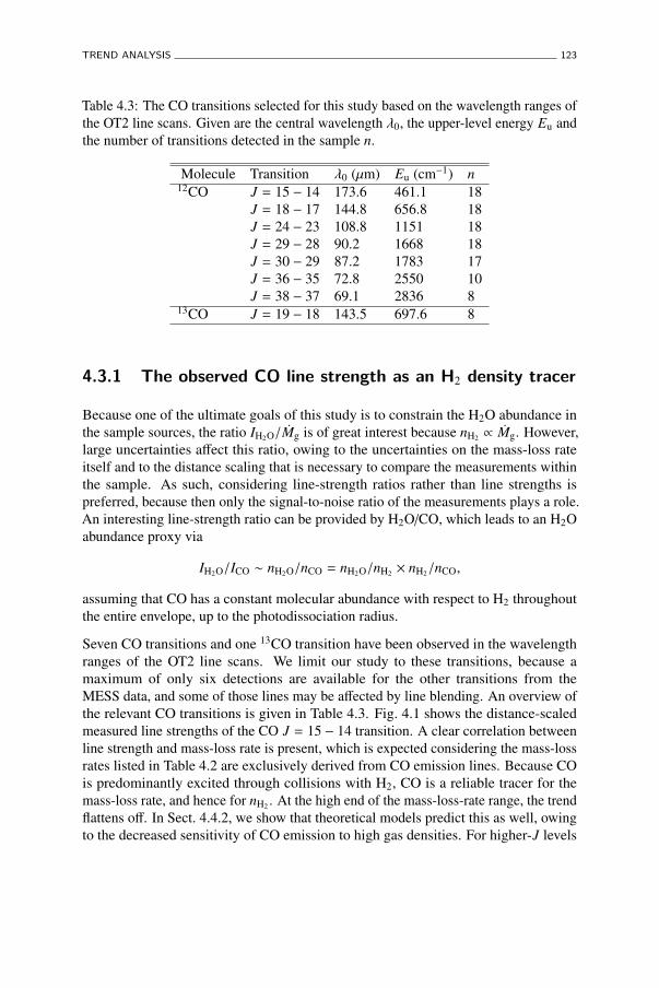
TREND ANALYSIS 123

Table 4.3: The CO transitions selected for this study based on the wavelength ranges ofthe OT2 line scans. Given are the central wavelength �0, the upper-level energy Eu andthe number of transitions detected in the sample n.

Molecule Transition �0 (µm) Eu (cm�1) n12CO J = 15 � 14 173.6 461.1 18

J = 18 � 17 144.8 656.8 18J = 24 � 23 108.8 1151 18J = 29 � 28 90.2 1668 18J = 30 � 29 87.2 1783 17J = 36 � 35 72.8 2550 10J = 38 � 37 69.1 2836 8

13CO J = 19 � 18 143.5 697.6 8

4.3.1 The observed CO line strength as an H2 density tracer

Because one of the ultimate goals of this study is to constrain the H2O abundance inthe sample sources, the ratio IH2O/Mg is of great interest because nH2 / Mg. However,large uncertainties a↵ect this ratio, owing to the uncertainties on the mass-loss rateitself and to the distance scaling that is necessary to compare the measurements withinthe sample. As such, considering line-strength ratios rather than line strengths ispreferred, because then only the signal-to-noise ratio of the measurements plays a role.An interesting line-strength ratio can be provided by H2O/CO, which leads to an H2Oabundance proxy via

IH2O/ICO ⇠ nH2O/nCO = nH2O/nH2 ⇥ nH2/nCO,

assuming that CO has a constant molecular abundance with respect to H2 throughoutthe entire envelope, up to the photodissociation radius.

Seven CO transitions and one 13CO transition have been observed in the wavelengthranges of the OT2 line scans. We limit our study to these transitions, because amaximum of only six detections are available for the other transitions from theMESS data, and some of those lines may be a↵ected by line blending. An overview ofthe relevant CO transitions is given in Table 4.3. Fig. 4.1 shows the distance-scaledmeasured line strengths of the CO J = 15 � 14 transition. A clear correlation betweenline strength and mass-loss rate is present, which is expected considering the mass-lossrates listed in Table 4.2 are exclusively derived from CO emission lines. Because COis predominantly excited through collisions with H2, CO is a reliable tracer for themass-loss rate, and hence for nH2 . At the high end of the mass-loss-rate range, the trendflattens o↵. In Sect. 4.4.2, we show that theoretical models predict this as well, owingto the decreased sensitivity of CO emission to high gas densities. For higher-J levels

124 CONSTRAINING H2O FORMATION IN CARBON-RICH AGB WINDS

�7.0 �6.5 �6.0 �5.5 �5.0 �4.5

log�Mg (M�/yr)

��16.0

�15.5

�15.0

�14.5

�14.0

�13.5

�13.0lo

g� I C

O(J

=15

�14

)(W

/m2 )

�

Figure 4.1: The distance-scaled line strengths of the CO J = 15 � 14 transition withrespect to the mass-loss rate Mg. The data points are color coded according to thevariability type: Miras in red, SRa sources in blue and SRb sources in black.

the linear trend flattens o↵ sooner, because the lines are formed closer to the stellarsurface where the gas density is higher. Therefore, the J = 15 � 14 transition is bestsuited to act as an H2 density tracer. CO J = 15 � 14 has been detected in all objects inthe sample, and none of them are flagged as a line blend.

As shown in Fig 4.1, the Miras and SRa sources cannot be distinguished based onCO line strength. The SRb sources cluster at the low end of the mass-loss-rate range,but still seem to follow the linear trend set by the Miras and SRa sources. Studieson large populations have shown that Miras are considered to be fundamental-modepulsators, while semiregulars are overtone pulsators or low-period fundamental-modepulsators (Wood et al. 1999; Wood 2010). The di↵erentiation between SRa and SRbvariables is based on the regularity of the light curves of these sources, but no definiteconclusion can be made about the pulsational mode they exhibit. As shown by Bowen(1988), overtone pulsators are significantly less e�cient at driving a stellar wind thanfundamental-mode pulsators. If one assumes SRa sources pulsate in a low-periodfundamental mode, and SRb sources in a first or second overtone, this could explainthe clear di↵erence in terms of mass-loss rate between these two variability classes.Another suggestion is that SRb sources are unstable in more than one pulsation mode,and thus experience more than one pulsation period characteristic of each mode,

TREND ANALYSIS 125

Figure 4.2: The line-strength ratio of the H2O JKa,Kc = 21,2 � 10,1 transition versus theCO J = 15 � 14 transition with respect to the mass-loss rate Mg. The data points arecolor coded according to the variability type: Miras in red, SRa sources in blue andSRb sources in black. A black cross superimposed on a point indicates that the H2Oline strength is flagged as a blend. The gray lines show the individual fit results ofIoH2O/ICO = a + bMg to a large number of guesses drawn from the Mg and IH2O/ICOdistributions of each data point for Miras and SRa sources. The green arrow indicatesthe mean linear relation, for which the coe�cients a and b are given in Table 4.4.

explaining the lower periodicity of their light curves (Soszynski & Wood 2013). Thismay also decrease the e�ciency with which a wind is driven.

4.3.2 The H2O/CO line-strength ratio versus Mg

Only the H2O transitions in the wavelength ranges of the OT2 line scans are taken intoaccount in this study. Their central wavelengths and upper-level energies are listedin the first columns of Table 4.4. Two additional transitions, with higher upper-levelenergies, are included in Table C.3 up to C.6, but both occur in a blend with anotherH2O transition listed in Table 4.4 and do not contribute significantly to the emissionline. We do not consider them in the remainder of this study.

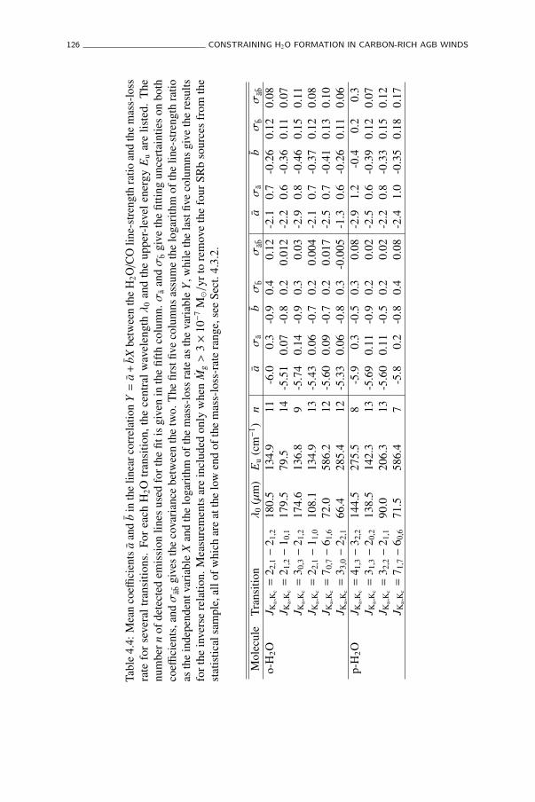
126 CONSTRAINING H2O FORMATION IN CARBON-RICH AGB WINDS

Tabl

e4.

4:M

ean

coe�

cien

tsa

and

bin

the

linea

rcor

rela

tion

Y=

a+

bXbe

twee

nth

eH

2O/C

Olin

e-st

reng

thra

tioan

dth

em

ass-

loss

rate

fors

ever

altra

nsiti

ons.

Fore

ach

H2O

trans

ition

,the

cent

ralw

avel

engt

h�

0an

dth

eup

per-

leve

lene

rgy

Eu

are

liste

d.Th

enu

mbe

rnof

dete

cted

emis

sion

lines

used

fort

hefit

isgi

ven

inth

efif

thco

lum

n.�

aan

d�

bgi

veth

efit

ting

unce

rtain

ties

onbo

thco

e�ci

ents

,and

�ab

give

sth

eco

varia

nce

betw

een

the

two.

The

first

five

colu

mns

assu

me

the

loga

rithm

ofth

elin

e-st

reng

thra

tioas

the

inde

pend

entv

aria

ble

Xan

dth

elo

garit

hmof

the

mas

s-lo

ssra

teas

the

varia

ble

Y,w

hile

the

last

five

colu

mns

give

the

resu

ltsfo

rthe

inve

rse

rela

tion.

Mea

sure

men

tsar

ein

clud

edon

lyw

hen

Mg>

3⇥

10�7

M�/

yrto

rem

ove

the

four

SRb

sour

ces

from

the

stat

istic

alsa

mpl

e,al

lofw

hich

are

atth

elo

wen

dof

the

mas

s-lo

ss-r

ate

rang

e,se

eSe

ct.4

.3.2

.

Mol

ecul

eTr

ansi

tion

�0

(µm

)E

u(c

m�1

)n

a�

ab

�b

�ab

a�

ab

�b

�ab

o-H

2OJ K

a,K

c=

2 2,1�

2 1,2

180.

513

4.9

11-6

.00.

3-0

.90.

40.

12-2

.10.

7-0

.26

0.12

0.08

J Ka,

Kc=

2 1,2�

1 0,1

179.

579

.514

-5.5

10.

07-0

.80.

20.

012

-2.2

0.6

-0.3

60.

110.

07J K

a,K

c=

3 0,3�

2 1,2

174.

613

6.8

9-5

.74

0.14

-0.9

0.3

0.03

-2.9

0.8

-0.4

60.

150.

11J K

a,K

c=

2 2,1�

1 1,0

108.

113

4.9

13-5

.43

0.06

-0.7

0.2

0.00

4-2

.10.

7-0

.37

0.12

0.08

J Ka,

Kc=

7 0,7�

6 1,6

72.0

586.

212

-5.6

00.

09-0

.70.

20.

017

-2.5

0.7

-0.4

10.

130.

10J K

a,K

c=

3 3,0�

2 2,1

66.4

285.

412

-5.3

30.

06-0

.80.

3-0

.005

-1.3

0.6

-0.2

60.

110.

06p-

H2O

J Ka,

Kc=

4 1,3�

3 2,2

144.

527

5.5

8-5

.90.

3-0

.50.

30.

08-2

.91.

2-0

.40.

20.

3J K

a,K

c=

3 1,3�

2 0,2

138.

514

2.3

13-5

.69

0.11

-0.9

0.2

0.02

-2.5

0.6

-0.3

90.

120.

07J K

a,K

c=

3 2,2�

2 1,1

90.0

206.

313

-5.6

00.

11-0

.50.

20.

02-2

.20.

8-0

.33

0.15

0.12

J Ka,

Kc=

7 1,7�

6 0,6

71.5

586.

47

-5.8

0.2

-0.8

0.4

0.08

-2.4

1.0

-0.3

50.

180.

17

TREND ANALYSIS 127

Fig. 4.2 shows the line-strength ratio of H2O JKa,Kc = 21,2 � 10,1 and CO J = 15 � 14with respect to the mass-loss rate. Several qualitative conclusions can be drawn. Adownward trend toward higher mass-loss rate is present in the H2O/CO line-strengthratios, indicated by the green arrow superimposed on the data points. Assuming H2O ishomogenously distributed within the formation region of a given line, this suggests thatthe H2O abundance also decreases with mass-loss rate in the same fashion. ThoughFig. 4.2 shows the line-strength ratios for only one H2O line, the trend exists forother H2O lines as well. However, contrarily to the CO line strengths, the H2O/COline-strength ratios of the SRb sources do not follow the trend set by the Miras andSRa sources. Instead they group together at the low end of the mass-loss-rate rangefeaturing line-strength ratios that are significantly lower than the trend in the othersources would predict. Though only four sources can be considered, of which oneis flagged as a line blend and cannot be relied on, it appears that no clear correlationbetween the line-strength ratio and the mass-loss rate within the SRb sample is present.

The di↵erence between the SRb sources on the one hand and the Miras and SRa sourceson the other hand suggests some dependence on pulsational properties. Previoustheoretical (Bowen 1988) and observational (Wood et al. 2007; De Beck et al. 2010)studies have shown that a strong correlation between the mass-loss rate and thepulsational period exists for AGB stars, especially toward higher period. This trendis also present in our H2O observations. Fig. 4.3 gives the line-strength ratio of theH2O JKa,Kc = 21,2 � 10,1 transition and the CO J = 15 � 14 transition with respect topulsational period. The data points are color coded according to the column-densityproxy m (see Eq. 4.1). The Miras and SRa sources are shown in blue, red and greenfor increasing m (as indicated in the legend). An increasing outflow density, and thusa decreasing H2O/CO line-strength ratio, is associated with an increasing pulsationalperiod. However, the SRb sources (shown in black in Fig. 4.3) do not follow this trend,e.g. Y CVn and U Hya have similar column densities while having the lowest andhighest pulsational period among the SRb sources, respectively. Instead, a weakerdownward trend with respect to pulsational period seems present throughout the wholeSRb sample, but this is far from conclusive.

4.3.3 Least-squares-fitting approach

To quantify the anticorrelation between measured H2O/CO line-strength ratios andmass-loss rates of the Miras and the SRa sources, we apply a least-squares-fittingtechnique to fit a linear function in logarithmic scale. To assess the accuracy of thefitted slope and intercept, the uncertainties on the measured values, which follow anormal distribution in linear space, as well as the uncertainty on the mass-loss ratehave to be taken into account. Studies investigating the mass-loss rate of AGB outflowstypically report uncertainties of a factor of three (Ramstedt et al. 2008; De Beck et al.2010; Lombaert et al. 2013; Schöier et al. 2013). For our purposes we assume that

128 CONSTRAINING H2O FORMATION IN CARBON-RICH AGB WINDS

Figure 4.3: The line-strength ratio of the H2O JKa,Kc = 21,2 � 10,1 transition versus theCO J = 15 � 14 transition with respect to the pulsational period. The points with errorbars give the measured H2O/CO line-strength ratios, color coded according to the valueof the column-density proxy m, indicated in the legend. Black crosses superimposedon the points indicate that the H2O line is flagged as a blend.

the derived Mg values follow a normal distribution in logarithmic scale, with the3�-confidence level equal to this factor of three accuracy.

To ensure a proper error propagation, we apply a Monte Carlo-like approach, in whichwe draw a large number of guesses (N = 106) for the relevant quantities from theirrespective distributions. Since we fit the observed line-strength ratios in logarithmicscale, we can also apply this approach to the mass-loss rate, for which we draw theguess from the normal distribution of logarithmic values. This results in N linearrelations from which we calculate the mean slope and intercept to arrive at a meanrelation between the relevant quantities. At the same time, we also determine if theslope and intercept of the N relations are correlated. This approach is applied to allH2O transitions. The number of data points n per transition taken into account for thelinear fit is given in column 5 of Table 4.4. The mean coe�cients a and b of the linearrelation Y = a + bX between IH2O/ICO and Mg are listed in the next ten columns ofTable 4.4, as well as their uncertainties and the covariance between them. We givethe results for IH2O/ICO as independent variable X in columns 6 through 10, and theresults for the inverse relation in columns 11 through 15. Taking the reciprocal of one

SAMPLE-WIDE H2O ABUNDANCE 129

relation does not necessarily result in the coe�cients of the inverse relation because theleast-squares minimization only takes into account the vertical residuals between thedata points and the best linear fit. The N individual linear-fit results in the Monte Carloapproach are shown in gray-black in Fig. 4.2. The green arrow indicates the mean linearrelation according to the coe�cients given in Table 4.4 for the H2O JKa,Kc = 21,2 � 10,1transition.

Notably, within the fitting uncertainties, the slope of the linear relation agrees betweenall ortho- and para-H2O lines. We list the covariance between the slope and the interceptof the linear relation as well, which is a measure of how closely correlated the slopeand the intercept are. With the exception of one, all relations listed in Table 4.4 show astrong correlation between the slope and the intercept, meaning that a larger interceptmust be associated with a steeper slope. This is evidenced by the gray lines in Fig. 4.2,which seem to knot together in the intermediate Mg region, while spreading out formore extreme values of Mg. The H2O/CO line-strength ratio for the JKa,Kc = 33,0 � 22,1transition is attributed to a small negative covariance when taking IH2O/ICO as theindependent variable X. This suggests that the slope and intercept of the linear relationare weakly anticorrelated, hence the negative value. However, the slope-interceptcorrelation is very weak for this particular transition due to a large scatter betweenthe data points. As such, the linear fit to this H2O/CO line-strength ratio and themass-loss rate is less reliable, but still confirms the observed downward trend based onthe negative slope b = �0.8.

The relations in columns 6 through 10 can serve as a mass-loss indicator as long asmeasurements for the relevant H2O and CO line strengths are available. The relations incolumns 11 through 15 are helpful in predicting the H2O/CO line-strength ratio, givena mass-loss rate. When using these relations to estimate a mass-loss rate or predict aline-strength ratio, the uncertainty on the result can be determined from the relation

�Y =q�2

a + b2�2X + X2�2

b+ X�2

ab.

Owing to the distance-independent H2O/CO line-strength ratios and barring systematice↵ects in the assumed Mg values for our sample, this leads to an uncertainty of about0.3 dex on the logarithmic values.

4.4 Sample-wide H2O abundance

A downward trend between the H2O/CO line-strength ratio and the mass-loss rateis evident for the Miras and the SRa sources. To exclude that this trend is causedby optical-depth e↵ects, and indeed points to an anticorrelation between the H2Oabundance and the mass-loss rate, theoretical radiative-transfer models are needed.However, modeling the line strengths for each source individually is beyond the scope

130 CONSTRAINING H2O FORMATION IN CARBON-RICH AGB WINDS

of this study. We opt for a qualitative approach in which we calculate theoretical modelsfor a set of parameters appropriate for Miras, SRa and SRb sources, with which weprobe the influence on the line strengths.

4.4.1 The model grid

We set up a theoretical model grid with a fine sampling of the H2O abundance1, themass-loss rate Mg and the gas temperature profile Tg(r), and with a coarse sampling ofthe other stellar and circumstellar properties: the gas terminal velocity 31,g, the stellare↵ective temperature T?, the stellar luminosity L?, the dust-to-gas ratio and the COabundance with respect to molecular hydrogen. In the following, we refer to a singleset of values for all stellar and circumstellar parameters, except the H2O abundance andthe mass-loss rate, as the standard model grid. To probe the sensitivity of the observedH2O emission to the stellar and circumstellar properties, we vary at most one additionalparameter in this standard grid. Table 4.5 lists both the adopted value for the standardmodel grid as well as the sampling range and step size of the parameters. Beam e↵ectsor other telescope-related properties have been corrected for during the PACS datareduction, such that measured line strengths can be directly compared with the intrinsicline strengths of theoretical predictions. This assumes that the PACS observations arenot spatially resolved, which is one of our target selection criteria (see Sect. 4.2.1).

We calculate line radiative transfer using GASTRoNOoM (Decin et al. 2006, 2010b;Lombaert et al. 2013). In these calculations, the density distribution of the outflow isassumed to be smooth and spherically symmetric, i.e. we do not take into account small-scale structure in the form of clumps or large-sscale structure in the form of a disk orpolar outflows. For an extensive overview of the molecular data of CO and H2O used inthis study, we refer to the appendix in Decin et al. (2010b). The molecular abundanceswith respect to H2 of both CO and H2O are assumed to be constant throughout theenvelope up to the photodissociation radius where interstellar UV photons destroythe molecules. The CO photodissociation radius is set by the formalism of Mamonet al. (1988). For H2O we use the analytic formula from Groenewegen (1994). Theacceleration of the wind to the terminal expansion velocity 31,g of the gas is set bymomentum transfer from dust to gas assuming full momentum coupling between thetwo components (Kwok 1975). The gas turbulent velocity 3stoch is fixed at 1.5 kms/s.Because the cooling contribution from HCN is not well constrained (Decin et al. 2010b;De Beck et al. 2012), we approximate the gas kinetic-temperature structure with apower law of the form

Tg(r) = T?

rR?

!�✏,

1All values for nH2O/nH2 are given in this study for ortho-H2O only.

SAMPLE-WIDE H2O ABUNDANCE 131

Table 4.5: Stellar and circumstellar parameters of the model grid described in Sect 4.4.1.The first and second column list the parameter and its unit, the third column lists theadopted value in the standard model grid, the fourth column indicates the samplingrange in which an individual parameter is allowed to vary, and the last column givesthe step size with which the parameter was probed. Listed are the gas mass-loss rate(Mg), the H2O abundance with respect to molecular hydrogen (nH2O/nH2 ), the power ofthe adopted gas kinetic-temperature profile (✏), the stellar e↵ective temperature (T?),the stellar luminosity (L?), the gas terminal velocity (31,g), the dust-to-gas ratio ( )and the CO abundance with respect to molecular hydrogen (nCO/nH2 ).

Parameter Unit Standard Range Step sizelog(Mg) M�/yr / [�8.0,�4.5] 0.5log(nH2O/nH2 ) / [�10,�4] 1✏ 0.4 [0.3, 0.9] 0.1T? 103 K 2 [2, 3] 0.5L? 103 L� 8 [4, 12] 431,g km/s 10 [10, 25] 5log( ) -2.3 [�2.7,�2] 0.35nCO/nH2 10�3 0.8 [0.6, 1.2] 0.2

where r is the distance to the center of the star. As shown by Lombaert et al. (2013),dust can play an important role in H2O excitation. Following Lombaert et al. (2012),we use a distribution of hollow spheres (DHS, Min et al. 2003) with filling factor 0.8 torepresent the dust extinction properties, and a dust composition that is 75% amorphouscarbon, 10% silicon carbide and 15% magnesium sulfide. The optical properties usedto calculate the extinction contribution from these species are taken from Jäger et al.(1998b), Pitman et al. (2008) and Begemann et al. (1994), respectively. We take theinner radius of the circumstellar envelope to match the dust condensation radius, whichis determined following Kama et al. (2009) with use of the dust radiative-transfer codeMCMax (Min et al. 2009).

4.4.2 CO line strengths

To allow for a direct comparison between measured and predicted H2O/CO line-strength ratios, it is important that the standard model grid predicts the observedCO line strengths well. The two most influential circumstellar properties that a↵ectCO emission are the gas kinetic temperature and the CO number density. A usefulparameter in studying the line-strength trends is the column-density proxy m, definedaccording to Eq. 4.1. The measured line strengths follow a more consistent trend when

132 CONSTRAINING H2O FORMATION IN CARBON-RICH AGB WINDS

�3.0 �2.5 �2.0 �1.5 �1.0 �0.5 0.0 0.5

log�m (g/cm2)

��16.5

�16.0

�15.5

�15.0

�14.5

�14.0

�13.5

�13.0

�12.5lo

g� I C

O(J

=15

�14

)(W

/m2 )

�

CO J = 15 � 14

MiraSRaSRb� = 0.3

� = 0.4

� = 0.5

� = 0.6

� = 0.7

� = 0.8

�3.0 �2.5 �2.0 �1.5 �1.0 �0.5 0.0 0.5

log�m (g/cm2)

��16.5

�16.0

�15.5

�15.0

�14.5

�14.0

�13.5

�13.0

log

� I CO

(J=

36�

35)(W

/m2 )

�

CO J = 36 � 35

MiraSRaSRb� = 0.3

� = 0.4

� = 0.5

� = 0.6

� = 0.7

� = 0.8

Blended

Figure 4.4: The distance-scaled line strengths of two CO transitions with respect tothe column-density proxy m: CO J = 15 � 14 at the top and CO J = 36 � 35 at thebottom. The points with error bars give the measured CO line strengths, color codedaccording to the variability type. Black crosses superimposed on the points indicatethat the CO line is flagged as a blend. The colored curves show the predicted CO linestrength for various values of the temperature power law exponent ✏. Adopted valuesfor other parameters are listed in Table 4.5.

SAMPLE-WIDE H2O ABUNDANCE 133

comparing them with m, shown in the top panel of Fig. 4.4, as opposed to comparingthem with Mg in Fig. 4.1.

Owing to the large uncertainty on the assumed distance for many sources, it is di�cultto constrain the exponent of the temperature law, as shown in Fig. 4.4 for J = 15 � 14at the top, and for J = 36 � 35 at the bottom. The most probable value taking intoaccount both these CO transitions as well as others (not shown here) is ✏ = 0.4. Asbriefly mentioned in Sect. 4.3.1, the linear trend in the observed CO line strengths withrespect to the mass-loss rate flattens o↵ at higher values. The theoretical predictionsconfirm this observed trend also for higher m values, but the e↵ect is less pronounced,especially for the higher-J transitions. The e↵ect on the CO J = 15 � 14 transitionappears to be limited, which confirms this line to be a suitable H2 density tracer. Otherstellar or circumstellar properties are less important for CO emission. Figs. 4.5 and 4.6present an overview of standard theoretical models for the CO J = 15 � 14 transition,in which only one additional parameter is allowed to vary. The top panel in Fig. 4.5shows that the CO molecular abundance with respect to H2 does not have a significante↵ect on the CO line strengths relative to the e↵ect of the explored range of mass-lossrates. The CO abundance is notoriously di�cult to constrain from CO observationsalone because it is completely degenerate with respect to the gas mass-loss rate. Wetherefore keep it fixed at 0.8⇥10�3 in our standard model grid. From chemical networkcalculations, Cherchne↵ (2012) found nCO/nH2 = 0.9 ⇥ 10�3 for CW Leo.

The bottom panel in Fig. 4.5 indicates that the gas terminal velocity only has a limitede↵ect on the predictions. The top and bottom panels in Fig. 4.6 show theoreticalpredictions for several values of T? and L?, respectively. In these figures, the colorcoding of the data points is such that the color matches that of the theoretical modelwith an analogous value for either T?, L? or 31,g. The observed spread in CO linestrengths versus m with respect to the theoretical predictions can be attributed mainlyto the di↵erence in the stellar luminosity and e↵ective temperature. As an example, twoSRb objects deviate significantly from the standard theoretical predictions given by thered curve in Fig. 4.6. The top panel shows that an increase in T? fixes this issue, whichis in agreement with the higher T? derived for SRb sources from infrared colors, seeTable 4.2. The large uncertainties on the distance, however, do not allow to constrainany of these properties further. To represent the sample well on average, we adopt31,g = 10 km/s, T? = 2000 K, and L? = 8000 L� for the standard model grid.

4.4.3 H2O/CO line-strength ratios

Fig. 4.7 shows the measured H2O/CO line-strength ratios for a cold H2O transition(JKa,Kc = 21,2 � 10,1) at the top, and a warm H2O transition (JKa,Kc = 33,0 � 22,1) atthe bottom. Additionally, predicted line-strength ratios from the standard model gridwith adopted parameters given in Table 4.5 are superimposed on the data points. The

134 CONSTRAINING H2O FORMATION IN CARBON-RICH AGB WINDS

�2.5 �2.0 �1.5 �1.0 �0.5 0.0 0.5

log�m (g/cm2)

��16.5

�16.0

�15.5

�15.0

�14.5

�14.0

�13.5

�13.0

�12.5

�12.0lo

g� I C

O(J

=15

�14

)(W

/m2 )

� MiraSRaSRbACO/AH2 = 0.6 � 10�3

ACO/AH2 = 0.8 � 10�3

ACO/AH2 = 1.0 � 10�3

ACO/AH2 = 1.2 � 10�3

�3.5 �3.0 �2.5 �2.0 �1.5 �1.0 �0.5 0.0 0.5

log�m (g/cm2)

��16.5

�16.0

�15.5

�15.0

�14.5

�14.0

�13.5

�13.0

�12.5

�12.0

log

� I CO

(J=

15�

14)(W

/m2 )

� v�,g < 10 km/s10 km/s � v�,g < 15 km/s15 km/s � v�,g < 20 km/sv�,g � 20 km/sv�,g = 10 km/sv�,g = 15 km/sv�,g = 20 km/sv�,g = 25 km/s

Figure 4.5: The distance-scaled line strengths of the CO J = 15 � 14 transition withrespect to the column-density proxy m. The points with error bars give the measuredCO line strengths, color coded according to the pulsational type or 31,g indicated in thelegend. Each panel shows curves for di↵erent values of a given parameter in the modelgrid, with similar color coding as the data points, if applicable. The top panel givesthe results for the CO abundance with respect to H2 and the bottom panel for the gasterminal velocity 31,g. Other adopted quantities are given in Table 4.5.

SAMPLE-WIDE H2O ABUNDANCE 135

�2.5 �2.0 �1.5 �1.0 �0.5 0.0 0.5 1.0

log�m (g/cm2)

��16.5

�16.0

�15.5

�15.0

�14.5

�14.0

�13.5

�13.0

�12.5lo

g� I C

O(J

=15

�14

)(W

/m2 )

� T� < 2000 K2000 K � T� < 2250 K2250 K � T� < 2500 KT� � 2500 KT� = 2000 KT� = 2500 KT� = 3000 K

�2.5 �2.0 �1.5 �1.0 �0.5 0.0 0.5

log�m (g/cm2)

��16.5

�16.0

�15.5

�15.0

�14.5

�14.0

�13.5

�13.0

�12.5

log

� I CO

(J=

15�

14)(W

/m2 )

� L� < 6000 L�

6000 L� � L� < 8000 L�

8000 L� � L� < 10000 L�

L� � 10000 L�

L� = 4000 L�

L� = 8000 L�

L� = 12000 L�

Figure 4.6: The distance-scaled line strengths of the CO J = 15 � 14 transition withrespect to the column-density proxy m. The points with error bars give the measuredCO line strengths, color coded according to the values of the relevant quantity indicatedin the legend. Each panel shows curves for di↵erent values of a given parameter in themodel grid, with similar color coding as the data points. The top panel gives the resultsfor the stellar e↵ective temperature T? and the bottom panel for the stellar luminosityL?. Other adopted quantities are given in Table 4.5.

136 CONSTRAINING H2O FORMATION IN CARBON-RICH AGB WINDS

observed line-strength ratios span more than three orders of magnitude in H2O vaporabundance. This is the case for all H2O lines in the sample, i.e. for both cold and warmH2O emission. For the SRb sources, a significantly di↵erent H2O abundance for coldand warm H2O is observed. To a lesser degree, this di↵erence also occurs in the Mirasand SRa sources. We discuss these findings in Sect. 4.5.

In terms of sensitivity to the assumptions of the standard model grid, only the gasterminal velocity and the dust-to-gas ratio have a significant impact on the calculatedH2O/CO line-strength ratios. Fig. 4.8 shows H2O/CO line-strength-ratio predictionsfor the standard model grid, in which either 31,g or is allowed to vary. The toppanel gives the results for 31,g = 10 km/s in black (standard model-grid value) and31,g = 25 km/s in green. In the optically thin regime, a change in 31,g, and therefore inthe column-density proxy m, does not a↵ect H2O emission, as shown by the modelsfor nH2O/nH2 = 10�7. For higher H2O abundances, the lines become optically thick,so that a change in 31,g and m a↵ects H2O line strengths significantly. The bottompanel in Fig. 4.8 gives the lowest and highest value in the grid. The H2O/CO line-strength-ratio sensitivity to the dust-to-gas ratio arises because H2O is primarily excitedradiatively by infrared photons emitted by dust in high-density environments (e.g. theright panel of Fig. 4.8 for log(m) > �1.5). Here, the higher results in stronger H2Oemission, while CO line strengths remain mostly una↵ected (Lombaert et al. 2013).In low-density environments, direct stellar light dominates H2O excitation, losing thesensitivity to the dust-to-gas ratio. Similarly to the CO line strengths, some spreadis likely introduced in the observed line-strength ratios by di↵erences in either 31,gor , but not enough to explain the observed trend in the Miras and the SRa sources.The assumed exponent of the temperature law ✏ = 0.4 has a significant impact onthe H2O/CO line-strength ratios because of its importance for the CO line strength,underlining the need to predict the observed CO line strengths accurately. Collisionsplay a minor role in H2O excitation, so the temperature law does not directly influencethe H2O line strengths (e.g. Lombaert et al. 2013 for the high-Mg case).

The comparison between the observed H2O/CO line-strength ratios and the theoreticalpredictions excludes radiative-transfer e↵ects as the sole cause of the downward trendbetween the H2O/CO line-strength ratio and the column-density proxy. This confirmsthat the H2O/CO line-strength ratio can be treated as an H2O abundance proxy and thatthe H2O abundance anticorrelates with the circumstellar column density. Because thedownward trend exists for all H2O transitions regardless of the energy levels involved,this implies that it is the H2O formation mechanism itself that becomes less e�cientwith increasing envelope column density.

SAMPLE-WIDE H2O ABUNDANCE 137

�3.0 �2.5 �2.0 �1.5 �1.0 �0.5 0.0 0.5log

�m (g/cm2)

��1.5

�1.0

�0.5

0.0

0.5

1.0lo

g� I o

H2O

(JK

a,K

c=

2 1,2�

1 0,1)/

I CO

(J=

15�

14)�

MiraSRaSRbAH2O/AH2 = 10�7

AH2O/AH2 = 10�6

AH2O/AH2 = 10�5

AH2O/AH2 = 10�4

Blended

�3.0 �2.5 �2.0 �1.5 �1.0 �0.5 0.0 0.5log

�m (g/cm2)

��1.0

�0.5

0.0

0.5

1.0

log

� I oH

2O

(JK

a,K

c=

3 3,0�

2 2,1)/

I CO

(J=

15�

14)�

MiraSRaSRbAH2O/AH2 = 10�7

AH2O/AH2 = 10�6

AH2O/AH2 = 10�5

AH2O/AH2 = 10�4

Blended

Figure 4.7: The line-strength ratio of two H2O transitions versus the CO J = 15 � 14transition with respect to the column-density proxy m: JKa,Kc = 21,2 � 10,1 at the top,and JKa,Kc = 33,0 � 22,1 at the bottom. The points with error bars give the measuredH2O/CO line-strength ratios, color coded according to the variability type. Blackcrosses superimposed on the points indicate that the H2O line is flagged as a blend.The colored curves show the predicted H2O/CO line-strength ratios for various valuesof the H2O abundance with respect to H2. Adopted values for other parameters arelisted in Table 4.5.

138 CONSTRAINING H2O FORMATION IN CARBON-RICH AGB WINDS

�4 �3 �2 �1 0log

�m (g/cm2)

��1.5

�1.0

�0.5

0.0

0.5lo

g� I o

H2O

(JK

a,K

c=

2 1,2�

1 0,1)/

I CO

(J=

15�

14)�

v�,g < 10 km/s10 km/s � v�,g < 15 km/s15 km/s � v�,g < 20 km/sv�,g � 20 km/s

AH2O/AH2 = 10�7, v�,g = 10 km/s

AH2O/AH2 = 10�7, v�,g = 25 km/s

AH2O/AH2 = 10�6, v�,g = 10 km/s

AH2O/AH2 = 10�6, v�,g = 25 km/s

AH2O/AH2 = 10�5, v�,g = 10 km/s

AH2O/AH2 = 10�5, v�,g = 25 km/s

AH2O/AH2 = 10�4, v�,g = 10 km/s

AH2O/AH2 = 10�4, v�,g = 25 km/s

Blended

�4 �3 �2 �1 0log

�m (g/cm2)

��1.5

�1.0

�0.5

0.0

0.5

log

� I oH

2O

(JK

a,K

c=

2 1,2�

1 0,1)/

I CO

(J=

15�

14)�

MiraSRaSRbAH2O/AH2 = 10�7, � = 0.002

AH2O/AH2 = 10�7, � = 0.01

AH2O/AH2 = 10�6, � = 0.002

AH2O/AH2 = 10�6, � = 0.01

AH2O/AH2 = 10�5, � = 0.002

AH2O/AH2 = 10�5, � = 0.01

AH2O/AH2 = 10�4, � = 0.002

AH2O/AH2 = 10�4, � = 0.01

Blended

Figure 4.8: The line-strength ratio of the H2O JKa,Kc = 21,2 � 10,1 transition versus theCO J = 15 � 14 transition with respect to the column-density proxy m. The pointswith error bars give the measured H2O/CO line-strength ratios, color coded accordingto the values of 31,g (top panel) or the variability type (bottom panel). Black crossessuperimposed on the points indicate that the H2O line is flagged as a blend. The blackand green curves show the predicted H2O/CO line-strength ratios for various valuesof the H2O abundance with respect to H2, as well as the gas terminal velocity in thetop panel, and the dust-to-gas ratio in the bottom panel. Adopted values for otherparameters are listed in Table 4.5.

H2O ABUNDANCE GRADIENTS WITHIN SINGLE SOURCES 139

4.5 H2O abundance gradients within single sources

In this section, we look for trends in the radial dependence of the H2O abundancewithin individual sources. To this end, multiple H2O transitions, which are formed indi↵erent regions in the CSE, can be compared to trace the radial profile of the H2Oabundance. Information on the H2O abundance structure can help to constrain the H2Oformation mechanism in carbon-rich envelopes.

4.5.1 Molecular line contribution regions

Radial abundance gradients of a molecular species can be probed by using emissionlines that are formed in di↵erent regions of the outflow. For CO the excitation occursprimarily through collisions with H2 and is thus coupled to the gas kinetic temperature.CO excitation is quantified in terms of the rotational quantum number J, which followsa simple ladder structure. A high-J transition forms closer to the stellar surface thandoes a low-J transition because the former is populated in a zone where the temperatureis higher. Hence, from simply studying the abundance as a function of J-value mayalready reveal whether a radial gradient is present or not. For H2O the situation isdi↵erent as the levels are mainly radiatively excited and H2O excitation does not followa simple J-ladder like CO. As a result, predicting the line contribution region of a givenH2O transition cannot be achieved through a straightforward scheme such as for CO,and requires models to establish which transitions trace which part of the CSE.

Fig. 4.9 shows the normalized quantity Ip ⇥ g(p2) with respect to the impact parameterp, where Ip is the predicted intensity at line center and g(p2) is a weighing factorproportional to pdp. This quantity is illustrative for where emission in a given lineoriginates in the CSE. From the top panel to the bottom panel in Fig. 4.9, m increases.For each case, a typical H2O abundance has been chosen based on the comparisonof the measured H2O/CO line-strength ratios to the theoretical results in Sect. 4.4.3.The top panel assumes m = 0.01, a typical value for the SRb sources, which clusteraround the theoretical model with nH2O/nH2 = 10�6 in Fig. 4.7. The middle panel andbottom panel represent the low and high end m values of the Mira and SRa sources:m = 0.1 and 1, values for which data points cluster around nH2O/nH2 = 10�5 and 10�7,respectively, in Fig. 4.7. In each panel, the gray area indicates the wind accelerationzone. In the m = 0.01 model, higher energy emission lines form close to the stellarsurface and may be a↵ected by stellar pulsations, ongoing dust formation or windacceleration. The CO J = 15 � 14 line is shown for comparison. Typically, a CO linewill form in a narrower region, due to its sensitivity to the temperature profile only,while an H2O line forms in a wider region owing to the nonlocal nature of radiativeexcitation.

140 CONSTRAINING H2O FORMATION IN CARBON-RICH AGB WINDS

Figure 4.9: Theoretical line contribution regions for ortho-H2O. The normalizedquantity I(p) ⇥ g(p2) is shown with respective to the impact parameter p for sixtransitions identified in the legend in the top panel. The di↵erent panels show the linecontributions for models with m = 0.01 g/cm2 and nH2O/nH2 = 10�6 in the top, m = 0.1g/cm2 and nH2O/nH2 = 10�5 in the middle, and m = 1 g/cm2 and nH2O/nH2 = 10�7 atthe bottom. The gray area indicates the wind acceleration zone in each model.

H2O ABUNDANCE GRADIENTS WITHIN SINGLE SOURCES 141

4.5.2 H2O/H2O line-strength ratios

By comparing the strengths of two H2O lines formed in di↵erent regions of the envelope,information on the radial dependence of the H2O abundance can be inferred. If theobserved H2O/H2O line-strength ratios di↵er from those predicted by our standardtheoretical models, at least one of three assumptions must be at fault.

1. A constant mass-loss rate. Though we assume a constant mass-loss rate, atime-variable mass loss can cause changes in the density profile throughout theenvelope. For instance, a recent decrease in mass loss results in less emissionfrom the region close to the stellar surface. Even though variable mass loss mayexplain discrepancies between observed and predicted line-strength ratios forspecific sources, it is highly unlikely that all sources in our sample su↵er from avariable mass loss on a short time scale of a few hundred years.

2. Instantaneous dust formation at inner radius of the CSE. After dust has formedat the inner radius, we assume that the properties and composition of the grainsas well as the dust-to-gas ratio remain the same throught the envelope. It ishowever likely that dust formation is still ongoing in the acceleration zone (r < 5R?). Because of the importance of dust in H2O excitation, the dust formationzone will impact the level populations of H2O close to the stellar surface. Forlow mass-loss-rate objects, the IR radiation field from dust is weak comparedto direct stellar radiation. The right panel in Fig. 4.8 shows that the sensitivityof H2O emission to the dust-to-gas ratio becomes negligible for log(m) < 1.5,which includes all the SRb sources.

3. A constant H2O abundance. The H2O abundance is assumed to be constantthroughout the CSE up to the photodissociation region. If this assumptionis incorrect, a radial dependence of the H2O abundance with respect to H2will manifest itself in the ratio of line strengths of di↵erent H2O transitions.Considering almost all H2O formation mechanisms predict either a positive ornegative H2O abundance gradient at some radial distance, a discrepancy betweenobserved and predicted line-strength ratios is expected. The photodissociationregion should not a↵ect the H2O emission lines included in this study, becauseall lines are formed well within the photodissociation radius as predicted by theanalytic formula from Groenewegen (1994).

Outside the acceleration zone, H2O/CO line-strength ratios are indeed useful as a probefor the H2O abundance. Ratios of strengths of di↵erent H2O lines can be compared totheoretical predictions to provide information on the H2O abundance gradient. Fig. 4.10shows two examples of a comparison between measured H2O/H2O line-strength ratiosand measured H2O/CO line-strength ratios. The theoretical predictions from thestandard model grid are superimposed on the data points. The color coding is such that

142 CONSTRAINING H2O FORMATION IN CARBON-RICH AGB WINDS

Figure 4.10: The H2O/H2O line-strength ratio versus the H2O/CO line-strength ratiofor a selection of H2O transitions. The points with error bars give the measured line-strength ratios, color coded according to the m range to which the sources belong.Note that the top panel shows no m < 0.07 g/cm2 points because one of the H2Otransitions was not detected in any of the SRb sources. Black crosses superimposed onthe points indicate that one of the H2O lines is flagged as a blend. The colored curvesshow the predicted line-strength ratios for various values of m, in the same range asthe data points for each color. The horizontal axis corresponds to an increasing H2Oabundance from left to right, with the highest value being 10�4. Adopted values forother parameters are listed in Table 4.5.

H2O ABUNDANCE GRADIENTS WITHIN SINGLE SOURCES 143

the same colors between data points and theoretical predictions have a similar m. Thepoints on the theoretical curves represent H2O abundance values, increasing from leftto right.

In the top panel of Fig. 4.10, the JKa,Kc = 21,2 � 10,1 transition is compared to theJKa,Kc = 22,1 � 21,2 transition. For m = 0.1 and 1 g/cm2, these transitions are formed ina similar, though not identical region of the envelope (the solid red curve versus thesolid black curve in Fig. 4.9). Hence, these lines would not be able to trace an H2Oabundance gradient. Our theoretical models are indeed able to predict the observedline-strength ratios fairly well. The top panel in Fig. 4.9 shows that these two linesform in di↵erent regions for m = 0.01 g/cm2. Unfortunately, the JKa,Kc = 22,1 � 21,2was undetected in the SRb sources, all of which have a similarly low m. Though, otherhigh-excitation H2O transitions were detected, albeit weakly (e.g. JKa,Kc = 70,7 � 61,6in U Hya).

The bottom panel in Fig. 4.10 shows the comparison of the JKa,Kc = 21,2�10,1 transitionwith the JKa,Kc = 33,0 � 22,1 transition. These lines are formed in a di↵erent region ofthe envelope (the solid red curve versus the solid blue curve in Fig. 4.9). The observedH2O/H2O line-strength ratios are irrevocably underestimated by the theoretical modelsfor all sources in the sample. Because all sources are a↵ected, the time-variable mass-loss scenario seems ruled out. Because both H2O transitions are formed outside theacceleration zone for m = 0.1 and 1 g/cm2 and dust plays no role in H2O excitationfor m = 0.01 g/cm2, this rules out the second model assumption in the list above asa possible cause of the discrepancy. By elimination, a radial dependence of the H2Oabundance profile likely explains why our predictions do not agree with the observeddata points. It implies that the H2O abundance must increase significantly between⇠ 10 R? and ⇠ 50 R? for m = 0.1 and 1 g/cm2, and between ⇠ 2 R? and ⇠ 15 R? form = 0.01 g/cm2. The change in H2O abundance is the largest for the SRb objects.

These results can be compared to those for oxygen-rich winds, where the H2Oabundance is expected to remain constant up to the H2O photodissociation radius.Khouri et al. (2013) show that models with a constant H2O abundance indeed resultin H2O/H2O line-strength ratios comparable to ratios of all observed H2O transitionsin the oxygen-rich AGB star W Hya. This contrasts sharply with our finding thatobserved line-strength ratios between H2O rotational transitions formed in di↵erentregions cannot be reproduced by the models. We conclude that the H2O abundanceis not constant throughout the envelope and must increase with radius at r . 50 R?.Whether this increase is gradual or rapid cannot be constrained. It is beyond the scopeof this investigation to model a radial gradient in the H2O abundance profile.

144 CONSTRAINING H2O FORMATION IN CARBON-RICH AGB WINDS

Tabl

e4.

6:Th

epr

opos

edH

2Ofo

rmat

ion

mec

hani

sms.

Typi

calv

alue

sfor

ase

tofs

tella

rand

circ

umst

ella

rpar

amet

ersa

regi

ven:

m(in

g/cm

2 ),th

epr

edic

ted

H2O

abun

danc

e,th

era

dius

R i(in

R?

)atw

hich

H2O

form

atio

nis

expe

cted

tobe

gin,

the

radi

usR o

(inR?

)fr

omw

hich

the

H2O

abun

danc

eis

expe

cted

tore

mai

nco

nsta

nt,a

typi

calt

empe

ratu

rera

nge

T f(in

K)f

orea

chm

echa

nism

,and

the

orig

inal

liter

atur

ere

fere

nce(

s):

1.M

elni

cket

al.(

2001

),2.

Saav

ikFo

rd&

Neu

feld

(200

1),3

.Will

acy

(200

4),4

.Agú

ndez

&C

erni

char

o(2

006)

,5.D

ecin

etal

.(20

10a)

,6.A

gúnd

ezet

al.(

2010

),7.

Che

rchn

e↵(2

011)

,8.C

herc

hne↵

(201

2),9

.Tal

bi&

Bac

chus

-Mon

tabo

nel(

2010

),10

.Neu

feld

etal

.(20

11a)

.The

last

colu

mn

lists

addi

tiona

lcom

men

ts.

H2O

form

atio

nm

echa

nism

mn H

2O/n

H2

R ?R i

R oT f

Ref

.C

omm

ents

(g/c

m2 )

(10�

7)(1

013cm

)(R

?)

(R?

)(K

)Ev

apor

atio

nof

icy

bodi

es0.

9-2.

34-

247.

6515

/<

500

1,2,

10Ru

led

out

Fisc

her-

Trop

sch

cata

lysi

s2.

51-

100

7.0

1545

<50

03

⇠Fe

-gra

inde

nsity

Rad

iativ

eas

soci

atio

nH

2+

O1.

61

6.5

150

750<

200

4,9

Rule

dou

tSh

ock-

indu

ced

NLT

Ech

emis

try0.

741-

76.

51.

23.

0>

850

7,8

⇠sh

ock

stre

ngth

UV

phot

odis

soci

atio

nin

inne

rCSE

1.4

25.

12

40>

300

5⇠

degr

eeof

clum

ping

0.7

25.

02

12>

300

6⇠

degr

eeof

clum

ping

0.07

25.

02

8>

300

6⇠

degr

eeof

clum

ping

0.00

710

5.0

25

>30

06

⇠de

gree

ofcl

umpi

ng

DISCUSSION 145

4.6 Discussion

Di↵erent H2O formation mechanisms lead to di↵erent properties of the H2O abundanceprofile in the envelope of carbon stars. In Table 4.6, we summarize these properties forfive proposed mechanisms, though we caution the reader that most of these predictionsare model dependent and have been tailored to explain the H2O observations of CW Leo,the prototypical high mass-loss rate carbon star. Hence a straightforward comparison ofpredicted values with the H2O observations reported in this study is not feasible, unlessthe model assumptions of the H2O formation mechanism agree with the properties ofour sample stars. Given in the table are the m value for which the H2O abundance wasderived and typical radii and temperatures associated with the formation mechanism.The mechanisms based on the evaporation of icy bodies and radiative association of H2and O are listed for completeness, but have been firmly ruled out as viable productionmechanisms by previous studies (Neufeld et al. 2011a; Talbi & Bacchus-Montabonel2010). That leaves one mechanisms capable of producing cold H2O from ⇠ 15 R?

onward, and two mechanisms for producing warm H2O in regions closer to the stellarsurface. Our observations place four constraints on the H2O formation mechanism.

1. As shown by previous studies for singular sources, and now confirmed to holdfor all stars in a sample of 18 sources, H2O exists in the innermost regions of theCSE. For high mass-loss-rate objects, we confirm the presence of H2O at leastas close to the stellar surface as ⇠ 10 R?, just outside the acceleration zone. Forlow mass-loss-rate objects, H2O is present close to the stellar surface, around⇠ 2 R?.

2. The H2O formation mechanism becomes less e�cient with increasing mass-lossrate.

3. The anticorrelation between H2O abundance and mass-loss rate (see point 2) isobserved for mass-loss rates higher than ⇠ 3 ⇥ 10�7 M�/yr. The SRb sources inour sample have lower mass-loss rates and do not follow the trend.

4. Every object in the sample shows indications of an H2O abundance gradient,with a significant increase in the inner wind up to ⇠ 50 R?. The transition pointgoing from lower abundance to higher abundance lies at a radial distance thatdepends on m.

4.6.1 Fischer-Tropsch catalysis

Only two constraints are at least partially fulfilled by Fischer-Tropsch catalysison the surface of small metallic-iron grains. First, it allows for a broad range ofH2O abundances to be produced by tweaking the Fe-grain number density, but it

146 CONSTRAINING H2O FORMATION IN CARBON-RICH AGB WINDS

is unclear how a di↵erent circumstellar column density a↵ects the Fe-grain numberdensity. Second, the abundance gradient required for the high m case agrees wellwith the theoretically predicted H2O abundance profile. However, in terms of theother requirements, the Fischer-Tropsch mechanism cannot be reconciled with ourobservations. Firstly, the presence of H2O in the innermost CSE cannot be explained.Secondly, the mechanism would have to become more e�cient at lower envelopedensities. This is counterintuitive for a mechanism based on dust grains acting as acatalyst because lower densities will reduce the amount of interaction between dust andgas that is needed to produce H2O. Lastly, the mechanism cannot explain the presencenor the abundance increase of H2O in SRb objects. In these sources H2O is locatedclose to the stellar surface in too hot of an environment for the mechanism to operate.Even though Fischer-Tropsch catalysis may contribute to H2O formation in carbon-richenvironments, it seems very unlikely that it is a universal mechanism. Further modelingof this production mechanism for low mass-loss-rate objects needs to be performed tosee if it still functions in low-density regions, and whether it becomes more e�cient.

4.6.2 Shock-induced NLTE chemistry

Shock-induced NLTE chemistry provides a universal method to produce H2O incarbon-rich AGB stars: all of them show regular or semiregular pulsational variability,providing the shockwaves needed to break up CO and allow H2O to form. H2O closeto the stellar surface is thus expected and a dependence on the variability type andpulsation amplitude could be explained in this framework. Important aspects of ourH2O analysis concerns the similar H2O line strengths between Miras and SRa sources,and the breakdown of the anticorrelation between the H2O/CO line-strength ratio andm in the low mass-loss-rate range that is populated by SRb sources. It could be thatSRa sources pulsate in a low-period fundamental mode and SRb sources in a first- orsecond-overtone mode. This could a↵ect the shock strengths and densities, which inturn could influence H2O formation. Indeed, Bowen (1988) found that the overtonepulsational modes experience smaller amplitude shocks. This could lead to a cleardi↵erentiation between Miras/SRa sources and SRb sources in terms of H2O formation.Alternatively, the decreased periodicity of SRb sources may also point to instabilities inmultiple pulsation modes (e.g. Soszynski & Wood 2013), which could result in weakershocks as well, whereas the SRa sources are unstable in one pulsation mode only.

Because Cherchne↵ (2011, 2012) has focused on the high mass-loss-rate sourceCW Leo that has a period of 650 days, it is di�cult to predict how her results wouldtranslate to the case of low or multiple periods. Cherchne↵ (2012) states that similartrends can be expected in carbon-rich AGB stars other than CW Leo. She explainsthat a lower shock strength can result in a higher H2O abundance due to the complexinterplay between the consumption of free oxygen by both H2O and SiO formationprocesses. As Cherchne↵ (2011, 2012) notes, these results rely heavily on the interplay

DISCUSSION 147

between H2O and SiO production, of which some involved reaction rates are not wellconstrained. If this process proves viable, it may explain why lower-period pulsators,and thus lower shock strengths (Bowen 1988), show higher H2O abundances. In SRbsources, not only are the pulsation periods lower, but they also pulsate less regularly.Cherchne↵ (2011, 2012) does not consider less regular shocks of lower strength, so itis unclear what their e↵ect would be.

Cherchne↵ (2012) predicts a strong line variability with time for lines formed within⇠ 3 R?, i.e. where the shocks are strong. H2O abundances can vary several ordersof magnitude in this region, and for up to ⇠ 80% of one pulsational phase they aresignificantly higher than at larger distances from the stellar surface. Outside this region,the H2O abundance chemically freezes out to its final value over the course of oneperiod. This seems to be at odds with our observations for SRb sources, which showsystematically lower H2O abundances close to the stellar surface. Unfortunately, insources with a higher column depth, the highest-excitation H2O lines that were observedare formed outside the acceleration zone, so no direct comparison with the modelsof Cherchne↵ (2012) can be made. The time variability for lines formed close to thestellar surface could provide an explanation for the erratic behavior of the H2O/H2Oline-strength ratios observed in SRb sources.

Of all the aspects that need to be fulfilled by a candidate H2O formation mechanism,the observed positive H2O abundance gradient in the inner wind up to ⇠ 50 R? cannotbe explained by shock-induced NLTE chemistry. Shocks can produce a significantamount of H2O in agreement with what would be required to explain the observedemission, but once outside the acceleration zone, no more H2O formation occurs. Ourobservations suggest that the H2O abundance increases with distance from the stellarsurface outside the acceleration zone (r > 5 R?), leaving no doubt that the shockmechanism falls short in that regard. This does not rule it out as a mechanism forproducing H2O, as it might provide a basic amount of H2O close to the stellar surface,after which another mechanism increases the H2O abundance further out.

4.6.3 UV photodissociation in the inner envelope

Whereas most H2O formation mechanisms have been specifically tailored to CW Leo,Agúndez et al. (2010) have looked into a broader range of mass-loss rates for themechanism of UV photodissociation, allowing a comparison with our results. Decinet al. (2010a) report results for the same mechanism for CW Leo. Table 4.6 summarizesthe results for the di↵erent m values. In short, the photodissociation mechanism reliesheavily on the degree of clumping in the CSE for interstellar UV photons to be able topenetrate deeply into the envelope. Therefore, the mechanism provides a natural wayto explain a broad range of H2O abundances.

148 CONSTRAINING H2O FORMATION IN CARBON-RICH AGB WINDS

The model results shown by Agúndez et al. (2010) also predict a decreasing H2Oabundance for high mass-loss-rate objects. The mechanism predicts similar H2Oabundances for high and intermediate mass loss, but a sharp increase in H2O abundancefor low mass-loss rates. The discontinuity occurs when the major UV-shieldedcomponent, i.e. the clumps, becomes transparent. Our observations do not showsuch a sharp increase at a given mass-loss rate, but the model still provides enoughflexibility in terms of the clump properties to allow for a more gradual dependencebetween the H2O abundance and m. Moreover, once both the UV-shielded and UV-exposed components become optically thin, the H2O abundance can be expected toflatten o↵. This would explain why the SRb sources at Mg < 3 ⇥ 10�7 M�/yr do notfollow the anticorrelation between the H2O/CO line-strength ratio and the mass-lossrate. However, the H2O abundance toward lower mass-loss rates does not flatten o↵,but decreases (as shown in Fig. 4.2), which is di�cult to reconcile with this mechanism.

Finally, an H2O abundance gradient naturally follows from the fact that UV photonsneed to penetrate into the envelope. H2O formation stops below a gas kinematictemperature of 300 K, which corresponds to a radial distance of ⇠ 30 R?. As a result,UV photodissociation predicts a gradually increasing H2O abundance profile startingclose to the stellar surface up to ⇠ 5–40 R? depending on m.

The UV-photodissociation scenario suggests that the C17O and C18O isotopologues alsoprovide atomic oxygen to produce the minor isotopologues H17

2 O and H182 O, while the

main CO isotope shields itself from UV radiation. As a result, one expects an isotope-selective enhancement of the H17

2 O and H182 O abundances with respect to the main H2O

isotopologue. Recently, Neufeld et al. (2013) have shown for CW Leo that this isotope-selective enhancement is less than expected. They suggest that dissociation of 12COhas to contribute a significant amount of oxygen atoms as well, if UV photodissociationlies at basis of H2O formation.

The UV-photodissociation mechanism fails at explaining the SRb H2O line strengths,which may be accommodated far better by the shock mechanism, pending furtherstudies concerning shock strengths and periodicity dependence. Additionally, theresults of Neufeld et al. (2013) can be naturally explained if H2O formation isbalanced between both the UV photodissociation and the shock mechanism. Theseconsiderations seem to suggest that both mechanisms are at play.

4.7 Conclusions

We report on new H2O observations made with the PACS instrument onboard theHerschel Space Telescope for a sample of 18 carbon-rich AGB stars in the frameworkof the MESS guaranteed-time key project (P.I.: M. Groenewegen) and an OT2 project(P.I.: L. Decin). H2O has been irrevocably detected in all sample stars, spanning a

CONCLUSIONS 149

broad range of mass-loss rates and several variability types. The H2O emission linesinclude both warm and cold H2O and trace the innermost and intermediate circumstellarenvelope, providing an unprecedented data set that contributes to solving the issue ofH2O formation in carbon-rich environments. We present line-strength measurementsfor CO, 13CO, ortho-H2O and para-H2O between 60 µm and 190 µm.

We look for general trends in the observed H2O line strengths with respect to thecircumstellar density and compare the measurements of the entire sample with atheoreticalmodel grid. The comparison with this model grid suggests that a singletemperature power law with an exponent ✏ = 0.4 can be used to explain all COobservations with a moderate sensitivity to other parameters. As such, CO linemeasurements can be used as a reliable H2 density tracer. We provide linear fittingcoe�cients for H2O/CO line-strength ratios versus the mass-loss rate, which can beused as either a distance-independent mass-loss indicator or to predict line-strengthratios if an estimate of the mass-loss rate is available.

A clear anticorrelation is evident between the H2O/CO line-strength ratios and thecolumn-density proxy m for Mg > 3 ⇥ 10�7 M�/yr, regardless of the upper excitationlevel of the H2O transitions or the variability type. The low mass-loss-rate SRb sourcesin our sample deviate from this trend. Only the gas terminal velocity and the dust-to-gas ratio significantly impact the H2O/CO line-strength ratios, but not enough toexplain the anticorrelation. This confirms that the H2O/CO line-strength ratio is a validdistance-independent H2O abundance tracer. As a result, the H2O abundance neededto explain the observed line strengths depends on m. Moreover, when comparingH2O/H2O line-strength ratios with our model grid, a constant H2O abundance profilefor individual sources does not su�ce to explain the observations. This points towardsa radially increasing H2O abundance gradient in the inner wind up to ⇠ 10 R? for lowcolumn density, and up to ⇠ 50 R? for high column density.

Until now, five H2O formation mechanisms have been suggested. Three of thesemechanisms explain the presence of cold H2O and two predict warm H2O close tothe stellar surface. Two cold-H2O formation mechanisms have already been ruledout on the basis of previous studies. This leaves a cold-H2O formation mechanismbased on Fischer-Tropsch catalysis on Fe grains, and two warm-H2O formationmechanisms: one induced by pulsational shocks just outside the stellar surface, andone by photodissociation of molecules such as 13CO and SiO in the inner envelopeby interstellar UV photons. We derive four constraints that must be fulfilled by anH2O formation mechanism: 1) warm H2O is present close to or inside the accelerationzone in all 18 sources in our sample, 2) H2O formation becomes less e�cient withincreasing mass loss regardless of the H2O formation zone, 3) the H2O properties ofthe SRb sources is disparate from that of SRa and Mira sources, and 4) a positive H2Oabundance gradient in the inner wind is present in individual sources over a limitedregion above the stellar surface, the properties of which depend on m.

150 CONSTRAINING H2O FORMATION IN CARBON-RICH AGB WINDS

The Fischer-Tropsch-catalysis scenario fails to fully explain up to three of these criteria.Both warm-H2O formation mechanisms look promising, although each fails at fulfillingall criteria. H2O formation induced by pulsational shocks cannot explain an H2Oabundance gradient outside the acceleration zone. A mechanism based on interstellarUV photons cannot easily explain the peculiar behavior of the SRb sources in terms ofH2O emission. Therefore, we suggest that the latter two mechanisms play an importantrole in carbon-rich environments, complementing each other.

Chapter 5

Conclusions

The research work presented in this thesis aimed to contribute to our understandingof the stellar wind of AGB stars. Studies on AGB winds often focus on either thecircumstellar dust or gas, but a clear dependence between the two components motivateda comprehensive approach. In Chapter 2, we discussed the molecular excitationmechanisms and chemistry of the high mass-loss-rate stellar wind of the oxygen-richOH/IR star OH 127.8+0.0. In Chapter 3, we considered the dust chemistry of the highmass-loss-rate carbon star LL Peg. Finally, Chapter 4 provides insights in the molecularchemistry of carbon-rich AGB stars with various stellar and circumstellar properties.

As one of the first OH/IR stars observed with the Herschel Space Telescope,OH 127.8+0.0 shows a rich H2O spectrum providing the opportunity to trace theH2O properties in the intermediate wind. We highlight the importance of consistencybetween the dust and gas components when modeling the stellar wind of an AGB star.This includes three major aspects. 1) The use of consistent dust opacity profiles and anaccurate dust-to-gas ratio are essential to determine the circumstellar H2O abundance,owing to the high sensitivity of H2O excitation to dust thermal emission. 2) In thehigh-density stellar wind of an OH/IR star a significant fraction of H2O vapor canfreeze out onto existing dust grains, which makes the H2O ice fraction of the wind’sdust component an important constraint on the H2O vapor abundance. 3) We derivethe dust-to-gas ratio according to three methods, each tracing a di↵erent region of theoutflow, and argue for a positive gradient in the dust-to-gas ratio with radial distancefrom the star. Finally, we confirm earlier findings of a recent onset of the superwind inOH 127.8+0.0 based on the low-J CO emission lines.

The identification of the 30-µm feature in the SED of carbon-rich evolved stars hasbeen questioned by several studies. Zhang et al. (2009) report that the amount of MgSneeded to explain the emission feature in the carbon-rich post-AGB star HD 56126

151

152 CONCLUSIONS

far exceeds the amount of available atmospheric sulfur. They suggest that the 30-µmfeature must be caused by a di↵erent carrier. We o↵er an alternative solution for thecarbon star LL Peg, independent of the unknown MgS optical properties below 10 µm.By placing the MgS dust in composite grains with amorphous carbon and SiC, theaverage temperature of MgS is significantly higher than if the wind contained pureMgS grains. This leads to a stronger 30-µm feature with an amount of MgS that doesnot conflict with the atmospheric sulfur abundance.

New PACS H2O observations of a sample of carbon-rich AGB stars of various stellarand circumstellar properties provide new insights into the mechanism responsible forH2O formation in these environments. By making use of a ratio of line strengths of COand H2O, we circumvent the uncertain distance to the sample targets and relate directmeasurements to the H2O abundance. The analysis of these line-strength ratios leadsto four constraints that must be fulfilled by an H2O formation mechanism: 1) warmH2O is present in all sample sources, 2) H2O formation becomes less e�cient withincreasing circumstellar column density, 3) the H2O properties of SRb sources deviatesignificantly from those of Miras and SRa sources, and 4) a positive H2O abundancegradient in the inner wind is present in individual sources. We consider three potentialH2O formation mechanisms previously suggested in the literature. These includeone mechanism to form cold H2O, and two mechanisms to produce warm H2O. Thecold-H2O formation mechanism is based on Fischer-Tropsch catalysis and criticallydepends on the Fe-grain density. We find that it may contribute to H2O formation, butit is highly unlikely to be a dominant process. The latter two mechanisms are basedon either shock-induced non-equilibrium chemistry or on UV photodissociation in theinner wind due to the clumpy nature of the circumstellar environment. Both of thesemechanisms fail to explain all observational constraints by themselves. We suggest thatboth mechanisms must play a complementary role in H2O formation in carbon-richAGB winds.

Chapter 6

Prospects

To o↵er a sneak preview of the future, the final chapter of this thesis highlights someof the most recent results relating to the research presented here. Sect. 6.1 speculateson the problematically short superwind of OH/IR stars and several options to tacklethis issue. Sect. 6.2 discusses plans to continue the work presented in Chapter 4. InSect. 6.3, we end with some long-term ideas involving the ALMA observatory.

6.1 OH/IR stars: key to solving mass-loss evolutionand wind driving

Our results on the CO emission from the wind of OH 127.8+0.0 have made itincreasingly clear that an essential part of the physics of these high mass-loss-ratestars is currently misunderstood or even missing altogether in our models. Severalindependent studies based on both CO and IR continuum modeling point out thatthe observed superwind in OH/IR stars must have started at most a thousand yearsago (Justtanont et al. 2013; de Vries et al. 2013). This actually leads to a paradox:intermediate-mass oxygen-rich stars must go through an extended phase of extrememass loss to lose the entire hydrogen mantle, but all observed OH/IR stars have onlyentered this phase recently (see Sect. 1.2.2.2). This raises a few questions.

153

154 PROSPECTS

Can several successive superwinds empty the hydrogen mantle? The shortsuperwind phase is not necessarily an issue, if a star can go through multiple suchphases. However, because they appear to be short, one would expect to see higher-density shells in the outer wind of at least some oxygen-rich stars. To date, these havenot been detected. In fact, even smaller-scale shells and arcs are primarily a feature ofcarbon-rich stars rather than oxygen-rich stars (Cox et al. 2012). Short-term increasesof mass loss seem di�cult in oxygen-rich winds, possibly owing to the weaker winddriving of silicates and oxides that dominate the dust component (e.g., oxygen-richwinds require a � = 1–2 parametrization of the velocity law, while carbon grainslead to a more e�cient acceleration with � = 0.2, see Sect. 1.3.4.1). Moreover, thehigh mass-loss rate of OH/IR stars is believed to be intricately linked with their largepulsational period, which in turn suggests that OH/IR stars are highly evolved objects.If multiple superwind phases occur, these objects would go through a dormant phaseof low mass loss. Because lower mass-loss rates have not been observed for AGBpulsators with a high period > 1000 days, this suggests that the pulsational periodwould also have to decrease significantly during the low mass-loss-rate phase. This is atodds with the idea that stars continuously ascend the AGB during their evolution, andtherefore experience an increasingly higher pulsational period. All these considerationssuggest that the OH/IR superwind really is the final phase of extreme mass loss; aconclusion de Vries et al. (2013) also made.

Is it possible that OH/IR stars already lost most of their envelope before enteringthe superwind phase? As soon as stars arrive on the TP-AGB, the mass-loss processstarts and depletes the stellar mantle of material. A common theory is that thisprocess starts slowly, and increases in strength as the star ascends the AGB. Thestrong correlation between pulsational period, luminosity and mass-loss rate supportsthis idea. With a period beyond a thousand days, OH/IR stars show the slowest light-curve variation and the highest mass-loss rate in AGB stars. The low 12C/13C isotopicratio in combination with, e.g., the 16O/17O and 16O/18O isotopic ratios indicate thathot-bottom burning (HBB) occurred in the stellar interior of many OH/IR stars. This isonly possible for stars of initial mass larger than ⇠ 5 M� (see Sect. 1.1.3.4, and, e.g.,Karakas 2010). In principle, an OH/IR star should have gone through an extendedmass-loss phase at lower rates of ⇠ 10�7–10�6 M�/yr, but evolutionary models suggestthat this phase does not last much longer than ⇠ 105 years for intermediate-mass stars(see, e.g., Fig. 4 in Fishlock et al. 2013). Hence, after the low mass-loss-rate phase,the central star likely still contains 4 M� or more. Since these stars are expected tobecome planetary nebulae with a white dwarf in the center, they have to lose at least anadditional ⇠ 2–3 M�, lest the core mass reach the Chandrasekhar limit of 1.44 M�. Theobserved superwind mass-loss rates of ⇠ 10�4 M�/yr and the onset of the superwind inthe last thousand years seem completely at odds with this finding.

OH/IR STARS: KEY TO SOLVING MASS-LOSS EVOLUTION AND WIND DRIVING 155

Do OH/IR stars evolve into an even more extreme object with a longer-lastingsuperwind and/or a higher mass-loss rate? As Justtanont et al. (2013) point out,there is some observational bias towards OH/IR stars due to the ease with which OHmasers and strong IR excesses can be detected. If more extreme objects exist, theyappear not to show strong OH masers and would have an IR excess even redder thanthat of OH/IR stars. Such objects could be the precursors of post-AGB stars such asIRAS 16342-3814 (Dijkstra et al. 2003b; Verhoelst et al. 2009) and IRAS 18276-1431(Murakawa et al. 2013), which have an extended dust shell corresponding to aprogenitor mass-loss rate of ⇠ 10�3–10�2 M�/yr. Objects with these extremely highmass-loss rates would be short-lived and — without the strong observational bias —even rarer than OH/IR stars. Detecting them would be a challenge, but could explain theproblematically short superwind observed in OH/IR stars. They may have already beendetected, but confused with other astronomical sources such as the young stellar objects(YSOs). These can also be very bright in the IR without an optical counterpart, similarto what one would expect for these extreme objects. However, YSOs are typicallyfound in star-formation regions, which are unlikely to contain highly evolved objectssuch as OH/IR stars or their potential successors, unless these stars don’t migrate farfrom their birthplace during the course of their evolution.

How would the wind of such an extreme oxygen-rich object be driven? Theabsorption e�ciency of oxygen-based dust species is so low that they are almosttransparent to optical and near-IR stellar light. However, scattering on large dustparticles may increase wind-driving e�ciency of oxygen-rich dust grains. The recentdetection of large grains close to the surface of oxygen-rich AGB stars (Norris et al.2012) supports the idea of a scattering contribution. Based on this contribution, valuesup to ⇠ 10�6 M�/yr are the highest predicted mass-loss rates so far (Höfner & Andersen2007; Höfner 2008); too low when compared to the measured mass-loss rates of⇠ 10�4 M�/yr in OH/IR stars. Clearly, solving the wind-driving mechanism willcontribute to understanding the OH/IR superwind as well and could provide pointers toan even more extreme mass-loss phase.

To solve these issues it is important that we improve our understanding of thethermodynamics in the wind of OH/IR stars. Our result concerning the dust-to-gasratio points out that some physics are missing in our treatment of high mass-loss-ratewinds. Clumping of material in the wind could explain some of the issues, but thisprovides a major challenge to numerical codes in terms of 3D radiative transfer, whichis time consuming and computationally expensive. Moreover, the e↵ect of clumping ondust formation and wind driving is far from understood. Additional in-depth modelingof other OH/IR stars with 1D codes can help to constrain how common a gradient inthe dust-to-gas ratio is. VLTI interferometric data as well as Herschel observations arestill waiting to be modeled, leaving a lot of room for improvement.

As a final note, the issues with H2O cooling cannot be disregarded. The impact onthe thermodynamics of the wind that H2O cooling can have, may indirectly influence

156 PROSPECTS

mass-loss-rate estimates based on CO modeling. Systematic errors could occur in mass-loss-rate determinations based on a theoretically computed temperature structure withapproximate H2O cooling. Alternatively, the temperature structure can be determinedempirically, but then measurements of high-J CO lines formed in the inner andintermediate stellar wind are required. If these lines are not available, derived mass-lossrates must be treated carefully.

6.2 Lessons from H2O in carbon stars

The detection and trend analysis of H2O emission in a large sample of carbon stars ratherthan individual targets is an important step forward in understanding the formationof H2O in carbon-rich winds. Though both UV photodissociation and shock-inducedchemistry appear to play an important role in H2O formation, the contribution fromeither mechanism is not yet well constrained. We note two research areas where thetopic is in great need of improvement. Firstly, the formation mechanisms have oftenbeen tailored to specific sets of stellar and circumstellar properties (e.g. CW Leo inthe work by Cherchne↵ 2011 and Willacy 2004) or have made major simplifyingassumptions (e.g. a given percentage of UV-exposed circumstellar material in the workby Agúndez et al. 2010). Secondly, our own approach was a qualitative one, in that wecompared the trends in a sample of observations with what one expects from theoreticalradiative-transfer calculations.

The main di�culty in comparing a sample of observations to H2O formation models isthat the latter are usually tailored to a specific object. We are in great need of chemicalmodels that probe the e↵ect of stellar and circumstellar parameters in more detail and toapply these models to larger samples of sources. For example, shock chemistry has onlybeen considered for large-amplitude shocks with the highly regular pulsation patternof a Mira. The e↵ect of lower shock strengths, the pulsation mode and the regularityof the pulsations require extensive exploratory modeling to constrain how much H2Osuch a mechanism can produce in various variability types. The strong dependence ofthese shock models on the chemical networks and reaction rates lowers the accuracy ofcalculated abundances significantly. The updated reaction rates involving SiO and H2Oin the work by Cherchne↵ (2011) increased predicted H2O abundances by four ordersof magnitude (see, e.g., Fig. 6.1). More detailed laboratory measurements of the keyreaction rates would greatly improve confidence in chemical-network calculations.

Deep-envelope penetration by interstellar UV photons is a thrilling concept. However,it is at the edge of the current modeling capabilities of radiative-transfer codes. Themodeling e↵orts by Decin et al. (2010a) and Agúndez et al. (2010) were an ad-hocapproach of considering a UV-shielded and a UV-exposed fraction of the inner wind ina 1D radiative-transfer code, rather than considering a real clumpy medium in which

LESSONS FROM H2O IN CARBON STARS 157

Figure 6.1: Shock-induced H2O formation results from Cherchne↵ (2006) andCherchne↵ (2011). The resulting H2O abundance strongly depends on several reactionrates, some of which are not well constrained, highlighting the need for more accuratelaboratory experiments. Credit: L. Decin

the circumstellar density profile consists of isolated high-density globules, or clumps,and a low-density interclump medium. Albeit a solid approach in terms of determiningthe qualitative behavior of H2O formation induced by inner-wind photodissociation, adetailed study of the dependencies on the stellar and circumstellar properties wouldrequire a full-3D model. For now, this is well beyond what is possible with the state-of-the-art 3D chemical and radiative-transfer models. Moreover, some of the underlyingmodel assumptions of Agúndez et al. (2010) remain unclear. Why and how do clumpsform? Do pulsations play a role in clump formation? Does the degree of clumpinessdepend on the column density in the inner wind?

While the chemical models may have room for improvement, so do our thermodynamicmodels of the intermediate wind. In-depth modeling of the temperature andkinematic structure of individual sources in the sample can contribute to an improvedunderstanding of why and especially how much H2O forms. Even though our qualitativeapproach indicates the presence of a positive H2O abundance gradient, the radial profilesvary depending on circumstellar column density as well as pulsational variability.However, modeling individual objects will require a more consistent treatment of theenergy balance. Though H2O may not be as important as a coolant in carbon-richenvironments, HCN definitely is and its cooling contribution is possibly even lessconstrained than that of H2O. An empirical approach works as well, in which thetemperature structure is constrained primarily by the CO line strengths in the innerand intermediate wind. However, interpreting mass-loss rates and abundance estimates

158 PROSPECTS

based on empirical temperature profiles in an absolute sense must be done carefullyif a full CO ladder is not available. Single, double and triple-component power lawshave been used to estimate the temperature structure (e.g. De Beck et al. 2012, andreferences therein for CW Leo), showcasing the complexity of the empirical solution.

6.3 The promise of ALMA

The PACS instrument onboard Herschel has o↵ered many opportunities to trace thecircumstellar chemistry deep in the envelope and has given access to a full CO ladder,which allows to probe the temperature profile in detail. Kinematic information providedby the HIFI instrument significantly improved our understanding of wind acceleration.However, some room for improvement remains in constraining the circumstellarstructure.

The huge resolving power of ALMA will be a major step forward in solvinglongstanding issues in both circumstellar chemistry and thermodynamics. One ofthe major roadblocks in studying circumstellar structure is the deviation from sphericalsymmetry and from overall smoothness of the wind. Small-scale structures such asclumps, and large-scale structures such as arcs or shells have been detected in varioustypes of evolved stars and will need further constraints from ALMA observations (see,e.g., the study by Maercker et al. 2012). The presence and persistence of clumpedmaterial in AGB winds is essential for chemical processes. The e↵ect of such small-scale structure on acceleration and the energy balance remains largely unexplored aswell. Spatial information on line formation regions will provide hard constraints on thethermodynamics in radiative-transfer models.

Combined with the wealth of data from Herschel, ALMA will allow researchers totackle some of the most fundamental problems in AGB winds, including those discussedin this thesis work.

Appendix A

Line strengths ofOH 127.8+0.0

Table A.1 lists integrated line strengths of all detected ortho- and para-H2O vaporemission lines and the 1612-MHz OH maser formation rotational cascade lines in thePACS spectrum shown in Figs. 2.10 up to 2.13. Because the OH emission lines occurin doublets, the integrated line strengths for both components have been summed. Werefer to Sylvester et al. (1997) for details on OH spectroscopy. Where confusion due toline blending occurs, we indicate this clearly, as well as list all H2O transitions that maycontribute to the emission line. As such, we cannot distinguish the relative contributionof each transition in the blend. Blends that might be caused by the emission of othermolecules not modeled in this study are not indicated.

159

160 LINE STRENGTHS OF OH 127.8+0.0

Tabl

eA

.1:

Line

stre

ngth

Fin

t(W/m

2 )of

dete

cted

orth

o-an

dpa

ra-H

2Ova

por

emis

sion

lines

and

the

1612

-MH

zO

Hm

aser

form

atio

nro

tatio

nalc

asca

delin

esin

the

PAC

Ssp

ectru

msh

own

inFi

gs.2

.10

upto

2.13

.Th

ere

stw

avel

engt

h�

0(µ

m)

ofth

etra

nsiti

onis

indi

cate

d.Th

epe

rcen

tage

sbe

twee

nbr

acke

tsin

dica

teth

eun

certa

inty

onF

int,

whi

chin

clud

esbo

thth

efit

ting

unce

rtain

tyan

dth

ePA

CS

abso

lute

-flux

-cal

ibra

tion

unce

rtain

tyof

20%

.Lin

est

reng

ths

mar

ked

with

(?)a

refla

gged

forp

oten

tial

line

blen

ds,s

eeSe

ct.2

.2.2

.Tra

nsiti

ons

that

mig

htca

use

the

line

blen

dar

em

entio

ned

imm

edia

tely

belo

wth

efla

gged

trans

ition

.Tr

ansi

tions

mar

ked

with

(a)a

rede

tect

edin

anem

issi

ondo

uble

t.Th

egi

ven

valu

eis

the

sum

ofth

elin

est

reng

thso

fbot

hem

issi

onlin

esin

the

doub

let.

The

sele

ctio

nof

H2O

vapo

rem

issi

onlin

esba

sed

onw

hich

we

have

deriv

edth

eH

2Ova

pora

bund

ance

are

mar

ked

with

(b),

see

Sect

.2.4

.2.3

.

PAC

SM

olec

ule

Vib

ratio

nal

Rot

atio

nal

�0

Fin

tba

ndst

ate

trans

ition

µm

(W/m

2 )B

2Ao-

H2O

⌫=

0J K

a,K

c=

4 3,2�

3 2,1

58.7

01.

99e-

16(2

5.8%

)o-

H2O

⌫ 3=

1J K

a,K

c=

4 3,1�

3 2,2

58.8

96.

64e-

17(4

5.2%

)p-

H2O

⌫=

0J K

a,K

c=

7 2,6�

6 1,5

59.9

9?

1.51

e-16

(38.

6%)

p-H

2O⌫=

0J K

a,K

c=

8 2,6�

7 3,5

60.1

6b 8.

90e-

17(3

4.8%

)o-

H2O

⌫ 2=

1J K

a,K

c=

3 3,0�

2 2,1

60.4

9b 8.

65e-

17(4

0.6%

)o-

H2O

⌫=

0J K

a,K

c=

6 6,1�

6 5,2

63.9

1?

4.50

e-16

(23.

1%)

o-H

2O⌫=

0J K

a,K

c=

6 6,0�

6 5,1

63.9

3o-

H2O

⌫ 2=

1J K

a,K

c=

8 0,8�

7 1,7

63.9

5o-

H2O

⌫=

0J K

a,K

c=

7 6,1�

7 5,2

63.9

6o-

H2O

⌫=

0J K

a,K

c=

6 2,5�

5 1,4

65.1

7?,b

1.31

e-16

(35.

2%)

o-H

2O⌫=

0J K

a,K

c=

3 3,0�

2 2,1

66.4

4b 1.

28e-

16(2

9.0%

)p-

H2O

⌫=

0J K

a,K

c=

3 3,1�

2 2,0

67.0

9?

2.59

e-16

(23.

1%)

p-H

2O⌫ 2=

1J K

a,K

c=

5 2,4�

4 1,3

67.2

6?

1.52

e-16

(25.

2%)

p-H

2O⌫=

0J K

a,K

c=

3 3,0�

3 0,3

67.2

7o-

H2O

⌫ 2=

1J K

a,K

c=

3 2,1�

2 1,2

70.2

97.

59e-

17(2

7.8%

)o-

H2O

⌫=

0J K

a,K

c=

8 2,7�

8 1,8

70.7

01.

31e-

16(2

2.4%

)C

ontin

ued

onne

xtpa

ge.

LINE STRENGTHS OF OH 127.8+0.0 161

Tabl

eA

.1:C

ontin

ued.

PAC

SM

olec

ule

Vib

ratio

nal

Rot

atio

nal

�0

Fin

tba

ndst

ate

trans

ition

µm

(W/m

2 )p-

H2O

⌫=

0J K

a,K

c=

5 2,4�

4 1,3

71.0

7b 1.

92e-

16(2

2.6%

)p-

H2O

⌫=

0J K

a,K

c=

7 1,7�

6 0,6

71.5

41.

11e-

16(2

9.2%

)o-

H2O

⌫=

0J K

a,K

c=

7 0,7�

6 1,6

71.9

51.

28e-

16(2

6.3%

)B

2Bo-

H2O

⌫ 2=

1J K

a,K

c=

3 2,1�

2 1,2

70.2

9?

1.14

e-16

(34.

4%)

o-H

2O⌫=

0J K

a,K

c=

8 2,7�

8 1,8

70.7

01.

27e-

16(2

9.1%

)p-

H2O

⌫=

0J K

a,K

c=

5 2,4�

4 1,3

71.0

7b 1.

88e-

16(2

2.8%

)p-

H2O

⌫=

0J K

a,K

c=

7 1,7�

6 0,6

71.5

49.

54e-

17(3

1.8%

)o-

H2O

⌫=

0J K

a,K

c=

7 0,7�

6 1,6

71.9

51.

47e-

16(2

5.8%

)p-

H2O

⌫=

0J K

a,K

c=

9 3,7�

9 2,8

73.6

19.

09e-

17(2

6.0%

)o-

H2O

⌫=

0J K

a,K

c=

7 2,5�

6 3,4

74.9

51.

26e-

16(2

2.7%

)o-

H2O

⌫=

0J K

a,K

c=

3 2,1�

2 1,2

75.3

8b 1.

05e-

16(2

3.7%

)o-

H2O

⌫=

0J K

a,K

c=

8 5,4�

8 4,5

75.5

05.

40e-

17(3

1.8%

)p-

H2O

⌫=

0J K

a,K

c=

5 5,1�

5 4,2

75.7

8?

3.11

e-16

(21.

1%)

p-H

2O⌫=

0J K

a,K

c=

7 5,3�

7 4,4

75.8

1p-

H2O

⌫=

0J K

a,K

c=

6 5,2�

6 4,3

75.8

3o-

H2O

⌫=

0J K

a,K

c=

5 5,0�

5 4,1

75.9

1?

1.09

e-16

(26.

8%)

p-H

2O⌫=

0J K

a,K

c=

6 5,1�

6 4,2

76.4

21.

08e-

16(2

5.4%

)o-

H2O

⌫=

0J K

a,K

c=

7 5,2�

7 4,3

77.7

6b 7.

39e-

17(2

5.6%

)o-

H2O

⌫=

0J K

a,K

c=

4 2,3�

3 1,2

78.7

41.

43e-

16(2

2.8%

)p-

H2O

⌫=

0J K

a,K

c=

6 1,5�

5 2,4

78.9

3?

8.61

e-17

(26.

6%)

p-H

2O⌫ 2=

1J K

a,K

c=

6 4,3�

6 3,4

78.9

5O

H⌫=

02 ⇧

1/2J=

1/2�2⇧

3/2J=

3/2

79.1

2-79

.18

a 3.09

e-16

(35.

9%)

o-H

2O⌫=

0J K

a,K

c=

8 3,6�

8 2,7

82.9

89.

18e-

17(2

5.7%

)C

ontin

ued

onne

xtpa

ge.

162 LINE STRENGTHS OF OH 127.8+0.0

Tabl

eA

.1:C

ontin

ued.

PAC

SM

olec

ule

Vib

ratio

nal

Rot

atio

nal

�0

Fin

tba

ndst

ate

trans

ition

µm

(W/m

2 )p-

H2O

⌫ 2=

1J K

a,K

c=

3 2,2�

2 1,1

83.2

45.

26e-

17(3

9.8%

)p-

H2O

⌫=

0J K

a,K

c=

6 0,6�

5 1,5

83.2

88.

80e-

17(2

8.1%

)o-

H2O

⌫=

0J K

a,K

c=

7 1,6�

7 0,7

84.7

7?

1.56

e-16

(22.

9%)

o-H

2O⌫=

0J K

a,K

c=

8 4,5�

8 3,6

85.7

7?

6.92

e-17

(25.

5%)

o-H

2O⌫ 2=

1J K

a,K

c=

6 4,2�

6 3,3

85.7

8p-

H2O

⌫=

0J K

a,K

c=

3 2,2�

2 1,1

89.9

9?

1.49

e-16

(22.

9%)

p-H

2O⌫=

0J K

a,K

c=

7 4,4�

7 3,5

90.0

58.

09e-

17(2

4.0%

)o-

H2O

⌫=

0J K

a,K

c=

6 4,3�

6 3,4

92.8

1b 1.

20e-

16(2

1.8%

)p-

H2O

⌫=

0J K

a,K

c=

7 3,5�

7 2,6

93.3

89.

90e-

17(2

2.4%

)o-

H2O

⌫=

0J K

a,K

c=

6 5,2�

7 2,5

94.1

7?

1.07

e-16

(23.

7%)

o-H

2O⌫=

0J K

a,K

c=

5 4,2�

5 3,3

94.2

1o-

H2O

⌫ 3=

1J K

a,K

c=

7 4,4�

7 3,5

94.6

1?

1.10

e-16

(23.

4%)

o-H

2O⌫=

0J K

a,K

c=

6 2,5�

6 1,6

94.6

4o-

H2O

⌫=

0J K

a,K

c=

4 4,1�

4 3,2

94.7

11.

40e-

16(2

2.5%

)p-

H2O

⌫ 2=

1J K

a,K

c=

5 1,5�

4 0,4

94.9

04.

91e-

17(3

2.5%

)o-

H2O

⌫=

0J K

a,K

c=

9 4,5�

8 5,4

95.1

82.

26e-

17(4

0.0%

)p-

H2O

⌫=

0J K

a,K

c=

5 1,5�

4 0,4

95.6

38.

59e-

17(2

8.8%

)p-

H2O

⌫=

0J K

a,K

c=

4 4,0�

4 3,1

95.8

8b 9.

46e-

17(2

6.3%

)o-

H2O

⌫=

0J K

a,K

c=

5 4,1�

5 3,2

98.4

9?

6.85

e-17

(51.

4%)

OH

⌫=

02 ⇧

1/2J=

5/2�2⇧

1/2J=

3/2

98.7

2-98

.74

?,a

1.54

e-16

(29.

6%)

p-H

2O⌫ 2=

1J K

a,K

c=

8 3,5�

7 4,4

98.7

3R

1Ap-

H2O

⌫=

0J K

a,K

c=

6 4,2�

6 3,3

103.

92?

1.70

e-16

(23.

4%)

p-H

2O⌫=

0J K

a,K

c=

6 1,5�

6 0,6

103.

94C

ontin

ued

onne

xtpa

ge.

LINE STRENGTHS OF OH 127.8+0.0 163

Tabl

eA

.1:C

ontin

ued.

PAC

SM

olec

ule

Vib

ratio

nal

Rot

atio

nal

�0

Fin

tba

ndst

ate

trans

ition

µm

(W/m

2 )o-

H2O

⌫=

0J K

a,K

c=

6 3,4�

6 2,5

104.

091.

27e-

16(2

6.4%

)o-

H2O

⌫ 3=

1J K

a,K

c=

2 2,0�

1 1,1

104.

814.

15e-

17(3

9.1%

)o-

H2O

⌫=

0J K

a,K

c=

2 2,1�

1 1,0

108.

07b 1.

25e-

16(2

1.4%

)p-

H2O

⌫=

0J K

a,K

c=

5 2,4�

5 1,5

111.

639.

51e-

17(2

4.1%

)o-

H2O

⌫=

0J K

a,K

c=

7 4,3�

7 3,4

112.

513.

53e-

17(3

3.9%

)o-

H2O

⌫ 2=

1J K

a,K

c=

6 4,3�

7 1,6

112.

80?

3.20

e-17

(39.

4%)

o-H

2O⌫=

0J K

a,K

c=

4 4,1�

5 1,4

112.

80o-

H2O

⌫ 3=

1J K

a,K

c=

5 2,4�

5 1,5

112.

89o-

H2O

⌫=

0J K

a,K

c=

4 1,4�

3 0,3

113.

549.

06e-

17(2

3.7%

)p-

H2O

⌫=

0J K

a,K

c=

5 3,3�

5 2,4

113.

951.

24e-

16(2

1.9%

)o-

H2O

⌫=

0J K

a,K

c=

4 3,2�

4 2,3

121.

72b 9.

60e-

17(2

1.2%

)p-

H2O

⌫=

0J K

a,K

c=

8 4,4�

8 3,5

122.

522.

63e-

17(3

4.0%

)o-

H2O

⌫=

0J K

a,K

c=

9 3,6�

9 2,7

123.

463.

11e-

17(3

0.1%

)o-

H2O

⌫ 2=

1J K

a,K

c=

5 1,4�

5 0,5

124.

85?

5.90

e-17

(24.

5%)

p-H

2O⌫=

0J K

a,K

c=

4 0,4�

3 1,3

125.

357.

52e-

17(2

2.4%

)p-

H2O

⌫=

0J K

a,K

c=

3 3,1�

3 2,2

126.

71b 8.

53e-

17(2

1.6%

)o-

H2O

⌫=

0J K

a,K

c=

7 2,5�

7 1,6

127.

88?

6.84

e-17

(26.

4%)

o-H

2O⌫=

0J K

a,K

c=

9 4,5�

9 3,6

129.

344.

27e-

17(2

4.0%

)o-

H2O

⌫=

0J K

a,K

c=

4 2,3�

4 1,4

132.

418.

39e-

17(2

1.3%

)o-

H2O

⌫=

0J K

a,K

c=

5 1,4�

5 0,5

134.

94b 7.

45e-

17(2

2.2%

)o-

H2O

⌫=

0J K

a,K

c=

3 3,0�

3 2,1

136.

508.

01e-

17(2

1.7%

)p-

H2O

⌫=

0J K

a,K

c=

3 1,3�

2 0,2

138.

53?

7.59

e-17

(21.

7%)

p-H

2O⌫=

0J K

a,K

c=

8 4,4�

7 5,3

138.

64C

ontin

ued

onne

xtpa

ge.

164 LINE STRENGTHS OF OH 127.8+0.0

Tabl

eA

.1:C

ontin

ued.

PAC

SM

olec

ule

Vib

ratio

nal

Rot

atio

nal

�0

Fin

tba

ndst

ate

trans

ition

µm

(W/m

2 )p-

H2O

⌫ 2=

1J K

a,K

c=

6 3,3�

6 2,4

140.

06?

2.99

e-17

(31.

7%)

p-H

2O⌫=

0J K

a,K

c=

4 1,3�

3 2,2

144.

52b 4.

63e-

17(2

3.5%

)R

1Bp-

H2O

⌫=

0J K

a,K

c=

4 1,3�

3 2,2

144.

52b 4.

80e-

17(2

3.7%

)p-

H2O

⌫=

0J K

a,K

c=

4 3,1�

4 2,2

146.

926.

72e-

17(2

2.0%

)o-

H2O

⌫ 3=

1J K

a,K

c=

8 3,5�

8 2,6

148.

64?

5.12

e-17

(25.

3%)

o-H

2O⌫=

0J K

a,K

c=

8 3,5�

8 2,6

148.

71o-

H2O

⌫=

0J K

a,K

c=

5 4,2�

6 1,5

148.

79o-

H2O

⌫ 2=

1J K

a,K

c=

2 2,1�

2 1,2

153.

271.

51e-

17(3

3.8%

)p-

H2O

⌫ 2=

1J K

a,K

c=

6 2,4�

6 1,5

154.

021.

01e-

17(4

5.7%

)p-

H2O

⌫=

0J K

a,K

c=

3 2,2�

3 1,3

156.

19?

1.28

e-16

(20.

7%)

p-H

2O⌫=

0J K

a,K

c=

5 2,3�

4 3,2

156.

27o-

H2O

⌫=

0J K

a,K

c=

5 3,2�

5 2,3

160.

51b 4.

60e-

17(2

3.6%

)O

H⌫=

02 ⇧

1/2J=

3/2�2⇧

1/2J=

1/2

163.

12-1

63.4

a 1.47

e-16

(30.

5%)

o-H

2O⌫=

0J K

a,K

c=

7 3,4�

7 2,5

166.

81?

3.77

e-17

(31.

7%)

o-H

2O⌫ 3=

1J K

a,K

c=

6 2,4�

6 1,5

166.

83p-

H2O

⌫=

0J K

a,K

c=

6 2,4�

6 1,5

167.

034.

11e-

17(2

7.9%

)p-

H2O

⌫=

0J K

a,K

c=

6 3,3�

6 2,4

170.

14?

4.50

e-17

(35.

1%)

p-H

2O⌫=

0J K

a,K

c=

5 3,3�

6 0,6

174.

61?

8.25

e-17

(21.

9%)

o-H

2O⌫=

0J K

a,K

c=

3 0,3�

2 1,2

174.

63p-

H2O

⌫ 3=

1J K

a,K

c=

3 0,3�

2 1,2

174.

66o-

H2O

⌫=

0J K

a,K

c=

4 3,2�

5 0,5

174.

921.

49e-

17(4

3.1%

)o-

H2O

⌫=

0J K

a,K

c=

2 1,2�

1 0,1

179.

53b 4.

93e-

17(2

4.1%

)o-

H2O

⌫=

0J K

a,K

c=

2 2,1�

2 1,2

180.

49b 5.

87e-

17(2

6.7%

)

Appendix B

Radial profiles of the 70-µmand 160-µm far-infraredbroadband emission

Figure B.1 shows the radial profiles for two di↵erent carbon-rich AGB stars (seeTable B.1) observed with PACS at 70 µm. The top panel shows a point source, LL Peg,while the bottom panel shows an extended source, R Scl. In each figure the radialprofile of Vesta, the PACS point-spread-function (PSF) calibration source, is also shownfor comparison. For each object the full width at half maximum (FWHM) given inTable B.1 is derived from a 2D Gaussian fit to the bright, central object. The radialprofiles1 are derived from aperture photometry using circular annuli up to 45”. Thesubtracted sky background is measured between annuli at 45 and 65”.

The FWHM at 70 µm is consistently ⇠7–8” for eleven carbon-rich objects includedin our sample. This is slightly larger than the ⇠6” found for VESTA. Di↵erences in,e.g., observing mode and data processing (HIPE photproject vs. scanamorphos) mayunderlie this small di↵erence. The brightness of the central object and any extendedemission also a↵ect the Gaussian fit. Furthermore, particularly below 10% flux intensitylevels the PSF deviates from a Gaussian shape showing a complicated tri-lobal PSFstructure with di↵raction spikes. At 160 µm the FHWM ranges from 12 to 14.5”,compared to the Vesta FWHM of 11.2”. At both wavelengths, RW LMi appears to bethe most extended ’point’ source.

1Azimuthally averaged profiles give similar result (not shown here).

165

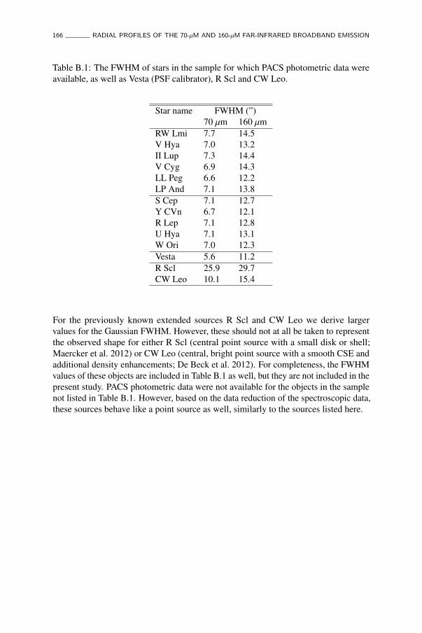
166 RADIAL PROFILES OF THE 70-µM AND 160-µM FAR-INFRARED BROADBAND EMISSION

Table B.1: The FWHM of stars in the sample for which PACS photometric data wereavailable, as well as Vesta (PSF calibrator), R Scl and CW Leo.

Star name FWHM (”)70 µm 160 µm

RW Lmi 7.7 14.5V Hya 7.0 13.2II Lup 7.3 14.4V Cyg 6.9 14.3LL Peg 6.6 12.2LP And 7.1 13.8S Cep 7.1 12.7Y CVn 6.7 12.1R Lep 7.1 12.8U Hya 7.1 13.1W Ori 7.0 12.3Vesta 5.6 11.2R Scl 25.9 29.7CW Leo 10.1 15.4

For the previously known extended sources R Scl and CW Leo we derive largervalues for the Gaussian FWHM. However, these should not at all be taken to representthe observed shape for either R Scl (central point source with a small disk or shell;Maercker et al. 2012) or CW Leo (central, bright point source with a smooth CSE andadditional density enhancements; De Beck et al. 2012). For completeness, the FWHMvalues of these objects are included in Table B.1 as well, but they are not included in thepresent study. PACS photometric data were not available for the objects in the samplenot listed in Table B.1. However, based on the data reduction of the spectroscopic data,these sources behave like a point source as well, similarly to the sources listed here.

RADIAL PROFILES OF THE 70-µM AND 160-µM FAR-INFRARED BROADBAND EMISSION 167

10 20 30 40 50 60 70 80R (arcsec)

10�3

10�2

10�1

100

Fnor

m

70 µm

10 20 30 40 50 60 70 80R (arcsec)

10�3

10�2

10�1

100

Fnor

m

160 µm

Figure B.1: The normalized flux with respect to the radial distance in arcsecondsobserved with PACS at 70 µm in the left panel, and at 160 µm in the right panel. Shownare Vesta (dashed black), LL Peg (solid blue) and R Scl (solid red).

Appendix C

PACS observations ofcarbon-rich AGB stars

Figures C.1 through C.24 show spectra of the sample sources observed in the frameworkof the MESS program. We subtracted the continuum of the spectra to improvereadability and indicate the identified CO and H2O emission lines. Other moleculeshave not been included. Figures C.25 up to C.37 show the line scans of the samplesources observed in the framework of an OT2 program (P.I.: L. Decin).

Tables C.1 up to C.6 list the measured strengths of CO and H2O lines in theMESS spectra and the OT2 line scans. Other molecules have not been taken intoaccount. See Sect. 4.2.3 for more details on the measurement process, and a fewcaveats. The line strengths reported in Tables C.1 and C.2 have been measured beforecontinuum subtraction is performed. The six sources, for which the line strengths arereported in Tables C.3 and C.4, were observed according to an old observation template,resulting in some overlapping wavelength regions between the line scans. For the otherspectra, for which the line strengths are reported in Tables C.5 and C.6, the observationscheme was optimized. Finally, Tables C.7, C.8 and C.9 list the significantly detectedemission lines in the OT2 data that are not attributed to CO or H2O and for which wehave not attempted to identify the molecular carrier.

169

170 PACS OBSERVATIONS OF CARBON-RICH AGB STARS

5758

5960

6162

6364

�10�505101520

F�(Jy)B

2A

6566

6768

6970

7172

73�

(µm

)�

10�505101520253035

F�(Jy)

B2A

Figu

reC

.1:

The

cont

inuu

m-s

ubtra

cted

PAC

Ssp

ectru

mof

RWLM

iis

show

nin

blac

kfo

rba

ndB

2A.T

heso

lidve

rtica

llin

esin

dica

tem

olec

ular

iden

tifica

tions

acco

rdin

gto

Tabl

esC

.1an

dC

.2:C

Oin

red,

13C

Oin

mag

enta

,orth

o-H

2Oin

gree

n,an

dpa

ra-H

2Oin

cyan

.If

ada

shed

blac

klin

eis

supe

rimpo

sed

over

the

iden

tifica

tion

line,

the

trans

ition

was

unde

tect

edby

our

line

fittin

gal

gorit

hm.L

ines

have

been

indi

cate

don

lyif

they

occu

rin

the

wav

elen

gth

rang

essh

ared

with

the

OT2

line

scan

s(in

dica

ted

inre

din

Tabl

esC

.1an

dC

.2),

beca

use

the

othe

ride

ntifi

catio

nsar

ele

ssre

liabl

e(s

eeSe

ct.4

.2.3

).

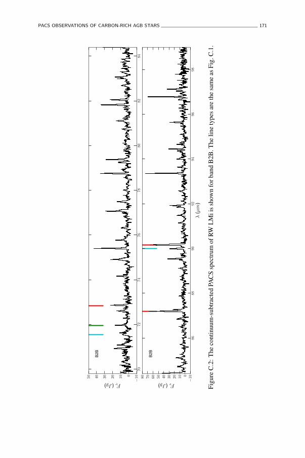
PACS OBSERVATIONS OF CARBON-RICH AGB STARS 171

7072

7476

7880

8284

�1001020304050

F�(Jy)

B2B

8688

9092

9496

98�

(µm

)�

1001020304050607080

F�(Jy)

B2B

Figu

reC

.2:T

heco

ntin

uum

-sub

tract

edPA

CS

spec

trum

ofRW

LMii

ssho

wn

forb

and

B2B

.The

line

type

sare

the

sam

eas

Fig.

C.1

.

172 PACS OBSERVATIONS OF CARBON-RICH AGB STARS

105

110

115

120

�1001020304050

F�(Jy)

R1A

125

130

135

140

145

�(µ

m)

�10010203040506070

F�(Jy)

R1A

Figu

reC

.3:T

heco

ntin

uum

-sub

tract

edPA

CS

spec

trum

ofRW

LMii

ssho

wn

forb

and

R1A

.The

line

type

sare

the

sam

eas

Fig.

C.1

.

PACS OBSERVATIONS OF CARBON-RICH AGB STARS 173

140

145

150

155

160

020406080 F�(Jy)

R1B

165

170

175

180

185

�(µ

m)

�20020406080100

F�(Jy)

R1B

Figu

reC

.4:T

heco

ntin

uum

-sub

tract

edPA

CS

spec

trum

ofRW

LMii

ssho

wn

forb

and

R1B

.The

line

type

sare

the

sam

eas

Fig.

C.1

.

174 PACS OBSERVATIONS OF CARBON-RICH AGB STARS

5657

5859

6061

6263

�4

�2024681012

F�(Jy)

B2A

6465

6667

6869

7071

72�

(µm

)�

505101520

F�(Jy)

B2A

Figu

reC

.5:T

heco

ntin

uum

-sub

tract

edPA

CS

spec

trum

ofV

Hya

issh

own

forb

and

B2A

.The

line

type

sar

eth

esa

me

asFi

g.C

.1.

PACS OBSERVATIONS OF CARBON-RICH AGB STARS 175

7274

7678

8082

�50510152025

F�(Jy)

B2B

8486

8890

9294

96�

(µm

)�

505101520253035

F�(Jy)

B2B

Figu

reC

.6:T

heco

ntin

uum

-sub

tract

edPA

CS

spec

trum

ofV

Hya

issh

own

forb

and

B2B

.The

line

type

sar

eth

esa

me

asFi

g.C

.1.

176 PACS OBSERVATIONS OF CARBON-RICH AGB STARS

105

110

115

120

�50510152025

F�(Jy)

R1A

125

130

135

140

145

�(µ

m)

�505101520253035

F�(Jy)

R1A

Figu

reC

.7:T

heco

ntin

uum

-sub

tract

edPA

CS

spec

trum

ofV

Hya

issh

own

forb

and

R1A

.The

line

type

sar

eth

esa

me

asFi

g.C

.1.

PACS OBSERVATIONS OF CARBON-RICH AGB STARS 177

145

150

155

160

�1001020304050

F�(Jy)

R1B

165

170

175

180

185

�(µ

m)

�1001020304050

F�(Jy)

R1B

Figu

reC

.8:T

heco

ntin

uum

-sub

tract

edPA

CS

spec

trum

ofV

Hya

issh

own

forb

and

R1B

.The

line

type

sar

eth

esa

me

asFi

g.C

.1.

178 PACS OBSERVATIONS OF CARBON-RICH AGB STARS

5657

5859

6061

6263

�6

�4

�20246810

F�(Jy)

B2A

6465

6667

6869

7071

72�

(µm

)�

4

�2024681012

F�(Jy)

B2A

Figu

reC

.9:T

heco

ntin

uum

-sub

tract

edPA

CS

spec

trum

ofII

Lup

issh

own

forb

and

B2A

.The

line

type

sar

eth

esa

me

asFi

g.C

.1.

PACS OBSERVATIONS OF CARBON-RICH AGB STARS 179

7274

7678

8082

�10�5051015

F�(Jy)

B2B

8486

8890

9294

96�

(µm

)�

10�5051015202530

F�(Jy)

B2B

Figu

reC

.10:

The

cont

inuu

m-s

ubtra

cted

PAC

Ssp

ectru

mof

IILu

pis

show

nfo

rban

dB

2B.T

helin

ety

pesa

reth

esa

me

asFi

g.C

.1.

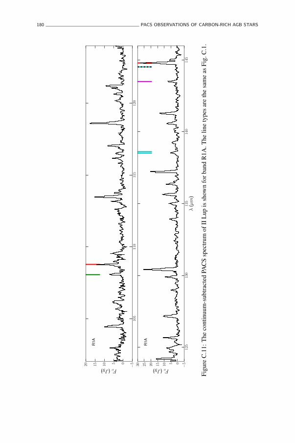
180 PACS OBSERVATIONS OF CARBON-RICH AGB STARS

105

110

115

120

�505101520

F�(Jy)

R1A

125

130

135

140

145

�(µ

m)

�5051015202530

F�(Jy)

R1A

Figu

reC

.11:

The

cont

inuu

m-s

ubtra

cted

PAC

Ssp

ectru

mof

IILu

pis

show

nfo

rban

dR

1A.T

helin

ety

pesa

reth

esa

me

asFi

g.C

.1.

PACS OBSERVATIONS OF CARBON-RICH AGB STARS 181

145

150

155

160

�50510152025303540

F�(Jy)

R1B

165

170

175

180

185

�(µ

m)

�1001020304050

F�(Jy)

R1B

Figu

reC

.12:

The

cont

inuu

m-s

ubtra

cted

PAC

Ssp

ectru

mof

IILu

pis

show

nfo

rban

dR

1B.T

helin

ety

pesa

reth

esa

me

asFi

g.C

.1.

182 PACS OBSERVATIONS OF CARBON-RICH AGB STARS

5657

5859

6061

6263

�4

�20246810

F�(Jy)

B2A

6465

6667

6869

7071

72�

(µm

)�

4

�202468

F�(Jy)

B2A

Figu

reC

.13:

The

cont

inuu

m-s

ubtra

cted

PAC

Ssp

ectru

mof

VC

ygis

show

nfo

rban

dB

2A.T

helin

ety

pesa

reth

esa

me

asFi

g.C

.1.

PACS OBSERVATIONS OF CARBON-RICH AGB STARS 183

7274

7678

8082

�10�5051015

F�(Jy)

B2B

8486

8890

9294

96�

(µm

)�

15

�10�505101520

F�(Jy)

B2B

Figu

reC

.14:

The

cont

inuu

m-s

ubtra

cted

PAC

Ssp

ectru

mof

VC

ygis

show

nfo

rban

dB

2B.T

helin

ety

pesa

reth

esa

me

asFi

g.C

.1.

184 PACS OBSERVATIONS OF CARBON-RICH AGB STARS

105

110

115

120

�4

�2024681012

F�(Jy)

R1A

125

130

135

140

145

�(µ

m)

�505101520

F�(Jy)

R1A

Figu

reC

.15:

The

cont

inuu

m-s

ubtra

cted

PAC

Ssp

ectru

mof

VC

ygis

show

nfo

rban

dR

1A.T

helin

ety

pesa

reth

esa

me

asFi

g.C

.1.

PACS OBSERVATIONS OF CARBON-RICH AGB STARS 185

145

150

155

160

�50510152025

F�(Jy)

R1B

165

170

175

180

185

�(µ

m)

�50510152025

F�(Jy)

R1B

Figu

reC

.16:

The

cont

inuu

m-s

ubtra

cted

PAC

Ssp

ectru

mof

VC

ygis

show

nfo

rban

dR

1B.T

helin

ety

pesa

reth

esa

me

asFi

g.C

.1.

186 PACS OBSERVATIONS OF CARBON-RICH AGB STARS

5657

5859

6061

6263

�10�505101520

F�(Jy)

B2A

6465

6667

6869

7071

72�

(µm

)�

10�5051015

F�(Jy)

B2A

Figu

reC

.17:

The

cont

inuu

m-s

ubtra

cted

PAC

Ssp

ectru

mof

LLPe

gis

show

nfo

rban

dB

2A.T

helin

ety

pesa

reth

esa

me

asFi

g.C

.1.

PACS OBSERVATIONS OF CARBON-RICH AGB STARS 187

7274

7678

8082

�10�5051015202530

F�(Jy)

B2B

8486

8890

9294

96�

(µm

)�

10�505101520

F�(Jy)

B2B

Figu

reC

.18:

The

cont

inuu

m-s

ubtra

cted

PAC

Ssp

ectru

mof

LLPe

gis

show

nfo

rban

dB

2B.T

helin

ety

pesa

reth

esa

me

asFi

g.C

.1.

188 PACS OBSERVATIONS OF CARBON-RICH AGB STARS

105

110

115

120

�4

�2024681012

F�(Jy)

R1A

125

130

135

140

145

�(µ

m)

�505101520

F�(Jy)

R1A

Figu

reC

.19:

The

cont

inuu

m-s

ubtra

cted

PAC

Ssp

ectru

mof

LLPe

gis

show

nfo

rban

dR

1A.T

helin

ety

pesa

reth

esa

me

asFi

g.C

.1.

PACS OBSERVATIONS OF CARBON-RICH AGB STARS 189

145

150

155

160

�50510152025

F�(Jy)

R1B

165

170

175

180

185

�(µ

m)

�10�5051015202530

F�(Jy)

R1B

Figu

reC

.20:

The

cont

inuu

m-s

ubtra

cted

PAC

Ssp

ectru

mof

LLPe

gis

show

nfo

rban

dR

1B.T

helin

ety

pesa

reth

esa

me

asFi

g.C

.1.

190 PACS OBSERVATIONS OF CARBON-RICH AGB STARS

5657

5859

6061

6263

�6

�4

�20246

F�(Jy)

B2A

6465

6667

6869

7071

72�

(µm

)�

2

�101234567

F�(Jy)

B2A

Figu

reC

.21:

The

cont

inuu

m-s

ubtra

cted

PAC

Ssp

ectru

mof

LPA

ndis

show

nfo

rban

dB

2A.T

helin

ety

pesa

reth

esa

me

asFi

g.C

.1.

PACS OBSERVATIONS OF CARBON-RICH AGB STARS 191

7274

7678

8082

�5051015

F�(Jy)

B2B

8486

8890

9294

96�

(µm

)�

50510152025

F�(Jy)

B2B

Figu

reC

.22:

The

cont

inuu

m-s

ubtra

cted

PAC

Ssp

ectru

mof

LPA

ndis

show

nfo

rban

dB

2B.T

helin

ety

pesa

reth

esa

me

asFi

g.C

.1.

192 PACS OBSERVATIONS OF CARBON-RICH AGB STARS

105

110

115

120

�202468101214

F�(Jy)

R1A

125

130

135

140

145

�(µ

m)

�50510152025

F�(Jy)

R1A

Figu

reC

.23:

The

cont

inuu

m-s

ubtra

cted

PAC

Ssp

ectru

mof

LPA

ndis

show

nfo

rban

dR

1A.T

helin

ety

pesa

reth

esa

me

asFi

g.C

.1.

PACS OBSERVATIONS OF CARBON-RICH AGB STARS 193

145

150

155

160

�5051015202530

F�(Jy)

R1B

165

170

175

180

185

�(µ

m)

�505101520253035

F�(Jy)

R1B

Figu

reC

.24:

The

cont

inuu

m-s

ubtra

cted

PAC

Ssp

ectru

mof

LPA

ndis

show

nfo

rban

dR

1B.T

helin

ety

pesa

reth

esa

me

asFi

g.C

.1.

194 PACS OBSERVATIONS OF CARBON-RICH AGB STARS

66.3

66.4

66.5

66.6

2025303540 F�(Jy)

B3A

68.8

69.0

69.2

69.4

69.6

69.8

161820222426

B2B

71.6

71.8

72.0

72.2

72.4

72.6

72.8

73.0

171819202122232425

B2B

86.4

86.6

86.8

87.0

87.2

87.4

87.6

87.8

1012141618202224

B2B

89.4

89.6

89.8

90.0

90.2

90.4

90.6

1012141618202224 F�(Jy)

B2B

107.

010

7.5

108.

010

8.5

109.

0

810121416

R1A

137.

513

8.0

138.

513

9.0

139.

5

�(µ

m)

456789

R1A

143.

014

3.5

144.

014

4.5

145.

014

5.5

�(µ

m)

4681012141618R

1A

173.

017

3.5

174.

017

4.5

175.

017

5.5

�(µ

m)

510152025 F�(Jy)

R1B

179.

017

9.5

180.

018

0.5

181.

0

�(µ

m)

24681012

R1B

Figu

reC

.25:

The

line

scan

sof

V38

4Pe

rare

show

nin

blac

k.Th

eso

lidve

rtica

llin

esin

dica

tem

olec

ular

iden

tifica

tions

acco

rdin

gto

Tabl

esC

.3,C

.4,C

.5,a

ndC

.6:C

Oin

red,

13C

Oin

mag

enta

,orth

o-H

2Oin

gree

n,an

dpa

ra-H

2Oin

cyan

.Ifa

dash

edbl

ack

line

issu

perim

pose

dov

erth

eid

entifi

catio

nlin

e,th

etra

nsiti

onw

asun

dete

cted

byou

rlin

efit

ting

algo

rithm

.The

PAC

Sba

ndis

indi

cate

din

the

top

left.

PACS OBSERVATIONS OF CARBON-RICH AGB STARS 195

68.8

69.0

69.2

69.4

69.6

69.8

3456789 F�(Jy)

B2B

71.6

71.8

72.0

72.2

72.4

72.6

72.8

73.0

3.0

3.5

4.0

4.5

5.0

5.5

6.0

6.5

B2B

86.4

86.6

86.8

87.0

87.2

87.4

87.6

87.8

123456B

2B

89.4

89.6

89.8

90.0

90.2

90.4

90.6

1234567B

2B

107.

010

7.5

108.

010

8.5

109.

01.

5

2.0

2.5

3.0

3.5

4.0

4.5

5.0

F�(Jy)

R1A

137.

513

8.0

138.

513

9.0

139.

5

�(µ

m)

0.5

1.0

1.5

2.0

2.5

3.0

R1A

143.

014

3.5

144.

014

4.5

145.

014

5.5

�(µ

m)

1234R

1A

173.

017

3.5

174.

017

4.5

175.

017

5.5

�(µ

m)

0123456R

1B

179.

017

9.5

180.

018

0.5

181.

0

�(µ

m)

0123456 F�(Jy)

R1B

Figu

reC

.26:

The

line

scan

sof

SA

ur.T

helin

ety

pes

are

the

sam

eas

Fig.

C.2

5.

196 PACS OBSERVATIONS OF CARBON-RICH AGB STARS

66.3

66.4

66.5

66.6

20304050 F�(Jy)

B3A

68.8

69.0

69.2

69.4

69.6

69.8

101214161820B

2B

71.6

71.8

72.0

72.2

72.4

72.6

72.8

73.0

152025B

2B

86.4

86.6

86.8

87.0

87.2

87.4

87.6

87.8

10152025B

2B

89.4

89.6

89.8

90.0

90.2

90.4

90.6

10152025 F�(Jy)

B2B

107.

010

7.5

108.

010

8.5

109.

010

9.5

681012141618R

1A

137.

513

8.0

138.

513

9.0

139.

5

�(µ

m)

468101214

R1A

143.

014

3.5

144.

014

4.5

145.

014

5.5

�(µ

m)

468101214R

1A

173.

017

3.5

174.

017

4.5

175.

017

5.5

�(µ

m)

51015 F�(Jy)

R1B

179.

017

9.5

180.

018

0.5

181.

0

�(µ

m)

510152025R

1B

Figu

reC

.27:

The

line

scan

sof

RLe

p.Th

elin

ety

pes

are

the

sam

eas

Fig.

C.2

5.

PACS OBSERVATIONS OF CARBON-RICH AGB STARS 197

66.3

66.4

66.5

66.6

678910 F�(Jy)

B3A

68.8

69.0

69.2

69.4

69.6

69.8

2345678910

B2B

71.6

71.8

72.0

72.2

72.4

72.6

72.8

73.0

56789B

2B

86.4

86.6

86.8

87.0

87.2

87.4

87.6

87.8

3456789B

2B

89.4

89.6

89.8

90.0

90.2

90.4

90.6

345678 F�(Jy)

B2B

107.

010

7.5

108.

010

8.5

109.

02.

5

3.0

3.5

4.0

4.5

5.0

5.5

R1A

137.

513

8.0

138.

513

9.0

139.

5

�(µ

m)

1.5

2.0

2.5

3.0

R1A

143.

014

3.5

144.

014

4.5

145.

014

5.5

�(µ

m)

1.0

1.5

2.0

2.5

3.0

3.5

4.0

4.5

R1A

173.

017

3.5

174.

017

4.5

175.

017

5.5

�(µ

m)

012345 F�(Jy)

R1B

179.

017

9.5

180.

018

0.5

181.

0

�(µ

m)

�0.

5

0.0

0.5

1.0

1.5

2.0

2.5

3.0

R1B

Figu

reC

.28:

The

line

scan

sof

WO

ri.Th

elin

ety

pes

are

the

sam

eas

Fig.

C.2

5.

198 PACS OBSERVATIONS OF CARBON-RICH AGB STARS

66.3

66.4

66.5

66.6

345678910 F�(Jy)

B3A

68.8

69.0

69.2

69.4

69.6

69.8

456789

B2B

71.6

71.8

72.0

72.2

72.4

72.6

72.8

73.0

45678

B2B

86.4

86.6

86.8

87.0

87.2

87.4

87.6

87.8

2345678B

2B

89.4

89.6

89.8

90.0

90.2

90.4

90.6

2345678 F�(Jy)

B2B

107.

010

7.5

108.

010

8.5

109.

0

2.0

2.5

3.0

3.5

4.0

4.5

R1A

137.

513

8.0

138.

513

9.0

139.

5

�(µ

m)

0.8

1.0

1.2

1.4

1.6

1.8

2.0

R1A

143.

014

3.5

144.

014

4.5

145.

014

5.5

�(µ

m)

1.0

1.5

2.0

2.5

3.0

3.5

4.0

R1A

173.

017

3.5

174.

017

4.5

175.

017

5.5

�(µ

m)

012345 F�(Jy)

R1B

179.

017

9.5

180.

018

0.5

181.

0

�(µ

m)

0.0

0.5

1.0

1.5

R1B

Figu

reC

.29:

The

line

scan

sof

UH

ya.T

helin

ety

pes

are

the

sam

eas

Fig.

C.2

5.

PACS OBSERVATIONS OF CARBON-RICH AGB STARS 199

66.3

66.4

66.5

66.6

101520253035 F�(Jy)

B3A

68.8

69.0

69.2

69.4

69.6

69.8

7891011121314

B2B

71.6

71.8

72.0

72.2

72.4

8910111213141516

B2B

86.4

86.6

86.8

87.0

87.2

68101214B

2B

89.4

89.6

89.8

90.0

90.2

468101214 F�(Jy)

B2B

89.8

89.9

90.0

90.1

90.2

90.3

90.4

90.5

46810121416B

2B

107.

010

7.5

108.

010

8.5

109.

0

46810R

1A

137.

513

8.0

138.

513

9.0

139.

5

234567R

1A

143.

014

3.5

144.

014

4.5

�(µ

m)

2345678910 F�(Jy)

R1A

173.

017

3.5

174.

017

4.5

�(µ

m)

246810121416

R1B

179.

017

9.5

180.

0

�(µ

m)

051015R

1B

179.

518

0.0

180.

518

1.0

�(µ

m)

051015R

1B

Figu

reC

.30:

The

line

scan

sof

QZ

Mus

.The

line

type

sar

eth

esa

me

asFi

g.C

.25.

200 PACS OBSERVATIONS OF CARBON-RICH AGB STARS

66.3

66.4

66.5

66.6

91011121314 F�(Jy)

B3A

68.8

69.0

69.2

69.4

69.6

69.8

5678910111213B

2B

71.6

71.8

72.0

72.2

72.4

72.6

72.8

73.0

789101112B

2B

86.4

86.6

86.8

87.0

87.2

87.4

87.6

87.8

5678910

B2B

89.4

89.6

89.8

90.0

90.2

90.4

90.6

5678910 F�(Jy)

B2B

107.

010

7.5

108.

010

8.5

109.

0

45678

R1A

137.

513

8.0

138.

513

9.0

139.

5

�(µ

m)

2345R

1A

143.

014

3.5

144.

014

4.5

145.

014

5.5

�(µ

m)

23456R

1A

173.

017

3.5

174.

017

4.5

175.

017

5.5

�(µ

m)

1234567 F�(Jy)

R1B

179.

017

9.5

180.

018

0.5

181.

0

�(µ

m)

1234R

1B

Figu

reC

.31:

The

line

scan

sof

YC

Vn.

The

line

type

sar

eth

esa

me

asFi

g.C

.25.

PACS OBSERVATIONS OF CARBON-RICH AGB STARS 201

66.3

66.4

66.5

66.6

2530354045 F�(Jy)

B3A

68.8

69.0

69.2

69.4

69.6

69.8

22242628303234B

2B

71.6

71.8

72.0

72.2

72.4

72.6

72.8

73.0

222426283032

B2B

86.4

86.6

86.8

87.0

87.2

87.4

87.6

87.8

14161820222426

B2B

89.4

89.6

89.8

90.0

90.2

90.4

90.6

14161820222426 F�(Jy)

B2B

107.

010

7.5

108.

010

8.5

109.

0101112131415161718

R1A

137.

513

8.0

138.

513

9.0

139.

5

�(µ

m)

67891011R

1A

143.

014

3.5

144.

014

4.5

145.

014

5.5

�(µ

m)

681012141618R

1A

173.

017

3.5

174.

017

4.5

175.

017

5.5

�(µ

m)

5101520 F�(Jy)

R1B

179.

017

9.5

180.

018

0.5

181.

0

�(µ

m)

4681012R

1B

Figu

reC

.32:

The

line

scan

sof

AFG

L42

02.T

helin

ety

pes

are

the

sam

eas

Fig.

C.2

5.

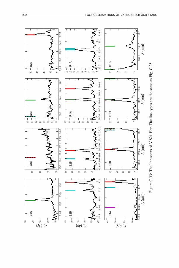
202 PACS OBSERVATIONS OF CARBON-RICH AGB STARS

66.3

66.4

66.5

66.6

4050607080 F�(Jy)

B3A

68.8

69.0

69.2

69.4

69.6

69.8

30354045B

2B

71.6

71.8

72.0

72.2

72.4

3234363840424446

B2B

86.4

86.6

86.8

87.0

87.2

2025303540B

2B

89.4

89.6

89.8

90.0

90.2

202530354045 F�(Jy)

B2B

89.8

89.9

90.0

90.1

90.2

90.3

90.4

90.5

90.6

2530354045

B2B

107.

010

7.5

108.

010

8.5

109.

01416182022242628

R1A

137.

513

8.0

138.

513

9.0

139.

58910111213141516

R1A

143.

014

3.5

144.

014

4.5

�(µ

m)

10152025 F�(Jy)

R1A

173.

017

3.5

174.

017

4.5

�(µ

m)

510152025R

1B

179.

017

9.5

180.

0

�(µ

m)

5101520R

1B

180.

018

0.5

181.

0

�(µ

m)

5101520R

1B

Figu

reC

.33:

The

line

scan

sof

V82

1H

er.T

helin

ety

pes

are

the

sam

eas

Fig.

C.2

5.

PACS OBSERVATIONS OF CARBON-RICH AGB STARS 203

66.3

66.4

66.5

66.6

3040506070 F�(Jy)

B3A

68.8

69.0

69.2

69.4

69.6

69.8

2628303234363840

B2B

71.6

71.8

72.0

72.2

72.4

2830323436384042

B2B

86.4

86.6

86.8

87.0

87.2

20253035B

2B

89.4

89.6

89.8

90.0

90.2

20253035 F�(Jy)

B2B

89.8

89.9

90.0

90.1

90.2

90.3

90.4

90.5

90.6

2025303540

B2B

107.

010

7.5

108.

010

8.5

109.

0

1214161820222426R

1A

137.

513

8.0

138.

513

9.0

139.

568101214

R1A

143.

014

3.5

144.

014

4.5

�(µ

m)

101520 F�(Jy)

R1A

173.

017

3.5

174.

017

4.5

�(µ

m)

51015202530

R1B

179.

017

9.5

180.

0

�(µ

m)

5101520R

1B

180.

018

0.5

181.

0

�(µ

m)

510152025

R1B

Figu

reC

.34:

The

line

scan

sof

V14

17A

ql.T

helin

ety

pes

are

the

sam

eas

Fig.

C.2

5.

204 PACS OBSERVATIONS OF CARBON-RICH AGB STARS

66.3

66.4

66.5

66.6

15202530354045 F�(Jy)

B3A

68.8

69.0

69.2

69.4

69.6

69.8

81012141618B

2B

71.6

71.8

72.0

72.2

72.4

121416182022

B2B

86.4

86.6

86.8

87.0

87.2

810121416182022

B2B

89.4

89.6

89.8

90.0

90.2

10152025 F�(Jy)

B2B

89.8

89.9

90.0

90.1

90.2

90.3

90.4

90.5

90.6

10152025

B2B

107.

010

7.5

108.

010

8.5

109.

0

681012141618

R1A

137.

513

8.0

138.

513

9.0

139.

5246810

R1A

143.

014

3.5

144.

014

4.5

�(µ

m)

246810121416 F�(Jy)

R1A

173.

017

3.5

174.

017

4.5

�(µ

m)

246810121416

R1B

179.

017

9.5

180.

0

�(µ

m)

5101520R

1B

179.

6179

.8180

.0180

.2180

.4180

.6180

.8181

.0

�(µ

m)

51015R

1B

Figu

reC

.35:

The

line

scan

sof

SC

ep.T

helin

ety

pes

are

the

sam

eas

Fig.

C.2

5.

PACS OBSERVATIONS OF CARBON-RICH AGB STARS 205

66.3

66.4

66.5

66.6

123456 F�(Jy)

B3A

68.8

69.0

69.2

69.4

69.6

69.8

123456B

2B

71.6

71.8

72.0

72.2

72.4

3.5

4.0

4.5

5.0

5.5

6.0

6.5

B2B

86.4

86.6

86.8

87.0

87.2

234567B

2B

89.4

89.6

89.8

90.0

90.2

23456 F�(Jy)

B2B

89.8

89.9

90.0

90.1

90.2

90.3

90.4

90.5

90.6

23456

B2B

107.

010

7.5

108.

010

8.5

109.

0

2.0

2.5

3.0

3.5

R1A

137.

513

8.0

138.

513

9.0

139.

5

0.8

1.0

1.2

1.4

1.6

1.8

2.0

R1A

143.

014

3.5

144.

014

4.5

�(µ

m)

0.5

1.0

1.5

2.0

2.5

F�(Jy)

R1A

173.

017

3.5

174.

017

4.5

�(µ

m)

0.0

0.5

1.0

1.5

2.0

2.5

3.0

R1B

179.

017

9.5

180.

0

�(µ

m)

�1012

R1B

179.

6179

.8180

.0180

.2180

.4180

.6180

.8181

.0

�(µ

m)

0.0

0.5

1.0

1.5

2.0

2.5

3.0

R1B

Figu

reC

.36:

The

line

scan

sof

RVC

yg.T

helin

ety

pes

are

the

sam

eas

Fig.

C.2

5.

206 PACS OBSERVATIONS OF CARBON-RICH AGB STARS

66.3

66.4

66.5

66.6

180

200

220

240

F�(Jy)

B3A

68.8

69.0

69.2

69.4

69.6

69.8

140

150

160

170

180

190

B2B

71.6

71.8

72.0

72.2

72.4

72.6

72.8

73.0

150

160

170

180

190

200

B2B

86.4

86.6

86.8

87.0

87.2

87.4

87.6

87.8

100

110

120

130

140

B2B

89.4

89.6

89.8

90.0

90.2

90.4

90.6

90100

110

120

130

F�(Jy)

B2B

107.

010

7.5

108.

010

8.5

109.

0

606570758085R

1A

137.

513

8.0

138.

513

9.0

139.

5

�(µ

m)

404550R

1A

143.

014

3.5

144.

014

4.5

145.

014

5.5

�(µ

m)

404550556065

R1A

173.

017

3.5

174.

017

4.5

175.

017

5.5

�(µ

m)

2530354045505560 F�(Jy)

R1B

179.

017

9.5

180.

018

0.5

181.

0

�(µ

m)

20222426283032R

1B

Figu

reC

.37:

The

line

scan

sof

LLPe

g.Th

elin

ety

pes

are

the

sam

eas

Fig.

C.2

5.

PACS OBSERVATIONS OF CARBON-RICH AGB STARS 207

Tabl

eC

.1:I

nteg

rate

dlin

est

reng

ths

Fin

t(W/m

2 )for

ase

lect

ion

oflin

esin

the

PAC

Ssp

ectra

ofRW

LMi,

VH

yaan

dII

Lup

inth

eM

ESS

sam

ple.

The

rest

wav

elen

gth�

0(µ

m)o

fthe

trans

ition

isin

dica

ted.

The

perc

enta

gesb

etw

een

brac

kets

give

the

unce

rtain

tyon

Fin

t,w

hich

incl

udes

both

the

fittin

gun

certa

inty

and

the

PAC

Sab

solu

te-fl

ux-c

alib

ratio

nun

certa

inty

of20

%.L

ine

stre

ngth

sin

dica

ted

with

?ar

efla

gged

forp

oten

tiall

ine

blen

ds.T

rans

ition

sth

atm

ight

caus

eth

elin

ebl

end

are

men

tione

dim

med

iate

lybe

low

the

flagg

edtra

nsiti

on.M

olec

ular

trans

ition

sin

dica

ted

inre

dco

inci

dew

ithth

ew

avel

engt

hra

nge

ofth

elin

esc

ans

inth

eO

T2pr

ogra

m.T

hese

dete

ctio

nsar

eno

texp

ecte

dto

bea↵

ecte

dby

blen

dsw

ithm

olec

ules

othe

rtha

nC

Oan

dH

2O.D

etec

tions

liste

din

blac

kha

veto

betre

ated

with

caut

ion,

asth

eyha

veno

tbee

nch

ecke

dfo

rpot

entia

lble

ndin

gw

ithot

herm

olec

ules

.

RWLM

iV

Hya

IILu

pPA

CS

Mol

ecul

eR

otat

iona

l�

0F

int

band

trans

ition

µm

(W/m

2 )R

1Bp-

H2O

J Ka,

Kc=

4 1,3�

4 0,4

187.

11/

?7.

71e-

17(2

6.2%

)5.

83e-

17(3

0.5%

)C

OJ=

14�

1318

6.00

9.19

e-16

(20.

3%)

4.61

e-16

(20.

2%)

4.57

e-16

(20.

4%)

13C

OJ=

15�

1418

1.61

6.11

e-17

(26.

1%)

/1.

28e-

16(2

1.9%

)o-

H2O

J Ka,

Kc=

2 2,1�

2 1,2

180.

491.

43e-

16(2

4.6%

)?

9.43

e-17

(24.

5%)

4.73

e-17

(33.

4%)

o-H

2OJ K

a,K

c=

2 1,2�

1 0,1

179.

534.

47e-

16(2

0.5%

)2.

98e-

16(2

0.3%

)1.

62e-

16(2

1.6%

)o-

H2O

J Ka,

Kc=

3 0,3�

2 1,2

174.

63?

3.01

e-16

(22.

0%)

?1.

86e-

16(2

1.1%

)?

1.08

e-16

(24.

1%)

p-H

2OJ K

a,K

c=

5 3,3�

6 0,6

174.

61B

lend

edB

lend

edB

lend

edC

OJ=

15�

1417

3.63

9.88

e-16

(20.

2%)

6.10

e-16

(20.

1%)

5.12

e-16

(20.

2%)

13C

OJ=

16�

1517

0.29

1.01

e-16

(28.

2%)

/9.

28e-

17(2

4.8%

)C

OJ=

16�

1516

2.81

1.05

e-15

(20.

1%)

6.35

e-16

(20.

1%)

5.45

e-16

(20.

3%)

o-H

2OJ K

a,K

c=

5 3,2�

5 2,3

160.

512.

65e-

16(2

1.3%

)1.

20e-

16(2

3.4%

)1.

20e-

16(2

3.4%

)13

CO

J=

17�

1616

0.30

1.36

e-16

(24.

0%)

/1.

89e-

16(2

1.6%

)o-

H2O

J Ka,

Kc=

8 4,5�

7 5,2

159.

05?

6.87

e-17

(29.

5%)

/2.

24e-

17(3

7.1%

)o-

H2O

J Ka,

Kc=

5 2,3�

4 3,2

156.

27?

2.95

e-16

(20.

8%)

?9.

70e-

17(2

2.0%

)?

6.93

e-17

(25.

5%)

p-H

2OJ K

a,K

c=

3 2,2�

3 1,3

156.

19B

lend

edB

lend

edB

lend

edC

OJ=

17�

1615

3.27

1.30

e-15

(20.

2%)

7.15

e-16

(20.

1%)

5.61

e-16

(20.

4%)

Con

tinue

don

next

page

.

208 PACS OBSERVATIONS OF CARBON-RICH AGB STARS

Tabl

eC

.1:C

ontin

ued.

RWLM

iV

Hya

IILu

pPA

CS

Mol

ecul

eR

otat

iona

l�

0F

int

band

trans

ition

µm

(W/m

2 )13

CO

J=

18�

1715

1.43

2.23

e-16

(23.

1%)

4.84

e-17

(27.

9%)

1.24

e-16

(22.

7%)

p-H

2OJ K

a,K

c=

4 3,1�

4 2,2

146.

929.

49e-

17(2

7.0%

)2.

87e-

17(3

2.7%

)/

CO

J=

18�

1714

4.78

1.07

e-15

(20.

4%)

5.83

e-16

(20.

2%)

4.27

e-16

(20.

4%)

13C

OJ=

19�

1814

3.49

//

1.08

e-16

(21.

9%)

R1A

CO

J=

18�

1714

4.78

9.84

e-16

(20.

4%)

5.52

e-16

(20.

1%)

4.59

e-16

(20.

3%)

13C

OJ=

19�

1814

3.49

//

1.19

e-16

(21.

3%)

p-H

2OJ K

a,K

c=

8 4,4�

7 5,3

138.

64?

2.58

e-16

(22.

0%)

?1.

74e-

16(2

1.0%

)?

9.89

e-17

(25.

9%)

p-H

2OJ K

a,K

c=

3 1,3�

2 0,2

138.

53B

lend

edB

lend

edB

lend

edC

OJ=

19�

1813

7.20

9.56

e-16

(20.

1%)

5.64

e-16

(20.

1%)

3.97

e-16

(20.

4%)

o-H

2OJ K

a,K

c=

3 3,0�

3 2,1

136.

50?

2.44

e-16

(27.

8%)

?5.

84e-

17(4

3.2%

)3.

45e-

17(3

6.8%

)13

CO

J=

20�

1913

6.35

2.02

e-16

(26.

2%)

Ble

nded

1.45

e-16

(22.

2%)

o-H

2OJ K

a,K

c=

5 1,4�

5 0,5

134.

943.

36e-

16(2

1.5%

)1.

78e-

16(2

1.1%

)1.

18e-

16(2

3.3%

)o-

H2O

J Ka,

Kc=

4 2,3�

4 1,4

132.

41?

2.22

e-16

(27.

4%)

9.81

e-17

(25.

2%)

/C

OJ=

20�

1913

0.37

?1.

64e-

15(2

0.1%

)?

9.09

e-16

(20.

1%)

?6.

55e-

16(2

0.2%

)p-

H2O

J Ka,

Kc=

7 5,3�

8 2,6

130.

32B

lend

edB

lend

edB

lend

ed13

CO

J=

21�

2012

9.89

3.00

e-16

(23.

6%)

1.35

e-16

(23.

8%)

1.93

e-16

(21.

9%)

p-H

2OJ K

a,K

c=

4 0,4�

3 1,3

125.

352.

84e-

16(2

3.7%

)1.

27e-

16(2

5.2%

)?

9.16

e-17

(31.

3%)

CO

J=

21�

2012

4.19

1.02

e-15

(20.

3%)

6.02

e-16

(20.

3%)

3.96

e-16

(20.

5%)

13C

OJ=

22�

2112

4.02

//

1.12

e-16

(25.

8%)

13C

OJ=

23�

2211

8.66

?1.

12e-

15(2

0.9%

)?

6.17

e-16

(20.

3%)

?4.

57e-

16(2

1.2%

)C

OJ=

22�

2111

8.58

Ble

nded

Ble

nded

Ble

nde

o-H

2OJ K

a,K

c=

7 3,4�

6 4,3

116.

78/

?9.

63e-

17(2

8.2%

)5.

66e-

17(3

7.2%

)C

ontin

ued

onne

xtpa

ge.

PACS OBSERVATIONS OF CARBON-RICH AGB STARS 209

Tabl

eC

.1:C

ontin

ued.

RWLM

iV

Hya

IILu

pPA

CS

Mol

ecul

eR

otat

iona

l�

0F

int

band

trans

ition

µm

(W/m

2 )p-

H2O

J Ka,

Kc=

5 3,3�

5 2,4

113.

95/

/?

1.26

e-16

(35.

5%)

13C

OJ=

24�

2311

3.75

//

5.40

e-17

(36.

1%)

o-H

2OJ K

a,K

c=

4 1,4�

3 0,3

113.

54?

1.49

e-15

(20.

3%)

?8.

92e-

16(2

0.2%

)?

4.79

e-16

(20.

5%)

CO

J=

23�

2211

3.46

Ble

nded

Ble

nded

Ble

nded

o-H

2OJ K

a,K

c=

7 4,3�

7 3,4

112.

511.

30e-

16(4

7.6%

)/

?1.

49e-

16(5

3.7%

)C

OJ=

24�

2310

8.76

1.03

e-15

(20.

9%)

5.71

e-16

(20.

5%)

3.24

e-16

(21.

7%)

o-H

2OJ K

a,K

c=

2 2,1�

1 1,0

108.

076.

63e-

16(2

1.6%

)2.

84e-

16(2

1.7%

)1.

74e-

16(2

4.8%

)C

OJ=

25�

2410

4.44

9.97

e-16

(21.

5%)

?6.

75e-

16(2

0.4%

)3.

36e-

16(2

2.2%

)B

2BC

OJ=

27�

2696

.77

5.41

e-16

(20.

8%)

?4.

00e-

16(2

1.5%

)?

2.44

e-16

(23.

5%)

p-H

2OJ K

a,K

c=

5 1,5�

4 0,4

95.6

32.

82e-

16(2

4.0%

)1.

13e-

16(2

4.5%

)5.

61e-

17(5

4.8%

)o-

H2O

J Ka,

Kc=

4 4,1�

4 3,2

94.7

19.

47e-

17(3

8.0%

)/

/o-

H2O

J Ka,

Kc=

6 2,5�

6 1,6

94.6

41.

60e-

16(2

9.2%

)6.

74e-

17(2

9.3%

)/

p-H

2OJ K

a,K

c=

7 3,5�

7 2,6

93.3

8?

7.03

e-16

(21.

1%)

?4.

98e-

16(2

0.7%

)?

2.61

e-16

(22.

1%)

CO

J=

28�

2793

.35

Ble

nded

Ble

nded

Ble

nded

13C

OJ=

30�

2991

.18

?1.

64e-

16(2

4.9%

)/

?8.

52e-

17(3

7.7%

)C

OJ=

29�

2890

.16

1.01

e-15

(20.

6%)

?5.

17e-

16(2

0.4%

)2.

11e-

16(2

2.2%

)p-

H2O

J Ka,

Kc=

3 2,2�

2 1,1

89.9

93.

71e-

16(2

4.1%

)1.

17e-

16(2

4.1%

)5.

49e-

17(4

1.3%

)13

CO

J=

31�

3088

.27

//

6.66

e-17

(29.

5%)

CO

J=

30�

2987

.19

8.55

e-16

(20.

4%)

4.76

e-16

(20.

5%)

1.75

e-16

(24.

9%)

o-H

2OJ K

a,K

c=

7 1,6�

7 0,7

84.7

7/

/6.

22e-

17(3

6.2%

)C

OJ=

31�

3084

.41

?8.

60e-

16(2

0.6%

)?

4.55

e-16

(20.

7%)

?2.

12e-

16(2

4.2%

)p-

H2O

J Ka,

Kc=

6 0,6�

5 1,5

83.2

8?

2.13

e-16

(32.

1%)

1.14

e-16

(22.

5%)

/

Con

tinue

don

next

page

.

210 PACS OBSERVATIONS OF CARBON-RICH AGB STARS

Tabl

eC

.1:C

ontin

ued.

RWLM

iV

Hya

IILu

pPA

CS

Mol

ecul

eR

otat

iona

l�

0F

int

band

trans

ition

µm

(W/m

2 )o-

H2O

J Ka,

Kc=

6 1,6�

5 0,5

82.0

34.

06e-

16(2

1.7%

)?

2.91

e-16

(20.

8%)

?1.

84e-

16(2

5.7%

)C

OJ=

32�

3181

.81

4.94

e-16

(21.

0%)

3.55

e-16

(20.

5%)

8.47

e-17

(27.

0%)

p-H

2OJ K

a,K

c=

7 2,6�

7 1,7

81.2

27.

07e-

17(3

9.8%

)/

/C

OJ=

33�

3279

.36

5.52

e-16

(21.

1%)

?4.

83e-

16(2

0.7%

)1.

65e-

16(2

8.1%

)p-

H2O

J Ka,

Kc=

6 1,5�

5 2,4

78.9

3?

3.45

e-16

(27.

0%)

//

o-H

2OJ K

a,K

c=

4 2,3�

3 1,2

78.7

46.

37e-

16(2

0.7%

)3.

23e-

16(2

1.3%

)1.

25e-

16(3

1.3%

)o-

H2O

J Ka,

Kc=

7 5,2�

7 4,3

77.7

64.

78e-

17(3

3.5%

)/

/C

OJ=

34�

3377

.06

?5.

89e-

16(2

1.8%

)?

4.48

e-16

(20.

6%)

8.66

e-17

(29.

4%)

13C

OJ=

36�

3576

.17

//

?9.

11e-

17(3

0.8%

)o-

H2O

J Ka,

Kc=

5 5,0�

5 4,1

75.9

1/

/5.

54e-

17(3

6.7%

)o-

H2O

J Ka,

Kc=

6 5,2�

6 4,3

75.8

3/

/?

1.72

e-17

(89.

9%)

p-H

2OJ K

a,K

c=

7 5,3�

7 4,4

75.8

1?

2.24

e-16

(25.

9%)

/B

lend

edp-

H2O

J Ka,

Kc=

5 5,1�

5 4,2

75.7

8B

lend

ed/

?1.

19e-

16(3

4.8%

)o-

H2O

J Ka,

Kc=

3 2,1�

2 1,2

75.3

87.

81e-

16(2

0.6%

)4.

47e-

16(2

0.4%

)2.

33e-

16(2

1.4%

)o-

H2O

J Ka,

Kc=

7 2,5�

6 3,4

74.9

5?

2.22

e-16

(39.

3%)

?1.

14e-

16(4

1.1%

)5.

39e-

17(3

7.2%

)C

OJ=

35�

3474

.89

?5.

46e-

16(2

3.2%

)3.

05e-

16(2

3.8%

)7.

94e-

17(2

7.8%

)13

CO

J=

37�

3674

.14

2.67

e-16

(22.

1%)

1.09

e-16

(23.

3%)

/C

OJ=

36�

3572

.84

3.82

e-16

(22.

4%)

?3.

47e-

16(2

0.9%

)/

o-H

2OJ K

a,K

c=

7 0,7�

6 1,6

71.9

53.

22e-

16(2

3.5%

)/

/p-

H2O

J Ka,

Kc=

7 1,7�

6 0,6

71.5

4?

2.90

e-16

(28.

0%)

//

p-H

2OJ K

a,K

c=

5 2,4�

4 1,3

71.0

72.

12e-

16(3

8.2%

)?

1.40

e-16

(36.

9%)

/C

OJ=

37�

3670

.91

4.33

e-16

(23.

6%)

?2.

80e-

16(2

5.7%

)/

Con

tinue

don

next

page

.

PACS OBSERVATIONS OF CARBON-RICH AGB STARS 211

Tabl

eC

.1:C

ontin

ued.

RWLM

iV

Hya

IILu

pPA

CS

Mol

ecul

eR

otat

iona

l�

0F

int

band

trans

ition

µm

(W/m

2 )o-

H2O

J Ka,

Kc=

8 2,7�

8 1,8

70.7

05.

65e-

17(7

0.5%

)/

/

B2A

CO

J=

36�

3572

.84

4.80

e-16

(22.

3%)

?3.

49e-

16(2

1.2%

)7.

06e-

17(3

4.7%

)o-

H2O

J Ka,

Kc=

7 0,7�

6 1,6

71.9

53.

47e-

16(2

4.4%

)2.

40e-

16(2

1.2%

)5.

97e-

17(3

5.5%

)p-

H2O

J Ka,

Kc=

7 1,7�

6 0,6

71.5

41.

98e-

16(2

3.3%

)?

1.28

e-16

(27.

7%)

5.27

e-17

(38.

6%)

p-H

2OJ K

a,K

c=

5 2,4�

4 1,3

71.0

73.

41e-

16(2

3.4%

)1.

38e-

16(2

4.4%

)/

CO

J=

37�

3670

.91

4.42

e-16

(21.

1%)

?3.

53e-

16(2

1.2%

)9.

89e-

17(2

6.4%

)o-

H2O

J Ka,

Kc=

8 2,7�

8 1,8

70.7

01.

37e-

16(2

8.9%

)/

/C

OJ=

38�

3769

.07

4.49

e-16

(22.

0%)

?3.

65e-

16(2

2.0%

)/

CO

J=

39�

3867

.34

?4.

44e-

16(2

4.7%

)?

2.89

e-16

(21.

8%)

1.44

e-16

(27.

8%)

o-H

2OJ K

a,K

c=

3 3,0�

3 0,3

67.2

7?

2.06

e-16

(35.

7%)

9.80

e-17

(29.

5%)

?7.

50e-

17(4

6.5%

)p-

H2O

J Ka,

Kc=

3 3,1�

2 2,0

67.0

9?

5.01

e-16

(23.

0%)

?2.

48e-

16(2

2.4%

)?

1.34

e-16

(34.

9%)

13C

OJ=

41�

4067

.04

//

1.86

e-17

(87.

9%)

o-H

2OJ K

a,K

c=

3 3,0�

2 2,1

66.4

48.

43e-

16(2

0.7%

)5.

03e-

16(2

0.4%

)?

3.02

e-16

(22.

7%)

o-H

2OJ K

a,K

c=

7 1,6�

6 2,5

66.0

92.

35e-

16(2

8.4%

)?

1.87

e-16

(24.

8%)

/C

OJ=

40�

3965

.69

?4.

30e-

16(2

5.9%

)?

2.98

e-16

(22.

2%)

6.68

e-17

(37.

5%)

o-H

2OJ K

a,K

c=

6 2,5�

5 1,4

65.1

7?

5.58

e-16

(22.

7%)

3.13

e-16

(22.

8%)

1.38

e-16

(32.

0%)

CO

J=

41�

4064

.12

/1.

64e-

16(2

7.6%

)/

p-H

2OJ K

a,K

c=

8 0,8�

7 1,7

63.4

6?

2.87

e-16

(28.

5%)

?1.

36e-

16(2

9.7%

)/

o-H

2OJ K

a,K

c=

8 1,8�

7 0,7

63.3

2?

3.95

e-16

(38.

6%)

?3.

05e-

16(2

3.6%

)/

13C

OJ=

45�

4461

.21

?2.

76e-

16(3

0.9%

)?

1.26

e-16

(35.

2%)

/C

OJ=

43�

4261

.20

Ble

nded

Ble

nded

/C

OJ=

44�

4359

.84

?3.

34e-

16(2

7.6%

)/

/

Con

tinue

don

next

page

.

212 PACS OBSERVATIONS OF CARBON-RICH AGB STARS

Tabl

eC

.1:C

ontin

ued.

RWLM

iV

Hya

IILu

pPA

CS

Mol

ecul

eR

otat

iona

l�

0F

int

band

trans

ition

µm

(W/m

2 )o-

H2O

J Ka,

Kc=

4 3,2�

3 2,1

58.7

0?

6.92

e-16

(23.

2%)

?4.

80e-

16(2

0.9%

)1.

92e-

16(2

6.0%

)C

OJ=

45�

4458

.55

1.59

e-16

(42.

1%)

?1.

35e-

16(3

9.6%

)/

p-H

2OJ K

a,K

c=

6 4,2�

7 1,7

58.3

8/

1.20

e-16

(31.

2%)

/p-

H2O

J Ka,

Kc=

4 2,2�

3 1,3

57.6

4?

5.12

e-16

(29.

1%)

2.32

e-16

(24.

6%)

/o-

H2O

J Ka,

Kc=

9 0,9�

8 1,8

56.8

2?

4.35

e-16

(33.

0%)

1.54

e-16

(28.

0%)

/p-

H2O

J Ka,

Kc=

9 1,9�

8 0,8

56.7

7B

lend

ed/

/13

CO

J=

49�

4856

.34

?5.

57e-

16(2

7.6%

)?

2.91

e-16

(25.

1%)

/p-

H2O

J Ka,

Kc=

4 3,1�

3 2,2

56.3

2B

lend

edB

lend

ed//

PACS OBSERVATIONS OF CARBON-RICH AGB STARS 213

Tabl

eC

.2:I

nteg

rate

dlin

est

reng

ths

Fin

t(W/m

2 )for

ase

lect

ion

oflin

esin

the

PAC

Ssp

ectra

ofV

Cyg

,LL

Peg

and

LPA

ndin

the

MES

Ssa

mpl

e.Se

eTa

ble

C.1

forf

urth

ercl

arifi

catio

nof

the

give

nin

form

atio

n.

VC

ygLL

Peg

LPA

ndPA

CS

Mol

ecul

eR

otat

iona

l�

0F

int

band

trans

ition

µm

(W/m

2 )R

1Bp-

H2O

J Ka,

Kc=

4 1,3�

4 0,4

187.

11/

/4.

23e-

17(2

5.0%

)C

OJ=

14�

1318

6.00

1.98

e-16

(21.

7%)

2.29

e-16

(21.

1%)

2.64

e-16

(20.

7%)

13C

OJ=

15�

1418

1.61

/5.

41e-

17(2

8.8%

)/

o-H

2OJ K

a,K

c=

2 2,1�

2 1,2

180.

49/

/5.

84e-

17(2

5.8%

)o-

H2O

J Ka,

Kc=

2 1,2�

1 0,1

179.

531.

72e-

16(2

0.9%

)/

1.25

e-16

(21.

7%)

o-H

2OJ K

a,K

c=

3 0,3�

2 1,2

174.

63?

8.27

e-17

(23.

6%)

/?

5.49

e-17

(26.

9%)

p-H

2OJ K

a,K

c=

5 3,3�

6 0,6

174.

61B

lend

ed/

Ble

nded

CO

J=

15�

1417

3.63

2.21

e-16

(20.

4%)

2.56

e-16

(20.

8%)

3.45

e-16

(20.

3%)

13C

OJ=

16�

1517

0.29

?1.

81e-

17(4

8.5%

)4.

60e-

17(2

9.4%

)?

6.49

e-17

(24.

5%)

p-H

2OJ K

a,K

c=

6 3,3�

6 2,4

170.

14B

lend

ed/

/C

OJ=

16�

1516

2.81

3.22

e-16

(20.

3%)

2.83

e-16

(20.

6%)

3.42

e-16

(20.

1%)

o-H

2OJ K

a,K

c=

5 3,2�

5 2,3

160.

51/

9.01

e-17

(25.

3%)

1.17

e-16

(21.

5%)

13C

OJ=

17�

1616

0.30

/1.

04e-

16(2

4.4%

)6.

79e-

17(2

2.8%

)o-

H2O

J Ka,

Kc=

5 2,3�

4 3,2

156.

27?

7.01

e-17

(28.

9%)

/?

5.49

e-17

(28.

8%)

p-H

2OJ K

a,K

c=

3 2,2�

3 1,3

156.

19B

lend

ed/

Ble

nded

CO

J=

17�

1615

3.27

2.90

e-16

(20.

3%)

3.51

e-16

(20.

7%)

4.55

e-16

(20.

3%)

13C

OJ=

18�

1715

1.43

?5.

95e-

17(2

8.7%

)3.

61e-

17(4

0.8%

)?

5.68

e-17

(31.

6%)

p-H

2OJ K

a,K

c=

4 3,1�

4 2,2

146.

92/

?5.

42e-

17(3

4.3%

)/

CO

J=

18�

1714

4.78

3.07

e-16

(20.

3%)

2.73

e-16

(21.

5%)

3.67

e-16

(20.

2%)

13C

OJ=

19�

1814

3.49

//

4.72

e-17

(26.

2%)

R1A

CO

J=

18�

1714

4.78

2.66

e-16

(20.

6%)

2.53

e-16

(20.

5%)

3.56

e-16

(20.

2%)

Con

tinue

don

next

page

.

214 PACS OBSERVATIONS OF CARBON-RICH AGB STARS

Tabl

eC

.2:c

ontin

ued. V

Cyg

LLPe

gLP

And

PAC

SM

olec

ule

Rot

atio

nal

�0

Fin

tba

ndtra

nsiti

onµ

m(W/m

2 )13

CO

J=

19�

1814

3.49

//

2.62

e-17

(36.

1%)

p-H

2OJ K

a,K

c=

8 4,4�

7 5,3

138.

64?

1.14

e-16

(22.

9%)

/?

5.62

e-17

(27.

7%)

p-H

2OJ K

a,K

c=

3 1,3�

2 0,2

138.

53B

lend

ed/

Ble

nded

CO

J=

19�

1813

7.20

2.91

e-16

(20.

4%)

2.83

e-16

(20.

7%)

3.22

e-16

(20.

2%)

o-H

2OJ K

a,K

c=

3 3,0�

3 2,1

136.

50?

6.86

e-17

(30.

3%)

/3.

53e-

17(4

4.0%

)13

CO

J=

20�

1913

6.35

2.12

e-17

(43.

6%)

/5.

50e-

17(3

2.5%

)o-

H2O

J Ka,

Kc=

5 1,4�

5 0,5

134.

945.

50e-

17(2

9.2%

)6.

48e-

17(3

0.9%

)9.

22e-

17(2

3.2%

)C

OJ=

20�

1913

0.37

?4.

29e-

16(2

0.3%

)?

4.19

e-16

(20.

4%)

?5.

89e-

16(2

0.1%

)p-

H2O

J Ka,

Kc=

7 5,3�

8 2,6

130.

32B

lend

edB

lend

edB

lend

ed13

CO

J=

21�

2012

9.89

/1.

12e-

16(2

4.4%

)1.

50e-

16(2

1.0%

)p-

H2O

J Ka,

Kc=

4 0,4�

3 1,3

125.

355.

07e-

17(2

8.5%

)/

?9.

55e-

17(2

5.2%

)C

OJ=

21�

2012

4.19

2.56

e-16

(20.

6%)

2.16

e-16

(22.

0%)

4.07

e-16

(20.

3%)

13C

OJ=

22�

2112

4.02

//

2.15

e-17

(46.

6%)

o-H

2OJ K

a,K

c=

4 3,2�

4 2,3

121.

72/

/?

4.94

e-17

(29.

6%)

13C

OJ=

23�

2211

8.66

?2.

65e-

16(2

1.0%

)?

2.65

e-16

(20.

9%)

?3.

71e-

16(2

0.5%

)C

OJ=

22�

2111

8.58

Ble

nded

Ble

nded

Ble

nded

o-H

2OJ K

a,K

c=

7 3,4�

6 4,3

116.

783.

14e-

17(5

1.1%

)?

1.13

e-16

(27.

0%)

?1.

00e-

16(2

4.0%

)p-

H2O

J Ka,

Kc=

5 3,3�

5 2,4

113.

95/

/4.

49e-

17(3

1.4%

)13

CO

J=

24�

2311

3.75

//

3.83

e-17

(29.

0%)

o-H

2OJ K

a,K

c=

4 1,4�

3 0,3

113.

54?

4.48

e-16

(20.

6%)

?2.

64e-

16(2

1.7%

)?

4.35

e-16

(20.

2%)

CO

J=

23�

2211

3.46

Ble

nded

Ble

nded

Ble

nded

o-H

2OJ K

a,K

c=

7 4,3�

7 3,4

112.

51/

?1.

27e-

16(3

5.2%

)/

Con

tinue

don

next

page

.

PACS OBSERVATIONS OF CARBON-RICH AGB STARS 215

Tabl

eC

.2:c

ontin

ued. V

Cyg

LLPe

gLP

And

PAC

SM

olec

ule

Rot

atio

nal

�0

Fin

tba

ndtra

nsiti

onµ

m(W/m

2 )C

OJ=

24�

2310

8.76

2.00

e-16

(21.

7%)

1.96

e-16

(23.

9%)

3.42

e-16

(20.

6%)

o-H

2OJ K

a,K

c=

2 2,1�

1 1,0

108.

071.

73e-

16(2

3.4%

)/

8.01

e-17

(27.

9%)

13C

OJ=

26�

2510

5.06

//

4.41

e-17

(34.

0%)

CO

J=

25�

2410

4.44

2.79

e-16

(22.

5%)

1.77

e-16

(30.

4%)

3.38

e-16

(20.

8%)

B2B

CO

J=

27�

2696

.77

1.67

e-16

(25.

9%)

8.39

e-17

(38.

9%)

1.82

e-16

(21.

7%)

p-H

2OJ K

a,K

c=

7 3,5�

7 2,6

93.3

8?

1.42

e-16

(23.

0%)

?1.

21e-

16(2

5.7%

)?

2.70

e-16

(20.

5%)

CO

J=

28�

2793

.35

Ble

nded

Ble

nded

Ble

nded

13C

OJ=

30�

2991

.18

//

5.15

e-17

(28.

6%)

CO

J=

29�

2890

.16

2.14

e-16

(21.

2%)

?2.

31e-

16(2

3.8%

)2.

89e-

16(2

0.9%

)p-

H2O

J Ka,

Kc=

3 2,2�

2 1,1

89.9

95.

09e-

17(4

0.6%

)9.

45e-

17(3

3.4%

)5.

53e-

17(3

7.3%

)C

OJ=

30�

2987

.19

1.24

e-16

(26.

1%)

/?

3.45

e-16

(20.

6%)

CO

J=

31�

3084

.41

1.82

e-16

(25.

3%)

/2.

55e-

16(2

1.1%

)13

CO

J=

33�

3282

.99

//

?3.

62e-

17(3

9.9%

)o-

H2O

J Ka,

Kc=

8 3,6�

8 2,7

82.9

8/

/B

lend

edo-

H2O

J Ka,

Kc=

6 1,6�

5 0,5

82.0

31.

25e-

16(2

7.1%

)/

?7.

73e-

17(2

6.0%

)C

OJ=

32�

3181

.81

1.12

e-16

(27.

8%)

/2.

07e-

16(2

0.8%

)p-

H2O

J Ka,

Kc=

8 3,5�

7 4,4

81.6

9/

/5.

02e-

17(2

8.3%

)C

OJ=

33�

3279

.36

8.18

e-17

(33.

3%)

/2.

20e-

16(2

1.8%

)p-

H2O

J Ka,

Kc=

6 1,5�

5 2,4

78.9

3/

/?

1.22

e-16

(28.

4%)

o-H

2OJ K

a,K

c=

4 2,3�

3 1,2

78.7

41.

84e-

16(2

3.6%

)/

1.53

e-16

(23.

6%)

CO

J=

34�

3377

.06

?1.

15e-

16(2

5.6%

)8.

88e-

17(3

1.6%

)1.

76e-

16(2

1.6%

)p-

H2O

J Ka,

Kc=

7 5,3�

7 4,4

75.8

1/

/?

1.58

e-16

(22.

6%)

Con

tinue

don

next

page

.

216 PACS OBSERVATIONS OF CARBON-RICH AGB STARS

Tabl

eC

.2:c

ontin

ued. V

Cyg

LLPe

gLP

And

PAC

SM

olec

ule

Rot

atio

nal

�0

Fin

tba

ndtra

nsiti

onµ

m(W/m

2 )p-

H2O

J Ka,

Kc=

5 5,1�

5 4,2

75.7

8/

/B

lend

edo-

H2O

J Ka,

Kc=

3 2,1�

2 1,2

75.3

82.

34e-

16(2

2.3%

)/

?1.

90e-

16(2

2.0%

)o-

H2O

J Ka,

Kc=

7 2,5�

6 3,4

74.9

5?

9.41

e-17

(58.

7%)

//

CO

J=

35�

3474

.89

6.76

e-17

(44.

1%)

?1.

36e-

16(2

5.0%

)1.

83e-

16(2

1.7%

)13

CO

J=

37�

3674

.14

//

?1.

61e-

16(2

3.4%

)C

OJ=

36�

3572

.84

//

?1.

91e-

16(2

2.8%

)B

2AC

OJ=

36�

3572

.84

7.48

e-17

(35.

7%)

/?

1.38

e-16

(25.

9%)

o-H

2OJ K

a,K

c=

7 0,7�

6 1,6

71.9

58.

00e-

17(3

4.7%

)/

?8.

21e-

17(2

5.4%

)p-

H2O

J Ka,

Kc=

7 1,7�

6 0,6

71.5

4?

7.35

e-17

(41.

7%)

/?

9.65

e-17

(26.

2%)

p-H

2OJ K

a,K

c=

5 2,4�

4 1,3

71.0

71.

01e-

16(2

5.8%

)/

/C

OJ=

37�

3670

.91

1.18

e-16

(24.

2%)

/1.

37e-

16(2

4.5%

)C

OJ=

38�

3769

.07

//

1.44

e-16

(23.

6%)

CO

J=

39�

3867

.34

//

1.16

e-16

(27.

1%)

p-H

2OJ K

a,K

c=

3 3,1�

2 2,0

67.0

91.

04e-

16(2

9.1%

)/

6.92

e-17

(35.

4%)

13C

OJ=

41�

4067

.04

//

1.23

e-16

(27.

0%)

o-H

2OJ K

a,K

c=

3 3,0�

2 2,1

66.4

4?

2.01

e-16

(25.

0%)

/?

2.06

e-16

(22.

1%)

CO

J=

40�

3965

.69

//

1.07

e-16

(25.

3%)

o-H

2OJ K

a,K

c=

6 2,5�

5 1,4

65.1

71.

21e-

16(2

8.9%

)/

8.93

e-17

(28.

8%)

o-H

2OJ K

a,K

c=

4 3,2�

3 2,1

58.7

01.

30e-

16(2

6.9%

)/

1.29

e-16

(27.

4%)

CO

J=

45�

4458

.55

//

?9.

61e-

17(3

4.8%

)o-

H2O

J Ka,

Kc=

8 2,7�

7 1,6

55.1

3/

/?

1.72

e-16

(27.

1%)

PACS OBSERVATIONS OF CARBON-RICH AGB STARS 217

Tabl

eC

.3:

Inte

grat

edlin

est

reng

ths

Fin

t(W/m

2 )fo

ra

sele

ctio

nof

lines

inth

ePA

CS

spec

traof

the

OT2

carb

onst

ars

QZ

Mus

,V82

1H

eran

dV

1417

Aql

.See

Tabl

eC

.1fo

rfur

ther

clar

ifica

tion

ofth

egi

ven

info

rmat

ion.

QZ

Mus

V82

1H

erV

1417

Aql

PAC

SM

olec

ule

Rot

atio

nal

�0

Fin

tba

ndtra

nsiti

onµ

m(W/m

2 )R

1Bo-

H2O

J Ka,

Kc=

2 2,1�

2 1,2

180.

493.

45e-

17(2

1.9%

)6.

34e-

17(2

0.9%

)5.

01e-

17(2

0.9%

)o-

H2O

J Ka,

Kc=

2 1,2�

1 0,1

179.

531.

50e-

16(2

0.2%

)1.

54e-

16(2

0.2%

)1.

75e-

16(2

0.1%

)C

OJ=

15�

1417

3.63

1.41

e-16

(20.

1%)

2.17

e-16

(20.

2%)

2.35

e-16

(20.

1%)

R1A

CO

J=

18�

1714

4.78

1.26

e-16

(20.

1%)

2.43

e-16

(20.

1%)

2.35

e-16

(20.

1%)

p-H

2OJ K

a,K

c=

4 1,3�

3 2,2

144.

521.

67e-

17(2

6.0%

)1.

35e-

17(3

3.2%

)2.

01e-

17(3

1.9%

)13

CO

J=

19�

1814

3.49

6.85

e-18

(31.

6%)

2.37

e-17

(23.

1%)

/p-

H2O

J Ka,

Kc=

8 4,4�

7 5,3

138.

64?

8.67

e-17

(20.

1%)

?1.

04e-

16(2

0.4%

)?

1.27

e-16

(20.

2%)

p-H

2OJ K

a,K

c=

3 1,3�

2 0,2

138.

53B

lend

edB

lend

edB

lend

edC

OJ=

24�

2310

8.76

1.34

e-16

(20.

5%)

2.28

e-16

(20.

2%)

1.91

e-16

(22.

4%)

o-H

2OJ K

a,K

c=

2 2,1�

1 1,0

108.

071.

81e-

16(2

0.3%

)2.

43e-

16(2

0.1%

)3.

02e-

16(2

0.0%

)B

2BC

OJ=

29�

2890

.16

1.21

e-16

(20.

4%)

2.25

e-16

(20.

4%)

2.00

e-16

(20.

2%)

p-H

2OJ K

a,K

c=

3 2,2�

2 1,1

89.9

98.

70e-

17(2

0.6%

)9.

63e-

17(2

1.8%

)1.

19e-

16(2

0.6%

)C

OJ=

30�

2987

.19

1.12

e-16

(26.

0%)

2.08

e-16

(20.

8%)

?2.

25e-

16(2

1.0%

)o-

H2O

J Ka,

Kc=

7 0,7�

6 1,6

71.9

51.

10e-

16(2

0.6%

)1.

02e-

16(2

0.8%

)1.

36e-

16(2

0.8%

)p-

H2O

J Ka,

Kc=

7 1,7�

6 0,6

71.5

47.

61e-

17(2

1.5%

)/

/C

OJ=

38�

3769

.07

4.97

e-17

(32.

7%)

//

B3A

o-H

2OJ K

a,K

c=

3 3,0�

2 2,1

66.4

42.

48e-

16(2

0.1%

)2.

97e-

16(2

0.1%

)3.

70e-

16(2

0.1%

)

218 PACS OBSERVATIONS OF CARBON-RICH AGB STARS

Tabl

eC

.4:I

nteg

rate

dlin

est

reng

ths

Fin

t(W/m

2 )for

ase

lect

ion

oflin

esin

the

PAC

Ssp

ectra

ofth

eO

T2ca

rbon

star

sSC

ep,R

VC

ygan

dLL

Peg.

See

Tabl

eC

.1fo

rfur

ther

clar

ifica

tion

ofth

egi

ven

info

rmat

ion. S

Cep

RVC

ygLL

Peg

PAC

SM

olec

ule

Rot

atio

nal

�0

Fin

tba

ndtra

nsiti

onµ

m(W/m

2 )R

1Bo-

H2O

J Ka,

Kc=

2 2,1�

2 1,2

180.

494.

17e-

17(2

1.7%

)/

/o-

H2O

J Ka,

Kc=

2 1,2�

1 0,1

179.

531.

92e-

16(2

0.1%

)1.

77e-

17(2

5.5%

)4.

26e-

17(2

2.4%

)C

OJ=

15�

1417

3.63

1.43

e-16

(20.

3%)

3.07

e-17

(22.

4%)

2.48

e-16

(20.

1%)

R1A

CO

J=

18�

1714

4.78

2.08

e-16

(20.

1%)

3.37

e-17

(27.

0%)

2.76

e-16

(20.

0%)

p-H

2OJ K

a,K

c=

4 1,3�

3 2,2

144.

523.

22e-

17(2

2.6%

)/

/13

CO

J=

19�

1814

3.49

//

6.38

e-17

(20.

3%)

p-H

2OJ K

a,K

c=

8 4,4�

7 5,3

138.

64?

1.30

e-16

(20.

1%)

?6.

65e-

18(3

2.5%

)/

p-H

2OJ K

a,K

c=

3 1,3�

2 0,2

138.

53B

lend

edB

lend

ed/

CO

J=

24�

2310

8.76

2.32

e-16

(20.

1%)

?3.

60e-

17(2

2.9%

)1.

94e-

16(2

1.2%

)o-

H2O

J Ka,

Kc=

2 2,1�

1 1,0

108.

072.

84e-

16(2

0.1%

)2.

22e-

17(2

3.7%

)/

B2B

CO

J=

29�

2890

.16

1.96

e-16

(20.

1%)

4.90

e-17

(36.

1%)

1.46

e-16

(20.

6%)

p-H

2OJ K

a,K

c=

3 2,2�

2 1,1

89.9

91.

15e-

16(2

0.4%

)/

/C

OJ=

30�

2987

.19

1.49

e-16

(20.

9%)

/1.

28e-

16(2

1.6%

)o-

H2O

J Ka,

Kc=

7 0,7�

6 1,6

71.9

51.

45e-

16(2

0.5%

)/

/C

OJ=

38�

3769

.07

?1.

19e-

16(2

8.1%

)/

/

B3A

o-H

2OJ K

a,K

c=

3 3,0�

2 2,1

66.4

43.

19e-

16(2

0.1%

)/

/

PACS OBSERVATIONS OF CARBON-RICH AGB STARS 219

Tabl

eC

.5:I

nteg

rate

dlin

est

reng

ths

Fin

t(W/m

2 )for

ase

lect

ion

oflin

esin

the

PAC

Ssp

ectra

ofth

eO

T2ca

rbon

star

sV

384

Per,

RLe

pan

dW

Ori.

See

Tabl

eC

.1fo

rfur

ther

clar

ifica

tion

ofth

egi

ven

info

rmat

ion.

V38

4Pe

rR

Lep

WO

riPA

CS

Mol

ecul

eR

otat

iona

l�

0F

int

band

trans

ition

µm

(W/m

2 )R

1Bo-

H2O

J Ka,

Kc=

2 2,1�

2 1,2

180.

492.

72e-

17(2

3.3%

)6.

41e-

17(2

0.5%

)/

o-H

2OJ K

a,K

c=

2 1,2�

1 0,1

179.

538.

45e-

17(2

0.2%

)2.

26e-

16(2

0.1%

)2.

38e-

17(2

3.1%

)o-

H2O

J Ka,

Kc=

3 0,3�

2 1,2

174.

63?

8.03

e-17

(20.

5%)

?1.

86e-

16(2

0.1%

)?

2.14

e-17

(25.

8%)

p-H

2OJ K

a,K

c=

5 3,3�

6 0,6

174.

61B

lend

edB

lend

edB

lend

edC

OJ=

15�

1417

3.63

2.11

e-16

(20.

1%)

1.54

e-16

(20.

2%)

4.94

e-17

(21.

2%)

R1A

CO

J=

18�

1714

4.78

2.14

e-16

(20.

0%)

1.75

e-16

(20.

2%)

4.45

e-17

(20.

4%)

p-H

2OJ K

a,K

c=

4 1,3�

3 2,2

144.

529.

07e-

18(3

1.9%

)3.

98e-

17(2

3.0%

)/

p-H

2OJ K

a,K

c=

8 4,4�

7 5,3

138.

64?

7.12

e-17

(20.

1%)

?1.

87e-

16(2

0.1%

)?

1.49

e-17

(21.

9%)

p-H

2OJ K

a,K

c=

3 1,3�

2 0,2

138.

53B

lend

edB

lend

edB

lend

edC

OJ=

24�

2310

8.76

1.67

e-16

(20.

4%)

2.22

e-16

(20.

1%)

?6.

07e-

17(2

2.7%

)o-

H2O

J Ka,

Kc=

2 2,1�

1 1,0

108.

071.

13e-

16(2

0.8%

)3.

00e-

16(2

0.1%

)3.

34e-

17(2

6.3%

)B

2BC

OJ=

29�

2890

.16

1.29

e-16

(20.

4%)

2.10

e-16

(20.

2%)

?6.

44e-

17(2

2.4%

)p-

H2O

J Ka,

Kc=

3 2,2�

2 1,1

89.9

96.

61e-

17(2

1.6%

)1.

57e-

16(2

0.4%

)/

CO

J=

30�

2987

.19

1.26

e-16

(20.

6%)

2.35

e-16

(20.

2%)

4.30

e-17

(21.

8%)

CO

J=

36�

3572

.84

5.39

e-17

(22.

5%)

1.70

e-16

(20.

8%)

4.52

e-17

(21.

7%)

o-H

2OJ K

a,K

c=

7 0,7�

6 1,6

71.9

55.

64e-

17(2

2.0%

)2.

52e-

16(2

0.4%

)/

p-H

2OJ K

a,K

c=

7 1,7�

6 0,6

71.5

4/

1.16

e-16

(27.

1%)

/C

OJ=

38�

3769

.07

/1.

31e-

16(2

3.0%

)/

B3A

o-H

2OJ K

a,K

c=

3 3,0�

2 2,1

66.4

41.

61e-

16(2

0.3%

)4.

15e-

16(2

0.1%

)1.

17e-

17(4

2.6%

)

220 PACS OBSERVATIONS OF CARBON-RICH AGB STARS

Tabl

eC

.6:I

nteg

rate

dlin

est

reng

ths

Fin

t(W/m

2 )for

ase

lect

ion

oflin

esin

the

PAC

Ssp

ectra

ofth

eO

T2ca

rbon

star

sS

Aur

,UH

ya,

YC

Vn

and

AFG

L42

02.S

eeTa

ble

C.1

forf

urth

ercl

arifi

catio

nof

the

give

nin

form

atio

n.

SA

urU

Hya

YC

Vn

AFG

L42

02PA

CS

Mol

ecul

eR

otat

iona

l�

0F

int

band

trans

ition

µm

(W/m

2 )R

1Bo-

H2O

J Ka,

Kc=

2 2,1�

2 1,2

180.

49/

//

3.45

e-17

(22.

9%)

o-H

2OJ K

a,K

c=

2 1,2�

1 0,1

179.

535.

87e-

17(2

0.5%

)?

1.71

e-17

(28.

0%)

3.43

e-17

(21.

9%)

9.28

e-17

(20.

7%)

o-H

2OJ K

a,K

c=

3 0,3�

2 1,2

174.

63?

5.70

e-17

(20.

8%)

?1.

57e-

17(2

4.3%

)?

2.29

e-17

(24.

0%)

?5.

53e-

17(2

1.3%

)p-

H2O

J Ka,

Kc=

5 3,3�

6 0,6

174.

61B

lend

edB

lend

edB

lend

edB

lend

edC

OJ=

15�

1417

3.63

6.36

e-17

(20.

6%)

5.36

e-17

(20.

5%)

4.88

e-17

(21.

1%)

1.53

e-16

(20.

2%)

R1A

CO

J=

18�

1714

4.78

5.84

e-17

(20.

1%)

4.13

e-17

(20.

4%)

5.70

e-17

(20.

3%)

1.65

e-16

(20.

1%)

p-H

2OJ K

a,K

c=

4 1,3�

3 2,2

144.

527.

95e-

18(2

5.9%

)/

/?

3.25

e-17

(24.

8%)

13C

OJ=

19�

1814

3.49

/7.

74e-

18(2

7.5%

)2.

19e-

17(2

0.8%

)1.

86e-

17(2

4.1%

)p-

H2O

J Ka,

Kc=

8 4,4�

7 5,3

138.

64?

3.68

e-17

(20.

2%)

?1.

02e-

17(2

5.7%

)?

2.72

e-17

(21.

8%)

?4.

88e-

17(2

1.1%

)p-

H2O

J Ka,

Kc=

3 1,3�

2 0,2

138.

53B

lend

edB

lend

edB

lend

edB

lend

edC

OJ=

24�

2310

8.76

6.12

e-17

(20.

4%)

4.83

e-17

(21.

7%)

6.76

e-17

(23.

3%)

1.02

e-16

(20.

6%)

o-H

2OJ K

a,K

c=

2 2,1�

1 1,0

108.

078.

40e-

17(2

0.2%

)1.

17e-

17(2

5.6%

)?

6.02

e-17

(23.

3%)

9.10

e-17

(20.

6%)

B2B

CO

J=

29�

2890

.16

?6.

11e-

17(2

1.9%

)6.

83e-

17(2

0.9%

)5.

07e-

17(2

4.6%

)8.

47e-

17(2

1.0%

)p-

H2O

J Ka,

Kc=

3 2,2�

2 1,1

89.9

9?

4.37

e-17

(23.

7%)

1.00

e-17

(34.

1%)

/4.

72e-

17(2

2.8%

)C

OJ=

30�

2987

.19

?4.

29e-

17(2

3.9%

)5.

99e-

17(2

1.2%

)3.

71e-

17(2

4.0%

)?

9.70

e-17

(21.

4%)

CO

J=

36�

3572

.84

3.25

e-17

(21.

9%)

4.89

e-17

(22.

1%)

//

o-H

2OJ K

a,K

c=

7 0,7�

6 1,6

71.9

53.

83e-

17(2

1.3%

)?

2.45

e-17

(28.

9%)

//

p-H

2OJ K

a,K

c=

7 1,7�

6 0,6

71.5

4/

3.83

e-17

(32.

7%)

//

CO

J=

38�

3769

.07

/3.

84e-

17(3

2.1%

)/

5.36

e-17

(38.

5%)

B3A

o-H

2OJ K

a,K

c=

3 3,0�

2 2,1

66.4

4/

?2.

20e-

17(3

0.9%

)2.

67e-

17(2

2.1%

)1.

24e-

16(2

0.3%

)

PACS OBSERVATIONS OF CARBON-RICH AGB STARS 221

Tabl

eC

.7:I

nteg

rate

dlin

est

reng

ths

Fin

t(W/m

2 )for

addi

tiona

lem

issi

onlin

esin

the

PAC

Ssp

ectra

ofth

eO

T2ca

rbon

star

sQZ

Mus

,V

821

Her

,V14

17A

ql,S

Cep

and

RVC

ygth

atca

nnot

beat

tribu

ted

toC

Oor

H2O

and

rem

ain

unid

entifi

ed.T

heap

prox

imat

ece

ntra

lwav

elen

gth�

0(µ

m)o

fthe

emis

sion

line

isin

dica

ted.

The

perc

enta

gesb

etw

een

brac

kets

give

the

unce

rtain

tyon

Fin

t,w

hich

incl

udes

both

the

fittin

gun

certa

inty

and

the

PAC

Sab

solu

te-fl

ux-c

alib

ratio

nun

certa

inty

of20

%.L

ine

stre

ngth

sin

dica

ted

with

(?)

are

flagg

edfo

rpot

entia

llin

ebl

ends

.

QZ

Mus

V82

1H

erV

1417

Aql

SC

epRV

Cyg

PAC

S�

0F

int

band

µm

(W/m

2 )R

1B18

0.7

?1.

90e-

17(2

6.55

%)

?2.

00e-

17(2

7.29

%)

?2.

80e-

17(2

3.79

%)

?1.

30e-

17(3

5.75

%)

/17

3.9

?1.

49e-

17(3

1.97

%)

/?

2.31

e-17

(29.

72%

)/

/17

3.4

?1.

90e-

17(2

6.55

%)

/1.

60e-

17(3

1.40

%)/

//

172.

81.

47e-

17(3

3.62

%)

//

//

R1A

143.

21.

41e-

17(2

2.58

%)

2.74

e-17

(22.

99%

)2.

83e-

17(2

2.20

%)

2.70

e-17

(21.

70%

)13

9.3

1.97

e-17

(23.

64%

)/

3.31

e-17

(27.

02%

)4.

87e-

17(2

0.94

%)

1.36

e-17

(23.

48%

)13

7.9

1.45

e-17

(22.

25%

)/

2.80

e-17

(23.

83%

)4.

61e-

17(2

1.45

%)

1.59

e-17

(22.

93%

)10

9.0

/2.

83e-

17(2

6.78

%)

5.03

e-17

(21.

45%

)?

4.16

e-17

(23.

67%

)/

108.

5/

3.09

e-17

(26.

27%

)?

1.87

e-17

(39.

49%

)?

5.26

e-17

(23.

64%

)/

B2B

90.3

//

/1.

45e-

17(3

3.86

%)

/89

.5?

5.84

e-17

(24.

64%

)/

?6.

78e-

17(2

3.04

%)

5.22

e-17

(23.

03%

)/

87.3

/5.

96e-

17(2

7.94

%)

5.61

e-17

(26.

36%

)3.

51e-

17(3

0.60

%)

/71

.8/

//

1.57

e-17

(35.

75%

)/

71.6

2.40

e-17

(32.

39%

)/

//

/

222 PACS OBSERVATIONS OF CARBON-RICH AGB STARS

Tabl

eC

.8:I

nteg

rate

dlin

est

reng

thsF

int(W/m

2 )for

addi

tiona

lem

issi

onlin

esin

the

PAC

Ssp

ectra

ofth

eO

T2ca

rbon

star

sV38

4Pe

r,R

Lep,

WO

ri,S

Aur

and

UH

yath

atca

nnot

beat

tribu

ted

toC

Oor

H2O

and

rem

ain

unid

entifi

ed.

See

Tabl

eC

.7fo

rfu

rther

clar

ifica

tion

ofth

egi

ven

info

rmat

ion.

V38

4Pe

rR

Lep

WO

riS

Aur

UH

yaPA

CS�

0F

int

band

µm

(W/m

2 )R

1B18

0.7

1.95

e-17

(25.

73%

)?

2.18

e-17

(25.

71%

)?

5.95

e-18

(35.

55%

)/

/17

3.9

1.24

e-17

(38.

63%

)1.

47e-

17(3

7.82

%)

7.40

e-18

(43.

41%

)/

7.59

e-18

(33.

54%

)17

3.4

//

/9.

52e-

18(3

4.03

%)

/R

1A14

5.0

?1.

90e-

17(2

5.25

%)

/?

1.98

e-17

(22.

86%

)?

1.10

e-17

(24.

37%

)/

143.

51.

46e-

17(2

3.57

%)

//

//

143.

21.

46e-

17(2

3.50

%)

3.86

e-17

(22.

35%

)/

/6.

71e-

18(2

6.92

%)

139.

32.

06e-

17(3

5.10

%)

2.87

e-17

(25.

67%

)1.

68e-

17(2

1.84

%)

/9.

31e-

18(2

7.22

%)

137.

91.

83e-

17(2

7.77

%)

2.32

e-17

(22.

14%

)2.

51e-

17(2

1.50

%)

?1.

30e-

17(2

2.55

%)

/10

9.0

3.60

e-17

(28.

44%

)4.

11e-

17(2

4.23

%)

/9.

03e-

18(5

0.00

%)

2.19

e-17

(28.

87%

)10

8.5

/1.

84e-

17(3

1.88

%)

/1.

23e-

17(2

6.41

%)

/10

7.6

//

1.69

e-17

(24.

99%

)/

/B

2B89

.55.

92e-

17(2

2.40

%)

7.54

e-17

(23.

63%

)/

/3.

88e-

17(2

8.88

%)

87.3

?4.

99e-

17(2

4.99

%)

?8.

31e-

17(2

1.38

%)

2.62

e-17

(24.

60%

)/

?3.

55e-

17(2

4.79

%)

86.9

/3.

69e-

17(2

8.39

%)

//

/72

.62.

41e-

17(2

8.20

%)

6.10

e-17

(25.

59%

)/

1.47

e-17

(29.

33%

)1.

45e-

17(3

4.68

%)

72.5

/4.

67e-

17(2

7.97

%)

//

/

PACS OBSERVATIONS OF CARBON-RICH AGB STARS 223

Tabl

eC

.9:I

nteg

rate

dlin

est

reng

ths

Fin

t(W/m

2 )for

addi

tiona

lem

issi

onlin

esin

the

PAC

Ssp

ectra

ofth

eO

T2ca

rbon

star

sLL

Peg,

YC

Vn

and

AFG

L42

02th

atca

nnot

beat

tribu

ted

toC

Oor

H2O

and

rem

ain

unid

entifi

ed.S

eeTa

ble

C.7

forf

urth

ercl

arifi

catio

nof

the

give

nin

form

atio

n.

LLPe

gY

CV

nA

FGL

4202

PAC

S�

0F

int

band

µm

(W/m

2 )R

1B18

0.7

//

?2.

08e-

17(2

7.59

%)

174.

4/

/6.

57e-

18(4

9.27

%)

173.

96.

05e-

17(2

2.01

%)

3.52

e-17

(22.

46%

)?

1.76

e-17

(32.

39%

)R

1A14

5.7

/8.

00e-

18(2

9.95

%)

/14

5.0

?8.

79e-

17(2

0.70

%)

?5.

45e-

17(2

0.46

%)

/13

9.3

/5.

15e-

17(2

0.40

%)

/13

7.9

/1.

84e-

17(2

2.59

%)

/10

9.0

9.49

e-17

(23.

80%

)?

1.18

e-16

(26.

50%

)/

108.

5/

?7.

15e-

17(2

5.05

%)

/10

7.6

/?

2.84

e-17

(30.

38%

)/

B2B

89.5

?8.

10e-

17(2

5.62

%)

?4.

45e-

17(2

6.32

%)

/87

.3/

2.73

e-17

(25.

43%

)2.

08e-

17(2

9.61

%)

B3A

66.4

//

?1.

66e-

17(2

6.53

%)

Bibliography

Abia, C., Cunha, K., Cristallo, S., et al. 2010, ApJ, 715, L94

Aerts, C., Christensen-Dalsgaard, J., & Kurtz, D. W. 2010, Asteroseismology

Agúndez, M. & Cernicharo, J. 2006, ApJ, 650, 374

Agúndez, M., Cernicharo, J., & Guélin, M. 2010, ApJ, 724, L133

Arenou, F., Grenon, M., & Gomez, A. 1992, A&A, 258, 104

Asplund, M., Grevesse, N., Sauval, A. J., & Scott, P. 2009, ARA&A, 47, 481

Barlow, M. J., Nguyen-Q-Rieu, Truong-Bach, et al. 1996, A&A, 315, L241

Beck, H. K. B., Gail, H.-P., Henkel, R., & Sedlmayr, E. 1992, A&A, 265, 626

Begemann, B., Dorschner, J., Henning, T., Mutschke, H., & Thamm, E. 1994, ApJ,423, L71

Bergeat, J. & Chevallier, L. 2005, A&A, 429, 235

Bergeat, J., Knapik, A., & Rutily, B. 2001, A&A, 369, 178

Bernatowicz, T. J., Cowsik, R., Gibbons, P. C., et al. 1996, ApJ, 472, 760

Bertie, J. E., Labbé, H. J., & Whalley, E. 1969, J. Chem. Phys., 50, 4501

Bjorkman, J. E. & Wood, K. 2001, ApJ, 554, 615

Bohren, C. F. & Hu↵man, D. R. 1983, Absorption and scattering of light by smallparticles, ed. C. F. Bohren & D. R. Hu↵man

Bowen, G. H. 1988, ApJ, 329, 299

Bowers, P. F. & Johnston, K. J. 1990, ApJ, 354, 676

Bujarrabal, V. & Alcolea, J. 1991, A&A, 251, 536

225

226 BIBLIOGRAPHY

Bujarrabal, V., Fuente, A., & Omont, A. 1994, A&A, 285, 247

Busso, M., Gallino, R., & Wasserburg, G. J. 1999, ARA&A, 37, 239

Cernicharo, J., Guélin, M., & Kahane, C. 2000, A&AS, 142, 181

Cherchne↵, I. 2006, A&A, 456, 1001

Cherchne↵, I. 2011, A&A, 526, L11

Cherchne↵, I. 2012, A&A, 545, A12

Chiar, J. E. & Tielens, A. G. G. M. 2006, ApJ, 637, 774

Clayton, D. D. & Nittler, L. R. 2004, Origin and Evolution of the Elements, 297

Clegg, P. E., Ade, P. A. R., Armand, C., et al. 1996, A&A, 315, L38

Cox, N. L. J., Kerschbaum, F., van Marle, A.-J., et al. 2012, A&A, 537, A35

Crosas, M. & Menten, K. M. 1997, ApJ, 483, 913

De Beck, E. 2011, PhD thesis, Institute of Astronomy, Katholieke Universiteit Leuven,Belgium

De Beck, E., Decin, L., de Koter, A., et al. 2010, A&A, 523, A18

De Beck, E., Lombaert, R., Agúndez, M., et al. 2012, A&A, 539, A108

de Graauw, T., Haser, L. N., Beintema, D. A., et al. 1996, A&A, 315, L49

de Graauw, T., Helmich, F. P., Phillips, T. G., et al. 2010, A&A, 518, L6

de Vries, B. L., Blommaert, J. A. D. L., Waters, L. B. F. M., et al. 2013, A&A, accepted

de Vries, B. L., Min, M., Waters, L. B. F. M., Blommaert, J. A. D. L., & Kemper, F.2010, A&A, 516, A86

Decin, L. 2012, Advances in Space Research, 50, 843

Decin, L., Agúndez, M., Barlow, M. J., et al. 2010a, Nature, 467, 64

Decin, L., Cherchne↵, I., Hony, S., et al. 2008, A&A, 480, 431

Decin, L., De Beck, E., Brünken, S., et al. 2010b, A&A, 516, A69

Decin, L. & Eriksson, K. 2007, A&A, 472, 1041

Decin, L., Hony, S., de Koter, A., et al. 2006, A&A, 456, 549

Decin, L., Hony, S., de Koter, A., et al. 2007, A&A, 475, 233

BIBLIOGRAPHY 227

Decin, L., Justtanont, K., De Beck, E., et al. 2010c, A&A, 521, L4

Decin, L., Royer, P., Cox, N. L. J., et al. 2011, A&A, 534, A1

Delfosse, X., Kahane, C., & Forveille, T. 1997, A&A, 320, 249

Dijkstra, C., Dominik, C., Bouwman, J., & de Koter, A. 2006, A&A, 449, 1101

Dijkstra, C., Dominik, C., Hoogzaad, S. N., de Koter, A., & Min, M. 2003a, A&A,401, 599

Dijkstra, C., Waters, L. B. F. M., Kemper, F., et al. 2003b, A&A, 399, 1037

Draine, B. T. & Lee, H. M. 1984, ApJ, 285, 89

Drimmel, R., Cabrera-Lavers, A., & López-Corredoira, M. 2003, A&A, 409, 205

Duari, D., Cherchne↵, I., & Willacy, K. 1999, A&A, 341, L47

Elitzur, M., Goldreich, P., & Scoville, N. 1976, ApJ, 205, 384

Engels, D., Schmid-Burgk, J., & Walmsley, C. M. 1986, A&A, 167, 129

Epchtein, N., Le Bertre, T., & Lepine, J. R. D. 1990, A&A, 227, 82

Fishlock, C. K., Karakas, A. I., & Stancli↵e, R. J. 2013, ArXiv e-prints

Ford, K. E. S., Neufeld, D. A., Goldsmith, P. F., & Melnick, G. J. 2003, ApJ, 589, 430

Gail, H.-P. & Sedlmayr, E. 1986, A&A, 166, 225

Gail, H.-P. & Sedlmayr, E. 1998, Faraday Discussions, 109, 303

Gail, H.-P. & Sedlmayr, E. 1999, A&A, 347, 594

Gail, H.-P., Wetzel, S., Pucci, A., & Tamanai, A. 2013, A&A, 555, A119

Gilman, R. C. 1969, ApJ, 155, L185

Gilman, R. C. 1972, ApJ, 178, 423

Goebel, J. H. & Moseley, S. H. 1985, ApJ, 290, L35

Goicoechea, J. R. & Nakagawa, T. 2011, in EAS Publications Series, Vol. 52, EASPublications Series, ed. M. Röllig, R. Simon, V. Ossenkopf, & J. Stutzki, 253–258

Goldreich, P. & Scoville, N. 1976, ApJ, 205, 144

Goumans, T. P. M. & Bromley, S. T. 2012, MNRAS, 420, 3344

Gray, M. D., Howe, D. A., & Lewis, B. M. 2005, MNRAS, 364, 783

228 BIBLIOGRAPHY

Gri�n, M. J., Abergel, A., Abreu, A., et al. 2010, A&A, 518, L3

Grishko, V. I., Tereszchuk, K., Duley, W. W., & Bernath, P. 2001, ApJ, 558, L129

Groenewegen, M. A. T. 1994, A&A, 290, 531

Groenewegen, M. A. T., Sevenster, M., Spoon, H. W. W., & Pérez, I. 2002, A&A, 390,511

Groenewegen, M. A. T., Waelkens, C., Barlow, M. J., et al. 2011, A&A, 526, A162

Groenewegen, M. A. T. & Whitelock, P. A. 1996, MNRAS, 281, 1347

Groenewegen, M. A. T., Whitelock, P. A., Smith, C. H., & Kerschbaum, F. 1998,MNRAS, 293, 18

Guandalini, R. & Cristallo, S. 2013, A&A, 555, A120

Gustafsson, B., Edvardsson, B., Eriksson, K., et al. 2008, A&A, 486, 951

Habing, H. J. 1968, Bull. Astron. Inst. Netherlands, 19, 421

Habing, H. J. & Olofsson, H., eds. 2003, Asymptotic giant branch stars

Hasegawa, T. I., Kwok, S., Koning, N., et al. 2006, ApJ, 637, 791

He, J. H., Dinh-V-Trung, Kwok, S., et al. 2008, ApJS, 177, 275

Henning, T. & Stognienko, R. 1996, A&A, 311, 291

Herman, J. & Habing, H. J. 1985, A&AS, 59, 523

Herwig, F. 2005, ARA&A, 43, 435

Heske, A., Forveille, T., Omont, A., van der Veen, W. E. C. J., & Habing, H. J. 1990,A&A, 239, 173

Höfner, S. 2008, A&A, 491, L1

Höfner, S. 2012, Nature, 484, 172

Höfner, S. & Andersen, A. C. 2007, A&A, 465, L39

Höfner, S. & Dorfi, E. A. 1997, A&A, 319, 648

Höfner, S., Jorgensen, U. G., Loidl, R., & Aringer, B. 1998, A&A, 340, 497

Hony, S., Waters, L. B. F. M., & Tielens, A. G. G. M. 2002, A&A, 390, 533

Hrivnak, B. J., Volk, K., & Kwok, S. 2000, ApJ, 535, 275

BIBLIOGRAPHY 229

Iben, Jr., I. & Renzini, A. 1983, ARA&A, 21, 271

Ivezic, Z. & Elitzur, M. 1997, MNRAS, 287, 799

Jäger, C., Dorschner, J., Mutschke, H., Posch, T., & Henning, T. 2003, A&A, 408, 193

Jäger, C., Molster, F. J., Dorschner, J., et al. 1998a, A&A, 339, 904

Jäger, C., Mutschke, H., & Henning, T. 1998b, A&A, 332, 291

Jiang, B. W., Szczerba, R., & Deguchi, S. 1999, A&A, 344, 918

Justtanont, K., Feuchtgruber, H., de Jong, T., et al. 1998, A&A, 330, L17

Justtanont, K., Olofsson, G., Dijkstra, C., & Meyer, A. W. 2006, A&A, 450, 1051

Justtanont, K., Teyssier, D., Barlow, M. J., et al. 2013, A&A, 556, A101

Justtanont, K. & Tielens, A. G. G. M. 1992, ApJ, 389, 400

Kama, M., Min, M., & Dominik, C. 2009, A&A, 506, 1199

Karakas, A. I. 2010, MNRAS, 403, 1413

Keller, S. C. & Wood, P. R. 2006, ApJ, 642, 834

Kemper, F., de Koter, A., Waters, L. B. F. M., Bouwman, J., & Tielens, A. G. G. M.2002, A&A, 384, 585

Kemper, F., Stark, R., Justtanont, K., et al. 2003, A&A, 407, 609

Kessler, M. F., Steinz, J. A., Anderegg, M. E., et al. 1996, A&A, 315, L27

Khouri, T., de Koter, A., Decin, L., et al. 2013, A&A, accepted

Kim, H. & Taam, R. E. 2012, ApJ, 759, L22

Kimura, Y., Kurumada, M., Tamura, K., et al. 2005, A&A, 442, 507

Knapik, A., Bergeat, J., & Rutily, B. 1999, A&A, 344, 263

Knapp, G. R., Dobrovolsky, S. I., Ivezic , Z., et al. 1999, A&A, 351, 97

Knapp, G. R., Jorissen, A., & Young, K. 1997, A&A, 326, 318

Knapp, G. R. & Morris, M. 1985, ApJ, 292, 640

Knapp, G. R., Young, K., Lee, E., & Jorissen, A. 1998, ApJS, 117, 209

Koike, C., Kaito, C., Yamamoto, T., et al. 1995, Icarus, 114, 203

230 BIBLIOGRAPHY

Kress, M. E. 1997, PhD thesis, Rensselaer Polytechnic Institute

Kwok, S. 1975, ApJ, 198, 583

Lamers, H. J. G. L. M. & Cassinelli, J. P. 1999, Introduction to Stellar Winds(Cambridge University Press)

Lattanzio, J. C. & Frost, C. A. 1997, in IAU Symposium, Vol. 189, IAU Symposium,ed. T. R. Bedding, A. J. Booth, & J. Davis, 373–380

Latter, W. B. & Charnley, S. B. 1996, ApJ, 463, L37

Lattimer, J. M., Schramm, D. N., & Grossman, L. 1978, ApJ, 219, 230

Le Bertre, T. 1992, A&AS, 94, 377

Leisenring, J. M., Kemper, F., & Sloan, G. C. 2008, ApJ, 681, 1557

Lepine, J. R. D., Ortiz, R., & Epchtein, N. 1995, A&A, 299, 453

Lodders, K. & Fegley, Jr., B. 1999, in IAU Symposium, Vol. 191, Asymptotic GiantBranch Stars, ed. T. Le Bertre, A. Lebre, & C. Waelkens, 279–+

Lombaert, R., de Vries, B. L., de Koter, A., et al. 2012, A&A, 544, L18

Lombaert, R., Decin, L., de Koter, A., et al. 2013, A&A, 554, A142

Loup, C., Forveille, T., Omont, A., & Paul, J. F. 1993, A&AS, 99, 291

MacGregor, K. B. & Stencel, R. E. 1992, ApJ, 397, 644

Maercker, M., Mohamed, S., Vlemmings, W. H. T., et al. 2012, Nature, 490, 232

Maercker, M., Schöier, F. L., Olofsson, H., et al. 2009, A&A, 494, 243

Maercker, M., Schöier, F. L., Olofsson, H., Bergman, P., & Ramstedt, S. 2008, A&A,479, 779

Mamon, G. A., Glassgold, A. E., & Huggins, P. J. 1988, ApJ, 328, 797

Mathis, J. S., Rumpl, W., & Nordsieck, K. H. 1977, ApJ, 217, 425

Mauron, N. & Huggins, P. J. 1999, A&A, 349, 203

Mauron, N. & Huggins, P. J. 2006, A&A, 452, 257

Meixner, M. 2011, in Astronomical Society of the Pacific Conference Series, Vol. 445,Why Galaxies Care about AGB Stars II: Shining Examples and Common Inhabitants,ed. F. Kerschbaum, T. Lebzelter, & R. F. Wing, 555

BIBLIOGRAPHY 231

Melnick, G. J., Neufeld, D. A., Ford, K. E. S., Hollenbach, D. J., & Ashby, M. L. N.2001, Nature, 412, 160

Melnick, G. J., Stau↵er, J. R., Ashby, M. L. N., et al. 2000, ApJ, 539, L77

Menten, K. M. & Melnick, G. J. 1989, ApJ, 341, L91

Menten, K. M., Philipp, S. D., Güsten, R., et al. 2006, A&A, 454, L107

Messenger, S. J., Speck, A., & Volk, K. 2013, ApJ, 764, 142

Min, M. 2009, in Astronomical Society of the Pacific Conference Series, Vol. 414,Cosmic Dust - Near and Far, ed. T. Henning, E. Grün, & J. Steinacker, 356

Min, M., Dullemond, C. P., Dominik, C., de Koter, A., & Hovenier, J. W. 2009, A&A,497, 155

Min, M., Hovenier, J. W., & de Koter, A. 2003, A&A, 404, 35

Min, M., Hovenier, J. W., & de Koter, A. 2005, A&A, 432, 909

Min, M., Hovenier, J. W., Waters, L. B. F. M., & de Koter, A. 2008, A&A, 489, 135

Mosser, B., Dziembowski, W. A., Belkacem, K., et al. 2013, ArXiv e-prints

Murakawa, K., Izumiura, H., Oudmaijer, R. D., & Maud, L. T. 2013, MNRAS, 430,3112

Mutschke, H., Min, M., & Tamanai, A. 2009, A&A, 504, 875

Netzer, N. & Knapp, G. R. 1987, ApJ, 323, 734

Neufeld, D. A., Chen, W., Melnick, G. J., et al. 1996, A&A, 315, L237

Neufeld, D. A., González-Alfonso, E., Melnick, G., et al. 2010, A&A, 521, L5

Neufeld, D. A., González-Alfonso, E., Melnick, G., et al. 2011a, ApJ, 727, L29

Neufeld, D. A., González-Alfonso, E., Melnick, G. J., et al. 2011b, ApJ, 727, L28

Neufeld, D. A., Tolls, V., Agúndez, M., et al. 2013, ApJ, 767, L3

Nordh, H. L., von Schéele, F., Frisk, U., et al. 2003, A&A, 402, L21

Norris, B. R. M., Tuthill, P. G., Ireland, M. J., et al. 2012, Nature, 484, 220

Nuth, J. A. & Donn, B. 1982, J. Chem. Phys., 77, 2639

Nuth, III, J. A. & Ferguson, F. T. 2006, ApJ, 649, 1178

Olivier, E. A., Whitelock, P., & Marang, F. 2001, MNRAS, 326, 490

232 BIBLIOGRAPHY

Olofsson, H. 2008, Physica Scripta Volume T, 133, 014028

Olofsson, H., Eriksson, K., Gustafsson, B., & Carlstrom, U. 1993, ApJS, 87, 267

Omont, A., Forveille, T., Moseley, S. H., et al. 1990, ApJ, 355, L27

Ostlie, D. A. & Cox, A. N. 1986, ApJ, 311, 864

Perrin, G., Ridgway, S. T., Mennesson, B., et al. 2004, A&A, 426, 279

Pilbratt, G. L., Riedinger, J. R., Passvogel, T., et al. 2010, A&A, 518, L1

Pitman, K. M., Hofmeister, A. M., Corman, A. B., & Speck, A. K. 2008, A&A, 483,661

Poglitsch, A., Waelkens, C., Geis, N., et al. 2010, A&A, 518, L2

Posch, T., Mutschke, H., Kerschbaum, F., & Lebzelter, T. 2006, in Reviews in ModernAstronomy, Vol. 19, Reviews in Modern Astronomy, ed. S. Roeser, 251–276

Price, S. D., Smith, B. J., Kuchar, T. A., Mizuno, D. R., & Kraemer, K. E. 2010, ApJS,190, 203

Ramstedt, S., Schöier, F. L., Olofsson, H., & Lundgren, A. A. 2006, A&A, 454, L103

Ramstedt, S., Schöier, F. L., Olofsson, H., & Lundgren, A. A. 2008, A&A, 487, 645

Redfield, S. & Linsky, J. L. 2008, ApJ, 673, 283

Renzini, A. 1981, in Astrophysics and Space Science Library, Vol. 88, PhysicalProcesses in Red Giants, ed. I. Iben Jr. & A. Renzini, 431–446

Russell, H. N. 1934, ApJ, 79, 317

Saavik Ford, K. E. & Neufeld, D. A. 2001, ApJ, 557, L113

Sahai, R., Morris, M., Knapp, G. R., Young, K., & Barnbaum, C. 2003, Nature, 426,261

Sahai, R., Sugerman, B. E. K., & Hinkle, K. 2009, ApJ, 699, 1015

Samus, N. N., Durlevich, O. V., & et al. 2009, VizieR Online Data Catalog, 1, 2025

Schöier, F. L. & Olofsson, H. 2001, A&A, 368, 969

Schöier, F. L., Olofsson, H., & Lundgren, A. A. 2006, A&A, 454, 247

Schöier, F. L., Ramstedt, S., Olofsson, H., et al. 2013, A&A, 550, A78

Schönberg, K. 1988, A&A, 195, 198

BIBLIOGRAPHY 233

Schönberg, K. & Hempe, K. 1986, A&A, 163, 151

Servoin, J. L. & Piriou, B. 1973, Phys. Status Solidi (B), 55, 677

Skinner, C. J., Justtanont, K., Tielens, A. G. G. M., et al. 1999, MNRAS, 302, 293

Sloan, G. C., Kraemer, K. E., Price, S. D., & Shipman, R. F. 2003, ApJS, 147, 379

Smolders, K., Neyskens, P., Blommaert, J. A. D. L., et al. 2012, ArXiv e-prints

Soszynski, I. & Wood, P. R. 2013, ApJ, 763, 103

Speck, A. K. 2012, Journal of the American Association of Variable Star Observers(JAAVSO), 40, 244

Speck, A. K., Corman, A. B., Wakeman, K., Wheeler, C. H., & Thompson, G. 2009,ApJ, 691, 1202

Speck, A. K., Whittington, A. G., & Tartar, J. B. 2008, ApJ, 687, L91

Stancli↵e, R. J. & Lattanzio, J. C. 2011, in Astronomical Society of the PacificConference Series, Vol. 445, Why Galaxies Care about AGB Stars II: ShiningExamples and Common Inhabitants, ed. F. Kerschbaum, T. Lebzelter, & R. F. Wing,29

Suh, K. 2004, ApJ, 615, 485

Suh, K. & Kim, H. 2002, A&A, 391, 665

Suto, H., Sogawa, H., Tachibana, S., et al. 2006, MNRAS, 370, 1599

Swinyard, B. M., Clegg, P. E., Ade, P. A. R., et al. 1996, A&A, 315, L43

Sylvester, R. J., Barlow, M. J., Nguyen-Q-Rieu, et al. 1997, MNRAS, 291, L42

Sylvester, R. J., Kemper, F., Barlow, M. J., et al. 1999, A&A, 352, 587

Szczerba, R., Henning, T., Volk, K., Kwok, S., & Cox, P. 1999, A&A, 345, L39

Talbi, D. & Bacchus-Montabonel, M. 2010, Chemical Physics Letters, 485, 56

Tamanai, A., Mutschke, H., Blum, J., & Meeus, G. 2006, ApJ, 648, L147

Tielens, A. G. G. M. 1983, ApJ, 271, 702

Tielens, A. G. G. M. 2005, The Physics and Chemistry of the Interstellar Medium(Cambridge University Press)

Tielens, A. G. G. M. & Allamandola, L. J. 1987, in Astrophysics and Space ScienceLibrary, Vol. 134, Interstellar Processes, ed. D. J. Hollenbach & H. A. Thronson Jr.,397–469

234 BIBLIOGRAPHY

Truong-Bach, Morris, D., & Nguyen-Q-Rieu. 1991, A&A, 249, 435

Truong-Bach, Sylvester, R. J., Barlow, M. J., et al. 1999, A&A, 345, 925

Tsuji, T. 1973, A&A, 23, 411

van Langevelde, H. J., van der Heiden, R., & van Schooneveld, C. 1990, A&A, 239,193

van Leeuwen, F. 2007, A&A, 474, 653

van Marle, A. J., Meliani, Z., Keppens, R., & Decin, L. 2011, ApJ, 734, L26

Vassiliadis, E. & Wood, P. R. 1993, ApJ, 413, 641

Verhoelst, T., Waters, L. B. F. M., Verhoe↵, A., et al. 2009, A&A, 503, 837

Volk, K., Kwok, S., Hrivnak, B. J., & Szczerba, R. 2002, ApJ, 567, 412

Volk, K., Xiong, G.-Z., & Kwok, S. 2000, ApJ, 530, 408

Warren, S. G. 1984, Appl. Opt., 23, 1206

Waters, L. B. F. M. 2004, in Astronomical Society of the Pacific Conference Series,Vol. 309, Astrophysics of Dust, ed. A. N. Witt, G. C. Clayton, & B. T. Draine, 229–+

Wetzel, S., Klevenz, M., Gail, H.-P., Pucci, A., & Trielo↵, M. 2013, A&A, 553, A92

Whitelock, P., Feast, M., & Catchpole, R. 1991, MNRAS, 248, 276

Whitelock, P., Marang, F., & Feast, M. 2000, MNRAS, 319, 728

Whitelock, P., Menzies, J., Feast, M., et al. 1994, MNRAS, 267, 711

Whitelock, P. A., Feast, M. W., Marang, F., & Groenewegen, M. A. T. 2006, MNRAS,369, 751

Whitelock, P. A., Feast, M. W., & van Leeuwen, F. 2008, MNRAS, 386, 313

Whittet, D. C. B. 1992, Dust in the galactic environment, ed. Whittet, D. C. B.

Willacy, K. 2004, ApJ, 600, L87

Willacy, K. & Cherchne↵, I. 1998, A&A, 330, 676

Willacy, K. & Millar, T. J. 1997, A&A, 324, 237

Willson, L. A. 2000, ARA&A, 38, 573

Woitke, P. 2006, A&A, 460, L9

BIBLIOGRAPHY 235

Wood, P., Groenewegen, M. A. T., Sloan, G. C., et al. 2007, in Astronomical Societyof the Pacific Conference Series, Vol. 378, Why Galaxies Care About AGB Stars:Their Importance as Actors and Probes, ed. F. Kerschbaum, C. Charbonnel, & R. F.Wing, 251

Wood, P. R. 2010, Mem. Soc. Astron. Italiana, 81, 883

Wood, P. R., Alcock, C., Allsman, R. A., et al. 1999, in IAU Symposium, Vol. 191,Asymptotic Giant Branch Stars, ed. T. Le Bertre, A. Lebre, & C. Waelkens, 151

Woodru↵, H. C., Ireland, M. J., Tuthill, P. G., et al. 2009, ApJ, 691, 1328

Xiong, D.-r. & Deng, L.-c. 2013, Chinese Astronomy and Astrophysics, 37, 1

Yamamura, I., de Jong, T., Justtanont, K., Cami, J., & Waters, L. 1998, Ap&SS, 255,351

Yesilyaprak, C. & Aslan, Z. 2004, MNRAS, 355, 601

Yildiz, U. 2013, PhD thesis, Leiden Observatory, Leiden University

Young, E. T., Becklin, E. E., Marcum, P. M., et al. 2012, ApJ, 749, L17

Zhang, K., Jiang, B. W., & Li, A. 2009, ApJ, 702, 680

Zhukovska, S. & Gail, H.-P. 2008, A&A, 486, 229

Curriculum vitae

Robin Lombaert

Birth: 19 April 1986, Anderlecht (Belgium)E-mail: robinlombaert@gmail.com

237

238 CURRICULUM VITAE

Positions and diplomas

• Post-doc at the Instituut voor SterrenkundeKU Leuven, start 2013Belgium

• PhD in Astronomy & AstrophysicsKU Leuven, 2009–2013Belgium

• MSc Astronomy & Astrophysics (Magna Cum Laude)KU Leuven, 2007–2009Belgium

• BSc Physics (Cum Laude)KU Leuven, 2004–2007Belgium

• High-school diplomaSint-Martinus Scholen Asse, 1998–2004Belgium

PhD schools and workshops

• AGB workshop, November 2013, Bonn, Germany.Subjects:

– Nucleosynthesis in AGB stars

– Radiative transfer in circumstellar environments of AGB stars.

My contribution: Constraining water formation in carbon-rich AGB stars.

• AGB workshop, January 2013, Bonn, Germany.Subjects:

– Observational astronomy for AGB stars.

– Radiative transfer in circumstellar environments of AGB stars.

My contributions:

– Radiative-transfer modeling with GASTRoNOoM and MCMax.

– MgS dust in carbon-rich AGB stars.

– Water excitation in oxygen-rich AGB stars.

CURRICULUM VITAE 239

• PhD school Uniter, Jan 2011, Liege, Belgium.Subject: Radiative transfer in stellar environments.Teachers: John Hillier, Ronny Blomme, Christophe Pinte, Peter van Hoof.

• HIFI ICC, February 2010, Groningen, the Netherlands.My contribution: Performance-verification phase.

• HIFI ICC, October–November 2009, Groningen, the Netherlands.Subject: HIFI data reduction and HIPE reduction software.My contribution: Performance-verification phase.

Conferences

• Dutch Astronomy Conference, May 2013, Lommel, Belgium.Talk: Milky Way’s very own Antarctic: OH 127.8+0.0.

• The Astrochemical Universe Unveiled With Herschel, July 2012, Rome, Italy.Poster: Water excitation in AGB envelopes. The importance of being dusty.Grant: FWO (Research Foundation Flanders) travel grant.

• NOVA Network II meeting, April 2012, Amsterdam, the Netherlands.Talk: Observational evidence for composite grains in AGB outflows.

• Dutch Astronomy Conference, May 2011, Texel, the Netherlands.Poster: Water excitation in AGB envelopes.Award: second poster prize.

• Why galaxies care about AGB stars II, August 2010, Vienna, Austria.Poster: A PACS view of the OH/IR star OH 127.8+0.0.Grant: FWO travel grant.

• First results symposium Herschel, May 2010, Noordwijk, the Netherlands.

• SDP first results symposium Herschel, December 2009, Madrid, Spain.

Telescope operational experience:1.2-m Mercator telescope, Roque de los Muchachos, La Palma, Spain.Three runs of ten days each in May 2010, April 2011, August 2011.

240 CURRICULUM VITAE

Teaching

• 2009–present: Teaching assistent for the course General Physics for first Bachelorstudents in exact sciences and bioengineering

• 2006–present: Skiing instructor for high-school children

• 2012: Supervision research project K. Hakim and M. Janssens on:The dust composition of low mass-loss-rate S-type stars.

• 2011–2012: Cosupervision of Master thesis by M. Nottebaere on:Genetic algorithms for automatic SED fitting.

• 2010–2011: Cosupervision of Master theses by Z. Bontinck and D. Camps on:The dust and CO content of the carbon-rich AGB stars V Hya and CIT 6.

• 2005–2006: Tutor at Educadomo for high-school children in the subjects ofphysics and mathematics

Outreach

• Public Observatory Urania, March 2012, Hove, Belgium.Talk: Water in the Universe.

• Public Observatory Beisbroek, January 2013, Brugge, Belgium.Talk: Water in the Universe.

List of publications

Journal abbreviations and impact factors (ISI JRC 2012)

• Nature: 38.6

• Astronomy & Astrophysics (A&A): 5.1

• Monthly Notices of the Royal Astronomical Society (MNRAS): 4.9

Publications in internationally peer-reviewed journals:

19. The wind of W Hya as seen by Herschel. I. The CO envelope2013, A&A acceptedKhouri, T., de Koter A., Decin, L., Waters, L. B. F. M., Lombaert, R., Royer,P., Swinyard, B., Barlow, B. J., Alcolea, J., Blommaert, J. A. D. L., Bujarrabal,V., Cernicharo, J., Groenewegen, M. A. T., Justtanont, K., Kerschbaum, F.,Maercker, M., Marston, A., Matsuura, M., Melnick, G., Menten, K. M., Olofsson,H., Planesas, P., Polehampton, E. T., Posch, T., Schmidt, M., Szczerba, R.,Vandenbussche, B., and Yates, J.

18. The problematically short superwind of OH/IR stars.Probing the outflow with the 69-µm spectral band of forsterite2013, A&A acceptedde Vries, B. L., Blommaert, J. A. D. L., Waters, L. B. F. M., Waelkens, C., Min,M., Lombaert, R., and Van Winckel, H.

17. Binaries discovered by the MUCHFUSS project. FBS 0117+396:An sdB+dM binary with a pulsating primary2013, A&A 559, A35Østensen, R. H., Geier, S., Scha↵enroth, V., Telting, J. H., Bloemen, S., Németh,

241

242 LIST OF PUBLICATIONS

P., Beck, P. G., Lombaert, R., Pápics, P. I., Tillich, A., Ziegerer, E., FoxMachado, L., Littlefair, S., Dhillon, V., Aerts, C., Heber, U., Maxted, P. F. L.,Gänsicke, B. T., and Marsh, T. R.

16. KIC 11285625: A double-lined spectroscopic binary with a � Doraduspulsator discovered from Kepler space photometry2013, A&A 556, A56 (5 citations)Debosscher, J., Aerts, C., Tkachenko, A., Pavlovski, K., Maceroni, C., Kurtz, D.,Beck, P. G., Bloemen, S., Degroote, P., Lombaert, R., and Southworth, J.

15. Detection of a large sample of � Doradus stars from Kepler spacephotometry and high-resolution ground-based spectroscopy2013, A&A 556, A52 (3 citations)Tkachenko, A., Aerts, C., Yakushechkin, A., Debosscher, J., Degroote, P.,Bloemen, S., Pápics, P. I., de Vries, B. L., Lombaert, R., Hrudkova, M., Frémat,Y., Raskin, G., and Van Winckel, H.

14. H2O vapor excitation in dusty AGB envelopes. A PACS view of OH 127.8+0.02013, A&A 554, A142 (2 citations) [This thesis: Chapter 2]Lombaert, R., Decin, L., de Koter, A., Blommaert, J. A. D. L., Royer, P., DeBeck, E., de Vries, B. L., Khouri, T., and Min, M.

13. Amorphous carbon in the disk around the post-AGB binary HR 4049.Discerning dust species with featureless opacity curves2013, A&A 551, A76 (3 citations)Acke, B., Degroote, P., Lombaert, R., de Vries, B. L., Smolders, K., Verhoelst,T., Lagadec, E., Gielen, C., Van Winckel, H., and Waelkens, C.

12. The orbits of subdwarf B + main-sequence binaries.I. The sdB+G0 system PG 1104+2432012, A&A 548, A6 (6 citations)Vos, J., Østensen, R. H., Degroote, P., De Smedt, K., Green, E. M., Heber, U.,Van Winckel, H., Acke, B., Bloemen, S., De Cat, P., Exter, K., Lampens, P.,Lombaert, R., Masseron, T., Menu, J., Neyskens, P., Raskin, G., Ringat, E.,Rauch, T., Smolders, K., and Tkachenko, A.

11. Observational evidence for composite grains in an AGB outflow.MgS in the extreme carbon star LL Pegasi2012, A&A 544, L18 (4 citations) [This thesis: Chapter 3]Lombaert, R., de Vries, B. L., de Koter, A., Decin, L., Min, M., Smolders, K.,Mutschke, H., and Waters, L. B. F. M.

10. Detection of gravity modes in the massive binary V380 Cyg from Keplerspace-based photometry and high-resolution spectroscopy2012, MNRAS 424, L21 (4 citations)

LIST OF PUBLICATIONS 243

Tkachenko, A., Aerts, C., Pavlovski, K., Southworth, J., Degroote, P.,Debosscher, J., Still, M., Bryson, S., Molenberghs, G., Bloemen, S., de Vries,B. L., Hrudkova, M., Lombaert, R., Neyskens, P., Pápics, P. I., Raskin, G., VanWinckel, H., Morris, R. L., Sanderfer, D. T., and Seader, S. E.

9. The CoRoT B-type binary HD 50230: a prototypical hybrid pulsator withg-mode period and p-mode frequency spacings2012, A&A 542, A88 (6 citations)Degroote, P., Aerts, C., Michel, E., Briquet, M., Pápics, P. I., Amado, P., Mathias,P., Poretti, E., Rainer, M., Lombaert, R., Hillen, M., Morel, T., Auvergne, M.,Baglin, A., Baudin, F., Catala, C., and Samadi, R.

8. Herschel/HIFI observation of highly excited rotational lines of HNCtoward IRC+102162012, A&A 542, A37 (3 citations)Daniel, F., Agúndez, M., Cernicharo, J., De Beck, E., Lombaert, R., Decin, L.,Kahane, C., Guélin, M., and Müller, H. S. P.

7. Mass ratio from Doppler beaming and Rømer delay versus ellipsoidalmodulation in the Kepler data of KOI-742012, MNRAS 422, 2600 (13 citations)Bloemen, S., Marsh, T. R., Degroote, P., Østensen, R. H., Pápics, P. I., Aerts, C.,Koester, D., Gänsicke, B. T., Breedt, E., Lombaert, R., Pyrzas, S., Copperwheat,C. M., Exter, K., Raskin, G., Van Winckel, H., Prins, S., Pessemier, W., Frémat,Y., Hensberge, H., Jorissen, A., and Van Eck, S.

6. On the physical structure of IRC +10216.Ground-based and Herschel observations of CO and C2H2012, A&A 539, A108 (9 citations)De Beck, E., Lombaert, R., Agúndez, M., Daniel, F., Decin, L., Cernicharo, J.,Müller, H. S. P., Min, M., Royer, P., Vandenbussche, B., de Koter, A., Waters,L. B. F. M., Groenewegen, M. A. T., Barlow, M. J., Guélin, M., Kahane, C.,Pearson, J. C., Encrenaz, P., Szczerba, R., and Schmidt, M. R.

5. In-orbit performance of Herschel-HIFI2012, A&A 537, A17 (76 citations)Roelfsema, P. R., Helmich, F. P., Teyssier, D., Ossenkopf, V., Morris, P., Olberg,M., Shipman, R., Risacher, C., Akyilmaz, M., Assendorp, R., Avruch, I. M.,Beintema, D., Biver, N., Boogert, A., Borys, C., Braine, J., Caris, M., Caux, E.,Cernicharo, J., Coeur-Joly, O., Comito, C., de Lange, G., Delforge, B., Dieleman,P., Dubbeldam, L., de Graauw, Th., Edwards, K., Fich, M., Flederus, F., Gal, C.,di Giorgio, A., Herpin, F., Higgins, D. R., Hoac, A., Huisman, R., Jarchow, C.,Jellema, W., de Jonge, A., Kester, D., Klein, T., Kooi, J., Kramer, C., Laauwen,W., Larsson, B., Leinz, C., Lord, S., Lorenzani, A., Luinge, W., Marston, A.,

244 LIST OF PUBLICATIONS

Martín-Pintado, J., McCoey, C., Melchior, M., Michalska, M., Moreno, R.,Müller, H., Nowosielski, W., Okada, Y., Orleanski, P., Phillips, T. G., Pearson,J., Rabois, D., Ravera, L., Rector, J., Rengel, M., Sagawa, H., Salomons, W.,Sánchez-Suárez, E., Schieder, R., Schlöder, F., Schmülling, F., Soldati, M.,Stutzki, J., Thomas, B., Tielens, A. G. G. M., Vastel, C., Wildeman, K., Xie, Q.,Xilouris, M., Wafelbakker, C., Whyborn, N., Zaal, P., Bell, T., Bjerkeli, P., DeBeck, E., Cavalié, T., Crockett, N. R., Hily-Blant, P., Kama, M., Kaminski, T.,Leflóch, B., Lombaert, R., de Luca, M., Makai, Z., Marseille, M., Nagy, Z.,Pacheco, S., van der Wiel, M. H. D., Wang, S., and Yıldız, U.

4. A high-resolution line survey of IRC +10216 with Herschel/HIFI.First results: Detection of warm silicon dicarbide (SiC2)2010, A&A 521, L8 (22 citations)Cernicharo, J., Waters, L. B. F. M., Decin, L., Encrenaz, P., Tielens, A. G. G. M.,Agúndez, M., De Beck, E., Müller, H. S. P., Goicoechea, J. R., Barlow, M. J.,Benz, A., Crimier, N., Daniel, F., di Giorgio, A. M., Fich, M., Gaier, T., García-Lario, P., de Koter, A., Khouri, T., Liseau, R., Lombaert, R., Erickson, N.,Pardo, J. R., Pearson, J. C., Shipman, R., Sánchez Contreras, C., and Teyssier, D.

3. Water content and wind acceleration in the envelope around the oxygen-rich AGB star IK Tauri as seen by Herschel/HIFI2010, A&A 521, L4 (29 citations)Decin, L., Justtanont, K., De Beck, E., Lombaert, R., de Koter, A., Waters,L. B. F. M., Marston, A. P., Teyssier, D., Schöier, F. L., Bujarrabal, V., Alcolea,J., Cernicharo, J., Dominik, C., Melnick, G., Menten, K., Neufeld, D. A.,Olofsson, H., Planesas, P., Schmidt, M., Szczerba, R., de Graauw, T., Helmich,F., Roelfsema, P., Dieleman, P., Morris, P., Gallego, J. D., Díez-González, M. C.,and Caux, E.

2. Warm water vapour in the sooty outflow from a luminous carbon star2010, Nature 467, 64 (35 citations)Decin, L., Agúndez, M., Barlow, M. J., Daniel, F., Cernicharo, J., Lombaert,R., De Beck, E., Royer, P., Vandenbussche, B., Wesson, R., Polehampton, E. T.,Blommaert, J. A. D. L., De Meester, W., Exter, K., Feuchtgruber, H., Gear, W. K.,Gomez, H. L., Groenewegen, M. A. T., Guélin, M., Hargrave, P. C., Huygen, R.,Imhof, P., Ivison, R. J., Jean, C., Kahane, C., Kerschbaum, F., Leeks, S. J., Lim,T., Matsuura, M., Olofsson, G., Posch, T., Regibo, S., Savini, G., Sibthorpe, B.,Swinyard, B. M., Yates, J. A., and Waelkens, C.

1. PACS and SPIRE spectroscopy of the red supergiant VY CMa2010, A&A 518, L145 (25 citations)Royer, P., Decin, L., Wesson, R., Barlow, M. J., Polehampton, E. T., Matsuura,M., Agúndez, M., Blommaert, J. A. D. L., Cernicharo, J., Cohen, M., Daniel,F., Degroote, P., De Meester, W., Exter, K., Feuchtgruber, H., Gear, W. K.,

LIST OF PUBLICATIONS 245

Gomez, H. L., Groenewegen, M. A. T., Hargrave, P. C., Huygen, R., Imhof, P.,Ivison, R. J., Jean, C., Kerschbaum, F., Leeks, S. J., Lim, T., Lombaert, R.,Olofsson, G., Posch, T., Regibo, S., Savini, G., Sibthorpe, B., Swinyard, B. M.,Vandenbussche, B., Waelkens, C., Witherick, D. K., and Yates, J. A.

Publications in international journals (without peer-review):

5. Modelling CO in the circumstellar envelope of IRAS 15194-51152012, Nuclei in the Cosmos (NIC XII)Smith, C., Zijlstra, A. A., Decin, L., and Lombaert, R.

4. Detection of the 69-µm Band of Crystalline Forsterite in the HerschelMESS program2011, Why Galaxies Care about AGB Stars II: Shining Examples and CommonInhabitants 445, 621 (3 citations)de Vries, B. L., Klotz, D., Lombaert, R., Baier, A., Blommaert, J. A. D. L.,Decin, L., Kerschbaum, F., Nowotny, W., Posch, T., van Winckel, H.,Groenewegen, M. A. T., Ueta, T., van de Steene, G., Vandenbussche, B., Royer,P., and Waelkens, C.

3. PACS Spectroscopy of OH/IR Stars2011, Why Galaxies Care about AGB Stars II: Shining Examples and CommonInhabitants 445, 341Lombaert, R., de Vries, B. L., Decin, L., Blommaert, J. A. D. L., Royer, P., DeBeck, E., de Koter, A., and Waters, L. B. F. M.

2. PACS molecular spectroscopy of OH/IR stars2011, IAU Symposium 280, 239PLombaert, R., de Vries, B. L., Decin, L., Blommaert, J. A. D. L., Royer, P., deBeck, E., de Koter, A., and Waters, L. B. F. M.

1. HNC in the C-rich envelope of the AGB star IRC+102162011, IAU Symposium 280, 145PDaniel, F., Agundez, M., de Beck, E., Cernicharo, J., Decin, L., and Lombaert,R.