Masaryk UniversityFaculty of Science

National Centre for Biomolecular Research

Study of Biomolecular Dynamics

by NMR Spectroscopy

Ph.D. thesis

Pavel Kaderavek

Supervisor:

doc. RNDr., Radovan Fiala, CSc.

Brno, 2013

Bibliograficka identifikace

Jmeno a prıjmenı autora: Pavel Kaderavek

Nazev disertacnı prace: Studium dynamiky biomolekul pomocı NMRspektroskopie

Nazev disertacnı prace anglicky: Study of Biomolecular Dynamics byNMR Spectroscopy

Studijnı program: Biochemie

Studijnı obor: Biomolekularnı chemie

Skolitel: doc. RNDr. Radovan Fiala, CSc.

Rok obhajoby: 2013

Klıcova slova v cestine: NMR, pohyby biomolekul, dynamika, relaxace,mapovanı funkcı spektralnı hustoty

Klıcova slova v anglictine: NMR, motions of biomolecules, dynamics,relaxation, spectral density mapping

c© Pavel Kaderavek, Masaryk University, 2013

Acknowledgments

I would like to thank Radovan Fiala for supervison of my Ph.D. study.I thank him for many helpful advices, introducing me into a field ofinvestigation of motions by analysis of NMR relaxation, and arrang-ing an inspirative collaboration with group of Prof. Mikael Akke. Iappreciate Lukas Zıdek for supervising several projects I participatedin, which form the core of the present thesis. I am grateful to him alsofor many helpful ideas, comments, and stimulating discussions aboutthe theory of nuclear magnetic resonance. I would like to acknowledgeProf. Vladimır Sklenar for providing me the opportunity to work in hislaboratory and Prof. Mikael Akke for a possibility to spend half a yearworking in his group. I thank to all colleagues from NMR group, par-ticularly Veronika Papouskova for being kind and friendly companionduring my studies, Jirı Novacek for helpful discussions regarding espe-cially the pulse programming, NMR data acquisition and processing,and Petr Padrta for advices in the field of statistics and informationtechnology.

A special thank is given to my parents for their understanding andsupport during my studies.

To my parents

Contents

Contents xi

List of Figures xv

List of Tables xvii

List of Abbreviations xix

Abstrakt 1

Abstract 3

1 Introduction 5

2 Theory 72.1 General introduction to relaxation . . . . . . . . . . . . 72.2 Spectral density function . . . . . . . . . . . . . . . . . . 82.3 Relaxation mechanisms . . . . . . . . . . . . . . . . . . 10

2.3.1 Dipole-dipole interaction . . . . . . . . . . . . . . 112.3.2 Chemical shielding . . . . . . . . . . . . . . . . . 11

2.4 Relaxation equations . . . . . . . . . . . . . . . . . . . . 122.4.1 Relaxation of an isolated IS spin system . . . . . 122.4.2 Relaxation in multinuclear spin systems . . . . . 14

2.5 Interpretation of the relaxation rates . . . . . . . . . . . 152.5.1 Model-free approach . . . . . . . . . . . . . . . . 162.5.2 Overall tumbling . . . . . . . . . . . . . . . . . . 172.5.3 Spectral density mapping . . . . . . . . . . . . . 19

2.6 Analysis of the chemical exchange . . . . . . . . . . . . 212.6.1 CPMG experiment . . . . . . . . . . . . . . . . . 22

xi

CONTENTS

2.6.2 T1ρ experiment . . . . . . . . . . . . . . . . . . . 23

3 Materials and Methods 253.1 Samples . . . . . . . . . . . . . . . . . . . . . . . . . . . 25

3.1.1 CD69 receptor . . . . . . . . . . . . . . . . . . . 253.1.2 N-terminal domain of the CA protein . . . . . . 263.1.3 δ subunit of RNA polymerase . . . . . . . . . . . 263.1.4 UUCG RNA hairpin . . . . . . . . . . . . . . . . 263.1.5 β-d-Glcp-(1→6)-α-d-Manp-OMe . . . . . . . . . 26

3.2 Spectra acquisition . . . . . . . . . . . . . . . . . . . . . 273.3 Spectra processing and data analysis . . . . . . . . . . . 273.4 Hydrodynamical simulations . . . . . . . . . . . . . . . . 283.5 Model-free analysis . . . . . . . . . . . . . . . . . . . . . 283.6 Spectral density mapping . . . . . . . . . . . . . . . . . 29

4 Results 334.1 Novel methods of spectral density mapping . . . . . . . 33

4.1.1 Single field reduction . . . . . . . . . . . . . . . . 354.1.2 Multiple field reduction . . . . . . . . . . . . . . 384.1.3 Minimal number of experiments . . . . . . . . . 474.1.4 Multiple interacting nuclei . . . . . . . . . . . . . 474.1.5 Multiple spectral density functions . . . . . . . . 524.1.6 Graphical interpretation . . . . . . . . . . . . . . 59

4.2 Dimerization of the CD69 receptor . . . . . . . . . . . . 624.3 N-terminal domain of the CA protein . . . . . . . . . . 654.4 δ subunit of RNA polymerase . . . . . . . . . . . . . . . 674.5 UUCG RNA hairpin . . . . . . . . . . . . . . . . . . . . 714.6 β-d-Glcp-(1→6)-α-d-Manp-OMe . . . . . . . . . . . . . 75

Bibliography 85

Curriculum Vitae 95

List of Publications 97

List of Presentations 99

Paper 1 101

Paper 2 145

xii

CONTENTS

Paper 3 179

Paper 4 183

Paper 5 199

xiii

List of Figures

4.1 Error of SFR protocols . . . . . . . . . . . . . . . . . . . 374.2 Error of MFR protocols . . . . . . . . . . . . . . . . . . 484.3 Effect of deviation from the ideal field ratio on the error

of MFR protocols . . . . . . . . . . . . . . . . . . . . . . 494.4 Effect of other dipole-dipole interactions on the error of

MFR protocols . . . . . . . . . . . . . . . . . . . . . . . 534.5 Effect of anisotropy of the motion on the MFR analysis 544.6 Graphical interpretation of spectral density mapping . . 614.7 Diffusion properties of CD69 . . . . . . . . . . . . . . . 644.8 Correlation between structure and hydrodynamic prop-

erties of CA protein from Mason-Pfizer monkey virus . . 664.9 Internal dynamics of capsid protein from Mason-Pfizer

monkey virus . . . . . . . . . . . . . . . . . . . . . . . . 674.10 SFR analyses of the δ subunit of RNA polymerase from

Bacillus subtilis . . . . . . . . . . . . . . . . . . . . . . . 704.11 Analyses of spectral density values of C-terminal do-

main of δ subunit of RNA polymerase from Bacillussubtilis . . . . . . . . . . . . . . . . . . . . . . . . . . . . 72

4.12 Results of CPMG experiments of residues from C-terminaldomain of δ subunit of RNA polymerase from Bacillussubtilis . . . . . . . . . . . . . . . . . . . . . . . . . . . . 73

4.13 Internal dynamics of UUCG hairpin . . . . . . . . . . . 764.14 Relative error of MFR analyses applied to UUCG hairpin 774.15 The dependence of error on orientation of nucleic acid

base . . . . . . . . . . . . . . . . . . . . . . . . . . . . . 784.16 Relative error of LTN-MFR analysis applied to disac-

charide . . . . . . . . . . . . . . . . . . . . . . . . . . . . 804.17 Auto-correlated spectral density values of disaccharide . 82

xv

LIST OF FIGURES

4.18 Cross-correlated spectral density values of disaccharide . 83

xvi

List of Tables

3.1 Definition of the spin systems . . . . . . . . . . . . . . . 31

4.1 Elements of matrix MLTCN . . . . . . . . . . . . . . . . . 414.2 Elements of matrix ΛLTCN-MFR . . . . . . . . . . . . . . . 424.3 Elements of matrix ΛLTN-MFR . . . . . . . . . . . . . . . 454.4 Elements of matrix ΛLTC-MFR . . . . . . . . . . . . . . . . 464.5 Elements of matrix MLTCN for a non-isolated IS spin pair 514.6 Elements of matrix ΛLTN-MFR4 . . . . . . . . . . . . . . . 58

xvii

List of Abbreviations

C transverse cross-correlated cross-relaxation rate, page 34

CA capsid protein, page 64

CPMG Carr-Purcell-Meiboom-Gill, page 21

CSA chemical shielding anisotropy, page 12

DMSO dimethyl sulfoxide, page 27

EDTA ethylenediaminetetraacetic acide, page 26

GAF Gaussian axial fluctuation, page 15

HSQC heteronuclear single quantum correlation, page 27

L longitudinal relaxation rate, page 34

MFR multiple field reduction, page 35

N steady-state nuclear Overhauser enhancement, page 34

NMR nuclear magnetic resonance, page 3

NOE nuclear Overhauser enhancement, page 14

NTP nucleosid triphosphate, page 26

RMSD root-mean square deviation, page 65

RNA ribonucleic acid, page 3

SFR single field reduction, page 35

SRLS slowly relaxing local structure, page 15

T transverse relaxation rate, page 34

TCEp tris(2-carboxyethyl)phosphine, page 26

xix

Abstrakt

Dynamika biomolekul je dulezita pro jejich spravnou funkci v organis-mech. Nuklearnı magneticka rezonance (NMR) je vhodna metoda kvyzkumu dynamiky biomolekul, protoze jako jedina z dostupnych me-tod umoznuje popis pohybu molekul s atomarnım rozlisenım. Analyzaje ovsem znacne komplikovana jak slozitou fyzikalnı podstatou pohybu(koexistence vıce pohybovych modu, jejich vzajemna provazanost, atd.),tak i praktickymi problemy (casova narocnost experimentu, omezenemnozstvı dostatecne presnych a spravnych dat, atd.).

Cılem teto dizertacnı prace byl vyvoj metod vhodnych k vyzkumupohybu biomolekul a jejich aplikace. Prvnım ukolem bylo resenı speci-fickych problemu spojenych s urcovanım struktury biomolekul (oligo-mernı stav biomolekuly, orientace strukturnıho motivu) pomocı stan-dardnıch metod analyzy NMR relaxacnıch dat. Druhym ukolem bylonavrhnout metodu analyzy relaxacnıch dat, ktera by snızila zatızenıvysledku systematickou chybou oproti existujıcım metodam.

Nejdrıve byly standardnı metody analyzy NMR relaxacnıch dataplikovany pri studiu proteinu lidskeho aktivacnıho antigenu lymfo-cytu, oznacovaneho jako CD69, a pri vyzkumu N-koncove domenykapsidoveho proteinu opicıho Mason-Pfizerova viru. V prvnım prıpadestudie potvrdila dimernı formu proteinu CD69 v roztoku. V druhemprıpade analyza navrhla preferovanou orientaci strukturnıho motivu,jenz nebyl dostatecne presne urcen pri vypoctu struktury kapsidovehoproteinu. Zaroven byly charakterizovany i vnitrnı pohyby tohoto pro-teinu.

V druhe casti prace jsou shrnuta omezenı a systematicke chybymetod mapovanı funkcı spektralnı hustoty, dale jsou navzeny modifi-kace teto metody a ty jsou srovnany s puvodnım prıstupem. Vyvinutemetody byly aplikovany pri studiu pohybu δ podjednotky RNA poly-merasy z bakterie Bacillus subtilis, kratke RNA molekuly obsahujıcı

1

Abstrakt

UUCG smycku a konecne molekuly disacharidu. Jednotlive prıkladyse nelisı pouze typem biomolekuly o nız se jedna (protein, nukleovakyselina, sacharid), ale take pouzitym izotopovym znacnım molekuly(neselektivnı znacenı pomocı dusıku 15N, neselektivnı dvojite znacenıpomocı dusıku 15N a uhlıku 13C a nakonec selektivnı znacenı izoto-pem 13C). Tato ruznorodost poukazuje na siroke pole aplikovatelnostivyvinute metody.

2

Abstract

The dynamics of the biomolecules is important for their correct func-tions in living organisms. Nuclear magnetic resonance (NMR) is el-igible method of the investigation of the motions of biomolecules asit is the only method which can provide dynamical information withatomic resolution. However, both a complex physical nature of mo-tions (several motional modes in action, coupling between them, etc.)and practical obstacles (experimental time demands, limited set ofsufficiently precise and accurate data available, etc.) complicate theanalysis.

The present thesis focuses on the methodology of investigation ofbiomolecular dynamics and its applications. The first goal was tosolve specific problems related to biomolecular structure (oligomericstate, orientation of a structural motif) by employing currently avail-able methods of analysis of NMR relaxation. The second task wasto increase the accuracy of the existing methods for investigation ofbiomolecular dynamics by the analysis of NMR relaxation data.

First, the standard methods were applied to investigate motions ofhuman activation antigen of lymphocytes CD69 and of the N-terminaldomain of capsid protein from Mason-Pfizer monkey virus. The com-parison of the experimental data with simulations of diffusive rotationof CD69 protein confirms its dimeric form in solution. A preferen-tial orientation of a structural motif was suggested by a similar studyapplied to the N-terminal domain where the structural data do notcharacterize the structure unambiguously. In addition, insight intothe dynamics of the protein was provided.

The second part summarizes first the limitations of the standardmethods of the reduced spectral density mapping. Then, alternativeapproaches are proposed and compared with the original technique.The developed methods were applied to the studies of the δ subunit of

3

Abstract

ribonucleic acid (RNA) polymerase from Bacillus subtilis, a short 14-ntRNA molecule including a UUCG loop, and a disaccharide molecule.Each of the last three molecules represents a specific case, where limi-tations as well as advantages of individual methods are demonstrated.The selected molecules differ not only in composition (protein, nucleicacid, carbohydrate) but also in the labeling schemes (uniform 15N la-beling, uniform 13C, 15N labeling and site specific selective labeling by13C isotope) and size. Such a variety documents a broad applicabilityof the developed methodology.

4

Chapter 1

Introduction

From the biochemical point of view, living organisms are complexchemical machineries, where each chemical component has its specificfunctions. In order to understand and potentially modify the chemi-cal behavior of biomolecules (proteins, nucleic acids, saccharides, andlipids), the most comprehensive and accurate description must be pro-vided.

Currently, sophisticated methods of X-ray crystallography and NMRspectroscopy yield an opportunity to obtain structural information onbiomolecules with atomic resolution. Straightforward interpretationof the structural data is complicated by the fact that the structuresof biomolecules are not static but vary in time. This heterogenity iscrucial for the multifunction behavior of biomolecules as well as for aproper and precise regulation of every biological mechanism.

The structures calculated based on the diffraction maps of cryo-cooled crystals of biomolecules represent space-averaged atomic coor-dinates of molecules packed in the crystal. The information aboutthe time variability of the atom position is reflected by the B-factor.However, the dynamic information is not relevant to the motional vari-ability in living organisms because of the low-temperature at which thediffraction experiments are performed.

NMR structural data of biomolecules might be collected at con-ditions closer to the physiological state, i.e., at room-temperature, inliquid solution, or even within a cell. Similarly to X-ray crystallogra-phy, the NMR structural data represent the space and time average.As the experimental restrains are usually sparse and less precise com-

5

Chapter 1. Introduction

pared to X-ray data, a higher ambiguity of calculated structure is ex-pected which is reflected by variations of structure models produced inindividual independent structure optimization trials. Apparently, sucha diversity reflects the lack of precise restrains rather than conforma-tional changes of biomolecules. However, independent NMR methodswere developed to provide dynamic information about the studied sys-tem with the atomic resolution. Such techniques are based on theobservation of the return of spin magnetization from the excited stateto equilibrium. The selection of the studied excited quantum state anddesign of the experiment allow to explore motions in a broad range offrequencies starting from the processes in the picosecond time regime.

Therefore, the vibrations and librations at the ps-ns timescale orthe methyl group rotation are the fastest processes which can be stud-ied. Somewhat slower subnanosecond motions are responsible for ex-ample for sugar pucker interconversions, variations of glycosidic anglesof nucleic acids bases in duplexes or rotations of smaller fragment ofsidechains in proteins. These motions are almost ubiquitous in thebiomolecules, but they differ in the extent. The analysis of the ampli-tude and frequency of such biomolecular motions and the study of theirchanges under different chemical conditions (interactions with efectors,inhibitors, etc.) is important to decipher the entropic contribution ofindividual parts of the biomolecule to the studied chemical process.Nanosecond motions are dominated by the Brownian rotational dif-fusion of the biomolecule in the solution. Flips of the aromatic ringsand reorientations of structural motives are examples of motions inthe µs-ms time window which covers very interesting biological eventsrelated to the ligand binding, catalysis, opening and closing access tothe interaction center, etc. Finally, folding and formation of the cor-rect three-dimensional structure belong to the slowest motion at themolecular level ranging from microseconds to seconds.

6

Chapter 2

Theory

2.1 General introduction to relaxation

The evolution of the spin system in the NMR experiment is describedby the Liouville-von Neumann equation [1, 2, 3, 4]:

ddt%(t) =

−ih

[H, %(t)] (2.1)

where %(t) is the time dependent density operator and H is Hamilto-nian. The Hamiltonian can be divided into the static and time depen-dent part, H0 and H1(t), respectively:

ddt%(t) =

−ih

[H0 + H1(t), %(t)]. (2.2)

The random perturbation of H1(t) is caused by a variation of the mag-netic field originating from the local interactions due to motions of themolecule. The H1(t) term can be rewritten as:

H1(t) =∑q

TqFq(t), (2.3)

where the spin operator term Tq and the time-dependent orientationalterm Fq(t) are separated. The Tq term represents components of theirreducible tensor operator of rank q and Fq(t) is proportional to thespherical harmonic function of the same order.

7

Chapter 2. Theory

The equation simplifies after transformation into the representation(denoted by a superscript I) which eliminates the effect of H0:

ddt%I(t) =

−ih

[HI1(t), %I(t)]. (2.4)

The operators acting on the spin variables Tq transform according to

Tq =∑r

T rq eiωrq , (2.5)

where ωrq are the differences between eigenfrequencies of H0.Using several assumptions, the solution of Equation 2.4 was found [2].

First it is assumed that %I(t) can be expanded into a series∑i %Ii (t)

%I0(t) = %I(0) (2.6)

%Ii+1(t) = −it∫

0

[HI1(t′), %Ii (t

′)]dt′ (2.7)

and the series can be truncated after the second term yielding

ddt%I(t) =

−ih

[HI(t), %I(0)]− 1h2

t∫0

[HI(t), [HI(t− t′), %I(0)]]dt′. (2.8)

Second, HI and %I can be averaged separately. Finally, %I(0) can bereplaced by %I(t) and the upper limit of the integral by∞. Then, %I(t)is substituted by the difference of %I(t) from the equilibrium, ∆%I(t),to obtain

ddt

∆%I(t) = −∑

q,q′,r,r′

(−1)q′ei(ωr

q+ωr′q′ )t[T r

′

q′ , [Trq ,∆%

I(t)]]

∫ ∞

0

Fq(t)F ∗−q′(t− t′)e−iωr

q t′dt′, (2.9)

where the asterisk stands for a complex conjugate operation and theoverbar represents an ensemble average.

2.2 Spectral density function

The ensemble average Fq(t)F ∗−q′(t− t′) on the right-hand side of Equa-tion 2.9 is called the correlation function C(t′). It reflects the average

8

2.2. Spectral density function

change in orientation over the time difference t′. If all orientations withrespect to the laboratory frame are equally probable (the definition ofan isotropic solution), only a few products do not average to zero:

C(t′) = F0(t)F0(t− t′). (2.10)

In the case when two mechanisms Q and Q′ contribute to the relax-ation, the term describing the correlation between these mechanismsalso contributes to the relaxation. Then the cross-correlation functionneeds to be defined:

CQ,Q′(t′) = FQ0 (t)FQ

′

0 (t− t′), (2.11)

which reduces to the auto-correlation function for Q = Q′.Equation 2.9 contains the Fourier transform of the time correlation

function, which is called the spectral density function:

JQ,Q′(ω) =

∫ ∞

0

C(t′)e−iωt′dt′. (2.12)

The Fq term represents the time reorientation of the interaction Qwith respect to the external static coordinate frame. It is convenientto describe the reorientation as a series of subsequent transformations,with the interaction tensor expressed in a newly-defined coordinateframe common to all interactions. The advantage of such an approachis that the transformation is time-independent for all interaction ten-sors if their mutual orientation is static. Then the time variabilityis accounted for by the subsequent transformations to the laboratoryframe, which is identical for all interactions.

The auto-correlation (Q = Q′) and cross-correlation (Q 6= Q′)spectral density functions for the interaction tensors of rank 2 havethe form

JQ,Q′(ω) =

2∑q=−2

2∑q′=−2

A∗qAq′Jq,q′(ω), (2.13)

where

Aq =D2q,0(ΘQ) + (ηQ/

√6)(D2

q,−2(ΘQ) +D2q,2(ΘQ))√

1 + η2Q/3

(2.14)

and

Jq,q′(ω) =

∞∫0

dte−iωt〈D2∗0,q(Ω(0))D2

0,q′(Ω(t))〉, (2.15)

9

Chapter 2. Theory

where ΘQ and Ω(t) are the Euler angles associated with the first andsecond transformation, respectively.

2.3 Relaxation mechanisms

The time-dependent Hamiltonian has a general form

H1(t) = ~ST ~B, (2.16)

where ~S is the spin angular momentum and T is the coupling tensorof the interaction. The tensor T is usually described by eigenvectorsdefining its orientation, its anisotropy

∆Q = Tzz −Txx + Tyy

2, (2.17)

and its asymmetry

ηQ =3(Tyy − Txx)

2∆Q, (2.18)

where Txx, Tyy, and Tzz are the eigenvalues of the tensor T .The contributions to the relaxation might be divided into secu-

lar and non-secular contributions. This terminology distinguishes theperturbation of Hamiltonian which changes just the energy of the sys-tem (secular contribution) or both the energy and the wavefunctionof the system (the non-secular contribution). The former correspondsto the case when the magnetic field disturbed is parallel to the staticexternal field. It changes just the energy of the individual states andconsequently the precession frequency of spins, but the spin state re-mains unaffected. On the contrary, an oscillation of the magneticfield in the transverse direction with respect to the external field mayinterfere with the frequencies corresponding to the energy differencebetween the spin states and it causes transitions between the states.While processes of an arbitrary frequency act as the secular contribu-tions, only a process which fulfills the resonance condition representsnon-secular contributions. The chemical shielding, dipole-dipole andquadrupolar interactions are local sources of the perturbing magneticfield ~B. Only chemical shielding and dipole-dipole interaction are rel-evant to the relaxation processes studied in this thesis and will bedescribed in more detail.

10

2.3. Relaxation mechanisms

2.3.1 Dipole-dipole interaction

An interaction of the spin magnetic moment with magnetic fields gen-erated by other spins is called the dipole-dipole interaction. The inter-action tensor is axially symmetric (ηIS = 0, ∆IS = −3/2), its eigenvec-tor is aligned to the I-S bond. For a two spin system, the correspondingHamiltonian can be written as

HIS(t) = −µ0

4πγIγS h

r3(t)S

−1 0 00 −1 00 0 2

I, (2.19)

where I and S denote operators of the spin angular momentum, γIand γS are magnetogyric ratios, µ0 is the permeability of a free space,h is the Planck constant divided by 2π, and r(t) is the internuclearvector. The Hamiltonian can be separated into the part reflecting theorientational dependence of the interaction and the spin operator part.Using the definition of the spherical harmonics Y2,l, the Hamiltoniancan be expressed in a compact form:

HIS(t) = ζIS

2∑l=−2

T2,lY2,l(t) , (2.20)

where ζIS covers the constants

ζIS = −µ0

4πγIγS h

r3(t)(2.21)

and T2,l are the linear combinations of Cartesian operators of the spinangular momentum:

T2,0 = − 2√6(2IzSz − IxSx − IySy), (2.22)

T2,±1 = ±(I±Sz + IzS±), (2.23)T2,±2 = I±S±. (2.24)

2.3.2 Chemical shielding

The interaction of a spin with the magnetic field of electrons inducedby the external magnetic field is called chemical shielding, only theanisotropic part of the chemical shielding (CSA) contributes to the

11

Chapter 2. Theory

relaxation. Chemical shielding is described by the Hamiltonian

HS(t) = γSS

σxx σxy σxzσyx σyy σyzσzx σzy σzz

~B0, (2.25)

where ~B0 is the external static magnetic field and σij are the elementsof the shielding tensor. The Hamiltonian might be re-written in theform in which the time-dependent orientational terms Fq(t) are sepa-rated:

HCSA(S) (t) = ζS

m=+2∑m=−2

TmFm. (2.26)

The Tm part depends only on the spin operator variables:

T0 = − B0Sz√6, (2.27)

T±1 = ±B0S±e±i(ωS)t, (2.28)T±2 = 0, (2.29)

and ζS is defined as

ζS =

√1 +

η2S

3γS∆S

3√

5. (2.30)

2.4 Relaxation equations

2.4.1 Relaxation of an isolated IS spin system

The relaxation of spin operators can be divided into several groups.The relaxation of operators Iz, Sz, and IzSz is described by the matrixequation

ddt

〈∆Iz〉〈∆Sz〉〈∆2IzSz〉

= −Rz

〈∆Iz〉〈∆Sz〉〈∆2IzSz〉

, (2.31)

where 〈∆Iz〉, 〈∆Sz〉, and 〈∆IzSz〉 denote the deviations of expectationvalues of the given spin operators from their equilibrium values. Thedefinition of the matrix Rz for a case when only the dipole-dipole

12

2.4. Relaxation equations

interaction and CSA of spin S contribute to the relaxation is: RIS,ISIz,Iz

RIS,ISIz,Sz

0RIS,ISIz,Sz

RIS,ISSz,Sz

+RS,SSz,Sz

RS,ISSz,2IzSz

0 RS,ISSz,2IzSz

RS,S2IzSz,2IzSz

+RIS,IS2IzSz,2IzSz

, (2.32)

where the contributions of the individual interactions to the relaxationrates are distinguished by the superscript: IS,IS for dipole-dipole in-teraction, S,S for CSA of spin S, and IS,S for dipole-dipole cross inter-action with CSA of the spins.

Each relaxation rate describes the mutual effect of disturbing thefirst spin operator given in the superscript from its equilibrium on therelaxation of the other operator in the superscript. The diagonal andoff-diagonal elements are called auto-relaxation and cross-relaxationrates, respectively. The elements of the matrix Rz are defined as

RIS,ISIz,Iz

= ζ2IS(6J IS,IS(ωI) + 2J IS,IS(ωI − ωS)

+12J IS,IS(ωI + ωS)), (2.33)

RIS,ISSz,Sz

= ζ2IS(6J IS,IS(ωS) + 2J IS,IS(ωI − ωS)

+12J IS,IS(ωI + ωS)), (2.34)

RS,SSz,Sz

= ζ2S

(6JS,S(ωS)

), (2.35)

RIS,ISIz,Sz

= ζ2IS

(12J IS,IS(ωI + ωS)− 2J IS,IS(ωI − ωS)

),(2.36)

RS,ISSz,2IzSz

= ζSζIS(12JS,IS(ωS)

), (2.37)

RIS,IS2IzSz,2IzSz

= ζ2IS

(6J IS,IS(ωI) + 6J IS,IS(ωS)

). (2.38)

The relaxation of single quantum operators with a transverse com-ponent of the S spin magnetization are described as

ddt

(〈∆Sx〉〈∆2SxIz〉

)= −Rx

(〈∆Sx〉〈∆2SxIz〉

). (2.39)

The relaxation matrix Rx has the form(RIS,ISSx,Sx

+RS,SSx,Sx

RS,ISSx,2SxIz

RS,ISSx,2SxIz

RIS,IS2SxIz,2SxIz

+RS,S2SxIz,2SxIz

)(2.40)

with the elements defined as

RIS,ISSx,Sx

=12RIS,ISSz,Sz

+ ζ2IS

(4J IS,IS(0) + 6J IS,IS(ωI)

),(2.41)

13

Chapter 2. Theory

RIS,IS2SxIz,2SxIz

= RIS,ISSx,Sx

− ζ2IS

(6J IS,IS(ωI)

), (2.42)

RS,SSx,Sx

=12RS,SSz,Sz

+ ζ2S

(4JS,S(0)

), (2.43)

RS,ISSx,2IzSx

= ζSζIS(8JS,IS(0) + 6JS,IS(ωS)

), (2.44)

RS,S2SxIz,2SxIz

= RS,SSx,Sx

. (2.45)

2.4.2 Relaxation in multinuclear spin systems

The matrices Rz and Rx can be generalized to complex systems ofmore than two interacting 1/2 spins [5]. The dimensions of relaxationmatrices rise proportionally to the spin operator basis. To avoid anunnecessary complexity, only the relaxation rates used in the thesisare expressed in this section.

The auto-relaxation rates of spin-operators Sz and Sx are calledlongitudinal and transverse auto-relaxation rate of spin S, respectively.They are given by the sums of terms describing the auto-relaxation ratecaused by the S spin CSA and relaxation rates causes by all dipole-dipole interactions of the spin S:

R1 = RS,SSz,Sz

+RIS,ISSz,Sz

+RKS,KSSz,Sz

+RLS,LSSz,Sz

+ . . . (2.46)

R2 = RS,SSx,Sx

+RIS,ISSx,Sx

+RKS,KSSx,Sx

+RLS,LSSx,Sx

+ . . . (2.47)

where K,L,. . . denote individual interacting spins. RKS,KSSz,Sz

, RLS,LSSz,Sz

, . . .

and RKS,KSSx,Sx

, RLS,LSSx,Sx

, . . . are defined in the same way as RIS,ISSz,Sz

in Equa-tion 2.34, and RIS,IS

Sx,Sxin Equation 2.41, respectively.

The longitudinal (Γz) and transverse (Γx) cross relaxation betweenthe IS dipole-dipole interaction and CSA are defined by Equations 2.37and 2.44, respectively. The longitudinal Ξz and transverse Ξx cross-relaxation rate of two dipole-dipole interactions are defined as

Ξz = 12ζISζKSJIS,KS(ωS), (2.48)

Ξx = ζISζKS

(8J IS,KS(0) + 6J IS,KS(ωS)

). (2.49)

Finally, the RKS,KSSz,Kz

, RLS,LSSz,Lz

, . . . cross-relaxation rates are expressedin a similar way as the RIS,IS

Sz,Izcross-relaxation rate Equation 2.36.

Experiments dedicated to the measurement of the steady-state nu-clear Overhauser enhancement (NOE) [6] and to the longitudinal auto-relaxation rate R1 are usually used for a determination of the sum of

14

2.5. Interpretation of the relaxation rates

cross-relaxation rates between the z-magnetization of nucleus S (de-noted Sz here) and z-magnetizations of the interacting protons:

RIS,ISSz,Iz

+RKSKSSz,Kz

+RLS,LSSz,Lz

+ . . . =(IssIref

− 1)R1

γSγI

(2.50)

where I,K,L,. . . refer to the interacting protons only, Iss and Iref aresignal intensities in steady-state and reference spectra, respectively.

2.5 Interpretation of the relaxation rates

There are two basic approaches to the interpretation of the relaxationrates. The first group of approaches defines a particular form of thespectral density function, while the other one does not attempt toreconstruct the whole spectral density function, but it extracts discretevalues of the spectral density function from the measured relaxationdata. The latter approach is called spectral density mapping [7, 8].

The first group of approaches assumes that independent motionalmodes can be distinguished. Usually, it treats separately the overalltumbling of the whole molecule and one or several local motions.

Several approaches of this sort define particular models of the inter-nal motions (Gaussian axial fluctuation, GAF [9], Jump models [10],Slowly relaxing local structure, SRLS [11], etc.). Each model is de-scribed by a certain form of the correlation function. SRLS is some-what different as it explicitely introduces a coupling between the localand global motion. On the contrary, a statistical independence of theinternal and overall motion is the fundamental condition of the Model-free approach [12, 13, 14]. The Model-free approach does not assumeany specific type of the internal motion(s), but it simply defines a gen-eral form of the correlation function of the internal motions. Therefore,a term model often used in the Model-free analysis terminology do notrefer to the particular type of motion but to a number of independentinternal motions considered. The number of the assumed internal mo-tions correlates with number of parameters that need to be optimized.Usually, several such models are tested and statistical criteria are usedto select the most appropriate one. This procedure is called modelselection.

15

Chapter 2. Theory

2.5.1 Model-free approach

Model-free approach [12, 13, 14] does not build a specific model ofmotion, but certain assumptions about the time correlation function(Equation 2.11) has to be made. Two motions were originally consid-ered, called global and local, referring to the overall rotational diffusionand local changes in structure of the molecule, respectively. The basicassumption is that the motions are statistically independent. Then,the overall correlation function can be factorized:

C(t) = CO(t)CI(t), (2.51)

where CO(t) is the correlation function of the orientational changes be-tween the external laboratory frame and the coordinate system rigidlyattached to the molecule and CI(t) captures the reorientation betweenthe coordinate system attached to the molecule and the coordinatesystem of the principal order frame of the interaction tensor. The de-scribed approach was originally limited to the isotropic global motion,but equations valid for asymmetric global motions can be derived. Inboth cases, the internal correlation function is defined as:

CI(t) = S2 + (1− S2)e−t/τi , (2.52)

where S2 is order parameter and τi is the internal correlation time.The order parameter can be interpreted as a limit loss of the corre-lation due to the internal motions. By definition, it ranges betweenzero (completely unrestricted internal motion) and unity (completelyrestricted internal motion).

Later, an extension of the Model-free approach was proposed [15].Three modes of motions contribute to the reorientation in the extendedModel-free approach, namely the fast local, slow local, and global mo-tion. Following the same ideas as discussed above, the internal time-correlation function can be obtained:

CI(t) = S2f S

2s + (1− S2

f )e−t/τf + S2f (1− S2

s )e−t/τs , (2.53)

where S2f , and S2

s have similar meaning as S2, but separately for thefast and slow motions, respectively, and τf and τs are correlation timesdescribing the time scale of the fast and slow internal motions, respec-tively. The number of parameters in Equations 2.52 and 2.53 can bereduced in the fast motional limit (τi → 0 and τf → 0) to

CI(t) = S2, (2.54)

16

2.5. Interpretation of the relaxation rates

andCI(t) = S2

f S2s + S2

f (1− S2s )e−t/τs , (2.55)

respectively.

2.5.2 Overall tumbling

The overall correlation function CO describes the reorientation be-tween the molecule-attached frame and the laboratory frame. Thetransformation between these frames is described by a set of time vari-able Euler angles Υ.The CO function is derived using the probabilityapproach [16]:

CO(t) =x

P (Υ(0))D2q,0(Υ(0))P (Υ, t|Υ(0))D2

q′,0(Υ(t))dΥ(0)dΥ,(2.56)

where P (Υ) is the probability of finding the molecule in the orientationdescribed by the set Euler angles Υ, and P (Υ, t|Υ(0)) defines the prob-ability of finding the molecule at time t in the orientation describedby Euler angles Υ(t) if the orientation at time t = 0 was described bythe Euler angles Υ(0). The conditional probability P (Υ, t|Υ(0)) of thediffusion rotation of the molecule in a solution is obtained by solvingthe equation

∂P(Υ, t|Υ(0)

)∂

=∑

q=x,y,z

LqDqqLqP(Υ, t|Υ(0)

)(2.57)

where Dqq are components of the diagonalized rotational diffusion ten-sor and Lq are the components of the angular momentum operator.Equation 2.57 is solved if the eigenfunctions and eigenvalues Em ofthe asymmetric rotator are found, the derivation has been describedby Werbelow et al. [5] in details. In the absence of the internal motion,the auto-correlated spectral density function is a sum of five terms:

J(ω) =2∑

m=−2

cmEm

ω2 + E2m

, (2.58)

where the eigenvalues Em are linear combinations of diffusion tensoreigenvalues:

E+2 = 2 (Dxx +Dyy +Dzz) + 2D, (2.59)E−2 = Dxx +Dyy + 4Dzz, (2.60)

17

Chapter 2. Theory

E+1 = 4Dxx +Dyy +Dzz, (2.61)E−1 = Dxx + 4Dyy +Dzz, (2.62)E0 = 2 (Dxx +Dyy +Dzz)− 2D, (2.63)

where

D =√D2xx +D2

yy +D2zz −DxxDyy −DyyDzz −DxxDzz, (2.64)

and cm depend both on the eigenvalues of diffusion tensor and Eulerangles (α, β, γ) defining the orientation between the diffusion andinteraction eigenframe:

c+2 =∆2Q∆2

D

5D∆D(∆D +D)

(−ηD

2(3 cos2 β − 1− ηQ sin2 β cos 2α)

+D + ∆D

2∆D

(+ 3 sin2 β cos 2γ

−ηQ(cos 2α cos 2γ(cos2 β + 1)− 2 sin 2α sin 2γ cosβ

))2)

(2.65)

c−2 =∆2Q

10

(− ηQ

(cos 2α sin 2γ(cos2 β + 1) + 2 sin 2α cos 2γ cosβ

)+3 sin2 β sin 2γ

)2

(2.66)

c+1 =∆2Q

10

(ηQ(cos 2α sin 2β sin γ + 2 sin 2α sinβ cos γ

)+3 sin 2β sin γ

)2

(2.67)

c−1 =∆2Q

10

(ηQ(cos 2α sin 2β cos γ − 2 sin 2α sinβ sin γ

)+3 sin 2β cos γ

)2

(2.68)

c0 =∆2Q∆2

D

15D∆D(∆D +D)

(3(D + ∆D)

2∆D

(3 sin2 β cos 2γ

−ηQ(cos 2α cos 2γ(cos2 β + 1)− 2 sin 2α sin 2γ cosβ

))18

2.5. Interpretation of the relaxation rates

+ηD2

(3 cos2 β − 1− ηQ sin2 β cos 2α)

)2

(2.69)

where ∆D and ηD are anisotropy and asymmetry of the diffusion ten-sor, respectively, and ∆Q and ηQ are anisotropy and asymmetry of aninteraction tensor.

2.5.3 Spectral density mapping

Spectral density mapping was proposed [7, 8] as a straightforwardmethod for determination of the values of the spectral density func-tion. Unlike the Model-free approach (Section 2.5.1) it does not as-sume a certain form of the spectral density function, neither it assumesany potential like GAF or SRLS (Section 2.5). The spectral densitymapping has no ambition to fully describe the motion, but it tries toextract the spectral density values from the relaxation data. No sophis-ticated mathematical procedures are needed for this purpose becausethe relaxation rates (Equation 2.46–2.50) are linear combinations ofthe spectral density values. The experimental data are simply com-bined in a ratio derived from the relaxation theory to give desiredspectral density values. The simplicity of the data handling is an ad-vantage compared to the methods based on fitting experimental datato a model because any minimization technique faces the potentialproblems in convergence to the global optimum. Moreover, the stepof model selection in the Model-free analysis may be tricky if testedmodels differ in number of parameters. These problems are even morepronounced in practice, because very limited number of experimentalvalues is available in a typical relaxation study.

The original spectral density mapping approach [7, 8] was suggestedto study relaxation of the protein backbone via relaxation of the amide15N-1H spin system. Six independent relaxation rates were combined:auto-relaxation rate of states described by the operators Iz, Sz, 2IzSz,Sx, 2IzSx, and the Iz ↔ Sz cross relaxation rate. Nitrogen relaxationis assumed to be dominated by the CSA and by the dipole-dipole in-teraction with the directly attached proton. Other protons close inspace were taken into account when describing the proton relaxation.Five spectral density values and contributions of interacting protonsto the longitudinal relaxation rate of the amide proton were obtainedby solving a the set of six linear equations. However, the difficultiesto treat the proton relaxation correctly made such an approach incon-

19

Chapter 2. Theory

venient. Later, it was proposed to perform the analysis based just onthe three most robust relaxation experiments, i.e., R1, R2, and steady-state NOE [17, 18]. While this approach eliminates the problems withthe proton relaxation rates, it introduces another complication: Fivespectral density values contribute to these three relaxation rates. Thereduction of the number of spectral density values is achieved by re-placing J(ωH − ωN) ≈ J(ωH) ≈ J(ωH + ωN) by a single value J(εω)based on the assumption ωH ωN.

Several approaches were suggested to reduce the error arising fromthe approximation J(ωH − ωN) ≈ J(ωH) ≈ J(ωH + ωN) [19]. Assum-ing that the spectral density function is proportional to k1/ω

2 + k2,the spectral density values at different frequencies might be replacedby a single value at averaged frequency. If the high frequencies aresubstituted with J(εω), R1, R2, and σ are approximated as

R1 = ζ2IS (6J(ωS) + 14J(ε1ωI)) + ζ2

S (6J(ωS)) , (2.70)R2 = ζ2

IS (4J(0) + 3J(ωS) + 26J(ε2ωI))+ζ2

S (4J(0) + 6J(ωS)) , (2.71)σ = ζ2

IS10J(ε3ωI), (2.72)

where ε1, ε2, and ε3 are calculated as:

ε1 =

√√√√ 1412γ2

I(γI+γS)2 + 2γ2

I(γI−γS)2

(2.73)

ε2 =

√√√√ 2612γ2

I(γI+γS)2 + 12 + 2γ2

I(γI−γS)2

(2.74)

ε3 =

√√√√ 1012γ2

I(γI+γS)2 −

2γ2I

(γI−γS)2

(2.75)

Several methods were suggested to deal with a fact that the optimaleffective frequencies differ in Equations 2.70–2.72:Method 1 The spectral density function is supposed to be constantfor larger values than εωI, where ε is the lowest value from ε1, ε2, andε3.Method 2 The spectral density function is assumed to be propor-tional to 1/ω2 at high frequencies. Then, the relation J(εiωI) =(εj/εi)2J(εjωI) between spectral density values at different frequencies

20

2.6. Analysis of the chemical exchange

can be applied. The method has been improved by deriving the J(εωI)values from relaxation rates measured at multiple magnetic fields [20].Method 3 The spectral density function is assumed to be linear. Thevalues at two higher frequencies are extrapolated from the εωI value(i.e., the lowest one): J(εiωI) = J(εωI) + (εi − ε)ωIJ

′(εωI), where theslope J ′(εωI) is estimated from J(εωI) obtained at two different fields.

2.6 Analysis of the chemical exchange

Motions on the µs–ms timescale are too slow to contribute to the non-secular terms of the relaxation equations, but they contribute to therelaxation as secular contributions. Several techniques were developedto study motions on this timescale because these motions are relatedto interesting biochemical processes as mentioned in Section 1.

Methods known as Carr-Purcell-Meiboom-Gill (CPMG) and T1ρ

experiments are the most sensitive techniques developed to detect andanalyze the slow exchange. Both of them are based on the analysisof the effect of the exchange on the transverse spin magnetization. Amethod based on the analysis of the effects of the slow exchange onthe longitudinal magnetization was also developed [21]. However, onlythe CPMG and T1ρ experiments can be applied in the cases when notall interconverting states are populated enough to give an observablesignal in the spectra.

The simplest case of the exchange is the interconversion betweentwo states (A and B):

Ak1

k−1

B, (2.76)

where k1 and k−1 are the forward and backward chemical rate con-stants. Upon the equilibrium condition, the chemical rate constantsand individual state populations (pA and pB) are in the relation:

pAk1 = pBk−1. (2.77)

The exchanging states must differ in their resonance frequencies oth-erwise the exchange is not observed. Details of the CPMG and T1ρ

experiments are described in the following sections.

21

Chapter 2. Theory

2.6.1 CPMG experiment

The interpretation of the CPMG experiment is based on the analysisof a dependence of the relaxation rate on the frequency of applyingrefocusing pulses νCPMG = 1/2τCPMG during the relaxation period,where τCPMG is the delay between two 180 pulses:

RCPMG2 = −νCPMGacosh(G+ + cosh(H+)−G− cos(H−))

+R02 +

kex

2(2.78)

where R02 is the relaxation rate of the measured spin state due to fast

motions exclusively and, assumed to be identical for both the states Aand B. G± and H± are defined as

G± =12

(±1 +

Ψ + 2∆$2

√Ψ2 + Φ2

)(2.79)

H± =

√±Ψ +

√Ψ2 + Φ2

2νCPMG

√2

, (2.80)

where

Ψ = (pBkex − pAkex)2 −∆$2 + 4pApBk

2ex (2.81)

Φ = 2∆$ (pBkex − pAkex) , (2.82)

R02 is the relaxation rates of the measured spin state due to fast motions

exclusively, ∆$ is the difference between the chemical shift of state A($A) and B ($B), and kex is the rate of the chemical exchange

kex = k1 + k−1 =k1

pB=k−1

pA. (2.83)

In the fast exchange limit, Equation 2.78 is approximated as [22]

RCPMG2 = R0

2 +pApB∆$2

kex

1−νCPMG tanh

(kex

4νCPMG

)kex

(2.84)

and in case of highly skewed populations (pA pB) the equation

RCPMG2 = R0

2 +pApB∆$2kex

k2ex +

√pA∆$2 + 2304ν4

CPMG

(2.85)

22

2.6. Analysis of the chemical exchange

is valid for all time-scales [23].Equations 2.78, 2.84, and 2.85 were derived assuming the refo-

cusing pulses have an infinitely short duration. In order to considereffects during the applied pulses of length τ180, a correction of RCPMG

2

was suggested [24]. If the refocusing pulses with the phase cyclex, x, y,−y, x, x,−y, y is applied [25], the obtained dependence of therelaxation rate on the frequency of the irradiation differs from RCPMG

2 ,as defined in Equation 2.78, 2.84, or 2.85:

RCPMG = RCPMG2 − (R0

2 −R01)νCPMGτ180

2, (2.86)

where R01 is the relaxation rate of the longitudinal component of the

spin state during application of refocusing pulse.

2.6.2 T1ρ experiment

The T1ρ experiment is based on the analysis of the relaxation rate asa function of the field strength $RF and carrier frequency $ of irradi-ation during the relaxation period [26], assuming that the relaxationrates R1 and R2 for both states A and B are equal:

R1ρ =((ϑ− ψϕ

κ )2 + ϕ2(k2ex+$2

RF)κ2 )R1 +$2

RFR2 +$2RFkexϕκ

(1 + ϕφk2exκ

2 )$2RF + (ϑ− ψϕ

κ )2 + κ2(k2ex +$2

RF)κ2, (2.87)

where

ϑ = pA$A + pB$B −$, (2.88)ψ = pB$A + pA$B −$, (2.89)φ = k2

ex(ψ2 − k2

ex +$2RF), (2.90)

κ = ψ2 + k2ex +$2

RF, (2.91)ϕ = pApB∆$. (2.92)

Equation 2.87 can be simplified if kex R1 and kex R2 [27]:

R1ρ =$2

$2 + ϑ2

R2 +pApB∆$2kex

($2RF+($B−$)2)($2

RF+($A−$)2)

$2RF+∆$2 + k2

ex

+

ϑ2

$2 + ϑ2R1 (2.93)

23

Chapter 2. Theory

Further simplifications [28] can be achieved if $RF ϑ

R1ρ =$2

$2 + ϑ2

(R2 +

pApBkexϑ2

k2ex +$2

RF + ∆$2

)+

ϑ2

$2 + ϑ2R1 (2.94)

or if pA pB

R1ρ =$2

$2 + ϑ2

(R2 +

pBkexϑ2

k2ex +$2

RF + ($B −$)2

)+

ϑ2

$2 + ϑ2R1.

(2.95)

24

Chapter 3

Materials and Methods

All results of the thesis has been published or submitted to scientificjournals for publications, and a complete collection of the articles andmanuscripts is included in Appendix 4.6. Each of the papers containsan experimental section describing materials and methods used in par-ticular study. In order not to duplicate the information, only a generaloverview of the applied methodology is described in this chapter, whileexperimental details can be find in the Materials and Methods sectionsof the individual attached papers.

3.1 Samples

3.1.1 CD69 receptor

The plasmid encoding the sequence of CD69 starting from residue70 was cloned into the expression vector pRSETB transformed intoEscherichia coli BL21(DE3)RIL strain. Bacteria were then grown in 2liters of the minimal M9 medium enriched by 15N labeled ammoniumchloride as a sole source of nitrogen. The protein was isolated in formof inclusion bodies, in vitro refolded, concentrated, and purified by agel filtration. Finally, the 0.3 mM sample of the protein in 10 mM Mesbuffer, pH∗ 5.8 (uncorrected reading), 50 mM sodium chloride, 10 %deuterium oxide, and 1mM sodium azide was prepared.

25

Chapter 3. Materials and Methods

3.1.2 N-terminal domain of the CA protein

The plasmid encoding the sequence of the N-terminal domain of cap-sid (CA) protein from the Mason-Pfizer monkey virus was cloned intopET22b vector, which was transformed into the host bacteria E. coliBL21(DE3) strain. The cells were grown in 400ml of minimal M9medium enriched with [15N] ammonium chloride as the only source ofnitrogen. After a purification [29], the sample of final concentration of1.0mM was prepared in 50 mM Tris buffer (pH∗ 8.0, uncorrected read-ing), 150 mM sodium chloride, 0.25mM TCEp , and 10 % deuteriumoxide.

3.1.3 δ subunit of RNA polymerase

Both the separated N-terminal domain and full length δ subunit ofRNA polymerase from Bacillus subtilis were prepared using bacterialexpression in the E. coli BL21(DE3) strain using the pET22b vectorwith cloned gene encoding the corresponding sequence. The expres-sions were performed in two liters of the M9 medium containing [15N]ammonium chloride as a sole source of nitrogen. The purified samples[30] were concentrated and 0.8 mM protein samples in 20mM phos-phate buffer, pH∗ 6.6 (uncorrected reading) containing 10 mM sodiumchloride, 10 % deuterium oxide, and 0.05% sodium azide were pre-pared.

3.1.4 UUCG RNA hairpin

The sample of RNA oligomer pppGGCACUUCGGUGCC was syn-thesized in-vitro using fully labeled 13C and 15N-labeled NTPs. T7RNA polymerase was used for the transcription from a DNA tem-plate [31, 32]. The synthesized RNA oligomer was purified by a gelelectrophoresis and the sample of 3.0 mM oligomer concentration wasprepared in 99.95% D2O at pH∗ 6.7 (uncorrected reading). The sam-ple contained 0.2mM EDTA, 10 mM sodium phosphate buffer, and asmall amount of sodium azide. A detailed description of the samplepreparation was published by Jiang et al. [33].

3.1.5 β-d-Glcp-(1→6)-α-d-Manp-OMe

The sample was prepared by dissolving 9.5 mg of freeze-dried methyl β-d-glucopyranosyl-(1→6)-α-d-[6-13C]-mannopyranoside synthetized ear-

26

3.2. Spectra acquisition

lier [34] in 367µl DMSO-d6 (99.96% 2H, Euriso-Top) and 204µl D2O(99.96% 2H, Aldrich). The solution was degassed by three cycles offreezing, application of a mild vacuum, and melting. Finally, the evac-uated 4mm NMR tube was heat-sealed.

3.2 Spectra acquisition

The standard pulse programs for measurement of protein backboneamide 15N longitudinal R1, transverse R2 auto-relaxation rates, andsteady state NOE [6] were used for data acquisition of protein samples.The spectra of full-length δ subunit were measured without the sensi-tivity enhancement [35, 36]. The saturation scheme recommended byFerrage et al. [37, 38] was used in the case of measurement of steady-state NOE of the full-length δ subunit. The spectra coupled in theindirect dimension [39, 40] were used for determination of transversecross-correlated cross-relaxation rates Γx, and the CPMG experiment[25] was used to study the slow exchange contribution. The pulse pro-grams dedicated to the measurements of longitudinal and transverseauto-relaxation rates were modified to acquire spectra with various re-laxation periods in the interleaved manner. The CPMG pulse programwas modified to make changing both a number of refocusing periodsand a length of delay between refocusing pulses possible.

The R1 and R1ρ relaxation rates of purine 13C8 and pyrimidine13C6 in nucleic acid bases were measured using the published [41]NMR pulse sequences. The constant time HSQC coupled in the indi-rect (13C) dimension [42] was used to determine the transverse cross-correlated cross-relaxation rate Γx.

The standard 1D versions of pulse programs for the measurementsof longitudinal R1, transverse R2 auto-relaxation rates and the steady-state NOE were used for the measurement of the relaxation data ofselectively 13C labeled disaccharide. The coupled spectra were ac-quired in order to determine the longitudinal (Γz, Ξz) and transverse(Γx, Ξx) cross-correlated cross-relaxation rates.

3.3 Spectra processing and data analysis

The NMR data processing using program nmrpipe [43], analysis ofspectra in program sparky 3.111 [44], fitting the experimental peakintensities to mono-exponential decay in program relax 1.2.6 [45,

27

Chapter 3. Materials and Methods

46], and visual inspection of results using program gnuplot [47] wereunified in a single script protocol. The script was written in the bashlanguage and it sequentially performs all steps of the analysis whichcould be fully automated using individual programs mentioned above.The script also communicates with a sparky 3.111 extension writtenin Python which automatically reads the peak heights from all spectraof the relaxation series and writes the values into a file.

The transverse cross-correlated cross-relaxation rates of δ subunitof RNA polymerase from B. subtilis were determined by combiningspectra with in-phase and anti-phase doublet signals in the indirect(15N) dimension. An extension of program sparky 3.111 was writtenin order to determine the optimal ratio in which the intensities of in-phase and anti-phase spectra should be combined to obtain spectrawith pure up- and down-field component. The extension was writtenas a modification of the program ipap.py developed in our laboratoryearlier.

The longitudinal (Γz, Ξz) and transverse (Γx, Ξx) cross-correlatedcross-relaxation rates of β-d-Glcp-(1→6)-α-d-Manp-OMe were deter-mined by a comparison of relaxation of individual lines of 13C tripletin coupled spectra according to the published protocol [48].

3.4 Hydrodynamical simulations

Hydrodynamical simulations were performed using program hydronmr[49, 50]. The temperature and the solvent viscosity were setup accord-ing to the experimental conditions. The shape of the molecule wasmodelled by placing beads of a radius of 3.2 A(the recommended value)in the position of each atom. The error introduced by the algorithmwhich builds the shell model of the molecule from the beads was mini-mized by setting the lowest value of bead radii as close to the minimumas possible without exceeding the limit number of beads in the shell(i.e. 2000). The error was estimated by repeating the calculation witha rotated atomic model of the molecule.

3.5 Model-free analysis

The Model-free analysis (Section 2.5.1) performed in order to investi-gate the internal dynamics was carried out using program relax 1.2.6[45, 46]. The axial symmetric chemical shielding tensor with the

28

3.6. Spectral density mapping

anisotropy ∆S equal to -160 ppm and 15N-1H bond length of 1.02 Awereused in the calculations [51]. If the global diffusion tensor was usedin the analysis, its orientation and eigenvalues were first estimated inprogram tensor2 2.0 [52] based on the R2 and R1 data. Then, thediffusion tensor was further optimized in the program relax 1.2.6 byrepeating cycles of optimization of internal dynamics with fixed param-eters describing the overall tumbling and optimization of eigenvaluesand orientation of the global diffusion tensor, while the parameters ofthe internal dynamics were fixed. Several models of the internal dy-namics were optimized in each cycle and the model with the lowestscore of Akaike model selection criteria was chosen. The procedurewas repeated until the convergence was reached.

3.6 Spectral density mapping

A script for the spectral density mapping was written in a mathemat-ical software octave [53]. Additional processing scripts were writtenwhich combine bash scripting language and gnuplot [47] graphicalsoftware to present the results in a clear graphical form.

Physical parameters used to describe the studied spin systems arelisted in Table 3.1. The backbone amide 15N-1H in the δ-subunit ofRNA polymerase from B. subtilis was considered as an isolated IS spinpair. The 15N chemical shielding tensor was assumed to be axiallysymmetric with anisotropy ∆S = −160 ppm [51] in the earlier studies(Papers 3 and 4). The chemical shielding anisotropy and orientationused for the full-length δ subunit were set according to recently pub-lished data [54]. The published orientations and eigenvalues of thechemical shielding tensors of studied carbons in nucleic acids basesand the C-H bond lengths [55] were used in spectral density mappinganalysis of UUCG RNA hairpin. The distances to other 1/2 spins inthe proximity were obtained based on the published structural data[56]. The relaxation of the 13C in the methylene group in the selective13C labeled β-d-Glcp-(1→6)-α-d-Manp-OMe was treated as an iso-lated IKS spin system. The C-H bond lengths and the angle betweenthem were set according to the published results of quantum chemicalcalculations [34]. The chemical shielding anisotropy and orientationwere published for a similar system [57].

The errors of the obtained spectral density values were estimated byrunning 20,000 independent Monte Carlo simulations of data assuming

29

Chapter 3. Materials and Methods

the normal distribution of the experimental errors.

30

3.6. Spectral density mapping

Table 3.1: Spin systems of the studied biomolecules, r is the distancebetween the observed nucleus S and other nuclei (I,K,L,M), ∆S, ηS, andθx,y,z are anisotropy, asymmetry and angles between the direction ofthe I-S bond and the x, y, and z eigenvectors of the chemical shieldingtensor of nucleus S, respectively.

Nucleus r/nm ∆S/ppm ηS/ppm θx θy θzguanine in RNA hairpin:S = C8 94.95 1.31 30.4 120.4 89.1

I = H8 0.108L = N7 0.131M= N9 0.137

adenine in RNA hairpin:S = C8 103.75 1.10 29.4 119.4 89.8

I = H8 0.108L = N7 0.131M= N9 0.137

cytosine in RNA hairpin:S = C6 168.8 0.75 26.9 117.9 89.3

I = H6 0.109K = H5 0.212L = C5 0.134M= N1 0.137

uracil in RNA hairpin:S = C6 160.7 0.97 25.7 115.7 89.5

I = H6 0.108K = H5 0.211L = C5 0.134M= N1 0.138

CH2 group of β-d-Glcp-(1→6)-α-d-Manp-OMe:S = C 57.9 0 - - 108.95

I = H 0.113K = H 0.113

backbone amide of δ subunit of RNA polymerase from B. subtillis:S = N -172.0 0 - - 18.0

I = H 0.102

31

Chapter 4

Results

Results of the thesis include the development of new methods of spec-tral density mapping and several relaxation studies of various molecules.The methodological achievements summarized in a manuscript recentlysubmitted to Journal of Physical Chemistry B (Paper 1) are describedin Section 4.1. Applications to real samples are reviewed in the follow-ing sections. The applications include (i) solving particular problemsrelated to structural characterization by combination of NMR relax-ation analysis with hydrodynamical simulations (Section 4.2 and 4.3)and (ii) testing the developed methods of spectral density mappingon challenging systems: a partially disordered protein (Section 4.4) anuniformly 13C-15N-labeled RNA hairpin (Section 4.5), and a flexiblean highly anisotropically moving disaccharide (Section 4.6). Hence,the unifying motif of the thesis is not a certain biological system, buta methodological approach, namely NMR relaxation analysis and itsapplicability to a wide range of biologically important molecules.

4.1 Novel methods of spectral density map-ping

An important goal of the thesis was the development of the method-ology of the reduced spectral density mapping (see Section 2.5.3). Inorder to simplify the formal description of the developed procedures,the relaxation rates defined by Equations 2.37, 2.44, 2.46, 2.47, 2.50

33

Chapter 4. Results

were replaced with the following rescaled quantities:

δ = (2R2 −R1)/ζ2IS, (4.1)

ρ = R1/ζ2IS, (4.2)

σ =(IssIref

− 1)R1

ζ2IS

γSγI, (4.3)

µ =ζ2IS + ζ2

S

ζSζ3IS

2√

1 + η2S/3

(3 + ηS) cos2 θy + (3− ηS) cos2 θx − 2Γx, (4.4)

λ =ζ2IS + ζ2

S

ζSζ3IS

2√

1 + η2S/3

(3 + ηS) cos2 θy + (3− ηS) cos2 θx − 2Γz, (4.5)

where θx,y are the angles between the direction of I-S bond and the xand y eigenvector of S chemical shielding tensor, respectively. If a sin-gle spectral density function J(ω) is sufficient to describe the motionsand only isolated IS spin pair is considered, the rescaled relaxationrates introduced above are given by the following equations:

δ = 2ξ + 8bJ(0) + 12J(ωI), (4.6)ρ = 6bJ(ωS) + 2J(ωI − ωS) + 12J(ωI + ωS), (4.7)σ = −2J(ωI − ωS) + 12J(ωI + ωS), (4.8)µ = 8bJ(0) + 6bJ(ωS), (4.9)λ = 6bJ(ωS), (4.10)

where b = 1 + ζ2S/ζ

2IS and ξ = Rex/ζ

2IS reflects the contribution of slow

conformational exchange Rex to R2. Equations 4.6–4.10 represent fiveindependent linear combinations of five spectral density values andthe chemical exchange contribution ξ. If the slow exchange does notcontribute to relaxation, it is possible to obtain all spectral densityvalues from the measured set of relaxation rates. However, it might bedifficult to measure all of them with a sufficient accuracy and precision.Therefore, the idea of reducing the number of unknown spectral densityvalues was utilized.

Several new variants of reduced spectral density mapping havebeen developed and compared to the original procedure [17, 18] de-scribed in Section 2.5.3. Individual procedures are described by thetypes of relaxation rates used, abbreviated L for longitudinal relax-ation rate R1, T for transverse relaxation rate R2, C for transversecross-correlated cross-relaxation rate Γx , and N for the steady-stateNOE. If the method is based on the analysis of data obtained at sin-gle magnetic field the method is labeled SFR (single field reduction)

34

4.1. Novel methods of spectral density mapping

because data measured at single magnetic field are analyzed. Addition-ally, we introduce also approaches based on combining data acquiredat more magnetic fields that are labeled as MFR (multiple field reduc-tion) ) were introduced. As will be shown below, the MFR protocolscompletely eliminate or significantly suppress the systematic error as-sociated with reducing the number of spectral density values, referredto as reduction bias in this thesis. The methodology and its applicationhave been described in two articles whose manuscripts are attached asappendices of the thesis (Paper 1 and 2).

4.1.1 Single field reduction

The original approach to the reduction of the number of spectral den-sity values is based on the assumption that ωI ωS at the givenmagnetic field. The values J(ωI − ωS) ≈ J(ωI) ≈ J(ωI + ωS) canbe replaced with a single value J(εωI) if Method 1 described in Sec-tion 2.5.3 is used to reduce the error. Then, J(0), J(ωS), and J(εωI)can be calculated as originally suggested (protocol abbreviated LTN-SFR according to the notation introduced above J(0) + ξ

4bJ(ωS)J(εωI)

=

18b 0 − 3

20b0 1

6b − 730b

0 0 110

δρσ

, (4.11)

where ε is equal to ε3 defined by Equation 2.75. We suggested toreplace the steady-state NOE experiment by the measurement of thetransverse CSA-dipole-dipole cross-correlated relaxation rate, result-ing in a LTC-SFR method J(0) + 7

4ξ13

J(ωS)− 73ξ13

J(εωI) + ξ13

=

7104b − 3

52b + 352b

− 778b

113b + 7

78b126

126 − 1

26

δρµ

. (4.12)

In LTC-SFR, ε is equal to ε2 defined by Equation 2.74. Both LTC-SFRand LTN-SFR are complicated by the presence of the slow exchangeterm ξ. Its contribution can not be separated unless all relaxationrates are employed (LTCN-SFR)

J(0)J(ωS)J(εωI)ξ

=

0 − 1

8b7

40b18b

0 16b − 7

30b 00 0 1

10 012

12 − 13

10 − 12

δρσµ

, (4.13)

35

Chapter 4. Results

for which ε = ε3 according to Equation 2.75. Note that ξ is the onlyvalue which requires measurement of transverse relaxation rate, whilethe spectral density values can be evaluated without this relaxationrate (LCN-SFR approach).

Equations 4.11–4.13 are slightly modified if Method 2 is utilized(see Section 2.5.3): J(0) + ξ

4bJ(ωS)J(εωI)

=

18b 0 − 3ε23

20b

0 16b − 7ε23

30bε210 0 1

10

δ

ρσ

, (4.14)

J(0) + 7ε23

b(28ε23+24ε21)

J(ωS)− 7ε23b(21ε23+18ε21)

J(εωI) + ε217ε23+6ε21

=

=

7ε23

b(56ε23+48ε21)

−3ε21b(28ε23+24ε21)

3ε21b(28ε23+24ε21)

−7ε23b(42ε23+36ε21)

ε21b(7ε23+6ε21)

7ε23b(42ε23+36ε21)

ε2114ε23+12ε21

ε2114ε23+12ε21

− ε2114ε23+12ε21

δ

ρµ

, (4.15)

J(0)J(ωS)J(εωI)ξ

=

0 − 1

8b7ε23

40bε21

18b

0 16b − 7ε23

30bε210

0 0 110 0

12

12 − ε23(6ε

21+7)

10ε21− 1

2

δρσµ

. (4.16)

The relaxation data simulated for amide 15N-1H from the proteinbackbone and for 13C6-1H6 from uracil were analyzed following Equa-tions 4.11–4.13 (Method 1) in order to evaluate the reduction bias.The errors of the obtained spectral density values were plotted as afunction of the correlation time of the motion used for the data sim-ulation. The condition ωI ωS is fulfilled better for 15N-1H than for13C-1H resulting in a lower relative error of values calculated for 15Nrelaxation data. The original approach (LTN-SFR) applied to 13C-1H significantly overestimates all spectral density values for motionscharacterized by correlation times shorter than 1 ns. The error ex-ceeds 15 % at the correlation time of approximately 0.5 ns. Moreover,J(ωC) is overestimated by 5 % even for motions with correlation times

36

4.1. Novel methods of spectral density mapping

-20

-10

0

10

20

-20

-10

0

10

20

rela

tive

erro

r / %

-20

-10

0

10

20

-2

-1

0

1

2

∆ R

ex /

Hz

aJ(0) bJ(0) cJ(0)

dJ(ωS) eJ(ωS) fJ(ωS)

gJ(εωI) hJ(εωI) iJ(εωI)

jRex kRex lRex

0 1 2 3 0 1 2 3

τ / ns

0 1 2 3 4

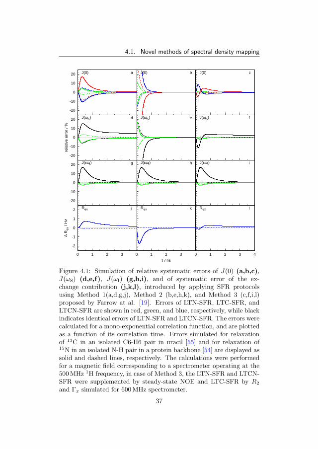
Figure 4.1: Simulation of relative systematic errors of J(0) (a,b,c),J(ωS) (d,e,f), J(ωI) (g,h,i), and of systematic error of the ex-change contribution (j,k,l), introduced by applying SFR protocolsusing Method 1(a,d,g,j), Method 2 (b,e,h,k), and Method 3 (c,f,i,l)proposed by Farrow at al. [19]. Errors of LTN-SFR, LTC-SFR, andLTCN-SFR are shown in red, green, and blue, respectively, while blackindicates identical errors of LTN-SFR and LTCN-SFR. The errors werecalculated for a mono-exponential correlation function, and are plottedas a function of its correlation time. Errors simulated for relaxationof 13C in an isolated C6-H6 pair in uracil [55] and for relaxation of15N in an isolated N-H pair in a protein backbone [54] are displayed assolid and dashed lines, respectively. The calculations were performedfor a magnetic field corresponding to a spectrometer operating at the500 MHz 1H frequency, in case of Method 3, the LTN-SFR and LTCN-SFR were supplemented by steady-state NOE and LTC-SFR by R2

and Γx simulated for 600 MHz spectrometer.

37

Chapter 4. Results

larger than 1 ns. The reduction bias of LTCN-MFR is given by thesame contribution as that of LTN-SFR, except for J(0), characterizedby the largest systematic error (approximately −10 %). LTC-SFR ex-hibits the smallest reduction bias within ±10 % for all spectral densityvalues.

Method 2 decreases the systematic error in all cases effectively onlyfor correlation times longer than the reciprocal value of the effectivehigh frequency. Otherwise, the systematic error raises rapidly becausethe assumption used to calculate the correction coefficients is violated.

4.1.2 Multiple field reduction

The multiple field reduction is based on the idea that certain eigen-frequencies may match different eigenfrequencies at another magneticfield. If relaxation data measured at three magnetic fields is analyzed,13 spectral density values contribute to relaxation rates, i.e., J(0),J(ωS,i), J(ωI,i − ωS,i), J(ωI,i) and J(ωI,i + ωS,i), where i = 1, 2, or 3distinguishes the spectral density values at individual magnetic fieldsB0,i. To apply the multiple field reduction, the choice of B0,i is re-strained by the following conditions:

ωI,1 = ωI,2 − ωS,2 (4.17)

andωI,3 = ωI,2 + ωS,2. (4.18)

If the conditions 4.17 and 4.18 are fulfilled, another two eigenfrequen-cies match each other as well:

ωI,1 + ωS,1 = ωI,3 − ωS,3. (4.19)

The optimal field ratio is close to 3:4:5 for 13C-1H and to 11:10:9 forthe 15N-1H pair. The reverse order of the magnetic field inductionis caused by the negative sign of the 15N magnetogyric ratio. If theoptimal magnetic field ratio is chosen, the number of spectral densityvalues contributing to the measured relaxation rates reduces from 13to 10.

In order to make the concept of elimination of systematic error moreobvious, let us assume that only σi, ρi, and µi, unaffected by a possibleslow exchange, are analyzed. At the first glance, the number of differ-ent spectral density values might still seem too large when comparedto the number of nine relaxation rates (σi, ρi, and µi, each measured

38

4.1. Novel methods of spectral density mapping

at three magnetic fields). However, one of ten spectral density val-ues, J(ωI,2), does not contribute to any of the considered relaxationrates (it only contributes to δ2 that is not analyzed). Therefore, theremaining nine spectral density values can be obtained without anysystematic error by solving a set of nine spectral density values defin-ing σi, ρi, and µi. The δi values, so far excluded from the analysis, arenot needed to obtain the mentioned nine spectral density values, butthey carry information on the exchange contributions ξi. Inspectionof the equations defining δ1 and δ3 shows that ξ1 and/or ξ3 can bedetermined accurately if δ1 and/or δ3, respectively, are included intothe analysis. The only parameter that is not available exactly is ξ2 be-cause J(ωI,2), contributing to δ2, remains undefined. Nevertheless, theeigenfrequency ωI,2 differs only slightly from ωI,1 + ωS,1 = ωI,3 − ωS,3.If this difference is neglected, twelve parameters (nine spectral den-sity values and three exchange contributions) can be derived fromtwelve relaxation rates measured. Interestingly, the accurate ξ2 canbe also obtained, but for a different magnetic field ratio, chosen sothat (ωI,1 + ωS,1) = ωI,2 = (ωI,3 − ωS,3). From the practical point ofview, exact determination of ξ2 would thus require another set of spec-trometers (e.g. 600MHz, 750MHz, and 1GHz for 13C-1H). In such acase conditions 4.17 and 4.18 are not fulfilled. Nevertheless, the condi-tion (ωI,1+ωS,1) = ωI,2 = (ωI,3−ωS,3) is sufficient to obtain all spectraldensity values without any bias. However, ξ1 and ξ3 can be evaluatedonly approximately if the difference between J(ωI,1) and J(ωI,2−ωS,2)and between J(ωI,3) and J(ωI,2 + ωS,2) is neglected, respectively. Thedescribed approach represents the LTCN-MFR protocol. Mathemat-ically, the LTCN-MFR protocol (including the approximate δ2, or δ1and δ3 for the sake of completeness) can be expressed in a form of amatrix equation:

~RLTCN = MLTCN~JLTCN, (4.20)

where the elements of the matrix MLTCN are listed in Table 4.1, vector

39

Chapter 4. Results

~RLTCN contains the relaxation data:

~RLTCN =

δ1δ2δ3ρ1

ρ2

ρ3

µ1

µ2

µ3

σ1

σ2

σ3

, (4.21)

and ~JLTCN contains ξi and spectral density values:

~JLTCN =

ξ1ξ2ξ3J(0)J(ωS,1)J(ωS,2)J(ωS,3)J(ε−(ωI,1 − ωS,1))J(ε1ωI,1)J(ε2ωI,2)J(ε3ωI,3)J(ε+(ωI,3 + ωS,3))

, (4.22)

where ε± = 1 and the coefficients εi are defined as

ε1 =B0,2(γI − γS)

B0,1γI, (4.23)

ε2 =B0,1(γI + γS)

B0,2γI=B0,3(γI − γS)

B0,2γI, (4.24)

ε3 =B0,2(γI + γS)

B0,3γI. (4.25)

Although the spectral density function is actually evaluated not forωI,i but for (ωI,i ± ωS,i), J(εiωI,i) values are reported for the LTCN-MFR protocol to keep the notation consistent with the other MFR

40

4.1. Novel methods of spectral density mapping

Table 4.1: Elements of matrix MLTCN from Equation 4.20.

2 0 0 8b1 0 0 0 0 12 0 0 0

0 2 0 8b2 0 0 0 0 0 12 0 0

0 0 2 8b3 0 0 0 0 0 0 12 0

0 0 0 0 6b1 0 0 2 0 12 0 0

0 0 0 0 0 6b2 0 0 2 0 12 0

0 0 0 0 0 0 6b3 0 0 2 0 12

0 0 0 8b1 6b1 0 0 0 0 0 0 0

0 0 0 8b2 b 6b2 0 0 0 0 0 0

0 0 0 8b3 b 0 6b3 0 0 0 0 0

0 0 0 0 0 0 0 −2 0 12 0 0

0 0 0 0 0 0 0 0 −2 0 12 0

0 0 0 0 0 0 0 0 0 −2 0 12

protocols. Solution of the equation is obtained in a straightforwardmanner as

~JLTCN =ΛLTCN

u~RLTCN, (4.26)

where ΛLTCN/u is an inversion of the matrix MLTCN and u = 24b3−4b1.The elements of the matrix ΛLTCN-MFR are listed in Table 4.2.

41

Chapter 4. Results

Tab

le4.

2:E

lem

ents

ofm

atri

xΛ

LT

CN

-MFR

from

Equ

atio

n4.

26.

u 20

0−

2b1−

6b2

−3u 2

36b2

+12b1

6b2

+2b1

3u 2

−36b2−

12b1

−6b2−

2b1

3u 2

−36b2−

12b1

0u 2

0−

6b3−

2b2

012b2

+6b1

6b3

+2b2

0−

12b2−

6b1

−6b3−

2b2

0−

12b2−

6b1

00

u 2−

2b3−b2

−u 4

6b2

+12b3

2b3

+b2

u 4−

12b3−

6b2

−2b3−b2

−u 4

−12b3−

6b2

00

01 2

0−

3−

1 20

31 2

03

00

0−

2 30

44b3

b1

0−

4−

2 30

−4

00

0−

2 30

42 3

u 6b2

−4

−2 3

0−

4

00

0−

2 30

42 3

0−

2b1

3b3

−2 3

0−

4

00

06b3

0−

6b1

−6b3

06b1

−6b3

+2b1

06b1

00

0b2

u 4−

6b2

−b2

−u 4

6b2

b2

−u 4

6b2

00

0b3

0−b1

−b3

0b1

b3

0b1

00

0b2 6

u 24

−b2

−b2 6

−u 24

b2

b2 6

u 24

b2

00

0b3 6

0−b1 6

−b3 6

0b1 6

b3 6

012b3−b1

6

42

4.1. Novel methods of spectral density mapping

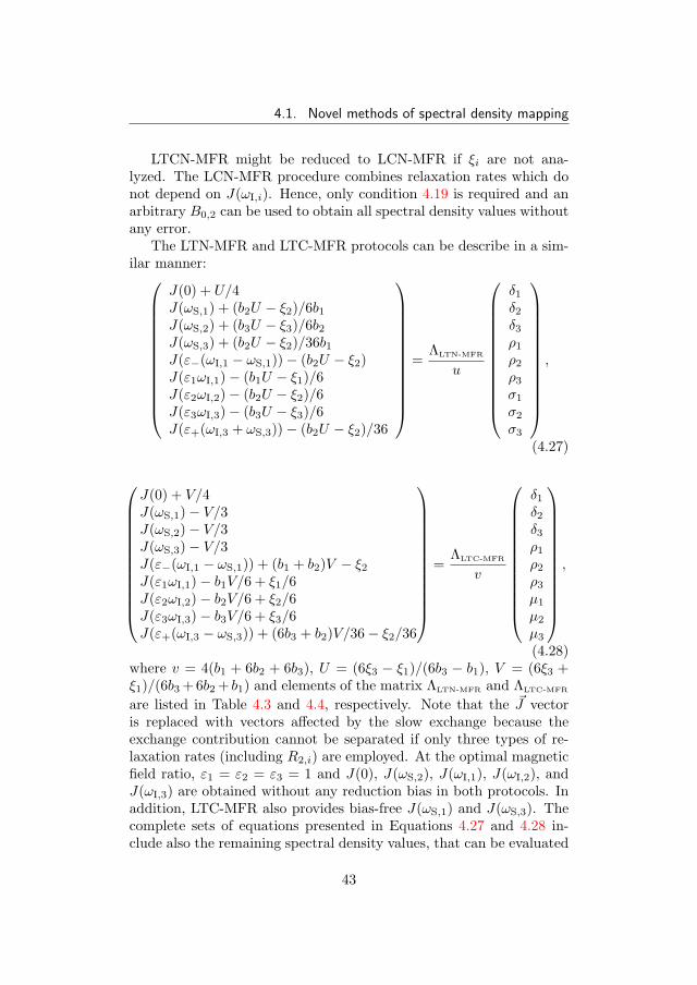
LTCN-MFR might be reduced to LCN-MFR if ξi are not ana-lyzed. The LCN-MFR procedure combines relaxation rates which donot depend on J(ωI,i). Hence, only condition 4.19 is required and anarbitrary B0,2 can be used to obtain all spectral density values withoutany error.

The LTN-MFR and LTC-MFR protocols can be describe in a sim-ilar manner:

J(0) + U/4J(ωS,1) + (b2U − ξ2)/6b1J(ωS,2) + (b3U − ξ3)/6b2J(ωS,3) + (b2U − ξ2)/36b1J(ε−(ωI,1 − ωS,1))− (b2U − ξ2)J(ε1ωI,1)− (b1U − ξ1)/6J(ε2ωI,2)− (b2U − ξ2)/6J(ε3ωI,3)− (b3U − ξ3)/6J(ε+(ωI,3 + ωS,3))− (b2U − ξ2)/36

=

ΛLTN-MFR

u

δ1δ2δ3ρ1

ρ2

ρ3

σ1

σ2

σ3

,

(4.27)

J(0) + V/4J(ωS,1)− V/3J(ωS,2)− V/3J(ωS,3)− V/3J(ε−(ωI,1 − ωS,1)) + (b1 + b2)V − ξ2J(ε1ωI,1)− b1V/6 + ξ1/6J(ε2ωI,2)− b2V/6 + ξ2/6J(ε3ωI,3)− b3V/6 + ξ3/6J(ε+(ωI,3 − ωS,3)) + (6b3 + b2)V/36− ξ2/36

=

ΛLTC-MFR

v

δ1δ2δ3ρ1

ρ2

ρ3

µ1

µ2

µ3

,

(4.28)where v = 4(b1 + 6b2 + 6b3), U = (6ξ3 − ξ1)/(6b3 − b1), V = (6ξ3 +ξ1)/(6b3 +6b2 + b1) and elements of the matrix ΛLTN-MFR and ΛLTC-MFR

are listed in Table 4.3 and 4.4, respectively. Note that the ~J vectoris replaced with vectors affected by the slow exchange because theexchange contribution cannot be separated if only three types of re-laxation rates (including R2,i) are employed. At the optimal magneticfield ratio, ε1 = ε2 = ε3 = 1 and J(0), J(ωS,2), J(ωI,1), J(ωI,2), andJ(ωI,3) are obtained without any reduction bias in both protocols. Inaddition, LTC-MFR also provides bias-free J(ωS,1) and J(ωS,3). Thecomplete sets of equations presented in Equations 4.27 and 4.28 in-clude also the remaining spectral density values, that can be evaluated

43

Chapter 4. Results

only approximately. The value of ε± for LTN-MFR and LTC-MFRcan be optimized if the spectral density values at high frequency areassumed to be proportional to 1/ω2 in analogy to Method 2 introducedin Section 2.5.3. The optimized values are

ε− =

√((B1(γI − γS))2

(1

(B2γI)2− 1

(B1(γI + γS))2

)+ 1)−1

(4.29)

ε+ =

√((B1(γI + γS))2

6

(1

(B2γI)2− 1

(B3(γI − γS))2

)+ 1)−1

(4.30)for LTN-MFR and

ε− =

√(6(B1(γI − γS))2

(1

(B1(γI + γS))2− 1

(B2γI)2

)+ 1)−1

(4.31)

ε+ =

√((B1(γI + γS))2

6

(1

(B3(γI − γS))2− 1

(B2γI)2

)+ 1)−1

(4.32)for LTC-MFR. In the case the field ratio is not optimal, both the ε±and εi factors can be optimized using the same assumptions as usedfor Equations 4.29–4.32. The dependence of the systematic error onthe timescale of the motion is demonstrated in Figure 4.2 and 4.3 forthe optimal and a sub-optimal field ratio.

44

4.1. Novel methods of spectral density mapping

Tab

le4.

3:E

lem

ents

ofm

atri

xΛ

LT

N-M

FR

from

Equ

atio

n4.

27.

−1 2

03

00

00

−3

0

−4b2

3b1

−u 3b1

8b2

b1

u 6b1

00

u 6b1

−8b2

b1

0

−4b3

3b2

04b1

3b2

0u 6b2

00

−u

+8b1

6b2

0

−2b2

9b3

−u

18b3

4b2

3b3

00

u 6b3

04b2

3b3

−u 6b3

2b2

u 2−

12b2

00

0−u 2

12b2

0

2b3

0−

2b1

00

00

2b1

0

b2 3

u 12

−2b2

00

00

2b2

0

b3 3

0−b1 3

00

00

2b3

0

b2

18

u 72

−b2 3

00

00

b2 3

u 12

45

Chapter 4. Results

Tab

le4.

4:E

lem

ents

ofm

atri

xΛ

LT

C-M

FR

from

Equ

atio

n4.

28.

1 20

30

−3

00

30

−2 3

0−

40

40

v

6b1

−4

0

−2 3

0−

40

40

012b3

+2b1

3b2

0

−2 3

0−

40

40

0−

4v

6b3

2(b

1+b2)

−v 2

12(b

1+b2)

v 2−

12(b

1+b2)

0−v 2

12(b

1+b2)

0

2(b

3+b2)

0−

2b1

02b1

00

−2b1

0

−b2 3

v 12

−2b2

02b2

00

−2b2

0

−b3 3

0b1

+6b2

30

2b3

00

−2b3

0

6b3

+b2

18

−v 72

6b3

+b2

30

−6b3

+b2

3

v 12

06b3

+b2

3−v 12

46

4.1. Novel methods of spectral density mapping

4.1.3 Minimal number of experiments

Nine experimental values are necessary to perform the LTN-MFR,LTC-MFR, or LCN-MFR analysis as described above. However, thenumber of experiments might be reduced if not all spectral densityvalues are required.

Values of J(0), J(ωS,1), J(ωS,3), J(ε−(ωI,1 −ωS,1)), J(ε2ωI,2), andJ(ε+(ωI,3 + ωS,3)) can be obtained from R1, Γx, and NOE data ac-quired at B0,1 and B0,3 only, as can be noticed from the distributionof zero and non-zero elements of matrices ΛLTCN-MFR. Hence, only datameasured at two fields are sufficient to perform the LCN-MFR analy-sis.

Six relaxation experiments (R1 at all three fields, R2 at B0,1 andB0,3, and steady-state NOE at B0,2) are sufficient to obtain J(0),J(ωS,2), J(ε1ωI,1), and J(ε3ωS,3) by LTN-MFR. J(ε2ωI,2) can be alsocalculated if the data is supplemented with R2 measured at B0,2.

Finally, R1 at all three fields, R2 at B0,1 and B0,3, and Γx atB0,2 are necessary to obtain J(0), J(ωS,2), J(ε1ωI,1), and J(ε3ωS,3)by LTC-MFR. Γx measured at B0,1 and B0,3 and R2 measured at themiddle field can be added to the analysis in order to get the J(ωS,1),J(ωS,3), and J(ε2ωI,2) value, respectively.

4.1.4 Multiple interacting nuclei

So far, only the isolated I-S spin system has been considered. In prac-tice, more spins may interact with spin S. The influence of more in-teracting spin-1/2 nuclei on the reduced spectral density approach isanalyzed in this section. Each dipole-dipole interaction contributes tothe R1 and R2 relaxation rates of nucleus S (Equation 2.46 and 2.47,respectively). Hence, the number of J(ω) values is extended by J(ωK)and J(ωS±ωK) in the presence of an additional interacting nucleus K.The effect on the reduced spectral density mapping analysis dependson the magnetogyric ratio of K. From this point of view, the nuclei K,can be classified as follows:

1. nuclei Kj have the same magnetogyric ratio as the interactingspin I (γKj = γI)

2. nuclei Kk have the same magnetogyric ratio as the interactingspin S (γKk

= γS)

47

Chapter 4. Results

-20

-10

0

10

20

-20

-10

0

10

20

rela

tive

erro

r / %

-20

-10

0

10

20

-2

-1

0

1

2

∆ R

ex /

Hz

aJ(0) bJ(ωS,1) cJ(ωS,2)

dJ(ωS,3) eJ(ε-(ωI,1-ωS,1)) fJ(ε1ωI,1)

gJ(ε2ωI,2) hJ(ε3ωI,3) iJ(ε+(ωI,3+ωS,3))

jRex,1 kRex,2 lRex,3

0 1 2 3 0 1 2 3

τ / ns

0 1 2 3 4

Figure 4.2: Relative systematic errors of J(0) (a), J(ωS,1) (b), J(ωS,2)(c), J(ωS,3) (d), J(ε−(ωI,1 − ωS,1)) (e), J(ε1ωI,1) (f), J(ε2ωI,2) (g),J(ε3ωI,3) (h), and J(ε+(ωI,3 + ωS,3)) (i) and systematic errors of theexchange contribution Rex at B0,1 (j), B0,2 (k), and B0,3 (l) introducedby applying MFR protocols at the optimal magnetic field ratio (3:4:5for 13C-1H). Errors of LTN-MFR, LTC-MFR, and LTCN-MFR areshown in red, green, and blue, respectively. The errors were calculatedfor a mono-exponential correlation function, and are plotted as a func-tion of its correlation time. The errors were simulated for relaxationof 13C in an isolated isotropically moving C6-H6 pair in uracil [55] atmagnetic fields corresponding to spectrometers operating at 300 MHz,400 MHz, and 500 MHz 1H frequency.

48

4.1. Novel methods of spectral density mapping

-20

-10

0

10

20

-20

-10

0

10

20

rela

tive

erro

r / %

-20

-10

0

10

20

-2

-1

0

1

2

∆ R

ex /

Hz

aJ(0) bJ(ωS,1) cJ(ωS,2)

dJ(ωS,3) eJ(ε-(ωI,1-ωS,1)) fJ(ε1ωI,1)

gJ(ε2ωI,2) hJ(ε3ωI,3) iJ(ε+(ωI,3+ωS,3))

jRex,1 kRex,2 lRex,3

0 1 2 3 0 1 2 3

τ / ns

0 1 2 3 4

Figure 4.3: Relative systematic errors of J(0) (a), J(ωS,1) (b), J(ωS,2)(c), J(ωS,3) (d), J(ε−(ωI,1 − ωS,1)) (e), J(ε1ωI,1) (f), J(ε2ωI,2) (g),J(ε3ωI,3) (h), and J(ε+(ωI,3 + ωS,3)) (i) and the exchange contribu-tion Rex at B0,1 (j), B0,2 (k), and B0,3 (l) introduced by applyingMFR protocols at a sub-optimal magnetic field ratio (4:5:6 instead of3:4:5). Errors of LTN-MFR, LTC-MFR, and LTCN-MFR are shown inred, green, and blue, respectively. The errors were simulated at mag-netic fields corresponding to spectrometers operating at the 400 MHz,500 MHz, and 600 MHz 1H frequencies (see Figure 4.2 for details).

49

Chapter 4. Results

3. nuclei Kl have the magnetogyric ratio different from both spin Iand S (γI 6= γKl

and γS 6= γKl)

The interaction of spin S with the first class of nuclei does not enlargethe set of spectral density values contributing to the relaxation ratescompared to the isolated I-S spin pair. An interaction with a spin ofthe second class introduces a new spectral density value J(2ωS), and,unlike for an isolated I-S spin pair, R1 depends also on J(0). The lastgroup of interacting nuclei complicates the analysis most severely as itintroduces three new spectral density values J(ωKl

) and J(ωKl± ωS)

for every type of nucleus belonging to the last class.The definition of the scaled relaxation rates δ, ρ, σ , µ, and λ is

modified for the analysis of a non-isolated I-S spin pair:

δ =2R2 −R1∑j

ζ2KjS

, (4.33)

ρ =R1∑

j

ζ2KjS

, (4.34)

σ =γSγI

(IssIref

− 1)

R1∑j

ζ2KjS

, (4.35)

µ =

2Γx√

1 + η2S/3

(∑j

ζ2KjS

+∑k

ζ2KkS +

∑l

ζ2KlS

+ ζ2S

)((3 + ηS) cos2 θ− + (3− ηS) cos2 θ+ − 2)ζSζIS

∑j

ζ2KjS

,

(4.36)

λ =

2Γz√

1 + η2S/3

(∑j

ζ2KjS

+∑k

ζ2KkS +

∑l

ζ2KlS

+ ζ2S

)((3 + ηS) cos2 θ− + (3− ηS) cos2 θ+ − 2)ζSζIS

∑j

ζ2KjS

,

(4.37)

where the index j, k, and l runs over all nuclei of class 1, 2, and 3,respectively.

The J(2ωS), J(ωK), and J(ωK ± ωS) values must be neglected tokeep the number of spectral density values unchanged. Then, theelements of the matrix MLTCN from the matrix Equation 4.20 are listed

50

4.1. Novel methods of spectral density mapping

Table 4.5: Elements of matrix MLTCN from Equation 4.20 for a non-isolated IS spin pair

2 0 0 8b1 12a 0 0 0 12 0 0 00 2 0 8b2 0 12a 0 0 0 12 0 00 0 2 8b3 0 0 12a 0 0 0 12 00 0 0 2a 6b1 0 0 2 0 12 0 00 0 0 2a 0 6b2 0 0 2 0 12 00 0 0 2a 0 0 6b3 0 0 2 0 120 0 0 8b1 6b1 0 0 0 0 0 0 00 0 0 8b2 b 6b2 0 0 0 0 0 00 0 0 8b3 b 0 6b3 0 0 0 0 00 0 0 0 0 0 0 −2 0 12 0 00 0 0 0 0 0 0 0 −2 0 12 00 0 0 0 0 0 0 0 0 −2 0 12

in Table 4.5 and parameters a and bi are defined as:

a =

∑k

ζ2KkS∑

j

ζ2KjS

(4.38)

bi = 1 +

∑k

ζ2KkS +

∑l

ζ2KlS

+ ζ2S∑

j

ζ2KjS

. (4.39)

The equation describing LTCN-MFR applied to a non-isolated I-S spin pair can be obtained by the inversion of the matrix M. Thematrices LTN-MFR and LTC-MFR are obtained in analogy to theisolated I-S spin system (Section 4.1.2). For more than two interactingspins, it is not possible to reduce the number of relaxation parametersneeded for the analysis in the case of LTC-MFR and LTN-MFR, in theway shown in Section 4.1.3. However, the reduction can be achieved ifthe terms 12a in matrix MLTCN (Table 4.5) are neglected. Figure 4.4shows that such a simplification does not have a severe effect on theaccuracy of the low-frequency spectral density values. On the otherhand, the systematic errors of the high frequency values are too highin both cases. Therefore, a careful analysis of possible systematicerrors has to precede the spectral density mapping if a relaxation in a

51

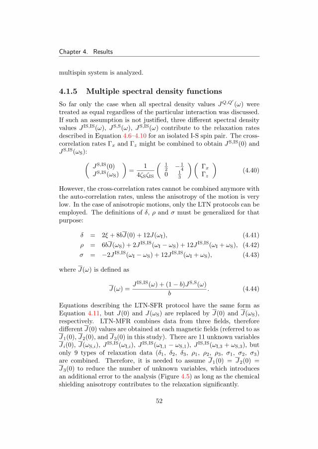
Chapter 4. Results

multispin system is analyzed.

4.1.5 Multiple spectral density functions

So far only the case when all spectral density values JQ,Q′(ω) were

treated as equal regardless of the particular interaction was discussed.If such an assumption is not justified, three different spectral densityvalues J IS,IS(ω), JS,S(ω), JS,IS(ω) contribute to the relaxation ratesdescribed in Equation 4.6–4.10 for an isolated I-S spin pair. The cross-correlation rates Γx and Γz might be combined to obtain JS,IS(0) andJS,IS(ωS):(

JS,IS(0)JS,IS(ωS)

)=

14ζSζIS

(12 − 1

40 1

3

)(ΓxΓz

)(4.40)

However, the cross-correlation rates cannot be combined anymore withthe auto-correlation rates, unless the anisotropy of the motion is verylow. In the case of anisotropic motions, only the LTN protocols can beemployed. The definitions of δ, ρ and σ must be generalized for thatpurpose:

δ = 2ξ + 8bJ(0) + 12J(ωI), (4.41)ρ = 6bJ(ωS) + 2J IS,IS(ωI − ωS) + 12J IS,IS(ωI + ωS), (4.42)σ = −2J IS,IS(ωI − ωS) + 12J IS,IS(ωI + ωS), (4.43)

where J(ω) is defined as

J(ω) =J IS,IS(ω) + (1− b)JS,S(ω)

b. (4.44)

Equations describing the LTN-SFR protocol have the same form asEquation 4.11, but J(0) and J(ωS) are replaced by J(0) and J(ωS),respectively. LTN-MFR combines data from three fields, thereforedifferent J(0) values are obtained at each magnetic fields (referred to asJ1(0), J2(0), and J3(0) in this study). There are 11 unknown variablesJ i(0), J(ωS,i), J IS,IS(ωI,i), J IS,IS(ωI,1 − ωS,1), J IS,IS(ωI,3 + ωS,3), butonly 9 types of relaxation data (δ1, δ2, δ3, ρ1, ρ2, ρ3, σ1, σ2, σ3)are combined. Therefore, it is needed to assume J1(0) = J2(0) =J3(0) to reduce the number of unknown variables, which introducesan additional error to the analysis (Figure 4.5) as long as the chemicalshielding anisotropy contributes to the relaxation significantly.

52

4.1. Novel methods of spectral density mapping

-20

-10

0

10

20

-20

-10

0

10

20

rela

tive

erro

r / %

-20

-10

0

10

20

-2

-1

0

1

2

∆ R

ex /

Hz

aJ(0) bJ(ωS,1) cJ(ωS,2)

dJ(ωS,3) eJ(ε-(ωI,1-ωS,1)) fJ(ε1ωI,1)

gJ(ε2ωI,2) hJ(ε3ωI,3) iJ(ε+(ωI,3+ωS,3))

jRex,1 kRex,2 lRex,3

0 1 2 3 0 1 2 3

τ / ns

0 1 2 3 4

Figure 4.4: Relative systematic errors of J(0) (a), J(ωS,1) (b), J(ωS,2)(c), J(ωS,3) (d), J(ε−(ωI,1 − ωS,1)) (e), J(ε1ωI,1) (f), J(ε2ωI,2) (g),J(ε3ωI,3) (h), and J(ε+(ωI,3 + ωS,3)) (i) and the exchange contribu-tion Rex at B0,1 (j), B0,2 (k), and B0,3 (l) introduced by applyingMFR protocols to 13C in an isotropically moving C6-H6 pair in fullylabeled uracil [55]. Errors of LTN-MFR, LTC-MFR, and LTCN-MFRare shown in red, green, and blue, respectively. The errors were simu-lated for magnetic fields corresponding to spectrometers operating atthe 300 MHz, 400 MHz, and 500MHz 1H frequencies (see Figure 4.2for details). Errors of spectral density values calculated using inver-sion of complete matrix MLTCN (Table 4.5) are shown as solid curves,while dotted curves indicate a simplified treatment with the term 12aneglected in the matrix MLTCN (Table 4.5).

53

Chapter 4. Results

-20

-10

0

10

20

-20

-10

0

10

20

rela

tive

erro

r / %

-20

-10

0

10

20

-2

-1

0

1

2

∆ R

ex /

Hz

aJ(0) bJ(ωS,1) cJ(ωS,2)

dJ(ωS,3) eJ(ε-(ωI,1-ωS,1)) fJ(ε1ωI,1)

gJ(ε2ωI,2) hJ(ε3ωI,3) iJ(ε+(ωI,3+ωS,3))

jRex,1 kRex,2 lRex,3

0 1 2 3 0 1 2 3

τ / ns

0 1 2 3 4

Figure 4.5: Relative systematic errors of J2(0) (a), J(ωS,1) (b), J(ωS,2)(c), J(ωS,3) (d), J(ε−(ωI,1 − ωS,1)) (e), J(ε1ωI,1) (f), J(ε2ωI,2) (g),J(ε3ωI,3) (h), and J(ε+(ωI,3 + ωS,3)) (i) and the exchange contribu-tion Rex at B0,1 (j), B0,2 (k), and B0,3 (l) introduced by applyingMFR protocols to a rigid molecule undergoing anisotropic rotationaldiffusion. Errors of LTN-MFR (red), LTC-MFR (green), and LTCN-MFR (blue) were simulated for data obtained at 300 MHz, 400 MHz,and 500 MHz spectrometers (see Figure 4.2 for details). Solid anddashed lines show the highest positive and negative error (selectedfrom all possible orientations of the C6-H6 bond), calculated for anaxially symmetric rotational diffusion tensor with ratio of eigenvaluesD‖/D⊥ = 1.35 and 2.00, respectively.

54

4.1. Novel methods of spectral density mapping

Simulated systematic errors introduced by the LTN-MFR, LTC-MFR, and LTCN-MFR protocols are shown in Figure 4.5 to docu-ment the effects discussed above. The results of the simulations foran axially symmetric rotational diffusion tensor with D‖/D⊥ = 1.35and uracil 13C6 as a motional probe showed that LTN-MFR providedaccurate J i(0) values, for which the systematic errors were less than2.5%. The highest systematic errors of J(ωC,2) and J(ωC,3) was lowonly for short correlation time, but it gradually increased above 5%for τ > 4 ns. LTCN-MFR yielded accurate J(ωC,2) and J(ωC,3) butexhibited up to 14 % maximum error of the J i(0) values. Finally, thehighest systematic error for J i(0) values did not exceed 6.5 % but thesystematic error was very large for other J(ω) values when LTC-MFRwas applied. The only high-frequency value with reasonable system-atic error was J(ε+(ωH,3+ωC,3)) obtained by LTCN-MFR, but limitedto a short correlation times (τ < 4 ns). The simulation of higher tum-bling anisotropy (D‖/D⊥ = 2.0) resulted in unacceptable systematicerrors of almost all spectral density values and MFR protocols.

The error of the LTN-MFR protocol can be avoided if R1, R2,and steady-state NOE data are measured at an additional field andJ IS,IS(0), JS,S(0) are evaluated separately. Exact determination ofJ IS,IS(0) and JS,S(0) would require additional conditions to be fulfilled:

ωI,4 = ωI,3 + ωS,2, (4.45)ωI,4 − ωS,4 = ωI,3. (4.46)

Then, the LTN-MFR protocol applied to data acquired at four mag-netic fields would provide 12 (apparent) spectral density values includ-

55

Chapter 4. Results

ing J IS,IS(0) and JS,S(0):

J IS,IS(0) + (c2−6c4)(ξ1−6ξ3)+(6c3−c1)(ξ2−6ξ4)5

JS,S(0) + ξ1 − ξ2 − 6ξ3 + 6ξ4J(ωS,1) + 16(c2−c4)(ξ1−ξ2−6ξ3−6ξ4)−4w(ξ2−ξ4)

5b1

J(ωS,2) + 8(c1−c3)(ξ1−ξ2−24ξ3+8ξ4)−2w(ξ1−ξ3)15b2

J(ωS,3) + 8(c2−c4)(ξ1−ξ2−24ξ3+24ξ4)−2w(ξ2−ξ4)15b3

J(ωS,4) + 4(c1−c3)(ξ1−4ξ2−24ξ3+24ξ4)+w(ξ1+ξ3)45b4

J IS,IS(ε−(ωI,1 − ωS,1)) + 24(c4−c2)(ξ1−ξ2−6ξ3+6ξ4)+6w(ξ2−ξ4)5w

J IS,IS(ε1ωI,1) + w(ξ1−ξ3)+4(c3−c1)(ξ1−4ξ2−24ξ3+24ξ4)5

J IS,IS(ε2ωI,2) + w(ξ2−ξ4)+4(c4−c2)(ξ1−ξ2−24ξ3+24ξ4)5

J IS,IS(ε3ωI,3) + w(ξ1−ξ3)+4(c3−c1)(ξ1−ξ2−ξ3+24ξ4)30

J IS,IS(ε4ωI,4) + w(ξ2−ξ4)+4(c4−c2)(ξ1−ξ2−24ξ3+24ξ4)30

J IS,IS(ε+(ωI,4 + ωS,4)) + w(ξ1−ξ3)+4(c3−c1)(ξ1−ξ2−6ξ3+36ξ4)180w

=

=ΛLTN-MFR4

w

δ1δ2δ3δ4ρ1

ρ2

ρ3

ρ4

σ1

σ2

σ3

σ4

, (4.47)

where w = 24c4 − 24c3 + 4c1 − 4c2, ci = (1 + bi)/bi, and the elementsof the matrix ΛLTN-MFR4 are listed in Table 4.6. The conditions givenat Equations 4.45 and 4.46 cannot be met simultaneously. However,the analysis of data simulated for uracil C6 at commercially available300, 400, 500, and 600 MHz spectrometers and for highly anisotropicdiffusion (D‖/D⊥ = 10) showed that the systematic error does notexceed 2.5% for J3(0), J4(0), J(ωS,2), J(ωS,3), J(ωS,4), J IS,IS(ε2ωI,2)J IS,IS(ε3ωI,3) J IS,IS(ε4ωI,4) and 5% for other four spectral density val-ues J2(0), J(ωS,1), J IS,IS(ε1ωI,1), and J IS,IS(ωI,4 + ωS,4).

It is possible to reduce somewhat the amount of required experi-mental data by omitting the steady-state NOE experiment at the low-est and highest magnetic field. However, it will preclude obtaining the

56

4.1. Novel methods of spectral density mapping

following spectral density values: J (ωS,1), J (ωS,4), J IS,IS(ωI,1 − ωS,1),and J IS,IS(ωI,4 + ωS,4).

57

Chapter 4. Results

Tab

le4.

6:E

lem

ents

ofm

atri

xΛ

LT

N-M

FR

4fr

omE

quat

ion

4.47

,w

=24c 4−

24c 3

+4c

1−

4c2,c i

=(1

+b i

)/b i

.c2−

6c4

10

6c3−

c1

10

18

c4−

3c2

53

c1−

18

c3

50

00

00

3c2−

18

c4

518

c3−

3c1

50

1 2−

1 2−

33

00

00

03

−3

0

8(c

2−

c4)

5b1

8(c

4−

c2)−

2w

5b1

48(c

4−

c2)

5b1

2w−

48(c

4−

c2)

5b1

w 6b1

00

0w 6b1

48(c

2−

c4)

5b1

48(c

4−

c2)−

2w

5b1

0

4(c

1−

c3)−

w

15

b2

4(c

3−

c1)

15

b2

w+

24(c

3−

c1)

15

b2

8(c

1−

c3)

5b2

0w 6b2

00

048(c

1−

c3)−

7w

30

b2

8(c

3−

c1)

5b2

0

4(c

2−

c4)

15

b3

4(c

4−

c2)−

w

15

b3

8(c

4−

c2)

5b3

w+

24(c

2−

c4)

15

b3

00

w 6b3

00

8(c

2−

c4)

5b3

48(c

4−

c2)−

7w

30

b3

0

4(c

1−

c3)+

w

90

b4

2(c

3−

c1)

45

b4

w+

24(c

3−

c1)

90

b4

4(c

1−

c3)

15

b4

00

0w 6b4

04(c

1−

c3)−

w

15

b4

4(c

3−

c1)

15

b4

−w

6b4

12(c

4−

c2)

53

w+

12(c

2−

c4)

572(c

2−

c4)

572(c

4−

c2)−

3w

50

00

0−

w 272(c

4−

c2)

53

w+

72(c

2−

c4)

50

w+

4c3−

4c1

10

2(c

1−

c3)

524(c

1−

c3)−

w

10

12(c

3−

c1)

50

00

00

w+

24(c

3−

c1)

10

12(c

1−

c3)

50

2(c

4−

c2)

5w

+4(c

2−

c4)

10

12(c

2−

c4)

524(c

4−

c2)−

w

10

00

00

012(c

4−

c2)

524(c

2−

c4)+

w

10

0

w+

4(c

3−

c1)

60

c1−

c3

15

4(c

1−

c3)−

w

60

2(c

3−

c1)

50

00

00

w+

4(c

3−

c1)

10

2(c

1−

c3)

50

c4−

c2

15

4(c

2−

c4)+

w

60

2(c

2−

c4)

524(c

4−

c2)−

w

60

00

00

02(c

4−

c2)

5w

+4(c

2−

c4)

10

0

w+

4(c

3−

c1)

360

c1−

c3

90

24(c

1−

c3)−

w

360

c3−

c1

15

00

00

0w

+4(c

3−

c1)

60

c1−

c3

15

w 12

58

4.1. Novel methods of spectral density mapping

4.1.6 Graphical interpretation

A method for graphical analysis of the low-frequency spectral densityvalues was proposed [58, 59, 60] to accompany the spectral densitymapping. The plot of experimental J(0) vs. J(ω) values was proposedto facilitate the interpretation of the results of spectral density map-ping. The J(ω) value was plotted as a function of J(0). A limit-curvewas defined by

J(ω) =J(0)

1 + (ωJ(0))2, (4.48)

representing the dependence of the J(0),J(ω) values on the correlationtime τ ≡ J(0) for motions defined by the mono-exponential function

C(t) = e−t/τ . (4.49)

It corresponds to the simplest isotropic stochastic diffusion rotation.A simple example of the graphical analysis is given in Figure 4.6.

Let us assume that dynamics in a molecule of a spherical shape is givenjust by three contributions: overall rotational diffusion, described bya monoexponential correlation function with the correlation time τ0,completely uncoupled fast internal motion described by a monoex-ponential correlation function with the correlation time τi, and slowexchange increasing δi by a factor of 2ξi at the magnetic field B0,i. In-terpretation of the plot is based on a comparison of these three contri-butions: (i) The limit case of a molecular motion completely describedas a rotational diffusion of a rigid spherical molecule corresponds to asingle point in the graph (blue circle in Figure 4.6) laying at a curvedefined by Equation 4.48. The blue point is common to all interactionsand it is determined by the value of the rotational-diffusion correlationtime τ0. (ii) Fast internal dynamics shifts the J(0), J(ωS) point (whitecircle) in the direction of the black arrow. The black arrow points tothe red circle determined by the timescale of the internal motion. Theposition of the red circle corresponds to a limit case of a completelyunrestricted internal motion which is effectively separated from theoverall tumbling of the whole molecule. The value of τ1 is defined bythe equation

τ1 = 1/(τ−10 + τ−1

i ). (4.50)

(iii) Finally, presence of an internal motion on the µs–ms time scaleshifts the white point in the direction of the green arrow for LTN-SFR and LTC-SFR. Both LCN-SFR and LCN-MFR are indifferent to

59

Chapter 4. Results

this effect. While the position of the J(0), J(ωS) point is identical forall approaches if no slow process contributes to δi, the effects of ξidiffer for individual approaches. The ξi contribution shifts the whitepoint horizontally to higher values of J(0) if the spectral density valuesare obtained by LTN-SFR method (Figure 4.6a), but shifts both J(0)and J(ωS,i) in a ratio that depends on the relative contributions ξiweighted by constants bi in the case of LTN-MFR. The J(0), J(ωS)point is shifted along the vector with a slope of −4/3 in plots of valuesobtained by LTC-SFR (Figure 4.6b) and LTC-MFR.

Comparison of the length and direction of the green arrows in Fig-ures 4.6a and 4.6b shows that the LTC plots are better indicators ofthe slow exchange than a plot of values obtained by LTN-SFR. Even asmall slow exchange contribution to the R2 relaxation rate is apparentin the case of the LTC-SFR method, while it can be easily overlookedin the case of LTN-SFR analysis. In such a case, the missed exchangecontribution is misinterpreted as higher rigidity.

Additional assumptions are needed to decompose the determinedspectral density values into exactly defined contributions of the indi-vidual motional modes. However, positions of the points in Figure 4.6indicate which type(s) of motional modes dominate(s). The experi-mental position can be converted to a coloring scheme, shown as abackground of plots in Figure 4.6, and it can be used for example forcoloring of the analyzed nuclei within the structure of the molecule todepict their motional behavior.

The color gradient in Figure 4.6 is defined by position of threepoints: the origin of the plot (red limit), the blue point (blue limit),and the experimental value most affected by the slow exchange (greenlimit).

An estimate of the overall rotational correlation time τ0 is necessaryto define the blue point. The overall rotational correlation time τ0 isestimated by setting J(ω) = τ0/(1 +ω2τ2

0 ) in Equations 2.46 and 2.47and fitting to the δ/ρ ratio [61]. Alternatively, µ/ρ can be fitted insteadof δ/ρ in order to eliminate the effect of the conformational exchange.

If the overall tumbling is anisotropic, but independent of the in-ternal motions, the theoretical limit of a rigid motion is no longerdescribed by a single correlation time τ0 common to all residues. In-stead, the effective τ0 value is given as

τ0 =2∑

m=−2

cm/Em, (4.51)

60

4.1. Novel methods of spectral density mapping

J(ω

S)

/ ns

(J(0)+ξ/4b) / ns

-0.2

-0.1

0.0

0.1

0.2

0.3

0.4

0.5

0.6

0.7

0 1 2 3τ0τ1

a

(J(ω

S)-

7ξ/3

9b)

/ ns

(J(0)+7ξ/52b) / ns

b

-0.2

-0.1

0.0

0.1

0.2

0.3

0.4

0.5

0.6

0.7

0 1 2 3τ0τ1

Figure 4.6: Illustration of interpretation of experimental data (blackdot) in the J(0) + ξ/4b, J(ωS) (a) and J(0) + 7ξ/52b, J(ωS) − 7ξ/39b(b) plot, obtained by LTN-SFR and LTC-SFR, respectively. The whitecircle represents the J(0), J(ωS) point, the blue and red circles corre-spond to the limits of the overall tumbling and of an internal motiondefined by correlation times τ0 and τ1, respectively. The black arrowdepicts the shift of the white point due to the internal flexibility onthe ps–ns time scale. The green arrow shows the shift due to the pres-ence of slow motions, described by identical ξ in both panels. A colorgradient from blue to red is used to distinguish relative contributionof fast motions on the sub-nanosecond timescale, while green indicatesslow dynamics on the µs–ms timescale.

where Em are eigenvalues of the rotation tensor (Equations 2.59–2.63)and cm depend on the mutual orientations of interaction and diffu-sion tensors (Equations 2.65–2.69) and on the eigenvalues of diffusiontensor.

The Em and cm values of sufficiently rigid molecules with knownstructure can be estimated by hydrodynamic simulations [49],[50] orby fitting diffusion properties of the molecule to the experimental δ/ρor µ/ρ ratio.

If the internal and overall motions are not separable, the limit ofthe overall tumbling looses its physical meaning. Nevertheless, it isstill instructive (and necessary for setting the color range) to comparethe plotted J(0), J(ω) values to a reference ”blue” point defined forexample as a theoretical τ0 value of a rigid spherical particle of the

61

Chapter 4. Results

same mass and density.If the multiple spectral density functions (Section 4.1.5) contribute

to the relaxation, the dynamic behaviour can be characterized by theplot of J(ω) vs. J(0) defined according to Equation 4.44. In the case ofthe studies discussed in the following sections, both multiple spectraldensity functions and multiple interacting nuclei must be considered.The explicit form of J(ω) are summarized here for amide 15N from thebackbone of δ subunit of RNA polymerase from B. subtilis

J(ω) =ζ2ISJ

IS,IS(ω) + ζ2SJ

S,S(ω)ζ2IS,IS + ζ2

S,S

, (4.52)

for pyrimidines C6 from fully 15N,13C labeled RNA UUCG hairpin

J(ω) =ζ2KSJ

KS,KS(ω) + ζ2LSJ

LS,LS(ω) + ζ2MSJ

MS,MS(ω)ζ2IS + ζ2

KS + ζ2LS + ζ2

MS + ζ2S

+ζ2ISJ

IS,IS(ω) + ζ2SJ

S,S(ω)ζ2IS + ζ2

KS + ζ2LS + ζ2

MS + ζ2S

, (4.53)

for purines C8 from fully 15N,13C labeled RNA UUCG hairpin

J(ω) =ζ2ISJ

IS,IS(ω) + ζ2LSJ

LS,LS(ω) + ζ2MSJ

MS,MS(ω) + ζ2SJ

S,S(ω)ζ2IS + ζ2

LS + ζ2MS + ζ2

S

,

(4.54)for β-d-Glcp-(1→6)-α-d-Manp-OMe

J(ω) =ζ2ISJ

IS,IS(ω) + ζ2KSJ

KS,KS(ω) + ζ2SJ

S,S(ω)ζ2IS,IS + ζ2

KS,KS + ζ2S,S

, (4.55)

where H′ and H′′ are the individual hydrogens of CH2 group. If theCSA contribution to the relaxation is neglected, Equation 4.55 simpli-fies to and for β-d-Glcp-(1→6)-α-d-Manp-OMe if the CSA contribu-tion to relaxation is neglected

J ′(ω) =J IS,IS(ω) + JKS,KS(ω)

2, (4.56)

4.2 Dimerization of the CD69 receptor

CD69 is a human activation antigen of lymphocytes. As a leukocytesignaling molecule, it affects the immune response. Native CD69 is

62

4.2. Dimerization of the CD69 receptor

a covalent homodimer with a disulfide bridge formed between C 68residues. Earlier studies suggested the importance of C 68 for thedimer formation [62, 63, 64, 65, 66, 67]. A shorter variant of CD69,labeled as CD69NG70 in Paper 5, has been investigated in this study.The sequence lacks the C 68 residue, which prevents the formationof the disulfide bond. Nevertheless, a series of experiments includingsedimentation equilibrium, sedimentation velocity, and dynamic lightscattering suggested that CD69N670 may form a dimer. In order toverify this hypothesis, I analyzed the 15N relaxation data using pro-gram relax 1.2.6 [45, 46] and performed hydrodynamic simulationsby program hydronmr [49, 50].

The R1 , R2 and steady-state NOE data were analyzed using theModel-free approach (Section 2.5.1). The two parameter model of theinternal dynamics (Equation 2.52) and the same model under the as-sumption of fast-motional limit (Equation 2.54) were fitted. A specificoverall diffusion model was not considered, but the residue-specificharmonic mean correlation time was optimized together with the pa-rameters of the internal dynamics. The results were compared withhydrodynamical calculations performed with a structure of a crystaldimer determined by X-ray crystalography, and with its monomericsubunits. First eleven N-terminal residues were missing in the X-raystructure compared to the studied CD69NG70 construct. The molec-ular dynamics simulations using software cns 1.2 [68] were performedto generate random orientations of the missing N-terminal chain. Thesimulated hydrodynamic properties of the modeled structures servedto estimate the rigid limit of the extended structure, while the crystalstructure represented the case when the tail moves completely inde-pendently of the structured part.

The comparison of residue-specific harmonic mean correlation timesis shown in Figure 4.7. The values of the hydrodynamically simulatedresidue-specific harmonic mean correlation time corresponding to themonomeric structure were systematically lower than the values ob-tained from the experiment, even when the rigid limit models of theterminal residues were applied. On the other hand, the experimentaldata nicely matched the values calculated for the crystal dimer. Theresults, showing that the disulfide bridge is not necessary for dimer-ization of CD69 receptor, were published in FEBS Journal (Paper 5in the appendix).

63

Chapter 4. Results

0

5

10

15

20

25

30

0 10 20 30 40 50 60 70 80 90 100 110 120 130

τ m /n

s

residue number

Figure 4.7: Residue-specific harmonic mean correlation time derivedfrom the experimental relaxation data (red crosses). The data arecompared with the residue-specific harmonic mean correlation timesimulated for subunits in a dimer (blue triangles) and for a monomericsubunit (dark green circles). Both simulations of the monomer anddimer structures were based on the X-ray structure. The up and downtriangles distinguish the subunits in the dimer. The light green circlesand cyan triangles correspond to the residue-specific harmonic meancorrelation time for extended structure models of the monomer anddimer, respectively.

64

4.3. N-terminal domain of the CA protein

4.3 N-terminal domain of the CA protein

The second relaxation study was part of an extensive characterizationof the N-terminal domain of capsid (CA) protein from the Mason-Pfizermonkey virus. I contributed to the project by the analysis of measured15N relaxation data and I performed and interpreted hydrodynamicalsimulations.

The structure of the protein was determined using NMR data(NOEs and residual dipolar couplings), but the position of the N-terminal β-hairpin remained poorly characterized. In order to testwhich structural model is consistent with the acquired 15N relaxationdata, hydrodynamical simulations were run for 50 calculated struc-ture with the lowest energy. The simulated residue-specific harmonicmean correlation times of individual models were compared with theharmonic mean correlation times calculated using experimental R1 ,R2 and steady-state NOE data. The root mean square deviation wasused to evaluate the agreement between the experimental and calcu-lated values for individual models. The structures with the less tightlypacked orientation of the N-terminal β-hairpin fit the experimentalcorrelation times best as indicated in Figure 4.8.

The experimental relaxation data was first analyzed by the reducedspectral density mapping LTN-SFR protocol (Equation 4.11), as thesimplest and mathematically most robust approach. Then, R1 and R2

data were used for the estimation of the diffusion tensor using programtensor2 2.0 [52]. The diffusion tensor was further optimized in pro-gram relax 1.2.6 [45, 46] using the complete set of available R1 , R2

and steady-state NOE data. Finally, the data was fitted to all mod-els of the correlation function defined in Section 2.5.1 whose numberof parameters does not exceed the number of experimental parame-ters (models defined by Equations 2.52, 2.54, 2.55). The possibilityto include potential chemical exchange contributions to the modelswas also tested, but only the exchange contributions Rex that couldbe clearly verified by reduced spectral density mapping were consid-ered significant. The slow exchange was revealed for residues in theloop between the second β sheet and the first α helix (residues 16–20), in the next loop and the following helix (residues 36, 57, 60), atthe beginning and in the middle of the fourth α helix (residues 70–72,79), at the end of the fourth α helix, in the following loop and at thebeginning of the next α helix (91, 93–94, 103–109, and 111), and atfour residues of the sixth α helix (119, 120, 122, and 125). The order

65

Chapter 4. Results

Figure 4.8: The stereo-view of the backbone of the N-terminal domainof capsid protein from the Mason-Pfizer monkey virus. The coordi-nates of backbone atoms from α-helices were used to superimposed50 structures obtained in structure calculations. The color of individ-ual structure reflects the root-mean square deviation (RMSD) betweenthe values of residue-specific harmonic mean correlation times calcu-lated for the structure and the residue-specific harmonic mean corre-lation times obtained by fitting to the experimental relaxation data.The color gradient ranges from green for the RMSD=4.3 ns to red forRMSD=12.9 ns.

66

4.4. δ subunit of RNA polymerase

0.0

0.1

0.2

0.3

0.4

0.5

0.6

0.7

0.8

0.9

1.0

1.1

0 10 20 30 40 50 60 70 80 90 100 110 120 130 140

S2

residue number

Figure 4.9: The order parameter of backbone amide 15N in the N-terminal domain of the capsid protein from Mason-Pfizer monkeyvirus. The blue and green bars on the top indicate β strands andα helices, respectively. The data in red correspond to the residuesfor which a graphical analysis of J(0), J(ωN) values obtained by theLTN-SFR protocol indicated a slow exchange contribution.

parameters for most of the residues are higher than 0.8, suggesting alow flexibility of the protein backbone. Residues 10 and 12 from theloop between the β strands are slightly more flexible (order parameterapproximately equal to 0.8). Three residues (48, 51, and 54) withinthe loop between the second and third α helix, together with residue120, represent the most flexible residues in the structured part of thesequence. Especially, the order parameter of the residue 48 lower than0.3 is outstanding. The most flexible part of the molecule is the C-terminal tail, where the order parameter decreases down to value lowerthan 0.1 for the last residue in the sequence. The sequence dependenceof the order parameter of all analyzed residues is shown in Figure 4.9.

4.4 δ subunit of RNA polymerase

RNA polymerase of gram-positive bacteria consists of seven subunits.The δ subunit was suggested to have a regulation function and it wasshown it is important for virulence of gram-positive pathogen. The δsubunit consists of two domains of approximately the same size. The

67

Chapter 4. Results

N-terminal domain has a well defined structure [30], while the otherdomain is intrinsically disordered.

First, the sample containing only the N-terminal domain of theδ subunit was studied. The backbone motions were investigated byanalyzing relaxation of the amide 15N-1H spin pairs. The motionsof the structured part are dominated by the rotational diffusion andthe assumption ωH ωN is fulfilled well enough to safely neglect thesystematic bias of reduced spectral density mapping (see Section 4.1.1).The analysis was based on the R1, R2 and steady-state NOE datameasured at two temperatures (7C and 27C).

The spectral density values obtained by the analysis of data mea-sured at 27C yield the following qualitative description of the dynam-ics. Five residues (17, 28, 31, 63, and 64) are influenced by slow µs–msmotions. The residues of the structured part are characterized by sim-ilar spectral density values, which is documented by a narrow rangeof J(0). The J(0) values of all investigated residues in the structuredpart are between 6 and 9 ns, except for the most flexible residue 52(5.36 ± 0.03) ns and the residues affected by the slow exchange. Thedecrease of J(0) values of the residues following the last helix in thestructure indicates an increased flexibility in the C-terminal tail. Theanalysis of data acquired at 7C yielded spectral density values thatreflect the slowed overall rotation. The data points in the J(0) vsJ(ωN) plot are closer to the rigid limit curve compared to the result ofthe analysis at 27C. The slow exchange contribution was confirmedfor residues 17, 28, 31, and 64 (residue 63 was not analyzed due to asignal overlap). The slow exchange contribution was detected also forother residues (18, 23, 33, 53, 59, 67, 72, 74, 76, and 79).

Subsequently, the analysis of motions of the full-length δ subunitwas performed. The original protocol of the reduced spectral densitymapping (LTN-SFR) can introduce a reduction bias (Section 4.1.1) ifthe motions with correlation time shorter than 1 ns dominate. There-fore, accurate results were obtained only for the well structured N-terminal domain whose motions are dominated by the rotation diffu-sion motion. On the contrary, relaxation data of the highly flexibleC-terminal domain should be analyzed more carefully. The resultsof the described methods LTN-SFR, LTC-SFR, and LCN-SFR 4.11–4.13 applied to analysis of data of the δ subunit are presented in Fig-ure 4.10a,d. Three residues (V 17, K 28, and N63) were identified bythe LTN-SFR approach as residues influenced by the slow exchangecontribution. Interestingly, more residues were identified to be af-

68

4.4. δ subunit of RNA polymerase

fected by a slow exchange when the LTC-SFR method was applied.LTC-SFR is more sensitive to the slow exchange as discussed in Sec-tion 4.1.6. An independent CPMG relaxation dispersion experiment(Section 2.6.1) was performed to verify the results. Unfortunately, thesensitivity of the experiment was not high enough to quantify relativelysmall slow exchange contributions in the structured part. Nevertheless,the results qualitatively support the conclusion that more residues areinfluenced by the slow exchange. The spectral density values free ofany exchange contribution were obtained by the LCN-SFR approach(Figure 4.10c,f). The comparison of results obtained by the LTN-SFR,LTC-SFR and LCN-SFR protocols documents the practical advantageof applying modified versions of SFR methods. The results of theLTN-SFR analysis might be misinterpreted as a higher internal rigid-ity, while introducing Γx to the analysis clearly distinguished effects ofslow motions from the fast dynamics.

The simple versions of the SFR methods are not adequate for themotional analysis of the backbone amides of fast moving C-terminalresidues due to the reduction bias. However, the reduction bias issufficiently reduced by employing Method 3 by Farrow et al. [19] ifdata from two fields are combined (Figure 4.1). The analysis is fur-ther complicated by the difference between spectral density functionsdescribing various interactions. The resulting systematic error α hasan effect similar to the exchange contribution ξ. In order to estimatethe effect of α, its value was simulated for a model case of a rigidmolecule described by a rotational diffusion tensor with D‖/D⊥ = 2and by an averaged correlation time of 2 ns. The α values rangedbetween −0.68 ns and +0.53 ns at the 500 MHz spectrometer and be-tween −0.60 ns and +0.46 ns at the 600MHz spectrometer. Finally,both LCN-SFR and LTN-SFR yield high frequency spectral densitydata with a systematic error less than ±4 % and with a sufficient pre-cision for the disordered residues.

The experimental results of the unstructured part of δ-subunit areshown in Figure 4.11. The disordered nature of the C-terminal domainof the δ subunit is in a good agreement with the obtained picture ofmolecular motions. C-terminal K 173 is the most flexible residue, withthe dynamics limited to sub-nanosecond motions. It is followed bythe Y 165 and D 167 residues showing somewhat slower motions. Thetrend continues with a cluster of residues 153–159 exhibiting a verysimilar motional behavior. The residues further from the C-terminusvary more in their dynamics. The values in Figure 4.11b,e are hori-

69

Chapter 4. Results

0.00.20.40.60.81.01.21.41.6

0 5 10 15 20

J(ω

N,3

) / n

s

(J(0)+ξ3/4b3) / ns

a

1728

63

-8

-6

-4

-2

0

2

0 5 10 15 20

(J(ω

N,3

)-7ξ

3/52

b 3)

/ ns

(J(0)+7ξ3/39b3) / ns

b

1728

63

0.0

0.2

0.4

0.6

0.8

1.0

1.2

1.4

1.6

0 5 10 15 20

J(ω

N,3

) / n

s

J(0) / ns

c

17

28

63

0.00.20.40.60.81.01.21.41.6

0 5 10 15 20

J(ω

N,1

) / n

s

(J(0)+ξ1/4b1) / ns

d

1728

63

-8

-6

-4

-2

0

2

0 5 10 15 20

(J(ω

N,1

)-7ξ

1/52

b 1)

/ ns

(J(0)+7ξ1/39b1) / ns

e

17

28

63

0.0

0.2

0.4

0.6

0.8

1.0

1.2

1.4

1.6

0 5 10 15 20

J(ω

N,1

) / n

s

J(0) / ns

f

17

28

63

Figure 4.10: Experimental J(ω) values obtained by LTN-SFR (a,d),LTC-SFR (b,e), and LCN-SFR (c,f), applied to the relaxation dataof the δ-subunit of RNA polymerase from B. subtilis, measured at the500 MHz (a,b,c) and 600 MHz (d,e,f) spectrometers. The subscripts3 and 1 refer to data recorded at the 500MHz and 600MHz spectrome-ter, respectively. Data for residues from the well-structured N-terminaldomain and disordered C-terminal region are displayed in blue and red,respectively. The ellipses indicate the experimental errors. Data forN-H bonds exhibiting the highest conformational exchange are labeledwith residue numbers.

70

4.5. UUCG RNA hairpin

zontally shifted compared to the values in Figure 4.11a,d by a factorof ξ − α. The ξ − α value can not be decomposed into individual ξand α contributions. However, the sufficiently large contribution ofa slow exchange may be distinguished from relatively small values ofα because the ξ value is always positive. The results of the CPMGexperiment (shown in Figure 4.12) confirm a small but significant slowexchange for most of the discussed residues of the flexible tail. Verylittle exchange was detected for residues V 106, E 116, F 139, E 141,Y 165, D 167, and K 173, while the residues 153–158 exhibited a signif-icant exchange contribution, which was not completely suppressed inthe R2 measurement. The average residual Rex contribution was esti-mated to be 0.1Hz for these residues, which is in agreement with thedifference between J(0) values obtained by the LTN-SFR and LCN-SFR methods (shown in Figure 4.11). The LTC-SFR protocol cor-rected by Method 3 was not applied because both ξ and α contributealso to high frequencies, which may results in an incorrect estimate ofthe slope describing the spectral density function at high frequencies.

Data acquired at 600 MHz and 500MHz spectrometers can alsobe analyzed by the LCN-MFR method as the field ratio is close to11:9, an optimum for the analysis of the 15N-1H relaxation data. Theobtained values are accurate but less precise compared to the resultsof LCN-SFR corrected by Method 3.

4.5 UUCG RNA hairpin

The analysis of motions within a small fragment of RNA moleculewas chosen as another typical example of a study where the developedMFR spectral density methods might be useful to apply. The inves-tigated RNA molecule consists of 14 nucleotides. The UUCG stretchin the middle of the sequence forms a loop, the other residues forma double-helical stem. The UUCG loop is a quite abundant motif inRNA molecules and its motions were investigated by numerous NMRtechniques [56, 69, 70, 71, 72, 73, 74, 75, 76, 77, 78, 79, 80, 81].

The lack of suitable imino N-H spin pairs limits motional studiesbased on the analysis of the 15N relaxation data. Only N3-H3 in uracilor thymine and N1-H1 in guanine are available in nucleic acids. Onthe other hand, there are two suitable C-H spin pairs in pyrimidines(C6-H6 and C5-H5) and in adenine (C8-H8, C2-H2) and one in theguanine base (C8-H8). Moreover, relaxation of the C1’-H1’ spin pair

71

Chapter 4. Results

0.2

0.3

0.4

0.5

0.6

0.7

0.8

0.0 0.5 1.0 1.5 2.0

J(ω

N,3

) / n

s

(J(0)+ξ3/4b3) / ns

a

91

94

106

116

128 129

135

139141

153154

156

157

158

159

165167

173

0.2

0.3

0.4

0.5

0.6

0.7

0.8

0.0 0.5 1.0 1.5 2.0

J(ω

N,3

) / n

s

(J(0)+α3/4b3) / ns

b

91 94

106 116

128129135

139

141

153

154156

157158

159165167

173

0.0

0.1

0.2

0.0 0.5 1.0 1.5 2.0

J(0.

87ω

H,3

) / n

s

(J(0)+α3/4b3) / ns

c

91 94

106 116

128 129

135

139

141153

154156 157

158

159165

167173

0.2

0.3

0.4

0.5

0.6

0.7

0.8

0.0 0.5 1.0 1.5 2.0

J(ω

N,1

) / n

s

(J(0)+ξ1/4b1) / ns

d

9194

106

116

129135

139 153

154

156

157

158

159

165167

173

0.2

0.3

0.4

0.5

0.6

0.7

0.8

0.0 0.5 1.0 1.5 2.0

J(ω

N,1

) / n

s

(J(0)+α1/4b1) / ns

e

9194

106

116

129135

139

153154

158157

156

159

165167

173

0.0

0.1

0.2

0.0 0.5 1.0 1.5 2.0

J(0.

87ω

H,1

) / n

s

(J(0)+α1/4b1) / ns

f

9194

106

116129

135

139

153

154

156157

158159

165

167173

Figure 4.11: The J(0) vs. J(ωN) values calculated by reduction-biascorrected LCN-SFR (a,d), the J(0) vs. J(ωN) values obtained byreduction-bias corrected LTN-SFR (b,c), and the J(0) vs. J(εωH)values obtained by reduction-bias corrected LCN-SFR (c,f) for thedisordered region of the δ-subunit of RNA polymerase from B. subtilis.The plotted values were calculated from data acquired at the 500MHz(a,b,c) (subscript 3) and 600 MHz (d,e,f) (subscript 1) spectrometers,respectively, utilizing the differences between the steady-state NOEmeasured at the individual fields in the process of the reduction biascorrection [19]. The experimental errors are indicated by the elipses.

72

4.5. UUCG RNA hairpinR

CP

MG

/ H

z

5.2

5.4

5.6

5.8T91

6.6

6.8

7.0

7.2T94

4.8

5.0

5.2

5.4V106

5.2

5.4

5.6

5.8E116

4.6

4.8

5.0

5.2V128

4.6

4.8

5.0

5.2E129

3.8

4.0

4.2

4.4 E135

3.2

3.4

3.6

3.8 F139

3.6

3.8

4.0

4.2 E141

4.0

4.2

4.4

4.6 I153

4.0

4.2

4.4

4.6 E154

4.0

4.2

4.4

4.6 D156

3.6

3.8

4.0

4.2 I157

4.0

4.2

4.4

4.6 I158

3.8

4.0

4.2

4.4 D159

2.6

2.8

3.0

3.2 Y165

2.6

2.8

3.0

3.2 D167

1.6

1.8

2.0

2.2 K173

0.0 0.5 1.0 0.0 0.5 1.0 0.0 0.5 1.0νCPMG / kHz

0.0 0.5 1.0 0.0 0.5 1.0 0.0 0.5 1.0

Figure 4.12: Results of the CPMG relaxation dispersion experimentsfor the residues of the disordered region of the δ-subunit of RNA poly-merase from B. subtilis whose resolution allowed spectral density map-ping based on 500 MHz and 600MHz data. Values of the apparentrelaxation rate measured at 600MHz are plotted as a function of thefrequency of the 180 pulses applied during the CPMG sequence.

73

Chapter 4. Results

from ribose is also convenient to analyze in order to obtain dynamicinformation on the sugar. Therefore, the description of the motionsof RNA molecules is more comprehensive if the 13C-1H relaxation isstudied. The analysis of the 13C relaxation in nucleic acid bases in com-plicated by the asymmetry and orientation of the 13C carbon shieldingtensor. A single spectral density function for both dipole-dipole andCSA may be used only if the molecule motions are isotropic.

Several sources of possible errors were analyzed in the presentstudy. First, the diffusion of the studied molecule is not strictlyisotropic, but it can be described by an axially symmetric diffusiontensor with D‖/D⊥ = 1.35 [79]. Second, the uniformly 13C, 15N-labeled molecule has been studied, and spin-1/2 nuclei other than thedirectly attached 1H thus contributed to the relaxation of the observed13C6 and 13C8 nuclei. Third, the relaxation data was acquired at asuboptimal field ratio of 4:5:6.

Simulations showed (Figures 4.3, 4.4, 4.5) that the MFR protocolscan be used even under such unfavorable conditions. However, theanalysis should be limited to the reliable spectral density values witha low systematic error.

Results of the spectral density mapping are shown in Figure 4.13where the most reliable values J(0), J(ωC,2) obtained from the experi-mental data using the LTN-MFR analysis, exchange free J(0), J(ωC,3)values calculated by LCN-MFR, and J(0), J(ωC,2) obtained by LTC-MFR and LTC-SFR are plotted.

In order to verify the results, the systematic error was simulatedfor various orientations of the nucleic acid base and of the diffusiontensor as a function of the mean correlation time, while the ratio ofthe eigenvalues of diffusion tensor was set to D‖/D⊥ = 1.35 (shownin Figure 4.14). LCN-MFR yields accurate J(ωC,3) but J(0) can beunderestimated by more than 10% for motions characterized by veryshort correlation times (shorter than 1 ns). Therefore, J(0) results ofhighly flexible residues can be considered accurate only under the as-sumption that fast internal motions are isotropic. LTN-MFR yieldssufficiently accurate spectral density values J(0), J(ωC,2), but a sim-ple interpretation is complicated if the slow exchange contributes asdiscussed in Section 4.1.6. Finally, J(ωC,2) can be highly overesti-mated or underestimated in the case of the LTC methods. However,the simulations showed that it is still convenient to analyze the J(0)vs. J(ωC,2) plot as a sensitive indicator of the slow exchange contri-bution for the stem residues. The simulations presented in Figure 4.15

74

4.6. β-d-Glcp-(1→6)-α-d-Manp-OMe

show that J(ωC,2) is overestimated for the orientations of bases in thedouble helical stem. On the contrary, the exchange contribution de-creases the J(ωC,2) value. Hence, the shift of the experimental pointto the lower values of J(ωC,2) can be still considered as the evidenceof the chemical exchange contribution.

The displayed values in Figure 4.13 provide the following qualita-tive description of the motions within the molecule. U 7 and C 8 withinthe UUCG loop exhibit the highest flexibility on the ns-ps time scalefrom all residues. Both of them are also affected by exchange contribu-tions on the µs-ms time scale. The fast motions are more pronouncedat U 7 compared to C 8, while the slow exchange is pronounced moreat C 8 than at U 7. Signal of C 8 from loop base G 9 has a too low in-tensity to obtain data sufficiently precise for a reliable interpretation.Nevertheless, the observed line broadening serves as an indirect evi-dence that G 9 is also influenced by motions on the µs-ms time scale.The same applies to the terminal base of G 1. The data of C 8 fromthe base G 2 were also affected by the line broadening but evaluationof J(ω) values was possible and positions of the experimental point inLTN-MFR, LTC-MFR, and LTC-SFR clearly indicated the slow ex-change contribution. The other residues from the double helical stemgave J(ω) values close to the limit of the overall tumbling. However,a comparison of the data with the exchange free values provided byLCN-MFR (Figure 4.13b) revealed that these residues also exhibit aslow exchange.

4.6 β-d-Glcp-(1→6)-α-d-Manp-OMe

The last molecule chosen to test the applicability of the MFR methodswas methyl β-d-glucopyranosyl-(1→6)-α-d-[6-13C]-mannopyranoside.The selective 13C labeling at the bridging methylene group simplifiedboth experiments and analysis of its relaxation significantly. Dipole-dipole interactions with the attached protons dominate the 13C re-laxation, while the chemical shift anisotropy contribution is relativelysmall. The motion of the molecule is highly anisotropic as was shownin an earlier study [34]. Therefore, a single spectral density functioncannot be used neither for individual auto-relaxation mechanism norcross-correlated relaxation. As discussed in Section 4.1.5, any spectraldensity mapping approach which combines auto- and cross-correlatedrelaxation rates are not applicable under these circumstances.

75

Chapter 4. Results

-0.3

-0.2

-0.1

0.0

0.1

0.2

0.3

0.4

0.5

0.6

App

aren

t J(ω

) / n

s

c

2

4

5

7

8

10

11

12

13

14

0.0

0.1

0.2

0.3

0.4

0.5

0.6

App

aren

t J(ω

) / n

s

a

2

4 57

8 10

11

12

1314

0.0

0.1

0.2

0.3

0.4

0.5

0.6

App

aren

t J(ω

) / n

s

d

45 12

13

14

2

7

8

10

11

0.0

0.1

0.2

0.3

0.4

0.5

App

aren

t J(ω

) / n

s

b2

45

7

10

11

12

14

0.0 0.5 1.0 1.5 2.0 2.5 3.0 3.5

Apparent J(0) / ns

0.0 0.5 1.0 1.5 2.0 2.5 3.0 3.5

Apparent J(0) / ns

Figure 4.13: Apparent J(ω) values obtained by LTN-MFR (a), LCN-MFR (b), LTC-SFR (c), and LTC-MFR (d), applied to the relax-ation data of the UUCG RNA hairpin. The plotted values correspondto J(0)−U/4 vs. J(ωC,2)− (b3U − ξ3)/3b2 (a), J(0) vs. J(ωC,3) (b),J(0)− 7ξ2/52 vs. J(ωC,2) + 7ξ2/39 (c), J(0)− V/4 vs. J(ωC,2) + V/3(d), where U = (6ξ3−ξ1)/(6b3−b1), V = (6ξ3+ξ1)/(6b3+6b2+b1), andsubscripts 1, 2, and 3 distinguish magnetic fields 400MHz, 500 MHz,and 600 MHz, respectively. The ellipses indicate the experimental er-rors. Data are labeled with residue numbers.

76

4.6. β-d-Glcp-(1→6)-α-d-Manp-OMe

-20

-10

0

10

20

-20

-10

0

10

20

rela

tive

erro

r / %

-20

-10

0

10

20

-20

-10

0

10

20

aJ(0) bJ(ωS,2) cJ(ωS,3)

dJ(0) eJ(ωS,2) fJ(ωS,3)

gJ(0) hJ(ωS,2) iJ(ωS,3)

jJ(0) kJ(ωS,2) lJ(ωS,3)

0 1 2 3 0 1 2 3

τ / ns

0 1 2 3 4

Figure 4.14: The simulation of the relative error of the analyzed spec-tral density values for 14-nt RNA hairpin as a function of mean correla-tion time. The axially symmetric diffusion tensor with a constant ratioof eigenvalues D‖/D⊥ = 1.35 was used in the simulation. The error ofaveraged spectral density values obtained by LTN-MFR, LTC-MFR,LCN-MFR, and LTC-SFR are shown in red solid, green solid, bluesolid, and green dashed line, respectively. The J2(0) and J(ωC,2) areshown in panels (a,d,g,j) and (b,e,h,k), respectively, for LTN-MFR,LTC-MFR, LTCN-SFR protocols. The J3(0) and J(ωC,3) are shownin panels (a,d,g,j) and (c,f,i,l), respectively, for LCN-MFR. The rela-tive errors in panels (a,b,c), (d,e,f), (g,h,i), and (j,k,l) correspond touracil C6, cytosine C6, guanine C8, and adenine C8 in fully 15N,13Clabeled nucleic acid bases. Subscripts 2 and 3 distinguish magneticfield 500MHz and 600 MHz, respectively.

77

Chapter 4. Results

0

20

40

60

80

0

20

40

60

80

α /

deg

0

20

40

60

80

0

20

40

60

80

a b

c d

relative error / %

20 15 10 5 0 -5

-10 -15 -20 -25 -30

e

relative error / %

f

relative error / %

g

relative error / %

h

0 20 40 60 80 100 120 140 160

β / deg

0 20 40 60 80 100 120 140 160 180

Figure 4.15: The dependence of the relative error of J(ωC,2) obtainedby LTC-SFR (a,c,e,g) and LTC-MFR (b,d,f,h) on the orientationof the nucleic acid base with respect to the axial diffusion tensor(1/(4D⊥ + 2D‖)) = 2.85 ns, D‖/D⊥ = 1.35). The numbers indicatethe value of the relative error (in units percent) for each contour line.The angles α and β are two Euler angles which define the relative ori-entation of the nucleic acid base and the diffusion tensor as follows:the C-H bond and symmetry axis of the diffusion tensor are alignedwith z-axis of the coordinate system and the plane of the aromaticring lies within the y,z plane of the coordinate system. The angle αdefines the initial clockwise rotation with the base around the z-axis.The angle β defines the subsequent anti-clockwise rotation with thebase around y-axis. The orientation of a base in the ideal double he-lical structure would corresponds to α = 0, β = 90. Relative errorsin panels (a,b), (c,d), (e,f), and (g,h) correspond to uracil C6, cyto-sine C6, guanine C8, and adenine C8, respectively, in fully 15N,13Clabeled nucleic acid bases. Subscripts 2 and 3 distinguish magneticfield 500MHz and 600 MHz, respectively.

78

4.6. β-d-Glcp-(1→6)-α-d-Manp-OMe

If the CSA mechanism does not contribute to the relaxation rate,LTN-MFR yields accurate linear combination of spectral density val-ues (J IS,IS(ω)+JKS,KS(ω))/2 at frequencies ω = 0, ωC,2, and ωH,i pro-vided data from 300 MHz, 400MHz, and 500 MHz spectrometers arecombined. Simulations showed that neglecting the CSA in the case ofthe β-d-glucopyranosyl-(1→6)-α-d-[6-13C]-mannopyranoside does notintroduce an error larger than 5 % if the correlation time of the motiondoes not exceed 0.6 ns (Figure 4.16). CSA can be taken into accountcorrectly if data from four fields are combined (Equation 4.47). Suchan analysis was performed based on the data obtained at 300 MHz,400 MHz, 500 MHz, and 600 MHz spectrometers, very close to the op-timal field ratios. The results of both (3-field an 4-field) variants ofLTN-MFR are shown in Figure 4.17. The difference between the mostaccurate spectral density values suggest that the CSA contributionmight be safely neglected if the auto-correlated spectral density valuesare calculated from the data acquired at magnetic field not exceeding12 T.

The graphical analysis documents that the data are not influencedby any slow motion. The experimental data point is close to the limitcurve at all frequencies, while the Rex contribution would shift thepoint along a line with a slope given by ratios of the exchange con-tributions to the individual spectral density values. The experimen-tal data obtained within this study were compared with the diffusiontensor optimized by the SRLS approach [34]. The eigenvalues of thediffusion tensor define five correlation times. The corresponding pointsof the single motional limit are depicted in Figure 4.17 together withtheir weighted average based on the mutual orientation of the diffusionand interaction tensors. The weighted average corresponds to the rigidlimit defined by the diffusion tensor. The weighted average is charac-terized by the value of J(0) somewhat lower than the value obtainedwithin this study.

The longitudinal and transverse cross-relaxation rates were com-bined to obtain values of the cross-correlated spectral density function(Equation 4.40). The comparison of auto- and cross-correlated spectraldensity values can be used for an assessment of the anisotropic char-acter of the motion. An isotropic motion implies that the auto- andcross-correlated spectral density function are related as (J IS,IS(ω) +JKS,KS(ω))/2 = 2J IS,KS(ω)/(3 cos2 θIS,KS− 1), where θIS,KS = 108.95

is the angle between the first and second C-H bond. Experimentalcross-correlated spectral density values are significantly lower than the

79

Chapter 4. Results

-20

-10

0

10

20

-20

-10

0

10

20

rela

tive

erro

r / %

-20

-10

0

10

20

aJ(0) bJ(ωS,1) cJ(ωS,2)

dJ(ωS,3) eJ(ε-(ωI,1-ωS,1)) fJ(ε1ωI,1)

gJ(ε2ωI,2) hJ(ε3ωI,3) iJ(ε+(ωI,3+ωS,3))

0 0.2 0.4 0.6 0.8 0 0.2 0.4 0.6 0.8

τ / ns

0 0.2 0.4 0.6 0.8 1.0

Figure 4.16: The simulated error of J ′(ω) values of disaccharide ob-tained by LTN-MFR with the chemical shielding neglected in the anal-ysis. Relative systematic errors of spectral density values at frequencies0 (a), ωS,1 (b), ωS,2 (c), ωS,3 (d), ε−(ωI,1−ωS,1) (e), ε1ωI,1 (f), ε2ωI,2

(g), ε3ωI,3 (h), and ε+(ωI,3 + ωS,3) (i) were simulated for data corre-sponding to 300 MHz, 400 MHz, and 500MHz spectrometers, assumingthe axially symmetric chemical shielding tensor (∆S = 57.9 ppm) withorientation of the symmetry axis in the direction of C-O bond [57].The displayed curves represent the ranges of the error for an axiallysymmetric rotational diffusion tensor with D‖/D⊥ = 3.3.

80

4.6. β-d-Glcp-(1→6)-α-d-Manp-OMe

values calculated from the auto-correlated spectral density values ac-cording to the relation valid for isotropic motions. It excludes thepossibility that the motion is isotropic.

The cross-correlated spectral density values can be compared withthe hydrodynamic model proposed for the molecule [34] as shown inFigure 4.18. The dashed line in Figure 4.18 represents the cross-correlation spectral density function caused by the overall rotationexclusively. The solid lines represent the limits of the cross-correlatedspectral density values defined by the eigenvalues of the diffusion ten-sor. The experimental values of the cross-correlated spectral densityfunction reflecting correlation between two C-H dipole-dipole inter-actions are in a better agreement to the calculated model than theCSA-dipole-dipole cross-correlated spectral density values. It mightreflect the fact that only the dipole-dipole cross-relaxation rates wereused for the diffusion model optimization in the original publication[34].

81

Chapter 4. Results

0.0

0.1

0.2

0.3

0.4

0.5

0.6

0.7

0.8

0.0 0.1 0.2 0.3 0.4 0.5 0.6 0.7 0.8

J’(ω

) / n

s

J’(0) / ns

a

0.0

0.1

0.2

0.3

0.4

0.5

0.6

0.7

0.8

0.0 0.1 0.2 0.3 0.4 0.5 0.6 0.7 0.8

J(ω

S,3

) / n

s

J(0) / ns

b

Figure 4.17: Experimental J(ω) values, marked with the arrows, ob-tained by LTN-MFR applied to the relaxation data of β-d-Glcp-(1→6)-α-d-Manp-OMe. The J ′(ω) values are plotted vs. J ′(0) values for ωS,1

(red), ωS,2 (green), ωS,3 (blue), 1.16(ωI,1−ωS,1) (gray), ωI,1 (magenta),ωI,2 (orange), ωI,3 (cyan), and 1.03(ωI,3+ωS,3) (black) (a) and J(ωS,3)value is plotted vs. J(0) (b). The ellipses indicate the experimental er-rors. The eigenvalues [51] of the diffusion tensor published by Zerbettoet al. [34] are shown as pentagon (E0), square (E1), diamond (E−1),triangle up (E2), and triangle down (E−2). The circles correspond tolimits of completely restricted internal motions, calculated from datapublished by Zerbetto et al. [34]. The limit curves, corresponding tomono-exponential correlation functions, and the symbols are coloredin the same manner as the experimental data. Solid and dashed limitcurves distinguish J(ω) values obtained with a systematic error lowerthan 3 % and potentially higher than 10%, respectively.

82

4.6. β-d-Glcp-(1→6)-α-d-Manp-OMe

-0.4

-0.3

-0.2

-0.1

0.0

0.1

0.2

0.3

0.4

0.5

JIS,K

S(ω

) / n

s

a

-0.7

-0.6

-0.5

-0.4

-0.3

-0.2

-0.1

0.0

0.1

0.2

0.3

0.4

0.5(

JIS,S

(ω)+

JKS

,S(ω

)) /

ns

b

0 50 100 150 200 250 300

ω / (2π MHz)

Figure 4.18: Experimental J IS,KS(ω) (a) and (J IS,S(ω)+JKS,S(ω))/2(b) values calculated from cross-correlated cross-relaxation rates ofβ-d-Glcp-(1→6)-α-d-Manp-OMe. The zero-frequency values are av-eraged for all magnetic fields. The dashed curves, corresponding tocompletely restricted internal motions, were calculated from the prin-cipal values and orientation of the rotational diffusion tensor publishedby Zerbetto et al. [34]. The solid curves were calculated from the sameprincipal values and from orientations corresponding to the highest andlowest cross-correlated spectral density values.

83

Bibliography

[1] Wangsness, R.K., Bloch, F., The Dynamical Theory of NuclearInduction, Phys. Rev. Lett. 89, 728 (1953).

[2] Abragam, A., The principles of nuclear magnetism. Oxford Uni-versity Press, 1961.

[3] Redfield, A.G., Adv. Magn. Reson. 1, 1. Academic Press, 1965.

[4] Cavanagh, J. , Faibrother, W.J., Palmer III, A.G., Rance, M.,Skelton, N.J., Protein NMR spectroscopy: principles and practise.Elsevire Academic Press, 2007.

[5] Werbelow, L.G., Grant, D.M., Intramolecular dipolar relaxationin multispin system, Adv. Magn. Reson. 9, 189 (1977).

[6] Farrow, N.A., Muhandiram, R., Singer, A.U., Pascal, S.M.,Kay, C.M., Gish, G., Shoelson, S.E., Pawson, T., Forman-Kay, J.D., Kay, L.E., Backbone dynamics of a free and aphosphopeptide-complexed src homology-2 domain studied by15N NMR relaxation, Biochemistry 33, 5984 (1994).

[7] Peng, J.W., Wagner, G., Mapping of spectral density-functionsusing heteronuclear NMR relaxation measurements, J. Magn. Re-son. 98, 308 (1992).

[8] Peng, J.W., Wagner, G., Mapping of the spectral densities of N-H bond motions in eglin c using heteronuclear relaxation experi-ments, Biochemistry 31, 8571 (1992).

[9] Lienin, S.F., Bremi, T., Brutscher, B., Bruschweiler, R,Ernst, R.R., Anisotropic intramolecular backbone dynamics ofubiquitin characterized by NMR relaxation and MD computersimulation, J. Am. Chem. Soc. 120, 9870 (1998).

85

BIBLIOGRAPHY

[10] Wittebort, R.J., Szabo, A., Theory of NMR relaxation in macro-molecules: Restricted diffusion and jump models for multiple in-ternal rotations in amino-acid side-chains, J. Chem. Phys. 69,1722 (1978).

[11] Meirovitch, E., Shapiro, Y.E., Polimeno, A., Freed, J.H., Struc-tural dynamics of bio-macromolecules by NMR: The slowly relax-ing local structure approach, Prog. Nucl. Magn. Reson. Spectrosc.56, 360 (2010).

[12] Lipari, G., Szabo, A., Model-free approach to the interpretation ofnuclear magnetic-resonance relaxation in macromolecules .1. The-ory and range of validity, J. Am. Chem. Soc. 104, 4546 (1982).

[13] Lipari, G., Szabo, A., Model-free approach to the interpretationof nuclear magnetic-resonance relaxation in macromolecules .2.Analysis of experimental results, J. Am. Chem. Soc. 104, 4559(1982).

[14] Halle, B., Andersson, T., Forsen, S., Lindman, B., Protein hydra-tion from water oxygen-17 magnetic-relaxation, J. Am. Chem.Soc. 103, 500 (1981).

[15] Clore, G.M., Szabo, A, Bax, A., Kay, L.E., Driscoll, P.C., Gro-nenborn, A.M., Deviations from the simple 2-parameter model-free approach to the interpretation of N-15 nuclear magnetic-relaxation of proteins, J. Am. Chem. Soc. 112, 4989 (1990).

[16] Favro, L.D., Theory of the rotational Brownian motion of a freerigid body, Phys. Rev. Lett. 119, 53 (1960).

[17] Ishima, R., Nagayama, K., Quasi-spectral-density function anal-ysis for nitrogen-15 nuclei in proteins, J. Magn. Reson. Ser. B108, 73 (1995).

[18] Ishima, R., Nagayama, K., protein backbone dynamics revealedby quasi spectral density function analysis of amide N-15 nuclei,Biochemistry 34, 3162 (1995).

[19] Farrow, N.A., Zhang, O., Szabo, A., Torchia, D.A., Kay, L.E.,Spectral density function mapping using 15N relaxation data ex-clusively, J. Biomol. NMR 6, 153 (1995).

86

BIBLIOGRAPHY

[20] Hill, R.B., Bracken, C., DeGrado, W.F., Palmer III, A.G., Molec-ular motions and protein folding: Characterization of the back-bone dynamics and folding equilibrium of α2D using 13C NMRspin relaxation, J. Am. Chem. Soc. 122, 11610 (2000).

[21] Farrow, N.A., Zhang, O.W., Forman-Kay, J.D., Kay, L.E., A het-eronuclear correlation experiment for simultaneous determinationof 15N longitudinal decay and chemical-exchange rates of systemsin slow equilibrium, J. Biomol. NMR 4, 727 (1994).

[22] Luz, Z., Meiboom, S., Nuclear magnetic resonance study of theprotolysis of trimethylammonium ion in aqueous solution - orderof reaction with respect to solvent, J. Chem. Phys. 39, 366 (1963).

[23] Ishima, R., Torchia, D.A., Estimating the time scale of chemicalexchange of proteins from measurements of transverse relaxationrates in solution, J. Biomol. NMR 14, 369 (1999).

[24] Myint, W., Ishima, R., Chemical exchange effects during refocus-ing pulses in constant-time CPMG relaxation dispersion experi-ments, J. Biomol. NMR 45, 207 (2009).

[25] Long, D., Liu, M., Yang, D., Accurately probing slow motions onmillisecond timescales with a robust NMR relaxation experiment,J. Am. Chem. Soc. 130, 2432 (2008).

[26] Trott, O., Abergel, D., Palmer III, A.G., An average-magnetization analysis of R1ρ relaxation outside of the fast ex-change, Mol. Phys. 101, 753 (2003).

[27] Trott, O., Palmer III, A.G., R1ρ relaxation outside of the fast-exchange limit, J. Magn. Reson. 154, 157 (2002).

[28] Davis, D.G., Perlman, M.E. London, R.E., Direct measurementsof the dissociation-rate constant for inhibitor-enzyme complexesvia the T1ρ and T2 (CPMG) Methods, J. Magn. Reson. Ser. B104, 266 (1994).

[29] Macek, P., Zıdek, L., Rumlova, M., Pichova, I., Sklenar, V., 1H,13C, and 15N resonance assignment of the N-terminal domain ofMason-Pfizer monkey virus capsid protein, CA 1-140, Biomol.NMR Assign. 2, 43 (2008).

87

BIBLIOGRAPHY

[30] Motackova, V., Sanderova, H., Zıdek, L., Novacek, J., Padrta, P.,Svenkova, A., Korelusova, J., Jonak, J., Krasny, L., Sklenar, V.,Solution structure of the N-terminal domain of Bacillus subtilis δsubunit of RNA polymerase and its classification based on struc-tural homologs, Proteins 78, 1807 (2010).

[31] Nikonowicz, E.P., Sirr, A., Legault, P., Jucker, F.M., Baer, L.M.,Pardi, A., Preparation of 13C and 15N labelled RNAs for heteronu-clear multidimensional NMR studies, Nucleic Acids Res. 20, 4507(1992).

[32] Batey, R.T., Inada, M., Kujawinski, E., Puglisi, J.D.,Williamson, J.R., Preparation of isotopically labeled ribonu-cleotides for multidimensional NMR spectroscopy of RNA, Nu-cleic Acids Res. 20, 4515 (1992).

[33] Jiang, F., Fiala, R., Live, D., Kumar, R.A., Patel, D.J., RNAfolding topology and intermolecular contacts in the AMP-RNAaptamer complex, Biochemistry 35, 13250 (1996).

[34] Zerbetto, M., Polimeno, A., Kotsyubynskyy, D., Ghalebani, L.,Kowalewski, J., Meirovitch, E., Olsson, U., Widmalm, G.,An integrated approach to NMR spin relaxation in flexiblebiomolecules: Application to beta-D-glucopyranosyl-(1 → 6)-alpha-D-mannopyranosyl-OMe, J. Chem. Phys. 131, 234501(2009).

[35] Palmer III, A.G., Cavanagh, J., Wright, P.E., Rance, M., Sensitiv-ity improvement in proton-detected 2-dimensional heteronuclearcorrelation NMR spectroscopy, J. Magn. Reson. 93, 151 (1991).

[36] Kay, L.E., Keifer, P., Saarinen, T., Pure absorption gradientenhanced heteronuclear single quantum correlation spectroscopywith improved sensitivity, J. Am. Chem. Soc. 114, 10663 (1992).

[37] Ferrage, Fabien and Reichel, Amy and Battacharya, Shibani andCowburn, David and Ghose, Ranajeet, On the measurement of15N-1H nuclear Overhauser effects. 2. Effects of the saturationscheme and water signal suppression, J. Magn. Reson. 207, 294(2010).

[38] Ferrage, F., Cowburn, D., Ghose, R., Accurate sampling ofhigh-frequency motions in proteins by steady-state 15N-1H nu-

88

BIBLIOGRAPHY

clear Overhauser effect measurements in the presence of cross-correlated relaxation, J. Am. Chem. Soc. 131, 6048 (2009).

[39] Hall, J.B., Dayie, K.T., Fushman, D., Direct measurement ofthe 15N CSA/dipolar relaxation interference from coupled HSQCspectra, J. Biomol. NMR 26, 181 (2003).

[40] Hall, J.B., Fushman, D., Direct measurement of the transverseand longitudinal 15N chemical shift anisotropy-dipolar cross-correlation rate constants using 1H-coupled HSQC spectra, Magn.Reson. Chem. 41, 837 (2003).

[41] Yamazaki, T., Muhandiram, R., Kay, L.E., NMR experimentsfor the measurement of carbon relaxation properties in highlyenriched, uniformly 13C,15N-labeled proteins - application to 13Cα

carbons, J. Am. Chem. Soc. 116, 8266 (1994).

[42] Tjandra, N., Bax, A., Solution NMR measurement of amide pro-ton chemical shift anisotropy in 15N-enriched proteins. Correlationwith hydrogen bond length, J. Am. Chem. Soc. 119, 8076 (1997).

[43] Delaglio, F., Grzesiek, S., Vuister, G.W., Zhu, G., Pfeifer, J.,Bax, A., NMRPipe - A multidimensional spectral processing sys-tem based on UNIX pipes, J. Biomol. NMR 6, 277 (1995).

[44] Goddard, T.D., Kneller, D.G., Sparky 3.1., University of Califor-nia, San Francisco, USA.

[45] d’Auvergne, E.J., Gooley, P.R., Optimisation of NMR dynamicmodels I. Minimisation algorithms and their performance withinthe model-free and Brownian rotational diffusion spaces, J.Biomol. NMR 40, 107 (2008).

[46] d’Auvergne, E.J., Gooley, P.R., Optimisation of NMR dynamicmodels II. A new methodology for the dual optimisation of themodel-free parameters and the Brownian rotational diffusion ten-sor, J. Biomol. NMR 40, 121 (2008).

[47] Gnuplot, http://www.gnuplot.info/.

[48] Ghalebani, L., Bernatowicz, P., Aski, S.N., Kowalewski, J.,Cross-correlated and conventional dipolar carbon-13 relaxation inmethylene groups in small, symmetric molecules, Concepts Magn.Reson. Part A 30A, 100 (2007).

89

BIBLIOGRAPHY

[49] de la Torre, J.G., Huertas, M.L., Carrasco, B., HYDRONMR:Prediction of NMR relaxation of globular proteins from atomic-level structures and hydrodynamic calculations, J. Magn. Reson.147, 138 (2000).

[50] de la Torre, J.G., Huertas, M.L., Carrasco, B., Calculation ofhydrodynamic properties of globular proteins from their atomic-level structure, Biophys. J. 78, 719 (2000).

[51] Korzhnev, D.M., Billeter, M., Arseniev, A.S., Orekhov, V.Y.,NMR studies of Brownian tumbling and internal motions in pro-teins, Prog. Nucl. Magn. Reson. Spectrosc. 38, 197 (2001).

[52] Dosset, P., Hus, J.C., Blackledge, M., Marion, D., Efficient anal-ysis of macromolecular rotational diffusion from heteronuclear re-laxation data, J. Biomol. NMR 16, 23 (2000).

[53] Eaton, J.W., et al., Octave, University of Wisconsin, Texas, USA,http://www.gnu.org/software/octave/.

[54] Pandey, M.K., Vivekanandan, S., Ahuja, S., Pichumani, K.,Im, S.-C., Waskell, L., Ramamoorthy, A., Determination of N-15 Chemical Shift Anisotropy from a Membrane-Bound Proteinby NMR Spectroscopy, J. Phys. Chem. B 116, 7181 (2012).

[55] Fiala, R., Czernek, J., Sklenar, V., Transverse relaxation op-timized triple-resonance NMR experiments for nucleic acids, J.Biomol. NMR 16, 291 (2000).

[56] Nozinovic, S., Furtig, B., Jonker, H.R.A., Richter, Ch.,Schwalbe, H., High-resolution NMR structure of an RNA modelsystem: the 14-mer cUUCGg tetraloop hairpin RNA, NucleicAcids Res. 38, 683 (2010).

[57] Ghalebani, L., Kotsyubynskyy, D., Kowalewski, J., NMR relax-ation interference effects and internal dynamics in γ-cyclodextrin,J. Magn. Reson. 195, 1 (2008).

[58] Lefevre, J.F., Dayie, K.T., Peng, J.W., Wagner, G., Internal mo-bility in the partially folded DNA binding and dimerization do-mains of GAL4: NMR analysis of the N-H spectral density func-tions, Biochemistry 35, 2674 (1996).

90

BIBLIOGRAPHY

[59] Barthe, P., Chiche, L., Declerck, N., Delsuc, M.A. Lefevre, J.F.Malliavin, T., Mispelter, J., Stern, M.H. Lhoste, J.M. Roume-stand, C., Refined solution structure and backbone dynamicsof N-15-labeled C12A-p8MTCP1 studied by NMR relaxation, J.Biomol. NMR 15, 271 (1999).

[60] Krızova, H., Zıdek, L., Stone, M.J., Novotny, M.V., Sklenar, V.,Temperature-dependent spectral density analysis applied to mon-itoring backbone dynamics of major urinary protein-I complexedwith the pheromone 2-sec-butyl-4,5-dihydrothiazole, J. Biomol.NMR 28, 369 (2004).

[61] Kay, L.E., Torchia, D.A., Bax, A., Backbone dynamics of pro-teins as studied by 15N inverse detected heteronuclear nmr-spectroscopy: Application to staphylococcal nuclease, Biochem-istry 28, 8972 (1989).

[62] Moretta, A., Poggi, A., Pende, D., Tripodi, G., Orengo, A.M.,Pella, N., Augugliaro, R., Bottino, C., Ciccone, E., Moretta, L.,CD69-mediated pathway of lymphocyte-activation: anti-CD69monoclonal-antibodies trigger the cytolytic activity of differentlymphoid effector-cells with the exception of cytolytic T lym-phocytes expressing T-cell receptor α/β, J. Exp. Med. 174, 1393(1991).

[63] Risso, A., Smilovich, D., Capra, M.C., Baldissarro, I., Yan, G.,Bargellesi, A., Cosulich, M.E., CD69 in resting and activated Tlymphocytes. Its association with a GTP binding-protein and bio-chemical requirements for its expression, J. Immunol. 146, 4105(1991).

[64] Bezouska, K., Nepovım, A., Horvath, O., Pospısil, M.,Hamann, J., Feizi, T., CD69 antigen of human-lymphocytes is acalcium-dependent carbohydrate-binding protein, Biochem. Bio-phys. Res. Commun. 208, 68 (1995).

[65] Borrego, F., Robertson, M.J.., Ritz, J., Pena, J., Solana, R., CD69is a stimulatory receptor for natural killer cell and its cytotoxiceffect is blocked by CD94 inhibitory receptor, Immunology 97,159 (1999).

[66] Esplugues, E., Sancho, D., Vega-Ramos, J., Martinez-A,C.Syrbe, U., Hamann, A., Engel, P., Sanchez-Madrid, F.,

91

BIBLIOGRAPHY

Lauzurica, P., Enhanced antitumor immunity in mice deficientin CD69, J. Exp. Med. 197, 1093 (2003).

[67] Sancho, D., Gomez, M., Sanchez-Madrid, F., CD69 is an im-munoregulatory molecule induced following activation, TrendsImmunol. 26, 136 (2005).

[68] Brunger, A.T., Adams, P.D., Clore, G.M., DeLano, W.L.,Gros, P., Grosse-Kunstleve, R.W., Jiang, J.S., Kuszewski, J.,Nilges, M., Pannu, N.S., Read, R.J., Rice, L.M., Simonson, T.,Warren, G.L., Crystallography & NMR system: A new softwaresuite for macromolecular structure determination, Acta Crystal-logr. Sect. D-Biol. Crystallogr. 54, 905 (1998).

[69] Cruse, W.B.T., Saludjian, P., Biala, E., Strazewski, P.,Prange, T., Kennard, O., Structure of a mispaired RNA dou-ble helix at 1.6-Aresolution and implications for the predictionof RNA secondary structure, Proc. Natl. Acad. Sci. U. S. A. 91,4160 (1994).

[70] Ennifar, E., Nikulin, A., Tishchenko, S., Serganov, A.,Nevskaya, N., Garber, M., Ehresmann, B., Ehresmann, C.,Nikonov, S., Dumas, P, The crystal structure of UUCG tetraloop,J. Mol. Biol. 304, 35 (2000).

[71] Eswaramoorthy, S., Rao, S.T., Pan, B.C., Sundaralingam, M.,Structure of the dodecamer r(GAUCACUUCGGU) with four 5 ‘-overhang nucleotides, Acta Crystallogr. Sect. D-Biol. Crystallogr.60, 8 (2004).

[72] Cheong, C.J., Varani, G., Tinoco, I., Solution structure of anunusually stable RNA hairpin, 5’GGAC(UUCG)GUCC, Nature346, 680 (1990).

[73] Varani, G., Cheong, C.J., Tinoco, I., Structure of an unusuallystable RNA hairpin, Biochemistry 30, 3280 (1991).

[74] Hines, J.V., Landry, S.M., Varani, G., Tinoco, I., Carbon-protonscalar couplings in RNA - 3D heteronuclear and 2D isotope-editedNMR of a 13C-labeled extra-stable hairpin, J. Am. Chem. Soc.116, 5823 (1994).

92

BIBLIOGRAPHY

[75] Lynch, S.R., Pelton, J.G., Tinoco, I., NMR assignment of a 2’-hydroxyl proton from the UUCG tetraloop through long-rangecorrelations with 13C, Magn. Reson. Chem. 34, S11 (1996).

[76] Abdelkafi, M Ghomi, M., Turpin, P.Y., Baumruk, V., duPen-hoat, C.H., Lampire, O., Bouchemal-Chibani, N., Goyer, P., Na-mane, A., Gouyette, C., Huynh-Dinh, T., Bednarova, L., Com-mon structural features of UUCG and UACG tetraloops in veryshort hairpins determined by UV absorption, Raman, IR andNMR spectroscopies, J. Biomol. Struct. Dyn. 14, 579 (1997).

[77] Denisov, A.Y., Hannoush, R.N., Gehring, K., Damha, M.J., Anovel RNA motif based on the structure of unusually stable 2′,5′-linked r(UUCG) loops, J. Am. Chem. Soc. 125, 11525 (2003).

[78] Akke, M., Fiala, R., Jiang, F., Patel, D., Palmer III, A.G., Basedynamics in a UUCG tetraloop RNA hairpin characterized by 15Nspin relaxation: Correlations with structure and stability, RNA-Publ. RNA Soc. 3, 702 (1997).

[79] Duchardt, E., Schwalbe, H., Residue specific ribose and nucle-obase dynamics of the cUUCGg RNA tetraloop motif by NMR13C relaxation, J. Biomol. NMR 32, 295 (2005).

[80] Vallurupalli, P., Kay, L.E., A suite of 2H NMR spin relaxation ex-periments for the measurement of RNA dynamics, J. Am. Chem.Soc. 127, 6893 (2005).

[81] Rinnenthal, J., Richter, Ch., Nozinovic, S., Furtig, B., Lopez, J.J.,Glaubitz, C., Schwalbe, H., RNA phosphodiester backbonedynamics of a perdeuterated cUUCGg tetraloop RNA fromphosphorus-31 NMR relaxation analysis, J. Biomol. NMR 45,143 (2009).

93

Curriculum Vitae

Mgr. Pavel KaderavekDate of birth: January 14, 1984Place of birth: Brno, Czech Republic

Education:2008–present PhD study in Biochemistry, Biomolecular Chemistry

Faculty of Science, Masaryk University, Brno, Czech Re-publicSupervisor: doc. RNDr., Radovan Fiala, CSc.Ph.D. thesis: Study of dynamics of biomolecules usingNMR spectroscopy

2006–2008 Master’s degree study in Biomolecular ChemistryFaculty of Science, Masaryk University, Brno, Czech Re-publicSupervisor: doc. RNDr., Radovan Fiala, CSc.Diploma thesis: Aspects of 13C Relaxation Analysis andApplication to Study Fast Motions in UUCG HairpinLoop

2003–2006 Bachelor’s degree study in ChemistryFaculty of Science, Masaryk University, Brno, Czech Re-publicSupervisor: doc. RNDr., Radovan Fiala, CSc.Bachelor thesis: Effect of Asymmetry of 13C ChemicalShielding Tensor in Bases of Nucleic Acids on RelaxationRates

95

Curriculum Vitae

Special Courses:International school of biological magnetic resonance, 10 th Course:Biophysics and Structure, Erice, Jun. 22–Jul. 2, 2010

Biomolecular Interactions by Computational Chemistry Tools, Brno,Nov. 3–7, 2008

NIH and University of Maryland Practical Training Course on Struc-ture Determination of Biological Macromolecules by Solution NMR,Washington, Aug. 17–21, 2008

Research stay:Erasmus student exchange in group of prof. Mikael Akke, Lund Uni-versity, Sweden, Jan. 13–Jul. 22, 2009

Grants:FRVS 2010 Vyuzıtı nuklearnı magneticke rezonance pro sledovanıvnitrnıch pohybu proteinu, Veronika Motackova, Lukas Zıdek, PavelKaderavek

Awards and stipends:2012 Student travel stipend of Suraj P. Manrao, 53rdENC, Miami2010 Josef Dadok Prize, 25th NMR Valtice, award for 2–3. position2008 Josef Dadok Prize, 23th NMR Valtice, award for 1–2. position

96

List of Publications

Kaderavek, P., Zapletal, V., Sklenar, V., and Zıdek, L., Accurate13C and 15N spectral density mapping for unbiased motional analysisof disordered proteins, nucleic acids, and carbohydrates: Principles, JPhys Chem B (submitted for publication)

Kaderavek, P., Zapletal, V., Fiala, R., Soltesova, M., Kowalewski,J., Widmalm, G., Chmelık, J., Rabatinova, A., Krasny, L., Sklenar,V., and Zıdek, L., Accurate 13C and 15N spectral density mapping forunbiased motional analysis of disordered proteins, nucleic acids, andcarbohydrates: Case studies, J Phys Chem B (submitted for publica-tion)

Kaderavek, P., Diehl, C., Papouskova, V., Sanderova, H., Padrta,P., Zıdek, L., Krasny, L., Sklenar, V., and Akke, M., Complementa-tion of 3D structure of delta subunit of RNA polymerase from Bacillussubtilis with description of internal motions in terms of reduced spec-tral density mapping , Materials Structure, 18, 3, (2011)

Macek, P., Chmelık, J., Krızova , I., Kaderavek, P., Zıdek, L.,Wildova, M., Hadravova, R., Chaloupkova, R., Pichova, I., Ruml,T., Rumlova, M., and Sklenar, V., NMR structure of the N-terminaldomain of capsid protein from the Mason-Pfizer monkey virus, J MolBiol, 392, 100 (2009)

Vanek, O., Nalezkova, M., Kavan, D., Borovickova, I., Pompach, P.,Novak, P., Kumar, V., Vannuci, L., Hudecek, J., Hofbauerova, K.,Kopecky Jr, V., Brynda, P Kolenko, J., Dohnalek, J., Kaderavek,P., Chmelık, J., Gorcık, L., Zıdek, L., Sklenar, V., and Bezouska, K.,Soluble recombinant CD69 receptors optimized to have an exceptional

97

List of Publications

physical and chemical stability display prolonged circulation and re-main intact in the blood of mice FEBS J, 275, 5589 (2008)

Trantırek, L., Caha, E., Kaderavek, P., Fiala, R., NMR 13C re-laxation Study of Base and Sugar Dynamics in GCAA RNA HairpinTetraloop.J Biomol Struct Dyn, 25, 243 (2007)

98

List of Presentations

Lectures

Kaderavek, P., Dynamics of δ-subunit of RNA polymerase fromBacillus subtilis, 1st Young Investigators Meeting, Istanbul, Sept. 28–Oct. 1 (2010)

Kaderavek, P., Motackova, V., Backbone Motions of Delta Subunitof RNA Polymerase from Bacillus Subtilis on Various Time Scales, 25th

Central Europen NMR Meeting Valtice, Valtice, Apr. 25–28 (2010)

Kaderavek, P., Motackova, V., Padrta, P., Diehl, C., Sanderova, H.,Zıdek, L., Krasny, L., Sklenar, V., Akke, M., Structure and dynamicsof delta subunit of RNA polymerase from Bacillus subtilis (lecture instudent section) International school of biological magnetic resonance,10th Course: Biophysics and Structure, Erice, Jun. 22–Jul. 2 (2010)

Kaderavek P., Fiala R., C-13 Relaxation Study of RNA Dynam-ics: Application to UUCG hairpin loop, 23rd Central Europen NMRMeeting Valtice, Valtice, Apr. 20–23 (2008)

Kaderavek P., Fiala R., Limits of Accuracy of RNA Dynamics Stud-ied by Model Free Analysis of C-13 Relaxation., 22nd Central EuropenNMR Meeting Valtice, Valtice, Apr. 15–18 (2007)

Kaderavek P., Fiala R., The effect of chemical shift tensor asymme-try on relaxation behavior of base carbons in nucleic acid, 21st CentralEuropen NMR Meeting Valtice, Valtice, Apr. 23–26 (2006)

99

List of Presentations

Posters

Kaderavek, P., Zapletal, V., Fiala, R., Sklenar, V., Zıdek L., Ac-curate Reduced Spectral Density Mapping for Analysis of 13C Relax-ation Rates, 53rd Experimental Nuclear Magnetic Resonance Confer-ence, Miami, Apr. 15–20 (2012)

Kaderavek, P., Diehl, C., Motackova, V., Zıdek, L., Krasny, L.,Akke, M., Backbone Dynamics of N-terminal Domain of Delta Sub-unit of Bacterial RNA Polymerase, Structural Biology Network, 13th

Annual Conference, Tallberg, Jun. 12–15, (2009)

Kaderavek,P., Fiala, R., C-13 Relaxation Studies of RNA Dynamics:Challenges and Solutions, XXIII International Conference on Mag-netic Resonance in Biological Systems, San Diego, Aug. 24–29, (2008)

Kaderavek, P., Fiala, R., Effect of asymmetric shielding tensor onmodel-free parameters of C-13 nuclei in nucleic acid bases, Advancesand management of NMR in life sciences, Florence, Jan. 18–20 (2007)

Kaderavek, P., Fiala, R., Evaluation of error in model-free parame-ters caused by asymmetric shielding tensor of base carbons in nucleicacids, XXII International Conference on Magnetic Resonance in Bio-logical Systems, Gottingen, Aug. 20–25 (2006)

100

Paper 1

Accurate 13C and 15N spectral density mapping for

unbiased motional analysis of disordered proteins,

nucleic acids, and carbohydrates: Principles

Pavel Kaderávek,†,¶ Vojtech Zapletal,† Vladimír Sklenár,† and Lukáš Žídek∗,†

National Centre for Biomolecular Research, Faculty of Science and Central European Institute of

Technology, Masaryk University, Kamenice 5, 625 00 Brno, Czech Republic, and Institute of

Biophysics of Academy of Sciences of the Czech Republic, Královopolská 135, 612 65 Brno,

Czech Republic

E-mail: lzidek@chemi.muni.cz

∗To whom correspondence should be addressed†Masaryk University‡Institute of Biophysics¶Institute of Biophysics

1

Abstract

A suite of methods of spectral density mapping have been developed that provide correct

and unbiased description of motions of N-H and C-H bonds in various molecules, including

disordered proteins and nucleic acids. The methods are based on an analysis of transverse

(R2) and longitudinal (R1) auto-relaxation rates, transverse and longitudinal cross-correlated

relaxation rates, and steady-state heteronuclear NOE obtained at multiple magnetic fields. Ex-

act versions of the proposed methods separate effects of micro- to millisecond exchange from

the pico- to nanosecond dynamics, and completely eliminate the large systematic errors of the

original spectral density mapping protocol for most spectral density values (i) if the magnetic

fields match combinations of magnetogyric constants of the involved nuclei, (ii) if only the

directly bonded protons significantly contribute to the relaxation of the observed nuclei, and

(iii) if the molecular motions are isotropic and/or if the relaxation is due to interactions de-

scribed by uni-axial tensors with collinear symmetry axes. Modified versions of the methods

providing very accurate results even if the above mentioned conditions are not fulfilled are also

presented.

Keywords: Nuclear magnetic resonance, relaxation, dynamics, spectral density function

2

Introduction

Nucleic acids, proteins, saccharides and other biologically important molecules exhibit a broad

variety of motions ranging from femtosecond vibrations to very slow processes. Description of

the internal dynamics not only contributes to the correct physical picture of the molecules, but it

is also essential for understanding their biological functions. X-ray crystallography provides only

a very limited insight into the conformational mobility. The temperature factors do not distinguish

various scales of the internal motions. Besides, the high-resolution structures are typically de-

rived from diffraction data collected at low temperature and do not reflect the molecular behavior

at physiological conditions. The molecular motions are not properly accounted for in structures

calculated from NMR data either, as the ensemble of NMR structures reflects more the lack of ex-

perimental restraints than conformational changes due to the molecular motions. However, NMR

not only serves as a source of structural data, but also provides insight into molecular motions on

a time scale ranging from 10−12 to 103 s. A detailed picture of molecular motions is obtained by

measuring and analyzing the NMR relaxation rates of individual nuclei, most typically of 15N, 13C,

and 2H.

Interpretation of NMR relaxation data relies upon a correct physical characterization of the

molecular motions. There are two directions of improving the accuracy of NMR relaxation analy-

sis. The first one is represented by protocols that attempt to describe internal motions as specifically

as possible. Gaussian axial fluctuation model1 or Slowly relaxing local structure model2 may serve

as examples. The second direction is opposite, characterized by interpretation of experimental data

on a general level, common to all motional models. The methodology presented in this article be-

longs to the latter type of approaches, that provide less specific information but do not require prior

description of the studied system.

Statistical mechanics describes random motions of molecules by time correlation functions.

The semi-classical NMR relaxation theory3–6 shows that the relaxation rates closely reflect the

molecular motions because they are given by linear combinations of discrete values of the real part

of the Fourier transformed time correlation function, known as spectral density function J(ω). In

3

order to describe various mechanisms of NMR relaxation, it is sufficient to evaluate the correspond-

ing spectral density function at the particular eigenfrequencies. For example, direct dipole-dipole

interactions of two nuclei depend on values of the spectral density function at five eigenfrequen-

cies (zero frequency, resonance frequencies of both nuclei, and their sum and difference). There-

fore, five independent experiments are needed to calculate all relevant spectral density values.7,8

A combination of different relaxation mechanisms increases the number of spectral density val-

ues. This complexity is reduced if the same spectral density function can describe all mechanisms

involved, but at least five J(ω) values are still needed for relaxation analysis of two or more inter-

acting nuclei. Since accurate measurement of such a number of relaxation rates is experimentally

challenging and time-demanding, two approaches to the relaxation data interpretation have been

introduced early in the history of biomolecular relaxation studies allowing to reduce the number of

independent measurements.

The first of them, known as model-free approach,9–11 is the most widely used method for in-

terpretation of NMR relaxation rates. It is based on the assumption of a statistical independence

of the overall rotational diffusion and internal motion(s). Each mode of motions on the ps-ns time

scale is described by a mono-exponential time correlation function, defined by an order parameter

(reflecting amplitude of the motion) and a correlation time (describing time scale of the motion).

Effects of µs-ms motions can be included as additional parameters. In this manner, a particular

form of the spectral density function J(ω) is defined. Instead of calculating the J(ω) values of in-

terest, parameters describing the assumed functional form of J(ω) are determined. If a sufficiently

simple J(ω) form is chosen, the number of parameters needed for its definition can be smaller than

the number of J(ω) values contributing to the relaxation rates. This elegant idea made the NMR

relaxation a widely used method of motional analysis of biomacromolecules.

As an alternative approach, the concept of reduced spectral density mapping has been devel-

oped.12,13 The reduction is based on a condition that three high-frequency spectral density values

can be replaced with a single effective value without introducing a too large error. This approach

is well suited for the analysis of relaxation of isolated 15N-1H spin pairs and became routine in the

4

studies of protein backbone motions.

In spite of numerous successful applications, both approaches mentioned above have serious

limitations. The model-free analysis is well applicable for relatively rigid molecular fragments

whose internal motions can be described reliably by a single motional mode. Higher motional

richness requires more complex functional forms of J(ω) described by more parameters and the

simplifying potential of the model-free approach disappears. Moreover, the correct choice of the

number of relevant motional modes is a difficult statistical problem, considering the low amount

of experimental data and high non-linearity of the target function. Additional data, improving

reliability of the analysis and allowing to employ more complex model-free motional models, are

typically obtained by measuring the relaxation rates at multiple magnetic fields.

The described method of reduced spectral density mapping is sufficiently accurate for 15N-1H

pairs but extending to protonated carbon atoms is not trivial. The differences of high-frequency

J(ω) values describing motions of 13C-1H bonds cannot be neglected, and a particular approx-

imated functional form of J(ω) has to be postulated.14 The analysis is further complicated in

aromatic systems with large and highly asymmetric chemical shielding. As a consequence, dy-

namics of nucleic acids is much more difficult to describe accurately than motions of the protein

backbone.

In this paper, several novel methods of reduced spectral density mapping applicable to both

15N-1H and 13C-1H groups and are presented. They allow to eliminate systematic errors introduced

by reducing the number of frequencies or by a presence of unnoticed slow dynamics. For the sake

of clarity, the methods will be first described for an ideal case, when isotropic motions and/or

collinearity of axially symmetric chemical shielding tensor with the internuclear vector allows

to describe all interactions by a single spectral density function, and when absence of additional

nulcear magnetic moments makes the analysis exact. Discussion of the complications faced if the

studied system substantially deviates from the ideal case will follow.

5

Theoretical Methods

Definition of relaxation rates

The semi-classical theory of spin relaxation in isotropic liquids3–6 was applied in order to interpret

the relaxation rates in terms of values of the spectral density function. NMR relaxation can be

described by various relaxation rates RQ,Q′P,P′ , where the indices P,P′ refer to the relaxing coherences

and indices Q,Q′ specify the physical interactions responsible for the relaxation. The relaxation

rates can be expressed as linear combinations of spectral density functions JQ,Q′(ω), evaluated

at particular eigenfrequencies ω . The following relaxation rates of a spin-1/2 nucleus S in an IS

nuclear pair are discussed in this paper:15

RIS,ISSz,Sz

= ζ2IS(6JIS,IS(ωS)+2JIS,IS(ωI−ωS)+12JIS,IS(ωI +ωS)

), (1)

RS,SSz,Sz

= ζ2S(6JS,S(ωS)

), (2)

RIS,ISSx,Sx

=12

RIS,ISSz,Sz

+ζ2IS(4JIS,IS(0)+6JIS,IS(ωI)

), (3)

RS,SSx,Sx

=12

RS,SSz,Sz

+ζ2S(4JS,S(0)

), (4)

RIS,ISIz,Sz

= ζ2IS(−2JIS,IS(ωI−ωS)+12JIS,IS(ωI +ωS)

), (5)

RS,ISSx,2IzSx

= ζSζIS(8JS,IS(0)+6JS,IS(ωS)

), (6)

RS,ISSz,2IzSz

= ζSζIS(12JS,IS(ωS)

). (7)

The constants ζQ are defined as ζQ = (1 + η2Q/3)1/2γSBQ∆Q/(3

√5), where γS is the magne-

togyric ratio of the observed nucleus S, BQ is the magnetic field interacting with the magnetic

moment of nucleus S, and ∆Q and ηQ are anisotropy and asymmetry of the tensor describing inter-

action Q. For an anisotropic chemical shielding of nucleus S, ∆S is the chemical shift anisotropy

of nucleus S and BS is the external magnetic field induction (B0). For dipole-dipole interactions,

∆IS =−3/2 and BIS = µ0hγI/(16π2r3IS), where γI is the magnetogyric ratio of nucleus I, rIS is the

I-S internuclear distance, µ0 is the permeability of vacuum, and h is the Planck’s constant.

6

Auto- and cross-correlation spectral density functions JQ,Q(ω) and JQ,Q′(ω), respectively, can

be described as linear combinations of Fourier-transformed correlation functions expressed in a

common coordinate frame rigidly attached to the observed nucleus:16

JQ,Q′(ω) =2

∑q=−2

2

∑q′=−2

A∗qAq′Jq,q′(ω), (8)

where

Aq =D2

q,0(ΞQ)+(ηQ/√

6)(D2q,−2(ΞQ)+D2

q,2(ΞQ))√1+η2

Q/3, (9)

Jq,q′(ω) =

∞∫0

dte−iωt〈D2∗0,q(Ω(0))D2

0,q′(Ω(t))〉, (10)

ηQ is the asymmetry of the tensor describing interaction Q, ΞQ is a set of Euler angles rotating

the tensor describing interaction Q to the common coordinate frame, Ω is a set of Euler angles

describing orientation of the common coordinate frame with respect to the laboratory frame, D2q,q′

are elements of the Wigner rotational matrix, and asterisk denotes complex conjugates.

In principle, the spectral density functions reflecting motional fluctuations of individual inter-

actions Q are different. However, if all involved motions are isotropic and/or the vectors describing

the individual interactions are collinear, a single spectral density function J(ω) can be used for all

interactions. In order to further simplify the analysis, the following quantities are used in this paper

instead of the relaxation rates defined in Equations 1–7:

7

δ = (2R2−R1)/ζ2IS, (11)

ρ = R1/ζ2IS, (12)

σ =γS

γI

(Iss

Iref−1)

R1/ζ2IS, (13)

µ =ζ 2

IS +ζ 2S

ζSζ 3IS

2√

1+η2S/3

(3+ηS)cos2 θ−+(3−ηS)cos2 θ+−2RS,IS

Sx,2IzSx, (14)

λ =ζ 2

IS +ζ 2S

ζSζ 3IS

2√

1+η2S/3

(3+ηS)cos2 θ−+(3−ηS)cos2 θ+−2RS,IS

Sx,2IzSx, (15)

where the nuclear Overhauser enhancement is defined as a ratio of peak intensities in the steady-

state (Iss) and reference (Iref) spectra, and θ± are the angles between the direction of I-S bond and

the x and y eigenvectors of S chemical shielding tensor, respectively.

Note that for an isolated pair of spin-1/2 nuclei, the measured auto-relaxation rates R1, R2,

cross-correlated relaxation rates Γz and Γx, and NOE are equal to RIS,ISSz,Sz

+ RS,SSz,Sz

, RIS,ISSx,Sx

+ RS,SSx,Sx

,

RS,ISSz,2IzSz

, RS,ISSx,2IzSx

and 1+ γIRIS,ISIz,Sz

/γSR1, respectively.

The overall relaxation rates are then described by a set of simple linear combinations:

δ = 2ξ +8bJ(0)+12J(ωI), (16)

ρ = 6bJ(ωS)+2J(ωI−ωS)+12J(ωI +ωS), (17)

σ = −2J(ωI−ωS)+12J(ωI +ωS), (18)

µ = 8bJ(0)+6bJ(ωS), (19)

λ = 6bJ(ωS), (20)

where b = 1 + ζ 2S/ζ 2

IS and ξ = Rex/ζ 2IS reflects the contribution of slow conformational ex-

change Rex to R2.

8

Results and Discussion

Reduced spectral density mapping

The relaxation rates described by Equations 16–20 represent a set of five linear combinations of

five discrete values of the same spectral density function J(ω). Therefore, all five J(ω) values

can be calculated easily if all five relaxation rates are measured and if the exchange contribution ξ

is negligible or determined separately. In the presence of a slow conformational exchange, J(0),

J(ωS), and J(ωI±ωS) can be calculated from ρ , σ , µ , and λ using Equations 17–20. In practice,

it is often impossible to follow such an ideal route. Some relaxation rates may be difficult to

obtain with a sufficient precision and accuracy, analysis may be complicated by the slow exchange,

or motional anisotropy combined with mutual orientation of individual interaction vectors does

not permit to use a single spectral density function. In such cases, the number of J(ω) values

is higher than the number of relaxation rates measured at each magnetic field. It is therefore

necessary to reduce the number of J(ω) values in order to make their extraction from the limited

set of the experimental data possible. The present study proposes and compares several reduction

procedures. They are described by the types of relaxation rates used, abbreviated L for longitudinal

relaxation rate R1, T for transverse relaxation rate R2, C for transverse cross-relaxation rate Γx,

and N for the steady-state NOE. In addition, approaches based on relaxation data acquired at a

single magnetic field (single field reduction, SFR) and approaches combining data obtained at

spectrometers with various magnetic fields (multiple field reduction, MFR) are distinguished.

Original approach: LTN-SFR

The original application of reduced spectral density mapping, referred to as LTN-SFR in this paper,

is based on the assumption that ωI ωS at any magnetic field. The reduction of the number of

J(ω) values is achieved by replacing J(ωI−ωS)≈ J(ωI)≈ J(ωI +ωS) with a single value J(εωI).

If three high-frequency spectral density values in Equations 17, 16, and 18 are substituted with a

single effective one J(εωI), δ , ρ , and σ can be expressed as linear combinations of three spectral

9

density values J(0), J(ωS), and J(εωI). These values can be calculated from Equations 17, 16, and

18:

J(0) =5δ −6σ

40b− ξ

4b, (21)

J(ωS) =5ρ−7σ

30b, (22)

J(εωI) =σ

10. (23)

It is important to analyze how the approximation of the high frequency spectral density values

affects the accuracy of calculated spectral density values from Equations 21–23. The condition

ωIωS is fulfilled relatively well for the 15N-1H pair, where the optimal ε values are very similar

for R1, R2, and NOE: 0.96, 0.91, and 0.87, respectively (calculated according to Method 1 pro-

posed by Farrow et al.17). On the other hand, such an analysis is less suitable for 13C-1H spin pairs

because ωC is not sufficiently smaller compared to ωH. As a result, the optimal ε value for NOE

(1.56) differs substantially from the values calculated for R1 (1.17) and R2 (1.06).18,19 Therefore,

the LTN-SFR method yields the J(0) and J(ωS) values biased, even in the absence of other nuclei

(e.g. in selectively 13C-labeled molecules). This type of systematic error is called reduction bias

in this paper. The relative magnitude of the bias introduced by LTN-SFR is presented as the red

curves in Figure 1. Physical properties of N-H from peptide bond and C6-H6 from uracile base

were chosen as I-S spin pair examples to demonstrate the reduction bias. The systematic errors are

plotted as a function of the correlation time in a limit of a single motional mode. The systematic

errors become most dramatic at short correlation times, where they may exceed 15 % of the spec-

tral density values. The original approach thus introduces substantial systematic deviations when

describing relatively small molecules or residues exhibiting a large contribution of sub-nanosecond

internal motions. Moreover, J(ωS) is systematically overestimated by approximately 5 % even for

slower motions characterized by larger correlation times. Therefore, the systematic error also af-

fects data describing rigid parts of large molecules whose motion is dominated by a slow overall

10

rotation.

The reduction bias can be addressed in several ways. Farrow et al. proposed to multiply the

high-frequency terms contributing to R1, R2, and NOE by different correcting factors in order to

account for the variation of ε (Method 2 proposed by Farrow et al.17). An improved protocol

deriving the J(εωI) values from relaxation rates measured at multiple magnetic fields has been

developed by Hill et al.14 As shown in Figure 2, corrections made by applying Farrow’s Method

2 increase the accuracy of spectral density mapping significantly, but only for correlation times

longer than the reciprocal value of the (effective) high frequency (an assumption used to calculate

the correcting coefficients). Another correction may be applied by approximating J(ω) with a

linear function between J(ωI +ωS) and J(ωI−ωS) with a slope calculated from NOE data acquired

at two magnetic fields (Method 3 proposed by Farrow et al.17). Method 3 efficiently reduces the

reduction bias for 15N-1H pairs but leaves a significant systematic error for 13C-1H pair at short

correlation times (shown in Figure 2). Several newly designed procedures that would not be limited

by such assumptions are presented in the following sections.

Exploring transverse cross-relaxation: LTC-SFR

The LTN-SFR approach can be modified by replacing NOE data with the transverse cross relax-

ation Γx (LTC-SFR), if the spectral density function J(ω) in Equation 19 is identical with that

in Equations 16 and 17. The spectral density values can be then calculated from δ , ρ , and µ by

combining Equations 16, 17, and 19:

J(0) =7δ −6ρ +6µ

104b− 7

4ξ

13b, (24)

J(ωS) =6ρ−7δ +7µ

78b+

73

ξ

13b, (25)

J(εωI) =ρ +δ −µ

26− ξ

13. (26)

11

The LTC-SFR approach has the following advantages compared to LTN-SFR. First, the reduc-

tion bias is lower (green curves in Figures 1 and 2) because µ is independent of the high-frequency

spectral density values. In addition, the experimental time needed to obtain the µ values is signif-

icantly shorter than the typical lengths of the steady-state NOE measurements. Finally, LTC-SFR

provides a better evidence of the slow exchange than LTN-SFR. As the exchange term appears

only in Equation 21, LTN-SFR overestimates J(0) by a factor of ξ/4b if the exchange contribution

is neglected. The other J(ω) values remain unaffected. This can mask the effect of a fast internal

motion that always lowers the value of J(0).20 On the contrary, the slow exchange contributes to

J(ωS) even more than to J(0) in LTC-SFR (Equations 24 and 25). Since the J(ωS) values are

smaller, the exchange contribution is more pronounced and less likely to be confused with a fast

internal dynamics.

Exchange-free mapping: LCN-SFR

If a slow exchange contributes to R2, apparent spectral density values calculated by the above

mentioned methods include the ξ terms. The exchange contribution is eliminated in the LCN-SFR

approach, where, compared to LTN-SFR, δ is replaced by µ . Then, the spectral density values are

calculated from a set of ρ , σ , and µ , none of which is influenced by the slow exchange. The J(0)

value is calculated as

J(0) =5µ−5ρ +7σ

40b(27)

and the values J(ωS) and J(ωI) can be obtained from Equations 22 and 23, respectively. If the

analysis is extended to R2, ξ can be evaluated as

ξ =5ρ +5δ −5µ−13σ

2(28)

The reduction bias of J(0) and ζ 2ISξ is described by the blue curves in Figures 1 and 2. The

J(0) value of a 13C-1H spin pair is underestimated by approximately 10 % for motions with the

12

correlation time of 0.5 ns. The relative error of the J(0) value for 15N-1H analysis is approximately

a half size and it has the opposite sign compared to the J(0) value for 13C-1H. Very accurate

Rex = ζ 2ISξ is obtained when analysing the 15N-1H spin pair, while its value is overestimated by up

to 0.8 Hz for the 13C-1H spin pair.

Inherently accurate reduction: LTN-MFR and LTC-MFR

The ultimate goal of this study was to eliminate the reduction bias completely. The inherently

exact reduced spectral density mapping is based on an idea that certain eigenfrequencies may

match different eigenfrequencies at another magnetic field. If R1 and R2 are measured at three

magnetic fields B0,1, B0,2, and B0,3 and NOE is determined at the middle field (LTN-MFR), the

J(0) and J(ωS,2) spectral density values can be expressed by combining Equations 16 and 18:

J(0) =6δ3−δ1−6σ2

2u− 6ξ3−ξ1

u

+6(J(ωI,1)−6J(ωI,3))

u

−6(J(ωI,2−ωS,2)−6J(ωI,2 +ωS,2))

u, (29)

J(ωS,2) =8(b1δ3−b3δ1)+uρ2− (u+8b1)σ2

6b2u+

8(b3ξ1−b1ξ3)

3b2u

+8(b3J(ωI,1)−b1J(ωI,3))

u

−8(b3J(ωI,2−ωS,2)−b1J(ωI,2 +ωS,2))

u, (30)

where bi represents the constant b evaluated for a magnetic field B0,i, and u = 24b3− 4b1. Obvi-

ously, the last two lines of Equations 29 and 30 cancel each other if

ωI,1 = ωI,2−ωS,2 (31)

13

and

ωI,3 = ωI,2 +ωS,2. (32)

Conditions 31 and 32 are thus sufficient to obtain J(0) and J(ωS,2) free of any reduction bias.

An alternative multiple-field reduction employing the transverse cross relaxation Γx instead of

the NOE data is governed by the same conditions as the LTN-MFR approach. The value of J(0)

can be obtained by combining Equation 16 for B0,1 and B0,3, and Equation 17 and 19 for B0,2

J(0) =δ1 +6µ2−6ρ2 +6δ3

2v− ξ1 +6ξ3

v

−6(J(ωI,1)+6J(ωI,3))

v

+6(J(ωI,2−ωS,2)+6J(ωI,2 +ωS,2))

v, (33)

where v = 4(b1 +6b2 +6b3). Unlike in the case of LTN-MFR, all three low-frequency spectral

density values can be calculated without any reduction bias using Equation 19:

J(ωS,i) =µi

6bi− 4

3J(0). (34)

Finally, both LTN-MFR and LTC-MFR provide three reduction bias-free high-frequency spec-

tral density values J(ωI,i) given by Equation 16:

J(ωI,i) =δi

12− 2

3biJ(0)− ξi

6. (35)

Conditions 31 and 32 are fulfilled exactly if the ratio of magnetic fields B0,1/B0,2 matches

1− γS/γI and the ratio B0,3/B0,2 matches 1 + γS/γI. The optimal ratio of magnetic fields is very

close to 3:4:5 for the 13C-1H pair and to 11:10:9 for the 15N-1H pair. Note the decreasing field

strength in the latter case due to the opposite sign of the magnetogyric ratio of 15N.

The multiple-field reduction obviously requires running more experiments than needed for an

14

SFR analysis of data obtained at a single magnetic field. However, when a decision to improve

reliability by measuring relaxation at various fields is already made, LTN-MFR and LTC-MFR

represent a natural approach to the analysis. Moreover, not all combinations of relaxation rates and

magnetic fields are needed for an exact evaluation of a subset of spectral density values, including

the most reliable ones. For example, J(0), J(ωS,2), J(ωI,1), and J(ωI,3) can be calculated from

data obtained in six experiments. Hence, less spectrometer time is needed for the MFR approaches

than for analyzing all relaxation rates at individual fields by SFR.

Inherently accurate separation of exchange: LCN-MFR and LTCN-MFR

The idea of avoiding the R2 relaxation data affected by the exchange contribution (LCN-SFR) can

be extended to data obtained at multiple magnetic fields (LCN-MFR). The value of J(0) is then

expressed by combining Equations 17, 18, and 19 written for B0,1 and B0,3:

J(0) =ρ1 +σ1−µ1−6(ρ3−σ3−µ3)

2u

−12d(J(ωI,1 +ωS,1)− J(ωI,3−ωS,3))

u(36)

The second line of Equation 36 disappears if

ωI,1 +ωS,1 = ωI,3−ωS,3, (37)

which represents the only condition needed to calculate all J(ω) values involved in LCN-

MFR free of the reduction bias. This condition is fulfilled exactly for the magnetic field ratio

B0,3/B0,1 = (γI + γS)/(γI − γS). The third magnetic field can be chosen arbitrarily or avoided

completely. In the latter case, six spectral density values (including J(0) and two low-frequency

values) can be still obtained from six measurements. The low-frequency spectral density values

are calculated from the same equation as described for LTC-MFR (Equation 34). The J(ωI,i±ωS,i)

15

-20

-10

0

10

20

rela

tive e

rror

/ %

-20

-10

0

10

20

rela

tive e

rror

/ %

-20

-10

0

10

20

rela

tive e

rror

/ %

-2

-1

0

1

2

∆ R

ex / H

z

aJ(0)

bJ(ωS)

cJ(εωI)

dRex

0 1 2 3 4

τ / ns

Figure 1: Simulation of relative systematic errors of J(0) (a), J(ωS) (b), J(ωI) (c), and of system-atic error of the exchange contribution (d), introduced by applying SFR protocols using Method 1proposed by Farrow at al.17 Errors of LTN-SFR, LTC-SFR, and LCN-SFR are shown in red, green,and blue, respectively, while black indicates identical errors of LTN-SFR and LCN-SFR. The er-rors were calculated for a mono-exponential correlation function, and are plotted as a function ofits correlation time. Errors simulated for relaxation of 13C in an isolated C6-H6 pair in uracil21

and for relaxation of 15N in an isolated N-H pair in a protein backbone22 are displayed as solid anddashed lines, respectively. The calculations were performed for a magnetic field corresponding toa spectrometer operating at the 500 MHz 1H frequency.

16

-20

-10

0

10

20

-20

-10

0

10

20

-2

-1

0

1

2

aJ(0)

bJ(ωS)

cRex

dJ(0)

eJ(ωS)

fRex

0 1 2 3

τ / ns

0 1 2 3 4

τ / ns

Figure 2: Simulation of relative systematic errors of J(0) (a,d) and J(ωS) (b,e), and of systematicerror of the exchange contribution (c,f), introduced by applying SFR protocols using Method 2(a,b,c) or Method 3 (d,e,f) proposed by Farrow at al.17 The errors were calculated and are displayedas described in Figure 1.

17

values can be obtained as a linear combinations of σi and ρi−6biJ(ωS,i) (Equations 17 and 18):

J(ωI,i +ωS,i) =1

24(ρi−6biJ(ωS,i)+σi) , (38)

J(ωI,i−ωS,i) =14

(ρi−6biJ(ωS,i)−σi) . (39)

LCN-MFR can be combined with the analysis of the R2 rates, as already described for LCN-

SFR. The R2 rates are then treated as additional experimental items of data, carrying information

on the slow exchange (approach LTCN-MFR). Accurate values of ξ1 and ξ3 are calculated from ρ ,

σ , and µ measured at three magnetic fields and from δ measured at B0,1 and B0,3:

ξ1 =2u(6b3−b1)(δ1−3(ρ2−µ2−σ2))

− 2u(3b2 +b1)(ρ1−µ1 +σ1−6(ρ3−µ3−σ3)), (40)

ξ3 =1u(6b3−b1)(2δ3− (ρ2−µ2 +σ2))

− 1u(2b3 +b2)(ρ1−µ1 +σ1−6(ρ3−µ3−σ3)). (41)

Accurate calculation of ξ2 is also possible, but for a different combination of magnetic fields.

The optimal B0,1 : B0,2 : B0,3 ratio is given by γI/(γI + γS) : 1 : γI/(γI− γS), corresponding e.g. to

600 MHz, 750 MHz, and 1 GHz for 13C-1H. In such a case,

ξ2 =2u(3b3 +b2)(2δ2− (ρ1−µ1 +σ1))

− 2u(2b2 +b1)(δ2−3(ρ3−µ3−σ3)) (42)

18

is defined exactly instead of ξ1 and ξ3.

Generalization at the price of approximation

In principle, analysis of four relaxation rates (R1, R2, Γx, and RIS,ISIz,Sz

calculated from NOE) at

three magnetic fields (LTCN-MFR) should allow one to determine twelve parameters. Since at

these magnetic fields these parameters include three exchange contributions ξ1, ξ2, ξ3, one J(0)

term, and three J(ωS,1), J(ωS,2), J(ωS,3) values, the subset of nine high-frequency spectral density

values J(ωI−ωS), J(ωI) and J(ωI +ωS) at each magnetic field) needs to be reduced to five. Such

reduction can be achieved in two different ways. In the inherently exact MFR protocols discussed

in two preceding sections, only such combinations of relaxation rates were exploited that allowed

us to avoid some eigenfrequencies. Alternatively, seven frequencies ωI,1, ωI,1 + ωS,1, ωI,2−ωS,2,

ωI,2, ωI,2 + ωS,2, ωI,3−ωS,3, and ωI,3 can be replaced with three effective frequencies ε1ωI,1,

ε2ωI,2, and ε3ωI,3. Such substitution offers a possibility to describe twelve relaxation rates as a

set of fully characterized linear combinations of three exchange contributions and nine spectral

density values:

19

δ1

δ2

δ3

ρ1

ρ2

ρ3

µ1

µ2

µ3

σ1

σ2

σ3

= M

ξ1

ξ2

ξ3

J(0)

J(ωS,1)

J(ωS,2)

J(ωS,3)

J(ε−(ωI,1−ωS,1))

J(ε1ωI,1)

J(ε2ωI,1)

J(ε3ωI,3)

J(ε+(ωI,3 +ωS,3))

. (43)

Elements of matrix M, derived from Equations 16–19, are summarized in Table 1.

Table 1: Elements of matrix M from Equation 43.

2 0 0 8b1 0 0 0 0 12 0 0 0

0 2 0 8b2 0 0 0 0 0 12 0 0

0 0 2 8b3 0 0 0 0 0 0 12 0

0 0 0 0 6b1 0 0 2 0 12 0 0

0 0 0 0 0 6b2 0 0 2 0 12 0

0 0 0 0 0 0 6b3 0 0 2 0 12

0 0 0 8b1 6b1 0 0 0 0 0 0 0

0 0 0 8b2 b 6b2 0 0 0 0 0 0

0 0 0 8b3 b 0 6b3 0 0 0 0 0

0 0 0 0 0 0 0 −2 0 12 0 0

0 0 0 0 0 0 0 0 −2 0 12 0

0 0 0 0 0 0 0 0 0 −2 0 12

The spectral density values and the ξi contributions are then calculated simply by inverting

Equation 43:

20

ξ1

ξ2

ξ3

J(0)

J(ωS,1)

J(ωS,2)

J(ωS,3)

J(ε−(ωI,1−ωS,1))

J(ε1ωI,1)

J(ε2ωI,2)

J(ε3ωI,3)

J(ε+(ωI,3 +ωS,3))

=ΛLTCN-MFR

u

δ1

δ2

δ3

ρ1

ρ2

ρ3

µ1

µ2

µ3

σ1

σ2

σ3

, (44)

where elements of the inverted matrix ΛLTCN-MFR are defined in Table 2. Since the R2 rates are

used only for evaluating ξi in LTCN-MFR and none of the other measured relaxation rates depends

on J(ωI,i), all spectral density values are determined exactly if the magnetic fields B0,1 and B0,3

are used in the ratio given by equation γI,1 + γS,1 = γI,3− γS,3 . The only parameter(s) defined

approximately are ξ2 (or ξ1 and ξ3). Although the spectral density function is actually evaluated

for ωI,1 + ωS,1 = ωI,3−ωS,3 (and for ωI,2−ωS,2, ωI,2 + ωS,2 if the third magnetic filed B0,2 is

used), J(εiωI,i) values are reported for LTCN-MFR in this paper to keep the notation consistent

with the other MFR protocols. The coefficients εi are defined as ε1 = B0,2(γI− γS)/B0,1γI, ε2 =

B0,1(γI + γS)/B0,2γI = B0,3(γI− γS)/B0,2γI, ε3 = B0,2(γI + γS)/B0,3γI for any B0,2, and ε± = 1. If

the B0,1/B0,3 ratio differs from the value given by Equation 37, εi and ε± are optimized in a similar

manner as in Method 2 reported by Farrow et al.17 in order to minimize the reduction bias (see the

discussion of a suboptimal choice of magnetic fields below).

The LTN-MFR, LTC-MFR, and LCN-MFR approaches correspond to inverting reduced forms

of Equation 43. The inverted matrix describing the LCN-MFR analysis is obtained simply by

21

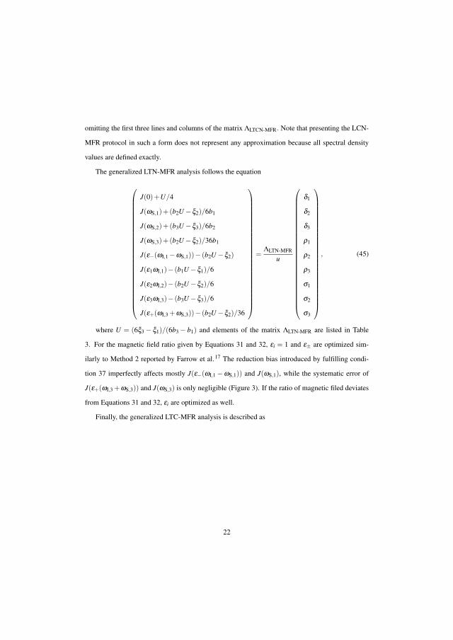
omitting the first three lines and columns of the matrix ΛLTCN-MFR. Note that presenting the LCN-

MFR protocol in such a form does not represent any approximation because all spectral density

values are defined exactly.

The generalized LTN-MFR analysis follows the equation

J(0)+U/4

J(ωS,1)+(b2U−ξ2)/6b1

J(ωS,2)+(b3U−ξ3)/6b2

J(ωS,3)+(b2U−ξ2)/36b1

J(ε−(ωI,1−ωS,1))− (b2U−ξ2)

J(ε1ωI,1)− (b1U−ξ1)/6

J(ε2ωI,2)− (b2U−ξ2)/6

J(ε3ωI,3)− (b3U−ξ3)/6

J(ε+(ωI,3 +ωS,3))− (b2U−ξ2)/36

=ΛLTN-MFR

u

δ1

δ2

δ3

ρ1

ρ2

ρ3

σ1

σ2

σ3

, (45)

where U = (6ξ3− ξ1)/(6b3− b1) and elements of the matrix ΛLTN-MFR are listed in Table

3. For the magnetic field ratio given by Equations 31 and 32, εi = 1 and ε± are optimized sim-

ilarly to Method 2 reported by Farrow et al.17 The reduction bias introduced by fulfilling condi-

tion 37 imperfectly affects mostly J(ε−(ωI,1−ωS,1)) and J(ωS,1), while the systematic error of

J(ε+(ωI,3 +ωS,3)) and J(ωS,3) is only negligible (Figure 3). If the ratio of magnetic filed deviates

from Equations 31 and 32, εi are optimized as well.

Finally, the generalized LTC-MFR analysis is described as

22

J(0)+V/4

J(ωS,1)−V/3

J(ωS,2)−V/3

J(ωS,3)−V/3

J(ε−(ωI,1−ωS,1))+(b1 +b2)V −ξ2

J(ε1ωI,1)−b1V/6+ξ1/6

J(ε2ωI,2)−b2V/6+ξ2/6

J(ε3ωI,3)−b3V/6+ξ3/6

J(ε+(ωI,3−ωS,3))+(6b3 +b2)V/36−ξ2/36

=ΛLTC-MFR

v

δ1

δ2

δ3

ρ1

ρ2

ρ3

µ1

µ2

µ3

, (46)

where V = (6ξ3 +ξ1)/(6b3 +6b2 +b1) and elements of the matrix ΛLTC-MFR are listed in Table 4.

Since the optimal ratio of magnetic fields is the same for LTC-MFR and LTN-MFR (Equations 31

and 32), εi and ε± have the same meaning as described for LTN-MFR. Only two spectral density

values, J(ε±(ωI,1±ωS,1)), are affected by the reduction bias, with a similar size of systematic

errors as in LTN-MFR (Figure 3).

Table 2: Elements of matrix ΛLTCN-MFR from Equation 44.

u2

0 0 −2b1−6b2 −3u2

36b2 +12b1 6b2 +2b13u2

−36b2−12b1 −6b2−2b13u2

−36b2−12b1

0u2

0 −6b3−2b2 0 12b2 +6b1 6b3 +2b2 0 −12b2−6b1 −6b3−2b2 0 −12b2−6b1

0 0u2

−2b3−b2 −u4

6b2 +12b3 2b3 +b2u4

−12b3−6b2 −2b3−b2 −u4

−12b3−6b2

0 0 012

0 −3 −12

0 312

0 3

0 0 0 −23

0 44b3

b10 −4 −2

30 −4

0 0 0 −23

0 423

u6b2

−4 −23

0 −4

0 0 0 −23

0 423

0 −2b1

3b3−2

30 −4

0 0 0 6b3 0 −6b1 −6b3 0 6b1 −6b3 +2b1 0 6b1

0 0 0 b2u4

−6b2 −b2 −u4

6b2 b2 −u4

6b2

0 0 0 b3 0 −b1 −b3 0 b1 b3 0 b1

0 0 0b2

6u

24−b2 −b2

6− u

24b2

b2

6u

24b2

0 0 0b3

60 −b1

6−b3

60

b1

6b3

60

12b3−b1

6

23

Table 3: Elements of matrix ΛLTN-MFR from Equation 45.

−12

0 3 0 0 0 0 −3 0

−4b2

3b1− u

3b1

8b2

b1

u6b1

0 0u

6b1−8b2

b10

−4b3

3b20

4b1

3b20

u6b2

0 0 −u+8b1

6b20

−2b2

9b3− u

18b3

4b2

3b30 0

u6b3

04b2

3b3− u

6b3

2b2u2

−12b2 0 0 0 −u2

12b2 0

2b3 0 −2b1 0 0 0 0 2b1 0

b2

3u

12−2b2 0 0 0 0 2b2 0

b3

30 −b1

30 0 0 0 2b3 0

b2

18u

72−b2

30 0 0 0

b2

3u

12

Table 4: Elements of matrix ΛLTC-MFR from Equation 46.

12

0 3 0 −3 0 0 3 0

−23

0 −4 0 4 0v

6b1−4 0

−23

0 −4 0 4 0 012b3 +2b1

3b20

−23

0 −4 0 4 0 0 −4v

6b3

2(b1 +b2) − v2

12(b1 +b2)v2

−12(b1 +b2) 0 − v2

12(b1 +b2) 0

2(b3 +b2) 0 −2b1 0 2b1 0 0 −2b1 0

−b2

3v

12−2b2 0 2b2 0 0 −2b2 0

−b3

30

b1 +6b2

30 2b3 0 0 −2b3 0

6b3 +b2

18− v

726b3 +b2

30 −6b3 +b2

3v

120

6b3 +b2

3− v

12

24

-20

-10

0

10

20

-20

-10

0

10

20

rela

tive e

rror

/ %

-20

-10

0

10

20

-2

-1

0

1

2

∆ R

ex / H

z

aJ(0) bJ(ωS,1) cJ(ωS,2)

dJ(ωS,3) eJ(ε-(ωI,1-ωS,1)) fJ(ε1ωI,1)

gJ(ε2ωI,2) hJ(ε3ωI,3) iJ(ε+(ωI,3+ωS,3))

jRex,1 kRex,2 lRex,3

0 1 2 3 0 1 2 3

τ / ns

0 1 2 3 4

Figure 3: Relative systematic errors of J(0) (a), J(ωS,1) (b), J(ωS,2) (c), J(ωS,3) (d), J(ε−(ωI,1−ωS,1)) (e), J(ε1ωI,1) (f), J(ε2ωI,2) (g), J(ε3ωI,3) (h), and J(ε+(ωI,3 + ωS,3)) (i) and systematicerrors of the exchange contribution Rex at B0,1 (j), B0,2 (k), and B0,3 (l) introduced by applyingMFR protocols at the optimal magnetic field ratio (3:4:5 for 13C-1H). Errors of LTN-MFR, LTC-MFR, and LCN-MFR are shown in red, green, and blue, respectively. The errors were calculatedfor a mono-exponential correlation function, and are plotted as a function of its correlation time.The errors were simulated for relaxation of 13C in an isolated isotropically moving C6-H6 pair inuracil21 at magnetic fields corresponding to spectrometers operating at the 300 MHz, 400 MHz,and 500 MHz 1H frequencies.

25

Propagation of random errors

Reliability of the obtained spectral density values depends not only on their accuracy but also on

the precision of their determination. In order to compare the relative precision of calculated J(ω)

values, propagation of random errors in the process of spectral density mapping was analyzed by

a Monte-Carlo simulation. The relaxation rates R1, R2, Γx, and NOE were simulated according to

Equations 16–19 with the standard deviation of 0.01 s−1, 0.1 s−1, 0.1 s−1, and 0.01 s, respectively,

for a mono-exponential correlation function with a correlation time of 10 ns, ideal combinations

of magnetic fields, and in the absence of the slow exchange. The J(ω) values calculated from the

relaxation data and their standard deviations are listed in Table 5. The simulations for the uracil

C6-H6 pair show that a low standard deviation of J(0), J(ωC,2), and J(ωC,3) was obtained for LTN-

MFR, while LTC-MFR and LCN-MFR provided a comparable precision for J(0) and J(ωC,3).

The most precise high-frequency value was J(ωH,2) calculated using LTN-MFR. In the case of

the N-H group of protein backbone, a high precision was achieved for J(0), and J(ωN,3) (i.e., for

the spectral density value calculated for the 15N frequency at the lower magnetic field). While

the presented data provides a general comparison, the actual experimental errors of individual

measurements should be taken into account when comparing precision achieved in a real case.

Graphical Interpretation

It is important not only to calculate the spectral density values but also to interpret them, which may

be less intuitive than in the case of correlation times and order parameters. Therefore, the picture of

molecular motions provided by spectral density values is briefly discussed in this section. Plots of

J(ω) values as a function of apparent J(0) were proposed earlier as a graphical output of spectral

density mapping allowing a straightforward interpretation.20,23,24 Considering typical precision of

the data, plotting the low-frequency spectral density values provides the most informative insight

into the molecular motions. Such type of graph is displayed in Figure 4 and referred to as Lefèver’s

plot in this paper.20,23

In order to illustrate interpretation of Lefèver’s plots, a simple model case will be discussed

26

Table 5: Values of spectral density function and their standard deviation simulated for anisotropic motion with the correlation time of 10 ns at magnetic fields corresponding to 500and 600 MHz (for a protein backbone amide 15N-1H pair) and to 300, 400, and 500 MHz (foruracil 13C-1H pair).

LCN-MFR LTN-MFR LTC-MFR LCN-MFR

J(ω) 15N-1H 13C-1H 13C-1H 13C-1H

J(0) 10.000± 0.137 10.000± 0.018 10.000± 0.016 10.000± 0.029

J(ωS,1) 0.640± 0.235 0.434± 0.074 0.426± 0.058 0.426± 0.073

J(ωS,2) not determined 0.244± 0.012 0.244± 0.025 0.244± 0.056

J(ωS,3) 0.897± 0.044 0.159± 0.010 0.158± 0.039 0.158± 0.010

J(ε−(ωI,1−ωS,1)) 0.006± 0.483 0.037± 0.128 0.063± 0.256 0.050± 0.126

J(ε1ωI,1) not determined 0.028± 0.022 0.028± 0.018 0.028± 0.107

J(ε2ωI,2) 0.009± 0.081 0.016± 0.021 0.016± 0.020 0.018± 0.021

J(ε3ωI,3) not determined 0.010± 0.004 0.010± 0.015 0.010± 0.018

J(ε+(ωI,3 +ωS,3)) 0.013± 0.014 0.006± 0.004 0.007± 0.029 0.006± 0.004

first. Let us assume that dynamics of each residue of a spherical macromolecule is given just

by three contributions: overall rotational diffusion, described by a monoexponential correlation

function with the correlation time τ0, completely uncoupled fast internal motion described by a

monoexponential correlation function with the correlation time τi, and slow exchange increasing

δi by a factor of 2ξi at the magnetic field B0,i. Interpretation of the Lefèver’s plot is based on a com-

parison of effects of the three contributions: (i) The limit case of a molecular motion completely

described as a rotational diffusion of a rigid spherical molecule corresponds to a single point in the

graph (blue circle in Figure 4) laying at a curve defined as J(ω) = J(0)/(1 +(ω(J(0))2)) (black

curve in Figure 4). This curve describes the relation between J(0) and J(ω) in a limit of a single

motional mode, described by a monoexponential correlation function. The blue point, common

to all residues, is determined by the value of the rotational-diffusion correlation time τ0. (ii) Fast

internal dynamics shifts the J(0),J(ωS) point (white circle) in the direction of the black arrow,

determined by the timescale of the internal motion. The position of the red circle corresponds

to a limit case of a completely unrestricted internal motion effectively separated from the overall

tumbling. The value of τ1 is defined as 1/(τ−10 + τ

−1i ). (iii) Presence of a slow internal motion

27

(on the µs–ms time scale) shifts the white point in the direction of the green arrow for LTN and

LTC, while LCN is indifferent to its effect. Note that while the Lefèver’s plots are identical for all

spectral density mapping protocols if no exchange contribution is present, effects of ξ dramatically

differ for individual approaches. The white point, identical in both panels of Figure 4, represents

the true, i.e., exchange-free, values of J(0) and J(ωS). These values are obtained if the LCN ap-

proaches are applied. The ξ contribution shifts the white point along a line with a slope of−4/3 in

plots of values obtained by LTC-SFR (Figure 4a) and LTC-MFR. Finally, ξ increases J(0) without

affecting J(ωS,i) in the case of LTN-SFR (Figure 4b) but shifts both J(0) and J(ωS,i) in a ratio

that depends on the relative contributions ξi weighted by constants bi in the case of LTN-MFR

(not shown in Figure 4). Comparison of the size and direction of the green arrows in individual

panels of Figure 4 shows why the LTC plots are better indicators of the slow exchange than a plot

of values obtained by LTN-SFR.

The determined spectral density values cannot be decomposed into exactly defined contribu-

tions of the individual motional modes without further assumptions. However, positions of the

points in Figure 4 indicate which type(s) of motional modes dominate(s). This information can be

converted to a coloring scheme, shown as a background of plots in Figure 4. The color-coding can

be used e.g. for coloring selected atoms in structural models according to their motional behavior.

Coloring based on the LTC plots is more reliable in the presence of a slow exchange for the reasons

discussed above.

The color gradient in Figure 4 is set by three points: the origin of the plot (red limit), the blue

point (blue limit), and the experimental value most affected by the slow exchange (green limit).

The estimate of the overall rotational correlation time τ0, defining the blue point, can be calculated

from the R2/R1 ratio.25 The δ values can be replaced by µ in order to eliminate the effect of

the conformational exchange. The overall rotational correlation time is then estimated by setting

J(ω) = τ0/(1 + ω2τ20 ) in Equations 16 and 19 and fitting τ0 to µ/ρ . If the overall tumbling is

anisotropic, but independent of the internal motions, the theoretical limit of a rigid motion is no

longer described by a correlation time τ0 identical for all residues. Instead, the effective τ0 value

28

is given as

τ0 =2

∑m=−2

cm/Em, (47)

where Em are eigenvalues of the rotation tensor and cm depend on the mutual orientations of

diffusion and interaction tensors and are thus different for individual residues.15 As a consequence,

the blue point deviates from the limit curve in Figure 4, unless the curvature is negligible within

the range of 1/Em values. The Em and cm values of sufficiently rigid molecules can be estimated

e.g. by fitting hydrodynamic simulations,26 27 to experimental τ0 calculated from the R1/R2 or

µ/ρ ratio, as described above. Lefèver’s plots of such molecules are then colored and analyzed

separately for each residue, with the position of the blue point given by τ0 and

J0(ω) =2

∑m=−2

cmEm/(E2m +ω

2). (48)

If the internal and overall motions are not separable, the limit of the overall tumbling looses its

physical meaning. However, it is still instructive (and needed to set the color range) to compare

the plotted J(0),J(ω) values to a reference "blue" point. Position of such a point can be based on

a theoretical τ0 value of a spherical particle of the same mass and specific volume as the studied

protein, of an ideal double-helix with the same number of residues as the studied nucleic acid, etc.

Suboptimal magnetic field ratio

Equations 31, 32, and 37 define what combination of magnetic fields provides spectral density

values free of any reduction bias. In practice, the choice of magnetic fields is also limited by

the availability of commercial magnets and by lower resolution of the low-field spectrometers.

For example, 13C relaxation data acquired at 400 MHz, 500 MHz, and 600 MHz spectrometers are

presented in this study. Such combination represents an easily accessible set of spectrometers with

fields close enough to the optimal ratio. Accuracy of the calculated J(ω) values is further improved

by optimizing εi and ε± in Equations 44, 45, and 46. Figure 5 shows the size of systematic errors

29

J(ω

S)

/ ns

(J(0)+ξ/4b) / ns

-0.2

-0.1

0.0

0.1

0.2

0.3

0.4

0.5

0.6

0.7

0 1 2 3τ0τ1

a

(J(ω

S)-

7ξ/

39b)

/ ns

(J(0)+7ξ/52b) / ns

b

-0.2

-0.1

0.0

0.1

0.2

0.3

0.4

0.5

0.6

0.7

0 1 2 3τ0τ1

Figure 4: Illustration of interpretation of experimental data (black dot) in the J(0)+ ξ/4b,J(ωS)(a) and J(0) + 7ξ/52b,J(ωS)− 7ξ/39b (b) plot, obtained by LTN-SFR and LTC-SFR, respec-tively. The white circle represents the J(0),J(ωS) point, the blue and red circles correspond tothe limits of the overall tumbling and of an internal motion defined by correlation times τ0 andτ1, respectively. The black arrow depicts the shift of the white point due to the internal flexibilityon the ps–ns time scale. The green arrow shows the shift due to the presence of slow motions,described by identical ξ in both panels. A color gradient from blue to red is used to distinguishrelative contribution of fast motions on the sub-nanosecond timescale, while green indicates slowdynamics on the µs–ms timescale.

30

of spectral density values calculated from Equations 44–45 for this combination of magnetic fields.

The systematic errors were simulated for an isolated 13C-1H pair and a single motional mode. A

negligible error (less than 4%) is obtained for J(0) and J(ωC,i) except J(ωC,2) calculated by LTN-

MFR. The systematic errors of spectral density values at εiωI,i obtained by all MFR protocols and

of J(ε+(ωI,3 +ωS,3)) obtained from LTC-MFR do not exceed 4% in this particular example.

Multiple interacting nuclei

The discussion of systematic errors introduced by various methods of reduced spectral density

mapping was so-far limited to isolated pairs of nuclei. Such a simple relaxation behavior can be

observed either if sample concentrations and dynamics allow to study relaxation at the natural

abundance, if the observed nuclei are isolated in the molecule (e.g., 15N in deuterated proteins and

nucleic acids), or if advanced techniques of selective isotope labeling are employed. The influence

of the surrounding spin-1/2 nuclei on the reduced spectral density mapping will be considered

in this section in order to discuss applicability of the proposed approaches to more accessible

uniformly labeled samples.

Dipole-dipole interactions with additional nuclei (K,L,. . . ) substantially expand the sets of

J(ω) values contributing to R1 and R2 rates of the observed I-S pairs because contributions of all

S-K, S-L, . . . dipole-dipole interactions (described by equations analogous to Equations 1 and 3)

add to the overall relaxation rates. The consequences of the presence of a nucleus K depend on its

magnetogyric ratio. If γK = γI, the effect of nucleus K can be accounted for exactly because J(ω)

is evaluated at the same frequencies. In this case, ζ 2IS in Equations 11–15 and in the definition of

b is replaced with a sum of ζ 2jS for all nuclei j with γ j = γI. If γK = γS, a new spectral density

value, J(2ωS), is introduced and R1 depends also on J(0). Nuclei with γK 6= γI 6= γS complicate the

definition of relaxation rates most severely as they introduce contributions of J(ω) at three new

frequencies, ωK and ωK±ωS. In such a case, the contributions J(ωS) and J(ωK±ωS) must be

neglected to keep the number of spectral density values unchanged. Taken together, Equations 17

and 16 can be modified to

31

-20

-10

0

10

20

-20

-10

0

10

20

rela

tive e

rror

/ %

-20

-10

0

10

20

-2

-1

0

1

2

∆ R

ex / H

z

aJ(0) bJ(ωS,1) cJ(ωS,2)

dJ(ωS,3) eJ(ε-(ωI,1-ωS,1)) fJ(ε1ωI,1)

gJ(ε2ωI,2) hJ(ε3ωI,3) iJ(ε+(ωI,3+ωS,3))

jRex,1 kRex,2 lRex,3

0 1 2 3 0 1 2 3

τ / ns

0 1 2 3 4

Figure 5: Relative systematic errors of J(0) (a), J(ωS,1) (b), J(ωS,2) (c), J(ωS,3) (d), J(ε−(ωI,1−ωS,1)) (e), J(ε1ωI,1) (f), J(ε2ωI,2) (g), J(ε3ωI,3) (h), and J(ε+(ωI,3 + ωS,3)) (i) and the exchangecontribution Rex at B0,1 (j), B0,2 (k), and B0,3 (l) introduced by applying MFR protocols at a sub-optimal magnetic field ratio (4:5:6 instead of 3:4:5). Errors of LTN-MFR, LTC-MFR, and LCN-MFR are shown in red, green, and blue, respectively. The errors were simulated at magnetic fieldscorresponding to spectrometers operating at the 400 MHz, 500 MHz, and 600 MHz 1H frequencies(see Figure 3 for details).

32

δ = 8bJ(0)+12aJ(ωS)+12J(ωI)+2ξ (49)

and

ρ = 2aJ(0)+6bJ(ωS)+2J(ωI−ωS)+12J(ωI +ωS), (50)

respectively, where a accounts for nuclei with the magnetogyric ratio equal to γS and the effects

of nuclei with the magnetogyric ratio different from γI and γS are taken into account in the constant

b only.

SFR and MFR protocols corrected for the presence of additional nuclei can be obtained by

applying the described modifications to Equations 21–28 and 44–45. The LCN-MFR protocol

is modified by replacing u in Equation 36 with u−5a. Modification of the LTC-MFR protocol is

achieved by replacing v with v−62a and adding the−a(µ1 +6µ3)/(v−62a) term to the right-hand

side of Equation 33. Such a modification obviously requires measurement of two additional rates,

µ1 and µ3. Fortunately, the relatively small term 12aJ(ωS) in Equation 49 can be safely neglected

when calculating J(0) and J(ωS). Then, the only modification of Equation 33 is a replacement

of v with v− 6a and measurement of µ1 and µ3 is not necessary. Modification of the LTN-MFR

approach is also straightforward, but the modified equations are relatively complicated and require

measurement of all relaxation rates at three magnetic fields. Similarly to LTC-MFR, the modified

LTN-MFR protocol simplifies dramatically if the 12aJ(ωS) term in Equation 49 is neglected. The

only modification is then a replacement of 8b1 with 8b1−6a and of 8b3 with 8b3−a in Equation

30.

The described modified spectral density mapping protocol relies on an assumption that con-

tributions of experimentally unaccessible J(ω) values can be neglected. While this is likely to be

true for calculating J(0) and J(ωS), the neglected contributions introduce large systematic errors

of the calculated high-frequency spectral density values (see simulated errors in Figure 6). As a

consequence, spectral density mapping should be strictly limited to zero- and low-frequency values

33

in the presence of additional spin-1/2 nuclei.

Multiple spectral density functions

Until now, the same spectral density function was used for all relaxation rates. Such simplification

is justified if all motions are isotropic and/or all interactions can be described by axially symmet-

ric second-rank tensors with collinear symmetry axes. If these conditions are not met, J(ω) in

Equations 16–19 must be replaced with individual spectral density functions JQ,Q′(ω), defined in

Equation 8. For an isolated pair of nuclei I and S, R1 and R2 depend on JIS,IS(ω) and JS,S(ω),

NOE depends on JIS,IS(ω), while the cross-correlated relaxations are given by JS,IS(ω). If both Γx

and Γz are measured, JS,IS(0) and JS,IS(ωS) can be determined easily for each magnetic field using

Equations 20 and 19. However, λ and µ cannot be combined with δ , ρ , and σ any more. The spec-

tral density mapping is thus limited to the LTN protocols. Moreover, δ , ρ , and σ depend on the

values of two spectral density functions, JIS,IS(ω) and JS,S(ω). Therefore, J(ω) in equations 16–

18 is replaced with JIS,IS(ω) for high-frequency terms and with J(ω) = (JIS(ω)+(b−1)JS(ω))/b

for zero- and low-frequency terms. As the J(ω) values are well suited for the Lefèver’s plots, spec-

tral density mapping describes molecular motions reliably if the J(ω) values are obtained from

experimental data and if the slow exchange contribution is evaluated separately.

If Method 2 is applicable, LTN-SFR yields J(0) and J(ωS) directly. LTN-MFR provides exact

values of J(0) and J(ωS,2), but JIS,IS(ωS,2) and JS,S(ωS,2) are combined in a different ratio than

JIS,IS(0) and JS,S(0). This drawback is overcome if R1 and R2 are measured at an additional

magnetic field B0,4 ≈ (1+ γS/γI)/B0,3, providing δ4. Equation 43 is then recast into

34

-20

-10

0

10

20

-20

-10

0

10

20

rela

tive e

rror

/ %

-20

-10

0

10

20

-2

-1

0

1

2

∆ R

ex / H

z

aJ(0) bJ(ωS,1) cJ(ωS,2)

dJ(ωS,3) eJ(ε-(ωI,1-ωS,1)) fJ(ε1ωI,1)

gJ(ε2ωI,2) hJ(ε3ωI,3) iJ(ε+(ωI,3+ωS,3))

jRex,1 kRex,2 lRex,3

0 1 2 3 0 1 2 3

τ / ns

0 1 2 3 4

Figure 6: Relative systematic errors of J(0) (a), J(ωS,1) (b), J(ωS,2) (c), J(ωS,3) (d), J(ε−(ωI,1−ωS,1)) (e), J(ε1ωI,1) (f), J(ε2ωI,2) (g), J(ε3ωI,3) (h), and J(ε+(ωI,3 + ωS,3)) (i) and the exchangecontribution Rex at B0,1 (j), B0,2 (k), and B0,3 (l) introduced by applying MFR protocols to 13C inan isotropically moving C6-H6 pair in fully labeled uracil.21 Errors of LTN-MFR, LTC-MFR, andLCN-MFR are shown in red, green, and blue, respectively. The errors were simulated for mag-netic fields corresponding to spectrometers operating at the 300 MHz, 400 MHz, and 500 MHz 1Hfrequencies (see Figure 3 for details). Errors of spectral density values calculated using completeEquations 49 and 50 are shown as solid curves, while dotted curves indicate a simplified treatmentwith the term 12aJ(ωS) neglected in Equation 49.

35

δ1

δ2

δ3

δ4

ρ2

ρ3

σ2

σ3

= N

JIS,IS(0)

JS,S(0)

J(ωS,2)

J(ωS,3)

J(ε1ωI,1)

J(ε2ωI,2)

J(ε3ωI,3)

J(ε4ωI,4)

, (51)

with the elements of matrix N given in Table 6. Solution of Equation 51 provides separated

values of JIS,IS(0) and JS,S(0).

JIS,IS(0) =(20−u)(6δ4−δ2−6σ3)

40(w−u)

− (20−w)(6δ3−δ1−6σ2)

40(w−u), (52)

JS,S(0) =12(6δ4−6δ3−δ2 +δ1−6σ3 +6σ2), (53)

where w = 24b4−4b2. Using JIS,IS(0) and JS,S(0), the value J(ωS,3) is calculated as

J(ωS,3) =4(b4−b2)(6δ3−δ1−6σ2)−u(δ4−δ2−σ3)

15b3(w−u)

+4(b2δ4−b4δ2)+(w−u)(ρ3−σ3)

6b3(w−u)(54)

with a systematic error less than 1 % (black curves in Figure 7).

The obtained J(ωS,3) can be plotted as a function of J(0) = (JIS,IS(0)+ (b3− 1)JS,S(0))/b3.

Such a plot is interpreted in a manner similar to Lefèver’s plots describing molecular motions char-

acterized by a single spectral density function. If the global and internal motions are independent,

36

Table 6: Elements of matrix N from Equation 51.

8 8(b1−1) 0 0 12 0 0 0

8 8(b2−1) 0 0 0 12 0 0

8 8(b3−1) 0 0 0 0 12 0

8 8(b4−1) 0 0 0 0 0 12

0 0 6b2 0 2 0 12 0

0 0 0 6b3 0 2 0 12

0 0 0 0 −2 0 12 0

0 0 0 0 0 −2 0 12

the rigid limit (blue point in Figure 4) is given by

τ0 =2

∑m=−2

cIS,ISm +(b3−1)cS,S

m

b3Em(55)

and

J0(ωS,3) =2

∑m=−2

cIS,ISm +(b3−1)cS,S

m

b3

Em

E2m +ω2

S,3, (56)

where cIS,ISm and cS,S

m are calculated from the orientation of the rotational diffusion tensor with

respect to the internuclear vector and to the chemical shielding tensor, respectively, and from Em. If

global and local motions are not separable, another reference point can be used, as described above.

In any case, position of the J(0),J(ωS,3) point indicates what motions dominate the dynamics, as

in the standard Lefèver’s plot.

The arguments presented in this section show that accurate spectral density mapping is possible

even if individual interactions contributing to relaxation cannot be described by the same spectral

density function. However, applicability of the MFR protocols is limited to LTN-MFR and requires

measurement at four different magnetic fields. It is therefore useful to test what anisotropy of

molecular motions can be tolerated in terms of accuracy of the LCN-MFR, LTC-MFR, and LTN-

MFR protocols described in previous sections.

The effect of a moderate motional anisotropy on 13C relaxation in C-H groups with asymmet-

37

ric chemical shielding of 13C was probed by simulating relaxation rates of uracil 13C6 in a rigid

RNA molecule undergoing an axially symmetric tumbling. The simulations were performed for an

isolated 13C6-1H6 pair at the optimal combination of magnetic fields. The results for a rotational

diffusion tensor with D‖/D⊥ = 1.35 showed that LTN-MFR provided very accurate J(0) (system-

atic error less than 2 %), while the highest systematic errors of J(ωC,2) and J(ωC,3) was low for

short correlation time, but gradually increased above 5 % for τ > 4 ns (solid red curves in Figure

7). On the other hand, LCN-MFR yielded accurate J(ωC,2) and J(ωC,3) but exhibited 6–12 %

maximum error of J(0) (solid blue curves in Figure 7). Finally, the highest systematic error was

acceptable for J(0) (below 5 %) but very large for other J(ω) values when LTC-MFR was applied

(solid green curves in Figure 7). Increasing the tumbling anisotropy to D‖/D⊥ = 2.0 resulted in

unacceptable systematic errors of almost all spectral density values (dashed curves in Figure 7).

The simulations show that LTN-MFR and LCN-MFR provide reasonable results for molecules

whose motions are dominated by an overall tumbling described by rotational diffusion tensor with

D‖/D⊥ < 4/3 at corelation time used. Considering the large effect of ξ on J(ωS,i), LTC-MFR

may still serve as a sensitive indicator of slow exchange. However, very inaccurate results should

be expected for molecules with D‖/D⊥ > 2.

Conclusions

Spectral density mapping allows to describe molecular motions without making assumption about

their nature. It is particularly useful when the model-free approach cannot be used, e.g. for dis-

ordered proteins and other flexible molecules. Lefèver’s plots convert the numerical values into a

pictorial form that is easy to interpret qualitatively by a visual inspection.

The proposed methods extend applicability of the spectral density mapping to cases that could

not be studied by the original protocol with sufficient accuracy. The SFR approaches are less de-

manding in terms of instrument requirement and experimental time. The original reduced spectral

density mapping protocol (LTN-SFR) is sufficiently accurate for 15N-1H groups but introduces a

substantial bias when applied to 13C-1H. This problem is most serious for short correlation times

38

-20

-10

0

10

20

-20

-10

0

10

20

rela

tive e

rror

/ %

-20

-10

0

10

20

-2

-1

0

1

2

∆ R

ex / H

z

aJ(0) bJ(ωS,1) cJ(ωS,2)

dJ(ωS,3) eJ(ε-(ωI,1-ωS,1)) fJ(ε1ωI,1)

gJ(ε2ωI,2) hJ(ε3ωI,3) iJ(ε+(ωI,3+ωS,3))

jRex,1 kRex,2 lRex,3

0 1 2 3 0 1 2 3

τ / ns

0 1 2 3 4

Figure 7: Relative systematic errors of J(0) (a), J(ωS,1) (b), J(ωS,2) (c), J(ωS,3) (d), J(ε−(ωI,1−ωS,1)) (e), J(ε1ωI,1) (f), J(ε2ωI,2) (g), J(ε3ωI,3) (h), and J(ε+(ωI,3 + ωS,3)) (i) and the exchangecontribution Rex at B0,1 (j), B0,2 (k), and B0,3 (l) introduced by applying MFR protocols to arigid molecule undergoing anisotropic rotational diffusion. Errors of LTN-MFR (red), LTC-MFR (green), and LCN-MFR (blue) were simulated for data obtained at 300 MHz, 400 MHz,and 500 MHz spectrometers (see Figure 3 for details), using J(ω) as a reference for zero- andlow-frequency values. The errors of J(0) and J(ωS,3) calculated from data obtained at 300 MHz,400 MHz, 500 MHz, and 600 MHz are displayed in black. Solid and dashed lines show the highestpositive and negative error (selected from all possible orientations of the C6-H6 bond), calculatedfor an axially symmetric rotational diffusion tensor with D‖/D⊥ = 1.35 and 2.00, respectively.

39

(i.e., for small or flexible molecules), when the systematic error is largest and methods based on

the assumption J(ω) ∝ 1/ω2 are not applicable. Moreover, the slow exchange has approximately

opposite effect on J(0) than fast local motions. Therefore, a moderate exchange contribution can

be misinterpreted as higher rigidity. The LTC-SFR approach reduces the bias and makes the pres-

ence of a slow exchange easier to spot. The LCN-SFR protocol is completely independent of the

slow exchange effects.

The combined analysis of relaxation rates acquired at well-chosen magnetic fields completely

eliminates systematic errors for isolated 15N-1H and 13C-1H pairs if a single spectral density func-

tion can be used. From the practical point of view, it is important that the MFR methods provide

reliable data even if the magnetic fields used and molecules studied do not strictly match the men-

tioned requirements. Systematic errors of some J(ω) values are negligible if the magnetic fields

deviate from the ideal ratio. Modified versions of the protocols provide very accurate zero- and

low-frequency spectral density values also for 13C with more spin-1/2 nuclei attached. Finally, re-

laxation rates can be analyzed even if they cannot be described by the same spectral density func-

tion: J(ω) values calculated by extended LTN-MFR provide a reliable picture of highly anisotropic

motions probed by 13C with asymmetric chemical shift tensors.

Acknowledgement

This work was supported by the projects "CEITEC - Central European Institute of Technology"

(grant number CZ.1.05/1.1.00/02.0068) from European Regional Development Fund and by the

Czech Science Foundation (grant number 203/09/H046) to P. K. The authors thank Jozef Kowalewski

and Göran Widmalm of University of Stockholm and Radovan Fiala of Masaryk University for

reading the manuscript.

References

(1) Lienin, S. F.; Bremi, T.; Brutscher, B.; Brüschweiler, R.; Ernst, R. R. 1998, 120, 9870–9879

40

(2) Meirovitch, E.; Shapiro, Y. E.; Polimeno, A.; Freed, J. H. Prog. Nucl. Magn. Reson. Spec-

trosc. 2010, 56, 360–405

(3) Wangsness, R. K.; Bloch, F. Phys. Rev. 1953, 89, 728–739

(4) Abragam, A. The Principles of nuclear magnetism; Clarendon Press: Oxford, 1961

(5) Redfield, A.G. Adv. Magn. Reson. 1965, 1, 1–32

(6) Cavanagh, J. Protein NMR spectroscopy: principles and practise; Academic Press: New

York, 1996

(7) Peng, J. W.; Wagner, G. J. Magn. Reson. 1992, 98, 308–332

(8) Peng, J. W.; Wagner, G. Biochemistry 1992, 31, 8571–8586

(9) Lipari, G.; Szabo, A. J. Am. Chem. Soc. 1982, 104, 4546–4559

(10) Lipari, G.; Szabo, A. J. Am. Chem. Soc. 1982, 104, 4559–4570

(11) Halle, B.; Andersson, T.; Forsén, S.; Lindman, B. J. Am. Chem. Soc. 1981, 103, 500–508

(12) Ishima, R.; Nagayama, K. J. Magn. Reson. Ser. B 1995, 108, 73–76

(13) Ishima, R.; Nagayama, K. Biochemistry 1995, 34, 3162–3171

(14) Hill, R. B.; Bracken, C.; DeGrado, W. F.; Palmer, A. G. J. Am. Chem. Soc. 2000, 122, 11610–

11619

(15) Korzhnev, D. M.; Billeter, M.; Arseniev, A. S.; Orekhov, V. Y. Prog. Nucl. Magn. Reson.

Spectrosc. 2001, 38, 197–266

(16) Halle, B. J. Chem. Phys. 2009, 131, 224507

(17) Farrow, N. A.; Zhang, O.; Szabo, A.; Torchia, D. A.; Kay, L. E. J. Biomol. NMR 1995, 6,

153–162

41

(18) Guenneugues, M.; Gilquin, B.; Wolff, N.; Menez, A.; Zinn-Justin, S. J. Biomol. NMR 1999,

14, 47–66

(19) Atkinson, R. A.; Lefevre, J. F. J. Biomol. NMR 1999, 13, 83–88

(20) Lefevre, J. F.; Dayie, K. T.; Peng, J. W.; Wagner, G. Biochemistry 1996, 35, 2674–2686

(21) Fiala, R.; Czernek, J.; Sklenár, V. J. Biomol. NMR 2000, 16, 291–302

(22) Pandey, M. K.; Vivekanandan, S.; Ahuja, S.; Pichumani, K.; Im, S.; Waskell, L.; Ramamoor-

thy, A. J. Phys. Chem. B 2012, 116, 7181–7189

(23) Barthe, P.; Chiche, L.; Declerck, N.; Delsuc, M. A.; Lefevre, J. F.; Malliavin, T.; Mispelter, J.;

Stern, M. H.; Lhoste, J. M.; Roumestand, C. J. Biomol. NMR 1999, 15, 271–288

(24) Krížová, H.; Žídek, L.; Stone, M. J.; Novotný, M. V.; Sklenár, V. J. Biomol. NMR 2004, 28,

369–384

(25) Kay, L. E.; Torchia, D. A.; Bax, A. Biochemistry 1989, 28, 8972–8979

(26) de la Torre, J. G.; Huertas, M. L.; Carrasco, B. J. Magn. Reson. 2000, 147, 138–146

(27) de la Torre, J. G.; Huertas, M. L.; Carrasco, B. Biophys. J. 2000, 78, 719–730

42

Paper 2

Accurate 13C and 15N spectral density mapping for

unbiased motional analysis of disordered proteins,

nucleic acids, and carbohydrates: Case studies

Pavel Kaderávek,†,@ Vojtech Zapletal,† Radovan Fiala,† Mária Šoltésová,¶ Jozef

Kowalewski,§ Göran Widmalm,‖ Josef Chmelík,⊥,4 Alžbeta Rabatinová,⊥ Libor

Krásný,⊥ Vladimír Sklenár,† and Lukáš Žídek∗,†

National Centre for Biomolecular Research, Faculty of Science and Central European Institute of

Technology, Masaryk University, Kamenice 5, 625 00 Brno, Czech Republic, Institute of

Biophysics of Academy of Sciences of the Czech Republic, Královopolská 135, 612 65 Brno,

Czech Republic, Faculty of Mathematics and Physics, Charles University, V Holešovickách 2,

180 00 Prague, Czech Republic, Department of Materials and Environmental Chemistry,

Stockholm University, S-106 91 Stockholm, Sweden, Department of Organic Chemistry,

Stockholm University, S-106 91 Stockholm, Sweden, Institute of Microbiology, Academy of

Sciences of the Czech Republic, Vídenská 1083, 142 00 Prague 4 - Krc, Czech Republic, and

Department of Biochemistry, Faculty of Sciences, Charles University, Hlavova 8, 128 40 Prague

2, Czech Republic

E-mail: lzidek@chemi.muni.cz

1

Abstract

Molecular motions of three different molecules were analyzed by a novel methodology of

spectral density mapping. The examined samples included a partially disordered protein, a

uniformly 13C,15N-labeled RNA hairpin, and a β -(1→6) linked disaccharide with a selectively

13C labeled bridging methylene group. Results showed that the proposed protocols clearly

separate slow exchange from fast dynamics and provide unbiased description of molecular

motions in cases when the frequently used model-free approach or the original reduced spectral

density mapping cannot be applied.

Keywords: Nuclear magnetic resonance, relaxation, spectral density function, intrinsically

disordered proteins, nucleic acids, carbohydrates

∗To whom correspondence should be addressed†Masaryk University‡Institute of Biophysics¶Charles University§Dept. of Materials and Environmental Chemistry, Stockholm University‖Dept. of Organic Chemistry, Stockholm University⊥Institute of Microbiology#Charles University

@Institute of Biophysics4Charles University

2

Introduction

Relaxation rates observed in nuclear magnetic resonance (NMR) experiments serve as a source

of information on molecular motions occuring on a time scale from 10−12 to 103 s. The Spectral

density mapping represents one of several approaches to the analysis of the relaxation data. It is

based on the fact that the relaxation rates are expressed as linear combinations of discrete values

of the spectral density function J(ω). This approach does not rely on definition of the number of

motional modes, assumption of their independence, or description of their coupling. Therefore,

spectral density mapping is well suited for studies of disordered proteins and other molecules

whose dynamics is impossible to decompose into independent contributions and whose structure

is difficult to describe by atomistic models. The most often examined relaxation rates are those of

15N nuclei in a protein backbone taking advantage of the favourable physical properties of amide

15N. The 15N chemical shift tensor is approximately symmetric and its symmetry axis is almost

collinear with the N-H bond, which allows to describe effects of both chemical shift anisotropy

and dipole-dipole interactions (and their cross-correlations) by the same spectral density function.

Moreover, 13C nuclei do not contribute to the relaxation of backbone amide 15N in uniformly 15N-

labeled protein. As a consequence, all relaxation rates of the 15N-1H group depend on the values

of the spectral density function at five eigenfrequencies (zero frequency, resonance frequencies of

both nuclei, and their sum and difference), three of which are very similar and can be approximated

with a single effective frequency. Therefore, three spectral density values, calculated from three

relaxation rates, are sufficient to describe the N-H dynamics reliably. This approach, known as

reduced spectral density mapping, allows to reduce the number of motional parameters (spectral

density values) to the number of experimentally available relaxation rates (three in this case).

The preceding paper1 introduced several methods that extend applicability of spectral density

mapping to 13C nuclei, both in selectively and uniformly labeled molecules. The 13C-1H group,

especially in aromatic moieties, represents a challenging system for spectral density mapping. In

aromatic systems, the 13C chemical shift tensor is highly asymmetric and the effects of chemical

shift anisotropy and dipole-dipole interactions depend on different spectral density functions, un-

3

less the molecular motions are isotropic. Moreover, uniformly 13C labeled molecules often have

several spin-1/2 nuclei attached to the observed 13C nucleus, in contrast to the uniform 15N label-

ing, when isolated 15N-1H pairs occur. Another level of complexity, common to both 15N and 13C,

is introduced if a slow exchange on the µs-ms time scale contributes to the relaxation.

The protocols presented in the accompanying paper1 were designed to address the issues listed

in the previous paragraph. These methods use various relaxation rates, abbreviated L for longitudi-

nal relaxation rate R1, T for transverse relaxation rate R2, C for transverse cross-relaxation rate Γx,

and N for the steady-state hetero-nuclear Overhauser effect (NOE). Among them, only R2 is influ-

enced by the slow exchange. Analyses of different combinations of relaxation rates thus provide

J(ω) values affected by exchange contributions in different ways. In the proposed method this has

been exploited to separate the effects of slow exchange from the fast dynamics.

In addition to the approaches based on relaxation data acquired at a single magnetic field (sin-

gle field reduction, SFR), approaches combining data obtained at various spectrometers (multiple

field reduction, MFR) were introduced. The SFR protocols rely on the assumption that the reso-

nance frequency of nucleus I, ωI, is much greater than the resonance frequency of nucleus S, ωS, in

a heteronuclear pair S-I. Therefore, three spectral density values J(ωI−ωS)≈ J(ωI)≈ J(ωI +ωS)

are replaced with a single value J(εωI). Only three different relaxation rates then need to be mea-

sured in order to obtain three spectral density values, J(0), J(ωS), J(εωI). On the other hand,

the MFR approaches utilize relaxation rates measured at several magnetic fields chosen so that

certain eigenfrequencies match different eigenfrequencies at another magnetic field. As a conse-

quence, the number of parameters is reduced without a need of any approximations. Therefore,

MFR protocols represent an inherently exact method of J(ω) reduction.

Simulations presented in the previous paper1 show that the novel spectral density mapping

protocols should provide an unbiased picture of molecular motions even if the original approach

fails. The aim of this article is to test the proposed methodology experimentally. In order to doc-

ument its practical applicability, relaxation data of three different molecules were analyzed. The

tested samples include (i) uniformly 15N-labeled delta subunit of RNA polymerase from Bacillus

4

subtilis, a protein consisting of a well folded N-terminal domain and an 81 amino-acid long intrin-

sically disordered C-terminal region, (ii) uniformly 13C,15N-labeled pppGGCACUUCGGUGCC,

an RNA hairpin containing the UUCG tetraloop, and (iii) methyl β -D-glucopyranosyl-(1→6)-α-D-

[6-13C]-mannopyranoside, a β -(1→6) linked disaccharide with a selectively 13C labeled bridging

methylene group.

Experimental Methods

Sample preparation

δ subunit of RNA polymerase

The rpoE gene encoding the δ subunit of RNA polymerase from Bacillus subtilis was cloned into

the pET22b vector. The Escherichia coli BL21(DE3) strain was transformed with the obtained

plasmid and the protein was expressed in two liters of the M9 medium containing [15N] ammonium

chloride as a sole source of nitrogen. The obtained protein was purified as described by Motácková

et al.2 A 0.8mM δ subunit sample was prepared in 20mM phosphate buffer, pH∗ 6.6 (uncorrected

reading) containing 10mM sodium chloride, 10 % deuterium oxide, and 0.05 % sodium azide.

UUCG haiprin

Fully 13C- and 15N-labeled sample of RNA oligomer pppGGCACUUCGGUGCC was synthesized

in-vitro from 13C and 15N-labeled NTPs. T7 RNA polymerase was used for the transcription from

a DNA template. The synthesized oligomer was purified by a gel electrophoresis.3,4 A 3.0mM

oligomer sample was prepared in 99.95% D2O at pH∗ 6.7 (uncorrected reading). The sample con-

tained 0.2mM EDTA and 10 mM sodium phosphate buffer. A small amount of sodium azide was

added to the sample. A detailed description of the sample preparation was published elsewhere.5

5

β -D-Glcp-(1→6)-α-D-Manp-OMe

The sample was prepared by dissolving 9.5 mg of freeze-dried methyl β -D-glucopyranosyl-(1→6)-

α-D-[6-13C]-mannopyranoside6 in 367 µl DMSO-d6 (99.96 % 2H, Euriso-Top) and 204 µl D2O

(99.96 % 2H, Aldrich). The solution in a 4 mm NMR tube was degassed by three cycles of freezing,

application of a mild vacuum, and melting. Then the evacuated NMR tube was heat-sealed.

NMR experiments

The following NMR spectrometers and probeheads were used: 400MHz Varian-unity with a dou-

ble resonance (1H, 13C) room-temperature probe, 500MHz and 600MHz Varian Unity with triple

resonance (1H, 13C, 15N) room-temperature probes, 300 MHz Bruker Avance III with a room-

temperature BBO-F probe, 400 MHz Bruker Avance III with a room-temperature BBI probe,

500 MHz Bruker Avance III with a cryogenic Prodigy BBO probe, 600 MHz Bruker Avance III

with TCI cryogenic probe, 700 MHz Bruker Avance III with a room-temperature TXI probe, and

950 MHz Bruker Avance III with TCI cryogenic probe. The temperature was calibrated based on

the chemical shift differences of pure methanol peaks. Delays of the polarization transfer periods

in protein backbone and nucleic acid bases were set for 90 Hz 15N-1H and 200 Hz 13C-1H scalar

couplings, respectively. The program NMRPIPE 7 was used to process the data. One-dimensional

spectra were processed by applying 10 Hz line broadening, four-fold zero filling, Fourier transform,

adjusting phase to obtain pure absorption lineshape, and using a zero-order polynomial function to

correct the baseline. Two-dimensional data were processed with the cosine square apodization and

four-fold zero filling. The phase in the direct dimension was manually adjusted to pure absorp-

tion. The spectra were analyzed and the peak heights were evaluated in the program SPARKY.8

The resonances were assigned according to the literature.9,10 Relaxation rates measured by vary-

ing relaxation delays were obtained by fitting peak intensities to a mono-exponential decay using

programs RELAX 11,12 (for 15N R1 and R2) and OCTAVE 13 (for other rates).

6

δ subunit of RNA polymerase

The measurements were performed at the 500 MHz and 600 MHz Bruker spectrometers at the tem-

perature of 300.2 K. Standard experiments14 were used for the measurements of R1, with relaxation

delays of 22.4, 67.2, 134.4*, 246.4, 380.8, 560*, 784, 1008, and 1232 ms at both 500 MHz and

600 MHz spectrometers, and of R2, with relaxation delays of 0, 17.283, 34.566*, 51.850, 69.133,

86.416*, 103.699, 138.266, and 172.832 ms at 500 MHz and of 0, 17.181, 34.362*, 51.542, 68.723,

85.904*, 103.085, 137.446, 171.808 ms at 600 MHz. The asterisk denotes the spectra recorded

twice in order to estimate the experimental error. The R2 rates were measured at CPMG frequen-

cies of 462.9 and 465.6 Hz at 500 MHz and 600 MHz spectrometers, respectively. A relaxation

compensated CPMG experiment15 with CPMG frequency ranging from 50 to 1000 Hz was used to

qualitatively verify the presence of slow exchange. For the sake of sensitivity, the CPMG data was

acquired at the 600 MHz spectrometer equipped with a cryogenic probe and the exchange contri-

bution at 500 MHz were assumed to be proportional to the square of the magnetic field ratio. The

15N-1H steady-state nuclear Overhauser effect (NOE)16 was measured with a 20 s inter-scan re-

laxation delay and 226 repeats of 200 µs 180 1H pulses separated by 22.22 ms delay were used to

achieve a steady state. The reference spectra were measured interleaved together with the spectra

under the steady state conditions. The experimental error was evaluated based on three inde-

pendent measurements. The transverse cross-correlated relaxation rates Γx were measured using

IPAP-HSQC17,18 with relaxation delays of 11.1, 22.2, 44.4, 66.6†, 88.8, and 111.1 ms at 500 MHz

and 44.4, 88.8, and 111.1 ms at 600 MHz, where the dagger denotes the spectra recorded three

times. The in-phase and anti-phase spectra were combined in a ratio optimized for each residue

to obtain a pure up-field and down-field component of the doublet. The value of Γx was obtained

by fitting the ratio of heights of the up-field and down-field peaks to the mono-exponential decay.

Standard deviation of the peak intensities was estimated from the noise using Monte-Carlo sim-

ulations. The measured experimental data were deposited in the Biological Magnetic Resonance

Data Bank (http://www.bmrb.wisc.edu) as entry 18903.

7

UUCG hairpin

NMR experiments were carried out at the 400MHz, 500MHz and 600MHz Varian spectrometers

at the temperature of 298.2 K. The published19 NMR pulse programs were used for the measure-

ments of the R1 and R1ρ relaxation rates with the R1 relaxation delays of 5, 30*, 60, 100, 145,

200, 280*, and 420 ms at 400 MHz; 5, 35, 65, 100, 135, 175, 220, 275, 335, 410, 585, and 835 ms

at 500 MHz; 5, 25*, 50, 80, 110, 150, 205, 265, 350, and 495 ms at 600 MHz and with the R1ρ

relaxation delays of 3, 9*, 21, 33, 48, 66, 93*, and 138 ms at 400 MHz; 3, 9, 15, 24, 33, 48, 63, 81,

108, and 150 ms at 500 MHz; 3, 9*, 15, 24, 33, 48, 63, 81, 108*, and 150 ms at 600 MHz. The as-

terisk denotes the spectra recorded twice. The R2 relaxation rate was calculated from the measured

R1 and R1ρ rates as R2 = (∆ν20 + ν2

1 )R1ρ/ν21 −∆ν2

0 R1/ν21 , where ∆ν0 is the difference between a

particular spin resonance frequency and spin lock carrier frequency and ν1 is the spin lock field

strength, determined based on the linearity of the power amplifier and verified by calibration. The

field strengths of the spin lock were 2783.96, 1964.06, and 4807.70 Hz at 400 MHz, 500 MHz, and

600 MHz spectrometers, respectively. The 13C-1H steady-state NOE19 at 500 MHz was measured

twice to test the effect of various length of the relaxation period (3.5 and 5.0s) and 1H irradiation

length (3.0 and 1.5s) used to achieve a steady state. Both experiments provided values which did

not differ significantly. NOE at 400 MHz and 600 MHz was measured with 3.0 s relaxation period

and 3.0 s 1H irradiation period to achieve a steady state. The reference spectra were measured

interleaved together with the spectra under the steady state conditions. The transverse cross relax-

ation rate Γx was measured using constant time HSQC coupled in the indirect dimension20 with

the constant time evolution delay T = 30 ms, and evaluated as (ln(I1/I2))/2T , where I1 and I2 are

the intensities of the coupled peaks. The error of transverse cross relaxation rate was determined

from the comparison of results of measurements with T = 30 ms and 15 ms, and errors of the other

measurements were recalculated based on the experimental noise. The measured experimental data

were deposited in the Biological Magnetic Resonance Data Bank (http://www.bmrb.wisc.edu) as

entry 18616.

8

β -D-Glcp-(1→6)-α-D-Manp-OMe

The NMR experiments were carried out at the 300 MHz, 400 MHz, 500 MHz, 600 MHz, 700 MHz,

and 950 MHz Bruker spectrometers at 293.2 K. The 1 s recycle delay was used in all experiments

except the heteronuclear NOE measurement, run with a 2 s recycle delay. The broadband proton

decoupling was achieved by a WALTZ-16 scheme with a 80µs length of the 90 pulse. Carbon

carrier frequency was placed on-resonance to the observed signal, the spectral width of 60 ppm and

1 s acquisition time was used in all experiments. The longitudinal relaxation rate of 13C was mea-

sured using the inversion recovery experiment with 1, 5, 10∗, 20, 30, 50, 80∗, 140, 220, 350∗, 500,

and 650 ms delays. The transverse relaxation rate was measured using R1ρ experiment at a spin-

lock frequency of 1 kHz (300 MHz, 400 MHz, 500 MHz, and 600 MHz) or 2 kHz (700 MHz and

950 MHz) and with the following relaxation delays: 1∗, 5, 10∗, 20, 35, 50, 70∗, 100, 140, 200∗, and

300 ms (asterisk denotes spectra recorded twice). The R1ρ experiment was repeated at 600 MHz

with the spin-lock field strength up to 2 kHz to check for possible slow exchange contribution. The

longitudinal and transverse cross-relaxation rates were measured without decoupling as described

earlier.21 The inversion recovery for determination of longitudinal cross-correlated relaxation was

measured with relaxation delays of 1∗, 5∗, 10, 15∗, 20, 25∗, 30, 35∗, 40, 45∗, 50, 55∗, 60, 70, 80, 90,

1000∗, 1500∗, and 2000∗ms. The coupled R1ρ experiment, used for the determination of the trans-

verse cross-correlated relaxation rate, was performed with a 1 kHz (300 MHz, 400 MHz, 500 MHz,

and 600 MHz) or 2 kHz (700 MHz and 950 MHz) spin-lock field applied for 1, 5∗, 10, 15∗, 20, 25,

30∗, 35, 40, 45∗, 50, 55∗, 60, 70, 80, 90 ms (asterisk denotes spectra recorded twice). The re-

laxation rates of left (R−), right (R+) and middle (R0) lines of the triplet in coupled spectra were

evaluated and the longitudinal and transverse cross-correlated relaxation rates Γi = (R−−R+)/2

and Ξi = ((R−+ R+)/2−R0)/2 were determined21 from data obtained with (i = x) and without

(i = z) applying the spin-lock field. The 13C-1H heteronuclear Overhauser enhancement was cal-

culated from the ratio of intensities in reference and saturated spectra measured by the dynamic

NOE technique.22 The dynamic NOE experiment was repeated five times and other experiments

three times to determine the experimental errors.

9

Analysis of relaxation rates

The measured auto-relaxation rates R1 and R2, nuclear Overhauser enhancement defined as a ratio

of peak intensities in the steady-state (Iss) and reference (Iref) spectra, and cross-correlated relax-

ation rates Ξz, Ξx, Γz, and Γx were assumed to be given by the following linear combinations of

spectral density functions:

R1 = ζ2IS(2aJLS,LS(0)+6bJ(ωS)+2J′(ωI−ωS)+12J′(ωI +ωS)

), (1)

R2 =12

R1 +Rex +ζ2IS(4bJ(0)+6aJLS,LS(ωS)+6J′(ωI)

), (2)

Iss/Iref = 1+γI

γS

ζ 2IS

R1

(−2J′(ωI−ωS)+12J′(ωI +ωS)

), (3)

Γz = 12ζISζSJΓ(ωS), (4)

Γx = ζISζS(8JΓ(0)+6JΓ(ωS)

), (5)

Ξz = 12ζISζKSJIS,KS(ωS), (6)

Ξx = ζISζKS(8JIS,KS(0)+6JIS,KS(ωS)

), (7)

where S is the observed nucleus, I is the directly attached proton, K is the second directly

attached proton in the disaccharide CH2 group and H5 in pyrimidine bases, L is C5 in pyrim-

idines and N7 in purines, M (see below) is N1 in pyrimidines and N9 in purines, contributions

of dipole-dipole interactions between nuclei I,S and of chemical shift anisotropy of nucleus S

are marked by symbols IS and S, respectively, a = 0 with the exception of pyrimidines, where

a = ζ 2LS/ζ 2

IS, b = 1 + ζ 2S/ζ 2

IS for 15N protein backbone relaxation, b = 1 + (ζ 2S + ζ 2

KS)/ζ 2IS for

13C relaxation in the CH2 group of the disaccharide, b = 1 +(ζ 2S + ζ 2

KS + ζ 2LS + ζ 2

MS)/ζ 2IS for 13C

relaxation in the CH group of nucleic acid bases, Rex is the slow exchange contribution, γI and

γS are the magnetogyric ratios of nuclei I and S, respectively, ζIS = µ0hγIγS/(16π2r3IS

√5), ζS =

(1+η2S/3)1/2γSB0∆S/(3

√5), rIS is the I-S internuclear distance, µ0 is the permeability of vacuum,

h is the Planck’s constant, ∆S and ηS are anisotropy and asymmetry of the chemical shift tensor,

10

respectively, constants ζKS, ζLS, ζMS are defined by replacing I with K, L, and M, respectively, in

the definition of ζIS, JΓ(ω) = JIS,S(ω) for NH and CH groups, JΓ(ω) = (JIS,S(ω)+ JKS,S(ω))/2

for CH2 groups, J′(ω) = JIS,IS(ω) for 15N protein backbone relaxation and for 13C8 relaxation

in purines, J′(ω) = JIS,IS(ω)+ ζ 2KSJKS,KS(ω)/ζ 2

IS for 13C6 relaxation in uracil, cytosine and the

mannopyranosyl moiety of the disaccharide, J(ω) = (J′(ω)+ ζ 2S JS,S(ω)/ζ 2

IS)/b for 15N protein

backbone relaxation and 13C relaxation in the disaccharide, and J(ω) = (J′(ω) + (ζ 2S JS,S(ω) +

ζ 2LSJLS,LS +ζ 2

MSJMS,MS)/ζ 2IS)/b for the 13C relaxation in nucleic acid bases. Internuclear distances

and chemical shift tensors were taken from the literature.23,24

The same definition of spectral density functions as in the preceding paper1 was used. Spec-

tral density values for individual eigenfrequencies were calculated by solving Equations 1–7 using

protocols described in the preceding article.1 Differences between spectral density functions de-

scribing individual contributions to the relaxation were treated in various manners, depending on

the molecule studied: A single spectral density function J(ω) was used in Equations 1–5 when

the interactions contributing to the relaxation were assumed to be described by collinear vectors

(analysis of the RNA polymerase δ subunit, Case Study I) and when the molecule was assumed to

move isotropically (analysis of the UUCG hairpin, Case Study II). When the differences between

individual spectral density functions could not be neglected, Equations 1–3, 4–5, and 6–7 were

solved separately (β -D-Glcp-(1→6)-α-D-Manp-OMe, Case Study III). Plots of J(ω) values as a

function of apparent J(0), referred to as Lefèver’s plot in this paper,25,26 were used to interpret the

obtained spectral density values.

Results and Discussion

Case study I: δ subunit of RNA polymerase

The goal of the first case study was to test performance of the spectral density mapping protocols

applied to protein 15N relaxation data. The selected protein molecule, δ subunit of RNA poly-

merase from Bacillus subtilis, consists of two distinct regions of similar size, N-terminal domain

11

forming a well-defined structure and a long disordered C-terminal tail.27 This composition makes

the δ subunit a good model system that allowed us to study relaxation of well-structured and in-

trinsically disordered protein residues within one molecule. Results of detailed investigation of

the δ subunit, performed recently in our laboratory, provided the necessary background for the

relaxation analysis in a structural context. Structure of the well-folded N-terminal domain has

been determined using NMR.2 Assignment of the disordered and highly repetitive C-terminal tail9

made residue-specific relaxation studies of this region possible.

The 15N nucleus in the backbone amide moiety was employed in the first case study as a

motional probe most typical for proteins. The used uniform 15N labeling simplified the analysis as

the N-H group could be treated as an isolated spin pair.

The 15N R1, R2, transverse cross relaxation rate Γx, and steady-state 15N-1H NOE were mea-

sured at two magnetic fields, corresponding to 500 MHz and 600 MHz proton frequencies. This

combination of spectrometers allowed us to apply all SFR approaches (at two fields), and LCN-

MFR at an almost ideal magnetic field ratio. The zero- and low-frequency spectral density values

obtained by the SFR analysis are presented in Figure 1. The J(ω) values of residues from the

ordered and disordered domain are clearly separated into two clusters, distinguished by colors in

Figure 1. The blue cluster at high J(0) reflects a major contribution of the overall rotational dif-

fusion to the motions of the well-ordered N-terminal domain, while the red cluster at low J(0)

indicates that the dynamics of the disordered C-terminal region is much faster and independent of

the overall tumbling.

When interpreting the obtained spectral density values, we first focused on residues of the N-

terminal domain, representing the routinely studied case of well-folded proteins. As shown by

simulations,1 the 15N reduction bias is small for correlation times longer than 1 ns. Also, the error

introduced by assuming that the same spectral density function describes dipolar and CSA relax-

ation (including the cross-correlated relaxation described by Equation 5) is small for backbone

amide 15N in proteins,1 as its chemical shielding tensor is almost axially symmetric, with the sym-

metry axis close to the direction of the N-H bond.14 Therefore, the SFR methods are sufficiently

12

accurate to analyze relaxation rates of amides from the structured part of the molecule, dominated

by the overall tumbling. The only significant source of a bias of the calculated spectral density val-

ues is the contribution of the slow exchange. A visual inspection of the LTN-SFR plots (Figure 1a)

revealed three residues (V 17, K 28, and N 63) significantly influenced by a slow exchange. Inter-

estingly, the LTC-SFR data (Figure 1b), which is much more sensitive to the exchange, exhibited

clear contributions of slow exchange for most residues of the N-terminal domain. An independent

CPMG relaxation dispersion experiment15 also indicated slow exchange for additional residues,

but the sensitivity did not allow a quantitative comparison (data not shown). Finally, the LCN-SFR

data served as a source of spectral density values free of any exchange contribution and allowed

us to evaluate the exchange contributions to both LTN-SFR and LTC-SFR data. Without this com-

parison, the J(0) values elevated by the exchange contribution in the LTN-SFR analysis could be

misinterpreted as a higher rigidity of the corresponding residues. It documents that extending the

standard analysis of R1, R2, and NOE to the cross-correlated relaxation rate Γx improves reliability

of reduced spectral density mapping, as it allows one to clearly distinguish effects of slow motions

from fast dynamics.

After analysing relaxation data of the N-terminal domain, we turned our attention to the dis-

ordered C-terminal region of the δ subunit. There are several reasons why the relaxation data of

disordered residues should be analyzed more carefully. First, in contrast to the rigid amino acids

with dynamics dominated by a relatively slow overall tumbling, relaxation of flexible residues is

much more influenced by motions with shorter correlation times. As a consequence, the reduction

bias is higher.1 Second, it is difficult to estimate what systematic error is introduced by neglecting

the difference between J(ω) and JΓ(ω) because motions of flexible residues cannot be described

in terms of elements of the overall rotational diffusion tensor and its orientation with respect to

the individual amide groups. Finally, the spectral density values of flexible residues are lower than

those of the rigid ones. Higher sensitivity, generally achieved for disordered residues, allows us to

evaluate small differences of spectral density values with a good precision, but systematic errors

safely neglected in the analysis of ordered proteins may become significant.

13

The relatively large difference between 1H and 15N resonance frequencies permits to greatly

suppress the reduction bias by applying a procedure described as Method 3 by Farrow et al.28

during the LTN-SFR and LCN-SFR analysis. The protocol is based on the assumption that the

spectral density function is linear between 0.87ωH,3 and 0.96ωH,1 (in order to keep the notation

consistent in this paper, all values relevant for the 15N data recorded at the 500 MHz and 600 MHz

spectrometers are distinguished by subscripts 3 and 1, respectively). The slope of the spectral

density function in this interval is estimated by comparing steady-state NOE measured at two

magnetic fields. The high-frequency spectral density values are then evaluated at optimized values

of frequency εωH, when they cancel out almost completely in linear combinations used in the

spectral density mapping. Simulation showed that spectral density values are obtained with a

reduction bias lower than 1.6 % for 500 MHz and 600 MHz spectrometers.

The error introduced by neglecting the difference J(ω) and JΓ(ω) complicates estimation of the

exchange contribution by comparing outputs of individual SFR protocols. While both LTN-SFR

and LCN-SFR provide correct J(ωN) and JIS,IS(εωH), LTN-SFR and LCN-SFR yields J(0) biased

by ξ/4b and α/4b, respectively, where ξ = Rex/ζ 2HN and α = 4b(JΓ(0)− J(0))+ 3b(JΓ(ωN)−

J(ωN)). In order to assess the effect of α , its values were calculated for anisotropic motions

simulated by a rotational diffusion tensor with D‖/D⊥ = 2. The values of α calculated for the

most sensitive orientations were between −0.68 ns and +0.53 ns for a correlation time of 2 ns at

the 500 MHz spectrometer and between −0.60 ns and +0.46 ns at the 600 MHz spectrometer.

Finally, J(εωH) rather than JIS,IS(εωH) should be presented as a function of J(0) in the Lefèver’s

plot. The introduced error was within a range of ±4 % for both fields in the simulation.

The experimental spectral density values calculated by applying the LCN-SFR and LTN-SFR

protocols (with the correction of the reduction bias, described above) are presented in Figure 2a,d

and in Figure 2b,e respectively. The high-frequency JIS,IS(εωH) value, determined with a suffi-

cient precision for the disordered residues, helped to discriminate contributions of sub-nanosecond

motions (Figure 2c,f).

The obtained picture of molecular motions of the C-terminal domain of the δ subunit is in a

14

good agreement with its disordered nature. The most flexible residue is C-terminal K 173, with dy-

namics limited to sub-nanosecond motions, followed by somewhat slower Y 165 and D 167. The

trend continues with a cluster of residues 153–159 exhibiting a very similar motional behavior.

The residues further from the C-terminus vary more in their dynamics. Contributions of motions

on the microsecond-to-millisecond timescale can be estimated by comparing the LTN-SFR and

LCN-SFR J(0) values. The values in Figure 2b,e are shifted from those in Figure 2a,d by a factor

of ξ −α . The ξ and α contributions cannot be separated directly, but sufficiently large and always

positive ξ may be distinguished from variations due to the relatively small factor α . In order to test

what values of Rex result in ξ > |α|, the shifts between data plotted in Figure 2a and 2b were com-

pared to results of the CPMG experiment, discussed above (Figure 3). The exchange contribution

was very small for V 106, E 116, F 139, E 141, Y 165, D 167, and K 173. All other residues studied

by spectral density mapping exhibited a small, but significant slow exchange. The data indicated

that the exchange effects were not completely suppressed in the R2 measurement, most notably

for residues 153–158. The average observed Rex value of these residues was estimated to be ap-

proximately 0.1 Hz. It correlates well with the direction of the shift between the corresponding

data in Figures 2a and 2b. Contributions of ξ > 0.4 ns corresponding to a Rex > 0.1 Hz exchange

contribution thus seem to exceed the range of variations of calculated spectral density values due

to the differences between J(ω) and JΓ(ω). It provides an indirect evidence that deviations of J(0)

obtained by LCN-SFR due to the α/4b term are not larger than approximately 0.1 ns.

It should be noted that the described correction of the reduction bias becomes largely inaccurate

in the presence of anisotropic motions for LTC-SFR and this protocol is thus not recommended for

disordered proteins. However, J(0) and J(ωN) values affected by ξ and α in a similar manner as

those provided by LTC-SFR can be obtained with a reduction bias lower than 1 % by combining R1,

R2, Γx, and steady-state 1H-15N NOE measured at the same magnetic field. LCN-MFR applied at

at two magnetic fields in the (γH−γN) : (γH +γN) ratio may serve as an alternative to the described

LCN-SFR protocol, but the obtained spectral density values are less precise.

In summary, the case study showed that SFR spectral density mapping approaches are well

15

suited for analysis of 15N relaxation of backbone amide in well-ordered proteins. However, the

original method (LTN-SFR) may fail to distinguish moderate contributions of a slow exchange

and overestimate rigidity of the N-H groups. The LTC-SFR plots reveal the "hidden" exchange

contribution much more reliably and the LCN-SFR plots provide exchange-free values, but with

a somewhat lower precision. Suppression of the reduction bias, achieved by utilizing steady state

1H-15N NOE measured at another magnetic field, is desirable when studying disordered proteins.

Evaluation of the exchange contribution is complicated by the systematic error due to the differ-

ences between J(ω) and JΓ(ω), but the case study indicated that exchange contributions larger

than 0.1 Hz may be identified by comparing the LCN-SFR and LTN-SFR data.

Case study II: UUCG hairpin

The UUCG hairpin was chosen as a well described model RNA molecule.29–42 The motional probe

used in this case study was the 13C nucleus in C8-H8 and C6-H6 groups of purines and pyrimidines,

respectively. This choice is typical in relaxation studies of nucleic acids because 15N relaxation

experiments are usually limited to imino groups of guanine and uracil/thymine, whose signals

might be too broad in unpaired bases. The C-H bonds are more frequent in nucleic acid bases and

their peaks are well resolved and not influenced by proton exchange. However, asymmetry and

orientation of the 13C chemical shielding tensor does not allow us to assume that all relaxation

rates can be expressed using a single spectral density function in all cases; this assumption is only

valid for isotropically tumbling molecules.

In our study, 13C R1, R2, transverse cross relaxation rate Γx, and steady-state 13C-1H NOE were

measured on a uniformly 13C,15N-labeled sample as described in Experimental Methods. This rel-

atively cheap labeling scheme introduces further complications because the measured 13C relax-

ation is influenced by 13C and/or 15N nuclei directly bonded to the observed 13C6/8 nucleus. The

resulting contributions of spectral density values at the ωN, ωC±ωN, 2ωC frequencies could not be

evaluated due to the lack of experimental data. Fortunately, the neglected J(ωN), J(ωC±ωN), and

J(2ωC) contributions are smaller than five J(ω) values defining relaxation of the I-S pair (repre-

16

senting 13C6-1H6 or 13C8-1H8) due to longer internuclear distances and lower magnetogyric ratios.

As a consequence, only the high-frequency spectral density values are significantly biased by ne-

glecting J(ωC±ωN), and J(2ωC). The remaining contributions of the other nuclei are accounted

for in Equations 1–3.

The relaxation rates were measured at three spectrometers with a magnetic field ratio 4:5:6

(400 MHz, 500 MHz, and 600 MHz, distinguished by subscripts 1, 2, and 3, respectively, in the

following text). Such data make application of all MFR protocols possible if the effects of motional

anisotropy are neglected and a single spectral density function is used. Simulations showed1 that

the slight deviation from the optimal magnetic field ratio (3:4:5) has only a marginal effect on the

values of J(0), J(ωC,2), and J(ωC,3) calculated using the MFR approaches (systematic error less

than 4 % in the limit of a single motional mode). On the contrary, only LTC-SFR provides an

acceptable accuracy when analyzing data obtained at a single magnetic field.

Finally, systematic errors can be caused by anisotropic motions of the molecule. Simulations

showed1 that the approximation of isotropic motions is acceptable for LTN-MFR and LCN-MFR

of the studied relatively small and rigid molecule whose tumbling can be described40 by an axially

symmetric diffusion tensor with D‖/D⊥ = 1.35. As the effect of a slow exchange on J(ωC,2)

calculated by LTC approaches is very strong, LTC-SFR and LTC-MFR plots may be useful for

a quick identification of the exchange contributions, in spite of their potentially lower accuracy.

Results of the spectral density mapping are presented in Figure 4. The most reliable values obtained

from the experimental data using the LTN-MFR analysis are plotted in Figure 4a. In addition,

exchange free J(0), J(ωC,3) values calculated by LCN-MFR are presented in Figure 4b. Finally,

results of the LTC-SFR and LTC-MFR mappings are plotted in Figure 4c and d, respectively.

The displayed spectral density values were determined with a good precision, with the excep-

tion of G1, G2, and G9. Signal-to-noise ratio of peaks of the mentioned residues was very low in

the spectra, resulting in a large experimental error of the obtained values. A visual inspection of

Figure 4a provides the following qualitative description of the hairpin dynamics. The loop residues

U7 and C8 exhibit higher flexibility on the ns-ps time scale and large exchange contributions on

17

the µs-ms time scale (with the fast motions more pronounced at U7 and slow motions more pro-

nounced at C8). Low signal intensities reflected by large experimental errors do not allow reliable

interpretation of J(ω) values for another loop base, G9. Nevertheless, the observed line broaden-

ing serves as an indirect evidence that G9 is also influenced by motions on a slow time scale. The

same applies to the terminal base of G1. The J(ω) values and line broadening show that G2 is also

affected by some sort of slow exchange. The remaining stem residues gave J(ω) values close to

the limit of overall tumbling, but a comparison of the data with the exchange free values provided

by LCN-MFR (Figure 4b) reveals that the stem residues also exhibit signs of a slow exchange.

These small exchange contributions are clearly manifested in the LTC plots (Figure 4c and d). The

signs of simulated systematic errors1 reveal that the mentioned differences in J(ω) values cannot

be attributed to neglecting the anisotropy of the hairpin motion.

As the studied RNA hairpin is well ordered, description of its dynamics can be included into

its structural model. The data presented in Figure 4d was converted into a color code defined in the

preceding paper.1 A structure of the RNA hairpin colored in this manner is presented in Figure 5.

In summary, the case study documented that MFR approaches are preferable for analyzing

the 13C relaxation data, but LTC-SFR is also acceptable. Unless a selective labeling is applied,

the analysis should be strictly limited to zero- and low-frequency J(ω) values. LTC-MFR reveals

a slow exchange better than LTN-MFR, but LTN-MFR is less prone to systematic errors due to

anisotropic motions of the molecule. LCN-MFR provides spectral density values free of the ex-

change contribution. It should be emphasized that rotational diffusion of the studied molecule

only moderately deviates from isotropic tumbling. In the case of nucleic acid molecules under-

going highly anisotropic rotational diffusion, LTN-MFR utilizing data acquired at four magnetic

fields (see the following section) combined with an independent evaluation of the slow exchange

contribution represents an approach that is experimentally demanding but sufficiently accurate.

18

Case study III: β -D-Glcp-(1→6)-α-D-Manp-OMe

The last examined molecule was a flexible, strongly anisotropically tumbling disaccharide. Relax-

ation experiments, reported recently,6 were repeated at magnetic fields in the 3:4:5 ratio, optimal

for the MFR analysis of the observed 13C and 1H nuclei. The obtained relaxation rates are listed

in Table 1 are in a good agreement with the previously published values.6 Thanks to the selective

labeling, the studied 1H-13C-1H group represents an isolated I-S-K spin system. The measured 13C

relaxation rates are dominated by dipole-dipole interactions with two attached protons, while the

chemical shift anisotropy is relatively small.43 As motions of the molecule are largely anisotropic,6

the disaccharide represents an example of a molecule which auto- and cross-correlated relaxation

rates cannot be described by the same spectral density function.

The first three magnetic fields listed in Table 1, corresponding to 300 MHz, 400 MHz, and

500 MHz, are optimal for application of the MFR approaches.1 The fourth magnetic field, corre-

sponding to 600 MHz, allowed us to apply the expended version of LTN-MFR, providing an ac-

curate analysis of systems that cannot be described by a single spectral density function. The 13C

and 1H frequencies at the mentioned magnetic fields are refered to as ωC,i and ωH,i, respectively,

in this paper, with i = 1,2,3,4 for 300 MHz, 400 MHz, 500 MHz, and 600 MHz, respectively. The

remaining two fields, corresponding to 700 MHz and 950 MHz are not well-suited for analyzing

the auto-correlated spectral density functions, but extended the range of frequencies covered by

mapping the cross-correlated spectral density values.

Equations 1–3 were used to describe relaxation of the H-C-H spin system and the LTN-MFR

analysis was performed. While the LTC and LCN approaches are not applicable to anisotropically

moving molecules, LTN-MFR applied to data acquired at 300 MHz, 400 MHz, and 500 MHz spec-

trometers provides exact J′(ω) values for ω = 0, ωC,2, and ωH,i in the absence the chemical shift

anisotropy. Results of the analysis of experimental data are plotted in Figure 6a. The systematic

error introduced by neglecting the chemical shift anisotropy was simulated for the given molecule.

Error lower than 5% was calculated for J′(0), J′(ωC,2), J′(ωH,3), and J′(ωH,3 +ωC,3) if the corre-

lation time did not exceed 1 ns and for J′(ωH,1) and J′(ωH,2) if the correlation time did not exceed

19

0.6 ns.

In order to take the chemical shift anisotropy into account, and extended version of the LTN-

MFR protocol1 was applied to data acquired at 300 MHz, 400 MHz, 500 MHz, and 600 MHz spec-

trometers. Simulations showed1 that such analysis provides J(0) and J(ωC,3) with a systematic

error below 1 %. The obtained J(0) and J(ωC,3) values are presented in Figure 6b. Comparison of

Figure 6a and b documents that the contribution of the chemical shift anisotropy is very small at

magnetic fileds lower than 12 T.

Figure 6 also includes a comparison with the tensor of the overall rotational diffusion, obtained

as a part of a comprehensive analysis by Zerbetto et al., combining quantum-chemical, hydrody-

namical, and stochastic approaches.6 Due to the small size of the molecule, the experimental data

fall much closer to the origin of the Lefèver’s plots than the data discussed in the preceding sec-

tions. As the overall diffusion is greatly anisotropic, the limit of rigid tumbling cannot be described

by a single correlation time. For an asymmetric rotator, the overall correlation time has to be re-

placed by reciprocal values of five eigenvalues Em14 of the diffusion operator. The eigenvalues

determined by Zerbetto et al.6 show that the J′(ω) values at the lowest frequencies approach a

limiting case, when J′(ω) values are equal to J′(0) (diagonal of the graph in Figure 6a). The fact

that the experimental data are close to the limit curve indicates that the relaxation is not influenced

by slow dynamics because slow exchange shifts the data along a line with a slope given by ratios of

the exchange contributions to the individual spectral density values. This conclusion is supported

by results of an R1ρ relaxation experiment, which did not reveal any exchange contribution at the

spin-lock power used in this study (data not shown). High precision of the measurement allowed us

to analyze high-frequency spectral density values as well. Position of the experimental data in the

graph leads to a general conclusion that the overall tumbling contributes to the dynamics of the dis-

accharide more than internal motions. The average overall correlation time, estimated in terms of

the simplest model-free description, is close to 0.49 ns, somewhat higher that the weighted average

of 1/Em calculated using the diffusion tensor orientation published by Zerbetto et al.6 (0.42 ns).

Cross-correlated spectral density values were also evaluated in order to further probe the orien-

20

Table 1: Relaxation data of β -D-Glcp-(1→6)-α-D-Manp-OMe. The errors of the last twodigits, expressed as standard deviations, are given in the parentheses.

B0/T R1/s−1 R2/s−1 Iss/Iref Ξz/s−1 Ξx/s−1 Γz/s−1 Γx/s−1

7.05 9.228(07) 10.408(68) 2.182(05) −0.652(39) −0.469(82) 0.797(25) 0.962(19)9.39 7.785(08) 9.135(11) 1.918(03) −0.660(26) −0.608(38) 0.834(08) 1.148(67)

11.74 6.840(04) 8.108(14) 1.726(01) −0.561(10) −0.604(18) 0.975(07) 1.460(48)14.09 5.999(03) 7.389(04) 1.600(04) −0.614(06) −0.630(06) 1.093(14) 1.792(06)16.44 5.368(14) 6.740(10) 1.515(04) −0.716(24) −0.529(61) 1.201(54) 1.963(31)22.31 4.261(04) 5.844(02) 1.315(01) −0.720(08) −0.637(13) 1.255(04) 2.505(33)

tation of the rotational diffusion tensor of the molecule. The values of the cross-correlated spectral

density functions JIS,KS(ω) and (JIS,S(ω)+ JKS,S(ω))/2 were calculated from Equations 4–7 for

each magnetic field:

JIS,KS(0) = (2Ξx−Ξz)/16ζ2HC, (8)

JIS,KS(ωC) = Ξz/12ζ2HC, (9)(

JIS,S(0)+ JKS,S(0))

= (2Γx−Γz)/16ζHCζC, (10)(JIS,S(ωC)+ JKS,S(ωC)

)= Γz/12ζHCζC. (11)

Since Equations 8–11 do not require combination of data acquired at several spectrometers

with given magnetic filed ratios, it was possible to vary the 13C frequency in a broad range (75–

238 MHz). The results are plotted in Figure 7. If the motions of the CH2 group were isotropic,

JIS,IS(ω), JKS,KS(ω), and JIS,KS(ω) could be replaced with a single function J(ω) = (JIS,IS(ω)+

JKS,KS(ω))/2 = 2JIS,KS(ω)/(3cos2 θIS,KS − 1), where (3cos2 θIS,KS − 1)/2 = −0.3418 for the

bond angle θIS,KS = 108.95. The fact that J(ω) values calculated from cross-correlated spectral

density functions are much lower than those calculated from the auto-correlated spectral density

functions documents that relaxation of the studied molecule cannot be described by a single spec-

tral density function. The cross-correlated spectral density values are compared to limit values

predicted for completely restricted internal motions in Figure 7. The dashed curves represent

21

prediction for the published orientation of the diffusion tensor,6 while the solid curves were calcu-

lated for orientations giving the highest and lowest cross-correlated spectral density values, using

the published principle values. The experimental data follow the trend predicted by the previ-

ously published model,6 with a better agreement observed for cross-correlations between dipolar

interactions of two C-H bonds.

In summary, the case study showed that the LTN-MFR approach makes spectral density map-

ping of anisotropically tumbling molecules possible. The analysis is greatly simplified if the chem-

ical shielding anisotropy can be neglected, but data taken at four magnetic fields make the full

treatment also possible. The study also documents specific features of spectral density mapping of

small molecules. Different regions of the J(0) vs. J(ω) plot were examined than in the two case

studies discussed above. Short correlation times constrained analysis of low-frequency values to

the linear region of the plot, where possible exchange contributions are easily identified. On the

other hand, high-frequency spectral density values, measured with a high precision, allowed us

to explore the region under hyperbolically decreasing limiting curve and to estimate what type of

motion dominates the dynamics. Finally, cross-correlated spectral density values were explored in

a broad range of frequencies. Comparison with a rotational diffusion tensor obtained from hydro-

dynamical calculations allowed us to estimate what type of motions dominates the dynamics.

Conclusion

Three case studies presented in this article document that the proposed spectral density mapping

protocols (LTC-SFR, LCN-SFR, and MFR variants) are applicable to real samples. The studied

molecules were chosen to differ in size (350–20 000 Da), flexibility, composition (protein, RNA,

saccharide), and labeling (uniform 15N, uniform 13C,15N, selective 13C), and to present a challenge

for standard methods of relaxation analysis: the δ subunit of RNA polymerase contained a disor-

dered flexible domain, 13C relaxation of C6/C8 in the uniformly labeled RNA hairpin was difficult

to analyze due to multiple dipolar interactions and the properties of the chemical shift tensor, and

22

the disaccharide moved highly anisotropically.

A simple visual inspection of Lefèver’s plots was used to estimate which motions dominate the

dynamics. Such a type of data interpretation does not allow one to decompose the dynamics into

individual motional modes quantitatively, but it is not biased by prior assumptions regarding the

number and independence of the motional modes.

The study showed that the LCN-SFR applied to 15N data obtained at 500 and 600 MHz spec-

trometers describes reliably the dynamics of ordered and disordered proteins without an interfer-

ence of slow exchange. The effect of anisotropic motions can be neglected for well-folded globular

proteins and introduces only a small systematic error to the J(0) values obtained for disordered pro-

tein by LCN-SFR (less than ±0.1 ns). The exchange contributions can be estimated by combining

the LCN-SFR data with results of another protocol. LTC-SFR is more convenient for well-folded

proteins, while LTN-SFR should be preferred for disordered proteins.

LTC-MFR combined with LCN-MFR is optimal for accurate analysis of 13C relaxation and

the separation of slow dynamics in isotropically moving molecules. Reliable zero- and low-

frequency spectral density values are obtained also for uniformly 13C,15N labeled molecules, as

documented for the RNA hairpin. LTN-MFR is the method of choice if a 13C-labeled molecule

moves anisotropically, but the slow dynamics has to be probed separately (e.g. by relaxation dis-

persion analysis), as shown for the selectively 13C-labeled disaccharide.

Acknowledgement

This work was supported by the projects "CEITEC - Central European Institute of Technology"

(grant CZ.1.05/1.1.00/02.0068) from European Regional Development Fund, by the Czech Science

Foundation (grants 204/09/0583 to P. K., A. R., L. K., V. S., L. Ž, and 203/09/H046 to P. K.), and

the Swedish Research Council (J. K. and G. W.). The authors thank Pavel Srb and Zdenek Moravec

of Masaryk University for a technical help and Dinshaw J. Patel of Memorial Sloan-Kettering

Cancer Center for permission to use relaxation data measured in his laboratory.

23

References

(1) Kaderávek, P.; Zapletal, V.; Žídek, L.; Sklenár, V. J. Phys. Chem. B 2013

(2) Motácková, V.; Šanderová, H.; Žídek, L.; Novácek, J.; Padrta, P.; Švenková, A.; Kore-

lusová, J.; Jonák, J.; Krásný, L.; Sklenár, V. Proteins 2010, 78, 1807–1810

(3) Nikonowicz, E. P.; Sirr, A.; Legault, P.; Jucker, F. M.; Baer, L. M.; Pardi, A. Nucleic Acids

Res. 1992, 20, 4507–4513

(4) Batey, R. T.; Inada, M.; Kujawinski, E.; Puglisi, J. D.; Williamson, J. R. Nucleic Acids Res.

1992, 20, 4515–4523

(5) Jiang, F.; Fiala, R.; Live, D.; Kumar, R. A.; Patel, D. J. Biochemistry 1996, 35, 13250–13266

(6) Zerbetto, M.; Polimeno, A.; Kotsyubynskyy, D.; Ghalebani, L.; Kowalewski, J.;

Meirovitch, E.; Olsson, U.; Widmalm, G. J. Chem. Phys. 2009, 131, 234501

(7) Delaglio, F.; Grzesiek, S.; Vuister, G. W.; Zhu, G.; Pfeifer, J.; Bax, A. J. Biomol. NMR 1995,

6, 277–293

(8) Goddard, T. D.; Kneller, D. G. UCSF, San Francisco, CA

(9) Motácková, V.; Novácek, J.; Zawadzka-Kazimierczuk, A.; Kazimierczuk, K.; Žídek, L.; Šan-

derová, H.; Krásný, L.; Kozminski, W.; Sklenár, V. J. Biomol. NMR 2010, 48, 169–177

(10) Fürtig, B.; Richter, C.; Bermel, W.; Schwalbe, H. J. Biomol. NMR 2004, 28, 69–79

(11) d’Auvergne, E. J.; Gooley, P. R. J. Biomol. NMR 2008, 40, 107–119

(12) d’Auvergne, E. J.; Gooley, P. R. J. Biomol. NMR 2008, 40, 121–133

(13) Eaton, e. a., J. W. University of Wisconsin

(14) Korzhnev, D. M.; Billeter, M.; Arseniev, A. S.; Orekhov, V. Y. Prog. Nucl. Magn. Reson.

Spectrosc. 2001, 38, 197–266

24

(15) Long, D.; Liu, M.; Yang, D. J. Am. Chem. Soc. 2008, 130, 2432–2433

(16) Ferrage, F.; Cowburn, D.; Ghose, R. J. Am. Chem. Soc. 2009, 131, 6048–6049

(17) Hall, J. B.; Dayie, K. T.; Fushman, D. J. Biomol. NMR 2003, 26, 181–186

(18) Hall, J. B.; Fushman, D. Magn. Reson. Chem. 2003, 41, 837–842

(19) Yamazaki, T.; Muhandiram, R.; Kay, L. E. J. Am. Chem. Soc. 1994, 116, 8266–8278

(20) Tjandra, N.; Bax, A. J. Am. Chem. Soc. 1997, 119, 8076–8082

(21) Ghalebani, L.; Bernatowicz, P.; Aski, S. N.; Kowalewski, J. Concepts Magn. Reson. Part A

2007, 30A, 100–115

(22) Kowalewski, J.; Ericsson, A.; Vestin, R. J. Magn. Reson. 1978, 31, 165–169

(23) Fiala, R.; Czernek, J.; Sklenár, V. J. Biomol. NMR 2000, 16, 291–302

(24) Pandey, M. K.; Vivekanandan, S.; Ahuja, S.; Pichumani, K.; Im, S.; Waskell, L.; Ramamoor-

thy, A. J. Phys. Chem. B 2012, 116, 7181–7189

(25) Lefèvre, J. F., Dayie, K. T., Peng, J. W., and Wagner, G.; Biochemistry 1996, 35, 2674–2686

(26) Barthe, P., Chiche, L., Declerck, N., Delsuc, M. A., Lefevre, J. F., Malliavin, T., Mispelter, J.,

Stern, M. H., Lhoste, J. M., and Roumestand, C; J. Biomol. NMR 1999, 15, 271–288

(27) DeSaro, F. J. L.; Woody, A. Y. M.; Helmann, J. D. J. Mol. Biol. 1995, 252, 189–202

(28) Farrow, N. A.; Zhang, O.; Szabo, A.; Torchia, D. A.; Kay, L. E. J. Biomol. NMR 1995, 6,

153–162

(29) Cruse, W. B. T.; Saludjian, P.; Biala, E.; Strazewski, P.; Prangé, T.; Kennard, O. Proc. Natl.

Acad. Sci. U. S. A. 1994, 91, 4160–4164

(30) Ennifar, E.; Nikulin, A.; Tishchenko, S.; Serganov, A.; Nevskaya, N.; Garber, M.; Ehres-

mann, B.; Ehresmann, C.; Nikonov, S.; Dumas, P. J. Mol. Biol. 2000, 304, 35–42

25

(31) Eswaramoorthy, S.; Rao, S. T.; Pan, B. C.; Sundaralingam, M. Acta Crystallogr. Sect. D-Biol.

Crystallogr. 2004, 60, 8–12

(32) Cheong, C. J.; Varani, G.; Tinoco, I. Nature 1990, 346, 680–682

(33) Varani, G.; Cheong, C. J.; Tinoco, I. Biochemistry 1991, 30, 3280–3289

(34) Hines, J. V.; Landry, S. M.; Varani, G.; Tinoco, I. J. Am. Chem. Soc. 1994, 116, 5823–5831

(35) Lynch, S. R.; Pelton, J. G.; Tinoco, I. Magn. Reson. Chem. 1996, 34, S11–S17

(36) Abdelkafi, M.; Ghomi, M.; Turpin, P. Y.; Baumruk, V.; duPenhoat, C. H.; Lampire, O.;

Bouchemal-Chibani, N.; Goyer, P.; Namane, A.; Gouyette, C.; Huynh-Dinh, T.; Bed-

nárová, L. J. Biomol. Struct. Dyn. 1997, 14, 579–593

(37) Nozinovic, S.; Fürtig, B.; Jonker, H. R. A.; Richter, C.; Schwalbe, H. Nucleic Acids Res.

2010, 38, 683–694

(38) Denisov, A. Y.; Hannoush, R. N.; Gehring, K.; Damha, M. J. J. Am. Chem. Soc. 2003, 125,

11525–11531

(39) Akke, M.; Fiala, R.; Jiang, F.; Patel, D.; Palmer, A. G. RNA-Publ. RNA Soc. 1997, 3, 702–709

(40) Duchardt, E.; Schwalbe, H. J. Biomol. NMR 2005, 32, 295–308

(41) Vallurupalli, P.; Kay, L. E. J. Am. Chem. Soc. 2005, 127, 6893–6901

(42) Rinnenthal, J.; Richter, C.; Nozinovic, S.; Fürtig, B.; Lopez, J. J.; Glaubitz, C.; Schwalbe, H.

J. Biomol. NMR 2009, 45, 143–155

(43) Ghalebani, L.; Kotsyubynskyy, D.; Kowalewski, J. J. Magn. Reson. 2008, 195, 1–8

26

0.0

0.2

0.4

0.6

0.8

1.0

1.2

1.4

1.6

0 5 10 15 20

J(ω

N,3

) /

ns

(J(0)+ξ3/4b3) / ns

a

17

28

63

-8

-6

-4

-2

0

2

0 5 10 15 20

(J(ω

N,3

)-7

ξ 3/5

2b

3)

/ ns

(J(0)+7ξ3/39b3) / ns

b

17

28

63

0.0

0.2

0.4

0.6

0.8

1.0

1.2

1.4

1.6

0 5 10 15 20

J(ω

N,3

) / ns

J(0) / ns

c

17

28

63

0.0

0.2

0.4

0.6

0.8

1.0

1.2

1.4

1.6

0 5 10 15 20

J(ω

N,1

) /

ns

(J(0)+ξ1/4b1) / ns

d

17

28

63

-8

-6

-4

-2

0

2

0 5 10 15 20

(J(ω

N,1

)-7

ξ 1/5

2b

1)

/ ns

(J(0)+7ξ1/39b1) / ns

e

17

28

63

0.0

0.2

0.4

0.6

0.8

1.0

1.2

1.4

1.6

0 5 10 15 20

J(ω

N,1

) / ns

J(0) / ns

f

17

28

63

Figure 1: Experimental J(ω) values obtained by LTN-SFR (a,d), LTC-SFR (b,e), and LCN-SFR(c,f), applied to the relaxation data of the δ -subunit of RNA polymerase from Bacillus subtilis,measured at the 500 MHz (a,b,c) and 600 MHz (d,e,f) spectrometers. The subscripts 3 and 1 referto data recorded at the lower and higher magnetic field, respectively. Data for residues from thewell-structured N-terminal domain and disordered C-terminal region are displayed in blue and red,respectively. The ellipses indicate the experimental errors. Data for N-H bonds exhibiting thehighest conformational exchange are labeled with residue numbers.

27

0.2

0.3

0.4

0.5

0.6

0.7

0.8

0.0 0.5 1.0 1.5 2.0

J(ω

N,3

) /

ns

(J(0)+ξ3/4b3) / ns

a

9194

106116

128 129135

139

141

153

154

156

157 158

159

165

167

173

0.2

0.3

0.4

0.5

0.6

0.7

0.8

0.0 0.5 1.0 1.5 2.0

J(ω

N,3

) /

ns

(J(0)+α3/4b3) / ns

b

91

94

106116

128 129135

139

141

153

154156

157158

159165167

173

0.0

0.1

0.2

0.0 0.5 1.0 1.5 2.0

J(0

.87

ωH

,3)

/ ns

(J(0)+α3/4b3) / ns

c

91

94

106 116128

129135

139

141

153

154156 157

158

159

165

167173

0.2

0.3

0.4

0.5

0.6

0.7

0.8

0.0 0.5 1.0 1.5 2.0

J(ω

N,1

) /

ns

(J(0)+ξ1/4b1) / ns

d

91

94

106

116

129135

139153

154

156

157

158

159

165

167

173

0.2

0.3

0.4

0.5

0.6

0.7

0.8

0.0 0.5 1.0 1.5 2.0

J(ω

N,1

) /

ns

(J(0)+α1/4b1) / ns

e

91

94

106

116

129135

139153

154158157

156

159

165

167

173

0.0

0.1

0.2

0.0 0.5 1.0 1.5 2.0

J(0

.87

ωH

,1)

/ ns

(J(0)+α1/4b1) / ns

f

91 94106 116

129

135

139

153

154

156157

158

159

165

167173

Figure 2: The J(0) vs. J(ωN,3) values calculated by reduction-bias corrected LCN-SFR (a,d),the J(0) vs. J(ωN) values obtained by reduction-bias corrected LTN-SFR (b,c), and the J(0) vs.J(εωH) values obtained by reduction-bias corrected LCN-SFR (c,f) for the disordered region ofthe δ -subunit of RNA polymerase from Bacillus subtilis. The plotted values were calculated fromdata acquired at the 500 MHz (a,b,c) and 600 MHz (d,e,f) spectrometers, respectively, utilizing thedifferences between the steady-state NOE measured at the individual fields in the process of thereduction bias correction.28 The experimental errors are indicated as described in Figure 1.

28

RC

PM

G /

Hz

5.2

5.4

5.6

5.8T91

6.6

6.8

7.0

7.2T94

4.8

5.0

5.2

5.4V106

5.2

5.4

5.6

5.8E116

4.6

4.8

5.0

5.2V128

4.6

4.8

5.0

5.2E129

3.8

4.0

4.2

4.4E135

3.2

3.4

3.6

3.8F139

3.6

3.8

4.0

4.2E141

4.0

4.2

4.4

4.6I153

4.0

4.2

4.4

4.6E154

4.0

4.2

4.4

4.6D156

3.6

3.8

4.0

4.2I157

4.0

4.2

4.4

4.6I158

3.8

4.0

4.2

4.4D159

2.6

2.8

3.0

3.2Y165

2.6

2.8

3.0

3.2D167

1.6

1.8

2.0

2.2K173

0.0 0.5 1.0 0.0 0.5 1.0 0.0 0.5 1.0

νCPMG / kHz

0.0 0.5 1.0 0.0 0.5 1.0 0.0 0.5 1.0

Figure 3: Results of the CPMG relaxation dispersion experiments for the residues of the disorderedregion of the δ -subunit of RNA polymerase from Bacillus subtilis whose resolution allowed spec-tral density mapping at 500 MHz and 600 MHz spectrometers. Values of the apparent relaxationrate measured at the 600 MHz spectrometer are plotted as a function of the frequency of the 180

pulses applied during the CPMG sequence.

29

-0.3

-0.2

-0.1

0.0

0.1

0.2

0.3

0.4

0.5

0.6

Appare

nt J(ω

) / ns

c

2

4

5

7

8

10

11

12

13

14

0.0

0.1

0.2

0.3

0.4

0.5

0.6

Appare

nt

J(ω

) / ns

a2

4 57

8

10

11

12

13

14

0.0

0.1

0.2

0.3

0.4

0.5

0.6

Appare

nt J(ω

) / ns

d

45 12

13

14

2

7

8

10

11

0.0

0.1

0.2

0.3

0.4

0.5

Appare

nt

J(ω

) /

ns

b2

45

7

10

11

12

14

0.0 0.5 1.0 1.5 2.0 2.5 3.0 3.5

Apparent J(0) / ns

Figure 4: Apparent J(ω) values obtained by LTN-MFR (a), LCN-MFR (b), LTC-SFR (c), andLTC-MFR (d), applied to the relaxation data of the UUCG RNA hairpin. The plotted valuescorrespond to J(0)−U/4 vs. J(ωC,2)− (b3U − ξ3)/3b2 (a), J(0) vs. J(ωC,3) (b), J(0)−7ξ2/52vs. J(ωC,2)+ 7ξ2/39 (c), J(0)−V/4 vs. J(ωC,2)+V/3 (d), where U = (6ξ3− ξ1)/(6b3− b1),V = (6ξ3 +ξ1)/(6b3 +6b2 +b1), and indices distinguish magnetic fields. The ellipses indicate theexperimental errors. Data are labeled with residue numbers.

30

Figure 5: Stereoview of the structure model of the RNA hairpin with carbon atoms whose relax-ation data were analyzed highlighted by spheres colored according to the zero- and low-frequencyJ(ω) values with the τ0 value estimated from the Γx/R1 ratio of residues 4, 5, 10–14. Slow ex-change that was obvious from line broadening but could not be described quantitatively due to ahigh experimental error is indicated by the green color.

31

0.0

0.1

0.2

0.3

0.4

0.5

0.6

0.7

0.0 0.1 0.2 0.3 0.4 0.5 0.6 0.7 0.8

0.5

J’(

ω)

/ ns

0.5J’(0) / ns

a

0.0

0.1

0.2

0.3

0.4

0.5

0.6

0.7

0.0 0.1 0.2 0.3 0.4 0.5 0.6 0.7 0.8

J(ω

S,3

) / ns

J(0) / ns

b

Figure 6: Experimental J(ω) values, marked with the arrows, obtained by LTN-MFR appliedto the relaxation data of β -D-Glcp-(1→6)-α-D-Manp-OMe. The J′(ω)/2 values are plotted vs.J′(0)/2 values for ωS,1 (red), ωS,2 (green), ωS,3 (blue), 1.16(ωI,1−ωS,1) (gray), ωI,1 (magenta),ωI,2 (orange), ωI,3 (cyan), and 1.03(ωI,3 + ωS,3) (black) (a) and J(ωS,3) value is plotted vs. J(0)(b). The ellipses indicate the experimental errors. The eigenvalues14 of the diffusion tensor pub-lished by Zerbetto et al.6 are shown as pentagon (E0), square (E1), diamond (E−1), triangle up(E2) and triangle down (E−2). The circles, correspond to limits of completely restricted inter-nal motions, calculated from data published by Zerbetto et al.6 The limit curves, corresponding tomono-exponential correlation functions, and the symbols are colored in the same manner as the ex-perimental data. Solid and dashed limit curves distinguish J(ω) values obtained with a systematicerror lower than 3 % and potentially higher than 10 %, respectively.

32

-0.4

-0.3

-0.2

-0.1

0.0

0.1

0.2

0.3

0.4

0.5

JIS

,KS(ω

) / ns

a

-0.7

-0.6

-0.5

-0.4

-0.3

-0.2

-0.1

0.0

0.1

0.2

0.3

0.4

0.5

(JIS

,S(ω

)+J

KS

,S(ω

)) / n

s

b

0 50 100 150 200 250 300

ω / (2π MHz)

Figure 7: Experimental JIS,KS(ω) (a) and (JIS,S(ω) + JKS,S(ω))/2 (b) values calculated fromcross-correlated relaxation rates of β -D-Glcp-(1→6)-α-D-Manp-OMe. The zero-frequency valuesare averaged for all magnetic fields. The dashed curves, corresponding to completely restricted in-ternal motions, were calculated from the principal values and orientation of the rotational diffusiontensor published by Zerbetto et al.6 The solid curves were calculated from the same principal val-ues and from orientations corresponding to the highest and lowest cross-correlated spectral densityvalues.

33

Paper 3

COMPLEMENTATION OF 3D STRUC TURE OF DELTA SUB UNIT OF RNAPOLY MER ASE FROM Ba cil lus subtilis WITH DE SCRIP TION OF

IN TER NAL MO TIONS IN TERMS OF RE DUCED SPEC TRAL DEN SITYMAP PING

P. Kadeøávek1,2*, C. Diehl3, V. Papoušková1,2, H. Šanderová4, P. Padrta1,2, L. Žídek1,2,

L. Krásný4, V. Sklenáø1,2, M. Akke3

1Na tional Cen tre for Biomolecular Re search, Fac ulty of Sci ence, Masaryk Uni ver sity, Kotlárská 2, CZ 611 37 Brno, Czech Re pub lic

2CEITEC, Masaryk Uni ver sity, Žerotínovo námestí 617/9, CZ 601 77 Brno, Czech Re pub lic3Cen ter for Mo lec u lar Pro tein Sci ence, Bio phys i cal Chem is try, Lund Uni ver sity, Getingevägen 60,

SE 22100 Lund, Swe den4Lab o ra tory of Mo lec u lar Ge net ics of Bac te ria and De part ment of Bac te ri ol ogy, In sti tute of Mi cro bi ol ogy,

Acad emy of Sci ences of the Czech Re pub lic, Vídenská 1083 , CZ 142 20 Prague, Czech Re pub lickada@ncbr.chemi.muni.cz

Keywords:

NMR, delta sub unit, RNA poly mer ase, spec tral den sityfunc tion

Ab stract

RNA polymerases of Gram pos i tive and Gram neg a tivebac te ria dif fer. The sub unit com po si tion in Gram pos i tivebac te ria in cludes two ad di tional sub units. One of them is

de noted d-sub unit. The struc ture of d-sub unit from Ba cil -lus subtilis has been solved re cently us ing meth ods of so lu -tion NMR [1] (PDB ID = 2KRC). Here, we ex tend thein for ma tion about the struc ture by the ba sic char ac ter iza -tion of its dy nam ics stud ied at two tem per a tures. The stan -dard re lax ation ex per i ments (R1, R2, ssNOE) wereper formed and data were an a lyzed us ing re duced spec tralden sity map ping as the most straight for ward ap proach. The anal y sis re veals flex i ble res i dues in the cen tral part ofthe se quence. It con firms ex pected in de pend ent sto chas ticmove ments in the C-ter mi nal part of the mol e cule. Re sultsalso yield an ev i dence of a slow conformational ex changeof sev eral res i dues in the well-struc tured re gion of the pro -tein.

In tro duc tion

Cur rently, the struc tural bi ol ogy re lies mostly on the de -scrip tion of static mod els of biomolecular struc tures. How -ever, such a de scrip tion may not be suf fi cient al though itde fines the rel e vant most pop u lated con for ma tion.Biomolecules are highly dy namic sys tems and the over allen ergy func tion might be very struc tured with shal lowmin ima. It al lows a co ex is tence of many con for ma tionswith a sim i lar po ten tial en ergy. Some of them might be cru -cial for the func tion of biomolecules even if they are not the most fa vor able ones. The in ter nal struc tural vari abil ity ofbiomolecules is some times over looked and mech a nis ticstud ies can be neg a tively influenced by the lack of thedynamic information.

Nu clear mag netic res o nance, X-ray crystalography,and cryo-elec tron mi cros copy are the most widely usedmeth ods for struc ture de ter mi na tion of biomolecules.X-ray crystalography and cryo-elec tron mi cros copy are not

well suited for a dy namic de scrip tion of biomolecules.How ever, a more com pre hen sive de scrip tion in clud ing in -for ma tion about the in ter nal mo tions of biomolecules is ac -ces si ble by NMR.

The dy namic in for ma tion ob tained by NMR meth odsshould not be con fused with a di ver sity within the en sem -ble of struc tures de fin ing var i ous so lu tions of struc ture cal -cu la tions based on the NMR data. The lat ter is caused bythe un cer tainty of the de ter mined struc ture due to the lackof struc tural re straints.

Dif fer ent NMR meth ods have been de vel oped to studymo tions at var i ous timescales. Thus, the tech niques coverall timescales start ing from ps-mo tions as the fast est ones,which can be stud ied by NMR. The anal y sis of auto- andcross-re lax ation rates of ex cited spin mag ne ti za tion [2]serves to the de scrip tion of the fast mo tions up to thetimescale given by the global Brownian tum bling of thestud ied mol e cule in a so lu tion. Re sid ual dipolar cou plings(RDCs) [3] may be used as a source of in for ma tion aboutslower mo tions up to ap prox i mately mi cro to mil li sec ondlevel. Mo tions on the mi cro to mil li sec ond timescale can be stud ied by the re lax ation dis per sion ex per i ments [4].Slower mo tions are ac ces si ble by ZZ-ex change [5] ex per i -ments and peak shape anal y sis [6][7].

Sev eral meth ods have been de vel oped to an a lyze the re -lax ation rates in or der to ex tract the in for ma tion about thepico- to nano-sec ond mo tions. The Model free ap proach[8][9] is the most pop u lar ap proach, later ex tended to in -clude even more than one in ter nal mo tion mode [10]. Nopar tic u lar model of mo tion needs to be spec i fied within this ap proach. Nev er the less, the fit ted pa ram e ters might be fur -ther in ter preted if some par tic u lar mod els of mo tions arerea son able to as sume. The anal y sis faces the prob lem ofsep a rat ing the in ter nal mo tion con tri bu tion to the re lax -ation rates from the con tri bu tion of a free mo lec u lar tum -bling in the so lu tion. The cor rect treat ment might bedif fi cult and sev eral ap proaches have been pro posed toover come this prob lem [11, 12]. Hence, it is of ten worthtak ing ad van tage of a more straight for ward ap proach, pro -vid ing pa ram e ters less in tu itive for in ter pre ta tion but lesssen si tive to mis in ter pre ta tion. Spec tral den sity map pingrep re sents such an ap proach. It is based on a sim ple re cal -cu la tion of mea sured re lax ation data and it thus avoids

Ó Krystalografická spoleènost

Ma te ri als Struc ture, vol. 18, no. 1 (2011) 3

com pli ca tions aris ing from the ne ces sity to uti lize non lin -ear fit ting pro ce dures. More over, it does not re quire as -sump tions the Model free ap proach is based on. It as sumesthat the stud ied re lax ing sys tem ful fills the con di tion of aniso lated spin pair, only sin gle di pole-di pole and CSA in ter -ac tions con trib ute to the re lax ation, and the CSA in ter ac -tion is ax i ally sym met ric and col lin ear with thedi pole-di pole in ter ac tion. To com pen sate the lack of data,re duced spec tral den sity map ping was in tro duced, i.e., asin gle ef fec tive value of the spec tral den sity func tion isused in stead of the spec tral den sity func tion val ues eval u -ated at the hy dro gen fre quency and at fre quen ciesincreased and decreased by the 15N frequency [13].

Ma te ri als and meth ods

Prep a ra tion of sam ple

The sam ple of d-sub unit of RNA poly mer ase from Ba cil lus subtilis was pre pared us ing the ex pres sion vec tor pET22b.

The gene cod ing the struc tured part of the d-sub unit was in -serted in be tween NdeI and XhoI sites. The pro tein was ex -pressed us ing 2 l of min i mal me dia M9 en riched by15NH4Cl to uni formly la bel the pro tein with iso tope 15N.The pro tein was pu ri fied by ion-ex change chro ma tog ra phy and di a lyzed twice against 20 mM phos phate buffer, pH =6.6, and 10 mM NaCl. The fi nal con cen tra tion of the sam -ple was 0.8 mM. The sam ple con tained 99 res i dues in clud -ing a His tag at the C-ter mi nus. The N-ter mi nal ini tialmethionine was cleaved off af ter ex pres sion.

NMR ex per i ments

The stan dard re lax ation mea sure ments of lon gi tu di nalauto-re lax ation rate (R1), trans verse auto-re lax ation rate(R2) and cross-re lax ation rate us ing the steady state NOEex per i ment (ssNOE) were per formed. The whole set of

data was ac quired at 7 °C and 27 °C. The tem per a ture wascare fully cal i brated us ing dry meth a nol sam ple [14]. NMRex per i ments were car ried out at 500 MHz Varian spec -

trom e ters ex cept the ssNOE mea sure ment at 7 °C, whichwas per formed at 500 MHz Bruker spec trom e ter. Bothspec trom e ters were equipped with a stan dard tri ple res o -nance probe. The interscan de lay was set to 2s in the mea -sure ments of auto-re lax ation rates. The se ries of 0.0*, 0.1,0.15, 0.25*, 0.35, 0.5*, 0.65, 0.75*, 0.9, 0.95, 1.0s and0.0*, 0.0192, 0.0384, 0.0576, 0.0768, 0.096*, 0.1152*,0.1344, 0.1536, 0.1728, 0.192* re lax ation de lays wereused for the de ter mi na tion of R1 and R2 re lax ation rates at

27 °C, re spec tively. The se ries of 0.0**, 0.1, 0.15*, 0.25**, 0.35, 0.4, 0.5**, 0.65*, 0.75*, 0.9, 0.95, 1.0*s and 0.0**,0.0192*, 0.0384*, 0.0576*, 0.0768*, 0.096**, 0.1152*,0.1344, 0.1536*, 0.1728* re lax ation de lays were used for

the de ter mi na tion of R1 and R2 re lax ation rates at 27 °C, re -spec tively. The de lays de noted by a star and dou ble starwere mea sured two and three times, re spec tively. ThessNOE ex per i ment was set up with a length of the sat u ra -tion pe riod 7s fol lowed af ter 3 s of interscan de lay and 5 s

fol lowed af ter 11 s of interscan de lay at 27 °C and at 7 °C,re spec tively.

Ana ly sis of re la xati on ex pe ri ments

The spec tra were pro cessed us ing the pro gram NMRPipe[15] and an a lyzed in the pro gram Sparky [16]. The pre vi -ously as signed am ide res o nances [1] were used to iden tify

peaks in the spec tra at 27 °C, while the as sign ment of spec -

tra mea sured at 7 °C was de ter mined fol low ing the trendsof changes in the peak po si tions within the se quence of

HSQC spec tra mea sured from 37 °C to 7 °C with a 10

°C-step. The de cay of the peak in ten si ties has been fit ted toa monoexponential de cay us ing the pro gram Re lax [17].The er ror of the ssNOE pa ram e ter has been es ti mated fromthe noise in the both ref er ence and sat u rated spec tra. Theex tracted re lax ation rates were an a lyzed by the re ducedspec tral den sity map ping, us ing an in-house writ ten script.

Re sults and dis cus sion

76 and 67 peaks were suit able for the anal y sis at 27 °C to 7

°C. The re sults of the cal cu lated spec tral den sity func tion at zero fre quency J(0), ni tro gen spin pre ces sion fre quency

J(wN), and hy dro gen spin pre ces sion fre quency J(wH) areshown for in di vid ual res i dues in Fig. 1, Fig. 2, and Fig. 3,re spec tively. The dif fer ences be tween data ob tained at 27

°C and 7 °C are caused by slow ing down the over all tum -bling of the mol e cule and in creas ing the in ter nal mo tion re -stric tions at the lower tem per a ture. The in crease in the

val ues of spec tral den sity func tion J(wH) ac com pa nied byvery low val ues of spec tral den sity func tion J(0) is ob -served for the C-ter mi nal res i dues. It sug gests that res i dueswith higher res i due num ber than 85 move rap idly and in de -pend ently of the over all mo lec u lar mo tion of the rest of themol e cule. The ef fect is ob served at both tem per a tures. TheN-ter mi nal part of the mol e cule ex hib its larger in ter nal mo -

tions as well. It is proved by the higher val ues of J(wH).How ever, it is more com pactly at tached to the core of thepro tein and fol lows its over all mo tions be cause the val uesof spec tral den sity func tion J(0) are sim i lar to the val ues ofthe ma jor ity of the res i dues. The res i dues sur round ing thecen tral part of the mol e cule show the same pat tern. It im -

Ó Krystalografická spoleènost

4 P. Kadeøávek et al Ma te ri als Struc ture, vol. 18, no. 1 (2011)

Fig ure 1. The de pend ence of the spec tral den sity func tion at zerofre quency on the res i due num ber. Data shown in red (bot tom) and

black cor re spond to the mea sure ments at 27 °C and 7 °C.

plies that the struc ture is rather dis or dered in this re gion al -though not com pletely free. Hence, the higher struc turalvari abil ity should be taken into ac count if some in ter ac -tions in this re gion are ex pected. The res i dues char ac ter -ized by sig nif i cantly higher val ues of the spec tral den sityfunc tion J(0) are sup posed to un dergo chem i cal ex change

at ms – ms timescale. J(wH) val ues typ i cal for well struc -tured pro teins were ob tained through out the mol e cule ex -cept the C-ter mi nal part.

In con clu sion, re lax ation mea sure ments an a lyzed byspec tral den sity map ping com ple mented the re cently de ter -

mined 3D struc ture of d-sub unit of RNA poly mer ase fromBa cil lus subtilis with the de scrip tion of in ter nal dy nam icsof the pro tein. The most ex ten sive fast mo tions were ob -served in the dis or dered C-ter mi nal tail. More in ter est -ingly, res i dues 52—54 ex hib ited higher flex i bil itycom pared to the re main ing res i dues of the struc tured partof the mol e cule. Fi nally, high val ues of J(0) found for V17,V31, N63, I64, and W76 re vealed slow mo tions of theseres i dues. Re lax ation dis per sion mea sure ments, aimed atfur ther quan ti ta tive anal y sis of the slow conformational dy -nam ics are cur rently in prog ress.

Ref er ences

1. V. Motáèková, H. Šanderová, L. Žídek, J. Nováèek, P.Padrta, A. Švenková, J. Korelusová, J. Jonák, L. Krásný, V. Sklenáø, Pro teins, 78, (2009), 1807.

2. D.M. Korzhnev, M. Billeter, A.S. Arseniev, V.Y.Orekhov, Prog. NMR Spec., 38, (2001), 197.

3. J.R. Tolman, J. Am. Chem. Soc., 124 , (2002), 12020.

4. A.G. Palmer, C.D. Kroenke, J.P. Loria, Meth ods inEnzymology, Ac a demic Press, Lon don, 339, (2001), 204.

5. J. Cavanagh, W. Fairbrother, A.G. Palmer, M.Rance, N.J.Skelton, Pro tein NMR Spec tros copy, Ac a demic Press, Lon -don.

6 B.D.N. Rao, Meth ods in Enzymology, Ac a demic Press,Lon don, 176, (1989), 279.

7 J. Sandstrom, Dy namic NMR Spec tros copy , Ac a demicPress, Lon don, (1982).

8. G. Lipari, A. Szabo, J. Am. Chem. Soc., 104 , (1982),4546.

9. G. Lipari, A. Szabo, J. Am. Chem. Soc., 104 , (1982),4559.

10. G.M. Clore, A. Szabo, A. Bax, L.E. Kay, P.C. Driscoll,A.M. Gronenborn, J. Am. Chem. Soc., 112 , (1990), 4989.

11. J.A. Butterwick, P.J. Loria, N.S. Astrof, C.D. Kroenke, R.Cole, M. Rance, A.G. Palmer, J. Mol. Biol., 339, (2004),855.

12. E. d’Auvergne, P. Gooley, J. Biomol. NMR, 40, (2008),121.

13. N.A. Far row, O.W. Zhang, A. Szabo, D.A. Torchia, L.E.Kay, J. Biomol. NMR, 6, (1995), 153.

14. N.R. Krishna, L.J. Ber liner, Bi o log i cal Mag netic Res o -nance, Kluwer Ac a demic, New York, (1999).

15. F. Delaglio, S. Grzesiek, G.W. Vuister, G. Zhu, J. Pfeifer,A. Bax, J. Biomol. NMR, 28, (2004), 69.

16. T.D. Goddard, D.G. Kneller, SPARKY 3, Uni ver sity ofCal i for nia, San Fran cisco.

17. E. d’Auvergne, P. Gooley, J. Biomol. NMR, 40, (2008),107.

Ac knowl edge ments

This pro ject was sup ported by the Swed ish Re search Coun -cil and by the Grants FRVŠ 1851/2010, MSM0021622413and LC06030 from the Min is try of Ed u ca tion, Youth andPhys i cal Cul ture of the Czech Re pub lic and by the Grants204/09/0583 and 301/09/H004 from Czech Sci ence Foun -da tion.

Ó Krystalografická spoleènost

Complementation of 3D struc ture of delta sub unit of RNA 5

Fig ure 2. The de pend ence of the spec tral den sity func tion at ni -tro gen spin fre quency on the res i due num ber. Data shown in red

and black (bot tom) cor re spond to the mea sure ments at 27 °C and

7 °C.

Fig ure 3. The de pend ence of the spec tral den sity func tion at ef -

fec tive fre quency (de fined as 0.87 wH) on the res i due num ber.Data shown in red and black (bot tom) cor re spond to the mea sure -

ments at 27 °C and 7 °C.

Paper 4

NMR Structure of the N-Terminal Domain of CapsidProtein from the Mason–Pfizer Monkey Virus

Pavel Macek1,5†, Josef Chmelík1,5†, Ivana Křížová2†, Pavel Kadeřávek1,Petr Padrta1, Lukáš Žídek1, Marcela Wildová2, Romana Hadravová2,Radka Chaloupková3, Iva Pichová2, Tomáš Ruml4, Michaela Rumlová2⁎and Vladimír Sklenář1⁎1National Centre forBiomolecular Research, Facultyof Science, Masaryk University,Kotlářská 2, 611 37 Brno,Czech Republic2Gilead Sciences and IOCBResearch Centre, Institute ofOrganic Chemistry andBiochemistry, Academy ofSciences of the Czech Republic,Flemingovo nám. 2, 166 10Prague, Czech Republic3Loschmidt Laboratories,Institute of ExperimentalBiology and National Centre forBiomolecular Research, MasarykUniversity, Kotlářská 2, 611 37Brno, Czech Republic4Institute of ChemicalTechnology, Technická 5, 166 28Prague, Czech Republic5Institute of Microbiology,Academy of Sciences of theCzech Republic, Vídeňská 1083,142 20, Prague, Czech Republic

Received 7 April 2009;received in revised form8 June 2009;accepted 10 June 2009Available online13 June 2009

The high-resolution structure of the N-terminal domain (NTD) of theretroviral capsid protein (CA) of Mason–Pfizer monkey virus (M-PMV), amember of the betaretrovirus family, has been determined by NMR. The M-PMV NTD CA structure is similar to the other retroviral capsid structuresand is characterized by a six α-helix bundle and an N-terminal β-hairpin,stabilized by an interaction of highly conserved residues, Pro1 and Asp57.Since the role of the β-hairpin has been shown to be critical for formationof infectious viral core, we also investigated the functional role of M-PMVβ-hairpin in two mutants (i.e., ΔP1NTDCA and D57ANTDCA) where thesalt bridge stabilizing the wild-type structure was disrupted. NMR dataobtained for these mutants were compared with those obtained for the wildtype. The main structural changes were observed within the β-hairpinstructure; within helices 2, 3, and 5; and in the loop connecting helices 2 and3. This observation is supported by biochemical data showing differentcleavage patterns of the wild-type and the mutated capsid–nucleocapsidfusion protein (CANC) by M-PMV protease. Despite these structuralchanges, the mutants with disrupted salt bridge are still able to assembleinto immature, spherical particles. This confirms that the mutual interactionand topology within the β-hairpin and helix 3 might correlate with thechanges in interaction between immature and mature lattices.

© 2009 Elsevier Ltd. All rights reserved.

Edited by M. F. SummersKeywords: M-PMV; betaretroviruses; capsid protein; NMR structure;internal dynamics

*Corresponding authors. E-mail addresses: rumlova@uochb.cas.cz; sklenar@chemi.muni.cz.† All authors contributed equally to this work.Abbreviations used: M-PMV, Mason–Pfizer monkey virus; HIV-1, human immunodeficiency virus 1; NTD, N-terminal

domain; RSV, Rous sarcoma virus; HTLV, human T-cell leukemia virus; EIAV, equine infectious anemia virus; B-MLV,B-tropic murine leukemia virus; JSRV, Jaagsiekte sheep retrovirus; WT, wild-type; NOE, nuclear Overhauserenhancement; RDCs, residual dipolar couplings; ssNOE, steady-state 1H–15N NOE enhancement; CCSP, combinedchemical shift perturbations.

doi:10.1016/j.jmb.2009.06.029 J. Mol. Biol. (2009) 392, 100–114

Available online at www.sciencedirect.com

0022-2836/$ - see front matter © 2009 Elsevier Ltd. All rights reserved.

Introduction

Mason–Pfizer monkey virus (M-PMV) belongs toa family of betaretroviruses that are characterized byan assembly of immature viral particles in thecytoplasm prior to their transport to the plasmamembrane and budding from the infected cells.Similar to other retroviruses, M-PMV is an envel-oped virus with two copies of genomic RNA packedwithin a mature core. In contrast to the C-typeretroviruses, for which human immunodeficiencyvirus 1 (HIV-1) may serve as a prototype, assemblyof the D-type Mason–Pfizer monkey virus is drivenby polymerization of Gag polyproteins within thecytoplasm of the infected cells. Resulting immaturespherical particles are transported and bud throughthe plasma membrane. A viral protease cleaves theGag polyprotein precursors, enabling formation ofinfectious virions outside of the infected cell.The mature, cylindrical core of M-PMV contains a

major structural protein, the capsid protein CA(p27). This protein is initially synthesized as a partof the Gag polyprotein precursor, from which it isreleased by a proteolytic cleavage together withmatrix protein MA (p10), phosphoprotein (pp24),protein p12, nucleocapsid protein NC (p14), andprotein p4. Three of these structural proteins,namely MA, CA, and NC, are common to allretroviruses. After the proteolytic cleavage, theproteins rearrange to form the mature, infectiousvirions. The matrix protein remains associated withthe viral membrane in mature virions. Recently, ithas been shown that the M-PMV matrix proteininteracts with Tctex-1 and, through the dyneinmotormachinery,mediates the transport to the cytoplasmicassembly site.1 The capsid protein forms the proteincore that surrounds the nucleocapsid–RNA complextogether with the viral enzymes, reverse transcrip-tase and integrase. Although assembly of theimmature retrovirus particles occurs at differentplaces, their shape is spherical regardless of the virustype. In contrast, the shape of a mature retroviralcore varies significantly among different genera:cylindrical shape is observed in Betaretroviridae(M-PMV), conical in Lentiviridae (HIV-1), and sphe-rical in Alpharetroviridae, Gammaretroviridae, Deltare-troviridae, and Spumaretroviridae. Although theretroviral capsid proteins do not exhibit significantsequence similarity, the tertiary structures of allthree-dimensional structures solved to date areremarkably similar.2–11 Retroviral CA proteins arecomposed of two structural domains, the N-terminalassembly domain (NTD) and the C-terminal dimer-ization domain, connected by short flexiblelinkers.5,6,12 Mutational analyses have demonstratedthat changes in the NTD affect especially the maturecore assembly, while mutations in the C-terminaldimerization domain influence the formation ofimmature particles.13–15

All structures of the N-terminal domains ofretroviral capsid proteins of HIV-1,5,6,12 Rous sar-coma virus (RSV),2,9 human T-cell leukemia virus(HTLV),3,8 equine infectious anemia virus (EIAV),7

N-tropic murine leukemia virus,16 B-tropic murineleukemia virus (B-MLV),10 and Jaagsiekte sheepretrovirus (JSRV)11 solved to date are composed ofsix to seven α-helices with almost identical topology.In addition, the N-terminal regions form well-defined β-hairpin structures, with the exception ofthe NTD CA protein structures of RSV and EIAVsolved by NMR and X-ray, respectively, where theβ-hairpin is missing. The β-hairpins are formed onlyupon Gag polyprotein processing, during which theN-terminal proline is released, and the structure isthen stabilized by formation of a salt bridge betweenthe released proline and a highly conserved aspar-tate D51 in HIV-1,6 D52 in RSV,9 D54 in HTLV-1,3

and D54 in N-tropic murine leukemia virus.16 Pointmutations throughout this region block the proteo-lytic processing of HIV-1,14 Moloney murine leuke-mia virus,17 and M-PMV18 and affect the virus coreassembly and infectivity of HIV-114,19–21 and M-PMV.18 Although the mutation data suggest that β-hairpin formation is important for viral maturationand proper core assembly, its exact role remainsunclear. von Schwedler et al. suggested that theproteolytic refolding and formation of the β-hairpincreates a new CA–CA interface in the mature capsidcore.14 This model is supported by the data obtainedalso for HIV-114,15,20 and M-PMV,22 which indicatesthat the formation of the β-hairpin structure canshift the assembly from immature, spherical parti-cles, when the β-hairpin is absent, to mature, tubularcores, when the β-hairpin is present. However,structuring of the β-hairpin is not crucial for theassembly of immature particles, since deletion of theentire β-hairpin (Δ20CANC) does not prevent virusassembly into the spherical particles (M.R., unpub-lished data). In their X-ray crystal structure, Mor-tuza et al. first showed a hexameric arrangement ofB-MLV NTD CA and suggested that six β-hairpinsmight form an extended interaction network withinthe mature CA hexamer.16 Recently, based on resultsof electron cryomicroscopy and image analysis ofhexameric arrays of full-length HIV-1 CA, Ganser-Pornillos et al. proposed that the β-hairpin maystabilize assembly-competent conformations ofimportant residues in helices 1 and 2 of HIV-1NTD CA and/or that β-hairpin formation disruptsinteractions that stabilize the immature lattice.23

Here, we present the NMR structure of NTD CAof a Betaretroviridae family member, M-PMV, with aspecial focus on a missing piece in the mosaic ofavailable information, namely, the comparison ofthe wild type with the constructs where residuescritical for β-hairpin formation were mutated. Thestructure of the wild-type (WT) NTD CA, composedof six helices and an N-terminal β-hairpin, stabilizedby an interaction of Pro1 and Asp57, is very similarto the other retroviral NTD CA structures. We alsoshow the NMR data of two mutants, ΔP1 NTD CAand D57A NTD CA. Both mutations dramaticallyinfluenced the structure within the region of β-hairpin and helices α3 and α5, which then becamesusceptible to cleavage by M-PMV protease. Theeffect of the mutations was investigated also in the

101NMR Structure of M–PMV NTD CA Protein

CANC fusion protein that was previously shown tobe assembly competent in its wild-type form. Des-pite the structural changes of the NTD CA, bothmutations introduced into the CANC fusion proteinresulted in the assembly of spherical immatureparticles, suggesting that the exact wild-type-likepositions of helices α1 to α3 and helix α5 of M-PMVCA are not crucial for their assembly.

Results

Solution structure of M-PMV NTD CA

The three-dimensional structure of the M-PMVNTD CA was calculated based on nuclear Over-hauser enhancement (NOE) distances, backbone φand ψ dihedral angles, hydrogen bonds, andresidual dipolar couplings (RDCs) as described inMaterials andMethods. Table 1 shows a summary ofthe restraints used for the structure calculation. Thesuperposition of 10 structures with the lowestenergy is shown in Fig. 1, and their structure qualitystatistics is summarized in Table 1 (for additionalstructural statistics, see Supplementary Table S1).No distance and dihedral angle restraints were vio-lated among 50 structures with the lowest energydeposited in the Protein Data Bank (PDB code 2kgf).The Q-factor for RDCs was 0.225. The axial com-ponent (normalized to the H–N bond) and rhom-bicity of the RDC tensor optimized during the struc-ture calculation were −8.73±0.19 Hz and 0.45±0.04,respectively. These values are close to those deter-mined from the RDC distribution.WHATIF Z-scores were superior to those calcu-

lated for NMR structures of related retroviral capsidproteins (PDB codes 1g03 and 1gwp), with theexception of RSV (PDB code 1d1d, Z-score of −2.7).Backbone torsion angles of five residues occasion-

ally occurred in the disallowed regions of the Rama-chandran plot: Asp97 in four structures; Thr102 intwo structures; Arg14, Asp117, and Val137 in onestructure. With the exception of Arg14, these resi-dues are located in the loop or terminal regions (seebelow). The negative WHATIF Z-scores in Table 1reflect somewhat lower quality of the refined struc-tures with respect to the reliable X-ray structures inthe PDB database.Figure 2 shows a ribbon diagram of the structure

with the lowest energy. The M-PMV NTD CAstructure is characterized by a five-memberedα-helical bundle with helical axes in an antiparallelarrangement and by an N-terminal β-hairpin.Helices of the bundle are formed by residues 21–33(helix α1), residues 39–48 (helix α2), residues 55–65(helix α3), residues 69–92 (helix α4), and residues118–132 (helix α6). The last two helices of the bundleare connected through a 24-residue chain includinga partially ordered loop (residues 93–109) and ashort α-helix (helix α5, residues 110–114). Amongthe retroviral capsid proteins, this region is the leastconserved and significantly varies in length.9 TheN-terminal β-hairpin, whose strands are formed byresidues 2–7 and 11–16, is in a parallel arrangementto the axes of the α-helices. The orientation of theβ-hairpin with respect to the α-helical core isdetermined by 14 NOEs defining distances betweenresidues 2–52, 4–52, 2–53, 16–110, and 2–114 andpositioning Pro1 near to Asp57. The close proximityof Pro1 and Asp57 indicates the salt-bridge forma-tion between positively charged Pro1 and negativelycharged Asp57.

Backbone 15N dynamics of M-PMV NTD CA

To assess the dynamic properties of M-PMV NTDCA on the picosecond/nanosecond timescale, quan-titative measurement of longitudinal relaxation time

Table 1. Statistics of NMR structure determination for 10 lowest-energy structures

Structural statisticsDistance restraints (intraresidual/sequential/medium/long) 2246 (836/515/450/445)Hydrogen bonding restraints 124Torsion angle restraints (φ/ψ) 107/107RDCs [N(i)–HN(i)/HN(i)–C(i−1)/N(i)–C(i−1)] 130 (73/31/26)

ViolationsDistance violations N 0.5 Å 0Dihedral angle violations N 5° 0

Pairwise Cartesian RMS deviation (Å)All heavy atoms 2.06±0.25Backbone heavy atoms 1.64±0.28

PROCHECK Ramachandran assessment (%)Most favoured region 86.8±2.1Additionally allowed region 9.3±1.4Generously allowed region 3.0±0.6Disallowed region 0.8±0.8

Average RMS deviation from current reliable structures (RMS Z-scores, null deviation=1)Bond lengths 0.884±0.028Bond angles 0.910±0.029Improper dihedral distribution 1.310±0.106

Average deviation from current reliable structures (Z-scores, null deviation=0)Second-generation packing quality −1.056±0.107Ramachandran plot appearance −4.818±0.367χ-1/χ-2 rotamer normality −4.266±0.416

102 NMR Structure of M–PMV NTD CA Protein

(T1), transverse relaxation time (T2), and steady-state1H–15N NOE enhancement (ssNOE) was per-formed. Experimental values of T1, T2, and1H–15N NOE were obtained for 111 of 135protonated backbone 15N nuclei. Plots of T1, T2,and 1H–15N NOE against residue number arepresented in Fig. 3.Relaxation times and steady-state NOE enhance-

ment are sensitive probes of backbone N–H vector

fluctuations.24 ssNOE values lower than 0.65 indi-cate significant internal motion. The average ssNOEof α-helical bundle residues (residues 19–132) was0.78±0.08. Within the α-helical core, there werethree residues with the ssNOE value lower than0.65: Val48 (0.56), Asn51 (0.26), and Gln90 (0.56). Theaverage ssNOE value of the C terminus was 0.43(residues 133–140), indicating increased mobility ofthe unstructured C-terminal tail. The ssNOE values

Fig. 2. Stereo view of the ribbon representation of the M-PMV CANTD lowest-energy structure. Secondary structuresare depicted in cyan (β-hairpin), orange (helix α1), magenta (helix α2), blue (helix α3), green (helix α4), yellow (helix α5),and red (helix α6).

Fig. 1. Stereo diagram showing backbone wire representations of 50 structures of M-PMV CA NTD with the lowestenergy. The structures are superimposed over the backbone atoms (Cα, N, C′) of secondary-structure elements. The green-to-red gradient color coding of the ensemble represents the RMSD of the experimental harmonic mean rotation correlationtime of individual structures versus the values predicted by HYDRONMR (green, RMSD=4.3 ns; red, RMSD=12.9 ns).

103NMR Structure of M–PMV NTD CA Protein

of residues of the β-hairpin decreased from 0.84 forVal2 to 0.57 for Ala12, and then increased againto 0.82 for His15. It is in a good agreement witha model involving Pro1 bound to Asp57 and β-hairpin with increased flexibility in the turn region.Relaxation data were interpreted in terms of

overall tumbling, described by an asymmetricdiffusion tensor; of internal motions, characterizedby generalized order parameter S2, internal correla-tion time, relaxation exchange rate Rex, orderparameter for the fast motion, and the internalcorrelation time for the slow motion; and of overalltumbling, described by an asymmetric diffusiontensor. Its determined principal elements were11.176 , 13.160 , and 16.088 μs−1. Residues exhibitingslow conformational exchange, including Pro1, theloop between β-hairpin and helix α1 (residues 16–20), a partially ordered loop between helix α4 andhelix α5 (residues 103–109 and 111), residues of helixα6 (119, 120, 122, 125), and residues 36, 57, 60, 70–72,79, 91, 93, and 94, were identified by analysisof spectral densities.25 The average value of thegeneralized order parameter S2 was equal to 0.91±0.13. Lower S2 values, indicating higher flexibility,were determined in helix α5, in loops, and in theC-terminal region, reflecting increased flexibility onthe nanosecond/picosecond timescale. All para-meters fitted in the analysis of the internal dynamicscan be found in Supplementary Fig. S7.

Values of the harmonic mean rotation correlationtime predicted by the HYDRONMR calculationwere compared with the experimental valuesderived from the relaxation measurements. In anensemble of 50 refined structures with the lowestenergy, the predicted values were close to theexperimental correlation time for the structureswith the least compact shape (Fig. 1). An alternativeexplanation of the difference between predicted andexperimental rotation correlation time might bepartial multimerization of the protein.26 However,no evidence of oligomerization was observed indilution experiments and measurements of the1H–15N heteronuclear single quantum coherence(HSQC) spectra using 1.0 and 0.05 mM samples(Supplementary Fig. S1).

Salt-bridge point mutations

As shown recently, destabilization of β-hairpin inM-PMV CA, by mutation of either P1 or D57(equivalent to D51 in HIV-1), has a dramatic effecton the formation of the mature core of the releasedvirus and completely blocks its infectivity.18

To elucidate whether the mutations altered thestructure of the CA NTD, the combined chemicalshift perturbations (CCSP) of backbone amidegroups were monitored in NMR spectra of a CANTD mutant with deletion of N-terminal proline

Fig. 3. Dynamics of P-PMV CANT studied by 15N NMR relaxation. (a) relaxation times T1; (b) relaxation times T2; (c)steady-state 1H–15N NOE; (d) generalized-order parameter S2 (crosses, residues without signs of conformationalexchange; open circles, residues with order parameter affected by conformational exchange); (e) harmonic mean rotationcorrelation time τm calculated from experimental T1, T2, and 1H–15N NOE values (crosses) and predicted byHYDRONMR for 36 repeated simulations with varied starting orientations of the molecule (cyan diamonds). Secondary-structure elements are marked by color bars at the bottom with the same color coding as in Fig. 2.

104 NMR Structure of M–PMV NTD CA Protein

(ΔP1 CA NTD) and of CA NTD containing D57Areplacement (D57A CA NTD) (Supplementary Fig.S6). The 1H–15N HSQC spectra of both mutantsexhibited a large dispersion of chemical shifts in theproton dimension, indicating that both mutants arewell ordered (Supplementary Fig. S2). Assignmentsof the 1HN, 15N, 13Cα, and 13Cβ nuclei wereobtained from HNCACB and CBCA(CO)NH spec-tra. Of 135 possible 1HN and 15N resonances, 127and 68 were obtained for ΔP1 CA NTD and D57ACA NTD, respectively. In contrast to the WT CANTD, His15 and Phe19 of the ΔP1 mutant could notbe assigned, while Gly69, not assigned in the wildtype, was identified unambiguously. The Pro1deletion resulted in substantial peak displacement,with CCSP higher than 0.1 ppm for residues Trp52,Thr54, Leu61, Met114, and Gln115 located in theloop between helices 2 and 3, in helix 3, and in helix5. Residues 18, 48, 56, 57, and 59, positioned withinthe loops between β-hairpin and helix 1 and helices2 and 3, display CCSP between 0.06 and 0.1 ppm.The smallest peak displacement is exhibited byresidues 70–110 (on average, 0.01 ppm) located inhelix 4 and a long partially ordered loop.Differences between the D57Amutant and theWT

CA NTD 1H–15N HSQC spectra were more dra-matic as 77 residues were not assigned: 2–27, 40, 45–54, 56–61, 68, 69, 90–96, 100, 106, 110, 116, 117, and119–128. The CCSP of the D57A mutant is higherthan 0.1 ppm for 10 residues (29, 32, 62, 65, 112–115,130, and 132), whereas for 9 residues (30, 44, 63, 71,74, 80, 82, 109, and 129) the CCSP is in the 0.06 to0.1 ppm range.A ribbon representation of the WT CA NTD color-

coded according to CCSP induced by ΔP1 andD57A mutation is shown in Fig. 4a and b for ΔP1NTD CA and D57A CANTD, respectively. Residueswithout backbone amide group assignment in WT

CA NTD and proline residues are in gray color,while residues that could be assigned in the wildtype but not in a particular mutant are coloredmagenta. Residues with CCSPN0.1 are shown in redand residues with CCSPb0.1 are colored usingblue–green–red coding.To assess ordering at the secondary-structure level

of the studied variants of NTD CA, far-UV CDspectra were measured. All proteins showed onemaximum at 195 nm and double minima at 208 and222 nm, which are typical of α-helical structures. Thefar-UV CD spectra of measured proteins slightlydiffered in the Θ222/Θ208 ratio and also in theintensity, suggesting that the inserted mutationsmay have an effect on the specific packing of aminoacids in the secondary structure of mutant variants,especially on the overall number of amino acidscontributing to the α-helical and β-sheet content(Supplementary Fig. S3).The secondary structures of CA NTD mutants as

well as WT CA NTD determined from the CDspectra are listed in Table 2. Quantitative evaluationof the content of helical and β-sheet parts of theprotein structure revealed a small secondary-struc-ture variation among the measured proteins. Theproportion of the β-sheet is lower in D57A CA NTD(11.0%) and ΔP1 CA NTD (12.4%) in comparisonwith WT CA NTD (14.7%), while somewhat higherhelical content was estimated for both mutants.

Fig. 4. Projection of CCSP of (a)ΔP1 and (b) D57A onto NMR structure of M-PMV CANTD. Residues are color-codedin blue–green–red. Blue, residues with CCSP=0; red, residues with CCSP≥0.1 ppm. Unassigned and proline residues ofWT CA NTD are colored gray, while residues assigned for the wild type but not for the mutant are colored magenta.

Table 2. Prediction of protein secondary structure basedon measured CD spectra

Helix (%) β-sheet (%) Turns (%) Others (%)

WT CA NTD 35.3 14.7 14.7 37.2ΔP1 CA NTD 40.0 12.4 14.5 28.7D57A CA NTD 40.3 11.0 14.8 33.2

105NMR Structure of M–PMV NTD CA Protein

Despite the large CCSP values indicating substantialvariations of tertiary structure introduced by themutations, the assigned chemical shifts did notreveal any significant changes at the secondary-structure level (see Supplementary Fig. S8).Although the predicted content of helices from thechemical shifts is higher than the estimationobtained by the analysis of CD spectra, both resultsshowed that the mutations did not disrupt thesecondary structure of CA NTD.The NMR data showing the dramatic change of

the overall structure of D57A CA NTD correlatewith our finding that this mutation caused animproper processing of the Gag polyprotein duringvirus maturation.18 This suggests that the D57Amutation might influence not only the CA NTDstructure itself but also the folding of adjacentregions within the Gag polyprotein. While thefunction of the N-terminal proline (P1) as a “shapedeterminant,” whose masking by a short extensionredirects the assembly from spherical to tubularstructure, is well known for HIV-1,14,20 M-PMV,22

and RSV,27 the role of its interacting partner (i.e.,aspartate residue) was not studied in detail. Toexamine whether the D57 residue can affect the

shape of the M-PMV virus-like particles similarly toΔP1, D57A mutation was introduced into M-PMVCANC fusion protein. A bacterial expression/assembly system and an in vitro assembly assay28

were employed to study the effect of the introducedmutation. Escherichia coli BL21(DE3) cells weretransformed with these constructs, and the thinsections of the cells expressing the ΔP1CANC orCANCD57A proteins were analyzed by electronmicroscopy. Structures closely resembling immature(spherical) particles for both ΔP1CANC andCANCD57A were observed within the bacterialintracytoplasmic inclusions (not shown). To analyzethe ability to assemble in vitro into organizedstructures, both ΔP1CANC and CANCD57A pro-teins were purified as described in Materials andMethods, mixed with nucleic acid, and dialyzedagainst the assembly buffer. The negatively stainedprotein samples were investigated by electronmicroscopy. As shown in Fig. 5, CANCD57Aforms spherical particles similar to those assembledfrom ΔP1CANC. This result indicates that blockingthe salt-bridge formation by D57A replacementproduced particles with the same phenotype asparticles produced from the constructs in which theN-terminal proline was removed. A mutation ofeither of these amino acids switches both thebacterial and the in vitro assembly of CANC fusionprotein from tubular, mature-like to spherical,immature-like particles.We previously showed that M-PMV CANC

protein is cleaved by M-PMV protease into the CAand NC proteins; however, CA is further cleavedwithin the major homology region to yield a 17 -kDacleavage product.29 To analyze whether the muta-tions that induce structural changes of CA affectthe processing pattern, in vitro cleavage of purifiedWT CANC, ΔP1CANC, and D57ACANC proteinswith recombinant M-PMV protease was carried out(Fig. 6).Products corresponding to a specific cleavage of

the WT CANC between CA and NC as well as anadditional protein representing the previouslyreported 17 -kDa cleavage product were observedon Western blots in all three samples (Fig. 6b).Unlike the WT CANC, another cleavage product ofmolecular weight 20,000 that was recognized by

Fig. 5. Comparison of ΔP1CANC and CANCD57Avirus-like particles using electron microscopy. Purifiedprotein samples of (a) ΔP1CANC and (b) CANCD57Awere mixed with nucleic acid and dialyzed against theassembly buffer, negatively stained, and examined byelectron microscopy.

Fig. 6. Analysis of proteolytic cleavage of CANC,ΔP1CANC, and CANCD57A. Purified proteins (a) wereincubated overnight with M-PMV protease (b) and thecleavage products were analyzed by SDS-PAGE andWestern blotting using rabbit anti-M-PMV CA antibody.

106 NMR Structure of M–PMV NTD CA Protein

anti-CA antibody was detected in both mutants,ΔP1CANC and D57ACANC. The products of theCANC digestion were characterized by an N-terminal sequencing analysis. The 17 -kDa cleavageproducts derived from all three fusion proteinsshared the N-terminal sequence of CA (i.e., PVTET).Based on the molecular mass determined, thiscleavage product was attributed to the 1–158fragment of CA, reported earlier.29 Edman degrada-tion of the 20 -kDa product, however, revealed theN-terminal sequence IVESV corresponding to the44–226 fragment of CA. The new cleavage site,PYTLA43⁎⁎44IVESV, resides within the helix 2 of CANTD. The same cleavage pattern was also identifiedin the M-PMV released virus with P1A and D57Amutations.18 These results clearly demonstrate that

the helix 2 of ΔP1CANC and D57ACANC mutantsbecame more susceptible to protease cleavage, mostlikely due to different packing of the helical bundle.

Discussion

The superfamily of N-terminal domains of retro-viral capsid proteins is an example of highlyconserved structures despite their low level ofsequence homology (Supplementary Fig. S4). Thestructure of the five-helix bundle is very similar in allretroviral CA NTDs (Fig. 7). The most significantdifferences occur in the cyclophilin binding loop,connecting helix 4 to the C-terminal α-helix, and inthe N-terminal β-hairpin.

Fig. 7. Comparison ofM-PMVCANTDwith retroviral structure homologues. (a) NMR structure of M-PMV (2kgf); (b)X-ray structure of B-MLV (3bp9); (c) NMR structure of HIV-1 (1gwp); (d) X-ray structure of HIV-1 (1ak4); (e) NMRstructure of HTLV-1 (1g03); (f) X-ray structure of RSV (1en9); (g) X-ray structure of JSRV (2v4x); (h) NMR structure of RSV(1d1d); (i) X-ray structure of EIAV (1eia).

107NMR Structure of M–PMV NTD CA Protein

The region spanning residues 85–93 of HIV-1 CANTD is termed cyclophilin binding loop accordingto its ability to bind cyclophilin A.5 The binding ofCypA to this domain of HIV-1 CA helps the virus toovercome the restriction by cellular protein TRIM5α.This mechanism seems to be specific for HIV-1, andthe CypA-like binding domain varies among the CANTD structures in length and conformation. There-fore, the variations in this region of the structuralmodels presented in Fig. 7 are likely to be related toreal differences in the physical behaviour of themolecules. M-PMV is not restricted by TRIM5α in itsnatural host cells, and it has been shown that M-PMV does not bind CypA.30 However, an interac-tion of M-PMVand TRIM5α in New World monkeycells has been reported,31 proposing binding ofTRIM5α to the capsid protein. Compared with theother CA NTD structures, M-PMV CA NTD has asignificantly shorter region reminiscent of cyclophi-lin binding loop with a single regular helical motif,while the corresponding regions of CA NTDstructures of most of the other retroviruses containtwo short helices. However, analysis of the mea-sured chemical shifts and RDCs indicated signs ofhelical conformation for residues 105–107 and 103–105, respectively. As the NMR relaxation datarevealed an increased flexibility of residues 103–112, it is possible that the experimental restraintsmeasured for this region represent an average valuefor a broader ensemble of structures present at roomtemperature. Such restraints cannot confine a singlephysically meaningful conformation in the refine-ment. It may also explain the lower backbone-normality WHATIF score of associated residues(Supplementary Fig. S5).The N-terminal β-hairpin has different orienta-

tions in CA NTD structures in various retrovirusesshown in Fig. 7. It should be noted that the position

of the β-hairpin varies significantly in the ensembleof 50 lowest-energy structures (Fig. 1). The higherflexibility detected in the connection between the β-hairpin and helix 1 and in the adjacent loop betweenhelices 2 and 3 suggests that the observed uncer-tainty in the hairpin orientation is not merely aconsequence of missing experimental restraints butreflects the real dynamics of the molecule. On theother hand, hydrodynamic calculations indicate thatthe refined ensemble of structures does not com-pletely describe the actual range of conformationsprobed by the relaxation measurements.The position of the β-hairpin relative to the α-

helical core is fixed by a salt bridge between the N-terminal Pro1 and Asp57 (see Fig. 8 for details) andby the electrostatic interactions of the β-hairpinresidues (14 and 16) with the short helix α5 (111 and117). Similar interactions between the highly con-served Pro1 and Asp at the beginning of helix 332

were found in structures of HIV-15,6 RSV,9 HTLV,3

B-MLV,10 and JSRV.11

It was suggested that processing of the Gagpolyprotein triggers β-hairpin folding that isinduced by the formation of a salt bridge. Thisstructural rearrangement is believed to be a mor-phological switch to formation of the mature capsid.To investigate the destabilization of the β-hairpinupon salt-bridge disruption, the effect of P1 deletionand D57A replacement on the backbone chemicalshifts of amide groups of M-PMV NTD CA wasanalyzed. Changes induced by P1 deletion werelocalized predominantly in the vicinity of residuesinvolved in β-hairpin formation and stabilization,but the loops connecting helices 2 and 3 and helicesα3 and α5 were also affected. The changes in theD57A mutant were more dramatic as a large portionof resonances, except that of helix α4, was signifi-cantly shifted. Many of the changes were scattered

Fig. 8. Details of the electrostatic interactions between the β-hairpin (residues 1, 14, and 16) and helices α3 (residue 57)and α5 (residues 111 and 117). The interacting residues are shown as stick models, while the secondary-structure elementsare colored as in Fig. 2. The surfaces of positively and negatively charged residues are colored blue and red, respectively,while hydrogen bonds are shown as dashed black lines.

108 NMR Structure of M–PMV NTD CA Protein

through helices α1, α2, α3, α5, and α6 (Fig. 4b). Wecan speculate that mutation of Asp57 destabilizesnot only the β-hairpin but also the interhelicalinteractions of helices α2, α3, and α5.As mentioned above, the structural changes in

both ΔP1 and D57A mutants induced the ability ofpurified CANC protein to assemble into sphericalparticles in vitro. This is consistent with the conceptthat β-hairpin is required for the formation ofmature core but prevents the assembly of sphericalparticles. In contrast, the capability to form spheresremains unchanged in both mutants, similarly to thesituation where the N terminus of CA is covalentlyattached to the upstream sequence of the Gagpolyproteins and thus incapable of forming β-hairpin.18 These results suggest that the N-terminalpart of CA protein is an important shape determi-nant, and its correct folding is required for theassembly of immature particles. Interestingly, dele-tion of the N-terminal 20 amino acids of M-PMVCANC did not abrogate the in vitro assembly ofspherical particles (our unpublished results).Both ΔP1 and D57A mutations influenced virus

maturation by improper processing of structuralGag polyproteins. Besides the expected products, aninternal cleavage site (i.e., PYTLA43⁎⁎44IVESV)within the helix 2 of CA, yielding a 20 -kDa protein,was detected after in vitro proteolytic cleavagewith M-PMV protease in both ΔP1CANC andD57ACANC mutants. Therefore, it is highly prob-able that mutations ΔP1 and D57A, which destabi-lize the β-hairpin, induce relaxation of the α-helicalbundle, opening an access to this cryptic cleavagesite for promiscuous retroviral protease.The effect of salt-bridge disruption by the muta-

tion of Asp in the helix 3 was also studied in HIV-1(D51A)14 and HTLV-1 (D54A).33 In the latter work, itwas shown that the structure of the D54A mutant isexclusively helical and, in contrast to the HTLV-1WT, no β-hairpin was formed. Except for Asp54,the largest structural changes were observed for theN-terminal residues Pro1–Met17 that form the β-hairpin in the WT HTLV CA. Smaller changes weredetected for helix 1, the carboxyl terminus of helix 2,helix 5, and helix 6. These results correlate with ourdata on M-PMV, specifically the decrease of β-sheetcontent in our CD measurements.The structural changes induced by the D51A

mutation in HIV-1 affect most residues of the β-hairpin and helices 1, 2, and 6 and the N-terminalparts of helices 3 and 7. The structural changesconnected with the D57A mutation in M-PMVclosely resemble those in the D51A mutation inHIV-1 as the positions of helices 5 and 6 in M-PMVNTD are similar to the CA HIV-1 NTD CA helices 6and 7. In HIV-1, the morphological switch fromimmature (spherical) to mature (conical) particle isassociated with conformational changes accompa-nying the formation and stabilization of the β-hairpin within helices 3 and 6 of NTD CA.34 Thereplacement of D51 in HIV-1 with glutamate,glutamine, or asparagine (i.e., more structurallyrelated amino acids compared with alanine) par-

tially restored the ability to assemble both in vitroand intracellularly. However, the mutated virus waspoorly released and was noninfectious.19 Thisindicates an indispensable and probably morecomplex role of this aspartate residue than onlysalt-bridge formation. The aspartate replacementmay also lead to reduced association of reversetranscriptase with the more loosely packed cores, assuggested by Tang et al.35 The β-hairpin stabilizationmight be common in the retroviruses where amorphological switch from spherical to conical orcylindrical particles occurs. This hypothesis corre-lates with the finding that in HTLV-1, where suchmorphological transition does not occur, as bothimmature and mature particles are spherical, theseregions were only minimally perturbed by the salt-bridge disruption.33

To summarize, we have determined the high-resolution structure of the N-terminal domain of theretroviral capsid protein of Mason–Pfizer monkeyvirus, a member of the betaretrovirus family, usinghigh-resolution NMR spectroscopy. The M-PMVNTD CA solution structure is similar to other retro-viral capsid structures solved to date and is char-acterized by a six-α-helix bundle and an N-terminalβ-hairpin. The structure shows that the N-terminalβ-hairpin is stabilized by a salt-bridge formationbetween Pro1 and Asp57. Orientation of the β-hairpin, almost parallel with the axis of a six-α-helixbundle, is determined by the electrostatic interac-tions of its residues with the short helix α5. Besidesstructure, the dynamics of the N-terminal domainwas also characterized using the 15N NMR relaxa-tion data. The structure is relatively rigid, with theexception of a partially flexible N-terminal β-hairpinand loops connecting helices. Compared with theother CANTD structures, a region reminiscent of thecyclophilin binding loop is shorter, having only asingle regular helical motif. In contrast, the corres-ponding regions of CANTD structures ofmost of theother retroviruses contain two short helices. Resi-dues in the range 102–113, where a second helicalturn could be formed, show increased flexibility,indicating that the measured experimental restraintsrepresent an average value for a broader ensemble ofstructures present at room temperature. In addition,NMR spectra of mutants ΔP1 NTD CA and D57ACA NTD showed that point mutations of residuesPro1 and Asp57 dramatically affect the structurewithin the region of β-hairpin and helices α3 and α5and lead to destabilization of the β-hairpin. Never-theless, bothmutations, when introduced into theM-PMV capsid–nucleocapsid fusion protein, did notblock the assembly of spherical, immature-likeparticles. Structural data also explained that theother putative interacting aspartate in position 50could not participate in the formation of the β-hairpin due to its orientation in the helix. This isconsistent with the fact that in contrast to D57A, theD50Amutant does not form spherical particles. BothΔP1 and D57A mutations induced an additionalcleavage by M-PMV protease within helix 2, sug-gesting different packing of the helical bundle.

109NMR Structure of M–PMV NTD CA Protein

Materials and Methods

Bacterial constructs

All DNA manipulations were carried out by usingstandard subcloning techniques, and plasmid DNAs werepropagated in E. coli DH5α. All newly created constructswere verified by DNA sequencing. The expression vectorsfor NTDCA1–140 and ΔP1CANC were prepared as des-cribed in Refs. 22 and 36. Bacterial expression vectors forD57ACANC were prepared by oligonucleotide-directedPfu-mediated mutagenesis using CANCpET22b template,constructed as described earlier.22 The DNA sequencescoding ΔP1NTDCA1–140 and D57ANTDCA1–140 wereamplified by PCR and inserted into pET22b bacterial ex-pression vector (Novagen) between the NdeI and XhoIsites.

Protein purification for NMR

To define the N-terminal domain of the full-lengthM-PMC capsid protein (1–226), a limited trypsin diges-tion was performed. A fragment of molecular weight of16,271 and the N terminus of PVTET, corresponding tothe fragment CA1–149, were identified using massspectrometry and N-terminal sequencing. After the initialNMR studies of CA1–149, a flanking nonstructured 9-amino-acid-long C-terminal sequence was removed andthe CA protein consisting of 1–140 amino acids was usedfor NMR measurement. The proteins NTDCA1–140,ΔP1NTDCA1–140, and D57ANTDCA1–140 were expressedand purified as described earlier.36 Shortly, the proteinswere expressed at high levels in E. coli and purified undernative conditions by gel chromatography. To achieve 13Cand 15N isotopic enrichment, the transformed bacterialcells were grown in M9 minimal medium supplementedwith 13C D-glucose and 15N ammonium chloride.

NMR spectroscopy

The NMR sample consisted of 1.0 mM 13C,15N-labeledM-PMVNTD CA in 50 mM Tris buffer (pH 8.0) containing150 mM NaCl, 0.25 mM TCEP, and 10% deuterium oxide.The volume of the sample was 550 μl.All NMR experiments were recorded at 295 K on a

Bruker Avance 600 MHz equipped with a cryogenic1H/13C/15N TCI probehead. Resonance assignment of theM-PMV CA NTD was performed using standard triple-resonance and HCCH–total correlated spectroscopyspectra,37 as reported previously.36 The 15N-edited and13C-edited NOE spectroscopy–HSQC spectra with mixingtime of 120 ms were recorded to obtain distance restraints.The sample described above and a comparable sample

aligned using the stretched 4.5% polyacrylamide gel wereused for extraction of residual dipolar couplings (RDCs).The IPAP 15N–1H HSQC,38 HN[C]S3E,39 and two-dimen-sional version of the 13C′ detected HCACO experiment40

with the IPAP procedure applied in the directly detecteddimension41,42 were used for the coupling constantmeasurements.The 15N relaxation data were measured on uniformly

15N-only-labeled sample. Longitudinal relaxation time T1,transversal relaxation time T2, and heteronuclear steady-state 1H–15N NOE were obtained using standardexperiments.43 The T1 and T2 relaxation delays weresampled at 11⁎, 56, 134, 235⁎, 381⁎, 560⁎, 896, and 1344⁎

ms and at 15⁎, 31, 62, 93⁎, 155⁎, 217⁎, 248⁎, and 403 ms,respectively. Values marked with asterisk denote times forwhich measurement was repeated. The heteronuclear1H–15N NOE spectra were acquired with 1H saturationcomposed of a train of sine-bell-shaped pulses applied at2.5 -kHz field strength for 665 ms. The reference spectrumwas obtained using the same conditions, but with thecarrier frequency set to 46 kHz off-resonance duringsaturation period. The relaxation delay was set to 12 s. Therows of the 1H–15N NOE and reference spectra wererecorded in interleaved manner.The CCSP was calculated using the following equation:

Dycomb =

ffiffiffiffiffiffiffiffiffiffiffiffiffiffiffiffiffiffiffiffiffiffiffiffiffiffiffiffiffiffiffiffiffiffiffiffiffiffiffiffiffiffiffiffiffiffiffiffiffiffiffiffiffiffiffiffiffiffiffiffiffiffiffiffiffiffiffiffiffiffiffiffiffiffiffiffiffiffiffiffiffiffiffiffiffiffiffiffiffiffiffiffiffiffiffiffiffiffiffiffiffiffiffiffiffi12

ðyHNðmutÞ yHNðwtÞÞ2 + 0:154ðyNðmutÞ yNðwtÞÞ2 r

where 0.154 is the weighting factor accounting for thedifferent sensitivities of 1H and 15N.44,45 All spectra wereprocessed using NMRPipe46 and analyzed using Sparky(T.D. Goddard and D.G. Kellner, UCSF, San Francisco,CA).

Distance, dihedral angle, and RDC restraints andstructure calculation

Backbone φ and ψ torsion angles were derived from theamide H, N, C′, Cα, and Cβ chemical shifts using theTALOS software47 and used as restraints with a minimalerror of ±20°. The CANDID 1.148 software package inconcert with XPLOR-NIH 2.1449,50 was used for the initialNOE assignment of unambiguously identified NOE cross-peaks. Subsequently, the obtained unambiguous long-range restraints were used as input distances for the ARIA2.2/CNS 1.2 software51–53 to obtain final NOE assignmentwith floating chirality. During all calculations, theintrahelical and β-strand hydrogen bonds were fixed byconstraining the O–H distance within the 1.8 to 2.3 Årange in the regions identified as regular secondary-structure elements based on TALOS prediction and onlong-range H–H NOEs. From the measured RDCs, onlythose exhibiting the internal consistency within thepeptide plane54 and/or in the regular helices55 wereused as structural restraints.Structure refinement was performed with CNS version

1.2 using the RECOORD water refinement protocol56 andmodified to include the TENSO module of CNS57 for theRDC potential term treatment.

NMR relaxation analysis

The backbone-amide model-free dynamic parameterswere derived using the Lipari–Szabo approach.58,59 TheT1, T2 fitting and the model-free analysis were performedusing the software Relax.60,61 The average steady-state1H–15N NOE enhancement and associated SD werecalculated from three independent measurements. Theinternuclear distance of the backbone N–H pair was setto 1.02 Å, and 15N chemical-shielding anisotropy to−160 ppm. The overall tumbling was treated in twodifferent ways according to the analysis used for therelaxation data (comparison with the hydrodynamicsimulation and estimation of parameters of internalmotions). For the sake of comparison with the hydro-dynamic calculation, the apparent overall correlation timewas fitted separately for each residue. For the analysis ofinternal motions, a rotational diffusion tensor describingtumbling of the whole molecule was applied. Theelements of the rotational diffusion tensor were deter-

110 NMR Structure of M–PMV NTD CA Protein

mined using the following procedure. First, based on theanalysis of spectral density function values described byKrizova et al.,25 a set of residues not influenced by che-mical exchange and/or a large extent of internal dynamicswas chosen. Second, the initial values of the diffusiontensor were obtained by the program Tensor2.62 Severalruns of the program were performed, and residuesexhibiting the largest differences between the back-calculated and experimental R2/R1 ratios in the previousrun were excluded from the next iteration until the fittedvalues of the rotational diffusion tensor elements wereaccepted by the χ2 test. Third, the program Relax60,61 wasrun to optimize parameters of the internal motions (i.e., S2

and τe), with the rotational diffusion tensor initially fixed.In the subsequent calculations, the obtained parameters ofthe internal motions were kept constant and the rotationaldiffusion tensor was optimized. Those two successiveRelax runs were repeated until a convergence wasreached. The refined rotational diffusion tensor was thenemployed in a model-free analysis of all residues forwhich reliable relaxation data were obtained. One of thefive standard models of the internal motion was selectedusing the Akaike information criteria.60,61

Hydrodynamic calculations

HYDRONMR26,63 was used for the calculation ofhydrodynamic parameters. A temperature of 295 K, aviscosity of 9.55 × 10−4 kg m−1 s−1, and an atomic elementradius of 3.2 Å were used in the simulations. In order tominimize the error introduced by the bead position settingalgorithm, the lowest-value minimum radius of beads inthe shell, which does not exceed the limiting number of2000 beads in the shell, was determined (1.04 Å) and set inthe calculations. The uncertainty of the obtained data wasassessed from 36 repeated simulations for varied startingorientations of the molecule.

Circular dichroism

Circular dichroism spectra were recorded at roomtemperature using a Jasco J-810 spectrometer (Jasco,Tokyo, Japan). Data were collected from 185 to 260 nm,at 100 nm/min, 1 s response time, and 2 nm bandwidthusing a 0.1 cm quartz cuvette containing the studiedprotein in 50mMpotassium phosphate buffer and 150mMKClO4 (pH 8.0). Each spectrum shown is the average of 10individual scans and was corrected for absorbance causedby the buffer. CD datawere expressed in terms of themeanresidue ellipticity (ΘMRE) using the equation

QMRE =Qobs Mw 100

ncJ

whereΘobs is the observed ellipticity in degrees,Mw is theprotein molecular weight (15,455.10 g/mol), n is thenumber of residues (140), l is the cell path length(0.1 cm), c is the protein concentration (0.135 and0.138 mg/ml for D57A CA NTD, 0.138 mg/ml for WTCA NTD, and 0.191 and 0.109 mg/ml for ΔP1 CA NTD),and the factor 100 originates from the conversion of themolecular weight to milligrams per decimole.Secondary-structure content was calculated from the

spectra using the Self Consistent method Selcon364–66

implemented in the program DICROPROT‡.67

Bacterial expression and purification of the wild-typeand mutant CANC

Bacterial expression and purification of recombinantproteins were carried out as described previously22 withsome modifications. Bacterial pellet obtained from 400 mlof Luria–Bertani medium, harvested 4 h post-inductionwith 0.4 mM IPTG, was resuspended in 12 ml of lysisbuffer A (50 mM Tris–HCl, 150 mM NaCl, 1 mMethylenediaminetetraacetic acid, pH 8) containing 0.1%2-mercaptoethanol, Pefablock (Roche), and cocktail ofinhibitors (Sigma). Cell lysate was stirred for 30 min at4 °C, sonicated on ice, and treated with sodiumdeoxycholate (final concentration of 0.1%) at 4 °C for30 min. After centrifugation at 10,000g for 15 min, theproteins were solubilized from the pellet by the additionof 10 ml of buffer A containing 0.5% Triton X-100, 1 MNaCl and centrifuged for 15 min at 10,000g. The pellet wassolubilized again in 10 ml of buffer A containing 0.1%Triton X-100, 0.1% 2-mercaptoethanol, 1 M NaCl andcentrifuged for 15 min at 10.000g. Proteins released intothe supernatant were dialyzed against buffer Z (50 mMphosphate, 500 mM NaCl, 0.05% 2-mercaptoethanol,pH 7.5) overnight at 4 °C. Dialyzed material was loadedon the top of a Zn-chelating fast-flow Sepharose chroma-tography column equilibrated in buffer Z. The boundproteins were eluted with 2 M NH4Cl. The fractionscontaining the desired proteins were dialyzed againstbuffer H (10 mM phosphate, 0.15 mM NaCl, pH 7.3) andloaded on a heparin–Sepharose CL-6B column (15 ml).The bound proteins were eluted by a salt gradient(100 mM–2 M); the fractions containing the pure proteinwere pooled, concentrated to 1 to 2 mg/ml, and stored at−70 °C.

In vitro assembly

A 60 μg aliquot of purifiedΔP1CANC and CANCD57Aproteins was mixed with 6 μg of oligodeoxyribonucleo-tides (76-mer) and dialyzed against the assembly buffer(50 mM Tris–HCl, 100 mM NaCl, 1 μM ZnCl2, pH 8)overnight at 4 °C using a 1 kDa dialysis tube (Spectra/Por).Particles formed during assembly were negatively stainedwith 4% sodium silicotungstate (pH 7.2) on carbon-coatedgrids and studied using a transmission electron micro-scope (JOEL JEM 120).

Proteolytic cleavage

Cleavage of CANC proteins with M-PMV protease wasperformed as published previously.29

Accession numbers

Coordinates and NMR restraints were deposited in theProtein Data Bank with accession number 2kgf. The 15NNMR relaxation data were deposited in the BiologicalMagnetic Resonance Bank with accession number 16234.

Acknowledgements

We thank Romana Cubínková for excellent tech-nical assistance. The work was supported by grants‡http://dicroprot-pbil.ibcp.fr

111NMR Structure of M–PMV NTD CA Protein

from the Ministry of Education, Youth, and Sports ofthe Czech Republic (MSM0021622413 to J.C., R.C..,and L.Ž.; LC06030 to P.K. and V.S.; LC545 to P.M.;LC7017 to J.C.), grant M6138896301 from the GrantAgency of the Czech Republic 204/09/1388 to MR,research projects from the Ministry of Education ofthe Czech Republic (1M0508 and Z 40550506), grantSCO/06/E001 (EUROCORES) from Czech ScienceFoundation, grants from the Czech Ministry ofEducation 1M0520 and MSM 6046137305), grant5CA 27834 from the National Institutes of Health,to T.R.

Supplementary Data

Supplementary data associated with this articlecan be found, in the online version, at 10.1016/j.jmb.2009.06.029

References

1. Vlach, J., Lipov, J., Rumlova, M., Veverka, V., Lang, J.,Srb, P. et al. (2008). D-retrovirus morphogenetic switchdriven by the targeting signal accessibility to Tctex-1of dynein. Proc. Natl Acad. Sci. USA, 105, 10565–10570.

2. Campos-Olivas, R., Newman, J. L. & Summers, M. F.(2000). Solution structure and dynamics of the Roussarcoma virus capsid protein and comparison withcapsid proteins of other retroviruses. J. Mol. Biol. 296,633–649.

3. Cornilescu, C. C., Bouamr, F., Yao, X., Carter, C. &Tjandra, N. (2001). Structural analysis of the N-terminal domain of the human T-cell leukemia viruscapsid protein. J. Mol. Biol. 306, 783–797.

4. Gamble, T. R., Yoo, S. H., Vajdos, F. F., vonSchwedler,U. K., Worthylake, D. K., Wang, H. et al. (1997). Struc-ture of the carboxyl-terminal dimerization domain ofthe HIV-1 capsid protein. Science, 278, 849–853.

5. Gamble, T. R., Vajdos, F. F., Yoo, S., Worthylake, D. K.,Houseweart, M., Sundquist, W. I. & Hill, C. P. (1996).Crystal structure of human cyclophilin A bound to theamino-terminal domain of HIV-1 capsid. Cell, 87,1285–1294.

6. Gitti, R. K., Lee, B. M., Walker, J., Summers, M. F., Yoo,S. & Sundquist, W. I. (1996). Structure of the amino-terminal core domain of the HIV-1 capsid protein.Science, 273, 231–235.

7. Jin, Z., Jin, L., Peterson, D. L. & Lawson, C. L. (1999).Model for lentivirus capsid core assembly based oncrystal dimers of EIAV p26. J. Mol. Biol. 286, 83–93.

8. Khorasanizadeh, S., Campos-Olivas, R. & Summers,M. F. (1999). Solution structure of the capsid proteinfrom the human T-cell leukemia virus type-I. J. Mol.Biol. 291, 491–505.

9. Kingston, R. L., Fitzon-Ostendorp, T., Eisenmesser,E. Z., Schatz, G.W., Vogt, V.M., Post, C. B. & Rossmann,M. G. (2000). Structure and self-association of the Roussarcoma virus capsid protein. Structure, 8, 617–628.

10. Mortuza, G. B., Dodding, M. P., Goldstone, D. C.,Haire, L. F., Stoye, J. P. & Taylor, I. A. (2008). Structureof B-MLV capsid amino-terminal domain reveals keyfeatures of viral tropism, Gag assembly and coreformation. J. Mol. Biol. 376, 1493–1508.

11. Mortuza, G. B., Goldstone, D. C., Pashley, C., Haire,L. F., Palmarini, M., Taylor,W. R. et al. (2009). Structure

of the capsid amino-terminal domain from thebetaretrovirus, Jaagsiekte sheep retrovirus. J. Mol.Biol. 386, 1179–1192.

12. Momany, C., Kovari, L. C., Prongay, A. J., Keller, W.,Gitti, R. K., Lee, B. M. et al. (1996). Crystal structure ofdimeric HIV-1 capsid protein. Nat. Struct. Mol. Biol. 3,763–770.

13. Ganser-Pornillos, B. K., von Schwedler, U. K., Stray,K. M., Aiken, C. & Sundquist, W. I. (2004). Assemblyproperties of the human immunodeficiency virustype 1 CA protein. J. Virol. 78, 2545–2552.

14. von Schwedler, U. K., Stemmler, T. L., Klishko, V. Y.,Li, S., Albertine, K. H., Davis, D. R. & Sundquist, W. I.(1998). Proteolytic refolding of the HIV-1 capsidprotein amino-terminus facilitates viral core assembly[erratum in EMBO J. 1998;19:2391]. EMBO J. 19,1555–1568.

15. von Schwedler, U. K., Stray, K. M., Garrus, J. E. &Sundquist, W. I. (2003). Functional surfaces of thehuman immunodeficiency virus type 1 capsid protein.J. Virol. 77, 5439–5450.

16. Mortuza, G. B., Haire, L. F., Stevens, A., Smerdon, S. J.,Stoye, J. P. & Taylor, I. A. (2004). High-resolutionstructure of a retroviral capsid hexameric amino-terminal domain. Nature, 431, 481–485.

17. Auerbach, M. R., Brown, K. R. & Singh, I. R. (2007).Mutational analysis of the N-terminal domain ofMoloney murine leukemia virus capsid protein.J. Virol. 81, 12337–12347.

18. Wildova, M., Hadravova, R., Stokrova, J., Krizova, I.,Ruml, T., Hunter, E. et al. (2008). The effect of pointmutations within the N-terminal domain of Mason–Pfizer monkey virus capsid protein on virus coreassembly and infectivity. Virology, 380, 157–163.

19. Abdurahman, S., Youssefi, M., Hoglund, S. & Vahlne,A. (2007). Characterization of the invariable residue 51mutations of human immunodeficiency virus type 1capsid protein on in vitro CA assembly and infectivity.Retrovirology, 4, 69.

20. Gross, I., Hohenberg, H., Huckhagel, C. & Krausslich,H. G. (1998). N-terminal extension of human immu-nodeficiency virus capsid protein converts the in vitroassembly phenotype from tubular to spherical parti-cles. J. Virol. 72, 4798–4810.

21. Leschonsky, B., Ludwig, C., Bieler, K. & Wagner, R.(2007). Capsid stability and replication of humanimmunodeficiency virus type 1 are influenced criti-cally by charge and size of Gag residue 183. J. Gen.Virol. 88, 207–216.

22. Rumlova-Klikova, M., Hunter, E., Nermut, M. V.,Pichova, I. & Ruml, T. (2000). Analysis of Mason–Pfizer monkey virus gag domains required for capsidassembly in bacteria: role of the N-terminal prolineresidue of CA in directing particle shape. J. Virol. 74,8452–8459.

23. Ganser-Pornillos, B. K., Cheng, A. & Yeager, M. (2007).Structure of full-length HIV-1 CA: a model for themature capsid lattice. Cell, 131, 70–79.

24. Kay, L. E., Torchia, D. A. & Bax, A. (1989). Backbonedynamics of proteins as studied by N-15 inversedetected heteronuclear NMR-spectroscopy—appli-cation to staphylococcal nuclease. Biochemistry, 28,8972–8979.

25. Krizova, H., Zidek, L., Stone, M. J., Novotny, M. V. &Sklenar, V. (2004). Temperature-dependent spectraldensity analysis applied to monitoring backbonedynamics of major urinary protein-I complexedwith the pheromone 2-sec-butyl-4,5-dihydrothiazole.J. Biomol. NMR, 28, 369–384.

112 NMR Structure of M–PMV NTD CA Protein

26. Bernado, P., de la Torre, J. G. & Pons, M. (2002).Interpretation of N-15 NMR relaxation data ofglobular proteins using hydrodynamic calculationswith HYDRONMR. J. Biomol. NMR, 23, 139–150.

27. Nandhagopal, N., Simpson, A. A., Johnson, M. C.,Francisco, A. B., Schatz, G. W., Rossmann, M. G. &Vogt, V. M. (2004). Dimeric Rous sarcoma virus capsidprotein structure relevant to immature Gag assembly.J. Mol. Biol. 335, 275–282.

28. Ulbrich, P., Haubova, S., Nermut, M. V., Hunter, E.,Rumlova, M. & Ruml, T. (2006). Distinct roles fornucleic acid in in vitro assembly of purified Mason–Pfizer monkey virus CANC proteins. J. Virol. 80,7089–7099.

29. Rumlova, M., Ruml, T., Pohl, J. & Pichova, I. (2003).Specific in vitro cleavage of Mason–Pfizer monkeyvirus capsid protein: evidence for a potential role ofretroviral protease in early stages of infection.Virology,310, 310–318.

30. Luban, J., Bossolt, K. L., Franke, E. K., Kalpana, G. V. &Goff, S. P. (1993). Human-immunodeficiency-virustype-1 Gag protein binds to cyclophilin-A andcyclophilin-B. Cell, 73, 1067–1078.

31. Diehl, W. E., Stansell, E., Kaiser, S. M., Emerman, M. &Hunter, E. (2008). Identification of postentry restric-tions to Mason–Pfizer monkey virus infection in NewWorld monkey cells. J. Virol. 82, 11140–11151.

32. Mcclure, M. A. (1991). Evolution of retroposons byacquisition or deletion of retrovirus-like genes. Mol.Biol. Evol. 8, 835–856.

33. Bouamr, F., Cornilescu, C. C., Goff, S. P., Tjandra, N. &Carter, C. A. (2005). Structural and dynamics studiesof the D54A mutant of human T cell leukemia virus-1capsid protein. J. Biol. Chem. 280, 6792–6801.

34. Tang, C., Ndassa, Y. & Summers, M. F. (2002).Structure of the N-terminal 283-residue fragment ofthe immature HIV-1 Gag polyprotein.Nat. Struct. Biol.9, 537–543.

35. Tang, S., Murakami, T., Cheng, N., Steven, A. C.,Freed, E. O. & Levin, J. G. (2003). Human immuno-deficiency virus type 1 N-terminal capsid mutantscontaining cores with abnormally high levels ofcapsid protein and virtually no reverse transcriptase.J. Virol. 77, 12592–12602.

36. Macek, P., Zidek, L., Rumlova, M., Pichova, I. &Sklenar, V. (2008). 1H, 13C, and 15N resonanceassignment of the N-terminal domain of Mason–Pfizer monkey virus capsid protein, CANTD-140.Biomol. NMR Assignments, 2, 43–45.

37. Sattler, M., Schleucher, J. & Griesinger, C. (1999).Heteronuclear multidimensional NMR experimentsfor the structure determination of proteins in solutionemploying pulsed field gradients. Prog. Nucl. Magn.Reson. Spectrosc. 34, 93–158.

38. Ottiger, M., Delaglio, F. & Bax, A. (1998). Measure-ment of J and dipolar couplings from simplified two-dimensional NMR spectra. J. Magn. Reson. 131,373–378.

39. Zidek, L., Wu, H. H., Feigon, J. & Sklenar, V. (2001).Measurement of small scalar and dipolar couplings inpurine and pyrimidine bases. J. Biomol. NMR, 21,153–160.

40. Serber, Z., Richter, C., Moskau, D., Bohlen, J. M.,Gerfin, T., Marek, D. et al. (2000). New carbon-detected protein NMR experiments using cryoprobes.J. Am. Chem. Soc. 122, 3554–3555.

41. Bermel, W., Bertini, I., Duma, L., Felli, I. C., Emsley, L.,Pierattelli, R. & Vasos, P. R. (2005). Complete assign-ment of heteronuclear protein resonances by proton-

less NMR spectroscopy. Angew. Chem., Int. Ed. 44,3089–3092.

42. Duma, L., Hediger, S., Lesage, A. & Emsley, L. (2003).Spin-state selection in solid-state NMR. J. Magn. Reson.164, 187–195.

43. Farrow, N. A., Muhandiram, R., Singer, A. U., Pascal,S. M., Kay, C. M., Gish, G. et al. (1994). Backbonedynamics of a free and a phosphopeptide-complexedSrc homology-2 domain studied by N-15 NMRrelaxation. Biochemistry, 33, 5984–6003.

44. Schumann, F. H., Riepl, H., Maurer, T., Gronwald, W.,Neidig, K. P. & Kalbitzer, H. R. (2007). Combinedchemical shift changes and amino acid specificchemical shift mapping of protein–protein interac-tions. J. Biomol. NMR, 39, 275–289.

45. Mulder, F. A., Schipper, D., Bott, R. & Boelens, R.(1999). Altered flexibility in the substrate-binding siteof related native and engineered high-alkaline Bacillussubtilisins. J. Mol. Biol. 292, 111–123.

46. Delaglio, F., Grzesiek, S., Vuister, G. W., Zhu, G.,Pfeifer, J. & Bax, A. (1995). NMRPipe—a multidimen-sional spectral processing system based on Unixpipes. J. Biomol. NMR, 6, 277–293.

47. Cornilescu, G., Delaglio, F. & Bax, A. (1999). Proteinbackbone angle restraints from searching a databasefor chemical shift and sequence homology. J. Biomol.NMR, 13, 289–302.

48. Herrmann, T., Guntert, P. & Wuthrich, K. (2002).Protein NMR structure determination with automatedNOE assignment using the new software CANDIDand the torsion angle dynamics algorithm DYANA.J. Mol. Biol. 319, 209–227.

49. Schwieters, C. D., Kuszewski, J. J., Tjandra, N. &Clore,G.M. (2003). The Xplor-NIHNMRmolecular structuredetermination package. J. Magn. Reson. 160, 65–73.

50. Schwieters, C. D., Kuszewski, J. J. & Clore, G. M.(2006). Using Xplor-NIH for NMRmolecular structuredetermination. Prog. Nucl. Magn. Reson. Spectrosc. 48,47–62.

51. Brunger, A. T., Adams, P. D., Clore, G. M., Delano,W. L., Gros, P., Grosse-Kunstleve, R. W. et al. (1998).Crystallography & NMR system: a new softwaresuite for macromolecular structure determination.Acta Crystallogr., Sect. D: Biol. Crystallogr. 54, 905–921.

52. Brunger, A. T. (2007). Version 1.2 of the crystallographyand NMR system. Nat. Protoc. 2, 2728–2733.

53. Rieping, W., Habeck, M., Bardiaux, B., Bernard, A.,Malliavin, T. E. & Nilges, M. (2007). ARIA2:automated NOE assignment and data integrationin NMR structure calculation. Bioinformatics, 23,381–382.

54. Zidek, L., Padrta, P., Chmelik, J. & Sklenar, V. (2003).Internal consistency of NMR data obtained in partiallyaligned biomacromolecules. J. Magn. Reson. 162,385–395.

55. Mesleh, M. F. & Opella, S. J. (2003). Dipolar waves asNMR maps of helices in proteins. J. Magn. Reson. 163,288–299.

56. Nederveen, A. J., Doreleijers, J. F., Vranken, W., Miller,Z., Spronk, C. A. E. M., Nabuurs, S. B. et al. (2005).RECOORD: a recalculated coordinate database of500+ proteins from the PDB using restraints from theBioMagResBank. Proteins, 59, 662–672.

57. Sass, H. J., Musco, G., Stahl, S. J., Wingfield, P. T. &Grzesiek, S. (2001). An easy way to include weakalignment constraints into NMR structure calcula-tions. J. Biomol. NMR, 21, 275–280.

58. Lipari, G. & Szabo, A. (1982). Model-free approach tothe interpretation of nuclear magnetic-resonance

113NMR Structure of M–PMV NTD CA Protein

relaxation in macromolecules. 1. Theory and range ofvalidity. J. Am. Chem. Soc. 104, 4546–4559.

59. Lipari, G. & Szabo, A. (1982). Model-free approach tothe interpretation of nuclear magnetic-resonancerelaxation in macromolecules. 2. Analysis of experi-mental results. J. Am. Chem. Soc. 104, 4559–4570.

60. d'Auvergne, E. J. &Gooley, P. R. (2008). Optimisation ofNMR dynamic models I. Minimisation algorithms andtheir performance within the model-free and Brownianrotational diffusion spaces. J. Biomol. NMR, 40, 107–119.

61. d'Auvergne, E. J. & Gooley, P. R. (2008). Optimisationof NMR dynamic models II. A new methodology forthe dual optimisation of the model-free parametersand the Brownian rotational diffusion tensor. J. Biomol.NMR, 40, 121–133.

62. Dosset, P., Hus, J. C., Blackledge, M. & Marion, D.(2000). Efficient analysis of macromolecular rotationaldiffusion from heteronuclear relaxation data. J. Biomol.NMR, 16, 23–28.

63. de la Torre, J. G., Huertas, M. L. & Carrasco, B. (2000).HYDRONMR: prediction of NMR relaxation of

globular proteins from atomic-level structures andhydrodynamic calculations. J. Magn. Reson. 147,138–146.

64. Sreerama, N., Venyaminov, S. Y. & Woody, R. W.(1999). Estimation of the number of α-helical and β-strand segments in proteins using circular dichroismspectroscopy. Protein Sci. 8, 370–380.

65. Sreerama, N. & Woody, R. W. (2000). Estimation ofprotein secondary structure from circular dichroismspectra: comparison of CONTIN, SELCON, andCDSSTR methods with an expanded reference set.Anal. Biochem. 287, 252–260.

66. Sreerama, N., Venyaminov, S. Y. & Woody, R. W.(2000). Estimation of protein secondary structure fromcircular dichroism spectra: inclusion of denaturedproteins with native proteins in the analysis. Anal.Biochem. 287, 243–251.

67. Deleage, G. & Geourjon, C. (1993). An interactivegraphic program for calculating the secondary struc-ture content of proteins from circular dichroismspectrum. Comput. Appl. Biosci. 9, 197–199.

114 NMR Structure of M–PMV NTD CA Protein

Paper 5

Soluble recombinant CD69 receptors optimized to havean exceptional physical and chemical stability displayprolonged circulation and remain intact in the bloodof miceOndrej Vanek1,2,*, Monika Nalezkova3,*, Daniel Kavan1,2, Ivana Borovickova1, Petr Pompach1,2, PetrNovak2, Vinay Kumar2, Luca Vannucci2, Jirı Hudecek1, Katerina Hofbauerova2,4, Vladimır Kopecky Jr4,Jirı Brynda5, Petr Kolenko6, Jan Dohnalek6, Pavel Kaderavek3, Josef Chmelık2,3, Lukas Gorcık3, LukasZıdek3, Vladimır Sklenar3 and Karel Bezouska1,2

1 Department of Biochemistry, Faculty of Science, Charles University, Prague, Czech Republic

2 Institute of Microbiology, Academy of Sciences of Czech Republic, Prague, Czech Republic

3 National Centre for Biomolecular Research, Faculty of Science, Masaryk University, Brno, Czech Republic

4 Institute of Physics, Faculty of Mathematics and Physics, Charles University, Prague, Czech Republic

5 Institute of Molecular Genetics, Academy of Sciences of Czech Republic, Prague, Czech Republic

6 Institute of Macromolecular Chemistry, Academy of Sciences of Czech Republic, Prague, Czech Republic

CD69, an earliest activation antigen of lymphocytes

and a versatile leukocyte signaling molecule, plays a

key role in a large number of immune effector func-

tions. This receptor is constitutively expressed at the

surface of CD3bright thymocytes, monocytes, neutro-

phils, epidermal Langerhans’ cells and platelets, and

appears very early upon the activation of T-lympho-

cytes, natural killer (NK) cells and some other cells of

Keywords

C-type lectin; leukocyte activation; plasma

clearance; refolding; stability

Correspondence

K. Bezouska, Department of Biochemistry,

Faculty of Science, Charles University

Prague, Hlavova 8, CZ-12840 Praha 2,

Czech Republic

Fax: +420 2 4172 1143

Tel: +420 2 4106 2383

E-mail: bezouska@biomed.cas.cz

*These authors contributed equally to this

work

(Received 5 June 2008, revised 2

September 2008, accepted 11 September

2008)

doi:10.1111/j.1742-4658.2008.06683.x

We investigated the soluble forms of the earliest activation antigen of

human leukocyte CD69. This receptor is expressed at the cell surface as a

type II homodimeric membrane protein. However, the elements necessary

to prepare the soluble recombinant CD69 suitable for structural studies are

a matter of controversy. We describe the physical, biochemical and in vivo

characteristics of a highly stable soluble form of CD69 obtained by bacte-

rial expression of an appropriate extracellular segment of this protein. Our

construct has been derived from one used for CD69 crystallization by

further optimization with regard to protein stability, solubility and easy

crystallization under conditions promoting ligand binding. The resulting

protein is stable at acidic pH and at temperatures of up to 65 C, as

revealed by long-term stability tests and thermal denaturation experiments.

Protein NMR and crystallography confirmed the expected protein fold,

and revealed additional details of the protein characteristics in solution.

The soluble CD69 refolded in a form of noncovalent dimers, as revealed

by gel filtration, sedimentation velocity measurements, NMR and dynamic

light scattering. The soluble CD69 proved to be remarkably stable in vivo

when injected into the bloodstream of experimental mice. More than 70%

of the most stable CD69 proteins is preserved intact in the blood 24 h after

injection, whereas the less stable CD69 variants are rapidly taken up by the

liver.

Abbreviations

AUC, analytical ultracentrifugation; CRD, carbohydrate-recognition domain; DLS, dynamic light scattering; FT-ICR, FT-ion cyclotron resonance;

NK, natural killer; Td, temperature of denaturation.

FEBS Journal 275 (2008) 5589–5606 ª 2008 The Authors Journal compilation ª 2008 FEBS 5589

hematopoietic origin [1]. Biochemically, CD69 is a

disulfide-linked homodimer with two constitutively

phosphorylated and variously glycosylated polypep-

tides [2]. It belongs to the type II integral membrane

proteins possessing an extracellular C-terminal protein

motif related to C-type animal lectins [3–5]. Functional

studies using a series of CD69 ⁄CD23 chimeras clarified

the role of individual protein segments in the biology

of this receptor [6]. While the transmembrane and

cytoplasmic domains are responsible for signaling and

cellular expression, the ‘stalk’ region of CD69 contain-

ing the dimerization Cys68 is important for the forma-

tion of homodimers and for proper surface expression

[7,8]. CD69 is associated with G-proteins, and its rapid

surface expression by transition from the intracellular

stores can be induced by cellular activation or by

heat shock, independently of new RNA and protein

synthesis [9].

It has also been shown that in killer lymphocytes,

such as cytotoxic T cells and NK cells, CD69 is impor-

tant for the activation of cytotoxic functions [10] and

forms a part of the signalization network involving

activating as well as inhibitory (e.g. CD94) receptors

on these cells [11]. However, more recent studies using

CD69 deficient mice revealed that this receptor may be

important in the downregulation of the immune

response, mostly through the production of the pleio-

tropic cytokine transforming growth factor-b [12].

Moreover, CD69) ⁄ ) mice that could not activate killer

cells through an engagement of CD69 receptor were

unexpectedly more resistant to experimentally induced

tumors [13], probably due to the fact that activated

killer lymphocytes were protected from apoptosis.

From these experiments, a working hypothesis was

proposed suggesting that cross-linking of CD69 on the

surface of killer cells by tumor membrane bound

ligands may cause hyperactivation of these cells, and

their subsequent elimination by apoptosis or other

mechanisms [12]. According to this concept, the inhibi-

tion of the above cross-linking by either soluble CD69

ligands, or by soluble CD69 receptors might protect

CD69+ killer cells from apoptosis, and render them

more available for killing of the tumors.

Structural and biochemical studies have been per-

formed to define the protein fold of soluble CD69, and

to identify its physiological ligands that may become

useful as potential modulators of many reactions in

the immune system. The globular protein segment cor-

responding to the carbohydrate recognition domain of

C-type lectins (Ser84 to Lys199) mediates the binding

of most monoclonal antibodies used for receptor cross-

linking. Moreover, this region, which is able to func-

tion independently of the rest of CD69 receptor, is

assumed to bind physiological ligands [6]. The struc-

ture of this part of the molecule has been solved by

protein crystallography [14,15] in the crystallized CD69

dimers, and shown to consist of the compact C-type

lectin fold stabilized by three disulfides. Two soluble

recombinant protein forms used in structural studies

and additional forms used previously for ligand identi-

fication [8,16–18] comprise potential candidates for

testing their immunological activities.

In the present study, we report the results of our

physicochemical, biochemical and biological studies of

soluble CD69 receptors, which show remarkable in vitro

and in vivo stability that is compatible with their poten-

tial use for therapeutical applications.

Results

Design and optimization of the expression

construct for soluble CD69

Previous studies using soluble CD69 receptors (for

amino acid sequence, see Fig. 1A) have provided some

insight into the elements necessary for the stability of

these proteins. These studies have emphasized the

limited stability of the ‘short carbohydrate-recognition

domain (CRD)’ construct compared to the ‘long CRD’

variant, and supported the importance of Cys68 for

the formation of covalent CD69 dimers [8–13]. We

decided to investigate these features systematically, and

produced four different expression constructs, starting

with Gln65, Gly70, Val82 and Ser84, designated

CD69CQ65, CD69NG70, CD69NV82 and CD69NS84,

respectively (Fig. 1A).

Only the protein expressed from the first construct

contains the interchain dimerization cysteine Cys68,

thus predisposing it to occur as a covalent dimer

(CD69C). Despite previously published work on the

production of disulfide-dimerized soluble CD69 [16],

only a very limited amount of this protein could be

produced after on-column refolding, removal of the

histidine tag and reverse phase separation. SDS ⁄PAGE

under nonreducing and reducing conditions (Fig. 1B,

lanes 2 and 3, respectively), as well as MS-ESI

(Fig. 1C), confirmed the expected characteristics of the

protein.

It was observed that, from the remaining three

human proteins predicted to occur as monomers or

noncovalent dimers (CD69N), the longest construct

containing an extended stalk region starting with

Gly70 (i.e. CD69NG70) displayed a number of inter-

esting characteristics, even if its initial production

using Protocol I led to some problems. Proteins pre-

pared using this protocol appeared homogenous by

Optimized stable recombinant CD69 receptors O. Vanek et al.

5590 FEBS Journal 275 (2008) 5589–5606 ª 2008 The Authors Journal compilation ª 2008 FEBS

SDS ⁄PAGE under reducing conditions (Fig. 1C, lane

5), whereas there was a notable shift in mobility under

nonreducing conditions (Fig. 1C, lane 4), most proba-

bly because of the more compact arrangements of the

protein subunits cross-linked by three disulfide bridges.

When examined by high resolution FT-ion cyclotron

resonance (ICR) MS, the protein displayed a notable

degradation of the N-terminal part of its stalk region

as shown by a clear ladder of the degradation products

that stopped only at Val82 (Fig. 1D). However, by

employing an alternative purification protocol (Proto-

col II), much more stable preparations predominantly

displaying the expected molecular peak at m ⁄ z 15119

could be obtained (Fig. 1E). The latter molecular form

represents the one expected for the protein sequence

with the initiation methionine removed, and all three

disulfide bonds closed. The complete removal of the

initiation methionine during prokaryotic protein pro-

duction was also confirmed by extensive N-terminal

sequencing (up to 45 cycles of automated Edman

degradation performed with reduced protein having

the cysteine residues modified by acrylamide).

A

B

C D

E F

Fig. 1. Amino acid sequences of soluble

CD69 proteins used in the present study,

and examples of their analyses.

(A) Sequence of the full length human CD69

with the intracellular part (italics), transmem-

brane domain (underlined) and the extracel-

lular portion including the C-terminal domain

homologous to the carbohydrate-recognition

domain of C-type lectin family. The extent

of CD69 soluble forms is marked by color

lines below the full length CD69 sequence.

(B) SDS ⁄ PAGE of CD68CQ65 (lanes 2 and

3), CD69NG70 (lanes 4 and 5), CD69NV82

(lanes 6 and 7) CD69NS84 (lanes 8 and 9),

rat CD69 (lanes 10 and 11) and mouse

CD69 (lanes 12 and 13) was performed

under nonreducing (even lanes) and

reducing (odd lanes) conditions. Lane 1 con-

tains protein size markers: BSA (66 kDa),

ovalbumin (44 kDa), trypsinogen (24 kDa)

and lysozyme (14 kDa). (C–F) FT-ICR mass

spectra are shown for CD69CQ65,

CD69NG70 (protocol I), CD69NG70 (proto-

col II) and CD69NV82, respectively.

O. Vanek et al. Optimized stable recombinant CD69 receptors

FEBS Journal 275 (2008) 5589–5606 ª 2008 The Authors Journal compilation ª 2008 FEBS 5591

For the last two constructs (CD69NV82 and

CD69NS84), homogenous proteins displaying similar

molecular characteristics could be prepared in high

yield and purity (Fig. 1C, lanes 6–9). High resolution

FT-ICR mass spectra of these proteins were very simi-

lar and the results for CD69NV82 are shown in

Fig. 1F. No extensive N-terminal degradation occurred

in these proteins and the minor heterogeneity observed

may be assigned to the incomplete removal of the ini-

tiation methionine from these proteins during recom-

binant production.

CD69NG70 has unusual solubility and stability

To assess the solubility and stability of the recom-

binant preparations of CD69, we concentrated both

CD69NG70 and CD69NV82 using a Centricon 10

device, and were able to confirm their very high solu-

bility. Both protein preparations could be concentrated

up to 40 mgÆmL)1 without any signs of precipitation

or aggregation (these experiments could not be per-

formed with CD69CQ65 and CD69NS84 because of

the limited amounts of material available).

To further evaluate the stability of CD69 prepara-

tions, we performed thermal denaturation experiments

using UV spectroscopy. Upon protein unfolding, many

aromatic amino acids forming the protein core become

exposed with the concomitant increase in the molar

extinction coefficient of the protein, and thus the

increase in absorbance in the aromatic region. Shortly

thereafter, a gradual unfolding of the protein occurs

that results in the increase of turbidity, aggregation

and precipitation. Interestingly, when CD69NG70 was

tested at moderately high concentration (0.5 mgÆmL)1)

in standard Mes buffer at pH 5.8, it displayed unusu-

ally high temperature stability, and no unfolding of

the protein could be seen, even after 1 h of incubation

at temperatures as high as 60 C (Fig. 2A). To verify

the critical role of disulfide bridges in this thermal sta-

bility, we performed similar experiments in the pres-

ence of dithiothreitol. Exploratory studies employing

the mobility shift of the oxidized form in SDS gels

revealed that at least 3 mm dithiothreitol is required

for a complete and quantitative breakage of all three

disulfides in CD69 (results not shown). The addition

of 5 mm dithiothreitol during the thermal denaturation

experiment indeed caused a significant reduction in the

thermal stability with notable unfolding starting

already at 44 C (Fig. 2B). The disulfide-independent

unfolding of the protein is also a function of the pH

of the reaction buffer and is higher in the alkaline

environment. Thus, the unfolding temperatures at

pH 6.8 or 7.8 were found to be 40 C and 30 C,

respectively (Fig. 2C and data not shown). On the

other hand, the protein is very stable in the acidic envi-

ronment and is not denatured or precipitated, even at

pH 2.0 in the presence of 40% acetonitrile (i.e. the

conditions used during its purification on the reversed

phase column).

FTIR spectroscopy represents an alternative method

for looking at the thermal stability of CD69 proteins

because the changes in the amide I and II bands

(Fig. 2D) are sensitive indicators of the change in con-

tents of the individual secondary structure elements.

This metodology was therefore employed to investigate

the stability of the produced proteins under thermal

and pH stress. The content of secondary structure ele-

ments upon heating remained constant up until 5 Cbelow the temperature of denaturation (Td) determined

by differential scanning calorimetry, when the periph-

eral a-helices started to unfold, and there were less

b-turns in some instances (see Table S1). To examine

the stability under pH stress, the content of secondary

structure elements was measured in buffers with differ-

ent pH at temperatures set to 5 C below the Td. Most

of the studied proteins retain their structure under a

broad range of pH, except the alkaline (pH 9.0), where

they are less stable, in particular CD69NV82 and

CD69NS84 (Table S2). Taken together, these investi-

gations support the hierarchy of stability of soluble

CD69 proteins in which the somewhat longer proteins

(CD69QC65, CD69NG70) appear to be more stable

than the shortened ones.

We routinely maintain the stocks of soluble CD69

concentrated to 10 mgÆmL)1 in moderately acidic buf-

fers [10 mm Mes (pH 5.8), with 49 mm NaCl and

1 mm NaN3] at both 4 C and 24 C. Under these con-

ditions of storage, we could not observe any signs of

precipitation or biochemical degradation, even after

several months. Addition of common salts containing

monovalent ions (NaCl, or KCl, up to 1 m concentra-

tions) appeared to have little influence on the stability

of the protein. Also, the use of several other common

protein stabilizers (mannitol, glycerol, non-ionic deter-

gents) had very little effect on protein stability. From

several bivalent ions tested, calcium ion (Ca2+) was

the only one with a moderate stabilizing effect. For

example, if the stability experiment described in

Fig. 2B was performed in the presence of 10 mm

CaCl2, the initial unfolding temperature was increased

by approximately 2 C (data not shown). However,

calcium bound to CD69 during refolding does not

dissociate from the protein at pH up to 5.5, and the

protein decalcified in acidic environment can be easily

recalcified upon the addition of the external calcium

(results not shown).

Optimized stable recombinant CD69 receptors O. Vanek et al.

5592 FEBS Journal 275 (2008) 5589–5606 ª 2008 The Authors Journal compilation ª 2008 FEBS

Because some experiments (NMR, in vivo studies)

require the long-term use of the protein at elevated

temperatures, we decided to follow experimentally the

stability at 37 C. Under these experimental conditions

(1 mgÆmL)1 of protein in 10 mm Mes buffer, pH 5.8),

the degradation of the protein depends solely on the

production protocol, and thus probably reflects the

purity of the final product. For example, as already

E

C

F

D

B A

Fig. 2. Physical and biochemical stability of soluble CD69 receptors. (A–C) Thermal denaturation of CD69NG70 was followed by UV spec-

troscopy. The protein was examined in (A) Mes buffer (pH 5.8) or (B) Mes buffer (pH 5.8) with 10 mM dithiothreitol, or (C) Pipes buffer

(pH 6.8) with 10 mM dithiothreitol at 0.5 mgÆmL)1, as described in the Exprimental procedures. UV spectra were measured in the termostat-

ed cuvette using the Beckman DU-70 spectrophotometer. When the denaturing temperature was reached, the temperature was kept con-

stant, and the spectra were taken in several time intervals (indicated on the right). (D) FTIR spectrum of CD69 protein in the region of the

amide I and II bands (the full line). The dash–dot line represents second derivative (smoothed by the Savitski–Golay function at 15 points) of

the spectrum. (E, F) Biochemical stability of CD69NG70 purified using protocols I and II, respectively, was observed by SDS ⁄ PAGE upon

incubation at 37 C for 1, 2, 3, 4 and 5 days, and compared with the preparation stored at 4 C (initial lane). Protein markers shown on the

left consist of BSA (65 kDa), trypsinogen (24 kDa) and lysozyme (14 kDa).

O. Vanek et al. Optimized stable recombinant CD69 receptors

FEBS Journal 275 (2008) 5589–5606 ª 2008 The Authors Journal compilation ª 2008 FEBS 5593

mentioned, CD69NG70 prepared using Protocol I is

degraded by approximately 50% to its lower molecular

mass variant, CD69NV82, after 3 days at 37 C(Fig. 2E). However, the same protein purified using

Protocol II is completely stable under these conditions

(Fig. 2F).

A summary of all the protein stability data for the

four different protein variants under study is provided

in Table 1. It is evident that, when purified using

Protocol II, CD69NG70 is the best protein from the

point of view of both its physical and long-term stabil-

ity. Protein CD69CQ65 displays an exceptional physi-

cal stability upon heating up to 67 C but it has a

much lower long-term biochemical stability. Interest-

ingly, the stability of the short proteins CD69NV82

and CD69NS84 is much lower using these criteria,

both from the point of view of their physical stability

upon heating and their biochemical stability.

CD69NG70 is a monodisperse, compactly folded

protein

Considering the protein stability results as well as the

practical aspects such as production yield and com-

plexity of the purification protocol, CD69NG70

appeared to be the best candidate for the stable soluble

form of human CD69. To prove its correct fold, we

applied NMR analysis as well as protein crystallo-

graphy.

We produced CD69NG70 in bacteria growing on

minimal medium containing 15NH4Cl as the sole nitro-

gen source and purified the uniformly labeled protein

(> 95% as judged by FT-ICR MS). The 1H-15N-

HSQC spectrum of 0.3 mm solution of this protein is

shown in Fig. 3A indicating good dispersion of the

backbone and side-chain signals (the latter including

those assigned to tryptophane indole groups in the

lower left corner of the spectrum and asparagine ⁄glutamine NH2 signals in the upper right region of the

spectrum). When the same sample was analyzed after

Table 1. Summary of the physical and biochemical stability of the

investigated proteins.

Protein Characteristic

Tda

(C)

Tdb

(C)

t1 ⁄ 2 at

30 Cc

(days)

t1 ⁄ 2 at

37 Cc

(days)

CD69CQ65 Covalent dimer 67 65 24 9

CD69NG70 Noncovalent dimer 65 63 > 30 > 30

CD69NV82 Noncovalent dimer 56 53 15 4

CD69NS84 Noncovalent dimer 55 52 15 3

Rat CD69 Monomeric 66 63 > 30 24

Mouse CD69 Noncovalent dimer 63 62 > 30 > 30

a Determined by differential scanning calorimetry. b Determined by

FTIR spectroscopy. c Calculated from densitometric evaluation of

SDS gels.

C

B

A

Fig. 3. Structure determination of CD69NG70 protein. (A) 1H-15N

HSQC spectra were measured using 0.3 mM CD69NG70 uniformly

labeled with 15N at 303 K (30 C) using the 600 MHz NMR spec-

trometer Bruker 600 UltraShield. (B) The crystal structure of the

CD69 noncovalent dimer (ribbon) with chloride anions (spheres with

Van der Waals atomic radius). (C) Showing the same molecule as

in (B) rotated by 90 around the vertical axis, with two neighboring

molecules shown as cyan and orange transparent molecular

surfaces.

Optimized stable recombinant CD69 receptors O. Vanek et al.

5594 FEBS Journal 275 (2008) 5589–5606 ª 2008 The Authors Journal compilation ª 2008 FEBS

6 months, essentially identical results were obtained,

again pointing to the high stability of the protein prep-

aration. Even spectra measured using several different

batches of the protein looked very similar (data not

shown), indicating reproducibility of the refolding and

purification protocol.

The crystallization of CD69 has been until now per-

formed in weakly acidic environment (pH of around

4.0) [14,15], supporting both the stability of the pro-

tein and its efficient crystallization. At the same time,

these conditions prevent the binding of ligands to

CD69 because most suggested ligands are at least half-

dissociated, even at a slightly acidic pH of around 5.5

[17]. The major incentive of the present study was an

attempt to crystallize soluble CD69 in buffers with

neutral or slightly alkaline pH under conditions com-

patible with binding of potential ligands. We suc-

ceeded in crystallizing the very stable CD69NG70

protein using l-arginine hydrochloride as buffer and

stabilizing agent at pH 7.0 (Fig. 3B). However, in our

crystallization trials, we found that attempts to crystal-

lize either the longer CD69CQ65, corresponding to the

one used by Natarajan et al. [14], or the shorter pro-

tein CD69NV92, identical to that used previously by

Llera et al. [15], produced only small crystals of

insufficient quality. The solved structure provided a

classical C-type lectin-like protein fold composed of

two a-helices and three b-sheets in which the first

11 N-terminal amino acids were not structurally

ordered possibly due to their flexibility (see below).

CD69NG70 formed noncovalent dimers structurally

ordered into the hexagonal crystal lattice. A single

dimer can be roughly described as an ellipsoid with

three axes extending to 7, 3.8 and 3.1 nm (including

the solvation shell), thus indicating the very compact

folding of the polypeptide chain (Fig. 3B). The dimer

interface is built by short intermolecular b-sheet and

hydrophobic aromatic side chains. Both overall fold

and dimer arrangement are identical to those described

previously [14,15].

NMR 15N relaxation measurements were performed

to monitor flexibility of the CD69NG70 backbone.

To interpret the data, resonance frequencies of the

backbone amides were assigned as described in the

Experimental procedures. Chemical shifts of alpha

and beta carbons and of backbone amide protons

and nitrogens were deposited together with the mea-

sured relaxation data in the BioMagResBank (http://

www.bmrb.wisc.edu) under Accession No. 15703. The

obtained assignment covered 77% of the sequence,

with most of the unassigned residues between Glu87

and Phe98. Order parameters calculated from the

relaxation data (Fig. 4D) revealed a low flexibility of

most residues, with the exception of the N-terminal

region, where the order parameter gradually

decreased from 0.75 (Val82) to 0.08 (Phe74). This

finding is in agreement with the X-ray structure

where the residues Gly70 to His81 are missing as dis-

ordered.

Because we were interested in co-crystallization of

CD69 with its low molecular weight ligands suggested

previously [17] in the crystal structure, calcium chlo-

ride was added both to the protein and precipitant

solution (see Experimental procedures). Based on

anomalous Fourier, three structurally ordered anoma-

lously contributing atoms were located in the asym-

metric unit of the crystal structure of CD69 (the

asymmetric unit comprises one dimer of CD69 and

three Cl) anions). Every monomer binds two Cl–

anions, one in a shallow pocket at the side of the

molecule and the second one forming crystal contact

with a neighboring dimer in the crystal structure

(Fig. 3B,C). Neither of these two binding sites resem-

bled the well-known calcium binding site for classical

C-type lectins (such as the mannose binding protein)

or the site predicted from our calcium binding data

and computer docking experiments [17]. Furthermore,

the amino acid neighbourhood of these ions (Ser, Thr,

Val, Tyr, Lys) and their distances from the nearest

atoms (3.1–3.3 A) would be rather atypical for the

calcium cation, but appropriate for the chloride anion,

which has approximately the same intensity of anoma-

lous scattering signal. We therefore assigned these

three ions to chlorides.

We also tried to crystallize CD69 in presence of

N-acetyl-D-glucosamine (in concentrations in the range

1 mm to 1 m), as well as several branched oligosaccha-

ride structures based on GlcNAc that were available in

our laboratory [18]. Despite the fact that we were able

to collect high resolution data for most of these

co-crystals (a total of eight complete datasets with

resolution 1.8–2.2 A), we could not observe any extra

electron density corresponding to these potential

ligands (data not shown). The crystal structure with

best resolution was selected for deposition (accession

number Protein Databank code 3CCK).

Examination of the native size of soluble CD69

Because the crystals of CD69NG70 contained mole-

cules packed as noncovalent dimers, we were interested

to determine the native size and the monodispersity of

the protein in solution. Gel filtration with a Superdex

200 column used for the final purification of the mono-

disperse proteins strongly suggested that all four pro-

teins examined elute exclusively as dimers (Fig. 4A).

O. Vanek et al. Optimized stable recombinant CD69 receptors

FEBS Journal 275 (2008) 5589–5606 ª 2008 The Authors Journal compilation ª 2008 FEBS 5595

To investigate further the stability and the native size

of CD69NG70, we employed hydrodynamic studies,

protein NMR and light scattering experiments. When

we sedimented CD69NG70 in sucrose density gradients

in a preparative ultracentrifuge, it appeared as a single

species with a mobility between that of ovalbumin

(45 kDa) and lysozyme (14 kDa) (Fig. 4B). Moreover,

we used the conditions of this experiment to investi-

gate the chemical factors affecting the dimeric arrange-

ment. The addition of non-ionic detergents such as

CHAPS, octyl glucoside or lauryl maltoside did not

change the sedimentation behavior of the soluble

CD69 receptor but incubation in the presence of the

anionic detergent SDS under mild conditions was able

to cause dissociation of the dimer into single subunits

(Fig. 4B). The single separated subunit remained

folded under these experimental conditions because the

totally unfolded CD69 obtained by boiling in the iden-

tical SDS concentration remained at the top of the

centrifugation cuvette (not shown). Moreover, mono-

meric CD69 subunits remained stable for up to 1 week

when stored at 4 C, displaying an identical sedimenta-

tion as in the original experiment. However, upon

heating to room temperature, these subunits unfolded

with a half-time of several hours, as shown by addi-

tional sedimentation analyses not presented here.

Additional experimental techniques confirmed

that both CD69NG70 and CD69NV82 are present

A B

C

D

E

Fig. 4. Estimation of the native size of soluble CD69. (A) The native size of the four different soluble CD69 proteins was determined by gel

filtration using a Superdex 200HR column (GE HealthCare) equilibrated in Mes buffer and eluted at 0.4 mLÆmin)1. From top to bottom:

CD69NS84 (blue), CD69NV82 (yellow), CD69NG70 (green) and CD69CQ65 (red). (B) Two hundred microlitres of 0.3 mM solution of

CD69NG70 was applied onto the sucrose linear gradient (5–20% sucrose in Mes buffer, pH 5.8) and spun at 392 000 gav. and 30 C in a

SW-60 rotor (Beckman Coulter). In the initial experiment, the optimal time for the separation of the protein markers ovalbumine (44 kDa) and

lysozyme (14 kDa) was found to be 15 h. The mobility of CD69NG70 separated under the same conditions, and also in the presence of

0.5% detergents (SDS, Chaps, octyl glucoside or lauryl maltoside, respectively), is shown in the corresponding lanes. (C) Sedimentation

velocity measurement. The dialyzed sample was spun at 130 000 gav. and individual scans were recorded at 5 min intervals. (D) Apparent

values of rotational diffusion coefficient, obtained from NMR 15N relaxation data fitted separately for each residue (red crosses), are com-

pared with the apparent mean rotational diffusion coefficients calculated by the software HYDRONMR for monomeric (green circles) and

dimeric (blue triangles) CD69 structures. Triangles (up and down) distinguish subunits of the dimer; small symbols and light colors refer to

individual structures of ensembles with the disordered N-terminal region modeled. (E) DLS measurements were performed as described in

the Experimental procedures.

Optimized stable recombinant CD69 receptors O. Vanek et al.

5596 FEBS Journal 275 (2008) 5589–5606 ª 2008 The Authors Journal compilation ª 2008 FEBS

exclusively as noncovalent dimers (under the experi-

mental conditions used). Sedimentation velocity mea-

surements (Fig. 4C) in the analytical ultracentrifuge

(AUC) provided a value of sedimentation coefficient of

3.51 ± 0.03 S for CD69NG70. When these values

were used for molecular mass calculation, a value

30 kDa was obtained, which corresponded very well to

the expected mass for the dimer (30.2 kDa). The corre-

sponding values for the CD69NV82 protein were

2.95 ± 0.04 S, and the calculated molecular mass was

27 kDa, again very close to the calculated molecular

mass of the dimer (27.5 kDa). The results obtained

using sedimentation equilibrium were very similar

(data not shown). Moreover, the apparent values of

the overall correlation time derived from NMR relaxa-

tion measurements (Fig. 4D, see below) are compatible

with the dimeric arrangement. Finally, dynamic light

scattering (DLS), a modern, fast and versatile experi-

mental technique, confirmed the monodispersity of the

CD69 preparation (Fig. 4E), and provided an addi-

tional estimation for several of the molecular parame-

ters measured by the previous techniques. These

included the radius of gyration [r = 1.91 nm (crystal-

lography) and 2.04 nm (DLS)], the translational diffu-

sion coefficient [D = 8.53 · 10)7 cm2Æs)1 (AUC) and

8.47 · 10)7 cm2Æs)1 (DLS)], the rotational diffusion

coefficient [Dr = 12 · 106 s)1 (NMR relaxation, see

below) and 9.36 · 106 s)1 (DLS)], and the sedimenta-

tion coefficient [s = 3.51 S (AUC) and 3.02 S (DLS)].

A more detailed picture of the rotational diffusion

was derived from the NMR 15N relaxation data. To

monitor the effect of the real shape of the molecule

on its tumbling, the values of the apparent rotational

diffusion coefficient Dr were evaluated for each resi-

due not effected by spectral overlap or slow confor-

mational exchange as described in the Experimental

procedures. The apparent Dr values were compared

with the values predicted from hydrodynamic calcula-

tions of several molecules, including the crystal dimer,

its monomeric subunit, and sets of dimeric and mono-

meric structures with the disordered N-terminal tail

modeled in various conformations (Fig. 4D). The

comparison clearly showed that largely overestimated

Dr values were predicted for the monomeric struc-

tures, including those with the N-terminal residues

added. On the other hand, values predicted for the

X-ray dimer structure closely matched the data

obtained form NMR 15N relaxation for the well-

ordered portion of the protein. The experimental Dr

values for the N-terminal residues deviated from the

average apparent Dr, estimated for the rigid core of

the protein, and from the values predicted by the

rigid-body hydrodynamic calculations. This indicates

that motions of the disordered N-terminal residues

are largely independent and have a little effect on the

rotational diffusion of the well-ordered portion of the

protein. In conclusion, NMR 15N relaxation combined

with hydrodynamic calculations demonstrated the

presence of the dimer. Somewhat higher apparent Dr

values (approximately 12 · 106 s)1) compared to those

obtained from DLS (see above) reflect the fact that

tumbling of the rigid portion of the protein is largely

independent of the motions of the disordered N-ter-

minal tail.

Production of soluble rat and mouse CD69

For in vivo stability studies in mice, it was desirable to

compare the properties of the variant soluble human

CD69 proteins with the corresponding rat and mouse

orthologs [18,19] that are more compatible with the

experimental model used. Therefore, we prepared the

corresponding soluble rat and mouse CD69 proteins

using the expression constructs having an extended

‘stalk’ similar to that found in the most stable human

CD69, CD69NG70. Thus, in the expression constructs

used, there were 15 amino acids before the first cyste-

ine residue defining the ‘long’ CRD in the human

CD69NG70 protein, whereas there were 12 and 15

amino acid residues in the corresponding rat and

mouse orthologs, respectively. The rat and mouse

CD69 refolded and purified efficiently, giving rise to

homogenous proteins on SDS ⁄PAGE (Fig. 1B, lanes

10–13). Moreover, the physical and biochemical stabil-

ity of the three proteins also appeared to be compara-

ble (Table 1; see also Supporting information, Tables

S1 and S2). Interestingly, although the mouse CD69

appeared to form noncovalent dimers similar to

human CD69, the rat CD69 protein appeared to be

monomeric [18] (Table 1).

Stability of soluble CD69 preparations in vivo

To assess the suitability of soluble CD69 preparations

for in vivo therapeutic applications, we radioiodinated

these proteins and followed the plasma clearance of

these proteins. When injected into the bloodstream of

C57BL ⁄ 6 mice, three of the soluble proteins

(CD69CQ65, CD69NG70 and CD69NV82) displayed

a prolonged circulation. After the initial dilution

caused by binding and retaining in the tissues, the

blood level of these proteins stabilized within 4 h, and

then remained nearly unchanged for up to 24 h after

injection (Fig. 5A). The circulation half-life for these

proteins (approximately 40 h) is comparable to that of

the endogenous serum proteins (Table 2). Moreover,

O. Vanek et al. Optimized stable recombinant CD69 receptors

FEBS Journal 275 (2008) 5589–5606 ª 2008 The Authors Journal compilation ª 2008 FEBS 5597

when we recovered the radiolabeled CD69 proteins

from serum samples, and examined the intactness of

the protein by SDS ⁄PAGE followed by autoradio-

graphy, very little degradation could be seen for these

proteins (Fig. 5B). Only the shortest soluble CD69

protein, CD69NS84, was quickly eliminated from the

circulation with half-life of approximately 1.4 h

(Table 2) concomitantly with the disappearance of this

protein (Fig. 5A,B). Both the rat and the mouse CD69

exhibited a prolonged circulation in the blood of mice,

which was comparable with the most stable human

CD69, CD69NG70 (Fig. 5A), and remained intact and

circulating in the blood for up to 24 h (Fig. 5B). Wes-

tern blot analyses of CD69 proteins extracted from the

serum of experimental mice using antibodies recogniz-

ing conformation sensitive epitopes on CD69 proteins

provide further evidence for the long-term stability of

the above mentioned preparations (Fig. 5B). Finally,

the best evidence for good in vivo stability is provided

by the rapid GlcNAc binding test indicating that even

the biological (carbohydrate binding) activity of solu-

ble CD69 proteins was preserved under these condi-

tions (Table 3).

Upon killing of the mice 24 h after the injection of

the proteins, we collected the most important organs

and body fluids for scintillation counting. Interestingly,

only approximately 10% of the initial radioactivity

was recovered outside the animals, and could be found

in urine and faeces (Fig. 6A,B). Otherwise, there were

only two major compartments that together accounted

for 60–70% of the injected radioactivity, namely liver

and blood. The distribution of CD69 radioactivity

between these two compartments appeared to be reci-

procal. Thus, for long-circulating proteins such as

human CD69NG70, and rat and mouse CD69, up to

40% of the injected radioactivity could be recovered in

the blood 24 h after injection, whereas the liver took

up approximately 20% of the initial dose. On the other

hand, CD69NS84, which could serve as an example of

a protein rapidly cleared from the blood (Fig. 5A),

was taken up predominantly by the liver, which

accumulated more than 60% of the initial dose

A

B

Fig. 5. Plasma clearance of soluble CD69 receptors in the blood-

stream of C57BL ⁄ 6 mice. (A) The 125I-radiolabeled recombinant pro-

teins were injected into the tail vein of the mice and the

radioactivity in individual collection times was related to the radioac-

tivity measured 1 h after injection, taken as 100%. (B) Degradation

of the radioiodinated proteins CD69CQ65 (upper left panel),

CD69NG70 (middle left panel), CD69NV82 (lower left panel),

CD69NS84 (upper right panel), rat CD69 (middle right panel) and

mouse CD69 (lower right panel), respectively, was determined in

mouse serum depleted of serum (glyco)proteins by 15%

SDS ⁄ PAGE followed by autoradiography, or western blotting. The

results in (A) indicate the average values from duplicate radioac-

tivity counting with the range indicated by the error bars.

Table 2. Evaluation of the pharmacokinetics parameters for plasma

clearance of soluble CD69 in mice.

Protein

Plasma

half

life (h)

First

order

rate

constant

Clearance

(mLÆh)1Ækg)1)

Apparent

volume of

distribution

(mLÆkg)1)

CD69CQ65 17.3 0.0509 6.68 71.0

CD69NG70 41.5 0.0268 3.16 48.2

CD69NV82 10.1 0.0803 6.87 59.7

CD69NS84 1.4 0.5047 7.81 71.0

Rat CD69 37.4 0.0291 2.15 41.2

Mouse CD69 47.7 0.0232 1.77 41.2

Table 3. Evaluation of the biological (carbohydrate-binding) activity

of soluble CD69 proteins circulating in the blood of mice for 24 h.

ND, not determined.

Protein

Total counts

recovered from

the serum

(c.p.m.)

Total counts

bound to

GlcNAc matrix

(c.p.m.)

Total counts

not bound to

GlcNAc matrix

(c.p.m.)

CD69CQ65 5956 5656 235

CD69NG70 7645 7345 302

CD69NV82 4350 2345 1987

CD69NS84 ND ND ND

Rat CD69 6504 5801 657

Mouse CD69 7868 7650 178

Optimized stable recombinant CD69 receptors O. Vanek et al.

5598 FEBS Journal 275 (2008) 5589–5606 ª 2008 The Authors Journal compilation ª 2008 FEBS

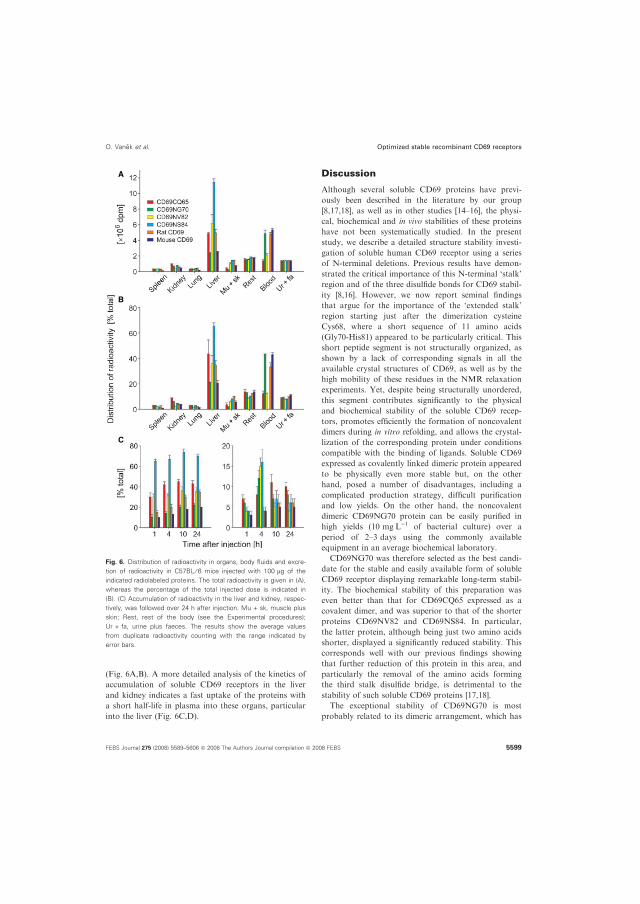
(Fig. 6A,B). A more detailed analysis of the kinetics of

accumulation of soluble CD69 receptors in the liver

and kidney indicates a fast uptake of the proteins with

a short half-life in plasma into these organs, particular

into the liver (Fig. 6C,D).

Discussion

Although several soluble CD69 proteins have previ-

ously been described in the literature by our group

[8,17,18], as well as in other studies [14–16], the physi-

cal, biochemical and in vivo stabilities of these proteins

have not been systematically studied. In the present

study, we describe a detailed structure stability investi-

gation of soluble human CD69 receptor using a series

of N-terminal deletions. Previous results have demon-

strated the critical importance of this N-terminal ‘stalk’

region and of the three disulfide bonds for CD69 stabil-

ity [8,16]. However, we now report seminal findings

that argue for the importance of the ‘extended stalk’

region starting just after the dimerization cysteine

Cys68, where a short sequence of 11 amino acids

(Gly70-His81) appeared to be particularly critical. This

short peptide segment is not structurally organized, as

shown by a lack of corresponding signals in all the

available crystal structures of CD69, as well as by the

high mobility of these residues in the NMR relaxation

experiments. Yet, despite being structurally unordered,

this segment contributes significantly to the physical

and biochemical stability of the soluble CD69 recep-

tors, promotes efficiently the formation of noncovalent

dimers during in vitro refolding, and allows the crystal-

lization of the corresponding protein under conditions

compatible with the binding of ligands. Soluble CD69

expressed as covalently linked dimeric protein appeared

to be physically even more stable but, on the other

hand, posed a number of disadvantages, including a

complicated production strategy, difficult purification

and low yields. On the other hand, the noncovalent

dimeric CD69NG70 protein can be easily purified in

high yields (10 mgÆL)1 of bacterial culture) over a

period of 2–3 days using the commonly available

equipment in an average biochemical laboratory.

CD69NG70 was therefore selected as the best candi-

date for the stable and easily available form of soluble

CD69 receptor displaying remarkable long-term stabil-

ity. The biochemical stability of this preparation was

even better than that for CD69CQ65 expressed as a

covalent dimer, and was superior to that of the shorter

proteins CD69NV82 and CD69NS84. In particular,

the latter protein, although being just two amino acids

shorter, displayed a significantly reduced stability. This

corresponds well with our previous findings showing

that further reduction of this protein in this area, and

particularly the removal of the amino acids forming

the third stalk disulfide bridge, is detrimental to the

stability of such soluble CD69 proteins [17,18].

The exceptional stability of CD69NG70 is most

probably related to its dimeric arrangement, which has

A

B

C

Fig. 6. Distribution of radioactivity in organs, body fluids and excre-

tion of radioactivity in C57BL ⁄ 6 mice injected with 100 lg of the

indicated radiolabeled proteins. The total radioactivity is given in (A),

whereas the percentage of the total injected dose is indicated in

(B). (C) Accumulation of radioactivity in the liver and kidney, respec-

tively, was followed over 24 h after injection. Mu + sk, muscle plus

skin; Rest, rest of the body (see the Experimental procedures);

Ur + fa, urine plus faeces. The results show the average values

from duplicate radioactivity counting with the range indicated by

error bars.

O. Vanek et al. Optimized stable recombinant CD69 receptors

FEBS Journal 275 (2008) 5589–5606 ª 2008 The Authors Journal compilation ª 2008 FEBS 5599

been demonstrated by a number of experimental tech-

niques, including gel filtration, sedimentation velocity

analysis, measurement of NMR relaxations and DLS.

Our studies attempting to dissociate the dimer in SDS

under mild conditions provided further support for

such a conclusion. It would appear from these experi-

ments that single globular carbohydrate-recognition

domains of CD69, even when stabilized by detergent

at the disrupted dimer interface, comprise short-lived

molecules that are only moderately stable at low tem-

peratures (4 C) and start to unfold when heated to

ambient temperature. However, the general validity of

this conclusion appears to be challenged by the data

for rat CD69, which appears to be monomeric.

The remarkable in vitro stability of the human solu-

ble CD69 receptor, CD69NG70 protein, makes it a

strong candidate for a protein that is potentially use-

ful for therapeutic purposes. Therefore, it was critical

to test the in vivo stability of this protein and to com-

pare it with the stability of its rat and mouse ortho-

logs that are more compatible with the experimental

models in use. The results of these tests revealed both

the long circulation and the intactness of the most

stable human CD69 protein (together with its rat and

mouse orthologs) in the blood of mice. For these

proteins, approximately 40% of the initial dose could

be still recovered 24 h after injection. Moreover, the

exclusion of the protein in urine and faeces, and

uptake by the liver, was relatively low. On the other

hand, the least stable human CD69NS84 protein dis-

played a rapid plasma clearance connected with the

transfer into the liver that took up more than 60% of

the injected dose.

Progress in our knowledge of CD69 biology has

advanced rapidly, allowing to propose the individual

therapeutic modalities involving the stable soluble

CD69 receptors described in the present study. One

such protocol may involve the reactivity of the soluble

long cirulating CD69 protein with the tumor surface

ligands, leading to their blocking or reduced availabil-

ity for the reaction with the cellular form of CD69 at

the surface of the killer lymphocytes. This should

result in the protection of these critical cells of antitu-

mor immunity from apoptotic cell death following

their hyperactivation by tumor surface ligands [12].

Such a possibility is further supported by recent results

obtained by our group as well as in studies by others

[20–23]. We have recently shown that mimetics of

tumor surface ligands for CD69, when presented in a

highly multivalent form, can bind strongly to CD69+

lymphocytes and cause their death by a massive trigger

of apoptosis. Graham et al. [20] recently reported that

hyperstimulation of human T lymphocytes with ligands

for CD28 or integrins results in their activation, as

demonstrated by high surface expression of CD69, and

massive cell death. North et al. [22] recently described

NK cells that, when primed by incubation with the

tumors, acquire the ability to lyse leukemic cell lines

and even solid tumors primarily through CD69 recep-

tors, as demonstrated by the ability to inhibit such

lysis with soluble recombinant CD69 protein. These

results appear to be supported by our histochemical

evidence showing that tumor infiltrating lymphocytes

significantly upregulate CD69 expression [21]. An

increased occurrence of CD69 positive lymphocytes in

tumor sites may also be related to its recently

described function as a downregulator of lymphocyte

egress from lymphoid organs due to the downmodula-

tion of sphingosine 1-phosphate receptor 1 [23]. Konj-

evic et al. [24] reported the predictive value of CD69

expression during the clinical response to chemoimmu-

notherapy in patients with metastatic melanomas.

Collectively, these results appear to support the role of

CD69 as one of critical receptors involved in the rec-

ognition and killing of tumors, including clinically

important solid tumors. In view of all these results, the

availability of long-circulating and in vivo stable solu-

ble CD69 proteins with a low toxicity for experimental

animals would be an advantage for their use in experi-

mental tumor therapy models using rats or mice [21].

In conclusion, our systematic studies of soluble

CD69 receptors that have been refolded in the form of

covalent or noncovalent dimers demonstrate large vari-

ation in the solubility and stability among these

proteins and allow us to select the human protein con-

taining amino acids Gly70 to Lys199 (and the rat and

mouse orthologs) as the most physically and biochemi-

cally stable variant. We have proven an exceptional

in vivo stability and low toxicity upon injection into

the blood of experimental mice in which these proteins

remain intact for the prolonged periods of time neces-

sary to elicit their therapeutic effects in our animal

tumor therapy models [21]. The availability of such

soluble CD69 receptors now opens the way for their

testing in various animal experimental models of CD69

related diseases, such as malignant or autoimmune

diseases.

Experimental procedures

Materials

All chemicals were analytical grade reagents of the high-

est commercially available quality. Chemicals used for

protein refolding were obtained from Serva (Heidelberg,

Germany). Plasmid pCDA401 containing the insert coding

Optimized stable recombinant CD69 receptors O. Vanek et al.

5600 FEBS Journal 275 (2008) 5589–5606 ª 2008 The Authors Journal compilation ª 2008 FEBS

the entire extracellular part of the CD69 was described

previously [8].

Expression and purification of recombinant

soluble human CD69 receptors

For the production of the covalent dimeric CD69,

CD69CQ65, an expression plasmid similar to that described

previously [16] was used. DNA was amplified using forward

primer 5¢-CTCGAGACAATACAATTGTCCAGG-3¢, and

reverse primer 5¢-ACAAAGCTTATTTGTAAGGTTTGTT

ACA-3¢, and the PCR product was cloned into pBSK+

vector using the SmaI restriction site, and then into

pRSETB vector using XhoI and HindIII restriction endo-

nucleases. His-Tag was removed using mild tryptic diges-

tion targeted to the two basic amino acids (Arg coded by

the XhoI site was followed immediately by CD69 sequence

Lys) preceding Gln65. For the production of soluble CD69

refolded as noncovalent dimers, three different DNA frag-

ments coding for the extracellular portion of human CD69

were amplified by PCR using Deep Vent DNA polymerase

(NEB, Ipswich, MA, USA) as the amplification enzyme,

pCDA401 as a template and the following primer pairs:

for CD69NG70, 5¢-ACATATGGGCCAATACACATTC-3¢and 5¢-ACAAAGCTTATTTGTAAGGTTTGTTACA-3¢; for

CD69NV82, 5¢-ACATATGGTTTCTTCATGCTCTG-3¢ and

5¢- ACAAAGCTTATTTGTAAGGTTTGTTACA-3¢; and for

CD69NS84, 5¢-ACATATGTCATGCTCTGAGGACTGG

GTT-3¢ and 5¢- ACAAAGCTTATTTGTAAGGTTTGTT

ACA-3¢. PCR products were directly cloned into pBSK+

cloning vector (Stratagene, LaJolla, CA, USA) using the

SmaI restriction site and the desired expression constructs

were subsequently cloned into pRSETB expression vector

(Invitrogen, Carlsbad, CA, USA) using the NdeI and

HindIII restriction sites introduced by the amplification

primers.

Plasmids were transformed into Escherichia coli BL-21

(DE3) RIL or Gold strains (Stratagene). Bacteria were

grown in 2 L Erlenmeyer flasks with 0.5 L of LB broth at

37 C with ampicillin and tetracycline (Gold) or chloram-

phenicol (RIL) as antibiotics. Induction of protein produc-

tion with isopropyl thio-b-d-galactoside was not necessary,

and the culture was left to grow for 16–24 h. Cells were

harvested by centrifugation, and inclusion bodies were

isolated [25]. Inclusion bodies were dissolved in 50 mm Tris–

HCl (pH 8.0) with 6 m guanidine-HCl and 100 mm dith-

ithreitol, centrifuged, and adjusted to 10 mgÆmL)1 protein.

In vitro refolding of denatured protein was carried out by

rapid dilution into the refolding buffer. Clarified protein

solution was quickly diluted 100-fold into the refolding buf-

fer composed of 50 mm Tris–HCl (pH 8.5), 0.4 m l-argi-

nine, 2 mm CaCl2, 1 mm NaN3, 18 mm cysteamine, 1 mm

cystamine, 1 mm phenylmethanesulfonyl fluoride, 1 lgÆmL)1

leupeptine and 1 lgÆmL)1 pepstatine. After slow stirring at

4 C for 5 h, the refolding mixture was dialyzed against 8 L

of 10 mm Tris–HCl (pH 8.5), 0.5 m NaCl and 1 mm NaN3

for 6 h, and then against 10 L of 10 mm Tris–HCl (pH 8.5),

50 mm NaCl and 1 mm NaN3 for 12 h at 4 C.Two protocols were used further. In Protocol I, protease

inhibitors were added to the dialyzed protein, and the pH of

the solution was adjusted with acetic acid to 5.5. The insolu-

ble precipitate of misfolded protein was centrifuged at

20 000 g for 30 min at room temperature. The refolded

CD69 protein was then captured on SP-Sepharose FF col-

umn (GE Healthcare Europe, Munich, Germany) equili-

brated in 20 mm sodium acetate (pH 5.5), 50 mm NaCl and

1 mm NaN3. The column was eluted by linear gradient of

NaCl from 50 mm to 2 m. Fractions containing CD69

protein were pooled and applied onto a reverse phase

column Vydac C4 (Dionex, Sunnyvale, CA, USA) with

0.1% trifluoroacetic acid as mobile phase A and eluted by

linear gradient of mobile phase B composed of 95% aceto-

nitrile and 5% of 0.1% trifluoroacetic acid from 30% to

40% B over 60 min. Concentrated fractions were further

purified by gel filtration on a Superdex 200 HR 10 ⁄ 30 col-

umn (GE Healthcare) in 10 mm Mes (pH 5.8) with 100 mm

NaCl, 2 mm CaCl2 and 1 mm NaN3, and concentrated to

10 mgÆmL)1 using a Centriprep and Centricon device (Milli-

pore, Billerica, MA, USA). In Protocol II, dialyzed protein

without any acidification was passed through Q-Sepharose

FF column (GE Healthcare) equilibrated with the dialysis

buffer. The protein passed through the column, and was

concentrated by ultrafiltration using PLGC regenerated

cellulose membranes (Millipore) with a 10 kDa cut-off. The

concentrated protein was finally purified by gel filtration on

a Superdex 200 HR 10 ⁄ 30 column, and concentrated as

described in Protocol I.

The preparation and analysis of rat CD69 has been

described previously [18]. DNA fragment coding for mouse

CD69 [5,19] was amplified from RNA prepared from spleens

of C57BL ⁄ 6 mice using RT-PCR with the forward primer

5¢-TGCATATGGGCCTTTACGAGAAGTTGGAA-3¢ con-taining the NdeI cloning site and the reverse primer 5¢-TGA

AGCTTCATTATCTGGAGGGCTTGCTGCA-3¢ contain-

ing the HindIII site. The amplified NdeI–HindIII fragment

was transferred into the pRSETB expression vector, and the

protein was produced as described above, and purified using

Protocol II.

Characterization of the purified soluble proteins

The identity of the prepared protein was confirmed by

sequence mapping of tryptic digests with MALDI-TOF MS

with a good sequence coverage. The total mass of the

protein was measured by means of FT-ICR MS. The size

distribution and polydispersity of human CD69 preparation

were assessed by DLS at a concentration of 2 mgÆmL)1 in

10 mm Hepes (pH 7.0) with 150 mm NaCl and 1 mm

NaN3. Samples were loaded into a 45 lL quartz cuvette

and particle size distribution measurements were performed

O. Vanek et al. Optimized stable recombinant CD69 receptors

FEBS Journal 275 (2008) 5589–5606 ª 2008 The Authors Journal compilation ª 2008 FEBS 5601

repeatedly at 291 K using a Zetasizer Nano (Malvern

Instruments, Malvern, UK). Estimates of hydrodynamic

radii of the expected molecular species were calculated with

the software hydropro [26]. The structures of monomers

and dimers of the human CD69 in the present study, and

as reported previously [15] (Protein Databank code 1E87),

were used as input coordinates for the calculations. The

dimer of hCD69 in the Protein Databank record 1E87 was

generated using symmetry operators. Calculated Stokes

radii were compared with experimental values.

Protein crystallography and data collection

Recombinant human CD69 was crystallized by hanging

drop vapor diffusion method using 24-well plates (Hampton

Research, Aliso Viejo, CA, USA). Initial crystallization con-

ditions were established at 291 K using selected precipitants

from JBScreen kits (Jena Bioscience, Jena, Germany). Each

drop was prepared by mixing equal volumes (1 lL) of the

protein and the precipitant solution and each drop was

equilibrated against 1 mL of precipitant solution. After

optimization of poly(ethylene glycol) molecular weight and

concentration, and after exchange of precipitant buffer, we

determined the suitable crystallization conditions. Needle-

shaped, but regular crystals were obtained by mixing 1 lLof protein at a concentration of 5 mgÆmL)1 in 10 mm Bis-

Tris–HCl (pH 6.5), 100 mm NaCl, 2 mm CaCl2 and 1 mm

NaN3 with 1 lL of reservoir solution containing 0.1 m Argi-

nine.HCl (pH 7.0), 20% PEG 3400, 10 mm CaCl2 and 1 mm

NaN3. Crystals appeared within 1 week. For X-ray data

collection, crystals were mounted in nylon loops and cryo-

protected by soaking in the reservoir solution containing

25% glycerol as a cryoprotectant and then flash frozen in

liquid nitrogen. The dataset was collected at 100 K at beam-

line 19-ID of the Structural Biology Center at the Advanced

Photon Source, Argonne National Laboratory (Argonne,

IL, USA). The diffraction data were processed using the

hkl-3000 software suite [27] (Table 4). The structure was

first determined to 4.0 A resolution by molecular replace-

ment. A search model constructed from the crystal structure

of CD69 (Protein Databank code 1E8I) [15] was used for

the simultaneous rotation and translation search of two

molecules by the software epmr [28]. The search yielded an

unambiguous solution in the P61 space group with an initial

Rcrys of 42.2% and a correlation coefficient of 0.57. In the

rigid body refinement, both molecules of the dimer were

allowed to move independently. During the restrained

refinement procedure, noncrystallographic symmetry

restraints were applied to the CD69 monomers. Rigid body

refinement and subsequent restrained refinement protocol

were performed with the software refmac 5.1.24 [29] from

the ccp4 package [30]. For manual model rebuilding, the

software coot was used [31]. The structure was refined to a

crystallographic R-factor of 19.0% at 1.8 A resolution.

Further refinement statistics are shown in Table 4.

Structure coordinates

The coordinates and structure factors have been submitted

to the RCSB Protein Databank under accession code

3CCK.

Thermal denaturation experiments

Recombinant proteins were diluted to 0.5 mgÆmL)1, and

UV spectra were taken in the 200–300 nm range in Beck-

man DU-70 spectrophotometer (Beckman Coulter, Fuller-

ton, CA, USA) equipped with the heated cuvette. The

initial UV scan was taken at 25 C, after which the temper-

ature in the cuvette was increased in 5 C increments up to

the denaturation temperature indicated by sudden increase

in the absorbance. The experiment was performed

in 10 mm Mes (pH 5.8) with 50 mm NaCl and 1 mm

NaN3, in the same buffer containing 5 mm dithiothreitol,

and also in 10 mm Pipes buffer (pH 6.8) with 50 mm NaCl,

1 mm NaN3 and 5 mm dithiothreitol, and in 10 mm Tris

buffer (pH 7.8) with 50 mm NaCl, 1 mm NaN3 and 5 mm

dithiothreitol. From the complete spectra, only the absor-

bance at 280 nm was extracted and plotted because of tech-

nical difficulties with buffer subtraction in the far UV

region. Alternatively, protein stability was followed using

FTIR spectroscopy.

Infrared spectra were recorded with a Bruker IFS-66 ⁄ SFTIR spectrometer (Bruker, Ettlingen, Germany) using a

standard MIR source, a KBr beamsplitter and an MCT

detector. Four thousand scans were collected with 4 cm)1

Table 4. Crystal parameters, data collection and refinement statis-

tics. Values in parentheses represent those obtained for the high-

est resolution shell.

Space group P61

Unit cell parameters (A, ) a = b = 85.69 and c = 61.88

a = b = 90.0 and c = 120.00

Resolution (A) 75.54–1.80 (1.83–1.80)

Total number of observations

to 1.80 A

422144

No. unique reflections 22276

Completeness 98.03% (76.5%)

I ⁄ r (I) 29.5 (2.6)

Rsyma 0.045 (0.575)

Refinement resolution (A) 74.54–1.80

Rmsd bond length from ideal (A) 0.015

Rmsd bond angles from ideal () 1.41

Rcrysb 0.190

Rfreec 0.222

a Rsym =Pj – ÆIæj ⁄

PÆIæ, where I is the observed intensity and ÆIæ is

the mean intensity of multiple observations of symmetry-related

reflections. b Rcrys =PkFoj – jFck ⁄

PjFoj, where Fo and Fc are the

observed and calculated structure factor amplitudes. c Rfree is as

for Rcrys but calculated for a randomly chosen 5% of reflections

that were omitted from the refinement.

Optimized stable recombinant CD69 receptors O. Vanek et al.

5602 FEBS Journal 275 (2008) 5589–5606 ª 2008 The Authors Journal compilation ª 2008 FEBS

spectral resolution and a Happ–Genzel apodization func-

tion. Aqueous protein solution was measured at the indi-

cated temperature in a thermostated CaF2-BioCell with

10 lm path length (BioTools, Jupiter, FL, USA). The spec-

tral contribution of a buffer was corrected using the stan-

dard algorithm [32]. The spectrum of water vapors was

subtracted and finally the spectrum was normalized. The

fraction content of the secondary structure elements was

calculated using the procedure contin with a set of 16

reference proteins [32].

Sedimentation velocity and sedimentation

equilibrium measurements

Initial sedimentation measurements were performed in the

preparative ultracentrifuge (Beckman Optima LE-80)

using the discontinuous sucrose gradient [1 mL each of

40%, 30%, 20% and 10% sucrose in 10 mm Mes buffer

(pH 5.8) with 50 mm NaCl and 1 mm NaN3] placed into

the UltraClear polycarbonate tube (Beckman Coulter).

The sucrose gradient was overlayed with 0.2 mL of pro-

tein samples (10 mgÆmL)1) that were spun in SW-60 rotor

for 16 h at 392 000 gav. Then, 0.35 mL samples were col-

lected from the top to the bottom of the tube, and the

protein distribution was examined in 10 lL by 17.5%

SDS ⁄PAGE. Further sedimentation velocity and sedimen-

tation equilibrium measurements were performed using an

analytical ultracentrifuge ProteomeLabXL-I (Beckman

Coulter) using (depending on the sample concentration)

absorbance or laser interference optics and an An50Ti

rotor. Before the experiment, 0.5 mL samples of recombi-

nant CD69 were dialyzed for 20 h against 2 L of 10 mm

Tris–HCl (pH 7.8) with 150 mm NaCl and 1 mm NaN3.

Sedimentation velocity experiments were carried out at

130 000 gav using an Epon aluminium-filled centerpiece

(Beckman Coulter). Sample (400 lL) and dialysate

(450 lL) were loaded in the sample and reference cells,

respectively. Absorbance scans were performed at 280 nm

at 5 min intervals and 0.003 cm spatial resolution, and

the data were analyzed by the second-moment method

using the software provided by the manufacturer. The

partial specific volume of CD69NG70 (0.73 mLÆg)1) was

calculated using the software sednterp (http://

www.rasmb.bbri.org). The molecular mass of CD69NG70

was calculated using the approximation for the spherical

molecules, as described previously by Lebowitz et al. [33],

according to the formula:

Ssphere ¼ 0:012ð½M2=3ð1 mqÞ=m1=3Þ:

For sedimentation equilibrium experiments, the protein

was examined at three different concentrations (0.8, 0.4 and

0.2 mgÆmL)1) in three different sample cuvettes placed into

an An50Ti rotor. The rotor was spun at 130 000 gav for

2 h, followed by 24 000 gav for 18 h. Thereafter, two

consecutive absorbance scans were taken, one at the end of

18 h period, and another after additional 2 h. The equilib-

rium distribution from three different loading concentra-

tions and up to three different rotor speeds (24 000, 14 000

and 7500 gav, respectively) were analyzed using the nonlin-

ear curve fit algorithm in the software package supplied

with the centrifuge [33].

NMR measurements

All NMR experiments were run at 300 K on Bruker

Avance 600 MHz spectrometer equipped with the cryogenic

H ⁄C ⁄N TCI probehead. 1H-15N HSQC spectra were used

as a routine check of protein folding and stability during

the sample preparation; 0.9 mm13C ⁄ 15N-labeled and

0.3 mm15N-labeled CD69NG70 samples were used for the

assignment and relaxation measurements, respectively. The

sample buffer consisted of 10 mm Mes (pH 5.8), 50 mm

NaCl, 1 mm NaN3 and 10% D2O. The standard set of

triple resonance experiments [34] and 13C ⁄ 15N-edited

NOESY [35] were used to obtain sequential assignment.

The assignment was confirmed by checking side-chain

resonances of selected residues in the HCCH-TOCSY

spectra [34]. The 15N T1, T2 and steady-state 1H-15N NOE

experiments were run as described by Farrow et al. [36].

The T1 and T2 relaxation delays were sampled at 11, 56,

134, 235, 381, 560, 896, 1344 ms and 16, 31, 62, 94, 156,

219, 250, 406 ms, respectively. All spectra were processed

using the software nmrpipe [37] and analyzed using the

software sparky (T. D. Goddard and D. G. Kneller,

sparky 3; University of California, San Francisco, CA,

USA).

Relaxation analysis and hydrodynamic

calculations

The backbone amide dynamic parameters were derived in

the spirit of the Lipari–Szabo model-free approach [38,39]

using the software relax [40,41]. The apparent rotational

diffusion coefficient (defined as 1 ⁄ 6sm, where sm is the over-

all correlation time) was fitted separately for each residue

for the sake of comparison with the hydrodynamics simula-

tions. The internuclear N-H distance of 0.102 nm and 15N

chemical shift anisotropy of 160 p.p.m. were used. The

hydrodynamic calculations were performed using software

hydronmr [42]. Viscosity was set to 0.852 mPaÆs. Default

effective radius (0.32 nm) and minibeads of six radii in the

range 0.15–0.2 nm were used. The structural models were

derived from the X-ray structure (Protein Databank code

3CCK). Coordinates of the dimeric and monomeric struc-

tures were taken directly from the Protein Databank file. In

addition, sets of monomeric and dimeric full-length struc-

tures were modeled by adding 11 N-terminal residues and

running short molecular dynamics simulations using the

software cns 1.2. The atoms taken from the X-ray structure

O. Vanek et al. Optimized stable recombinant CD69 receptors

FEBS Journal 275 (2008) 5589–5606 ª 2008 The Authors Journal compilation ª 2008 FEBS 5603

were kept fixed during the simulation, whereas the added

11 N-terminal amino acids were restrained by the measured

chemical shifts only. The simulation protocol consisted of a

15 ps high temperature (50 000 K) torsion dynamics run,

two 15 ps cooling stages (the first one employing torsion

dynamics, the second one employing cartesian dynamics)

and gradient minimization. Out of 100 structures calculated

for each set, 20 structures with the lowest energy were used

in hydrodynamics calculations.

NMR data

NMR data were submitted to the BioMagResBank data-

base with an accession number 15703.

Protein distribution in vivo

All animal experiments were approved by the Institute Eth-

ical Committee and were performed in accordance with the

European Communities Council Directive of 24 November

1986 (86 ⁄ 609 ⁄EEC). Recombinant proteins for animal stud-

ies were made free of lipopolysaccharide using polymyxin B

resin (Bio-Rad, Hercules, CA, USA), radiolabeled using

Na125I (GE Healthcare) to a specific activity of

106 BqÆlg)1, and repurified by reverse phase chromatogra-

phy to remove the noncovalently bound iodine. Ten micro-

grams of each radiolabeled protein was administred in

50 lL of NaCl ⁄Pi into the tail vein of two male C57BL ⁄ 6mice, aged 7–8 weeks old (Charles River, Wilmington, MA,

USA) that had been accommodated for at least 2 weeks in

the conventional housing facility. Blood samples (50 lL)were collected 1, 4, 10 and 24 h after the administration of

radioactivity in view of our experience with the rapid effect

of the ligands for these receptors on the immune system

[21]. From each sample, 20 lL was mixed with 80 lL of

10 mm NH4Cl and after 1 h at room temperature to lyse

the erythrocytes, was used for hemoglobin determination

by direct spectrophotometry at 400 nm, and for radioactiv-

ity counting. From the remaining 30 lL of sample, the

most abundant serum proteins were removed using IgY12

resin (Beckman Coulter), and two 10 lL aliquots of the

remaining proteins were resolved by 15% SDS ⁄PAGE, and

the gels were exposed to the autoradiographic films Agfa

CP-VB (Agfa-Gevaert, Mortsel, Belgium) with intensifying

screens, or developed by western blotting using mouse

monoclonal antibodies against human CD69 (BL-Ac ⁄ p26)[17], rat CD69 [5] and mouse CD69 (Invitrogen), and ECL

detection (GE Healthcare). The remaining 10 lL of the

clarified protein was used for the solid phase binding using

GlcNAc agarose (Sigma, St Louis, MO, USA).

Plasma half-life was calculated using the formula:

c = c0 · e(–kt), where c is the concentration at the indicated

time, c0 is the initial concentration and k is the first order

rate constant [43]. The calculation of the plasma clearance

and the apparent volume of distribution was based on a

one-compartment kinetic model with instantaneous absorp-

tion according to the equation: CP = (D ⁄Vd) · e(–CL ⁄ Vd)t,

where CP is the plasma level at time t, CL is the clearance,

D is the administered dose and Vd is the apparent volume

of distribution [43].

For organ distribution studies, mice were killed 24 h after

injection of the radiolabeled protein, individual organs

(spleen, kidney, liver, muscle, skin) were collected, and dis-

solved completely (60 C, 48 h) in NCS-II tissue solubilizer,

in accordance with the manufacturer’s instructions (GE

Healthcare) before scintillation counting. The difference

between the total initial dose of radioactivity, and the sum

of radioactivities recovered in the individual organs, and in

the urine and faeces, was designated as the rest of the body

(rest), consisting mostly of the bowel, heart, bones, brain

and reproductive organs. Because all six mice were housed

in a single cage during the experiment, the radioactivity

recovered in urine and faeces represents the average value.

In an alternative time course experiment, liver and kidney

were collected after 1, 4, 10 and 24 h after injection, and

processed as described above.

Acknowledgements

This work is dedicated to Professor Danuse Sofrova and

Professor Marie Ticha. We thank Pavlına Rezacova for

data collection at the APS synchrotron facility at Argo-

nne National Laboratory; Jan Bıly for his help with the

thermal denaturation experiments; Anna Fiserova,

Marketa Vancurova and Jozef Hritz for their help with

the experiments; and the reviewers for their valuable

comments on the manuscript. This work was supported

by Ministry of Education of Czech Republic (MSM

21620808, MSM 21620835, MSM 21622413, LC 545,

LC 6030, LC 7017 and 1M 4635608802), by the Institu-

tional Research Concept for the Institute of Microbiol-

ogy (AVOZ 50200510), by the Grant Agency of the

Academy of Sciences (IAA5020403 and IAA500-

200509), and by the European Commission, Project

SPINE2-Complexes (contract LSHG-CT-2006-031220).

References

1 Testi R, D’Ambrosio D, De Maria R & Santoni A

(1994) The CD69 receptor: a multipurpose cell surface

trigger for hematopoietic cells. Immunol Today 15, 479–

483.

2 Gerosa F, Tommasi M, Scardoni M, Accolla RS,

Pozzan T, Libonati M, Tridente G & Carra G (1991)

Structural analysis of the CD69 early activation antigen

by two monoclonal antibodies directed to different

epitopes. Mol Immunol 28, 159–168.

3 Hamann J, Fiebig H & Strauss M (1993) Expression

cloning of the early activation antigen CD69, a type II

Optimized stable recombinant CD69 receptors O. Vanek et al.

5604 FEBS Journal 275 (2008) 5589–5606 ª 2008 The Authors Journal compilation ª 2008 FEBS

integral membrane protein with a C-type lectin domain.

J Immunol 150, 4920–4927.

4 Lopez-Cabrera M, Santis AG, Fernandez-Ruiz E,

Blacher R, Esch F, Sanchez-Mateos P & Sanchez-

Madrid F (1993) Molecular cloning, expression, and

chromosomal localization of the human earliest lym-

phocyte activation antigen AIM ⁄CD69, a new member

of the C-type lectin superfamily of signal-transmitting

receptors. J Exp Med 178, 537–547.

5 Ziegler SF, Ramsdell F, Hjerrild KA, Armitage RJ,

Grabstein KH, Hennen KB, Fatrach T, Fanslow WC,

Shevach EM & Alderson MR (1993) Molecular charac-

terization of the early activation antigen CD69: a type

II membrane glycoprotein related to a family of natural

killer cell activation antigens. Eur J Immunol 23, 1643–

1648.

6 Sancho D, Santis AG, Alonso-Lebrero JL, Viedma F,

Tejedor R & Sanchez-Madrid F (2000) Functional anal-

ysis of ligand-binding and signal transduction domains

of CD69 and CD23 C-type lectin leukocyte receptors.

J Immunol 165, 3868–3875.

7 Pisegna S, Zingoni A, Pirozzi G, Cinque B, Cifone

MG, Morrone S, Picolli M, Frati L, Palmieri G & San-

toni A (2002) Src-dependent Syk activation controls

CD69-mediated signaling and function of human NK

cells. J Immunol 169, 68–74.

8 Bezouska K, Nepovım A, Horvath O, Pospısil M,

Hamann J & Feizi T (1995) CD69 antigen of human

leukocytes is a calcium-dependent carbohydrate-binding

protein. Biochem Biophys Res Commun 208, 68–74.

9 Risso A, Smilovich D, Capra MC, Baldissarro I, Yan

G, Bargellesi A & Cosulich ME (1991) CD69 in resting

and activated T lymphocytes. Its association with a

GTP binding protein and biochemical requirements for

its expression. J Immunol 146, 4105–4114.

10 Moretta A, Poggi A, Pende D, Tripodi G, Orengo AM,

Pella N, Augugliaro R, Bottino C, Ciccone E & Moret-

ta L (1991) CD69-mediated pathway of lymphocyte

activation: anti-CD69 monoclonal antibodies trigger the

cytolytic activity of different lymphoid effector cells

with the exception of cytolytic T lymphocytes express-

ing T cell receptor a ⁄ b. J Exp Med 174, 1393–1398.

11 Borrego F, Robertson MJ, Ritz J, Pena J & Solana R

(1999) CD69 is a stimulatory receptor for natural killer

cells and its cytotoxic effect is blocked by CD94 inhibi-

tory receptor. Immunology 97, 159–165.

12 Sancho D, Gomez M & Sanchez-Madrid F (2004)

CD69 is an immunoregulatory molecule induced follow-

ing activation. Trends Immunol 26, 136–140.

13 Esplugues E, Sancho D, Vega-Ramos J, Martinez C,

Syrbe U, Hamann A, Engel P, Sanchez-Madrid F &

Lauzurica P (2003) Enhanced antitumor immunity in

mice deficient in CD69. J Exp Med 197, 1093–1106.

14 Natarajan K, Sawicki MW, Margulies DH & Mariuzza

RA (2000) Crystal structure of human CD69: a C-type

lectin-like activation marker of hematopoietic cells. Bio-

chemistry 39, 14779–14786.

15 Llera AS, Viedma F, Sanchez-Madrid F & Tormo J

(2001) Crystal structure of the C-type lectin-like domain

from the human hematopoietic cell receptor CD69.

J Biol Chem 276, 7312–7319.

16 Childs RA, Galustian C, Lawson AM, Dougan G,

Benwell K, Frankel G & Feizi T (2000) Recombinant

soluble human CD69 dimer produced in Escherichia

coli: reevaluation of saccharide binding. Biochem

Biophys Res Commun 266, 19–23.

17 Pavlıcek J, Sopko B, Ettrich R, Kopecky V, Baumruk V,

Man P, Havlıcek V, Vrbacky M, Martınkova L, Kren V

et al. (2003) Molecular characterization of binding of cal-

cium and carbohydrates by an early activation antigen of

lymphocytes CD69. Biochemistry 42, 9295–9306.

18 Pavlıcek J, Kavan D, Pompach P, Novak P, Luksan O

& Bezouska K (2004) Lymphocyte activation receptors:

new structural paradigm in group V of C-type animal

lectins. Biochem Soc Trans 32, 1124–1126.

19 Ziegler SF, Levin SD, Johnson L, Copeland NG, Gil-

bert DJ, Jenkins NA, Baker E, Sutherland GR, Feld-

haus AL & Ramsdell F (1994) The mouse CD69 gene.

Structure, expression, and mapping to the NK gene

complex. J Immunol 152, 1228–1236.

20 Graham DB, Bell MP, Huntoon CJ, Griffin MD, Tai

X, Singer A & McKean DJ (2006) CD28 ligation costi-

mulates cell death but not maturation of double-posi-

tive thymocytes due to defective ERK MAPK signaling.

J Immunol 177, 6098–6107.

21 Vannucci L, Fiserova A, Sadalapure K, Lindhorst TK,

Kuldova M, Rossmann P, Horvath O, Kren V, Krist P,

Bezouska K et al. (2003) Effects of N-acetyl-D-glucosa-

mine-coated glycodendrimers as biological modulators

in the B16F10 melanoma model in vivo. Int J Oncol 23,

285–296.

22 North J, Bakhsh I, Marden C, Pittman H, Addison E,

Navarrete C, Anderson R & Lowdell MW (2007)

Tumor-primed human natural killer cells lyse NK-resis-

tant tumor targets: evidence of a two-stage process in

resting NK cell activation. J Immunol 178, 85–94.

23 Shiow LR, Rosen DB, Brdickova N, Xu Y, An J, Langer

LL, Cyster JG & Matloubian M (2006) CD69 acts down-

stream of interferon-a ⁄ b to inhibit S1P1 and lymphocyte

egress from lymphoid organs. Nature 440, 540–544.

24 Konjevic G, Jovic V, Vuletic A, Radulovic S, Jelic S &

Spuzic I (2007) CD69 on CD56+ NK cells and

response to chemoimmunotherapy in metastatic mela-

noma. Eur J Clin Invest 37, 887–896.

25 Valez-Gomez M, Reyburn HT, Mandelboim M &

Strominger JL (1998) Kinetics of interaction of HLA-C

ligands with natural killer cell inhibitory receptors.

Immunity 9, 337–344.

26 de la Torre JG, Huertas ML & Carrasco B (2000) Cal-

culation of hydrodynamic properties of globular

O. Vanek et al. Optimized stable recombinant CD69 receptors

FEBS Journal 275 (2008) 5589–5606 ª 2008 The Authors Journal compilation ª 2008 FEBS 5605

proteins from their atomic-level structure. Biophys J 78,

719–730.

27 Minor W, Cymborowski M, Otwinowski Z & Chruszcz

M (2006) HKL-3000: the integration of data reduction

and structure solution – from diffraction images to an

initial model in minutes. Acta Crystallogr D 62, 859–866.

28 Kissinger CR, Gehlhaar DK & Fogel DB (1999) Rapid

automated molecular replacement by evolutionary

search. Acta Crystallogr D 55, 484–491.

29 Murshudov GN, Vagin AA & Dodson EJ (1997) Refine-

ment of macromolecular structure by the maximum-like-

lihood method. Acta Crystallogr D 53, 240–255.

30 Collaborative Computational Project, Number 4 (1994)

The CCP4 suite: programs for protein crystallography.

Acta Crystallogr D 50, 760–763.

31 Emsley P & Cowtan K (2004) Coot: model-building

tools for molecular graphics. Acta Crystallogr D 60,

2126–2132.

32 Dousseau F, Therrien M & Pezole M (1989) On the

spectral subtraction of water from the FT-IR spectra of

aqueous solution of proteins. Appl Spectrosc 43, 538–542.

33 Lebowitz J, Lewis MS & Schuck P (2002) Modern ana-

lytical ultracentrifuge in protein science: a tutorial

review. Protein Sci 11, 2067–2079.

34 Sattler M, Schleucher J & Griesinger C (1999) Hetero-

nuclear multidimensional NMR experiments for the

structure determination of proteins in solution employ-

ing pulsed field gradients. Prog NMR Spectrosc 34,

93–158.

35 Xia Y, Arrowsmith CH & Gao X (2003) 1HC and

1HN total NOE correlations in a single 3D NMR

experiment. 15N and 13C time-sharing in t1 and t2

dimensions for simultaneous data acquisition. J Biomol

NMR 27, 193–203.

36 Farrow NA, Muhandiram R, Singer AU, Pascal SM,

Kay CM, Gish G, Shoelson SE, Pawson T, Forman-

Kay JD & Kay LE (1994) Backbone dynamics of a free

and a phosphopeptide-complexed Src homology 2

domain studied by 15N NMR relaxation. Biochemistry

33, 5984–6003.

37 Delaglio F, Grzesiek S, Vuister GW, Zhu G, Pfeifer J

& Bax A (1995) NMRPipe: a multidimensional spectral

processing system based on Unix pipes. J Biomol NMR

6, 277–293.

38 Lipari G & Szabo A (1982) Model-free approach to the

interpretation of nuclear magnetic resonance relaxation

in macromolecules. 1. Theory and range of validity.

J Am Chem Soc 104, 4546–4559.

39 Lipari G & Szabo A (1982) Model-free approach to the

interpretation of nuclear magnetic resonance relaxation

in macromolecules. 2. Analysis of experimental results.

J Am Chem Soc 104, 4559–4570.

40 d’Auvergne EJ & Gooley PR (2008) Optimisation of

NMR dynamic models I. Minimisation algorithms and

their performance within the model-free and Brownian

rotational diffusion spaces. J Biomol NMR 40, 107–119.

41 d’Auvergne EJ & Gooley PR (2008) Optimisation of

NMR dynamic models II. A new methodology for the

dual optimisation of the model-free parameters and the

Brownian rotational diffusion tensor. J Biomol NMR

40, 121–133.

42 Bernado P, de la Torre JG & Pons M (2000) Interpreta-

tion of 15N NMR relaxation data of globular proteins

using hydrodynamic calculations with HYDRONMR.

J Biomol NMR 23, 139–150.

43 Ruffo S, Messori A, Grasela TH, Longo G, Donati-

Cori G, Matucci M, Morfini M & Tendi E (1985) A

calculator program for clinical application of the Bayes-

ian method of predicting plasma drug levels. Comput

Programs Biomed. 19, 167–177.

Supporting information

The following supplementary material is available:

Table S1. Secondary structure elements measured by

FTIR spectroscopy in soluble CD69 proteins subjected

to thermal stress.

Table S2. Secondary structure elements measured by

FTIR spectroscopy in soluble CD69 proteins subjected

to pH stress at temperatures 5 C below the Td.

This supplementary material can be found in the

online version of this article.

Please note: Wiley-Blackwell is not responsible for

the content or functionality of any supplementary

materials supplied by the authors. Any queries (other

than missing material) should be directed to the corre-

sponding author for the article.

Optimized stable recombinant CD69 receptors O. Vanek et al.

5606 FEBS Journal 275 (2008) 5589–5606 ª 2008 The Authors Journal compilation ª 2008 FEBS