1

MASARYK UNIVERSITY

Faculty of Arts

Psychology

Diploma thesis

Comparison of ipsative and normative measures from the

perspective of their psychometric properties

Supervisor: PhDr. Martin Jelínek, Ph.D.

Brno 2015 Author: Dávid Rédli

2

Declaration

I declare that I worked on this thesis on my own and that I used only sources mentioned in the

References. I agree with storing my work in the library of the Faculty of Arts of Masaryk

University in Brno in order to be available for educational purposes.

Prehlásenie

Prehlasujem, že som diplomovú prácu spracoval samostatne a použil som len pramene uvedené

v zozname literatúry. Súhlasím, aby bola práca uložená na Masarykovej univerzite v Brne

v knižnici Filozofickej fakulty a sprístupnená k študijným účelom.

Brno, 30th April 2015 ………………..

3

Acknowledgement

I would hereby like to thank my parents, who supported me over my studies, helped me and

encouraged me even if I hesitated and were always there for me. I would like to thank heartily

to my bellowed Veronika, who supported me every time I needed and bore with me in good and

bad times. Lastly, I am thankful to PhDr. Martin Jelínek, Ph.D. for his useful advices and

comments, helpful attitude and his tolerance. Thank you all.

4

Table of contents

Table of contents ..................................................................................................................................... 4

Foreword ................................................................................................................................................. 7

1. Introduction ..................................................................................................................................... 8

1.1. A brief history of psychological assessment ........................................................................... 8

1.2. Classical Test Theory .............................................................................................................. 9

1.3. Psychological measurement and types of variables .............................................................. 10

1.4. Normative measurement ........................................................................................................ 11

1.4.1. Disadvantages of normative measures .......................................................................... 12

1.4.2. Response bias ................................................................................................................ 13

1.5. Ipsative measurement ............................................................................................................ 14

1.5.1. Types of ipsative measures ............................................................................................ 15

1.5.2. Problematic properties of ipsative measures ................................................................. 16

1.5.3. Differences between normative measures and ipsative measures ................................. 18

1.6. Psychometric properties of ipsative measures ....................................................................... 19

1.6.1. Statistical methods applicable with ipsative data .......................................................... 19

1.6.2. Untestable reliability of ipsative measures .................................................................... 21

1.6.2.1. Problems with comparing of measures in order to estimate reliability ................. 22

1.6.2.2. Problems with estimating internal consistency...................................................... 23

1.6.3. Factor analysis ............................................................................................................... 25

1.6.4. Cluster analysis .............................................................................................................. 28

1.7. Advantages of ipsative measures ........................................................................................... 29

1.7.1. Reduction of Response Bias .......................................................................................... 29

1.7.2. Moderate responding ..................................................................................................... 30

1.7.3. Decision making in responding to normative vs. ipsative questionnaires ..................... 30

1.7.4. Summary of advantages and disadvantages of ipsative measures ................................. 31

1.7.5. Applicability and use of ipsative measures ................................................................... 32

1.8. Summary of ipsative measurements ...................................................................................... 33

1.9. NEO personality inventory .................................................................................................... 33

1.9.1. History of Big Five Model and NEO inventory ............................................................ 33

1.9.2. Description of the Big Five personality traits ................................................................ 35

1.9.3. Psychometric properties of NEO-FFI ............................................................................ 36

2. Hypothesis ..................................................................................................................................... 37

3. Method........................................................................................................................................... 38

3.1. Administration ....................................................................................................................... 38

5

3.2. Creating an ipsative version of normative NEO-FFI ............................................................. 39

3.2.1. Grouping the items ........................................................................................................ 40

3.2.2. Determining the maximum points to be distributed in groups in form B ...................... 41

3.2.3. Transformation of negative questions ........................................................................... 42

3.3. Experimental design .............................................................................................................. 43

3.4. Respondents........................................................................................................................... 43

4. Results ........................................................................................................................................... 44

4.1. Total data ............................................................................................................................... 44

4.2. Normative data ...................................................................................................................... 44

4.2.1. Description of normative data ....................................................................................... 44

4.2.2. NEO-FFI Results ........................................................................................................... 45

4.2.3. Internal consistency ....................................................................................................... 46

4.2.4. Factor analysis ............................................................................................................... 48

4.2.5. Reliability - test-retest group ......................................................................................... 48

4.3. Ipsative data ........................................................................................................................... 50

4.3.1. Description of ipsative data ........................................................................................... 50

4.3.2. NEO FFI Results – Ipsative ........................................................................................... 50

4.3.3. Internal consistency ....................................................................................................... 53

4.3.4. Factor analysis ............................................................................................................... 55

4.3.5. Cluster analysis .............................................................................................................. 55

4.3.6. Reliability - test-retest group ......................................................................................... 56

4.4. Comparing ipsative and normative data ................................................................................ 57

4.4.1. Graphical representation of relations between Ipsative and normative data ................. 58

4.4.2. Correlation coefficient ................................................................................................... 60

4.4.3. Comparison of correlations in test and re-test in various groups .................................. 61

4.4.4. Analysis of items – reliability of separate items ............................................................ 62

4.4.5. Comparison of final rank results ................................................................................... 63

4.5. Variability of total data .......................................................................................................... 64

4.6. Social desirability .................................................................................................................. 66

5. Discussion ..................................................................................................................................... 67

5.1. Limitations of study ............................................................................................................... 67

5.1.1. Respondents ................................................................................................................... 67

5.1.2. Administration through internet .................................................................................... 68

5.1.3. Qualitative analysis – some comments from respondents ............................................. 68

5.1.4. Distribution of points ..................................................................................................... 69

5.2. Properties of the semi-ipsative and normative measure and applicable statistics ................. 70

6

5.2.1. Ipsativity of the hybrid measure .................................................................................... 70

5.2.2. The similarity of the two forms ..................................................................................... 70

5.2.3. Applicability of methods for statistical analysis ............................................................ 71

5.2.4. Reliability of the semi-ipsative vs. normative scale ...................................................... 72

5.2.5. Advantages of the semi-ipsative measure ..................................................................... 73

5.3. Improvements ........................................................................................................................ 74

5.3.1. Testing the validity of two forms .................................................................................. 74

5.3.2. Adjustment of design in order to reveal response bias .................................................. 74

5.3.3. Use of same scale for ipsative and normative data ........................................................ 75

6. Conclusion ..................................................................................................................................... 76

References ............................................................................................................................................. 77

List of tables .......................................................................................................................................... 81

Attachments ........................................................................................................................................... 82

1. Factor Analysis Normative data - Rotated Component Matrix ............................................. 82

2. Factor Analysis Ipsative data - Rotated Component Matrix ................................................. 83

3. Example of statistics used for Item analysis .......................................................................... 84

4. Inter-item correlation table .................................................................................................... 87

7

Foreword

“Data will not object. That is why they are misused so often”

prof. PhDr. Tomáš Urbánek, Ph.D.

The above quote of my teacher of Methodology in Psychology precisely describes the current

situation of misuse of psychological measures in practice. Based on my own experience with

the use of dubious measures I decided to dedicate my Diploma thesis to discussing properties

of such measures. When I came over a certain personality inventory that used the ipsative

format I was at first enlightened to see that there is an alternative to normative measures.

However, the more I learned about ipsative measures, the more questions about their

appropriateness arose. Since the literature on this topic was not conclusive, I wanted to test it

personally. Therefore the following study was conducted.

8

1. Introduction

1.1. A brief history of psychological assessment

The establishment of psychometrics is accounted to Sir Francis Galton and its beginning is

dated in the second half of the 19th century (Rust, 2008).1 Historians of psychology consider

Galton the “father of mental testing”, because of his attempts to create the first tests measuring

psychological attributes (Boring, 1950). Another important researcher was James McKeen

Cattell. Cattell worked on studying individual differences and he Introduced the term “mental

test”2 (Gregory, 1991). Galton’s and Cattell’s attempts can be considered the first “intelligence

test”. Especially Cattell developed a set of measurements that were supposed to predict

intelligence by measuring simple psychological stimuli (Urbánek, Denglerová, & Širuček,

2011). However, this approach was proven unsuccessful by Wissler in 1901.

Later, in 1905 Simon and Binet created the Binet-Simon scale for measuring “mental age”. In

1912 William Stern created the index known as “classical intelligence quotient”. Since then the

era of testing intelligence followed, which gave rise to the first psychometric instruments. The

Binet-Simon scale was many times revised and adapted. It was first used to test children in

schools, but when WWI begun, special adaptations of it were created for the army as a selection

tool for recruits.3 The measurement of IQ as we know it today began with the construction of

Stanford-Binet IQ test in 1916 (Gregory, 1991).

After the increasing use of intelligence tests, the focus was aimed also on personality traits and

thus personality questionnaires started to emerge. The first of its type was the Woodworth

Personal Data Sheet published in 1919, followed by Thurston’s Personality Schedule in 1930,

Allport-Vernon´s Study of Values in 1931, Minnesota Multiphasic Personal Inventory (MMPI)

in 1943, Cattell’s 16 Personality factors Questionnaire in 1949, Myers-Briggs Type Indicators

in 1944, and many others (Gregory, 1991).

Hand in hand with the boom of testing in the beginning of 20th century, the need for statistics

to describe the tests mathematically rose steadily. That is why many researchers especially in

the 1940ties and 1950ties focused on constructing psychological measures, searched for new

methods to analyse these measures and the results obtained and tried to predict properties of

1 The birth of psychometrics by many authors connected to the publication of the book „Inquiries into Human Faculty and Its Development“ by Sir Francis Galton in 1983 (Urbánek, Denglerová, & Širuček, 2011) 2 This term was introduced in his paper „Mental Tests and Measurements“ published in Psychological journal Mind in 1890. (Gregory, 1991) 3 For this purpose the adaptations of intelligence test Army Alpha and Army Beta were created by R. Yerkes.

9

such measures (Urbánek, Denglerová, & Širuček, 2011). This gave rise to modern

psychometrics, which is about procedures used to “estimate and evaluate the attributes of tests”

(Furr, 2014).

1.2. Classical Test Theory

Since the emergence of intelligence tests the main approach for evaluating the test have been

Classical Test Theory (CTT)4. This approach emerged upon 3 important achievements:

recognition of presence of errors as a random variable and conception of correlation by Charles

Spearman in 1904; publication of Kuder-Richardson formulas for estimating reliability and the

idea of lower bounds to reliability; and lastly by a systematic treatment of CTT by Melvin

Novick in 1966 (Traub, 1997).

The CTT is based on the proposition that the observed score random variable consists of the

latent trait (or true score) and a measurement error. The measurement error is a random variable.

Furthermore, the measurement error is considered to have zero covariance with the latent trait,

ergo they are independent of each other. Next, the error component of a measure is independent

of the error components of other measures (Novick, 1965).

The results of CTT, or rather the means by which tests are evaluated, are coefficients of

reliability and standard errors of measurement (Traub, 1997). As for reliability, it is the

consistency of measurement or stability of measurement over a variety of conditions in which

the same results should be obtained. It is estimated by using test-retest, split-half or parallel

forms of a test and by correlating the results of one group with results obtained in a different

measurement from the same test. The correlation is estimated by using Pearson’s product

moment correlation coefficient (Pearson’s R). Another estimate of reliability is internal

consistency, which is measured by Cronbach’s Alpha. Alpha is a statistical method introduced

by Lee Crombach in 1951 and it represents the expected correlation of two tests that measure

the same construct (Drost, 2012). All the statistical instruments used in estimating reliability

stem from the basic propositions of CTT.

4 Even though currently other approaches are gaining on popularity. One of the most influential recent approach that could in the near future replace CTT is Item-Response Theory.

10

1.3. Psychological measurement and types of variables

In order to understand the mathematical background of psychological measures the concept of

measurement as such must be described.

Measuring is a process of assigning arbitrary numbers to attributes that are connected to a

specific theory (Hendl, 2004). In psychology indirect measuring is used, which means that

numbers are not assigned by direct comparison to a scale, but by using third variables, which

help estimate the correct value.

This occurs using several types of scales of measure. These scales differ from each other

depending on how well they convey the measured information into real numbers and what

operations can be done with the measured numbers. Currently there are 4 types of scales used

in social sciences according to Stevenson’s typology (Stevens, 1946): nominal, ordinal, interval

and ratio.

Nominal scale differentiates between items based only on their categories. They can assign an

item to a certain category or other. With nominal scales only the number of types of scales can

be determined – we can have either dichotomous data (male/ female), or polynomial (language).

Ordinal scales have an additional feature of ordering. They also assign categories to objects but

furthermore they can also be ordered according to a certain criterion. Ordinal scale data can be

arranged but cannot be compared – since we do not know the differences between them. As for

the statistics, central tendency indicators such as median and mode can be used, but arithmetic

mean would again provide uninterpretable results. Some authors claim that all psychological

questionnaires use this type of data, since they measure opinions on peoples cognitive or other

abilities and at present there is little evidence to suggest that such attributes are more than

ordinal (Michel, 2008).

Interval scale has all the attributes of the previous scales and in addition it allows for degree of

difference between items. Also, there is no absolute zero in interval data, therefore they cannot

be used for ratios (20 degrees is not twice as much as 10 degrees). As for their mathematical

description, the central tendency can be estimated using mode, median and arithmetic means.

The statistical dispersion includes range and standard deviation, but measures that require ratios

(such as coefficient of variation) cannot be used. Furthermore, it is possible to define

standardized moments, since ratios of differences are meaningful.

11

As for rational scale, it includes the characteristics of all previous types plus ratios can be made.

This is possible due to the fact, that rational scales include an absolute zero (non-arbitrary), and

thus the unit magnitude is given in a continuous quantity. With ratio scale data all statistical

measures are allowed, because all necessary mathematical operations are defined for the

rational scale.

1.4. Normative measurement

Normative measurement is such, in which “subjects are placed in order relative to one another

and assigned a standard score in term of the population distribution” (Cattell, 1944).

The creation of intelligence tests in the beginning of 20th century meant also the beginning of

use of normative data and standardization in psychological assessment. In psychological

assessment the concept of inter individual differences is of crucial importance. In researches in

social studies scientists try to understand differences among people or among groups.

Variability is also fundamental to psychological measurement, since it is based on the

assumption that psychological differences exist. According to Furr (Furr, 2014) all research in

psychology depends on the ability to measure inter-individual differences. He also states, that

“psychometric concepts as reliability and validity are entirely dependent on the ability to

quantify differences among people”. By inspecting the differences of individuals and their

variability norms and models can be obtained that represent the whole population. Then,

normative measures are such that compare the raw scores of the individual to a theoretical score

of the population and thus assign individuals relative positions in the population. In other words

normative means relating to an ideal standard or model.

The normativity is given by a function called normal distribution defined by Pierre-Simon

Laplace and adjusted by Carl Friedrich Gauss (Howell, 2013). In psychology it is assumed that

the values of personality traits in the population can be described by this inverted bell shaped

curve. This function assumes that every trait has such a distribution in the population that most

people have an average value of the trait and with the increasing (and decreasing) value of the

trait the frequency of it decreases. In other words, there is a certain population mean of each

trait, that is the “norm”, simply because most people are like this norm. Deviations to one or

the other direction from this norm means higher or lower value of the trait than the normal

value. Since the normal value is the value occurring in most people, it is logical that there will

12

be less people with values below or above average. Also, the more the values are below or

above average the less people will have those values. These characteristics are essential for

inter-individual comparison.

Assuming the amount in which normal distribution is used, the past century can be considered

a “normative paradigm” in psychological measurement. The advancement of psychological

measures in the beginning of the 20th century facilitated the application of CTT, which operates

nearly solely on normative data. However, this is not the only reason why normative measures

are still used. As the name indicates, the results of individuals can be compared to a norm. This

is an extremely useful characteristic, since thanks to the normalization of data researchers can

compare individuals in respect to the amount of their latent personality traits. Such comparisons

are used for example in occupancy psychology for selection of appropriate candidates based on

their scores compared to others, in clinical psychology to distinguish “normal” people from

“pathological” etc.

1.4.1. Disadvantages of normative measures

On the other hand, normative tests have also a number of drawbacks. Firstly, in order to apply

normative measures, the “norms” must be detected. To explain, after obtaining the raw scores

of respondents in a test it is necessary to transform these raw scores to normative scores (scores

that can be displayed on the normal distribution function) and thus estimate the value of the

measured traits as compared to the values of the population (referred to as “parameters”)

(Cattell, 1944). The problem is that in order to estimate the individuals’ position within the

population the values of the whole population must be considered. Obviously it is not possible

to test every person in the world (or even in a country) to estimate these norms. Therefore,

psychologists use “sampling” (Emmel, 2013). They select a representative sample from the

population to estimate the norm of the population. Then the results are transformed into the

standard normal distribution (this is called standardization) (Geisinger, 2012).

There are several issues with sampling, but the most difficult task is to select a truly

representable sample. As Furr mentioned (Furr, 2014), there are entire books written on this

issue and therefore it is not in the scope of this study to cover. However, it has to be pointed out

that usually the samples are very limited, since there is not enough time nor money to test huge

amounts of people. For example, one of the most used personality questionnaires (NEO-FFI)

13

was tested on approximately 2000 people in the Czech Republic (Hřebíčková, 2011). This

seems to be a considerably high amount of respondents, but when expressed absolutely it

represents data from only 0.05 % of the population of the Czech Republic. Obviously, it is very

ambitious to describe the population based on data from 0.05% of its members.

The selection of the sample is important, because the norms can be distorted depending on the

selection of respondents for the standardization. Also, the norms must be updated in order to be

precise, since the true scores may change in the population over time. Having said that,

normative measures are limited by the appropriateness of sample in terms of their precision.

1.4.2. Response bias

Another problem connected directly to personality inventories is response bias. It is defined as

a “systematic tendency to answer to test items in a certain way, which interferes with the exact

picture of self” (Paulhus, 2002). Since response bias negatively influences the psychometric

properties of a test (mainly validity and reliability) psychologists showed increased interest in

methods to eliminate it. Furr (2014) extensively describes a number of different response biases

and proposes ways to decrease their effects.

One of the most problematic response biases is “social desirability”. It means that people tend

to answer the test questions in a way they think is desirable, without taking into account the

truth (Kubička, Csémy, 1999). This is especially problematic in applied psychology for

example in selection procedures, when people can make very specific predictions about what

personality traits or behaviour are desirable for the position they are applying for. This way, the

results can be distorted and will not describe the personality of the respondent, but merely his

opinion of what is expected of him. This is an example Paulhus (2002) describes as “impression

management”. The other process leading to social desirability according to Paulhus is self-

deception, in other words having unrealistic views of self. In a meta-analysis by Ones et al

(1999) it was shown that respondents can raise scores on a normative scale by 0.5 to 1 standard

deviation and lower even more, when asked to do so.

Another important response bias is “moderate responding”. According to Furr (2014) it is a

tendency of respondents to reply with around the average values. It is connected to the fact that

respondents avoid extreme answers (Baron, 1996). As a result the data is clustered around the

14

mean and is problematic to interpret correctly. Moderate results are usually of little value to the

examiner, since average results in a personality test does not say much about one’s personality.

As a treat to response bias Furr (2014) summarizes several techniques to eliminate its effects.

These include reducing situational factors that can elicit socially desirable responding, use of a

balanced scale of positively and negatively keyed items, use of special validity scales or use of

forced-choice items. The last option leads us to a different area of psychological measures,

namely ipsative measurement.

1.5. Ipsative measurement

Cattell (1944) used the term “ipsative” when “scale units were designated relative to other

measurements on the person himself” (Latin ipse = he, himself) (Cattell, 1944). A more

eloquent definition was provided by Hicks (1970), who states that “ipsative measurement yields

scores such that each score for an individual is dependent on his own scores on other variables,

but is independent of, and not comparable with the scores of other individuals”5. Hicks (1970)

also stated that it is typically tests using forced choices between scales (such as preferential-

choice, paired-comparison or other) or ranking of scales that result in ipsative measurement6.

This is understandable, since the nature of ipsative measurement is to estimate the preferences

of the individual (or order of some traits).

The beginning of ipsative measurement dates back to the creation of first psychometric tools

for measuring values (e.g. Allport-Vernon-Lindzey Study of Values published in 1931

(Kopelman & Rovenpor, 2006). However, they became more popular in the 1950ties, where

also a fierce discussion on their applicability and psychometric properties began. Even then,

psychometricians were aware of the limitations of ipsative data and as a consequence recent

researchers still refer to papers from Cattel (1944), Guilford (1954), Clemans (1966) and Hicks

(1970) while further researching the limitations of ipsative measures.

Some researchers gave up on ipsative data, because from the beginning it was obvious that their

validity is dubious and reliability untestable. Others consider ipsative data more real than

5 Nowadays there is a certain terminological chaos in what exactly ipsative means. For example according to Paul Vogt (Vogt, 2011) a test is ipsative if its goal is to rank orders in a way that no rank can be used twice. Such measure would by definition gain the same means, medians and standard deviations. 6 The ipsativity of a test can be reduced in various ways. A list of ways was proposed by Hicks (Hicks, 1970)

15

normative, because of the decision processes included in the choices, namely choosing

preferences (Tamir & Lunetta, 1977).

As Johnson et al. put it in their astounding study “Spurionuser and Spuriouser: the use of

ipsative personality tests” (1988) the problems of ipsative tests were well documented, but most

textbooks on psychometrics ignore this topic. This was true in 1988 and is unfortunately true

even now in 2015. In fact, as the title indicates Johnson et al. attempted to warn researchers

from misuse of ipsative format, since as they noted more and more personality test were built

on ipsative bases without realising the dangers and limitations of ipsative measures. On the

other hand, they did not disregard the ipsative format as such, they merely stressed that ipsative

must be evaluated carefully and warned that such data cannot be evaluated like normative data.

1.5.1. Types of ipsative measures

Over the years social scientists proposed a number of typologies of ipsative measures. First

Cattell (1944) differentiated between Simple ipsative, Ratio ipsative, Fractional Ipsative,

Normative Ipsative and he also proposed an Ipsative Normative category, which was

categorised as a normative measure with ipsative elements. Because of terminological

inconsistencies this typology is not used nowadays.

The most coherent differentiation was conducted by Hicks, who recognised purely ipsative and

partially ipsative measures. Under purely ipsative he understood measures, in which the sum

of scores is a constant. However, items are not purely ipsative if respondents only partially

order item alternatives rather than ordering them completely (Waters, 1964). Even though Hicks

did not explicitly name this category of non-ipsative measures, we might consider them “semi

ipsative” (since their ipsativity is only decreased). Under partially ipsative, Hicks (Hicks, 1970)

understood measures that fulfil the less strict criterion of ipsativity proposed by Guilford (1952),

which considers ipsative measures as such, in which a score elevation on one attribute causes a

score depression on a different attribute or attributes.

16

1.5.2. Problematic properties of ipsative measures

One of the most notable characteristics of ipsative measures is that they are supposed to reflect

only relative strengths of traits within an individual. This is best described by (Cornwell &

Manfredo , 1994) stating that “ipsative scores and ipsative profiles of attributes can convey

distinctiveness among individuals, but are not measurements of quantity or degree of

attributes”. The relativity of ipsative scales is demonstrated in more ways. Firstly, in ipsative

measures respondents have to order certain statements (or rank them) from one they most agree

with to the least agreed. They, however, do not indicate how much they agree with the

statements. Secondly, the result of such measurement is a profile of preferences. It only shows

what the respondents prefer in comparison to some other variable, but does not indicate how

much they he like it.

Next, probably the strongest ipsative property is that scale scores for an individual always add

to the same total (Johnson, Wood, & Blinkhorn, 1988). According to some researchers this is

actually the defining element of ipsativity. It means that all subjects have the same total score

on each scale. Because the sum of the scales in a test is a constant, any one scale score is

predictable from the remaining scale scores. As a result, there must mathematically be negative

inter-correlations among the scores. This forced negative dependence causes that ipsative scales

are non-independent and thus cannot be evaluated using the same psychometric methods as

normative scales (Cornwell & Dunlap, 1991).

A different problem connected to the items that sum up to a constant is that individuals having

extremely high or low latent trait values will end up with the same results. The resulting profiles

would be the same even if one respondent’s true scores were on the high end of the distribution,

and the other’s scores were at the lower end. Baron (1996) attempted to show that this is not

true for all ipsative measures. He suggested that when using measures with a high number of

scales (30 and more) the probability of having a person who would have extremely high true

scores is less than one in a hundred million. Another argument presented by Anna Brown

(Brown, 2010) is that most people have around mean values, so extreme values are rare. Both

these arguments appear to be alibistic, because even though they might be true, their practical

application is questionable.

Another property of ipsative measures is that they might lead to unwanted or even untrue results

by forcing a respondent to choose between items. As Mead (2004) proposes, if respondents are

17

forced to choose between certain statements, it can occur that they will have very low true

scores for each trait, but still they will be forced to choose one (or more) that they agree with.

E.g. If a respondent have to choose which describes him better, agreeable or hard-working, but

none of these describe him, he will still have to indicate one. The resulting answer will not be

different from if he was presented with two statements, from which one described him very

well and the other not at all, nor from the situation when both properties described him very

well.

Next, Mead described a confounding variable in tests known as item threshold, which is similar

to the concept of item difficulty, only item threshold can distort results severely in ipsative

measures. Put simply, some items measuring Extraversion need more latent trait in order to be

chosen, where other items will need lees of the latent treat. Therefore if two items put in a set

of items have different thresholds, they will distort the resulting ranks.

Finally, because of all the above mentioned properties, ipsative measures have constrained use

of statistical tools for evaluation. Generally, the ipsative measures do not fulfil the basic

assumptions of CTT and therefore it is problematic to estimate the reliability and validity of

ipsative measures.

The following points summarize the problematic properties of ipsative data according to

Johnson et al. (1988):

1. They cannot be used for comparing individuals on a scale by scale basis;

2. Correlations amongst ipsative scales cannot legitimately be factor analysed in the usual

way;

3. Reliabilities of ipsative tests overestimate the actual reliability of the scales;

4. The whole error is problematical, and thus reliabilities are troublesome;

5. Validities of ipsative tests overestimate their utility;

6. Means, standard deviations and correlations derived from ipsative tests scales are not

independent and cannot be interpreted and further utilized in the usual way.

18

1.5.3. Differences between normative measures and ipsative measures

The biggest difference between ipsative and normative measures is that normative measures

use the ranking of individuals within a group on a specific personality trait, whereas ipsative

measures use the ranking of specific abilities within an individual regarding strengths and

weaknesses (Cornwell & Dunlap, 1991). While normative data can be arranged using

parameters of the population, this is not true for ipsative data (they can be arranged only using

data from the same individual).

Next, Cornwell states that ipsative scales cannot substitute for normative scales. The reason is

because ipsative measures include the ranking of the individual’s abilities, but creating a list of

preferences does not include any information regarding that individual’s strengths and

weaknesses on the abilities measured. On the other hand, normative data does not compare the

abilities as such, but gather information on the absolute values of these abilities (Cornwell &

Dunlap, 1991). Furthermore, Cattel (1944) pointed out that ipsative scores and normative scores

are not interchangeable. Purely ipsative results cannot be transformed to normative scores and

similarly, purely normative scores cannot be transformed to ipsative scores, since they exist in

different “universes”.7

Next, Closs (1996) stated that it is not possible to validly use ipsative data for inter-individual

comparisons. In this argument he assumes that for inter-individual comparison the raw score of

an individual must be converted to percentiles, stanines or other standardised values. However,

his study showed that ipsative results differed greatly from normative results after they were

standardised. In this study he used the JIIG-CAL Occupational Interests Guide, which is both

an ipsative and normative test widely used in the UK. The normative part consists of assigning

one of the values “agree, neutral, disagree” to statements presented. The ipsative part consisted

of stating, which from a pair of statements, does the respondent prefer. This test design allowed

for Closs to directly compare ipsative and normative data. His results were that the percentiles

obtained from the ipsative form were entirely different from those in normative form (these

results were also confirmed by Cornwell and Dunlap (1991) in their study). Closs also showed

that ipsative measures created negative correlations between scales, even though normative

7 Beyond the scope of this work it must be mentioned that recent researchers attempted to estimate normative results from ipsative scores using Item Response Theory and Coombs extended idea of unidimensional unfolding to a multidimensional model (Mccloy, Heggestad, & Reeve, 2005)

19

scores were clearly positively correlated. Therefore he concluded that normative interpretation

should never be used with ipsative data.

Last, Hick (1970) summed up the properties of ipsative data described statistically by Clemans

in his extensive paper (Clemans, 1966). His paper was later cited by many researchers and his

findings were all confirmed. Obviously, none of these properties apply to normative data:

1. The sums of the columns or rows of an ipsative covariance matrix must equal zero;

2. The sums of the columns and rows of an ipsative inter-correlation matrix will equal zero

if the ipsative variances are equal;

3. The average inter-correlations of ipsative variables have -1/(m – 1) as a limiting value

where m is the number of variables;

4. The sum of covariance obtained between a criterion and a set of ipsative scores equals

zero;

5. The sum of ipsative validity coefficients will equal zero if the ipsative variances are

equal.

1.6. Psychometric properties of ipsative measures

1.6.1. Statistical methods applicable with ipsative data

The task to identify statistic methods that can be used to assess ipsative measures is very

difficult. The first problem is that the term “ipsative” is very broadly defined, and it includes

several types of questionnaires or tests that use very different ways for collecting data. This also

causes a problem when different researchers conduct studies using different types of measures

(tests) and try to address the problematic of ipsativity in general. It must be noted that similarly

like in normative measures, some tests methods are better than other and negative attributes of

test should not be without further consideration assigned to the ipsativity of a measure.

To begin with, the type of variable that can be obtained using ipsative measures cannot be

higher than interval. However, most researchers claim, that ipsative measures can only obtain

ordinal type of data. The properties of ordinal data does not allow for central tendency estimates

such as means and the use of medians or modes is also questionable. For example Baron in his

study (1996) states that ipsative data constitute only ordinal level of measurement. Therefore

20

he came to the conclusion that such data do not meet the criteria for standard parametric

analyses. It must be noted that Baron also claims that normative data are not true interval level

scales either, since the difference between agree and strongly agree is not the same as between

disagree and neither agree nor disagree.

Even though this Barons argument is generally true, by summing the results of items for scales,

more than ordinal data are achieved. The total scores can be ordered and what is more they will

also quantify distances between the averages of scales. Therefore the total scores can be

averaged and variance can also be achieved. On the other hand, it is true that the nature of these

total scores are of question, since we sum relative scores (not absolute). It is not clear whether

we can achieve absolute scores by summing relative scores. This particular issue was addressed

by Vries (2008) who also claims that summation of scores in ipsative measures produce

uninterpretable test scores. Therefore he proposed alternative scoring methods a weak and a

strict rank preserving scoring method, which both allow an ordinal interpretation of test scores.

Next, because ipsative data are relative, it is difficult to compare individuals’ scores. According

to Cornwell and Manfredo (1994), the only between-subjects comparison that can be used with

ipsative scored variables is to consider them as categorical. Therefore they proposed that for

example contingency table analysis can be used.

Furthermore, after considering the inter-dependencies scales of ipsative measures, one must

arrive at the same conclusion as Johnson et al.: “correlations of any sort, between ipsative scales

are uninterpretable, because scales are mathematically interdependent”. Therefore, any

method that relies on correlations or analysis of correlation matrices is unacceptable and

unusable with ipsative data. This way Johnson et al. ruled out partial correlations, multiple

correlations, and multiple regressions, reliability coefficients using correlation, discriminant

analyses, cluster analyses and factor analyses.

On the other hand as for more complex methods, such as factor analysis according to Guilford

(1952) and supported also by Johnson et al. (1988) it should be possible to apply the Q factor

analysis on ipsative data and receive relevant results.

Next, Cornwell and Manfredo (1994) proposed that ipsative data can be analysed using

multinomial statistical techniques, more specifically they used multinomial logistic regression

to regress four learning style categories from Kolb´s Learning Style Inventory to intelligence.

21

Barrett and Hammond (1996) used principal component decomposition as an alternative to

factor analysis. For analysing the correlations between normative and ipsative measures they

used the Multi trait multi method analysis, in a version developed especially for ipsative data.

It used nonmetric multidimensional scaling procedures, which tried to reconstruct relative rank

order of inter-variate similarities. The result was, again, low correspondence between the two

test versions. Last they used a categorical correspondence/dual-scaling analysis procedure using

a contingency table, similar to Cornwell and Dunlap (1991).

Recent researchers are more and more liberal in the use of statistical methods. In a study

conducted by Geldhof et al. (2014) they used polyserial correlations (tetrachoric correlations)

and robust weighted least square estimations. However, in this study the inter-correlations

between scales were not considered.

1.6.2. Untestable reliability of ipsative measures

Reliability is defined as a consistency of a test internally from one use to the next, expressed by

freedom from measurement random error (Vogt, 2011). On the other hand, some researchers

address reliability as the reproducibility of measurements or in other words, “the degree to

which a measure produces the same values when applied repeatedly to a person or process that

has not changed” (Shrout, 2012).

To estimate the reliability of a test there are 4 methods that are most frequently used. They are

the test-retest method, parallel tests method, the split half-test method and internal consistency.

The first three rely on comparing the results from two measurements under the same conditions

and the fourth on analysing the relations of items. Having said that, all methods use correlations,

especially Pearson’s R. In the test-retest method the subjects complete a measurement and after

a certain time the measurement is repeated, therefore test-retest is also referred to as an estimate

of reliability in time. In the parallel forms method the subjects are tested for the same trait by

two various tests, which are equivalent. As for the split-half method, subjects are tested with

one test divided into two equivalent halves (Urbánek, Denglerová, & Širuček, 2011).

As for internal consistency, it is the degree to which items bond together. Especially in multi-

scale measures it is expected that items determining one trait will be correlated with other items

determining this trait and they will not correlate with items determining other traits. The idea

22

behind this is that items in a scale are replicate measures of the same construct. In order to

estimate the relations between items Pearson’s R is often used. Then to estimate the total

internal consistency, Cronbach’s alpha is the most used tool (Shrout, 2012). Since Cronbach’s

alpha is a number between 0-1, it is generally agreed that values above 0.7 are evidence of a

reliable test. There are several guidelines, from which for example Kline (2000) states that

reliabilities above 0.7 are accepted as reliable, above 0.8 are highly reliable and above 0.9 are

perfectly reliable. Scores lower than 0.7 are considered not to be sufficiently reliable.

1.6.2.1. Problems with comparing of measures in order to estimate reliability

Since reliability is a concept of CTT, and ipsative measures do not fulfil the basic assumptions

of CTT (see Chapter 1.2), it is difficult or even impossible to estimate it. For the first three

methods of estimating reliability the main argument is that the concept of error mean in ipsative

scales is uninterpretable (Hicks, 1970) and therefore measures such as means of scales, variance

of means and comparison between groups by t-tests are meaningless (Johnson, Wood, &

Blinkhorn, 1988).

To explain, CTT supposes that there is a degree of random error in all test scores. The purpose

of estimating the reliability of a test is to quantify this random error. Ipsative tests by definition

and by their construction do not have any random error as such. In addition, if there are k-scales,

the score of any scale can be calculated from the scores of other k – 1 scales. Johnson et al. adds

that all estimators of reliability share a common theoretical justification and this justification

does not apply to ipsative tests, therefore the term reliability cannot be used in the sense it is

used in normative tests (and it cannot be estimated by methods used in classical tests).

Moreover, Mead (2004) concluded, that scores observed by ipsative measures contain true and

error scores of all other traits measured in the same set of items. This claim is a more radical

expression of the fact that the true score values and error scores in one item are highly dependent

on the true scores and errors in the other items from the same item set. However, the

mathematical relationships of items were not so far described.

Most authors claim that reliability cannot be measured in ipsative measures, because of the

interdependencies of the scales. The reason for this is that reliability can be mathematically

described as “freedom from random error and is operationalised as the amount of shared

variance between two parallel measures” (Allen & Yen, 1979) as cited in (Cornwell & Dunlap,

23

1991). The problems with ipsative data is that they include certain error but the nature of this

error is unknown, because the inter-dependency of scales causes the random errors of all items

to be mixed up. Furthermore, since items within an item set are interdependent, their

correlations with other items are distorted. Therefore the scale means and the scale correlations

are also interdependent.

In addition, most researchers stated that for the above mentioned reasons not even test-retest

reliability can be measured in ipsative measures (Cornwell & Dunlap, 1991) (Johnson, Wood,

& Blinkhorn, 1988) (Hammond & Barrett, 1996). However, if we consider reliability as a

reproducibility of measurement none of the problematic properties of ipsative data can

influence the results. This type of analysis consists of correlating the results of one item with

itself from different measurements or the total result of a scale in different measurements. From

the practical point of view, if the retest results will be similar to results in the first test it should

be sufficient evidence for reliability. If respondents rank the items in the same way (or very

similarly) in each item set, then the test is reliable. Moreover, the closeness of relations of the

test and retest results can be shown without calculation, using scatter plots for example. This

way, there are no statistical methods that could be distorted.

1.6.2.2. Problems with estimating internal consistency

Reliability estimated through internal consistency is more complicated with ipsative measures.

It must first be noted that some studies claim that ipsative measures by nature yield higher

reliabilities than normative (Cornwell & Dunlap, 1991), while other studies report lower

reliabilities in ipsative measures (Baron, 1996). This inconsistency is probably caused by

different methods for estimating reliability. The key concept to consider is that the internal

consistencies of scales in all ipsative measures are necessarily interdependent. As explained by

Tenopyr (1988) by assigning high rank to one item, the respondent imminently deprive the

other items of a high rank. Since items are grouped in sets of items, this means that items in one

set must be negatively correlated among each other. Johnson et al. sum it up that: „Any

consistency within one scale automatically creates consistency in some or all other scales”.

This must result in elevated reliability coefficients, especially in case of internal consistency

(1988). Also, since items for each scale correlate negatively with items from other scales there

is higher probability that they will correlate positively only with items from the same scale.

Therefore artificial reliability within scales is created.

24

Since the scales are interdependent, reliability estimated in one scale must necessarily influence

the reliabilities of other scales. This was most conveniently demonstrated by Tenopyr (1988).

He created several tests in which he introduced one scale that was perfectly reliable (r=1). The

findings were, that the more items were in a scale, the higher were the reliabilities observed in

other scales. Even though this study was conducted using dyads of forced-choice scale, the

results apply generally. To explain, if a scale has very high or very low internal consistency (1

or 0) the other scales will be influenced more by this and will also obtain higher (or lower)

reliabilities than they really have. In addition Bartram showed (1996) that compared to

normative data, ipsative scale reliabilities decrease with the decreasing number of scales and

also with the increasing correlation between normative scales.

Secondly the inherent negative correlations between the scales can be estimated using the

formula

−1 /(𝑚 − 1) , where m represents the number of scales (Clemans, 1966).This formula sums

up that if there are 4 scales, the inter-correlations between them will converge to -1/3. 8 It applies

to measures, in which entire set of rank orders are assigned and in which only the largest and

smallest are assigned (Hicks, 1970).9 It is clear from this formula that the more scales there will

be, the inter-correlations will tend to 0. This can create the illusion of independence of the

scales. On the other hand, according to the formula there will never occur positive correlations

among the scales.

Because the above mentioned problems are evident, researchers proposed several methods to

be able to conduct reliability analysis in ipsative measures. For example Clemans (1966) and

Johnson et al. (1988) advised that upon deleting one or more scales, the data should become

less interdependent and it would be possible to conduct analysis using methods based on CTT.

However, Johnson et al. warned that the other scales would still be at least partially

interdependent.

Others, such as Baron (1996) propose that ipsative data should be used with a large number of

scales (more than 30 scales) in order to achieve low inter-correlations between scales. Under

these conditions reliability can be analysed and will give satisfying results. However, a test

8 The mathematical estimate was empirically confirmed by Hicks (Hicks, 1970), who compared the obtained average inter-correlations of 4 ipsative measures with the expected inter-correlations. 9 For the purpose of my study a different setting was prepared and thus this formula should not apply

25

constructed of 30 scales would not be practical. Either it would have to be extremely long, or

the scales would consist only of a few items, which could compromise the validity of results.

Having said that, Baron was an advocate of ipsative scales. Therefore it is not surprising that

her studies found that ipsative measures have only by little lower reliability than normative

scales (when there is a large amount of scales). Also she is very optimistic about reliability of

ipsative scores. Particularly, she points out that a number of studies showed high correlations

with an external criterion ( (Borkowski, 1989) (Gibbons, 1995) (Gordon, 1976). This statement

is rather surprising since it is in conflict with the above described nature of ipsative data,

especially that correlations cannot be meaningfully interpreted.

To sum up, it is not possible to estimate reliability of ipsative measures using conventional

statistical methods. The reliabilities will always be influenced by the artificial correlations of

scales (even though negative) and the results will not be interpretable.

1.6.3. Factor analysis

Factor analysis is a statistical method used to reduce the number of variables by arranging them

in factors based on their inter-correlations. This method is often used in psychology, especially

in test creating. The main idea of factor analysis is to search for joint variations in response to

unobserved latent variables. The observed variables are modelled as linear combinations of the

potential factors, plus “error” terms. Factors are created based on information about the inter-

dependencies between observed variables. Thus one of the basic assumptions of factor analysis

is that “error” terms are independently distributed.

There are several types of factor analysis. They can be generally divided into exploratory factor

analysis and confirmatory factor analysis. As the title indicates, the first is used to identify the

relationships among items and group items that measure the same concept under one factor.

The former type is used to test the researchers’ hypothesis that some items are associated with

specific factors.

Another typology is based on the variable that is being reduced. In this sense R-factor analysis

is most often used. The R-factor analysis is an attempt to explain the whole by reducing it to

components. This type also assumes that the whole is the equal of the sum of components plus

error. It uses the Principal component analysis (PCA), which is a type of factor extraction. In

26

this, factor weights are computed in order to extract the maximum possible variance (Gabor,

2013).

The opposite, Q-factor analysis is a method to determine dimensions or patterns that exist

within responses and other data from the respondents. In other words, it is the analysis of profile

types, which identify groups of people using by-person factor analysis (Ramlo & Newman,

2010). As compared to R-factor analysis, Q-factor analysis works not with a representative

population sample but with a representative sample of opinions. According to Gabor (2013)

this type of factor analysis is both inter- and intra- personal. Furthermore, Q-factor analysis uses

the centroid analysis method of Thurstone.

The question that emerges in connection with factor analysis is firstly, whether there is any

valid way to apply it to ipsative measures, and secondly, whether there is any purpose to it. To

explain the second question, ipsative measures are built on ranking items in item sets and thus

ordering them. Their construction requests to group items from various scales in sets of items.

Therefore each item must represent a factor. For this reason factors must be known before

creating a test, in order to group them accordingly. Then the only purpose factor analysis can

serve is to confirm the factor structure, which is already known (or at least presumed).

The application of Factor analysis on ipsative measures is not a new topic. Ever since ipsative

measures were used, there was a blazing discussion about whether ipsative data can be factor

analysed and produce valid results. In his book Guilford noted that “R technique factor analysis

calls for normative data” (1954) as cited in (Johnson, Wood, & Blinkhorn, 1988). The reason

for this was the above described relative nature of ipsative data. Johnson et al. support their

statement by the following argumentation.

In factor analysis, the only relationships between scales should be those showing the existence

of common factors. However, ipsative scales are not independent by their nature, due to their

feature that scores from scales add up to the same total every time. The spurious correlations

existing between scales of ipsative measurements break down the factor analysis thanks to these

built in dependencies and the results are “degenerate and illegal” (Johnson, Wood, &

Blinkhorn, 1988).

As they demonstrate, the basic R factor analysis model can be written as

𝑋𝑖𝑗 = ∑ 𝛾𝑖𝑘𝑓𝑘 + 𝜀𝑖𝑗𝑚𝑘=1

27

, where the 𝛾𝑖𝑘 are the factor loadings and the 𝜀𝑖𝑗 are the specific factors or residuals. The

𝜀𝑖𝑗 are assumed to be independent of all other 𝜀 and of 𝑓𝑘. Because of ipsative data always add

up, it means that 𝑋𝑖𝑗 will have the same value for all respondents and therefore whatever errors

are present they must be correlated (Johnson, Wood, & Blinkhorn, 1988).

On the other hand, in Guilford’s opinion Q technique factor analysis can be used for inter-

correlations of ipsative data. Johnson et al. disagreed by stating that Q factor analysis could be

an option but only with very weakly ipsative data, and even then it is not certain if the results

would be reliable.

Another suggestion that should enable factor analysis of ipsative measures is increasing the

number of scales. By doing so the interdependencies of scales would decrease (Loo, 1999). In

1991 Saville (Saville & Willson, 1991) tried to show that an ipsative measure with more than

30 scales had inter-correlations close to 0 and conducted factor analysis on it. Even though, the

results seemed promising, this study was severely criticised for methodological misconducts.

His results were not replicated. As a direct reaction to this paper Cornwell and Dunlop (1991)

published a study where they refuted and empirically disproved all the statements of Saville.

They showed that factor analysis of ipsative data suffers from imposed multicollinearity.

It is noteworthy that certain test publishers would not give up on their ipsative measures and try

to determine ways in which to decrease their problematic properties arising from ipsativity. As

an example of this10, in 2013 the PH.D. Thesis of Anna Brown (2010) was published in which

she stated that the problems of ipsative data can be overcome using a newer approach – item

response theory (“IRT”). In her thesis she empirically confirmed that is possible to

meaningfully estimate reliability of ipsative data in IRT. Furthermore, she attempted to conduct

factor analysis on ipsative measures and her attempt seems to have succeeded. Therefore, it is

possible to suggest that ipsative measures should be analysed using the IRT approach.

10 Incidentally, Anna Brown worked at SHL Group, which developed the ipsative vocational inventory OPQ32 and OPQ32i.

28

1.6.4. Cluster analysis

Cluster analysis is an exploratory data analysis tool designed to group individuals similar to one

another into clusters. Similarly like factor analysis it examines the full complement of inter-

relationships between variables, to maximise the dissimilarity between clusters. The clusters

are defined through analysis of data, mainly multi-variate analyses. Cluster analysis does not

serve for interpreting the groups, nor for estimating the underlying common trait. It only creates

groups of individuals similar to each other, but dissimilar of individuals in other groups.

It differs from factor analysis in more points. Firstly, while factor analysis reduces variables by

grouping them into a smaller number of factors, cluster analysis actually reduces the number of

cases by grouping them into less clusters. Therefore it is said to be the obverse of factor analysis

(Burns & Burns, 2009). Usually, cluster analysis is conducted in two steps. First the clusters

are identified using one of the numerous methods and in the next step the cases are allocated to

a particular cluster (Romesburg, 2004). However, it is also possible to conduct cluster analysis

on the variables, not respondents. This way, clusters of variables are created.

The first step of cluster analysis is conducted usually through hierarchical cluster analysis which

estimates the clusters using distances between data points. The distance can be measured in a

number of ways from which the Squared Euclidean distance (estimating distances in

multidimensional space), Wards method (estimating standard deviations from the mean) and k-

means clustering are the most often used (Romesburg, 2004).

The nature of cluster analysis allows for estimating higher order groups without using

complicated statistical methods like in factor analysis. Therefore its applicability for ipsative

measures will be empirically tested in this study.

29

1.7. Advantages of ipsative measures

1.7.1. Reduction of Response Bias

One of the main advantages of ipsative measures is that they prevent respondents from faking,

thus decreasing the distortion of results caused by social desirability11. As Mccloy et al. (2005)

stated there are two characteristics that make ipsative measure resistant to systematic faking.

Firstly, it is their format, which prevents respondents from providing high ratings on all

constructs. Secondly, it is possible to group the items in such a way that all items will be equally

desirable. Also, the ranking of items prevents respondents from obtaining socially desirable

results.

This effect of ipsative measures was corroborated by more researchers, such as Jackson,

Woebelski & Ashton (2000), White & Yong (1986), Wright & Miederhoff (1999), Chen et al.

(2008) and others. It must be noted, that forced-choice format does not eliminate social

desirability, but decrease its effect considerably (Jackson, Worbelski, & Ashton, 2000). Mccloy

et al. (2005) is well aware of the limitations of reducing social desirability in ipsative data. He

discusses that even though it is highly unlikely for respondents to fake within sets of items, they

can fake the results in total scores. To explain, if someone wants to achieve high score in one

desired scale, he will rank high items connected to this scale in each set of items. On the other

hand, in order to do so he would need to correctly identify which items belong to which scale.

As always there is another side of the coin. In this case there is a number of researches that did

not find evidence for reducing social desirability in ipsative measures. As Furnham et al. cited

Anastasi in (Furnham, Steele, & Pendleton, 1993) “it appears that the forced-choice technique

has not proved as effective as had been anticipated in controlling faking or social desirability”.

Also, Hammond & Barrett (1996) point out that ipsative measures could reduce response bias

only if all items in a set of items had the same amount of average affectivities. It this is not true

and some items are more desirable than others, the test will produce even worse artefactual

distortions than normative tests by building response bias into itself.

11 It must be noted that Mccloy connected reduction of social desirability to forced-choice format. However, this format is closely related with in ipsative data.

30

1.7.2. Moderate responding

Another positive property of ipsative measures is that they partially eliminate the moderate

responding problem. According to Tamir & Lunetta (1977) Ipsative measures have higher

discriminability value than normative tests, which means that they emphasise true scores of

measured traits of individuals. This notion is supported also by Baron (1996) who states that

forced-choice format generates higher differentiation, because people are forced to choose

between items, and cannot chose the same two items. The argument behind the higher

differentiation is that in ipsative measures people cannot avoid extreme values, since in each

item set they must assign the highest and the lowest rank to some items. What is more, the

construction of ranking itself prevents respondents from assigning only extreme values.

Therefore the resulting points will be evenly distributed using the whole range available (in an

item set).

1.7.3. Decision making in responding to normative vs. ipsative

questionnaires

The decision processes in ipsative data are somewhat different from those in normative data.

The greatest difference is that in normative questionnaires there are no reference points,

whereas in ipsative measures the other items serve as this purpose. According to Kahneman,

reference points are extremely important in making decisions (2012). In his book “Thinking

Fast and Slow” he stated that human decisions are highly dependent on references. When

making decisions people need some virtual point, which we can use for comparison (Kahneman

refers to it as a reference point). Without reference points the world would be confusing and

chaotic.

Another issue are the cognitive procedures ongoing when filling a questionnaire. Mead is rather

sceptical when he states that the decision procedures in ipsative measures are not fully

understood (2004). We only know that ipsative measures include more cognitive complexity

on the part of the respondent. As a result, it is harder to fake results, but also it may be harder

for respondents to correctly decipher the meanings of the statements and rank them according

31

the actual levels of latent traits. Also, the increased mental strain can demotivate the respondents

in longer and more complicated questionnaires.

Undoubtedly, the decision procedure in ipsative tests are more difficult than in normative tests.

This can, however, be considered an advantage, since respondents must think about their

answers. Furthermore the items are not considered individually, but together with other items

from an item set. Thus the filling of an ipsative measure demands more motivation from the

respondent, but on the other hand the results should better reflect the true score in terms of

ranks.

1.7.4. Summary of advantages and disadvantages of ipsative measures

The most frequently mentioned advantages of ipsative measures include the following:

1. Ipsative measures have higher discriminability value than normative tests;

2. They are said to be resistant to social desirability and respondents can alter their results

less than in normative tests;

3. Ipsative measures seems to be resistant to “moderate responding”;

4. Ipsative measures might better reflect choices people make in real life, since they cannot

choose all the possibilities, but are forced to choose only some;

5. Hicks (1970) suggested that in some circumstances ipsativity may increase validity – if

it reduces response bias.

On the other hand, the greatest disadvantages of ipsative measures are that:

1. the results are only relative values, which means that in general they cannot be compared

with results from other individuals;

2. generally it is not advisable to calculate means from ipsative scores, since they are

ordinal data; which are furthermore inter-dependent and therefore it is not clear what

would the means show;

3. because of the inter-dependency neither variance can be estimated, nor standard

deviation;

4. correlations and correlation based analysis cannot be used with ipsative data – thus

psychometric tools for assessment such as reliability estimates, factor analysis, t-tests

etc. are unusable;

32

5. ipsative measures will not allow for respondents to reach high level in more traits,

therefore respondents with high true scores on all scales will obtain distorted results;

6. ipsative measures can be cognitively challenging for respondents and therefore more

motivation is needed in order to finish them adequately.

1.7.5. Applicability and use of ipsative measures

From the beginning of their use until now, ipsative measures are being mostly used in

counselling psychology as tools to determine vocational preferences. They help psychologists

to determine, which career field would be appropriate for the respondent.

Obviously, the question is, whether ipsative measures provide more valid estimates. There were

several studies comparing the usability of ipsative and normative measures in personnel

selection. As Meade (2004) showed, the selection of test form can highly influence the results.

He summarised that ipsative measures could be useful in personnel selection, especially for

creating desired personality profiles for certain positions. Then these profiles could be used for

comparison with the profiles of applicants. However, so far there are no conclusive results on

which type of measures are more valid.

Furthermore, ipsative measures might be used in other fields as well. According to Tamir &

Lunetta (1977) ipsative measures produced more valid results than normative ones when they

researched cognitive preferences of people. Similarly Fredrick and Hilliard (Frederick & Foster,

1991) proposed and empirically confirmed that ipsative measures could be included into

cognitive tests in order to detect malingering and non-compliance.

As for personality traits, ipsative measures should be used only to create personality profiles.

According to Johnson et al. (1988) these profiles can be compared with profiles of other people

(even if a common metric is not present). Even though there is number of ipsative personality

tests, it is difficult to estimate whether they measure what they claim to measure.

33

1.8. Summary of ipsative measurements

After analysing the most important studies and scientific publications concerning ipsative data

it occurs that more scientists are against the use of ipsative measures than in favour of them. It

is a fact that some studies such as Cornwell & Dunlap (1991), Johnson et al. (1988) and Meade

(2004) have provided very strong arguments against using any type of CTT analysis on data

from ipsative measures. Therefore, advocates of ipsative data were not left too much to defend.

Currently, it is mainly test producers creating ipsative test, who try to fix the reputation of

ipsative measures. In fact, most psychometricians would not recommend the use of ipsative

measures and some would eliminate them entirely - in the study conducted by Hammond &

Barrett (1996), which was published under the British Psychological Society, they concluded

that “there seems little point in continuing with the development or use of ipsative tests. At best

they approximate normative data, at worst, they distort and change completely the

psychological import of trait scores and their interpretation”.

Having said that, the reason this study was conducted, is to confirm whether the properties

described by researchers previously do also apply to a hybrid semi-ipsative measure, which was

designed in a way that it should possess the positive attributes of both normative and ipsative

measures. Since for creating this hybrid test the well-known NEO FFI inventory was used, the

original version will be briefly described in the following chapter.

1.9. NEO personality inventory

1.9.1. History of Big Five Model and NEO inventory

The NEO Personal inventory is one of the most used and most researched personality

inventories in psychology. It is based on the Big Five Model that became one of the most

influential models in personality psychology in the past century. It was first advanced in 1961

by Ernest Tupes and Raymond Christal, but was recognised by academic audience only in the

late 80ties.

The Big Five personality traits are five dimensions of personality that are used to describe

human personality. The theory based on the Big Five factors is called the Five factor model

(FFM). These five factors are Openness, Conscientiousness, Extraversion, Agreeableness and

Neuroticism also referred to as OCEAN. It is assumed that these five domains subsume most

know personality traits (Hřebíčková, 2011).

34

The greatness of the FFM is given by the fact, that it was defined by several independent

researchers consequently (Digman, 1990). The origins of the Five Factor model date back to

the work of Galton, who hypothesised that by sampling language it is possible to derive a

comprehensive taxonomy of personality traits. Later Gordon Allport followed up on Galton’s

theory and extracted 4.504 adjectives describing personality from dictionaries. In 1940,

Raymond Cattell retained the adjectives and eliminated synonyms by which he reduced to the

total amount to 171. Based on this he constructed a personality test called 16 PF. Then, the

adjectives were factor analysed and researchers who followed up arrived at 5 factors. For these,

the best descriptions were OCEAN as stated above. Thanks to the empirical support, the FFM

traits contain most known personality traits and are assumed to represent basic structure behind

all personality traits (Hřebíčková, 2011). Furthermore, the validity of the theory is empirically

corroborated, since all research teams starting from the earlier Ernest Tupes and Raymond

Christal, through Lewis Goldberg, Cattel until the latest work of Costa and McCray used

different methods, but arrived at results, that were highly inter-correlated.

Costa and McRae conducted an analysis of items from Cattell’s 16 PF personality inventory,

where they identified three traits, namely Neuroticism, Extraversion and Openness. These items

became the origin for construction of the NEO inventories, hence the name NEO. However,

later analysis and further research suggested that there are in fact five basal personality traits,

therefore they added two scales. In addition, the lexical analysis in other languages (especially

Czech language) also resulted in the same 5 factors (Hřebíčková, 1997).

The first version of the NEO personality inventory was published in 1978 as the Neuroticism-

Extraversion-Openness Inventory. Since Costa and McCrae added two more factors the test

was modified. The revised version was named NEO Personality Inventory. It consists of 180

questions intended to measure Big Five personality traits. It was developed for use with adults

without overt psychopathology. The first 3 scales, namely NEO consist of 48 items divided into

6 subscales. The two other traits, Openness and Conscientiousness contain 18 items each and

have no subscales. The currently most used version is the revised version of NEO PI, which

contain 240 items, 48 items for each scale and every scale is divided into 6 subscales. Because

of its length it is used when an in-depth analysis of the personality profile is necessary

(Hřebíčková, 2011).

Later also a shorter version of the NEO PI-R was created, called NEO Five-Factor Inventory

(NEO FFI). It uses 60 items, which means 12 items per domain. Because of the relatively fast

administration (10-15 minutes) it is gaining on popularity in the past years. It also provides

35

information about the five personality traits and it can be used in research, in clinics, in

counselling and in occupational psychology.

1.9.2. Description of the Big Five personality traits

Neuroticism is a measure that differentiates between emotionally stable or instable individuals.

Generally individuals with high amount of this trait tend to experience negative emotions such

as anger, anxiety or depression. They also show lower tolerance for stress and averse stimuli

and tent to be emotionally reactive. As for individuals with low Neuroticism scores, they can

be described as being calm, emotionally stable and they also experience less negative feelings.

Extraversion measures the extent to which an individual is sociable, self-confident, active,

energetic, happy and optimistic. Individuals with high Extraversion score enjoy interacting with

people and are often full of energy. Individuals with low score are closed, reserved, independent

and self-reliable. These individuals are referred to as introverts.

Openness to experience is a dimension connected to rigid or original, non-conventional ways

of behaviour or thinking. Individuals with high value of this trait are endowed with lively

imagination and are generally more sensitive to aesthetic stimuli. On the other hand, individuals

with low Openness tend to behave in conventional ways and are also rather rigid in their beliefs.

They prefer simple and plain over complex and ambiguous. Hřebíčková (2011) adds that they

can be inhibited in their emotional reactions.

Agreeableness is the dimension best characterizing interpersonal behaviour. People with high

scores on this scale are more altruistic, they have better abilities to understand other people and

to trust other people. They are generally described as kind, trusting and trustworthy and helpful

and possess an optimistic view of human nature. Individuals with low scores are generally

unfriendly and egocentric, meaning that the well-being of others is of little interest to them.

Conscientiousness is the trait connected to ones approach to organization and work. High scores

are connected to determination, assertiveness but mostly hard work and systematic work.

Furthermore characteristics as strong will, discipline, reliability, exactness and precision are

well describing conscientious individuals. The other pole of the scale is described by indifferent

attitude, little interest, chaotic organisation and low will power. Low scores on

Conscientiousness can also account for more spontaneous behaviour (Hřebíčková, 2011).

36

1.9.3. Psychometric properties of NEO-FFI

The NEO FFI inventory consists of 60 items, in which the respondent indicates how well a

given statement describes him. The test is thus constructed using a 5 point Likert scale ranging

from 0-4.

NEO PI-R as well as NEO FFI are reported to have very high reliability. According to

Hřebíčková (2011) the NEO PI-R was processed on a sample of 2296 respondents. The internal

consistency of the NEO-PI-R was high on every scale, for N = 0.92; E = 0.89; O = 0.87; A =

0.86; C = 0.90. As for the NEO FFI, the internal consistencies reported were also relatively

high, but lower than in NEO-PI-R. The respective values were N = 0.86; E = 0.77; O = 0.73; A

= 0.68; C = 0.81. Even though the literature in most cases supports the internal consistencies

stated in the manual, different studies resulted in slightly different reliabilities (the reliabilities

for the tests published in the Czech Republic were almost the same as mentioned above).

The retest reliability of NEO PI-R is also satisfying. A group of respondents was retested after

6 years using NEO PI-R and the following reliabilities were estimated: N = 0.83; E = 0.82; O

= 0.63; C = 0.79. This result shows not only that the test is reliable and precise for measurement,

it also shows that the traits measured are stable in time and change little after a certain age.

Kurtz and Parrish (Kurtz & Parrish, 2010) measured the short term test-retest reliability, and

the results were satisfying, ranging from 0.91 – 0.93 within a one week interval between tests.

Terrracciano et al. (2006) showed that the test also has high long term reliabilities. He measured

reliability in the interval of 10 years and the results ranged from 0.78 – 0.85.

In the manual to the NEO FFI, the validity of NEO PI-R is also described, with a focus on the

convergent, discriminant validity and criterion validity. For comparisons other widely used

personality tests were used such as Myers-Briggs Type indicator and Self-Directed Search by

Holland. According to Conrad (2006) Conscientiousness predicted the GPA of college students

over using SAT scores alone. Neuroticism was correlated to emotional exhaustion in a Spanish

study of teachers conducted by Cano-Garcia et al. (2005).

There are many other studies that confirm high reliability and validity of the NEO personal

inventory.

37

2. Hypothesis

The aim of this study is to find out whether the form of a personality test influences the results

of the respondents. In order to answer this question, I have prepared two versions of the same

test (NEO-FFI), which consist of the same questions but are different in the way they are filled

out. Namely, the first version of the test is normative (hereinafter referred to as “Form A”) and

the second version of the test is ipsative (hereinafter referred to as “Form B”).

Research Question: Does the form of a personality inventory influence the results of

respondents? And if so which form offers more advantages?

1) The basic hypothesis was that the results acquired by Form A will not differ significantly

from those obtained from Form B.

This includes the hypotheses that:

a) The results from Form A and Form B will show a linear relation;

b) The results from Form A and Form B will be highly correlated;

c) Form A and Form B will detect the same level of measured trait in individuals;

d) The items used in Form A and Form B will give similar results (highly correlated);

e) The order (rank) of the big five traits in each individual will be the same in Form A than

in Form B.

2) The second hypothesis was that Form B will eliminate some of the disadvantages connected

to Form A, namely:

a) Form B will show distinctively less response bias especially moderate responding;

b) Form B will eliminate the influence of Social Desirability.

The goal of this study was also to compare the psychometric properties of Form A and Form

B, especially in respect to reliability and validity of these measures.

38

3. Method

3.1. Administration

As for the administration method the electronic form was chosen and the tests were

administered through the internet.

Both versions of the questionnaire were completely anonymous. The respondents were

requested to fill out only basic information such as email, gender, age and occupation (the last

field was optional). The email address was necessary because of the re-test. Since no other

personal information was requested, the respondents could have been contacted in order to fill

out the questionnaire for the second time only through the provided email.

The normative version of the NEO-FFI (referred to as “form A”) was created using google

documents in the form of an online questionnaire. This form contains a short introduction with

basic instructions on how to fill it out. The questionnaire is self-explanatory and can be

administered without any further explanation. Therefore no errors in the process of filling out

were expected.

As for the ipsative version, at first an interactive worksheet in Microsoft Excel was created,

since no online form would work with ipsative measurements. The worksheet created consisted

of an introduction page, where the respondents were debriefed and informed that a re-test will

take place within 3 months. They were also requested to fill out basic information mentioned

above. After filing out the information they could click at a button “Spustiť test” (“start the

test”) and they were automatically redirected to the second sheet.

The second sheet contained the test itself – 60 statements (or items) arranged into 12 groups

each consisting of 5 items. This sheet was interactive and included control scripts that would

not allow the respondents to fill in the questionnaire in a wrong way. As it will be described

below, respondents could not assign more than 5 points to a statement and the total points

assigned in one group could not be more than 10. The control worked in the fashion that at first

only one group of items was visible – the others were hidden (conditional formatting was used

and set the background colour and the text colour to yellow). Only after they assigned points

correctly to the first group of items, the second group of items appeared (thanks to conditional

formatting, once the sum in the first group was 10 the background changed from yellow to

39

white and the text changed from yellow to black). This mechanism worked through the whole

sheet, which secured that the respondents filled it out correctly.

This control mechanism was needed, since the method of filling out the ipsative questionnaire

was not so simple and comprehensible. All instructions were provided in a textbox beneath the

test, however, it was expected that most respondents will not take their time to read it properly

(if they read it at all).

After filling out the test, the respondents could click on the “Vyhodnoť test” (“evaluate test”)

button, which would take them to the third sheet. On the third sheet there was a graph (bar

chart) displaying their results (instantly calculated). On the right hand side there was a text box

containing a basic description of each of the five traits measured by NEO-FFI (and presumably

my test).

As for Form B it was not so practical, since in order to be filled out the respondent must have

first downloaded it, after filling out save it and then send it back to the email address provided

in instructions. All the instructions were stated on more places within the worksheet as well as

in the e-mail or post by which respondents were approached. However, the problem was that

people did not want to download the worksheet, mainly because of security reasons.

Therefore, a website was programmed, which consisted of similar elements as the excel

worksheet, especially four sheets from excel were rewritten into web pages. It also included the

same control mechanism in order to secure that the questionnaire was filled out correctly. It is

very user friendly, and similarly anonymous like the excel sheet. Unfortunately, it was not able

to set up a functioning interactive graph that would display the results, therefore the results were

sent individually to each respondent after filling out the form.

3.2. Creating an ipsative version of normative NEO-FFI

For the experiment two versions of the NEO-FFI test were prepared. Form A was the same as

NEO-FFI, except that all the negative questions were reformulated to positive ones. To prepare

an ipsative form of NEO-FFI it was necessary to create groups of items (taken from NEO-FFI).

The result was that in Form A people could assign points to every question on a 5 point Likert

scale, whereas in the ipsative version of the test (form B) people could distribute 10 points

within 5 items.

40

3.2.1. Grouping the items

Ipsative tests consist of statements (or items) organised into questions (group of items)12. In

each question a respondent can either order the items based on which describes him the best, or

he can assign points to the items (as described in introduction). One of the criteria of grouping

is that each item set should contain items from all traits being measured (in this case

Neuroticism, Extraversion, Open-mindedness (or Openness), Agreeableness,

Conscientiousness).

In most ipsative tests, items are organized in item sets based on some unifying variable. E.g. in

Belbin’s Team Roles Self-Perception Inventory the item sets contain an introduction sentence,

which describes a certain situation and 10 items are presented (each representing one trait, or

more precisely team role). This introductory question provides a logical background for the

respondent who can better conceptualize the meaning of the items, imagine himself in the

concrete position and easier assign a value that is representing his subjective opinion based on

a recollection connected to a specific situation presented (Belbin, 2003).

In this study the groups of items were created randomly, based on their order in NEO-FFI.

Unfortunately, it was not possible to introduce the items with an introductory sentence. In order

to do so, 12 groups of 5 items by 1 for each trait would have to be found, so that each items in

one group would have a common factor that would be able to depict by a certain situation. It

would not be possible to find such groups within NEO-FFI questions without major changes.

A very important aspect of grouping of items was to create appropriate sets of items. According

to Meade (2004), it is most desirable for scale items to appear in item sets with other scales an

equal number of times. To explain, if items from one scale would occur more often with items

from some scales than with items from other scales it would lead to higher negative correlations

between the scales with more items occurring together. The scales occurring in fewer set would

have lower correlations with other scales. The easiest way to achieve this is to include items

from each scale to every item set.

In this particular study, the number of maximum items per set was not issued, since there were

only 5 scales. However, in tests with more scales it could be problematic to include items from

all scales in one set of items. With an increasing amount of items the difficulty and cognitive

12 This is because of the character of ipsative tests, which lies in ordering the items.

41

strain posed on respondents would raise proportionally. Also, the possible ways of arranging

the ranking would also be higher, thus increasing the variance. Furthermore, with the increasing

number of scales the interdependency decreases, therefore it the covariance-level of

interdependence would be reduced. On the other hand, the true score would be influenced by

more distorting factors (meaning the true and error scores of other scales) (Meade, 2004).

3.2.2. Determining the maximum points to be distributed in groups in

form B

Since purely ipsative tests can only rank the items, this method creates ordinary data. However,

the aim of this work was to create an ipsative measure with higher level of data (at least

interval). After in-depth analysis of the well-known ipsative Belbin’s test of team roles (Belbin,

2013) a similar model of point distribution was considered for use. However, in Belbin´s test

respondents could distribute only so many points as there were items. Experience from work

with Belbin´s test showed that it is very limiting to distribute only 10 points within 10

statements. Therefore the hypothesis arose, that if people could distribute more points than there

are statements, this will result in higher variability and more exact results.

The drawback of distributing points are, however, that the more points can be distributed the

harder it is to calculate. The criteria on which the choice of the amount of points to be distributed

for each question was decided were the following:

The sum must be divisible by the number of traits (5)

The sum must be a number that is easily calculated (round numbers are generally easier

to add up)

The sum must not be too high (50 is definitely too high)

To briefly explain these criteria, as for the first one, in case that none of the statements describe

the respondent well, he should be able to distribute the points evenly. Even though this does not

happen very often, if the sum of points to distribute was not divisible by 5 the respondent would

be forced to give some answer more points than he wanted to.

The second criterion is connected with the user-friendliness of the test. Very difficult formats

of test often fail to collect relevant data, since people are exhausted by the method itself and

cannot focus on the actual content of the test (Oppenheim, 1996). In this case, it would be

42

unnecessarily difficult for the respondents to calculate sums of 5 numbers to numbers that are

hard to add up (e.g. 17, 19 etc.). Generally, the easiest numbers to add up are round numbers

like 10, 20, 30 etc.

Finally, the easier it is to assign the points, the best. In other words, the less demanding the

calculation will be, the more the respondents can think about the content of their answer.

Therefore the sum of 10 points to be distributed among the 5 items was chosen.

3.2.3. Transformation of negative questions

Since the ipsative version of the test required a distribution of certain points among different

items, this form could not contain negative questions in group with positive ones. The reason

for this is that when there is a negative question in NEO-FFI, it is evaluated in a reversed way

compared to positive statements (in order to detect the true score of certain trait, negative

questions must be transformed as if they were positive questions. E.g. if someone choose 4

points on a 5 points Likert scale in a negative question this would be transformed to 2 points in

the evaluation). However, in ipsative measures it is not possible to transform points. The nature

of ipsative scale is such that there is no certain range of how much points can be assigned to

one statement and how much to another. This applies also if there is a limitation on the

maximum of points that can be assigned to one statement (in this study, the maximum was 5

point out of the total 10 to be distributed).

To explain, even though one can assign at most 5 points to one statement, there is a secondary

limitation in the form of other questions. Because, this maximum cap can be changed by

assigning values to other questions. Since he can distribute only 10 points, assigning 6 points

to the other 4 statements would decrease the maximum he can assign to the negative question

to 4. Because of this nature of ipsative tests, it is not possible to evaluate negative questions by

assigning them reversed values (we do not know what the scale on which we would calculate

the reversed value is).

Since the ipsative form cannot bear with both negative and positive questions at the same time,

there were a few options on how to eliminate this methodological problem. First, there was the

possibility to transform all questions to either positive or negative. The second option was to

group questions so that in one group there would be only positive or only negative questions.

43

This option seemed more complicated and methodologically problematic. First of all it was not

even possible, since the amount of negatively formulated questions was not equal within the

five traits (in the ipsative form of the test there must be one statement for each trait in a group).

However, even if it was possible, it would be difficult for the respondents to decode the

negatively formulated questions and assigned them the correct values (not only would they have

to create the positive formulation of each question and keep it in their working memory, they

would also have to order these questions according to the relevance to them).

The option chosen was to transform all negative questions to positive and thus the whole test

contained of positively formulated questions. This option allowed to create groups of five items

with items from each trait and evaluate the responses without any problems.

3.3. Experimental design

The transformation of questions mentioned above posed a change of the NEO-FFI test. The

psychometrical values such as reliability and validity of this “modified” NEO-FFI were

unknown. Therefore the reliability of this test had to be estimated first (the question of validity

was of no importance for the purpose of this study).

In order to test the reliability both forms of the test were re-tested. Apart from this Form A was

to be compared to Form B. It logically follows that the experimental setting used was within

subject design. This design needed respondents to be divided into 4 groups as depicted in Table

1.

Group A Group B Group C Group D

Test Ipsative Normative Ipsative Normative

Re-test Normative Ipsative Ipsative Normative

Table 1 : Within subject design

3.4. Respondents

In this study volunteers were used from available sources (school, friends etc.). Initially it was

planned to gather at least 50 respondents for each group. Since data were collected through

online questionnaires no specific group of the population was targeted. However, it is obvious

that the majority of the respondents were students.

44

The total amount of respondents was 303. From these, only 183 participated in both the test and

re-test measurement. Thus the experimental mortality was 40%.

The data collected from respondents were as anonymous as possible. Only information

regarding gender, age and email address was collected from each respondent. Respondents

could optionally provide their occupation. The email address was necessary for contacting the

respondents after 3 months of the first administration in order to conduct the re-test. If the

respondents did not react within one week either by a reply or by filling out the questionnaire,

they were contacted a second time13. After the second notification, no further emails were sent.

Respondents who participated in both the test and re-test measurement obtained a graph with

results together with a description of scales as promised.

4. Results

The data were analysed in SPSS, Excel and Statistica. If not indicated otherwise SPSS was

used.

4.1. Total data

The total amount of questionnaires collected was slightly below 500, in exact terms 495. From

these 259 was collected for the normative form, 214 was collected for the ipsative form and

around 30 was excluded, because the respondents did not fill them out properly (ipsative form).

After deducting the repeated measurements in groups C and D from this total, the remaining

number of questionnaires is 214 for normative form and 169 for ipsative form.

4.2. Normative data

4.2.1. Description of normative data

From the total amount 214 respondents filled out the normative version of the test (from Groups

A, B and D). From these 30.8 % were males and 69.2 % were females. As for the age, most

respondents were around their twenties. The range from 18 to 24 years constituted 84% of the

respondents. The minimum age was 16 and the maximum age was 65, thus establishing the

13 More than 500 notification e-mails were sent individually to respondents throughout the experiment

45

range of 49 years. The estimation of central tendency indicators showed similar results, the

mean was at 22.7 years, the median at 21 years and the mode was 20 years. Only 2.5 % of

respondents were younger than 18 years and 13.6 % were older than 24.

As for the occupation, 106 respondents (49.5 %) stated that they are students, 75 respondents

(35 %) did not mention their occupation and the rest of 35 respondents stated various

occupancies, which differed for each of these remaining respondents.

4.2.2. NEO-FFI Results

The results of means for respective scales were obtained at following values:

N = 23, E= 30.2, O= 29.1, A=29.3, C= 29.6.

The medians were the same, except without the decimals. The standard deviations were not

high, only for Neuroticism and Conscientiousness. Results in various scales ranged from

minimal values of 2 points up to maximum 48 points (maximum achievable on the scales). The

respective ranges, minimums and maximums are described below in Table 2.

Neuroticis

m

Extraversio

n Openness Agreeableness

Conscientiousnes

s

Mean 23.00 30.18 29.08 29.33 29.62

Median 23.00 31.00 30.00 30.00 30.00

Std. Deviation 9.91 7.97 6.78 6.35 8.66

Variance 98.36 63.65 46.004 40.34 75.12

Range 46.00 38.00 40.00 38.00 41.00

Percentiles 25 15.00 25.00 24.00 26.00 24.00

50 23.00 31.00 30.00 30.00 30.00

75 31.00 36.00 34.00 34.00 36.25

Table 2: Descriptive statistics of NEO-FFI scales for normative sample (N = 214)

Differences between groups of males and females were analysed and only minor discrepancies

were found, without statistically significant differences. In general, female scored by 0.5 -1 raw

points higher on scales than males, except for Neuroticism, where females scored by 3 raw

points more.

46

The effect of age was also considered. Respondents were divided into two groups, where

“young” were defined as 24 years old and younger, and “adults” were defined as 25 years old

and older (these ages were used because there was a significant decrease of frequency of

respondents above 24 years). It is important to notice that the former group consisted only of

23 respondents. The means of scales of this group differed significantly from the “young”

group, especially on the scale of Neuroticism, Agreeableness and Conscientiousness (t-test

analysis showed significant differences with t = 2.72, df = 211, p < 0.01 for Neuroticism; t = -

2.7 df = 211, p < 0.01 for Agreeableness and t = -4.36, df = 211, p < 0.001 for Conscientiousness

scale). As it can be seen in Table 3Table 3 Descriptive statistics comparing "Young" vs. "Adult" respondents

below, the greatest difference appeared in the scale for Conscientiousness, where the mean of

“adults” was by 8 points higher than those of “young” people. Furthermore, Levene’s Test

showed that the sample was not homogenous in Conscientiousness scale.

age_groups N Mean Std. Deviation

Neuroticism Young 191 23.63 9.95

Adults 22 17.63 8.26

Extraversion Young 191 30.17 8.00

Adults 22 30.41 8.10

Openness Young 191 29.28 6.91

Adults 22 27.09 5.41

Agreeability Young 191 28.92 6.43

Adults 22 32.73 4.56

Conscientiousness Young 191 28.76 8.61

Adults 22 36.96 5.30

Table 3 Descriptive statistics comparing "Young" vs. "Adult" respondents

4.2.3. Internal consistency

The internal consistencies for respective scales were estimated using Cronbach’s Alphas. For

all of the scales the Cronbach’s Alpha was very high thus indicating very high internal

consistency. The respective coefficients ranged from 0.7 for the scale of Openness to 0. 86 for

the scale of Neuroticism. The results are summarized in Table 4 below.

47

Scale Cronbach's Alpha N of Items

Neuroticism 0.89 12

Extraversion 0.84 12

Openness 0.70 12

Agreeableness 0.72 12

Consciousness 0.89 12

Table 4 Reliability statistics: Crombach Alphas for Normative form

Upon more detailed analysis of the reliability statistics it can be stated that the items measuring

Neuroticism showed medium inter-item correlations ranging from 0.02 to 0.66 with the average

correlation of 0.4. No extremely high or very low correlations were observed. This pattern was

also confirmed in the indicator of Cronbach’s Alpha if certain items were deleted. No items

would increase the reliability, in fact if an item was deleted it would decrease the reliability of

this scale except for the first one, but the increase would be only slight.

The scale of Extraversion can be described in the same way, except that there was higher

variance in the inter-item correlations (ranging from 0.01 to 0.71). Also, item number 12

appeared to be lowering the overall reliability and upon deleting the reliability would increase

to 0.85.

In the scale of Openness there appeared also some near zero negative correlations. The lowest

correlation was -0.06 and the highest was 0.64 with the mean at 0.16. This scale appeared to be

less consistent since deleting items 1, 4 and 8 would increase the reliability. The first two only

slightly, the last one by 0.02.

The items measuring Agreeableness showed little lower correlations ranging from -0.03 to 0.44

with a mean of 0.19. There were again three items that would increase the reliability slightly if

deleted (item 6, 9 and 12).

Last, items for Conscientiousness showed highest Cronbach’s Alpha at 0.89. The correlation

matrix revealed a general pattern of medium positive inter-correlations ranging from 0.25 to

0.68 with a mean of 0.41. No item would increase the reliability of this scale upon deletion.

Finally it should be noted that the reliabilities received for the modified NEO FFI test were

nearly the same as the reliabilities publicised in the manual to the test and in other studies.

Compared with the scores of NEO-FFI from the manual (see chapter 1.9.3.) the result obtained

48

in this study were higher by 0.03 in N; 0.07 in E; 0.04 in A and 0.08 in C. As for Openness

scale the results from this study were slightly lower, by 0.03.

4.2.4. Factor analysis

The factor analysis was conducted with fixed 5 factors (Varimax rotation was used). The

cumulative variance described by the 5 factors was 43.12%. From this the first factor was

assigned 17% and the other factors 8%, 7%, 6% and 4% respectively.

In-depth analysis of the Rotated Component Matrix (Attachment 1) showed evidence of the

presence of Neuroticism, Conscientiousness, Extraversion, Agreeableness and Openness (in

order of factors). As for the first factor, all items from the Neuroticism scale correlated with it,

most of them highly (mostly above 0.6). There occurred some items from other scales that

correlated moderately negatively. Next, the second factor was related to items form the

Conscientiousness scale. In fact, in this case a perfect pattern was observed, since all items from

this scale correlated with the factor. What is more, all these correlations were high – above 0.6.

On the other hand, 3 items from different scales correlated moderately with this factor as well.

Factor 3 can be described similarly, but with slightly lower average correlations. Again, all

items from Extraversion scale correlated highly with this factor, but additional 4 items from

other scales correlated moderately as well. Factor 4 was correlated to 10 items from

Agreeableness scale and 3 other items. The average correlation was 0.50. As for Factor 5, only

6 out of 12 items from Openness scale correlated with this factor. On the other hand, the

correlations were high, the average correlation was 0.62.

4.2.5. Reliability - test-retest group

The reliability of the normative version of test was also subjected to estimating the differences

in results obtained from the same respondents in the test and re-test, which occurred 3 months

later. Hence, the stability of the measure was tested. Group D was used for comparison with the

total of 46 respondents.

Firstly, a paired sample t-test was conducted for each scale of NEO-FFI comparing the test and

retest results of the subjects. The t-tests did not find significant differences between the two

groups, as expected. This was, however, not true for Extraversion scale, where the test and

49

retest results differed significantly with a t = -3.51, df = 45, p = 0.001. The difference between

the means of the two measurements was 2.2 points (Table 6).

All correlations between the two measurements were high and all of them had a statistically

significant result. The highest correlations were obtained for the Extraversion scale with a very

high 0.86 Pearson’s R. The lowest correlation was on the Agreeableness scale at 0.67. The other

values are listed in Table 5 below.

Correlation Sig.

Pair 1 Neuroticism & Neuroticism_2 0.80 0.00

Pair 2 Extraversion & Extraversion_2 0.86 0.00

Pair 3 Openness & Openness_2 0.76 0.00

Pair 4 Agreeableness & Agreeableness_2 0.67 0.00

Pair 5 Conscientiousness & Conscientiousness_2 0.83 0.00

Table 5 Reliability: Correlation of test and re-test results in Group D (N = 45)

Paired Differences

Mean

Std.

Deviatio

n

t Sig. (2-

tailed)

Pair 1 Neuroticism & Neuroticism_2 -0.48 6,17 -0.53 0.60

Pair 2 Extraversion & Extraversion_2 -2.20 4,24 -3.51 0.00

Pair 3 Openness & Openness_2 -0.04 5,09 -0.06 0.95

Pair 4 Agreeableness & Agreeableness_2 -1.19 4,88 -1.66 0.10

Pair 5 Conscientiousness & Conscientiousness_2 -1.39 5,31 -1.81 0.07

Table 6 Reliability: t-test results for test and re-test total results in Group D (N = 45)

50

4.3. Ipsative data

The ipsative form of test was administered in groups A, B and C. Altogether 169 respondents

filled out the form (not including the duplicates).

4.3.1. Description of ipsative data

The average age of the respondents was estimated at 21.4 years (mean = 21.4, median = 21).

The youngest person was 16 years old, whereas the oldest person was 64 years old, thus the

range was 48. The most respondents were in their early twenties, since 79.5 % of the

respondents were 18 – 24 years old. There were only 14 persons older than 30 years old.

As for the occupation of respondents, most of them were students. In fact 36.3 % explicitly

stated that they were students and another 48.8 % did not state their occupation. The remaining

14.9 % of respondents stated different occupations, none of which was represented by more

than one person.

The representation of gender was similar like in the normative version of test. From the total

32.1 % were males and 64.9 % were females.

4.3.2. NEO FFI Results – Ipsative

The results of means for respective scales were obtained at following values:

N = 17.4, E= 24.08, O= 24.97, A= 25.86, C= 27.63

The medians were very similar. The standard deviations and variances were slightly higher than

in the normative form. Especially high variance was observed in Neuroticism scale N = 146.4

(as seen in Table 7).

The ranges of scores in various scales were different from those observed in normative data,

this was however given by the construction differences of scales in the two forms. For

Neuroticism and Extraversion a rather unexpected result was observed were the scale ranged

from 0 to the total amount 60. For other scales the ranges were also high, with very low

51

minimum scores. The respective ranges, minimums and maximums are described below in

Table 7.

Descriptive statistic of NEO FFI scales for ipsative form

Neuroticism Extraversion Openness Agreeableness Conscientiousness

Mean 17.37 17.37 24.08 24.97 25.86

Median 16.00 16.00 23.00 24.00 25.00

Std. Deviation 12.10 12.10 9.93 8.41 6.46

Variance 146.44 146.44 98.61 70.72 41.78

Range 60.0 60.00 47.00 49.00 42.00

Minimum 0.0 0.00 2.00 3.00 8.00

Maximum 60.0 60.00 49.00 52.00 50.00

Percentiles 25 7.25 17.00 19.00 22.00 20.25

50 16.00 23.00 24.00 25.00 27.00

75 25.00 31.00 30.00 30.00 34.00

Table 7 Descriptive statistic of NEO FFI scales for ipsative form (N = 168)

The frequency graphs of scores of respective scales showed that the scores followed the normal

distribution curve in every scale except for Neuroticism. The frequencies of total scores in

Neuroticism were skewed towards lower values.

Because gender was not equally distributed, the homogeneity of total results of males and

females was analysed. For this analysis comparison of results was conducted using t-tests.

Significant difference was received on Agreeableness scale with a t = 1.99, df = 161 and p =

0.048. Also statistically significant result in Leven’s test for equality was achieved in this scale

(Table 8). These results indicate that the sample is heteroscedastic, therefore a further analysis

was conducted, using the non-parametric Mann-Withney test. This second test did not show

any statistically significant differences. Even though males achieved higher total means on

Agreeableness scale by 2 points, the conclusion is that gender did not significantly affect the

results.

52

Levene's Test for

Equality of

Variances

t-test for Equality of Means

F Sig. t df Sig. (2-

tailed)

Mean

Difference

Neuroticism Equal variances

assumed 0,73 0.39 -0.71 161.00 0.48 -1.44

Extraversion Equal variances

assumed 2,22 0.14 -0.17 161.00 0.86 -0.28

Openness Equal variances

assumed 4,65 0.03 -0.37 161.00 0.72 -0.51

Equal variances

not assumed -0,40 133,03 0,69 -0,51

Agreeableness Equal variances

assumed 0,00 0.97 I.99 161.00 0.05 2,10

Conscientiousness Equal variances

assumed 0,63 0.43 -0.18 161.00 0.85 -0.29

Table 8 t-test: effect of gender on total scores

Next, the influence of age was calculated with a similar procedure as in normative data.

Statistically significant differences were obtained in Neuroticism scale with a t = 2.76, df = 163

and p= 0.01, as well as in Agreeableness scale with a t = -2.94, df =163 and p= 0.01. These

results were also confirmed by a non-parametric Mann-Withney test, which showed significant

difference in Neuroticism scale with p= 0.003, Agreeableness scale with p = 0.001 and in

addition also in Extraversion scale with p = 0.022. The result on the Extraversion scale in t-test

were slightly above significance, p= 0.054 t= -1.94 df= 163. Therefore age did influence the

results on N, E and A scale significantly. On Neuroticism scale “adults” achieved significantly

lower scores, whereas on Conscientiousness scale they achieved significantly higher scores

(Table 9). On the other hand Levene’s test did not show any statistically significant results,

therefore suggesting that the sample did not violate the assumption of homogeneity.

Age_group N Mean Std. Deviation

Neuroticism 1,00 131 18.83 12.24

2,00 34 12.50 10.18

Extraversion 1,00 131 23.28 10.12

2,00 34 26.94 8.34

Openness 1,00 131 25.32 8.27

2,00 34 23.27 8.73

Agreeableness 1,00 131 25.00 6.49

53

2,00 34 28.53 5.11

Conscientiousness 1,00 131 27.45 9.67

2,00 34 28.71 8.18

Table 9 Comparison of means of age groups in ipsative form (1 = young; 2 = adults)

In the ipsative version I also analysed the correlation between scales using Pearson’s R. Because

of the nature of ipsative data the correlations between the scales should be around the

mathematically estimated value, which is -0.25 (since we have 5 scales) (see chapter 1.6.2.2).

In reality, the correlations were different. Even though they were mostly negative (as they

should have been) a slightly positive correlation occurred between Neuroticism and Openness

(0.13), as well as between Extraversion and Agreeability (0.14). Also the correlations do not

add up to -1 as expected. The whole correlation matrix is shown in Table 11Table 10 below.

Neuroticism Extraversion Openness Agreeability Conscientiousness

Neuroticism Pearson

Correlation 1 -0.68** 0.13 -0.40** -0.42**

Extraversion Pearson

Correlation -0.69** 1 -0.28** 0.14 -0.02

Openness Pearson

Correlation 0.13 -0.28** 1 -0.38** -0.50**

Agreeability Pearson

Correlation -0.40** 0.14 -0.38** 1 0.02

Conscientiousness Pearson

Correlation -0.42** -0.02 -0.50** 0.02 1

**. Correlation is significant at the 0.01 level (2-tailed).

Table 10 Pearson´s Correlations among scales of NEO-FFI for ipsative form (N = 168)

4.3.3. Internal consistency

The internal consistencies for respective scales were estimated using Cronbach’s Alphas (the

appropriateness of this analysis is discussed below). For all of the scales the Cronbach’s Alpha

was very high indicating very high internal consistency. The respective coefficients ranged

from 0.67 for the scale of Openness to 0.86 for the scale of Neuroticism. The results are

summarized in Table 11 below.

54

Scale Cronbach's Alpha N of Items

Neuroticism 0.93 12

Extraversion 0.88 12

Openness 0.78 12

Agreeableness 0.68 12

Consciousness 0.86 12

Table 11 Reliability: Cronbach’s alphas for Ipsative form

Upon more detailed analysis of the reliability statistics it can be stated that the items measuring

Neuroticism showed medium inter-item correlations ranging from 0.3 to 0.7 with the average

correlation of relative high 0.5. No extremely high or very low correlations were observed. The

results also showed that no items would increase the reliability if deleted, therefore we can

conclude that all items constituted a highly reliable scale.

The scale of Extraversion followed a similar pattern, with different minimal and maximal inter-

item correlations at 0.17 and 0.7 (mean inter-item correlation was 0.39). Also all the items were

confirmed to add to the internal consistency of the scale, except for question 47, which would

not change the overall reliability if deleted.

In the scale of Openness there appeared also some near zero negative correlations. The lowest

inter-item correlation was -0.02 and the highest was 0.54 with the mean at 0.23. There were

two items that did not increase the internal consistency, namely Question8 and Question33 and

if deleted the consistency would not change.

The items measuring Agreeableness showed slightly lower correlations than in other scales

ranging from -0.04 to 0.44 with a mean of 0.15. As for the “if deleted” analysis, Question29

would very slightly increase the internal consistency if deleted.

Last, the correlation matrix for Conscientiousness revealed a general pattern of medium positive

inter-correlations ranging from 0.15 to 0.56 with a mean of 0.34. No item would increase the

reliability of this scale if deleted.

55

4.3.4. Factor analysis

For the Factor analysis the same procedure was used as with normative data (5 fixed factors

and Varimax rotation). The results of factor analysis were, however, different.

The cumulative variance described by the 5 factors was 46.19%. From this the first factor was

assigned 18.5% and the other factors 11%, 7%, 5% and 4.5% respectively.

The Rotated Component Matrix (Attachment Factor Analysis Ipsative data - Rotated

Component Matrix2) showed uninterpretable results. This table contained a mixture of

positive and negative correlations without any meaning. Having said that, factor 1 was the

mixture of items from Extraversion scale that were in average highly positively correlated with

the factor, and of items from Neuroticism scale, which were in average highly negatively

correlated. The second factor yielded high correlations with all items from Conscientiousness

scale, but also many highly negatively correlated items were observed from other scales. Thus

the expectation that the interdependencies of scales will not allow for factor analysis were

observed.

4.3.5. Cluster analysis

Since factor analysis cannot be applied to ipsative data a different approach was considered.

Namely, to conduct cluster analysis with creating clusters from respondents but rather from

variables. This way a reduction of scales can be achieved without using correlations. In cluster

analysis the Euclidean differences of items from each other were measured and based on the

differences the items were grouped into clusters (Romesburg, 2004).14

The cluster analysis showed a nearly perfect pattern of clusters (Table 12). From this table it

can be seen that Cluster 1 contains all questions for Conscientiousness scale; Cluster 2 contains

all questions for Extraversion scale, cluster 3 contains all questions for Neuroticism scale;

cluster 4 contains 9 out of 12 questions for Agreeableness scale and cluster 5 contains all

questions for Openness scale. The only discrepancies observed are such that 3 questions that

14 For this purpose K-means hierarchical Cluster Analysis was conducted using Statistica software.

56

belong to cluster 4 (under Agreeableness) are located in cluster 1. Otherwise the clusters

perfectly modelled the expected factors.

Cluster 1 Cluster 2 Cluster 3 Cluster 4 Cluster 5

Question4 Question2 Question1 Question9 Question3

Question5 Question7 Question6 Question14 Question8

Question10 Question12 Question11 Question19 Question13

Question15 Question17 otakza16 Question24 Question18

Question20 Question22 Question21 Question29 Question23

Question25 Question27 Question26 Question39 Question28

Question30 Question32 Question31 Question44 Question33

Question34 Question37 Question36 Question54 Question38

Question35 Question42 Question41 Question59 Question43

Question40 Question47 Question46

Question48

Question45 Question52 Question51 Question53

Question49 Question57 Question56 Question58

Question50

Question55

Question60

Table 12 Cluster Analysis of Ipsative Form – Results

4.3.6. Reliability - test-retest group

For the reliability or (stability of results in time) data from group C were used. Respondents in

this group filled out the ipsative form and after 3 months were retested using the same form

with mixed order of questions.

The number of respondents who filled out both the test and re-test was 45. From this, 9 (20%)

were males and 36 (80%) were women. More than 90% of the respondents in this group were

students of Psychology from Masaryk University. The mean age was 22.4 years, with a variance

of 10 (the youngest was 17 years old and the oldest was 30).

For the comparison of the results a paired sample t-test was conducted. The results showed no

significant differences between the test and retest form (Table 13 and Table 14).

57

Mean N Std. Deviation

Pair 1 Neuroticism 18.47 45.00 13.12

Neurotiicism_2 19.24 45.00 12.90

Pair 2 Extraversion 21.84 45.00 8.90

Extraversion_2 21.27 45.00 9.14

Pair 3 Openness 26.73 45.00 9.85

Openness_2 26.82 45.00 9.78

Pair 4 Agreeability 24.51 45.00 6.80

Agreeableness_2 24.82 45.00 6.58

Pair 5 Conscientiousness 28.22 45.00 11.09

Conscientiousness_2 27.60 45.00 9.80

Table 13 Reliability statistics: Comparison of test and re-test results in Group C (Ipsative Form)

Mean

Std.

Deviation t df

Sig. (2-

tailed)

Pair 1 Neuroticism - Neurotiicism_2 -0,78 5,94 -0,88 44,00 -0,78

Pair 2 Extraversion - Extraversion_2 0,58 4,88 0,79 44,00 0,58

Pair 3 Openness - Openness_2 -0,09 4,23 -0,14 44,00 -0,09

Pair 4 Agreeability - Agreeableness_2 -0,31 5,32 -0,39 44,00 -0,31

Pair 5

Conscientiousness -

Conscientiousness_2 0,62 4,67 0,89 44,00 0,62

Table 14 Reliability statistics: t-test results of test and re-test in Group C (Ipsative Form)

4.4. Comparing ipsative and normative data

For the comparison of results from ipsative form and normative form groups A and B were

used. Altogether data from 93 respondents was analysed. Since the comparison of normative

with ipsative results is complicated I used several methods for each step to confirm the findings.

First non-statistical methods were used such as scatter plots, next correlation coefficients were

estimated using non-parametric as well as parametric coefficients, then I calculated the

58

positions (rank or percentile) of each individual in the whole sample for each scale and I

compared the positions obtained from normative and ipsative form. In the last part I analysed

each item of the NEO inventory separately in order to find out whether the results obtained in

various forms were different for the same item. Finally I compared the ranking of scales for

each individual in the ipsative form (order of scales) and compared it with the ranking of

normative scales.

4.4.1. Graphical representation of relations between Ipsative and

normative data

The easiest and statistically least controversial method to show the relations of results of

ipsative and normative forms for each respondent is depicting them graphically in a scatter plot.

This way the real data is compared without any constraints in use of improper statistical

methods.

As expected, the total scores of respondents from ipsative and normative forms are closely

related. With the increasing scores from normative form also the scores from ipsative form tend

to rise. After scrutinizing the scatter plots it can be concluded that the relation is the weakest in

Openness scale, whereas the strongest relations are in Neuroticism, and Consciousness (Graphs

1 - 5).

Graph 1 Scatter plot Neuroticism: Normative vs. Ipsative results

0

10

20

30

40

50

60

0 10 20 30 40 50 60

No

rmat

ive

sco

res

Ipsative scores

Neuroticism scale

59

Graph 2 Scatter plot Extraversions: Normative vs. Ipsative results

Graph 3 Scatter plot Openness: Normative vs. Ipsative results

0

10

20

30

40

50

60

0 10 20 30 40 50 60

No

rmat

ive

sco

res

Ipsative scores

Extraversion scale

0

10

20

30

40

50

60

0 10 20 30 40 50

No

rmat

ive

sco

res

Ipsative scores

Openness scale

0

10

20

30

40

50

60

0 10 20 30 40 50 60

No

rmat

ive

sco

res

Ipsative scores

Agreableness scale

60

Graph 4 Scatter plot Agreeableness: Normative vs. Ipsative results

Graph 5 Scatter plot Conscientiousness: Normative vs. Ipsative results

4.4.2. Correlation coefficient

In order to qualify the differences and to quantify the relations between the two forms statistical

methods must be applied. For this purpose the correlation of the total results for each scale was

estimated using Pearson’s R and results were also confirmed using Spearman´s correlation

coefficient. All the correlations were statistically significant. As we can see in Table 15, which

represents the respective correlations, Neuroticism, Extraversion and Conscientiousness all

showed high correlation (0.78). On the other hand scores from Openness scale and

Agreeableness scale showed only moderate correlations (0.56 and 0.54).

Spearman’s coefficient Pearson’s R Count

Neuroticism 0.78 0.78 93

Extraversion 0.78 0.77 93

Openness 0.56 0.59 93

Agreeableness 0.54 0.53 93

Conscientiousness 0.76 0.75 93

Table 15 Correlations between total scores of ipsative and normative form

0

10

20

30

40

50

60

70

0 10 20 30 40 50

No

rmat

ive

sco

res

Ipsative scores

Conscientiousness scale

61

Considering the fact that the scores compared were obtained from exactly the same questions

administered to the same persons in different test forms, we would expect very high

correlations. According to Kline’s guidelines, reliability over 0.7 is acceptable (Kline, 2000).

It is apparent that Neuroticism, Extraversion and Conscientiousness showed high or even very

high correlations. Therefore it can be concluded that the ipsative test form did not differ from

the ipsative test form in total results in these scales. As for scales of Openness and

Agreeableness, their reliability is low and depending on what criterion would be used they could

be said to have poor reliability or are not reliable at all. Therefore it cannot be concluded that

the ipsative form is equivalent to the normative form in these two scales.

4.4.3. Comparison of correlations in test and re-test in various groups

The differences in orders were the following. In the Neuroticism scale, persons differed in their

ranks in average by 12.15 position out of 93. It means that a person who had the 20 lowest score

could have a rank from the 8 lowest to the 32 lowest score in normative form (and vice versa).

The difference in ranks for Extraversion were in average 12.75 positions, which is similarly

high as for Neuroticism. For the Openness scale and Agreeableness scale the differences were

even higher, more specifically 18 and 18.3 positions respectively. For Conscientiousness the

difference in positions was estimated at 13.8. To estimate the closeness of the resulting ranks

Spearman’s correlation was used and it showed high correlation (in Table 16).

As it can be seen, correlations of scales in test and re-test version were high in all groups. Only

for Openness and Agreeableness scale in Group A + B they appeared to be slightly lower (0.56

and 0.54) than in other scales. It must be noted that Agreeableness scale had lowest correlations

of all scales and for all three groups it was around 0,6. As for Openness, the correlation scores

in Groups C and D were much higher than in Group A + B. Otherwise, there are no other notable

differences in the correlations or in the distances.

To compare these result among groups, in Group C the correlations between the ranks from test

and re-test were notably higher than in the comparing group (A + B). The average differences

in ranks are shown in Table 16 (the numbers in the prentices are the real obtained differences,

but since the sample size was double in the first group, the results were adjusted accordingly).

62

As for Group D, correlations between ranks in test and re-test were also high, but they were in

between Group C and Group A+B.

As it is visible from the table below, the correlations were lowest when comparing ranks in

ipsative form to normative form. The absolute distances between the ranks were, on the other

hand, the highest in this group. Still, the final correlations suggest that the forms are similar.

Group A + B (Ipsative vs.

Norm) Group C (Ipsative) Group D (normative)

Spearman

Average

Difference Spearman

Average

Difference Spearman

Average

Difference

N 0.78 12.23 0.91 8.61 (4.31) 0.76 13.20 (6.60)

E 0.78 12.75 0.81 10.01 (5.50) 0.83 11.10 (5.60)

O 0.56 18.04 0.91 8.41 (4.20) 0.79 13.70 (6.90)

A 0.54 18.34 0.66 15.42 (7.71) 0.63 17.10 (8.50)

C 0.76 13.78 0.87 9.02 (4.51) 0.82 11.30 (5.70)

Table 16 Correlations and distances between ranks from test and re-test in each group

4.4.4. Analysis of items – reliability of separate items

For more detailed comparison of ipsative versus normative items results obtained in groups A

and B were used. The comparison was conducted using cross-tables with graphical

representation in form of histograms and with resulting correlation coefficients. The main goal

was to find out whether there is a relation between the scoring profiles in the two forms in each

group of items. For this each group of items was studied separately. First a graph of frequencies

was created for every item in a group of items, in order to see how many points respondents

assigned in the ipsative form, if they assigned 1, 2, 3, 4 or 5 points in the normative form.

Assuming that the result were similar in both forms, there should have been high correlation

between the points assigned by respondents to items in a group of items in different forms. To

explain, if respondent No. 1 assigned 1 point to item 1 in the normative version, it is expected

that he also assigned a low point value to this item in the ipsative form (an example of the

statistics used is in Attachment 3).

63

For estimating the strength of relationships non-parametric correlation methods such as

Spearman’s correlation coefficient and Kendall Tau were used, since the scale for points to

assign ranged from 1-5 respectively from 0-5 in ipsative form. The results showed positive

correlations in every item. However, the resulting correlations were not very high, in average

they achieved 0.47 for Spearman’s coefficient and 0.4 for Kendall’s tau. On the other hand, half

of the items obtained Spearman’s correlations higher than 0.5 and only 6 items received

coefficients below 0.3. The table of all correlations is shown in Attachment 4.

4.4.5. Comparison of final rank results

The last step in comparing the forms was to find out whether there is a similarity in the final

ranks of the scales. For this each respondents results from ipsative and normative form were

compared individually. Firstly the ranking of scales in ipsative form were determined using the

total score values. Then the ranking of scales in normative was done. The rankings of ipsative

data were arranged from smallest to largest for each individual and the rankings of scales from

normative form were assigned accordingly. Then the distance between rankings in the scales

were determined by distracting the rank of specific scale obtained in normative form from the

rank of the same scale in ipsative form. The results showed, that out of 93 comparison, 11

respondents had identical ranks in both forms.

The rest of the respondents had different ranks and thus the correlation of the ranks of scales

for the two forms were calculated - in order to estimate the closeness of the rankings. For this

purpose Spearman’s correlation and Kendall’s tau appeared to be the best method. Pearson’s R

can be used with parametrical data only, which was not the case (since the ranks of scales were

ordinal data at most).

The correlations obtained for each individual were averaged. The results were 0.7 correlation

in average for Spearman’s correlation. As for Kendall’s tau the average correlation of

respondents was estimated at a satisfying 0.63. The results showed that 60% of respondents

achieved correlations higher than 0.8 and more than 80% of respondents had correlations higher

64

than 0.5. On the other hand 8 out of 93 respondents obtained zero or negative correlations in

their rankings.15

4.5. Variability of total data

The results did not confirm Hypothesis 2 that the ipsative form will obtain results with greater

variability. Firstly, descriptive analysis of the total results of scales was used. The comparison

of variance indicators of ipsative and normative form is presented in Table 17 below. This table

presents the actual total variability.

Neuroticism Extraversion Openness Agreeableness Conscienceless

Range

normative 41 38 40 38 41

Range ipsative 60 47 49 42 46

ST DEV

normative 9.19 7.98 6.79 6.35 8.67

ST DEV

ipsative 12.10 9.93 8.41 6.46 9.32

Table 17 Frequency table of Standard deviation and Range in Normative an Ipsative form

However, these results were adjusted, since in ipsative form respondents could assign 0-5 points

in each item, whereas in normative form they could assign 1-5 points. The fact that in ipsative

form they could decide for 6 answers and in normative for only 5 answers causes higher

construct variability in favour of ipsative data. Therefore, all the points obtained from

respondents were divided by 6 for ipsative data and by 5 for normative data. This way a unified

point scale was achieved for both tests, so that variability estimators such as standard deviation

could be calculated. The variability and standard deviations in the two forms were comparable

after the unification of point scale (Table 17).

15 For estimating Spearman´s correlation and Kendall’s tau a software plug-in called Analyse-it for Microsoft Excell was used.

65

Neuroticism Extraversion Openness Agreeableness Consciousness

Range normative 8,20 7,60 8,00 7,60 8,20

Range ipsative 10,00 7,83 8,17 7,00 7,67

ST DEV

normative 1.84 1.60 1.36 1.27 1.73

ST DEV

ipsative 2.02 1.66 1.40 1.08 1.55

Table 18 Frequency table of Standard deviation and Range in Normative an Ipsative form (adjusted scores)

Secondly, in order to find out whether there were statistically significant differences between

normative and ipsative form in their variances Levene’s test analysis was used.16 For this the

same adjusted set of data was used, because this set had a unified scale. Levene’s tests showed

significant difference only for Agreeableness scale, with F = 4.92, N = 358 and p = 0.027.

The problem of moderate responding must be explored also using a different method. The

question is, how often respondents chose to give a certain number of points compared to other

numbers in total. For this Graph 6 was created, where the frequencies of points from the total

data (from all respective groups) are shown for both test forms.

Graph 6 Histogram of distribution of points used in total

16 For estimating Levene’s scores a software plug-in called Analyse-it for Microsoft Excell was used.

0 1 2 3 4 5

Ipsative data 15,8% 21,4% 26,8% 22,9% 9,1% 3,9%

Normative data 9% 17% 25% 30% 20%

15,8%

21,4%

26,8%

22,9%

9,1%

3,9%

9%

17%

25%

30%

20%

0,0%

5,0%

10,0%

15,0%

20,0%

25,0%

30,0%

35,0%

CO

UN

T

Frequency of points used in items in total

66

In this graph it is shown, that the points were distributed partially according to the normal

distribution curve. In the normative form, data were skewed towards higher points (4 or 5)

indicating, that most people chose higher values. In the ipsative form on the other hand the

normal curve is skewed towards lower points (0.1.2), which in this case can be the result of

forced choice and especially of the limit on points to distribute.

More importantly, it is visible that in normative form the most frequently chosen points, were

assigned with a high frequency (4 points 30% of times and 3 points 25 % of time), whereas in

ipsative data the frequencies were slightly lower (2 points with 27 % frequency and 3 points

with 23% frequency). On the other hand, clearly the distribution of points was very similar in

both forms, which suggests that the ipsative results did not eliminate the effect of moderate

responding.

4.6. Social desirability

In this experiment there were no specific items or scales used to measure social desirability.

Therefore the analysis of social desirability was conducted using frequency graphs for scales

from different forms. Upon comparing the frequency graphs of means for each scale, it appears

that for some scales the ipsativity of the test did not prevent social desirability answers as

predicted and therefore hypothesis 2 was not proven (however, this is just an estimate). This

was the case of Neuroticism, where the ipsative results did not resemble the shape of the normal

distribution curve, but to the contrary, the histogram resembled rather an inverted logarithmic

function. This pattern is visible from Graph 8. While in the normative form the total score of

respondents were distributed asymmetrically around the mean, in the ipsative form frequencies

decreased with the increasing score.

Graph 7 Neuroticism Normative

Graph 8 Neuroticism Ipsative

67

On the other hand, the opposite was true for Extraversion. In this scale social desirability effect

was indicated in the normative form (graphs 9 and 10), since the histogram is skewed towards

higher values, and the results in ipsative form were more symmetrically distributed. This

indicates that in this case normative data were influenced by social desirability, but not ipsative.

Graph 9 Extraversion Normative Form

Graph 10 Extraversion Ipsative

5. Discussion

5.1. Limitations of study

5.1.1. Respondents The fact that mostly students participated did not influence the results of this study. It would

have been of importance if external validity was tested.

What is important to mention, is the possible negative effect of non-homogenous groups within

the sample, which could influence the t-tests and correlations of test and re-test. In the normative

sample (Groups A, B, D without duplicates) there were 23 persons older than 25 years. Their

results were significantly different from those of younger respondents in the scales Neuroticism,

Extraversion and Conscientiousness. As for the ipsative sample, statistically significant

differences between young and “adults” were observed in C scale. This indicate that different

age groups could influence the total results.

The non-homogeneity could be eliminated by administering the test to a certain age group only

or by simply not including the results of the small subclass (in this case “adults”) in the

evaluation.

68

As for the gender, even though there were two times more female than male respondents it did

not negatively affect the results, because no significant differences were detected between the

total scores of males and females (see chapter 4.2.1).

5.1.2. Administration through internet

Initially there was a problem to distribute the data through the internet because of more reasons.

First, because of greater distance between administrator and respondents lower collaboration

was expected. This was overcome by the fact that data from more than 300 respondents were

selected. Later an experimental mortality of 40% was experienced, but thanks to the high initial

number the planned amount of data to collect was achieved.

The experimental mortality of 40% is considerably high. It can be explained by the lack of

motivation of respondents to participate in the re-test. Since it was clear that the experimental

mortality will be high respondents were motivated by a promise that they will receive their

results in a form of a personality profile with a short description after finishing both test forms.

No financial compensation was offered.

Another problem with administering the test online was with the rather difficult instructions on

how to fill out the ipsative version. However, as It was described in chapter 3.2, this problem

was overcome by including control mechanism into the excel worksheet that was administered

in group A as well as to the online version available on the website, which was administered to

group C and B.

It is true that despite these precautions there were 18 cases out of 186 (nearly 10 %), when

people disregarded the instructions and the control mechanism as well and distributed the point

as on Likert scales. Therefore these result were unusable and the respondents must have been

excluded from the data. On the other hand, it is probable that a similar amount of wrongly filled

tests would appear also if they were administered face-to-face.

5.1.3. Qualitative analysis – some comments from respondents

As from the qualitative viewpoint I received feedback from a couple of respondents. Generally

they disliked the ipsative form, because they could not assign as many points as they wanted to

69

each item in an item set. This was especially true in group B, where they completed first the

normative form and then the ipsative. Some of the respondents even refused to fill out the

ipsative form because of this. In addition they reported problems with assigning high scores to

more items if they thought that these items describe them much better than other items.

Generally, respondents found Form B more demanding, because they had to consider all items

from a set together. Some of them informed me that they had difficulties filling out the form

because after assigning certain points to some items in a set they realised that their sum will

exceed 10 and then they had to start over and reassign the values given to respective items.

Some found this very frustrating.

5.1.4. Distribution of points

Based on the comments from respondents I considered the effect of a different distribution

system. My original goal was to improve the pointing system used by Belbin in his Team roles

test, by increasing the number of points to distribute. This was partially successful, but the

respondents felt still very confined in the distribution. The question that emerged is whether it

would have any effect if the number of points to distribute would be double (20) triple (30) or

half (5) in each item set? I believe that a very little number of points would lead respondents to

basically just ranking the items. That is why I introduced the increased number of points in the

first place – in order to allow for quantification of difference between ranks.

I also believe than increasing the total points to distribute to 20 or 30 would not have a positive

effect on the results, nor would it satisfy the respondents. To explain by 10 points respondents

can already quantify the differences between items. More points could result to greater absolute

differences, but probably would not increase the total difference between scales. For example

assigning 0.2.4.6.8 if the limit was 20, would be exactly the same as assigning 0.1.2.3.4 if the

limit is 10. This however would not be possible if the limit was 5. Furthermore, very high

numbers to distribute would cause additional difficulties for respondents in calculating.

There is one further aspect to consider, namely the limit of 5 points per item. This was set in

order to prevent extreme values in some scales, which would result in extreme values in other

scales from the other pole of the scale. The number 5 was chosen also in order to produce

similar conditions like in the normative form, where the scale ranged from 1 to 5. It would be

interesting to observe how the results would differ if there was no limit.

70

5.2. Properties of the semi-ipsative and normative measure and

applicable statistics

5.2.1. Ipsativity of the hybrid measure

The correlation table in chapter 4.3.2 indicates that the semi-ipsative measure did not show

typical ipsative properties, since the inter-correlations of scales were not all negative

(Extraversion correlated positively with Agreeability (0.144) as well as with Openness (0.128)).

Furthermore, the data did not have the properties of ipsative measures as summarised by

Johnson et al. (1988). Firstly, the sums of rows and columns in a correlation matrix did not

equal 0. In this case, the sums of correlations in rows were very close to 0 in Conscientiousness

and Openness (0.08 and -0.03), close to 0 in Extraversion (0.16) and far from 0 in Neuroticism

(-0.37) and Agreeableness (0.39). Next, the scales should have inter-correlations converging to

-0.25, as indicates the formula of inter-correlation of scales. However, different inter-

correlations were observed. These results indicates that the test lacked some of the typical

ipsative characteristics. Therefore the format of limited distribution of points is mathematically

less ipsative than other comparable measures.

5.2.2. The similarity of the two forms

Various methods were used to assess the similarity or difference of Form A and Form B (scatter

plots, non-parametric correlations, comparison of final ranks, item analysis). All these methods

indicated close linear relations between the two test forms (see chapter 4.4).

Furthermore, the correlations observed were high in all groups. It was also shown that in

ipsative group there were the lowest rank distances and highest correlations. This result was not

expected since more researchers such as Hammond & Barrett (1996) showed that ipsative

measures obtained insufficient test-retest reliability. Therefore it was assumed that the

correlations will not be high. A possible explanation for this result could be the forced choice

format, since this format is based on ordering the items in a set of items. Since the items are

inter-dependent if the respondent in re-test version chose the same value in one item like he did

in the test version, the probability is high that he will chose the same values for the other items

as well. Because he will have less options to rank the remaining items (or distribute the points).

71

On the other hand, this is applies both ways, so in case the respondent in re-test chose different

rank or amount of points on one item than in the test version, it is highly probable that the

discrepancies between the other items (as comparing their results in test and re-test) will be

higher as well. Therefore, this result might have been a coincidence only.

Next, the comparison of final ranks of the scales (chapter 4.4.5) showed that the final ranks

obtained in the two forms also correlated highly. This is yet another indicator of the similarity

of the two form.

5.2.3. Applicability of methods for statistical analysis

Even though in chapter 1.6.2.1 it is stated that means and standard deviations should not be

used with ipsative data, there is reason to believe that this limitation does not apply for the semi-

ipsative measure used. The argument against such methods generally is that ipsative data takes

the form of categorical data or ordinal at most (Baron, 1996). This is true with some types of

ipsative measures, however, the form used in this study would probably satisfy the requirements

of higher level of variables. In fact the data possess comparable qualities to those obtained from

Likert scales (normative form) in terms of use of mathematical operations, except for the

unclear concept of error of measurement and inter-dependencies of scales.

The next argument against the use of means is that the means and standard deviations are not

independent and therefore they cannot be further analysed by methods of CTT (Johnson, Wood,

& Blinkhorn, 1988). It is true that purely ipsative measures, in which only ranking is possible,

would result in distorted results, since the distances between ranks are entirely relative.

However, as it was shown in the results, Form A and Form B were highly correlated, which

means that there is high similarity between ipsative (rather semi-ipsative) and normative forms

used in this study. Also, as mentioned in Chapter The similarity of the two forms5.2.2 the

semi-ipsative format reduced the ipsativity of the measure. Last, the measure did not provide

relative scores only, but partially absolute scores, because respondents did not only order the

items, but also quantified their preferences. Therefore I would suggest that the means and

standard deviations can be calculated in this measure.

Secondly, the use of t-test will be discussed. As mentioned in the introduction, ipsative

measures are intra-individual only, and should not be used for inter-individual comparison

72

(Closs, 1996). Thus parametric tests such as t-test should be out of question. However, for the

justification of their use the previous arguments apply, since t-test are calculated means and

standard deviation. Obviously, this justification does not solve the problem of relativity of data.

The counter-argument for this is that the semi-ipsative measure was not only relative, and

because of the quantification inter-individual comparison should be possible. In addition, in

order to confirm the results obtained from t-tests, also Mann-Whitney’s non-parametric test was

used and it showed the same results. Also, alternative non-parametric comparison tools such as

comparison of the final position ranks of respondents on respective scales were used. All these

indicated similar results like the t-test.

Next, neither correlations based on standard deviations (Pearson’s R) were appropriate to be

used for analysis, because of the interdependencies of scales (Johnson, Wood, & Blinkhorn,

1988). Nonetheless, as discussed in chapter 5.2.1 the ipsativity of this measure was lower than

of other instruments, therefore the correlations should be less influenced and can give relevant

results. When it was necessary to use correlations (to estimate the closeness of relations) non-

parametric correlation coefficients were applied such as Spearman’s correlation or Kendall’s

tau (Pearson’s R was conducted only for comparison). However, as Table 15 shows, the

correlation coefficients estimated by Spearman’s method were very similar to those estimated

by Pearson’s R. They differed only by 0.01 in average. This indicates that for the “semi-

ipsative” form also Pearson’s R would be appropriate for analysis.

Concerning factor analysis, it was conducted only to show that its results are not

uninterpretable. The results confirmed this assumption since the Rotated Correlation Matrix

was perpetuated by illogical correlations. As is stated in chapter 1.6.3 factor analysis cannot be

used with ipsative data under CTT.

Last, the use of cluster analysis is justifiable on the same reasons as the use of non-parametric

correlation coefficients. This method will not substitute factor analysis as for the results, but it

will at least provide an indication about groups of items that belong together.

5.2.4. Reliability of the semi-ipsative vs. normative scale

The test-retest reliability conducted in Group D for normative form showed that the normative

form of the measure was reliable. High correlations were achieved in all scales. On the other

hand, the t-test comparing test and retest results showed significant difference on Extraversion

73

scale. Since this scale showed the highest correlation of all scales between test and retest results,

there is no adequate explanation for this result.

Next, the results showed that the ipsative form had slightly higher internal consistency as

compared to normative form. Nonetheless, as discussed in chapter 1.6.2.2 Cronbach’s alphas

should not be used in ipsative measures at all, because of the inter-dependency of scales, which

influences the final results (Tenopyr, 1988). Having said that, a scale showing high internal

consistency, such as Conscientiousness (0.89) could artificially higher the alphas of other scales

as well. Therefore these results must be interpreted with caution.

As for the reliabilities of individual items described in chapter 4.4.4, the analysis showed

moderate or high correlations. Considering the fact that respondents answered the same items

in the two forms, the expected correlations should be high. On the other hand, this analysis is

much different than the test-retest analysis conducted in chapter 4.2.5. The comparison of the

relations between the points assigned was difficult, since in the ipsative version respondents

had to assign the point by calculating them in groups. The interdependency of items in ipsative

form might have caused that respondents had to assign a different point value than they wanted

to certain items. That is the reason why the correlations obtained are not so high. However, I

believe that in this analysis any coefficient above 0.5 can be considered acceptable.

5.2.5. Advantages of the semi-ipsative measure

As described in chapter 1.7.1 the ipsative format of test can highly influence the response bias

(Mccloy, Heggestad, & Reeve, 2005). If the items are well grouped, the bias can be lower than

in normative tests, otherwise the opposite is true (Hammond & Barrett, 1996). In this study only

the frequency graphs were observed, in order to analyse whether there were any abnormalities

in the distribution of average scores in scales over the tested population. Such irregularities

were observed both in ipsative and normative form. In the ipsative form, respondents attempted

to obtain as low scores as possible on Neuroticism scale (this is indicated by the shape of

frequency distribution in Graph 8). Interestingly, this trend was not observed in normative form.

On the other hand in the normative form, respondents tended to higher scores on extraversion

scale (Graph 9). Therefore the results are not conclusive.

74

Furthermore, the analysis of frequencies of points assigned in various forms from all

respondents did not reveal significant differences between the two forms in this respect. Thus,

the expected reduction of moderate responding was not confirmed.

As for the greater differentiation of profiles as suggested by Tamir (Tamir & Lunetta, 1977),

the analysis of variance of the total results did not provide evidence for it. It must be noted that

the data were adjusted in order to compare the variances, because of different scales.

To summarize, none of the advantages of ipsative testing were observed.

5.3. Improvements

5.3.1. Testing the validity of two forms

Even though the two forms were compared in respect of their psychometric properties, there is

no evidence about their validity. Therefore, we cannot say, which form estimates better the true

scores of respondents.

Initially, in the excel file there was included an evaluation question, in which respondents

indicated on a scale from 1-10 how well the results described them. The intention behind this

was to compare the subjective agreement with the resulting profile in the two forms. This way

the appropriateness (or validity) of each test form could be estimated using quantitative data.

However, the question regarding the subjective evaluation of the result was not asked in the

normative version, because of methodological constraints (and perhaps notably different results

would undermine the remainder of respondents’ faith in the validity of psychological tests).

On the other hand, the estimate of validity is of important question and was extensively

approached by other researches. Since there is no conclusive evidence on which form is more

valid, this remains a fruitful topic for further research.

5.3.2. Adjustment of design in order to reveal response bias

Another suggestion for improving the experimental design is to introduce a validation scale.

This would be especially useful to estimate the effect of response bias in the various forms,

especially Social Desirability. Apart from that, the circumstances of administration could be

manipulated in order to infer desired attributes. This way respondents would be motivated to

achieve high scores on certain scales. The results would reveal if the ipsative format could

reduce the faking.

75

5.3.3. Use of same scale for ipsative and normative data

A major drawback of this experiment was that in Form A a 5 point scale was used, whereas in

Form B a 6 point scale was used for each item. In order to be able to better compare the result

this should be adjusted and same length scales should be used. For example in Form B the

instruction could be to assign 10 points with the maximum limited at 4.

76

6. Conclusion

The data obtained from ipsative form were similar to those obtained from normative form.

Namely, they appeared to be closely related when graphically represented, and this close

relation was verified by Spearman´s correlation coefficient, which in 3 scales was above 0.7

and in the remaining two scales (Agreeableness and Openness) it was above 0.55. Therefore it

was confirmed that this particular semi-ipsative measure is similar to its normative counterpart.

Furthermore the test-retest results showed that the ipsative form had higher correlations after

retesting then normative. As for the second hypothesis, the positive properties of ipsative

measures that were expected (reduction of response bias and higher variability) were not

observed. Concerning the psychometrical properties, some of the statistical methods could be

applied to this specific test form even though are not generally applicable to ipsative measures

(e.g. standard deviations and t-tests, correlation coefficients etc.). This is not true for factor

analysis, where the results appeared to be uninterpretable. On the other hand, it can be partially

replaced by cluster analysis, which showed promising results. Still, no benefits of the ipsative

measure were confirmed, therefore I would not suggest the use of ipsative (or semi-ipsative)

measures in psychological measurement (at least not in classical test theory approach).

77

References

Allen, M. J., & Yen, W. M. (1979). Introduction to Measurement Theory. Belmont: Wadsworth.

Baron, H. (1996). Strenghts and limitations of ipsative measurement. Journal of Occupational and

Organizational psychology, 49-56.

Bartram, D. (1996). The Relationship Between Ipsatized and Normative Measures of Personality.

Journal of Occupational Psychology, 69, 25-39.

Belbin, M. (2003). Team roles at work (1 ed.). Amsterdam: Elsevier. doi:ISBN: 0-7506-2675-5

Belbin, M. (2013). Method, Reliability & Validity, Statistics & Research: A Comprehensive Review of

belbin Team Roles. London: Belbin. Retrieved from

http://www.belbin.com/content/page/4343/BELBIN%28uk%29-2013-

A%20Comprehensive%20Review.pdf

Boring, E. G. (1950). A History of Experimental Psychology (2nd ed.). New York: Appleton-Century-

Crofts.

Borkowski, T. (1989). Validation Review. Thames Ditton: Saville & Holdsworth Ltd.

Brown, A. (2010). How Item Response Theory can Solve Problems of Ipsative Data. Barcelona:

Department of Personality, Evaluation and Psychology.

Burns, R. P., & Burns, R. (2009). Business Research Methods and Statistics Using SPSS. (1), 560.

London: SAGE Publications ltd. Retrieved April 20, 2015, from

http://www.uk.sagepub.com/burns/website%20material/Chapter%2023%20-

%20Cluster%20Analysis.pdf

Cano-García, F. J., Padilla-Muňoz, E. M., & Carasco-Ortiz, M. (2005). Personality and contextual

variables in teacher burnout. Personality and Individual Differences , 4(38), 929-940.

Cattell, R. B. (1944). Psychological Measurement: Normative, Ipsative, Interactive. Psychological

Review(51), 291-302.

Clemans, W. V. (1966). An Analytical and Empirical Examination of some properties of ipsative

measures. Psychometric Monograph No. 14, Richmond, VA: PSychometic Society., 14.

Retrieved from http://www.psychometrika.org/journal/online/MN14.pdf

Closs, J. (1996). On the factoring and interpretation of ipsative data. Journal of Occupational an

Organizational Psychology, 41-47.

Conrad, M. A. (2006). Aptitude is not enough: How personality and behavior predict academic

performance. Journal of Research in Personality, 3(40), 339-346.

doi:10.1016/j.jrp.2004.10.003

Cornwell, J. M., & Manfredo , P. A. (1994). Kolb´s Learning Style Theory Revisited. Educational and

Psychological Measurement, 54(2), 317-327.

Cornwell, J., & Dunlap, P. (1991, 67). On the questionable soundness of factoring ipsative data: A

response to Saville & Willson. Journal of Occupational and Organizational Psychology, pp. 89-

100.

78

Digman, J. M. (1990). Personality structure: Emergence of the five-factor model. Annual Review of

Psychology, 41, 417-440.

Drost, E. A. (2012, July). Validity and Reliability in Social Science Research. Retrieved 4 20, 2015, from

http://www.erpjournal.net/wp-content/uploads/2012/07/ERPV38-1.-Drost-E.-2011.-Validity-

and-Reliability-in-Social-Science-Research.pdf

Emmel, N. (2013). Sampling and choosing cases in qualitative research: arealist approach (1 ed.).

London: Sage. doi:ISBN 978-0-85702-510-4

Frederick, R., & Foster, H. (1991). Multiple Measures of Malingering on a Forced-Choice Test of

Cognitive Ability. Psychological Assessment: A Journal of Consulting and Clinical Psychology,

3(4), 596-602.

Furnham, A., Steele, H., & Pendleton, D. (1993). A psychometric assessment of the Belbin Team-Role

Self-Perception Inventory. Journal of Occupational and Organizational Psychology, 66, 245-

257.

Furr, M. R. (2014). Psychometrics An Introduction (2 ed.). California: SAGE Publications, Inc.

Gabor, M. R. (2013). Q Methodology (Q Factor Analysis) - Particularities and Theoretical

Considerations for Marketing Data. International Journal of Arts and Commerce, 2(4), 116-

126. Retrieved from

http://www.ijac.org.uk/images/frontImages/gallery/Vol._2_No._4_April_2013/10.pdf

Geisinger, K. (2012). Norm- and Criterion-Referenced Testing. In H. Cooper (Ed.), APA Handbook of

Research Methods in PSychology (pp. 371-394). Washington: American Psychological

Association.

Geldhof, J., Steinunn, G., & Stefansson, K. (2014). Selection, Optimization and Compensation: The

Structure, Reliability and Validity of Forced-Choice versus Likert-type Measures in a Sample

of Late Adolescents. International Journal of Behavioral Development, 1-15. Retrieved from

ijbd.sagepub.com

Gibbons, P. J. (1995). Hypothesis Testing in Personal Questionnaire Validation Research . European

Congress of Psychology.

Gordon, L. V. (1976). Survey of Interpersonal Values: Revised Manual. Chicago: IL: Science Researhc

Associates.

Gregory, R. J. (1991). Psychological Testing: History, Principles and Applications (Vol. 1). Boston:

Pearson Education.

Guilford, J. P. (1952). When not to Factor Analyze. Psychological Bulletion, 49(1), 26-37.

Guilford, J. P. (1954). Psychometric methods (Vol. 2). New York: McGraw-Hill.

Hammond, S., & Barrett, P. (1996). The Psychometric and Practical Implications of the use o Ipsative,

Forced-choice Frommat, Questionnaires. The British Psychological Society: Occupational

Psychology Conference, Book of proceedings, 1(1), 135-144.

Hendl, J. (2004). Přehled statistických metod zpracování dat: analýza a metaanalýza dat. Praha:

Portál: Vyd. 1. 583 s. ISBN 8071788201.

79

Hicks, L. E. (1970). Some Properties of Ipsative, Normative and Forced-Choice Normative Measures.

Psychological Bulletin, 74(3), 167-184.

Howell, D. (2013). Statistical Methods for Psychology (8 ed.). Wadsworth: Cengage Learning.

doi:ISBN-10: 1-111-84085-7

Hřebíčková, M. (1997). Jazyk a osobnost: pětifaktorová struktura popisu osobnosti (1 ed.). Brno:

Masarykova univerzita ve spolupráci s Psychologickým ústavem AV ČR. doi:ISBN 8021015225

Hřebíčková, M. (2011). Pětifaktorový model v psychologii osobnosti: Přístupy, diagnostika, uplatnění

(1 ed.). Praha: Grada Publishing.

Chen, Chen, H. T., Underhil, C. M., & Bearden, R. (2008). Evaluation of the Fake Resistance of a

Forced-choice Paired-comparison Computer Adaptive Personality Measure. Millington: Navy

PErsonnel REsearch, Studies and Technology Division.

Jackson, D. N., Worbelski, V. R., & Ashton, M. C. (2000). The Impact of Faking on Employment tests:

Does forced-choice offer a solution? . Human Performance, 13, 371-388.

Johnson, C., Wood, R., & Blinkhorn, S. F. (1988). Spuriouser and spuriouser: The use of ipsative

personality tests. Journal of Occupational Psychology, The British Psychological Society, pp.

152-162.

Kahneman, D. (2012). Thinking, Fast and Slow (1 ed.). London: Penguin Books. doi:ISBN: 978-0-14-

103357-0

Kline, P. (2000). Handbook of Psychological Testing (2 ed.). London: Routledge.

Kopelman, R., & Rovenpor, J. (2006). Allport-Vernon-Lindzey Study of Values. In Encyclopedia of

Career Development (p. [online]). SAGE Publications. Retrieved April 15, 2015, from

http://www.sage-ereference.com/view/careerdevelopment/n6.xml

Kurtz, J., & Parrish, C. (2010). Semantic Response Consistency and Protocol Validity in Structured

Personality Assessment: The Case of the NEO-PI-R. Journal of Persinality Assessment, 76(2),

315-332.

Loo, R. (1999). Issues in Factor-Analyzing Ipsative Measures: The Learning Style Inventory Example.

Journal of Business and Psychology, 14(1).

Mccloy, R. A., Heggestad, E. D., & Reeve, C. (2005). A Silk Purse From the Sow’s Ear: Retrieving

Normative Information From Multidimensional Forced-choice Items. Organizational Research

Methods, 8(2), 222-248. Retrieved from http://www.pabst-publishers.de/psychology-

science/3-2006/ps_3_2006_209-225.pdf

Meade, A. (2004). Psychometric problems and issues involved with creating and using ipsative

measures for selection. Journal of Occupational and Organizational Psychology (2004), 531-

552.

Michel, J. (2008). Is Psychometrics Pathological Science? Measurement: Interdisciplinary Research

and Perspectives, 6(1), 7-24. Retrieved from http://dx.doi.org/10.1080/15366360802035489

Novick, M. R. (1965). The axioms and principal results of classical test theory. Educational Testing

Sevice Research Bulletin, 1965(1), 1-18.

80

Ones, D., & Viswesvaran, C. (1999). Meta-analyses of Fakability Estimates: Implications for

Personality Measurement. Educational and Psychological Measurement, 59(2), 197-210.

Oppenheim, A. N. (1996). Questionnaire Design, Interviewing and Attitude Measurement (2 ed.).

London: Continuum.

Paulhus, D. L. (2002). Socially desirable responding: The evolution of a construct. In The role of

constructs in psychological and educational measurements (pp. 49-69). Erlbaum: H.I. Braun.

D.N. Jackson, D.E. Wiley (Eds.).

Ramlo, S., & Newman, I. (2010). Classifying individuals using Q Methodological Analysis: Applications

of two mixed methodologies for program evaluation. Journal of Research in Education, 21-

31(2), 20. Retrieved from

http://www.academia.edu/2215077/Classifying_individuals_using_Q_Methodology_and_Q_

Factor_Analysis_Applications_of_two_mixed_methodologies_for_program_evaluation

Romesburg, C. (2004). Cluster Analysis for Researchers (1 ed.). North Carolina: LULU Press. doi:ISBN

1-4116-0617-5

Rust, J. (2008, August). Psychometrics. Retrieved from First Psychometric Laboratory: "The Birth of

Psychometrics in Cambridge": http://www.psychometrics.cam.ac.uk/about-us/our-

history/first-psychometric-laboratory

Saville, P., & Willson, E. (1991). The Reliability and Validity of Normative and Ipsative Approaches in

the Measurement of Personality. Journal of Occupational and Organizational Psychology, 64,

219-238.

Shrout, P. (2012). Reliability. In C. Harris (Ed.), APA Handbook of Research Methods in Psychology (pp.

643-660). Washington: American Psychological Association.

Stevens, S. S. (1946). On the Theory of Scales of Measurement. Science, New Series, Vol. 103, No.

2684, 677-680.

Tamir, P., & Lunetta, V. (1977). A comparison of Ipsative and Normative Procedures in the Study of

Congnitive Preferences. American Educational Research Association, 4-8.

Tenopyr, M. L. (1988). Artifactual Reliability of Forced-Choice Scales. Journal of Applied Psychology,

73(4), 749-751.

Terracciano , A., Costa, P. T., & McCrae, R. R. (2006). Personality plasticity after age 30. Pesrsonal and

Social Psychology Bulletin, 32(8), 999-1000. doi:10.1177/0146167206288599

Traub, R. E. (1997). Classical Test Theory in Historical Perspective. The Ontario Institute for Studies in

Education of the University of Toronto, 16(4), 8-14.

Urbánek, T., Denglerová, D., & Širuček, J. (2011). Psychometrika - Měření v Psychologii (Vol. 1). Praha:

Portál. doi:ISBN 978-80-7367-836-4

Vogt, P. W. (2011). Dictionary of Statistics & Methodology: a Nontechnical Guide for the Social

Sciences (4th ed.). Thousand Oaks: SAGE. doi:ISBN 9781412971096

Vries, A. L., & Van der Ark, A. L. (2008). Scoring Methods for Ordinal Multidimensional Forced-Choice

Items. Maastricht: Tilburg University. Retrieved from http://dugi-

doc.udg.edu/bitstream/handle/10256/744/VriesArknew2b.pdf?sequence=1

81

Waters, C. W. (1964). Construction and validation of a Forced-Choice Over- and Under- Achievement

Scale. Educational and Psychological Measurement, 24(4), 921-928.

doi:10.1177/001316446402400419

White, L. A., & Young, M. C. (1986). Development and Validation of the Assessment of Individual

Motivation. Paper presented at the annual meeting of the American Psychological

Association. San Francisco: CA.

Wright, S. S., & Miederhoff, P. A. (1999). Selecting Students with Personal Characteristics Relevant to

Pharmaceutical Care. American Journal of Pharmaceutical Education, 63, 132-138.

List of tables

Table 1 : Within subject design ............................................................................................................. 43

Table 2: Descriptive statistics of NEO-FFI scales for normative sample (N = 214) ............................. 45

Table 3 Descriptive statistics comparing "Young" vs. "Adult" respondents ......................................... 46

Table 4 Reliability statistics: Crombach Alphas for Normative form ................................................... 47

Table 5 Reliability: Correlation of test and re-test results in Group D (N = 45) ................................... 49

Table 6 Reliability: t-test results for test and re-test total results in Group D (N = 45) ........................ 49

Table 7 Descriptive statistic of NEO FFI scales for ipsative form (N = 168) ....................................... 51

Table 8 t-test: effect of gender on total scores ...................................................................................... 52

Table 9 Comparison of means of age groups in ipsative form (1 = young; 2 = adults) ........................ 53

Table 10 Pearson´s Correlations among scales of NEO-FFI for ipsative form (N = 168) .................... 53

Table 11 Reliability: Cronbach’s alphas for Ipsative form ................................................................... 54

Table 12 Cluster Analysis of Ipsative Form – Results .......................................................................... 56

Table 13 Reliability statistics: Comparison of test and re-test results in Group C (Ipsative Form) ...... 57

Table 14 Reliability statistics: t-test results of test and re-test in Group C (Ipsative Form) ................. 57

Table 15 Correlations between total scores of ipsative and normative form ....................................... 60

Table 16 Correlations and distances between ranks from test and re-test in each group ...................... 62

Table 17 Frequency table of Standard deviation and Range in Normative an Ipsative form ................ 64

Table 18 Frequency table of Standard deviation and Range in Normative an Ipsative form (adjusted

scores) .................................................................................................................................................... 65

Table 19: Inter-item correlations between ipsative and normative form ............................................... 87

82

Attachments

1. Factor Analysis Normative data - Rotated Component Matrix

Rotated Component Matrixa

Component

1 2 3 4 5

Question 21 0.78

Question 31 0.75

Question 26 0.73

Question 6 0.70

Question 11 0.68

Question 16 0.66

Question 51 0.66

Question 46 0.64 -0.38

Question 41 0.59

Question 56 0.56

Question 36 0.49

Question 33 0.47

Question 3 0.40

Question 1 0.39

Question 20 0.80

Question 25 0.71

Question 60 0.70

Question 55 -0.35 0.69

Question 10 0.69

Question 45 0.69

Question 35 0.64 0.30

Question 50 0.64

Question 40 0.64

Question 5 0.59

Question 15 0.58

Question 30 0.56

Question 22 0.75

Question 17 0.72

Question 12 -0.36 0.67

Question 37 -0.40 0.63

Question 2 0.61

Question 52 0.42 0.58

Question 32 0.57

Question 27 0.51

Question 7 0.50

Question 42 -0.46 0.49

Question 47 0.49

Question 8 0.36 0.42 0.37

Question 34 0.40 0.31

Question 28 0.36 0.35

Question 57 0.31

Question 19 0.67

Question 49 0.61

Question 4 0.56

Question 39 0.53

Question 14 0.51

Question 54 0.49

Question 24 0.37 0.46

Question 9 -0.31 0.46

Question 44 0.40

Question 59 0.38

Question 18 0.37

Question 38

Question 29

Question 58 0.67

Question 48 0.65

Question 43 0.64

Question 23 0.64

Question 13 0.62

Question 53 0.35 0.54

83

2. Factor Analysis Ipsative data - Rotated Component Matrix

Rotated Component Matrixa

Component

1 2 3 4 5

otazka46 -0.81

otazka12 0.81

otazka42 0.79

otazka37 0.75

otazka26 -0.74

otazka6 -0.72 -0.31

otazka31 -0.72

otazka21 -0.70

otakza16 -0.69

otazka11 -0.67 -0.31

otazka51 -0.66 -0.37

otazka1 -0.66

otazka2 0.63 -0.31

otazka41 -0.61 -0.40

otazka32 0.61

otazka52 0.61 -0.31

otazka17 0.59 -0.32

otazka22 0.57 -0.33

otazka7 0.55

otazka57 0.52 -0.32

otazka27 0.50

otazka36 -0.50 -0.33

otazka56 -0.47 -0.31

otazka34 0.45 0.38

otazka25 0.70

otazka20 0.68

otazka30 0.67

otazka15 0.66

otazka55 0.66

otazka35 0.64

otazka10 0.61 -0.37

otazka5 0.61

otazka50 0.59

otazka45 0.58

otazka60 0.49

otazka40 0.49

otazka33 -0.35 -0.39

otazka13 -0.66

otazka23 -0.64

otazka58 -0.35 -0.63

otazka48 -0.62

otazka43 -0.60

otazka53 -0.51

otazka47 0.34 0.46

otazka8 -0.42

otazka3 -0.34 -0.41 -0.42

otazka38 -0.38 -0.37

otazka28 -0.33 -0.32

otazka49 0.65

otazka54 0.54

otazka9 0.50 0.34

otazka4 0.43 0.45

otazka59 0.42

otazka19 0.32 0.41

otazka24

otazka39 0.75

otazka14 0.61

otazka44 0.34

otazka18 -0.32

otazka29

a. Rotation converged in 11 iterations.

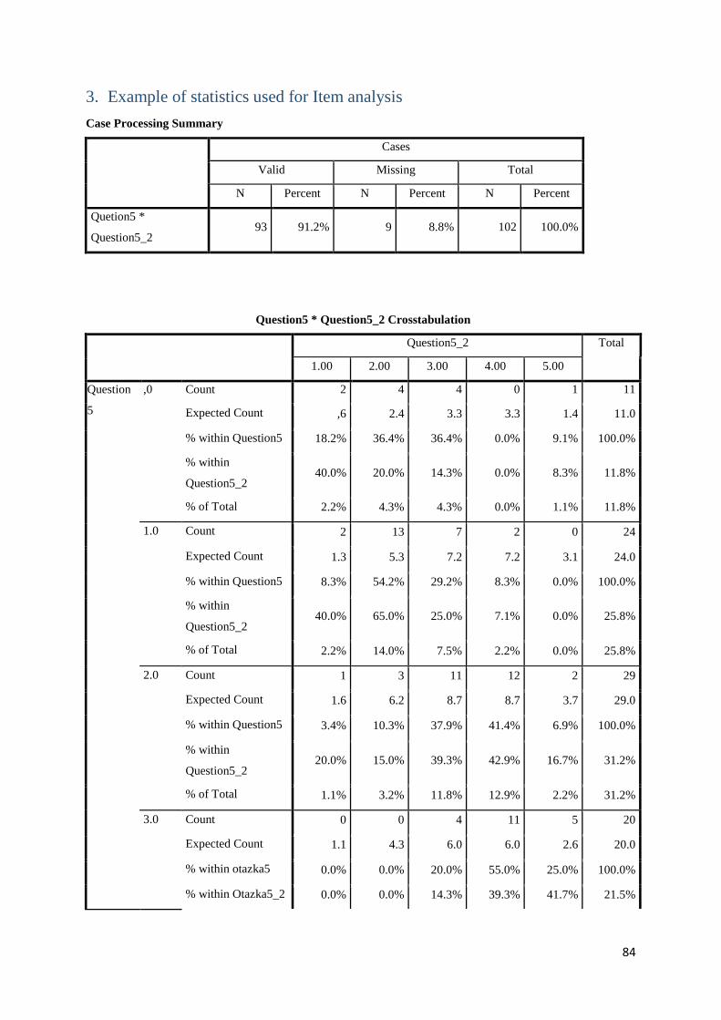
84

3. Example of statistics used for Item analysis

Case Processing Summary

Cases

Valid Missing Total

N Percent N Percent N Percent

Quetion5 *

Question5_2 93 91.2% 9 8.8% 102 100.0%

Question5 * Question5_2 Crosstabulation

Question5_2 Total

1.00 2.00 3.00 4.00 5.00

Question

5

,0 Count 2 4 4 0 1 11

Expected Count ,6 2.4 3.3 3.3 1.4 11.0

% within Question5 18.2% 36.4% 36.4% 0.0% 9.1% 100.0%

% within

Question5_2 40.0% 20.0% 14.3% 0.0% 8.3% 11.8%

% of Total 2.2% 4.3% 4.3% 0.0% 1.1% 11.8%

1.0 Count 2 13 7 2 0 24

Expected Count 1.3 5.3 7.2 7.2 3.1 24.0

% within Question5 8.3% 54.2% 29.2% 8.3% 0.0% 100.0%

% within

Question5_2 40.0% 65.0% 25.0% 7.1% 0.0% 25.8%

% of Total 2.2% 14.0% 7.5% 2.2% 0.0% 25.8%

2.0 Count 1 3 11 12 2 29

Expected Count 1.6 6.2 8.7 8.7 3.7 29.0

% within Question5 3.4% 10.3% 37.9% 41.4% 6.9% 100.0%

% within

Question5_2 20.0% 15.0% 39.3% 42.9% 16.7% 31.2%

% of Total 1.1% 3.2% 11.8% 12.9% 2.2% 31.2%

3.0 Count 0 0 4 11 5 20

Expected Count 1.1 4.3 6.0 6.0 2.6 20.0

% within otazka5 0.0% 0.0% 20.0% 55.0% 25.0% 100.0%

% within Otazka5_2 0.0% 0.0% 14.3% 39.3% 41.7% 21.5%

85

% of Total 0.0% 0.0% 4.3% 11.8% 5.4% 21.5%

4.0 Count 0 0 2 3 3 8

Expected Count ,4 1.7 2.4 2.4 1.0 8.0

% within Question5 0.0% 0.0% 25.0% 37.5% 37.5% 100.0%

% within

Question5_2 0.0% 0.0% 7.1% 10.7% 25.0% 8.6%

% of Total 0.0% 0.0% 2.2% 3.2% 3.2% 8.6%

5.0 Count 0 0 0 0 1 1

Expected Count ,1 ,2 ,3 ,3 ,1 1.0

% within Question5 0.0% 0.0% 0.0% 0.0% 100.0% 100.0%

% within

Question5_2 0.0% 0.0% 0.0% 0.0% 8.3% 1.1%

% of Total 0.0% 0.0% 0.0% 0.0% 1.1% 1.1%

Total Count 5 20 28 28 12 93

Expected Count 5.0 20.0 28.0 28.0 12.0 93.0

% within Question5 5.4% 21.5% 30.1% 30.1% 12.9% 100.0%

% within

Question5_2 100.0% 100.0% 100.0% 100.0% 100.0% 100.0%

% of Total 5.4% 21.5% 30.1% 30.1% 12.9% 100.0%

Directional Measures

Value

Asymp. Std.

Errora Approx. Tb Approx. Sig.

Ordinal by Ordinal Somers' d Symmetric 0.55 0.06 8.82 0.00

Question5 Dependent 0.56 0.06 8.82 0.00

Question5_2

Dependent 0.55 0.06 8.82 0.00

Nominal by

Interval

Eta Question5 Dependent 0.63

Question5_2

Dependent 0.66

a. Not assuming the null hypothesis.

86

b. Using the asymptotic standard error assuming the null hypothesis.

Symmetric Measures

Value

Asymp. Std.

Errora Approx. Tb Approx. Sig.

Nominal by Nominal 0.78 0.000 0.00

0.39 0.000 0.00

0.62 0.000 0.00

Ordinal by Ordinal 0.53 0.06 8.82 0.00 0.00

0.69 0.07 8.82 0.00 0.00

0.64 0.07 8.02 0.00c 0.00

Interval by Interval 0.62 0.07 7.48 0.00c 0.00

N of Valid Cases 93

a. Not assuming the null hypothesis.

b. Using the asymptotic standard error assuming the null hypothesis.

c. Based on normal approximation.

87

4. Inter-item correlation table

Spearman

Kendall

Tau Spearman

Kendall

Tau

Question46 0.71 0.65 Question53 0.50 0.43

Question5 0.64 0.55 Question40 0.49 0.44

Question25 0.64 0.54 Question42 0.48 0.43

Question23 0.63 0.55 Question57 0.47 0.39

Question43 0.63 0.55 Question27 0.47 0.41

Question21 0.61 0.51 Question13 0.47 0.39

Question20 0.60 0.52 Question6 0.47 0.40

Question12 0.60 0.53 Question49 0.45 0.40

Question11 0.59 0.49 Question15 0.42 0.36

Question16 0.59 0.50 Question55 0.41 0.35

Question48 0.59 0.50 Question45 0.40 0.33

Question7 0.59 0.51 Question60 0.40 0.34

Question17 0.59 0.49 Question10 0.40 0.34

Question2 0.58 0.51 Question4 0.35 0.31

Question47 0.57 0.48 Question9 0.34 0.28

Question26 0.57 0.48 Question36 0.33 0.28

Question31 0.57 0.49 Question19 0.33 0.29

Question3 0.55 0.47 Question44 0.32 0.27

Question28 0.55 0.46 Question54 0.32 0.27

Question41 0.55 0.46 Question33 0.32 0.27

Question30 0.55 0.46 Question14 0.31 0.28

Question56 0.55 0.46 Question24 0.31 0.26

Question51 0.54 0.46 Question8 0.29 0.26

Question58 0.54 0.45 Question38 0.26 0.22

Question52 0.53 0.45 Question59 0.25 0.22

Question37 0.52 0.45 Question39 0.24 0.21

Question22 0.52 0.45 Question18 0.22 0.19

Question34 0.52 0.46 Question29 0.14 0.11

Question35 0.52 0.43 Question1 -0.37 -0.31

Question32 0.51 0.44

Question50 0.50 0.43 Average 0.57 0.49

Table 19: Inter-item correlations between ipsative and normative form