Search for the sources of ultra-high energycosmic rays with the

Pierre Auger Observatory

Von der Fakultat fur Mathematik, Informatik und Naturwissenschaften derRWTH Aachen University zur Erlangung des akademischen Grades eines

Doktors der Naturwissenschaften genehmigte Dissertation

vorgelegt von

Markus Lauscher, M.Sc. RWTH

aus Rohren

Berichter: Universitatsprofessor Dr. rer. nat. Thomas HebbekerUniversitatsprofessor Dr. rer. nat. Christopher Wiebusch

Tag der mundlichen Prufung: 02.12.2016

Diese Dissertation ist auf den Internetseiten der Hochschulbibliothek online verfugbar

Erstgutachter und Betreuer

Prof. Dr. Thomas HebbekerIII. Physikalisches Institut ARWTH Aachen

Zweitgutachter

Prof. Dr. Christopher WiebuschIII. Physikalisches Institut BRWTH Aachen

i

Test

ii

Contents

1. Introduction 3

2. Ultra-High Energy Cosmic Rays 52.1. Introduction . . . . . . . . . . . . . . . . . . . . . . . . . . . . . . . . . . 52.2. Extensive Air Showers . . . . . . . . . . . . . . . . . . . . . . . . . . . . 6

2.2.1. Detection Techniques . . . . . . . . . . . . . . . . . . . . . . . . . 92.3. Acceleration and Possible Sources of Cosmic Rays . . . . . . . . . . . . . 102.4. Magnetic Fields . . . . . . . . . . . . . . . . . . . . . . . . . . . . . . . . 13

2.4.1. The Galactic Magnetic Fields (GMF) . . . . . . . . . . . . . . . . 132.4.2. The Extra-Galactic Magnetic Field (EGMF) . . . . . . . . . . . . 14

2.5. Status of Searches for Anisotropies in the Arrival Directions of UHECRs 14

3. The Pierre Auger Observatory 193.1. The Fluorescence Detector . . . . . . . . . . . . . . . . . . . . . . . . . . 19

3.1.1. Reconstruction of FD Events . . . . . . . . . . . . . . . . . . . . 203.2. The Surface Detector . . . . . . . . . . . . . . . . . . . . . . . . . . . . . 24

3.2.1. Reconstruction of Vertical SD Events . . . . . . . . . . . . . . . . 243.2.2. Reconstruction of Horizontal SD Events . . . . . . . . . . . . . . 263.2.3. Coverage, Trigger Efficiency and Angular Resolution of the SD . . 27

3.3. AugerPrime . . . . . . . . . . . . . . . . . . . . . . . . . . . . . . . . . . 293.3.1. The Surface Scintillator Detectors (SSD) . . . . . . . . . . . . . . 303.3.2. Surface Detector Upgrade . . . . . . . . . . . . . . . . . . . . . . 313.3.3. The Underground Muon Detector (UMD) . . . . . . . . . . . . . 313.3.4. Extended FD Duty Cycle . . . . . . . . . . . . . . . . . . . . . . 323.3.5. Photon Detectors for AugerPrime . . . . . . . . . . . . . . . . . . 32

4. Dynamic Range Measurements and Calibration of SiPMs 354.1. Introduction . . . . . . . . . . . . . . . . . . . . . . . . . . . . . . . . . . 35

4.1.1. SiPM Overview . . . . . . . . . . . . . . . . . . . . . . . . . . . . 364.1.2. The Energy Reconstruction Challenge . . . . . . . . . . . . . . . 38

4.2. Experimental Setup . . . . . . . . . . . . . . . . . . . . . . . . . . . . . . 394.2.1. Custom-made LED Pulser: the “Universal Pulser” . . . . . . . . . 404.2.2. Characterised SiPMs . . . . . . . . . . . . . . . . . . . . . . . . . 42

4.3. Preparatory Measurements: Basic SiPM Features . . . . . . . . . . . . . 434.3.1. Charge per Cell and Breakdown Voltage . . . . . . . . . . . . . . 444.3.2. Dark Count Rate and Cross-talk Probability . . . . . . . . . . . . 454.3.3. Exposing the SiPM to Long-lasting and Intensive Light Fluxes . . 47

iii

4.4. The Dynamic Range: Measurement Procedure and Analysis . . . . . . . 484.4.1. General Measurement Setup . . . . . . . . . . . . . . . . . . . . . 484.4.2. Conversion of the Photodiode Current to Photons on the SiPM . 514.4.3. Conversion of SiPM Charge Spectra to Average Number of Fired

Cells . . . . . . . . . . . . . . . . . . . . . . . . . . . . . . . . . . 534.5. The Dynamic Range: Results and Discussion . . . . . . . . . . . . . . . . 55

4.5.1. The Calibration Method . . . . . . . . . . . . . . . . . . . . . . . 584.5.2. Discussion . . . . . . . . . . . . . . . . . . . . . . . . . . . . . . . 59

4.6. Summary and Conclusions . . . . . . . . . . . . . . . . . . . . . . . . . . 63

5. The Needlet Wavelet Analysis Method 675.1. Introduction . . . . . . . . . . . . . . . . . . . . . . . . . . . . . . . . . . 675.2. The Needlet Wavelet Analysis . . . . . . . . . . . . . . . . . . . . . . . . 67

5.2.1. Spherical Harmonics Expansion . . . . . . . . . . . . . . . . . . . 685.2.2. The Needlet Wavelet . . . . . . . . . . . . . . . . . . . . . . . . . 705.2.3. Convolution of Signal and Needlet . . . . . . . . . . . . . . . . . . 715.2.4. Normalisation and Threshold Cut . . . . . . . . . . . . . . . . . . 735.2.5. Combination of Skymaps and Anisotropy Search . . . . . . . . . . 80

6. Monte Carlo Benchmark Studies and Optimisations 836.1. Overview . . . . . . . . . . . . . . . . . . . . . . . . . . . . . . . . . . . . 836.2. Resolution and Binning of the Data . . . . . . . . . . . . . . . . . . . . . 836.3. Benchmark Scenarios and Results . . . . . . . . . . . . . . . . . . . . . . 84

6.3.1. Dipole and Quadrupole Scenarios . . . . . . . . . . . . . . . . . . 856.3.2. Single Point Source Scenario . . . . . . . . . . . . . . . . . . . . . 936.3.3. Single Point Deflected through the GMF . . . . . . . . . . . . . . 986.3.4. Combined Dipole and Point Source Scenario . . . . . . . . . . . . 1046.3.5. Catalogue Based Scenario . . . . . . . . . . . . . . . . . . . . . . 1096.3.6. Analysis Parameters . . . . . . . . . . . . . . . . . . . . . . . . . 115

6.4. Performance of the Angular Power Spectrum compared to the NeedletWavelet Analysis . . . . . . . . . . . . . . . . . . . . . . . . . . . . . . . 1166.4.1. The Angular Power Spectrum in Case of an Incomplete Sky Coverage1166.4.2. Discussion . . . . . . . . . . . . . . . . . . . . . . . . . . . . . . . 121

6.5. Summary . . . . . . . . . . . . . . . . . . . . . . . . . . . . . . . . . . . 126

7. Data Set 1277.1. Correction for Detector Effects . . . . . . . . . . . . . . . . . . . . . . . . 127

8. Data Analysis 1298.1. Global Anisotropy Search . . . . . . . . . . . . . . . . . . . . . . . . . . 1298.2. A Detailed Look at the Dipole Scale . . . . . . . . . . . . . . . . . . . . 136

8.2.1. Dipole Position . . . . . . . . . . . . . . . . . . . . . . . . . . . . 1368.2.2. Dipole Amplitude . . . . . . . . . . . . . . . . . . . . . . . . . . . 1388.2.3. Cross-checks of the Observed Dipolar Pattern . . . . . . . . . . . 138

iv

8.2.4. Summary and Discussion of the Results of the Dipole Scale . . . . 1438.3. Search for a Point Source Deflected through the (Extra) Galactic Mag-

netic Field . . . . . . . . . . . . . . . . . . . . . . . . . . . . . . . . . . . 1458.3.1. Simulation and Analysis . . . . . . . . . . . . . . . . . . . . . . . 1458.3.2. Extra-galactic Magnetic Field . . . . . . . . . . . . . . . . . . . . 1458.3.3. Galactic Magnetic Field . . . . . . . . . . . . . . . . . . . . . . . 1468.3.4. Detection of the Particles at Earth . . . . . . . . . . . . . . . . . 1488.3.5. Defining the Region of Interest . . . . . . . . . . . . . . . . . . . 1498.3.6. Analysis . . . . . . . . . . . . . . . . . . . . . . . . . . . . . . . . 1538.3.7. Results and Discussion . . . . . . . . . . . . . . . . . . . . . . . . 156

9. Summary 159

Bibliography 173

A. Appendix 175A.1. List of Abbreviations . . . . . . . . . . . . . . . . . . . . . . . . . . . . . 175

B. Appendix 177B.1. Additional Plots: Benchmark Scenarios and Results . . . . . . . . . . . . 177B.2. Additional Plots: Performance of the Angular Power Spectrum compared

to the Needlet Wavelet Analysis . . . . . . . . . . . . . . . . . . . . . . . 184B.3. Additional Plots: Auger Data Analysis . . . . . . . . . . . . . . . . . . . 187

Acknowledgements 189

C. Declaration of pre-released extracts 191

1

1. Introduction

The observation that the earth is constantly hit by highly energetic particles, nowadaysreferred to as cosmic rays, dates back to the year 1912 and to Victor Hess and his balloonflight experiments. In 1938, by using distant coincidence detectors, Pierre Auger realisedthat the impact of these cosmic rays create cascades of particles in the form of extensiveair showers in the atmosphere.

Ever since cosmic rays have been extensively studied using these extensive air showersto reconstruct their properties. However, the most energetic of these particles, rangingfrom 1018 eV to over 1020 eV, still pose many questions - first and foremost: What istheir origin?

One way to address this question is to analyse their measured arrival directions at earthin search for possible source regions in, and more likely, outside of our galaxy. This ischallenging, as cosmic rays are charged nuclei and are hence deflected by magnetic fieldsin and between galaxies. This deflection becomes even stronger in the case of heavynuclei. This leads to a largely isotropic distributions of their arrival directions at earth.

In this work two approaches are used to address this challenge. First a Needlet Waveletbased analysis method is used to search for patterns in the arrival distribution of theseultra-high energy cosmic rays (UHECRs), measured at the worlds largest observatoryfor UHECRs: The Pierre Auger Observatory in Argentina. This technique was origin-ally introduced to search for structures in the, also highly isotropic, cosmic microwavebackground.

The second approach lies in the currently undergoing upgrade of the Pierre AugerObservatory. One goal of the upgrade is to achieve the capability of measuring the masscomposition of cosmic rays on an event by event basis. Currently this is only possibleon a statistical basis. This would allow future searches for patterns in the measuredarrival directions to be restricted to the lightest and hence least deflected cosmic rays.One necessary component of this upgrade is the deployment of a new detector withefficient, robust and cost-effective light sensors with a sufficient dynamic range. Silicon-Photomultipliers (SiPMs) are a recent form of semiconductor light detectors that couldfulfil these requirements. To establish this it is necessary to characterise their responseto a wide range of light fluxes and to be able to reconstruct the incident signal fromtheir response. In this work a dedicated technique to achieve this characterisation andreconstruction is developed.

This work is structured as follows. In chapter 2 an introduction to cosmic rays isgiven. This includes a description of their properties, observational techniques usingextensive air showers, the effect galactic and extra-galactic magnetic fields have on theirpropagation and an overview over the current status in search for patterns in theirmeasured arrival directions.

3

In chapter 3 the Pierre Auger Observatory, the techniques used to reconstruct theproperties of observed cosmic rays and the components of the upgrade of the PierreAuger Observatory: AugerPrime are described.

Chapter 4 details a technique to fully characterise the response of SiPMs, from verylow light fluxes up to saturation, and describes a method to reconstruct the incidentsignal from their response.

The main part of this work consists in the analysis of the measured arrival directionsat the Pierre Auger Observatory. The Wavelet analysis method used to analyse thearrival directions is described in chapter 5.

In chapter 6 the optimal choice of the free parameters of the analysis method isdetermined and its sensitivity is compared to another commonly used analysis method:The angular power spectrum.

Chapter 7 gives an overview on the used data set and the applied corrections to ensureno artificial patterns are introduced in the analysis.

Finally, the method is applied to the data in chapter 8. In the first step a search forpatterns of any angular scale in the data is performed. As this leads to the detectionof a dipolar pattern this pattern is fully characterised in the second step. Lastly, theanalysis is restricted to a portion of the sky to study possible signals from Centaurus A,the active galactic nuclei closest to earth and a suspected source of UHECRs.

This thesis ends in chapter 9 with a summary of all obtained results.

4

2. Ultra-High Energy Cosmic Rays

In this chapter we give a general overview over ultra-high energy cosmic rays (UHECRs).We begin with a general description of their properties and the energy spectrum at earthin section 2.1. Afterwards, in section 2.2, we describe the extensive air showers theycause in the atmosphere. In the following, we discuss possible origins for cosmic rayswithin our galaxy in section 2.3 and of even higher energy cosmic rays from outside ourgalaxy in section 2.3. This includes a discussion of the magnetic fields the cosmic rayspropagate through their way to earth. Finally, we describe the status of the search forpatterns, and hence possible origins, in the observed arrival directions of UHECRs atearth in section 2.5.

2.1. Introduction

The observation that the earth is constantly hit by high-energy particles dates back over100 years to Victor Hess and his balloon flights. Today, they are referred to as cosmicrays and have been studied extensively ever since. Cosmic rays are defined as chargedparticles that originate from outside the solar system and range from kinetic energies Eof 106 eV to above 1020 eV [1].

The focus in this work is on ultra-high energy cosmic rays (UHECRs). While there isno clear demarcation where the ultra-high energy range starts, we refer to cosmic rayswith energies E above 1018 eV (= 1 EeV) as UHECRs. For low energies E the cosmicray flux is modulated by the sun but above E ≈ 1011 eV the spectrum dN/dE of cosmicrays can be approximated by a power law

dN/dE ∝ E−γ (2.1)

with spectral index γ ≈ 2.7 [1]. The power law has a very steep slope and hence the fluxfalls rapidly with the energy. While the rate is around one particle per square metre andsecond at 1012 eV, it drops to one particle per square kilometre and year around 1018 eVand even down to one particle per square kilometre and century around 1020 eV. Dueto the steeply falling flux a direct observation of UHECRs via satellites is not possible.Instead large, ground based observatories are required which study the extensive airshowers which cosmic rays cause in the atmosphere.To compare experiments of different size and acceptance usually the differential flux Φof cosmic rays

Φ(E) =dN

dE · dA · dΩ · dt(2.2)

5

is reported. Here N is the number of particles, A the area of the detector, Ω the solidangle and t the active time of the detector. This differential spectrum, as obtained byvarious measurements, is shown at the top of figure 2.1. At the bottom the spectrum isalso shown but weighted with E2.5 to enhance particular features of the spectrum: Upto energies of 1015 eV, the ’knee’, the flux follows a power law with a spectral index ofγ = 2.7 [3]. After the knee the spectrum steepens to an index of γ = 3.1, a furthersteepening occurs at the ’second knee’ around an energy of 4 · 1017 eV. Finally at the’ankle’, around energies of 4 · 1018 eV, the spectrum flattens again with an index ofγ = 2.6 [3]. After around 4 · 1019 eV a suppression of the flux becomes apparent [1].Later in the chapter we discuss possible reasons for the observed structures.

Almost all chemical elements have been observed in cosmic rays arriving at earth [2].Shown in figure 2.2 is the abundance of elements at a kinetic energy around 1 GeV pernucleon, normalised to the abundance of silicon. As a comparison the abundance ofelements in the solar system is also shown. On average cosmic rays are composed ofmainly nuclei (92%) and electrons (2%) [4]. Of the nuclei protons dominate with 98%followed by helium (15%) and the remainder being heavier elements [4]. However, thecomposition of UHECRs is still largely unknown. Measurements by the Pierre AugerCollaboration suggest a transition of a proton dominated mixed flux around 1018 EeVtowards a heavier composition at higher energies [5]. Measurements by the HiRes andTelescope Array Collaboration however suggest a proton composition up to the highestenergies [6, 7]. In both cases the interpretation of the achieved results depends onMonte Carlo (MC) simulations which use different models describing the propagation ofparticles in the air-shower cascade. With the upgrade of the Pierre Auger Observatory amodel-independent measurement of the composition could be possible (see section 3.3).In the following we discuss the extensive air showers cosmic rays cause in the atmosphere,and techniques to reconstruct the properties of the arriving cosmic ray particles.

2.2. Extensive Air Showers

When a cosmic ray particle of high energy impacts the atmosphere, it usually undergoesan inelastic scattering with an air molecule. This first interaction creates a multitudeof additional particles, which in turn create new particles leading to a self-sustainingcascade. A schematic of this is shown on the left-hand side of figure 2.3. The shower canbe considered to consist of three components: an electromagnetic, a hadronic and a piongenerated muonic/neutrino component [1]. In the most simple case the primary particleis a photon or an electron and the shower will only consist out of an electromagneticcascade. In this case the photons produce electron-positron pairs by the interactionwith a nucleus N via γ + N −→ e+e− + N and the electrons/ positrons generateBremsstrahlung via e± +N → e± + γ +N . The produced Bremsstrahlung photons canthen again create electron-positron pairs and so on. The cascade terminates when theenergy of the electrons and positrons drops below the critical energy of EC ≈ 80 MeVin air, where they start loosing more energy via ionisation then through radiation [1].

6

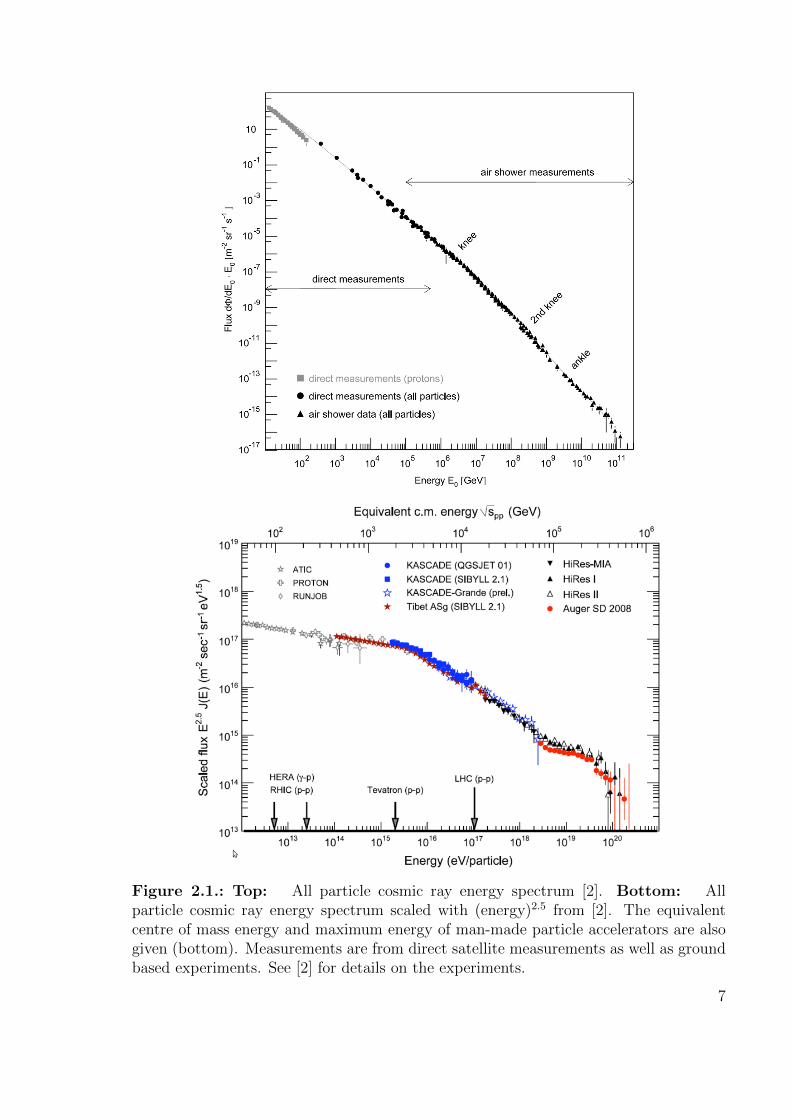
Figure 2.1.: Top: All particle cosmic ray energy spectrum [2]. Bottom: Allparticle cosmic ray energy spectrum scaled with (energy)2.5 from [2]. The equivalentcentre of mass energy and maximum energy of man-made particle accelerators are alsogiven (bottom). Measurements are from direct satellite measurements as well as groundbased experiments. See [2] for details on the experiments.

7

Figure 2.2.: Abundance of elements in cosmic rays at energies around a kinetic energyof 1 GeV per nucleon as a function of their nuclear charge Z. The grey filled, upwardpointing triangles show the abundance of elements in the solar system. Taken from [2].See [2] for details on the experiments.

Figure 2.3.: Left: Illustration of the three main components of an extensive air shower.Right: Illustration of detection mechanisms. The shower particles form a shower frontof several meters thickness and a lateral extend in the order of kilometres. The particlesimpacting the ground level can be studied by an extensive array of surface detector(SD) stations. The propagation of the particles through the air can be observed viaoptical, ground based telescopes. This fluorescence detector (FD) stations observe theisotropically emitted fluorescence light caused by the propagation of the electromagneticcascade through the atmospheric nitrogen. Taken from [8].

8

In the more general and common case where the primary particle is a nucleus, thefirst collision will produce new nuclei, neutral and charged pions (π±, π0) and kaons(K±, K0

S/L). These hadrons then collide with further air molecules driving the hadroniccomponent forward, or, depending on their lifetime and density of the atmosphere sur-rounding them, decay before interacting. For example the charged pions, with a lifetimeof τ = 2.6 · 10−8 s [9], decay mainly via π± −→ µ± + ν. Especially at higher altitudeswith a less dense atmosphere, pions may decay before interacting, giving rise (togetherwith the charged kaons) to the muonic component of the shower [1]. Due to the ratherlong muon lifetime of τ = 2.2 · 10−6 s and the very low neutrino cross-section these com-ponents largely decouple from the shower development.The produced neutral pions have a very short lifetime of τ = 8.4 · 10−17 s and decaynearly instantly via π0 −→ γ+ γ (98.8% of decays) or π0 −→ e+e−+ γ (1.2% of decays)[9] giving rise to the previously described electromagnetic cascade. During the showerdevelopment about 85-90% of the energy of the primary particle will be transferred tothe electromagnetic component of the shower [1].

On a macroscopic level the shower moves towards the ground with nearly the speed oflight. The shower particles form a shower front, with a thickness of up to a few metres,while the lateral extent can reach several kilometres. The air shower ends when theinvolved particles have insufficient energy to drive the cascade further, or the showerimpacts on the ground.

At sea level a 1019 eV vertical, proton induced shower, will have around 3·1010 particles.Of these 99% will be photons and electrons/positrons in a 6 to 1 ratio carrying around85% of the energy. The remaining particles are muons with an energy around 1 GeVand carrying 10% of the energy, pions also with a typical energy of 1 GeV, carrying 4%of the energy. The remainder consists of kaons, neutrinos and baryons [1].

A more detailed discussion of extensive air showers can be found in [10].

2.2.1. Detection Techniques

One method to gain information about the primary particle is to study the absolutenumber and the distribution of the electrons/positrons and muons on the ground. Bymeasuring the distribution of particles on the ground, together with the information ontheir arrival time, it is possible to reconstruct the energy of the primary particle, as wellas the arrival direction. This method can be dated back to the late 1930s and to P.Auger, who used Wilson chambers and Geiger Muller tubes to study coincidences. Hewas able to find coincidences from counters separated up to 300 m and concluded thatthis was due to secondary particles generated by cosmic rays.With this method, the reconstruction of the energy of the primary particle normally relieson shower simulations, introducing systematic uncertainties on the result. A schematicview of this principle of using the lateral distribution of the ground particles is shownon the right-hand side of figure 2.3.Another method to gain information about the primary particle is to study the longit-udinal shower profile using optical telescopes. Here the electromagnetic component isvery significant as it carries about 90% of the cascade components. The longitudinal

9

profile can be studied using the emission of fluorescence or Cherenkov light the electro-magnetic component of the shower causes in the atmosphere. This is also illustratedon the right-hand side of figure 2.3. A detailed over-view on the historical evolution ofexperiments studying UHECRs and of observational techniques of extensive air showerscan be found in [11]. In the next chapter we illustrate both lateral and longitudinalreconstruction techniques using the example of the Pierre Auger Observatory.

2.3. Acceleration and Possible Sources of Cosmic Rays

As described the cosmic ray spectrum follows a power law. To accelerate particles to highenergies and to give rise to a power-law spectrum ’stochastic-acceleration’ is consideredas a likely mechanism. First introduced by Fermi in 1949 [12] and further refined (e.g.[13, 14]) to what is now referred to as ’diffusive shock acceleration’. The general idea isthe transfer of energy from a moving shock front to a particle. Such shock fronts can, forexample, exist in front of expanding supernova remnants (SNR) as the velocity is muchlarger than the surrounding interstellar medium [1]. Regardless of the specific nature ofthe shock front the general idea behind the acceleration is the same. A particle, boundto the shock region of extent rs by a magnetic filed of strength B, bounces back and forthacross the shock front. Each passing of the front leads to an energy gain proportionalto β on average, where β is the velocity of the shock front in units of the speed of lightor, in a more generalized manner, the ’efficiency’ of the accelerator. In the case of anon relativistic moving shock front the energy gain by one pass back and forth throughthe shock is 4

3β [10]. During each passing with energy gain ∆E = εE there is a chance

Pesc for the particle to escape the source region. This leads (see e.g. [10]) naturally toa power law spectrum where the number of particles N remaining in the source regionwith an energy greater En is given by

N(En) ∝ 1

Pesc

(EnE0

)−γ. (2.3)

With

γ =Pesc

ε. (2.4)

Hillas [15] summarized the maximum achievable energy Emax via this process by

Emax = βze

(B

1µG

)(rs

1kpc

)EeV (2.5)

with Ze being the charge of the accelerated particle. Hence the larger the source regionand the larger the magnetic field the higher energies are possible.

Within our galaxy SNR are considered as a likely source for cosmic rays. Indeed, ifonly 5% - 10% of the kinetic energy in SNR would be transferred to the acceleration ofcosmic rays this would be sufficient to explain the observed flux [1].

Using this mechanism a possible explanation of the observed steepening of the cosmicray flux at the knee could be that here galactic accelerators become insufficient to

10

accelerate protons to even higher energies. As heavier particles can be accelerated tohigher energies, proportional to their charge, the steepening can be explained by thegradual disappearance of elements from the flux until even iron cannot be accelerated tohigher energies, here we observe the second knee [1]. In this transition the extra-galacticcosmic ray flux becomes dominant until the spectrum flattens again at the ankle [3].This rigidity1 dependent flux change could e.g. explain the obtained flux measurementsof the Kascade Collaboration [1, 16]. Another explanation for the features in the fluxis a rigidity dependent escape of the particles from the galaxy [3] when the galacticmagnetic field is no longer strong enough to contain them.

Much less is known on the origin of extra-galactic cosmic rays which likely dominatethe flux above the ankle. In 1984, Hillas [15] summarized the requirements on possiblesource regions to accelerate cosmic rays to a certain energy in what is now referred to asa ’Hillas diagram’. A modern version of this plots is shown in figure 2.4. As equation 2.5indicates, only a source region of sufficient size and/or with a sufficient magnetic field iscapable to accelerate particles above a certain energy. In the case of figure 2.4 this energyis 100 EeV. As can be seen even for relativistic shocks or highly efficient accelerators(i.e. β = 1), only few known objects can accelerate iron and even fewer objects protonsto such high energies. Rapidly rotating Neutron stars or pulsars and gamma-ray bursts(GRB), despite their relatively small size, posses a high enough magnetic field to bepossible sources candidates. Other possible sources are active galactic nuclei (AGN)both in their core region containing super-massive black holes or in the jets they extendover long distances into the galaxy [1]. With exception of the pulsar the source of theenergy is accretion of matter onto stars and consequent collapse into a black hole (GRB)or onto a central black hole (AGN). The transfer of angular momentum from this flowforms an accretion disk which can lead to powerful plasma flow perpendicular to thedisk (jets). For a more detailed overview on both galactic and extra-galactic sources ofUHECRs and acceleration mechanisms see [17, 18].

The last observable feature in the cosmic ray spectrum is a rapid drop or cut-off of theflux near 4 · 1019 eV. One possible explanation is that here, similar to galactic sources ofcosmic rays, the sources of UHECRs reach their maximum energy. As in the case of theknee, this would result in a rigidity dependent cut-off [7]. However, the most prominentexplanation for the drop off is the Greisen-Zatsepin-Kuzmin cut-off (GZK cut-off). Atenergies above about 4·1019 eV photo-hadronic interactions between protons and photonsof the cosmic-microwave background lead to the production of pions

pγ → N + nπ

or to the production of e+e− pairs

pγ → p+ e+e−.

1The rigidity of a particle is its momentum p (or energy E in the relativistic limit) divided by itscharge Ze and is an indicator of its resistance to being deflected by a magnetic field. At the sameenergy, particles with a larger charge will be deflected more strongly.

11

Figure 2.4.: Hillas diagram of possible source regions of UHECRs based on equation 2.5.To accelerate a particle above 100 EeV the source region must lie above the correspondinglines. Taken from [1].

Here N is a nucleon and n the number of produced pions [3]. For heavier nucleiphoto-disintegration on cosmic microwave background (CMB) and IR-UV photons canoccur and break up nuclei at ultra-high energies. This effect is especially strong fornuclei with a mass number A < 20 which cannot travel farther than a few Mpc withoutdisintegrating [3].

As the mass-composition of UHECRs is currently unclear (see section 2.1), an answeron the origin of the cut-off is currently not possible. In the future it could be addressedwith the proposed upgrade of the Pierre Auger Observatory (see section 3.3). For anoverview on experimental results on UHECRs from the ankle to the cut-off and possibleexplanations for the cut-off see [7].

12

2.4. Magnetic Fields

While we outlined possible sources of UHECRs in the previous section to date no sourceshave been found experimentally. One likely contributor to this observation is the exist-ence of magnetic fields which exist throughout the universe [19]. During propagation toearth UHECRs are deflected by the magnetic fields via the Lorentz force

dp

dt= Zv ×B, (2.6)

where p is the relativistic momentum, Z the charge and v the velocity (approximatelythe speed of light) of the cosmic ray and B the magnetic field vector. This leads to agyroradius rg of the particle of:

rg ∝E

ZeB⊥, (2.7)

and a deflection angle ϑ of a cosmic ray travelling a distance D rg of [20]:

ϑ =D

r. (2.8)

Hence cosmic rays are deflected with a strength inversely proportional to their rigidityE/Z and thus the deflection depends on the charge and energy of UHECRs.

In general magnetic fields in the universe will not be aligned but are turbulent withonly a certain coherence length lc. If an ensemble of cosmic rays travels from a singlesource over a certain distance d lc through a magnetic field with average strengthBrms this can be viewed as a directed random walk and will result, with respect to anobserver, in an average smearing around the source of:

σrms = 0.87

[41 EeV

E/Z

Brms

5 µG

√d

2 kpc

√lc

50 pc

](2.9)

in the limit of small deflections [21]. Here the units have been chosen relevant to thegalactic magnetic field with typical field strengths of a few µG and coherence lengths ofup to 100 pc [21]. Equation 8.2 on page 145 uses units more appropriate to extra-galacticmagnetic fields.

In the following we give a short overview on the galactic and extra-galactic magneticfields and their expected effects on the propagation of UHECRs.

2.4.1. The Galactic Magnetic Fields (GMF)

In comparison to the extra-galactic magnetic field (EGMF) (see next section) more isknown about the GMF. The currently most advanced, observation based model of theGMF exists in the form of the JF12 model [22, 23]. The model was obtained usingsynchrotron measurements of the WMAP satellite and Faraday rotation measurementsof extragalactic sources. A description of the observational results used and a derivationof the model can be found in [22, 23]. This model will be used in section 8.3 in this

13

thesis. In the following we give an overview over the components of the model and byproxy an overview of the structure of the GMF.The model is composed out of three main parts, i) a coherent large-scale field, withdisk, halo and out-of-plane components, ii) a random field with spatially-varying fieldstrength and iii) a striated random field [22, 23]. The structure and strength of thefield is illustrated in figure 2.5. The coherent large-scale disk field is shown on the top,right-hand side of the figure. Around an inner toroidal core of inner radius of 3 kpcand of an outer radius of 5 kpc the field follows a logarithmic-spiral geometry along andbetween the spiral arms of the galaxy. The typical strength of this field is around 1µG. The average strength of the random (turbulent) field also follows this structure asillustrated on the top, left-hand side of figure 2.5. The disc field is super-imposed withan X-shaped field perpendicular to the galaxy and symmetric in azimuth as illustrated atthe bottom of figure 2.5. The striated random field is scaled with the strength of the discfield with is aligned either parallel or anti-parallel to it on a scale around 100 pc. Thefinal component is a toroidal halo component [22, 23]. The expected average deflectionby this GMF model for cosmic rays, averaged over cosmic rays arriving isotropically atearth, is shown on the bottom, left-hand side of figure 2.6. As can be seen, even for aproton with an energy of 1019 eV the average deflection will be around 30 making theidentification of UHECRs, especially in case of a heavy composition, challenging. Dueto the structure of the GMF the average deflection will depend upon the point of entryin the galaxy as is illustrated at the top, left-hand side of figure 2.6.

2.4.2. The Extra-Galactic Magnetic Field (EGMF)

The origin of EGMF (i.e. magnetic fields between galaxies) are not well known. Somemodels suggest their origin in the early universe while others see them as originatingfrom magnetic pollution from sources such as galactic winds from jets or radio galaxiesor a combination thereof [3]. Similar is the uncertainty on the expected deflection ofUHECRs, ranging from expectation of deflections around 10 − 20 down to less thana degree for protons with E > 100 EeV and sources with a distance up to 100 Mpc[26, 27, 3]. Current upper limits on the average strength of EGMFs are around 1 nG[28] and lower limits down to 10−6 nG [29].

An illustration of the expected deflection as a function of rigidity and various fieldstrengths is shown on the bottom, right-hand side of figure 2.6.

2.5. Status of Searches for Anisotropies in the ArrivalDirections of UHECRs

In the following we give a short overview on the current status on searches for anisotropiesin the arrival directions of UHECRs and hence the search for their sources. We focuson the two current largest UHECRs observatories, the Telescope array and the PierreAuger Observatory. With the former being located in the northern and the latter in

14

Figure 2.5.: Illustration of the components of the JF12 GMF model. Top,Left/Right: Random/Coherent field component and strength. In contrast to thecoherent field particles traversing through the random field will be deflected randomly,according to equation 2.9. Bottom: X-shaped coherent field shown as a cross-sectionthrough the galaxy. The field is symmetrical in azimuth. Modified from [23].

the southern hemisphere they are able the study cosmic rays arriving anywhere (if theirdata is combined) at earth up to the highest energies.

First we focus on results obtained by the Pierre Auger Observatory. A large scale fluxmodulation in right ascension (α) [30, 31] and in both declination (δ) and right ascension[32, 33, 31] has been reported by the Pierre Auger Collaboration from the analysis ofevents with zenith angles smaller than 60. The amplitude of the modulation is below∼ 2% at EeV energies, and shows a marginally significant indication of a transition froma direction near α ' 270 below 1 EeV, consistent with the direction of the galacticcentre, towards directions near α ' 100 above 4 EeV. The amplitude increases toseveral percent around 10 EeV. A more recent report from the Auger Collaboration,extending the maximum zenith angle up to 80 and using events up to the end of 2013,gives a hint of a large-scale dipolar anisotropy for energies E > 8 EeV [34]. Under the

15

Figure 2.6.: Top: Expected average deflection of 60 EeV protons in the JF12 GMFmodel, displayed by arrival direction in galactic coordinates. Modified from [23]. Left,Bottom: Expected average deflection as a function of particle rigidity in the JF-12GMF model. Modified from [24]. Right, Bottom: Expected average deflection as afunction of particle rigidity through an EGMF with a coherence length of 1 Mpc and anobserver distance of 10 Mpc. Modified from [25].

assumption that this flux is dominated by a dipole, the results correspond to a dipolewith an amplitude of r = (7.3± 1.5)% directed towards (α, δ) = (95± 13,−39± 13).A smoothed skymap of the data above 8 EeV in [34] is shown on the left-hand side offigure 2.7 indicating the dipolar structure.

At energies above 40 EeV the Pierre Auger Collaboration has searched for intrinsicanisotropies in cosmic rays by using angular auto-correlation and searching for possibleexcesses in circular windows across the exposed sky. The results of these studies werefound to be compatible with an isotropic expectation [35].

The region around the closest AGN to earth - Centaurus A - has also been studied.More specifically the expected vs. observed number of events as a function of the angulardistance to Centaurus A and as a function of the energy threshold between 40 and 80EeV was studied. The largest excess of events was observed at an angular distance of

16

Figure 2.7.: Left: Skymap of arrival directions in equatorial coordinates, measuredat the Pierre Auger Observatory with energies greater than 8 EeV, smoothed with a 45

filter [34]. An indication of a dipolar structure can be seen. Modified from [35]. Right:Exploration of a possible excess of events at a certain angular distance from CentaurusA using events detected at the Pierre Auger Observatory with an energy greater than58 EeV. Modified from [35].

15 and for an energy threshold of 58 EeV, with a penalized probability of 1.4% [35].This is illustrated on the right-hand side of figure 2.7.

The Telescope Array (TA) has recently observed a hotspot in the arrival direction ofUHECRs with E > 57 EeV with a post-trial probability of 3.7× 10−4. The hotspot lieswithin a 20 circle centred around (α, δ) = (147, 43) [36].

As the Telescope Array and the Pierre Auger Observatory together have access tothe complete sky, both collaborations have begun to analyse their combined data. Thelower limit of this analysis is due to the full-efficiency threshold of the TA which is at10 EeV. As both experiments do not necessarily share the same energy calibration aniterative method was used to determine the energy above which events measured bythe Auger Observatory were included in the analysis. To find this energy a declinationband in the sky, where both experiments are sensitive, was used and the Auger energythreshold was chosen to equalize the flux of both experiments. As a result Auger eventswith energies greater than 8.8 EeV, in terms of the Auger energy scale, were used inthe combined data set [37, 38]. By taking advantage of full sky coverage, the multipolecoefficients of the UHECR flux have been measured for the first time [37]. No significantdeviation from isotropic expectations was found in the angular power spectrum up tomultipoles ` = 20 and upper limits on the dipole and quadrupole moments were reportedas a function of the direction in the sky, varying between 8% and 13% for the dipoleand between 7.5% and 10% for a symmetric quadrupole. An update of this study [39]above 10 EeV, including one additional year of data recorded at the Telescope Array andextending the zenithal range of the data recorded at the Pierre Auger Observatory upto θ = 80 reconstructed a dipolar signal with an amplitude of r = (6.5± 1.9) % and achance probability of 5×10−3 with reference to a purely isotropic distribution. No otherdeviation from isotropy was observed neither on the quadrupolar or on other angular

17

scales. Due to the full-sky exposure this measurement of the dipole moment does not relyon any assumption on the underlying flux of cosmic rays. Furthermore, the resolutionof the quadrupole and higher order moments is the best obtained to present [39].

The origin of the observed dipolar anisotropy is currently unclear. A small dipolepattern of extra-galactic cosmic rays is expected due to our motion with respect to theframe in which they are isotropic. This is referred to as the Compton–Getting effect[40], and has been observed at lower energies, but the effect is expected to be below the1% level [40, 41]. Due to the inhomogeneous distribution of nearby galaxies, a dipolepattern may also be caused at energies around and above 1019 eV [41].

18

3. The Pierre Auger Observatory

The Pierre Auger Observatory is currently the largest experiment for the observation ofUHECRs and can observe cosmic rays with energies from 1017 eV to above 1020 eV [42].It is located in the Argentinian pampa near the town of Malargue. The observatoryis a hybrid detector consisting of a surface detector (SD) array of water-Cherenkovdetectors and a fluorescence detector (FD). The SD consists of 1600 detector stations,each filled with 12 tonnes of water, positioned in a hexagonal grid with 1500 m spacing.The surface detector uses the distribution and timing of the electrons and muons onthe ground to reconstruct the energy of the primary particle and its arrival direction asdescribed in the following. The resulting instrumented area of 3000 km2 is overlookedby the fluorescence detector. Each of the 27 FD fluorescence telescopes has a field ofview (FOV) of 30 x 30. 24 of these are housed in four telescope buildings, enclosingthe array. The remaining three of these are part of the HEAT extension of the AugerObservatory and are located near one of the telescope buildings, Coihueco, in threeindividual housings which can be tilted upwards by 29 degrees. This allows themto observe showers with a lower energy, down to 1017, which develop higher in theatmosphere [42]. A schematic view of the Auger Observatory is shown in figure 3.1.The hybrid, i.e. two detector-nature allows to calibrate the SD using a nearly calorimetricmeasurement of the shower in the atmosphere by the FD. Similarly the reconstructionaccuracy of the shower geometry can be significantly enhanced in ’hybrid’ events whereboth the FD and SD observe the same shower.

Unless otherwise noted the information in this chapter are based on [42, 44, 45].A detailed overview on the observatory operation, monitoring, detector systems andenhancements, reconstruction and performance of the Pierre Auger Observatory can befound in [42].

3.1. The Fluorescence Detector

As mentioned previously each of the regular 24 FD telescopes has a field of view of30 x 30 with 6 of them housed in the four fluorescence telescope buildings Coihueco,Loma Amarilla, Los Morados and Los Leones. Shown on the top, left-hand side of figure3.2 is a photograph of the Los Leones building and on the bottom, left-hand side ofthe figure a schematic view of a single FD telescope is shown. The aperture of thetelescope has a diameter of 2.2 m and consists of an optical filter and a corrector ring.After the aperture the light is focussed on the spherical focal surface by a sphericalmirror. The focal surface consists of 440 hexagonal camera pixels, each with a field ofview of 1.5 . Every pixel consists of one photomultiplier tube (PMT). The signal of

19

Figure 3.1.: Schematic layout of the Pierre Auger Observatory located near Malargue,Argentina. Blue and orange dots and lines indicate the position and FOV of the 5 FDdetector stations. Red dots indicate the central laser facility (CLF) and extreme laserfacility (XLF). The black dots show the SD detector stations, which are more denselyplaced in the infill-array near Coihueco. Also located there is the AERA radio extensionas indicated by the light blue circle. Source: http://augerpc.in2p3.fr/sites/default/files/augerbuilt 3045.jpg.

each pixel is digitised by an analogue to digital converter (ADC) with a sampling rateof 10 MHz. This time resolved signal is used for the reconstruction of first the showergeometry and then secondly the longitudinal shower profile as described in the nextsection. The 3 HEAT telescopes are functionally identical to the regular FD telescopeswith the exception that they are read-out with twice the sampling rate and they can betilted to observe lower energy showers higher in the atmosphere. With this configurationthe FD can observe events from 1017 eV up to the highest energies, reaching a triggerefficiency of 100% for energies above 1019 eV over the entire array of the surface detector.Since showers can only be observed during clear and moonless nights the duty cycle isaround 13%.

More detailed information on the FD can be found in [44].

3.1.1. Reconstruction of FD Events

A shower passing through the atmosphere excites the atmospheric nitrogen. Upon de-excitation the nitrogen emits fluorescence light isotropically. This light can be observed

20

Figure 3.2.: Top, Left: Photograph of the Los Leones telescope building. Shown arethe two central telescope apertures [42].Bottom, Left: Schematic illustration of one FD telescope. The incoming fluorescencelight is focused through the aperture onto the segmented mirror and background lightis reduced through an UV-pass filter. The camera consists of 440 photomultiplier tubes[42].Top, Right: Photograph of one SD detector station with its various components out-lined [42].Bottom, Right: Schematic illustration of one SD detector station. The passage ofparticles from an air shower causes the emission of Cherenkov light in the water withinthe detector. The walls of the detector are covered with reflective foil to increase theamount of light detected by the PMTs [43].

21

by the FD telescopes. The passing of a shower through an FD camera is illustrated inthe bottom, left-hand side of figure 3.3. The timing of the individual triggering of therespective pixels is colour coded. As the shower moves down in the atmosphere, firstthe pixels at the top of the camera are hit (due to the optics) and the shower imagemoves downwards. As camera pixels can also be triggered by other causes certain triggercriteria have to be met (for details see [44]) for a track in the camera to be consideredas caused by an air shower. Once a shower has been detected by the FD, its propertiescan be reconstructed.

The shower forms a shower-detector-plane (SDP) with the telescope as illustrated atthe top, left-hand side of figure 3.3. This plane is first determined as the plane throughthe telescope which most closely contains the pointing directions of the FD pixels centredon the shower axis as illustrated by the fitted line in the bottom, left-hand side of figure3.3.

Within the SDP the trigger time t(χi) of an individual pixel which observes an angleχi with respect to the SDP is related to the closest shower distance Rp of a showermoving with an angle χ0 with respect to the ground in the SDP:

t(χi) = T0 +Rp

ctan

(χ0 − χi

2

). (3.1)

Via minimisation using the observed times t(χi) the free parameters Rp, χ0 and thestart time T0 can be determined. Once the geometry is known, the collected light atthe aperture at a given time can be converted to the energy deposited by the showeras a function of the slant depth as illustrated at the top, right-hand side of figure 3.3.To achieve this, the light attenuation from the shower to the telescope needs to beaccounted for and all contributing light sources need to be distinguished. This includesthe fluorescence light, Cherenkov light and multiply scattered light. Once this is done,the fluorescence light intensity can be related to the deposited energy via the fluorescenceyield, which can be measured experimentally in the laboratory [46].

To determine the shower energy a Gaisser-Hillas function

fgh(X) =

(dE

dX

)max

(X −X0

Xmax −X0

)(Xmax−X)/λ

exp

(Xmax −X

λ

)(3.2)

is fitted to the energy deposit per slant depth (dE/dX). Here Xmax is the position ofthe shower maximum and X0 and λ are shape parameters. Finally, the calorimetricenergy of the shower is reconstructed by integrating equation 3.2 and correcting for the’invisible energy’ that is carried away by high energy muons and neutrinos.

In the case of the Pierre Auger Observatory the accuracy of the reconstruction of theshower geometry is significantly enhanced in ’hybrid events’, for which one or more SDdetector stations provide additional information on the position of the shower on theground. Likewise, the calorimetric measurement of the shower energy by the FD is usedto calibrate the energy reconstruction of the SD as illustrated in the bottom, right-handside of figure 3.2 and as explained in the next section.

22

Figure 3.3.: Top, Left: Illustration of the reconstruction of the geometry of theshower from observables of the FD. From the point of view of a telescope the showermoves within a plane the telescope forms with the shower axis: the SDP. For details onthe reconstruction see section 3.1.1 [44].Bottom, Left: Light-track of an air shower observed by two fluorescence telescopes.The trigger time of the individual triggered pixels is colour coded. The shower movesdownwards in time with respect to the camera. The black dots indicate the reconstruc-ted shower profile. Individual camera pixels are represented by the hollow circles. Pixelswhich were triggered but were determined as too far from the shower axis by the recon-struction algorithm or are out of time are marked with an X and are not included in thereconstruction [44].Top, Right: Reconstructed energy profile from the fluorescence light arriving atthe telescopes as a function of the slant depth. The black line illustrates a fit with aGaisser-Hillas function (see equation 3.2). The reconstructed energy of the shower isE = (3.0± 0.2) · 1019 eV [42].Bottom, Right: Calibration of the SD energy estimator S38 (see next section) usingthe energy EFD measured by the FD using many hybrid events [42].

23

3.2. The Surface Detector

Each SD detector station consists of a water tank of 3.6 m diameter and 1.2 m heightfilled with 12 m3 of ultra-pure water. All three PMTs of the Photonis XP1805/D1 typeare symmetrically distributed and at a distance of 1.2 m from the tank centre and at thetop of the tank. These collect the Cherenkov light that is emitted in the water by therelativistic electrons, positrons, muons and photons (that convert to electron-positronpairs in water) from the shower on the ground. To increase the collected light each tankis outlined with highly reflective liner. A photograph and a schematic view of one SDdetector station is shown on the top and bottom, right-hand side of figure 3.2. Eachdetector station operates autonomously using a 10 W solar panel and a battery. Eachstation has an electronics package consisting of a read-out board for the PMTs, a GPSreceiver and a radio transceiver to send the data to communication towers at the FDdetector stations which in turn communicate with the central data acquisition system(CDAS) located at the Malargue Campus. The SD stations are calibrated so that thecollected charge of a PMT can be converted to the signal that would be produced froma minimally ionizing muon passing vertically through the detector, called a vertical-equivalent-muon (VEM) [47].

More detailed information on the SD can be found in [45].

3.2.1. Reconstruction of Vertical SD Events

In the following we describe the reconstruction of air showers with a maximum zenithangle of 60, referred to as ’vertical’ showers. The reconstruction of inclined or ’hori-zontal’ showers with zenith angles between 60 and 80 degree differs as explained inthe next section and in [48]. In order to identify a signal from a set of stations to beconsidered to be originating from an air shower, certain trigger-conditions have to bemet (for details see [49]). As in the case of the FD the first step in reconstruction isthe reconstruction of the geometry of the shower, which is performed in two steps: thedetermination of the shower origin xsh and the shower impact on the ground xgr whichtogether form the shower axis. The first step obtains an approximation of the showergeometry by fitting the start time to the signals ti in each individual detector stationwith position xi to a shower front approximated as a sphere inflating at the speed oflight c:

c(ti − t0) = |xsh − xi|. (3.3)

Here xsh and t0 are the mentioned virtual origin and start-time of the shower as illus-trated on the top and bottom, left-hand side of figure 3.4.

To obtain the impact point of the shower on the ground, xgr is obtained by fittinga lateral density function (LDF) to the signal of the stations. An illustration of thefootprint of a shower with an energy of (104 ± 11) EeV and a zenith angle of (25.1 ±0.1) is shown on the top, right-hand side of figure 3.4 together with the reconstructedshower axis (projected onto the ground). The lateral distribution of the signals is shownon the bottom, right-hand side of the same figure, together with the fitted LDF. The

24

Figure 3.4.: Top, Left: Reconstruction of the shower geometry. Shown is an illus-tration of the evolution of the spherical shower front, originating from xsh and at timet0. These parameters can be determined using the timings of the individual stations iusing equation 3.3.Bottom, Left: Reconstruction of the shower geometry. Dependence of the signal starttimes (relative to the shower front) on perpendicular distance to the shower axis.Top, Right: Shower footprint on the ground as viewed by the SD. The time differencesare colour coded (yellow early, red late), the size of the coloured stations corresponds tothe signal size. The reconstructed shower axis is indicated by the line. The end pointof the line marks the impact point of the shower centre on the ground.Bottom, Right: Fit of the LDF (see equation 3.4) for a single shower to the signalof candidate stations (full circles), as determined by local station trigger. Stations closeto the shower axis can saturate due to the high particle density. If the signal can be ex-tracted from the stations (as described in [31]), they are included in the fit (full squares)otherwise they are excluded (empty squares). Stations that have a local trigger but aredetermined by the reconstruction algorithm as not belonging to the shower are excludedfrom the fit (empty circles). The probability of stations that could have triggered dueto the shower but did not (downward triangles) is also considered by the fit.Modified from [42].

25

function used to describe the distribution of the signal, and by proxy the particle densityon the ground, is a modified Nishimura-Kamata-Greisen function (NKG) [42, 50, 51]:

S(r) = S(ropt)

(r

ropt

)β (r + r1

ropt + r1

)β+γ

. (3.4)

here ropt is the optimum distance, specific for the geometry of the array, r1 = 700 m andS(ropt) is an estimate of the shower size and is used later to determine the energy of theshower. For the SD with a spacing of 1.5 km ropt = 1000 m is chosen as this minimisesthe uncertainty from the choice of parameters for the LDF. The parameter S(ropt = 1000m) is referred to as S(1000). The parameter β depends on the zenith angle and showersize. For events with only 3 stations β and γ are fixed using a parametrisation obtainedby events with a larger number of stations.

With the reconstructed shower origin from the geometrical reconstruction and theshower impact, the shower axis is then given as the line connecting these two points.

With the shower geometry known and the parameter S(1000), which is the signal adetector station 1000 m from the shower centre would measure, the energy of the showercan be reconstructed.

As S(1000) still depends on the zenith angle θ it is transformed to a quantity inde-pendent of the zenith angle [42]

S38 =S(1000)

CIC(θ). (3.5)

Here the constant intensity cut method

CIC(θ) = 1 + a(cos2(θ)− cos2(38) + b(cos2(θ)− cos2(38))2 (3.6)

[42] is used with the parameters a and b being determined experimentally. Here CIC(θ)corrects for the attenuation and geometrical effects a shower of given energy experiencesin the atmosphere and hence leads to a smaller S(1000) (at a given energy) the largerthe zenith angle is. This energy estimator S38 is now independent on the zenith angleand corresponds to the signal a shower with S(1000) would have produced had it arrivedwith a zenith angle of 38, which is the most common zenith angle in Auger data.

Using high-quality hybrid events, where both reconstructions from the FD and SDexist, the S38 parameter is related to the FD energy as shown on the bottom, right-handside of figure 3.3. This way the calorimetric energy of the FD is used to obtain an energycalibration for SD events, even when the FD does not observe the particular event.

For the vertical events used in this thesis (see chapter 7) the energy resolution isbetter than 17% and for the horizontal events (see next section) the average SD energyresolution is 19.3% [34]. The systematic uncertainty in the energy due to the FD energyscale, applied to both vertical and horizontal events, is 14% [31].

3.2.2. Reconstruction of Horizontal SD Events

Events with a zenith angle above 60 degree pass a longer way through the atmosphereand hence are observed at a later shower age, i.e. at a later stage of shower develop-ment. By the time they are observed the electromagnetic cascade has stopped and most

26

electrons and positrons are absorbed, so that the muonic component is dominant [48].The muons traverse a long way through the geomagnetic field introducing an asymmetryin the lateral distribution which needs to be accounted for in the reconstruction. Thefirst step is again the determination of the shower geometry. The origin of the showeris determined as in the case of vertical showers. The impact point of the shower centreon the ground (xgr) is also reconstructed using a LDF. In the case of horizontal showersthe LDF is given by [48]:

ηµ = N19 · ρµ,19(xgr; θ, φ) · A⊥(θ). (3.7)

Here N19 is the equivalent to the vertical S38 energy estimator and is the relativenormalization of a particular event with respect to the muon reference distributionρµ,19(xgr; θ, φ). This reference distribution is obtained using extensive simulations [48]and includes implicitly the local zenith and azimuth angles (θ, φ) and the geomagneticfield. A⊥ is the detector area project onto the shower plane. The energy reconstructionis performed by relating N19 to the energy measurement of the FD in high quality hybridevents [48]. Detailed information on the reconstruction of horizontal events can be foundin [48].

3.2.3. Coverage, Trigger Efficiency and Angular Resolution of theSD

In order to search for patters and deviations from isotropy in the arrival directions ofUHECRs it is necessary to know the exposure, i.e. the geometrical coverage of thedetector integrated over the active observation time, of the detector to calculate anexpectation which distributions of arrival directions are expected, for example in thecase of a purely isotropic flux. Due to the limited duty cycle of the FD the calculation ofthe exposure of the FD usually is determined using extensive MC simulations. Howeveras the SD operates nearly in full time it is possible to calculate the coverage analytically,under certain assumptions.

For a full-time operating detector with full efficiency the relative exposure of thedetector, as a function of the declination δ is given by [52]:

ω(δ) ∝ cos(α0) cos(δ) sin(αm) + αm sin(a0) sin(δ). (3.8)

Here αm is given by

αm =

0 if ξ > 1

π if ξ < −1

cos−1(ξ) otherwise

(3.9)

and [52]

ξ =cos(θm)− sin(a0) sin(δ)

cos(a0) cos(δ). (3.10)

27

Here the latitude1 of the detector is given by a0, θ is the zenith and θm the maximumzenith angle above which events are not considered. An illustration of this equationis shown in figure 7.1. Unless otherwise noted we refer to this formula if we mentionAuger coverage in the following. In order to ensure that measured events indeed followthis formula, even above the energy of reaching full efficiency, certain corrections haveto be applied to the observed data. These are described in chapter 7. As the detectoris assumed to be operational full-time and hence has no variation in sidereal time thereis no dependence on the right-ascension. Full efficiency means that the zenith angleacceptance depends only on the reduced perpendicular detector area given by cos(θ)[52]. This is achieved when the SD reaches full trigger efficiency, at which point ashower can be reconstructed, regardless of the geometry. Shown in figure 3.5 is thetrigger efficiency of the SD for events up to a maximum zenith angle of 60. On theleft-hand side the expected efficiency is shown based on MC simulations for proton, ironand photon primaries. On the right-hand side the efficiency, averaged over the chemicalcomposition of hadronic showers, based on SD data and hybrid events is shown. As canbe seen the array reaches an efficiency above 99% above about 3 EeV. For horizontalevents this threshold increases to 4 EeV [53]. In this thesis only events with a minimumenergy of 4 EeV will be considered. At full efficiency the detection area per elementalhexagon cell, as illustrated on the right-hand side of figure 3.6, can be calculated fromthe geometry and is 1.95 km2. The corresponding aperture for showers with a maximumzenith angle of 60 is acell = 4.58 km2sr. In the case of a maximum zenith angle of

80 the aperture is acell = 1.95 km2∫ 2π

0dφ∫ 80

0dϑ cos(ϑ) sin(ϑ) = 5.94 km2sr. With

the knowledge of the active elemental hexagons as a function of time Ncell(t), which isprovided by the monitoring, the integrated exposure over a given time can be obtainedby integrating acell ·Ncell(t) over the number of live seconds [49].

A further quantity of interest is the angular resolution of the SD. In theory thisquantity would be measured using a known point source of UHECRs. Unfortunatelyno such known source exists. Another possibility would lie in the exploitation thatcertain celestial objects, such as the moon or the sun, block UHECRs on their way toearth. Such a blocking would appear as a deficit in a coordinate system centred onthe celestial body. As this position is known, this could also be used to determine theangular resolution. However, due to the small size of these objects, this requires a highamount of collected events of a certain quality.Currently the angular resolution is determined using MC simulations [54]. Shown onthe left-hand side of figure 3.5 is the determined angular resolution of the SD using MCsimulations as a function of the zenith angle and for a different amount of triggeredstations. The angular resolution ση is defined so that the angle between a reconstructedevent and a given point source would contain 68% of events. If the resolution of theazimuth and zenith angle is given by a 1-D Gaussian with width σ around the equator,the relation between the two resolutions is given by ση = 1.5 ·σ [54]. As can be seen, theangular resolution depends on the zenith angle and the number of stations used in the

1The centre of the Auger Observatory is located at 35.21 southern latitude.

28

Figure 3.5.: Left: SD trigger efficiency up to zenith angles of 60 as a function ofMC energy for protons (circles), iron (triangles) and photons (squares). Right: SDtrigger efficiency as a function of reconstructed energy derived from SD data (triangles)and hybrid data (circles). As the points are based on measured rather than MC datathe composition is unknown. Modified from [49].

reconstruction. Larger zenith angles are generally reconstructed better with an increasein the uncertainty for very inclined showers. Similarly the more stations are part of thereconstruction the lower the uncertainty reaching an angular resolution below 1 with 6or more stations regardless of the zenith angle. In terms of energy this corresponds toan angular resolution in the order of ∼ 1.5 for events with 3 EeV < E < 10 EeV whichgoes down to ∼ 1 for events E > 10 EeV [54].

3.3. AugerPrime

The current Pierre Auger Observatory will be upgraded with new detector componentsin the next years. The goal of this upgrade is to be capable to have access to the masscomposition of cosmic rays on an event by event base. As discussed in the previouschapter, the mass composition can currently only be determined on a statistical basisand under the use of different hadronic interaction models. Based on these techniquesthere exists a tension between the results from different observatories.

The goal of the upgrade is to determine the mass composition without the reliance onthese models. This would allow to determine the cause of the observed flux suppressionat the highest energies. It would also be a great benefit in the search of the sourcesof UHECRs. As particles with a low charge, such as protons, are least deflected bymagnetic fields, anisotropy searches could be improved using only such particles [55].

In the following we give an overview on the components of the upgrade based on thepreliminary design report [55]. As the report is still preliminary, details may be subjectto subsequent change.

29

Figure 3.6.: Left: Angular resolution of the SD as a function of the zenith angle andtriggered detector stations. The angular resolution ση is relative to the spatial angle ηbetween the incident and the reconstructed event. If the resolution on the azimuth andzenith angle is σ around the equator, the relation between them is given by ση = 1.5 · σ[54]. Right: Scheme of an hexagon of SD stations. The elemental hexagon cell is theone in the middle, coloured, hexagonal box and has an area of 1.95 km2 [49].

3.3.1. The Surface Scintillator Detectors (SSD)

Each SD detector station will be equipped with a scintillating detector on top. Thisallows the sampling of the shower particles with two different detectors, thus the meas-urement of the muonic component of the shower disentangled from the electromagneticcomponent. This enables an independent access to the primary mass composition as themuon component of an air shower is sensitive to the mass composition of the primaryparticle (for details see [55]).

The core of the SSD consists of two modules, equipped with 12 plastic scintillatorbars each of a total area of 4 m2 positioned on top of each current SD station as il-lustrated on the left-hand side of figure 3.7. Wavelength shifting fibres run throughthe scintillator bars, as illustrated on the right-hand side of figure 3.7. The fibres areall read-out with one PMT per station or, in an alternative configuration, via Silicon-Photomultipliers (SiPMs) (see below). With this setup the light produced by chargedparticles in the scintillator can be directly compared to the signal in the water-Cherenkovdetector (WCD). In the SSD the signal amplitude will be dominated by electrons andpositrons while the signal in the WCD will be dominated by photons and muons [55].

30

Figure 3.7.: Left: Illustration of the SSD. A plastic scintillator module is positionedon top of the existing SD station [55]. Right: Illustration of two plastic scintillatorbars. Two modules, each composed of 12 of the illustrated scintillator bars (i.e. 6 timesthe shown number) are used per station. The plastic scintillator contains wavelengthshifting fibres in a ’U-shape’ which are all read out with one PMT. The fibres arewavelength shifting to effectively collect the light from the scintillator [55].

3.3.2. Surface Detector Upgrade

The electronics of each SD detector station will be upgraded to read out the currentdetector station and the new SSD. Additional improvements will include an increase ofthe sampling rate and an increase of the dynamic range due to the installation of anadditional, smaller PMT in the WCD. This addition will reduce the saturation of stationsclose to the shower core (see the bottom, right-hand side of figure 3.4). Currently thesignal information from saturated stations can sometimes be recovered, but only at theexpense of an increased uncertainty. The inclusion of an additional, smaller PMT couldreduce the fraction of saturated events down to 2% at the highest energies and allowsfor the measurement of complete signals as close to 300 m from the shower core.

3.3.3. The Underground Muon Detector (UMD)

The current SD infill area of 23.5 km2 will be equipped with an underground muondetector. As the electro-magnetic component of the shower will be absorbed by theearth, this allows for an independent measurement of the muonic component of theshower and serves as a verification of the upgraded SD stations. The UMD will consistof 61 stations deployed in a 750 m grid in the infill area (see figure 3.1) where the SDstation are also more densely spaced. Each detector station will have an instrumentedarea of 30 m2 and will be buried at a depth of 1.3 m next to the SD stations. As in thecase of the SSD, the particles are detected via modules of plastic scintillator bars readout by an PMT. On the left-hand side of figure 3.8 one such scintillator bar module of 10m2 is shown and on the right-hand side an in-field instrumented area of 30 m2 is shown.Besides as serving as an independent verification of the results of the SSD the spacingof the detectors makes them ideal to study the chemical composition around the energy

31

Figure 3.8.: Left: Illustration of a 10 m2 UMD scintillator module. The moduleconsists of 32 scintillator bars read out with 64 optical fibres coming from each side ofthe module. As shown in the upper left corner the 64 fibres are concentrated to be readout in common [55]. Right: Illustration of one UMD station. The scintillator barsare placed underground. The housings contain the electronics and allow access to them.This image contains two 10 m2 and two 5 m2 modules, resulting in a total instrumentedarea of 30 m2 [55].

region of the ankle in the cosmic ray spectrum (see figure 2.1).

3.3.4. Extended FD Duty Cycle

The operation mode of the FD will be changed to extend the measurements into periodswith higher night sky background (e.g. before sunrise and after sunset and during fullermoon phases). This will increase the duty cycle up to 50%. To achieve this goal the gainof the PMTs in the FD telescopes will be reduced during periods of higher brightnessto avoid damage of the PMTs.

3.3.5. Photon Detectors for AugerPrime

Currently PMTs are proposed to be used to read out the SSD and the UMD. An-other interesting light sensor that could be used in either of these detectors are Silicon-Photomultipliers (SiPMs) which are currently also explored as an option. SiPMs aresemiconductor light-detectors that have become increasingly used in high-energy phys-ics. They possess important advantages to PMTs in some cases. They are able to beoperated at low operating voltages around 20-100 V, have a very high photon detectionefficiency (PDE) of currently up to 50% [56] and can be operated in the presence of highmagnetic fields. They are also robust [57], an important feature in field use, and canwithstand high light fluxes without being damaged. In comparison to PMTs which re-quire manual labour during assembly they can be produced en masse relatively cheaply[58].

32

They also come with some disadvantages. Their behaviour depends on the operatingtemperature but this can be controlled easily using electronics [57]. The most significantchallenge in using SiPMs is their dynamic range, which is limited by the number of cellsthey are composed of. At high light fluxes SiPMs tend to saturate and have a non-linearresponse to the incoming light flux. This, along with additional challenges which aredescribed in the next chapter, makes the determination of the incoming light-flux on theSiPMs and hence the determination of the signal strength not straightforward [58].

In the next chapter we give an introduction to SiPMs and explore these topics indetail. We present a measurement technique that allows to fully characterise SiPMs upto saturation and to reconstruct the incident photons flux onto the sensor.

33

4. Dynamic Range Measurements andCalibration of SiPMs

The results of this chapter have already been (partially) published in the followingpublication:

• T. Bretz, T. Hebbeker, M. Lauscher, L. Middendorf, T. Niggemann, J. Schu-macher, M. Stephan, A. Bueno, S. Navas and A.G. Ruiz Dynamic rangemeasurement and calibration of SiPMs, Journal of Instrumentation, Volume 11,March 2016, (2016).

This chapter is based on this publication with some additions and modifications by theauthor of this work. The work in this publication is based on ideas from the author of thiswork. The measurements used in this work where either performed by the author of thiswork or under his supervision. More specifically the measurements described in section4.4.2 were performed by the author of this work, while the remaining measurements wereperformed at the university of Granada by S. Navas and A.G. Ruiz. The majority of theanalyses and text haven been performed and been written by the author of this work.The contained text in the publication was revised and copy-edited by the co-authors ofthe publication. The author of this work is the corresponding author of this publication.

4.1. Introduction

Silicon Photomultipliers (SiPMs) are semiconductor devices which allow the detection ofvery low photon fluxes down to the single photon level. In the past years they have beenextensively studied and characterised (e.g. [59, 60, 61, 62, 63, 64]). Due to their relativecost-efficiency, high detection efficiency and insensitivity to magnetic fields, they havebecome of interest in various fields. For example, in medicine they are considered for usein PET scanners [65], in Particle physics as part of an upgrade to the trigger systems incollider experiments [66] and in Astroparticle physics as detectors for Cherenkov [67, 68]and fluorescence light [69] and possible as read-out sensors for scintillators to measurethe ground distribution of particles [55] from extensive air showers. Some applications,such as trigger systems, only require that the signal from the SiPM exceeds a certainthreshold. Other applications, such as calorimetric measurements of fluorescence andCherenkov light, require the reconstruction of the absolute light flux incident to thesensor. This is more difficult to achieve when SiPMs are used instead of PMTs. In

35

the following we describe a method to measure the dynamic range of an SiPM up tosaturation, that provides an estimation of the real number of photons impinging onto thedevice and hence, a calorimetric measurement of the incident energy. In the following,we give a short introduction to SiPMs and elaborate the challenge in the reconstructionof the light flux in more detail.

4.1.1. SiPM Overview

An SiPM is essentially a matrix of self quenching Geiger-mode avalanche photodiodes(GAPDs) (referred to as pixels or cells) read-out in common. An avalanche photodiodebasically consists out of a semiconductor pn-junction with an externally applied bias-voltage as illustrated in figure 4.1. A detailed introduction on the working principle ofpn-junctions and photodiodes can be found in [70] as well as in [58] which also includesa detailed description of SiPMs. An incoming photon can create an electron-holepair within the depletion zone formed in the contact region of a p- and n-dopedsemiconductor. The pair is separated by the electric field due to the applied voltage.In the proportional mode the electric field is high enough so that electrons, traversingtowards the n-doped end of the junction, can create additional electron-hole pairs ontheir way through impact ionisation as illustrated on the left-hand side of figure 4.1[58]. If the bias-voltage is not too high the created holes do not create electron-holepairs and the multiplication occurs only in the directions the electrons travel and endsintrinsically once the electrons leave the high field region. However, if the photodiode isoperated in Geiger-mode both holes and electrons can create further pairs as illustratedon the right-hand side of figure 4.1. The avalanche now diverges and does not endintrinsically. To stop the avalanche ”passive-quenching” is used. A high-ohmic resistor,the quenching resistor, is placed in series with the GAPD. During the avalanche thecurrent through the GAPD and hence the voltage drop across the quenching resistorincreases. This causes a voltage drop across the GAPD until the voltage falls below alevel required to sustain the avalanche and the avalanche ends [58]. An SiPM consistsouf of many GAPDs and their quenching resistors read-out in common as illustrated infigure 4.2. A photograph of an SiPM with an active area of 1x1 mm2 composed of 100cells is shown in figure 4.3.

SiPMs are normally operated at a bias-voltage Vbias in the order of several tens ofvolts [58]. The more important quantity is however the over-voltage VOV. This is thevoltage the SiPM is operated at above the breakdown voltage Vbreak (i.e. Vbias = Vbreak

+ VOV) from which the cells of the SiPM operate in Geiger-mode i.e., where a selfsustaining avalanche takes place. The over-voltage usually is in the order of a few volts.When an incoming photon creates an electron-hole pair in a cell and creates an avalanchebreakdown this is referred to as the firing of a cell. Due to the avalanche, the electron-hole pair is multiplied by a factor ∼ 105 − 106 (increasing with VOV ), which is referredto as the “gain”. Since the cells are read-out in sum, the total output signal of N firedcells is, therefore, on average, N -times the single cell signal.

Each pulse is followed by a dead time due to the finite time taken to quench the

36

Figure 4.1.: Left/Right: Avalanche development in proportional (left) and in Geiger-mode (right). In proportional mode the APD is biased with a voltage below the break-down voltage and the avalanche is only driven by electrons, develops only into onedirection and ends intrinsically. In Geiger-mode the avalanche is driven in both direc-tions by electrons and holes and hence diverges and needs to be quenched externally[71].

avalanche and reset the cell voltage to its initial bias value. Typical cell “recovery”times are of the order of few tens of nanoseconds depending on the SiPM model (smallerfor small cell sizes). If another breakdown occurs in the same cell during the rechargetime, the second signal will be of reduced size.

Besides the detection of a photon, a cell-breakdown can also be caused via undesirableeffects: thermal excitation and correlated noise in the form of “optical cross-talk” and“after-pulsing”. The thermal noise rate usually lies in the order of a few kHz per cellat room temperature. The optical cross-talk is caused by photons generated during theavalanche which nearly simultaneously excite cells surrounding the fired cell [59, 58, 73].After-pulsing is caused by charge carriers trapped in lattice defects during the avalancheand released at a later time with typical release time constants ranging from a few tento hundred nanoseconds [59, 58]. Both, correlated and uncorrelated (thermal) noiseincrease the effective recovery time of the SiPM as each noisy pulse starts the recoveryprocess anew.

In the case of low intensity light fluxes (i.e., when few cells are fired) and negligiblenoise, even though each cell operates as a binary device, the whole SiPM acts as ananalogue detector: the proportionality between the analog output signal and the num-ber of fired cells allows the reconstruction of the number of photons hitting the SiPMactive surface (nγ,SiPM). Unless the cell is still recharging after a previous avalanche,a new breakdown avalanche will produce the same signal in terms of signal height andgenerated charge. However, in the event of high intensity light fluxes the calorimetricreconstruction becomes more difficult and the measure of nγ,SiPM degrades due to severalfactors, among which the cell recovery time, the noise and naturally the finite number

37

Figure 4.2.: Basic layout of an SiPM.Many GAPDs and their quenching res-istors Rq are connected in series andread out via a common load Rcommon.

Figure 4.3.: Microscope image of anSiPM composed of 100 cells. (1x1 mm2,100 µm cell pitch) [72].

of cells dominate.

4.1.2. The Energy Reconstruction Challenge

The reconstruction of nγ,SiPM from a light pulse is, therefore, not straightforward. Dueto the binary nature of each SiPM cell, a simultaneous hit of multiple photons producesthe same signal as a single hit in one cell. The result is in a degradation of the energyresolution due to loss of information. Hence, for high light fluxes where multiple photonshit the individual SiPM cells simultaneously or within their recovery time the SiPMoutput will not be proportional to the incoming light flux. This scenario may appearin short (few nanoseconds) light pulses provided they are intense enough, but also inlight pulses of lower intensity, provided they extend over a long time period (& cellrecovery time). Additionally, correlated noise in the form of cross-talk and after-pulsesis present. Hence, even in the absence of thermal noise, the firing of a single cell cannot

38

be attributed to the detection of a signal photon.To explore and address these challenges we present in this chapter a measurement

of the response (in terms of impinging photons and fired cells) of three different SiPMtypes to light pulses over a wide range of pulse amplitudes, pulse widths and SiPMover-voltages. By using a calibrated reference sensor, we calculate the average of thetotal number of photons impinging on the surface of the SiPM. To ensure that allphoton and noise signals are included in the response of the SiPM, the integration gate,i.e. the time interval during which the charge is accumulated, is always kept long relativeto the varying pulse widths. For each given over-voltage we scan over a wide range ofincoming light flux intensities and widths and carefully study the smooth evolution ofthe SiPM response from linear (low intensity and small width) to saturated. Based onthese measurements we present a method which allows to reconstruct the light flux onthe SiPM, nγ,SiPM.

This chapter is organised as follows. In section 4.2 we describe in detail the exper-imental setup, aimed to facilitate an easy replication of the presented measurementprocedure. In section 4.3 we give a short overview of the required preparatory SiPMmeasurements, needed to characterise the basic properties of the devices: gain, break-down voltage and noise rates. The dynamic range measurements and the analysis of thedata are depicted in section 4.4. Finally, a discussion and interpretation of the resultsis given in section 4.5.

4.2. Experimental Setup

The core of the experimental setup (figure 4.4) consists of an integrating sphere (IS)1

with three ports. A light input optical fiber (IS port 1), a calibrated silicon photodiode2

(IS port 3) and a SiPM3 (IS port 2) are coupled to the ports of the sphere. Noneof the components faces another directly. The used connection circuit of the SiPM isshown in figure 4.5. A low-noise signal amplifier4 is also connected to the SiPM whena gain measurement is performed. As explained later, this data is acquired with a verylow light intensity flux, i.e. with a very small cell occupancy rate down to the levelof few photo-electrons (p.e.). These measurements are used to establish the equivalencebetween “collected charge” and “number of cell breakdowns”. The manufacturer states anominal gain GAmp of 100 for the amplifier which we verified experimentally as shown infigure 4.8 and explained in section 4.4.3. With the mentioned read-out circuit, the SiPMdynamic range measurements (section 4.4.1) are performed, however, without the signalamplifier which saturates much earlier than the SiPM, typically if more than ∼10% of

1Model IS200 from Thorlabs [74]. Operating range: 250 to 2500 nm.2Model S2281 from Hamamatsu [75]. Sensitive range: 190 to 1100 nm. Active area: 100 mm2.3The SiPM and the connection circuit are placed together inside a small aluminium box to reduce the

electronic noise as much as possible.4Model PS 6954B-100 from Phillips Scientific [76]. Bipolar amplifier 100 kHz to 1.5 GHz with nominal

gain ×100.

39

the cells are fired5.These components are held inside a light tight aluminium box which is placed inside

a cooling chamber6 to guarantee a stable temperature environment during data taking.Figure 4.6 shows the data recorded by the internal temperature probe during a long-period stability test performed at a benchmark temperature of 0C. The systematicoffset of the measured average temperature (∼ 0.15C) as well as the quoted temperaturefluctuations (below±0.1C) meet the requirements of our measurement. The light sourceis a blue LED with maximum intensity at a wavelength of 480 nm (FWHM = 10 nm)triggered by a custom-made pulser (section 4.2.1). The peak intensity and time durationof the light shots can be tuned remotely through a software interface installed on a PCconnected to the pulser. A single optical fiber is used to guide the light from the LED tothe integrating sphere. The current generated in the reference photodiode is measuredwith a pico-ammeter7, and it is used to determine the absolute amount of light whichreaches the SiPM (section 4.4). The quantum efficiency of the calibrated photodiode is(62±3)% at 480 nm. A remotely controlled, low voltage supply unit8 is used to applythe SiPM bias voltage Vbias.

The final component of the setup is a rack consisting of a number of VME and NIMmodules9, an oscilloscope10 and a PC for data acquisition and signal processing. The useof the charge accumulated by the Charge-to-Digital Converter (QDC), instead of e.g.ADC traces, allows for simpler measurement setups and the usage of pre-existing SiPMreadout chipsets such as the MAROC [82]. Standard LEMO and BNC cables/plugs areused to transmit the signals. The complete system is controlled via software programsto automate the preparatory (section 4.3) and linearity (section 4.4) measurements.This includes the recording of the temperature of the cooling chamber, the setting andrecording of the bias voltage of the SiPM and the LED, the time duration of the lightpulse (tpulse), and the data acquisition from the pico-ammeter and VME modules.

4.2.1. Custom-made LED Pulser: the “Universal Pulser”

An important aspect of this measurement is to study the response of the SiPM to agiven number of photons stretched over the varying time lapse of the light pulse. Thisrequires an LED pulser capable of sustaining the LED bias voltage for short (≈ 10ns) and long (≈ 100 ns) periods, compared to the cell recovery time of the SiPM. Toprovide enough light from the LED over a wide range of pulse amplitudes (VLED) andpulse widths (tpulse), a custom made pulser named the “Universal Pulser” was developedat the III Physikalisches Institut A, RWTH Aachen University. It allows to generateLED pulse amplitudes VLED between 0 V and 50 V and pulse widths tpulse between 3ns and 120 ns, which can be set via PC. An example of superimposed pulses provided

5The maximum output signal driven by the amplifier is 2 Volts across a single 50 Ω load [76].6Model CCK-25-100 from DYCOMETAL [77]. Temperature range: −20C to +100C.7Model 6485 from Keithley [78].8Model CPX 400 Dual from TTi [79].9QDC V965A, ADC V1729, SCALER V560AE, LTD V814B, FanIn/FanOut V925 all from CAEN [80].

10Model Waverunner 1600 from LeCroy [81]. 1 GHz bandwidth, 5 GS s−1.

40

/ 50Ω

50Ω

Figure 4.4.: Experimental setup used for SiPM characterisation tests at the Universityof Granada (see introduction to this chapter). Left: photo of the light tight aluminiumbox holding a three-ports integrating sphere to which the optical fiber, the SiPM and thecalibrated photodiode are connected. The SiPM signal amplifier, used only in gain meas-urements, is also visible. Right: Schematic drawing of the full setup. The aluminiumbox is placed inside a cooling chamber; the LED is triggered by a custom-made pulser;the photodiode signal is read-out by a pico-ammeter; the SiPM signal is integrated bya QDC module (VME).

by the pulser measured with a test probe is shown in figure 4.7. The pulser has a slewrate around 9 V ns−1 and, after a small overshoot, delivers a constant voltage to theLED. A constant voltage, even at high amplitudes and pulse widths, is important as thisshows that the LED is indeed emitting light for the whole duration of the pulse and notjust a short burst followed by a slow recharge. With the high slew rate generated, themaximum amplitude of the pulser can be reached within 5 to 6 ns. A pulse is emittedupon receiving a TTL signal, given by a waveform generator11 which also works as thegeneral trigger for the data acquisition system. The LED voltage is provided by anexternal voltage supply unit12. We note that permanent operating voltages of up to 50V are normally not possible with this LED. However, the LED is not damaged due tothe low duty cycle with the pulse frequency being of the order of 20 kHz (16 kHz to beprecise) in our case. The wide range of possible pulse amplitudes and widths provided

11Model TGA 1242 from TTi [79].12Model PLH120-P from TTi [79].

41

SiPMR

50100 nF

10 k

Rs

100 nF

Cout

coupling:

AC 50

coupling:

DC 50

saturation

Amp

QDC

measurementsV

bias

single p.e.

measurements

Figure 4.5.: Readout circuit used in thesetup as proposed by KETEK [83] andHamamatsu [84]. The amplifier is only usedduring the single p.e. level measurements.

Figure 4.6.: Example of cooling chambertemperature stability over 19 hours of datataking (benchmark temperature 0C).

by the pulser allows delivering to the SiPM a similar number of photons per pulse eitherfrom short but intense light-pulses or from longer but less intense light-pulses (see section4.4). This allows to evaluate the uniformity of the SiPM response or deviation thereof(i.e. saturation) to the identical number of photons spread over a varying time interval.

4.2.2. Characterised SiPMs

Table 4.1 summarises the main features of the three SiPM models analysed in this work:one manufactured by KETEK [83] and two by Hamamatsu [84]. The three units have thesame active area of 3×3 mm2 but two different cell pitches of 50 and 100 µm resulting inconfigurations with different number of cells (N cell = 3600 and 900, respectively). Theyalso show different fill factors and cell recharge times. The devices are sensitive to awide range of photon wavelengths (from ∼300 nm to ∼800 nm) with a peak sensitivityat 420 nm in all cases, which may make them suitable for Cherenkov and fluorescencelight detection. One difference between the KETEK and Hamamatsu sensors concernsthe breakdown voltage being a factor 2.5 smaller for the former. The dark count rateat the higher over-voltages13 and room temperature (20 − 25C) ranges between 1 and10 MHz depending on the type. Typical cross-talk and after-pulse probabilities for theused SiPMs are in the order of a few 10% (see section 4.3 and [63]).

13VOV from 1.3 V to 2.5 V, depending on the type.

42

Figure 4.7.: Oscilloscope screenshot of exampleof pulses produced by the ”Universal Pulser”.The measurements were performed with the LEDattached and using a test probe (÷10, 9.5 pF,10 MΩ). The pulser achieves a slew rate around9 V ns−1 and, after a small initial overshoot, de-livers a constant voltage at the LED. Shown areoverlays of pulse widths of 12, 17, 35 and 73 nsFWHM (from left to right).

Figure 4.8.: Ratio of the SiPM integ-rated QDC charge measured with andwithout signal amplifier. Points cor-respond to different integration gatelengths and are averaged over sev-eral illumination levels. The resultsare compatible with the nominal gain(×100) provided by the manufacturer.

Table 4.1.: General specifications of the SiPM types characterised in this work (frommanufacturer data-sheets [84, 83]). The fill factor refers to the ratio of the sum of theactive areas of the cells to the entire area where the cells are contained. The fill factoris less than unity as electrical connection between the cells and the quenching resistorof each cell take up space.

Active Num. Cell Fill BreakdownManufacturer Type area cells pitch factor voltage Gain

(mm2) (N cell) (µm) (%) (V) (×106)

KETEK [83] PM3350 3×3 3600 50 70 ∼27 ∼ 2Hamamatsu [84] S10362-33-050C 3×3 3600 50 61.5 ∼70 ∼ 0.8Hamamatsu [84] S10362-33-100C 3×3 900 100 78.5 ∼70 ∼ 2.4

4.3. Preparatory Measurements: Basic SiPM Features

We report here on some measurements which are crucial in understanding fundamentalSiPM effects arising later in the dynamic range measurement discussed in section 4.4.The procedure to determine the gain and over-voltage of the devices is briefly illustrated

43

in section 4.3.1, whereas in section 4.3.2 we summarise the measured dark count rates,cross talk probabilities and other parameters relevant to the SiPM response. Theseexperiments were carried out at low light levels, with a signal amplifier [76] and usingthe read-out circuit recommended by both manufacturers [83, 84] (figure 4.5). Thisallows the resolution of the number of individual fired cells (c.f. figure 4.9). Then,section 4.3.3 features a series of qualitative tests aiming at understanding the behaviourof the detectors when exposed to a long-lasting and high-amplitude light flux. The sameexperimental conditions used for the SiPM dynamic range studies was used here. Inparticular, due to its early saturation5, the amplifier was removed from the setup andthe signal read directly from the SiPM output. While individual cell breakdowns cannotbe distinguished this way, a sufficient light flux allows for SiPM signals to be observedon an oscilloscope providing a basis to understand the behaviour of the SiPM in thedynamic range measurements.

4.3.1. Charge per Cell and Breakdown Voltage

The gain of a SiPM is a dimensionless quantity defined as the number of generatedelection-hole pairs per avalanche of an SiPM cell. Hence it is proportional to the chargeproduced by a single avalanche in a cell (∆Q/cell), commonly referred to as singlephotoelectron (p.e.) level. Figure 4.9 (left) shows typical waveforms obtained with theoscilloscope when, on average, only a few SiPM cells are hit by photons. Pulses ofincreasing amplitude corresponding to increasing numbers of fired cells are recognisable.For the dynamic range studies described in this work, the charge per cell at differentover-voltages is needed to estimate the number of fired cells from the measured chargespectrum when the SiPM is exposed to high or long light fluxes (section 4.4.3).

In practice, the distance of two adjacent photo-peaks in the QDC charge spectrum(right plot in figure 4.9) gives the charge per cell [63, 64]. The length of the QDCintegration gate has to be large enough to capture the complete pulse, avoiding anunderestimation of the gain. However, integrating over long gates heavily degrades theresolution of the charge spectrum if the device is very noisy (dark counts and after-pulsing predominantly, see section 4.3.2), making single peaks indistinguishable. Themain effect of noise pulses synchronous to the real photon pulses is to change the relativeheight of the peaks in the charge spectrum, but they have no impact on the mean valueof ∆Q/cell. Besides, asynchronous noise pulses also populate the inter-peak region witha rate increasing with the gate size. Hence, the choice of the gate length varies dependingon the properties of the SiPM under investigation (noise and pulse duration, mainly).The aim is to have the gate as long as possible to include all of the pulse and correlatednoise effects, while still being able to estimate the gain from the QDC charge spectrum.For the KETEK model, a satisfactory multiple peak identification was possible withgate lengths up to tpulse = 400 ns at T = 0C. Unfortunately no peak identification waspossible with the two Hamamatsu SiPMs at this gate length. Instead it was necessaryto reduce the gate length to 250 ns and 150 ns when operating with the Hamamatsu-050C and -100C devices respectively due to a higher noise activity (see table 4.2). Inany case, the integration of the entire signal for the selected gates is guaranteed, given

44

the much shorter duration of the generated LED light-pulses (from 12 ns to 73 ns).

QDC Charge (fC)

0 100 200 300 400 500

310×

# T

rig

ge

rs

0

500

1000

1500

2000

2500

3000

pe

de

sta

l

1 p.e.

2 p.e.3 p.e.

9 p.e.

Figure 4.9.: Data from SiPM KETEK type PM3350 (VOV = 2.6 V, T = 0C, amplifiergain = 100, QDC integration gate 400 ns width exposed to a pulsed, low light-flux. Left:oscilloscope picture (50 mV/div, 50 ns/div) of superimposed signal pulses and NIM signalwhich gates the QDC (lower trace). Right: the corresponding charge spectrum (QDCdata) from which the average charge per cell is calculated.

It is well known that the breakdown voltage Vbreak of a SiPM (and hence, the gain ata fixed bias Voltage Vbias ) depend strongly on the temperature due to the interaction ofthe charge carriers with phonons [85]. To minimise the influence of the temperature onthe measured parameters, the sensors were housed inside a cooling chamber6 and kept atfixed temperature during data taking (±0.15C stability around benchmark temperature,see figure 4.6). The uncertainty on the reconstruction of the breakdown voltage Vbreak

and hence VOV is 0.03 V. An example of the determination of the breakdown voltage isshown in figure 4.10. As the gain depends linearly on the over-voltage the breakdownvoltage is obtained by fitting a linear function to the charge per cell breakdown asa function of the bias voltage and then extrapolating to down to a gain of zero asillustrated in figure 4.10. The determined charge per cell breakdown (∆Q/cell) is laterused in equation 4.4.3 to evaluate the number of fired cells of the SiPM in case of thesaturation measurements without the amplifier as described in section 4.4.3.

4.3.2. Dark Count Rate and Cross-talk Probability

Even in complete darkness, breakdown of cells can occur in the SiPM due to uncorrelated(random thermal noise) and correlated (cross-talk and after-pulsing) phenomena [59, 58,

45

Figure 4.10.: Determination of the breakdown voltage of an SiPM. Data from SiPMKETEK type PM3350 and with the amplifier.

73, 86]. The increased pixel occupancy caused by these hits has two pernicious effects.Firstly, it leads to an overestimation of the photo-detection efficiency and, hence, to amiss-reconstruction of the number of photons. Secondly, it reduces the dynamic rangeof the sensor. Both, the thermal noise and cross-talk probabilities are expected torise with the over-voltage (an increase of the trigger probability and gain resulting inthe generation of more photons per avalanche) and the former additionally rises withtemperature.

The measurements of the thermal noise rate and the optical cross-talk probabilityare performed in darkness following the method described in [63]. The SiPM signal isamplified and fed into a low threshold discriminator module connected to a scaler14.Pulses with amplitudes above a defined threshold level are counted by this module. Thecrosstalk probability is given by the ratio of pulses over the 1.5 p.e. level to pulses overthe 0.5 p.e. level. The results of the measurements are summarised in table 4.2. We alsoinclude measurements of the after-pulse probability [63, 87] and recovery time for thesame type of SiPM [88].

As can be seen the S10362-33-100C SiPM is by far the ’noisiest’ of all studied SiPMswith both a hight crosstalk and after-pulsing probability. Despite its 50 µm cell size theKETEK PM3350 SiPM has the highest cell recovery time of the studied SiPMs.

14LTD V814B and SCALER V560 AE from CAEN [80].

46

Table 4.2.: Summary of the parameters relevant to SiPM saturation for all studiedSiPM types. Referenced measurements are for the same type of SiPM. We only quotethe cell recovery and not the grid recovery time (see [89] for details).

Over- Dark Noise Cross-talk After-pulse Cellvoltage (T = 0 C) probability probability recovery time

VOV (V) (kHz) (%) (%) [63] (ns) [88]

50 µm Hamamatsu - S10362-33-50C

1.25 1090 10 11 20

1.45 1210 13 18 20

1.65 1540 17 22 20

100 µm Hamamatsu - S10362-33-100C

0.70 1320 9 17 48

0.90 1660 15 28 48

1.30 2270 29 49 48

50 µm KETEK SiPM - PM3350

2.10 110 3 - 83

3.10 200 6 ≤ 9 [87] 83

4.10 330 10 - 83

4.3.3. Exposing the SiPM to Long-lasting and Intensive LightFluxes

For the dynamic range measurements we use hereafter unamplified SiPM signals in orderto avoid saturation of the amplifier. Illustrations of how the unamplified SiPM signalsbehave under light of varying pulse heights (VLED ) and pulse duration (tpulse) are shownin figure 4.11. Starting with the top left figure of the -050C Hamamatsu SiPM, a steadyincrease of the maximum amplitude Vmax with increased VLED , and hence more firedcells, can be observed at a fixed pulse duration of 12 ns. After the voltage reaches Vmax

an exponential recharge back to the baseline is observed. A similar plot but with a pulsewidth of 73 ns is shown on the top right. At moderate pulse heights (VLED . 5 V) theSiPM does not saturate, the signal reaches Vmax and smoothly goes back to the baseline.However, at large pulse heights (VLED & 10 V) the signal saturates and stays almostflat in a plateau until the light pulse ends.Here the SiPM enters a state of continuous breakdown where the cells break down again(as soon as they are able to) although with a reduced pulse height. The plateau likelyrepresents the limit of how quickly the cells can recharge over their quenching resistors.At low values of VLED, the KETEK SiPM shows a similar behaviour (bottom left) albeiton a slower time scale due to its larger cell recovery time (see table 4.2). However at ahigh values (bottom right) the plateau only starts after the voltage has already droppedtowards the baseline. A visual comparison between the two right-column figures indicatesclear differences of the response of the two devices to long-lasting light pulses.

The form of the response of the KETEK SiPM suggests a contribution of more than

47

one time constant in the recharge process. Indeed in the electrical SiPM model presentedin [60] the recharge behaviour is characterised via two exponentials with two differenttime constants. The first and longer one corresponds to the mentioned cell recoverytime and is determined via the quenching resistor and diode capacitance. The secondand shorter one is determined by the shunt resistor and parasitic and grid capacitancesof the SiPM. However whether this second contribution is observable in a voltage tracedepends on the specific values of each SiPM as well as the read out electronics and hencethe SiPM type [60]. For a more detailed overview we refer to [60].

4.4. The Dynamic Range: Measurement Procedureand Analysis

4.4.1. General Measurement Setup

The layout of the experimental setup (figure 4.4) is similar to the one used in thepreparatory measurements (described in sections 4.3.1 and 4.3.2), with the exceptionthat the signal amplifier is removed. The SiPM signals are now recorded unamplified bythe Charge-to-Digital Converter (QDC). A number of data points is acquired changingthe three following parameters in an automated way:

• The SiPM over-voltage VOV. For each SiPM several values of VOV (typically insteps of 0.2 V) covering the full range of each individual sensor are selected to studythe behaviour of the dynamic range in different gain and noise level scenarios.

• The LED pulse width tpulse. Discrete values between 12 ns and 73 ns (determinedby the pulser) are selected to study the dependence of the SiPM response on thepulse length for a given number of photons impinging on the SiPM.

• The LED bias voltage VLED, which is increased from 0 to 50 V in steps of 100 mV,allowing a detailed investigation of the dynamic range and a full scan over a fewfired cells up to saturation.

The intensity and the duration of the light pulses are controlled via a program inter-face between the PC and the Universal Pulser. Figure 4.12 (left) displays the correlationbetween the LED voltage and the current from the calibrated photodiode (PD) coupledto the integrating sphere. For a given VLED, increasing the length of the light pulse in-creases the photodiode current, as expected. For instance, the same current (i.e. numberof detected photons) of 10 nA can be reached with three combinations of VLED and tpulse.The right panel of figure 4.12 illustrates the distributions of integrated charge measuredby the QDC for tpulse = 12 ns. Each of the observed Gaussian peaks corresponds to onevalue of VLED. Even though shown together, the distributions are recorded and analysed

48

50 m

V / d

iv

QDC Gate = 400 nsQDC Gate = 400 ns

QDC Gate = 150 ns

LED pulse

LED pulses

LED pulses

LED pulses

Hamamatsu S10362-050C

Hamamatsu S10362-100C

Ketek PM3350

6400

28000

90000

Figure 4.11.: Unamplified response of all SiPM types to light fluxes (with a frequency of16 kHz) of various pulse widths (duration of the LED pulse tpulse) and pulse heights (VLED

). Top: Hamamatsu S10362-050C, Vbias = 70.0 V, Middle: KETEK PM3550, Vbias = 25.5V, Bottom: Hamamatsu S10362-100C, Vbias = 69.3 V. The rectangular waveforms representsthe QDC-gate and the black waveforms the (scaled) LED pulse(s) from figure 4.7.

separately. The non-uniform spacing of the Gaussian peaks, the quick increase of peakdensity with VLED and the maximum charge reached at the highest LED values givealready a qualitative hint of the magnitude of the saturation process.

For each individual combination of VLED and tpulse the automated data acquisitionsystem records roughly 50 measurements of the photodiode current and about 40,000QDC triggers. The mean and spread of the charge distributions are obtained from Gaus-sian fits. Moreover, additional “dark”-measurements (LED switched off) are performed

49

and used in the analysis to correct for the dark noise of the SiPM and dark current ofthe photodiode.

These measurements provide “photodiode current” data together with distributions of“SiPM charge”. However, the “number of photons impinging the SiPM surface” and the“number of SiPM fired cells” are needed to complete the dynamic range characterisationof the devices and to evaluate their calorimetric performances. In order to achieve thisobjective, the analysis of the recorded raw data follows two basic steps:

1. Conversion of the photodiode current (IPD) to the number of photons impingingon the active surface of the SiPM (nγ,SiPM), described in section 4.4.2.

2. Conversion of the mean charge in the charge spectra measured by the QDC (QSiPM)to the average number of fired cells or number of effective fired cells (neff), explainedin section 4.4.3.

QDC charge [fC]

0 100 200 300 400 500 600 700

310×

# triggers

0

2000

4000

6000

8000

10000

12000

14000

16000

18000 = 0 VLEDV

= 3 VLEDV

= 4 VLEDV

5 V6 V

8 V

10 V15 V

20 V

30 V

50 V

,SiPM ;n 400

;n 1900

;n 18000

n

110000,SiPM

,SiPM

,SiPM

Figure 4.12.: Left: Increase of the photodiode current with the intensity (VLED) ofthe LED light pulse. Different lines correspond to different values of the pulse duration(tpulse). Right: Superposition of QDC charge spectra from a scan on VLED between 0and 50 V. Although the scan is performed in steps of 0.2 V only selected voltages areshown (tpulse = 12 ns, data from KETEK PM3350, light pulse frequency: 16 kHz).

50

4.4.2. Conversion of the Photodiode Current to Photons on theSiPM

Using the fact that the quantum efficiencyQeff of the photodiode is known15, the numberof photons impinging on the surface of the photodiode nγ,PD can be obtained via

nγ,PD =∆IPD

qe ·Qeff · f(4.1)

Here ∆IPD is the difference between the mean photodiode current at a given combinationof VLED and tpulse and the mean photodiode current in darkness (i.e. the pedestal), qethe elementary charge and f the frequency of the pulser. At low illumination levels,the statistical uncertainty on nγ,PD is dominated by the fluctuations on the measuredphotodiode current. The next step is to calculate the mean number of photons per pulseimpinging on the active surface16 of the SiPM (nγ,SiPM). This was also required for thephoton detection efficiency measurements (PDE) in [63]. There a similar setup wasused, being the only difference that the SiPM was always located behind an aperture,exposing only a fraction of the active detection area. A conversion factor RPD wasused to convert the number of photons between the SiPM and the reference sensor(nγ,SiPM = nγ,PD/RPD). This factor is obtained by measuring the photodiode current ata constant light flux at a) the normal position of the diode (IS port 3) without aperturein front (∆IPD,w/o Aper) and b) at the position of the SiPM (IS port 2) with the aperturein front (∆IPD, Aper) [63]:

RPD =∆IPD,w/o Aper

∆IPD,Aper

(4.2)

However, for this work it is necessary to illuminate the entire surface of the SiPM andretain the information on the amount of photons impinging on the entire surface. Toobtain this information we modify the procedure to determine the correction factor RGeo

as follows:

RGeo =RPD

RSiPM

(4.3)

where RPD is obtained from equation 4.2 and RSiPM is the ratio of the SiPM responsewith and without an aperture in front but measuring in both cases at its normal positionon the integrating sphere (IS port 2). This means that both sensors are at the sameposition and have the same field of view when using the aperture. By taking the ratioof RPD and RSiPM the effect of the (unknown) field of view with the aperture cancels.Now RGeo can be used to convert the number of photons per pulse on the photodiodeto the amount of photons impinging on the whole SiPM:

nγ,SiPM =nγ,PD

RGeo

(4.4)

15Qeff (λ) was calibrated by the manufacturer with a 3% precision at λ ∼ 480 nm.16The area of the cells including the dead space in-between the cells

51

The challenge here lies in obtaining an exact (unbiased) measurement of RSiPM whichis only determined by the geometry of the setup. The limited dynamic range togetherwith the unavoidable correlated noise of the SiPM (section 4.3.2) make the estimation ofRSiPM much more difficult than the geometrical factor of the (linear) photodiode RPD.To test how RSiPM is influenced by these phenomena, we perform multiple measurementsat different SiPM over-voltages and LED-voltages. The SiPM signal is amplified andthe light level is kept relatively low to achieve well separated charge spectra (as insection 4.3). We use custom made apertures for each SiPM which only expose the activearea of each SiPM. If RSiPM is affected by the dynamic range this would manifest in adependence of RSiPM on the light flux. Likewise a correlated noise effect would showa dependence on the over-voltage because these effects increase with the over-voltage.Moreover, using an additional photodiode we perform further measurements to ensurethat the final measured value of RGeo is not influenced by the fact that some aperturemeasurements require that IS port 3 is closed with an end-cap with possibly differentreflective properties than the photodiode which is normally located at this port.

To be more resistant to correlated noise effects we use the Poissonian mean (as in e.g.[63]) to evaluate RSiPM. Assuming that a given charge spectrum (e.g. figure 4.9 right)follows that a Poissonian distribution the Poissonian mean µ can be obtained from theprobability P (µ, 0) that no light has been observed. More specifically µ can be extractedfrom the number of events in the pedestal NPed (i.e. the peak where no light has beendetected and hence no cell breakdown has occurred) in relation to the total number ofevents in the spectrum NTot [63]:

P (µ, k) =µke−µ

k!(4.5)

⇒ P (µ, 0) = e−µ (4.6)

⇒ µ = − ln(P (µ, 0)) (4.7)

⇒ µ = − ln

(NPed

NTot

)(4.8)

The advantage of this method is that µ can be calculated without being affected bycorrelated noise since the pedestal peak of the charge distribution (which correspondsto light flashes not resulting in the detection of a photon) does not contain correlatednoise events.

We then obtain RSiPM similar to RPD (equation 4.2):

RSiPM =∆µSiPM,w/o Aper

∆µSiPM,Aper

(4.9)

The subscripts “Aper” and “w/o Aper” again refer to measurements with and withoutthe aperture, respectively. Here ∆µSiPM = µLight

SiPM − µDarkSiPM is the difference of the Poisso-

nian mean of the charge spectrum obtained with the LED turned on and off (pedestal).In the measurement µDark

SiPM is obtained once for each new over-voltage. After all over-voltages are cycled the aperture is either added or removed from the setup and the

52

measurement cycle starts again. In between the measurements with and without aper-ture and for each over-voltage the measured value of µDark

SiPM is stable on average within2.5%, 3% and 6% for the Hamamatsu -100C, 50C and KETEK PM3350 SiPMs respect-ively.

The outcome of this approach is shown on the left hand side of figure 4.13 for theHamamatsu S10362-050C SiPM type. A scan in VLED at four selected values of VOV

is performed. The result of a fit to a constant parameter R (horizontal lines) is alsoshown. The χ2/ndf values of the fits obtained with the Poissonian mean method showgood compatibility with a constant. Some measurements show a slight trend towards alarger R value at very low-light levels which however quickly disappears as the light fluxincreases. This is likely due to the relatively larger effect the dark noise correction has, atthe same light level, on measurements where the aperture is present and hence less cellsfire. The low-light values are still within 5% around the fit average and measurementswith and without this trend converge to compatible ratios. Additionally the resultsindicate a negligible dependence on the over-voltage. The measurements of RSiPM andRPD were carried out twice with several changes to the setup in between to evaluatethe reproducibility of RGeo due to mechanical accuracy. The final value of RGeo ischosen as the mean between the maximum deviations observed with half the distanceas uncertainty. The results for all SiPMs are shown in table 4.3. All SiPMs had anindividual and dedicated custom-made aperture and mount, which results in the spreadin RGeo between the different models. We also investigated the possibility of using themean of the charge instead of the Poissonian mean. However this technique provided aless satisfactory result showing higher dependence on VOV and VLED.

We note that this technique may also be used to measure the PDE over the totalactive area of a SiPM (equation 4.4), avoiding the requirement that the SiPM has to belocated behind an aperture during the whole measurement. An example of this is shownon the right hand side of figure 4.13. Shown is the Poissonian mean of the HamamatsuS10362-100C SiPM type vs. the number of photons impinging on the SiPM (c.f. equation(4.4)) using RGeo, without an additional aperture. The obtained PDE of 37 % at VOV

= 1.35 V matches well with previous results for the same type of SiPM and wavelength(35%, VOV=1.30 V [63]).

4.4.3. Conversion of SiPM Charge Spectra to Average Number ofFired Cells

The calculation of the average or effective number of fired cells neff is a straightforwardprocess. From the obtained charge Gaussian peaks of unamplified SiPM signals (see forinstance right-hand side of figure 4.12) we calculate the mean deposited charge correctedby dark noise (∆Q = Qlight −Qdark) and its uncertainty, per setting of VLED and tpulse.From this we derive:

neff =∆Q

∆Q1 cell(VOV) · 1/GAmp

(4.10)

53

,SiPMγNumber of photons per pulse on SiPM n

0 2 4 6 8 10 12

w /o

Ap

ert

ure

Po

isso

nia

n m

ean

0

0.5

1

1.5

2

2.5

3

3.5

4

/ ndf 2χ 44.17 / 28

PDE 0.0004785±0.3683

/ ndf 2χ 44.17 / 28

PDE 0.0005±0.3683

V= 1.3 5OVV

Figure 4.13.: Left: Ratio of the SiPM response RSiPM from the Poissonian meanfor Hamamatsu S10362-050C. Data points at each over-voltage (in Volts) are fit to aconstant parameter R (horizontal lines). The used value of RSiPM is the mean valuebetween the two most extreme values observed. The largest observed value in thismeasurement was RSiPM = 3.72. During a measurement carried out a few days later,with other measurements with other apertures in between, the smallest observed valuewas RSiPM = 3.52, leading to a final value of RSiPM = 3.62 ± 0.10 in table 4.3. Right:Poissonian mean vs. number of photons on the active surface of the Hamamatsu S10362-100C SiPM. The proportionality constant is the PDE.

where ∆Q1 cell(VOV) is the (amplified) charge produced by a single avalanche in a cell(see 4.3.1) and GAmp = 100 the nominal gain of the used amplifier provided by themanufacturer. This value was verified by comparing the SiPM response measured withthe QDC, recorded with and without amplifier, for multiple widths of the integrationgate and several illumination levels (see figure 5). This quantity is now independentof the used amplifier. Note that the expression effective is introduced since ∆Q alsoincludes contributions from still recovering cells.

The values of the integrated charges by the SiPM are plotted against the number ofphotons impinging onto the photodiode (equation 4.1) in figure 4.14. The plot includesthree values of VOV and tpulse (small, medium and large). The right hand side representsa zoom of the lower light levels of the corresponding left hand plot. Several conclusionscan be drawn from this result. First, the correlation between nγ,PD and ∆Q is very

54

Table 4.3.: Geometrical correction factor RGeo for the different SiPM types, togetherwith the photodiode RPD and SiPM RSiPM conversion factors (from equations 4.2 and 4.9,respectively). Absolute and relative uncertainties are given.

50 µm KETEK SiPM - PM3350RPD : 63.2 ± 0.10 (0.2 %)RSiPM: 3.25 ± 0.10 (3.1 %)

RGeo = RPD/RSiPM : 19.4 ± 0.7 (3.2 %)

100 µm Hamamatsu - S10362-33-100CRPD : 43.3 ± 0.8 ( 2.0 %)RSiPM : 2.82 ± 0.12 (4.5 %)

RGeo = RPD/RSiPM: 15.4 ± 0.8 (5.0 %)

50 µm Hamamatsu S10362-33-50CRPD : 73.5 ± 0.2 (0.3 %)RSiPM : 3.62 ± 0.10 (2.8 %)

RGeo = RPD/RSiPM: 20.3 ± 0.6 (2.9 %)

clean, the charge smoothly increases with the photon flux up to saturation. Moreover,the slope of the curves and the saturation value of the charge both rise with VOV as aconsequence of the increase of gain. Finally, enlarging the duration of the light pulse tpulse

also increases the probability to fire new cells (or the same cell more than once) andhence, the total integrated charge.

The geometrical correction factor RGeo (from table 4.3) is used to convert the numberof photons per pulse on the photodiode to the number of photons per pulse on theSiPM. This forms the abscissa of the plots in figure 4.15 where the results of all SiPMsare shown. The systematic uncertainties on this axis are dominated by the uncertaintiesof RGeo (3-5%) and the calibration accuracy of the photodiode (3%).

4.5. The Dynamic Range: Results and Discussion

Given that, by construction, the devices have a finite number of cellsN cell, the maximalnumber of photons that can be detected in a given time frame (i.e. the dynamic range) islimited. The dynamic behaviour of the three tested SiPMs is shown in figure 4.15. Thenumber of effective fired cells neff is plotted as a function of the number of photons perpulse impinging on the active SiPM surface. When the effective number of fired cells issmall compared to the total number of cells of the SiPM (i.e. at low light fluxes) a smoothlinear behaviour is observed. In the case of an ideal SiPM without correlated noise theslope of this linear behaviour would correspond the the photon detection efficiency (PDE)

55

,PDγNumber of photons per pulse on PhotoDiode n

0 2 4 6 8 10 12

610×

Q / pC

∆SiPM integrated charge

0

100

200

300

400

500

600

310×

= 1.65 V, 73 nsOVV

= 1.65 V, 35 nsOVV

= 1.65 V, 12 nsOVV

= 1.45 V, 73 nsOVV

= 1.45 V, 35 nsOVV

= 1.45 V, 12 nsOVV

= 1.25 V, 73 nsOVV

= 1.25 V, 35 nsOVV

= 1.25 V, 12 nsOVV

= 1.65 V, 73 nsOVV

= 1.65 V, 35 nsOVV

= 1.65 V, 12 nsOVV

= 1.45 V, 73 nsOVV

= 1.45 V, 35 nsOVV

= 1.45 V, 12 nsOVV

= 1.25 V, 73 nsOVV

= 1.25 V, 35 nsOVV

= 1.25 V, 12 nsOVV

,PDγNumber of photons per pulse on PhotoDiode n

0 100 200 300 400 500 600

310×

Q / pC

∆SiPM integrated charge

0

50

100

150

200

250

310×

= 1.65 V, 73 nsOVV

= 1.65 V, 35 nsOVV

= 1.65 V, 12 nsOVV

= 1.45 V, 73 nsOVV

= 1.45 V, 35 nsOVV

= 1.45 V, 12 nsOVV

= 1.25 V, 73 nsOVV

= 1.25 V, 35 nsOVV

= 1.25 V, 12 nsOVV

= 1.65 V, 73 nsOVV

= 1.65 V, 35 nsOVV

= 1.65 V, 12 nsOVV

= 1.45 V, 73 nsOVV

= 1.45 V, 35 nsOVV

= 1.45 V, 12 nsOVV

= 1.25 V, 73 nsOVV

= 1.25 V, 35 nsOVV

= 1.25 V, 12 nsOVV

Figure 4.14.: Integrated charge of the SiPM as a function of the number of photons perpulse (left: full, right: zoom) on the photodiode (equation 4.1). The wider spacing ofthe data points at larger values of tpulse is due to the same step size of VLED for all pulsewidths and hence more light is emitted from the LED (at the same VLED ) when thepulse width is larger. Data from Hamamatsu S10362-050C type. Integration gate lengthof 250 ns and various over-voltages VOV and values of tpulse are shown. A discussion ofthe individual features of the responses of the SiPMs can be found in section 4.5.2.

of the sensor. As correlated noise is present the slope represents an over-estimation ofthe PDE. On the other hand, increasing the light intensity eventually brings the SiPMto saturation due to the non zero recharge time of the cells. The reached maximumvalue of neff depends on the over-voltage and on the pulse width. The former may becaused by the increase of the SiPM detection efficiency at higher VOV values, but alsoby the corresponding increase of the correlated noise. The latter is due to the fact that,for longer light pulses, some cells can trigger again at various states of recharge duringthe extended light pulse. This also leads to the fact that, at the longest pulse widths,the responses of the tested SiPMs do not seem to saturate but instead continue toincrease, albeit at a much reduced rate compared to low light fluxes. Consequently, dueto the non zero length of the light pulse and the presence of correlated noise (especiallyafter-pulsing) the saturation value is not equal to the total number of cells N cell.

Furthermore, the zoom on the non-saturated region (see for instance right-hand plotsin figure 4.15) illustrates another outstanding result: the correlation between neff andnγ,SiPM is measured to be independent of the light pulse width tpulse up to a certain pointand only dependent on the over-voltage. In other words, light pulses of different widthsand intensities sending the same number of photons to the SiPM surface give the samenumber of equivalent fired cells. This is possible because we only use the integratednumber of photons per pulse on the SiPM nγ,SiPM, estimated through RGeo as describedin section 4.4.2 instead of a quantity expressed in terms of a rate.

56

,SiPMγNumber of photons per pulse on SiPM n

0 100000 200000 300000 400000 500000 600000

eff

SiP

M e

ffecti

ve f

ired

cells n

0

1000

2000

3000

4000

5000

6000

7000

= 1.65 V, 73 nsOVV

= 1.65 V, 35 nsOVV

= 1.65 V, 12 nsOVV

= 1.45 V, 73 nsOVV

= 1.45 V, 35 nsOVV

= 1.45 V, 12 nsOVV

= 1.25 V, 73 nsOVV

= 1.25 V, 35 nsOVV

= 1.25 V, 12 nsOVV

= 1.65 V, 73 nsOVV

= 1.65 V, 35 nsOVV

= 1.65 V, 12 nsOVV

= 1.45 V, 73 nsOVV

= 1.45 V, 35 nsOVV

= 1.45 V, 12 nsOVV

= 1.25 V, 73 nsOVV

= 1.25 V, 35 nsOVV

= 1.25 V, 12 nsOVV

S10362-050C

250 ns gate

,SiPMγNumber of photons per pulse on SiPM n

0 5000 10000 15000 20000 25000

eff

SiP

M e

ffecti

ve f

ired

cells n

0

500

1000

1500

2000

2500

3000

= 1.65 V, 73 nsOVV

= 1.65 V, 35 nsOVV

= 1.65 V, 12 nsOVV

= 1.45 V, 73 nsOVV

= 1.45 V, 35 nsOVV

= 1.45 V, 12 nsOVV

= 1.25 V, 73 nsOVV

= 1.25 V, 35 nsOVV

= 1.25 V, 12 nsOVV

= 1.65 V, 73 nsOVV

= 1.65 V, 35 nsOVV

= 1.65 V, 12 nsOVV

= 1.45 V, 73 nsOVV

= 1.45 V, 35 nsOVV

= 1.45 V, 12 nsOVV

= 1.25 V, 73 nsOVV

= 1.25 V, 35 nsOVV

= 1.25 V, 12 nsOVV

,SiPMγNumber of photons per pulse on SiPM n

0 100000 200000 300000 400000 500000 600000

eff

SiP

M e

ffecti

ve f

ired

cells n

0

500

1000

1500

2000

2500

3000

3500

4000

4500

5000

= 4.10 V, 73 nsOVV

= 4.10 V, 35 nsOVV

= 4.10 V, 12 nsOVV

= 3.10 V, 73 nsOVV

= 3.10 V, 35 nsOVV

= 3.10 V, 12 nsOVV

= 2.10 V, 73 nsOVV

= 2.10 V, 35 nsOVV

= 2.10 V, 12 nsOVV

= 4.10 V, 73 nsOVV

= 4.10 V, 35 nsOVV

= 4.10 V, 12 nsOVV

= 3.10 V, 73 nsOVV

= 3.10 V, 35 nsOVV

= 3.10 V, 12 nsOVV

= 2.10 V, 73 nsOVV

= 2.10 V, 35 nsOVV

= 2.10 V, 12 nsOVV

PM3350

400 ns gate

,SiPMγNumber of photons per pulse on SiPM n

0 5000 10000 15000 20000

eff

SiP

M e

ffecti

ve f

ired

cells n

0

500

1000

1500

2000

2500

3000

= 4.10 V, 73 nsOVV

= 4.10 V, 35 nsOVV

= 4.10 V, 12 nsOVV

= 3.10 V, 73 nsOVV

= 3.10 V, 35 nsOVV

= 3.10 V, 12 nsOVV

= 2.10 V, 73 nsOVV

= 2.10 V, 35 nsOVV

= 2.10 V, 12 nsOVV

= 4.10 V, 73 nsOVV

= 4.10 V, 35 nsOVV

= 4.10 V, 12 nsOVV

= 3.10 V, 73 nsOVV

= 3.10 V, 35 nsOVV

= 3.10 V, 12 nsOVV

= 2.10 V, 73 nsOVV

= 2.10 V, 35 nsOVV

= 2.10 V, 12 nsOVV

,SiPMγNumber of photons per pulse on SiPM n

0 100000 200000 300000 400000 500000 600000

eff

SiP

M e

ffecti

ve f

ired

cells n

0

200

400

600

800

1000

1200

1400

1600

1800

2000

= 1.30 V, 73 nsOVV

= 1.30 V, 35 nsOVV

= 1.30 V, 12 nsOVV

= 0.90 V, 73 nsOVV

= 0.90 V, 35 nsOVV

= 0.90 V, 12 nsOVV

= 0.70 V, 73 nsOVV

= 0.70 V, 35 nsOVV

= 0.70 V, 12 nsOVV

= 1.30 V, 73 nsOVV

= 1.30 V, 35 nsOVV

= 1.30 V, 12 nsOVV

= 0.90 V, 73 nsOVV

= 0.90 V, 35 nsOVV

= 0.90 V, 12 nsOVV

= 0.70 V, 73 nsOVV

= 0.70 V, 35 nsOVV

= 0.70 V, 12 nsOVV

S10362-100C

150 ns gate

,SiPMγNumber of photons per pulse on SiPM n

0 5000 10000 15000 20000

eff

SiP

M e

ffecti

ve f

ired

cells n

0

200

400

600

800

1000

1200

1400

= 1.30 V, 73 nsOVV

= 1.30 V, 35 nsOVV

= 1.30 V, 12 nsOVV

= 0.90 V, 73 nsOVV

= 0.90 V, 35 nsOVV

= 0.90 V, 12 nsOVV

= 0.70 V, 73 nsOVV

= 0.70 V, 35 nsOVV

= 0.70 V, 12 nsOVV

= 1.30 V, 73 nsOVV

= 1.30 V, 35 nsOVV

= 1.30 V, 12 nsOVV

= 0.90 V, 73 nsOVV

= 0.90 V, 35 nsOVV

= 0.90 V, 12 nsOVV

= 0.70 V, 73 nsOVV

= 0.70 V, 35 nsOVV

= 0.70 V, 12 nsOVV

Figure 4.15.: Effective fired cells as a function of the number of photons per pulse onthe active SiPM surface (full and zoom). Top: Hamamatsu S10362-050C type, 250 nsgate length. Middle: KETEK PM3350 type, 400 ns gate length (data points outside ofQDC range not shown). Bottom: Hamamatsu S10362-0100C type, 150 ns gate length.The number of cells is indicated by the straight black line on the left hand side. All plotscontain various over-voltages VOV and values of tpulse. The wider spacing of the datapoints at larger values of tpulse is due to the constant step size of VLED. A discussion ofthe observed features of all devices can be found in section 4.5.

4.5.1. The Calibration Method

The results obtained in the previous section provide already an experimental method toestimate the flux of incoming photons from the measured number of fired cells. That is,the parametrisation of the nγ,PD vs. nγ,SiPM dependence for a particular SiPM character-ises the dynamic range and hence, the calorimetric performances of the device. We focusnow on quantifying and parameterising the region of the data where the response of theSiPM in terms of neff is the same (within a chosen accuracy) regardless of tpulse. Un-der this condition we approximate the number of fired cells and the number of photonsimpinging onto the detector by the following parametrisation:

neff(nγ,SiPM) = n ·(

1− exp

(−nγ,SiPM · k

n

))+ C (4.11)

Here, in the case of an ideal SiPM (without noise effects, zero cell recovery time, etc.)and an infinitely short light pulse, n ≡ N cell would correspond to the total numberof cells of the SiPM and k would correspond to the mean number of cells avalanchingper photon impinging onto the SiPM [61, 58] and hence the PDE. Since a dark-noisecorrection has been performed (see section 4.4.3) the additional constant C should becompatible with zero.

Under real experimental conditions k (the PDE in the ideal case) will be over-estimated due to the correlated noise effects and n will not match the expectations dueto several reasons as discussed in section 4.5.2 and also depend on the range to whichthe fit of equation 4.11 is restricted, as described in the following. Additionally the pro-posed parametrisation can not represent the observed (see figure 4.15) non-saturationof the signal at the largest pulse widths, where recharging cells begin contributing againduring the duration of the pulse. However the goal is to establish a common paramet-risation for all pulse-widths including the shortest one. Equation 4.11 is expected toapproximately (more on that later) describe the data from zero up to a maximum valueof effective fired cells neff,cut. The parametrisation becomes incompatible (i.e. the re-sponses diverge by more than the chosen accuracy criterion, which is 5% in this work)with the experimental data if more points above this value are included in the fit.

How and which value of neff,cut is chosen as the end point for the fit depends on thespecific purpose and accuracy for which the calibration is needed. Among others, apossible criterion is to require that the fit is only performed until the response at thelargest pulse width does not diverge by more than a chosen degree of accuracy ε fromthe data points with the smallest pulse width. As an example we use the topmost plotin the left-hand side of figure 4.15. Here the curves with the smallest value of tpulse endaround 3000 fired cells. In contrast, at the same number of photons per pulse and atthe largest value of tpulse the number of fired cells reaches about 4700. To include datapoints up to this point the chosen degree of accuracy would need to be around 56%. Asa more realistic example, we choose an accuracy of ε = 5% and determine the value ofneff,cut by linearly interpolating between the data points.

The black curves in figure 4.16 show the result of the fits to equation 4.11 for the threegroups of VOV as obtained for the Hamamatsu S10362-50C type. This result shows how,

58

for each over-voltage VOV, data points for different settings of tpulse overlap. For a singlevalue of VOV the fit is applied to all data points (including all measured tpulse values) upto neff,cut ≈ 700 − 880, where the 5% accuracy limit is exceeded. Increasing the rangedegrades the fit and hence, the quality of the neff – nγ,SiPM calibration.

The fits for the remaining Hamamatsu SiPM and the KETEK model are shown infigures 4.18 and 4.19, respectively. The values of neff,cut, together with the correspondingmaximum number of hit cells nγ,SiPM,cut, for all SiPM types and VOV are summarised intable 4.4.

The value of neff,cut, which limits the fit range, actually depends not only on theaccuracy criterion ε but also on the particular SiPM features (type, working conditions,etc.). This becomes evident when the fit is applied to the KETEK SiPM as shown infigure 4.19. While data points still satisfy the accuracy criterion, the parametrisation ofequation (4.11) becomes increasingly worse as indicated by the large value of the constantC. The keep the parametrisation as simple as possible we use a different criterion andsimply fix neff,cut equal to a fraction of the nominal number of cells N cell. Figure 4.20shows the result for neff,cut = 0.8×N cell.

We may interpret the fit results as “calibration curves” of the SiPM dynamic responsedespite the simple parametrisation proposed in equation 4.11. The method ensures anuncertainty better than a certain value fixed by the analysis (5% in this work) in thefitted range (≤ neff,cut). To better illustrate this idea, the inverse of equation 4.11 isplotted in figure 4.17 with the parameters n and k obtained from figure 4.16 at VOV =1.65 V for the Hamamatsu -50C SiPM. The solid line directly translates the measurednumber of neff to the actual number of photons impinging onto the SiPM. The dashedlines (blue) lines represent the uncertainty on the calibration curve arising from the

quadratically combined relative uncertainties σrel =√σ2

rgeo + σ2PIN + σε

2

= 8% on the

geometrical correction factor (σrgeo = 2.8%, see table 4.3), the calibration accuracy ofthe PIN-diode (σPIN = 0.03/0.63 = 4.8%), the 5% criterion (σε = 5%) and the non-zeroconstant C. Likewise, a “calibration curve” for the KETEK SiPM is shown in figure 4.21.

For the KETEK SiPM the contributions are σrel =√

(σrgeo = 3.1%)2 + σ2PIN + σε

2= 8%

and for the Hamamatsu -100C SiPM σrel =√

(σrgeo = 4.5%)2 + σ2PIN + σε

2= 9%. We

note that the only assumption made for these results is of a homogeneous spacing ofthe photons during the light pulse. The outcome of the fits for all over-voltages and thediscussion of the results are reported in section 4.5.2.

4.5.2. Discussion

In general all three studied SiPMs show a similar behaviour. Initially, the number ofeffective fired cells rises with the number of photons impinging on the SiPM and theresponse of the sensor is homogeneous, regardless of the light pulse width (provided thesame number of photons hit the SiPM). Equation 4.11, even though not exact, allows fora satisfactory parameterisation of nγ,SiPM as a function of neff as shown in figures 4.17,4.18 and 4.20 and summarised in table 4.4. At higher light levels, the SiPMs responsesdeviate from each other, the output degrades and the SiPMs saturate.

59

,SiPMγNumber of photons per pulse on SiPM n

0 2000 4000 6000 8000

eff

SiPM effective fired cells n

0

200

400

600

800

1000

= 1.65 V, 73 nsOVV

= 1.65 V, 35 nsOVV

= 1.65 V, 12 nsOVV

= 1.45 V, 73 nsOVV

= 1.45 V, 35 nsOVV

= 1.45 V, 12 nsOVV

= 1.25 V, 73 nsOVV

= 1.25 V, 35 nsOVV

= 1.25 V, 12 nsOVV

= 1.65 V, 73 nsOVV

= 1.65 V, 35 nsOVV

= 1.65 V, 12 nsOVV

= 1.45 V, 73 nsOVV

= 1.45 V, 35 nsOVV

= 1.45 V, 12 nsOVV

= 1.25 V, 73 nsOVV

= 1.25 V, 35 nsOVV

= 1.25 V, 12 nsOVV

Figure 4.16.: Effective fired cells neff as afunction of the number of photons per pulseon the active SiPM surface (S10362-050Ctype, 250 ns gate length). Equation 4.11fitted to all values of tpulse . Above neff,cut ≈800 the results of the different settings oftpulse start to deviate.

effSiPM effective fired cells n

0 100 200 300 400 500 600 700 800

,SiP

Mγ

Nu

mb

er

of

ph

oto

ns p

er

pu

lse o

n S

iPM

n

0

500

1000

1500

2000

2500

3000

3500

4000

4500

Figure 4.17.: Dynamic range calibrationcurve (Hamamatsu S10362-050C type,250 ns gate length, VOV = 1.65 V) The solidline corresponds to the inverse of equation4.11 with the parameters from figure 4.16(C is set to zero). The dashed (blue) linesrepresent the uncertainty on the calibrationcurve arising from the combined uncertain-ties on the geometrical correction factor,the calibration accuracy of the PIN-diode,the 5% criterion and the non-zero constantC. For a detailed breakdown of the contri-butions see section 4.5.1.

,SiPMγNumber of photons per pulse on SiPM n

0 2000 4000 6000 8000 1000012000

eff

SiPM effective fired cells n

0

200

400

600

800

1000

1200

= 1.30 V, 73 nsOVV

= 1.30 V, 35 nsOVV

= 1.30 V, 12 nsOVV

= 0.90 V, 73 nsOVV

= 0.90 V, 35 nsOVV

= 0.90 V, 12 nsOVV

= 0.70 V, 73 nsOVV

= 0.70 V, 35 nsOVV

= 0.70 V, 12 nsOVV

= 1.30 V, 73 nsOVV

= 1.30 V, 35 nsOVV

= 1.30 V, 12 nsOVV

= 0.90 V, 73 nsOVV

= 0.90 V, 35 nsOVV

= 0.90 V, 12 nsOVV

= 0.70 V, 73 nsOVV

= 0.70 V, 35 nsOVV

= 0.70 V, 12 nsOVV

Figure 4.18.: Effective fired cells neff as afunction of the number of photons per pulseon the active SiPM surface (S10362-100Ctype, 150 ns gate length).

,SiPMγNumber of photons per pulse on SiPM n

0 20000 40000 60000 80000 100000 120000

eff

SiP

M e

ffective fir

ed c

ells n

0

500

1000

1500

2000

2500

3000

3500

4000

= 4.10 V, 73 nsOVV

= 4.10 V, 35 nsOVV

= 4.10 V, 12 nsOVV

= 3.10 V, 73 nsOVV

= 3.10 V, 35 nsOVV

= 3.10 V, 12 nsOVV

= 2.10 V, 73 nsOVV

= 2.10 V, 35 nsOVV

= 2.10 V, 12 nsOVV

= 4.10 V, 73 nsOVV

= 4.10 V, 35 nsOVV

= 4.10 V, 12 nsOVV

= 3.10 V, 73 nsOVV

= 3.10 V, 35 nsOVV

= 3.10 V, 12 nsOVV

= 2.10 V, 73 nsOVV

= 2.10 V, 35 nsOVV

= 2.10 V, 12 nsOVV

Figure 4.19.: Effective fired cells neff asa function of the number of photons perpulse on the active SiPM surface (KETEKPM3350 type, 400 ns gate length).

,SiPMγNumber of photons per pulse on SiPM n

0 5000 10000 15000 20000 25000 30000 35000

eff

SiPM effective fired cells n

0

500

1000

1500

2000

2500

3000

= 4.10 V, 73 nsOVV

= 4.10 V, 35 nsOVV

= 4.10 V, 12 nsOVV

= 3.10 V, 73 nsOVV

= 3.10 V, 35 nsOVV

= 3.10 V, 12 nsOVV

= 2.10 V, 73 nsOVV

= 2.10 V, 35 nsOVV

= 2.10 V, 12 nsOVV

= 4.10 V, 73 nsOVV

= 4.10 V, 35 nsOVV

= 4.10 V, 12 nsOVV

= 3.10 V, 73 nsOVV

= 3.10 V, 35 nsOVV

= 3.10 V, 12 nsOVV

= 2.10 V, 73 nsOVV

= 2.10 V, 35 nsOVV

= 2.10 V, 12 nsOVV

Figure 4.20.: Same as figure 4.19 withneff,cut = 0.8 × N cell (KETEK PM3350type, 400 ns gate length).

effSiPM effective fired cells n

0 500 1000 1500 2000 2500

,SiPM

γNumber of photons per pulse on SiPM n

0

2000

4000

6000

8000

10000

12000

14000

16000

18000

20000

Figure 4.21.: Dynamic range calibrationcurve (KETEK PM3350 type, 450 nsgate length, VOV = 4.10 V) The solid linecorresponds to the inverse of equation 4.11with the parameters from figure 4.20 (C isset to zero). The dashed (blue) lines repres-ent the uncertainty on the calibration curvearising from the combined uncertainties onthe geometrical correction factor, the cal-ibration accuracy of the PIN-diode, the 5%criterion and the non-zero constant C.

Table 4.4.: Summary of the parameters obtained from fitting equation 4.11 to themeasured data up to neff,cut and tpulse = 12, 35 and 73 ns. The value of neff,cut is chosenas the number of effective fired cells where the data points of the smallest and largestpulse widths start to deviate above a certain degree (5% here) for the same over-voltage.

VOV (V) neff,cut nγ,SiPM,cut n k C

50 µm Hamamatsu - S10362-33-50C, N cell = 3600

1.25 710 4634 1640 ± 50 0.20 ± 0.01 1 ± 1

1.45 794 4510 1690 ± 50 0.24 ± 0.01 1 ± 2

1.65 887 4313 1740 ± 50 0.28 ± 0.01 2 ± 1

100 µm Hamamatsu - S10362-33-100C, N cell = 900

0.70 1044 8264 1066 ± 6 0.43 ± 0.01 2 ± 3

0.90 1031 6686 1054 ± 8 0.53 ± 0.02 2 ± 4

1.30 1029 5213 1030 ± 6 0.76 ± 0.02 2 ± 4

50 µm KETEK SiPM - PM3350, N cell = 3600

2.10 3739 109252 3707 ± 6 0.19 ± 0.01 21 ± 5

3.10 3734 79046 3710 ± 7 0.24 ± 0.01 18 ± 5

4.10 3738 66681 3710 ± 9 0.28 ± 0.01 20 ± 6

50 µm KETEK SiPM - PM3350, neff,cut = 0.8×N cell, N cell = 3600

2.10 2880 29012 3425 ± 13 0.21 ± 0.01 2 ± 2

3.10 2880 23254 3422 ± 14 0.26 ± 0.01 3 ± 2

4.10 2880 20377 3386 ± 16 0.31 ± 0.01 4 ± 3

There is however, a difference in the response of the -050C Hamamatsu type in com-parison to the -100C and KETEK types as shown in figure 4.15. The -050C Hamamatsutype shows a much earlier divergence of its response compared to the -100C and KETEKtypes. This is readily apparent from the small values of neff,cut as compared to the totalnumber of cells. Several reasons may explain this behaviour. On the one hand, witharound 20 ns the recovery time of the -050C type is much smaller in comparison with therecovery time of 48 ns and 83 ns of the -100C and KETEK SiPMs, respectively [88] (c.f.table 4.2). On the other, the gain of the -100C and KETEK types is much higher [83, 84],which results in a higher voltage drop at the 10 kΩ series resistor (c.f. 4.5) in the readoutcircuit. In turn, this results in an effectively reduced over-voltage for the SiPM whenmany cells fire synchronously, slightly enlarging the dynamic range.

The effect of smaller recovery time of the Hamamatsu -050C in comparison to theKETEK SiPM with the same cell size is also visible in the regime of extreme saturationat the largest pulse width of 73 ns. Here, the output of the Hamamatsu SiPM keepsincreasing even at a very high number of photons, in the end reaching nearly 6800effective fired cells. The response of the KETEK SiPM also keeps increasing but at amuch slower rate and in the end reaching a lower number of fired cells. This also leadsto the larger spread in the responses to the 35 ns and 73 ns pulses.

Another difference in the response of the different types is visible at the shortest pulselength. Here the two 50 µm cell size SiPMs saturate roughly around their nominal

62

number of cells. The Hamamatsu -100C on the other hand saturates at around 1300effective fired cells, well above the nominal value.

While the number of photons per cell is effectively four times larger due to the largercell size this alone cannot explain the difference. A contributing factor can be the largerafter-pulsing and crosstalk probability for this SiPM (c.f. table 4.2). This however isunlikely to be the complete answer as the saturation value is only slightly smaller atthe lowest over-voltage where the correlated noise is also lower. This behaviour of over-saturation was also observed in [90]. In that publication a laser with a very short pulsewidth of 32 ps was used to saturate the smaller 1x1 mm2 versions of the HamamatsuSiPMs studied in this work. In contrast to the work described in this chapter, thepulse amplitude was used in that work to reconstruct the number of fired cells insteadof the integrated charge, making the method less susceptible to the effects of after-pulsing and crosstalk [90]. A quantitatively similar over-saturation behaviour to theHamamatsu -100C was observed in that work, finally resulting in an output twice ashigh as a naıve expectation would suggest. In that publication the authors speculatethat under conditions of a high number of photons per cell impinging in a short timeinterval (relative to the recovery time) several avalanches may be triggered in the SiPMresulting in a higher effective gain. The authors also note that the behaviour of SiPMsunder these extreme conditions is currently not completely understood. We note that,in contrast to [90], we did not observe a similar behaviour in the Hamamatsu -050Ctype. A possible explanation could be the larger minimum pulse width in this work of12 ns, which comes close to the recovery time of the -050C type. A detailed explorationof this issue however is beyond the scope of this work.

Despite these issues the underlying idea of the presented calibration method onlyrequires that the response of the SiPM is homogeneous in a range of effective fired cellswhich can be specified by each particular analysis according to the desired accuracylevel. This is the case for all studied SiPMs.

4.6. Summary and Conclusions

Nowadays, many applications using silicon photomultipliers in several fields of researchneed the largest possible dynamic range and a precise measurement of the incidentphoton flux (calorimeters for high energy physics, PET and SPECT facilities, Cherenkovand fluorescence light detection in Astroparticle physics experiments, etc.). The dynamicrange of an SiPM is largely determined by three factors: the cell pitch, the cell recoverytime and the inherent SiPM noise. If the number of simultaneously arriving incidentphotons (times the photon detection efficiency) is much smaller than the number ofcells, as in the case of experiments exposed to very low light intensities, the linearresponse of the SiPM can be easily measured and parametrised. If the incident lightflux increases, however, two or more photons can hit the same cell at the same instant(i.e. synchronously) or within the cell recovery time, before the output pulse of thefirst photon is completely restored. In the first case the cell outputs only one pulse,regardless of whether one or more photons enter the cell. In the second, the output

63

pulse will have an amplitude and shape that varies according to the charge state of thecell. As a consequence, in both events the SiPM linearity degrades. The third limitingfactor comes obviously from the noise triggers caused by any source (thermal, cross-talkor after-pulses) which a) increase the number of “busy” cells and b) create fake signalswhich worsen the photon counting resolution.

Therefore, SiPMs with high number of cells per unit area, short cell recovery time andsmall noise will exhibit, in general, extended dynamic ranges. Devices in a wide rangeof cell sizes from 10 µm up to 100 µm can be found on the market. The time neededfor 50 µm pitch cells to restore the full gain is typically of the order of 10 ns, increasingwith the pitch size.

In this chapter we have presented an experimental approach to characterise the fulldynamic range of an SiPM, i.e. the measurement of the effective number of fired cellsas a function of the absolute number of incident photons per pulse on the SiPM surface.The main procedure and conclusions can be summarised as follows:

- Three SiPM models from Hamamatsu and KETEK companies were tested(table 4.1). They have the same active area (3×3 mm2) but different cell pitches(50 and 100 µm). A number of preparatory measurements, later required by thedynamic range studies, were carried out to characterise the basic features of thesensors (section 4.3). The dark count rate, the cross-talk probability and the gainwere calculated at several over-voltages, enabling the estimation of the charge percell, a basic quantity to compute the effective number of fired cells neff from thetotal deposited charge (section 4.4.3). A cooling chamber ensures a stable temper-ature of the sensors during data taking around 0C.

- The other fundamental quantity is the number of photons per pulse impinging onthe active SiPM surface nγ,SiPM. The experimental setup (section 4.2) allows toilluminate a fraction (using dedicated apertures) or the total active surface of theSiPMs while measuring the pulsed light flux with a calibrated photodiode, as wellas to physically interchange their positions on the experimental arrangement. Fol-lowing the method described in section 4.4.2, the combined information providedby a calibrated photodiode and the SiPM allows the estimation of nγ,SiPM with afew percent precision.

- To perform a more complete characterisation of the dynamic range behaviour,the study is carried out through an automated scanning of the three followingparameters: the SiPM over-voltage, the intensity of the light pulse and its timeduration tpulse (section 4.4.1). Data at different over-voltages provides informationat different SiPM gains and noise levels. Increasing smoothly the intensity of thelight flux allows a precise scan from the single photon detection up to saturation.Finally, exposing the SiPMs to short and long pulses, compared to the typical cellrecovery times, gives knowledge on their response in case several photons overlapin time before cells have fully recovered.

- Several conclusions can be drawn from the final dynamic range data (see for in-stance figure 4.16). For a fixed over-voltage, the relation between the number of

64

impinging photons on the SiPM surface nγ,SiPM and the effective number of firedcells neff is a smooth increase the higher the amount of impinging photons. Dis-carding data close to saturation, i.e. with a very high number of “busy” cells, thedynamic range trend can be well reproduced by a simple three parameter expo-nential formula (equation 4.11). As expected, in this regime data from short andlong pulses give an equivalent number of fired cells provided the same number ofphotons is delivered from the light source. As a consequence, a satisfactory res-ult is obtained even when including all tpulse points in a common fit. Moreover,increasing the over-voltage for a fixed value of nγ,SiPM has the effect of increasingneff, as expected. These results confirm that the technique proposed in this chapterallows for the reconstruction of the number of photons hitting the SiPM surfaceand hence a caloric measurement.

- The one-to-one correspondence between nγ,SiPM and neff regardless of tpulse is brokenat high light fluxes. As expected, data obtained with large values of tpulse tend todiverge from small tpulse data points when the cell occupancy rate is high. Theprecise starting point and the trend of this divergence will depend on several factorslike the cell recovery time, the pulse shape or the noise rate, therefore they shouldbe evaluated for each particular SiPM model.

- We have shown that the knowledge of the dynamic behaviour of the devices throughthe characterisation in the laboratory of the parameters in equation 4.11 allowsto deduce the number of photons arriving on the detector from the measurementof the effective number of fired cells. Besides the explicit results obtained withthe three particular models tested in this work, it is worth remarking that theproposed technique can be easily applied to any other scenario requiring differentspecific light pulse forms (i.e. not homogeneously spaced in time as in this work)or another type of SiPMs.

In the context of the upgrade of the Pierre Auger Observatory, described in the previ-ous chapter, this method can be easily used to study the dynamic range of any proposedSiPM type to be used in the upgrade. The results can than be evaluated to see whetherthe sensor meets the requirement for the physics goals outlined in [55]. In the rest ofthis work we focus on the analysis of data measured at the Pierre Auger Observatory inits current form. The used method is described in the next chapter.

65

5. The Needlet Wavelet AnalysisMethod

5.1. Introduction

As described in chapter 2 the current distribution of measured arrival directions ofUHECRs at the Pierre Auger Observatory is largely isotropic. Due to the high degreeof isotropic noise a sophisticated analysis is required to filter out any possible deviationsfrom a purely isotropic distribution which could give a hint on the origin and propagationprocesses of UHECRs. In this work we use a Wavelet based analysis. We make use of aspherical Wavelet, the Needlet [91], allowing a spatially resolved analysis, across a widerange of angular scales on spherical data of measured arrival directions. The Needletwas originally introduced to study the data of the cosmic-microwave background (CMB)[92, 93]. The Needlet analysis may be viewed as a filter which enhances existing globaland localised anisotropies of a given size. It is composed of multiple scales j, (i.e. filters)which are sensitive to angular structures of different sizes, ranging from large-scale tosmall-scale structures.A detailed description of the derivation and properties of the Needlet can be found in[91]. We also point out previous publications which have proposed to use other kinds ofWavelets in the context of Auger data analysis [94, 95].

5.2. The Needlet Wavelet Analysis

In this work we continue the Needlet analysis method, originally developed in [96] in thecontext of analysing data measured at the Pierre Auger Observatory.

The general procedure of the analysis is to first represent the measured data on thesphere and then to expand the data into spherical harmonics. The expanded data isconvoluted with the individual Needlet scales j and transformed back, resulting in a setof skymaps sensitive to structures of different angular extend. These skymaps are furtherprocessed to enhance possible deviations from isotropy across these angular scales. Theresult is an output skymap revealing features masked by noise in the original skymap.To illustrate this we show two Monte-Carlo (MC) input test skymaps on the top offigure 5.1. One skymap, on the left-hand side, contains an isotropic distribution aswould be measured at the Auger Observatory with a maximum zenith angle of 60. Theother skymap contains a hidden dipole and a point source signature. These featuresand the generation of skymaps with such features are described the next chapter. Thecorresponding output skymaps, resulting from the Needlet analysis, are shown on the

67

bottom of figure 5.1. In the case of isotropy only a few insignificant random deviationsfrom isotropy remain whereas the dipole signature and point source are clearly revealed.Based on these skymaps we define a global estimator of anisotropy to determine whethera given output skymap deviates from the isotropic expectation as illustrated in figure5.11 as explained in later in this chapter.

In the following we describe the Needlet Wavelet and the analysis method, as de-veloped in [96], in detail, using the two test skymaps shown on the top of figure 5.1 asan example.

5.2.1. Spherical Harmonics Expansion

In order to represent the data, i.e. the arrival directions in equatorial coordinates indeclination δ and right ascension α, on the sphere and to expand it into spherical har-monics we use the the software package Healpix1 [97] which was developed to analysetemperature fluctuations in the CMB. In the Healpix scheme the sphere is divided into kpixels or bins, each of equal area along constant latitudes allowing a fast transformationinto spherical harmonics [97]. In all analyses in this work we use the Healpix parameterNside = 32 which corresponds to a total of Npixels = 12, 228 pixels on the sphere. Thechoice of this and all further parameters is motivated in the following chapter. An ex-ample of two skymaps, binned in the Healpix representation, is shown on the top offigure 5.1.

The next step is the expansion of the data into spherical harmonics. In general anyspherical function f(δ, α) can be expanded in terms of spherical harmonics

f(δ, α) =∞∑l≥0

m∑m=−l

almYlm(δ, α), (5.1)

representing the equivalent of Fourier transformation on the sphere. Here, alm are themultipole coefficients of the spherical harmonic functions Ylm(δ, α). A visualisation ofthe first three orders l = 0, 1, 2 of the spherical harmonic functions is shown in figure5.2. The first order l = 0 corresponds to a monopole, i.e. a constant value over thewhole sphere with its magnitude defined by the first spherical harmonic coefficient a00.The next orders are the dipole (l = 1), the quadrupole (l = 2) and so on. The angularextend of structures described by a particular order in l are of extend ∝ 180/l [52]. Ingeneral the index m goes from −l to l. However in the case of real valued input functionscoefficients with m < 0 are redundant and can be obtained via [99]:

al−m = (−1)ma∗lm. (5.2)

In practice, the spherical harmonics expansion can only be performed up to a certainlmax = 64, in case of this work, which is motivated in the next chapter. The expansionof the Healpix representation of data into spherical harmonics is performed with the

1Hierarchical Equal Area isoLatitude Pixelization.

68

Figure 5.1.: All figures in this chapter are shown in equatorial coordinates (α, δ). Top,Left: Isotropic MC input test skymap with 50,000 events in total as seen by a detectorwith an Auger coverage and a maximum zenith angle of 60.Top, Right: Signal MC input test skymap with the same parameters as in theprevious figure. Hidden in the skymap is a dipole signature with an amplitude of 3%centred around (α, δ) = (0, 0) and a point source signature centred around (α, δ) =(150,−60), which is marked via the red arrow.Bottom, Left/Right: Resulting output skymaps after the Needlet analysis combiningscales j = 0 − 5. In the case of an isotropic input skymap (left) only few fluctuationsremain. In the case of a signal input skymap (right) the hidden dipole and the pointsource signature are revealed. To establish whether the resulting skymap deviates fromisotropy the S-value (see equation 5.7) is used as illustrated in figure 5.11.

Figure 5.2.: Illustration of the spherical harmonics coefficients. From top to bottoml = 0, 1, 2 and from left to right m = −2,−1, 0, 1, 2 [98]. l = 0 represents the monopolescale, i.e. a constant value over the whole sphere. The dipole and quadrupole scale aregiven by l = 1 and l = 2, respectively.

program ’anafast’ which is also part of Healpix.Before the expansion, the skymap is weighted with the inverse of the relative exposure1/ω(δ) (see equation 3.8). In contrast to the work in [96] we do not perform a mono-pole removing fit on the input skymap before expansion. In the performance studies,described in the next chapter, this step was observed to degrade the detection powerand spatial reconstruction accuracy to large scale anisotropies.

5.2.2. The Needlet Wavelet

Wavelets were originally introduced within geophysics to decompose a time series intotime-frequency space [100], unlike e.g. the Fourier decomposition which is only locatedin frequency space. There they are used to establish both the dominant modes, of e.g.weather patterns, of variability as well as their variation in time [100]. Such featuresare usually obscured by random noise requiring Wavelets analyses to be able to findpatterns within the noise.

As described in the introduction, this analysis uses the Needlet Wavelet, a spher-ical Wavelet introduced by the CMB community to search for structures in the CMBbackground. It offers a variety of advantages generally not available in other sphericalWavelets. It is well defined in the spatial and in the harmonic domain and does notrely on the tangent plane approximation, i.e. the localised approximation of parts ofthe sphere as flat. We use the localisation in spatial space in section 8.3 of this workwhere we restrict the analysis to a portion of the sky. Likewise we use the localisationin harmonic space when we reconstruct the properties of the observed dipolar pattern insection 8.2. The Needlet is directly defined in harmonic space making it computationally

70

Figure 5.3.: Needlet kernel b(l, B−j) as a function of the multipole moment l at differentNeedlet scales j. Left: Width parameter B = 2.0 (which is used in the followinganalyses), Right: B = 2.8. The range of multipole moments where b(l) is non-zero(j = 0 − 5 for B = 2.0 and j = 0 − 3 for B = 2.8) is also summarised in table 5.1 andtable 5.2. Needlet scales which are sensitive to l > 64 are not shown. The derivation ofthe Needlet kernel is described in [91].

very effective [91].The Needlet analysis is based on two parameters: the Needlet scale j and the Needlet

width parameter B. To illustrate this, we show the Needlet kernel b(l, B−j), whichessentially acts as a filter on the multipole moments l (see formula 5.3), in figure 5.3 atdifferent j scales for two different width parameters B. The specific covered ranges in lare additionally given in tables 5.1 and 5.2. As one can see, the Needlet splits in differentscales j, with only directly consecutive scales overlapping each other and the width ofa given scale increasing with the width parameter. This introduces a small correlationbetween neighbouring Needlet scales. An additional correlation is introduced due to theincomplete sky coverage, however less so than for other Wavelet bases [91]. For a givenB parameter, small Needlet scales are sensitive to large structures and vice versa. A onedimensional, spatial projection of the Needlet scales j = 2 and j = 3 is shown in figure5.4 with a width of B = 2.0 on the left-hand and with B = 2.8 on the right-hand side.In this work a B parameter of 2.0 is used (as motivated in the next chapter) resultingin a total of 6 (j = 0− 5) scales up to the used lmax as illustrated on the left-hand sideof figure 5.3.

5.2.3. Convolution of Signal and Needlet

After the expansion into spherical harmonic coefficients alm the next step in the analysisis the convolution of the individual Needlet scales j with these coefficients.

To obtain these skymaps each of the Needlet scales j is convoluted with the almcoefficients. After a backwards transformation into pixel space the ’pixel power’ βjk of

71

Figure 5.4.: Projection of the Needlet scale widths j = 2 and j = 3 with B = 2.0 onthe left-hand side and with B = 2.8 on the right-hand side. For better visibility theindividual Needlet scales have been scaled to share the same maximum b(l, B−j) value.

Table 5.1.: Needlet range for Needletwidth B = 2.0

Needlet scale j Multipole moments l0 1 (Dipole)1 2-32 3-73 5-154 9-315 17-63

Table 5.2.: Needlet range for Needletwidth B = 2.8

Needlet scale j Multipole moments l0 1-21 2-72 3-213 8-61

each pixel k in each Needlet scale j is given by [91]:

βjk(ξk) =√λ ·

lmax∑l=0

b(l, B−j)l∑

m=−l

alm · Ylm(ξk). (5.3)

Here, ξk denotes the coordinates of the pixel centre in the Healpix scheme and√λ is a

normalisation factor given by λ = 1/Npixels. The resulting set of ’power’ skymaps βjk isshown in figure 5.5, in the case of the isotropic skymap as shown in figure 5.1 and infigure 5.6 in case of the signal skymap also shown in figure 5.1. As is expected from theproperties of the Needlet, the structure sizes become smaller with larger j scales. Clearpatterns however do not yet emerge, for these the power skymaps need to be processedfurther.

72

5.2.4. Normalisation and Threshold Cut

To reveal deviations from isotropy in the power skymap we proceed as described in thefollowing. First, a large set of isotropic power skymaps with a given number of observedevents is simulated as would be detected by an observatory with a given exposure.Second, from this set the mean pixel power 〈βjk,iso〉 and the pixel power fluctuationsσjk,iso of each pixel k in each scale j are determined. In the case of a uniform skyexposure, the means and the variances would be identical for all pixels (in the limit ofan infinite amount of events) within a given scale j. On the other hand, in the case of nonuniform/incomplete exposure, they depend on the declination and/or right ascension.Third, each pixel power value is replaced by the (non-thresholded) pixel significance (asin [92])

SNTjk :=|βjk − 〈βjk,iso〉|

σjk,iso· sgn(βjk). (5.4)

Additionally every pixel outside the exposure is assigned a value of zero. An example ofthis step is shown, again in case of an isotropic input skymap in figure 5.7 and in case ofa signal input sky in figure 5.8. In comparison to the isotropic SNTjk skymaps the hiddendipole signature emerges in the j = 0 scale and the point source can be seen in the scalej = 4 (marked with a red arrow).

Fourth, to reduce the still remaining noise in the individual scales each pixel whichsatisfies

|Sjk| < T (5.5)

is assigned a value of zero. The optimal value of the chosen threshold T depends onthe statistics in the input skymap and also on the particular kind of anisotropic patternthe search is intended to observe. This is described in more detail in the next chapter.Unless otherwise noted, a threshold of T = 3.0 is used in this work. The resulting Sjkskymaps for both input skymaps are shown in figure 5.9 and in figure 5.10.

73

Figure 5.5.: Reconstructed pixel power skymaps βjk in case of an isotropic inputskymap with Auger coverage, as illustrated on the left-hand side of figure 5.1. Fromleft to right and from top to bottom the Needlet scales are j = 0, 1, 2, 3, 4, 5. For bettervisibility of particular features all scales have their individual range.

74

Figure 5.6.: Reconstructed pixel power skymaps βjk in case of a signal input skymapwith Auger coverage, as illustrated on the right-hand side of figure 5.1. In this stepthe hidden dipole signature does not appear yet, as it is obscured by the incompletesky coverage. However the hidden point source can already be seen at the correct place(α, δ) = (150,−60) in scales j = 3, 4 (marked with a red arrow) as these scales areless affected by the (large-scale) incomplete sky coverage. From left to right and fromtop to bottom the Needlet scales are j = 0, 1, 2, 3, 4, 5. For better visibility of particularfeatures all scales have their individual range.

Figure 5.7.: Reconstructed but not thresholded skymaps SNTjk in case of an isotropicinput skymap as illustrated in figure 5.1. From left to right and from top to bottomthe Needlet scales are j = 0, 1, 2, 3, 4, 5. For better visibility of particular features allscales have their individual range (which differs between the isotropic and signal inputskymaps).

Figure 5.8.: Reconstructed but not thresholded skymaps SNTjk in case of a signal inputskymap as illustrated in figure 5.1. In comparison to the isotropic case in the previousfigure the appearance of the hidden dipole (in j = 0) and point source signature (inj = 3, 4) (see figure 5.1) can be seen. From left to right and from top to bottomthe Needlet scales are j = 0, 1, 2, 3, 4, 5. For better visibility of particular features allscales have their individual range (which differs between the isotropic and signal inputskymaps).

Figure 5.9.: Reconstructed and thresholded (T = 3.0) skymaps Sjk in case of anisotropic input skymap as illustrated in figure 5.1. In comparison to the signal case inthe next figure only few fluctuations remain. From left to right and from top to bottomthe Needlet scales are j = 0, 1, 2, 3, 4, 5. For better visibility of particular features allscales have their individual range.

Figure 5.10.: Reconstructed and thresholded (T = 3.0) skymaps Sjk in case of a signalinput skymap as illustrated in figure 5.1. In comparison to the isotropic case in theprevious, not thresholded figure a clearer appearance of the hidden dipole (in j = 0)and point source signature (in j = 4, marked with a red arrow, see figure 5.1) can beseen. From left to right and from top to bottom the Needlet scales are j = 0, 1, 2, 3, 4, 5.For better visibility of particular features all scales have their individual range (whichdiffers between the isotropic and signal input skymaps).

5.2.5. Combination of Skymaps and Anisotropy Search

Finally, a renormalised and thresholded combined skymap is created by summing up allscales j of interest

Sk =∑j

Sjk . (5.6)

Depending on the intended analysis one may only use one or two scales (e.g. j = 0 andj = 1 for large-scale structure search) or all scales which are sensitive up to a givenmultipole moment l for an undirected search for anisotropy, i.e. over all angular scales.If e.g. we sum up all scales from 0 to 5 we refer to this as considering the Needlet scalesj = 0− 5, if we analyse one or more scales by itself we specify this explicitly. Shown inthe bottom of figure 5.1 are two examples of renormalised, thresholded and combinedskymaps, with the corresponding input test skymaps shown at the top. The left skymaponly contains isotropic noise and only a few fluctuations remain. In the case of the inputskymap with the hidden dipole and point source signature both signatures are clearlyreconstructed.

Finally, to determine the anisotropy level of a given combined, filtered and thresholdedskymap Sk, we define the S-value anisotropy estimator (inspired from the contributionof Hulss in [101]):

S := log

(∑Npixels

k=1 |Sk|Nnonzero

), Nnonzero > 0 (5.7)

where Nnonzero is the number of pixels in the combined threshold skymap which are notzero.The S-values of a large set of isotropic test skymaps are then combined to create adistribution of S-values as shown in figure 5.11. Now a given signal skymap whichcontains the same number of events and possesses the same exposure can be tested foranisotropy by evaluating its S-value in comparison to the isotropic reference S−valuedistribution at a given confidence level (C.L.) as illustrated in figure 5.11.

In case of this figure, 99% of 20,000 simulated isotropic skymaps have an S-valuesmaller or equal to 1.33 considering j = 0−5 . In contrast the test input skymap shownat the right-hand side of figure 5.1 has an S-value of 1.58 making it incompatible withthe expectation of an isotropic distribution at a C.L. of 99%.

In the case of analysing only one single j-scale, no pixel of a given skymap might passthe threshold introduced in equation (5.5). In this case a flat S-value distribution inskymaps not passing the cut is assumed.

In the next chapter we determine the optimal choice for the Needlet width B and thethreshold T parameters, using MC simulations. We also compare the detection powerof the Needlet method presented here with the performance of the also commonly usedangular power spectrum.

80

Figure 5.11.: S-value distribution of 20,000 simulated isotropic skymaps in blue (Augercoverage,B = 2.0, T = 3.0) and S-value of the MC signal test skymap (see right-handside of figure 5.1 as indicated by the black, dotted arrow. The S−value at 99% ofisotropic reference skymaps is indicated by the red, solid arrow.

6. Monte Carlo Benchmark Studiesand Optimisations

6.1. Overview

The goal described in this chapter is to optimise the free parameters for the Needletanalysis introduced in the previous chapter. The parameters to be determined are thewidth B of the Needlet kernel, the applied threshold T , and the resolution of the binningin Healpix Nside. The chosen resolution determines the maximum multipole moment lmax

up to which the spherical harmonics expansion is performed which also determines themaximum Needlet scale jmax included in the analysis. As the aim of the first analysis inthis work is to perform an undirected search, i.e. a search for deviations from isotropy ofany angular size, the goal is to find a set of parameters which provides a high sensitivityto various kinds of deviations from isotropy. To achieve this various Monte Carlo (MC)anisotropy scenarios, ranging from large to small scale anisotropies, are simulated andanalysed with the Needlet analysis.

The description of the various scenarios can be found in section 6.3 as well as thecorresponding results. A summary of the results as well as the choice for all parameterscan be found in section 6.3.6. Finally the sensitivity of another method, the angularpower spectrum (APS), also widely used to search for anisotropy in cosmic microwavebackground (CMB) and ultra-high energy cosmic rays (UHECR) experiments [102, 103,104, 105, 106, 39, 37], is compared to the sensitivity of the Needlet analysis in section6.4.

6.2. Resolution and Binning of the Data

In order to analyse the measured arrival directions of the Pierre Auger Observatory thedata needs to be represented on the sphere. As described in the previous chapter, thiswork uses the widely used Healpix [97] distribution to bin the data on the sphere andexpand the data into spherical harmonics. This extension can be performed up to anlmax corresponding to the angular resolution of the experiment. The analysis of Augerdata, described in chapter 8, uses cosmic ray energies above the full efficiency of thesurface detector, which is above 3 EeV for showers with a maximum zenith angle of 60

and above 4 EeV for showers with a zenith angle between 60 and 80. In this range theangular resolution of the surface detector is in the order of ∼ 1.5 for events within anenergy range of 3 EeV < E < 10 EeV and goes down to ∼ 1 for events E > 10 EeV[54].

83

This corresponds roughly to an lmax of 128 and a corresponding Healpix parameter Nside

of 64 resulting in 49,152 pixels on the sphere1.However, the expected deflection of even the highest energetic protons is around ∼ 3o

[107] through the galactic magnetic field (GMF) alone, according to the two most recentGMF models [108, 22], as described in section 2.4.1 (see also section 8.3).

Considering this minimum expected smearing of UHECRs and additionally aiming toincrease the per-pixel statistics as well as to reduce the computing time, we choose thenext lower Nside resolution of 32. This corresponds to 12,228 pixels on the sphere. Theharmonic expansion is performed up to the corresponding lmax = 64 [109] ∼ 2.8 pixelsize.

With this choice of the resolution the remaining free parameters are the Needlet widthB and the used threshold T . Their choice and the used MC scenarios are described inthe following.

6.3. Benchmark Scenarios and Results

To find the optimal parameters for the Needlet width B and the threshold T we generatea variety of benchmark scenarios. We begin with the two most basic scenarios at bothends of the angular size, a dipolar and a quadrupolar anisotropy at the largest scalesand a single point source at the smaller scales. Further scenarios include a cataloguebased scenario, a skymap composed of a dipolar pattern combined with a single pointsource and a point source signature deflected through a model of the galactic magneticfield.In the scenarios either the Needlet width B is fixed and the threshold T is varied or viceversa with their fixed values being identical to the previous work in [96] (B = 2.0, T =3.0). The parameter B is varied between 1.6 and 3.0. Below these B values the Needletis not defined and above the maximum number of available scales below lmax = 64 islimited. The parameter T is varied from 0.1 to 3.5, both for signal and isotropic scenarios.A higher threshold significantly reduces the sensitivity to all anisotropic patters.Different sets of events per skymap are simulated. Three different numbers of eventsare chosen, 7,000, 14,000 and 50,000, very roughly corresponding to the number ofAuger events with a maximum zenith angle ϑmax = 60 above an energy of 9, 6 and 3EeV respectively. A summary of the parameters common to all benchmark scenariosis given in table 6.1. We choose a confidence level (C.L.) of 99.0% to classify whethera given test skymap differs from isotropy as illustrated in figure 5.11. Each isotropicreference distribution is composed of 20,000 skymaps and for each set of parameters inthe scenarios 1,000 MC test skymaps are simulated. The detection efficiency is thengiven by the percentage of test skymaps that have a larger S-value (i.e. S = 1.33 forB = 2.0 and T = 3.0, see equation 5.7 and figure 5.11) than 99.0% of isotropic referenceskymaps.

1Npixel = 12 * N2side

84

Table 6.1.: Synoptic table containing the parameters common to all benchmark scen-arios. The maximum Needlet scales jmax included in the analysis are listed in the sameorder as their corresponding B parameters.

Parameters Values

Number of events per skymap 7000, 14,000, 50,000Detector coverage Auger (see eqn. 3.8), maximum zenith angle ϑmax = 60

Confidence level C.L. (%) 99.0Isotropic reference skymaps 20,000

MC test skymaps 1,000Fixed Needlet width B B = 2.0; T = 0.1; 0.5; 1.0; 0.1; 1.5; 2.0; 2.5; 3.0; 3.5

Fixed threshold T T = 3.0; B = 1.6; 1.8; 2.0; 2.2; 2.4; 2.6; 2.8; 3.0Max. Needlet scale jmax 7; 6; 5; 4; 3; 3; 3; 2

Nside used for MC generation 64Nside used for MC analysis 32lmax used for expansion 64

6.3.1. Dipole and Quadrupole Scenarios

Description

The first two possible large scale anisotropic patterns are the dipole and the quadrupole.A pure dipole contribution to an otherwise isotropic flux Φ(n) can be expressed as [33]:

Φ(n) =Φ0

4π(1 + r · d · n) . (6.1)

Here, Φ0/(4π) is the average flux over the whole sphere, n is the unit direction, r is theamplitude of the dipole and d the unit vector in the direction of the dipole. The latterexpressed in e. g. equatorial coordinates (αd, δd) denotes the position of the maximumamplitude of the dipole. In the case of equation 6.1 the dipole amplitude r is given bythe maximum anisotropy contrast:

r =Φmax − Φmin

Φmax + Φmin

.

The dipole can also be expressed in spherical harmonics, in its corresponding multipolescale l = 1 [33]:

a10 =r√3· sin(δd) ·a00 ; a11 =

√1/2 · (r · a2

00/3.0− a210) · eiαd ; a1−1 = −1 ·a∗11 (6.2)

The parameters used in this scenario are listed in table 6.2. An example of one resultingdipole probability distribution (PDF) over the whole sphere is shown on the left-handside of figure 6.1. From this distribution events are drawn and either accepted orrejected according to the Auger coverage (see eqn. 3.8) until the desired number of

85

events is achieved. This procedure is common to all MC simulations and an example isshown on the right-hand side of figure 6.1.

The next large scale anisotropy is the quadrupole and can be viewed as an extensionof eqn. 6.1 [33]:

Φ(n) =Φ0

4π

(1 + r · d · n +

1

2

∑Qijninj

). (6.3)

Here Q is a traceless and symmetric second order tensor. Its five independent compon-ents are determined from the l = 2 spherical harmonic moments a2m. A quadrupolarmoment could be caused by an excess of cosmic rays along a plane [33]. In this scen-ario we set a00 = 1 and all other multipole moments, except a20, to zero and vary themagnitude of a20 as summarized in table 6.3. These values expressed in galactic coordin-ates, as illustrated on the left hand side of figure 6.2, correspond to an excess along thegalactic plane. The resulting PDF in equatorial coordinates is shown on the right-handside of figure 6.2.

Table 6.2.: Synoptic table containing the parameters used in the simulations of thedipolar sky patterns.

Dipole Parameters Values

Declination 0, −30 and −60

Amplitude (%) 1.0; 3.0 and 5.0

Table 6.3.: Synoptic table containing the parameters used in the simulations of thequadrupolar sky patterns. The parameters (expressed in galactic coordinates) corres-pond to an excess along the galactic plane.

Quadrupole Parameters Values

a00 1a20 -0.010; -0.025; -0.050; -0.075; -0.100alm 0 ∀ (l,m) /∈ [(0, 0), (2, 0)]

Results and Discussion

The results of both, the dipole and the quadrupole scenarios are shown in figure 6.3. Inthe case of a fixed threshold T and a variable Needlet width B no clear trend emergesin the case of the dipole although a slight trend to a higher sensitivity can be seen forsmaller values of B. This may be understood through the fact that for B values up toand including 2.0 the first Needlet scale j = 0 extends only over l = 1 and hence noadditional noise overlaps the dipole signal in this scale. In the case of the quadrupolethe two first B values, 1.6 and 1.8, give the highest sensitivity while the other B valuescluster slightly below this sensitivity. Again, in this case, j = 1 consists only of l = 2

86

Figure 6.1.: Left: Dipole PDF with amplitude r = 5.0% at (αd, δd) = (0,−30) inequatorial coordinates. Right: Example of a test skymap with 50.000 input events anddrawn from the figure on the left using the Auger coverage with a maximum zenith angleof 60.

Figure 6.2.: Left: Quadrupole PDF in galactic coordinates with a00 = 1; a20 = −0.01and alm = 0 for all other coefficients. A quadrupole with these parameters correspondsto an excess along the galactic plane. Right: The same quadrupole PDF transformedinto equatorial coordinates.

for B = 1.6 and has only a minor contribution from l = 3 for B = 1.8.At a fixed width B and a variable threshold T a clear trend emerges for both the, dipoleand quadrupole scenarios. Above a minimum threshold around T = 1.5 to T = 2.0an even higher threshold leads to a reduced sensitivity. How strongly the sensitivityis reduced depends on the number of events in the skymap. For 50,000 events only athreshold of T = 3.5 leads to a strong reduction. If only 7,000 events are present inthe skymap even a threshold of T = 2.5 strongly reduces the sensitivity. Below thisminimum threshold the results are comparable. This can be explained by the fact that,for these large scale anisotropies, the values of all pixels are highly correlated. Indeed,only the position of the dipole and its amplitude determine the properties of the dipolePDF. Hence when a significant dipole or quadrupole is present a large number of pixelswill have a high significance in the corresponding j-scale. When the thresholded j-scales

87

are summed up a lower threshold will lead to more significant pixels in the resultingtest skymap and hence will push the skymap above the chosen confidence level. Thishappens faster the lower the threshold is chosen as the noise from the other scales issuppressed relative to the many significant pixels from the dipolar or quadrupolar scale.

The sensitivity over the whole sphere to a 5.0% amplitude dipole anisotropy is shownin figure 6.4 with a total of 50,000 events and B = 2.0 and T = 3.0. As can be seen,the highest sensitivity is reached when only j = 0 is considered and the sensitivity isslightly reduced more and more for each additionally included Needlet scale. This isnot surprising, as with B = 2 the Needlet scale j = 0 includes only the multipole scalel = 1, i.e. the dipole scale. The other Needlet scales contain only isotropic noise andhence add no further significance. The sensitivity is fairly symmetric in declination buta slightly higher sensitivity is achieved if the maximum of the dipole is located above≈ 70 in comparison to below ≈ −70.

88

Figure 6.3.: Sensitivity to the dipole and quadrupole scenarios in section 6.3.1. Top3 figures: Variable Needlet width B. Bottom 3 figures: Variable threshold T .

Figure 6.4.: Sensitivity to a dipole with 5% amplitude in a skymap with 50,000 eventsand B = 2.0. The different sensitivities, depending on the number of included Needletscales jmax, is also shown.

6.3.2. Single Point Source Scenario

Description

On the side of possible small scale anisotropies a single point source is the most basicone. Such an anisotropy could arise in the case of a single, strong cosmic ray sourcewhose particles travel through a weak extra and intra galactic magnetic field ((E)GMF).Naturally the source itself is still a point source in the case of strong magnetic fields butthrough the deflections it would not necessarily appear that way at earth.

To generate the equivalent of a point source on the sphere we use the Mises-Fisherdistribution [110]:

f(n,µ, κ) =κ

2(eκ − e−κ)· exp(κµTn). (6.4)

Here n is the unit vector on the sphere, µ the mean direction of the source and κthe concentration parameter which is a measure of how closely points are located onthe sphere. In our case we use the approximation, of κ = 1/σ2 where σ is the standarddeviation of a 2D Gaussian. For a given source width σ we generate the PDF, overlaythe PDF with the Auger exposure and draw the desired number of source events asis illustrated on the left-hand side of figure 6.5. The input skymap is generated byadditionally adding isotropic noise (as seen by Auger) until the desired total number ofevents is reached, as can be seen on the right-hand side of figure 6.5.

Table 6.4 summarizes the set of parameters used, i.e, the point source direction, itsangular width and the fraction of signal events of the total number of event in theskymap.

Figure 6.5.: Left: 14000 · 0.5% = 700 source events drawn from a Mises-Fisher distri-bution with σ = 3, located at (α, δ) = (0, −60). Right: Test input skymap with thedrawn source events plus isotropic noise (Auger coverage, 14,000 events in total).

Results and Discussion

The results of the single point source scenario are shown in figure 6.6. When the Bvalue is varied no clear trend is visible but medium values between B = 2.0 and B = 2.8generally achieve the highest sensitivity. If the threshold is varied a clear trend emerges.The higher the chosen threshold the higher the sensitivity. This is the opposite trendobserved in the case of the dipolar and quadrupole scenarios making it clear that a

93

Table 6.4.: Parameters used in the point source scenario. The results from parametersmarked with an ∗ can be found in appendix B

.

Point Source Parameters Values

Point Source Directions (α, δ) = (0, −60) and (α, δ) = (0, 0)∗

FWHM (2.35 · σ) 2, 5, 7, 17

Signal Fraction/% 0.02, 0.1, 0.5 and 1.0

trade-off between the sensitivity to large and small scale structures needs to be made inthe search for anisotropies over all scales. The reason for this trend lies in the differenceof how the chosen threshold affects small scale and large scale structures. As pointed outin the last discussion, large scale anisotropies affect the significance of all pixels in theirrespective j-scale and hence a lower threshold leads towards more significant pixels inthe final sum of skymaps. The exact opposite is the case for small scale structures. Herea higher threshold filters out the remaining noise in the scale where the point sourceappears most prominent and amplifies the contribution of the significant pixels aroundthe point source relative to the remaining noise.

94

Figure 6.6.: Sensitivity to the single point source scenario in section 6.3.2. Top 3figures: Variable Needlet width B. Bottom 3 figures: Variable threshold T .

6.3.3. Single Point Deflected through the GMF

Description

As mention in the previous scenario, a clear point source signature is only expectedin the case of weak extra and intra galactic magnetic fields. This is a very idealisticscenario. Even though limits of the EGMF still allow for a weak EGMF, current modelsof the GMF do not suggest that the GMF is weak (see section 2.4.1).

In this scenario we use a GMF lens2 derived from the JF12 model[22], as described in[111] (see 2.4.1 for details). The details on the construction of the lens can be found in[111] and details on the usage of the lens in section 8.3 of this work.

The lens consists of 175 lens bins each of which transform the PDF of arrival directionsof a particular energy (or more specific rigidity) arriving at the edge of the galaxy tothe PDF at earth. The lens bins cover a rigidity range equidistant in the logarithm ofthe rigidity, from 1017 eV to 3 · 1020 eV.

The generation of the MC test skymaps in this scenario follows the work in [112, 25].First, we generate a point source PDF at the edge of the galaxy. In this scenario we usethe position and approximate size of Centaurus A (see table 6.5) as illustrated in thetop, left-hand side of figure 6.7. This PDF is then folded through the lens bins resultingin 175 PDFs at earth which are convoluted with the Auger coverage. An example of thisis shown on the top, right-hand side of figure 6.7 in the case of protons with an energyof 3 EeV.

Since the deflection in the GMF depends on the energy and charge of the particle, weneed to make assumptions on the composition and energy spectrum. In this scenariowe assume a power law spectrum with an index of γ = −2.6 (see section 2.1), a pureproton composition and neglect the EGMF3. Further we use a different starting energyfor each given number of total events as shown in table 6.5.

Once the source PDFs at earth is derived, test input skymaps are generated. For thiswe dice an energy according to the specific starting energy and power law. From thecorresponding PDF a random arrival direction is drawn. This is repeated until a skymapwith a given signal fraction is achieved . To this we add isotropic noise (according tothe Auger coverage) until the desired total number of events is reached. An example ofthese two steps is shown on the bottom of figure 6.7 for an energy threshold of 3 EeV.

Table 6.5 summarizes the set of parameters used in this scenario considering protons asthe primary particle, the energy ranges of the simulated events, signal fractions, sourcesize and source direction.

2Including the regular and a realisation of the turbulent field. Taken from http://web.physik.rwth-aachen.de/Auger MagneticFields/PARSEC/downloads.php

3For an analysis additionally using a strong EGMF see section 8.3

98

Extra-galactic PDF

Signal events, Auger exposure

PDF at earth, E = 3 · 1018 eV

Isotropy events, Auger exposure

Figure 6.7.: All plots are shown in Galactic coordinates. Top, Left: Point sourcesignature at the edge of the galaxy. Top, Right: Point source signature at earthtransformed through the GMF lens (E = 3 EeV). Bottom, Left (Right): Draw of1,000 (49,000) signal (isotropic) events, including the GMF lens, with energy E ≥ 3EeV. The energy is colour coded.

Table 6.5.: Parameters of the Centaurs A point source scenario using a GMF lens.

Energy/ Total Events ≥ 3 EeV / 50,000, ≥ 6 EeV / 14,000, ≥ 9 EeV / 7,000Composition Pure protonSignal-Fraction (%) 0.00, 0.02, 0.05, 0.1, 0.5, 1.0, 2.0Source σ 2

Source Position / (α, δ) (201,−43)

Results and Discussion

The results of the GMF scenario are shown in figure 6.8. Again no clear trend in the Bvalues arises although, similar to the point source scenario without the GMF, B valuesbetween B = 1.8 and B = 3.0 achieve a slightly higher sensitivity. When the threshold isvaried nearly the same trend as in the point source scenario without the GMF emerges:A higher threshold gives a higher sensitivity and vice versa. The reasons are the sameas described in the previous discussion. The only deviation to the previous scenarioappears at the highest chosen threshold of T = 3.5. Here the threshold is so high thatthe signal from the smeared point source starts to become suppressed.

100

Figure 6.8.: Sensitivity to the single point GMF source scenario in section 6.3.3. Top3 figures: Variable Needlet width B. Bottom 3 figures: Variable threshold T .

6.3.4. Combined Dipole and Point Source Scenario

Description

In this scenario we combine a dipole and a point source signature in a single skymap todemonstrate the ability of the method to simultaneously detect patterns in a wide rangeof angular scales.We reuse the input skymaps with a hidden dipole signature already used in the dipolescenario and the point source events (see figure 6.5) generated previously. For a givenparameter set of dipole amplitude and point source signal fraction we randomly discardevents from the dipole skymap to fill it up with point source events. An example ofa reconstructed, mixed skymap is shown in figure 6.9. Table 6.6 summarizes the setof parameters used in this scenario, i.e, the point source direction, its angular width,fraction of point source signal used in the simulations, dipole amplitude and dipoledirection.

Table 6.6.: Parameters used in the point source plus dipole simulated scenario. Theresults from parameters marked with an ∗ can be found in appendix B.

Mixed Scenario Parameters Values

Dipole Amplitude 3%Dipole Position (αd, δd) = (0, 0)Point Source Signal-Fraction (%) 0.1, 0.5, 1.0Point Source σ 2, 3

Point Source Directions (α, δ) = (0, −60), (150, −60)∗

Results and Discussion

The results are shown in figure 6.10. Again no clear trend in the B values emerges buta slightly higher sensitivity is seen for B values between B = 1.8 and B = 2.2. Asexpected, in this scenario composed of a dipole and a point source, the trend in thethreshold is a mix of the individual trends for both signatures. If the point sources isweak, i.e. has a low signal fraction, a higher threshold provides a higher sensitivity. Thetrend reverses once the signal fractions of the point source becomes larger.

104

Figure 6.9.: A skymap in equatorial coordinates, with 50,000 input events, reconstruc-ted with the Needlet analysis (j = 0−5). The input skymap contains a dipole signatureat (0, 0) with an amplitude of 3% and a point source (marked with a red arrow) ata declination and right-ascension at −60 and 150 respectively. Both, the dipole andpoint source signatures are visible.

Figure 6.10.: Sensitivity to the mixed dipole and point source scenario in section 6.3.4.Top 3 figures: Variable Needlet width B. Bottom 3 figures: Variable threshold T .

6.3.5. Catalogue Based Scenario

Description

In contrast to the previous scenarios which used one particular (or combinations thereof)kind of anisotropy, this scenario uses the measured distribution of structures around ourgalaxy. To generate the catalogue scenario we use the 2MASS Red-shift Survey (2MRS)catalogue. The 2MRS aims to map the distribution of galaxies and dark matter in thelocal universe out to a mean red-shift of z = 0.03 [113].

From this catalogue we randomly choose a set of 1,000 entries up to a zmax = 0.018 ≡76 MPC4. We note that this excludes the region around the galactic centre/bulge wherethe catalogue is empty. To not introduce a spurious anisotropy due the lack of informa-tion in the catalogue, we add an isotropic distribution of arrival directions in this region.We describe the process to get from these components to a set of test skymaps in thefollowing:

• Generation of the catalogue probability density distribution (PDF):The signal fraction determines the number of source events in the final skymapNS. To generate NS events we randomly draw ND events from the previouslymentioned set of 1,000 entries and additionally smear the drawn events with aMises-Fisher distribution (see the single point source scenario) with σ = 2 togive an angular extend to the selected sources. Each draw is either accepted orrejected randomly according to the Auger coverage until NS events are generated.An example is shown in the top left of figure 6.11.

• Generation of the filler:Since the region of the galactic plane and bulge are empty we additionally generatean isotropic filler in this region to avoid an artificial anisotropy. If pempty percentof the sky are empty, we draw pempty · ND

1−pemptyevents uniformly distributed in the

empty region. These events are then accepted or rejected by the Auger exposure.An example of one filler is shown in the top right of figure 6.11.

Both filler and the source events are combined into an input skymap which is filled withadditional isotropic noise (as seen by Auger) until the desired number of total eventsis reached. An example of such an input skymap is shown in the middle part of figure6.11 with the resulting reconstructed skymap being shown on the bottom of the figure.The parameters used in this catalogue scenario are shown in table 6.7.

Catalogue Parameters Values

Signal-Fraction (excluding the galactic plane) (%) 0.0, 0.5, 2.0, 5.0, 10.0, 15.0

Table 6.7.: Parameters used in the catalogue scenario.

4For brevity, we use zmax = 0.018 as used in [114].

109

Galactic coordinates, fullsky

Galactic coordinates, fullsky

Dummy text

Galactic coordinates, fullsky

Equatorial coordinates, Auger exposure

Equatorial coordinates, Reconstructedskymap

Figure 6.11.: Top, Left: Smeared signal events drawn from a set of 1,000 entriesof the 2MRS catalogue. Top, Right: Isotropic filler for the galactic plane and bulge.Middle, Left: Sum of signal and filler events. Middle, Right: Test input skymapwith additional isotropic noise (as seen by Auger). (Parameters: 50,000 total events, 10%signal fraction). Bottom, Right: Reconstructed,thresholded and combined significanceskymap Sj=0−5 of the MC input skymap, shown in the middle, right-hand side of thisfigure.

Results and Discussion

The results of the catalogue scenario are shown in figure 6.12. No clear B value providesa larger sensitivity. The values cluster around each other. If the threshold is varied,the results are comparable provided the threshold is not too large. The point at whichthe threshold starts to suppress the sensitivity depends on the number of events inthe skymap. At 50,000 events only the highest threshold of T = 3.5 leads to a largereduction of the sensitivity followed by a small reduction for T = 3.0. This mainly holdsalso true for 14,000 events although at a small signal fraction also T = 3.0 suppresses thesensitivity. At 7,000 events even a threshold of T = 2.5 leads to a reduced sensitivity.

111

Figure 6.12.: Sensitivity to the catalogue scenario in section 6.3.5. Top 3 figures:Variable Needlet width B. Bottom 3 figures: Variable threshold T .

6.3.6. Analysis Parameters

Based on the results from the previous scenarios, one value for the Needlet width Band one value for the threshold needs to be chosen for the following analyses. In mostscenarios there was no strong influence of the B parameter with a slightly higher overallsensitivity for B value between B = 1.8 and B=2.8 and preference for B = 1.8 to B = 2.2in the case of the point source smeared with the GMF lens. For the following analyseswe chose a value of B = 2.0 providing 6 Needlet scales (j = 0− 5) to analyse the data.The choice of the threshold T is more difficult. There is an opposite preference for largeand small scale scenarios and also a dependence on the total number of events in theskymap. Based on the results it would appear that it is beneficial to choose a differentthreshold for each of the Neetlet scales j. For example a low threshold for the dipolescale and a high threshold for smaller scales. However a low threshold on the dipolescale will still decrease the sensitivity to point sources as it still introduces additionalnoise in the combined skymap. Hence we continue to choose one threshold T for allscales to achieve an overall good sensitivity. We focus on the results from skymaps with14,000 and 50,000 events as these numbers are close to the total number of events inthe two energy bins used in the Auger data analysis in chapter 8. In the case of 50,000events a value of T = 3.0 gives a high sensitivity to small scale structures without alarge reduction in the sensitivity to large scale structures and the catalogue scenario.When 14, 000 events are present arguably T = 2.5 and T = 3.0 are reasonable choices toachieve an overall high sensitivity to various kinds of anisotropy. To keep the numbersof free parameters to a minimum and also in the expectation of an even higher eventstatistic in the future we choose a value of T = 3.0 for the following analyses. In thecase of skymaps with a total number of events around 7,000 T = 2.0 would be a betteroverall choice.

Unless otherwise noted all following analyses will use the parameters summarised intable 6.8.

Table 6.8.: Analysis parameters

HealpixResolution Nside 32

Pixels NPixels 12228Needlet

Needlet width B 2.0Threshold T 3.0

Considered scales j 0 to 5↔ Max. multipole moment lmax 64

115

6.4. Performance of the Angular Power Spectrumcompared to the Needlet Wavelet Analysis

In this section we use the previously generated MC scenarios to compare the sensitivityof the Needlet analysis to that of the angular power spectrum (APS). Both methods arecurrently used to analyse the arrival directions detected at the Pierre Auger Observatory.We first give a short introduction to the angular power spectrum and its evaluation inthe case of data which does not cover the whole sphere. After that we compare thesensitivities of both methods using the parameters from table 6.8. In the discussionwe focus on the results of the skymaps with 14,000 and 50,000 events. The resultsfrom skymaps with 7,000 events can be found in the appendix B. We note that theanalysis was not performed nor developed by the author of this work; instead the analysisand the results were kindly provided by Jaime Souza and Rogerio Menezes de Almeidaof Universidade Federal Fluminense of Brazil which are also members of the PierreAuger Collaboration. Both methods and their results are currently being prepared aspublication from the Pierre Auger Collaboration (see Declaration of pre-released extractsat the end of this thesis).

6.4.1. The Angular Power Spectrum in Case of an Incomplete SkyCoverage

In its most basic form the APS is given by [115]:

C` =1

2`+ 1

∑m=−`

|a`m|2. (6.5)

The Cl coefficient is a measure of the averaged amplitude of the a`m in a particularscale l. It can be thought of as the standard deviation of a Gaussian on the sphere at aparticular angular size. If the APS is plotted as a function of the multipole moment, itvisualises how much correlation exists at a given angular scale. More specifically the APScan be viewed as a two point correlation function on the sphere encoding the correlationbetween two directions separated by an angular size of ≈ 180/l [52]. In the case of a fullsky observatory a deviation from the isotropic expectation in a given Cl can be directlyrelated to the presence of an anisotropy in the corresponding l scale. E.g. a significantC1 or C2 would indicate the presence of a dipole or quadrupole. Due to the non uniformand incomplete sky coverage of the Auger observatory a mixing between the multipolescales is introduced [103] and this inference is no longer valid. However, it has beenshown in [115] that with the knowledge of the relative coverage of the experiment W (n)(see equation 3.8) it is, on average, possible to decouple the different Cl coefficients. Thebasic idea behind the decoupling is that the harmonic expansion of the measured fluxΦ(n) = Φ(n)∗W (n) which is the convolution of the actual flux and the relative exposure,is itself the convolution of the harmonic transforms of Φ(n) and W (n) separately[115].

Based on this, it is possible to, on average, relate the mode-coupled APS⟨C`

⟩of Φ(n)

116

to the true underlying APS 〈C`〉 via

⟨C`1

⟩=∑`2

M`1`2 〈C`2〉 . (6.6)

The matrix M`1`2 is given by

M`1`2 =2`2 + 1

4π

∑`3

(2`3 + 1)W`3

(`1 `2 `3

0 0 0

)2

. (6.7)

Here W`3 = 12`3+1

∑m |ω`3m |2 is the APS of the relative coverage W (n).

The true underlying C` can be recovered (on average) via inversion of the matrixM`1`2 : ⟨

Cexp`2

⟩=∑`1

M−1`1`2

⟨C`1

⟩. (6.8)

Based on the recovered APS a global anisotropy estimator is defined (see also 5.7, in-spired from Hulss in [101]):

D2 :=1

`max

`max∑`=1

(C`,data − 〈C`,iso〉

σ`,iso

)2

. (6.9)

Here, C`,data is obtained from a given data or test skymap. C`,iso and σ`,iso are the averageand standard deviation of the Cl coefficients, obtained from isotropic MC simulationswith the same number of events in the data/test skymap. As in the case of the Needletanalysis, the evaluation of the APS and the global anisotropy estimator can be restrictedup to an lmax appropriate to the intended search. In the following, we show the sensitivityof both methods to the previously described benchmark scenarios5 at a C.L. of 99%. TheNeedlet parameters are given by table 6.8. The chosen lmax for the APS is 64 equivalentto the considered Needlet scale j = 0− 5. The commonly analysed scenarios include theAuger coverage with a maximum zenith angle of 60.

Dipole and Quadrupole Scenarios

The comparison of the sensitivity of both methods is shown in figure 6.13. The corres-ponding scenario is described in section 6.3.1. In the case of 50,000 events in the skymapthe APS has a slightly higher dipole sensitivity compared to the Needlet analysis. Thisis further increased when the number of total events drops down to 14,000. As pointedout previously, the sensitivity of the Needlet analysis can be increased by lowering thethreshold at the expense of sensitivity to small scale structures. No conclusion can bedrawn in the case of the quadrupole as only one data point is available for the APS andboth methods have a negligible sensitivity to the weak quadrupole in this case. The

5In some cases no information on the sensitivity of the APS is available for a given set of parameters.These are omitted from the figures.

117

Figure 6.13.: Sensitivity of the APS (black circles) and Needlet analysis (red triangles)to the dipole and quadrupole scenario described in section 6.3.1.

sensitivity of both analyses restricted to be most sensitive to dipolar and quadrupolaranisotropy are shown in figure 6.14. The APS was restricted to an lmax = 1 and lmax = 2for the dipolar and quadrupole analysis respectively. The Needlet analyses either toj = 0 or j = 0 − 1. Here the situation is different from the unrestricted analysis. Inmost cases the APS and Needlet analyses provide a similar sensitivity. An exception ispresent when the declination of the dipole is at δd = −60. Here the Needlet analysisachieves a higher sensitivity suggesting a faster drop in dipole sensitivity of the APStowards the poles.

119

Figure 6.14.: Sensitivity of the APS (black circles) and Needlet analysis (red triangles)to the dipole and quadrupole scenario described in section 6.3.1. The analysis rangesare restricted to be most sensitive to a dipolar and quadrupolar anisotropy.

Single Point Source Scenario

The comparison of the sensitivity of both methods is shown in figure 6.15. The cor-responding scenario is described in section 6.3.2. In this scenario the Needlet analysisclearly possesses a higher sensitivity in comparison to the APS. The reason is the abilityof the Needlet analysis to filter out localised noise in the corresponding Needlet scalewhere the point source is present. In contrast the averaging over all alm coefficients andhence over the whole (visible) sky of the APS reduces its sensitivity to localized excesses.

Single Point Deflected through the GMF

The comparison of the sensitivity of both methods is shown in figure 6.16 with andwithout the application of the GMF lens. The corresponding scenario is described insection 6.3.3. As in the previous scenario the Needlet analysis achieves a higher sensit-ivity in comparison to the APS and for the same reason as outlined before.

Combined Dipole and Point Source Scenario

The comparison of the sensitivity of both methods is shown in figure 6.17. The corres-ponding scenario is described in section 6.3.4. As expected from the previous resultsthe APS has a slightly higher sensitivity when the signal fraction of the point sourceis small and hence the contribution of the dipole is relatively strong. When the pointsource signal fraction becomes larger the Needlet analysis achieves a higher sensitivity.

Catalogue Based Scenario

The comparison of the sensitivity of both methods is shown in figure 6.18. The cor-responding scenario is described in section 6.3.5. In this case both methods achieve acomparable performance with a slightly higher sensitivity of the APS.

6.4.2. Discussion

The sensitivity to various kinds of anisotropy of the APS and the Needlet analysis werecompared. In general the APS provides a slightly higher sensitivity towards large scalestructures in comparison to the Needlet analysis. In contrast, the localized filtering ofthe Needlet analysis allows for a higher sensitivity towards small scale structure. Anadvantage of the APS as described here is that it corrects for the correlation between theCls whereas this is not the case in the Needlet analysis. On the other hand the Needletanalysis gives a reconstructed skymap of the observed anisotropies allowing both toobtain the position of the anisotropy, as described in section 8.2, and also to restrict theanalysis to parts of the sky, as described in section 8.3.

121

Figure 6.15.: Sensitivity of the APS (black circles) and Needlet analysis (red triangles)to the single point source scenario described in section 6.3.2.

Figure 6.16.: Sensitivity of the APS (black triangles) and Needlet analysis (red tri-angles) to the single point source smeared through the GMF scenario described in section6.3.3.

Figure 6.17.: Sensitivity of the APS (black circles) and Needlet analysis (red triangles)to the mixed dipole and point source scenario described in section 6.3.4.

Figure 6.18.: Sensitivity of the APS (black circles) and Needlet analysis (red triangles)to the catalogue scenario described in section 6.3.5.

6.5. Summary

In this chapter the sensitivity of the Needlet analysis to various kinds of anisotropieswas evaluated and compared to the sensitivity of the APS. Based on the results theparameters for the following analyses have been chosen as summarized in table 6.8 onpage 115. The next chapter will present the used data set to which the analysis is appliedin chapter 8 using the parameters determined here.

126

7. Data Set

The data set and reconstruction used in this analysis is the same used in [34], consist-ing of events detected with the surface detector (SD) of the Pierre Auger Observatorystarting at 1/1/2004 up to 31/12/2013. It consists of both events with a zenith anglesmaller than 60 (vertical events) and of events with a zenith angle from 60 up to 80

(inclined events). The data set is divided in two energy bins: 4 EeV ≤ E < 8 EeV andE ≥ 8 EeV. Above 4 EeV the SD becomes fully efficient for both vertical and horizontalevents. This allows to determine the exposure (see figure 7.1) using equation 3.8, as sys-tematic uncertainties on trigger and other effects become negligible. The correspondingtotal exposures are 37,142 km2 sr yr for the vertical events and 10,887 km2 sr yr for theinclined events. Shown in figure 7.1 is the exposure of both vertical and horizontal eventsas well as the combined exposure as a function of the declination. Table 7.1 summarisesthe total number of events used in this work for both energy ranges.

Energy range (EeV) θ < 60 60 ≤ θ ≤ 80

4 - 8 39,049 11,368≥ 8 15,418 4,379

Table 7.1.: Number of events for vertical and inclined data sets of the two energy binsused in this analysis. A skymap of both energy bins is shown in figure 8.1.

For vertical events we require that all six water-Cherenkov detectors (WCD) surround-ing the station with the largest signal are operational at the time the event was recorded(6T5-trigger). An illustration of this configuration is shown on the right-hand side offigure 3.6. For inclined events we require that six stations around the station closest tothe core position to be active at the time of detection. These requirements assure anaccurate reconstruction of the shower geometry [42].

7.1. Correction for Detector Effects

In order to avoid spurious effects due to array growth1 as well as the dead periods ofeach detector, we correct the exposures considering the variations in the number of activeelemental cells. The small tilt of the array of about 0.2 towards a direction 30 from the

1The deployment of the SD detector stations started in 2004 and was completed in 2007. During thattime the deployed detector stations recorded data leading to a steadily increasing detector area.

127

East to the South (φtilt = −30) modulates the effective elemental cell area. To correctfor these two effects, every event is weighted by a factor given by

[∆Ncell(α0)]−1 × [1 + 0.003 tanθ cos(φ− φtilt)]−1 . (7.1)

Here ∆Ncell(α0) is the relative variation of the total number of active cells as a functionof the sidereal time, α0, and θ and φ are the local arrival direction coordinates (zenithand azimuth respectively) of the air shower [32]. The correction for the number ofactive elemental cells includes the exclusion of ’bad-periods’ from the data. Causes forbad-periods include maintenance, software updates and instabilities in communications.

Moreover, the energy estimator S(1000) (see section 3.2) is affected by the geomag-netic field as described in [116] and by current atmospheric conditions such as pressureas described in [117]. In a fixed energy threshold analysis, such as this one, these effectscould introduce spurious anisotropies into the analysis. To avoid this, the energy estim-ator is corrected for these weather and geomagnetic effects as described in [116, 117]. Acorrection of the energy estimator of inclined events N19 (see section 3.2) is not neces-sary as the geomagnetic field is already included in the reconstructions and the weathereffects do not influence the muonic component which dominates horizontal events [34].

An overview over the individual corrections can be found in [32].

Figure 7.1.: Exposure of vertical, horizontal and combined data set as a function ofthe declination [34].

128

8. Data Analysis

The Needlet analysis described in chapter 5 with the analysis parameters summarisedin table 6.8 is now applied to the data set described in the previous chapter. In section8.1 both energy bins (E = 4 − 8 EeV, E ≥ 8 EeV) are analysed using all availableNeedlet scales j = 0−5 to search for anisotropy of various kinds in the measured arrivaldirections of UHECRs at the Pierre Auger Observatory. As the only observed significantdeviation from isotropy is a dipolar signal in the E ≥ 8 EeV bin, we further analyse andcharacterise this signal in section 8.2. This includes data based cross-checks to establishthe stability of the observed signal; this is described in section 8.2.3. Finally, in section8.3, we exploit the localized nature of the higher Needlet scales to restrict the search toa region of the sky to look for a signal from the AGN closest to earth, Centaurus A.

8.1. Global Anisotropy Search

As described in the previous chapter, we divide the data into two separate energy bins:4 EeV ≤ E < 8 EeV with a total number of events of 50,417 and E ≥ 8 EeV with atotal number of events of 19,797. The binned input data of both energy bins is shownin figure 8.1. Using the analysis parameters outlined in table 6.8, on page 115 we applythe Needlet analysis to both energy bins.

First we analyse, the 4 EeV ≤ E < 8 EeV bin. The individual reconstructed Sjkskymaps are shown in figure 8.4. On the left-hand side of figure 8.2 the global anisotropyestimator as well as the reference S-value distribution (j = 0 − 5) of 500,000 isotropicMonte Carlo skymaps are shown. The black (dashed) line shows the S-value of theAuger data set and the red (straight) line represents the 99% C.L. limit. Of all isotropicskymaps 27% have either the same or a higher significance (p-value) and hence nodeviation from isotropy is detected. The p-values of the individual reconstructed Sjkskymaps are shown on the right-hand side of figure 8.2 as a function of the Needlet scalej. Again no deviation from isotropy is observed in any j-scale. The filtered sum skymapof all scales j = 0 − 5 is shown on the top of figure 8.6, sharing the same range withthe E ≥ 8 EeV skymap below. A version with the range limited to the maximum andminimum of the 4 EeV ≤ E < 8 EeV skymap can be found in appendix B (B.8). Ascan be seen, no large scale structure is visible in the skymap. Only small scale excessesremain. The largest excess is located around (α, δ) = (280,−35). The maximumcorresponding Sk,j=1−5 value is around 7.1, however the global significance is low as seenin figure 8.2. The high local excess arises due to the addition of a small scale excess inj=5 (see figure 8.4) of around Sk,j=5 = 3.5 and additional contributions from j = 1 andj = 2 (also see figure 8.4).

129

4 EeV < E < 8 EeV E ≥ 8 EeV

Figure 8.1.: Measured arrival directions by the SD of the Pierre Auger Observatoryfrom 01/01/2004 to 12/31/2013 with a maximum zenith angle of 80 and an energy Eof 4 EeV ≤ E < 8 EeV (left) and E ≥ 8 EeV (right).

4 EeV < E < 8 EeV

Figure 8.2.: The results from the Needlet analysis for 4 EeV < E < 8 EeV and j = 0−5.In the left image the S-value distribution from 500,000 isotropic simulations for j = 0−5is shown. The red (straight) arrow represents the S-value threshold to accept/reject theisotropy hypothesis with 99% C.L.. The S-value from data, represented by the black(dashed) arrow, is smaller than that threshold supporting the isotropy hypothesis. Inthe right image the p-value of the individual reconstructed Sjk skymaps, as a functionof the Needlet scale j, as well as of j = 0−5 is shown. The large p-values are due to thefact that the individual Sjk skymaps do not pass the applied threshold (see eqn. (5.5)).

E ≥ 8 EeV

Figure 8.3.: The results from the Needlet analysis for E ≥ 8 EeV and j = 0 − 5. Inthe left image the S-value distribution from 500,000 isotropic simulations for j = 0− 5is shown. The red (straight) arrow represents the S-value threshold to accept/reject theisotropy hypothesis with 99% C.L.. The S-value from data, represented by the black(dashed) arrow, is larger than that threshold which gives a hint of deviation from theisotropy hypothesis. A detailed look into the individual Needlet scales shows that onlythe Needlet scale j = 0 deviates from isotropy pointing towards an anisotropy compatiblewith a dipolar anisotropy. In the right image the p-value of the individual reconstructedSjk skymaps, as a function of the Needlet scale j, as well as of j = 0− 5 is shown.

Next, we analyse the E ≥ 8 EeV bin. The individual reconstructed Sjk skymaps areshown in figure 8.5. The global anisotropy estimator of the E ≥ 8 EeV energy bin isshown on the left-hand side of figure 8.3. In the case of this bin, a hint of deviationfrom isotropy of the global anisotropy estimator from j = 0 − 5 is observable. Theprobability of this global estimator to arise by chance from an isotropic distribution isp = 2.5 × 10−3 (not accounting for the search in two energy bins). A look into theindividual reconstructed Sjk skymaps, as a function of the Needlet scale j, on the righthand side of figure 8.3 shows that the only significant deviation from isotropy is detectedin the j = 0 (i.e. dipolar) scale. Indeed only 0.0014% of the 500,000 simulated isotropyskymaps possesses an equal or higher significance if the search is explicitly restricted toj = 0 a posteriori. If the search includes all (i.e. j = 0 − 5) Needlet scales the p-valueincreases to the above mentioned value. The dipole also appears as the most dominantstructure in the filtered, sum skymap of all scales j = 0− 5 at the bottom of 8.6.

In summary, a hint of deviation from isotropy was observed from the global anisotropyestimator of the E ≥ 8 EeV bin with a probability of the global anisotropy estimatorarising by chance of p = 2.5×10−3. A look into the individual Needlet scales shows onlythe j = 0, i.e. dipolar, scale deviates from isotropy. No other deviations from isotropywere observed for any other Needlet scale or energy. This observation is compatible withand extends the results reported by the Pierre Auger Collaboration in [34] which alsoobserved a dipolar deviation from isotropy in the same data set and energy bins, but was

131

4 EeV < E < 8 EeV

Figure 8.4.: Reconstructed but not thresholded skymaps SNTjk for 4 EeV < E < 8 EeV.From left to right and from top to bottom the Needlet scales are j = 0, 1, 2, 3, 4, 5. Forbetter visibility of particular features all scales have their individual range.

E ≥ 8 EeV

Figure 8.5.: Reconstructed but not thresholded skymaps SNTjk for E ≥ 8 EeV. Fromleft to right and from top to bottom the Needlet scales are j = 0, 1, 2, 3, 4, 5. For bettervisibility of particular features all scales have their individual range.

4 EeV < E < 8 EeV

E ≥ 8 EeV

Figure 8.6.: Reconstructed,thresholded and combined significance skymap Sj=0−5 for4 EeV < E < 8 EeV (top) and E ≥ 8 EeV (bottom). The most prominent visiblefeatures are the dipole signature for E ≥ 8 EeV and a localised excess around (α, δ) =(280,−35) for 4 EeV < E < 8 EeV. However, the global significance of this localexcess is low as shown in figure 8.2. The high local excess arises due to the additionof a small scale excess in j=5 (see figure 8.4) of around Sk,j=5 = 3.5 and additionalcontributions from j = 1 and j = 2 (also see figure 8.4). On the other hand the globalanisotropy estimator of E ≥ 8 EeV shows a hint of deviation from isotropy (see figure8.3). The dipole-signature is further analysed and characterised in section 8.2. Tocompare both energy bins the two figures share the same colour range, versions of theplot with individual ranges can be found in appendix B (B.8).

restricted to searches to dipolar and quadrupolar patterns. In the following, we studythe observed dipolar pattern in more detail and compare the results with published datafrom the Pierre Auger Collaboration [34] and a joint publication by the Pierre AugerCollaboration and the Telescope Array [37, 39].

135

Figure 8.7.: Reconstructed (non-thresholded) significance skymap SNTj=0 in Galacticcoordinates, E ≥ 8 EeV. Areas outside the Auger coverage are coloured in white.

8.2. A Detailed Look at the Dipole Scale

As the only observed significant Needlet scale was j = 0 for E ≥ 8 EeV, we have a closerlook at this scale and this energy bin. The flux is still expanded to lmax = 64 but onlyj = 0 is analysed. The (non-thresholded) j = 0 significance skymap SNTjk is again shownin figure 8.7, in Galactic coordinates. The maximum is located at (ld, bd) = (247,−21).

8.2.1. Dipole Position

Under the assumption that the observed pattern is indeed due to a dipole dominatedflux1 we continue to reconstruct its parameters. We use the position of the bin withthe maximum significance to reconstruct the position of the dipole. In the case of theE ≥ 8 EeV data bin this position is at (αd, δd) = (97,−33). To give an estimate of thesystematic and statistical uncertainties of this method of reconstruction we simulate aset of Monte Carlo (MC) dipoles over a wide range of amplitudes and declinations. Theparameters of this simulation are summarised in table 8.1.

Using the same method of reconstruction we show the average reconstructed dipoledeclination vs. the Monte Carlo truth in figure 8.8 for various amplitudes. As one can seethe systematic offset in the reconstructed declination is below 3−4 if the true declinationis between −70 to 70. The offset increases only around the poles. The right ascensionis reconstructed without a significant bias as well. Using the MC dipoles we also estimatethe statistical uncertainties, resulting in a position of the reconstructed, significant dipoleof (αd, δd) = (97± 16,−39± 17) in equatorial and (ld, bd) = (247± 16,−21± 17)in Galactic coordinates.

1We relax the assumption later in this chapter.

136

Table 8.1.: Table containing the parameters used in the simulations of the dipolar skypatterns. For each combination of parameters 1,000 MC skymaps with the same numberof events as in the E ≥ 8 EeV data set were simulated assuming a sky coverage up to amaximum zenith angle of 80.

Dipole Parameters Range Step-size

Declination δ −90 to 90 10 (plus additionally −35)Amplitude r 0.0% to 10.0% 1.0%

Figure 8.8.: Reconstructed average dipole declination vs. the MC truth for variousMC dipole amplitudes r (with the Needlet analysis in j = 0). The number of simulatedevents in each MC skymap is equal to the number of events in the E ≥ 8 EeV data setwith 1,000 MC dipoles per parameter set. The dashed black line represents a perfectreconstruction. With the exception of the poles the declination is reconstructed withonly a minor systematic shift, depending on the true declination of the input MC dipole.

8.2.2. Dipole Amplitude

The reconstructed S0k skymap does not give a direct access to the amplitude of thedipole, but only to the position of the maximum significance and its value. To obtainthe amplitude using the Needlet analysis we instead choose to use the simulated MonteCarlo dipoles to obtain a ’calibration’ which relates the information in the significanceskymaps to the amplitude. Empirically we find that the quantity

(Smax − 〈Smax,iso〉)√cos(δd)

(8.1)

is suited to relate the reconstructed information to the true amplitude. Here Smax isthe maximum significance in the reconstructed skymap, 〈Smax,iso〉 the average maximumsignificance in the case of isotropy and cos(δd) is the cosine of the reconstructed declin-ation. A plot of the average of this quantity vs. the true MC dipole amplitude is shownin figure 8.9 for all simulated MC dipole skymaps. The red (dashed) line shows the valueof the quantity of the E ≥ 8 EeV data set and the blue (dot-dashed) lines its statisticaluncertainties estimated from a MC dipole with the best-fit parameters as input.

By projecting the y-axis values and uncertainties onto the x-axis a dipole amplituder = (6.8 ± 1.6)% is reconstructed. As the declination is not known exactly (−39 ±17) the calibration curves used to reconstruct the uncertainty are chosen to provide aconservative estimate of the uncertainty within the allowed declinations.

8.2.3. Cross-checks of the Observed Dipolar Pattern

Cross-checks Based on Data Subsets

To establish the stability of the observed dipolar signal in the E ≥ 8 EeV bin we analysevarious subsets of the data. These sub-sets consist of random sub-sets, date or day andnight ordered sub-sets, and sets using different maximum zenith angels or energy cuts.The uncertainties on the direction and amplitude of the dipolar pattern are calculatedthe same way as previously described. In the case of the day and night time sub-set thecorrection for the number of active hexagons (see equation 7.1) is calculated again asdescribed in section 7.1. In accordance with the results from section 6.3 the threshold forall skymaps with 12,000 or less events is lowered from T = 3.0 to T = 2.0. Most sub-setscontain 9,501 events which is slightly lower than half of the total events (9898) in the8 EeV energy bin to allow for fluctuations in the number of events measured e.g. onlyduring day and night time where a split would not necessarily result in the same numberof events2. Thus only one set of MC dipoles is required to reconstruct the amplitude ofthese sub-sets. In the case that more events are available these are discarded randomly.

In the following we describe the various sub-sets used and discuss the results from eachsub-set. All results are listed in table 8.2, including the position of the reconstructeddipolar signal, its amplitude and whether the sub-set is significant at a C.L. of 99%either using only j = 0 or all Needlet scales j = 0− 5.

2I.e. 9798 events measured during the day and 9998 events during the night.

138

Figure 8.9.: MC calibration curves to reconstruct the dipole amplitude with the Needletanalysis restricted to j = 0 for various MC dipole declinations. The dashed (red) linerepresents the reconstructed dipole amplitude for the E ≥ 8 EeV data set. The statisticaluncertainties are represented by the dot-dashed (blue) lines. The number of simulatedevents in each MC skymap is equal to the number of events in the E ≥ 8 EeV data set.

1. Random sub-sets: We select 5 random subsets from the otherwise unmodifiedE ≥ 8 EeV energy bin. Each sub-set consists of 9501 events. The reconstructeddipole parameters vary around the best-fit parameters in a non-systematic way andare compatible within the uncertainties. Out of the 5 subsets 3 skymaps containa significant dipole scale j = 0.

2. Chronological order of events: We order the events chronologically and use thefirst and last 9501 observed events. Again the reconstructed dipole parametersare compatible with the results using the whole data set and all j = 0 scales aresignificant at a 99% C.L..

3. Local detection time: We separate the events by their local detection time at thePierre Auger Observatory. We roughly define day-time detections as between 6AM up to 6 PM and night-time between 6 PM up to 6 AM. Again both sets aresignificant in the j = 0 scale and the dipole parameters are compatible with thecomplete data set.

4. Vertical events only: Here we only use the events from the vertical data set (seechapter 7). This is important to establish that the addition of the horizontal data

139

set does not introduce spurious anisotropies into the result. We use two maximumzenith angles θmax = 50 and θmax = 60. Again the results are compatible withthe whole data set and remain significant at the j = 0 scale.

5. Different energy cuts: While the ≥ 8 EeV cut was chosen a priori before analysingthe data with the Needlet analysis we now vary the minimum energy cut in bothdirections to investigate whether the dipolar signature remains or is only presentfor the 8 EeV cut. In one sub-set we lower the energy to 7 EeV and in the otherwe raise it to 10 EeV. In both cases the reconstructed parameters are compatiblewith the 8 EeV energy cut and both j = 0 scales are significant at the 99% C.L..At the higher energy cut the reconstructed declination trends towards a smallervalue of -50 ± 18. Similarly the dipole amplitude shows a trend to rise with thelower energy cut from (5.5 ± 1.5)% to (6.8 ± 1.6)% and to (7.5 ± 2.4)% for alower energy cut of 7, 8 and 10 EeV, respectively.

In summary all cross-checks provide dipole parameters which are compatible withthe whole data set indicating that the observed dipolar signal is indeed present in thedata set and not the result of the exact chosen energy cut or an artificially introducedanisotropy due to the combination of vertical and horizontal events.

Dipole Amplitude: Relaxing the Dominant Dipole Flux Assumption

By taking advantage of the full sky coverage when using data from both the TelescopeArray and the Pierre Auger Observatory, the results reported in [39] also include anunbiased measurement of the angular power spectrum up to multipoles of l = 20 abovean energy of 8.8 EeV in terms of the Auger energy scale. While all Cls with the exceptionof l = 1 are compatible with fluctuations from isotropy they represent hitherto themost accurate measurement of the angular power spectrum (APS) at these energies.As explained previously the reconstruction of the amplitude of the observed dipolaranisotropy assumes that the observed flux is indeed dominated by a dipole. However,due to the incomplete coverage of the sky it is possible that higher order anisotropiesartificially increase the reconstructed properties of the dipole. In the following we usethe measured Cls to evaluate what influence the additional contributions to the fluxhave on the reconstruction of the dipole amplitude.

To achieve this we follow the same reconstruction procedure as outlined previously.However, instead of using the data skymap based on the observed arrival directionswe use a set of 1,000 MC skymaps with the reconstructed parameters of the dipolaranisotropy (see table 8.4) as input. If no additional anisotropies are included in theskymaps, the reconstructed amplitude naturally fluctuates around the input value asshown in table 8.3. Now we add to the already present dipole an additional anisotropybased on the measured APS in [39] up to l = 6. The values of the individual Cls arealso listed in table 8.3. As only the APS and not the individual multipole moments arereported in [39] we have no information on the direction of the specific anisotropies. In-stead we randomly generate the absolute value of the multipole moments alm to producethe observed Cl (see equation 6.5). This is sufficient for the real-valued al0 coefficient.

140

Table 8.2.: Summary of cross-checks on different samples from the data set with en-ergy E ≥ 8 EeV unless otherwise mentioned. Reconstructed dipole right-ascension αd,declination δd and amplitude r are listed. The information whether the given data setis significant at a C.L. of 99% using the first Needlet scale j = 0 or all scales j = 0− 5is also given. The uncertainties on the direction and amplitude of the dipolar patternare calculated the same way as for the full data set as previously described.

Sig. @ 99% C.L.Selection Events αd/(

) δd/() Amp. r/(%) j = 0 j = 0− 5

Original Events

All Events 19797 97 ± 16 -39 ± 17 6.8 ± 1.6 Yes Yes

Random Subset

Random #1 9501 97 ± 26 -39 ± 25 6.9 ± 2.5 Yes NoRandom #2 9501 103 ± 42 -42 ± 28 5.6 ± 2.6 No NoRandom #3 9501 86 ± 25 -36 ± 24 7.2 ± 2.4 Yes YesRandom #4 9501 116 ± 40 -51 ± 31 4.8 ± 3.3 No NoRandom #5 9501 89 ± 30 -20 ± 28 6.0 ± 2.1 Yes No

Chronological order of events

Earliest 9501 96 ± 20 -23 ± 24 6.2 ± 2.2 Yes YesLatest 9501 95 ± 30 -53 ± 19 7.9 ± 3.0 Yes Yes

Day or Night measurements ( 6 PM < night-time < 6 AM )

Day 9501 127 ± 23 -42 ± 20 7.2 ± 2.5 Yes YesNight 9501 69 ± 19 -30 ± 21 7.7 ± 2.3 Yes Yes

Vertical events only, Different max. zenith angle ϑmax

θmax = 50 12000 104 ± 21 -40 ± 33 6.0 ± 2.6 Yes Yesθmax = 60 15418 94 ± 17 -28 ± 23 6.3 ± 2.0 Yes No

Different energy cut

E ≥ 7 EeV 25106 91 ± 16 -43 ± 16 5.5 ± 1.5 Yes YesE ≥ 10 EeV 13195 79 ± 25 -50 ± 18 7.5 ± 2.4 Yes No

For the other, complex-valued, coefficients we randomly align the complex angle in auniform manner. A summary of the reconstructed amplitudes is listed in table 8.3 forenergies greater than 8 EeV. As can be seen, with the exception of C2, no additional Clintroduced a significant shift in the reconstructed amplitude. However, in the case ofusing C2 the reconstructed amplitude is 0.5% percentage points larger than in the caseof a pure dipolar input. Consequently we simulate a set of MC skymaps with this C2

and a lower amplitude of 6.3% as input values. In this case an amplitude equal to 6.8%is reconstructed, which is equal to the previously discussed results for energies greaterthan 8 EeV.

In summary, with one exception, including additional anisotropies based on the meas-ured APS up to l = 6 in [39] do not significantly alter the reconstruction of the amplitudeof the observed dipolar pattern. The exception is the presence of a possible quadrupolarmoment C2. In this case the reconstructed amplitude of 6.8% ± 1.6% could be overes-timated by 0.5% percentage points.

For comparison the table also shows the results if an energy cut of 10 EeV is used.

Table 8.3.: Influence on the reconstructed amplitude by an additional Cl component inthe simulated flux. The measured Cls are taken from figure 4 on page 24 in [39]. Shownis the input amplitude of the 1,000 MC dipoles and the included additional Cl andcompared to the average of the reconstructed output amplitude. Only am additional C2

changes the reconstructed amplitude for both E ≥ 8 EeV and E ≥ 10 EeV. A presenceof the maximum allowed C2 could lead to an over-estimation of the dipole amplitudeof about 0.5%. This is shown when the same C2 is included in a MC dipole with anamplitude of 6.3% for E ≥8 EeV.

Input Amp. r / (%) Additional Cl Output Amp. r / (%)

Energy ≥ 8 EeV

6.8 none 6.8 ± 1.66.8 C2 = 0.0020 7.3 ± 1.66.8 C3 = 0.0010 6.8 ± 1.66.8 C4 = 0.0010 6.8 ± 1.66.8 C5 = 0.0010 6.8 ± 1.66.8 C6 = 0.0018 6.8 ± 1.6

6.3 C2 = 0.0020 6.8 ± 1.6

Energy ≥ 10 EeV

7.5 none 7.5 ± 2.47.5 C2 = 0.0020 7.7 ± 2.47.5 C3 = 0.0010 7.5 ± 2.47.5 C4 = 0.0010 7.5 ± 2.47.5 C5 = 0.0010 7.5 ± 2.47.5 C6 = 0.0018 7.5 ± 2.4

142

8.2.4. Summary and Discussion of the Results of the Dipole Scale

A summary of all results is contained in table 8.4 including the results which occurwhen the correction for the active number of hexagons or the correction for the tiltof the array are not included (see section 7). As discussed in section 2.5 the same

Table 8.4.: Reconstructed dipole amplitude and direction with the Needlet analysisin the ≥ 8 EeV bin. The last column indicates whether the corrections for the activenumber of hexagons (Hexa.) and tilt of the array (Tilt) have been applied to the data.

E / EeV Amplitude r/% δd αd Corrections

E ≥ 8 6.8 ± 1.6 -39 ± 17 97 ± 16 Hexa. + Tilt

E ≥ 8 7.2 ± 1.6 -42 ± 17 97 ± 16 Hexa.E ≥ 8 7.2 ± 1.6 -40 ± 17 96 ± 16 -

data set and bins were also analysed in [34]. There two Rayleigh analyses (see [30] foran overview on the method), one in the right ascension and one in the azimuth angledistributions, were performed. As in this work, a departure from isotropy appears inthe E ≥ 8 EeV energy bin, with an amplitude for the first harmonic in right ascensionof (4.4± 1.0) · 10−2, and a chance probability of 6.4 · 10−5. This corresponds to a dipoleamplitude of r = (7.3± 1.5)% in the direction of (α, δ) = (95± 13,−39± 13). Theseresults are compatible with the results obtained in this analysis.

Similarly (also discussed in section 2.5) a joint, full-sky, analysis of the arrival direc-tions measured at the Telescope Array (TA, data from May 2008 to May 2014) and thePierre Auger Observatory (data from 2004-2013, max. zenith of 80) also observed, bymeasuring the spherical harmonic coefficients with a multipole analysis, a dipolar flux[39] with an amplitude r = (6.5± 1.9) % and a chance probability of 5× 10−3 pointingto (α, δ) = (93±24,−46±18). This flux was observed above 10 EeV in terms of theTA energy scale and above 8.8 EeV in terms of the Auger energy scale. While this doesnot exactly match the E ≥ 8 EeV data analysed here, the results are still compatible.The performed cross-checks show that the obtained dipolar anisotropy is robust andis also present if the energy threshold is varied to 7 and 10 EeV. The obtained dipoleamplitude is also stable. However, a possible quadrupolar contribution to the flux couldlead to a slight over-estimation of the amplitude.

Naturally the question on the origin of the dipolar pattern arises.As discussed in chapter 2.5 a dipolar pattern can arise if an observer moves relative to

a cosmic ray rest frame, referred to as the Compton–Getting effect [40]. For example, ifthe rest frame of UHECRs coincides with the CMB rest frame, an observer in the solarsystem would move with a velocity around 368 km/s with respect to that frame [40].However, the expected dipole amplitude from this motion would be around 0.6% [40]- far too low to explain the observed amplitude.

Another possible source of a dipole anisotropy could be an inhomogeneous distributionof nearby sources of UHECRs. In this case the direction of the maximum of the dipole

143

distribution would point towards the highest concentration of nearby sources [34]. Thediffusion of particles from sources through turbulent (i.e. non-regular) extra-galacticmagnetic fields (EGMFs) can also create a dipolar anisotropy [41] whereby the amp-litude depends on the density of sources and the direction depends on the positioningof the sources. In [41] an attempt was made to combine the last two effects, i.e. the in-homogeneous distribution of nearby sources and the propagation of particles from thesesources through a turbulent EGMF. In case of sources with a density around 10−5−10−4

per Mpc−3 modelled around the measured local matter distribution of the 2MRS cata-logue [113] (see section 6.3.5) within 100 Mpc around the galaxy, a dipole anisotropywith an amplitude around 3%-10% and pointing towards the Local Group (coordinates(α, δ) = (163,−27)) was simulated. The results suggest that a combination of the twodescribed effects could at least be a plausible explanation of the observed dipolar pat-tern. Naturally the modelling of the propagation of UHECRs depends on the strengthand coherence length of the EGMF and the mass composition.

Further uncertainties are introduced due to the galactic magnetic field (GMF), whichcan modify the amplitude and direction of a dipolar anisotropic pattern arriving at thegalaxy [41].

In summary, while possible mechanisms exist which can give rise to the observedpattern a clear identification of the cause depends on better understanding of the com-position of UHECRs and the properties of the EGMF and GMF.

144

8.3. Search for a Point Source Deflected through the(Extra) Galactic Magnetic Field

In the previous, full-sky analysis only one, large-scale, deviation from isotropy was ob-served, at the Needlet scale j = 0 for energies greater than 8 EeV. We now use thelocalized properties of the larger Needlet scales to restrict the search to a portion of thesky. More specifically we try to identify a possible signal from the AGN closest to earth:Centaurus A. In contrast to previous analyses using Auger data [35] we do not scanthe region around Centaurus A as a function of the angular distance. Instead we use amodel of the GMF [22, 111] and assumptions on the EGMF to identify an a priori regionof interest (ROI) where a possible signal from Centaurus A would be most prominent.As the deflection of UHECR depends on their charge and energy, each is assigned anindividual ROI. We use three different energy thresholds 8, 10 and 12 EeV and consideronly a proton composition. The larger charge of heavier elements, such as iron, increasesthe deflection to such a degree that a discrimination from isotropy is not possible withthe approach outlined in the following.

8.3.1. Simulation and Analysis

To derive the expected contribution of Centaurus A to an otherwise assumed isotropicsky (in the scales analysed) the following steps are required. First, the propagation ofthe particles from Centaurus A to the Milky Way needs to be modelled. Then, they needto be propagated through the GMF to earth. Finally, the detector response needs tobe included and the data analysed. In the following we describe this process. First thepropagation through the EGMF and GMF, then the definition of the ROIs and finallythe analysis.

8.3.2. Extra-galactic Magnetic Field

As described in section 2.4.2 the propagation of cosmic rays through the EGMF can,under certain circumstances and under the neglect of energy loss, be modelled as asmearing of the original source via an average deflection [21]. Using more appropriateunits in formula 2.9 on page 13 yields for the average deflection:

σEGMF ≈ 21.6 ·(E/Z

EeV

)−1

·(Brms

nG

)·

√(d · lcMpc2

). (8.2)

Here, E is the energy and Z the charge of the particle, Brms the average strength ofthe turbulent EGMF, d the distance of the source to the observer and lc the coherencelength of the EGMF. In this analysis we approximate Centaurus A as an extendedpoint source, modelled by a Fisher-distribution (see equation 6.4 on page 93), located at(l, b) = (309.5, 19.4) with an intrinsic width (including the lobes) of 2 and a distanceof d = 3.8 Mpc [118]. We consider two possible values for the strength of the EGMF.First, a ’strong’ EGMF with a value of B = 0.65 nG and a coherence length of lc = 1

145

Mpc. This corresponds to the current upper limit [28]. Second, a ’weak’ EGMF witha value of B = 0.001 nG. This is still far above the lower limit [29], however, at thisvalue the average deflection becomes negligible in comparison to the intrinsic sourcesize. Both the intrinsic size and average deflection are added quadratically and insertedinto a Fisher-distribution (see equation 6.4) with κ = σ−2. An example of the resultingdistribution for low and high energies can be found at the top of figures 8.10. Here, thelower energy proton signature at 8 EeV is only slightly enlarged compared to the highestenergies where the effect of the EGMF is negligible.While it would be of interest to compare a pure proton composition to a pure ironcomposition in this scenario, this is not possible at the studied energies. Due to the26 times larger deflection of iron the propagation through a strong EGMF can not bemodelled via an average deflection, here the particles enter a diffusive propagationsregime and loose the information on their source direction [21]. In the case of a weakEGMF this also holds true for the GMF (see the left-hand side of figure 2.6) withthe additional difficulty that particles can become trapped in the galaxy making thederivation of a GMF lens, as described in the following, unreliable [119].

8.3.3. Galactic Magnetic Field

To model the propagation of the UHECRs through the galaxy we use the forward lensingtechnique from [111] in combination with the JF-12 model [22] used e.g. in [25, 112].As discussed in section 2.4.1, the JF-12 model is a model of the GMF based on variousmeasurements [22, 23]. Using this model and the technique described in the following,it is possible to trace forward particles arriving at the edge of the galaxy, through theGMF to earth. The forward lensing is performed using a galactic magnetic field lens Lwhich is derived as described in the following.

While the goal in this chapter is the forward tracing of particles, the lens itself is de-rived by back tacking anti-particles of energy Ei emerging isotropically at earth, throughthe JF-12 model to their exit location at the edge of the galaxy. This way one can derivethe probability of observing a particle at earth with direction mi, which arrived at thegalaxy with direction ni. The set of all lim,n then represents a matrix or lens bin Li forparticles of energy Ei [111].

This way an extra galactic probability vector of arrival directions P eqi can be trans-

formed to the expected probability vector at earth P obsi using lens bin i:

Li · P eqi = P obs

i (8.3)

[111]. The combination of all lens bins Li then forms the GMF lens L. In this work weuse the lens published under [120] and derived as described previously. The lens consistsof 175 lens bins which cover a rigidity range equidistant in the logarithm of the rigidity,from 1017 eV to 3 · 1020 eV.

In the case of this analysis the extra galactic probability vectors P eqi correspond to the

previously generated, energy and composition dependent, Centaurus A signature. Eachavailable lens bin i is combined with the corresponding extra galactic signature, resulting

146

(a) Extra-galactic PDF, E = 8 · 1018 eV, proton (b) Extra-galactic PDF, E = 3 · 1021 eV, proton

(c) PDF at earth, E = 8 · 1018 eV, proton (d) PDF at earth, E = 3 · 1021 eV, proton

(e) Drawn signal (2%), E ≥ 8 · 1018 eV, Augercoverage

(f) Drawn isotropy, E ≥ 8 · 1018 eV, Auger cov-erage

Figure 8.10.: Illustration of the simulation method to obtain the expected flux fromCentaurus A. Centaurus A is assumed to be an extended point source of 2 size. Theintrinsic width is widened by the expected average deflection through the EGMF asdescribed in formula 8.2. In (a) the widening of the probability density function (PDF)in case of a proton composition through a EGMF of 0.65 nG with 8 EeV is shown. Incontrast the widening becomes negligible at the highest energies (b). The PDFs at theedge of the galaxy are folded through the corresponding GMF-lens bins. The PDF atearth for protons with 8 EeV is shown in (c) and at the highest energies in (d). Anenergy is then drawn according to the energy spectrum ( E ≥ 8 · 1018 eV here) and anarrival direction from the corresponding PDF is diced and either rejected or acceptedaccording to the Auger coverage. This is repeated until the number of draws correspondsto the signal-fraction (s.f.) as indicated in the scatter plot (e). The rest of the inputskymap is filled with isotropy as indicated in the scatter plot (f). This is different fromthe benchmark scenario in section 6.3.3 where the s.f. gave the number of source eventsin a simulated Auger skymap. In this scenario the s.f. corresponds to the s.f. at earth.All figures are shown in Galactic coordinates.

in, at most, 175 PDFs at earth. An example of the lens applied to the extra-galacticdistribution of low and high energy protons in the case of a strong EGMF can be foundin the middle of figure 8.10.

In the case of an energy of 8 EeV a clear smearing out of the extra-galactic signaturecan be observed. At the highest energies the source is only marginally widened.

A caveat in using the lensing technique is that, during the generation of the lens viaback tracking, anti-particles emerging isotropically from earth do not leave the galaxyuniformly. Due to the GMF particular regions of exit from the galaxy are preferred overothers [25]. In regions where fewer particles leave the galaxy the relative fluctuationsbetween individual realizations are stronger than in other regions [25]. This introducesan uncertainty on the observed probability distribution, especially at lower rigiditieswhere the particles are strongly affected by the GMF. In [25] a spherical Gaussian Gsmoothing with a width of 4 was shown to reduce this effect drastically for energies &4 EeV via

Li · G · P eqi = P obs

i . (8.4)

(see figure 3.5 and equation 3.18 in [25]). As this approach is very computationallyexpensive we apply the smoothing to the resulting PDF instead (G · P obs

i ).Because this effect is of a statistical nature, future realisations of the lens with a

larger number of backtracked particles will reduce this effect. With the current lensthe method above is used. As this further smears the observed probability distributionthis may worsen any derived limits on the flux (see below) but is necessary to avoid toostringed limits.

8.3.4. Detection of the Particles at Earth

To obtain test skymaps including the detector from the previously obtained PDFs weproceed the following way:

• We draw a random energy Ei according to an energy spectrum with a power lawindex of γ = −2.6 (see section 2.1) beginning at the starting energy of either 8, 10or 12 EeV.

• According to the chosen signal fraction (see table 8.5), we randomly dice whetherthe event with energy Ei is a signal or isotropic event. If the event is isotropic, wedice a randomly distributed direction on the sphere. If it is a signal event, we dicea direction according to the PDF with the corresponding rigidity.

• The event is either accepted or rejected according to the Auger coverage (seeequation 3.8) with a maximum zenith angle of 80.

This is repeated until the desired number of total events is generated and signal andisotropic events are added to a complete skymap. An example scatter-plot of thusgenerated isotropy and signal skymaps is shown in the bottom of figure 8.10 as a functionof rigidity and in the case of a strong EGMF. Here a clustering of the signal events aroundthe same region can be seen, which grows stronger as the rigidity increases. A summary

148

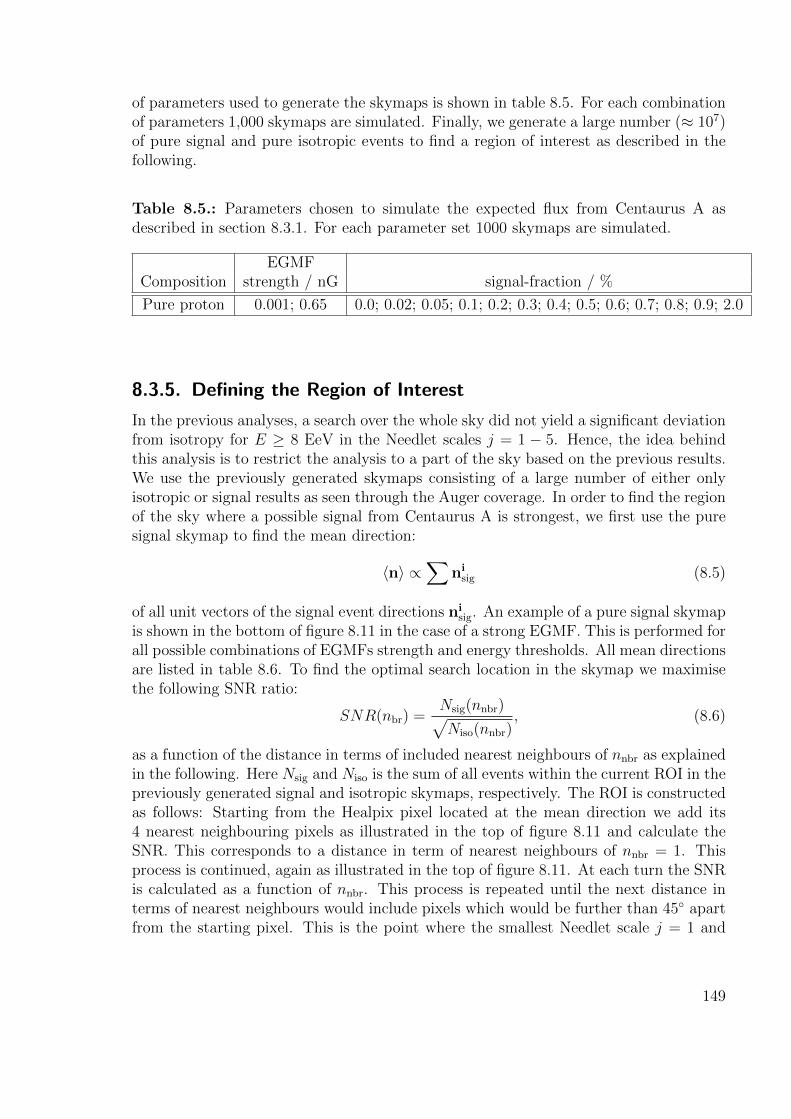
of parameters used to generate the skymaps is shown in table 8.5. For each combinationof parameters 1,000 skymaps are simulated. Finally, we generate a large number (≈ 107)of pure signal and pure isotropic events to find a region of interest as described in thefollowing.

Table 8.5.: Parameters chosen to simulate the expected flux from Centaurus A asdescribed in section 8.3.1. For each parameter set 1000 skymaps are simulated.

EGMFComposition strength / nG signal-fraction / %

Pure proton 0.001; 0.65 0.0; 0.02; 0.05; 0.1; 0.2; 0.3; 0.4; 0.5; 0.6; 0.7; 0.8; 0.9; 2.0

8.3.5. Defining the Region of Interest

In the previous analyses, a search over the whole sky did not yield a significant deviationfrom isotropy for E ≥ 8 EeV in the Needlet scales j = 1 − 5. Hence, the idea behindthis analysis is to restrict the analysis to a part of the sky based on the previous results.We use the previously generated skymaps consisting of a large number of either onlyisotropic or signal results as seen through the Auger coverage. In order to find the regionof the sky where a possible signal from Centaurus A is strongest, we first use the puresignal skymap to find the mean direction:

〈n〉 ∝∑

nisig (8.5)

of all unit vectors of the signal event directions nisig. An example of a pure signal skymap

is shown in the bottom of figure 8.11 in the case of a strong EGMF. This is performed forall possible combinations of EGMFs strength and energy thresholds. All mean directionsare listed in table 8.6. To find the optimal search location in the skymap we maximisethe following SNR ratio:

SNR(nbr) =Nsig(nnbr)√Niso(nnbr)

, (8.6)

as a function of the distance in terms of included nearest neighbours of nnbr as explainedin the following. Here Nsig and Niso is the sum of all events within the current ROI in thepreviously generated signal and isotropic skymaps, respectively. The ROI is constructedas follows: Starting from the Healpix pixel located at the mean direction we add its4 nearest neighbouring pixels as illustrated in the top of figure 8.11 and calculate theSNR. This corresponds to a distance in term of nearest neighbours of nnbr = 1. Thisprocess is continued, again as illustrated in the top of figure 8.11. At each turn the SNRis calculated as a function of nnbr. This process is repeated until the next distance interms of nearest neighbours would include pixels which would be further than 45 apartfrom the starting pixel. This is the point where the smallest Needlet scale j = 1 and

149

hence the one sensitive to larger structures starts to become less sensitive of even largerstructures. The scale j = 1 includes the spherical harmonic moments with l = 2 andl = 3 and hence is sensitive to angular distances up to ∝ 180/2 = 90, or in terms ofthe half angle of 45.Finally the distance of nnbr,max which provides the maximum SNR ratio is defined asthe used ROI. In the case of a threshold of 8 EeV and a strong EGMF the determinedROI is shown in the bottom of figure 8.11 and includes all pixels up to a distance ofnnbr,max = 10. The position of Centaurs A is marked with a black star. As can beseen the highest concentration of events lies slightly more towards the galactic planeand slightly more towards higher longitudes in comparison to the actual position ofCentaurus A. This can be explained due to pull of the flux towards the galactic planeby the GMF as can be seen in the middle, left-hand side panel in figure 8.10. This hasalso been observed in other works using the same GMF model [119]. The found ROIsand the distances which maximise the SNR in terms of nearest neighbours nnbr,max areshown in table 8.6. Also shown are the used Needlet scales which are selected to be mostsensitive to the size of the ROI and even smaller scales as well as the angular distanceof the end of the ROI to the centre of the ROI.As can be seen from the results the relatively low influence of the strength of the EGMFon a pure proton composition leads to the same ROI for protons regardless of the EGMFstrength. Also the ROI shrinks as the energy threshold rises as is expected since higherenergy particles are less deflected.

150

(a) ROI scheme, Nside = 4

(b) ROI, E ≥ 8 · 1018 eV, pure proton signal, Galactic coordinates

Figure 8.11.: a) Illustration how the ROI region is defined with Healpix Nside parameter=4. The black pixel with number 99 is the pixel where the average direction of all signalevent points to. At a distance of nnbr = 1 nearest neighbour the pixels directly attaching,i.e. NE, SE, SW and NE of the starting pixel, are added to the ROI. In this case theseare the green pixels with numbers 84, 116, 115 and 83. Continuing at distance nnbr = 2all pixels attached to these pixels are included and so on. The corresponding colours toa nearest neighbour distance of nnbr = 2, 3, 4 and 5 are yellow, light blue, red and darkblue. Each new ROI includes the previous ROIS. The ROI chosen for the analysis is theROI with the highest SNR ratio as defined by equation 8.5.b) Pure signal skymap, and ROI (in pink) in galactic coordinates in the case of a strongEGMF for a pure proton composition. The position of Centaurs A is marked with a blackstar. Within this ROI the respective SNR is maximised with nnbr = 10 . The structureof the ROI is due to the fact that it has been calculated in equatorial coordinates. Herethe signal events are located closer to the south pole and the Healpix pixels have a morecomplicated structure closer to the poles (see at the top and at the bottom of a)).

Table 8.6.: Determined regions of interest (ROIs) as described in section 8.3.5. Due tothe relatively low effect of even a strong EGMF on the direction of protons (see figure8.10) the ROIs and their angular extend for both a weak and strong EGMF is similar.For comparison the equatorial coordinates of Centaurus A are (α, δ) = (201,−43).The shift in coordinates can be explained by two factors. First, the Auger coveragerises towards the south leading to a higher SNR ratio. Second, the flux experiences apull towards the galactic plane by the GMF as can be seen in the middle, left-hand sidepanel in figure 8.10. As the energy rises the ROIs move closer towards the position ofCentaurus A. Due to the size of the ROIs the position of Centaurs A is included in theanalysis as illustrated in figure 8.11.

EGMF Mean direction Max. SNR Maximum NeedletComposition strength / nG (α, δ) / (, ) at nnbr,max ang. dist. / scales j

Energy E ≥ 8 EeV

Pure proton 0.001 (185, -56) 10 25 2− 5Pure proton 0.65 (185, -56) 10 25 2− 5

Energy E ≥ 10 EeV

Pure proton 0.001 (189, -55) 9 22 2− 5Pure proton 0.65 (189, -55) 9 22 2− 5

Energy E ≥ 12 EeV

Pure proton 0.001 (192, -54) 8 20 2− 5Pure proton 0.65 (192, -54) 8 20 2− 5

Figure 8.12.: Illustration of the CLs method. Adapted from [123].

8.3.6. Analysis

Using the defined ROIs the Needlet analysis is applied to the data. The analysis isidentical to the previously discussed results with one exception. When the S-value iscalculated, only pixels in the ROI are included. As the search region is now defined bythe ROI and does not extend over the whole sky, the used threshold T (see equation5.5) is lowered3 to 1.The measured S-value, as well as an isotropic reference distribution, in the case of aweak EGMF (top) and a strong EGMF (bottom) and an energy threshold of 8 EeV,are shown on the left-hand side of figure 8.13. In both cases and in all other cases nosignificant deviation from isotropy was observed. Therefore we can use the simulatedskymaps with varying signal fractions to obtain a limit on the flux from Centaurus Aunder the previously outlined conditions.To establish the limits we use the CLs method, commonly used in high energy experi-ments (e.g. to exclude mass ranges for the Higgs boson at the LEP and LHC [121, 122]before its discovery.). In our case we need to distinguish between two hypotheses H0

and Hs. H0 is the null hypothesis, that the observed data is due to an isotropic (referredto as background) distribution. Hs is the hypothesis that the observed data is due toan isotropic background plus a contribution of a flux from Centaurus A (referred to asbackground plus signal) with a given signal fraction4. On the left-hand side of figure8.13 the isotropic distribution (in blue) corresponds to the expected distribution of theS-value if H0 is true and the signal distribution (in red) to the expected distribution ifHs is true.

3The expected limits worsen if T = 3 is used.4Signal fraction here means the average fraction of events in the completely generated full sky test-

skymaps.

153

To distinguish between the two hypotheses we use the likelihood ratio

Q =LHs

LH0

, (8.7)

as illustrated in figure 8.12. We built two distributions of this ratio by sampling randomvalues from the simulated S-value distribution either in the case of isotropy or isotropyplus a given signal fraction and calculating the corresponding Q vale. An example ofthese distributions is shown on the right-hand side of figure 8.13 in the case of a weakand a strong EGMF on the top and bottom respectively. To exclude a given signalfraction at a given confidence level α one can calculate the probability to obtain thesame or higher Q-value as the observed data from the distribution for isotropy andsignal, CLs+b, as illustrated in figure 8.12. Conversely the probability CLb to obtain thesame or higher Q-value from the isotropic distribution can be similarly determined (seeagain figure 8.12). If the CLs+b value is smaller than α one can say the hypothesis Hs

is excluded at a confidence level CL = 1−α. This however leads to too stringent limitsif both hypotheses largely overlap, i.e. near the sensitivity limit of the experiment [123].A more conservative choice is to use the ratio

CLs =CLs+b

CLb

, (8.8)

where the confidence in the (combines) signal and background hypothesis is weightedwith the confidence in the background (i.e. isotropy) hypothesis [123]. To exclude agiven signal fraction we use a 95% confidence limit and hence require

CLs < 0.05 . (8.9)

On the contrary, if the observed data point is compatible with a pure isotropic arrivaldistribution but the CLs is larger than 0.05 we cannot rule out that the given signalfraction of events from Centaurus A is present in the data. As an example we show theQ-value distributions and the observed data value for the largest possible signal fractionof 0.3%, which is still compatible with the data value on the right-hand side of figure8.13. The figure shows the results for an assumed proton composition with a signalfraction of 0.3% and an energy threshold of 8 EeV in the case of a weak (top) and strong(bottom) EGMF. Consequently, MC data with a signal fraction of 0.4% and larger isnot compatible with the observed value and can hence be excluded.

154

Figure 8.13.: CLs method applied to the≥ 8 EeV data set for a weak (top) and a strong(bottom) EGMF. The two shown signal fractions are the largest (both 0.3%) which arecompatible with the observed data (see table 8.5). As in both cases no deviation fromisotropy was observed, the next larger (i.e. incompatible at a 95% C.L.) signal fractioncan be interpreted as the limit on the flux from Centaurus A (0.4%) assuming the usedGMF-lens and EGMF field strength and deflection model.

8.3.7. Results and Discussion

A summary of all obtained limits is shown in table 8.7 for energy thresholds 8, 10 and12 EeV. The limit on the proton fractions is 0.4% regardless of EGMF strength andenergy threshold. Within the Auger coverage with a maximum zenith angle of 80 thislimit translates to a signal fraction of 0.7% due to the location of the Pierre AugerObservatory in the southern hemisphere. A comparison to previously established resultsis difficult as comparable analyses using the JF-12 model do not currently exist.

Of the two current UHECR observatories, the Pierre Auger Observatory and theTelescope Array, only the Pierre Auger Observatory has access to the sky region ofCentaurus A. In case of the Auger observatory the expected number of events wascompared to the observed number of events for energy thresholds ranging from 40 to80 EeV and as a function of the angular distance to Centaurus A [35]. In contrast tothe work described in this chapter, this analysis ([35]) makes no assumptions on thepropagation of UHECRs and instead uses the observed data to define a ROI. The latestincluded events in the data set are from March 2014, which is only 3 months of moredata in comparison to this work. As described in section 2.5, the largest observed excessof events was at an angular distance of 15 and for an energy threshold of 58 EeV (seeright-hand side of figure 2.7 on page 17), with a penalized probability of 1.4% [35]. Whilethe chance probability of this scenario is rather low it does not reach significance whichis also the case in this work (with energies around 10 EeV).

156

Table 8.7.: Limits on the flux from Centaurus A using the CLs method at a confidencelevel of 95% as a function of the composition and the strength of the EGMF. The searchis restricted to the ROI windows around the mean directions and to the Needlet scaleslisted in table 8.6. The limit is given in terms of the signal fraction either at Earthand also, on average, within the Auger coverage with a maximum zenith angle of 80.Due to the position of the Pierre Auger Observatory the signal fraction is larger withinthe Auger coverage than averaged over the whole Earth. The included GMF field isdescribed in section 2.4.1 and the derivation and usage of the lens obtained from theGMF model is described in section 8.3.3.

EGMF Limit of s.f. @95% C.L.Composition strength / nG at Earth in Auger coverage

Energy E ≥ 8 EeV, 19797 Events

Proton 0.001 ≤ 0.4 % ≤ 0.7 %Proton 0.65 ≤ 0.4% ≤ 0.7 %

Energy E ≥ 10 EeV, 13195 Events

Proton 0.001 ≤ 0.4 % ≤ 0.7 %Proton 0.65 ≤ 0.4% ≤ 0.7 %

Energy E ≥ 12 EeV, 9264 Events

Proton 0.001 ≤ 0.4 % ≤ 0.7 %Proton 0.65 ≤ 0.4% ≤ 0.7 %

9. Summary

Until today the origin of ultra-high energy cosmic rays (UHECRs) is unknown. Thesearch for the origin of UHECRs is difficult as they are deflected by magnetic fields ontheir way to earth. This deflection is stronger the heavier the composition of the arrivingcosmic rays is, leading to a largely isotropic distribution at earth.

In this work a Needlet Wavelet based analysis has been applied on the measuredarrival directions of UHECRs at the Pierre Auger Observatory. The aim was to findany deviations in various angular sizes from a purely isotropic distribution of arrivaldirections. The analysis was applied to energies above the full trigger efficiency ofthe surface detector of the Pierre Auger Observatory. Two energy bins were analysed:E = 4 − 8 EeV and E ≥ 8 EeV. In the case of energies E ≥ 8 EeV a deviation ofthe expectation of pure isotropy was observed by the global anisotropy estimator with achance probability of p = 2.5× 10−3 (not accounting for the search in two energy bins).

The only significant deviation in the individual Needlet scales j was observed in thedipolar scale j = 0 for E ≥ 8 EeV with only 0.0014% of isotropic reference skymaps pos-sessing an equal or higher deviation from isotropy in this particular scale. No deviationsfrom isotropy were observed in any other angular scale or energy.

Under the assumption of a dipole dominated flux the properties of the dipolar patternwere reconstructed. The dipolar pattern points towards a direction with a right ascensionof αd = 97 ± 16 and a declination of δd = −39 ± 17 and possesses an amplitude ofr = (6.8±1.6)%. Various data based cross-checks were performed to verify the robustnessof the observed dipolar pattern. By relaxing the dominant dipole assumption it wasfound that a possible total of 0.5% percentage points of the observed dipole amplitudecould be explained by the presence of a quadrupolar anisotropy.

Using the JF-12 model of the galactic magnetic field (GMF) the analysis was restrictedto a portion of the sky where a possible signal from the active galactic nucleus closestto earth, Centaurus A, would be strongest in the case of a pure proton composition.No signal was observed, either in the case of a strong or a weak extra galactic magneticfield (EGMF) for energies E ≥ 8 EeV, E ≥ 10 EeV and E ≥ 12 EeV. Due to the non-observation of a signal limits were set using the CLS method. The limit on the signalfraction at earth for a pure proton composition from Centaurus A under the assumptionof the JF-12 GMF model and an otherwise isotropic distribution of arrival direction is0.4% for all analysed energies and strengths of the EGMF.

A future application of the analysis used in this work to a subset of the lightest,and hence least deflected, UHECRs could significantly increase the change to observefurther deviations from isotropy. One of the goals of the currently starting upgradeof the Pierre Auger Observatory is to achieve this capability. A requirement for thisupgrade are efficient, robust and cost-effective light sensors with a sufficient dynamic

159

range. Silicon-Photomultipliers (SiPMs) are such sensors. In this work a technique tofully characterise their response to a wide variety of light pulses and to reconstruct theincident signal from their response was developed. This is an important requirement fortheir usage in the upgrade of the Pierre Auger Observatory or similar, future usage inthe study of UHECRs.

160

Bibliography

[1] A. Letessier-Selvon and T. Stanev, “Ultrahigh energy cosmic rays,” Rev. Mod.Phys. 83 (Sep, 2011) 907–942.http://link.aps.org/doi/10.1103/RevModPhys.83.907.

[2] J. Blumer, R. Engel, and J. R. Horandel, “Cosmic rays from the knee to thehighest energies,” Progress in Particle and Nuclear Physics 63 no. 2, (2009) 293– 338. http://www.sciencedirect.com/science/article/pii/S0146641009000362.

[3] K. Kotera and A. V. Olinto, “The astrophysics of ultrahigh-energy cosmic rays,”Annual Review of Astronomy and Astrophysics 49 no. 1, (2011) 119–153,http://dx.doi.org/10.1146/annurev-astro-081710-102620.http://dx.doi.org/10.1146/annurev-astro-081710-102620.

[4] M. Longair, High Energy Astrophysics. Cambridge University Press, 2011.

[5] Pierre Auger Collaboration Collaboration, J. Abraham et al., “Measurement ofthe depth of maximum of extensive air showers above 1018 eV,” Phys. Rev. Lett.104 (2010) 091101. http://link.aps.org/doi/10.1103/PhysRevLett.104.091101.

[6] The High Resolution Fly’s Eye Collaboration Collaboration, R. U. Abbasi et al.,“Indications of Proton-Dominated Cosmic-Ray Composition above 1.6 EeV,”Physical Review Letters 104 no. 16, (Apr., 2010) 161101, arXiv:0910.4184[astro-ph.HE]. http://adsabs.harvard.edu/abs/2010PhRvL.104p1101A.

[7] K.-H. Kampert and P. Tinyakov, “Cosmic rays from the ankle to the cutoff,”Comptes Rendus Physique 15 (2014) 318–328, arXiv:1405.0575[astro-ph.HE].

[8] B. Keilhauer, Investigation of Atmospheric Effects on the Development ofExtensive Air Showers and their Detection with the Pierre Auger Observatory.Phd thesis, Universitaet Karlsruhe, Karlsruhe, 2003.

[9] Particle Data Group Collaboration, K. A. Olive et al., “Review of ParticlePhysics,” Chin. Phys. C38 (2014) 090001.

[10] T. K. Gaisser, Cosmic Rays and Particle Physics. Cambridge University Press,1990.

[11] K.-H. Kampert and A. Watson, “Extensive air showers and ultra high-energycosmic rays: a historical review,” The European Physical Journal H 37 no. 3,(2012) 359–412. http://dx.doi.org/10.1140/epjh/e2012-30013-x.

161

[12] E. Fermi, “On the origin of the cosmic radiation,” Phys. Rev. 75 (Apr, 1949)1169–1174. http://link.aps.org/doi/10.1103/PhysRev.75.1169.

[13] A. R. Bell, “The acceleration of cosmic rays in shock fronts – ii,” MonthlyNotices of the Royal Astronomical Society 182 no. 3, (1978) 443–455,http://mnras.oxfordjournals.org/content/182/3/443.full.pdf+html.http://mnras.oxfordjournals.org/content/182/3/443.abstract.

[14] R. D. Blandford and J. P. Ostriker, “Particle acceleration by astrophysicalshocks,” The Astrophysical Journal Letters 221 (Apr., 1978) L29–L32.http://adsabs.harvard.edu/abs/1978ApJ...221L..29B.

[15] A. M. Hillas, “The origin of ultra-high-energy cosmic rays,” Annual Review ofAstronomy and Astrophysics 22 no. 1, (1984) 425–444,http://dx.doi.org/10.1146/annurev.aa.22.090184.002233.http://dx.doi.org/10.1146/annurev.aa.22.090184.002233.

[16] T. Antoni, W. Apel, A. Badea, K. Bekk et al., “Kascade measurements of energyspectra for elemental groups of cosmic rays: Results and open problems,”Astroparticle Physics 24 no. 1–2, (2005) 1 – 25.http://www.sciencedirect.com/science/article/pii/S0927650505000691.

[17] R. L. Diehl, “Particle acceleration in cosmic sites. Astrophysics issues in ourunderstanding of cosmic rays,” European Physical Journal D 55 (Nov., 2009)509–518, arXiv:0902.4795 [astro-ph.HE].http://adsabs.harvard.edu/abs/2009EPJD...55..509D.

[18] P. Bhattacharjee, “Origin and propagation of extremely high energy cosmicrays,” Physics Reports 327 (Mar., 2000) 109–247, astro-ph/9811011.http://adsabs.harvard.edu/abs/2000PhR...327..109B.

[19] R. M. Kulsrud and E. G. Zweibel, “On the origin of cosmic magnetic fields,”Reports on Progress in Physics 71 no. 4, (2008) 046901.http://stacks.iop.org/0034-4885/71/i=4/a=046901.

[20] A. Achterberg, Y. A. Gallant, C. A. Norman, and D. B. Melrose, “IntergalacticPropagation of UHE Cosmic Rays,” ArXiv Astrophysics e-prints (July, 1999) ,astro-ph/9907060. http://adsabs.harvard.edu/abs/1999astro.ph..7060A.

[21] D. Harari, S. Mollerach, E. Roulet, and F. Sanchez, “Lensing of ultrahigh-energycosmic rays in turbulent magnetic fields,” JHEP 03 (2002) 045,arXiv:astro-ph/0202362 [astro-ph].

[22] R. Jansson and G. R. Farrar, “The Galactic Magnetic Field,” The AstrophysicalJournal Letters 761 (Dec., 2012) L11, arXiv:1210.7820 [astro-ph.GA].http://adsabs.harvard.edu/abs/2012ApJ...761L..11J.

162

[23] G. R. Farrar, “The Galactic Magnetic Field and Ultrahigh-Energy Cosmic RayDeflections,” Comptes Rendus Physique 15 (2014) 339–348, arXiv:1405.3680[astro-ph.HE].

[24] D. Walz, Constraining Models of the Extragalactic Cosmic Ray Origin with thePierre Auger Observatory. PhD thesis, RWTH Aachen University, Germany,2016.

[25] T. Winchen, The Principal Axes of the Directional Energy Distribution of CosmicRays Measured with the Pierre Auger Observatory. PhD thesis, RWTH AachenUniversity, Germany, 2013. http://wwwo.physik.rwth-aachen.de/fileadmin/user upload/www physik/Personen/erdmann/Dissertation-Winchen.pdf.

[26] K. Dolag, D. Grasso, V. Springel, and I. Tkachev, “Constrained simulations ofthe magnetic field in the local Universe and the propagation of UHECRs,” JCAP0501 (2005) 009, arXiv:astro-ph/0410419 [astro-ph].

[27] K. Dolag, D. Grasso, V. Springel, and I. Tkachev, “Mapping deflections ofextragalactic ultrahigh-energy cosmic rays in magnetohydrodynamic simulationsof the local universe,” Journal of Experimental and Theoretical Physics Letters79 no. 12, (2004) 583–587. http://dx.doi.org/10.1134/1.1790011.

[28] M. S. Pshirkov, P. G. Tinyakov, and F. R. Urban, “New Limits on ExtragalacticMagnetic Fields from Rotation Measures,” Physical Review Letters 116 no. 19,(May, 2016) 191302, arXiv:1504.06546.http://adsabs.harvard.edu/abs/2016PhRvL.116s1302P.

[29] K. Dolag, M. Kachelriess, S. Ostapchenko, and R. Tomas, “Lower Limit on theStrength and Filling Factor of Extragalactic Magnetic Fields,” The AstrophysicalJournal Letters 727 (Jan., 2011) L4, arXiv:1009.1782 [astro-ph.HE].

[30] The Pierre Auger Collaboration, P. Abreu, M. Aglietta, E. J. Ahn et al., “Searchfor first harmonic modulation in the right ascension distribution of cosmic raysdetected at the Pierre Auger Observatory,” Astroparticle Physics 34 (Mar.,2011) 627–639, arXiv:1103.2721 [astro-ph.HE].http://adsabs.harvard.edu/abs/2011APh....34..627P.

[31] The Pierre Auger Collaboration, A. Aab, P. Abreu, M. Aglietta et al., “ThePierre Auger Observatory: Contributions to the 33rd International Cosmic RayConference (ICRC 2013),” ArXiv e-prints (July, 2013) , arXiv:1307.5059[astro-ph.HE]. http://adsabs.harvard.edu/abs/2013arXiv1307.5059T.

[32] The Pierre Auger Collaboration, P. Abreu, M. Aglietta, M. Ahlers et al.,“Large-scale Distribution of Arrival Directions of Cosmic Rays Detected Above1018 eV at the Pierre Auger Observatory,” The Astrophysical Journal,Supplement 203 (Dec., 2012) 34, arXiv:1210.3736 [astro-ph.HE].http://adsabs.harvard.edu/abs/2012ApJS..203...34P.

163

[33] The Pierre Auger Collaboration, P. Abreu, M. Aglietta, M. Ahlers et al.,“Constraints on the Origin of Cosmic Rays above 1018 eV from Large-scaleAnisotropy Searches in Data of the Pierre Auger Observatory,” TheAstrophysical Journal Letters 762 (Jan., 2013) L13, arXiv:1212.3083[astro-ph.HE]. http://adsabs.harvard.edu/abs/2013ApJ...762L..13P.

[34] The Pierre Auger Collaboration, A. Aab et al., “Large Scale Distribution ofUltra High Energy Cosmic Rays Detected at the Pierre Auger Observatory WithZenith Angles up to 80,” Astrophys. J. 802 no. 2, (2015) 111, arXiv:1411.6953[astro-ph.HE].

[35] The Pierre Auger Collaboration, A. Aab et al., “The Pierre Auger Observatory:Contributions to the 34th International Cosmic Ray Conference (ICRC 2015),”ArXiv e-prints (2015) , arXiv:1509.03732 [astro-ph.HE].https://inspirehep.net/record/1393211/files/arXiv:1509.03732.pdf.

[36] Telescope Array Collaboration, R. U. Abbasi et al., “Indications ofIntermediate-Scale Anisotropy of Cosmic Rays with Energy Greater Than 57 EeVin the Northern Sky Measured with the Surface Detector of the Telescope ArrayExperiment,” Astrophys. J. 790 (2014) L21, arXiv:1404.5890 [astro-ph.HE].

[37] The Pierre Auger, Telescope Array Collaboration, A. Aab et al., “Searches forlarge-scale anisotropy in the arrival directions of cosmic rays detected aboveenergy of 1019 ev at the pierre auger observatory and the telescope array,” TheAstrophysical Journal 794 no. 2, (2014) 172.http://stacks.iop.org/0004-637X/794/i=2/a=172.

[38] J. R. Vazquez, J. Rosado, D. Garcıa-Pinto, and F. Arqueros, “The effect of thefluorescence yield selection on the energy scales of Auger, HiRes and TA,” inEuropean Physical Journal Web of Conferences, vol. 53 of European PhysicalJournal Web of Conferences, p. 10002. June, 2013. arXiv:1303.2945[astro-ph.IM]. http://adsabs.harvard.edu/abs/2013EPJWC..5310002V.

[39] The Pierre Auger, Telescope Array Collaboration, R. U. Abbasi et al., “PierreAuger Observatory and Telescope Array: Joint Contributions to the 34thInternational Cosmic Ray Conference (ICRC 2015),” ArXiv e-prints (2015) ,arXiv:1511.02103 [astro-ph.HE].

[40] M. Kachelrieß and P. Serpico, “The compton–getting effect on ultra-high energycosmic rays of cosmological origin,” Physics Letters B 640 no. 5–6, (2006) 225 –229. http://www.sciencedirect.com/science/article/pii/S037026930600983X.

[41] D. Harari, S. Mollerach, and E. Roulet, “Anisotropies of ultrahigh energy cosmicrays diffusing from extragalactic sources,” Phys. Rev. D 89 (Jun, 2014) 123001.http://link.aps.org/doi/10.1103/PhysRevD.89.123001.

164

[42] The Pierre Auger Collaboration, “The pierre auger cosmic ray observatory,”Nuclear Instruments and Methods in Physics Research Section A: Accelerators,Spectrometers, Detectors and Associated Equipment 798 (2015) 172 – 213.http://www.sciencedirect.com/science/article/pii/S0168900215008086.

[43] A. Nelles, “Search for anomalies in cosmic air showers measured with the surfacedetector of the pierre auger observatory,” masters thesis, RWTH AachenUniversity, Germany, 2010.https://web.physik.rwth-aachen.de/∼hebbeker/theses/nelles diploma.pdf.

[44] The Pierre Auger Collaboration, J. Abraham, P. Abreu, M. Aglietta et al., “Thefluorescence detector of the pierre auger observatory,” Nuclear Instruments andMethods in Physics Research Section A: Accelerators, Spectrometers, Detectorsand Associated Equipment 620 no. 2–3, (2010) 227 – 251.http://www.sciencedirect.com/science/article/pii/S0168900210008727.

[45] The Pierre Auger Collaboration, I. Allekotte, A. F. Barbosa, P. Bauleo et al.,“The surface detector system of the Pierre Auger Observatory,” NuclearInstruments and Methods in Physics Research A 586 (Mar., 2008) 409–420,arXiv:0712.2832. http://adsabs.harvard.edu/abs/2008NIMPA.586..409A.

[46] F. Arqueros, J. R. Hoerandel, and B. Keilhauer, “Air fluorescence relevant forcosmic-ray detection. summary of the 5th fluorescence workshop, el escorial2007,” Nuclear Instruments and Methods in Physics Research Section A:Accelerators, Spectrometers, Detectors and Associated Equipment 597 no. 1,(2008) 1 – 22. Proceedings of the 5th Fluorescence Workshop.

[47] The Pierre Auger Collaboration, X. Bertou, P. Allison, C. Bonifazi, P. Bauleoet al., “Calibration of the surface array of the pierre auger observatory,” NuclearInstruments and Methods in Physics Research Section A: Accelerators,Spectrometers, Detectors and Associated Equipment 568 no. 2, (2006) 839 – 846.http://www.sciencedirect.com/science/article/pii/S0168900206013593.

[48] The Pierre Auger Collaboration, “Reconstruction of inclined air showers detectedwith the Pierre Auger Observatory,” Journal of Cosmology and AstroparticlePhysics 8 (Aug., 2014) 019, arXiv:1407.3214 [astro-ph.HE].http://adsabs.harvard.edu/abs/2014JCAP...08..019T.

[49] The Pierre Auger Collaboration, J. Abraham, P. Abreu, M. Aglietta, E. J. Ahnet al., “Trigger and aperture of the surface detector array of the Pierre AugerObservatory,” Nuclear Instruments and Methods in Physics Research A 613(Jan., 2010) 29–39, arXiv:1111.6764 [astro-ph.IM].http://adsabs.harvard.edu/abs/2010NIMPA.613...29A.

[50] K. Kamata and J. Nishimura, “The lateral and the angular structure functions ofelectron showers,” Progress of Theoretical Physics Supplement 6 (1958) 93–155,

165

http://ptps.oxfordjournals.org/content/6/93.full.pdf+html.http://ptps.oxfordjournals.org/content/6/93.abstract.

[51] K. Greisen Progress in Cosmic Ray Physics 3 (1956) . https://archive.org/stream/progressincosmic031401mbp/progressincosmic031401mbp djvu.txt.

[52] P. Sommers, “Cosmic ray anisotropy analysis with a full-sky observatory,”Astroparticle Physics 14 (Jan., 2001) 271–286, astro-ph/0004016.http://adsabs.harvard.edu/abs/2001APh....14..271S.

[53] The Pierre Auger Collaboration, P. Abreu et al., “The Pierre Auger ObservatoryI: The Cosmic Ray Energy Spectrum and Related Measurements,” in Proceedingsof the 32nd International Cosmic Ray Conference (ICRC 2011). 2011.arXiv:1107.4809 [astro-ph.HE].https://inspirehep.net/record/919725/files/arXiv:1107.4809.pdf.

[54] Pierre Auger Collaboration and C. Bonifazi, “The angular resolution of thePierre Auger Observatory,” Nuclear Physics B Proceedings Supplements 190(May, 2009) 20–25, arXiv:0901.3138 [astro-ph.HE].http://adsabs.harvard.edu/abs/2009NuPhS.190...20B.

[55] The Pierre Auger Collaboration, A. Aab, P. Abreu, M. Aglietta et al., “ThePierre Auger Observatory Upgrade - Preliminary Design Report,” ArXiv e-prints(Apr., 2016) , arXiv:1604.03637 [astro-ph.IM].http://adsabs.harvard.edu/abs/2016arXiv160403637T.

[56] SensL, “J-series data sheet,” 2016, last visited 08/2016.http://sensl.com/products/j-series/.

[57] J. Buss, “FACT - How stable are the silicon photon detectors?,” in Proceedings,33rd International Cosmic Ray Conference (ICRC2013): Rio de Janeiro, Brazil,July 2-9, 2013, p. 0683.http://www.cbpf.br/%7Eicrc2013/papers/icrc2013-0683.pdf.

[58] D. Renker and E. Lorenz, “Advances in solid state photon detectors,” Journal ofInstrumentation 4 no. 04, (2009) P04004.http://stacks.iop.org/1748-0221/4/i=04/a=P04004.

[59] Y. Du and F. Retiere, “After-pulsing and cross-talk in multi-pixel photoncounters,” Nuclear Instruments and Methods in Physics Research Section A:Accelerators, Spectrometers, Detectors and Associated Equipment 596 no. 3,(2008) 396 – 401.http://www.sciencedirect.com/science/article/pii/S0168900208012643.

[60] F. Corsi, C. Marzocca, A. Perrotta, A. Dragone et al., “Electricalcharacterization of silicon photo-multiplier detectors for optimal front-enddesign,” in 2006 IEEE Nuclear Science Symposium Conference Record, vol. 2,pp. 1276–1280. Oct, 2006.

166

[61] P. Buzhan, B. Dolgoshein, L. Filatov, A. Ilyin et al., “Silicon photomultiplier andits possible applications,” Nuclear Instruments and Methods in Physics ResearchSection A: Accelerators, Spectrometers, Detectors and Associated Equipment 504no. 1–3, (2003) 48 – 52.http://www.sciencedirect.com/science/article/pii/S0168900203007496.Proceedings of the 3rd International Conference on New Developments inPhotodetection.

[62] M. Petasecca, B. Alpat, G. Ambrosi, P. Azzarello et al., “Thermal and electricalcharacterization of silicon photomultiplier,” IEEE Transactions on NuclearScience 55 no. 3, (June, 2008) 1686–1690.

[63] P. Eckert, H.-C. Schultz-Coulon, W. Shen, R. Stamen et al., “Characterisationstudies of silicon photomultipliers,” Nuclear Instruments and Methods in PhysicsResearch A 620 (Aug., 2010) 217–226, arXiv:1003.6071 [physics.ins-det].http://adsabs.harvard.edu/abs/2010NIMPA.620..217E.

[64] A. Vacheret, G. Barker, M. Dziewiecki, P. Guzowski et al., “Characterization andsimulation of the response of multi-pixel photon counters to low light levels,”Nuclear Instruments and Methods in Physics Research Section A: Accelerators,Spectrometers, Detectors and Associated Equipment 656 no. 1, (2011) 69 – 83.http://www.sciencedirect.com/science/article/pii/S0168900211014513.

[65] A. D. Guerra, N. Belcari, M. G. Bisogni, G. LLosa et al., “Advantages andpitfalls of the silicon photomultiplier (sipm) as photodetector for the nextgeneration of PET scanners,” Nuclear Instruments and Methods in PhysicsResearch Section A: Accelerators, Spectrometers, Detectors and AssociatedEquipment 617 no. 1–3, (2010) 223 – 226.http://www.sciencedirect.com/science/article/pii/S0168900209019056. 11th PisaMeeting on Advanced DetectorsProceedings of the 11th Pisa Meeting onAdvanced Detectors.

[66] T. Liu, J. Anderson, J. Freeman, S. Los et al., “Proceedings of the 2ndinternational conference on technology and instrumentation in particle physics(tipp 2011) upgrade of the cms hadron outer calorimeter with sipms,” PhysicsProcedia 37 (2012) 72 – 78.http://www.sciencedirect.com/science/article/pii/S1875389212016677.

[67] H. Anderhub, M. Backes, A. Biland, A. Boller et al., “Fact—the first cherenkovtelescope using a g-apd camera for tev gamma-ray astronomy,” NuclearInstruments and Methods in Physics Research Section A: Accelerators,Spectrometers, Detectors and Associated Equipment 639 no. 1, (2011) 58 – 61.http://www.sciencedirect.com/science/article/pii/S0168900210023466.Proceedings of the Seventh International Workshop on Ring Imaging CherenkovDetectors.

167

[68] CTA Consortium Collaboration, M. Actis, G. Agnetta, F. Aharonian,A. Akhperjanian et al., “Design concepts for the Cherenkov Telescope ArrayCTA: an advanced facility for ground-based high-energy gamma-ray astronomy,”Experimental Astronomy 32 (Dec., 2011) 193–316, arXiv:1008.3703[astro-ph.IM]. http://adsabs.harvard.edu/abs/2011ExA....32..193A.

[69] T. Niggemann, P. Assis, P. Brogueira, A. Bueno et al., “Status of the SiliconPhotomultiplier Telescope FAMOUS for the Fluorescence Detection ofUHECRs,” Proceedings of the 33rd International Cosmic Ray Conference (ICRC2013) (2013) , arXiv:1502.00792 [astro-ph.IM].http://adsabs.harvard.edu/abs/2015arXiv150200792N.

[70] S. M. Sze, Physics of Semiconductor Devices. Wiley-Interscience, 2007.

[71] A. N. Otte, Observation of VHE Gamma-Rays from the Vicinity of magnetizedNeutron Stars and Development of new Photon-Detectors for Future Groundbased Gamma-Ray Detectors. Phd thesis, Technische Universitaet Muenchen,Muenchen, 2007.

[72] J. Rennefeld, Studien zur Eignung von Silizium Photomultipliern fuer denEinsatz im erweiterten CMS Detektor am SLHC. Diploma thesis, RWTH AachenUniversity, Germany, 2010.

[73] A. L. Lacaita, F. Zappa, S. Bigliardi, and M. Manfredi, “On the bremsstrahlungorigin of hot-carrier-induced photons in silicon devices,” IEEE Transactions onElectron Devices 40 no. 3, (Mar, 1993) 577–582.

[74] Thorlabs, “Is200 data sheet.” http://www.thorlabs.de.

[75] Hamamatsu Photonics, “S2281-photodiode data sheet,” last visited 08/2016.https://www.hamamatsu.com/resources/pdf/ssd/s2281 series kspd1044e.pdf.

[76] Phillips Scientific, “Ps 6945b-100 data sheet.” http://www.phillipsscientific.com.

[77] Dycometal, “Cck-25-100 model data sheet.” http://www.dycometal.com.

[78] Keithley, “6485 model data sheet.” http://www.keithley.com.

[79] Aim and Thurlby Thandar Instruments, “models plh120-p, tga 1242, cpx 400dual data sheets.” http://www.tti-test.com.

[80] CAEN, “models qdc v965a, adc v1729, scaler v560ae, ltd v814b, fanin/fanoutv925 data sheets.” http://www.caen.it.

[81] LeCroy, “Waverunnter 1600 data sheet.” http://www.teledynelecroy.com.

168

[82] N. Seguin-Moreau, “Latest generation of asics for photodetector readout,”Nuclear Instruments and Methods in Physics Research Section A: Accelerators,Spectrometers, Detectors and Associated Equipment 718 (2013) 173 – 179.http://www.sciencedirect.com/science/article/pii/S0168900212014817.Proceedings of the 12th Pisa Meeting on Advanced DetectorsLa Biodola, Isolad’Elba, Italy, May 20 – 26, 2012.

[83] KETEK GmbH, “Pm3350 series data sheet,” last visited 08/2016.http://www.ketek.net/products/sipm/pm3350/. http://www.ketek.net/products/sipm/pm3350/?no cache=1&cid=5749&did=2251&sechash=1b16f9d1.

[84] Hamamatsu Photonics, “S10362-33 series data sheet,” last visited 08/2016.http://www.datasheetlib.com/datasheet/707358/s10362-33 hamamatsu-photonics.html.

[85] C. R. Crowell and S. M. Sze, “Temperature dependence of avalanchemultiplication in semiconductors,” Applied Physics Letters 9 no. 6, (1966)242–244.http://scitation.aip.org/content/aip/journal/apl/9/6/10.1063/1.1754731.

[86] R. Newman, “Visible light from a silicon p− n junction,” Phys. Rev. 100 (Oct,1955) 700–703. http://link.aps.org/doi/10.1103/PhysRev.100.700.

[87] F. R. Schneider, T. R. Ganka, G. Seker, E. Engelmann et al., “Characterizationof blue sensitive 3x3 mm2 sipms and their use in pet,” Journal ofInstrumentation 9 no. 07, (2014) P07027.http://stacks.iop.org/1748-0221/9/i=07/a=P07027.

[88] P. Hallen, “Determination of the recovery time of silicon photomultipliers,”bachelor thesis, RWTH Aachen University, Germany, 2011.http://web.physik.rwth-aachen.de/∼hebbeker/theses/hallen bachelor.pdf.

[89] F. Scheuch, “Measurement and simulation of electrical properties of sipm photondetectors,” masters thesis, RWTH Aachen University, Germany, 2012.http://web.physik.rwth-aachen.de/∼hebbeker/theses/scheuch master.pdf.

[90] L. Gruber, S. Brunner, J. Marton, and K. Suzuki, “Over saturation behavior ofsipms at high photon exposure,” Nuclear Instruments and Methods in PhysicsResearch Section A: Accelerators, Spectrometers, Detectors and AssociatedEquipment 737 (2014) 11 – 18.http://www.sciencedirect.com/science/article/pii/S0168900213015520.

[91] D. Marinucci, D. Pietrobon, A. Balbi, P. Baldi et al., “Spherical Needlets forCMB Data Analysis,” Mon. Not. Roy. Astron. Soc. 383 (2008) 539,arXiv:0707.0844 [astro-ph].

169

[92] D. Pietrobon, A. Amblard, A. Balbi, P. Cabella et al., “Needlet Detection ofFeatures in WMAP CMB Sky and the Impact on Anisotropies and HemisphericalAsymmetries,” Phys. Rev. D78 (2008) 103504, arXiv:0809.0010 [astro-ph].

[93] S. M. Feeney, M. C. Johnson, D. J. Mortlock, and H. V. Peiris, “FirstObservational Tests of Eternal Inflation: Analysis Methods and WMAP 7-YearResults,” Phys. Rev. D84 (2011) 043507, arXiv:1012.3667 [astro-ph.CO].

[94] R. Alves Batista, E. Kemp, R. M. de Almeida, and B. Daniel, “Wavelets Appliedto the Detection of Point Sources of UHECRs,” Physicae Proc. 1 (2010) 223,arXiv:1012.3645 [astro-ph.IM].

[95] R. Alves Batista, E. Kemp, and B. Daniel, “Detection of Point Sources in CosmicRay Maps Using the Mexican Hat Wavelet Family,” International Journal ofModern Physics E 20 (2011) 61–66, arXiv:1201.2799 [astro-ph.IM].

[96] M. Plum, “Wavelet analysis of the arrival directions of ultra high energy cosmicrays at the pierre auger observatory,” masters thesis, RWTH Aachen University,Germany, 2011.https://web.physik.rwth-aachen.de/∼hebbeker/theses/plum diploma.pdf.

[97] K. M. Gorski, E. Hivon, A. J. Banday, B. D. Wandelt et al., “HEALPix: AFramework for High-Resolution Discretization and Fast Analysis of DataDistributed on the Sphere,” The Astrophysical Journal 622 (Apr., 2005) 759–771,astro-ph/0409513. http://adsabs.harvard.edu/abs/2005ApJ...622..759G.

[98] W. K, “Evaluation of active and passive shimming in magnetic resonanceimaging,” Research and Reports in Nuclear Medicinel 4 (Oct., 2014) 1–12.https://dx.doi.org/10.2147/RRNM.S46526.

[99] N. Schaeffer, “Efficient spherical harmonic transforms aimed at pseudospectralnumerical simulations,” Geochemistry, Geophysics, Geosystems 14 (Mar., 2013)751–758, arXiv:1202.6522 [physics.comp-ph].

[100] T. C. and C. G., “A Practical Guide to Wavelet Analysis,” Bulletin of theAmerican Meteorological Society (Jan., 1998) .http://dx.doi.org/10.1175/1520-0477(1998)079〈0061:APGTWA〉2.0.CO;2.

[101] The IceCube Collaboration, “The IceCube Collaboration: contributions to the30th International Cosmic Ray Conference (ICRC 2007),” ArXiv e-prints (Nov.,2007) , arXiv:0711.0353. http://adsabs.harvard.edu/abs/2007arXiv0711.0353T.

[102] D. Harari, S. Mollerach, and E. Roulet, “Effects of the galactic magnetic fieldupon large scale anisotropies of extragalactic cosmic rays,” Journal of Cosmologyand Astroparticle Physics 11 (Nov., 2010) 033, arXiv:1009.5891[astro-ph.HE]. http://adsabs.harvard.edu/abs/2010JCAP...11..033H.

170

[103] O. Deligny, E. Armengaud, T. Beau, P. Da Silva et al., “Angular powerspectrum estimation of cosmic ray anisotropies with full or partial sky coverage,”Journal of Cosmology and Astroparticle Physics 10 (Oct., 2004) 008,astro-ph/0404253. http://adsabs.harvard.edu/abs/2004JCAP...10..008D.

[104] C. B. Netterfield, P. A. R. Ade, J. J. Bock, J. R. Bond et al., “A Measurement byBOOMERANG of Multiple Peaks in the Angular Power Spectrum of the CosmicMicrowave Background,” The Astrophysical Journal 571 (June, 2002) 604–614,astro-ph/0104460. http://cdsads.u-strasbg.fr/abs/2002ApJ...571..604N.

[105] C. L. Bennett, D. Larson, J. L. Weiland, N. Jarosik et al., “Nine-year WilkinsonMicrowave Anisotropy Probe (WMAP) Observations: Final Maps and Results,”The Astrophysical Journal Supplement 208 (Oct., 2013) 20, arXiv:1212.5225.http://adsabs.harvard.edu/abs/2013ApJS..208...20B.

[106] Planck Collaboration, P. A. R. Ade, N. Aghanim, Y. Akrami et al., “Planck 2015results. XVI. Isotropy and statistics of the CMB,” ArXiv e-prints (June, 2015) ,arXiv:1506.07135. http://adsabs.harvard.edu/abs/2015arXiv150607135P.

[107] IceCube Collaboration, Pierre Auger Collaboration, and Telescope ArrayCollaboration, “Search for correlations between the arrival directions of IceCubeneutrino events and ultrahigh-energy cosmic rays detected by the Pierre AugerObservatory and the Telescope Array,” Journal of Cosmology and AstroparticlePhysics 1 (Jan., 2016) 037, arXiv:1511.09408 [astro-ph.HE].http://adsabs.harvard.edu/abs/2016JCAP...01..037I.

[108] M. S. Pshirkov, P. G. Tinyakov, P. P. Kronberg, and K. J. Newton-McGee,“Deriving the Global Structure of the Galactic Magnetic Field from FaradayRotation Measures of Extragalactic Sources,” The Astrophysical Journal Letters738 (Sept., 2011) 192, arXiv:1103.0814.http://adsabs.harvard.edu/abs/2011ApJ...738..192P.

[109] “Healpix documentation.” http://healpix.sourceforge.net/documentation.php.

[110] R. Fisher, “Dispersion on a sphere,” Proceedings of the Royal Society of LondonA: Mathematical, Physical and Engineering Sciences 217 no. 1130, (1953) 295–305,http://rspa.royalsocietypublishing.org/content/217/1130/295.full.pdf.http://rspa.royalsocietypublishing.org/content/217/1130/295.

[111] H.-P. Bretz, M. Erdmann, P. Schiffer, D. Walz et al., “Parsec: A parametrizedsimulation engine for ultra-high energy cosmic ray protons,” AstroparticlePhysics 54 (2014) 110 – 117.http://www.sciencedirect.com/science/article/pii/S0927650513001874.

[112] P. Bigalke, “A method for searching for anisotropy in the arrival directions ofcosmic nuclei traversing the galactic magnetic field,” bachelor thesis, RWTHAachen University, Germany, 2014.

171

http://wwwo.physik.rwth-aachen.de/fileadmin/user upload/www physik/Personen/erdmann/Bachelorthesis-Bigalke.pdf.

[113] J. P. Huchra, L. M. Macri, K. L. Masters, T. H. Jarrett et al., “The 2MASSRedshift Survey - Description and Data Release,” The Astrophysical JournalLetters Supplements 199 (Apr., 2012) 26, arXiv:1108.0669.http://adsabs.harvard.edu/abs/2012ApJS..199...26H.

[114] Pierre Auger Collaboration, J. Abraham et al., “Astrophysical Sources of CosmicRays and Related Measurements with the Pierre Auger Observatory,” in 31stInternational Cosmic Ray Conference (ICRC 2009) Lodz, Poland, July 7-15,2009. 2009. arXiv:0906.2347 [astro-ph.HE].http://lss.fnal.gov/cgi-bin/find paper.pl?conf-09-351.

[115] E. Hivon, K. M. Gorski, C. B. Netterfield, B. P. Crill et al., “Master of thecosmic microwave background anisotropy power spectrum: A fast method forstatistical analysis of large and complex cosmic microwave background datasets,” The Astrophysical Journal 567 no. 1, (2002) 2.http://stacks.iop.org/0004-637X/567/i=1/a=2.

[116] The Pierre Auger Collaboration, P. Abreu, M. Aglietta, E. J. Ahn et al., “Theeffect of the geomagnetic field on cosmic ray energy estimates and large scaleanisotropy searches on data from the Pierre Auger Observatory,” Journal ofCosmology and Astroparticle Physics 11 (Nov., 2011) 022, arXiv:1111.7122[astro-ph.IM]. http://adsabs.harvard.edu/abs/2011JCAP...11..022P.

[117] The Pierre Auger Collaboration, J. Abraham, P. Abreu, M. Aglietta et al.,“Atmospheric effects on extensive air showers observed with the surface detectorof the Pierre Auger observatory,” Astroparticle Physics 32 (Sept., 2009) 89–99,arXiv:0906.5497 [astro-ph.IM].http://adsabs.harvard.edu/abs/2009APh....32...89P.

[118] G. L. H. Harris, M. Rejkuba, and W. E. Harris, “The Distance to NGC 5128(Centaurus A),” Publications of the Astron. Soc. of Australia 27 (Oct., 2010)457–462, arXiv:0911.3180.http://adsabs.harvard.edu/abs/2010PASA...27..457H.

[119] A. Keivani, G. R. Farrar, and M. Sutherland, “Magnetic deflections of ultra-highenergy cosmic rays from Centaurus A,” Astroparticle Physics 61 (Feb., 2015)47–55, arXiv:1406.5249 [astro-ph.HE].http://adsabs.harvard.edu/abs/2015APh....61...47K.

[120] “Galactic magnetic field lense download, last visited 08/2016.” http://web.physik.rwth-aachen.de/Auger MagneticFields/PARSEC/downloads.php.

[121] ALEPH Collaboration, DELPHI Collaboration, L3 Collaboration, OPALCollaboration et al., “Search for the Standard Model Higgs boson at LEP,”

172

Physics Letters B 565 (July, 2003) 61–75, hep-ex/0306033.http://adsabs.harvard.edu/abs/2003PhLB..565...61.

[122] CMS Collaboration, S. Chatrchyan et al., “Combined results of searches for thestandard model Higgs boson in pp collisions at

√s = 7 TeV,” Phys. Lett. B710

(2012) 26–48, arXiv:1202.1488 [hep-ex].

[123] A. L. Read, “Presentation of search results: the cl s technique,” Journal ofPhysics G: Nuclear and Particle Physics 28 no. 10, (2002) 2693.http://stacks.iop.org/0954-3899/28/i=10/a=313.

173

A. Appendix

A.1. List of Abbreviations

AGN Active Galactic NucleiAPS Angular Power SpectrumAuger Pierre Auger ObservatoryCDAS Central Data Acquisition SystemCMB Cosmic Microwave BackgroundC.L. Confidence LevelFOV Field of ViewGAPD Geiger-Mode Avalanche PhotodiodeGZK Greisen-Zatsepin-Kuzmin-cutoff(E)GMF (Extra-) Galactic Magnetic FieldLDF Lateral Density FunctionNKG Nishimura-Kamata-GreisenPDE Photon Detection EfficiencyPMT Photomultiplier tubePAO Pierre Auger ObservatoryPDF Probability Density FunctionROI Region of InterestSD Surface DetectorS.F. Signal FractionSDP Sower Detector PlaneSNR Signal to Noise RatioSiPM Silicon PhotomultiplierSNR Supernova RemnantSSD Surface Scintillator DetectorsTA Telescope ArrayUHECR Ultra-High Energy Cosmic RayUMD Underground Muon DetectorVEM Vertical Equivalent MuonWCD Water-Cherenkov detector

175

B. Appendix

B.1. Additional Plots: Benchmark Scenarios and Results

177

Figure B.1.: Sensitivity to the single point GMF source scenario in section 6.3.3. Top3: Variable Needlet width B. Bottom 3: Variable threshold T .

Figure B.2.: Sensitivity to the mixed dipole and point source scenario in section 6.3.4.Top 3: Variable Needlet width B. Bottom 3: Variable threshold T .

B.2. Additional Plots: Performance of the AngularPower Spectrum compared to the Needlet WaveletAnalysis

Figure B.3.: Sensitivity of the APS (black circles) and Needlet analysis (red triangles)to the dipole and quadrupole scenario described in section 6.3.1.

184

Figure B.4.: Sensitivity of the APS (black circles) and Needlet analysis (red triangles)to the single point source scenario described in section 6.3.2.

Figure B.5.: Sensitivity of the APS (black triangles) and Needlet analysis (red triangles)to the single point source smeared through the GMF scenario described in section 6.3.3.

Figure B.6.: Sensitivity of the APS (black circles) and Needlet analysis (red triangles)to the mixed dipole and point source scenario described in section 6.3.4.

Figure B.7.: Sensitivity of the APS (black circles) and Needlet analysis (red triangles)to the catalogue scenario described in section 6.3.5.

B.3. Additional Plots: Auger Data Analysis

187

Figure B.8.: Reconstructed,thresholded and combined significance skymap Sj=0−5 for4 EeV < E < 8 EeV (top) and E ≥ 8 EeV (bottom). The most prominent visiblefeatures are the dipole signature for E ≥ 8 EeV and a localised excess around (α, δ) =(280,−35) for 4 EeV < E < 8 EeV. However, the global significance of this local excessis low as shown in figure 8.2. On the other hand the global anisotropy estimator of E≥ 8 EeV shows a hint of deviation from isotropy (see figure 8.3). The dipole-signatureis further analysed and characterised in section 8.2.

Acknowledgements

An dieser Stelle mochte ich mich bei allen bedanken die mir diese Arbeit ermoglicht undmir dabei geholfen haben.

Zu aller erst mochte ich mich bei meinem Betreuer Prof. Dr. Hebbeker fur die Gelegen-heit bedanken uberhaupt diese Arbeit durchgefuhrt haben zu konnen. Seine Anleitung,Ratschlage und Hinweise konnten meine Arbeit stets in eine bessere Richtung lenken undauch aus vermeintlichen Sackgassen helfen. Auch mochte ich mich fur die Gelegenheitenbedanken meine Arbeit auf Meetings und Konferenzen auf der ganzen Welt zeigen zukonnen und eine Teleskopschicht vor Ort durchfuhren zu konnen.

Weiterhin mochte ich mich Prof. Dr. Christopher Wiebusch fur die Begutachtungmeiner Arbeit und die Anregungen und Diskussionen bei den Treffen in Bad Honnefbedanken.

Ein ganz besonderer Dank gilt meinen zwei (ehemaligen) Buro Kollegen Maurice Ste-phan und Christine Peters. Nicht nur fachlich sondern auch personlich war es eine tolleErfahrung mit euch zu Arbeiten. Danke fur die tollen Jahre.

Meinen generellen Dank mochte ich der gesamten Auger Gruppe am Institut ausspre-chen. Die kollegiale Arbeitsweise und die regelmaßen Treffen und Diskussionen warenstets eine Hilfe und Anregung fur meine Arbeit.

Gleiches gilt fur die gesamte”Hallen Mannschaft“.

Ebenso mochte ich mich bei Matthias Plum fur die Diskussionen uber und die Start-hilfe in sein altes Thema herzlich bedanken.

Ein großes Danke geht an meine Korrekturleser, Tim Niggemann, Matthias Plum undinsbesondere Christine Peters fur das Lesen der gesamten Arbeit.

189

C. Declaration of pre-released extracts

The following publications and internal notes of the Pierre Auger Collaboration containpre-released extracts of this work. The used text from these publications has been writtenby the author of this thesis and was revised and copy-edited by the co-authors of thepublications.

• T. Bretz, T. Hebbeker, M. Lauscher, L. Middendorf, T. Niggemann, J. Schumacher,M. Stephan, A. Bueno, S. Navas and A.G. Ruiz, Dynamic range measurement andcalibration of SiPMs, Journal of Instrumentation, Volume 11, March 2016, (2016),URL: http://iopscience.iop.org/article/10.1088/1748-0221/11/03/P03009The results of chapter 4 have been published in the above reference. The chapter isbased on this publication with some additions and modifications by the author ofthis work. The author of this work is the corresponding author of this publication.An additional and more detailed declaration has been added to the beginning ofchapter 4.

• R. M. de Almeida, U. Giaccari, T. Hebbeker, M. Lauscher, J. R. T. de Mello Ne-to, J. S. de Oliveira and M. Plum, Multiresolution anisotropy studies of UHECRdetected by the Pierre Auger Observatory, Internal Note of the Pierre Auger Col-laboration GAP-2015-044 (2015)The internal note of the Pierre Auger Collaboration contains parts of chapter 2,5, 7 and 8.

• R. M. de Almeida, T. Hebbeker, E. Kemp, M. Lauscher, J. R. T. de Mello Neto, J.S. de Oliveira and M. Plum, On the sensitivities of Angular Power Spectrum andNeedlet analysis to detect UHECRs flux anisotropies in multiple scales, InternalNote of the Pierre Auger Collaboration GAP-2014-087 (2014)The internal note of the Pierre Auger Collaboration contains parts of chapter 6and appendix B.

• M. Lauscher, M. Plum, Analysis of the Arrival Direction of Cosmic Rays with theNeedlet Wavelet, Internal Note of the Pierre Auger Collaboration GAP-2013-082(2013)The internal note of the Pierre Auger Collaboration contains parts of chapter 5.

The following publications based on work presented in this thesis are in preparation.

• A. Aab, et. al. (The Pierre Auger Collaboration), Multi-resolution anisotropy stu-dies of ultra-high energy cosmic rays detected at the Pierre Auger Observatory, inpreparation (2016)This publication will contain parts of chapter 2, 5, 7 and 8.

191