Data mining
772
-
Upload
independent -
Category
Documents
-
view
0 -
download
0
Transcript of Data mining


Data Mining:Concepts and Techniques
Second Edition

The Morgan Kaufmann Series in Data Management SystemsSeries Editor: Jim Gray, Microsoft Research
Data Mining: Concepts and Techniques, Second EditionJiawei Han and Micheline Kamber
Querying XML: XQuery, XPath, and SQL/XML in contextJim Melton and Stephen Buxton
Foundations of Multidimensional and Metric Data StructuresHanan Samet
Database Modeling and Design: Logical Design, Fourth EditionToby J. Teorey, Sam S. Lightstone and Thomas P. Nadeau
Joe Celko’s SQL for Smarties: Advanced SQL Programming, Third EditionJoe Celko
Moving Objects DatabasesRalf G �uting and Markus Schneider
Joe Celko’s SQL Programming StyleJoe Celko
Data Mining: Practical Machine Learning Tools and Techniques, Second EditionIan Witten and Eibe Frank
Fuzzy Modeling and Genetic Algorithms for Data Mining and ExplorationEarl Cox
Data Modeling Essentials, Third EditionGraeme C. Simsion and Graham C. Witt
Location-Based ServicesJochen Schiller and Agnès Voisard
Database Modeling with Microsft® Visio for Enterprise ArchitectsTerry Halpin, Ken Evans, Patrick Hallock, Bill Maclean
Designing Data-Intensive Web ApplicationsStephano Ceri, Piero Fraternali, Aldo Bongio, Marco Brambilla, Sara Comai, and Maristella Matera
Mining the Web: Discovering Knowledge from Hypertext DataSoumen Chakrabarti
Advanced SQL:II 1999—Understanding Object-Relational and Other Advanced FeaturesJim Melton
Database Tuning: Principles, Experiments, and Troubleshooting TechniquesDennis Shasha and Philippe Bonnet
SQL:1999—Understanding Relational Language ComponentsJim Melton and Alan R. Simon
Information Visualization in Data Mining and Knowledge DiscoveryEdited by Usama Fayyad, Georges G. Grinstein, and Andreas Wierse
Transactional Information Systems: Theory, Algorithms, and Practice of ConcurrencyControl and RecoveryGerhard Weikum and Gottfried Vossen
Spatial Databases: With Application to GISPhilippe Rigaux, Michel Scholl, and Agnes Voisard
Information Modeling and Relational Databases: From Conceptual Analysis to Logical DesignTerry Halpin
Component Database SystemsEdited by Klaus R. Dittrich and Andreas Geppert

Managing Reference Data in Enterprise Databases: Binding Corporate Data to the Wider WorldMalcolm Chisholm
Data Mining: Concepts and TechniquesJiawei Han and Micheline Kamber
Understanding SQL and Java Together: A Guide to SQLJ, JDBC, and Related TechnologiesJim Melton and Andrew Eisenberg
Database: Principles, Programming, and Performance, Second EditionPatrick and Elizabeth O’Neil
The Object Data Standard: ODMG 3.0Edited by R. G. G. Cattell and Douglas K. Barry
Data on the Web: From Relations to Semistructured Data and XMLSerge Abiteboul, Peter Buneman, and Dan Suciu
Data Mining: Practical Machine Learning Tools and Techniques with Java ImplementationsIan Witten and Eibe Frank
Joe Celko’s SQL for Smarties: Advanced SQL Programming, Second EditionJoe Celko
Joe Celko’s Data and Databases: Concepts in PracticeJoe Celko
Developing Time-Oriented Database Applications in SQLRichard T. Snodgrass
Web Farming for the Data WarehouseRichard D. Hackathorn
Management of Heterogeneous and Autonomous Database SystemsEdited by Ahmed Elmagarmid, Marek Rusinkiewicz, and Amit Sheth
Object-Relational DBMSs: Tracking the Next Great Wave, Second EditionMichael Stonebraker and Paul Brown,with Dorothy Moore
A Complete Guide to DB2 Universal DatabaseDon Chamberlin
Universal Database Management: A Guide to Object/Relational TechnologyCynthia Maro Saracco
Readings in Database Systems, Third EditionEdited by Michael Stonebraker and Joseph M. Hellerstein
Understanding SQL’s Stored Procedures: A Complete Guide to SQL/PSMJim Melton
Principles of Multimedia Database SystemsV. S. Subrahmanian
Principles of Database Query Processing for Advanced ApplicationsClement T. Yu and Weiyi Meng
Advanced Database SystemsCarlo Zaniolo, Stefano Ceri, Christos Faloutsos, Richard T. Snodgrass,V. S. Subrahmanian, and Roberto Zicari
Principles of Transaction ProcessingPhilip A. Bernstein and Eric Newcomer
Using the New DB2: IBMs Object-Relational Database SystemDon Chamberlin
Distributed AlgorithmsNancy A. Lynch

Active Database Systems: Triggers and Rules For Advanced Database ProcessingEdited by Jennifer Widom and Stefano Ceri
Migrating Legacy Systems: Gateways, Interfaces, & the Incremental ApproachMichael L. Brodie and Michael Stonebraker
Atomic TransactionsNancy Lynch, Michael Merritt, William Weihl, and Alan Fekete
Query Processing for Advanced Database SystemsEdited by Johann Christoph Freytag, David Maier, and Gottfried Vossen
Transaction Processing: Concepts and TechniquesJim Gray and Andreas Reuter
Building an Object-Oriented Database System: The Story of O2Edited by François Bancilhon, Claude Delobel, and Paris Kanellakis
Database Transaction Models for Advanced ApplicationsEdited by Ahmed K. Elmagarmid
A Guide to Developing Client/Server SQL ApplicationsSetrag Khoshafian, Arvola Chan, Anna Wong, and Harry K. T. Wong
The Benchmark Handbook for Database and Transaction Processing Systems, Second EditionEdited by Jim Gray
Camelot and Avalon: A Distributed Transaction FacilityEdited by Jeffrey L. Eppinger, Lily B. Mummert, and Alfred Z. Spector
Readings in Object-Oriented Database SystemsEdited by Stanley B. Zdonik and David Maier

Data Mining:Concepts and Techniques
Second Edition
Jiawei HanUniversity of Illinois at Urbana-Champaign
Micheline Kamber
A M S T E R D A M B O S T O NH E I D E L B E R G L O N D O N
N E W Y O R K O X F O R D P A R I SS A N D I E G O S A N F R A N C I S C OS I N G A P O R E S Y D N E Y T O K Y O

Publisher Diane CerraPublishing Services Managers Simon Crump, George MorrisonEditorial Assistant Asma StephanCover Design Ross Carron DesignCover Mosaic c© Image Source/Getty ImagesComposition diacriTechTechnical Illustration Dartmouth Publishing, Inc.Copyeditor Multiscience PressProofreader Multiscience PressIndexer Multiscience PressInterior printer Maple-Vail Book Manufacturing GroupCover printer Phoenix Color
Morgan Kaufmann Publishers is an imprint of Elsevier.500 Sansome Street, Suite 400, San Francisco, CA 94111
This book is printed on acid-free paper.c© 2006 by Elsevier Inc. All rights reserved.
Designations used by companies to distinguish their products are often claimed as trademarks orregistered trademarks. In all instances in which Morgan Kaufmann Publishers is aware of a claim,the product names appear in initial capital or all capital letters. Readers, however, should contactthe appropriate companies for more complete information regarding trademarks andregistration.
No part of this publication may be reproduced, stored in a retrieval system, or transmitted in anyform or by any means—electronic, mechanical, photocopying, scanning, or otherwise—withoutprior written permission of the publisher.
Permissions may be sought directly from Elsevier’s Science & Technology Rights Department inOxford, UK: phone: (+44) 1865 843830, fax: (+44) 1865 853333, e-mail:[email protected]. You may also complete your request on-line via the Elsevier homepage(http://elsevier.com) by selecting “Customer Support” and then “Obtaining Permissions.”
Library of Congress Cataloging-in-Publication Data
Application submitted
ISBN 13: 978-1-55860-901-3ISBN 10: 1-55860-901-6
For information on all Morgan Kaufmann publications, visit our Web site atwww.mkp.com or www.books.elsevier.com
Printed in the United States of America06 07 08 09 10 5 4 3 2 1

Dedication
To Y. Dora and Lawrence for your love and encouragement
J.H.
To Erik, Kevan, Kian, and Mikael for your love and inspiration
M.K.
vii


Contents
Foreword xix
Preface xxi
Chapter 1 Introduction 11.1 What Motivated Data Mining? Why Is It Important? 1
1.2 So, What Is Data Mining? 5
1.3 Data Mining—On What Kind of Data? 91.3.1 Relational Databases 101.3.2 Data Warehouses 121.3.3 Transactional Databases 141.3.4 Advanced Data and Information Systems and Advanced
Applications 151.4 Data Mining Functionalities—What Kinds of Patterns Can Be
Mined? 211.4.1 Concept/Class Description: Characterization and
Discrimination 211.4.2 Mining Frequent Patterns, Associations, and Correlations 231.4.3 Classification and Prediction 241.4.4 Cluster Analysis 251.4.5 Outlier Analysis 261.4.6 Evolution Analysis 27
1.5 Are All of the Patterns Interesting? 27
1.6 Classification of Data Mining Systems 29
1.7 Data Mining Task Primitives 31
1.8 Integration of a Data Mining System witha Database or Data Warehouse System 34
1.9 Major Issues in Data Mining 36
ix

x Contents
1.10 Summary 39
Exercises 40
Bibliographic Notes 42
Chapter 2 Data Preprocessing 472.1 Why Preprocess the Data? 48
2.2 Descriptive Data Summarization 512.2.1 Measuring the Central Tendency 512.2.2 Measuring the Dispersion of Data 532.2.3 Graphic Displays of Basic Descriptive Data Summaries 56
2.3 Data Cleaning 612.3.1 Missing Values 612.3.2 Noisy Data 622.3.3 Data Cleaning as a Process 65
2.4 Data Integration and Transformation 672.4.1 Data Integration 672.4.2 Data Transformation 70
2.5 Data Reduction 722.5.1 Data Cube Aggregation 732.5.2 Attribute Subset Selection 752.5.3 Dimensionality Reduction 772.5.4 Numerosity Reduction 80
2.6 Data Discretization and Concept Hierarchy Generation 862.6.1 Discretization and Concept Hierarchy Generation for
Numerical Data 882.6.2 Concept Hierarchy Generation for Categorical Data 94
2.7 Summary 97
Exercises 97
Bibliographic Notes 101
Chapter 3 Data Warehouse and OLAP Technology: An Overview 1053.1 What Is a Data Warehouse? 105
3.1.1 Differences between Operational Database Systemsand Data Warehouses 108
3.1.2 But, Why Have a Separate Data Warehouse? 1093.2 A Multidimensional Data Model 110
3.2.1 From Tables and Spreadsheets to Data Cubes 1103.2.2 Stars, Snowflakes, and Fact Constellations:
Schemas for Multidimensional Databases 1143.2.3 Examples for Defining Star, Snowflake,
and Fact Constellation Schemas 117

Contents xi
3.2.4 Measures: Their Categorization and Computation 1193.2.5 Concept Hierarchies 1213.2.6 OLAP Operations in the Multidimensional Data Model 1233.2.7 A Starnet Query Model for Querying
Multidimensional Databases 1263.3 Data Warehouse Architecture 127
3.3.1 Steps for the Design and Construction of Data Warehouses 1283.3.2 A Three-Tier Data Warehouse Architecture 1303.3.3 Data Warehouse Back-End Tools and Utilities 1343.3.4 Metadata Repository 1343.3.5 Types of OLAP Servers: ROLAP versus MOLAP
versus HOLAP 1353.4 Data Warehouse Implementation 137
3.4.1 Efficient Computation of Data Cubes 1373.4.2 Indexing OLAP Data 1413.4.3 Efficient Processing of OLAP Queries 144
3.5 From Data Warehousing to Data Mining 1463.5.1 Data Warehouse Usage 1463.5.2 From On-Line Analytical Processing
to On-Line Analytical Mining 1483.6 Summary 150
Exercises 152
Bibliographic Notes 154
Chapter 4 Data Cube Computation and Data Generalization 1574.1 Efficient Methods for Data Cube Computation 157
4.1.1 A Road Map for the Materialization of Different Kindsof Cubes 158
4.1.2 Multiway Array Aggregation for Full Cube Computation 1644.1.3 BUC: Computing Iceberg Cubes from the Apex Cuboid
Downward 1684.1.4 Star-cubing: Computing Iceberg Cubes Using
a Dynamic Star-tree Structure 1734.1.5 Precomputing Shell Fragments for Fast High-Dimensional
OLAP 1784.1.6 Computing Cubes with Complex Iceberg Conditions 187
4.2 Further Development of Data Cube and OLAPTechnology 1894.2.1 Discovery-Driven Exploration of Data Cubes 1894.2.2 Complex Aggregation at Multiple Granularity:
Multifeature Cubes 1924.2.3 Constrained Gradient Analysis in Data Cubes 195

xii Contents
4.3 Attribute-Oriented Induction—An AlternativeMethod for Data Generalization and Concept Description 1984.3.1 Attribute-Oriented Induction for Data Characterization 1994.3.2 Efficient Implementation of Attribute-Oriented Induction 2054.3.3 Presentation of the Derived Generalization 2064.3.4 Mining Class Comparisons: Discriminating between
Different Classes 2104.3.5 Class Description: Presentation of Both Characterization
and Comparison 2154.4 Summary 218
Exercises 219
Bibliographic Notes 223
Chapter 5 Mining Frequent Patterns, Associations, and Correlations 2275.1 Basic Concepts and a Road Map 227
5.1.1 Market Basket Analysis: A Motivating Example 2285.1.2 Frequent Itemsets, Closed Itemsets, and Association Rules 2305.1.3 Frequent Pattern Mining: A Road Map 232
5.2 Efficient and Scalable Frequent Itemset Mining Methods 2345.2.1 The Apriori Algorithm: Finding Frequent Itemsets Using
Candidate Generation 2345.2.2 Generating Association Rules from Frequent Itemsets 2395.2.3 Improving the Efficiency of Apriori 2405.2.4 Mining Frequent Itemsets without Candidate Generation 2425.2.5 Mining Frequent Itemsets Using Vertical Data Format 2455.2.6 Mining Closed Frequent Itemsets 248
5.3 Mining Various Kinds of Association Rules 2505.3.1 Mining Multilevel Association Rules 2505.3.2 Mining Multidimensional Association Rules
from Relational Databases and Data Warehouses 2545.4 From Association Mining to Correlation Analysis 259
5.4.1 Strong Rules Are Not Necessarily Interesting: An Example 2605.4.2 From Association Analysis to Correlation Analysis 261
5.5 Constraint-Based Association Mining 2655.5.1 Metarule-Guided Mining of Association Rules 2665.5.2 Constraint Pushing: Mining Guided by Rule Constraints 267
5.6 Summary 272
Exercises 274
Bibliographic Notes 280

Contents xiii
Chapter 6 Classification and Prediction 2856.1 What Is Classification? What Is Prediction? 285
6.2 Issues Regarding Classification and Prediction 2896.2.1 Preparing the Data for Classification and Prediction 2896.2.2 Comparing Classification and Prediction Methods 290
6.3 Classification by Decision Tree Induction 2916.3.1 Decision Tree Induction 2926.3.2 Attribute Selection Measures 2966.3.3 Tree Pruning 3046.3.4 Scalability and Decision Tree Induction 306
6.4 Bayesian Classification 3106.4.1 Bayes’ Theorem 3106.4.2 Naïve Bayesian Classification 3116.4.3 Bayesian Belief Networks 3156.4.4 Training Bayesian Belief Networks 317
6.5 Rule-Based Classification 3186.5.1 Using IF-THEN Rules for Classification 3196.5.2 Rule Extraction from a Decision Tree 3216.5.3 Rule Induction Using a Sequential Covering Algorithm 322
6.6 Classification by Backpropagation 3276.6.1 A Multilayer Feed-Forward Neural Network 3286.6.2 Defining a Network Topology 3296.6.3 Backpropagation 3296.6.4 Inside the Black Box: Backpropagation and Interpretability 334
6.7 Support Vector Machines 3376.7.1 The Case When the Data Are Linearly Separable 3376.7.2 The Case When the Data Are Linearly Inseparable 342
6.8 Associative Classification: Classification by AssociationRule Analysis 344
6.9 Lazy Learners (or Learning from Your Neighbors) 3476.9.1 k-Nearest-Neighbor Classifiers 3486.9.2 Case-Based Reasoning 350
6.10 Other Classification Methods 3516.10.1 Genetic Algorithms 3516.10.2 Rough Set Approach 3516.10.3 Fuzzy Set Approaches 352
6.11 Prediction 3546.11.1 Linear Regression 3556.11.2 Nonlinear Regression 3576.11.3 Other Regression-Based Methods 358

xiv Contents
6.12 Accuracy and Error Measures 3596.12.1 Classifier Accuracy Measures 3606.12.2 Predictor Error Measures 362
6.13 Evaluating the Accuracy of a Classifier or Predictor 3636.13.1 Holdout Method and Random Subsampling 3646.13.2 Cross-validation 3646.13.3 Bootstrap 365
6.14 Ensemble Methods—Increasing the Accuracy 3666.14.1 Bagging 3666.14.2 Boosting 367
6.15 Model Selection 3706.15.1 Estimating Confidence Intervals 3706.15.2 ROC Curves 372
6.16 Summary 373
Exercises 375
Bibliographic Notes 378
Chapter 7 Cluster Analysis 3837.1 What Is Cluster Analysis? 383
7.2 Types of Data in Cluster Analysis 3867.2.1 Interval-Scaled Variables 3877.2.2 Binary Variables 3897.2.3 Categorical, Ordinal, and Ratio-Scaled Variables 3927.2.4 Variables of Mixed Types 3957.2.5 Vector Objects 397
7.3 A Categorization of Major Clustering Methods 398
7.4 Partitioning Methods 4017.4.1 Classical Partitioning Methods: k-Means and k-Medoids 4027.4.2 Partitioning Methods in Large Databases: From
k-Medoids to CLARANS 4077.5 Hierarchical Methods 408
7.5.1 Agglomerative and Divisive Hierarchical Clustering 4087.5.2 BIRCH: Balanced Iterative Reducing and Clustering
Using Hierarchies 4127.5.3 ROCK: A Hierarchical Clustering Algorithm for
Categorical Attributes 4147.5.4 Chameleon: A Hierarchical Clustering Algorithm
Using Dynamic Modeling 4167.6 Density-Based Methods 418
7.6.1 DBSCAN: A Density-Based Clustering Method Based onConnected Regions with Sufficiently High Density 418
Contents xv
7.6.2 OPTICS: Ordering Points to Identify the ClusteringStructure 420
7.6.3 DENCLUE: Clustering Based on DensityDistribution Functions 422
7.7 Grid-Based Methods 4247.7.1 STING: STatistical INformation Grid 4257.7.2 WaveCluster : Clustering Using Wavelet Transformation 427
7.8 Model-Based Clustering Methods 4297.8.1 Expectation-Maximization 4297.8.2 Conceptual Clustering 4317.8.3 Neural Network Approach 433
7.9 Clustering High-Dimensional Data 4347.9.1 CLIQUE: A Dimension-Growth Subspace Clustering Method 4367.9.2 PROCLUS: A Dimension-Reduction Subspace Clustering
Method 4397.9.3 Frequent Pattern–Based Clustering Methods 440
7.10 Constraint-Based Cluster Analysis 4447.10.1 Clustering with Obstacle Objects 4467.10.2 User-Constrained Cluster Analysis 4487.10.3 Semi-Supervised Cluster Analysis 449
7.11 Outlier Analysis 4517.11.1 Statistical Distribution-Based Outlier Detection 4527.11.2 Distance-Based Outlier Detection 4547.11.3 Density-Based Local Outlier Detection 4557.11.4 Deviation-Based Outlier Detection 458
7.12 Summary 460
Exercises 461
Bibliographic Notes 464
Chapter 8 Mining Stream, Time-Series, and Sequence Data 4678.1 Mining Data Streams 468
8.1.1 Methodologies for Stream Data Processing andStream Data Systems 469
8.1.2 Stream OLAP and Stream Data Cubes 4748.1.3 Frequent-Pattern Mining in Data Streams 4798.1.4 Classification of Dynamic Data Streams 4818.1.5 Clustering Evolving Data Streams 486
8.2 Mining Time-Series Data 4898.2.1 Trend Analysis 4908.2.2 Similarity Search in Time-Series Analysis 493

xvi Contents
8.3 Mining Sequence Patterns in Transactional Databases 4988.3.1 Sequential Pattern Mining: Concepts and Primitives 4988.3.2 Scalable Methods for Mining Sequential Patterns 5008.3.3 Constraint-Based Mining of Sequential Patterns 5098.3.4 Periodicity Analysis for Time-Related Sequence Data 512
8.4 Mining Sequence Patterns in Biological Data 5138.4.1 Alignment of Biological Sequences 5148.4.2 Hidden Markov Model for Biological Sequence Analysis 518
8.5 Summary 527
Exercises 528
Bibliographic Notes 531
Chapter 9 Graph Mining, Social Network Analysis, and MultirelationalData Mining 535
9.1 Graph Mining 5359.1.1 Methods for Mining Frequent Subgraphs 5369.1.2 Mining Variant and Constrained Substructure Patterns 5459.1.3 Applications: Graph Indexing, Similarity Search, Classification,
and Clustering 5519.2 Social Network Analysis 556
9.2.1 What Is a Social Network? 5569.2.2 Characteristics of Social Networks 5579.2.3 Link Mining: Tasks and Challenges 5619.2.4 Mining on Social Networks 565
9.3 Multirelational Data Mining 5719.3.1 What Is Multirelational Data Mining? 5719.3.2 ILP Approach to Multirelational Classification 5739.3.3 Tuple ID Propagation 5759.3.4 Multirelational Classification Using Tuple ID Propagation 5779.3.5 Multirelational Clustering with User Guidance 580
9.4 Summary 584
Exercises 586
Bibliographic Notes 587
Chapter 10 Mining Object, Spatial, Multimedia, Text, and Web Data 59110.1 Multidimensional Analysis and Descriptive Mining of Complex
Data Objects 59110.1.1 Generalization of Structured Data 59210.1.2 Aggregation and Approximation in Spatial and Multimedia Data
Generalization 593

Contents xvii
10.1.3 Generalization of Object Identifiers and Class/SubclassHierarchies 594
10.1.4 Generalization of Class Composition Hierarchies 59510.1.5 Construction and Mining of Object Cubes 59610.1.6 Generalization-Based Mining of Plan Databases by
Divide-and-Conquer 59610.2 Spatial Data Mining 600
10.2.1 Spatial Data Cube Construction and Spatial OLAP 60110.2.2 Mining Spatial Association and Co-location Patterns 60510.2.3 Spatial Clustering Methods 60610.2.4 Spatial Classification and Spatial Trend Analysis 60610.2.5 Mining Raster Databases 607
10.3 Multimedia Data Mining 60710.3.1 Similarity Search in Multimedia Data 60810.3.2 Multidimensional Analysis of Multimedia Data 60910.3.3 Classification and Prediction Analysis of Multimedia Data 61110.3.4 Mining Associations in Multimedia Data 61210.3.5 Audio and Video Data Mining 613
10.4 Text Mining 61410.4.1 Text Data Analysis and Information Retrieval 61510.4.2 Dimensionality Reduction for Text 62110.4.3 Text Mining Approaches 624
10.5 Mining the World Wide Web 62810.5.1 Mining the Web Page Layout Structure 63010.5.2 Mining the Web’s Link Structures to Identify
Authoritative Web Pages 63110.5.3 Mining Multimedia Data on the Web 63710.5.4 Automatic Classification of Web Documents 63810.5.5 Web Usage Mining 640
10.6 Summary 641
Exercises 642
Bibliographic Notes 645
Chapter 11 Applications and Trends in Data Mining 64911.1 Data Mining Applications 649
11.1.1 Data Mining for Financial Data Analysis 64911.1.2 Data Mining for the Retail Industry 65111.1.3 Data Mining for the Telecommunication Industry 65211.1.4 Data Mining for Biological Data Analysis 65411.1.5 Data Mining in Other Scientific Applications 65711.1.6 Data Mining for Intrusion Detection 658

xviii Contents
11.2 Data Mining System Products and Research Prototypes 66011.2.1 How to Choose a Data Mining System 66011.2.2 Examples of Commercial Data Mining Systems 663
11.3 Additional Themes on Data Mining 66511.3.1 Theoretical Foundations of Data Mining 66511.3.2 Statistical Data Mining 66611.3.3 Visual and Audio Data Mining 66711.3.4 Data Mining and Collaborative Filtering 670
11.4 Social Impacts of Data Mining 67511.4.1 Ubiquitous and Invisible Data Mining 67511.4.2 Data Mining, Privacy, and Data Security 678
11.5 Trends in Data Mining 681
11.6 Summary 684
Exercises 685
Bibliographic Notes 687
Appendix An Introduction to Microsoft’s OLE DB forData Mining 691
A.1 Model Creation 693
A.2 Model Training 695
A.3 Model Prediction and Browsing 697
Bibliography 703
Index 745
Foreword
We are deluged by data—scientific data, medical data, demographic data, financial data,and marketing data. People have no time to look at this data. Human attention hasbecome the precious resource. So, we must find ways to automatically analyze the data,to automatically classify it, to automatically summarize it, to automatically discover andcharacterize trends in it, and to automatically flag anomalies. This is one of the mostactive and exciting areas of the database research community. Researchers in areas includ-ing statistics, visualization, artificial intelligence, and machine learning are contributingto this field. The breadth of the field makes it difficult to grasp the extraordinary progressover the last few decades.
Six years ago, Jiawei Han’s and Micheline Kamber’s seminal textbook organized andpresented Data Mining. It heralded a golden age of innovation in the field. This revisionof their book reflects that progress; more than half of the references and historical notesare to recent work. The field has matured with many new and improved algorithms, andhas broadened to include many more datatypes: streams, sequences, graphs, time-series,geospatial, audio, images, and video. We are certainly not at the end of the golden age—indeed research and commercial interest in data mining continues to grow—but we areall fortunate to have this modern compendium.
The book gives quick introductions to database and data mining concepts withparticular emphasis on data analysis. It then covers in a chapter-by-chapter tour the con-cepts and techniques that underlie classification, prediction, association, and clustering.These topics are presented with examples, a tour of the best algorithms for each prob-lem class, and with pragmatic rules of thumb about when to apply each technique. TheSocratic presentation style is both very readable and very informative. I certainly learneda lot from reading the first edition and got re-educated and updated in reading the secondedition.
Jiawei Han and Micheline Kamber have been leading contributors to data miningresearch. This is the text they use with their students to bring them up to speed on the
xix

xx Foreword
field. The field is evolving very rapidly, but this book is a quick way to learn the basic ideas,and to understand where the field is today. I found it very informative and stimulating,and believe you will too.
Jim GrayMicrosoft Research
San Francisco, CA, USA

Preface
Our capabilities of both generating and collecting data have been increasing rapidly.Contributing factors include the computerization of business, scientific, and governmenttransactions; the widespread use of digital cameras, publication tools, and bar codes formost commercial products; and advances in data collection tools ranging from scannedtext and image platforms to satellite remote sensing systems. In addition, popular useof the World Wide Web as a global information system has flooded us with a tremen-dous amount of data and information. This explosive growth in stored or transient datahas generated an urgent need for new techniques and automated tools that can intelli-gently assist us in transforming the vast amounts of data into useful information andknowledge.
This book explores the concepts and techniques of data mining, a promising andflourishing frontier in data and information systems and their applications. Data mining,also popularly referred to as knowledge discovery from data (KDD), is the automated orconvenient extraction of patterns representing knowledge implicitly stored or capturedin large databases, data warehouses, the Web, other massive information repositories, ordata streams.
Data mining is a multidisciplinary field, drawing work from areas including databasetechnology, machine learning, statistics, pattern recognition, information retrieval,neural networks, knowledge-based systems, artificial intelligence, high-performancecomputing, and data visualization. We present techniques for the discovery of patternshidden in large data sets, focusing on issues relating to their feasibility, usefulness, effec-tiveness, and scalability. As a result, this book is not intended as an introduction todatabase systems, machine learning, statistics, or other such areas, although we do pro-vide the background necessary in these areas in order to facilitate the reader’s compre-hension of their respective roles in data mining. Rather, the book is a comprehensiveintroduction to data mining, presented with effectiveness and scalability issues in focus.It should be useful for computing science students, application developers, and businessprofessionals, as well as researchers involved in any of the disciplines listed above.
Data mining emerged during the late 1980s, made great strides during the 1990s, andcontinues to flourish into the new millennium. This book presents an overall pictureof the field, introducing interesting data mining techniques and systems and discussing
xxi

xxii Preface
applications and research directions. An important motivation for writing this book wasthe need to build an organized framework for the study of data mining—a challengingtask, owing to the extensive multidisciplinary nature of this fast-developing field. Wehope that this book will encourage people with different backgrounds and experiencesto exchange their views regarding data mining so as to contribute toward the furtherpromotion and shaping of this exciting and dynamic field.
Organization of the Book
Since the publication of the first edition of this book, great progress has been made inthe field of data mining. Many new data mining methods, systems, and applications havebeen developed. This new edition substantially revises the first edition of the book, withnumerous enhancements and a reorganization of the technical contents of the entirebook. In addition, several new chapters are included to address recent developments onmining complex types of data, including stream data, sequence data, graph structureddata, social network data, and multirelational data.
The chapters are described briefly as follows, with emphasis on the new material.Chapter 1 provides an introduction to the multidisciplinary field of data mining.
It discusses the evolutionary path of database technology, which has led to the needfor data mining, and the importance of its applications. It examines the types of datato be mined, including relational, transactional, and data warehouse data, as well ascomplex types of data such as data streams, time-series, sequences, graphs, social net-works, multirelational data, spatiotemporal data, multimedia data, text data, and Webdata. The chapter presents a general classification of data mining tasks, based on thedifferent kinds of knowledge to be mined. In comparison with the first edition, twonew sections are introduced: Section 1.7 is on data mining primitives, which allowusers to interactively communicate with data mining systems in order to direct themining process, and Section 1.8 discusses the issues regarding how to integrate a datamining system with a database or data warehouse system. These two sections repre-sent the condensed materials of Chapter 4, “Data Mining Primitives, Languages andArchitectures,” in the first edition. Finally, major challenges in the field are discussed.
Chapter 2 introduces techniques for preprocessing the data before mining. Thiscorresponds to Chapter 3 of the first edition. Because data preprocessing precedes theconstruction of data warehouses, we address this topic here, and then follow with anintroduction to data warehouses in the subsequent chapter. This chapter describes var-ious statistical methods for descriptive data summarization, including measuring bothcentral tendency and dispersion of data. The description of data cleaning methods hasbeen enhanced. Methods for data integration and transformation and data reduction arediscussed, including the use of concept hierarchies for dynamic and static discretization.The automatic generation of concept hierarchies is also described.
Chapters 3 and 4 provide a solid introduction to data warehouse, OLAP (On-LineAnalytical Processing), and data generalization. These two chapters correspond toChapters 2 and 5 of the first edition, but with substantial enhancement regarding data

Preface xxiii
warehouse implementation methods. Chapter 3 introduces the basic concepts, archi-tectures and general implementations of data warehouse and on-line analytical process-ing, as well as the relationship between data warehousing and data mining. Chapter 4takes a more in-depth look at data warehouse and OLAP technology, presenting adetailed study of methods of data cube computation, including the recently developedstar-cubing and high-dimensional OLAP methods. Further explorations of data ware-house and OLAP are discussed, such as discovery-driven cube exploration, multifeaturecubes for complex data mining queries, and cube gradient analysis. Attribute-orientedinduction, an alternative method for data generalization and concept description, isalso discussed.
Chapter 5 presents methods for mining frequent patterns, associations, and corre-lations in transactional and relational databases and data warehouses. In addition tointroducing the basic concepts, such as market basket analysis, many techniques for fre-quent itemset mining are presented in an organized way. These range from the basicApriori algorithm and its variations to more advanced methods that improve on effi-ciency, including the frequent-pattern growth approach, frequent-pattern mining withvertical data format, and mining closed frequent itemsets. The chapter also presents tech-niques for mining multilevel association rules, multidimensional association rules, andquantitative association rules. In comparison with the previous edition, this chapter hasplaced greater emphasis on the generation of meaningful association and correlationrules. Strategies for constraint-based mining and the use of interestingness measures tofocus the rule search are also described.
Chapter 6 describes methods for data classification and prediction, including decisiontree induction, Bayesian classification, rule-based classification, the neural network tech-nique of backpropagation, support vector machines, associative classification, k-nearestneighbor classifiers, case-based reasoning, genetic algorithms, rough set theory, and fuzzyset approaches. Methods of regression are introduced. Issues regarding accuracy and howto choose the best classifier or predictor are discussed. In comparison with the corre-sponding chapter in the first edition, the sections on rule-based classification and supportvector machines are new, and the discussion of measuring and enhancing classificationand prediction accuracy has been greatly expanded.
Cluster analysis forms the topic of Chapter 7. Several major data clustering approachesare presented, including partitioning methods, hierarchical methods, density-basedmethods, grid-based methods, and model-based methods. New sections in this editionintroduce techniques for clustering high-dimensional data, as well as for constraint-based cluster analysis. Outlier analysis is also discussed.
Chapters 8 to 10 treat advanced topics in data mining and cover a large body ofmaterials on recent progress in this frontier. These three chapters now replace our pre-vious single chapter on advanced topics. Chapter 8 focuses on the mining of streamdata, time-series data, and sequence data (covering both transactional sequences andbiological sequences). The basic data mining techniques (such as frequent-pattern min-ing, classification, clustering, and constraint-based mining) are extended for these typesof data. Chapter 9 discusses methods for graph and structural pattern mining, socialnetwork analysis and multirelational data mining. Chapter 10 presents methods for

xxiv Preface
mining object, spatial, multimedia, text, and Web data, which cover a great deal of newprogress in these areas.
Finally, in Chapter 11, we summarize the concepts presented in this book and discussapplications and trends in data mining. New material has been added on data mining forbiological and biomedical data analysis, other scientific applications, intrusion detection,and collaborative filtering. Social impacts of data mining, such as privacy and data secu-rity issues, are discussed, in addition to challenging research issues. Further discussionof ubiquitous data mining has also been added.
The Appendix provides an introduction to Microsoft’s OLE DB for Data Mining(OLEDB for DM).
Throughout the text, italic font is used to emphasize terms that are defined, while boldfont is used to highlight or summarize main ideas. Sans serif font is used for reservedwords. Bold italic font is used to represent multidimensional quantities.
This book has several strong features that set it apart from other texts on data min-ing. It presents a very broad yet in-depth coverage from the spectrum of data mining,especially regarding several recent research topics on data stream mining, graph min-ing, social network analysis, and multirelational data mining. The chapters precedingthe advanced topics are written to be as self-contained as possible, so they may be readin order of interest by the reader. All of the major methods of data mining are pre-sented. Because we take a database point of view to data mining, the book also presentsmany important topics in data mining, such as scalable algorithms and multidimensionalOLAP analysis, that are often overlooked or minimally treated in other books.
To the Instructor
This book is designed to give a broad, yet detailed overview of the field of data mining. Itcan be used to teach an introductory course on data mining at an advanced undergraduatelevel or at the first-year graduate level. In addition, it can also be used to teach an advancedcourse on data mining.
If you plan to use the book to teach an introductory course, you may find that thematerials in Chapters 1 to 7 are essential, among which Chapter 4 may be omitted if youdo not plan to cover the implementation methods for data cubing and on-line analyticalprocessing in depth. Alternatively, you may omit some sections in Chapters 1 to 7 anduse Chapter 11 as the final coverage of applications and trends on data mining.
If you plan to use the book to teach an advanced course on data mining, you may useChapters 8 through 11. Moreover, additional materials and some recent research papersmay supplement selected themes from among the advanced topics of these chapters.
Individual chapters in this book can also be used for tutorials or for special topicsin related courses, such as database systems, machine learning, pattern recognition, andintelligent data analysis.
Each chapter ends with a set of exercises, suitable as assigned homework. The exercisesare either short questions that test basic mastery of the material covered, longer questionsthat require analytical thinking, or implementation projects. Some exercises can also be

Preface xxv
used as research discussion topics. The bibliographic notes at the end of each chapter canbe used to find the research literature that contains the origin of the concepts and meth-ods presented, in-depth treatment of related topics, and possible extensions. Extensiveteaching aids are available from the book’s websites, such as lecture slides, reading lists,and course syllabi.
To the Student
We hope that this textbook will spark your interest in the young yet fast-evolving field ofdata mining. We have attempted to present the material in a clear manner, with carefulexplanation of the topics covered. Each chapter ends with a summary describing the mainpoints. We have included many figures and illustrations throughout the text in order tomake the book more enjoyable and reader-friendly. Although this book was designed asa textbook, we have tried to organize it so that it will also be useful to you as a referencebook or handbook, should you later decide to perform in-depth research in the relatedfields or pursue a career in data mining.
What do you need to know in order to read this book?
You should have some knowledge of the concepts and terminology associated withdatabase systems, statistics, and machine learning. However, we do try to provideenough background of the basics in these fields, so that if you are not so familiar withthese fields or your memory is a bit rusty, you will not have trouble following thediscussions in the book.
You should have some programming experience. In particular, you should be able toread pseudo-code and understand simple data structures such as multidimensionalarrays.
To the Professional
This book was designed to cover a wide range of topics in the field of data mining. As aresult, it is an excellent handbook on the subject. Because each chapter is designed to beas stand-alone as possible, you can focus on the topics that most interest you. The bookcan be used by application programmers and information service managers who wish tolearn about the key ideas of data mining on their own. The book would also be useful fortechnical data analysis staff in banking, insurance, medicine, and retailing industries whoare interested in applying data mining solutions to their businesses. Moreover, the bookmay serve as a comprehensive survey of the data mining field, which may also benefitresearchers who would like to advance the state-of-the-art in data mining and extendthe scope of data mining applications.
The techniques and algorithms presented are of practical utility. Rather than select-ing algorithms that perform well on small “toy” data sets, the algorithms describedin the book are geared for the discovery of patterns and knowledge hidden in large,

xxvi Preface
real data sets. In Chapter 11, we briefly discuss data mining systems in commercialuse, as well as promising research prototypes. Algorithms presented in the book areillustrated in pseudo-code. The pseudo-code is similar to the C programming lan-guage, yet is designed so that it should be easy to follow by programmers unfamiliarwith C or C++. If you wish to implement any of the algorithms, you should find thetranslation of our pseudo-code into the programming language of your choice to bea fairly straightforward task.
Book Websites with Resources
The book has a website at www.cs.uiuc.edu/∼hanj/bk2 and another with Morgan Kauf-mann Publishers at www.mkp.com/datamining2e. These websites contain many sup-plemental materials for readers of this book or anyone else with an interest in datamining. The resources include:
Slide presentations per chapter. Lecture notes in Microsoft PowerPoint slides areavailable for each chapter.
Artwork of the book. This may help you to make your own slides for your class-room teaching.
Instructors’ manual. This complete set of answers to the exercises in the book isavailable only to instructors from the publisher’s website.
Course syllabi and lecture plan. These are given for undergraduate and graduateversions of introductory and advanced courses on data mining, which use the textand slides.
Supplemental reading lists with hyperlinks. Seminal papers for supplemental read-ing are organized per chapter.
Links to data mining data sets and software. We will provide a set of links to datamining data sets and sites containing interesting data mining software pack-ages, such as IlliMine from the University of Illinois at Urbana-Champaign(http://illimine.cs.uiuc.edu).
Sample assignments, exams, course projects. A set of sample assignments, exams,and course projects will be made available to instructors from the publisher’swebsite.
Table of contents of the book in PDF.
Errata on the different printings of the book. We welcome you to point out anyerrors in the book. Once the error is confirmed, we will update this errata list andinclude acknowledgment of your contribution.
Comments or suggestions can be sent to [email protected]. We would be happy tohear from you.

Preface xxvii
Acknowledgments for the First Edition of the Book
We would like to express our sincere thanks to all those who have worked or are cur-rently working with us on data mining–related research and/or the DBMiner project, orhave provided us with various support in data mining. These include Rakesh Agrawal,Stella Atkins, Yvan Bedard, Binay Bhattacharya, (Yandong) Dora Cai, Nick Cercone,Surajit Chaudhuri, Sonny H. S. Chee, Jianping Chen, Ming-Syan Chen, Qing Chen,Qiming Chen, Shan Cheng, David Cheung, Shi Cong, Son Dao, Umeshwar Dayal,James Delgrande, Guozhu Dong, Carole Edwards, Max Egenhofer, Martin Ester, UsamaFayyad, Ling Feng, Ada Fu, Yongjian Fu, Daphne Gelbart, Randy Goebel, Jim Gray,Robert Grossman, Wan Gong, Yike Guo, Eli Hagen, Howard Hamilton, Jing He, LarryHenschen, Jean Hou, Mei-Chun Hsu, Kan Hu, Haiming Huang, Yue Huang, JuliaItskevitch, Wen Jin, Tiko Kameda, Hiroyuki Kawano, Rizwan Kheraj, Eddie Kim, WonKim, Krzysztof Koperski, Hans-Peter Kriegel, Vipin Kumar, Laks V. S. Lakshmanan,Joyce Man Lam, James Lau, Deyi Li, George (Wenmin) Li, Jin Li, Ze-Nian Li, NancyLiao, Gang Liu, Junqiang Liu, Ling Liu, Alan (Yijun) Lu, Hongjun Lu, Tong Lu, Wei Lu,Xuebin Lu, Wo-Shun Luk, Heikki Mannila, Runying Mao, Abhay Mehta, Gabor Melli,Alberto Mendelzon, Tim Merrett, Harvey Miller, Drew Miners, Behzad Mortazavi-Asl,Richard Muntz, Raymond T. Ng, Vicent Ng, Shojiro Nishio, Beng-Chin Ooi, TamerOzsu, Jian Pei, Gregory Piatetsky-Shapiro, Helen Pinto, Fred Popowich, Amynmo-hamed Rajan, Peter Scheuermann, Shashi Shekhar, Wei-Min Shen, Avi Silberschatz,Evangelos Simoudis, Nebojsa Stefanovic, Yin Jenny Tam, Simon Tang, Zhaohui Tang,Dick Tsur, Anthony K. H. Tung, Ke Wang, Wei Wang, Zhaoxia Wang, Tony Wind, LaraWinstone, Ju Wu, Betty (Bin) Xia, Cindy M. Xin, Xiaowei Xu, Qiang Yang, Yiwen Yin,Clement Yu, Jeffrey Yu, Philip S. Yu, Osmar R. Zaiane, Carlo Zaniolo, Shuhua Zhang,Zhong Zhang, Yvonne Zheng, Xiaofang Zhou, and Hua Zhu. We are also grateful toJean Hou, Helen Pinto, Lara Winstone, and Hua Zhu for their help with some of theoriginal figures in this book, and to Eugene Belchev for his careful proofreading ofeach chapter.
We also wish to thank Diane Cerra, our Executive Editor at Morgan KaufmannPublishers, for her enthusiasm, patience, and support during our writing of this book,as well as Howard Severson, our Production Editor, and his staff for their conscien-tious efforts regarding production. We are indebted to all of the reviewers for theirinvaluable feedback. Finally, we thank our families for their wholehearted supportthroughout this project.
Acknowledgments for the Second Edition of the Book
We would like to express our grateful thanks to all of the previous and current mem-bers of the Data Mining Group at UIUC, the faculty and students in the Data andInformation Systems (DAIS) Laboratory in the Department of Computer Science,the University of Illinois at Urbana-Champaign, and many friends and colleagues,

xxviii Preface
whose constant support and encouragement have made our work on this edition arewarding experience. These include Gul Agha, Rakesh Agrawal, Loretta Auvil, PeterBajcsy, Geneva Belford, Deng Cai, Y. Dora Cai, Roy Cambell, Kevin C.-C. Chang, Sura-jit Chaudhuri, Chen Chen, Yixin Chen, Yuguo Chen, Hong Cheng, David Cheung,Shengnan Cong, Gerald DeJong, AnHai Doan, Guozhu Dong, Charios Ermopoulos,Martin Ester, Christos Faloutsos, Wei Fan, Jack C. Feng, Ada Fu, Michael Garland,Johannes Gehrke, Hector Gonzalez, Mehdi Harandi, Thomas Huang, Wen Jin, Chu-lyun Kim, Sangkyum Kim, Won Kim, Won-Young Kim, David Kuck, Young-Koo Lee,Harris Lewin, Xiaolei Li, Yifan Li, Chao Liu, Han Liu, Huan Liu, Hongyan Liu, Lei Liu,Ying Lu, Klara Nahrstedt, David Padua, Jian Pei, Lenny Pitt, Daniel Reed, Dan Roth,Bruce Schatz, Zheng Shao, Marc Snir, Zhaohui Tang, Bhavani M. Thuraisingham, JosepTorrellas, Peter Tzvetkov, Benjamin W. Wah, Haixun Wang, Jianyong Wang, Ke Wang,Muyuan Wang, Wei Wang, Michael Welge, Marianne Winslett, Ouri Wolfson, AndrewWu, Tianyi Wu, Dong Xin, Xifeng Yan, Jiong Yang, Xiaoxin Yin, Hwanjo Yu, JeffreyX. Yu, Philip S. Yu, Maria Zemankova, ChengXiang Zhai, Yuanyuan Zhou, and WeiZou. Deng Cai and ChengXiang Zhai have contributed to the text mining and Webmining sections, Xifeng Yan to the graph mining section, and Xiaoxin Yin to the mul-tirelational data mining section. Hong Cheng, Charios Ermopoulos, Hector Gonzalez,David J. Hill, Chulyun Kim, Sangkyum Kim, Chao Liu, Hongyan Liu, Kasif Manzoor,Tianyi Wu, Xifeng Yan, and Xiaoxin Yin have contributed to the proofreading of theindividual chapters of the manuscript.
We also which to thank Diane Cerra, our Publisher at Morgan Kaufmann Pub-lishers, for her constant enthusiasm, patience, and support during our writing of thisbook. We are indebted to Alan Rose, the book Production Project Manager, for histireless and ever prompt communications with us to sort out all details of the pro-duction process. We are grateful for the invaluable feedback from all of the reviewers.Finally, we thank our families for their wholehearted support throughout this project.

1Introduction
This book is an introduction to a young and promising field called data mining and knowledgediscovery from data. The material in this book is presented from a database perspective,where emphasis is placed on basic data mining concepts and techniques for uncoveringinteresting data patterns hidden in large data sets. The implementation methods dis-cussed are particularly oriented toward the development of scalable and efficient datamining tools. In this chapter, you will learn how data mining is part of the naturalevolution of database technology, why data mining is important, and how it is defined.You will learn about the general architecture of data mining systems, as well as gaininsight into the kinds of data on which mining can be performed, the types of patternsthat can be found, and how to tell which patterns represent useful knowledge. Youwill study data mining primitives, from which data mining query languages can bedesigned. Issues regarding how to integrate a data mining system with a database ordata warehouse are also discussed. In addition to studying a classification of data min-ing systems, you will read about challenging research issues for building data miningtools of the future.
1.1 What Motivated Data Mining? Why Is It Important?
Necessity is the mother of invention. —Plato
Data mining has attracted a great deal of attention in the information industry and insociety as a whole in recent years, due to the wide availability of huge amounts of dataand the imminent need for turning such data into useful information and knowledge.The information and knowledge gained can be used for applications ranging from mar-ket analysis, fraud detection, and customer retention, to production control and scienceexploration.
Data mining can be viewed as a result of the natural evolution of informationtechnology. The database system industry has witnessed an evolutionary path in thedevelopment of the following functionalities (Figure 1.1): data collection and databasecreation, data management (including data storage and retrieval, and database
1

2 Chapter 1 Introduction
Figure 1.1 The evolution of database system technology.

1.1 What Motivated Data Mining? Why Is It Important? 3
transaction processing), and advanced data analysis (involving data warehousing anddata mining). For instance, the early development of data collection and databasecreation mechanisms served as a prerequisite for later development of effective mech-anisms for data storage and retrieval, and query and transaction processing. Withnumerous database systems offering query and transaction processing as commonpractice, advanced data analysis has naturally become the next target.
Since the 1960s, database and information technology has been evolving system-atically from primitive file processing systems to sophisticated and powerful databasesystems. The research and development in database systems since the 1970s has pro-gressed from early hierarchical and network database systems to the development ofrelational database systems (where data are stored in relational table structures; seeSection 1.3.1), data modeling tools, and indexing and accessing methods. In addition,users gained convenient and flexible data access through query languages, user inter-faces, optimized query processing, and transaction management. Efficient methodsfor on-line transaction processing (OLTP), where a query is viewed as a read-onlytransaction, have contributed substantially to the evolution and wide acceptance ofrelational technology as a major tool for efficient storage, retrieval, and managementof large amounts of data.
Database technology since the mid-1980s has been characterized by the popularadoption of relational technology and an upsurge of research and developmentactivities on new and powerful database systems. These promote the development ofadvanced data models such as extended-relational, object-oriented, object-relational,and deductive models. Application-oriented database systems, including spatial, tem-poral, multimedia, active, stream, and sensor, and scientific and engineering databases,knowledge bases, and office information bases, have flourished. Issues related to thedistribution, diversification, and sharing of data have been studied extensively. Hetero-geneous database systems and Internet-based global information systems such as theWorld Wide Web (WWW) have also emerged and play a vital role in the informationindustry.
The steady and amazing progress of computer hardware technology in the pastthree decades has led to large supplies of powerful and affordable computers, datacollection equipment, and storage media. This technology provides a great boost tothe database and information industry, and makes a huge number of databases andinformation repositories available for transaction management, information retrieval,and data analysis.
Data can now be stored in many different kinds of databases and informationrepositories. One data repository architecture that has emerged is the data warehouse(Section 1.3.2), a repository of multiple heterogeneous data sources organized under aunified schema at a single site in order to facilitate management decision making. Datawarehouse technology includes data cleaning, data integration, and on-line analyticalprocessing (OLAP), that is, analysis techniques with functionalities such as summa-rization, consolidation, and aggregation as well as the ability to view information fromdifferent angles. Although OLAP tools support multidimensional analysis and deci-sion making, additional data analysis tools are required for in-depth analysis, such as

4 Chapter 1 Introduction
Figure 1.2 We are data rich, but information poor.
data classification, clustering, and the characterization of data changes over time. Inaddition, huge volumes of data can be accumulated beyond databases and data ware-houses. Typical examples include the World Wide Web and data streams, where dataflow in and out like streams, as in applications like video surveillance, telecommunica-tion, and sensor networks. The effective and efficient analysis of data in such differentforms becomes a challenging task.
The abundance of data, coupled with the need for powerful data analysis tools, hasbeen described as a data rich but information poor situation. The fast-growing, tremen-dous amount of data, collected and stored in large and numerous data repositories, hasfar exceeded our human ability for comprehension without powerful tools (Figure 1.2).As a result, data collected in large data repositories become “data tombs”—data archivesthat are seldom visited. Consequently, important decisions are often made based not onthe information-rich data stored in data repositories, but rather on a decision maker’sintuition, simply because the decision maker does not have the tools to extract the valu-able knowledge embedded in the vast amounts of data. In addition, consider expertsystem technologies, which typically rely on users or domain experts to manually inputknowledge into knowledge bases. Unfortunately, this procedure is prone to biases anderrors, and is extremely time-consuming and costly. Data mining tools perform dataanalysis and may uncover important data patterns, contributing greatly to business
1.2 So, What Is Data Mining? 5
strategies, knowledge bases, and scientific and medical research. The widening gapbetween data and information calls for a systematic development of data mining toolsthat will turn data tombs into “golden nuggets” of knowledge.
1.2 So, What Is Data Mining?
Simply stated, data mining refers to extracting or “mining” knowledge from large amountsof data. The term is actually a misnomer. Remember that the mining of gold from rocksor sand is referred to as gold mining rather than rock or sand mining. Thus, data miningshould have been more appropriately named “knowledge mining from data,” which isunfortunately somewhat long. “Knowledge mining,” a shorter term, may not reflect theemphasis on mining from large amounts of data. Nevertheless, mining is a vivid termcharacterizing the process that finds a small set of precious nuggets from a great deal ofraw material (Figure 1.3). Thus, such a misnomer that carries both “data” and “min-ing” became a popular choice. Many other terms carry a similar or slightly differentmeaning to data mining, such as knowledge mining from data, knowledge extraction,data/pattern analysis, data archaeology, and data dredging.
Many people treat data mining as a synonym for another popularly used term, Knowl-edge Discovery from Data, or KDD. Alternatively, others view data mining as simply an
Knowledge
Figure 1.3 Data mining—searching for knowledge (interesting patterns) in your data.

6 Chapter 1 Introduction
Figure 1.4 Data mining as a step in the process of knowledge discovery.

1.2 So, What Is Data Mining? 7
essential step in the process of knowledge discovery. Knowledge discovery as a processis depicted in Figure 1.4 and consists of an iterative sequence of the following steps:
1. Data cleaning (to remove noise and inconsistent data)
2. Data integration (where multiple data sources may be combined)1
3. Data selection (where data relevant to the analysis task are retrieved from the database)
4. Data transformation (where data are transformed or consolidated into forms appro-priate for mining by performing summary or aggregation operations, for instance)2
5. Data mining (an essential process where intelligent methods are applied in order toextract data patterns)
6. Pattern evaluation (to identify the truly interesting patterns representing knowledgebased on some interestingness measures; Section 1.5)
7. Knowledge presentation (where visualization and knowledge representation tech-niques are used to present the mined knowledge to the user)
Steps 1 to 4 are different forms of data preprocessing, where the data are preparedfor mining. The data mining step may interact with the user or a knowledge base. Theinteresting patterns are presented to the user and may be stored as new knowledge inthe knowledge base. Note that according to this view, data mining is only one step in theentire process, albeit an essential one because it uncovers hidden patterns for evaluation.
We agree that data mining is a step in the knowledge discovery process. However, inindustry, in media, and in the database research milieu, the term data mining is becomingmore popular than the longer term of knowledge discovery from data. Therefore, in thisbook, we choose to use the term data mining. We adopt a broad view of data miningfunctionality: data mining is the process of discovering interesting knowledge from largeamounts of data stored in databases, data warehouses, or other information repositories.
Based on this view, the architecture of a typical data mining system may have thefollowing major components (Figure 1.5):
Database, data warehouse, World Wide Web, or other information repository: Thisis one or a set of databases, data warehouses, spreadsheets, or other kinds of informa-tion repositories. Data cleaning and data integration techniques may be performedon the data.
Database or data warehouse server: The database or data warehouse server is respon-sible for fetching the relevant data, based on the user’s data mining request.
1A popular trend in the information industry is to perform data cleaning and data integration as apreprocessing step, where the resulting data are stored in a data warehouse.2Sometimes data transformation and consolidation are performed before the data selection process,particularly in the case of data warehousing. Data reduction may also be performed to obtain a smallerrepresentation of the original data without sacrificing its integrity.

8 Chapter 1 Introduction
Database
Data Warehouse
World Wide Web
Other Info Repositories
User Interface
Pattern Evaluation
Data Mining Engine
Database or Data Warehouse Server
data cleaning, integration and selection
Knowledge Base
Figure 1.5 Architecture of a typical data mining system.
Knowledge base: This is the domain knowledge that is used to guide the search orevaluate the interestingness of resulting patterns. Such knowledge can include con-cept hierarchies, used to organize attributes or attribute values into different levels ofabstraction. Knowledge such as user beliefs, which can be used to assess a pattern’sinterestingness based on its unexpectedness, may also be included. Other examplesof domain knowledge are additional interestingness constraints or thresholds, andmetadata (e.g., describing data from multiple heterogeneous sources).
Data mining engine: This is essential to the data mining system and ideally consists ofa set of functional modules for tasks such as characterization, association and correla-tion analysis, classification, prediction, cluster analysis, outlier analysis, and evolutionanalysis.
Pattern evaluation module: This component typically employs interestingness mea-sures (Section 1.5) and interacts with the data mining modules so as to focus thesearch toward interesting patterns. It may use interestingness thresholds to filterout discovered patterns. Alternatively, the pattern evaluation module may be inte-grated with the mining module, depending on the implementation of the datamining method used. For efficient data mining, it is highly recommended to push

1.3 Data Mining—On What Kind of Data? 9
the evaluation of pattern interestingness as deep as possible into the mining processso as to confine the search to only the interesting patterns.
User interface: This module communicates between users and the data mining system,allowing the user to interact with the system by specifying a data mining query ortask, providing information to help focus the search, and performing exploratory datamining based on the intermediate data mining results. In addition, this componentallows the user to browse database and data warehouse schemas or data structures,evaluate mined patterns, and visualize the patterns in different forms.
From a data warehouse perspective, data mining can be viewed as an advanced stageof on-line analytical processing (OLAP). However, data mining goes far beyond the nar-row scope of summarization-style analytical processing of data warehouse systems byincorporating more advanced techniques for data analysis.
Although there are many “data mining systems” on the market, not all of them canperform true data mining. A data analysis system that does not handle large amounts ofdata should be more appropriately categorized as a machine learning system, a statisticaldata analysis tool, or an experimental system prototype. A system that can only per-form data or information retrieval, including finding aggregate values, or that performsdeductive query answering in large databases should be more appropriately categorizedas a database system, an information retrieval system, or a deductive database system.
Data mining involves an integration of techniques from multiple disciplines such asdatabase and data warehouse technology, statistics, machine learning, high-performancecomputing, pattern recognition, neural networks, data visualization, informationretrieval, image and signal processing, and spatial or temporal data analysis. We adopta database perspective in our presentation of data mining in this book. That is, empha-sis is placed on efficient and scalable data mining techniques. For an algorithm to bescalable, its running time should grow approximately linearly in proportion to the sizeof the data, given the available system resources such as main memory and disk space.By performing data mining, interesting knowledge, regularities, or high-level informa-tion can be extracted from databases and viewed or browsed from different angles. Thediscovered knowledge can be applied to decision making, process control, informationmanagement, and query processing. Therefore, data mining is considered one of the mostimportant frontiers in database and information systems and one of the most promisinginterdisciplinary developments in the information technology.
1.3 Data Mining—On What Kind of Data?
In this section, we examine a number of different data repositories on which miningcan be performed. In principle, data mining should be applicable to any kind of datarepository, as well as to transient data, such as data streams. Thus the scope of ourexamination of data repositories will include relational databases, data warehouses,transactional databases, advanced database systems, flat files, data streams, and the

10 Chapter 1 Introduction
World Wide Web. Advanced database systems include object-relational databases andspecific application-oriented databases, such as spatial databases, time-series databases,text databases, and multimedia databases. The challenges and techniques of mining maydiffer for each of the repository systems.
Although this book assumes that readers have basic knowledge of informationsystems, we provide a brief introduction to each of the major data repository systemslisted above. In this section, we also introduce the fictitious AllElectronics store, whichwill be used to illustrate concepts throughout the text.
1.3.1 Relational Databases
A database system, also called a database management system (DBMS), consists of acollection of interrelated data, known as a database, and a set of software programs tomanage and access the data. The software programs involve mechanisms for the defini-tion of database structures; for data storage; for concurrent, shared, or distributed dataaccess; and for ensuring the consistency and security of the information stored, despitesystem crashes or attempts at unauthorized access.
A relational database is a collection of tables, each of which is assigned a unique name.Each table consists of a set of attributes (columns or fields) and usually stores a large setof tuples (records or rows). Each tuple in a relational table represents an object identifiedby a unique key and described by a set of attribute values. A semantic data model, suchas an entity-relationship (ER) data model, is often constructed for relational databases.An ER data model represents the database as a set of entities and their relationships.
Consider the following example.
Example 1.1 A relational database for AllElectronics. The AllElectronics company is described by thefollowing relation tables: customer, item, employee, and branch. Fragments of the tablesdescribed here are shown in Figure 1.6.
The relation customer consists of a set of attributes, including a unique customeridentity number (cust ID), customer name, address, age, occupation, annual income,credit information, category, and so on.
Similarly, each of the relations item, employee, and branch consists of a set of attributesdescribing their properties.
Tables can also be used to represent the relationships between or among multiplerelation tables. For our example, these include purchases (customer purchases items,creating a sales transaction that is handled by an employee), items sold (lists theitems sold in a given transaction), and works at (employee works at a branch ofAllElectronics).
Relational data can be accessed by database queries written in a relational querylanguage, such as SQL, or with the assistance of graphical user interfaces. In the latter,the user may employ a menu, for example, to specify attributes to be included in thequery, and the constraints on these attributes. A given query is transformed into a set of

1.3 Data Mining—On What Kind of Data? 11
Figure 1.6 Fragments of relations from a relational database for AllElectronics.
relational operations, such as join, selection, and projection, and is then optimized forefficient processing. A query allows retrieval of specified subsets of the data. Suppose thatyour job is to analyze the AllElectronics data. Through the use of relational queries, youcan ask things like “Show me a list of all items that were sold in the last quarter.” Rela-tional languages also include aggregate functions such as sum, avg (average), count, max(maximum), and min (minimum). These allow you to ask things like “Show me the totalsales of the last month, grouped by branch,” or “How many sales transactions occurredin the month of December?” or “Which sales person had the highest amount of sales?”

12 Chapter 1 Introduction
When data mining is applied to relational databases, we can go further by searching fortrends or data patterns. For example, data mining systems can analyze customer data topredict the credit risk of new customers based on their income, age, and previous creditinformation. Data mining systems may also detect deviations, such as items whose salesare far from those expected in comparison with the previous year. Such deviations canthen be further investigated (e.g., has there been a change in packaging of such items, ora significant increase in price?).
Relational databases are one of the most commonly available and rich informationrepositories, and thus they are a major data form in our study of data mining.
1.3.2 Data Warehouses
Suppose that AllElectronics is a successful international company, with branches aroundthe world. Each branch has its own set of databases. The president of AllElectronics hasasked you to provide an analysis of the company’s sales per item type per branch for thethird quarter. This is a difficult task, particularly since the relevant data are spread outover several databases, physically located at numerous sites.
If AllElectronics had a data warehouse, this task would be easy. A data ware-house is a repository of information collected from multiple sources, stored undera unified schema, and that usually resides at a single site. Data warehouses are con-structed via a process of data cleaning, data integration, data transformation, dataloading, and periodic data refreshing. This process is discussed in Chapters 2 and 3.Figure 1.7 shows the typical framework for construction and use of a data warehousefor AllElectronics.
Data source in Chicago
Data source in Toronto
Data source in Vancouver
Data source in New York Data Warehouse
Clean Integrate Transform Load Refresh
Query and Analysis Tools
Client
Client
Figure 1.7 Typical framework of a data warehouse for AllElectronics.

1.3 Data Mining—On What Kind of Data? 13
To facilitate decision making, the data in a data warehouse are organized aroundmajor subjects, such as customer, item, supplier, and activity. The data are stored toprovide information from a historical perspective (such as from the past 5–10 years)and are typically summarized. For example, rather than storing the details of eachsales transaction, the data warehouse may store a summary of the transactions peritem type for each store or, summarized to a higher level, for each sales region.
A data warehouse is usually modeled by a multidimensional database structure,where each dimension corresponds to an attribute or a set of attributes in the schema,and each cell stores the value of some aggregate measure, such as count or sales amount.The actual physical structure of a data warehouse may be a relational data store or amultidimensional data cube. A data cube provides a multidimensional view of dataand allows the precomputation and fast accessing of summarized data.
Example 1.2 A data cube for AllElectronics. A data cube for summarized sales data of AllElectronicsis presented in Figure 1.8(a). The cube has three dimensions: address (with city valuesChicago, New York, Toronto, Vancouver), time (with quarter values Q1, Q2, Q3, Q4), anditem (with item type values home entertainment, computer, phone, security). The aggregatevalue stored in each cell of the cube is sales amount (in thousands). For example, the totalsales forthefirstquarter,Q1, for itemsrelatingtosecuritysystemsinVancouveris$400,000,as stored in cell 〈Vancouver, Q1, security〉. Additional cubes may be used to store aggregatesums over each dimension, corresponding to the aggregate values obtained using differentSQL group-bys (e.g., the total sales amount per city and quarter, or per city and item, orper quarter and item, or per each individual dimension).
“I have also heard about data marts. What is the difference between a data warehouse anda data mart?” you may ask. A data warehouse collects information about subjects thatspan an entire organization, and thus its scope is enterprise-wide. A data mart, on theother hand, is a department subset of a data warehouse. It focuses on selected subjects,and thus its scope is department-wide.
By providing multidimensional data views and the precomputation of summarizeddata, data warehouse systems are well suited for on-line analytical processing, orOLAP. OLAP operations use background knowledge regarding the domain of thedata being studied in order to allow the presentation of data at different levels ofabstraction. Such operations accommodate different user viewpoints. Examples ofOLAP operations include drill-down and roll-up, which allow the user to view thedata at differing degrees of summarization, as illustrated in Figure 1.8(b). For instance,we can drill down on sales data summarized by quarter to see the data summarizedby month. Similarly, we can roll up on sales data summarized by city to view the datasummarized by country.
Although data warehouse tools help support data analysis, additional tools for datamining are required to allow more in-depth and automated analysis. An overview ofdata warehouse and OLAP technology is provided in Chapter 3. Advanced issues regard-ing data warehouse and OLAP implementation and data generalization are discussed inChapter 4.

14 Chapter 1 Introduction
605 825 14 400Q1
Q2
Q3
Q4
Chicago
New York
Toronto
440
1560
395
Vancouver
tim
e (q
uar
ters
)
address
(cities)
home entertainment
computerphone
item (types)
security
<Vancouver, Q1, security>
Q1
Q2
Q3
Q4
USA
Canada
2000
1000
tim
e (q
uar
ters
)
address
(countri
es)
home entertainment
computerphone
item (types)
security
150
100
150
Jan
Feb
March
Chicago
New York
Toronto
Vancouver
tim
e (m
onth
s)
address
(cities)
home entertainment
computerphone
item (types)
security
Drill-down on time data for Q1
Roll-up on address
(a)
(b)
Figure 1.8 A multidimensional data cube, commonly used for data warehousing, (a) showing summa-rized data for AllElectronics and (b) showing summarized data resulting from drill-down androll-up operations on the cube in (a). For improved readability, only some of the cube cellvalues are shown.
1.3.3 Transactional Databases
In general, a transactional database consists of a file where each record represents a trans-action. A transaction typically includes a unique transaction identity number (trans ID)and a list of the items making up the transaction (such as items purchased in a store).

1.3 Data Mining—On What Kind of Data? 15
trans ID list of item IDs
T100 I1, I3, I8, I16
T200 I2, I8
. . . . . .
Figure 1.9 Fragment of a transactional database for sales at AllElectronics.
The transactional database may have additional tables associated with it, which containother information regarding the sale, such as the date of the transaction, the customer IDnumber, the ID number of the salesperson and of the branch at which the sale occurred,and so on.
Example 1.3 A transactional database for AllElectronics. Transactions can be stored in a table, withone record per transaction. A fragment of a transactional database for AllElectronicsis shown in Figure 1.9. From the relational database point of view, the sales table inFigure 1.9 is a nested relation because the attribute list of item IDs contains a set of items.Because most relational database systems do not support nested relational structures, thetransactional database is usually either stored in a flat file in a format similar to that ofthe table in Figure 1.9 or unfolded into a standard relation in a format similar to that ofthe items sold table in Figure 1.6.
As an analyst of the AllElectronics database, you may ask, “Show me all the itemspurchased by Sandy Smith” or “How many transactions include item number I3?”Answering such queries may require a scan of the entire transactional database.
Suppose you would like to dig deeper into the data by asking, “Which items sold welltogether?” This kind of market basket data analysis would enable you to bundle groups ofitems together as a strategy for maximizing sales. For example, given the knowledge thatprinters are commonly purchased together with computers, you could offer an expensivemodel of printers at a discount to customers buying selected computers, in the hopes ofselling more of the expensive printers. A regular data retrieval system is not able to answerqueries like the one above. However, data mining systems for transactional data can doso by identifying frequent itemsets, that is, sets of items that are frequently sold together.The mining of such frequent patterns for transactional data is discussed in Chapter 5.
1.3.4 Advanced Data and Information Systems andAdvanced Applications
Relational database systems have been widely used in business applications. With theprogress of database technology, various kinds of advanced data and information sys-tems have emerged and are undergoing development to address the requirements of newapplications.

16 Chapter 1 Introduction
The new database applications include handling spatial data (such as maps),engineering design data (such as the design of buildings, system components, or inte-grated circuits), hypertext and multimedia data (including text, image, video, and audiodata), time-related data (such as historical records or stock exchange data), stream data(such as video surveillance and sensor data, where data flow in and out like streams), andthe World Wide Web (a huge, widely distributed information repository made availableby the Internet). These applications require efficient data structures and scalable meth-ods for handling complex object structures; variable-length records; semistructured orunstructured data; text, spatiotemporal, and multimedia data; and database schemaswith complex structures and dynamic changes.
Inresponsetotheseneeds,advanceddatabasesystemsandspecificapplication-orienteddatabase systems have been developed. These include object-relational database systems,temporal and time-series database systems, spatial and spatiotemporal database systems,text and multimedia database systems, heterogeneous and legacy database systems, datastream management systems, and Web-based global information systems.
While such databases or information repositories require sophisticated facilities toefficiently store, retrieve, and update large amounts of complex data, they also providefertile grounds and raise many challenging research and implementation issues for datamining. In this section, we describe each of the advanced database systems listed above.
Object-Relational DatabasesObject-relational databases are constructed based on an object-relational data model.This model extends the relational model by providing a rich data type for handling com-plex objects and object orientation. Because most sophisticated database applicationsneed to handle complex objects and structures, object-relational databases are becom-ing increasingly popular in industry and applications.
Conceptually, the object-relational data model inherits the essential concepts ofobject-oriented databases, where, in general terms, each entity is considered as anobject. Following the AllElectronics example, objects can be individual employees, cus-tomers, or items. Data and code relating to an object are encapsulated into a singleunit. Each object has associated with it the following:
A set of variables that describe the objects. These correspond to attributes in theentity-relationship and relational models.
A set of messages that the object can use to communicate with other objects, or withthe rest of the database system.
A set of methods, where each method holds the code to implement a message. Uponreceiving a message, the method returns a value in response. For instance, the methodfor the message get photo(employee) will retrieve and return a photo of the givenemployee object.
Objects that share a common set of properties can be grouped into an object class.Each object is an instance of its class. Object classes can be organized into class/subclass

1.3 Data Mining—On What Kind of Data? 17
hierarchies so that each class represents properties that are common to objects in thatclass. For instance, an employee class can contain variables like name, address, and birth-date. Suppose that the class, sales person, is a subclass of the class, employee. A sales personobject would inherit all of the variables pertaining to its superclass of employee. In addi-tion, it has all of the variables that pertain specifically to being a salesperson (e.g., com-mission). Such a class inheritance feature benefits information sharing.
For data mining in object-relational systems, techniques need to be developed forhandling complex object structures, complex data types, class and subclass hierarchies,property inheritance, and methods and procedures.
Temporal Databases, Sequence Databases, andTime-Series DatabasesA temporal database typically stores relational data that include time-related attributes.These attributes may involve several timestamps, each having different semantics.A sequence database stores sequences of ordered events, with or without a concretenotion of time. Examples include customer shopping sequences, Web click streams, andbiological sequences. A time-series database stores sequences of values or events obtainedover repeated measurements of time (e.g., hourly, daily, weekly). Examples include datacollected from the stock exchange, inventory control, and the observation of naturalphenomena (like temperature and wind).
Data mining techniques can be used to find the characteristics of object evolution, orthe trend of changes for objects in the database. Such information can be useful in deci-sion making and strategy planning. For instance, the mining of banking data may aid inthe scheduling of bank tellers according to the volume of customer traffic. Stock exchangedata can be mined to uncover trends that could help you plan investment strategies (e.g.,when is the best time to purchase AllElectronics stock?). Such analyses typically requiredefining multiple granularity of time. For example, time may be decomposed accordingto fiscal years, academic years, or calendar years. Years may be further decomposed intoquarters or months.
Spatial Databases and Spatiotemporal DatabasesSpatial databases contain spatial-related information. Examples include geographic(map) databases, very large-scale integration (VLSI) or computed-aided design databases,and medical and satellite image databases. Spatial data may be represented in raster for-mat, consisting of n-dimensional bit maps or pixel maps. For example, a 2-D satelliteimage may be represented as raster data, where each pixel registers the rainfall in a givenarea. Maps can be represented in vector format, where roads, bridges, buildings, andlakes are represented as unions or overlays of basic geometric constructs, such as points,lines, polygons, and the partitions and networks formed by these components.
Geographic databases have numerous applications, ranging from forestry and ecol-ogy planning to providing public service information regarding the location of telephoneand electric cables, pipes, and sewage systems. In addition, geographic databases are

18 Chapter 1 Introduction
commonly used in vehicle navigation and dispatching systems. An example of such asystem for taxis would store a city map with information regarding one-way streets, sug-gested routes for moving from region A to region B during rush hour, and the locationof restaurants and hospitals, as well as the current location of each driver.
“What kind of data mining can be performed on spatial databases?” you may ask. Datamining may uncover patterns describing the characteristics of houses located near a spec-ified kind of location, such as a park, for instance. Other patterns may describe the cli-mate of mountainous areas located at various altitudes, or describe the change in trendof metropolitan poverty rates based on city distances from major highways. The relation-ships among a set of spatial objects can be examined in order to discover which subsets ofobjects are spatially auto-correlated or associated. Clusters and outliers can be identifiedby spatial cluster analysis. Moreover, spatial classification can be performed to constructmodels for prediction based on the relevant set of features of the spatial objects. Further-more, “spatial data cubes” may be constructed to organize data into multidimensionalstructures and hierarchies, on which OLAP operations (such as drill-down and roll-up)can be performed.
A spatial database that stores spatial objects that change with time is called aspatiotemporal database, from which interesting information can be mined. For exam-ple, we may be able to group the trends of moving objects and identify some strangelymoving vehicles, or distinguish a bioterrorist attack from a normal outbreak of the flubased on the geographic spread of a disease with time.
Text Databases and Multimedia DatabasesText databases are databases that contain word descriptions for objects. These worddescriptions are usually not simple keywords but rather long sentences or paragraphs,such as product specifications, error or bug reports, warning messages, summary reports,notes, or other documents. Text databases may be highly unstructured (such as someWeb pages on the World Wide Web). Some text databases may be somewhat structured,that is, semistructured (such as e-mail messages and many HTML/XML Web pages),whereas others are relatively well structured (such as library catalogue databases). Textdatabases with highly regular structures typically can be implemented using relationaldatabase systems.
“What can data mining on text databases uncover?” By mining text data, one mayuncover general and concise descriptions of the text documents, keyword or contentassociations, as well as the clustering behavior of text objects. To do this, standard datamining methods need to be integrated with information retrieval techniques and theconstruction or use of hierarchies specifically for text data (such as dictionaries and the-sauruses), as well as discipline-oriented term classification systems (such as in biochemi-stry, medicine, law, or economics).
Multimedia databases store image, audio, and video data. They are used in appli-cations such as picture content-based retrieval, voice-mail systems, video-on-demandsystems, the World Wide Web, and speech-based user interfaces that recognize spokencommands. Multimedia databases must support large objects, because data objects such
1.3 Data Mining—On What Kind of Data? 19
as video can require gigabytes of storage. Specialized storage and search techniques arealso required. Because video and audio data require real-time retrieval at a steady andpredetermined rate in order to avoid picture or sound gaps and system buffer overflows,such data are referred to as continuous-media data.
For multimedia data mining, storage and search techniques need to be integratedwith standard data mining methods. Promising approaches include the construction ofmultimedia data cubes, the extraction of multiple features from multimedia data, andsimilarity-based pattern matching.
Heterogeneous Databases and Legacy DatabasesA heterogeneous database consists of a set of interconnected, autonomous componentdatabases. The components communicate in order to exchange information and answerqueries. Objects in one component database may differ greatly from objects in othercomponent databases, making it difficult to assimilate their semantics into the overallheterogeneous database.
Many enterprises acquire legacy databases as a result of the long history of infor-mation technology development (including the application of different hardware andoperating systems). A legacy database is a group of heterogeneous databases that com-bines different kinds of data systems, such as relational or object-oriented databases,hierarchical databases, network databases, spreadsheets, multimedia databases, or filesystems. The heterogeneous databases in a legacy database may be connected by intra-or inter-computer networks.
Information exchange across such databases is difficult because it would requireprecise transformation rules from one representation to another, considering diversesemantics. Consider, for example, the problem in exchanging information regardingstudent academic performance among different schools. Each school may have its owncomputer system and use its own curriculum and grading system. One university mayadopt a quarter system, offer three courses on database systems, and assign grades fromA+ to F, whereas another may adopt a semester system, offer two courses on databases,and assign grades from 1 to 10. It is very difficult to work out precise course-to-gradetransformation rules between the two universities, making information exchange dif-ficult. Data mining techniques may provide an interesting solution to the informationexchange problem by performing statistical data distribution and correlation analysis,and transforming the given data into higher, more generalized, conceptual levels (suchas fair, good, or excellent for student grades), from which information exchange can thenmore easily be performed.
Data StreamsMany applications involve the generation and analysis of a new kind of data, called streamdata, where data flow in and out of an observation platform (or window) dynamically.Such data streams have the following unique features: huge or possibly infinite volume,dynamically changing, flowing in and out in a fixed order, allowing only one or a small

20 Chapter 1 Introduction
number of scans, and demanding fast (often real-time) response time. Typical examples ofdata streams include various kinds of scientific and engineering data, time-series data,and data produced in other dynamic environments, such as power supply, network traf-fic, stock exchange, telecommunications, Web click streams, video surveillance, andweather or environment monitoring.
Because data streams are normally not stored in any kind of data repository, effec-tive and efficient management and analysis of stream data poses great challenges toresearchers. Currently, many researchers are investigating various issues relating to thedevelopment of data stream management systems. A typical query model in such a systemis the continuous query model, where predefined queries constantly evaluate incomingstreams, collect aggregate data, report the current status of data streams, and respond totheir changes.
Mining data streams involves the efficient discovery of general patterns and dynamicchanges within stream data. For example, we may like to detect intrusions of a computernetwork based on the anomaly of message flow, which may be discovered by clusteringdata streams, dynamic construction of stream models, or comparing the current frequentpatterns with that at a certain previous time. Most stream data reside at a rather low levelof abstraction, whereas analysts are often more interested in higher and multiple levelsof abstraction. Thus, multilevel, multidimensional on-line analysis and mining shouldbe performed on stream data as well.
The World Wide WebThe World Wide Web and its associated distributed information services, such asYahoo!, Google, America Online, and AltaVista, provide rich, worldwide, on-line infor-mation services, where data objects are linked together to facilitate interactive access.Users seeking information of interest traverse from one object via links to another.Such systems provide ample opportunities and challenges for data mining. For exam-ple, understanding user access patterns will not only help improve system design (byproviding efficient access between highly correlated objects), but also leads to bettermarketing decisions (e.g., by placing advertisements in frequently visited documents,or by providing better customer/user classification and behavior analysis). Capturinguser access patterns in such distributed information environments is called Web usagemining (or Weblog mining).
Although Web pages may appear fancy and informative to human readers, they can behighly unstructured and lack a predefined schema, type, or pattern. Thus it is difficult forcomputers to understand the semantic meaning of diverse Web pages and structure themin an organized way for systematic information retrieval and data mining. Web servicesthat provide keyword-based searches without understanding the context behind the Webpages can only offer limited help to users. For example, a Web search based on a singlekeyword may return hundreds of Web page pointers containing the keyword, but mostof the pointers will be very weakly related to what the user wants to find. Data miningcan often provide additional help here than Web search services. For example, authori-tative Web page analysis based on linkages among Web pages can help rank Web pages

1.4 Data Mining Functionalities—What Kinds of Patterns Can Be Mined? 21
based on their importance, influence, and topics. Automated Web page clustering andclassification help group and arrange Web pages in a multidimensional manner basedon their contents. Web community analysis helps identify hidden Web social networksand communities and observe their evolution. Web mining is the development of scal-able and effective Web data analysis and mining methods. It may help us learn about thedistribution of information on the Web in general, characterize and classify Web pages,and uncover Web dynamics and the association and other relationships among differentWeb pages, users, communities, and Web-based activities.
Data mining in advanced database and information systems is discussed in Chapters 8to 10.
1.4 Data Mining Functionalities—What Kinds of PatternsCan Be Mined?
We have observed various types of databases and information repositories on which datamining can be performed. Let us now examine the kinds of data patterns that can bemined.
Data mining functionalities are used to specify the kind of patterns to be found indata mining tasks. In general, data mining tasks can be classified into two categories:descriptive and predictive. Descriptive mining tasks characterize the general propertiesof the data in the database. Predictive mining tasks perform inference on the current datain order to make predictions.
In some cases, users may have no idea regarding what kinds of patterns in their datamay be interesting, and hence may like to search for several different kinds of patterns inparallel. Thus it is important to have a data mining system that can mine multiple kinds ofpatterns to accommodate different user expectations or applications. Furthermore, datamining systems should be able to discover patterns at various granularity (i.e., differentlevels of abstraction). Data mining systems should also allow users to specify hints toguide or focus the search for interesting patterns. Because some patterns may not holdfor all of the data in the database, a measure of certainty or “trustworthiness” is usuallyassociated with each discovered pattern.
Data mining functionalities, and the kinds of patterns they can discover, are describedbelow.
1.4.1 Concept/Class Description: Characterization andDiscrimination
Data can be associated with classes or concepts. For example, in the AllElectronics store,classes of items for sale include computers and printers, and concepts of customers includebigSpenders and budgetSpenders. It can be useful to describe individual classes and con-cepts in summarized, concise, and yet precise terms. Such descriptions of a class ora concept are called class/concept descriptions. These descriptions can be derived via(1) data characterization, by summarizing the data of the class under study (often called

22 Chapter 1 Introduction
the target class) in general terms, or (2) data discrimination, by comparison of the targetclass with one or a set of comparative classes (often called the contrasting classes), or(3) both data characterization and discrimination.
Data characterization is a summarization of the general characteristics or features ofa target class of data. The data corresponding to the user-specified class are typically col-lected by a database query. For example, to study the characteristics of software productswhose sales increased by 10% in the last year, the data related to such products can becollected by executing an SQL query.
There are several methods for effective data summarization and characterization.Simple data summaries based on statistical measures and plots are described inChapter 2. The data cube–based OLAP roll-up operation (Section 1.3.2) can be usedto perform user-controlled data summarization along a specified dimension. Thisprocess is further detailed in Chapters 3 and 4, which discuss data warehousing. Anattribute-oriented induction technique can be used to perform data generalization andcharacterization without step-by-step user interaction. This technique is described inChapter 4.
The output of data characterization can be presented in various forms. Examplesinclude pie charts, bar charts, curves, multidimensional data cubes, and multidimen-sional tables, including crosstabs. The resulting descriptions can also be presented asgeneralized relations or in rule form (called characteristic rules). These different outputforms and their transformations are discussed in Chapter 4.
Example 1.4 Data characterization. A data mining system should be able to produce a descriptionsummarizing the characteristics of customers who spend more than $1,000 a year atAllElectronics. The result could be a general profile of the customers, such as they are40–50 years old, employed, and have excellent credit ratings. The system should allowusers to drill down on any dimension, such as on occupation in order to view thesecustomers according to their type of employment.
Data discrimination is a comparison of the general features of target class data objectswith the general features of objects from one or a set of contrasting classes. The targetand contrasting classes can be specified by the user, and the corresponding data objectsretrieved through database queries. For example, the user may like to compare the gen-eral features of software products whose sales increased by 10% in the last year with thosewhose sales decreased by at least 30% during the same period. The methods used for datadiscrimination are similar to those used for data characterization.
“How are discrimination descriptions output?” The forms of output presentation aresimilar to those for characteristic descriptions, although discrimination descriptionsshould include comparative measures that help distinguish between the target and con-trasting classes. Discrimination descriptions expressed in rule form are referred to asdiscriminant rules.
Example 1.5 Data discrimination. A data mining system should be able to compare two groups ofAllElectronics customers, such as those who shop for computer products regularly (more

1.4 Data Mining Functionalities—What Kinds of Patterns Can Be Mined? 23
than two times a month) versus those who rarely shop for such products (i.e., less thanthree times a year). The resulting description provides a general comparative profile ofthe customers, such as 80% of the customers who frequently purchase computer prod-ucts are between 20 and 40 years old and have a university education, whereas 60% ofthe customers who infrequently buy such products are either seniors or youths, and haveno university degree. Drilling down on a dimension, such as occupation, or adding newdimensions, such as income level, may help in finding even more discriminative featuresbetween the two classes.
Concept description, including characterization and discrimination, is described inChapter 4.
1.4.2 Mining Frequent Patterns, Associations, and Correlations
Frequent patterns, as the name suggests, are patterns that occur frequently in data. Thereare many kinds of frequent patterns, including itemsets, subsequences, and substruc-tures. A frequent itemset typically refers to a set of items that frequently appear togetherin a transactional data set, such as milk and bread. A frequently occurring subsequence,such as the pattern that customers tend to purchase first a PC, followed by a digital cam-era, and then a memory card, is a (frequent) sequential pattern. A substructure can referto different structural forms, such as graphs, trees, or lattices, which may be combinedwith itemsets or subsequences. If a substructure occurs frequently, it is called a (frequent)structured pattern. Mining frequent patterns leads to the discovery of interesting associ-ations and correlations within data.
Example 1.6 Association analysis. Suppose, as a marketing manager of AllElectronics, you would like todetermine which items are frequently purchased together within the same transactions.An example of such a rule, mined from the AllElectronics transactional database, is
buys(X ,“computer”)⇒ buys(X ,“software”) [support = 1%, confidence = 50%]
where X is a variable representing a customer. A confidence, or certainty, of 50% meansthat if a customer buys a computer, there is a 50% chance that she will buy softwareas well. A 1% support means that 1% of all of the transactions under analysis showedthat computer and software were purchased together. This association rule involves asingle attribute or predicate (i.e., buys) that repeats. Association rules that contain a singlepredicate are referred to as single-dimensional association rules. Dropping the predicatenotation, the above rule can be written simply as “computer⇒ software [1%, 50%]”.
Suppose, instead, that we are given the AllElectronics relational database relating topurchases. A data mining system may find association rules like
age(X , “20...29”)∧ income(X , “20K...29K”)⇒ buys(X , “CD player”)[support = 2%, confidence = 60%]
The rule indicates that of the AllElectronics customers under study, 2% are 20 to29 years of age with an income of 20,000 to 29,000 and have purchased a CD player

24 Chapter 1 Introduction
at AllElectronics. There is a 60% probability that a customer in this age and incomegroup will purchase a CD player. Note that this is an association between more thanone attribute, or predicate (i.e., age, income, and buys). Adopting the terminology usedin multidimensional databases, where each attribute is referred to as a dimension, theabove rule can be referred to as a multidimensional association rule.
Typically, association rules are discarded as uninteresting if they do not satisfy botha minimum support threshold and a minimum confidence threshold. Additional anal-ysis can be performed to uncover interesting statistical correlations between associatedattribute-value pairs.
Frequent itemset mining is the simplest form of frequent pattern mining. The miningof frequent patterns, associations, and correlations is discussed in Chapter 5, where par-ticular emphasis is placed on efficient algorithms for frequent itemset mining. Sequentialpattern mining and structured pattern mining are considered advanced topics. They arediscussed in Chapters 8 and 9, respectively.
1.4.3 Classification and Prediction
Classification is the process of finding a model (or function) that describes and distin-guishes data classes or concepts, for the purpose of being able to use the model to predictthe class of objects whose class label is unknown. The derived model is based on the anal-ysis of a set of training data (i.e., data objects whose class label is known).
“How is the derived model presented?” The derived model may be represented in vari-ous forms, such as classification (IF-THEN) rules, decision trees, mathematical formulae,or neural networks (Figure 1.10). A decision tree is a flow-chart-like tree structure, whereeach node denotes a test on an attribute value, each branch represents an outcome of thetest, and tree leaves represent classes or class distributions. Decision trees can easily beconverted to classification rules. A neural network, when used for classification, is typi-cally a collection of neuron-like processing units with weighted connections between theunits. There are many other methods for constructing classification models, such as naïveBayesian classification, support vector machines, and k-nearest neighbor classification.
Whereas classification predicts categorical (discrete, unordered) labels, predictionmodels continuous-valued functions. That is, it is used to predict missing or unavail-able numerical data values rather than class labels. Although the term prediction mayrefer to both numeric prediction and class label prediction, in this book we use it to referprimarily to numeric prediction. Regression analysis is a statistical methodology that ismost often used for numeric prediction, although other methods exist as well. Predictionalso encompasses the identification of distribution trends based on the available data.
Classification and prediction may need to be preceded by relevance analysis, whichattempts to identify attributes that do not contribute to the classification or predictionprocess. These attributes can then be excluded.
Example 1.7 Classification and prediction. Suppose, as sales manager of AllElectronics, you wouldlike to classify a large set of items in the store, based on three kinds of responses to a

1.4 Data Mining Functionalities—What Kinds of Patterns Can Be Mined? 25
Figure 1.10 A classification model can be represented in various forms, such as (a) IF-THEN rules,(b) a decision tree, or a (c) neural network.
sales campaign: good response, mild response, and no response. You would like to derivea model for each of these three classes based on the descriptive features of the items,such as price, brand, place made, type, and category. The resulting classification shouldmaximally distinguish each class from the others, presenting an organized picture of thedata set. Suppose that the resulting classification is expressed in the form of a decisiontree. The decision tree, for instance, may identify price as being the single factor that bestdistinguishes the three classes. The tree may reveal that, after price, other features thathelp further distinguish objects of each class from another include brand and place made.Such a decision tree may help you understand the impact of the given sales campaign anddesign a more effective campaign for the future.
Suppose instead, that rather than predicting categorical response labels for each storeitem, you would like to predict the amount of revenue that each item will generate duringan upcoming sale at AllElectronics, based on previous sales data. This is an example of(numeric) prediction because the model constructed will predict a continuous-valuedfunction, or ordered value.
Chapter 6 discusses classification and prediction in further detail.
1.4.4 Cluster Analysis
“What is cluster analysis?” Unlike classification and prediction, which analyze class-labeleddata objects, clustering analyzes data objects without consulting a known class label.

26 Chapter 1 Introduction
1
1
1
Figure 1.11 A 2-D plot of customer data with respect to customer locations in a city, showing three dataclusters. Each cluster “center” is marked with a “+”.
In general, the class labels are not present in the training data simply because they arenot known to begin with. Clustering can be used to generate such labels. The objects areclustered or grouped based on the principle of maximizing the intraclass similarity andminimizing the interclass similarity. That is, clusters of objects are formed so that objectswithin a cluster have high similarity in comparison to one another, but are very dissimilarto objects in other clusters. Each cluster that is formed can be viewed as a class of objects,from which rules can be derived. Clustering can also facilitate taxonomy formation, thatis, the organization of observations into a hierarchy of classes that group similar eventstogether.
Example 1.8 Cluster analysis. Cluster analysis can be performed on AllElectronics customer data inorder to identify homogeneous subpopulations of customers. These clusters may repre-sent individual target groups for marketing. Figure 1.11 shows a 2-D plot of customerswith respect to customer locations in a city. Three clusters of data points are evident.
Cluster analysis forms the topic of Chapter 7.
1.4.5 Outlier Analysis
A database may contain data objects that do not comply with the general behavior ormodel of the data. These data objects are outliers. Most data mining methods discard

1.5 Are All of the Patterns Interesting? 27
outliers as noise or exceptions. However, in some applications such as fraud detection, therare events can be more interesting than the more regularly occurring ones. The analysisof outlier data is referred to as outlier mining.
Outliers may be detected using statistical tests that assume a distribution or proba-bility model for the data, or using distance measures where objects that are a substantialdistance from any other cluster are considered outliers. Rather than using statistical ordistance measures, deviation-based methods identify outliers by examining differencesin the main characteristics of objects in a group.
Example 1.9 Outlier analysis. Outlier analysis may uncover fraudulent usage of credit cards by detect-ing purchases of extremely large amounts for a given account number in comparison toregular charges incurred by the same account. Outlier values may also be detected withrespect to the location and type of purchase, or the purchase frequency.
Outlier analysis is also discussed in Chapter 7.
1.4.6 Evolution Analysis
Data evolution analysis describes and models regularities or trends for objects whosebehavior changes over time. Although this may include characterization, discrimina-tion, association and correlation analysis, classification, prediction, or clustering of time-related data, distinct features of such an analysis include time-series data analysis,sequence or periodicity pattern matching, and similarity-based data analysis.
Example 1.10 Evolution analysis. Suppose that you have the major stock market (time-series) dataof the last several years available from the New York Stock Exchange and you wouldlike to invest in shares of high-tech industrial companies. A data mining study of stockexchange data may identify stock evolution regularities for overall stocks and for thestocks of particular companies. Such regularities may help predict future trends in stockmarket prices, contributing to your decision making regarding stock investments.
Data evolution analysis is discussed in Chapter 8.
1.5 Are All of the Patterns Interesting?
A data mining system has the potential to generate thousands or even millions of pat-terns, or rules.
“So,” you may ask, “are all of the patterns interesting?” Typically not—only a small frac-tion of the patterns potentially generated would actually be of interest to any given user.
This raises some serious questions for data mining. You may wonder, “What makes apattern interesting? Can a data mining system generate all of the interesting patterns? Cana data mining system generate only interesting patterns?”
To answer the first question, a pattern is interesting if it is (1) easily understood byhumans, (2) valid on new or test data with some degree of certainty, (3) potentially useful,

28 Chapter 1 Introduction
and (4) novel. A pattern is also interesting if it validates a hypothesis that the user soughtto confirm. An interesting pattern represents knowledge.
Several objective measures of pattern interestingness exist. These are based on thestructure of discovered patterns and the statistics underlying them. An objective measurefor association rules of the form X ⇒ Y is rule support, representing the percentage oftransactions from a transaction database that the given rule satisfies. This is taken to bethe probability P(X∪Y ), where X∪Y indicates that a transaction contains both X and Y ,that is, the union of itemsets X and Y . Another objective measure for association rulesis confidence, which assesses the degree of certainty of the detected association. This istaken to be the conditional probability P(Y |X), that is, the probability that a transactioncontaining X also contains Y . More formally, support and confidence are defined as
support(X ⇒ Y ) = P(X ∪Y ).
confidence(X ⇒ Y ) = P(Y |X).
In general, each interestingness measure is associated with a threshold, which may becontrolled by the user. For example, rules that do not satisfy a confidence threshold of,say, 50% can be considered uninteresting. Rules below the threshold likely reflect noise,exceptions, or minority cases and are probably of less value.
Although objective measures help identify interesting patterns, they are insufficientunless combined with subjective measures that reflect the needs and interests of a par-ticular user. For example, patterns describing the characteristics of customers who shopfrequently at AllElectronics should interest the marketing manager, but may be of littleinterest to analysts studying the same database for patterns on employee performance.Furthermore, many patterns that are interesting by objective standards may representcommon knowledge and, therefore, are actually uninteresting. Subjective interesting-ness measures are based on user beliefs in the data. These measures find patterns inter-esting if they are unexpected (contradicting a user’s belief) or offer strategic informationon which the user can act. In the latter case, such patterns are referred to as actionable.Patterns that are expected can be interesting if they confirm a hypothesis that the userwished to validate, or resemble a user’s hunch.
The second question—“Can a data mining system generate all of the interestingpatterns?”—refers to the completeness of a data mining algorithm. It is often unre-alistic and inefficient for data mining systems to generate all of the possible patterns.Instead, user-provided constraints and interestingness measures should be used to focusthe search. For some mining tasks, such as association, this is often sufficient to ensurethe completeness of the algorithm. Association rule mining is an example where the useof constraints and interestingness measures can ensure the completeness of mining. Themethods involved are examined in detail in Chapter 5.
Finally, the third question—“Can a data mining system generate only interesting pat-terns?”—is an optimization problem in data mining. It is highly desirable for data min-ing systems to generate only interesting patterns. This would be much more efficient forusers and data mining systems, because neither would have to search through the pat-terns generated in order to identify the truly interesting ones. Progress has been made inthis direction; however, such optimization remains a challenging issue in data mining.

1.6 Classification of Data Mining Systems 29
Measures of pattern interestingness are essential for the efficient discovery of patternsof value to the given user. Such measures can be used after the data mining step in orderto rank the discovered patterns according to their interestingness, filtering out the unin-teresting ones. More importantly, such measures can be used to guide and constrain thediscovery process, improving the search efficiency by pruning away subsets of the patternspace that do not satisfy prespecified interestingness constraints. Such constraint-basedmining is described in Chapter 5 (with respect to association mining) and Chapter 7(with respect to clustering).
Methods to assess pattern interestingness, and their use to improve data mining effi-ciency, are discussed throughout the book, with respect to each kind of pattern that canbe mined.
1.6 Classification of Data Mining Systems
Data mining is an interdisciplinary field, the confluence of a set of disciplines, includ-ing database systems, statistics, machine learning, visualization, and information science(Figure 1.12). Moreover, depending on the data mining approach used, techniques fromother disciplines may be applied, such as neural networks, fuzzy and/or rough set theory,knowledge representation, inductive logic programming, or high-performance comput-ing. Depending on the kinds of data to be mined or on the given data mining application,the data mining system may also integrate techniques from spatial data analysis, informa-tion retrieval, pattern recognition, image analysis, signal processing, computer graphics,Web technology, economics, business, bioinformatics, or psychology.
Becauseof thediversityofdisciplinescontributingtodatamining,dataminingresearchis expected to generate a large variety of data mining systems. Therefore, it is necessary toprovide a clear classification of data mining systems, which may help potential users dis-tinguish between such systems and identify those that best match their needs. Data miningsystems can be categorized according to various criteria, as follows:
Database technology
Machine learning
Data Mining
Information science
Statistics
Visualization Other disciplines
Figure 1.12 Data mining as a confluence of multiple disciplines.

30 Chapter 1 Introduction
Classification according to the kinds of databases mined: A data mining system can beclassified according to the kinds of databases mined. Database systems can be classi-fied according to different criteria (such as data models, or the types of data or appli-cations involved), each of which may require its own data mining technique. Datamining systems can therefore be classified accordingly.
For instance, if classifying according to data models, we may have a relational,transactional, object-relational, or data warehouse mining system. If classifyingaccording to the special types of data handled, we may have a spatial, time-series, text,stream data, multimedia data mining system, or a World Wide Web mining system.
Classification according to the kinds of knowledge mined: Data mining systems can becategorized according to the kinds of knowledge they mine, that is, based on datamining functionalities, such as characterization, discrimination, association and cor-relation analysis, classification, prediction, clustering, outlier analysis, and evolutionanalysis. A comprehensive data mining system usually provides multiple and/or inte-grated data mining functionalities.
Moreover, data mining systems can be distinguished based on the granularity orlevels of abstraction of the knowledge mined, including generalized knowledge (at ahigh level of abstraction), primitive-level knowledge (at a raw data level), or knowledgeat multiple levels (considering several levels of abstraction). An advanced data miningsystem should facilitate the discovery of knowledge at multiple levels of abstraction.
Data mining systems can also be categorized as those that mine data regularities(commonly occurring patterns) versus those that mine data irregularities (such asexceptions, or outliers). In general, concept description, association and correlationanalysis, classification, prediction, and clustering mine data regularities, rejecting out-liers as noise. These methods may also help detect outliers.
Classification according to the kinds of techniques utilized: Data mining systems canbe categorized according to the underlying data mining techniques employed. Thesetechniques can be described according to the degree of user interaction involved (e.g.,autonomous systems, interactive exploratory systems, query-driven systems) or themethods of data analysis employed (e.g., database-oriented or data warehouse–oriented techniques, machine learning, statistics, visualization, pattern recognition,neural networks, and so on). A sophisticated data mining system will often adoptmultiple data mining techniques or work out an effective, integrated technique thatcombines the merits of a few individual approaches.
Classification according to the applications adapted: Data mining systems can also becategorized according to the applications they adapt. For example, data miningsystems may be tailored specifically for finance, telecommunications, DNA, stockmarkets, e-mail, and so on. Different applications often require the integration ofapplication-specific methods. Therefore, a generic, all-purpose data mining systemmay not fit domain-specific mining tasks.
In general, Chapters 4 to 7 of this book are organized according to the various kindsof knowledge mined. In Chapters 8 to 10, we discuss the mining of complex types of

1.7 Data Mining Task Primitives 31
data on a variety of advanced database systems. Chapter 11 describes major data miningapplications as well as typical commercial data mining systems. Criteria for choosing adata mining system are also provided.
1.7 Data Mining Task Primitives
Each user will have a data mining task in mind, that is, some form of data analysis thathe or she would like to have performed. A data mining task can be specified in the formof a data mining query, which is input to the data mining system. A data mining query isdefined in terms of data mining task primitives. These primitives allow the user to inter-actively communicate with the data mining system during discovery in order to directthe mining process, or examine the findings from different angles or depths. The datamining primitives specify the following, as illustrated in Figure 1.13.
The set of task-relevant data to be mined: This specifies the portions of the databaseor the set of data in which the user is interested. This includes the database attributesor data warehouse dimensions of interest (referred to as the relevant attributes ordimensions).
The kind of knowledge to be mined: This specifies the data mining functions to be per-formed, such as characterization, discrimination, association or correlation analysis,classification, prediction, clustering, outlier analysis, or evolution analysis.
The background knowledge to be used in the discovery process: This knowledge aboutthe domain to be mined is useful for guiding the knowledge discovery process andfor evaluating the patterns found. Concept hierarchies are a popular form of back-ground knowledge, which allow data to be mined at multiple levels of abstraction.An example of a concept hierarchy for the attribute (or dimension) age is shown inFigure 1.14. User beliefs regarding relationships in the data are another form of back-ground knowledge.
The interestingness measures and thresholds for pattern evaluation: They may be usedto guide the mining process or, after discovery, to evaluate the discovered patterns.Different kinds of knowledge may have different interestingness measures. For exam-ple, interestingness measures for association rules include support and confidence.Rules whose support and confidence values are below user-specified thresholds areconsidered uninteresting.
The expected representation for visualizing the discovered patterns: This refers to theform in which discovered patterns are to be displayed, which may include rules, tables,charts, graphs, decision trees, and cubes.
A data mining query language can be designed to incorporate these primitives,allowing users to flexibly interact with data mining systems. Having a data mining querylanguage provides a foundation on which user-friendly graphical interfaces can be built.

32 Chapter 1 Introduction
Task-relevant data Database or data warehouse name Database tables or data warehouse cubes Conditions for data selection Relevant attributes or dimensions Data grouping criteria
Knowledge type to be mined Characterization Discrimination Association/correlation Classification/prediction Clustering
Background knowledge Concept hierarchies User beliefs about relationships in the data
Pattern interestingness measures Simplicity Certainty (e.g., confidence) Utility (e.g., support) Novelty
Visualization of discovered patterns Rules, tables, reports, charts, graphs, decision trees, and cubes Drill-down and roll-up
Figure 1.13 Primitives for specifying a data mining task.
This facilitates a data mining system’s communication with other information systemsand its integration with the overall information processing environment.
Designing a comprehensive data mining language is challenging because data miningcovers a wide spectrum of tasks, from data characterization to evolution analysis. Eachtask has different requirements. The design of an effective data mining query languagerequires a deep understanding of the power, limitation, and underlying mechanisms ofthe various kinds of data mining tasks.

1.7 Data Mining Task Primitives 33
middle_agedyouth
40..5920..39
senior
60..89
all
Figure 1.14 A concept hierarchy for the attribute (or dimension) age. The root node represents the mostgeneral abstraction level, denoted as all.
There are several proposals on data mining languages and standards. In this book,we use a data mining query language known as DMQL (Data Mining Query Language),which was designed as a teaching tool, based on the above primitives. Examples of itsuse to specify data mining queries appear throughout this book. The language adoptsan SQL-like syntax, so that it can easily be integrated with the relational query language,SQL. Let’s look at how it can be used to specify a data mining task.
Example 1.11 Mining classification rules. Suppose, as a marketing manager of AllElectronics, youwould like to classify customers based on their buying patterns. You are especiallyinterested in those customers whose salary is no less than $40,000, and who havebought more than $1,000 worth of items, each of which is priced at no less than$100. In particular, you are interested in the customer’s age, income, the types of itemspurchased, the purchase location, and where the items were made. You would liketo view the resulting classification in the form of rules. This data mining query isexpressed in DMQL3 as follows, where each line of the query has been enumerated toaid in our discussion.
(1) use database AllElectronics db(2) use hierarchy location hierarchy for T.branch, age hierarchy for C.age(3) mine classification as promising customers(4) in relevance to C.age, C.income, I.type, I.place made, T.branch(5) from customer C, item I, transaction T(6) where I.item ID = T.item ID and C.cust ID = T.cust ID
and C.income≥ 40,000 and I.price≥ 100(7) group by T.cust ID
3Note that in this book, query language keywords are displayed in sans serif font.

34 Chapter 1 Introduction
(8) having sum(I.price)≥ 1,000(9) display as rules
The data mining query is parsed to form an SQL query that retrieves the set oftask-relevant data specified by lines 1 and 4 to 8. That is, line 1 specifies the All-Electronics database, line 4 lists the relevant attributes (i.e., on which mining is to beperformed) from the relations specified in line 5 for the conditions given in lines 6and 7. Line 2 specifies that the concept hierarchies location hierarchy and age hierarchybe used as background knowledge to generalize branch locations and customer agevalues, respectively. Line 3 specifies that the kind of knowledge to be mined for thistask is classification. Note that we want to generate a classification model for “promis-ing customers” versus “non promising customers.” In classification, often, an attributemay be specified as the class label attribute, whose values explicitly represent the classes.However, in this example, the two classes are implicit. That is, the specified data areretrieved and considered examples of “promising customers,” whereas the remainingcustomers in the customer table are considered as “non-promising customers.” Clas-sification is performed based on this training set. Line 9 specifies that the miningresults are to be displayed as a set of rules. Several detailed classification methods areintroduced in Chapter 6.
There is no standard data mining query language as of yet; however, researchers andindustry have been making good progress in this direction. Microsoft’s OLE DB forData Mining (described in the appendix of this book) includes DMX, an XML-styleddata mining language. Other standardization efforts include PMML (Programming dataModel Markup Language) and CRISP-DM (CRoss-Industry Standard Process for DataMining).
1.8 Integration of a Data Mining System witha Database or Data Warehouse System
Section 1.2 outlined the major components of the architecture for a typical data miningsystem (Figure 1.5). A good system architecture will facilitate the data mining system tomake best use of the software environment, accomplish data mining tasks in an efficientand timely manner, interoperate and exchange information with other information sys-tems, be adaptable to users’ diverse requirements, and evolve with time.
A critical question in the design of a data mining (DM) system is how to integrateor couple the DM system with a database (DB) system and/or a data warehouse (DW)system. If a DM system works as a stand-alone system or is embedded in an applicationprogram, there are no DB or DW systems with which it has to communicate. This simplescheme is called no coupling, where the main focus of the DM design rests on developingeffective and efficient algorithms for mining the available data sets. However, when a DMsystem works in an environment that requires it to communicate with other informationsystem components, such as DB and DW systems, possible integration schemes include

1.8 Integration of a Data Mining System 35
no coupling, loose coupling, semitight coupling, and tight coupling. We examine each ofthese schemes, as follows:
No coupling: No coupling means that a DM system will not utilize any function of aDB or DW system. It may fetch data from a particular source (such as a file system),process data using some data mining algorithms, and then store the mining results inanother file.
Such a system, though simple, suffers from several drawbacks. First, a DB systemprovides a great deal of flexibility and efficiency at storing, organizing, accessing, andprocessing data. Without using a DB/DW system, a DM system may spend a substan-tial amount of time finding, collecting, cleaning, and transforming data. In DB and/orDW systems, data tend to be well organized, indexed, cleaned, integrated, or consoli-dated, so that finding the task-relevant, high-quality data becomes an easy task. Sec-ond, there are many tested, scalable algorithms and data structures implemented inDB and DW systems. It is feasible to realize efficient, scalable implementations usingsuch systems. Moreover, most data have been or will be stored in DB/DW systems.Without any coupling of such systems, a DM system will need to use other tools toextract data, making it difficult to integrate such a system into an information pro-cessing environment. Thus, no coupling represents a poor design.
Loose coupling: Loose coupling means that a DM system will use some facilities of aDB or DW system, fetching data from a data repository managed by these systems,performing data mining, and then storing the mining results either in a file or in adesignated place in a database or data warehouse.
Loose coupling is better than no coupling because it can fetch any portion of datastored in databases or data warehouses by using query processing, indexing, and othersystem facilities. It incurs some advantages of the flexibility, efficiency, and other fea-tures provided by such systems. However, many loosely coupled mining systems aremain memory-based. Because mining does not explore data structures and queryoptimization methods provided by DB or DW systems, it is difficult for loose cou-pling to achieve high scalability and good performance with large data sets.
Semitight coupling: Semitight coupling means that besides linking a DM system toa DB/DW system, efficient implementations of a few essential data mining prim-itives (identified by the analysis of frequently encountered data mining functions)can be provided in the DB/DW system. These primitives can include sorting, index-ing, aggregation, histogram analysis, multiway join, and precomputation of someessential statistical measures, such as sum, count, max, min, standard deviation, andso on. Moreover, some frequently used intermediate mining results can be precom-puted and stored in the DB/DW system. Because these intermediate mining resultsare either precomputed or can be computed efficiently, this design will enhance theperformance of a DM system.
Tight coupling: Tight coupling means that a DM system is smoothly integratedinto the DB/DW system. The data mining subsystem is treated as one functional

36 Chapter 1 Introduction
component of an information system. Data mining queries and functions areoptimized based on mining query analysis, data structures, indexing schemes,and query processing methods of a DB or DW system. With further technologyadvances, DM, DB, and DW systems will evolve and integrate together as oneinformation system with multiple functionalities. This will provide a uniforminformation processing environment.
This approach is highly desirable because it facilitates efficient implementationsof data mining functions, high system performance, and an integrated informationprocessing environment.
With this analysis, it is easy to see that a data mining system should be coupled with aDB/DW system. Loose coupling, though not efficient, is better than no coupling becauseit uses both data and system facilities of a DB/DW system. Tight coupling is highlydesirable, but its implementation is nontrivial and more research is needed in this area.Semitight coupling is a compromise between loose and tight coupling. It is important toidentify commonly used data mining primitives and provide efficient implementationsof such primitives in DB or DW systems.
1.9 Major Issues in Data Mining
The scope of this book addresses major issues in data mining regarding mining methodo-logy, user interaction, performance, and diverse data types. These issues are introducedbelow:
Mining methodology and user interaction issues: These reflect the kinds of knowledgemined, the ability to mine knowledge at multiple granularities, the use of domainknowledge, ad hoc mining, and knowledge visualization.
Mining different kinds of knowledge in databases: Because different users canbe interested in different kinds of knowledge, data mining should cover a widespectrum of data analysis and knowledge discovery tasks, including data char-acterization, discrimination, association and correlation analysis, classification,prediction, clustering, outlier analysis, and evolution analysis (which includestrend and similarity analysis). These tasks may use the same database in differ-ent ways and require the development of numerous data mining techniques.
Interactive mining of knowledge at multiple levels of abstraction: Because it isdifficult to know exactly what can be discovered within a database, the datamining process should be interactive. For databases containing a huge amountof data, appropriate sampling techniques can first be applied to facilitate inter-active data exploration. Interactive mining allows users to focus the searchfor patterns, providing and refining data mining requests based on returnedresults. Specifically, knowledge should be mined by drilling down, rolling up,

1.9 Major Issues in Data Mining 37
and pivoting through the data space and knowledge space interactively, similarto what OLAP can do on data cubes. In this way, the user can interact withthe data mining system to view data and discovered patterns at multiple gran-ularities and from different angles.
Incorporation of background knowledge: Background knowledge, or informationregarding the domain under study, may be used to guide the discovery process andallow discovered patterns to be expressed in concise terms and at different levels ofabstraction. Domain knowledge related to databases, such as integrity constraintsand deduction rules, can help focus and speed up a data mining process, or judgethe interestingness of discovered patterns.
Data mining query languages and ad hoc data mining: Relational query languages(such as SQL) allow users to pose ad hoc queries for data retrieval. In a similarvein, high-level data mining query languages need to be developed to allow usersto describe ad hoc data mining tasks by facilitating the specification of the rele-vant sets of data for analysis, the domain knowledge, the kinds of knowledge tobe mined, and the conditions and constraints to be enforced on the discoveredpatterns. Such a language should be integrated with a database or data warehousequery language and optimized for efficient and flexible data mining.
Presentation and visualization of data mining results: Discovered knowledge shouldbe expressed in high-level languages, visual representations, or other expressiveforms so that the knowledge can be easily understood and directly usable byhumans. This is especially crucial if the data mining system is to be interactive.This requires the system to adopt expressive knowledge representation techniques,such as trees, tables, rules, graphs, charts, crosstabs, matrices, or curves.
Handling noisy or incomplete data: The data stored in a database may reflect noise,exceptional cases, or incomplete data objects. When mining data regularities, theseobjects may confuse the process, causing the knowledge model constructed tooverfit the data. As a result, the accuracy of the discovered patterns can be poor.Data cleaning methods and data analysis methods that can handle noise arerequired, as well as outlier mining methods for the discovery and analysis ofexceptional cases.
Pattern evaluation—the interestingness problem: A data mining system can uncoverthousands of patterns. Many of the patterns discovered may be uninteresting tothe given user, either because they represent common knowledge or lack nov-elty. Several challenges remain regarding the development of techniques to assessthe interestingness of discovered patterns, particularly with regard to subjectivemeasures that estimate the value of patterns with respect to a given user class,based on user beliefs or expectations. The use of interestingness measures oruser-specified constraints to guide the discovery process and reduce the searchspace is another active area of research.

38 Chapter 1 Introduction
Performance issues: These include efficiency, scalability, and parallelization of datamining algorithms.
Efficiency and scalability of data mining algorithms: To effectively extract informa-tion from a huge amount of data in databases, data mining algorithms must beefficient and scalable. In other words, the running time of a data mining algorithmmust be predictable and acceptable in large databases. From a database perspectiveon knowledge discovery, efficiency and scalability are key issues in the implemen-tation of data mining systems. Many of the issues discussed above under miningmethodology and user interaction must also consider efficiency and scalability.
Parallel, distributed, and incremental mining algorithms: The huge size of manydatabases, the wide distribution of data, and the computational complexity ofsome data mining methods are factors motivating the development of parallel anddistributed data mining algorithms. Such algorithms divide the data into par-titions, which are processed in parallel. The results from the partitions are thenmerged. Moreover, the high cost of some data mining processes promotes the needfor incremental data mining algorithms that incorporate database updates with-out having to mine the entire data again “from scratch.” Such algorithms performknowledge modification incrementally to amend and strengthen what was previ-ously discovered.
Issues relating to the diversity of database types:
Handling of relational and complex types of data: Because relational databases anddata warehouses are widely used, the development of efficient and effective datamining systems for such data is important. However, other databases may containcomplex data objects, hypertext and multimedia data, spatial data, temporal data,or transaction data. It is unrealistic to expect one system to mine all kinds ofdata, given the diversity of data types and different goals of data mining. Specificdata mining systems should be constructed for mining specific kinds of data.Therefore, one may expect to have different data mining systems for differentkinds of data.
Mining information from heterogeneous databases and global information systems:Local- and wide-area computer networks (such as the Internet) connect manysources of data, forming huge, distributed, and heterogeneous databases. The dis-covery of knowledge from different sources of structured, semistructured, orunstructured data with diverse data semantics poses great challenges to datamining. Data mining may help disclose high-level data regularities in multipleheterogeneous databases that are unlikely to be discovered by simple query sys-tems and may improve information exchange and interoperability in heteroge-neous databases. Web mining, which uncovers interesting knowledge about Webcontents, Web structures, Web usage, and Web dynamics, becomes a very chal-lenging and fast-evolving field in data mining.

1.10 Summary 39
The above issues are considered major requirements and challenges for the furtherevolution of data mining technology. Some of the challenges have been addressed inrecent data mining research and development, to a certain extent, and are now consid-ered requirements, while others are still at the research stage. The issues, however, con-tinue to stimulate further investigation and improvement. Additional issues relating toapplications, privacy, and the social impacts of data mining are discussed in Chapter 11,the final chapter of this book.
1.10 Summary
Database technology has evolved from primitive file processing to the development ofdatabase management systems with query and transaction processing. Furtherprogress has led to the increasing demand for efficient and effective advanced dataanalysis tools. This need is a result of the explosive growth in data collected from appli-cations, including business and management, government administration, scienceand engineering, and environmental control.
Data mining is the task of discovering interesting patterns from large amounts of data,where the data can be stored in databases, data warehouses, or other information repos-itories. It is a young interdisciplinary field, drawing from areas such as database sys-tems, data warehousing, statistics, machine learning, data visualization, informationretrieval, and high-performance computing. Other contributing areas include neuralnetworks,patternrecognition, spatial dataanalysis, imagedatabases, signalprocessing,and many application fields, such as business, economics, and bioinformatics.
A knowledge discovery process includes data cleaning, data integration, data selec-tion, data transformation, data mining, pattern evaluation, and knowledgepresentation.
The architecture of a typical data mining system includes a database and/or datawarehouse and their appropriate servers, a data mining engine and pattern evalua-tion module (both of which interact with a knowledge base), and a graphical userinterface. Integration of the data mining components, as a whole, with a databaseor data warehouse system can involve either no coupling, loose coupling, semitightcoupling, or tight coupling. A well-designed data mining system should offer tight orsemitight coupling with a database and/or data warehouse system.
Data patterns can be mined from many different kinds of databases, such as relationaldatabases, data warehouses, and transactional, and object-relational databases. Inter-esting data patterns can also be extracted from other kinds of information reposito-ries, including spatial, time-series, sequence, text, multimedia, and legacy databases,data streams, and the World Wide Web.
A data warehouse is a repository for long-term storage of data from multiple sources,organized so as to facilitate management decision making. The data are stored under

40 Chapter 1 Introduction
a unified schema and are typically summarized. Data warehouse systems providesome data analysis capabilities, collectively referred to as OLAP (on-line analyticalprocessing).
Data mining functionalities include the discovery of concept/class descriptions,associations and correlations, classification, prediction, clustering, trend analysis, out-lier and deviation analysis, and similarity analysis. Characterization and discrimina-tion are forms of data summarization.
A pattern represents knowledge if it is easily understood by humans; valid on testdata with some degree of certainty; and potentially useful, novel, or validates a hunchabout which the user was curious. Measures of pattern interestingness, either objec-tive or subjective, can be used to guide the discovery process.
Data mining systems can be classified according to the kinds of databases mined, thekinds of knowledge mined, the techniques used, or the applications adapted.
We have studied five primitives for specifying a data mining task in the form of a datamining query. These primitives are the specification of task-relevant data (i.e., thedata set to be mined), the kind of knowledge to be mined, background knowledge(typically in the form of concept hierarchies), interestingness measures, and knowl-edge presentation and visualization techniques to be used for displaying the discov-ered patterns.
Data mining query languages can be designed to support ad hoc and interactive datamining. A data mining query language, such as DMQL, should provide commandsfor specifying each of the data mining primitives. Such query languages are SQL-based and may eventually form a standard on which graphical user interfaces for datamining can be based.
Efficient and effective data mining in large databases poses numerous requirementsand great challenges to researchers and developers. The issues involved include datamining methodology, user interaction, performance and scalability, and the process-ing of a large variety of data types. Other issues include the exploration of data miningapplications and their social impacts.
Exercises
1.1 What is data mining? In your answer, address the following:
(a) Is it another hype?
(b) Is it a simple transformation of technology developed from databases, statistics, andmachine learning?
(c) Explain how the evolution of database technology led to data mining.
(d) Describe the steps involved in data mining when viewed as a process of knowledgediscovery.

Exercises 41
1.2 Present an example where data mining is crucial to the success of a business. What datamining functions does this business need? Can they be performed alternatively by dataquery processing or simple statistical analysis?
1.3 Suppose your task as a software engineer at Big University is to design a data miningsystem to examine the university course database, which contains the following infor-mation: the name, address, and status (e.g., undergraduate or graduate) of each student,the courses taken, and the cumulative grade point average (GPA). Describe the architec-ture you would choose. What is the purpose of each component of this architecture?
1.4 How is a data warehouse different from a database? How are they similar?
1.5 Briefly describe the following advanced database systems and applications: object-relational databases, spatial databases, text databases, multimedia databases, stream data,the World Wide Web.
1.6 Define each of the following data mining functionalities: characterization, discrimina-tion, association and correlation analysis, classification, prediction, clustering, and evo-lution analysis. Give examples of each data mining functionality, using a real-life databasewith which you are familiar.
1.7 What is the difference between discrimination and classification? Between characteri-zation and clustering? Between classification and prediction? For each of these pairs oftasks, how are they similar?
1.8 Based on your observation, describe another possible kind of knowledge that needs to bediscovered by data mining methods but has not been listed in this chapter. Does it requirea mining methodology that is quite different from those outlined in this chapter?
1.9 List and describe the five primitives for specifying a data mining task.
1.10 Describe why concept hierarchies are useful in data mining.
1.11 Outliers are often discarded as noise. However, one person’s garbage could be another’streasure. For example, exceptions in credit card transactions can help us detect the fraud-ulent use of credit cards. Taking fraudulence detection as an example, propose two meth-ods that can be used to detect outliers and discuss which one is more reliable.
1.12 Recent applications pay special attention to spatiotemporal data streams. A spatiotem-poral data stream contains spatial information that changes over time, and is in the formof stream data (i.e., the data flow in and out like possibly infinite streams).
(a) Present three application examples of spatiotemporal data streams.
(b) Discuss what kind of interesting knowledge can be mined from such data streams,with limited time and resources.
(c) Identify and discuss the major challenges in spatiotemporal data mining.
(d) Using one application example, sketch a method to mine one kind of knowledgefrom such stream data efficiently.
1.13 Describe the differences between the following approaches for the integration of a datamining system with a database or data warehouse system: no coupling, loose coupling,

42 Chapter 1 Introduction
semitight coupling, and tight coupling. State which approach you think is the mostpopular, and why.
1.14 Describe three challenges to data mining regarding data mining methodology and userinteraction issues.
1.15 What are the major challenges of mining a huge amount of data (such as billions oftuples) in comparison with mining a small amount of data (such as a few hundred tupledata set)?
1.16 Outline the major research challenges of data mining in one specific application domain,such as stream/sensor data analysis, spatiotemporal data analysis, or bioinformatics.
Bibliographic Notes
The book Knowledge Discovery in Databases, edited by Piatetsky-Shapiro and Frawley[PSF91], is an early collection of research papers on knowledge discovery from data. Thebook Advances in Knowledge Discovery and Data Mining, edited by Fayyad, Piatetsky-Shapiro, Smyth, and Uthurusamy [FPSSe96], is a collection of later research results onknowledge discovery and data mining. There have been many data mining books pub-lished in recent years, including Predictive Data Mining by Weiss and Indurkhya [WI98],Data Mining Solutions: Methods and Tools for Solving Real-World Problems by Westphaland Blaxton [WB98], Mastering Data Mining: The Art and Science of Customer Rela-tionship Management by Berry and Linoff [BL99], Building Data Mining Applications forCRM by Berson, Smith, and Thearling [BST99], Data Mining: Practical Machine LearningTools and Techniques with Java Implementations by Witten and Frank [WF05], Principlesof Data Mining (Adaptive Computation and Machine Learning) by Hand, Mannila, andSmyth [HMS01], The Elements of Statistical Learning by Hastie, Tibshirani, and Fried-man [HTF01], Data Mining: Introductory and Advanced Topics by Dunham [Dun03],Data Mining: Multimedia, Soft Computing, and Bioinformatics by Mitra and Acharya[MA03], and Introduction to Data Mining by Tan, Steinbach and Kumar [TSK05]. Thereare also books containing collections of papers on particular aspects of knowledgediscovery, such as Machine Learning and Data Mining: Methods and Applications editedby Michalski, Brakto, and Kubat [MBK98], and Relational Data Mining edited byDzeroski and Lavrac [De01], as well as many tutorial notes on data mining in majordatabase, data mining, and machine learning conferences.
KDnuggets News, moderated by Piatetsky-Shapiro since 1991, is a regular, free elec-tronic newsletter containing information relevant to data mining and knowledge discov-ery. The KDnuggets website, located at www.kdnuggets.com, contains a good collection ofinformation relating to data mining.
The data mining community started its first international conference on knowledgediscovery and data mining in 1995 [Fe95]. The conference evolved from the four inter-national workshops on knowledge discovery in databases, held from 1989 to 1994 [PS89,PS91a, FUe93, Fe94]. ACM-SIGKDD, a Special Interest Group on Knowledge Discovery

Bibliographic Notes 43
in Databases, was set up under ACM in 1998. In 1999, ACM-SIGKDD organized thefifth international conference on knowledge discovery and data mining (KDD’99). TheIEEE Computer Science Society has organized its annual data mining conference, Inter-national Conference on Data Mining (ICDM), since 2001. SIAM (Society on Industrialand Applied Mathematics) has organized its annual data mining conference, SIAM DataMining conference (SDM), since 2002. A dedicated journal, Data Mining and Knowl-edge Discovery, published by Kluwers Publishers, has been available since 1997. ACM-SIGKDD also publishes a biannual newsletter, SIGKDD Explorations. There are a fewother international or regional conferences on data mining, such as the Pacific AsianConference on Knowledge Discovery and Data Mining (PAKDD), the European Con-ference on Principles and Practice of Knowledge Discovery in Databases (PKDD), andthe International Conference on Data Warehousing and Knowledge Discovery (DaWaK).
Research in data mining has also been published in books, conferences, and jour-nals on databases, statistics, machine learning, and data visualization. References to suchsources are listed below.
Popular textbooks on database systems include Database Systems: The Complete Bookby Garcia-Molina, Ullman, and Widom [GMUW02], Database Management Systems byRamakrishnan and Gehrke [RG03], Database System Concepts by Silberschatz, Korth,and Sudarshan [SKS02], and Fundamentals of Database Systems by Elmasri and Navathe[EN03]. For an edited collection of seminal articles on database systems, see Readingsin Database Systems by Hellerstein and Stonebraker [HS05]. Many books on data ware-house technology, systems, and applications have been published in the last several years,such as The Data Warehouse Toolkit: The Complete Guide to Dimensional Modeling byKimball and M. Ross [KR02], The Data Warehouse Lifecycle Toolkit: Expert Methods forDesigning, Developing, and Deploying Data Warehouses by Kimball, Reeves, Ross, et al.[KRRT98], Mastering Data Warehouse Design: Relational and Dimensional Techniques byImhoff, Galemmo, and Geiger [IGG03], Building the Data Warehouse by Inmon [Inm96],and OLAP Solutions: Building Multidimensional Information Systems by Thomsen[Tho97]. A set of research papers on materialized views and data warehouse implementa-tions were collected in Materialized Views: Techniques, Implementations, and Applicationsby Gupta and Mumick [GM99]. Chaudhuri and Dayal [CD97] present a comprehensiveoverview of data warehouse technology.
Research results relating to data mining and data warehousing have been published inthe proceedings of many international database conferences, including the ACM-SIGMOD International Conference on Management of Data (SIGMOD), the InternationalConference on Very Large Data Bases (VLDB), the ACM SIGACT-SIGMOD-SIGART Sym-posium on Principles of Database Systems (PODS), the International Conference on DataEngineering (ICDE), the International Conference on Extending Database Technology(EDBT), the International Conference on Database Theory (ICDT), the International Con-ference on Information and Knowledge Management (CIKM), the International Conferenceon Database and Expert Systems Applications (DEXA), and the International Symposiumon Database Systems for Advanced Applications (DASFAA). Research in data mining isalso published in major database journals, such as IEEE Transactions on Knowledge andData Engineering (TKDE), ACM Transactions on Database Systems (TODS), Journal of

44 Chapter 1 Introduction
ACM (JACM), Information Systems, The VLDB Journal, Data and Knowledge Engineering,International Journal of Intelligent Information Systems (JIIS), and Knowledge and Infor-mation Systems (KAIS).
Many effective data mining methods have been developed by statisticians and patternrecognition researchers, and introduced in a rich set of textbooks. An overview of classi-fication from a statistical pattern recognition perspective can be found in Pattern Classi-fication by Duda, Hart, Stork [DHS01]. There are also many textbooks covering differenttopics in statistical analysis, such as Mathematical Statistics: Basic Ideas and Selected Topicsby Bickel and Doksum [BD01], The Statistical Sleuth: A Course in Methods of Data Anal-ysis by Ramsey and Schafer [RS01], Applied Linear Statistical Models by Neter, Kutner,Nachtsheim, and Wasserman [NKNW96], An Introduction to Generalized Linear Modelsby Dobson [Dob05], Applied Statistical Time Series Analysis by Shumway [Shu88], andApplied Multivariate Statistical Analysis by Johnson and Wichern [JW05].
Research in statistics is published in the proceedings of several major statistical confer-ences, including Joint Statistical Meetings, International Conference of the Royal StatisticalSociety, and Symposium on the Interface: Computing Science and Statistics. Other sourcesof publication include the Journal of the Royal Statistical Society, The Annals of Statistics,Journal of American Statistical Association, Technometrics, and Biometrika.
Textbooks and reference books on machine learning include Machine Learning, AnArtificial Intelligence Approach, Vols. 1–4, edited by Michalski et al. [MCM83, MCM86,KM90, MT94], C4.5: Programs for Machine Learning by Quinlan [Qui93], Elements ofMachine Learning by Langley [Lan96], and Machine Learning by Mitchell [Mit97]. Thebook Computer Systems That Learn: Classification and Prediction Methods from Statistics,Neural Nets, Machine Learning, and Expert Systems by Weiss and Kulikowski [WK91]compares classification and prediction methods from several different fields. For anedited collection of seminal articles on machine learning, see Readings in Machine Learn-ing by Shavlik and Dietterich [SD90].
Machine learning research is published in the proceedings of several large machinelearning and artificial intelligence conferences, including the International Conference onMachine Learning (ML), the ACM Conference on Computational Learning Theory (COLT),the International Joint Conference on Artificial Intelligence (IJCAI), and the American Asso-ciation of Artificial Intelligence Conference (AAAI). Other sources of publication includemajor machine learning, artificial intelligence, pattern recognition, and knowledgesystem journals, some of which have been mentioned above. Others include MachineLearning (ML), Artificial Intelligence Journal (AI), IEEE Transactions on Pattern Analysisand Machine Intelligence (PAMI), and Cognitive Science.
Pioneering work on data visualization techniques is described in The Visual Displayof Quantitative Information [Tuf83], Envisioning Information [Tuf90], and Visual Expla-nations: Images and Quantities, Evidence and Narrative [Tuf97], all by Tufte, in additionto Graphics and Graphic Information Processing by Bertin [Ber81], Visualizing Data byCleveland [Cle93], and Information Visualization in Data Mining and Knowledge Dis-covery edited by Fayyad, Grinstein, and Wierse [FGW01]. Major conferences and sym-posiums on visualization include ACM Human Factors in Computing Systems (CHI),Visualization, and the International Symposium on Information Visualization. Research

Bibliographic Notes 45
on visualization is also published in Transactions on Visualization and ComputerGraphics, Journal of Computational and Graphical Statistics, and IEEE Computer Graphicsand Applications.
The DMQL data mining query language was proposed by Han, Fu, Wang,et al. [HFW+96] for the DBMiner data mining system. Other examples include Discov-ery Board (formerly Data Mine) by Imielinski, Virmani, and Abdulghani [IVA96], andMSQL by Imielinski and Virmani [IV99]. MINE RULE, an SQL-like operator for miningsingle-dimensional association rules, was proposed by Meo, Psaila, and Ceri [MPC96]and extended by Baralis and Psaila [BP97]. Microsoft Corporation has made a majordata mining standardization effort by proposing OLE DB for Data Mining (DM) [Cor00]and the DMX language [TM05, TMK05]. An introduction to the data mining languageprimitives of DMX can be found in the appendix of this book. Other standardizationefforts include PMML (Programming data Model Markup Language) [Ras04], describedat www.dmg.org, and CRISP-DM (CRoss-Industry Standard Process for Data Mining),described at www.crisp-dm.org.
Architectures of data mining systems have been discussed by many researchers in con-ference panels and meetings. The recent design of data mining languages, such as [BP97,IV99, Cor00, Ras04], the proposal of on-line analytical mining, such as [Han98], andthe study of optimization of data mining queries, such as [NLHP98, STA98, LNHP99],can be viewed as steps toward the tight integration of data mining systems with databasesystems and data warehouse systems. For relational or object-relational systems, datamining primitives as proposed by Sarawagi, Thomas, and Agrawal [STA98] may be usedas building blocks for the efficient implementation of data mining in such databasesystems.


2Data Preprocessing
Today’s real-world databases are highly susceptible to noisy, missing, and inconsistent data dueto their typically huge size (often several gigabytes or more) and their likely origin frommultiple, heterogenous sources. Low-quality data will lead to low-quality mining results.“How can the data be preprocessed in order to help improve the quality of the data and,consequently, of the mining results? How can the data be preprocessed so as to improve theefficiency and ease of the mining process?”
There are a number of data preprocessing techniques. Data cleaning can be applied toremove noise and correct inconsistencies in the data. Data integration merges data frommultiple sources into a coherent data store, such as a data warehouse. Data transforma-tions, such as normalization, may be applied. For example, normalization may improvethe accuracy and efficiency of mining algorithms involving distance measurements. Datareduction can reduce the data size by aggregating, eliminating redundant features, or clus-tering, for instance. These techniques are not mutually exclusive; they may work together.For example, data cleaning can involve transformations to correct wrong data, such asby transforming all entries for a date field to a common format. Data processing tech-niques, when applied before mining, can substantially improve the overall quality of thepatterns mined and/or the time required for the actual mining.
In this chapter, we introduce the basic concepts of data preprocessing in Section 2.1.Section 2.2 presents descriptive data summarization, which serves as a foundation fordata preprocessing. Descriptive data summarization helps us study the general charac-teristics of the data and identify the presence of noise or outliers, which is useful forsuccessful data cleaning and data integration. The methods for data preprocessing areorganized into the following categories: data cleaning (Section 2.3), data integration andtransformation (Section 2.4), and data reduction (Section 2.5). Concept hierarchies canbe used in an alternative form of data reduction where we replace low-level data (suchas raw values for age) with higher-level concepts (such as youth, middle-aged, or senior).This form of data reduction is the topic of Section 2.6, wherein we discuss the automaticeneration of concept hierarchies from numerical data using data discretizationtechniques. The automatic generation of concept hierarchies from categorical data is alsodescribed.
47

48 Chapter 2 Data Preprocessing
2.1 Why Preprocess the Data?
Imagine that you are a manager at AllElectronics and have been charged with analyzingthe company’s data with respect to the sales at your branch. You immediately set outto perform this task. You carefully inspect the company’s database and data warehouse,identifying and selecting the attributes or dimensions to be included in your analysis,such as item, price, and units sold. Alas! You notice that several of the attributes for var-ious tuples have no recorded value. For your analysis, you would like to include infor-mation as to whether each item purchased was advertised as on sale, yet you discoverthat this information has not been recorded. Furthermore, users of your database sys-tem have reported errors, unusual values, and inconsistencies in the data recorded forsome transactions. In other words, the data you wish to analyze by data mining tech-niques are incomplete (lacking attribute values or certain attributes of interest, or con-taining only aggregate data), noisy (containing errors, or outlier values that deviate fromthe expected), and inconsistent (e.g., containing discrepancies in the department codesused to categorize items). Welcome to the real world!
Incomplete, noisy, and inconsistent data are commonplace properties of large real-world databases and data warehouses. Incomplete data can occur for a number of rea-sons. Attributes of interest may not always be available, such as customer informationfor sales transaction data. Other data may not be included simply because it was notconsidered important at the time of entry. Relevant data may not be recorded due to amisunderstanding, or because of equipment malfunctions. Data that were inconsistentwith other recorded data may have been deleted. Furthermore, the recording of the his-tory or modifications to the data may have been overlooked. Missing data, particularlyfor tuples with missing values for some attributes, may need to be inferred.
There are many possible reasons for noisy data (having incorrect attribute values). Thedata collection instruments used may be faulty. There may have been human or computererrors occurring at data entry. Errors in data transmission can also occur. There may betechnology limitations, such as limited buffer size for coordinating synchronized datatransfer and consumption. Incorrect data may also result from inconsistencies in namingconventions or data codes used, or inconsistent formats for input fields, such as date.Duplicate tuples also require data cleaning.
Data cleaning routines work to “clean” the data by filling in missing values, smooth-ing noisy data, identifying or removing outliers, and resolving inconsistencies. If usersbelieve the data are dirty, they are unlikely to trust the results of any data mining thathas been applied to it. Furthermore, dirty data can cause confusion for the mining pro-cedure, resulting in unreliable output. Although most mining routines have some pro-cedures for dealing with incomplete or noisy data, they are not always robust. Instead,they may concentrate on avoiding overfitting the data to the function being modeled.Therefore, a useful preprocessing step is to run your data through some data cleaningroutines. Section 2.3 discusses methods for cleaning up your data.
Getting back to your task at AllElectronics, suppose that you would like to includedata from multiple sources in your analysis. This would involve integrating multiple

2.1 Why Preprocess the Data? 49
databases, data cubes, or files, that is, data integration. Yet some attributes representinga given concept may have different names in different databases, causing inconsistenciesand redundancies. For example, the attribute for customer identification may be referredto as customer id in one data store and cust id in another. Naming inconsistencies mayalso occur for attribute values. For example, the same first name could be registered as“Bill” in one database, but “William” in another, and “B.” in the third. Furthermore, yoususpect that some attributes may be inferred from others (e.g., annual revenue). Havinga large amount of redundant data may slow down or confuse the knowledge discoveryprocess. Clearly, in addition to data cleaning, steps must be taken to help avoid redundan-cies during data integration. Typically, data cleaning and data integration are performedas a preprocessing step when preparing the data for a data warehouse. Additional datacleaning can be performed to detect and remove redundancies that may have resultedfrom data integration.
Getting back to your data, you have decided, say, that you would like to use a distance-based mining algorithm for your analysis, such as neural networks, nearest-neighborclassifiers, or clustering.1 Such methods provide better results if the data to be ana-lyzed have been normalized, that is, scaled to a specific range such as [0.0, 1.0]. Yourcustomer data, for example, contain the attributes age and annual salary. The annualsalary attribute usually takes much larger values than age. Therefore, if the attributes areleft unnormalized, the distance measurements taken on annual salary will generally out-weigh distance measurements taken on age. Furthermore, it would be useful for youranalysis to obtain aggregate information as to the sales per customer region—somethingthat is not part of any precomputed data cube in your data warehouse. You soon realizethat data transformation operations, such as normalization and aggregation, are addi-tional data preprocessing procedures that would contribute toward the success of themining process. Data integration and data transformation are discussed in Section 2.4.
“Hmmm,” you wonder, as you consider your data even further. “The data set I haveselected for analysis is HUGE, which is sure to slow down the mining process. Is there anyway I can reduce the size of my data set, without jeopardizing the data mining results?”Data reduction obtains a reduced representation of the data set that is much smallerin volume, yet produces the same (or almost the same) analytical results. There are anumber of strategies for data reduction. These include data aggregation (e.g., building adata cube), attribute subset selection (e.g., removing irrelevant attributes through correla-tion analysis), dimensionality reduction (e.g., using encoding schemes such as minimumlength encoding or wavelets), and numerosity reduction (e.g., “replacing” the data byalternative, smaller representations such as clusters or parametric models). Data reduc-tion is the topic of Section 2.5. Data can also be “reduced” by generalization with theuse of concept hierarchies, where low-level concepts, such as city for customer location,are replaced with higher-level concepts, such as region or province or state. A concepthierarchy organizes the concepts into varying levels of abstraction. Data discretization is
1Neural networks and nearest-neighbor classifiers are described in Chapter 6, and clustering is discussedin Chapter 7.

50 Chapter 2 Data Preprocessing
Data cleaning
Data integration
Data transformation
Data reduction attributes attributes
A1 A2 A3 ... A126
22, 32, 100, 59, 48 20.02, 0.32, 1.00, 0.59, 0.48
T1 T2 T3 T4 ... T2000
tran
sact
ion
s
tran
sact
ion
s A1 A3 ...
T1 T4 ... T1456
A115
Figure 2.1 Forms of data preprocessing.
a form of data reduction that is very useful for the automatic generation of concept hier-archies from numerical data. This is described in Section 2.6, along with the automaticgeneration of concept hierarchies for categorical data.
Figure 2.1 summarizes the data preprocessing steps described here. Note that theabove categorization is not mutually exclusive. For example, the removal of redundantdata may be seen as a form of data cleaning, as well as data reduction.
In summary, real-world data tend to be dirty, incomplete, and inconsistent. Datapreprocessing techniques can improve the quality of the data, thereby helping to improvethe accuracy and efficiency of the subsequent mining process. Data preprocessing is an

2.2 Descriptive Data Summarization 51
important step in the knowledge discovery process, because quality decisions must bebased on quality data. Detecting data anomalies, rectifying them early, and reducing thedata to be analyzed can lead to huge payoffs for decision making.
2.2 Descriptive Data Summarization
For data preprocessing to be successful, it is essential to have an overall picture of yourdata. Descriptive data summarization techniques can be used to identify the typical prop-erties of your data and highlight which data values should be treated as noise or outliers.Thus, we first introduce the basic concepts of descriptive data summarization before get-ting into the concrete workings of data preprocessing techniques.
For many data preprocessing tasks, users would like to learn about data character-istics regarding both central tendency and dispersion of the data. Measures of centraltendency include mean, median, mode, and midrange, while measures of data dispersioninclude quartiles, interquartile range (IQR), and variance. These descriptive statistics areof great help in understanding the distribution of the data. Such measures have beenstudied extensively in the statistical literature. From the data mining point of view, weneed to examine how they can be computed efficiently in large databases. In particular,it is necessary to introduce the notions of distributive measure, algebraic measure, andholistic measure. Knowing what kind of measure we are dealing with can help us choosean efficient implementation for it.
2.2.1 Measuring the Central Tendency
In this section, we look at various ways to measure the central tendency of data. Themost common and most effective numerical measure of the “center” of a set of data isthe (arithmetic) mean. Let x1,x2, . . . ,xN be a set of N values or observations, such as forsome attribute, like salary. The mean of this set of values is
x =
N
∑i=1
xi
N=
x1 + x2 + · · ·+ xN
N. (2.1)
This corresponds to the built-in aggregate function, average (avg() in SQL), provided inrelational database systems.
A distributive measure is a measure (i.e., function) that can be computed for agiven data set by partitioning the data into smaller subsets, computing the measurefor each subset, and then merging the results in order to arrive at the measure’s valuefor the original (entire) data set. Both sum() and count() are distributive measuresbecause they can be computed in this manner. Other examples include max() andmin(). An algebraic measure is a measure that can be computed by applying an alge-braic function to one or more distributive measures. Hence, average (or mean()) isan algebraic measure because it can be computed by sum()/count(). When computing

52 Chapter 2 Data Preprocessing
data cubes2, sum() and count() are typically saved in precomputation. Thus, thederivation of average for data cubes is straightforward.
Sometimes, each value xi in a set may be associated with a weight wi, for i = 1, . . . ,N.The weights reflect the significance, importance, or occurrence frequency attached totheir respective values. In this case, we can compute
x =
N
∑i=1
wixi
N
∑i=1
wi
=w1x1 + w2x2 + · · ·+ wNxN
w1 + w2 + · · ·+ wN. (2.2)
This is called the weighted arithmetic mean or the weighted average. Note that theweighted average is another example of an algebraic measure.
Although the mean is the single most useful quantity for describing a data set, it is notalways the best way of measuring the center of the data. A major problem with the meanis its sensitivity to extreme (e.g., outlier) values. Even a small number of extreme valuescan corrupt the mean. For example, the mean salary at a company may be substantiallypushed up by that of a few highly paid managers. Similarly, the average score of a classin an exam could be pulled down quite a bit by a few very low scores. To offset the effectcaused by a small number of extreme values, we can instead use the trimmed mean,which is the mean obtained after chopping off values at the high and low extremes. Forexample, we can sort the values observed for salary and remove the top and bottom 2%before computing the mean. We should avoid trimming too large a portion (such as20%) at both ends as this can result in the loss of valuable information.
For skewed (asymmetric) data, a better measure of the center of data is the median.Suppose that a given data set of N distinct values is sorted in numerical order. If N is odd,then the median is the middle value of the ordered set; otherwise (i.e., if N is even), themedian is the average of the middle two values.
A holistic measure is a measure that must be computed on the entire data set as awhole. It cannot be computed by partitioning the given data into subsets and mergingthe values obtained for the measure in each subset. The median is an example of a holis-tic measure. Holistic measures are much more expensive to compute than distributivemeasures such as those listed above.
We can, however, easily approximate the median value of a data set. Assume that data aregrouped in intervals according to their xi data values and that the frequency (i.e., numberof data values) of each interval is known. For example, people may be grouped accordingto their annual salary in intervals such as 10–20K, 20–30K, and so on. Let the interval thatcontains the median frequency be the median interval. We can approximate the medianof the entire data set (e.g., the median salary) by interpolation using the formula:
median = L1 +(
N/2− (∑ freq)l
freqmedian
)
width, (2.3)
2Data cube computation is described in detail in Chapters 3 and 4.

2.2 Descriptive Data Summarization 53
Mode
Median
Mean Mode
Median
MeanMean Median Mode
(a) symmetric data (b) positively skewed data (c) negatively skewed data
Figure 2.2 Mean, median, and mode of symmetric versus positively and negatively skewed data.
where L1 is the lower boundary of the median interval, N is the number of values in theentire data set, (∑ f req)l is the sum of the frequencies of all of the intervals that are lowerthan the median interval, f reqmedian is the frequency of the median interval, and widthis the width of the median interval.
Another measure of central tendency is the mode. The mode for a set of data is thevalue that occurs most frequently in the set. It is possible for the greatest frequency tocorrespond to several different values, which results in more than one mode. Data setswith one, two, or three modes are respectively called unimodal, bimodal, and trimodal.In general, a data set with two or more modes is multimodal. At the other extreme, ifeach data value occurs only once, then there is no mode.
For unimodal frequency curves that are moderately skewed (asymmetrical), we havethe following empirical relation:
mean−mode = 3× (mean−median). (2.4)
This implies that the mode for unimodal frequency curves that are moderately skewedcan easily be computed if the mean and median values are known.
In a unimodal frequency curve with perfect symmetric data distribution, the mean,median, and mode are all at the same center value, as shown in Figure 2.2(a). However,data in most real applications are not symmetric. They may instead be either positivelyskewed, where the mode occurs at a value that is smaller than the median (Figure 2.2(b)),or negatively skewed, where the mode occurs at a value greater than the median(Figure 2.2(c)).
The midrange can also be used to assess the central tendency of a data set. It is theaverage of the largest and smallest values in the set. This algebraic measure is easy tocompute using the SQL aggregate functions, max() and min().
2.2.2 Measuring the Dispersion of Data
The degree to which numerical data tend to spread is called the dispersion, or variance ofthe data. The most common measures of data dispersion are range, the five-number sum-mary (based on quartiles), the interquartile range, and the standard deviation. Boxplots

54 Chapter 2 Data Preprocessing
can be plotted based on the five-number summary and are a useful tool for identifyingoutliers.
Range, Quartiles, Outliers, and BoxplotsLet x1,x2, . . . ,xN be a set of observations for some attribute. The range of the set is thedifference between the largest (max()) and smallest (min()) values. For the remainder ofthis section, let’s assume that the data are sorted in increasing numerical order.
The kth percentile of a set of data in numerical order is the value xi having the propertythat k percent of the data entries lie at or below xi. The median (discussed in the previoussubsection) is the 50th percentile.
The most commonly used percentiles other than the median are quartiles. The firstquartile, denoted by Q1, is the 25th percentile; the third quartile, denoted by Q3, is the75th percentile. The quartiles, including the median, give some indication of the center,spread, and shape of a distribution. The distance between the first and third quartiles isa simple measure of spread that gives the range covered by the middle half of the data.This distance is called the interquartile range (IQR) and is defined as
IQR = Q3−Q1. (2.5)
Based on reasoning similar to that in our analysis of the median in Section 2.2.1, we canconclude that Q1 and Q3 are holistic measures, as is IQR.
No single numerical measure of spread, such as IQR, is very useful for describingskewed distributions. The spreads of two sides of a skewed distribution are unequal(Figure 2.2). Therefore, it is more informative to also provide the two quartiles Q1 andQ3, along with the median. A common rule of thumb for identifying suspected outliersis to single out values falling at least 1.5× IQR above the third quartile or below the firstquartile.
Because Q1, the median, and Q3 together contain no information about the endpoints(e.g., tails) of the data, a fuller summary of the shape of a distribution can be obtainedby providing the lowest and highest data values as well. This is known as the five-numbersummary. The five-number summary of a distribution consists of the median, the quar-tiles Q1 and Q3, and the smallest and largest individual observations, written in the orderMinimum, Q1, Median, Q3, Maximum.
Boxplots are a popular way of visualizing a distribution. A boxplot incorporates thefive-number summary as follows:
Typically, the ends of the box are at the quartiles, so that the box length is the interquar-tile range, IQR.
The median is marked by a line within the box.
Two lines (called whiskers) outside the box extend to the smallest (Minimum) andlargest (Maximum) observations.
When dealing with a moderate number of observations, it is worthwhile to plotpotential outliers individually. To do this in a boxplot, the whiskers are extended to

2.2 Descriptive Data Summarization 55
20
40
60
80
100
120
140
160
180
200
Uni
t pric
e ($
)
Branch 1 Branch 4Branch 3Branch 2
Figure 2.3 Boxplot for the unit price data for items sold at four branches of AllElectronics during a giventime period.
the extreme low and high observations only if these values are less than 1.5× IQRbeyond the quartiles. Otherwise, the whiskers terminate at the most extreme obser-vations occurring within 1.5× IQR of the quartiles. The remaining cases are plottedindividually. Boxplots can be used in the comparisons of several sets of compatibledata. Figure 2.3 shows boxplots for unit price data for items sold at four branches ofAllElectronics during a given time period. For branch 1, we see that the median priceof items sold is $80, Q1 is $60, Q3 is $100. Notice that two outlying observations forthis branch were plotted individually, as their values of 175 and 202 are more than1.5 times the IQR here of 40. The efficient computation of boxplots, or even approximateboxplots (based on approximates of the five-number summary), remains achallenging issue for the mining of large data sets.
Variance and Standard DeviationThe variance of N observations, x1,x2, . . . ,xN , is
σ2 =1N
N
∑i=1
(xi− x)2 =1N
[
∑x2i −
1N
(∑xi)2]
, (2.6)
where x is the mean value of the observations, as defined in Equation (2.1). The standarddeviation, σ, of the observations is the square root of the variance, σ2.

56 Chapter 2 Data Preprocessing
The basic properties of the standard deviation, σ, as a measure of spread are
σ measures spread about the mean and should be used only when the mean is chosenas the measure of center.
σ = 0 only when there is no spread, that is, when all observations have the same value.Otherwise σ> 0.
The variance and standard deviation are algebraic measures because they can be com-puted from distributive measures. That is, N (which is count() in SQL), ∑xi (which isthe sum() of xi), and ∑x2
i (which is the sum() of x2i ) can be computed in any partition
and then merged to feed into the algebraic Equation (2.6). Thus the computation of thevariance and standard deviation is scalable in large databases.
2.2.3 Graphic Displays of Basic Descriptive Data Summaries
Aside from the bar charts, pie charts, and line graphs used in most statistical or graph-ical data presentation software packages, there are other popular types of graphs forthe display of data summaries and distributions. These include histograms, quantileplots, q-q plots, scatter plots, and loess curves. Such graphs are very helpful for the visualinspection of your data.
Plotting histograms, or frequency histograms, is a graphical method for summariz-ing the distribution of a given attribute. A histogram for an attribute A partitions the datadistribution of A into disjoint subsets, or buckets. Typically, the width of each bucket isuniform. Each bucket is represented by a rectangle whose height is equal to the count orrelative frequency of the values at the bucket. If A is categoric, such as automobile modelor item type, then one rectangle is drawn for each known value of A, and the resultinggraph is more commonly referred to as a bar chart. If A is numeric, the term histogramis preferred. Partitioning rules for constructing histograms for numerical attributes arediscussed in Section 2.5.4. In an equal-width histogram, for example, each bucket rep-resents an equal-width range of numerical attribute A.
Figure 2.4 shows a histogram for the data set of Table 2.1, where buckets are defined byequal-width ranges representing $20 increments and the frequency is the count of itemssold. Histograms are at least a century old and are a widely used univariate graphicalmethod. However, they may not be as effective as the quantile plot, q-q plot, and boxplotmethods for comparing groups of univariate observations.
A quantile plot is a simple and effective way to have a first look at a univariatedata distribution. First, it displays all of the data for the given attribute (allowing theuser to assess both the overall behavior and unusual occurrences). Second, it plotsquantile information. The mechanism used in this step is slightly different from thepercentile computation discussed in Section 2.2.2. Let xi, for i = 1 to N, be the datasorted in increasing order so that x1 is the smallest observation and xN is the largest.Each observation, xi, is paired with a percentage, fi, which indicates that approximately100 fi% of the data are below or equal to the value, xi. We say “approximately” because

2.2 Descriptive Data Summarization 57
6000
5000
4000
3000
2000
1000
0
Cou
nt o
f ite
ms
sold
40–59 60–79 80–99 100–119 120–139
Unit Price ($)
Figure 2.4 A histogram for the data set of Table 2.1.
Table 2.1 A set of unit price data for items sold at a branch of AllElectronics.
Unit price ($) Count of items sold
40 275
43 300
47 250
.. ..
74 360
75 515
78 540
.. ..
115 320
117 270
120 350
there may not be a value with exactly a fraction, fi, of the data below or equal to xi.Note that the 0.25 quantile corresponds to quartile Q1, the 0.50 quantile is the median,and the 0.75 quantile is Q3.
Let
fi =i−0.5
N. (2.7)
These numbers increase in equal steps of 1/N, ranging from 1/2N (which is slightlyabove zero) to 1−1/2N (which is slightly below one). On a quantile plot, xi is graphedagainst fi. This allows us to compare different distributions based on their quantiles.For example, given the quantile plots of sales data for two different time periods, we can

58 Chapter 2 Data Preprocessing
140
120
100
80
60
40
20
00.000 0.250 0.500 0.750 1.000
f-value
Un
it p
rice
($)
Figure 2.5 A quantile plot for the unit price data of Table 2.1.
compare their Q1, median, Q3, and other fi values at a glance. Figure 2.5 shows a quantileplot for the unit price data of Table 2.1.
A quantile-quantile plot, or q-q plot, graphs the quantiles of one univariatedistribution against the corresponding quantiles of another. It is a powerful visualizationtool in that it allows the user to view whether there is a shift in going from one distributionto another.
Suppose that we have two sets of observations for the variable unit price, taken fromtwo different branch locations. Let x1, . . . ,xN be the data from the first branch, andy1, . . . ,yM be the data from the second, where each data set is sorted in increasing order.If M = N (i.e., the number of points in each set is the same), then we simply plot yiagainst xi, where yi and xi are both (i−0.5)/N quantiles of their respective data sets.If M < N (i.e., the second branch has fewer observations than the first), there can beonly M points on the q-q plot. Here, yi is the (i−0.5)/M quantile of the y data, whichis plotted against the (i− 0.5)/M quantile of the x data. This computation typicallyinvolves interpolation.
Figure 2.6 shows a quantile-quantile plot for unit price data of items sold at two dif-ferent branches of AllElectronics during a given time period. Each point corresponds tothe same quantile for each data set and shows the unit price of items sold at branch 1versus branch 2 for that quantile. For example, here the lowest point in the left cornercorresponds to the 0.03 quantile. (To aid in comparison, we also show a straight line thatrepresents the case of when, for each given quantile, the unit price at each branch is thesame. In addition, the darker points correspond to the data for Q1, the median, and Q3,respectively.) We see that at this quantile, the unit price of items sold at branch 1 wasslightly less than that at branch 2. In other words, 3% of items sold at branch 1 were lessthan or equal to $40, while 3% of items at branch 2 were less than or equal to $42. At thehighest quantile, we see that the unit price of items at branch 2 was slightly less than thatat branch 1. In general, we note that there is a shift in the distribution of branch 1 withrespect to branch 2 in that the unit prices of items sold at branch 1 tend to be lower thanthose at branch 2.
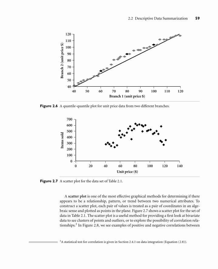
2.2 Descriptive Data Summarization 59
120
110
100
90
80
70
60
50
4040 50 60 70 80
Branch 1 (unit price $)
Bra
nch
2 (
un
it p
rice
$)
90 100 110 120
Figure 2.6 A quantile-quantile plot for unit price data from two different branches.
Unit price ($)
Item
s so
ld
700
600
500
400
300
200
100
00 20 40 60 80 100 120 140
Figure 2.7 A scatter plot for the data set of Table 2.1.
A scatter plot is one of the most effective graphical methods for determining if thereappears to be a relationship, pattern, or trend between two numerical attributes. Toconstruct a scatter plot, each pair of values is treated as a pair of coordinates in an alge-braic sense and plotted as points in the plane. Figure 2.7 shows a scatter plot for the set ofdata in Table 2.1. The scatter plot is a useful method for providing a first look at bivariatedata to see clusters of points and outliers, or to explore the possibility of correlation rela-tionships.3 In Figure 2.8, we see examples of positive and negative correlations between
3A statistical test for correlation is given in Section 2.4.1 on data integration (Equation (2.8)).

60 Chapter 2 Data Preprocessing
Figure 2.8 Scatter plots can be used to find (a) positive or (b) negative correlations between attributes.
Figure 2.9 Three cases where there is no observed correlation between the two plotted attributes in eachof the data sets.
two attributes in two different data sets. Figure 2.9 shows three cases for which there isno correlation relationship between the two attributes in each of the given data sets.
When dealing with several attributes, the scatter-plot matrix is a useful extension tothe scatter plot. Given n attributes, a scatter-plot matrix is an n×n grid of scatter plotsthat provides a visualization of each attribute (or dimension) with every other attribute.The scatter-plot matrix becomes less effective as the number of attributes under studygrows. In this case, user interactions such as zooming and panning become necessary tohelp interpret the individual scatter plots effectively.
A loess curve is another important exploratory graphic aid that adds a smooth curveto a scatter plot in order to provide better perception of the pattern of dependence. Theword loess is short for “local regression.” Figure 2.10 shows a loess curve for the set ofdata in Table 2.1.
To fit a loess curve, values need to be set for two parameters—α, a smoothing param-eter, and λ, the degree of the polynomials that are fitted by the regression. While α can beany positive number (typical values are between 1/4 and 1), λ can be 1 or 2. The goal inchoosing α is to produce a fit that is as smooth as possible without unduly distorting theunderlying pattern in the data. The curve becomes smoother as α increases. There may besome lack of fit, however, indicating possible “missing” data patterns. If α is very small, theunderlying pattern is tracked, yet overfitting of the data may occur where local “wiggles”in the curve may not be supported by the data. If the underlying pattern of the data has a

2.3 Data Cleaning 61
Unit price ($)
Item
s so
ld
700
600
500
400
300
200
100
00 20 40 60 80 100 120 140
Figure 2.10 A loess curve for the data set of Table 2.1.
“gentle” curvature with no local maxima and minima, then local linear fitting is usuallysufficient (λ = 1). However, if there are local maxima or minima, then local quadraticfitting (λ = 2) typically does a better job of following the pattern of the data and main-taining local smoothness.
In conclusion, descriptive data summaries provide valuable insight into the overallbehavior of your data. By helping to identify noise and outliers, they are especially usefulfor data cleaning.
2.3 Data Cleaning
Real-world data tend to be incomplete, noisy, and inconsistent. Data cleaning (or datacleansing) routines attempt to fill in missing values, smooth out noise while identify-ing outliers, and correct inconsistencies in the data. In this section, you will study basicmethods for data cleaning. Section 2.3.1 looks at ways of handling missing values.Section 2.3.2 explains data smoothing techniques. Section 2.3.3 discusses approaches todata cleaning as a process.
2.3.1 Missing Values
Imagine that you need to analyze AllElectronics sales and customer data. You note thatmany tuples have no recorded value for several attributes, such as customer income. Howcan you go about filling in the missing values for this attribute? Let’s look at the followingmethods:
1. Ignore the tuple: This is usually done when the class label is missing (assuming themining task involves classification). This method is not very effective, unless the tuplecontains several attributes with missing values. It is especially poor when the percent-age of missing values per attribute varies considerably.

62 Chapter 2 Data Preprocessing
2. Fill in the missing value manually: In general, this approach is time-consuming andmay not be feasible given a large data set with many missing values.
3. Use a global constant to fill in the missing value: Replace all missing attribute valuesby the same constant, such as a label like “Unknown” or −∞. If missing values arereplaced by, say, “Unknown,” then the mining program may mistakenly think thatthey form an interesting concept, since they all have a value in common—that of“Unknown.” Hence, although this method is simple, it is not foolproof.
4. Use the attribute mean to fill in the missing value: For example, suppose that theaverage income of AllElectronics customers is $56,000. Use this value to replace themissing value for income.
5. Use the attribute mean for all samples belonging to the same class as the given tuple:For example, if classifying customers according to credit risk, replace the missing valuewith the average income value for customers in the same credit risk category as thatof the given tuple.
6. Use the most probable value to fill in the missing value: This may be determinedwith regression, inference-based tools using a Bayesian formalism, or decision treeinduction. For example, using the other customer attributes in your data set, youmay construct a decision tree to predict the missing values for income. Decisiontrees, regression, and Bayesian inference are described in detail in Chapter 6.
Methods 3 to 6 bias the data. The filled-in value may not be correct. Method 6,however, is a popular strategy. In comparison to the other methods, it uses the mostinformation from the present data to predict missing values. By considering the valuesof the other attributes in its estimation of the missing value for income, there is a greaterchance that the relationships between income and the other attributes are preserved.
It is important to note that, in some cases, a missing value may not imply an errorin the data! For example, when applying for a credit card, candidates may be asked tosupply their driver’s license number. Candidates who do not have a driver’s license maynaturally leave this field blank. Forms should allow respondents to specify values such as“not applicable”. Software routines may also be used to uncover other null values, suchas “don’t know”, “?”, or “none”. Ideally, each attribute should have one or more rulesregarding the null condition. The rules may specify whether or not nulls are allowed,and/or how such values should be handled or transformed. Fields may also be inten-tionally left blank if they are to be provided in a later step of the business process. Hence,although we can try our best to clean the data after it is seized, good design of databasesand of data entry procedures should help minimize the number of missing values orerrors in the first place.
2.3.2 Noisy Data
“What is noise?” Noise is a random error or variance in a measured variable. Given anumerical attribute such as, say, price, how can we “smooth” out the data to remove thenoise? Let’s look at the following data smoothing techniques:

2.3 Data Cleaning 63
Sorted data for price (in dollars): 4, 8, 15, 21, 21, 24, 25, 28, 34
Partition into (equal-frequency) bins:
Bin 1: 4, 8, 15Bin 2: 21, 21, 24Bin 3: 25, 28, 34
Smoothing by bin means:
Bin 1: 9, 9, 9Bin 2: 22, 22, 22Bin 3: 29, 29, 29
Smoothing by bin boundaries:
Bin 1: 4, 4, 15Bin 2: 21, 21, 24Bin 3: 25, 25, 34
Figure 2.11 Binning methods for data smoothing.
1. Binning: Binning methods smooth a sorted data value by consulting its “neighbor-hood,” that is, the values around it. The sorted values are distributed into a numberof “buckets,” or bins. Because binning methods consult the neighborhood of values,they perform local smoothing. Figure 2.11 illustrates some binning techniques. In thisexample, the data for price are first sorted and then partitioned into equal-frequencybins of size 3 (i.e., each bin contains three values). In smoothing by bin means, eachvalue in a bin is replaced by the mean value of the bin. For example, the mean of thevalues 4, 8, and 15 in Bin 1 is 9. Therefore, each original value in this bin is replacedby the value 9. Similarly, smoothing by bin medians can be employed, in which eachbin value is replaced by the bin median. In smoothing by bin boundaries, the mini-mum and maximum values in a given bin are identified as the bin boundaries. Eachbin value is then replaced by the closest boundary value. In general, the larger thewidth, the greater the effect of the smoothing. Alternatively, bins may be equal-width,where the interval range of values in each bin is constant. Binning is also used as adiscretization technique and is further discussed in Section 2.6.
2. Regression: Data can be smoothed by fitting the data to a function, such as withregression. Linear regression involves finding the “best” line to fit two attributes (orvariables), so that one attribute can be used to predict the other. Multiple linearregression is an extension of linear regression, where more than two attributes areinvolved and the data are fit to a multidimensional surface. Regression is furtherdescribed in Section 2.5.4, as well as in Chapter 6.

64 Chapter 2 Data Preprocessing
Figure 2.12 A 2-D plot of customer data with respect to customer locations in a city, showing threedata clusters. Each cluster centroid is marked with a “+”, representing the average pointin space for that cluster. Outliers may be detected as values that fall outside of the setsof clusters.
3. Clustering: Outliers may be detected by clustering, where similar values are organizedinto groups, or “clusters.” Intuitively, values that fall outside of the set of clusters maybe considered outliers (Figure 2.12). Chapter 7 is dedicated to the topic of clusteringand outlier analysis.
Many methods for data smoothing are also methods for data reduction involv-ing discretization. For example, the binning techniques described above reduce thenumber of distinct values per attribute. This acts as a form of data reduction forlogic-based data mining methods, such as decision tree induction, which repeatedlymake value comparisons on sorted data. Concept hierarchies are a form of data dis-cretization that can also be used for data smoothing. A concept hierarchy for price, forexample, may map real price values into inexpensive, moderately priced, and expensive,thereby reducing the number of data values to be handled by the mining process.Data discretization is discussed in Section 2.6. Some methods of classification, suchas neural networks, have built-in data smoothing mechanisms. Classification is thetopic of Chapter 6.

2.3 Data Cleaning 65
2.3.3 Data Cleaning as a Process
Missing values, noise, and inconsistencies contribute to inaccurate data. So far, we havelooked at techniques for handling missing data and for smoothing data. “But data clean-ing is a big job. What about data cleaning as a process? How exactly does one proceed intackling this task? Are there any tools out there to help?”
The first step in data cleaning as a process is discrepancy detection. Discrepancies canbe caused by several factors, including poorly designed data entry forms that have manyoptional fields, human error in data entry, deliberate errors (e.g., respondents not wantingto divulge information about themselves), and data decay (e.g., outdated addresses). Dis-crepancies may also arise from inconsistent data representations and the inconsistent useofcodes.Errors in instrumentationdevices that recorddata,andsystemerrors, areanothersource of discrepancies. Errors can also occur when the data are (inadequately) used forpurposes other than originally intended. There may also be inconsistencies due to dataintegration (e.g., where a given attribute can have different names in different databases).4
“So, how can we proceed with discrepancy detection?” As a starting point, use any knowl-edge you may already have regarding properties of the data. Such knowledge or “dataabout data” is referred to as metadata. For example, what are the domain and data type ofeach attribute? What are the acceptable values for each attribute? What is the range of thelength of values? Do all values fall within the expected range? Are there any known depen-dencies between attributes? The descriptive data summaries presented in Section 2.2 areuseful here for grasping data trends and identifying anomalies. For example, values thatare more than two standard deviations away from the mean for a given attribute maybe flagged as potential outliers. In this step, you may write your own scripts and/or usesome of the tools that we discuss further below. From this, you may find noise, outliers,and unusual values that need investigation.
As a data analyst, you should be on the lookout for the inconsistent use of codes and anyinconsistent data representations (such as “2004/12/25” and “25/12/2004” for date). Fieldoverloading is another source of errors that typically results when developers squeeze newattribute definitions into unused (bit) portions of already defined attributes (e.g., usingan unused bit of an attribute whose value range uses only, say, 31 out of 32 bits).
The data should also be examined regarding unique rules, consecutive rules, and nullrules. A unique rule says that each value of the given attribute must be different fromall other values for that attribute. A consecutive rule says that there can be no miss-ing values between the lowest and highest values for the attribute, and that all valuesmust also be unique (e.g., as in check numbers). A null rule specifies the use of blanks,question marks, special characters, or other strings that may indicate the null condi-tion (e.g., where a value for a given attribute is not available), and how such valuesshould be handled. As mentioned in Section 2.3.1, reasons for missing values may include(1) the person originally asked to provide a value for the attribute refuses and/or finds
4Data integration and the removal of redundant data that can result from such integration are furtherdescribed in Section 2.4.1.

66 Chapter 2 Data Preprocessing
that the information requested is not applicable (e.g., a license-number attribute left blankby nondrivers); (2) the data entry person does not know the correct value; or (3) the valueis to be provided by a later step of the process. The null rule should specify how to recordthe null condition, for example, such as to store zero for numerical attributes, a blankfor character attributes, or any other conventions that may be in use (such as that entrieslike “don’t know” or “?” should be transformed to blank).
There are a number of different commercial tools that can aid in the step of discrepancydetection. Data scrubbing tools use simple domain knowledge (e.g., knowledge of postaladdresses, and spell-checking) to detect errors and make corrections in the data. Thesetools rely on parsing and fuzzy matching techniques when cleaning data from multiplesources. Data auditing tools find discrepancies by analyzing the data to discover rulesand relationships, and detecting data that violate such conditions. They are variants ofdata mining tools. For example, they may employ statistical analysis to find correlations,or clustering to identify outliers. They may also use the descriptive data summaries thatwere described in Section 2.2.
Some data inconsistencies may be corrected manually using external references. Forexample, errors made at data entry may be corrected by performing a paper trace. Mosterrors, however, will require data transformations. This is the second step in data cleaningas a process. That is, once we find discrepancies, we typically need to define and apply(a series of) transformations to correct them.
Commercial tools can assist in the data transformation step. Data migration toolsallow simple transformations to be specified, such as to replace the string “gender” by“sex”. ETL (extraction/transformation/loading) tools allow users to specify transformsthrough a graphical user interface (GUI). These tools typically support only a restrictedset of transforms so that, often, we may also choose to write custom scripts for this stepof the data cleaning process.
The two-step process of discrepancy detection and data transformation (to correct dis-crepancies) iterates. This process, however, is error-prone and time-consuming. Sometransformations may introduce more discrepancies. Some nested discrepancies may onlybe detected after others have been fixed. For example, a typo such as “20004” in a year fieldmay only surface once all date values have been converted to a uniform format. Transfor-mations are often done as a batch process while the user waits without feedback. Onlyafter the transformation is complete can the user go back and check that no new anoma-lies have been created by mistake. Typically, numerous iterations are required before theuser is satisfied.Anytuples thatcannotbeautomaticallyhandledbyagiventransformationare typically written to a file without any explanation regarding the reasoning behind theirfailure. As a result, the entire data cleaning process also suffers from a lack of interactivity.
New approaches to data cleaning emphasize increased interactivity. Potter’s Wheel, forexample, is a publicly available data cleaning tool (see http://control.cs.berkeley.edu/abc)that integrates discrepancy detection and transformation. Users gradually build a series oftransformations by composing and debugging individual transformations, one step at atime, on a spreadsheet-like interface. The transformations can be specified graphically orby providing examples. Results are shown immediately on the records that are visible onthe screen. The user can choose to undo the transformations, so that transformations

2.4 Data Integration and Transformation 67
that introduced additional errors can be “erased.” The tool performs discrepancychecking automatically in the background on the latest transformed view of the data.Users can gradually develop and refine transformations as discrepancies are found,leading to more effective and efficient data cleaning.
Another approach to increased interactivity in data cleaning is the development ofdeclarative languages for the specification of data transformation operators. Such workfocuses on defining powerful extensions to SQL and algorithms that enable users toexpress data cleaning specifications efficiently.
As we discover more about the data, it is important to keep updating the metadatato reflect this knowledge. This will help speed up data cleaning on future versions of thesame data store.
2.4 Data Integration and Transformation
Data mining often requires data integration—the merging of data from multiple datastores. The data may also need to be transformed into forms appropriate for mining.This section describes both data integration and data transformation.
2.4.1 Data Integration
It is likely that your data analysis task will involve data integration, which combines datafrom multiple sources into a coherent data store, as in data warehousing. These sourcesmay include multiple databases, data cubes, or flat files.
There are a number of issues to consider during data integration. Schema integrationand object matching can be tricky. How can equivalent real-world entities from multipledata sources be matched up? This is referred to as the entity identification problem.For example, how can the data analyst or the computer be sure that customer id in onedatabase and cust number in another refer to the same attribute? Examples of metadatafor each attribute include the name, meaning, data type, and range of values permittedfor the attribute, and null rules for handling blank, zero, or null values (Section 2.3).Such metadata can be used to help avoid errors in schema integration. The metadatamay also be used to help transform the data (e.g., where data codes for pay type in onedatabase may be “H” and “S”, and 1 and 2 in another). Hence, this step also relates todata cleaning, as described earlier.
Redundancy is another important issue. An attribute (such as annual revenue, forinstance) may be redundant if it can be “derived” from another attribute or set ofattributes. Inconsistencies in attribute or dimension naming can also cause redundan-cies in the resulting data set.
Some redundancies can be detected by correlation analysis. Given two attributes, suchanalysis can measure how strongly one attribute implies the other, based on the availabledata. For numerical attributes, we can evaluate the correlation between two attributes, Aand B, by computing the correlation coefficient (also known as Pearson’s product momentcoefficient, named after its inventer, Karl Pearson). This is

68 Chapter 2 Data Preprocessing
rA,B =
N
∑i=1
(ai−A)(bi−B)
NσAσB=
N
∑i=1
(aibi)−NAB
NσAσB, (2.8)
where N is the number of tuples, ai and bi are the respective values of A and B in tuple i,A and B are the respective mean values of A and B, σA and σB are the respective standarddeviations of A and B (as defined in Section 2.2.2), and Σ(aibi) is the sum of the ABcross-product (that is, for each tuple, the value for A is multiplied by the value for B inthat tuple). Note that−1≤ rA,B≤+1. If rA,B is greater than 0, then A and B are positivelycorrelated, meaning that the values of A increase as the values of B increase. The higherthe value, the stronger the correlation (i.e., the more each attribute implies the other).Hence, a higher value may indicate that A (or B) may be removed as a redundancy. If theresulting value is equal to 0, then A and B are independent and there is no correlationbetween them. If the resulting value is less than 0, then A and B are negatively correlated,where the values of one attribute increase as the values of the other attribute decrease.This means that each attribute discourages the other. Scatter plots can also be used toview correlations between attributes (Section 2.2.3).
Note that correlation does not imply causality. That is, if A and B are correlated, thisdoes not necessarily imply that A causes B or that B causes A. For example, in analyzing ademographic database, we may find that attributes representing the number of hospitalsand the number of car thefts in a region are correlated. This does not mean that onecauses the other. Both are actually causally linked to a third attribute, namely, population.
For categorical (discrete) data, a correlation relationship between two attributes, Aand B, can be discovered by a χ2 (chi-square) test. Suppose A has c distinct values, namelya1,a2, . . .ac. B has r distinct values, namely b1,b2, . . .br. The data tuples described by Aand B can be shown as a contingency table, with the c values of A making up the columnsand the r values of B making up the rows. Let (Ai,B j) denote the event that attribute Atakes on value ai and attribute B takes on value b j, that is, where (A = ai,B = b j). Eachand every possible (Ai,B j) joint event has its own cell (or slot) in the table. The χ2 value(also known as the Pearson χ2 statistic) is computed as:
χ2 =c
∑i=1
r
∑j=1
(oi j− ei j)2
ei j, (2.9)
where oi j is the observed frequency (i.e., actual count) of the joint event (Ai,B j) and ei jis the expected frequency of (Ai,B j), which can be computed as
ei j =count(A = ai)× count(B = b j)
N, (2.10)
where N is the number of data tuples, count(A = ai) is the number of tuples having valueai for A, and count(B = b j) is the number of tuples having value b j for B. The sum inEquation (2.9) is computed over all of the r× c cells. Note that the cells that contributethe most to the χ2 value are those whose actual count is very different from that expected.

2.4 Data Integration and Transformation 69
Table 2.2 A 2× 2 contingency table for the data of Example 2.1.Are gender and preferred Reading correlated?
male female Total
fiction 250 (90) 200 (360) 450
non fiction 50 (210) 1000 (840) 1050
Total 300 1200 1500
The χ2 statistic tests the hypothesis that A and B are independent. The test is based ona significance level, with (r−1)× (c−1) degrees of freedom. We will illustrate the useof this statistic in an example below. If the hypothesis can be rejected, then we say that Aand B are statistically related or associated.
Let’s look at a concrete example.
Example 2.1 Correlation analysis of categorical attributes using χ2. Suppose that a group of 1,500people was surveyed. The gender of each person was noted. Each person was polled as towhether their preferred type of reading material was fiction or nonfiction. Thus, we havetwo attributes, gender and preferred reading. The observed frequency (or count) of eachpossible joint event is summarized in the contingency table shown in Table 2.2, wherethe numbers in parentheses are the expected frequencies (calculated based on the datadistribution for both attributes using Equation (2.10)).
Using Equation (2.10), we can verify the expected frequencies for each cell. For exam-ple, the expected frequency for the cell (male, fiction) is
e11 =count(male)× count(fiction)
N=
300×4501500
= 90,
and so on. Notice that in any row, the sum of the expected frequencies must equal thetotal observed frequency for that row, and the sum of the expected frequencies in any col-umn must also equal the total observed frequency for that column. Using Equation (2.9)for χ2 computation, we get
χ2 =(250−90)2
90+
(50−210)2
210+
(200−360)2
360+
(1000−840)2
840= 284.44 + 121.90 + 71.11 + 30.48 = 507.93.
For this 2 × 2 table, the degrees of freedom are (2− 1)(2− 1) = 1. For 1 degree offreedom, the χ2 value needed to reject the hypothesis at the 0.001 significance level is10.828 (taken from the table of upper percentage points of the χ2 distribution, typicallyavailable from any textbook on statistics). Since our computed value is above this, we canreject the hypothesis that gender and preferred reading are independent and conclude thatthe two attributes are (strongly) correlated for the given group of people.
In addition to detecting redundancies between attributes, duplication should alsobe detected at the tuple level (e.g., where there are two or more identical tuples for a

70 Chapter 2 Data Preprocessing
given unique data entry case). The use of denormalized tables (often done to improveperformance by avoiding joins) is another source of data redundancy. Inconsistenciesoften arise between various duplicates, due to inaccurate data entry or updating somebut not all of the occurrences of the data. For example, if a purchase order database con-tains attributes for the purchaser’s name and address instead of a key to this informationin a purchaser database, discrepancies can occur, such as the same purchaser’s nameappearing with different addresses within the purchase order database.
A third important issue in data integration is the detection and resolution of datavalue conflicts. For example, for the same real-world entity, attribute values fromdifferent sources may differ. This may be due to differences in representation, scaling,or encoding. For instance, a weight attribute may be stored in metric units in onesystem and British imperial units in another. For a hotel chain, the price of roomsin different cities may involve not only different currencies but also different services(such as free breakfast) and taxes. An attribute in one system may be recorded ata lower level of abstraction than the “same” attribute in another. For example, thetotal sales in one database may refer to one branch of All Electronics, while an attributeof the same name in another database may refer to the total sales for All Electronicsstores in a given region.
When matching attributes from one database to another during integration, specialattention must be paid to the structure of the data. This is to ensure that any attributefunctional dependencies and referential constraints in the source system match those inthe target system. For example, in one system, a discount may be applied to the order,whereas in another system it is applied to each individual line item within the order.If this is not caught before integration, items in the target system may be improperlydiscounted.
The semantic heterogeneity and structure of data pose great challenges in data inte-gration. Careful integration of the data from multiple sources can help reduce and avoidredundancies and inconsistencies in the resulting data set. This can help improve theaccuracy and speed of the subsequent mining process.
2.4.2 Data Transformation
In data transformation, the data are transformed or consolidated into forms appropriatefor mining. Data transformation can involve the following:
Smoothing, which works to remove noise from the data. Such techniques includebinning, regression, and clustering.
Aggregation, where summary or aggregation operations are applied to the data. Forexample, the daily sales data may be aggregated so as to compute monthly and annualtotal amounts. This step is typically used in constructing a data cube for analysis ofthe data at multiple granularities.
Generalization of the data, where low-level or “primitive” (raw) data are replaced byhigher-level concepts through the use of concept hierarchies. For example, categorical

2.4 Data Integration and Transformation 71
attributes, like street, can be generalized to higher-level concepts, like city or country.Similarly, values for numerical attributes, like age, may be mapped to higher-levelconcepts, like youth, middle-aged, and senior.
Normalization, where the attribute data are scaled so as to fall within a small specifiedrange, such as−1.0 to 1.0, or 0.0 to 1.0.
Attribute construction (or feature construction), where new attributes are constructedand added from the given set of attributes to help the mining process.
Smoothing is a form of data cleaning and was addressed in Section 2.3.2. Section 2.3.3on the data cleaning process also discussed ETL tools, where users specify transforma-tions to correct data inconsistencies. Aggregation and generalization serve as forms ofdata reduction and are discussed in Sections 2.5 and 2.6, respectively. In this section, wetherefore discuss normalization and attribute construction.
An attribute is normalized by scaling its values so that they fall within a small specifiedrange, such as 0.0 to 1.0. Normalization is particularly useful for classification algorithmsinvolving neural networks, or distance measurements such as nearest-neighbor classifi-cation and clustering. If using the neural network backpropagation algorithm for clas-sification mining (Chapter 6), normalizing the input values for each attribute measuredin the training tuples will help speed up the learning phase. For distance-based methods,normalization helps prevent attributes with initially large ranges (e.g., income) from out-weighing attributes with initially smaller ranges (e.g., binary attributes). There are manymethods for data normalization. We study three: min-max normalization, z-score nor-malization, and normalization by decimal scaling.
Min-max normalization performs a linear transformation on the original data. Sup-pose that minA and maxA are the minimum and maximum values of an attribute, A.Min-max normalization maps a value, v, of A to v′ in the range [new minA,new maxA]by computing
v′ =v−minA
maxA−minA(new maxA−new minA)+ new minA. (2.11)
Min-max normalization preserves the relationships among the original data values.It will encounter an “out-of-bounds” error if a future input case for normalization fallsoutside of the original data range for A.
Example 2.2 Min-max normalization. Suppose that the minimum and maximum values for theattribute income are $12,000 and $98,000, respectively. We would like to map income tothe range [0.0,1.0]. By min-max normalization, a value of $73,600 for income is trans-formed to 73,600−12,000
98,000−12,000 (1.0−0)+ 0 = 0.716.
In z-score normalization (or zero-mean normalization), the values for an attribute,A, are normalized based on the mean and standard deviation of A. A value, v, of A isnormalized to v′ by computing

72 Chapter 2 Data Preprocessing
v′ =v−A
σA, (2.12)
where A and σA are the mean and standard deviation, respectively, of attribute A. Thismethod of normalization is useful when the actual minimum and maximum of attributeA are unknown, or when there are outliers that dominate the min-max normalization.
Example 2.3 z-score normalization Suppose that the mean and standard deviation of the values forthe attribute income are $54,000 and $16,000, respectively. With z-score normalization,a value of $73,600 for income is transformed to 73,600−54,000
16,000 = 1.225.
Normalization by decimal scaling normalizes by moving the decimal point of valuesof attribute A. The number of decimal points moved depends on the maximum absolutevalue of A. A value, v, of A is normalized to v′ by computing
v′ =v
10 j , (2.13)
where j is the smallest integer such that Max(|v′|)< 1.
Example 2.4 Decimal scaling. Suppose that the recorded values of A range from −986 to 917. Themaximum absolute value of A is 986. To normalize by decimal scaling, we therefore divideeach value by 1,000 (i.e., j = 3) so that−986 normalizes to−0.986 and 917 normalizesto 0.917.
Note that normalization can change the original data quite a bit, especially the lat-ter two methods shown above. It is also necessary to save the normalization parameters(such as the mean and standard deviation if using z-score normalization) so that futuredata can be normalized in a uniform manner.
In attribute construction,5 new attributes are constructed from the given attributesand added in order to help improve the accuracy and understanding of structure inhigh-dimensional data. For example, we may wish to add the attribute area based onthe attributes height and width. By combining attributes, attribute construction can dis-cover missing information about the relationships between data attributes that can beuseful for knowledge discovery.
2.5 Data Reduction
Imagine that you have selected data from the AllElectronics data warehouse for analysis.The data set will likely be huge! Complex data analysis and mining on huge amounts ofdata can take a long time, making such analysis impractical or infeasible.
5In the machine learning literature, attribute construction is known as feature construction.

2.5 Data Reduction 73
Data reduction techniques can be applied to obtain a reduced representation of thedata set that is much smaller in volume, yet closely maintains the integrity of the originaldata. That is, mining on the reduced data set should be more efficient yet produce thesame (or almost the same) analytical results.
Strategies for data reduction include the following:
1. Data cube aggregation, where aggregation operations are applied to the data in theconstruction of a data cube.
2. Attribute subset selection, where irrelevant, weakly relevant, or redundant attributesor dimensions may be detected and removed.
3. Dimensionality reduction, where encoding mechanisms are used to reduce the dataset size.
4. Numerosity reduction, where the data are replaced or estimated by alternative, smallerdata representations such as parametric models (which need store only the modelparameters instead of the actual data) or nonparametric methods such as clustering,sampling, and the use of histograms.
5. Discretization and concept hierarchy generation, where raw data values for attributesare replaced by ranges or higher conceptual levels. Data discretization is a form ofnumerosity reduction that is very useful for the automatic generation of concept hier-archies. Discretization and concept hierarchy generation are powerful tools for datamining, in that they allow the mining of data at multiple levels of abstraction. Wetherefore defer the discussion of discretization and concept hierarchy generation toSection 2.6, which is devoted entirely to this topic.
Strategies 1 to 4 above are discussed in the remainder of this section. The computationaltime spent on data reduction should not outweigh or “erase” the time saved by miningon a reduced data set size.
2.5.1 Data Cube Aggregation
Imagine that you have collected the data for your analysis. These data consist of theAllElectronics sales per quarter, for the years 2002 to 2004. You are, however, interestedin the annual sales (total per year), rather than the total per quarter. Thus the datacan be aggregated so that the resulting data summarize the total sales per year insteadof per quarter. This aggregation is illustrated in Figure 2.13. The resulting data set issmaller in volume, without loss of information necessary for the analysis task.
Data cubes are discussed in detail in Chapter 3 on data warehousing. We brieflyintroduce some concepts here. Data cubes store multidimensional aggregated infor-mation. For example, Figure 2.14 shows a data cube for multidimensional analysis ofsales data with respect to annual sales per item type for each AllElectronics branch.Each cell holds an aggregate data value, corresponding to the data point in mul-tidimensional space. (For readability, only some cell values are shown.) Concept

74 Chapter 2 Data Preprocessing
Quarter
Year 2004
Sales
Q1 Q2 Q3 Q4
$224,000�$408,000�$350,000�$586,000
Quarter
Year 2003
Sales
Q1 Q2 Q3 Q4
$224,000�$408,000�$350,000�$586,000
Quarter
Year 2002
Sales
Q1 Q2 Q3 Q4
$224,000�$408,000�$350,000�$586,000
Year Sales
2002�2003�2004
$1,568,000�$2,356,000�$3,594,000
Figure 2.13 Sales data for a given branch of AllElectronics for the years 2002 to 2004. On the left, the salesare shown per quarter. On the right, the data are aggregated to provide the annual sales.
568
A
B
C
D
750
150
50
home entertainment
computer
phone
security
2002 2003
year
item
type
branch
2004
Figure 2.14 A data cube for sales at AllElectronics.
hierarchies may exist for each attribute, allowing the analysis of data at multiplelevels of abstraction. For example, a hierarchy for branch could allow branches tobe grouped into regions, based on their address. Data cubes provide fast access toprecomputed, summarized data, thereby benefiting on-line analytical processing aswell as data mining.
The cube created at the lowest level of abstraction is referred to as the basecuboid. The base cuboid should correspond to an individual entity of interest, suchas sales or customer. In other words, the lowest level should be usable, or usefulfor the analysis. A cube at the highest level of abstraction is the apex cuboid. Forthe sales data of Figure 2.14, the apex cuboid would give one total—the total sales

2.5 Data Reduction 75
for all three years, for all item types, and for all branches. Data cubes created forvarying levels of abstraction are often referred to as cuboids, so that a data cube mayinstead refer to a lattice of cuboids. Each higher level of abstraction further reducesthe resulting data size. When replying to data mining requests, the smallest availablecuboid relevant to the given task should be used. This issue is also addressed inChapter 3.
2.5.2 Attribute Subset Selection
Data sets for analysis may contain hundreds of attributes, many of which may beirrelevant to the mining task or redundant. For example, if the task is to classifycustomers as to whether or not they are likely to purchase a popular new CD atAllElectronics when notified of a sale, attributes such as the customer’s telephone num-ber are likely to be irrelevant, unlike attributes such as age or music taste. Althoughit may be possible for a domain expert to pick out some of the useful attributes,this can be a difficult and time-consuming task, especially when the behavior of thedata is not well known (hence, a reason behind its analysis!). Leaving out relevantattributes or keeping irrelevant attributes may be detrimental, causing confusion forthe mining algorithm employed. This can result in discovered patterns of poor qual-ity. In addition, the added volume of irrelevant or redundant attributes can slowdown the mining process.
Attribute subset selection6 reduces the data set size by removing irrelevant orredundant attributes (or dimensions). The goal of attribute subset selection is tofind a minimum set of attributes such that the resulting probability distribution ofthe data classes is as close as possible to the original distribution obtained using allattributes. Mining on a reduced set of attributes has an additional benefit. It reducesthe number of attributes appearing in the discovered patterns, helping to make thepatterns easier to understand.
“How can we find a ‘good’ subset of the original attributes?” For n attributes, there are2n possible subsets. An exhaustive search for the optimal subset of attributes can be pro-hibitively expensive, especially as n and the number of data classes increase. Therefore,heuristic methods that explore a reduced search space are commonly used for attributesubset selection. These methods are typically greedy in that, while searching throughattribute space, they always make what looks to be the best choice at the time. Theirstrategy is to make a locally optimal choice in the hope that this will lead to a globallyoptimal solution. Such greedy methods are effective in practice and may come close toestimating an optimal solution.
The “best” (and “worst”) attributes are typically determined using tests of statisticalsignificance, which assume that the attributes are independent of one another. Many
6In machine learning, attribute subset selection is known as feature subset selection.

76 Chapter 2 Data Preprocessing
Forward selection
Initial attribute set:�{A1, A2, A3, A4, A5, A6}��Initial reduced set: {} => {A1}�=> {A1, A4}�=> Reduced attribute set: {A1, A4, A6}�
Initial attribute set:�{A1, A2, A3, A4, A5, A6}� => {A1, A3, A4, A5, A6}�=> {A1, A4, A5, A6}�=> Reduced attribute set: {A1, A4, A6}�
Initial attribute set:�{A1, A2, A3, A4, A5, A6}
=> Reduced attribute set: {A1, A4, A6}�
Backward elimination Decision tree induction
A4?
A1? A6?
Class 1 Class 2 Class 1 Class 2
Y N
Y N Y N
Figure 2.15 Greedy (heuristic) methods for attribute subset selection.
other attribute evaluation measures can be used, such as the information gain measureused in building decision trees for classification.7
Basic heuristic methods of attribute subset selection include the following techniques,some of which are illustrated in Figure 2.15.
1. Stepwise forward selection: The procedure starts with an empty set of attributes asthe reduced set. The best of the original attributes is determined and added to thereduced set. At each subsequent iteration or step, the best of the remaining originalattributes is added to the set.
2. Stepwise backward elimination: The procedure starts with the full set of attributes.At each step, it removes the worst attribute remaining in the set.
3. Combination of forward selection and backward elimination: The stepwise forwardselection and backward elimination methods can be combined so that, at each step,the procedure selects the best attribute and removes the worst from among the remain-ing attributes.
4. Decision tree induction: Decision tree algorithms, such as ID3, C4.5, and CART, wereoriginally intended for classification. Decision tree induction constructs a flowchart-like structure where each internal (nonleaf) node denotes a test on an attribute, eachbranch corresponds to an outcome of the test, and each external (leaf) node denotes a
7The information gain measure is described in detail in Chapter 6. It is briefly described in Section 2.6.1with respect to attribute discretization.

2.5 Data Reduction 77
class prediction. At each node, the algorithm chooses the “best” attribute to partitionthe data into individual classes.
When decision tree induction is used for attribute subset selection, a tree isconstructedfromthegivendata.Allattributes thatdonotappear inthetreeareassumedto be irrelevant. The set of attributes appearing in the tree form the reduced subset ofattributes.
The stopping criteria for the methods may vary. The procedure may employ a thresh-old on the measure used to determine when to stop the attribute selection process.
2.5.3 Dimensionality Reduction
In dimensionality reduction, data encoding or transformations are applied so as to obtaina reduced or “compressed” representation of the original data. If the original data canbe reconstructed from the compressed data without any loss of information, the datareduction is called lossless. If, instead, we can reconstruct only an approximation ofthe original data, then the data reduction is called lossy. There are several well-tunedalgorithms for string compression. Although they are typically lossless, they allow onlylimited manipulation of the data. In this section, we instead focus on two popular andeffective methods of lossy dimensionality reduction: wavelet transforms and principalcomponents analysis.
Wavelet TransformsThe discrete wavelet transform (DWT) is a linear signal processing technique that, whenapplied to a data vector X, transforms it to a numerically different vector, X′, of waveletcoefficients. The two vectors are of the same length. When applying this technique todata reduction, we consider each tuple as an n-dimensional data vector, that is, X =(x1,x2, . . . ,xn), depicting n measurements made on the tuple from n database attributes.8
“How can this technique be useful for data reduction if the wavelet transformed data areof the same length as the original data?” The usefulness lies in the fact that the wavelettransformed data can be truncated. A compressed approximation of the data can beretained by storing only a small fraction of the strongest of the wavelet coefficients.For example, all wavelet coefficients larger than some user-specified threshold can beretained. All other coefficients are set to 0. The resulting data representation is there-fore very sparse, so that operations that can take advantage of data sparsity are compu-tationally very fast if performed in wavelet space. The technique also works to removenoise without smoothing out the main features of the data, making it effective for datacleaning as well. Given a set of coefficients, an approximation of the original data can beconstructed by applying the inverse of the DWT used.
8In our notation, any variable representing a vector is shown in bold italic font; measurements depictingthe vector are shown in italic font.

78 Chapter 2 Data Preprocessing
21.0 20.5 0.0 0.5 1.0 1.5 2.0 0 2 4 6
(a) Haar-2 (b) Daubechies-4
0.8
0.6
0.4
0.2
0.0
0.6
0.4
0.2
0.0
Figure 2.16 Examples of wavelet families. The number next to a wavelet name is the number of vanishingmoments of the wavelet. This is a set of mathematical relationships that the coefficients mustsatisfy and is related to the number of coefficients.
The DWT is closely related to the discrete Fourier transform (DFT), a signal processingtechnique involving sines and cosines. In general, however, the DWT achieves better lossycompression. That is, if the same number of coefficients is retained for a DWT and a DFTof a given data vector, the DWT version will provide a more accurate approximation ofthe original data. Hence, for an equivalent approximation, the DWT requires less spacethan the DFT. Unlike the DFT, wavelets are quite localized in space, contributing to theconservation of local detail.
There is only one DFT, yet there are several families of DWTs. Figure 2.16 showssome wavelet families. Popular wavelet transforms include the Haar-2, Daubechies-4,and Daubechies-6 transforms. The general procedure for applying a discrete wavelettransform uses a hierarchical pyramid algorithm that halves the data at each iteration,resulting in fast computational speed. The method is as follows:
1. The length, L, of the input data vector must be an integer power of 2. This conditioncan be met by padding the data vector with zeros as necessary (L≥ n).
2. Each transform involves applying two functions. The first applies some data smooth-ing, such as a sum or weighted average. The second performs a weighted difference,which acts to bring out the detailed features of the data.
3. The two functions are applied to pairs of data points in X, that is, to all pairs ofmeasurements (x2i,x2i+1). This results in two sets of data of length L/2. In general,these represent a smoothed or low-frequency version of the input data and the high-frequency content of it, respectively.
4. The two functions are recursively applied to the sets of data obtained in the previousloop, until the resulting data sets obtained are of length 2.
5. Selected values from the data sets obtained in the above iterations are designated thewavelet coefficients of the transformed data.

2.5 Data Reduction 79
Equivalently, a matrix multiplication can be applied to the input data in order toobtain the wavelet coefficients, where the matrix used depends on the given DWT. Thematrix must be orthonormal, meaning that the columns are unit vectors and aremutually orthogonal, so that the matrix inverse is just its transpose. Although we donot have room to discuss it here, this property allows the reconstruction of the data fromthe smooth and smooth-difference data sets. By factoring the matrix used into a productof a few sparse matrices, the resulting “fast DWT” algorithm has a complexity of O(n)for an input vector of length n.
Wavelet transforms can be applied to multidimensional data, such as a data cube.This is done by first applying the transform to the first dimension, then to the second,and so on. The computational complexity involved is linear with respect to the numberof cells in the cube. Wavelet transforms give good results on sparse or skewed data andon data with ordered attributes. Lossy compression by wavelets is reportedly better thanJPEG compression, the current commercial standard. Wavelet transforms have manyreal-world applications, including the compression of fingerprint images, computervision, analysis of time-series data, and data cleaning.
Principal Components AnalysisIn this subsection we provide an intuitive introduction to principal components analysisas a method of dimesionality reduction. A detailed theoretical explanation is beyond thescope of this book.
Suppose that the data to be reduced consist of tuples or data vectors described byn attributes or dimensions. Principal components analysis, or PCA (also called theKarhunen-Loeve, or K-L, method), searches for k n-dimensional orthogonal vectorsthat can best be used to represent the data, where k ≤ n. The original data are thusprojected onto a much smaller space, resulting in dimensionality reduction. Unlikeattribute subset selection, which reduces the attribute set size by retaining a subsetof the initial set of attributes, PCA “combines” the essence of attributes by creatingan alternative, smaller set of variables. The initial data can then be projected ontothis smaller set. PCA often reveals relationships that were not previously suspectedand thereby allows interpretations that would not ordinarily result.
The basic procedure is as follows:
1. The input data are normalized, so that each attribute falls within the same range. Thisstep helps ensure that attributes with large domains will not dominate attributes withsmaller domains.
2. PCA computes k orthonormal vectors that provide a basis for the normalized inputdata. These are unit vectors that each point in a direction perpendicular to the others.These vectors are referred to as the principal components. The input data are a linearcombination of the principal components.
3. The principal components are sorted in order of decreasing “significance” orstrength. The principal components essentially serve as a new set of axes for the

80 Chapter 2 Data Preprocessing
Y2
X2
Y1
X1
Figure 2.17 Principal components analysis. Y1 and Y2 are the first two principal components for thegiven data.
data, providing important information about variance. That is, the sorted axes aresuch that the first axis shows the most variance among the data, the second axisshows the next highest variance, and so on. For example, Figure 2.17 shows thefirst two principal components, Y1 and Y2, for the given set of data originallymapped to the axes X1 and X2. This information helps identify groups or patternswithin the data.
4. Because the components are sorted according to decreasing order of “significance,”the size of the data can be reduced by eliminating the weaker components, thatis, those with low variance. Using the strongest principal components, it shouldbe possible to reconstruct a good approximation of the original data.
PCA is computationally inexpensive, can be applied to ordered and unorderedattributes, and can handle sparse data and skewed data. Multidimensional dataof more than two dimensions can be handled by reducing the problem to twodimensions. Principal components may be used as inputs to multiple regressionand cluster analysis. In comparison with wavelet transforms, PCA tends to be betterat handling sparse data, whereas wavelet transforms are more suitable for data ofhigh dimensionality.
2.5.4 Numerosity Reduction
“Can we reduce the data volume by choosing alternative, ‘smaller’ forms of data represen-tation?” Techniques of numerosity reduction can indeed be applied for this purpose.These techniques may be parametric or nonparametric. For parametric methods, amodel is used to estimate the data, so that typically only the data parameters need tobe stored, instead of the actual data. (Outliers may also be stored.) Log-linear models,which estimate discrete multidimensional probability distributions, are an example.Nonparametric methods for storing reduced representations of the data include his-tograms, clustering, and sampling.
Let’s look at each of the numerosity reduction techniques mentioned above.

2.5 Data Reduction 81
Regression and Log-Linear ModelsRegression and log-linear models can be used to approximate the given data. In (simple)linear regression, the data are modeled to fit a straight line. For example, a random vari-able, y (called a response variable), can be modeled as a linear function of another randomvariable, x (called a predictor variable), with the equation
y = wx + b, (2.14)
where the variance of y is assumed to be constant. In the context of data mining, x and yare numerical database attributes. The coefficients, w and b (called regression coefficients),specify the slope of the line and the Y -intercept, respectively. These coefficients can besolved for by the method of least squares, which minimizes the error between the actualline separating the data and the estimate of the line. Multiple linear regression is anextension of (simple) linear regression, which allows a response variable, y, to be modeledas a linear function of two or more predictor variables.
Log-linear models approximate discrete multidimensional probability distribu-tions. Given a set of tuples in n dimensions (e.g., described by n attributes), wecan consider each tuple as a point in an n-dimensional space. Log-linear modelscan be used to estimate the probability of each point in a multidimensional spacefor a set of discretized attributes, based on a smaller subset of dimensional combi-nations. This allows a higher-dimensional data space to be constructed from lower-dimensional spaces. Log-linear models are therefore also useful for dimensionalityreduction (since the lower-dimensional points together typically occupy less spacethan the original data points) and data smoothing (since aggregate estimates in thelower-dimensional space are less subject to sampling variations than the estimates inthe higher-dimensional space).
Regression and log-linear models can both be used on sparse data, although theirapplication may be limited. While both methods can handle skewed data, regression doesexceptionally well. Regression can be computationally intensive when applied to high-dimensional data, whereas log-linear models show good scalability for up to 10 or sodimensions. Regression and log-linear models are further discussed in Section 6.11.
HistogramsHistograms use binning to approximate data distributions and are a popular formof data reduction. Histograms were introduced in Section 2.2.3. A histogram for anattribute, A, partitions the data distribution of A into disjoint subsets, or buckets. Ifeach bucket represents only a single attribute-value/frequency pair, the buckets arecalled singleton buckets. Often, buckets instead represent continuous ranges for thegiven attribute.
Example 2.5 Histograms. The following data are a list of prices of commonly sold items at AllElec-tronics (rounded to the nearest dollar). The numbers have been sorted: 1, 1, 5, 5, 5, 5, 5,8, 8, 10, 10, 10, 10, 12, 14, 14, 14, 15, 15, 15, 15, 15, 15, 18, 18, 18, 18, 18, 18, 18, 18, 20,20, 20, 20, 20, 20, 20, 21, 21, 21, 21, 25, 25, 25, 25, 25, 28, 28, 30, 30, 30.

82 Chapter 2 Data Preprocessing
10
9
8
7
6
5
4
3
2
1
05 10 15 20 25 30
price ($)
cou
nt
Figure 2.18 A histogram for price using singleton buckets—each bucket represents one price-value/frequency pair.
Figure 2.18 shows a histogram for the data using singleton buckets. To further reducethe data, it is common to have each bucket denote a continuous range of values for thegiven attribute. In Figure 2.19, each bucket represents a different $10 range for price.
“How are the buckets determined and the attribute values partitioned?” There are severalpartitioning rules, including the following:
Equal-width: In an equal-width histogram, the width of each bucket range is uniform(such as the width of $10 for the buckets in Figure 2.19).
Equal-frequency (or equidepth): In an equal-frequency histogram, the buckets arecreated so that, roughly, the frequency of each bucket is constant (that is, each bucketcontains roughly the same number of contiguous data samples).
V-Optimal: If we consider all of the possible histograms for a given number of buckets,the V-Optimal histogram is the one with the least variance. Histogram variance is aweighted sum of the original values that each bucket represents, where bucket weightis equal to the number of values in the bucket.
MaxDiff: In a MaxDiff histogram, we consider the difference between each pair ofadjacent values. A bucket boundary is established between each pair for pairs havingthe β−1 largest differences, where β is the user-specified number of buckets.

2.5 Data Reduction 83
25
20
15
10
5
01–10 11–20 21–30
price ($)
cou
nt
Figure 2.19 An equal-width histogram for price, where values are aggregated so that each bucket has auniform width of $10.
V-Optimal and MaxDiff histograms tend to be the most accurate and practical. His-tograms are highly effective at approximating both sparse and dense data, as well as highlyskewed and uniform data. The histograms described above for single attributes can beextended for multiple attributes. Multidimensional histograms can capture dependenciesbetween attributes. Such histograms have been found effective in approximating datawith up to five attributes. More studies are needed regarding the effectiveness of multidi-mensional histograms for very high dimensions. Singleton buckets are useful for storingoutliers with high frequency.
ClusteringClustering techniques consider data tuples as objects. They partition the objects intogroups or clusters, so that objects within a cluster are “similar” to one another and“dissimilar” to objects in other clusters. Similarity is commonly defined in terms of how“close” the objects are in space, based on a distance function. The “quality” of a clustermay be represented by its diameter, the maximum distance between any two objects inthe cluster. Centroid distance is an alternative measure of cluster quality and is defined asthe average distance of each cluster object from the cluster centroid (denoting the “aver-age object,” or average point in space for the cluster). Figure 2.12 of Section 2.3.2 shows a2-D plot of customer data with respect to customer locations in a city, where the centroidof each cluster is shown with a “+”. Three data clusters are visible.
In data reduction, the cluster representations of the data are used to replace theactual data. The effectiveness of this technique depends on the nature of the data. Itis much more effective for data that can be organized into distinct clusters than forsmeared data.
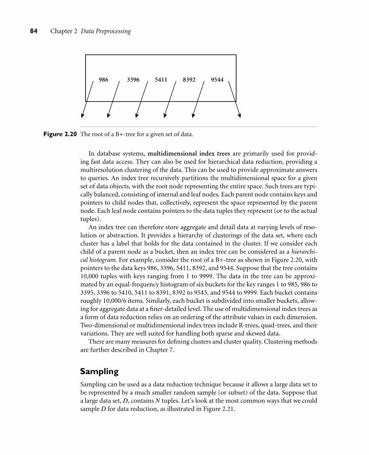
84 Chapter 2 Data Preprocessing
986 3396 5411 8392 9544
Figure 2.20 The root of a B+-tree for a given set of data.
In database systems, multidimensional index trees are primarily used for provid-ing fast data access. They can also be used for hierarchical data reduction, providing amultiresolution clustering of the data. This can be used to provide approximate answersto queries. An index tree recursively partitions the multidimensional space for a givenset of data objects, with the root node representing the entire space. Such trees are typi-cally balanced, consisting of internal and leaf nodes. Each parent node contains keys andpointers to child nodes that, collectively, represent the space represented by the parentnode. Each leaf node contains pointers to the data tuples they represent (or to the actualtuples).
An index tree can therefore store aggregate and detail data at varying levels of reso-lution or abstraction. It provides a hierarchy of clusterings of the data set, where eachcluster has a label that holds for the data contained in the cluster. If we consider eachchild of a parent node as a bucket, then an index tree can be considered as a hierarchi-cal histogram. For example, consider the root of a B+-tree as shown in Figure 2.20, withpointers to the data keys 986, 3396, 5411, 8392, and 9544. Suppose that the tree contains10,000 tuples with keys ranging from 1 to 9999. The data in the tree can be approxi-mated by an equal-frequency histogram of six buckets for the key ranges 1 to 985, 986 to3395, 3396 to 5410, 5411 to 8391, 8392 to 9543, and 9544 to 9999. Each bucket containsroughly 10,000/6 items. Similarly, each bucket is subdivided into smaller buckets, allow-ing for aggregate data at a finer-detailed level. The use of multidimensional index trees asa form of data reduction relies on an ordering of the attribute values in each dimension.Two-dimensional or multidimensional index trees include R-trees, quad-trees, and theirvariations. They are well suited for handling both sparse and skewed data.
There are many measures for defining clusters and cluster quality. Clustering methodsare further described in Chapter 7.
SamplingSampling can be used as a data reduction technique because it allows a large data set tobe represented by a much smaller random sample (or subset) of the data. Suppose thata large data set, D, contains N tuples. Let’s look at the most common ways that we couldsample D for data reduction, as illustrated in Figure 2.21.

2.5 Data Reduction 85
Figure 2.21 Sampling can be used for data reduction.
86 Chapter 2 Data Preprocessing
Simple random sample without replacement (SRSWOR) of size s: This is created bydrawing s of the N tuples from D (s< N), where the probability of drawing any tuplein D is 1/N, that is, all tuples are equally likely to be sampled.
Simple random sample with replacement (SRSWR) of size s: This is similar toSRSWOR, except that each time a tuple is drawn from D, it is recorded and thenreplaced. That is, after a tuple is drawn, it is placed back in D so that it may be drawnagain.
Cluster sample: If the tuples in D are grouped into M mutually disjoint “clusters,”then an SRS of s clusters can be obtained, where s < M. For example, tuples in adatabase are usually retrieved a page at a time, so that each page can be considereda cluster. A reduced data representation can be obtained by applying, say, SRSWORto the pages, resulting in a cluster sample of the tuples. Other clustering criteria con-veying rich semantics can also be explored. For example, in a spatial database, wemay choose to define clusters geographically based on how closely different areas arelocated.
Stratified sample: If D is divided into mutually disjoint parts called strata, a stratifiedsample of D is generated by obtaining an SRS at each stratum. This helps ensure arepresentative sample, especially when the data are skewed. For example, a stratifiedsample may be obtained from customer data, where a stratum is created for each cus-tomer age group. In this way, the age group having the smallest number of customerswill be sure to be represented.
An advantage of sampling for data reduction is that the cost of obtaining a sampleis proportional to the size of the sample, s, as opposed to N, the data set size. Hence,sampling complexity is potentially sublinear to the size of the data. Other data reduc-tion techniques can require at least one complete pass through D. For a fixed samplesize, sampling complexity increases only linearly as the number of data dimensions, n,increases, whereas techniques using histograms, for example, increase exponentially in n.
When applied to data reduction, sampling is most commonly used to estimate theanswer to an aggregate query. It is possible (using the central limit theorem) to determinea sufficient sample size for estimating a given function within a specified degree of error.This sample size, s, may be extremely small in comparison to N. Sampling is a naturalchoice for the progressive refinement of a reduced data set. Such a set can be furtherrefined by simply increasing the sample size.
2.6 Data Discretization and Concept Hierarchy Generation
Data discretization techniques can be used to reduce the number of values for a givencontinuous attribute by dividing the range of the attribute into intervals. Interval labelscan then be used to replace actual data values. Replacing numerous values of a continuousattribute by a small number of interval labels thereby reduces and simplifies the originaldata.This leadstoaconcise,easy-to-use,knowledge-levelrepresentationofminingresults.

2.6 Data Discretization and Concept Hierarchy Generation 87
Discretization techniques can be categorized based on how the discretization isperformed, such as whether it uses class information or which direction it proceeds(i.e., top-down vs. bottom-up). If the discretization process uses class information,then we say it is supervised discretization. Otherwise, it is unsupervised. If the processstarts by first finding one or a few points (called split points or cut points) to split theentire attribute range, and then repeats this recursively on the resulting intervals, it iscalled top-down discretization or splitting. This contrasts with bottom-up discretizationor merging, which starts by considering all of the continuous values as potentialsplit-points, removes some by merging neighborhood values to form intervals, andthen recursively applies this process to the resulting intervals. Discretization can beperformed recursively on an attribute to provide a hierarchical or multiresolutionpartitioning of the attribute values, known as a concept hierarchy. Concept hierarchiesare useful for mining at multiple levels of abstraction.
A concept hierarchy for a given numerical attribute defines a discretization of theattribute. Concept hierarchies can be used to reduce the data by collecting and replac-ing low-level concepts (such as numerical values for the attribute age) with higher-levelconcepts (such as youth, middle-aged, or senior). Although detail is lost by such data gen-eralization, the generalized data may be more meaningful and easier to interpret. Thiscontributes to a consistent representation of data mining results among multiple miningtasks, which is a common requirement. In addition, mining on a reduced data set requiresfewer input/output operations and is more efficient than mining on a larger, ungeneral-ized data set. Because of these benefits, discretization techniques and concept hierarchiesare typically applied before data mining as a preprocessing step, rather than during min-ing. An example of a concept hierarchy for the attribute price is given in Figure 2.22. Morethan one concept hierarchy can be defined for the same attribute in order to accommo-date the needs of various users.
Manual definition of concept hierarchies can be a tedious and time-consumingtask for a user or a domain expert. Fortunately, several discretization methods canbe used to automatically generate or dynamically refine concept hierarchies fornumerical attributes. Furthermore, many hierarchies for categorical attributes are
($600...$800] ($800...$1000] ($400...$600] ($200...$400] ($0...$200]
($0...$1000]
($900... $1000]
($800... $900]
($700... $800]
($600... $700]
($500... $600]
($100... $200]
($400... $500]
($0... $100]
($200... $300]
($300... $400]
Figure 2.22 A concept hierarchy for the attribute price, where an interval ($X . . .$Y ] denotes the rangefrom $X (exclusive) to $Y (inclusive).

88 Chapter 2 Data Preprocessing
implicit within the database schema and can be automatically defined at the schemadefinition level.
Let’s look at the generation of concept hierarchies for numerical and categorical data.
2.6.1 Discretization and Concept Hierarchy Generation forNumerical Data
It is difficult and laborious to specify concept hierarchies for numerical attributes becauseof the wide diversity of possible data ranges and the frequent updates of data values. Suchmanual specification can also be quite arbitrary.
Concept hierarchies for numerical attributes can be constructed automatically basedon data discretization. We examine the following methods: binning, histogram analysis,entropy-based discretization, χ2-merging, cluster analysis, and discretization by intuitivepartitioning. In general, each method assumes that the values to be discretized are sortedin ascending order.
BinningBinning is a top-down splitting technique based on a specified number of bins.Section 2.3.2 discussed binning methods for data smoothing. These methods arealso used as discretization methods for numerosity reduction and concept hierarchygeneration. For example, attribute values can be discretized by applying equal-widthor equal-frequency binning, and then replacing each bin value by the bin mean ormedian, as in smoothing by bin means or smoothing by bin medians, respectively. Thesetechniques can be applied recursively to the resulting partitions in order to gener-ate concept hierarchies. Binning does not use class information and is therefore anunsupervised discretization technique. It is sensitive to the user-specified number ofbins, as well as the presence of outliers.
Histogram AnalysisLike binning, histogram analysis is an unsupervised discretization technique becauseit does not use class information. Histograms partition the values for an attribute, A,into disjoint ranges called buckets. Histograms were introduced in Section 2.2.3. Parti-tioning rules for defining histograms were described in Section 2.5.4. In an equal-widthhistogram, for example, the values are partitioned into equal-sized partitions or ranges(such as in Figure 2.19 for price, where each bucket has a width of $10). With an equal-frequency histogram, the values are partitioned so that, ideally, each partition containsthe same number of data tuples. The histogram analysis algorithm can be applied recur-sively to each partition in order to automatically generate a multilevel concept hierarchy,with the procedure terminating once a prespecified number of concept levels has beenreached. A minimum interval size can also be used per level to control the recursive pro-cedure. This specifies the minimum width of a partition, or the minimum number ofvalues for each partition at each level. Histograms can also be partitioned based on clus-ter analysis of the data distribution, as described below.
2.6 Data Discretization and Concept Hierarchy Generation 89
Entropy-Based DiscretizationEntropy is one of the most commonly used discretization measures. It was first intro-duced by Claude Shannon in pioneering work on information theory and the conceptof information gain. Entropy-based discretization is a supervised, top-down splittingtechnique. It explores class distribution information in its calculation and determinationof split-points (data values for partitioning an attribute range). To discretize a numer-ical attribute, A, the method selects the value of A that has the minimum entropy as asplit-point, and recursively partitions the resulting intervals to arrive at a hierarchicaldiscretization. Such discretization forms a concept hierarchy for A.
Let D consist of data tuples defined by a set of attributes and a class-label attribute.The class-label attribute provides the class information per tuple. The basic method forentropy-based discretization of an attribute A within the set is as follows:
1. Each value of A can be considered as a potential interval boundary or split-point(denoted split point) to partition the range of A. That is, a split-point for A can par-tition the tuples in D into two subsets satisfying the conditions A ≤ split point andA> split point, respectively, thereby creating a binary discretization.
2. Entropy-based discretization, as mentioned above, uses information regarding theclass label of tuples. To explain the intuition behind entropy-based discretization,we must take a glimpse at classification. Suppose we want to classify the tuples inD by partitioning on attribute A and some split-point. Ideally, we would like thispartitioning to result in an exact classification of the tuples. For example, if we hadtwo classes, we would hope that all of the tuples of, say, class C1 will fall into onepartition, and all of the tuples of class C2 will fall into the other partition. However,this is unlikely. For example, the first partition may contain many tuples of C1, butalso some of C2. How much more information would we still need for a perfectclassification, after this partitioning? This amount is called the expected informationrequirement for classifying a tuple in D based on partitioning by A. It is given by
InfoA(D) =|D1||D|
Entropy(D1)+|D2||D|
Entropy(D2), (2.15)
where D1 and D2 correspond to the tuples in D satisfying the conditions A ≤split point and A> split point, respectively; |D| is the number of tuples in D, and soon. The entropy function for a given set is calculated based on the class distributionof the tuples in the set. For example, given m classes, C1,C2, . . . ,Cm, the entropy ofD1 is
Entropy(D1) =−m
∑i=1
pi log2(pi), (2.16)
where pi is the probability of class Ci in D1, determined by dividing the number oftuples of class Ci in D1 by |D1|, the total number of tuples in D1. Therefore, whenselecting a split-point for attribute A, we want to pick the attribute value that gives theminimum expected information requirement (i.e., min(InfoA(D))). This would result

90 Chapter 2 Data Preprocessing
in the minimum amount of expected information (still) required to perfectly classifythe tuples after partitioning by A≤ split point and A> split point. This is equivalentto the attribute-value pair with the maximum information gain (the further detailsof which are given in Chapter 6 on classification.) Note that the value of Entropy(D2)can be computed similarly as in Equation (2.16).
“But our task is discretization, not classification!”, you may exclaim. This is true. Weuse the split-point to partition the range of A into two intervals, corresponding toA≤ split point and A> split point.
3. The process of determining a split-point is recursively applied to each partitionobtained, until some stopping criterion is met, such as when the minimum infor-mation requirement on all candidate split-points is less than a small threshold, ε, orwhen the number of intervals is greater than a threshold, max interval.
Entropy-based discretization can reduce data size. Unlike the other methods mentionedhere so far, entropy-based discretization uses class information. This makes it more likelythat the interval boundaries (split-points) are defined to occur in places that may helpimprove classification accuracy. The entropy and information gain measures describedhere are also used for decision tree induction. These measures are revisited in greaterdetail in Section 6.3.2.
Interval Merging by χ2 AnalysisChiMerge is a χ2-based discretization method. The discretization methods that we havestudied up to this point have all employed a top-down, splitting strategy. This contrastswith ChiMerge, which employs a bottom-up approach by finding the best neighbor-ing intervals and then merging these to form larger intervals, recursively. The method issupervised in that it uses class information. The basic notion is that for accuratediscretization, the relative class frequencies should be fairly consistent within an interval.Therefore, if two adjacent intervals have a very similar distribution of classes, then theintervals can be merged. Otherwise, they should remain separate.
ChiMerge proceeds as follows. Initially, each distinct value of a numerical attribute Ais considered to be one interval. χ2 tests are performed for every pair of adjacent intervals.Adjacent intervals with the least χ2 values are merged together, because low χ2 values fora pair indicate similar class distributions. This merging process proceeds recursively untila predefined stopping criterion is met.
The χ2 statistic was introduced in Section 2.4.1 on data integration, where weexplained its use to detect a correlation relationship between two categorical attributes(Equation (2.9)). Because ChiMerge treats intervals as discrete categories, Equation (2.9)can be applied. The χ2 statistic tests the hypothesis that two adjacent intervals for a givenattribute are independent of the class. Following the method in Example 2.1, we can con-struct a contingency table for our data. The contingency table has two columns (repre-senting the two adjacent intervals) and m rows, where m is the number of distinct classes.Applying Equation (2.9) here, the cell value oi j is the count of tuples in the ith intervaland jth class. Similarly, the expected frequency of oi j is ei j = (number of tuples in interval

2.6 Data Discretization and Concept Hierarchy Generation 91
i)× (number of tuples in class j)/N, where N is the total number of data tuples. Low χ2
values for an interval pair indicate that the intervals are independent of the class and can,therefore, be merged.
The stopping criterion is typically determined by three conditions. First, mergingstops when χ2 values of all pairs of adjacent intervals exceed some threshold, which isdetermined by a specified significance level. A too (or very) high value of significancelevel for the χ2 test may cause overdiscretization, whereas a too (or very) low value maylead to underdiscretization. Typically, the significance level is set between 0.10 and 0.01.Second, the number of intervals cannot be over a prespecified max-interval, such as 10 to15. Finally, recall that the premise behind ChiMerge is that the relative class frequenciesshould be fairly consistent within an interval. In practice, some inconsistency is allowed,although this should be no more than a prespecified threshold, such as 3%, which maybe estimated from the training data. This last condition can be used to remove irrelevantattributes from the data set.
Cluster AnalysisCluster analysis is a popular data discretization method. A clustering algorithm can beapplied to discretize a numerical attribute, A, by partitioning the values of A into clustersor groups. Clustering takes the distribution of A into consideration, as well as the close-ness of data points, and therefore is able to produce high-quality discretization results.Clustering can be used to generate a concept hierarchy for A by following either a top-down splitting strategy or a bottom-up merging strategy, where each cluster forms anode of the concept hierarchy. In the former, each initial cluster or partition may be fur-ther decomposed into several subclusters, forming a lower level of the hierarchy. In thelatter, clusters are formed by repeatedly grouping neighboring clusters in order to formhigher-level concepts. Clustering methods for data mining are studied in Chapter 7.
Discretization by Intuitive PartitioningAlthough the above discretization methods are useful in the generation of numericalhierarchies, many users would like to see numerical ranges partitioned into relativelyuniform, easy-to-read intervals that appear intuitive or “natural.” For example, annualsalaries broken into ranges like ($50,000, $60,000] are often more desirable than rangeslike ($51,263.98, $60,872.34], obtained by, say, some sophisticated clustering analysis.
The 3-4-5 rule can be used to segment numerical data into relatively uniform, natural-seeming intervals. In general, the rule partitions a given range of data into 3, 4, or 5relatively equal-width intervals, recursively and level by level, based on the value rangeat the most significant digit. We will illustrate the use of the rule with an example furtherbelow. The rule is as follows:
If an interval covers 3, 6, 7, or 9 distinct values at the most significant digit, thenpartition the range into 3 intervals (3 equal-width intervals for 3, 6, and 9; and 3intervals in the grouping of 2-3-2 for 7).

92 Chapter 2 Data Preprocessing
If it covers 2, 4, or 8 distinct values at the most significant digit, then partition therange into 4 equal-width intervals.
If it covers 1, 5, or 10 distinct values at the most significant digit, then partition therange into 5 equal-width intervals.
The rule can be recursively applied to each interval, creating a concept hierarchy forthe given numerical attribute. Real-world data often contain extremely large posi-tive and/or negative outlier values, which could distort any top-down discretizationmethod based on minimum and maximum data values. For example, the assets ofa few people could be several orders of magnitude higher than those of others inthe same data set. Discretization based on the maximal asset values may lead to ahighly biased hierarchy. Thus the top-level discretization can be performed basedon the range of data values representing the majority (e.g., 5th percentile to 95thpercentile) of the given data. The extremely high or low values beyond the top-leveldiscretization will form distinct interval(s) that can be handled separately, but in asimilar manner.
The following example illustrates the use of the 3-4-5 rule for the automatic construc-tion of a numerical hierarchy.
Example 2.6 Numeric concept hierarchy generation by intuitive partitioning. Suppose that prof-its at different branches of AllElectronics for the year 2004 cover a wide range, from−$351,976.00 to $4,700,896.50. A user desires the automatic generation of a concepthierarchy for profit. For improved readability, we use the notation (l...r] to representthe interval (l,r]. For example, (−$1,000,000...$0] denotes the range from −$1,000,000(exclusive) to $0 (inclusive).
Suppose that the data within the 5th percentile and 95th percentile are between−$159,876 and $1,838,761. The results of applying the 3-4-5 rule are shown inFigure 2.23.
1. Based on the above information, the minimum and maximum values are MIN =−$351,976.00, and MAX = $4,700,896.50. The low (5th percentile) and high (95thpercentile) values to be considered for the top or first level of discretization are LOW =−$159,876, and HIGH = $1,838,761.
2. Given LOW and HIGH, the most significant digit (msd) is at the million dollar digitposition (i.e., msd = 1,000,000). Rounding LOW down to the million dollar digit,we get LOW ′ =−$1,000,000; rounding HIGH up to the million dollar digit, we getHIGH ′ = +$2,000,000.
3. Since this interval ranges over three distinct values at the most significant digit, thatis, (2,000,000−(−1,000,000))/1,000,000 = 3, the segment is partitioned into threeequal-width subsegments according to the 3-4-5 rule: (−$1,000,000 . . .$0],($0 . . .$1,000,000], and ($1,000,000 . . .$2,000,000]. This represents the top tier ofthe hierarchy.

2.6 Data Discretization and Concept Hierarchy Generation 93
(2$400,000... 2$300,000]
(2$300,000... 2$200,000]
($0... $200,000]
(2$200,000... 2$100,000]
($200,000... $400,000]
($400,000... $600,000]
($600,000... $800,000]
($800,000... $1,000,000]
(2$100,000... $0]
(2$1,000,000...$0]
($1,000,000... $1,200,000]
($2,000,000... $3,000,000]
($2,000,000...$5,000,000]($1,000,000...$2,000,000](0...$1,000,000](2$400,000...0]
(2$400,000...$5,000,000]Step 4
Step 5
($3,000,000... $4,000,000]
($4,000,000... $5,000,000]
($1,200,000... $1,400,000]
($1,400,000... $1,600,000]
($1,600,000... $1,800,000]
($1,800,000... $2,000,000]
($0...$1,000,000] ($1,000,000...$2,000,000]
(2$1,000,000...$2,000,000]Step 3
Count
Step 1
Step 2 msd 5 1,000,000 LOW´ 5 2$1,000,000 HIGH´ 5 $2,000,000
2$351,976 MIN
2$159,876 LOW (i.e., 5th percentile)
$1,838,761 HIGH (i.e., 95th percentile)
$4,700,896.50 MAX
Profit
Figure 2.23 Automatic generation of a concept hierarchy for profit based on the 3-4-5 rule.
4. We now examine the MIN and MAX values to see how they “fit” into the first-levelpartitions. Since the first interval (−$1,000,000 . . .$0] covers the MIN value, that is,LOW ′ < MIN, we can adjust the left boundary of this interval to make the intervalsmaller. The most significant digit of MIN is the hundred thousand digit position.
94 Chapter 2 Data Preprocessing
Rounding MIN down to this position, we get MIN′ = −$400,000. Therefore, thefirst interval is redefined as (−$400,000 . . .0].Since the last interval, ($1,000,000 . . .$2,000,000], does not cover the MAX value,that is, MAX > HIGH ′, we need to create a new interval to cover it. Roundingup MAX at its most significant digit position, the new interval is ($2,000,000. . .$5,000,000]. Hence, the topmost level of the hierarchy contains four par-titions, (−$400,000 . . .$0], ($0 . . .$1,000,000], ($1,000,000 . . .$2,000,000], and($2,000,000 . . .$5,000,000].
5. Recursively, each interval can be further partitioned according to the 3-4-5 rule toform the next lower level of the hierarchy:
The first interval, (−$400,000. . . $0], is partitioned into 4 subintervals:(−$400,000. . .−$300,000], (−$300,000. . .−$200,000],(−$200,000. . .−$100,000],and (−$100,000. . . $0].
The second interval, ($0. . . $1,000,000], is partitioned into 5 subintervals: ($0 . . .$200,000],($200,000. . . $400,000],($400,000. . . $600,000],($600,000. . . $800,000],and ($800,000. . . $1,000,000].
The third interval, ($1,000,000. . . $2,000,000], is partitioned into 5 subintervals:($1,000,000. . . $1,200,000],($1,200,000. . . $1,400,000],($1,400,000. . . $1,600,000],($1,600,000 . . . $1,800,000], and ($1,800,000 . . . $2,000,000].
The last interval, ($2,000,000. . . $5,000,000], is partitioned into 3 subintervals:($2,000,000. . . $3,000,000], ($3,000,000. . . $4,000,000], and ($4,000,000. . . $5,000,000].
Similarly, the 3-4-5 rule can be carried on iteratively at deeper levels, as necessary.
2.6.2 Concept Hierarchy Generation for Categorical Data
Categorical data are discrete data. Categorical attributes have a finite (but possibly large)number of distinct values, with no ordering among the values. Examples include geo-graphic location, job category, and item type. There are several methods for the generationof concept hierarchies for categorical data.
Specification of a partial ordering of attributes explicitly at the schema level by users orexperts: Concept hierarchies for categorical attributes or dimensions typically involvea group of attributes. A user or expert can easily define a concept hierarchy by spec-ifying a partial or total ordering of the attributes at the schema level. For example,a relational database or a dimension location of a data warehouse may contain thefollowing group of attributes: street, city, province or state, and country. A hierarchycan be defined by specifying the total ordering among these attributes at the schemalevel, such as street < city < province or state < country.
Specification of a portion of a hierarchy by explicit data grouping: This is essentiallythe manual definition of a portion of a concept hierarchy. In a large database, it

2.6 Data Discretization and Concept Hierarchy Generation 95
is unrealistic to define an entire concept hierarchy by explicit value enumeration.On the contrary, we can easily specify explicit groupings for a small portion ofintermediate-level data. For example, after specifying that province and countryform a hierarchy at the schema level, a user could define some intermediate levelsmanually, such as “{Alberta, Saskatchewan, Manitoba} ⊂ prairies Canada” and“{British Columbia, prairies Canada} ⊂ Western Canada”.
Specification of a set of attributes, but not of their partial ordering: A user may spec-ify a set of attributes forming a concept hierarchy, but omit to explicitly state theirpartial ordering. The system can then try to automatically generate the attributeordering so as to construct a meaningful concept hierarchy. “Without knowledgeof data semantics, how can a hierarchical ordering for an arbitrary set of categoricalattributes be found?” Consider the following observation that since higher-level con-cepts generally cover several subordinate lower-level concepts, an attribute defininga high concept level (e.g., country) will usually contain a smaller number of dis-tinct values than an attribute defining a lower concept level (e.g., street). Based onthis observation, a concept hierarchy can be automatically generated based on thenumber of distinct values per attribute in the given attribute set. The attribute withthe most distinct values is placed at the lowest level of the hierarchy. The lowerthe number of distinct values an attribute has, the higher it is in the generatedconcept hierarchy. This heuristic rule works well in many cases. Some local-levelswapping or adjustments may be applied by users or experts, when necessary, afterexamination of the generated hierarchy.
Let’s examine an example of this method.
Example 2.7 Concept hierarchy generation based on the number of distinct values per attribute. Sup-pose a user selects a set of location-oriented attributes, street, country, province or state,and city, from the AllElectronics database, but does not specify the hierarchical orderingamong the attributes.
A concept hierarchy for location can be generated automatically, as illustrated inFigure 2.24. First, sort the attributes in ascending order based on the number ofdistinct values in each attribute. This results in the following (where the number ofdistinct values per attribute is shown in parentheses): country (15), province or state(365), city (3567), and street (674,339). Second, generate the hierarchy from the topdown according to the sorted order, with the first attribute at the top level andthe last attribute at the bottom level. Finally, the user can examine the generatedhierarchy, and when necessary, modify it to reflect desired semantic relationshipsamong the attributes. In this example, it is obvious that there is no need to modifythe generated hierarchy.
Note that this heuristic rule is not foolproof. For example, a time dimension in adatabase may contain 20 distinct years, 12 distinct months, and 7 distinct days of theweek. However, this does not suggest that the time hierarchy should be “year < month< days of the week”, with days of the week at the top of the hierarchy.

96 Chapter 2 Data Preprocessing
country 15 distinct values
province_or_state
city
street
365 distinct values
3,567 distinct values
674,339 distinct values
Figure 2.24 Automatic generation of a schema concept hierarchy based on the number of distinctattribute values.
Specification of only a partial set of attributes: Sometimes a user can be sloppy whendefining a hierarchy, or have only a vague idea about what should be included in ahierarchy. Consequently, the user may have included only a small subset of the rel-evant attributes in the hierarchy specification. For example, instead of including allof the hierarchically relevant attributes for location, the user may have specified onlystreet and city. To handle such partially specified hierarchies, it is important to embeddata semantics in the database schema so that attributes with tight semantic connec-tions can be pinned together. In this way, the specification of one attribute may triggera whole group of semantically tightly linked attributes to be “dragged in” to form acomplete hierarchy. Users, however, should have the option to override this feature,as necessary.
Example 2.8 Concept hierarchy generation using prespecified semantic connections. Suppose thata data mining expert (serving as an administrator) has pinned together the five attri-butes number, street, city, province or state, and country, because they are closely linkedsemantically regarding the notion of location. If a user were to specify only the attributecity for a hierarchy defining location, the system can automatically drag in all of the abovefive semantically related attributes to form a hierarchy. The user may choose to drop anyof these attributes, such as number and street, from the hierarchy, keeping city as thelowest conceptual level in the hierarchy.

2.7 Summary 97
2.7 Summary
Data preprocessing is an important issue for both data warehousing and data mining,as real-world data tend to be incomplete, noisy, and inconsistent. Data preprocessingincludes data cleaning, data integration, data transformation, and data reduction.
Descriptive data summarization provides the analytical foundation for data pre-processing. The basic statistical measures for data summarization include mean,weighted mean, median, and mode for measuring the central tendency of data, andrange, quartiles, interquartile range, variance, and standard deviation for measur-ing the dispersion of data. Graphical representations, such as histograms, boxplots,quantile plots, quantile-quantile plots, scatter plots, and scatter-plot matrices, facili-tate visual inspection of the data and are thus useful for data preprocessing andmining.
Data cleaning routines attempt to fill in missing values, smooth out noise whileidentifying outliers, and correct inconsistencies in the data. Data cleaning is usuallyperformed as an iterative two-step process consisting of discrepancy detection anddata transformation.
Data integration combines data from multiple sources to form a coherent data store.Metadata, correlation analysis, data conflict detection, and the resolution of semanticheterogeneity contribute toward smooth data integration.
Data transformation routines convert the data into appropriate forms for mining.For example, attribute data may be normalized so as to fall between a small range,such as 0.0 to 1.0.
Data reduction techniques such as data cube aggregation, attribute subset selection,dimensionality reduction, numerosity reduction, and discretization can be used toobtain a reduced representation of the data while minimizing the loss of informationcontent.
Data discretization and automatic generation of concept hierarchies for numericaldata can involve techniques such as binning, histogram analysis, entropy-based dis-cretization, χ2 analysis, cluster analysis, and discretization by intuitive partitioning.For categorical data, concept hierarchies may be generated based on the number ofdistinct values of the attributes defining the hierarchy.
Although numerous methods of data preprocessing have been developed, data pre-processing remains an active area of research, due to the huge amount of inconsistentor dirty data and the complexity of the problem.
Exercises
2.1 Data quality can be assessed in terms of accuracy, completeness, and consistency. Proposetwo other dimensions of data quality.

98 Chapter 2 Data Preprocessing
2.2 Suppose that the values for a given set of data are grouped into intervals. The intervalsand corresponding frequencies are as follows.
age frequency
1–5 200
5–15 450
15–20 300
20–50 1500
50–80 700
80–110 44
Compute an approximate median value for the data.
2.3 Give three additional commonly used statistical measures (i.e., not illustrated in thischapter) for the characterization of data dispersion, and discuss how they can be com-puted efficiently in large databases.
2.4 Suppose that the data for analysis includes the attribute age. The age values for the datatuples are (in increasing order) 13, 15, 16, 16, 19, 20, 20, 21, 22, 22, 25, 25, 25, 25, 30, 33,33, 35, 35, 35, 35, 36, 40, 45, 46, 52, 70.
(a) What is the mean of the data? What is the median?
(b) What is the mode of the data? Comment on the data’s modality (i.e., bimodal,trimodal, etc.).
(c) What is the midrange of the data?
(d) Can you find (roughly) the first quartile (Q1) and the third quartile (Q3) of the data?
(e) Give the five-number summary of the data.
(f) Show a boxplot of the data.
(g) How is a quantile-quantile plot different from a quantile plot?
2.5 In many applications, new data sets are incrementally added to the existing large data sets.Thus an important consideration for computing descriptive data summary is whether ameasure can be computed efficiently in incremental manner. Use count, standard devia-tion, and median as examples to show that a distributive or algebraic measure facilitatesefficient incremental computation, whereas a holistic measure does not.
2.6 In real-world data, tuples with missing values for some attributes are a common occur-rence. Describe various methods for handling this problem.
2.7 Using the data for age given in Exercise 2.4, answer the following.
(a) Use smoothing by bin means to smooth the data, using a bin depth of 3. Illustrateyour steps. Comment on the effect of this technique for the given data.
(b) How might you determine outliers in the data?
(c) What other methods are there for data smoothing?

Exercises 99
2.8 Discuss issues to consider during data integration.
2.9 Suppose a hospital tested the age and body fat data for 18 randomly selected adults withthe following result:
age 23 23 27 27 39 41 47 49 50
%fat 9.5 26.5 7.8 17.8 31.4 25.9 27.4 27.2 31.2
age 52 54 54 56 57 58 58 60 61
%fat 34.6 42.5 28.8 33.4 30.2 34.1 32.9 41.2 35.7
(a) Calculate the mean, median, and standard deviation of age and %fat.
(b) Draw the boxplots for age and %fat.
(c) Draw a scatter plot and a q-q plot based on these two variables.
(d) Normalize the two variables based on z-score normalization.
(e) Calculate the correlation coefficient (Pearson’s product moment coefficient). Are thesetwo variables positively or negatively correlated?
2.10 What are the value ranges of the following normalization methods?
(a) min-max normalization
(b) z-score normalization
(c) normalization by decimal scaling
2.11 Use the two methods below to normalize the following group of data:200, 300, 400, 600, 1000
(a) min-max normalization by setting min = 0 and max = 1(b) z-score normalization
2.12 Using the data for age given in Exercise 2.4, answer the following:
(a) Usemin-maxnormalization to transformthevalue35 for ageontotherange [0.0,1.0].(b) Use z-score normalization to transform the value 35 for age, where the standard
deviation of age is 12.94 years.
(c) Use normalization by decimal scaling to transform the value 35 for age.
(d) Comment on which method you would prefer to use for the given data, givingreasons as to why.
2.13 Use a flowchart to summarize the following procedures for attribute subset selection:
(a) stepwise forward selection
(b) stepwise backward elimination
(c) a combination of forward selection and backward elimination

100 Chapter 2 Data Preprocessing
2.14 Suppose a group of 12 sales price records has been sorted as follows:5, 10, 11, 13, 15, 35, 50, 55, 72, 92, 204, 215Partition them into three bins by each of the following methods:
(a) equal-frequency (equidepth) partitioning
(b) equal-width partitioning
(c) clustering
2.15 Using the data for age given in Exercise 2.4,
(a) Plot an equal-width histogram of width 10.
(b) Sketch examples of each of the following sampling techniques: SRSWOR, SRSWR,cluster sampling, stratified sampling. Use samples of size 5 and the strata “youth,”“middle-aged,” and “senior.”
2.16 [Contributed by Chen Chen] The median is one of the most important holistic mea-sures in data analysis. Propose several methods for median approximation. Analyze theirrespective complexity under different parameter settings and decide to what extent thereal value can be approximated. Moreover, suggest a heuristic strategy to balance betweenaccuracy and complexity and then apply it to all methods you have given.
2.17 [Contributed by Deng Cai] It is important to define or select similarity measures in dataanalysis. However, there is no commonly accepted subjective similarity measure. Usingdifferent similarity measures may deduce different results. Nonetheless, some apparentlydifferent similarity measures may be equivalent after some transformation.
Suppose we have the following two-dimensional data set:
A1 A2
x1 1.5 1.7
x2 2 1.9
x3 1.6 1.8
x4 1.2 1.5
x5 1.5 1.0
(a) Consider the data as two-dimensional data points. Given a new data point, x =(1.4,1.6) as a query, rank the database points based on similarity with the query using(1) Euclidean distance (Equation 7.5), and (2) cosine similarity (Equation 7.16).
(b) Normalize the data set to make the norm of each data point equal to 1. Use Euclideandistance on the transformed data to rank the data points.
2.18 ChiMerge [Ker92] is a supervised, bottom-up (i.e., merge-based) data discretizationmethod. It relies on χ2 analysis: adjacent intervals with the least χ2 values are mergedtogether until the stopping criterion is satisfied.

Bibliographic Notes 101
(a) Briefly describe how ChiMerge works.
(b) Take the IRIS data set, obtained from http://www.ics.uci.edu/∼mlearn/MLRepository.html (UC-Irvine Machine Learning Data Repository), as a data set to be discretized.Perform data discretization for each of the four numerical attributes using theChiMerge method. (Let the stopping criteria be: max-interval = 6.) You need towrite a small program to do this to avoid clumsy numerical computation. Submityour simple analysis and your test results: split points, final intervals, and your doc-umented source program.
2.19 Propose an algorithm, in pseudo-code or in your favorite programming language, forthe following:
(a) The automatic generation of a concept hierarchy for categorical data based on thenumber of distinct values of attributes in the given schema
(b) The automatic generation of a concept hierarchy for numerical data based on theequal-width partitioning rule
(c) The automatic generation of a concept hierarchy for numerical data based on theequal-frequency partitioning rule
2.20 Robust data loading poses a challenge in database systems because the input data areoften dirty. In many cases, an input record may have several missing values and somerecords could be contaminated (i.e., with some data values out of range or of a differentdata type than expected). Work out an automated data cleaning and loading algorithmso that the erroneous data will be marked and contaminated data will not be mistakenlyinserted into the database during data loading.
Bibliographic Notes
Data preprocessing is discussed in a number of textbooks, including English [Eng99],Pyle [Pyl99], Loshin [Los01], Redman [Red01], and Dasu and Johnson [DJ03]. Morespecific references to individual preprocessing techniques are given below.
Methods for descriptive data summarization have been studied in the statistics liter-ature long before the onset of computers. Good summaries of statistical descriptive datamining methods include Freedman, Pisani, and Purves [FPP97], and Devore [Dev95].For statistics-based visualization of data using boxplots, quantile plots, quantile-quantileplots, scatter plots, and loess curves, see Cleveland [Cle93].
For discussion regarding data quality, see Redman [Red92], Wang, Storey, and Firth[WSF95], Wand and Wang [WW96], Ballou and Tayi [BT99], and Olson [Ols03]. Pot-ter’s Wheel (http://control.cs.berkeley.edu/abc), the interactive data cleaning tool des-cribed in Section 2.3.3, is presented in Raman and Hellerstein [RH01]. An exampleof the development of declarative languages for the specification of data transforma-tion operators is given in Galhardas, Florescu, Shasha, et al. [GFS+01]. The handling ofmissing attribute values is discussed in Friedman [Fri77], Breiman, Friedman, Olshen,

102 Chapter 2 Data Preprocessing
and Stone [BFOS84], and Quinlan [Qui89]. A method for the detection of outlier or“garbage” patterns in a handwritten character database is given in Guyon, Matic, andVapnik [GMV96]. Binning and data normalization are treated in many texts, includingKennedy, Lee, Van Roy, et al. [KLV+98], Weiss and Indurkhya [WI98], and Pyle [Pyl99].Systems that include attribute (or feature) construction include BACON by Langley,Simon, Bradshaw, and Zytkow [LSBZ87], Stagger by Schlimmer [Sch86], FRINGE byPagallo [Pag89], and AQ17-DCI by Bloedorn and Michalski [BM98]. Attribute con-struction is also described in Liu and Motoda [LM98], [Le98]. Dasu, Johnson, Muthukr-ishnan, and Shkapenyuk [DJMS02] developed a system called Bellman wherein theypropose a set of methods for building a data quality browser by mining on thestructure of the database.
A good survey of data reduction techniques can be found in Barbará, Du Mouchel,Faloutos, et al. [BDF+97]. For algorithms on data cubes and their precomputation, seeSarawagi and Stonebraker [SS94], Agarwal, Agrawal, Deshpande, et al. [AAD+96],Harinarayan, Rajaraman, and Ullman [HRU96], Ross and Srivastava [RS97], and Zhao,Deshpande, and Naughton [ZDN97]. Attribute subset selection (or feature subset selec-tion) is described in many texts, such as Neter, Kutner, Nachtsheim, and Wasserman[NKNW96], Dash and Liu [DL97], and Liu and Motoda [LM98, LM98b]. A combi-nation forward selection and backward elimination method was proposed in Siedleckiand Sklansky [SS88]. A wrapper approach to attribute selection is described in Kohaviand John [KJ97]. Unsupervised attribute subset selection is described in Dash, Liu, andYao [DLY97]. For a description of wavelets for dimensionality reduction, see Press,Teukolosky, Vetterling, and Flannery [PTVF96]. A general account of wavelets can befound in Hubbard [Hub96]. For a list of wavelet software packages, see Bruce, Donoho,and Gao [BDG96]. Daubechies transforms are described in Daubechies [Dau92]. Thebook by Press et al. [PTVF96] includes an introduction to singular value decompositionfor principal components analysis. Routines for PCA are included in most statistical soft-ware packages, such as SAS (www.sas.com/SASHome.html).
An introduction to regression and log-linear models can be found in several text-books, such as James [Jam85], Dobson [Dob90], Johnson and Wichern [JW92], Devore[Dev95], and Neter et al. [NKNW96]. For log-linear models (known as multiplicativemodels in the computer science literature), see Pearl [Pea88]. For a general introductionto histograms, see Barbará et al. [BDF+97] and Devore and Peck [DP97]. For exten-sions of single attribute histograms to multiple attributes, see Muralikrishna and DeWitt[MD88] and Poosala and Ioannidis [PI97]. Several references to clustering algorithmsare given in Chapter 7 of this book, which is devoted to the topic. A survey of mul-tidimensional indexing structures is given in Gaede and Günther [GG98]. The use ofmultidimensional index trees for data aggregation is discussed in Aoki [Aok98]. Indextrees include R-trees (Guttman [Gut84]), quad-trees (Finkel and Bentley [FB74]), andtheir variations. For discussion on sampling and data mining, see Kivinen and Mannila[KM94] and John and Langley [JL96].
There are many methods for assessing attribute relevance. Each has its own bias. Theinformation gain measure is biased toward attributes with many values. Many alterna-tives have been proposed, such as gain ratio (Quinlan [Qui93]), which considers the

Bibliographic Notes 103
probability of each attribute value. Other relevance measures include the gini index(Breiman, Friedman, Olshen, and Stone [BFOS84]), the χ2 contingency table statistic,and the uncertainty coefficient (Johnson and Wichern [JW92]). For a comparison ofattribute selection measures for decision tree induction, see Buntine and Niblett [BN92].For additional methods, see Liu and Motoda [LM98b], Dash and Liu [DL97], andAlmuallim and Dietterich [AD91].
Liu, Hussain, Tan, and Dash [LHTD02] performed a comprehensive survey of datadiscretization methods. Entropy-based discretization with the C4.5 algorithm is descri-bed in Quinlan [Qui93]. In Catlett [Cat91], the D-2 system binarizes a numerical fea-ture recursively. ChiMerge by Kerber [Ker92] and Chi2 by Liu and Setiono [LS95] aremethods for the automatic discretization of numerical attributes that both employ theχ2 statistic. Fayyad and Irani [FI93] apply the minimum description length principle todetermine the number of intervals for numerical discretization. Concept hierarchies andtheir automatic generation from categorical data are described in Han and Fu [HF94].


3Data Warehouse and OLAPTechnology: An Overview
Data warehouses generalize and consolidate data in multidimensional space. The construction ofdata warehouses involves data cleaning, data integration, and data transformation andcan be viewed as an important preprocessing step for data mining. Moreover, data ware-houses provide on-line analytical processing (OLAP) tools for the interactive analysis ofmultidimensional data of varied granularities, which facilitates effective data generaliza-tion and data mining. Many other data mining functions, such as association, classifi-cation, prediction, and clustering, can be integrated with OLAP operations to enhanceinteractive mining of knowledge at multiple levels of abstraction. Hence, the data ware-house has become an increasingly important platform for data analysis and on-line ana-lytical processing and will provide an effective platform for data mining. Therefore, datawarehousing and OLAP form an essential step in the knowledge discovery process. Thischapter presents an overview of data warehouse and OLAP technology. Such an overviewis essential for understanding the overall data mining and knowledge discovery process.
In this chapter, we study a well-accepted definition of the data warehouse and seewhy more and more organizations are building data warehouses for the analysis of theirdata. In particular, we study the data cube, a multidimensional data model for data ware-houses and OLAP, as well as OLAP operations such as roll-up, drill-down, slicing, anddicing. We also look at data warehouse architecture, including steps on data warehousedesign and construction. An overview of data warehouse implementation examines gen-eral strategies for efficient data cube computation, OLAP data indexing, and OLAP queryprocessing. Finally, we look at on-line-analytical mining, a powerful paradigm that inte-grates data warehouse and OLAP technology with that of data mining.
3.1 What Is a Data Warehouse?
Data warehousing provides architectures and tools for business executives to systemat-ically organize, understand, and use their data to make strategic decisions. Data ware-house systems are valuable tools in today’s competitive, fast-evolving world. In the lastseveral years, many firms have spent millions of dollars in building enterprise-wide data
105

106 Chapter 3 Data Warehouse and OLAP Technology: An Overview
warehouses. Many people feel that with competition mounting in every industry, datawarehousing is the latest must-have marketing weapon—a way to retain customers bylearning more about their needs.
“Then, what exactly is a data warehouse?” Data warehouses have been defined in manyways, making it difficult to formulate a rigorous definition. Loosely speaking, a datawarehouse refers to a database that is maintained separately from an organization’s oper-ational databases. Data warehouse systems allow for the integration of a variety of appli-cation systems. They support information processing by providing a solid platform ofconsolidated historical data for analysis.
According to William H. Inmon, a leading architect in the construction of data ware-house systems, “A data warehouse is a subject-oriented, integrated, time-variant, andnonvolatile collection of data in support of management’s decision making process”[Inm96]. This short, but comprehensive definition presents the major features of a datawarehouse. The four keywords, subject-oriented, integrated, time-variant, and nonvolatile,distinguish data warehouses from other data repository systems, such as relationaldatabase systems, transaction processing systems, and file systems. Let’s take a closerlook at each of these key features.
Subject-oriented: A data warehouse is organized around major subjects, such as cus-tomer, supplier, product, and sales. Rather than concentrating on the day-to-day oper-ations and transaction processing of an organization, a data warehouse focuses on themodeling and analysis of data for decision makers. Hence, data warehouses typicallyprovide a simple and concise view around particular subject issues by excluding datathat are not useful in the decision support process.
Integrated: A data warehouse is usually constructed by integrating multiple heteroge-neous sources, such as relational databases, flat files, and on-line transaction records.Data cleaning and data integration techniques are applied to ensure consistency innaming conventions, encoding structures, attribute measures, and so on.
Time-variant: Data are stored to provide information from a historical perspective(e.g., the past 5–10 years). Every key structure in the data warehouse contains, eitherimplicitly or explicitly, an element of time.
Nonvolatile: A data warehouse is always a physically separate store of data trans-formed from the application data found in the operational environment. Due tothis separation, a data warehouse does not require transaction processing, recovery,and concurrency control mechanisms. It usually requires only two operations in dataaccessing: initial loading of data and access of data.
In sum, a data warehouse is a semantically consistent data store that serves as a phys-ical implementation of a decision support data model and stores the information onwhich an enterprise needs to make strategic decisions. A data warehouse is also oftenviewed as an architecture, constructed by integrating data from multiple heterogeneoussources to support structured and/or ad hoc queries, analytical reporting, and decisionmaking.

3.1 What Is a Data Warehouse? 107
Based on this information, we view data warehousing as the process of constructingand using data warehouses. The construction of a data warehouse requires data cleaning,data integration, and data consolidation. The utilization of a data warehouse often neces-sitates a collection of decision support technologies. This allows “knowledge workers”(e.g., managers, analysts, and executives) to use the warehouse to quickly and conve-niently obtain an overview of the data, and to make sound decisions based on informa-tion in the warehouse. Some authors use the term “data warehousing” to refer only tothe process of data warehouse construction, while the term “warehouse DBMS” is usedto refer to the management and utilization of data warehouses. We will not make thisdistinction here.
“How are organizations using the information from data warehouses?” Many organi-zations use this information to support business decision-making activities, including(1) increasing customer focus, which includes the analysis of customer buying pat-terns (such as buying preference, buying time, budget cycles, and appetites for spend-ing); (2) repositioning products and managing product portfolios by comparing theperformance of sales by quarter, by year, and by geographic regions in order to fine-tune production strategies; (3) analyzing operations and looking for sources of profit;and (4) managing the customer relationships, making environmental corrections, andmanaging the cost of corporate assets.
Data warehousing is also very useful from the point of view of heterogeneous databaseintegration. Many organizations typically collect diverse kinds of data and maintain largedatabases from multiple, heterogeneous, autonomous, and distributed informationsources. To integrate such data, and provide easy and efficient access to it, is highly desir-able, yet challenging. Much effort has been spent in the database industry and researchcommunity toward achieving this goal.
The traditional database approach to heterogeneous database integration is to buildwrappers and integrators (or mediators), on top of multiple, heterogeneous databases.When a query is posed to a client site, a metadata dictionary is used to translate the queryinto queries appropriate for the individual heterogeneous sites involved. These queriesare then mapped and sent to local query processors. The results returned from the dif-ferent sites are integrated into a global answer set. This query-driven approach requirescomplex information filtering and integration processes, and competes for resourceswith processing at local sources. It is inefficient and potentially expensive for frequentqueries, especially for queries requiring aggregations.
Data warehousing provides an interesting alternative to the traditional approach ofheterogeneous database integration described above. Rather than using a query-drivenapproach, data warehousing employs an update-driven approach in which informationfrom multiple, heterogeneous sources is integrated in advance and stored in a warehousefor direct querying and analysis. Unlike on-line transaction processing databases, datawarehouses do not contain the most current information. However, a data warehousebrings high performance to the integrated heterogeneous database system because dataare copied, preprocessed, integrated, annotated, summarized, and restructured into onesemantic data store. Furthermore, query processing in data warehouses does not interferewith the processing at local sources. Moreover, data warehouses can store and integrate

108 Chapter 3 Data Warehouse and OLAP Technology: An Overview
historical information and support complex multidimensional queries. As a result, datawarehousing has become popular in industry.
3.1.1 Differences between Operational Database Systemsand Data Warehouses
Because most people are familiar with commercial relational database systems, it is easyto understand what a data warehouse is by comparing these two kinds of systems.
The major task of on-line operational database systems is to perform on-line trans-action and query processing. These systems are called on-line transaction processing(OLTP) systems. They cover most of the day-to-day operations of an organization, suchas purchasing, inventory, manufacturing, banking, payroll, registration, and accounting.Data warehouse systems, on the other hand, serve users or knowledge workers in the roleof data analysis and decision making. Such systems can organize and present data in var-ious formats in order to accommodate the diverse needs of the different users. Thesesystems are known as on-line analytical processing (OLAP) systems.
The major distinguishing features between OLTP and OLAP are summarized asfollows:
Users and system orientation: An OLTP system is customer-oriented and is used fortransaction and query processing by clerks, clients, and information technology pro-fessionals. An OLAP system is market-oriented and is used for data analysis by knowl-edge workers, including managers, executives, and analysts.
Data contents: An OLTP system manages current data that, typically, are too detailedto be easily used for decision making. An OLAP system manages large amounts ofhistorical data, provides facilities for summarization and aggregation, and stores andmanages information at different levels of granularity. These features make the dataeasier to use in informed decision making.
Database design: An OLTP system usually adopts an entity-relationship (ER) datamodel and an application-oriented database design. An OLAP system typically adoptseither a star or snowflake model (to be discussed in Section 3.2.2) and a subject-oriented database design.
View: An OLTP system focuses mainly on the current data within an enterprise ordepartment, without referring to historical data or data in different organizations.In contrast, an OLAP system often spans multiple versions of a database schema,due to the evolutionary process of an organization. OLAP systems also deal withinformation that originates from different organizations, integrating informationfrom many data stores. Because of their huge volume, OLAP data are stored onmultiple storage media.
Access patterns: The access patterns of an OLTP system consist mainly of short, atomictransactions. Such a system requires concurrency control and recovery mechanisms.However, accesses to OLAP systems are mostly read-only operations (because most

3.1 What Is a Data Warehouse? 109
Table 3.1 Comparison between OLTP and OLAP systems.
Feature OLTP OLAP
Characteristic operational processing informational processing
Orientation transaction analysis
User clerk, DBA, database professional knowledge worker (e.g., manager,executive, analyst)
Function day-to-day operations long-term informational requirements,decision support
DB design ER based, application-oriented star/snowflake, subject-oriented
Data current; guaranteed up-to-date historical; accuracy maintainedover time
Summarization primitive, highly detailed summarized, consolidated
View detailed, flat relational summarized, multidimensional
Unit of work short, simple transaction complex query
Access read/write mostly read
Focus data in information out
Operations index/hash on primary key lots of scans
Number of recordsaccessed tens millions
Number of users thousands hundreds
DB size 100 MB to GB 100 GB to TB
Priority high performance, high availability high flexibility, end-user autonomy
Metric transaction throughput query throughput, response time
NOTE: Table is partially based on [CD97].
data warehouses store historical rather than up-to-date information), although manycould be complex queries.
Other features that distinguish between OLTP and OLAP systems include database size,frequency of operations, and performance metrics. These are summarized in Table 3.1.
3.1.2 But, Why Have a Separate Data Warehouse?
Because operational databases store huge amounts of data, you may wonder, “why notperform on-line analytical processing directly on such databases instead of spending addi-tional time and resources to construct a separate data warehouse?” A major reason for sucha separation is to help promote the high performance of both systems. An operationaldatabase is designed and tuned from known tasks and workloads, such as indexing andhashing using primary keys, searching for particular records, and optimizing “canned”

110 Chapter 3 Data Warehouse and OLAP Technology: An Overview
queries. On the other hand, data warehouse queries are often complex. They involve thecomputation of large groups of data at summarized levels, and may require the use of spe-cial data organization, access, and implementation methods based on multidimensionalviews. Processing OLAP queries in operational databases would substantially degradethe performance of operational tasks.
Moreover, an operational database supports the concurrent processing of multipletransactions. Concurrency control and recovery mechanisms, such as locking and log-ging, are required to ensure the consistency and robustness of transactions. An OLAPquery often needs read-only access of data records for summarization and aggregation.Concurrency control and recovery mechanisms, if applied for such OLAP operations,may jeopardize the execution of concurrent transactions and thus substantially reducethe throughput of an OLTP system.
Finally, the separation of operational databases from data warehouses is based on thedifferent structures, contents, and uses of the data in these two systems. Decision sup-port requires historical data, whereas operational databases do not typically maintainhistorical data. In this context, the data in operational databases, though abundant, isusually far from complete for decision making. Decision support requires consolidation(such as aggregation and summarization) of data from heterogeneous sources, result-ing in high-quality, clean, and integrated data. In contrast, operational databases con-tain only detailed raw data, such as transactions, which need to be consolidated beforeanalysis. Because the two systems provide quite different functionalities and require dif-ferent kinds of data, it is presently necessary to maintain separate databases. However,many vendors of operational relational database management systems are beginning tooptimize such systems to support OLAP queries. As this trend continues, the separationbetween OLTP and OLAP systems is expected to decrease.
3.2 A Multidimensional Data Model
Data warehouses and OLAP tools are based on a multidimensional data model. Thismodel views data in the form of a data cube. In this section, you will learn how datacubes model n-dimensional data. You will also learn about concept hierarchies and howthey can be used in basic OLAP operations to allow interactive mining at multiple levelsof abstraction.
3.2.1 From Tables and Spreadsheets to Data Cubes
“What is a data cube?” A data cube allows data to be modeled and viewed in multipledimensions. It is defined by dimensions and facts.
In general terms, dimensions are the perspectives or entities with respect to whichan organization wants to keep records. For example, AllElectronics may create a salesdata warehouse in order to keep records of the store’s sales with respect to thedimensions time, item, branch, and location. These dimensions allow the store tokeep track of things like monthly sales of items and the branches and locations

3.2 A Multidimensional Data Model 111
Table 3.2 A 2-D view of sales data for AllElectronics according to the dimensions time and item,where the sales are from branches located in the city of Vancouver. The measure dis-played is dollars sold (in thousands).
location = “Vancouver”
item (type)
hometime (quarter) entertainment computer phone security
Q1 605 825 14 400
Q2 680 952 31 512
Q3 812 1023 30 501
Q4 927 1038 38 580
at which the items were sold. Each dimension may have a table associated withit, called a dimension table, which further describes the dimension. For example,a dimension table for item may contain the attributes item name, brand, and type.Dimension tables can be specified by users or experts, or automatically generatedand adjusted based on data distributions.
A multidimensional data model is typically organized around a central theme, likesales, for instance. This theme is represented by a fact table. Facts are numerical mea-sures. Think of them as the quantities by which we want to analyze relationships betweendimensions. Examples of facts for a sales data warehouse include dollars sold(sales amount in dollars), units sold (number of units sold), and amount budgeted. Thefact table contains the names of the facts, or measures, as well as keys to each of the relateddimension tables. You will soon get a clearer picture of how this works when we look atmultidimensional schemas.
Although we usually think of cubes as 3-D geometric structures, in data warehousingthe data cube is n-dimensional. To gain a better understanding of data cubes and themultidimensional data model, let’s start by looking at a simple 2-D data cube that is, infact, a table or spreadsheet for sales data from AllElectronics. In particular, we will look atthe AllElectronics sales data for items sold per quarter in the city of Vancouver. These dataare shown in Table 3.2. In this 2-D representation, the sales for Vancouver are shown withrespect to the time dimension (organized in quarters) and the item dimension (organizedaccording to the types of items sold). The fact or measure displayed is dollars sold (inthousands).
Now, suppose that we would like to view the sales data with a third dimension. Forinstance, suppose we would like to view the data according to time and item, as well aslocation for the cities Chicago, New York, Toronto, and Vancouver. These 3-D data areshown in Table 3.3. The 3-D data of Table 3.3 are represented as a series of 2-D tables.Conceptually, we may also represent the same data in the form of a 3-D data cube, as inFigure 3.1.

112 Chapter 3 Data Warehouse and OLAP Technology: An Overview
Table 3.3 A 3-D view of sales data for AllElectronics, according to the dimensions time, item, andlocation. The measure displayed is dollars sold (in thousands).
location = “Chicago” location = “New York” location = “Toronto” location = “Vancouver”
item item item item
home home home home
time ent. comp. phone sec. ent. comp. phone sec. ent. comp. phone sec. ent. comp. phone sec.
Q1 854 882 89 623 1087 968 38 872 818 746 43 591 605 825 14 400
Q2 943 890 64 698 1130 1024 41 925 894 769 52 682 680 952 31 512
Q3 1032 924 59 789 1034 1048 45 1002 940 795 58 728 812 1023 30 501
Q4 1129 992 63 870 1142 1091 54 984 978 864 59 784 927 1038 38 580
8181087
854
746968
882
4338
89
591872
623
698
925
789682
8701002
728984
784
Q1
Q2
Q3
Q4
ChicagoNew York
TorontoVancouver
time
(qua
rter
s)
locati
on (c
ities)
home entertainment
computer
item (types)
phone
security
605 825 14 400
51231952680
812 1023 30 501
580381038927
Figure 3.1 A 3-D data cube representation of the data in Table 3.3, according to the dimensions time,item, and location. The measure displayed is dollars sold (in thousands).
Suppose that we would now like to view our sales data with an additional fourthdimension, such as supplier. Viewing things in 4-D becomes tricky. However, we canthink of a 4-D cube as being a series of 3-D cubes, as shown in Figure 3.2. If we continuein this way, we may display any n-D data as a series of (n−1)-D “cubes.” The data cube isa metaphor for multidimensional data storage. The actual physical storage of such datamay differ from its logical representation. The important thing to remember is that datacubes are n-dimensional and do not confine data to 3-D.
The above tables show the data at different degrees of summarization. In the datawarehousing research literature, a data cube such as each of the above is often referred to

3.2 A Multidimensional Data Model 113
605 825 14 400Q1
Q2
Q3
Q4
ChicagoNew YorkToronto
Vancouver
time
(qua
rter
s)locati
on (c
ities)
home entertainment
computer
item (types)
phonesecurity
home entertainment
computer
item (types)
phonesecurity
home entertainment
computer
item (types)
phonesecurity
supplier = “SUP1” supplier = “SUP2” supplier = “SUP3”
Figure 3.2 A 4-D data cube representation of sales data, according to the dimensions time, item, location,and supplier. The measure displayed is dollars sold (in thousands). For improved readability,only some of the cube values are shown.
supplier
time, item, location, supplier
item, locationtime, location
item, suppliertime, supplier
time, location, supplier
item, location, supplier
location, supplier
time, item, supplier
timeitem location
time, item
time, item, location
0-D (apex) cuboid
1-D cuboids
2-D cuboids
3-D cuboids
4-D (base) cuboid
Figure 3.3 Lattice of cuboids, making up a 4-D data cube for the dimensions time, item, location, andsupplier. Each cuboid represents a different degree of summarization.
as a cuboid. Given a set of dimensions, we can generate a cuboid for each of the possiblesubsets of the given dimensions. The result would form a lattice of cuboids, each showingthe data at a different level of summarization, or group by. The lattice of cuboids is thenreferred to as a data cube. Figure 3.3 shows a lattice of cuboids forming a data cube forthe dimensions time, item, location, and supplier.

114 Chapter 3 Data Warehouse and OLAP Technology: An Overview
The cuboid that holds the lowest level of summarization is called the base cuboid. Forexample, the 4-D cuboid in Figure 3.2 is the base cuboid for the given time, item, location,and supplier dimensions. Figure 3.1 is a 3-D (nonbase) cuboid for time, item, and location,summarized for all suppliers. The 0-D cuboid, which holds the highest level of summa-rization, is called the apex cuboid. In our example, this is the total sales, or dollars sold,summarized over all four dimensions. The apex cuboid is typically denoted by all.
3.2.2 Stars, Snowflakes, and Fact Constellations:Schemas for Multidimensional Databases
The entity-relationship data model is commonly used in the design of relationaldatabases, where a database schema consists of a set of entities and the relationshipsbetween them. Such a data model is appropriate for on-line transaction processing.A data warehouse, however, requires a concise, subject-oriented schema that facilitateson-line data analysis.
The most popular data model for a data warehouse is a multidimensional model.Such a model can exist in the form of a star schema, a snowflake schema, or a fact con-stellation schema. Let’s look at each of these schema types.
Star schema: The most common modeling paradigm is the star schema, in which thedata warehouse contains (1) a large central table (fact table) containing the bulk ofthe data, with no redundancy, and (2) a set of smaller attendant tables (dimensiontables), one for each dimension. The schema graph resembles a starburst, with thedimension tables displayed in a radial pattern around the central fact table.
Example 3.1 Star schema. A star schema for AllElectronics sales is shown in Figure 3.4. Sales are consid-ered along four dimensions, namely, time, item, branch, and location. The schema containsa central fact table for sales that contains keys to each of the four dimensions, along withtwo measures: dollars sold and units sold. To minimize the size of the fact table, dimensionidentifiers (such as time key and item key) are system-generated identifiers.
Notice that in the star schema, each dimension is represented by only one table, andeach table contains a set of attributes. For example, the location dimension table containsthe attribute set {location key, street, city, province or state, country}. This constraint mayintroduce some redundancy. For example, “Vancouver” and “Victoria” are both cities inthe Canadian province of British Columbia. Entries for such cities in the location dimen-sion table will create redundancy among the attributes province or state and country,that is, (..., Vancouver, British Columbia, Canada) and (..., Victoria, British Columbia,Canada). Moreover, the attributes within a dimension table may form either a hierarchy(total order) or a lattice (partial order).
Snowflake schema: The snowflake schema is a variant of the star schema model, wheresome dimension tables are normalized, thereby further splitting the data into addi-tional tables. The resulting schema graph forms a shape similar to a snowflake.

3.2 A Multidimensional Data Model 115
time dimension table
time_ key day day_of_the_week month quarter year
sales fact table
time_key item_key branch_key location_key dollars_sold units_sold
item dimension tableitem_key item_name brand type supplier_type
branch dimension table
branch_key branch_name branch_type
location dimension table
location_key street city province_or_state country
Figure 3.4 Star schema of a data warehouse for sales.
The major difference between the snowflake and star schema models is that thedimension tables of the snowflake model may be kept in normalized form to reduceredundancies. Such a table is easy to maintain and saves storage space. However,this saving of space is negligible in comparison to the typical magnitude of the facttable. Furthermore, the snowflake structure can reduce the effectiveness of browsing,since more joins will be needed to execute a query. Consequently, the system per-formance may be adversely impacted. Hence, although the snowflake schema reducesredundancy, it is not as popular as the star schema in data warehouse design.
Example 3.2 Snowflake schema. A snowflake schema for AllElectronics sales is given in Figure 3.5.Here, the sales fact table is identical to that of the star schema in Figure 3.4. Themain difference between the two schemas is in the definition of dimension tables.The single dimension table for item in the star schema is normalized in the snowflakeschema, resulting in new item and supplier tables. For example, the item dimensiontable now contains the attributes item key, item name, brand, type, and supplier key,where supplier key is linked to the supplier dimension table, containing supplier keyand supplier type information. Similarly, the single dimension table for location in thestar schema can be normalized into two new tables: location and city. The city key inthe new location table links to the city dimension. Notice that further normalizationcan be performed on province or state and country in the snowflake schema shownin Figure 3.5, when desirable.
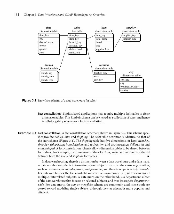
116 Chapter 3 Data Warehouse and OLAP Technology: An Overview
time dimension tabletime_key day day_of_week month quarter year
sales fact table
time_key item_key branch_key location_key dollars_sold units_sold
item dimension tableitem_key item_name brand type supplier_key
branch dimension table
branch_key branch_name branch_type
location dimension table
location_key street city_key
supplier dimension tablesupplier_key supplier_type
city dimension table
city_key city province_or_state country
Figure 3.5 Snowflake schema of a data warehouse for sales.
Fact constellation: Sophisticated applications may require multiple fact tables to sharedimension tables. This kind of schema can be viewed as a collection of stars, and henceis called a galaxy schema or a fact constellation.
Example 3.3 Fact constellation. A fact constellation schema is shown in Figure 3.6. This schema spec-ifies two fact tables, sales and shipping. The sales table definition is identical to that ofthe star schema (Figure 3.4). The shipping table has five dimensions, or keys: item key,time key, shipper key, from location, and to location, and two measures: dollars cost andunits shipped. A fact constellation schema allows dimension tables to be shared betweenfact tables. For example, the dimensions tables for time, item, and location are sharedbetween both the sales and shipping fact tables.
In data warehousing, there is a distinction between a data warehouse and a data mart.A data warehouse collects information about subjects that span the entire organization,such as customers, items, sales, assets, and personnel, and thus its scope is enterprise-wide.For data warehouses, the fact constellation schema is commonly used, since it can modelmultiple, interrelated subjects. A data mart, on the other hand, is a department subsetof the data warehouse that focuses on selected subjects, and thus its scope is department-wide. For data marts, the star or snowflake schema are commonly used, since both aregeared toward modeling single subjects, although the star schema is more popular andefficient.

3.2 A Multidimensional Data Model 117
time dimension tabletime_key day day_of_week month quarter year
sales fact table
time_key item_key branch_key location_key dollars_sold units_sold
item dimension table
item_key item_name brand type supplier_type
branch dimension tablebranch_key branch_name branch_type
location dimension table
location_key street city province_or_state country
shipping fact table
item_key time_key shipper_key from_location to_location dollars_cost units_shipped
shipper dimension table
shipper_key shipper_name location_key shipper_type
Figure 3.6 Fact constellation schema of a data warehouse for sales and shipping.
3.2.3 Examples for Defining Star, Snowflake,and Fact Constellation Schemas
“How can I define a multidimensional schema for my data?” Just as relational querylanguages like SQL can be used to specify relational queries, a data mining query lan-guage can be used to specify data mining tasks. In particular, we examine how to definedata warehouses and data marts in our SQL-based data mining query language, DMQL.
Data warehouses and data marts can be defined using two language primitives, onefor cube definition and one for dimension definition. The cube definition statement has thefollowing syntax:
define cube 〈cube name〉 [〈dimension list〉]: 〈measure list〉
The dimension definition statement has the following syntax:
define dimension 〈dimension name〉 as (〈attribute or dimension list〉)
Let’s look at examples of how to define the star, snowflake, and fact constellationschemas of Examples 3.1 to 3.3 using DMQL. DMQL keywords are displayed in sansserif font.
Example 3.4 Star schema definition. The star schema of Example 3.1 and Figure 3.4 is defined inDMQL as follows:
define cube sales star [time, item, branch, location]:dollars sold = sum(sales in dollars), units sold = count(*)

118 Chapter 3 Data Warehouse and OLAP Technology: An Overview
define dimension time as (time key, day, day of week, month, quarter, year)define dimension item as (item key, item name, brand, type, supplier type)define dimension branch as (branch key, branch name, branch type)define dimension location as (location key, street, city, province or state,
country)
The define cube statement defines a data cube called sales star, which correspondsto the central sales fact table of Example 3.1. This command specifies the dimensionsand the two measures, dollars sold and units sold. The data cube has four dimensions,namely, time, item, branch, and location. A define dimension statement is used to defineeach of the dimensions.
Example 3.5 Snowflake schema definition. The snowflake schema of Example 3.2 and Figure 3.5 isdefined in DMQL as follows:
define cube sales snowflake [time, item, branch, location]:dollars sold = sum(sales in dollars), units sold = count(*)
define dimension time as (time key, day, day of week, month, quarter, year)define dimension item as (item key, item name, brand, type, supplier
(supplier key, supplier type))define dimension branch as (branch key, branch name, branch type)define dimension location as (location key, street, city
(city key, city, province or state, country))
This definition is similar to that of sales star (Example 3.4), except that, here, the itemand location dimension tables are normalized. For instance, the item dimension of thesales star data cube has been normalized in the sales snowflake cube into two dimensiontables, item and supplier. Note that the dimension definition for supplier is specified withinthe definition for item. Defining supplier in this way implicitly creates a supplier key in theitem dimension table definition. Similarly, the location dimension of the sales star datacube has been normalized in the sales snowflake cube into two dimension tables, locationand city. The dimension definition for city is specified within the definition for location.In this way, a city key is implicitly created in the location dimension table definition.
Finally, a fact constellation schema can be defined as a set of interconnected cubes.Below is an example.
Example 3.6 Fact constellation schema definition. The fact constellation schema of Example 3.3 andFigure 3.6 is defined in DMQL as follows:
define cube sales [time, item, branch, location]:dollars sold = sum(sales in dollars), units sold = count(*)
define dimension time as (time key, day, day of week, month, quarter, year)define dimension item as (item key, item name, brand, type, supplier type)define dimension branch as (branch key, branch name, branch type)define dimension location as (location key, street, city, province or state,
country)

3.2 A Multidimensional Data Model 119
define cube shipping [time, item, shipper, from location, to location]:dollars cost = sum(cost in dollars), units shipped = count(*)
define dimension time as time in cube salesdefine dimension item as item in cube salesdefine dimension shipper as (shipper key, shipper name, location as
location in cube sales, shipper type)define dimension from location as location in cube salesdefine dimension to location as location in cube sales
A define cube statement is used to define data cubes for sales and shipping, cor-responding to the two fact tables of the schema of Example 3.3. Note that the time,item, and location dimensions of the sales cube are shared with the shipping cube.This is indicated for the time dimension, for example, as follows. Under the definecube statement for shipping, the statement “define dimension time as time in cubesales” is specified.
3.2.4 Measures: Their Categorization and Computation
“How are measures computed?” To answer this question, we first study how measures canbe categorized.1 Note that a multidimensional point in the data cube space can be definedby a set of dimension-value pairs, for example, 〈time = “Q1”, location = “Vancouver”,item = “computer”〉. A data cube measure is a numerical function that can be evaluatedat each point in the data cube space. A measure value is computed for a given point byaggregating the data corresponding to the respective dimension-value pairs defining thegiven point. We will look at concrete examples of this shortly.
Measures can be organized into three categories (i.e., distributive, algebraic, holistic),based on the kind of aggregate functions used.
Distributive: An aggregate function is distributive if it can be computed in a distributedmanner as follows. Suppose the data are partitioned into n sets. We apply the functionto each partition, resulting in n aggregate values. If the result derived by applying thefunction to the n aggregate values is the same as that derived by applying the func-tion to the entire data set (without partitioning), the function can be computed ina distributed manner. For example, count() can be computed for a data cube by firstpartitioning the cube into a set of subcubes, computing count() for each subcube, andthen summing up the counts obtained for each subcube. Hence, count() is a distribu-tive aggregate function. For the same reason, sum(), min(), and max() are distributiveaggregate functions. A measure is distributive if it is obtained by applying a distribu-tive aggregate function. Distributive measures can be computed efficiently becausethey can be computed in a distributive manner.
1This categorization was briefly introduced in Chapter 2 with regards to the computation of measuresfor descriptive data summaries. We reexamine it here in the context of data cube measures.
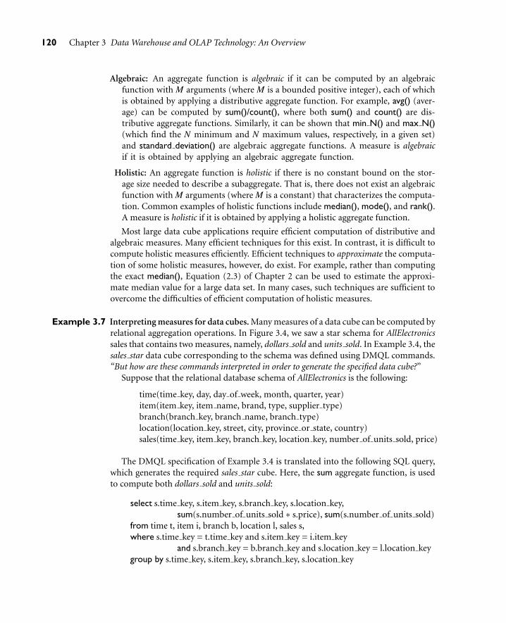
120 Chapter 3 Data Warehouse and OLAP Technology: An Overview
Algebraic: An aggregate function is algebraic if it can be computed by an algebraicfunction with M arguments (where M is a bounded positive integer), each of whichis obtained by applying a distributive aggregate function. For example, avg() (aver-age) can be computed by sum()/count(), where both sum() and count() are dis-tributive aggregate functions. Similarly, it can be shown that min N() and max N()(which find the N minimum and N maximum values, respectively, in a given set)and standard deviation() are algebraic aggregate functions. A measure is algebraicif it is obtained by applying an algebraic aggregate function.
Holistic: An aggregate function is holistic if there is no constant bound on the stor-age size needed to describe a subaggregate. That is, there does not exist an algebraicfunction with M arguments (where M is a constant) that characterizes the computa-tion. Common examples of holistic functions include median(), mode(), and rank().A measure is holistic if it is obtained by applying a holistic aggregate function.
Most large data cube applications require efficient computation of distributive andalgebraic measures. Many efficient techniques for this exist. In contrast, it is difficult tocompute holistic measures efficiently. Efficient techniques to approximate the computa-tion of some holistic measures, however, do exist. For example, rather than computingthe exact median(), Equation (2.3) of Chapter 2 can be used to estimate the approxi-mate median value for a large data set. In many cases, such techniques are sufficient toovercome the difficulties of efficient computation of holistic measures.
Example 3.7 Interpreting measures for data cubes. Many measures of a data cube can be computed byrelational aggregation operations. In Figure 3.4, we saw a star schema for AllElectronicssales that contains two measures, namely, dollars sold and units sold. In Example 3.4, thesales star data cube corresponding to the schema was defined using DMQL commands.“But how are these commands interpreted in order to generate the specified data cube?”
Suppose that the relational database schema of AllElectronics is the following:
time(time key, day, day of week, month, quarter, year)item(item key, item name, brand, type, supplier type)branch(branch key, branch name, branch type)location(location key, street, city, province or state, country)sales(time key, item key, branch key, location key, number of units sold, price)
The DMQL specification of Example 3.4 is translated into the following SQL query,which generates the required sales star cube. Here, the sum aggregate function, is usedto compute both dollars sold and units sold:
select s.time key, s.item key, s.branch key, s.location key,sum(s.number of units sold ∗ s.price), sum(s.number of units sold)
from time t, item i, branch b, location l, sales s,where s.time key = t.time key and s.item key = i.item key
and s.branch key = b.branch key and s.location key = l.location keygroup by s.time key, s.item key, s.branch key, s.location key

3.2 A Multidimensional Data Model 121
The cube created in the above query is the base cuboid of the sales star data cube. Itcontains all of the dimensions specified in the data cube definition, where the granularityof each dimension is at the join key level. A join key is a key that links a fact table anda dimension table. The fact table associated with a base cuboid is sometimes referred toas the base fact table.
By changing the group by clauses, we can generate other cuboids for the sales star datacube. For example, instead of grouping by s.time key, we can group by t.month, which willsum up the measures of each group by month. Also, removing “group by s.branch key”will generate a higher-level cuboid (where sales are summed for all branches, rather thanbroken down per branch). Suppose we modify the above SQL query by removing all ofthe group by clauses. This will result in obtaining the total sum of dollars sold and thetotal count of units sold for the given data. This zero-dimensional cuboid is the apexcuboid of the sales star data cube. In addition, other cuboids can be generated by apply-ing selection and/or projection operations on the base cuboid, resulting in a lattice ofcuboids as described in Section 3.2.1. Each cuboid corresponds to a different degree ofsummarization of the given data.
Most of the current data cube technology confines the measures of multidimensionaldatabases to numerical data. However, measures can also be applied to other kinds ofdata, such as spatial, multimedia, or text data. This will be discussed in future chapters.
3.2.5 Concept Hierarchies
A concept hierarchy defines a sequence of mappings from a set of low-level conceptsto higher-level, more general concepts. Consider a concept hierarchy for the dimensionlocation. City values for location include Vancouver, Toronto, New York, and Chicago. Eachcity, however, can be mapped to the province or state to which it belongs. For example,Vancouver can be mapped to British Columbia, and Chicago to Illinois. The provinces andstates can in turn be mapped to the country to which they belong, such as Canada or theUSA. These mappings form a concept hierarchy for the dimension location, mapping a setof low-level concepts (i.e., cities) to higher-level, more general concepts (i.e., countries).The concept hierarchy described above is illustrated in Figure 3.7.
Many concept hierarchies are implicit within the database schema. For example, sup-pose that the dimension location is described by the attributes number, street, city,province or state,zipcode, andcountry.Theseattributesarerelatedbyatotalorder, forminga concept hierarchy such as “street < city < province or state < country”. This hierarchyis shown in Figure 3.8(a). Alternatively, the attributes of a dimension may be organizedin a partial order, forming a lattice. An example of a partial order for the time dimensionbased on the attributes day, week, month, quarter, and year is “day < {month <quarter;week} < year”.2 This lattice structure is shown in Figure 3.8(b). A concept hierarchy
2Since a week often crosses the boundary of two consecutive months, it is usually not treated as a lowerabstraction of month. Instead, it is often treated as a lower abstraction of year, since a year containsapproximately 52 weeks.

122 Chapter 3 Data Warehouse and OLAP Technology: An Overview
Canada
British Columbia Ontario
Vancouver Victoria OttawaToronto Chicago UrbanaBuffalo
New York
New York
Illinois
USA
location
country
city
province_or_state
Figure 3.7 A concept hierarchy for the dimension location. Due to space limitations, not all of the nodesof the hierarchy are shown (as indicated by the use of “ellipsis” between nodes).
country
city
province_or_state
month week
year
day
quarter
street
(a) (b)
Figure 3.8 Hierarchical and lattice structures of attributes in warehouse dimensions: (a) a hierarchy forlocation; (b) a lattice for time.
that is a total or partial order among attributes in a database schema is called a schemahierarchy. Concept hierarchies that are common to many applications may be prede-fined in the data mining system, such as the concept hierarchy for time. Data miningsystems should provide users with the flexibility to tailor predefined hierarchies accord-ing to their particular needs. For example, users may like to define a fiscal year startingon April 1 or an academic year starting on September 1.

3.2 A Multidimensional Data Model 123
($0 $1000]
($800 $1000]
($0 … �$100]
($100… $200]
($800… $900]
($900… $1000]
($600… $700]
($700… $800]
($200… $300]
($300… $400]
($400… $500]
($500… $600]
($600 $800]($400 $600]($200 $400]($0 $200]
Figure 3.9 A concept hierarchy for the attribute price.
Concept hierarchies may also be defined by discretizing or grouping values for a givendimension or attribute, resulting in a set-grouping hierarchy. A total or partial order canbe defined among groups of values. An example of a set-grouping hierarchy is shown inFigure 3.9 for the dimension price, where an interval ($X . . .$Y ] denotes the range from$X (exclusive) to $Y (inclusive).
There may be more than one concept hierarchy for a given attribute or dimension,based on different user viewpoints. For instance, a user may prefer to organize price bydefining ranges for inexpensive, moderately priced, and expensive.
Concept hierarchies may be provided manually by system users, domain experts, orknowledge engineers, or may be automatically generated based on statistical analysis ofthe data distribution. The automatic generation of concept hierarchies is discussed inChapter 2 as a preprocessing step in preparation for data mining.
Concept hierarchies allow data to be handled at varying levels of abstraction, as weshall see in the following subsection.
3.2.6 OLAP Operations in the Multidimensional Data Model
“How are concept hierarchies useful in OLAP?” In the multidimensional model, data areorganized into multiple dimensions, and each dimension contains multiple levels ofabstraction defined by concept hierarchies. This organization provides users with theflexibility to view data from different perspectives. A number of OLAP data cube opera-tions exist to materialize these different views, allowing interactive querying and analysisof the data at hand. Hence, OLAP provides a user-friendly environment for interactivedata analysis.
Example 3.8 OLAP operations. Let’s look at some typical OLAP operations for multidimensionaldata. Each of the operations described below is illustrated in Figure 3.10. At the centerof the figure is a data cube for AllElectronics sales. The cube contains the dimensionslocation, time, and item, where location is aggregated with respect to city values, time isaggregated with respect to quarters, and item is aggregated with respect to item types. To

124 Chapter 3 Data Warehouse and OLAP Technology: An Overview
Q1
Q2
Q3
Q4
1000
Canada USA 2000
time
(qua
rter
s) loc
ation
(cou
ntries)
home entertainment
computer
item (types)
phone security
Toronto 395
Q1
Q2
605
Vancouver
time
(qua
rter
s)
locati
on (c
ities)
home entertainment
computer
item (types)
January February March April May June July August September October November December
Chicago New York
Toronto Vancouver
time
(mon
ths)
locati
on (c
ities)
home entertainment
computer
item (types)
phone security
150 100 150
605 825 14 400 Q1
Q2
Q3
Q4
Chicago New York
Toronto Vancouver
time
(qua
rter
s)
locati
on (c
ities)
home entertainment
computer
item (types)
phone security
440
395 1560
dice for (location = “Toronto” or “Vancouver”) and (time = “Q1” or “Q2”) and (item = “home entertainment” or “computer”)
roll-up on location (from cities to countries)
slice for time = “Q1”
Chicago
New York
Toronto
Vancouver
home entertainment
computer
item (types)
phone security
loca
tion
(cit
ies)
605 825 14 400
home entertainment
computer
phone
security
605
825
14
400
Chicago New York
location (cities)
item
(typ
es)
Toronto Vancouver
pivot
drill-down on time (from quarters to months)
Figure 3.10 Examples of typical OLAP operations on multidimensional data.

3.2 A Multidimensional Data Model 125
aid in our explanation, we refer to this cube as the central cube. The measure displayedis dollars sold (in thousands). (For improved readability, only some of the cubes’ cellvalues are shown.) The data examined are for the cities Chicago, New York, Toronto, andVancouver.
Roll-up: The roll-up operation (also called the drill-up operation by some vendors)performs aggregation on a data cube, either by climbing up a concept hierarchy fora dimension or by dimension reduction. Figure 3.10 shows the result of a roll-upoperation performed on the central cube by climbing up the concept hierarchy forlocation given in Figure 3.7. This hierarchy was defined as the total order “street< city < province or state < country.” The roll-up operation shown aggregatesthe data by ascending the location hierarchy from the level of city to the level ofcountry. In other words, rather than grouping the data by city, the resulting cubegroups the data by country.
When roll-up is performed by dimension reduction, one or more dimensions areremoved from the given cube. For example, consider a sales data cube containing onlythe two dimensions location and time. Roll-up may be performed by removing, say,the time dimension, resulting in an aggregation of the total sales by location, ratherthan by location and by time.
Drill-down: Drill-down is the reverse of roll-up. It navigates from less detailed data tomore detailed data. Drill-down can be realized by either stepping down a concept hier-archy for a dimension or introducing additional dimensions. Figure 3.10 shows theresult of a drill-down operation performed on the central cube by stepping down aconcept hierarchy for time defined as “day < month < quarter < year.” Drill-downoccurs by descending the time hierarchy from the level of quarter to the more detailedlevel of month. The resulting data cube details the total sales per month rather thansummarizing them by quarter.
Because a drill-down adds more detail to the given data, it can also be performedby adding new dimensions to a cube. For example, a drill-down on the central cube ofFigure 3.10 can occur by introducing an additional dimension, such as customer group.
Slice and dice: The slice operation performs a selection on one dimension of thegiven cube, resulting in a subcube. Figure 3.10 shows a slice operation wherethe sales data are selected from the central cube for the dimension time usingthe criterion time = “Q1”. The dice operation defines a subcube by performing aselection on two or more dimensions. Figure 3.10 shows a dice operation on thecentral cube based on the following selection criteria that involve three dimensions:(location = “Toronto” or “Vancouver”) and (time = “Q1” or “Q2”) and (item =“home entertainment” or “computer”).
Pivot (rotate): Pivot (also called rotate) is a visualization operation that rotates the dataaxes in view in order to provide an alternative presentation of the data. Figure 3.10shows a pivot operation where the item and location axes in a 2-D slice are rotated.
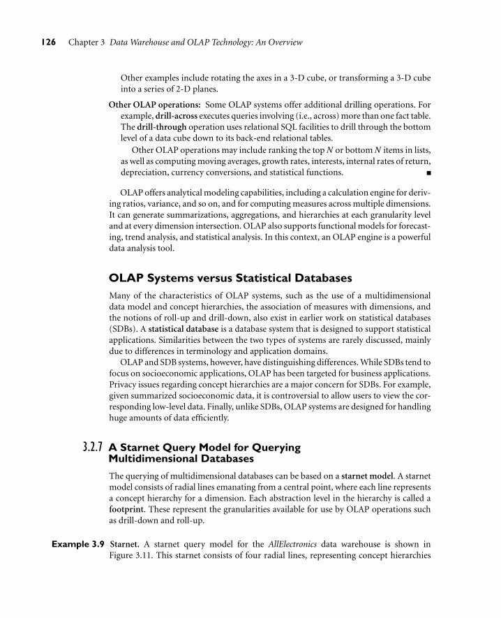
126 Chapter 3 Data Warehouse and OLAP Technology: An Overview
Other examples include rotating the axes in a 3-D cube, or transforming a 3-D cubeinto a series of 2-D planes.
Other OLAP operations: Some OLAP systems offer additional drilling operations. Forexample, drill-across executes queries involving (i.e., across) more than one fact table.The drill-through operation uses relational SQL facilities to drill through the bottomlevel of a data cube down to its back-end relational tables.
Other OLAP operations may include ranking the top N or bottom N items in lists,as well as computing moving averages, growth rates, interests, internal rates of return,depreciation, currency conversions, and statistical functions.
OLAP offers analytical modeling capabilities, including a calculation engine for deriv-ing ratios, variance, and so on, and for computing measures across multiple dimensions.It can generate summarizations, aggregations, and hierarchies at each granularity leveland at every dimension intersection. OLAP also supports functional models for forecast-ing, trend analysis, and statistical analysis. In this context, an OLAP engine is a powerfuldata analysis tool.
OLAP Systems versus Statistical DatabasesMany of the characteristics of OLAP systems, such as the use of a multidimensionaldata model and concept hierarchies, the association of measures with dimensions, andthe notions of roll-up and drill-down, also exist in earlier work on statistical databases(SDBs). A statistical database is a database system that is designed to support statisticalapplications. Similarities between the two types of systems are rarely discussed, mainlydue to differences in terminology and application domains.
OLAP and SDB systems, however, have distinguishing differences. While SDBs tend tofocus on socioeconomic applications, OLAP has been targeted for business applications.Privacy issues regarding concept hierarchies are a major concern for SDBs. For example,given summarized socioeconomic data, it is controversial to allow users to view the cor-responding low-level data. Finally, unlike SDBs, OLAP systems are designed for handlinghuge amounts of data efficiently.
3.2.7 A Starnet Query Model for QueryingMultidimensional Databases
The querying of multidimensional databases can be based on a starnet model. A starnetmodel consists of radial lines emanating from a central point, where each line representsa concept hierarchy for a dimension. Each abstraction level in the hierarchy is called afootprint. These represent the granularities available for use by OLAP operations suchas drill-down and roll-up.
Example 3.9 Starnet. A starnet query model for the AllElectronics data warehouse is shown inFigure 3.11. This starnet consists of four radial lines, representing concept hierarchies

3.3 Data Warehouse Architecture 127
continent
country
province_or_state
city
street
name brand category type
name
category
group
year
quarter
month
day
time
item
locationcustomer
Figure 3.11 Modeling business queries: a starnet model.
for the dimensions location, customer, item, and time, respectively. Each line consists offootprints representing abstraction levels of the dimension. For example, the time linehas four footprints: “day,” “month,” “quarter,” and “year.” A concept hierarchy mayinvolve a single attribute (like date for the time hierarchy) or several attributes (e.g.,the concept hierarchy for location involves the attributes street, city, province or state,and country). In order to examine the item sales at AllElectronics, users can roll upalong the time dimension from month to quarter, or, say, drill down along the locationdimension from country to city. Concept hierarchies can be used to generalize databy replacing low-level values (such as “day” for the time dimension) by higher-levelabstractions (such as “year”), or to specialize data by replacing higher-level abstractionswith lower-level values.
3.3 Data Warehouse Architecture
In this section, we discuss issues regarding data warehouse architecture. Section 3.3.1gives a general account of how to design and construct a data warehouse. Section 3.3.2describes a three-tier data warehouse architecture. Section 3.3.3 describes back-endtools and utilities for data warehouses. Section 3.3.4 describes the metadata repository.Section 3.3.5 presents various types of warehouse servers for OLAP processing.

128 Chapter 3 Data Warehouse and OLAP Technology: An Overview
3.3.1 Steps for the Design and Construction of Data Warehouses
This subsection presents a business analysis framework for data warehouse design. Thebasic steps involved in the design process are also described.
The Design of a Data Warehouse: A BusinessAnalysis Framework
“What can business analysts gain from having a data warehouse?” First, having a datawarehouse may provide a competitive advantage by presenting relevant information fromwhich to measure performance and make critical adjustments in order to help win overcompetitors. Second, a data warehouse can enhance business productivity because it isable to quickly and efficiently gather information that accurately describes the organi-zation. Third, a data warehouse facilitates customer relationship management because itprovides a consistent view of customers and items across all lines of business, all depart-ments, and all markets. Finally, a data warehouse may bring about cost reduction by track-ing trends, patterns, and exceptions over long periods in a consistent and reliable manner.
To design an effective data warehouse we need to understand and analyze businessneeds and construct a business analysis framework. The construction of a large and com-plex information system can be viewed as the construction of a large and complex build-ing, for which the owner, architect, and builder have different views. These views arecombined to form a complex framework that represents the top-down, business-driven,or owner’s perspective, as well as the bottom-up, builder-driven, or implementor’s viewof the information system.
Four different views regarding the design of a data warehouse must be considered: thetop-down view, the data source view, the data warehouse view, and the businessquery view.
The top-down view allows the selection of the relevant information necessary forthe data warehouse. This information matches the current and future businessneeds.
The data source view exposes the information being captured, stored, and man-aged by operational systems. This information may be documented at variouslevels of detail and accuracy, from individual data source tables to integrateddata source tables. Data sources are often modeled by traditional data model-ing techniques, such as the entity-relationship model or CASE (computer-aidedsoftware engineering) tools.
The data warehouse view includes fact tables and dimension tables. It represents theinformation that is stored inside the data warehouse, including precalculated totalsand counts, as well as information regarding the source, date, and time of origin,added to provide historical context.
Finally, the business query view is the perspective of data in the data warehouse fromthe viewpoint of the end user.
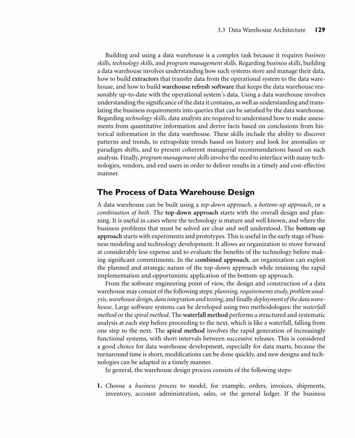
3.3 Data Warehouse Architecture 129
Building and using a data warehouse is a complex task because it requires businessskills, technology skills, and program management skills. Regarding business skills, buildinga data warehouse involves understanding how such systems store and manage their data,how to build extractors that transfer data from the operational system to the data ware-house, and how to build warehouse refresh software that keeps the data warehouse rea-sonably up-to-date with the operational system’s data. Using a data warehouse involvesunderstanding the significance of the data it contains, as well as understanding and trans-lating the business requirements into queries that can be satisfied by the data warehouse.Regarding technology skills, data analysts are required to understand how to make assess-ments from quantitative information and derive facts based on conclusions from his-torical information in the data warehouse. These skills include the ability to discoverpatterns and trends, to extrapolate trends based on history and look for anomalies orparadigm shifts, and to present coherent managerial recommendations based on suchanalysis. Finally, program management skills involve the need to interface with many tech-nologies, vendors, and end users in order to deliver results in a timely and cost-effectivemanner.
The Process of Data Warehouse DesignA data warehouse can be built using a top-down approach, a bottom-up approach, or acombination of both. The top-down approach starts with the overall design and plan-ning. It is useful in cases where the technology is mature and well known, and where thebusiness problems that must be solved are clear and well understood. The bottom-upapproach starts with experiments and prototypes. This is useful in the early stage of busi-ness modeling and technology development. It allows an organization to move forwardat considerably less expense and to evaluate the benefits of the technology before mak-ing significant commitments. In the combined approach, an organization can exploitthe planned and strategic nature of the top-down approach while retaining the rapidimplementation and opportunistic application of the bottom-up approach.
From the software engineering point of view, the design and construction of a datawarehouse may consist of the following steps: planning, requirements study, problem anal-ysis, warehouse design, data integration and testing, and finally deployment of the data ware-house. Large software systems can be developed using two methodologies: the waterfallmethod or the spiral method. The waterfall method performs a structured and systematicanalysis at each step before proceeding to the next, which is like a waterfall, falling fromone step to the next. The spiral method involves the rapid generation of increasinglyfunctional systems, with short intervals between successive releases. This is considereda good choice for data warehouse development, especially for data marts, because theturnaround time is short, modifications can be done quickly, and new designs and tech-nologies can be adapted in a timely manner.
In general, the warehouse design process consists of the following steps:
1. Choose a business process to model, for example, orders, invoices, shipments,inventory, account administration, sales, or the general ledger. If the business

130 Chapter 3 Data Warehouse and OLAP Technology: An Overview
process is organizational and involves multiple complex object collections, a datawarehouse model should be followed. However, if the process is departmentaland focuses on the analysis of one kind of business process, a data mart modelshould be chosen.
2. Choose the grain of the business process. The grain is the fundamental, atomic levelof data to be represented in the fact table for this process, for example, individualtransactions, individual daily snapshots, and so on.
3. Choose the dimensions that will apply to each fact table record. Typical dimensionsare time, item, customer, supplier, warehouse, transaction type, and status.
4. Choose the measures that will populate each fact table record. Typical measures arenumeric additive quantities like dollars sold and units sold.
Because data warehouse construction is a difficult and long-term task, its imple-mentation scope should be clearly defined. The goals of an initial data warehouseimplementation should be specific, achievable, and measurable. This involves deter-mining the time and budget allocations, the subset of the organization that is to bemodeled, the number of data sources selected, and the number and types of depart-ments to be served.
Once a data warehouse is designed and constructed, the initial deployment ofthe warehouse includes initial installation, roll-out planning, training, and orienta-tion. Platform upgrades and maintenance must also be considered. Data warehouseadministration includes data refreshment, data source synchronization, planning fordisaster recovery, managing access control and security, managing data growth, man-aging database performance, and data warehouse enhancement and extension. Scopemanagement includes controlling the number and range of queries, dimensions, andreports; limiting the size of the data warehouse; or limiting the schedule, budget, orresources.
Various kinds of data warehouse design tools are available. Data warehouse devel-opment tools provide functions to define and edit metadata repository contents (suchas schemas, scripts, or rules), answer queries, output reports, and ship metadata toand from relational database system catalogues. Planning and analysis tools study theimpact of schema changes and of refresh performance when changing refresh rates ortime windows.
3.3.2 A Three-Tier Data Warehouse Architecture
Data warehouses often adopt a three-tier architecture, as presented in Figure 3.12.
1. The bottom tier is a warehouse database server that is almost always a relationaldatabase system. Back-end tools and utilities are used to feed data into the bottomtier from operational databases or other external sources (such as customer profileinformation provided by external consultants). These tools and utilities perform dataextraction, cleaning, and transformation (e.g., to merge similar data from different

3.3 Data Warehouse Architecture 131
Query/report Analysis Data mining
OLAP server OLAP server
Top tier:
front-end tools
Middle tier:
OLAP server
Bottom tier:
data warehouse
server
Data
Output
Extract
Clean
Transform
Load
Refresh
Data warehouse Data martsMonitoring
Metadata repository
Operational databases External sources
Administration
Figure 3.12 A three-tier data warehousing architecture.
sources into a unified format), as well as load and refresh functions to update thedata warehouse (Section 3.3.3). The data are extracted using application programinterfaces known as gateways. A gateway is supported by the underlying DBMS andallows client programs to generate SQL code to be executed at a server. Examplesof gateways include ODBC (Open Database Connection) and OLEDB (Open Link-ing and Embedding for Databases) by Microsoft and JDBC (Java Database Connec-tion). This tier also contains a metadata repository, which stores information aboutthe data warehouse and its contents. The metadata repository is further described inSection 3.3.4.
2. The middle tier is an OLAP server that is typically implemented using either(1) a relational OLAP (ROLAP) model, that is, an extended relational DBMS that

132 Chapter 3 Data Warehouse and OLAP Technology: An Overview
maps operations on multidimensional data to standard relational operations; or(2) a multidimensional OLAP (MOLAP) model, that is, a special-purpose serverthat directly implements multidimensional data and operations. OLAP servers arediscussed in Section 3.3.5.
3. The top tier is a front-end client layer, which contains query and reporting tools,analysis tools, and/or data mining tools (e.g., trend analysis, prediction, and so on).
From the architecture point of view, there are three data warehouse models: the enter-prise warehouse, the data mart, and the virtual warehouse.
Enterprise warehouse: An enterprise warehouse collects all of the information aboutsubjects spanning the entire organization. It provides corporate-wide data inte-gration, usually from one or more operational systems or external informationproviders, and is cross-functional in scope. It typically contains detailed data aswell as summarized data, and can range in size from a few gigabytes to hundredsof gigabytes, terabytes, or beyond. An enterprise data warehouse may be imple-mented on traditional mainframes, computer superservers, or parallel architectureplatforms. It requires extensive business modeling and may take years to designand build.
Data mart: A data mart contains a subset of corporate-wide data that is of value to aspecific group of users. The scope is confined to specific selected subjects. For exam-ple, a marketing data mart may confine its subjects to customer, item, and sales. Thedata contained in data marts tend to be summarized.Data marts are usually implemented on low-cost departmental servers that areUNIX/LINUX- or Windows-based. The implementation cycle of a data mart ismore likely to be measured in weeks rather than months or years. However, itmay involve complex integration in the long run if its design and planning werenot enterprise-wide.Depending on the source of data, data marts can be categorized as independent ordependent. Independent data marts are sourced from data captured from one or moreoperational systems or external information providers, or from data generated locallywithin a particular department or geographic area. Dependent data marts are sourceddirectly from enterprise data warehouses.
Virtual warehouse: A virtual warehouse is a set of views over operational databases. Forefficient query processing, only some of the possible summary views may be materi-alized. A virtual warehouse is easy to build but requires excess capacity on operationaldatabase servers.
“What are the pros and cons of the top-down and bottom-up approaches to data ware-house development?” The top-down development of an enterprise warehouse serves asa systematic solution and minimizes integration problems. However, it is expensive,takes a long time to develop, and lacks flexibility due to the difficulty in achieving

3.3 Data Warehouse Architecture 133
consistency and consensus for a common data model for the entire organization. Thebottom-up approach to the design, development, and deployment of independentdata marts provides flexibility, low cost, and rapid return of investment. It, however,can lead to problems when integrating various disparate data marts into a consistententerprise data warehouse.
A recommended method for the development of data warehouse systems is toimplement the warehouse in an incremental and evolutionary manner, as shown inFigure 3.13. First, a high-level corporate data model is defined within a reasonablyshort period (such as one or two months) that provides a corporate-wide, consistent,integrated view of data among different subjects and potential usages. This high-levelmodel, although it will need to be refined in the further development of enterprisedata warehouses and departmental data marts, will greatly reduce future integrationproblems. Second, independent data marts can be implemented in parallel withthe enterprise warehouse based on the same corporate data model set as above.Third, distributed data marts can be constructed to integrate different data marts viahub servers. Finally, a multitier data warehouse is constructed where the enterprisewarehouse is the sole custodian of all warehouse data, which is then distributed tothe various dependent data marts.
Enterprise data
warehouse
Multitier data
warehouse
Distributed data marts
Data mart
Define a high-level corporate data model
Data mart
Model refinement Model refinement
Figure 3.13 A recommended approach for data warehouse development.

134 Chapter 3 Data Warehouse and OLAP Technology: An Overview
3.3.3 Data Warehouse Back-End Tools and Utilities
Data warehouse systems use back-end tools and utilities to populate and refresh theirdata (Figure 3.12). These tools and utilities include the following functions:
Data extraction, which typically gathers data from multiple, heterogeneous, and exter-nal sources
Data cleaning, which detects errors in the data and rectifies them when possible
Data transformation, which converts data from legacy or host format to warehouseformat
Load, which sorts, summarizes, consolidates, computes views, checks integrity, andbuilds indices and partitions
Refresh, which propagates the updates from the data sources to the warehouse
Besides cleaning, loading, refreshing, and metadata definition tools, data warehouse sys-tems usually provide a good set of data warehouse management tools.
Data cleaning and data transformation are important steps in improving the qualityof the data and, subsequently, of the data mining results. They are described in Chapter 2on Data Preprocessing. Because we are mostly interested in the aspects of data warehous-ing technology related to data mining, we will not get into the details of the remainingtools and recommend interested readers to consult books dedicated to data warehousingtechnology.
3.3.4 Metadata Repository
Metadata are data about data. When used in a data warehouse, metadata are the data thatdefine warehouse objects. Figure 3.12 showed a metadata repository within the bottomtier of the data warehousing architecture. Metadata are created for the data names anddefinitions of the given warehouse. Additional metadata are created and captured fortimestamping any extracted data, the source of the extracted data, and missing fieldsthat have been added by data cleaning or integration processes.
A metadata repository should contain the following:
A description of the structure of the data warehouse, which includes the warehouseschema, view, dimensions, hierarchies, and derived data definitions, as well as datamart locations and contents
Operational metadata, which include data lineage (history of migrated data and thesequence of transformations applied to it), currency of data (active, archived, orpurged), and monitoring information (warehouse usage statistics, error reports, andaudit trails)
The algorithms used for summarization, which include measure and dimension defi-nition algorithms, data on granularity, partitions, subject areas, aggregation, summa-rization, and predefined queries and reports
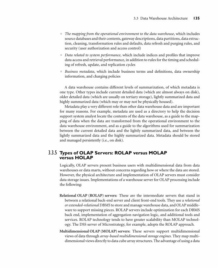
3.3 Data Warehouse Architecture 135
The mapping from the operational environment to the data warehouse, which includessource databases and their contents, gateway descriptions, data partitions, data extrac-tion, cleaning, transformation rules and defaults, data refresh and purging rules, andsecurity (user authorization and access control)
Data related to system performance, which include indices and profiles that improvedata access and retrieval performance, in addition to rules for the timing and schedul-ing of refresh, update, and replication cycles
Business metadata, which include business terms and definitions, data ownershipinformation, and charging policies
A data warehouse contains different levels of summarization, of which metadata isone type. Other types include current detailed data (which are almost always on disk),older detailed data (which are usually on tertiary storage), lightly summarized data andhighly summarized data (which may or may not be physically housed).
Metadata play a very different role than other data warehouse data and are importantfor many reasons. For example, metadata are used as a directory to help the decisionsupport system analyst locate the contents of the data warehouse, as a guide to the map-ping of data when the data are transformed from the operational environment to thedata warehouse environment, and as a guide to the algorithms used for summarizationbetween the current detailed data and the lightly summarized data, and between thelightly summarized data and the highly summarized data. Metadata should be storedand managed persistently (i.e., on disk).
3.3.5 Types of OLAP Servers: ROLAP versus MOLAPversus HOLAP
Logically, OLAP servers present business users with multidimensional data from datawarehouses or data marts, without concerns regarding how or where the data are stored.However, the physical architecture and implementation of OLAP servers must considerdata storage issues. Implementations of a warehouse server for OLAP processing includethe following:
Relational OLAP (ROLAP) servers: These are the intermediate servers that stand inbetween a relational back-end server and client front-end tools. They use a relationalor extended-relational DBMS to store and manage warehouse data, and OLAP middle-ware to support missing pieces. ROLAP servers include optimization for each DBMSback end, implementation of aggregation navigation logic, and additional tools andservices. ROLAP technology tends to have greater scalability than MOLAP technol-ogy. The DSS server of Microstrategy, for example, adopts the ROLAP approach.
Multidimensional OLAP (MOLAP) servers: These servers support multidimensionalviews of data through array-based multidimensional storage engines. They map multi-dimensional views directly to data cube array structures. The advantage of using a data

136 Chapter 3 Data Warehouse and OLAP Technology: An Overview
cube is that it allows fast indexing to precomputed summarized data. Notice that withmultidimensional data stores, the storage utilization may be low if the data set is sparse.In such cases, sparse matrix compression techniques should be explored (Chapter 4).Many MOLAP servers adopt a two-level storage representation to handle dense andsparse data sets: denser subcubes are identified and stored as array structures, whereassparse subcubes employ compression technology for efficient storage utilization.
Hybrid OLAP (HOLAP) servers: The hybrid OLAP approach combines ROLAP andMOLAP technology, benefiting from the greater scalability of ROLAP and the fastercomputation of MOLAP. For example, a HOLAP server may allow large volumesof detail data to be stored in a relational database, while aggregations are kept in aseparate MOLAP store. The Microsoft SQL Server 2000 supports a hybrid OLAPserver.
Specialized SQL servers: To meet the growing demand of OLAP processing in relationaldatabases, some database system vendors implement specialized SQL servers that pro-vide advanced query language and query processing support for SQL queries over starand snowflake schemas in a read-only environment.
“How are data actually stored in ROLAP and MOLAP architectures?” Let’s first lookat ROLAP. As its name implies, ROLAP uses relational tables to store data for on-lineanalytical processing. Recall that the fact table associated with a base cuboid is referredto as a base fact table. The base fact table stores data at the abstraction level indicated bythe join keys in the schema for the given data cube. Aggregated data can also be storedin fact tables, referred to as summary fact tables. Some summary fact tables store bothbase fact table data and aggregated data, as in Example 3.10. Alternatively, separate sum-mary fact tables can be used for each level of abstraction, to store only aggregated data.
Example 3.10 A ROLAP data store. Table 3.4 shows a summary fact table that contains both base factdata and aggregated data. The schema of the table is “〈record identifier (RID), item, . . . ,day, month, quarter, year, dollars sold〉”, where day, month, quarter, and year define thedate of sales, and dollars sold is the sales amount. Consider the tuples with an RID of 1001and 1002, respectively. The data of these tuples are at the base fact level, where the dateof sales is October 15, 2003, and October 23, 2003, respectively. Consider the tuple withan RID of 5001. This tuple is at a more general level of abstraction than the tuples 1001
Table 3.4 Single table for base and summary facts.
RID item . . . day month quarter year dollars sold
1001 TV . . . 15 10 Q4 2003 250.60
1002 TV . . . 23 10 Q4 2003 175.00
. . . . . . . . . . . . . . . . . . . . . . . .
5001 TV . . . all 10 Q4 2003 45,786.08
. . . . . . . . . . . . . . . . . . . . . . . .

3.4 Data Warehouse Implementation 137
and 1002. The day value has been generalized to all, so that the corresponding time valueis October 2003. That is, the dollars sold amount shown is an aggregation representingthe entire month of October 2003, rather than just October 15 or 23, 2003. The specialvalue all is used to represent subtotals in summarized data.
MOLAP uses multidimensional array structures to store data for on-line analyticalprocessing. This structure is discussed in the following section on data warehouse imple-mentation and, in greater detail, in Chapter 4.
Most data warehouse systems adopt a client-server architecture. A relational data storealways resides at the data warehouse/data mart server site. A multidimensional data storecan reside at either the database server site or the client site.
3.4 Data Warehouse Implementation
Data warehouses contain huge volumes of data. OLAP servers demand that decisionsupport queries be answered in the order of seconds. Therefore, it is crucial for data ware-house systems to support highly efficient cube computation techniques, access methods,and query processing techniques. In this section, we present an overview of methods forthe efficient implementation of data warehouse systems.
3.4.1 Efficient Computation of Data Cubes
At the core of multidimensional data analysis is the efficient computation of aggregationsacross many sets of dimensions. In SQL terms, these aggregations are referred to asgroup-by’s. Each group-by can be represented by a cuboid, where the set of group-by’sforms a lattice of cuboids defining a data cube. In this section, we explore issues relatingto the efficient computation of data cubes.
The compute cube Operator and theCurse of Dimensionality
One approach to cube computation extends SQL so as to include a compute cube oper-ator. The compute cube operator computes aggregates over all subsets of the dimensionsspecified in the operation. This can require excessive storage space, especially for largenumbers of dimensions. We start with an intuitive look at what is involved in the efficientcomputation of data cubes.
Example 3.11 A data cube is a lattice of cuboids. Suppose that you would like to create a data cube forAllElectronics sales that contains the following: city, item, year, and sales in dollars. Youwould like to be able to analyze the data, with queries such as the following:
“Compute the sum of sales, grouping by city and item.”
“Compute the sum of sales, grouping by city.”
“Compute the sum of sales, grouping by item.”
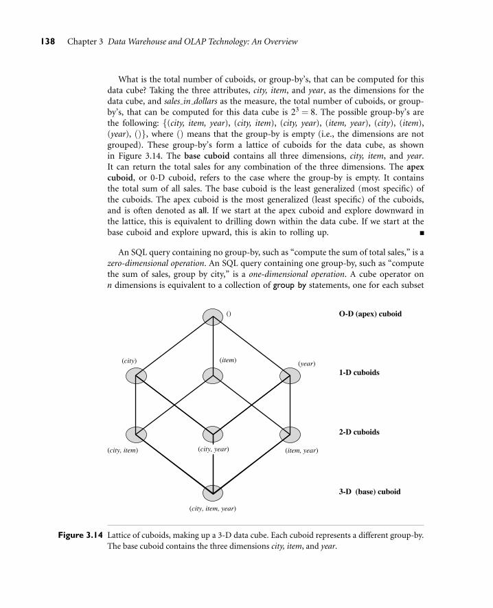
138 Chapter 3 Data Warehouse and OLAP Technology: An Overview
What is the total number of cuboids, or group-by’s, that can be computed for thisdata cube? Taking the three attributes, city, item, and year, as the dimensions for thedata cube, and sales in dollars as the measure, the total number of cuboids, or group-by’s, that can be computed for this data cube is 23 = 8. The possible group-by’s arethe following: {(city, item, year), (city, item), (city, year), (item, year), (city), (item),(year), ()}, where () means that the group-by is empty (i.e., the dimensions are notgrouped). These group-by’s form a lattice of cuboids for the data cube, as shownin Figure 3.14. The base cuboid contains all three dimensions, city, item, and year.It can return the total sales for any combination of the three dimensions. The apexcuboid, or 0-D cuboid, refers to the case where the group-by is empty. It containsthe total sum of all sales. The base cuboid is the least generalized (most specific) ofthe cuboids. The apex cuboid is the most generalized (least specific) of the cuboids,and is often denoted as all. If we start at the apex cuboid and explore downward inthe lattice, this is equivalent to drilling down within the data cube. If we start at thebase cuboid and explore upward, this is akin to rolling up.
An SQL query containing no group-by, such as “compute the sum of total sales,” is azero-dimensional operation. An SQL query containing one group-by, such as “computethe sum of sales, group by city,” is a one-dimensional operation. A cube operator onn dimensions is equivalent to a collection of group by statements, one for each subset
(item) (year)(city)
()
(item, year)
(city, item, year)
(city, item) (city, year)
O-D (apex) cuboid
1-D cuboids
2-D cuboids
3-D (base) cuboid
Figure 3.14 Lattice of cuboids, making up a 3-D data cube. Each cuboid represents a different group-by.The base cuboid contains the three dimensions city, item, and year.

3.4 Data Warehouse Implementation 139
of the n dimensions. Therefore, the cube operator is the n-dimensional generalization ofthe group by operator.
Based on the syntax of DMQL introduced in Section 3.2.3, the data cube inExample 3.11 could be defined as
define cube sales cube [city, item, year]: sum(sales in dollars)
For a cube with n dimensions, there are a total of 2n cuboids, including the basecuboid. A statement such as
compute cube sales cube
would explicitly instruct the system to compute the sales aggregate cuboids for all of theeight subsets of the set {city, item, year}, including the empty subset. A cube computationoperator was first proposed and studied by Gray et al. [GCB+97].
On-line analytical processing may need to access different cuboids for different queries.Therefore, it may seem like a good idea to compute all or at least some of the cuboidsin a data cube in advance. Precomputation leads to fast response time and avoids someredundant computation. Most, if not all, OLAP products resort to some degree of pre-computation of multidimensional aggregates.
A major challenge related to this precomputation, however, is that the required storagespace may explode if all of the cuboids in a data cube are precomputed, especially whenthe cube has many dimensions. The storage requirements are even more excessive whenmany of the dimensions have associated concept hierarchies, each with multiple levels.This problem is referred to as the curse of dimensionality. The extent of the curse ofdimensionality is illustrated below.
“How many cuboids are there in an n-dimensional data cube?” If there were nohierarchies associated with each dimension, then the total number of cuboids foran n-dimensional data cube, as we have seen above, is 2n. However, in practice,many dimensions do have hierarchies. For example, the dimension time is usually notexplored at only one conceptual level, such as year, but rather at multiple conceptuallevels, such as in the hierarchy “day < month < quarter < year”. For an n-dimensionaldata cube, the total number of cuboids that can be generated (including the cuboidsgenerated by climbing up the hierarchies along each dimension) is
Total number o f cuboids =n
∏i=1
(Li + 1), (3.1)
where Li is the number of levels associated with dimension i. One is added to Li inEquation (3.1) to include the virtual top level, all. (Note that generalizing to all is equiv-alent to the removal of the dimension.) This formula is based on the fact that, at most,one abstraction level in each dimension will appear in a cuboid. For example, the timedimension as specified above has 4 conceptual levels, or 5 if we include the virtual level all.If the cube has 10 dimensions and each dimension has 5 levels (including all), the totalnumber of cuboids that can be generated is 510 ≈ 9.8× 10⁶. The size of each cuboidalso depends on the cardinality (i.e., number of distinct values) of each dimension. Forexample, if the AllElectronics branch in each city sold every item, there would be

140 Chapter 3 Data Warehouse and OLAP Technology: An Overview
|city| × |item| tuples in the city-item group-by alone. As the number of dimensions,number of conceptual hierarchies, or cardinality increases, the storage space requiredfor many of the group-by’s will grossly exceed the (fixed) size of the input relation.
By now, you probably realize that it is unrealistic to precompute and materialize allof the cuboids that can possibly be generated for a data cube (or from a base cuboid). Ifthere are many cuboids, and these cuboids are large in size, a more reasonable option ispartial materialization, that is, to materialize only some of the possible cuboids that canbe generated.
Partial Materialization: SelectedComputation of Cuboids
There are three choices for data cube materialization given a base cuboid:
1. No materialization: Do not precompute any of the “nonbase” cuboids. This leads tocomputing expensive multidimensional aggregates on the fly, which can be extremelyslow.
2. Full materialization: Precompute all of the cuboids. The resulting lattice of computedcuboids is referred to as the full cube. This choice typically requires huge amounts ofmemory space in order to store all of the precomputed cuboids.
3. Partial materialization: Selectively compute a proper subset of the whole set of possi-ble cuboids. Alternatively, we may compute a subset of the cube, which contains onlythose cells that satisfy some user-specified criterion, such as where the tuple count ofeach cell is above some threshold. We will use the term subcube to refer to the latter case,where only some of the cells may be precomputed for various cuboids. Partial materi-alization represents an interesting trade-off between storage space and response time.
The partial materialization of cuboids or subcubes should consider three factors:(1) identify the subset of cuboids or subcubes to materialize; (2) exploit the mate-rialized cuboids or subcubes during query processing; and (3) efficiently update thematerialized cuboids or subcubes during load and refresh.
The selection of the subset of cuboids or subcubes to materialize should take intoaccount the queries in the workload, their frequencies, and their accessing costs. In addi-tion, it should consider workload characteristics, the cost for incremental updates, and thetotal storage requirements. The selection must also consider the broad context of physicaldatabase design, such as the generation and selection of indices. Several OLAP productshave adopted heuristic approaches for cuboid and subcube selection. A popular approachis to materialize the set of cuboids on which other frequently referenced cuboids are based.Alternatively, we can compute an iceberg cube, which is a data cube that stores only thosecube cells whose aggregate value (e.g., count) is above some minimum support threshold.Another common strategy is to materialize a shell cube. This involves precomputing thecuboids for only a small number of dimensions (such as 3 to 5) of a data cube. Querieson additional combinations of the dimensions can be computed on-the-fly. Because our

3.4 Data Warehouse Implementation 141
aim in this chapter is to provide a solid introduction and overview of data warehousingfor data mining, we defer our detailed discussion of cuboid selection and computationto Chapter 4, which studies data warehouse and OLAP implementation in greater depth.
Once the selected cuboids have been materialized, it is important to take advantage ofthem during query processing. This involves several issues, such as how to determine therelevant cuboid(s) from among the candidate materialized cuboids, how to use availableindex structures on the materialized cuboids, and how to transform the OLAP opera-tions onto the selected cuboid(s). These issues are discussed in Section 3.4.3 as well as inChapter 4.
Finally, during load and refresh, the materialized cuboids should be updated effi-ciently. Parallelism and incremental update techniques for this operation should beexplored.
3.4.2 Indexing OLAP Data
To facilitate efficient data accessing, most data warehouse systems support index struc-tures and materialized views (using cuboids). General methods to select cuboids formaterialization were discussed in the previous section. In this section, we examine howto index OLAP data by bitmap indexing and join indexing.
The bitmap indexing method is popular in OLAP products because it allows quicksearching in data cubes. The bitmap index is an alternative representation of therecord ID (RID) list. In the bitmap index for a given attribute, there is a distinct bitvector, Bv, for each value v in the domain of the attribute. If the domain of a givenattribute consists of n values, then n bits are needed for each entry in the bitmap index(i.e., there are n bit vectors). If the attribute has the value v for a given row in the datatable, then the bit representing that value is set to 1 in the corresponding row of thebitmap index. All other bits for that row are set to 0.
Example 3.12 Bitmap indexing. In the AllElectronics data warehouse, suppose the dimension item at thetop level has four values (representing item types): “home entertainment,” “computer,”“phone,” and “security.” Each value (e.g., “computer”) is represented by a bit vector inthe bitmap index table for item. Suppose that the cube is stored as a relation table with100,000 rows. Because the domain of item consists of four values, the bitmap index tablerequires four bit vectors (or lists), each with 100,000 bits. Figure 3.15 shows a base (data)table containing the dimensions item and city, and its mapping to bitmap index tablesfor each of the dimensions.
Bitmap indexing is advantageous compared to hash and tree indices. It is especiallyuseful for low-cardinality domains because comparison, join, and aggregation opera-tions are then reduced to bit arithmetic, which substantially reduces the processing time.Bitmap indexing leads to significant reductions in space and I/O since a string of charac-ters can be represented by a single bit. For higher-cardinality domains, the method canbe adapted using compression techniques.
The join indexing method gained popularity from its use in relational database queryprocessing. Traditional indexing maps the value in a given column to a list of rows having

142 Chapter 3 Data Warehouse and OLAP Technology: An Overview
RID item city
R1 R2 R3 R4 R5 R6 R7 R8
H C P S H C P S
V V V V T T T T
RID H C
R1 R2 R3 R4 R5 R6 R7 R8
1 0 0 0 1 0 0 0
0 1 0 0 0 1 0 0
P S
0 0 1 0 0 0 1 0
0 0 0 1 0 0 0 1
RID V T
R1 R2 R3 R4 R5 R6 R7 R8
1 1 1 1 0 0 0 0
0 0 0 0 1 1 1 1
Base table Item bitmap index table City bitmap index table
Note: H for “home entertainment, ” C for “computer, ” P for “phone, ” S for “security, ” V for “Vancouver, ” T for “Toronto.”
Figure 3.15 Indexing OLAP data using bitmap indices.
that value. In contrast, join indexing registers the joinable rows of two relations from arelational database. For example, if two relations R(RID, A) and S(B, SID) join on theattributes A and B, then the join index record contains the pair (RID, SID), where RIDand SID are record identifiers from the R and S relations, respectively. Hence, the joinindex records can identify joinable tuples without performing costly join operations. Joinindexing is especially useful for maintaining the relationship between a foreign key3 andits matching primary keys, from the joinable relation.
The star schema model of data warehouses makes join indexing attractive for cross-table search, because the linkage between a fact table and its corresponding dimensiontables comprises the foreign key of the fact table and the primary key of the dimen-sion table. Join indexing maintains relationships between attribute values of a dimension(e.g., within a dimension table) and the corresponding rows in the fact table. Join indicesmay span multiple dimensions to form composite join indices. We can use join indicesto identify subcubes that are of interest.
Example 3.13 Join indexing. In Example 3.4, we defined a star schema for AllElectronics of the form“sales star [time, item, branch, location]: dollars sold = sum (sales in dollars)”. An exam-ple of a join index relationship between the sales fact table and the dimension tables forlocation and item is shown in Figure 3.16. For example, the “Main Street” value in thelocation dimension table joins with tuples T57, T238, and T884 of the sales fact table.Similarly, the “Sony-TV” value in the item dimension table joins with tuples T57 andT459 of the sales fact table. The corresponding join index tables are shown in Figure 3.17.
3A set of attributes in a relation schema that forms a primary key for another relation schema is calleda foreign key.

3.4 Data Warehouse Implementation 143
location
sales
item
Sony-TV
T57
T238
T459
Main Street
T884
Figure 3.16 Linkages between a sales fact table and dimension tables for location and item.
Figure 3.17 Join index tables based on the linkages between the sales fact table and dimension tables forlocation and item shown in Figure 3.16.
Suppose that there are 360 time values, 100 items, 50 branches, 30 locations, and10 million sales tuples in the sales star data cube. If the sales fact table has recordedsales for only 30 items, the remaining 70 items will obviously not participate in joins.If join indices are not used, additional I/Os have to be performed to bring the joiningportions of the fact table and dimension tables together.

144 Chapter 3 Data Warehouse and OLAP Technology: An Overview
To further speed up query processing, the join indexing and bitmap indexing methodscan be integrated to form bitmapped join indices.
3.4.3 Efficient Processing of OLAP Queries
The purpose of materializing cuboids and constructing OLAP index structures is tospeed up query processing in data cubes. Given materialized views, query processingshould proceed as follows:
1. Determine which operations should be performed on the available cuboids: Thisinvolves transforming any selection, projection, roll-up (group-by), and drill-downoperations specified in the query into corresponding SQL and/or OLAP operations.For example, slicing and dicing a data cube may correspond to selection and/or pro-jection operations on a materialized cuboid.
2. Determinetowhichmaterializedcuboid(s) therelevantoperationsshouldbeapplied:This involves identifying all of the materialized cuboids that may potentially be usedto answer the query, pruning the above set using knowledge of “dominance” relation-ships among the cuboids, estimating the costs of using the remaining materializedcuboids, and selecting the cuboid with the least cost.
Example 3.14 OLAP query processing. Suppose that we define a data cube for AllElectronics of the form“sales cube [time, item, location]: sum(sales in dollars)”. The dimension hierarchies usedare “day<month< quarter< year” for time, “item name< brand< type” for item, and“street < city < province or state < country” for location.
Suppose that the query to be processed is on {brand, province or state}, with theselection constant “year = 2004”. Also, suppose that there are four materialized cuboidsavailable, as follows:
cuboid 1: {year, item name, city}cuboid 2: {year, brand, country}cuboid 3: {year, brand, province or state}cuboid 4: {item name, province or state} where year = 2004
“Which of the above four cuboids should be selected to process the query?” Finer-granularity data cannot be generated from coarser-granularity data. Therefore, cuboid 2cannot be used because country is a more general concept than province or state.Cuboids 1, 3, and 4 can be used to process the query because (1) they have the same setor a superset of the dimensions in the query, (2) the selection clause in the query canimply the selection in the cuboid, and (3) the abstraction levels for the item and loca-tion dimensions in these cuboids are at a finer level than brand and province or state,respectively.
“How would the costs of each cuboid compare if used to process the query?” It islikely that using cuboid 1 would cost the most because both item name and city are

3.5 Data Warehouse Implementation 145
at a lower level than the brand and province or state concepts specified in the query.If there are not many year values associated with items in the cube, but there areseveral item names for each brand, then cuboid 3 will be smaller than cuboid 4, andthus cuboid 3 should be chosen to process the query. However, if efficient indicesare available for cuboid 4, then cuboid 4 may be a better choice. Therefore, somecost-based estimation is required in order to decide which set of cuboids should beselected for query processing.
Because the storage model of a MOLAP server is an n-dimensional array, the front-end multidimensional queries are mapped directly to server storage structures, whichprovide direct addressing capabilities. The straightforward array representation of thedata cube has good indexing properties, but has poor storage utilization when the dataare sparse. For efficient storage and processing, sparse matrix and data compression tech-niques should therefore be applied. The details of several such methods of cube compu-tation are presented in Chapter 4.
The storage structures used by dense and sparse arrays may differ, making it advan-tageous to adopt a two-level approach to MOLAP query processing: use array structuresfor dense arrays, and sparse matrix structures for sparse arrays. The two-dimensionaldense arrays can be indexed by B-trees.
To process a query in MOLAP, the dense one- and two-dimensional arrays must firstbe identified. Indices are then built to these arrays using traditional indexing structures.The two-level approach increases storage utilization without sacrificing direct addressingcapabilities.
“Are there any other strategies for answering queries quickly?” Some strategies for answer-ing queries quickly concentrate on providing intermediate feedback to the users. For exam-ple, in on-line aggregation, a data mining system can display “what it knows so far” insteadof waiting until the query is fully processed. Such an approximate answer to the given datamining query is periodically refreshed and refined as the computation process continues.Confidence intervals are associated with each estimate, providing the user with additionalfeedback regarding the reliability of the answer so far. This promotes interactivity withthe system—the user gains insight as to whether or not he or she is probing in the “right”direction without having to wait until the end of the query. While on-line aggregationdoes not improve the total time to answer a query, the overall data mining process shouldbe quicker due to the increased interactivity with the system.
Another approach is to employ top N queries. Suppose that you are interested in find-ing only the best-selling items among the millions of items sold at AllElectronics. Ratherthan waiting to obtain a list of all store items, sorted in decreasing order of sales, youwould like to see only the top N. Using statistics, query processing can be optimized toreturn the top N items, rather than the whole sorted list. This results in faster responsetime while helping to promote user interactivity and reduce wasted resources.
The goal of this section was to provide an overview of data warehouse implementa-tion. Chapter 4 presents a more advanced treatment of this topic. It examines the efficientcomputation of data cubes and processing of OLAP queries in greater depth, providingdetailed algorithms.

146 Chapter 3 Data Warehouse and OLAP Technology: An Overview
3.5 From Data Warehousing to Data Mining
“How do data warehousing and OLAP relate to data mining?” In this section, we study theusage of data warehousing for information processing, analytical processing, and datamining. We also introduce on-line analytical mining (OLAM), a powerful paradigm thatintegrates OLAP with data mining technology.
3.5.1 Data Warehouse Usage
Data warehouses and data marts are used in a wide range of applications. Businessexecutives use the data in data warehouses and data marts to perform data analysis andmake strategic decisions. In many firms, data warehouses are used as an integral partof a plan-execute-assess “closed-loop” feedback system for enterprise management.Data warehouses are used extensively in banking and financial services, consumergoods and retail distribution sectors, and controlled manufacturing, such as demand-based production.
Typically, the longer a data warehouse has been in use, the more it will have evolved.This evolution takes place throughout a number of phases. Initially, the data warehouseis mainly used for generating reports and answering predefined queries. Progressively, itis used to analyze summarized and detailed data, where the results are presented in theform of reports and charts. Later, the data warehouse is used for strategic purposes, per-forming multidimensional analysis and sophisticated slice-and-dice operations. Finally,the data warehouse may be employed for knowledge discovery and strategic decisionmaking using data mining tools. In this context, the tools for data warehousing can becategorized into access and retrieval tools, database reporting tools, data analysis tools, anddata mining tools.
Business users need to have the means to know what exists in the data warehouse(through metadata), how to access the contents of the data warehouse, how to examinethe contents using analysis tools, and how to present the results of such analysis.
There are three kinds of data warehouse applications: information processing, analyt-ical processing, and data mining:
Information processing supports querying, basic statistical analysis, and reportingusing crosstabs, tables, charts, or graphs. A current trend in data warehouse infor-mation processing is to construct low-cost Web-based accessing tools that are thenintegrated with Web browsers.
Analytical processing supports basic OLAP operations, including slice-and-dice,drill-down, roll-up, and pivoting. It generally operates on historical data in both sum-marized and detailed forms. The major strength of on-line analytical processing overinformation processing is the multidimensional data analysis of data warehouse data.
Data mining supports knowledge discovery by finding hidden patterns and associa-tions, constructing analytical models, performing classification and prediction, andpresenting the mining results using visualization tools.

3.5 From Data Warehousing to Data Mining 147
“How does data mining relate to information processing and on-line analyticalprocessing?” Information processing, based on queries, can find useful information. How-ever, answers to such queries reflect the information directly stored in databases or com-putable by aggregate functions. They do not reflect sophisticated patterns or regularitiesburied in the database. Therefore, information processing is not data mining.
On-line analytical processing comes a step closer to data mining because it canderive information summarized at multiple granularities from user-specified subsetsof a data warehouse. Such descriptions are equivalent to the class/concept descrip-tions discussed in Chapter 1. Because data mining systems can also mine generalizedclass/concept descriptions, this raises some interesting questions: “Do OLAP systemsperform data mining? Are OLAP systems actually data mining systems?”
The functionalities of OLAP and data mining can be viewed as disjoint: OLAP isa data summarization/aggregation tool that helps simplify data analysis, while datamining allows the automated discovery of implicit patterns and interesting knowledgehidden in large amounts of data. OLAP tools are targeted toward simplifying andsupporting interactive data analysis, whereas the goal of data mining tools is toautomate as much of the process as possible, while still allowing users to guide theprocess. In this sense, data mining goes one step beyond traditional on-line analyticalprocessing.
An alternative and broader view of data mining may be adopted in which datamining covers both data description and data modeling. Because OLAP systems canpresent general descriptions of data from data warehouses, OLAP functions are essen-tially for user-directed data summary and comparison (by drilling, pivoting, slicing,dicing, and other operations). These are, though limited, data mining functionalities.Yet according to this view, data mining covers a much broader spectrum than simpleOLAP operations because it performs not only data summary and comparison butalso association, classification, prediction, clustering, time-series analysis, and otherdata analysis tasks.
Data mining is not confined to the analysis of data stored in data warehouses. It mayanalyze data existing at more detailed granularities than the summarized data providedin a data warehouse. It may also analyze transactional, spatial, textual, and multimediadata that are difficult to model with current multidimensional database technology. Inthis context, data mining covers a broader spectrum than OLAP with respect to datamining functionality and the complexity of the data handled.
Because data mining involves more automated and deeper analysis than OLAP,data mining is expected to have broader applications. Data mining can help busi-ness managers find and reach more suitable customers, as well as gain criticalbusiness insights that may help drive market share and raise profits. In addi-tion, data mining can help managers understand customer group characteristicsand develop optimal pricing strategies accordingly, correct item bundling basednot on intuition but on actual item groups derived from customer purchase pat-terns, reduce promotional spending, and at the same time increase the overall neteffectiveness of promotions.

148 Chapter 3 Data Warehouse and OLAP Technology: An Overview
3.5.2 From On-Line Analytical Processing toOn-Line Analytical Mining
In the field of data mining, substantial research has been performed for data mining onvarious platforms, including transaction databases, relational databases, spatial databases,text databases, time-series databases, flat files, data warehouses, and so on.
On-line analytical mining (OLAM) (also called OLAP mining) integrates on-lineanalytical processing (OLAP) with data mining and mining knowledge in multidi-mensional databases. Among the many different paradigms and architectures of datamining systems, OLAM is particularly important for the following reasons:
High quality of data in data warehouses: Most data mining tools need to workon integrated, consistent, and cleaned data, which requires costly data clean-ing, data integration, and data transformation as preprocessing steps. A datawarehouse constructed by such preprocessing serves as a valuable source of high-quality data for OLAP as well as for data mining. Notice that data mining mayalso serve as a valuable tool for data cleaning and data integration as well.
Available information processing infrastructure surrounding data warehouses:Comprehensive information processing and data analysis infrastructures have beenor will be systematically constructed surrounding data warehouses, which includeaccessing, integration, consolidation, and transformation of multiple heterogeneousdatabases, ODBC/OLE DB connections, Web-accessing and service facilities, andreporting and OLAP analysis tools. It is prudent to make the best use of theavailable infrastructures rather than constructing everything from scratch.
OLAP-based exploratory data analysis: Effective data mining needs exploratorydata analysis. A user will often want to traverse through a database, select por-tions of relevant data, analyze them at different granularities, and present knowl-edge/results in different forms. On-line analytical mining provides facilities fordata mining on different subsets of data and at different levels of abstraction,by drilling, pivoting, filtering, dicing, and slicing on a data cube and on someintermediate data mining results. This, together with data/knowledge visualizationtools, will greatly enhance the power and flexibility of exploratory data mining.
On-line selection of data mining functions: Often a user may not know whatkinds of knowledge she would like to mine. By integrating OLAP with multipledata mining functions, on-line analytical mining provides users with the flexibilityto select desired data mining functions and swap data mining tasks dynamically.
Architecture for On-Line Analytical MiningAn OLAM server performs analytical mining in data cubes in a similar manner as anOLAP server performs on-line analytical processing. An integrated OLAM and OLAParchitecture is shown in Figure 3.18, where the OLAM and OLAP servers both acceptuser on-line queries (or commands) via a graphical user interface API and work withthe data cube in the data analysis via a cube API. A metadata directory is used to

3.5 From Data Warehousing to Data Mining 149
Graphical user interface API
Cube API
Database API
OLAP engine
MDDBMeta data
Data warehouse
Data filtering Data integration
Data cleaning
Data integration
Filtering
OLAM engine
Constraint-based mining query
Mining result
Layer 4 user interface
Layer 3 OLAP/OLAM
Layer 2 multidimensional
database
Layer 1 data repository
Databases Databases
Figure 3.18 An integrated OLAM and OLAP architecture.
guide the access of the data cube. The data cube can be constructed by accessingand/or integrating multiple databases via an MDDB API and/or by filtering a datawarehouse via a database API that may support OLE DB or ODBC connections.Since an OLAM server may perform multiple data mining tasks, such as conceptdescription, association, classification, prediction, clustering, time-series analysis, andso on, it usually consists of multiple integrated data mining modules and is moresophisticated than an OLAP server.

150 Chapter 3 Data Warehouse and OLAP Technology: An Overview
Chapter 4 describes data warehouses on a finer level by exploring implementationissues such as data cube computation, OLAP query answering strategies, and methodsof generalization. The chapters following it are devoted to the study of data min-ing techniques. As we have seen, the introduction to data warehousing and OLAPtechnology presented in this chapter is essential to our study of data mining. Thisis because data warehousing provides users with large amounts of clean, organized,and summarized data, which greatly facilitates data mining. For example, rather thanstoring the details of each sales transaction, a data warehouse may store a summaryof the transactions per item type for each branch or, summarized to a higher level,for each country. The capability of OLAP to provide multiple and dynamic viewsof summarized data in a data warehouse sets a solid foundation for successful datamining.
Moreover, we also believe that data mining should be a human-centered process.Rather than asking a data mining system to generate patterns and knowledge automat-ically, a user will often need to interact with the system to perform exploratory dataanalysis. OLAP sets a good example for interactive data analysis and provides the necessarypreparations for exploratory data mining. Consider the discovery of association patterns,for example. Instead of mining associations at a primitive (i.e., low) data level amongtransactions, users should be allowed to specify roll-up operations along any dimension.For example, a user may like to roll up on the item dimension to go from viewing the datafor particular TV sets that were purchased to viewing the brands of these TVs, such asSONY or Panasonic. Users may also navigate from the transaction level to the customerlevel or customer-type level in the search for interesting associations. Such an OLAP-style of data mining is characteristic of OLAP mining. In our study of the principles ofdata mining in this book, we place particular emphasis on OLAP mining, that is, on theintegration of data mining and OLAP technology.
3.6 Summary
A data warehouse is a subject-oriented, integrated, time-variant, and nonvolatilecollection of data organized in support of management decision making. Severalfactors distinguish data warehouses from operational databases. Because the twosystems provide quite different functionalities and require different kinds of data,it is necessary to maintain data warehouses separately from operational databases.
A multidimensional data model is typically used for the design of corporate datawarehouses and departmental data marts. Such a model can adopt a star schema,snowflake schema, or fact constellation schema. The core of the multidimensionalmodel is the data cube, which consists of a large set of facts (or measures) and anumber of dimensions. Dimensions are the entities or perspectives with respect towhich an organization wants to keep records and are hierarchical in nature.
A data cube consists of a lattice of cuboids, each corresponding to a differentdegree of summarization of the given multidimensional data.

3.6 Summary 151
Concept hierarchies organize the values of attributes or dimensions into graduallevels of abstraction. They are useful in mining at multiple levels of abstraction.
On-line analytical processing (OLAP) can be performed in data warehouses/martsusing the multidimensional data model. Typical OLAP operations include roll-up, drill-(down, across, through), slice-and-dice, pivot (rotate), as well as statisticaloperations such as ranking and computing moving averages and growth rates.OLAP operations can be implemented efficiently using the data cube structure.
Data warehouses often adopt a three-tier architecture. The bottom tier is a warehousedatabase server, which is typically a relational database system. The middle tier is anOLAP server, and the top tier is a client, containing query and reporting tools.
A data warehouse contains back-end tools and utilities for populating and refresh-ing the warehouse. These cover data extraction, data cleaning, data transformation,loading, refreshing, and warehouse management.
Data warehouse metadata are data defining the warehouse objects. A metadatarepository provides details regarding the warehouse structure, data history, thealgorithms used for summarization, mappings from the source data to warehouseform, system performance, and business terms and issues.
OLAP servers may use relational OLAP (ROLAP), or multidimensional OLAP(MOLAP), or hybrid OLAP (HOLAP). A ROLAP server uses an extended rela-tional DBMS that maps OLAP operations on multidimensional data to standardrelational operations. A MOLAP server maps multidimensional data views directlyto array structures. A HOLAP server combines ROLAP and MOLAP. For example,it may use ROLAP for historical data while maintaining frequently accessed datain a separate MOLAP store.
Full materialization refers to the computation of all of the cuboids in the lattice defin-ing a data cube. It typically requires an excessive amount of storage space, particularlyas the number of dimensions and size of associated concept hierarchies grow. Thisproblem is known as the curse of dimensionality. Alternatively, partial materializa-tion is the selective computation of a subset of the cuboids or subcubes in the lattice.For example, an iceberg cube is a data cube that stores only those cube cells whoseaggregate value (e.g., count) is above some minimum support threshold.
OLAP query processing can be made more efficient with the use of indexing tech-niques. In bitmap indexing, each attribute has its own bitmap index table. Bitmapindexing reduces join, aggregation, and comparison operations to bit arithmetic.Join indexing registers the joinable rows of two or more relations from a rela-tional database, reducing the overall cost of OLAP join operations. Bitmappedjoin indexing, which combines the bitmap and join index methods, can be usedto further speed up OLAP query processing.
Data warehouses are used for information processing (querying and reporting), ana-lytical processing (which allows users to navigate through summarized and detailed

152 Chapter 3 Data Warehouse and OLAP Technology: An Overview
data by OLAP operations), and data mining (which supports knowledge discovery).OLAP-based data mining is referred to as OLAP mining, or on-line analytical mining(OLAM), which emphasizes the interactive and exploratory nature of OLAPmining.
Exercises
3.1 State why, for the integration of multiple heterogeneous information sources, manycompanies in industry prefer the update-driven approach (which constructs and usesdata warehouses), rather than the query-driven approach (which applies wrappers andintegrators). Describe situations where the query-driven approach is preferable overthe update-driven approach.
3.2 Briefly compare the following concepts. You may use an example to explain yourpoint(s).
(a) Snowflake schema, fact constellation, starnet query model
(b) Data cleaning, data transformation, refresh
(c) Enterprise warehouse, data mart, virtual warehouse
3.3 Suppose that a data warehouse consists of the three dimensions time, doctor, andpatient, and the two measures count and charge, where charge is the fee that a doctorcharges a patient for a visit.
(a) Enumerate three classes of schemas that are popularly used for modeling datawarehouses.
(b) Draw a schema diagram for the above data warehouse using one of the schemaclasses listed in (a).
(c) Starting with the base cuboid [day, doctor, patient], what specific OLAP operationsshould be performed in order to list the total fee collected by each doctor in 2004?
(d) To obtain the same list, write an SQL query assuming the data are stored in arelational database with the schema fee (day, month, year, doctor, hospital, patient,count, charge).
3.4 Suppose that a data warehouse for Big University consists of the following four dimen-sions: student, course, semester, and instructor, and two measures count and avg grade.When at the lowest conceptual level (e.g., for a given student, course, semester, andinstructor combination), the avg grade measure stores the actual course grade of thestudent. At higher conceptual levels, avg grade stores the average grade for the givencombination.
(a) Draw a snowflake schema diagram for the data warehouse.
(b) Starting with the base cuboid [student, course, semester, instructor], what specificOLAP operations (e.g., roll-up from semester to year) should one perform in orderto list the average grade of CS courses for each Big University student.

Exercises 153
(c) If each dimension has five levels (including all), such as “student < major <status < university < all”, how many cuboids will this cube contain (includingthe base and apex cuboids)?
3.5 Suppose that a data warehouse consists of the four dimensions, date, spectator, loca-tion, and game, and the two measures, count and charge, where charge is the fare thata spectator pays when watching a game on a given date. Spectators may be students,adults, or seniors, with each category having its own charge rate.
(a) Draw a star schema diagram for the data warehouse.
(b) Starting with the base cuboid [date, spectator, location, game], what specific OLAPoperations should one perform in order to list the total charge paid by studentspectators at GM Place in 2004?
(c) Bitmap indexing is useful in data warehousing. Taking this cube as an example,briefly discuss advantages and problems of using a bitmap index structure.
3.6 A data warehouse can be modeled by either a star schema or a snowflake schema.Briefly describe the similarities and the differences of the two models, and thenanalyze their advantages and disadvantages with regard to one another. Give youropinion of which might be more empirically useful and state the reasons behindyour answer.
3.7 Design a data warehouse for a regional weather bureau. The weather bureau has about1,000 probes, which are scattered throughout various land and ocean locations in theregion to collect basic weather data, including air pressure, temperature, and precipita-tion at each hour. All data are sent to the central station, which has collected such datafor over 10 years. Your design should facilitate efficient querying and on-line analyticalprocessing, and derive general weather patterns in multidimensional space.
3.8 A popular data warehouse implementation is to construct a multidimensional database,known as a data cube. Unfortunately, this may often generate a huge, yet very sparsemultidimensional matrix. Present an example illustrating such a huge and sparse datacube.
3.9 Regarding the computation of measures in a data cube:
(a) Enumerate three categories of measures, based on the kind of aggregate functionsused in computing a data cube.
(b) For a data cube with the three dimensions time, location, and item, which categorydoes the function variance belong to? Describe how to compute it if the cube ispartitioned into many chunks.Hint: The formula for computing variance is 1
N ∑Ni=1(xi− xi)2, where xi is the
average of N xis.
(c) Suppose the function is “top 10 sales”. Discuss how to efficiently compute thismeasure in a data cube.
3.10 Suppose that we need to record three measures in a data cube: min, average, andmedian. Design an efficient computation and storage method for each measure given

154 Chapter 3 Data Warehouse and OLAP Technology: An Overview
that the cube allows data to be deleted incrementally (i.e., in small portions at a time)from the cube.
3.11 In data warehouse technology, a multiple dimensional view can be implemented by arelational database technique (ROLAP), or by a multidimensional database technique(MOLAP), or by a hybrid database technique (HOLAP).
(a) Briefly describe each implementation technique.
(b) For each technique, explain how each of the following functions may beimplemented:
i. The generation of a data warehouse (including aggregation)
ii. Roll-up
iii. Drill-down
iv. Incremental updating
Which implementation techniques do you prefer, and why?
3.12 Suppose that a data warehouse contains 20 dimensions, each with about five levelsof granularity.
(a) Users are mainly interested in four particular dimensions, each having threefrequently accessed levels for rolling up and drilling down. How would you designa data cube structure to efficiently support this preference?
(b) At times, a user may want to drill through the cube, down to the raw data forone or two particular dimensions. How would you support this feature?
3.13 A data cube, C, has n dimensions, and each dimension has exactly p distinct valuesin the base cuboid. Assume that there are no concept hierarchies associated with thedimensions.
(a) What is the maximum number of cells possible in the base cuboid?
(b) What is the minimum number of cells possible in the base cuboid?
(c) What is the maximum number of cells possible (including both base cells andaggregate cells) in the data cube, C?
(d) What is the minimum number of cells possible in the data cube, C?
3.14 What are the differences between the three main types of data warehouse usage:information processing, analytical processing, and data mining? Discuss the motivationbehind OLAP mining (OLAM).
Bibliographic Notes
There are a good number of introductory level textbooks on data warehousingand OLAP technology, including Kimball and Ross [KR02], Imhoff, Galemmo, andGeiger [IGG03], Inmon [Inm96], Berson and Smith [BS97b], and Thomsen [Tho97].

Bibliographic Notes 155
Chaudhuri and Dayal [CD97] provide a general overview of data warehousing andOLAP technology. A set of research papers on materialized views and data warehouseimplementations were collected in Materialized Views: Techniques, Implementations,and Applications by Gupta and Mumick [GM99].
The history of decision support systems can be traced back to the 1960s. However,the proposal of the construction of large data warehouses for multidimensional dataanalysis is credited to Codd [CCS93], who coined the term OLAP for on-line analyticalprocessing. The OLAP council was established in 1995. Widom [Wid95] identifiedseveral research problems in data warehousing. Kimball and Ross [KR02] provide anoverview of the deficiencies of SQL regarding the ability to support comparisons thatare common in the business world and present a good set of application cases thatrequire data warehousing and OLAP technology. For an overview of OLAP systemsversus statistical databases, see Shoshani [Sho97].
Gray, Chauduri, Bosworth et al. [GCB+97] proposed the data cube as a relationalaggregation operator generalizing group-by, crosstabs, and subtotals. Harinarayan,Rajaraman, and Ullman [HRU96] proposed a greedy algorithm for the partial mate-rialization of cuboids in the computation of a data cube. Sarawagi and Stonebraker[SS94] developed a chunk-based computation technique for the efficient organiza-tion of large multidimensional arrays. Agarwal, Agrawal, Deshpande, et al. [AAD+96]proposed several methods for the efficient computation of multidimensional aggre-gates for ROLAP servers. A chunk-based multiway array aggregation method for datacube computation in MOLAP was proposed in Zhao, Deshpande, and Naughton[ZDN97]. Ross and Srivastava [RS97] pointed out the problem of the curse of dimen-sionality in cube materialization and developed a method for computing sparse datacubes. Iceberg queries were first described in Fang, Shivakumar, Garcia-Molina, et al.[FSGM+98]. BUC, an efficient bottom-up method for computing iceberg cubes wasintroduced by Beyer and Ramakrishnan [BR99]. References for the further develop-ment of cube computation methods are given in the Bibliographic Notes of Chapter 4.The use of join indices to speed up relational query processing was proposed by Val-duriez [Val87]. O’Neil and Graefe [OG95] proposed a bitmapped join index methodto speed up OLAP-based query processing. A discussion of the performance of bitmap-ping and other nontraditional index techniques is given in O’Neil and Quass [OQ97].
For work regarding the selection of materialized cuboids for efficient OLAP queryprocessing, see Chaudhuri and Dayal [CD97], Harinarayan, Rajaraman, and Ullman[HRU96], and Sristava, Dar, Jagadish, and Levy [SDJL96]. Methods for cube size esti-mation can be found in Deshpande, Naughton, Ramasamy, et al. [DNR+97], Ross andSrivastava [RS97], and Beyer and Ramakrishnan [BR99]. Agrawal, Gupta, and Sarawagi[AGS97] proposed operations for modeling multidimensional databases. Methods foranswering queries quickly by on-line aggregation are described in Hellerstein, Haas, andWang [HHW97] and Hellerstein, Avnur, Chou, et al. [HAC+99]. Techniques for esti-mating the top N queries are proposed in Carey and Kossman [CK98] and Donjerkovicand Ramakrishnan [DR99]. Further studies on intelligent OLAP and discovery-drivenexploration of data cubes are presented in the Bibliographic Notes of Chapter 4.


4Data Cube Computation andData Generalization
Data generalization is a process that abstracts a large set of task-relevant data in a database froma relatively low conceptual level to higher conceptual levels. Users like the ease and flex-ibility of having large data sets summarized in concise and succinct terms, at differentlevels of granularity, and from different angles. Such data descriptions help provide anoverall picture of the data at hand.
Data warehousing and OLAP perform data generalization by summarizing data atvarying levels of abstraction. An overview of such technology was presented inChapter 3. From a data analysis point of view, data generalization is a form of descriptivedata mining, which describes data in a concise and summarative manner and presentsinteresting general properties of the data. In this chapter, we look at descriptive data min-ing in greater detail. Descriptive data mining differs from predictive data mining, whichanalyzes data in order to construct one or a set of models and attempts to predict thebehavior of new data sets. Predictive data mining, such as classification, regression anal-ysis, and trend analysis, is covered in later chapters.
This chapter is organized into three main sections. The first two sections expandon notions of data warehouse and OLAP implementation presented in the previouschapter, while the third presents an alternative method for data generalization. Inparticular, Section 4.1 shows how to efficiently compute data cubes at varying levelsof abstraction. It presents an in-depth look at specific methods for data cube com-putation. Section 4.2 presents methods for further exploration of OLAP and datacubes. This includes discovery-driven exploration of data cubes, analysis of cubeswith sophisticated features, and cube gradient analysis. Finally, Section 4.3 presentsanother method of data generalization, known as attribute-oriented induction.
4.1 Efficient Methods for Data Cube Computation
Data cube computation is an essential task in data warehouse implementation. Theprecomputation of all or part of a data cube can greatly reduce the response time andenhance the performance of on-line analytical processing. However, such computationis challenging because it may require substantial computational time and storage
157
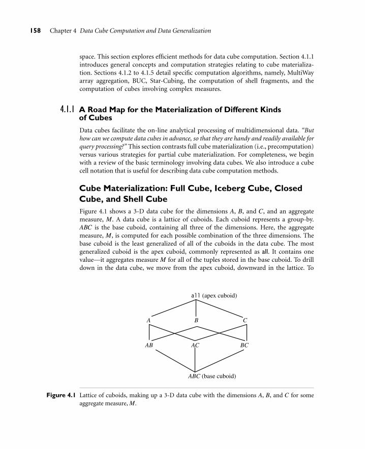
158 Chapter 4 Data Cube Computation and Data Generalization
space. This section explores efficient methods for data cube computation. Section 4.1.1introduces general concepts and computation strategies relating to cube materializa-tion. Sections 4.1.2 to 4.1.5 detail specific computation algorithms, namely, MultiWayarray aggregation, BUC, Star-Cubing, the computation of shell fragments, and thecomputation of cubes involving complex measures.
4.1.1 A Road Map for the Materialization of Different Kindsof Cubes
Data cubes facilitate the on-line analytical processing of multidimensional data. “Buthow can we compute data cubes in advance, so that they are handy and readily available forquery processing?” This section contrasts full cube materialization (i.e., precomputation)versus various strategies for partial cube materialization. For completeness, we beginwith a review of the basic terminology involving data cubes. We also introduce a cubecell notation that is useful for describing data cube computation methods.
Cube Materialization: Full Cube, Iceberg Cube, ClosedCube, and Shell CubeFigure 4.1 shows a 3-D data cube for the dimensions A, B, and C, and an aggregatemeasure, M. A data cube is a lattice of cuboids. Each cuboid represents a group-by.ABC is the base cuboid, containing all three of the dimensions. Here, the aggregatemeasure, M, is computed for each possible combination of the three dimensions. Thebase cuboid is the least generalized of all of the cuboids in the data cube. The mostgeneralized cuboid is the apex cuboid, commonly represented as all. It contains onevalue—it aggregates measure M for all of the tuples stored in the base cuboid. To drilldown in the data cube, we move from the apex cuboid, downward in the lattice. To
Figure 4.1 Lattice of cuboids, making up a 3-D data cube with the dimensions A, B, and C for someaggregate measure, M.

4.1 Efficient Methods for Data Cube Computation 159
roll up, we move from the base cuboid, upward. For the purposes of our discussionin this chapter, we will always use the term data cube to refer to a lattice of cuboidsrather than an individual cuboid.
A cell in the base cuboid is a base cell. A cell from a nonbase cuboid is an aggregatecell. An aggregate cell aggregates over one or more dimensions, where each aggregateddimension is indicated by a “∗” in the cell notation. Suppose we have an n-dimensionaldata cube. Let a = (a1, a2, . . . , an, measures) be a cell from one of the cuboids makingup the data cube. We say that a is an m-dimensional cell (that is, from an m-dimensionalcuboid) if exactly m (m≤ n) values among {a1, a2, . . . , an} are not “∗”. If m = n, then ais a base cell; otherwise, it is an aggregate cell (i.e., where m< n).
Example 4.1 Base and aggregate cells. Consider a data cube with the dimensions month, city, andcustomer group, and the measure price. (Jan, ∗ , ∗ , 2800) and (∗, Toronto, ∗ , 1200)are 1-D cells, (Jan, ∗ , Business, 150) is a 2-D cell, and (Jan, Toronto, Business, 45) is a3-D cell. Here, all base cells are 3-D, whereas 1-D and 2-D cells are aggregate cells.
An ancestor-descendant relationship may exist between cells. In an n-dimensionaldata cube, an i-D cell a = (a1, a2, . . . , an, measuresa) is an ancestor of a j-D cellb = (b1, b2, . . . , bn, measuresb), and b is a descendant of a, if and only if (1) i < j, and(2) for 1≤ m≤ n, am = bm whenever am 6= “∗”. In particular, cell a is called a parent ofcell b, and b is a child of a, if and only if j = i + 1 and b is a descendant of a.
Example 4.2 Ancestor and descendant cells. Referring to our previous example, 1-D cell a = (Jan,∗ , ∗ , 2800), and 2-D cell b = (Jan, ∗ , Business, 150), are ancestors of 3-D cellc = (Jan, Toronto, Business, 45); c is a descendant of both a and b; b is a parentof c, and c is a child of b.
In order to ensure fast on-line analytical processing, it is sometimes desirable to pre-compute the full cube (i.e., all the cells of all of the cuboids for a given data cube). This,however, is exponential to the number of dimensions. That is, a data cube of n dimen-sions contains 2n cuboids. There are even more cuboids if we consider concept hierar-chies for each dimension.1 In addition, the size of each cuboid depends on the cardinalityof its dimensions. Thus, precomputation of the full cube can require huge and oftenexcessive amounts of memory.
Nonetheless, full cube computation algorithms are important. Individual cuboidsmay be stored on secondary storage and accessed when necessary. Alternatively, we canuse such algorithms to compute smaller cubes, consisting of a subset of the given setof dimensions, or a smaller range of possible values for some of the dimensions. Insuch cases, the smaller cube is a full cube for the given subset of dimensions and/ordimension values. A thorough understanding of full cube computation methods will
1Equation (3.1) gives the total number of cuboids in a data cube where each dimension has an associatedconcept hierarchy.
160 Chapter 4 Data Cube Computation and Data Generalization
help us develop efficient methods for computing partial cubes. Hence, it is important toexplore scalable methods for computing all of the cuboids making up a data cube, that is,for full materialization. These methods must take into consideration the limited amountof main memory available for cuboid computation, the total size of the computed datacube, as well as the time required for such computation.
Partial materialization of data cubes offers an interesting trade-off between storagespace and response time for OLAP. Instead of computing the full cube, we can computeonly a subset of the data cube’s cuboids, or subcubes consisting of subsets of cells fromthe various cuboids.
Many cells in a cuboid may actually be of little or no interest to the data analyst.Recall that each cell in a full cube records an aggregate value. Measures such as count,sum, or sales in dollars are commonly used. For many cells in a cuboid, the measurevalue will be zero. When the product of the cardinalities for the dimensions in acuboid is large relative to the number of nonzero-valued tuples that are stored in thecuboid, then we say that the cuboid is sparse. If a cube contains many sparse cuboids,we say that the cube is sparse.
In many cases, a substantial amount of the cube’s space could be taken up by a largenumber of cells with very low measure values. This is because the cube cells are often quitesparsely distributed within a multiple dimensional space. For example, a customer mayonly buy a few items in a store at a time. Such an event will generate only a few nonemptycells, leaving most other cube cells empty. In such situations, it is useful to materializeonly those cells in a cuboid (group-by) whose measure value is above some minimumthreshold. In a data cube for sales, say, we may wish to materialize only those cells forwhich count ≥ 10 (i.e., where at least 10 tuples exist for the cell’s given combination ofdimensions), or only those cells representing sales≥ $100. This not only saves processingtime and disk space, but also leads to a more focused analysis. The cells that cannotpass the threshold are likely to be too trivial to warrant further analysis. Such partiallymaterialized cubes are known as iceberg cubes. The minimum threshold is called theminimum support threshold, or minimum support(min sup), for short. By materializingonly a fraction of the cells in a data cube, the result is seen as the “tip of the iceberg,”where the “iceberg” is the potential full cube including all cells. An iceberg cube can bespecified with an SQL query, as shown in the following example.
Example 4.3 Iceberg cube.
compute cube sales iceberg asselect month, city, customer group, count(*)from salesInfocube by month, city, customer grouphaving count(*)>= min sup
The compute cube statement specifies the precomputation of the iceberg cube,sales iceberg, with the dimensions month, city, and customer group, and the aggregate mea-sure count(). The input tuples are in the salesInfo relation. The cube by clause specifiesthat aggregates (group-by’s) are to be formed for each of the possible subsets of the given
4.1 Efficient Methods for Data Cube Computation 161
dimensions. If we were computing the full cube, each group-by would correspond to acuboid in the data cube lattice. The constraint specified in the having clause is known asthe iceberg condition. Here, the iceberg measure is count. Note that the iceberg cube com-puted for Example 4.3 could be used to answer group-by queries on any combination ofthe specified dimensions of the form having count(*)>= v, where v≥min sup. Insteadof count, the iceberg condition could specify more complex measures, such as average.
If we were to omit the having clause of our example, we would end up with the fullcube. Let’s call this cube sales cube. The iceberg cube, sales iceberg, excludes all the cellsof sales cube whose count is less than min sup. Obviously, if we were to set the minimumsupport to 1 in sales iceberg, the resulting cube would be the full cube, sales cube.
A naïve approach to computing an iceberg cube would be to first compute the fullcube and then prune the cells that do not satisfy the iceberg condition. However, this isstill prohibitively expensive. An efficient approach is to compute only the iceberg cubedirectly without computing the full cube. Sections 4.1.3 and 4.1.4 discuss methods forefficient iceberg cube computation.
Introducing iceberg cubes will lessen the burden of computing trivial aggregate cellsin a data cube. However, we could still end up with a large number of uninteresting cellsto compute. For example, suppose that there are 2 base cells for a database of 100 dimen-sions, denoted as {(a1, a2, a3, . . . , a100) : 10, (a1, a2, b3, . . . , b100) : 10}, where each hasa cell count of 10. If the minimum support is set to 10, there will still be an impermis-sible number of cells to compute and store, although most of them are not interesting.For example, there are 2101−6 distinct aggregate cells,2 like {(a1, a2, a3, a4, . . . , a99, ∗) :10, . . . , (a1, a2, ∗ , a4, . . . , a99, a100) : 10, . . . , (a1, a2, a3, ∗ , . . . , ∗ , ∗) : 10}, but most ofthem do not contain much new information. If we ignore all of the aggregate cells that canbe obtained by replacing some constants by ∗’s while keeping the same measure value,there are only three distinct cells left: {(a1, a2, a3, . . . , a100) : 10, (a1, a2, b3, . . . , b100) :10, (a1, a2, ∗ , . . . , ∗) : 20}. That is, out of 2101−6 distinct aggregate cells, only 3 reallyoffer new information.
To systematically compress a data cube, we need to introduce the concept of closedcoverage. A cell, c, is a closed cell if there exists no cell, d, such that d is a specialization(descendant) of cell c (that is, where d is obtained by replacing a∗ in c with a non-∗ value),and d has the same measure value as c. A closed cube is a data cube consisting of onlyclosed cells. For example, the three cells derived above are the three closed cells of the datacube for the data set:{(a1, a2, a3, . . . , a100) : 10, (a1, a2, b3, . . . , b100) : 10}. They form thelattice of a closed cube as shown in Figure 4.2. Other nonclosed cells can be derived fromtheir corresponding closed cells in this lattice. For example, “(a1, ∗ , ∗ , . . . , ∗) : 20” canbe derived from “(a1, a2, ∗ , . . . , ∗) : 20” because the former is a generalized nonclosedcell of the latter. Similarly, we have “(a1, a2, b3, ∗ , . . . , ∗) : 10”.
Another strategy for partial materialization is to precompute only the cuboidsinvolving a small number of dimensions, such as 3 to 5. These cuboids form a cube
2The proof is left as an exercise for the reader.

162 Chapter 4 Data Cube Computation and Data Generalization
(a1, a2, a3, ..., a100 ) : 10
(a1, a2, *, ..., *) : 20
(a1, a2, b3, ..., b100 ) : 10
Figure 4.2 Three closed cells forming the lattice of a closed cube.
shell for the corresponding data cube. Queries on additional combinations of thedimensions will have to be computed on the fly. For example, we could compute allcuboids with 3 dimensions or less in an n-dimensional data cube, resulting in a cubeshell of size 3. This, however, can still result in a large number of cuboids to compute,particularly when n is large. Alternatively, we can choose to precompute only portionsor fragments of the cube shell, based on cuboids of interest. Section 4.1.5 discusses amethod for computing such shell fragments and explores how they can be used forefficient OLAP query processing.
General Strategies for Cube ComputationWith different kinds of cubes as described above, we can expect that there are a goodnumber of methods for efficient computation. In general, there are two basic data struc-tures used for storing cuboids. Relational tables are used as the basic data structure for theimplementation of relational OLAP (ROLAP), while multidimensional arrays are usedas the basic data structure in multidimensional OLAP (MOLAP). Although ROLAP andMOLAP may each explore different cube computation techniques, some optimization“tricks” can be shared among the different data representations. The following are gen-eral optimization techniques for the efficient computation of data cubes.
Optimization Technique 1: Sorting, hashing, and grouping. Sorting, hashing, andgrouping operations should be applied to the dimension attributes in order to reorderand cluster related tuples.
In cube computation, aggregation is performed on the tuples (or cells) that sharethe same set of dimension values. Thus it is important to explore sorting, hashing, andgrouping operations to access and group such data together to facilitate computation ofsuch aggregates.
For example, to compute total sales by branch, day, and item, it is more efficient tosort tuples or cells by branch, and then by day, and then group them according to theitem name. Efficient implementations of such operations in large data sets have beenextensively studied in the database research community. Such implementations can beextended to data cube computation.
4.1 Efficient Methods for Data Cube Computation 163
This technique can also be further extended to perform shared-sorts (i.e., sharingsorting costs across multiple cuboids when sort-based methods are used), or to performshared-partitions (i.e., sharing the partitioning cost across multiple cuboids when hash-based algorithms are used).
Optimization Technique 2: Simultaneous aggregation and caching intermediate results.In cube computation, it is efficient to compute higher-level aggregates from previouslycomputed lower-level aggregates, rather than from the base fact table. Moreover, simulta-neous aggregation from cached intermediate computation results may lead to the reduc-tion of expensive disk I/O operations.
For example, to compute sales by branch, we can use the intermediate results derivedfrom the computation of a lower-level cuboid, such as sales by branch and day. Thistechnique can be further extended to perform amortized scans (i.e., computing as manycuboids as possible at the same time to amortize disk reads).
Optimization Technique 3: Aggregation from the smallest child, when there existmultiple child cuboids. When there exist multiple child cuboids, it is usually more effi-cient to compute the desired parent (i.e., more generalized) cuboid from the smallest,previously computed child cuboid.
For example, to compute a sales cuboid, Cbranch, when there exist two previously com-puted cuboids, C{branch,year} and C{branch,item}, it is obviously more efficient to computeCbranch from the former than from the latter if there are many more distinct items thandistinct years.
Many other optimization tricks may further improve the computational efficiency.For example, string dimension attributes can be mapped to integers with values rangingfrom zero to the cardinality of the attribute. However, the following optimization tech-nique plays a particularly important role in iceberg cube computation.
Optimization Technique 4: The Apriori pruning method can be explored to computeiceberg cubes efficiently. The Apriori property,3 in the context of data cubes, states asfollows: If a given cell does not satisfy minimum support, then no descendant (i.e., morespecialized or detailed version) of the cell will satisfy minimum support either. This propertycan be used to substantially reduce the computation of iceberg cubes.
Recall that the specification of iceberg cubes contains an iceberg condition, which isa constraint on the cells to be materialized. A common iceberg condition is that the cellsmust satisfy a minimum support threshold, such as a minimum count or sum.In this situation, the Apriori property can be used to prune away the exploration of thedescendants of the cell. For example, if the count of a cell, c, in a cuboid is less thana minimum support threshold, v, then the count of any of c’s descendant cells in thelower-level cuboids can never be greater than or equal to v, and thus can be pruned.In other words, if a condition (e.g., the iceberg condition specified in a having clause)
3The Apriori property was proposed in the Apriori algorithm for association rule mining by R. Agrawaland R. Srikant [AS94]. Many algorithms in association rule mining have adopted this property. Associ-ation rule mining is the topic of Chapter 5.

164 Chapter 4 Data Cube Computation and Data Generalization
is violated for some cell c, then every descendant of c will also violate that condition.Measures that obey this property are known as antimonotonic.4 This form of pruningwas made popular in association rule mining, yet also aids in data cube computationby cutting processing time and disk space requirements. It can lead to a more focusedanalysis because cells that cannot pass the threshold are unlikely to be of interest.
In the following subsections, we introduce several popular methods for efficient cubecomputation that explore some or all of the above optimization strategies. Section 4.1.2describes the multiway array aggregation (MultiWay) method for computing full cubes.The remaining sections describe methods for computing iceberg cubes. Section 4.1.3 des-cribes a method known as BUC, which computes iceberg cubes from the apex cuboid,downward. Section 4.1.4 describes the Star-Cubing method, which integrates top-downand bottom-up computation. Section 4.1.5 describes a minimal cubing approach thatcomputes shell fragments for efficient high-dimensional OLAP. Finally, Section 4.1.6describes a method for computing iceberg cubes with complex measures, such as average.To simplify our discussion, we exclude the cuboids that would be generated by climbingup any existing hierarchies for the dimensions. Such kinds of cubes can be computedby extension of the discussed methods. Methods for the efficient computation of closedcubes are left as an exercise for interested readers.
4.1.2 Multiway Array Aggregation for Full Cube Computation
The Multiway Array Aggregation (or simply MultiWay) method computes a full datacube by using a multidimensional array as its basic data structure. It is a typical MOLAPapproach that uses direct array addressing, where dimension values are accessed via theposition or index of their corresponding array locations. Hence, MultiWay cannot per-form any value-based reordering as an optimization technique. A different approach isdeveloped for the array-based cube construction, as follows:
1. Partition the array into chunks. A chunk is a subcube that is small enough to fit intothe memory available for cube computation. Chunking is a method for dividing ann-dimensional array into small n-dimensional chunks, where each chunk is stored asan object on disk. The chunks are compressed so as to remove wasted space resultingfrom empty array cells (i.e., cells that do not contain any valid data, whose cell countis zero). For instance, “chunkID + offset” can be used as a cell addressing mechanismto compress a sparse array structure and when searching for cells within a chunk.Such a compression technique is powerful enough to handle sparse cubes, both ondisk and in memory.
2. Compute aggregates by visiting (i.e., accessing the values at) cube cells. The order inwhich cells are visited can be optimized so as to minimize the number of times that eachcell must be revisited, thereby reducing memory access and storage costs. The trick is
4Antimonotone is based on condition violation. This differs from monotone, which is based on conditionsatisfaction.

4.1 Efficient Methods for Data Cube Computation 165
to exploit this ordering so that partial aggregates can be computed simultaneously,and any unnecessary revisiting of cells is avoided.
Because this chunking technique involves “overlapping” some of the aggrega-tion computations, it is referred to as multiway array aggregation. It performssimultaneous aggregation—that is, it computes aggregations simultaneously onmultiple dimensions.
We explain this approach to array-based cube construction by looking at a concreteexample.
Example 4.4 Multiway array cube computation. Consider a 3-D data array containing the three dimen-sions A, B, and C. The 3-D array is partitioned into small, memory-based chunks. In thisexample, the array is partitioned into 64 chunks as shown in Figure 4.3. Dimension Ais organized into four equal-sized partitions, a0, a1, a2, and a3. Dimensions B and Care similarly organized into four partitions each. Chunks 1, 2, . . . , 64 correspond to thesubcubes a0b0c0, a1b0c0, . . . , a3b3c3, respectively. Suppose that the cardinality of thedimensions A, B, and C is 40, 400, and 4000, respectively. Thus, the size of the array foreach dimension, A, B, and C, is also 40, 400, and 4000, respectively. The size of each par-tition in A, B, and C is therefore 10, 100, and 1000, respectively. Full materialization ofthe corresponding data cube involves the computation of all of the cuboids defining thiscube. The resulting full cube consists of the following cuboids:
The base cuboid, denoted by ABC (from which all of the other cuboids are directlyor indirectly computed). This cube is already computed and corresponds to the given3-D array.
The 2-D cuboids, AB, AC, and BC, which respectively correspond to the group-by’sAB, AC, and BC. These cuboids must be computed.
The 1-D cuboids, A, B, and C, which respectively correspond to the group-by’s A, B,and C. These cuboids must be computed.
The 0-D (apex) cuboid, denoted by all, which corresponds to the group-by (); that is,there is no group-by here. This cuboid must be computed. It consists of one value. If,say, the data cube measure is count, then the value to be computed is simply the totalcount of all of the tuples in ABC.
Let’s look at how the multiway array aggregation technique is used in this computa-tion. There are many possible orderings with which chunks can be read into memoryfor use in cube computation. Consider the ordering labeled from 1 to 64, shown inFigure 4.3. Suppose we would like to compute the b0c0 chunk of the BC cuboid. Weallocate space for this chunk in chunk memory. By scanning chunks 1 to 4 of ABC,the b0c0 chunk is computed. That is, the cells for b0c0 are aggregated over a0 to a3.The chunk memory can then be assigned to the next chunk, b1c0, which completesits aggregation after the scanning of the next four chunks of ABC: 5 to 8. Continuing

166 Chapter 4 Data Cube Computation and Data Generalization
b3
b2
b1
b0
B
C
c3
c2
c1
61
45
29
62
46
30
63
47
31
64
48
32
c0
a0 a1
A
a2 a3
1
5
9
13 14 15 16
2 3 4
28
44
60
24
40
56
20
36
52
Figure 4.3 A 3-D array for the dimensions A, B, and C, organized into 64 chunks. Each chunk is smallenough to fit into the memory available for cube computation.
in this way, the entire BC cuboid can be computed. Therefore, only one chunk of BCneeds to be in memory, at a time, for the computation of all of the chunks of BC.
In computing the BC cuboid, we will have scanned each of the 64 chunks. “Is therea way to avoid having to rescan all of these chunks for the computation of other cuboids,such as AC and AB?” The answer is, most definitely—yes. This is where the “multiwaycomputation” or “simultaneous aggregation” idea comes in. For example, when chunk 1(i.e., a0b0c0) is being scanned (say, for the computation of the 2-D chunk b0c0 of BC, asdescribed above), all of the other 2-D chunks relating to a0b0c0 can be simultaneouslycomputed. That is, when a0b0c0 is being scanned, each of the three chunks, b0c0, a0c0,and a0b0, on the three 2-D aggregation planes, BC, AC, and AB, should be computedthen as well. In other words, multiway computation simultaneously aggregates to eachof the 2-D planes while a 3-D chunk is in memory.

4.1 Efficient Methods for Data Cube Computation 167
Now let’s look at how different orderings of chunk scanning and of cuboid compu-tation can affect the overall data cube computation efficiency. Recall that the size of thedimensions A, B, and C is 40, 400, and 4000, respectively. Therefore, the largest 2-D planeis BC (of size 400× 4000 = 1, 600, 000). The second largest 2-D plane is AC (of size40×4000 = 160, 000). AB is the smallest 2-D plane (with a size of 40×400 = 16, 000).
Suppose that the chunks are scanned in the order shown, from chunk 1 to 64. Byscanning in this order, one chunk of the largest 2-D plane, BC, is fully computed foreach row scanned. That is, b0c0 is fully aggregated after scanning the row containingchunks 1 to 4; b1c0 is fully aggregated after scanning chunks 5 to 8, and so on.In comparison, the complete computation of one chunk of the second largest 2-Dplane, AC, requires scanning 13 chunks, given the ordering from 1 to 64. That is,a0c0 is fully aggregated only after the scanning of chunks 1, 5, 9, and 13. Finally,the complete computation of one chunk of the smallest 2-D plane, AB, requiresscanning 49 chunks. For example, a0b0 is fully aggregated after scanning chunks 1,17, 33, and 49. Hence, AB requires the longest scan of chunks in order to completeits computation. To avoid bringing a 3-D chunk into memory more than once, theminimum memory requirement for holding all relevant 2-D planes in chunk memory,according to the chunk ordering of 1 to 64, is as follows: 40× 400 (for the wholeAB plane) + 40×1000 (for one row of the AC plane) + 100×1000 (for one chunkof the BC plane) = 16,000 + 40,000 + 100,000 = 156,000 memory units.
Suppose, instead, that the chunks are scanned in the order 1, 17, 33, 49, 5, 21, 37,53, and so on. That is, suppose the scan is in the order of first aggregating toward theAB plane, and then toward the AC plane, and lastly toward the BC plane. The minimummemory requirement for holding 2-D planes in chunk memory would be as follows:400×4000 (for the whole BC plane) + 40×1000 (for one row of the AC plane) + 10×100 (for one chunk of the AB plane) = 1,600,000 + 40,000 + 1000 = 1,641,000 memoryunits. Notice that this is more than 10 times the memory requirement of the scan orderingof 1 to 64.
Similarly, we can work out the minimum memory requirements for the multiwaycomputation of the 1-D and 0-D cuboids. Figure 4.4 shows the most efficient orderingand the least efficient ordering, based on the minimum memory requirements for thedata cube computation. The most efficient ordering is the chunk ordering of 1 to 64.
Example 4.4 assumes that there is enough memory space for one-pass cube compu-tation (i.e., to compute all of the cuboids from one scan of all of the chunks). If thereis insufficient memory space, the computation will require more than one pass throughthe 3-D array. In such cases, however, the basic principle of ordered chunk computa-tion remains the same. MultiWay is most effective when the product of the cardinalitiesof dimensions is moderate and the data are not too sparse. When the dimensionality ishigh or the data are very sparse, the in-memory arrays become too large to fit in memory,and this method becomes infeasible.
With the use of appropriate sparse array compression techniques and careful orderingof the computation of cuboids, it has been shown by experiments that MultiWay arraycube computation is significantly faster than traditional ROLAP (relationa record-based)

168 Chapter 4 Data Cube Computation and Data Generalization
A
AB AC AB
ABC ABC
AC
AB
BC BC
C B C
all all
Figure 4.4 Two orderings of multiway array aggregation for computation of the 3-D cube of Example 4.4:(a) most efficient ordering of array aggregation (minimum memory requirements = 156,000memory units); (b) least efficient ordering of array aggregation (minimum memory require-ments = 1,641,000 memory units).
computation. Unlike ROLAP, the array structure of MultiWay does not require savingspace to store search keys. Furthermore, MultiWay uses direct array addressing, which isfaster than the key-based addressing search strategy of ROLAP. For ROLAP cube compu-tation, instead of cubing a table directly, it can be faster to convert the table to an array, cubethe array, and then convert the result back to a table. However, this observation works onlyfor cubes with a relatively small number of dimensions because the number of cuboids tobe computed is exponential to the number of dimensions.
“What would happen if we tried to use MultiWay to compute iceberg cubes?” Rememberthat the Apriori property states that if a given cell does not satisfy minimum support, thenneither will any of its descendants. Unfortunately, MultiWay’s computation starts fromthe base cuboid and progresses upward toward more generalized, ancestor cuboids. Itcannot take advantage of Apriori pruning, which requires a parent node to be computedbefore its child (i.e., more specific) nodes. For example, if the count of a cell c in, say,AB, does not satisfy the minimum support specified in the iceberg condition, then wecannot prune away computation of c’s ancestors in the A or B cuboids, because the countof these cells may be greater than that of c.
4.1.3 BUC: Computing Iceberg Cubes from the Apex CuboidDownward
BUC is an algorithm for the computation of sparse and iceberg cubes. Unlike MultiWay,BUC constructs the cube from the apex cuboid toward the base cuboid. This allows BUC

4.1 Efficient Methods for Data Cube Computation 169
to share data partitioning costs. This order of processing also allows BUC to prune duringconstruction, using the Apriori property.
Figure 4.1 shows a lattice of cuboids, making up a 3-D data cube with the dimensionsA, B, and C. The apex (0-D) cuboid, representing the concept all (that is, (∗, ∗ , ∗)), isat the top of the lattice. This is the most aggregated or generalized level. The 3-D basecuboid, ABC, is at the bottom of the lattice. It is the least aggregated (most detailed orspecialized) level. This representation of a lattice of cuboids, with the apex at the top andthe base at the bottom, is commonly accepted in data warehousing. It consolidates thenotions of drill-down (where we can move from a highly aggregated cell to lower, moredetailed cells) and roll-up (where we can move from detailed, low-level cells to higher-level, more aggregated cells).
BUC stands for “Bottom-Up Construction.” However, according to the lattice con-vention described above and used throughout this book, the order of processing of BUCis actually top-down! The authors of BUC view a lattice of cuboids in the reverse order,with the apex cuboid at the bottom and the base cuboid at the top. In that view, BUCdoes bottom-up construction. However, because we adopt the application worldviewwhere drill-down refers to drilling from the apex cuboid down toward the base cuboid,the exploration process of BUC is regarded as top-down. BUC’s exploration for thecomputation of a 3-D data cube is shown in Figure 4.5.
The BUC algorithm is shown in Figure 4.6. We first give an explanation of thealgorithm and then follow up with an example. Initially, the algorithm is called withthe input relation (set of tuples). BUC aggregates the entire input (line 1) and writes
all
AB
ABC
AC BC
BA C
Figure 4.5 BUC’s exploration for the computation of a 3-D data cube. Note that the computation startsfrom the apex cuboid.

170 Chapter 4 Data Cube Computation and Data Generalization
Algorithm: BUC. Algorithm for the computation of sparse and iceberg cubes.
Input:
input: the relation to aggregate;
dim: the starting dimension for this iteration.
Globals:
constant numDims: the total number of dimensions;
constant cardinality[numDims]: the cardinality of each dimension;
constant min sup: the minimum number of tuples in a partition in order for it to be output;
outputRec: the current output record;
dataCount[numDims]: stores the size of each partition. dataCount[i] is a list of integers of sizecardinality[i].
Output: Recursively output the iceberg cube cells satisfying the minimum support.
Method:
(1) Aggregate(input); // Scan input to compute measure, e.g., count. Place result in outputRec.(2) if input.count() == 1 then // Optimization
WriteAncestors(input[0], dim); return;endif
(3) write outputRec;(4) for (d = dim; d < numDims; d ++) do //Partition each dimension(5) C = cardinality[d];(6) Partition(input, d, C, dataCount[d]); //create C partitions of data for dimension d(7) k = 0;(8) for (i = 0; i<C; i ++) do // for each partition (each value of dimension d)(9) c = dataCount[d][i];(10) if c>= min sup then // test the iceberg condition(11) outputRec.dim[d] = input[k].dim[d];(12) BUC(input[k . . .k + c], d + 1); // aggregate on next dimension(13) endif(14) k +=c;(15) endfor(16) outputRec.dim[d] = all;(17) endfor
Figure 4.6 BUC algorithm for the computation of sparse or iceberg cubes [BR99].
the resulting total (line 3). (Line 2 is an optimization feature that is discussed later in ourexample.) For each dimension d (line 4), the input is partitioned on d (line 6). On returnfrom Partition(), dataCount contains the total number of tuples for each distinct valueof dimension d. Each distinct value of d forms its own partition. Line 8 iterates througheach partition. Line 10 tests the partition for minimum support. That is, if the numberof tuples in the partition satisfies (i.e., is ≥) the minimum support, then the partitionbecomes the input relation for a recursive call made to BUC, which computes the ice-berg cube on the partitions for dimensions d + 1 to numDims (line 12). Note that for afull cube (i.e., where minimum support in the having clause is 1), the minimum support

4.1 Efficient Methods for Data Cube Computation 171
condition is always satisfied. Thus, the recursive call descends one level deeper into thelattice. Upon return from the recursive call, we continue with the next partition for d.After all the partitions have been processed, the entire process is repeated for each of theremaining dimensions.
We explain how BUC works with the following example.
Example 4.5 BUC construction of an iceberg cube. Consider the iceberg cube expressed in SQL asfollows:
compute cube iceberg cube asselect A, B, C, D, count(*)from R
cube by A, B, C, D
having count(*)>= 3
Let’s see how BUC constructs the iceberg cube for the dimensions A, B, C, and D,where the minimum support count is 3. Suppose that dimension A has four distinctvalues, a1, a2, a3, a4; B has four distinct values, b1, b2, b3, b4; C has two distinct values,c1, c2; and D has two distinct values, d1, d2. If we consider each group-by to be a par-tition, then we must compute every combination of the grouping attributes that satisfyminimum support (i.e., that have 3 tuples).
Figure 4.7 illustrates how the input is partitioned first according to the different attri-bute values of dimension A, and then B, C, and D. To do so, BUC scans the input,aggregating the tuples to obtain a count for all, corresponding to the cell (∗, ∗ , ∗ , ∗).Dimension A is used to split the input into four partitions, one for each distinct value ofA. The number of tuples (counts) for each distinct value of A is recorded in dataCount.
BUC uses the Apriori property to save time while searching for tuples that satisfythe iceberg condition. Starting with A dimension value, a1, the a1 partition is aggre-gated, creating one tuple for the A group-by, corresponding to the cell (a1, ∗ , ∗ , ∗).Suppose (a1, ∗ , ∗ , ∗) satisfies the minimum support, in which case a recursive call ismade on the partition for a1. BUC partitions a1 on the dimension B. It checks the countof (a1, b1, ∗ , ∗) to see if it satisfies the minimum support. If it does, it outputs the aggre-gated tuple to the AB group-by and recurses on (a1, b1, ∗ , ∗) to partition on C, startingwith c1. Suppose the cell count for (a1, b1, c1, ∗) is 2, which does not satisfy the min-imum support. According to the Apriori property, if a cell does not satisfy minimumsupport, then neither can any of its descendants. Therefore, BUC prunes any furtherexploration of (a1, b1, c1, ∗). That is, it avoids partitioning this cell on dimension D. Itbacktracks to the a1, b1 partition and recurses on (a1, b1, c2, ∗), and so on. By checkingthe iceberg condition each time before performing a recursive call, BUC saves a greatdeal of processing time whenever a cell’s count does not satisfy the minimum support.
The partition process is facilitated by a linear sorting method, CountingSort. Count-ingSort is fast because it does not perform any key comparisons to find partition bound-aries. In addition, the counts computed during the sort can be reused to compute thegroup-by’s in BUC. Line 2 is an optimization for partitions having a count of 1, such as
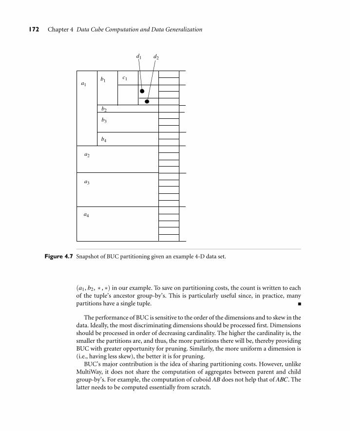
172 Chapter 4 Data Cube Computation and Data Generalization
a4
a3
a2
a1
b4
b3
b2
b1
d2d1
c1
Figure 4.7 Snapshot of BUC partitioning given an example 4-D data set.
(a1, b2, ∗ , ∗) in our example. To save on partitioning costs, the count is written to eachof the tuple’s ancestor group-by’s. This is particularly useful since, in practice, manypartitions have a single tuple.
The performance of BUC is sensitive to the order of the dimensions and to skew in thedata. Ideally, the most discriminating dimensions should be processed first. Dimensionsshould be processed in order of decreasing cardinality. The higher the cardinality is, thesmaller the partitions are, and thus, the more partitions there will be, thereby providingBUC with greater opportunity for pruning. Similarly, the more uniform a dimension is(i.e., having less skew), the better it is for pruning.
BUC’s major contribution is the idea of sharing partitioning costs. However, unlikeMultiWay, it does not share the computation of aggregates between parent and childgroup-by’s. For example, the computation of cuboid AB does not help that of ABC. Thelatter needs to be computed essentially from scratch.

4.1 Efficient Methods for Data Cube Computation 173
4.1.4 Star-Cubing: Computing Iceberg Cubes Usinga Dynamic Star-tree Structure
In this section, we describe the Star-Cubing algorithm for computing iceberg cubes.Star-Cubing combines the strengths of the other methods we have studied up to thispoint. It integrates top-down and bottom-up cube computation and explores both mul-tidimensional aggregation (similar to MultiWay) and Apriori-like pruning (similar toBUC). It operates from a data structure called a star-tree, which performs lossless datacompression, thereby reducing the computation time and memory requirements.
The Star-Cubing algorithm explores both the bottom-up and top-down computa-tion models as follows: On the global computation order, it uses the bottom-up model.However, it has a sublayer underneath based on the top-down model, which exploresthe notion of shared dimensions, as we shall see below. This integration allows the algo-rithm to aggregate on multiple dimensions while still partitioning parent group-by’s andpruning child group-by’s that do not satisfy the iceberg condition.
Star-Cubing’s approach is illustrated in Figure 4.8 for the computation of a 4-Ddata cube. If we were to follow only the bottom-up model (similar to Multiway), thenthe cuboids marked as pruned by Star-Cubing would still be explored. Star-Cubing isable to prune the indicated cuboids because it considers shared dimensions. ACD/Ameans cuboid ACD has shared dimension A, ABD/AB means cuboid ABD has shareddimension AB, ABC/ABC means cuboid ABC has shared dimension ABC, and soon. This comes from the generalization that all the cuboids in the subtree rootedat ACD include dimension A, all those rooted at ABD include dimensions AB, andall those rooted at ABC include dimensions ABC (even though there is only onesuch cuboid). We call these common dimensions the shared dimensions of thoseparticular subtrees.
Figure 4.8 Star-Cubing: Bottom-up computation with top-down expansion of shared dimensions.

174 Chapter 4 Data Cube Computation and Data Generalization
The introduction of shared dimensions facilitates shared computation. Becausethe shared dimensions are identified early on in the tree expansion, we can avoidrecomputing them later. For example, cuboid AB extending from ABD in Figure 4.8would actually be pruned because AB was already computed in ABD/AB. Similarly,cuboid A extending from AD would also be pruned because it was already computedin ACD/A.
Shared dimensions allow us to do Apriori-like pruning if the measure of an ice-berg cube, such as count, is antimonotonic; that is, if the aggregate value on a shareddimension does not satisfy the iceberg condition, then all of the cells descending fromthis shared dimension cannot satisfy the iceberg condition either. Such cells and all oftheir descendants can be pruned, because these descendant cells are, by definition,more specialized (i.e., contain more dimensions) than those in the shared dimen-sion(s). The number of tuples covered by the descendant cells will be less than orequal to the number of tuples covered by the shared dimensions. Therefore, if theaggregate value on a shared dimension fails the iceberg condition, the descendantcells cannot satisfy it either.
Example 4.6 Pruning shared dimensions. If the value in the shared dimension A is a1 and it failsto satisfy the iceberg condition, then the whole subtree rooted at a1CD/a1 (includinga1C/a1C, a1D/a1, a1/a1) can be pruned because they are all more specialized versionsof a1.
To explain how the Star-Cubing algorithm works, we need to explain a few moreconcepts, namely, cuboid trees, star-nodes, and star-trees.
We use trees to represent individual cuboids. Figure 4.9 shows a fragment of thecuboid tree of the base cuboid, ABCD. Each level in the tree represents a dimension, andeach node represents an attribute value. Each node has four fields: the attribute value,aggregate value, pointer(s) to possible descendant(s), and pointer to possible sibling.Tuples in the cuboid are inserted one by one into the tree. A path from the root to a leaf
a1: 30 a2: 20 a3: 20 a4: 20
b1: 10 b2: 10 b3: 10
c1: 5 c2: 5
d2: 3d1: 2
Figure 4.9 A fragment of the base cuboid tree.

4.1 Efficient Methods for Data Cube Computation 175
node represents a tuple. For example, node c2 in the tree has an aggregate (count) valueof 5, which indicates that there are five cells of value (a1, b1, c2, ∗). This representationcollapses the common prefixes to save memory usage and allows us to aggregate the val-ues at internal nodes. With aggregate values at internal nodes, we can prune based onshared dimensions. For example, the cuboid tree of AB can be used to prune possiblecells in ABD.
If the single dimensional aggregate on an attribute value p does not satisfy the icebergcondition, it is useless to distinguish such nodes in the iceberg cube computation. Thusthe node p can be replaced by ∗ so that the cuboid tree can be further compressed. Wesay that the node p in an attribute A is a star-node if the single dimensional aggregate onp does not satisfy the iceberg condition; otherwise, p is a non-star-node. A cuboid treethat is compressed using star-nodes is called a star-tree.
The following is an example of star-tree construction.
Example 4.7 Star-tree construction. A base cuboid table is shown in Table 4.1. There are 5 tuplesand 4 dimensions. The cardinalities for dimensions A, B, C, D are 2, 4, 4, 4,respectively. The one-dimensional aggregates for all attributes are shown in Table 4.2.Suppose min sup = 2 in the iceberg condition. Clearly, only attribute values a1, a2,b1, c3, d4 satisfy the condition. All the other values are below the threshold and thusbecome star-nodes. By collapsing star-nodes, the reduced base table is Table 4.3.Notice that the table contains two fewer rows and also fewer distinct values thanTable 4.1.
We use the reduced base table to construct the cuboid tree because it is smaller. Theresultant star-tree is shown in Figure 4.10. To help identify which nodes are star-nodes, a
Table 4.1 Base (Cuboid) Table: Before star reduction.
A B C D count
a1 b1 c1 d1 1
a1 b1 c4 d3 1
a1 b2 c2 d2 1
a2 b3 c3 d4 1
a2 b4 c3 d4 1
Table 4.2 One-Dimensional Aggregates.
Dimension count = 1 count ≥ 2
A — a1(3), a2(2)
B b2, b3, b4 b1(2)
C c1, c2, c4 c3(2)
D d1, d2, d3 d4(2)

176 Chapter 4 Data Cube Computation and Data Generalization
Table 4.3 Compressed Base Table: After star reduction.
A B C D count
a1 b1 ∗ ∗ 2
a1 ∗ ∗ ∗ 1
a2 ∗ c3 d4 2
a1:3
root:5
a2:2
b*:2
c3:2
d4:2
b*:1 b1:2
c*:1
d*:1
c*:2
d*:2
Star Table
b3
b2
b4
c1
c2
d1
...
*
*
*
*
*
c4 *
*
Figure 4.10 Star-tree and star-table.
star-table is constructed for each star-tree. Figure 4.10 also shows the corresponding star-table for the star-tree (where only the star-nodes are shown in the star-table). In actualimplementation, a bit-vector or hash table could be used to represent the star-table forfast lookup.
By collapsing star-nodes, the star-tree provides a lossless compression of the originaldata. It provides a good improvement in memory usage, yet the time required to searchfor nodes or tuples in the tree is costly. To reduce this cost, the nodes in the star-treeare sorted in alphabetic order for each dimension, with the star-nodes appearing first. Ingeneral, nodes are sorted in the order ∗, p1, p2, . . . , pn at each level.
Now, let’s see how the Star-Cubing algorithm uses star-trees to compute an icebergcube. The algorithm is given in Figure 4.13.
Example 4.8 Star-Cubing. Using the star-tree generated in Example 4.7 (Figure 4.10), we start theprocess of aggregation by traversing in a bottom-up fashion. Traversal is depth-first. Thefirst stage (i.e., the processing of the first branch of the tree) is shown in Figure 4.11.The leftmost tree in the figure is the base star-tree. Each attribute value is shown with itscorresponding aggregate value. In addition, subscripts by the nodes in the tree show the

4.1 Efficient Methods for Data Cube Computation 177
a1:32
b*:13 b1:2
c*:14
d*:15
c*:2
d*:2
b*:13
c*:14
BCD:11root:51
a2:2
b*:2
c3:2
d4:2
d*:15
a1CD/a1:1 a1b*D/a1b*:13
d*:15
a1b*c*/a1b*c*:14
Base–Tree BCD–Tree ACD/A–Tree ADB/AB–Tree ABC/ABC–Tree
c*:14
d*:15
Figure 4.11 Aggregation Stage One: Processing of the left-most branch of BaseTree.
order of traversal. The remaining four trees are BCD, ACD/A, ABD/AB, ABC/ABC. Theyare the child trees of the base star-tree, and correspond to the level of three-dimensionalcuboids above the base cuboid in Figure 4.8. The subscripts in them correspond to thesame subscripts in the base tree—they denote the step or order in which they are createdduring the tree traversal. For example, when the algorithm is at step 1, the BCD child treeroot is created. At step 2, the ACD/A child tree root is created. At step 3, the ABD/ABtree root and the b∗ node in BCD are created.
When the algorithm has reached step 5, the trees in memory are exactly as shown inFigure 4.11. Because the depth-first traversal has reached a leaf at this point, it starts back-tracking. Before traversing back, the algorithm notices that all possible nodes in the basedimension (ABC) have been visited. This means the ABC/ABC tree is complete, so thecount is output and the tree is destroyed. Similarly, upon moving back from d∗ to c∗ andseeing that c∗has no siblings, the count in ABD/AB is also output and the tree is destroyed.
When the algorithm is at b∗ during the back-traversal, it notices that there exists asibling in b1. Therefore, it will keep ACD/A in memory and perform a depth-first searchon b1 just as it did on b∗. This traversal and the resultant trees are shown in Figure 4.12.The child trees ACD/A and ABD/AB are created again but now with the new values fromthe b1 subtree. For example, notice that the aggregate count of c∗ in the ACD/A tree hasincreased from 1 to 3. The trees that remained intact during the last traversal are reusedand the new aggregate values are added on. For instance, another branch is added to theBCD tree.
Just like before, the algorithm will reach a leaf node at d∗ and traverse back. Thistime, it will reach a1 and notice that there exists a sibling in a2. In this case, all childtrees except BCD in Figure 4.12 are destroyed. Afterward, the algorithm will perform thesame traversal on a2. BCD continues to grow while the other subtrees start fresh with a2instead of a1.
A node must satisfy two conditions in order to generate child trees: (1) the measureof the node must satisfy the iceberg condition; and (2) the tree to be generated must

178 Chapter 4 Data Cube Computation and Data Generalization
Figure 4.12 Aggregation Stage Two: Processing of the second branch of BaseTree.
include at least one non-star (i.e., nontrivial) node. This is because if all the nodes werestar-nodes, then none of them would satisfy min sup. Therefore, it would be a completewaste to compute them. This pruning is observed in Figures 4.11 and 4.12. For example,the left subtree extending from node a1 in the base-tree in Figure 4.11 does not includeany non-star-nodes. Therefore, the a1CD/a1 subtree should not have been generated. Itis shown, however, for illustration of the child tree generation process.
Star-Cubing is sensitive to the ordering of dimensions, as with other iceberg cubeconstruction algorithms. For best performance, the dimensions are processed in order ofdecreasing cardinality. This leads to a better chance of early pruning, because the higherthe cardinality, the smaller the partitions, and therefore the higher possibility that thepartition will be pruned.
Star-Cubing can also be used for full cube computation. When computing the fullcube for a dense data set, Star-Cubing’s performance is comparable with MultiWay andis much faster than BUC. If the data set is sparse, Star-Cubing is significantly fasterthan MultiWay and faster than BUC, in most cases. For iceberg cube computation, Star-Cubing is faster than BUC, where the data are skewed and the speedup factor increasesas min sup decreases.
4.1.5 Precomputing Shell Fragments for Fast High-DimensionalOLAP
Recall the reason that we are interested in precomputing data cubes: Data cubes facili-tate fast on-line analytical processing (OLAP) in a multidimensional data space. How-ever, a full data cube of high dimensionality needs massive storage space and unrealisticcomputation time. Iceberg cubes provide a more feasible alternative, as we have seen,wherein the iceberg condition is used to specify the computation of only a subset of thefull cube’s cells. However, although an iceberg cube is smaller and requires less com-putation time than its corresponding full cube, it is not an ultimate solution. For one,the computation and storage of the iceberg cube can still be costly. For example, if the

4.1 Efficient Methods for Data Cube Computation 179
Algorithm: Star-Cubing. Compute iceberg cubes by Star-Cubing.
Input:
R: a relational table
min support: minimum support threshold for the iceberg condition (taking count as the measure).
Output: The computed iceberg cube.
Method: Each star-tree corresponds to one cuboid tree node, and vice versa.
BEGINscan R twice, create star-table S and star-tree T ;output count of T.root;call starcubing(T, T.root);
END
procedure starcubing(T, cnode)// cnode: current node{(1) for each non-null child C of T ’s cuboid tree(2) insert or aggregate cnode to the corresponding
position or node in C’s star-tree;(3) if (cnode.count≥min support) then {(4) if (cnode 6= root) then(5) output cnode.count;(6) if (cnode is a leaf) then(7) output cnode.count;(8) else { // initiate a new cuboid tree(9) create CC as a child of T ’s cuboid tree;(10) let TC be CC ’s star-tree;(11) TC.root ′s count = cnode.count;(12) }(13) }(14) if (cnode is not a leaf) then(15) starcubing(T, cnode.first child);(16) if (CC is not null) then {(17) starcubing(TC,TC.root);(18) remove CC from T ’s cuboid tree; }(19) if (cnode has sibling) then(20) starcubing(T, cnode.sibling);(21) remove T ;}
Figure 4.13 The Star-Cubing algorithm.
base cuboid cell, (a1, a2, . . . , a60), passes minimum support (or the iceberg threshold),it will generate 260 iceberg cube cells. Second, it is difficult to determine an appropriateiceberg threshold. Setting the threshold too low will result in a huge cube, whereas set-ting the threshold too high may invalidate many useful applications. Third, an icebergcube cannot be incrementally updated. Once an aggregate cell falls below the icebergthreshold and is pruned, its measure value is lost. Any incremental update would requirerecomputing the cells from scratch. This is extremely undesirable for large real-life appli-cations where incremental appending of new data is the norm.

180 Chapter 4 Data Cube Computation and Data Generalization
One possible solution, which has been implemented in some commercial datawarehouse systems, is to compute a thin cube shell. For example, we could computeall cuboids with three dimensions or less in a 60-dimensional data cube, resulting incube shell of size 3. The resulting set of cuboids would require much less computationand storage than the full 60-dimensional data cube. However, there are two disadvan-tages of this approach. First, we would still need to compute
(603
)
+(60
2
)
+60 = 36,050cuboids, each with many cells. Second, such a cube shell does not support high-dimensional OLAP because (1) it does not support OLAP on four or more dimen-sions, and (2) it cannot even support drilling along three dimensions, such as, say,(A4, A5, A6), on a subset of data selected based on the constants provided in threeother dimensions, such as (A1, A2, A3). This requires the computation of the corre-sponding six-dimensional cuboid.
Instead of computing a cube shell, we can compute only portions or fragments of it.This section discusses the shell fragment approach for OLAP query processing. It is basedon the following key observation about OLAP in high-dimensional space. Although adata cube may contain many dimensions, most OLAP operations are performed on onlya small number of dimensions at a time. In other words, an OLAP query is likely toignore many dimensions (i.e., treating them as irrelevant), fix some dimensions (e.g.,using query constants as instantiations), and leave only a few to be manipulated (fordrilling, pivoting, etc.). This is because it is neither realistic nor fruitful for anyone tocomprehend the changes of thousands of cells involving tens of dimensions simultane-ously in a high-dimensional space at the same time. Instead, it is more natural to firstlocate some cuboids of interest and then drill along one or two dimensions to examinethe changes of a few related dimensions. Most analysts will only need to examine, at anyone moment, the combinations of a small number of dimensions. This implies that ifmultidimensional aggregates can be computed quickly on a small number of dimensionsinside a high-dimensional space, we may still achieve fast OLAP without materializing theoriginal high-dimensional data cube. Computing the full cube (or, often, even an icebergcube or shell cube) can be excessive. Instead, a semi-on-line computation model with cer-tain preprocessing may offer a more feasible solution. Given a base cuboid, some quickpreparation computation can be done first (i.e., off-line). After that, a query can then becomputed on-line using the preprocessed data.
The shell fragment approach follows such a semi-on-line computation strategy. Itinvolves two algorithms: one for computing shell fragment cubes and one for query pro-cessing with the fragment cubes. The shell fragment approach can handle databases ofextremely high dimensionality and can quickly compute small local cubes on-line. Itexplores the inverted index data structure, which is popular in information retrieval andWeb-based information systems. The basic idea is as follows. Given a high-dimensionaldata set, we partition the dimensions into a set of disjoint dimension fragments, converteach fragment into its corresponding inverted index representation, and then constructshell fragment cubes while keeping the inverted indices associated with the cube cells.Using the precomputed shell fragment cubes, we can dynamically assemble and computecuboid cells of the required data cube on-line. This is made efficient by set intersectionoperations on the inverted indices.

4.1 Efficient Methods for Data Cube Computation 181
To illustrate the shell fragment approach, we use the tiny database of Table 4.4as a running example. Let the cube measure be count(). Other measures will bediscussed later. We first look at how to construct the inverted index for the givendatabase.
Example 4.9 Construct the inverted index. For each attribute value in each dimension, list the tupleidentifiers (TIDs) of all the tuples that have that value. For example, attribute value a2appears in tuples 4 and 5. The TIDlist for a2 then contains exactly two items, namely4 and 5. The resulting inverted index table is shown in Table 4.5. It retains all of theinformation of the original database. It uses exactly the same amount of memory as theoriginal database.
“How do we compute shell fragments of a data cube?” The shell fragment compu-tation algorithm, Frag-Shells, is summarized in Figure 4.14. We first partition all thedimensions of the given data set into independent groups of dimensions, called frag-ments (line 1). We scan the base cuboid and construct an inverted index for each attribute(lines 2 to 6). Line 3 is for when the measure is other than the tuple count(), which will
Table 4.4 The original database.
TID A B C D E
1 a1 b1 c1 d1 e1
2 a1 b2 c1 d2 e1
3 a1 b2 c1 d1 e2
4 a2 b1 c1 d1 e2
5 a2 b1 c1 d1 e3
Table 4.5 The inverted index.
Attribute Value Tuple ID List List Size
a1 {1, 2, 3} 3
a2 {4, 5} 2
b1 {1, 4, 5} 3
b2 {2, 3} 2
c1 {1, 2, 3, 4, 5} 5
d1 {1, 3, 4, 5} 4
d2 {2} 1
e1 {1, 2} 2
e2 {3, 4} 2
e3 {5} 1

182 Chapter 4 Data Cube Computation and Data Generalization
Algorithm: Frag-Shells. Compute shell fragments on a given high-dimensional base table (i.e., base cuboid).
Input: A base cuboid, B, of n dimensions, namely, (A1, . . . ,An).
Output:
a set of fragment partitions, {P1, . . .Pk}, and their corresponding (local) fragment cubes, {S1, . . . , Sk},where Pi represents some set of dimension(s) and P1 ∪ . . .∪Pk make up all the n dimensions
an ID measure array if the measure is not the tuple count, count()
Method:
(1) partition the set of dimensions (A1, . . . , An) intoa set of k fragments P1, . . . , Pk (based on data & query distribution)
(2) scan base cuboid, B, once and do the following {(3) insert each 〈TID, measure〉 into ID measure array(4) for each attribute value a j of each dimension Ai(5) build an inverted index entry: 〈a j , TIDlist〉(6) }(7) for each fragment partition Pi(8) build a local fragment cube, Si, by intersecting their
corresponding TIDlists and computing their measures
Figure 4.14 Algorithm for shell fragment computation.
be described later. For each fragment, we compute the full local (i.e., fragment-based)data cube while retaining the inverted indices (lines 7 to 8). Consider a database of60 dimensions, namely, A1, A2, . . . , A60. We can first partition the 60 dimensions into 20fragments of size 3: (A1, A2, A3), (A4, A5, A6), . . ., (A58, A59, A60). For each fragment, wecompute its full data cube while recording the inverted indices. For example, in fragment(A1, A2, A3), we would compute seven cuboids: A1, A2, A3, A1A2, A2A3, A1A3, A1A2A3.Furthermore, an inverted index is retained for each cell in the cuboids. That is, for eachcell, its associated TIDlist is recorded.
The benefit of computing local cubes of each shell fragment instead of computingthe complete cube shell can be seen by a simple calculation. For a base cuboid of 60dimensions, there are only 7×20 = 140 cuboids to be computed according to the aboveshell fragment partitioning. This is in contrast to the 36,050 cuboids computed for thecube shell of size 3 described earlier! Notice that the above fragment partitioning is basedsimply on the grouping of consecutive dimensions. A more desirable approach would beto partition based on popular dimension groupings. Such information can be obtainedfrom domain experts or the past history of OLAP queries.
Let’s return to our running example to see how shell fragments are computed.
Example 4.10 Compute shell fragments. Suppose we are to compute the shell fragments of size 3. Wefirst divide the five dimensions into two fragments, namely (A, B, C) and (D, E). For eachfragment, we compute the full local data cube by intersecting the TIDlists in Table 4.5in a top-down depth-first order in the cuboid lattice. For example, to compute the cell
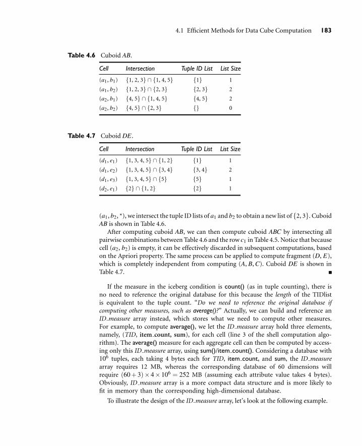
4.1 Efficient Methods for Data Cube Computation 183
Table 4.6 Cuboid AB.
Cell Intersection Tuple ID List List Size
(a1, b1) {1, 2, 3} ∩ {1, 4, 5} {1} 1
(a1, b2) {1, 2, 3} ∩ {2, 3} {2, 3} 2
(a2, b1) {4, 5} ∩ {1, 4, 5} {4, 5} 2
(a2, b2) {4, 5} ∩ {2, 3} {} 0
Table 4.7 Cuboid DE .
Cell Intersection Tuple ID List List Size
(d1, e1) {1, 3, 4, 5} ∩ {1, 2} {1} 1
(d1, e2) {1, 3, 4, 5} ∩ {3, 4} {3, 4} 2
(d1, e3) {1, 3, 4, 5} ∩ {5} {5} 1
(d2, e1) {2} ∩ {1, 2} {2} 1
(a1, b2, *), we intersect the tuple ID lists of a1 and b2 to obtain a new list of {2, 3}. CuboidAB is shown in Table 4.6.
After computing cuboid AB, we can then compute cuboid ABC by intersecting allpairwise combinations between Table 4.6 and the row c1 in Table 4.5. Notice that becausecell (a2, b2) is empty, it can be effectively discarded in subsequent computations, basedon the Apriori property. The same process can be applied to compute fragment (D, E),which is completely independent from computing (A, B, C). Cuboid DE is shown inTable 4.7.
If the measure in the iceberg condition is count() (as in tuple counting), there isno need to reference the original database for this because the length of the TIDlistis equivalent to the tuple count. “Do we need to reference the original database ifcomputing other measures, such as average()?” Actually, we can build and reference anID measure array instead, which stores what we need to compute other measures.For example, to compute average(), we let the ID measure array hold three elements,namely, (TID, item count, sum), for each cell (line 3 of the shell computation algo-rithm). The average() measure for each aggregate cell can then be computed by access-ing only this ID measure array, using sum()/item count(). Considering a database with106 tuples, each taking 4 bytes each for TID, item count, and sum, the ID measurearray requires 12 MB, whereas the corresponding database of 60 dimensions willrequire (60 + 3)× 4× 106 = 252 MB (assuming each attribute value takes 4 bytes).Obviously, ID measure array is a more compact data structure and is more likely tofit in memory than the corresponding high-dimensional database.
To illustrate the design of the ID measure array, let’s look at the following example.

184 Chapter 4 Data Cube Computation and Data Generalization
Example 4.11 Computing cubes with the average() measure. Suppose that Table 4.8 shows an examplesales database where each tuple has two associated values, such as item count and sum,where item count is the count of items sold.
To compute a data cube for this database with the measure average(), we need tohave a TIDlist for each cell: {T ID1, . . . , T IDn}. Because each TID is uniquely asso-ciated with a particular set of measure values, all future computations just need tofetch the measure values associated with the tuples in the list. In other words, bykeeping an ID measure array in memory for on-line processing, we can handle com-plex algebraic measures, such as average, variance, and standard deviation. Table 4.9shows what exactly should be kept for our example, which is substantially smallerthan the database itself.
The shell fragments are negligible in both storage space and computation time incomparison with the full data cube. Note that we can also use the Frag-Shells algo-rithm to compute the full data cube by including all of the dimensions as a single frag-ment. Because the order of computation with respect to the cuboid lattice is top-downand depth-first (similar to that of BUC), the algorithm can perform Apriori pruning ifapplied to the construction of iceberg cubes.
“Once we have computed the shell fragments, how can they be used to answer OLAPqueries?” Given the precomputed shell fragments, we can view the cube space as a virtualcube and perform OLAP queries related to the cube on-line. In general, there are twotypes of queries: (1) point query and (2) subcube query.
Table 4.8 A database with two measure values.
TID A B C D E item count sum
1 a1 b1 c1 d1 e1 5 70
2 a1 b2 c1 d2 e1 3 10
3 a1 b2 c1 d1 e2 8 20
4 a2 b1 c1 d1 e2 5 40
5 a2 b1 c1 d1 e3 2 30
Table 4.9 ID measure array of Table 4.8.
TID item count sum
1 5 70
2 3 10
3 8 20
4 5 40
5 2 30

4.1 Efficient Methods for Data Cube Computation 185
In a point query, all of the relevant dimensions in the cube have been instantiated(that is, there are no inquired dimensions in the relevant set of dimensions). Forexample, in an n-dimensional data cube, A1A2 . . .An, a point query could be in theform of 〈A1, A5, A9 : M?〉, where A1 = {a11, a18}, A5 = {a52, a55, a59}, A9 = a94, andM is the inquired measure for each corresponding cube cell. For a cube with a smallnumber of dimensions, we can use “*” to represent a “don’t care” position where thecorresponding dimension is irrelevant, that is, neither inquired nor instantiated. Forexample, in the query 〈a2, b1, c1, d1, ∗ : count()?〉 for the database in Table 4.4, thefirst four dimension values are instantiated to a2, b1, c1, and d1, respectively, whilethe last dimension is irrelevant, and count() (which is the tuple count by context) isthe inquired measure.
In a subcube query, at least one of the relevant dimensions in the cube is inquired.For example, in an n-dimensional data cube A1A2 . . .An, a subcube query could be in theform 〈A1, A5?, A9, A21? : M?〉, where A1 = {a11, a18} and A9 = a94, A5 and A21 are theinquired dimensions, and M is the inquired measure. For a cube with a small numberof dimensions, we can use “∗” for an irrelevant dimension and “?” for an inquired one.For example, in the query 〈a2, ?, c1, ∗ , ? : count()?〉 we see that the first and thirddimension values are instantiated to a2 and c1, respectively, while the fourth is irrelevant,and the second and the fifth are inquired. A subcube query computes all possible valuecombinations of the inquired dimensions. It essentially returns a local data cube consistingof the inquired dimensions.
“How can we use shell fragments to answer a point query?” Because a point query explic-itly provides the set of instantiated variables on the set of relevant dimensions, we canmake maximal use of the precomputed shell fragments by finding the best fitting (thatis, dimension-wise completely matching) fragments to fetch and intersect the associatedTIDlists.
Let the point query be of the form 〈αi, α j, αk, αp : M?〉, where αi represents a set ofinstantiated values of dimension Ai, and so on for α j, αk, and αp. First, we check theshell fragment schema to determine which dimensions among Ai, A j, Ak, and Ap are inthe same fragment(s). Suppose Ai and A j are in the same fragment, while Ak and Apare in two other fragments. We fetch the corresponding TIDlists on the precomputed2-D fragment for dimensions Ai and A j using the instantiations αi and α j, and fetchthe TIDlists on the 1-D fragments for dimensions Ak and Ap using the instantiations αkand αp, respectively. The obtained TIDlists are intersected to derive the TIDlist table.This table is then used to derive the specified measure (e.g., by taking the length of theTIDlists for tuple count(), or by fetching item count() and sum() from the ID measurearray to compute average()) for the final set of cells.
Example 4.12 Point query. Suppose a user wants to compute the point query, 〈a2, b1, c1, d1, ∗:count()?〉, for our database in Table 4.4 and that the shell fragments for the partitions(A, B, C) and (D, E) are precomputed as described in Example 4.10. The query is brokendown into two subqueries based on the precomputed fragments: 〈a2, b1, c1, ∗ , ∗〉 and〈∗, ∗ , ∗ , d1, ∗〉. The best fit precomputed shell fragments for the two subqueries areABC and D. The fetch of the TIDlists for the two subqueries returns two lists: {4, 5} and

186 Chapter 4 Data Cube Computation and Data Generalization
{1, 3, 4, 5}. Their intersection is the list {4, 5}, which is of size 2. Thus the final answeris count() = 2.
A subcube query returns a local data cube based on the instantiated and inquireddimensions. Such a data cube needs to be aggregated in a multidimensional wayso that on-line analytical processing (such as drilling, dicing, pivoting, etc.) can bemade available to users for flexible manipulation and analysis. Because instantiateddimensions usually provide highly selective constants that dramatically reduce thesize of the valid TIDlists, we should make maximal use of the precomputed shellfragments by finding the fragments that best fit the set of instantiated dimensions,and fetching and intersecting the associated TIDlists to derive the reduced TIDlist.This list can then be used to intersect the best-fitting shell fragments consisting ofthe inquired dimensions. This will generate the relevant and inquired base cuboid,which can then be used to compute the relevant subcube on the fly using an efficienton-line cubing algorithm.
Let the subcube query be of the form 〈αi, α j, Ak?, αp, Aq? : M?〉, where αi, α j, andαp represent a set of instantiated values of dimension Ai, A j, and Ap, respectively, and Akand Aq represent two inquired dimensions. First, we check the shell fragment schema todetermine which dimensions among (1) Ai, A j, and Ap, and (2) among Ak and Aq are inthe same fragment partition. Suppose Ai and A j belong to the same fragment, as do Akand Aq, but that Ap is in a different fragment. We fetch the corresponding TIDlists in theprecomputed 2-D fragment for Ai and A j using the instantiations αi and α j, then fetchthe TIDlist on the precomputed 1-D fragment for Ap using instantiation αp, and thenfetch the TIDlists on the precomputed 1-D fragments for Ak and Aq, respectively, using noinstantiations (i.e., all possible values). The obtained TIDlists are intersected to derive thefinal TIDlists, which are used to fetch the corresponding measures from the ID measurearray to derive the “base cuboid” of a 2-D subcube for two dimensions (Ak, Aq). A fast cubecomputation algorithm can be applied to compute this 2-D cube based on the derived basecuboid. The computed 2-D cube is then ready for OLAP operations.
Example 4.13 Subcube query. Suppose a user wants to compute the subcube query, 〈a2, b1, ?, ∗ , ? :count()?〉, for our database in Table 4.4, and that the shell fragments have been pre-computed as described in Example 4.10. The query can be broken into three best-fitfragments according to the instantiated and inquired dimensions: AB, C, and E , whereAB has the instantiation (a2, b1). The fetch of the TIDlists for these partitions returns:(a2, b1):{4, 5}, (c1):{1, 2, 3, 4, 5}, and {(e1:{1, 2}), (e2:{3, 4}), (e3:{5})}, respectively.The intersection of these corresponding TIDlists contains a cuboid with two tuples: {(c1,e2):{4}5, (c1, e3):{5}}. This base cuboid can be used to compute the 2-D data cube,which is trivial.
5That is, the intersection of the TIDlists for (a2, b1), (c1), and (e2) is {4}.

4.1 Efficient Methods for Data Cube Computation 187
For large data sets, a fragment size of 2 or 3 typically results in reasonable storagerequirements for the shell fragments and for fast query response time. Querying withshell fragments is substantially faster than answering queries using precomputed datacubes that are stored on disk. In comparison to full cube computation, Frag-Shells isrecommended if there are less than four inquired dimensions. Otherwise, more efficientalgorithms, such as Star-Cubing, can be used for fast on-line cube computation. Frag-Shells can easily be extended to allow incremental updates, the details of which are leftas an exercise.
4.1.6 Computing Cubes with Complex Iceberg Conditions
The iceberg cubes we have discussed so far contain only simple iceberg conditions,such as count ≥ 50 or price sum ≥ 1000 (specified in the having clause). Such con-ditions have a nice property: if the condition is violated for some cell c, then everydescendant of c will also violate that condition. For example, if the quantity of an itemI sold in a region R1 is less than 50, then the same item I sold in a subregion of R1can never satisfy the condition count ≥ 50. Conditions that obey this property areknown as antimonotonic.
Not all iceberg conditions are antimonotonic. For example, the condition avg(price)≥ 800 is not antimonotonic. This is because if the average price of an item, such as,say, “TV”, in region R1, is less than $800, then a descendant of the cell representing“TV” and R1, such as “TV” in a subregion of R1, can still have an average price ofover $800.
“Can we still push such an iceberg condition deep into the cube computation process forimproved efficiency?” To answer this question, we first look at an example.
Example 4.14 Iceberg cube with the average measure. Consider the salesInfo table given in Table 4.10,which registers sales related to month, day, city, customer group, item, and price.
Suppose, as data analysts, we have the following query: Find groups of sales that containat least 50 items and whose average item price is at least $800, grouped by month, city, and/orcustomer group. We can specify an iceberg cube, sales avg iceberg, to answer the query, asfollows:
Table 4.10 A salesInfo table.
month day city cust group item price
Jan 10 Chicago Education HP Printer 485
Jan 15 Chicago Household Sony TV 1,200
Jan 20 New York Education Canon Camera 1,280
Feb 20 New York Business IBM Laptop 2,500
Mar 4 Vancouver Education Seagate HD 520
· · · · · · · · · · · · · · · · · ·

188 Chapter 4 Data Cube Computation and Data Generalization
compute cube sales avg iceberg as
select month, city, customer group, avg(price), count(∗)from salesInfo
cube by month, city, customer group
having avg(price) >= 800 and count(∗)>= 50
Here, the iceberg condition involves the measure average, which is not antimonotonic.This implies that if a cell, c, cannot satisfy the iceberg condition, “average(c) ≥ v”, wecannot prune away the descendants of c because it is possible that the average value forsome of them may satisfy the condition.
“How can we compute sales avg iceberg?” It would be highly inefficient to firstmaterialize the full data cube and then select the cells satisfying the having clauseof the iceberg condition. We have seen that a cube with an antimonotonic icebergcondition can be computed efficiently by exploring the Apriori property. However,because this iceberg cube involves a non-antimonotonic iceberg condition, Apri-ori pruning cannot be applied. “Can we transform the non-antimonotonic conditionto a somewhat weaker but antimonotonic one so that we can still take advantage ofpruning?”
The answer is “yes.” Here we examine one interesting such method. A cell c is said tohave n base cells if it covers n nonempty descendant base cells. The top-k average of c,denoted as avgk(c), is the average value (i.e., price) of the top-k base cells of c (i.e., the firstk cells when all the base cells in c are sorted in value-descending order) if k ≤ n; or −∞if k > n. With this notion of top-k average, we can transform the original iceberg con-dition “avg(price)≥ v and count(∗)≥ k” into the weaker but antimonotonic condition“avgk(c) ≥ v”. The reasoning is that if the average of the top-k nonempty descendantbase cells of a cell c is less than v, there exists no subset from this set of base cells thatcan contain k or more base cells and have a bigger average value than v. Thus, it is safeto prune away the cell c.
It is costly to sort and keep the top-k base cell values for each aggregated cell. For effi-cient implementation, we can use only a few records to register some aggregated valuesto facilitate similar pruning. For example, we could use one record, r0, to keep the sumand count of the cells whose value is no less than v, and a few records, such as r1, r2, andr3, to keep the sum and count of the cells whose price falls into the range of [0.8−1.0),[0.6−0.8), [0.4−0.6) of v, respectively. If the counts of r0 and r1 are no less than k butthe average of the two is less than v, there is no hope of finding any descendants of c thatcan satisfy the iceberg condition. Thus c and its descendants can be pruned off in icebergcube computation.
Similar transformation methods can be applied to many other iceberg conditions,such as those involving average on a set of positive and negative values, range, variance,and standard deviation. Details of the transformation methods are left as an exercise forinterested readers.

4.2 Further Development of Data Cube and OLAP Technology 189
4.2 Further Development of Data Cube and OLAPTechnology
In this section, we study further developments of data cube and OLAP technology.Section 4.2.1 describes data mining by discovery-driven exploration of data cubes,where anomalies in the data are automatically detected and marked for the userwith visual cues. Section 4.2.2 describes multifeature cubes for complex data miningqueries involving multiple dependent aggregates at multiple granularity. Section 4.2.3presents methods for constrained gradient analysis in data cubes, which identifies cubecells that have dramatic changes in value in comparison with their siblings, ancestors,or descendants.
4.2.1 Discovery-Driven Exploration of Data Cubes
As studied in previous sections, a data cube may have a large number of cuboids, and eachcuboid may contain a large number of (aggregate) cells. With such an overwhelminglylarge space, it becomes a burden for users to even just browse a cube, let alone think ofexploring it thoroughly. Tools need to be developed to assist users in intelligently explor-ing the huge aggregated space of a data cube.
Discovery-driven exploration is such a cube exploration approach. In discovery-driven exploration, precomputed measures indicating data exceptions are used to guidethe user in the data analysis process, at all levels of aggregation. We hereafter refer tothese measures as exception indicators. Intuitively, an exception is a data cube cell valuethat is significantly different from the value anticipated, based on a statistical model. Themodel considers variations and patterns in the measure value across all of the dimensionsto which a cell belongs. For example, if the analysis of item-sales data reveals an increasein sales in December in comparison to all other months, this may seem like an exceptionin the time dimension. However, it is not an exception if the item dimension is consid-ered, since there is a similar increase in sales for other items during December. The modelconsiders exceptions hidden at all aggregated group-by’s of a data cube. Visual cues suchas background color are used to reflect the degree of exception of each cell, based onthe precomputed exception indicators. Efficient algorithms have been proposed for cubeconstruction, as discussed in Section 4.1. The computation of exception indicators canbe overlapped with cube construction, so that the overall construction of data cubes fordiscovery-driven exploration is efficient.
Three measures are used as exception indicators to help identify data anomalies. Thesemeasures indicate the degree of surprise that the quantity in a cell holds, with respect toits expected value. The measures are computed and associated with every cell, for alllevels of aggregation. They are as follows:
SelfExp: This indicates the degree of surprise of the cell value, relative to other cellsat the same level of aggregation.

190 Chapter 4 Data Cube Computation and Data Generalization
InExp: This indicates the degree of surprise somewhere beneath the cell, if we were todrill down from it.
PathExp: This indicates the degree of surprise for each drill-down path from the cell.
The use of these measures for discovery-driven exploration of data cubes is illustrated inthe following example.
Example 4.15 Discovery-driven exploration of a data cube. Suppose that you would like to analyze themonthly sales at AllElectronics as a percentage difference from the previous month. Thedimensions involved are item, time, and region. You begin by studying the data aggregatedover all items and sales regions for each month, as shown in Figure 4.15.
To view the exception indicators, you would click on a button marked highlight excep-tions on the screen. This translates the SelfExp and InExp values into visual cues, dis-played with each cell. The background color of each cell is based on its SelfExp value. Inaddition, a box is drawn around each cell, where the thickness and color of the box area function of its InExp value. Thick boxes indicate high InExp values. In both cases, thedarker the color, the greater the degree of exception. For example, the dark, thick boxesfor sales during July, August, and September signal the user to explore the lower-levelaggregations of these cells by drilling down.
Drill-downs can be executed along the aggregated item or region dimensions. “Whichpath has more exceptions?” you wonder. To find this out, you select a cell of interest andtrigger a path exception module that colors each dimension based on the PathExp valueof the cell. This value reflects the degree of surprise of that path. Suppose that the pathalong item contains more exceptions.
A drill-down along item results in the cube slice of Figure 4.16, showing the sales overtime for each item. At this point, you are presented with many different sales values toanalyze. By clicking on the highlight exceptions button, the visual cues are displayed,bringing focus toward the exceptions. Consider the sales difference of 41% for “Sonyb/w printers” in September. This cell has a dark background, indicating a high SelfExpvalue, meaning that the cell is an exception. Consider now the sales difference of −15%for “Sony b/w printers” in November, and of −11% in December. The −11% value forDecember is marked as an exception, while the−15% value is not, even though−15% isa bigger deviation than−11%. This is because the exception indicators consider all of thedimensions that a cell is in. Notice that the December sales of most of the other items havea large positive value, while the November sales do not. Therefore, by considering the
Sum of sales Month
Total
Jan Feb Mar Apr May Jun Jul Aug Sep Oct Nov Dec
1% −1% 0% 1% 3% −1% −9% −1% 2% −4% 3%
Figure 4.15 Change in sales over time.

4.2 Further Development of Data Cube and OLAP Technology 191
Figure 4.16 Change in sales for each item-time combination.
Avg. sales Month
North
South
East
West
JanRegion Feb Mar Apr May Jun Jul Aug Sep Oct Nov Dec
−1%
−1%
−1%
4%
−3%
1%
−2%
0%
−1%
−9%
2%
−1%
0%
6%
−3%
−3%
3%
−1%
1%
5%
4%
−39%
18%
1%
−7%
9%
−2%
−18%
1%
−34%
11%
8%
0%
4%
−3%
5%
−3%
1%
−2%
−8%
−3%
7%
−1%
1%
Figure 4.17 Change in sales for the item IBM desktop computer per region.
position of the cell in the cube, the sales difference for “Sony b/w printers” in Decemberis exceptional, while the November sales difference of this item is not.
The InExp values can be used to indicate exceptions at lower levels that are not visibleat the current level. Consider the cells for “IBM desktop computers” in July and September.These both have a dark, thick box around them, indicating high InExp values. You maydecide to further explore the sales of “IBM desktop computers” by drilling down alongregion. The resulting sales difference by region is shown in Figure 4.17, where the highlightexceptions option has been invoked. The visual cues displayed make it easy to instantlynotice an exception for the sales of “IBM desktop computers” in the southern region,where such sales have decreased by−39% and−34% in July and September, respectively.These detailed exceptions were far from obvious when we were viewing the data as anitem-time group-by, aggregated over region in Figure 4.16. Thus, the InExp value is usefulfor searching for exceptions at lower-level cells of the cube. Because no other cells inFigure 4.17 have a high InExp value, you may roll up back to the data of Figure 4.16 and

192 Chapter 4 Data Cube Computation and Data Generalization
choose another cell from which to drill down. In this way, the exception indicators canbe used to guide the discovery of interesting anomalies in the data.
“How are the exception values computed?” The SelfExp, InExp, and PathExp measuresare based on a statistical method for table analysis. They take into account all of thegroup-by’s (aggregations) in which a given cell value participates. A cell value is con-sidered an exception based on how much it differs from its expected value, where itsexpected value is determined with a statistical model described below. The differencebetween a given cell value and its expected value is called a residual. Intuitively, the largerthe residual, the more the given cell value is an exception. The comparison of residualvalues requires us to scale the values based on the expected standard deviation associatedwith the residuals. A cell value is therefore considered an exception if its scaled residualvalue exceeds a prespecified threshold. The SelfExp, InExp, and PathExp measures arebased on this scaled residual.
The expected value of a given cell is a function of the higher-level group-by’s of thegiven cell. For example, given a cube with the three dimensions A, B, and C, the expectedvalue for a cell at the ith position in A, the jth position in B, and the kth position in Cis a function of γ, γ A
i , γ Bj , γ C
k , γ ABi j , γ AC
ik , and γ BCjk , which are coefficients of the statistical
model used. The coefficients reflect how different the values at more detailed levels are,based on generalized impressions formed by looking at higher-level aggregations. In thisway, the exception quality of a cell value is based on the exceptions of the values below it.Thus, when seeing an exception, it is natural for the user to further explore the exceptionby drilling down.
“How can the data cube be efficiently constructed for discovery-driven exploration?”This computation consists of three phases. The first step involves the computation ofthe aggregate values defining the cube, such as sum or count, over which exceptionswill be found. The second phase consists of model fitting, in which the coefficientsmentioned above are determined and used to compute the standardized residuals.This phase can be overlapped with the first phase because the computations involvedare similar. The third phase computes the SelfExp, InExp, and PathExp values, basedon the standardized residuals. This phase is computationally similar to phase 1. There-fore, the computation of data cubes for discovery-driven exploration can be doneefficiently.
4.2.2 Complex Aggregation at Multiple Granularity:Multifeature Cubes
Data cubes facilitate the answering of data mining queries as they allow the computa-tion of aggregate data at multiple levels of granularity. In this section, you will learnabout multifeature cubes, which compute complex queries involving multiple dependentaggregates at multiple granularity. These cubes are very useful in practice. Many com-plex data mining queries can be answered by multifeature cubes without any significantincrease in computational cost, in comparison to cube computation for simple querieswith standard data cubes.

4.2 Further Development of Data Cube and OLAP Technology 193
All of the examples in this section are from the Purchases data of AllElectronics, wherean item is purchased in a sales region on a business day (year, month, day). The shelf lifein months of a given item is stored in shelf. The item price and sales (in dollars) at a givenregion are stored in price and sales, respectively. To aid in our study of multifeature cubes,let’s first look at an example of a simple data cube.
Example 4.16 Query 1: A simple data cube query. Find the total sales in 2004, broken down by item,region, and month, with subtotals for each dimension.
To answer Query 1, a data cube is constructed that aggregates the total sales at thefollowing eight different levels of granularity: {(item, region, month), (item, region),(item, month), (month, region), (item), (month), (region), ()}, where () represents all.Query 1 uses a typical data cube like that introduced in the previous chapter. Wecall such a data cube a simple data cube because it does not involve any dependent aggre-gates.
“What is meant by ‘dependent aggregates’?” We answer this by studying the followingexample of a complex query.
Example 4.17 Query 2: A complex query. Grouping by all subsets of {item, region, month}, find themaximum price in 2004 for each group and the total sales among all maximum pricetuples.
The specification of such a query using standard SQL can be long, repetitive, anddifficult to optimize and maintain. Alternatively, Query 2 can be specified concisely usingan extended SQL syntax as follows:
select item, region, month, max(price), sum(R.sales)from Purchaseswhere year = 2004cube by item, region, month: Rsuch that R.price = max(price)
The tuples representing purchases in 2004 are first selected. The cube by clausecomputes aggregates (or group-by’s) for all possible combinations of the attributes item,region, and month. It is an n-dimensional generalization of the group by clause. Theattributes specified in the cube by clause are the grouping attributes. Tuples with thesame value on all grouping attributes form one group. Let the groups be g1, . . . , gr. Foreach group of tuples gi, the maximum price maxgi among the tuples forming the groupis computed. The variable R is a grouping variable, ranging over all tuples in group giwhose price is equal to maxgi (as specified in the such that clause). The sum of sales of thetuples in gi that R ranges over is computed and returned with the values of the groupingattributes of gi. The resulting cube is a multifeature cube in that it supports complexdata mining queries for which multiple dependent aggregates are computed at a varietyof granularities. For example, the sum of sales returned in Query 2 is dependent on theset of maximum price tuples for each group.

194 Chapter 4 Data Cube Computation and Data Generalization
{ 5 MIN(R1.shelf)} R2
{ 5 MAX(R1.shelf)} R3
{ = MAX(price)}
R1
R0
Figure 4.18 A multifeature cube graph for Query 3.
Let’s look at another example.
Example 4.18 Query 3: An even more complex query. Grouping by all subsets of {item, region, month},find the maximum price in 2004 for each group. Among the maximum price tuples, findthe minimum and maximum item shelf lives. Also find the fraction of the total sales dueto tuples that have minimum shelf life within the set of all maximum price tuples, andthe fraction of the total sales due to tuples that have maximum shelf life within the set ofall maximum price tuples.
The multifeature cube graph of Figure 4.18 helps illustrate the aggregate dependen-cies in the query. There is one node for each grouping variable, plus an additional initialnode, R0. Starting from node R0, the set of maximum price tuples in 2004 is first com-puted (node R1). The graph indicates that grouping variables R2 and R3 are “dependent”on R1, since a directed line is drawn from R1 to each of R2 and R3. In a multifeature cubegraph, a directed line from grouping variable Ri to R j means that R j always ranges over asubset of the tuples that Ri ranges over. When expressing the query in extended SQL, wewrite “R j in Ri” as shorthand to refer to this case. For example, the minimum shelf lifetuples at R2 range over the maximum price tuples at R1, that is, “R2 in R1.” Similarly,the maximum shelf life tuples at R3 range over the maximum price tuples at R1, that is,“R3 in R1.”
From the graph, we can express Query 3 in extended SQL as follows:
select item, region, month, max(price), min(R1.shelf), max(R1.shelf),sum(R1.sales), sum(R2.sales), sum(R3.sales)
from Purchaseswhere year = 2004cube by item, region, month: R1, R2, R3
4.2 Further Development of Data Cube and OLAP Technology 195
such that R1.price = max(price) andR2 in R1 and R2.shelf = min(R1.shelf) andR3 in R1 and R3.shelf = max(R1.shelf)
“How can multifeature cubes be computed efficiently?” The computation of a multifea-ture cube depends on the types of aggregate functions used in the cube. In Chapter 3,we saw that aggregate functions can be categorized as either distributive, algebraic, orholistic. Multifeature cubes can be organized into the same categories and computedefficiently by minor extension of the previously studied cube computation methods.
4.2.3 Constrained Gradient Analysis in Data Cubes
Many data cube applications need to analyze the changes of complex measures in multidi-mensional space. For example, in real estate, we may want to ask what are the changes ofthe average house price in the Vancouver area in the year 2004 compared against 2003,and the answer could be “the average price for those sold to professionals in the West Endwent down by 20%, while those sold to business people in Metrotown went up by 10%,etc.” Expressions such as “professionals in the West End” correspond to cuboid cells anddescribe sectors of the business modeled by the data cube.
The problem of mining changes of complex measures in a multidimensional space wasfirst proposed by Imielinski, Khachiyan, and Abdulghani [IKA02] as the cubegrade prob-lem, which can be viewed as a generalization of association rules6 and data cubes. It stud-ies how changes in a set of measures (aggregates) of interest are associated with changesin the underlying characteristics of sectors, where changes in sector characteristics areexpressed in terms of dimensions of the cube and are limited to specialization (drill-down), generalization (roll-up), and mutation (a change in one of the cube’s dimensions).For example, we may want to ask “what kind of sector characteristics are associated withmajor changes in average house price in the Vancouver area in 2004?” The answer willbe pairs of sectors, associated with major changes in average house price, including, forexample, “the sector of professional buyers in the West End area of Vancouver” versus“the sector of all buyers in the entire area of Vancouver” as a specialization (or general-ization). The cubegrade problem is significantly more expressive than association rules,because it captures data trends and handles complex measures, not just count, as asso-ciation rules do. The problem has broad applications, from trend analysis to answering“what-if ” questions and discovering exceptions or outliers.
The curse of dimensionality and the need for understandable results pose serious chal-lenges for finding an efficient and scalable solution to the cubegrade problem. Here weexamine a confined but interesting version of the cubegrade problem, called
6Association rules were introduced in Chapter 1. They are often used in market basket analysis tofind associations between items purchased in transactional sales databases. Association rule mining isdescribed in detail in Chapter 5.

196 Chapter 4 Data Cube Computation and Data Generalization
constrained multidimensional gradient analysis, which reduces the search space andderives interesting results. It incorporates the following types of constraints:
1. Significance constraint: This ensures that we examine only the cells that have certain“statistical significance” in the data, such as containing at least a specified numberof base cells or at least a certain total sales. In the data cube context, this constraintacts as the iceberg condition, which prunes a huge number of trivial cells from theanswer set.
2. Probe constraint: This selects a subset of cells (called probe cells) from all of the pos-sible cells as starting points for examination. Because the cubegrade problem needsto compare each cell in the cube with other cells that are either specializations, gener-alizations, or mutations of the given cell, it extracts pairs of similar cell characteristicsassociated with big changes in measure in a data cube. Given three cells, a, b, and c, ifa is a specialization of b, then we say it is a descendant of b, in which case, b is a gen-eralization or ancestor of a. Cell c is a mutation of a if the two have identical values inall but one dimension, where the dimension for which they vary cannot have a value of“∗”. Cells a and c are considered siblings. Even when considering only iceberg cubes,a large number of pairs may still be generated. Probe constraints allow the user tospecify a subset of cells that are of interest for the analysis task. In this way, the studyis focused only on these cells and their relationships with corresponding ancestors,descendants, and siblings.
3. Gradient constraint: This specifies the user’s range of interest on the gradient(measure change). A user is typically interested in only certain types of changesbetween the cells (sectors) under comparison. For example, we may be interestedin only those cells whose average profit increases by more than 40% compared tothat of the probe cells. Such changes can be specified as a threshold in the formof either a ratio or a difference between certain measure values of the cells undercomparison. A cell that captures the change from the probe cell is referred to asa gradient cell.
The following example illustrates each of the above types of constraints.
Example 4.19 Constrained average gradient analysis. The base table, D, for AllElectronics sales has theschema
sales(year, city, customer group, item group, count, avg price).
Attributes year, city, customer group, and item group are the dimensional attributes;count and avg price are the measure attributes. Table 4.11 shows a set of base and aggre-gate cells. Tuple c1 is a base cell, while tuples c2, c3, and c4 are aggregate cells. Tuple c3 isa sibling of c2, c4 is an ancestor of c2, and c1 is a descendant of c2.
Suppose that the significance constraint, Csig, is (count ≥ 100), meaning that a cellwith count no less than 100 is regarded as significant. Suppose that the probe constraint,Cprb, is (city = “Vancouver,” customer group = “Business,” item group = *). This means

4.2 Further Development of Data Cube and OLAP Technology 197
Table 4.11 A set of base and aggregate cells.
c1 (2000, Vancouver, Business, PC, 300, $2100)
c2 (∗, Vancouver, Business, PC, 2800, $1900)
c3 (∗, Toronto, Business, PC, 7900, $2350)
c4 (∗, ∗, Business, PC, 58600, $2250)
that the set of probe cells, P, is the set of aggregate tuples regarding the sales of theBusiness customer group in Vancouver, for every product group, provided the count inthe tuple is greater than or equal to 100. It is easy to see that c2 ∈ P.
Let the gradient constraint, Cgrad(cg, cp), be (avg price(cg)/avg price(cp) ≥ 1.4).The constrained gradient analysis problem is thus to find all pairs, (cg, cp), where cp isa probe cell in P; cg is a sibling, ancestor, or descendant of cp; cg is a significant cell, andcg’s average price is at least 40% more than cp’s.
If a data cube is fully materialized, the query posed in Example 4.19 becomes a rela-tively simple retrieval of the pairs of computed cells that satisfy the constraints. Unfor-tunately, the number of aggregate cells is often too huge to be precomputed and stored.Typically, only the base table or cuboid is available, so that the task then becomes how toefficiently compute the gradient-probe pairs from it.
One rudimentary approach to computing such gradients is to conduct a search for thegradient cells, once per probe cell. This approach is inefficient because it would involvea large amount of repeated work for different probe cells. A suggested method is a set-oriented approach that starts with a set of probe cells, utilizes constraints early on duringsearch, and explores pruning, when possible, during progressive computation of pairs ofcells. With each gradient cell, the set of all possible probe cells that might co-occur ininteresting gradient-probe pairs are associated with some descendants of the gradientcell. These probe cells are considered “live probe cells.” This set is used to search forfuture gradient cells, while considering significance constraints and gradient constraintsto reduce the search space as follows:
1. The significance constraints can be used directly for pruning: If a cell, c, cannot satisfythe significance constraint, then c and its descendants can be pruned because none ofthem can be significant, and
2. Because the gradient constraint may specify a complex measure (such as avg ≥ v),the incorporation of both the significance constraint and the gradient constraint canbe used for pruning in a manner similar to that discussed in Section 4.1.6 on com-puting cubes with complex iceberg conditions. That is, we can explore a weaker butantimonotonic form of the constraint, such as the top-k average, avgk(c)≥ v, where kis the significance constraint (such as 100 in Example 4.19), and v is derived from thegradient constraint based on v = cg×vp, where cg is the gradient contraint threshold,and vp is the value of the corresponding probe cell. That is, if the current cell, c, cannot

198 Chapter 4 Data Cube Computation and Data Generalization
satisfy this constraint, further exploration of its descendants will be useless and thuscan be pruned.
The constrained cube gradient analysis has been shown to be effective at exploring thesignificant changes among related cube cells in multidimensional space.
4.3 Attribute-Oriented Induction—An Alternative Methodfor Data Generalization and Concept Description
Data generalization summarizes data by replacing relatively low-level values (such asnumeric values for an attribute age) with higher-level concepts (such as young, middle-aged, and senior). Given the large amount of data stored in databases, it is useful to beable to describe concepts in concise and succinct terms at generalized (rather than low)levels of abstraction. Allowing data sets to be generalized at multiple levels of abstractionfacilitates users in examining the general behavior of the data. Given the AllElectron-ics database, for example, instead of examining individual customer transactions, salesmanagers may prefer to view the data generalized to higher levels, such as summarizedby customer groups according to geographic regions, frequency of purchases per group,and customer income.
This leads us to the notion of concept description, which is a form of data generaliza-tion. A concept typically refers to a collection of data such as frequent buyers,graduate students, and so on. As a data mining task, concept description is not a sim-ple enumeration of the data. Instead, concept description generates descriptions for thecharacterization and comparison of the data. It is sometimes called class description,when the concept to be described refers to a class of objects. Characterization providesa concise and succinct summarization of the given collection of data, while concept orclass comparison (also known as discrimination) provides descriptions comparing twoor more collections of data.
Up to this point, we have studied data cube (or OLAP) approaches to concept descrip-tion using multidimensional, multilevel data generalization in data warehouses. “Is datacube technology sufficient to accomplish all kinds of concept description tasks for large datasets?” Consider the following cases.
Complex data types and aggregation: Data warehouses and OLAP tools are based on amultidimensional data model that views data in the form of a data cube, consisting ofdimensions (or attributes) and measures (aggregate functions). However, many cur-rent OLAP systems confine dimensions to nonnumeric data and measures to numericdata. In reality, the database can include attributes of various data types, includingnumeric, nonnumeric, spatial, text, or image, which ideally should be included inthe concept description. Furthermore, the aggregation of attributes in a databasemay include sophisticated data types, such as the collection of nonnumeric data,the merging of spatial regions, the composition of images, the integration of texts,

4.3 Attribute-Oriented Induction—An Alternative Method 199
and the grouping of object pointers. Therefore, OLAP, with its restrictions on thepossible dimension and measure types, represents a simplified model for data analy-sis. Concept description should handle complex data types of the attributes and theiraggregations, as necessary.
User-control versus automation: On-line analytical processing in data warehouses isa user-controlled process. The selection of dimensions and the application of OLAPoperations, such as drill-down, roll-up, slicing, and dicing, are primarily directedand controlled by the users. Although the control in most OLAP systems is quiteuser-friendly, users do require a good understanding of the role of each dimension.Furthermore, in order to find a satisfactory description of the data, users may need tospecify a long sequence of OLAP operations. It is often desirable to have a more auto-mated process that helps users determine which dimensions (or attributes) shouldbe included in the analysis, and the degree to which the given data set should begeneralized in order to produce an interesting summarization of the data.
This section presents an alternative method for concept description, called attribute-oriented induction, which works for complex types of data and relies on a data-drivengeneralization process.
4.3.1 Attribute-Oriented Induction for Data Characterization
The attribute-oriented induction (AOI) approach to concept description was firstproposed in 1989, a few years before the introduction of the data cube approach. Thedata cube approach is essentially based on materialized views of the data, which typ-ically have been precomputed in a data warehouse. In general, it performs off-lineaggregation before an OLAP or data mining query is submitted for processing. Onthe other hand, the attribute-oriented induction approach is basically a query-oriented,generalization-based, on-line data analysis technique. Note that there is no inherentbarrier distinguishing the two approaches based on on-line aggregation versus off-lineprecomputation. Some aggregations in the data cube can be computed on-line, whileoff-line precomputation of multidimensional space can speed up attribute-orientedinduction as well.
The general idea of attribute-oriented induction is to first collect the task-relevantdata using a database query and then perform generalization based on the exami-nation of the number of distinct values of each attribute in the relevant set of data.The generalization is performed by either attribute removal or attribute generalization.Aggregation is performed by merging identical generalized tuples and accumulatingtheir respective counts. This reduces the size of the generalized data set. The resultinggeneralized relation can be mapped into different forms for presentation to the user,such as charts or rules.
The following examples illustrate the process of attribute-oriented induction. We firstdiscuss its use for characterization. The method is extended for the mining of classcomparisons in Section 4.3.4.

200 Chapter 4 Data Cube Computation and Data Generalization
Example 4.20 A data mining query for characterization. Suppose that a user would like to describethe general characteristics of graduate students in the Big University database, given theattributes name, gender, major, birth place, birth date, residence, phone# (telephonenumber), and gpa (grade point average). A data mining query for this characterizationcan be expressed in the data mining query language, DMQL, as follows:
use Big University DBmine characteristics as “Science Students”in relevance to name, gender, major, birth place, birth date, residence,
phone#, gpafrom studentwhere status in “graduate”
We will see how this example of a typical data mining query can apply attribute-oriented induction for mining characteristic descriptions.
First, data focusing should be performed before attribute-oriented induction. Thisstep corresponds to the specification of the task-relevant data (i.e., data for analysis). Thedata are collected based on the information provided in the data mining query. Because adata mining query is usually relevant to only a portion of the database, selecting the rele-vant set of data not only makes mining more efficient, but also derives more meaningfulresults than mining the entire database.
Specifying the set of relevant attributes (i.e., attributes for mining, as indicated inDMQL with the in relevance to clause) may be difficult for the user. A user may selectonly a few attributes that he or she feels may be important, while missing others thatcould also play a role in the description. For example, suppose that the dimensionbirth place is defined by the attributes city, province or state, and country. Of theseattributes, let’s say that the user has only thought to specify city. In order to allowgeneralization on the birth place dimension, the other attributes defining this dimen-sion should also be included. In other words, having the system automatically includeprovince or state and country as relevant attributes allows city to be generalized to thesehigher conceptual levels during the induction process.
At the other extreme, suppose that the user may have introduced too many attributesby specifying all of the possible attributes with the clause “in relevance to ∗”. In this case,all of the attributes in the relation specified by the from clause would be included in theanalysis. Many of these attributes are unlikely to contribute to an interesting description.A correlation-based (Section 2.4.1) or entropy-based (Section 2.6.1) analysis method canbe used to perform attribute relevance analysis and filter out statistically irrelevant orweakly relevant attributes from the descriptive mining process. Other approaches, suchas attribute subset selection, are also described in Chapter 2.
“What does the ‘where status in “graduate”’ clause mean?” This where clause impliesthat a concept hierarchy exists for the attribute status. Such a concept hierarchy organizesprimitive-level data values for status, such as “M.Sc.”, “M.A.”, “M.B.A.”, “Ph.D.”, “B.Sc.”,“B.A.”, into higher conceptual levels, such as “graduate” and “undergraduate.” This use

4.3 Attribute-Oriented Induction—An Alternative Method 201
Table 4.12 Initial working relation: a collection of task-relevant data.
name gender major birth place birth date residence phone# gpa
Jim Woodman M CS Vancouver, BC, Canada 8-12-76 3511 Main St., Richmond 687-4598 3.67
Scott Lachance M CS Montreal, Que, Canada 28-7-75 345 1st Ave., Richmond 253-9106 3.70
Laura Lee F physics Seattle, WA, USA 25-8-70 125 Austin Ave., Burnaby 420-5232 3.83
· · · · · · · · · · · · · · · · · · · · · · · ·
of concept hierarchies does not appear in traditional relational query languages, yet islikely to become a common feature in data mining query languages.
The data mining query presented above is transformed into the following relationalquery for the collection of the task-relevant set of data:
use Big University DBselect name, gender, major, birth place, birth date, residence, phone#, gpafrom studentwhere status in {“M.Sc.”, “M.A.”, “M.B.A.”, “Ph.D.”}
The transformed query is executed against the relational database, Big University DB,and returns the data shown in Table 4.12. This table is called the (task-relevant) initialworking relation. It is the data on which induction will be performed. Note that eachtuple is, in fact, a conjunction of attribute-value pairs. Hence, we can think of a tuplewithin a relation as a rule of conjuncts, and of induction on the relation as the general-ization of these rules.
“Now that the data are ready for attribute-oriented induction, how is attribute-orientedinduction performed?” The essential operation of attribute-oriented induction is datageneralization, which can be performed in either of two ways on the initial working rela-tion: attribute removal and attribute generalization.
Attribute removal is based on the following rule: If there is a large set of distinctvalues for an attribute of the initial working relation, but either (1) there is no generalizationoperator on the attribute (e.g., there is no concept hierarchy defined for the attribute), or (2)its higher-level concepts are expressed in terms of other attributes, then the attribute shouldbe removed from the working relation.
Let’s examine the reasoning behind this rule. An attribute-value pair represents a con-junct in a generalized tuple, or rule. The removal of a conjunct eliminates a constraintand thus generalizes the rule. If, as in case 1, there is a large set of distinct values for anattribute but there is no generalization operator for it, the attribute should be removedbecause it cannot be generalized, and preserving it would imply keeping a large numberof disjuncts, which contradicts the goal of generating concise rules. On the other hand,consider case 2, where the higher-level concepts of the attribute are expressed in termsof other attributes. For example, suppose that the attribute in question is street, whosehigher-level concepts are represented by the attributes 〈city, province or state, country〉.

202 Chapter 4 Data Cube Computation and Data Generalization
The removal of street is equivalent to the application of a generalization operator. Thisrule corresponds to the generalization rule known as dropping conditions in the machinelearning literature on learning from examples.
Attribute generalization is based on the following rule: If there is a large set of distinctvalues for an attribute in the initial working relation, and there exists a set of generalizationoperators on the attribute, then a generalization operator should be selected and appliedto the attribute. This rule is based on the following reasoning. Use of a generalizationoperator to generalize an attribute value within a tuple, or rule, in the working relationwill make the rule cover more of the original data tuples, thus generalizing the concept itrepresents. This corresponds to the generalization rule known as climbing generalizationtrees in learning from examples, or concept tree ascension.
Both rules, attribute removal and attribute generalization, claim that if there is a largeset of distinct values for an attribute, further generalization should be applied. This raisesthe question: how large is “a large set of distinct values for an attribute” considered to be?
Depending on the attributes or application involved, a user may prefer some attributesto remain at a rather low abstraction level while others are generalized to higher levels.The control of how high an attribute should be generalized is typically quite subjective.The control of this process is called attribute generalization control. If the attribute isgeneralized “too high,” it may lead to overgeneralization, and the resulting rules maynot be very informative. On the other hand, if the attribute is not generalized to a“sufficiently high level,” then undergeneralization may result, where the rules obtainedmay not be informative either. Thus, a balance should be attained in attribute-orientedgeneralization.
There are many possible ways to control a generalization process. We will describetwo common approaches and then illustrate how they work with an example.
The first technique, called attribute generalization threshold control, either sets onegeneralization threshold for all of the attributes, or sets one threshold for each attribute.If the number of distinct values in an attribute is greater than the attribute threshold,further attribute removal or attribute generalization should be performed. Data miningsystems typically have a default attribute threshold value generally ranging from 2 to 8and should allow experts and users to modify the threshold values as well. If a user feelsthat the generalization reaches too high a level for a particular attribute, the thresholdcan be increased. This corresponds to drilling down along the attribute. Also, to furthergeneralize a relation, the user can reduce the threshold of a particular attribute, whichcorresponds to rolling up along the attribute.
The second technique, called generalized relation threshold control, sets a thresholdfor the generalized relation. If the number of (distinct) tuples in the generalizedrelation is greater than the threshold, further generalization should be performed.Otherwise, no further generalization should be performed. Such a threshold mayalso be preset in the data mining system (usually within a range of 10 to 30), orset by an expert or user, and should be adjustable. For example, if a user feels thatthe generalized relation is too small, he or she can increase the threshold, whichimplies drilling down. Otherwise, to further generalize a relation, the threshold canbe reduced, which implies rolling up.
4.3 Attribute-Oriented Induction—An Alternative Method 203
These two techniques can be applied in sequence: first apply the attribute thresholdcontrol technique to generalize each attribute, and then apply relation threshold con-trol to further reduce the size of the generalized relation. No matter which generaliza-tion control technique is applied, the user should be allowed to adjust the generalizationthresholds in order to obtain interesting concept descriptions.
In many database-oriented induction processes, users are interested in obtainingquantitative or statistical information about the data at different levels of abstraction.Thus, it is important to accumulate count and other aggregate values in the inductionprocess. Conceptually, this is performed as follows. The aggregate function, count, isassociated with each database tuple. Its value for each tuple in the initial working relationis initialized to 1. Through attribute removal and attribute generalization, tuples withinthe initial working relation may be generalized, resulting in groups of identical tuples. Inthis case, all of the identical tuples forming a group should be merged into one tuple.The count of this new, generalized tuple is set to the total number of tuples from the ini-tial working relation that are represented by (i.e., were merged into) the new generalizedtuple. For example, suppose that by attribute-oriented induction, 52 data tuples from theinitial working relation are all generalized to the same tuple, T . That is, the generalizationof these 52 tuples resulted in 52 identical instances of tuple T . These 52 identical tuplesare merged to form one instance of T , whose count is set to 52. Other popular aggregatefunctions that could also be associated with each tuple include sum and avg. For a givengeneralized tuple, sum contains the sum of the values of a given numeric attribute forthe initial working relation tuples making up the generalized tuple. Suppose that tupleT contained sum(units sold) as an aggregate function. The sum value for tuple T wouldthen be set to the total number of units sold for each of the 52 tuples. The aggregate avg(average) is computed according to the formula, avg = sum/count.
Example 4.21 Attribute-oriented induction. Here we show how attribute-oriented induction is per-formed on the initial working relation of Table 4.12. For each attribute of the relation,the generalization proceeds as follows:
1. name: Since there are a large number of distinct values for name and there is nogeneralization operation defined on it, this attribute is removed.
2. gender: Since there are only two distinct values for gender, this attribute is retainedand no generalization is performed on it.
3. major: Suppose that a concept hierarchy has been defined that allows the attributemajor to be generalized to the values {arts&science, engineering, business}. Supposealso that the attribute generalization threshold is set to 5, and that there are more than20 distinct values for major in the initial working relation. By attribute generalizationand attribute generalization control, major is therefore generalized by climbing thegiven concept hierarchy.
4. birth place: This attribute has a large number of distinct values; therefore, we wouldlike to generalize it. Suppose that a concept hierarchy exists for birth place, defined

204 Chapter 4 Data Cube Computation and Data Generalization
as “city < province or state < country”. If the number of distinct values for countryin the initial working relation is greater than the attribute generalization threshold,then birth place should be removed, because even though a generalization operatorexists for it, the generalization threshold would not be satisfied. If instead, the numberof distinct values for country is less than the attribute generalization threshold, thenbirth place should be generalized to birth country.
5. birth date: Suppose that a hierarchy exists that can generalize birth date to age, and ageto age range, and that the number of age ranges (or intervals) is small with respect tothe attribute generalization threshold. Generalization of birth date should thereforetake place.
6. residence:Supposethatresidence isdefinedbytheattributesnumber,street,residence city,residence province or state, and residence country. The number of distinct values fornumber and street will likely be very high, since these concepts are quite low level. Theattributes number and street should therefore be removed, so that residence is thengeneralized to residence city, which contains fewer distinct values.
7. phone#: As with the attribute name above, this attribute contains too many distinctvalues and should therefore be removed in generalization.
8. gpa: Suppose that a concept hierarchy exists for gpa that groups values for gradepoint average into numerical intervals like {3.75–4.0, 3.5–3.75,. . .}, which in turnare grouped into descriptive values, such as {excellent, very good,. . .}. The attributecan therefore be generalized.
The generalization process will result in groups of identical tuples. For example, thefirst two tuples of Table 4.12 both generalize to the same identical tuple (namely, the firsttuple shown in Table 4.13). Such identical tuples are then merged into one, with theircounts accumulated. This process leads to the generalized relation shown in Table 4.13.
Based on the vocabulary used in OLAP, we may view count as a measure, and theremaining attributes as dimensions. Note that aggregate functions, such as sum, may beapplied to numerical attributes, like salary and sales. These attributes are referred to asmeasure attributes.
Implementation techniques and methods of presenting the derived generalization arediscussed in the following subsections.
Table 4.13 A generalized relation obtained by attribute-oriented induction on the data ofTable 4.12.
gender major birth country age range residence city gpa count
M Science Canada 20 – 25 Richmond very good 16
F Science Foreign 25 – 30 Burnaby excellent 22
· · · · · · · · · · · · · · · · · · · · ·

4.3 Attribute-Oriented Induction—An Alternative Method 205
4.3.2 Efficient Implementation of Attribute-Oriented Induction
“How is attribute-oriented induction actually implemented?” The previous subsectionprovided an introduction to attribute-oriented induction. The general procedure is sum-marized in Figure 4.19. The efficiency of this algorithm is analyzed as follows:
Step 1 of the algorithm is essentially a relational query to collect the task-relevant datainto the working relation, W . Its processing efficiency depends on the query process-ing methods used. Given the successful implementation and commercialization ofdatabase systems, this step is expected to have good performance.
Algorithm: Attribute oriented induction. Mining generalized characteristics in a relational database given auser’s data mining request.
Input:
DB, a relational database;
DMQuery, a data mining query;
a list, a list of attributes (containing attributes, ai);
Gen(ai), a set of concept hierarchies or generalization operators on attributes, ai;
a gen thresh(ai), attribute generalization thresholds for each ai.
Output: P, a Prime generalized relation.
Method:
1. W ← get task relevant data (DMQuery, DB); // Let W , the working relation, hold the task-relevantdata.
2. prepare for generalization (W ); // This is implemented as follows.
(a) Scan W and collect the distinct values for each attribute, ai. (Note: If W is very large, this may bedone by examining a sample of W .)
(b) For each attribute ai, determine whether ai should be removed, and if not, compute its minimumdesired level Li based on its given or default attribute threshold, and determine the mapping-pairs (v, v′), where v is a distinct value of ai in W , and v′ is its corresponding generalized value atlevel Li.
3. P← generalization (W ),
The Prime generalized relation, P, is derived by replacing each value v in W by its corresponding v′ inthe mapping while accumulating count and computing any other aggregate values.
This step can be implemented efficiently using either of the two following variations:
(a) For each generalized tuple, insert the tuple into a sorted prime relation P by a binary search: if thetuple is already in P, simply increase its count and other aggregate values accordingly; otherwise,insert it into P.
(b) Since in most cases the number of distinct values at the prime relation level is small, the primerelation can be coded as an m-dimensional array where m is the number of attributes in P,and each dimension contains the corresponding generalized attribute values. Each array elementholds the corresponding count and other aggregation values, if any. The insertion of a generalizedtuple is performed by measure aggregation in the corresponding array element.
Figure 4.19 Basic algorithm for attribute-oriented induction.

206 Chapter 4 Data Cube Computation and Data Generalization
Step 2 collects statistics on the working relation. This requires scanning the relationat most once. The cost for computing the minimum desired level and determiningthe mapping pairs, (v, v′), for each attribute is dependent on the number of distinctvalues for each attribute and is smaller than N, the number of tuples in the initialrelation.
Step 3 derives the prime relation, P. This is performed by inserting generalized tuplesinto P. There are a total of N tuples in W and p tuples in P. For each tuple, t, inW , we substitute its attribute values based on the derived mapping-pairs. This resultsin a generalized tuple, t′. If variation (a) is adopted, each t′ takes O(log p) to findthe location for count increment or tuple insertion. Thus the total time complexityis O(N × log p) for all of the generalized tuples. If variation (b) is adopted, each t′
takes O(1) to find the tuple for count increment. Thus the overall time complexity isO(N) for all of the generalized tuples.
Many data analysis tasks need to examine a good number of dimensions or attributes.This may involve dynamically introducing and testing additional attributes rather thanjust those specified in the mining query. Moreover, a user with little knowledge of thetruly relevant set of data may simply specify “in relevance to ∗” in the mining query,which includes all of the attributes into the analysis. Therefore, an advanced conceptdescription mining process needs to perform attribute relevance analysis on large setsof attributes to select the most relevant ones. Such analysis may employ correlation orentropy measures, as described in Chapter 2 on data preprocessing.
4.3.3 Presentation of the Derived Generalization
“Attribute-oriented induction generates one or a set of generalized descriptions. How canthese descriptions be visualized?” The descriptions can be presented to the user in a num-ber of different ways. Generalized descriptions resulting from attribute-oriented induc-tion are most commonly displayed in the form of a generalized relation (or table).
Example 4.22 Generalized relation (table). Suppose that attribute-oriented induction was performedon a sales relation of the AllElectronics database, resulting in the generalized descriptionof Table 4.14 for sales in 2004. The description is shown in the form of a generalizedrelation. Table 4.13 of Example 4.21 is another example of a generalized relation.
Descriptions can also be visualized in the form of cross-tabulations, or crosstabs. Ina two-dimensional crosstab, each row represents a value from an attribute, and each col-umn represents a value from another attribute. In an n-dimensional crosstab (for n> 2),the columns may represent the values of more than one attribute, with subtotals shownfor attribute-value groupings. This representation is similar to spreadsheets. It is easy tomap directly from a data cube structure to a crosstab.
Example 4.23 Cross-tabulation. The generalized relation shown in Table 4.14 can be transformed intothe 3-D cross-tabulation shown in Table 4.15.

4.3 Attribute-Oriented Induction—An Alternative Method 207
Table 4.14 A generalized relation for the sales in 2004.
location item sales (in million dollars) count (in thousands)
Asia TV 15 300
Europe TV 12 250
North America TV 28 450
Asia computer 120 1000
Europe computer 150 1200
North America computer 200 1800
Table 4.15 A crosstab for the sales in 2004.
item
TV computer both items
location sales count sales count sales count
Asia 15 300 120 1000 135 1300
Europe 12 250 150 1200 162 1450
North America 28 450 200 1800 228 2250
all regions 45 1000 470 4000 525 5000
Generalized data can be presented graphically, using bar charts, pie charts, and curves.Visualization with graphs is popular in data analysis. Such graphs and curves canrepresent 2-D or 3-D data.
Example 4.24 Bar chart and pie chart. The sales data of the crosstab shown in Table 4.15 can be trans-formed into the bar chart representation of Figure 4.20 and the pie chart representationof Figure 4.21.
Finally, a 3-D generalized relation or crosstab can be represented by a 3-D data cube,which is useful for browsing the data at different levels of generalization.
Example 4.25 Cube view. Consider the data cube shown in Figure 4.22 for the dimensions item, location,and cost. This is the same kind of data cube that we have seen so far, although it is presentedin a slightly different way. Here, the size of a cell (displayed as a tiny cube) represents thecount of the corresponding cell, while the brightness of the cell can be used to representanother measure of the cell, such as sum (sales). Pivoting, drilling, and slicing-and-dicingoperations can be performed on the data cube browser by mouse clicking.
A generalized relation may also be represented in the form of logic rules. Typically,each generalized tuple represents a rule disjunct. Because data in a large database usuallyspan a diverse range of distributions, a single generalized tuple is unlikely to cover, or

208 Chapter 4 Data Cube Computation and Data Generalization
250
200
150
100
50
0
TV
Sale
s
Computers TV + Computers
Asia Europe North America
Figure 4.20 Bar chart representation of the sales in 2004.
North America (50.91%)
Asia (27.27%)
Europe (21.82%)
North America (42.56%)
Asia (25.53%)
Europe (31.91%)
TV Sales
Computer Sales
North America (43.43%)
Asia (25.71%)
Europe (30.86%)
TV 1 Computer Sales
Figure 4.21 Pie chart representation of the sales in 2004.
represent, 100% of the initial working relation tuples, or cases. Thus, quantitative infor-mation, such as the percentage of data tuples that satisfy the left- and right-hand side ofthe rule, should be associated with each rule. A logic rule that is associated with quanti-tative information is called a quantitative rule.
To define a quantitative characteristic rule, we introduce the t-weight as an interest-ingness measure that describes the typicality of each disjunct in the rule, or of each tuple

4.3 Attribute-Oriented Induction—An Alternative Method 209
loca
tion
item
cost
23.00–799.00
799.00–3,916.00
3,916.00–25,677.00
Not specifie
d
North America Europe
Australia
Asia
Alarm systemCD playerCompact disc
ComputerCordless phoneMousePrinterSoftwareSpeakersTV
Figure 4.22 A 3-D cube view representation of the sales in 2004.
in the corresponding generalized relation. The measure is defined as follows. Let the classof objects that is to be characterized (or described by the rule) be called the target class.Let qa be a generalized tuple describing the target class. The t-weight for qa is the per-centage of tuples of the target class from the initial working relation that are covered byqn. Formally, we have
t weight = count(qa)/Σni=1count(qa), (4.1)
where n is the number of tuples for the target class in the generalized relation; q1, . . ., qnare tuples for the target class in the generalized relation; and qa is in q1, . . ., qn. Obviously,the range for the t-weight is [0.0, 1.0] or [0%, 100%].
A quantitative characteristic rule can then be represented either (1) in logic form byassociating the corresponding t-weight value with each disjunct covering the target class,or (2) in the relational table or crosstab form by changing the count values in these tablesfor tuples of the target class to the corresponding t-weight values.
Each disjunct of a quantitative characteristic rule represents a condition. In general,the disjunction of these conditions forms a necessary condition of the target class, sincethe condition is derived based on all of the cases of the target class; that is, all tuplesof the target class must satisfy this condition. However, the rule may not be a sufficientcondition of the target class, since a tuple satisfying the same condition could belong toanother class. Therefore, the rule should be expressed in the form
∀X, target class(X)⇒ condition1(X)[t : w1]∨·· ·∨ conditionm(X)[t : wm]. (4.2)

210 Chapter 4 Data Cube Computation and Data Generalization
The rule indicates that if X is in the target class, there is a probability of wi that Xsatisfies conditioni, where wi is the t-weight value for condition or disjunct i, and i isin {1, . . . , m}.
Example 4.26 Quantitative characteristic rule. The crosstab shown in Table 4.15 can be transformedinto logic rule form. Let the target class be the set of computer items. The correspondingcharacteristic rule, in logic form, is
∀X, item(X) = “computer”⇒(location(X) = “Asia”) [t : 25.00%]∨ (location(X) = “Europe”) [t : 30.00%]∨(location(X) = “North America”) [t : 45, 00%]
Notice that the first t-weight value of 25.00% is obtained by 1000, the value corres-ponding to the count slot for “(Asia,computer)”, divided by 4000, the value correspond-ing to the count slot for “(all regions, computer)”. (That is, 4000 represents the totalnumber of computer items sold.) The t-weights of the other two disjuncts were simi-larly derived. Quantitative characteristic rules for other target classes can be computedin a similar fashion.
“How can the t-weight and interestingness measures in general be used by the datamining system to display only the concept descriptions that it objectively evaluates asinteresting?” A threshold can be set for this purpose. For example, if the t-weightof a generalized tuple is lower than the threshold, then the tuple is considered torepresent only a negligible portion of the database and can therefore be ignoredas uninteresting. Ignoring such negligible tuples does not mean that they should beremoved from the intermediate results (i.e., the prime generalized relation, or the datacube, depending on the implementation) because they may contribute to subsequentfurther exploration of the data by the user via interactive rolling up or drilling downof other dimensions and levels of abstraction. Such a threshold may be referred toas a significance threshold or support threshold, where the latter term is commonlyused in association rule mining.
4.3.4 Mining Class Comparisons: Discriminating betweenDifferent Classes
In many applications, users may not be interested in having a single class (or concept)described or characterized, but rather would prefer to mine a description that comparesor distinguishes one class (or concept) from other comparable classes (or concepts). Classdiscrimination or comparison (hereafter referred to as class comparison) mines descrip-tions that distinguish a target class from its contrasting classes. Notice that the target andcontrasting classes must be comparable in the sense that they share similar dimensionsand attributes. For example, the three classes, person, address, and item, are not compara-ble. However, the sales in the last three years are comparable classes, and so are computerscience students versus physics students.

4.3 Attribute-Oriented Induction—An Alternative Method 211
Our discussions on class characterization in the previous sections handle multileveldata summarization and characterization in a single class. The techniques developedcan be extended to handle class comparison across several comparable classes. Forexample, the attribute generalization process described for class characterization canbe modified so that the generalization is performed synchronously among all theclasses compared. This allows the attributes in all of the classes to be generalizedto the same levels of abstraction. Suppose, for instance, that we are given the AllElec-tronics data for sales in 2003 and sales in 2004 and would like to compare these twoclasses. Consider the dimension location with abstractions at the city, province or state,and country levels. Each class of data should be generalized to the same locationlevel. That is, they are synchronously all generalized to either the city level, or theprovince or state level, or the country level. Ideally, this is more useful than comparing,say, the sales in Vancouver in 2003 with the sales in the United States in 2004 (i.e.,where each set of sales data is generalized to a different level). The users, however,should have the option to overwrite such an automated, synchronous comparisonwith their own choices, when preferred.
“How is class comparison performed?” In general, the procedure is as follows:
1. Data collection: The set of relevant data in the database is collected by query process-ing and is partitioned respectively into a target class and one or a set of contrastingclass(es).
2. Dimension relevance analysis: If there are many dimensions, then dimension rele-vance analysis should be performed on these classes to select only the highly relevantdimensions for further analysis. Correlation or entropy-based measures can be usedfor this step (Chapter 2).
3. Synchronous generalization: Generalization is performed on the target class to thelevel controlled by a user- or expert-specified dimension threshold, which results ina prime target class relation. The concepts in the contrasting class(es) are general-ized to the same level as those in the prime target class relation, forming the primecontrasting class(es) relation.
4. Presentation of the derived comparison: The resulting class comparison descriptioncan be visualized in the form of tables, graphs, and rules. This presentation usuallyincludes a “contrasting” measure such as count% (percentage count) that reflects thecomparison between the target and contrasting classes. The user can adjust the com-parison description by applying drill-down, roll-up, and other OLAP operations tothe target and contrasting classes, as desired.
The above discussion outlines a general algorithm for mining comparisons in data-bases. In comparison with characterization, the above algorithm involves synchronousgeneralization of the target class with the contrasting classes, so that classes are simulta-neously compared at the same levels of abstraction.
The following example mines a class comparison describing the graduate studentsand the undergraduate students at Big University.

212 Chapter 4 Data Cube Computation and Data Generalization
Example 4.27 Mining a class comparison. Suppose that you would like to compare the generalproperties between the graduate students and the undergraduate students at Big Univer-sity, given the attributes name, gender, major, birth place, birth date, residence, phone#,and gpa.
This data mining task can be expressed in DMQL as follows:
use Big University DBmine comparison as “grad vs undergrad students”in relevance to name, gender, major, birth place, birth date, residence,
phone#, gpafor “graduate students”where status in “graduate”versus “undergraduate students”where status in “undergraduate”analyze count%from student
Let’s see how this typical example of a data mining query for mining comparisondescriptions can be processed.
First, the query is transformed into two relational queries that collect two sets oftask-relevant data: one for the initial target class working relation, and the other forthe initial contrasting class working relation, as shown in Tables 4.16 and 4.17. Thiscan also be viewed as the construction of a data cube, where the status {graduate,undergraduate} serves as one dimension, and the other attributes form the remainingdimensions.
Table 4.16 Initial working relations: the target class (graduate students)
name gender major birth place birth date residence phone# gpa
Jim Woodman M CS Vancouver, BC, Canada 8-12-76 3511 Main St., Richmond 687-4598 3.67
Scott Lachance M CS Montreal, Que, Canada 28-7-75 345 1st Ave., Vancouver 253-9106 3.70
Laura Lee F Physics Seattle, WA, USA 25-8-70 125 Austin Ave., Burnaby 420-5232 3.83
· · · · · · · · · · · · · · · · · · · · · · · ·
Table 4.17 Initial working relations: the contrasting class (undergraduate students)
name gender major birth place birth date residence phone# gpa
Bob Schumann M Chemistry Calgary, Alt, Canada 10-1-78 2642 Halifax St., Burnaby 294-4291 2.96
Amy Eau F Biology Golden, BC, Canada 30-3-76 463 Sunset Cres., Vancouver 681-5417 3.52
· · · · · · · · · · · · · · · · · · · · · · · ·
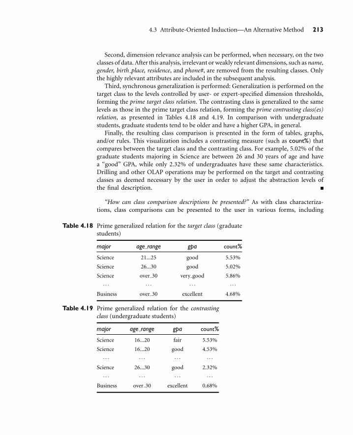
4.3 Attribute-Oriented Induction—An Alternative Method 213
Second, dimension relevance analysis can be performed, when necessary, on the twoclasses of data. After this analysis, irrelevant or weakly relevant dimensions, such as name,gender, birth place, residence, and phone#, are removed from the resulting classes. Onlythe highly relevant attributes are included in the subsequent analysis.
Third, synchronous generalization is performed: Generalization is performed on thetarget class to the levels controlled by user- or expert-specified dimension thresholds,forming the prime target class relation. The contrasting class is generalized to the samelevels as those in the prime target class relation, forming the prime contrasting class(es)relation, as presented in Tables 4.18 and 4.19. In comparison with undergraduatestudents, graduate students tend to be older and have a higher GPA, in general.
Finally, the resulting class comparison is presented in the form of tables, graphs,and/or rules. This visualization includes a contrasting measure (such as count%) thatcompares between the target class and the contrasting class. For example, 5.02% of thegraduate students majoring in Science are between 26 and 30 years of age and havea “good” GPA, while only 2.32% of undergraduates have these same characteristics.Drilling and other OLAP operations may be performed on the target and contrastingclasses as deemed necessary by the user in order to adjust the abstraction levels ofthe final description.
“How can class comparison descriptions be presented?” As with class characteriza-tions, class comparisons can be presented to the user in various forms, including
Table 4.18 Prime generalized relation for the target class (graduatestudents)
major age range gpa count%
Science 21...25 good 5.53%
Science 26...30 good 5.02%
Science over 30 very good 5.86%
· · · · · · · · · · · ·Business over 30 excellent 4.68%
Table 4.19 Prime generalized relation for the contrastingclass (undergraduate students)
major age range gpa count%
Science 16...20 fair 5.53%
Science 16...20 good 4.53%
· · · · · · · · · · · ·Science 26...30 good 2.32%
· · · · · · · · · · · ·Business over 30 excellent 0.68%

214 Chapter 4 Data Cube Computation and Data Generalization
generalized relations, crosstabs, bar charts, pie charts, curves, cubes, and rules. Withthe exception of logic rules, these forms are used in the same way for characterizationas for comparison. In this section, we discuss the visualization of class comparisonsin the form of discriminant rules.
As is similar with characterization descriptions, the discriminative features of the tar-get and contrasting classes of a comparison description can be described quantitativelyby a quantitative discriminant rule, which associates a statistical interestingness measure,d-weight, with each generalized tuple in the description.
Let qa be a generalized tuple, and C j be the target class, where qa covers some tuples ofthe target class. Note that it is possible that qa also covers some tuples of the contrastingclasses, particularly since we are dealing with a comparison description. The d-weightfor qa is the ratio of the number of tuples from the initial target class working relationthat are covered by qa to the total number of tuples in both the initial target class andcontrasting class working relations that are covered by qa. Formally, the d-weight of qafor the class C j is defined as
d weight = count(qa ∈C j)/Σmi=1count(qa ∈Ci), (4.3)
where m is the total number of the target and contrasting classes, C j is in {C1, . . . , Cm},and count (qa ∈Ci) is the number of tuples of class Ci that are covered by qa. The rangefor the d-weight is [0.0, 1.0] (or [0%, 100%]).
A high d-weight in the target class indicates that the concept represented by the gen-eralized tuple is primarily derived from the target class, whereas a low d-weight impliesthat the concept is primarily derived from the contrasting classes. A threshold can be setto control the display of interesting tuples based on the d-weight or other measures used,as described in Section 4.3.3.
Example 4.28 Computing the d-weight measure. In Example 4.27, suppose that the count distributionfor the generalized tuple, major = “Science” AND age range = “21. . . 25” ANDgpa = “good”, from Tables 4.18 and 4.19 is as shown in Table 20.
The d-weight for the given generalized tuple is 90/(90 + 210) = 30% with respect tothe target class, and 210/(90 + 210) = 70% with respect to the contrasting class. That is,if a student majoring in Science is 21 to 25 years old and has a “good” gpa, then based on thedata, there is a 30% probability that she is a graduate student, versus a 70% probability that
Table 4.20 Count distribution between graduate and undergraduatestudents for a generalized tuple.
status major age range gpa count
graduate Science 21...25 good 90
undergraduate Science 21...25 good 210

4.3 Attribute-Oriented Induction—An Alternative Method 215
she is an undergraduate student. Similarly, the d-weights for the other generalized tuplesin Tables 4.18 and 4.19 can be derived.
A quantitative discriminant rule for the target class of a given comparison descriptionis written in the form
∀X, target class(X)⇐condition(X) [d:d weight], (4.4)
where the condition is formed by a generalized tuple of the description. This is differentfrom rules obtained in class characterization, where the arrow of implication is from leftto right.
Example 4.29 Quantitative discriminant rule. Based on the generalized tuple and count distribution inExample 4.28, a quantitative discriminant rule for the target class graduate student canbe written as follows:
∀X, Status(X) = “graduate student”⇐major(X) = “Science”∧age range(X) = “21...25” (4.5)
∧ gpa(X) = “good”[d : 30%].
Notice that a discriminant rule provides a sufficient condition, but not a necessary one,for an object (or tuple) to be in the target class. For example, Rule (4.6) implies that if Xsatisfies the condition, then the probability that X is a graduate student is 30%. However,it does not imply the probability that X meets the condition, given that X is a graduatestudent. This is because although the tuples that meet the condition are in the targetclass, other tuples that do not necessarily satisfy this condition may also be in the targetclass, because the rule may not cover all of the examples of the target class in the database.Therefore, the condition is sufficient, but not necessary.
4.3.5 Class Description: Presentation of Both Characterizationand Comparison
“Because class characterization and class comparison are two aspects forming a class descrip-tion, can we present both in the same table or in the same rule?” Actually, as long as wehave a clear understanding of the meaning of the t-weight and d-weight measures andcan interpret them correctly, there is no additional difficulty in presenting both aspectsin the same table. Let’s examine an example of expressing both class characterization andclass comparison in the same crosstab.
Example 4.30 Crosstab for class characterization and class comparison. Let Table 4.21 be a crosstabshowing the total number (in thousands) of TVs and computers sold at AllElectronicsin 2004.

216 Chapter 4 Data Cube Computation and Data Generalization
Table 4.21 A crosstab for the total number (count) of TVs andcomputers sold in thousands in 2004.
item
location TV computer both items
Europe 80 240 320
North America 120 560 680
both regions 200 800 1000
Table 4.22 The same crosstab as in Table 4.21, but here the t-weight and d-weight values associatedwith each class are shown.
item
TV computer both items
location count t-weight d-weight count t-weight d-weight count t-weight d-weight
Europe 80 25% 40% 240 75% 30% 320 100% 32%
North America 120 17.65% 60% 560 82.35% 70% 680 100% 68%
both regions 200 20% 100% 800 80% 100% 1000 100% 100%
Let Europe be the target class and North America be the contrasting class. The t-weightsand d-weights of the sales distribution between the two classes are presented in Table 4.22.According to the table, the t-weight of a generalized tuple or object (e.g., item = “TV”)for a given class (e.g., the target class Europe) shows how typical the tuple is of the givenclass (e.g., what proportion of these sales in Europe are for TVs?). The d-weight of a tupleshows how distinctive the tuple is in the given (target or contrasting) class in comparisonwith its rival class (e.g., how do the TV sales in Europe compare with those in NorthAmerica?).
For example, the t-weight for “(Europe, TV)” is 25% because the number of TVs soldin Europe (80,000) represents only 25% of the European sales for both items (320,000).The d-weight for “(Europe, TV)” is 40% because the number of TVs sold in Europe(80,000) represents 40% of the number of TVs sold in both the target and the contrastingclasses of Europe and North America, respectively (which is 200,000).
Notice that the count measure in the crosstab of Table 4.22 obeys the general prop-erty of a crosstab (i.e., the count values per row and per column, when totaled, matchthe corresponding totals in the both items and both regions slots, respectively). How-ever, this property is not observed by the t-weight and d-weight measures, becausethe semantic meaning of each of these measures is different from that of count, aswe explained in Example 4.30.

4.3 Attribute-Oriented Induction—An Alternative Method 217
“Can a quantitative characteristic rule and a quantitative discriminant rule be expressedtogether in the form of one rule?” The answer is yes—a quantitative characteristic ruleand a quantitative discriminant rule for the same class can be combined to form aquantitative description rule for the class, which displays the t-weights and d-weightsassociated with the corresponding characteristic and discriminant rules. To see howthis is done, let’s quickly review how quantitative characteristic and discriminant rulesare expressed.
As discussed in Section 4.3.3, a quantitative characteristic rule provides a necessarycondition for the given target class since it presents a probability measurement for eachproperty that can occur in the target class. Such a rule is of the form
∀X, target class(X)⇒condition1(X)[t : w1]∨·· ·∨ conditionm(X)[t : wm], (4.6)
where each condition represents a property of the target class. The rule indicates thatif X is in the target class, the probability that X satisfies conditioni is the value of thet-weight, wi, where i is in {1, . . . , m}.
As previously discussed in Section 4.3.4, a quantitative discriminant rule provides asufficient condition for the target class since it presents a quantitative measurement ofthe properties that occur in the target class versus those that occur in the contrastingclasses. Such a rule is of the form
∀X, target class(X)⇐condition1(X)[d : w1]∧·· ·∧ conditionm(X)[d : wm]. (4.7)
The rule indicates that if X satisfies conditioni, there is a probability of wi (thed-weight value) that X is in the target class, where i is in {1, . . . , m}.
A quantitative characteristic rule and a quantitative discriminant rule for a given classcan be combined as follows to form a quantitative description rule: (1) For each con-dition, show both the associated t-weight and d-weight, and (2) a bidirectional arrowshould be used between the given class and the conditions. That is, a quantitative descrip-tion rule is of the form
∀X, target class(X)⇔ condition1(X)[t : w1, d : w′1] (4.8)
θ · · ·θ conditionm(X)[t : wm, d : w′m],
where θ represents a logical disjunction/conjuction. (That is, if we consider the rule as acharacteristic rule, the conditions are ORed to from a disjunct. Otherwise, if we considerthe rule as a discriminant rule, the conditions are ANDed to form a conjunct). The ruleindicates that for i from 1 to m, if X is in the target class, there is a probability of wi thatX satisfies conditioni; and if X satisfies conditioni, there is a probability of w′i that X is inthe target class.
Example 4.31 Quantitative description rule. It is straightforward to transform the crosstab of Table 4.22in Example 4.30 into a class description in the form of quantitative description rules. Forexample, the quantitative description rule for the target class, Europe, is
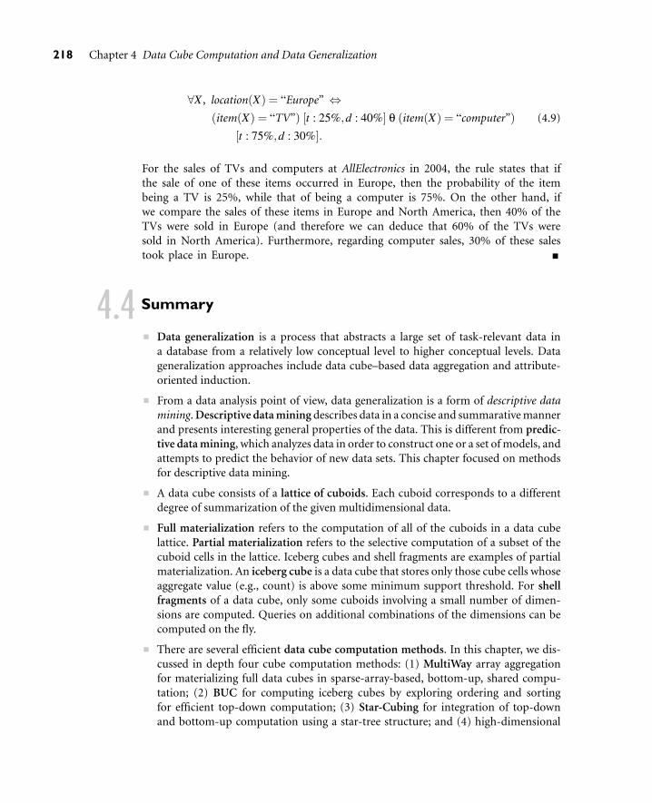
218 Chapter 4 Data Cube Computation and Data Generalization
∀X , location(X) = “Europe” ⇔(item(X) = “TV”) [t : 25%,d : 40%] θ (item(X) = “computer”) (4.9)
[t : 75%,d : 30%].
For the sales of TVs and computers at AllElectronics in 2004, the rule states that ifthe sale of one of these items occurred in Europe, then the probability of the itembeing a TV is 25%, while that of being a computer is 75%. On the other hand, ifwe compare the sales of these items in Europe and North America, then 40% of theTVs were sold in Europe (and therefore we can deduce that 60% of the TVs weresold in North America). Furthermore, regarding computer sales, 30% of these salestook place in Europe.
4.4 Summary
Data generalization is a process that abstracts a large set of task-relevant data ina database from a relatively low conceptual level to higher conceptual levels. Datageneralization approaches include data cube–based data aggregation and attribute-oriented induction.
From a data analysis point of view, data generalization is a form of descriptive datamining. Descriptive data mining describes data in a concise and summarative mannerand presents interesting general properties of the data. This is different from predic-tive data mining, which analyzes data in order to construct one or a set of models, andattempts to predict the behavior of new data sets. This chapter focused on methodsfor descriptive data mining.
A data cube consists of a lattice of cuboids. Each cuboid corresponds to a differentdegree of summarization of the given multidimensional data.
Full materialization refers to the computation of all of the cuboids in a data cubelattice. Partial materialization refers to the selective computation of a subset of thecuboid cells in the lattice. Iceberg cubes and shell fragments are examples of partialmaterialization. An iceberg cube is a data cube that stores only those cube cells whoseaggregate value (e.g., count) is above some minimum support threshold. For shellfragments of a data cube, only some cuboids involving a small number of dimen-sions are computed. Queries on additional combinations of the dimensions can becomputed on the fly.
There are several efficient data cube computation methods. In this chapter, we dis-cussed in depth four cube computation methods: (1) MultiWay array aggregationfor materializing full data cubes in sparse-array-based, bottom-up, shared compu-tation; (2) BUC for computing iceberg cubes by exploring ordering and sortingfor efficient top-down computation; (3) Star-Cubing for integration of top-downand bottom-up computation using a star-tree structure; and (4) high-dimensional

Exercises 219
OLAP by precomputing only the partitioned shell fragments (thus called minimalcubing).
There are several methods for effective and efficient exploration of data cubes, includ-ing discovery-driven cube exploration, multifeature data cubes, and constrained cubegradient analysis. Discovery-driven exploration of data cubes uses precomputed mea-sures and visual cues to indicate data exceptions at all levels of aggregation, guiding theuser in the data analysis process. Multifeature cubes compute complex queries involv-ing multiple dependent aggregates at multiple granularity. Constrained cube gradientanalysis explores significant changes in measures in a multidimensional space, basedon a given set of probe cells, where changes in sector characteristics are expressed interms of dimensions of the cube and are limited to specialization (drill-down), gener-alization (roll-up), and mutation (a change in one of the cube’s dimensions).
Concept description is the most basic form of descriptive data mining. It describesa given set of task-relevant data in a concise and summarative manner, presentinginteresting general properties of the data. Concept (or class) description consists ofcharacterization and comparison (or discrimination). The former summarizes anddescribes a collection of data, called the target class, whereas the latter summarizesand distinguishes one collection of data, called the target class, from other collec-tion(s) of data, collectively called the contrasting class(es).
Concept characterization can be implemented using data cube (OLAP-based)approaches and the attribute-oriented induction approach. These are attribute- ordimension-based generalization approaches. The attribute-oriented inductionapproach consists of the following techniques: data focusing, data generalization byattribute removal or attribute generalization, count and aggregate value accumulation,attribute generalization control, and generalization data visualization.
Concept comparison can be performed using the attribute-oriented induction ordata cube approaches in a manner similar to concept characterization. Generalizedtuples from the target and contrasting classes can be quantitatively compared andcontrasted.
Characterization and comparison descriptions (which form a concept description)can both be presented in the same generalized relation, crosstab, or quantitativerule form, although they are displayed with different interestingness measures. Thesemeasures include the t-weight (for tuple typicality) and d-weight (for tuplediscriminability).
Exercises
4.1 Assume a base cuboid of 10 dimensions contains only three base cells: (1) (a1, d2, d3, d4,. . . , d9, d10), (2) (d1,b2, d3, d4, . . . , d9, d10), and (3) (d1, d2, c3, d4, . . . , d9, d10), wherea1 6= d1, b2 6= d2, and c3 6= d3. The measure of the cube is count.

220 Chapter 4 Data Cube Computation and Data Generalization
(a) How many nonempty cuboids will a full data cube contain?
(b) How many nonempty aggregate (i.e., nonbase) cells will a full cube contain?
(c) How many nonempty aggregate cells will an iceberg cube contain if the condition ofthe iceberg cube is “count ≥ 2”?
(d) A cell, c, is a closed cell if there exists no cell, d, such that d is a specialization ofcell c (i.e., d is obtained by replacing a ∗ in c by a non-∗ value) and d has the samemeasure value as c. A closed cube is a data cube consisting of only closed cells. Howmany closed cells are in the full cube?
4.2 There are several typical cube computation methods, such as Multiway array computation(MultiWay)[ZDN97],BUC(bottom-upcomputation)[BR99],andStar-Cubing[XHLW03].
Briefly describe these three methods (i.e., use one or two lines to outline the key points),and compare their feasibility and performance under the following conditions:
(a) Computing a dense full cube of low dimensionality (e.g., less than 8 dimensions)
(b) Computing an iceberg cube of around 10 dimensions with a highly skewed datadistribution
(c) Computing a sparse iceberg cube of high dimensionality (e.g., over 100 dimensions)
4.3 [Contributed by Chen Chen] Suppose a data cube, C, has D dimensions, and the basecuboid contains k distinct tuples.
(a) Present a formula to calculate the minimum number of cells that the cube, C, maycontain.
(b) Present a formula to calculate the maximum number of cells that C may contain.
(c) Answer parts (a) and (b) above as if the count in each cube cell must be no less thana threshold, v.
(d) Answer parts (a) and (b) above as if only closed cells are considered (with the mini-mum count threshold, v).
4.4 Suppose that a base cuboid has three dimensions, A, B, C, with the following numberof cells: |A| = 1, 000, 000, |B| = 100, and |C| = 1000. Suppose that each dimension isevenly partitioned into 10 portions for chunking.
(a) Assuming each dimension has only one level, draw the complete lattice of the cube.
(b) If each cube cell stores one measure with 4 bytes, what is the total size of thecomputed cube if the cube is dense?
(c) State the order for computing the chunks in the cube that requires the least amountof space, and compute the total amount of main memory space required for com-puting the 2-D planes.
4.5 Often, the aggregate measure value of many cells in a large data cuboid is zero, resultingin a huge, yet sparse, multidimensional matrix.

Exercises 221
(a) Design an implementation method that can elegantly overcome this sparse matrixproblem. Note that you need to explain your data structures in detail and discuss thespace needed, as well as how to retrieve data from your structures.
(b) Modify your design in (a) to handle incremental data updates. Give the reasoningbehind your new design.
4.6 When computing a cube of high dimensionality, we encounter the inherent curse ofdimensionality problem: there exists a huge number of subsets of combinations ofdimensions.
(a) Suppose that there are only two base cells, {(a1, a2, a3, . . . , a100), (a1, a2, b3, . . . ,b100)}, in a 100-dimensional base cuboid. Compute the number of nonempty aggre-gate cells. Comment on the storage space and time required to compute these cells.
(b) Suppose we are to compute an iceberg cube from the above. If the minimum supportcount in the iceberg condition is two, how many aggregate cells will there be in theiceberg cube? Show the cells.
(c) Introducing iceberg cubes will lessen the burden of computing trivial aggregate cellsin a data cube. However, even with iceberg cubes, we could still end up having tocompute a large number of trivial uninteresting cells (i.e., with small counts). Sup-pose that a database has 20 tuples that map to (or cover) the two following base cellsin a 100-dimensional base cuboid, each with a cell count of 10: {(a1, a2, a3, . . . , a100) :10, (a1, a2, b3, . . . , b100) : 10}.
i. Let the minimum support be 10. How many distinct aggregate cells will therebe like the following: {(a1, a2, a3, a4, . . . , a99, ∗) : 10, . . . , (a1, a2, ∗ , a4, . . . , a99,a100) : 10, . . . , (a1, a2, a3, ∗ , . . . , ∗ , ∗) : 10}?
ii. If we ignore all the aggregate cells that can be obtained by replacing some con-stants with ∗’s while keeping the same measure value, how many distinct cellsare left? What are the cells?
4.7 Propose an algorithm that computes closed iceberg cubes efficiently.
4.8 Suppose that we would like to compute an iceberg cube for the dimensions, A, B, C, D,where we wish to materialize all cells that satisfy a minimum support count of at leastv, and where cardinality(A) <cardinality(B) <cardinality(C) <cardinality(D). Show theBUC processing tree (which shows the order in which the BUC algorithm explores thelattice of a data cube, starting from all) for the construction of the above iceberg cube.
4.9 Discuss how you might extend the Star-Cubing algorithm to compute iceberg cubeswhere the iceberg condition tests for an avg that is no bigger than some value, v.
4.10 A flight data warehouse for a travel agent consists of six dimensions: traveler, depar-ture (city), departure time, arrival, arrival time, and flight; and two measures: count, andavg fare, where avg fare stores the concrete fare at the lowest level but average fare atother levels.
(a) Suppose the cube is fully materialized. Starting with the base cuboid [traveller,departure, departure time, arrival, arrival time, flight], what specific OLAP operations

222 Chapter 4 Data Cube Computation and Data Generalization
(e.g., roll-up flight to airline) should one perform in order to list the average fare permonth for each business traveler who flies American Airlines (AA) from L.A. in theyear 2004?
(b) Suppose we want to compute a data cube where the condition is that the minimumnumber of records is 10 and the average fare is over $500. Outline an efficient cubecomputation method (based on common sense about flight data distribution).
4.11 (Implementation project) There are four typical data cube computation methods:MultiWay [ZDN97], BUC [BR99], H-cubing [HPDW01], and Star-Cubing [XHLW03].
(a) Implement any one of these cube computation algorithms and describe yourimplementation, experimentation, and performance. Find another student who hasimplemented a different algorithm on the same platform (e.g., C++ on Linux) andcompare your algorithm performance with his/hers.Input:
i. An n-dimensional base cuboid table (for n< 20), which is essentially a relationaltable with n attributes
ii. An iceberg condition: count (C)≥ k where k is a positive integer as a parameter
Output:
i. The set of computed cuboids that satisfy the iceberg condition, in the order ofyour output generation
ii. Summary of the set of cuboids in the form of “cuboid ID: the number ofnonempty cells”, sorted in alphabetical order of cuboids, e.g., A:155, AB: 120,ABC: 22, ABCD: 4, ABCE: 6, ABD: 36, where the number after “:” represents thenumber of nonempty cells. (this is used to quickly check the correctness of yourresults)
(b) Based on your implementation, discuss the following:
i. What challenging computation problems are encountered as the number ofdimensions grows large?
ii. How can iceberg cubing solve the problems of part (a) for some data sets (andcharacterize such data sets)?
iii. Give one simple example to show that sometimes iceberg cubes cannot providea good solution.
(c) Instead of computing a data cube of high dimensionality, we may choose to mate-rialize the cuboids that have only a small number of dimension combinations. Forexample, for a 30-dimensional data cube, we may only compute the 5-dimensionalcuboids for every possible 5-dimensional combination. The resulting cuboids forma shell cube. Discuss how easy or hard it is to modify your cube computationalgorithm to facilitate such computation.
4.12 Consider the following multifeature cube query: Grouping by all subsets of {item, region,month}, find the minimum shelf life in 2004 for each group and the fraction of the totalsales due to tuples whose price is less than $100 and whose shelf life is between 1.25 and1.5 of the minimum shelf life.

Bibliographic Notes 223
(a) Draw the multifeature cube graph for the query.
(b) Express the query in extended SQL.
(c) Is this a distributive multifeature cube? Why or why not?
4.13 For class characterization, what are the major differences between a data cube–basedimplementation and a relational implementation such as attribute-oriented induction?Discuss which method is most efficient and under what conditions this is so.
4.14 Suppose that the following table is derived by attribute-oriented induction.
class birth place count
USA 180Programmer
others 120
USA 20DBA
others 80
(a) Transform the table into a crosstab showing the associated t-weights and d-weights.
(b) Map the class Programmer into a (bidirectional) quantitative descriptive rule, forexample,
∀X, Programmer(X)⇔ (birth place(X) = “USA”∧ . . .)[t : x%,d : y%] . . .θ (. . .)[t : w%,d : z%].
4.15 Discuss why relevance analysis is beneficial and how it can be performed and integratedinto the characterization process. Compare the result of two induction methods: (1) withrelevance analysis and (2) without relevance analysis.
4.16 Given a generalized relation, R, derived from a database, DB, suppose that a set,4DB,of tuples needs to be deleted from DB. Outline an incremental updating procedure forapplying the necessary deletions to R.
4.17 Outline a data cube–based incremental algorithm for mining class comparisons.
Bibliographic Notes
Gray, Chauduri, Bosworth, et al. [GCB+97] proposed the data cube as a relationalaggregation operator generalizing group-by, crosstabs, and subtotals. Harinarayan,Rajaraman, and Ullman [HRU96] proposed a greedy algorithm for the partial mate-rialization of cuboids in the computation of a data cube. Sarawagi and Stonebraker[SS94] developed a chunk-based computation technique for the efficient organizationof large multidimensional arrays. Agarwal, Agrawal, Deshpande, et al. [AAD+96] pro-posed several methods for the efficient computation of multidimensional aggregatesfor ROLAP servers. The chunk-based MultiWay array aggregation method for data

224 Chapter 4 Data Cube Computation and Data Generalization
cube computation in MOLAP was proposed in Zhao, Deshpande, and Naughton[ZDN97]. Ross and Srivastava [RS97] developed a method for computing sparsedata cubes. Iceberg queries were first described in Fang, Shivakumar, Garcia-Molina,et al. [FSGM+98]. BUC, a scalable method that computes iceberg cubes from theapex cuboid, downward, was introduced by Beyer and Ramakrishnan [BR99]. Han,Pei, Dong, and Wang [HPDW01] introduced an H-cubing method for computingiceberg cubes with complex measures using an H-tree structure. The Star-cubingmethod for computing iceberg cubes with a dynamic star-tree structure was intro-duced by Xin, Han, Li, and Wah [XHLW03]. MMCubing, an efficient iceberg cubecomputation method that factorizes the lattice space, was developed by Shao, Han,and Xin [SHX04]. The shell-fragment-based minimal cubing approach for efficienthigh-dimensional OLAP introduced in this chapter was proposed by Li, Han, andGonzalez [LHG04].
Aside from computing iceberg cubes, another way to reduce data cube computationis to materialize condensed, dwarf, or quotient cubes, which are variants of closed cubes.Wang, Feng, Lu, and Yu proposed computing a reduced data cube, called a condensedcube [WLFY02]. Sismanis, Deligiannakis, Roussopoulos, and Kotids proposed comput-ing a compressed data cube, called a dwarf cube. Lakshmanan, Pei, and Han proposeda quotient cube structure to summarize the semantics of a data cube [LPH02], whichwas further extended to a qc-tree structure by Lakshmanan, Pei, and Zhao [LPZ03]. Xin,Han, Shao, and Liu [Xin+06] developed C-Cubing (i.e., Closed-Cubing), an aggregation-based approach that performs efficient closed-cube computation using a new algebraicmeasure called closedness.
There are also various studies on the computation of compressed data cubes by app-roximation, such as quasi-cubes by Barbara and Sullivan [BS97a], wavelet cubes by Vit-ter, Wang, and Iyer [VWI98], compressed cubes for query approximation on continuousdimensions by Shanmugasundaram, Fayyad, and Bradley [SFB99], and using log-linearmodels to compress data cubes by Barbara and Wu [BW00]. Computation of streamdata “cubes” for multidimensional regression analysis has been studied by Chen, Dong,Han, et al. [CDH+02].
For works regarding the selection of materialized cuboids for efficient OLAPquery processing, see Chaudhuri and Dayal [CD97], Harinarayan, Rajaraman, andUllman [HRU96], Sristava, Dar, Jagadish, and Levy [SDJL96], Gupta [Gup97], Baralis,Paraboschi, and Teniente [BPT97], and Shukla, Deshpande, and Naughton [SDN98].Methods for cube size estimation can be found in Deshpande, Naughton, Ramasamy,et al. [DNR+97], Ross and Srivastava [RS97], and Beyer and Ramakrishnan [BR99].Agrawal, Gupta, and Sarawagi [AGS97] proposed operations for modeling multidimen-sional databases.
The discovery-driven exploration of OLAP data cubes was proposed by Sarawagi,Agrawal, and Megiddo [SAM98]. Further studies on the integration of OLAP with datamining capabilities include the proposal of DIFF and RELAX operators for intelligentexploration of multidimensional OLAP data by Sarawagi and Sathe [SS00, SS01]. Theconstruction of multifeature data cubes is described in Ross, Srivastava, and Chatzianto-niou [RSC98]. Methods for answering queries quickly by on-line aggregation are

Bibliographic Notes 225
described in Hellerstein, Haas, and Wang [HHW97] and Hellerstein, Avnur, Chou,et al. [HAC+99]. A cube-gradient analysis problem, called cubegrade, was first proposedby Imielinski, Khachiyan, and Abdulghani [IKA02]. An efficient method for multidi-mensional constrained gradient analysis in data cubes was studied by Dong, Han, Lam,et al. [DHL+01].
Generalization and concept description methods have been studied in the statisticsliterature long before the onset of computers. Good summaries of statistical descriptivedata mining methods include Cleveland [Cle93] and Devore [Dev95]. Generalization-based induction techniques, such as learning from examples, were proposed andstudied in the machine learning literature before data mining became active. A theoryand methodology of inductive learning was proposed by Michalski [Mic83]. Thelearning-from-examples method was proposed by Michalski [Mic83]. Version space wasproposed by Mitchell [Mit77, Mit82]. The method of factoring the version space waspresented by Subramanian and Feigenbaum [SF86b]. Overviews of machine learningtechniques can be found in Dietterich and Michalski [DM83], Michalski, Carbonell, andMitchell [MCM86], and Mitchell [Mit97].
Database-oriented methods for concept description explore scalable and efficienttechniques for describing large sets of data. The attribute-oriented induction methoddescribed in this chapter was first proposed by Cai, Cercone, and Han [CCH91] andfurther extended by Han, Cai, and Cercone [HCC93], Han and Fu [HF96], Carter andHamilton [CH98], and Han, Nishio, Kawano, and Wang [HNKW98].


5Mining Frequent Patterns,Associations, and Correlations
Frequent patterns are patterns (such as itemsets, subsequences, or substructures) that appear ina data set frequently. For example, a set of items, such as milk and bread, that appearfrequently together in a transaction data set is a frequent itemset. A subsequence, such asbuying first a PC, then a digital camera, and then a memory card, if it occurs frequentlyin a shopping history database, is a (frequent) sequential pattern. A substructure can referto different structural forms, such as subgraphs, subtrees, or sublattices, which may becombined with itemsets or subsequences. If a substructure occurs frequently, it is calleda (frequent) structured pattern. Finding such frequent patterns plays an essential role inmining associations, correlations, and many other interesting relationships among data.Moreover, it helps in data classification, clustering, and other data mining tasks as well.Thus, frequent pattern mining has become an important data mining task and a focusedtheme in data mining research.
In this chapter, we introduce the concepts of frequent patterns, associations, and cor-relations, and study how they can be mined efficiently. The topic of frequent patternmining is indeed rich. This chapter is dedicated to methods of frequent itemset mining.We delve into the following questions: How can we find frequent itemsets from largeamounts of data, where the data are either transactional or relational? How can we mineassociation rules in multilevel and multidimensional space? Which association rules arethe most interesting? How can we help or guide the mining procedure to discover inter-esting associations or correlations? How can we take advantage of user preferences orconstraints to speed up the mining process? The techniques learned in this chapter mayalso be extended for more advanced forms of frequent pattern mining, such as fromsequential and structured data sets, as we will study in later chapters.
5.1 Basic Concepts and a Road Map
Frequent pattern mining searches for recurring relationships in a given data set. Thissection introduces the basic concepts of frequent pattern mining for the discovery ofinteresting associations and correlations between itemsets in transactional and relational
227

228 Chapter 5 Mining Frequent Patterns, Associations, and Correlations
databases. We begin in Section 5.1.1 by presenting an example of market basket analysis,the earliest form of frequent pattern mining for association rules. The basic conceptsof mining frequent patterns and associations are given in Section 5.1.2. Section 5.1.3presents a road map to the different kinds of frequent patterns, association rules, andcorrelation rules that can be mined.
5.1.1 Market Basket Analysis: A Motivating Example
Frequent itemset mining leads to the discovery of associations and correlations amongitems in large transactional or relational data sets. With massive amounts of datacontinuously being collected and stored, many industries are becoming interested inmining such patterns from their databases. The discovery of interesting correlationrelationships among huge amounts of business transaction records can help in manybusiness decision-making processes, such as catalog design, cross-marketing, and cus-tomer shopping behavior analysis.
A typical example of frequent itemset mining is market basket analysis. This processanalyzes customer buying habits by finding associations between the different items thatcustomers place in their “shopping baskets” (Figure 5.1). The discovery of such associa-tions can help retailers develop marketing strategies by gaining insight into which itemsare frequently purchased together by customers. For instance, if customers are buying
Which items are frequently purchased together by my customers?
milkcereal
bread milk bread
butter
milk breadsugar eggs
Customer 1
Market Analyst
Customer 2
sugareggs
Customer n
Customer 3
Shopping Baskets
Figure 5.1 Market basket analysis.

5.1 Basic Concepts and a Road Map 229
milk, how likely are they to also buy bread (and what kind of bread) on the same tripto the supermarket? Such information can lead to increased sales by helping retailers doselective marketing and plan their shelf space.
Let’s look at an example of how market basket analysis can be useful.
Example 5.1 Market basket analysis. Suppose, as manager of an AllElectronics branch, you wouldlike to learn more about the buying habits of your customers. Specifically, you wonder,“Which groups or sets of items are customers likely to purchase on a given trip to the store?”To answer your question, market basket analysis may be performed on the retail data ofcustomer transactions at your store. You can then use the results to plan marketing oradvertising strategies, or in the design of a new catalog. For instance, market basket anal-ysis may help you design different store layouts. In one strategy, items that are frequentlypurchased together can be placed in proximity in order to further encourage the saleof such items together. If customers who purchase computers also tend to buy antivirussoftware at the same time, then placing the hardware display close to the software displaymay help increase the sales of both items. In an alternative strategy, placing hardware andsoftware at opposite ends of the store may entice customers who purchase such items topick up other items along the way. For instance, after deciding on an expensive computer,a customer may observe security systems for sale while heading toward the software dis-play to purchase antivirus software and may decide to purchase a home security systemas well. Market basket analysis can also help retailers plan which items to put on saleat reduced prices. If customers tend to purchase computers and printers together, thenhaving a sale on printers may encourage the sale of printers as well as computers.
If we think of the universe as the set of items available at the store, then each itemhas a Boolean variable representing the presence or absence of that item. Each basketcan then be represented by a Boolean vector of values assigned to these variables.The Boolean vectors can be analyzed for buying patterns that reflect items that arefrequently associated or purchased together. These patterns can be represented in theform of association rules. For example, the information that customers who purchasecomputers also tend to buy antivirus software at the same time is represented inAssociation Rule (5.1) below:
computer⇒ antivirus software [support = 2%, confidence = 60%] (5.1)
Rule support and confidence are two measures of rule interestingness. They respec-tively reflect the usefulness and certainty of discovered rules. A support of 2% for Associ-ation Rule (5.1) means that 2% of all the transactions under analysis show that computerand antivirus software are purchased together. A confidence of 60% means that 60% ofthe customers who purchased a computer also bought the software. Typically, associa-tion rules are considered interesting if they satisfy both a minimum support thresholdand a minimum confidence threshold. Such thresholds can be set by users or domainexperts. Additional analysis can be performed to uncover interesting statistical correla-tions between associated items.

230 Chapter 5 Mining Frequent Patterns, Associations, and Correlations
5.1.2 Frequent Itemsets, Closed Itemsets, and Association Rules
Let I = {I1, I2, . . . , Im} be a set of items. Let D, the task-relevant data, be a set of databasetransactions where each transaction T is a set of items such that T ⊆ I . Each transactionis associated with an identifier, called TID. Let A be a set of items. A transaction T issaid to contain A if and only if A⊆ T . An association rule is an implication of the formA⇒ B, where A⊂ I , B⊂ I , and A∩B = φ. The rule A⇒ B holds in the transaction set Dwith support s, where s is the percentage of transactions in D that contain A∪B (i.e., theunion of sets A and B, or say, both A and B). This is taken to be the probability, P(A∪B).1
The rule A⇒ B has confidence c in the transaction set D, where c is the percentage oftransactions in D containing A that also contain B. This is taken to be the conditionalprobability, P(B|A). That is,
support(A⇒B) = P(A∪B) (5.2)
confidence(A⇒B) = P(B|A). (5.3)
Rules that satisfy both a minimum support threshold (min sup) and a minimum confi-dence threshold (min conf) are called strong. By convention, we write support and con-fidence values so as to occur between 0% and 100%, rather than 0 to 1.0.
A set of items is referred to as an itemset.2 An itemset that contains k items is ak-itemset. The set {computer, antivirus software} is a 2-itemset. The occurrencefrequency of an itemset is the number of transactions that contain the itemset. This isalso known, simply, as the frequency, support count, or count of the itemset. Note thatthe itemset support defined in Equation (5.2) is sometimes referred to as relative support,whereas the occurrence frequency is called the absolute support. If the relative supportof an itemset I satisfies a prespecified minimum support threshold (i.e., the absolutesupport of I satisfies the corresponding minimum support count threshold), then I is afrequent itemset.3 The set of frequent k-itemsets is commonly denoted by Lk.4
From Equation (5.3), we have
confidence(A⇒B) = P(B|A) =support(A∪B)
support(A)=
support count(A∪B)support count(A)
. (5.4)
Equation (5.4) shows that the confidence of rule A⇒B can be easily derived from thesupport counts of A and A∪B. That is, once the support counts of A, B, and A∪B are
1Notice that the notation P(A∪B) indicates the probability that a transaction contains the union of setA and set B (i.e., it contains every item in A and in B). This should not be confused with P(A or B),which indicates the probability that a transaction contains either A or B.2In the data mining research literature, “itemset” is more commonly used than “item set.”3In early work, itemsets satisfying minimum support were referred to as large. This term, however, issomewhat confusing as it has connotations to the number of items in an itemset rather than the fre-quency of occurrence of the set. Hence, we use the more recent term frequent.4Although the term frequent is preferred over large, for historical reasons frequent k-itemsets are stilldenoted as Lk.

5.1 Basic Concepts and a Road Map 231
found, it is straightforward to derive the corresponding association rules A⇒B and B⇒Aand check whether they are strong. Thus the problem of mining association rules can bereduced to that of mining frequent itemsets.
In general, association rule mining can be viewed as a two-step process:
1. Find all frequent itemsets: By definition, each of these itemsets will occur at least asfrequently as a predetermined minimum support count, min sup.
2. Generate strong association rules from the frequent itemsets: By definition, theserules must satisfy minimum support and minimum confidence.
Additional interestingness measures can be applied for the discovery of correlationrelationships between associated items, as will be discussed in Section 5.4. Because thesecond step is much less costly than the first, the overall performance of mining associ-ation rules is determined by the first step.
A major challenge in mining frequent itemsets from a large data set is the fact thatsuch mining often generates a huge number of itemsets satisfying the minimum support(min sup) threshold, especially when min sup is set low. This is because if an itemset isfrequent, each of its subsets is frequent as well. A long itemset will contain a combinato-rial number of shorter, frequent sub-itemsets. For example, a frequent itemset of length100, such as {a1, a2, . . . , a100}, contains
(1001
)
= 100 frequent 1-itemsets: a1, a2, . . . , a100,(100
2
)
frequent 2-itemsets: (a1, a2), (a1, a3), . . . , (a99, a100), and so on. The total numberof frequent itemsets that it contains is thus,
(
1001
)
+(
1002
)
+ · · ·+(
100100
)
= 2100−1≈ 1.27×1030. (5.5)
This is too huge a number of itemsets for any computer to compute or store. To overcomethis difficulty, we introduce the concepts of closed frequent itemset and maximal frequentitemset.
An itemset X is closed in a data set S if there exists no proper super-itemset5 Y suchthat Y has the same support count as X in S. An itemset X is a closed frequent itemsetin set S if X is both closed and frequent in S. An itemset X is a maximal frequent itemset(or max-itemset) in set S if X is frequent, and there exists no super-itemset Y such thatX ⊂ Y and Y is frequent in S.
Let C be the set of closed frequent itemsets for a data set S satisfying a minimum sup-port threshold, min sup. Let M be the set of maximal frequent itemsets for S satisfyingmin sup. Suppose that we have the support count of each itemset in C and M . Noticethat C and its count information can be used to derive the whole set of frequent item-sets. Thus we say that C contains complete information regarding its corresponding fre-quent itemsets. On the other hand, M registers only the support of the maximal itemsets.
5Y is a proper super-itemset of X if X is a proper sub-itemset of Y , that is, if X ⊂Y . In other words, everyitem of X is contained in Y but there is at least one item of Y that is not in X .

232 Chapter 5 Mining Frequent Patterns, Associations, and Correlations
It usually does not contain the complete support information regarding its correspond-ing frequent itemsets. We illustrate these concepts with the following example.
Example 5.2 Closed and maximal frequent itemsets. Suppose that a transaction database has onlytwo transactions: {〈a1, a2, . . . , a100〉; 〈a1, a2, . . . , a50〉}. Let the minimum support countthreshold be min sup = 1. We find two closed frequent itemsets and their support counts,that is, C = {{a1, a2, . . . , a100} : 1; {a1, a2, . . . , a50} : 2}. There is one maximal frequentitemset: M = {{a1, a2, . . . , a100} : 1}. (We cannot include {a1, a2, . . . , a50} as a maximalfrequent itemset because it has a frequent super-set, {a1, a2, . . . , a100}.) Compare this tothe above, where we determined that there are 2100− 1 frequent itemsets, which is toohuge a set to be enumerated!
The set of closed frequent itemsets contains complete information regarding thefrequent itemsets. For example, from C , we can derive, say, (1){a2, a45 : 2} since{a2, a45}is a sub-itemset of the itemset {a1, a2, . . . , a50 : 2}; and (2) {a8, a55 : 1} since {a8, a55}is not a sub-itemset of the previous itemset but of the itemset {a1, a2, . . . , a100 : 1}.However, from the maximal frequent itemset, we can only assert that both itemsets({a2, a45} and {a8, a55}) are frequent, but we cannot assert their actual support counts.
5.1.3 Frequent Pattern Mining: A Road Map
Market basket analysis is just one form of frequent pattern mining. In fact, there are manykinds of frequent patterns, association rules, and correlation relationships. Frequent pat-tern mining can be classified in various ways, based on the following criteria:
Based on the completeness of patterns to be mined: As we discussed in the previoussubsection, we can mine the complete set of frequent itemsets, the closed frequentitemsets, and the maximal frequent itemsets, given a minimum support threshold.We can also mine constrained frequent itemsets (i.e., those that satisfy a set ofuser-defined constraints), approximate frequent itemsets (i.e., those that derive onlyapproximate support counts for the mined frequent itemsets), near-match frequentitemsets (i.e., those that tally the support count of the near or almost matching item-sets), top-k frequent itemsets (i.e., the k most frequent itemsets for a user-specifiedvalue, k), and so on.Different applications may have different requirements regarding the completeness ofthe patterns to be mined, which in turn can lead to different evaluation andoptimization methods. In this chapter, our study of mining methods focuses onmining the complete set of frequent itemsets, closed frequent itemsets, and constrainedfrequent itemsets. We leave the mining of frequent itemsets under other completenessrequirements as an exercise.
Based on the levels of abstraction involved in the rule set: Some methods for associa-tion rule mining can find rules at differing levels of abstraction. For example, supposethat a set of association rules mined includes the following rules where X is a variablerepresenting a customer:
buys(X , “computer”)⇒ buys(X , “HP printer”) (5.6)

5.1 Basic Concepts and a Road Map 233
buys(X , “laptop computer”)⇒ buys(X , “HP printer”) (5.7)
In Rules (5.6) and (5.7), the items bought are referenced at different levels ofabstraction (e.g., “computer” is a higher-level abstraction of “laptop computer”). Werefer to the rule set mined as consisting of multilevel association rules. If, instead,the rules within a given set do not reference items or attributes at different levels ofabstraction, then the set contains single-level association rules.
Based on the number of data dimensions involved in the rule: If the items or attributesin an association rule reference only one dimension, then it is a single-dimensionalassociation rule. Note that Rule (5.1), for example, could be rewritten as Rule (5.8):
buys(X , “computer”)⇒ buys(X , “antivirus software”) (5.8)
Rules (5.6), (5.7), and (5.8) are single-dimensional association rules because they eachrefer to only one dimension, buys.6
If a rule references two or more dimensions, such as the dimensions age, income, andbuys, then it is a multidimensional association rule. The following rule is an exampleof a multidimensional rule:
age(X , “30 . . .39”)∧ income(X , “42K . . .48K”)⇒buys(X , “high resolution TV”).(5.9)
Based on the types of values handled in the rule: If a rule involves associations betweenthe presence or absence of items, it is a Boolean association rule. For example,Rules (5.1), (5.6), and (5.7) are Boolean association rules obtained from market bas-ket analysis.
If a rule describes associations between quantitative items or attributes, then it is aquantitative association rule. In these rules, quantitative values for items or attributesare partitioned into intervals. Rule (5.9) is also considered a quantitative associationrule. Note that the quantitative attributes, age and income, have been discretized.
Based on the kinds of rules to be mined: Frequent pattern analysis can generate vari-ous kinds of rules and other interesting relationships. Association rules are the mostpopular kind of rules generated from frequent patterns. Typically, such mining cangenerate a large number of rules, many of which are redundant or do not indicatea correlation relationship among itemsets. Thus, the discovered associations can befurther analyzed to uncover statistical correlations, leading to correlation rules.
We can also mine strong gradient relationships among itemsets, where a gradientis the ratio of the measure of an item when compared with that of its parent (a gen-eralized itemset), its child (a specialized itemset), or its sibling (a comparable item-set). One such example is: “The average sales from Sony Digital Camera increase over16% when sold together with Sony Laptop Computer”: both Sony Digital Camera andSony Laptop Computer are siblings, where the parent itemset is Sony.
6Following the terminology used in multidimensional databases, we refer to each distinct predicate in arule as a dimension.

234 Chapter 5 Mining Frequent Patterns, Associations, and Correlations
Based on the kinds of patterns to be mined: Many kinds of frequent patterns can bemined from different kinds of data sets. For this chapter, our focus is on frequent item-set mining, that is, the mining of frequent itemsets (sets of items) from transactionalor relational data sets. However, other kinds of frequent patterns can be found fromother kinds of data sets. Sequential pattern mining searches for frequent subsequencesin a sequence data set, where a sequence records an ordering of events. For example,with sequential pattern mining, we can study the order in which items are frequentlypurchased. For instance, customers may tend to first buy a PC, followed by a digitalcamera, and then a memory card. Structured pattern mining searches for frequent sub-structures in a structured data set. Notice that structure is a general concept that coversmany different kinds of structural forms, such as graphs, lattices, trees, sequences, sets,single items, or combinations of such structures. Single items are the simplest form ofstructure. Each element of an itemset may contain a subsequence, a subtree, and so on,and such containment relationships can be defined recursively. Therefore, structuredpattern mining can be considered as the most general form of frequent pattern mining.
In the next section, we will study efficient methods for mining the basic (i.e., single-level, single-dimensional, Boolean) frequent itemsets from transactional databases, andshow how to generate association rules from such itemsets. The extension of this scopeof mining to multilevel, multidimensional, and quantitative rules is discussed inSection 5.3. The mining of strong correlation relationships is studied in Section 5.4.Constraint-based mining is studied in Section 5.5. We address the more advanced topicof mining sequence and structured patterns in later chapters. Nevertheless, most of themethods studied here can be easily extended for mining more complex kinds of patterns.
5.2 Efficient and Scalable Frequent Itemset Mining Methods
In this section, you will learn methods for mining the simplest form of frequentpatterns—single-dimensional, single-level, Boolean frequent itemsets, such as those dis-cussed for market basket analysis in Section 5.1.1. We begin by presenting Apriori, thebasic algorithm for finding frequent itemsets (Section 5.2.1). In Section 5.2.2, we look athow to generate strong association rules from frequent itemsets. Section 5.2.3 describesseveral variations to the Apriori algorithm for improved efficiency and scalability.Section 5.2.4 presents methods for mining frequent itemsets that, unlike Apriori, do notinvolve the generation of “candidate” frequent itemsets. Section 5.2.5 presents methodsfor mining frequent itemsets that take advantage of vertical data format. Methods formining closed frequent itemsets are discussed in Section 5.2.6.
5.2.1 The Apriori Algorithm: Finding Frequent Itemsets UsingCandidate Generation
Apriori is a seminal algorithm proposed by R. Agrawal and R. Srikant in 1994 for miningfrequent itemsets for Boolean association rules. The name of the algorithm is based on

5.2 Efficient and Scalable Frequent Itemset Mining Methods 235
the fact that the algorithm uses prior knowledge of frequent itemset properties, as we shallsee following. Apriori employs an iterative approach known as a level-wise search, wherek-itemsets are used to explore (k+1)-itemsets. First, the set of frequent 1-itemsets is foundby scanning the database to accumulate the count for each item, and collecting those itemsthat satisfy minimum support. The resulting set is denoted L1. Next, L1 is used to find L2,the set of frequent 2-itemsets, which is used to find L3, and so on, until no more frequentk-itemsets can be found. The finding of each Lk requires one full scan of the database.
To improve the efficiency of the level-wise generation of frequent itemsets, an impor-tant property called the Apriori property, presented below, is used to reduce the searchspace. We will first describe this property, and then show an example illustrating its use.
Apriori property: All nonempty subsets of a frequent itemset must also be frequent.
The Apriori property is based on the following observation. By definition, if an itemsetI does not satisfy the minimum support threshold, min sup, then I is not frequent; thatis, P(I)<min sup. If an item A is added to the itemset I, then the resulting itemset (i.e.,I∪A) cannot occur more frequently than I. Therefore, I∪A is not frequent either; thatis, P(I∪A)< min sup.
This property belongs to a special category of properties called antimonotone in thesense that if a set cannot pass a test, all of its supersets will fail the same test as well. It iscalled antimonotone because the property is monotonic in the context of failing a test.7
“How is the Apriori property used in the algorithm?” To understand this, let us look athow Lk−1 is used to find Lk for k ≥ 2. A two-step process is followed, consisting of joinand prune actions.
1. The join step: To find Lk, a set of candidate k-itemsets is generated by joining Lk−1with itself. This set of candidates is denoted Ck. Let l1 and l2 be itemsets in Lk−1.The notation li[ j] refers to the jth item in li (e.g., l1[k−2] refers to the second to thelast item in l1). By convention, Apriori assumes that items within a transaction oritemset are sorted in lexicographic order. For the (k− 1)-itemset, li, this means thatthe items are sorted such that li[1] < li[2] < .. . < li[k− 1]. The join, Lk−1 on Lk−1,is performed, where members of Lk−1 are joinable if their first (k− 2) items are incommon. That is, members l1 and l2 of Lk−1 are joined if (l1[1] = l2[1])∧ (l1[2] =l2[2]) ∧ . . .∧ (l1[k−2] = l2[k−2]) ∧(l1[k−1]< l2[k−1]). The condition l1[k−1]<l2[k−1] simply ensures that no duplicates are generated. The resulting itemset formedby joining l1 and l2 is l1[1], l1[2], . . . , l1[k−2], l1[k−1], l2[k−1].
2. The prune step:Ck is a superset of Lk, that is, its members may or may not be frequent,but all of the frequent k-itemsets are included inCk. A scan of the database to determinethe count of each candidate in Ck would result in the determination of Lk (i.e., allcandidates having a count no less than the minimum support count are frequent bydefinition, and therefore belong to Lk). Ck, however, can be huge, and so this could
7The Apriori property has many applications. It can also be used to prune search during data cubecomputation (Chapter 4).
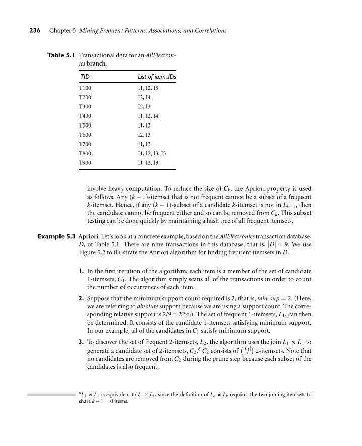
236 Chapter 5 Mining Frequent Patterns, Associations, and Correlations
Table 5.1 Transactional data for an AllElectron-ics branch.
TID List of item IDs
T100 I1, I2, I5
T200 I2, I4
T300 I2, I3
T400 I1, I2, I4
T500 I1, I3
T600 I2, I3
T700 I1, I3
T800 I1, I2, I3, I5
T900 I1, I2, I3
involve heavy computation. To reduce the size of Ck, the Apriori property is usedas follows. Any (k− 1)-itemset that is not frequent cannot be a subset of a frequentk-itemset. Hence, if any (k− 1)-subset of a candidate k-itemset is not in Lk−1, thenthe candidate cannot be frequent either and so can be removed from Ck. This subsettesting can be done quickly by maintaining a hash tree of all frequent itemsets.
Example 5.3 Apriori. Let’s look at a concrete example, based on the AllElectronics transaction database,D, of Table 5.1. There are nine transactions in this database, that is, |D| = 9. We useFigure 5.2 to illustrate the Apriori algorithm for finding frequent itemsets in D.
1. In the first iteration of the algorithm, each item is a member of the set of candidate1-itemsets, C1. The algorithm simply scans all of the transactions in order to countthe number of occurrences of each item.
2. Suppose that the minimum support count required is 2, that is, min sup = 2. (Here,we are referring to absolute support because we are using a support count. The corre-sponding relative support is 2/9 = 22%). The set of frequent 1-itemsets, L1, can thenbe determined. It consists of the candidate 1-itemsets satisfying minimum support.In our example, all of the candidates in C1 satisfy minimum support.
3. To discover the set of frequent 2-itemsets, L2, the algorithm uses the join L1 on L1 to
generate a candidate set of 2-itemsets, C2.8 C2 consists of(|L1|
2
)
2-itemsets. Note thatno candidates are removed from C2 during the prune step because each subset of thecandidates is also frequent.
8L1 on L1 is equivalent to L1×L1, since the definition of Lk on Lk requires the two joining itemsets toshare k−1 = 0 items.

5.2 Efficient and Scalable Frequent Itemset Mining Methods 237
Figure 5.2 Generation of candidate itemsets and frequent itemsets, where the minimum supportcount is 2.
4. Next, the transactions in D are scanned and the support count of each candidate item-set in C2 is accumulated, as shown in the middle table of the second row in Figure 5.2.
5. The set of frequent 2-itemsets, L2, is then determined, consisting of those candidate2-itemsets in C2 having minimum support.
6. The generation of the set of candidate 3-itemsets,C3, is detailed in Figure 5.3. From thejoin step, we first get C3 = L2 on L2 = {{I1, I2, I3}, {I1, I2, I5}, {I1, I3, I5}, {I2, I3, I4},{I2, I3, I5}, {I2, I4, I5}}. Based on the Apriori property that all subsets of a frequentitemset must also be frequent, we can determine that the four latter candidates cannotpossibly be frequent. We therefore remove them from C3, thereby saving the effort ofunnecessarily obtaining their counts during the subsequent scan of D to determine L3.Note that when given a candidate k-itemset, we only need to check if its (k−1)-subsetsare frequent since the Apriori algorithm uses a level-wise search strategy. The resultingpruned version of C3 is shown in the first table of the bottom row of Figure 5.2.
7. The transactions in D are scanned in order to determine L3, consisting of those can-didate 3-itemsets in C3 having minimum support (Figure 5.2).

238 Chapter 5 Mining Frequent Patterns, Associations, and Correlations
(a) Join: C3 = L2 on L2 = {{I1, I2}, {I1, I3}, {I1, I5}, {I2, I3}, {I2, I4}, {I2, I5}}on{{I1, I2}, {I1, I3}, {I1, I5}, {I2, I3}, {I2, I4}, {I2, I5}}
= {{I1, I2, I3}, {I1, I2, I5}, {I1, I3, I5}, {I2, I3, I4}, {I2, I3, I5}, {I2, I4, I5}}.
(b) Prune using the Apriori property: All nonempty subsets of a frequent itemset must also be frequent. Doany of the candidates have a subset that is not frequent?
The 2-item subsets of {I1, I2, I3} are {I1, I2}, {I1, I3}, and {I2, I3}. All 2-item subsets of {I1, I2,I3} are members of L2. Therefore, keep {I1, I2, I3} in C3.
The 2-item subsets of {I1, I2, I5} are {I1, I2}, {I1, I5}, and {I2, I5}. All 2-item subsets of {I1, I2,I5} are members of L2. Therefore, keep {I1, I2, I5} in C3.
The 2-item subsets of {I1, I3, I5} are {I1, I3}, {I1, I5}, and {I3, I5}. {I3, I5} is not a member of L2,and so it is not frequent. Therefore, remove {I1, I3, I5} from C3.
The 2-item subsets of {I2, I3, I4} are {I2, I3}, {I2, I4}, and {I3, I4}. {I3, I4} is not a member of L2,and so it is not frequent. Therefore, remove {I2, I3, I4} from C3.
The 2-item subsets of {I2, I3, I5} are {I2, I3}, {I2, I5}, and {I3, I5}. {I3, I5} is not a member of L2,and so it is not frequent. Therefore, remove {I2, I3, I5} from C3.
The 2-item subsets of {I2, I4, I5} are {I2, I4}, {I2, I5}, and {I4, I5}. {I4, I5} is not a member ofL2, and so it is not frequent. Therefore, remove {I2, I4, I5} from C3.
(c) Therefore, C3 = {{I1, I2, I3}, {I1, I2, I5}} after pruning.
Figure 5.3 Generation and pruning of candidate 3-itemsets, C3, from L2 using the Apriori property.
8. The algorithm uses L3 on L3 to generate a candidate set of 4-itemsets, C4. Althoughthe join results in {{I1, I2, I3, I5}}, this itemset is pruned because its subset {{I2, I3,I5}} is not frequent. Thus, C4 = φ, and the algorithm terminates, having found all ofthe frequent itemsets.
Figure 5.4 shows pseudo-code for the Apriori algorithm and its related procedures.Step 1 of Apriori finds the frequent 1-itemsets, L1. In steps 2 to 10, Lk−1 is usedto generate candidates Ck in order to find Lk for k ≥ 2. The apriori gen proceduregenerates the candidates and then uses the Apriori property to eliminate those havinga subset that is not frequent (step 3). This procedure is described below. Once allof the candidates have been generated, the database is scanned (step 4). For eachtransaction, a subset function is used to find all subsets of the transaction thatare candidates (step 5), and the count for each of these candidates is accumulated(steps 6 and 7). Finally, all of those candidates satisfying minimum support (step 9)form the set of frequent itemsets, L (step 11). A procedure can then be called togenerate association rules from the frequent itemsets. Such a procedure is describedin Section 5.2.2.
The apriori gen procedure performs two kinds of actions, namely, join and prune, asdescribed above. In the join component, Lk−1 is joined with Lk−1 to generate potentialcandidates (steps 1 to 4). The prune component (steps 5 to 7) employs the Apriori prop-erty to remove candidates that have a subset that is not frequent. The test for infrequentsubsets is shown in procedure has infrequent subset.

5.2 Efficient and Scalable Frequent Itemset Mining Methods 239
Algorithm: Apriori. Find frequent itemsets using an iterative level-wise approach based on candidategeneration.
Input:
D, a database of transactions;
min sup, the minimum support count threshold.
Output: L, frequent itemsets in D.
Method:
(1) L1 = find frequent 1-itemsets(D);(2) for (k = 2;Lk−1 6= φ;k++) {(3) Ck = apriori gen(Lk−1);(4) for each transaction t ∈ D { // scan D for counts(5) Ct = subset(Ck , t); // get the subsets of t that are candidates(6) for each candidate c ∈Ct(7) c.count++;(8) }(9) Lk = {c ∈Ck|c.count ≥min sup}(10) }(11) return L = ∪kLk ;
procedure apriori gen(Lk−1:frequent (k−1)-itemsets)(1) for each itemset l1 ∈ Lk−1(2) for each itemset l2 ∈ Lk−1(3) if (l1[1] = l2[1])∧ (l1[2] = l2[2])∧ ...∧ (l1[k−2] = l2[k−2])∧ (l1[k−1]< l2[k−1]) then {(4) c = l1 on l2; // join step: generate candidates(5) if has infrequent subset(c, Lk−1) then(6) delete c; // prune step: remove unfruitful candidate(7) else add c to Ck ;(8) }(9) return Ck ;
procedure has infrequent subset(c: candidate k-itemset;Lk−1: frequent (k−1)-itemsets); // use prior knowledge
(1) for each (k−1)-subset s of c(2) if s 6∈ Lk−1 then(3) return TRUE;(4) return FALSE;
Figure 5.4 The Apriori algorithm for discovering frequent itemsets for mining Boolean association rules.
5.2.2 Generating Association Rules from Frequent Itemsets
Once the frequent itemsets from transactions in a database D have been found,it is straightforward to generate strong association rules from them (where strongassociation rules satisfy both minimum support and minimum confidence). Thiscan be done using Equation (5.4) for confidence, which we show again here forcompleteness:
confidence(A⇒ B) = P(B|A) =support count(A∪B)
support count(A).

240 Chapter 5 Mining Frequent Patterns, Associations, and Correlations
The conditional probability is expressed in terms of itemset support count, wheresupport count(A∪B) is the number of transactions containing the itemsets A∪B, andsupport count(A) is the number of transactions containing the itemset A. Based on thisequation, association rules can be generated as follows:
For each frequent itemset l, generate all nonempty subsets of l.
For every nonempty subset s of l, output the rule “s⇒ (l− s)” if support count(l)support count(s) ≥
min conf, where min conf is the minimum confidence threshold.
Because the rules are generated from frequent itemsets, each one automatically sat-isfies minimum support. Frequent itemsets can be stored ahead of time in hash tablesalong with their counts so that they can be accessed quickly.
Example 5.4 Generating association rules. Let’s try an example based on the transactional datafor AllElectronics shown in Table 5.1. Suppose the data contain the frequent itemsetl = {I1, I2, I5}. What are the association rules that can be generated from l? Thenonempty subsets of l are {I1, I2}, {I1, I5}, {I2, I5}, {I1}, {I2}, and {I5}. Theresulting association rules are as shown below, each listed with its confidence:
I1∧ I2⇒ I5, confidence = 2/4 = 50%I1∧ I5⇒ I2, confidence = 2/2 = 100%I2∧ I5⇒ I1, confidence = 2/2 = 100%I1⇒ I2∧ I5, confidence = 2/6 = 33%I2⇒ I1∧ I5, confidence = 2/7 = 29%I5⇒ I1∧ I2, confidence = 2/2 = 100%
If the minimum confidence threshold is, say, 70%, then only the second, third, andlast rules above are output, because these are the only ones generated that are strong.Note that, unlike conventional classification rules, association rules can contain morethan one conjunct in the right-hand side of the rule.
5.2.3 Improving the Efficiency of Apriori
“How can we further improve the efficiency of Apriori-based mining?” Many variations ofthe Apriori algorithm have been proposed that focus on improving the efficiency of theoriginal algorithm. Several of these variations are summarized as follows:
Hash-based technique (hashing itemsets into corresponding buckets): A hash-basedtechnique can be used to reduce the size of the candidate k-itemsets, Ck, for k > 1.For example, when scanning each transaction in the database to generate the fre-quent 1-itemsets, L1, from the candidate 1-itemsets in C1, we can generate all of the2-itemsets for each transaction, hash (i.e., map) them into the different buckets ofa hash table structure, and increase the corresponding bucket counts (Figure 5.5).A 2-itemset whose corresponding bucket count in the hash table is below the support

5.2 Efficient and Scalable Frequent Itemset Mining Methods 241
bucket addressbucket countbucket contents
Create hash table H2using hash function
h(x, y) 5 ((order of x) 3101 (order of y)) mod 7
02
{I1, I4}{I3, I5}
12
{I1, I5}{I1, I5}
24
{I2, I3}{I2, I3}{I2, I3}{I2, I3}
32
{I2, I4}{I2, I4}
42
{I2, I5}{I2, I5}
54
{I1, I2}{I1, I2}{I1, I2}{I1, I2}
64
{I1, I3}{I1, I3}{I1, I3}{I1, I3}
H2
Figure 5.5 Hash table, H2, for candidate 2-itemsets: This hash table was generated by scanning the trans-actions of Table 5.1 while determining L1 from C1. If the minimum support count is, say, 3,then the itemsets in buckets 0, 1, 3, and 4 cannot be frequent and so they should not beincluded in C2.
threshold cannot be frequent and thus should be removed from the candidate set.Such a hash-based technique may substantially reduce the number of the candidatek-itemsets examined (especially when k = 2).
Transaction reduction (reducing the number of transactions scanned in future itera-tions): A transaction that does not contain any frequent k-itemsets cannot contain anyfrequent (k + 1)-itemsets. Therefore, such a transaction can be marked or removedfrom further consideration because subsequent scans of the database for j-itemsets,where j > k, will not require it.
Partitioning (partitioning the data to find candidate itemsets): A partitioning tech-nique can be used that requires just two database scans to mine the frequent itemsets(Figure 5.6). It consists of two phases. In Phase I, the algorithm subdivides the trans-actions of D into n nonoverlapping partitions. If the minimum support thresholdfor transactions in D is min sup, then the minimum support count for a partition ismin sup× the number of transactions in that partition. For each partition, all frequentitemsets within the partition are found. These are referred to as local frequent item-sets. The procedure employs a special data structure that, for each itemset, recordsthe TIDs of the transactions containing the items in the itemset. This allows it to findall of the local frequent k-itemsets, for k = 1, 2, . . . , in just one scan of the database.
A local frequent itemset may or may not be frequent with respect to the entiredatabase, D. Any itemset that is potentially frequent with respect to D must occur as afrequent itemset in at least one of the partitions. Therefore, all local frequent itemsetsare candidate itemsets with respect to D. The collection of frequent itemsets from allpartitions forms the global candidate itemsets with respect to D. In Phase II, a secondscan of D is conducted in which the actual support of each candidate is assessed inorder to determine the global frequent itemsets. Partition size and the number ofpartitions are set so that each partition can fit into main memory and therefore beread only once in each phase.
Sampling (mining on a subset of the given data): The basic idea of the samplingapproach is to pick a random sample S of the given data D, and then search for fre-quent itemsets in S instead of D. In this way, we trade off some degree of accuracy

242 Chapter 5 Mining Frequent Patterns, Associations, and Correlations
Transactions
in D
Frequent
itemsets
in D
Divide D
into n
partitions
Find the
frequent
itemsets
local to each
partition
(1 scan)
Combine
all local
frequent
itemsets
to form
candidate
itemset
Find global
frequent
itemsets
among
candidates
(1 scan)
Phase I Phase II
Figure 5.6 Mining by partitioning the data.
against efficiency. The sample size of S is such that the search for frequent itemsetsin S can be done in main memory, and so only one scan of the transactions in S isrequired overall. Because we are searching for frequent itemsets in S rather than in D,it is possible that we will miss some of the global frequent itemsets. To lessen this pos-sibility, we use a lower support threshold than minimum support to find the frequentitemsets local to S (denoted LS). The rest of the database is then used to compute theactual frequencies of each itemset in LS. A mechanism is used to determine whetherall of the global frequent itemsets are included in LS. If LS actually contains all of thefrequent itemsets in D, then only one scan of D is required. Otherwise, a second passcan be done in order to find the frequent itemsets that were missed in the first pass.The sampling approach is especially beneficial when efficiency is of utmost impor-tance, such as in computationally intensive applications that must be run frequently.
Dynamic itemset counting (adding candidate itemsets at different points during a scan):A dynamic itemset counting technique was proposed in which the database ispartitioned into blocks marked by start points. In this variation, new candidate item-sets can be added at any start point, unlike in Apriori, which determines new candi-date itemsets only immediately before each complete database scan. The technique isdynamic in that it estimates the support of all of the itemsets that have been countedso far, adding new candidate itemsets if all of their subsets are estimated to be fre-quent. The resulting algorithm requires fewer database scans than Apriori.
Other variations involving the mining of multilevel and multidimensional associationrules are discussed in the rest of this chapter. The mining of associations related to spatialdata and multimedia data are discussed in Chapter 10.
5.2.4 Mining Frequent Itemsets without Candidate Generation
As we have seen, in many cases the Apriori candidate generate-and-test method signifi-cantly reduces the size of candidate sets, leading to good performance gain. However, itcan suffer from two nontrivial costs:

5.2 Efficient and Scalable Frequent Itemset Mining Methods 243
It may need to generate a huge number of candidate sets. For example, if there are104 frequent 1-itemsets, the Apriori algorithm will need to generate more than 107
candidate 2-itemsets. Moreover, to discover a frequent pattern of size 100, such as{a1, . . . , a100}, it has to generate at least 2100−1≈ 1030 candidates in total.
It may need to repeatedly scan the database and check a large set of candidates by patternmatching. It is costly to go over each transaction in the database to determine thesupport of the candidate itemsets.
“Can we design a method that mines the complete set of frequent itemsets without candi-date generation?” An interesting method in this attempt is called frequent-pattern growth,or simply FP-growth, which adopts a divide-and-conquer strategy as follows. First, itcompresses the database representing frequent items into a frequent-pattern tree, orFP-tree, which retains the itemset association information. It then divides the compresseddatabase into a set of conditional databases (a special kind of projected database), eachassociated with one frequent item or “pattern fragment,” and mines each such databaseseparately. You’ll see how it works with the following example.
Example 5.5 FP-growth (finding frequent itemsets without candidate generation). We re-examinethe mining of transaction database, D, of Table 5.1 in Example 5.3 using the frequent-pattern growth approach.
The first scan of the database is the same as Apriori, which derives the set of fre-quent items (1-itemsets) and their support counts (frequencies). Let the minimum sup-port count be 2. The set of frequent items is sorted in the order of descending supportcount. This resulting set or list is denoted L. Thus, we have L ={{I2: 7}, {I1: 6}, {I3: 6},{I4: 2}, {I5: 2}}.
An FP-tree is then constructed as follows. First, create the root of the tree, labeled with“null.” Scan database D a second time. The items in each transaction are processed inL order (i.e., sorted according to descending support count), and a branch is created foreach transaction. For example, the scan of the first transaction, “T100: I1, I2, I5,” whichcontains three items (I2, I1, I5 in L order), leads to the construction of the first branch ofthe tree with three nodes, 〈I2: 1〉, 〈I1:1〉, and 〈I5: 1〉, where I2 is linked as a child of theroot, I1 is linked to I2, and I5 is linked to I1. The second transaction, T200, contains theitems I2 and I4 in L order, which would result in a branch where I2 is linked to the rootand I4 is linked to I2. However, this branch would share a common prefix, I2, with theexisting path for T100. Therefore, we instead increment the count of the I2 node by 1, andcreate a new node, 〈I4: 1〉, which is linked as a child of 〈I2: 2〉. In general, when consideringthe branch to be added for a transaction, the count of each node along a common prefixis incremented by 1, and nodes for the items following the prefix are created and linkedaccordingly.
To facilitate tree traversal, an item header table is built so that each item points to itsoccurrences in the tree via a chain of node-links. The tree obtained after scanning all ofthe transactions is shown in Figure 5.7 with the associated node-links. In this way, theproblem of mining frequent patterns in databases is transformed to that of mining theFP-tree.

244 Chapter 5 Mining Frequent Patterns, Associations, and Correlations
I2 I1 I3 I4 I5
7 6 6 2 2
I1:2
I3:2I4:1I3:2
I4:1
I5:1
I5:1
I1:4
I2:7
null{}
I3:2
Node-linkItem ID
Support count
Figure 5.7 An FP-tree registers compressed, frequent pattern information.
Table 5.2 Mining the FP-tree by creating conditional (sub-)pattern bases.
Item Conditional Pattern Base Conditional FP-tree Frequent Patterns Generated
I5 {{I2, I1: 1}, {I2, I1, I3: 1}} 〈I2: 2, I1: 2〉 {I2, I5: 2}, {I1, I5: 2}, {I2, I1, I5: 2}I4 {{I2, I1: 1}, {I2: 1}} 〈I2: 2〉 {I2, I4: 2}I3 {{I2, I1: 2}, {I2: 2}, {I1: 2}} 〈I2: 4, I1: 2〉, 〈I1: 2〉 {I2, I3: 4}, {I1, I3: 4}, {I2, I1, I3: 2}I1 {{I2: 4}} 〈I2: 4〉 {I2, I1: 4}
The FP-tree is mined as follows. Start from each frequent length-1 pattern (as an initialsuffix pattern), construct its conditional pattern base (a “subdatabase,” which consists ofthe set of prefix paths in the FP-tree co-occurring with the suffix pattern), then constructits (conditional) FP-tree, and perform mining recursively on such a tree. The patterngrowth is achieved by the concatenation of the suffix pattern with the frequent patternsgenerated from a conditional FP-tree.
Mining of the FP-tree is summarized in Table 5.2 and detailed as follows. We firstconsider I5, which is the last item in L, rather than the first. The reason for starting at theend of the list will become apparent as we explain the FP-tree mining process. I5 occursin two branches of the FP-tree of Figure 5.7. (The occurrences of I5 can easily be foundby following its chain of node-links.) The paths formed by these branches are 〈I2, I1,I5: 1〉 and 〈I2, I1, I3, I5: 1〉. Therefore, considering I5 as a suffix, its corresponding twoprefix paths are 〈I2, I1: 1〉 and 〈I2, I1, I3: 1〉, which form its conditional pattern base. Itsconditional FP-tree contains only a single path, 〈I2: 2, I1: 2〉; I3 is not included becauseits support count of 1 is less than the minimum support count. The single path generatesall the combinations of frequent patterns: {I2, I5: 2}, {I1, I5: 2}, {I2, I1, I5: 2}.
For I4, its two prefix paths form the conditional pattern base, {{I2 I1: 1}, {I2: 1}},which generates a single-node conditional FP-tree, 〈I2: 2〉, and derives one frequent

5.2 Efficient and Scalable Frequent Itemset Mining Methods 245
I2 I1
4 4
I2:4
I1:2
I1:2
Node-linkItem ID
Support count null{}
Figure 5.8 The conditional FP-tree associated with the conditional node I3.
pattern, {I2, I1: 2}. Notice that although I5 follows I4 in the first branch, there is noneed to include I5 in the analysis here because any frequent pattern involving I5 is ana-lyzed in the examination of I5.
Similar to the above analysis, I3’s conditional pattern base is {{I2, I1: 2}, {I2: 2},{I1: 2}}. Its conditional FP-tree has two branches, 〈I2: 4, I1: 2〉 and 〈I1: 2〉, as shown inFigure 5.8, which generates the set of patterns, {{I2, I3: 4}, {I1, I3: 4}, {I2, I1, I3: 2}}.Finally, I1’s conditional pattern base is {{I2: 4}}, whose FP-tree contains only onenode, 〈I2: 4〉, which generates one frequent pattern, {I2, I1: 4}. This mining processis summarized in Figure 5.9.
The FP-growth method transforms the problem of finding long frequent patterns tosearching for shorter ones recursively and then concatenating the suffix. It uses the leastfrequent items as a suffix, offering good selectivity. The method substantially reduces thesearch costs.
When the database is large, it is sometimes unrealistic to construct a main memory-based FP-tree. An interesting alternative is to first partition the database into a set of pro-jected databases, and then construct an FP-tree and mine it in each projected database.Such a process can be recursively applied to any projected database if its FP-tree stillcannot fit in main memory.
A study on the performance of the FP-growth method shows that it is efficient andscalable for mining both long and short frequent patterns, and is about an order of mag-nitude faster than the Apriori algorithm. It is also faster than a Tree-Projection algorithm,which recursively projects a database into a tree of projected databases.
5.2.5 Mining Frequent Itemsets Using Vertical Data Format
Both the Apriori and FP-growth methods mine frequent patterns from a set of transac-tions in TID-itemset format (that is, {T ID : itemset}), where TID is a transaction-id anditemset is the set of items bought in transaction TID. This data format is known as hori-zontal data format. Alternatively, data can also be presented in item-TID set format (thatis, {item : T ID set}), where item is an item name, and TID set is the set of transactionidentifiers containing the item. This format is known as vertical data format.
In this section, we look at how frequent itemsets can also be mined efficiently usingvertical data format, which is the essence of the ECLAT (Equivalence CLASS Transfor-mation) algorithm developed by Zaki [Zak00].

246 Chapter 5 Mining Frequent Patterns, Associations, and Correlations
Algorithm: FP growth. Mine frequent itemsets using an FP-tree by pattern fragment growth.
Input:
D, a transaction database;
min sup, the minimum support count threshold.
Output: The complete set of frequent patterns.
Method:
1. The FP-tree is constructed in the following steps:
(a) Scan the transaction database D once. Collect F , the set of frequent items, and their support counts.Sort F in support count descending order as L, the list of frequent items.
(b) Create the root of an FP-tree, and label it as “null.” For each transaction Trans in D do the following.
Select and sort the frequent items in Trans according to the order of L. Let the sorted frequent itemlist in Trans be [p|P], where p is the first element and P is the remaining list. Call insert tree([p|P], T ),which is performed as follows. If T has a child N such that N.item-name = p.item-name, then incrementN’s count by 1; else create a new node N, and let its count be 1, its parent link be linked to T , and itsnode-link to the nodes with the same item-name via the node-link structure. If P is nonempty, callinsert tree(P, N) recursively.
2. The FP-tree is mined by calling FP growth(FP tree, null), which is implemented as follows.
procedure FP growth(Tree, α)(1) if Tree contains a single path P then(2) for each combination (denoted as β) of the nodes in the path P(3) generate pattern β∪α with support count = minimum support count o f nodes in β;(4) else for each ai in the header of Tree {(5) generate pattern β = ai ∪α with support count = ai.support count;(6) construct β’s conditional pattern base and then β’s conditional FP tree Treeβ;(7) if Treeβ 6= /0 then(8) call FP growth(Treeβ, β); }
Figure 5.9 The FP-growth algorithm for discovering frequent itemsets without candidate generation.
Table 5.3 The vertical data format of the transaction data set D ofTable 5.1.
itemset TID set
I1 {T100, T400, T500, T700, T800, T900}I2 {T100, T200, T300, T400, T600, T800, T900}I3 {T300, T500, T600, T700, T800, T900}I4 {T200, T400}I5 {T100, T800}
Example 5.6 Mining frequent itemsets using vertical data format. Consider the horizontal data for-mat of the transaction database, D, of Table 5.1 in Example 5.3. This can be transformedinto the vertical data format shown in Table 5.3 by scanning the data set once.

5.2 Efficient and Scalable Frequent Itemset Mining Methods 247
Mining can be performed on this data set by intersecting the TID sets of every pair offrequent single items. The minimum support count is 2. Because every single item is fre-quent in Table 5.3, there are 10 intersections performed in total, which lead to 8 nonempty2-itemsets as shown in Table 5.4. Notice that because the itemsets{I1, I4}and{I3, I5} eachcontain only one transaction, they do not belong to the set of frequent 2-itemsets.
Based on the Apriori property, a given 3-itemset is a candidate 3-itemset only if everyone of its 2-itemset subsets is frequent. The candidate generation process here will gen-erate only two 3-itemsets: {I1, I2, I3} and {I1, I2, I5}. By intersecting the TID sets of anytwo corresponding 2-itemsets of these candidate 3-itemsets, it derives Table 5.5, wherethere are only two frequent 3-itemsets: {I1, I2, I3: 2} and {I1, I2, I5: 2}.
Example 5.6 illustrates the process of mining frequent itemsets by exploring the verti-cal data format. First, we transform the horizontally formatted data to the vertical formatby scanning the data set once. The support count of an itemset is simply the length of theTID set of the itemset. Starting with k = 1, the frequent k-itemsets can be used to con-struct the candidate (k +1)-itemsets based on the Apriori property. The computation isdone by intersection of the TID sets of the frequent k-itemsets to compute the TID setsof the corresponding (k+1)-itemsets. This process repeats, with k incremented by 1 eachtime, until no frequent itemsets or no candidate itemsets can be found.
Besides taking advantage of the Apriori property in the generation of candidate(k + 1)-itemset from frequent k-itemsets, another merit of this method is that there isno need to scan the database to find the support of (k + 1) itemsets (for k ≥ 1). This
Table 5.4 The 2-itemsets in vertical data format.
itemset TID set
{I1, I2} {T100, T400, T800, T900}{I1, I3} {T500, T700, T800, T900}{I1, I4} {T400}{I1, I5} {T100, T800}{I2, I3} {T300, T600, T800, T900}{I2, I4} {T200, T400}{I2, I5} {T100, T800}{I3, I5} {T800}
Table 5.5 The 3-itemsets in vertical dataformat.
itemset TID set
{I1, I2, I3} {T800, T900}{I1, I2, I5} {T100, T800}

248 Chapter 5 Mining Frequent Patterns, Associations, and Correlations
is because the TID set of each k-itemset carries the complete information required forcounting such support. However, the TID sets can be quite long, taking substantial mem-ory space as well as computation time for intersecting the long sets.
To further reduce the cost of registering long TID sets, as well as the subsequent costsof intersections, we can use a technique called diffset, which keeps track of only the differ-ences of the TID sets of a (k+1)-itemset and a corresponding k-itemset. For instance, inExample 5.6 we have {I1}= {T100, T400, T500, T700, T800, T900} and {I1, I2}= {T100,T400, T800, T900}. The diffset between the two is diffset({I1, I2}, {I1}) = {T500, T700}.Thus, rather than recording the four TIDs that make up the intersection of {I1} and{I2}, we can instead use diffset to record just two TIDs indicating the difference between{I1} and {I1, I2}. Experiments show that in certain situations, such as when the data setcontains many dense and long patterns, this technique can substantially reduce the totalcost of vertical format mining of frequent itemsets.
5.2.6 Mining Closed Frequent Itemsets
In Section 5.1.2 we saw how frequent itemset mining may generate a huge number offrequent itemsets, especially when the min sup threshold is set low or when there existlong patterns in the data set. Example 5.2 showed that closed frequent itemsets9 cansubstantially reduce the number of patterns generated in frequent itemset mining whilepreserving the complete information regarding the set of frequent itemsets. That is, fromthe set of closed frequent itemsets, we can easily derive the set of frequent itemsets andtheir support. Thus in practice, it is more desirable to mine the set of closed frequentitemsets rather than the set of all frequent itemsets in most cases.
“How can we mine closed frequent itemsets?” A naïve approach would be to first minethe complete set of frequent itemsets and then remove every frequent itemset that is aproper subset of, and carries the same support as, an existing frequent itemset. However,this is quite costly. As shown in Example 5.2, this method would have to first derive2100−1 frequent itemsets in order to obtain a length-100 frequent itemset, all before itcould begin to eliminate redundant itemsets. This is prohibitively expensive. In fact, thereexist only a very small number of closed frequent itemsets in the data set of Example 5.2.
A recommended methodology is to search for closed frequent itemsets directly duringthe mining process. This requires us to prune the search space as soon as we can identifythe case of closed itemsets during mining. Pruning strategies include the following:
Item merging: If every transaction containing a frequent itemset X also contains an itemsetY but not any proper superset of Y , then X ∪Y forms a frequent closed itemset and thereis no need to search for any itemset containing X but no Y .For example, in Table 5.2 of Example 5.5, the projected conditional database forprefix itemset {I5:2} is {{I2, I1},{I2, I1, I3}}, from which we can see that each of
9Remember that X is a closed frequent itemset in a data set S if there exists no proper super-itemset Ysuch that Y has the same support count as X in S, and X satisfies minimum support.

5.2 Efficient and Scalable Frequent Itemset Mining Methods 249
its transactions contains itemset {I2, I1} but no proper superset of {I2, I1}. Itemset{I2, I1} can be merged with {I5} to form the closed itemset, {I5, I2, I1: 2}, andwe do not need to mine for closed itemsets that contain I5 but not {I2, I1}.
Sub-itemset pruning: If a frequent itemset X is a proper subset of an already found frequentclosed itemset Y and support count(X) = support count(Y ), then X and all of X ’sdescendants in the set enumeration tree cannot be frequent closed itemsets and thus canbe pruned.Similar to Example 5.2, suppose a transaction database has only two transactions:{〈a1, a2, . . . , a100〉, 〈a1, a2, . . . , a50〉}, and the minimum support count is min sup =2. The projection on the first item, a1, derives the frequent itemset, {a1, a2, . . . , a50 :2}, based on the itemset merging optimization. Because support({a2}) = support({a1, a2, . . . , a50}) = 2, and {a2} is a proper subset of {a1, a2, . . . , a50}, there isno need to examine a2 and its projected database. Similar pruning can be donefor a3, . . . , a50 as well. Thus the mining of closed frequent itemsets in this data setterminates after mining a1’s projected database.
Item skipping: In the depth-first mining of closed itemsets, at each level, there will be aprefix itemset X associated with a header table and a projected database. If a local fre-quent item p has the same support in several header tables at different levels, we cansafely prune p from the header tables at higher levels.Consider, for example, the transaction database above having only two transactions:{〈a1, a2, . . . , a100〉, 〈a1, a2, . . . , a50〉}, where min sup = 2. Because a2 in a1’s projecteddatabase has the same support as a2 in the global header table, a2 can be pruned fromthe global header table. Similar pruning can be done for a3, . . . , a50. There is no needto mine anything more after mining a1’s projected database.
Besides pruning the search space in the closed itemset mining process, another impor-tant optimization is to perform efficient checking of a newly derived frequent itemset tosee whether it is closed, because the mining process cannot ensure that every generatedfrequent itemset is closed.
When a new frequent itemset is derived, it is necessary to perform two kinds of closurechecking: (1) superset checking, which checks if this new frequent itemset is a superset ofsome already found closed itemsets with the same support, and (2) subset checking, whichchecks whether the newly found itemset is a subset of an already found closed itemsetwith the same support.
If we adopt the item merging pruning method under a divide-and-conquer frame-work, then the superset checking is actually built-in and there is no need to explicitlyperform superset checking. This is because if a frequent itemset X ∪Y is found later thanitemset X , and carries the same support as X , it must be in X ’s projected database andmust have been generated during itemset merging.
To assist in subset checking, a compressed pattern-tree can be constructed to main-tain the set of closed itemsets mined so far. The pattern-tree is similar in structure to theFP-tree except that all of the closed itemsets found are stored explicitly in the correspond-ing tree branches. For efficient subset checking, we can use the following property: If the

250 Chapter 5 Mining Frequent Patterns, Associations, and Correlations
current itemset Sc can be subsumed by another already found closed itemset Sa, then (1) Scand Sa have the same support, (2) the length of Sc is smaller than that of Sa, and (3) all ofthe items in Sc are contained in Sa. Based on this property, a two-level hash index struc-ture can be built for fast accessing of the pattern-tree: The first level uses the identifierof the last item in Sc as a hash key (since this identifier must be within the branch of Sc),and the second level uses the support of Sc as a hash key (since Sc and Sa have the samesupport). This will substantially speed up the subset checking process.
The above discussion illustrates methods for efficient mining of closed frequent item-sets. “Can we extend these methods for efficient mining of maximal frequent itemsets?”Because maximal frequent itemsets share many similarities with closed frequent item-sets, many of the optimization techniques developed here can be extended to miningmaximal frequent itemsets. However, we leave this method as an exercise for interestedreaders.
5.3 Mining Various Kinds of Association Rules
We have studied efficient methods for mining frequent itemsets and association rules.In this section, we consider additional application requirements by extending our scopeto include mining multilevel association rules, multidimensional association rules, andquantitative association rules in transactional and/or relational databases and datawarehouses. Multilevel association rules involve concepts at different levels of abstrac-tion. Multidimensional association rules involve more than one dimension or predicate(e.g., rules relating what a customer buys as well as the customer’s age.) Quantitativeassociation rules involve numeric attributes that have an implicit ordering among values(e.g., age).
5.3.1 Mining Multilevel Association Rules
For many applications, it is difficult to find strong associations among data items at lowor primitive levels of abstraction due to the sparsity of data at those levels. Strong associ-ations discovered at high levels of abstraction may represent commonsense knowledge.Moreover, what may represent common sense to one user may seem novel to another.Therefore, data mining systems should provide capabilities for mining association rulesat multiple levels of abstraction, with sufficient flexibility for easy traversal among dif-ferent abstraction spaces.
Let’s examine the following example.
Example 5.7 Mining multilevel association rules. Suppose we are given the task-relevant set of trans-actional data in Table 5.6 for sales in an AllElectronics store, showing the items purchasedfor each transaction. The concept hierarchy for the items is shown in Figure 5.10. A con-cept hierarchy defines a sequence of mappings from a set of low-level concepts to higher-level, more general concepts. Data can be generalized by replacing low-level conceptswithin the data by their higher-level concepts, or ancestors, from a concept hierarchy.

5.3 Mining Various Kinds of Association Rules 251
Table 5.6 Task-relevant data, D.
TID Items Purchased
T100 IBM-ThinkPad-T40/2373, HP-Photosmart-7660
T200 Microsoft-Office-Professional-2003, Microsoft-Plus!-Digital-Media
T300 Logitech-MX700-Cordless-Mouse, Fellowes-Wrist-Rest
T400 Dell-Dimension-XPS, Canon-PowerShot-S400
T500 IBM-ThinkPad-R40/P4M, Symantec-Norton-Antivirus-2003
. . . . . .
all
Figure 5.10 A concept hierarchy for AllElectronics computer items.
The concept hierarchy of Figure 5.10 has five levels, respectively referred to as levels 0to 4, starting with level 0 at the root node for all (the most general abstraction level).Here, level 1 includes computer, software, printer&camera, and computer accessory, level2 includes laptop computer, desktop computer, office software, antivirus software, . . . , andlevel 3 includes IBM desktop computer, . . . , Microsoft office software, and so on. Level 4 isthe most specific abstraction level of this hierarchy. It consists of the raw data values. Con-cept hierarchies for categorical attributes are often implicit within the database schema,in which case they may be automatically generated using methods such as those describedin Chapter 2. For our example, the concept hierarchy of Figure 5.10 was generated fromdata on product specifications. Concept hierarchies for numerical attributes can be gen-erated using discretization techniques, many of which were introduced in Chapter 2.Alternatively, concept hierarchies may be specified by users familiar with the data, suchas store managers in the case of our example.
The items in Table 5.6 are at the lowest level of the concept hierarchy of Figure 5.10.It is difficult to find interesting purchase patterns at such raw or primitive-level data.For instance, if “IBM-ThinkPad-R40/P4M” or “Symantec-Norton-Antivirus-2003” each

252 Chapter 5 Mining Frequent Patterns, Associations, and Correlations
occurs in a very small fraction of the transactions, then it can be difficult to find strongassociations involving these specific items. Few people may buy these items together,making it unlikely that the itemset will satisfy minimum support. However, we wouldexpect that it is easier to find strong associations between generalized abstractions ofthese items, such as between “IBM laptop computer” and “antivirus software.”
Association rules generated from mining data at multiple levels of abstraction arecalled multiple-level or multilevel association rules. Multilevel association rules canbe mined efficiently using concept hierarchies under a support-confidence framework.In general, a top-down strategy is employed, where counts are accumulated for thecalculation of frequent itemsets at each concept level, starting at the concept level1 and working downward in the hierarchy toward the more specific concept levels,until no more frequent itemsets can be found. For each level, any algorithm fordiscovering frequent itemsets may be used, such as Apriori or its variations. A numberof variations to this approach are described below, where each variation involves“playing” with the support threshold in a slightly different way. The variations areillustrated in Figures 5.11 and 5.12, where nodes indicate an item or itemset thathas been examined, and nodes with thick borders indicate that an examined item oritemset is frequent.
Using uniform minimum support for all levels (referred to as uniform support):The same minimum support threshold is used when mining at each level ofabstraction. For example, in Figure 5.11, a minimum support threshold of 5% isused throughout (e.g., for mining from “computer” down to “laptop computer”).Both “computer” and “laptop computer” are found to be frequent, while “desktopcomputer” is not.
When a uniform minimum support threshold is used, the search procedure issimplified. The method is also simple in that users are required to specify only oneminimum support threshold. An Apriori-like optimization technique can be adopted,based on the knowledge that an ancestor is a superset of its descendants: The searchavoids examining itemsets containing any item whose ancestors do not have mini-mum support.
computer [support 5 10%]
laptop computer [support 5 6%]
Level 1 min_sup 5 5%
Level 2 min_sup 55%
desktop computer [support 5 4%]
Figure 5.11 Multilevel mining with uniform support.

5.3 Mining Various Kinds of Association Rules 253
computer [support 5 10%]
laptop computer [support 5 6%]
Level 1 min_sup 5 5%
Level 2 min_sup 5 3%
desktop computer [support 5 4%]
Figure 5.12 Multilevel mining with reduced support.
The uniform support approach, however, has some difficulties. It is unlikely thatitems at lower levels of abstraction will occur as frequently as those at higher levelsof abstraction. If the minimum support threshold is set too high, it could miss somemeaningful associations occurring at low abstraction levels. If the threshold is set toolow, it may generate many uninteresting associations occurring at high abstractionlevels. This provides the motivation for the following approach.
Using reduced minimum support at lower levels (referred to as reduced support):Each level of abstraction has its own minimum support threshold. The deeperthe level of abstraction, the smaller the corresponding threshold is. For example,in Figure 5.12, the minimum support thresholds for levels 1 and 2 are 5% and 3%,respectively. In this way, “computer,” “laptop computer,” and “desktop computer” areall considered frequent.
Using item or group-based minimum support (referred to as group-based support):Because users or experts often have insight as to which groups are more importantthan others, it is sometimes more desirable to set up user-specific, item, or group-based minimal support thresholds when mining multilevel rules. For example, a usercould set up the minimum support thresholds based on product price, or on items ofinterest, such as by setting particularly low support thresholds for laptop computersand flash drives in order to pay particular attention to the association patterns con-taining items in these categories.
Notice that the Apriori property may not always hold uniformly across all of the itemswhen mining under reduced support and group-based support. However, efficient meth-ods can be developed based on the extension of the property. The details are left as anexercise for interested readers.
A serious side effect of mining multilevel association rules is its generation of manyredundant rules across multiple levels of abstraction due to the “ancestor” relationshipsamong items. For example, consider the following rules where “laptop computer” isan ancestor of “IBM laptop computer” based on the concept hierarchy of Figure 5.10,and where X is a variable representing customers who purchased items in AllElectronicstransactions.

254 Chapter 5 Mining Frequent Patterns, Associations, and Correlations
buys(X , “laptop computer”)⇒ buys(X , “HP printer”)[support = 8%, confidence = 70%] (5.10)
buys(X , “IBM laptop computer”)⇒ buys(X , “HP printer”)[support = 2%, confidence = 72%] (5.11)
“If Rules (5.10) and (5.11) are both mined, then how useful is the latter rule?” youmay wonder. “Does it really provide any novel information?” If the latter, less generalrule does not provide new information, then it should be removed. Let’s look at howthis may be determined. A rule R1 is an ancestor of a rule R2, if R1 can be obtainedby replacing the items in R2 by their ancestors in a concept hierarchy. For example,Rule (5.10) is an ancestor of Rule (5.11) because “laptop computer” is an ancestor of“IBM laptop computer.” Based on this definition, a rule can be considered redundantif its support and confidence are close to their “expected” values, based on an ancestorof the rule. As an illustration, suppose that Rule (5.10) has a 70% confidence and 8%support, and that about one-quarter of all “laptop computer” sales are for “IBM laptopcomputers.” We may expect Rule (5.11) to have a confidence of around 70% (sinceall data samples of “IBM laptop computer” are also samples of “laptop computer”) anda support of around 2% (i.e., 8%× 1
4 ). If this is indeed the case, then Rule (5.11) isnot interesting because it does not offer any additional information and is less generalthan Rule (5.10).
5.3.2 Mining Multidimensional Association Rulesfrom Relational Databases and Data Warehouses
So far in this chapter, we have studied association rules that imply a single predicate,that is, the predicate buys. For instance, in mining our AllElectronics database, we maydiscover the Boolean association rule
buys(X , “digital camera”)⇒ buys(X , “HP printer”). (5.12)
Following the terminology used in multidimensional databases, we refer to each dis-tinct predicate in a rule as a dimension. Hence, we can refer to Rule (5.12) as a single-dimensional or intradimensional association rule because it contains a single distinctpredicate (e.g., buys) with multiple occurrences (i.e., the predicate occurs more than oncewithin the rule). As we have seen in the previous sections of this chapter, such rules arecommonly mined from transactional data.
Suppose, however, that rather than using a transactional database, sales and relatedinformation are stored in a relational database or data warehouse. Such data stores aremultidimensional, by definition. For instance, in addition to keeping track of the itemspurchased in sales transactions, a relational database may record other attributes associ-ated with the items, such as the quantity purchased or the price, or the branch location ofthe sale. Additional relational information regarding the customers who purchased theitems, such as customer age, occupation, credit rating, income, and address, may also be

5.3 Mining Various Kinds of Association Rules 255
stored. Considering each database attribute or warehouse dimension as a predicate, wecan therefore mine association rules containing multiple predicates, such as
age(X , “20...29”)∧ occupation(X , “student”)⇒buys(X , “laptop”). (5.13)
Association rules that involve two or more dimensions or predicates can be referred toas multidimensional association rules. Rule (5.13) contains three predicates (age, occu-pation, and buys), each of which occurs only once in the rule. Hence, we say that it has norepeated predicates. Multidimensional association rules with no repeated predicates arecalled interdimensional association rules. We can also mine multidimensional associa-tion rules with repeated predicates, which contain multiple occurrences of some predi-cates. These rules are called hybrid-dimensional association rules. An example of sucha rule is the following, where the predicate buys is repeated:
age(X , “20...29”)∧buys(X , “laptop”)⇒buys(X , “HP printer”) (5.14)
Note that database attributes can be categorical or quantitative. Categorical attributeshave a finite number of possible values, with no ordering among the values (e.g., occu-pation, brand, color). Categorical attributes are also called nominal attributes, becausetheir values are “names of things.” Quantitative attributes are numeric and have animplicit ordering among values (e.g., age, income, price). Techniques for mining mul-tidimensional association rules can be categorized into two basic approaches regardingthe treatment of quantitative attributes.
In the first approach, quantitative attributes are discretized using predefined concepthierarchies. This discretization occurs before mining. For instance, a concept hierarchyfor income may be used to replace the original numeric values of this attribute by intervallabels, such as “0. . . 20K”, “21K . . . 30K”, “31K . . . 40K”, and so on. Here, discretizationis static and predetermined. Chapter 2 on data preprocessing gave several techniques fordiscretizing numeric attributes. The discretized numeric attributes, with their intervallabels, can then be treated as categorical attributes (where each interval is considereda category). We refer to this as mining multidimensional association rules using staticdiscretization of quantitative attributes.
In the second approach, quantitative attributes are discretized or clustered into “bins”based on the distribution of the data. These bins may be further combined during themining process. The discretization process is dynamic and established so as to satisfysome mining criteria, such as maximizing the confidence of the rules mined. Becausethis strategy treats the numeric attribute values as quantities rather than as predefinedranges or categories, association rules mined from this approach are also referred to as(dynamic) quantitative association rules.
Let’s study each of these approaches for mining multidimensional association rules.For simplicity, we confine our discussion to interdimensional association rules. Note thatrather than searching for frequent itemsets (as is done for single-dimensional associationrule mining), in multidimensional association rule mining we search for frequent pred-icate sets. A k-predicate set is a set containing k conjunctive predicates. For instance, theset of predicates {age, occupation, buys} from Rule (5.13) is a 3-predicate set. Similar
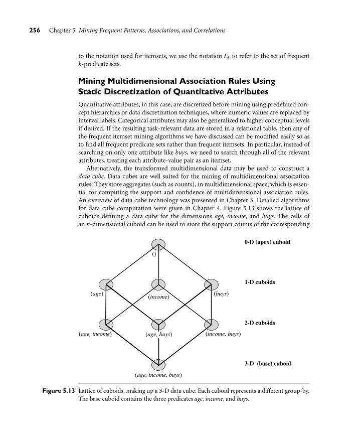
256 Chapter 5 Mining Frequent Patterns, Associations, and Correlations
to the notation used for itemsets, we use the notation Lk to refer to the set of frequentk-predicate sets.
Mining Multidimensional Association Rules UsingStatic Discretization of Quantitative AttributesQuantitative attributes, in this case, are discretized before mining using predefined con-cept hierarchies or data discretization techniques, where numeric values are replaced byinterval labels. Categorical attributes may also be generalized to higher conceptual levelsif desired. If the resulting task-relevant data are stored in a relational table, then any ofthe frequent itemset mining algorithms we have discussed can be modified easily so asto find all frequent predicate sets rather than frequent itemsets. In particular, instead ofsearching on only one attribute like buys, we need to search through all of the relevantattributes, treating each attribute-value pair as an itemset.
Alternatively, the transformed multidimensional data may be used to construct adata cube. Data cubes are well suited for the mining of multidimensional associationrules: They store aggregates (such as counts), in multidimensional space, which is essen-tial for computing the support and confidence of multidimensional association rules.An overview of data cube technology was presented in Chapter 3. Detailed algorithmsfor data cube computation were given in Chapter 4. Figure 5.13 shows the lattice ofcuboids defining a data cube for the dimensions age, income, and buys. The cells ofan n-dimensional cuboid can be used to store the support counts of the corresponding
(income) (buys)(age)
()
(income, buys)
(age, income, buys)
(age, income) (age, buys)
0-D (apex) cuboid
1-D cuboids
2-D cuboids
3-D (base) cuboid
Figure 5.13 Lattice of cuboids, making up a 3-D data cube. Each cuboid represents a different group-by.The base cuboid contains the three predicates age, income, and buys.

5.3 Mining Various Kinds of Association Rules 257
n-predicate sets. The base cuboid aggregates the task-relevant data by age, income, andbuys; the 2-D cuboid, (age, income), aggregates by age and income, and so on; the 0-D(apex) cuboid contains the total number of transactions in the task-relevant data.
Due to the ever-increasing use of data warehouse and OLAP technology, it ispossible that a data cube containing the dimensions that are of interest to the usermay already exist, fully materialized. If this is the case, we can simply fetch thecorresponding aggregate values and return the rules needed using a rule generationalgorithm (Section 5.2.2). Notice that even in this case, the Apriori property can stillbe used to prune the search space. If a given k-predicate set has support sup, whichdoes not satisfy minimum support, then further exploration of this set should beterminated. This is because any more specialized version of the k-itemset will havesupport no greater that sup and, therefore, will not satisfy minimum support either.In cases where no relevant data cube exists for the mining task, we must create oneon the fly. This becomes an iceberg cube computation problem, where the minimumsupport threshold is taken as the iceberg condition (Chapter 4).
Mining Quantitative Association RulesQuantitative association rules are multidimensional association rules in which thenumeric attributes are dynamically discretized during the mining process so as to sat-isfy some mining criteria, such as maximizing the confidence or compactness of the rulesmined. In this section, we focus specifically on how to mine quantitative association ruleshaving two quantitative attributes on the left-hand side of the rule and one categoricalattribute on the right-hand side of the rule. That is,
Aquan1∧Aquan2⇒ Acat
where Aquan1 and Aquan2 are tests on quantitative attribute intervals (where the intervalsare dynamically determined), and Acat tests a categorical attribute from the task-relevantdata. Such rules have been referred to as two-dimensional quantitative association rules,because they contain two quantitative dimensions. For instance, suppose you are curiousabout the association relationship between pairs of quantitative attributes, like customerage and income, and the type of television (such as high-definition TV, i.e., HDTV) thatcustomers like to buy. An example of such a 2-D quantitative association rule is
age(X , “30...39”)∧ income(X , “42K...48K”)⇒buys(X , “HDTV”) (5.15)
“How can we find such rules?” Let’s look at an approach used in a system called ARCS(Association Rule Clustering System), which borrows ideas from image processing.Essentially, this approach maps pairs of quantitative attributes onto a 2-D grid for tuplessatisfying a given categorical attribute condition. The grid is then searched for clusters ofpoints from which the association rules are generated. The following steps are involvedin ARCS:
Binning: Quantitative attributes can have a very wide range of values defining theirdomain. Just think about how big a 2-D grid would be if we plotted age and income as

258 Chapter 5 Mining Frequent Patterns, Associations, and Correlations
axes, where each possible value of age was assigned a unique position on one axis, andsimilarly, each possible value of income was assigned a unique position on the otheraxis! To keep grids down to a manageable size, we instead partition the ranges of quan-titative attributes into intervals. These intervals are dynamic in that they may later befurther combined during the mining process. The partitioning process is referred toas binning, that is, where the intervals are considered “bins.” Three common binningstrategies area as follows:
Equal-width binning, where the interval size of each bin is the same
Equal-frequency binning, where each bin has approximately the same number oftuples assigned to it,
Clustering-based binning, where clustering is performed on the quantitative attri-bute to group neighboring points (judged based on various distance measures) intothe same bin
ARCS uses equal-width binning, where the bin size for each quantitative attributeis input by the user. A 2-D array for each possible bin combination involving bothquantitative attributes is created. Each array cell holds the corresponding count dis-tribution for each possible class of the categorical attribute of the rule right-hand side.By creating this data structure, the task-relevant data need only be scanned once. Thesame 2-D array can be used to generate rules for any value of the categorical attribute,based on the same two quantitative attributes. Binning is also discussed in Chapter 2.
Finding frequent predicate sets: Once the 2-D array containing the count distributionfor each category is set up, it can be scanned to find the frequent predicate sets (thosesatisfying minimum support) that also satisfy minimum confidence. Strong associ-ation rules can then be generated from these predicate sets, using a rule generationalgorithm like that described in Section 5.2.2.
Clustering the association rules: The strong association rules obtained in the previousstep are then mapped to a 2-D grid. Figure 5.14 shows a 2-D grid for 2-D quantitativeassociation rules predicting the condition buys(X, “HDTV”) on the rule right-handside, given the quantitative attributes age and income. The four Xs correspond to therules
age(X , 34)∧ income(X , “31K...40K”)⇒buys(X , “HDTV”) (5.16)
age(X , 35)∧ income(X , “31K...40K”)⇒buys(X , “HDTV”) (5.17)
age(X , 34)∧ income(X , “41K...50K”)⇒buys(X , “HDTV”) (5.18)
age(X , 35)∧ income(X , “41K...50K”)⇒buys(X , “HDTV”). (5.19)
“Can we find a simpler rule to replace the above four rules?” Notice that these rules arequite “close” to one another, forming a rule cluster on the grid. Indeed, the four rulescan be combined or “clustered” together to form the following simpler rule, whichsubsumes and replaces the above four rules:

5.4 From Association Mining to Correlation Analysis 259
inco
me
71K...80K
61K...70K
51K...60K
41K...50K
31K...40K
21K...30K
<520K
32 33 34 35 36 37 38age
Figure 5.14 A 2-D grid for tuples representing customers who purchase high-definition TVs.
age(X , “34...35”)∧ income(X , “31K...50K”)⇒buys(X , “HDTV”) (5.20)
ARCS employs a clustering algorithm for this purpose. The algorithm scans thegrid, searching for rectangular clusters of rules. In this way, bins of the quantita-tive attributes occurring within a rule cluster may be further combined, and hencefurther dynamic discretization of the quantitative attributes occurs.
The grid-based technique described here assumes that the initial association rulescan be clustered into rectangular regions. Before performing the clustering, smoothingtechniques can be used to help remove noise and outliers from the data. Rectangularclusters may oversimplify the data. Alternative approaches have been proposed, based onother shapes of regions that tend to better fit the data, yet require greater computationeffort.
A non-grid-based technique has been proposed to find quantitative association rulesthat are more general, where any number of quantitative and categorical attributes canappear on either side of the rules. In this technique, quantitative attributes are dynami-cally partitioned using equal-frequency binning, and the partitions are combined basedon a measure of partial completeness, which quantifies the information lost due to parti-tioning. For references on these alternatives to ARCS, see the bibliographic notes.
5.4 From Association Mining to Correlation Analysis
Most association rule mining algorithms employ a support-confidence framework.Often, many interesting rules can be found using low support thresholds. Althoughminimum support and confidence thresholds help weed out or exclude the exploration

260 Chapter 5 Mining Frequent Patterns, Associations, and Correlations
of a good number of uninteresting rules, many rules so generated are still not interestingto the users. Unfortunately, this is especially true when mining at low support thresholdsor mining for long patterns. This has been one of the major bottlenecks for successfulapplication of association rule mining.
In this section, we first look at how even strong association rules can be uninterestingand misleading. We then discuss how the support-confidence framework can be sup-plemented with additional interestingness measures based on statistical significance andcorrelation analysis.
5.4.1 Strong Rules Are Not Necessarily Interesting: An Example
Whether or not a rule is interesting can be assessed either subjectively or objectively.Ultimately, only the user can judge if a given rule is interesting, and this judgment, beingsubjective, may differ from one user to another. However, objective interestingness mea-sures, based on the statistics “behind” the data, can be used as one step toward the goalof weeding out uninteresting rules from presentation to the user.
“How can we tell which strong association rules are really interesting?” Let’s examine thefollowing example.
Example 5.8 A misleading “strong” association rule. Suppose we are interested in analyzing transac-tions at AllElectronics with respect to the purchase of computer games and videos. Letgame refer to the transactions containing computer games, and video refer to those con-taining videos. Of the 10,000 transactions analyzed, the data show that 6,000 of the cus-tomer transactions included computer games, while 7,500 included videos, and 4,000included both computer games and videos. Suppose that a data mining program for dis-covering association rules is run on the data, using a minimum support of, say, 30% anda minimum confidence of 60%. The following association rule is discovered:
buys(X , “computer games”)⇒buys(X , “videos”) [support = 40%, confidence = 66%](5.21)
Rule (5.21) is a strong association rule and would therefore be reported, since its supportvalue of 4,000
10,000 = 40% and confidence value of 4,0006,000 = 66% satisfy the minimum support
and minimum confidence thresholds, respectively. However, Rule (5.21) is misleadingbecause the probability of purchasing videos is 75%, which is even larger than 66%. Infact, computer games and videos are negatively associated because the purchase of oneof these items actually decreases the likelihood of purchasing the other. Without fullyunderstanding this phenomenon, we could easily make unwise business decisions basedon Rule (5.21).
The above example also illustrates that the confidence of a rule A⇒B can be deceivingin that it is only an estimate of the conditional probability of itemset B given itemset A.It does not measure the real strength (or lack of strength) of the correlation and impli-cation between A and B. Hence, alternatives to the support-confidence framework canbe useful in mining interesting data relationships.

5.4 From Association Mining to Correlation Analysis 261
5.4.2 From Association Analysis to Correlation Analysis
As we have seen above, the support and confidence measures are insufficient at filteringout uninteresting association rules. To tackle this weakness, a correlation measure canbe used to augment the support-confidence framework for association rules. This leadsto correlation rules of the form
A⇒ B [support, confidence. correlation]. (5.22)
That is, a correlation rule is measured not only by its support and confidence but alsoby the correlation between itemsets A and B. There are many different correlation mea-sures from which to choose. In this section, we study various correlation measures todetermine which would be good for mining large data sets.
Lift is a simple correlation measure that is given as follows. The occurrence of itemsetA is independent of the occurrence of itemset B if P(A∪ B) = P(A)P(B); otherwise,itemsets A and B are dependent and correlated as events. This definition can easily beextended to more than two itemsets. The lift between the occurrence of A and B can bemeasured by computing
lift(A, B) =P(A∪B)P(A)P(B)
. (5.23)
If the resulting value of Equation (5.23) is less than 1, then the occurrence of A is neg-atively correlated with the occurrence of B. If the resulting value is greater than 1, thenA and B are positively correlated, meaning that the occurrence of one implies the occur-rence of the other. If the resulting value is equal to 1, then A and B are independent andthere is no correlation between them.
Equation (5.23) is equivalent to P(B|A)/P(B), or con f (A⇒ B)/sup(B), which is alsoreferred as the lift of the association (or correlation) rule A⇒B. In other words, it assessesthe degree to which the occurrence of one “lifts” the occurrence of the other. For example,if A corresponds to the sale of computer games and B corresponds to the sale of videos,then given the current market conditions, the sale of games is said to increase or “lift”the likelihood of the sale of videos by a factor of the value returned by Equation (5.23).
Let’s go back to the computer game and video data of Example 5.8.
Example 5.9 Correlation analysis using lift. To help filter out misleading “strong” associations of theform A⇒B from the data of Example 5.8, we need to study how the two itemsets, A andB, are correlated. Let game refer to the transactions of Example 5.8 that do not containcomputer games, and video refer to those that do not contain videos. The transactionscan be summarized in a contingency table, as shown in Table 5.7. From the table, wecan see that the probability of purchasing a computer game is P({game}) = 0.60, theprobability of purchasing a video is P({video}) = 0.75, and the probability of pur-chasing both is P({game,video}) = 0.40. By Equation (5.23), the lift of Rule (5.21)is P({game, video})/(P({game})×P({video})) = 0.40/(0.60×0.75) = 0.89. Becausethis value is less than 1, there is a negative correlation between the occurrence of {game}and {video}. The numerator is the likelihood of a customer purchasing both, while the

262 Chapter 5 Mining Frequent Patterns, Associations, and Correlations
Table 5.7 A 2 × 2 contingency table summarizing the trans-actions with respect to game and video purchases.
game game Σrow
video 4,000 3,500 7,500
video 2,000 500 2,500
Σcol 6,000 4,000 10,000
Table 5.8 The above contingency table, now shown with the expected values.
game game Σrow
video 4,000 (4,500) 3,500 (3,000) 7,500
video 2,000 (1,500) 500 (1,000) 2,500
Σcol 6,000 4,000 10,000
denominator is what the likelihood would have been if the two purchases were com-pletely independent. Such a negative correlation cannot be identified by a support-confidence framework.
The second correlation measure that we study is the χ2 measure, which was intro-duced in Chapter 2 (Equation 2.9). To compute the χ2 value, we take the squared differ-ence between the observed and expected value for a slot (A and B pair) in the contingencytable, divided by the expected value. This amount is summed for all slots of the contin-gency table. Let’s perform a χ2 analysis of the above example.
Example 5.10 Correlation analysis using χ2. To compute the correlation using χ2 analysis, we needthe observed value and expected value (displayed in parenthesis) for each slot of thecontingency table, as shown in Table 5.8. From the table, we can compute the χ2 valueas follows:
χ2 = Σ(observed - expected)2
expected=
(4,000−4,500)2
4,500+
(3,500−3,000)2
3,000+
(2,000−1,500)2
1,500+
(500−1,000)2
1,000= 555.6.
Because the χ2 value is greater than one, and the observed value of the slot (game, video) =4,000, which is less than the expected value 4,500, buying game and buying video arenegatively correlated. This is consistent with the conclusion derived from the analysis ofthe lift measure in Example 5.9.
Let’s examine two other correlation measures, all confidence and cosine, as definedbelow.

5.4 From Association Mining to Correlation Analysis 263
Given an itemset X = {i1, i2, . . . , ik}, the all confidence of X is defined as
all conf(X) =sup(X)
max item sup(X)=
sup(X)max{sup(i j)|∀i j ∈ X}
, (5.24)
where max{sup(i j)|∀i j ∈ X} is the maximum (single) item support of all the items inX , and hence is called the max item sup of the itemset X . The all confidence of X is theminimal confidence among the set of rules i j→ X− i j, where i j ∈ X .
Given two itemsets A and B, the cosine measure of A and B is defined as
cosine(A, B) =P(A∪B)
√
P(A)×P(B)=
sup(A∪B)√
sup(A)× sup(B). (5.25)
The cosine measure can be viewed as a harmonized lift measure: the two formulae aresimilar except that for cosine, the square root is taken on the product of the probabilitiesof A and B. This is an important difference, however, because by taking the square root,the cosine value is only influenced by the supports of A, B, and A∪B, and not by thetotal number of transactions.
“Are these two measures better than lift and χ2 in assessing the correlation relationship?”To answer this question, we first look at some other typical data sets before returning toour running example.
Example 5.11 Comparison of four correlation measures on typical data sets. The correlation relation-ships between the purchases of two items, milk and coffee, can be examined by summa-rizing their purchase history in the form of Table 5.9, a 2×2 contingency table, where anentry such as mc represents the number of transactions containing both milk and coffee.For the derivation of all confidence, we let itemset X = {m, c} so that sup(X) = mc inEquation (5.24).
Table 5.10 shows a set of transactional data sets with their corresponding contingencytables and values for each of the four correlation measures. From the table, we see thatm and c are positively correlated in A1 through A4, independent in B1, and negativelycorrelated in C1 through C3. All four measures are good indicators for the independentcase, B1. Lift and χ2 are poor indicators of the other relationships, whereas all confidenceand cosine are good indicators. Another interesting fact is that between all confidence andcosine, cosine is the better indicator when mc and mc are not balanced. This is becausecosine considers the supports of both A and B, whereas all confidence considers only the
Table 5.9 A 2×2 contingency table for two items.
milk milk Σrow
coffee mc mc c
coffee mc mc c
Σcol m m Σ

264 Chapter 5 Mining Frequent Patterns, Associations, and Correlations
Table 5.10 Comparison of four correlation measures using contingency tables for differentdata sets.
Data Set mc mc mc mc all conf. cosine lift χ2
A1 1,000 100 100 100,000 0.91 0.91 83.64 83,452.6
A2 1,000 100 100 10,000 0.91 0.91 9.26 9,055.7
A3 1,000 100 100 1,000 0.91 0.91 1.82 1,472.7
A4 1,000 100 100 0 0.91 0.91 0.99 9.9
B1 1,000 1,000 1,000 1,000 0.50 0.50 1.00 0.0
C1 100 1,000 1,000 100,000 0.09 0.09 8.44 670.0
C2 1,000 100 10,000 100,000 0.09 0.29 9.18 8,172.8
C3 1 1 100 10,000 0.01 0.07 50.0 48.5
maximal support. Such a difference can be seen by comparing C1 and C2. C1 should bemore negatively correlated for m and c than C2 because mc is the smallest among thethree counts, mc, mc, and mc, in C1. However, this can only be seen by checking thecosine measure because the all confidence values are identical in C1 and C2.
“Why are lift and χ2 so poor at distinguishing correlation relationships in the abovetransactional data sets?” To answer this, we have to consider the null-transactions.A null-transaction is a transaction that does not contain any of the itemsets beingexamined. In our example, mc represents the number of null-transactions. Lift and χ2
have difficulty distinguishing correlation relationships because they are both stronglyinfluenced by mc. Typically, the number of null-transactions can outweigh the numberof individual purchases, because many people may buy neither milk nor coffee. Onthe other hand, all confidence and cosine values are good indicators of correlationbecause their definitions remove the influence of mc (i.e., they are not influenced bythe number of null-transactions).
A measure is null-invariant if its value is free from the influence of null-transactions.Null-invariance is an important property for measuring correlations in large transactiondatabases. Among the four above measures, all confidence and cosine are null-invariantmeasures.
“Are all confidence and cosine the best at assessing correlation in all cases?” Let’s examinethe game-and-video examples again.
Example 5.12 Comparison of four correlation meaures on game-and-video data. We revisitExamples 5.4.1 to 5.4.2. Let D1 be the original game (g) and video (v) data set fromTable 5.7. We add two more data sets, D0 and D2, where D0 has zero null-transactions,and D2 has 10,000 null-transactions (instead of only 500 as in D1). The values of all fourcorrelation measures are shown in Table 5.11.
In Table 5.11, gv, gv, and gv remain the same in D0, D1, and D2. However, lift andχ2 change from rather negative to rather positive correlations, whereas all confidenceand cosine have the nice null-invariant property, and their values remain the same in
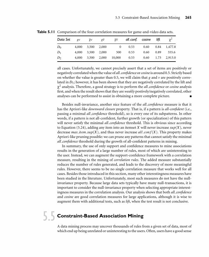
5.5 Constraint-Based Association Mining 265
Table 5.11 Comparison of the four correlation measures for game-and-video data sets.
Data Set gv gv gv gv all conf. cosine lift χ2
D0 4,000 3,500 2,000 0 0.53 0.60 0.84 1,477.8
D1 4,000 3,500 2,000 500 0.53 0.60 0.89 555.6
D2 4,000 3,500 2,000 10,000 0.53 0.60 1.73 2,913.0
all cases. Unfortunately, we cannot precisely assert that a set of items are positively ornegatively correlated when the value of all confidence or cosine is around 0.5. Strictly basedon whether the value is greater than 0.5, we will claim that g and v are positively corre-lated in D1; however, it has been shown that they are negatively correlated by the lift andχ2 analysis. Therefore, a good strategy is to perform the all confidence or cosine analysisfirst, and when the result shows that they are weakly postively/negatively correlated, otheranalyses can be performed to assist in obtaining a more complete picture.
Besides null-invariance, another nice feature of the all confidence measure is that ithas the Apriori-like downward closure property. That is, if a pattern is all-confident (i.e.,passing a minimal all confidence threshold), so is every one of its subpatterns. In otherwords, if a pattern is not all-confident, further growth (or specialization) of this patternwill never satisfy the minimal all confidence threshold. This is obvious since accordingto Equation (5.24), adding any item into an itemset X will never increase sup(X), neverdecrease max item sup(X), and thus never increase all con f (X). This property makesApriori-like pruning possible: we can prune any patterns that cannot satisfy the minimalall confidence threshold during the growth of all-confident patterns in mining.
In summary, the use of only support and confidence measures to mine associationsresults in the generation of a large number of rules, most of which are uninteresting tothe user. Instead, we can augment the support-confidence framework with a correlationmeasure, resulting in the mining of correlation rules. The added measure substantiallyreduces the number of rules generated, and leads to the discovery of more meaningfulrules. However, there seems to be no single correlation measure that works well for allcases. Besides those introduced in this section, many other interestingness measures havebeen studied in the literature. Unfortunately, most such measures do not have the null-invariance property. Because large data sets typically have many null-transactions, it isimportant to consider the null-invariance property when selecting appropriate interest-ingness measures in the correlation analysis. Our analysis shows that both all confidenceand cosine are good correlation measures for large applications, although it is wise toaugment them with additional tests, such as lift, when the test result is not conclusive.
5.5 Constraint-Based Association Mining
A data mining process may uncover thousands of rules from a given set of data, most ofwhich end up being unrelated or uninteresting to the users. Often, users have a good sense

266 Chapter 5 Mining Frequent Patterns, Associations, and Correlations
of which “direction” of mining may lead to interesting patterns and the “form” of thepatterns or rules they would like to find. Thus, a good heuristic is to have the users specifysuch intuition or expectations as constraints to confine the search space. This strategy isknown as constraint-based mining. The constraints can include the following:
Knowledge type constraints: These specify the type of knowledge to be mined, suchas association or correlation.
Data constraints: These specify the set of task-relevant data.
Dimension/level constraints: These specify the desired dimensions (or attributes) ofthe data, or levels of the concept hierarchies, to be used in mining.
Interestingness constraints: These specify thresholds on statistical measures of ruleinterestingness, such as support, confidence, and correlation.
Rule constraints: These specify the form of rules to be mined. Such constraints maybe expressed as metarules (rule templates), as the maximum or minimum numberof predicates that can occur in the rule antecedent or consequent, or as relationshipsamong attributes, attribute values, and/or aggregates.
The above constraints can be specified using a high-level declarative data mining querylanguage and user interface.
The first four of the above types of constraints have already been addressed in ear-lier parts of this book and chapter. In this section, we discuss the use of rule constraintsto focus the mining task. This form of constraint-based mining allows users to describethe rules that they would like to uncover, thereby making the data mining process moreeffective. In addition, a sophisticated mining query optimizer can be used to exploitthe constraints specified by the user, thereby making the mining process more efficient.Constraint-based mining encourages interactive exploratory mining and analysis. InSection 5.5.1, you will study metarule-guided mining, where syntactic rule constraintsare specified in the form of rule templates. Section 5.5.2 discusses the use of additionalrule constraints, specifying set/subset relationships, constant initiation of variables, andaggregate functions. For ease of discussion, we assume that the user is searching for asso-ciation rules. The procedures presented can easily be extended to the mining of correla-tion rules by adding a correlation measure of interestingness to the support-confidenceframework, as described in the previous section.
5.5.1 Metarule-Guided Mining of Association Rules
“How are metarules useful?” Metarules allow users to specify the syntactic form of rulesthat they are interested in mining. The rule forms can be used as constraints to helpimprove the efficiency of the mining process. Metarules may be based on the analyst’sexperience, expectations, or intuition regarding the data or may be automatically gener-ated based on the database schema.

5.5 Constraint-Based Association Mining 267
Example 5.13 Metarule-guided mining. Suppose that as a market analyst for AllElectronics, you haveaccess to the data describing customers (such as customer age, address, and credit rating)as well as the list of customer transactions. You are interested in finding associationsbetween customer traits and the items that customers buy. However, rather than findingall of the association rules reflecting these relationships, you are particularly interestedonly in determining which pairs of customer traits promote the sale of office software.A metarule can be used to specify this information describing the form of rules you areinterested in finding. An example of such a metarule is
P1(X , Y )∧P2(X , W )⇒buys(X , “office software”), (5.26)
where P1 and P2 are predicate variables that are instantiated to attributes from the givendatabase during the mining process, X is a variable representing a customer, and Y andW take on values of the attributes assigned to P1 and P2, respectively. Typically, a user willspecify a list of attributes to be considered for instantiation with P1 and P2. Otherwise, adefault set may be used.
In general, a metarule forms a hypothesis regarding the relationships that the useris interested in probing or confirming. The data mining system can then search forrules that match the given metarule. For instance, Rule (5.27) matches or complieswith Metarule (5.26).
age(X , “30...39”)∧ income(X , “41K...60K”)⇒buys(X , “office software”) (5.27)
“How can metarules be used to guide the mining process?” Let’s examine this problemclosely. Suppose that we wish to mine interdimensional association rules, such as in theexample above. A metarule is a rule template of the form
P1∧P2∧·· ·∧Pl ⇒ Q1∧Q2∧·· ·∧Qr, (5.28)
where Pi (i = 1, . . . , l) and Q j ( j = 1, . . . , r) are either instantiated predicates or predicatevariables. Let the number of predicates in the metarule be p = l + r. In order to findinterdimensional association rules satisfying the template,
We need to find all frequent p-predicate sets, Lp.
We must also have the support or count of the l-predicate subsets of Lp in order tocompute the confidence of rules derived from Lp.
This is a typical case of mining multidimensional association rules, which was dis-cussed in Section 5.3.2. By extending such methods using techniques described in thefollowing section, we can derive efficient methods for metarule-guided mining.
5.5.2 Constraint Pushing: Mining Guided by Rule Constraints
Rule constraints specify expected set/subset relationships of the variables in the minedrules, constant initiation of variables, and aggregate functions. Users typically employ

268 Chapter 5 Mining Frequent Patterns, Associations, and Correlations
their knowledge of the application or data to specify rule constraints for the mining task.These rule constraints may be used together with, or as an alternative to, metarule-guidedmining. In this section, we examine rule constraints as to how they can be used to makethe mining process more efficient. Let’s study an example where rule constraints are usedto mine hybrid-dimensional association rules.
Example 5.14 A closer look at mining guided by rule constraints. Suppose that AllElectronics has a salesmultidimensional database with the following interrelated relations:
sales(customer name, item name, TID)
lives in(customer name, region, city)
item(item name, group, price)
transaction(TID, day, month, year)
where lives in, item, and transaction are three dimension tables, linked to the fact tablesales via three keys, customer name, item name, and TID (transaction id), respectively.
Our association mining query is to “Find the sales of which cheap items (where the sumof the prices is less than $100) may promote the sales of which expensive items (where theminimum price is $500) of the same group for Chicago customers in 2004.” This can beexpressed in the DMQL data mining query language as follows, where each line of thequery has been enumerated to aid in our discussion:
(1) mine associations as(2) lives in(C, , “Chicago”) ∧ sales+(C,?{I},{S})⇒ sales+(C, ?{J}, {T})(3) from sales(4) where S.year = 2004 and T.year = 2004 and I.group = J.group(5) group by C, I.group(6) having sum(I.price) < 100 and min(J.price)≥ 500(7) with support threshold = 1%(8) with confidence threshold = 50%
Before we discuss the rule constraints, let’s look at the above query. Line 1 is aknowledge type constraint, where association patterns are to be discovered. Line 2specifies a metarule. This is an abbreviated form for the following metarule forhybrid-dimensional association rules (multidimensional association rules where therepeated predicate here is sales):
lives in(C, , “Chicago”)∧ sales(C, ?I1, S1) ∧ . . .∧ sales(C, ?Ik, Sk) ∧ I = {I1, . . . , Ik} ∧ S = {S1, . . . , Sk}⇒ sales(C, ?J1, T1) ∧ . . .∧ sales(C, ?Jm, Tm) ∧ J = {J1, . . . , Jm} ∧ T = {T1, . . . , Tm}
which means that one or more sales records in the form of “sales(C, ?I1, S1)∧ . . .sales(C, ?Ik, Sk)” will reside at the rule antecedent (left-hand side), and the question mark “?”

5.5 Constraint-Based Association Mining 269
means that only item name, I1,. . . , Ik need be printed out. “I = {I1, . . . , Ik}” means thatall the Is at the antecedent are taken from a set I, obtained from the SQL-like whereclause of line 4. Similar notational conventions are used at the consequent (right-handside).
The metarule may allow the generation of association rules like the following:
lives in(C, , “Chicago”)∧ sales(C, “Census CD”, )∧sales(C, “MS/Office”, )⇒sales(C, “MS/SQLServer”, ) [1.5%, 68%], (5.29)
which means that if a customer in Chicago bought “Census CD” and “MS/Office,” it islikely (with a probability of 68%) that the customer also bought “MS/SQLServer,” and1.5% of all of the customers bought all three.
Data constraints are specified in the “lives in(C, , “Chicago”)” portion of themetarule (i.e., all the customers who live in Chicago) and in line 3, which specifiesthat only the fact table, sales, need be explicitly referenced. In such a multidimensionaldatabase, variable reference is simplified. For example, “S.year = 2004” is equivalent tothe SQL statement “from sales S, transaction T where S.TID = T.TID and T.year =2004.”All three dimensions (lives in, item, and transaction) are used. Level constraints areas follows: for lives in, we consider just customer name since region is not referencedand city = “Chicago” is only used in the selection; for item, we consider the levelsitem name and group since they are used in the query; and for transaction, we areonly concerned with TID since day and month are not referenced and year is usedonly in the selection.
Rule constraints include most portions of the where (line 4) and having (line 6)clauses, such as “S.year = 2004,” “T.year = 2004,” “I.group = J.group,” “sum(I.price)≤ 100,” and “min(J.price) ≥ 500.” Finally, lines 7 and 8 specify two interestingnessconstraints (i.e., thresholds), namely, a minimum support of 1% and a minimumconfidence of 50%.
Dimension/level constraints and interestingness constraints can be applied aftermining to filter out discovered rules, although it is generally more efficient and lessexpensive to use them during mining, to help prune the search space. Dimension/levelconstraints were discussed in Section 5.3, and interestingness constraints have beendiscussed throughout this chapter. Let’s focus now on rule constraints.
“How can we use rule constraints to prune the search space? More specifically, what kindof rule constraints can be ‘pushed’ deep into the mining process and still ensure the com-pleteness of the answer returned for a mining query?”
Rule constraints can be classified into the following five categories with respect tofrequent itemset mining: (1) antimonotonic, (2) monotonic, (3) succinct, (4) convertible,and (5) inconvertible. For each category, we will use an example to show its characteristicsand explain how such kinds of constraints can be used in the mining process.
The first category of constraints is antimonotonic. Consider the rule constraint“sum(I.price) ≤ 100” of Example 5.14. Suppose we are using the Apriori framework,which at each iteration k explores itemsets of size k. If the price summation of the items

270 Chapter 5 Mining Frequent Patterns, Associations, and Correlations
in an itemset is no less than 100, this itemset can be pruned from the search space, sinceadding more items into the set will only make it more expensive and thus will neversatisfy the constraint. In other words, if an itemset does not satisfy this rule constraint,none of its supersets can satisfy the constraint. If a rule constraint obeys this property, itis antimonotonic. Pruning by antimonotonic constraints can be applied at each iterationof Apriori-style algorithms to help improve the efficiency of the overall mining processwhile guaranteeing completeness of the data mining task.
The Apriori property, which states that all nonempty subsets of a frequent itemsetmust also be frequent, is antimonotonic. If a given itemset does not satisfy minimumsupport, none of its supersets can. This property is used at each iteration of the Apriorialgorithm to reduce the number of candidate itemsets examined, thereby reducing thesearch space for association rules.
Other examples of antimonotonic constraints include “min(J.price) ≥ 500,”“count(I) ≤ 10,” and so on. Any itemset that violates either of these constraints can bediscarded since adding more items to such itemsets can never satisfy the constraints. Notethat a constraint such as “avg(I.price) ≤ 100” is not antimonotonic. For a given item-set that does not satisfy this constraint, a superset created by adding some (cheap) itemsmay result in satisfying the constraint. Hence, pushing this constraint inside the miningprocess will not guarantee completeness of the data mining task. A list of SQL-primitives-based constraints is given in the first column of Table 5.12. The antimonotonicity of theconstraints is indicated in the second column of the table. To simplify our discussion,only existence operators (e.g., = , ∈, but not 6= , /∈) and comparison (or containment)operators with equality (e.g.,≤ , ⊆) are given.
The second category of constraints is monotonic. If the rule constraint in Example 5.14were “sum(I.price)≥ 100,” the constraint-based processing method would be quite dif-ferent. If an itemset I satisfies the constraint, that is, the sum of the prices in the set is noless than 100, further addition of more items to I will increase cost and will always satisfythe constraint. Therefore, further testing of this constraint on itemset I becomes redun-dant. In other words, if an itemset satisfies this rule constraint, so do all of its supersets. Ifa rule constraint obeys this property, it is monotonic. Similar rule monotonic constraintsinclude “min(I.price) ≤ 10,” “count(I) ≥ 10,” and so on. The monotonicity of the listof SQL-primitives-based constraints is indicated in the third column of Table 5.12.
The third category is succinct constraints. For this category of constraints, we canenumerate all and only those sets that are guaranteed to satisfy the constraint. That is,if a rule constraint is succinct, we can directly generate precisely the sets that satisfyit, even before support counting begins. This avoids the substantial overhead of thegenerate-and-test paradigm. In other words, such constraints are precounting prunable.For example, the constraint “min(J.price)≥ 500” in Example 5.14 is succinct, becausewe can explicitly and precisely generate all the sets of items satisfying the constraint.Specifically, such a set must contain at least one item whose price is no less than$500. It is of the form S1∪S2, where S1 6= /0 is a subset of the set of all those itemswith prices no less than $500, and S2, possibly empty, is a subset of the set of allthose items with prices no greater than $500. Because there is a precise “formula”for generating all of the sets satisfying a succinct constraint, there is no need to

5.5 Constraint-Based Association Mining 271
Table 5.12 Characterization of commonly used SQL-based constraints.
Constraint Antimonotonic Monotonic Succinct
v ∈ S no yes yes
S⊇V no yes yes
S⊆V yes no yes
min(S)≤ v no yes yes
min(S)≥ v yes no yes
max(S)≤ v yes no yes
max(S)≥ v no yes yes
count(S)≤ v yes no weakly
count(S)≥ v no yes weakly
sum(S)≤ v (∀a ∈ S, a≥ 0) yes no no
sum(S)≥ v (∀a ∈ S, a≥ 0) no yes no
range(S)≤ v yes no no
range(S)≥ v no yes no
avg(S) θ v, θ ∈ {≤ , ≥} convertible convertible no
support(S)≥ ξ yes no no
support(S)≤ ξ no yes no
all con f idence(S)≥ ξ yes no no
all con f idence(S)≤ ξ no yes no
iteratively check the rule constraint during the mining process. The succinctness ofthe list of SQL-primitives-based constraints is indicated in the fourth column ofTable 5.12.10
The fourth category is convertible constraints. Some constraints belong to none of theabove three categories. However, if the items in the itemset are arranged in a particularorder, theconstraintmaybecomemonotonicorantimonotonicwithregardtothefrequentitemset mining process. For example, the constraint “avg(I.price) ≤ 100” is neitherantimonotonic nor monotonic. However, if items in a transaction are added to an itemsetin price-ascending order, the constraint becomes antimonotonic, because if an itemset Iviolates the constraint (i.e., with an average price greater than $100), then further additionof more expensive items into the itemset will never make it satisfy the constraint. Similarly,if items in a transaction are added to an itemset in price-descending order, it becomesmonotonic, because if the itemset satisfies the constraint (i.e., with an average price no
10For constraint count(S)≤ v (and similarly for count(S)≥ v), we can have a member generationfunction based on a cardinality constraint (i.e., {X | X ⊆ Itemset ∧ |X | ≤ v}). Member generationin this manner takes a different flavor and thus is called weakly succinct.

272 Chapter 5 Mining Frequent Patterns, Associations, and Correlations
greater than $100), then adding cheaper items into the current itemset will still make theaverage price no greater than $100. Aside from “avg(S) ≤ v,” and “avg(S) ≥ v,” givenin Table 5.12, there are many other convertible constraints, such as “variance(S) ≥ v,”“standard deviation(S)≥ v,” and so on.
Note that the above discussion does not imply that every constraint is convertible.For example, “sum(S)θv,” where θ ∈ {≤ , ≥} and each element in S could be of anyreal value, is not convertible. Therefore, there is yet a fifth category of constraints, calledinconvertible constraints. The good news is that although there still exist some toughconstraints that are not convertible, most simple SQL expressions with built-in SQLaggregates belong to one of the first four categories to which efficient constraint miningmethods can be applied.
5.6 Summary
The discovery of frequent patterns, association, and correlation relationships amonghuge amounts of data is useful in selective marketing, decision analysis, and businessmanagement. A popular area of application is market basket analysis, which studiesthe buying habits of customers by searching for sets of items that are frequentlypurchased together (or in sequence). Association rule mining consists of first findingfrequent itemsets (set of items, such as A and B, satisfying a minimum supportthreshold, or percentage of the task-relevant tuples), from which strong associationrules in the form of A⇒B are generated. These rules also satisfy a minimum confidencethreshold (a prespecified probability of satisfying B under the condition that A issatisfied). Associations can be further analyzed to uncover correlation rules, whichconvey statistical correlations between itemsets A and B.Frequent pattern mining can be categorized in many different ways according to var-ious criteria, such as the following:
1. Based on the completeness of patterns to be mined, categories of frequent pat-tern mining include mining the complete set of frequent itemsets, the closed frequentitemsets, the maximal frequent itemsets, and constrained frequent itemsets.
2. Based on the levels and dimensions of data involved in the rule, categories caninclude the mining of single-level association rules, multilevel association rules, single-dimensional association rules, and multidimensional association rules.
3. Based on the types of values handled in the rule, the categories can include miningBoolean association rules and quantitative association rules.
4. Based on the kinds of rules to be mined, categories include mining association rulesand correlation rules.
5. Based on the kinds of patterns to be mined, frequent pattern mining can be clas-sified into frequent itemset mining, sequential pattern mining, structured patternmining, and so on. This chapter has focused on frequent itemset mining.

5.6 Summary 273
Many efficient and scalable algorithms have been developed for frequent itemsetmining, from which association and correlation rules can be derived. These algo-rithms can be classified into three categories: (1) Apriori-like algorithms, (2) frequent-pattern growth-based algorithms, such as FP-growth, and (3) algorithms that use thevertical data format.
The Apriori algorithm is a seminal algorithm for mining frequent itemsets for Booleanassociation rules. It explores the level-wise mining Apriori property that all nonemptysubsets of a frequent itemset must also be frequent. At the kth iteration (for k ≥ 2), itforms frequent k-itemset candidates based on the frequent (k−1)-itemsets, and scansthe database once to find the complete set of frequent k-itemsets, Lk.Variations involving hashing and transaction reduction can be used to make the pro-cedure more efficient. Other variations include partitioning the data (mining on eachpartition and then combining the results) and sampling the data (mining on a subsetof the data). These variations can reduce the number of data scans required to as littleas two or one.
Frequent pattern growth (FP-growth) is a method of mining frequent itemsets with-out candidate generation. It constructs a highly compact data structure (an FP-tree)to compress the original transaction database. Rather than employing the generate-and-test strategy of Apriori-like methods, it focuses on frequent pattern (fragment)growth, which avoids costly candidate generation, resulting in greater efficiency.
Mining frequent itemsets using vertical data format (ECLAT) is a method that trans-forms a given data set of transactions in the horizontal data format of TID-itemset intothe vertical data format of item-TID set. It mines the transformed data set by TID setintersections based on the Apriori property and additional optimization techniques,such as diffset.
Methods for mining frequent itemsets can be extended for the mining of closed fre-quent itemsets (from which the set of frequent itemsets can easily be derived). Theseincorporate additional optimization techniques, such as item merging, sub-itemsetpruning, and item skipping, as well as efficient subset checking of generated itemsetsin a pattern-tree.
Mining frequent itemsets and associations has been extended in various waysto include mining multilevel association rules and multidimensional association rules.
Multilevel association rules can be mined using several strategies, based on howminimum support thresholds are defined at each level of abstraction, such asuniform support, reduced support, and group-based support. Redundant multilevel(descendant) association rules can be eliminated if their support and confidenceare close to their expected values, based on their corresponding ancestor rules.
Techniques for mining multidimensional association rules can be categorized accord-ing to their treatment of quantitative attributes. First, quantitative attributes may bediscretized statically, based on predefined concept hierarchies. Data cubes are wellsuited to this approach, because both the data cube and quantitative attributes can
274 Chapter 5 Mining Frequent Patterns, Associations, and Correlations
use concept hierarchies. Second, quantitative association rules can be mined wherequantitative attributes are discretized dynamically based on binning and/or cluster-ing, where “adjacent” association rules may be further combined by clustering to gen-erate concise and meaningful rules.
Not all strong association rules are interesting. It is more effective to mine items thatare statistically correlated. Therefore, association rules should be augmented with acorrelation measure to generate more meaningful correlation rules. There are severalcorrelation measures to choose from, including lift, χ2, all confidence, and cosine.A measure is null-invariant if its value is free from the influence of null-transactions(i.e., transactions that do not contain any of the itemsets being examined). Becauselarge databases typically have numerous null-transactions, a null-invariant correla-tion measure should be used, such as all confidence or cosine. When interpreting cor-relation measure values, it is important to understand their implications andlimitations.
Constraint-based rule mining allows users to focus the search for rules by providingmetarules (i.e., pattern templates) and additional mining constraints. Such mining isfacilitated with the use of a declarative data mining query language and user interface,and poses great challenges for mining query optimization. Rule constraints can beclassified into five categories: antimonotonic, monotonic, succinct, convertible, andinconvertible. Constraints belonging to the first four of these categories can be usedduring frequent itemset mining to guide the process, leading to more efficient andeffective mining.Association rules should not be used directly for prediction without further analysisor domain knowledge. They do not necessarily indicate causality. They are, however, ahelpful starting point for further exploration, making them a popular tool for under-standing data. The application of frequent patterns to classification, cluster analysis,and other data mining tasks will be discussed in subsequent chapters.
Exercises
5.1 The Apriori algorithm uses prior knowledge of subset support properties.
(a) Prove that all nonempty subsets of a frequent itemset must also be frequent.
(b) Prove that the support of any nonempty subset s′ of itemset s must be at least as greatas the support of s.
(c) Given frequent itemset l and subset s of l, prove that the confidence of the rule “s′⇒(l− s′)” cannot be more than the confidence of “s⇒ (l− s)”, where s′ is a subsetof s.
(d) A partitioning variation of Apriori subdivides the transactions of a database D inton nonoverlapping partitions. Prove that any itemset that is frequent in D must befrequent in at least one partition of D.

Exercises 275
5.2 Section 5.2.2 describes a method for generating association rules from frequent itemsets.Propose a more efficient method. Explain why it is more efficient than the one pro-posed in Section 5.2.2. (Hint: Consider incorporating the properties of Exercise 5.1(b)and 5.1(c) into your design.)
5.3 A database has five transactions. Let min sup = 60% and min con f = 80%.
TID items bought
T100 {M, O, N, K, E, Y}T200 {D, O, N, K, E, Y }T300 {M, A, K, E}T400 {M, U, C, K, Y}T500 {C, O, O, K, I ,E}
(a) Find all frequent itemsets using Apriori and FP-growth, respectively. Compare theefficiency of the two mining processes.
(b) List all of the strong association rules (with support s and confidence c) matching thefollowing metarule, where X is a variable representing customers, and itemi denotesvariables representing items (e.g., “A”, “B”, etc.):
∀x ∈ transaction, buys(X , item1)∧buys(X , item2)⇒ buys(X , item3) [s, c]
5.4 (Implementation project) Implement three frequent itemset mining algorithms intro-duced in this chapter: (1) Apriori [AS94b], (2) FP-growth [HPY00], and (3) ECLAT[Zak00] (mining using vertical data format), using a programming language that you arefamiliar with, such as C++ or Java. Compare the performance of each algorithm with var-ious kinds of large data sets. Write a report to analyze the situations (such as data size,data distribution, minimal support threshold setting, and pattern density) where onealgorithm may perform better than the others, and state why.
5.5 A database has four transactions. Let min sup = 60% and min con f = 80%.
cust ID TID items bought (in the form of brand-item category)
01 T100 {King’s-Crab, Sunset-Milk, Dairyland-Cheese, Best-Bread}02 T200 {Best-Cheese, Dairyland-Milk, Goldenfarm-Apple, Tasty-Pie,
Wonder-Bread}01 T300 {Westcoast-Apple, Dairyland-Milk, Wonder-Bread, Tasty-Pie}03 T400 {Wonder-Bread, Sunset-Milk, Dairyland-Cheese}
(a) At the granularity of item category (e.g., itemi could be “Milk”), for the followingrule template,
∀X ∈ transaction, buys(X , item1)∧buys(X , item2)⇒ buys(X , item3) [s, c]

276 Chapter 5 Mining Frequent Patterns, Associations, and Correlations
list the frequent k-itemset for the largest k, and all of the strong association rules (withtheir support s and confidence c) containing the frequent k-itemset for the largest k.
(b) At the granularity of brand-item category (e.g., itemi could be “Sunset-Milk”), forthe following rule template
∀X ∈ customer, buys(X , item1)∧buys(X , item2)⇒ buys(X , item3),
list the frequent k-itemset for the largest k (but do not print any rules).
5.6 Suppose that a large store has a transaction database that is distributed among fourlocations. Transactions in each component database have the same format, namelyTj : {i1, . . . , im}, where Tj is a transaction identifier, and ik (1≤ k≤m) is the identifierof an item purchased in the transaction. Propose an efficient algorithm to mine globalassociation rules (without considering multilevel associations). You may present youralgorithm in the form of an outline. Your algorithm should not require shippingall of the data to one site and should not cause excessive network communicationoverhead.
5.7 Suppose that frequent itemsets are saved for a large transaction database, DB. Dis-cuss how to efficiently mine the (global) association rules under the same minimumsupport threshold if a set of new transactions, denoted as ∆DB, is (incrementally)added in?
5.8 [Contributed by Tao Cheng] Most frequent pattern mining algorithms consider only dis-tinct items in a transaction. However, multiple occurrences of an item in the same shop-ping basket, such as four cakes and three jugs of milk, can be important in transactiondata analysis. How can one mine frequent itemsets efficiently considering multiple occur-rences of items? Propose modifications to the well-known algorithms, such as Aprioriand FP-growth, to adapt to such a situation.
5.9 (Implementation project) Implement three closed frequent itemset mining methods (1)A-Close [PBTL99] (based on an extension of Apriori [AS94b]), (2) CLOSET+ [WHP03](based on an extension of FP-growth [HPY00]), and (3) CHARM [ZH02] (based on anextension of ECLAT [Zak00]). Compare their performance with various kinds of largedata sets. Write a report to answer the following questions:
(a) Why is mining the set of closed frequent itemsets often more desirable than miningthe complete set of frequent itemsets (based on your experiments on the same dataset as Exercise 5.4)?
(b) Analyze in which situations (such as data size, data distribution, minimal supportthreshold setting, and pattern density) and why one algorithm performs better thanthe others.
5.10 Suppose that a data relation describing students at Big University has been generalized tothe generalized relation R in Table 5.13.
Let the concept hierarchies be as follows:

Exercises 277
status : {freshman, sophomore, junior, senior} ∈ undergraduate.{M.Sc.,M.A., Ph.D.} ∈ graduate.
major : {physics, chemistry, math} ∈ science.{cs, engineering} ∈ appl. sciences.{French, philosophy} ∈ arts.
age : {16...20,21...25} ∈ young.{26...30, over 30} ∈ old.
nationality : {Asia, Europe, Latin America} ∈ foreign.{U.S.A., Canada} ∈ North America.
Table 5.13 Generalized relation for Exercise 5.9.
major status age nationality gpa count
French M.A over 30 Canada 2.8 3.2 3
cs junior 16...20 Europe 3.2 3.6 29
physics M.S 26...30 Latin America 3.2 3.6 18
engineering Ph.D 26...30 Asia 3.6 4.0 78
philosophy Ph.D 26...30 Europe 3.2 3.6 5
French senior 16...20 Canada 3.2 3.6 40
chemistry junior 21...25 USA 3.6 4.0 25
cs senior 16...20 Canada 3.2 3.6 70
philosophy M.S over 30 Canada 3.6 4.0 15
French junior 16...20 USA 2.8 3.2 8
philosophy junior 26...30 Canada 2.8 3.2 9
philosophy M.S 26...30 Asia 3.2 3.6 9
French junior 16...20 Canada 3.2 3.6 52
math senior 16...20 USA 3.6 4.0 32
cs junior 16...20 Canada 3.2 3.6 76
philosophy Ph.D 26...30 Canada 3.6 4.0 14
philosophy senior 26...30 Canada 2.8 3.2 19
French Ph.D over 30 Canada 2.8 3.2 1
engineering junior 21...25 Europe 3.2 3.6 71
math Ph.D 26...30 Latin America 3.2 3.6 7
chemistry junior 16...20 USA 3.6 4.0 46
engineering junior 21...25 Canada 3.2 3.6 96
French M.S over 30 Latin America 3.2 3.6 4
philosophy junior 21...25 USA 2.8 3.2 8
math junior 16...20 Canada 3.6 4.0 59

278 Chapter 5 Mining Frequent Patterns, Associations, and Correlations
Let the minimum support threshold be 20% and the minimum confidence threshold be50% (at each of the levels).
(a) Draw the concept hierarchies for status, major, age, and nationality.
(b) Write a program to find the set of strong multilevel association rules in R using uni-form support for all levels, for the following rule template,
∀S ∈ R, P(S, x)∧Q(S, y)⇒ gpa(S, z) [s, c]
where P, Q ∈ {status, major, age, nationality}.(c) Use the program to find the set of strong multilevel association rules in R using level-
cross filtering by single items. In this strategy, an item at the ith level is examined if andonly if its parent node at the (i−1)th level in the concept hierarchy is frequent. Thatis, if a node is frequent, its children will be examined; otherwise, its descendants arepruned from the search. Use a reduced support of 10% for the lowest abstractionlevel, for the preceding rule template.
5.11 Propose and outline a level-shared mining approach to mining multilevel associationrules in which each item is encoded by its level position, and an initial scan of the databasecollects the count for each item at each concept level, identifying frequent and subfre-quent items. Comment on the processing cost of mining multilevel associations withthis method in comparison to mining single-level associations.
5.12 (Implementation project) Many techniques have been proposed to further improvethe performance of frequent-itemset mining algorithms. Taking FP-tree-based fre-quent pattern-growth algorithms, such as FP-growth, as an example, implement oneof the following optimization techniques, and compare the performance of your newimplementation with the one that does not incorporate such optimization.
(a) The previously proposed frequent pattern mining with FP-tree generates conditionalpattern bases using a bottom-up projection technique (i.e., project on the prefix pathof an item p). However, one can develop a top-down projection technique (i.e.,project on the suffix path of an item p in the generation of a conditional pattern-base). Design and implement such a top-down FP-tree mining method and compareyour performance with the bottom-up projection method.
(b) Nodes and pointers are used uniformly in FP-tree in the design of the FP-growthalgorithm. However, such a structure may consume a lot of space when the dataare sparse. One possible alternative design is to explore array- and pointer-basedhybrid implementation, where a node may store multiple items when it containsno splitting point to multiple subbranches. Develop such an implementation andcompare it with the original one.
(c) It is time- and space-consuming to generate numerous conditional pattern basesduring pattern-growth mining. One interesting alternative is to push right thebranches that have been mined for a particular item p, that is, to push them tothe remaining branch(es) of the FP-tree. This is done so that fewer conditional

Exercises 279
pattern bases have to be generated and additional sharing can be explored whenmining the remaining branches of the FP-tree. Design and implement such amethod and conduct a performance study on it.
5.13 Give a short example to show that items in a strong association rule may actually benegatively correlated.
5.14 The following contingency table summarizes supermarket transaction data, where hotdogs refers to the transactions containing hot dogs, hot dogs refers to the transactionsthat do not contain hot dogs, hamburgers refers to the transactions containing hamburg-ers, and hamburgers refers to the transactions that do not contain hamburgers.
hot dogs hot dogs Σrow
hamburgers 2,000 500 2,500
hamburgers 1,000 1,500 2,500
Σcol 3,000 2,000 5,000
(a) Suppose that the association rule “hot dogs⇒ hamburgers” is mined. Given a min-imum support threshold of 25% and a minimum confidence threshold of 50%, isthis association rule strong?
(b) Based on the given data, is the purchase of hot dogs independent of the purchase ofhamburgers? If not, what kind of correlation relationship exists between the two?
5.15 In multidimensional data analysis, it is interesting to extract pairs of similar cellcharacteristics associated with substantial changes in measure in a data cube, wherecells are considered similar if they are related by roll-up (i.e., ancestors), drill-down(i.e., descendants), or one-dimensional mutation (i.e., siblings) operations. Such ananalysis is called cube gradient analysis. Suppose the cube measure is average. A userposes a set of probe cells and would like to find their corresponding sets of gradientcells, each of which satisfies a certain gradient threshold. For example, find the setof corresponding gradient cells whose average sale price is greater than 20% of thatof the given probe cells. Develop an algorithm than mines the set of constrainedgradient cells efficiently in a large data cube.
5.16 Association rule mining often generates a large number of rules. Discuss effective meth-ods that can be used to reduce the number of rules generated while still preserving mostof the interesting rules.
5.17 Sequential patterns can be mined in methods similar to the mining of association rules.Design an efficient algorithm to mine multilevel sequential patterns from a transactiondatabase. An example of such a pattern is the following: “A customer who buys a PCwill buy Microsoft software within three months,” on which one may drill down to find amore refined version of the pattern, such as “A customer who buys a Pentium PC will buyMicrosoft Office within three months.”

280 Chapter 5 Mining Frequent Patterns, Associations, and Correlations
5.18 Prove that each entry in the following table correctly characterizes its corresponding ruleconstraint for frequent itemset mining.
Rule constraint Antimonotonic Monotonic Succinct
a) v ∈ S no yes yes
b) S⊆V yes no yes
c) min(S)≤ v no yes yes
d) range(S)≤ v yes no no
5.19 The price of each item in a store is nonnegative. The store manager is only interested inrules of the form: “one free item may trigger $200 total purchases in the same transaction.”State how to mine such rules efficiently.
5.20 The price of each item in a store is nonnegative. For each of the following cases, identifythe kinds of constraint they represent and briefly discuss how to mine such associationrules efficiently.
(a) Containing at least one Nintendo game
(b) Containing items the sum of whose prices is less than $150
(c) Containing one free item and other items the sum of whose prices is at least $200
(d) Where the average price of all the items is between $100 and $500
Bibliographic Notes
Association rule mining was first proposed by Agrawal, Imielinski, and Swami [AIS93].The Apriori algorithm discussed in Section 5.2.1 for frequent itemset mining was pre-sented in Agrawal and Srikant [AS94b]. A variation of the algorithm using a similarpruning heuristic was developed independently by Mannila, Tiovonen, and Verkamo[MTV94]. A joint publication combining these works later appeared in Agrawal, Man-nila, Srikant, Toivonen, and Verkamo [AMS+96]. A method for generating associationrules from frequent itemsets is described in Agrawal and Srikant [AS94a].
References for the variations of Apriori described in Section 5.2.3 include thefollowing. The use of hash tables to improve association mining efficiency wasstudied by Park, Chen, and Yu [PCY95a]. Transaction reduction techniques aredescribed in Agrawal and Srikant [AS94b], Han and Fu [HF95], and Park, Chen,and Yu [PCY95a]. The partitioning technique was proposed by Savasere, Omiecin-ski, and Navathe [SON95]. The sampling approach is discussed in Toivonen [Toi96].A dynamic itemset counting approach is given in Brin, Motwani, Ullman, and Tsur[BMUT97]. An efficient incremental updating of mined association rules was pro-posed by Cheung, Han, Ng, and Wong [CHNW96]. Parallel and distributed asso-ciation data mining under the Apriori framework was studied by Park, Chen, andYu [PCY95b], Agrawal and Shafer [AS96], and Cheung, Han, Ng, et al. [CHN+96].Another parallel association mining method, which explores itemset clustering using

Bibliographic Notes 281
a vertical database layout, was proposed in Zaki, Parthasarathy, Ogihara, and Li[ZPOL97].
Other scalable frequent itemset mining methods have been proposed as alternatives tothe Apriori-based approach. FP-growth, a pattern-growth approach for mining frequentitemsets without candidate generation, was proposed by Han, Pei, and Yin [HPY00](Section 5.2.4). An exploration of hyperstructure mining of frequent patterns, calledH-Mine, was proposed by Pei, Han, Lu, Nishio, Tang, and Yang [PHMA+01]. OP, amethod that integrates top-down and bottom-up traversal of FP-trees in pattern-growthmining, was proposed by Liu, Pan, Wang, and Han [LPWH02]. An array-based imple-mentation of prefix-tree-structure for efficient pattern growth mining was proposed byGrahne and Zhu [GZ03b]. ECLAT, an approach for mining frequent itemsets by explor-ing the vertical data format, was proposed by Zaki [Zak00]. A depth-first generation offrequent itemsets was proposed by Agarwal, Aggarwal, and Prasad [AAP01].
The mining of frequent closed itemsets was proposed in Pasquier, Bastide, Taouil, andLakhal [PBTL99], where an Apriori-based algorithm called A-Close for such mining waspresented. CLOSET, an efficient closed itemset mining algorithm based on the frequent-pattern growth method, was proposed by Pei, Han, and Mao [PHM00], and furtherrefined as CLOSET+ in Wang, Han, and Pei [WHP03]. FPClose, a prefix-tree-based algo-rithm for mining closed itemsets using the pattern-growth approach, was proposed byGrahne and Zhu [GZ03b]. An extension for mining closed frequent itemsets with thevertical data format, called CHARM, was proposed by Zaki and Hsiao [ZH02]. Miningmax-patterns was first studied by Bayardo [Bay98]. Another efficient method for min-ing maximal frequent itemsets using vertical data format, called MAFIA, was proposedby Burdick, Calimlim, and Gehrke [BCG01]. AFOPT, a method that explores a rightpush operation on FP-trees during the mining process, was proposed by Liu, Lu, Lou,and Yu [LLLY03]. Pan, Cong, Tung, et al. [PCT+03] proposed CARPENTER, a methodfor finding closed patterns in long biological datasets, which integrates the advantagesof row-enumeration and pattern-growth methods. A FIMI (Frequent Itemset MiningImplementation) workshop dedicated to the implementation methods of frequent item-set mining was reported by Goethals and Zaki [GZ03a].
Frequent itemset mining has various extensions, including sequential pattern mining(Agrawal and Srikant [AS95]), episodes mining (Mannila, Toivonen, and Verkamo[MTV97]), spatial association rule mining (Koperski and Han [KH95]), cyclic associ-ation rule mining ( �Ozden, Ramaswamy, and Silberschatz [ORS98]), negative associationrule mining (Savasere, Omiecinski, and Navathe [SON98]), intertransactionassociation rule mining (Lu, Han, and Feng [LHF98]), and calendric market basket anal-ysis (Ramaswamy, Mahajan, and Silberschatz [RMS98]). Multilevel association miningwas studied in Han and Fu [HF95], and Srikant and Agrawal [SA95]. In Srikant andAgrawal [SA95], such mining was studied in the context of generalized association rules,and an R-interest measure was proposed for removing redundant rules. A non-grid-based technique for mining quantitative association rules, which uses a measure of par-tial completeness, was proposed by Srikant and Agrawal [SA96]. The ARCS system formining quantitative association rules based on rule clustering was proposed by Lent,Swami, and Widom [LSW97]. Techniques for mining quantitative rules based on

282 Chapter 5 Mining Frequent Patterns, Associations, and Correlations
x-monotone and rectilinear regions were presented by Fukuda, Morimoto, Morishita,and Tokuyama [FMMT96], and Yoda, Fukuda, Morimoto, et al. [YFM+97]. Mining mul-tidimensional association rules using static discretization of quantitative attributes anddata cubes was studied by Kamber, Han, and Chiang [KHC97]. Mining (distance-based)association rules over interval data was proposed by Miller and Yang [MY97]. Miningquantitative association rules based on a statistical theory to present only those that devi-ate substantially from normal data was studied by Aumann and Lindell [AL99].
The problem of mining interesting rules has been studied by many researchers. Thestatistical independence of rules in data mining was studied by Piatetski-Shapiro [PS91b].The interestingness problem of strong association rules is discussed in Chen, Han, andYu [CHY96], Brin, Motwani, and Silverstein [BMS97], and Aggarwal and Yu [AY99],which cover several interestingness measures including lift. An efficient method for gen-eralizing associations to correlations is given in Brin, Motwani, and Silverstein [BMS97].Other alternatives to the support-confidence framework for assessing the interestingnessof association rules are proposed in Brin, Motwani, Ullman, and Tsur [BMUT97] andAhmed, El-Makky, and Taha [AEMT00]. A method for mining strong gradient relation-ships among itemsets was proposed by Imielinski, Khachiyan, and Abdulghani [IKA02].Silverstein, Brin, Motwani, and Ullman [SBMU98] studied the problem of mining causalstructures over transaction databases. Some comparative studies of different interesting-ness measures were done by Hilderman and Hamilton [HH01] and by Tan, Kumar, andSrivastava [TKS02]. The use of all confidence as a correlation measure for generating inter-esting association rules was studied by Omiecinski [Omi03] and by Lee, Kim, Cai, andHan [LKCH03].
To reduce the huge set of frequent patterns generated in data mining, recent stud-ies have been working on mining compressed sets of frequent patterns. Mining closedpatterns can be viewed as lossless compression of frequent patterns. Lossy compressionof patterns include maximal patterns by Bayardo [Bay98]), top-k patterns by Wang,Han, Lu, and Tsvetkov [WHLT05], and error-tolerant patterns by Yang, Fayyad, andBradley [YFB01]. Afrati, Gionis, and Mannila [AGM04] proposed to use K itemsets tocover a collection of frequent itemsets. Yan, Cheng, Xin, and Han proposed a profile-based approach [YCXH05], and Xin, Han, Yan, and Cheng proposed a clustering-basedapproach [XHYC05] for frequent itemset compression.
The use of metarules as syntactic or semantic filters defining the form of interestingsingle-dimensional association rules was proposed in Klemettinen, Mannila, Ronkainen,et al. [KMR+94]. Metarule-guided mining, where the metarule consequent specifies anaction (such as Bayesian clustering or plotting) to be applied to the data satisfying themetarule antecedent, was proposed in Shen, Ong, Mitbander, and Zaniolo [SOMZ96].A relation-based approach to metarule-guided mining of association rules was stud-ied in Fu and Han [FH95]. Methods for constraint-based association rule mining dis-cussed in this chapter were studied by Ng, Lakshmanan, Han, and Pang [NLHP98],Lakshmanan, Ng, Han, and Pang [LNHP99], and Pei, Han, and Lakshmanan [PHL01].An efficient method for mining constrained correlated sets was given in Grahne, Laksh-manan, and Wang [GLW00]. A dual mining approach was proposed by Bucila, Gehrke,Kifer, and White [BGKW03]. Other ideas involving the use of templates or predicate

Bibliographic Notes 283
constraints in mining have been discussed in [AK93], [DT93], [HK91], [LHC97], [ST96],and [SVA97].
The association mining language presented in this chapter was based on an exten-sion of the data mining query language, DMQL, proposed in Han, Fu, Wang, et al.[HFW+96], by incorporation of the spirit of the SQL-like operator for mining single-dimensional association rules proposed by Meo, Psaila, and Ceri [MPC96]. MSQL, aquery language for mining flexible association rules, was proposed by Imielinski and Vir-mani [IV99]. OLE DB for Data Mining (DM), a data mining query language that includesassociation mining modules, was proposed by Microsoft Corporation [Cor00].

6Classification and Prediction
Databases are rich with hidden information that can be used for intelligent decision making.Classification and prediction are two forms of data analysis that can be used to extractmodels describing important data classes or to predict future data trends. Such analysiscan help provide us with a better understanding of the data at large. Whereas classifi-cation predicts categorical (discrete, unordered) labels, prediction models continuous-valued functions. For example, we can build a classification model to categorize bankloan applications as either safe or risky, or a prediction model to predict the expendituresin dollars of potential customers on computer equipment given their income and occu-pation. Many classification and prediction methods have been proposed by researchersin machine learning, pattern recognition, and statistics. Most algorithms are memoryresident, typically assuming a small data size. Recent data mining research has built onsuch work, developing scalable classification and prediction techniques capable of han-dling large disk-resident data.
In this chapter, you will learn basic techniques for data classification, such as how tobuild decision tree classifiers, Bayesian classifiers, Bayesian belief networks, and rule-based classifiers. Backpropagation (a neural network technique) is also discussed, inaddition to a more recent approach to classification known as support vector machines.Classification based on association rule mining is explored. Other approaches to classifi-cation, such as k-nearest-neighbor classifiers, case-based reasoning, genetic algorithms,rough sets, and fuzzy logic techniques, are introduced. Methods for prediction, includinglinear regression, nonlinear regression, and other regression-based models, are brieflydiscussed. Where applicable, you will learn about extensions to these techniques for theirapplication to classification and prediction in large databases. Classification and predic-tion have numerous applications, including fraud detection, target marketing, perfor-mance prediction, manufacturing, and medical diagnosis.
6.1 What Is Classification? What Is Prediction?
A bank loans officer needs analysis of her data in order to learn which loan applicants are“safe” and which are “risky” for the bank. A marketing manager at AllElectronics needs data
285

286 Chapter 6 Classification and Prediction
analysis to help guess whether a customer with a given profile will buy a new computer.A medical researcher wants to analyze breast cancer data in order to predict which one ofthree specific treatments a patient should receive. In each of these examples, the data anal-ysis task is classification, where a model or classifier is constructed to predict categoricallabels, such as “safe” or “risky” for the loan application data; “yes” or “no” for the market-ing data; or “treatment A,” “treatment B,” or “treatment C” for the medical data. Thesecategories can be represented by discrete values, where the ordering among values has nomeaning. For example, the values 1, 2, and 3 may be used to represent treatments A, B,and C, where there is no ordering implied among this group of treatment regimes.
Suppose that the marketing manager would like to predict how much a given cus-tomer will spend during a sale at AllElectronics. This data analysis task is an example ofnumeric prediction, where the model constructed predicts a continuous-valued function,or ordered value, as opposed to a categorical label. This model is a predictor. Regressionanalysis is a statistical methodology that is most often used for numeric prediction, hencethe two terms are often used synonymously. We do not treat the two terms as synonyms,however, because several other methods can be used for numeric prediction, as we shallsee later in this chapter. Classification and numeric prediction are the two major types ofprediction problems. For simplicity, when there is no ambiguity, we will use the short-ened term of prediction to refer to numeric prediction.
“How does classification work? Data classification is a two-step process, as shown forthe loan application data of Figure 6.1. (The data are simplified for illustrative pur-poses. In reality, we may expect many more attributes to be considered.) In the first step,a classifier is built describing a predetermined set of data classes or concepts. This isthe learning step (or training phase), where a classification algorithm builds the clas-sifier by analyzing or “learning from” a training set made up of database tuples and theirassociated class labels. A tuple, X, is represented by an n-dimensional attribute vector,X = (x1, x2, . . . , xn), depicting n measurements made on the tuple from n databaseattributes, respectively, A1, A2, . . . , An.1 Each tuple, X, is assumed to belong to a prede-fined class as determined by another database attribute called the class label attribute.The class label attribute is discrete-valued and unordered. It is categorical in that eachvalue serves as a category or class. The individual tuples making up the training set arereferred to as training tuples and are selected from the database under analysis. In thecontext of classification, data tuples can be referred to as samples, examples, instances,data points, or objects.2
Because the class label of each training tuple is provided, this step is also known assupervised learning (i.e., the learning of the classifier is “supervised” in that it is told
1Each attribute represents a “feature” of X. Hence, the pattern recognition literature uses the term featurevector rather than attribute vector. Since our discussion is from a database perspective, we propose theterm “attribute vector.” In our notation, any variable representing a vector is shown in bold italic font;measurements depicting the vector are shown in italic font, e.g., X = (x1, x2, x3).2In the machine learning literature, training tuples are commonly referred to as training samples.Throughout this text, we prefer to use the term tuples instead of samples, since we discuss the themeof classification from a database-oriented perspective.

6.1 What Is Classification? What Is Prediction? 287
loan_decisionname age income
Training data
Classification algorithm
Classification rules
...(a)
name age income loan_decision
Classification rules
(John Henry, middle_aged, low)Loan decision?
risky(b)
Test data New data
IF age = youth THEN loan_decision = riskyIF income = high THEN loan_decision = safeIF age = middle_aged AND income = low THEN loan_decision = risky
Sandy Jones Bill Lee Caroline Fox Rick Field Susan Lake Claire Phips Joe Smith ...
young young middle_aged middle_aged senior senior middle_aged ...
low low high low low medium high ...
risky risky safe risky safe safe safe ...
Juan Bello Sylvia Crest Anne Yee ...
senior middle_aged middle_aged ...
low low high ...
safe risky safe ...
Figure 6.1 The data classification process: (a) Learning: Training data are analyzed by a classificationalgorithm. Here, the class label attribute is loan decision, and the learned model or classifier isrepresented in the form of classification rules. (b) Classification: Test data are used to estimatethe accuracy of the classification rules. If the accuracy is considered acceptable, the rules canbe applied to the classification of new data tuples.
to which class each training tuple belongs). It contrasts with unsupervised learning (orclustering), in which the class label of each training tuple is not known, and the numberor set of classes to be learned may not be known in advance. For example, if we did nothave the loan decision data available for the training set, we could use clustering to try to

288 Chapter 6 Classification and Prediction
determine “groups of like tuples,” which may correspond to risk groups within the loanapplication data. Clustering is the topic of Chapter 7.
This first step of the classification process can also be viewed as the learning of a map-ping or function, y = f (X), that can predict the associated class label y of a given tupleX. In this view, we wish to learn a mapping or function that separates the data classes.Typically, this mapping is represented in the form of classification rules, decision trees,or mathematical formulae. In our example, the mapping is represented as classificationrules that identify loan applications as being either safe or risky (Figure 6.1(a)). The rulescan be used to categorize future data tuples, as well as provide deeper insight into thedatabase contents. They also provide a compressed representation of the data.
“What about classification accuracy?” In the second step (Figure 6.1(b)), the model isused for classification. First, the predictive accuracy of the classifier is estimated. If we wereto use the training set to measure the accuracy of the classifier, this estimate would likelybe optimistic, because the classifier tends to overfit the data (i.e., during learning it mayincorporate some particular anomalies of the training data that are not present in the gen-eral data set overall). Therefore, a test set is used, made up of test tuples and their asso-ciated class labels. These tuples are randomly selected from the general data set. They areindependent of the training tuples, meaning that they are not used to construct the clas-sifier.
The accuracy of a classifier on a given test set is the percentage of test set tuples thatare correctly classified by the classifier. The associated class label of each test tuple is com-pared with the learned classifier’s class prediction for that tuple. Section 6.13 describesseveral methods for estimating classifier accuracy. If the accuracy of the classifier is con-sidered acceptable, the classifier can be used to classify future data tuples for which theclass label is not known. (Such data are also referred to in the machine learning literatureas “unknown” or “previously unseen” data.) For example, the classification rules learnedin Figure 6.1(a) from the analysis of data from previous loan applications can be used toapprove or reject new or future loan applicants.
“How is (numeric) prediction different from classification?” Data prediction is a two-step process, similar to that of data classification as described in Figure 6.1. However,for prediction, we lose the terminology of “class label attribute” because the attributefor which values are being predicted is continuous-valued (ordered) rather than cate-gorical (discrete-valued and unordered). The attribute can be referred to simply as thepredicted attribute.3 Suppose that, in our example, we instead wanted to predict theamount (in dollars) that would be “safe” for the bank to loan an applicant. The datamining task becomes prediction, rather than classification. We would replace the cate-gorical attribute, loan decision, with the continuous-valued loan amount as the predictedattribute, and build a predictor for our task.
Note that prediction can also be viewed as a mapping or function, y = f (X), where Xis the input (e.g., a tuple describing a loan applicant), and the output y is a continuous or
3We could also use this term for classification, although for that task the term “class label attribute” ismore descriptive.

6.2 Issues Regarding Classification and Prediction 289
ordered value (such as the predicted amount that the bank can safely loan the applicant);That is, we wish to learn a mapping or function that models the relationship betweenX and y.
Prediction and classification also differ in the methods that are used to build theirrespective models. As with classification, the training set used to build a predictor shouldnot be used to assess its accuracy. An independent test set should be used instead. Theaccuracy of a predictor is estimated by computing an error based on the differencebetween the predicted value and the actual known value of y for each of the test tuples, X.There are various predictor error measures (Section 6.12.2). General methods for errorestimation are discussed in Section 6.13.
6.2 Issues Regarding Classification and Prediction
This section describes issues regarding preprocessing the data for classification and pre-diction. Criteria for the comparison and evaluation of classification methods are alsodescribed.
6.2.1 Preparing the Data for Classification and Prediction
The following preprocessing steps may be applied to the data to help improve the accu-racy, efficiency, and scalability of the classification or prediction process.
Data cleaning: This refers to the preprocessing of data in order to remove or reducenoise (by applying smoothing techniques, for example) and the treatment of missingvalues (e.g., by replacing a missing value with the most commonly occurring valuefor that attribute, or with the most probable value based on statistics). Although mostclassification algorithms have some mechanisms for handling noisy or missing data,this step can help reduce confusion during learning.
Relevance analysis: Many of the attributes in the data may be redundant. Correla-tion analysis can be used to identify whether any two given attributes are statisticallyrelated. For example, a strong correlation between attributes A1 and A2 would sug-gest that one of the two could be removed from further analysis. A database may alsocontain irrelevant attributes. Attribute subset selection4 can be used in these casesto find a reduced set of attributes such that the resulting probability distribution ofthe data classes is as close as possible to the original distribution obtained using allattributes. Hence, relevance analysis, in the form of correlation analysis and attributesubset selection, can be used to detect attributes that do not contribute to the classi-fication or prediction task. Including such attributes may otherwise slow down, andpossibly mislead, the learning step.
4In machine learning, this is known as feature subset selection.

290 Chapter 6 Classification and Prediction
Ideally, the time spent on relevance analysis, when added to the time spent on learningfrom the resulting “reduced” attribute (or feature) subset, should be less than the timethat would have been spent on learning from the original set of attributes. Hence, suchanalysis can help improve classification efficiency and scalability.
Data transformation and reduction: The data may be transformed by normalization,particularly when neural networks or methods involving distance measurements areused in the learning step. Normalization involves scaling all values for a given attributeso that they fall within a small specified range, such as −1.0 to 1.0, or 0.0 to 1.0. Inmethods that use distance measurements, for example, this would prevent attributeswith initially large ranges (like, say, income) from outweighing attributes with initiallysmaller ranges (such as binary attributes).The data can also be transformed by generalizing it to higher-level concepts. Concepthierarchies may be used for this purpose. This is particularly useful for continuous-valued attributes. For example, numeric values for the attribute income can be gener-alized to discrete ranges, such as low, medium, and high. Similarly, categoricalattributes, like street, can be generalized to higher-level concepts, like city. Becausegeneralization compresses the original training data, fewer input/output operationsmay be involved during learning.Data can also be reduced by applying many other methods, ranging from wavelettransformation and principle components analysis to discretization techniques, suchas binning, histogram analysis, and clustering.
Data cleaning, relevance analysis (in the form of correlation analysis and attributesubset selection), and data transformation are described in greater detail in Chapter 2 ofthis book.
6.2.2 Comparing Classification and Prediction Methods
Classification and prediction methods can be compared and evaluated according to thefollowing criteria:
Accuracy: The accuracy of a classifier refers to the ability of a given classifier to cor-rectly predict the class label of new or previously unseen data (i.e., tuples without classlabel information). Similarly, the accuracy of a predictor refers to how well a givenpredictor can guess the value of the predicted attribute for new or previously unseendata. Accuracy measures are given in Section 6.12. Accuracy can be estimated usingone or more test sets that are independent of the training set. Estimation techniques,such as cross-validation and bootstrapping, are described in Section 6.13. Strategiesfor improving the accuracy of a model are given in Section 6.14. Because the accuracycomputed is only an estimate of how well the classifier or predictor will do on newdata tuples, confidence limits can be computed to help gauge this estimate. This isdiscussed in Section 6.15.

6.3 Classification by Decision Tree Induction 291
Speed: This refers to the computational costs involved in generating and using thegiven classifier or predictor.
Robustness: This is the ability of the classifier or predictor to make correct predictionsgiven noisy data or data with missing values.
Scalability: This refers to the ability to construct the classifier or predictor efficientlygiven large amounts of data.
Interpretability: This refers to the level of understanding and insight that is providedby the classifier or predictor. Interpretability is subjective and therefore more diffi-cult to assess. We discuss some work in this area, such as the extraction of classi-fication rules from a “black box” neural network classifier called backpropagation(Section 6.6.4).
These issues are discussed throughout the chapter with respect to the various classifi-cation and prediction methods presented. Recent data mining research has contributedto the development of scalable algorithms for classification and prediction. Additionalcontributions include the exploration of mined “associations” between attributes andtheir use for effective classification. Model selection is discussed in Section 6.15.
6.3 Classification by Decision Tree Induction
Decision tree induction is the learning of decision trees from class-labeled training tuples.A decision tree is a flowchart-like tree structure, where each internal node (nonleaf node)denotes a test on an attribute, each branch represents an outcome of the test, and each leafnode (or terminal node) holds a class label. The topmost node in a tree is the root node.
age?
youth senior
student? yes
yes
credit_rating?
no
yesno yesno
fair excellent
middle_aged
Figure 6.2 A decision tree for the concept buys computer, indicating whether a customer at AllElectronicsis likely to purchase a computer. Each internal (nonleaf) node represents a test on an attribute.Each leaf node represents a class (either buys computer = yes or buys computer = no).

292 Chapter 6 Classification and Prediction
A typical decision tree is shown in Figure 6.2. It represents the concept buys computer,that is, it predicts whether a customer at AllElectronics is likely to purchase a computer.Internal nodes are denoted by rectangles, and leaf nodes are denoted by ovals. Somedecision tree algorithms produce only binary trees (where each internal node branchesto exactly two other nodes), whereas others can produce nonbinary trees.
“How are decision trees used for classification?” Given a tuple, X, for which the associ-ated class label is unknown, the attribute values of the tuple are tested against the decisiontree. A path is traced from the root to a leaf node, which holds the class prediction forthat tuple. Decision trees can easily be converted to classification rules.
“Why are decision tree classifiers so popular?” The construction of decision treeclassifiers does not require any domain knowledge or parameter setting, and therefore isappropriate for exploratory knowledge discovery. Decision trees can handle high dimen-sional data. Their representation of acquired knowledge in tree form is intuitive and gen-erally easy to assimilate by humans. The learning and classification steps of decision treeinduction are simple and fast. In general, decision tree classifiers have good accuracy.However, successful use may depend on the data at hand. Decision tree induction algo-rithms have been used for classification in many application areas, such as medicine,manufacturing and production, financial analysis, astronomy, and molecular biology.Decision trees are the basis of several commercial rule induction systems.
In Section 6.3.1, we describe a basic algorithm for learning decision trees. Duringtree construction, attribute selection measures are used to select the attribute that bestpartitions the tuples into distinct classes. Popular measures of attribute selection aregiven in Section 6.3.2. When decision trees are built, many of the branches may reflectnoise or outliers in the training data. Tree pruning attempts to identify and remove suchbranches, with the goal of improving classification accuracy on unseen data. Tree prun-ing is described in Section 6.3.3. Scalability issues for the induction of decision treesfrom large databases are discussed in Section 6.3.4.
6.3.1 Decision Tree Induction
During the late 1970s and early 1980s, J. Ross Quinlan, a researcher in machine learning,developed a decision tree algorithm known as ID3 (Iterative Dichotomiser). This workexpanded on earlier work on concept learning systems, described by E. B. Hunt, J. Marin,and P. T. Stone. Quinlan later presented C4.5 (a successor of ID3), which became abenchmark to which newer supervised learning algorithms are often compared. In 1984,a group of statisticians (L. Breiman, J. Friedman, R. Olshen, and C. Stone) publishedthe book Classification and Regression Trees (CART), which described the generation ofbinary decision trees. ID3 and CART were invented independently of one another ataround the same time, yet follow a similar approach for learning decision trees fromtraining tuples. These two cornerstone algorithms spawned a flurry of work on decisiontree induction.
ID3, C4.5, and CART adopt a greedy (i.e., nonbacktracking) approach in which deci-sion trees are constructed in a top-down recursive divide-and-conquer manner. Mostalgorithms for decision tree induction also follow such a top-down approach, which

6.3 Classification by Decision Tree Induction 293
Algorithm: Generate decision tree. Generate a decision tree from the training tuples of datapartition D.
Input:
Data partition, D, which is a set of training tuples and their associated class labels;
attribute list, the set of candidate attributes;
Attribute selection method, a procedure to determine the splitting criterion that “best” par-titions the data tuples into individual classes. This criterion consists of a splitting attributeand, possibly, either a split point or splitting subset.
Output: A decision tree.
Method:
(1) create a node N;(2) if tuples in D are all of the same class, C then(3) return N as a leaf node labeled with the class C;(4) if attribute list is empty then(5) return N as a leaf node labeled with the majority class in D; // majority voting(6) apply Attribute selection method(D, attribute list) to find the “best” splitting criterion;(7) label node N with splitting criterion;(8) if splitting attribute is discrete-valued and
multiway splits allowed then // not restricted to binary trees(9) attribute list← attribute list− splitting attribute; // remove splitting attribute(10) for each outcome j of splitting criterion
// partition the tuples and grow subtrees for each partition(11) let D j be the set of data tuples in D satisfying outcome j; // a partition(12) if D j is empty then(13) attach a leaf labeled with the majority class in D to node N;(14) else attach the node returned by Generate decision tree(D j , attribute list) to node N;
endfor(15) return N;
Figure 6.3 Basic algorithm for inducing a decision tree from training tuples.
starts with a training set of tuples and their associated class labels. The training set isrecursively partitioned into smaller subsets as the tree is being built. A basic decisiontree algorithm is summarized in Figure 6.3. At first glance, the algorithm may appearlong, but fear not! It is quite straightforward. The strategy is as follows.
The algorithm is called with three parameters: D, attribute list, and Attribute selec-tion method. We refer to D as a data partition. Initially, it is the complete set of train-ing tuples and their associated class labels. The parameter attribute list is a list ofattributes describing the tuples. Attribute selection method specifies a heuristic pro-cedure for selecting the attribute that “best” discriminates the given tuples according

294 Chapter 6 Classification and Prediction
to class. This procedure employs an attribute selection measure, such as informationgain or the gini index. Whether the tree is strictly binary is generally driven by theattribute selection measure. Some attribute selection measures, such as the gini index,enforce the resulting tree to be binary. Others, like information gain, do not, thereinallowing multiway splits (i.e., two or more branches to be grown from a node).
The tree starts as a single node, N, representing the training tuples in D (step 1).5
If the tuples in D are all of the same class, then node N becomes a leaf and is labeledwith that class (steps 2 and 3). Note that steps 4 and 5 are terminating conditions. Allof the terminating conditions are explained at the end of the algorithm.
Otherwise, the algorithm calls Attribute selection method to determine the splittingcriterion. The splitting criterion tells us which attribute to test at node N by deter-mining the “best” way to separate or partition the tuples in D into individual classes(step 6). The splitting criterion also tells us which branches to grow from node Nwith respect to the outcomes of the chosen test. More specifically, the splitting cri-terion indicates the splitting attribute and may also indicate either a split-point ora splitting subset. The splitting criterion is determined so that, ideally, the resultingpartitions at each branch are as “pure” as possible. A partition is pure if all of thetuples in it belong to the same class. In other words, if we were to split up the tuplesin D according to the mutually exclusive outcomes of the splitting criterion, we hopefor the resulting partitions to be as pure as possible.
The node N is labeled with the splitting criterion, which serves as a test at the node(step 7). A branch is grown from node N for each of the outcomes of the splittingcriterion. The tuples in D are partitioned accordingly (steps 10 to 11). There are threepossible scenarios, as illustrated in Figure 6.4. Let A be the splitting attribute. A has vdistinct values, {a1, a2, . . . , av}, based on the training data.
1. A is discrete-valued: In this case, the outcomes of the test at node N corresponddirectly to the known values of A. A branch is created for each known value,a j, of A and labeled with that value (Figure 6.4(a)). Partition D j is the subsetof class-labeled tuples in D having value a j of A. Because all of the tuples ina given partition have the same value for A, then A need not be considered inany future partitioning of the tuples. Therefore, it is removed from attribute list(steps 8 to 9).
2. A is continuous-valued: In this case, the test at node N has two possible outcomes,corresponding to the conditions A ≤ split point and A > split point, respectively,
5The partition of class-labeled training tuples at node N is the set of tuples that follow a path from theroot of the tree to node N when being processed by the tree. This set is sometimes referred to in theliterature as the family of tuples at node N. We have referred to this set as the “tuples represented at nodeN,” “the tuples that reach node N,” or simply “the tuples at node N.” Rather than storing the actualtuples at a node, most implementations store pointers to these tuples.

6.3 Classification by Decision Tree Induction 295
Figure 6.4 Three possibilities for partitioning tuples based on the splitting criterion, shown withexamples. Let A be the splitting attribute. (a) If A is discrete-valued, then one branch isgrown for each known value of A. (b) If A is continuous-valued, then two branches aregrown, corresponding to A ≤ split point and A > split point. (c) If A is discrete-valuedand a binary tree must be produced, then the test is of the form A ∈ SA, where SA is thesplitting subset for A.
where split point is the split-point returned by Attribute selection method as part ofthe splitting criterion. (In practice, the split-point, a, is often taken as the midpointof two known adjacent values of A and therefore may not actually be a pre-existingvalue of A from the training data.) Two branches are grown from N and labeledaccording to the above outcomes (Figure 6.4(b)). The tuples are partitioned suchthat D1 holds the subset of class-labeled tuples in D for which A≤ split point, whileD2 holds the rest.
3. A is discrete-valued and a binary tree must be produced (as dictated by the attributeselection measure or algorithm being used): The test at node N is of the form“A ∈ SA?”. SA is the splitting subset for A, returned by Attribute selection methodas part of the splitting criterion. It is a subset of the known values of A. If a giventuple has value a j of A and if a j ∈ SA, then the test at node N is satisfied. Twobranches are grown from N (Figure 6.4(c)). By convention, the left branch out ofN is labeled yes so that D1 corresponds to the subset of class-labeled tuples in D

296 Chapter 6 Classification and Prediction
that satisfy the test. The right branch out of N is labeled no so that D2 correspondsto the subset of class-labeled tuples from D that do not satisfy the test.
The algorithm uses the same process recursively to form a decision tree for the tuplesat each resulting partition, D j, of D (step 14).
The recursive partitioning stops only when any one of the following terminating con-ditions is true:
1. All of the tuples in partition D (represented at node N) belong to the same class(steps 2 and 3), or
2. There are no remaining attributes on which the tuples may be further partitioned(step 4). In this case, majority voting is employed (step 5). This involves convertingnode N into a leaf and labeling it with the most common class in D. Alternatively,the class distribution of the node tuples may be stored.
3. There are no tuples for a given branch, that is, a partition D j is empty (step 12).In this case, a leaf is created with the majority class in D (step 13).
The resulting decision tree is returned (step 15).
The computational complexity of the algorithm given training set D is O(n× |D| ×log(|D|)), where n is the number of attributes describing the tuples in D and |D| is thenumber of training tuples in D. This means that the computational cost of growing atree grows at most n×|D|× log(|D|) with |D| tuples. The proof is left as an exercise forthe reader.
Incremental versions of decision tree induction have also been proposed. When givennew training data, these restructure the decision tree acquired from learning on previoustraining data, rather than relearning a new tree from scratch.
Differences in decision tree algorithms include how the attributes are selected in cre-ating the tree (Section 6.3.2) and the mechanisms used for pruning (Section 6.3.3). Thebasic algorithm described above requires one pass over the training tuples in D for eachlevel of the tree. This can lead to long training times and lack of available memory whendealing with large databases. Improvements regarding the scalability of decision treeinduction are discussed in Section 6.3.4. A discussion of strategies for extracting rulesfrom decision trees is given in Section 6.5.2 regarding rule-based classification.
6.3.2 Attribute Selection Measures
An attribute selection measure is a heuristic for selecting the splitting criterion that“best” separates a given data partition, D, of class-labeled training tuples into individ-ual classes. If we were to split D into smaller partitions according to the outcomes ofthe splitting criterion, ideally each partition would be pure (i.e., all of the tuples that fallinto a given partition would belong to the same class). Conceptually, the “best” splittingcriterion is the one that most closely results in such a scenario. Attribute selection

6.3 Classification by Decision Tree Induction 297
measures are also known as splitting rules because they determine how the tuples ata given node are to be split. The attribute selection measure provides a ranking for eachattribute describing the given training tuples. The attribute having the best score for themeasure6 is chosen as the splitting attribute for the given tuples. If the splitting attributeis continuous-valued or if we are restricted to binary trees then, respectively, either asplit point or a splitting subset must also be determined as part of the splitting criterion.The tree node created for partition D is labeled with the splitting criterion, branchesare grown for each outcome of the criterion, and the tuples are partitioned accord-ingly. This section describes three popular attribute selection measures—informationgain, gain ratio, and gini index.
The notation used herein is as follows. Let D, the data partition, be a training set ofclass-labeled tuples. Suppose the class label attribute has m distinct values defining mdistinct classes, Ci (for i = 1, . . . , m). Let Ci,D be the set of tuples of class Ci in D. Let |D|and |Ci,D| denote the number of tuples in D and Ci,D, respectively.
Information gainID3 uses information gain as its attribute selection measure. This measure is based onpioneering work by Claude Shannon on information theory, which studied the value or“information content” of messages. Let node N represent or hold the tuples of partitionD. The attribute with the highest information gain is chosen as the splitting attribute fornode N. This attribute minimizes the information needed to classify the tuples in theresulting partitions and reflects the least randomness or “impurity” in these partitions.Such an approach minimizes the expected number of tests needed to classify a given tupleand guarantees that a simple (but not necessarily the simplest) tree is found.
The expected information needed to classify a tuple in D is given by
Info(D) =−m
∑i=1
pi log2(pi), (6.1)
where pi is the probability that an arbitrary tuple in D belongs to class Ci and is estimatedby |Ci,D|/|D|. A log function to the base 2 is used, because the information is encoded inbits. Info(D) is just the average amount of information needed to identify the class labelof a tuple in D. Note that, at this point, the information we have is based solely on theproportions of tuples of each class. Info(D) is also known as the entropy of D.
Now, suppose we were to partition the tuples in D on some attribute A having v dis-tinct values, {a1, a2, . . . , av}, as observed from the training data. If A is discrete-valued,these values correspond directly to the v outcomes of a test on A. Attribute A can be usedto split D into v partitions or subsets, {D1, D2, . . . , Dv}, where D j contains those tuples inD that have outcome a j of A. These partitions would correspond to the branches grownfrom node N. Ideally, we would like this partitioning to produce an exact classification
6Depending on the measure, either the highest or lowest score is chosen as the best (i.e., some measuresstrive to maximize while others strive to minimize).

298 Chapter 6 Classification and Prediction
of the tuples. That is, we would like for each partition to be pure. However, it is quitelikely that the partitions will be impure (e.g., where a partition may contain a collec-tion of tuples from different classes rather than from a single class). How much moreinformation would we still need (after the partitioning) in order to arrive at an exactclassification? This amount is measured by
InfoA(D) =v
∑j=1
|D j||D|× Info(D j). (6.2)
The term|D j ||D| acts as the weight of the jth partition. InfoA(D) is the expected informa-
tion required to classify a tuple from D based on the partitioning by A. The smaller theexpected information (still) required, the greater the purity of the partitions.
Information gain is defined as the difference between the original information require-ment (i.e., based on just the proportion of classes) and the new requirement (i.e., obtainedafter partitioning on A). That is,
Gain(A) = Info(D)− InfoA(D). (6.3)
In other words, Gain(A) tells us how much would be gained by branching on A. It is theexpected reduction in the information requirement caused by knowing the value of A.The attribute A with the highest information gain, (Gain(A)), is chosen as the splittingattribute at node N. This is equivalent to saying that we want to partition on the attributeA that would do the “best classification,” so that the amount of information still requiredto finish classifying the tuples is minimal (i.e., minimum InfoA(D)).
Example 6.1 Induction of a decision tree using information gain. Table 6.1 presents a training set,D, of class-labeled tuples randomly selected from the AllElectronics customer database.(The data are adapted from [Qui86]. In this example, each attribute is discrete-valued.Continuous-valued attributes have been generalized.) The class label attribute, buyscomputer, has two distinct values (namely, {yes, no}); therefore, there are two distinctclasses (that is, m = 2). Let class C1 correspond to yes and class C2 correspond to no.There are nine tuples of class yes and five tuples of class no. A (root) node N is createdfor the tuples in D. To find the splitting criterion for these tuples, we must compute theinformation gain of each attribute. We first use Equation (6.1) to compute the expectedinformation needed to classify a tuple in D:
Info(D) =− 914
log2
( 914
)
− 514
log2
( 514
)
= 0.940 bits.
Next, we need to compute the expected information requirement for each attribute.Let’s start with the attribute age. We need to look at the distribution of yes and no tuplesfor each category of age. For the age category youth, there are two yes tuples and threeno tuples. For the category middle aged, there are four yes tuples and zero no tuples. Forthe category senior, there are three yes tuples and two no tuples. Using Equation (6.2),

6.3 Classification by Decision Tree Induction 299
Table 6.1 Class-labeled training tuples from the AllElectronics customer database.
RID age income student credit rating Class: buys computer
1 youth high no fair no
2 youth high no excellent no
3 middle aged high no fair yes
4 senior medium no fair yes
5 senior low yes fair yes
6 senior low yes excellent no
7 middle aged low yes excellent yes
8 youth medium no fair no
9 youth low yes fair yes
10 senior medium yes fair yes
11 youth medium yes excellent yes
12 middle aged medium no excellent yes
13 middle aged high yes fair yes
14 senior medium no excellent no
the expected information needed to classify a tuple in D if the tuples are partitionedaccording to age is
Infoage(D) =5
14× (−2
5log2
25− 3
5log2
35
)
+414× (−4
4log2
44− 0
4log2
04
)
+514× (−3
5log2
35− 2
5log2
25
)
= 0.694 bits.
Hence, the gain in information from such a partitioning would be
Gain(age) = Info(D)− Infoage(D) = 0.940−0.694 = 0.246 bits.
Similarly, we can compute Gain(income) = 0.029 bits, Gain(student) = 0.151 bits, andGain(credit rating) = 0.048 bits. Because age has the highest information gain amongthe attributes, it is selected as the splitting attribute. Node N is labeled with age, andbranches are grown for each of the attribute’s values. The tuples are then partitionedaccordingly, as shown in Figure 6.5. Notice that the tuples falling into the partition forage = middle aged all belong to the same class. Because they all belong to class “yes,” aleaf should therefore be created at the end of this branch and labeled with “yes.” The finaldecision tree returned by the algorithm is shown in Figure 6.2.

300 Chapter 6 Classification and Prediction
Figure 6.5 The attribute age has the highest information gain and therefore becomes the splittingattribute at the root node of the decision tree. Branches are grown for each outcome of age.The tuples are shown partitioned accordingly.
“But how can we compute the information gain of an attribute that is continuous-valued,unlike above?” Suppose, instead, that we have an attribute A that is continuous-valued,rather than discrete-valued. (For example, suppose that instead of the discretized versionof age above, we instead have the raw values for this attribute.) For such a scenario, wemust determine the “best” split-point for A, where the split-point is a threshold on A.We first sort the values of A in increasing order. Typically, the midpoint between eachpair of adjacent values is considered as a possible split-point. Therefore, given v values ofA, then v−1 possible splits are evaluated. For example, the midpoint between the valuesai and ai+1 of A is
ai + ai+1
2. (6.4)
If the values of A are sorted in advance, then determining the best split for A requires onlyone pass through the values. For each possible split-point for A, we evaluate InfoA(D),where the number of partitions is two, that is v = 2 (or j = 1,2) in Equation (6.2).The point with the minimum expected information requirement for A is selected as thesplit point for A. D1 is the set of tuples in D satisfying A ≤ split point, and D2 is the setof tuples in D satisfying A> split point.

6.3 Classification by Decision Tree Induction 301
Gain ratioThe information gain measure is biased toward tests with many outcomes. That is, itprefers to select attributes having a large number of values. For example, consider anattribute that acts as a unique identifier, such as product ID. A split on product ID wouldresult in a large number of partitions (as many as there are values), each one containingjust one tuple. Because each partition is pure, the information required to classify data setD based on this partitioning would be Infoproduct ID(D) = 0. Therefore, the informationgained by partitioning on this attribute is maximal. Clearly, such a partitioning is uselessfor classification.
C4.5, a successor of ID3, uses an extension to information gain known as gain ratio,which attempts to overcome this bias. It applies a kind of normalization to informationgain using a “split information” value defined analogously with Info(D) as
SplitInfoA(D) =−v
∑j=1
|D j||D|× log2
( |D j||D|
)
. (6.5)
This value represents the potential information generated by splitting the trainingdata set, D, into v partitions, corresponding to the v outcomes of a test on attribute A.Note that, for each outcome, it considers the number of tuples having that outcome withrespect to the total number of tuples in D. It differs from information gain, which mea-sures the information with respect to classification that is acquired based on the samepartitioning. The gain ratio is defined as
GainRatio(A) =Gain(A)
SplitInfo(A). (6.6)
The attribute with the maximum gain ratio is selected as the splitting attribute. Note,however, that as the split information approaches 0, the ratio becomes unstable. A con-straint is added to avoid this, whereby the information gain of the test selected must belarge—at least as great as the average gain over all tests examined.
Example 6.2 Computation of gain ratio for the attribute income. A test on income splits the data ofTable 6.1 into three partitions, namely low, medium, and high, containing four, six, andfour tuples, respectively. To compute the gain ratio of income, we first use Equation (6.5)to obtain
SplitInfoA(D) = − 414× log2
( 414
)
− 614× log2
( 614
)
− 414× log2
( 414
)
.
= 0.926.
From Example 6.1, we have Gain(income) = 0.029. Therefore, GainRatio(income) =0.029/0.926 = 0.031.

302 Chapter 6 Classification and Prediction
Gini indexThe Gini index is used in CART. Using the notation described above, the Gini indexmeasures the impurity of D, a data partition or set of training tuples, as
Gini(D) = 1−m
∑i=1
p2i , (6.7)
where pi is the probability that a tuple in D belongs to class Ci and is estimated by|Ci,D|/|D|. The sum is computed over m classes.
The Gini index considers a binary split for each attribute. Let’s first consider the casewhere A is a discrete-valued attribute having v distinct values, {a1, a2, . . . , av}, occurringin D. To determine the best binary split on A, we examine all of the possible subsets thatcan be formed using known values of A. Each subset, SA, can be considered as a binarytest for attribute A of the form “A ∈ SA?”. Given a tuple, this test is satisfied if the valueof A for the tuple is among the values listed in SA. If A has v possible values, then thereare 2v possible subsets. For example, if income has three possible values, namely {low,medium, high}, then the possible subsets are {low, medium, high}, {low, medium}, {low,high}, {medium, high}, {low}, {medium}, {high}, and {}. We exclude the power set,{low, medium, high}, and the empty set from consideration since, conceptually, they donot represent a split. Therefore, there are 2v−2 possible ways to form two partitions ofthe data, D, based on a binary split on A.
When considering a binary split, we compute a weighted sum of the impurity of eachresulting partition. For example, if a binary split on A partitions D into D1 and D2, thegini index of D given that partitioning is
GiniA(D) =|D1||D|
Gini(D1)+|D2||D|
Gini(D2). (6.8)
For each attribute, each of the possible binary splits is considered. For a discrete-valuedattribute, the subset that gives the minimum gini index for that attribute is selected as itssplitting subset.
For continuous-valued attributes, each possible split-point must be considered. Thestrategy is similar to that described above for information gain, where the midpointbetween each pair of (sorted) adjacent values is taken as a possible split-point. The pointgiving the minimum Gini index for a given (continuous-valued) attribute is taken asthe split-point of that attribute. Recall that for a possible split-point of A, D1 is theset of tuples in D satisfying A ≤ split point, and D2 is the set of tuples in D satisfyingA> split point.
The reduction in impurity that would be incurred by a binary split on a discrete- orcontinuous-valued attribute A is
∆Gini(A) = Gini(D)−GiniA(D). (6.9)
The attribute that maximizes the reduction in impurity (or, equivalently, has the mini-mum Gini index) is selected as the splitting attribute. This attribute and either its

6.3 Classification by Decision Tree Induction 303
splitting subset (for a discrete-valued splitting attribute) or split-point (for a continuous-valued splitting attribute) together form the splitting criterion.
Example 6.3 Induction of a decision tree using gini index. Let D be the training data of Table 6.1 wherethere are nine tuples belonging to the class buys computer = yes and the remaining fivetuples belong to the class buys computer = no. A (root) node N is created for the tuplesin D. We first use Equation (6.7) for Gini index to compute the impurity of D:
Gini(D) = 1−( 9
14
)2−( 5
14
)2= 0.459.
To find the splitting criterion for the tuples in D, we need to compute the gini indexfor each attribute. Let’s start with the attribute income and consider each of the possiblesplitting subsets. Consider the subset {low, medium}. This would result in 10 tuples inpartition D1 satisfying the condition “income ∈ {low, medium}.” The remaining fourtuples of D would be assigned to partition D2. The Gini index value computed based onthis partitioning is
Giniincome ∈ {low,medium}(D)
=1014
Gini(D1)+414
Gini(D2)
=1014
(
1−(
610
)2
−(
410
)2)
+414
(
1−(
14
)2
−(
34
)2)
= 0.450
= Giniincome ∈ {high}(D).
Similarly, the Gini index values for splits on the remaining subsets are: 0.315 (for the sub-sets {low, high} and {medium}) and 0.300 (for the subsets {medium, high} and {low}).Therefore, the best binary split for attribute income is on {medium, high} (or {low})because it minimizes the gini index. Evaluating the attribute, we obtain{youth, senior} (or{middle aged}) as the best split for age with a Gini index of 0.375; the attributes {student}and{credit rating}are both binary, with Gini index values of 0.367 and 0.429, respectively.
The attribute income and splitting subset {medium, high} therefore give the minimumgini index overall, with a reduction in impurity of 0.459− 0.300 = 0.159. The binary split“income ∈ {medium, high}” results in the maximum reduction in impurity of the tuplesin D and is returned as the splitting criterion. Node N is labeled with the criterion, twobranches are grown from it, and the tuples are partitioned accordingly. Hence, the Giniindex has selected income instead of age at the root node, unlike the (nonbinary) treecreated by information gain (Example 6.1).
This section on attribute selection measures was not intended to be exhaustive. Wehave shown three measures that are commonly used for building decision trees. Thesemeasures are not without their biases. Information gain, as we saw, is biased toward mul-tivalued attributes. Although the gain ratio adjusts for this bias, it tends to prefer unbal-anced splits in which one partition is much smaller than the others. The Gini index is

304 Chapter 6 Classification and Prediction
biased toward multivalued attributes and has difficulty when the number of classes islarge. It also tends to favor tests that result in equal-sized partitions and purity in bothpartitions. Although biased, these measures give reasonably good results in practice.
Many other attribute selection measures have been proposed. CHAID, a decision treealgorithm that is popular in marketing, uses an attribute selection measure that is basedon the statistical χ2 test for independence. Other measures include C-SEP (which per-forms better than information gain and Gini index in certain cases) and G-statistic (aninformation theoretic measure that is a close approximation to χ2 distribution).
Attribute selection measures based on the Minimum Description Length (MDL) prin-ciple have the least bias toward multivalued attributes. MDL-based measures useencoding techniques to define the “best” decision tree as the one that requires the fewestnumber of bits to both (1) encode the tree and (2) encode the exceptions to the tree (i.e.,cases that are not correctly classified by the tree). Its main idea is that the simplest ofsolutions is preferred.
Other attribute selection measures consider multivariate splits (i.e., where the parti-tioning of tuples is based on a combination of attributes, rather than on a single attribute).The CART system, for example, can find multivariate splits based on a linear combina-tion of attributes. Multivariate splits are a form of attribute (or feature) construction,where new attributes are created based on the existing ones. (Attribute construction isalso discussed in Chapter 2, as a form of data transformation.) These other measuresmentioned here are beyond the scope of this book. Additional references are given in theBibliographic Notes at the end of this chapter.
“Which attribute selection measure is the best?” All measures have some bias. It has beenshown that the time complexity of decision tree induction generally increases exponen-tially with tree height. Hence, measures that tend to produce shallower trees (e.g., withmultiway rather than binary splits, and that favor more balanced splits) may be pre-ferred. However, some studies have found that shallow trees tend to have a large numberof leaves and higher error rates. Despite several comparative studies, no one attributeselection measure has been found to be significantly superior to others. Most measuresgive quite good results.
6.3.3 Tree Pruning
When a decision tree is built, many of the branches will reflect anomalies in the trainingdata due to noise or outliers. Tree pruning methods address this problem of overfit-ting the data. Such methods typically use statistical measures to remove the least reli-able branches. An unpruned tree and a pruned version of it are shown in Figure 6.6.Pruned trees tend to be smaller and less complex and, thus, easier to comprehend. Theyare usually faster and better at correctly classifying independent test data (i.e., of previ-ously unseen tuples) than unpruned trees.
“How does tree pruning work?” There are two common approaches to tree pruning:prepruning and postpruning.
In the prepruning approach, a tree is “pruned” by halting its construction early (e.g.,by deciding not to further split or partition the subset of training tuples at a given node).

6.3 Classification by Decision Tree Induction 305
A1?
A2?
A5? A4?
A2?
A1?
A4?
A3?
class B
class B
class A
class A
yes no
yes no yes no
yes no
class B
class B
class A
class A
yes no
yes no
yes noyes no
class B class A
Figure 6.6 An unpruned decision tree and a pruned version of it.
Upon halting, the node becomes a leaf. The leaf may hold the most frequent class amongthe subset tuples or the probability distribution of those tuples.
When constructing a tree, measures such as statistical significance, information gain,Gini index, and so on can be used to assess the goodness of a split. If partitioning thetuples at a node would result in a split that falls below a prespecified threshold, then fur-ther partitioning of the given subset is halted. There are difficulties, however, in choosingan appropriate threshold. High thresholds could result in oversimplified trees, whereaslow thresholds could result in very little simplification.
The second and more common approach is postpruning, which removes subtreesfrom a “fully grown” tree. A subtree at a given node is pruned by removing its branchesand replacing it with a leaf. The leaf is labeled with the most frequent class among thesubtree being replaced. For example, notice the subtree at node “A3?” in the unprunedtree of Figure 6.6. Suppose that the most common class within this subtree is “class B.”In the pruned version of the tree, the subtree in question is pruned by replacing it withthe leaf “class B.”
The cost complexity pruning algorithm used in CART is an example of the postprun-ing approach. This approach considers the cost complexity of a tree to be a functionof the number of leaves in the tree and the error rate of the tree (where the error rateis the percentage of tuples misclassified by the tree). It starts from the bottom of thetree. For each internal node, N, it computes the cost complexity of the subtree at N, andthe cost complexity of the subtree at N if it were to be pruned (i.e., replaced by a leafnode). The two values are compared. If pruning the subtree at node N would result in asmaller cost complexity, then the subtree is pruned. Otherwise, it is kept. A pruning set ofclass-labeled tuples is used to estimate cost complexity. This set is independent of thetraining set used to build the unpruned tree and of any test set used for accuracy estima-tion. The algorithm generates a set of progressively pruned trees. In general, the smallestdecision tree that minimizes the cost complexity is preferred.

306 Chapter 6 Classification and Prediction
C4.5 uses a method called pessimistic pruning, which is similar to the cost complex-ity method in that it also uses error rate estimates to make decisions regarding subtreepruning. Pessimistic pruning, however, does not require the use of a prune set. Instead,it uses the training set to estimate error rates. Recall that an estimate of accuracy or errorbased on the training set is overly optimistic and, therefore, strongly biased. The pes-simistic pruning method therefore adjusts the error rates obtained from the training setby adding a penalty, so as to counter the bias incurred.
Rather than pruning trees based on estimated error rates, we can prune trees basedon the number of bits required to encode them. The “best” pruned tree is the one thatminimizes the number of encoding bits. This method adopts the Minimum DescriptionLength (MDL) principle, which was briefly introduced in Section 6.3.2. The basic ideais that the simplest solution is preferred. Unlike cost complexity pruning, it does notrequire an independent set of tuples.
Alternatively, prepruning and postpruning may be interleaved for a combinedapproach. Postpruning requires more computation than prepruning, yet generally leadsto a more reliable tree. No single pruning method has been found to be superior overall others. Although some pruning methods do depend on the availability of additionaldata for pruning, this is usually not a concern when dealing with large databases.
Although pruned trees tend to be more compact than their unpruned counterparts,they may still be rather large and complex. Decision trees can suffer from repetition andreplication (Figure 6.7), making them overwhelming to interpret. Repetition occurs whenan attribute is repeatedly tested along a given branch of the tree (such as “age < 60?”,followed by “age < 45”?, and so on). In replication, duplicate subtrees exist within thetree. These situations can impede the accuracy and comprehensibility of a decision tree.The use of multivariate splits (splits based on a combination of attributes) can preventthese problems. Another approach is to use a different form of knowledge representation,such as rules, instead of decision trees. This is described in Section 6.5.2, which shows howa rule-based classifier can be constructed by extracting IF-THEN rules from a decision tree.
6.3.4 Scalability and Decision Tree Induction
“What if D, the disk-resident training set of class-labeled tuples, does not fit in memory?In other words, how scalable is decision tree induction?” The efficiency of existing deci-sion tree algorithms, such as ID3, C4.5, and CART, has been well established for rel-atively small data sets. Efficiency becomes an issue of concern when these algorithmsare applied to the mining of very large real-world databases. The pioneering decisiontree algorithms that we have discussed so far have the restriction that the training tuplesshould reside in memory. In data mining applications, very large training sets of millionsof tuples are common. Most often, the training data will not fit in memory! Decision treeconstruction therefore becomes inefficient due to swapping of the training tuples inand out of main and cache memories. More scalable approaches, capable of handlingtraining data that are too large to fit in memory, are required. Earlier strategies to “savespace” included discretizing continuous-valued attributes and sampling data at eachnode. These techniques, however, still assume that the training set can fit in memory.

6.3 Classification by Decision Tree Induction 307
student?
yes no
yes no
yes no
yes no
yes no
excellent fair
low med high
credit_rating?
income?
class B
class B
class A
class A
class C
excellent fair
low med high
credit_rating?
income?
class Bclass A
class A
class C
A1 < 45?
A1 < 50?
A1 < 60?
age = youth?
…
…
class Bclass A
(b)
(a)
Figure 6.7 An example of subtree (a) repetition (where an attribute is repeatedly tested along a givenbranch of the tree, e.g., age) and (b) replication (where duplicate subtrees exist within a tree,such as the subtree headed by the node “credit rating?”).
More recent decision tree algorithms that address the scalability issue have beenproposed. Algorithms for the induction of decision trees from very large training setsinclude SLIQ and SPRINT, both of which can handle categorical and continuous-valued attributes. Both algorithms propose presorting techniques on disk-resident datasets that are too large to fit in memory. Both define the use of new data structuresto facilitate the tree construction. SLIQ employs disk-resident attribute lists and asingle memory-resident class list. The attribute lists and class list generated by SLIQ forthe tuple data of Table 6.2 are shown in Figure 6.8. Each attribute has an associatedattribute list, indexed by RID (a record identifier). Each tuple is represented by alinkage of one entry from each attribute list to an entry in the class list (holding theclass label of the given tuple), which in turn is linked to its corresponding leaf node

308 Chapter 6 Classification and Prediction
Table 6.2 Tuple data for the class buys computer.
RID credit rating age buys computer
1 excellent 38 yes
2 excellent 26 yes
3 fair 35 no
4 excellent 49 no
. . . . . . . . . . . .
credit_rating excellent excellent excellent fair ...
RID 1 2 4 3 ...
age 26 35 38 49 ...
RID 2 3 1 4 ...
RID 1 2 3 4 ...
node 5 2 3 6 ...
buys_computer yes yes no no ...
0
1
3
5 6
4
2
Disk-resident attribute lists Memory-resident class list
Figure 6.8 Attribute list and class list data structures used in SLIQ for the tuple data of Table 6.2.
credit_rating excellent excellent excellent fair ...
age 26 35 38 49 ...
RID 2 3 1 4 ...
RID 1 2 4 3 ...
buys_computer yes yes no no ...
buys_computer yes no yes no ...
Figure 6.9 Attribute list data structure used in SPRINT for the tuple data of Table 6.2.
in the decision tree. The class list remains in memory because it is often accessedand modified in the building and pruning phases. The size of the class list growsproportionally with the number of tuples in the training set. When a class list cannotfit into memory, the performance of SLIQ decreases.
SPRINT uses a different attribute list data structure that holds the class and RIDinformation, as shown in Figure 6.9. When a node is split, the attribute lists are par-titioned and distributed among the resulting child nodes accordingly. When a list is

6.3 Classification by Decision Tree Induction 309
Figure 6.10 The use of data structures to hold aggregate information regarding the training data (such asthese AVC-sets describing the data of Table 6.1) are one approach to improving the scalabilityof decision tree induction.
partitioned, the order of the records in the list is maintained. Hence, partitioninglists does not require resorting. SPRINT was designed to be easily parallelized, furthercontributing to its scalability.
While both SLIQ and SPRINT handle disk-resident data sets that are too large to fit intomemory, the scalability of SLIQ is limited by the use of its memory-resident data structure.SPRINT removes all memory restrictions, yet requires the use of a hash tree proportionalin size to the training set. This may become expensive as the training set size grows.
To further enhance the scalability of decision tree induction, a method called Rain-Forest was proposed. It adapts to the amount of main memory available and applies toany decision tree induction algorithm. The method maintains an AVC-set (where AVCstands for “Attribute-Value, Classlabel”) for each attribute, at each tree node, describingthe training tuples at the node. The AVC-set of an attribute A at node N gives the classlabel counts for each value of A for the tuples at N. Figure 6.10 shows AVC-sets for thetuple data of Table 6.1. The set of all AVC-sets at a node N is the AVC-group of N. Thesize of an AVC-set for attribute A at node N depends only on the number of distinct val-ues of A and the number of classes in the set of tuples at N. Typically, this size should fitin memory, even for real-world data. RainForest has techniques, however, for handlingthe case where the AVC-group does not fit in memory. RainForest can use any attributeselection measure and was shown to be more efficient than earlier approaches employingaggregate data structures, such as SLIQ and SPRINT.
BOAT (Bootstrapped Optimistic Algorithm for Tree Construction) is a decision treealgorithm that takes a completely different approach to scalability—it is not based on theuse of any special data structures. Instead, it uses a statistical technique known as “boot-strapping” (Section 6.13.3) to create several smaller samples (or subsets) of the giventraining data, each of which fits in memory. Each subset is used to construct a tree, result-ing in several trees. The trees are examined and used to construct a new tree, T ′, that turnsout to be “very close” to the tree that would have been generated if all of the original train-ing data had fit in memory. BOAT can use any attribute selection measure that selects

310 Chapter 6 Classification and Prediction
binary splits and that is based on the notion of purity of partitions, such as thegini index. BOAT uses a lower bound on the attribute selection measure in order todetect if this “very good” tree, T ′, is different from the “real” tree, T , that would havebeen generated using the entire data. It refines T ′ in order to arrive at T .
BOAT usually requires only two scans of D. This is quite an improvement, even incomparison to traditional decision tree algorithms (such as the basic algorithm inFigure 6.3), which require one scan per level of the tree! BOAT was found to be twoto three times faster than RainForest, while constructing exactly the same tree. An addi-tional advantage of BOAT is that it can be used for incremental updates. That is, BOATcan take new insertions and deletions for the training data and update the decision treeto reflect these changes, without having to reconstruct the tree from scratch.
6.4 Bayesian Classification
“What are Bayesian classifiers?” Bayesian classifiers are statistical classifiers. They can pre-dict class membership probabilities, such as the probability that a given tuple belongs toa particular class.
Bayesian classification is based on Bayes’ theorem, described below. Studies compar-ing classification algorithms have found a simple Bayesian classifier known as the naiveBayesian classifier to be comparable in performance with decision tree and selected neu-ral network classifiers. Bayesian classifiers have also exhibited high accuracy and speedwhen applied to large databases.
Naïve Bayesian classifiers assume that the effect of an attribute value on a given classis independent of the values of the other attributes. This assumption is called class condi-tional independence. It is made to simplify the computations involved and, in this sense,is considered “naïve.” Bayesian belief networks are graphical models, which unlike naïveBayesian classifiers, allow the representation of dependencies among subsets of attributes.Bayesian belief networks can also be used for classification.
Section 6.4.1 reviews basic probability notation and Bayes’ theorem. In Section 6.4.2you will learn how to do naïve Bayesian classification. Bayesian belief networks are des-cribed in Section 6.4.3.
6.4.1 Bayes’ Theorem
Bayes’ theorem is named after Thomas Bayes, a nonconformist English clergyman whodid early work in probability and decision theory during the 18th century. Let X be adata tuple. In Bayesian terms, X is considered “evidence.” As usual, it is described bymeasurements made on a set of n attributes. Let H be some hypothesis, such as thatthe data tuple X belongs to a specified class C. For classification problems, we want todetermine P(H|X), the probability that the hypothesis H holds given the “evidence” orobserved data tuple X. In other words, we are looking for the probability that tuple Xbelongs to class C, given that we know the attribute description of X.
P(H|X) is the posterior probability, or a posteriori probability, of H conditioned onX. For example, suppose our world of data tuples is confined to customers described by

6.4 Bayesian Classification 311
the attributes age and income, respectively, and that X is a 35-year-old customer withan income of $40,000. Suppose that H is the hypothesis that our customer will buy acomputer. Then P(H|X) reflects the probability that customer X will buy a computergiven that we know the customer’s age and income.
In contrast, P(H) is the prior probability, or a priori probability, of H. For our exam-ple, this is the probability that any given customer will buy a computer, regardless of age,income, or any other information, for that matter. The posterior probability, P(H|X),is based on more information (e.g., customer information) than the prior probability,P(H), which is independent of X.
Similarly, P(X|H) is the posterior probability of X conditioned on H. That is, it is theprobability that a customer, X, is 35 years old and earns $40,000, given that we know thecustomer will buy a computer.
P(X) is the prior probability of X. Using our example, it is the probability that a personfrom our set of customers is 35 years old and earns $40,000.
“How are these probabilities estimated?” P(H), P(X|H), and P(X) may be estimatedfrom the given data, as we shall see below. Bayes’ theorem is useful in that it providesa way of calculating the posterior probability, P(H|X), from P(H), P(X|H), and P(X).Bayes’ theorem is
P(H|X) =P(X|H)P(H)
P(X). (6.10)
Now that we’ve got that out of the way, in the next section, we will look at how Bayes’theorem is used in the naive Bayesian classifier.
6.4.2 Naïve Bayesian Classification
The naïve Bayesian classifier, or simple Bayesian classifier, works as follows:
1. Let D be a training set of tuples and their associated class labels. As usual, each tupleis represented by an n-dimensional attribute vector, X = (x1, x2, . . . , xn), depicting nmeasurements made on the tuple from n attributes, respectively, A1, A2, . . . , An.
2. Suppose that there are m classes, C1, C2, . . . , Cm. Given a tuple, X, the classifier willpredict that X belongs to the class having the highest posterior probability, condi-tioned on X. That is, the naïve Bayesian classifier predicts that tuple X belongs to theclass Ci if and only if
P(Ci|X)> P(C j|X) for 1≤ j ≤ m, j 6= i.
Thus we maximize P(Ci|X). The class Ci for which P(Ci|X) is maximized is called themaximum posteriori hypothesis. By Bayes’ theorem (Equation (6.10)),
P(Ci|X) =P(X|Ci)P(Ci)
P(X). (6.11)
3. As P(X) is constant for all classes, only P(X|Ci)P(Ci) need be maximized. If the classprior probabilities are not known, then it is commonly assumed that the classes are

312 Chapter 6 Classification and Prediction
equally likely, that is, P(C1) = P(C2) = · · · = P(Cm), and we would therefore maxi-mize P(X|Ci). Otherwise, we maximize P(X|Ci)P(Ci). Note that the class prior prob-abilities may be estimated by P(Ci) = |Ci,D|/|D|, where |Ci,D| is the number of trainingtuples of class Ci in D.
4. Given data sets with many attributes, it would be extremely computationally expen-sive to compute P(X|Ci). In order to reduce computation in evaluating P(X|Ci), thenaive assumption of class conditional independence is made. This presumes thatthe values of the attributes are conditionally independent of one another, given theclass label of the tuple (i.e., that there are no dependence relationships among theattributes). Thus,
P(X|Ci) =n
∏k=1
P(xk|Ci) (6.12)
= P(x1|Ci)×P(x2|Ci)×·· ·×P(xn|Ci).
We can easily estimate the probabilities P(x1|Ci), P(x2|Ci), . . . , P(xn|Ci) from the train-ing tuples. Recall that here xk refers to the value of attribute Ak for tuple X. For eachattribute, we look at whether the attribute is categorical or continuous-valued. Forinstance, to compute P(X|Ci), we consider the following:
(a) If Ak is categorical, then P(xk|Ci) is the number of tuples of class Ci in D havingthe value xk for Ak, divided by |Ci,D|, the number of tuples of class Ci in D.
(b) If Ak is continuous-valued, then we need to do a bit more work, but the calculationis pretty straightforward. A continuous-valued attribute is typically assumed tohave a Gaussian distribution with a mean µ and standard deviation σ, defined by
g(x, µ, σ) =1√2πσ
e−(x−µ)2
2σ2 , (6.13)
so thatP(xk|Ci) = g(xk, µCi , σCi). (6.14)
These equations may appear daunting, but hold on! We need to compute µCi andσCi , which are the mean (i.e., average) and standard deviation, respectively, ofthe values of attribute Ak for training tuples of class Ci. We then plug these twoquantities into Equation (6.13), together with xk, in order to estimate P(xk|Ci).For example, let X = (35, $40,000), where A1 and A2 are the attributes age andincome, respectively. Let the class label attribute be buys computer. The associatedclass label for X is yes (i.e., buys computer = yes). Let’s suppose that age has notbeen discretized and therefore exists as a continuous-valued attribute. Supposethat from the training set, we find that customers in D who buy a computer are38± 12 years of age. In other words, for attribute age and this class, we have µ =38 years and σ = 12. We can plug these quantities, along with x1 = 35 for our tupleX into Equation (6.13) in order to estimate P(age = 35|buys computer = yes). For aquick review of mean and standard deviation calculations, please see Section 2.2.

6.4 Bayesian Classification 313
5. In order to predict the class label of X, P(X|Ci)P(Ci) is evaluated for each class Ci.The classifier predicts that the class label of tuple X is the class Ci if and only if
P(X|Ci)P(Ci)> P(X|C j)P(C j) for 1≤ j ≤ m, j 6= i. (6.15)
In other words, the predicted class label is the class Ci for which P(X|Ci)P(Ci) is themaximum.
“How effective are Bayesian classifiers?” Various empirical studies of this classifier incomparison to decision tree and neural network classifiers have found it to be compa-rable in some domains. In theory, Bayesian classifiers have the minimum error rate incomparison to all other classifiers. However, in practice this is not always the case, owingto inaccuracies in the assumptions made for its use, such as class conditional indepen-dence, and the lack of available probability data.
Bayesian classifiers are also useful in that they provide a theoretical justification forother classifiers that do not explicitly use Bayes’ theorem. For example, under certainassumptions, it can be shown that many neural network and curve-fitting algorithmsoutput the maximum posteriori hypothesis, as does the naïve Bayesian classifier.
Example 6.4 Predicting a class label using naïve Bayesian classification. We wish to predict the classlabel of a tuple using naïve Bayesian classification, given the same training data as inExample 6.3 for decision tree induction. The training data are in Table 6.1. The datatuples are described by the attributes age, income, student, and credit rating. The classlabel attribute, buys computer, has two distinct values (namely, {yes, no}). Let C1 corre-spond to the class buys computer = yes and C2 correspond to buys computer = no. Thetuple we wish to classify is
X = (age = youth, income = medium, student = yes, credit rating = fair)
We need to maximize P(X|Ci)P(Ci), for i = 1, 2. P(Ci), the prior probability of eachclass, can be computed based on the training tuples:
P(buys computer = yes) = 9/14 = 0.643
P(buys computer = no) = 5/14 = 0.357
To compute PX|Ci), for i = 1, 2, we compute the following conditional probabilities:
P(age = youth | buys computer = yes) = 2/9 = 0.222
P(age = youth | buys computer = no) = 3/5 = 0.600
P(income = medium | buys computer = yes) = 4/9 = 0.444
P(income = medium | buys computer = no) = 2/5 = 0.400
P(student = yes | buys computer = yes) = 6/9 = 0.667
P(student = yes | buys computer = no) = 1/5 = 0.200
P(credit rating = fair | buys computer = yes) = 6/9 = 0.667
P(credit rating = fair | buys computer = no) = 2/5 = 0.400

314 Chapter 6 Classification and Prediction
Using the above probabilities, we obtain
P(X|buys computer = yes) = P(age = youth | buys computer = yes)×P(income = medium | buys computer = yes)×P(student = yes | buys computer = yes)×P(credit rating = fair | buys computer = yes)
= 0.222×0.444×0.667×0.667 = 0.044.
Similarly,
P(X|buys computer = no) = 0.600×0.400×0.200×0.400 = 0.019.
To find the class, Ci, that maximizes P(X|Ci)P(Ci), we compute
P(X|buys computer = yes)P(buys computer = yes) = 0.044×0.643 = 0.028
P(X|buys computer = no)P(buys computer = no) = 0.019×0.357 = 0.007Therefore, the naïve Bayesian classifier predicts buys computer = yes for tuple X.
“What if I encounter probability values of zero?” Recall that in Equation (6.12), weestimate P(X|Ci) as the product of the probabilities P(x1|Ci), P(x2|Ci), . . . , P(xn|Ci),based on the assumption of class conditional independence. These probabilities canbe estimated from the training tuples (step 4). We need to compute P(X|Ci) for eachclass (i = 1, 2, . . . , m) in order to find the class Ci for which P(X|Ci)P(Ci) is the maxi-mum (step 5). Let’s consider this calculation. For each attribute-value pair (i.e., Ak = xk,for k = 1, 2, . . . , n) in tuple X, we need to count the number of tuples having thatattribute-value pair, per class (i.e., per Ci, for i = 1, . . . , m). In Example 6.4, we havetwo classes (m = 2), namely buys computer = yes and buys computer = no. Therefore,for the attribute-value pair student = yes of X, say, we need two counts—the numberof customers who are students and for which buys computer = yes (which contributesto P(X|buys computer = yes)) and the number of customers who are students and forwhich buys computer = no (which contributes to P(X|buys computer = no)). But what if,say, there are no training tuples representing students for the class buys computer = no,resulting in P(student = yes|buys computer = no) = 0? In other words, what happens if weshould end up with a probability value of zero for some P(xk|Ci)? Plugging this zero valueinto Equation (6.12) would return a zero probability for P(X|Ci), even though, withoutthe zero probability, we may have ended up with a high probability, suggesting that Xbelonged to class Ci! A zero probability cancels the effects of all of the other (posteriori)probabilities (on Ci) involved in the product.
There is a simple trick to avoid this problem. We can assume that our training data-base, D, is so large that adding one to each count that we need would only make a negli-gible difference in the estimated probability value, yet would conveniently avoid the caseof probability values of zero. This technique for probability estimation is known as theLaplacian correction or Laplace estimator, named after Pierre Laplace, a French math-ematician who lived from 1749 to 1827. If we have, say, q counts to which we each addone, then we must remember to add q to the corresponding denominator used in theprobability calculation. We illustrate this technique in the following example.

6.4 Bayesian Classification 315
Example 6.5 Using the Laplacian correction to avoid computing probability values of zero. Supposethat for the class buys computer = yes in some training database, D, containing 1,000tuples, we have 0 tuples with income = low, 990 tuples with income = medium, and 10tuples with income = high. The probabilities of these events, without the Laplacian cor-rection, are 0, 0.990 (from 999/1000), and 0.010 (from 10/1,000), respectively. Usingthe Laplacian correction for the three quantities, we pretend that we have 1 more tuplefor each income-value pair. In this way, we instead obtain the following probabilities(rounded up to three decimal places):
11,003
= 0.001,991
1,003= 0.988, and
111,003
= 0.011,
respectively. The “corrected” probability estimates are close to their “uncorrected” coun-terparts, yet the zero probability value is avoided.
6.4.3 Bayesian Belief Networks
The naïve Bayesian classifier makes the assumption of class conditional independence,that is, given the class label of a tuple, the values of the attributes are assumed to be con-ditionally independent of one another. This simplifies computation. When the assump-tion holds true, then the naïve Bayesian classifier is the most accurate in comparisonwith all other classifiers. In practice, however, dependencies can exist between variables.Bayesian belief networks specify joint conditional probability distributions. They allowclass conditional independencies to be defined between subsets of variables. They pro-vide a graphical model of causal relationships, on which learning can be performed.Trained Bayesian belief networks can be used for classification. Bayesian belief networksare also known as belief networks, Bayesian networks, and probabilistic networks. Forbrevity, we will refer to them as belief networks.
A belief network is defined by two components—a directed acyclic graph and a set ofconditional probability tables (Figure 6.11). Each node in the directed acyclic graph repre-sents a random variable. The variables may be discrete or continuous-valued. They maycorrespond to actual attributes given in the data or to “hidden variables” believed to forma relationship (e.g., in the case of medical data, a hidden variable may indicate a syndrome,representing a number of symptoms that, together, characterize a specific disease). Eacharc represents a probabilistic dependence. If an arc is drawn from a node Y to a node Z,thenY is a parent or immediate predecessor of Z, and Z is a descendant ofY . Each variableis conditionally independent of its nondescendants in the graph, given its parents.
Figure 6.11 is a simple belief network, adapted from [RBKK95] for six Boolean vari-ables. The arcs in Figure 6.11(a) allow a representation of causal knowledge. For example,having lung cancer is influenced by a person’s family history of lung cancer, as well aswhether or not the person is a smoker. Note that the variable PositiveXRay is indepen-dent of whether the patient has a family history of lung cancer or is a smoker, giventhat we know the patient has lung cancer. In other words, once we know the outcomeof the variable LungCancer, then the variables FamilyHistory and Smoker do not provide

316 Chapter 6 Classification and Prediction
FamilyHistory
LungCancer
PositiveXRay
Smoker FH, S FH, ~S ~FH, S ~FH, ~S0.8 0.5 0.7 0.10.2
LC~LC 0.5 0.3 0.9
Emphysema
Dyspnea
(a) (b)
Figure 6.11 A simple Bayesian belief network: (a) A proposed causal model, represented by a directedacyclic graph. (b) The conditional probability table for the values of the variable LungCancer(LC) showing each possible combination of the values of its parent nodes, FamilyHistory (FH)and Smoker (S). Figure is adapted from [RBKK95].
any additional information regarding PositiveXRay. The arcs also show that the variableLungCancer is conditionally independent of Emphysema, given its parents, FamilyHistoryand Smoker.
A belief network has one conditional probability table (CPT) for each variable. TheCPT for a variable Y specifies the conditional distribution P(Y |Parents(Y )), whereParents(Y ) are the parents of Y . Figure 6.11(b) shows a CPT for the variable LungCancer.The conditional probability for each known value of LungCancer is given for each pos-sible combination of values of its parents. For instance, from the upper leftmost andbottom rightmost entries, respectively, we see that
P(LungCancer = yes | FamilyHistory = yes, Smoker = yes) = 0.8
P(LungCancer = no | FamilyHistory = no, Smoker = no) = 0.9
Let X = (x1, . . . , xn) be a data tuple described by the variables or attributes Y1, . . . , Yn,respectively. Recall that each variable is conditionally independent of its nondescen-dants in the network graph, given its parents. This allows the network to provide acomplete representation of the existing joint probability distribution with thefollowing equation:
P(x1, . . . , xn) =n
∏i=1
P(xi|Parents(Yi)), (6.16)
where P(x1, . . . , xn) is the probability of a particular combination of values of X, and thevalues for P(xi|Parents(Yi)) correspond to the entries in the CPT for Yi.

6.4 Bayesian Classification 317
A node within the network can be selected as an “output” node, representing aclass label attribute. There may be more than one output node. Various algorithms forlearning can be applied to the network. Rather than returning a single class label, theclassification process can return a probability distribution that gives the probabilityof each class.
6.4.4 Training Bayesian Belief Networks
“How does a Bayesian belief network learn?” In the learning or training of a belief network,a number of scenarios are possible. The network topology (or “layout” of nodes andarcs) may be given in advance or inferred from the data. The network variables may beobservable or hidden in all or some of the training tuples. The case of hidden data is alsoreferred to as missing values or incomplete data.
Several algorithms exist for learning the network topology from the training datagiven observable variables. The problem is one of discrete optimization. For solutions,please see the bibliographic notes at the end of this chapter. Human experts usually havea good grasp of the direct conditional dependencies that hold in the domain under anal-ysis, which helps in network design. Experts must specify conditional probabilities forthe nodes that participate in direct dependencies. These probabilities can then be usedto compute the remaining probability values.
If the network topology is known and the variables are observable, then training thenetwork is straightforward. It consists of computing the CPT entries, as is similarly donewhen computing the probabilities involved in naive Bayesian classification.
When the network topology is given and some of the variables are hidden, thereare various methods to choose from for training the belief network. We will describea promising method of gradient descent. For those without an advanced math back-ground, the description may look rather intimidating with its calculus-packed formulae.However, packaged software exists to solve these equations, and the general idea is easyto follow.
Let D be a training set of data tuples, X1, X2, . . . , X|D|. Training the belief networkmeans that we must learn the values of the CPT entries. Let wi jk be a CPT entry forthe variable Yi = yi j having the parents Ui = uik, where wi jk ≡ P(Yi = yi j|Ui = uik). Forexample, if wi jk is the upper leftmost CPT entry of Figure 6.11(b), then Yi is LungCancer;yi j is its value, “yes”; Ui lists the parent nodes of Yi, namely, {FamilyHistory, Smoker};and uik lists the values of the parent nodes, namely, {“yes”, “yes”}. The wi jk are viewed asweights, analogous to the weights in hidden units of neural networks (Section 6.6). Theset of weights is collectively referred to as W. The weights are initialized to random proba-bility values. A gradient descent strategy performs greedy hill-climbing. At each iteration,the weights are updated and will eventually converge to a local optimum solution.
A gradient descent strategy is used to search for the wi jk values that best model thedata, based on the assumption that each possible setting of wi jk is equally likely. Sucha strategy is iterative. It searches for a solution along the negative of the gradient (i.e.,steepest descent) of a criterion function. We want to find the set of weights, W, that maxi-mize this function. To start with, the weights are initialized to random probability values.

318 Chapter 6 Classification and Prediction
The gradient descent method performs greedy hill-climbing in that, at each iteration orstep along the way, the algorithm moves toward what appears to be the best solution atthe moment, without backtracking. The weights are updated at each iteration. Eventu-ally, they converge to a local optimum solution.
For our problem, we maximize Pw(D) = ∏|D|d=1 Pw(Xd). This can be done by followingthe gradient of lnPw(S), which makes the problem simpler. Given the network topologyand initialized wi jk, the algorithm proceeds as follows:
1. Compute the gradients: For each i, j, k, compute
∂lnPw(D)∂wi jk
=|D|
∑d=1
P(Yi = yi j, Ui = uik|Xd)wi jk
. (6.17)
The probability in the right-hand side of Equation (6.17) is to be calculated for eachtraining tuple, Xd, in D. For brevity, let’s refer to this probability simply as p. Whenthe variables represented by Yi and Ui are hidden for some Xd, then the correspondingprobability p can be computed from the observed variables of the tuple using standardalgorithms for Bayesian network inference such as those available in the commercialsoftware package HUGIN (http://www.hugin.dk).
2. Take a small step in the direction of the gradient: The weights are updated by
wi jk← wi jk +(l)∂lnPw(D)
∂wi jk, (6.18)
where l is the learning rate representing the step size and ∂lnPw(D)∂wi jk
is computed
from Equation (6.17). The learning rate is set to a small constant and helps withconvergence.
3. Renormalize the weights: Because the weights wi jk are probability values, they mustbe between 0.0 and 1.0, and ∑ j wi jk must equal 1 for all i, k. These criteria are achievedby renormalizing the weights after they have been updated by Equation (6.18).
Algorithms that follow this form of learning are called Adaptive Probabilistic Networks.Other methods for training belief networks are referenced in the bibliographic notes atthe end of this chapter. Belief networks are computationally intensive. Because belief net-works provide explicit representations of causal structure, a human expert can provideprior knowledge to the training process in the form of network topology and/or condi-tional probability values. This can significantly improve the learning rate.
6.5 Rule-Based Classification
In this section, we look at rule-based classifiers, where the learned model is representedas a set of IF-THEN rules. We first examine how such rules are used for classification.

6.5 Rule-Based Classification 319
We then study ways in which they can be generated, either from a decision tree or directlyfrom the training data using a sequential covering algorithm.
6.5.1 Using IF-THEN Rules for Classification
Rules are a good way of representing information or bits of knowledge. A rule-basedclassifier uses a set of IF-THEN rules for classification. An IF-THEN rule is an expres-sion of the form
IF condition THEN conclusion.
An example is rule R1,
R1: IF age = youth AND student = yes THEN buys computer = yes.
The “IF”-part (or left-hand side) of a rule is known as the rule antecedent or precondition.The “THEN”-part (or right-hand side) is the rule consequent. In the rule antecedent, thecondition consists of one or more attribute tests (such as age = youth, and student = yes)that are logically ANDed. The rule’s consequent contains a class prediction (in this case,we are predicting whether a customer will buy a computer). R1 can also be written as
R1: (age = youth) ∧ (student = yes)⇒ (buys computer = yes).
If the condition (that is, all of the attribute tests) in a rule antecedent holds true for agiven tuple, we say that the rule antecedent is satisfied (or simply, that the rule is satisfied)and that the rule covers the tuple.
A rule R can be assessed by its coverage and accuracy. Given a tuple, X, from a class-labeled data set, D, let ncovers be the number of tuples covered by R; ncorrect be the numberof tuples correctly classified by R; and |D| be the number of tuples in D. We can definethe coverage and accuracy of R as
coverage(R) =ncovers
|D|(6.19)
accuracy(R) =ncorrect
ncovers. (6.20)
That is, a rule’s coverage is the percentage of tuples that are covered by the rule (i.e.,whose attribute values hold true for the rule’s antecedent). For a rule’s accuracy, we lookat the tuples that it covers and see what percentage of them the rule can correctly classify.
Example 6.6 Rule accuracy and coverage. Let’s go back to our data of Table 6.1. These are class-labeledtuples from the AllElectronics customer database. Our task is to predict whether a cus-tomer will buy a computer. Consider rule R1 above, which covers 2 of the 14 tuples. It cancorrectly classify both tuples. Therefore, coverage(R1) = 2/14 = 14.28% and accuracy(R1) = 2/2 = 100%.

320 Chapter 6 Classification and Prediction
Let’s see how we can use rule-based classification to predict the class label of a giventuple, X. If a rule is satisfied by X, the rule is said to be triggered. For example, supposewe have
X= (age = youth, income = medium, student = yes, credit rating = fair).
We would like to classify X according to buys computer. X satisfies R1, which triggersthe rule.
If R1 is the only rule satisfied, then the rule fires by returning the class predictionfor X. Note that triggering does not always mean firing because there may be more thanone rule that is satisfied! If more than one rule is triggered, we have a potential problem.What if they each specify a different class? Or what if no rule is satisfied by X?
We tackle the first question. If more than one rule is triggered, we need a conflictresolution strategy to figure out which rule gets to fire and assign its class predictionto X. There are many possible strategies. We look at two, namely size ordering and ruleordering.
The size ordering scheme assigns the highest priority to the triggering rule that hasthe “toughest” requirements, where toughness is measured by the rule antecedent size.That is, the triggering rule with the most attribute tests is fired.
The rule ordering scheme prioritizes the rules beforehand. The ordering may be class-based or rule-based. With class-based ordering, the classes are sorted in order of decreas-ing “importance,” such as by decreasing order of prevalence. That is, all of the rules for themost prevalent (or most frequent) class come first, the rules for the next prevalent classcome next, and so on. Alternatively, they may be sorted based on the misclassificationcost per class. Within each class, the rules are not ordered—they don’t have to be becausethey all predict the same class (and so there can be no class conflict!). With rule-basedordering, the rules are organized into one long priority list, according to some measureof rule quality such as accuracy, coverage, or size (number of attribute tests in the ruleantecedent), or based on advice from domain experts. When rule ordering is used, therule set is known as a decision list. With rule ordering, the triggering rule that appearsearliest in the list has highest priority, and so it gets to fire its class prediction. Any otherrule that satisfies X is ignored. Most rule-based classification systems use a class-basedrule-ordering strategy.
Note that in the first strategy, overall the rules are unordered. They can be applied inany order when classifying a tuple. That is, a disjunction (logical OR) is implied betweeneach of the rules. Each rule represents a stand-alone nugget or piece of knowledge. Thisis in contrast to the rule-ordering (decision list) scheme for which rules must be appliedin the prescribed order so as to avoid conflicts. Each rule in a decision list implies thenegation of the rules that come before it in the list. Hence, rules in a decision list aremore difficult to interpret.
Now that we have seen how we can handle conflicts, let’s go back to the scenario wherethere is no rule satisfied by X. How, then, can we determine the class label of X? In thiscase, a fallback or default rule can be set up to specify a default class, based on a trainingset. This may be the class in majority or the majority class of the tuples that were notcovered by any rule. The default rule is evaluated at the end, if and only if no other rule

6.5 Rule-Based Classification 321
covers X. The condition in the default rule is empty. In this way, the rule fires when noother rule is satisfied.
In the following sections, we examine how to build a rule-based classifier.
6.5.2 Rule Extraction from a Decision Tree
In Section 6.3, we learned how to build a decision tree classifier from a set of trainingdata. Decision tree classifiers are a popular method of classification—it is easy to under-stand how decision trees work and they are known for their accuracy. Decision trees canbecome large and difficult to interpret. In this subsection, we look at how to build a rule-based classifier by extracting IF-THEN rules from a decision tree. In comparison with adecision tree, the IF-THEN rules may be easier for humans to understand, particularlyif the decision tree is very large.
To extract rules from a decision tree, one rule is created for each path from the rootto a leaf node. Each splitting criterion along a given path is logically ANDed to form therule antecedent (“IF” part). The leaf node holds the class prediction, forming the ruleconsequent (“THEN” part).
Example 6.7 Extracting classification rules from a decision tree. The decision tree of Figure 6.2 canbe converted to classification IF-THEN rules by tracing the path from the root node toeach leaf node in the tree. The rules extracted from Figure 6.2 are
R1: IF age = youth AND student = no THEN buys computer = noR2: IF age = youth AND student = yes THEN buys computer = yesR3: IF age = middle aged THEN buys computer = yesR4: IF age = senior AND credit rating = excellent THEN buys computer = yesR5: IF age = senior AND credit rating = fair THEN buys computer = no
A disjunction (logical OR) is implied between each of the extracted rules. Because therules are extracted directly from the tree, they are mutually exclusive and exhaustive. Bymutually exclusive, this means that we cannot have rule conflicts here because no tworules will be triggered for the same tuple. (We have one rule per leaf, and any tuple canmap to only one leaf.) By exhaustive, there is one rule for each possible attribute-valuecombination, so that this set of rules does not require a default rule. Therefore, the orderof the rules does not matter—they are unordered.
Since we end up with one rule per leaf, the set of extracted rules is not much simplerthan the corresponding decision tree! The extracted rules may be even more difficultto interpret than the original trees in some cases. As an example, Figure 6.7 showeddecision trees that suffer from subtree repetition and replication. The resulting set ofrules extracted can be large and difficult to follow, because some of the attribute testsmay be irrelevant or redundant. So, the plot thickens. Although it is easy to extractrules from a decision tree, we may need to do some more work by pruning the resultingrule set.
322 Chapter 6 Classification and Prediction
“How can we prune the rule set?” For a given rule antecedent, any condition that doesnot improve the estimated accuracy of the rule can be pruned (i.e., removed), therebygeneralizing the rule. C4.5 extracts rules from an unpruned tree, and then prunes therules using a pessimistic approach similar to its tree pruning method. The training tuplesand their associated class labels are used to estimate rule accuracy. However, because thiswould result in an optimistic estimate, alternatively, the estimate is adjusted to compen-sate for the bias, resulting in a pessimistic estimate. In addition, any rule that does notcontribute to the overall accuracy of the entire rule set can also be pruned.
Other problems arise during rule pruning, however, as the rules will no longer bemutually exclusive and exhaustive. For conflict resolution, C4.5 adopts a class-basedordering scheme. It groups all rules for a single class together, and then determines aranking of these class rule sets. Within a rule set, the rules are not ordered. C4.5 ordersthe class rule sets so as to minimize the number of false-positive errors (i.e., where a rulepredicts a class, C, but the actual class is not C). The class rule set with the least numberof false positives is examined first. Once pruning is complete, a final check is done toremove any duplicates. When choosing a default class, C4.5 does not choose the major-ity class, because this class will likely have many rules for its tuples. Instead, it selects theclass that contains the most training tuples that were not covered by any rule.
6.5.3 Rule Induction Using a Sequential Covering Algorithm
IF-THEN rules can be extracted directly from the training data (i.e., without having togenerate a decision tree first) using a sequential covering algorithm. The name comesfrom the notion that the rules are learned sequentially (one at a time), where each rulefor a given class will ideally cover many of the tuples of that class (and hopefully noneof the tuples of other classes). Sequential covering algorithms are the most widely usedapproach to mining disjunctive sets of classification rules, and form the topic of thissubsection. Note that in a newer alternative approach, classification rules can be gener-ated using associative classification algorithms, which search for attribute-value pairs thatoccur frequently in the data. These pairs may form association rules, which can be ana-lyzed and used in classification. Since this latter approach is based on association rulemining (Chapter 5), we prefer to defer its treatment until later, in Section 6.8.
There are many sequential covering algorithms. Popular variations include AQ,CN2, and the more recent, RIPPER. The general strategy is as follows. Rules arelearned one at a time. Each time a rule is learned, the tuples covered by the rule areremoved, and the process repeats on the remaining tuples. This sequential learningof rules is in contrast to decision tree induction. Because the path to each leaf ina decision tree corresponds to a rule, we can consider decision tree induction aslearning a set of rules simultaneously.
A basic sequential covering algorithm is shown in Figure 6.12. Here, rules are learnedfor one class at a time. Ideally, when learning a rule for a class, Ci, we would like the ruleto cover all (or many) of the training tuples of class C and none (or few) of the tuplesfrom other classes. In this way, the rules learned should be of high accuracy. The rulesneed not necessarily be of high coverage. This is because we can have more than one

6.5 Rule-Based Classification 323
Algorithm: Sequential covering. Learn a set of IF-THEN rules for classification.
Input:
D, a data set class-labeled tuples;
Att vals, the set of all attributes and their possible values.
Output: A set of IF-THEN rules.
Method:
(1) Rule set = {}; // initial set of rules learned is empty(2) for each class c do(3) repeat(4) Rule = Learn One Rule(D, Att vals, c);(5) remove tuples covered by Rule from D;(6) until terminating condition;(7) Rule set = Rule set + Rule; // add new rule to rule set(8) endfor(9) return Rule Set;
Figure 6.12 Basic sequential covering algorithm.
rule for a class, so that different rules may cover different tuples within the same class.The process continues until the terminating condition is met, such as when there are nomore training tuples or the quality of a rule returned is below a user-specified threshold.The Learn One Rule procedure finds the “best” rule for the current class, given the cur-rent set of training tuples.
“How are rules learned?” Typically, rules are grown in a general-to-specific manner(Figure 6.13). We can think of this as a beam search, where we start off with an emptyrule and then gradually keep appending attribute tests to it. We append by adding theattribute test as a logical conjunct to the existing condition of the rule antecedent. Sup-pose our training set, D, consists of loan application data. Attributes regarding eachapplicant include their age, income, education level, residence, credit rating, and theterm of the loan. The classifying attribute is loan decision, which indicates whether aloan is accepted (considered safe) or rejected (considered risky). To learn a rule for theclass “accept,” we start off with the most general rule possible, that is, the condition ofthe rule antecedent is empty. The rule is:
IF THEN loan decision = accept.
We then consider each possible attribute test that may be added to the rule. Thesecan be derived from the parameter Att vals, which contains a list of attributes with theirassociated values. For example, for an attribute-value pair (att, val), we can consider

324 Chapter 6 Classification and Prediction
Figure 6.13 A general-to-specific search through rule space.
attribute tests such as att = val, att ≤ val, att > val, and so on. Typically, the trainingdata will contain many attributes, each of which may have several possible values. Find-ing an optimal rule set becomes computationally explosive. Instead, Learn One Ruleadopts a greedy depth-first strategy. Each time it is faced with adding a new attributetest (conjunct) to the current rule, it picks the one that most improves the rule qual-ity, based on the training samples. We will say more about rule quality measures in aminute. For the moment, let’s say we use rule accuracy as our quality measure. Gettingback to our example with Figure 6.13, suppose Learn One Rule finds that the attributetest income = high best improves the accuracy of our current (empty) rule. We append itto the condition, so that the current rule becomes
IF income = high THEN loan decision = accept.
Each time we add an attribute test to a rule, the resulting rule should cover moreof the “accept” tuples. During the next iteration, we again consider the possibleattribute tests and end up selecting credit rating = excellent. Our current rule growsto become
IF income = high AND credit rating = excellent THEN loan decision = accept.
The process repeats, where at each step, we continue to greedily grow rules until theresulting rule meets an acceptable quality level.
Greedy search does not allow for backtracking. At each step, we heuristically add whatappears to be the best choice at the moment. What if we unknowingly made a poorchoice along the way? To lessen the chance of this happening, instead of selecting thebest attribute test to append to the current rule, we can select the best k attribute tests. In

6.5 Rule-Based Classification 325
this way, we perform a beam search of width k wherein we maintain the k best candidatesoverall at each step, rather than a single best candidate.
Rule Quality MeasuresLearn One Rule needs a measure of rule quality. Every time it considers an attribute test,it must check to see if appending such a test to the current rule’s condition will result inan improved rule. Accuracy may seem like an obvious choice at first, but consider thefollowing example.
Example 6.8 Choosing between two rules based on accuracy. Consider the two rules as illustratedin Figure 6.14. Both are for the class loan decision = accept. We use “a” to represent thetuples of class “accept” and “r” for the tuples of class “reject.” Rule R1 correctly classifies38 of the 40 tuples it covers. Rule R2 covers only two tuples, which it correctly classifies.Their respective accuracies are 95% and 100%. Thus, R2 has greater accuracy than R1,but it is not the better rule because of its small coverage.
From the above example, we see that accuracy on its own is not a reliable estimate ofrule quality. Coverage on its own is not useful either—for a given class we could havea rule that covers many tuples, most of which belong to other classes! Thus, we seekother measures for evaluating rule quality, which may integrate aspects of accuracy andcoverage. Here we will look at a few, namely entropy, another based on information gain,and a statistical test that considers coverage. For our discussion, suppose we are learningrules for the class c. Our current rule is R: IF condition THEN class = c. We want tosee if logically ANDing a given attribute test to condition would result in a better rule.We call the new condition, condition′, where R′: IF condition′ THEN class = c is ourpotential new rule. In other words, we want to see if R′ is any better than R.
R1
R2
r
r
r
rr
r
r
r
r
r
a a a a aa
aaa
a
a
a
a aa
a
a
aa
a
a
a
aa
aa
aa
aaa
aa a a
aa
aa a
Figure 6.14 Rules for the class loan decision = accept, showing accept (a) and reject (r) tuples.

326 Chapter 6 Classification and Prediction
We have already seen entropy in our discussion of the information gain measure usedfor attribute selection in decision tree induction (Section 6.3.2, Equation 6.1). It is alsoknown as the expected information needed to classify a tuple in data set, D. Here, D is theset of tuples covered by condition′ and pi is the probability of class Ci in D. The lower theentropy, the better condition′ is. Entropy prefers conditions that cover a large number oftuples of a single class and few tuples of other classes.
Another measure is based on information gain and was proposed in FOIL (First OrderInductive Learner), a sequential covering algorithm that learns first-order logic rules.Learning first-order rules is more complex because such rules contain variables, whereasthe rules we are concerned with in this section are propositional (i.e., variable-free).7
In machine learning, the tuples of the class for which we are learning rules are called pos-itive tuples, while the remaining tuples are negative. Let pos (neg) be the number of pos-itive (negative) tuples covered by R. Let pos′ (neg′) be the number of positive (negative)tuples covered by R′. FOIL assesses the information gained by extending condition as
FOIL Gain = pos′×(
log2pos′
pos′+ neg′− log2
pos
pos + neg
)
. (6.21)
It favors rules that have high accuracy and cover many positive tuples.We can also use a statistical test of significance to determine if the apparent effect
of a rule is not attributed to chance but instead indicates a genuine correlation betweenattribute values and classes. The test compares the observed distribution among classes oftuples covered by a rule with the expected distribution that would result if the rule madepredictions at random. We want to assess whether any observed differences between thesetwo distributions may be attributed to chance. We can use the likelihood ratio statistic,
Likelihood Ratio = 2m
∑i=1
fi log( fi
ei
)
, (6.22)
where m is the number of classes. For tuples satisfying the rule, fi is the observed fre-quency of each class i among the tuples. ei is what we would expect the frequency ofeach class i to be if the rule made random predictions. The statistic has a χ2 distributionwith m− 1 degrees of freedom. The higher the likelihood ratio is, the more likely thatthere is a significant difference in the number of correct predictions made by our rule incomparison with a “random guessor.” That is, the performance of our rule is not due tochance. The ratio helps identify rules with insignificant coverage.
CN2 uses entropy together with the likelihood ratio test, while FOIL’s informationgain is used by RIPPER.
Rule PruningLearn One Rule does not employ a test set when evaluating rules. Assessments ofrule quality as described above are made with tuples from the original training data.
7Incidentally, FOIL was also proposed by Quinlan, the father of ID3.

6.6 Classification by Backpropagation 327
Such assessment is optimistic because the rules will likely overfit the data. That is,the rules may perform well on the training data, but less well on subsequent data. Tocompensate for this, we can prune the rules. A rule is pruned by removing a conjunct(attribute test). We choose to prune a rule, R, if the pruned version of R has greaterquality, as assessed on an independent set of tuples. As in decision tree pruning, werefer to this set as a pruning set. Various pruning strategies can be used, such as thepessimistic pruning approach described in the previous section. FOIL uses a simpleyet effective method. Given a rule, R,
FOIL Prune(R) =pos−neg
pos + neg, (6.23)
where pos and neg are the number of positive and negative tuples covered by R, respec-tively. This value will increase with the accuracy of R on a pruning set. Therefore, if theFOIL Prune value is higher for the pruned version of R, then we prune R. By conven-tion, RIPPER starts with the most recently added conjunct when considering pruning.Conjuncts are pruned one at a time as long as this results in an improvement.
6.6 Classification by Backpropagation
“What is backpropagation?” Backpropagation is a neural network learning algorithm. Thefield of neural networks was originally kindled by psychologists and neurobiologists whosought to develop and test computational analogues of neurons. Roughly speaking, a neu-ral network is a set of connected input/output units in which each connection has a weightassociated with it. During the learning phase, the network learns by adjusting the weightsso as to be able to predict the correct class label of the input tuples. Neural network learn-ing is also referred to as connectionist learning due to the connections between units.
Neural networks involve long training times and are therefore more suitable for appli-cations where this is feasible. They require a number of parameters that are typically bestdetermined empirically, such as the network topology or “structure.” Neural networkshave been criticized for their poor interpretability. For example, it is difficult for humansto interpret the symbolic meaning behind the learned weights and of “hidden units” inthe network. These features initially made neural networks less desirable for data mining.
Advantages of neural networks, however, include their high tolerance of noisy dataas well as their ability to classify patterns on which they have not been trained. Theycan be used when you may have little knowledge of the relationships between attributesand classes. They are well-suited for continuous-valued inputs and outputs, unlike mostdecision tree algorithms. They have been successful on a wide array of real-world data,including handwritten character recognition, pathology and laboratory medicine, andtraining a computer to pronounce English text. Neural network algorithms are inherentlyparallel; parallelization techniques can be used to speed up the computation process.In addition, several techniques have recently been developed for the extraction of rulesfrom trained neural networks. These factors contribute toward the usefulness of neuralnetworks for classification and prediction in data mining.

328 Chapter 6 Classification and Prediction
There are many different kinds of neural networks and neural network algorithms.The most popular neural network algorithm is backpropagation, which gained reputein the 1980s. In Section 6.6.1 you will learn about multilayer feed-forward networks, thetype of neural network on which the backpropagation algorithm performs. Section 6.6.2discusses defining a network topology. The backpropagation algorithm is described inSection 6.6.3. Rule extraction from trained neural networks is discussed in Section 6.6.4.
6.6.1 A Multilayer Feed-Forward Neural Network
The backpropagation algorithm performs learning on a multilayer feed-forward neuralnetwork. It iteratively learns a set of weights for prediction of the class label of tuples. Amultilayer feed-forward neural network consists of an input layer, one or more hiddenlayers, and an output layer. An example of a multilayer feed-forward network is shownin Figure 6.15.
Each layer is made up of units. The inputs to the network correspond to the attributesmeasured for each training tuple. The inputs are fed simultaneously into the units mak-ing up the input layer. These inputs pass through the input layer and are then weightedand fed simultaneously to a second layer of “neuronlike” units, known as a hiddenlayer. The outputs of the hidden layer units can be input to another hidden layer, and soon. The number of hidden layers is arbitrary, although in practice, usually only one is used.The weighted outputs of the last hidden layer are input to units making up the outputlayer, which emits the network’s prediction for given tuples.
The units in the input layer are called input units. The units in the hidden layers andoutput layer are sometimes referred to as neurodes, due to their symbolic biological basis,or as output units. The multilayer neural network shown in Figure 6.15 has two layers
Figure 6.15 A multilayer feed-forward neural network.

6.6 Classification by Backpropagation 329
of output units. Therefore, we say that it is a two-layer neural network. (The input layeris not counted because it serves only to pass the input values to the next layer.) Similarly,a network containing two hidden layers is called a three-layer neural network, and so on.The network is feed-forward in that none of the weights cycles back to an input unit orto an output unit of a previous layer. It is fully connected in that each unit provides inputto each unit in the next forward layer.
Each output unit takes, as input, a weighted sum of the outputs from units in the pre-vious layer (see Figure 6.17). It applies a nonlinear (activation) function to the weightedinput. Multilayer feed-forward neural networks are able to model the class predictionas a nonlinear combination of the inputs. From a statistical point of view, they performnonlinear regression. Multilayer feed-forward networks, given enough hidden units andenough training samples, can closely approximate any function.
6.6.2 Defining a Network Topology
“How can I design the topology of the neural network?” Before training can begin, the usermust decide on the network topology by specifying the number of units in the input layer,the number of hidden layers (if more than one), the number of units in each hidden layer,and the number of units in the output layer.
Normalizing the input values for each attribute measured in the training tuples willhelp speed up the learning phase. Typically, input values are normalized so as to fallbetween 0.0 and 1.0. Discrete-valued attributes may be encoded such that there is oneinput unit per domain value. For example, if an attribute A has three possible or knownvalues, namely {a0, a1, a2}, then we may assign three input units to represent A. That is,we may have, say, I0, I1, I2 as input units. Each unit is initialized to 0. If A = a0, then I0 is setto 1. If A = a1, I1 is set to 1, and so on. Neural networks can be used for both classification(to predict the class label of a given tuple) or prediction (to predict a continuous-valuedoutput). For classification, one output unit may be used to represent two classes (wherethe value 1 represents one class, and the value 0 represents the other). If there are morethan two classes, then one output unit per class is used.
There are no clear rules as to the “best” number of hidden layer units. Network designis a trial-and-error process and may affect the accuracy of the resulting trained network.The initial values of the weights may also affect the resulting accuracy. Once a networkhas been trained and its accuracy is not considered acceptable, it is common to repeatthe training process with a different network topology or a different set of initial weights.Cross-validation techniques for accuracy estimation (described in Section 6.13) can beused to help decide when an acceptable network has been found. A number of automatedtechniques have been proposed that search for a “good” network structure. These typicallyuse a hill-climbing approach that starts with an initial structure that is selectively modified.
6.6.3 Backpropagation
“How does backpropagation work?” Backpropagation learns by iteratively processing adata set of training tuples, comparing the network’s prediction for each tuple with the

330 Chapter 6 Classification and Prediction
actual known target value. The target value may be the known class label of thetraining tuple (for classification problems) or a continuous value (for prediction). Foreach training tuple, the weights are modified so as to minimize the mean squared errorbetween the network’s prediction and the actual target value. These modifications aremade in the “backwards” direction, that is, from the output layer, through each hiddenlayer down to the first hidden layer (hence the name backpropagation). Although it isnot guaranteed, in general the weights will eventually converge, and the learning processstops. The algorithm is summarized in Figure 6.16. The steps involved are expressed interms of inputs, outputs, and errors, and may seem awkward if this is your first look atneural network learning. However, once you become familiar with the process, you willsee that each step is inherently simple. The steps are described below.
Algorithm: Backpropagation. Neural network learning for classification or prediction, usingthe backpropagation algorithm.
Input:
D, a data set consisting of the training tuples and their associated target values;
l, the learning rate;
network, a multilayer feed-forward network.
Output: A trained neural network.
Method:
(1) Initialize all weights and biases in network;(2) while terminating condition is not satisfied {(3) for each training tuple X in D {(4) // Propagate the inputs forward:(5) for each input layer unit j {(6) O j = I j ; // output of an input unit is its actual input value(7) for each hidden or output layer unit j {(8) I j = ∑i wi jOi + θ j; //compute the net input of unit j with respect to the
previous layer, i(9) O j = 1
1+e−I j; } // compute the output of each unit j
(10) // Backpropagate the errors:(11) for each unit j in the output layer(12) Err j = O j(1−O j)(Tj−O j); // compute the error(13) for each unit j in the hidden layers, from the last to the first hidden layer(14) Err j = O j(1−O j)∑k Errkw jk; // compute the error with respect to the
next higher layer, k(15) for each weight wi j in network {(16) ∆wi j = (l)Err jOi; // weight increment(17) wi j = wi j +∆wi j ; } // weight update(18) for each bias θ j in network {(19) ∆θ j = (l)Err j ; // bias increment(20) θ j = θ j +∆θ j ; } // bias update(21) } }
Figure 6.16 Backpropagation algorithm.

6.6 Classification by Backpropagation 331
Initialize the weights: The weights in the network are initialized to small random num-bers (e.g., ranging from−1.0 to 1.0, or−0.5 to 0.5). Each unit has a bias associated withit, as explained below. The biases are similarly initialized to small random numbers.
Each training tuple, X, is processed by the following steps.Propagate the inputs forward: First, the training tuple is fed to the input layer of thenetwork. The inputs pass through the input units, unchanged. That is, for an input unit,j, its output, O j, is equal to its input value, I j. Next, the net input and output of eachunit in the hidden and output layers are computed. The net input to a unit in the hiddenor output layers is computed as a linear combination of its inputs. To help illustrate thispoint, a hidden layer or output layer unit is shown in Figure 6.17. Each such unit has anumber of inputs to it that are, in fact, the outputs of the units connected to it in theprevious layer. Each connection has a weight. To compute the net input to the unit, eachinput connected to the unit is multiplied by its corresponding weight, and this is summed.Given a unit j in a hidden or output layer, the net input, I j, to unit j is
I j = ∑i
wi jOi + θ j, (6.24)
where wi j is the weight of the connection from unit i in the previous layer to unit j; Oi isthe output of unit i from the previous layer; and θ j is the bias of the unit. The bias actsas a threshold in that it serves to vary the activity of the unit.
Each unit in the hidden and output layers takes its net input and then applies an acti-vation function to it, as illustrated in Figure 6.17. The function symbolizes the activation
y1
y2
yn
∑
Weights
w1j
w2 j
wnj
Bias
Outputf
Inputs (outputs from
previous layer)
Weighted sum
Activation function
. . .
j
Figure 6.17 A hidden or output layer unit j: The inputs to unit j are outputs from the previous layer.These are multiplied by their corresponding weights in order to form a weighted sum, whichis added to the bias associated with unit j. A nonlinear activation function is applied to the netinput. (For ease of explanation, the inputs to unit j are labeled y1, y2, . . . , yn. If unit j were inthe first hidden layer, then these inputs would correspond to the input tuple (x1, x2, . . . , xn).)

332 Chapter 6 Classification and Prediction
of the neuron represented by the unit. The logistic, or sigmoid, function is used. Giventhe net input I j to unit j, then O j, the output of unit j, is computed as
O j =1
1 + e−I j. (6.25)
This function is also referred to as a squashing function, because it maps a large inputdomain onto the smaller range of 0 to 1. The logistic function is nonlinear and differ-entiable, allowing the backpropagation algorithm to model classification problems thatare linearly inseparable.
We compute the output values, O j, for each hidden layer, up to and including theoutput layer, which gives the network’s prediction. In practice, it is a good idea to cache(i.e., save) the intermediate output values at each unit as they are required again later,when backpropagating the error. This trick can substantially reduce the amount of com-putation required.Backpropagate the error: The error is propagated backward by updating the weights andbiases to reflect the error of the network’s prediction. For a unit j in the output layer, theerror Err j is computed by
Err j = O j(1−O j)(Tj−O j), (6.26)
where O j is the actual output of unit j, and Tj is the known target value of the giventraining tuple. Note that O j(1−O j) is the derivative of the logistic function.
To compute the error of a hidden layer unit j, the weighted sum of the errors of theunits connected to unit j in the next layer are considered. The error of a hidden layerunit j is
Err j = O j(1−O j)∑k
Errkw jk, (6.27)
where w jk is the weight of the connection from unit j to a unit k in the next higher layer,and Errk is the error of unit k.
The weights and biases are updated to reflect the propagated errors. Weights are updatedby the following equations, where ∆wi j is the change in weight wi j:
∆wi j = (l)Err jOi (6.28)
wi j = wi j + ∆wi j (6.29)
“What is the ‘l’ in Equation (6.28)?” The variable l is the learning rate, a constanttypically having a value between 0.0 and 1.0. Backpropagation learns using a method ofgradient descent to search for a set of weights that fits the training data so as to minimizethe mean squared distance between the network’s class prediction and the known tar-get value of the tuples.8 The learning rate helps avoid getting stuck at a local minimum
8A method of gradient descent was also used for training Bayesian belief networks, as described inSection 6.4.4.

6.6 Classification by Backpropagation 333
in decision space (i.e., where the weights appear to converge, but are not the optimumsolution) and encourages finding the global minimum. If the learning rate is too small,then learning will occur at a very slow pace. If the learning rate is too large, then oscilla-tion between inadequate solutions may occur. A rule of thumb is to set the learning rateto 1/t, where t is the number of iterations through the training set so far.
Biases are updated by the following equations below, where ∆θ j is the change inbias θ j:
∆θ j = (l)Err j (6.30)
θ j = θ j + ∆θ j (6.31)
Note that here we are updating the weights and biases after the presentation of eachtuple. This is referred to as case updating. Alternatively, the weight and bias incrementscould be accumulated in variables, so that the weights and biases are updated after allof the tuples in the training set have been presented. This latter strategy is called epochupdating, where one iteration through the training set is an epoch. In theory, the math-ematical derivation of backpropagation employs epoch updating, yet in practice, caseupdating is more common because it tends to yield more accurate results.Terminating condition: Training stops when
All ∆wi j in the previous epoch were so small as to be below some specified threshold, or
The percentage of tuples misclassified in the previous epoch is below some threshold,or
A prespecified number of epochs has expired.
In practice, several hundreds of thousands of epochs may be required before theweights will converge.
“How efficient is backpropagation?” The computational efficiency depends on the timespent training the network. Given |D| tuples and w weights, each epoch requires O(|D|×w) time. However, in the worst-case scenario, the number of epochs can be exponentialin n, the number of inputs. In practice, the time required for the networks to convergeis highly variable. A number of techniques exist that help speed up the training time.For example, a technique known as simulated annealing can be used, which also ensuresconvergence to a global optimum.
Example 6.9 Sample calculations for learning by the backpropagation algorithm. Figure 6.18 showsa multilayer feed-forward neural network. Let the learning rate be 0.9. The initial weightand bias values of the network are given in Table 6.3, along with the first training tuple,X = (1, 0, 1), whose class label is 1.
This example shows the calculations for backpropagation, given the first trainingtuple, X. The tuple is fed into the network, and the net input and output of each unitare computed. These values are shown in Table 6.4. The error of each unit is computed

334 Chapter 6 Classification and Prediction
5
4
6
w46
w56
w35
w34
w25
w24
w15
w14x1
x2
x3
1
2
3
Figure 6.18 An example of a multilayer feed-forward neural network.
Table 6.3 Initial input, weight, and bias values.
x1 x2 x3 w14 w15 w24 w25 w34 w35 w46 w56 θ4 θ5 θ6
1 0 1 0.2 −0.3 0.4 0.1 −0.5 0.2 −0.3 −0.2 −0.4 0.2 0.1
Table 6.4 The net input and output calculations.
Unit j Net input, I j Output, O j
4 0.2 + 0−0.5−0.4 =−0.7 1/(1 + e0.7) = 0.332
5 −0.3 + 0 + 0.2 + 0.2 = 0.1 1/(1 + e−0.1) = 0.525
6 (−0.3)(0.332)− (0.2)(0.525)+ 0.1 =−0.105 1/(1 + e0.105) = 0.474
and propagated backward. The error values are shown in Table 6.5. The weight and biasupdates are shown in Table 6.6.
Several variations and alternatives to the backpropagation algorithm have been pro-posed for classification in neural networks. These may involve the dynamic adjustment ofthe network topology and of the learning rate or other parameters, or the use of differenterror functions.
6.6.4 Inside the Black Box: Backpropagation and Interpretability
“Neural networks are like a black box. How can I ‘understand’ what the backpropagationnetwork has learned?” A major disadvantage of neural networks lies in their knowledge

6.6 Classification by Backpropagation 335
Table 6.5 Calculation of the error at each node.
Unit j Err j
6 (0.474)(1−0.474)(1−0.474) = 0.1311
5 (0.525)(1−0.525)(0.1311)(−0.2) =−0.0065
4 (0.332)(1−0.332)(0.1311)(−0.3) =−0.0087
Table 6.6 Calculations for weight and bias updating.
Weight or bias New value
w46 −0.3 +(0.9)(0.1311)(0.332) =−0.261
w56 −0.2 +(0.9)(0.1311)(0.525) =−0.138
w14 0.2 +(0.9)(−0.0087)(1) = 0.192
w15 −0.3 +(0.9)(−0.0065)(1) =−0.306
w24 0.4 +(0.9)(−0.0087)(0) = 0.4
w25 0.1 +(0.9)(−0.0065)(0) = 0.1
w34 −0.5 +(0.9)(−0.0087)(1) =−0.508
w35 0.2 +(0.9)(−0.0065)(1) = 0.194
θ6 0.1 +(0.9)(0.1311) = 0.218
θ5 0.2 +(0.9)(−0.0065) = 0.194
θ4 −0.4 +(0.9)(−0.0087) =−0.408
representation. Acquired knowledge in the form of a network of units connected byweighted links is difficult for humans to interpret. This factor has motivated research inextracting the knowledge embedded in trained neural networks and in representing thatknowledge symbolically. Methods include extracting rules from networks and sensitivityanalysis.
Various algorithms for the extraction of rules have been proposed. The methods typi-cally impose restrictions regarding procedures used in training the given neural network,the network topology, and the discretization of input values.
Fully connected networks are difficult to articulate. Hence, often the first step towardextracting rules from neural networks is network pruning. This consists of simplifyingthe network structure by removing weighted links that have the least effect on the trainednetwork. For example, a weighted link may be deleted if such removal does not result ina decrease in the classification accuracy of the network.
Once the trained network has been pruned, some approaches will then performlink, unit, or activation value clustering. In one method, for example, clustering isused to find the set of common activation values for each hidden unit in a giventrained two-layer neural network (Figure 6.19). The combinations of these activationvalues for each hidden unit are analyzed. Rules are derived relating combinations ofactivation values with corresponding output unit values. Similarly, the sets of input
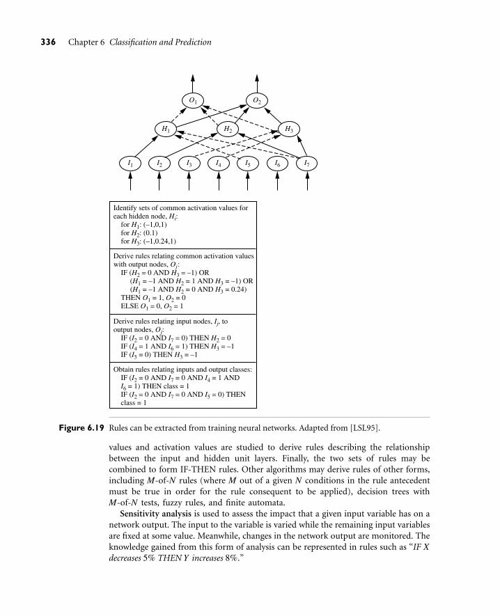
336 Chapter 6 Classification and Prediction
H1 H2 H3
O1 O2
I1 I2 I3 I4 I5 I6 I7
Identify sets of common activation values for each hidden node, Hi: for H1: (–1,0,1) for H2: (0.1) for H3: (–1,0.24,1)
Derive rules relating common activation values with output nodes, Oj: IF (H2 = 0 AND H3 = –1) OR (H1 = –1 AND H2 = 1 AND H3 = –1) OR (H1 = –1 AND H2 = 0 AND H3 = 0.24) THEN O1 = 1, O2 = 0 ELSE O1 = 0, O2 = 1
Derive rules relating input nodes, Ij, to output nodes, Oj: IF (I2 = 0 AND I7 = 0) THEN H2 = 0 IF (I4 = 1 AND I6 = 1) THEN H3 = –1 IF (I5 = 0) THEN H3 = –1
Obtain rules relating inputs and output classes: IF (I2 = 0 AND I7 = 0 AND I4 = 1 AND I6 = 1) THEN class = 1 IF (I2 = 0 AND I7 = 0 AND I5 = 0) THEN class = 1
Figure 6.19 Rules can be extracted from training neural networks. Adapted from [LSL95].
values and activation values are studied to derive rules describing the relationshipbetween the input and hidden unit layers. Finally, the two sets of rules may becombined to form IF-THEN rules. Other algorithms may derive rules of other forms,including M-of-N rules (where M out of a given N conditions in the rule antecedentmust be true in order for the rule consequent to be applied), decision trees withM-of-N tests, fuzzy rules, and finite automata.
Sensitivity analysis is used to assess the impact that a given input variable has on anetwork output. The input to the variable is varied while the remaining input variablesare fixed at some value. Meanwhile, changes in the network output are monitored. Theknowledge gained from this form of analysis can be represented in rules such as “IF Xdecreases 5% THEN Y increases 8%.”

6.7 Support Vector Machines 337
6.7 Support Vector Machines
In this section, we study Support Vector Machines, a promising new method for theclassification of both linear and nonlinear data. In a nutshell, a support vector machine(or SVM) is an algorithm that works as follows. It uses a nonlinear mapping to trans-form the original training data into a higher dimension. Within this new dimension,it searches for the linear optimal separating hyperplane (that is, a “decision boundary”separating the tuples of one class from another). With an appropriate nonlinear map-ping to a sufficiently high dimension, data from two classes can always be separated bya hyperplane. The SVM finds this hyperplane using support vectors (“essential” trainingtuples) and margins (defined by the support vectors). We will delve more into these newconcepts further below.
“I’ve heard that SVMs have attracted a great deal of attention lately. Why?” The firstpaper on support vector machines was presented in 1992 by Vladimir Vapnik and col-leagues Bernhard Boser and Isabelle Guyon, although the groundwork for SVMs hasbeen around since the 1960s (including early work by Vapnik and Alexei Chervonenkison statistical learning theory). Although the training time of even the fastest SVMs can beextremely slow, they are highly accurate, owing to their ability to model complex nonlin-ear decision boundaries. They are much less prone to overfitting than other methods. Thesupport vectors found also provide a compact description of the learned model. SVMscan be used for prediction as well as classification. They have been applied to a num-ber of areas, including handwritten digit recognition, object recognition, and speakeridentification, as well as benchmark time-series prediction tests.
6.7.1 The Case When the Data Are Linearly Separable
To explain the mystery of SVMs, let’s first look at the simplest case—a two-class problemwhere the classes are linearly separable. Let the data set D be given as (X1, y1),(X2, y2), . . . , (X|D|, y|D|), where Xi is the set of training tuples with associated class labels, yi.Each yi can take one of two values, either +1 or−1 (i.e., yi ∈ {+1, −1}), correspondingto the classes buys computer = yes and buys computer = no, respectively. To aid in visual-ization, let’s consider an example based on two input attributes, A1 and A2, as shown inFigure 6.20. From the graph, we see that the 2-D data are linearly separable (or “linear,”for short) because a straight line can be drawn to separate all of the tuples of class +1 fromall of the tuples of class−1. There are an infinite number of separating lines that could bedrawn. We want to find the “best” one, that is, one that (we hope) will have the minimumclassification error on previously unseen tuples. How can we find this best line? Note thatif our data were 3-D (i.e., with three attributes), we would want to find the best separatingplane. Generalizing to n dimensions, we want to find the best hyperplane. We will use theterm “hyperplane” to refer to the decision boundary that we are seeking, regardless of thenumber of input attributes. So, in other words, how can we find the best hyperplane?
An SVM approaches this problem by searching for the maximum marginal hyper-plane. Consider Figure 6.21, which shows two possible separating hyperplanes and

338 Chapter 6 Classification and Prediction
A1
A2
class 1, y = +1 ( buys_computer = yes )
class 2, y = –1 ( buys_computer = no )
Figure 6.20 The 2-D training data are linearly separable. There are an infinite number of (possible)separating hyperplanes or “decision boundaries.” Which one is best?
their associated margins. Before we get into the definition of margins, let’s take anintuitive look at this figure. Both hyperplanes can correctly classify all of the givendata tuples. Intuitively, however, we expect the hyperplane with the larger marginto be more accurate at classifying future data tuples than the hyperplane with thesmaller margin. This is why (during the learning or training phase), the SVM searchesfor the hyperplane with the largest margin, that is, the maximum marginal hyperplane(MMH). The associated margin gives the largest separation between classes. Gettingto an informal definition of margin, we can say that the shortest distance from ahyperplane to one side of its margin is equal to the shortest distance from the hyper-plane to the other side of its margin, where the “sides” of the margin are parallel tothe hyperplane. When dealing with the MMH, this distance is, in fact, the shortestdistance from the MMH to the closest training tuple of either class.
A separating hyperplane can be written as
W ·X + b = 0, (6.32)
where W is a weight vector, namely, W = {w1, w2, . . . , wn}; n is the number of attributes;and b is a scalar, often referred to as a bias. To aid in visualization, let’s consider two inputattributes, A1 and A2, as in Figure 6.21(b). Training tuples are 2-D, e.g., X = (x1, x2),where x1 and x2 are the values of attributes A1 and A2, respectively, for X. If we think ofb as an additional weight, w0, we can rewrite the above separating hyperplane as
w0 + w1x1 + w2x2 = 0. (6.33)

6.7 Support Vector Machines 339
A1
A2
class 1, y = +1 ( buys_computer = yes )
class 2, y = –1 ( buys_computer = no )
A1
A2
class 1, y = +1 ( buys_computer = yes )
class 2, y = –1 ( buys_computer = no )
large
marg
in
small margin
Figure 6.21 Here we see just two possible separating hyperplanes and their associated margins. Whichone is better? The one with the larger margin should have greater generalization accuracy.
Thus, any point that lies above the separating hyperplane satisfies
w0 + w1x1 + w2x2 > 0. (6.34)
Similarly, any point that lies below the separating hyperplane satisfies
w0 + w1x1 + w2x2 < 0. (6.35)

340 Chapter 6 Classification and Prediction
A1
A2
class 1, y = +1 ( buys_computer = yes )
class 2, y = –1 ( buys_computer = no )
large
marg
in
Figure 6.22 Support vectors. The SVM finds the maximum separating hyperplane, that is, the one withmaximum distance between the nearest training tuples. The support vectors are shown witha thicker border.
The weights can be adjusted so that the hyperplanes defining the “sides” of the margincan be written as
H1 : w0 + w1x1 + w2x2 ≥ 1 for yi = +1, and (6.36)H2 : w0 + w1x1 + w2x2 ≤−1 for yi =−1. (6.37)
That is, any tuple that falls on or above H1 belongs to class +1, and any tuple that fallson or below H2 belongs to class−1. Combining the two inequalities of Equations (6.36)and (6.37), we get
yi(w0 + w1x1 + w2x2)≥ 1, ∀i. (6.38)
Any training tuples that fall on hyperplanes H1 or H2 (i.e., the “sides” defining themargin) satisfy Equation (6.38) and are called support vectors. That is, they are equallyclose to the (separating) MMH. In Figure 6.22, the support vectors are shown encircledwith a thicker border. Essentially, the support vectors are the most difficult tuples toclassify and give the most information regarding classification.
From the above, we can obtain a formulae for the size of the maximal margin. Thedistance from the separating hyperplane to any point on H1 is 1
||W|| , where ||W || is the
Euclidean norm of W, that is√
W ·W.9 By definition, this is equal to the distance fromany point on H2 to the separating hyperplane. Therefore, the maximal margin is 2
||W|| .
“So, how does an SVM find the MMH and the support vectors?” Using some “fancy mathtricks,” we can rewrite Equation (6.38) so that it becomes what is known as a constrained
9If W = {w1, w2, . . . , wn} then√
W ·W =√
w21 + w2
2 + · · ·+ w2n.

6.7 Support Vector Machines 341
(convex) quadratic optimization problem. Such fancy math tricks are beyond the scopeof this book. Advanced readers may be interested to note that the tricks involve rewritingEquation (6.38) using a Lagrangian formulation and then solving for the solution usingKarush-Kuhn-Tucker (KKT) conditions. Details can be found in references at the end ofthis chapter. If the data are small (say, less than 2,000 training tuples), any optimizationsoftware package for solving constrained convex quadratic problems can then be usedto find the support vectors and MMH. For larger data, special and more efficient algo-rithms for training SVMs can be used instead, the details of which exceed the scope of thisbook. Once we’ve found the support vectors and MMH (note that the support vectorsdefine the MMH!), we have a trained support vector machine. The MMH is a linear classboundary, and so the corresponding SVM can be used to classify linearly separable data.We refer to such a trained SVM as a linear SVM.
“Once I’ve got a trained support vector machine, how do I use it to classify test (i.e.,new) tuples?” Based on the Lagrangian formulation mentioned above, the MMH can berewritten as the decision boundary
d(XT ) =l
∑i=1
yiαiXiXT + b0, (6.39)
where yi is the class label of support vector Xi; XT is a test tuple; αi and b0 are numericparameters that were determined automatically by the optimization or SVM algorithmabove; and l is the number of support vectors.
Interested readers may note that the αi are Lagrangian multipliers. For linearly sepa-rable data, the support vectors are a subset of the actual training tuples (although therewill be a slight twist regarding this when dealing with nonlinearly separable data, as weshall see below).
Given a test tuple, XT , we plug it into Equation (6.39), and then check to see the sign ofthe result. This tells us on which side of the hyperplane the test tuple falls. If the sign is pos-itive, then XT falls on or above the MMH, and so the SVM predicts that XT belongs to class+1 (representing buys computer = yes, in our case). If the sign is negative, then XT falls onor below the MMH and the class prediction is−1 (representing buys computer = no).
Notice that the Lagrangian formulation of our problem (Equation (6.39)) contains adot product between support vector Xi and test tuple XT . This will prove very useful forfinding the MMH and support vectors for the case when the given data are nonlinearlyseparable, as described further below.
Before we move on to the nonlinear case, there are two more important things tonote. The complexity of the learned classifier is characterized by the number of supportvectors rather than the dimensionality of the data. Hence, SVMs tend to be less proneto overfitting than some other methods. The support vectors are the essential or criticaltraining tuples—they lie closest to the decision boundary (MMH). If all other trainingtuples were removed and training were repeated, the same separating hyperplane wouldbe found. Furthermore, the number of support vectors found can be used to computean (upper) bound on the expected error rate of the SVM classifier, which is independentof the data dimensionality. An SVM with a small number of support vectors can havegood generalization, even when the dimensionality of the data is high.

342 Chapter 6 Classification and Prediction
A1
A2
class 1, y = +1 ( buys_computer = yes )
class 2, y = –1 ( buys_computer = no )
Figure 6.23 A simple 2-D case showing linearly inseparable data. Unlike the linear separable data ofFigure 6.20, here it is not possible to draw a straight line to separate the classes. Instead, thedecision boundary is nonlinear.
6.7.2 The Case When the Data Are Linearly Inseparable
In Section 6.7.1 we learned about linear SVMs for classifying linearly separable data, butwhat if the data are not linearly separable, as in Figure 6.23? In such cases, no straightline can be found that would separate the classes. The linear SVMs we studied would notbe able to find a feasible solution here. Now what?
The good news is that the approach described for linear SVMs can be extended tocreate nonlinear SVMs for the classification of linearly inseparable data (also called non-linearly separable data, or nonlinear data, for short). Such SVMs are capable of findingnonlinear decision boundaries (i.e., nonlinear hypersurfaces) in input space.
“So,” you may ask, “how can we extend the linear approach?” We obtain a nonlinearSVM by extending the approach for linear SVMs as follows. There are two main steps.In the first step, we transform the original input data into a higher dimensional spaceusing a nonlinear mapping. Several common nonlinear mappings can be used in thisstep, as we will describe further below. Once the data have been transformed into thenew higher space, the second step searches for a linear separating hyperplane in the newspace. We again end up with a quadratic optimization problem that can be solved usingthe linear SVM formulation. The maximal marginal hyperplane found in the new spacecorresponds to a nonlinear separating hypersurface in the original space.
Example 6.10 Nonlinear transformation of original input data into a higher dimensional space. Con-sider the following example. A 3D input vector X = (x1, x2, x3) is mapped into a 6D space,Z, using the mappings φ1(X) = x1, φ2(X) = x2, φ3(X) = x3, φ4(X) = (x1)2, φ5(X) =x1x2, and φ6(X) = x1x3. A decision hyperplane in the new space is d(Z) = WZ + b,where W and Z are vectors. This is linear. We solve for W and b and then substitute back

6.7 Support Vector Machines 343
so that the linear decision hyperplane in the new (Z) space corresponds to a nonlinearsecond-order polynomial in the original 3-D input space,
d(Z) = w1x1 + w2x2 + w3x3 + w4(x1)2 + w5x1x2 + w6x1x3 + b
= w1z1 + w2z2 + w3z3 + w4z4 + w5z5 + w6z6 + b
But there are some problems. First, how do we choose the nonlinear mapping to ahigher dimensional space? Second, the computation involved will be costly. Refer backto Equation (6.39) for the classification of a test tuple, XT . Given the test tuple, we have tocompute its dot product with every one of the support vectors.10 In training, we have tocompute a similar dot product several times in order to find the MMH. This is especiallyexpensive. Hence, the dot product computation required is very heavy and costly. Weneed another trick!
Luckily, we can use another math trick. It so happens that in solving the quadraticoptimization problem of the linear SVM (i.e., when searching for a linear SVM in the newhigher dimensional space), the training tuples appear only in the form of dot products,φ(Xi) ·φ(Xj), where φ(X) is simply the nonlinear mapping function applied to transformthe training tuples. Instead of computing the dot product on the transformed data tuples,it turns out that it is mathematically equivalent to instead apply a kernel function, K(Xi,Xj), to the original input data. That is,
K(Xi, Xj) = φ(Xi) ·φ(Xj). (6.40)
In other words, everywhere that φ(Xi) ·φ(Xj) appears in the training algorithm, we canreplace it with K(Xi,Xj). In this way, all calculations are made in the original input space,which is of potentially much lower dimensionality! We can safely avoid the mapping—itturns out that we don’t even have to know what the mapping is! We will talk more laterabout what kinds of functions can be used as kernel functions for this problem.
After applying this trick, we can then proceed to find a maximal separating hyper-plane. The procedure is similar to that described in Section 6.7.1, although it involvesplacing a user-specified upper bound, C, on the Lagrange multipliers, αi. This upperbound is best determined experimentally.
“What are some of the kernel functions that could be used?” Properties of the kinds ofkernel functions that could be used to replace the dot product scenario described abovehave been studied. Three admissible kernel functions include:
Polynomial kernel of degree h : K(Xi, Xj) = (Xi ·Xj + 1)h (6.41)
Gaussian radial basis function kernel : K(Xi, Xj) = e−‖Xi−Xj‖2/2σ2(6.42)
Sigmoid kernel : K(Xi, Xj) = tanh(κXi ·Xj−δ) (6.43)
10The dot product of two vectors, XT = (xT1 , xT
2 , . . . , xTn ) and Xi = (xi1, xi2, . . . , xin) is xT
1 xi1 +xT2 xi2 + · · ·+
xTn xin. Note that this involves one multiplication and one addition for each of the n dimensions.

344 Chapter 6 Classification and Prediction
Each of these results in a different nonlinear classifier in (the original) input space.Neural network aficionados will be interested to note that the resulting decision hyper-planes found for nonlinear SVMs are the same type as those found by other well-knownneural network classifiers. For instance, an SVM with a Gaussian radial basis function(RBF) gives the same decision hyperplane as a type of neural network known as a radialbasis function (RBF) network. An SVM with a sigmoid kernel is equivalent to a sim-ple two-layer neural network known as a multilayer perceptron (with no hidden layers).There are no golden rules for determining which admissible kernel will result in the mostaccurate SVM. In practice, the kernel chosen does not generally make a large difference inresulting accuracy. SVM training always finds a global solution, unlike neural networkssuch as backpropagation, where many local minima usually exist (Section 6.6.3).
So far, we have described linear and nonlinear SVMs for binary (i.e., two-class) classi-fication. SVM classifiers can be combined for the multiclass case. A simple and effectiveapproach, given m classes, trains m classifiers, one for each class (where classifier j learnsto return a positive value for class j and a negative value for the rest). A test tuple isassigned the class corresponding to the largest positive distance.
Aside from classification, SVMs can also be designed for linear and nonlinear regres-sion. Here, instead of learning to predict discrete class labels (like the yi ∈ {+1, − 1}above), SVMs for regression attempt to learn the input-output relationship betweeninput training tuples, Xi, and their corresponding continuous-valued outputs, yi ∈ R .An approach similar to SVMs for classification is followed. Additional user-specifiedparameters are required.
A major research goal regarding SVMs is to improve the speed in training and testingso that SVMs may become a more feasible option for very large data sets (e.g., of millionsof support vectors). Other issues include determining the best kernel for a given data setand finding more efficient methods for the multiclass case.
6.8 Associative Classification: Classificationby Association Rule Analysis
Frequent patterns and their corresponding association or correlation rules character-ize interesting relationships between attribute conditions and class labels, and thus havebeen recently used for effective classification. Association rules show strong associationsbetween attribute-value pairs (or items) that occur frequently in a given data set. Asso-ciation rules are commonly used to analyze the purchasing patterns of customers in astore. Such analysis is useful in many decision-making processes, such as product place-ment, catalog design, and cross-marketing. The discovery of association rules is based onfrequent itemset mining. Many methods for frequent itemset mining and the generationof association rules were described in Chapter 5. In this section, we look at associativeclassification, where association rules are generated and analyzed for use in classifica-tion. The general idea is that we can search for strong associations between frequentpatterns (conjunctions of attribute-value pairs) and class labels. Because association rules

6.8 Associative Classification: Classification by Association Rule Analysis 345
explore highly confident associations among multiple attributes, this approach may over-come some constraints introduced by decision-tree induction, which considers only oneattribute at a time. In many studies, associative classification has been found to be moreaccurate than some traditional classification methods, such as C4.5. In particular, westudy three main methods: CBA, CMAR, and CPAR.
Before we begin, let’s look at association rule mining, in general. Association rules aremined in a two-step process consisting of frequent itemset mining, followed by rule gener-ation. The first step searches for patterns of attribute-value pairs that occur repeatedly ina data set, where each attribute-value pair is considered an item. The resulting attribute-value pairs form frequent itemsets. The second step analyzes the frequent itemsets in orderto generate association rules. All association rules must satisfy certain criteria regardingtheir “accuracy” (or confidence) and the proportion of the data set that they actually rep-resent (referred to as support). For example, the following is an association rule minedfrom a data set, D, shown with its confidence and support.
age = youth∧credit = OK⇒ buys computer = yes [support = 20%, confidence = 93%](6.44)
where “∧” represents a logical “AND.” We will say more about confidence and supportin a minute.
More formally, let D be a data set of tuples. Each tuple in D is described by n attributes,A1, A2, . . . , An, and a class label attribute, Aclass. All continuous attributes are discretizedand treated as categorical attributes. An item, p, is an attribute-value pair of the form(Ai, v), where Ai is an attribute taking a value, v. A data tuple X = (x1, x2, . . . , xn) satis-fies an item, p = (Ai, v), if and only if xi = v, where xi is the value of the ith attributeof X. Association rules can have any number of items in the rule antecedent (left-handside) and any number of items in the rule consequent (right-hand side). However, whenmining association rules for use in classification, we are only interested in associationrules of the form p1 ∧ p2 ∧ . . . pl ⇒ Aclass = C where the rule antecedent is a conjunc-tion of items, p1, p2, . . . , pl (l ≤ n), associated with a class label, C. For a given rule, R,the percentage of tuples in D satisfying the rule antecedent that also have the class labelC is called the confidence of R. From a classification point of view, this is akin to ruleaccuracy. For example, a confidence of 93% for Association Rule (6.44) means that 93%of the customers in D who are young and have an OK credit rating belong to the classbuys computer = yes. The percentage of tuples in D satisfying the rule antecedent and hav-ing class label C is called the support of R. A support of 20% for Association Rule (6.44)means that 20% of the customers in D are young, have an OK credit rating, and belongto the class buys computer = yes.
Methods of associative classification differ primarily in the approach used for frequentitemset mining and in how the derived rules are analyzed and used for classification. Wenow look at some of the various methods for associative classification.
One of the earliest and simplest algorithms for associative classification is CBA(Classification-Based Association). CBA uses an iterative approach to frequent itemsetmining, similar to that described for Apriori in Section 5.2.1, where multiple passes are

346 Chapter 6 Classification and Prediction
made over the data and the derived frequent itemsets are used to generate and test longeritemsets. In general, the number of passes made is equal to the length of the longest rulefound. The complete set of rules satisfying minimum confidence and minimum sup-port thresholds are found and then analyzed for inclusion in the classifier. CBA uses aheuristic method to construct the classifier, where the rules are organized according todecreasing precedence based on their confidence and support. If a set of rules has thesame antecedent, then the rule with the highest confidence is selected to represent theset. When classifying a new tuple, the first rule satisfying the tuple is used to classify it.The classifier also contains a default rule, having lowest precedence, which specifies adefault class for any new tuple that is not satisfied by any other rule in the classifier. Inthis way, the set of rules making up the classifier form a decision list. In general, CBA wasempirically found to be more accurate than C4.5 on a good number of data sets.
CMAR (Classification based on Multiple Association Rules) differs from CBA in itsstrategy for frequent itemset mining and its construction of the classifier. It also employsseveral rule pruning strategies with the help of a tree structure for efficient storage andretrieval of rules. CMAR adopts a variant of the FP-growth algorithm to find the com-plete set of rules satisfying the minimum confidence and minimum support thresholds.FP-growth was described in Section 5.2.4. FP-growth uses a tree structure, called anFP-tree, to register all of the frequent itemset information contained in the given dataset, D. This requires only two scans of D. The frequent itemsets are then mined from theFP-tree. CMAR uses an enhanced FP-tree that maintains the distribution of class labelsamong tuples satisfying each frequent itemset. In this way, it is able to combine rule gen-eration together with frequent itemset mining in a single step.
CMAR employs another tree structure to store and retrieve rules efficiently and toprune rules based on confidence, correlation, and database coverage. Rule pruning strate-gies are triggered whenever a rule is inserted into the tree. For example, given two rules,R1 and R2, if the antecedent of R1 is more general than that of R2 and conf(R1) ≥conf(R2), then R2 is pruned. The rationale is that highly specialized rules with low confi-dence can be pruned if a more generalized version with higher confidence exists. CMARalso prunes rules for which the rule antecedent and class are not positively correlated,based on a χ2 test of statistical significance.
As a classifier, CMAR operates differently than CBA. Suppose that we are given a tupleX to classify and that only one rule satisfies or matches X.11 This case is trivial—we simplyassign the class label of the rule. Suppose, instead, that more than one rule satisfies X.These rules form a set, S. Which rule would we use to determine the class label of X? CBAwould assign the class label of the most confident rule among the rule set, S. CMARinstead considers multiple rules when making its class prediction. It divides the rulesinto groups according to class labels. All rules within a group share the same class labeland each group has a distinct class label. CMAR uses a weighted χ2 measure to find the“strongest” group of rules, based on the statistical correlation of rules within a group.It then assigns X the class label of the strongest group. In this way it considers multiple
11If the antecedent of a rule satisfies or matches X, then we say that the rule satisfies X.

6.9 Lazy Learners (or Learning from Your Neighbors) 347
rules, rather than a single rule with highest confidence, when predicting the class label ofa new tuple. On experiments, CMAR had slightly higher average accuracy in comparisonwith CBA. Its runtime, scalability, and use of memory were found to be more efficient.
CBA and CMAR adopt methods of frequent itemset mining to generate candidateassociation rules, which include all conjunctions of attribute-value pairs (items) satisfy-ing minimum support. These rules are then examined, and a subset is chosen to representthe classifier. However, such methods generate quite a large number of rules. CPAR takesa different approach to rule generation, based on a rule generation algorithm for classi-fication known as FOIL (Section 6.5.3). FOIL builds rules to distinguish positive tuples(say, having class buys computer = yes) from negative tuples (such as buys computer =no). For multiclass problems, FOIL is applied to each class. That is, for a class, C, alltuples of class C are considered positive tuples, while the rest are considered negativetuples. Rules are generated to distinguish C tuples from all others. Each time a rule isgenerated, the positive samples it satisfies (or covers) are removed until all the positivetuples in the data set are covered. CPAR relaxes this step by allowing the covered tuples toremain under consideration, but reducing their weight. The process is repeated for eachclass. The resulting rules are merged to form the classifier rule set.
During classification, CPAR employs a somewhat different multiple rule strategy thanCMAR. If more than one rule satisfies a new tuple, X, the rules are divided into groupsaccording to class, similar to CMAR. However, CPAR uses the best k rules of each groupto predict the class label of X, based on expected accuracy. By considering the best k rulesrather than all of the rules of a group, it avoids the influence of lower ranked rules. Theaccuracy of CPAR on numerous data sets was shown to be close to that of CMAR. How-ever, since CPAR generates far fewer rules than CMAR, it shows much better efficiencywith large sets of training data.
In summary, associative classification offers a new alternative to classification schemesby building rules based on conjunctions of attribute-value pairs that occur frequentlyin data.
6.9 Lazy Learners (or Learning from Your Neighbors)
The classification methods discussed so far in this chapter—decision tree induction,Bayesian classification, rule-based classification, classification by backpropagation, sup-port vector machines, and classification based on association rule mining—are all exam-ples of eager learners. Eager learners, when given a set of training tuples, will construct ageneralization (i.e., classification) model before receiving new (e.g., test) tuples to clas-sify. We can think of the learned model as being ready and eager to classify previouslyunseen tuples.
Imagine a contrasting lazy approach, in which the learner instead waits until the lastminute before doing any model construction in order to classify a given test tuple. Thatis, when given a training tuple, a lazy learner simply stores it (or does only a little minorprocessing) and waits until it is given a test tuple. Only when it sees the test tuple does itperform generalization in order to classify the tuple based on its similarity to the stored
348 Chapter 6 Classification and Prediction
training tuples. Unlike eager learning methods, lazy learners do less work when a trainingtuple is presented and more work when making a classification or prediction. Becauselazy learners store the training tuples or “instances,” they are also referred to as instance-based learners, even though all learning is essentially based on instances.
When making a classification or prediction, lazy learners can be computationallyexpensive. They require efficient storage techniques and are well-suited to implemen-tation on parallel hardware. They offer little explanation or insight into the structure ofthe data. Lazy learners, however, naturally support incremental learning. They are ableto model complex decision spaces having hyperpolygonal shapes that may not be as eas-ily describable by other learning algorithms (such as hyper-rectangular shapes modeledby decision trees). In this section, we look at two examples of lazy learners: k-nearest-neighbor classifiers and case-based reasoning classifiers.
6.9.1 k-Nearest-Neighbor Classifiers
The k-nearest-neighbor method was first described in the early 1950s. The method islabor intensive when given large training sets, and did not gain popularity until the 1960swhen increased computing power became available. It has since been widely used in thearea of pattern recognition.
Nearest-neighbor classifiers are based on learning by analogy, that is, by comparing agiven test tuple with training tuples that are similar to it. The training tuples are describedby n attributes. Each tuple represents a point in an n-dimensional space. In this way,all of the training tuples are stored in an n-dimensional pattern space. When given anunknown tuple, a k-nearest-neighbor classifier searches the pattern space for the k train-ing tuples that are closest to the unknown tuple. These k training tuples are the k “nearestneighbors” of the unknown tuple.
“Closeness” is defined in terms of a distance metric, such as Euclidean distance.The Euclidean distance between two points or tuples, say, X1 = (x11, x12, . . . , x1n) andX2 = (x21, x22, . . . , x2n), is
dist(X1, X2) =
√
n
∑i=1
(x1i− x2i)2. (6.45)
In other words, for each numeric attribute, we take the difference between the corre-sponding values of that attribute in tuple X1 and in tuple X2, square this difference,and accumulate it. The square root is taken of the total accumulated distance count.Typically, we normalize the values of each attribute before using Equation (6.45). Thishelps prevent attributes with initially large ranges (such as income) from outweighingattributes with initially smaller ranges (such as binary attributes). Min-max normaliza-tion, for example, can be used to transform a value v of a numeric attribute A to v′ in therange [0, 1] by computing
v′ =v−minA
maxA−minA, (6.46)

6.9 Lazy Learners (or Learning from Your Neighbors) 349
where minA and maxA are the minimum and maximum values of attribute A. Chapter 2describes other methods for data normalization as a form of data transformation.
For k-nearest-neighbor classification, the unknown tuple is assigned the mostcommon class among its k nearest neighbors. When k = 1, the unknown tuple isassigned the class of the training tuple that is closest to it in pattern space. Nearest-neighbor classifiers can also be used for prediction, that is, to return a real-valuedprediction for a given unknown tuple. In this case, the classifier returns the averagevalue of the real-valued labels associated with the k nearest neighbors of the unknowntuple.
“But how can distance be computed for attributes that not numeric, but categorical, suchas color?” The above discussion assumes that the attributes used to describe the tuples areall numeric. For categorical attributes, a simple method is to compare the correspondingvalue of the attribute in tuple X1 with that in tuple X2. If the two are identical (e.g., tuplesX1 and X2 both have the color blue), then the difference between the two is taken as 0.If the two are different (e.g., tuple X1 is blue but tuple X2 is red), then the differenceis considered to be 1. Other methods may incorporate more sophisticated schemes fordifferential grading (e.g., where a larger difference score is assigned, say, for blue andwhite than for blue and black).
“What about missing values?” In general, if the value of a given attribute A is missing intuple X1 and/or in tuple X2, we assume the maximum possible difference. Suppose thateach of the attributes have been mapped to the range [0, 1]. For categorical attributes, wetake the difference value to be 1 if either one or both of the corresponding values of Aare missing. If A is numeric and missing from both tuples X1 and X2, then the differenceis also taken to be 1. If only one value is missing and the other (which we’ll call v′) ispresent and normalized, then we can take the difference to be either |1− v′| or |0− v′|(i.e., 1− v′ or v′), whichever is greater.
“How can I determine a good value for k, the number of neighbors?” This can be deter-mined experimentally. Starting with k = 1, we use a test set to estimate the error rateof the classifier. This process can be repeated each time by incrementing k to allow forone more neighbor. The k value that gives the minimum error rate may be selected. Ingeneral, the larger the number of training tuples is, the larger the value of k will be (sothat classification and prediction decisions can be based on a larger portion of the storedtuples). As the number of training tuples approaches infinity and k = 1, the error rate canbe no worse then twice the Bayes error rate (the latter being the theoretical minimum).If k also approaches infinity, the error rate approaches the Bayes error rate.
Nearest-neighbor classifiers use distance-based comparisons that intrinsically assignequal weight to each attribute. They therefore can suffer from poor accuracy when givennoisy or irrelevant attributes. The method, however, has been modified to incorporateattribute weighting and the pruning of noisy data tuples. The choice of a distance metriccan be critical. The Manhattan (city block) distance (Section 7.2.1), or other distancemeasurements, may also be used.
Nearest-neighbor classifiers can be extremely slow when classifying test tuples. If Dis a training database of |D| tuples and k = 1, then O(|D|) comparisons are requiredin order to classify a given test tuple. By presorting and arranging the stored tuples

350 Chapter 6 Classification and Prediction
into search trees, the number of comparisons can be reduced to O(log(|D|). Parallelimplementation can reduce the running time to a constant, that is O(1), which is inde-pendent of |D|. Other techniques to speed up classification time include the use of par-tial distance calculations and editing the stored tuples. In the partial distance method,we compute the distance based on a subset of the n attributes. If this distance exceeds athreshold, then further computation for the given stored tuple is halted, and the processmoves on to the next stored tuple. The editing method removes training tuples that proveuseless. This method is also referred to as pruning or condensing because it reduces thetotal number of tuples stored.
6.9.2 Case-Based Reasoning
Case-based reasoning (CBR) classifiers use a database of problem solutions to solvenew problems. Unlike nearest-neighbor classifiers, which store training tuples as pointsin Euclidean space, CBR stores the tuples or “cases” for problem solving as complexsymbolic descriptions. Business applications of CBR include problem resolution forcustomer service help desks, where cases describe product-related diagnostic problems.CBR has also been applied to areas such as engineering and law, where cases are eithertechnical designs or legal rulings, respectively. Medical education is another area forCBR, where patient case histories and treatments are used to help diagnose and treatnew patients.
When given a new case to classify, a case-based reasoner will first check if an iden-tical training case exists. If one is found, then the accompanying solution to that caseis returned. If no identical case is found, then the case-based reasoner will search fortraining cases having components that are similar to those of the new case. Conceptu-ally, these training cases may be considered as neighbors of the new case. If cases arerepresented as graphs, this involves searching for subgraphs that are similar to sub-graphs within the new case. The case-based reasoner tries to combine the solutionsof the neighboring training cases in order to propose a solution for the new case. Ifincompatibilities arise with the individual solutions, then backtracking to search forother solutions may be necessary. The case-based reasoner may employ backgroundknowledge and problem-solving strategies in order to propose a feasible combinedsolution.
Challenges in case-based reasoning include finding a good similarity metric (e.g., formatching subgraphs) and suitable methods for combining solutions. Other challengesinclude the selection of salient features for indexing training cases and the developmentof efficient indexing techniques. A trade-off between accuracy and efficiency evolves asthe number of stored cases becomes very large. As this number increases, the case-basedreasoner becomes more intelligent. After a certain point, however, the efficiency of thesystem will suffer as the time required to search for and process relevant cases increases.As with nearest-neighbor classifiers, one solution is to edit the training database. Casesthat are redundant or that have not proved useful may be discarded for the sake ofimproved performance. These decisions, however, are not clear-cut and their automa-tion remains an active area of research.

6.10 Other Classification Methods 351
6.10 Other Classification Methods
In this section, we give a brief description of several other classification methods,including genetic algorithms, rough set approach, and fuzzy set approaches. In general,these methods are less commonly used for classification in commercial data mining sys-tems than the methods described earlier in this chapter. However, these methods do showtheir strength in certain applications, and hence it is worthwhile to include them here.
6.10.1 Genetic Algorithms
Genetic algorithms attempt to incorporate ideas of natural evolution. In general, geneticlearning starts as follows. An initial population is created consisting of randomly gener-ated rules. Each rule can be represented by a string of bits. As a simple example, supposethat samples in a given training set are described by two Boolean attributes, A1 and A2,and that there are two classes, C1 and C2. The rule “IF A1 AND NOT A2 THEN C2” can beencoded as the bit string “100,” where the two leftmost bits represent attributes A1 andA2, respectively, and the rightmost bit represents the class. Similarly, the rule “IF NOTA1 AND NOT A2 THEN C1” can be encoded as “001.” If an attribute has k values, wherek > 2, then k bits may be used to encode the attribute’s values. Classes can be encodedin a similar fashion.
Based on the notion of survival of the fittest, a new population is formed to consist ofthe fittest rules in the current population, as well as offspring of these rules. Typically, thefitness of a rule is assessed by its classification accuracy on a set of training samples.
Offspring are created by applying genetic operators such as crossover and mutation.In crossover, substrings from pairs of rules are swapped to form new pairs of rules. Inmutation, randomly selected bits in a rule’s string are inverted.
The process of generating new populations based on prior populations of rules con-tinues until a population, P, evolves where each rule in P satisfies a prespecified fitnessthreshold.
Genetic algorithms are easily parallelizable and have been used for classification aswell as other optimization problems. In data mining, they may be used to evaluate thefitness of other algorithms.
6.10.2 Rough Set Approach
Rough set theory can be used for classification to discover structural relationships withinimprecise or noisy data. It applies to discrete-valued attributes. Continuous-valuedattributes must therefore be discretized before its use.
Rough set theory is based on the establishment of equivalence classes within the giventraining data. All of the data tuples forming an equivalence class are indiscernible, thatis, the samples are identical with respect to the attributes describing the data. Given real-world data, it is common that some classes cannot be distinguished in terms of the avail-able attributes. Rough sets can be used to approximately or “roughly” define such classes.A rough set definition for a given class, C, is approximated by two sets—a lower

352 Chapter 6 Classification and Prediction
C
Upper approximation of CLower approximation of C
Figure 6.24 A rough set approximation of the set of tuples of the class C using lower and upper approxi-mation sets of C. The rectangular regions represent equivalence classes.
approximation of C and an upper approximation of C. The lower approximation of Cconsists of all of the data tuples that, based on the knowledge of the attributes, are certainto belong to C without ambiguity. The upper approximation of C consists of all of thetuples that, based on the knowledge of the attributes, cannot be described as not belong-ing to C. The lower and upper approximations for a class C are shown in Figure 6.24,where each rectangular region represents an equivalence class. Decision rules can begenerated for each class. Typically, a decision table is used to represent the rules.
Rough sets can also be used for attribute subset selection (or feature reduction,where attributes that do not contribute toward the classification of the given trainingdata can be identified and removed) and relevance analysis (where the contributionor significance of each attribute is assessed with respect to the classification task). Theproblem of finding the minimal subsets (reducts) of attributes that can describe all ofthe concepts in the given data set is NP-hard. However, algorithms to reduce the com-putation intensity have been proposed. In one method, for example, a discernibilitymatrix is used that stores the differences between attribute values for each pair of datatuples. Rather than searching on the entire training set, the matrix is instead searchedto detect redundant attributes.
6.10.3 Fuzzy Set Approaches
Rule-based systems for classification have the disadvantage that they involve sharp cutoffsfor continuous attributes. For example, consider the following rule for customer creditapplication approval. The rule essentially says that applications for customers who havehad a job for two or more years and who have a high income (i.e., of at least $50,000) areapproved:
IF (years employed ≥ 2) AND (income≥ 50K) T HEN credit = approved. (6.47)
By Rule (6.47), a customer who has had a job for at least two years will receive credit if herincome is, say, $50,000, but not if it is $49,000. Such harsh thresholding may seem unfair.

6.10 Other Classification Methods 353
Instead, we can discretize income into categories such as {low income, medium income,high income}, and then apply fuzzy logic to allow “fuzzy” thresholds or boundaries tobe defined for each category (Figure 6.25). Rather than having a precise cutoff betweencategories, fuzzy logic uses truth values between 0.0 and 1.0 to represent the degree ofmembership that a certain value has in a given category. Each category then represents afuzzy set. Hence, with fuzzy logic, we can capture the notion that an income of $49,000is, more or less, high, although not as high as an income of $50,000. Fuzzy logic systemstypically provide graphical tools to assist users in converting attribute values to fuzzy truthvalues.
Fuzzy set theory is also known as possibility theory. It was proposed by Lotfi Zadeh in1965 as an alternative to traditional two-value logic and probability theory. It lets us workat a high level of abstraction and offers a means for dealing with imprecise measurementof data. Most important, fuzzy set theory allows us to deal with vague or inexact facts. Forexample, being a member of a set of high incomes is inexact (e.g., if $50,000 is high, thenwhat about $49,000? Or $48,000?) Unlike the notion of traditional “crisp” sets where anelement either belongs to a set S or its complement, in fuzzy set theory, elements canbelong to more than one fuzzy set. For example, the income value $49,000 belongs toboth the medium and high fuzzy sets, but to differing degrees. Using fuzzy set notationand following Figure 6.25, this can be shown as
mmedium income($49K) = 0.15 and mhigh income($49K) = 0.96,
where m denotes the membership function, operating on the fuzzy sets of mediumincome and high income, respectively. In fuzzy set theory, membership values for agiven element, x, (e.g., such as for $49,000) do not have to sum to 1. This is unlike tradi-tional probability theory, which is constrained by a summation axiom.
1.0
10K 20K 30K 40K 50K 60K 70K
income
0.5
00
highmediumlow
fuzz
y m
embe
rshi
p
Figure 6.25 Fuzzy truth values for income, representing the degree of membership of income values withrespect to the categories {low, medium, high}. Each category represents a fuzzy set. Note thata given income value, x, can have membership in more than one fuzzy set. The membershipvalues of x in each fuzzy set do not have to total to 1.

354 Chapter 6 Classification and Prediction
Fuzzy set theory is useful for data mining systems performing rule-based classifica-tion. It provides operations for combining fuzzy measurements. Suppose that in additionto the fuzzy sets for income, we defined the fuzzy sets junior employee and senior employeefor the attribute years employed. Suppose also that we have a rule that, say, tests highincome and senior employee in the rule antecedent (IF part) for a given employee, x. Ifthese two fuzzy measures are ANDed together, the minimum of their measure is takenas the measure of the rule. In other words,
m(high income AND senior employee)(x) = min(mhigh income(x), msenior employee(x)).
This is akin to saying that a chain is as strong as its weakest link. If the two measures areORed, the maximum of their measure is taken as the measure of the rule. In other words,
m(high income OR senior employee)(x) = max(mhigh income(x), msenior employee(x)).
Intuitively, this is like saying that a rope is as strong as its strongest strand.Given a tuple to classify, more than one fuzzy rule may apply. Each applicable rule con-
tributesavoteformembershipinthecategories.Typically,thetruthvaluesforeachpredictedcategory are summed, and these sums are combined. Several procedures exist for translat-ing the resulting fuzzy output into a defuzzified or crisp value that is returned by the system.
Fuzzy logic systems have been used in numerous areas for classification, includingmarket research, finance, health care, and environmental engineering.
6.11 Prediction
“What if we would like to predict a continuous value, rather than a categorical label?”Numeric prediction is the task of predicting continuous (or ordered) values for giveninput. For example, we may wish to predict the salary of college graduates with 10 yearsof work experience, or the potential sales of a new product given its price. By far, themost widely used approach for numeric prediction (hereafter referred to as prediction)is regression, a statistical methodology that was developed by Sir Frances Galton (1822–1911), a mathematician who was also a cousin of Charles Darwin. In fact, many texts usethe terms “regression” and “numeric prediction” synonymously. However, as we haveseen, some classification techniques (such as backpropagation, support vector machines,and k-nearest-neighbor classifiers) can be adapted for prediction. In this section, we dis-cuss the use of regression techniques for prediction.
Regression analysis can be used to model the relationship between one or moreindependent or predictor variables and a dependent or response variable (which iscontinuous-valued). In the context of data mining, the predictor variables are theattributes of interest describing the tuple (i.e., making up the attribute vector). In gen-eral, the values of the predictor variables are known. (Techniques exist for handling caseswhere such values may be missing.) The response variable is what we want to predict—itis what we referred to in Section 6.1 as the predicted attribute. Given a tuple describedby predictor variables, we want to predict the associated value of the response variable.

6.11 Prediction 355
Regression analysis is a good choice when all of the predictor variables are continuous-valued as well. Many problems can be solved by linear regression, and even more can betackled by applying transformations to the variables so that a nonlinear problem canbe converted to a linear one. For reasons of space, we cannot give a fully detailed treat-ment of regression. Instead, this section provides an intuitive introduction to the topic.Section 6.11.1 discusses straight-line regression analysis (which involves a single pre-dictor variable) and multiple linear regression analysis (which involves two or morepredictor variables). Section 6.11.2 provides some pointers on dealing with nonlinearregression. Section 6.11.3 mentions other regression-based methods, such as generalizedlinear models, Poisson regression, log-linear models, and regression trees.
Several software packages exist to solve regression problems. Examples include SAS(www.sas.com), SPSS (www.spss.com), and S-Plus (www.insightful.com). Another usefulresource is the book Numerical Recipes in C, by Press, Flannery, Teukolsky, and Vetterling,and its associated source code.
6.11.1 Linear Regression
Straight-line regression analysis involves a response variable, y, and a single predictorvariable, x. It is the simplest form of regression, and models y as a linear function of x.That is,
y = b + wx, (6.48)
where the variance of y is assumed to be constant, and b and w are regression coefficientsspecifying the Y-intercept and slope of the line, respectively. The regression coefficients,w and b, can also be thought of as weights, so that we can equivalently write,
y = w0 + w1x. (6.49)
These coefficients can be solved for by the method of least squares, which estimates thebest-fitting straight line as the one that minimizes the error between the actual data andthe estimate of the line. Let D be a training set consisting of values of predictor variable,x, for some population and their associated values for response variable, y. The trainingset contains |D| data points of the form (x1, y1), (x2, y2), . . . , (x|D|, y|D|).12 The regressioncoefficients can be estimated using this method with the following equations:
w1 =
|D|
∑i=1
(xi− x)(yi− y)
|D|
∑i=1
(xi− x)2
(6.50)
12Note that earlier, we had used the notation (Xi, yi) to refer to training tuple i having associatedclass label yi, where Xi was an attribute (or feature) vector (that is, Xi was described by more thanone attribute). Here, however, we are dealing with just one predictor variable. Since the Xi here areone-dimensional, we use the notation xi over Xi in this case.

356 Chapter 6 Classification and Prediction
w0 = y−w1x (6.51)
where x is the mean value of x1, x2, . . . , x|D|, and y is the mean value of y1, y2, . . . , y|D|.The coefficients w0 and w1 often provide good approximations to otherwise complicatedregression equations.
Example 6.11 Straight-line regression using the method of least squares. Table 6.7 shows a set of paireddata where x is the number of years of work experience of a college graduate and y is the
Table 6.7 Salary data.
x years experience y salary (in $1000s)
3 30
8 57
9 64
13 72
3 36
6 43
11 59
21 90
1 20
16 83
Figure 6.26 Plot of the data in Table 6.7 for Example 6.11. Although the points do not fall on a straight line,the overall pattern suggests a linear relationship between x (years experience) and y (salary).

6.11 Prediction 357
corresponding salary of the graduate. The 2-D data can be graphed on a scatter plot, asin Figure 6.26. The plot suggests a linear relationship between the two variables, x and y.We model the relationship that salary may be related to the number of years of workexperience with the equation y = w0 + w1x.
Given the above data, we compute x = 9.1 and y = 55.4. Substituting these valuesinto Equations (6.50) and (6.51), we get
w1 =(3−9.1)(30−55.4)+(8−9.1)(57−55.4)+ · · ·+(16−9.1)(83−55.4)
(3−9.1)2 +(8−9.1)2 + · · ·+(16−9.1)2 = 3.5
w0 = 55.4− (3.5)(9.1) = 23.6
Thus, the equation of the least squares line is estimated by y = 23.6 + 3.5x. Using thisequation, we can predict that the salary of a college graduate with, say, 10 years of expe-rience is $58,600.
Multiple linear regression is an extension of straight-line regression so as to involvemore than one predictor variable. It allows response variable y to be modeled as a linearfunction of, say, n predictor variables or attributes, A1, A2, . . . , An, describing a tuple, X.(That is, X = (x1, x2, . . . , xn).) Our training data set, D, contains data of the form(X1, y1), (X2, y2), . . . , (X|D|, y|D|), where the Xi are the n-dimensional training tupleswith associated class labels, yi. An example of a multiple linear regression model basedon two predictor attributes or variables, A1 and A2, is
y = w0 + w1x1 + w2x2, (6.52)
where x1 and x2 are the values of attributes A1 and A2, respectively, in X. The method ofleast squares shown above can be extended to solve for w0, w1, and w2. The equations,however, become long and are tedious to solve by hand. Multiple regression problemsare instead commonly solved with the use of statistical software packages, such as SAS,SPSS, and S-Plus (see references above.)
6.11.2 Nonlinear Regression
“How can we model data that does not show a linear dependence? For example, what if agiven response variable and predictor variable have a relationship that may be modeled by apolynomial function?” Think back to the straight-line linear regression case above wheredependent response variable, y, is modeled as a linear function of a single independentpredictor variable, x. What if we can get a more accurate model using a nonlinear model,such as a parabola or some other higher-order polynomial? Polynomial regression isoften of interest when there is just one predictor variable. It can be modeled by addingpolynomial terms to the basic linear model. By applying transformations to the variables,we can convert the nonlinear model into a linear one that can then be solved by themethod of least squares.

358 Chapter 6 Classification and Prediction
Example 6.12 Transformation of a polynomial regression model to a linear regression model.Consider a cubic polynomial relationship given by
y = w0 + w1x + w2x2 + w3x3. (6.53)
To convert this equation to linear form, we define new variables:
x1 = x x2 = x2 x3 = x3 (6.54)
Equation (6.53) can then be converted to linear form by applying the above assignments,resulting in the equation y = w0 + w1x1 + w2x2 + w3x3, which is easily solved by themethod of least squares using software for regression analysis. Note that polynomialregression is a special case of multiple regression. That is, the addition of high-orderterms like x2, x3, and so on, which are simple functions of the single variable, x, can beconsidered equivalent to adding new independent variables.
In Exercise 15, you are asked to find the transformations required to convert a non-linear model involving a power function into a linear regression model.
Some models are intractably nonlinear (such as the sum of exponential terms, forexample) and cannot be converted to a linear model. For such cases, it may be possible toobtain least square estimates through extensive calculations on more complex formulae.
Various statistical measures exist for determining how well the proposed model canpredict y. These are described in Section 6.12.2. Obviously, the greater the number ofpredictor attributes is, the slower the performance is. Before applying regression analysis,it is common to perform attribute subset selection (Section 2.5.2) to eliminate attributesthat are unlikely to be good predictors for y. In general, regression analysis is accuratefor prediction, except when the data contain outliers. Outliers are data points that arehighly inconsistent with the remaining data (e.g., they may be way out of the expectedvalue range). Outlier detection is discussed in Chapter 7. Such techniques must be usedwith caution, however, so as not to remove data points that are valid, although they mayvary greatly from the mean.
6.11.3 Other Regression-Based Methods
Linear regression is used to model continuous-valued functions. It is widely used, owinglargely to its simplicity. “Can it also be used to predict categorical labels?” Generalizedlinear models represent the theoretical foundation on which linear regression can beapplied to the modeling of categorical response variables. In generalized linear models,the variance of the response variable, y, is a function of the mean value of y, unlike inlinear regression, where the variance of y is constant. Common types of generalized linearmodels include logistic regression and Poisson regression. Logistic regression modelsthe probability of some event occurring as a linear function of a set of predictor variables.Count data frequently exhibit a Poisson distribution and are commonly modeled usingPoisson regression.

6.12 Accuracy and Error Measures 359
Log-linear models approximate discrete multidimensional probability distributions.They may be used to estimate the probability value associated with data cube cells. Forexample, suppose we are given data for the attributes city, item, year, and sales. In thelog-linear method, all attributes must be categorical; hence continuous-valued attributes(like sales) must first be discretized. The method can then be used to estimate the proba-bility of each cell in the 4-D base cuboid for the given attributes, based on the 2-D cuboidsfor city and item, city and year, city and sales, and the 3-D cuboid for item, year, and sales.In this way, an iterative technique can be used to build higher-order data cubes fromlower-order ones. The technique scales up well to allow for many dimensions. Aside fromprediction, the log-linear model is useful for data compression (since the smaller-ordercuboids together typically occupy less space than the base cuboid) and data smoothing(since cell estimates in the smaller-order cuboids are less subject to sampling variationsthan cell estimates in the base cuboid).
Decision tree induction can be adapted so as to predict continuous (ordered) values,rather than class labels. There are two main types of trees for prediction—regression treesand model trees. Regression trees were proposed as a component of the CART learningsystem. (Recall that the acronym CART stands for Classification and Regression Trees.)Each regression tree leaf stores a continuous-valued prediction, which is actually theaverage value of the predicted attribute for the training tuples that reach the leaf. Sincethe terms “regression” and “numeric prediction” are used synonymously in statistics, theresulting trees were called “regression trees,” even though they did not use any regressionequations. By contrast, in model trees, each leaf holds a regression model—a multivari-ate linear equation for the predicted attribute. Regression and model trees tend to bemore accurate than linear regression when the data are not represented well by a simplelinear model.
6.12 Accuracy and Error Measures
Now that you may have trained a classifier or predictor, there may be many questionsgoing through your mind. For example, suppose you used data from previous sales totrain a classifier to predict customer purchasing behavior. You would like an estimate ofhow accurately the classifier can predict the purchasing behavior of future customers,that is, future customer data on which the classifier has not been trained. You may evenhave tried different methods to build more than one classifier (or predictor) and nowwish to compare their accuracy. But what is accuracy? How can we estimate it? Are therestrategies for increasing the accuracy of a learned model? These questions are addressedin the next few sections. Section 6.12.1 describes measures for computing classifier accu-racy. Predictor error measures are given in Section 6.12.2. We can use these measuresin techniques for accuracy estimation, such as the holdout, random subsampling, k-foldcross-validation, and bootstrap methods (Section 6.13). In Section 6.14, we’ll learn sometricks for increasing model accuracy, such as bagging and boosting. Finally, Section 6.15discusses model selection (i.e., choosing one classifier or predictor over another).

360 Chapter 6 Classification and Prediction
Classes buys computer = yes buys computer = no Total Recognition (%)
buys computer = yes 6,954 46 7,000 99.34
buys computer = no 412 2,588 3,000 86.27
Total 7,366 2,634 10,000 95.52
Figure 6.27 A confusion matrix for the classes buys computer = yes and buys computer = no, where anentry is row i and column j shows the number of tuples of class i that were labeled by theclassifier as class j. Ideally, the nondiagonal entries should be zero or close to zero.
6.12.1 Classifier Accuracy Measures
Using training data to derive a classifier or predictor and then to estimate the accuracyof the resulting learned model can result in misleading overoptimistic estimates due tooverspecialization of the learning algorithm to the data. (We’ll say more on this in amoment!) Instead, accuracy is better measured on a test set consisting of class-labeledtuples that were not used to train the model. The accuracy of a classifier on a given testset is the percentage of test set tuples that are correctly classified by the classifier. In thepattern recognition literature, this is also referred to as the overall recognition rate of theclassifier, that is, it reflects how well the classifier recognizes tuples of the various classes.
We can also speak of the error rate or misclassification rate of a classifier, M, which issimply 1−Acc(M), where Acc(M) is the accuracy of M. If we were to use the training setto estimate the error rate of a model, this quantity is known as the resubstitution error.This error estimate is optimistic of the true error rate (and similarly, the correspondingaccuracy estimate is optimistic) because the model is not tested on any samples that ithas not already seen.
The confusion matrix is a useful tool for analyzing how well your classifier can recog-nize tuples of different classes. A confusion matrix for two classes is shown in Figure 6.27.Given m classes, a confusion matrix is a table of at least size m by m. An entry, CMi, j inthe first m rows and m columns indicates the number of tuples of class i that were labeledby the classifier as class j. For a classifier to have good accuracy, ideally most of the tupleswould be represented along the diagonal of the confusion matrix, from entry CM1, 1 toentry CMm, m, with the rest of the entries being close to zero. The table may have addi-tional rows or columns to provide totals or recognition rates per class.
Given two classes, we can talk in terms of positive tuples (tuples of the main class ofinterest, e.g., buys computer = yes) versus negative tuples (e.g., buys computer = no).13
True positives refer to the positive tuples that were correctly labeled by the classifier,while true negatives are the negative tuples that were correctly labeled by the classifier.False positives are the negative tuples that were incorrectly labeled (e.g., tuples of classbuys computer = no for which the classifier predicted buys computer = yes). Similarly,
13In the machine learning and pattern recognition literature, these are referred to as positive samples andnegatives samples, respectively.

6.12 Accuracy and Error Measures 361
Predicted class
C1 C2
Actual class C1 true positives false negatives
C2 false positives true negatives
Figure 6.28 A confusion matrix for positive and negative tuples.
false negatives are the positive tuples that were incorrectly labeled (e.g., tuples of classbuys computer = yes for which the classifier predicted buys computer = no). These termsare useful when analyzing a classifier’s ability and are summarized in Figure 6.28.
“Are there alternatives to the accuracy measure?” Suppose that you have trained a clas-sifier to classify medical data tuples as either “cancer” or “not cancer.” An accuracy rateof, say, 90% may make the classifier seem quite accurate, but what if only, say, 3–4% ofthe training tuples are actually “cancer”? Clearly, an accuracy rate of 90% may not beacceptable—the classifier could be correctly labelling only the “not cancer” tuples, forinstance. Instead, we would like to be able to access how well the classifier can recognize“cancer” tuples (the positive tuples) and how well it can recognize “not cancer” tuples(the negative tuples). The sensitivity and specificity measures can be used, respectively,for this purpose. Sensitivity is also referred to as the true positive (recognition) rate (thatis, the proportion of positive tuples that are correctly identified), while specificity is thetrue negative rate (that is, the proportion of negative tuples that are correctly identified).In addition, we may use precision to access the percentage of tuples labeled as “cancer”that actually are “cancer” tuples. These measures are defined as
sensitivity =t pospos
(6.55)
specificity =t negneg
(6.56)
precision =t pos
(t pos + f pos)(6.57)
where t pos is the number of true positives (“cancer” tuples that were correctly classi-fied as such), pos is the number of positive (“cancer”) tuples, t neg is the number of truenegatives (“not cancer” tuples that were correctly classified as such), neg is the number ofnegative (“not cancer”) tuples, and f pos is the number of false positives (“not cancer”tuples that were incorrectly labeled as “cancer”). It can be shown that accuracy is a func-tion of sensitivity and specificity:
accuracy = sensitivitypos
(pos + neg)+ specificity
neg(pos + neg)
. (6.58)
The true positives, true negatives, false positives, and false negatives are also usefulin assessing the costs and benefits (or risks and gains) associated with a classificationmodel. The cost associated with a false negative (such as, incorrectly predicting that a
362 Chapter 6 Classification and Prediction
cancerous patient is not cancerous) is far greater than that of a false positive (incorrectlyyet conservatively labeling a noncancerous patient as cancerous). In such cases, we canoutweigh one type of error over another by assigning a different cost to each. Thesecosts may consider the danger to the patient, financial costs of resulting therapies, andother hospital costs. Similarly, the benefits associated with a true positive decision maybe different than that of a true negative. Up to now, to compute classifier accuracy, wehave assumed equal costs and essentially divided the sum of true positives and truenegatives by the total number of test tuples. Alternatively, we can incorporate costsand benefits by instead computing the average cost (or benefit) per decision. Otherapplications involving cost-benefit analysis include loan application decisions and tar-get marketing mailouts. For example, the cost of loaning to a defaulter greatly exceedsthat of the lost business incurred by denying a loan to a nondefaulter. Similarly, in anapplication that tries to identify households that are likely to respond to mailouts ofcertain promotional material, the cost of mailouts to numerous households that do notrespond may outweigh the cost of lost business from not mailing to households thatwould have responded. Other costs to consider in the overall analysis include the coststo collect the data and to develop the classification tool.
“Are there other cases where accuracy may not be appropriate?” In classification prob-lems, it is commonly assumed that all tuples are uniquely classifiable, that is, that eachtraining tuple can belong to only one class. Yet, owing to the wide diversity of datain large databases, it is not always reasonable to assume that all tuples are uniquelyclassifiable. Rather, it is more probable to assume that each tuple may belong to morethan one class. How then can the accuracy of classifiers on large databases be mea-sured? The accuracy measure is not appropriate, because it does not take into accountthe possibility of tuples belonging to more than one class.
Rather than returning a class label, it is useful to return a probability class distribu-tion. Accuracy measures may then use a second guess heuristic, whereby a class pre-diction is judged as correct if it agrees with the first or second most probable class.Although this does take into consideration, to some degree, the nonunique classifica-tion of tuples, it is not a complete solution.
6.12.2 Predictor Error Measures
“How can we measure predictor accuracy?” Let DT be a test set of the form (X1, y1),(X2,y2), . . . , (Xd, yd), where the Xi are the n-dimensional test tuples with associatedknown values, yi, for a response variable, y, and d is the number of tuples in DT . Sincepredictors return a continuous value rather than a categorical label, it is difficult to sayexactly whether the predicted value, y′i, for Xi is correct. Instead of focusing on whethery′i is an “exact” match with yi, we instead look at how far off the predicted value is fromthe actual known value. Loss functions measure the error between yi and the predictedvalue, y′i. The most common loss functions are:
Absolute error : |yi− y′i| (6.59)
Squared error : (yi− y′i)2 (6.60)

6.13 Evaluating the Accuracy of a Classifier or Predictor 363
Based on the above, the test error (rate), or generalization error, is the average lossover the test set. Thus, we get the following error rates.
Mean absolute error :
d
∑i=1|yi− y′i|
d (6.61)
Mean squared error :
d
∑i=1
(yi− y′i)2
d (6.62)
The mean squared error exaggerates the presence of outliers, while the mean absoluteerror does not. If we were to take the square root of the mean squared error, the result-ing error measure is called the root mean squared error. This is useful in that it allowsthe error measured to be of the same magnitude as the quantity being predicted.
Sometimes, we may want the error to be relative to what it would have been if wehad just predicted y, the mean value for y from the training data, D. That is, we cannormalize the total loss by dividing by the total loss incurred from always predictingthe mean. Relative measures of error include:
Relative absolute error :
d
∑i=1|yi− y′i|
d
∑i=1|yi− y|
(6.63)
Relative squared error :
d
∑i=1
(yi− y′i)2
d
∑i=1
(yi− y)2(6.64)
where y is the mean value of the yi’s of the training data, that is y = ∑ti=1 yi
d. We can
take the root of the relative squared error to obtain the root relative squared error sothat the resulting error is of the same magnitude as the quantity predicted.
In practice, the choice of error measure does not greatly affect prediction modelselection.
6.13 Evaluating the Accuracy of a Classifier or Predictor
How can we use the above measures to obtain a reliable estimate of classifier accu-racy (or predictor accuracy in terms of error)? Holdout, random subsampling, cross-validation, and the bootstrap are common techniques for assessing accuracy based on

364 Chapter 6 Classification and Prediction
Test set
Training set
Derive model
Data
Estimate accuracy
Figure 6.29 Estimating accuracy with the holdout method.
randomly sampled partitions of the given data. The use of such techniques to estimateaccuracy increases the overall computation time, yet is useful for model selection.
6.13.1 Holdout Method and Random Subsampling
The holdout method is what we have alluded to so far in our discussions about accu-racy. In this method, the given data are randomly partitioned into two independentsets, a training set and a test set. Typically, two-thirds of the data are allocated to thetraining set, and the remaining one-third is allocated to the test set. The training set isused to derive the model, whose accuracy is estimated with the test set (Figure 6.29).The estimate is pessimistic because only a portion of the initial data is used to derivethe model.
Random subsampling is a variation of the holdout method in which the holdoutmethod is repeated k times. The overall accuracy estimate is taken as the average of theaccuracies obtained from each iteration. (For prediction, we can take the average of thepredictor error rates.)
6.13.2 Cross-validation
In k-fold cross-validation, the initial data are randomly partitioned into k mutuallyexclusive subsets or “folds,” D1, D2, . . . , Dk, each of approximately equal size. Train-ing and testing is performed k times. In iteration i, partition Di is reserved as the testset, and the remaining partitions are collectively used to train the model. That is, inthe first iteration, subsets D2, . . . , Dk collectively serve as the training set in order toobtain a first model, which is tested on D1; the second iteration is trained on subsetsD1, D3, . . . , Dk and tested on D2; and so on. Unlike the holdout and random subsam-pling methods above, here, each sample is used the same number of times for trainingand once for testing. For classification, the accuracy estimate is the overall number ofcorrect classifications from the k iterations, divided by the total number of tuples in theinitial data. For prediction, the error estimate can be computed as the total loss fromthe k iterations, divided by the total number of initial tuples.

6.13 Evaluating the Accuracy of a Classifier or Predictor 365
Leave-one-out is a special case of k-fold cross-validation where k is set to the numberof initial tuples. That is, only one sample is “left out” at a time for the test set. Instratified cross-validation, the folds are stratified so that the class distribution of thetuples in each fold is approximately the same as that in the initial data.
In general, stratified 10-fold cross-validation is recommended for estimating accu-racy (even if computation power allows using more folds) due to its relatively low biasand variance.
6.13.3 Bootstrap
Unlike the accuracy estimation methods mentioned above, the bootstrap methodsamples the given training tuples uniformly with replacement. That is, each time atuple is selected, it is equally likely to be selected again and readded to the training set.For instance, imagine a machine that randomly selects tuples for our training set. Insampling with replacement, the machine is allowed to select the same tuple more thanonce.
There are several bootstrap methods. A commonly used one is the .632 bootstrap,which works as follows. Suppose we are given a data set of d tuples. The data set issampled d times, with replacement, resulting in a bootstrap sample or training set of dsamples. It is very likely that some of the original data tuples will occur more than oncein this sample. The data tuples that did not make it into the training set end up formingthe test set. Suppose we were to try this out several times. As it turns out, on average,63.2% of the original data tuples will end up in the bootstrap, and the remaining 36.8%will form the test set (hence, the name, .632 bootstrap.)
“Where does the figure, 63.2%, come from?” Each tuple has a probability of 1/d ofbeing selected, so the probability of not being chosen is (1−1/d). We have to select dtimes, so the probability that a tuple will not be chosen during this whole time is (1−1/d)d . If d is large, the probability approaches e−1 = 0.368.14 Thus, 36.8% of tupleswill not be selected for training and thereby end up in the test set, and the remaining63.2% will form the training set.
We can repeat the sampling procedure k times, where in each iteration, we use thecurrent test set to obtain an accuracy estimate of the model obtained from the currentbootstrap sample. The overall accuracy of the model is then estimated as
Acc(M) =k
∑i=1
(0.632×Acc(Mi)test set + 0.368×Acc(Mi)train set), (6.65)
where Acc(Mi)test set is the accuracy of the model obtained with bootstrap sample iwhen it is applied to test set i. Acc(Mi)train set is the accuracy of the model obtained withbootstrap sample i when it is applied to the original set of data tuples. The bootstrapmethod works well with small data sets.
14e is the base of natural logarithms, that is, e = 2.718.

366 Chapter 6 Classification and Prediction
M1
Data
M2
•
•
Mk
Combine votes
New data sample
Prediction
Figure 6.30 Increasing model accuracy: Bagging and boosting each generate a set of classification orprediction models, M1, M2, . . . , Mk. Voting strategies are used to combine the predictionsfor a given unknown tuple.
6.14 Ensemble Methods—Increasing the Accuracy
In Section 6.3.3, we saw how pruning can be applied to decision tree induction to helpimprove the accuracy of the resulting decision trees. Are there general strategies forimproving classifier and predictor accuracy?
The answer is yes. Bagging and boosting are two such techniques (Figure 6.30). Theyare examples of ensemble methods, or methods that use a combination of models. Eachcombines a series of k learned models (classifiers or predictors), M1, M2, . . . , Mk, withthe aim of creating an improved composite model, M∗. Both bagging and boosting canbe used for classification as well as prediction.
6.14.1 Bagging
We first take an intuitive look at how bagging works as a method of increasing accuracy.For ease of explanation, we will assume at first that our model is a classifier. Supposethat you are a patient and would like to have a diagnosis made based on your symptoms.Instead of asking one doctor, you may choose to ask several. If a certain diagnosis occursmore than any of the others, you may choose this as the final or best diagnosis. Thatis, the final diagnosis is made based on a majority vote, where each doctor gets anequal vote. Now replace each doctor by a classifier, and you have the basic idea behindbagging. Intuitively, a majority vote made by a large group of doctors may be morereliable than a majority vote made by a small group.
Given a set, D, of d tuples, bagging works as follows. For iteration i (i = 1, 2, . . . , k), atraining set, Di, of d tuples is sampled with replacement from the original set of tuples, D.Note that the term bagging stands for bootstrap aggregation. Each training set is a bootstrapsample, as described in Section 6.13.3. Because sampling with replacement is used, some

6.14 Ensemble Methods—Increasing the Accuracy 367
Algorithm: Bagging. The bagging algorithm—create an ensemble of models (classifiers or pre-dictors) for a learning scheme where each model gives an equally-weighted prediction.
Input:
D, a set of d training tuples;
k, the number of models in the ensemble;
a learning scheme (e.g., decision tree algorithm, backpropagation, etc.)
Output: A composite model, M∗.Method:
(1) for i = 1 to k do // create k models:(2) create bootstrap sample, Di, by sampling D with replacement;(3) use Di to derive a model, Mi;(4) endfor
To use the composite model on a tuple, X:
(1) if classification then(2) let each of the k models classify X and return the majority vote;(3) if prediction then(4) let each of the k models predict a value for X and return the average predicted value;
Figure 6.31 Bagging.
of the original tuples of D may not be included in Di, whereas others may occur more thanonce. A classifier model, Mi, is learned for each training set, Di. To classify an unknowntuple, X, each classifier, Mi, returns its class prediction, which counts as one vote. Thebagged classifier, M∗, counts the votes and assigns the class with the most votes to X.Bagging can be applied to the prediction of continuous values by taking the average valueof each prediction for a given test tuple. The algorithm is summarized in Figure 6.31.
The bagged classifier often has significantly greater accuracy than a single classifierderived from D, the original training data. It will not be considerably worse and ismore robust to the effects of noisy data. The increased accuracy occurs because thecomposite model reduces the variance of the individual classifiers. For prediction, itwas theoretically proven that a bagged predictor will always have improved accuracyover a single predictor derived from D.
6.14.2 Boosting
We now look at the ensemble method of boosting. As in the previous section, supposethat as a patient, you have certain symptoms. Instead of consulting one doctor, youchoose to consult several. Suppose you assign weights to the value or worth of eachdoctor’s diagnosis, based on the accuracies of previous diagnoses they have made. The

368 Chapter 6 Classification and Prediction
final diagnosis is then a combination of the weighted diagnoses. This is the essencebehind boosting.
In boosting, weights are assigned to each training tuple. A series of k classifiers isiteratively learned. After a classifier Mi is learned, the weights are updated to allow thesubsequent classifier, Mi+1, to “pay more attention” to the training tuples that were mis-classified by Mi. The final boosted classifier, M∗, combines the votes of each individualclassifier, where the weight of each classifier’s vote is a function of its accuracy. Theboosting algorithm can be extended for the prediction of continuous values.
Adaboost is a popular boosting algorithm. Suppose we would like to boost the accuracyof some learning method. We are given D, a data set of d class-labeled tuples, (X1, y1),(X2, y2), . . ., (Xd, yd), where yi is the class label of tuple Xi. Initially, Adaboost assigns eachtraining tuple an equal weight of 1/d. Generating k classifiers for the ensemble requiresk rounds through the rest of the algorithm. In round i, the tuples from D are sampled toform a training set, Di, of size d. Sampling with replacement is used—the same tuple maybe selected more than once. Each tuple’s chance of being selected is based on its weight.A classifier model, Mi, is derived from the training tuples of Di. Its error is then calculatedusing Di as a test set. The weights of the training tuples are then adjusted according to howthey were classified. If a tuple was incorrectly classified, its weight is increased. If a tuplewas correctly classified, its weight is decreased. A tuple’s weight reflects how hard it is toclassify—the higher the weight, the more often it has been misclassified. These weightswill be used to generate the training samples for the classifier of the next round. The basicidea is that when we build a classifier, we want it to focus more on the misclassified tuplesof the previous round. Some classifiers may be better at classifying some “hard” tuplesthan others. In this way, we build a series of classifiers that complement each other. Thealgorithm is summarized in Figure 6.32.
Now, let’s look at some of the math that’s involved in the algorithm. To computethe error rate of model Mi, we sum the weights of each of the tuples in Di that Mimisclassified. That is,
error(Mi) =d
∑j
w j× err(Xj), (6.66)
where err(Xj) is the misclassification error of tuple Xj: If the tuple was misclassified,then err(Xj) is 1. Otherwise, it is 0. If the performance of classifier Mi is so poor thatits error exceeds 0.5, then we abandon it. Instead, we try again by generating a new Ditraining set, from which we derive a new Mi.
The error rate of Mi affects how the weights of the training tuples are updated. If a tuplein round i was correctly classified, its weight is multiplied by error(Mi)/(1−error(Mi)).Once the weights of all of the correctly classified tuples are updated, the weights for alltuples (including the misclassified ones) are normalized so that their sum remains thesame as it was before. To normalize a weight, we multiply it by the sum of the old weights,divided by the sum of the new weights. As a result, the weights of misclassified tuples areincreased and the weights of correctly classified tuples are decreased, as described above.
“Once boosting is complete, how is the ensemble of classifiers used to predict the classlabel of a tuple, X?” Unlike bagging, where each classifier was assigned an equal vote,

6.14 Ensemble Methods—Increasing the Accuracy 369
Algorithm: Adaboost. A boosting algorithm—create an ensemble of classifiers. Each one givesa weighted vote.
Input:
D, a set of d class-labeled training tuples;
k, the number of rounds (one classifier is generated per round);
a classification learning scheme.
Output: A composite model.
Method:
(1) initialize the weight of each tuple in D to 1/d;
(2) for i = 1 to k do // for each round:
(3) sample D with replacement according to the tuple weights to obtain Di;
(4) use training set Di to derive a model, Mi;
(5) compute error(Mi), the error rate of Mi (Equation 6.66)
(6) if error(Mi)> 0.5 then(7) reinitialize the weights to 1/d(8) go back to step 3 and try again;
(9) endif(10) for each tuple in Di that was correctly classified do(11) multiply the weight of the tuple by error(Mi)/(1− error(Mi)); // update weights
(12) normalize the weight of each tuple;
(13) endfor
To use the composite model to classify tuple, X:
(1) initialize weight of each class to 0;
(2) for i = 1 to k do // for each classifier:
(3) wi = log 1−error(Mi)error(Mi)
; // weight of the classifier’s vote
(4) c = Mi(X); // get class prediction for X from Mi
(5) add wi to weight for class c(6) endfor(7) return the class with the largest weight;
Figure 6.32 Adaboost, a boosting algorithm.
boosting assigns a weight to each classifier’s vote, based on how well the classifier per-formed. The lower a classifier’s error rate, the more accurate it is, and therefore, thehigher its weight for voting should be. The weight of classifier Mi’s vote is
log1− error(Mi)
error(Mi)(6.67)
370 Chapter 6 Classification and Prediction
For each class, c, we sum the weights of each classifier that assigned class c to X. The classwith the highest sum is the “winner” and is returned as the class prediction for tuple X.
“How does boosting compare with bagging?” Because of the way boosting focuses onthe misclassified tuples, it risks overfitting the resulting composite model to such data.Therefore, sometimes the resulting “boosted” model may be less accurate than a sin-gle model derived from the same data. Bagging is less susceptible to model overfitting.While both can significantly improve accuracy in comparison to a single model, boost-ing tends to achieve greater accuracy.
6.15 Model Selection
Suppose that we have generated two models, M1 and M2 (for either classification orprediction), from our data. We have performed 10-fold cross-validation to obtain amean error rate for each. How can we determine which model is best? It may seemintuitive to select the model with the lowest error rate, however, the mean error ratesare just estimates of error on the true population of future data cases. There can be con-siderable variance between error rates within any given 10-fold cross-validation exper-iment. Although the mean error rates obtained for M1 and M2 may appear different,that difference may not be statistically significant. What if any difference between thetwo may just be attributed to chance? This section addresses these questions.
6.15.1 Estimating Confidence Intervals
To determine if there is any “real” difference in the mean error rates of two models,we need to employ a test of statistical significance. In addition, we would like to obtainsome confidence limits for our mean error rates so that we can make statements like“any observed mean will not vary by +/− two standard errors 95% of the time for futuresamples” or “one model is better than the other by a margin of error of +/− 4%.”
What do we need in order to perform the statistical test? Suppose that for eachmodel, we did 10-fold cross-validation, say, 10 times, each time using a different 10-foldpartitioning of the data. Each partitioning is independently drawn. We can average the10 error rates obtained each for M1 and M2, respectively, to obtain the mean errorrate for each model. For a given model, the individual error rates calculated in thecross-validations may be considered as different, independent samples from a proba-bility distribution. In general, they follow a t distribution with k-1 degrees of freedomwhere, here, k = 10. (This distribution looks very similar to a normal, or Gaussian,distribution even though the functions defining the two are quite different. Both areunimodal, symmetric, and bell-shaped.) This allows us to do hypothesis testing wherethe significance test used is the t-test, or Student’s t-test. Our hypothesis is that the twomodels are the same, or in other words, that the difference in mean error rate betweenthe two is zero. If we can reject this hypothesis (referred to as the null hypothesis), thenwe can conclude that the difference between the two models is statistically significant,in which case we can select the model with the lower error rate.

6.15 Model Selection 371
In data mining practice, we may often employ a single test set, that is, the same testset can be used for both M1 and M2. In such cases, we do a pairwise comparison of thetwo models for each 10-fold cross-validation round. That is, for the ith round of 10-foldcross-validation, the same cross-validation partitioning is used to obtain an error ratefor M1 and an error rate for M2. Let err(M1)i (or err(M2)i) be the error rate of modelM1 (or M2) on round i. The error rates for M1 are averaged to obtain a mean errorrate for M1, denoted err(M1). Similarly, we can obtain err(M2). The variance of thedifference between the two models is denoted var(M1−M2). The t-test computes thet-statistic with k− 1 degrees of freedom for k samples. In our example we have k = 10since, here, the k samples are our error rates obtained from ten 10-fold cross-validationsfor each model. The t-statistic for pairwise comparison is computed as follows:
t =err(M1)− err(M2)√
var(M1−M2)/k, (6.68)
where
var(M1−M2) =1k
k
∑i=1
[
err(M1)i− err(M2)i− (err(M1)− err(M2))]2. (6.69)
To determine whether M1 and M2 are significantly different, we compute t and selecta significance level, sig. In practice, a significance level of 5% or 1% is typically used. Wethen consult a table for the t distribution, available in standard textbooks on statistics.This table is usually shown arranged by degrees of freedom as rows and significancelevels as columns. Suppose we want to ascertain whether the difference between M1 andM2 is significantly different for 95% of the population, that is, sig = 5% or 0.05. Weneed to find the t distribution value corresponding to k−1 degrees of freedom (or 9degrees of freedom for our example) from the table. However, because the t distributionis symmetric, typically only the upper percentage points of the distribution are shown.Therefore, we look up the table value for z = sig/2, which in this case is 0.025, wherez is also referred to as a confidence limit. If t > z or t <−z, then our value of t lies inthe rejection region, within the tails of the distribution. This means that we can rejectthe null hypothesis that the means of M1 and M2 are the same and conclude that thereis a statistically significant difference between the two models. Otherwise, if we cannotreject the null hypothesis, we then conclude that any difference between M1 and M2can be attributed to chance.
If two test sets are available instead of a single test set, then a nonpaired version ofthe t-test is used, where the variance between the means of the two models is estimatedas
var(M1−M2) =
√
var(M1)k1
+var(M2)
k2, (6.70)
and k1 and k2 are the number of cross-validation samples (in our case, 10-fold cross-validation rounds) used for M1 and M2, respectively. When consulting the table of tdistribution, the number of degrees of freedom used is taken as the minimum numberof degrees of the two models.

372 Chapter 6 Classification and Prediction
6.15.2 ROC Curves
ROC curves are a useful visual tool for comparing two classification models. The nameROC stands for Receiver Operating Characteristic. ROC curves come from signal detec-tion theory that was developed during World War II for the analysis of radar images. AnROC curve shows the trade-off between the true positive rate or sensitivity (proportionof positive tuples that are correctly identified) and the false-positive rate (proportionof negative tuples that are incorrectly identified as positive) for a given model. Thatis, given a two-class problem, it allows us to visualize the trade-off between the rate atwhich the model can accurately recognize ‘yes’ cases versus the rate at which it mis-takenly identifies ‘no’ cases as ‘yes’ for different “portions” of the test set. Any increasein the true positive rate occurs at the cost of an increase in the false-positive rate. Thearea under the ROC curve is a measure of the accuracy of the model.
In order to plot an ROC curve for a given classification model, M, the model mustbe able to return a probability or ranking for the predicted class of each test tuple.That is, we need to rank the test tuples in decreasing order, where the one the classifierthinks is most likely to belong to the positive or ‘yes’ class appears at the top of the list.Naive Bayesian and backpropagation classifiers are appropriate, whereas others, suchas decision tree classifiers, can easily be modified so as to return a class probabilitydistribution for each prediction. The vertical axis of an ROC curve represents the truepositive rate. The horizontal axis represents the false-positive rate. An ROC curve forM is plotted as follows. Starting at the bottom left-hand corner (where the true positiverate and false-positive rate are both 0), we check the actual class label of the tuple atthe top of the list. If we have a true positive (that is, a positive tuple that was correctlyclassified), then on the ROC curve, we move up and plot a point. If, instead, the tuplereally belongs to the ‘no’ class, we have a false positive. On the ROC curve, we moveright and plot a point. This process is repeated for each of the test tuples, each timemoving up on the curve for a true positive or toward the right for a false positive.
Figure 6.33 shows the ROC curves of two classification models. The plot also showsa diagonal line where for every true positive of such a model, we are just as likely toencounter a false positive. Thus, the closer the ROC curve of a model is to the diago-nal line, the less accurate the model. If the model is really good, initially we are morelikely to encounter true positives as we move down the ranked list. Thus, the curvewould move steeply up from zero. Later, as we start to encounter fewer and fewer truepositives, and more and more false positives, the curve cases off and becomes morehorizontal.
To assess the accuracy of a model, we can measure the area under the curve. Severalsoftware packages are able to perform such calculation. The closer the area is to 0.5,the less accurate the corresponding model is. A model with perfect accuracy will havean area of 1.0.

6.16 Summary 373
0.00.0 0.2 0.4 0.6 0.8 1.0
0.2
0.4
0.6
0.8
1.0
true
pos
itive
rate
false positive rate
Figure 6.33 The ROC curves of two classification models.
6.16 Summary
Classification and prediction are two forms of data analysis that can be used to extractmodels describing important data classes or to predict future data trends. While clas-sification predicts categorical labels (classes), prediction models continuous-valuedfunctions.
Preprocessing of the data in preparation for classification and prediction can involvedata cleaning to reduce noise or handle missing values, relevance analysis to removeirrelevant or redundant attributes, and data transformation, such as generalizing thedata to higher-level concepts or normalizing the data.
Predictive accuracy, computational speed, robustness, scalability, and interpretabilityare five criteria for the evaluation of classification and prediction methods.
ID3, C4.5, and CART are greedy algorithms for the induction of decision trees. Eachalgorithm uses an attribute selection measure to select the attribute tested for eachnonleaf node in the tree. Pruning algorithms attempt to improve accuracy by remov-ing tree branches reflecting noise in the data. Early decision tree algorithms typi-cally assume that the data are memory resident—a limitation to data mining on largedatabases. Several scalable algorithms, such as SLIQ, SPRINT, and RainForest, havebeen proposed to address this issue.
Naïve Bayesian classification and Bayesian belief networks are based on Bayes, theo-rem of posterior probability. Unlike naïve Bayesian classification (which assumes class

374 Chapter 6 Classification and Prediction
conditional independence), Bayesian belief networks allow class conditional inde-pendencies to be defined between subsets of variables.
A rule-based classifier uses a set of IF-THEN rules for classification. Rules can beextracted from a decision tree. Rules may also be generated directly from trainingdata using sequential covering algorithms and associative classification algorithms.
Backpropagation is a neural network algorithm for classification that employs amethod of gradient descent. It searches for a set of weights that can model the dataso as to minimize the mean squared distance between the network’s class predictionand the actual class label of data tuples. Rules may be extracted from trained neuralnetworks in order to help improve the interpretability of the learned network.
A Support Vector Machine (SVM) is an algorithm for the classification of both linearand nonlinear data. It transforms the original data in a higher dimension, from whereit can find a hyperplane for separation of the data using essential training tuples calledsupport vectors.
Associative classification uses association mining techniques that search for frequentlyoccurring patterns in large databases. The patterns may generate rules, which can beanalyzed for use in classification.
Decision tree classifiers, Bayesian classifiers, classification by backpropagation, sup-port vector machines, and classification based on association are all examples of eagerlearners in that they use training tuples to construct a generalization model and in thisway are ready for classifying new tuples. This contrasts with lazy learners or instance-based methods of classification, such as nearest-neighbor classifiers and case-basedreasoning classifiers, which store all of the training tuples in pattern space and waituntil presented with a test tuple before performing generalization. Hence, lazy learnersrequire efficient indexing techniques.
In genetic algorithms, populations of rules “evolve” via operations of crossover andmutation until all rules within a population satisfy a specified threshold. Rough settheory can be used to approximately define classes that are not distinguishable basedon the available attributes. Fuzzy set approaches replace “brittle” threshold cutoffs forcontinuous-valued attributes with degree of membership functions.
Linear, nonlinear, and generalized linear models of regression can be used for predic-tion. Many nonlinear problems can be converted to linear problems by performingtransformations on the predictor variables. Unlike decision trees, regression trees andmodel trees are used for prediction. In regression trees, each leaf stores a continuous-valued prediction. In model trees, each leaf holds a regression model.
Stratified k-fold cross-validation is a recommended method for accuracy estimation.Bagging and boosting methods can be used to increase overall accuracy by learningand combining a series of individual models. For classifiers, sensitivity, specificity, andprecision are useful alternatives to the accuracy measure, particularly when the mainclass of interest is in the minority. There are many measures of predictor error, such as
Exercises 375
the mean squared error, the mean absolute error, the relative squared error, and therelative absolute error. Significance tests and ROC curves are useful for modelselection.
There have been numerous comparisons of the different classification and predictionmethods, and the matter remains a research topic. No single method has been foundto be superior over all others for all data sets. Issues such as accuracy, training time,robustness, interpretability, and scalability must be considered and can involve trade-offs, further complicating the quest for an overall superior method. Empirical studiesshow that the accuracies of many algorithms are sufficiently similar that their differ-ences are statistically insignificant, while training times may differ substantially. Forclassification, most neural network and statistical methods involving splines tend tobe more computationally intensive than most decision tree methods.
Exercises
6.1 Briefly outline the major steps of decision tree classification.
6.2 Why is tree pruning useful in decision tree induction? What is a drawback of using aseparate set of tuples to evaluate pruning?
6.3 Given a decision tree, you have the option of (a) converting the decision tree to rulesand then pruning the resulting rules, or (b) pruning the decision tree and then con-verting the pruned tree to rules. What advantage does (a) have over (b)?
6.4 It is important to calculate the worst-case computational complexity of the decisiontree algorithm. Given data set D, the number of attributes n, and the number oftraining tuples |D|, show that the computational cost of growing a tree is at mostn×|D|× log(|D|).
6.5 Why is naïve Bayesian classification called “naïve”? Briefly outline the major ideas ofnaïve Bayesian classification.
6.6 Given a 5 GB data set with 50 attributes (each containing 100 distinct values) and512 MB of main memory in your laptop, outline an efficient method that constructsdecision trees in such large data sets. Justify your answer by rough calculation of yourmain memory usage.
6.7 RainForest is an interesting scalable algorithm for decision tree induction. Develop ascalable naive Bayesian classification algorithm that requires just a single scan of theentire data set for most databases. Discuss whether such an algorithm can be refinedto incorporate boosting to further enhance its classification accuracy.
6.8 Compare the advantages and disadvantages of eager classification (e.g., decision tree,Bayesian, neural network) versus lazy classification (e.g., k-nearest neighbor, case-based reasoning).
6.9 Design an efficient method that performs effective naïve Bayesian classification overan infinite data stream (i.e., you can scan the data stream only once). If we wanted to

376 Chapter 6 Classification and Prediction
discover the evolution of such classification schemes (e.g., comparing the classificationscheme at this moment with earlier schemes, such as one from a week ago), whatmodified design would you suggest?
6.10 What is associative classification? Why is associative classification able to achieve higherclassification accuracy than a classical decision tree method? Explain how associativeclassification can be used for text document classification.
6.11 The following table consists of training data from an employee database. The datahave been generalized. For example, “31 . . . 35” for age represents the age range of 31to 35. For a given row entry, count represents the number of data tuples having thevalues for department, status, age, and salary given in that row.
department status age salary count
sales senior 31. . . 35 46K. . . 50K 30
sales junior 26. . . 30 26K. . . 30K 40
sales junior 31. . . 35 31K. . . 35K 40
systems junior 21. . . 25 46K. . . 50K 20
systems senior 31. . . 35 66K. . . 70K 5
systems junior 26. . . 30 46K. . . 50K 3
systems senior 41. . . 45 66K. . . 70K 3
marketing senior 36. . . 40 46K. . . 50K 10
marketing junior 31. . . 35 41K. . . 45K 4
secretary senior 46. . . 50 36K. . . 40K 4
secretary junior 26. . . 30 26K. . . 30K 6
Let status be the class label attribute.
(a) How would you modify the basic decision tree algorithm to take into considera-tion the count of each generalized data tuple (i.e., of each row entry)?
(b) Use your algorithm to construct a decision tree from the given data.
(c) Given a data tuple having the values “systems,” “26. . . 30,” and “46–50K” for theattributes department, age, and salary, respectively, what would a naive Bayesianclassification of the status for the tuple be?
(d) Design a multilayer feed-forward neural network for the given data. Label thenodes in the input and output layers.
(e) Using the multilayer feed-forward neural network obtained above, show the weightvalues after one iteration of the backpropagation algorithm, given the traininginstance “(sales, senior, 31. . . 35, 46K. . . 50K).” Indicate your initial weight values andbiases, and the learning rate used.
6.12 The support vector machine (SVM) is a highly accurate classification method. However,SVM classifiers suffer from slow processing when training with a large set of data

Exercises 377
tuples. Discuss how to overcome this difficulty and develop a scalable SVM algorithmfor efficient SVM classification in large datasets.
6.13 Write an algorithm for k-nearest-neighbor classification given k and n, the number ofattributes describing each tuple.
6.14 The following table shows the midterm and final exam grades obtained for studentsin a database course.
x y
Midterm exam Final exam
72 84
50 63
81 77
74 78
94 90
86 75
59 49
83 79
65 77
33 52
88 74
81 90
(a) Plot the data. Do x and y seem to have a linear relationship?
(b) Use the method of least squares to find an equation for the prediction of a student’sfinal exam grade based on the student’s midterm grade in the course.
(c) Predict the final exam grade of a student who received an 86 on the midtermexam.
6.15 Some nonlinear regression models can be converted to linear models by applying trans-formations to the predictor variables. Show how the nonlinear regression equationy = αXβ can be converted to a linear regression equation solvable by the method ofleast squares.
6.16 What is boosting? State why it may improve the accuracy of decision tree induction.
6.17 Showthataccuracyisafunctionof sensitivityand specificity, that is,proveEquation(6.58).
6.18 Suppose that we would like to select between two prediction models, M1 and M2. Wehave performed 10 rounds of 10-fold cross-validation on each model, where the samedata partitioning in round i is used for both M1 and M2. The error rates obtained forM1 are 30.5, 32.2, 20.7, 20.6, 31.0, 41.0, 27.7, 26.0, 21.5, 26.0. The error rates for M2are 22.4, 14.5, 22.4, 19.6, 20.7, 20.4, 22.1, 19.4, 16.2, 35.0. Comment on whether onemodel is significantly better than the other considering a significance level of 1%.

378 Chapter 6 Classification and Prediction
6.19 It is difficult to assess classification accuracy when individual data objects may belongto more than one class at a time. In such cases, comment on what criteria you woulduse to compare different classifiers modeled after the same data.
Bibliographic Notes
Classification from machine learning, statistics, and pattern recognition perspectiveshas been described in many books, such as Weiss and Kulikowski [WK91], Michie,Spiegelhalter, and Taylor [MST94], Russel and Norvig [RN95], Langley [Lan96], Mitchell[Mit97], Hastie, Tibshirani, and Friedman [HTF01], Duda, Hart, and Stork [DHS01],Alpaydin [Alp04], Tan, Steinbach, and Kumar [TSK05], and Witten and Frank [WF05].Many of these books describe each of the basic methods of classification discussed in thischapter, as well as practical techniques for the evaluation of classifier performance. Editedcollections containing seminal articles on machine learning can be found in Michalski,Carbonell, and Mitchell [MCM83,MCM86], Kodratoff and Michalski [KM90], Shavlikand Dietterich [SD90], and Michalski and Tecuci [MT94]. For a presentation of machinelearning with respect to data mining applications, see Michalski, Bratko, and Kubat[MBK98].
The C4.5 algorithm is described in a book by Quinlan [Qui93]. The CART system isdetailed in Classification and Regression Trees by Breiman, Friedman, Olshen, and Stone[BFOS84]. Both books give an excellent presentation of many of the issues regardingdecision tree induction. C4.5 has a commercial successor, known as C5.0, which can befound at www.rulequest.com. ID3, a predecessor of C4.5, is detailed in Quinlan [Qui86].It expands on pioneering work on concept learning systems, described by Hunt, Marin,and Stone [HMS66]. Other algorithms for decision tree induction include FACT (Lohand Vanichsetakul [LV88]), QUEST (Loh and Shih [LS97]), PUBLIC (Rastogi and Shim[RS98]), and CHAID (Kass [Kas80] and Magidson [Mag94]). INFERULE (Uthurusamy,Fayyad, and Spangler [UFS91]) learns decision trees from inconclusive data, where prob-abilistic rather than categorical classification rules are obtained. KATE (Manago andKodratoff [MK91]) learns decision trees from complex structured data. Incremental ver-sions of ID3 include ID4 (Schlimmer and Fisher [SF86a]) and ID5 (Utgoff [Utg88]), thelatter of which is extended in Utgoff, Berkman, and Clouse [UBC97]. An incrementalversion of CART is described in Crawford [Cra89]. BOAT (Gehrke, Ganti, Ramakrish-nan, and Loh [GGRL99]), a decision tree algorithm that addresses the scalabilty issuein data mining, is also incremental. Other decision tree algorithms that address scalabil-ity include SLIQ (Mehta, Agrawal, and Rissanen [MAR96]), SPRINT (Shafer, Agrawal,and Mehta [SAM96]), RainForest (Gehrke, Ramakrishnan, and Ganti [GRG98]), andearlier approaches, such as Catlet [Cat91], and Chan and Stolfo [CS93a, CS93b]. Theintegration of attribution-oriented induction with decision tree induction is proposedin Kamber, Winstone, Gong, et al. [KWG+97]. For a comprehensive survey of manysalient issues relating to decision tree induction, such as attribute selection and pruning,see Murthy [Mur98].

Bibliographic Notes 379
For a detailed discussion on attribute selection measures, see Kononenko and Hong[KH97]. Information gain was proposed by Quinlan [Qui86] and is based on pioneeringwork on information theory by Shannon and Weaver [SW49]. The gain ratio, proposedas an extension to information gain, is described as part of C4.5 [Qui93]. The Gini indexwas proposed for CART [BFOS84]. The G-statistic, based on information theory, is givenin Sokal and Rohlf [SR81]. Comparisons of attribute selection measures include Bun-tine and Niblett [BN92], Fayyad and Irani [FI92], Kononenko [Kon95], Loh and Shih[LS97], and Shih [Shi99]. Fayyad and Irani [FI92] show limitations of impurity-basedmeasures such as information gain and Gini index. They propose a class of attributeselection measures called C-SEP (Class SEParation), which outperform impurity-basedmeasures in certain cases. Kononenko [Kon95] notes that attribute selection measuresbased on the minimum description length principle have the least bias toward multival-ued attributes. Martin and Hirschberg [MH95] proved that the time complexity of deci-sion tree induction increases exponentially with respect to tree height in the worst case,and under fairly general conditions in the average case. Fayad and Irani [FI90] foundthat shallow decision trees tend to have many leaves and higher error rates for a largevariety of domains. Attribute (or feature) construction is described in Liu and Motoda[LM98, Le98]. Examples of systems with attribute construction include BACON by Lan-gley, Simon, Bradshaw, and Zytkow [LSBZ87], Stagger by Schlimmer [Sch86], FRINGEby Pagallo [Pag89], and AQ17-DCI by Bloedorn and Michalski [BM98].
There are numerous algorithms for decision tree pruning, including cost complex-ity pruning (Breiman, Friedman, Olshen, and Stone [BFOS84]), reduced error prun-ing (Quinlan [Qui87]), and pessimistic pruning (Quinlan [Qui86]). PUBLIC (Rastogiand Shim [RS98]) integrates decision tree construction with tree pruning. MDL-basedpruning methods can be found in Quinlan and Rivest [QR89], Mehta, Agrawal, andRissanen [MRA95], and Rastogi and Shim [RS98]. Other methods include Niblett andBratko [NB86], and Hosking, Pednault, and Sudan [HPS97]. For an empirical compar-ison of pruning methods, see Mingers [Min89] and Malerba, Floriana, and Semeraro[MFS95]. For a survey on simplifying decision trees, see Breslow and Aha [BA97].
There are several examples of rule-based classifiers. These include AQ15 (Hong,Mozetic, and Michalski [HMM86]), CN2 (Clark and Niblett [CN89]), ITRULE (Smythand Goodman [SG92]), RISE (Domingos [Dom94]), IREP (Furnkranz and Widmer[FW94]), RIPPER (Cohen [Coh95]), FOIL (Quinlan and Cameron-Jones [Qui90,QCJ93]), and Swap-1 (Weiss and Indurkhya [WI98]). For the extraction of rules fromdecision trees, see Quinlan [Qui87, Qui93]. Rule refinement strategies that identify themost interesting rules among a given rule set can be found in Major and Mangano[MM95].
Thorough presentations of Bayesian classification can be found in Duda, Hart, andStork [DHS01], Weiss and Kulikowski [WK91], and Mitchell [Mit97]. For an anal-ysis of the predictive power of naïve Bayesian classifiers when the class conditionalindependence assumption is violated, see Domingos and Pazzani [DP96]. Experimentswith kernel density estimation for continuous-valued attributes, rather than Gaussianestimation, have been reported for naïve Bayesian classifiers in John [Joh97]. For anintroduction to Bayesian belief networks, see Heckerman [Hec96]. For a thorough

380 Chapter 6 Classification and Prediction
presentation of probabilistic networks, see Pearl [Pea88]. Solutions for learning thebelief network structure from training data given observable variables are proposed inCooper and Herskovits [CH92], Buntine [Bun94], and Heckerman, Geiger, and Chick-ering [HGC95]. Algorithms for inference on belief networks can be found in Russelland Norvig [RN95] and Jensen [Jen96]. The method of gradient descent, described inSection 6.4.4 for training Bayesian belief networks, is given in Russell, Binder, Koller,and Kanazawa [RBKK95]. The example given in Figure 6.11 is adapted from Russellet al. [RBKK95]. Alternative strategies for learning belief networks with hidden vari-ables include application of Dempster, Laird, and Rubin’s [DLR77] EM (ExpectationMaximization) algorithm (Lauritzen [Lau95]) and methods based on the minimumdescription length principle (Lam [Lam98]). Cooper [Coo90] showed that the generalproblem of inference in unconstrained belief networks is NP-hard. Limitations of beliefnetworks, such as their large computational complexity (Laskey and Mahoney [LM97]),have prompted the exploration of hierarchical and composable Bayesian models (Pfef-fer, Koller, Milch, and Takusagawa [PKMT99] and Xiang, Olesen, and Jensen [XOJ00]).These follow an object-oriented approach to knowledge representation.
The perceptron is a simple neural network, proposed in 1958 by Rosenblatt [Ros58],which became a landmark in early machine learning history. Its input units are ran-domly connected to a single layer of output linear threshold units. In 1969, Minskyand Papert [MP69] showed that perceptrons are incapable of learning concepts thatare linearly inseparable. This limitation, as well as limitations on hardware at the time,dampened enthusiasm for research in computational neuronal modeling for nearly 20years. Renewed interest was sparked following presentation of the backpropagationalgorithm in 1986 by Rumelhart, Hinton, and Williams [RHW86], as this algorithmcan learn concepts that are linearly inseparable. Since then, many variations for back-propagation have been proposed, involving, for example, alternative error functions(Hanson and Burr [HB88]), dynamic adjustment of the network topology (Mézardand Nadal [MN89], Fahlman and Lebiere [FL90], Le Cun, Denker, and Solla [LDS90],and Harp, Samad, and Guha [HSG90] ), and dynamic adjustment of the learning rateand momentum parameters (Jacobs [Jac88]). Other variations are discussed in Chauvinand Rumelhart [CR95]. Books on neural networks include Rumelhart and McClelland[RM86], Hecht-Nielsen [HN90], Hertz, Krogh, and Palmer [HKP91], Bishop [Bis95],Ripley [Rip96], and Haykin [Hay99]. Many books on machine learning, such as [Mit97,RN95], also contain good explanations of the backpropagation algorithm. There areseveral techniques for extracting rules from neural networks, such as [SN88, Gal93,TS93, Avn95, LSL95, CS96b, LGT97]. The method of rule extraction described in Sec-tion 6.6.4 is based on Lu, Setiono, and Liu [LSL95]. Critiques of techniques for ruleextraction from neural networks can be found in Craven and Shavlik [CS97]. Roy[Roy00] proposes that the theoretical foundations of neural networks are flawed withrespect to assumptions made regarding how connectionist learning models the brain.An extensive survey of applications of neural networks in industry, business, and sci-ence is provided in Widrow, Rumelhart, and Lehr [WRL94].
Support Vector Machines (SVMs) grew out of early work by Vapnik and Chervonenkison statistical learning theory [VC71]. The first paper on SVMs was presented by Boser,

Bibliographic Notes 381
Guyon, and Vapnik [BGV92]. More detailed accounts can be found in books by Vapnik[Vap95, Vap98]. Good starting points include the tutorial on SVMs by Burges [Bur98] andtextbook coverage by Kecman [Kec01]. For methods for solving optimization problems,see Fletcher [Fle87] and Nocedal and Wright [NW99]. These references give additionaldetails alluded to as “fancy math tricks” in our text, such as transformation of the problemto a Lagrangian formulation and subsequent solving using Karush-Kuhn-Tucker (KKT)conditions. For the application of SVMs to regression, see Schlkopf, Bartlett, Smola, andWilliamson [SBSW99], and Drucker, Burges, Kaufman, Smola, and Vapnik [DBK+97].Approaches to SVM for large data include the sequential minimal optimization algo-rithm by Platt [Pla98], decomposition approaches such as in Osuna, Freund, and Girosi[OFG97], and CB-SVM, a microclustering-based SVM algorithm for large data sets, byYu, Yang, and Han [YYH03].
Many algorithms have been proposed that adapt association rule mining to the taskof classification. The CBA algorithm for associative classification was proposed by Liu,Hsu, and Ma [LHM98]. A classifier, using emerging patterns, was proposed by Dongand Li [DL99] and Li, Dong, and Ramamohanarao [LDR00]. CMAR (Classificationbased on Multiple Association Rules) was presented in Li, Han, and Pei [LHP01]. CPAR(Classification based on Predictive Association Rules) was proposed in Yin and Han[YH03b]. Cong, Tan, Tung, and Xu proposed a method for mining top-k covering rulegroups for classifying gene expression data with high accuracy [CTTX05]. Lent, Swami,and Widom [LSW97] proposed the ARCS system, which was described in Section 5.3on mining multidimensional association rules. It combines ideas from association rulemining, clustering, and image processing, and applies them to classification. Meretakisand Wüthrich [MW99] proposed to construct a naïve Bayesian classifier by mininglong itemsets.
Nearest-neighbor classifiers were introduced in 1951 by Fix and Hodges [FH51].A comprehensive collection of articles on nearest-neighbor classification can be foundin Dasarathy [Das91]. Additional references can be found in many texts on classifica-tion, such as Duda et al. [DHS01] and James [Jam85], as well as articles by Cover andHart [CH67] and Fukunaga and Hummels [FH87]. Their integration with attribute-weighting and the pruning of noisy instances is described in Aha [Aha92]. The use ofsearch trees to improve nearest-neighbor classification time is detailed in Friedman,Bentley, and Finkel [FBF77]. The partial distance method was proposed by researchersin vector quantization and compression. It is outlined in Gersho and Gray [GG92].The editing method for removing “useless” training tuples was first proposed by Hart[Har68]. The computational complexity of nearest-neighbor classifiers is described inPreparata and Shamos [PS85]. References on case-based reasoning (CBR) include thetexts Riesbeck and Schank [RS89] and Kolodner [Kol93], as well as Leake [Lea96] andAamodt and Plazas [AP94]. For a list of business applications, see Allen [All94]. Exam-ples in medicine include CASEY by Koton [Kot88] and PROTOS by Bareiss, Porter, andWeir [BPW88], while Rissland and Ashley [RA87] is an example of CBR for law. CBRis available in several commercial software products. For texts on genetic algorithms, seeGoldberg [Gol89], Michalewicz [Mic92], and Mitchell [Mit96]. Rough sets wereintroduced in Pawlak [Paw91]. Concise summaries of rough set theory in data

382 Chapter 6 Classification and Prediction
mining include Ziarko [Zia91], and Cios, Pedrycz, and Swiniarski [CPS98]. Roughsets have been used for feature reduction and expert system design in many applica-tions, including Ziarko [Zia91], Lenarcik and Piasta [LP97], and Swiniarski [Swi98].Algorithms to reduce the computation intensity in finding reducts have been proposedin Skowron and Rauszer [SR92]. Fuzzy set theory was proposed by Zadeh in [Zad65,Zad83]. Additional descriptions can be found in [YZ94, Kec01].
Many good textbooks cover the techniques of regression. Examples include James[Jam85], Dobson [Dob01], Johnson and Wichern [JW02], Devore [Dev95], Hogg andCraig [HC95], Neter, Kutner, Nachtsheim, and Wasserman [NKNW96], and Agresti[Agr96]. The book by Press, Teukolsky, Vetterling, and Flannery [PTVF96] and accom-panying source code contain many statistical procedures, such as the method of leastsquares for both linear and multiple regression. Recent nonlinear regression modelsinclude projection pursuit and MARS (Friedman [Fri91]). Log-linear models are alsoknown in the computer science literature as multiplicative models. For log-linear mod-els from a computer science perspective, see Pearl [Pea88]. Regression trees (Breiman,Friedman, Olshen, and Stone [BFOS84]) are often comparable in performance withother regression methods, particularly when there exist many higher-order dependen-cies among the predictor variables. For model trees, see Quinlan [Qui92].
Methods for data cleaning and data transformation are discussed in Kennedy, Lee,Van Roy, et al. [KLV+98], Weiss and Indurkhya [WI98], Pyle [Pyl99], and Chapter 2of this book. Issues involved in estimating classifier accuracy are described in Weissand Kulikowski [WK91] and Witten and Frank [WF05]. The use of stratified 10-foldcross-validation for estimating classifier accuracy is recommended over the holdout,cross-validation, leave-one-out (Stone [Sto74]) and bootstrapping (Efron and Tibshi-rani [ET93]) methods, based on a theoretical and empirical study by Kohavi [Koh95].Bagging is proposed in Breiman [Bre96]. The boosting technique of Freund andSchapire [FS97] has been applied to several different classifiers, including decision treeinduction (Quinlan [Qui96]) and naive Bayesian classification (Elkan [Elk97]). Sensi-tivity, specificity, and precision are discussed in Frakes and Baeza-Yates [FBY92]. ForROC analysis, see Egan [Ega75] and Swets [Swe88].
The University of California at Irvine (UCI) maintains a Machine Learning Repos-itory of data sets for the development and testing of classification algorithms. It alsomaintains a Knowledge Discovery in Databases (KDD) Archive, an online repository oflarge data sets that encompasses a wide variety of data types, analysis tasks, and appli-cation areas. For information on these two repositories, see www.ics.uci.edu/~mlearn/MLRepository.html and http://kdd.ics.uci.edu.
No classification method is superior over all others for all data types and domains.Empirical comparisons of classification methods include [Qui88, SMT91, BCP93,CM94, MST94, BU95], and [LLS00].

7Cluster Analysis
Imagine that you are given a set of data objects for analysis where, unlike in classification, the classlabel of each object is not known. This is quite common in large databases, becauseassigning class labels to a large number of objects can be a very costly process. Clusteringis the process of grouping the data into classes or clusters, so that objects within a clus-ter have high similarity in comparison to one another but are very dissimilar to objectsin other clusters. Dissimilarities are assessed based on the attribute values describing theobjects. Often, distance measures are used. Clustering has its roots in many areas, includ-ing data mining, statistics, biology, and machine learning.
In this chapter, we study the requirements of clustering methods for large amounts ofdata. We explain how to compute dissimilarities between objects represented by variousattribute or variable types. We examine several clustering techniques, organized into thefollowing categories: partitioning methods, hierarchical methods, density-based methods,grid-based methods, model-based methods, methods for high-dimensional data (such asfrequent pattern–based methods), and constraint-based clustering. Clustering can also beused for outlier detection, which forms the final topic of this chapter.
7.1 What Is Cluster Analysis?
The process of grouping a set of physical or abstract objects into classes of similar objectsis called clustering. A cluster is a collection of data objects that are similar to one anotherwithin the same cluster and are dissimilar to the objects in other clusters. A cluster of dataobjects can be treated collectively as one group and so may be considered as a form of datacompression. Although classification is an effective means for distinguishing groups orclasses of objects, it requires the often costly collection and labeling of a large set of trainingtuples or patterns, which the classifier uses to model each group. It is often more desirableto proceed in the reverse direction: First partition the set of data into groups based on datasimilarity (e.g., using clustering), and then assign labels to the relatively small number ofgroups. Additional advantages of such a clustering-based process are that it is adaptableto changes and helps single out useful features that distinguish different groups.
383

384 Chapter 7 Cluster Analysis
Cluster analysis is an important human activity. Early in childhood, we learn howto distinguish between cats and dogs, or between animals and plants, by continuouslyimproving subconscious clustering schemes. By automated clustering, we can identifydense and sparse regions in object space and, therefore, discover overall distribution pat-terns and interesting correlations among data attributes. Cluster analysis has been widelyused in numerous applications, including market research, pattern recognition, dataanalysis, and image processing. In business, clustering can help marketers discover dis-tinct groups in their customer bases and characterize customer groups based onpurchasing patterns. In biology, it can be used to derive plant and animal taxonomies,categorize genes with similar functionality, and gain insight into structures inherent inpopulations. Clustering may also help in the identification of areas of similar land usein an earth observation database and in the identification of groups of houses in a cityaccording to house type, value, and geographic location, as well as the identification ofgroups of automobile insurance policy holders with a high average claim cost. It can alsobe used to help classify documents on the Web for information discovery.
Clustering is also called data segmentation in some applications because clusteringpartitions large data sets into groups according to their similarity. Clustering can also beused for outlier detection, where outliers (values that are “far away” from any cluster)may be more interesting than common cases. Applications of outlier detection includethe detection of credit card fraud and the monitoring of criminal activities in electroniccommerce. For example, exceptional cases in credit card transactions, such as very expen-sive and frequent purchases, may be of interest as possible fraudulent activity. As a datamining function, cluster analysis can be used as a stand-alone tool to gain insight intothe distribution of data, to observe the characteristics of each cluster, and to focus on aparticular set of clusters for further analysis. Alternatively, it may serve as a preprocessingstep for other algorithms, such as characterization, attribute subset selection, and clas-sification, which would then operate on the detected clusters and the selected attributesor features.
Data clustering is under vigorous development. Contributing areas of research includedata mining, statistics, machine learning, spatial database technology, biology, and mar-keting. Owing to the huge amounts of data collected in databases, cluster analysis hasrecently become a highly active topic in data mining research.
As a branch of statistics, cluster analysis has been extensively studied for many years,focusing mainly on distance-based cluster analysis. Cluster analysis tools based onk-means, k-medoids, and several other methods have also been built into many statisticalanalysis software packages or systems, such as S-Plus, SPSS, and SAS. In machine learn-ing, clustering is an example of unsupervised learning. Unlike classification, clusteringand unsupervised learning do not rely on predefined classes and class-labeled trainingexamples. For this reason, clustering is a form of learning by observation, rather thanlearning by examples. In data mining, efforts have focused on finding methods for effi-cient and effective cluster analysis in large databases. Active themes of research focus onthe scalability of clustering methods, the effectiveness of methods for clustering complexshapes and types of data, high-dimensional clustering techniques, and methods for clus-tering mixed numerical and categorical data in large databases.

7.1 What Is Cluster Analysis? 385
Clustering is a challenging field of research in which its potential applications posetheir own special requirements. The following are typical requirements of clustering indata mining:
Scalability: Many clustering algorithms work well on small data sets containing fewerthan several hundred data objects; however, a large database may contain millions ofobjects. Clustering on a sample of a given large data set may lead to biased results.Highly scalable clustering algorithms are needed.
Ability to deal with different types of attributes: Many algorithms are designed tocluster interval-based (numerical) data. However, applications may require cluster-ing other types of data, such as binary, categorical (nominal), and ordinal data, ormixtures of these data types.
Discovery of clusters with arbitrary shape: Many clustering algorithms determineclusters based on Euclidean or Manhattan distance measures. Algorithms based onsuch distance measures tend to find spherical clusters with similar size and density.However, a cluster could be of any shape. It is important to develop algorithms thatcan detect clusters of arbitrary shape.
Minimal requirements for domain knowledge to determine input parameters: Manyclustering algorithms require users to input certain parameters in cluster analysis(such as the number of desired clusters). The clustering results can be quite sensi-tive to input parameters. Parameters are often difficult to determine, especially fordata sets containing high-dimensional objects. This not only burdens users, but italso makes the quality of clustering difficult to control.
Ability to deal with noisy data: Most real-world databases contain outliers or missing,unknown, or erroneous data. Some clustering algorithms are sensitive to such dataand may lead to clusters of poor quality.
Incremental clustering and insensitivity to the order of input records: Some clus-tering algorithms cannot incorporate newly inserted data (i.e., database updates)into existing clustering structures and, instead, must determine a new clusteringfrom scratch. Some clustering algorithms are sensitive to the order of input data.That is, given a set of data objects, such an algorithm may return dramaticallydifferent clusterings depending on the order of presentation of the input objects.It is important to develop incremental clustering algorithms and algorithms thatare insensitive to the order of input.
High dimensionality: A database or a data warehouse can contain several dimensionsor attributes. Many clustering algorithms are good at handling low-dimensional data,involving only two to three dimensions. Human eyes are good at judging the qualityof clustering for up to three dimensions. Finding clusters of data objects in high-dimensional space is challenging, especially considering that such data can be sparseand highly skewed.

386 Chapter 7 Cluster Analysis
Constraint-based clustering: Real-world applications may need to perform clusteringunder various kinds of constraints. Suppose that your job is to choose the locationsfor a given number of new automatic banking machines (ATMs) in a city. To decideupon this, you may cluster households while considering constraints such as the city’srivers and highway networks, and the type and number of customers per cluster. Achallenging task is to find groups of data with good clustering behavior that satisfyspecified constraints.
Interpretability and usability: Users expect clustering results to be interpretable, com-prehensible, and usable. That is, clustering may need to be tied to specific semanticinterpretations and applications. It is important to study how an application goal mayinfluence the selection of clustering features and methods.
With these requirements in mind, our study of cluster analysis proceeds as follows. First,we study different types of data and how they can influence clustering methods. Second,we present a general categorization of clustering methods. We then study each clusteringmethod in detail, including partitioning methods, hierarchical methods, density-basedmethods, grid-based methods, and model-based methods. We also examine clustering inhigh-dimensional space, constraint-based clustering, and outlier analysis.
7.2 Types of Data in Cluster Analysis
In this section, we study the types of data that often occur in cluster analysis and howto preprocess them for such an analysis. Suppose that a data set to be clustered containsn objects, which may represent persons, houses, documents, countries, and so on. Mainmemory-based clustering algorithms typically operate on either of the following two datastructures.
Data matrix (or object-by-variable structure): This represents n objects, such as per-sons, with p variables (also called measurements or attributes), such as age, height,weight, gender, and so on. The structure is in the form of a relational table, or n-by-pmatrix (n objects×p variables):
x11 · · · x1 f · · · x1p
· · · · · · · · · · · · · · ·xi1 · · · xi f · · · xip
· · · · · · · · · · · · · · ·xn1 · · · xn f · · · xnp
(7.1)
Dissimilarity matrix (or object-by-object structure): This stores a collection of prox-imities that are available for all pairs of n objects. It is often represented by an n-by-ntable:

7.2 Types of Data in Cluster Analysis 387
0
d(2, 1) 0
d(3, 1) d(3, 2) 0...
......
d(n, 1) d(n, 2) · · · · · · 0
(7.2)
where d(i, j) is the measured difference or dissimilarity between objects i and j. Ingeneral, d(i, j) is a nonnegative number that is close to 0 when objects i and j arehighly similar or “near” each other, and becomes larger the more they differ. Sinced(i, j) = d( j, i), and d(i, i) = 0, we have the matrix in (7.2). Measures of dissimilarityare discussed throughout this section.
The rows and columns of the data matrix represent different entities, while those of thedissimilarity matrix represent the same entity. Thus, the data matrix is often called atwo-mode matrix, whereas the dissimilarity matrix is called a one-mode matrix. Manyclustering algorithms operate on a dissimilarity matrix. If the data are presented in theform of a data matrix, it can first be transformed into a dissimilarity matrix before apply-ing such clustering algorithms.
In this section, we discuss how object dissimilarity can be computed for objectsdescribed by interval-scaled variables; by binary variables; by categorical, ordinal, andratio-scaled variables; or combinations of these variable types. Nonmetric similaritybetween complex objects (such as documents) is also described. The dissimilarity datacan later be used to compute clusters of objects.
7.2.1 Interval-Scaled Variables
This section discusses interval-scaled variables and their standardization. It then describesdistance measures that are commonly used for computing the dissimilarity of objectsdescribed by such variables. These measures include the Euclidean, Manhattan,and Minkowski distances.
“What are interval-scaled variables?” Interval-scaled variables are continuous mea-surements of a roughly linear scale. Typical examples include weight and height, latitudeand longitude coordinates (e.g., when clustering houses), and weather temperature.
The measurement unit used can affect the clustering analysis. For example, changingmeasurement units from meters to inches for height, or from kilograms to pounds forweight, may lead to a very different clustering structure. In general, expressing a variablein smaller units will lead to a larger range for that variable, and thus a larger effect on theresulting clustering structure. To help avoid dependence on the choice of measurementunits, the data should be standardized. Standardizing measurements attempts to giveall variables an equal weight. This is particularly useful when given no prior knowledgeof the data. However, in some applications, users may intentionally want to give more

388 Chapter 7 Cluster Analysis
weight to a certain set of variables than to others. For example, when clustering basketballplayer candidates, we may prefer to give more weight to the variable height.
“How can the data for a variable be standardized?” To standardize measurements, onechoice is to convert the original measurements to unitless variables. Given measurementsfor a variable f , this can be performed as follows.
1. Calculate the mean absolute deviation, s f :
s f =1n
(|x1 f −m f |+ |x2 f −m f |+ · · ·+ |xn f −m f |), (7.3)
where x1 f , . . . , xn f are n measurements of f , and m f is the mean value of f , that is,m f = 1
n (x1 f + x2 f + · · ·+ xn f ).
2. Calculate the standardized measurement, or z-score:
zi f =xi f −m f
s f. (7.4)
The mean absolute deviation, s f , is more robust to outliers than the standard devia-tion, σ f . When computing the mean absolute deviation, the deviations from the mean(i.e., |xi f −m f |) are not squared; hence, the effect of outliers is somewhat reduced.There are more robust measures of dispersion, such as the median absolute deviation.However, the advantage of using the mean absolute deviation is that the z-scores ofoutliers do not become too small; hence, the outliers remain detectable.
Standardization may or may not be useful in a particular application. Thus the choiceof whether and how to perform standardization should be left to the user. Methods ofstandardization are also discussed in Chapter 2 under normalization techniques for datapreprocessing.
After standardization, or without standardization in certain applications, the dissimi-larity (or similarity) between the objects described by interval-scaled variables is typicallycomputed based on the distance between each pair of objects. The most popular distancemeasure is Euclidean distance, which is defined as
d(i, j) =√
(xi1− x j1)2 +(xi2− x j2)2 + · · ·+(xin− x jn)2, (7.5)
where i = (xi1, xi2, . . . , xin) and j = (x j1, x j2, . . . , x jn) are two n-dimensional data objects.Another well-known metric is Manhattan (or city block) distance, defined as
d(i, j) = |xi1− x j1|+ |xi2− x j2|+ · · ·+ |xin− x jn|. (7.6)
Both the Euclidean distance and Manhattan distance satisfy the following mathematicrequirements of a distance function:

7.2 Types of Data in Cluster Analysis 389
1. d(i, j)≥ 0: Distance is a nonnegative number.
2. d(i, i) = 0: The distance of an object to itself is 0.
3. d(i, j) = d( j, i): Distance is a symmetric function.
4. d(i, j)≤ d(i, h)+d(h, j): Going directly from object i to object j in space is no morethan making a detour over any other object h (triangular inequality).
Example 7.1 Euclidean distance and Manhattan distance. Let x1 = (1, 2) and x2 = (3, 5) represent twoobjects as in Figure 7.1. The Euclidean distance between the two is
√
(22 + 32) = 3.61.The Manhattan distance between the two is 2 + 3 = 5.
Minkowski distance is a generalization of both Euclidean distance and Manhattandistance. It is defined as
d(i, j) = (|xi1− x j1|p + |xi2− x j2|p + · · ·+ |xin− x jn|p)1/p, (7.7)
where p is a positive integer. Such a distance is also called Lp norm, in some literature.It represents the Manhattan distance when p = 1 (i.e., L1 norm) and Euclidean distancewhen p = 2 (i.e., L2 norm).
If each variable is assigned a weight according to its perceived importance, the weightedEuclidean distance can be computed as
d(i, j) =√
w1|xi1− x j1|2 + w2|xi2− x j2|2 + · · ·+ wm|xin− x jn|2. (7.8)
Weighting can also be applied to the Manhattan and Minkowski distances.
7.2.2 Binary Variables
Let us see how to compute the dissimilarity between objects described by either symmet-ric or asymmetric binary variables.
1 2
2
3
5
4
33
2
1
x2 = (3,5)
x1 = (1,2)
Euclidean distance = (22 + 32)1/2 = 3.61
Manhattan distance = 2 + 3 = 5
Figure 7.1 Euclidean and Manhattan distances between two objects.

390 Chapter 7 Cluster Analysis
A binary variable has only two states: 0 or 1, where 0 means that the variableis absent, and 1 means that it is present. Given the variable smoker describing apatient, for instance, 1 indicates that the patient smokes, while 0 indicates that thepatient does not. Treating binary variables as if they are interval-scaled can lead tomisleading clustering results. Therefore, methods specific to binary data are necessaryfor computing dissimilarities.
“So, how can we compute the dissimilarity between two binary variables?” One approachinvolves computing a dissimilarity matrix from the given binary data. If all binary vari-ables are thought of as having the same weight, we have the 2-by-2 contingency table ofTable 7.1, where q is the number of variables that equal 1 for both objects i and j, r isthe number of variables that equal 1 for object i but that are 0 for object j, s is the num-ber of variables that equal 0 for object i but equal 1 for object j, and t is the number ofvariables that equal 0 for both objects i and j. The total number of variables is p, wherep = q + r + s + t.
“What is the difference between symmetric and asymmetric binary variables?” A binaryvariable is symmetric if both of its states are equally valuable and carry the same weight;that is, there is no preference on which outcome should be coded as 0 or 1. One suchexample could be the attribute gender having the states male and female. Dissimilaritythat is based on symmetric binary variables is called symmetric binary dissimilarity. Itsdissimilarity (or distance) measure, defined in Equation (7.9), can be used to assess thedissimilarity between objects i and j.
d(i, j) =r + s
q + r + s + t. (7.9)
A binary variable is asymmetric if the outcomes of the states are not equallyimportant, such as the positive and negative outcomes of a disease test. By convention,we shall code the most important outcome, which is usually the rarest one, by 1(e.g., HIV positive) and the other by 0 (e.g., HIV negative). Given two asymmetricbinary variables, the agreement of two 1s (a positive match) is then considered moresignificant than that of two 0s (a negative match). Therefore, such binary variables areoften considered “monary” (as if having one state). The dissimilarity based on suchvariables is called asymmetric binary dissimilarity, where the number of negative
Table 7.1 A contingency table for binary variables.
object j
1 0 sum
1 q r q + r
object i 0 s t s + t
sum q + s r + t p

7.2 Types of Data in Cluster Analysis 391
matches, t, is considered unimportant and thus is ignored in the computation, asshown in Equation (7.10).
d(i, j) =r + s
q + r + s. (7.10)
Complementarily, we can measure the distance between two binary variables basedon the notion of similarity instead of dissimilarity. For example, the asymmetric binarysimilarity between the objects i and j, or sim(i, j), can be computed as,
sim(i, j) =q
q + r + s= 1−d(i, j). (7.11)
The coefficient sim(i, j) is called the Jaccard coefficient, which is popularly referencedin the literature.
When both symmetric and asymmetric binary variables occur in the same data set,the mixed variables approach described in Section 7.2.4 can be applied.
Example 7.2 Dissimilarity between binary variables. Suppose that a patient record table (Table 7.2)contains the attributes name, gender, fever, cough, test-1, test-2, test-3, and test-4, wherename is an object identifier, gender is a symmetric attribute, and the remaining attributesare asymmetric binary.
For asymmetric attribute values, let the valuesY (yes) andP (positive) be set to 1, and thevalue N (no or negative) be set to 0. Suppose that the distance between objects (patients)is computed based only on the asymmetric variables. According to Equation (7.10), thedistance between each pair of the three patients, Jack, Mary, and Jim, is
d(Jack, Mary) = 0+12+0+1 = 0.33
d(Jack, Jim) = 1+11+1+1 = 0.67
d(Mary, Jim) = 1+21+1+2 = 0.75
Table 7.2 A relational table where patients are described by binary attributes.
name gender fever cough test-1 test-2 test-3 test-4
Jack M Y N P N N N
Mary F Y N P N P N
Jim M Y Y N N N N...
......
......
......
...

392 Chapter 7 Cluster Analysis
These measurements suggest that Mary and Jim are unlikely to have a similar diseasebecause they have the highest dissimilarity value among the three pairs. Of the threepatients, Jack and Mary are the most likely to have a similar disease.
7.2.3 Categorical, Ordinal, and Ratio-Scaled Variables
“How can we compute the dissimilarity between objects described by categorical, ordinal,and ratio-scaled variables?”
Categorical VariablesA categorical variable is a generalization of the binary variable in that it can take on morethan two states. For example, map color is a categorical variable that may have, say, fivestates: red, yellow, green, pink, and blue.
Let the number of states of a categorical variable be M. The states can be denoted byletters, symbols, or a set of integers, such as 1, 2, . . . , M. Notice that such integers are usedjust for data handling and do not represent any specific ordering.
“How is dissimilarity computed between objects described by categorical variables?”The dissimilarity between two objects i and j can be computed based on the ratio ofmismatches:
d(i, j) =p−m
p, (7.12)
where m is the number of matches (i.e., the number of variables for which i and j arein the same state), and p is the total number of variables. Weights can be assigned toincrease the effect of m or to assign greater weight to the matches in variables having alarger number of states.
Example 7.3 Dissimilarity between categorical variables. Suppose that we have the sample data ofTable 7.3, except that only the object-identifier and the variable (or attribute) test-1 areavailable, where test-1 is categorical. (We will use test-2 and test-3 in later examples.) Let’scompute the dissimilarity matrix (7.2), that is,
Table 7.3 A sample data table containing variables of mixed type.
object test-1 test-2 test-3
identifier (categorical) (ordinal) (ratio-scaled)
1 code-A excellent 445
2 code-B fair 22
3 code-C good 164
4 code-A excellent 1,210

7.2 Types of Data in Cluster Analysis 393
0
d(2, 1) 0
d(3, 1) d(3, 2) 0
d(4, 1) d(4, 2) d(4, 3) 0
Since here we have one categorical variable, test-1, we set p = 1 in Equation (7.12) sothat d(i, j) evaluates to 0 if objects i and j match, and 1 if the objects differ. Thus,we get
0
1 0
1 1 0
0 1 1 0
Categorical variables can be encoded by asymmetric binary variables by creating anew binary variable for each of the M states. For an object with a given state value, thebinary variable representing that state is set to 1, while the remaining binary variablesare set to 0. For example, to encode the categorical variable map color, a binary variablecan be created for each of the five colors listed above. For an object having the coloryellow, the yellow variable is set to 1, while the remaining four variables are set to 0. Thedissimilarity coefficient for this form of encoding can be calculated using the methodsdiscussed in Section 7.2.2.
Ordinal VariablesA discrete ordinal variable resembles a categorical variable, except that the M states ofthe ordinal value are ordered in a meaningful sequence. Ordinal variables are veryuseful for registering subjective assessments of qualities that cannot be measuredobjectively. For example, professional ranks are often enumerated in a sequentialorder, such as assistant, associate, and full for professors. A continuous ordinal vari-able looks like a set of continuous data of an unknown scale; that is, the relativeordering of the values is essential but their actual magnitude is not. For example,the relative ranking in a particular sport (e.g., gold, silver, bronze) is often moreessential than the actual values of a particular measure. Ordinal variables may also beobtained from the discretization of interval-scaled quantities by splitting the valuerange into a finite number of classes. The values of an ordinal variable can bemapped to ranks. For example, suppose that an ordinal variable f has M f states.These ordered states define the ranking 1, . . . , M f .
“How are ordinal variables handled?” The treatment of ordinal variables is quitesimilar to that of interval-scaled variables when computing the dissimilarity betweenobjects. Suppose that f is a variable from a set of ordinal variables describing

394 Chapter 7 Cluster Analysis
n objects. The dissimilarity computation with respect to f involves the followingsteps:
1. The value of f for the ith object is xi f , and f has M f ordered states, representing theranking 1, . . . , M f . Replace each xi f by its corresponding rank, ri f ∈ {1, . . . , M f }.
2. Since each ordinal variable can have a different number of states, it is often nec-essary to map the range of each variable onto [0.0,1.0] so that each variable hasequal weight. This can be achieved by replacing the rank ri f of the ith object inthe f th variable by
zi f =ri f −1M f −1
. (7.13)
3. Dissimilarity can then be computed using any of the distance measures described inSection 7.2.1 for interval-scaled variables, using zi f to represent the f value for the ithobject.
Example 7.4 Dissimilarity between ordinal variables. Suppose that we have the sample data ofTable 7.3, except that this time only the object-identifier and the continuous ordinal vari-able, test-2, are available. There are three states for test-2, namely fair, good, and excellent,that is M f = 3. For step 1, if we replace each value for test-2 by its rank, the four objects areassigned the ranks 3, 1, 2, and 3, respectively. Step 2 normalizes the ranking by mappingrank 1 to 0.0, rank 2 to 0.5, and rank 3 to 1.0. For step 3, we can use, say, the Euclideandistance (Equation (7.5)), which results in the following dissimilarity matrix:
0
1 0
0.5 0.5 0
0 1.0 0.5 0
Ratio-Scaled VariablesA ratio-scaled variable makes a positive measurement on a nonlinear scale, such as anexponential scale, approximately following the formula
AeBt or Ae−Bt (7.14)
where A and B are positive constants, and t typically represents time. Common examplesinclude the growth of a bacteria population or the decay of a radioactive element.
“How can I compute the dissimilarity between objects described by ratio-scaled vari-ables?” There are three methods to handle ratio-scaled variables for computing the dis-similarity between objects.

7.2 Types of Data in Cluster Analysis 395
Treat ratio-scaled variables like interval-scaled variables. This, however, is not usuallya good choice since it is likely that the scale may be distorted.
Apply logarithmic transformation to a ratio-scaled variable f having value xi f forobject i by using the formula yi f = log(xi f ). The yi f values can be treated as interval-valued, as described in Section 7.2.1. Notice that for some ratio-scaled variables, log-log or other transformations may be applied, depending on the variable’s definitionand the application.
Treat xi f as continuous ordinal data and treat their ranks as interval-valued.
The latter two methods are the most effective, although the choice of method used maydepend on the given application.
Example 7.5 Dissimilarity between ratio-scaled variables. This time, we have the sample data ofTable 7.3, except that only the object-identifier and the ratio-scaled variable, test-3, areavailable. Let’s try a logarithmic transformation. Taking the log of test-3 results in thevalues 2.65, 1.34, 2.21, and 3.08 for the objects 1 to 4, respectively. Using the Euclideandistance (Equation (7.5)) on the transformed values, we obtain the following dissimilar-ity matrix:
0
1.31 0
0.44 0.87 0
0.43 1.74 0.87 0
7.2.4 Variables of Mixed Types
Sections 7.2.1 to 7.2.3 discussed how to compute the dissimilarity between objectsdescribed by variables of the same type, where these types may be either interval-scaled,symmetric binary, asymmetric binary, categorical, ordinal, or ratio-scaled. However, inmany real databases, objects are described by a mixture of variable types. In general, adatabase can contain all of the six variable types listed above.
“So, how can we compute the dissimilarity between objects of mixed variable types?”One approach is to group each kind of variable together, performing a separate clusteranalysis for each variable type. This is feasible if these analyses derive compatible results.However, in real applications, it is unlikely that a separate cluster analysis per variabletype will generate compatible results.
A more preferable approach is to process all variable types together, performing asingle cluster analysis. One such technique combines the different variables into a singledissimilarity matrix, bringing all of the meaningful variables onto a common scale of theinterval [0.0,1.0].

396 Chapter 7 Cluster Analysis
Suppose that the data set contains p variables of mixed type. The dissimilarity d(i, j)between objects i and j is defined as
d(i, j) =∑p
f =1 δ( f )i j d( f )
i j
∑pf =1 δ( f )
i j
, (7.15)
where the indicator δ( f )i j = 0 if either (1) xi f or x j f is missing (i.e., there is no measure-
ment of variable f for object i or object j), or (2) xi f = x j f = 0 and variable f is asym-
metric binary; otherwise, δ( f )i j = 1. The contribution of variable f to the dissimilarity
between i and j, that is, d( f )i j , is computed dependent on its type:
If f is interval-based: d( f )i j = |xi f−x j f |
maxhxh f−minhxh f, where h runs over all nonmissing objects
for variable f .
If f is binary or categorical: d( f )i j = 0 if xi f = x j f ; otherwise d( f )
i j = 1.
If f is ordinal: compute the ranks ri f and zi f = ri f−1M f−1 , and treat zi f as interval-
scaled.
If f is ratio-scaled: either perform logarithmic transformation and treat the trans-formed data as interval-scaled; or treat f as continuous ordinal data, compute ri fand zi f , and then treat zi f as interval-scaled.
The above steps are identical to what we have already seen for each of the individualvariable types. The only difference is for interval-based variables, where here wenormalize so that the values map to the interval [0.0,1.0]. Thus, the dissimilaritybetween objects can be computed even when the variables describing the objects areof different types.
Example 7.6 Dissimilarity between variables of mixed type. Let’s compute a dissimilarity matrixfor the objects of Table 7.3. Now we will consider all of the variables, which areof different types. In Examples 7.3 to 7.5, we worked out the dissimilarity matricesfor each of the individual variables. The procedures we followed for test-1 (which iscategorical) and test-2 (which is ordinal) are the same as outlined above for processingvariables of mixed types. Therefore, we can use the dissimilarity matrices obtainedfor test-1 and test-2 later when we compute Equation (7.15). First, however, we needto complete some work for test-3 (which is ratio-scaled). We have already applied alogarithmic transformation to its values. Based on the transformed values of 2.65,1.34, 2.21, and 3.08 obtained for the objects 1 to 4, respectively, we let maxhxh = 3.08and minhxh = 1.34. We then normalize the values in the dissimilarity matrix obtainedin Example 7.5 by dividing each one by (3.08− 1.34) = 1.74. This results in thefollowing dissimilarity matrix for test-3:

7.2 Types of Data in Cluster Analysis 397
0
0.75 0
0.25 0.50 0
0.25 1.00 0.50 0
We can now use the dissimilarity matrices for the three variables in our computation of
Equation (7.15). For example, we get d(2, 1) = 1(1)+1(1)+1(0.75)3 = 0.92. The resulting
dissimilarity matrix obtained for the data described by the three variables of mixedtypes is:
0
0.92 0
0.58 0.67 0
0.08 1.00 0.67 0
If we go back and look at Table 7.3, we can intuitively guess that objects 1 and 4 arethe most similar, based on their values for test-1 and test-2. This is confirmed by thedissimilarity matrix, where d(4, 1) is the lowest value for any pair of different objects.Similarly, the matrix indicates that objects 2 and 4 are the least similar.
7.2.5 Vector Objects
In some applications, such as information retrieval, text document clustering, and bio-logical taxonomy, we need to compare and cluster complex objects (such as documents)containing a large number of symbolic entities (such as keywords and phrases). To mea-sure the distance between complex objects, it is often desirable to abandon traditionalmetric distance computation and introduce a nonmetric similarity function.
There are several ways to define such a similarity function, s(x, y), to compare twovectors x and y. One popular way is to define the similarity function as a cosine measureas follows:
s(x, y) =xt · y||x||||y||
, (7.16)
where xt is a transposition of vector x, ||x|| is the Euclidean norm of vector x,1 ||y|| is theEuclidean norm of vector y, and s is essentially the cosine of the angle between vectors xand y. This value is invariant to rotation and dilation, but it is not invariant to translationand general linear transformation.
1The Euclidean normal of vector x = (x1, x2, . . . , xp) is defined as√
x21 + x2
2 + . . .+ x2p. Conceptually, it
is the length of the vector.

398 Chapter 7 Cluster Analysis
When variables are binary-valued (0 or 1), the above similarity function can beinterpreted in terms of shared features and attributes. Suppose an object x possessesthe ith attribute if xi = 1. Then xt · y is the number of attributes possessed by both xand y, and |x||y| is the geometric mean of the number of attributes possessed by x andthe number possessed by y. Thus s(x, y) is a measure of relative possession of commonattributes.
Example 7.7 Nonmetric similarity between two objects using cosine. Suppose we are given two vec-tors, x = (1, 1, 0, 0) and y = (0, 1, 1, 0). By Equation (7.16), the similarity between x and
y is s(x, y) = (0+1+0+0)√2√
2= 0.5.
A simple variation of the above measure is
s(x, y) =xt · y
xt ·x + yt · y−xt · y(7.17)
which is the ratio of the number of attributes shared by x and y to the number of attributespossessed by x or y. This function, known as the Tanimoto coefficient or Tanimoto dis-tance, is frequently used in information retrieval and biology taxonomy.
Notice that there are many ways to select a particular similarity (or distance) func-tion or normalize the data for cluster analysis. There is no universal standard toguide such selection. The appropriate selection of such measures will heavily dependon the given application. One should bear this in mind and refine the selection ofsuch measures to ensure that the clusters generated are meaningful and useful for theapplication at hand.
7.3 A Categorization of Major Clustering Methods
Many clustering algorithms exist in the literature. It is difficult to provide a crisp cate-gorization of clustering methods because these categories may overlap, so that a methodmay have features from several categories. Nevertheless, it is useful to present a relativelyorganized picture of the different clustering methods.
In general, the major clustering methods can be classified into the followingcategories.
Partitioning methods: Given a database of n objects or data tuples, a partitioningmethod constructs k partitions of the data, where each partition represents a clus-ter and k ≤ n. That is, it classifies the data into k groups, which together satisfy thefollowing requirements: (1) each group must contain at least one object, and (2) eachobject must belong to exactly one group. Notice that the second requirement can berelaxed in some fuzzy partitioning techniques. References to such techniques are givenin the bibliographic notes.
Given k, the number of partitions to construct, a partitioning method creates aninitial partitioning. It then uses an iterative relocation technique that attempts to

7.3 A Categorization of Major Clustering Methods 399
improve the partitioning by moving objects from one group to another. The generalcriterion of a good partitioning is that objects in the same cluster are “close” or relatedto each other, whereas objects of different clusters are “far apart” or very different.There are various kinds of other criteria for judging the quality of partitions.
To achieve global optimality in partitioning-based clustering would require theexhaustive enumeration of all of the possible partitions. Instead, most applicationsadopt one of a few popular heuristic methods, such as (1) the k-means algorithm,where each cluster is represented by the mean value of the objects in the cluster, and(2) the k-medoids algorithm, where each cluster is represented by one of the objectslocated near the center of the cluster. These heuristic clustering methods work well forfinding spherical-shaped clusters in small to medium-sized databases. To find clus-ters with complex shapes and for clustering very large data sets, partitioning-basedmethods need to be extended. Partitioning-based clustering methods are studied indepth in Section 7.4.
Hierarchical methods: A hierarchical method creates a hierarchical decomposition ofthe given set of data objects. A hierarchical method can be classified as being eitheragglomerative or divisive, based on how the hierarchical decomposition is formed. Theagglomerative approach, also called the bottom-up approach, starts with each objectforming a separate group. It successively merges the objects or groups that are closeto one another, until all of the groups are merged into one (the topmost level of thehierarchy), or until a termination condition holds. The divisive approach, also calledthe top-down approach, starts with all of the objects in the same cluster. In each suc-cessive iteration, a cluster is split up into smaller clusters, until eventually each objectis in one cluster, or until a termination condition holds.
Hierarchical methods suffer from the fact that once a step (merge or split) is done,it can never be undone. This rigidity is useful in that it leads to smaller computationcosts by not having to worry about a combinatorial number of different choices. How-ever, such techniques cannot correct erroneous decisions. There are two approachesto improving the quality of hierarchical clustering: (1) perform careful analysis ofobject “linkages” at each hierarchical partitioning, such as in Chameleon, or (2) inte-grate hierarchical agglomeration and other approaches by first using a hierarchicalagglomerative algorithm to group objects into microclusters, and then performingmacroclustering on the microclusters using another clustering method such as itera-tive relocation, as in BIRCH. Hierarchical clustering methods are studied inSection 7.5.
Density-based methods: Most partitioning methods cluster objects based on the dis-tance between objects. Such methods can find only spherical-shaped clusters andencounter difficulty at discovering clusters of arbitrary shapes. Other clustering meth-ods have been developed based on the notion of density. Their general idea is to con-tinue growing the given cluster as long as the density (number of objects or datapoints) in the “neighborhood” exceeds some threshold; that is, for each data pointwithin a given cluster, the neighborhood of a given radius has to contain at least a

400 Chapter 7 Cluster Analysis
minimum number of points. Such a method can be used to filter out noise (outliers)and discover clusters of arbitrary shape.
DBSCAN and its extension, OPTICS, are typical density-based methods that growclusters according to a density-based connectivity analysis. DENCLUE is a methodthat clusters objects based on the analysis of the value distributions of density func-tions. Density-based clustering methods are studied in Section 7.6.
Grid-based methods: Grid-based methods quantize the object space into a finite num-ber of cells that form a grid structure. All of the clustering operations are performedon the grid structure (i.e., on the quantized space). The main advantage of thisapproach is its fast processing time, which is typically independent of the numberof data objects and dependent only on the number of cells in each dimension in thequantized space.
STING is a typical example of a grid-based method. WaveCluster applies wavelettransformation for clustering analysis and is both grid-based and density-based. Grid-based clustering methods are studied in Section 7.7.
Model-based methods: Model-based methods hypothesize a model for each of the clus-ters and find the best fit of the data to the given model. A model-based algorithm maylocate clusters by constructing a density function that reflects the spatial distributionof the data points. It also leads to a way of automatically determining the number ofclusters based on standard statistics, taking “noise” or outliers into account and thusyielding robust clustering methods.
EM is an algorithm that performs expectation-maximization analysis based on sta-tistical modeling. COBWEB is a conceptual learning algorithm that performs prob-ability analysis and takes concepts as a model for clusters. SOM (or self-organizingfeature map) is a neural network-based algorithm that clusters by mapping high-dimensional data into a 2-D or 3-D feature map, which is also useful for data visual-ization. Model-based clustering methods are studied in Section 7.8.
The choice of clustering algorithm depends both on the type of data available and onthe particular purpose of the application. If cluster analysis is used as a descriptive orexploratory tool, it is possible to try several algorithms on the same data to see what thedata may disclose.
Some clustering algorithms integrate the ideas of several clustering methods, so thatit is sometimes difficult to classify a given algorithm as uniquely belonging to only oneclustering method category. Furthermore, some applications may have clustering criteriathat require the integration of several clustering techniques.
Aside from the above categories of clustering methods, there are two classes of clus-tering tasks that require special attention. One is clustering high-dimensional data, andthe other is constraint-based clustering.
Clustering high-dimensional data is a particularly important task in cluster analysisbecause many applications require the analysis of objects containing a large

7.4 Partitioning Methods 401
number of features or dimensions. For example, text documents may contain thou-sands of terms or keywords as features, and DNA microarray data may provide infor-mation on the expression levels of thousands of genes under hundreds of conditions.Clustering high-dimensional data is challenging due to the curse of dimensionality.Many dimensions may not be relevant. As the number of dimensions increases, thedata become increasingly sparse so that the distance measurement between pairs ofpoints become meaningless and the average density of points anywhere in the data islikely to be low. Therefore, a different clustering methodology needs to be developedfor high-dimensional data. CLIQUE and PROCLUS are two influential subspace clus-tering methods, which search for clusters in subspaces (or subsets of dimensions) ofthe data, rather than over the entire data space. Frequent pattern–based clustering,another clustering methodology, extracts distinct frequent patterns among subsets ofdimensions that occur frequently. It uses such patterns to group objects and generatemeaningful clusters. pCluster is an example of frequent pattern–based clustering thatgroups objects based on their pattern similarity. High-dimensional data clusteringmethods are studied in Section 7.9.
Constraint-based clustering is a clustering approach that performs clustering by incor-poration of user-specified or application-oriented constraints. A constraint expressesa user’s expectation or describes “properties” of the desired clustering results, andprovides an effective means for communicating with the clustering process. Variouskinds of constraints can be specified, either by a user or as per application require-ments. Our focus of discussion will be on spatial clustering with the existence ofobstacles and clustering under user-specified constraints. In addition, semi-supervisedclustering is described, which employs, for example, pairwise constraints (such as pairsof instances labeled as belonging to the same or different clusters) in order to improvethe quality of the resulting clustering. Constraint-based clustering methods are stud-ied in Section 7.10.
In the following sections, we examine each of the above clustering methods indetail. We also introduce algorithms that integrate the ideas of several clustering meth-ods. Outlier analysis, which typically involves clustering, is described in Section 7.11.In general, the notation used in these sections is as follows. Let D be a data set of nobjects to be clustered. An object is described by d variables (attributes or dimen-sions) and therefore may also be referred to as a point in d-dimensional object space.Objects are represented in bold italic font (e.g., p).
7.4 Partitioning Methods
Given D, a data set of n objects, and k, the number of clusters to form, a partitioningalgorithm organizes the objects into k partitions (k≤ n), where each partition repre-sents a cluster. The clusters are formed to optimize an objective partitioning criterion,such as a dissimilarity function based on distance, so that the objects within a clusterare “similar,” whereas the objects of different clusters are “dissimilar” in terms of thedata set attributes.

402 Chapter 7 Cluster Analysis
7.4.1 Classical Partitioning Methods: k-Means and k-Medoids
The most well-known and commonly used partitioning methods are k-means, k-medoids,and their variations.
Centroid-Based Technique: The k-Means MethodThe k-means algorithm takes the input parameter, k, and partitions a set of n objects intok clusters so that the resulting intracluster similarity is high but the intercluster similarityis low. Cluster similarity is measured in regard to the mean value of the objects in a cluster,which can be viewed as the cluster’s centroid or center of gravity.
“How does the k-means algorithm work?” The k-means algorithm proceeds as follows.First, it randomly selects k of the objects, each of which initially represents a cluster meanor center. For each of the remaining objects, an object is assigned to the cluster to whichit is the most similar, based on the distance between the object and the cluster mean. Itthen computes the new mean for each cluster. This process iterates until the criterionfunction converges. Typically, the square-error criterion is used, defined as
E =k
∑i=1
∑p∈Ci
|p−mi|2, (7.18)
where E is the sum of the square error for all objects in the data set; p is the point inspace representing a given object; and mi is the mean of cluster Ci (both p and mi aremultidimensional). In other words, for each object in each cluster, the distance from theobject to its cluster center is squared, and the distances are summed. This criterion triesto make the resulting k clusters as compact and as separate as possible. The k-meansprocedure is summarized in Figure 7.2.
Example 7.8 Clustering by k-means partitioning. Suppose that there is a set of objects located in spaceas depicted in the rectangle shown in Figure 7.3(a). Let k = 3; that is, the user would likethe objects to be partitioned into three clusters.
According to the algorithm in Figure 7.2, we arbitrarily choose three objects as thethree initial cluster centers, where cluster centers are marked by a “+”. Each object isdistributed to a cluster based on the cluster center to which it is the nearest. Such a dis-tribution forms silhouettes encircled by dotted curves, as shown in Figure 7.3(a).
Next, the cluster centers are updated. That is, the mean value of each cluster is recalcu-lated based on the current objects in the cluster. Using the new cluster centers, the objectsare redistributed to the clusters based on which cluster center is the nearest. Such a redis-tribution forms new silhouettes encircled by dashed curves, as shown in Figure 7.3(b).
This process iterates, leading to Figure 7.3(c). The process of iteratively reassigningobjects to clusters to improve the partitioning is referred to as iterative relocation.Eventually, no redistribution of the objects in any cluster occurs, and so the process ter-minates. The resulting clusters are returned by the clustering process.
The algorithm attempts to determine k partitions that minimize the square-errorfunction. It works well when the clusters are compact clouds that are rather well

7.4 Partitioning Methods 403
Algorithm: k-means. The k-means algorithm for partitioning, where each cluster’scenter is represented by the mean value of the objects in the cluster.
Input:
k: the number of clusters,
D: a data set containing n objects.
Output: A set of k clusters.
Method:
(1) arbitrarily choose k objects from D as the initial cluster centers;(2) repeat(3) (re)assign each object to the cluster to which the object is the most similar,
based on the mean value of the objects in the cluster;(4) update the cluster means, i.e., calculate the mean value of the objects for
each cluster;(5) until no change;
Figure 7.2 The k-means partitioning algorithm.
1
1
1
1
1
11
1
1
(a) (b) (c)
Figure 7.3 Clustering of a set of objects based on the k-means method. (The mean of each cluster ismarked by a “+”.)
separated from one another. The method is relatively scalable and efficient in processinglarge data sets because the computational complexity of the algorithm is O(nkt), wheren is the total number of objects, k is the number of clusters, and t is the number of iter-ations. Normally, k� n and t� n. The method often terminates at a local optimum.
The k-means method, however, can be applied only when the mean of a cluster isdefined. This may not be the case in some applications, such as when data with categor-ical attributes are involved. The necessity for users to specify k, the number of clusters,in advance can be seen as a disadvantage. The k-means method is not suitable for dis-covering clusters with nonconvex shapes or clusters of very different size. Moreover, it

404 Chapter 7 Cluster Analysis
is sensitive to noise and outlier data points because a small number of such data cansubstantially influence the mean value.
There are quite a few variants of the k-means method. These can differ in the selectionof the initial k means, the calculation of dissimilarity, and the strategies for calculatingcluster means. An interesting strategy that often yields good results is to first apply a hier-archical agglomeration algorithm, which determines the number of clusters and finds aninitial clustering, and then use iterative relocation to improve the clustering.
Another variant to k-means is the k-modes method, which extends the k-meansparadigm to cluster categorical data by replacing the means of clusters with modes, usingnew dissimilarity measures to deal with categorical objects and a frequency-based methodto update modes of clusters. The k-means and the k-modes methods can be integratedto cluster data with mixed numeric and categorical values.
The EM (Expectation-Maximization) algorithm (which will be further discussed inSection 7.8.1) extends the k-means paradigm in a different way. Whereas the k-meansalgorithm assigns each object to a cluster, in EM each object is assigned to each clusteraccording to a weight representing its probability of membership. In other words, thereare no strict boundaries between clusters. Therefore, new means are computed based onweighted measures.
“How can we make the k-means algorithm more scalable?” A recent approach to scal-ing the k-means algorithm is based on the idea of identifying three kinds of regions indata: regions that are compressible, regions that must be maintained in main memory,and regions that are discardable. An object is discardable if its membership in a cluster isascertained. An object is compressible if it is not discardable but belongs to a tight sub-cluster. A data structure known as a clustering feature is used to summarize objects thathave been discarded or compressed. If an object is neither discardable nor compressible,then it should be retained in main memory. To achieve scalability, the iterative cluster-ing algorithm only includes the clustering features of the compressible objects and theobjects that must be retained in main memory, thereby turning a secondary-memory-based algorithm into a main-memory-based algorithm. An alternative approach to scal-ing the k-means algorithm explores the microclustering idea, which first groups nearbyobjects into “microclusters” and then performs k-means clustering on the microclusters.Microclustering is further discussed in Section 7.5.
Representative Object-Based Technique:The k-Medoids MethodThe k-means algorithm is sensitive to outliers because an object with an extremely largevalue may substantially distort the distribution of data. This effect is particularly exacer-bated due to the use of the square-error function (Equation (7.18)).
“How might the algorithm be modified to diminish such sensitivity?” Instead of tak-ing the mean value of the objects in a cluster as a reference point, we can pick actualobjects to represent the clusters, using one representative object per cluster. Each remain-ing object is clustered with the representative object to which it is the most similar. Thepartitioning method is then performed based on the principle of minimizing the sum of

7.4 Partitioning Methods 405
the dissimilarities between each object and its corresponding reference point. That is, anabsolute-error criterion is used, defined as
E =k
∑j=1
∑p∈C j
|p−oj|, (7.19)
where E is the sum of the absolute error for all objects in the data set; p is the point inspace representing a given object in cluster C j; and oj is the representative object of C j. Ingeneral, the algorithm iterates until, eventually, each representative object is actually themedoid, or most centrally located object, of its cluster. This is the basis of the k-medoidsmethod for grouping n objects into k clusters.
Let’s look closer at k-medoids clustering. The initial representative objects (or seeds)are chosen arbitrarily. The iterative process of replacing representative objects by nonrep-resentative objects continues as long as the quality of the resulting clustering is improved.This quality is estimated using a cost function that measures the average dissimilaritybetween an object and the representative object of its cluster. To determine whethera nonrepresentative object, orandom, is a good replacement for a current representativeobject, oj, the following four cases are examined for each of the nonrepresentative objects,p, as illustrated in Figure 7.4.
Case 1: p currently belongs to representative object, oj. If oj is replaced by orandom asa representative object and p is closest to one of the other representative objects, oi,i 6= j, then p is reassigned to oi.
Case 2: p currently belongs to representative object, oj. If oj is replaced by orandom asa representative object and p is closest to orandom, then p is reassigned to orandom.
Case 3: p currently belongs to representative object, oi, i 6= j. If oj is replaced by orandomas a representative object and p is still closest to oi, then the assignment does notchange.
OiOj
Orandom
p
1. Reassigned to Oi
data object cluster center before swapping after swapping
OiOj
Orandomp
2. Reassigned to Orandom
OiOj
Orandom
p
3. No change
OiOj
Orandomp
4. Reassigned to Orandom
Figure 7.4 Four cases of the cost function for k-medoids clustering.

406 Chapter 7 Cluster Analysis
Case 4: p currently belongs to representative object, oi, i 6= j. If oj is replaced byorandom as a representative object and p is closest to orandom, then p is reassignedto orandom.
Each time a reassignment occurs, a difference in absolute error, E , is contributed tothe cost function. Therefore, the cost function calculates the difference in absolute-errorvalue if a current representative object is replaced by a nonrepresentative object. Thetotal cost of swapping is the sum of costs incurred by all nonrepresentative objects. If thetotal cost is negative, then oj is replaced or swapped with orandom since the actual absoluteerror E would be reduced. If the total cost is positive, the current representative object,oj, is considered acceptable, and nothing is changed in the iteration.
PAM (Partitioning Around Medoids) was one of the first k-medoids algorithms intro-duced (Figure 7.5). It attempts to determine k partitions for n objects. After an initial ran-dom selection of k representative objects, the algorithm repeatedly tries to make a betterchoice of cluster representatives. All of the possible pairs of objects are analyzed, whereone object in each pair is considered a representative object and the other is not. Thequality of the resulting clustering is calculated for each such combination. An object, oj,is replaced with the object causing the greatest reduction in error. The set of best objectsfor each cluster in one iteration forms the representative objects for the next iteration.The final set of representative objects are the respective medoids of the clusters. The com-plexity of each iteration is O(k(n− k)2). For large values of n and k, such computationbecomes very costly.
Algorithm: k-medoids. PAM, a k-medoids algorithm for partitioning based on medoidor central objects.
Input:
k: the number of clusters,
D: a data set containing n objects.
Output: A set of k clusters.
Method:
(1) arbitrarily choose k objects in D as the initial representative objects or seeds;(2) repeat(3) assign each remaining object to the cluster with the nearest representative object;(4) randomly select a nonrepresentative object, orandom;(5) compute the total cost, S, of swapping representative object, oj, with orandom;(6) if S < 0 then swap oj with orandom to form the new set of k representative objects;(7) until no change;
Figure 7.5 PAM, a k-medoids partitioning algorithm.

7.4 Partitioning Methods 407
“Which method is more robust—k-means or k-medoids?” The k-medoids method ismore robust than k-means in the presence of noise and outliers, because a medoid is lessinfluenced by outliers or other extreme values than a mean. However, its processing ismore costly than the k-means method. Both methods require the user to specify k, thenumber of clusters.
Aside from using the mean or the medoid as a measure of cluster center, other alter-native measures are also commonly used in partitioning clustering methods. The mediancan be used, resulting in the k-median method, where the median or “middle value” istaken for each ordered attribute. Alternatively, in the k-modes method, the most frequentvalue for each attribute is used.
7.4.2 Partitioning Methods in Large Databases:From k-Medoids to CLARANS
“How efficient is the k-medoids algorithm on large data sets?” A typical k-medoids parti-tioning algorithm like PAM works effectively for small data sets, but does not scale wellfor large data sets. To deal with larger data sets, a sampling-based method, called CLARA(Clustering LARge Applications), can be used.
The idea behind CLARA is as follows: Instead of taking the whole set of data intoconsideration, a small portion of the actual data is chosen as a representative of the data.Medoids are then chosen from this sample using PAM. If the sample is selected in afairly random manner, it should closely represent the original data set. The representativeobjects (medoids) chosen will likely be similar to those that would have been chosenfrom the whole data set. CLARA draws multiple samples of the data set, applies PAMon each sample, and returns its best clustering as the output. As expected, CLARA candeal with larger data sets than PAM. The complexity of each iteration now becomesO(ks2 + k(n− k)), where s is the size of the sample, k is the number of clusters, and n isthe total number of objects.
The effectiveness of CLARA depends on the sample size. Notice that PAM searchesfor the best k medoids among a given data set, whereas CLARA searches for the best kmedoids among the selected sample of the data set. CLARA cannot find the best clusteringif any of the best sampled medoids is not among the best k medoids. That is, if an objectoi is one of the best k medoids but is not selected during sampling, CLARA will neverfind the best clustering. This is, therefore, a trade-off for efficiency. A good clusteringbased on sampling will not necessarily represent a good clustering of the whole data setif the sample is biased.
“How might we improve the quality and scalability of CLARA?” A k-medoids typealgorithm called CLARANS (Clustering Large Applications based upon RANdomizedSearch) was proposed, which combines the sampling technique with PAM. However,unlike CLARA, CLARANS does not confine itself to any sample at any given time.While CLARA has a fixed sample at each stage of the search, CLARANS draws asample with some randomness in each step of the search. Conceptually, the clusteringprocess can be viewed as a search through a graph, where each node is a potentialsolution (a set of k medoids). Two nodes are neighbors (that is, connected by an arc in

408 Chapter 7 Cluster Analysis
the graph) if their sets differ by only one object. Each node can be assigned a cost thatis defined by the total dissimilarity between every object and the medoid of its cluster.At each step, PAM examines all of the neighbors of the current node in its search fora minimum cost solution. The current node is then replaced by the neighbor withthe largest descent in costs. Because CLARA works on a sample of the entire dataset, it examines fewer neighbors and restricts the search to subgraphs that are smallerthan the original graph. While CLARA draws a sample of nodes at the beginning of asearch, CLARANS dynamically draws a random sample of neighbors in each step ofa search. The number of neighbors to be randomly sampled is restricted by a user-specified parameter. In this way, CLARANS does not confine the search to a localizedarea. If a better neighbor is found (i.e., having a lower error), CLARANS moves tothe neighbor’s node and the process starts again; otherwise, the current clusteringproduces a local minimum. If a local minimum is found, CLARANS starts with newrandomly selected nodes in search for a new local minimum. Once a user-specifiednumber of local minima has been found, the algorithm outputs, as a solution, thebest local minimum, that is, the local minimum having the lowest cost.
CLARANS has been experimentally shown to be more effective than both PAMand CLARA. It can be used to find the most “natural” number of clusters using asilhouette coefficient—a property of an object that specifies how much the object trulybelongs to the cluster. CLARANS also enables the detection of outliers. However, thecomputational complexity of CLARANS is about O(n2), where n is the number ofobjects. Furthermore, its clustering quality is dependent on the sampling methodused. The ability of CLARANS to deal with data objects that reside on disk can befurther improved by focusing techniques that explore spatial data structures, such asR*-trees.
7.5 Hierarchical Methods
A hierarchical clustering method works by grouping data objects into a tree of clusters.Hierarchical clustering methods can be further classified as either agglomerative or divi-sive, depending on whether the hierarchical decomposition is formed in a bottom-up(merging) or top-down (splitting) fashion. The quality of a pure hierarchical clusteringmethod suffers from its inability to perform adjustment once a merge or split decision hasbeen executed. That is, if a particular merge or split decision later turns out to have been apoor choice, the method cannot backtrack and correct it. Recent studies have emphasizedthe integration of hierarchical agglomeration with iterative relocation methods.
7.5.1 Agglomerative and Divisive Hierarchical Clustering
In general, there are two types of hierarchical clustering methods:
Agglomerative hierarchical clustering: This bottom-up strategy starts by placing eachobject in its own cluster and then merges these atomic clusters into larger and larger

7.5 Hierarchical Methods 409
clusters, until all of the objects are in a single cluster or until certain terminationconditions are satisfied. Most hierarchical clustering methods belong to this category.They differ only in their definition of intercluster similarity.
Divisive hierarchical clustering: This top-down strategy does the reverse of agglom-erative hierarchical clustering by starting with all objects in one cluster. It subdividesthe cluster into smaller and smaller pieces, until each object forms a cluster on itsown or until it satisfies certain termination conditions, such as a desired number ofclusters is obtained or the diameter of each cluster is within a certain threshold.
Example 7.9 Agglomerative versus divisive hierarchical clustering. Figure 7.6 shows the applicationof AGNES (AGglomerative NESting), an agglomerative hierarchical clustering method,and DIANA (DIvisive ANAlysis), a divisive hierarchical clustering method, to a data setof five objects, {a, b, c, d, e}. Initially, AGNES places each object into a cluster of itsown. The clusters are then merged step-by-step according to some criterion. For exam-ple, clusters C1 and C2 may be merged if an object in C1 and an object in C2 form theminimum Euclidean distance between any two objects from different clusters. This isa single-linkage approach in that each cluster is represented by all of the objects in thecluster, and the similarity between two clusters is measured by the similarity of the closestpair of data points belonging to different clusters. The cluster merging process repeatsuntil all of the objects are eventually merged to form one cluster.
In DIANA, all of the objects are used to form one initial cluster. The cluster is splitaccording to some principle, such as the maximum Euclidean distance between the clos-est neighboring objects in the cluster. The cluster splitting process repeats until, eventu-ally, each new cluster contains only a single object.
aab
b
c
d
ede
cde
abcde
step 0 step 1 step 2 step 3 step 4
step 4 step 3 step 2 step 1 step 0
Divisive (DIANA)
Agglomerative (AGNES)
Figure 7.6 Agglomerative and divisive hierarchical clustering on data objects {a, b, c, d, e}.

410 Chapter 7 Cluster Analysis
In either agglomerative or divisive hierarchical clustering, the user can specify thedesired number of clusters as a termination condition.
A tree structure called a dendrogram is commonly used to represent the process ofhierarchical clustering. It shows how objects are grouped together step by step. Figure 7.7shows a dendrogram for the five objects presented in Figure 7.6, where l = 0 shows thefive objects as singleton clusters at level 0. At l = 1, objects a and b are grouped togetherto form the first cluster, and they stay together at all subsequent levels. We can also usea vertical axis to show the similarity scale between clusters. For example, when the sim-ilarity of two groups of objects, {a, b} and {c, d, e}, is roughly 0.16, they are mergedtogether to form a single cluster.
Four widely used measures for distance between clusters are as follows, where |p−p′|is the distance between two objects or points, p and p′; mi is the mean for cluster, Ci; andni is the number of objects in Ci.
Minimum distance : dmin(Ci, C j) = minp∈Ci, p′∈C j |p−p′| (7.20)
Maximum distance : dmax(Ci, C j) = maxp∈Ci, p′∈C j |p−p′| (7.21)
Mean distance : dmean(Ci, C j) = |mi−mj| (7.22)
Average distance : davg(Ci, C j) =1
nin j∑
p∈Ci
∑p′∈C j
|p−p′| (7.23)
When an algorithm uses the minimum distance, dmin(Ci, C j), to measure the distancebetween clusters, it is sometimes called a nearest-neighbor clustering algorithm. More-over, if the clustering process is terminated when the distance between nearest clustersexceeds an arbitrary threshold, it is called a single-linkage algorithm. If we view the datapoints as nodes of a graph, with edges forming a path between the nodes in a cluster,then the merging of two clusters, Ci and C j, corresponds to adding an edge between
level l = 0
l = 1l = 2
l = 3
l = 4
a b c d e1.0
0.8
0.6
0.4
0.2
0.0
sim
ilari
ty s
cale
Figure 7.7 Dendrogram representation for hierarchical clustering of data objects {a, b, c, d, e}.

7.5 Hierarchical Methods 411
the nearest pair of nodes in Ci and C j. Because edges linking clusters always go betweendistinct clusters, the resulting graph will generate a tree. Thus, an agglomerative hier-archical clustering algorithm that uses the minimum distance measure is also called aminimal spanning tree algorithm.
When an algorithm uses the maximum distance, dmax(Ci, C j), to measure the distancebetween clusters, it is sometimes called a farthest-neighbor clustering algorithm. If theclustering process is terminated when the maximum distance between nearest clustersexceeds an arbitrary threshold, it is called a complete-linkage algorithm. By viewingdata points as nodes of a graph, with edges linking nodes, we can think of each clus-ter as a complete subgraph, that is, with edges connecting all of the nodes in the clusters.The distance between two clusters is determined by the most distant nodes in the twoclusters. Farthest-neighbor algorithms tend to minimize the increase in diameter of theclusters at each iteration as little as possible. If the true clusters are rather compact andapproximately equal in size, the method will produce high-quality clusters. Otherwise,the clusters produced can be meaningless.
The above minimum and maximum measures represent two extremes in measur-ing the distance between clusters. They tend to be overly sensitive to outliers or noisydata. The use of mean or average distance is a compromise between the minimum andmaximum distances and overcomes the outlier sensitivity problem. Whereas the meandistance is the simplest to compute, the average distance is advantageous in that it canhandle categoric as well as numeric data.2 The computation of the mean vector for cat-egoric data can be difficult or impossible to define.
“What are some of the difficulties with hierarchical clustering?” The hierarchical cluster-ing method, though simple, often encounters difficulties regarding the selection of mergeor split points. Such a decision is critical because once a group of objects is merged orsplit, the process at the next step will operate on the newly generated clusters. It willneither undo what was done previously nor perform object swapping between clusters.Thus merge or split decisions, if not well chosen at some step, may lead to low-qualityclusters. Moreover, the method does not scale well, because each decision to merge orsplit requires the examination and evaluatation of a good number of objects or clusters.
One promising direction for improving the clustering quality of hierarchical meth-ods is to integrate hierarchical clustering with other clustering techniques, resulting inmultiple-phase clustering. Three such methods are introduced in the following subsec-tions. The first, called BIRCH, begins by partitioning objects hierarchically using treestructures, where the leaf or low-level nonleaf nodes can be viewed as “microclusters”depending on the scale of resolution. It then applies other clustering algorithms to per-form macroclustering on the microclusters. The second method, called ROCK, mergesclusters based on their interconnectivity. The third method, called Chameleon, exploresdynamic modeling in hierarchical clustering.
2To handle categoric data, dissimilarity measures such as those described in Sections 7.2.2 and 7.2.3 canbe used to replace |p−p′| with d(p, p′) in Equation (7.23).

412 Chapter 7 Cluster Analysis
7.5.2 BIRCH: Balanced Iterative Reducing and ClusteringUsing Hierarchies
BIRCH is designed for clustering a large amount of numerical data by integration ofhierarchical clustering (at the initial microclustering stage) and other clustering methodssuch as iterative partitioning (at the later macroclustering stage). It overcomes the twodifficulties of agglomerative clustering methods: (1) scalability and (2) the inability toundo what was done in the previous step.
BIRCH introduces two concepts, clustering feature and clustering feature tree(CF tree), which are used to summarize cluster representations. These structures help theclustering method achieve good speed and scalability in large databases and also make iteffective for incremental and dynamic clustering of incoming objects.
Let’s look closer at the above-mentioned structures. Given n d-dimensional dataobjects or points in a cluster, we can define the centroid x0, radius R, and diameter Dof the cluster as follows:
x0 =
n
∑i=1
xi
n (7.24)
R =
√
√
√
√
n
∑i=1
(xi−x0)2
n (7.25)
D =
√
√
√
√
√
n
∑i=1
n
∑j=1
(xi−xj)2
n(n−1) (7.26)
where R is the average distance from member objects to the centroid, and D is the aver-age pairwise distance within a cluster. Both R and D reflect the tightness of the clusteraround the centroid. A clustering feature (CF) is a three-dimensional vector summariz-ing information about clusters of objects. Given n d-dimensional objects or points in acluster, {xi}, then the CF of the cluster is defined as
CF = 〈n, LS, SS〉, (7.27)
where n is the number of points in the cluster, LS is the linear sum of the n points (i.e.,∑n
i=1 xi), and SS is the square sum of the data points (i.e., ∑ni=1 xi
2).A clustering feature is essentially a summary of the statistics for the given cluster:
the zeroth, first, and second moments of the cluster from a statistical point of view.Clustering features are additive. For example, suppose that we have two disjoint clus-ters, C1 and C2, having the clustering features, CF1 and CF2, respectively. The cluster-ing feature for the cluster that is formed by merging C1 and C2 is simply CF1 + CF2.

7.5 Hierarchical Methods 413
Clustering features are sufficient for calculating all of the measurements that are neededfor making clustering decisions in BIRCH. BIRCH thus utilizes storage efficiently byemploying the clustering features to summarize information about the clusters of objects,thereby bypassing the need to store all objects.
Example 7.10 Clustering feature. Suppose that there are three points, (2, 5), (3, 2), and (4, 3), in acluster, C1. The clustering feature of C1 is
CF1 = 〈3,(2 + 3 + 4,5 + 2 + 3),(22 + 32 + 42,52 + 22 + 32)〉= 〈3,(9,10),(29,38)〉.
Suppose that C1 is disjoint to a second cluster, C2, where CF2 = 〈3, (35, 36), (417, 440)〉.The clustering feature of a new cluster,C3, that is formed by mergingC1 andC2, is derivedby adding CF1 and CF2. That is,
CF3 = 〈3 + 3,(9 + 35,10 + 36),(29 + 417,38 + 440)〉= 〈6,(44,46),(446,478)〉.
A CF tree is a height-balanced tree that stores the clustering features for a hierarchicalclustering. An example is shown in Figure 7.8. By definition, a nonleaf node in a tree hasdescendants or “children.” The nonleaf nodes store sums of the CFs of their children, andthus summarize clustering information about their children. A CF tree has two param-eters: branching factor, B, and threshold, T . The branching factor specifies the maximumnumber of children per nonleaf node. The threshold parameter specifies the maximumdiameter of subclusters stored at the leaf nodes of the tree. These two parameters influ-ence the size of the resulting tree.
BIRCH tries to produce the best clusters with the available resources. Given a limitedamount of main memory, an important consideration is to minimize the time requiredfor I/O. BIRCH applies a multiphase clustering technique: a single scan of the data setyields a basic good clustering, and one or more additional scans can (optionally) be usedto further improve the quality. The primary phases are:
Phase 1: BIRCH scans the database to build an initial in-memory CF tree, which canbe viewed as a multilevel compression of the data that tries to preserve the inherentclustering structure of the data.
CF1 CF2 Root levelCFk
CF11 CF12 First levelCF1k– – – –
Figure 7.8 A CF tree structure.

414 Chapter 7 Cluster Analysis
Phase 2: BIRCH applies a (selected) clustering algorithm to cluster the leaf nodes ofthe CF tree, which removes sparse clusters as outliers and groups dense clusters intolarger ones.
For Phase 1, the CF tree is built dynamically as objects are inserted. Thus, the methodis incremental. An object is inserted into the closest leaf entry (subcluster). If the diameterof the subcluster stored in the leaf node after insertion is larger than the threshold value,then the leaf node and possibly other nodes are split. After the insertion of the new object,information about it is passed toward the root of the tree. The size of the CF tree can bechanged by modifying the threshold. If the size of the memory that is needed for storingthe CF tree is larger than the size of the main memory, then a smaller threshold valuecan be specified and the CF tree is rebuilt. The rebuild process is performed by buildinga new tree from the leaf nodes of the old tree. Thus, the process of rebuilding the tree isdone without the necessity of rereading all of the objects or points. This is similar to theinsertion and node split in the construction of B+-trees. Therefore, for building the tree,data has to be read just once. Some heuristics and methods have been introduced to dealwith outliers and improve the quality of CF trees by additional scans of the data. Oncethe CF tree is built, any clustering algorithm, such as a typical partitioning algorithm,can be used with the CF tree in Phase 2.
“How effective is BIRCH?” The computation complexity of the algorithm is O(n),where n is the number of objects to be clustered. Experiments have shown the linearscalability of the algorithm with respect to the number of objects and good quality ofclustering of the data. However, since each node in a CF tree can hold only a limitednumber of entries due to its size, a CF tree node does not always correspond to what auser may consider a natural cluster. Moreover, if the clusters are not spherical in shape,BIRCH does not perform well, because it uses the notion of radius or diameter to controlthe boundary of a cluster.
7.5.3 ROCK: A Hierarchical Clustering Algorithm forCategorical Attributes
ROCK (RObust Clustering using linKs) is a hierarchical clustering algorithm thatexplores the concept of links (the number of common neighbors between two objects)for data with categorical attributes. Traditional clustering algorithms for clustering datawith Boolean and categorical attributes use distance functions (such as those introducedfor binary variables in Section 7.2.2). However, experiments show that such distancemeasures cannot lead to high-quality clusters when clustering categorical data. Further-more, most clustering algorithms assess only the similarity between points when cluster-ing; that is, at each step, points that are the most similar are merged into a single cluster.This “localized” approach is prone to errors. For example, two distinct clusters may havea few points or outliers that are close; therefore, relying on the similarity between pointsto make clustering decisions could cause the two clusters to be merged. ROCK takes amore global approach to clustering by considering the neighborhoods of individual pairs

7.5 Hierarchical Methods 415
of points. If two similar points also have similar neighborhoods, then the two pointslikely belong to the same cluster and so can be merged.
More formally, two points, pi and pj, are neighbors if sim(pi, pj) ≥ θ, where sim is asimilarity function and θ is a user-specified threshold. We can choose sim to be a distancemetric or even a nonmetric (provided by a domain expert or as in Section 7.2.5) thatis normalized so that its values fall between 0 and 1, with larger values indicating thatthe points are more similar. The number of links between pi and pj is defined as thenumber of common neighbors between pi and pj. If the number of links between twopoints is large, then it is more likely that they belong to the same cluster. By consideringneighboring data points in the relationship between individual pairs of points, ROCK ismore robust than standard clustering methods that focus only on point similarity.
A good example of data containing categorical attributes is market basket data(Chapter 5). Such data consists of a database of transactions, where each transactionis a set of items. Transactions are considered records with Boolean attributes, each corre-sponding to an individual item, such as bread or cheese. In the record for a transaction,the attribute corresponding to an item is true if the transaction contains the item; oth-erwise, it is false. Other data sets with categorical attributes can be handled in a similarmanner. ROCK’s concepts of neighbors and links are illustrated in the following exam-ple, where the similarity between two “points” or transactions, Ti and Tj, is defined withthe Jaccard coefficient as
sim(Ti, Tj) =|Ti∩Tj||Ti∪Tj|
. (7.28)
Example 7.11 Using neighborhood link information together with point similarity. Suppose that amarket basket database contains transactions regarding the items a, b, . . . , g. Considertwo clusters of transactions, C1 and C2. C1, which references the items 〈a, b, c, d, e〉, con-tains the transactions {a, b, c}, {a, b, d}, {a, b, e}, {a, c, d}, {a, c, e}, {a, d, e}, {b, c, d},{b, c, e}, {b, d, e}, {c, d, e}. C2 references the items 〈a, b, f , g〉. It contains the trans-actions {a, b, f}, {a, b, g}, {a, f , g}, {b, f , g}. Suppose, first, that we consider only thesimilarity between points while ignoring neighborhood information. The Jaccard coeffi-cient between the transactions {a, b, c} and {b, d, e} of C1 is 1
5 = 0.2. In fact, the Jaccardcoefficient between any pair of transactions in C1 ranges from 0.2 to 0.5 (e.g., {a, b, c}and {a, b, d}). The Jaccard coefficient between transactions belonging to different clus-ters may also reach 0.5 (e.g., {a, b, c} of C1 with {a, b, f} or {a, b, g} of C2). Clearly, byusing the Jaccard coefficient on its own, we cannot obtain the desired clusters.
On the other hand, the link-based approach of ROCK can successfully separatethe transactions into the appropriate clusters. As it turns out, for each transaction,the transaction with which it has the most links is always another transaction fromthe same cluster. For example, let θ = 0.5. Transaction {a, b, f} of C2 has five linkswith transaction {a, b, g} of the same cluster (due to common neighbors {a, b, c},{a, b, d}, {a, b, e}, {a, f , g}, and {b, f , g}). However, transaction {a, b, f} of C2 hasonly three links with {a, b, c} of C1 (due to {a, b, d}, {a, b, e}, and {a, b, g}). Similarly,transaction {a, f , g} of C2 has two links with every other transaction in C2, and

416 Chapter 7 Cluster Analysis
zero links with each transaction in C1. Thus, the link-based approach, which considersneighborhood information in addition to object similarity, can correctly distinguishthe two clusters of transactions.
Based on these ideas, ROCK first constructs a sparse graph from a given data similaritymatrix using a similarity threshold and the concept of shared neighbors. It then performsagglomerative hierarchical clustering on the sparse graph. A goodness measure is usedto evaluate the clustering. Random sampling is used for scaling up to large data sets. Theworst-casetimecomplexityofROCKisO(n2 +nmmma +n2logn),wheremm andma arethemaximum and average number of neighbors, respectively, and n is the number of objects.
In several real-life data sets, such as the congressional voting data set and the mush-room data set at UC-Irvine Machine Learning Repository, ROCK has demonstrated itspower at deriving much more meaningful clusters than the traditional hierarchical clus-tering algorithms.
7.5.4 Chameleon: A Hierarchical Clustering AlgorithmUsing Dynamic Modeling
Chameleon is a hierarchical clustering algorithm that uses dynamic modeling to deter-mine the similarity between pairs of clusters. It was derived based on the observed weak-nesses of two hierarchical clustering algorithms: ROCK and CURE. ROCK and relatedschemes emphasize cluster interconnectivity while ignoring information regardingcluster proximity. CURE and related schemes consider cluster proximity yet ignore clus-ter interconnectivity. In Chameleon, cluster similarity is assessed based on howwell-connected objects are within a cluster and on the proximity of clusters. That is, twoclusters are merged if their interconnectivity is high and they are close together. Thus,Chameleon does not depend on a static, user-supplied model and can automaticallyadapt to the internal characteristics of the clusters being merged. The merge process facil-itates the discovery of natural and homogeneous clusters and applies to all types of dataas long as a similarity function can be specified.
“How does Chameleon work?” The main approach of Chameleon is illustrated inFigure 7.9. Chameleon uses a k-nearest-neighbor graph approach to construct a sparsegraph, where each vertex of the graph represents a data object, and there exists an edgebetween two vertices (objects) if one object is among the k-most-similar objects of theother. The edges are weighted to reflect the similarity between objects. Chameleon uses agraph partitioning algorithm to partition the k-nearest-neighbor graph into a large num-ber of relatively small subclusters. It then uses an agglomerative hierarchical clusteringalgorithm that repeatedly merges subclusters based on their similarity. To determine thepairs of most similar subclusters, it takes into account both the interconnectivity as wellas the closeness of the clusters. We will give a mathematical definition for these criteriashortly.
Note that the k-nearest-neighbor graph captures the concept of neighborhood dynam-ically: the neighborhood radius of an object is determined by the density of the region inwhich the object resides. In a dense region, the neighborhood is defined narrowly; in a

7.5 Hierarchical Methods 417
Data set
Contruct a sparse graph
Partition the graph
Merge partitions
k-nearest-neighbor graph Final clusters
Figure 7.9 Chameleon: Hierarchical clustering based on k-nearest neighbors and dynamic modeling.Based on [KHK99].
sparse region, it is defined more widely. This tends to result in more natural clusters, incomparison with density-based methods like DBSCAN (described in Section 7.6.1) thatinstead use a global neighborhood. Moreover, the density of the region is recorded as theweight of the edges. That is, the edges of a dense region tend to weigh more than that ofa sparse region.
The graph-partitioning algorithm partitions the k-nearest-neighbor graph such thatit minimizes the edge cut. That is, a cluster C is partitioned into subclusters Ci and C j soas to minimize the weight of the edges that would be cut should C be bisected into Ci andC j. Edge cut is denoted EC(Ci, C j) and assesses the absolute interconnectivity betweenclusters Ci and C j.
Chameleon determines the similarity between each pair of clusters Ci and C j accord-ing to their relative interconnectivity, RI(Ci, C j), and their relative closeness, RC(Ci, C j):
The relative interconnectivity, RI(Ci, C j), between two clusters, Ci and C j, is definedas the absolute interconnectivity between Ci and C j, normalized with respect to theinternal interconnectivity of the two clusters, Ci and C j. That is,
RI(Ci, C j) =|EC{Ci, C j}|
12 (|ECCi |+ |ECC j |)
, (7.29)
where EC{Ci, C j} is the edge cut, defined as above, for a cluster containing both Ci andC j. Similarly, ECCi (or ECC j ) is the minimum sum of the cut edges that partition Ci(or C j) into two roughly equal parts.
The relative closeness, RC(Ci, C j), between a pair of clusters,Ci andC j, is the absolutecloseness between Ci and C j, normalized with respect to the internal closeness of thetwo clusters, Ci and C j. It is defined as
RC(Ci, C j) =SEC{Ci, Cj}
|Ci||Ci|+|C j |SECCi
+ |C j ||Ci|+|C j |SECCj
, (7.30)

418 Chapter 7 Cluster Analysis
where SEC{Ci,Cj}is the average weight of the edges that connect vertices in Ci to vertices
in C j, and SECCi(or SECCj
) is the average weight of the edges that belong to the min-
cut bisector of cluster Ci (or C j).
Chameleon has been shown to have greater power at discovering arbitrarily shapedclusters of high quality than several well-known algorithms such as BIRCH and density-based DBSCAN. However, the processing cost for high-dimensional data may requireO(n2) time for n objects in the worst case.
7.6 Density-Based Methods
To discover clusters with arbitrary shape, density-based clustering methods have beendeveloped. These typically regard clusters as dense regions of objects in the data spacethat are separated by regions of low density (representing noise). DBSCAN grows clus-ters according to a density-based connectivity analysis. OPTICS extends DBSCAN toproduce a cluster ordering obtained from a wide range of parameter settings. DENCLUEclusters objects based on a set of density distribution functions.
7.6.1 DBSCAN: A Density-Based Clustering Method Based onConnected Regions with Sufficiently High Density
DBSCAN (Density-Based Spatial Clustering of Applications with Noise) is a density-based clustering algorithm. The algorithm grows regions with sufficiently high densityinto clusters and discovers clusters of arbitrary shape in spatial databases with noise.It defines a cluster as a maximal set of density-connected points.
The basic ideas of density-based clustering involve a number of new definitions. Weintuitively present these definitions, and then follow up with an example.
The neighborhood within a radius ε of a given object is called the ε-neighborhood ofthe object.
If the ε-neighborhood of an object contains at least a minimum number, MinPts, ofobjects, then the object is called a core object.
Given a set of objects, D, we say that an object p is directly density-reachable fromobject q if p is within the ε-neighborhood of q, and q is a core object.
An object p is density-reachable from object q with respect to ε and MinPts in a set ofobjects, D, if there is a chain of objects p1, . . . , pn, where p1 = q and pn = p such thatpi+1 is directly density-reachable from pi with respect to ε and MinPts, for 1≤ i≤ n,pi ∈ D.
An object p is density-connected to object q with respect to ε and MinPts in a set ofobjects, D, if there is an object o ∈ D such that both p and q are density-reachablefrom o with respect to ε and MinPts.
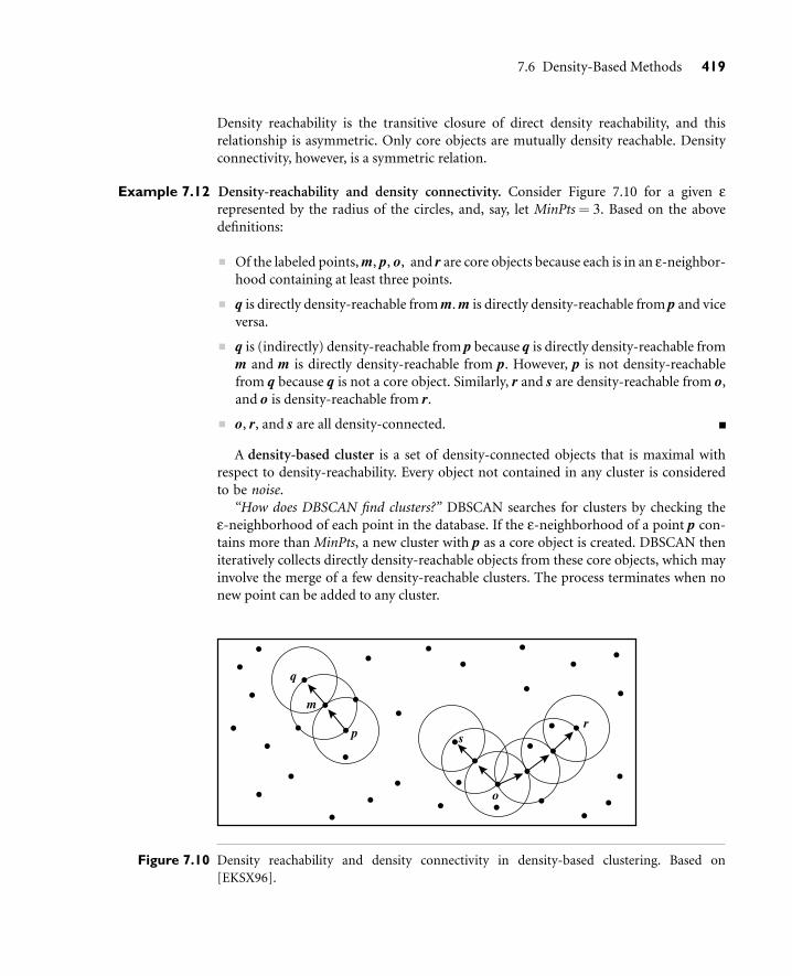
7.6 Density-Based Methods 419
Density reachability is the transitive closure of direct density reachability, and thisrelationship is asymmetric. Only core objects are mutually density reachable. Densityconnectivity, however, is a symmetric relation.
Example 7.12 Density-reachability and density connectivity. Consider Figure 7.10 for a given εrepresented by the radius of the circles, and, say, let MinPts = 3. Based on the abovedefinitions:
Of the labeled points, m, p, o, and r are core objects because each is in an ε-neighbor-hood containing at least three points.
q is directly density-reachable from m. m is directly density-reachable from p and viceversa.
q is (indirectly) density-reachable from p because q is directly density-reachable fromm and m is directly density-reachable from p. However, p is not density-reachablefrom q because q is not a core object. Similarly, r and s are density-reachable from o,and o is density-reachable from r.
o, r, and s are all density-connected.
A density-based cluster is a set of density-connected objects that is maximal withrespect to density-reachability. Every object not contained in any cluster is consideredto be noise.
“How does DBSCAN find clusters?” DBSCAN searches for clusters by checking theε-neighborhood of each point in the database. If the ε-neighborhood of a point p con-tains more than MinPts, a new cluster with p as a core object is created. DBSCAN theniteratively collects directly density-reachable objects from these core objects, which mayinvolve the merge of a few density-reachable clusters. The process terminates when nonew point can be added to any cluster.
q
m
p s
o
r
Figure 7.10 Density reachability and density connectivity in density-based clustering. Based on[EKSX96].

420 Chapter 7 Cluster Analysis
If a spatial index is used, the computational complexity of DBSCAN is O(n logn),where n is the number of database objects. Otherwise, it is O(n2). With appropriate set-tings of the user-defined parameters ε and MinPts, the algorithm is effective at findingarbitrary-shaped clusters.
7.6.2 OPTICS: Ordering Points to Identify the ClusteringStructure
Although DBSCAN can cluster objects given input parameters such as ε and MinPts, itstill leaves the user with the responsibility of selecting parameter values that will leadto the discovery of acceptable clusters. Actually, this is a problem associated with manyother clustering algorithms. Such parameter settings are usually empirically set and diffi-cult to determine, especially for real-world, high-dimensional data sets. Most algorithmsare very sensitive to such parameter values: slightly different settings may lead to very dif-ferent clusterings of the data. Moreover, high-dimensional real data sets often have veryskewed distributions, such that their intrinsic clustering structure may not be character-ized by global density parameters.
To help overcome this difficulty, a cluster analysis method called OPTICS wasproposed. Rather than produce a data set clustering explicitly, OPTICS computes anaugmented cluster ordering for automatic and interactive cluster analysis. This order-ing represents the density-based clustering structure of the data. It contains infor-mation that is equivalent to density-based clustering obtained from a wide range ofparameter settings. The cluster ordering can be used to extract basic clustering infor-mation (such as cluster centers or arbitrary-shaped clusters) as well as provide theintrinsic clustering structure.
By examining DBSCAN, we can easily see that for a constant MinPts value, density-based clusters with respect to a higher density (i.e., a lower value for ε) are completelycontained in density-connected sets obtained with respect to a lower density. Recallthat the parameter ε is a distance—it is the neighborhood radius. Therefore, in orderto produce a set or ordering of density-based clusters, we can extend the DBSCANalgorithm to process a set of distance parameter values at the same time. To con-struct the different clusterings simultaneously, the objects should be processed in aspecific order. This order selects an object that is density-reachable with respect tothe lowest ε value so that clusters with higher density (lower ε) will be finished first.Based on this idea, two values need to be stored for each object—core-distance andreachability-distance:
The core-distance of an object p is the smallest ε′ value that makes {p} a coreobject. If p is not a core object, the core-distance of p is undefined.
The reachability-distance of an object q with respect to another object p is thegreater value of the core-distance of p and the Euclidean distance between p and q.If p is not a core object, the reachability-distance between p and q is undefined.

7.6 Density-Based Methods 421
pe95 3 mm
e9
Core-distance of p
e 5 6 mm
p q1
q2
Reachability-distance (p, q1) 5 e95 3 mm Reachability-distance (p, q2) 5 d(p, q2)
e 5 6 mm
Figure 7.11 OPTICS terminology. Based on [ABKS99].
Example 7.13 Core-distance and reachability-distance. Figure 7.11 illustrates the concepts of core-distance and reachability-distance. Suppose that ε = 6 mm and MinPts = 5. The core-distance of p is the distance, ε′, between p and the fourth closest data object. Thereachability-distance of q1 with respect to p is the core-distance of p (i.e., ε′= 3 mm)because this is greater than the Euclidean distance from p to q1. The reachability-distance of q2 with respect to p is the Euclidean distance from p to q2 because thisis greater than the core-distance of p.
“How are these values used?” The OPTICS algorithm creates an ordering of theobjects in a database, additionally storing the core-distance and a suitable reachability-distance for each object. An algorithm was proposed to extract clusters based onthe ordering information produced by OPTICS. Such information is sufficient forthe extraction of all density-based clusterings with respect to any distance ε′ that issmaller than the distance ε used in generating the order.
The cluster ordering of a data set can be represented graphically, which helpsin its understanding. For example, Figure 7.12 is the reachability plot for a simpletwo-dimensional data set, which presents a general overview of how the data arestructured and clustered. The data objects are plotted in cluster order (horizontalaxis) together with their respective reachability-distance (vertical axis). The threeGaussian “bumps” in the plot reflect three clusters in the data set. Methods havealso been developed for viewing clustering structures of high-dimensional data atvarious levels of detail.
Because of the structural equivalence of the OPTICS algorithm to DBSCAN, theOPTICS algorithm has the same runtime complexity as that of DBSCAN, that is,O(n logn) if a spatial index is used, where n is the number of objects.
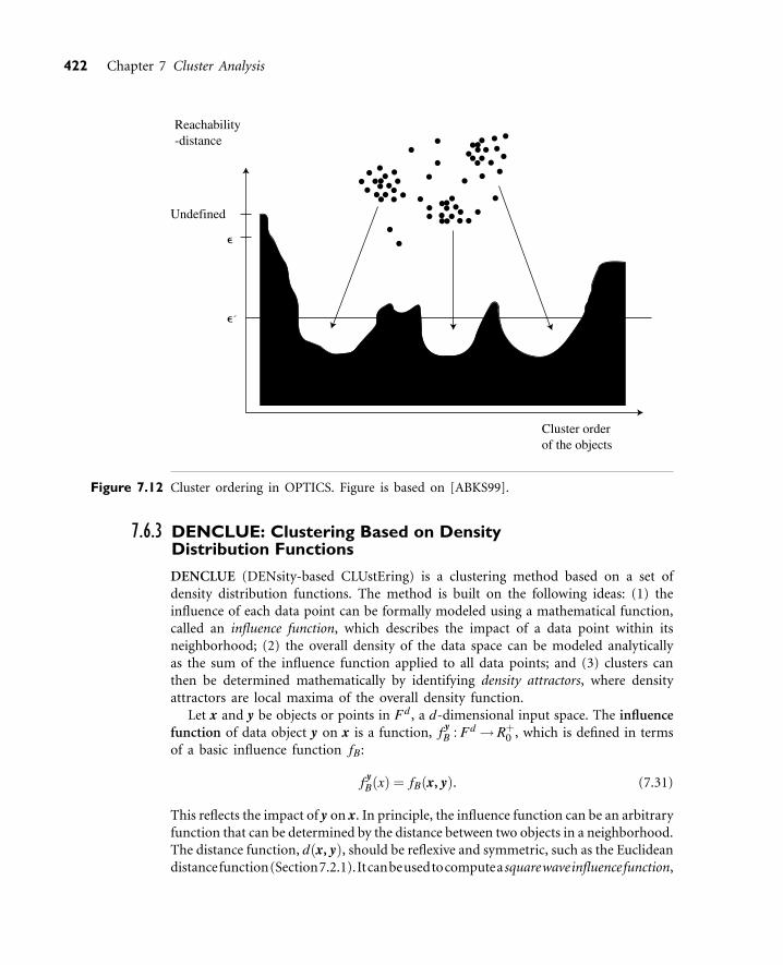
422 Chapter 7 Cluster Analysis
Cluster order of the objects
Undefined
Reachability -distance
e
e´
Figure 7.12 Cluster ordering in OPTICS. Figure is based on [ABKS99].
7.6.3 DENCLUE: Clustering Based on DensityDistribution Functions
DENCLUE (DENsity-based CLUstEring) is a clustering method based on a set ofdensity distribution functions. The method is built on the following ideas: (1) theinfluence of each data point can be formally modeled using a mathematical function,called an influence function, which describes the impact of a data point within itsneighborhood; (2) the overall density of the data space can be modeled analyticallyas the sum of the influence function applied to all data points; and (3) clusters canthen be determined mathematically by identifying density attractors, where densityattractors are local maxima of the overall density function.
Let x and y be objects or points in Fd , a d-dimensional input space. The influencefunction of data object y on x is a function, f y
B : Fd→ R+0 , which is defined in terms
of a basic influence function fB:
f yB(x) = fB(x, y). (7.31)
This reflects the impact of y on x. In principle, the influence function can be an arbitraryfunction that can be determined by the distance between two objects in a neighborhood.The distance function, d(x, y), should be reflexive and symmetric, such as the Euclideandistancefunction(Section7.2.1).Itcanbeusedtocomputea squarewaveinfluencefunction,

7.6 Density-Based Methods 423
fSquare(x, y) =
{
0 i f d(x, y)> σ1 otherwise,
(7.32)
or a Gaussian influence function,
fGauss(x, y) = e−
d(x, y)2
2σ2 . (7.33)
To help understand the concept of influence function, the following example offerssome additional insight.
Example 7.14 Influence function. Consider the square wave influence function of Equation (7.32).If objects x and y are far apart from one another in the d-dimensional space, then thedistance, d(x, y), will be above some threshold, σ. In this case, the influence functionreturns a 0, representing the lack of influence between distant points. On the otherhand, if x and y are “close” (where closeness is determined by the parameter σ), avalue of 1 is returned, representing the notion that one influences the other.
The density function at an object or point x ∈ Fd is defined as the sum of influ-ence functions of all data points. That is, it is the total influence on x of all of thedata points. Given n data objects, D = {x1, . . . , xn} ⊂ Fd , the density function at xis defined as
f DB (x) =
n
∑i=1
f xiB (x) = f x1
B (x)+ f x2B (x)+ · · ·+ f xn
B (x). (7.34)
For example, the density function that results from the Gaussian influence function(7.33) is
f DGauss(x) =
n
∑i=1
e−
d(x, xi)2
2σ2 . (7.35)
Figure 7.13 shows a 2-D data set together with the corresponding overall densityfunctions for a square wave and a Gaussian influence function.
From the density function, we can define the gradient of the function and thedensity attractor, the local maxima of the overall density function. A point x is said tobe density attracted to a density attractor x∗ if there exists a set of points x0, x1. . ., xksuch that x0 = x, xk = x∗ and the gradient of xi−1 is in the direction of xi for 0< i<k. Intuitively, a density attractor influences many other points. For a continuous anddifferentiable influence function, a hill-climbing algorithm guided by the gradientcan be used to determine the density attractor of a set of data points.
In general, points that are density attracted to x∗ may form a cluster. Based on theabove notions, both center-defined cluster and arbitrary-shape cluster can be formallydefined. A center-defined cluster for a density attractor, x∗, is a subset of points, C⊆D,that are density-attracted by x∗, and where the density function at x∗ is no less than a

424 Chapter 7 Cluster Analysis
(b) Square Wave (c) Gaussian(a) Data Set
Den
sity
Den
sity
Figure 7.13 Possible density functions for a 2-D data set. From [HK98].
threshold, ξ. Points that are density-attracted by x∗, but for which the density functionvalue is less than ξ, are considered outliers. That is, intuitively, points in a cluster areinfluenced by many points, but outliers are not. An arbitrary-shape cluster for a set ofdensity attractors is a set of Cs, each being density-attracted to its respective density-attractor, where (1) the density function value at each density-attractor is no less than athreshold, ξ, and (2) there exists a path, P, from each density-attractor to another, wherethe density function value for each point along the path is no less than ξ. Examples ofcenter-defined and arbitrary-shape clusters are shown in Figure 7.14.
“What major advantages does DENCLUE have in comparison with other clusteringalgorithms?” There are several: (1) it has a solid mathematical foundation and general-izes various clustering methods, including partitioning, hierarchical, and density-basedmethods; (2) it has good clustering properties for data sets with large amounts of noise;(3) it allows a compact mathematical description of arbitrarily shaped clusters in high-dimen sional data sets; and (4) it uses grid cells, yet only keeps information about gridcells that actually contain data points. It manages these cells in a tree-based access struc-ture, and thus is significantly faster than some influential algorithms, such as DBSCAN.However, the method requires careful selection of the density parameter σ and noisethreshold ξ, as the selection of such parameters may significantly influence the qualityof the clustering results.
7.7 Grid-Based Methods
The grid-based clustering approach uses a multiresolution grid data structure. It quan-tizes the object space into a finite number of cells that form a grid structure on whichall of the operations for clustering are performed. The main advantage of the approachis its fast processing time, which is typically independent of the number of data objects,yet dependent on only the number of cells in each dimension in the quantized space.
Some typical examples of the grid-based approach include STING, which explores sta-tistical information stored in the grid cells; WaveCluster, which clusters objects using awavelet transform method; and CLIQUE, which represents a grid-and density-based app-roach for clustering in high-dimensional data space that will be introduced in Section 7.9.

7.7 Grid-Based Methods 425
Figure 7.14 Examples of center-defined clusters (top row) and arbitrary-shape clusters (bottom row).
7.7.1 STING: STatistical INformation Grid
STING is a grid-based multiresolution clustering technique in which the spatial area isdivided into rectangular cells. There are usually several levels of such rectangular cellscorresponding to different levels of resolution, and these cells form a hierarchical struc-ture: each cell at a high level is partitioned to form a number of cells at the next lowerlevel. Statistical information regarding the attributes in each grid cell (such as the mean,maximum, and minimum values) is precomputed and stored. These statistical parame-ters are useful for query processing, as described below.
Figure 7.15 shows a hierarchical structure for STING clustering. Statistical parametersof higher-level cells can easily be computed from the parameters of the lower-level cells.These parameters include the following: the attribute-independent parameter, count; theattribute-dependent parameters, mean, stdev (standard deviation), min (minimum), max(maximum); and the type of distribution that the attribute value in the cell follows, suchas normal, uniform, exponential, or none (if the distribution is unknown). When the dataare loaded into the database, the parameters count, mean, stdev, min, and max of thebottom-level cells are calculated directly from the data. The value of distribution mayeither be assigned by the user if the distribution type is known beforehand or obtainedby hypothesis tests such as the χ2 test. The type of distribution of a higher-level cell canbe computed based on the majority of distribution types of its corresponding lower-levelcells in conjunction with a threshold filtering process. If the distributions of the lower-level cells disagree with each other and fail the threshold test, the distribution type of thehigh-level cell is set to none.

426 Chapter 7 Cluster Analysis
1st layer
(i-1)-st layer
ith layer
Figure 7.15 A hierarchical structure for STING clustering.
“How is this statistical information useful for query answering?” The statistical param-eters can be used in a top-down, grid-based method as follows. First, a layer within thehierarchical structure is determined from which the query-answering process is to start.This layer typically contains a small number of cells. For each cell in the current layer, wecompute the confidence interval (or estimated range of probability) reflecting the cell’srelevancy to the given query. The irrelevant cells are removed from further considera-tion. Processing of the next lower level examines only the remaining relevant cells. Thisprocess is repeated until the bottom layer is reached. At this time, if the query specifica-tion is met, the regions of relevant cells that satisfy the query are returned. Otherwise, thedata that fall into the relevant cells are retrieved and further processed until they meetthe requirements of the query.
“What advantages does STING offer over other clustering methods?” STING offers sev-eral advantages: (1) the grid-based computation is query-independent, because the sta-tistical information stored in each cell represents the summary information of the datain the grid cell, independent of the query; (2) the grid structure facilitates parallel pro-cessing and incremental updating; and (3) the method’s efficiency is a major advan-tage: STING goes through the database once to compute the statistical parameters ofthe cells, and hence the time complexity of generating clusters is O(n), where n is thetotal number of objects. After generating the hierarchical structure, the query process-ing time is O(g), where g is the total number of grid cells at the lowest level, which isusually much smaller than n.

7.7 Grid-Based Methods 427
Because STING uses a multiresolution approach to cluster analysis, the quality ofSTING clustering depends on the granularity of the lowest level of the grid structure. Ifthe granularity is very fine, the cost of processing will increase substantially; however, ifthe bottom level of the grid structure is too coarse, it may reduce the quality of clusteranalysis. Moreover, STING does not consider the spatial relationship between the chil-dren and their neighboring cells for construction of a parent cell. As a result, the shapesof the resulting clusters are isothetic; that is, all of the cluster boundaries are either hori-zontal or vertical, and no diagonal boundary is detected. This may lower the quality andaccuracy of the clusters despite the fast processing time of the technique.
7.7.2 WaveCluster: Clustering Using Wavelet Transformation
WaveCluster is a multiresolution clustering algorithm that first summarizes the data byimposing a multidimensional grid structure onto the data space. It then uses a wavelettransformation to transform the original feature space, finding dense regions in the trans-formed space.
In this approach, each grid cell summarizes the information of a group of points thatmap into the cell. This summary information typically fits into main memory for use bythe multiresolution wavelet transform and the subsequent cluster analysis.
A wavelet transform is a signal processing technique that decomposes a signal intodifferent frequency subbands. The wavelet model can be applied to d-dimensional sig-nals by applying a one-dimensional wavelet transform d times. In applying a wavelettransform, data are transformed so as to preserve the relative distance between objectsat different levels of resolution. This allows the natural clusters in the data to becomemore distinguishable. Clusters can then be identified by searching for dense regions inthe new domain. Wavelet transforms are also discussed in Chapter 2, where they are usedfor data reduction by compression. Additional references to the technique are given inthe bibliographic notes.
“Why is wavelet transformation useful for clustering?” It offers the followingadvantages:
It provides unsupervised clustering. It uses hat-shaped filters that emphasize regionswhere the points cluster, while suppressing weaker information outside of the clus-ter boundaries. Thus, dense regions in the original feature space act as attractors fornearby points and as inhibitors for points that are further away. This means that theclusters in the data automatically stand out and “clear” the regions around them.Thus, another advantage is that wavelet transformation can automatically result inthe removal of outliers.
The multiresolution property of wavelet transformations can help detect clusters atvarying levels of accuracy. For example, Figure 7.16 shows a sample of two-dimensional feature space, where each point in the image represents the attributeor feature values of one object in the spatial data set. Figure 7.17 shows the result-ing wavelet transformation at different resolutions, from a fine scale (scale 1) toa coarse scale (scale 3). At each level, the four subbands into which the original
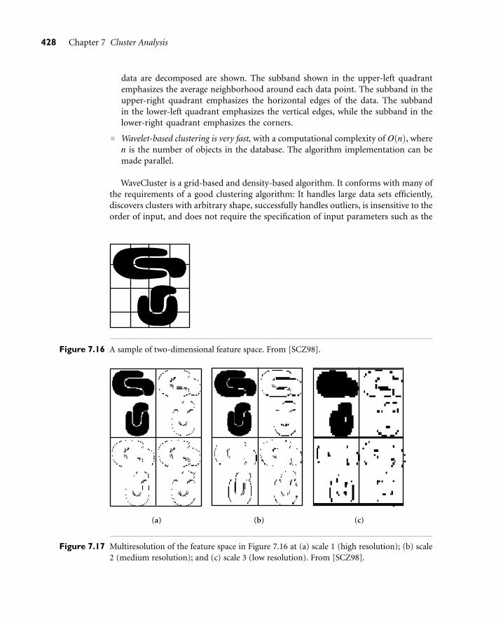
428 Chapter 7 Cluster Analysis
data are decomposed are shown. The subband shown in the upper-left quadrantemphasizes the average neighborhood around each data point. The subband in theupper-right quadrant emphasizes the horizontal edges of the data. The subbandin the lower-left quadrant emphasizes the vertical edges, while the subband in thelower-right quadrant emphasizes the corners.
Wavelet-based clustering is very fast, with a computational complexity of O(n), wheren is the number of objects in the database. The algorithm implementation can bemade parallel.
WaveCluster is a grid-based and density-based algorithm. It conforms with many ofthe requirements of a good clustering algorithm: It handles large data sets efficiently,discovers clusters with arbitrary shape, successfully handles outliers, is insensitive to theorder of input, and does not require the specification of input parameters such as the
Figure 7.16 A sample of two-dimensional feature space. From [SCZ98].
(a) (b) (c)
Figure 7.17 Multiresolution of the feature space in Figure 7.16 at (a) scale 1 (high resolution); (b) scale2 (medium resolution); and (c) scale 3 (low resolution). From [SCZ98].

7.8 Model-Based Clustering Methods 429
number of clusters or a neighborhood radius. In experimental studies, WaveCluster wasfound to outperform BIRCH, CLARANS, and DBSCAN in terms of both efficiency andclustering quality. The study also found WaveCluster capable of handling data with upto 20 dimensions.
7.8 Model-Based Clustering Methods
Model-based clustering methods attempt to optimize the fit between the given data andsome mathematical model. Such methods are often based on the assumption that thedata are generated by a mixture of underlying probability distributions. In this section,we describe three examples of model-based clustering. Section 7.8.1 presents an exten-sion of the k-means partitioning algorithm, called Expectation-Maximization. Concep-tual clustering is discussed in Section 7.8.2. A neural network approach to clustering isgiven in Section 7.8.3.
7.8.1 Expectation-Maximization
In practice, each cluster can be represented mathematically by a parametric probabilitydistribution. The entire data is a mixture of these distributions, where each individualdistribution is typically referred to as a component distribution. We can therefore clus-ter the data using a finite mixture density model of k probability distributions, whereeach distribution represents a cluster. The problem is to estimate the parameters of theprobability distributions so as to best fit the data. Figure 7.18 is an example of a simplefinite mixture density model. There are two clusters. Each follows a normal or Gaussiandistribution with its own mean and standard deviation.
The EM (Expectation-Maximization) algorithm is a popular iterative refinement algo-rithm that can be used for finding the parameter estimates. It can be viewed as an exten-sion of the k-means paradigm, which assigns an object to the cluster with which it is mostsimilar, based on the cluster mean (Section 7.4.1). Instead of assigning each object to adedicated cluster, EM assigns each object to a cluster according to a weight representingthe probability of membership. In other words, there are no strict boundaries betweenclusters. Therefore, new means are computed based on weighted measures.
EM starts with an initial estimate or “guess” of the parameters of the mixture model(collectively referred to as the parameter vector). It iteratively rescores the objects againstthe mixture density produced by the parameter vector. The rescored objects are then usedto update the parameter estimates. Each object is assigned a probability that it wouldpossess a certain set of attribute values given that it was a member of a given cluster. Thealgorithm is described as follows:
1. Make an initial guess of the parameter vector: This involves randomly selecting kobjects to represent the cluster means or centers (as in k-means partitioning), as wellas making guesses for the additional parameters.

430 Chapter 7 Cluster Analysis
g(m1, s1)
g(m2, s2)
Figure 7.18 Each cluster can be represented by a probability distribution, centered at a mean, and with astandard deviation. Here, we have two clusters, corresponding to the Gaussian distributionsg(m1, σ1) and g(m2, σ2), respectively, where the dashed circles represent the first standarddeviation of the distributions.
2. Iteratively refine the parameters (or clusters) based on the following two steps:
(a) Expectation Step: Assign each object xi to cluster Ck with the probability
P(xi ∈Ck) = p(Ck|xi) =p(Ck)p(xi|Ck)
p(xi), (7.36)
where p(xi|Ck) = N(mk, Ek(xi)) follows the normal (i.e., Gaussian) distributionaround mean, mk, with expectation, Ek. In other words, this step calculates theprobability of cluster membership of object xi, for each of the clusters. These prob-abilities are the “expected” cluster memberships for object xi.
(b) Maximization Step: Use the probability estimates from above to re-estimate (orrefine) the model parameters. For example,
mk =1n
n
∑i=1
xiP(xi ∈Ck)∑ j P(xi ∈C j)
. (7.37)
This step is the “maximization” of the likelihood of the distributions given the data.
The EM algorithm is simple and easy to implement. In practice, it converges fast butmay not reach the global optima. Convergence is guaranteed for certain forms of opti-mization functions. The computational complexity is linear in d (the number of inputfeatures), n (the number of objects), and t (the number of iterations).
Bayesian clustering methods focus on the computation of class-conditionalprobability density. They are commonly used in the statistics community. In industry,

7.8 Model-Based Clustering Methods 431
AutoClass is a popular Bayesian clustering method that uses a variant of the EM algorithm.The best clustering maximizes the ability to predict the attributes of an object given thecorrect cluster of the object. AutoClass can also estimate the number of clusters. It has beenapplied to several domains and was able to discover a new class of stars based on infraredastronomy data. Further references are provided in the bibliographic notes.
7.8.2 Conceptual Clustering
Conceptual clustering is a form of clustering in machine learning that, given a set ofunlabeled objects, produces a classification scheme over the objects. Unlike conventionalclustering, which primarily identifies groups of like objects, conceptual clustering goesone step further by also finding characteristic descriptions for each group, where eachgroup represents a concept or class. Hence, conceptual clustering is a two-step process:clustering is performed first, followed by characterization. Here, clustering quality is notsolely a function of the individual objects. Rather, it incorporates factors such as thegenerality and simplicity of the derived concept descriptions.
Most methods of conceptual clustering adopt a statistical approach that uses proba-bility measurements in determining the concepts or clusters. Probabilistic descriptionsare typically used to represent each derived concept.
COBWEB is a popular and simple method of incremental conceptual clustering. Itsinput objects are described by categorical attribute-value pairs. COBWEB creates a hier-archical clustering in the form of a classification tree.
“But what is a classification tree? Is it the same as a decision tree?” Figure 7.19 showsa classification tree for a set of animal data. A classification tree differs from a decisiontree. Each node in a classification tree refers to a concept and contains a probabilisticdescription of that concept, which summarizes the objects classified under the node. Theprobabilistic description includes the probability of the concept and conditional proba-bilities of the form P(Ai = vi j|Ck), where Ai = vi j is an attribute-value pair (that is, theith attribute takes its jth possible value) and Ck is the concept class. (Counts are accu-mulated and stored at each node for computation of the probabilities.) This is unlikedecision trees, which label branches rather than nodes and use logical rather than prob-abilistic descriptors.3 The sibling nodes at a given level of a classification tree are saidto form a partition. To classify an object using a classification tree, a partial matchingfunction is employed to descend the tree along a path of “best” matching nodes.
COBWEB uses a heuristic evaluation measure called category utility to guide con-struction of the tree. Category utility (CU) is defined as
∑nk=1 P(Ck)[∑i ∑ j P(Ai = vi j|Ck)2−∑i ∑ j P(Ai = vi j)2]
n, (7.38)
where n is the number of nodes, concepts, or “categories” forming a partition,{C1, C2, . . . , Cn}, at the given level of the tree. In other words, category utility is the
3Decision trees are described in Chapter 6.

432 Chapter 7 Cluster Analysis
Animal P(C0) 5 1.0 P(scales C0) 5 0.25 …
Amphibian P(C2) 5 0.25 P(moist C2) 5 1.0 …
Mammal/bird P(C3) 5 0.5 P(hair C3) 5 0.5 …
Bird P(C5) 5 0.5 P(feathers C5) 5 1.0 …
Mammal P(C4) 5 0.5 P(hair C4) 5 1.0 …
Fish P(C1) 5 0.25 P(scales C1) 5 1.0 …
Figure 7.19 A classification tree. Figure is based on [Fis87].
increase in the expected number of attribute values that can be correctly guessed givena partition (where this expected number corresponds to the term P(Ck)ΣiΣ jP(Ai =vi j|Ck)2) over the expected number of correct guesses with no such knowledge (corre-sponding to the term ΣiΣ jP(Ai = vi j)2). Although we do not have room to show thederivation, category utility rewards intraclass similarity and interclass dissimilarity,where:
Intraclass similarity is the probability P(Ai = vi j|Ck). The larger this value is, thegreater the proportion of class members that share this attribute-value pair and themore predictable the pair is of class members.
Interclass dissimilarity is the probability P(Ck|Ai = vi j). The larger this value is, thefewer the objects in contrasting classes that share this attribute-value pair and themore predictive the pair is of the class.
Let’s look at how COBWEB works. COBWEB incrementally incorporates objects intoa classification tree.
“Given a new object, how does COBWEB decide where to incorporate it into the classi-fication tree?” COBWEB descends the tree along an appropriate path, updating countsalong the way, in search of the “best host” or node at which to classify the object. Thisdecision is based on temporarily placing the object in each node and computing the cat-egory utility of the resulting partition. The placement that results in the highest categoryutility should be a good host for the object.

7.8 Model-Based Clustering Methods 433
“What if the object does not really belong to any of the concepts represented in the tree sofar? What if it is better to create a new node for the given object?” That is a good point. Infact, COBWEB also computes the category utility of the partition that would result if anew node were to be created for the object. This is compared to the above computationbased on the existing nodes. The object is then placed in an existing class, or a new classis created for it, based on the partition with the highest category utility value. Notice thatCOBWEB has the ability to automatically adjust the number of classes in a partition. Itdoes not need to rely on the user to provide such an input parameter.
The two operators mentioned above are highly sensitive to the input order of theobject. COBWEB has two additional operators that help make it less sensitive to inputorder. These are merging and splitting. When an object is incorporated, the two besthosts are considered for merging into a single class. Furthermore, COBWEB considerssplitting the children of the best host among the existing categories. These decisions arebased on category utility. The merging and splitting operators allow COBWEB to per-form a bidirectional search—for example, a merge can undo a previous split.
COBWEB has a number of limitations. First, it is based on the assumption that prob-ability distributions on separate attributes are statistically independent of one another.This assumption is, however, not always true because correlation between attributes oftenexists. Moreover, the probability distribution representation of clusters makes it quiteexpensive to update and store the clusters. This is especially so when the attributes havea large number of values because the time and space complexities depend not only on thenumber of attributes, but also on the number of values for each attribute. Furthermore,the classification tree is not height-balanced for skewed input data, which may cause thetime and space complexity to degrade dramatically.
CLASSIT is an extension of COBWEB for incremental clustering of continuous (orreal-valued) data. It stores a continuous normal distribution (i.e., mean and standarddeviation) for each individual attribute in each node and uses a modified category utilitymeasure that is an integral over continuous attributes instead of a sum over discreteattributes as in COBWEB. However, it suffers similar problems as COBWEB and thus isnot suitable for clustering large database data.
Conceptual clustering is popular in the machine learning community. However, themethod does not scale well for large data sets.
7.8.3 Neural Network Approach
The neural network approach is motivated by biological neural networks.4 Roughlyspeaking, a neural network is a set of connected input/output units, where each connec-tion has a weight associated with it. Neural networks have several properties that makethem popular for clustering. First, neural networks are inherently parallel and distributedprocessing architectures. Second, neural networks learn by adjusting their interconnec-tion weights so as to best fit the data. This allows them to “normalize” or “prototype”
4Neural networks were also introduced in Chapter 6 on classification and prediction.

434 Chapter 7 Cluster Analysis
the patterns and act as feature (or attribute) extractors for the various clusters. Third,neural networks process numerical vectors and require object patterns to be representedby quantitative features only. Many clustering tasks handle only numerical data or cantransform their data into quantitative features if needed.
The neural network approach to clustering tends to represent each cluster as an exem-plar. An exemplar acts as a “prototype” of the cluster and does not necessarily have tocorrespond to a particular data example or object. New objects can be distributed tothe cluster whose exemplar is the most similar, based on some distance measure. Theattributes of an object assigned to a cluster can be predicted from the attributes of thecluster’s exemplar.
Self-organizing feature maps (SOMs) are one of the most popular neural networkmethods for cluster analysis. They are sometimes referred to as Kohonen self-organizingfeature maps, after their creator, Teuvo Kohonon, or as topologically ordered maps.SOMs’ goal is to represent all points in a high-dimensional source space by pointsin a low-dimensional (usually 2-D or 3-D) target space, such that the distance andproximity relationships (hence the topology) are preserved as much as possible. Themethod is particularly useful when a nonlinear mapping is inherent in the problemitself.
SOMs can also be viewed as a constrained version of k-means clustering, in which thecluster centers tend to lie in a low-dimensional manifold in the feature or attribute space.With SOMs, clustering is performed by having several units competing for the currentobject. The unit whose weight vector is closest to the current object becomes the winningor active unit. So as to move even closer to the input object, the weights of the winningunit are adjusted, as well as those of its nearest neighbors. SOMs assume that there issome topology or ordering among the input objects and that the units will eventuallytake on this structure in space. The organization of units is said to form a feature map.SOMs are believed to resemble processing that can occur in the brain and are useful forvisualizing high-dimensional data in 2-D or 3-D space.
The SOM approach has been used successfully for Web document clustering. The leftgraph of Figure 7.20 shows the result of clustering 12,088 Web articles from the usenetnewsgroup comp.ai.neural-nets using the SOM approach, while the right graph of thefigure shows the result of drilling down on the keyword: “mining.”
The neural network approach to clustering has strong theoretical links with actualbrain processing. Further research is required to make it more effective and scalable inlarge databases due to long processing times and the intricacies of complex data.
7.9 Clustering High-Dimensional Data
Most clustering methods are designed for clustering low-dimensional data and encounterchallenges when the dimensionality of the data grows really high (say, over 10dimensions, or even over thousands of dimensions for some tasks). This is because whenthe dimensionality increases, usually only a small number of dimensions are relevant to

7.9 Clustering High-Dimensional Data 435
interpreted warren
neuron phoneme
programmer
connect
extrapolation curves
weightless
paradigm elman
pdp neurocomputing
personnel judgement
conjugate
fortran principle
trading
alamos
ga
brain intelligence
toolbox
scheduling
robot
snns
tdl mining
papers
unsupervised
popular
tools
backpropagator’s
neurotransmitters rbf
signals
noise variable
encoding decay
hidden
levenberg-narquardt consciousness
java ai
signal
costa postdoctoral aisb
genesis
bootstrap interactions
missing
exploration
mining
saturation
annealing
annealing alizing
cture
analysts
mining
packages
packa
atree x
engines
universities workshop
neurofuzzy
bayes
benchmark
rate validation sigmoid
Figure 7.20 The result of SOM clustering of 12,088 Web articles on comp.ai.neural-nets (left), andof drilling down on the keyword: “mining” (right). Based on http://websom.hut.fi/web-som/comp.ai.neural-nets-new/html/root.html.
certain clusters, but data in the irrelevant dimensions may produce much noise and maskthe real clusters to be discovered. Moreover, when dimensionality increases, data usuallybecome increasingly sparse because the data points are likely located in different dimen-sional subspaces. When the data become really sparse, data points located at differentdimensions can be considered as all equally distanced, and the distance measure, whichis essential for cluster analysis, becomes meaningless.
To overcome this difficulty, we may consider using feature (or attribute) transforma-tion and feature (or attribute) selection techniques.
Feature transformation methods, such as principal component analysis5 and singularvalue decomposition,6 transform the data onto a smaller space while generally preserving
5Principal component analysis was introduced in Chapter 2 as a method of dimensionality reduction.6Singular value decomposition is discussed in Chapter 8.

436 Chapter 7 Cluster Analysis
the original relative distance between objects. They summarize data by creating linearcombinations of the attributes, and may discover hidden structures in the data. How-ever, such techniques do not actually remove any of the original attributes from analysis.This is problematic when there are a large number of irrelevant attributes. The irrele-vant information may mask the real clusters, even after transformation. Moreover, thetransformed features (attributes) are often difficult to interpret, making the clusteringresults less useful. Thus, feature transformation is only suited to data sets where mostof the dimensions are relevant to the clustering task. Unfortunately, real-world data setstend to have many highly correlated, or redundant, dimensions.
Another way of tackling the curse of dimensionality is to try to remove some of thedimensions. Attribute subset selection (or feature subset selection7) is commonly usedfor data reduction by removing irrelevant or redundant dimensions (or attributes). Givena set of attributes, attribute subset selection finds the subset of attributes that are mostrelevant to the data mining task. Attribute subset selection involves searching throughvarious attribute subsets and evaluating these subsets using certain criteria. It is mostcommonly performed by supervised learning—the most relevant set of attributes arefound with respect to the given class labels. It can also be performed by an unsupervisedprocess, such as entropy analysis, which is based on the property that entropy tends tobe low for data that contain tight clusters. Other evaluation functions, such as categoryutility, may also be used.
Subspace clustering is an extension to attribute subset selection that has shown itsstrength at high-dimensional clustering. It is based on the observation that differentsubspaces may contain different, meaningful clusters. Subspace clustering searches forgroups of clusters within different subspaces of the same data set. The problem becomeshow to find such subspace clusters effectively and efficiently.
In this section, we introduce three approaches for effective clustering ofhigh-dimensional data: dimension-growth subspace clustering, represented by CLIQUE,dimension-reduction projected clustering, represented by PROCLUS, and frequent pattern-based clustering, represented by pCluster.
7.9.1 CLIQUE: A Dimension-Growth Subspace Clustering Method
CLIQUE (CLustering In QUEst) was the first algorithm proposed for dimension-growthsubspace clustering in high-dimensional space. In dimension-growth subspace cluster-ing, the clustering process starts at single-dimensional subspaces and grows upward tohigher-dimensional ones. Because CLIQUE partitions each dimension like a grid struc-ture and determines whether a cell is dense based on the number of points it contains,it can also be viewed as an integration of density-based and grid-based clustering meth-ods. However, its overall approach is typical of subspace clustering for high-dimensionalspace, and so it is introduced in this section.
7Attribute subset selection is known in the machine learning literature as feature subset selection. Itwas discussed in Chapter 2.

7.9 Clustering High-Dimensional Data 437
The ideas of the CLIQUE clustering algorithm are outlined as follows.
Given a large set of multidimensional data points, the data space is usually not uni-formly occupied by the data points. CLIQUE’s clustering identifies the sparse andthe “crowded” areas in space (or units), thereby discovering the overall distributionpatterns of the data set.
A unit is dense if the fraction of total data points contained in it exceeds an inputmodel parameter. In CLIQUE, a cluster is defined as a maximal set of connected denseunits.
“How does CLIQUE work?” CLIQUE performs multidimensional clustering in twosteps.
In the first step, CLIQUE partitions the d-dimensional data space into nonoverlap-ping rectangular units, identifying the dense units among these. This is done (in 1-D)for each dimension. For example, Figure 7.21 shows dense rectangular units found withrespect to age for the dimensions salary and (number of weeks of) vacation. The sub-spaces representing these dense units are intersected to form a candidate search space inwhich dense units of higher dimensionality may exist.
“Why does CLIQUE confine its search for dense units of higher dimensionality to theintersection of the dense units in the subspaces?” The identification of the candidate searchspace is based on the Apriori property used in association rule mining.8 In general, theproperty employs prior knowledge of items in the search space so that portions of thespace can be pruned. The property, adapted for CLIQUE, states the following: If ak-dimensional unit is dense, then so are its projections in (k−1)-dimensional space. That is,given a k-dimensional candidate dense unit, if we check its (k−1)-th projection units andfind any that are not dense, then we know that the kth dimensional unit cannot be denseeither. Therefore, we can generate potential or candidate dense units in k-dimensionalspace from the dense units found in (k− 1)-dimensional space. In general, the result-ing space searched is much smaller than the original space. The dense units are thenexamined in order to determine the clusters.
In the second step, CLIQUE generates a minimal description for each cluster asfollows. For each cluster, it determines the maximal region that covers the cluster ofconnected dense units. It then determines a minimal cover (logic description) for eachcluster.
“How effective is CLIQUE?” CLIQUE automatically finds subspaces of the highestdimensionality such that high-density clusters exist in those subspaces. It is insensitive tothe order of input objects and does not presume any canonical data distribution. It scaleslinearly with the size of input and has good scalability as the number of dimensions inthe data is increased. However, obtaining meaningful clustering results is dependent on
8Association rule mining is described in detail in Chapter 5. In particular, the Apriori property isdescribed in Section 5.2.1. The Apriori property can also be used for cube computation, as describedin Chapter 4.

438 Chapter 7 Cluster Analysis
7
6
5
4
3
2
1
0
sala
ry (
10,0
00)
20 30 40 50 60
7
6
5
4
3
2
1
0
vaca
tion
(w
eek)
20 30 40 50 60
age
age
salar
yva
cati
on
age30 50
Figure 7.21 Dense units found with respect to age for the dimensions salary and vacation are intersectedin order to provide a candidate search space for dense units of higher dimensionality.

7.9 Clustering High-Dimensional Data 439
proper tuning of the grid size (which is a stable structure here) and the density threshold.This is particularly difficult because the grid size and density threshold are used across allcombinations of dimensions in the data set. Thus, the accuracy of the clustering resultsmay be degraded at the expense of the simplicity of the method. Moreover, for a givendense region, all projections of the region onto lower-dimensionality subspaces will alsobe dense. This can result in a large overlap among the reported dense regions. Further-more, it is difficult to find clusters of rather different density within different dimensionalsubspaces.
Several extensions to this approach follow a similar philosophy. For example, let’sthink of a grid as a set of fixed bins. Instead of using fixed bins for each of the dimensions,we can use an adaptive, data-driven strategy to dynamically determine the bins for eachdimension based on data distribution statistics. Alternatively, instead of using a densitythreshold, we would use entropy (Chapter 6) as a measure of the quality of subspaceclusters.
7.9.2 PROCLUS: A Dimension-Reduction Subspace ClusteringMethod
PROCLUS (PROjected CLUStering) is a typical dimension-reduction subspace clus-tering method. That is, instead of starting from single-dimensional spaces, it startsby finding an initial approximation of the clusters in the high-dimensional attributespace. Each dimension is then assigned a weight for each cluster, and the updatedweights are used in the next iteration to regenerate the clusters. This leads to the explo-ration of dense regions in all subspaces of some desired dimensionality and avoidsthe generation of a large number of overlapped clusters in projected dimensions oflower dimensionality.
PROCLUS finds the best set of medoids by a hill-climbing process similar to that usedin CLARANS, but generalized to deal with projected clustering. It adopts a distance mea-sure called Manhattan segmental distance, which is the Manhattan distance on a set ofrelevant dimensions. The PROCLUS algorithm consists of three phases: initialization,iteration, and cluster refinement. In the initialization phase, it uses a greedy algorithmto select a set of initial medoids that are far apart from each other so as to ensure thateach cluster is represented by at least one object in the selected set. More concretely, itfirst chooses a random sample of data points proportional to the number of clusterswe wish to generate, and then applies the greedy algorithm to obtain an even smallerfinal subset for the next phase. The iteration phase selects a random set of k medoidsfrom this reduced set (of medoids), and replaces “bad” medoids with randomly cho-sen new medoids if the clustering is improved. For each medoid, a set of dimensions ischosen whose average distances are small compared to statistical expectation. The totalnumber of dimensions associated to medoids must be k× l, where l is an input param-eter that selects the average dimensionality of cluster subspaces. The refinement phasecomputes new dimensions for each medoid based on the clusters found, reassigns pointsto medoids, and removes outliers.

440 Chapter 7 Cluster Analysis
Experiments on PROCLUS show that the method is efficient and scalable atfinding high-dimensional clusters. Unlike CLIQUE, which outputs many overlappedclusters, PROCLUS finds nonoverlapped partitions of points. The discovered clustersmay help better understand the high-dimensional data and facilitate other subse-quence analyses.
7.9.3 Frequent Pattern–Based Clustering Methods
This section looks at how methods of frequent pattern mining can be applied to cluster-ing, resulting in frequent pattern–based cluster analysis. Frequent pattern mining, asthe name implies, searches for patterns (such as sets of items or objects) that occur fre-quently in large data sets. Frequent pattern mining can lead to the discovery of interestingassociations and correlations among data objects. Methods for frequent pattern miningwere introduced in Chapter 5. The idea behind frequent pattern–based cluster analysis isthat the frequent patterns discovered may also indicate clusters. Frequent pattern–basedcluster analysis is well suited to high-dimensional data. It can be viewed as an extensionof the dimension-growth subspace clustering approach. However, the boundaries of dif-ferent dimensions are not obvious, since here they are represented by sets of frequentitemsets. That is, rather than growing the clusters dimension by dimension, we growsets of frequent itemsets, which eventually lead to cluster descriptions. Typical examplesof frequent pattern–based cluster analysis include the clustering of text documents thatcontain thousands of distinct keywords, and the analysis of microarray data that con-tain tens of thousands of measured values or “features.” In this section, we examine twoforms of frequent pattern–based cluster analysis: frequent term–based text clustering andclustering by pattern similarity in microarray data analysis.
In frequent term–based text clustering, text documents are clustered based on thefrequent terms they contain. Using the vocabulary of text document analysis, a term isany sequence of characters separated from other terms by a delimiter. A term can bemade up of a single word or several words. In general, we first remove nontext informa-tion (such as HTML tags and punctuation) and stop words. Terms are then extracted.A stemming algorithm is then applied to reduce each term to its basic stem. In this way,each document can be represented as a set of terms. Each set is typically large. Collec-tively, a large set of documents will contain a very large set of distinct terms. If we treateach term as a dimension, the dimension space will be of very high dimensionality! Thisposes great challenges for document cluster analysis. The dimension space can be referredto as term vector space, where each document is represented by a term vector.
This difficulty can be overcome by frequent term–based analysis. That is, by using anefficient frequent itemset mining algorithm introduced in Section 5.2, we can mine aset of frequent terms from the set of text documents. Then, instead of clustering onhigh-dimensional term vector space, we need only consider the low-dimensional fre-quent term sets as “cluster candidates.” Notice that a frequent term set is not a clusterbut rather the description of a cluster. The corresponding cluster consists of the set ofdocuments containing all of the terms of the frequent term set. A well-selected subset ofthe set of all frequent term sets can be considered as a clustering.

7.9 Clustering High-Dimensional Data 441
“How, then, can we select a good subset of the set of all frequent term sets?” This stepis critical because such a selection will determine the quality of the resulting clustering.Let Fi be a set of frequent term sets and cov(Fi) be the set of documents covered by Fi.That is, cov(Fi) refers to the documents that contain all of the terms in Fi. The generalprinciple for finding a well-selected subset, F1, . . . , Fk, of the set of all frequent term setsis to ensure that (1) Σk
i=1cov(Fi) = D (i.e., the selected subset should cover all of thedocuments to be clustered); and (2) the overlap between any two partitions, Fi and Fj(for i 6= j), should be minimized. An overlap measure based on entropy9 is used to assesscluster overlap by measuring the distribution of the documents supporting some clusterover the remaining cluster candidates.
An advantage of frequent term–based text clustering is that it automatically gener-ates a description for the generated clusters in terms of their frequent term sets. Tradi-tional clustering methods produce only clusters—a description for the generated clustersrequires an additional processing step.
Another interesting approach for clustering high-dimensional data is based on patternsimilarity among the objects on a subset of dimensions. Here we introduce the pClus-ter method, which performs clustering by pattern similarity in microarray data anal-ysis. In DNA microarray analysis, the expression levels of two genes may rise and fallsynchronously in response to a set of environmental stimuli or conditions. Under thepCluster model, two objects are similar if they exhibit a coherent pattern on a subset ofdimensions. Although the magnitude of their expression levels may not be close, the pat-terns they exhibit can be very much alike. This is illustrated in Example 7.15. Discovery ofsuch clusters of genes is essential in revealing significant connections in gene regulatorynetworks.
Example 7.15 Clustering by pattern similarity in DNA microarray analysis. Figure 7.22 shows a frag-ment of microarray data containing only three genes (taken as “objects” here) and tenattributes (columns a to j). No patterns among the three objects are visibly explicit. How-ever, if two subsets of attributes, {b, c, h, j, e} and { f , d, a, g, i}, are selected and plottedas in Figure 7.23(a) and (b) respectively, it is easy to see that they form some interest-ing patterns: Figure 7.23(a) forms a shift pattern, where the three curves are similar toeach other with respect to a shift operation along the y-axis; while Figure 7.23(b) forms ascaling pattern, where the three curves are similar to each other with respect to a scalingoperation along the y-axis.
Let us first examine how to discover shift patterns. In DNA microarray data, each rowcorresponds to a gene and each column or attribute represents a condition under whichthe gene is developed. The usual Euclidean distance measure cannot capture patternsimilarity, since the y values of different curves can be quite far apart. Alternatively, wecould first transform the data to derive new attributes, such as Ai j = vi−v j (where vi and
9Entropy is a measure from information theory. It was introduced in Chapter 2 regarding data dis-cretization and is also described in Chapter 6 regarding decision tree construction.

442 Chapter 7 Cluster Analysis
a b c d e f g h i j
90
80
70
60
50
40
30
20
10
0
Object 1
Object 2
Object 3
Figure 7.22 Raw data from a fragment of microarray data containing only 3 objects and 10 attributes.
a b c d e f g h i j
90 80 70 60 50 40
30 20 10 0
90 80 70 60 50 40 30
20 10 0
Object 1 Object 2 Object 3
Object 1 Object 2 Object 3
(a) (b)
Figure 7.23 Objects in Figure 7.22 form (a) a shift pattern in subspace {b, c, h, j, e}, and (b) a scalingpattern in subspace { f , d, a, g, i}.
v j are object values for attributes Ai and A j, respectively), and then cluster on the derivedattributes. However, this would introduce d(d− 1)/2 dimensions for a d-dimensionaldata set, which is undesirable for a nontrivial d value. A biclustering method was pro-posed in an attempt to overcome these difficulties. It introduces a new measure, the mean

7.9 Clustering High-Dimensional Data 443
squared residue score, which measures the coherence of the genes and conditions in asubmatrix of a DNA array. Let I ⊂ X and J ⊂ Y be subsets of genes, X , and conditions,Y , respectively. The pair, (I, J), specifies a submatrix, AIJ , with the mean squared residuescore defined as
H(IJ) =1|I||J| ∑
i∈I, j∈J(di j−diJ−dI j + dIJ)2, (7.39)
where di j is the measured value of gene i for condition j, and
diJ =1|J| ∑j∈J
di j, dI j =1|I|∑i∈I
di j, dIJ =1|I||J| ∑
i∈I, j∈Jdi j, (7.40)
where diJ and dI j are the row and column means, respectively, and dIJ is the mean ofthe subcluster matrix, AIJ . A submatrix, AIJ , is called a δ-bicluster if H(I, J) ≤ δ forsome δ > 0. A randomized algorithm is designed to find such clusters in a DNA array.There are two major limitations of this method. First, a submatrix of a δ-bicluster is notnecessarily a δ-bicluster, which makes it difficult to design an efficient pattern growth–based algorithm. Second, because of the averaging effect, a δ-bicluster may contain someundesirable outliers yet still satisfy a rather small δ threshold.
To overcome the problems of the biclustering method, a pCluster model was intro-duced as follows. Given objects x, y ∈ O and attributes a, b ∈ T , pScore is defined by a2×2 matrix as
pScore(
[
dxa dxb
dya dyb
]
) = |(dxa−dxb)− (dya−dyb)|, (7.41)
where dxa is the value of object (or gene) x for attribute (or condition) a, and so on.A pair, (O, T ), forms a δ-pCluster if, for any 2× 2 matrix, X , in (O, T ), we havepScore(X)≤ δ for some δ > 0. Intuitively, this means that the change of values on thetwo attributes between the two objects is confined by δ for every pair of objects in O andevery pair of attributes in T .
It is easy to see that δ-pCluster has the downward closure property; that is, if (O, T )forms a δ-pCluster, then any of its submatrices is also a δ-pCluster. Moreover, becausea pCluster requires that every two objects and every two attributes conform with theinequality, the clusters modeled by the pCluster method are more homogeneous thanthose modeled by the bicluster method.
In frequent itemset mining, itemsets are considered frequent if they satisfy a minimumsupport threshold, which reflects their frequency of occurrence. Based on the definitionof pCluster, the problem of mining pClusters becomes one of mining frequent patternsin which each pair of objects and their corresponding features must satisfy the specifiedδ threshold. A frequent pattern–growth method can easily be extended to mine suchpatterns efficiently.

444 Chapter 7 Cluster Analysis
Now, let’s look into how to discover scaling patterns. Notice that the original pScoredefinition, though defined for shift patterns in Equation (7.41), can easily be extendedfor scaling by introducing a new inequality,
dxa/dya
dxb/dyb≤ δ′. (7.42)
This can be computed efficiently because Equation (7.41) is a logarithmic form ofEquation (7.42). That is, the same pCluster model can be applied to the data set afterconverting the data to the logarithmic form. Thus, the efficient derivation of δ-pClustersfor shift patterns can naturally be extended for the derivation of δ-pClusters for scalingpatterns.
The pCluster model, though developed in the study of microarray data clusteranalysis, can be applied to many other applications that require finding similar or coher-ent patterns involving a subset of numerical dimensions in large, high-dimensionaldata sets.
7.10 Constraint-Based Cluster Analysis
In the above discussion, we assume that cluster analysis is an automated, algorithmiccomputational process, based on the evaluation of similarity or distance functions amonga set of objects to be clustered, with little user guidance or interaction. However, users oftenhave a clear view of the application requirements, which they would ideally like to use toguide the clustering process and influence the clustering results. Thus, in many applica-tions, it is desirable to have the clustering process take user preferences and constraintsinto consideration. Examples of such information include the expected number of clus-ters, the minimal or maximal cluster size, weights for different objects or dimensions,and other desirable characteristics of the resulting clusters. Moreover, when a clusteringtask involves a rather high-dimensional space, it is very difficult to generate meaningfulclusters by relying solely on the clustering parameters. User input regarding importantdimensions or the desired results will serve as crucial hints or meaningful constraintsfor effective clustering. In general, we contend that knowledge discovery would be mosteffective if one could develop an environment for human-centered, exploratory min-ing of data, that is, where the human user is allowed to play a key role in the process.Foremost, a user should be allowed to specify a focus—directing the mining algorithmtoward the kind of “knowledge” that the user is interested in finding. Clearly, user-guidedmining will lead to more desirable results and capture the application semantics.
Constraint-based clustering finds clusters that satisfy user-specified preferences orconstraints. Depending on the nature of the constraints, constraint-based clusteringmay adopt rather different approaches. Here are a few categories of constraints.
1. Constraints on individual objects: We can specify constraints on the objects to beclustered. In a real estate application, for example, one may like to spatially cluster only

7.10 Constraint-Based Cluster Analysis 445
those luxury mansions worth over a million dollars. This constraint confines the setof objects to be clustered. It can easily be handled by preprocessing (e.g., performingselection using an SQL query), after which the problem reduces to an instance ofunconstrained clustering.
2. Constraints on the selection of clustering parameters: A user may like to set a desiredrange for each clustering parameter. Clustering parameters are usually quite specificto the given clustering algorithm. Examples of parameters include k, the desired num-ber of clusters in a k-means algorithm; or ε (the radius) and MinPts (the minimumnumber of points) in the DBSCAN algorithm. Although such user-specified param-eters may strongly influence the clustering results, they are usually confined to thealgorithm itself. Thus, their fine tuning and processing are usually not considered aform of constraint-based clustering.
3. Constraints on distance or similarity functions: We can specify different distance orsimilarity functions for specific attributes of the objects to be clustered, or differentdistance measures for specific pairs of objects. When clustering sportsmen, for exam-ple, we may use different weighting schemes for height, body weight, age, and skilllevel. Although this will likely change the mining results, it may not alter the cluster-ing process per se. However, in some cases, such changes may make the evaluationof the distance function nontrivial, especially when it is tightly intertwined with theclustering process. This can be seen in the following example.
Example 7.16 Clustering with obstacle objects. A city may have rivers, bridges, highways, lakes, andmountains. We do not want to swim across a river to reach an automated bankingmachine. Such obstacle objects and their effects can be captured by redefining thedistance functions among objects. Clustering with obstacle objects using a partition-ing approach requires that the distance between each object and its correspondingcluster center be reevaluated at each iteration whenever the cluster center is changed.However, such reevaluation is quite expensive with the existence of obstacles. In thiscase, efficient new methods should be developed for clustering with obstacle objectsin large data sets.
4. User-specified constraints on the properties of individual clusters: A user may like tospecify desired characteristics of the resulting clusters, which may strongly influencethe clustering process. Such constraint-based clustering arises naturally in practice,as in Example 7.17.
Example 7.17 User-constrained cluster analysis. Suppose a package delivery company would like todetermine the locations for k service stations in a city. The company has a databaseof customers that registers the customers’ names, locations, length of time sincethe customers began using the company’s services, and average monthly charge.We may formulate this location selection problem as an instance of unconstrainedclustering using a distance function computed based on customer location. How-ever, a smarter approach is to partition the customers into two classes: high-value

446 Chapter 7 Cluster Analysis
customers (who need frequent, regular service) and ordinary customers (who requireoccasional service). In order to save costs and provide good service, the manageradds the following constraints: (1) each station should serve at least 100 high-valuecustomers; and (2) each station should serve at least 5,000 ordinary customers.Constraint-based clustering will take such constraints into consideration during theclustering process.
5. Semi-supervised clustering based on “partial” supervision: The quality of unsuper-vised clustering can be significantly improved using some weak form of supervision.This may be in the form of pairwise constraints (i.e., pairs of objects labeled as belong-ing to the same or different cluster). Such a constrained clustering process is calledsemi-supervised clustering.
In this section, we examine how efficient constraint-based clustering methods can bedeveloped for large data sets. Since cases 1 and 2 above are trivial, we focus on cases 3 to5 as typical forms of constraint-based cluster analysis.
7.10.1 Clustering with Obstacle Objects
Example 7.16 introduced the problem of clustering with obstacle objects regarding theplacement of automated banking machines. The machines should be easily accessible tothe bank’s customers. This means that during clustering, we must take obstacle objectsinto consideration, such as rivers, highways, and mountains. Obstacles introduce con-straints on the distance function. The straight-line distance between two points is mean-ingless if there is an obstacle in the way. As pointed out in Example 7.16, we do not wantto have to swim across a river to get to a banking machine!
“How can we approach the problem of clustering with obstacles?” A partitioning clus-tering method is preferable because it minimizes the distance between objects andtheir cluster centers. If we choose the k-means method, a cluster center may not beaccessible given the presence of obstacles. For example, the cluster mean could turnout to be in the middle of a lake. On the other hand, the k-medoids method choosesan object within the cluster as a center and thus guarantees that such a problem can-not occur. Recall that every time a new medoid is selected, the distance between eachobject and its newly selected cluster center has to be recomputed. Because there couldbe obstacles between two objects, the distance between two objects may have to bederived by geometric computations (e.g., involving triangulation). The computationalcost can get very high if a large number of objects and obstacles are involved.
The clustering with obstacles problem can be represented using a graphical nota-tion. First, a point, p, is visible from another point, q, in the region, R, if the straightline joining p and q does not intersect any obstacles. A visibility graph is the graph,V G = (V , E), such that each vertex of the obstacles has a corresponding node inV and two nodes, v1 and v2, in V are joined by an edge in E if and only if thecorresponding vertices they represent are visible to each other. Let V G′ = (V ′, E ′)be a visibility graph created from V G by adding two additional points, p and q, in
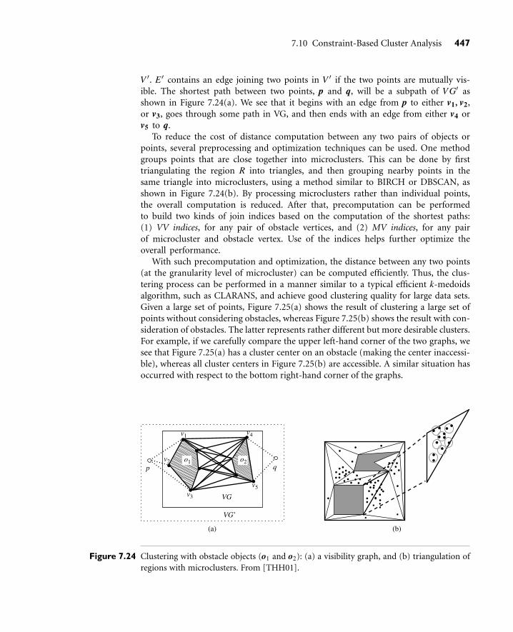
7.10 Constraint-Based Cluster Analysis 447
V ′. E ′ contains an edge joining two points in V ′ if the two points are mutually vis-ible. The shortest path between two points, p and q, will be a subpath of V G′ asshown in Figure 7.24(a). We see that it begins with an edge from p to either v1, v2,or v3, goes through some path in VG, and then ends with an edge from either v4 orv5 to q.
To reduce the cost of distance computation between any two pairs of objects orpoints, several preprocessing and optimization techniques can be used. One methodgroups points that are close together into microclusters. This can be done by firsttriangulating the region R into triangles, and then grouping nearby points in thesame triangle into microclusters, using a method similar to BIRCH or DBSCAN, asshown in Figure 7.24(b). By processing microclusters rather than individual points,the overall computation is reduced. After that, precomputation can be performedto build two kinds of join indices based on the computation of the shortest paths:(1) VV indices, for any pair of obstacle vertices, and (2) MV indices, for any pairof microcluster and obstacle vertex. Use of the indices helps further optimize theoverall performance.
With such precomputation and optimization, the distance between any two points(at the granularity level of microcluster) can be computed efficiently. Thus, the clus-tering process can be performed in a manner similar to a typical efficient k-medoidsalgorithm, such as CLARANS, and achieve good clustering quality for large data sets.Given a large set of points, Figure 7.25(a) shows the result of clustering a large set ofpoints without considering obstacles, whereas Figure 7.25(b) shows the result with con-sideration of obstacles. The latter represents rather different but more desirable clusters.For example, if we carefully compare the upper left-hand corner of the two graphs, wesee that Figure 7.25(a) has a cluster center on an obstacle (making the center inaccessi-ble), whereas all cluster centers in Figure 7.25(b) are accessible. A similar situation hasoccurred with respect to the bottom right-hand corner of the graphs.
p q
VG
VG’
(a) (b)
o2 o1
v1
v2
v3
v4
v5
Figure 7.24 Clustering with obstacle objects (o1 and o2): (a) a visibility graph, and (b) triangulation ofregions with microclusters. From [THH01].

448 Chapter 7 Cluster Analysis
(a) (b)
Figure 7.25 Clustering results obtained without and with consideration of obstacles (where rivers andinaccessible highways or city blocks are represented by polygons): (a) clustering without con-sidering obstacles, and (b) clustering with obstacles.
7.10.2 User-Constrained Cluster Analysis
Let’s examine the problem of relocating package delivery centers, as illustrated inExample 7.17. Specifically, a package delivery company with n customers would liketo determine locations for k service stations so as to minimize the traveling distancebetween customers and service stations. The company’s customers are regarded aseither high-value customers (requiring frequent, regular services) or ordinary customers(requiring occasional services). The manager has stipulated two constraints: each sta-tion should serve (1) at least 100 high-value customers and (2) at least 5,000 ordinarycustomers.
This can be considered as a constrained optimization problem. We could considerusing a mathematical programming approach to handle it. However, such a solution isdifficult to scale to large data sets. To cluster n customers into k clusters, a mathematicalprogramming approach will involve at least k× n variables. As n can be as large as afew million, we could end up having to solve a few million simultaneous equations—a very expensive feat. A more efficient approach is proposed that explores the idea ofmicroclustering, as illustrated below.
The general idea of clustering a large data set into k clusters satisfying user-specifiedconstraints goes as follows. First, we can find an initial “solution” by partitioning thedata set into k groups, satisfying the user-specified constraints, such as the two con-straints in our example. We then iteratively refine the solution by moving objects fromone cluster to another, trying to satisfy the constraints. For example, we can move a setof m customers from cluster Ci to C j if Ci has at least m surplus customers (under thespecified constraints), or if the result of moving customers into Ci from some otherclusters (including from C j) would result in such a surplus. The movement is desirable

7.10 Constraint-Based Cluster Analysis 449
if the total sum of the distances of the objects to their corresponding cluster centers isreduced. Such movement can be directed by selecting promising points to be moved,such as objects that are currently assigned to some cluster, Ci, but that are actually closerto a representative (e.g., centroid) of some other cluster, C j. We need to watch out forand handle deadlock situations (where a constraint is impossible to satisfy), in whichcase, a deadlock resolution strategy can be employed.
To increase the clustering efficiency, data can first be preprocessed using the micro-clustering idea to form microclusters (groups of points that are close together), therebyavoiding the processing of all of the points individually. Object movement, deadlockdetection, and constraint satisfaction can be tested at the microcluster level, which re-duces the number of points to be computed. Occasionally, such microclusters may needto be broken up in order to resolve deadlocks under the constraints. This methodol-ogy ensures that the effective clustering can be performed in large data sets under theuser-specified constraints with good efficiency and scalability.
7.10.3 Semi-Supervised Cluster Analysis
In comparison with supervised learning, clustering lacks guidance from users or classi-fiers (such as class label information), and thus may not generate highly desirable clus-ters. The quality of unsupervised clustering can be significantly improved using someweak form of supervision, for example, in the form of pairwise constraints (i.e., pairs ofobjects labeled as belonging to the same or different clusters). Such a clustering processbased on user feedback or guidance constraints is called semi-supervised clustering.
Methods for semi-supervised clustering can be categorized into two classes:constraint-based semi-supervised clustering and distance-based semi-supervised clustering.Constraint-based semi-supervised clustering relies on user-provided labels or constraintsto guide the algorithm toward a more appropriate data partitioning. This includes mod-ifying the objective function based on constraints, or initializing and constraining theclustering process based on the labeled objects. Distance-based semi-supervised clus-tering employs an adaptive distance measure that is trained to satisfy the labels or con-straints in the supervised data. Several different adaptive distance measures have beenused, such as string-edit distance trained using Expectation-Maximization (EM), andEuclidean distance modified by a shortest distance algorithm.
An interesting clustering method, called CLTree (CLustering based on decisionTREEs), integrates unsupervised clustering with the idea of supervised classification. Itis an example of constraint-based semi-supervised clustering. It transforms a clusteringtask into a classification task by viewing the set of points to be clustered as belonging toone class, labeled as “Y ,” and adds a set of relatively uniformly distributed, “nonexistencepoints” with a different class label, “N.” The problem of partitioning the data space intodata (dense) regions and empty (sparse) regions can then be transformed into a classifi-cation problem. For example, Figure 7.26(a) contains a set of data points to be clustered.These points can be viewed as a set of “Y ” points. Figure 7.26(b) shows the addition ofa set of uniformly distributed “N” points, represented by the “◦” points. The original

450 Chapter 7 Cluster Analysis
(a) (b) (c)
Figure 7.26 Clustering through decision tree construction: (a) the set of data points to be clustered,viewed as a set of “Y ” points, (b) the addition of a set of uniformly distributed “N” points,represented by “◦”, and (c) the clustering result with “Y ” points only.
clustering problem is thus transformed into a classification problem, which works outa scheme that distinguishes “Y ” and “N” points. A decision tree induction method canbe applied10 to partition the two-dimensional space, as shown in Figure 7.26(c). Twoclusters are identified, which are from the “Y ” points only.
Adding a large number of “N” points to the original data may introduce unneces-sary overhead in computation. Furthermore, it is unlikely that any points added wouldtruly be uniformly distributed in a very high-dimensional space as this would require anexponential number of points. To deal with this problem, we do not physically add anyof the “N” points, but only assume their existence. This works because the decision treemethod does not actually require the points. Instead, it only needs the number of “N”points at each decision tree node. This number can be computed when needed, with-out having to add points to the original data. Thus, CLTree can achieve the results inFigure 7.26(c) without actually adding any “N” points to the original data. Again, twoclusters are identified.
The question then is how many (virtual) “N” points should be added in order toachieve good clustering results. The answer follows this simple rule: At the root node, thenumber of inherited “N” points is 0. At any current node, E , if the number of “N” pointsinherited from the parent node of E is less than the number of “Y ” points in E , then thenumber of “N” points for E is increased to the number of “Y ” points in E . (That is, we setthe number of “N” points to be as big as the number of “Y ” points.) Otherwise, the numberof inherited “N” points is used in E . The basic idea is to use an equal number of “N”points to the number of “Y ” points.
Decision tree classification methods use a measure, typically based on informationgain, to select the attribute test for a decision node (Section 6.3.2). The data are thensplit or partitioned according the test or “cut.” Unfortunately, with clustering, this canlead to the fragmentation of some clusters into scattered regions. To address this problem,methods were developed that use information gain, but allow the ability to look ahead.
10Decision tree induction was described in Chapter 6 on classification.

7.11 Outlier Analysis 451
That is, CLTree first finds initial cuts and then looks ahead to find better partitions thatcut less into cluster regions. It finds those cuts that form regions with a very low relativedensity. The idea is that we want to split at the cut point that may result in a big empty(“N”) region, which is more likely to separate clusters. With such tuning, CLTree can per-form high-quality clustering in high-dimensional space. It can also find subspace clustersas the decision tree method normally selects only a subset of the attributes. An interest-ing by-product of this method is the empty (sparse) regions, which may also be usefulin certain applications. In marketing, for example, clusters may represent different seg-ments of existing customers of a company, while empty regions reflect the profiles ofnoncustomers. Knowing the profiles of noncustomers allows the company to tailor theirservices or marketing to target these potential customers.
7.11 Outlier Analysis
“What is an outlier?” Very often, there exist data objects that do not comply with thegeneral behavior or model of the data. Such data objects, which are grossly differentfrom or inconsistent with the remaining set of data, are called outliers.
Outliers can be caused by measurement or execution error. For example, the displayof a person’s age as−999 could be caused by a program default setting of an unrecordedage. Alternatively, outliers may be the result of inherent data variability. The salary of thechief executive officer of a company, for instance, could naturally stand out as an outlieramong the salaries of the other employees in the firm.
Many data mining algorithms try to minimize the influence of outliers or eliminatethem all together. This, however, could result in the loss of important hidden informationbecause one person’s noise could be another person’s signal. In other words, the outliersmay be of particular interest, such as in the case of fraud detection, where outliers mayindicate fraudulent activity. Thus, outlier detection and analysis is an interesting datamining task, referred to as outlier mining.
Outlier mining has wide applications. As mentioned previously, it can be used in frauddetection, for example, by detecting unusual usage of credit cards or telecommunica-tion services. In addition, it is useful in customized marketing for identifying the spend-ing behavior of customers with extremely low or extremely high incomes, or in medicalanalysis for finding unusual responses to various medical treatments.
Outlier mining can be described as follows: Given a set of n data points or objectsand k, the expected number of outliers, find the top k objects that are considerablydissimilar, exceptional, or inconsistent with respect to the remaining data. The outliermining problem can be viewed as two subproblems: (1) define what data can beconsidered as inconsistent in a given data set, and (2) find an efficient method tomine the outliers so defined.
The problem of defining outliers is nontrivial. If a regression model is used for datamodeling, analysis of the residuals can give a good estimation for data “extremeness.”The task becomes tricky, however, when finding outliers in time-series data, as they maybe hidden in trend, seasonal, or other cyclic changes. When multidimensional data are

452 Chapter 7 Cluster Analysis
analyzed, not any particular one but rather a combination of dimension values may beextreme. For nonnumeric (i.e., categorical) data, the definition of outliers requires specialconsideration.
“What about using data visualization methods for outlier detection?” This may seem likean obvious choice, since human eyes are very fast and effective at noticing data inconsis-tencies. However, this does not apply to data containing cyclic plots, where values thatappear to be outliers could be perfectly valid values in reality. Data visualization meth-ods are weak in detecting outliers in data with many categorical attributes or in data ofhigh dimensionality, since human eyes are good at visualizing numeric data of only twoto three dimensions.
In this section, we instead examine computer-based methods for outlier detection.These can be categorized into four approaches: the statistical approach, the distance-basedapproach, the density-based local outlier approach, and the deviation-based approach, eachof which are studied here. Notice that while clustering algorithms discard outliers asnoise, they can be modified to include outlier detection as a by-product of their execu-tion. In general, users must check that each outlier discovered by these approaches isindeed a “real” outlier.
7.11.1 Statistical Distribution-Based Outlier Detection
The statistical distribution-based approach to outlier detection assumes a distributionor probability model for the given data set (e.g., a normal or Poisson distribution) andthen identifies outliers with respect to the model using a discordancy test. Application ofthe test requires knowledge of the data set parameters (such as the assumed data distri-bution), knowledge of distribution parameters (such as the mean and variance), and theexpected number of outliers.
“How does the discordancy testing work?” A statistical discordancy test examines twohypotheses: a working hypothesis and an alternative hypothesis. A working hypothesis,H, is a statement that the entire data set of n objects comes from an initial distributionmodel, F , that is,
H : oi ∈ F , where i = 1, 2, . . . , n. (7.43)
The hypothesis is retained if there is no statistically significant evidence supporting itsrejection. A discordancy test verifies whether an object, oi, is significantly large (or small)in relation to the distribution F . Different test statistics have been proposed for use asa discordancy test, depending on the available knowledge of the data. Assuming thatsome statistic, T , has been chosen for discordancy testing, and the value of the statistic forobject oi is vi, then the distribution of T is constructed. Significance probability, SP(vi) =Prob(T > vi), is evaluated. If SP(vi) is sufficiently small, then oi is discordant and theworking hypothesis is rejected. An alternative hypothesis, H, which states that oi comesfrom another distribution model, G, is adopted. The result is very much dependent onwhich model F is chosen because oi may be an outlier under one model and a perfectlyvalid value under another.

7.11 Outlier Analysis 453
The alternative distribution is very important in determining the power of the test,that is, the probability that the working hypothesis is rejected when oi is really an outlier.There are different kinds of alternative distributions.
Inherent alternative distribution: In this case, the working hypothesis that all of theobjects come from distribution F is rejected in favor of the alternative hypothesis thatall of the objects arise from another distribution, G:
H : oi ∈ G, where i = 1, 2, . . . , n. (7.44)
F and G may be different distributions or differ only in parameters of the same dis-tribution. There are constraints on the form of the G distribution in that it must havepotential to produce outliers. For example, it may have a different mean or dispersion,or a longer tail.
Mixture alternative distribution: The mixture alternative states that discordant valuesare not outliers in the F population, but contaminants from some other population,G. In this case, the alternative hypothesis is
H : oi ∈ (1−λ)F + λG, where i = 1, 2, . . . , n. (7.45)
Slippage alternative distribution: This alternative states that all of the objects (apartfrom some prescribed small number) arise independently from the initial model, F ,with its given parameters, whereas the remaining objects are independent observa-tions from a modified version of F in which the parameters have been shifted.
There are two basic types of procedures for detecting outliers:
Block procedures: In this case, either all of the suspect objects are treated as outliersor all of them are accepted as consistent.
Consecutive (or sequential) procedures: An example of such a procedure is the inside-out procedure. Its main idea is that the object that is least “likely” to be an outlier istested first. If it is found to be an outlier, then all of the more extreme values are alsoconsidered outliers; otherwise, the next most extreme object is tested, and so on. Thisprocedure tends to be more effective than block procedures.
“How effective is the statistical approach at outlier detection?” A major drawback is thatmost tests are for single attributes, yet many data mining problems require finding out-liers in multidimensional space. Moreover, the statistical approach requires knowledgeabout parameters of the data set, such as the data distribution. However, in many cases,the data distribution may not be known. Statistical methods do not guarantee that alloutliers will be found for the cases where no specific test was developed, or where theobserved distribution cannot be adequately modeled with any standard distribution.

454 Chapter 7 Cluster Analysis
7.11.2 Distance-Based Outlier Detection
The notion of distance-based outliers was introduced to counter the main limitationsimposed by statistical methods. An object, o, in a data set, D, is a distance-based (DB)outlier with parameters pct and dmin,11 that is, a DB(pct,dmin)-outlier, if at least a frac-tion, pct, of the objects in D lie at a distance greater than dmin from o. In other words,rather than relying on statistical tests, we can think of distance-based outliers as thoseobjects that do not have “enough” neighbors, where neighbors are defined based ondistance from the given object. In comparison with statistical-based methods, distance-based outlier detection generalizes the ideas behind discordancy testing for various stan-dard distributions. Distance-based outlier detection avoids the excessive computationthat can be associated with fitting the observed distribution into some standard distri-bution and in selecting discordancy tests.
For many discordancy tests, it can be shown that if an object, o, is an outlier accordingto the given test, then o is also a DB(pct, dmin)-outlier for some suitably defined pct anddmin. For example, if objects that lie three or more standard deviations from the meanare considered to be outliers, assuming a normal distribution, then this definition canbe generalized by a DB(0.9988, 0.13σ) outlier.12
Several efficient algorithms for mining distance-based outliers have been developed.These are outlined as follows.
Index-based algorithm: Given a data set, the index-based algorithm uses multidimen-sional indexing structures, such as R-trees or k-d trees, to search for neighbors of eachobject o within radius dmin around that object. Let M be the maximum number ofobjects within the dmin-neighborhood of an outlier. Therefore, once M +1 neighborsof object o are found, it is clear that o is not an outlier. This algorithm has a worst-casecomplexity of O(n2k), where n is the number of objects in the data set and k is thedimensionality. The index-based algorithm scales well as k increases. However, thiscomplexity evaluation takes only the search time into account, even though the taskof building an index in itself can be computationally intensive.
Nested-loop algorithm: The nested-loop algorithm has the same computational com-plexity as the index-based algorithm but avoids index structure construction and triesto minimize the number of I/Os. It divides the memory buffer space into two halvesand the data set into several logical blocks. By carefully choosing the order in whichblocks are loaded into each half, I/O efficiency can be achieved.
11The parameter dmin is the neighborhood radius around object o. It corresponds to the parameter εin Section 7.6.1.12The parameters pct and dmin are computed using the normal curve’s probability density function tosatisfy the probability condition (P|x−3| ≤ dmin)< 1− pct, i.e., P(3−dmin≤ x≤ 3+dmin)<−pct,where x is an object. (Note that the solution may not be unique.) A dmin-neighborhood of radius 0.13indicates a spread of ±0.13 units around the 3 σ mark (i.e., [2.87, 3.13]). For a complete proof of thederivation, see [KN97].

7.11 Outlier Analysis 455
Cell-based algorithm: To avoid O(n2) computational complexity, a cell-based algorithmwas developed for memory-resident data sets. Its complexity is O(ck + n), where cis a constant depending on the number of cells and k is the dimensionality. In thismethod, the data space is partitioned into cells with a side length equal to dmin
2√
k. Each
cell has two layers surrounding it. The first layer is one cell thick, while the secondis d2√
k− 1e cells thick, rounded up to the closest integer. The algorithm countsoutliers on a cell-by-cell rather than an object-by-object basis. For a given cell, itaccumulates three counts—the number of objects in the cell, in the cell and the firstlayer together, and in the cell and both layers together. Let’s refer to these counts ascell count, cell + 1 layer count, and cell + 2 layers count, respectively.“How are outliers determined in this method?” Let M be the maximum number ofoutliers that can exist in the dmin-neighborhood of an outlier.
An object, o, in the current cell is considered an outlier only if cell + 1 layer countis less than or equal to M. If this condition does not hold, then all of the objectsin the cell can be removed from further investigation as they cannot be outliers.
If cell + 2 layers count is less than or equal to M, then all of the objects in thecell are considered outliers. Otherwise, if this number is more than M, then itis possible that some of the objects in the cell may be outliers. To detect theseoutliers, object-by-object processing is used where, for each object, o, in the cell,objects in the second layer of o are examined. For objects in the cell, only thoseobjects having no more than M points in their dmin-neighborhoods are outliers.The dmin-neighborhood of an object consists of the object’s cell, all of its firstlayer, and some of its second layer.
A variation to the algorithm is linear with respect to n and guarantees that no morethan three passes over the data set are required. It can be used for large disk-residentdata sets, yet does not scale well for high dimensions.
Distance-based outlier detection requires the user to set both the pct and dminparameters. Finding suitable settings for these parameters can involve much trial anderror.
7.11.3 Density-Based Local Outlier Detection
Statistical and distance-based outlier detection both depend on the overall or “global”distribution of the given set of data points, D. However, data are usually not uniformlydistributed. These methods encounter difficulties when analyzing data with rather dif-ferent density distributions, as illustrated in the following example.
Example 7.18 Necessity for density-based local outlier detection. Figure 7.27 shows a simple 2-D dataset containing 502 objects, with two obvious clusters. Cluster C1 contains 400 objects.Cluster C2 contains 100 objects. Two additional objects, o1 and o2 are clearly outliers.However, by distance-based outlier detection (which generalizes many notions from

456 Chapter 7 Cluster Analysis
C2
C1
o2
o1
Figure 7.27 The necessity of density-based local outlier analysis. From [BKNS00].
statistical-based outlier detection), only o1 is a reasonable DB(pct, dmin)-outlier, becauseif dmin is set to be less than the minimum distance between o2 andC2, then all 501 objectsare further away from o2 than dmin. Thus, o2 would be considered a DB(pct, dmin)-outlier, but so would all of the objects in C1! On the other hand, if dmin is set to be greaterthan the minimum distance between o2 and C2, then even when o2 is not regarded as anoutlier, some points in C1 may still be considered outliers.
This brings us to the notion of local outliers. An object is a local outlier if it is outlyingrelative to its local neighborhood, particulary with respect to the density of the neighbor-hood. In this view, o2 of Example 7.18 is a local outlier relative to the density of C2.Object o1 is an outlier as well, and no objects in C1 are mislabeled as outliers. This formsthe basis of density-based local outlier detection. Another key idea of this approach tooutlier detection is that, unlike previous methods, it does not consider being an out-lier as a binary property. Instead, it assesses the degree to which an object is an out-lier. This degree of “outlierness” is computed as the local outlier factor (LOF) of anobject. It is local in the sense that the degree depends on how isolated the object is withrespect to the surrounding neighborhood. This approach can detect both global and localoutliers.
To define the local outlier factor of an object, we need to introduce the concepts ofk-distance, k-distance neighborhood, reachability distance,13 and local reachability den-sity. These are defined as follows:
The k-distance of an object p is the maximal distance that p gets from its k-nearestneighbors. This distance is denoted as k-distance(p). It is defined as the distance,d(p, o), between p and an object o ∈ D, such that (1) for at least k objects, o′ ∈ D, it
13The reachability distance here is similar to the reachability distance defined for OPTICS inSection 7.6.2, although it is given in a somewhat different context.
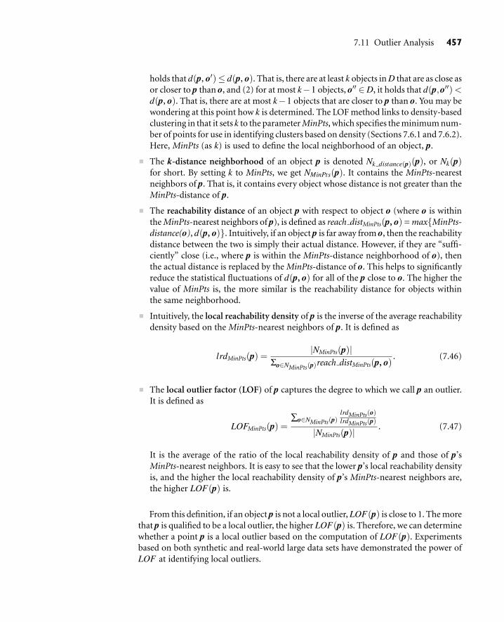
7.11 Outlier Analysis 457
holds that d(p, o′)≤ d(p, o). That is, there are at least k objects in D that are as close asor closer to p than o, and (2) for at most k−1 objects, o′′ ∈D, it holds that d(p,o′′)<d(p, o). That is, there are at most k−1 objects that are closer to p than o. You may bewondering at this point how k is determined. The LOF method links to density-basedclustering in that it sets k to the parameter MinPts, which specifies the minimum num-ber of points for use in identifying clusters based on density (Sections 7.6.1 and 7.6.2).Here, MinPts (as k) is used to define the local neighborhood of an object, p.
The k-distance neighborhood of an object p is denoted Nk distance(p)(p), or Nk(p)for short. By setting k to MinPts, we get NMinPts(p). It contains the MinPts-nearestneighbors of p. That is, it contains every object whose distance is not greater than theMinPts-distance of p.
The reachability distance of an object p with respect to object o (where o is withinthe MinPts-nearest neighbors of p), is defined as reach distMinPts(p, o) = max{MinPts-distance(o), d(p, o)}. Intuitively, if an object p is far away from o, then the reachabilitydistance between the two is simply their actual distance. However, if they are “suffi-ciently” close (i.e., where p is within the MinPts-distance neighborhood of o), thenthe actual distance is replaced by the MinPts-distance of o. This helps to significantlyreduce the statistical fluctuations of d(p, o) for all of the p close to o. The higher thevalue of MinPts is, the more similar is the reachability distance for objects withinthe same neighborhood.
Intuitively, the local reachability density of p is the inverse of the average reachabilitydensity based on the MinPts-nearest neighbors of p. It is defined as
lrdMinPts(p) =|NMinPts(p)|
Σo∈NMinPts(p)reach distMinPts(p, o). (7.46)
The local outlier factor (LOF) of p captures the degree to which we call p an outlier.It is defined as
LOFMinPts(p) =∑o∈NMinPts(p)
lrdMinPts(o)lrdMinPts(p)
|NMinPts(p)|. (7.47)
It is the average of the ratio of the local reachability density of p and those of p’sMinPts-nearest neighbors. It is easy to see that the lower p’s local reachability densityis, and the higher the local reachability density of p’s MinPts-nearest neighbors are,the higher LOF(p) is.
From this definition, if an object p is not a local outlier, LOF(p) is close to 1. The morethat p is qualified to be a local outlier, the higher LOF(p) is. Therefore, we can determinewhether a point p is a local outlier based on the computation of LOF(p). Experimentsbased on both synthetic and real-world large data sets have demonstrated the power ofLOF at identifying local outliers.

458 Chapter 7 Cluster Analysis
7.11.4 Deviation-Based Outlier Detection
Deviation-based outlier detection does not use statistical tests or distance-basedmeasures to identify exceptional objects. Instead, it identifies outliers by examining themain characteristics of objects in a group. Objects that “deviate” from this description areconsidered outliers. Hence, in this approach the term deviations is typically used to referto outliers. In this section, we study two techniques for deviation-based outlier detec-tion. The first sequentially compares objects in a set, while the second employs an OLAPdata cube approach.
Sequential Exception TechniqueThe sequential exception technique simulates the way in which humans can distinguishunusual objects from among a series of supposedly like objects. It uses implicit redun-dancy of the data. Given a data set, D, of n objects, it builds a sequence of subsets,{D1, D2, . . . , Dm}, of these objects with 2≤ m≤ n such that
D j−1 ⊂ D j, where D j ⊆ D. (7.48)
Dissimilarities are assessed between subsets in the sequence. The technique introducesthe following key terms.
Exception set: This is the set of deviations or outliers. It is defined as the smallestsubset of objects whose removal results in the greatest reduction of dissimilarity inthe residual set.14
Dissimilarity function: This function does not require a metric distance between theobjects. It is any function that, if given a set of objects, returns a low value if the objectsare similar to one another. The greater the dissimilarity among the objects, the higherthe value returned by the function. The dissimilarity of a subset is incrementally com-puted based on the subset prior to it in the sequence. Given a subset of n numbers,{x1, . . . , xn}, a possible dissimilarity function is the variance of the numbers in theset, that is,
1n
n
∑i=1
(xi− x)2, (7.49)
where x is the mean of the n numbers in the set. For character strings, the dissimilarityfunction may be in the form of a pattern string (e.g., containing wildcard characters)that is used to cover all of the patterns seen so far. The dissimilarity increases whenthe pattern covering all of the strings in D j−1 does not cover any string in D j that isnot in D j−1.
14For interested readers, this is equivalent to the greatest reduction in Kolmogorov complexity for theamount of data discarded.
7.12 Outlier Analysis 459
Cardinality function: This is typically the count of the number of objects in a given set.
Smoothing factor: This function is computed for each subset in the sequence. Itassesses how much the dissimilarity can be reduced by removing the subset from theoriginal set of objects. This value is scaled by the cardinality of the set. The subsetwhose smoothing factor value is the largest is the exception set.
The general task of finding an exception set can be NP-hard (i.e., intractable).A sequential approach is computationally feasible and can be implemented using a linearalgorithm.
“How does this technique work?” Instead of assessing the dissimilarity of the currentsubset with respect to its complementary set, the algorithm selects a sequence of subsetsfrom the set for analysis. For every subset, it determines the dissimilarity difference ofthe subset with respect to the preceding subset in the sequence.
“Can’t the order of the subsets in the sequence affect the results?” To help alleviate anypossible influence of the input order on the results, the above process can be repeatedseveral times, each with a different random ordering of the subsets. The subset with thelargest smoothing factor value, among all of the iterations, becomes the exception set.
OLAP Data Cube TechniqueAn OLAP approach to deviation detection uses data cubes to identify regions of anoma-lies in large multidimensional data. This technique was described in detail in Chapter 4.For added efficiency, the deviation detection process is overlapped with cube compu-tation. The approach is a form of discovery-driven exploration, in which precomputedmeasures indicating data exceptions are used to guide the user in data analysis, at all lev-els of aggregation. A cell value in the cube is considered an exception if it is significantlydifferent from the expected value, based on a statistical model. The method uses visualcues such as background color to reflect the degree of exception of each cell. The usercan choose to drill down on cells that are flagged as exceptions. The measure value of acell may reflect exceptions occurring at more detailed or lower levels of the cube, wherethese exceptions are not visible from the current level.
The model considers variations and patterns in the measure value across all of thedimensions to which a cell belongs. For example, suppose that you have a data cube forsales data and are viewing the sales summarized per month. With the help of the visualcues, you notice an increase in sales in December in comparison to all other months.This may seem like an exception in the time dimension. However, by drilling down onthe month of December to reveal the sales per item in that month, you note that thereis a similar increase in sales for other items during December. Therefore, an increasein total sales in December is not an exception if the item dimension is considered. Themodel considers exceptions hidden at all aggregated group-by’s of a data cube. Manualdetection of such exceptions is difficult because the search space is typically very large,particularly when there are many dimensions involving concept hierarchies with severallevels.

460 Chapter 7 Cluster Analysis
7.12 Summary
A cluster is a collection of data objects that are similar to one another within the samecluster and are dissimilar to the objects in other clusters. The process of grouping aset of physical or abstract objects into classes of similar objects is called clustering.
Cluster analysis has wide applications, including market or customer segmentation,pattern recognition, biological studies, spatial data analysis, Web document classifi-cation, and many others. Cluster analysis can be used as a stand-alone data miningtool to gain insight into the data distribution or can serve as a preprocessing step forother data mining algorithms operating on the detected clusters.
The quality of clustering can be assessed based on a measure of dissimilarity of objects,which can be computed for various types of data, including interval-scaled, binary,categorical, ordinal, and ratio-scaled variables, or combinations of these variable types.For nonmetric vector data, the cosine measure and the Tanimoto coefficient are oftenused in the assessment of similarity.
Clustering is a dynamic field of research in data mining. Many clustering algorithmshave been developed. These can be categorized into partitioning methods, hierarchicalmethods, density-based methods, grid-based methods, model-based methods, methodsfor high-dimensional data (including frequent pattern–based methods), and constraint-based methods. Some algorithms may belong to more than one category.
A partitioning method first creates an initial set of k partitions, where parameterk is the number of partitions to construct. It then uses an iterative relocation tech-nique that attempts to improve the partitioning by moving objects from one groupto another. Typical partitioning methods include k-means, k-medoids, CLARANS,and their improvements.
A hierarchical method creates a hierarchical decomposition of the given set of dataobjects. The method can be classified as being either agglomerative (bottom-up) ordivisive (top-down), based on how the hierarchical decomposition is formed. To com-pensate for the rigidity of merge or split, the quality of hierarchical agglomeration canbe improved by analyzing object linkages at each hierarchical partitioning (such asin ROCK and Chameleon), or by first performing microclustering (that is, group-ing objects into “microclusters”) and then operating on the microclusters with otherclustering techniques, such as iterative relocation (as in BIRCH).
A density-based method clusters objects based on the notion of density. It eithergrows clusters according to the density of neighborhood objects (such as in DBSCAN)or according to some density function (such as in DENCLUE). OPTICS is a density-based method that generates an augmented ordering of the clustering structure ofthe data.
A grid-based method first quantizes the object space into a finite number of cells thatform a grid structure, and then performs clustering on the grid structure. STING is

Exercises 461
a typical example of a grid-based method based on statistical information stored ingrid cells. WaveCluster and CLIQUE are two clustering algorithms that are both grid-based and density-based.
A model-based method hypothesizes a model for each of the clusters and finds thebest fit of the data to that model. Examples of model-based clustering include theEM algorithm (which uses a mixture density model), conceptual clustering (suchas COBWEB), and neural network approaches (such as self-organizing featuremaps).
Clustering high-dimensional data is of crucial importance, because in manyadvanced applications, data objects such as text documents and microarray dataare high-dimensional in nature. There are three typical methods to handle high-dimensional data sets: dimension-growth subspace clustering, represented by CLIQUE,dimension-reduction projected clustering, represented by PROCLUS, and frequentpattern–based clustering, represented by pCluster.
A constraint-based clustering method groups objects based on application-dependent or user-specified constraints. For example, clustering with the existence ofobstacle objects and clustering under user-specified constraints are typical methods ofconstraint-based clustering. Typical examples include clustering with the existenceof obstacle objects, clustering under user-specified constraints, and semi-supervisedclustering based on “weak” supervision (such as pairs of objects labeled as belongingto the same or different cluster).
One person’s noise could be another person’s signal. Outlier detection and analysis arevery useful for fraud detection, customized marketing, medical analysis, and manyother tasks. Computer-based outlier analysis methods typically follow either a statisti-cal distribution-based approach, a distance-based approach, a density-based local outlierdetection approach, or a deviation-based approach.
Exercises
7.1 Briefly outline how to compute the dissimilarity between objects described by thefollowing types of variables:
(a) Numerical (interval-scaled) variables
(b) Asymmetric binary variables
(c) Categorical variables
(d) Ratio-scaled variables
(e) Nonmetric vector objects
7.2 Given the following measurements for the variable age:
18, 22, 25, 42, 28, 43, 33, 35, 56, 28,

462 Chapter 7 Cluster Analysis
standardize the variable by the following:
(a) Compute the mean absolute deviation of age.
(b) Compute the z-score for the first four measurements.
7.3 Given two objects represented by the tuples (22, 1, 42, 10) and (20, 0, 36, 8):
(a) Compute the Euclidean distance between the two objects.
(b) Compute the Manhattan distance between the two objects.
(c) Compute the Minkowski distance between the two objects, using q = 3.
7.4 Section 7.2.3 gave a method wherein a categorical variable having M states can be encodedby M asymmetric binary variables. Propose a more efficient encoding scheme and statewhy it is more efficient.
7.5 Briefly describe the following approaches to clustering: partitioning methods, hierarchicalmethods, density-based methods, grid-based methods, model-based methods, methodsfor high-dimensional data, and constraint-based methods. Give examples in each case.
7.6 Suppose that the data mining task is to cluster the following eight points (with (x, y)representing location) into three clusters:
A1(2, 10), A2(2, 5), A3(8, 4), B1(5, 8), B2(7, 5), B3(6, 4), C1(1, 2), C2(4, 9).
The distance function is Euclidean distance. Suppose initially we assign A1, B1, and C1as the center of each cluster, respectively. Use the k-means algorithm to show only
(a) The three cluster centers after the first round execution
(b) The final three clusters
7.7 Both k-means and k-medoids algorithms can perform effective clustering. Illustrate thestrength and weakness of k-means in comparison with the k-medoids algorithm. Also,illustrate the strength and weakness of these schemes in comparison with a hierarchicalclustering scheme (such as AGNES).
7.8 Use a diagram to illustrate how, for a constant MinPts value, density-based clusters withrespect to a higher density (i.e., a lower value for ε, the neighborhood radius) are com-pletely contained in density-connected sets obtained with respect to a lower density.
7.9 Why is it that BIRCH encounters difficulties in finding clusters of arbitrary shape butOPTICS does not? Can you propose some modifications to BIRCH to help it find clustersof arbitrary shape?
7.10 Present conditions under which density-based clustering is more suitable thanpartitioning-based clustering and hierarchical clustering. Given some application exam-ples to support your argument.
7.11 Give an example of how specific clustering methods may be integrated, for example,where one clustering algorithm is used as a preprocessing step for another. In
Exercises 463
addition, provide reasoning on why the integration of two methods may sometimes leadto improved clustering quality and efficiency.
7.12 Clustering has been popularly recognized as an important data mining task with broadapplications. Give one application example for each of the following cases:
(a) An application that takes clustering as a major data mining function
(b) An application that takes clustering as a preprocessing tool for data preparation forother data mining tasks
7.13 Data cubes and multidimensional databases contain categorical, ordinal, and numericaldata in hierarchical or aggregate forms. Based on what you have learned about the cluster-ing methods, design a clustering method that finds clusters in large data cubes effectivelyand efficiently.
7.14 Subspace clustering is a methodology for finding interesting clusters in high-dimensionalspace. This methodology can be applied to cluster any kind of data. Outline an efficientalgorithm that may extend density connectivity-based clustering for finding clusters ofarbitrary shapes in projected dimensions in a high-dimensional data set.
7.15 [Contributed by Alex Kotov] Describe each of the following clustering algorithms in termsof the following criteria: (i) shapes of clusters that can be determined; (ii) input para-meters that must be specified; and (iii) limitations.
(a) k-means
(b) k-medoids
(c) CLARA
(d) BIRCH
(e) ROCK
(f) Chameleon
(g) DBSCAN
7.16 [Contributed by Tao Cheng] Many clustering algorithms handle either only numericaldata, such as BIRCH, or only categorical data, such as ROCK, but not both. Analyze whythis is the case. Note, however, that the EM clustering algorithm can easily be extendedto handle data with both numerical and categorical attributes. Briefly explain why it cando so and how.
7.17 Human eyes are fast and effective at judging the quality of clustering methods for two-dimensional data. Can you design a data visualization method that may help humansvisualize data clusters and judge the clustering quality for three-dimensional data? Whatabout for even higher-dimensional data?
7.18 Suppose that you are to allocate a number of automatic teller machines (ATMs) in agiven region so as to satisfy a number of constraints. Households or places of workmay be clustered so that typically one ATM is assigned per cluster. The clustering, how-ever, may be constrained by two factors: (1) obstacle objects (i.e., there are bridges,

464 Chapter 7 Cluster Analysis
rivers, and highways that can affect ATM accessibility), and (2) additional user-specifiedconstraints, such as each ATM should serve at least 10,000 households. How can a cluster-ing algorithm such as k-means be modified for quality clustering under both constraints?
7.19 For constraint-based clustering, aside from having the minimum number of customersin each cluster (for ATM allocation) as a constraint, there could be many other kinds ofconstraints. For example, a constraint could be in the form of the maximum numberof customers per cluster, average income of customers per cluster, maximum distancebetween every two clusters, and so on. Categorize the kinds of constraints that can beimposed on the clusters produced and discuss how to perform clustering efficiently undersuch kinds of constraints.
7.20 Design a privacy-preserving clustering method so that a data owner would be able toask a third party to mine the data for quality clustering without worrying about thepotential inappropriate disclosure of certain private or sensitive information storedin the data.
7.21 Why is outlier mining important? Briefly describe the different approaches behindstatistical-based outlier detection, distanced-based outlier detection, density-based local out-lier detection, and deviation-based outlier detection.
7.22 Local outlier factor (LOF) is an interesting notion for the discovery of local outliersin an environment where data objects are distributed rather unevenly. However, itsperformance should be further improved in order to efficiently discover local outliers.Can you propose an efficient method for effective discovery of local outliers in largedata sets?
Bibliographic Notes
Clustering has been studied extensively for more then 40 years and across many disci-plines due to its broad applications. Most books on pattern classification and machinelearning contain chapters on cluster analysis or unsupervised learning. Several textbooksare dedicated to the methods of cluster analysis, including Hartigan [Har75], Jain andDubes [JD88], Kaufman and Rousseeuw [KR90], and Arabie, Hubert, and De Sorte[AHS96]. There are also many survey articles on different aspects of clustering meth-ods. Recent ones include Jain, Murty, and Flynn [JMF99] and Parsons, Haque, and Liu[PHL04].
Methods for combining variables of different types into a single dissimilarity matrixwere introduced by Kaufman and Rousseeuw [KR90].
For partitioning methods, the k-means algorithm was first introduced byLloyd [Llo57] and then MacQueen [Mac67]. The k-medoids algorithms of PAM andCLARA were proposed by Kaufman and Rousseeuw [KR90]. The k-modes (for clusteringcategorical data) and k-prototypes (for clustering hybrid data) algorithms were proposedby Huang [Hua98]. The k-modes clustering algorithm was also proposed independentlyby Chaturvedi, Green, and Carroll [CGC94, CGC01].

Bibliographic Notes 465
The CLARANS algorithm was proposed by Ng and Han [NH94]. Ester, Kriegel, andXu [EKX95] proposed techniques for further improvement of the performance ofCLARANS using efficient spatial access methods, such as R*-tree and focusingtechniques. A k-means–based scalable clustering algorithm was proposed by Bradley,Fayyad, and Reina [BFR98].
An early survey of agglomerative hierarchical clustering algorithms was conducted byDay and Edelsbrunner [DE84]. Agglomerative hierarchical clustering, such as AGNES,and divisive hierarchical clustering, such as DIANA, were introduced by Kaufman andRousseeuw [KR90]. An interesting direction for improving the clustering quality of hier-archical clustering methods is to integrate hierarchical clustering with distance-basediterative relocation or other nonhierarchical clustering methods. For example, BIRCH,by Zhang, Ramakrishnan, and Livny [ZRL96], first performs hierarchical clustering witha CF-tree before applying other techniques. Hierarchical clustering can also be performedby sophisticated linkage analysis, transformation, or nearest-neighbor analysis, such asCURE by Guha, Rastogi, and Shim [GRS98], ROCK (for clustering categorical attributes)by Guha, Rastogi, and Shim [GRS99b], and Chameleon by Karypis, Han, and Kumar[KHK99].
For density-based clustering methods, DBSCAN was proposed by Ester, Kriegel,Sander, and Xu [EKSX96]. Ankerst, Breunig, Kriegel, and Sander [ABKS99] developedOPTICS, a cluster-ordering method that facilitates density-based clustering without wor-rying about parameter specification. The DENCLUE algorithm, based on a set of densitydistribution functions, was proposed by Hinneburg and Keim [HK98].
A grid-based multiresolution approach called STING, which collects statistical infor-mation in grid cells, was proposed by Wang, Yang, and Muntz [WYM97]. WaveCluster,developed by Sheikholeslami, Chatterjee, and Zhang [SCZ98], is a multiresolution clus-tering approach that transforms the original feature space by wavelet transform.
For model-based clustering, the EM (Expectation-Maximization) algorithm wasdeveloped by Dempster, Laird, and Rubin [DLR77]. AutoClass is a Bayesian statistics-based method for model-based clustering by Cheeseman and Stutz [CS96a] that uses avariant of the EM algorithm. There are many other extensions and applications of EM,such as Lauritzen [Lau95]. For a set of seminal papers on conceptual clustering, see Shav-lik and Dietterich [SD90]. Conceptual clustering was first introduced by Michalski andStepp [MS83]. Other examples of the conceptual clustering approach include COBWEBby Fisher [Fis87], and CLASSIT by Gennari, Langley, and Fisher [GLF89]. Studies of theneural network approach [He99] include SOM (self-organizing feature maps) by Koho-nen [Koh82], [Koh89], by Carpenter and Grossberg [Ce91], and by Kohonen, Kaski,Lagus, et al. [KKL+00], and competitive learning by Rumelhart and Zipser [RZ85].
Scalable methods for clustering categorical data were studied by Gibson, Kleinberg,and Raghavan [GKR98], Guha, Rastogi, and Shim [GRS99b], and Ganti, Gehrke, andRamakrishnan [GGR99]. There are also many other clustering paradigms. For exam-ple, fuzzy clustering methods are discussed in Kaufman and Rousseeuw [KR90], Bezdek[Bez81], and Bezdek and Pal [BP92].
For high-dimensional clustering, an Apriori-based dimension-growth subspace clus-tering algorithm called CLIQUE was proposed by Agrawal, Gehrke, Gunopulos, and

466 Chapter 7 Cluster Analysis
Raghavan [AGGR98]. It integrates density-based and grid-based clustering methods.A sampling-based, dimension-reduction subspace clustering algorithm called PROCLUS,and its extension, ORCLUS, were proposed by Aggarwal et al. [APW+99] and by Aggarwaland Yu [AY00], respectively. An entropy-based subspace clustering algorithm for min-ing numerical data, called ENCLUS, was proposed by Cheng, Fu, and Zhang [CFZ99].For a frequent pattern–based approach to handling high-dimensional data, Beil, Ester,and Xu [BEX02] proposed a method for frequent term–based text clustering. H. Wang,W. Wang, Yang, and Yu proposed pCluster, a pattern similarity–based clustering method[WWYY02].
Recent studies have proceeded to clustering stream data, as in Babcock, Babu, Datar,et al. [BBD+02]. A k-median-based data stream clustering algorithm was proposed byGuha, Mishra, Motwani, and O’Callaghan [GMMO00], and by O’Callaghan, Mishra,Meyerson, et al. [OMM+02]. A method for clustering evolving data streams was pro-posed by Aggarwal, Han, Wang, and Yu [AHWY03]. A framework for projected cluster-ing of high-dimensional data streams was proposed by Aggarwal, Han, Wang, and Yu[AHWY04a].
A framework for constraint-based clustering based on user-specified constraints wasbuilt by Tung, Han, Lakshmanan, and Ng [THLN01]. An efficient method for constraint-based spatial clustering in the existence of physical obstacle constraints was proposedby Tung, Hou, and Han [THH01]. The quality of unsupervised clustering can be sig-nificantly improved using supervision in the form of pairwise constraints (i.e., pairsof instances labeled as belonging to the same or different clustering). Such a process isconsidered semi-supervised clustering. A probabilistic framework for semi-supervisedclustering was proposed by Basu, Bilenko, and Mooney [BBM04]. The CLTree method,which transforms the clustering problem into a classification problem and then usesdecision tree induction for cluster analysis, was proposed by Liu, Xia, and Yu [LXY01].
Outlier detection and analysis can be categorized into four approaches: the statisticalapproach, the distance-based approach, the density-based local outlier detection, and thedeviation-based approach. The statistical approach and discordancy tests are describedin Barnett and Lewis [BL94]. Distance-based outlier detection is described in Knorrand Ng [KN97, KN98]. The detection of density-based local outliers was proposed byBreunig, Kriegel, Ng, and Sander [BKNS00]. Outlier detection for high-dimensional datais studied by Aggarwal and Yu [AY01]. The sequential problem approach to deviation-based outlier detection was introduced in Arning, Agrawal, and Raghavan [AAR96].Sarawagi, Agrawal, and Megiddo [SAM98] introduced a discovery-driven method foridentifying exceptions in large multidimensional data using OLAP data cubes. Jagadish,Koudas, and Muthukrishnan [JKM99] introduced an efficient method for miningdeviants in time-series databases.

8Mining Stream, Time-Series,and Sequence Data
Our previous chapters introduced the basic concepts and techniques of data mining. The techniquesstudied, however, were for simple and structured data sets, such as data in relationaldatabases, transactional databases, and data warehouses. The growth of data in variouscomplex forms (e.g., semi-structured and unstructured, spatial and temporal, hypertextand multimedia) has been explosive owing to the rapid progress of data collection andadvanced database system technologies, and the World Wide Web. Therefore, an increas-ingly important task in data mining is to mine complex types of data. Furthermore, manydata mining applications need to mine patterns that are more sophisticated than thosediscussed earlier, including sequential patterns, subgraph patterns, and features in inter-connected networks. We treat such tasks as advanced topics in data mining.
In the following chapters, we examine how to further develop the essential data min-ing techniques (such as characterization, association, classification, and clustering) andhow to develop new ones to cope with complex types of data. We start off, in this chapter,by discussing the mining of stream, time-series, and sequence data. Chapter 9 focuseson the mining of graphs, social networks, and multirelational data. Chapter 10 examinesmining object, spatial, multimedia, text, and Web data. Research into such mining is fastevolving. Our discussion provides a broad introduction. We expect that many new booksdedicated to the mining of complex kinds of data will become available in the future.
As this chapter focuses on the mining of stream data, time-series data, and sequencedata, let’s look at each of these areas.
Imagine a satellite-mounted remote sensor that is constantly generating data. Thedata are massive (e.g., terabytes in volume), temporally ordered, fast changing, and poten-tially infinite. This is an example of stream data. Other examples include telecommu-nications data, transaction data from the retail industry, and data from electric powergrids. Traditional OLAP and data mining methods typically require multiple scans ofthe data and are therefore infeasible for stream data applications. In Section 8.1, we studyadvanced mining methods for the analysis of such constantly flowing data.
A time-series database consists of sequences of values or events obtained over repeatedmeasurements of time. Suppose that you are given time-series data relating to stockmarket prices. How can the data be analyzed to identify trends? Given such data for
467

468 Chapter 8 Mining Stream, Time-Series, and Sequence Data
two different stocks, can we find any similarities between the two? These questions areexplored in Section 8.2. Other applications involving time-series data include economicand sales forecasting, utility studies, and the observation of natural phenomena (such asatmosphere, temperature, and wind).
A sequence database consists of sequences of ordered elements or events, recordedwith or without a concrete notion of time. Sequential pattern mining is the discoveryof frequently occurring ordered events or subsequences as patterns. An example of asequential pattern is “Customers who buy a Canon digital camera are likely to buy an HPcolor printer within a month.” Periodic patterns, which recur in regular periods or dura-tions, are another kind of pattern related to sequences. Section 8.3 studies methods ofsequential pattern mining.
Recent research in bioinformatics has resulted in the development of numerous meth-ods for the analysis of biological sequences, such as DNA and protein sequences.Section 8.4 introduces several popular methods, including biological sequence alignmentalgorithms and the hidden Markov model.
8.1 Mining Data Streams
Tremendous and potentially infinite volumes of data streams are often generated byreal-time surveillance systems, communication networks, Internet traffic, on-line trans-actions in the financial market or retail industry, electric power grids, industry pro-duction processes, scientific and engineering experiments, remote sensors, and otherdynamic environments. Unlike traditional data sets, stream data flow in and out of acomputer system continuously and with varying update rates. They are temporally ordered,fast changing, massive, and potentially infinite. It may be impossible to store an entiredata stream or to scan through it multiple times due to its tremendous volume. More-over, stream data tend to be of a rather low level of abstraction, whereas most analystsare interested in relatively high-level dynamic changes, such as trends and deviations. Todiscover knowledge or patterns from data streams, it is necessary to develop single-scan,on-line, multilevel, multidimensional stream processing and analysis methods.
Such single-scan, on-line data analysis methodology should not be confined to onlystream data. It is also critically important for processing nonstream data that are mas-sive. With data volumes mounting by terabytes or even petabytes, stream data nicelycapture our data processing needs of today: even when the complete set of data is col-lected and can be stored in massive data storage devices, single scan (as in data streamsystems) instead of random access (as in database systems) may still be the most realisticprocessing mode, because it is often too expensive to scan such a data set multiple times.
In this section, we introduce several on-line stream data analysis and mining methods.Section 8.1.1 introduces the basic methodologies for stream data processing and query-ing. Multidimensional analysis of stream data, encompassing stream data cubes andmultiple granularities of time, is described in Section 8.1.2. Frequent-pattern miningand classification are presented in Sections 8.1.3 and 8.1.4, respectively. The clusteringof dynamically evolving data streams is addressed in Section 8.1.5.

8.1 Mining Data Streams 469
8.1.1 Methodologies for Stream Data Processing andStream Data Systems
As seen from the previous discussion, it is impractical to scan through an entire datastream more than once. Sometimes we cannot even “look” at every element of a streambecause the stream flows in so fast and changes so quickly. The gigantic size of suchdata sets also implies that we generally cannot store the entire stream data set in mainmemory or even on disk. The problem is not just that there is a lot of data, it is that theuniverses that we are keeping track of are relatively large, where a universe is the domainof possible values for an attribute. For example, if we were tracking the ages of millions ofpeople, our universe would be relatively small, perhaps between zero and one hundredand twenty. We could easily maintain exact summaries of such data. In contrast, theuniverse corresponding to the set of all pairs of IP addresses on the Internet is very large,which makes exact storage intractable. A reasonable way of thinking about data streamsis to actually think of a physical stream of water. Heraclitus once said that you can neverstep in the same stream twice,1 and so it is with stream data.
For effective processing of stream data, new data structures, techniques, and algo-rithms are needed. Because we do not have an infinite amount of space to store streamdata, we often trade off between accuracy and storage. That is, we generally are willingto settle for approximate rather than exact answers. Synopses allow for this by provid-ing summaries of the data, which typically can be used to return approximate answersto queries. Synopses use synopsis data structures, which are any data structures that aresubstantially smaller than their base data set (in this case, the stream data). From thealgorithmic point of view, we want our algorithms to be efficient in both space and time.Instead of storing all or most elements seen so far, using O(N) space, we often want touse polylogarithmic space, O(logk N), where N is the number of elements in the streamdata. We may relax the requirement that our answers are exact, and ask for approximateanswers within a small error range with high probability. That is, many data stream–based algorithms compute an approximate answer within a factor ε of the actual answer,with high probability. Generally, as the approximation factor (1+ε) goes down, the spacerequirements go up. In this section, we examine some common synopsis data structuresand techniques.
Random SamplingRather than deal with an entire data stream, we can think of sampling the stream at peri-odic intervals. “To obtain an unbiased sampling of the data, we need to know the lengthof the stream in advance. But what can we do if we do not know this length in advance?”In this case, we need to modify our approach.
1Plato citing Heraclitus: “Heraclitus somewhere says that all things are in process and nothing staysstill, and likening existing things to the stream of a river he says you would not step twice into the sameriver.”

470 Chapter 8 Mining Stream, Time-Series, and Sequence Data
A technique called reservoir sampling can be used to select an unbiased randomsample of s elements without replacement. The idea behind reservoir sampling is rel-atively simple. We maintain a sample of size at least s, called the “reservoir,” from whicha random sample of size s can be generated. However, generating this sample from thereservoir can be costly, especially when the reservoir is large. To avoid this step, we main-tain a set of s candidates in the reservoir, which form a true random sample of the ele-ments seen so far in the stream. As the data stream flows, every new element has a certainprobability of replacing an old element in the reservoir. Let’s say we have seen N elementsthus far in the stream. The probability that a new element replaces an old one, chosenat random, is then s/N. This maintains the invariant that the set of s candidates in ourreservoir forms a random sample of the elements seen so far.
Sliding WindowsInstead of sampling the data stream randomly, we can use the sliding window model toanalyze stream data. The basic idea is that rather than running computations on all ofthe data seen so far, or on some sample, we can make decisions based only on recent data.More formally, at every time t, a new data element arrives. This element “expires” at timet + w, where w is the window “size” or length. The sliding window model is useful forstocks or sensor networks, where only recent events may be important. It also reducesmemory requirements because only a small window of data is stored.
HistogramsThe histogram is a synopsis data structure that can be used to approximate the frequencydistribution of element values in a data stream. A histogram partitions the data into aset of contiguous buckets. Depending on the partitioning rule used, the width (bucketvalue range) and depth (number of elements per bucket) can vary. The equal-width par-titioning rule is a simple way to construct histograms, where the range of each bucket isthe same. Although easy to implement, this may not sample the probability distributionfunction well. A better approach is to use V-Optimal histograms (see Section 2.5.4). Sim-ilar to clustering, V-Optimal histograms define bucket sizes that minimize the frequencyvariance within each bucket, which better captures the distribution of the data. Thesehistograms can then be used to approximate query answers rather than using samplingtechniques.
Multiresolution MethodsA common way to deal with a large amount of data is through the use of data reductionmethods (see Section 2.5). A popular data reduction method is the use of divide-and-conquer strategies such as multiresolution data structures. These allow a program totrade off between accuracy and storage, but also offer the ability to understand a datastream at multiple levels of detail.

8.1 Mining Data Streams 471
A concrete example is a balanced binary tree, where we try to maintain this balance asnew data come in. Each level of the tree provides a different resolution. The farther awaywe are from the tree root, the more detailed is the level of resolution.
A more sophisticated way to form multiple resolutions is to use a clustering methodto organize stream data into a hierarchical structure of trees. For example, we can use atypical hierarchical clustering data structure like CF-tree in BIRCH (see Section 7.5.2)to form a hierarchy of microclusters. With dynamic stream data flowing in and out, sum-mary statistics of data streams can be incrementally updated over time in the hierarchyof microclusters. Information in such microclusters can be aggregated into larger macro-clusters depending on the application requirements to derive general data statistics atmultiresolution.
Wavelets (Section 2.5.3), a technique from signal processing, can be used to build amultiresolution hierarchy structure over an input signal, in this case, the stream data.Given an input signal, we would like to break it down or rewrite it in terms of simple,orthogonal basis functions. The simplest basis is the Haar wavelet. Using this basis cor-responds to recursively performing averaging and differencing at multiple levels of reso-lution. Haar wavelets are easy to understand and implement. They are especially good atdealing with spatial and multimedia data. Wavelets have been used as approximations tohistograms for query optimization. Moreover, wavelet-based histograms can be dynam-ically maintained over time. Thus, wavelets are a popular multiresolution method fordata stream compression.
SketchesSynopses techniques mainly differ by how exactly they trade off accuracy for storage.Sampling techniques and sliding window models focus on a small part of the data,whereas other synopses try to summarize the entire data, often at multiple levels of detail.Some techniques require multiple passes over the data, such as histograms and wavelets,whereas other methods, such as sketches, can operate in a single pass.
Suppose that, ideally, we would like to maintain the full histogram over the universeof objects or elements in a data stream, where the universe is U = {1, 2, . . . , v} and thestream is A = {a1, a2, . . . , aN}. That is, for each value i in the universe, we want to main-tain the frequency or number of occurrences of i in the sequence A. If the universe is large,this structure can be quite large as well. Thus, we need a smaller representation instead.
Let’s consider the frequency moments of A. These are the numbers, Fk, defined as
Fk =v
∑i=1
mki , (8.1)
where v is the universe or domain size (as above), mi is the frequency of i in the sequence,and k ≥ 0. In particular, F0 is the number of distinct elements in the sequence. F1 isthe length of the sequence (that is, N, here). F2 is known as the self-join size, the repeatrate, or as Gini’s index of homogeneity. The frequency moments of a data set provideuseful information about the data for database applications, such as query answering. Inaddition, they indicate the degree of skew or asymmetry in the data (Section 2.2.1), which

472 Chapter 8 Mining Stream, Time-Series, and Sequence Data
is useful in parallel database applications for determining an appropriate partitioningalgorithm for the data.
When the amount of memory available is smaller than v, we need to employ a synop-sis. The estimation of the frequency moments can be done by synopses that are known assketches. These build a small-space summary for a distribution vector (e.g., histogram)using randomized linear projections of the underlying data vectors. Sketches provideprobabilistic guarantees on the quality of the approximate answer (e.g., the answer tothe given query is 12± 1 with a probability of 0.90). Given N elements and a universeU of v values, such sketches can approximate F0, F1, and F2 in O(logv + logN) space.The basic idea is to hash every element uniformly at random to either zi ∈ {−1, + 1},and then maintain a random variable, X = ∑i mizi. It can be shown that X2 is a goodestimate for F2. To explain why this works, we can think of hashing elements to −1 or+1 as assigning each element value to an arbitrary side of a tug of war. When we sum upto get X , we can think of measuring the displacement of the rope from the center point.By squaring X , we square this displacement, capturing the data skew, F2.
To get an even better estimate, we can maintain multiple random variables, Xi. Thenby choosing the median value of the square of these variables, we can increase our con-fidence that the estimated value is close to F2.
From a database perspective, sketch partitioning was developed to improve theperformance of sketching on data stream query optimization. Sketch partitioning usescoarse statistical information on the base data to intelligently partition the domain of theunderlying attributes in a way that provably tightens the error guarantees.
Randomized AlgorithmsRandomized algorithms, in the form of random sampling and sketching, are often usedto deal with massive, high-dimensional data streams. The use of randomization oftenleads to simpler and more efficient algorithms in comparison to known deterministicalgorithms.
If a randomized algorithm always returns the right answer but the running times vary,it is known as a Las Vegas algorithm. In contrast, a Monte Carlo algorithm has boundson the running time but may not return the correct result. We mainly consider MonteCarlo algorithms. One way to think of a randomized algorithm is simply as a probabilitydistribution over a set of deterministic algorithms.
Given that a randomized algorithm returns a random variable as a result, we wouldlike to have bounds on the tail probability of that random variable. This tells us that theprobability that a random variable deviates from its expected value is small. One basictool is Chebyshev’s Inequality. Let X be a random variable with mean µ and standarddeviation σ (variance σ2). Chebyshev’s inequality says that
P(|X−µ|> k)≤ σ2
k2 (8.2)
for any given positive real number, k. This inequality can be used to bound the varianceof a random variable.

8.1 Mining Data Streams 473
In many cases, multiple random variables can be used to boost the confidence in ourresults. As long as these random variables are fully independent, Chernoff bounds can beused. Let X1, X2, . . . , Xn be independent Poisson trials. In a Poisson trial, the probabilityof success varies from trial to trial. If X is the sum of X1 to Xn, then a weaker version ofthe Chernoff bound tells us that
Pr[X < (1 + δ)µ]< e−µδ2/4 (8.3)
where δ ∈ (0, 1]. This shows that the probability decreases exponentially as we movefrom the mean, which makes poor estimates much more unlikely.
Data Stream Management Systems and Stream QueriesIn traditional database systems, data are stored in finite and persistent databases. However,stream data are infinite and impossible to store fully in a database. In a Data Stream Man-agement System (DSMS), there may be multiple data streams. They arrive on-line andare continuous, temporally ordered, and potentially infinite. Once an element from a datastream has been processed, it is discarded or archived, and it cannot be easily retrievedunless it is explicitly stored in memory.
A stream data query processing architecture includes three parts: end user, query pro-cessor, and scratch space (which may consist of main memory and disks). An end userissues a query to the DSMS, and the query processor takes the query, processes it usingthe information stored in the scratch space, and returns the results to the user.
Queries can be either one-time queries or continuous queries. A one-time query is eval-uated once over a point-in-time snapshot of the data set, with the answer returned to theuser. A continuous query is evaluated continuously as data streams continue to arrive.The answer to a continuous query is produced over time, always reflecting the streamdata seen so far. A continuous query can act as a watchdog, as in “sound the alarm if thepower consumption for Block 25 exceeds a certain threshold.” Moreover, a query can be pre-defined (i.e., supplied to the data stream management system before any relevant datahave arrived) or ad hoc (i.e., issued on-line after the data streams have already begun).A predefined query is generally a continuous query, whereas an ad hoc query can beeither one-time or continuous.
Stream Query ProcessingThe special properties of stream data introduce new challenges in query processing.In particular, data streams may grow unboundedly, and it is possible that queries mayrequire unbounded memory to produce an exact answer. How can we distinguishbetween queries that can be answered exactly using a given bounded amount of memoryand queries that must be approximated? Actually, without knowing the size of the inputdata streams, it is impossible to place a limit on the memory requirements for most com-mon queries, such as those involving joins, unless the domains of the attributes involvedin the query are restricted. This is because without domain restrictions, an unbounded

474 Chapter 8 Mining Stream, Time-Series, and Sequence Data
number of attribute values must be remembered because they might turn out to joinwith tuples that arrive in the future.
Providing an exact answer to a query may require unbounded main memory; thereforea more realistic solution is to provide an approximate answer to the query. Approximatequery answering relaxes the memory requirements and also helps in handling systemload, because streams can come in too fast to process exactly. In addition, ad hoc queriesneed approximate history to return an answer. We have already discussed common syn-opses that are useful for approximate query answering, such as random sampling, slidingwindows, histograms, and sketches.
As this chapter focuses on stream data mining, we will not go into any further detailsof stream query processing methods. For additional discussion, interested readers mayconsult the literature recommended in the bibliographic notes of this chapter.
8.1.2 Stream OLAP and Stream Data Cubes
Stream data are generated continuously in a dynamic environment, with huge volume,infinite flow, and fast-changing behavior. It is impossible to store such data streams com-pletely in a data warehouse. Most stream data represent low-level information, consistingof various kinds of detailed temporal and other features. To find interesting or unusualpatterns, it is essential to perform multidimensional analysis on aggregate measures (suchas sum and average). This would facilitate the discovery of critical changes in the data athigher levels of abstraction, from which users can drill down to examine more detailedlevels, when needed. Thus multidimensional OLAP analysis is still needed in stream dataanalysis, but how can we implement it?
Consider the following motivating example.
Example 8.1 Multidimensional analysis for power supply stream data. A power supply station gen-erates infinite streams of power usage data. Suppose individual user, street address, andsecond are the attributes at the lowest level of granularity. Given a large number of users,it is only realistic to analyze the fluctuation of power usage at certain high levels, suchas by city or street district and by quarter (of an hour), making timely power supplyadjustments and handling unusual situations.
Conceptually, for multidimensional analysis, we can view such stream data as a virtualdata cube, consisting of one or a few measures and a set of dimensions, including onetime dimension, and a few other dimensions, such as location, user-category, and so on.However, in practice, it is impossible to materialize such a data cube, because the mate-rialization requires a huge amount of data to be computed and stored. Some efficientmethods must be developed for systematic analysis of such data.
Data warehouse and OLAP technology is based on the integration and consolidationof data in multidimensional space to facilitate powerful and fast on-line data analysis.A fundamental difference in the analysis of stream data from that of relational and ware-house data is that the stream data are generated in huge volume, flowing in and outdynamically and changing rapidly. Due to limited memory, disk space, and processing

8.1 Mining Data Streams 475
power, it is impossible to register completely the detailed level of data and compute a fullymaterialized cube. A realistic design is to explore several data compression techniques,including (1) tilted time frame on the time dimension, (2) storing data only at some crit-ical layers, and (3) exploring efficient computation of a very partially materialized datacube. The (partial) stream data cubes so constructed are much smaller than those con-structed from the raw stream data but will still be effective for multidimensional streamdata analysis. We examine such a design in more detail.
Time Dimension with Compressed TimeScale: Tilted Time FrameIn stream data analysis, people are usually interested in recent changes at a fine scale butin long-term changes at a coarse scale. Naturally, we can register time at different levels ofgranularity. The most recent time is registered at the finest granularity; the more distanttime is registered at a coarser granularity; and the level of coarseness depends on theapplication requirements and on how old the time point is (from the current time). Sucha time dimension model is called a tilted time frame. This model is sufficient for manyanalysis tasks and also ensures that the total amount of data to retain in memory or tobe stored on disk is small.
There are many possible ways to design a titled time frame. Here we introduce threemodels, as illustrated in Figure 8.1: (1) natural tilted time frame model, (2) logarithmictilted time frame model, and (3) progressive logarithmic tilted time frame model.
A natural tilted time frame model is shown in Figure 8.1(a), where the time frame(or window) is structured in multiple granularities based on the “natural” or usual timescale: the most recent 4 quarters (15 minutes), followed by the last 24 hours, then31 days, and then 12 months (the actual scale used is determined by the application).Based on this model, we can compute frequent itemsets in the last hour with the pre-cision of a quarter of an hour, or in the last day with the precision of an hour, and
Time
Time
tt2t4t8t16t32t64t
Now
Now
4 qtrs24 hours 31 days 12 months
(b) A logarithmic tilted time frame model.
(a) A natural tilted time frame model.
69 67 65�66 62 58�68 60 52 56 40 24
48 16�64 32
0�1�2�3�4�5
Snapshots (by clock time)Frame no.
(c) A progressive logarithmic tilted time frame table.
Figure 8.1 Three models for tilted time frames.
476 Chapter 8 Mining Stream, Time-Series, and Sequence Data
so on until the whole year with the precision of a month.2 This model registers only4 + 24 + 31 + 12 = 71 units of time for a year instead of 365× 24× 4 = 35,040 units,with an acceptable trade-off of the grain of granularity at a distant time.
The second model is the logarithmic tilted time frame model, as shown inFigure 8.1(b), where the time frame is structured in multiple granularities accordingto a logarithmic scale. Suppose that the most recent slot holds the transactions of thecurrent quarter. The remaining slots are for the last quarter, the next two quarters (ago),4 quarters, 8 quarters, 16 quarters, and so on, growing at an exponential rate. Accordingto this model, with one year of data and the finest precision at a quarter, we would needlog2(365×24×4)+1 = 16.1 units of time instead of 365×24×4 = 35,040 units. Thatis, we would just need 17 time frames to store the compressed information.
The third method is the progressive logarithmic tilted time frame model, where snap-shots are stored at differing levels of granularity depending on the recency. Let T be theclock time elapsed since the beginning of the stream. Snapshots are classified into differ-ent frame numbers, which can vary from 0 to max frame, where log2(T )−max capacity≤max frame ≤ log2(T ), and max capacity is the maximal number of snapshots held ineach frame.
Each snapshot is represented by its timestamp. The rules for insertion of a snapshott (at time t) into the snapshot frame table are defined as follows: (1) if (t mod 2i) = 0but (t mod 2i+1) 6= 0, t is inserted into frame number i if i≤max frame; otherwise (i.e.,i>max frame), t is inserted into max frame; and (2) each slot has a max capacity. At theinsertion of t into frame number i, if the slot already reaches its max capacity, the oldestsnapshot in this frame is removed and the new snapshot inserted.
Example 8.2 Progressive logarithmic tilted time frame. Consider the snapshot frame table ofFigure 8.1(c), where max frame is 5 and max capacity is 3. Let’s look at how timestamp64 was inserted into the table. We know (64 mod 26) = 0 but (64 mod 27) 6= 0, that is,i = 6. However, since this value of i exceeds max frame, 64 was inserted into frame 5 insteadof frame 6. Suppose we now need to insert a timestamp of 70. At time 70, since (70mod 21) = 0 but (70 mod 22) 6= 0, we would insert 70 into frame number 1. This wouldknock out the oldest snapshot of 58, given the slot capacity of 3. From the table, we see thatthe closer a timestamp is to the current time, the denser are the snapshots stored.
In the logarithmic and progressive logarithmic models discussed above, we haveassumed that the base is 2. Similar rules can be applied to any base α, where α is aninteger and α > 1. All three tilted time frame models provide a natural way for incre-mental insertion of data and for gradually fading out older values.
The tilted time frame models shown are sufficient for typical time-related queries,and at the same time, ensure that the total amount of data to retain in memory and/orto be computed is small.
2We align the time axis with the natural calendar time. Thus, for each granularity level of the tilted timeframe, there might be a partial interval, which is less than a full unit at that level.

8.1 Mining Data Streams 477
Depending on the given application, we can provide different fading factors in thetitled time frames, such as by placing more weight on the more recent time frames. Wecan also have flexible alternative ways to design the tilted time frames. For example, sup-pose that we are interested in comparing the stock average from each day of the currentweek with the corresponding averages from the same weekdays last week, last month, orlast year. In this case, we can single out Monday to Friday instead of compressing theminto the whole week as one unit.
Critical LayersEven with the tilted time frame model, it can still be too costly to dynamically computeand store a materialized cube. Such a cube may have quite a few dimensions, each con-taining multiple levels with many distinct values. Because stream data analysis has onlylimited memory space but requires fast response time, we need additional strategies thatwork in conjunction with the tilted time frame model. One approach is to compute andstore only some mission-critical cuboids of the full data cube.
In many applications, it is beneficial to dynamically and incrementally compute andstore two critical cuboids (or layers), which are determined based on their conceptualand computational importance in stream data analysis. The first layer, called the minimalinterest layer, is the minimally interesting layer that an analyst would like to study. It isnecessary to have such a layer because it is often neither cost effective nor interestingin practice to examine the minute details of stream data. The second layer, called theobservation layer, is the layer at which an analyst (or an automated system) would liketo continuously study the data. This can involve making decisions regarding the signalingof exceptions, or drilling down along certain paths to lower layers to find cells indicatingdata exceptions.
Example 8.3 Critical layers for a power supply stream data cube. Let’s refer back to Example 8.1regarding the multidimensional analysis of stream data for a power supply station.Dimensions at the lowest level of granularity (i.e., the raw data layer) included individ-ual user, street address, and second. At the minimal interest layer, these three dimensionsare user group, street block, and minute, respectively. Those at the observation layer are∗ (meaning all user), city, and quarter, respectively, as shown in Figure 8.2.
Based on this design, we would not need to compute any cuboids that are lower thanthe minimal interest layer because they would be beyond user interest. Thus, to computeour base cuboid, representing the cells of minimal interest, we need to compute and storethe (three-dimensional) aggregate cells for the (user group, street block, minute) group-by. This can be done by aggregations on the dimensions user and address by rolling upfrom individual user to user group and from street address to street block, respectively,and by rolling up on the time dimension from second to minute.
Similarly, the cuboids at the observation layer should be computed dynamically, tak-ing the tilted time frame model into account as well. This is the layer that an analysttakes as an observation deck, watching the current stream data by examining the slopeof changes at this layer to make decisions. This layer can be obtained by rolling up the

478 Chapter 8 Mining Stream, Time-Series, and Sequence Data
observation layer
minimal interest layer
primitive data layer(individual_user, street_address, second)
(user_group, street_block, minute)
(*, city, quarter)
Figure 8.2 Two critical layers in a “power supply station” stream data cube.
cube along the user dimension to ∗ (for all user), along the address dimension to city, andalong the time dimension to quarter. If something unusual is observed, the analyst caninvestigate by drilling down to lower levels to find data exceptions.
Partial Materialization of a Stream Cube“What if a user needs a layer that would be between the two critical layers?” Materializinga cube at only two critical layers leaves much room for how to compute the cuboids inbetween. These cuboids can be precomputed fully, partially, or not at all (i.e., leave every-thing to be computed on the fly). An interesting method is popular path cubing, whichrolls up the cuboids from the minimal interest layer to the observation layer by followingone popular drilling path, materializes only the layers along the path, and leaves otherlayers to be computed only when needed. This method achieves a reasonable trade-offbetween space, computation time, and flexibility, and has quick incremental aggregationtime, quick drilling time, and small space requirements.
To facilitate efficient computation and storage of the popular path of the stream cube,a compact data structure needs to be introduced so that the space taken in the compu-tation of aggregations is minimized. A hyperlinked tree structure called H-tree is revisedand adopted here to ensure that a compact structure is maintained in memory for effi-cient computation of multidimensional and multilevel aggregations.
Each branch of the H-tree is organized in the same order as the specified popularpath. The aggregate cells are stored in the nonleaf nodes of the H-tree, formingthe computed cuboids along the popular path. Aggregation for each correspondingslot in the tilted time frame is performed from the minimal interest layer all theway up to the observation layer by aggregating along the popular path. The step-by-step aggregation is performed while inserting the new generalized tuples into thecorresponding time slots.

8.1 Mining Data Streams 479
The H-tree ordering is based on the popular drilling path given by users or experts.This ordering facilitates the computation and storage of the cuboids along the path.The aggregations along the drilling path from the minimal interest layer to the obser-vation layer are performed during the generalizing of the stream data to the minimalinterest layer, which takes only one scan of stream data. Because all the cells to becomputed are the cuboids along the popular path, and the cuboids to be computed arethe nonleaf nodes associated with the H-tree, both space and computation overheadsare minimized.
Although it is impossible to materialize all the cells of a stream cube, the stream datacube so designed facilitates fast on-line drilling along any single dimension or alongcombinations of a small number of dimensions. The H-tree-based architecture facili-tates incremental updating of stream cubes as well.
8.1.3 Frequent-Pattern Mining in Data Streams
As discussed in Chapter 5, frequent-pattern mining finds a set of patterns that occurfrequently in a data set, where a pattern can be a set of items (called an itemset),a subsequence, or a substructure. A pattern is considered frequent if its count sat-isfies a minimum support. Scalable methods for mining frequent patterns have beenextensively studied for static data sets. However, mining such patterns in dynamicdata streams poses substantial new challenges. Many existing frequent-pattern min-ing algorithms require the system to scan the whole data set more than once, butthis is unrealistic for infinite data streams. How can we perform incremental updatesof frequent itemsets for stream data since an infrequent itemset can become frequentlater on, and hence cannot be ignored? Moreover, a frequent itemset can becomeinfrequent as well. The number of infrequent itemsets is exponential and so it isimpossible to keep track of all of them.
To overcome this difficulty, there are two possible approaches. One is to keeptrack of only a predefined, limited set of items and itemsets. This method has verylimited usage and expressive power because it requires the system to confine thescope of examination to only the set of predefined itemsets beforehand. The sec-ond approach is to derive an approximate set of answers. In practice, approximateanswers are often sufficient. A number of approximate item or itemset countingalgorithms have been developed in recent research. Here we introduce one suchalgorithm: the Lossy Counting algorithm. It approximates the frequency of itemsor itemsets within a user-specified error bound, ε. This concept is illustrated asfollows.
Example 8.4 Approximate frequent items. A router is interested in all items whose frequency is at least1% (min support) of the entire traffic stream seen so far. It is felt that 1/10 of min support(i.e., ε = 0.1%) is an acceptable margin of error. This means that all frequent items witha support of at least min support will be output, but that some items with a support ofat least (min support− ε) will also be output.

480 Chapter 8 Mining Stream, Time-Series, and Sequence Data
Lossy Counting AlgorithmWe first introduce the Lossy Counting algorithm for frequent items. This algorithm isfairly simple but quite efficient. We then look at how the method can be extended to findapproximate frequent itemsets.
“How does the Lossy Counting algorithm find frequent items?” A user first provides twoinput parameters: (1) the min support threshold, σ, and (2) the error bound mentionedpreviously, denoted as ε. The incoming stream is conceptually divided into buckets ofwidth w = d1/εe. Let N be the current stream length, that is, the number of items seen sofar. The algorithm uses a frequency-list data structure for all items with frequency greaterthan 0. For each item, the list maintains f , the approximate frequency count, and ∆, themaximum possible error of f .
The algorithm processes buckets of items as follows. When a new bucket comes in, theitems in the bucket are added to the frequency list. If a given item already exists in thelist, we simply increase its frequency count, f . Otherwise, we insert it into the list with afrequency count of 1. If the new item is from the bth bucket, we set ∆, the maximum pos-sible error on the frequency count of the item, to be b−1. Based on our discussion so far,the item frequency counts hold the actual frequencies rather than approximations. Theybecome approximates, however, because of the next step. Whenever a bucket “bound-ary” is reached (that is, N has reached a multiple of width w, such as w, 2w, 3w, etc.), thefrequency list is examined. Let b be the current bucket number. An item entry is deletedif, for that entry, f + ∆ ≤ b. In this way, the algorithm aims to keep the frequency listsmall so that it may fit in main memory. The frequency count stored for each item willeither be the true frequency of the item or an underestimate of it.
“By how much can a frequency count be underestimated?” One of the most importantfactors in approximation algorithms is the approximation ratio (or error bound). Let’slook at the case where an item is deleted. This occurs when f +∆≤ b for an item, whereb is the current bucket number. We know that b ≤ N/w, that is, b ≤ εN. The actualfrequency of an item is at most f +∆. Thus, the most that an item can be underestimatedis εN. If the actual support of this item is σ (this is the minimum support or lower boundfor it to be considered frequent), then the actual frequency is σN, and the frequency, f ,on the frequency list should be at least (σN− εN). Thus, if we output all of the items inthe frequency list having an f value of at least (σN− εN), then all of the frequent itemswill be output. In addition, some subfrequent items (with an actual frequency of at leastσN− εN but less than σN) will be output, too.
The Lossy Counting algorithm has three nice properties: (1) there are no false neg-atives, that is, there is no true frequent item that is not output; (2) false positives arequite “positive” as well, since the output items will have a frequency of at least σN−εN;and (3) the frequency of a frequent item can be underestimated by at most εN. For fre-quent items, this underestimation is only a small fraction of its true frequency, so thisapproximation is acceptable.
“How much space is needed to save the frequency list?” It has been shown that thealgorithm takes at most 1
ε log(εN) entries in computation, where N is the streamlength so far. If we assume that elements with very low frequency tend to occur

8.1 Mining Data Streams 481
more or less uniformly at random, then it has been shown that Lossy Countingrequires no more than 7
ε space. Thus, the space requirement for this algorithm isreasonable.
It is much more difficult to find frequent itemsets than to find frequent items in datastreams, because the number of possible itemsets grows exponentially with that of dif-ferent items. As a consequence, there will be many more frequent itemsets. If we stillprocess the data bucket by bucket, we will probably run out of memory. An alternativeis to process as many buckets as we can at a time.
To find frequent itemsets, transactions are still divided by buckets with bucket size,w = d1/εe. However, this time, we will read as many buckets as possible into mainmemory. As before, we maintain a frequency list, although now it pertains to itemsetsrather than items. Suppose we can read β buckets into main memory. After that, weupdate the frequency list by all these buckets as follows. If a given itemset alreadyexists in the frequency list, we update f by counting the occurrences of the itemsetamong the current batch of β buckets. If the updated entry satisfies f + ∆≤ b, whereb is the current bucket number, we delete the entry. If an itemset has frequency f ≥ βand does not appear in the list, it is inserted as a new entry where ∆ is set to b−β asthe maximum error of f .
In practice, β will be large, such as greater than 30. This approach will save memorybecause all itemsets with frequency less than β will not be recorded in the frequency listanymore. For smaller values of β (such as 1 for the frequent item version of the algorithmdescribed earlier), more spurious subsets will find their way into the frequency list. Thiswould drastically increase the average size and refresh rate of the frequency list and harmthe algorithm’s efficiency in both time and space.
In general, Lossy Counting is a simple but effective algorithm for finding frequentitems and itemsets approximately. Its limitations lie in three aspects: (1) the spacebound is insufficient because the frequency list may grow infinitely as the stream goeson; (2) for frequent itemsets, the algorithm scans each transaction many times and thesize of main memory will greatly impact the efficiency of the algorithm; and (3) theoutput is based on all of the previous data, although users can be more interestedin recent data than that in the remote past. A tilted time frame model with differenttime granularities can be integrated with Lossy Counting in order to emphasize therecency of the data.
8.1.4 Classification of Dynamic Data Streams
In Chapter 6, we studied several methods for the classification of static data. Classifica-tion is a two-step process consisting of learning, or model construction (where a model isconstructed based on class-labeled tuples from a training data set), and classification, ormodel usage (where the model is used to predict the class labels of tuples from new datasets). The latter lends itself to stream data, as new examples are immediately classified bythe model as they arrive.
“So, does this mean we can apply traditional classification methods to stream data aswell?” In a traditional setting, the training data reside in a relatively static database. Many

482 Chapter 8 Mining Stream, Time-Series, and Sequence Data
classification methods will scan the training data multiple times. Therefore, the firststep of model construction is typically performed off-line as a batch process. With datastreams, however, there is typically no off-line phase. The data flow in so quickly thatstorage and multiple scans are infeasible.
To further illustrate how traditional classification methods are inappropriate forstream data, consider the practice of constructing decision trees as models. Most decisiontree algorithms tend to follow the same basic top-down, recursive strategy, yet differ inthe statistical measure used to choose an optimal splitting attribute. To review, a decisiontree consists of internal (nonleaf) nodes, branches, and leaf nodes. An attribute selectionmeasure is used to select the splitting attribute for the current node. This is taken to bethe attribute that best discriminates the training tuples according to class. In general,branches are grown for each possible value of the splitting attribute, the training tuplesare partitioned accordingly, and the process is recursively repeated at each branch. How-ever, in the stream environment, it is neither possible to collect the complete set of datanor realistic to rescan the data, thus such a method has to be re-examined.
Another distinguishing characteristic of data streams is that they are time-varying,as opposed to traditional database systems, where only the current state is stored. Thischange in the nature of the data takes the form of changes in the target classificationmodel over time and is referred to as concept drift. Concept drift is an important con-sideration when dealing with stream data.
Several methods have been proposed for the classification of stream data. We intro-duce four of them in this subsection. The first three, namely the Hoeffding tree algorithm,Very Fast Decision Tree (VFDT), and Concept-adapting Very Fast Decision Tree (CVFDT),extend traditional decision tree induction. The fourth uses a classifier ensemble approach,in which multiple classifiers are considered using a voting method.
Hoeffding Tree AlgorithmThe Hoeffding tree algorithm is a decision tree learning method for stream data classi-fication. It was initially used to track Web clickstreams and construct models to predictwhich Web hosts and Web sites a user is likely to access. It typically runs in sublineartime and produces a nearly identical decision tree to that of traditional batch learners.It uses Hoeffding trees, which exploit the idea that a small sample can often be enoughto choose an optimal splitting attribute. This idea is supported mathematically by theHoeffding bound (or additive Chernoff bound). Suppose we make N independent obser-vations of a random variable r with range R, where r is an attribute selection measure.(For a probability, R is one, and for an information gain, it is log c, where c is the numberof classes.) In the case of Hoeffding trees, r is information gain. If we compute the mean,r, of this sample, the Hoeffding bound states that the true mean of r is at least r−ε, withprobability 1−δ, where δ is user-specified and
ε =
√
R2ln(1/δ)2N
. (8.4)

8.1 Mining Data Streams 483
The Hoeffding tree algorithm uses the Hoeffding bound to determine, with highprobability, the smallest number, N, of examples needed at a node when selecting a split-ting attribute. This attribute would be the same as that chosen using infinite examples!We’ll see how this is done shortly. The Hoeffding bound is independent of the probabilitydistribution, unlike most other bound equations. This is desirable, as it may be impossi-ble to know the probability distribution of the information gain, or whichever attributeselection measure is used.
“How does the Hoeffding tree algorithm use the Hoeffding bound?” The algorithm takesas input a sequence of training examples, S, described by attributes A, and the accuracyparameter, δ. In addition, the evaluation function G(Ai) is supplied, which could beinformation gain, gain ratio, Gini index, or some other attribute selection measure. Ateach node in the decision tree, we need to maximize G(Ai) for one of the remainingattributes, Ai. Our goal is to find the smallest number of tuples, N, for which the Hoeffd-ing bound is satisfied. For a given node, let Aa be the attribute that achieves the highestG, and Ab be the attribute that achieves the second highest G. If G(Aa)−G(Ab) > ε,where ε is calculated from Equation (8.4), we can confidently say that this difference islarger than zero. We select Aa as the best splitting attribute with confidence 1−δ.
The only statistics that must be maintained in the Hoeffding tree algorithm are thecounts nijk for the value v j of attribute Ai with class label yk. Therefore, if d is the numberof attributes, v is the maximum number of values for any attribute, c is the number ofclasses, and l is the maximum depth (or number of levels) of the tree, then the totalmemory required is O(ldvc). This memory requirement is very modest compared toother decision tree algorithms, which usually store the entire training set in memory.
“How does the Hoeffding tree compare with trees produced by traditional decision treesalgorithms that run in batch mode?” The Hoeffding tree becomes asymptotically closeto that produced by the batch learner. Specifically, the expected disagreement betweenthe Hoeffding tree and a decision tree with infinite examples is at most δ/p, where pis the leaf probability, or the probability that an example will fall into a leaf. If the twobest splitting attributes differ by 10% (i.e., ε/R = 0.10), then by Equation (8.4), it wouldtake 380 examples to ensure a desired accuracy of 90% (i.e., δ = 0.1). For δ = 0.0001,it would take only 725 examples, demonstrating an exponential improvement in δ withonly a linear increase in the number of examples. For this latter case, if p = 1%, theexpected disagreement between the trees would be at most δ/p = 0.01%, with only 725examples per node.
In addition to high accuracy with a small sample, Hoeffding trees have other attrac-tive properties for dealing with stream data. First, multiple scans of the same dataare never performed. This is important because data streams often become too largeto store. Furthermore, the algorithm is incremental, which can be seen in Figure 8.3(adapted from [GGR02]). The figure demonstrates how new examples are integratedinto the tree as they stream in. This property contrasts with batch learners, which waituntil the data are accumulated before constructing the model. Another advantage ofincrementally building the tree is that we can use it to classify data even while it is beingbuilt. The tree will continue to grow and become more accurate as more training datastream in.

484 Chapter 8 Mining Stream, Time-Series, and Sequence Data
yes no
yes no
Packets > 10
Protocol = http
Protocol = ftp
yes
Packets > 10
Bytes > 60K
Protocol = http
Data Stream
Data Stream
Figure 8.3 The nodes of the Hoeffding tree are created incrementally as more samples stream in.
There are, however, weaknesses to the Hoeffding tree algorithm. For example,the algorithm spends a great deal of time with attributes that have nearly identicalsplitting quality. In addition, the memory utilization can be further optimized. Finally,the algorithm cannot handle concept drift, because once a node is created, it can neverchange.
Very Fast Decision Tree (VFDT) and Concept-adaptingVery Fast Decision Tree (CVFDT)The VFDT (Very Fast Decision Tree) algorithm makes several modifications to theHoeffding tree algorithm to improve both speed and memory utilization. Themodifications include breaking near-ties during attribute selection more aggressively,computing the G function after a number of training examples, deactivating the leastpromising leaves whenever memory is running low, dropping poor splitting attributes,and improving the initialization method. VFDT works well on stream data and also com-pares extremely well to traditional classifiers in both speed and accuracy. However, it stillcannot handle concept drift in data streams.
“What can we do to manage concept drift?” Basically, we need a way to identifyin a timely manner those elements of the stream that are no longer consistent withthe current concepts. A common approach is to use a sliding window. The intuitionbehind it is to incorporate new examples yet eliminate the effects of old ones. We
8.1 Mining Data Streams 485
can repeatedly apply a traditional classifier to the examples in the sliding window.As new examples arrive, they are inserted into the beginning of the window; acorresponding number of examples is removed from the end of the window, andthe classifier is reapplied. This technique, however, is sensitive to the window size, w.If w is too large, the model will not accurately represent the concept drift. On theother hand, if w is too small, then there will not be enough examples to constructan accurate model. Moreover, it will become very expensive to continually constructa new classifier model.
To adapt to concept-drifting data streams, the VFDT algorithm was further developedinto the Concept-adapting Very Fast Decision Tree algorithm (CVFDT). CVFDT alsouses a sliding window approach; however, it does not construct a new model from scratcheach time. Rather, it updates statistics at the nodes by incrementing the counts associatedwith new examples and decrementing the counts associated with old ones. Therefore, ifthere is a concept drift, some nodes may no longer pass the Hoeffding bound. When thishappens, an alternate subtree will be grown, with the new best splitting attribute at theroot. As new examples stream in, the alternate subtree will continue to develop, withoutyet being used for classification. Once the alternate subtree becomes more accurate thanthe existing one, the old subtree is replaced.
Empirical studies show that CVFDT achieves better accuracy than VFDT withtime-changing data streams. In addition, the size of the tree in CVFDT is muchsmaller than that in VFDT, because the latter accumulates many outdated examples.
A Classifier Ensemble Approach to StreamData ClassificationLet’s look at another approach to classifying concept drifting data streams, where weinstead use a classifier ensemble. The idea is to train an ensemble or group of classifiers(using, say, C4.5, or naïve Bayes) from sequential chunks of the data stream. That is,whenever a new chunk arrives, we build a new classifier from it. The individual clas-sifiers are weighted based on their expected classification accuracy in a time-changingenvironment. Only the top-k classifiers are kept. The decisions are then based on theweighted votes of the classifiers.
“Why is this approach useful?” There are several reasons for involving more thanone classifier. Decision trees are not necessarily the most natural method for han-dling concept drift. Specifically, if an attribute near the root of the tree in CVFDTno longer passes the Hoeffding bound, a large portion of the tree must be regrown.Many other classifiers, such as naïve Bayes, are not subject to this weakness. Inaddition, naïve Bayesian classifiers also supply relative probabilities along with theclass labels, which expresses the confidence of a decision. Furthermore, CVFDT’sautomatic elimination of old examples may not be prudent. Rather than keepingonly the most up-to-date examples, the ensemble approach discards the least accu-rate classifiers. Experimentation shows that the ensemble approach achieves greateraccuracy than any one of the single classifiers.

486 Chapter 8 Mining Stream, Time-Series, and Sequence Data
8.1.5 Clustering Evolving Data Streams
Imagine a huge amount of dynamic stream data. Many applications require theautomated clustering of such data into groups based on their similarities. Examplesinclude applications for network intrusion detection, analyzing Web clickstreams, andstock market analysis. Although there are many powerful methods for clustering staticdata sets (Chapter 7), clustering data streams places additional constraints on such algo-rithms. As we have seen, the data stream model of computation requires algorithms tomake a single pass over the data, with bounded memory and limited processing time,whereas the stream may be highly dynamic and evolving over time.
For effective clustering of stream data, several new methodologies have been devel-oped, as follows:
Compute and store summaries of past data: Due to limited memory space andfast response requirements, compute summaries of the previously seen data, storethe relevant results, and use such summaries to compute important statistics whenrequired.
Apply a divide-and-conquer strategy: Divide data streams into chunks based on orderof arrival, compute summaries for these chunks, and then merge the summaries. Inthis way, larger models can be built out of smaller building blocks.
Incremental clustering of incoming data streams: Because stream data enter the sys-tem continuously and incrementally, the clusters derived must be incrementallyrefined.
Perform microclustering as well as macroclustering analysis: Stream clusters canbe computed in two steps: (1) compute and store summaries at the microclusterlevel, where microclusters are formed by applying a hierarchical bottom-up clusteringalgorithm (Section 7.5.1), and (2) compute macroclusters (such as by using anotherclustering algorithm to group the microclusters) at the user-specified level. This two-step computation effectively compresses the data and often results in a smaller marginof error.
Explore multiple time granularity for the analysis of cluster evolution: Because themore recent data often play a different role from that of the remote (i.e., older) data instream data analysis, use a tilted time frame model to store snapshots of summarizeddata at different points in time.
Divide stream clustering into on-line and off-line processes: While data are stream-ing in, basic summaries of data snapshots should be computed, stored, and incremen-tally updated. Therefore, an on-line process is needed to maintain such dynamicallychanging clusters. Meanwhile, a user may pose queries to ask about past, current, orevolving clusters. Such analysis can be performed off-line or as a process independentof on-line cluster maintenance.
Several algorithms have been developed for clustering data streams. Two of them,namely, STREAM and CluStream, are introduced here.

8.1 Mining Data Streams 487
STREAM: A k-Medians-based Stream ClusteringAlgorithmGiven a data stream model of points, X1, . . . ,XN , with timestamps, T1, . . . , TN , the objec-tive of stream clustering is to maintain a consistently good clustering of the sequenceseen so far using a small amount of memory and time.
STREAM is a single-pass, constant factor approximation algorithm that was devel-oped for the k-medians problem. The k-medians problem is to cluster N data points intok clusters or groups such that the sum squared error (SSQ) between the points and thecluster center to which they are assigned is minimized. The idea is to assign similar pointsto the same cluster, where these points are dissimilar from points in other clusters.
Recall that in the stream data model, data points can only be seen once, and memoryand time are limited. To achieve high-quality clustering, the STREAM algorithm pro-cesses data streams in buckets (or batches) of m points, with each bucket fitting in mainmemory. For each bucket, bi, STREAM clusters the bucket’s points into k clusters. It thensummarizes the bucket information by retaining only the information regarding the kcenters, with each cluster center being weighted by the number of points assigned to itscluster. STREAM then discards the points, retaining only the center information. Onceenough centers have been collected, the weighted centers are again clustered to produceanother set of O(k) cluster centers. This is repeated so that at every level, at most m pointsare retained. This approach results in a one-pass, O(kN)-time, O(Nε)-space (for someconstant ε< 1), constant-factor approximation algorithm for data stream k-medians.
STREAM derives quality k-medians clusters with limited space and time. However,it considers neither the evolution of the data nor time granularity. The clustering canbecome dominated by the older, outdated data of the stream. In real life, the nature ofthe clusters may vary with both the moment at which they are computed, as well as thetime horizon over which they are measured. For example, a user may wish to examineclusters occurring last week, last month, or last year. These may be considerably differ-ent. Therefore, a data stream clustering algorithm should also provide the flexibility tocompute clusters over user-defined time periods in an interactive manner. The followingalgorithm, CluStream, addresses these concerns.
CluStream: Clustering Evolving Data StreamsCluStream is an algorithm for the clustering of evolving data streams based on user-specified, on-line clustering queries. It divides the clustering process into on-line and off-line components. The on-line component computes and stores summary statistics aboutthe data stream using microclusters, and performs incremental on-line computation andmaintenance of the microclusters. The off-line component does macroclustering andanswers various user questions using the stored summary statistics, which are based onthe tilted time frame model.
To cluster evolving data streams based on both historical and current stream datainformation, the tilted time frame model (such as a progressive logarithmic model) isadopted, which stores the snapshots of a set of microclusters at different levels of

488 Chapter 8 Mining Stream, Time-Series, and Sequence Data
granularity depending on recency. The intuition here is that more information will beneeded for more recent events as opposed to older events. The stored information canbe used for processing history-related, user-specific clustering queries.
A microcluster in CluStream is represented as a clustering feature. CluStream extendsthe concept of the clustering feature developed in BIRCH (see Section 7.5.2) to include thetemporal domain. As a temporal extension of the clustering feature, a microcluster for a setof d-dimensional points, X1, . . . , Xn, with timestamps, T1, . . . , Tn, is defined as the (2d +3)tuple (CF2x,CF1x,CF2t , CF1t , n), wherein CF2x and CF1x are d-dimensional vectorswhile CF2t , CF1t , and n are scalars. CF2x maintains the sum of the squares of the datavalues per dimension, that is, ∑n
i=1 X2i . Similarly, for each dimension, the sum of the data
values is maintained in CF1x. From a statistical point of view, CF2x and CF1x representthe second- and first-order moments (Section 8.1.1) of the data, respectively. The sum ofsquaresof the timestamps ismaintained inCF2t .Thesumof the timestamps ismaintainedin CF1t . Finally, the number of data points in the microcluster is maintained in n.
Clustering features have additive and subtractive properties that make them very use-ful for data stream cluster analysis. For example, two microclusters can be merged byadding their respective clustering features. Furthermore, a large number of microclusterscan be maintained without using a great deal of memory. Snapshots of these microclus-ters are stored away at key points in time based on the tilted time frame.
The on-line microcluster processing is divided into two phases: (1) statistical datacollection and (2) updating of microclusters. In the first phase, a total of q microclus-ters, M1, . . . , Mq, are maintained, where q is usually significantly larger than the numberof natural clusters and is determined by the amount of available memory. In the secondphase, microclusters are updated. Each new data point is added to either an existing clus-ter or a new one. To decide whether a new cluster is required, a maximum boundary foreach cluster is defined. If the new data point falls within the boundary, it is added to thecluster; otherwise, it is the first data point in a new cluster. When a data point is added toan existing cluster, it is “absorbed” because of the additive property of the microclusters.When a data point is added to a new cluster, the least recently used existing cluster hasto be removed or two existing clusters have to be merged, depending on certain criteria,in order to create memory space for the new cluster.
The off-line component can perform user-directed macroclustering or cluster evolu-tion analysis. Macroclustering allows a user to explore the stream clusters over differenttime horizons. A time horizon, h, is a history of length h of the stream. Given a user-specified time horizon, h, and the number of desired macroclusters, k, macroclusteringfinds k high-level clusters over h. This is done as follows: First, the snapshot at time tc−his subtracted from the snapshot at the current time, tc. Clusters older than the begin-ning of the horizon are not included. The microclusters in the horizon are considered asweighted pseudo-points and are reclustered in order to determine higher-level clusters.Notice that the clustering process is similar to the method used in STREAM but requiresonly two snapshots (the beginning and end of the horizon) and is more flexible over arange of user queries.
“What if a user wants to see how clusters have changed over, say, the last quarter or thelast year?” Cluster evolution analysis looks at how clusters change over time. Given a

8.2 Mining Time-Series Data 489
user-specified time horizon, h, and two clock times, t1 and t2 (where t1 < t2), clusterevolution analysis examines the evolving nature of the data arriving between (t2−h, t2)and that arriving between (t1−h, t1). This involves answering questions like whether newclusters in the data at time t1 were not present at time t2, or whether some of the originalclusters were lost. This also involves analyzing whether some of the original clusters attime t1 shifted in position and nature. With the available microcluster information, thiscan be done by computing the net snapshots of the microclusters, N(t1, h) and N(t2, h),and then computing the snapshot changes over time. Such evolution analysis of the dataover time can be used for network intrusion detection to identify new types of attackswithin the network.
CluStream was shown to derive high-quality clusters, especially when the changes aredramatic. Moreover, it offers rich functionality to the user because it registers the essen-tial historical information with respect to cluster evolution. The tilted time frame alongwith the microclustering structure allow for better accuracy and efficiency on real data.Finally, it maintains scalability in terms of stream size, dimensionality, and the numberof clusters.
In general, stream data mining is still a fast-evolving research field. With the mas-sive amount of data streams populating many applications, it is expected that manynew stream data mining methods will be developed, especially for data streams contain-ing additional semantic information, such as time-series streams, spatiotemporal datastreams, and video and audio data streams.
8.2 Mining Time-Series Data
“What is a time-series database?” A time-series database consists of sequences of val-ues or events obtained over repeated measurements of time. The values are typicallymeasured at equal time intervals (e.g., hourly, daily, weekly). Time-series databases arepopular in many applications, such as stock market analysis, economic and sales fore-casting, budgetary analysis, utility studies, inventory studies, yield projections, work-load projections, process and quality control, observation of natural phenomena (suchas atmosphere, temperature, wind, earthquake), scientific and engineering experiments,and medical treatments. A time-series database is also a sequence database. However, asequence database is any database that consists of sequences of ordered events, with orwithout concrete notions of time. For example, Web page traversal sequences and cus-tomer shopping transaction sequences are sequence data, but they may not be time-seriesdata. The mining of sequence data is discussed in Section 8.3.
With the growing deployment of a large number of sensors, telemetry devices, andother on-line data collection tools, the amount of time-series data is increasing rapidly,often in the order of gigabytes per day (such as in stock trading) or even per minute(such as from NASA space programs). How can we find correlation relationships withintime-series data? How can we analyze such huge numbers of time series to find similaror regular patterns, trends, bursts (such as sudden sharp changes), and outliers, with

490 Chapter 8 Mining Stream, Time-Series, and Sequence Data
fast or even on-line real-time response? This has become an increasingly important andchallenging problem. In this section, we examine several aspects of mining time-seriesdatabases, with a focus on trend analysis and similarity search.
8.2.1 Trend Analysis
A time series involving a variable Y , representing, say, the daily closing price of a share ina stock market, can be viewed as a function of time t, that is, Y = F(t). Such a functioncan be illustrated as a time-series graph, as shown in Figure 8.4, which describes a pointmoving with the passage of time.
“How can we study time-series data?” In general, there are two goals in time-seriesanalysis: (1) modeling time series (i.e., to gain insight into the mechanisms or underlyingforces that generate the time series), and (2) forecasting time series (i.e., to predict thefuture values of the time-series variables).
Trend analysis consists of the following four major components or movements forcharacterizing time-series data:
Trend or long-term movements: These indicate the general direction in which a time-series graph is moving over a long interval of time. This movement is displayed by atrend curve, or a trend line. For example, the trend curve of Figure 8.4 is indicated bya dashed curve. Typical methods for determining a trend curve or trend line includethe weighted moving average method and the least squares method, discussed later.
Cyclic movements or cyclic variations: These refer to the cycles, that is, the long-termoscillations about a trend line or curve, which may or may not be periodic. That is,the cycles need not necessarily follow exactly similar patterns after equal intervals oftime.
pric
e
time
AllElectronics stock10 day moving average
Figure 8.4 Time-series data of the stock price of AllElectronics over time. The trend is shown with adashed curve, calculated by a moving average.

8.2 Mining Time-Series Data 491
Seasonal movements or seasonal variations: These are systematic or calendar related.Examples include events that recur annually, such as the sudden increase in sales ofchocolates and flowers before Valentine’s Day or of department store items beforeChristmas. The observed increase in water consumption in summer due to warmweather is another example. In these examples, seasonal movements are the identicalor nearly identical patterns that a time series appears to follow during correspondingmonths of successive years.
Irregular or random movements: These characterize the sporadic motion of timeseries due to random or chance events, such as labor disputes, floods, or announcedpersonnel changes within companies.
Note that regression analysis has been a popular tool for modeling time series, findingtrends and outliers in such data sets. Regression is a fundamental topic in statistics andis described in many textbooks. Thus, we will not spend much time on this theme.3
However, pure regression analysis cannot capture all of the four movements describedabove that occur in real-world applications. Hence, our discussion of trend analysis andmodeling time series focuses on the above movements.
The trend, cyclic, seasonal, and irregular movements are represented by the variablesT , C, S, I, respectively. Time-series modeling is also referred to as the decomposition of atime series into these four basic movements. The time-series variable Y can be modeledas either the product of the four variables (i.e., Y = T ×C× S× I) or their sum. Thischoice is typically empirical.
“Given a sequence of values for Y (i.e., y1, y2, y3, . . .) for analysis, how can we adjust thedata for seasonal fluctuations?” This can be performed by estimating and then removingfrom the time series the influences of the data that are systematic or calendar related.In many business transactions, for example, there are expected regular seasonal fluctua-tions, such as higher sales volumes during the Christmas season. Such fluctuations canconceal both the true underlying movement of the series as well as certain nonseasonalcharacteristics that may be of interest. Therefore, it is important to identify such seasonalvariations and “deseasonalize” the data. For this purpose, the concept of seasonal indexis introduced, as a set of numbers showing the relative values of a variable during themonths of a year. For example, if the sales during October, November, and December are80%, 120%, and 140% of the average monthly sales for the whole year, respectively, then80, 120, and 140 are the seasonal index numbers for the year. If the original monthly dataare divided by the corresponding seasonal index numbers, the resulting data are said tobe deseasonalized, or adjusted for seasonal variations. Such data still include trend, cyclic,and irregular movements.
To detect seasonal patterns, we can also look for correlations between each ith elementof the series and (i−k)th element (where k is referred to as the lag) using autocorrelationanalysis. For example, we can measure the correlation in sales for every twelfth month,
3A simple introduction to regression is included in Chapter 6: Classification and Prediction.

492 Chapter 8 Mining Stream, Time-Series, and Sequence Data
where here, k = 12. The correlation coefficient given in Chapter 2 (Equation (2.8)) canbe used. Let 〈y1, y2, . . . , yN〉 be the time series. To apply Equation (2.8), the two attributesin the equation respectively refer to the two random variables representing the time seriesviewed with lag k. These times series are 〈y1, y2, . . . , yN−k〉 and 〈yk+1, yk+2, . . . , yN〉. A zerovalue indicates that there is no correlation relationship. A positive value indicates a positivecorrelation, that is, both variables increase together. A negative value indicates a negativecorrelation, that is, one variable increases as the other decreases. The higher the positive(or negative) value is, the greater is the positive (or negative) correlation relationship.
“How can we determine the trend of the data?” A common method for determiningtrend is to calculate a moving average of order n as the following sequence of arithmeticmeans:
y1 + y2 + · · ·+ yn
n,
y2 + y3 + · · ·+ yn+1
n,
y3 + y4 + · · ·+ yn+2
n, · · · (8.5)
A moving average tends to reduce the amount of variation present in the data set. Thusthe process of replacing the time series by its moving average eliminates unwanted fluc-tuations and is therefore also referred to as the smoothing of time series. If weightedarithmetic means are used in Sequence (8.5), the resulting sequence is called a weightedmoving average of order n.
Example 8.5 Moving averages. Given a sequence of nine values, we can compute its moving averageof order 3, and its weighted moving average of order 3 using the weights (1, 4, 1). Thisinformation can be displayed in tabular form, where each value in the moving averageis the mean of the three values immediately above it, and each value in the weightedmoving average is the weighted average of the three values immediately above it.
Original data: 3 7 2 0 4 5 9 7 2
Moving average of order 3: 4 3 2 3 6 7 6
Weighted (1, 4, 1) moving average of order 3: 5.5 2.5 1 3.5 5.5 8 6.5
Using the first equation in Sequence 8.5, we calculate the first moving average as3 + 7 + 2
3 = 4. The first weighted average value is calculated as 1×3 + 4×7 + 1×21 + 4 + 1 = 5.5.
The weighted average typically assigns greater weights to the central elements in orderto offset the smoothing effect.
A moving average loses the data at the beginning and end of a series; may some-times generate cycles or other movements that are not present in the original data; andmay be strongly affected by the presence of extreme values. Notice that the influence ofextreme values can be reduced by employing a weighted moving average with appropriateweights as shown in Example 8.5. An appropriate moving average can help smooth outirregular variations in the data. In general, small deviations tend to occur with large fre-quency, whereas large deviations tend to occur with small frequency, following a normaldistribution.
“Are there other ways to estimate the trend?” Yes, one such method is the freehandmethod, where an approximate curve or line is drawn to fit a set of data based on the

8.2 Mining Time-Series Data 493
user’s own judgment. This method is costly and barely reliable for any large-scale datamining. An alternative is the least squares method,4 where we consider the best-fittingcurveC as the least squares curve, that is, the curve having the minimum of ∑n
i=1 d2i , where
the deviation or error, di, is the difference between the value yi of a point (xi, yi) and thecorresponding value as determined from the curve C.
The data can then be adjusted for trend by dividing the data by their correspondingtrend values. As mentioned earlier, an appropriate moving average will smooth out theirregular variations. This leaves us with only cyclic variations for further analysis. If peri-odicity or approximate periodicity of cycles occurs, cyclic indexes can be constructed ina manner similar to that for seasonal indexes.
In practice, it is useful to first graph the time series and qualitatively estimate thepresence of long-term trends, seasonal variations, and cyclic variations. This may helpin selecting a suitable method for analysis and in comprehending its results.
Time-series forecasting finds a mathematical formula that will approximately gen-erate the historical patterns in a time series. It is used to make long-term or short-term predictions of future values. There are several models for forecasting: ARIMA(Auto-Regressive Integrated Moving Average), also known as the Box-Jenkins method-ology (after its creators), is a popular example. It is powerful yet rather complex touse. The quality of the results obtained may depend on the user’s level of experience.Interested readers may consult the bibliographic notes for references to the technique.
8.2.2 Similarity Search in Time-Series Analysis
“What is a similarity search?” Unlike normal database queries, which find data that matchthe given query exactly, a similarity search finds data sequences that differ only slightlyfrom the given query sequence. Given a set of time-series sequences, S, there are twotypes of similarity searches: subsequence matching and whole sequence matching. Subse-quence matching finds the sequences in S that contain subsequences that are similarto a given query sequence x, while whole sequence matching finds a set of sequencesin S that are similar to each other (as a whole). Subsequence matching is a more fre-quently encountered problem in applications. Similarity search in time-series analysis isuseful for financial market analysis (e.g., stock data analysis), medical diagnosis (e.g., car-diogram analysis), and in scientific or engineering databases (e.g., power consumptionanalysis).
Data Reduction and Transformation TechniquesDue to the tremendous size and high-dimensionality of time-series data, data reductionoften serves as the first step in time-series analysis. Data reduction leads to not only muchsmaller storage space but also much faster processing. As discussed in Chapter 2, major
4The least squares method was introduced in Section 6.11.1 under the topic of linear regression.

494 Chapter 8 Mining Stream, Time-Series, and Sequence Data
strategies for data reduction include attribute subset selection (which removesirrelevant or redundant attributes or dimensions), dimensionality reduction (which typi-callyemployssignalprocessingtechniquestoobtainareducedversionof theoriginaldata),and numerosity reduction (where data are replaced or estimated by alternative, smaller rep-resentations, such as histograms, clustering, and sampling). Because time series can beviewed as data of very high dimensionality where each point of time can be viewed as adimension, dimensionality reduction is our major concern here. For example, to computecorrelations between two time-series curves, the reduction of the time series from length(i.e., dimension) n to k may lead to a reduction from O(n) to O(k) in computational com-plexity. If k� n, the complexity of the computation will be greatly reduced.
Several dimensionality reduction techniques can be used in time-series analysis.Examples include (1) the discrete Fourier transform (DFT) as the classical data reductiontechnique, (2) more recently developed discrete wavelet transforms (DWT), (3) Singu-lar Value Decomposition (SVD) based on Principle Components Analysis (PCA),5 and(4) random projection-based sketch techniques (as discussed in Section 8.1.1), whichcan also give a good-quality synopsis of data. Because we have touched on these topicsearlier in this book, and because a thorough explanation is beyond our scope, we will notgo into great detail here. The first three techniques listed are signal processing techniques.A given time series can be considered as a finite sequence of real values (or coefficients),recorded over time in some object space. The data or signal is transformed (using a spe-cific transformation function) into a signal in a transformed space. A small subset of the“strongest” transformed coefficients are saved as features. These features form a featurespace, which is simply a projection of the transformed space. This representation is sparseso that operations that can take advantage of data sparsity are computationally very fastif performed in feature space. The features can be transformed back into object space,resulting in a compressed approximation of the original data.
Many techniques for signal analysis require the data to be in the frequency domain.Therefore, distance-preserving orthonormal transformations are often used to trans-form the data from the time domain to the frequency domain. Usually, a data-independenttransformation is applied, where the transformation matrix is determined a priori, inde-pendent of the input data. Because the distance between two signals in the time domainis the same as their Euclidean distance in the frequency domain, the DFT does a goodjob of preserving essentials in the first few coefficients. By keeping only the first few (i.e.,“strongest”) coefficients of the DFT, we can compute the lower bounds of the actualdistance.
Indexing Methods for Similarity Search“Once the data are transformed by, say, a DFT, how can we provide support for efficientsearch in time-series data?” For efficient accessing, a multidimensional index can be
5The Discrete Fourier transform, wavelet transforms, and principal components analysis are brieflyintroduced in Section 2.5.3.

8.2 Mining Time-Series Data 495
constructed using the first few Fourier coefficients. When a similarity query is submittedto the system, the index can be used to retrieve the sequences that are at most a certainsmall distance away from the query sequence. Postprocessing is then performed by com-puting the actual distance between sequences in the time domain and discarding anyfalse matches.
For subsequence matching, each sequence can be broken down into a set of “pieces”of windows with length w. In one approach, the features of the subsequence inside eachwindow are then extracted. Each sequence is mapped to a “trail” in the feature space.The trail of each sequence is divided into “subtrails,” each represented by a minimumbounding rectangle. A multipiece assembly algorithm can then be used to search forlonger sequence matches.
Various kinds of indexing methods have been explored to speed up the similaritysearch. For example, R-trees and R?-trees have been used to store the minimal boundingrectangles mentioned above. In addition, the ε-kdB tree has been developed for faster spa-tial similarity joins on high-dimensional points, and suffix trees have also been explored.References are given in the bibliographic notes.
Similarity Search MethodsThe above trail-based approach to similarity search was pioneering, yet has a number oflimitations. In particular, it uses the Euclidean distance as a similarity measure, which issensitive to outliers. Furthermore, what if there are differences in the baseline and scale ofthe two time series being compared? What if there are gaps? Here, we discuss an approachthat addresses these issues.
For similarity analysis of time-series data, Euclidean distance is typically used as asimilarity measure. Here, the smaller the distance between two sets of time-series data,the more similar are the two series. However, we cannot directly apply the Euclideandistance. Instead, we need to consider differences in the baseline and scale (or amplitude)of our two series. For example, one stock’s value may have a baseline of around $20 andfluctuate with a relatively large amplitude (such as between $15 and $25), while anothercould have a baseline of around $100 and fluctuate with a relatively small amplitude(such as between $90 and $110). The distance from one baseline to another is referredto as the offset.
A straightforward approach to solving the baseline and scale problem is to apply a nor-malization transformation. For example, a sequence X = 〈x1, x2, . . . , xn〉 can be replacedby a normalized sequence X ′ = 〈x′1, x′2, . . . , x′n〉, using the following formula,
x′i =xi−µ
σ(8.6)
where µ is the mean value of the sequence X and σ is the standard deviation of X . Wecan transform other sequences using the same formula, and then compare them forsimilarity.
Most real-world applications do not require the matching subsequences to beperfectly aligned along the time axis. In other words, we should allow for pairs of

496 Chapter 8 Mining Stream, Time-Series, and Sequence Data
subsequences to match if they are of the same shape, but differ due to the presenceof gaps within a sequence (where one of the series may be missing some of thevalues that exist in the other) or differences in offsets or amplitudes. This is partic-ularly useful in many similar sequence analyses, such as stock market analysis andcardiogram analysis.
“How can subsequence matching be performed to allow for such differences?” Usersor experts can specify parameters such as a sliding window size, the width of anenvelope for similarity, the maximum gap, a matching fraction, and so on. Figure 8.5illustrates the process involved, starting with two sequences in their original form.First, gaps are removed. The resulting sequences are normalized with respect to offsettranslation (where one time series is adjusted to align with the other by shifting thebaseline or phase) and amplitude scaling. For this normalization, techniques such
(1) Original sequences (2) Removing gap
Sequence S
Sequence T
Sequence S
Sequence T
O
O
O
O
T1
S1
T2
S2
T2T1
S2
S1
g1
g2
(4) Amplitude scaling(3) Offset translation
Sequence S
Sequence T
O
O T1
S1
T1 T2
S1Sequence S
Sequence T
S2
T2
S2
(5) Subsequence matching
S1, T1 S2, T2
Figure 8.5 Subsequence matching in time-series data: The original sequences are of the same shape,yet adjustments need to be made to deal with differences in gaps, offsets, and amplitudes.These adjustments allow subsequences to be matched within an envelope of width ε. Basedon [ALSS95].

8.3 Mining Time-Series Data 497
as those described in Section 2.4.2 may be used. Two subsequences are consideredsimilar and can be matched if one lies within an envelope of ε width around theother (where ε is a small number, specified by a user or expert), ignoring outliers.Two sequences are similar if they have enough nonoverlapping time-ordered pairs ofsimilar subsequences.
Based on the above, a similarity search that handles gaps and differences in offsets andamplitudes can be performed by the following steps:
1. Atomic matching: Normalize the data. Find all pairs of gap-free windows of a smalllength that are similar.
2. Window stitching: Stitch similar windows to form pairs of large similar subsequences,allowing gaps between atomic matches.
3. Subsequence ordering: Linearly order the subsequence matches to determine whetherenough similar pieces exist.
With such processing, sequences of similar shape but with gaps or differences in offsetsor amplitudes can be found to match each other or to match query templates.
Query Languages for Time Sequences“How can I specify the similarity search to be performed?” We need to design anddevelop powerful query languages to facilitate the specification of similarity searchesin time sequences. A time-sequence query language should be able to specify not onlysimple similarity queries like “Find all of the sequences similar to a given subsequenceQ,” but also sophisticated queries like “Find all of the sequences that are similar tosome sequence in class C1, but not similar to any sequence in class C2.” Moreover,it should be able to support various kinds of queries, such as range queries andnearest-neighbor queries.
An interesting kind of time-sequence query language is a shape definition lan-guage. It allows users to define and query the overall shape of time sequences usinghuman-readable series of sequence transitions or macros, while ignoring the specificdetails.
Example 8.6 Using a shape definition language. The pattern up, Up, UP can be used to describeincreasing degrees of rising slopes. A macro, such as spike, can denote a sequence like(SteepUps, flat, SteepDowns), where SteepUps is defined as ({Up, UP}, {Up, UP},{Up, UP}), which means that one SteepUps consists of three steep up-slopes, each cor-responding to either Up or UP. SteepDowns is similarly defined.
Such a shape definition language increases the users’ flexibility at specifying queriesof desired shapes for sequence similarity search.
498 Chapter 8 Mining Stream, Time-Series, and Sequence Data
8.3 Mining Sequence Patterns in Transactional Databases
A sequence database consists of sequences of ordered elements or events, recorded withor without a concrete notion of time. There are many applications involving sequencedata. Typical examples include customer shopping sequences, Web clickstreams, bio-logical sequences, sequences of events in science and engineering, and in natural andsocial developments. In this section, we study sequential pattern mining in transactionaldatabases. In particular, we start with the basic concepts of sequential pattern mining inSection 8.3.1. Section 8.3.2 presents several scalable methods for such mining.Constraint-based sequential pattern mining is described in Section 8.3.3. Periodicityanalysis for sequence data is discussed in Section 8.3.4. Specific methods for miningsequence patterns in biological data are addressed in Section 8.4.
8.3.1 Sequential Pattern Mining: Concepts and Primitives
“What is sequential pattern mining?” Sequential pattern mining is the mining of fre-quently occurring ordered events or subsequences as patterns. An example of a sequen-tial pattern is “Customers who buy a Canon digital camera are likely to buy an HP colorprinter within a month.” For retail data, sequential patterns are useful for shelf placementand promotions. This industry, as well as telecommunications and other businesses, mayalso use sequential patterns for targeted marketing, customer retention, and many othertasks. Other areas in which sequential patterns can be applied include Web access pat-tern analysis, weather prediction, production processes, and network intrusion detec-tion. Notice that most studies of sequential pattern mining concentrate on categorical (orsymbolic) patterns, whereas numerical curve analysis usually belongs to the scope of trendanalysis and forecasting in statistical time-series analysis, as discussed in Section 8.2.
The sequential pattern mining problem was first introduced by Agrawal and Srikantin 1995 [AS95] based on their study of customer purchase sequences, as follows: “Given aset of sequences, where each sequence consists of a list of events (or elements) and each eventconsists of a set of items, and given a user-specified minimum support threshold of min sup,sequential pattern mining finds all frequent subsequences, that is, the subsequences whoseoccurrence frequency in the set of sequences is no less than min sup.”
Let’s establish some vocabulary for our discussion of sequential pattern mining. LetI = {I1, I2, . . . , Ip} be the set of all items. An itemset is a nonempty set of items.A sequence is an ordered list of events. A sequence s is denoted 〈e1e2e3 · · ·el〉, whereevent e1 occurs before e2, which occurs before e3, and so on. Event e j is also called anelement of s. In the case of customer purchase data, an event refers to a shopping trip inwhich a customer bought items at a certain store. The event is thus an itemset, that is,an unordered list of items that the customer purchased during the trip. The itemset (orevent) is denoted (x1x2 · · ·xq), where xk is an item. For brevity, the brackets are omittedif an element has only one item, that is, element (x) is written as x. Suppose that a cus-tomer made several shopping trips to the store. These ordered events form a sequencefor the customer. That is, the customer first bought the items in s1, then later bought

8.3 Mining Sequence Patterns in Transactional Databases 499
the items in s2, and so on. An item can occur at most once in an event of a sequence,but can occur multiple times in different events of a sequence. The number of instancesof items in a sequence is called the length of the sequence. A sequence with length l iscalled an l-sequence. A sequence α = 〈a1a2 · · ·an〉 is called a subsequence of anothersequence β = 〈b1b2 · · ·bm〉, and β is a supersequence of α, denoted as α v β, if thereexist integers 1≤ j1 < j2 < · · ·< jn ≤ m such that a1 ⊆ b j1 , a2 ⊆ b j2 , . . . , an ⊆ b jn . Forexample, if α = 〈(ab), d〉 and β = 〈(abc), (de)〉, where a, b, c, d, and e are items, then αis a subsequence of β and β is a supersequence of α.
A sequence database, S, is a set of tuples, 〈SID, s〉, where SID is a sequence ID ands is a sequence. For our example, S contains sequences for all customers of the store.A tuple 〈SID, s〉 is said to contain a sequence α, if α is a subsequence of s. The supportof a sequence α in a sequence database S is the number of tuples in the database con-taining α, that is, supportS(α) = | {〈SID, s〉|(〈SID, s〉 ∈ S)∧(αv s)} |. It can be denotedas support(α) if the sequence database is clear from the context. Given a positive inte-ger min sup as the minimum support threshold, a sequence α is frequent in sequencedatabase S if supportS(α)≥min sup. That is, for sequence α to be frequent, it must occurat least min sup times in S. A frequent sequence is called a sequential pattern. A sequen-tial pattern with length l is called an l-pattern. The following example illustrates theseconcepts.
Example 8.7 Sequential patterns. Consider the sequence database, S, given in Table 8.1, which willbe used in examples throughout this section. Let min sup = 2. The set of items in thedatabase is {a, b, c, d, e, f , g}. The database contains four sequences.
Let’s look at sequence 1, which is 〈a(abc)(ac)d(cf )〉. It has five events, namely (a),(abc), (ac), (d), and (cf ), which occur in the order listed. Items a and c each appearmore than once in different events of the sequence. There are nine instances of items insequence 1; therefore, it has a length of nine and is called a 9-sequence. Item a occurs threetimes in sequence 1 and so contributes three to the length of the sequence. However,the entire sequence contributes only one to the support of 〈a〉. Sequence 〈a(bc)df 〉 isa subsequence of sequence 1 since the events of the former are each subsets of eventsin sequence 1, and the order of events is preserved. Consider subsequence s = 〈(ab)c〉.Looking at the sequence database, S, we see that sequences 1 and 3 are the only ones thatcontain the subsequence s. The support of s is thus 2, which satisfies minimum support.
Table 8.1 A sequence database
Sequence ID Sequence
1 〈a(abc)(ac)d(c f )〉2 〈(ad)c(bc)(ae)〉3 〈(e f )(ab)(d f )cb〉4 〈eg(a f )cbc〉

500 Chapter 8 Mining Stream, Time-Series, and Sequence Data
Therefore, s is frequent, and so we call it a sequential pattern. It is a 3-pattern since it is asequential pattern of length three.
This model of sequential pattern mining is an abstraction of customer-shoppingsequence analysis. Scalable methods for sequential pattern mining on such data aredescribed in Section 8.3.2, which follows. Many other sequential pattern mining appli-cations may not be covered by this model. For example, when analyzing Web clickstreamsequences, gaps between clicks become important if one wants to predict what the nextclick might be. In DNA sequence analysis, approximate patterns become useful sinceDNA sequences may contain (symbol) insertions, deletions, and mutations. Such diverserequirements can be viewed as constraint relaxation or enforcement. In Section 8.3.3, wediscuss how to extend the basic sequential mining model to constrained sequential pat-tern mining in order to handle these cases.
8.3.2 Scalable Methods for Mining Sequential Patterns
Sequential pattern mining is computationally challenging because such mining may gen-erate and/or test a combinatorially explosive number of intermediate subsequences.
“How can we develop efficient and scalable methods for sequential pattern mining?”Recent developments have made progress in two directions: (1) efficient methods formining the full set of sequential patterns, and (2) efficient methods for mining onlythe set of closed sequential patterns, where a sequential pattern s is closed if there existsno sequential pattern s′ where s′ is a proper supersequence of s, and s′ has the same(frequency) support as s.6 Because all of the subsequences of a frequent sequence arealso frequent, mining the set of closed sequential patterns may avoid the generation ofunnecessary subsequences and thus lead to more compact results as well as more effi-cient methods than mining the full set. We will first examine methods for mining thefull set and then study how they can be extended for mining the closed set. In addition,we discuss modifications for mining multilevel, multidimensional sequential patterns(i.e., with multiple levels of granularity).
The major approaches for mining the full set of sequential patterns are similar tothose introduced for frequent itemset mining in Chapter 5. Here, we discuss three suchapproaches for sequential pattern mining, represented by the algorithms GSP, SPADE,and PrefixSpan, respectively. GSP adopts a candidate generate-and-test approach usinghorizonal data format (where the data are represented as 〈sequence ID : sequence ofitemsets〉, as usual, where each itemset is an event). SPADE adopts a candidate generate-and-test approach using vertical data format (where the data are represented as 〈itemset :(sequence ID, event ID)〉). The vertical data format can be obtained by transformingfrom a horizontally formatted sequence database in just one scan. PrefixSpan is a pat-tern growth method, which does not require candidate generation.
6Closed frequent itemsets were introduced in Chapter 5. Here, the definition is applied to sequentialpatterns.

8.3 Mining Sequence Patterns in Transactional Databases 501
All three approaches either directly or indirectly explore the Apriori property, statedas follows: every nonempty subsequence of a sequential pattern is a sequential pattern.(Recall that for a pattern to be called sequential, it must be frequent. That is, it must sat-isfy minimum support.) The Apriori property is antimonotonic (or downward-closed)in that, if a sequence cannot pass a test (e.g., regarding minimum support), all of itssupersequences will also fail the test. Use of this property to prune the search space canhelp make the discovery of sequential patterns more efficient.
GSP: A Sequential Pattern Mining AlgorithmBased on Candidate Generate-and-TestGSP (Generalized Sequential Patterns) is a sequential pattern mining method thatwas developed by Srikant and Agrawal in 1996. It is an extension of their seminalalgorithm for frequent itemset mining, known as Apriori (Section 5.2). GSP uses thedownward-closure property of sequential patterns and adopts a multiple-pass, candi-date generate-and-test approach. The algorithm is outlined as follows. In the first scanof the database, it finds all of the frequent items, that is, those with minimum sup-port. Each such item yields a 1-event frequent sequence consisting of that item. Eachsubsequent pass starts with a seed set of sequential patterns—the set of sequentialpatterns found in the previous pass. This seed set is used to generate new potentiallyfrequent patterns, called candidate sequences. Each candidate sequence contains onemore item than the seed sequential pattern from which it was generated (where eachevent in the pattern may contain one or multiple items). Recall that the number ofinstances of items in a sequence is the length of the sequence. So, all of the candidatesequences in a given pass will have the same length. We refer to a sequence withlength k as a k-sequence. Let Ck denote the set of candidate k-sequences. A passover the database finds the support for each candidate k-sequence. The candidatesin Ck with at least min sup form Lk, the set of all frequent k-sequences. This set thenbecomes the seed set for the next pass, k+1. The algorithm terminates when no newsequential pattern is found in a pass, or no candidate sequence can be generated.
The method is illustrated in the following example.
Example 8.8 GSP: Candidate generate-and-test (using horizontal data format). Suppose we are giventhe same sequence database, S, of Table 8.1 from Example 8.7, with min sup = 2. Notethat the data are represented in horizontal data format. In the first scan (k = 1), GSPcollects the support for each item. The set of candidate 1-sequences is thus (shownhere in the form of “sequence:support”): 〈a〉 : 4, 〈b〉 : 4, 〈c〉 : 3, 〈d〉 : 3, 〈e〉 : 3,〈 f 〉 : 3, 〈g〉 : 1.
The sequence 〈g〉 has a support of only 1 and is the only sequence that does not satisfyminimum support. By filtering it out, we obtain the first seed set, L1 = {〈a〉, 〈b〉, 〈c〉, 〈d〉,〈e〉, 〈 f 〉}. Each member in the set represents a 1-event sequential pattern. Each subsequentpass starts with the seed set found in the previous pass and uses it to generate new candidatesequences, which are potentially frequent.
502 Chapter 8 Mining Stream, Time-Series, and Sequence Data
Using L1 as the seed set, this set of six length-1 sequential patterns generates a set of6× 6 + 6 × 5
2 = 51 candidate sequences of length 2, C2 = {〈aa〉, 〈ab〉, . . . , 〈a f 〉, 〈ba〉,〈bb〉, . . . , 〈 f f 〉, 〈(ab)〉, 〈(ac)〉, . . . , 〈(e f )〉}.
In general, the set of candidates is generated by a self-join of the sequential patternsfound in the previous pass (see Section 5.2.1 for details). GSP applies the Apriori propertyto prune the set of candidates as follows. In the k-th pass, a sequence is a candidate onlyif each of its length-(k−1) subsequences is a sequential pattern found at the (k−1)-thpass. A new scan of the database collects the support for each candidate sequence andfinds a new set of sequential patterns, Lk. This set becomes the seed for the next pass. Thealgorithm terminates when no sequential pattern is found in a pass or when no candidatesequence is generated. Clearly, the number of scans is at least the maximum length ofsequential patterns. GSP needs one more scan if the sequential patterns obtained in thelast scan still generate new candidates (none of which are found to be frequent).
Although GSP benefits from the Apriori pruning, it still generates a large number ofcandidates. In this example, six length-1 sequential patterns generate 51 length-2 candi-dates; 22 length-2 sequential patterns generate 64 length-3 candidates; and so on. Somecandidates generated by GSP may not appear in the database at all. In this example, 13out of 64 length-3 candidates do not appear in the database, resulting in wasted time.
The example shows that although an Apriori-like sequential pattern mining method,such as GSP, reduces search space, it typically needs to scan the database multiple times.It will likely generate a huge set of candidate sequences, especially when mining longsequences. There is a need for more efficient mining methods.
SPADE: An Apriori-Based Vertical Data FormatSequential Pattern Mining AlgorithmThe Apriori-like sequential pattern mining approach (based on candidate generate-and-test) can also be explored by mapping a sequence database into vertical data format. Invertical data format, the database becomes a set of tuples of the form 〈itemset :(sequence ID, event ID)〉. That is, for a given itemset, we record the sequence identifierand corresponding event identifier for which the itemset occurs. The event identifierserves as a timestamp within a sequence. The event ID of the ith itemset (or event) ina sequence is i. Note than an itemset can occur in more than one sequence. The set of(sequence ID, event ID) pairs for a given itemset forms the ID list of the itemset. Themapping from horizontal to vertical format requires one scan of the database. A majoradvantage of using this format is that we can determine the support of any k-sequenceby simply joining the ID lists of any two of its (k−1)-length subsequences. The lengthof the resulting ID list (i.e., unique sequence ID values) is equal to the support of thek-sequence, which tells us whether the sequence is frequent.
SPADE (Sequential PAttern Discovery using Equivalent classes) is an Apriori-basedsequential pattern mining algorithm that uses vertical data format. As with GSP, SPADErequires one scan to find the frequent 1-sequences. To find candidate 2-sequences,we join all pairs of single items if they are frequent (therein, it applies the Apriori

8.3 Mining Sequence Patterns in Transactional Databases 503
property), if they share the same sequence identifier, and if their event identifiers follow asequential ordering. That is, the first item in the pair must occur as an event before thesecond item, where both occur in the same sequence. Similarly, we can grow the lengthof itemsets from length 2 to length 3, and so on. The procedure stops when no frequentsequences can be found or no such sequences can be formed by such joins. The followingexample helps illustrate the process.
Example 8.9 SPADE: Candidate generate-and-test using vertical data format. Let min sup = 2. Ourrunning example sequence database, S, of Table 8.1 is in horizonal data format. SPADEfirst scans S and transforms it into vertical format, as shown in Figure 8.6(a). Each item-set (or event) is associated with its ID list, which is the set of SID (sequence ID) and EID(event ID) pairs that contain the itemset. The ID list for individual items, a, b, and soon, is shown in Figure 8.6(b). For example, the ID list for item b consists of the follow-ing (SID, EID) pairs: {(1, 2), (2, 3), (3, 2), (3, 5), (4, 5)}, where the entry (1, 2) meansthat b occurs in sequence 1, event 2, and so on. Items a and b are frequent. They canbe joined to form the length-2 sequence, 〈a, b〉. We find the support of this sequenceas follows. We join the ID lists of a and b by joining on the same sequence ID wher-ever, according to the event IDs, a occurs before b. That is, the join must preserve thetemporal order of the events involved. The result of such a join for a and b is shownin the ID list for ab of Figure 8.6(c). For example, the ID list for 2-sequence ab is aset of triples, (SID, EID(a), EID(b)), namely {(1, 1, 2), (2, 1, 3), (3, 2, 5), (4, 3, 5)}. Theentry (2, 1, 3), for example, shows that both a and b occur in sequence 2, and that a(event 1 of the sequence) occurs before b (event 3), as required. Furthermore, the fre-quent 2-sequences can be joined (while considering the Apriori pruning heuristic thatthe (k-1)-subsequences of a candidate k-sequence must be frequent) to form 3-sequences,as in Figure 8.6(d), and so on. The process terminates when no frequent sequences canbe found or no candidate sequences can be formed. Additional details of the method canbe found in Zaki [Zak01].
The use of vertical data format, with the creation of ID lists, reduces scans of thesequence database. The ID lists carry the information necessary to find the support ofcandidates. As the length of a frequent sequence increases, the size of its ID list decreases,resulting in very fast joins. However, the basic search methodology of SPADE and GSPis breadth-first search (e.g., exploring 1-sequences, then 2-sequences, and so on) andApriori pruning. Despite the pruning, both algorithms have to generate large sets ofcandidates in breadth-first manner in order to grow longer sequences. Thus, most ofthe difficulties suffered in the GSP algorithm recur in SPADE as well.
PrefixSpan: Prefix-Projected Sequential Pattern GrowthPattern growth is a method of frequent-pattern mining that does not require candi-date generation. The technique originated in the FP-growth algorithm for transactiondatabases, presented in Section 5.2.4. The general idea of this approach is as follows: itfinds the frequent single items, then compresses this information into a frequent-pattern

504 Chapter 8 Mining Stream, Time-Series, and Sequence Data
SID EID itemset
1 1 a
1 2 abc
1 3 ac
1 4 d
1 5 cf
2 1 ad
2 2 c
2 3 bc
2 4 ae
3 1 ef
3 2 ab
3 3 df
3 4 c
3 5 b
4 1 e
4 2 g
4 3 af
4 4 c
4 5 b
4 6 c
(a) vertical format database
a b · · ·SID EID SID EID · · ·
1 1 1 2
1 2 2 3
1 3 3 2
2 1 3 5
2 4 4 5
3 2
4 3
(b) ID lists for some 1-sequences
ab ba · · ·SID EID(a) EID(b) SID EID(b) EID(a) · · ·
1 1 2 1 2 3
2 1 3 2 3 4
3 2 5
4 3 5
(c) ID lists for some 2-sequences
aba · · ·SID EID(a) EID(b) EID(a) · · ·
1 1 2 3
2 1 3 4
(d) ID lists for some 3-sequences
Figure 8.6 The SPADE mining process: (a) vertical format database; (b) to (d) show fragments of theID lists for 1-sequences, 2-sequences, and 3-sequences, respectively.
tree, or FP-tree. The FP-tree is used to generate a set of projected databases, each associ-ated with one frequent item. Each of these databases is mined separately. The algorithmbuilds prefix patterns, which it concatenates with suffix patterns to find frequent pat-terns, avoiding candidate generation. Here, we look at PrefixSpan, which extends thepattern-growth approach to instead mine sequential patterns.
Suppose that all the items within an event are listed alphabetically. For example,instead of listing the items in an event as, say, (bac), we list them as (abc) without loss ofgenerality. Given a sequence α = 〈e1e2 · · ·en〉 (where each ei corresponds to a frequentevent in a sequence database, S), a sequence β = 〈e′1e′2 · · ·e′m〉 (m ≤ n) is called a prefixof α if and only if (1) e′i = ei for (i≤ m−1); (2) e′m ⊆ em; and (3) all the frequent itemsin (em− e′m) are alphabetically after those in e′m. Sequence γ = 〈e′′mem+1 · · ·en〉 is called

8.3 Mining Sequence Patterns in Transactional Databases 505
the suffix of α with respect to prefix β, denoted as γ = α/β, where e′′m = (em− e′m).7 Wealso denote α = β · γ. Note if β is not a subsequence of α, the suffix of α with respect toβ is empty.
We illustrate these concepts with the following example.
Example 8.10 Prefix and suffix. Let sequences = 〈a(abc)(ac)d(c f )〉,whichcorresponds tosequence1ofour running example sequence database. 〈a〉, 〈aa〉, 〈a(ab)〉, and 〈a(abc)〉 are four prefixesof s. 〈(abc)(ac)d(c f )〉 is the suffix of s with respect to the prefix 〈a〉; 〈( bc)(ac)d(c f )〉 isits suffix with respect to the prefix 〈aa〉; and 〈( c)(ac)d(c f )〉 is its suffix with respect tothe prefix 〈a(ab)〉.
Based on the concepts of prefix and suffix, the problem of mining sequential patternscan be decomposed into a set of subproblems as shown:
1. Let {〈x1〉, 〈x2〉, . . . , 〈xn〉} be the complete set of length-1 sequential patterns in asequence database, S. The complete set of sequential patterns in S can be partitionedinto n disjoint subsets. The ith subset (1≤ i≤ n) is the set of sequential patterns withprefix 〈xi〉.
2. Let α be a length-l sequential pattern and {β1, β2, . . . , βm} be the set of all length-(l +1) sequential patterns with prefix α. The complete set of sequential patterns withprefix α, except for α itself, can be partitioned into m disjoint subsets. The jth subset(1≤ j ≤ m) is the set of sequential patterns prefixed with β j.
Based on this observation, the problem can be partitioned recursively. That is, eachsubset of sequential patterns can be further partitioned when necessary. This forms adivide-and-conquer framework. To mine the subsets of sequential patterns, we constructcorresponding projected databases and mine each one recursively.
Let’s use our running example to examine how to use the prefix-based projectionapproach for mining sequential patterns.
Example 8.11 PrefixSpan: A pattern-growth approach. Using the same sequence database, S, of Table 8.1with min sup = 2, sequential patterns in S can be mined by a prefix-projection methodin the following steps.
1. Find length-1 sequential patterns. Scan S once to find all of the frequent items insequences. Each of these frequent items is a length-1 sequential pattern. They are〈a〉 : 4, 〈b〉 : 4, 〈c〉 : 4, 〈d〉 : 3, 〈e〉 : 3, and 〈 f 〉 : 3, where the notation “〈pattern〉 : count”represents the pattern and its associated support count.
7If e′′m is not empty, the suffix is also denoted as 〈( items in e′′m)em+1 · · ·en〉.

506 Chapter 8 Mining Stream, Time-Series, and Sequence Data
Table 8.2 Projected databases and sequential patterns
prefix projected database sequential patterns
〈a〉 〈(abc)(ac)d(c f )〉,〈( d)c(bc)(ae)〉,〈( b)(d f )eb〉, 〈( f )cbc〉
〈a〉, 〈aa〉, 〈ab〉, 〈a(bc)〉, 〈a(bc)a〉, 〈aba〉,〈abc〉, 〈(ab)〉, 〈(ab)c〉, 〈(ab)d〉, 〈(ab) f 〉,〈(ab)dc〉, 〈ac〉, 〈aca〉, 〈acb〉, 〈acc〉, 〈ad〉,〈adc〉, 〈a f 〉
〈b〉 〈( c)(ac)d(c f )〉,〈( c)(ae)〉, 〈(d f )cb〉,〈c〉
〈b〉, 〈ba〉, 〈bc〉, 〈(bc)〉, 〈(bc)a〉, 〈bd〉, 〈bdc〉,〈b f 〉
〈c〉 〈(ac)d(c f )〉,〈(bc)(ae)〉, 〈b〉, 〈bc〉
〈c〉, 〈ca〉, 〈cb〉, 〈cc〉
〈d〉 〈(c f )〉, 〈c(bc)(ae)〉,〈( f )cb〉
〈d〉, 〈db〉, 〈dc〉, 〈dcb〉
〈e〉 〈( f )(ab)(d f )cb〉,〈(a f )cbc〉
〈e〉, 〈ea〉, 〈eab〉, 〈eac〉, 〈eacb〉, 〈eb〉, 〈ebc〉,〈ec〉, 〈ecb〉, 〈e f 〉, 〈e f b〉, 〈e f c〉, 〈e f cb〉.
〈 f 〉 〈(ab)(d f )cb〉, 〈cbc〉 〈 f 〉, 〈 f b〉, 〈 f bc〉, 〈 f c〉, 〈 f cb〉
2. Partition the search space. The complete set of sequential patterns can be partitionedinto the following six subsets according to the six prefixes: (1) the ones with prefix〈a〉, (2) the ones with prefix 〈b〉, . . . , and (6) the ones with prefix 〈 f 〉.
3. Find subsets of sequential patterns. The subsets of sequential patterns mentionedin step 2 can be mined by constructing corresponding projected databases andmining each recursively. The projected databases, as well as the sequential patternsfound in them, are listed in Table 8.2, while the mining process is explained asfollows:
(a) Find sequential patterns with prefix 〈a〉. Only the sequences containing 〈a〉 shouldbe collected. Moreover, in a sequence containing 〈a〉, only the subsequence prefixedwith the first occurrence of 〈a〉 should be considered. For example, in sequence〈(e f )(ab)(d f )cb〉, only the subsequence 〈( b)(d f )cb〉 should be considered formining sequential patterns prefixed with 〈a〉. Notice that ( b) means that the lastevent in the prefix, which is a, together with b, form one event.The sequences in S containing 〈a〉 are projected with respect to 〈a〉 to form the〈a〉-projected database, which consists of four suffix sequences: 〈(abc)(ac)d(c f )〉,〈( d)c(bc)(ae)〉, 〈( b)(d f )cb〉, and 〈( f )cbc〉.By scanning the 〈a〉-projected database once, its locally frequent items are iden-tified as a : 2, b : 4, b : 2, c : 4, d : 2, and f : 2. Thus all the length-2 sequentialpatterns prefixed with 〈a〉 are found, and they are: 〈aa〉 : 2, 〈ab〉 : 4, 〈(ab)〉 : 2,〈ac〉 : 4, 〈ad〉 : 2, and 〈a f 〉 : 2.

8.3 Mining Sequence Patterns in Transactional Databases 507
Recursively, all sequential patterns with prefix 〈a〉 can be partitioned into sixsubsets: (1) those prefixed with 〈aa〉, (2) those with 〈ab〉, . . . , and finally, (6) thosewith 〈af 〉. These subsets can be mined by constructing respective projected data-bases and mining each recursively as follows:
i. The 〈aa〉-projected database consists of two nonempty (suffix) subsequencesprefixed with 〈aa〉: {〈( bc)(ac)d(c f )〉, {〈( e)〉}. Because there is no hope ofgenerating any frequent subsequence from this projected database, the pro-cessing of the 〈aa〉-projected database terminates.
ii. The 〈ab〉-projected database consists of three suffix sequences: 〈( c)(ac)d(cf )〉, 〈( c)a〉, and 〈c〉. Recursively mining the 〈ab〉-projected databasereturns four sequential patterns: 〈( c)〉, 〈( c)a〉, 〈a〉, and 〈c〉 (i.e., 〈a(bc)〉,〈a(bc)a〉, 〈aba〉, and 〈abc〉.) They form the complete set of sequential pat-terns prefixed with 〈ab〉.
iii. The 〈(ab)〉-projected database contains only two sequences: 〈( c)(ac) d(c f )〉and 〈(df )cb〉, which leads to the finding of the following sequential patternsprefixed with 〈(ab)〉: 〈c〉, 〈d〉, 〈 f 〉, and 〈dc〉.
iv. The 〈ac〉-, 〈ad〉-, and 〈af 〉- projected databases can be constructed and recur-sively mined in a similar manner. The sequential patterns found are shown inTable 8.2.
(b) Find sequential patterns with prefix 〈b〉, 〈c〉, 〈d〉, 〈e〉, and 〈 f 〉, respectively. Thiscan be done by constructing the 〈b〉-, 〈c〉-, 〈d〉-, 〈e〉-, and 〈 f 〉-projected databasesand mining them respectively. The projected databases as well as the sequentialpatterns found are also shown in Table 8.2.
4. The set of sequential patterns is the collection of patterns found in the above recursivemining process.
The method described above generates no candidate sequences in the mining pro-cess. However, it may generate many projected databases, one for each frequent prefix-subsequence. Forming a large number of projected databases recursively may become themajor cost of the method, if such databases have to be generated physically. An impor-tant optimization technique is pseudo-projection, which registers the index (or identi-fier) of the corresponding sequence and the starting position of the projected suffix inthe sequence instead of performing physical projection. That is, a physical projectionof a sequence is replaced by registering a sequence identifier and the projected posi-tion index point. Pseudo-projection reduces the cost of projection substantially whensuch projection can be done in main memory. However, it may not be efficient if thepseudo-projection is used for disk-based accessing because random access of disk spaceis costly. The suggested approach is that if the original sequence database or the projecteddatabases are too big to fit in memory, the physical projection should be applied; how-ever, the execution should be swapped to pseudo-projection once the projected databasescan fit in memory. This methodology is adopted in the PrefixSpan implementation.

508 Chapter 8 Mining Stream, Time-Series, and Sequence Data
a
c
c a
cc
b e
bbb
e
(a) backward subpattern (b) backward superpattern
Figure 8.7 A backward subpattern and a backward superpattern.
A performance comparison of GSP, SPADE, and PrefixSpan shows that PrefixSpan hasthe best overall performance. SPADE, although weaker than PrefixSpan in most cases,outperforms GSP. Generating huge candidate sets may consume a tremendous amountof memory, thereby causing candidate generate-and-test algorithms to become very slow.The comparison also found that when there is a large number of frequent subsequences,all three algorithms run slowly. This problem can be partially solved by closed sequentialpattern mining.
Mining Closed Sequential PatternsBecause mining the complete set of frequent subsequences can generate a huge numberof sequential patterns, an interesting alternative is to mine frequent closed subsequencesonly, that is, those containing no supersequence with the same support. Mining closedsequential patterns can produce a significantly less number of sequences than the full setof sequential patterns. Note that the full set of frequent subsequences, together with theirsupports, can easily be derived from the closed subsequences. Thus, closed subsequenceshave the same expressive power as the corresponding full set of subsequences. Becauseof their compactness, they may also be quicker to find.
CloSpan is an efficient closed sequential pattern mining method. The method is basedon a property of sequence databases, called equivalence of projected databases, stated asfollows: Two projected sequence databases, S|α = S|β,8 αv β (i.e.,α is a subsequence of β),are equivalent if and only if the total number of items in S|α is equal to the total number ofitems in S|β.
Based on this property, CloSpan can prune the nonclosed sequences from furtherconsideration during the mining process. That is, whenever we find two prefix-basedprojected databases that are exactly the same, we can stop growing one of them. Thiscan be used to prune backward subpatterns and backward superpatterns as indicated inFigure 8.7.
8In S|α, a sequence database S is projected with respect to sequence (e.g., prefix) α. The notation S|β canbe similarly defined.
8.3 Mining Sequence Patterns in Transactional Databases 509
After such pruning and mining, a postprocessing step is still required in order to deletenonclosed sequential patterns that may exist in the derived set. A later algorithm calledBIDE (which performs a bidirectional search) can further optimize this process to avoidsuch additional checking.
Empirical results show that CloSpan often derives a much smaller set of sequentialpatterns in a shorter time than PrefixSpan, which mines the complete set of sequentialpatterns.
Mining Multidimensional, Multilevel Sequential PatternsSequence identifiers (representing individual customers, for example) and sequenceitems (such as products bought) are often associated with additional pieces of infor-mation. Sequential pattern mining should take advantage of such additional informa-tion to discover interesting patterns in multidimensional, multilevel information space.Take customer shopping transactions, for instance. In a sequence database for such data,the additional information associated with sequence IDs could include customer age,address, group, and profession. Information associated with items could include itemcategory, brand, model type, model number, place manufactured, and manufacture date.Mining multidimensional, multilevel sequential patterns is the discovery of interestingpatterns in such a broad dimensional space, at different levels of detail.
Example 8.12 Multidimensional, multilevel sequential patterns. The discovery that “Retired customerswho purchase a digital camera are likely to purchase a color printer within a month” andthat “Young adults who purchase a laptop are likely to buy a flash drive within two weeks”are examples of multidimensional, multilevel sequential patterns. By grouping customersinto “retired customers” and “young adults” according to the values in the age dimension,and by generalizing items to, say, “digital camera” rather than a specific model, the pat-terns mined here are associated with additional dimensions and are at a higher level ofgranularity.
“Can a typical sequential pattern algorithm such as PrefixSpan be extended to efficientlymine multidimensional, multilevel sequential patterns?” One suggested modification is toassociate the multidimensional, multilevel information with the sequence ID anditem ID, respectively, which the mining method can take into consideration when find-ing frequent subsequences. For example, (Chicago, middle aged, business) can be asso-ciated with sequence ID 1002 (for a given customer), whereas (Digital camera, Canon,Supershot, SD400, Japan, 2005) can be associated with item ID 543005 in the sequence.A sequential pattern mining algorithm will use such information in the mining processto find sequential patterns associated with multidimensional, multilevel information.
8.3.3 Constraint-Based Mining of Sequential Patterns
As shown in our study of frequent-pattern mining in Chapter 5, mining that is performedwithout user- or expert-specified constraints may generate numerous patterns that are

510 Chapter 8 Mining Stream, Time-Series, and Sequence Data
of no interest. Such unfocused mining can reduce both the efficiency and usability offrequent-pattern mining. Thus, we promote constraint-based mining, which incorpo-rates user-specified constraints to reduce the search space and derive only patterns thatare of interest to the user.
Constraints can be expressed in many forms. They may specify desired relation-ships between attributes, attribute values, or aggregates within the resulting patternsmined. Regular expressions can also be used as constraints in the form of “patterntemplates,” which specify the desired form of the patterns to be mined. The gen-eral concepts introduced for constraint-based frequent pattern mining in Section 5.5.1apply to constraint-based sequential pattern mining as well. The key idea to note is thatthese kinds of constraints can be used during the mining process to confine the searchspace, thereby improving (1) the efficiency of the mining and (2) the interestingnessof the resulting patterns found. This idea is also referred to as “pushing the constraintsdeep into the mining process.”
We now examine some typical examples of constraints for sequential pattern mining.First, constraints can be related to the duration, T , of a sequence. The duration maybe the maximal or minimal length of the sequence in the database, or a user-specifiedduration related to time, such as the year 2005. Sequential pattern mining can then beconfined to the data within the specified duration, T .
Constraints relating to the maximal or minimal length (duration) can be treated asantimonotonic or monotonic constraints, respectively. For example, the constraint T ≤ 10is antimonotonic since, if a sequence does not satisfy this constraint, then neither willany of its supersequences (which are, obviously, longer). The constraint T > 10 is mono-tonic. This means that if a sequence satisfies the constraint, then all of its supersequenceswill also satisfy the constraint. We have already seen several examples in this chapterof how antimonotonic constraints (such as those involving minimum support) can bepushed deep into the mining process to prune the search space. Monotonic constraintscan be used in a way similar to its frequent-pattern counterpart as well.
Constraints related to a specific duration, such as a particular year, are consideredsuccinct constraints. A constraint is succinct if we can enumerate all and only thosesequences that are guaranteed to satisfy the constraint, even before support countingbegins. Suppose, here, T = 2005. By selecting the data for which year = 2005, we canenumerate all of the sequences guaranteed to satisfy the constraint before mining begins.In other words, we don’t need to generate and test. Thus, such constraints contributetoward efficiency in that they avoid the substantial overhead of the generate-and-testparadigm.
Durations may also be defined as being related to sets of partitioned sequences, suchas every year, or every month after stock dips, or every two weeks before and after anearthquake. In such cases, periodic patterns (Section 8.3.4) can be discovered.
Second, the constraint may be related to an event folding window, w. A set of eventsoccurring within a specified period can be viewed as occurring together. If w is set to be aslong as the duration, T , it finds time-insensitive frequent patterns—these are essentiallyfrequent patterns, such as “In 1999, customers who bought a PC bought a digital cameraas well” (i.e., without bothering about which items were bought first). If w is set to 0

8.3 Mining Sequence Patterns in Transactional Databases 511
(i.e., no event sequence folding), sequential patterns are found where each event occursat a distinct time instant, such as “A customer who bought a PC and then a digital camerais likely to buy an SD memory chip in a month.” If w is set to be something in between(e.g., for transactions occurring within the same month or within a sliding window of24 hours), then these transactions are considered as occurring within the same period,and such sequences are “folded” in the analysis.
Third, a desired (time) gap between events in the discovered patterns may be speci-fied as a constraint. Possible cases are: (1) gap = 0 (no gap is allowed), which is to findstrictly consecutive sequential patterns like ai−1aiai+1. For example, if the event fold-ing window is set to a week, this will find frequent patterns occurring in consecutiveweeks; (2) min gap ≤ gap ≤ max gap, which is to find patterns that are separated by atleast min gap but at most max gap, such as “If a person rents movie A, it is likely she willrent movie B within 30 days” implies gap ≤ 30 (days); and (3) gap = c 6= 0, which is tofind patterns with an exact gap, c. It is straightforward to push gap constraints into thesequential pattern mining process. With minor modifications to the mining process, itcan handle constraints with approximate gaps as well.
Finally, a user can specify constraints on the kinds of sequential patterns by provid-ing “pattern templates” in the form of serial episodes and parallel episodes using regularexpressions. A serial episode is a set of events that occurs in a total order, whereas a paral-lel episode is a set of events whose occurrence ordering is trivial. Consider the followingexample.
Example 8.13 Specifying serial episodes and parallel episodes with regular expressions. Let the nota-tion (E , t) represent event type E at time t. Consider the data (A, 1), (C, 2), and (B, 5) withan event folding window width of w = 2, where the serial episode A→ B and the parallelepisode A & C both occur in the data. The user can specify constraints in the form of aregular expression, such as (A|B)C ∗ (D|E), which indicates that the user would like tofind patterns where event A and B first occur (but they are parallel in that their relativeordering is unimportant), followed by one or a set of events C, followed by the events Dand E (where D can occur either before or after E). Other events can occur in betweenthose specified in the regular expression.
A regular expression constraint may be neither antimonotonic nor monotonic. Insuch cases, we cannot use it to prune the search space in the same ways as described above.However, by modifying the PrefixSpan-based pattern-growth approach, such constraintscan be handled elegantly. Let’s examine one such example.
Example 8.14 Constraint-based sequential pattern mining with a regular expression constraint. Sup-pose that our task is to mine sequential patterns, again using the sequence database, S,of Table 8.1. This time, however, we are particularly interested in patterns that match theregular expression constraint, C = 〈a?{bb|(bc)d|dd}〉, with minimum support.
Such a regular expression constraint is neither antimonotonic, nor monotonic, norsuccinct. Therefore, it cannot be pushed deep into the mining process. Nonetheless, thisconstraint can easily be integrated with the pattern-growth mining process as follows.

512 Chapter 8 Mining Stream, Time-Series, and Sequence Data
First, only the 〈a〉-projected database, S|〈a〉, needs to be mined, since the regular
expression constraint C starts with a. Retain only the sequences in S|〈a〉 that contain
items within the set {b, c, d}. Second, the remaining mining can proceed from the suf-fix. This is essentially the SuffixSpan algorithm, which is symmetric to PrefixSpan in thatit grows suffixes from the end of the sequence forward. The growth should match thesuffix as the constraint, 〈{bb|(bc)d|dd}〉. For the projected databases that match thesesuffixes, we can grow sequential patterns either in prefix- or suffix-expansion manner tofind all of the remaining sequential patterns.
Thus, we have seen several ways in which constraints can be used to improve theefficiency and usability of sequential pattern mining.
8.3.4 Periodicity Analysis for Time-Related Sequence Data
“What is periodicity analysis?” Periodicity analysis is the mining of periodic patterns, thatis, the search for recurring patterns in time-related sequence data. Periodicity analysis canbe applied to many important areas. For example, seasons, tides, planet trajectories, dailypower consumptions, daily traffic patterns, and weekly TV programs all present certainperiodic patterns. Periodicity analysis is often performed over time-series data, whichconsists of sequences of values or events typically measured at equal time intervals (e.g.,hourly, daily, weekly). It can also be applied to other time-related sequence data wherethe value or event may occur at a nonequal time interval or at any time (e.g., on-linetransactions). Moreover, the items to be analyzed can be numerical data, such as dailytemperature or power consumption fluctuations, or categorical data (events), such aspurchasing a product or watching a game.
The problem of mining periodic patterns can be viewed from different perspectives.Based on the coverage of the pattern, we can categorize periodic patterns into full versuspartial periodic patterns:
A full periodic pattern is a pattern where every point in time contributes (preciselyor approximately) to the cyclic behavior of a time-related sequence. For example, allof the days in the year approximately contribute to the season cycle of the year.
A partial periodic pattern specifies the periodic behavior of a time-related sequenceat some but not all of the points in time. For example, Sandy reads the New YorkTimes from 7:00 to 7:30 every weekday morning, but her activities at other times donot have much regularity. Partial periodicity is a looser form of periodicity than fullperiodicity and occurs more commonly in the real world.
Based on the precision of the periodicity, a pattern can be either synchronous or asyn-chronous, where the former requires that an event occur at a relatively fixed offset ineach “stable” period, such as 3 p.m. every day, whereas the latter allows that the eventfluctuates in a somewhat loosely defined period. A pattern can also be either precise orapproximate, depending on the data value or the offset within a period. For example, if

8.4 Mining Sequence Patterns in Biological Data 513
Sandy reads the newspaper at 7:00 on some days, but at 7:10 or 7:15 on others, this is anapproximate periodic pattern.
Techniques for full periodicity analysis for numerical values have been studied insignal analysis and statistics. Methods like FFT (Fast Fourier Transformation) are com-monly used to transform data from the time domain to the frequency domain in orderto facilitate such analysis.
Mining partial, categorical, and asynchronous periodic patterns poses more challeng-ing problems in regards to the development of efficient data mining solutions. This isbecause most statistical methods or those relying on time-to-frequency domain trans-formations are either inapplicable or expensive at handling such problems.
Take mining partial periodicity as an example. Because partial periodicity mixes peri-odic events and nonperiodic events together in the same period, a time-to-frequencytransformation method, such as FFT, becomes ineffective because it treats the time seriesas an inseparable flow of values. Certain periodicity detection methods can uncoversome partial periodic patterns, but only if the period, length, and timing of the segment(subsequence of interest) in the partial patterns have certain behaviors and are explicitlyspecified. For the newspaper reading example, we need to explicitly specify details suchas “Find the regular activities of Sandy during the half-hour after 7:00 for a period of24 hours.” A naïve adaptation of such methods to the partial periodic pattern miningproblem would be prohibitively expensive, requiring their application to a huge numberof possible combinations of the three parameters of period, length, and timing.
Most of the studies on mining partial periodic patterns apply the Apriori propertyheuristic and adopt some variations of Apriori-like mining methods. Constraints canalso be pushed deep into the mining process. Studies have also been performed on theefficient mining of partially periodic event patterns or asynchronous periodic patternswith unknown or with approximate periods.
Mining partial periodicity may lead to the discovery of cyclic or periodic associationrules, which are rules that associate a set of events that occur periodically. An exam-ple of a periodic association rule is “Based on day-to-day transactions, if afternoon tea iswell received between 3:00 to 5:00 p.m., dinner will sell well between 7:00 to 9:00 p.m. onweekends.”
Due to the diversity of applications of time-related sequence data, further develop-ment of efficient algorithms for mining various kinds of periodic patterns in sequencedatabases is desired.
8.4 Mining Sequence Patterns in Biological Data
Bioinformatics is a promising young field that applies computer technology in molecu-lar biology and develops algorithms and methods to manage and analyze biological data.Because DNA and protein sequences are essential biological data and exist in huge vol-umes as well, it is important to develop effective methods to compare and align biologicalsequences and discover biosequence patterns.

514 Chapter 8 Mining Stream, Time-Series, and Sequence Data
Before we get into further details, let’s look at the type of data being analyzed. DNA andproteins sequences are long linear chains of chemical components. In the case of DNA,these components or “building blocks” are four nucleotides (also called bases), namelyadenine (A), cytosine (C), guanine (G), and thymine (T). In the case of proteins, the com-ponents are 20 amino acids, denoted by 20 different letters of the alphabet. A gene is asequence of typically hundreds of individual nucleotides arranged in a particular order.A genome is the complete set of genes of an organism. When proteins are needed, the cor-responding genes are transcribed into RNA. RNA is a chain of nucleotides. DNA directsthe synthesis of a variety of RNA molecules, each with a unique role in cellular function.
“Why is it useful to compare and align biosequences?” The alignment is based on the factthat all living organisms are related by evolution. This implies that the nucleotide (DNA,RNA) and proteins sequences of the species that are closer to each other in evolutionshould exhibit more similarities. An alignment is the process of lining up sequences toachieve a maximal level of identity, which also expresses the degree of similarity betweensequences. Two sequences are homologous if they share a common ancestor. The degreeof similarity obtained by sequence alignment can be useful in determining the possibilityof homology between two sequences. Such an alignment also helps determine the relativepositions of multiple species in an evolution tree, which is called a phylogenetic tree.
In Section 8.4.1, we first study methods for pairwise alignment (i.e., the alignmentof two biological sequences). This is followed by methods for multiple sequence align-ment. Section 8.4.2 introduces the popularly used Hidden Markov Model (HMM) forbiological sequence analysis.
8.4.1 Alignment of Biological Sequences
The problem of alignment of biological sequences can be described as follows: Giventwo or more input biological sequences, identify similar sequences with long conserved sub-sequences. If the number of sequences to be aligned is exactly two, it is called pairwisesequence alignment; otherwise, it is multiple sequence alignment. The sequences to becompared and aligned can be either nucleotides (DNA/RNA) or amino acids (proteins).For nucleotides, two symbols align if they are identical. However, for amino acids, twosymbols align if they are identical, or if one can be derived from the other by substitutionsthat are likely to occur in nature. There are two kinds of alignments: local alignments ver-sus global alignments. The former means that only portions of the sequences are aligned,whereas the latter requires alignment over the entire length of the sequences.
For either nucleotides or amino acids, insertions, deletions, and substitutions occurin nature with different probabilities. Substitution matrices are used to represent theprobabilities of substitutions of nucleotides or amino acids and probabilities of inser-tions and deletions. Usually, we use the gap character, “−”, to indicate positions whereit is preferable not to align two symbols. To evaluate the quality of alignments, a scor-ing mechanism is typically defined, which usually counts identical or similar symbols aspositive scores and gaps as negative ones. The algebraic sum of the scores is taken as thealignment measure. The goal of alignment is to achieve the maximal score among all the

8.4 Mining Sequence Patterns in Biological Data 515
possible alignments. However, it is very expensive (more exactly, an NP-hard problem)to find optimal alignment. Therefore, various heuristic methods have been developed tofind suboptimal alignments.
Pairwise Alignment
Example 8.15 Pairwise alignment. Suppose we have two amino acid sequences as follows, and the sub-stitution matrix of amino acids for pairwise alignment is shown in Table 8.3.
Suppose the penalty for initiating a gap (called the gap penalty) is −8 and that forextending a gap (i.e., gap extension penalty) is also−8. We can then compare two poten-tial sequence alignment candidates, as shown in Figure 8.8 (a) and (b) by calculatingtheir total alignment scores.
The total score of the alignment for Figure 8.8(a) is (−2) + (−8) + (5) + (−8) +(−8) + (15) + (−8) + (10) + (6) + (−8) + (6) = 0, whereas that for Figure 8.8(b) is
Table 8.3 The substitution matrix of amino acids.
HEAGAWGHEE
PAWHEAE
A E G H W
A 5 −1 0 −2 −3
E −1 6 −3 0 −3
H −2 0 −2 10 −3
P −1 −1 −2 −2 −4
W −3 −3 −3 −3 15
H E A G A W G H E − E
| | | | |P − A − − W − H E A E
(a)
H E A G A W G H E − E
| | | | |− − P − A W − H E A E
(b)
Figure 8.8 Scoring two potential pairwise alignments, (a) and (b), of amino acids.

516 Chapter 8 Mining Stream, Time-Series, and Sequence Data
(−8) + (−8) + (−1) + (−8) + (5) + (15) + (−8) + (10) + (6) + (−8) + (6) = 1. Thusthe alignment of Figure 8.8(b) is slightly better than that in Figure 8.8(a).
Biologists have developed 20 × 20 triangular matrices that provide the weights forcomparing identical and different amino acids as well as the penalties that should beattributed to gaps. Two frequently used matrices are PAM (Percent Accepted Mutation)and BLOSUM (BlOcks SUbstitution Matrix). These substitution matrices represent theweights obtained by comparing the amino acid substitutions that have occurred throughevolution.
For global pairwise sequence alignment, two influential algorithms have been pro-posed: the Needleman-Wunsch Algorithm and the Smith-Waterman Algorithm. The for-mer uses weights for the outmost edges that encourage the best overall global alignment,whereas the latter favors the contiguity of segments being aligned. Both build up “opti-mal” alignment from “optimal” alignments of subsequences. Both use the methodologyof dynamic programming. Since these algorithms use recursion to fill in an intermediateresults table, it takes O(mn) space and O(n2) time to execute them. Such computationalcomplexity could be feasible for moderate-sized sequences but is not feasible for align-ing large sequences, especially for entire genomes, where a genome is the complete setof genes of an organism. Another approach called dot matrix plot uses Boolean matri-ces to represent possible alignments that can be detected visually. The method is simpleand facilitates easy visual inspection. However, it still takes O(n2) in time and space toconstruct and inspect such matrices.
To reduce the computational complexity, heuristic alignment algorithms have beenproposed. Heuristic algorithms speed up the alignment process at the price of possiblymissing the best scoring alignment. There are two influential heuristic alignment pro-grams: (1) BLAST (Basic Local Alignment Search Tool), and (2) FASTA (Fast AlignmentTool). Both find high-scoring local alignments between a query sequence and a targetdatabase. Their basic idea is to first locate high-scoring short stretches and then extendthem to achieve suboptimal alignments. Because the BLAST algorithm has been verypopular in biology and bioinformatics research, we examine it in greater detail here.
The BLAST Local Alignment AlgorithmThe BLAST algorithm was first developed by Altschul, Gish, Miller, et al. around 1990at the National Center for Biotechnology Information (NCBI). The software, its tutori-als, and a wealth of other information can be accessed at www.ncbi.nlm.nih.gov/BLAST/.BLAST finds regions of local similarity between biosequences. The program comparesnucleotide or protein sequences to sequence databases and calculates the statistical signif-icance of matches. BLAST can be used to infer functional and evolutionary relationshipsbetween sequences as well as to help identify members of gene families.
The NCBI website contains many common BLAST databases. According to their con-tent, they are grouped into nucleotide and protein databases. NCBI also provides spe-cialized BLAST databases such as the vector screening database, a variety of genomedatabases for different organisms, and trace databases.

8.4 Mining Sequence Patterns in Biological Data 517
BLAST applies a heuristic method to find the highest local alignments between aquery sequence and a database. BLAST improves the overall speed of search by breakingthe sequences to be compared into sequences of fragments (referred to as words) andinitially seeking matches between these words. In BLAST, the words are considered ask-tuples. For DNA nucleotides, a word typically consists of 11 bases (nucleotides),whereas for proteins, a word typically consists of 3 amino acids. BLAST first creates a hashtable of neighborhood (i.e., closely matching) words, while the threshold for “closeness”is set based on statistics. It starts from exact matches to neighborhood words. Becausegood alignments should contain many close matches, we can use statistics to determinewhich matches are significant. By hashing, we can find matches in O(n) (linear) time. Byextending matches in both directions, the method finds high-quality alignments consist-ing of many high-scoring and maximum segment pairs.
There are many versions and extensions of the BLAST algorithms. For example,MEGABLAST, Discontiguous MEGABLAST, and BLASTN all can be used to identify anucleotide sequence. MEGABLAST is specifically designed to efficiently find long align-ments between very similar sequences, and thus is the best tool to use to find the identicalmatch to a query sequence. Discontiguous MEGABLAST is better at finding nucleotidesequencesthataresimilar,butnotidentical(i.e.,gappedalignments), toanucleotidequery.One of the important parameters governing the sensitivity of BLAST searches is the lengthof the initial words, or word size. The word size is adjustable in BLASTN and can be reducedfrom the default value to a minimum of 7 to increase search sensitivity. Thus BLASTNis better than MEGABLAST at finding alignments to related nucleotide sequences fromother organisms. For protein searches, BLASTP, PSI-BLAST, and PHI-BLAST are popular.Standard protein-protein BLAST (BLASTP) is used for both identifying a query aminoacid sequence and for finding similar sequences in protein databases. Position-SpecificIterated (PSI)-BLAST is designed for more sensitive protein-protein similarity searches.It is useful for finding very distantly related proteins. Pattern-Hit Initiated (PHI)-BLASTcan do a restricted protein pattern search. It is designed to search for proteins that containa pattern specified by the user and are similar to the query sequence in the vicinity of thepattern. This dual requirement is intended to reduce the number of database hits thatcontain the pattern, but are likely to have no true homology to the query.
Multiple Sequence Alignment MethodsMultiple sequence alignment is usually performed on a set of sequences of amino acidsthat are believed to have similar structures. The goal is to find common patterns that areconserved among all the sequences being considered.
The alignment of multiple sequences has many applications. First, such an alignmentmay assist in the identification of highly conserved residues (amino acids), which arelikely to be essential sites for structure and function. This will guide or help pairwisealignment as well. Second, it will help build gene or protein families using conservedregions, forming a basis for phylogenetic analysis (i.e., the inference of evolutionary rela-tionships between genes). Third, conserved regions can be used to develop primers foramplifying DNA sequences and probes for DNA microarray analysis.
518 Chapter 8 Mining Stream, Time-Series, and Sequence Data
From the computational point of view, it is more challenging to align multiplesequences than to perform pairwise alignment of two sequences. This is because mul-tisequence alignment can be considered as a multidimensional alignment problem, andthere are many more possibilities for approximate alignments of subsequences in multi-ple dimensions.
There are two major approaches for approximate multiple sequence alignment. Thefirst method reduces a multiple alignment to a series of pairwise alignments and thencombines the result. The popular Feng-Doolittle alignment method belongs to thisapproach. Feng-Doolittle alignment first computes all of the possible pairwise align-ments by dynamic programming and converts or normalizes alignment scores to dis-tances. It then constructs a “guide tree” by clustering and performs progressive alignmentbased on the guide tree in a bottom-up manner. Following this approach, a multiplealignment tool, Clustal W, and its variants have been developed as software packages formultiple sequence alignments. The software handles a variety of input/output formatsand provides displays for visual inspection.
The second multiple sequence alignment method uses hidden Markov models(HMMs). Due to the extensive use and popularity of hidden Markov models, we devotean entire section to this approach. It is introduced in Section 8.4.2, which follows.
From the above discussion, we can see that several interesting methods have beendeveloped for multiple sequence alignment. Due to its computational complexity, thedevelopment of effective and scalable methods for multiple sequence alignment remainsan active research topic in biological data mining.
8.4.2 Hidden Markov Model for Biological Sequence Analysis
Given a biological sequence, such as a DNA sequence or an amino acid (protein),biologists would like to analyze what that sequence represents. For example, is a givenDNA sequence a gene or not? Or, to which family of proteins does a particular aminoacid sequence belong? In general, given sequences of symbols from some alphabet, wewould like to represent the structure or statistical regularities of classes of sequences. Inthis section, we discuss Markov chains and hidden Markov models—probabilistic mod-els that are well suited for this type of task. Other areas of research, such as speech andpattern recognition, are faced with similar sequence analysis tasks.
ToillustrateourdiscussionofMarkovchainsandhiddenMarkovmodels,weuseaclassicproblem in biological sequence analysis—that of finding CpG islands in a DNA sequence.Here, the alphabet consists of four nucleotides, namely, A (adenine), C (cytosine), G (gua-nine),andT(thymine).CpGdenotesapair(orsubsequence)ofnucleotides,whereGappearsimmediately after C along a DNA strand. The C in a CpG pair is often modified by a processknownasmethylation(wheretheCisreplacedbymethyl-C,whichtendstomutatetoT).Asaresult,CpGpairsoccurinfrequentlyinthehumangenome.However,methylationisoftensuppressed around promotors or “start” regions of many genes. These areas contain a rela-tivelyhighconcentrationofCpGpairs, collectivelyreferredtoalongachromosomeas CpGislands, which typically vary in length from a few hundred to a few thousand nucleotideslong. CpG islands are very useful in genome mapping projects.

8.4 Mining Sequence Patterns in Biological Data 519
Two important questions that biologists have when studying DNA sequences are(1) given a short sequence, is it from a CpG island or not? and (2) given a long sequence,can we find all of the CpG islands within it? We start our exploration of these questionsby introducing Markov chains.
Markov ChainA Markov chain is a model that generates sequences in which the probability of a sym-bol depends only on the previous symbol. Figure 8.9 is an example Markov chain model.A Markov chain model is defined by (a) a set of states, Q, which emit symbols and (b) aset of transitions between states. States are represented by circles and transitions are rep-resented by arrows. Each transition has an associated transition probability, ai j, whichrepresents the conditional probability of going to state j in the next step, given that thecurrent state is i. The sum of all transition probabilities from a given state must equal 1,that is, ∑ j∈Q ai j = 1 for all j ∈ Q. If an arc is not shown, it is assumed to have a 0 prob-ability. The transition probabilities can also be written as a transition matrix, A = {ai j}.
Example 8.16 Markov chain. The Markov chain in Figure 8.9 is a probabilistic model for CpG islands.The states are A, C, G, and T. For readability, only some of the transition probabilitiesare shown. For example, the transition probability from state G to state T is 0.14, that is,P(xi = T|xi−1 = G) = 0.14. Here, the emitted symbols are understood. For example, thesymbol C is emitted when transitioning from state C. In speech recognition, the symbolsemitted could represent spoken words or phrases.
Given some sequence x of length L, how probable is x given the model? If x is a DNAsequence, we could use our Markov chain model to determine how probable it is that xis from a CpG island. To do so, we look at the probability of x as a path, x1x2 . . .xL, inthe chain. This is the probability of starting in the first state, x1, and making successivetransitions to x2, x3, and so on, to xL. In a Markov chain model, the probability of xL
A G
TC
0.14
0.440.36
Figure 8.9 A Markov chain model.

520 Chapter 8 Mining Stream, Time-Series, and Sequence Data
depends on the value of only the previous one state, xL−1, not on the entire previoussequence.9 This characteristic is known as the Markov property, which can be written as
P(x) = P(xL|xL−1)P(xL−1|xL−2) · · ·P(x2|x1)P(x1)(8.7)
= P(x1)L
∏i=2
P(xi|xi−1).
That is, the Markov chain can only “remember” the previous one state of its history.Beyond that, it is “memoryless.”
In Equation (8.7), we need to specify P(x1), the probability of the starting state. Forsimplicity, we would like to model this as a transition too. This can be done by addinga begin state, denoted 0, so that the starting state becomes x0 = 0. Similarly, we can addan end state, also denoted as 0. Note that P(xi|xi−1) is the transition probability, axi−1xi .Therefore, Equation (8.7) can be rewritten as
P(x) =L
∏i=1
axi−1xi , (8.8)
which computes the probability that sequence x belongs to the given Markov chain model,that is, P(x|model). Note that the begin and end states are silent in that they do not emitsymbols in the path through the chain.
We can use the Markov chain model for classification. Suppose that we want to distin-guish CpG islands from other “non-CpG” sequence regions. Given training sequencesfrom CpG islands (labeled “+”) and from non-CpG islands (labeled “−”), we can con-struct two Markov chain models—the first, denoted “+”, to represent CpG islands, andthe second, denoted “−”, to represent non-CpG islands. Given a sequence, x, we use therespective models to compute P(x|+), the probability that x is from a CpG island, andP(x|−), the probability that it is from a non-CpG island. The log-odds ratio can then beused to classify x based on these two probabilities.
“But first, how can we estimate the transition probabilities for each model?” Before wecan compute the probability of x being from either of the two models, we need to estimatethe transition probabilities for the models. Given the CpG (+) training sequences, we canestimate the transition probabilities for the CpG island model as
a+i j =
c+i j
∑k c+ik
, (8.9)
where c+i j is the number of times that nucleotide j follows nucleotide i in the given
sequences labeled “+”. For the non-CpG model, we use the non-CpG island sequences(labeled “−”) in a similar way to estimate a−i j .
9This is known as a first-order Markov chain model, since xL depends only on the previous state, xL−1.In general, for the k-th-order Markov chain model, the probability of xL depends on the values of onlythe previous k states.
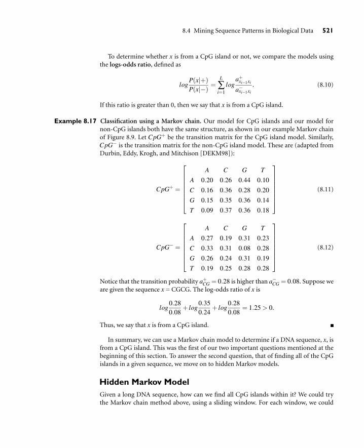
8.4 Mining Sequence Patterns in Biological Data 521
To determine whether x is from a CpG island or not, we compare the models usingthe logs-odds ratio, defined as
logP(x|+)P(x|−)
=L
∑i=1
loga+
xi−1xi
a−xi−1xi
. (8.10)
If this ratio is greater than 0, then we say that x is from a CpG island.
Example 8.17 Classification using a Markov chain. Our model for CpG islands and our model fornon-CpG islands both have the same structure, as shown in our example Markov chainof Figure 8.9. Let CpG+ be the transition matrix for the CpG island model. Similarly,CpG− is the transition matrix for the non-CpG island model. These are (adapted fromDurbin, Eddy, Krogh, and Mitchison [DEKM98]):
CpG+ =
A C G T
A 0.20 0.26 0.44 0.10
C 0.16 0.36 0.28 0.20
G 0.15 0.35 0.36 0.14
T 0.09 0.37 0.36 0.18
(8.11)
CpG− =
A C G T
A 0.27 0.19 0.31 0.23
C 0.33 0.31 0.08 0.28
G 0.26 0.24 0.31 0.19
T 0.19 0.25 0.28 0.28
(8.12)
Notice that the transition probability a+CG = 0.28 is higher than a−CG = 0.08. Suppose we
are given the sequence x = CGCG. The log-odds ratio of x is
log0.280.08
+ log0.350.24
+ log0.280.08
= 1.25> 0.
Thus, we say that x is from a CpG island.
In summary, we can use a Markov chain model to determine if a DNA sequence, x, isfrom a CpG island. This was the first of our two important questions mentioned at thebeginning of this section. To answer the second question, that of finding all of the CpGislands in a given sequence, we move on to hidden Markov models.
Hidden Markov ModelGiven a long DNA sequence, how can we find all CpG islands within it? We could trythe Markov chain method above, using a sliding window. For each window, we could

522 Chapter 8 Mining Stream, Time-Series, and Sequence Data
compute the log-odds ratio. CpG islands within intersecting windows could be mergedto determine CpG islands within the long sequence. This approach has some difficulties:It is not clear what window size to use, and CpG islands tend to vary in length.
What if, instead, we merge the two Markov chains from above (for CpG islands andnon-CpG islands, respectively) and add transition probabilities between the two chains?The result is a hidden Markov model, as shown in Figure 8.10. The states are renamedby adding “+” and “−” labels to distinguish them. For readability, only the transitionsbetween “+” and “−” states are shown, in addition to those for the begin and end states.Let π = π1π2 . . .πL be a path of states that generates a sequence of symbols, x = x1x2 . . .xL.In a Markov chain, the path through the chain for x is unique. With a hidden Markovmodel, however, different paths can generate the same sequence. For example, the statesC+ and C− both emit the symbol C. Therefore, we say the model is “hidden” in thatwe do not know for sure which states were visited in generating the sequence. The tran-sition probabilities between the original two models can be determined using trainingsequences containing transitions between CpG islands and non-CpG islands.
A Hidden Markov Model (HMM) is defined by
a set of states, Q
a set of transitions, where transition probability akl = P(πi = l|πi−1 = k) is the prob-ability of transitioning from state k to state l for k, l ∈ Q
an emission probability, ek(b) = P(xi = b|πi = k), for each state, k, and each symbol,b, where ek(b) is the probability of seeing symbol b in state k. The sum of all emissionprobabilities at a given state must equal 1, that is, ∑b ek = 1 for each state, k.
Example 8.18 A hidden Markov model. The transition matrix for the hidden Markov model ofFigure 8.10 is larger than that of Example 8.16 for our earlier Markov chain example.
G+C+
G– C–
T+A+
T– A–
O O
Figure 8.10 A hidden Markov model.

8.4 Mining Sequence Patterns in Biological Data 523
It contains the states A+, C+, G+, T+, A−, C−, G−, T− (not shown). The transitionprobabilities between the “+” states are as before. Similarly, the transition probabili-ties between the “−” states are as before. The transition probabilities between “+” and“−” states can be determined as mentioned above, using training sequences containingknown transitions from CpG islands to non-CpG islands, and vice versa. The emis-sion probabilities are eA+(A) = 1, eA+(C) = 0, eA+(G) = 0, eA+(T ) = 0, eA−(A) = 1,eA−(C) = 0, eA−(G) = 0, eA−(T ) = 0, and so on. Although here the probability of emit-ting a symbol at a state is either 0 or 1, in general, emission probabilities need not bezero-one.
Tasks using hidden Markov models include:
Evaluation: Given a sequence, x, determine the probability, P(x), of obtaining x in themodel.
Decoding: Given a sequence, determine the most probable path through the modelthat produced the sequence.
Learning: Given a model and a set of training sequences, find the model parameters(i.e., the transition and emission probabilities) that explain the training sequenceswith relatively high probability. The goal is to find a model that generalizes well tosequences we have not seen before.
Evaluation, decoding, and learning can be handled using the forward algorithm,Viterbi algorithm, and Baum-Welch algorithm, respectively. These algorithms are dis-cussed in the following sections.
Forward AlgorithmWhat is the probability, P(x), that sequence x was generated by a given hidden Markovmodel (where, say, the model represents a sequence class)? This problem can be solvedusing the forward algorithm.
Let x = x1x2 . . . xL be our sequence of symbols. A path is a sequence of states. Manypaths can generate x. Consider one such path, which we denote π = π1π2 . . .πL. If weincorporate the begin and end states, denoted as 0, we can write π as π0 = 0, π1π2 . . .πL,πL+1 = 0. The probability that the model generated sequence x using path π is
P(x, π) = a0π1 eπ1(x1) ·aπ1π2 eπ2(x2) · · · ·aπL−1πL eπL(xL) ·aπL0
(8.13)= a0π1
L
∏i=1
eπi(xi)aπiπi+1
where πL+1 = 0. We must, however, consider all of the paths that can generate x. There-fore, the probability of x given the model is
P(x) = ∑π
P(x, π). (8.14)
That is, we add the probabilities of all possible paths for x.

524 Chapter 8 Mining Stream, Time-Series, and Sequence Data
Algorithm: Forward algorithm. Find the probability, P(x), that sequence x was generated by the given hiddenMarkov model.
Input:
A hidden Markov model, defined by a set of states, Q, that emit symbols, and by transition and emissionprobabilities;
x, a sequence of symbols.
Output: Probability, P(x).
Method:
(1) Initialization (i = 0): f0(0) = 1, fk(0) = 0 for k > 0(2) Recursion (i = 1 . . .L): fl(i) = el(xi)∑k fk(i−1)akl
(3) Termination: P(x) = ∑k fk(L)ak0
Figure 8.11 Forward algorithm.
Unfortunately, the number of paths can be exponential with respect to the length,L, of x, so brute force evaluation by enumerating all paths is impractical. The forwardalgorithm exploits a dynamic programming technique to solve this problem. It definesforward variables, fk(i), to be the probability of being in state k having observed the firsti symbols of sequence x. We want to compute fπL+1=0(L), the probability of being in theend state having observed all of sequence x.
The forward algorithm is shown in Figure 8.11. It consists of three steps. In step 1,the forward variables are initialized for all states. Because we have not viewed any part ofthe sequence at this point, the probability of being in the start state is 1 (i.e., f0(0) = 1),and the probability of being in any other state is 0. In step 2, the algorithm sums over allthe probabilities of all the paths leading from one state emission to another. It does thisrecursively for each move from state to state. Step 3 gives the termination condition. Thewhole sequence (of length L) has been viewed, and we enter the end state, 0. We end upwith the summed-over probability of generating the required sequence of symbols.
Viterbi AlgorithmGiven a sequence, x, what is the most probable path in the model that generates x? Thisproblem of decoding can be solved using the Viterbi algorithm.
Many paths can generate x. We want to find the most probable one, π?, that is, thepath that maximizes the probability of having generated x. This is π? = argmaxπP(π|x).10
It so happens that this is equal to argmaxπP(x, π). (The proof is left as an exercise for thereader.) We saw how to compute P(x, π) in Equation (8.13). For a sequence of length L,there are |Q|L possible paths, where |Q| is the number of states in the model. It is
10In mathematics, argmax stands for the argument of the maximum. Here, this means that we want thepath, π, for which P(π|x) attains its maximum value.

8.4 Mining Sequence Patterns in Biological Data 525
infeasible to enumerate all of these possible paths! Once again, we resort to a dynamicprogramming technique to solve the problem.
At each step along the way, the Viterbi algorithm tries to find the most probablepath leading from one symbol of the sequence to the next. We define vl(i) to be theprobability of the most probable path accounting for the first i symbols of x andending in state l. To find π?, we need to compute maxkvk(L), the probability of themost probable path accounting for all of the sequence and ending in the end state.The probability, vl(i), is
vl(i) = el(xi) ·maxk(vl(k)akl), (8.15)
which states that the most probable path that generates x1 . . .xi and ends in state l has toemit xi in state xl (hence, the emission probability, el(xi)) and has to contain the mostprobable path that generates x1 . . .xi−1 and ends in state k, followed by a transition fromstate k to state l (hence, the transition probability, akl). Thus, we can compute vk(L) forany state, k, recursively to obtain the probability of the most probable path.
The Viterbi algorithm is shown in Figure 8.12. Step 1 performs initialization. Everypath starts at the begin state (0) with probability 1. Thus, for i = 0, we have v0(0) = 1, andthe probability of starting at any other state is 0. Step 2 applies the recurrence formula fori = 1 to L. At each iteration, we assume that we know the most likely path for x1 . . . xi−1that ends in state k, for all k ∈Q. To find the most likely path to the i-th state from there,we maximize vk(i−1)akl over all predecessors k ∈Q of l. To obtain vl(i), we multiply byel(xi) since we have to emit xi from l. This gives us the first formula in step 2. The valuesvk(i) are stored in a Q×L dynamic programming matrix. We keep pointers (ptr) in thismatrix so that we can obtain the path itself. The algorithm terminates in step 3, wherefinally, we have maxkvk(L). We enter the end state of 0 (hence, the transition probability,ak0) but do not emit a symbol. The Viterbi algorithm runs in O(|Q|2|L|) time. It is moreefficient than the forward algorithm because it investigates only the most probable pathand avoids summing over all possible paths.
Algorithm: Viterbi algorithm. Find the most probable path that emits the sequence of symbols, x.
Input:
A hidden Markov model, defined by a set of states, Q, that emit symbols, and by transition and emissionprobabilities;
x, a sequence of symbols.
Output: The most probable path, π∗.
Method:
(1) Initialization (i = 0): v0(0) = 1, vk(0) = 0 for k > 0(2) Recursion (i = 1 . . .L): vl(i) = el(xi)maxk(vk(i−1)akl)
ptri(l) = argmaxk(vk(i−1)akl)(3) Termination: P(x,π∗) = maxk(vk(L)ak0)
π∗L = argmaxk(vk(L)ak0)
Figure 8.12 Viterbi (decoding) algorithm.

526 Chapter 8 Mining Stream, Time-Series, and Sequence Data
Baum-Welch AlgorithmGiven a training set of sequences, how can we determine the parameters of a hiddenMarkov model that will best explain the sequences? In other words, we want to learn oradjust the transition and emission probabilities of the model so that it can predict thepath of future sequences of symbols. If we know the state path for each training sequence,learning the model parameters is simple. We can compute the percentage of times eachparticular transition or emission is used in the set of training sequences to determine akl ,the transition probabilities, and ek(b), the emission probabilities.
When the paths for the training sequences are unknown, there is no longer a directclosed-form equation for the estimated parameter values. An iterative procedure must beused, like the Baum-Welch algorithm. The Baum-Welch algorithm is a special case of theEM algorithm (Section 7.8.1), which is a family of algorithms for learning probabilisticmodels in problems that involve hidden states.
The Baum-Welch algorithm is shown in Figure 8.13. The problem of finding theoptimal transition and emission probabilities is intractable. Instead, the Baum-Welchalgorithm finds a locally optimal solution. In step 1, it initializes the probabilities toan arbitrary estimate. It then continuously re-estimates the probabilities (step 2) untilconvergence (i.e., when there is very little change in the probability values between iter-ations). The re-estimation first calculates the expected transmission and emission prob-abilities. The transition and emission probabilities are then updated to maximize thelikelihood of the expected values.
In summary, Markov chains and hidden Markov models are probabilistic models inwhich the probability of a state depends only on that of the previous state. They are par-ticularly useful for the analysis of biological sequence data, whose tasks include evalua-tion, decoding, and learning. We have studied the forward, Viterbi, and Baum-Welchalgorithms. The algorithms require multiplying many probabilities, resulting in very
Algorithm: Baum-Welch algorithm. Find the model parameters (transition and emission probabilities) thatbest explain the training set of sequences.
Input:
A training set of sequences.
Output:
Transition probabilities, akl ;
Emission probabilities, ek(b);
Method:
(1) initialize the transmission and emission probabilities;
(2) iterate until convergence
(2.1) calculate the expected number of times each transition or emission is used
(2.2) adjust the parameters to maximize the likelihood of these expected values
Figure 8.13 Baum-Welch (learning) algorithm.

8.5 Summary 527
small numbers that can cause underflow arithmetic errors. A way around this is to usethe logarithms of the probabilities.
8.5 Summary
Stream data flow in and out of a computer system continuously and with varyingupdate rates. They are temporally ordered, fast changing, massive (e.g., gigabytes to ter-abytes in volume), and potentially infinite. Applications involving stream data includetelecommunications, financial markets, and satellite data processing.
Synopses provide summaries of stream data, which typically can be used to returnapproximate answers to queries. Random sampling, sliding windows, histograms, mul-tiresolution methods (e.g., for data reduction), sketches (which operate in a singlepass), and randomized algorithms are all forms of synopses.
The tilted time frame model allows data to be stored at multiple granularities of time.The most recent time is registered at the finest granularity. The most distant time isat the coarsest granularity.
A stream data cube can store compressed data by (1) using the tilted time frame modelon the time dimension, (2) storing data at only some critical layers, which reflectthe levels of data that are of most interest to the analyst, and (3) performing partialmaterialization based on “popular paths” through the critical layers.
Traditional methods of frequent itemset mining, classification, and clustering tend toscan the data multiple times, making them infeasible for stream data. Stream-basedversions of such mining instead try to find approximate answers within a user-specifiederror bound. Examples include the Lossy Counting algorithm for frequent itemsetstream mining; the Hoeffding tree, VFDT, and CVFDT algorithms for stream dataclassification; and the STREAM and CluStream algorithms for stream data clustering.
A time-series database consists of sequences of values or events changing with time,typically measured at equal time intervals. Applications include stock market analysis,economic and sales forecasting, cardiogram analysis, and the observation of weatherphenomena.
Trend analysis decomposes time-series data into the following: trend (long-term)movements, cyclic movements, seasonal movements (which are systematic or calendarrelated), and irregular movements (due to random or chance events).
Subsequence matching is a form of similarity search that finds subsequences thatare similar to a given query sequence. Such methods match subsequences that havethe same shape, while accounting for gaps (missing values) and differences in base-line/offset and scale.
A sequence database consists of sequences of ordered elements or events, recordedwith or without a concrete notion of time. Examples of sequence data include cus-tomer shopping sequences, Web clickstreams, and biological sequences.

528 Chapter 8 Mining Stream, Time-Series, and Sequence Data
Sequential pattern mining is the mining of frequently occurring ordered events orsubsequences as patterns. Given a sequence database, any sequence that satisfies min-imum support is frequent and is called a sequential pattern. An example of a sequen-tial pattern is “Customers who buy a Canon digital camera are likely to buy an HPcolor printer within a month.” Algorithms for sequential pattern mining include GSP,SPADE, and PrefixSpan, as well as CloSpan (which mines closed sequential patterns).
Constraint-based mining of sequential patterns incorporates user-specifiedconstraints to reduce the search space and derive only patterns that are of interestto the user. Constraints may relate to the duration of a sequence, to an event fold-ing window (where events occurring within such a window of time can be viewed asoccurring together), and to gaps between events. Pattern templates may also be spec-ified as a form of constraint using regular expressions.
Periodicity analysis is the mining of periodic patterns, that is, the search for recurringpatterns in time-related sequence databases. Full periodic and partial periodic patternscan be mined, as well as periodic association rules.
Biological sequence analysis compares, aligns, indexes, and analyzes biologicalsequences, which can be either sequences of nucleotides or of amino acids. Biose-quenceanalysisplaysacrucial role inbioinformaticsandmodernbiology.Suchanalysiscan be partitioned into two essential tasks: pairwise sequence alignment and multi-ple sequence alignment. The dynamic programming approach is commonly used forsequence alignments. Among many available analysis packages, BLAST (Basic LocalAlignment Search Tool) is one of the most popular tools in biosequence analysis.
Markov chains and hidden Markov models are probabilistic models in which theprobability of a state depends only on that of the previous state. They are particu-larly useful for the analysis of biological sequence data. Given a sequence of symbols,x, the forward algorithm finds the probability of obtaining x in the model, whereasthe Viterbi algorithm finds the most probable path (corresponding to x) through themodel. The Baum-Welch algorithm learns or adjusts the model parameters (transitionand emission probabilities) so as to best explain a set of training sequences.
Exercises
8.1 A stream data cube should be relatively stable in size with respect to infinite data streams.Moreover, it should be incrementally updateable with respect to infinite data streams.Show that the stream cube proposed in Section 8.1.2 satisfies these two requirements.
8.2 In stream data analysis, we are often interested in only the nontrivial or exceptionallylarge cube cells. These can be formulated as iceberg conditions. Thus, it may seem thatthe iceberg cube [BR99] is a likely model for stream cube architecture. Unfortunately,this is not the case because iceberg cubes cannot accommodate the incremental updatesrequired due to the constant arrival of new data. Explain why.

Exercises 529
8.3 An important task in stream data analysis is to detect outliers in a multidimensionalenvironment. An example is the detection of unusual power surges, where the dimen-sions include time (i.e., comparing with the normal duration), region (i.e., comparingwith surrounding regions), sector (i.e., university, residence, government), and so on.Outline an efficient stream OLAP method that can detect outliers in data streams. Pro-vide reasons as to why your design can ensure such quality.
8.4 Frequent itemset mining in data streams is a challenging task. It is too costly to keep thefrequency count for every itemset. However, because a currently infrequent itemset maybecome frequent, and a currently frequent one may become infrequent in the future,it is important to keep as much frequency count information as possible. Given a fixedamount of memory, can you work out a good mechanism that may maintain high-qualityapproximation of itemset counting?
8.5 For the above approximate frequent itemset counting problem, it is interesting to incor-porate the notion of tilted time frame. That is, we can put less weight on more remoteitemsets when counting frequent itemsets. Design an efficient method that may obtainhigh-quality approximation of itemset frequency in data streams in this case.
8.6 A classification model may change dynamically along with the changes of training datastreams. This is known as concept drift. Explain why decision tree induction may notbe a suitable method for such dynamically changing data sets. Is naïve Bayesian a bettermethod on such data sets? Comparing with the naïve Bayesian approach, is lazy evalua-tion (such as the k-nearest-neighbor approach) even better? Explain your reasoning.
8.7 The concept of microclustering has been popular for on-line maintenance of cluster-ing information for data streams. By exploring the power of microclustering, design aneffective density-based clustering method for clustering evolving data streams.
8.8 Suppose that a power station stores data regarding power consumption levels by time andby region, in addition to power usage information per customer in each region. Discusshow to solve the following problems in such a time-series database:
(a) Find similar power consumption curve fragments for a given region on Fridays.
(b) Every time a power consumption curve rises sharply, what may happen within thenext 20 minutes?
(c) How can we find the most influential features that distinguish a stable power con-sumption region from an unstable one?
8.9 Regression is commonly used in trend analysis for time-series data sets. An item in atime-series database is usually associated with properties in multidimensional space.For example, an electric power consumer may be associated with consumer location,category, and time of usage (weekdays vs. weekends). In such a multidimensionalspace, it is often necessary to perform regression analysis in an OLAP manner (i.e.,drilling and rolling along any dimension combinations that a user desires). Designan efficient mechanism so that regression analysis can be performed efficiently inmultidimensional space.

530 Chapter 8 Mining Stream, Time-Series, and Sequence Data
8.10 Suppose that a restaurant chain would like to mine customers’ consumption behaviorrelating to major sport events, such as “Every time there is a major sport event on TV, thesales of Kentucky Fried Chicken will go up 20% one hour before the match.”
(a) For this problem, there are multiple sequences (each corresponding to one restau-rant in the chain). However, each sequence is long and contains multiple occurrencesof a (sequential) pattern. Thus this problem is different from the setting of sequentialpattern mining problem discussed in this chapter. Analyze what are the differencesin the two problem definitions and how such differences may influence the develop-ment of mining algorithms.
(b) Develop a method for finding such patterns efficiently.
8.11 (Implementation project) The sequential pattern mining algorithm introduced bySrikant and Agrawal [SA96] finds sequential patterns among a set of sequences. Althoughthere have been interesting follow-up studies, such as the development of the algorithmsSPADE (Zaki [Zak01]), PrefixSpan (Pei, Han, Mortazavi-Asl, et al. [PHMA+01]), andCloSpan (Yan, Han, and Afshar [YHA03]), the basic definition of “sequential pattern”has not changed. However, suppose we would like to find frequently occurring subse-quences (i.e., sequential patterns) within one given sequence, where, say, gaps are notallowed. (That is, we do not consider AG to be a subsequence of the sequence ATG.)For example, the string ATGCTCGAGCT contains a substring GCT with a support of2. Derive an efficient algorithm that finds the complete set of subsequences satisfying aminimum support threshold. Explain how your algorithm works using a small example,and show some performance results for your implementation.
8.12 Suppose frequent subsequences have been mined from a sequence database, with a given(relative) minimum support, min sup. The database can be updated in two cases:(i) adding new sequences (e.g., new customers buying items), and (ii) appending newsubsequences to some existing sequences (e.g., existing customers buying new items). Foreach case, work out an efficient incremental mining method that derives the complete sub-sequences satisfying min sup, without mining the whole sequence database from scratch.
8.13 Closed sequential patterns can be viewed as a lossless compression of a large set of sequen-tial patterns. However, the set of closed sequential patterns may still be too large for effec-tive analysis. There should be some mechanism for lossy compression that may furtherreduce the set of sequential patterns derived from a sequence database.
(a) Provide a good definition of lossy compression of sequential patterns, and reasonwhy such a definition may lead to effective compression with minimal informationloss (i.e., high compression quality).
(b) Develop an efficient method for such pattern compression.
(c) Develop an efficient method that mines such compressed patterns directly from asequence database.
8.14 As discussed in Section 8.3.4, mining partial periodic patterns will require a user to spec-ify the length of the period. This may burden the user and reduces the effectiveness of

Bibliographic Notes 531
mining. Propose a method that will automatically mine the minimal period of a patternwithout requiring a predefined period. Moreover, extend the method to find approximateperiodicity where the period will not need to be precise (i.e., it can fluctuate within aspecified small range).
8.15 There are several major differences between biological sequential patterns and transac-tional sequential patterns. First, in transactional sequential patterns, the gaps betweentwo events are usually nonessential. For example, the pattern “purchasing a digital cameratwo months after purchasing a PC” does not imply that the two purchases are consecutive.However, for biological sequences, gaps play an important role in patterns. Second, pat-terns in a transactional sequence are usually precise. However, a biological pattern can bequite imprecise, allowing insertions, deletions, and mutations. Discuss how the miningmethodologies in these two domains are influenced by such differences.
8.16 BLAST is a typical heuristic alignment method for pairwise sequence alignment. It firstlocates high-scoring short stretches and then extends them to achieve suboptimal align-ments. When the sequences to be aligned are really long, BLAST may run quite slowly.Propose and discuss some enhancements to improve the scalability of such a method.
8.17 The Viterbi algorithm uses the equality, argmaxπP(π|x) = argmaxπP(x, π), in its searchfor the most probable path, π∗, through a hidden Markov model for a given sequence ofsymbols, x. Prove the equality.
8.18 (Implementation project) A dishonest casino uses a fair die most of the time. However, itswitches to a loaded die with a probability of 0.05, and switches back to the fair die witha probability 0.10. The fair die has a probability of 1
6 of rolling any number. The loadeddie has P(1) = P(2) = P(3) = P(4) = P(5) = 0.10 and P(6) = 0.50.
(a) Draw a hidden Markov model for the dishonest casino problem using two states,Fair (F) and Loaded (L). Show all transition and emission probabilities.
(b) Suppose you pick up a die at random and roll a 6. What is the probability that thedie is loaded, that is, find P(6|DL)? What is the probability that it is fair, that is, findP(6|DF)? What is the probability of rolling a 6 from the die you picked up? If youroll a sequence of 666, what is the probability that the die is loaded?
(c) Write a program that, given a sequence of rolls (e.g., x = 5114362366 . . .), predictswhen the fair die was used and when the loaded die was used. (Hint: This is similarto detecting CpG islands and non-CPG islands in a given long sequence.) Use theViterbi algorithm to get the most probable path through the model. Describe yourimplementation in report form, showing your code and some examples.
Bibliographic Notes
Stream data mining research has been active in recent years. Popular surveys on streamdata systems and stream data processing include Babu and Widom [BW01], Babcock,Babu, Datar, et al. [BBD+02], Muthukrishnan [Mut03], and the tutorial by Garofalakis,Gehrke, and Rastogi [GGR02].

532 Chapter 8 Mining Stream, Time-Series, and Sequence Data
There have been extensive studies on stream data management and the processingof continuous queries in stream data. For a description of synopsis data structures forstream data, see Gibbons and Matias [GM98]. Vitter introduced the notion of reservoirsampling as a way to select an unbiased random sample of n elements without replace-ment from a larger ordered set of size N, where N is unknown [Vit85]. Stream queryor aggregate processing methods have been proposed by Chandrasekaran and Franklin[CF02], Gehrke, Korn, and Srivastava [GKS01], Dobra, Garofalakis, Gehrke, and Ras-togi [DGGR02], and Madden, Shah, Hellerstein, and Raman [MSHR02]. A one-passsummary method for processing approximate aggregate queries using wavelets was pro-posed by Gilbert, Kotidis, Muthukrishnan, and Strauss [GKMS01]. Statstream, a statisti-cal method for the monitoring of thousands of data streams in real time, was developedby Zhu and Shasha [ZS02, SZ04].
There are also many stream data projects. Examples include Aurora by Zdonik,Cetintemel, Cherniack, et al. [ZCC+02], which is targeted toward stream monitoringapplications; STREAM, developed at Stanford University by Babcock, Babu, Datar,et al., aims at developing a general-purpose Data Stream Management System (DSMS)[BBD+02]; and an early system called Tapestry by Terry, Goldberg, Nichols, and Oki[TGNO92], which used continuous queries for content-based filtering over an append-only database of email and bulletin board messages. A restricted subset of SQL wasused as the query language in order to provide guarantees about efficient evaluationand append-only query results.
A multidimensional stream cube model was proposed by Chen, Dong, Han, et al.[CDH+02] in their study of multidimensional regression analysis of time-series datastreams. MAIDS (Mining Alarming Incidents from Data Streams), a stream data miningsystem built on top of such a stream data cube, was developed by Cai, Clutter, Pape, et al.[CCP+04].
For mining frequent items and itemsets on stream data, Manku and Motwani pro-posed sticky sampling and lossy counting algorithms for approximate frequency countsover data streams [MM02]. Karp, Papadimitriou, and Shenker proposed a counting algo-rithm for finding frequent elements in data streams [KPS03]. Giannella, Han, Pei, et al.proposed a method for mining frequent patterns in data streams at multiple time gran-ularities [GHP+04]. Metwally, Agrawal, and El Abbadi proposed a memory-efficientmethod for computing frequent and top-k elements in data streams [MAA05].
For stream data classification, Domingos and Hulten proposed the VFDT algorithm,based on their Hoeffding tree algorithm [DH00]. CVFDT, a later version of VFDT, wasdeveloped by Hulten, Spencer, and Domingos [HSD01] to handle concept drift in time-changing data streams. Wang, Fan, Yu, and Han proposed an ensemble classifier to mineconcept-drifting data streams [WFYH03]. Aggarwal, Han, Wang, and Yu developed ak-nearest-neighbor-based method for classify evolving data streams [AHWY04b].
Several methods have been proposed for clustering data streams. The k-median-based STREAM algorithm was proposed by Guha, Mishra, Motwani, and O’Callaghan[GMMO00] and by O’Callaghan, Mishra, Meyerson, et al. [OMM+02]. Aggarwal, Han,Wang, and Yu proposed CluStream, a framework for clustering evolving data streams

Bibliographic Notes 533
[AHWY03], and HPStream, a framework for projected clustering of high-dimensionaldata streams [AHWY04a].
Statistical methods for time-series analysis have been proposed and studied extensivelyin statistics, such as in Chatfield [Cha03], Brockwell and Davis [BD02], and Shumway andStoffer [SS05]. StatSoft’s Electronic Textbook (www.statsoft.com/textbook/ stathome.html)is a useful online resource that includes a discussion on time-series data analysis. TheARIMA forecasting method is described in Box, Jenkins, and Reinsel [BJR94]. Efficientsimilarity search in sequence databases was studied by Agrawal, Faloutsos, and Swami[AFS93]. A fast subsequence matching method in time-series databases was presented byFaloutsos, Ranganathan, and Manolopoulos [FRM94]. Agrawal, Lin, Sawhney, and Shim[ALSS95] developed a method for fast similarity search in the presence of noise, scaling,and translation in time-series databases. Language primitives for querying shapes of his-tories were proposed by Agrawal, Psaila, Wimmers, and Zait [APWZ95]. Other work onsimilarity-based search of time-series data includes Rafiei and Mendelzon [RM97], andYi, Jagadish, and Faloutsos [YJF98]. Yi, Sidiropoulos, Johnson, Jagadish, et al. [YSJ+00]introduced a method for on-line mining for co-evolving time sequences. Chen, Dong,Han, et al. [CDH+02] proposed a multidimensional regression method for analysis ofmultidimensional time-series data. Shasha and Zhu present a state-of-the-art overview ofthe methods for high-performance discovery in time series [SZ04].
The problem of mining sequential patterns was first proposed by Agrawal and Srikant[AS95]. In the Apriori-based GSP algorithm, Srikant and Agrawal [SA96] generalizedtheir earlier notion to include time constraints, a sliding time window, and user-definedtaxonomies. Zaki [Zak01] developed a vertical-format-based sequential pattern miningmethod called SPADE, which is an extension of vertical-format-based frequent itemsetmining methods, like Eclat and Charm [Zak98, ZH02]. PrefixSpan, a pattern growthapproach to sequential pattern mining, and its predecessor, FreeSpan, were developedby Pei, Han, Mortazavi-Asl, et al. [HPMA+00, PHMA+01, PHMA+04]. The CloSpanalgorithm for mining closed sequential patterns was proposed by Yan, Han, and Afshar[YHA03]. BIDE, a bidirectional search for mining frequent closed sequences, was devel-oped by Wang and Han [WH04].
The studies of sequential pattern mining have been extended in several differentways. Mannila, Toivonen, and Verkamo [MTV97] consider frequent episodes in se-quences, where episodes are essentially acyclic graphs of events whose edges specifythe temporal before-and-after relationship but without timing-interval restrictions.Sequence pattern mining for plan failures was proposed in Zaki, Lesh, and Ogihara[ZLO98]. Garofalakis, Rastogi, and Shim [GRS99a] proposed the use of regular expres-sions as a flexible constraint specification tool that enables user-controlled focus to beincorporated into the sequential pattern mining process. The embedding of multidi-mensional, multilevel information into a transformed sequence database for sequen-tial pattern mining was proposed by Pinto, Han, Pei, et al. [PHP+01]. Pei, Han, andWang studied issues regarding constraint-based sequential pattern mining [PHW02].CLUSEQ is a sequence clustering algorithm, developed by Yang and Wang [YW03].An incremental sequential pattern mining algorithm, IncSpan, was proposed byCheng, Yan, and Han [CYH04]. SeqIndex, efficient sequence indexing by frequent and

534 Chapter 8 Mining Stream, Time-Series, and Sequence Data
discriminative analysis of sequential patterns, was studied by Cheng, Yan, and Han[CYH05]. A method for parallel mining of closed sequential patterns was proposedby Cong, Han, and Padua [CHP05].
Data mining for periodicity analysis has been an interesting theme in data mining.Özden, Ramaswamy, and Silberschatz [ORS98] studied methods for mining periodic
or cyclic association rules. Lu, Han, and Feng [LHF98] proposed intertransaction asso-ciation rules, which are implication rules whose two sides are totally ordered episodeswith timing-interval restrictions (on the events in the episodes and on the two sides).Bettini, Wang, and Jajodia [BWJ98] consider a generalization of intertransaction associ-ation rules. The notion of mining partial periodicity was first proposed by Han, Dong,and Yin, together with a max-subpattern hit set method [HDY99]. Ma and Hellerstein[MH01a] proposed a method for mining partially periodic event patterns with unknownperiods. Yang, Wang, and Yu studied mining asynchronous periodic patterns in time-series data [YWY03].
Methods for the analysis of biological sequences have been introduced in many text-books, such as Waterman [Wat95], Setubal and Meidanis [SM97], Durbin, Eddy, Krogh,and Mitchison [DEKM98], Baldi and Brunak [BB01], Krane and Raymer [KR03], Jonesand Pevzner [JP04], and Baxevanis and Ouellette [BO04]. BLAST was developed byAltschul, Gish, Miller, et al. [AGM+90]. Information about BLAST can be foundat the NCBI Web site www.ncbi.nlm.nih.gov/BLAST/. For a systematic introduction ofthe BLAST algorithms and usages, see the book “BLAST” by Korf, Yandell, andBedell [KYB03].
For an introduction to Markov chains and hidden Markov models from a biologicalsequence perspective, see Durbin, Eddy, Krogh, and Mitchison [DEKM98] and Jones andPevzner [JP04]. A general introduction can be found in Rabiner [Rab89]. Eddy and Kroghhave each respectively headed the development of software packages for hidden Markovmodels forproteinsequenceanalysis,namelyHMMER(pronounced“hammer,”availableat http://hmmer.wustl.edu/) and SAM (www.cse.ucsc.edu/research/ compbio/sam.html).

9Graph Mining, Social NetworkAnalysis, and Multirelational
Data Mining
We have studied frequent-itemset mining in Chapter 5 and sequential-pattern mining in Section3 of Chapter 8. Many scientific and commercial applications need patterns that are morecomplicated than frequent itemsets and sequential patterns and require extra effort todiscover. Such sophisticated patterns go beyond sets and sequences, toward trees, lattices,graphs, networks, and other complex structures.
As a general data structure, graphs have become increasingly important in modelingsophisticated structures and their interactions, with broad applications including chemi-cal informatics, bioinformatics, computer vision, video indexing, text retrieval, and Webanalysis. Mining frequent subgraph patterns for further characterization, discrimination,classification, and cluster analysis becomes an important task. Moreover, graphs that linkmany nodes together may form different kinds of networks, such as telecommunicationnetworks, computer networks, biological networks, and Web and social community net-works. Because such networks have been studied extensively in the context of social net-works, their analysis has often been referred to as social network analysis. Furthermore,in a relational database, objects are semantically linked across multiple relations. Miningin a relational database often requires mining across multiple interconnected relations,which is similar to mining in connected graphs or networks. Such kind of mining acrossdata relations is considered multirelational data mining.
In this chapter, we study knowledge discovery in such interconnected and complexstructured data. Section 9.1 introduces graph mining, where the core of the problem ismining frequent subgraph patterns over a collection of graphs. Section 9.2 presents con-cepts and methods for social network analysis. Section 9.3 examines methods for mul-tirelational data mining, including both cross-relational classification and user-guidedmultirelational cluster analysis.
9.1 Graph Mining
Graphs become increasingly important in modeling complicated structures, such ascircuits, images, chemical compounds, protein structures, biological networks, social
535

536 Chapter 9 Graph Mining, Social Network Analysis, and Multirelational Data Mining
networks, the Web, workflows, and XML documents. Many graph search algorithmshave been developed in chemical informatics, computer vision, video indexing, and textretrieval. With the increasing demand on the analysis of large amounts of structureddata, graph mining has become an active and important theme in data mining.
Among the various kinds of graph patterns, frequent substructures are the very basicpatterns that can be discovered in a collection of graphs. They are useful for charac-terizing graph sets, discriminating different groups of graphs, classifying and cluster-ing graphs, building graph indices, and facilitating similarity search in graph databases.Recent studies have developed several graph mining methods and applied them to thediscovery of interesting patterns in various applications. For example, there have beenreports on the discovery of active chemical structures in HIV-screening datasets by con-trasting the support of frequent graphs between different classes. There have been stud-ies on the use of frequent structures as features to classify chemical compounds, on thefrequent graph mining technique to study protein structural families, on the detectionof considerably large frequent subpathways in metabolic networks, and on the use offrequent graph patterns for graph indexing and similarity search in graph databases.Although graph mining may include mining frequent subgraph patterns, graph classifi-cation, clustering, and other analysis tasks, in this section we focus on mining frequentsubgraphs. We look at various methods, their extensions, and applications.
9.1.1 Methods for Mining Frequent Subgraphs
Before presenting graph mining methods, it is necessary to first introduce some prelim-inary concepts relating to frequent graph mining.
We denote the vertex set of a graph g by V (g) and the edge set by E(g). A label func-tion, L, maps a vertex or an edge to a label. A graph g is a subgraph of another graphg′ if there exists a subgraph isomorphism from g to g′. Given a labeled graph data set,D = {G1,G2, . . . ,Gn}, we define support(g) (or f requency(g)) as the percentage (ornumber) of graphs in D where g is a subgraph. A frequent graph is a graph whose sup-port is no less than a minimum support threshold, min sup.
Example 9.1 Frequent subgraph. Figure 9.1 shows a sample set of chemical structures. Figure 9.2depicts two of the frequent subgraphs in this data set, given a minimum support of66.6%.
“How can we discover frequent substructures?” The discovery of frequent substructuresusually consists of two steps. In the first step, we generate frequent substructure candi-dates. The frequency of each candidate is checked in the second step. Most studies onfrequent substructure discovery focus on the optimization of the first step, because thesecond step involves a subgraph isomorphism test whose computational complexity isexcessively high (i.e., NP-complete).
In this section, we look at various methods for frequent substructure mining. In gen-eral, there are two basic approaches to this problem: an Apriori-based approach and apattern-growth approach.

9.1 Graph Mining 537
S C C N
O
C C C
O
N
S
C S C
N O
C
(g3)(g2)(g1)
Figure 9.1 A sample graph data set.
C C O C C N
N
S
frequency: 2 frequency: 3
Figure 9.2 Frequent graphs.
Apriori-based ApproachApriori-based frequent substructure mining algorithms share similar characteristics withApriori-based frequent itemset mining algorithms (Chapter 5). The search for frequentgraphs starts with graphs of small “size,” and proceeds in a bottom-up manner by gen-erating candidates having an extra vertex, edge, or path. The definition of graph sizedepends on the algorithm used.
The general framework of Apriori-based methods for frequent substructure mining isoutlined in Figure 9.3. We refer to this algorithm as AprioriGraph. Sk is the frequent sub-structure set of size k. We will clarify the definition of graph size when we describe specificApriori-based methods further below. AprioriGraph adopts a level-wise mining method-ology. At each iteration, the size of newly discovered frequent substructures is increasedby one. These new substructures are first generated by joining two similar but slightlydifferent frequent subgraphs that were discovered in the previous call to AprioriGraph.This candidate generation procedure is outlined on line 4. The frequency of the newlyformed graphs is then checked. Those found to be frequent are used to generate largercandidates in the next round.
The main design complexity of Apriori-based substructure mining algorithms isthe candidate generation step. The candidate generation in frequent itemset mining isstraightforward. For example, suppose we have two frequent itemsets of size-3: (abc) and(bcd). The frequent itemset candidate of size-4 generated from them is simply (abcd),derived from a join. However, the candidate generation problem in frequent substruc-ture mining is harder than that in frequent itemset mining, because there are many waysto join two substructures.

538 Chapter 9 Graph Mining, Social Network Analysis, and Multirelational Data Mining
Algorithm: AprioriGraph. Apriori-based frequent substructure mining.
Input:
D, a graph data set;
min sup, the minimum support threshold.
Output:
Sk, the frequent substructure set.
Method:S1← frequent single-elements in the data set;Call AprioriGraph(D, min sup, S1);
procedure AprioriGraph(D, min sup, Sk)
(1) Sk+1←?;
(2) for each frequent gi ∈ Sk do
(3) for each frequent g j ∈ Sk do
(4) for each size (k + 1) graph g formed by the merge of gi and g j do
(5) if g is frequent in D and g 6∈ Sk+1 then
(6) insert g into Sk+1;
(7) if sk+1 6=? then
(8) AprioriGraph(D, min sup, Sk+1);
(9) return;
Figure 9.3 AprioriGraph.
Recent Apriori-based algorithms for frequent substructure mining include AGM,FSG, and a path-join method. AGM shares similar characteristics with Apriori-baseditemset mining. FSG and the path-join method explore edges and connections in anApriori-based fashion. Each of these methods explores various candidate generationstrategies.
The AGM algorithm uses a vertex-based candidate generation method that increasesthe substructure size by one vertex at each iteration of AprioriGraph. Two size-k fre-quent graphs are joined only if they have the same size-(k−1) subgraph. Here, graphsize is the number of vertices in the graph. The newly formed candidate includes thesize-(k−1) subgraph in common and the additional two vertices from the two size-kpatterns. Because it is undetermined whether there is an edge connecting the addi-tional two vertices, we actually can form two substructures. Figure 9.4 depicts the twosubstructures joined by two chains (where a chain is a sequence of connected edges).
The FSG algorithm adopts an edge-based candidate generation strategy that increasesthe substructure size by one edge in each call of AprioriGraph. Two size-k patterns are

9.1 Graph Mining 539
+
Figure 9.4 AGM: Two substructures joined by two chains.
+
Figure 9.5 FSG: Two substructure patterns and their potential candidates.
merged if and only if they share the same subgraph having k− 1 edges, which is calledthe core. Here, graph size is taken to be the number of edges in the graph. The newlyformed candidate includes the core and the additional two edges from the size-k patterns.Figure 9.5 shows potential candidates formed by two structure patterns. Each candidatehas one more edge than these two patterns. This example illustrates the complexity ofjoining two structures to form a large pattern candidate.
In the third Apriori-based approach, an edge-disjoint path method was proposed,where graphs are classified by the number of disjoint paths they have, and two pathsare edge-disjoint if they do not share any common edge. A substructure pattern withk + 1 disjoint paths is generated by joining substructures with k disjoint paths.
Apriori-based algorithms have considerable overhead when joining two size-k fre-quent substructures to generate size-(k + 1) graph candidates. In order to avoid suchoverhead, non-Apriori-based algorithms have recently been developed, most of whichadopt the pattern-growth methodology. This methodology tries to extend patternsdirectly from a single pattern. In the following, we introduce the pattern-growthapproach for frequent subgraph mining.
Pattern-Growth ApproachThe Apriori-based approach has to use the breadth-first search (BFS) strategy because ofits level-wise candidate generation. In order to determine whether a size-(k + 1) graphis frequent, it must check all of its corresponding size-k subgraphs to obtain an upperbound of its frequency. Thus, before mining any size-(k + 1) subgraph, the Apriori-like

540 Chapter 9 Graph Mining, Social Network Analysis, and Multirelational Data Mining
Algorithm: PatternGrowthGraph. Simplistic pattern growth-based frequent substructuremining.
Input:
g, a frequent graph;
D, a graph data set;
min sup, minimum support threshold.
Output:
The frequent graph set, S.
Method:
S←?;Call PatternGrowthGraph(g, D, min sup, S);
procedure PatternGrowthGraph(g, D, min sup, S)
(1) if g ∈ S then return;
(2) else insert g into S;
(3) scan D once, find all the edges e such that g can be extended to g�x e;
(4) for each frequent g�x e do
(5) PatternGrowthGraph(g�x e, D, min sup, S);
(6) return;
Figure 9.6 PatternGrowthGraph.
approach usually has to complete the mining of size-k subgraphs. Therefore, BFS isnecessary in the Apriori-like approach. In contrast, the pattern-growth approach is moreflexible regarding its search method. It can use breadth-first search as well as depth-firstsearch (DFS), the latter of which consumes less memory.
A graph g can be extended by adding a new edge e. The newly formed graph is denotedby g�x e. Edge e may or may not introduce a new vertex to g. If e introduces a new vertex,we denote the new graph by g �x f e, otherwise, g �xb e, where f or b indicates that theextension is in a forward or backward direction.
Figure 9.6 illustrates a general framework for pattern growth–based frequent sub-structure mining. We refer to the algorithm as PatternGrowthGraph. For each discov-ered graph g, it performs extensions recursively until all the frequent graphs with gembedded are discovered. The recursion stops once no frequent graph can be generated.
PatternGrowthGraph is simple, but not efficient. The bottleneck is at the ineffi-ciency of extending a graph. The same graph can be discovered many times. Forexample, there may exist n different (n− 1)-edge graphs that can be extended tothe same n-edge graph. The repeated discovery of the same graph is computation-ally inefficient. We call a graph that is discovered a second time a duplicate graph.Although line 1 of PatternGrowthGraph gets rid of duplicate graphs, the generationand detection of duplicate graphs may increase the workload. In order to reduce the

9.1 Graph Mining 541
a a a
a
(a) (b)
b
b
X
Z Y
X
v0
v1
v2 v3
a b
b
X
Z Y
X
(c)
v0
v1
v2 v3
b a
b
X
Y Z
X
(d)
b
v0
v1
v2 v3
a
b
a
Y
X Z
X
Figure 9.7 DFS subscripting.
generation of duplicate graphs, each frequent graph should be extended as conser-vatively as possible. This principle leads to the design of several new algorithms. Atypical such example is the gSpan algorithm, as described below.
The gSpan algorithm is designed to reduce the generation of duplicate graphs. It neednot search previously discovered frequent graphs for duplicate detection. It does notextend any duplicate graph, yet still guarantees the discovery of the complete set of fre-quent graphs.
Let’s see how the gSpan algorithm works. To traverse graphs, it adopts a depth-firstsearch. Initially, a starting vertex is randomly chosen and the vertices in a graph aremarked so that we can tell which vertices have been visited. The visited vertex set isexpanded repeatedly until a full depth-first search (DFS) tree is built. One graph mayhave various DFS trees depending on how the depth-first search is performed (i.e., thevertex visiting order). The darkened edges in Figure 9.7(b) to 9.7(d) show three DFStrees for the same graph of Figure 9.7(a). The vertex labels are x, y, and z; the edge labelsare a and b. Alphabetic order is taken as the default order in the labels. When buildinga DFS tree, the visiting sequence of vertices forms a linear order. We use subscripts torecord this order, where i< j means vi is visited before v j when the depth-first search isperformed. A graph G subscripted with a DFS tree T is written as GT . T is called a DFSsubscripting of G.
Given a DFS tree T , we call the starting vertex in T , v0, the root. The last visited vertex,vn, is called the right-most vertex. The straight path from v0 to vn is called the right-mostpath. In Figure 9.7(b) to 9.7(d), three different subscriptings are generated based on thecorresponding DFS trees. The right-most path is (v0,v1,v3) in Figure 9.7(b) and 9.7(c),and (v0,v1,v2,v3) in Figure 9.7(d).
PatternGrowth extends a frequent graph in every possible position, which may gener-ate a large number of duplicate graphs. The gSpan algorithm introduces a more sophis-ticated extension method. The new method restricts the extension as follows: Given agraph G and a DFS tree T in G, a new edge e can be added between the right-most vertexand another vertex on the right-most path (backward extension); or it can introduce anew vertex and connect to a vertex on the right-most path (forward extension). Becauseboth kinds of extensions take place on the right-most path, we call them right-most exten-sion, denoted by G�r e (for brevity, T is omitted here).

542 Chapter 9 Graph Mining, Social Network Analysis, and Multirelational Data Mining
Example 9.2 Backward extension and forward extension. If we want to extend the graph inFigure 9.7(b), the backward extension candidates can be (v3,v0). The forward exten-sion candidates can be edges extending from v3, v1, or v0 with a new vertex introduced.
Figure 9.8(b) to 9.8(g) shows all the potential right-most extensions of Figure 9.8(a).The darkened vertices show the right-most path. Among these, Figure 9.8(b) to 9.8(d)grows from the right-most vertex while Figure 9.8(e) to 9.8(g) grows from other verticeson the right-most path. Figure 9.8(b.0) to 9.8(b.4) are children of Figure 9.8(b), andFigure 9.8(f.0) to 9.8(f.3) are children of Figure 9.8(f). In summary, backward extensiononly takes place on the right-most vertex, while forward extension introduces a new edgefrom vertices on the right-most path.
Because many DFS trees/subscriptings may exist for the same graph, we choose oneof them as the base subscripting and only conduct right-most extension on that DFStree/subscripting. Otherwise, right-most extension cannot reduce the generation of dupli-cate graphs because we would have to extend the same graph for every DFS subscripting.
We transform each subscripted graph to an edge sequence, called a DFS code, so thatwe can build an order among these sequences. The goal is to select the subscripting thatgenerates the minimum sequence as its base subscripting. There are two kinds of ordersin this transformation process: (1) edge order, which maps edges in a subscripted graphinto a sequence; and (2) sequence order, which builds an order among edge sequences(i.e., graphs).
(a) (b) (c) (d) (e) (f) (g)
(b.0) (b.1) (b.2) (b.3) (b.4) (f.0) (f.1) (f.2) (f.3)
Figure 9.8 Right-most extension.

9.1 Graph Mining 543
First, we introduce edge order. Intuitively, DFS tree defines the discovery order offorward edges. For the graph shown in Figure 9.7(b), the forward edges are visited in theorder of (0,1),(1,2),(1,3). Now we put backward edges into the order as follows. Givena vertex v, all of its backward edges should appear just before its forward edges. If v doesnot have any forward edge, we put its backward edges after the forward edge, where v isthe second vertex. For vertex v2 in Figure 9.7(b), its backward edge (2,0) should appearafter (1,2) because v2 does not have any forward edge. Among the backward edges fromthe same vertex, we can enforce an order. Assume that a vertex vi has two backwardedges, (i, j1) and (i, j2). If j1 < j2, then edge (i, j1) will appear before edge (i, j2). Sofar, we have completed the ordering of the edges in a graph. Based on this order, a graphcan be transformed into an edge sequence. A complete sequence for Figure 9.7(b) is(0,1),(1,2),(2,0),(1,3).
Based on this ordering, three different DFS codes, γ0, γ1, and γ2, generated by DFSsubscriptings in Figure 9.7(b), 9.7(c), and 9.7(d), respectively, are shown in Table 9.1.An edge is represented by a 5-tuple, (i, j, li, l(i, j), l j); li and l j are the labels of vi and v j,respectively, and l(i, j) is the label of the edge connecting them.
Through DFS coding, a one-to-one mapping is built between a subscripted graph anda DFS code (a one-to-many mapping between a graph and DFS codes). When the contextis clear, we treat a subscripted graph and its DFS code as the same. All the notations onsubscripted graphs can also be applied to DFS codes. The graph represented by a DFScode α is written Gα.
Second, we define an order among edge sequences. Since one graph may have severalDFS codes, we want to build an order among these codes and select one code to representthe graph. Because we are dealing with labeled graphs, the label information should beconsidered as one of the ordering factors. The labels of vertices and edges are used tobreak the tie when two edges have the exact same subscript, but different labels. Let theedge order relation ≺T take the first priority, the vertex label li take the second priority,the edge label l(i, j) take the third, and the vertex label l j take the fourth to determinethe order of two edges. For example, the first edge of the three DFS codes in Table 9.1 is(0,1,X ,a,X), (0,1,X ,a,X), and (0,1,Y,b,X), respectively. All of them share the samesubscript (0,1). So relation ≺T cannot tell the difference among them. But using labelinformation, following the order of first vertex label, edge label, and second vertex label,we have (0,1,X ,a,X) < (0,1,Y,b,X). The ordering based on the above rules is called
Table 9.1 DFS code for Figure 9.7(b), 9.7(c), and 9.7(d).
edge γ0 γ1 γ2
e0 (0,1,X ,a,X) (0,1,X ,a,X) (0,1,Y,b,X)
e1 (1,2,X ,a,Z) (1,2,X ,b,Y ) (1,2,X ,a,X)
e2 (2,0,Z,b,X) (1,3,X ,a,Z) (2,3,X ,b,Z)
e3 (1,3,X ,b,Y ) (3,0,Z,b,X) (3,1,Z,a,X)

544 Chapter 9 Graph Mining, Social Network Analysis, and Multirelational Data Mining
Figure 9.9 Lexicographic search tree.
DFS Lexicographic Order. According to this ordering, we have γ0 < γ1 < γ2 for the DFScodes listed in Table 9.1.
Based on the DFS lexicographic ordering, the minimum DFS code of a given graph G,written as dfs(G), is the minimal one among all the DFS codes. For example, code γ0 inTable 9.1 is the minimum DFS code of the graph in Figure 9.7(a). The subscripting thatgenerates the minimum DFS code is called the base subscripting.
We have the following important relationship between the minimum DFS code andthe isomorphism of the two graphs: Given two graphs G and G
′, G is isomorphic to G
′
if and only if dfs(G) = dfs(G′). Based on this property, what we need to do for mining
frequent subgraphs is to perform only the right-most extensions on the minimum DFScodes, since such an extension will guarantee the completeness of mining results.
Figure 9.9 shows how to arrange all DFS codes in a search tree through right-mostextensions. The root is an empty code. Each node is a DFS code encoding a graph. Eachedge represents a right-most extension from a (k−1)-length DFS code to a k-length DSFcode. The tree itself is ordered: left siblings are smaller than right siblings in the senseof DFS lexicographic order. Because any graph has at least one DFS code, the searchtree can enumerate all possible subgraphs in a graph data set. However, one graph mayhave several DFS codes, minimum and nonminimum. The search of nonminimum DFScodes does not produce useful results. “Is it necessary to perform right-most extension onnonminimum DFS codes?” The answer is “no.” If codes s and s′ in Figure 9.9 encode thesame graph, the search space under s′ can be safely pruned.
The details of gSpan are depicted in Figure 9.10. gSpan is called recursively to extendgraph patterns so that their frequent descendants are found until their support is lowerthan min sup or its code is not minimum any more. The difference between gSpan andPatternGrowth is at the right-most extension and extension termination of nonmini-mum DFS codes (lines 1-2). We replace the existence judgement in lines 1-2 of Pattern-Growth with the inequation s 6= d f s(s). Actually, s 6= d f s(s) is more efficient to calculate.Line 5 requires exhaustive enumeration of s in D in order to count the frequency of allthe possible right-most extensions of s.
The algorithm of Figure 9.10 implements a depth-first search version of gSpan.Actually, breadth-first search works too: for each newly discovered frequent subgraph

9.1 Graph Mining 545
Algorithm: gSpan. Pattern growth-based frequent substructure mining that reduces duplicategraph generation.
Input:
s, a DFS code;
D, a graph data set;
min sup, the minimum support threshold.
Output:
The frequent graph set, S.
Method:S←?;Call gSpan(s, D, min sup, S);
procedure PatternGrowthGraph(s, D, min sup, S)
(1) if s 6= d f s(s), then
(2) return;
(3) insert s into S;
(4) set C to?;
(5) scan D once, find all the edges e such that s can be right-most extended to s�r e;insert s�r e into C and count its frequency;
(6) sort C in DFS lexicographic order;
(7) for each frequent s�r e in C do
(8) gSpan(s�r e, D, min sup, S);
(9) return;
Figure 9.10 gSpan: A pattern-growth algorithm for frequent substructure mining.
in line 8, instead of directly calling gSpan, we insert it into a global first-in-first-outqueue Q, which records all subgraphs that have not been extended. We then “gSpan”each subgraph in Q one by one. The performance of a breadth-first search versionof gSpan is very close to that of the depth-first search, although the latter usuallyconsumes less memory.
9.1.2 Mining Variant and Constrained Substructure Patterns
The frequent subgraph mining discussed in the previous section handles only one spe-cial kind of graphs: labeled, undirected, connected simple graphs without any specific con-straints. That is, we assume that the database to be mined contains a set of graphs, each

546 Chapter 9 Graph Mining, Social Network Analysis, and Multirelational Data Mining
consisting of a set of labeled vertices and labeled but undirected edges, with no otherconstraints. However, many applications or users may need to enforce various kinds ofconstraints on the patterns to be mined or seek variant substructure patterns. For exam-ple, we may like to mine patterns, each of which contains certain specific vertices/edges,or where the total number of vertices/edges is within a specified range. Or what if we seekpatterns where the average density of the graph patterns is above a threshold? Althoughit is possible to develop customized algorithms for each such case, there are too manyvariant cases to consider. Instead, a general framework is needed—one that can classifyconstraints on the graph patterns. Efficient constraint-based methods can then be devel-oped for mining substructure patterns and their variants. In this section, we study severalvariants and constrained substructure patterns and look at how they can be mined.
Mining Closed Frequent SubstructuresThe first important variation of a frequent substructure is the closed frequent substruc-ture. Take mining frequent subgraphs as an example. As with frequent itemset miningand sequential pattern mining, mining graph patterns may generate an explosive numberof patterns. This is particularly true for dense data sets, because all of the subgraphs of afrequent graph are also frequent. This is an inherent problem, because according to theApriori property, all the subgraphs of a frequent substructure must be frequent. A largegraph pattern may generate an exponential number of frequent subgraphs. For exam-ple, among 423 confirmed active chemical compounds in an AIDS antiviral screen dataset, there are nearly 1 million frequent graph patterns whose support is at least 5%. Thisrenders the further analysis on frequent graphs nearly impossible.
One way to alleviate this problem is to mine only frequent closed graphs, where afrequent graph G is closed if and only if there is no proper supergraph G′ that has thesame support as G. Alternatively, we can mine maximal subgraph patterns where a fre-quent pattern G is maximal if and only if there is no frequent super-pattern of G. A set ofclosed subgraph patterns has the same expressive power as the full set of subgraph pat-terns under the same minimum support threshold, because the latter can be generatedby the derived set of closed graph patterns. On the other hand, the maximal pattern set isa subset of the closed pattern set. It is usually more compact than the closed pattern set.However, we cannot use it to reconstruct the entire set of frequent patterns—the sup-port information of a pattern is lost if it is a proper subpattern of a maximal pattern, yetcarries a different support.
Example 9.3 Maximal frequent graph. The two graphs in Figure 9.2 are closed frequent graphs, butonly the first graph is a maximal frequent graph. The second graph is not maximalbecause it has a frequent supergraph.
Mining closed graphs leads to a complete but more compact representation. For exam-ple, for the AIDS antiviral data set mentioned above, among the 1 million frequentgraphs, only about 2,000 are closed frequent graphs. If further analysis, such as

9.1 Graph Mining 547
classification or clustering, is performed on closed frequent graphs instead of frequentgraphs, it will achieve similar accuracy with less redundancy and higher efficiency.
An efficient method, called CloseGraph, was developed for mining closed frequentgraphs by extension of the gSpan algorithm. Experimental study has shown that Close-Graph often generates far fewer graph patterns and runs more efficiently than gSpan,which mines the full pattern set.
Extension of Pattern-Growth Approach: MiningAlternative Substructure PatternsA typical pattern-growth graph mining algorithm, such as gSpan or CloseGraph, mineslabeled, connected, undirected frequent or closed subgraph patterns. Such a graph miningframework can easily be extended for mining alternative substructure patterns. Here wediscuss a few such alternatives.
First, the method can be extended for mining unlabeled or partially labeled graphs.Each vertex and each edge in our previously discussed graphs contain labels. Alterna-tively, if none of the vertices and edges in a graph are labeled, the graph is unlabeled.A graph is partially labeled if only some of the edges and/or vertices are labeled. Tohandle such cases, we can build a label set that contains the original label set anda new empty label, φ. Label φ is assigned to vertices and edges that do not havelabels. Notice that label φ may match with any label or with φ only, depending on theapplication semantics. With this transformation, gSpan (and CloseGraph) can directlymine unlabeled or partially labeled graphs.
Second, we examine whether gSpan can be extended to mining nonsimple graphs. Anonsimple graph may have a self-loop (i.e., an edge joins a vertex to itself) and multipleedges (i.e., several edges connecting two of the same vertices). In gSpan, we always firstgrow backward edges and then forward edges. In order to accommodate self-loops, thegrowing order should be changed to backward edges, self-loops, and forward edges. If weallow sharing of the same vertices in two neighboring edges in a DFS code, the definitionof DFS lexicographic order can handle multiple edges smoothly. Thus gSpan can minenonsimple graphs efficiently, too.
Third, we see how gSpan can be extended to handle mining directed graphs. In adirected graph, each edge of the graph has a defined direction. If we use a 5-tuple,(i, j, li, l(i, j), l j), to represent an undirected edge, then for directed edges, a new state isintroduced to form a 6-tuple, (i, j,d, li, l(i, j), l j), where d represents the direction of anedge. Let d = +1 be the direction from i (vi) to j (v j), whereas d = −1 is that fromj (v j) to i (vi). Notice that the sign of d is not related to the forwardness or backwardnessof an edge. When extending a graph with one more edge, this edge may have two choicesof d, which only introduces a new state in the growing procedure and need not changethe framework of gSpan.
Fourth, the method can also be extended to mining disconnected graphs. There aretwo cases to be considered: (1) the graphs in the data set may be disconnected, and(2) the graph patterns may be disconnected. For the first case, we can transform theoriginal data set by adding a virtual vertex to connect the disconnected graphs in each

548 Chapter 9 Graph Mining, Social Network Analysis, and Multirelational Data Mining
graph. We then apply gSpan on the new graph data set. For the second case, we redefinethe DFS code. A disconnected graph pattern can be viewed as a set of connected graphs,r = {g0,g1, . . . ,gm}, where gi is a connected graph, 0 ≤ i ≤ m. Because each graph canbe mapped to a minimum DFS code, a disconnected graph r can be translated into acode, γ = (s0,s1, . . . ,sm), where si is the minimum DFS code of gi. The order of gi in ris irrelevant. Thus, we enforce an order in {si} such that s0 ≤ s1 ≤ . . . ≤ sm. γ can beextended by either adding one-edge sm+1 (sm ≤ sm+1) or by extending sm, . . . , and s0.When checking the frequency of γ in the graph data set, make sure that g0,g1, . . . , andgm are disconnected with each other.
Finally, if we view a tree as a degenerated graph, it is straightforward to extend themethod to mining frequent subtrees. In comparison with a general graph, a tree can beconsidered as a degenerated direct graph that does not contain any edges that can go backto its parent or ancestor nodes. Thus if we consider that our traversal always starts at theroot (because the tree does not contain any backward edges), gSpan is ready to mine treestructures. Based on the mining efficiency of the pattern growth–based approach, it isexpected that gSpan can achieve good performance in tree-structure mining.
Constraint-Based Mining of Substructure PatternsAs we have seen in previous chapters, various kinds of constraints can be associated witha user’s mining request. Rather than developing many case-specific substructure miningalgorithms, it is more appropriate to set up a general framework of constraint-basedsubstructure mining so that systematic strategies can be developed to push constraintsdeep into the mining process.
Constraint-based mining of frequent substructures can be developed systematically,similar to the constraint-based mining of frequent patterns and sequential patterns intro-duced in Chapters 5 and 8. Take graph mining as an example. As with the constraint-based frequent pattern mining framework outlined in Chapter 5, graph constraints canbe classified into a few categories, including antimonotonic, monotonic, and succinct. Effi-cient constraint-based mining methods can be developed in a similar way by extendingefficient graph-pattern mining algorithms, such as gSpan and CloseGraph.
Example 9.4 Constraint-based substructure mining. Let’s examine a few commonly encounteredclasses of constraints to see how the constraint-pushing technique can be integrated intothe pattern-growth mining framework.
1. Element, set, or subgraph containment constraint. Suppose a user requires that themined patterns contain a particular set of subgraphs. This is a succinct constraint,which can be pushed deep into the beginning of the mining process. That is, we cantake the given set of subgraphs as a query, perform selection first using the constraint,and then mine on the selected data set by growing (i.e., extending) the patterns fromthe given set of subgraphs. A similar strategy can be developed if we require that themined graph pattern must contain a particular set of edges or vertices.

9.1 Graph Mining 549
2. Geometric constraint. A geometric constraint can be that the angle between eachpair of connected edges must be within a range, written as “CG = min angle≤ angle(e1,e2,v,v1,v2) ≤ max angle,” where two edges e1 and e2 are connected at vertex vwith the two vertices at the other ends as v1 and v2, respectively. CG is an antimono-tonic constraint because if one angle in a graph formed by two edges does not satisfyCG, further growth on the graph will never satisfy CG. Thus CG can be pushed deepinto the edge growth process and reject any growth that does not satisfy CG.
3. Value-sum constraint. For example, such a constraint can be that the sum of (positive)weights on the edges, Sume, be within a range low and high. This constraint can besplit into two constraints, Sume ≥ low and Sume ≤ high. The former is a monotonicconstraint, because once it is satisfied, further “growth” on the graph by adding moreedges will always satisfy the constraint. The latter is an antimonotonic constraint,because once the condition is not satisfied, further growth of Sume will never satisfyit. The constraint pushing strategy can then be easily worked out.
Notice that a graph-mining query may contain multiple constraints. For example,we may want to mine graph patterns that satisfy constraints on both the geometric andminimal sum of edge weights. In such cases, we should try to push multiple constraintssimultaneously, exploring a method similar to that developed for frequent itemset min-ing. For the multiple constraints that are difficult to push in simultaneously, customizedconstraint-based mining algorithms should be developed accordingly.
Mining Approximate Frequent SubstructuresAn alternative way to reduce the number of patterns to be generated is to mineapproximate frequent substructures, which allow slight structural variations. With thistechnique, we can represent several slightly different frequent substructures using oneapproximate substructure.
The principle of minimum description length (Chapter 6) is adopted in a substructurediscovery system called SUBDUE, which mines approximate frequent substructures. Itlooks for a substructure pattern that can best compress a graph set based on the Mini-mum Description Length (MDL) principle, which essentially states that the simplest rep-resentation is preferred. SUBDUE adopts a constrained beam search method. It grows asingle vertex incrementally by expanding a node in it. At each expansion, it searches forthe best total description length: the description length of the pattern and the descriptionlength of the graph set with all the instances of the pattern condensed into single nodes.SUBDUE performs approximate matching to allow slight variations of substructures,thus supporting the discovery of approximate substructures.
There should be many different ways to mine approximate substructure patterns.Some may lead to a better representation of the entire set of substructure patterns,whereas others may lead to more efficient mining techniques. More research is neededin this direction.

550 Chapter 9 Graph Mining, Social Network Analysis, and Multirelational Data Mining
Mining Coherent SubstructuresA frequent substructure G is a coherent subgraph if the mutual information betweenG and each of its own subgraphs is above some threshold. The number of coher-ent substructures is significantly smaller than that of frequent substructures. Thus,mining coherent substructures can efficiently prune redundant patterns (i.e., patternsthat are similar to each other and have similar support). A promising method wasdeveloped for mining such substructures. Its experiments demonstrate that in miningspatial motifs from protein structure graphs, the discovered coherent substructuresare usually statistically significant. This indicates that coherent substructure miningselects a small subset of features that have high distinguishing power between proteinclasses.
Mining Dense SubstructuresIn the analysis of graph pattern mining, researchers have found that there exists a spe-cific kind of graph structure, called a relational graph, where each node label is used onlyonce per graph. The relational graph is widely used in modeling and analyzing massivenetworks (e.g., biological networks, social networks, transportation networks, and theWorld Wide Web). In biological networks, nodes represent objects like genes, proteins,and enzymes, whereas edges encode the relationships, such as control, reaction, and cor-relation, between these objects. In social networks, each node represents a unique entity,and an edge describes a kind of relationship between entities. One particular interestingpattern is the frequent highly connected or dense subgraph in large relational graphs. Insocial networks, this kind of pattern can help identify groups where people are stronglyassociated. In computational biology, a highly connected subgraph could represent a setof genes within the same functional module (i.e., a set of genes participating in the samebiological pathways).
This may seem like a simple constraint-pushing problem using the minimal or averagedegree of a vertex, where the degree of a vertex v is the number of edges that connect v.Unfortunately, things are not so simple. Although average degree and minimum degreedisplay some level of connectivity in a graph, they cannot guarantee that the graph isconnected in a balanced way. Figure 9.11 shows an example where some part of a graphmay be loosely connected even if its average degree and minimum degree are both high.The removal of edge e1 would make the whole graph fall apart. We may enforce the
e1
Figure 9.11 Average Degree: 3.25, Minimum Degree: 3.

9.1 Graph Mining 551
following downward closure constraint: a graph is highly connected if and only if eachof its connected subgraphs is highly connected. However, some global tightly connectedgraphs may not be locally well connected. It is too strict to have this downward closureconstraint. Thus, we adopt the concept of edge connectivity, as follows: Given a graph G,an edge cut is a set of edges Ec such that E(G)−Ec is disconnected. A minimum cutis the smallest set in all edge cuts. The edge connectivity of G is the size of a minimumcut. A graph is dense if its edge connectivity is no less than a specified minimum cutthreshold.
Now the problem becomes how to mine closed frequent dense relational graphsthat satisfy a user-specified connectivity constraint. There are two approaches to min-ing such closed dense graphs efficiently: a pattern-growth approach called Close-Cut and a pattern-reduction approach called Splat. We briefly outline their ideas asfollows.
Similar to pattern-growth frequent itemset mining, CloseCut first starts with a smallfrequent candidate graph and extends it as much as possible by adding new edges untilit finds the largest supergraph with the same support (i.e., its closed supergraph). Thediscovered graph is decomposed to extract subgraphs satisfying the connectivity con-straint. It then extends the candidate graph by adding new edges, and repeats the aboveoperations until no candidate graph is frequent.
Instead of enumerating graphs from small ones to large ones, Splat directly intersectsrelational graphs to obtain highly connected graphs. Let pattern g be a highly connectedgraph in relational graphs Gi1 ,Gi2 , . . ., and Gil (i1 < i2 < .. . < il). In order to minepatterns in a larger set {Gi1 ,Gi2 , . . ., Gil , Gil+1}, Splat intersects g with graph Gil+1 . Letg′ = g∩Gil+1 . Some edges in g may be removed because they do not exist in graph Gil+1 .Thus, the connectivity of the new graph g′may no longer satisfy the constraint. If so, g′ isdecomposed into smaller highly connected subgraphs. We progressively reduce the sizeof candidate graphs by intersection and decomposition operations. We call this approacha pattern-reduction approach.
Both methods have shown good scalability in large graph data sets. CloseCut hasbetter performance on patterns with high support and low connectivity. On the con-trary, Splat can filter frequent graphs with low connectivity in the early stage of min-ing, thus achieving better performance for the high-connectivity constraints. Bothmethods are successfully used to extract interesting patterns from multiple biologicalnetworks.
9.1.3 Applications: Graph Indexing, Similarity Search, Classification,and Clustering
In the previous two sections, we discussed methods for mining various kinds offrequent substructures. There are many interesting applications of the discoveredstructured patterns. These include building graph indices in large graph databases,performing similarity search in such data sets, characterizing structure data sets, andclassifying and clustering the complex structures. We examine such applications inthis section.

552 Chapter 9 Graph Mining, Social Network Analysis, and Multirelational Data Mining
Graph Indexing with Discriminative FrequentSubstructuresIndexing is essential for efficient search and query processing in database and infor-mation systems. Technology has evolved from single-dimensional to multidimensionalindexing, claiming a broad spectrum of successful applications, including relationaldatabase systems and spatiotemporal, time-series, multimedia, text-, and Web-basedinformation systems. However, the traditional indexing approach encounters challengesin databases involving complex objects, like graphs, because a graph may contain anexponential number of subgraphs. It is ineffective to build an index based on verticesor edges, because such features are nonselective and unable to distinguish graphs. Onthe other hand, building index structures based on subgraphs may lead to an explosivenumber of index entries.
Recent studies on graph indexing have proposed a path-based indexing approach,which takes the path as the basic indexing unit. This approach is used in the GraphGrepand Daylight systems. The general idea is to enumerate all of the existing paths ina database up to maxL length and index them, where a path is a vertex sequence,v1,v2, . . . ,vk, such that, ∀1≤ i≤ k−1, (vi,vi+1) is an edge. The method uses the indexto identify every graph, gi, that contains all of the paths (up to maxL length) in queryq. Even though paths are easier to manipulate than trees and graphs, and the indexspace is predefined, the path-based approach may not be suitable for complex graphqueries, because the set of paths in a graph database is usually huge. The structuralinformation in the graph is lost when a query graph is broken apart. It is likely thatmany false-positive answers will be returned. This can be seen from the followingexample.
Example 9.5 Difficulty with the path-based indexing approach. Figure 9.12 is a sample chemicaldata set extracted from an AIDS antiviral screening database.1 For simplicity, we ignorethe bond type. Figure 9.13 shows a sample query: 2,3-dimethylbutane. Assume that thisquery is posed to the sample database. Although only graph (c) in Figure 9.12 is theanswer, graphs (a) and (b) cannot be pruned because both of them contain all of thepaths existing in the query graph: c, c− c, c− c− c, and c− c− c− c. In this case,carbon chains (up to length 3) are not discriminative enough to distinguish the samplegraphs. This indicates that the path may not be a good structure to serve as an indexfeature.
A method called gIndex was developed to build a compact and effective graph indexstructure. It takes frequent and discriminative substructures as index features. Frequentsubstructures are ideal candidates because they explore the shared structures in the dataand are relatively stable to database updates. To reduce the index size (i.e., the numberof frequent substructures that are used in the indices), the concept of discriminative
1http://dtp.nci.nih.gov/docs/aids/aids data.html.

9.1 Graph Mining 553
CCC C
C
CC
CC
CC
CC
C
C
C
CC
CC
(a) (b) (c)
Figure 9.12 A sample chemical data set.
C
C C
C
C
C
Figure 9.13 A sample query.
frequent substructure is introduced. A frequent substructure is discriminative if itssupport cannot be well approximated by the intersection of the graph sets that containone of its subgraphs. The experiments on the AIDS antiviral data sets and others showthat this method leads to far smaller index structures. In addition, it achieves similar per-formance in comparison with the other indexing methods, such as the path index andthe index built directly on frequent substructures.
Substructure Similarity Search in Graph DatabasesBioinformatics and chem-informatics applications involve query-based search in mas-sive, complex structural data. Even with a graph index, such search can encounter chal-lenges because it is often too restrictive to search for an exact match of an index entry.Efficient similarity search of complex structures becomes a vital operation. Let’s examinea simple example.
Example 9.6 Similarity search of chemical structures. Figure 9.14 is a chemical data set with threemolecules. Figure 9.15 shows a substructure query. Obviously, no match exists for thisquery graph. If we relax the query by taking out one edge, then caffeine and thesal inFigure 9.14(a) and 9.14(b) will be good matches. If we relax the query further, the struc-ture in Figure 9.14(c) could also be an answer.

554 Chapter 9 Graph Mining, Social Network Analysis, and Multirelational Data Mining
N
N
N
N
O
O(a) caffeine
NN
S
O O
N
NN
N
O
O
N
N
N
N
O
O(b) thesal
(c) viagra
Figure 9.14 A chemical database.
N
N
N
N
O
Figure 9.15 A query graph.
A naïve solution to this similarity search problem is to form a set of subgraph querieswith one or more edge deletions and then use the exact substructure search. This doesnot work when the number of deletions is more than 1. For example, if we allow threeedges to be deleted in a 20-edge query graph, it may generate
(203
)
= 1140 substructurequeries, which are too expensive to check.

9.2 Social Network Analysis 555
A feature-based structural filtering algorithm, called Grafil (Graph Similarity Filter-ing), was developed to filter graphs efficiently in large-scale graph databases. Grafil mod-els each query graph as a set of features and transforms the edge deletions into “featuremisses” in the query graph. It is shown that using too many features will not leverage thefiltering performance. Therefore, a multifilter composition strategy is developed, whereeach filter uses a distinct and complementary subset of the features. The filters are con-structed by a hierarchical, one-dimensional clustering algorithm that groups featureswith similar selectivity into a feature set. Experiments have shown that the multifilterstrategy can significantly improve performance for a moderate relaxation ratio.
Classification and Cluster Analysis Using Graph Patterns“Can we apply the discovered patterns to classification and cluster analysis? If so, how?”The discovered frequent graph patterns and/or their variants can be used as features forgraph classification. First, we mine frequent graph patterns in the training set. The fea-tures that are frequent in one class but rather infrequent in the other class(es) should beconsidered as highly discriminative features. Such features will then be used for modelconstruction. To achieve high-quality classification, we can adjust the thresholds onfrequency, discriminativeness, and graph connectivity based on the data, the numberand quality of the features generated, and the classification accuracy. Various classifi-cation approaches, including support vector machines, naïve Bayesian, and associativeclassification, can be used in such graph-based classification.
Similarly, cluster analysis can be explored with mined graph patterns. The set of graphsthat share a large set of similar graph patterns should be considered as highly similar andshould be grouped into similar clusters. Notice that the concept of graph connectivity (orminimal cuts) introduced in the section for mining frequent dense graphs can be usedas an important measure to group similar graphs into clusters. In addition, the mini-mal support threshold can be used as a way to adjust the number of frequent clustersor generate hierarchical clusters. The graphs that do not belong to any cluster or thatare far away from the derived clusters can be considered as outliers. Thus outliers can beconsidered as a by-product of cluster analysis.
Many different kinds of graphs can be discovered in graph pattern mining, espe-cially when we consider the possibilities of setting different kinds of thresholds. Differentgraph patterns may likely lead to different classification and clustering results, thus itis important to consider mining graph patterns and graph classification/clustering asan intertwined process rather than a two-step process. That is, the qualities of graphclassification and clustering can be improved by exploring alternative methods andthresholds when mining graph patterns.
9.2 Social Network Analysis
The notion of social networks, where relationships between entities are represented aslinks in a graph, has attracted increasing attention in the past decades. Thus social

556 Chapter 9 Graph Mining, Social Network Analysis, and Multirelational Data Mining
network analysis, from a data mining perspective, is also called link analysis or linkmining. In this section, we introduce the concept of social networks in Section 9.2.1, andstudy the characteristics of social networks in Section 9.2.2. In Section 9.2.3, we look atthe tasks and challenges involved in link mining, and finally, explore exemplar forms ofmining on social networks in Section 9.2.4.
9.2.1 What Is a Social Network?
From the point of view of data mining, a social network is a heterogeneous and multire-lational data set represented by a graph. The graph is typically very large, with nodescorresponding to objects and edges corresponding to links representing relationships orinteractions between objects. Both nodes and links have attributes. Objects may haveclass labels. Links can be one-directional and are not required to be binary.
Social networks need not be social in context. There are many real-world instancesof technological, business, economic, and biologic social networks. Examples includeelectrical power grids, telephone call graphs, the spread of computer viruses, the WorldWide Web, and coauthorship and citation networks of scientists. Customer networksand collaborative filtering problems (where product recommendations are made basedon the preferences of other customers) are other examples. In biology, examples rangefrom epidemiological networks, cellular and metabolic networks, and food webs, to theneural network of the nematode worm Caenorhabditis elegans (the only creature whoseneural network has been completely mapped). The exchange of e-mail messages withincorporations, newsgroups, chat rooms, friendships, sex webs (linking sexual partners),and the quintessential “old-boy” network (i.e., the overlapping boards of directors of thelargest companies in the United States) are examples from sociology.
Small world (social) networks have received considerable attention as of late. Theyreflect the concept of “small worlds,” which originally focused on networks among indi-viduals. The phrase captures the initial surprise between two strangers (“What a smallworld!”) when they realize that they are indirectly linked to one another through mutualacquaintances. In 1967, Harvard sociologist, Stanley Milgram, and his colleaguesconducted experiments in which people in Kansas and Nebraska were asked to direct let-ters to strangers in Boston by forwarding them to friends who they thought might knowthe strangers in Boston. Half of the letters were successfully delivered through no morethan five intermediaries. Additional studies by Milgram and others, conducted betweenother cities, have shown that there appears to be a universal “six degrees of separation”between any two individuals in the world. Examples of small world networks are shown inFigure 9.16. Small world networks have been characterized as having a high degree oflocal clustering for a small fraction of the nodes (i.e., these nodes are interconnectedwith one another), which at the same time are no more than a few degrees of separationfrom the remaining nodes. It is believed that many social, physical, human-designed,and biological networks exhibit such small world characteristics. These characteristicsare further described and modeled in Section 9.2.2.
“Why all this interest in small world networks and social networks, in general? What is theinterest in characterizing networks and in mining them to learn more about their structure?”

9.2 Social Network Analysis 557
Figure 9.16 Real-world examples of social networks: (a) science coauthor network, (b) connected pages ona part of the Internet, (c) biochemical pathway network, and (d) New York state electric power grid. Figure9.16 (a), (b), and (c) are from www.nd.edu/∼networks/publications.html#talks0001 by Barabási, Oltvai, Jeonget al. Figure 9.11(d) is from [Str01], available at http://tam.cornell.edu/Strogatz.html#pub.
The reason is that structure always affects function. For example, the topology of socialnetworks affects the spread of infectious disease through a structured population. Thetopology of a power grid affects the stability and robustness of its power transmission.For instance, a power failure in Cleveland, Ohio, on August 14, 2003, triggered, throughan interconnecting grid system, the shutting down of nuclear power plants in New York

558 Chapter 9 Graph Mining, Social Network Analysis, and Multirelational Data Mining
state and Ohio, and led to widespread power blackouts in many parts of the NortheasternUnited States and Southeastern Canada, which affected approximately 50 million people.The interest in networks is part of broader research in the accurate and complete descrip-tion of complex systems. Previously, the networks available for experimental study weresmall and few, with very little information available regarding individual nodes. Thanksto the Internet, huge amounts of data on very large social networks are now available.These typically contain from tens of thousands to millions of nodes. Often, a great dealof information is available at the level of individual nodes. The availability of powerfulcomputers has made it possible to probe the structure of networks. Searching social net-works can help us better understand how we can reach other people. In addition, researchon small worlds, with their relatively small separation between nodes, can help us designnetworks that facilitate the efficient transmission of information or other resources with-out having to overload the network with too many redundant connections. For example,it may help us design smarter search agents on the Web, which can find relevant websitesin response to a query, all within the smallest number of degrees of separation from theinitial website (which is, typically, a search engine).
9.2.2 Characteristics of Social Networks
As seen in the previous section, knowing the characteristics of small world networks isuseful in many situations. We can build graph generation models, which incorporatethe characteristics. These may be used to predict how a network may look in the future,answering “what-if ” questions. Taking the Internet as an example, we may ask “Whatwill the Internet look like when the number of nodes doubles?” and “What will the numberof edges be?”. If a hypothesis contradicts the generally accepted characteristics, this raisesa flag as to the questionable plausibility of the hypothesis. This can help detect abnormal-ities in existing graphs, which may indicate fraud, spam, or Distributed Denial of Service(DDoS) attacks. Models of graph generation can also be used for simulations when realgraphs are excessively large and thus, impossible to collect (such as a very large networkof friendships). In this section, we study the basic characteristics of social networks aswell as a model for graph generation.
“What qualities can we look at when characterizing social networks?” Most studiesexamine the nodes’ degrees, that is, the number of edges incident to each node, and thedistances between a pair of nodes, as measured by the shortest path length. (This measureembodies the small world notion that individuals are linked via short chains.) In particu-lar, the network diameter is the maximum distance between pairs of nodes. Other node-to-node distances include the average distance between pairs and the effective diameter(i.e., the minimum distance, d, such that for at least 90% of the reachable node pairs, thepath length is at most d).
Social networks are rarely static. Their graph representations evolve as nodes andedges are added or deleted over time. In general, social networks tend to exhibit thefollowing phenomena:
1. Densification power law: Previously, it was believed that as a network evolves, thenumber of degrees grows linearly in the number of nodes. This was known as the

9.2 Social Network Analysis 559
constant average degree assumption. However, extensive experiments have shown that,on the contrary, networks become increasingly dense over time with the average degreeincreasing (and hence, the number of edges growing superlinearly in the number ofnodes). The densification follows the densification power law (or growth power law),which states
e(t) ∝ n(t)a, (9.1)
where e(t) and n(t), respectively, represent the number of edges and nodes of thegraph at time t, and the exponent a generally lies strictly between 1 and 2. Note thatif a = 1, this corresponds to constant average degree over time, whereas a = 2 corre-sponds to an extremely dense graph where each node has edges to a constant fractionof all nodes.
2. Shrinking diameter: It has been experimentally shown that the effective diametertends to decrease as the network grows. This contradicts an earlier belief that the diam-eter slowly increases as a function of network size. As an intuitive example, considera citation network, where nodes are papers and a citation from one paper to anotheris indicated by a directed edge. The out-links of a node, v (representing the paperscited by v), are “frozen” at the moment it joins the graph. The decreasing distancesbetween pairs of nodes consequently appears to be the result of subsequent papersacting as “bridges” by citing earlier papers from other areas.
3. Heavy-tailed out-degree and in-degree distributions: The number of out-degrees fora node tends to follow a heavy-tailed distribution by observing the power law, 1/na,where n is the rank of the node in the order of decreasing out-degrees and typi-cally, 0 < a < 2 (Figure 9.17). The smaller the value of a, the heavier the tail. Thisphenomena is represented in the preferential attachment model, where each newnode attaches to an existing network by a constant number of out-links, following a
Figure 9.17 The number of out-degrees (y-axis) for a node tends to follow a heavy-tailed distribution.The node rank (x-axis) is defined as the order of deceasing out-degrees of the node.

560 Chapter 9 Graph Mining, Social Network Analysis, and Multirelational Data Mining
“rich-get-richer” rule. The in-degrees also follow a heavy-tailed distribution, althoughit tends be more skewed than the out-degrees distribution.
A Forest Fire model for graph generation was proposed, which captures these charac-teristics of graph evolution over time. It is based on the notion that new nodes attach tothe network by “burning” through existing edges in epidemic fashion. It uses two param-eters, forward burning probability, p, and backward burning ratio, r, which are describedbelow. Suppose a new node, v, arrives at time t. It attaches to Gt , the graph constructedso far, in the following steps:
1. It chooses an ambassador node, w, at random, and forms a link to w.
2. It selects x links incident to w, where x is a random number that is binomially dis-tributed with mean (1− p)−1. It chooses from out-links and in-links of w but selectsin-links with probability r times lower than out-links. Let w1,w2, . . . ,wx denote thenodes at the other end of the selected edges.
3. Our new node, v, forms out-links to w1,w2, . . . ,wx and then applies step 2 recursivelyto each of w1,w2, . . . ,wx. Nodes cannot be visited a second time so as to prevent theconstruction from cycling. The process continues until it dies out.
For an intuitive feel of the model, we return to our example of a citation network.The author of a new paper, v, initially consults w, and follows a subset of its references(which may be either forward or backward) to the papers w1,w2, . . . ,wx. It continuesaccumulating references recursively by consulting these papers.
Several earlier models of network evolution were based on static graphs, identifyingnetwork characteristics from a single or small number of snapshots, with little empha-sis on finding trends over time. The Forest Fire model combines the essence of severalearlier models, while considering the evolution of networks over time. The heavy-tailedout-degrees property is observed in that, owing to the recursive nature of link formation,new nodes have a good chance of burning many edges and thus producing large out-degrees. The heavy-tailed in-degrees property is preserved in that Forest Fire follows the“rich-get-richer” rule: highly linked nodes can easily be reached by a new node, regard-less of which ambassador the new node starts from. The flavor of a model known as thecopying model is also observed in that a new node copies many of the neighbors of itsambassador. The densification power law is upheld in that a new node will have manylinks near the community of its ambassador, a few links beyond this, and much fewerfarther away. Rigorous empirical studies found that the shrinking diameter property wasupheld. Nodes with heavy-tailed out-degrees may serve as “bridges” that connect for-merly disparate parts of the network, decreasing the network diameter.
9.2.3 Link Mining: Tasks and Challenges
“How can we mine social networks?” Traditional methods of machine learning and datamining, taking, as input, a random sample of homogenous objects from a single

9.2 Social Network Analysis 561
relation, may not be appropriate here. The data comprising social networks tend to beheterogeneous, multirelational, and semi-structured. As a result, a new field of researchhas emerged called link mining. Link mining is a confluence of research in social net-works, link analysis, hypertext and Web mining, graph mining, relational learning, andinductive logic programming. It embodies descriptive and predictive modeling. By con-sidering links (the relationships between objects), more information is made availableto the mining process. This brings about several new tasks. Here, we list these tasks withexamples from various domains:
1. Link-based object classification. In traditional classification methods, objects are clas-sified based on the attributes that describe them. Link-based classification predicts thecategory of an object based not only on its attributes, but also on its links, and on theattributes of linked objects.Web page classification is a well-recognized example of link-based classification. It pre-dicts the category of a Web page based on word occurrence (words that occur on thepage) and anchor text (the hyperlink words, that is, the words you click on when youclick on a link), both of which serve as attributes. In addition, classification is basedon links between pages and other attributes of the pages and links. In the bibliogra-phy domain, objects include papers, authors, institutions, journals, and conferences.A classification task is to predict the topic of a paper based on word occurrence, cita-tions (other papers that cite the paper), and cocitations (other papers that are citedwithin the paper), where the citations act as links. An example from epidemiology isthe task of predicting the disease type of a patient based on characteristics (e.g., symp-toms) of the patient, and on characteristics of other people with whom the patient hasbeen in contact. (These other people are referred to as the patients’ contacts.)
2. Object type prediction. This predicts the type of an object, based on its attributes andits links, and on the attributes of objects linked to it. In the bibliographic domain, wemay want to predict the venue type of a publication as either conference, journal,or workshop. In the communication domain, a similar task is to predict whether acommunication contact is by e-mail, phone call, or mail.
3. Link type prediction. This predicts the type or purpose of a link, based on prop-erties of the objects involved. Given epidemiological data, for instance, we maytry to predict whether two people who know each other are family members,coworkers, or acquaintances. In another example, we may want to predict whetherthere is an advisor-advisee relationship between two coauthors. Given Web pagedata, we can try to predict whether a link on a page is an advertising link or anavigational link.
4. Predicting link existence. Unlike link type prediction, where we know a connectionexists between two objects and we want to predict its type, instead we may wantto predict whether a link exists between two objects. Examples include predictingwhether there will be a link between two Web pages, and whether a paper will cite

562 Chapter 9 Graph Mining, Social Network Analysis, and Multirelational Data Mining
another paper. In epidemiology, we can try to predict with whom a patient camein contact.
5. Link cardinality estimation. There are two forms of link cardinality estimation. First,we may predict the number of links to an object. This is useful, for instance, in predict-ing the authoritativeness of a Web page based on the number of links to it (in-links).Similarly, the number of out-links can be used to identify Web pages that act as hubs,where a hub is one or a set of Web pages that point to many authoritative pages of thesame topic. In the bibliographic domain, the number of citations in a paper may indi-cate the impact of the paper—the more citations the paper has, the more influentialit is likely to be. In epidemiology, predicting the number of links between a patientand his or her contacts is an indication of the potential for disease transmission.A more difficult form of link cardinality estimation predicts the number of objectsreached along a path from an object. This is important in estimating the number ofobjects that will be returned by a query. In the Web page domain, we may predict thenumber of pages that would be retrieved by crawling a site (where crawling refers toa methodological, automated search through the Web, mainly to create a copy of allof the visited pages for later processing by a search engine). Regarding citations, wecan also use link cardinality estimation to predict the number of citations of a specificauthor in a given journal.
6. Object reconciliation. In object reconciliation, the task is to predict whether twoobjects are, in fact, the same, based on their attributes and links. This task is com-mon in information extraction, duplication elimination, object consolidation, andcitation matching, and is also known as record linkage or identity uncertainty. Exam-ples include predicting whether two websites are mirrors of each other, whether twocitations actually refer to the same paper, and whether two apparent disease strainsare really the same.
7. Group detection. Group detection is a clustering task. It predicts when a set of objectsbelong to the same group or cluster, based on their attributes as well as their linkstructure. An area of application is the identification of Web communities, where aWeb community is a collection of Web pages that focus on a particular theme ortopic. A similar example in the bibliographic domain is the identification of researchcommunities.
8. Subgraph detection. Subgraph identification finds characteristic subgraphs withinnetworks. This is a form of graph search and was described in Section 9.1. An examplefrom biology is the discovery of subgraphs corresponding to protein structures. Inchemistry, we can search for subgraphs representing chemical substructures.
9. Metadata mining. Metadata are data about data. Metadata provide semi-structureddata about unstructured data, ranging from text and Web data to multimedia data-bases. It is useful for data integration tasks in many domains. Metadata mining canbe used for schema mapping (where, say, the attribute customer id from one databaseis mapped to cust number from another database because they both refer to the

9.2 Social Network Analysis 563
same entity); schema discovery, which generates schema from semi-structured data;and schema reformulation, which refines the schema based on the mined metadata.Examples include matching two bibliographic sources, discovering schema fromunstructured or semi-structured data on the Web, and mapping between two medi-cal ontologies.
In summary, the exploitation of link information between objects brings on addi-tional tasks for link mining in comparison with traditional mining approaches. Theimplementation of these tasks, however, invokes many challenges. We examine severalof these challenges here:
1. Logical versus statistical dependencies. Two types of dependencies reside in thegraph—link structures (representing the logical relationship between objects) andprobabilistic dependencies (representing statistical relationships, such as correlationbetween attributes of objects where, typically, such objects are logically related). Thecoherent handling of these dependencies is also a challenge for multirelational datamining, where the data to be mined exist in multiple tables. We must search over thedifferent possible logical relationships between objects, in addition to the standardsearch over probabilistic dependencies between attributes. This takes a huge searchspace, which further complicates finding a plausible mathematical model. Methodsdeveloped in inductive logic programming may be applied here, which focus on searchover logical relationships.
2. Feature construction. In link-based classification, we consider the attributes of anobject as well as the attributes of objects linked to it. In addition, the links may alsohave attributes. The goal of feature construction is to construct a single feature rep-resenting these attributes. This can involve feature selection and feature aggregation.In feature selection, only the most discriminating features are included.2 Featureaggregation takes a multiset of values over the set of related objects and returns a sum-mary of it. This summary may be, for instance, the mode (most frequently occurringvalue); the mean value of the set (if the values are numerical); or the median or “mid-dle” value (if the values are ordered). However, in practice, this method is not alwaysappropriate.
3. Instances versus classes. This alludes to whether the model refers explicitly to indi-viduals or to classes (generic categories) of individuals. An advantage of the formermodel is that it may be used to connect particular individuals with high probability.An advantage of the latter model is that it may be used to generalize to new situations,with different individuals.
4. Collective classification and collective consolidation. Consider training a model forclassification, based on a set of class-labeled objects. Traditional classification
2Feature (or attribute) selection was introduced in Chapter 2.

564 Chapter 9 Graph Mining, Social Network Analysis, and Multirelational Data Mining
methods consider only the attributes of the objects. After training, suppose we aregiven a new set of unlabeled objects. Use of the model to infer the class labels for thenew objects is complicated due to possible correlations between objects—the labels oflinked objects may be correlated. Classification should therefore involve an additionaliterative step that updates (or consolidates) the class label of each object based on thelabels of objects linked to it. In this sense, classification is done collectively rather thanindependently.
5. Effective use of labeled and unlabeled data. A recent strategy in learning is to incorpo-rate a mix of both labeled and unlabeled data. Unlabeled data can help infer the objectattribute distribution. Links between unlabeled (test) data allow us to use attributes oflinked objects. Links between labeled (training) data and unlabeled (test) data inducedependencies that can help make more accurate inferences.
6. Link prediction. A challenge in link prediction is that the prior probability of a par-ticular link between objects is typically extremely low. Approaches to link predictionhave been proposed based on a number of measures for analyzing the proximity ofnodes in a network. Probabilistic models have been proposed as well. For large datasets, it may be more effective to model links at a higher level.
7. Closed versus open world assumption. Most traditional approaches assume that weknow all the potential entities in the domain. This “closed world” assumption is unre-alistic in real-world applications. Work in this area includes the introduction of a lan-guage for specifying probability distributions over relational structures that involve avarying set of objects.
8. Community mining from multirelational networks. Typical work on social networkanalysis includes the discovery of groups of objects that share similar properties. Thisis known as community mining. Web page linkage is an example, where a discoveredcommunity may be a set of Web pages on a particular topic. Most algorithms forcommunity mining assume that there is only one social network, representing a rela-tively homogenous relationship. In reality, there exist multiple, heterogeneous socialnetworks, representing various relationships. A new challenge is the mining of hid-den communities on such heterogeneous social networks, which is also known ascommunity mining on multirelational social networks.
These challenges will continue to stimulate much research in link mining.
9.2.4 Mining on Social Networks
In this section, we explore exemplar areas of mining on social networks, namely, linkprediction, mining customer networks for viral marketing, mining newsgroups usingnetworks, and community mining from multirelational networks. Other exemplarsinclude characteristic subgraph detection (discussed in Section 9.1) and mining linkstructures on the Web (addressed in Chapter 10 on text and Web mining). Pointers to

9.2 Social Network Analysis 565
research on link-based classification and clustering are given in the bibliographic notesand exercises.
Link Prediction: What Edges Will Be Added to theNetwork?Social networks are dynamic. New links appear, indicating new interactions betweenobjects. In the link prediction problem, we are given a snapshot of a social network attime t and wish to predict the edges that will be added to the network during the intervalfrom time t to a given future time, t ′. In essence, we seek to uncover the extent to whichthe evolution of a social network can be modeled using features intrinsic to the modelitself. As an example, consider a social network of coauthorship among scientists. Intu-itively, we may predict that two scientists who are “close” in the network may be likelyto collaborate in the future. Hence, link prediction can be thought of as a contributionto the study of social network evolution models.
Approaches to link prediction have been proposed based on several measures foranalyzing the “proximity” of nodes in a network. Many measures originate from tech-niques in graph theory and social network analysis. The general methodology is asfollows: All methods assign a connection weight, score(X, Y), to pairs of nodes, Xand Y, based on the given proximity measure and input graph, G. A ranked list indecreasing order of score(X, Y) is produced. This gives the predicted new links indecreasing order of confidence. The predictions can be evaluated based on real obser-vations on experimental data sets.
The simplest approach ranks pairs, 〈X, Y〉, by the length of their shortest path inG. This embodies the small world notion that all individuals are linked through shortchains. (Since the convention is to rank all pairs in order of decreasing score, here,score(X, Y) is defined as the negative of the shortest path length.) Several measuresuse neighborhood information. The simplest such measure is common neighbors—thegreater the number of neighbors that X and Y have in common, the more likely Xand Y are to form a link in the future. Intuitively, if authors X and Y have neverwritten a paper together but have many colleagues in common, the more likely theyare to collaborate in the future. Other measures are based on the ensemble of all pathsbetween two nodes. The Katz measure, for example, computes a weighted sum over allpaths between X and Y, where shorter paths are assigned heavier weights. All of themeasures can be used in conjunction with higher-level approaches, such as clustering.For instance, the link prediction method can be applied to a cleaned-up version ofthe graph, in which spurious edges have been removed.
In experiments conducted on bibliographic citation data sets, no one method issuperior to all others. Several methods significantly outperform a random predictor,which suggests that network topology can provide useful information for link prediction.The Katz measure, and variations of it based on clustering, performed consistently well,although the accuracy of prediction is still very low. Future work on link prediction mayfocus on finding better ways to use network topology information, as well as to improvethe efficiency of node distance calculations such as by approximation.
566 Chapter 9 Graph Mining, Social Network Analysis, and Multirelational Data Mining
Mining Customer Networks for Viral MarketingViral marketing is an application of social network mining that explores how individu-als can influence the buying behavior of others. Traditionally, companies have employeddirect marketing (where the decision to market to a particular individual is based solelyon her characteristics) or mass marketing (where individuals are targeted based on thepopulation segment to which they belong). These approaches, however, neglect the influ-ence that customers can have on the purchasing decisions of others. For example, con-sider a person who decides to see a particular movie and persuades a group of friends tosee the same film. Viral marketing aims to optimize the positive word-of-mouth effectamong customers. It can choose to spend more money marketing to an individual ifthat person has many social connections. Thus, by considering the interactions betweencustomers, viral marketing may obtain higher profits than traditional marketing, whichignores such interactions.
The growth of the Internet over the past two decades has led to the availability of manysocial networks that can be mined for the purposes of viral marketing. Examples includee-mail mailing lists, UseNet groups, on-line forums, instant relay chat (IRC), instantmessaging, collaborative filtering systems, and knowledge-sharing sites. Knowledge-sharing sites (such as Epinions at www.epinions.com) allow users to offer advice or rateproducts to help others, typically for free. Users can rate the usefulness or “trustworthi-ness” of a review, and may possibly rate other reviewers as well. In this way, a networkof trust relationships between users (known as a “web of trust”) evolves, representing asocial network for mining.
The network value of a customer is the expected increase in sales to others that resultsfrom marketing to that customer. In the example given, if our customer convincesothers to see a certain movie, then the movie studio is justified in spending more moneyon promoting the film to her. If, instead, our customer typically listens to others whendeciding what movie to see, then marketing spent on her may be a waste of resources.Viral marketing considers a customer’s network value. Ideally, we would like to mine acustomer’s network (e.g., of friends and relatives) to predict how probable she is to buya certain product based not only on the characteristics of the customer, but also on theinfluence of the customer’s neighbors in the network. If we market to a particular set ofcustomers then, through viral marketing, we may query the expected profit from the entirenetwork, after the influence of those customers has propagated throughout. This wouldallow us to search for the optimal set of customers to which to market. Considering thenetwork value of customers (which is overlooked by traditional direct marketing), thismay result in an improved marketing plan.
Given a set of n potential customers, let Xi be a Boolean variable that is set to 1 ifcustomer i purchases the product being marketed, and 0 otherwise. The neighbors of Xiare the customers who directly influence Xi. Mi is defined as the marketing action thatis taken for customer i. Mi could be Boolean (such as, set to 1 if the customer is senta coupon, and 0 otherwise) or categoric (indicating which of several possible actions istaken). Alternatively, Mi may be continuous-valued (indicating the size of the discountoffered, for example). We would like to find the marketing plan that maximizes profit.

9.2 Social Network Analysis 567
A probabilistic model was proposed that optimizes Mi as a continuous value. That is,it optimizes the amount of marketing money spent on each customer, rather than justmaking a binary decision on whether to target the customer.
The model considers the following factors that influence a customer’s network value.First, the customer should have high connectivity in the network and also give the prod-uct a good rating. If a highly-connected customer gives a negative review, her networkvalue can be negative, in which case, marketing to her is not recommended. Second, thecustomer should have more influence on others (preferably, much more) than they haveon her. Third, the recursive nature of this word-of-mouth type of influence should beconsidered. A customer may influence acquaintances, who in turn, may like the productand influence other people, and so on, until the whole network is reached. The modelalso incorporates another important consideration: it may pay to lose money on somecustomers if they are influential enough in a positive way. For example, giving a productfor free to a well-selected customer may pay off many times in sales to other customers.This is a big twist from traditional direct marketing, which will only offer a customera discount if the expected profits from the customer alone exceed the cost of the offer.The model takes into consideration the fact that we have only partial knowledge of thenetwork and that gathering such knowledge can have an associated cost.
The task of finding the optimal set of customers is formalized as a well-defined opti-mization problem: find the set of customers that maximizes the net profits. This problem isknown to be NP-hard (intractable); however, it can be approximated within 63% of theoptimal using a simple hill-climbing search procedure. Customers are added to the set aslong as this improves overall profit. The method was found to be robust in the presenceof incomplete knowledge of the network.
Viral marketing techniques may be applied to other areas that require a large socialoutcome with only limited resources. Reducing the spread of HIV, combatting teenagesmoking, and grass-roots political initiative are some examples. The application ofviral marketing techniques to the Web domain, and vice versa, is an area of furtherresearch.
Mining Newsgroups Using NetworksWeb-based social network analysis is closely related to Web mining, a topic to be studiedin the next chapter. There we will introduce two popular Web page ranking algorithms,PageRank and HITS, which are proposed based on the fact that a link of Web page A toB usually indicates the endorsement of B by A.
The situation is rather different in newsgroups on topic discussions. A typical news-group posting consists of one or more quoted lines from another posting followed bythe opinion of the author. Such quoted responses form “quotation links” and create anetwork in which the vertices represent individuals and the links “responded-to” rela-tionships. An interesting phenomenon is that people more frequently respond to a mes-sage when they disagree than when they agree. This behavior exists in many newsgroupsand is in sharp contrast to the Web page link graph, where linkage is an indicator ofagreement or common interest. Based on this behavior, one can effectively classify and

568 Chapter 9 Graph Mining, Social Network Analysis, and Multirelational Data Mining
partition authors in the newsgroup into opposite camps by analyzing the graph structureof the responses.
This newsgroup classification process can be performed using a graph-theoreticapproach. The quotation network (or graph) can be constructed by building a quo-tation link between person i and person j if i has quoted from an earlier postingwritten by j. We can consider any bipartition of the vertices into two sets: F representsthose for an issue and A represents those against it. If most edges in a newsgroupgraph represent disagreements, then the optimum choice is to maximize the num-ber of edges across these two sets. Because it is known that theoretically the max-cutproblem (i.e., maximizing the number of edges to cut so that a graph is partitionedinto two disconnected subgraphs) is an NP-hard problem, we need to explore somealternative, practical solutions. In particular, we can exploit two additional facts thathold in our situation: (1) rather than being a general graph, our instance is largelya bipartite graph with some noise edges added, and (2) neither side of the bipartitegraph is much smaller than the other. In such situations, we can transform the probleminto a minimum-weight, approximately balanced cut problem, which in turn can bewell approximated by computationally simple spectral methods. Moreover, to furtherenhance the classification accuracy, we can first manually categorize a small numberof prolific posters and tag the corresponding vertices in the graph. This informationcan then be used to bootstrap a better overall partitioning by enforcing the constraintthat those classified on one side by human effort should remain on that side duringthe algorithmic partitioning of the graph.
Based on these ideas, an efficient algorithm was proposed. Experiments with somenewsgroup data sets on several highly debatable social topics, such as abortion, guncontrol, and immigration, demonstrate that links carry less noisy information thantext. Methods based on linguistic and statistical analysis of text yield lower accuracyon such newsgroup data sets than that based on the link analysis shown earlierbecause the vocabulary used by the opponent sides tends to be largely identical,and many newsgroup postings consist of too-brief text to facilitate reliable linguisticanalysis.
Community Mining from Multirelational NetworksWith the growth of the Web, community mining has attracted increasing attention.A great deal of such work has focused on mining implicit communities of Web pages,of scientific literature from the Web, and of document citations. In principle, a com-munity can be defined as a group of objects sharing some common properties. Com-munity mining can be thought of as subgraph identification. For example, in Webpage linkage, two Web pages (objects) are related if there is a hyperlink between them.A graph of Web page linkages can be mined to identify a community or set of Webpages on a particular topic.
Most techniques for graph mining and community mining are based on a homoge-nous graph, that is, they assume only one kind of relationship exists between the objects.However, in real social networks, there are always various kinds of relationships

9.2 Social Network Analysis 569
between the objects. Each relation can be viewed as a relation network. In this sense,the multiple relations form a multirelational social network (also referred to as aheterogeneous social network). Each kind of relation may play a distinct role in aparticular task. Here, the different relation graphs can provide us with differentcommunities.
To find a community with certain properties, we first need to identify which relationplays an important role in such a community. Such a relation might not exist explicitly,that is, we may need to first discover such a hidden relation before finding the communityon such a relation network. Different users may be interested in different relations withina network. Thus, if we mine networks by assuming only one kind of relation, we may endup missing out on a lot of valuable hidden community information, and such miningmay not be adaptable to the diverse information needs of various users. This brings us tothe problem of multirelational community mining, which involves the mining of hiddencommunities on heterogeneous social networks.
Let us consider a simple example. In a typical human community, there may existmany relations: some people work at the same place; some share the same interests; somego to the same hospital, and so on. Mathematically, this community can be characterizedby a large graph in which the nodes represent people and the edges evaluate their relationstrength. Because there are different kinds of relations, the edges of this graph should beheterogeneous. For some tasks, we can also model this community using several homo-geneous graphs. Each graph reflects one kind of relation. Suppose an infectious diseasebreaks out, and the government tries to find those most likely to be infected. Obviously,the existing relationships among people cannot play an equivalent role. It seems reason-able to assume that under such a situation the relation “works at the same place” or “livestogether” should play a critical role. The question becomes: “How can we select the rela-tion that is most relevant to the disease spreading? Is there a hidden relation (based on theexplicit relations) that best reveals the spread path of the disease?”
These questions can be modeled mathematically as relation selection and extractionin multirelational social network analysis. The problem of relation extraction can be sim-ply stated as follows: In a heterogeneous social network, based on some labeled examples(e.g., provided by a user as queries), how can we evaluate the importance of different rela-tions? In addition, how can we obtain a combination of the existing relations, which bestmatches the relation of labeled examples?
As an example, consider the network in Figure 9.18, which has three differentrelations, shown as (a), (b), and (c), respectively. Suppose a user requires that the fourcolored objects belong to the same community and specifies this with a query. Clearly,the relative importance of each of the three relations differs with respect to the user’sinformation need. Of the three relations, we see that (a) is the most relevant to the user’sneed and is thus the most important, while (b) comes in second. Relation (c) can be seenas noise in regards to the user’s information need. Traditional social network analysisdoes not distinguish these relations. The different relations are treated equally. They aresimply combined together for describing the structure between objects. Unfortunately,in this example, relation (c) has a negative effect for this purpose. However, if we com-bine these relations according to their importance, relation (c) can be easily excluded,

570 Chapter 9 Graph Mining, Social Network Analysis, and Multirelational Data Mining
(a) (b) (c)
Figure 9.18 There are three relations in the network. The four colored objects are required to belong tothe same community, according to a user query.
leaving relations (a) and (b) to be used to discover the community structure, which isconsistent with the user’s requirement.
A user might submit a more complex query in some situations. For example, a usermay specify that, say, the two upper colored objects and the two lower colored objectsshould belong to different communities. In this situation, the importance of the threerelations of Figure 9.18 changes. Relation (b) becomes the most important, while relation(a) becomes useless (and even has a negative effect with regards to the query). Thus, ina multirelational social network, community mining should be dependent on the user’squery (or information need). A user’s query can be very flexible. Earlier techniques focuson only a single relational network and are independent of the user’s query and thuscannot cope with such a complex situation.
An algorithm for relation extraction and selection was proposed, which models thetask as an optimization problem. The problem can be mathematically defined as follows.Given are a set of objects and a set of relations, which can be represented by a set of graphsGi(V,Ei), i = 1, . . . ,n, where n is the number of relations, V is the set of nodes (objects),and Ei is the set of edges with respect to the i-th relation. The weights on the edges can benaturally defined according to the relation strength of two objects. The algorithm char-acterizes each relation by a graph with a weight matrix. Let Mi denote the weight matrixassociated with Gi, i = 1, . . . ,n. Each element in the matrix reflects the relation strengthbetween a pair of objects in the relation. Suppose a hidden relation is represented by agraph ̂G(V, ̂E), and ̂M denotes the weight matrix associated with ̂G. A user specifies herinformation need as a query in the form of a set of labeled objects X = [x1, · · · ,xm] andy = [y1, · · · ,ym], where y j is the label of xj (such labeled objects indicate partial informa-
tion of the hidden relation ̂G). The algorithm aims at finding a linear combination ofthese weight matrices that can best approximate ̂G (the weight matrix associated with thelabeled examples.) The obtained combination is more likely to meet the user’s informa-tion need, so it leads to better performance in community mining.
The algorithm was tested on bibliographic data. Naturally, multiple relations existbetween authors. Authors can publish papers in thousands of different conferences, andeach conference can be considered as a relation, resulting in a multirelational social net-work. Given some user-provided examples (like a group of authors), the algorithm can

9.3 Multirelational Data Mining 571
extract a new relation using the examples and find all other groups in that relation. Theextracted relation can be interpreted as the groups of authors that share certain kinds ofsimilar interests.
9.3 Multirelational Data Mining
Relational databases are the most popular repository for structured data. In a relationaldatabase, multiple relations are linked together via entity-relationship links (Chap-ter 1). Many classification approaches (such as neural networks and support vectormachines) can only be applied to data represented in single, “flat” relational form—that is, they expect data in a single table. However, many real-world applications, suchas credit card fraud detection, loan applications, and biological data analysis, involvedecision-making processes based on information stored in multiple relations in a rela-tional database. Thus, multirelational data mining has become a field of strategicimportance.
9.3.1 What Is Multirelational Data Mining?
Multirelational data mining (MRDM) methods search for patterns that involve multi-ple tables (relations) from a relational database. Consider the multirelational schema ofFigure 9.19, which defines a financial database. Each table or relation represents an entityorarelationship,describedbyasetofattributes.Linksbetweenrelationsshowtherelation-ship between them. One method to apply traditional data mining methods (which assumethat the data reside in a single table) is propositionalization, which converts multiple rela-tional data into a single flat data relation, using joins and aggregations. This, however,could lead to the generation of a huge, undesirable “universal relation” (involving all ofthe attributes). Furthermore, it can result in the loss of information, including essentialsemantic information represented by the links in the database design.
Multirelational data mining aims to discover knowledge directly from relational data.There are different multirelational data mining tasks, including multirelational classi-fication, clustering, and frequent pattern mining. Multirelational classification aims tobuild a classification model that utilizes information in different relations. Multirela-tional clustering aims to group tuples into clusters using their own attributes as wellas tuples related to them in different relations. Multirelational frequent pattern miningaims at finding patterns involving interconnected items in different relations. We firstuse multirelational classification as an example to illustrate the purpose and procedureof multirelational data mining. We then introduce multirelational classification and mul-tirelational clustering in detail in the following sections.
In a database for multirelational classification, there is one target relation, Rt , whosetuples are called target tuples and are associated with class labels. The other relations arenontarget relations. Each relation may have one primary key (which uniquely identifiestuples in the relation) and several foreign keys (where a primary key in one relation can

572 Chapter 9 Graph Mining, Social Network Analysis, and Multirelational Data Mining
Figure 9.19 A financial database (from [PKDD CUP 99]).
be linked to the foreign key in another). If we assume a two-class problem, then we pickone class as the positive class and the other as the negative class. The most important taskfor building an accurate multirelational classifier is to find relevant features in differentrelations that help distinguish positive and negative target tuples.
Example 9.7 A database for multirelational classification. Consider the relational database ofFigure 9.19. Arrows go from primary keys to corresponding foreign keys. Suppose thetarget relation is Loan. Each target tuple is either positive or negative, indicating whe-ther the loan is paid on time. The task of multirelational classification is to build ahypothesis to distinguish positive and negative target tuples, using information in dif-ferent relations.
For classification, in general, we search for hypotheses that help distinguish positiveand negative target tuples. The most popular form of hypotheses for multirelational clas-sification is sets of rules. Each rule is a list (logical conjunct) of predicates, associated with

9.3 Multirelational Data Mining 573
Loan
loan ID account ID amount duration payment class
1 124 1000 12 120 +
2 124 4000 12 350 +
3 108 10000 24 500 −4 45 12000 36 400 −5 45 2000 24 90 +
Account
account ID frequency date
124 monthly 960227
108 weekly 950923
45 monthly 941209
67 weekly 950101
Figure 9.20 An example database (the last column of the Loan relation contains the class labels.)
a class label. A predicate is a constraint on an attribute in a relation. A predicate is oftendefined based on a certain join path, as illustrated in Example 9.8. A target tuple satisfiesa rule if and only if it satisfies every predicate of the rule.
Example 9.8 Predicates and rules. Predicate “p1 = Loan(L, , , , payment >= 12, )” means thatthe duration of loan L is no less than 12 months. It is an example of a numerical predi-cate. Predicate “p2 = Loan(L, A, , , , ), Account(A, , f requency = monthly, )” isdefined on the join path, Loan ./ Account, which means that the associated account of aloan has frequency “monthly.” It is a categorical predicate. Suppose that a rule for positive(+) target tuples is “r = Loan(L,+) :−Loan(L, A, , , , ), Account(A, , f requency =monthly, ).” We say a tuple, t, in Loan satisfies r if and only if any tuple in Account thatis joinable with t has the value “monthly” in the frequency attribute of Account. Considerthe example database of Figure 9.20. Two such tuples (namely, with account IDs of 124and 45) in Account satisfy the predicate Account(A, , f requency = monthly, ). There-fore, four tuples (with loan IDs of 1, 2, 4, and 5) in Loan satisfy the rule.
Given the training data that contain a target relation and a set of nontarget relations,a rule-based multirelational classification approach will build a model consisting of a setof rules. When predicting the class label of a target tuple t, it will make the predictionbased on all rules satisfied by t. For example, it may predict t’s class label based on therule with highest accuracy on the training set.
9.3.2 ILP Approach to Multirelational Classification
Inductive Logic Programming (ILP) is the most widely used category of approaches tomultirelational classification. There are many ILP approaches. In general, they aim tofind hypotheses of a certain format that can predict the class labels of target tuples, basedon background knowledge (i.e., the information stored in all relations). The ILP problemis defined as follows: Given background knowledge B, a set of positive examples P, and a setof negative examples N, find a hypothesis H such that: (1) ∀t ∈P : H∪B |= t (completeness),and (2) ∀t ∈ N : H ∪B |6= t (consistency), where |= stands for logical implication.

574 Chapter 9 Graph Mining, Social Network Analysis, and Multirelational Data Mining
Well-known ILP systems include FOIL, Golem, and Progol. FOIL is a top-downlearner, which builds rules that cover many positive examples and few negative ones.Golem is a bottom-up learner, which performs generalizations from the most specificrules. Progol uses a combined search strategy. Recent approaches, like TILDE, Mr-SMOTI, and RPTs, use the idea of C4.5 and inductively construct decision trees fromrelational data.
Although many ILP approaches achieve good classification accuracy, most of themare not highly scalable with respect to the number of relations in the database. The targetrelation can usually join with each nontarget relation via multiple join paths. Thus, ina database with reasonably complex schema, a large number of join paths will need tobe explored. In order to identify good features, many ILP approaches repeatedly join therelations along different join paths and evaluate features based on the joined relation.This is time consuming, especially when the joined relation contains many more tuplesthan the target relation.
We look at FOIL as a typical example of ILP approaches. FOIL is a sequentialcovering algorithm that builds rules one at a time. After building a rule, all positivetarget tuples satisfying that rule are removed, and FOIL will focus on tuples that havenot been covered by any rule. When building each rule, predicates are added one byone. At each step, every possible predicate is evaluated, and the best one is appendedto the current rule.
To evaluate a predicate p, FOIL temporarily appends it to the current rule. This formsthe rule r + p. FOIL constructs a new data set, which contains all target tuples satisfyingr + p, together with the relevant nontarget tuples on the join path specified by r + p.Predicate p is evaluated based on the number of positive and negative target tuples sat-isfying r + p, using the foil gain measure, which is defined as follows: Let P(r) and N(r)denote the number of positive and negative tuples satisfying a rule r, respectively. Sup-pose the current rule is r. The foil gain of p is computed as follows:
I(r) =− logP(r)
P(r)+ N(r)(9.2)
foil gain(p) = P(r + p) · [I(r)− I(r + p)] (9.3)
Intuitively, foil gain(p) represents the total number of bits saved in representing positivetuples by appending p to the current rule. It indicates how much the predictive power ofthe rule can be increased by appending p to it. The best predicate found is the one withthe highest foil gain.
Example 9.9 Search for predicates by joins. Consider the example database of Figure 9.20. Our taskis to learn rules to distinguish positive (+) and negative (−) target tuples. In order tocompute the foil gain of predicates in a nontarget relation like Account, FOIL needs tofirst create a joined relation of Loan and Account, as in Figure 9.21. For each predicatep in Account, FOIL needs to find all positive and negative tuples satisfying r + p, wherer is the current rule.

9.3 Multirelational Data Mining 575
Loan ./ Account
loan ID account ID amount duration payment frequency date class
1 124 1000 12 120 monthly 960227 +
2 124 4000 12 350 monthly 960227 +
3 108 10000 24 500 weekly 950923 −4 45 12000 36 400 monthly 941209 −5 45 2000 24 90 monthly 941209 +
Figure 9.21 The joined relation of Loan and Account.
The foil gain of all predicates on a certain attribute can be computed by scanningthe corresponding column in the joined relation once. It can also find the best predi-cate in a continuous attribute, by first sorting that column and then iterating from thesmallest value to the largest one to compute the foil gain, using each value as the splittingpoint.
Many ILP approaches for multirelational classification use similar methods to evalu-ate predicates. For databases with complex schema, the search space is huge, and there aremany possible predicates at each step. For example, in the database in Figure 9.19, Loancan join with Account, Order, Transaction, and Disposition, each of which can join withseveral other relations. To build rules, FOIL needs to repeatedly construct many joinedrelations by physical joins to find good predicates. This procedure becomes very timeconsuming for databases with reasonably complex schemas.
9.3.3 Tuple ID Propagation
Tuple ID propagation is a technique for performing virtual join, which greatly improvesefficiency of multirelational classification. Instead of physically joining relations, they arevirtually joined by attaching the IDs of target tuples to tuples in nontarget relations. Inthis way the predicates can be evaluated as if a physical join were performed. Tuple IDpropagation is flexible and efficient, because IDs can easily be propagated between anytwo relations, requiring only small amounts of data transfer and extra storage space. Bydoing so, predicates in different relations can be evaluated with little redundantcomputation.
Suppose that the primary key of the target relation is an attribute of integers, whichrepresents the ID of each target tuple (we can create such a primary key if there isn’t one).Suppose two relations, R1 and R2, can be joined by attributes R1.A and R2.A. In tupleID propagation, each tuple t in R1 is associated with a set of IDs in the target relation,represented by IDset(t). For each tuple u in R2, we set IDset(u) =
⋃
t∈R1,t.A=u.A IDset(t).That is, the tuple IDs in the IDset for tuple t of R1 are propagated to each tuple, u, in R2that is joinable with t on attribute A.

576 Chapter 9 Graph Mining, Social Network Analysis, and Multirelational Data Mining
Loan
loan ID account ID · · · class
1 124 +
2 124 +
3 108 −4 45 −5 45 +
Account
account ID frequency date ID set class labels
124 monthly 960227 1, 2 2+, 0−108 weekly 950923 3 0+, 1−
45 monthly 941209 4, 5 1+, 1−67 weekly 950101 – 0+, 0−
Figure 9.22 Example of tuple ID propagation (some attributes in Loan are not shown).
Example 9.10 Tuple ID propagation. Consider the example database shown in Figure 9.22, which hasthe same schema as in Figure 9.20. The relations are joinable on the attribute account ID.Instead of performing a physical join, the IDs and class labels of target (Loan) tuplescan be propagated to the Account relation. For example, the first two tuples in Loan arejoinable with the first tuple in Account, thus their tuple IDs ({1,2}) are propagated tothe first tuple in Account. The other tuple IDs are propagated in the same way.
To further illustrate tuple ID propagation, let’s see how it can be used to computethe foil gain of predicates without having to perform physical joins. Given relations R1and R2 as above, suppose that R1 is the target relation, and all tuples in R1 satisfy thecurrent rule (others have been eliminated). For convenience, let the current rule containa predicate on R1.A, which enables the join of R1 with R2. For each tuple u of R2, IDset(u)represents all target tuples joinable with u, using the join path specified in the currentrule. If tuple IDs are propagated from R1 to R2, then the foil gain of every predicate inR2 can be computed using the propagated IDs on R2.
Example 9.11 Computing foil gain using tuple ID propagation (IDsets). Suppose the current rule, r,is “Loan(L,+) : − Loan(L, A, , , , ).” From Figure 9.22, we note that three pos-itive and two negative target tuples satisfy r. Therefore, P(r) = 3 and N(r) = 2. (Thiswould have been determined during the process of building the current rule.) To eval-uate predicate p = “Account(A, , frequency = monthly, ),” we need to find the tuplesin the Account relation that satisfy p. There are two such tuples, namely, {124, 45}.We find the IDs of target tuples that can be joined with these two tuples by taking the
9.3 Multirelational Data Mining 577
union of their corresponding IDsets. This results in {1, 2, 4, 5}. Among these, there arethree positive and one negative target tuples. Thus, P(r + p) = 3 and N(r + p) = 1.The foil gain of predicate p can easily be computed from Equations 9.2 and 9.3. That is,foil gain(p) = 3 · [− log2(3/5)+ log2(3/4)] = 0.966. Thus, with tuple propagation, weare able to compute the foil gain without having to perform any physical joins.
Besides propagating IDs from the target relation to relations directly joinable with it,we can also propagate IDs transitively from one nontarget relation to another. Supposetwo nontarget relations, R2 and R3, can be joined by attributes R2.A and R3.A. For eachtuple v in R2, IDset(v) represents the target tuples joinable with v (using the join pathspecified by the current rule). By propagating IDs from R2 to R3 through the join R2.A =R3.A, for each tuple u in R3, IDset(u) represents target tuples that can be joined with u(using the join path in the current rule, plus the join R2.A = R3.A). Thus, by tuple IDpropagation between nontarget relations, we can also compute the foil gain based on thepropagated IDs.
Tuple ID propagation, although valuable, should be enforced with certain constraints.There are two cases where such propagation could be counterproductive: (1) propagationvia large fan-outs, and (2) propagation via long, weak links. The first case occurs when,after propagating the IDs to a relation R, it is found that every tuple in R is joined withmany target tuples and every target tuple is joined with many tuples in R. The semanticlink between R and the target relation is then typically very weak because the link isunselective. For example, propagation among people via birth-country links may not beproductive. The second case occurs when the propagation goes through long links (e.g.,linking a student with his car dealer’s pet may not be productive, either). From the sakeof efficiency and accuracy, propagation via such links is discouraged.
9.3.4 Multirelational Classification Using Tuple ID Propagation
In this section we introduce CrossMine, an approach that uses tuple ID propagationfor multirelational classification. To better integrate the information of ID propagation,CrossMine uses complex predicates as elements of rules. A complex predicate, p, containstwo parts:
1. prop-path: This indicates how to propagate IDs. For example, the path “Loan.account ID → Account.account ID” indicates propagating IDs from Loan toAccount using account ID. If no ID propagation is involved, prop-path is empty.
2. constraint: This is a predicate indicating the constraint on the relation to which theIDs are propagated. It can be either categorical or numerical.
A complex predicate is usually equivalent to two conventional predicates. For exam-ple, the rule “Loan(L,+) :−Loan(L, A, , , , ), Account(A, , frequent = monthly, )”can be represented by “Loan(+) : −[Loan.account ID → Account.account ID,Account.frequency = monthly].”

578 Chapter 9 Graph Mining, Social Network Analysis, and Multirelational Data Mining
CrossMine builds a classifier containing a set of rules, each containing a list of com-plex predicates and a class label. The algorithm of CrossMine is shown in Figure 9.23.CrossMine is also a sequential covering algorithm like FOIL. It builds rules one at a time.After a rule r is built, all positive target tuples satisfying r are removed from the data
Algorithm: CrossMine. Rule-based classification across multiple relations.
Input:
D, a relational database;
Rt a target relation.
Output:
A set of rules for predicting class labels of target tuples.
Method:
(1) rule set R← /0;
(2) while (true)
(3) rule r← empty-rule;
(4) set Rt to active;
(5) repeat
(6) Complex predicate p← the predicate with highest foil gain;
(7) if foil gain(p)< MIN FOIL GAIN then
(8) break;
(9) else
(10) r← r + p; // append predicate, increasing rule length by 1
(11) remove all target tuples not satisfying r;
(12) update IDs on every active relation;
(13) if p.constraint is on an inactive relation then
(14) set that relation active;
(15) endif
(16) until (r.length = MAX RULE LENGTH)
(17) if r = empty-rule then break;
(18) R← R∪{r};(19) remove all positive target tuples satisfying r;
(20) set all relations inactive;
(21) endwhile
(22) return R;
Figure 9.23 Algorithm CrossMine.

9.3 Multirelational Data Mining 579
set. To build a rule, CrossMine repeatedly searches for the best complex predicate andappends it to the current rule, until the stop criterion is met. A relation is active if itappears in the current rule. Before searching for the next best predicate, each active rela-tion is required to have the IDset of propagated IDs for each of its tuples. When searchingfor a predicate, CrossMine evaluates all of the possible predicates on any active relationor any relation that is joinable with an active relation. When there are more than twoclasses of target tuples, CrossMine builds a set of rules for each class.
“How does CrossMine find the best predicate to append to the current rule?” At eachstep, CrossMine uses tuple ID propagation to search for the best predicate in all of theactive relations, or relations that are joinable with any active relation. In our example, atfirst only the Loan relation is active. If the first best predicate is found in, say, the Accountrelation, Account becomes active as well. CrossMine tries to propagate the tuple IDs fromLoan or Account to other relations to find the next best predicate. In this way, the searchrange is gradually expanded along promising directions reflecting strong semantic linksbetween entities. This avoids aimless search in the huge hypothesis space.
Suppose that CrossMine is searching for the best predicate on a categorical attribute,Ac, in a relation, R. CrossMine evaluates all possible predicates and selects the best one.For each value ai of Ac, a predicate pi = [R.Ac = ai] is built. CrossMine scans the values ofeach tuple on Ac to find the numbers of positive and negative target tuples satisfying eachpredicate, pi. The foil gain of each pi can then be computed to find the best predicate.For numerical predicates, it uses the method described in Section 9.3.2.
The above algorithm may fail to find good predicates in databases containing rela-tions that are only used to join with other relations. For example, in the database ofFigure 9.24, there is no useful attribute in the Has Loan relation. Therefore, the rules builtwill not involve any predicates on the Client and District relations. CrossMine adopts alook-one-ahead method to solve this problem. After IDs have been propagated to a rela-tion R (such as Has Loan), if R contains a foreign key referencing the primary key of a
relation R′
(such as client ID of Client), then IDs are propagated from R to R′, and used
Figure 9.24 Another example database.

580 Chapter 9 Graph Mining, Social Network Analysis, and Multirelational Data Mining
to search for good predicates in R′. By this method, in the example of Figure 9.24, we can
find rules like “Loan(+) :−[Loan.loan ID →Has Loan.loan ID, Has Loan.client ID →Client.client ID, Client.birthdate < 01/01/60].”
After generating a classifier, CrossMine needs to predict the class labels of unlabeledtarget tuples. Suppose there is a rule, r = Rt(+) : −p1, p2, . . . , pk, where each pi is acomplex predicate. CrossMine propagates the IDs of target tuples along the prop-path ofeach predicate, and prunes all IDs of target tuples not satisfying the constraint of pi. Inthis way it can easily find all target tuples satisfying each rule. For each target tuple t, themost accurate rule that is satisfied by t is used to predict the class label of t.
“How does CrossMine fare in terms of scalability and accuracy?” Experiments haveshown that CrossMine is highly scalable compared with traditional ILP approaches andalso achieves high accuracy. These features make it attractive for multirelational classifi-cation in real-world databases.
9.3.5 Multirelational Clustering with User Guidance
Multirelational clustering is the process of partitioning data objects into a set of clustersbased on their similarity, utilizing information in multiple relations. In this section wewill introduce CrossClus (Cross-relational Clustering with user guidance), an algorithmfor multirelational clustering that explores how to utilize user guidance in clustering andtuple ID propagation to avoid physical joins.
One major challenge in multirelational clustering is that there are too many attributesin different relations, and usually only a small portion of them are relevant to a specificclustering task. Consider the computer science department database of Figure 9.25. Inorder to cluster students, attributes cover many different aspects of information, suchas courses taken by students, publications of students, advisors and research groups ofstudents, and so on. A user is usually interested in clustering students using a certainaspect of information (e.g., clustering students by their research areas). Users often havea good grasp of their application’s requirements and data semantics. Therefore, a user’sguidance, even in the form of a simple query, can be used to improve the efficiency andquality of high-dimensional multirelational clustering. CrossClus accepts user queriesthat contain a target relation and one or more pertinent attributes, which together specifythe clustering goal of the user.
Example 9.12 User guidance in the form of a simple query. Consider the database of Figure 9.25.Suppose the user is interested in clustering students based on their research areas. Here,the target relation is Student and the pertinent attribute is area from the Group relation.A user query for this task can be specified as “cluster Student with Group.area.”
In order to utilize attributes in different relations for clustering, CrossClus definesmultirelational attributes. A multirelational attribute à is defined by a join pathRt ./ R1 ./ · · · ./ Rk, an attribute Rk.A of Rk, and possibly an aggregation operator(e.g., average, count, max). à is formally represented by [Ã. joinpath, Ã.attr, Ã.aggr],in which Ã.aggr is optional. A multirelational attribute à is either a categorical feature
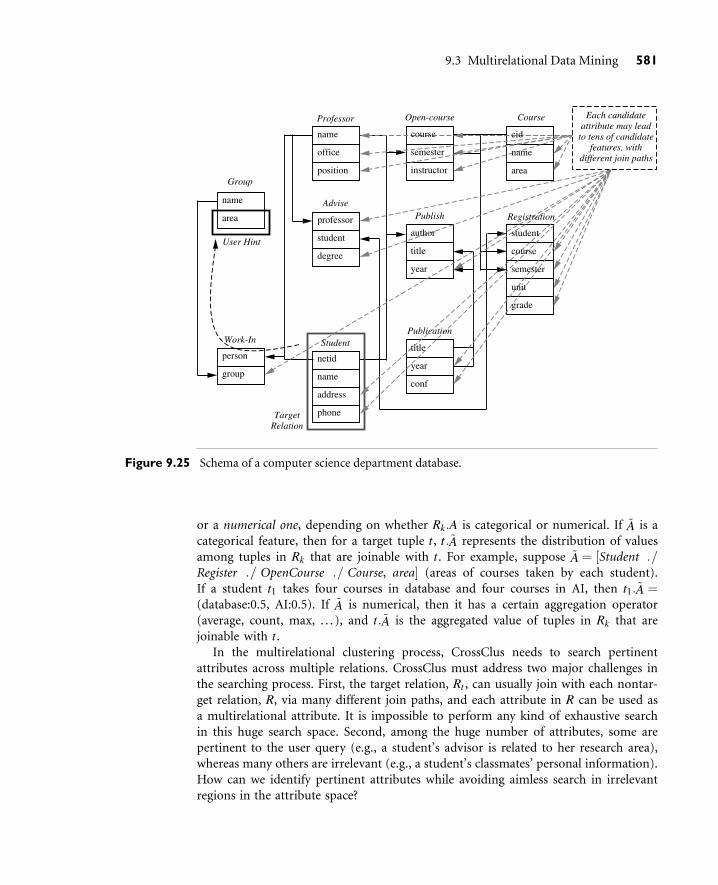
9.3 Multirelational Data Mining 581
grade
unit
semester
course
student
area
name
cid
year
title
author
conf
year
title
instructor
semester
course
degree
student
professorarea
name
group
person
Work-In
Group
Professor
Advise
StudentPublication
Publish
Open-course Course
Registration
position
office
name
phone
address
name
netid
User Hint
TargetRelation
Each candidateattribute may lead
to tens of candidatefeatures, with
different join paths
Figure 9.25 Schema of a computer science department database.
or a numerical one, depending on whether Rk.A is categorical or numerical. If à is acategorical feature, then for a target tuple t, t.à represents the distribution of valuesamong tuples in Rk that are joinable with t. For example, suppose à = [Student ./Register ./ OpenCourse ./ Course, area] (areas of courses taken by each student).If a student t1 takes four courses in database and four courses in AI, then t1.à =(database:0.5, AI:0.5). If à is numerical, then it has a certain aggregation operator(average, count, max, . . . ), and t.à is the aggregated value of tuples in Rk that arejoinable with t.
In the multirelational clustering process, CrossClus needs to search pertinentattributes across multiple relations. CrossClus must address two major challenges inthe searching process. First, the target relation, Rt , can usually join with each nontar-get relation, R, via many different join paths, and each attribute in R can be used asa multirelational attribute. It is impossible to perform any kind of exhaustive searchin this huge search space. Second, among the huge number of attributes, some arepertinent to the user query (e.g., a student’s advisor is related to her research area),whereas many others are irrelevant (e.g., a student’s classmates’ personal information).How can we identify pertinent attributes while avoiding aimless search in irrelevantregions in the attribute space?

582 Chapter 9 Graph Mining, Social Network Analysis, and Multirelational Data Mining
To overcome these challenges, CrossClus must confine the search process. It considersthe relational schema as a graph, with relations being nodes and joins being edges. Itadopts a heuristic approach, which starts search from the user-specified attribute, andthen repeatedly searches for useful attributes in the neighborhood of existing attributes.In this way it gradually expands the search scope to related relations, but will not go deepinto random directions.
“How does CrossClus decide if a neighboring attribute is pertinent?” CrossClus looks athow attributes cluster target tuples. The pertinent attributes are selected based on theirrelationships to the user-specified attributes. In essence, if two attributes cluster tuplesvery differently, their similarity is low and they are unlikely to be related. If they clustertuples in a similar way, they should be considered related. However, if they cluster tuplesin almost the same way, their similarity is very high, which indicates that they containredundant information. From the set of pertinent features found, CrossClus selects a setof nonredundant features so that the similarity between any two features is no greaterthan a specified maximum.
CrossClus uses the similarity vector of each attribute for evaluating the similaritybetween attributes, which is defined as follows. Suppose there are N target tuples,
t1, . . . , tN . Let VÃ be the similarity vector of attribute Ã. It is an N2-dimensional vec-tor that indicates the similarity between each pair of target tuples, ti and t j, based onÃ. To compare two attributes by the way they cluster tuples, we can look at how aliketheir similarity vectors are, by computing the inner product of the two similarity vec-tors. However, this is expensive to compute. Many applications cannot even afford tostore N2-dimensional vectors. Instead, CrossClus converts the hard problem of comput-ing the similarity between similarity vectors to an easier problem of computing similar-ities between attribute values, which can be solved in linear time.
Example 9.13 Multirelational search for pertinent attributes. Let’s look at how CrossClus proceeds inanswering the query of Example 9.12, where the user has specified her desire to clus-ter students by their research areas. To create the initial multirelational attribute for thisquery, CrossClus searches for the shortest join path from the target relation, Student, tothe relation Group, and creates a multirelational attribute à using this path. We simulatethe procedure of attribute searching, as shown in Figure 9.26. An initial pertinent mul-tirelational attribute [Student ./ WorkIn ./ Group , area] is created for this query (step 1in the figure). At first CrossClus considers attributes in the following relations that arejoinable with either the target relation or the relation containing the initial pertinentattribute: Advise, Publish, Registration, WorkIn, and Group. Suppose the best attributeis [Student ./ Advise , professor], which corresponds to the student’s advisor (step 2). Thisbrings the Professor relation into consideration in further search. CrossClus will searchfor additional pertinent features until most tuples are sufficiently covered. CrossClus usestuple ID propagation (Section 9.3.3) to virtually join different relations, thereby avoid-ing expensive physical joins during its search.

9.4 Multirelational Data Mining 583
Figure 9.26 Search for pertinent attributes in CrossClus.
Now that we have an intuitive idea of how CrossClus employs user guidance to searchfor attributes that are highly pertinent to the user’s query, the next question is, how does itperform the actual clustering? With the potentially large number of target tuples, an effi-cient and scalable clustering algorithm is needed. Because the multirelational attributesdo not form a Euclidean space, the k-medoids method (Section 7.4.1) was chosen, whichrequires only a distance measure between tuples. In particular, CLARANS (Section 7.4.2),an efficient k-medoids algorithm for large databases, was used. The main idea ofCLARANS is to consider the whole space of all possible clusterings as a graph and to userandomized search to find good clusterings in this graph. It starts by randomly select-ing k tuples as the initial medoids (or cluster representatives), from which it constructsk clusters. In each step, an existing medoid is replaced by a new randomly selected medoid.If the replacement leads to better clustering, the new medoid is kept. This procedure isrepeated until the clusters remain stable.
CrossClus provides the clustering results to the user, together with information abouteach attribute. From the attributes of multiple relations, their join paths, and aggre-gation operators, the user learns the meaning of each cluster, and thus gains a betterunderstanding of the clustering results.

584 Chapter 9 Graph Mining, Social Network Analysis, and Multirelational Data Mining
9.4 Summary
Graphs represent a more general class of structures than sets, sequences, lattices, andtrees. Graph mining is used to mine frequent graph patterns, and perform character-ization, discrimination, classification, and cluster analysis over large graph data sets.Graph mining has a broad spectrum of applications in chemical informatics, bioin-formatics, computer vision, video indexing, text retrieval, and Web analysis.
Efficient methods have been developed for mining frequent subgraph patterns. Theycan be categorized into Apriori-based and pattern growth–based approaches. TheApriori-based approach has to use the breadth-first search (BFS) strategy because ofits level-wise candidate generation. The pattern-growth approach is more flexible withrespect to the search method. A typical pattern-growth method is gSpan, whichexplores additional optimization techniques in pattern growth and achieves high per-formance. The further extension of gSpan for mining closed frequent graph patternsleads to the CloseGraph algorithm, which mines more compressed but complete setsof graph patterns, given the minimum support threshold.
There are many interesting variant graph patterns, including approximate frequentgraphs, coherent graphs, and dense graphs. A general framework that considers con-straints is needed for mining such patterns. Moreover, various user-specificconstraints can be pushed deep into the graph pattern mining process to improvemining efficiency.
Application development of graph mining has led to the generation of compact andeffective graph index structures using frequent and discriminative graph patterns.Structure similarity search can be achieved by exploration of multiple graph features.Classification and cluster analysis of graph data sets can be explored by their inte-gration with the graph pattern mining process.
A social network is a heterogeneous and multirelational data set represented by a graph,which is typically very large, with nodes corresponding to objects, and edges (or links)representing relationships between objects.
Small world networks reflect the concept of small worlds, which originally focused onnetworks among individuals. They have been characterized as having a high degree oflocal clustering for a small fraction of the nodes (i.e., these nodes are interconnectedwith one another), while being no more than a few degrees of separation from theremaining nodes.
Social networks exhibit certain characteristics. They tend to follow the densificationpower law, which states that networks become increasingly dense over time. Shrinkingdiameter is another characteristic, where the effective diameter often decreases as thenetwork grows. Node out-degrees and in-degrees typically follow a heavy-tailed distri-bution. A Forest Fire model for graph generation was proposed, which incorporatesthese characteristics.

9.4 Summary 585
Link mining is a confluence of research in social networks, link analysis, hypertextand Web mining, graph mining, relational learning, and inductive logic program-ming. Link mining tasks include link-based object classification, object type predic-tion, link type prediction, link existence prediction, link cardinality estimation, objectreconciliation (which predicts whether two objects are, in fact, the same), and groupdetection (which clusters objects). Other tasks include subgraph identification (whichfinds characteristic subgraphs within networks) and metadata mining (which uncov-ers schema-type information regarding unstructured data).
In link prediction, measures for analyzing the proximity of network nodes can beused to predict and rank new links. Examples include the shortest path (which ranksnode pairs by their shortest path in the network) and common neighbors (where thegreater the number of neighbors that two nodes share, the more likely they are toform a link). Other measures may be based on the ensemble of all paths between twonodes.
Viral marketing aims to optimize the positive word-of-mouth effect amongcustomers. By considering the interactions between customers, it can choose tospend more money marketing to an individual if that person has many socialconnections.
Newsgroup discussions form a kind of network based on the “responded-to” rela-tionships. Because people generally respond more frequently to a message when theydisagree than when they agree, graph partitioning algorithms can be used to minenewsgroups based on such a network to effectively classify authors in the newsgroupinto opposite camps.
Most community mining methods assume that there is only one kind of relation in thenetwork, and moreover, the mining results are independent of the users’ informationneeds. In reality, there may be multiple relations between objects, which collectivelyform a multirelational social network (or heterogeneous social network). Relation selec-tion and extraction in such networks evaluates the importance of the different relationswith respect to user information provided as queries. In addition, it searches for acombination of the existing relations that may reveal a hidden community within themultirelational network.
Multirelational data mining (MRDM) methods search for patterns that involve mul-tiple tables (relations) from a relational database.
Inductive Logic Programming (ILP) is the most widely used category of approachesto multirelational classification. It finds hypotheses of a certain format that can pre-dict the class labels of target tuples, based on background knowledge. Although manyILP approaches achieve good classification accuracy, most are not highly scalable dueto the computational expense of repeated joins.
Tuple ID propagation is a method for virtually joining different relations by attachingthe IDs of target tuples to tuples in nontarget relations. It is much less costly thanphysical joins, in both time and space.

586 Chapter 9 Graph Mining, Social Network Analysis, and Multirelational Data Mining
CrossMine and CrossClus are methods for multirelational classification andmultirelational clustering, respectively. Both use tuple ID propagation to avoid phys-ical joins. In addition, CrossClus employs user guidance to constrain the search space.
Exercises
9.1 Given two predefined sets of graphs, contrast patterns are substructures that are frequentin one set but infrequent in the other. Discuss how to mine contrast patterns efficientlyin large graph data sets.
9.2 Multidimensional information can be associated with the vertices and edges of each graph.Study how to develop efficient methods for mining multidimensional graph patterns.
9.3 Constraints often play an important role in efficient graph mining. There are many poten-tialconstraintsbasedonusers’ requests ingraphmining.Forexample,onemaywantgraphpatterns containing or excluding certain vertices (or edges), with minimal or maximal size,containing certain subgraphs, with certain summation values, and so on. Based on howa constraint behaves in graph mining, give a systematic classification of constraints andwork out rules on how to maximally use such constraints in efficient graph mining.
9.4 Our discussion of frequent graph pattern mining was confined to graph transactions (i.e.,considering each graph in a graph database as a single “transaction” in a transactionaldatabase). In many applications, one needs to mine frequent subgraphs in a large singlegraph (such as the Web or a large social network). Study how to develop efficient methodsfor mining frequent and closed graph patterns in such data sets.
9.5 What are the challenges for classification in a large social network in comparison with clas-sification in a single data relation? Suppose each node in a network represents a paper,associated with certain properties, such as author, research topic, and so on, and eachdirected edge from node A to node B indicates that paper A cites paper B. Design an effec-tive classification scheme that may effectively build a model for highly regarded paperson a particular topic.
9.6 A group of students are linked to each other in a social network via advisors, courses,research groups, and friendship relationships. Present a clustering method that may par-tition students into different groups according to their research interests.
9.7 Many diseases spread via people’s physical contacts in public places, such as offices, class-rooms, buses, shopping centers, hotels, and restaurants. Suppose a database registers theconcrete movement of many people (e.g., location, time, duration, and activity). Designa method that can be used to rank the “not visited” places during a virus-spreadingseason.
9.8 Design an effective method that discovers hierarchical clusters in a social network, such asa hierarchical network of friends.
9.9 Social networks evolve with time. Suppose the history of a social network is kept. Designa method that may discover the trend of evolution of the network.

Bibliographic Notes 587
9.10 There often exist multiple social networks linking a group of objects. For example, astudent could be in a class, a research project group, a family member, member of aneighborhood, and so on. It is often beneficial to consider their joint effects or interac-tions. Design an efficient method in social network analysis that may incorporate mul-tiple social networks in data mining.
9.11 Outline an efficient method that may find strong correlation rules in a large, multirela-tional database.
9.12 It is important to take a user’s advice to cluster objects across multiple relations, becausemany features among these relations could be relevant to the objects. A user may select asample set of objects and claim that some should be in the same cluster but some cannot.Outline an effective clustering method with such user guidance.
9.13 As a result of the close relationships among multiple departments or enterprises, it isnecessary to perform data mining across multiple but interlinked databases. In compar-ison with multirelational data mining, one major difficulty with mining across multipledatabases is semantic heterogeneity across databases. For example, “William Nelson” inone database could be “Bill Nelson” or “B. Nelson” in another one. Design a data miningmethod that may consolidate such objects by exploring object linkages among multipledatabases.
9.14 Outline an effective method that performs classification across multiple heterogeneousdatabases.
Bibliographic Notes
Research into graph mining has developed many frequent subgraph mining methods.Washio and Motoda [WM03] performed a survey on graph-based data mining. Manywell-known pairwise isomorphism testing algorithms were developed, such as Ullmann’sBacktracking [Ull76] and McKay’s Nauty [McK81]. Dehaspe, Toivonen, and King[DTK98] applied inductive logic programming to predict chemical carcinogenicity bymining frequent substructures. Several Apriori-based frequent substructure mining algo-rithms have been proposed, including AGM by Inokuchi, Washio, and Motoda [IWM98],FSG by Kuramochi and Karypis [KK01], and an edge-disjoint path-join algorithm byVanetik, Gudes, and Shimony [VGS02]. Pattern-growth-based graph pattern miningalgorithms include gSpan by Yan and Han [YH02], MoFa by Borgelt and Berthold [BB02],FFSM and SPIN by Huan, Wang, and Prins [HWP03] and Prins, Yang, Huan, and Wang[PYHW04], respectively, and Gaston by Nijssen and Kok [NK04]. These algorithms wereinspired by PrefixSpan [PHMA+01] for mining sequences, and TreeMinerV [Zak02] andFREQT [AAK+02] for mining trees. A disk-based frequent graph mining method wasproposed by Wang, Wang, Pei, et al. [WWP+04].
Mining closed graph patterns was studied by Yan and Han [YH03], with the pro-posal of the algorithm, CloseGraph, as an extension of gSpan and CloSpan [YHA03].Holder, Cook, and Djoko [HCD9] proposed SUBDUE for approximate substructure

588 Chapter 9 Graph Mining, Social Network Analysis, and Multirelational Data Mining
pattern discovery based on minimum description length and background knowledge.Mining coherent subgraphs was studied by Huan, Wang, Bandyopadhyay, et al.[HWB+04]. For mining relational graphs, Yan, Zhou, and Han [YZH05] proposed twoalgorithms, CloseCut and Splat, to discover exact dense frequent substructures in a setof relational graphs.
Many studies have explored the applications of mined graph patterns. Path-basedgraph indexing approaches are used in GraphGrep, developed by Shasha, Wang, andGiugno [SWG02], and in Daylight, developed by James, Weininger, and Delany [JWD03].Frequent graph patterns were used as graph indexing features in the gIndex and Grafilmethods proposed by Yan, Yu, and Han [YYH04, YYH05] to perform fast graph searchand structure similarity search. Borgelt and Berthold [BB02] illustrated the discovery ofactive chemical structures in an HIV-screening data set by contrasting the support of fre-quent graphs between different classes. Deshpande, Kuramochi, and Karypis [DKK02]used frequent structures as features to classify chemical compounds. Huan, Wang, Bandy-opadhyay, et al. [HWB+04] successfully applied the frequent graph mining techniqueto study protein structural families. Koyuturk, Grama, and Szpankowski [KGS04] pro-posed a method to detect frequent subgraphs in biological networks. Hu, Yan, Yu, et al.[HYY+05] developed an algorithm called CoDense to find dense subgraphs across mul-tiple biological networks.
There has been a great deal of research on social networks. For texts on social networkanalysis, see Wasserman and Faust [WF94], Degenne and Forse [DF99], Scott [Sco05],Watts [Wat03a], Barabási [Bar03], and Carrington, Scott, and Wasserman [CSW05].For a survey of work on social network analysis, see Newman [New03]. Barabási, Olt-vai, Jeong, et al. have several comprehensive tutorials on the topic, available at www.nd.edu/∼networks/publications.htm#talks0001. Books on small world networks includeWatts [Wat03b] and Buchanan [Buc03]. Milgram’s “six degrees of separation” exper-iment is presented in [Mil67].
The Forest Fire model for network generation was proposed in Leskovec, Kleinberg,and Faloutsos [LKF05]. The preferential attachment model was studied in Albert and Bar-basi [AB99] and Cooper and Frieze [CF03]. The copying model was explored in Klein-berg, Kumar, Raghavan, et al. [KKR+99] and Kumar, Raghavan, Rajagopalan, et al.[KRR+00].
Link mining tasks and challenges were overviewed by Getoor [Get03]. A link-basedclassification method was proposed in Lu and Getoor [LG03]. Iterative classification andinference algorithms have been proposed for hypertext classification by Chakrabarti,Dom, and Indyk [CDI98] and Oh, Myaeng, and Lee [OML00]. Bhattacharya and Getoor[BG04] proposed a method for clustering linked data, which can be used to solve the datamining tasks of entity deduplication and group discovery. A method for group discov-ery was proposed by Kubica, Moore, and Schneider [KMS03]. Approaches to link pre-diction, based on measures for analyzing the “proximity” of nodes in a network, weredescribed in Liben-Nowell and Kleinberg [LNK03]. The Katz measure was presentedin Katz [Kat53]. A probabilistic model for learning link structure was given in Getoor,Friedman, Koller, and Taskar [GFKT01]. Link prediction for counterterrorism was pro-posed by Krebs [Kre02]. Viral marketing was described by Domingos [Dom05] and his

Bibliographic Notes 589
work with Richardson [DR01, RD02]. BLOG (Bayesian LOGic), a language for reasoningwith unknown objects, was proposed by Milch, Marthi, Russell, et al. [MMR05] to add-ress the closed world assumption problem. Mining newsgroups to partition discussionparticipants into opposite camps using quotation networks was proposed by Agrawal,Rajagopalan, Srikant, and Xu [ARSX04]. The relation selection and extraction approachto community mining from multirelational networks was described in Cai, Shao, He,et al. [CSH+05].
Multirelational data mining has been investigated extensively in the Inductive LogicProgramming (ILP) community. Lavrac and Dzeroski [LD94] and Muggleton [Mug95]provided comprehensive introductions to Inductive Logic Programming (ILP). Anoverview of multirelational data mining was given by Dzeroski [Dze03]. Well-knownILP systems include FOIL by Quinlan and Cameron-Jones [QCJ93], Golem by Muggle-ton and Feng [MF90], and Progol by Muggleton [Mug95]. More recent systems includeTILDE by Blockeel, De Raedt, and Ramon [BRR98], Mr-SMOTI by Appice, Ceci, andMalerba [ACM03], and RPTs by Neville, Jensen, Friedland, and Hay [NJFH03], whichinductively construct decision trees from relational data. Probabilistic approaches tomultirelational classification include probabilistic relational models by Getoor, Fried-man, Koller, and Taskar [GFKT01] and by Taskar, Segal, and Koller [TSK01]. Popescul,Ungar, Lawrence, and Pennock [PULP02] proposed an approach to integrate ILP andstatistical modeling for document classification and retrieval. The CrossMine approachwas described in Yin, Han, Yang, and Yu [YHYY04]. The look-one-ahead method used inCrossMine was developed by Blockeel, De Raedt, and Ramon [BRR98]. Multirelationalclustering was explored by Gartner, Lloyd, and Flach [GLF04], and Kirsten and Wrobel[KW98, KW00]. CrossClus performs multirelational clustering with user guidance andwas proposed by Yin, Han, and Yu [YHY05].


10Mining Object, Spatial,Multimedia, Text, and
Web Data
Our previous chapters on advanced data mining discussed how to uncover knowledge fromstream, time-series, sequence, graph, social network, and multirelational data. In thischapter, we examine data mining methods that handle object, spatial, multimedia,text, and Web data. These kinds of data are commonly encountered in many social,economic, scientific, engineering, and governmental applications, and pose new chal-lenges in data mining. We first examine how to perform multidimensional analysis anddescriptive mining of complex data objects in Section 10.1. We then study methodsfor mining spatial data (Section 10.2), multimedia data (Section 10.3), text (Section10.4), and the World Wide Web (Section 10.5) in sequence.
10.1 Multidimensional Analysis and Descriptive Mining ofComplex Data Objects
Many advanced, data-intensive applications, such as scientific research and engineeringdesign, need to store, access, and analyze complex but relatively structured data objects.These objects cannot be represented as simple and uniformly structured records (i.e.,tuples) in data relations. Such application requirements have motivated the design anddevelopment of object-relational and object-oriented database systems. Both kinds of sys-tems deal with the efficient storage and access of vast amounts of disk-based complexstructured data objects. These systems organize a large set of complex data objects intoclasses, which are in turn organized into class/subclass hierarchies. Each object in a classis associated with (1) an object-identifier, (2) a set of attributes that may contain sophis-ticated data structures, set- or list-valued data, class composition hierarchies, multi-media data, and (3) a set of methods that specify the computational routines or rulesassociated with the object class. There has been extensive research in the field of databasesystems on how to efficiently index, store, access, and manipulate complex objects inobject-relational and object-oriented database systems. Technologies handling theseissues are discussed in many books on database systems, especially on object-orientedand object-relational database systems.
591

592 Chapter 10 Mining Object, Spatial, Multimedia, Text, and Web Data
One step beyond the storage and access of massive-scaled, complex object data is thesystematic analysis and mining of such data. This includes two major tasks: (1) con-struct multidimensional data warehouses for complex object data and perform onlineanalytical processing (OLAP) in such data warehouses, and (2) develop effective andscalable methods for mining knowledge from object databases and/or data warehouses.The second task is largely covered by the mining of specific kinds of data (such as spatial,temporal, sequence, graph- or tree-structured, text, and multimedia data), since thesedata form the major new kinds of complex data objects. As in Chapters 8 and 9, in thischapter we continue to study methods for mining complex data. Thus, our focus in thissection will be mainly on how to construct object data warehouses and perform OLAPanalysis on data warehouses for such data.
A major limitation of many commercial data warehouse and OLAP tools for multi-dimensional database analysis is their restriction on the allowable data types for dimen-sions and measures. Most data cube implementations confine dimensions to nonnumericdata, and measures to simple, aggregated values. To introduce data mining and multi-dimensional data analysis for complex objects, this section examines how to performgeneralization on complex structured objects and construct object cubes for OLAP andmining in object databases.
To facilitate generalization and induction in object-relational and object-orienteddatabases, it is important to study how each component of such databases can be gene-ralized, and how the generalized data can be used for multidimensional data analysis anddata mining.
10.1.1 Generalization of Structured DataAn important feature of object-relational and object-oriented databases is their capabil-ity of storing, accessing, and modeling complex structure-valued data, such as set- andlist-valued data and data with nested structures.
“How can generalization be performed on such data?” Let’s start by looking at thegeneralization of set-valued, list-valued, and sequence-valued attributes.
A set-valued attribute may be of homogeneous or heterogeneous type. Typically,set-valued data can be generalized by (1) generalization of each value in the set to itscorresponding higher-level concept, or (2) derivation of the general behavior of the set,such as the number of elements in the set, the types or value ranges in the set, theweighted average for numerical data, or the major clusters formed by the set. More-over, generalization can be performed by applying different generalization operators toexplore alternative generalization paths. In this case, the result of generalization is aheterogeneous set.
Example 10.1 Generalization of a set-valued attribute. Suppose that the hobby of a person is a set-valuedattribute containing the set of values {tennis, hockey, soccer, violin, SimCity}. This set canbe generalized to a set of high-level concepts, such as {sports, music, computer games}or into the number 5 (i.e., the number of hobbies in the set). Moreover, a count canbe associated with a generalized value to indicate how many elements are generalized to

10.1 Multidimensional Analysis and Descriptive Mining of Complex Data Objects 593
that value, as in {sports(3), music(1), computer games(1)}, where sports(3) indicates threekinds of sports, and so on.
A set-valued attribute may be generalized to a set-valued or a single-valued attribute;a single-valued attribute may be generalized to a set-valued attribute if the values form alattice or “hierarchy” or if the generalization follows different paths. Further generaliza-tions on such a generalized set-valued attribute should follow the generalization path ofeach value in the set.
List-valued attributes and sequence-valued attributes can be generalized in a mannersimilar to that for set-valued attributes except that the order of the elements in the list orsequence should be preserved in the generalization. Each value in the list can be genera-lized into its corresponding higher-level concept. Alternatively, a list can be generalizedaccording to its general behavior, such as the length of the list, the type of list elements, thevalue range, the weighted average value for numerical data, or by dropping unimportantelements in the list. A list may be generalized into a list, a set, or a single value.
Example 10.2 Generalization of list-valued attributes. Consider the following list or sequence of datafor a person’s education record: “((B.Sc. in Electrical Engineering, U.B.C., Dec., 1998),(M.Sc. in Computer Engineering, U. Maryland, May, 2001), (Ph.D. in Computer Science,UCLA, Aug., 2005))”. This can be generalized by dropping less important descriptions(attributes) of each tuple in the list, such as by dropping the month attribute to obtain“((B.Sc., U.B.C., 1998), . . .)”, and/or by retaining only the most important tuple(s) in thelist, e.g., “(Ph.D. in Computer Science, UCLA, 2005)”.
A complex structure-valued attribute may contain sets, tuples, lists, trees, records,and their combinations, where one structure may be nested in another at any level. In gen-eral, a structure-valued attribute can be generalized in several ways, such as (1) genera-lizing each attribute in the structure while maintaining the shape of the structure,(2) flattening the structure and generalizing the flattened structure, (3) summarizing thelow-level structures by high-level concepts or aggregation, and (4) returning the type oran overview of the structure.
In general, statistical analysis and cluster analysis may help toward deciding on thedirections and degrees of generalization to perform, since most generalization processesare to retain main features and remove noise, outliers, or fluctuations.
10.1.2 Aggregation and Approximation in Spatialand Multimedia Data GeneralizationAggregation and approximation are another important means of generalization. Theyare especially useful for generalizing attributes with large sets of values, complex struc-tures, and spatial or multimedia data.
Let’s take spatial data as an example. We would like to generalize detailed geo-graphic points into clustered regions, such as business, residential, industrial, or agri-cultural areas, according to land usage. Such generalization often requires the mergeof a set of geographic areas by spatial operations, such as spatial union or spatial

594 Chapter 10 Mining Object, Spatial, Multimedia, Text, and Web Data
clustering methods. Aggregation and approximation are important techniques forthis form of generalization. In a spatial merge, it is necessary to not only merge theregions of similar types within the same general class but also to compute the totalareas, average density, or other aggregate functions while ignoring some scatteredregions with different types if they are unimportant to the study. Other spatial oper-ators, such as spatial-union, spatial-overlapping, and spatial-intersection (which mayrequire the merging of scattered small regions into large, clustered regions) can alsouse spatial aggregation and approximation as data generalization operators.
Example 10.3 Spatial aggregation and approximation. Suppose that we have different pieces of landfor various purposes of agricultural usage, such as the planting of vegetables, grains,and fruits. These pieces can be merged or aggregated into one large piece of agriculturalland by a spatial merge. However, such a piece of agricultural land may contain highways,houses, and small stores. If the majority of the land is used for agriculture, the scatteredregions for other purposes can be ignored, and the whole region can be claimed as anagricultural area by approximation.
A multimedia database may contain complex texts, graphics, images, video fragments,maps, voice, music, and other forms of audio/video information. Multimedia data aretypically stored as sequences of bytes with variable lengths, and segments of data arelinked together or indexed in a multidimensional way for easy reference.
Generalization on multimedia data can be performed by recognition and extractionof the essential features and/or general patterns of such data. There are many ways toextract such information. For an image, the size, color, shape, texture, orientation, andrelative positions and structures of the contained objects or regions in the image canbe extracted by aggregation and/or approximation. For a segment of music, its melodycan be summarized based on the approximate patterns that repeatedly occur in the seg-ment, while its style can be summarized based on its tone, tempo, or the major musicalinstruments played. For an article, its abstract or general organizational structure (e.g.,the table of contents, the subject and index terms that frequently occur in the article,etc.) may serve as its generalization.
In general, it is a challenging task to generalize spatial data and multimedia data inorder to extract interesting knowledge implicitly stored in the data. Technologies deve-loped in spatial databases and multimedia databases, such as spatial data accessing andanalysis techniques, pattern recognition, image analysis, text analysis, content-basedimage/text retrieval and multidimensional indexing methods, should be integrated withdata generalization and data mining techniques to achieve satisfactory results. Tech-niques for mining such data are further discussed in the following sections.
10.1.3 Generalization of Object Identifiersand Class/Subclass Hierarchies“How can object identifiers be generalized?” At first glance, it may seem impossibleto generalize an object identifier. It remains unchanged even after structural reor-ganization of the data. However, since objects in an object-oriented database are

10.1 Multidimensional Analysis and Descriptive Mining of Complex Data Objects 595
organized into classes, which in turn are organized into class/subclass hierarchies,the generalization of an object can be performed by referring to its associatedhierarchy. Thus, an object identifier can be generalized as follows. First, the objectidentifier is generalized to the identifier of the lowest subclass to which the objectbelongs. The identifier of this subclass can then, in turn, be generalized to a higher-level class/subclass identifier by climbing up the class/subclass hierarchy. Similarly, aclass or a subclass can be generalized to its corresponding superclass(es) by climbingup its associated class/subclass hierarchy.
“Can inherited properties of objects be generalized?” Since object-oriented databases areorganized into class/subclass hierarchies, some attributes or methods of an object classare not explicitly specified in the class but are inherited from higher-level classes of theobject. Some object-oriented database systems allow multiple inheritance, where proper-ties can be inherited from more than one superclass when the class/subclass “hierarchy”is organized in the shape of a lattice. The inherited properties of an object can be derivedby query processing in the object-oriented database. From the data generalization pointof view, it is unnecessary to distinguish which data are stored within the class and whichare inherited from its superclass. As long as the set of relevant data are collected by queryprocessing, the data mining process will treat the inherited data in the same manner asthe data stored in the object class, and perform generalization accordingly.
Methods are an important component of object-oriented databases. They can also beinherited by objects. Many behavioral data of objects can be derived by the applicationof methods. Since a method is usually defined by a computational procedure/functionor by a set of deduction rules, it is impossible to perform generalization on the methoditself. However, generalization can be performed on the data derived by application ofthe method. That is, once the set of task-relevant data is derived by application of themethod, generalization can then be performed on these data.
10.1.4 Generalization of Class Composition Hierarchies
An attribute of an object may be composed of or described by another object, some ofwhose attributes may be in turn composed of or described by other objects, thus forminga class composition hierarchy. Generalization on a class composition hierarchy can beviewed as generalization on a set of nested structured data (which are possibly infinite,if the nesting is recursive).
In principle, the reference to a composite object may traverse via a long sequenceof references along the corresponding class composition hierarchy. However, in mostcases, the longer the sequence of references traversed, the weaker the semantic link-age between the original object and the referenced composite object. For example, anattribute vehicles owned of an object class student could refer to another object class car,which may contain an attribute auto dealer, which may refer to attributes describingthe dealer’s manager and children. Obviously, it is unlikely that any interesting generalregularities exist between a student and her car dealer’s manager’s children. Therefore,generalization on a class of objects should be performed on the descriptive attribute val-ues and methods of the class, with limited reference to its closely related components

596 Chapter 10 Mining Object, Spatial, Multimedia, Text, and Web Data
via its closely related linkages in the class composition hierarchy. That is, in order todiscover interesting knowledge, generalization should be performed on the objects in theclass composition hierarchy that are closely related in semantics to the currently focusedclass(es), but not on those that have only remote and rather weak semantic linkages.
10.1.5 Construction and Mining of Object Cubes
In an object database, data generalization and multidimensional analysis are not appliedto individual objects but to classes of objects. Since a set of objects in a class may sharemany attributes and methods, and the generalization of each attribute and method mayapply a sequence of generalization operators, the major issue becomes how to makethe generalization processes cooperate among different attributes and methods in theclass(es).
“So, how can class-based generalization be performed for a large set of objects?” For class-based generalization, the attribute-oriented induction method developed in Chapter 4 formining characteristics of relational databases can be extended to mine data character-istics in object databases. Consider that a generalization-based data mining process canbe viewed as the application of a sequence of class-based generalization operators ondifferent attributes. Generalization can continue until the resulting class contains a smallnumber of generalized objects that can be summarized as a concise, generalized rule inhigh-level terms. For efficient implementation, the generalization of multidimensionalattributes of a complex object class can be performed by examining each attribute (ordimension), generalizing each attribute to simple-valued data, and constructing a mul-tidimensional data cube, called an object cube. Once an object cube is constructed,multidimensional analysis and data mining can be performed on it in a manner simi-lar to that for relational data cubes.
Notice that from the application point of view, it is not always desirable to generalizea set of values to single-valued data. Consider the attribute keyword, which may containa set of keywords describing a book. It does not make much sense to generalize this setof keywords to one single value. In this context, it is difficult to construct an object cubecontaining the keyword dimension. We will address some progress in this direction inthe next section when discussing spatial data cube construction. However, it remains achallenging research issue to develop techniques for handling set-valued data effectivelyin object cube construction and object-based multidimensional analysis.
10.1.6 Generalization-Based Mining of Plan Databasesby Divide-and-Conquer
To show how generalization can play an important role in mining complex databases,we examine a case of mining significant patterns of successful actions in a plan databaseusing a divide-and-conquer strategy.
A plan consists of a variable sequence of actions. A plan database, or simply aplanbase, is a large collection of plans. Plan mining is the task of mining significant

10.1 Multidimensional Analysis and Descriptive Mining of Complex Data Objects 597
patterns or knowledge from a planbase. Plan mining can be used to discover travelpatterns of business passengers in an air flight database or to find significant patternsfrom the sequences of actions in the repair of automobiles. Plan mining is differ-ent from sequential pattern mining, where a large number of frequently occurringsequences are mined at a very detailed level. Instead, plan mining is the extractionof important or significant generalized (sequential) patterns from a planbase.
Let’s examine the plan mining process using an air travel example.
Example 10.4 An air flight planbase. Suppose that the air travel planbase shown in Table 10.1 storescustomer flight sequences, where each record corresponds to an action in a sequentialdatabase, and a sequence of records sharing the same plan number is considered as oneplan with a sequence of actions. The columns departure and arrival specify the codes ofthe airports involved. Table 10.2 stores information about each airport.
There could be many patterns mined from a planbase like Table 10.1. For example,we may discover that most flights from cities in the Atlantic United States to Midwesterncities have a stopover at ORD in Chicago, which could be because ORD is the princi-pal hub for several major airlines. Notice that the airports that act as airline hubs (suchas LAX in Los Angeles, ORD in Chicago, and JFK in New York) can easily be derivedfrom Table 10.2 based on airport size. However, there could be hundreds of hubs in atravel database. Indiscriminate mining may result in a large number of “rules” that lacksubstantial support, without providing a clear overall picture.
Table 10.1 A database of travel plans: a travel planbase.
plan# action# departure departure time arrival arrival time airline · · ·1 1 ALB 800 JFK 900 TWA · · ·1 2 JFK 1000 ORD 1230 UA · · ·1 3 ORD 1300 LAX 1600 UA · · ·1 4 LAX 1710 SAN 1800 DAL · · ·2 1 SPI 900 ORD 950 AA · · ·...
......
......
......
...
Table 10.2 An airport information table.
airport code city state region airport size · · ·ORD Chicago Illinois Mid-West 100000 · · ·SPI Springfield Illinois Mid-West 10000 · · ·LAX Los Angeles California Pacific 80000 · · ·ALB Albany New York Atlantic 20000 · · ·
......
......
......

598 Chapter 10 Mining Object, Spatial, Multimedia, Text, and Web Data
Figure 10.1 A multidimensional view of a database.
“So, how should we go about mining a planbase?” We would like to find a smallnumber of general (sequential) patterns that cover a substantial portion of the plans,and then we can divide our search efforts based on such mined sequences. The key tomining such patterns is to generalize the plans in the planbase to a sufficiently high level.A multidimensional database model, such as the one shown in Figure 10.1 for the airflight planbase, can be used to facilitate such plan generalization. Since low-level infor-mation may never share enough commonality to form succinct plans, we should do thefollowing: (1) generalize the planbase in different directions using the multidimensionalmodel; (2) observe when the generalized plans share common, interesting, sequentialpatterns with substantial support; and (3) derive high-level, concise plans.
Let’s examine this planbase. By combining tuples with the same plan number, thesequences of actions (shown in terms of airport codes) may appear as follows:
ALB - JFK - ORD - LAX - SAN
SPI - ORD - JFK - SYR
. . .

10.1 Multidimensional Analysis and Descriptive Mining of Complex Data Objects 599
Table 10.3 Multidimensional generalization of a planbase.
plan# loc seq size seq state seq region seq · · ·1 ALB-JFK-ORD-LAX-SAN S-L-L-L-S N-N-I-C-C E-E-M-P-P · · ·2 SPI-ORD-JFK-SYR S-L-L-S I-I-N-N M-M-E-E · · ·...
......
......
...
Table 10.4 Merging consecutive, identical actions in plans.
plan# size seq state seq region seq · · ·1 S-L+-S N+-I-C+ E+-M-P+ · · ·2 S-L+-S I+-N+ M+-E+ · · ·...
......
......
These sequences may look very different. However, they can be generalized in multipledimensions. When they are generalized based on the airport size dimension, we observesome interesting sequential patterns, like S-L-L-S, where L represents a large airport (i.e.,a hub), and S represents a relatively small regional airport, as shown in Table 10.3.
The generalization of a large number of air travel plans may lead to some rather gen-eral but highly regular patterns. This is often the case if the merge and optional operatorsare applied to the generalized sequences, where the former merges (and collapses) con-secutive identical symbols into one using the transitive closure notation “+” to representa sequence of actions of the same type, whereas the latter uses the notation “[ ]” to indi-cate that the object or action inside the square brackets “[ ]” is optional. Table 10.4 showsthe result of applying the merge operator to the plans of Table 10.3.
By merging and collapsing similar actions, we can derive generalized sequential pat-terns, such as Pattern (10.1):
[S]−L+− [S] [98.5%] (10.1)
The pattern states that 98.5% of travel plans have the pattern [S]− L+− [S], where[S] indicates that action S is optional, and L+ indicates one or more repetitions of L.In other words, the travel pattern consists of flying first from possibly a small airport,hopping through one to many large airports, and finally reaching a large (or possibly, asmall) airport.
After a sequential pattern is found with sufficient support, it can be used to parti-tion the planbase. We can then mine each partition to find common characteristics. Forexample, from a partitioned planbase, we may find
flight(x,y)∧airport size(x,S)∧airport size(y,L)⇒region(x) = region(y) [75%], (10.2)

600 Chapter 10 Mining Object, Spatial, Multimedia, Text, and Web Data
which means that for a direct flight from a small airport x to a large airport y, there is a75% probability that x and y belong to the same region.
This example demonstrates a divide-and-conquer strategy, which first finds interest-ing, high-level concise sequences of plans by multidimensional generalization of aplanbase, and then partitions the planbase based on mined patterns to discover the corre-sponding characteristics of subplanbases. This mining approach can be applied to manyother applications. For example, in Weblog mining, we can study general access patternsfrom the Web to identify popular Web portals and common paths before digging intodetailed subordinate patterns.
The plan mining technique can be further developed in several aspects. For instance,a minimum support threshold similar to that in association rule mining can be used todetermine the level of generalization and ensure that a pattern covers a sufficient num-ber of cases. Additional operators in plan mining can be explored, such as less than.Other variations include extracting associations from subsequences, or mining sequencepatterns involving multidimensional attributes—for example, the patterns involvingboth airport size and location. Such dimension-combined mining also requires the gen-eralization of each dimension to a high level before examination of the combined sequencepatterns.
10.2 Spatial Data Mining
A spatial database stores a large amount of space-related data, such as maps, prepro-cessed remote sensing or medical imaging data, and VLSI chip layout data. Spatialdatabases have many features distinguishing them from relational databases. Theycarry topological and/or distance information, usually organized by sophisticated,multidimensional spatial indexing structures that are accessed by spatial data accessmethods and often require spatial reasoning, geometric computation, and spatialknowledge representation techniques.
Spatial data mining refers to the extraction of knowledge, spatial relationships, orother interesting patterns not explicitly stored in spatial databases. Such mining demandsan integration of data mining with spatial database technologies. It can be used for under-standing spatial data, discovering spatial relationships and relationships between spatialand nonspatial data, constructing spatial knowledge bases, reorganizing spatial databases,and optimizing spatial queries. It is expected to have wide applications in geographicinformation systems, geomarketing, remote sensing, image database exploration, medi-cal imaging, navigation, traffic control, environmental studies, and many other areaswhere spatial data are used. A crucial challenge to spatial data mining is the explorationof efficient spatial data mining techniques due to the huge amount of spatial data and thecomplexity of spatial data types and spatial access methods.
“What about using statistical techniques for spatial data mining?” Statistical spatial dataanalysis has been a popular approach to analyzing spatial data and exploring geographicinformation. The term geostatistics is often associated with continuous geographic space,

10.2 Spatial Data Mining 601
whereas the term spatial statistics is often associated with discrete space. In a statisticalmodel that handles nonspatial data, one usually assumes statistical independence amongdifferent portions of data. However, different from traditional data sets, there is no suchindependence among spatially distributed data because in reality, spatial objects are ofteninterrelated, or more exactly spatially co-located, in the sense that the closer the two objectsare located, the more likely they share similar properties. For example, nature resource,climate, temperature, and economic situations are likely to be similar in geographicallyclosely located regions. People even consider this as the first law of geography: “Everythingis related to everything else, but nearby things are more related than distant things.” Sucha property of close interdependency across nearby space leads to the notion of spatialautocorrelation. Based on this notion, spatial statistical modeling methods have beendeveloped with good success. Spatial data mining will further develop spatial statisticalanalysis methods and extend them for huge amounts of spatial data, with more emphasison efficiency, scalability, cooperation with database and data warehouse systems,improved user interaction, and the discovery of new types of knowledge.
10.2.1 Spatial Data Cube Construction and Spatial OLAP
“Can we construct a spatial data warehouse?” Yes, as with relational data, we can integratespatial data to construct a data warehouse that facilitates spatial data mining. A spatialdata warehouse is a subject-oriented, integrated, time-variant, and nonvolatile collectionof both spatial and nonspatial data in support of spatial data mining and spatial-data-related decision-making processes.
Let’s look at the following example.
Example 10.5 Spatial data cube and spatial OLAP. There are about 3,000 weather probes distributed inBritish Columbia (BC), Canada, each recording daily temperature and precipitation fora designated small area and transmitting signals to a provincial weather station. With aspatial data warehouse that supports spatial OLAP, a user can view weather patterns on amap by month, by region, and by different combinations of temperature and precipita-tion, and can dynamically drill down or roll up along any dimension to explore desiredpatterns, such as “wet and hot regions in the Fraser Valley in Summer 1999.”
There are several challenging issues regarding the construction and utilization ofspatial data warehouses. The first challenge is the integration of spatial data from het-erogeneous sources and systems. Spatial data are usually stored in different industryfirms and government agencies using various data formats. Data formats are not onlystructure-specific (e.g., raster- vs. vector-based spatial data, object-oriented vs. relationalmodels, different spatial storage and indexing structures), but also vendor-specific (e.g.,ESRI, MapInfo, Intergraph). There has been a great deal of work on the integration andexchange of heterogeneous spatial data, which has paved the way for spatial data inte-gration and spatial data warehouse construction.
The second challenge is the realization of fast and flexible on-line analytical processingin spatial data warehouses. The star schema model introduced in Chapter 3 is a good

602 Chapter 10 Mining Object, Spatial, Multimedia, Text, and Web Data
choice for modeling spatial data warehouses because it provides a concise and organizedwarehouse structure and facilitates OLAP operations. However, in a spatial warehouse,both dimensions and measures may contain spatial components.
There are three types of dimensions in a spatial data cube:
A nonspatial dimension contains only nonspatial data. Nonspatial dimensionstemperature and precipitation can be constructed for the warehouse in Example 10.5,since each contains nonspatial data whose generalizations are nonspatial (such as“hot” for temperature and “wet” for precipitation).
A spatial-to-nonspatial dimension is a dimension whose primitive-level data are spa-tial but whose generalization, starting at a certain high level, becomes nonspatial. Forexample, the spatial dimension city relays geographic data for the U.S. map. Supposethat the dimension’s spatial representation of, say, Seattle is generalized to the string“pacific northwest.” Although “pacific northwest” is a spatial concept, its representa-tion is not spatial (since, in our example, it is a string). It therefore plays the role of anonspatial dimension.
A spatial-to-spatial dimension is a dimension whose primitive level and all of its high-level generalized data are spatial. For example, the dimension equi temperature regioncontains spatial data, as do all of its generalizations, such as with regions covering0-5 degrees (Celsius), 5-10 degrees, and so on.
We distinguish two types of measures in a spatial data cube:
A numerical measure contains only numerical data. For example, one measure in aspatial data warehouse could be the monthly revenue of a region, so that a roll-up maycompute the total revenue by year, by county, and so on. Numerical measures can befurther classified into distributive, algebraic, and holistic, as discussed in Chapter 3.
A spatial measure contains a collection of pointers to spatial objects. For example,in a generalization (or roll-up) in the spatial data cube of Example 10.5, the regionswith the same range of temperature and precipitation will be grouped into the samecell, and the measure so formed contains a collection of pointers to those regions.
A nonspatial data cube contains only nonspatial dimensions and numerical measures.If a spatial data cube contains spatial dimensions but no spatial measures, its OLAPoperations, such as drilling or pivoting, can be implemented in a manner similar to thatfor nonspatial data cubes.
“But what if I need to use spatial measures in a spatial data cube?” This notion raisessome challenging issues on efficient implementation, as shown in the following example.
Example 10.6 Numerical versus spatial measures. A star schema for the BC weather warehouse ofExample 10.5 is shown in Figure 10.2. It consists of four dimensions: region temperature,time, and precipitation, and three measures: region map, area, and count. A concept hier-archy for each dimension can be created by users or experts, or generated automatically

10.2 Spatial Data Mining 603
by data clustering analysis. Figure 10.3 presents hierarchies for each of the dimensionsin the BC weather warehouse.
Of the three measures, area and count are numerical measures that can be computedsimilarly as for nonspatial data cubes; region map is a spatial measure that represents acollection of spatial pointers to the corresponding regions. Since different spatial OLAPoperations result in different collections of spatial objects in region map, it is a majorchallenge to compute the merges of a large number of regions flexibly and dynami-cally. For example, two different roll-ups on the BC weather map data (Figure 10.2) mayproduce two different generalized region maps, as shown in Figure 10.4, each being theresult of merging a large number of small (probe) regions from Figure 10.2.
Figure 10.2 A star schema of the BC weather spatial data warehouse and corresponding BC weatherprobes map.
region name dimension: time dimension:
probe location < district < city < region hour < day < month < season
< province
temperature dimension: precipitation dimension:
(cold, mild, hot)⊂ all(temperature) (dry, fair, wet)⊂ all(precipitation)
(below −20,−20...−11,−10...0)⊂ cold (0...0.05, 0.06...0.2)⊂ dry
(0...10, 11...15, 16...20)⊂mild (0.2...0.5, 0.6...1.0, 1.1...1.5)⊂ fair
(20...25, 26...30, 31...35, above 35)⊂ hot (1.5...2.0, 2.1...3.0, 3.1...5.0, above 5.0)
⊂ wet
Figure 10.3 Hierarchies for each dimension of the BC weather data warehouse.
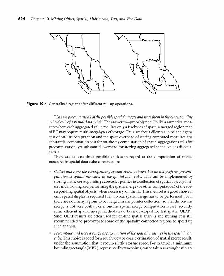
604 Chapter 10 Mining Object, Spatial, Multimedia, Text, and Web Data
Figure 10.4 Generalized regions after different roll-up operations.
“Can we precompute all of the possible spatial merges and store them in the correspondingcuboid cells of a spatial data cube?” The answer is—probably not. Unlike a numerical mea-sure where each aggregated value requires only a few bytes of space, a merged region mapof BC may require multi-megabytes of storage. Thus, we face a dilemma in balancing thecost of on-line computation and the space overhead of storing computed measures: thesubstantial computation cost for on-the-fly computation of spatial aggregations calls forprecomputation, yet substantial overhead for storing aggregated spatial values discour-ages it.
There are at least three possible choices in regard to the computation of spatialmeasures in spatial data cube construction:
Collect and store the corresponding spatial object pointers but do not perform precom-putation of spatial measures in the spatial data cube. This can be implemented bystoring, in the corresponding cube cell, a pointer to a collection of spatial object point-ers, and invoking and performing the spatial merge (or other computation) of the cor-responding spatial objects, when necessary, on the fly. This method is a good choice ifonly spatial display is required (i.e., no real spatial merge has to be performed), or ifthere are not many regions to be merged in any pointer collection (so that the on-linemerge is not very costly), or if on-line spatial merge computation is fast (recently,some efficient spatial merge methods have been developed for fast spatial OLAP).Since OLAP results are often used for on-line spatial analysis and mining, it is stillrecommended to precompute some of the spatially connected regions to speed upsuch analysis.
Precompute and store a rough approximation of the spatial measures in the spatial datacube. This choice is good for a rough view or coarse estimation of spatial merge resultsunder the assumption that it requires little storage space. For example, a minimumbounding rectangle (MBR), representedbytwopoints, canbetakenasaroughestimate

10.2 Spatial Data Mining 605
of a merged region. Such a precomputed result is small and can be presented quicklyto users. If higher precision is needed for specific cells, the application can either fetchprecomputed high-quality results, if available, or compute them on the fly.
Selectively precompute some spatial measures in the spatial data cube. This can be asmart choice. The question becomes, “Which portion of the cube should be selectedfor materialization?” The selection can be performed at the cuboid level, that is, eitherprecompute and store each set of mergeable spatial regions for each cell of a selectedcuboid, or precompute none if the cuboid is not selected. Since a cuboid usually con-sists of a large number of spatial objects, it may involve precomputation and storageof a large number of mergeable spatial objects, some of which may be rarely used.Therefore, it is recommended to perform selection at a finer granularity level: exam-ining each group of mergeable spatial objects in a cuboid to determine whether sucha merge should be precomputed. The decision should be based on the utility (such asaccess frequency or access priority), shareability of merged regions, and the balancedoverall cost of space and on-line computation.
With efficient implementation of spatial data cubes and spatial OLAP, generalization-based descriptive spatial mining, such as spatial characterization and discrimination, canbe performed efficiently.
10.2.2 Mining Spatial Association and Co-location Patterns
Similar to the mining of association rules in transactional and relational databases,spatial association rules can be mined in spatial databases. A spatial association rule is ofthe form A⇒ B [s%,c%], where A and B are sets of spatial or nonspatial predicates, s%is the support of the rule, and c% is the confidence of the rule. For example, the followingis a spatial association rule:
is a(X ,“school”)∧ close to(X ,“sports center”)⇒ close to(X ,“park”) [0.5%,80%].
This rule states that 80% of schools that are close to sports centers are also close toparks, and 0.5% of the data belongs to such a case.
Various kinds of spatial predicates can constitute a spatial association rule. Examplesinclude distance information (such as close to and far away), topological relations (likeintersect, overlap, and disjoint), and spatial orientations (like left of and west of).
Since spatial association mining needs to evaluate multiple spatial relationships amonga large number of spatial objects, the process could be quite costly. An interesting miningoptimization method called progressive refinement can be adopted in spatial associationanalysis. The method first mines large data sets roughly using a fast algorithm and thenimproves the quality of mining in a pruned data set using a more expensive algorithm.
To ensure that the pruned data set covers the complete set of answers when applyingthe high-quality data mining algorithms at a later stage, an important requirement for therough mining algorithm applied in the early stage is the superset coverage property: thatis, it preserves all of the potential answers. In other words, it should allow a false-positive

606 Chapter 10 Mining Object, Spatial, Multimedia, Text, and Web Data
test, which might include some data sets that do not belong to the answer sets, but itshould not allow a false-negative test, which might exclude some potential answers.
For mining spatial associations related to the spatial predicate close to, we can firstcollect the candidates that pass the minimum support threshold by
Applying certain rough spatial evaluation algorithms, for example, using an MBRstructure (which registers only two spatial points rather than a set of complexpolygons), and
Evaluating the relaxed spatial predicate, g close to, which is a generalized close tocovering a broader context that includes close to, touch, and intersect.
If two spatial objects are closely located, their enclosing MBRs must be closely located,matching g close to. However, the reverse is not always true: if the enclosing MBRs areclosely located, the two spatial objects may or may not be located so closely. Thus, theMBR pruning is a false-positive testing tool for closeness: only those that pass the roughtest need to be further examined using more expensive spatial computation algorithms.With this preprocessing, only the patterns that are frequent at the approximation level willneed to be examined by more detailed and finer, yet more expensive, spatial computation.
Besides mining spatial association rules, one may like to identify groups of particularfeatures that appear frequently close to each other in a geospatial map. Such a problemis essentially the problem of mining spatial co-locations. Finding spatial co-locationscan be considered as a special case of mining spatial associations. However, based on theproperty of spatial autocorrelation, interesting features likely coexist in closely locatedregions. Thus spatial co-location can be just what one really wants to explore. Efficientmethods can be developed for mining spatial co-locations by exploring the methodolo-gies like Aprori and progressive refinement, similar to what has been done for miningspatial association rules.
10.2.3 Spatial Clustering Methods
Spatial data clustering identifies clusters, or densely populated regions, according to somedistance measurement in a large, multidimensional data set. Spatial clustering methodswere thoroughly studied in Chapter 7 since cluster analysis usually considers spatial dataclustering in examples and applications. Therefore, readers interested in spatial cluster-ing should refer to Chapter 7.
10.2.4 Spatial Classification and Spatial Trend Analysis
Spatial classification analyzes spatial objects to derive classification schemes in relevanceto certain spatial properties, such as the neighborhood of a district, highway, or river.
Example 10.7 Spatial classification. Suppose that you would like to classify regions in a province intorich versus poor according to the average family income. In doing so, you would liketo identify the important spatial-related factors that determine a region’s classification.

10.3 Multimedia Data Mining 607
Many properties are associated with spatial objects, such as hosting a university,containing interstate highways, being near a lake or ocean, and so on. These prop-erties can be used for relevance analysis and to find interesting classification schemes.Such classification schemes may be represented in the form of decision trees or rules,for example, as described in Chapter 6.
Spatial trend analysis deals with another issue: the detection of changes and trendsalong a spatial dimension. Typically, trend analysis detects changes with time, such as thechanges of temporal patterns in time-series data. Spatial trend analysis replaces time withspace and studies the trend of nonspatial or spatial data changing with space. For example,we may observe the trend of changes in economic situation when moving away from thecenter of a city, or the trend of changes of the climate or vegetation with the increasingdistance from an ocean. For such analyses, regression and correlation analysis methodsare often applied by utilization of spatial data structures and spatial access methods.
There are also many applications where patterns are changing with both space andtime. For example, traffic flows on highways and in cities are both time and space related.Weather patterns are also closely related to both time and space. Although there havebeen a few interesting studies on spatial classification and spatial trend analysis, the inves-tigation of spatiotemporal data mining is still in its early stage. More methods and appli-cations of spatial classification and trend analysis, especially those associated with time,need to be explored.
10.2.5 Mining Raster Databases
Spatial database systems usually handle vector data that consist of points, lines, polygons(regions), and their compositions, such as networks or partitions. Typical examples ofsuch data include maps, design graphs, and 3-D representations of the arrangement ofthe chains of protein molecules. However, a huge amount of space-related data are indigital raster (image) forms, such as satellite images, remote sensing data, and computertomography. It is important to explore data mining in raster or image databases. Methodsfor mining raster and image data are examined in the following section regarding themining of multimedia data.
10.3 Multimedia Data Mining
“What is a multimedia database?” A multimedia database system stores and manages alarge collection of multimedia data, such as audio, video, image, graphics, speech, text,document, and hypertext data, which contain text, text markups, and linkages. Multi-media database systems are increasingly common owing to the popular use of audio-video equipment, digital cameras, CD-ROMs, and the Internet. Typical multimediadatabase systems include NASA’s EOS (Earth Observation System), various kinds ofimage and audio-video databases, and Internet databases.
In this section, our study of multimedia data mining focuses on image data mining.Mining text data and mining the World Wide Web are studied in the two subsequent
608 Chapter 10 Mining Object, Spatial, Multimedia, Text, and Web Data
sections. Here we introduce multimedia data mining methods, including similaritysearch in multimedia data, multidimensional analysis, classification and predictionanalysis, and mining associations in multimedia data.
10.3.1 Similarity Search in Multimedia Data
“When searching for similarities in multimedia data, can we search on either the datadescription or the data content?” That is correct. For similarity searching in multimediadata, we consider two main families of multimedia indexing and retrieval systems: (1)description-based retrieval systems, which build indices and perform object retrievalbased on image descriptions, such as keywords, captions, size, and time of creation;and (2) content-based retrieval systems, which support retrieval based on the imagecontent, such as color histogram, texture, pattern, image topology, and the shape ofobjects and their layouts and locations within the image. Description-based retrievalis labor-intensive if performed manually. If automated, the results are typically ofpoor quality. For example, the assignment of keywords to images can be a tricky andarbitrary task. Recent development of Web-based image clustering and classificationmethods has improved the quality of description-based Web image retrieval, becauseimagesurrounded text information as well as Web linkage information can be usedto extract proper description and group images describing a similar theme together.Content-based retrieval uses visual features to index images and promotes objectretrieval based on feature similarity, which is highly desirable in many applications.
In a content-based image retrieval system, there are often two kinds of queries: image-sample-based queries and image feature specification queries. Image-sample-based queriesfind all of the images that are similar to the given image sample. This search comparesthe feature vector (or signature) extracted from the sample with the feature vectors ofimages that have already been extracted and indexed in the image database. Based onthis comparison, images that are close to the sample image are returned. Image featurespecification queries specify or sketch image features like color, texture, or shape, whichare translated into a feature vector to be matched with the feature vectors of the images inthe database. Content-based retrieval has wide applications, including medical diagnosis,weather prediction, TV production, Web search engines for images, and e-commerce.Some systems, such as QBIC (Query By Image Content), support both sample-based andimage feature specification queries. There are also systems that support both content-based and description-based retrieval.
Several approaches have been proposed and studied for similarity-based retrieval inimage databases, based on image signature:
Color histogram–based signature: In this approach, the signature of an imageincludes color histograms based on the color composition of an image regardless ofits scale or orientation. This method does not contain any information about shape,image topology, or texture. Thus, two images with similar color composition butthat contain very different shapes or textures may be identified as similar, althoughthey could be completely unrelated semantically.

10.3 Multimedia Data Mining 609
Multifeature composed signature: In this approach, the signature of an imageincludes a composition of multiple features: color histogram, shape, image topol-ogy, and texture. The extracted image features are stored as metadata, and imagesare indexed based on such metadata. Often, separate distance functions can bedefined for each feature and subsequently combined to derive the overall results.Multidimensional content-based search often uses one or a few probe features tosearch for images containing such (similar) features. It can therefore be used tosearch for similar images. This is the most popularly used approach in practice.
Wavelet-based signature: This approach uses the dominant wavelet coefficients of animage as its signature. Wavelets capture shape, texture, and image topology informa-tion in a single unified framework.1 This improves efficiency and reduces the needfor providing multiple search primitives (unlike the second method above). How-ever, since this method computes a single signature for an entire image, it may fail toidentify images containing similar objects where the objects differ in location or size.
Wavelet-based signature with region-based granularity: In this approach, the com-putation and comparison of signatures are at the granularity of regions, not the entireimage. This is based on the observation that similar images may contain similarregions, but a region in one image could be a translation or scaling of a matchingregion in the other. Therefore, a similarity measure between the query image Q anda target image T can be defined in terms of the fraction of the area of the two imagescovered by matching pairs of regions from Q and T . Such a region-based similar-ity search can find images containing similar objects, where these objects may betranslated or scaled.
10.3.2 Multidimensional Analysis of Multimedia Data
“Can we construct a data cube for multimedia data analysis?” To facilitate the multidimen-sional analysis of large multimedia databases, multimedia data cubes can be designed andconstructed in a manner similar to that for traditional data cubes from relational data.A multimedia data cube can contain additional dimensions and measures for multime-dia information, such as color, texture, and shape.
Let’s examine a multimedia data mining system prototype called MultiMediaMiner,which extends the DBMiner system by handling multimedia data. The example databasetested in the MultiMediaMiner system is constructed as follows. Each image containstwo descriptors: a feature descriptor and a layout descriptor. The original image is notstored directly in the database; only its descriptors are stored. The description informa-tion encompasses fields like image file name, image URL, image type (e.g., gif, tiff, jpeg,mpeg, bmp, avi), a list of all known Web pages referring to the image (i.e., parent URLs), alist of keywords, and a thumbnail used by the user interface for image and video brows-ing. The feature descriptor is a set of vectors for each visual characteristic. The main
1Wavelet analysis was introduced in Section 2.5.3.

610 Chapter 10 Mining Object, Spatial, Multimedia, Text, and Web Data
vectors are a color vector containing the color histogram quantized to 512 colors (8×8×8 for R×G×B), an MFC (Most Frequent Color) vector, and an MFO (Most FrequentOrientation) vector. The MFC and MFO contain five color centroids and five edge ori-entation centroids for the five most frequent colors and five most frequent orientations,respectively. The edge orientations used are 0◦, 22.5◦, 45◦, 67.5◦, 90◦, and so on. Thelayout descriptor contains a color layout vector and an edge layout vector. Regardlessof their original size, all images are assigned an 8× 8 grid. The most frequent color foreach of the 64 cells is stored in the color layout vector, and the number of edges for eachorientation in each of the cells is stored in the edge layout vector. Other sizes of grids,like 4×4, 2×2, and 1×1, can easily be derived.
The Image Excavator component of MultiMediaMiner uses image contextual infor-mation, like HTML tags in Web pages, to derive keywords. By traversing on-line direc-tory structures, like the Yahoo! directory, it is possible to create hierarchies of keywordsmapped onto the directories in which the image was found. These graphs are used asconcept hierarchies for the dimension keyword in the multimedia data cube.
“What kind of dimensions can a multimedia data cube have?” A multimedia datacube can have many dimensions. The following are some examples: the size of theimage or video in bytes; the width and height of the frames (or pictures), constitutingtwo dimensions; the date on which the image or video was created (or last modified);the format type of the image or video; the frame sequence duration in seconds;the image or video Internet domain; the Internet domain of pages referencing theimage or video (parent URL); the keywords; a color dimension; an edge-orientationdimension; and so on. Concept hierarchies for many numerical dimensions may beautomatically defined. For other dimensions, such as for Internet domains or color,predefined hierarchies may be used.
The construction of a multimedia data cube will facilitate multidimensional analysisof multimedia data primarily based on visual content, and the mining of multiple kinds ofknowledge, including summarization, comparison, classification, association,and clustering. The Classifier module of MultiMediaMiner and its output are presentedin Figure 10.5.
The multimedia data cube seems to be an interesting model for multidimensionalanalysis of multimedia data. However, we should note that it is difficult to implementa data cube efficiently given a large number of dimensions. This curse of dimensiona-lity is especially serious in the case of multimedia data cubes. We may like to modelcolor, orientation, texture, keywords, and so on, as multiple dimensions in a multimediadata cube. However, many of these attributes are set-oriented instead of single-valued.For example, one image may correspond to a set of keywords. It may contain a set ofobjects, each associated with a set of colors. If we use each keyword as a dimension oreach detailed color as a dimension in the design of the data cube, it will create a hugenumber of dimensions. On the other hand, not doing so may lead to the modeling of animage at a rather rough, limited, and imprecise scale. More research is needed on howto design a multimedia data cube that may strike a balance between efficiency and thepower of representation.

10.3 Multimedia Data Mining 611
Figure 10.5 An output of the Classifier module of MultiMediaMiner.
10.3.3 Classification and Prediction Analysis of Multimedia Data
Classification and predictive modeling have been used for mining multimedia data, espe-cially in scientific research, such as astronomy, seismology, and geoscientific research. Ingeneral, all of the classification methods discussed in Chapter 6 can be used in imageanalysis and pattern recognition. Moreover, in-depth statistical pattern analysis methodsare popular for distinguishing subtle features and building high-quality models.
Example 10.8 Classification and prediction analysis of astronomy data. Taking sky images that havebeen carefully classified by astronomers as the training set, we can construct modelsfor the recognition of galaxies, stars, and other stellar objects, based on properties likemagnitudes, areas, intensity, image moments, and orientation. A large number of skyimages taken by telescopes or space probes can then be tested against the constructedmodels in order to identify new celestial bodies. Similar studies have successfully beenperformed to identify volcanoes on Venus.
Data preprocessing is important when mining image data and can include datacleaning, data transformation, and feature extraction. Aside from standard methods usedin pattern recognition, such as edge detection and Hough transformations, techniques

612 Chapter 10 Mining Object, Spatial, Multimedia, Text, and Web Data
can be explored, such as the decomposition of images to eigenvectors or the adoptionof probabilistic models to deal with uncertainty. Since the image data are often in hugevolumes and may require substantial processing power, parallel and distributed process-ing are useful. Image data mining classification and clustering are closely linked to imageanalysis and scientific data mining, and thus many image analysis techniques and scien-tific data analysis methods can be applied to image data mining.
The popular use of the World Wide Web has made the Web a rich and gigantic reposi-tory of multimedia data. The Web not only collects a tremendous number of photos, pic-tures, albums, and video images in the form of on-line multimedia libraries, but also hasnumerous photos, pictures, animations, and other multimedia forms on almost everyWeb page. Such pictures and photos, surrounded by text descriptions, located at thedifferent blocks of Web pages, or embedded inside news or text articles, may serve ratherdifferent purposes, such as forming an inseparable component of the content, serving asan advertisement, or suggesting an alternative topic. Furthermore, these Web pages arelinked with other Web pages in a complicated way. Such text, image location, and Weblinkage information, if used properly, may help understand the contents of the text orassist classification and clustering of images on the Web. Data mining by making gooduse of relative locations and linkages among images, text, blocks within a page, and pagelinks on the Web becomes an important direction in Web data analysis, which will befurther examined in Section 10.5 on Web mining.
10.3.4 Mining Associations in Multimedia Data
“What kinds of associations can be mined in multimedia data?” Association rules involvingmultimedia objects can be mined in image and video databases. At least three categoriescan be observed:
Associations between image content and nonimage content features: A rule like “If atleast 50% of the upper part of the picture is blue, then it is likely to represent sky” belongsto this category since it links the image content to the keyword sky.
Associations among image contents that are not related to spatial relationships: Arule like “If a picture contains two blue squares, then it is likely to contain one red circleas well” belongs to this category since the associations are all regarding image contents.
Associations among image contents related to spatial relationships: A rule like “Ifa red triangle is between two yellow squares, then it is likely a big oval-shaped objectis underneath” belongs to this category since it associates objects in the image withspatial relationships.
To mine associations among multimedia objects, we can treat each image as a tran-saction and find frequently occurring patterns among different images.
“What are the differences between mining association rules in multimedia databasesversus in transaction databases?” There are some subtle differences. First, an image maycontain multiple objects, each with many features such as color, shape, texture,

10.3 Multimedia Data Mining 613
keyword, and spatial location, so there could be many possible associations. In manycases, a feature may be considered as the same in two images at a certain level of resolu-tion, but different at a finer resolution level. Therefore, it is essential to promote a pro-gressive resolution refinement approach. That is, we can first mine frequently occurringpatterns at a relatively rough resolution level, and then focus only on those that havepassed the minimum support threshold when mining at a finer resolution level. This isbecause the patterns that are not frequent at a rough level cannot be frequent at finerresolution levels. Such a multiresolution mining strategy substantially reduces the over-all data mining cost without loss of the quality and completeness of data mining results.This leads to an efficient methodology for mining frequent itemsets and associations inlarge multimedia databases.
Second, because a picture containing multiple recurrent objects is an importantfeature in image analysis, recurrence of the same objects should not be ignored in asso-ciation analysis. For example, a picture containing two golden circles is treated quitedifferently from that containing only one. This is quite different from that in a transac-tion database, where the fact that a person buys one gallon of milk or two may often betreated the same as “buys milk.” Therefore, the definition of multimedia association andits measurements, such as support and confidence, should be adjusted accordingly.
Third, there often exist important spatial relationships among multimedia objects,such as above, beneath, between, nearby, left-of, and so on. These features are very use-ful for exploring object associations and correlations. Spatial relationships together withother content-based multimedia features, such as color, shape, texture, and keywords,may form interesting associations. Thus, spatial data mining methods and properties oftopological spatial relationships become important for multimedia mining.
10.3.5 Audio and Video Data Mining
Besides still images, an incommensurable amount of audiovisual information is becom-ing available in digital form, in digital archives, on the World Wide Web, in broadcast datastreams, and in personal and professional databases. This amount is rapidly growing.There are great demands for effective content-based retrieval and data mining methodsfor audio and video data. Typical examples include searching for and multimedia editingof particular video clips in a TV studio, detecting suspicious persons or scenes in surveil-lance videos, searching for particular events in a personal multimedia repository such asMyLifeBits, discovering patterns and outliers in weather radar recordings, and finding aparticular melody or tune in your MP3 audio album.
To facilitate the recording, search, and analysis of audio and video information frommultimedia data, industry and standardization committees have made great stridestoward developing a set of standards for multimedia information description and com-pression. For example, MPEG-k (developed by MPEG: Moving Picture Experts Group)and JPEG are typical video compression schemes. The most recently released MPEG-7,formally named “Multimedia Content Description Interface,” is a standard for describ-ing the multimedia content data. It supports some degree of interpretation of the infor-mation meaning, which can be passed onto, or accessed by, a device or a computer.

614 Chapter 10 Mining Object, Spatial, Multimedia, Text, and Web Data
MPEG-7 is not aimed at any one application in particular; rather, the elements thatMPEG-7 standardizes support as broad a range of applications as possible. The audiovi-sual data description in MPEG-7 includes still pictures, video, graphics, audio, speech,three-dimensional models, and information about how these data elements are com-bined in the multimedia presentation.
The MPEG committee standardizes the following elements in MPEG-7: (1) a set ofdescriptors, where each descriptor defines the syntax and semantics of a feature, such ascolor, shape, texture, image topology, motion, or title; (2) a set of descriptor schemes,where each scheme specifies the structure and semantics of the relationships betweenits components (descriptors or description schemes); (3) a set of coding schemes forthe descriptors, and (4) a description definition language (DDL) to specify schemes anddescriptors. Such standardization greatly facilitates content-based video retrieval andvideo data mining.
It is unrealistic to treat a video clip as a long sequence of individual still pictures andanalyze each picture since there are too many pictures, and most adjacent images couldbe rather similar. In order to capture the story or event structure of a video, it is betterto treat each video clip as a collection of actions and events in time and first temporarilysegment them into video shots. A shot is a group of frames or pictures where the videocontent from one frame to the adjacent ones does not change abruptly. Moreover, themost representative frame in a video shot is considered the key frame of the shot. Each keyframe can be analyzed using the image feature extraction and analysis methods studiedabove in the content-based image retrieval. The sequence of key frames will then be usedto define the sequence of the events happening in the video clip. Thus the detection ofshots and the extraction of key frames from video clips become the essential tasks invideo processing and mining.
Video data mining is still in its infancy. There are still a lot of research issues to besolved before it becomes general practice. Similarity-based preprocessing, compression,indexing and retrieval, information extraction, redundancy removal, frequent patterndiscovery, classification, clustering, and trend and outlier detection are important datamining tasks in this domain.
10.4 Text Mining
Most previous studies of data mining have focused on structured data, such as relational,transactional, and data warehouse data. However, in reality, a substantial portion ofthe available information is stored in text databases (or document databases), whichconsist of large collections of documents from various sources, such as news articles,research papers, books, digital libraries, e-mail messages, and Web pages. Text databasesare rapidly growing due to the increasing amount of information available in electronicform, such as electronic publications, various kinds of electronic documents, e-mail, andthe World Wide Web (which can also be viewed as a huge, interconnected, dynamic textdatabase). Nowadays most of the information in government, industry, business, andother institutions are stored electronically, in the form of text databases.

10.4 Text Mining 615
Data stored in most text databases are semistructured data in that they are neithercompletely unstructured nor completely structured. For example, a document maycontain a few structured fields, such as title, authors, publication date, category, andso on, but also contain some largely unstructured text components, such as abstractand contents. There have been a great deal of studies on the modeling and imple-mentation of semistructured data in recent database research. Moreover, informationretrieval techniques, such as text indexing methods, have been developed to handleunstructured documents.
Traditional information retrieval techniques become inadequate for the increasinglyvast amounts of text data. Typically, only a small fraction of the many available docu-ments will be relevant to a given individual user. Without knowing what could be in thedocuments, it is difficult to formulate effective queries for analyzing and extracting usefulinformation from the data. Users need tools to compare different documents, rank theimportance and relevance of the documents, or find patterns and trends across multipledocuments. Thus, text mining has become an increasingly popular and essential themein data mining.
10.4.1 Text Data Analysis and Information Retrieval
“What is information retrieval?” Information retrieval (IR) is a field that has been devel-oping in parallel with database systems for many years. Unlike the field of databasesystems, which has focused on query and transaction processing of structured data, infor-mation retrieval is concerned with the organization and retrieval of information from alarge number of text-based documents. Since information retrieval and database sys-tems each handle different kinds of data, some database system problems are usually notpresent in information retrieval systems, such as concurrency control, recovery, trans-action management, and update. Also, some common information retrieval problemsare usually not encountered in traditional database systems, such as unstructured docu-ments, approximate search based on keywords, and the notion of relevance.
Due to the abundance of text information, information retrieval has found manyapplications. There exist many information retrieval systems, such as on-line librarycatalog systems, on-line document management systems, and the more recently devel-oped Web search engines.
A typical information retrieval problem is to locate relevant documents in a docu-ment collection based on a user’s query, which is often some keywords describing aninformation need, although it could also be an example relevant document. In such asearch problem, a user takes the initiative to “pull” the relevant information out fromthe collection; this is most appropriate when a user has some ad hoc (i.e., short-term)information need, such as finding information to buy a used car. When a user has along-term information need (e.g., a researcher’s interests), a retrieval system may alsotake the initiative to “push” any newly arrived information item to a user if the itemis judged as being relevant to the user’s information need. Such an information accessprocess is called information filtering, and the corresponding systems are often called fil-tering systems or recommender systems. From a technical viewpoint, however, search and

616 Chapter 10 Mining Object, Spatial, Multimedia, Text, and Web Data
filtering share many common techniques. Below we briefly discuss the major techniquesin information retrieval with a focus on search techniques.
Basic Measures for Text Retrieval: Precision and Recall“Suppose that a text retrieval system has just retrieved a number of documents for me basedon my input in the form of a query. How can we assess how accurate or correct the systemwas?” Let the set of documents relevant to a query be denoted as {Relevant}, and the setof documents retrieved be denoted as {Retrieved}. The set of documents that are bothrelevant and retrieved is denoted as {Relevant} ∩ {Retrieved}, as shown in the Venndiagram of Figure 10.6. There are two basic measures for assessing the quality of textretrieval:
Precision: This is the percentage of retrieved documents that are in fact relevant tothe query (i.e., “correct” responses). It is formally defined as
precision =|{Relevant}∩{Retrieved}|
|{Retrieved}|.
Recall: This is the percentage of documents that are relevant to the query and were,in fact, retrieved. It is formally defined as
recall =|{Relevant}∩{Retrieved}|
|{Relevant}|.
An information retrieval system often needs to trade off recall for precision or viceversa. One commonly used trade-off is the F-score, which is defined as the harmonicmean of recall and precision:
F score =recall× precision
(recall + precision)/2.
The harmonic mean discourages a system that sacrifices one measure for another toodrastically.
All documents
Retrieveddocuments
Relevantdocuments
Relevant andretrieved
Figure 10.6 Relationship between the set of relevant documents and the set of retrieved documents.

10.4 Text Mining 617
Precision, recall, and F-score are the basic measures of a retrieved set of documents.These three measures are not directly useful for comparing two ranked lists of documentsbecause they are not sensitive to the internal ranking of the documents in a retrieved set.In order to measure the quality of a ranked list of documents, it is common to compute anaverage of precisions at all the ranks where a new relevant document is returned. It is alsocommon to plot a graph of precisions at many different levels of recall; a higher curverepresents a better-quality information retrieval system. For more details about thesemeasures, readers may consult an information retrieval textbook, such as [BYRN99].
Text Retrieval Methods“What methods are there for information retrieval?” Broadly speaking, retrieval methodsfall into two categories: They generally either view the retrieval problem as a documentselection problem or as a document ranking problem.
In document selection methods, the query is regarded as specifying constraints forselecting relevant documents. A typical method of this category is the Boolean retrievalmodel, in which a document is represented by a set of keywords and a user providesa Boolean expression of keywords, such as “car and repair shops,” “tea or coffee,” or“database systems but not Oracle.” The retrieval system would take such a Boolean queryand return documents that satisfy the Boolean expression. Because of the difficulty inprescribing a user’s information need exactly with a Boolean query, the Boolean retrievalmethod generally only works well when the user knows a lot about the document collec-tion and can formulate a good query in this way.
Document ranking methods use the query to rank all documents in the order ofrelevance. For ordinary users and exploratory queries, these methods are more appro-priate than document selection methods. Most modern information retrieval systemspresent a ranked list of documents in response to a user’s keyword query. There aremany different ranking methods based on a large spectrum of mathematical founda-tions, including algebra, logic, probability, and statistics. The common intuition behindall of these methods is that we may match the keywords in a query with those in thedocuments and score each document based on how well it matches the query. The goalis to approximate the degree of relevance of a document with a score computed based oninformation such as the frequency of words in the document and the whole collection.Notice that it is inherently difficult to provide a precise measure of the degree of relevancebetween a set of keywords. For example, it is difficult to quantify the distance betweendata mining and data analysis. Comprehensive empirical evaluation is thus essential forvalidating any retrieval method.
A detailed discussion of all of these retrieval methods is clearly out of the scope of thisbook. Following we briefly discuss the most popular approach—the vector space model.For other models, readers may refer to information retrieval textbooks, as referencedin the bibliographic notes. Although we focus on the vector space model, some stepsdiscussed are not specific to this particular approach.
The basic idea of the vector space model is the following: We represent a documentand a query both as vectors in a high-dimensional space corresponding to all the

618 Chapter 10 Mining Object, Spatial, Multimedia, Text, and Web Data
keywords and use an appropriate similarity measure to compute the similarity betweenthe query vector and the document vector. The similarity values can then be used forranking documents.
“How do we tokenize text?” The first step in most retrieval systems is to identify key-words for representing documents, a preprocessing step often called tokenization. Toavoid indexing useless words, a text retrieval system often associates a stop list with a setof documents. A stop list is a set of words that are deemed “irrelevant.” For example, a,the, of, for, with, and so on are stop words, even though they may appear frequently. Stoplists may vary per document set. For example, database systems could be an importantkeyword in a newspaper. However, it may be considered as a stop word in a set of researchpapers presented in a database systems conference.
A group of different words may share the same word stem. A text retrieval systemneeds to identify groups of words where the words in a group are small syntactic variantsof one another and collect only the common word stem per group. For example, thegroup of words drug, drugged, and drugs, share a common word stem, drug, and can beviewed as different occurrences of the same word.
“How can we model a document to facilitate information retrieval?” Starting with a setof d documents and a set of t terms, we can model each document as a vector v in thet dimensional space R
t , which is why this method is called the vector-space model. Letthe term frequency be the number of occurrences of term t in the document d, that is,freq(d, t). The (weighted) term-frequency matrix TF(d, t) measures the association of aterm t with respect to the given document d: it is generally defined as 0 if the documentdoes not contain the term, and nonzero otherwise. There are many ways to define theterm-weighting for the nonzero entries in such a vector. For example, we can simply setTF(d, t) = 1 if the term t occurs in the document d, or use the term frequency freq(d, t),or the relative term frequency, that is, the term frequency versus the total number ofoccurrences of all the terms in the document. There are also other ways to normalize theterm frequency. For example, the Cornell SMART system uses the following formula tocompute the (normalized) term frequency:
TF(d, t) =
{
0 if freq(d, t) = 0
1 + log(1 + log(freq(d, t))) otherwise.(10.3)
Besides the term frequency measure, there is another important measure, calledinverse document frequency (IDF), that represents the scaling factor, or the importance,of a term t. If a term t occurs in many documents, its importance will be scaled downdue to its reduced discriminative power. For example, the term database systems maylikely be less important if it occurs in many research papers in a database system confer-ence. According to the same Cornell SMART system, IDF(t) is defined by the followingformula:
IDF(t) = log1 + |d||dt |
, (10.4)
where d is the document collection, and dt is the set of documents containing term t. If|dt | � |d|, the term t will have a large IDF scaling factor and vice versa.

10.4 Text Mining 619
In a complete vector-space model, TF and IDF are combined together, which formsthe TF-IDF measure:
TF-IDF(d, t) = TF(d, t)× IDF(t). (10.5)
Let us examine how to compute similarity among a set of documents based on thenotions of term frequency and inverse document frequency.
Example 10.9 Term frequency and inverse document frequency. Table 10.5 shows a term frequencymatrix where each row represents a document vector, each column represents a term,and each entry registers freq(di, t j), the number of occurrences of term t j in document di.Based on this table we can calculate the TF-IDF value of a term in a document. Forexample, for t6 in d4, we have
TF(d4, t6) = 1 + log(1 + log(15)) = 1.3377
IDF(t6) = log1 + 5
3= 0.301.
Therefore,TF-IDF(d4, t6) = 1.3377×0.301 = 0.403
“How can we determine if two documents are similar?” Since similar documents areexpected to have similar relative term frequencies, we can measure the similarity among aset of documents or between a document and a query (often defined as a set of keywords),based on similar relative term occurrences in the frequency table. Many metrics havebeen proposed for measuring document similarity based on relative term occurrencesor document vectors. A representative metric is the cosine measure, defined as follows.Let v1 and v2 be two document vectors. Their cosine similarity is defined as
sim(v1,v2) =v1 · v2
|v1||v2|, (10.6)
where the inner product v1 · v2 is the standard vector dot product, defined as Σti=1v1iv2i,
and the norm |v1| in the denominator is defined as |v1|=√
v1 · v1.
Table 10.5 A term frequency matrix showing the frequency of terms per document.
document/term t1 t2 t3 t4 t5 t6 t7
d1 0 4 10 8 0 5 0
d2 5 19 7 16 0 0 32
d3 15 0 0 4 9 0 17
d4 22 3 12 0 5 15 0
d5 0 7 0 9 2 4 12

620 Chapter 10 Mining Object, Spatial, Multimedia, Text, and Web Data
Text Indexing TechniquesThere are several popular text retrieval indexing techniques, including inverted indicesand signature files.
An inverted index is an index structure that maintains two hash indexed or B+-treeindexed tables: document table and term table, where
document table consists of a set of document records, each containing two fields:doc id and posting list, where posting list is a list of terms (or pointers to terms) thatoccur in the document, sorted according to some relevance measure.
term table consists of a set of term records, each containing two fields: term id andposting list, where posting list specifies a list of document identifiers in which the termappears.
With such organization, it is easy to answer queries like “Find all of the documents asso-ciated with a given set of terms,” or “Find all of the terms associated with a given set ofdocuments.” For example, to find all of the documents associated with a set of terms, wecan first find a list of document identifiers in term table for each term, and then inter-sect them to obtain the set of relevant documents. Inverted indices are widely used inindustry. They are easy to implement. The posting lists could be rather long, making thestorage requirement quite large. They are easy to implement, but are not satisfactory athandling synonymy (where two very different words can have the same meaning) andpolysemy (where an individual word may have many meanings).
A signature file is a file that stores a signature record for each document in the database.Each signature has a fixed size of b bits representing terms. A simple encoding schemegoes as follows. Each bit of a document signature is initialized to 0. A bit is set to 1 if theterm it represents appears in the document. A signature S1 matches another signature S2if each bit that is set in signature S2 is also set in S1. Since there are usually more termsthan available bits, multiple terms may be mapped into the same bit. Such multiple-to-one mappings make the search expensive because a document that matches the signatureof a query does not necessarily contain the set of keywords of the query. The documenthas to be retrieved, parsed, stemmed, and checked. Improvements can be made by firstperforming frequency analysis, stemming, and by filtering stop words, and then using ahashing technique and superimposed coding technique to encode the list of terms intobit representation. Nevertheless, the problem of multiple-to-one mappings still exists,which is the major disadvantage of this approach.
Readers can refer to [WMB99] for more detailed discussion of indexing techniques,including how to compress an index.
Query Processing TechniquesOnce an inverted index is created for a document collection, a retrieval system can answera keyword query quickly by looking up which documents contain the query keywords.Specifically, we will maintain a score accumulator for each document and update these

10.4 Text Mining 621
accumulators as we go through each query term. For each query term, we will fetch all ofthe documents that match the term and increase their scores. More sophisticated queryprocessing techniques are discussed in [WMB99].
When examples of relevant documents are available, the system can learn from suchexamples to improve retrieval performance. This is called relevance feedback and hasproven to be effective in improving retrieval performance. When we do not have suchrelevant examples, a system can assume the top few retrieved documents in some initialretrieval results to be relevant and extract more related keywords to expand a query. Suchfeedback is called pseudo-feedback or blind feedback and is essentially a process of mininguseful keywords from the top retrieved documents. Pseudo-feedback also often leads toimproved retrieval performance.
One major limitation of many existing retrieval methods is that they are based onexact keyword matching. However, due to the complexity of natural languages, keyword-based retrieval can encounter two major difficulties. The first is the synonymy problem:two words with identical or similar meanings may have very different surface forms. Forexample, a user’s query may use the word “automobile,” but a relevant document mayuse “vehicle” instead of “automobile.” The second is the polysemy problem: the samekeyword, such as mining, or Java, may mean different things in different contexts.
We now discuss some advanced techniques that can help solve these problems as wellas reduce the index size.
10.4.2 Dimensionality Reduction for Text
With the similarity metrics introduced in Section 10.4.1, we can construct similarity-based indices on text documents. Text-based queries can then be represented as vectors,which can be used to search for their nearest neighbors in a document collection. How-ever, for any nontrivial document database, the number of terms T and the number ofdocuments D are usually quite large. Such high dimensionality leads to the problem ofinefficient computation, since the resulting frequency table will have size T ×D. Fur-thermore, the high dimensionality also leads to very sparse vectors and increases thedifficulty in detecting and exploiting the relationships among terms (e.g., synonymy).To overcome these problems, dimensionality reduction techniques such as latentsemantic indexing, probabilistic latent semantic analysis, and locality preserving indexingcan be used.
We now briefly introduce these methods. To explain the basic idea beneath latentsemantic indexing and locality preserving indexing, we need to use some matrix andvector notations. In the following part, we use x1, . . . ,xtn ∈ Rm to represent the n doc-uments with m features (words). They can be represented as a term-document matrixX = [x1,x2, . . . ,xn].
Latent Semantic IndexingLatent semantic indexing (LSI) is one of the most popular algorithms for docu-ment dimensionality reduction. It is fundamentally based on SVD (singular value

622 Chapter 10 Mining Object, Spatial, Multimedia, Text, and Web Data
decomposition). Suppose the rank of the term-document X is r, then LSI decomposes Xusing SVD as follows:
X = UΣV T , (10.7)
where Σ = diag(σ1, . . . ,σr) and σ1 ≥ σ2 ≥ ·· · ≥ σr are the singular values of X , U =[a1, . . . ,ar] and ai is called the left singular vector, and V = [v1, . . . ,vr], and vi is calledthe right singular vector. LSI uses the first k vectors in U as the transformation matrix toembed the original documents into a k-dimensional subspace. It can be easily checkedthat the column vectors of U are the eigenvectors of XXT . The basic idea of LSI is toextract the most representative features, and at the same time the reconstruction errorcan be minimized. Let a be the transformation vector. The objective function of LSI canbe stated as follows:
aopt = argmina‖X−aaT X‖2 = argmax
aaT XXT a, (10.8)
with the constraint,aT a = 1. (10.9)
Since XXT is symmetric, the basis functions of LSI are orthogonal.
Locality Preserving IndexingDifferent from LSI, which aims to extract the most representative features, Locality Pre-serving Indexing (LPI) aims to extract the most discriminative features. The basic idea ofLPI is to preserve the locality information (i.e., if two documents are near each other inthe original document space, LPI tries to keep these two documents close together in thereduced dimensionality space). Since the neighboring documents (data points in high-dimensional space) probably relate to the same topic, LPI is able to map the documentsrelated to the same semantics as close to each other as possible.
Given the document set x1, . . . ,xn ∈Rm, LPI constructs a similarity matrix S ∈Rn×n.The transformation vectors of LPI can be obtained by solving the following minimizationproblem:
aopt = argmina ∑
i, j
(
aT xi−aT x j)2
Si j = argmina
aT XLXT a, (10.10)
with the constraint,aT XDXT a = 1, (10.11)
where L = D−S is the Graph Laplacian and Dii = ∑ j Si j. Dii measures the local densityaround xi. LPI constructs the similarity matrix S as
Si j =
xTi x j
‖xTi x j‖
, if xi is among the p nearest neighbors of x j
or x j is among the p nearest neighbors of xi
0, otherwise.
(10.12)
Thus, the objective function in LPI incurs a heavy penalty if neighboring points xi and x jare mapped far apart. Therefore, minimizing it is an attempt to ensure that if xi and x j are

10.4 Text Mining 623
“close” then yi (= aT xi) and y j (= aT x j) are close as well. Finally, the basis functions of LPIare the eigenvectors associated with the smallest eigenvalues of the following generalizedeigen-problem:
XLXT a = λXDXT a. (10.13)
LSI aims to find the best subspace approximation to the original document spacein the sense of minimizing the global reconstruction error. In other words, LSI seeksto uncover the most representative features. LPI aims to discover the local geometricalstructure of the document space. Since the neighboring documents (data points in high-dimensional space) probably relate to the same topic, LPI can have more discriminatingpower than LSI. Theoretical analysis of LPI shows that LPI is an unsupervised approxi-mation of the supervised Linear Discriminant Analysis (LDA). Therefore, for documentclustering and document classification, we might expect LPI to have better performancethan LSI. This was confirmed empirically.
Probabilistic Latent Semantic IndexingThe probabilistic latent semantic indexing (PLSI) method is similar to LSI, but achievesdimensionality reduction through a probabilistic mixture model. Specifically, we assumethere are k latent common themes in the document collection, and each is character-ized by a multinomial word distribution. A document is regarded as a sample of a mix-ture model with these theme models as components. We fit such a mixture model to allthe documents, and the obtained k component multinomial models can be regarded asdefining k new semantic dimensions. The mixing weights of a document can be used asa new representation of the document in the low latent semantic dimensions.
Formally, let C = {d1,d2, . . . ,dn} be a collection of n documents. Let θ1, . . . ,θk be ktheme multinomial distributions. A word w in document di is regarded as a sample ofthe following mixture model.
pdi(w) =k
∑j=1
[πdi, j p(w|θ j)] (10.14)
where πdi, j is a document-specific mixing weight for the j-th aspect theme, and ∑kj=1
πdi, j = 1.The log-likelihood of the collection C is
log p(C|Λ) =n
∑i=1
∑w∈V
[c(w,di) log(k
∑j=1
(πdi, j p(w|θ j)))], (10.15)
where V is the set of all the words (i.e., vocabulary), c(w,di) is the count of word w indocument di, andΛ= ({θ j,{πdi, j}n
i=1}kj=1) is the set of all the theme model parameters.
The model can be estimated using the Expectation-Maximization (EM) algorithm(Chapter 7), which computes the following maximum likelihood estimate:
Λ̂= argmaxΛ log p(C|Λ). (10.16)
Once the model is estimated, θ1, . . . ,θk define k new semantic dimensions and πdi, jgives a representation of di in this low-dimension space.

624 Chapter 10 Mining Object, Spatial, Multimedia, Text, and Web Data
10.4.3 Text Mining Approaches
There are many approaches to text mining, which can be classified from differentperspectives, based on the inputs taken in the text mining system and the data min-ing tasks to be performed. In general, the major approaches, based on the kinds ofdata they take as input, are: (1) the keyword-based approach, where the input isa set of keywords or terms in the documents, (2) the tagging approach, where theinput is a set of tags, and (3) the information-extraction approach, which inputssemantic information, such as events, facts, or entities uncovered by informationextraction. A simple keyword-based approach may only discover relationships at arelatively shallow level, such as rediscovery of compound nouns (e.g., “database”and “systems”) or co-occurring patterns with less significance (e.g., “terrorist” and“explosion”). It may not bring much deep understanding to the text. The taggingapproach may rely on tags obtained by manual tagging (which is costly and is unfeasi-ble for large collections of documents) or by some automated categorization algorithm(which may process a relatively small set of tags and require defining the categoriesbeforehand). The information-extraction approach is more advanced and may leadto the discovery of some deep knowledge, but it requires semantic analysis of text bynatural language understanding and machine learning methods. This is a challengingknowledge discovery task.
Various text mining tasks can be performed on the extracted keywords, tags, or seman-tic information. These include document clustering, classification, information extrac-tion, association analysis, and trend analysis. We examine a few such tasks in the followingdiscussion.
Keyword-Based Association Analysis“What is keyword-based association analysis?” Such analysis collects sets of keywords orterms that occur frequently together and then finds the association or correlation rela-tionships among them.
Like most of the analyses in text databases, association analysis first preprocesses thetext data by parsing, stemming, removing stop words, and so on, and then evokes asso-ciation mining algorithms. In a document database, each document can be viewed as atransaction, while a set of keywords in the document can be considered as a set of itemsin the transaction. That is, the database is in the format
{document id,a set of keywords}.
The problem of keyword association mining in document databases is thereby mappedto item association mining in transaction databases, where many interesting methodshave been developed, as described in Chapter 5.
Notice that a set of frequently occurring consecutive or closely located keywords mayform a term or a phrase. The association mining process can help detect compoundassociations, that is, domain-dependent terms or phrases, such as [Stanford, University]or [U.S., President, George W. Bush], or noncompound associations, such as [dollars,

10.4 Text Mining 625
shares, exchange, total, commission, stake, securities]. Mining based on these associationsis referred to as “term-level association mining” (as opposed to mining on individualwords). Term recognition and term-level association mining enjoy two advantages intext analysis: (1) terms and phrases are automatically tagged so there is no need forhuman effort in tagging documents; and (2) the number of meaningless results is greatlyreduced, as is the execution time of the mining algorithms.
With such term and phrase recognition, term-level mining can be evoked to find asso-ciations among a set of detected terms and keywords. Some users may like to find asso-ciations between pairs of keywords or terms from a given set of keywords or phrases,whereas others may wish to find the maximal set of terms occurring together. Therefore,based on user mining requirements, standard association mining or max-pattern miningalgorithms may be evoked.
Document Classification AnalysisAutomated document classification is an important text mining task because, with theexistence of a tremendous number of on-line documents, it is tedious yet essential tobe able to automatically organize such documents into classes to facilitate documentretrieval and subsequent analysis. Document classification has been used in automatedtopic tagging (i.e., assigning labels to documents), topic directory construction, identifi-cation of the document writing styles (which may help narrow down the possible authorsof anonymous documents), and classifying the purposes of hyperlinks associated with aset of documents.
“How can automated document classification be performed?” A general procedure is asfollows: First, a set of preclassified documents is taken as the training set. The training setis then analyzed in order to derive a classification scheme. Such a classification schemeoften needs to be refined with a testing process. The so-derived classification scheme canbe used for classification of other on-line documents.
This process appears similar to the classification of relational data. However, there isa fundamental difference. Relational data are well structured: each tuple is defined bya set of attribute-value pairs. For example, in the tuple {sunny, warm, dry, not windy,play tennis}, the value “sunny” corresponds to the attribute weather outlook, “warm”corresponds to the attribute temperature, and so on. The classification analysis decideswhich set of attribute-value pairs has the greatest discriminating power in determiningwhether a person is going to play tennis. On the other hand, document databases are notstructured according to attribute-value pairs. That is, a set of keywords associated with aset of documents is not organized into a fixed set of attributes or dimensions. If we vieweach distinct keyword, term, or feature in the document as a dimension, there may bethousands of dimensions in a set of documents. Therefore, commonly used relationaldata-oriented classification methods, such as decision tree analysis, may not be effectivefor the classification of document databases.
Based on our study of a wide spectrum of classification methods in Chapter 6, herewe examine a few typical classification methods that have been used successfully in text

626 Chapter 10 Mining Object, Spatial, Multimedia, Text, and Web Data
classification. These include nearest-neighbor classification, feature selection methods,Bayesian classification, support vector machines, and association-based classification.
According to the vector-space model, two documents are similar if they share simi-lar document vectors. This model motivates the construction of the k-nearest-neighborclassifier, based on the intuition that similar documents are expected to be assigned thesame class label. We can simply index all of the training documents, each associated withits corresponding class label. When a test document is submitted, we can treat it as aquery to the IR system and retrieve from the training set k documents that are mostsimilar to the query, where k is a tunable constant. The class label of the test documentcan be determined based on the class label distribution of its k nearest neighbors. Suchclass label distribution can also be refined, such as based on weighted counts instead ofraw counts, or setting aside a portion of labeled documents for validation. By tuning kand incorporating the suggested refinements, this kind of classifier can achieve accuracycomparable with the best classifier. However, since the method needs nontrivial space tostore (possibly redundant) training information and additional time for inverted indexlookup, it has additional space and time overhead in comparison with other kinds ofclassifiers.
The vector-space model may assign large weight to rare items disregarding its classdistribution characteristics. Such rare items may lead to ineffective classification. Let’sexamine an example in the TF-IDF measure computation. Suppose there are two termst1 and t2 in two classes C1 and C2, each having 100 training documents. Term t1 occurs infive documents in each class (i.e., 5% of the overall corpus), but t2 occurs in 20 documentsin class C1 only (i.e., 10% of the overall corpus). Term t1 will have a higher TF-IDF valuebecause it is rarer, but it is obvious t2 has stronger discriminative power in this case.A feature selection2 process can be used to remove terms in the training documentsthat are statistically uncorrelated with the class labels. This will reduce the set of termsto be used in classification, thus improving both efficiency and accuracy.
After feature selection, which removes nonfeature terms, the resulting “cleansed”training documents can be used for effective classification. Bayesian classification isone of several popular techniques that can be used for effective document classifica-tion. Since document classification can be viewed as the calculation of the statisticaldistribution of documents in specific classes, a Bayesian classifier first trains the modelby calculating a generative document distribution P(d|c) to each class c of documentd and then tests which class is most likely to generate the test document. Since bothmethods handle high-dimensional data sets, they can be used for effective documentclassification. Other classification methods have also been used in documentation clas-sification. For example, if we represent classes by numbers and construct a direct map-ping function from term space to the class variable, support vector machines can beused to perform effective classification since they work well in high-dimensional space.The least-square linear regression method is also used as a method for discriminativeclassification.
2Feature (or attribute) selection is described in Chapter 2.

10.4 Text Mining 627
Finally, we introduce association-based classification, which classifies documentsbased on a set of associated, frequently occurring text patterns. Notice that very frequentterms are likely poor discriminators. Thus only those terms that are not very frequentand that have good discriminative power will be used in document classification. Such anassociation-based classification method proceeds as follows: First, keywords and termscan be extracted by information retrieval and simple association analysis techniques.Second, concept hierarchies of keywords and terms can be obtained using available termclasses, such as WordNet, or relying on expert knowledge, or some keyword classificationsystems. Documents in the training set can also be classified into class hierarchies. A termassociation mining method can then be applied to discover sets of associated terms thatcan be used to maximally distinguish one class of documents from others. This derivesa set of association rules associated with each document class. Such classification rulescan be ordered based on their discriminative power and occurrence frequency, and usedto classify new documents. Such kind of association-based document classifier has beenproven effective.
For Web document classification, the Web page linkage information can be used tofurther assist the identification of document classes. Web linkage analysis methods arediscussed in Section 10.5.
Document Clustering AnalysisDocument clustering is one of the most crucial techniques for organizing documents inan unsupervised manner. When documents are represented as term vectors, the clus-tering methods described in Chapter 7 can be applied. However, the document space isalways of very high dimensionality, ranging from several hundreds to thousands. Due tothe curse of dimensionality, it makes sense to first project the documents into a lower-dimensional subspace in which the semantic structure of the document space becomesclear. In the low-dimensional semantic space, the traditional clustering algorithms canthen be applied. To this end, spectral clustering, mixture model clustering, clusteringusing Latent Semantic Indexing, and clustering using Locality Preserving Indexing arethe most well-known techniques. We discuss each of these methods here.
The spectral clustering method first performs spectral embedding (dimensionalityreduction) on the original data, and then applies the traditional clustering algorithm(e.g., k-means) on the reduced document space. Recently, work on spectral clusteringshows its capability to handle highly nonlinear data (the data space has high curvatureat every local area). Its strong connections to differential geometry make it capable ofdiscovering the manifold structure of the document space. One major drawback of thesespectral clustering algorithms might be that they use the nonlinear embedding (dimen-sionality reduction), which is only defined on “training” data. They have to use all ofthe data points to learn the embedding. When the data set is very large, it is computa-tionally expensive to learn such an embedding. This restricts the application of spectralclustering on large data sets.
Themixturemodelclusteringmethodmodels thetextdatawithamixturemodel,ofteninvolving multinomial component models. Clustering involves two steps: (1) estimating

628 Chapter 10 Mining Object, Spatial, Multimedia, Text, and Web Data
the model parameters based on the text data and any additional prior knowledge, and(2) inferring the clusters based on the estimated model parameters. Depending on howthe mixture model is defined, these methods can cluster words and documents at the sametime.ProbabilisticLatentSemanticAnalysis(PLSA)andLatentDirichletAllocation(LDA)are two examples of such techniques. One potential advantage of such clustering methodsis that the clusters can be designed to facilitate comparative analysis of documents.
The Latent Semantic Indexing (LSI) and Locality Preserving Indexing (LPI) meth-ods introduced in Section 10.4.2 are linear dimensionality reduction methods. We canacquire the transformation vectors (embedding function) in LSI and LPI. Such embed-ding functions are defined everywhere; thus, we can use part of the data to learn theembedding function and embed all of the data to low-dimensional space. With this trick,clustering using LSI and LPI can handle large document data corpus.
As discussed in the previous section, LSI aims to find the best subspace approxima-tion to the original document space in the sense of minimizing the global reconstruc-tion error. In other words, LSI seeks to uncover the most representative features ratherthan the most discriminative features for document representation. Therefore, LSI mightnot be optimal in discriminating documents with different semantics, which is the ulti-mate goal of clustering. LPI aims to discover the local geometrical structure and can havemore discriminating power. Experiments show that for clustering, LPI as a dimension-ality reduction method is more suitable than LSI. Compared with LSI and LPI, the PLSImethod reveals the latent semantic dimensions in a more interpretable way and can easilybe extended to incorporate any prior knowledge or preferences about clustering.
10.5 Mining the World Wide Web
The World Wide Web serves as a huge, widely distributed, global information service cen-ter for news, advertisements, consumer information, financial management, education,government, e-commerce, and many other information services. The Web also containsa rich and dynamic collection of hyperlink information and Web page access and usageinformation, providing rich sources for data mining. However, based on the followingobservations, the Web also poses great challenges for effective resource and knowledgediscovery.
The Web seems to be too huge for effective data warehousing and data mining. The sizeof the Web is in the order of hundreds of terabytes and is still growing rapidly. Manyorganizations and societies place most of their public-accessible information on theWeb. It is barely possible to set up a data warehouse to replicate, store, or integrate allof the data on the Web.3
3There have been efforts to store or integrate all of the data on the Web. For example, a huge Internetarchive can be accessed at www.archive.org.

10.5 Mining the World Wide Web 629
The complexity of Web pages is far greater than that of any traditional text documentcollection. Web pages lack a unifying structure. They contain far more authoring styleand content variations than any set of books or other traditional text-based docu-ments. The Web is considered a huge digital library; however, the tremendous numberof documents in this library are not arranged according to any particular sorted order.There is no index by category, nor by title, author, cover page, table of contents, andso on. It can be very challenging to search for the information you desire in such alibrary!
The Web is a highly dynamic information source. Not only does the Web grow rapidly,but its information is also constantly updated. News, stock markets, weather, sports,shopping, company advertisements, and numerous other Web pages are updated reg-ularly on the Web. Linkage information and access records are also updated frequently.
The Web serves a broad diversity of user communities. The Internet currently connectsmore than 100 million workstations, and its user community is still rapidly expand-ing. Users may have very different backgrounds, interests, and usage purposes. Mostusers may not have good knowledge of the structure of the information network andmay not be aware of the heavy cost of a particular search. They can easily get lost bygroping in the “darkness” of the network, or become bored by taking many access“hops” and waiting impatiently for a piece of information.
Only a small portion of the information on the Web is truly relevant or useful. It is saidthat 99% of the Web information is useless to 99% of Web users. Although this maynot seem obvious, it is true that a particular person is generally interested in only atiny portion of the Web, while the rest of the Web contains information that is unin-teresting to the user and may swamp desired search results. How can the portion ofthe Web that is truly relevant to your interest be determined? How can we find high-quality Web pages on a specified topic?
These challenges have promoted research into efficient and effective discovery and useof resources on the Internet.
There are many index-based Web search engines. These search the Web, index Webpages, and build and store huge keyword-based indices that help locate sets ofWeb pages containing certain keywords. With such search engines, an experienced usermay be able to quickly locate documents by providing a set of tightly constrained key-words and phrases. However, a simple keyword-based search engine suffers from severaldeficiencies. First, a topic of any breadth can easily contain hundreds of thousands ofdocuments. This can lead to a huge number of document entries returned by a searchengine, many of which are only marginally relevant to the topic or may contain materialsof poor quality. Second, many documents that are highly relevant to a topic may not con-tain keywords defining them. This is referred to as the polysemy problem, discussed inthe previous section on text mining. For example, the keyword Java may refer to the Javaprogramming language, or an island in Indonesia, or brewed coffee. As another example,a search based on the keyword search engine may not find even the most popular Web

630 Chapter 10 Mining Object, Spatial, Multimedia, Text, and Web Data
search engines like Google, Yahoo!, AltaVista, or America Online if these services do notclaim to be search engines on their Web pages. This indicates that a simple keyword-based Web search engine is not sufficient for Web resource discovery.
“If a keyword-based Web search engine is not sufficient for Web resource discovery, howcan we even think of doing Web mining?” Compared with keyword-based Web search, Webmining is a more challenging task that searches for Web structures, ranks the importanceof Web contents, discovers the regularity and dynamics of Web contents, and mines Webaccess patterns. However, Web mining can be used to substantially enhance the power ofa Web search engine since Web mining may identify authoritative Web pages, classify Webdocuments, and resolve many ambiguities and subtleties raised in keyword-based Websearch. In general, Web mining tasks can be classified into three categories: Web contentmining, Web structure mining, and Web usage mining. Alternatively, Web structures canbe treated as a part of Web contents so that Web mining can instead be simply classifiedinto Web content mining and Web usage mining.
In the following subsections, we discuss several important issues related to Web min-ing: mining the Web page layout structure (Section 10.5.1), mining the Web’s link structures(Section 10.5.2), mining multimedia data on the Web (Section 10.5.3), automatic classifi-cation of Web documents (Section 10.5.4), and Weblog mining (Section 10.5.5).
10.5.1 Mining the Web Page Layout Structure
Compared with traditional plain text, a Web page has more structure. Web pages arealso regarded as semi-structured data. The basic structure of a Web page is its DOM4
(Document Object Model) structure. The DOM structure of a Web page is a tree struc-ture, where every HTML tag in the page corresponds to a node in the DOM tree. TheWeb page can be segmented by some predefined structural tags. Useful tags include 〈P〉(paragraph), 〈TABLE〉 (table), 〈UL〉 (list), 〈H1〉 ∼ 〈H6〉 (heading), etc. Thus the DOMstructure can be used to facilitate information extraction.
Unfortunately, due to the flexibility of HTML syntax, many Web pages do not obeythe W3C HTML specifications, which may result in errors in the DOM tree structure.Moreover, the DOM tree was initially introduced for presentation in the browser ratherthan description of the semantic structure of the Web page. For example, even thoughtwo nodes in the DOM tree have the same parent, the two nodes might not be moresemantically related to each other than to other nodes. Figure 10.7 shows an examplepage.5 Figure 10.7(a) shows part of the HTML source (we only keep the backbone code),and Figure 10.7(b) shows the DOM tree of the page. Although we have surroundingdescription text for each image, the DOM tree structure fails to correctly identify thesemantic relationships between different parts.
In the sense of human perception, people always view a Web page as differentsemantic objects rather than as a single object. Some research efforts show that users
4www.w3c.org/DOM5http://yahooligans.yahoo.com/content/ecards/content/ecards/category?c=133&g=16

10.5 Mining the World Wide Web 631
Figure 10.7 The HTML source and DOM tree structure of a sample page. It is difficult to extract thecorrect semantic content structure of the page.
always expect that certain functional parts of a Web page (e.g., navigational linksor an advertisement bar) appear at certain positions on the page. Actually, whena Web page is presented to the user, the spatial and visual cues can help the userunconsciously divide the Web page into several semantic parts. Therefore, it is possibleto automatically segment the Web pages by using the spatial and visual cues. Basedon this observation, we can develop algorithms to extract the Web page contentstructure based on spatial and visual information.
Here, we introduce an algorithm called VIsion-based Page Segmentation (VIPS).VIPS aims to extract the semantic structure of a Web page based on its visual presen-tation. Such semantic structure is a tree structure: each node in the tree correspondsto a block. Each node will be assigned a value (Degree of Coherence) to indicatehow coherent is the content in the block based on visual perception. The VIPS algo-rithm makes full use of the page layout feature. It first extracts all of the suitableblocks from the HTML DOM tree, and then it finds the separators between theseblocks. Here separators denote the horizontal or vertical lines in a Web page thatvisually cross with no blocks. Based on these separators, the semantic tree of the Webpage is constructed. A Web page can be represented as a set of blocks (leaf nodesof the semantic tree). Compared with DOM-based methods, the segments obtainedby VIPS are more semantically aggregated. Noisy information, such as navigation,advertisement, and decoration can be easily removed because these elements are oftenplaced in certain positions on a page. Contents with different topics are distinguishedas separate blocks. Figure 10.8 illustrates the procedure of VIPS algorithm, andFigure 10.9 shows the partition result of the same page as in Figure 10.7.
10.5.2 Mining the Web’s Link Structures to IdentifyAuthoritative Web Pages
“What is meant by authoritative Web pages?” Suppose you would like to search for Webpages relating to a given topic, such as financial investing. In addition to retrieving pagesthat are relevant, you also hope that the pages retrieved will be of high quality, or authori-tative on the topic.

632 Chapter 10 Mining Object, Spatial, Multimedia, Text, and Web Data
… … … …
Figure 10.8 The process flow of vision-based page segmentation algorithm.
Figure 10.9 Partition using VIPS (The image with their surrounding text are accurately identified)
“But how can a search engine automatically identify authoritative Web pages for mytopic?” Interestingly, the secrecy of authority is hiding in Web page linkages. The Webconsists not only of pages, but also of hyperlinks pointing from one page to another.These hyperlinks contain an enormous amount of latent human annotation that canhelp automatically infer the notion of authority. When an author of a Web page cre-ates a hyperlink pointing to another Web page, this can be considered as the author’sendorsement of the other page. The collective endorsement of a given page by differentauthors on the Web may indicate the importance of the page and may naturally leadto the discovery of authoritative Web pages. Therefore, the tremendous amount of Weblinkage information provides rich information about the relevance, the quality, and thestructure of the Web’s contents, and thus is a rich source for Web mining.
This idea has motivated some interesting studies on mining authoritative pages on theWeb. In the 1970s, researchers in information retrieval proposed methods of using cita-tions among journal articles to evaluate the quality of research papers. However, unlikejournal citations, the Web linkage structure has some unique features. First, not everyhyperlink represents the endorsement we seek. Some links are created for other pur-poses, such as for navigation or for paid advertisements. Yet overall, if the majority of

10.5 Mining the World Wide Web 633
hyperlinks are for endorsement, then the collective opinion will still dominate. Second,for commercial or competitive interests, one authority will seldom have its Web pagepoint to its rival authorities in the same field. For example, Coca-Cola may prefer notto endorse its competitor Pepsi by not linking to Pepsi’s Web pages. Third, authoritativepages are seldom particularly descriptive. For example, the main Web page of Yahoo!may not contain the explicit self-description “Web search engine.”
These properties of Web link structures have led researchers to consider anotherimportant category of Web pages called a hub. A hub is one or a set of Web pages that pro-vides collections of links to authorities. Hub pages may not be prominent, or there mayexist few links pointing to them; however, they provide links to a collection of promi-nent sites on a common topic. Such pages could be lists of recommended links on indi-vidual home pages, such as recommended reference sites from a course home page, orprofessionally assembled resource lists on commercial sites. Hub pages play the role ofimplicitly conferring authorities on a focused topic. In general, a good hub is a page thatpoints to many good authorities; a good authority is a page pointed to by many goodhubs. Such a mutual reinforcement relationship between hubs and authorities helps themining of authoritative Web pages and automated discovery of high-quality Web struc-tures and resources.
“So, how can we use hub pages to find authoritative pages?” An algorithm using hubs,called HITS (Hyperlink-Induced Topic Search), was developed as follows. First, HITSuses the query terms to collect a starting set of, say, 200 pages from an index-based searchengine. These pages form the root set. Since many of these pages are presumably relevantto the search topic, some of them should contain links to most of the prominent author-ities. Therefore, the root set can be expanded into a base set by including all of the pagesthat the root-set pages link to and all of the pages that link to a page in the root set, upto a designated size cutoff such as 1,000 to 5,000 pages (to be included in the base set).
Second, a weight-propagation phase is initiated. This iterative process determinesnumerical estimates of hub and authority weights. Notice that links between two pageswith the same Web domain (i.e., sharing the same first level in their URLs) often serveas a navigation function and thus do not confer authority. Such links are excluded fromthe weight-propagation analysis.
We first associate a non-negative authority weight, ap, and a non-negative hub weight,hp, with each page p in the base set, and initialize all a and h values to a uniform constant.The weights are normalized and an invariant is maintained that the squares of all weightssum to 1. The authority and hub weights are updated based on the following equations:
ap = Σ(q such that q→p) hq (10.17)
hp = Σ(q such that q←p) aq (10.18)
Equation (10.17) implies that if a page is pointed to by many good hubs, its authorityweight should increase (i.e., it is the sum of the current hub weights of all of the pagespointing to it). Equation (10.18) implies that if a page is pointing to many good author-ities, its hub weight should increase (i.e., it is the sum of the current authority weights ofall of the pages it points to).

634 Chapter 10 Mining Object, Spatial, Multimedia, Text, and Web Data
These equations can be written in matrix form as follows. Let us number the pages{1,2, . . . ,n} and define their adjacency matrix A to be an n× n matrix where A(i, j) is1 if page i links to page j, or 0 otherwise. Similarly, we define the authority weight vectora = (a1,a2, . . . ,an), and the hub weight vector h = (h1,h2, . . . ,hn). Thus, we have
h = A ·a (10.19)
a = AT ·h, (10.20)
where AT is the transposition of matrix A. Unfolding these two equations k times,we have
h = A ·a = AAT h = (AAT )h = (AAT )2h = · · ·= (AAT )kh (10.21)
a = AT ·h = AT Aa = (AT A)a = (AT A)2a = · · ·= (AT A)ka. (10.22)
According to linear algebra, these two sequences of iterations, when normalized, con-verge to the principal eigenvectors of AAT and AT A, respectively. This also proves thatthe authority and hub weights are intrinsic features of the linked pages collected and arenot influenced by the initial weight settings.
Finally, the HITS algorithm outputs a short list of the pages with large hub weights,and the pages with large authority weights for the given search topic. Many experimentshave shown that HITS provides surprisingly good search results for a wide range ofqueries.
Although relying extensively on links can lead to encouraging results, the method mayencounter some difficulties by ignoring textual contexts. For example, HITS sometimesdrifts when hubs contain multiple topics. It may also cause “topic hijacking” when manypages from a single website point to the same single popular site, giving the site too largea share of the authority weight. Such problems can be overcome by replacing the sums ofEquations (10.17) and (10.18) with weighted sums, scaling down the weights of multiplelinks from within the same site, using anchor text (the text surrounding hyperlink defini-tions in Web pages) to adjust the weight of the links along which authority is propagated,and breaking large hub pages into smaller units.
Google’s PageRank algorithm is based on a similar principle. By analyzing Web linksand textual context information, it has been reported that such systems can achievebetter-quality search results than those generated by term-index engines like AltaVistaand those created by human ontologists such as at Yahoo!.
The above link analysis algorithms are based on the following two assumptions. First,links convey human endorsement. That is, if there exists a link from page A to page B andthese two pages are authored by different people, then the link implies that the author ofpage A found page B valuable. Thus the importance of a page can be propagated to thosepages it links to. Second, pages that are co-cited by a certain page are likely related tothe same topic. However, these two assumptions may not hold in many cases. A typicalexample is the Web page at http://news.yahoo.com (Figure 10.10), which contains mul-tiple semantics (marked with rectangles with different colors) and many links only fornavigation and advertisement (the left region). In this case, the importance of each pagemay be miscalculated by PageRank, and topic drift may occur in HITS when the popular

10.5 Mining the World Wide Web 635
Figure 10.10 Part of a sample Web page (news.yahoo.com). Clearly, this page is made up of differentsemantic blocks (with different color rectangles). Different blocks have different importancesin the page. The links in different blocks point to the pages with different topics.
sites such as Web search engines are so close to any topic, and thus are ranked at the topregardless of the topics.
These two problems are caused by the fact that a single Web page often contains mul-tiple semantics, and the different parts of the Web page have different importance in thatpage. Thus, from the perspective of semantics, a Web page should not be the smallestunit. The hyperlinks contained in different semantic blocks usually point to the pagesof different topics. Naturally, it is more reasonable to regard the semantic blocks as thesmallest units of information.
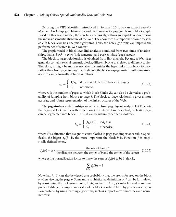
636 Chapter 10 Mining Object, Spatial, Multimedia, Text, and Web Data
By using the VIPS algorithm introduced in Section 10.5.1, we can extract page-to-block and block-to-page relationships and then construct a page graph and a block graph.Based on this graph model, the new link analysis algorithms are capable of discoveringthe intrinsic semantic structure of the Web. The above two assumptions become reason-able in block-level link analysis algorithms. Thus, the new algorithms can improve theperformance of search in Web context.
The graph model in block-level link analysis is induced from two kinds of relation-ships, that is, block-to-page (link structure) and page-to-block (page layout).
The block-to-page relationship is obtained from link analysis. Because a Web pagegenerally contains several semantic blocks, different blocks are related to different topics.Therefore, it might be more reasonable to consider the hyperlinks from block to page,rather than from page to page. Let Z denote the block-to-page matrix with dimensionn× k. Z can be formally defined as follows:
Zi j =
{
1/si, if there is a link from block i to page j
0, otherwise,(10.23)
where si is the number of pages to which block i links. Zi j can also be viewed as a prob-ability of jumping from block i to page j. The block-to-page relationship gives a moreaccurate and robust representation of the link structures of the Web.
The page-to-block relationships are obtained from page layout analysis. Let X denotethe page-to-block matrix with dimension k× n. As we have described, each Web pagecan be segmented into blocks. Thus, X can be naturally defined as follows:
Xi j =
{
fpi(b j), if b j ∈ pi
0, otherwise,(10.24)
where f is a function that assigns to every block b in page p an importance value. Speci-fically, the bigger fp(b) is, the more important the block b is. Function f is empi-rically defined below,
fp(b) = α× the size of block bthe distance between the center of b and the center of the screen
, (10.25)
where α is a normalization factor to make the sum of fp(b) to be 1, that is,
∑b∈p
fp(b) = 1
Note that fp(b) can also be viewed as a probability that the user is focused on the blockb when viewing the page p. Some more sophisticated definitions of f can be formulatedby considering the background color, fonts, and so on. Also, f can be learned from someprelabeled data (the importance value of the blocks can be defined by people) as a regres-sion problem by using learning algorithms, such as support vector machines and neuralnetworks.

10.5 Mining the World Wide Web 637
Based on the block-to-page and page-to-block relations, a new Web page graph thatincorporates the block importance information can be defined as
WP
= XZ, (10.26)
where X is a k×n page-to-block matrix, and Z is a n×k block-to-page matrix. Thus WP
is a k× k page-to-page matrix.The block-level PageRank can be calculated on the new Web page graph. Experiments
have shown the powerfulness of block-level link analysis.
10.5.3 Mining Multimedia Data on the Web
A huge amount of multimedia data are available on the Web in different forms. Theseinclude video, audio, images, pictures, and graphs. There is an increasing demand foreffective methods for organizing and retrieving such multimedia data.
Compared with the general-purpose multimedia data mining, the multimedia dataon the Web bear many different properties. Web-based multimedia data are embeddedon the Web page and are associated with text and link information. These texts and linkscan also be regarded as features of the multimedia data. Using some Web page layoutmining techniques (like VIPS), a Web page can be partitioned into a set of semantic blocks.Thus, the block that contains multimedia data can be regarded as a whole. Searching andorganizing the Web multimedia data can be referred to as searching and organizing themultimedia blocks.
Let’s consider Web images as an example. Figures 10.7 and 10.9 already show thatVIPS can help identify the surrounding text for Web images. Such surrounding text pro-vides a textual description of Web images and can be used to build an image index. TheWeb image search problem can then be partially completed using traditional text searchtechniques. Many commercial Web image search engines, such as Google and Yahoo!,use such approaches.
The block-level link analysis technique described in Section 10.5.2 can be used toorganize Web images. In particular, the image graph deduced from block-level link anal-ysis can be used to achieve high-quality Web image clustering results.
To construct a Web-image graph, in addition to the block-to-page and page-to-blockrelations, we need to consider a new relation: block-to-image relation. Let Y denote theblock-to-image matrix with dimension n×m. For each image, at least one block containsthis image. Thus, Y can be simply defined below:
Yi j =
{
1/si, if I j ∈ bi
0, otherwise,(10.27)
where si is the number of images contained in the image block bi.
Now we first construct the block graph from which the image graph can be furtherinduced. In block-level link analysis, the block graph is defined as:
WB
= (1− t)ZX + tD−1U, (10.28)
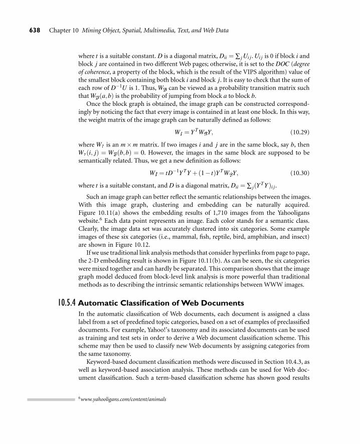
638 Chapter 10 Mining Object, Spatial, Multimedia, Text, and Web Data
where t is a suitable constant. D is a diagonal matrix, Dii = ∑ j Ui j. Ui j is 0 if block i andblock j are contained in two different Web pages; otherwise, it is set to the DOC (degreeof coherence, a property of the block, which is the result of the VIPS algorithm) value ofthe smallest block containing both block i and block j. It is easy to check that the sum ofeach row of D−1U is 1. Thus, W
Bcan be viewed as a probability transition matrix such
that WB
(a,b) is the probability of jumping from block a to block b.Once the block graph is obtained, the image graph can be constructed correspond-
ingly by noticing the fact that every image is contained in at least one block. In this way,the weight matrix of the image graph can be naturally defined as follows:
WI
= Y TWB
Y, (10.29)
where WI
is an m×m matrix. If two images i and j are in the same block, say b, thenW
I(i, j) = W
B(b,b) = 0. However, the images in the same block are supposed to be
semantically related. Thus, we get a new definition as follows:
WI
= tD−1Y TY +(1− t)Y TWB
Y, (10.30)
where t is a suitable constant, and D is a diagonal matrix, Dii = ∑ j(Y TY )i j.
Such an image graph can better reflect the semantic relationships between the images.With this image graph, clustering and embedding can be naturally acquired.Figure 10.11(a) shows the embedding results of 1,710 images from the Yahooliganswebsite.6 Each data point represents an image. Each color stands for a semantic class.Clearly, the image data set was accurately clustered into six categories. Some exampleimages of these six categories (i.e., mammal, fish, reptile, bird, amphibian, and insect)are shown in Figure 10.12.
If we use traditional link analysis methods that consider hyperlinks from page to page,the 2-D embedding result is shown in Figure 10.11(b). As can be seen, the six categorieswere mixed together and can hardly be separated. This comparison shows that the imagegraph model deduced from block-level link analysis is more powerful than traditionalmethods as to describing the intrinsic semantic relationships between WWW images.
10.5.4 Automatic Classification of Web DocumentsIn the automatic classification of Web documents, each document is assigned a classlabel from a set of predefined topic categories, based on a set of examples of preclassifieddocuments. For example, Yahoo!’s taxonomy and its associated documents can be usedas training and test sets in order to derive a Web document classification scheme. Thisscheme may then be used to classify new Web documents by assigning categories fromthe same taxonomy.
Keyword-based document classification methods were discussed in Section 10.4.3, aswell as keyword-based association analysis. These methods can be used for Web doc-ument classification. Such a term-based classification scheme has shown good results
6www.yahooligans.com/content/animals

10.5 Mining the World Wide Web 639
Figure 10.11 2-D embedding of the WWW images. (a) The image graph is constructed using block-levellink analysis. Each color (shape) represents a semantic category. Clearly, they are well sepa-rated. (b) The image graph was constructed based on traditional perspective that the hyper-links are considered from pages to pages. The image graph was induced from the page-to-pageand page-to-image relationships.
Mammal Amphibian Insect
Bird Reptile Fish
Figure 10.12 Six image categories.
in Web page classification. However, because a Web page may contain multiple themes,advertisement, and navigation information, block-based page content analysis may play animportant role in construction of high-quality classification models. Moreover, becausehyperlinks contain high-quality semantic clues to a page’s topic, it is beneficial to make

640 Chapter 10 Mining Object, Spatial, Multimedia, Text, and Web Data
good use of such semantic information in order to achieve even better accuracy thanpure keyword-based classification. Note that because the hyperlinks surrounding a doc-ument may be quite noisy, naïve use of terms in a document’s hyperlink neighborhoodcan even degrade accuracy. The use of block-based Web linkage analysis as introducedin the previous subsections will reduce such noise and enhance the quality of Webdocument classification.
There have been extensive research activities on the construction and use of thesemantic Web, a Web information infrastructure that is expected to bring structure tothe Web based on the semantic meaning of the contents of Web pages. Web documentclassification by Web mining will help in the automatic extraction of the semanticmeaning of Web pages and build up ontology for the semantic Web. Conversely, thesemantic Web, if successfully constructed, will greatly help automated Web documentclassification as well.
10.5.5 Web Usage Mining
“What is Web usage mining?” Besides mining Web contents and Web linkage structures,another important task for Web mining is Web usage mining, which mines Weblogrecords to discover user access patterns of Web pages. Analyzing and exploring regulari-ties in Weblog records can identify potential customers for electronic commerce, enhancethe quality and delivery of Internet information services to the end user, and improveWeb server system performance.
A Web server usually registers a (Web) log entry, or Weblog entry, for every access ofa Web page. It includes the URL requested, the IP address from which the request orig-inated, and a timestamp. For Web-based e-commerce servers, a huge number of Webaccess log records are being collected. Popular websites may register Weblog records inthe order of hundreds of megabytes every day. Weblog databases provide rich informa-tion about Web dynamics. Thus it is important to develop sophisticated Weblog miningtechniques.
In developing techniques for Web usage mining, we may consider the following. First,although it is encouraging and exciting to imagine the various potential applications ofWeblog file analysis, it is important to know that the success of such applications dependson what and how much valid and reliable knowledge can be discovered from the largeraw log data. Often, raw Weblog data need to be cleaned, condensed, and transformedin order to retrieve and analyze significant and useful information. In principle, thesepreprocessing methods are similar to those discussed in Chapter 2, although Weblogcustomized preprocessing is often needed.
Second, with the available URL, time, IP address, and Web page content information,a multidimensional view can be constructed on the Weblog database, and multidimen-sional OLAP analysis can be performed to find the top N users, top N accessed Web pages,most frequently accessed time periods, and so on, which will help discover potential cus-tomers, users, markets, and others.
Third, data mining can be performed on Weblog records to find association patterns,sequential patterns, and trends of Web accessing. For Web access pattern mining, it is

10.6 Summary 641
often necessary to take further measures to obtain additional information of user traversalto facilitate detailed Weblog analysis. Such additional information may include user-browsing sequences of the Web pages in the Web server buffer.
With the use of such Weblog files, studies have been conducted on analyzing systemperformance, improving system design by Web caching, Web page prefetching, and Webpage swapping; understanding the nature of Web traffic; and understanding user reactionand motivation. For example, some studies have proposed adaptive sites: websites thatimprove themselves by learning from user access patterns. Weblog analysis may also helpbuild customized Web services for individual users.
Because Weblog data provide information about what kind of users will access whatkind of Web pages, Weblog information can be integrated with Web content and Weblinkage structure mining to help Web page ranking, Web document classification, and theconstruction of a multilayered Web information base as well. A particularly interestingapplication of Web usage mining is to mine a user’s interaction history and search contexton the client side to extract useful information for improving the ranking accuracy forthe given user. For example, if a user submits a keyword query “Java” to a search engine,and then selects “Java programming language” from the returned entries for viewing,the system can infer that the displayed snippet for this Web page is interesting to theuser. It can then raise the rank of pages similar to “Java programming language” andavoid presenting distracting pages about “Java Island.” Hence the quality of search isimproved, because search is contextualized and personalized.
10.6 Summary
Vast amounts of data are stored in various complex forms, such as structured orunstructured, hypertext, and multimedia. Thus, mining complex types of data, includ-ing object data, spatial data, multimedia data, text data, and Web data, has become anincreasingly important task in data mining.
Multidimensional analysis and data mining can be performed in object-relationaland object-oriented databases, by (1) class-based generalization of complex objects,including set-valued, list-valued, and other sophisticated types of data, class/subclasshierarchies, and class composition hierarchies; (2) constructing object data cubes; and(3) performing generalization-based mining. A plan database can be mined by ageneralization-based, divide-and-conquer approach in order to find interesting gen-eral patterns at different levels of abstraction.
Spatial data mining is the discovery of interesting patterns from large geospatialdatabases. Spatial data cubes that contain spatial dimensions and measures can beconstructed. Spatial OLAP can be implemented to facilitate multidimensional spatialdata analysis. Spatial data mining includes mining spatial association and co-locationpatterns, clustering, classification, and spatial trend and outlier analysis.
Multimedia data mining is the discovery of interesting patterns from multimediadatabases that store and manage large collections of multimedia objects, including

642 Chapter 10 Mining Object, Spatial, Multimedia, Text, and Web Data
audio data, image data, video data, sequence data, and hypertext data containingtext, text markups, and linkages. Issues in multimedia data mining include content-based retrieval and similarity search, and generalization and multidimensional analysis.Multimedia data cubes contain additional dimensions and measures for multimediainformation. Other topics in multimedia mining include classification and predictionanalysis, mining associations, and audio and video data mining.
A substantial portion of the available information is stored in text or documentdatabases that consist of large collections of documents, such as news articles, techni-cal papers, books, digital libraries, e-mail messages, and Web pages. Text informationretrieval and data mining has thus become increasingly important. Precision, recall,and the F-score are three based measures from Information Retrieval (IR). Varioustext retrieval methods have been developed. These typically either focus on documentselection (where the query is regarded as providing constraints) or document ranking(where the query is used to rank documents in order of relevance). The vector-spacemodel is a popular example of the latter kind. Latex Sementic Indexing (LSI), LocalityPreserving Indexing (LPI), and Probabilistic LSI can be used for text dimensionalityreduction. Text mining goes one step beyond keyword-based and similarity-basedinformation retrieval and discovers knowledge from semistructured text data usingmethods such as keyword-based association analysis, document classification, and doc-ument clustering.
The World Wide Web serves as a huge, widely distributed, global information ser-vice center for news, advertisements, consumer information, financial management,education, government, e-commerce, and many other services. It also contains a richand dynamic collection of hyperlink information, and access and usage information,providing rich sources for data mining. Web mining includes mining Web linkagestructures, Web contents, and Web access patterns. This involves mining the Web pagelayout structure, mining the Web’s link structures to identify authoritative Web pages,mining multimedia data on the Web, automatic classification of Web documents, andWeb usage mining.
Exercises
10.1 An object cube can be constructed by generalization of an object-oriented or object-relational database into relatively structured data before performing multidimensionalanalysis. Because a set of complex data objects or properties can be generalized in mul-tiple directions and thus derive multiple generalized features, such generalization maylead to a high-dimensional, but rather sparse (generalized) “object cube.” Discuss howto perform effective online analytical processing in such an object cube.
10.2 A heterogeneous database system consists of multiple database systems that are definedindependently, but that need to exchange and transform information among themselvesand answer local and global queries. Discuss how to process a descriptive mining queryin such a system using a generalization-based approach.

Exercises 643
10.3 A plan database consists of a set of action sequences, such as legs of connecting flights,which can be generalized to find generalized sequence plans. Similarly, a structure databasemay consists of a set of structures, such as trees or graphs, which may also be generalizedto find generalized structures. Outline a scalable method that may effectively performsuch generalized structure mining.
10.4 Suppose that a city transportation department would like to perform data analysis onhighway traffic for the planning of highway construction based on the city traffic datacollected at different hours every day.
(a) Design a spatial data warehouse that stores the highway traffic information so thatpeople can easily see the average and peak time traffic flow by highway, by time ofday, and by weekdays, and the traffic situation when a major accident occurs.
(b) What information can we mine from such a spatial data warehouse to help cityplanners?
(c) This data warehouse contains both spatial and temporal data. Propose one miningtechnique that can efficiently mine interesting patterns from such a spatiotemporaldata warehouse.
10.5 Spatial association mining can be implemented in at least two ways: (1) dynamic com-putation of spatial association relationships among different spatial objects, based onthe mining query, and (2) precomputation of spatial distances between spatial objects,where the association mining is based on such precomputed results. Discuss (1) how toimplement each approach efficiently and (2) which approach is preferable under whatsituation.
10.6 Traffic situations are often auto-correlated: the congestion at one highway intersectionmay trigger the congestion in nearby highway segments after a short period of time.Suppose we are given highway traffic history data in Chicago, including road construc-tion segment, traffic speed associated with highway segment, direction, time, and so on.Moreover, we are given weather conditions by weather bureau in Chicago. Design a datamining method to find high-quality spatiotemporal association rules that may guide us topredict what could be the expected traffic situation at a given highway location.
10.7 Similarity search in multimedia has been a major theme in developing multimedia dataretrieval systems. However, many multimedia data mining methods are based on the anal-ysis of isolated simple multimedia features, such as color, shape, description, keywords,and so on.
(a) Can you show that an integration of similarity-based search with data mining maybring important progress in multimedia data mining? You may take any one miningtask as an example, such as multidimensional analysis, classification, association, orclustering.
(b) Outline an implementation technique that applies a similarity-based search methodto enhance the quality of clustering in multimedia data.

644 Chapter 10 Mining Object, Spatial, Multimedia, Text, and Web Data
10.8 It is challenging but important to discover unusual events from video data in real time orin a very short time frame. An example is the detection of an explosion near a bus stopor a car collision at a highway junction. Outline a video data mining method that can beused for this purpose.
10.9 Precision and recall are two essential quality measures of an information retrieval system.
(a) Explain why it is the usual practice to trade one measure for the other. Explain whythe F-score is a good measure for this purpose.
(b) Illustrate the methods that may effectively improve the F-score in an informationretrieval system.
10.10 TF-IDF has been used as an effective measure in document classification.
(a) Give one example to show that TF-IDF may not be always a good measure in docu-ment classification.
(b) Define another measure that may overcome this difficulty.
10.11 An e-mail database is a database that stores a large number of electronic mail (e-mail)messages. It can be viewed as a semistructured database consisting mainly of text data.Discuss the following.
(a) How can such an e-mail database be structured so as to facilitate multidimensionalsearch, such as by sender, by receiver, by subject, and by time?
(b) What can be mined from such an e-mail database?
(c) Suppose you have roughly classified a set of your previous e-mail messages as junk,unimportant, normal, or important. Describe how a data mining system may takethis as the training set to automatically classify new e-mail messages or unclassifiedones.
10.12 Junk e-mail is one of the most annoying things in Web-based business or personal com-munications. Design an effective scheme (which may consist of a set of methods) thatcan be used to filter out junk e-mails effectively and discuss how such methods should beevolved along with time.
10.13 It is difficult to construct a global data warehouse for the World Wide Web due to itsdynamic nature and the huge amounts of data stored in it. However, it is still interestingand useful to construct data warehouses for summarized, localized, multidimensionalinformation on the Internet. Suppose that an Internet information service companywould like to set up an Internet-based data warehouse to help tourists choose local hotelsand restaurants.
(a) Can you design a Web-based tourist data warehouse that would facilitate such aservice?
(b) Suppose each hotel and/or restaurant contains a Web page of its own. Discuss howto locate such Web pages and what methods should be used to extract informationfrom these Web pages in order to populate your Web-based tourist data warehouse.

Bibliographic Notes 645
(c) Discuss how to implement a mining method that may provide additional associ-ated information, such as “90% of customers who stay at the Downtown Hilton dineat the Emperor Garden Restaurant at least twice,” each time a search returns a newWeb page.
10.14 Each scientific or engineering discipline has its own subject index classification standardthat is often used for classifying documents in its discipline.
(a) Design a Web document classification method that can take such a subject index toclassify a set of Web documents automatically.
(b) Discuss how to use Web linkage information to improve the quality of such classifi-cation.
(c) Discuss how to use Web usage information to improve the quality of such classifica-tion.
10.15 It is interesting to cluster a large set of Web pages based on their similarity.
(a) Discuss what should be the similarity measure in such cluster analysis.
(b) Discuss how the block-level analysis may influence the clustering results and how todevelop an efficient algorithms based on this philosophy.
(c) Since different users may like to cluster a set of Web pages differently, discuss howa user may interact with a system to influence the final clustering results, and howsuch a mechanism can be developed systematically.
10.16 Weblog records provide rich Web usage information for data mining.
(a) Mining Weblog access sequences may help prefetch certain Web pages into a Webserver buffer, such as those pages that are likely to be requested in the next severalclicks. Design an efficient implementation method that may help mining such accesssequences.
(b) Mining Weblog access records can help cluster users into separate groups to facilitatecustomized marketing. Discuss how to develop an efficient implementation methodthat may help user clustering.
Bibliographic Notes
Mining complex types of data has been a fast-developing, popular research field, withmany research papers and tutorials appearing in conferences and journals on data miningand database systems. This chapter covers a few important themes, including multidi-mensional analysis and mining of complex data objects, spatial data mining, multimediadata mining, text mining, and Web mining.
Zaniolo, Ceri, Faloutsos, et al. [ZCF+97] present a systematic introduction of adva-nced database systems for handling complex types of data. For multidimensional anal-ysis and mining of complex data objects, Han, Nishio, Kawano, and Wang [HNKW98]

646 Chapter 10 Mining Object, Spatial, Multimedia, Text, and Web Data
proposed a method for the design and construction of object cubes by multidimensionalgeneralization and its use for mining complex types of data in object-oriented and object-relational databases. A method for the construction of multiple-layered databases bygeneralization-based data mining techniques for handling semantic heterogeneity wasproposed by Han, Ng, Fu, and Dao [HNFD98]. Zaki, Lesh, and Ogihara worked outa system called PlanMine, which applies sequence mining for plan failures [ZLO98].A generalization-based method for mining plan databases by divide-and-conquer wasproposed by Han, Yang, and Kim [HYK99].
Geospatial database systems and spatial data mining have been studied extensively.Some introductory materials about spatial database can be found in Maguire, Goodchild,and Rhind [MGR92], Güting [Gue94], Egenhofer [Ege89], Shekhar, Chawla, Ravada,et al. [SCR+99], Rigaux, Scholl, and Voisard [RSV01], and Shekhar and Chawla [SC03].For geospatial data mining, a comprehensive survey on spatial data mining methods canbe found in Ester, Kriegel, and Sander [EKS97] and Shekhar and Chawla [SC03]. A col-lection of research contributions on geographic data mining and knowledge discoveryare in Miller and Han [MH01b]. Lu, Han, and Ooi [LHO93] proposed a generalization-based spatial data mining method by attribute-oriented induction. Ng and Han [NH94]proposed performing descriptive spatial data analysis based on clustering results insteadof on predefined concept hierarchies. Zhou, Truffet, and Han proposed efficient poly-gon amalgamation methods for on-line multidimensional spatial analysis and spatialdata mining [ZTH99]. Stefanovic, Han, and Koperski [SHK00] studied the problemsassociated with the design and construction of spatial data cubes. Koperski and Han[KH95] proposed a progressive refinement method for mining spatial association rules.Knorr and Ng [KN96] presented a method for mining aggregate proximity relationshipsand commonalities in spatial databases. Spatial classification and trend analysis methodshave been developed by Ester, Kriegel, Sander, and Xu [EKSX97] and Ester, Frommelt,Kriegel, and Sander [EFKS98]. A two-step method for classification of spatial data wasproposed by Koperski, Han, and Stefanovic [KHS98].
Spatial clustering is a highly active area of recent research into geospatial data mining.For a detailed list of references on spatial clustering methods, please see the bibliographicnotes of Chapter 7. A spatial data mining system prototype, GeoMiner, was developedby Han, Koperski, and Stefanovic [HKS97]. Methods for mining spatiotemporal pat-terns have been studied by Tsoukatos and Gunopulos [TG01], Hadjieleftheriou, Kol-lios, Gunopulos, and Tsotras [HKGT03], and Mamoulis, Cao, Kollios, Hadjieleftheriou,et al. [MCK+04]. Mining spatiotemporal information related to moving objects havebeen studied by Vlachos, Gunopulos, and Kollios [VGK02] and Tao, Faloutsos, Papa-dias, and Liu [TFPL04]. A bibliography of temporal, spatial, and spatiotemporal datamining research was compiled by Roddick, Hornsby, and Spiliopoulou [RHS01].
Multimedia data mining has deep roots in image processing and pattern recogni-tion, which has been studied extensively in computer science, with many textbookspublished, such as Gonzalez and Woods [GW02], Russ [Rus02], and Duda, Hart,and Stork [DHS01]. The theory and practice of multimedia database systems havebeen introduced in many textbooks and surveys, including Subramanian [Sub98], Yuand Meng [YM97], Perner [Per02], and Mitra and Acharya [MA03]. The IBM QBIC
Bibliographic Notes 647
(Query by Image and Video Content) system was introduced by Flickner, Sawhney,Niblack, Ashley, et al. [FSN+95]. Faloutsos and Lin [FL95] developed a fast algo-rithm, FastMap, for indexing, data mining, and visualization of traditional and mul-timedia datasets. Natsev, Rastogi, and Shim [NRS99] developed WALRUS, a simi-larity retrieval algorithm for image databases that explores wavelet-based signatureswith region-based granularity. Fayyad and Smyth [FS93] developed a classificationmethod to analyze high-resolution radar images for identification of volcanoes onVenus. Fayyad, Djorgovski, and Weir [FDW96] applied decision tree methods to theclassification of galaxies, stars, and other stellar objects in the Palomar ObservatorySky Survey (POSS-II) project. Stolorz and Dean [SD96] developed Quakefinder, a datamining system for detecting earthquakes from remote sensing imagery. Zaïane, Han,and Zhu [ZHZ00] proposed a progressive deepening method for mining object andfeature associations in large multimedia databases. A multimedia data mining systemprototype, MultiMediaMiner, was developed by Zaïane, Han, Li, et al. [ZHL+98] as anextension of the DBMiner system proposed by Han, Fu, Wang, et al. [HFW+96]. Anoverview of image mining methods is performed by Hsu, Lee, and Zhang [HLZ02].
Text data analysis has been studied extensively in information retrieval, with manygood textbooks and survey articles, such as Salton and McGill [SM83], Faloutsos [Fal85],Salton [Sal89], van Rijsbergen [vR90], Yu and Meng [YM97], Raghavan [Rag97], Sub-ramanian [Sub98], Baeza-Yates and Riberio-Neto [BYRN99], Kleinberg and Tomkins[KT99], Berry [Ber03], and Weiss, Indurkhya, Zhang, and Damerau [WIZD04]. Thetechnical linkage between information filtering and information retrieval was addressedby Belkin and Croft [BC92]. The latent semantic indexing method for document sim-ilarity analysis was developed by Deerwester, Dumais, Furnas, et al. [DDF+90]. Theprobabilistic latent semantic analysis method was introduced to information retrieval byHofmann [Hof98]. The locality preserving indexing method for document representa-tion was developed by He, Cai, Liu, and Ma [HCLM04]. The use of signature files isdescribed in Tsichritzis and Christodoulakis [TC83]. Feldman and Hirsh [FH98] stud-ied methods for mining association rules in text databases. Method for automated docu-ment classification has been studied by many researchers, such as Wang, Zhou, and Liew[WZL99], Nigam, McCallum, Thrun, and Mitchell [NMTM00] and Joachims [Joa01].An overview of text classification is given by Sebastiani [Seb02]. Document clustering byProbabilistic Latent Semantic Analysis (PLSA) was introduced by Hofmann [Hof98] andthat using the Latent Dirichlet Allocation (LDA) method was proposed by Blei, Ng, andJordan [BNJ03]. Zhai, Velivelli, and Yu [ZVY04] studied using such clustering methodsto facilitate comparative analysis of documents. A comprehensive study of using dimen-sionality reduction methods for document clustering can be found in Cai, He, and Han[CHH05].
Web mining started in recent years together with the development of Web searchengines and Web information service systems. There has been a great deal of workon Web data modeling and Web query systems, such as W3QS by Konopnicki andShmueli [KS95], WebSQL by Mendelzon, Mihaila, and Milo [MMM97], Lorel by Abit-boul, Quass, McHugh, et al. [AQM+97], Weblog by Lakshmanan, Sadri, and Subra-manian [LSS96], WebOQL by Arocena and Mendelzon [AM98], and NiagraCQ by

648 Chapter 10 Mining Object, Spatial, Multimedia, Text, and Web Data
Chen, DeWitt, Tian, and Wang [CDTW00]. Florescu, Levy, and Mendelzon [FLM98]presented a comprehensive overview of research on Web databases. An introduction tothe the semantic Web was presented by Berners-Lee, Hendler, and Lassila [BLHL01].
Chakrabarti [Cha02] presented a comprehensive coverage of data mining for hyper-text and the Web. Mining the Web’s link structures to recognize authoritative Web pageswas introduced by Chakrabarti, Dom, Kumar, et al. [CDK+99] and Kleinberg andTomkins [KT99]. The HITS algorithm was developed by Kleinberg [Kle99]. The Page-Rank algorithm was developed by Brin and Page [BP98b]. Embley, Jiang, and Ng [EJN99]developed some heuristic rules based on the DOM structure to discover record bound-aries within a page, which assist data extraction from the Web page. Wong and Fu [WF00]defined tag types for page segmentation and gave a label to each part of the Web pagefor assisting classification. Chakrabarti et al. [Cha01, CJT01] addressed the fine-grainedtopic distillation and disaggregated hubs into regions by analyzing DOM structure aswell as intrapage text distribution. Lin and Ho [LH02] considered 〈TABLE〉 tag and itsoffspring as a content block and used an entropy-based approach to discover informa-tive ones. Bar-Yossef and Rajagopalan [BYR02] proposed the template detection prob-lem and presented an algorithm based on the DOM structure and the link information.Cai et al. [CYWM03, CHWM04] proposed the Vision-based Page Segmentation algo-rithm and developed the block-level link analysis techniques. They have also successfullyapplied the block-level link analysis on Web search [CYWM04] and Web image organiz-ing and mining [CHM+04, CHL+04].
Web page classification was studied by Chakrabarti, Dom, and Indyk [CDI98] andWang, Zhou, and Liew [WZL99]. A multilayer database approach for constructing a Webwarehouse was studied by Zaïane and Han [ZH95]. Web usage mining has been pro-moted and implemented by many industry firms. Automatic construction of adaptivewebsites based on learning from Weblog user access patterns was proposed by Perkowitzand Etzioni [PE99]. The use of Weblog access patterns for exploring Web usability wasstudied by Tauscher and Greenberg [TG97]. A research prototype system, WebLogMiner,was reported by Zaïane, Xin, and Han [ZXH98]. Srivastava, Cooley, Deshpande, and Tan[SCDT00] presented a survey of Web usage mining and its applications. Shen, Tan, andZhai used Weblog search history to facilitate context-sensitive information retrieval andpersonalized Web search [STZ05].

11Applications and Trends inData Mining
As a young research field, data mining has made broad and significant progress since its earlybeginnings in the 1980s. Today, data mining is used in a vast array of areas, and numerouscommercial data mining systems are available. Many challenges, however, still remain.In this final chapter, we study applications and trends in data mining. We begin by view-ing data mining applications in business and in science. We then provide tips on what toconsider when purchasing a data mining software system. Additional themes in datamining are described, such as theoretical foundations of data mining, statistical tech-niques for data mining, visual and audio mining, and collaborative recommender sys-tems that incorporate data mining techniques. The social impacts of data mining arediscussed, including ubiquitous and invisible data mining and privacy issues. Finally, weexamine current and expected data mining trends that arise in response to challenges inthe field.
11.1 Data Mining Applications
In the previous chapters of this book, we have studied principles and methods formining relational data, data warehouses, and complex types of data (including streamdata, time-series and sequence data, complex structured data, spatiotemporal data,multimedia data, heterogeneous multidatabase data, text data, and Web data). Becausedata mining is a relatively young discipline with wide and diverse applications, thereis still a nontrivial gap between general principles of data mining and application-specific, effective data mining tools. In this section, we examine a few applicationdomains and discuss how customized data mining tools should be developed for suchapplications.
11.1.1 Data Mining for Financial Data Analysis
Most banks and financial institutions offer a wide variety of banking services (such aschecking and savings accounts for business or individual customers), credit (such as
649

650 Chapter 11 Applications and Trends in Data Mining
business, mortgage, and automobile loans), and investment services (such as mutualfunds). Some also offer insurance services and stock investment services.
Financial data collected in the banking and financial industry are often relatively com-plete, reliable, and of high quality, which facilitates systematic data analysis and datamining. Here we present a few typical cases:
Design and construction of data warehouses for multidimensional data analysis anddata mining: Like many other applications, data warehouses need to be constructedfor banking and financial data. Multidimensional data analysis methods should beused to analyze the general properties of such data. For example, one may like to viewthe debt and revenue changes by month, by region, by sector, and by other factors,along with maximum, minimum, total, average, trend, and other statistical infor-mation. Data warehouses, data cubes, multifeature and discovery-driven data cubes,characterization and class comparisons, and outlier analysis all play important rolesin financial data analysis and mining.
Loan payment prediction and customer credit policy analysis: Loan payment predic-tion and customer credit analysis are critical to the business of a bank. Many factorscan strongly or weakly influence loan payment performance and customer credit rat-ing. Data mining methods, such as attribute selection and attribute relevance ranking,may help identify important factors and eliminate irrelevant ones. For example, fac-tors related to the risk of loan payments include loan-to-value ratio, term of the loan,debt ratio (total amount of monthly debt versus the total monthly income), payment-to-income ratio, customer income level, education level, residence region, and credithistory. Analysis of the customer payment history may find that, say, payment-to-income ratio is a dominant factor, while education level and debt ratio are not. Thebank may then decide to adjust its loan-granting policy so as to grant loans to thosecustomers whose applications were previously denied but whose profiles show rela-tively low risks according to the critical factor analysis.
Classification and clustering of customers for targeted marketing: Classification andclustering methods can be used for customer group identification and targeted mar-keting. For example, we can use classification to identify the most crucial factorsthat may influence a customer’s decision regarding banking. Customers with similarbehaviors regarding loan payments may be identified by multidimensional clusteringtechniques. These can help identify customer groups, associate a new customer withan appropriate customer group, and facilitate targeted marketing.
Detection of money laundering and other financial crimes: To detect money laun-dering and other financial crimes, it is important to integrate information from mul-tiple databases (like bank transaction databases, and federal or state crime historydatabases), as long as they are potentially related to the study. Multiple data analysistools can then be used to detect unusual patterns, such as large amounts of cash flowat certain periods, by certain groups of customers. Useful tools include data visual-ization tools (to display transaction activities using graphs by time and by groupsof customers), linkage analysis tools (to identify links among different customers

11.1 Data Mining Applications 651
and activities), classification tools (to filter unrelated attributes and rank the highlyrelated ones), clustering tools (to group different cases), outlier analysis tools (todetect unusual amounts of fund transfers or other activities), and sequential patternanalysis tools (to characterize unusual access sequences). These tools may identifyimportant relationships and patterns of activities and help investigators focus onsuspicious cases for further detailed examination.
11.1.2 Data Mining for the Retail Industry
The retail industry is a major application area for data mining, since it collects hugeamounts of data on sales, customer shopping history, goods transportation, consump-tion, and service. The quantity of data collected continues to expand rapidly, especiallydue to the increasing ease, availability, and popularity of business conducted on the Web,or e-commerce. Today, many stores also have websites where customers can make pur-chases on-line. Some businesses, such as Amazon.com (www.amazon.com), exist solelyon-line, without any brick-and-mortar (i.e., physical) store locations. Retail data providea rich source for data mining.
Retail data mining can help identify customer buying behaviors, discover customershopping patterns and trends, improve the quality of customer service, achieve bet-ter customer retention and satisfaction, enhance goods consumption ratios, designmore effective goods transportation and distribution policies, and reduce the cost ofbusiness.
A few examples of data mining in the retail industry are outlined as follows.
Design and construction of data warehouses based on the benefits of data mining:Because retail data cover a wide spectrum (including sales, customers, employees,goods transportation, consumption, and services), there can be many ways to design adata warehouse for this industry. The levels of detail to include may also vary substan-tially. The outcome of preliminary data mining exercises can be used to help guide thedesign and development of data warehouse structures. This involves deciding whichdimensions and levels to include and what preprocessing to perform in order to facil-itate effective data mining.
Multidimensional analysis of sales, customers, products, time, and region: The retailindustry requires timely information regarding customer needs, product sales, trends,and fashions, as well as the quality, cost, profit, and service of commodities. It is there-fore important to provide powerful multidimensional analysis and visualization tools,including the construction of sophisticated data cubes according to the needs of dataanalysis. The multifeature data cube, introduced in Chapter 4, is a useful data struc-ture in retail data analysis because it facilitates analysis on aggregates with complexconditions.
Analysis of the effectiveness of sales campaigns: The retail industry conducts salescampaigns using advertisements, coupons, and various kinds of discounts and bonusesto promote products and attract customers. Careful analysis of the effectiveness

652 Chapter 11 Applications and Trends in Data Mining
of sales campaigns can help improve company profits. Multidimensional analysis canbe used for this purpose by comparing the amount of sales and the number of trans-actions containing the sales items during the sales period versus those containing thesame items before or after the sales campaign. Moreover, association analysis may dis-close which items are likely to be purchased together with the items on sale, especiallyin comparison with the sales before or after the campaign.
Customer retention—analysis of customer loyalty: With customer loyalty card infor-mation, one can register sequences of purchases of particular customers. Customerloyalty and purchase trends can be analyzed systematically. Goods purchased at differ-ent periods by the same customers can be grouped into sequences. Sequential patternmining (Chapter 8) can then be used to investigate changes in customer consump-tion or loyalty and suggest adjustments on the pricing and variety of goods in orderto help retain customers and attract new ones.
Product recommendation and cross-referencing of items: By mining associationsfrom sales records, one may discover that a customer who buys a digital camera islikely to buy another set of items. Such information can be used to form productrecommendations. Collaborative recommender systems use data mining techniquesto make personalized product recommendations during live customer transactions,based on the opinions of other customers (Section 11.3.4). Product recommenda-tions can also be advertised on sales receipts, in weekly flyers, or on the Web to helpimprove customer service, aid customers in selecting items, and increase sales. Sim-ilarly, information such as “hot items this week” or attractive deals can be displayedtogether with the associative information in order to promote sales.
11.1.3 Data Mining for the Telecommunication Industry
The telecommunication industry has quickly evolved from offering local and long-distance telephone services to providing many other comprehensive communication ser-vices, including fax, pager, cellular phone, Internet messenger, images, e-mail, computerand Web data transmission, and other data traffic. The integration of telecommunica-tion, computer network, Internet, and numerous other means of communication andcomputing is also underway. Moreover, with the deregulation of the telecommunicationindustry in many countries and the development of new computer and communicationtechnologies, the telecommunication market is rapidly expanding and highly competi-tive. This creates a great demand for data mining in order to help understand the businessinvolved, identify telecommunication patterns, catch fraudulent activities, make betteruse of resources, and improve the quality of service.
The following are a few scenarios for which data mining may improve telecommu-nication services:
Multidimensional analysis of telecommunication data: Telecommunication data areintrinsically multidimensional, with dimensions such as calling-time, duration,location of caller, location of callee, and type of call. The multidimensional analysis

11.1 Data Mining Applications 653
of such data can be used to identify and compare the data traffic, system workload,resource usage, user group behavior, and profit. For example, analysts in the industrymay wish to regularly view charts and graphs regarding calling source, destination,volume, and time-of-day usage patterns. Therefore, it is often useful to consolidatetelecommunication data into large data warehouses and routinely perform multidi-mensional analysis using OLAP and visualization tools.
Fraudulent pattern analysis and the identification of unusual patterns: Fraudu-lent activity costs the telecommunication industry millions of dollars per year. Itis important to (1) identify potentially fraudulent users and their atypical usagepatterns; (2) detect attempts to gain fraudulent entry to customer accounts; and(3) discover unusual patterns that may need special attention, such as busy-hourfrustrated call attempts, switch and route congestion patterns, and periodic callsfrom automatic dial-out equipment (like fax machines) that have been improperlyprogrammed. Many of these patterns can be discovered by multidimensional analysis,cluster analysis, and outlier analysis.
Multidimensional association and sequential pattern analysis: The discovery of asso-ciation and sequential patterns in multidimensional analysis can be used to promotetelecommunication services. For example, suppose you would like to find usage pat-terns for a set of communication services by customer group, by month, and by timeof day. The calling records may be grouped by customer in the following form:
〈customer ID, residence,office, time,date, service 1, service 2, · · ·〉
A sequential pattern like “If a customer in the Los Angeles area works in a city differentfrom her residence, she is likely to first use long-distance service between two cities around5 p.m. and then use a cellular phone for at least 30 minutes in the subsequent hour everyweekday” can be further probed by drilling up and down in order to determine whetherit holds for particular pairs of cities and particular groups of persons (e.g., engineers,doctors). This can help promote the sales of specific long-distance and cellular phonecombinations and improve the availability of particular services in the region.
Mobile telecommunication services: Mobile telecommunication, Web and infor-mation services, and mobile computing are becoming increasingly integrated andcommon in our work and life. One important feature of mobile telecommunica-tion data is its association with spatiotemporal information. Spatiotemporal datamining may become essential for finding certain patterns. For example, unusuallybusy mobile phone traffic at certain locations may indicate something abnormalhappening in these locations. Moreover, ease of use is crucial for enticing cus-tomers to adopt new mobile services. Data mining will likely play a major role inthe design of adaptive solutions enabling users to obtain useful information withrelatively few keystrokes.
Use of visualization tools in telecommunication data analysis: Tools for OLAPvisualization, linkage visualization, association visualization, clustering, and outliervisualization have been shown to be very useful for telecommunication data analysis.

654 Chapter 11 Applications and Trends in Data Mining
11.1.4 Data Mining for Biological Data Analysis
The past decade has seen an explosive growth in genomics, proteomics, functionalgenomics, and biomedical research. Examples range from the identification and com-parative analysis of the genomes of human and other species (by discovering sequencingpatterns, gene functions, and evolution paths) to the investigation of genetic networksand protein pathways, and the development of new pharmaceuticals and advances incancer therapies. Biological data mining has become an essential part of a new researchfield called bioinformatics. Since the field of biological data mining is broad, rich, anddynamic, it is impossible to cover such an important and flourishing theme in one sub-section. Here we outline only a few interesting topics in this field, with an emphasison genomic and proteomic data analysis. A comprehensive introduction to biologicaldata mining could fill several books. A good set of bioinformatics and biological dataanalysis books have already been published, and more are expected to come. Referencesare provided in our bibliographic notes.
DNA sequences form the foundation of the genetic codes of all living organisms. AllDNA sequences are comprised of four basic building blocks, called nucleotides: adenine(A), cytosine (C), guanine (G), and thymine (T). These four nucleotides (or bases) arecombined to form long sequences or chains that resemble a twisted ladder. The DNAcarry the information and biochemical machinery that can be copied from generation togeneration. During the processes of “copying,” insertions, deletions, or mutations (alsocalled substitutions) of nucleotides are introduced into the DNA sequence, formingdifferent evolution paths. A gene usually comprises hundreds of individual nucleotidesarranged in a particular order. The nucleotides can be ordered and sequenced in analmost unlimited number of ways to form distinct genes. A genome is the complete setof genes of an organism. The human genome is estimated to contain around 20,000 to25,000 genes. Genomics is the analysis of genome sequences.
Proteins are essential molecules for any organism. They perform life functions andmake up the majority of cellular structures. The approximately 25,000 human genes giverise to about 1 million proteins through a series of translational modifications and genesplicing mechanisms. Amino acids (or residues) are the building blocks of proteins. Thereare 20 amino acids, denoted by 20 different letters of the alphabet. Each of the aminoacids is coded for by one or more triplets of nucleotides making up DNA. The end of thechain is coded for by another set of triplets. Thus, a linear string or sequence of DNA istranslated into a sequence of amino acids, forming a protein (Figure 11.1). A proteomeis the complete set of protein molecules present in a cell, tissue, or organism. Proteomicsis the study of proteome sequences. Proteomes are dynamic, changing from minute tominute in response to tens of thousands of intra- and extracellular environmental signals.
DNA sequence . . . CTA CAC ACG T GT AAC · · ·
amino acid sequence . . . L H T C N · · ·
Figure 11.1 A DNA sequence and corresponding amino acid sequence.

11.1 Data Mining Applications 655
Chemical properties of the amino acids cause the protein chains to fold up into specificthree-dimensional structures. This three-dimensional folding of the chain determinesthe biological function of a protein. Genes make up only about 2% of the human genome.The remainder consists of noncoding regions. Recent studies have found that a lot ofnoncoding DNA sequences may also have played crucial roles in protein generation andspecies evolution.
The identification of DNA or amino acid sequence patterns that play roles in variousbiological functions, genetic diseases, and evolution is challenging. This requires a greatdeal of research in computational algorithms, statistics, mathematical programming,data mining, machine learning, information retrieval, and other disciplines to developeffective genomic and proteomic data analysis tools.
Data mining may contribute to biological data analysis in the following aspects:
Semantic integration of heterogeneous, distributed genomic and proteomic data-bases: Genomic and proteomic data sets are often generated at different labs and bydifferent methods. They are distributed, heterogenous, and of a wide variety. Thesemantic integration of such data is essential to the cross-site analysis of biologicaldata. Moreover, it is important to find correct linkages between research literatureand their associated biological entities. Such integration and linkage analysis wouldfacilitate the systematic and coordinated analysis of genome and biological data.This has promoted the development of integrated data warehouses and distributedfederated databases to store and manage the primary and derived biological data.Data cleaning, data integration, reference reconciliation, classification, and clusteringmethods will facilitate the integration of biological data and the construction of datawarehouses for biological data analysis.
Alignment, indexing, similarity search, and comparative analysis of multiple nucleo-tide/protein sequences: Various biological sequence alignment methods have beendeveloped in the past two decades. BLAST and FASTA, in particular, are tools for thesystematic analysis of genomic and proteomic data. Biological sequence analysis meth-ods differ from many sequential pattern analysis algorithms proposed in data miningresearch. They should allow for gaps and mismatches between a query sequence andthe sequence data to be searched in order to deal with insertions, deletions, and muta-tions. Moreover, for protein sequences, two amino acids should also be considered a“match” if one can be derived from the other by substitutions that are likely to occurin nature. Sophisticated statistical analysis and dynamic programming methods oftenplay a key role in the development of alignment algorithms. Indices can be constructedon such data sets so that precise and similarity searches can be performed efficiently.
There is a combinatorial number of ways to approximately align multiplesequences. Therefore, multiple sequence alignment is considered a more challeng-ing task. Methods that can help include (1) reducing a multiple alignment to a seriesof pairwise alignments and then combining the result, and (2) using Hidden MarkovModels or HMMs (Chapter 8). However, the efficient and systematic alignment ofmultiple biological sequences remains an active research topic. Multiple sequence

656 Chapter 11 Applications and Trends in Data Mining
alignments can be used to identify highly conserved residues among genomes, andsuch conserved regions can be used to build phylogenetic trees to infer evolutionaryrelationships among species. Moreover, it may help disclose the secrets of evolutionat the genomic level.
From the point of view of medical sciences, genomic and proteomic sequencesisolated from diseased and healthy tissues can be compared to identify critical dif-ferences between them. Sequences occurring more frequently in the diseased sam-ples may indicate the genetic factors of the disease. Those occurring more frequentlyonly in the healthy samples may indicate mechanisms that protect the body from thedisease. Although genetic analysis requires similarity search, the technique neededhere is different from that used for time-series data (Chapter 8). The analysis of timeseries typically uses data transformation methods such as scaling, normalization, andwindow stitching, which are ineffective for genetic data because such data are non-numeric. These methods do not consider the interconnections between nucleotides,which play an important role in biologic function. It is important to further developefficient sequential pattern analysis methods for comparative analysis of biologicalsequences.
Discovery of structural patterns and analysis of genetic networks and protein path-ways: In biology, protein sequences are folded into three-dimensional structures,and such structures interact with each other based on their relative positions and thedistances between them. Such complex interactions form the basis of sophisticatedgenetic networks and protein pathways. It is crucial to discover structural patternsand regularities among such huge but complex biological networks. To this extent,it is important to develop powerful and scalable data mining methods to discoverapproximate and frequent structural patterns and to study the regularities and irreg-ularities among such interconnected biological networks.
Association and path analysis: identifying co-occurring gene sequences and link-ing genes to different stages of disease development: Currently, many studies havefocused on the comparison of one gene to another. However, most diseases are nottriggered by a single gene but by a combination of genes acting together. Associationanalysis methods can be used to help determine the kinds of genes that are likely toco-occur in target samples. Such analysis would facilitate the discovery of groups ofgenes and the study of interactions and relationships between them.
While a group of genes may contribute to a disease process, different genes maybecome active at different stages of the disease. If the sequence of genetic activitiesacross the different stages of disease development can be identified, it may be possibleto develop pharmaceutical interventions that target the different stages separately,therefore achieving more effective treatment of the disease. Such path analysis isexpected to play an important role in genetic studies.
Visualization tools in genetic data analysis: Alignments among genomic orproteomic sequences and the interactions among complex biological structures aremost effectively presented in graphic forms, transformed into various kinds of
11.1 Data Mining Applications 657
easy-to-understand visual displays. Such visually appealing structures and patternsfacilitate pattern understanding, knowledge discovery, and interactive data explo-ration. Visualization and visual data mining therefore play an important role inbiological data analysis.
11.1.5 Data Mining in Other Scientific Applications
Previously, most scientific data analysis tasks tended to handle relatively small and homo-geneous data sets. Such data were typically analyzed using a “formulate hypothesis, buildmodel, and evaluate results” paradigm. In these cases, statistical techniques were appro-priate and typically employed for their analysis (see Section 11.3.2). Data collectionand storage technologies have recently improved, so that today, scientific data can beamassed at much higher speeds and lower costs. This has resulted in the accumula-tion of huge volumes of high-dimensional data, stream data, and heterogenous data,containing rich spatial and temporal information. Consequently, scientific applicationsare shifting from the “hypothesize-and-test” paradigm toward a “collect and store data,mine for new hypotheses, confirm with data or experimentation” process. This shiftbrings about new challenges for data mining.
Vast amounts of data have been collected from scientific domains (including geo-sciences, astronomy, and meteorology) using sophisticated telescopes, multispectralhigh-resolution remote satellite sensors, and global positioning systems. Large data setsare being generated due to fast numerical simulations in various fields, such as cli-mate and ecosystem modeling, chemical engineering, fluid dynamics, and structuralmechanics. Other areas requiring the analysis of large amounts of complex data includetelecommunications (Section 11.1.3) and biomedical engineering (Section 11.1.4).In this section, we look at some of the challenges brought about by emerging scien-tific applications of data mining, such as the following:
Data warehouses and data preprocessing: Data warehouses are critical for infor-mation exchange and data mining. In the area of geospatial data, however, no truegeospatial data warehouse exists today. Creating such a warehouse requires findingmeans for resolving geographic and temporal data incompatibilities, such as reconcil-ing semantics, referencing systems, geometry, accuracy, and precision. For scientificapplications in general, methods are needed for integrating data from heterogeneoussources (such as data covering different time periods) and for identifying events.For climate and ecosystem data, for instance (which are spatial and temporal), theproblem is that there are too many events in the spatial domain and too few in thetemporal domain. (For example, El Niño events occur only every four to seven years,and previous data might not have been collected as systematically as today.) Methodsare needed for the efficient computation of sophisticated spatial aggregates and thehandling of spatial-related data streams.
Mining complex data types: Scientific data sets are heterogeneous in nature, typi-cally involving semi-structured and unstructured data, such as multimedia data and

658 Chapter 11 Applications and Trends in Data Mining
georeferenced stream data. Robust methods are needed for handling spatiotemporaldata, related concept hierarchies, and complex geographic relationships (e.g., non-Euclidian distances).
Graph-based mining: It is often difficult or impossible to model several physicalphenomena and processes due to limitations of existing modeling approaches. Alter-natively, labeled graphs may be used to capture many of the spatial, topological,geometric, and other relational characteristics present in scientific data sets. In graph-modeling, each object to be mined is represented by a vertex in a graph, and edgesbetween vertices represent relationships between objects. For example, graphs canbe used to model chemical structures and data generated by numerical simulations,such as fluid-flow simulations. The success of graph-modeling, however, depends onimprovements in the scalability and efficiency of many classical data mining tasks,such as classification, frequent pattern mining, and clustering.
Visualization tools and domain-specific knowledge: High-level graphical user inter-faces and visualization tools are required for scientific data mining systems. Theseshould be integrated with existing domain-specific information systems and databasesystems to guide researchers and general users in searching for patterns, interpretingand visualizing discovered patterns, and using discovered knowledge in their decisionmaking.
11.1.6 Data Mining for Intrusion Detection
The security of our computer systems and data is at continual risk. The extensive growthof the Internet and increasing availability of tools and tricks for intruding and attackingnetworks have prompted intrusion detection to become a critical component of net-work administration. An intrusion can be defined as any set of actions that threaten theintegrity, confidentiality, or availability of a network resource (such as user accounts, filesystems, system kernels, and so on).
Most commercial intrusion detection systems are limiting and do not provide acomplete solution. Such systems typically employ a misuse detection strategy. Misusedetection searches for patterns of program or user behavior that match known intrusionscenarios, which are stored as signatures. These hand-coded signatures are laboriouslyprovided by human experts based on their extensive knowledge of intrusion techniques.If a pattern match is found, this signals an event for which an alarm is raised. Humansecurity analysts evaluate the alarms to decide what action to take, whether it be shuttingdown part of the system, alerting the relevant Internet service provider of suspicious traf-fic, or simply noting unusual traffic for future reference. An intrusion detection systemfor a large complex network can typically generate thousands or millions of alarms perday, representing an overwhelming task for the security analysts. Because systems arenot static, the signatures need to be updated whenever new software versions arrive orchanges in network configuration occur. An additional, major drawback is that misusedetection can only identify cases that match the signatures. That is, it is unable to detectnew or previously unknown intrusion techniques.

11.1 Data Mining Applications 659
Novel intrusions may be found by anomaly detection strategies. Anomaly detectionbuilds models of normal network behavior (called profiles), which it uses to detect newpatterns that significantly deviate from the profiles. Such deviations may represent actualintrusions or simply be new behaviors that need to be added to the profiles. The mainadvantage of anomaly detection is that it may detect novel intrusions that have not yetbeen observed. Typically, a human analyst must sort through the deviations to ascertainwhich represent real intrusions. A limiting factor of anomaly detection is the high per-centage of false positives. New patterns of intrusion can be added to the set of signaturesfor misuse detection.
As we can see from this discussion, current traditional intrusion detection systemsface many limitations. This has led to an increased interest in data mining for intrusiondetection. The following are areas in which data mining technology may be applied orfurther developed for intrusion detection:
Development of data mining algorithms for intrusion detection: Data miningalgorithms can be used for misuse detection and anomaly detection. In misuse detec-tion, training data are labeled as either “normal” or “intrusion.” A classifier canthen be derived to detect known intrusions. Research in this area has included theapplication of classification algorithms, association rule mining, and cost-sensitivemodeling. Anomaly detection builds models of normal behavior and automaticallydetects significant deviations from it. Supervised or unsupervised learning can beused. In a supervised approach, the model is developed based on training data thatare known to be “normal.” In an unsupervised approach, no information is givenabout the training data. Anomaly detection research has included the application ofclassification algorithms, statistical approaches, clustering, and outlier analysis. Thetechniques used must be efficient and scalable, and capable of handling network dataof high volume, dimensionality, and heterogeneity.
Association and correlation analysis, and aggregation to help select and build dis-criminating attributes: Association and correlation mining can be applied to findrelationships between system attributes describing the network data. Such informa-tion can provide insight regarding the selection of useful attributes for intrusiondetection. New attributes derived from aggregated data may also be helpful, such assummary counts of traffic matching a particular pattern.
Analysis of stream data: Due to the transient and dynamic nature of intrusions andmalicious attacks, it is crucial to perform intrusion detection in the data streamenvironment. Moreover, an event may be normal on its own, but considered mali-cious if viewed as part of a sequence of events. Thus it is necessary to study whatsequences of events are frequently encountered together, find sequential patterns,and identify outliers. Other data mining methods for finding evolving clusters andbuilding dynamic classification models in data streams are also necessary for real-timeintrusion detection.
Distributed data mining: Intrusions can be launched from several different locationsand targeted to many different destinations. Distributed data mining methods may

660 Chapter 11 Applications and Trends in Data Mining
be used to analyze network data from several network locations in order to detectthese distributed attacks.
Visualization and querying tools: Visualization tools should be available for viewingany anomalous patterns detected. Such tools may include features for viewing associ-ations, clusters, and outliers. Intrusion detection systems should also have a graphicaluser interface that allows security analysts to pose queries regarding the network dataor intrusion detection results.
In comparison to traditional intrusion detection systems, intrusion detection systemsbased on data mining are generally more precise and require far less manual processingand input from human experts.
11.2 Data Mining System Products and Research Prototypes
Although data mining is a relatively young field with many issues that still need tobe researched in depth, many off-the-shelf data mining system products and domain-specific data mining application softwares are available. As a discipline, data mining hasa relatively short history and is constantly evolving—new data mining systems appearon the market every year; new functions, features, and visualization tools are added toexisting systems on a constant basis; and efforts toward the standardization of data min-ing language are still underway. Therefore, it is not our intention in this book to providea detailed description of commercial data mining systems. Instead, we describe the fea-tures to consider when selecting a data mining product and offer a quick introductionto a few typical data mining systems. Reference articles, websites, and recent surveys ofdata mining systems are listed in the bibliographic notes.
11.2.1 How to Choose a Data Mining System
With many data mining system products available on the market, you may ask, “Whatkind of system should I choose?” Some people may be under the impression that datamining systems, like many commercial relational database systems, share the same well-defined operations and a standard query language, and behave similarly on commonfunctionalities. If such were the case, the choice would depend more on the systems’hardware platform, compatibility, robustness, scalability, price, and service. Unfortu-nately, this is far from reality. Many commercial data mining systems have little in com-mon with respect to data mining functionality or methodology and may even work withcompletely different kinds of data sets.
To choose a data mining system that is appropriate for your task, it is important tohave a multidimensional view of data mining systems. In general, data mining systemsshould be assessed based on the following multiple features:
Data types: Most data mining systems that are available on the market handle for-matted, record-based, relational-like data with numerical, categorical, and symbolic

11.2 Data Mining System Products and Research Prototypes 661
attributes. The data could be in the form of ASCII text, relational database data, ordata warehouse data. It is important to check what exact format(s) each system youare considering can handle. Some kinds of data or applications may require special-ized algorithms to search for patterns, and so their requirements may not be handledby off-the-shelf, generic data mining systems. Instead, specialized data mining sys-tems may be used, which mine either text documents, geospatial data, multimediadata, stream data, time-series data, biological data, or Web data, or are dedicated tospecific applications (such as finance, the retail industry, or telecommunications).Moreover, many data mining companies offer customized data mining solutions thatincorporate essential data mining functions or methodologies.
System issues: A given data mining system may run on only one operating system oron several. The most popular operating systems that host data mining software areUNIX/Linux and Microsoft Windows. There are also data mining systems that runon Macintosh, OS/2, and others. Large industry-oriented data mining systems oftenadopt a client/server architecture, where the client could be a personal computer,and the server could be a set of powerful parallel computers. A recent trend has datamining systems providing Web-based interfaces and allowing XML data as inputand/or output.
Data sources: This refers to the specific data formats on which the data mining systemwill operate. Some systems work only on ASCII text files, whereas many others workon relational data, or data warehouse data, accessing multiple relational data sources.It is important that a data mining system supports ODBC connections or OLE DBfor ODBC connections. These ensure open database connections, that is, the abilityto access any relational data (including those in IBM/DB2, Microsoft SQL Server,Microsoft Access, Oracle, Sybase, etc.), as well as formatted ASCII text data.
Data mining functions and methodologies: Data mining functions form the coreof a data mining system. Some data mining systems provide only one data miningfunction, such as classification. Others may support multiple data mining functions,such as concept description, discovery-driven OLAP analysis, association mining,linkage analysis, statistical analysis, classification, prediction, clustering, outlier anal-ysis, similarity search, sequential pattern analysis, and visual data mining. For a givendata mining function (such as classification), some systems may support only onemethod, whereas others may support a wide variety of methods (such as decisiontree analysis, Bayesian networks, neural networks, support vector machines, rule-based classification, k-nearest-neighbor methods, genetic algorithms, and case-basedreasoning). Data mining systems that support multiple data mining functions andmultiple methods per function provide the user with greater flexibility and analysispower. Many problems may require users to try a few different mining functions orincorporate several together, and different methods can be more effective than othersfor different kinds of data. In order to take advantage of the added flexibility, how-ever, users may require further training and experience. Thus such systems shouldalso provide novice users with convenient access to the most popular function andmethod, or to default settings.

662 Chapter 11 Applications and Trends in Data Mining
Coupling data mining with database and/or data warehouse systems: A data miningsystem should be coupled with a database and/or data warehouse system, where thecoupled components are seamlessly integrated into a uniform information processingenvironment. In general, there are four forms of such coupling: no coupling, loose cou-pling, semitight coupling, and tight coupling (Chapter 1). Some data mining systemswork only with ASCII data files and are not coupled with database or data warehousesystems at all. Such systems have difficulties using the data stored in database systemsand handling large data sets efficiently. In data mining systems that are loosely cou-pled with database and data warehouse systems, the data are retrieved into a bufferor main memory by database or warehouse operations, and then mining functionsare applied to analyze the retrieved data. These systems may not be equipped withscalable algorithms to handle large data sets when processing data mining queries.The coupling of a data mining system with a database or data warehouse system maybe semitight, providing the efficient implementation of a few essential data miningprimitives (such as sorting, indexing, aggregation, histogram analysis, multiway join,and the precomputation of some statistical measures). Ideally, a data mining systemshould be tightly coupled with a database system in the sense that the data miningand data retrieval processes are integrated by optimizing data mining queries deepinto the iterative mining and retrieval process. Tight coupling of data mining withOLAP-based data warehouse systems is also desirable so that data mining and OLAPoperations can be integrated to provide OLAP-mining features.
Scalability: Data mining has two kinds of scalability issues: row (or database size)scalability and column (or dimension) scalability. A data mining system is consideredrow scalable if, when the number of rows is enlarged 10 times, it takes no morethan 10 times to execute the same data mining queries. A data mining system isconsidered column scalable if the mining query execution time increases linearlywith the number of columns (or attributes or dimensions). Due to the curse ofdimensionality, it is much more challenging to make a system column scalable thanrow scalable.
Visualization tools: “A picture is worth a thousand words”—this is very true in datamining. Visualization in data mining can be categorized into data visualization, min-ing result visualization, mining process visualization, and visual data mining, as dis-cussed in Section 11.3.3. The variety, quality, and flexibility of visualization tools maystrongly influence the usability, interpretability, and attractiveness of a data miningsystem.
Data mining query language and graphical user interface: Data mining is an explora-tory process. An easy-to-use and high-quality graphical user interface is essential inorder to promote user-guided, highly interactive data mining. Most data mining sys-tems provide user-friendly interfaces for mining. However, unlike relational databasesystems, where most graphical user interfaces are constructed on top of SQL (whichserves as a standard, well-designed database query language), most data mining sys-tems do not share any underlying data mining query language. Lack of a standarddata mining language makes it difficult to standardize data mining products and to

11.2 Data Mining System Products and Research Prototypes 663
ensure the interoperability of data mining systems. Recent efforts at defining andstandardizing data mining query languages include Microsoft’s OLE DB for DataMining, which is described in the appendix of this book. Other standardization effortsinclude PMML (or Predictive Model Markup Language), part of an international con-sortium led by DMG (www.dmg.org), and CRISP-DM (or Cross-Industry StandardProcess for Data Mining), described at www.crisp-dm.org.
11.2.2 Examples of Commercial Data Mining Systems
As mentioned earlier, due to the infancy and rapid evolution of the data mining market,it is not our intention in this book to describe any particular commercial data miningsystem in detail. Instead, we briefly outline a few typical data mining systems in order togive the reader an idea of what is available. We organize these systems into three groups:data mining products offered by large database or hardware vendors, those offered byvendors of statistical analysis software, and those originating from the machine learningcommunity.
Many data mining systems specialize in one data mining function, such as classifica-tion, or just one approach for a data mining function, such as decision tree classification.Other systems provide a broad spectrum of data mining functions. Most of the systemsdescribed below provide multiple data mining functions and explore multiple knowl-edge discovery techniques. Website URLs for the various systems are provided in thebibliographic notes.
From database system and graphics system vendors:
Intelligent Miner is an IBM data mining product that provides a wide range of datamining functions, including association mining, classification, regression, predic-tive modeling, deviation detection, clustering, and sequential pattern analysis. Italso provides an application toolkit containing neural network algorithms, statisticalmethods, data preparation tools, and data visualization tools. Distinctive features ofIntelligent Miner include the scalability of its mining algorithms and its tight inte-gration with IBM’s DB2 relational database system.
Microsoft SQL Server 2005 is a database management system that incorporates mul-tiple data mining functions smoothly in its relational database system and datawarehouse system environments. It includes association mining, classification (usingdecision tree, naïve Bayes, and neural network algorithms), regression trees, sequenceclustering, and time-series analysis. In addition, Microsoft SQL Server 2005 supportsthe integration of algorithms developed by third-party vendors and application users.
MineSet, available from Purple Insight, was introduced by SGI in 1999. It pro-vides multiple data mining functions, including association mining and classifica-tion, as well as advanced statistics and visualization tools. A distinguishing featureof MineSet is its set of robust graphics tools, including rule visualizer, tree visualizer,map visualizer, and (multidimensional data) scatter visualizer for the visualizationof data and data mining results.

664 Chapter 11 Applications and Trends in Data Mining
Oracle Data Mining (ODM), an option to Oracle Database 10g Enterprise Edition,provides several data mining functions, including association mining, classification,prediction, regression, clustering, and sequence similarity search and analysis. OracleDatabase 10g also provides an embedded data warehousing infrastructure for multi-dimensional data analysis.
From vendors of statistical analysis or data mining software:
Clementine, from SPSS, provides an integrated data mining development environ-ment for end users and developers. Multiple data mining functions, includingassociation mining, classification, prediction, clustering, and visualization tools, areincorporated into the system. A distinguishing feature of Clementine is its object-oriented, extended module interface, which allows users’ algorithms and utilities tobe added to Clementine’s visual programming environment.
Enterprise Miner was developed by SAS Institute, Inc. It provides multiple data miningfunctions, including association mining, classification, regression, clustering, time-series analysis, and statistical analysis packages. A distinctive feature of EnterpriseMiner is its variety of statistical analysis tools, which are built based on the long historyof SAS in the market of statistical analysis.
Insightful Miner, from Insightful Inc., provides several data mining functions,including data cleaning, classification, prediction, clustering, and statistical analysispackages, along with visualization tools. A distinguishing feature is its visual inter-face, which allows users to wire components together to create self-documentingprograms.
Originating from the machine learning community:
CART, available from Salford Systems, is the commercial version of the CART (Clas-sification and Regression Trees) system discussed in Chapter 6. It creates decisiontrees for classification and regression trees for prediction. CART employs boostingto improve accuracy. Several attribute selection measures are available.
See5 and C5.0, available from RuleQuest, are commercial versions of the C4.5 decisiontree and rule generation method described in Chapter 6. See5 is the Windows versionof C4.5, while C5.0 is its UNIX counterpart. Both incorporate boosting. The sourcecode is also provided.
Weka, developed at the University of Waikato in New Zealand, is open-source datamining software in Java. It contains a collection of algorithms for data mining tasks,including data preprocessing, association mining, classification, regression, cluster-ing, and visualization.
Many other commercial data mining systems and research prototypes are also fast evolv-ing. Interested readers may wish to consult timely surveys on data warehousing and datamining products.

11.3 Additional Themes on Data Mining 665
11.3 Additional Themes on Data Mining
Due to the broad scope of data mining and the large variety of data miningmethodologies, not all of the themes on data mining can be thoroughly covered in thisbook. In this section, we briefly discuss several interesting themes that were not fullyaddressed in the previous chapters of this book.
11.3.1 Theoretical Foundations of Data Mining
Research on the theoretical foundations of data mining has yet to mature. A solid andsystematic theoretical foundation is important because it can help provide a coherentframework for the development, evaluation, and practice of data mining technology.Several theories for the basis of data mining include the following:
Data reduction: In this theory, the basis of data mining is to reduce the data repre-sentation. Data reduction trades accuracy for speed in response to the need to obtainquick approximate answers to queries on very large databases. Data reduction tech-niques include singular value decomposition (the driving element behind principalcomponents analysis), wavelets, regression, log-linear models, histograms, clustering,sampling, and the construction of index trees.
Data compression: According to this theory, the basis of data mining is to compressthe given data by encoding in terms of bits, association rules, decision trees, clusters,and so on. Encoding based on the minimum description length principle states thatthe “best” theory to infer from a set of data is the one that minimizes the length ofthe theory and the length of the data when encoded, using the theory as a predictorfor the data. This encoding is typically in bits.
Pattern discovery: In this theory, the basis of data mining is to discover patternsoccurring in the database, such as associations, classification models, sequential pat-terns, and so on. Areas such as machine learning, neural network, association mining,sequential pattern mining, clustering, and several other subfields contribute to thistheory.
Probability theory: This is based on statistical theory. In this theory, the basis of datamining is to discover joint probability distributions of random variables, for example,Bayesian belief networks or hierarchical Bayesian models.
Microeconomic view: The microeconomic view considers data mining as the taskof finding patterns that are interesting only to the extent that they can be used inthe decision-making process of some enterprise (e.g., regarding marketing strategiesand production plans). This view is one of utility, in which patterns are consideredinteresting if they can be acted on. Enterprises are regarded as facing optimizationproblems, where the object is to maximize the utility or value of a decision. In thistheory, data mining becomes a nonlinear optimization problem.

666 Chapter 11 Applications and Trends in Data Mining
Inductive databases: According to this theory, a database schema consists of dataand patterns that are stored in the database. Data mining is therefore the problemof performing induction on databases, where the task is to query the data and thetheory (i.e., patterns) of the database. This view is popular among many researchersin database systems.
These theories are not mutually exclusive. For example, pattern discovery can also beseen as a form of data reduction or data compression. Ideally, a theoretical frameworkshould be able to model typical data mining tasks (such as association, classification, andclustering), have a probabilistic nature, be able to handle different forms of data, andconsider the iterative and interactive essence of data mining. Further efforts are requiredtoward the establishment of a well-defined framework for data mining, which satisfiesthese requirements.
11.3.2 Statistical Data Mining
The data mining techniques described in this book are primarily database-oriented,that is, designed for the efficient handling of huge amounts of data that are typicallymultidimensional and possibly of various complex types. There are, however, manywell-established statistical techniques for data analysis, particularly for numeric data.These techniques have been applied extensively to some types of scientific data (e.g., datafrom experiments in physics, engineering, manufacturing, psychology, and medicine), aswell as to data from economics and the social sciences. Some of these techniques, suchas principal components analysis (Chapter 2), regression (Chapter 6), and clustering(Chapter 7), have already been addressed in this book. A thorough discussion of majorstatistical methods for data analysis is beyond the scope of this book; however, severalmethods are mentioned here for the sake of completeness. Pointers to these techniquesare provided in the bibliographic notes.
Regression: In general, these methods are used to predict the value of a response(dependent) variable from one or more predictor (independent) variables where thevariables are numeric. There are various forms of regression, such as linear, multi-ple, weighted, polynomial, nonparametric, and robust (robust methods are usefulwhen errors fail to satisfy normalcy conditions or when the data contain significantoutliers).
Generalized linear models: These models, and their generalization (generalized addi-tive models), allow a categorical response variable (or some transformation of it) tobe related to a set of predictor variables in a manner similar to the modeling of anumeric response variable using linear regression. Generalized linear models includelogistic regression and Poisson regression.
Analysis of variance: These techniques analyze experimental data for two or morepopulations described by a numeric response variable and one or more categoricalvariables (factors). In general, an ANOVA (single-factor analysis of variance) problem

11.3 Additional Themes on Data Mining 667
involves a comparison of k population or treatment means to determine if at leasttwo of the means are different. More complex ANOVA problems also exist.
Mixed-effect models: These models are for analyzing grouped data—data that can beclassified according to one or more grouping variables. They typically describe rela-tionships between a response variable and some covariates in data grouped accordingto one or more factors. Common areas of application include multilevel data, repeatedmeasures data, block designs, and longitudinal data.
Factor analysis: This method is used to determine which variables are combined togenerate a given factor. For example, for many psychiatric data, it is not possible tomeasure a certain factor of interest directly (such as intelligence); however, it is oftenpossible to measure other quantities (such as student test scores) that reflect the factorof interest. Here, none of the variables are designated as dependent.
Discriminant analysis: This technique is used to predict a categorical response vari-able. Unlike generalized linear models, it assumes that the independent variables fol-low a multivariate normal distribution. The procedure attempts to determine severaldiscriminant functions (linear combinations of the independent variables) that dis-criminate among the groups defined by the response variable. Discriminant analysisis commonly used in social sciences.
Time series analysis: There are many statistical techniques for analyzing time-seriesdata, such as autoregression methods, univariate ARIMA (autoregressive integratedmoving average) modeling, and long-memory time-series modeling.
Survival analysis: Several well-established statistical techniques exist for survival anal-ysis. These techniques originally were designed to predict the probability that a patientundergoing a medical treatment would survive at least to time t. Methods for survivalanalysis, however, are also commonly applied to manufacturing settings to estimatethe life span of industrial equipment. Popular methods include Kaplan-Meier esti-mates of survival, Cox proportional hazards regression models, and their extensions.
Quality control: Various statistics can be used to prepare charts for quality control,such as Shewhart charts and cusum charts (both of which display group summarystatistics). These statistics include the mean, standard deviation, range, count, movingaverage, moving standard deviation, and moving range.
11.3.3 Visual and Audio Data Mining
Visual data mining discovers implicit and useful knowledge from large data sets usingdata and/or knowledge visualization techniques. The human visual system is controlledby the eyes and brain, the latter of which can be thought of as a powerful, highly parallelprocessing and reasoning engine containing a large knowledge base. Visual data min-ing essentially combines the power of these components, making it a highly attractiveand effective tool for the comprehension of data distributions, patterns, clusters, andoutliers in data.

668 Chapter 11 Applications and Trends in Data Mining
Visual data mining can be viewed as an integration of two disciplines: data visualiza-tion and data mining. It is also closely related to computer graphics, multimedia systems,human computer interaction, pattern recognition, and high-performance computing.In general, data visualization and data mining can be integrated in the following ways:
Data visualization: Data in a database or data warehouse can be viewed at differentlevels of granularity or abstraction, or as different combinations of attributes or dimen-sions. Data can be presented in various visual forms, such as boxplots, 3-D cubes, datadistribution charts, curves, surfaces, link graphs, and so on. Figures 11.2 and 11.3 fromStatSoft showdatadistributions inmultidimensionalspace.Visualdisplaycanhelpgiveusers a clear impression and overview of the data characteristics in a database.
Data mining result visualization: Visualization of data mining results is the presen-tation of the results or knowledge obtained from data mining in visual forms. Suchforms may include scatter plots and boxplots (obtained from descriptive data min-ing), as well as decision trees, association rules, clusters, outliers, generalized rules,and so on. For example, scatter plots are shown in Figure 11.4 from SAS EnterpriseMiner. Figure 11.5, from MineSet, uses a plane associated with a set of pillars to
Figure 11.2 Boxplots showing multiple variable combinations in StatSoft.

11.3 Additional Themes on Data Mining 669
Figure 11.3 Multidimensional data distribution analysis in StatSoft.
describe a set of association rules mined from a database. Figure 11.6, also fromMineSet, presents a decision tree. Figure 11.7, from IBM Intelligent Miner, presentsa set of clusters and the properties associated with them.
Data mining process visualization: This type of visualization presents the variousprocesses of data mining in visual forms so that users can see how the data areextracted and from which database or data warehouse they are extracted, as well ashow the selected data are cleaned, integrated, preprocessed, and mined. Moreover, itmay also show which method is selected for data mining, where the results are stored,and how they may be viewed. Figure 11.8 shows a visual presentation of data miningprocesses by the Clementine data mining system.
Interactive visual data mining: In (interactive) visual data mining, visualization toolscan be used in the data mining process to help users make smart data mining deci-sions. For example, the data distribution in a set of attributes can be displayed usingcolored sectors (where the whole space is represented by a circle). This display helpsusers determine which sector should first be selected for classification and where agood split point for this sector may be. An example of this is shown in Figure 11.9,which is the output of a perception-based classification system (PBC) developed atthe University of Munich.

670 Chapter 11 Applications and Trends in Data Mining
Figure 11.4 Visualization of data mining results in SAS Enterprise Miner.
Audio data mining uses audio signals to indicate the patterns of data or the featuresof data mining results. Although visual data mining may disclose interesting pat-terns using graphical displays, it requires users to concentrate on watching patternsand identifying interesting or novel features within them. This can sometimes bequite tiresome. If patterns can be transformed into sound and music, then insteadof watching pictures, we can listen to pitches, rhythms, tune, and melody in orderto identify anything interesting or unusual. This may relieve some of the burden ofvisual concentration and be more relaxing than visual mining. Therefore, audio datamining is an interesting complement to visual mining.
11.3.4 Data Mining and Collaborative Filtering
Today’s consumers are faced with millions of goods and services when shoppingon-line. Recommender systems help consumers by making product recommen-dations during live customer transactions. A collaborative filtering approach iscommonly used, in which products are recommended based on the opinions of

11.3 Additional Themes on Data Mining 671
Figure 11.5 Visualization of association rules in MineSet.
Figure 11.6 Visualization of a decision tree in MineSet.

672 Chapter 11 Applications and Trends in Data Mining
Figure 11.7 Visualization of cluster groupings in IBM Intelligent Miner.
other customers. Collaborative recommender systems may employ data mining orstatistical techniques to search for similarities among customer preferences. Considerthe following example.
Example 11.1 Collaborative Filtering. Suppose that you visit the website of an on-line bookstore (suchas Amazon.com) with the intention of purchasing a book that you’ve been wantingto read. You type in the name of the book. This is not the first time you’ve visitedthe website. You’ve browsed through it before and even made purchases from it lastChristmas. The web-store remembers your previous visits, having stored clickstreaminformation and information regarding your past purchases. The system displays thedescription and price of the book you have just specified. It compares your interestswith other customers having similar interests and recommends additional book titles,saying “Customers who bought the book you have specified also bought these other titles aswell.” From surveying the list, you see another title that sparks your interest and decideto purchase that one as well.
Now for a bigger purchase. You go to another on-line store with the intention ofpurchasing a digital camera. The system suggests additional items to consider based onpreviously mined sequential patterns, such as “Customers who buy this kind ofdigital camera are likely to buy a particular brand of printer, memory card, or photo

11.3 Additional Themes on Data Mining 673
Figure 11.8 Visualization of data mining processes by Clementine.
editing software within three months.” You decide to buy just the camera, withoutany additional items. A week later, you receive coupons from the store regarding theadditional items.
A collaborative recommender system works by finding a set of customers, referred toas neighbors, that have a history of agreeing with the target customer (such as, they tendto buy similar sets of products, or give similar ratings for certain products). Collabo-rative recommender systems face two major challenges: scalability and ensuring qualityrecommendations to the consumer. Scalability is important, because e-commerce sys-tems must be able to search through millions of potential neighbors in real time. Ifthe site is using browsing patterns as indications of product preference, it may havethousands of data points for some of its customers. Ensuring quality recommendationsis essential in order to gain consumers’ trust. If consumers follow a system recommenda-tion but then do not end up liking the product, they are less likely to use the recommendersystem again. As with classification systems, recommender systems can make two typesof errors: false negatives and false positives. Here, false negatives are products that thesystem fails to recommend, although the consumer would like them. False positives areproducts that are recommended, but which the consumer does not like. False positivesare less desirable because they can annoy or anger consumers.

674 Chapter 11 Applications and Trends in Data Mining
Figure 11.9 Perception-based classification (PBC): An interactive visual mining approach.
An advantage of recommender systems is that they provide personalization forcustomers of e-commerce, promoting one-to-one marketing. Amazon.com, a pio-neer in the use of collaborative recommender systems, offers “a personalized storefor every customer” as part of their marketing strategy. Personalization can benefitboth the consumers and the company involved. By having more accurate models oftheir customers, companies gain a better understanding of customer needs. Servingthese needs can result in greater success regarding cross-selling of related products,upselling, product affinities, one-to-one promotions, larger baskets, and customerretention.
Dimension reduction, association mining, clustering, and Bayesian learning are someof the techniques that have been adapted for collaborative recommender systems. Whilecollaborative filtering explores the ratings of items provided by similar users, some rec-ommender systems explore a content-based method that provides recommendationsbased on the similarity of the contents contained in an item. Moreover, some sys-tems integrate both content-based and user-based methods to achieve further improvedrecommendations.
Collaborative recommender systems are a form of intelligent query answering, whichconsists of analyzing the intent of a query and providing generalized, neighborhood, or

11.4 Social Impacts of Data Mining 675
associated information relevant to the query. For example, rather than simply returningthe book description and price in response to a customer’s query, returning additionalinformation that is related to the query but that was not explicitly asked for (such as bookevaluation comments, recommendations of other books, or sales statistics) provides anintelligent answer to the same query.
11.4 Social Impacts of Data Mining
For most of us, data mining is part of our daily lives, although we may often be unawareof its presence. Section 11.4.1 looks at several examples of “ubiquitous and invisible”data mining, affecting everyday things from the products stocked at our local supermar-ket, to the ads we see while surfing the Internet, to crime prevention. Data mining canoffer the individual many benefits by improving customer service and satisfaction, andlifestyle, in general. However, it also has serious implications regarding one’s right toprivacy and data security. These issues are the topic of Section 11.4.2.
11.4.1 Ubiquitous and Invisible Data Mining
Data mining is present in many aspects of our daily lives, whether we realize it or not. Itaffects how we shop, work, search for information, and can even influence our leisuretime, health, and well-being. In this section, we look at examples of such ubiquitous(or ever-present) data mining. Several of these examples also represent invisible datamining, in which “smart” software, such as Web search engines, customer-adaptive Webservices (e.g., using recommender algorithms), “intelligent” database systems, e-mailmanagers, ticket masters, and so on, incorporates data mining into its functional com-ponents, often unbeknownst to the user.
From grocery stores that print personalized coupons on customer receipts to on-linestores that recommend additional items based on customer interests, data mining hasinnovatively influenced what we buy, the way we shop, as well as our experience whileshopping. One example is Wal-Mart, which has approximately 100 million customersvisiting its more than 3,600 stores in the United States every week. Wal-Mart has 460terabytes of point-of-sale data stored on Teradata mainframes, made by NCR. To put thisinto perspective, experts estimate that the Internet has less than half this amount of data.Wal-Mart allows suppliers to access data on their products and perform analyses usingdata mining software. This allows suppliers to identify customer buying patterns, controlinventory and product placement, and identify new merchandizing opportunities. Allof these affect which items (and how many) end up on the stores’ shelves—somethingto think about the next time you wander through the aisles at Wal-Mart.
Data mining has shaped the on-line shopping experience. Many shoppers routinelyturn to on-line stores to purchase books, music, movies, and toys. Section 11.3.4 dis-cussed the use of collaborative recommender systems, which offer personalized productrecommendations based on the opinions of other customers. Amazon.com was at theforefront of using such a personalized, data mining–based approach as a marketing

676 Chapter 11 Applications and Trends in Data Mining
strategy. CEO and founder Jeff Bezos had observed that in traditional brick-and-mortarstores, the hardest part is getting the customer into the store. Once the customer isthere, she is likely to buy something, since the cost of going to another store is high.Therefore, the marketing for brick-and-mortar stores tends to emphasize drawing cus-tomers in, rather than the actual in-store customer experience. This is in contrastto on-line stores, where customers can “walk out” and enter another on-line storewith just a click of the mouse. Amazon.com capitalized on this difference, offering a“personalized store for every customer.” They use several data mining techniques toidentify customer’s likes and make reliable recommendations.
While we’re on the topic of shopping, suppose you’ve been doing a lot of buyingwith your credit cards. Nowadays, it is not unusual to receive a phone call from one’scredit card company regarding suspicious or unusual patterns of spending. Credit cardcompanies (and long-distance telephone service providers, for that matter) use datamining to detect fraudulent usage, saving billions of dollars a year.
Many companies increasingly use data mining for customer relationship manage-ment (CRM), which helps provide more customized, personal service addressingindividual customer’s needs, in lieu of mass marketing. By studying browsing andpurchasing patterns on Web stores, companies can tailor advertisements and promo-tions to customer profiles, so that customers are less likely to be annoyed with unwantedmass mailings or junk mail. These actions can result in substantial cost savings for com-panies. The customers further benefit in that they are more likely to be notified of offersthat are actually of interest, resulting in less waste of personal time and greater satisfac-tion. This recurring theme can make its way several times into our day, as we shall seelater.
Data mining has greatly influenced the ways in which people use computers, searchfor information, and work. Suppose that you are sitting at your computer and have justlogged onto the Internet. Chances are, you have a personalized portal, that is, the initialWeb page displayed by your Internet service provider is designed to have a look andfeel that reflects your personal interests. Yahoo (www.yahoo.com) was the first to intro-duce this concept. Usage logs from MyYahoo are mined to provide Yahoo with valuableinformation regarding an individual’s Web usage habits, enabling Yahoo to provide per-sonalized content. This, in turn, has contributed to Yahoo’s consistent ranking as oneof the top Web search providers for years, according to Advertising Age’s BtoB maga-zine’s Media Power 50 (www.btobonline.com), which recognizes the 50 most powerfuland targeted business-to-business advertising outlets each year.
After logging onto the Internet, you decide to check your e-mail. Unbeknownstto you, several annoying e-mails have already been deleted, thanks to a spam filterthat uses classification algorithms to recognize spam. After processing your e-mail,you go to Google (www.google.com), which provides access to information from over2 billion Web pages indexed on its server. Google is one of the most popular and widelyused Internet search engines. Using Google to search for information has become a wayof life for many people. Google is so popular that it has even become a new verb inthe English language, meaning “to search for (something) on the Internet using the

11.4 Social Impacts of Data Mining 677
Google search engine or, by extension, any comprehensive search engine.”1 You decideto type in some keywords for a topic of interest. Google returns a list of websites onyour topic of interest, mined and organized by PageRank. Unlike earlier search engines,which concentrated solely on Web content when returning the pages relevant to a query,PageRank measures the importance of a page using structural link information from theWeb graph. It is the core of Google’s Web mining technology.
While you are viewing the results of your Google query, various ads pop up relatingto your query. Google’s strategy of tailoring advertising to match the user’s interests issuccessful—it has increased the clicks for the companies involved by four to five times.This also makes you happier, because you are less likely to be pestered with irrelevantads. Google was named a top-10 advertising venue by Media Power 50.
Web-wide tracking is a technology that tracks a user across each site she visits. So, whilesurfingtheWeb, informationabouteverysite youvisitmayberecorded,whichcanprovidemarketers with information reflecting your interests, lifestyle, and habits. DoubleClickInc.’s DART ad management technology uses Web-wide tracking to target advertisingbased on behavioral or demographic attributes. Companies pay to use DoubleClick’s ser-vice on their websites. The clickstream data from all of the sites using DoubleClick arepooled and analyzed for profile information regarding users who visit any of these sites.DoubleClick can then tailor advertisements to end users on behalf of its clients. In general,customer-tailored advertisements are not limited to ads placed on Web stores or companymail-outs. In the future, digital television and on-line books and newspapers may alsoprovide advertisements that are designed and selected specifically for the given viewer orviewer group based on customer profiling information and demographics.
While you’re using the computer, you remember to go to eBay (www.ebay.com) tosee how the bidding is coming along for some items you had posted earlier this week.You are pleased with the bids made so far, implicitly assuming that they are authentic.Luckily, eBay now uses data mining to distinguish fraudulent bids from real ones.
As we have seen throughout this book, data mining and OLAP technologies can helpus in our work in many ways. Business analysts, scientists, and governments can all usedata mining to analyze and gain insight into their data. They may use data mining andOLAP tools, without needing to know the details of any of the underlying algorithms.All that matters to the user is the end result returned by such systems, which they canthen process or use for their decision making.
Data mining can also influence our leisure time involving dining and entertainment.Suppose that, on the way home from work, you stop for some fast food. A major fast-food restaurant used data mining to understand customer behavior via market-basketand time-series analyses. Consequently, a campaign was launched to convert “drinkers”to “eaters” by offering hamburger-drink combinations for little more than the price of thedrink alone. That’s food for thought, the next time you order a meal combo. With a littlehelp from data mining, it is possible that the restaurant may even know what you want to
1http://open-dictionary.com.

678 Chapter 11 Applications and Trends in Data Mining
order before you reach the counter. Bob, an automated fast-food restaurant managementsystem developed by HyperActive Technologies (www.hyperactivetechnologies.com),predicts what people are likely to order based on the type of car they drive to the restaurant,and on their height. For example, if a pick-up truck pulls up, the customer is likely to ordera quarter pounder. A family car is likely to include children, which means chicken nuggetsand fries. The idea is to advise the chefs of the right food to cook for incoming customersto provide faster service, better-quality food, and reduce food wastage.
After eating, you decide to spend the evening at home relaxing on the couch. Block-buster (www.blockbuster.com) uses collaborative recommender systems to suggest movierentals to individual customers. Other movie recommender systems available on the Inter-net include MovieLens (www.movielens.umn.edu) and Netflix (www.netflix.com). (Thereare even recommender systems for restaurants, music, and books that are not specificallytied to any company.) Or perhaps you may prefer to watch television instead. NBC usesdata mining to profile the audiences of each show. The information gleaned contributestoward NBC’s programming decisions and advertising. Therefore, the time and day ofweek of your favorite show may be determined by data mining.
Finally, data mining can contribute toward our health and well-being. Several phar-maceutical companies use data mining software to analyze data when developing drugsand to find associations between patients, drugs, and outcomes. It is also being used todetect beneficial side effects of drugs. The hair-loss pill Propecia, for example, was firstdeveloped to treat prostrate enlargement. Data mining performed on a study of patientsfound that it also promoted hair growth on the scalp. Data mining can also be used to keepour streets safe. The data mining system Clementine from SPSS is being used by policedepartments to identify key patterns in crime data. It has also been used by police todetect unsolved crimes that may have been committed by the same criminal. Many policedepartments around the world are using data mining software for crime prevention, suchas the Dutch police’s use of DataDetective (www.sentient.nl) to find patterns in criminaldatabases. Such discoveries can contribute toward controlling crime.
As we can see, data mining is omnipresent. For data mining to become furtheraccepted and used as a technology, continuing research and development are neededin the many areas mentioned as challenges throughout this book—efficiency and scal-ability, increased user interaction, incorporation of background knowledge and visual-ization techniques, the evolution of a standardized data mining query language, effectivemethods for finding interesting patterns, improved handling of complex data types andstream data, real-time data mining, Web mining, and so on. In addition, the integrationof data mining into existing business and scientific technologies, to provide domain-specific data mining systems, will further contribute toward the advancement of thetechnology. The success of data mining solutions tailored for e-commerce applications,as opposed to generic data mining systems, is an example.
11.4.2 Data Mining, Privacy, and Data Security
With more and more information accessible in electronic forms and available on theWeb, and with increasingly powerful data mining tools being developed and put into

11.4 Social Impacts of Data Mining 679
use, there are increasing concerns that data mining may pose a threat to our privacyand data security. However, it is important to note that most of the major data miningapplications do not even touch personal data. Prominent examples include applica-tions involving natural resources, the prediction of floods and droughts, meteorology,astronomy, geography, geology, biology, and other scientific and engineering data. Fur-thermore, most studies in data mining focus on the development of scalable algorithmsand also do not involve personal data. The focus of data mining technology is on thediscovery of general patterns, not on specific information regarding individuals. In thissense, we believe that the real privacy concerns are with unconstrained access of individ-ual records, like credit card and banking applications, for example, which must accessprivacy-sensitive information. For those data mining applications that do involve per-sonal data, in many cases, simple methods such as removing sensitive IDs from data mayprotect the privacy of most individuals. Numerous data security–enhancing techniqueshave been developed recently. In addition, there has been a great deal of recent effort ondeveloping privacy-preserving data mining methods. In this section, we look at some ofthe advances in protecting privacy and data security in data mining.
In 1980, the Organization for Economic Co-operation and Development (OECD)established a set of international guidelines, referred to as fair information practices.These guidelines aim to protect privacy and data accuracy. They cover aspects relatingto data collection, use, openness, security, quality, and accountability. They include thefollowing principles:
Purpose specification and use limitation: The purposes for which personal data arecollected should be specified at the time of collection, and the data collected shouldnot exceed the stated purpose. Data mining is typically a secondary purpose of thedata collection. It has been argued that attaching a disclaimer that the data may alsobe used for mining is generally not accepted as sufficient disclosure of intent. Due tothe exploratory nature of data mining, it is impossible to know what patterns maybe discovered; therefore, there is no certainty over how they may be used.
Openness: There should be a general policy of openness about developments, prac-tices, and policies with respect to personal data. Individuals have the right to know thenature of the data collected about them, the identity of the data controller (respon-sible for ensuring the principles), and how the data are being used.
Security Safeguards: Personal data should be protected by reasonable security safe-guards against such risks as loss or unauthorized access, destruction, use, modifi-cation, or disclosure of data.
Individual Participation: An individual should have the right to learn whether the datacontroller has data relating to him or her, and if so, what that data is. The individualmay also challenge such data. If the challenge is successful, the individual has the rightto have the data erased, corrected, or completed. Typically, inaccurate data are onlydetected when an individual experiences some repercussion from it, such as the denialof credit or withholding of a payment. The organization involved usually cannot detectsuch inaccuracies because they lack the contextual knowledge necessary.

680 Chapter 11 Applications and Trends in Data Mining
“How can these principles help protect customers from companies that collect personalclient data?” One solution is for such companies to provide consumers with multipleopt-out choices, allowing consumers to specify limitations on the use of their personaldata, such as (1) the consumer’s personal data are not to be used at all for data mining;(2) the consumer’s data can be used for data mining, but the identity of each consumeror any information that may lead to the disclosure of a person’s identity should beremoved; (3) the data may be used for in-house mining only; or (4) the data may beused in-house and externally as well. Alternatively, companies may provide consumerswith positive consent, that is, by allowing consumers to opt in on the secondary use oftheir information for data mining. Ideally, consumers should be able to call a toll-freenumber or access a company website in order to opt in or out and request access to theirpersonal data.
Counterterrorism is a new application area for data mining that is gaining interest.Data mining for counterterrorism may be used to detect unusual patterns, terroristactivities (including bioterrorism), and fraudulent behavior. This application area is inits infancy because it faces many challenges. These include developing algorithms forreal-time mining (e.g., for building models in real time, so as to detect real-time threatssuch as that a building is scheduled to be bombed by 10 a.m. the next morning); formultimedia data mining (involving audio, video, and image mining, in addition to textmining); and in finding unclassified data to test such applications. While this new formof data mining raises concerns about individual privacy, it is again important to notethat the data mining research is to develop a tool for the detection of abnormal patternsor activities, and the use of such tools to access certain data to uncover terrorist patternsor activities is confined only to authorized security agents.
“What can we do to secure the privacy of individuals while collecting and mining data?”Many data security–enhancing techniques have been developed to help protect data.Databases can employ a multilevel security model to classify and restrict data accordingto various security levels, with users permitted access to only their authorized level.It has been shown, however, that users executing specific queries at their authorizedsecurity level can still infer more sensitive information, and that a similar possibility canoccur through data mining. Encryption is another technique in which individual dataitems may be encoded. This may involve blind signatures (which build on public keyencryption), biometric encryption (e.g., where the image of a person’s iris or fingerprintis used to encode his or her personal information), and anonymous databases (whichpermit the consolidation of various databases but limit access to personal information toonly those who need to know; personal information is encrypted and stored at differentlocations). Intrusion detection is another active area of research that helps protect theprivacy of personal data.
Privacy-preserving data mining is a new area of data mining research that is emergingin response to privacy protection during mining. It is also known as privacy-enhanced orprivacy-sensitive data mining. It deals with obtaining valid data mining results withoutlearning the underlying data values. There are two common approaches: secure multi-party computation and data obscuration. In secure multiparty computation, data valuesare encoded using simulation and cryptographic techniques so that no party can learn

11.5 Trends in Data Mining 681
another’s data values. This approach can be impractical when mining large databases.In data obscuration, the actual data are distorted by aggregation (such as using the aver-age income for a neighborhood, rather than the actual income of residents) or by addingrandom noise. The original distribution of a collection of distorted data values can beapproximated using a reconstruction algorithm. Mining can be performed using theseapproximated values, rather than the actual ones. Although a common framework fordefining, measuring, and evaluating privacy is needed, many advances have been made.The field is expected to flourish.
Like any other technology, data mining may be misused. However, we must notlose sight of all the benefits that data mining research can bring, ranging from insightsgained from medical and scientific applications to increased customer satisfaction byhelping companies better suit their clients’ needs. We expect that computer scientists,policy experts, and counterterrorism experts will continue to work with social scien-tists, lawyers, companies and consumers to take responsibility in building solutionsto ensure data privacy protection and security. In this way, we may continue to reapthe benefits of data mining in terms of time and money savings and the discovery ofnew knowledge.
11.5 Trends in Data Mining
The diversity of data, data mining tasks, and data mining approaches poses many chal-lenging research issues in data mining. The development of efficient and effective datamining methods and systems, the construction of interactive and integrated data miningenvironments, the design of data mining languages, and the application of data min-ing techniques to solve large application problems are important tasks for data miningresearchers and data mining system and application developers. This section describessome of the trends in data mining that reflect the pursuit of these challenges:
Application exploration: Early data mining applications focused mainly on helpingbusinesses gain a competitive edge. The exploration of data mining for businessescontinues to expand as e-commerce and e-marketing have become mainstream ele-ments of the retail industry. Data mining is increasingly used for the explorationof applications in other areas, such as financial analysis, telecommunications,biomedicine, and science. Emerging application areas include data mining for coun-terterrorism (including and beyond intrusion detection) and mobile (wireless) datamining. As generic data mining systems may have limitations in dealing withapplication-specific problems, we may see a trend toward the development of moreapplication-specific data mining systems.
Scalable and interactive data mining methods: In contrast with traditional data anal-ysis methods, data mining must be able to handle huge amounts of data efficientlyand, if possible, interactively. Because the amount of data being collected continuesto increase rapidly, scalable algorithms for individual and integrated data mining

682 Chapter 11 Applications and Trends in Data Mining
functions become essential. One important direction toward improving the overallefficiency of the mining process while increasing user interaction is constraint-basedmining. This provides users with added control by allowing the specification and useof constraints to guide data mining systems in their search for interesting patterns.
Integration of data mining with database systems, data warehouse systems, andWeb database systems: Database systems, data warehouse systems, and the Web havebecome mainstream information processing systems. It is important to ensure thatdata mining serves as an essential data analysis component that can be smoothlyintegrated into such an information processing environment. As discussed earlier,a data mining system should be tightly coupled with database and data warehousesystems. Transaction management, query processing, on-line analytical processing,and on-line analytical mining should be integrated into one unified framework. Thiswill ensure data availability, data mining portability, scalability, high performance,and an integrated information processing environment for multidimensional dataanalysis and exploration.
Standardization of data mining language: A standard data mining language or otherstandardization efforts will facilitate the systematic development of data mining solu-tions, improve interoperability among multiple data mining systems and functions,and promote the education and use of data mining systems in industry and society.Recent efforts in this direction include Microsoft’s OLE DB for Data Mining (theappendix of this book provides an introduction), PMML, and CRISP-DM.
Visual data mining: Visual data mining is an effective way to discover knowledgefrom huge amounts of data. The systematic study and development of visual datamining techniques will facilitate the promotion and use of data mining as a tool fordata analysis.
New methods for mining complex types of data: As shown in Chapters 8 to 10,mining complex types of data is an important research frontier in data mining.Although progress has been made in mining stream, time-series, sequence, graph,spatiotemporal, multimedia, and text data, there is still a huge gap between the needsfor these applications and the available technology. More research is required, espe-cially toward the integration of data mining methods with existing data analysistechniques for these types of data.
Biological data mining: Although biological data mining can be considered under“application exploration” or “mining complex types of data,” the unique combi-nation of complexity, richness, size, and importance of biological data warrantsspecial attention in data mining. Mining DNA and protein sequences, mining high-dimensional microarray data, biological pathway and network analysis, link analysisacross heterogeneous biological data, and information integration of biological databy data mining are interesting topics for biological data mining research.
Data mining and software engineering: As software programs become increasinglybulky in size, sophisticated in complexity, and tend to originate from the integration

11.5 Trends in Data Mining 683
of multiple components developed by different software teams, it is an increasinglychallenging task to ensure software robustness and reliability. The analysis of theexecutions of a buggy software program is essentially a data mining process—tracing the data generated during program executions may disclose importantpatterns and outliers that may lead to the eventual automated discovery of softwarebugs. We expect that the further development of data mining methodologies for soft-ware debugging will enhance software robustness and bring new vigor to softwareengineering.
Web mining: Issues related to Web mining were also discussed in Chapter 10. Giventhe huge amount of information available on the Web and the increasingly importantrole that the Web plays in today’s society, Web content mining, Weblog mining, anddata mining services on the Internet will become one of the most important andflourishing subfields in data mining.
Distributed data mining: Traditional data mining methods, designed to work at acentralized location, do not work well in many of the distributed computing environ-ments present today (e.g., the Internet, intranets, local area networks, high-speedwireless networks, and sensor networks). Advances in distributed data mining meth-ods are expected.
Real-time or time-critical data mining: Many applications involving stream data(such as e-commerce, Web mining, stock analysis, intrusion detection, mobile datamining, and data mining for counterterrorism) require dynamic data mining modelsto be built in real time. Additional development is needed in this area.
Graph mining, link analysis, and social network analysis: Graph mining, link analy-sis, and social network analysis are useful for capturing sequential, topological, geo-metric, and other relational characteristics of many scientific data sets (such as forchemical compounds and biological networks) and social data sets (such as for theanalysis of hidden criminal networks). Such modeling is also useful for analyzing linksin Web structure mining. The development of efficient graph and linkage models isa challenge for data mining.
Multirelational and multidatabase data mining: Most data mining approaches searchfor patterns in a single relational table or in a single database. However, most real-world data and information are spread across multiple tables and databases. Multire-lational data mining methods search for patterns involving multiple tables (relations)from a relational database. Multidatabase mining searches for patterns across mul-tiple databases. Further research is expected in effective and efficient data miningacross multiple relations and multiple databases.
Privacy protection and information security in data mining: An abundance ofrecorded personal information available in electronic forms and on the Web, cou-pled with increasingly powerful data mining tools, poses a threat to our privacyand data security. Growing interest in data mining for counterterrorism also addsto the threat. Further development of privacy-preserving data mining methods is
684 Chapter 11 Applications and Trends in Data Mining
foreseen. The collaboration of technologists, social scientists, law experts, andcompanies is needed to produce a rigorous definition of privacy and a formalismto prove privacy-preservation in data mining.
We look forward to the next generation of data mining technology and the furtherbenefits that it will bring with confidence.
11.6 Summary
Many customized data mining tools have been developed for domain-specific appli-cations, including finance, the retail industry, telecommunications, bioinformatics,intrusion detection, and other science, engineering, and government data analysis.Such practice integrates domain-specific knowledge with data analysis techniquesand provides mission-specific data mining solutions.
There are many data mining systems and research prototypes to choose from. Whenselecting a data mining product that is appropriate for one’s task, it is important toconsider various features of data mining systems from a multidimensional point ofview. These include data types, system issues, data sources, data mining functionsand methodologies, tight coupling of the data mining system with a database or datawarehouse system, scalability, visualization tools, and data mining query languageand graphical user interfaces.
Researchers have been striving to build theoretical foundations for data mining.Several interesting proposals have appeared, based on data reduction, data com-pression, pattern discovery, probability theory, microeconomic theory, and inductivedatabases.
Visual data mining integrates data mining and data visualization in order to discoverimplicit and useful knowledge from large data sets. Forms of visual data mininginclude data visualization, data mining result visualization, data mining process visu-alization, and interactive visual data mining. Audio data mining uses audio signals toindicate data patterns or features of data mining results.
Several well-established statistical methods have been proposed for data analysis,such as regression, generalized linear models, analysis of variance, mixed-effectmodels, factor analysis, discriminant analysis, time-series analysis, survival analy-sis, and quality control. Full coverage of statistical data analysis methods is beyondthe scope of this book. Interested readers are referred to the statistical literaturecited in the bibliographic notes for background on such statistical analysis tools.
Collaborative recommender systems offer personalized product recommendationsbased on the opinions of other customers. They may employ data mining or statisticaltechniques to search for similarities among customer preferences.

Exercises 685
Ubiquitous data mining is the ever presence of data mining in many aspects ofour daily lives. It can influence how we shop, work, search for information, and usea computer, as well as our leisure time, health, and well-being. In invisible data min-ing, “smart” software, such as Web search engines, customer-adaptive Web services(e.g., using recommender algorithms), e-mail managers, and so on, incorporatesdata mining into its functional components, often unbeknownst to the user.
A major social concern of data mining is the issue of privacy and data security,particularly as the amount of data collected on individuals continues to grow.Fair information practices were established for privacy and data protection andcover aspects regarding the collection and use of personal data. Data mining forcounterterrorism can benefit homeland security and save lives, yet raises additionalconcerns for privacy due to the possible access of personal data. Efforts towardsensuring privacy and data security include the development of privacy-preservingdata mining (which deals with obtaining valid data mining results without learn-ing the underlying data values) and data security–enhancing techniques (such asencryption).
Trends in data mining include further efforts toward the exploration of new appli-cation areas, improved scalable and interactive methods (including constraint-basedmining), the integration of data mining with data warehousing and database systems,the standardization of data mining languages, visualization methods, and new meth-ods for handling complex data types. Other trends include biological data mining,mining software bugs, Web mining, distributed and real-time mining, graph mining,social network analysis, multirelational and multidatabase data mining, data privacyprotection, and data security.
Exercises
11.1 Research and describe an application of data mining that was not presented in this chapter.Discuss how different forms of data mining can be used in the application.
11.2 Suppose that you are in the market to purchase a data mining system.
(a) Regarding the coupling of a data mining system with a database and/or data ware-house system, what are the differences between no coupling, loose coupling, semitightcoupling, and tight coupling?
(b) What is the difference between row scalability and column scalability?(c) Which feature(s) from those listed above would you look for when selecting a data
mining system?
11.3 Study an existing commercial data mining system. Outline the major features of such asystem from a multidimensional point of view, including data types handled, architectureof the system, data sources, data mining functions, data mining methodologies, couplingwith database or data warehouse systems, scalability, visualization tools, and graphical

686 Chapter 11 Applications and Trends in Data Mining
user interfaces. Can you propose one improvement to such a system and outline how torealize it?
11.4 (Research project) Relational database query languages, like SQL, have played an essen-tial role in the development of relational database systems. Similarly, a data mining querylanguage may provide great flexibility for users to interact with a data mining systemand pose various kinds of data mining queries and constraints. It is expected that dif-ferent data mining query languages may be designed for mining different types of data(such as relational, text, spatiotemporal, and multimedia data) and for different kinds ofapplications (such as financial data analysis, biological data analysis, and social networkanalysis). Select an application. Based on your application requirements and the typesof data to be handled, design such a data mining language and study its implementationand optimization issues.
11.5 Why is the establishment of theoretical foundations important for data mining? Nameand describe the main theoretical foundations that have been proposed for data mining.Comment on how they each satisfy (or fail to satisfy) the requirements of an idealtheoretical framework for data mining.
11.6 (Research project) Building a theory for data mining is to set up a theoretical frameworkso that the major data mining functions can be explained under this framework. Takeone theory as an example (e.g., data compression theory) and examine how the majordata mining functions can fit into this framework. If some functions cannot fit well inthe current theoretical framework, can you propose a way to extend the framework sothat it can explain these functions?
11.7 There is a strong linkage between statistical data analysis and data mining. Some peoplethink of data mining as automated and scalable methods for statistical data analysis. Doyou agree or disagree with this perception? Present one statistical analysis method thatcan be automated and/or scaled up nicely by integration with the current data miningmethodology.
11.8 What are the differences between visual data mining and data visualization? Data visualiza-tion may suffer from the data abundance problem. For example, it is not easy to visuallydiscover interesting properties of network connections if a social network is huge, withcomplex and dense connections. Propose a data mining method that may help people seethrough the network topology to the interesting features of the social network.
11.9 Propose a few implementation methods for audio data mining. Can we integrate audioand visual data mining to bring fun and power to data mining? Is it possible to developsome video data mining methods? State some scenarios and your solutions to make suchintegrated audiovisual mining effective.
11.10 General-purpose computers and domain-independent relational database systems havebecome a large market in the last several decades. However, many people feel that genericdata mining systems will not prevail in the data mining market. What do you think? Fordata mining, should we focus our efforts on developing domain-independent data miningtools or on developing domain-specific data mining solutions? Present your reasoning.

Bibliographic Notes 687
11.11 What is a collaborative recommender system? In what ways does it differ from a customerorproduct-based clustering system? How does it differ from a typical classification or pre-dictive modeling system? Outline one method of collaborative filtering. Discuss why itworks and what its limitations are in practice.
11.12 Suppose that your local bank has a data mining system. The bank has been studyingyour debit card usage patterns. Noticing that you make many transactions at homerenovation stores, the bank decides to contact you, offering information regarding theirspecial loans for home improvements.
(a) Discuss how this may conflict with your right to privacy.
(b) Describe another situation in which you feel that data mining can infringe on yourprivacy.
(c) Describe a privacy-preserving data mining method that may allow the bank to per-form customer pattern analysis without infringing on customers’ right to privacy.
(d) What are some examples where data mining could be used to help society? Can youthink of ways it could be used that may be detrimental to society?
11.13 What are the major challenges faced in bringing data mining research to market? Illus-trate one data mining research issue that, in your view, may have a strong impact on themarket and on society. Discuss how to approach such a research issue.
11.14 Based on your view, what is the most challenging research problem in data mining? If youwere given a number of years of time and a good number of researchers and implemen-tors, can you work out a plan so that progress can be made toward a solution to sucha problem? How?
11.15 Based on your study, suggest a possible new frontier in data mining that was not men-tioned in this chapter.
Bibliographic Notes
Many books discuss applications of data mining. For financial data analysis and financialmodeling, see Benninga and Czaczkes [BC00] and Higgins [Hig03]. For retail data min-ing and customer relationship management, see books by Berry and Linoff [BL04]and Berson, Smith, and Thearling [BST99], and the article by Kohavi [Koh01]. Fortelecommunication-related data mining, see the book by Mattison [Mat97]. Chen, Hsu,and Dayal [CHD00] reported their work on scalable telecommunication tandem trafficanalysis under a data warehouse/OLAP framework. For bioinformatics and biologicaldata analysis, there are many introductory references and textbooks. An introductoryoverview of bioinformatics for computer scientists was presented by Cohen [Coh04].Recent textbooks on bioinformatics include Krane and Raymer [KR03], Jones andPevzner [JP04], Durbin, Eddy, Krogh, and Mitchison [DEKM98], Setubal and Meida-nis [SM97], Orengo, Jones, and Thornton [OJT+03], and Pevzner [Pev03]. Summariesof biological data analysis methods and algorithms can also be found in many other

688 Chapter 11 Applications and Trends in Data Mining
books, such as Gusfield [Gus97], Waterman [Wat95], Baldi and Brunak [BB01], andBaxevanis and Ouellette [BO04]. There are many books on scientific data analysis, suchas Grossman, Kamath, Kegelmeyer, et al. (eds.) [GKK+01]. For geographic data mining,see the book edited by Miller and Han [MH01b]. Valdes-Perez [VP99] discusses theprinciples of human-computer collaboration for knowledge discovery in science. Forintrusion detection, see Barbará [Bar02] and Northcutt and Novak [NN02].
Many data mining books contain introductions to various kinds of data miningsystems and products. KDnuggets maintains an up-to-date list of data mining prod-ucts at www.kdnuggets.com/companies/products.html and the related software at www.kdnug gets.com/software/index.html, respectively. For a survey of data mining and knowl-edge discovery software tools, see Goebel and Gruenwald [GG99]. Detailed informationregarding specific data mining systems and products can be found by consulting the Webpages of the companies offering these products, the user manuals for the products inquestion, or magazines and journals on data mining and data warehousing. For example,the Web page URLs for the data mining systems introduced in this chapter are www-4.ibm.com/software/data/iminer for IBM Intelligent Miner, www.microsoft.com/sql/eva-luation/features/datamine.asp for Microsoft SQL Server, www.purpleinsight.com/productsfor MineSet of Purple Insight, www.oracle.com/technology/products/bi/odm for OracleData Mining (ODM), www.spss.com/clementine for Clementine of SPSS, www.sas.com/technologies/analytics/datamining/miner for SAS Enterprise Miner, and www.insight-ful.com/products/iminer for Insightful Miner of Insightful Inc. CART and See5/C5.0 areavailable from www.salford-systems.com and www.rulequest.com, respectively. Weka isavailable from the University of Waikato at www.cs.waikato.ac.nz/ml/weka. Since datamining systems and their functions evolve rapidly, it is not our intention to provide anykind of comprehensive survey on data mining systems in this book. We apologize if yourdata mining systems or tools were not included.
Issues on the theoretical foundations of data mining are addressed in many researchpapers. Mannila presented a summary of studies on the foundations of data mining in[Man00]. The data reduction view of data mining was summarized in The New JerseyData Reduction Report by Barbará, DuMouchel, Faloutos, et al. [BDF+97]. The datacompression view can be found in studies on the minimum description length (MDL)principle, such as Quinlan and Rivest [QR89] and Chakrabarti, Sarawagi, and Dom[CSD98]. The pattern discovery point of view of data mining is addressed in numerousmachine learning and data mining studies, ranging from association mining, decisiontree induction, and neural network classification to sequential pattern mining, cluster-ing, and so on. The probability theory point of view can be seen in the statistics literature,such as in studies on Bayesian networks and hierarchical Bayesian models, as addressedin Chapter 6. Kleinberg, Papadimitriou, and Raghavan [KPR98] presented a microeco-nomic view, treating data mining as an optimization problem. The view of data miningas the querying of inductive databases was proposed by Imielinski and Mannila [IM96].
Statistical techniques for data analysis are described in several books, including Intel-ligent Data Analysis (2nd ed.), edited by Berthold and Hand [BH03]; Probability andStatistics for Engineering and the Sciences (6th ed.) by Devore [Dev03]; Applied LinearStatistical Models with Student CD by Kutner, Nachtsheim, Neter, and Li [KNNL04]; An

Bibliographic Notes 689
Introduction to Generalized Linear Models (2nd ed.) by Dobson [Dob01]; Classificationand Regression Trees by Breiman, Friedman, Olshen, and Stone [BFOS84]; Mixed EffectsModels in S and S-PLUS by Pinheiro and Bates [PB00]; Applied Multivariate Statisti-cal Analysis (5th ed.) by Johnson and Wichern [JW02]; Applied Discriminant Analysisby Huberty [Hub94]; Time Series Analysis and Its Applications by Shumway and Stoffer[SS05]; and Survival Analysis by Miller [Mil98].
For visual data mining, popular books on the visual display of data and informationinclude those by Tufte [Tuf90, Tuf97, Tuf01]. A summary of techniques for visualizingdata was presented in Cleveland [Cle93]. For information about StatSoft, a statisticalanalysis system that allows data visualization, see www.statsoft.inc. A VisDB system fordatabase exploration using multidimensional visualization methods was developedby Keim and Kriegel [KK94]. Ankerst, Elsen, Ester, and Kriegel [AEEK99] presenta perception-based classification approach (PBC), for interactive visual classification.The book Information Visualization in Data Mining and Knowledge Discovery, editedby Fayyad, Grinstein, and Wierse [FGW01], contains a collection of articles on visualdata mining methods.
There are many research papers on collaborative recommender systems. These includethe GroupLens architecture for collaborative filtering by Resnick, Iacovou, Suchak, et al.[RIS+94]; empirical analysis of predictive algorithms for collaborative filtering by Breese,Heckerman, and Kadie [BHK98]; its applications in information tapestry by Goldberg,Nichols, Oki, and Terry [GNOT92]; a method for learning collaborative informationfilters by Billsus and Pazzani [BP98a]; an algorithmic framework for performing collab-orative filtering proposed by Herlocker, Konstan, Borchers, and Riedl [HKBR98]; item-based collaborative filtering recommendation algorithms by Sarwar, Karypis, Konstan,and Riedl [SKKR01] and Lin, Alvarez, and Ruiz [LAR02]; and content-boosted collab-orative filtering for improved recommendations by Melville, Mooney, and Nagarajan[MMN02].
Many examples of ubiquitous and invisible data mining can be found in an insight-ful and entertaining article by John [Joh99], and a survey of Web mining by Srivastava,Desikan, and Kumar [SDK04]. The use of data mining at Wal-Mart was depicted in Hays[Hay04]. Bob, the automated fast food management system of HyperActive Technolo-gies, is described at www.hyperactivetechnologies.com. The book Business @ the Speedof Thought: Succeeding in the Digital Economy by Gates [Gat00] discusses e-commerceand customer relationship management, and provides an interesting perspective on datamining in the future. For an account on the use of Clementine by police to control crime,see Beal [Bea04]. Mena [Men03] has an informative book on the use of data mining todetect and prevent crime. It covers many forms of criminal activities, including frauddetection, money laundering, insurance crimes, identity crimes, and intrusion detection.
Data mining issues regarding privacy and data security are substantially addressed inliterature. One of the first papers on data mining and privacy was by Clifton and Marks[CM96]. The Fair Information Practices discussed in Section 11.4.2 were presented by theOrganization for Economic Co-operation and Development (OECD) [OEC98]. Laudon[Lau96] proposed a regulated national information market that would allow personalinformation to be bought and sold. Cavoukian [Cav98] considered opt-out choices

690 Chapter 11 Applications and Trends in Data Mining
and data security–enhancing techniques. Data security–enhancing techniques and otherissues relating to privacy were discussed in Walstrom and Roddick [WR01]. Data miningfor counterterrorism and its implications for privacy were discussed in Thuraisingham[Thu04]. A survey on privacy-preserving data mining can be found in Verykios, Bertino,Fovino, and Provenza [VBFP04]. Many algorithms have been proposed, including workby Agrawal and Srikant [AS00], Evfimievski, Srikant, Agrawal, and Gehrke [ESAG02],and Vaidya and Clifton [VC03]. Agrawal and Aggarwal [AA01] proposed a metric forassessing privacy preservation, based on differential entropy. Clifton, Kantarcioğlu, andVaidya [CKV04] discussed the need to produce a rigorous definition of privacy and aformalism to prove privacy-preservation in data mining.
Data mining standards and languages have been discussed in several forums. Thenew book Data Mining with SQL Server 2005, by Tang and MacLennan [TM05],describes Microsoft’s OLE DB for Data Mining. Other efforts toward standardizeddata mining languages include Predictive Model Markup Language (PMML), descri-bed at www.dmg.org, and Cross-Industry Standard Process for Data Mining (CRISP-DM), described at www.crisp-dm.org.
There have been lots of discussions on trend and research directions in data mining invarious forums and occasions. A recent book that collects a set of articles on trends andchallenges of data mining was edited by Kargupta, Joshi, Sivakumar, and Yesha [KJSY04].For a tutorial on distributed data mining, see Kargupta and Sivakumar [KS04]. Formultirelational data mining, see the introduction by Dzeroski [Dze03], as well as workby Yin, Han, Yang, and Yu [YHYY04]. For mobile data mining, see Kargupta, Bhargava,Liu, et al. [KBL+04]. Washio and Motoda [WM03] presented a survey on graph-basedmining, that also covers several typical pieces of work, including Su, Cook, and Holder[SCH99], Kuramochi and Karypis [KK01], and Yan and Han [YH02]. ACM SIGKDDExplorations had special issues on several of the topics we have addressed, includingDNA microarray data mining (volume 5, number 2, December 2003); constraints indata mining (volume 4, number 1, June 2002); multirelational data mining (volume 5,number 1, July 2003); and privacy and security (volume 4, number 2, December 2002).

Appendix
An Introduction to Microsoft’sOLE DB for Data Mining
Most data mining products are difficult to integrate with user applications due to the lack ofstandardization protocols. This current state of the data mining industry can be con-sidered similar to the database industry before the introduction of SQL. Consider, forexample, a classification application that uses a decision tree package from some ven-dor. Later, it is decided to employ, say, a support vector machine package from anothervendor. Typically, each data mining vendor has its own data mining package, which doesnot communicate with other products. A difficulty arises as the products from the twodifferent vendors do not have a common interface. The application must be rebuilt fromscratch. An additional problem is that most commercial data mining products do notperform mining directly on relational databases, where most data are stored. Instead,the data must be extracted from a relational database to an intermediate storage format.This requires expensive data porting and transformation operations.
A solution to these problems has been proposed in the form of Microsoft’s OLE DB forData Mining (OLE DB for DM).1 OLE DB for DM is a major step toward the standardi-zation of data mining language primitives and aims to become the industry standard. Itadopts many concepts in relational database systems and applies them to the data miningfield, providing a standard programming API. It is designed to allow data mining clientapplications (or data mining consumers) to consume data mining services from a widevariety of data mining software packages (or data mining providers). Figure A.1 shows thebasic architecture of OLE DB for DM. It allows consumer applications to communicatewith different data mining providers through the same API (SQL style). This appendixprovides an introduction to OLE DB for DM.
1OLE DB for DM API Version 1.0 was introduced in July 2000. As of late 2005, Version 2.0 has notyet been released, although its release is planned shortly. The information presented in this appendix isbased on Tang, MacLennan, and Kim [TMK05] and on a draft of Chapter 3: OLE DB for Data Miningfrom the upcoming book, Data Mining with SQL Server 2005, by Z. Tang and J. MacLennan from Wiley& Sons (2005) [TM05]. For additional details not presented in this appendix, readers may refer to thebook and to Microsoft’s forthcoming document on Version 2.0 (see www.Microsoft.com).
691

692 Appendix An Introduction to Microsoft’s OLE DB for Data Mining
DM Provider 1
DM Provider 2
DM Provider 3
Misc. Data Source
Consumer
Cube RDBMS
OLD DB for DM (API)
OLE DB
Consumer
Figure A.1 Basic architecture of OLE DB for Data Mining [TMK05].
At the core of OLE DB for DM is DMX (Data Mining eXtensions), an SQL-like datamining query language. As an extension of OLE (Object Linking and Embedding) DB,OLE DB for DM allows the definition of a virtual object called a Data Mining Model.DMX statements can be used to create, modify, and work with data mining models.DMX also contains several functions that can be used to retrieve and display statisti-cal information about the mining models. The manipulation of a data mining model issimilar to that of an SQL table.
OLE DB for DM describes an abstraction of the data mining process. The three mainoperations performed are model creation, model training, and model prediction and brows-ing. These are described as follows:
1. Model creation. First, we must create a data mining model object (hereafter referredto as a data mining model), which is similar to the creation of a table in a relationaldatabase. At this point, we can think of the model as an empty table, defined by inputcolumns, one or more predictable columns, and the name of the data mining algo-rithm to be used when the model is later trained by the data mining provider. Thecreate command is used in this operation.
2. Model training. In this operation, data are loaded into the model and used to train it.The data mining provider uses the algorithm specified during creation of the model tosearch for patterns in the data. The resulting discovered patterns make up the model

A.1 Model Creation 693
content. They are stored in the data mining model, instead of the training data. Theinsert command is used in this operation.
3. Model prediction and browsing. A select statement is used to consult the data miningmodel content in order to make predictions and browse statistics obtained by themodel.
Let’s talk a bit about data. The data pertaining to a single entity (such as a customer)are referred to as a case. A simple case corresponds to a row in a table (defined by theattributes customer ID, gender, and age, for example). Cases can also be nested, providinga list of information associated with a given entity. For example, if in addition to thecustomer attributes above, we also include the list of items purchased by the customer,this is an example of a nested case. A nested case contains at least one table column. OLEDB for DM uses table columns as defined by the Data Shaping Service included withMicrosoft Data Access Components (MDAC) products.
Example A.1 A nested case of customer data. A given customer entity may be described by the columns(or attributes) customer ID, gender, and age, and the table column, item purchases,describing the set of items purchased by the customer (i.e., item name and item quantity),as follows:
customer ID gender age item purchases
item name item quantity
101 F 34 milk 3
bread 2
diapers 1
For the remainder of this appendix, we will study examples of each of the major datamining model operations: creation, training, and prediction and browsing.
A.1 Model Creation
A data mining model is considered as a relational table. The create command is used tocreate a mining model, as shown in the following example.
Example A.2 Model creation. The following statement specifies the columns of (or attributes defining)a data mining model for home ownership prediction and the data mining algorithm tobe used later for its training.

694 Appendix An Introduction to Microsoft’s OLE DB for Data Mining
create mining model home ownership prediction(
customer ID long key,gender text discrete,age long discretized(),income long continuous,profession text discrete,home ownership text discrete predict,
)using Microsoft Decision Trees
The statement includes the following information. The model uses gender, age, income,and profession to predict the home ownership category of the customer. Attribute cus-tomer ID is of type key, meaning that it can uniquely identify a customer case row.Attributes gender and profession are of type text. Attribute age is continuous (of typelong) but is to be discretized. The specification discretized() indicates that a defaultmethod of discretization is to be used. Alternatively, we could have used discretized(method, n), where method is a discretization method of the provider and n is the recom-mended number of buckets (intervals) to be used in dividing up the value range for age.The keyword predict shows that home ownership is the predicted attribute for the model.Note that it is possible to have more than one predicted attribute, although, in this case,there is only one. Other attribute types not appearing above include ordered, cyclical,sequence time, probability, variance, stdev, and support. The using clause specifies thedecision tree algorithm to be used by the provider to later train the model. This clausemay be followed by provider-specific pairs of parameter-value settings to be used by thealgorithm.
Let’s look at another example. This one includes a table column, which lists the itemspurchased by each customer.
Example A.3 Model creation involving a table column (for nested cases). Suppose that we would liketo predict the items (and their associated quantity and name) that a customer may beinterested in buying, based on the customer’s gender, age, income, profession, homeownership status, and items already purchased by the customer. The specification forthis market basket model is:
create mining model market basket prediction(
customer ID long key,gender text discrete,age long discretized(),income long continuous,profession text discrete,home ownership text discrete,
item purchases table predict

A.2 Model Training 695
(item name text key,item quantity long normal continuous,
))using Microsoft Decision Trees
The predicted attribute item purchases is actually a table column (for nested cases)defined by item name (a key of item purchases) and item quantity. Knowledge of thedistribution of continuous attributes may be used by some data mining providers. Here,item quantity is known to have a normal distribution, and so this is specified. Otherdistribution models include uniform, lognormal, binomial, multinomial, and Poisson.
If we do not want the items already purchased to be considered by the model, wewould replace the keyword predict by predict only. This specifies that items purchased isto be used only as a predictable column and not as an input column as well.
Creating data mining models is straightforward with the insert command. In the nextsection, we look at how to train the models.
A.2 Model Training
In model training, data are loaded into the data mining model. The data miningalgorithm that was specified during model creation is now invoked. It “consumes” oranalyzes the data to discover patterns among the attribute values. These patterns (suchas rules, for example) or an abstraction of them are then inserted into or stored in themining model, forming part of the model content. Hence, an insert command is usedto specify model training. At the end of the command’s execution, it is the discoveredpatterns, not the training data, that populate the mining model.
The model training syntax is
insert into 〈mining model name〉[ 〈mapped model columns〉]
〈source data query〉,
where 〈mining model name〉 specifies the model to be trained and 〈mapped modelcolumns〉 lists the columns of the model to which input data are to be mapped. Typi-cally, 〈source data query〉 is a select query from a relational database, which retrievesthe training data. Most data mining providers are embedded within the relational data-base management system (RDBMS) containing the source data, in which case, 〈sourcedata query〉 needs to read data from other data sources. The openrowset statement ofOLE DB supports querying data from a data source through an OLE DB provider. Thesyntax is
openrowset(‘provider name’, ‘provider string’, ‘database query’),

696 Appendix An Introduction to Microsoft’s OLE DB for Data Mining
where ‘provider name’ is the name of the OLE DB provider (such as MSSQL forMicrosoft SQL Server), ‘provider string’ is the connection string for the provider, and‘database query’ is the SQL query supported by the provider. The query returns a rowset,which is the training data. Note that the training data does not have to be loaded aheadof time and does not have to be transformed into any intermediate storage format.
If the training data contains nested cases, then the database query must use the shapecommand, provided by the Data Shaping Service defined in OLE DB. This creates ahierarchical rowset, that is, it loads the nested cases into the relevant table columns, asnecessary.
Let’s look at an example that brings all of these ideas together.
Example A.4 Model training. The following statement specifies the training data to be used to populatethe model basket prediction model. Training the model results in populating it with thediscovered patterns. The line numbers are shown only to aid in our explanation.
(1) insert into market basket prediction(2) ( customer ID, gender, age, income, profession, home ownership(3) item purchases (skip, item name, item quantity)(4) )(5) openrowset(‘sqloledb’, ‘myserver’; ‘mylogin’; ‘mypwd’,(6) ‘shape(7) { select customer ID, gender, age, income, profession,
home ownership from Customers }(8) append(9) ( { select cust ID, item name, item quantity from Purchases }(10) relate customer ID to cust ID)(11) as item purchases’(12) )
Line 1 uses the insert into command to populate the model, with lines 2 and 3 speci-fying the fields in the model to be populated. The keyword skip in line 3 is used becausethe source data contains a column that is not used by the data mining model. The open-rowset command accesses the source data. Because our model contains a table column,the shape command (lines 6 to 11) is used to create the nested table, item purchases.
Suppose instead that we wanted to train our simpler model, home ownership predic-tion, which does not contain any table column. The statement would be the same as aboveexcept that lines 6 to 11 would be replaced by the line
‘select customer ID, gender, age, income, profession, home ownershipfrom Customers’
In summary, the manner in which the data mining model is populated is similar tothat for populating an ordinary table. Note that the statement is independent of the datamining algorithm used.

A.3 Model Prediction and Browsing 697
A.3 Model Prediction and Browsing
A trained model can be considered a sort of “truth table,” conceptually containing a rowfor every possible combination of values for each column (attribute) in the data miningmodel, including any predicted columns as well. This table is a major component of themodel content. It can be browsed to make predictions or to look up learned statistics.
Predictions are made for a set of test data (containing, say, new customers for whichthe home ownership status is not known). The test data are “joined” with the miningmodel (i.e., the truth table) using a special kind of join known as prediction join. A selectcommand retrieves the resulting predictions.
In this section, we look at several examples of using a data mining model to makepredictions, as well as querying and browsing the model content.
Example A.5 Model prediction. This statement predicts the home ownership status of customers basedon the model home ownership prediction. In particular, we are only interested in the sta-tus of customers older than 35 years of age.
(1) select t.customer ID, home ownership prediction.home ownership(2) from home ownership prediction(3) prediction join(4) openrowset(‘Provider=Microsoft.Jet.OLEDB’; ‘datasource=c\:customer.db,’(5) ‘select * from Customers’) as t(6) on home ownership prediction.gender = t.gender and(7) home ownership prediction.age = t.age and(8) home ownership prediction.income = t.income and(9) home ownership prediction.profession = t.profession(10) where t.age > 35
The prediction join operator joins the model’s “truth table” (set of all possible cases)with the test data specified by the openrowset command (lines 4 to 5). The join is madeon the conditions specified by the on clause (in lines 6 to 9), where customers must beat least 35 years old (line 10). Note that the dot operator (“.”) can be used to refer to acolumn from the scope of a nested case. The select command (line 1) operates on theresulting join, returning a home ownership prediction for each customer ID.
Note that if the column names of the input table (test cases) are exactly the same asthe column names of the mining model, we can alternatively use natural prediction joinin line 3 and omit the on clause (lines 6 to 9).
In addition, the model can be queried for various values and statistics, as shown inthe following example.
Example A.6 List distinct values for an attribute. The set of distinct values for profession can be retrievedwith the statement
select distinct profession from home ownership prediction

698 Appendix An Introduction to Microsoft’s OLE DB for Data Mining
Similarly, the list of all items that may be purchased can be obtained with the statement
select distinct item purchases.item name from home ownership prediction
OLE DB for DM provides several functions that can be used to statistically describepredictions. For example, the likelihood of a predicted value can be viewed with thePredictProbability() function, as shown in the following example.
Example A.7 List predicted probability for each class/category or cluster. This statement returns atable with the predicted home ownership status of each customer, along with the associ-ated probability.
select customer ID, Predict(home ownership), PredictProbability(home ownership) as prob
. . .
The output is:
101 102 103 104 …
owns_house�rents�owns_house�owns_condo�…
customer_ID home_ownership
0.78 0.85 0.90 0.55 …
prob
For each customer, the model returns the most probable class value (here, the statusof home ownership) and the corresponding probability. Note that, as a shortcut, we couldhave selected home ownership directly, that is, “select home ownership” is the same as“select Predict(home ownership).”
If, instead, we are interested in the predicted probability of a particular home owner-ship status, such as owns house, we can add this as a parameter of the PredictProbabilityfunction, as follows:
select customer ID, Predict(home ownership, ‘owns house’) as prob owns house. . .

A.3 Model Prediction and Browsing 699
This returns:
101 102 103 104 …
customer_ID prob_owns_house
0.78 0.05 0.90 0.27 …
Suppose, instead, that we have a model that groups the data into clusters. The Cluster()and ClusterProbability() functions can be similarly used to view the probability associ-ated with each cluster membership assignment, as in:
select customer ID, gender, Cluster() as C, ClusterProbability() as CP. . .
This returns:
101 102 …
F Μ …
customer_ID gender
3 5 …
C
0.37 0.26 …
CP
where C is a cluster identifier showing the most likely cluster to which a case belongs andCP is the associated probability.
OLE DB for DM provides several other prediction functions that return a scalar(nontable) value, such as PredictSupport(), which returns the count of cases in sup-port of the predicted column value; PredictStdev() and PredictVariance() for thestandard deviation and variance, respectively, of the predicted attribute (generallyfor continuous attributes); and PredictProbabilityStdev() and PredictProbabilityVari-ance(). The functions RangeMid(), RangeMin(), and RangeMax(), respectively, returnthe midpoint, minimum, and maximum value of the predicted bucket for a dis-cretized column.
The PredictHistogram() function can be used to return a histogram of all possiblevalues and associated statistics for a predicted or clustered column. The histogram is inthe form of a table column, which includes the columns $Support, $Variance, $Stdev,$Probability, $ProbabilityVariance, and $ProbabilityStdev.
Example A.8 List histogram with predictions. The following provides a histogram for the predictedattribute, home ownership, showing the support and probability of each home ownershipcategory:
select customer ID, PredictHistogram(home ownership) as histogram

700 Appendix An Introduction to Microsoft’s OLE DB for Data Mining
101 owns_house owns_condo rents …
customer_ID histogram
home_ownership
786 134 80 …
$Support
0.786 0.134 0.080
…
… … … …
$Probability
…
…
If the argument of PredictHistogram is Cluster(), then a histogram is returned for eachcase showing the possible cluster identifiers and associated support, probability, and soon. OLE DB for DM provides other functions that also return table columns. For exam-ple, TopCount can be used to view the top k rows in a nested table, per case, as deter-mined according to a user-specified rank function. This is useful when the number ofnested rows per case is large. TopSum returns the top k rows, per case, such that the totalvalue for a specified reference column is at least a specified sum. Other examples includePredictAssociation, PredictSequence, and PredictTimeSeries. Note that some functionscan take either table columns or scalar (nontable) columns as input, such as Predict andthe latter two above.
Let’s look at how we may predict associations.
Example A.9 Predict associations. The following uses the PredictAssociation function to produce alist of items a customer may be interested in buying, based on the items the customerhas already bought. It uses our market basket model of Example A.3:
select customer ID, PredictAssociation(item purchases, exclusive)from market basket predictionprediction join
openrowset(. . .)
The PredictAssociation function returns the table column, item purchases.
101 F
customer_ID item_ purchasesgender
milk bread cereal eggs
item_name
3 2 2 1
item_quantity
The parameter exclusive specifies that any items the customer may have purchasedare not to be included (i.e., only a prediction of what other items a customer is likely tobuy is shown).
There are a few things to note regarding this example. First, the Predict function isspecial in that it knows what kind of knowledge is being predicted, based on the data

A.3 Model Prediction and Browsing 701
mining algorithm specified for the model. Therefore, specifying Predict(item purchases)in this query is equivalent to specifying PredictAssociation(item purchases).
There are two alternatives to the exclusive parameter, namely, inclusive and input only.We use inclusive if we want the prediction to contain the complete set of items availablein the store, with associated predicted quantities. Suppose instead that we are only inter-ested in a subset of the complete set of items (where this subset is the “input case”).Specifically, for each of these items, we want to predict the quantity that a customermay purchase, or the likelihood of purchasing the item. In this case, we would specifyinput only as the parameter.
How do we specify that we are interested in the likelihood that the customer will pur-chase an item, for each item in a given input set? We add the include statistics param-eter to the Predict (or PredictAssociation) function. These statistics are $Support and$Probability, which are included as columns in the output for item purchases. For a givenitem and customer combination, $Support is the number of similar cases (i.e., customerswho bought the same item as the given customer and who have the same profile informa-tion). $Probability is the likelihood we mentioned earlier. That is, it is the likelihood thata customer will buy the given item. (Note that this is not the likelihood of the predictedquantity.) This results in the query:
select customer ID, Predict(item purchases, include statistics, input only)from market basket predictionprediction join
openrowset(. . .)
OLE DB for DM has defined a set of schema rowsets, which are tables of metadata.We can access such metadata regarding the mining services available on a server (wherethe services may come from different providers); the parameters for each of the miningalgorithms; mining models; model columns; and model content. Such information canbe queried.
Example A.10 Model content query. The following returns the discovered patterns, represented intabular format. (This is the “truth table” we referred to earlier.)
select * from home ownership prediction.content
The model’s content may also be queried to view a set of nodes (e.g., for a decisiontree), rules, formulae, or distributions. This content depends on the data mining algo-rithm used. The content may also be viewed by extracting an XML description of it inthe form of a string. Interpretation of such a string, however, requires expertise on behalfof the client application. Navigational operations are provided for browsing model con-tent represented as a directed graph (e.g., a decision tree). Discovered rules may also beextracted in PMML (Predictive Model Markup Language) format.
For these methods to function, the client must have certain components, namely, theOLE DB client for ADO programming or the DSO libraries for DSO programming.

702 Appendix An Introduction to Microsoft’s OLE DB for Data Mining
However, in cases where it is not feasible to install the client components, developerscan use Microsoft’s XML for Analysis. XML for Analysis is a SOAP-based XML API thatstandardizes the interaction between clients and analytical data providers. It allows con-nection and interaction from any client platform without any specific client componentsto communicate to the server. This facilitates application deployment and allows cross-platform development.
As we have seen, OLE DB for DM is a powerful tool for creating and training data min-ing models and using them for predictions. It is a major step toward the standardizationof a provider-independent data mining language. Together with XML for Analysis, datamining algorithms from various vendors can easily plug into consumer applications.

Bibliography
[AA01] D. Agrawal and C. C. Aggarwal. On the design and quantification of privacy preservingdata mining algorithms. In Proc. 2001 ACM SIGMOD-SIGACT-SIGART Symp. Principlesof Database Systems (PODS’01), pages 247–255, Santa Barbara, CA, May 2001.
[AAD+96] S. Agarwal, R. Agrawal, P. M. Deshpande, A. Gupta, J. F. Naughton, R. Ramakrishnan,and S. Sarawagi. On the computation of multidimensional aggregates. In Proc. 1996 Int.Conf. Very Large Data Bases (VLDB’96), pages 506–521, Bombay, India, Sept. 1996.
[AAK+02] T. Asai, K. Abe, S. Kawasoe, H. Arimura, H. Satamoto, and S. Arikawa. Efficient sub-structure discovery from large semi-structured data. In Proc. 2002 SIAM Int. Conf. DataMining (SDM’02), pages 158–174, Arlington, VA, April 2002.
[AAP01] R. Agarwal, C. C. Aggarwal, and V. V. V. Prasad. A tree projection algorithm for genera-tion of frequent itemsets. J. Parallel and Distributed Computing, 61:350–371, 2001.
[AAR96] A. Arning, R. Agrawal, and P. Raghavan. A linear method for deviation detection in largedatabases. In Proc. 1996 Int. Conf. Data Mining and Knowledge Discovery (KDD’96), pages164–169, Portland, Oregon, Aug. 1996.
[AB99] R. Albert and A.-L. Barabasi. Emergence of scaling in random networks. Science, 286:509–512, 1999.
[ABKS99] M. Ankerst, M. Breunig, H.-P. Kriegel, and J. Sander. OPTICS: Ordering points to iden-tify the clustering structure. In Proc. 1999 ACM-SIGMOD Int. Conf. Management of Data(SIGMOD’99), pages 49–60, Philadelphia, PA, June 1999.
[ACM03] A. Appice, M. Ceci, and D. Malerba. Mining model trees: A multi-relational approach. InProc. 2003 Int. Conf. Inductive Logic Programming (ILP’03), pages 4–21, Szeged, Hungary,Sept. 2003.
[AD91] H. Almuallim and T. G. Dietterich. Learning with many irrelevant features. In Proc. 1991Nat. Conf. Artificial Intelligence (AAAI’91), pages 547–552, Anaheim, CA, July 1991.
[AEEK99] M. Ankerst, C. Elsen, M. Ester, and H.-P. Kriegel. Visual classification: An interactiveapproach to decision tree construction. In Proc. 1999 Int. Conf. Knowledge Discovery andData Mining (KDD’99), pages 392–396, San Diego, CA, Aug. 1999.
[AEMT00] K. M. Ahmed, N. M. El-Makky, and Y. Taha. A note on “beyond market basket: Gener-alizing association rules to correlations.” SIGKDD Explorations, 1:46–48, 2000.
[AFS93] R. Agrawal, C. Faloutsos, and A. Swami. Efficient similarity search in sequence databases.In Proc. 4th Int. Conf. Foundations of Data Organization and Algorithms, pages 69–84,Chicago, IL, Oct. 1993.
703
704 Bibliography
[AGGR98] R. Agrawal, J. Gehrke, D. Gunopulos, and P. Raghavan. Automatic subspace clusteringof high dimensional data for data mining applications. In Proc. 1998 ACM-SIGMOD Int.Conf. Management of Data (SIGMOD’98), pages 94–105, Seattle, WA, June 1998.
[AGM+90] S. F. Altschul, W. Gish, W, Miller, E. W. Myers, and D. J. Lipman. Basic local alignmentsearch tool. J. Mol. Biol., 215(3): 403–410, Oct 1990.
[AGM04] F. N. Afrati, A. Gionis, and H. Mannila. Approximating a collection of frequent sets. InProc. 2004 ACM SIGKDD Int. Conf. Knowledge Discovery in Databases (KDD’04), pages12–19, Seattle, WA, Aug. 2004.
[Agr96] A. Agresti. An Introduction to Categorical Data Analysis. John Wiley & Sons, 1996.[AGS97] R. Agrawal, A. Gupta, and S. Sarawagi. Modeling multidimensional databases. In Proc.
1997 Int. Conf. Data Engineering (ICDE’97), pages 232–243, Birmingham, England,April 1997.
[Aha92] D. Aha. Tolerating noisy, irrelevant, and novel attributes in instance-based learningalgorithms. Int. J. Man-Machine Studies, 36:267–287, 1992.
[AHS96] P. Arabie, L. J. Hubert, and G. De Soete. Clustering and Classification. World Scientific,1996.
[AHWY03] C. C. Aggarwal, J. Han, J. Wang, and P. S. Yu. A framework for clustering evolving datastreams. In Proc. 2003 Int. Conf. Very Large Data Bases (VLDB’03), pages 852–863, Berlin,Germany, Sept. 2003.
[AHWY04a] C. Aggarwal, J. Han, J. Wang, and P. S. Yu. A framework for projected clustering of highdimensional data streams. In Proc. 2004 Int. Conf. Very Large Data Bases (VLDB’04),pages 852–863, Toronto, Canada, Aug. 2004.
[AHWY04b] C. Aggarwal, J. Han, J. Wang, and P. S. Yu. On demand classification of data streams. InProc. 2004 ACM SIGKDD Int. Conf. Knowledge Discovery in Databases (KDD’04), pages503–508, Seattle, WA, Aug. 2004.
[AIS93] R. Agrawal, T. Imielinski, and A. Swami. Mining association rules between sets ofitems in large databases. In Proc. 1993 ACM-SIGMOD Int. Conf. Management of Data(SIGMOD’93), pages 207–216, Washington, DC, May 1993.
[AK93] T. Anand and G. Kahn. Opportunity explorer: Navigating large databases usingknowledge discovery templates. In Proc. AAAI-93 Workshop Knowledge Discovery inDatabases, pages 45–51, Washington, DC, July 1993.
[AL99] Y. Aumann and Y. Lindell. A statistical theory for quantitative association rules. In Proc.1999 Int. Conf. Knowledge Discovery and Data Mining (KDD’99), pages 261–270, SanDiego, CA, Aug. 1999.
[All94] B. P. Allen. Case-based reasoning: Business applications. Comm. ACM, 37:40–42, 1994.[Alp04] E. Alpaydin. Introduction to Machine Learning (Adaptive Computation and Machine
Learning). MIT Press, 2004.[ALSS95] R. Agrawal, K.-I. Lin, H. S. Sawhney, and K. Shim. Fast similarity search in the presence
of noise, scaling, and translation in time-series databases. In Proc. 1995 Int. Conf. VeryLarge Data Bases (VLDB’95), pages 490–501, Zurich, Switzerland, Sept. 1995.
[AM98] G. Arocena and A. O. Mendelzon. WebOQL: Restructuring documents, databases, andwebs. In Proc. 1998 Int. Conf. Data Engineering (ICDE’98), pages 24–33, Orlando, FL,Feb. 1998.

Bibliography 705
[AMS+96] R. Agrawal, M. Mehta, J. Shafer, R. Srikant, A. Arning, and T. Bollinger. The Quest datamining system. In Proc. 1996 Int. Conf. Data Mining and Knowledge Discovery (KDD’96),pages 244–249, Portland, Oregon, Aug. 1996.
[Aok98] P. M. Aoki. Generalizing “search” in generalized search trees. In Proc. 1998 Int. Conf. DataEngineering (ICDE’98), pages 380–389, Orlando, FL, Feb. 1998.
[AP94] A. Aamodt and E. Plazas. Case-based reasoning: Foundational issues, methodologicalvariations, and system approaches. AI Comm., 7:39–52, 1994.
[APW+99] C. C. Aggarwal, C. Procopiuc, J. Wolf, P. S. Yu, and J.-S. Park. Fast algorithms forprojected clustering. In Proc. 1999 ACM-SIGMOD Int. Conf. Management of Data(SIGMOD’99), pages 61–72, Philadelphia, PA, June 1999.
[APWZ95] R. Agrawal, G. Psaila, E. L. Wimmers, and M. Zait. Querying shapes of histories. In Proc.1995 Int. Conf. Very Large Data Bases (VLDB’95), pages 502–514, Zurich, Switzerland,Sept. 1995.
[AQM+97] S. Abitboul, D. Quass, J. McHugh, J. Widom, and J. Wiener. The Lorel query languagefor semistructured data. Int. J. Digital Libraries, 1:68–88, 1997.
[ARSX04] R. Agrawal, S. Rajagopalan, R. Srikant, and Y. Xu. Mining newsgroups using networksarising from social behavior. In Proc. 2003 Int. World Wide Web Conf. (WWW’03), pages529–535, New York, NY, May 2004.
[AS94a] R. Agrawal and R. Srikant. Fast algorithm for mining association rules in large databases.In Research Report RJ 9839, IBM Almaden Research Center, San Jose, CA, June 1994.
[AS94b] R. Agrawal and R. Srikant. Fast algorithms for mining association rules. In Proc. 1994Int. Conf. Very Large Data Bases (VLDB’94), pages 487–499, Santiago, Chile, Sept. 1994.
[AS95] R. Agrawal and R. Srikant. Mining sequential patterns. In Proc. 1995 Int. Conf. Data Engi-neering (ICDE’95), pages 3–14, Taipei, Taiwan, Mar. 1995.
[AS96] R. Agrawal and J. C. Shafer. Parallel mining of association rules: Design, implementation,and experience. IEEE Trans. Knowledge and Data Engineering, 8:962–969, 1996.
[AS00] R. Agrawal and R. Srikant. Privacy-preserving data mining. In Proc. 2000 ACM-SIGMODInt. Conf. Management of Data (SIGMOD’00), pages 439–450, Dallas, TX, May 2000.
[Avn95] S. Avner. Discovery of comprehensible symbolic rules in a neural network. In Proc. 1995Int. Symp. Intelligence in Neural and Biological Systems, pages 64–67, 1995.
[AY99] C. C. Aggarwal and P. S. Yu. A new framework for itemset generation. In Proc. 1998 ACMSymp. Principles of Database Systems (PODS’98), pages 18–24, Seattle, WA, June 1999.
[AY00] C. C. Aggarwal and P. S. Yu. Finding generalized projected clusters in high dimensionalspaces. In Proc. 2000 ACM-SIGMOD Int. Conf. Management of Data (SIGMOD’00),pages 70–81, Dallas, TX, May 2000.
[AY01] C. C. Aggarwal and P. S. Yu. Outlier detection for high dimensional data. In Proc.2001 ACM-SIGMOD Int. Conf. Management of Data (SIGMOD’01), pages 37–46, SantaBarbara, CA, May 2001.
[BA97] L. A. Breslow and D. W. Aha. Simplifying decision trees: A survey. Knowledge EngineeringReview, 12:1–40, 1997.
[Bar02] D. Barbará. Applications of Data Mining in Computer Security (Advances in InformationSecurity, 6). Kluwer Academic Publishers, 2002.

706 Bibliography
[Bar03] A.-L. Barabasi. Linked: How everything is connected to everything else and what it means.Plume, 2003.
[Bay98] R. J. Bayardo. Efficiently mining long patterns from databases. In Proc. 1998 ACM-SIGMOD Int. Conf. Management of Data (SIGMOD’98), pages 85–93, Seattle, WA,June 1998.
[BB01] P. Baldi and S. Brunak. Bioinformatics: The Machine Learning Approach (2nd ed.). MITPress, 2001.
[BB02] C. Borgelt and M. R. Berthold. Mining molecular fragments: Finging relevant substruc-tures of molecules. In Proc. 2002 Int. Conf. Data Mining (ICDM’02), pages 211–218,Maebashi, Japan, Dec. 2002.
[BBD+02] B. Babcock, S. Babu, M. Datar, R. Motwani, and J. Widom. Models and issues in datastream systems. In Proc. 2002 ACM Symp. Principles of Database Systems (PODS’02),pages 1–16, Madison, WI, June 2002.
[BBM04] S. Basu, M. Bilenko, and R. J. Mooney. A probabilistic framework for semi-supervisedclustering. In Proc. 2004 ACM SIGKDD Int. Conf. Knowledge Discovery in Databases(KDD’04), pages 59–68, Seattle, WA, Aug. 2004.
[BC92] N. Belkin and B. Croft. Information filtering and information retrieval: Two sides of thesame coin? Comm. ACM, 35:29–38, 1992.
[BC00] S. Benninga and B. Czaczkes. Financial Modeling (2nd ed.). MIT Press, 2000.[BCG01] D. Burdick, M. Calimlim, and J. Gehrke. MAFIA: A maximal frequent itemset algorithm
for transactional databases. In Proc. 2001 Int. Conf. Data Engineering (ICDE’01), pages443–452, Heidelberg, Germany, April 2001.
[BCP93] D. E. Brown, V. Corruble, and C. L. Pittard. A comparison of decision tree classifierswith back-propagation neural networks for multimodal classification problems. PatternRecognition, 26:953–961, 1993.
[BD01] P. J. Bickel and K. A. Doksum. Mathematical Statistics: Basic Ideas and Selected Topics,Vol. 1. Prentice Hall, 2001.
[BD02] P. J. Brockwell and R. A. Davis. Introduction to Time Series and Forecasting (2nd ed.).Springer, 2002.
[BDF+97] D. Barbará, W. DuMouchel, C. Faloutos, P. J. Haas, J. H. Hellerstein, Y. Ioannidis, H. V.Jagadish, T. Johnson, R. Ng, V. Poosala, K. A. Ross, and K. C. Servcik. The New Jersey datareduction report. Bull. Technical Committee on Data Engineering, 20:3–45, Dec. 1997.
[BDG96] A. Bruce, D. Donoho, and H.-Y. Gao. Wavelet analysis. In IEEE Spectrum, pages 26–35,Oct 1996.
[Bea04] B. Beal. Case study: Analytics take a bite out of crime. In searchCRM.com(http://www.searchCRM.techtarget.com), Jan. 2004.
[Ber81] J. Bertin. Graphics and Graphic Information Processing. Berlin, 1981.[Ber03] M. W. Berry. Survey of Text Mining: Clustering, Classification, and Retrieval. Springer,
2003.[BEX02] F. Beil, M. Ester, and X. Xu. Frequent term-based text clustering. In Proc. 2002
ACM SIGKDD Int. Conf. Knowledge Discovery in Databases (KDD’02), pages 436–442,Edmonton, Canada, July 2002.
[Bez81] J. C. Bezdek. Pattern Recognition with Fuzzy Objective Function Algorithms. Plenum Press,1981.
Bibliography 707
[BFOS84] L. Breiman, J. Friedman, R. Olshen, and C. Stone. Classification and Regression Trees.Wadsworth International Group, 1984.
[BFR98] P. Bradley, U. Fayyad, and C. Reina. Scaling clustering algorithms to large databases.In Proc. 1998 Int. Conf. Knowledge Discovery and Data Mining (KDD’98), pages 9–15,New York, NY, Aug. 1998.
[BG04] I. Bhattacharya and L. Getoor. Iterative record linkage for cleaning and integration.In Proc. SIGMOD 2004 Workshop on Research Issues on Data Mining and KnowledgeDiscovery (DMKD’04), Paris, France, pages 11–18, June 2004.
[BGKW03] C. Bucila, J. Gehrke, D. Kifer, and W. White. DualMiner: A dual-pruning algorithm foritemsets with constraints. Data Mining and Knowledge Discovery, 7:241–272, 2003.
[BGV92] B. Boser, I. Guyon, and V. N. Vapnik. A training algorithm for optimal margin classifiers.In Proc. Fifth Annual Workshop on Computational Learning Theory, pages 144–152, ACMPress: San Mateo, CA, 1992.
[BH03] M. Berthold and D. J. Hand. Intelligent Data Analysis: An Introduction (2nd ed.).Springer-Verlag, 2003.
[BHK98] J. Breese, D. Heckerman, and C. Kadie. Empirical analysis of predictive algorithms forcollaborative filtering. In Proc. 1998 Conf. Uncertainty in Artificial Intelligence, pages43–52, Madison, WI, July 1998.
[Bis95] C. M. Bishop. Neural Networks for Pattern Recognition. Oxford University Press, 1995.[BJR94] G. E. P. Box, G. M. Jenkins, and G. C. Reinsel. Time Series Analysis: Forecasting and Control
(3rd ed.). Prentice-Hall, 1994.[BKNS00] M. M. Breunig, H.-P. Kriegel, R. Ng, and J. Sander. LOF: Identifying density-based local
outliers. In Proc. 2000 ACM-SIGMOD Int. Conf. Management of Data (SIGMOD’00),pages 93–104, Dallas, TX, May 2000.
[BL94] V. Barnett and T. Lewis. Outliers in Statistical Data. John Wiley & Sons, 1994.[BL99] M. J. A. Berry and G. Linoff. Mastering Data Mining: The Art and Science of Customer
Relationship Management. John Wiley & Sons, 1999.[BL04] M. J. A. Berry and G. S. Linoff. Data Mining Techniques: For Marketing, Sales, and
Customer Relationship Management. John Wiley & Sons, 2004.[BLHL01] T. Berners-Lee, J. Hendler, and O. Lassila. The Semantic Web. Scientific American,
284(5):34–43, 2001.[BM98] E. Bloedorn and R. S. Michalski. Data-driven constructive induction: A methodology
and its applications. In H. Liu, H. Motoda, editors, Feature Selection for KnowledgeDiscovery and Data Mining. Kluwer Academic Publishers, 1998.
[BMS97] S. Brin, R. Motwani, and C. Silverstein. Beyond market basket: Generalizing associationrules to correlations. In Proc. 1997 ACM-SIGMOD Int. Conf. Management of Data (SIG-MOD’97), pages 265–276, Tucson, AZ, May 1997.
[BMUT97] S. Brin, R. Motwani, J. D. Ullman, and S. Tsur. Dynamic itemset counting and implicationrules for market basket analysis. In Proc. 1997 ACM-SIGMOD Int. Conf. Management ofData (SIGMOD’97), pages 255–264, Tucson, AZ, May 1997.
[BN92] W. L. Buntine and T. Niblett. A further comparison of splitting rules for decision-treeinduction. Machine Learning, 8:75–85, 1992.
[BNJ03] D. Blei, A. Ng, and M. Jordan. Latent Dirichlet allocation. J. Machine Learning Research,3:993–1022, 2003.

708 Bibliography
[BO04] A. Baxevanis and B. F. F. Ouellette. Bioinformatics: A Practical Guide to the Analysis ofGenes and Proteins (3rd ed.). John Wiley & Sons, 2004.
[BP92] J. C. Bezdek and S. K. Pal. Fuzzy Models for Pattern Recognition: Methods That Search forStructures in Data. IEEE Press, 1992.
[BP97] E. Baralis and G. Psaila. Designing templates for mining association rules. J. IntelligentInformation Systems, 9:7–32, 1997.
[BP98a] D. Billsus and M. J. Pazzani. Learning collaborative information filters. In Proc. 1998 Int.Conf. Machine Learning (ICML’98), pages 46–54, Madison, WI, Aug. 1998.
[BP98b] S. Brin and L. Page. The anatomy of a large-scale hypertextual web search engine. InProc. 7th Int. World Wide Web Conf. (WWW’98), pages 107–117, Brisbane, Australia,April 1998.
[BPT97] E. Baralis, S. Paraboschi, and E. Teniente. Materialized view selection in a multidimen-sional database. In Proc. 1997 Int. Conf. Very Large Data Bases (VLDB’97), pages 98–12,Athens, Greece, Aug. 1997.
[BPW88] E. R. Bareiss, B. W. Porter, and C. C. Weir. Protos: An exemplar-based learning appren-tice. Int. J. Man-Machine Studies, 29:549–561, 1988.
[BR99] K. Beyer and R. Ramakrishnan. Bottom-up computation of sparse and iceberg cubes. InProc. 1999 ACM-SIGMOD Int. Conf. Management of Data (SIGMOD’99), pages 359–370,Philadelphia, PA, June 1999.
[Bre96] L. Breiman. Bagging predictors. Machine Learning, 24:123–140, 1996.[BRR98] H. Blockeel, L. De Raedt, and J. Ramon. Top-down induction of logical decision trees.
In Proc. 1998 Int. Conf. Machine Learning (ICML’98), pages 55–63, Madison, WI,Aug. 1998.
[BS97a] D. Barbara and M. Sullivan. Quasi-cubes: Exploiting approximation in multidimen-sional databases. SIGMOD Record, 26:12–17, 1997.
[BS97b] A. Berson and S. J. Smith. Data Warehousing, Data Mining, and OLAP. McGraw-Hill, 1997.[BST99] A. Berson, S. J. Smith, and K. Thearling. Building Data Mining Applications for CRM.
McGraw-Hill, 1999.[BT99] D. P. Ballou and G. K. Tayi. Enhancing data quality in data warehouse environments.
Comm. ACM, 42:73–78, 1999.[BU95] C. E. Brodley and P. E. Utgoff. Multivariate decision trees. Machine Learning, 19:45–77,
1995.[Buc03] M. Buchanan. Nexus: Small worlds and the groundbreaking theory of networks. W. W. Nor-
ton Company, 2003.[Bun94] W. L. Buntine. Operations for learning with graphical models. J. Artificial Intelligence
Research, 2:159–225, 1994.[Bur98] C. J. C. Burges. A tutorial on support vector machines for pattern recognition. Data Min-
ing and Knowledge Discovery, 2:121–168, 1998.[BW00] D. Barbará and X. Wu. Using loglinear models to compress datacube. In Proc. 1st Int.
Conf. on Web-Age Information (WAIM’2000), pages 311–322, 2000.[BW01] S. Babu and J. Widom. Continuous queries over data streams. SIGMOD Record, 30:109–
120, 2001.[BWJ98] C. Bettini, X. Sean Wang, and S. Jajodia. Mining temporal relationships with multiple
granularities in time sequences. Data Engineering Bulletin, 21:32–38, 1998.

Bibliography 709
[BYR02] Z. Bar-Yossef and S. Rajagopalan. Template detection via data mining and its applica-tions. In Proc. 2002 Int. World Wide Web Conf. (WWW’02), pages 580–591, Honolulu,HI, May 2002.
[BYRN99] R. A. Baeza-Yates and B. A. Ribeiro-Neto. Modern Information Retrieval. ACMPress/Addison-Wesley, 1999.
[Cat91] J. Catlett. Megainduction: Machine Learning on Very Large Databases. Ph.D. Thesis, Uni-versity of Sydney, 1991.
[Cav98] A. Cavoukian. Data mining: Staking a claim on your privacy. In Office of the Informa-tion and Privacy Commissioner, Ontario (www.ipc.on.ca/docs/datamine.pdv, viewed Mar.2005), Jan. 1998.
[CCH91] Y. Cai, N. Cercone, and J. Han. Attribute-oriented induction in relational databases. InG. Piatetsky-Shapiro and W. J. Frawley, editors, Knowledge Discovery in Databases, pages213–228. AAAI/MIT Press, 1991.
[CCP+04] Y. D. Cai, D. Clutter, G. Pape, J. Han, M. Welge, and L. Auvil. MAIDS: Mining alarmingincidents from data streams. In Proc. 2004 ACM-SIGMOD Int. Conf. Management of Data(SIGMOD’04), pages 919–920, Paris, France, June 2004.
[CCS93] E. F. Codd, S. B. Codd, and C. T. Salley. Beyond decision support. Computer World, 27,July 1993.
[CD88] F. Cuppens and R. Demolombe. Cooperative answering: A methodology to provide intel-ligent access to databases. In Proc. 2nd Int. Conf. Expert Database Systems, pages 621–643,Fairfax, VA, April 1988.
[CD97] S. Chaudhuri and U. Dayal. An overview of data warehousing and OLAP technology.SIGMOD Record, 26:65–74, 1997.
[CDH+02] Y. Chen, G. Dong, J. Han, B. W. Wah, and J. Wang. Multi-dimensional regression analysisof time-series data streams. In Proc. 2002 Int. Conf. Very Large Data Bases (VLDB’02),pages 323–334, Hong Kong, China, Aug. 2002.
[CDI98] S. Chakrabarti, B. E. Dom, and P. Indyk. Enhanced hypertext classification using hyper-links. In Proc. 1998 ACM-SIGMOD Int. Conf. Management of Data (SIGMOD’98), pages307–318, Seattle, WA, June 1998.
[CDK+99] S. Chakrabarti, B. E. Dom, S. R. Kumar, P. Raghavan, S. Rajagopalan, A. Tomkins,D. Gibson, and J. M. Kleinberg. Mining the web’s link structure. COMPUTER, 32:60–67, 1999.
[CDTW00] J. Chen, D. DeWitt, F. Tian, and Y. Wang. NiagraCQ: A scalable continuous query sys-tem for internet databases. In Proc. 2000 ACM-SIGMOD Int. Conf. Management of Data(SIGMOD’00), pages 379–390, Dallas, TX, May 2000.
[Ce91] G. A. Carpenter and S. Grossberg (eds.). Pattern Recognition by Self-Organizing NeuralNetworks. MIT Press, 1991.
[CF02] S. Chandrasekaran and M. Franklin. Streaming queries over streaming data. In Proc.2002 Int. Conf. Very Large Data Bases (VLDB’02), pages 203–214, Hong Kong, China,Aug. 2002.
[CF03] C. Cooper and A Frieze. A general model of web graphs. Algorithms, 22:311–335, 2003.[CFZ99] C.-H. Cheng, A. W. Fu, and Y. Zhang. Entropy-based subspace clustering for mining
numerical data. In Proc. 1999 Int. Conf. Knowledge Discovery and Data Mining (KDD’99),pages 84–93, San Diego, CA, Aug. 1999.

710 Bibliography
[CGC94] A. Chaturvedi, P. Green, and J. Carroll. K-means, k-medians and k-modes: Special casesof partitioning multiway data. In The Classification Society of North America (CSNA)Meeting Presentation, Houston, TX, 1994.
[CGC01] A. Chaturvedi, P. Green, and J. Carroll. K-modes clustering. J. Classification, 18:35–55,2001.
[CH67] T. Cover and P. Hart. Nearest neighbor pattern classification. IEEE Trans. InformationTheory, 13:21–27, 1967.
[CH92] G. Cooper and E. Herskovits. A Bayesian method for the induction of probabilisticnetworks from data. Machine Learning, 9:309–347, 1992.
[CH98] C. Carter and H. Hamilton. Efficient attribute-oriented generalization for knowledgediscovery from large databases. IEEE Trans. Knowledge and Data Engineering, 10:193–208, 1998.
[Cha01] S. Chakrabarti. Integrating the document object model with hyperlinks for enhancedtopic distillation and information extraction. In Proc. 2001 Int. World Wide Web Conf.(WWW’01), pages 211–220, Hong Kong, China, May 2001.
[Cha02] S. Chakrabarti. Mining the Web: Statistical Analysis of Hypertext and Semi-StructuredData. Morgan Kaufmann, 2002.
[Cha03] C. Chatfield. The Analysis of Time Series: An Introduction (6th ed.). Chapman and Hall,2003.
[CHD00] Q. Chen, M. Hsu, and U. Dayal. A data-warehouse/OLAP framework for scalabletelecommunication tandem traffic analysis. In Proc. 2000 Int. Conf. Data Engineering(ICDE’00), pages 201–210, San Diego, CA, Feb. 2000.
[CHH05] D. Cai, X. He, and J. Han. Document clustering using locality preserving indexing. InIEEE Trans. Knowledge and Data Engineering, 17(12): 1624–1637, 2005.
[CHL+04] D. Cai, X. He, Z. Li, W.-Y. Ma, and J.-R. Wen. Hierarchical clustering of WWW imagesearch results using visual, textual and link analysis. In Proc. ACM Multimedia 2004, pages952–959, New York, NY, Oct. 2004.
[CHM+04] D. Cai, X. He, W.-Y. Ma, J.-R. Wen, and H.-J. Zhang. Organizing WWW images basedon the analysis of page layout and web link structure. In Proc. 2004 IEEE Int. Conf. Mul-timedia and EXPO (ICME’04), pages 113–116, Taipei, Taiwan, June 2004.
[CHN+96] D. W. Cheung, J. Han, V. Ng, A. Fu, and Y. Fu. A fast distributed algorithm for miningassociation rules. In Proc. 1996 Int. Conf. Parallel and Distributed Information Systems,pages 31–44, Miami Beach, FL, Dec. 1996.
[CHNW96] D. W. Cheung, J. Han, V. Ng, and C. Y. Wong. Maintenance of discovered associationrules in large databases: An incremental updating technique. In Proc. 1996 Int. Conf. DataEngineering (ICDE’96), pages 106–114, New Orleans, LA, Feb. 1996.
[CHP05] S. Cong, J. Han, and D. Padua. Parallel mining of closed sequential patterns. In Proc.2005 ACM SIGKDD Int. Conf. Knowledge Discovery in Databases (KDD’05), pages 562–567, Chicago, IL, Aug. 2005.

Bibliography 711
[CHWM04] D. Cai, X. He, J.-R. Wen, and W.-Y. Ma. Block-level link analysis. In Proc. Int. 2004 ACMSIGIR Conf. Research and Development in Information Retrieval (SIGIR’04), pages 440–447, Sheffield, UK, July 2004.
[CHY96] M. S. Chen, J. Han, and P. S. Yu. Data mining: An overview from a database perspective.IEEE Trans. Knowledge and Data Engineering, 8:866–883, 1996.
[CJT01] S. Chakrabarti, M. Joshi, and V. Tawde. Enhanced topic distillation using text, markuptags, and hyperlinks. In Proc. Int. 2001 ACM SIGIR Conf. Research and Development inInformation Retrieval (SIGIR’01), pages 208–216, New Orleans, LA, Sept. 2001.
[CK98] M. Carey and D. Kossman. Reducing the braking distance of an SQL query engine. InProc. 1998 Int. Conf. Very Large Data Bases (VLDB’98), pages 158–169, New York, NY,Aug. 1998.
[CKV04] C. Clifton, M. Kantarcioğlu, and J. Vaidya. Defining privacy for data mining. InH. Kargupta, A. Joshi, K. Sivakumar, and Y. Yesha, editors, Data Mining: Next GenerationChallenges and Future Directions, pages 255–270. AAAI/MIT Press, 2004.
[Cle93] W. Cleveland. Visualizing Data. Hobart Press, 1993.[CM94] S. P. Curram and J. Mingers. Neural networks, decision tree induction and discriminant
analysis: An empirical comparison. J. Operational Research Society, 45:440–450, 1994.[CM96] C. Clifton and D. Marks. Security and privacy implications of data mining. In Proc.
1996 SIGMOD’96 Workshop Research Issues on Data Mining and Knowledge Discovery(DMKD’96), pages 15–20, Montreal, Canada, June 1996.
[CN89] P. Clark and T. Niblett. The CN2 induction algorithm. Machine Learning, 3:261–283,1989.
[Coh95] W. Cohen. Fast effective rule induction. In Proc. 1995 Int. Conf. Machine Learning(ICML’95), pages 115–123, Tahoe City, CA, July 1995.
[Coh04] J. Cohen. Bioinformatics—an introduction for computer scientists. ACM ComputingSurveys, 36:122–158, 2004.
[Coo90] G. F. Cooper. The computational complexity of probabilistic inference using Bayesianbelief networks. Artificial Intelligence, 42:393–405, 1990.
[Cor00] Microsoft Corporation. OLEDB for Data Mining draft specification, version 0.9. Inhttp://www.microsoft.com/data/oledb/dm, Feb. 2000.
[CPS98] K. Cios, W. Pedrycz, and R. Swiniarski. Data Mining Methods for Knowledge Discovery.Kluwer Academic Publishers, 1998.
[CR95] Y. Chauvin and D. Rumelhart. Backpropagation: Theory, Architectures, and Applications.Lawrence Erlbaum Assoc., 1995.
[Cra89] S. L. Crawford. Extensions to the cart algorithm. Int. J. Man-Machine Studies, 31:197–217, Aug. 1989.
[CS93a] P. K. Chan and S. J. Stolfo. Experiments on multistrategy learning by metalearning. InProc. 2nd. Int. Conf. Information and Knowledge Management, pages 314–323, 1993.
[CS93b] P. K. Chan and S. J. Stolfo. Toward multi-strategy parallel & distributed learningin sequence analysis. In Proc. 1st Int. Conf. Intelligent Systems for Molecular Biology(ISMB’03), pages 65–75, Bethesda, MD, July 1993.
[CS96a] P. Cheeseman and J. Stutz. Bayesian classification (AutoClass): Theory and results. InU. M. Fayyad, G. Piatetsky-Shapiro, P. Smyth, and R. Uthurusamy, editors, Advances inKnowledge Discovery and Data Mining, pages 153–180. AAAI/MIT Press, 1996.

712 Bibliography
[CS96b] M. W. Craven and J. W. Shavlik. Extracting tree-structured representations of trainednetworks. In D. Touretzky, M. Mozer, and M. Hasselmo, editors, Advances in NeuralInformation Processing Systems. MIT Press, 1996.
[CS97] M. W. Craven and J. W. Shavlik. Using neural networks in data mining. Future GenerationComputer Systems, 13:211–229, 1997.
[CSD98] S. Chakrabarti, S. Sarawagi, and B. Dom. Mining surprising patterns using temporaldescription length. In Proc. 1998 Int. Conf. Very Large Data Bases (VLDB’98), pages 606–617, New York, NY, Aug. 1998.
[CSH+05] D. Cai, Z. Shao, X. He, X. Yan, and J. Han. Community mining from multi-relationalnetworks. In Proc. 2005 European Conf. Principles and Practice of Knowledge Discovery inDatabases (PKDD’05), pages 445–452, Porto, Portugal, Oct. 2005.
[CSW05] P. J. Carrington, J. Scott, and S. Wasserman. Models and methods in social network anal-ysis. Cambridge University Press, 2005.
[CTTX05] G. Cong, K.-Lee Tan, A. K. H. Tung, and X. Xu. Mining top-k covering rule groups forgene expression data. In Proc. 2005 ACM-SIGMOD Int. Conf. Management of Data (SIG-MOD’05), pages 670–681, Baltimore, MD, June 2005.
[CYH04] H. Cheng, X. Yan, and J. Han. IncSpan: Incremental mining of sequential patterns inlarge database. In Proc. 2004 ACM SIGKDD Int. Conf. Knowledge Discovery in Databases(KDD’04), pages 527–532, Seattle, WA, Aug. 2004.
[CYH05] H. Cheng, X. Yan, and J. Han. Seqindex: Indexing sequences by sequential pattern analy-sis. In Proc. 2005 SIAM Int. Conf. Data Mining (SDM’05), pages 601–605, Newport Beach,CA, April 2005.
[CYWM03] D. Cai, S. Yu, J.-R. Wen, and W.-Y. Ma. Vips: A vision based page segmentation algorithm.In MSR-TR-2003-79, Microsoft Research Asia, 2003.
[CYWM04] D. Cai, S. Yu, J.-R. Wen, and W.-Y. Ma. Block-based web search. In Proc. 2004 Int. ACMSIGIR Conf. Research and Development in Information Retrieval (SIGIR’04), pages 456–463, Sheffield, UK, July 2004.
[Das91] B. V. Dasarathy. Nearest Neighbor (NN) Norms: NN Pattern Classification Techniques.IEEE Computer Society Press, 1991.
[Dau92] I. Daubechies. Ten Lectures on Wavelets. Capital City Press, 1992.[DBK+97] H. Drucker, C. J. C. Burges, L. Kaufman, A. Smola, and V. N. Vapnik. Support vector
regression machines. In M. Mozer, M. Jordan, and T. Petsche, editors, Advances in NeuralInformation Processing Systems 9, pages 155–161. MIT Press, 1997.
[DDF+90] S. Deerwester, S. Dumais, G. Furnas, T. Landauer, and R. Harshman. Indexingby latent semantic analysis. J. American Society for Information Science, 41:391–407,1990.
[DE84] W. H. E. Day and H. Edelsbrunner. Efficient algorithms for agglomerative hierarchicalclustering methods. J. Classification, 1:7–24, 1984.
[De01] S. Dzeroski and N. Lavrac (eds.). Relational Data Mining. Springer, 2001.[DEKM98] R. Durbin, S. Eddy, A. Krogh, and G. Mitchison. Biological Sequence Analysis: Probability
Models of Proteins and Nucleic Acids. Cambridge University Press, 1998.

Bibliography 713
[Dev03] J. L. Devore. Probability and Statistics for Engineering and the Sciences (6th ed.). DuxburyPress, 2003.
[DF99] A. Degenne and M. Forse. Introducing social networks. Sage Publications, 1999.[DGGR02] A. Dobra, M. Garofalakis, J. Gehrke, and R. Rastogi. Processing complex aggregate
queries over data streams. In Proc. 2002 ACM-SIGMOD Int. Conf. Management of Data(SIGMOD’02), pages 61–72, Madison, WI, June 2002.
[DH00] P. Domingos and G. Hulten. Mining high-speed data streams. In Proc. 2000 ACMSIGKDD Int. Conf. Knowledge Discovery in Databases (KDD’00), pages 71–80,Boston, MA, Aug. 2000.
[DHL+01] G. Dong, J. Han, J. Lam, J. Pei, and K. Wang. Mining multi-dimensional constrainedgradients in data cubes. In Proc. 2001 Int. Conf. on Very Large Data Bases (VLDB’01),pages 321–330, Rome, Italy, Sept. 2001.
[DHS01] R. O. Duda, P. E. Hart, and D. G. Stork. Pattern Classification (2nd. ed.). John Wiley andSons, 2001.
[DJ03] T. Dasu and T. Johnson. Exploratory Data Mining and Data Cleaning. John Wiley & Sons,2003.
[DJMS02] T. Dasu, T. Johnson, S. Muthukrishnan, and V. Shkapenyuk. Mining database struc-ture; or how to build a data quality browser. In Proc. 2002 ACM-SIGMOD Int. Conf.on Management of Data (SIGMOD’02), pages 240–251, Madison, WI, June 2002.
[DKK02] M. Deshpande, M. Kuramochi, and G. Karypis. Automated approaches for classifyingstructures. In Proc. 2002 Workshop on Data Mining in Bioinformatics (BIOKDD’02), pages11–18, Edmonton, Canada, July 2002.
[DL97] M. Dash and H. Liu. Feature selection methods for classification. Intelligent DataAnalysis, 1(3):131–156, 1997.
[DL99] G. Dong and J. Li. Efficient mining of emerging patterns: Discovering trends and differ-ences. In Proc. 1999 Int. Conf. Knowledge Discovery and Data Mining (KDD’99), pages43–52, San Diego, CA, Aug. 1999.
[DLR77] A. Dempster, N. Laird, and D. Rubin. Maximum likelihood from incomplete data via theEM algorithm. J. Royal Statistical Society, 39:1–38, 1977.
[DLY97] M. Dash, H. Liu, and J. Yao. Dimensionality reduction of unsupervised data. In Proc.1997 IEEE Int. Conf. Tools with AI (ICTAI’97), pages 532–539, IEEE Computer Society,1997.
[DM83] T. G. Dietterich and R. S. Michalski. A comparative review of selected methods forlearning from examples. In Michalski et al., editors, Machine Learning: An Artificial Intel-ligence Approach, Vol. 1, pages 41–82. Morgan Kaufmann, 1983.
[DNR+97] P. Deshpande, J. Naughton, K. Ramasamy, A. Shukla, K. Tufte, and Y. Zhao. Cubing algo-rithms, storage estimation, and storage and processing alternatives for OLAP. Data Engi-neering Bulletin, 20:3–11, 1997.
[Dob01] A. J. Dobson. An Introduction to Generalized Linear Models (2nd ed.). Chapman and Hall,2001.
[Dom94] P. Domingos. The RISE system: Conquering without separating. In Proc. 1994 IEEE Int.Conf. Tools with Artificial Intelligence (TAI’94), pages 704–707, New Orleans, LA, 1994.

714 Bibliography
[Dom05] P. Domingos. Mining social networks for viral marketing. IEEE Intelligent Systems, 20:80–82, 2005.
[DP96] P. Domingos and M. Pazzani. Beyond independence: Conditions for the optimality ofthe simple Bayesian classifier. In Proc. 1996 Int. Conf. Machine Learning (ML’96), pages105–112, Bari, Italy, July 1996.
[DP97] J. Devore and R. Peck. Statistics: The Exploration and Analysis of Data. Duxbury Press,1997.
[DR99] D. Donjerkovic and R. Ramakrishnan. Probabilistic optimization of top N queries. InProc. 1999 Int. Conf. Very Large Data Bases (VLDB’99), pages 411–422, Edinburgh, UK,Sept. 1999.
[DR01] P. Domingos and M. Richardson. Mining the network value of customers. In Proc. 2001ACM SIGKDD Int. Conf. Knowledge Discovery in Databases (KDD’01), pages 57–66, SanFrancisco, CA, Aug. 2001.
[DT93] V. Dhar and A. Tuzhilin. Abstract-driven pattern discovery in databases. IEEE Trans.Knowledge and Data Engineering, 5:926–938, 1993.
[DTK98] L. Dehaspe, H. Toivonen, and R. King. Finding frequent substructures in chemicalcompounds. In Proc. 1998 Int. Conf. Knowledge Discovery and Data Mining (KDD’98),pages 30–36, New York, NY, Aug. 1998.
[Dze03] S. Dzeroski. Multirelational data mining: An introduction. ACM SIGKDD Explorations,5:1–16, July 2003.
[EFKS98] M. Ester, A. Frommelt, H.-P. Kriegel, and J. Sander. Algorithms for characterization andtrend detection in spatial databases. In Proc. 1998 Int. Conf. Knowledge Discovery andData Mining (KDD’98), pages 44–50, New York, NY, Aug. 1998.
[Ega75] J. P. Egan. Signal detection theory and ROC analysis. Academic Press, 1975.[Ege89] M. J. Egenhofer. Spatial Query Languages. UMI Research Press, 1989.[EJN99] D. W. Embley, Y. Jiang, and Y.-K. Ng. Record-boundary discovery in web documents. In
Proc. 1999 ACM-SIGMOD Int. Conf. Management of Data (SIGMOD’99), pages 467–478,Philadelphia, PA, June 1999.
[EKS97] M. Ester, H.-P. Kriegel, and J. Sander. Spatial data mining: A database approach. In Proc.1997 Int. Symp. Large Spatial Databases (SSD’97), pages 47–66, Berlin, Germany, July1997.
[EKSX96] M. Ester, H.-P. Kriegel, J. Sander, and X. Xu. A density-based algorithm for discoveringclusters in large spatial databases. In Proc. 1996 Int. Conf. Knowledge Discovery and DataMining (KDD’96), pages 226–231, Portland, OR, Aug. 1996.
[EKSX97] M. Ester, H.-P. Kriegel, J. Sander, and X. Xu. Density-connected sets and their applicationfor trend detection in spatial databases. In Proc. 1997 Int. Conf. Knowledge Discovery andData Mining (KDD’97), pages 10–15, Newport Beach, CA, Aug. 1997.
[EKX95] M. Ester, H.-P. Kriegel, and X. Xu. Knowledge discovery in large spatial databases: Focus-ing techniques for efficient class identification. In Proc. 1995 Int. Symp. Large SpatialDatabases (SSD’95), pages 67–82, Portland, ME, Aug. 1995.
[Elk97] C. Elkan. Boosting and naïve Bayesian learning. In Technical Report CS97-557, Dept.Computer Science and Engineering, Univ. Calif. at San Diego, Sept. 1997.
[EN03] R. Elmasri and S. B. Navathe. Fundamental of Database Systems (4th ed.). AddisonWesley, 2003.

Bibliography 715
[Eng99] L. English. Improving Data Warehouse and Business Information Quality: Methods forReducing Costs and Increasing Profits. John Wiley & Sons, 1999.
[ESAG02] A. Evfimievski, R. Srikant, R. Agrawal, and J. Gehrke. Privacy preserving mining ofassociation rules. In Proc. 2002 ACM SIGKDD Int. Conf. on Knowledge Discovery andData Mining (KDD’02), pages 217–228, Edmonton, Canada, July 2002.
[ET93] B. Efron and R. Tibshirani. An Introduction to the Bootstrap. Chapman & Hall, 1993.[Fal85] C. Faloutsos. Access methods for text. ACM Comput. Surv., 17:49–74, 1985.[FB74] R. A. Finkel and J. L. Bentley. Quad-trees: A data structure for retrieval on composite
keys. ACTA Informatica, 4:1–9, 1974.[FBF77] J. H. Friedman, J. L. Bentley, and R. A. Finkel. An algorithm for finding best matches in
logarithmic expected time. ACM Transactions on Math Software, 3:209–226, 1977.[FBY92] W. Frakes and R. Baeza-Yates. Information Retrieval: Data Structures and Algorithms.
Prentice Hall, 1992.[FDW96] U. M. Fayyad, S. G. Djorgovski, and N. Weir. Automating the analysis and cataloging
of sky surveys. In U. M. Fayyad, G. Piatetsky-Shapiro, P. Smyth, and R. Uthurusamy,editors, Advances in Knowledge Discovery and Data Mining, pages 471–493. AAAI/MITPress, 1996.
[Fe94] U. M. Fayyad and R. Uthurusamy (eds.). Notes of AAAI’94 Workshop Knowledge Discoveryin Databases (KDD’94). Seattle, WA, July 1994.
[Fe95] U. M. Fayyad and R. Uthurusamy (eds.). Proc. 1995 Int. Conf. Knowledge Discovery andData Mining (KDD’95). AAAI Press, Aug. 1995.
[FGW01] U. Fayyad, G. Grinstein, and A. Wierse (eds.). Information Visualization in Data Miningand Knowledge Discovery. Morgan Kaufmann, 2001.
[FH51] E. Fix and J. L. Hodges Jr. Discriminatory analysis, non-parametric discrimination: con-sistency properties. In Technical Report 21-49-004(4), USAF School of Aviation Medicine,Randolph Field, Texas, 1951.
[FH87] K. Fukunaga and D. Hummels. Bayes error estimation using parzen and k-nn procedure.In IEEE Trans. Pattern Analysis and Machine Learning, pages 634–643, 1987.
[FH95] Y. Fu and J. Han. Meta-rule-guided mining of association rules in relational databases. InProc. 1995 Int. Workshop Integration of Knowledge Discovery with Deductive and Object-Oriented Databases (KDOOD’95), pages 39–46, Singapore, Dec. 1995.
[FH98] R. Feldman and H. Hirsh. Finding associations in collections of text. In R. S. Michal-ski, I. Bratko, and M. Kubat, editors, Machine Learning and Data Mining: Methods andApplications, pages 223–240. John Wiley & Sons, 1998.
[FI90] U. M. Fayyad and K. B. Irani. What should be minimized in a decision tree? In Proc. 1990Nat. Conf. Artificial Intelligence (AAAI’90), pages 749–754, AAAI/MIT Press, 1990.
[FI92] U. M. Fayyad and K. B. Irani. The attribute selection problem in decision tree genera-tion. In Proc. 1992 Nat. Conf. Artificial Intelligence (AAAI’92), pages 104–110, AAAI/MITPress, 1992.
[FI93] U. Fayyad and K. Irani. Multi-interval discretization of continuous-values attributes forclassification learning. In Proc. 1993 Int. Joint Conf. Artificial Intelligence (IJCAI’93), pages1022–1029, Chambery, France, 1993.
[Fis87] D. Fisher. Improving inference through conceptual clustering. In Proc. 1987 Nat. Conf.Artificial Intelligence (AAAI’87), pages 461–465, Seattle, WA, July 1987.

716 Bibliography
[FL90] S. Fahlman and C. Lebiere. The cascade-correlation learning algorithm. In TechnicalReport CMU-CS-90-100, Computer Science Department, Carnegie Mellon University,Pittsburgh, PA, 1990.
[FL95] C. Faloutsos and K.-I. Lin. FastMap: A fast algorithm for indexing, data-mining andvisualization of traditional and multimedia datasets. In Proc. 1995 ACM-SIGMOD Int.Conf. Management of Data (SIGMOD’95), pages 163–174, San Jose, CA, May 1995.
[Fle87] R. Fletcher. Practical Methods of Optimization. John Wiley & Sons, 1987.[FLM98] D. Florescu, A. Y. Levy, and A. O. Mendelzon. Database techniques for the world-wide
web: A survey. SIGMOD Record, 27:59–74, 1998.[FMMT96] T. Fukuda, Y. Morimoto, S. Morishita, and T. Tokuyama. Data mining using two-
dimensional optimized association rules: Scheme, algorithms, and visualization. InProc. 1996 ACM-SIGMOD Int. Conf. Management of Data (SIGMOD’96), pages 13–23,Montreal, Canada, June 1996.
[FPP97] D. Freedman, R. Pisani, and R. Purves. Statistics (3rd ed.). W. W. Norton & Co., 1997.[FPSSe96] U. M. Fayyad, G. Piatetsky-Shapiro, P. Smyth, and R. Uthurusamy (eds.). Advances in
Knowledge Discovery and Data Mining. AAAI/MIT Press, 1996.[Fri77] J. H. Friedman. A recursive partitioning decision rule for nonparametric classifiers. IEEE
Trans. on Comp., 26:404–408, 1977.[Fri91] J. H. Friedman. Multivariate adaptive regression. Annals of Statistics, 19:1–141, 1991.[FRM94] C. Faloutsos, M. Ranganathan, and Y. Manolopoulos. Fast subsequence matching in
time-series databases. In Proc. 1994 ACM-SIGMOD Int. Conf. Management of Data(SIGMOD’94), pages 419–429, Minneapolis, MN, May 1994.
[FS93] U. Fayyad and P. Smyth. Image database exploration: progress and challenges. InProc. AAAI’93 Workshop Knowledge Discovery in Databases (KDD’93), pages 14–27,Washington, DC, July 1993.
[FS97] Y. Freund and R. E. Schapire. A decision-theoretic generalization of on-line learningand an application to boosting. J. Computer and System Sciences, 55:119–139, 1997.
[FSGM+98] M. Fang, N. Shivakumar, H. Garcia-Molina, R. Motwani, and J. D. Ullman. Computingiceberg queries efficiently. In Proc. 1998 Int. Conf. Very Large Data Bases (VLDB’98), pages299–310, New York, NY, Aug. 1998.
[FSN+95] M. Flickner, H. Sawhney, W. Niblack, J. Ashley, B. Dom, Q. Huang, M. Gorkani, J. Hafner,D. Lee, D. Petkovic, S. Steele, and P. Yanker. Query by image and video content: The QBICsystem. IEEE Computer, 28:23–32, 1995.
[FUe93] U. M. Fayyad, R. Uthurusamy, and G. Piatetsky-Shapiro (eds.). Notes of AAAI’93Workshop Knowledge Discovery in Databases (KDD’93). Washington, DC, July 1993.
[FW94] J. Furnkranz and G. Widmer. Incremental reduced error pruning. In Proc. 1994 Int. Conf.Machine Learning (ICML’94), pages 70–77, New Brunswick, NJ, 1994.
[Gal93] S. I. Gallant. Neural Network Learning and Expert Systems. MIT Press, 1993.[Gat00] B. Gates. Business @ the Speed of Thought: Succeeding in the Digital Economy. Warner
Books, 2000.[GCB+97] J. Gray, S. Chaudhuri, A. Bosworth, A. Layman, D. Reichart, M. Venkatrao, F. Pellow,
and H. Pirahesh. Data cube: A relational aggregation operator generalizing group-by,cross-tab and sub-totals. Data Mining and Knowledge Discovery, 1:29–54, 1997.

Bibliography 717
[Get03] L. Getoor. Link mining: a new data mining challenge. SIGKDD Explorations, 5:84–89,2003.
[GFKT01] L. Getoor, N. Friedman, D. Koller, and B. Taskar. Learning probabilistic models ofrelational structure. In Proc. 2001 Int. Conf. Machine Learning (ICML’01), pages 170–177, Williamstown, MA, 2001.
[GFS+01] H. Galhardas, D. Florescu, D. Shasha, E. Simon, and C.-A. Saita. Declarative datacleaning: Language, model, and algorithms. In Proc. 2001 Int. Conf. on Very Large DataBases (VLDB’01), pages 371–380, Rome, Italy, Sept. 2001.
[GG92] A. Gersho and R. M. Gray. Vector Quantization and Signal Compression. Kluwer, 1992.[GG98] V. Gaede and O. Günther. Multidimensional access methods. ACM Comput. Surv.,
30:170–231, 1998.[GG99] M. Goebel and L. Gruenwald. A survey of data mining and knowledge discovery software
tools. SIGKDD Explorations, 1:20–33, 1999.[GGR99] V. Ganti, J. E. Gehrke, and R. Ramakrishnan. CACTUS—clustering categorical data using
summaries. In Proc. 1999 Int. Conf. Knowledge Discovery and Data Mining (KDD’99),pages 73–83, San Diego, CA, 1999.
[GGR02] M. Garofalakis, J. Gehrke, and R. Rastogi. Querying and mining data streams: You onlyget one look (a tutorial). In Proc. 2002 ACM-SIGMOD Int. Conf. on Management of Data(SIGMOD’02), page 635, Madison, WI, June 2002.
[GGRL99] J. Gehrke, V. Ganti, R. Ramakrishnan, and W.-Y. Loh. BOAT—optimistic decisiontree construction. In Proc. 1999 ACM-SIGMOD Int. Conf. Management of Data(SIGMOD’99), pages 169–180, Philadelphia, PA, June 1999.
[GHP+04] C. Giannella, J. Han, J. Pei, X. Yan, and P. S. Yu. Mining frequent patterns in data streamsat multiple time granularities. In H. Kargupta, A. Joshi, K. Sivakumar, and Y. Yesha,editors, Data Mining: Next Generation Challenges and Future Directions. AAAI/MITPress, 2004.
[GKK+01] R. L. Grossman, C. Kamath, P. Kegelmeyer, V. Kumar, and R. R. Namburu. Data Miningfor Scientific and Engineering Applications. Kluwer Academic Publishers, 2001.
[GKMS01] A. C. Gilbert, Y. Kotidis, S. Muthukrishnan, and M. Strauss. Surfing wavelets on streams:One-pass summaries for approximate aggregate queries. In Proc. 2001 Int. Conf. on VeryLarge Data Bases (VLDB’01), pages 79–88, Rome, Italy, Sept. 2001.
[GKR98] D. Gibson, J. Kleinberg, and P. Raghavan. Inferring web communities from link topology.In Proc. 9th ACM Conf. Hypertext and Hypermedia, pages 225–234, Pittsburgh, PA, June1998.
[GKS01] J. Gehrke, F. Korn, and D. Srivastava. On computing correlated aggregates over con-tinuous data streams. In Proc. 2001 ACM-SIGMOD Int. Conf. Management of Data(SIGMOD’01), pages 13–24, Santa Barbara, CA, May 2001.
[GLF89] J. Gennari, P. Langley, and D. Fisher. Models of incremental concept formation. ArtificialIntelligence, 40:11–61, 1989.
[GLF04] T. Garner, J. W. Lloyd, and P. A. Flach. Kernels and distances for structured data. MachineLearning, 57:205–232, 2004.
[GM98] P. B. Gibbons and Y. Matias. New sampling-based summary statistics for improvingapproximate query answers. In Proc. 1998 ACM-SIGMOD Int. Conf. Management of Data(SIGMOD’98), pages 331–342, Seattle, WA, June 1998.

718 Bibliography
[GM99] A. Gupta and I. S. Mumick. Materialized Views: Techniques, Implementations, and Appli-cations. MIT Press, 1999.
[GMMO00] S. Guha, N. Mishra, R. Motwani, and L. O’Callaghan. Clustering data streams. In Proc.2000 Symp. Foundations of Computer Science (FOCS’00), pages 359–366, Redondo Beach,CA, 2000.
[GMUW02] H. Garcia-Molina, J. D. Ullman, and J. Widom. Database Systems: The Complete Book.Prentice Hall, 2002.
[GMV96] I. Guyon, N. Matic, and V. Vapnik. Discovering informative patterns and data cleaning.In U. M. Fayyad, G. Piatetsky-Shapiro, P. Smyth, and R. Uthurusamy, editors, Advancesin Knowledge Discovery and Data Mining, pages 181–203. AAAI/MIT Press, 1996.
[GNOT92] D. Goldberg, D. Nichols, B. M. Oki, and D. Terry. Using collaborative filtering to weavean information tapestry. Comm. ACM, 35(12): 61–70, 1992.
[Gol89] D. Goldberg. Genetic Algorithms in Search, Optimization, and Machine Learning.Addison-Wesley, 1989.
[GRG98] J. Gehrke, R. Ramakrishnan, and V. Ganti. Rainforest: A framework for fast decision treeconstruction of large datasets. In Proc. 1998 Int. Conf. Very Large Data Bases (VLDB’98),pages 416–427, New York, NY, Aug. 1998.
[GRS98] S. Guha, R. Rastogi, and K. Shim. Cure: An efficient clustering algorithm for largedatabases. In Proc. 1998 ACM-SIGMOD Int. Conf. Management of Data (SIGMOD’98),pages 73–84, Seattle, WA, June 1998.
[GRS99a] M. Garofalakis, R. Rastogi, and K. Shim. SPIRIT: Sequential pattern mining with regularexpression constraints. In Proc. 1999 Int. Conf. Very Large Data Bases (VLDB’99), pages223–234, Edinburgh, UK, Sept. 1999.
[GRS99b] S. Guha, R. Rastogi, and K. Shim. ROCK: A robust clustering algorithm for categoricalattributes. In Proc. 1999 Int. Conf. Data Engineering (ICDE’99), pages 512–521, Sydney,Australia, Mar. 1999.
[Gue94] R. H. Gueting. An introduction to spatial database systems. The VLDB Journal, 3:357–400, 1994.
[Gup97] H. Gupta. Selection of views to materialize in a data warehouse. In Proc. 7th Int. Conf.Database Theory (ICDT’97), pages 98–112, Delphi, Greece, Jan. 1997.
[Gus97] D. Gusfield. Algorithms on Strings, Trees and Sequences, Computer Science andComputation Biology. Cambridge University Press, 1997.
[Gut84] A. Guttman. R-tree: A dynamic index structure for spatial searching. In Proc. 1984 ACM-SIGMOD Int. Conf. Management of Data (SIGMOD’84), pages 47–57, Boston, MA, June1984.
[GW02] R. C. Gonzalez and R. E. Woods. Digital Image Processing (2nd ed.). Prentice Hall, 2002.[GZ03a] B. Goethals and M. Zaki. An introduction to workshop on frequent itemset mining
implementations. In Proc. ICDM Workshop on Frequent Itemset Mining Implementations(FIMI’03), Melbourne, FL, Nov. 2003.
[GZ03b] G. Grahne and J. Zhu. Efficiently using prefix-trees in mining frequent itemsets. In Proc.ICDM’03 Int. Workshop on Frequent Itemset Mining Implementations (FIMI’03), Mel-bourne, FL, Nov. 2003.
[HAC+99] J. M. Hellerstein, R. Avnur, A. Chou, C. Hidber, C. Olston, V. Raman, T. Roth, and P. J.Haas. Interactive data analysis: The control project. IEEE Computer, 32:51–59, July 1999.
Bibliography 719
[Han98] J. Han. Towards on-line analytical mining in large databases. SIGMOD Record, 27:97–107, 1998.
[Har68] P. E. Hart. The condensed nearest neighbor rule. IEEE Transactions on Information The-ory, 14:515–516, 1968.
[Har75] J. A. Hartigan. Clustering Algorithms. John Wiley & Sons, 1975.[Hay99] S. S. Haykin. Neural Networks: A Comprehensive Foundation. Prentice Hall, 1999.[Hay04] C. L. Hays. What Wal-Mart knows about customers’ habits. New York Times, Section 3,
page 1, column 1, Nov. 14, 2004.[HB88] S. J. Hanson and D. J. Burr. Minkowski back-propagation: Learning in connection-
ist models with non-euclidean error signals. In Neural Information Processing Systems,American Institute of Physics, 1988.
[HoCr04] R. V. Hogg and A. T. Craig. Introduction to Mathematical Statistics (6th ed.). PrenticeHall, 2004.
[HCC93] J. Han, Y. Cai, and N. Cercone. Data-driven discovery of quantitative rules in relationaldatabases. IEEE Trans. Knowledge and Data Engineering, 5:29–40, 1993.
[HCD94] L. B. Holder, D. J. Cook, and S. Djoko. Substructure discovery in the subdue system. InProc. AAAI’94 Workshop Knowledge Discovery in Databases (KDD’94), pages 169–180,Seattle, WA, July 1994.
[HCLM04] X. He, D. Cai, H. Liu, and W.-Y. Ma. Locality preserving indexing for document repre-sentation. In Proc. 2004 Int. ACM SIGIR Conf. Research and Development in InformationRetrieval (SIGIR’04), pages 96–103, Sheffield, UK, July 2004.
[HDY99] J. Han, G. Dong, and Y. Yin. Efficient mining of partial periodic patterns in time seriesdatabase. In Proc. 1999 Int. Conf. Data Engineering (ICDE’99), pages 106–115, Sydney,Australia, April 1999.
[He99] G. E. Hinton and T. J. Sejnowski (eds.). Unsupervised Learning: Foundation of NeuralNetwork Computation. MIT Press, 1999.
[Hec96] D. Heckerman. Bayesian networks for knowledge discovery. In U. M. Fayyad,G. Piatetsky-Shapiro, P. Smyth, and R. Uthurusamy, editors, Advances in Knowledge Dis-covery and Data Mining, pages 273–305. MIT Press, 1996.
[HF94] J. Han and Y. Fu. Dynamic generation and refinement of concept hierarchies forknowledge discovery in databases. In Proc. AAAI’94 Workshop Knowledge Discovery inDatabases (KDD’94), pages 157–168, Seattle, WA, July 1994.
[HF95] J. Han and Y. Fu. Discovery of multiple-level association rules from large databases. InProc. 1995 Int. Conf. Very Large Data Bases (VLDB’95), pages 420–431, Zurich, Switzer-land, Sept. 1995.
[HF96] J. Han and Y. Fu. Exploration of the power of attribute-oriented induction in data mining.In U. M. Fayyad, G. Piatetsky-Shapiro, P. Smyth, and R. Uthurusamy, editors, Advances inKnowledge Discovery and Data Mining, pages 399–421. AAAI/MIT Press, 1996.
[HFW+96] J. Han, Y. Fu, W. Wang, J. Chiang, W. Gong, K. Koperski, D. Li, Y. Lu, A. Rajan,N. Stefanovic, B. Xia, and O. R. Zaïane. DBMiner: A system for mining knowledge inlarge relational databases. In Proc. 1996 Int. Conf. Data Mining and Knowledge Discovery(KDD’96), pages 250–255, Portland, OR, Aug. 1996.
[HGC95] D. Heckerman, D. Geiger, and D. M. Chickering. Learning Bayesian networks: Thecombination of knowledge and statistical data. Machine Learning, 20:197–243, 1995.

720 Bibliography
[HH01] R. J. Hilderman and H. J. Hamilton. Knowledge Discovery and Measures of Interest. KluwerAcademic, 2001.
[HHW97] J. Hellerstein, P. Haas, and H. Wang. Online aggregation. In Proc. 1997 ACM-SIGMODInt. Conf. Management of Data (SIGMOD’97), pages 171–182, Tucson, AZ, May 1997.
[Hig03] R. C. Higgins. Analysis for Financial Management (7th ed.). Irwin/McGraw-Hill,2003.
[HK91] P. Hoschka and W. Klösgen. A support system for interpreting statistical data. InG. Piatetsky-Shapiro and W. J. Frawley, editors, Knowledge Discovery in Databases, pages325–346. AAAI/MIT Press, 1991.
[HK98] A. Hinneburg and D. A. Keim. An efficient approach to clustering in large multime-dia databases with noise. In Proc. 1998 Int. Conf. Knowledge Discovery and Data Mining(KDD’98), pages 58–65, New York, NY, Aug. 1998.
[HKBR98] J. L. Herlocker, J. A. Konstan, J. R. A. Borchers, and J. Riedl. An algorithmic frameworkfor performing collaborative filtering. In Proc. 1999 Int. ACM SIGIR Conf. Research andDevelopment in Information Retrieval (SIGIR’99), pages 230–237, Berkeley, CA, Aug.1998.
[HKGT03] M. Hadjieleftheriou, G. Kollios, D. Gunopulos, and V. J. Tsotras. On-line discovery ofdense areas in spatio-temporal databases. In Proc. 2003 Int. Symp. Spatial and TemporalDatabases (SSTD’03), pages 306–324, Santorini Island, Greece, 2003.
[HKP91] J. Hertz, A. Krogh, and R. G. Palmer. Introduction to the Theory of Neural Computation.Addison-Wesley, 1991.
[HKS97] J. Han, K. Koperski, and N. Stefanovic. GeoMiner: A system prototype for spatial datamining. In Proc. 1997 ACM-SIGMOD Int. Conf. Management of Data (SIGMOD’97),pages 553–556, Tucson, AZ, May 1997.
[HLZ02] W. Hsu, M. L. Lee, and J. Zhang. Image mining: Trends and developments. J. Int. Info.Systems, 19:7–23, 2002.
[HMM86] J. Hong, I. Mozetic, and R. S. Michalski. AQ15: Incremental learning of attribute-baseddescriptions from examples, the method and user’s guide. In Report ISG 85-5, UIUCDCS-F-86-949, Dept. Comp. Science, University of Illinois at Urbana-Champaign, 1986.
[HMS66] E. B. Hunt, J. Marin, and P. T. Stone. Experiments in Induction. Academic Press, 1966.[HMS01] D. J. Hand, H. Mannila, and P. Smyth. Principles of Data Mining. MIT Press, 2001.[HN90] R. Hecht-Nielsen. Neurocomputing. Addison-Wesley, 1990.[HNFD98] J. Han, R. T. Ng, Y. Fu, and S. Dao. Dealing with semantic heterogeneity by generalization-
based data mining techniques. In M. P. Papazoglou and G. Schlageter (eds.), CooperativeInformation Systems: Current Trends & Directions, pages 207–231, Academic Press, 1998.
[HNKW98] J. Han, S. Nishio, H. Kawano, and W. Wang. Generalization-based data mining in object-oriented databases using an object-cube model. Data and Knowledge Engineering, 25:55–97, 1998.
[Hof98] T. Hofmann. Probabilistic latent semantic indexing. In Proc. 1999 Int. ACM SIGIR Conf.Research and Development in Information Retrieval (SIGIR’99), pages 50–57, Berkeley,CA, Aug. 1998.
[HPDW01] J. Han, J. Pei, G. Dong, and K. Wang. Efficient computation of iceberg cubes withcomplex measures. In Proc. 2001 ACM-SIGMOD Int. Conf. Management of Data(SIGMOD’01), pages 1–12, Santa Barbara, CA, May 2001.

Bibliography 721
[HPMA+00] J. Han, J. Pei, B. Mortazavi-Asl, Q. Chen, U. Dayal, and M.-C. Hsu. FreeSpan: Frequentpattern-projected sequential pattern mining. In Proc. 2000 ACM SIGKDD Int. Conf.Knowledge Discovery in Databases (KDD’00), pages 355–359, Boston, MA, Aug. 2000.
[HPS97] J. Hosking, E. Pednault, and M. Sudan. A statistical perspective on data mining. FutureGeneration Computer Systems, 13:117–134, 1997.
[HPY00] J. Han, J. Pei, and Y. Yin. Mining frequent patterns without candidate generation. In Proc.2000 ACM-SIGMOD Int. Conf. Management of Data (SIGMOD’00), pages 1–12, Dallas,TX, May 2000.
[HRU96] V. Harinarayan, A. Rajaraman, and J. D. Ullman. Implementing data cubes efficiently. InProc. 1996 ACM-SIGMOD Int. Conf. Management of Data (SIGMOD’96), pages 205–216,Montreal, Canada, June 1996.
[HS05] J. M. Hellerstein and M. Stonebraker. Readings in Database Systems (4th ed.). MIT Press,2005.
[HSD01] G. Hulten, L. Spencer, and P. Domingos. Mining time-changing data streams. InProc. 2001 ACM SIGKDD Int. Conf. Knowledge Discovery in Databases (KDD’01), SanFrancisco, CA, Aug. 2001.
[HSG90] S. A. Harp, T. Samad, and A. Guha. Designing application-specific neural networksusing the genetic algorithm. In D. S. Touretzky, editor, Advances in Neural InformationProcessing Systems II, pages 447–454. Morgan Kaufmann, 1990.
[HSK98] J. Han, N. Stefanovic, and K. Koperski. Selective materialization: An efficient method forspatial data cube construction. In Proc. 1998 Pacific-Asia Conf. Knowledge Discovery andData Mining (PAKDD’98) [Lecture Notes in Artificial Intelligence, 1394, Springer Verlag,1998], Melbourne, Australia, April 1998.
[HTF01] T. Hastie, R. Tibshirani, and J. Friedman. The Elements of Statistical Learning: DataMining, Inference, and Prediction. Springer-Verlag, 2001.
[Hua98] Z. Huang. Extensions to the k-means algorithm for clustering large data sets withcategorical values. Data Mining and Knowledge Discovery, 2:283–304, 1998.
[Hub94] C. H. Huberty. Applied Discriminant Analysis. John Wiley & Sons, 1994.[Hub96] B. B. Hubbard. The World According to Wavelets. A. K. Peters, 1996.[HWB+04] J. Huan, W. Wang, D. Bandyopadhyay, J. Snoeyink, J. Prins, and A. Tropsha. Mining spa-
tial motifs from protein structure graphs. In Proc. 8th Int. Conf. Research in Computa-tional Molecular Biology (RECOMB), pages 308–315, San Diego, CA, March 2004.
[HWP03] J. Huan, W. Wang, and J. Prins. Efficient mining of frequent subgraph in the pres-ence of isomorphism. In Proc. 2003 Int. Conf. Data Mining (ICDM’03), pages 549–552,Melbourne, FL, Nov. 2003.
[HYK99] J. Han, Q. Yang, and E. Kim. Plan mining by divide-and-conquer. In Proc. 1999 SIGMODWorkshop Research Issues on Data Mining and Knowledge Discovery (DMKD’99), pages8:1–8:6, Philadelphia, PA, May 1999.
[HYY+05] H. Hu, X. Yan, H. Yu, J. Han, and X. J. Zhou. Mining coherent dense subgraphs acrossmassive biological networks for functional discovery. In Proc. 2005 Int. Conf. IntelligentSystems for Molecular Biology (ISMB’05), pages 213–221, Ann Arbor, MI, June 2005.
[IGG03] C. Imhoff, N. Galemmo, and J. G. Geiger. Mastering Data Warehouse Design: Relationaland Dimensional Techniques. John Wiley & Sons, 2003.

722 Bibliography
[IKA02] T. Imielinski, L. Khachiyan, and A. Abdulghani. Cubegrades: Generalizing associationrules. Data Mining and Knowledge Discovery, 6:219–258, 2002.
[IM96] T. Imielinski and H. Mannila. A database perspective on knowledge discovery. Comm.ACM, 39:58–64, 1996.
[Inm96] W. H. Inmon. Building the Data Warehouse. John Wiley & Sons, 1996.[IV99] T. Imielinski and A. Virmani. MSQL: A query language for database mining. Data Mining
and Knowledge Discovery, 3:373–408, 1999.[IVA96] T. Imielinski, A. Virmani, and A. Abdulghani. DataMine—application programming
interface and query language for KDD applications. In Proc. 1996 Int. Conf. Data Miningand Knowledge Discovery (KDD’96), pages 256–261, Portland, OR, Aug. 1996.
[IWM98] A. Inokuchi, T. Washio, and H. Motoda. An apriori-based algorithm for miningfrequent substructures from graph data. In Proc. 2000 European Symp. Principle ofData Mining and Knowledge Discovery (PKDD’00), pages 13–23, Lyon, France, Sept.1998.
[Jac88] R. Jacobs. Increased rates of convergence through learning rate adaptation. NeuralNetworks, 1:295–307, 1988.
[Jam85] M. James. Classification Algorithms. John Wiley & Sons, 1985.[JD88] A. K. Jain and R. C. Dubes. Algorithms for Clustering Data. Prentice Hall, 1988.[Jen96] F. V. Jensen. An Introduction to Bayesian Networks. Springer Verlag, 1996.[JKM99] H. V. Jagadish, N. Koudas, and S. Muthukrishnan:. Mining deviants in a time series
database. In Proc. 1999 Int. Conf. Very Large Data Bases (VLDB’99), pages 102–113, Edin-burgh, UK, Sept. 1999.
[JL96] G. H. John and P. Langley. Static versus dynamic sampling for data mining. In Proc. 1996Int. Conf. Knowledge Discovery and Data Mining (KDD’96), pages 367–370, Portland,OR, Aug. 1996.
[JMF99] A. K. Jain, M. N. Murty, and P. J. Flynn. Data clustering: A survey. ACM Comput. Surv.,31:264–323, 1999.
[Joa01] T. Joachims. A statistical learning model of text classification with support vectormachines. In Proc. Int. 2001 ACM SIGIR Conf. Research and Development in InformationRetrieval (SIGIR’01), pages 128–136, New Orleans, LA, Sept. 2001.
[Joh97] G. H. John. Enhancements to the Data Mining Process. Ph.D. Thesis, Computer ScienceDept., Stanford University, 1997.
[Joh99] G. H. John. Behind-the-scenes data mining: A report on the KDD-98 panel. SIGKDDExplorations, 1:6–8, 1999.
[JP04] N. C. Jones and P. A. Pevzner. An Introduction to Bioinformatics Algorithms. MIT Press,2004.
[JW02] R. A. Johnson and D. A. Wichern. Applied Multivariate Statistical Analysis (5th ed.). Pren-tice Hall, 2002.
[Kas80] G. V. Kass. An exploratory technique for investigating large quantities of categorical data.Applied Statistics, 29:119–127, 1980.
[Kat53] L. Katz. A new status index derived from sociometric analysis. Psychometrika, 18:39–43,March 1953.
[KBL+04] H. Kargupta, B. Bhargava, K. Liu, M. Powers, P. Blair, S. Bushra, J. Dull, K. Sarkar,M. Klein, M. Vasa, and D. Handy. VEDAS: A mobile and distributed data stream

Bibliography 723
mining system for real-time vehicle monitoring. In Proc. 2004 SIAM Int. Conf. DataMining (SDM’04), Lake Buena Vista, FL, April 2004.
[Kec01] V. Kecman. Learning and Soft Computing. MIT Press, 2001.[Ker92] R. Kerber. Discretization of numeric attributes. In Proc. 1992 Nat. Conf. Artificial Intelli-
gence (AAAI’92), pages 123–128, AAAI/MIT Press, 1992.[KGS04] M. Koyuturk, A. Grama, and W. Szpankowski. An efficient algorithm for detecting fre-
quent subgraphs in biological networks. Bioinformatics, 20:I200–I207, 2004.[KH95] K. Koperski and J. Han. Discovery of spatial association rules in geographic information
databases. In Proc. 1995 Int. Symp. Large Spatial Databases (SSD’95), pages 47–66,Portland, ME, Aug. 1995.
[KH97] I. Kononenko and S. J. Hong. Attribute selection for modeling. Future GenerationComputer Systems, 13:181–195, 1997.
[KHC97] M. Kamber, J. Han, and J. Y. Chiang. Metarule-guided mining of multi-dimensional asso-ciation rules using data cubes. In Proc. 1997 Int. Conf. Knowledge Discovery and DataMining (KDD’97), pages 207–210, Newport Beach, CA, Aug. 1997.
[KHK99] G. Karypis, E.-H. Han, and V. Kumar. CHAMELEON: A hierarchical clusteringalgorithm using dynamic modeling. COMPUTER, 32:68–75, 1999.
[KHS98] K. Koperski, J. Han, and N. Stefanovic. An efficient two-step method for classification ofspatial data. In Proc. 8th Symp. Spatial Data Handling, pages 45–55, Vancouver, Canada,1998.
[KJ97] R. Kohavi and G. H. John. Wrappers for feature subset selection. Artificial Intelligence,97:273–324, 1997.
[KJSY04] H. Kargupta, A. Joshi, K. Sivakumar, and Y. Yesha. Data Mining: Next Generation Chal-lenges and Future Directions. AAAI/MIT Press, 2004.
[KK01] M. Kuramochi and G. Karypis. Frequent subgraph discovery. In Proc. 2001 Int. Conf.Data Mining (ICDM’01), pages 313–320, San Jose, CA, Nov. 2001.
[KK94] D. A. Keim and H.-P. Kriegel. VisDB: Database exploration using multidimensional visu-alization. In Computer Graphics and Applications, pages 40–49, Sept. 94.
[KKL+00] T. Kohonen, S. Kaski, K. Lagus, J. Solojärvi, A. Paatero, and A. Saarela. Self-organizationof massive document collection. IEEE Trans. Neural Networks, 11:574–585, 2000.
[KKR+99] J. M. Kleinberg, R. Kumar, P. Raghavan, S. Rajagopalan, and A. Tomkins. The Web as agraph: Measurements, models, and methods. In Proc. Int. Conf. and Combinatorics Com-puting (COCOON ’99), pages 1–17, Tokyo, Japan, July 1999.
[Kle99] J. M. Kleinberg. Authoritative sources in a hyperlinked environment. J. ACM, 46:604–632, 1999.
[KLV+98] R. L. Kennedy, Y. Lee, B. Van Roy, C. D. Reed, and R. P. Lippman. Solving Data MiningProblems Through Pattern Recognition. Prentice Hall, 1998.
[KM90] Y. Kodratoff and R. S. Michalski. Machine Learning, An Artificial Intelligence Approach,Vol. 3. Morgan Kaufmann, 1990.
[KM94] J. Kivinen and H. Mannila. The power of sampling in knowledge discovery. In Proc. 13thACM Symp. Principles of Database Systems, pages 77–85, Minneapolis, MN, May 1994.
[KMR+94] M. Klemettinen, H. Mannila, P. Ronkainen, H. Toivonen, and A. I. Verkamo. Findinginteresting rules from large sets of discovered association rules. In Proc. 3rd Int. Conf.Information and Knowledge Management, pages 401–408, Gaithersburg, MD, Nov. 1994.
724 Bibliography
[KMS03] J. Kubica, A. Moore, and J. Schneider. Tractable group detection on large link data sets.In Proc. 3rd IEEE International Conference on Data Mining, pages 573–576, Melbourne,FL, Nov. 2003.
[KN96] E. Knorr and R. Ng. Finding aggregate proximity relationships and commonalities inspatial data mining. IEEE Trans. Knowledge and Data Engineering, 8:884–897, 1996.
[KN97] E. Knorr and R. Ng. A unified notion of outliers: Properties and computation. In Proc.1997 Int. Conf. Knowledge Discovery and Data Mining (KDD’97), pages 219–222, New-port Beach, CA, Aug. 1997.
[KN98] E. Knorr and R. Ng. Algorithms for mining distance-based outliers in large datasets. InProc. 1998 Int. Conf. Very Large Data Bases (VLDB’98), pages 392–403, New York, NY,Aug. 1998.
[KNNL04] M. H. Kutner, C. J. Nachtsheim, J. Neter, and W. Li. Applied Linear Statistical Models withStudent CD. Irwin, 2004.
[Koh82] T. Kohonen. Self-organized formation of topologically correct feature maps. BiologicalCybernetics, 43:59–69, 1982.
[Koh89] T. Kohonen. Self-Organization and Associative Memory (3rd ed.). Springer-Verlag, 1989.[Koh95] R. Kohavi. A study of cross-validation and bootstrap for accuracy estimation and model
selection. In Proc. 14th Joint Int. Conf. Artificial Intelligence (IJCAI’95), vol. 2, pages 1137–1143, Montreal, Canada, Aug. 1995.
[Koh01] R. Kohavi. Mining e-commerce data: The good, the bad, and the ugly. In Proc. 2001 ACMSIGKDD Int. Conf. Knowledge Discovery in Databases (KDD’01), pages 8–13, San Fran-cisco, CA, Aug. 2001.
[Kol93] J. L. Kolodner. Case-Based Reasoning. Morgan Kaufmann, 1993.[Kon95] I. Kononenko. On biases in estimating multi-valued attributes. In Proc. 14th Joint Int. Conf.
Artificial Intelligence (IJCAI’95), vol. 2, pages 1034–1040, Montreal, Canada, Aug. 1995.[Kot88] P. Koton. Reasoning about evidence in causal explanation. In Proc. 7th Nat. Conf. Artifi-
cial Intelligence (AAAI’88), pages 256–263, Aug. 1988.[KPR98] J. M. Kleinberg, C. Papadimitriou, and P. Raghavan. A microeconomic view of data min-
ing. Data Mining and Knowledge Discovery, 2:311–324, 1998.[KPS03] R. M. Karp, C. H. Papadimitriou, and S. Shenker. A simple algorithm for finding frequent
elements in streams and bags. ACM Trans. Database Systems, 28(1):51–55, March, 2003.[KR90] L. Kaufman and P. J. Rousseeuw. Finding Groups in Data: An Introduction to Cluster Anal-
ysis. John Wiley & Sons, 1990.[KR02] R. Kimball and M. Ross. The Data Warehouse Toolkit: The Complete Guide to Dimensional
Modeling (2nd ed.). John Wiley & Sons, 2002.[KR03] D. Krane and R. Raymer. Fundamental Concepts of Bioinformatics. Benjamin Cummings,
2003.[Kre02] V. Krebs. Mapping networks of terrorist cells. Connections, 24:43–52, Winter 2002.[KRR+00] R. Kumar, P. Raghavan, S. Rajagopalan, D. Sivakumar, A. Tomkins, and E. Upfal. Stochas-
tic models for the web graph. In Proc. 2000 IEEE Symp. Foundations of Computer Science(FOCS’00), pages 57–65, Redondo Beach, CA, Nov. 2000.
[KRRT98] R. Kimball, L. Reeves, M. Ross, and W. Thornthwaite. The Data Warehouse LifecycleToolkit: Expert Methods for Designing, Developing, and Deploying Data Warehouses. JohnWiley & Sons, 1998.
Bibliography 725
[KS95] D. Konopnicki and O. Shmueli. W3QS: A query system for the world-wide-web. In Proc.1995 Int. Conf. Very Large Data Bases (VLDB’95), pages 54–65, Zurich, Switzerland, Sept.1995.
[KS04] H. Kargupta and K. Sivakumar. Existential pleasures of distributed data mining. InH. Kargupta, A. Joshi, K. Sivakumar, and Y. Yesha, editors, Data Mining: Next Gener-ation Challenges and Future Directions, pages 3–25. AAAI/MIT Press, 2004.
[KT99] J. M. Kleinberg and A. Tomkins. Application of linear algebra in information retrievaland hypertext analysis. In Proc. 18th ACM Symp. Principles of Database Systems(PODS’99), pages 185–193, Philadelphia, PA, May 1999.
[KW98] M. Kirsten and S. Wrobel. Relational distance-based clustering. In Proc. 1998 Int. Conf.Inductive Logic Programming (ILP’98), pages 261–270, Madison, WI, 1998.
[KW00] M. Kirsten and S. Wrobel. Extending k-means clustering to first-order representations.In Proc. 2000 Int. Conf. Inductive Logic Programming (ILP’00), pages 112–129, London,UK, July 2000.
[KWG+97] M. Kamber, L. Winstone, W. Gong, S. Cheng, and J. Han. Generalization and deci-sion tree induction: Efficient classification in data mining. In Proc. 1997 Int. WorkshopResearch Issues on Data Engineering (RIDE’97), pages 111–120, Birmingham, England,April 1997.
[KYB03] I. Korf, M. Yandell, and J. Bedell. BLAST. O’Reilly, 2003.[Lam98] W. Lam. Bayesian network refinement via machine learning approach. IEEE Trans. Pat-
tern Analysis and Machine Intelligence, 20:240–252, 1998.[Lan96] P. Langley. Elements of Machine Learning. Morgan Kaufmann, 1996.[LAR02] W. Lin, S. Alvarez, and C. Ruiz. Efficient adaptive-support association rule mining for
recommender systems. Data Mining and Knowledge Discovery, 6:83–105, 2002.[Lau95] S. L. Lauritzen. The EM algorithm for graphical association models with missing data.
Computational Statistics and Data Analysis, 19:191–201, 1995.[Lau96] K. C. Laudon. Markets and privacy. Comm. ACM, 39:92–104, Sept. 96.[LD94] N. Lavrac and S. Dzeroski. Inductive Logic Programming: Techniques and Applications.
Ellis Horwood, 1994.[LDR00] J. Li, G. Dong, and K. Ramamohanrarao. Making use of the most expressive jumping
emerging patterns for classification. In Proc. 2000 Pacific-Asia Conf. Knowledge Discoveryand Data Mining (PAKDD’00), pages 220–232, Kyoto, Japan, April 2000.
[LDS90] Y. Le Cun, J. S. Denker, and S. A. Solla. Optimal brain damage. In D. Touretzky, editor,Advances in Neural Information Processing Systems 2. Morgan Kaufmann, 1990.
[Le98] H. Liu and H. Motoda (eds.). Feature Extraction, Construction, and Selection: A DataMining Perspective. Kluwer Academic Publishers, 1998.
[Lea96] D. B. Leake. CBR in context: The present and future. In D. B. Leake, editor, Case-BasedReasoning: Experiences, Lessons, and Future Directions, pages 3–30. AAAI Press, 1996.
[LG03] Q. Lu and L. Getoor. Link-based classification. In Proc. 2003 Int. Conf. Machine Learning(ICML’03), pages 496–503, Washington, DC, 2003.
[LGT97] S. Lawrence, C. L Giles, and A. C. Tsoi. Symbolic conversion, grammatical inferenceand rule extraction for foreign exchange rate prediction. In Y. Abu-Mostafa, A. S.Weigend, and P. N Refenes, editors, Neural Networks in the Capital Markets. WorldScientific, 1997.

726 Bibliography
[LH02] S.-H. Lin and J.-M. Ho. Discovering informative content blocks from web documents. InProc. 2002 ACM SIGKDD Int. Conf. on Knowledge Discovery and Data Mining (KDD’02),pages 588–593, Edmonton, Canada, July 2002.
[LHC97] B. Liu, W. Hsu, and S. Chen. Using general impressions to analyze discovered classifi-cation rules. In Proc. 1997 Int. Conf. Knowledge Discovery and Data Mining (KDD’97),pages 31–36, Newport Beach, CA, Aug. 1997.
[LHF98] H. Lu, J. Han, and L. Feng. Stock movement and n-dimensional inter-transaction associ-ation rules. In Proc. 1998 SIGMOD Workshop Research Issues on Data Mining and Knowl-edge Discovery (DMKD’98), pages 12:1–12:7, Seattle, WA, June 1998.
[LHG04] X. Li, J. Han, and H. Gonzalez. High-dimensional OLAP: A minimal cubing approach. InProc. 2004 Int. Conf. Very Large Data Bases (VLDB’04), pages 528–539, Toronto, Canada,Aug. 2004.
[LHM98] B. Liu, W. Hsu, and Y. Ma. Integrating classification and association rule mining. In Proc.1998 Int. Conf. Knowledge Discovery and Data Mining (KDD’98), pages 80–86, New York,NY, Aug. 1998.
[LHO93] W. Lu, J. Han, and B. C. Ooi. Knowledge discovery in large spatial databases. In Proc. FarEast Workshop Geographic Information Systems, pages 275–289, Singapore, June 1993.
[LHP01] W. Li, J. Han, and J. Pei. CMAR: Accurate and efficient classification based on multipleclass-association rules. In Proc. 2001 Int. Conf. Data Mining (ICDM’01), pages 369–376,San Jose, CA, Nov. 2001.
[LHTD02] H. Liu, F. Hussain, C. L. Tan, and M. Dash. Discretization: An enabling technique. DataMining and Knowledge Discovery, 6:393–423, 2002.
[LKCH03] Y.-K. Lee, W.-Y. Kim, Y. D. Cai, and J. Han. CoMine: Efficient mining of correlated pat-terns. In Proc. 2003 Int. Conf. Data Mining (ICDM’03), pages 581–584, Melbourne, FL,Nov. 2003.
[LKF05] J. Leskovec, J. Kleinberg, and C. Faloutsos. Graphs over time: Densification laws, shrink-ing diameters and possible explanations. In Proc. 2005 ACM SIGKDD Int. Conf. onKnowledge Discovery and Data Mining (KDD’05), pages 177–187, Chicago, IL, Aug. 2005.
[LLLY03] G. Liu, H. Lu, W. Lou, and J. X. Yu. On computing, storing and querying frequentpatterns. In Proc. 2003 ACM SIGKDD Int. Conf. Knowledge Discovery and Data Mining(KDD’03), pages 607–612, Washington, D.C., Aug. 2003.
[Lloy57] S. P. Lloyd. Least Squares Quantization in PCM. IEEE Trans. Information Theory, 28:128–137, 1982, (original version: Technical Report, Bell Labs, 1957.)
[LLS00] T.-S. Lim, W.-Y. Loh, and Y.-S. Shih. A comparison of prediction accuracy, complexity,and training time of thirty-three old and new classification algorithms. Machine Learn-ing, 40(3):203–228, Sept. 2000.
[LM97] K. Laskey and S. Mahoney. Network fragments: Representing knowledge for constructingprobabilistic models. In Proc. 13th Annual Conf. on Uncertainty in Artificial Intelligence,pages 334–341, San Francisco, CA, Aug. 1997.
[LM98] H. Liu and H. Motoda. Feature Selection for Knowledge Discovery and Data Mining.Kluwer Academic Publishers, 1998.
[LNHP99] L. V. S. Lakshmanan, R. Ng, J. Han, and A. Pang. Optimization of constrained frequentset queries with 2-variable constraints. In Proc. 1999 ACM-SIGMOD Int. Conf. Manage-ment of Data (SIGMOD’99), pages 157–168, Philadelphia, PA, June 1999.

Bibliography 727
[LNK03] D. Liben-Nowell and J. Kleinberg. The link prediction problem for social networks. InProc. 2003 Int. Conf. Information and Knowledge Management (CIKM’03), pages 556–559, New Orleans, LA, Nov. 2003.
[Los01] D. Loshin. Enterprise Knowledge Management: The Data Quality Approach. Morgan Kauf-mann, 2001.
[LP97] A. Lenarcik and Z. Piasta. Probabilistic rough classifiers with mixture of discrete andcontinuous variables. In T. Y. Lin and N. Cercone, editors, Rough Sets and Data Mining:Analysis for Imprecise Data, pages 373–383. Kluwer Academic Publishers, 1997.
[LPH02] L. V. S. Lakshmanan, J. Pei, and J. Han. Quotient cube: How to summarize the semanticsof a data cube. In Proc. 2002 Int. Conf. on Very Large Data Bases (VLDB’02), pages 778–789, Hong Kong, China, Aug. 2002.
[LPWH02] J. Liu, Y. Pan, K. Wang, and J. Han. Mining frequent item sets by opportunistic projection.In Proc. 2002 ACM SIGKDD Int. Conf. Knowledge Discovery in Databases (KDD’02), pages239–248, Edmonton, Canada, July 2002.
[LPZ03] L. V. S. Lakshmanan, J. Pei, and Y. Zhao. QC-Trees: An efficient summary structurefor semantic OLAP. In Proc. 2003 ACM-SIGMOD Int. Conf. Management of Data(SIGMOD’03), pages 64–75, San Diego, CA, June 2003.
[LS95] H. Liu and R. Setiono. Chi2: Feature selection and discretization of numeric attributes.Proc. 1995 IEEE Int. Conf. Tools with AI (ICTAI’95), pages 388–391, Washington, DC,Nov. 1995.
[LS97] W. Y. Loh and Y. S. Shih. Split selection methods for classification trees. Statistica Sinica,7:815–840, 1997.
[LSBZ87] P. Langley, H. A. Simon, G. L. Bradshaw, and J. M. Zytkow. Scientific Discovery: Compu-tational Explorations of the Creative Processes. MIT Press, 1987.
[LSL95] H. Lu, R. Setiono, and H. Liu. Neurorule: A connectionist approach to data mining. InProc. 1995 Int. Conf. Very Large Data Bases (VLDB’95), pages 478–489, Zurich, Switzer-land, Sept. 1995.
[LSS96] L. V. S. Lakshmanan, F. Sadri, and S. Subramanian. A declarative query language forquerying and restructuring the web. In Proc. Int. Workshop Research Issues in Data Engi-neering, pages 12–21, Tempe, AZ, 1996.
[LSW97] B. Lent, A. Swami, and J. Widom. Clustering association rules. In Proc. 1997 Int. Conf.Data Engineering (ICDE’97), pages 220–231, Birmingham, England, April 1997.
[LV88] W. Y. Loh and N. Vanichsetakul. Tree-structured classificaiton via generalized discrimi-nant analysis. J. American Statistical Association, 83:715–728, 1988.
[LXY01] B. Liu, Y. Xia, and P. S. Yu. Clustering through decision tree construction. In Proc. 2000ACM CIKM Int. Conf. Information and Knowledge Management (CIKM’00), pages 20–29,McLean, VA, Nov. 2001.
[MA03] S. Mitra and T. Acharya. Data Mining: Multimedia, Soft Computing, and Bioinformatics.John Wiley & Sons, 2003.
[MAA05] A. Metwally, D. Agrawal, and A. El Abbadi. Efficient computation of frequent andtop-k elements in data streams. In Proc. 2005 Int. Conf. Database Theory (ICDT’05),Edinburgh, UK, Jan. 2005.
[Mac67] J. MacQueen. Some methods for classification and analysis of multivariate observations.Proc. 5th Berkeley Symp. Math. Statist. Prob., 1:281–297, 1967.

728 Bibliography
[Mag94] J. Magidson. The CHAID approach to segmentation modeling: CHI-squared automaticinteraction detection. In R. P. Bagozzi, editor, Advanced Methods of Marketing Research,pages 118–159. Blackwell Business, 1994.
[Man00] H. Mannila. Theoretical frameworks of data mining. SIGKDD Explorations, 1:30–32,2000.
[MAR96] M. Mehta, R. Agrawal, and J. Rissanen. SLIQ: A fast scalable classifier for data mining. InProc. 1996 Int. Conf. Extending Database Technology (EDBT’96), pages 18–32, Avignon,France, Mar. 1996.
[Mat97] R. Mattison. Data Warehousing and Data Mining for Telecommunications. ArtechHouse, 1997.
[MBK98] R. S. Michalski, I. Brakto, and M. Kubat. Machine Learning and Data Mining: Methodsand Applications. John Wiley & Sons, 1998.
[McK81] B. D. McKay. Practical graph isomorphism. Congressus Numerantium, 30:45–87, 1981.[MCK+04] N. Mamoulis, H. Cao, G. Kollios, M. Hadjieleftheriou, Y. Tao, and D. Cheung. Min-
ing, indexing, and querying historical spatiotemporal data. In Proc. 2004 ACM SIGKDDInt. Conf. Knowledge Discovery in Databases (KDD’04), pages 236–245, Seattle, WA,Aug. 2004.
[MCM83] R. S. Michalski, J. G. Carbonell, and T. M. Mitchell. Machine Learning, An Artificial Intel-ligence Approach, Vol. 1. Morgan Kaufmann, 1983.
[MCM86] R. S. Michalski, J. G. Carbonell, and T. M. Mitchell. Machine Learning, An Artificial Intel-ligence Approach, Vol. 2. Morgan Kaufmann, 1986.
[MD88] M. Muralikrishna and D. J. DeWitt. Equi-depth histograms for extimating selectivity fac-tors for multi-dimensional queries. In Proc. 1988 ACM-SIGMOD Int. Conf. Managementof Data (SIGMOD’88), pages 28–36, Chicago, IL, June 1988.
[Men03] J. Mena. Investigative Data Mining with Security and Criminal Detection. Butterworth-Heinemann, 2003.
[MF90] S. Muggleton and C. Feng. Efficient induction of logic programs. In Proc. 1990 Conf.Algorithmic Learning Theory (ALT’90), pages 368–381, Tokyo, Japan, Oct. 1990.
[MFS95] D. Malerba, E. Floriana, and G. Semeraro. A further comparison of simplification meth-ods for decision tree induction. In D. Fisher and H. Lenz, editors, Learning from Data:AI and Statistics. Springer-Verlag, 1995.
[MGR92] D. J. Maguire, M. Goodchild, and D. W. Rhind. Geographical Information Systems: Prin-ciples and Applications. Longman, 1992.
[MH95] J. K. Martin and D. S. Hirschberg. The time complexity of decision tree induction.In Technical Report ICS-TR 95-27, Dept. Information and Computer Science, Univ.California, Irvine, Aug. 1995.
[MH01a] S. Ma and J. L. Hellerstein. Mining partially periodic event patterns with unknown peri-ods. In Proc. 2001 Int. Conf. Data Engineering (ICDE’01), pages 205–214, Heidelberg,Germany, April 2001.
[MH01b] H. Miller and J. Han. Geographic Data Mining and Knowledge Discovery. Taylor andFrancis, 2001.
[Mic83] R. S. Michalski. A theory and methodology of inductive learning. In Michalski et al., edi-tors, Machine Learning: An Artificial Intelligence Approach, Vol. 1, pages 83–134. MorganKaufmann, 1983.

Bibliography 729
[Mic92] Z. Michalewicz. Genetic Algorithms + Data Structures = Evolution Programs. Springer-Verlag, 1992.
[Mil67] S. Milgram. The small world problem. Psychology Today, 2:60–67, 1967.[Mil98] R. G. Miller. Survival Analysis. John Wiley & Sons, 1998.[Min89] J. Mingers. An empirical comparison of pruning methods for decision-tree induction.
Machine Learning, 4:227–243, 1989.[Mit77] T. M. Mitchell. Version spaces: A candidate elimination approach to rule learning. In
Proc. 5th Int. Joint Conf. Artificial Intelligence, pages 305–310, Cambridge, MA, 1977.[Mit82] T. M. Mitchell. Generalization as search. Artificial Intelligence, 18:203–226, 1982.[Mit96] M. Mitchell. An Introduction to Genetic Algorithms. MIT Press, 1996.[Mit97] T. M. Mitchell. Machine Learning. McGraw-Hill, 1997.[MK91] M. Manago and Y. Kodratoff. Induction of decision trees from complex structured data.
In G. Piatetsky-Shapiro and W. J. Frawley, editors, Knowledge Discovery in Databases,pages 289–306. AAAI/MIT Press, 1991.
[MM95] J. Major and J. Mangano. Selecting among rules induced from a hurricane database.J. Intelligent Information Systems, 4:39–52, 1995.
[MM02] G. Manku and R. Motwani. Approximate frequency counts over data streams. In Proc.2002 Int. Conf. Very Large Data Bases (VLDB’02), pages 346–357, Hong Kong, China,Aug. 2002.
[MMM97] A. O. Mendelzon, G. A. Mihaila, and T. Milo. Querying the world-wide web. Int. J. DigitalLibraries, 1:54–67, 1997.
[MMN02] P. Melville, R. J. Mooney, and R. Nagarajan. Content-boosted collaborative filtering forimproved recommendations. In Proc. 2002 Nat. Conf. Artificial Intelligence (AAAI’02),pages 187–192, Edmonton, Canada, July 2002.
[MMR04] B. Milch, B. Marthi, S. Russell, D. Sontag, D. L. Ong, and A. Kolobov. BLOG: Probabilis-tic Models with unknown objects. In Proc. 19th Int. Joint Conf. on Artificial Intelligence(IJCAI’05), pages 1352–1359, Edinburgh, Scotland, Aug. 2005.
[MN89] M. Mézard and J.-P. Nadal. Learning in feedforward layered networks: The tiling algo-rithm. J. Physics, 22:2191–2204, 1989.
[MP69] M. L. Minsky and S. Papert. Perceptrons: An Introduction to Computational Geometry.MIT Press, 1969.
[MPC96] R. Meo, G. Psaila, and S. Ceri. A new SQL-like operator for mining association rules. InProc. 1996 Int. Conf. Very Large Data Bases (VLDB’96), pages 122–133, Bombay, India,Sept. 1996.
[MRA95] M. Metha, J. Rissanen, and R. Agrawal. MDL-based decision tree pruning. In Proc. 1995Int. Conf. Knowledge Discovery and Data Mining (KDD’95), pages 216–221, Montreal,Canada, Aug. 1995.
[MS83] R. S. Michalski and R. E. Stepp. Learning from observation: Conceptual clustering. InR. S. Michalski, J. G. Carbonell, and T. M. Mitchell, editors, Machine Learning: An Arti-ficial Intelligence Approach (Vol. 1). Morgan Kaufmann, 1983.
[MSHR02] S. Madden, M. Shah, J. M. Hellerstein, and V. Raman. Continuously adaptive continu-ous queries over streams. In Proc. 2002 ACM-SIGMOD Int. Conf. Management of Data(SIGMOD’02), Madison, WI, June 2002.

730 Bibliography
[MST94] D. Michie, D. J. Spiegelhalter, and C. C. Taylor. Machine Learning, Neural and StatisticalClassification. Ellis Horwood, 1994.
[MT94] R. S. Michalski and G. Tecuci. Machine Learning, A Multistrategy Approach, Vol. 4.Morgan Kaufmann, 1994.
[MTV94] H. Mannila, H. Toivonen, and A. I. Verkamo. Efficient algorithms for discovering asso-ciation rules. In Proc. AAAI’94 Workshop Knowledge Discovery in Databases (KDD’94),pages 181–192, Seattle, WA, July 1994.
[MTV97] H. Mannila, H Toivonen, and A. I. Verkamo. Discovery of frequent episodes in eventsequences. Data Mining and Knowledge Discovery, 1:259–289, 1997.
[Mug95] S. Muggleton. Inverse entailment and progol. New Generation Computing, Special issueon Inductive Logic Programming, 3:245–286, 1995.
[Mur98] S. K. Murthy. Automatic construction of decision trees from data: A multi-disciplinarysurvey. Data Mining and Knowledge Discovery, 2:345–389, 1998.
[Mut03] S. Muthukrishnan. Data streams: algorithms and applications. In Proc. 2003 AnnualACM-SIAM Symp. Discrete Algorithms (SODA’03), pages 413–413, Baltimore, MD,Jan. 2003.
[MW99] D. Meretakis and B. Wüthrich. Extending naïve Bayes classifiers using long itemsets. InProc. 1999 Int. Conf. Knowledge Discovery and Data Mining (KDD’99), pages 165–174,San Diego, CA, Aug. 1999.
[MY97] R. J. Miller and Y. Yang. Association rules over interval data. In Proc. 1997 ACM-SIGMOD Int. Conf. Management of Data (SIGMOD’97), pages 452–461, Tucson, AZ,May 1997.
[NB86] T. Niblett and I. Bratko. Learning decision rules in noisy domains. In M. A. Bramer,editor, Expert Systems ’86: Research and Development in Expert Systems III, pages 25–34.British Computer Society Specialist Group on Expert Systems, Dec. 1986.
[New03] M. E. J. Newman. The structure and function of complex networks. SIAM Review,45:167–256, 2003.
[NH94] R. Ng and J. Han. Efficient and effective clustering method for spatial data mining. InProc. 1994 Int. Conf. Very Large Data Bases (VLDB’94), pages 144–155, Santiago, Chile,Sept. 1994.
[NJFH03] J. Neville, D. Jensen, L. Friedland, and M. Hay. Learning relational probability trees. InProc. 2003 ACM SIGKDD Int. Conf. Knowledge Discovery and Data Mining (KDD’03),pages 625–630, Washington, DC, Aug. 2003.
[NK04] S. Nijssen and J. Kok. A quickstart in frequent structure mining can make a difference.In Proc. 2004 ACM SIGKDD Int. Conf. Knowledge Discovery in Databases (KDD’04), pages647–652, Seattle, WA, Aug. 2004.
[NKNW96] J. Neter, M. H. Kutner, C. J. Nachtsheim, and L. Wasserman. Applied Linear StatisticalModels (4th ed.) Irwin, 1996.
[NLHP98] R. Ng, L. V. S. Lakshmanan, J. Han, and A. Pang. Exploratory mining and pruning opti-mizations of constrained associations rules. In Proc. 1998 ACM-SIGMOD Int. Conf. Man-agement of Data (SIGMOD’98), pages 13–24, Seattle, WA, June 1998.
[NMTM00] K. Nigam, A. McCallum, S. Thrun, and T. Mitchell. Text classification from labeled andunlabeled documents using EM. Machine Learning, 39:103–134, 2000.
[NN02] S. Northcutt and J. Novak. Network Intrusion Detection. Sams, 2002.

Bibliography 731
[NRS99] A. Natsev, R. Rastogi, and K. Shim. Walrus: A similarity retrieval algorithm for imagedatabases. In Proc. 1999 ACM-SIGMOD Int. Conf. Management of Data (SIGMOD’99),pages 395–406, Philadelphia, PA, June 1999.
[NW99] J. Nocedal and S. J. Wright. Numerical Optimization. Springer-Verlag, 1999.[OEC98] OECD. Guidelines on the Protection of Privacy and Transborder Flows of Personal Data.
Organization for Economic Co-operation and Development, 1998.[OFG97] E. Osuna, R. Freund, and F. Girosi. An improved training algorithm for support vec-
tor machines. In Proc. 1997 IEEE Workshop on Neural Networks for Signal Processing(NNSP’97), pages 276–285, Amelia Island, FL, Sept. 1997.
[OG95] P. O’Neil and G. Graefe. Multi-table joins through bitmapped join indices. SIGMODRecord, 24:8–11, Sept. 1995.
[OJT+03] C. A. Orengo, D. T. Jones, and J. M. Thornton. Bioinformatics: Genes, Proteins andComputers. BIOS Scientific Pub., 2003.
[Ols03] J. E. Olson. Data Quality: The Accuracy Dimension. Morgan Kaufmann, 2003.[Omi03] E. Omiecinski. Alternative interest measures for mining associations. IEEE Trans. Knowl-
edge and Data Engineering, 15:57–69, 2003.[OML00] H.-J. Oh, S. H. Myaeng, and M.-H. Lee. A practical hypertext categorization method
using links and incrementally available class information. In Proc. Int. 2000 ACM SIGIRConf. Research and Development in Information Retrieval (SIGIR’00), pages 264–271,Athens, Greece, July 2000.
[OMM+02] L. O’Callaghan, A. Meyerson, R. Motwani, N. Mishra, and S. Guha. Streaming-data algo-rithms for high-quality clustering. In Proc. 2002 Int. Conf. Data Engineering (ICDE’02),pages 685–696, San Francisco, CA, April 2002.
[OQ97] P. O’Neil and D. Quass. Improved query performance with variant indexes. In Proc. 1997ACM-SIGMOD Int. Conf. Management of Data (SIGMOD’97), pages 38–49, Tucson, AZ,May 1997.
[ORS98] B. Özden, S. Ramaswamy, and A. Silberschatz. Cyclic association rules. In Proc. 1998 Int.Conf. Data Engineering (ICDE’98), pages 412–421, Orlando, FL, Feb. 1998.
[Pag89] G. Pagallo. Learning DNF by decision trees. In Proc. 1989 Int. Joint Conf. Artificial Intel-ligence (IJCAI’89), pages 639–644, Morgan Kaufmann, 1989.
[Paw91] Z. Pawlak. Rough Sets, Theoretical Aspects of Reasoning about Data. Kluwer AcademicPublishers, 1991.
[PB00] J. C. Pinheiro and D. M. Bates. Mixed Effects Models in S and S-PLUS. Springer-Verlag,2000.
[PBTL99] N. Pasquier, Y. Bastide, R. Taouil, and L. Lakhal. Discovering frequent closed itemsetsfor association rules. In Proc. 7th Int. Conf. Database Theory (ICDT’99), pages 398–416,Jerusalem, Israel, Jan. 1999.
[PCT+03] F. Pan, G. Cong, A. K. H. Tung, J. Yang, and M. Zaki. CARPENTER: Finding closedpatterns in long biological datasets. In Proc. 2003 ACM SIGKDD Int. Conf. KnowledgeDiscovery and Data Mining (KDD’03), pages 637–642, Washington, DC, Aug. 2003.
[PCY95a] J. S. Park, M. S. Chen, and P. S. Yu. An effective hash-based algorithm for mining associ-ation rules. In Proc. 1995 ACM-SIGMOD Int. Conf. Management of Data (SIGMOD’95),pages 175–186, San Jose, CA, May 1995.

732 Bibliography
[PCY95b] J. S. Park, M. S. Chen, and P. S. Yu. Efficient parallel mining for association rules. InProc. 4th Int. Conf. Information and Knowledge Management, pages 31–36, Baltimore,MD, Nov. 1995.
[PE99] M. Perkowitz and O. Etzioni. Adaptive web sites: Conceptual cluster mining. In Proc. 1999Joint Int. Conf. Artificial Intelligence (IJCAI’99), pages 264–269, Stockholm, Sweden, 1999.
[Pea88] J. Pearl. Probabilistic Reasoning in Intelligent Systems. Morgan Kauffman, 1988.[Per02] P. Perner. Data Mining on Multimedia Data. Springer-Verlag, 2002.[Pev03] J. Pevzner. Bioinformatics and Functional Genomics. Wiley-Liss, 2003.[PHL01] J. Pei, J. Han, and L. V. S. Lakshmanan. Mining frequent itemsets with convertible con-
straints. In Proc. 2001 Int. Conf. Data Engineering (ICDE’01), pages 433–332, Heidelberg,Germany, April 2001.
[PHL04] L. Parsons, E. Haque, and H. Liu. Subspace clustering for high dimensional data:A review. SIGKDD Explorations, 6:90–105, 2004.
[PHM00] J. Pei, J. Han, and R. Mao. CLOSET: An efficient algorithm for mining frequent closeditemsets. In Proc. 2000 ACM-SIGMOD Int. Workshop Data Mining and Knowledge Dis-covery (DMKD’00), pages 11–20, Dallas, TX, May 2000.
[PHMA+01] J. Pei, J. Han, B. Mortazavi-Asl, H. Pinto, Q. Chen, U. Dayal, and M.-C. Hsu. PrefixSpan:Mining sequential patterns efficiently by prefix-projected pattern growth. In Proc. 2001Int. Conf. Data Engineering (ICDE’01), pages 215–224, Heidelberg, Germany, April 2001.
[PHMA+04] J. Pei, J. Han, B. Mortazavi-Asl, J. Wang, H. Pinto, Q. Chen, U. Dayal, and M.-C. Hsu.Mining sequential patterns by pattern-growth: The prefixspan approach. IEEE Trans.Knowledge and Data Engineering, 16:1424–1440, 2004.
[PHP+01] H. Pinto, J. Han, J. Pei, K. Wang, Q. Chen, and U. Dayal. Multi-dimensional sequen-tial pattern mining. In Proc. 2001 Int. Conf. Information and Knowledge Management(CIKM’01), pages 81–88, Atlanta, GA, Nov. 2001.
[PHW02] J. Pei, J. Han, and W. Wang. Constraint-based sequential pattern mining in largedatabases. In Proc. 2002 Int. Conf. Information and Knowledge Management (CIKM’02),pages 18–25, McLean, VA, Nov. 2002.
[PI97] V. Poosala and Y. Ioannidis. Selectivity estimation without the attribute value indepen-dence assumption. In Proc. 1997 Int. Conf. Very Large Data Bases (VLDB’97), pages 486–495, Athens, Greece, Aug. 1997.
[PKMT99] A. Pfeffer, D. Koller, B. Milch, and K. Takusagawa. SPOOK: A system for probabilisticobjectoriented knowledge representation. In Proc. 15th Annual Conf. on Uncertainty inArtificial Intelligence (UAI’99), pages 541–550, Stockholm, Sweden, 1999.
[Pla98] J. C. Platt. Fast training of support vector machines using sequential minimal opti-mization. In B. Schotolkopf, C. J. C. Burges, and A. Smola, editors, Advances in KernelMethods—Support Vector Learning, pages 185–208. MIT Press, 1998.
[PS85] F. P. Preparata and M. I. Shamos. Computational Geometry: An Introduction. Springer-Verlag, 1985.
[PS89] G. Piatetsky-Shapiro. Notes of IJCAI’89 Workshop Knowledge Discovery in Databases(KDD’89). Detroit, MI, July 1989.
[PS91a] G. Piatetsky-Shapiro. Discovery, analysis, and presentation of strong rules. InG. Piatetsky-Shapiro and W. J. Frawley, editors, Knowledge Discovery in Databases, pages229–238. AAAI/MIT Press, 1991.

Bibliography 733
[PS91b] G. Piatetsky-Shapiro. Notes of AAAI’91 Workshop Knowledge Discovery in Databases(KDD’91). Anaheim, CA, July 1991.
[PSF91] G. Piatetsky-Shapiro and W. J. Frawley. Knowledge Discovery in Databases. AAAI/MITPress, 1991.
[PTVF96] W. H. Press, S. A. Teukolosky, W. T. Vetterling, and B. P. Flannery. Numerical Recipes inC: The Art of Scientific Computing. Cambridge University Press, 1996.
[PULP03] A. Popescul, L. Ungar, S. Lawrence, and M. Pennock. Statistical relational learning fordocument mining. In Proc. 2003 Int. Conf. Data Mining (ICDM’03), pages 275–282,Melbourne, FL, Nov. 2003.
[PYHW04] J. Prins, J. Yang, J. Huan, and W. Wang. Spin: Mining maximal frequent subgraphs fromgraph databases. In Proc. 2004 ACM SIGKDD Int. Conf. Knowledge Discovery in Databases(KDD’04), pages 581–586, Seattle, WA, Aug. 2004.
[Pyl99] D. Pyle. Data Preparation for Data Mining. Morgan Kaufmann, 1999.[QCJ93] J. R. Quinlan and R. M. Cameron-Jones. FOIL: A midterm report. In Proc. 1993 European
Conf. Machine Learning, pages 3–20, Vienna, Austria, 1993.[QR89] J. R. Quinlan and R. L. Rivest. Inferring decision trees using the minimum description
length principle. Information and Computation, 80:227–248, Mar. 1989.[Qui86] J. R. Quinlan. Induction of decision trees. Machine Learning, 1:81–106, 1986.[Qui87] J. R. Quinlan. Simplifying decision trees. Int. J. Man-Machine Studies, 27:221–234, 1987.[Qui88] J. R. Quinlan. An empirical comparison of genetic and decision-tree classifiers. In Proc.
1988 Int. Conf. Machine Learning (ML’88), pages 135–141, San Mateo, CA, 1988.[Qui89] J. R. Quinlan. Unknown attribute values in induction. In Proc. 6th Int. Workshop Machine
Learning, pages 164–168, Ithaca, NY, June 1989.[Qui90] J. R. Quinlan. Learning logic definitions from relations. Machine Learning, 5:139–166,
1990.[Qui92] J. R. Quinlan. Learning with continuous classes. In Proc. 1992 Australian Joint Conf. on
Artificial Intelligence, pages 343–348, Hobart, Tasmania, 1992.[Qui93] J. R. Quinlan. C4.5: Programs for Machine Learning. Morgan Kaufmann, 1993.[Qui96] J. R. Quinlan. Bagging, boosting, and C4.5. In Proc. 1996 Nat. Conf. Artificial Intelligence
(AAAI’96), volume 1, pages 725–730, Portland, OR, Aug. 1996.[RA87] E. L. Rissland and K. Ashley. HYPO: A case-based system for trade secret law. In Proc.
1st Int. Conf. on Artificial Intelligence and Law, pages 60–66, Boston, MA, May 1987.[Rab89] L. R. Rabiner. A tutorial on hidden markov models and selected applications in speech
recognition. Proc. IEEE, 77:257–286, 1989.[Rag97] P. Raghavan. Information retrieval algorithms: A survey. In Proc. 1997 ACM-SIAM Symp.
Discrete Algorithms, pages 11–18, New Orleans, LA, 1997.[Ras04] S. Raspl. PMML version 3.0—overview and status. In Proc. 2004 KDD Worshop on Data
Mining Standards, Services and Platforms (DM-SSP04), Seattle, WA, Aug. 2004.[RBKK95] S. Russell, J. Binder, D. Koller, and K. Kanazawa. Local learning in probabilistic networks
with hidden variables. In Proc. 1995 Joint Int. Conf. Artificial Intelligence (IJCAI’95), pages1146–1152, Montreal, Canada, Aug. 1995.
[RD02] M. Richardson and P. Domingos. Mining knowledge-sharing sites for viral marketing. InProc. 2002 ACM SIGKDD Int. Conf. Knowledge Discovery in Databases (KDD’02), pages61–70, Edmonton, Canada, July 2002.

734 Bibliography
[Red92] T. Redman. Data Quality: Management and Technology. Bantam Books, 1992.[Red01] T. Redman. Data Quality: The Field Guide. Digital Press (Elsevier), 2001.[RG03] R. Ramakrishnan and J. Gehrke. Database Management Systems, (3rd ed.). McGraw-Hill,
2003.[RH01] V. Raman and J. M. Hellerstein. Potter’s wheel: An interactive data cleaning system. In
Proc. 2001 Int. Conf. on Very Large Data Bases (VLDB’01), pages 381–390, Rome, Italy,Sept. 2001.
[RHS01] J. F. Roddick, K. Hornsby, and M. Spiliopoulou. An updated bibliography of temporal,spatial, and spatio-temporal data mining research. In Lecture Notes in Computer Science2007, pages 147–163, Springer, 2001.
[RHW86] D. E. Rumelhart, G. E. Hinton, and R. J. Williams. Learning internal representations byerror propagation. In D. E. Rumelhart and J. L. McClelland, editors, Parallel DistributedProcessing. MIT Press, 1986.
[Rip96] B. D. Ripley. Pattern Recognition and Neural Networks. Cambridge University Press, 1996.[RIS+94] P. Resnick, N. Iacovou, M. Suchak, P. Bergstrom, and J. Riedl. Grouplens: An open
architecture for collaborative filtering of netnews. In Proc. 1994 Conf. Computer Sup-ported Cooperative Work (CSCW’94), pages 175–186, Chapel Hill, NC, Oct. 1994.
[RM86] D. E. Rumelhart and J. L. McClelland. Parallel Distributed Processing. MIT Press, 1986.[RM97] D. Rafiei and A. Mendelzon. Similarity-based queries for time series data. In Proc. 1997
ACM-SIGMOD Int. Conf. Management of Data (SIGMOD’97), pages 13–25, Tucson, AZ,May 1997.
[RMS98] S. Ramaswamy, S. Mahajan, and A. Silberschatz. On the discovery of interesting patternsin association rules. In Proc. 1998 Int. Conf. Very Large Data Bases (VLDB’98), pages368–379, New York, NY, Aug. 1998.
[RN95] S. Russell and P. Norvig. Artificial Intelligence: A Modern Approach. Prentice Hall, 1995.[Ros58] F. Rosenblatt. The perceptron: A probabilistic model for information storage and orga-
nization in the brain. Psychological Review, 65:386–498, 1958.[RS89] C. Riesbeck and R. Schank. Inside Case-Based Reasoning. Lawrence Erlbaum, 1989.[RS97] K. Ross and D. Srivastava. Fast computation of sparse datacubes. In Proc. 1997 Int. Conf.
Very Large Data Bases (VLDB’97), pages 116–125, Athens, Greece, Aug. 1997.[RS98] R. Rastogi and K. Shim. Public: A decision tree classifer that integrates building and
pruning. In Proc. 1998 Int. Conf. Very Large Data Bases (VLDB’98), pages 404–415, NewYork, NY, Aug. 1998.
[RS01] F. Ramsey and D. Schafer. The Statistical Sleuth: A Course in Methods of Data Analysis.Duxbury Press, 2001.
[RSC98] K. A. Ross, D. Srivastava, and D. Chatziantoniou. Complex aggregation at multiple gran-ularities. In Proc. Int. Conf. of Extending Database Technology (EDBT’98), pages 263–277,Valencia, Spain, Mar. 1998.
[RSV01] P. Rigaux, M. O. Scholl, and A. Voisard. Spatial Databases: With Application to GIS.Morgan Kaufmann, 2001.
[Rus02] J. C. Russ. The Image Processing Handbook, (4th ed.). CRC Press, 2002.[RZ85] D. E. Rumelhart and D. Zipser. Feature discovery by competitive learning. Cognitive Sci-
ence, 9:75–112, 1985.

Bibliography 735
[SA95] R. Srikant and R. Agrawal. Mining generalized association rules. In Proc. 1995 Int. Conf.Very Large Data Bases (VLDB’95), pages 407–419, Zurich, Switzerland, Sept. 1995.
[SA96] R. Srikant and R. Agrawal. Mining sequential patterns: Generalizations and performanceimprovements. In Proc. 5th Int. Conf. Extending Database Technology (EDBT’96), pages3–17, Avignon, France, Mar. 1996.
[Sal89] G. Salton. Automatic Text Processing. Addison-Wesley, 1989.[SAM96] J. Shafer, R. Agrawal, and M. Mehta. SPRINT: A scalable parallel classifier for data min-
ing. In Proc. 1996 Int. Conf. Very Large Data Bases (VLDB’96), pages 544–555, Bombay,India, Sept. 1996.
[SAM98] S. Sarawagi, R. Agrawal, and N. Megiddo. Discovery-driven exploration of OLAP datacubes. In Proc. Int. Conf. of Extending Database Technology (EDBT’98), pages 168–182,Valencia, Spain, Mar. 1998.
[SBSW99] B. Schölkopf, P. L. Bartlett, A. Smola, and R. Williamson. Shrinking the tube: a new sup-port vector regression algorithm. In M. S. Kearns, S. A. Solla, and D. A. Cohn, editors,Advances in Neural Information Processing Systems 11, pages 330–336. MIT Press, 1999.
[SC03] S. Shekhar and S. Chawla. Spatial Databases: A Tour. Prentice Hall, 2003.[SCDT00] J. Srivastava, R. Cooley, M. Deshpande, and P. N. Tan. Web usage mining: Discovery and
applications of usage patterns from web data. SIGKDD Explorations, 1:12–23, 2000.[Sch86] J. C. Schlimmer. Learning and representation change. In Proc. 1986 Nat. Conf. Artificial
Intelligence (AAAI’86), pages 511–515, Philadelphia, PA, 1986.[SCH99] S. Su, D. J. Cook, and L. B. Holder. Knowledge discovery in molecular biology: Identifying
structural regularities in proteins. Intelligent Data Analysis, 3:413–436, 1999.[Sco05] J. P. Scott. Social network analysis: A handbook. Sage Publications, 2005.[SCR+99] S. Shekhar, S. Chawla, S. Ravada, A. Fetterer, X. Liu, and C.-T. Lu. Spatial databases—
accomplishments and research needs. IEEE Trans. Knowledge and Data Engineering,11:45–55, 1999.
[SCZ98] G. Sheikholeslami, S. Chatterjee, and A. Zhang. WaveCluster: A multi-resolution clus-tering approach for very large spatial databases. In Proc. 1998 Int. Conf. Very Large DataBases (VLDB’98), pages 428–439, New York, NY, Aug. 1998.
[SD90] J. W. Shavlik and T. G. Dietterich. Readings in Machine Learning. Morgan Kaufmann,1990.
[SD96] P. Stolorz and C. Dean. Quakefinder: A scalable data mining system for detecting earth-quakes from space. In Proc. 1996 Int. Conf. Data Mining and Knowledge Discovery(KDD’96), pages 208–213, Portland, OR, Aug. 1996.
[SDJL96] D. Sristava, S. Dar, H. V. Jagadish, and A. V. Levy. Answering queries with aggregationusing views. In Proc. 1996 Int. Conf. Very Large Data Bases (VLDB’96), pages 318–329,Bombay, India, Sept. 1996.
[SDK04] J. Srivastava, P. Desikan, and V. Kumar. Web mining—concepts, applications, andresearch directions. In H. Kargupta, A. Joshi, K. Sivakumar, and Y. Yesha, editors, DataMining: Next Generation Challenges and Future Directions, pages 405–423. AAAI/MITPress, 2004.
[SDN98] A. Shukla, P. M. Deshpande, and J. F. Naughton. Materialized view selection for multi-dimensional datasets. In Proc. 1998 Int. Conf. Very Large Data Bases (VLDB’98), pages488–499, New York, NY, Aug. 1998.

736 Bibliography
[Seb02] F. Sebastiani. Machine learning in automated text categorization. ACM Computing Sur-veys, 34:1–47, 2002.
[SF86a] J. C. Schlimmer and D. Fisher. A case study of incremental concept induction. InProc. 1986 Nat. Conf. Artificial Intelligence (AAAI’86), pages 496–501, Philadelphia,PA, 1986.
[SF86b] D. Subramanian and J. Feigenbaum. Factorization in experiment generation. In Proc.1986 Nat. Conf. Artificial Intelligence (AAAI’86), pages 518–522, Philadelphia, PA,Aug. 1986.
[SFB99] J. Shanmugasundaram, U. M. Fayyad, and P. S. Bradley. Compressed data cubes forOLAP aggregate query approximation on continuous dimensions. In Proc. 1999 Int.Conf. Knowledge Discovery and Data Mining (KDD’99), pages 223–232, San Diego, CA,Aug. 1999.
[SG92] P. Smyth and R. M. Goodman. An information theoretic approach to rule induction.IEEE Trans. Knowledge and Data Engineering, 4:301–316, 1992.
[Shi99] Y.-S. Shih. Families of splitting criteria for classification trees. In Statistics and Computing,9:309–315, 1999.
[SHK00] N. Stefanovic, J. Han, and K. Koperski. Object-based selective materialization for effi-cient implementation of spatial data cubes. IEEE Transactions on Knowledge and DataEngineering, 12:938–958, 2000.
[Sho97] A. Shoshani. OLAP and statistical databases: Similarities and differences. In Proc. 16thACM Symp. Principles of Database Systems, pages 185–196, Tucson, AZ, May 1997.
[Shu88] R. H. Shumway. Applied Statistical Time Series Analysis. Prentice Hall, 1988.[SHX04] Z. Shao, J. Han, and D. Xin. MM-Cubing: Computing iceberg cubes by factorizing the
lattice space. In Proc. 2004 Int. Conf. on Scientific and Statistical Database Management(SSDBM’04), pages 213–222, Santorini Island, Greece, June 2004.
[SKKR01] B. Sarwar, G. Karypis, J. Konstan, and J. Riedl. Item-based collaborative filtering rec-ommendation algorithms. In Proc. 2001 Int. World Wide Web Conf. (WWW’01), pages158–167, Hong Kong, China, May 2001.
[SKS02] A. Silberschatz, H. F. Korth, and S. Sudarshan. Database System Concepts, (4th ed.).McGraw-Hill, 2002.
[SM83] G. Salton and M. McGill. Introduction to Modern Information Retrieval. McGraw-Hill,1983.
[SM97] J. C. Setubal and J. Meidanis. Introduction to Computational Molecular Biology. PWS PubCo., 1997.
[SMT91] J. W. Shavlik, R. J. Mooney, and G. G. Towell. Symbolic and neural learning algorithms:An experimental comparison. Machine Learning, 6:111–144, 1991.
[SN88] K. Saito and R. Nakano. Medical diagnostic expert system based on PDP model. In Proc.1988 IEEE International Conf. Neural Networks, pages 225–262, San Mateo, CA, 1988.
[SOMZ96] W. Shen, K. Ong, B. Mitbander, and C. Zaniolo. Metaqueries for data mining. In U. M.Fayyad, G. Piatetsky-Shapiro, P. Smyth, and R. Uthurusamy, editors, Advances in Knowl-edge Discovery and Data Mining, pages 375–398. AAAI/MIT Press, 1996.
[SON95] A. Savasere, E. Omiecinski, and S. Navathe. An efficient algorithm for mining associationrules in large databases. In Proc. 1995 Int. Conf. Very Large Data Bases (VLDB’95), pages432–443, Zurich, Switzerland, Sept. 1995.

Bibliography 737
[SON98] A. Savasere, E. Omiecinski, and S. Navathe. Mining for strong negative associationsin a large database of customer transactions. In Proc. 1998 Int. Conf. Data Engineering(ICDE’98), pages 494–502, Orlando, FL, Feb. 1998.
[SR81] R. Sokal and F. Rohlf. Biometry. Freeman, 1981.[SR92] A. Skowron and C. Rauszer. The discernibility matrices and functions in information
systems. In R. Slowinski, editor, Intelligent Decision Support, Handbook of Applicationsand Advances of the Rough Set Theory, pages 331–362. Kluwer Academic Publishers, 1992.
[SS88] W. Siedlecki and J. Sklansky. On automatic feature selection. Int. J. Pattern Recognitionand Artificial Intelligence, 2:197–220, 1988.
[SS94] S. Sarawagi and M. Stonebraker. Efficient organization of large multidimensional arrays.In Proc. 1994 Int. Conf. Data Engineering (ICDE’94), pages 328–336, Houston, TX,Feb. 1994.
[SS00] S. Sarawagi and G. Sathe. Intelligent, interactive investigation of OLAP data cubes. InProc. 2000 ACM-SIGMOD Int. Conf. Management of Data (SIGMOD’00), page 589,Dallas, TX, May 2000.
[SS01] G. Sathe and S. Sarawagi. Intelligent rollups in multidimensional OLAP data. In Proc.2001 Int. Conf. Very Large Data Bases (VLDB’01), pages 531–540, Rome, Italy, Sept. 2001.
[SS05] R. H. Shumway and D. S. Stoffer. Time Series Analysis and Its Applications. Springer, 2005.[ST96] A. Silberschatz and A. Tuzhilin. What makes patterns interesting in knowledge discovery
systems. IEEE Trans. on Knowledge and Data Engineering, 8:970–974, Dec. 1996.[STA98] S. Sarawagi, S. Thomas, and R. Agrawal. Integrating association rule mining with rela-
tional database systems: Alternatives and implications. In Proc. 1998 ACM-SIGMOD Int.Conf. Management of Data (SIGMOD’98), pages 343–354, Seattle, WA, June 1998.
[Sto74] M. Stone. Cross-validatory choice and assessment of statistical predictions. J. Royal Sta-tistical Society, 36:111–147, 1974.
[STZ05] X. Shen, B. Tan, and C. Zhai. Context-sensitive information retrieval with implicit feed-back. In Proc. 2005 Int. ACM SIGIR Conf. Research and Development in InformationRetrieval (SIGIR’05), pages 43–50, Salvador, Brazil, Aug. 2005.
[Sub98] V. S. Subrahmanian. Principles of Multimedia Database Systems. Morgan Kaufmann,1998.
[SVA97] R. Srikant, Q. Vu, and R. Agrawal. Mining association rules with item constraints. In Proc.1997 Int. Conf. Knowledge Discovery and Data Mining (KDD’97), pages 67–73, NewportBeach, CA, Aug. 1997.
[SW49] C. E. Shannon and W. Weaver. The mathematical theory of communication. University ofIllinois Press, Urbana, IL, 1949.
[Swe88] J. Swets. Measuring the accuracy of diagnostic systems. Science, 240:1285–1293, 1988.[Swi98] R. Swiniarski. Rough sets and principal component analysis and their applications in
feature extraction and selection, data model building and classification. In S. Pal andA. Skowron, editors, Fuzzy Sets, Rough Sets and Decision Making Processes. Springer-Verlag, 1998.
[SZ04] D. Shasha and Y. Zhu. High Performance Discovery In Time Series: Techniques and CaseStudies. Springer, 2004.
[TC83] D. Tsichritzis and S. Christodoulakis. Message files. ACM Trans. Office InformationSystems, 1:88–98, 1983.

738 Bibliography
[TFPL04] Y. Tao, C. Faloutsos, D. Papadias, and B. Liu. Prediction and indexing of moving objectswith unknown motion patterns. In Proc. 2004 ACM-SIGMOD Int. Conf. Management ofData (SIGMOD’04), Paris, France, June 2004.
[TG97] L. Tauscher and S. Greenberg. How people revisit web pages: Empirical findings andimplications for the design of history systems. Int. J. Human Computer Studies, Specialissue on World Wide Web Usability, 47:97–138, 1997.
[TG01] I. Tsoukatos and D. Gunopulos. Efficient mining of spatiotemporal patterns. In Proc.2001 Int. Symp. Spatial and Temporal Databases (SSTD’01), pages 425–442, RedondoBeach, CA, July 2001.
[TGNO92] D. Terry, D. Goldberg, D. Nichols, and B. Oki. Continuous queries over append-onlydatabases. In Proc. 1992 ACM-SIGMOD Int. Conf. Management of Data (SIGMOD’92),pages 321–330, 1992.
[THH01] A. K. H. Tung, J. Hou, and J. Han. Spatial clustering in the presence of obstacles. In Proc.2001 Int. Conf. Data Engineering (ICDE’01), pages 359–367, Heidelberg, Germany, April2001.
[THLN01] A. K. H. Tung, J. Han, L. V. S. Lakshmanan, and R. T. Ng. Constraint-based clusteringin large databases. In Proc. 2001 Int. Conf. Database Theory (ICDT’01), pages 405–419,London, UK, Jan. 2001.
[Tho97] E. Thomsen. OLAP Solutions: Building Multidimensional Information Systems. JohnWiley & Sons, 1997.
[Thu04] B. Thuraisingham. Data mining for counterterrorism. In H. Kargupta, A. Joshi,K. Sivakumar, and Y. Yesha, editors, Data Mining: Next Generation Challenges and FutureDirections, pages 157–183. AAAI/MIT Press, 2004.
[TKS02] P.-N. Tan, V. Kumar, and J. Srivastava. Selecting the right interestingness measure forassociation patterns. In Proc. 2002 ACM SIGKDD Int. Conf. Knowledge Discovery inDatabases (KDD’02), pages 32–41, Edmonton, Canada, July 2002.
[TM05] Z. Tang and J. MacLennan. Data Mining with SQL Server 2005. John Wiley & Sons, 2005.[TMK05] Z. Tang, J. MacLennan, and P. P. Kim. Building data mining solutions with OLE DB for
DM and XML analysis. SIGMOD Record, 34:80–85, June 2005.[Toi96] H. Toivonen. Sampling large databases for association rules. In Proc. 1996 Int. Conf. Very
Large Data Bases (VLDB’96), pages 134–145, Bombay, India, Sept. 1996.[TS93] G. G. Towell and J. W. Shavlik. Extracting refined rules from knowledge-based neural
networks. Machine Learning, 13:71–101, Oct. 1993.[TSK01] B. Taskar, E. Segal, and D. Koller. Probabilistic classification and clustering in relational
data. In Proc. 2001 Int. Joint Conf. Artificial Intelligence (IJCAI’01), pages 870–878, Seattle,WA, 2001.
[TSK05] P. Tan, M. Steinbach, and V. Kumar. Introduction to Data Mining. Addison-Wesley, 2005.[Tuf90] E. R. Tufte. Envisioning Information. Graphics Press, 1990.[Tuf97] E. R. Tufte. Visual Explanations: Images and Quantities, Evidence and Narrative. Graphics
Press, 1997.[Tuf01] E. R. Tufte. The Visual Display of Quantitative Information (2nd ed.). Graphics Press, 2001.[UBC97] P. E. Utgoff, N. C. Berkman, and J. A. Clouse. Decision tree induction based on efficient
tree restructuring. Machine Learning, 29:5–44, 1997.

Bibliography 739
[UFS91] R. Uthurusamy, U. M. Fayyad, and S. Spangler. Learning useful rules from inconclu-sive data. In G. Piatetsky-Shapiro and W. J. Frawley, editors, Knowledge Discovery inDatabases, pages 141–157. AAAI/MIT Press, 1991.
[Ull76] J. R. Ullmann. An algorithm for subgraph isomorphism. J. ACM, 23:31–42, 1976.[Utg88] P. E. Utgoff. An incremental ID3. In Proc. Fifth Int. Conf. Machine Learning, pages 107–
120, San Mateo, CA, 1988.[Val87] P. Valduriez. Join indices. ACM Trans. Database Systems, 12:218–246, 1987.[Vap95] V. N. Vapnik. The Nature of Statistical Learning Theory. Springer-Verlag, 1995.[Vap98] V. N. Vapnik. Statistical Learning Theory. John Wiley & Sons, 1998.[VBFP04] V. S. Verykios, E. Bertino, I. N. Fovino, and L. P. Provenza. State-of-the-art in privacy
preserving data mining. SIGMOD Record, 33:50–57, March 2004.[VC71] V. N. Vapnik and A. Y. Chervonenkis. On the uniform convergence of relative frequencies
of events to their probabilities. Theory of Probability and its Applications, 16:264–280,1971.
[VC03] J. Vaidya and C. Clifton. Privacy-preserving k-means clustering over vertically parti-tioned data. In Proc. 2003 ACM SIGKDD Int. Conf. Knowledge Discovery and Data Mining(KDD’03), Washington, DC, Aug. 2003.
[VGK02] M. Vlachos, D. Gunopulos, and G. Kollios. Discovering similar multidimensional trajec-tories. In Proc. 2002 Int. Conf. Data Engineering (ICDE’02), pages 673–684, San Francisco,CA, April 2002.
[VGS02] N. Vanetik, E. Gudes, and S. E. Shimony. Computing frequent graph patterns fromsemistructured data. In Proc. 2002 Int. Conf. on Data Mining (ICDM’02), pages 458–465,Maebashi, Japan, Dec. 2002.
[Vit85] J. S. Vitter. Random sampling with a reservoir. ACM Trans. Math. Softw., 11:37–57, 1985.[VP99] P. Valdes-Perez. Principles of human-computer collaboration for knowledge-discovery
in science. Artificial Intellifence, 107:335–346, 1999.[VR90] C. J. van Rijsbergen. Information Retrieval. Butterworth, 1990.[VWI98] J. S. Vitter, M. Wang, and B. R. Iyer. Data cube approximation and histograms via
wavelets. In Proc. 1998 Int. Conf. Information and Knowledge Management (CIKM’98),pages 96–104, Washington, DC, Nov. 1998.
[Wat95] M. S. Waterman. Introduction to Computational Biology: Maps, Sequences, and Genomes(Interdisciplinary Statistics). CRC Press, 1995.
[Wat03a] D. J. Watts. Six degrees: The science of a connected age. W. W. Norton Company, 2003.[Wat03b] D. J. Watts. Small worlds: The dynamics of networks between order and randomness.
Princeton University Press, 2003.[WB98] C. Westphal and T. Blaxton. Data Mining Solutions: Methods and Tools for Solving Real-
World Problems. John Wiley & Sons, 1998.[WF94] S. Wasserman and K. Faust. Social Network Analysis: Methods and Applications. Cam-
bridge University Press, 1994.[WF00] W. Wong and A. W. Fu. Finding structure and characteristics of web documents for clas-
sification. In Proc. 2000 ACM-SIGMOD Int. Workshop Data Mining and Knowledge Dis-covery (DMKD’00), pages 96–105, Dallas, TX, May 2000.
[WF05] I. H. Witten and E. Frank. Data Mining: Practical Machine Learning Tools and Techniques,(2nd ed.). Morgan Kaufmann, 2005.

740 Bibliography
[WFYH03] H. Wang, W. Fan, P. S. Yu, and J. Han. Mining concept-drifting data streams using ensem-ble classifiers. In Proc. 2003 ACM SIGKDD Int. Conf. Knowledge Discovery and Data Min-ing (KDD’03), pages 226–235, Washington, DC, Aug. 2003.
[WH04] J. Wang and J. Han. BIDE: Efficient mining of frequent closed sequences. In Proc. 2004Int. Conf. Data Engineering (ICDE’04), pages 79–90, Boston, MA, Mar. 2004.
[WHLT05] J. Wang, J. Han, Y. Lu, and P. Tzvetkov. TFP: An efficient algorithm for mining top-kfrequent closed itemsets. IEEE Trans. Knowledge and Data Engineering, 17:652–664,2005.
[WHP03] J. Wang, J. Han, and J. Pei. CLOSET+: Searching for the best strategies for mining fre-quent closed itemsets. In Proc. 2003 ACM SIGKDD Int. Conf. Knowledge Discovery andData Mining (KDD’03), pages 236–245, Washington, DC, Aug. 2003.
[WI98] S. M. Weiss and N. Indurkhya. Predictive Data Mining. Morgan Kaufmann, 1998.[Wid95] J. Widom. Research problems in data warehousing. In Proc. 4th Int. Conf. Information
and Knowledge Management, pages 25–30, Baltimore, MD, Nov. 1995.[WIZD04] S. Weiss, N. Indurkhya, T. Zhang, and F. Damerau. Text Mining: Predictive Methods for
Analyzing Unstructured Information. Springer, 2004.[WK91] S. M. Weiss and C. A. Kulikowski. Computer Systems that Learn: Classification and Predic-
tion Methods from Statistics, Neural Nets, Machine Learning, and Expert Systems. MorganKaufmann, 1991.
[WLFY02] W. Wang, H. Lu, J. Feng, and J. X. Yu. Condensed cube: An effective approach to reducingdata cube size. In Proc. 2002 Int. Conf. Data Engineering (ICDE’02), pages 155–165, SanFrancisco, CA, April 2002.
[WM03] T. Washio and H. Motoda. State of the art of graph-based data mining. SIGKDD Explo-rations, 5:59–68, 2003.
[WMB99] I. H. Witten, A. Moffat, and T. C. Bell. Managing Gigabytes: Compressing and IndexingDocuments and Images. Morgan Kaufmann, 1999.
[WR01] K. Wahlstrom and J. F. Roddick. On the impact of knowledge discovery and data min-ing. In Selected Papers from the 2nd Australian Institute of Computer Ethics Conference(AICE2000), pages 22–27, Canberra, Australia, 2001.
[WRL94] B. Widrow, D. E. Rumelhart, and M. A. Lehr. Neural networks: Applications in industry,business and science. Comm. ACM, 37:93–105, 1994.
[WSF95] R. Wang, V. Storey, and C. Firth. A framework for analysis of data quality research. IEEETrans. Knowledge and Data Engineering, 7:623–640, 1995.
[WW96] Y. Wand and R. Wang. Anchoring data quality dimensions in ontological foundations.Comm. ACM, 39:86–95, 1996.
[WWP+04] C. Wang, W. Wang, J. Pei, Y. Zhu, and B. Shi. Scalable mining of large disk-base graphdatabases. In Proc. 2004 ACM SIGKDD Int. Conf. Knowledge Discovery in Databases(KDD’04), pages 316–325, Seattle, WA, Aug. 2004.
[WWYY02] H. Wang, W. Wang, J. Yang, and P. S. Yu. Clustering by pattern similarity in large datasets. In Proc. 2002 ACM-SIGMOD Int. Conf. Management of Data (SIGMOD’02), pages418–427, Madison, WI, June 2002.
[WYM97] W. Wang, J. Yang, and R. Muntz. STING: A statistical information grid approach to spa-tial data mining. In Proc. 1997 Int. Conf. Very Large Data Bases (VLDB’97), pages 186–195, Athens, Greece, Aug. 1997.

Bibliography 741
[WZL99] K. Wang, S. Zhou, and S. C. Liew. Building hierarchical classifiers using class proximity.In Proc. 1999 Int. Conf. Very Large Data Bases (VLDB’99), pages 363–374, Edinburgh,UK, Sept. 1999.
[XHLW03] D. Xin, J. Han, X. Li, and B. W. Wah. Star-cubing: Computing iceberg cubes by top-downand bottom-up integration. In Proc. 2003 Int. Conf. Very Large Data Bases (VLDB’03),Berlin, Germany, pages 476–487, Sept. 2003.
[XHSLW06] D. Xin, J. Han, Z. Shao, H. Liu. C-Cubing: Efficient computation of closed cubesby aggregation-based checking, In Proc. 2006 Int. Conf. Data Engineering (ICDE’06),Atlanta, Georgia, April 2006.
[XHYC05] D. Xin, J. Han, X. Yan, and H. Cheng. Mining compressed frequent-pattern sets. In Proc.2005 Int. Conf. Very Large Data Bases (VLDB’05), pages 709–720, Trondheim, Norway,Aug. 2005.
[XOJ00] Y. Xiang, K. G. Olesen, and F. V. Jensen. Practical issues in modeling large diagnostic sys-tems with multiply sectioned Bayesian networks. Intl. J. Pattern Recognition and ArtificialIntelligence (IJPRAI), 14:59–71, 2000.
[YCXH05] X. Yan, H. Cheng, D. Xin, and J. Han. Summarizing itemset patterns: A profile-basedapproach. In Proc. 2005 ACM SIGKDD Int. Conf. Knowledge Discovery in Databases(KDD’05), pages 314–323, Chicago, IL, Aug, 2005.
[YFB01] C. Yang, U. Fayyad, and P. S. Bradley. Efficient discovery of error-tolerant frequent item-sets in high dimensions. In Proc. 2001 ACM SIGKDD Int. Conf. Knowledge Discovery inDatabases (KDD’01), pages 194–203, San Francisco, CA, Aug. 2001.
[YFM+97] K. Yoda, T. Fukuda, Y. Morimoto, S. Morishita, and T. Tokuyama. Computing optimizedrectilinear regions for association rules. In Proc. 1997 Int. Conf. Knowledge Discovery andData Mining (KDD’97), pages 96–103, Newport Beach, CA, Aug. 1997.
[YH02] X. Yan and J. Han. gSpan: Graph-based substructure pattern mining. In Proc. 2002 Int.Conf. Data Mining (ICDM’02), pages 721–724, Maebashi, Japan, Dec. 2002.
[YH03a] X. Yan and J. Han. CloseGraph: Mining closed frequent graph patterns. In Proc. 2003ACM SIGKDD Int. Conf. Knowledge Discovery and Data Mining (KDD’03), pages 286–295, Washington, DC, Aug. 2003.
[YH03b] X. Yin and J. Han. CPAR: Classification based on predictive association rules. In Proc.2003 SIAM Int. Conf. Data Mining (SDM’03), pages 331–335, San Francisco, CA, May2003.
[YHA03] X. Yan, J. Han, and R. Afshar. CloSpan: Mining closed sequential patterns in largedatasets. In Proc. 2003 SIAM Int. Conf. Data Mining (SDM’03), pages 166–177, San Fran-cisco, CA, May 2003.
[YHY05] X. Yin, J. Han, and P.S. Yu. Cross-relational clustering with user’s guidance. In Proc. 2005ACM SIGKDD Int. Conf. Knowledge Discovery in Databases (KDD’05), pages 344–353,Chicago, IL, Aug. 2005.
[YHYY04] X. Yin, J. Han, J. Yang, and P. S. Yu. CrossMine: Efficient classification across multipledatabase relations. In Proc. 2004 Int. Conf. Data Engineering (ICDE’04), pages 399–410,Boston, MA, Mar. 2004.
[YJF98] B.-K. Yi, H. V. Jagadish, and C. Faloutsos. Efficient retrieval of similar time sequencesunder time warping. In Proc. 1998 Int. Conf. Data Engineering (ICDE’98), pages 201–208, Orlando, FL, Feb. 1998.

742 Bibliography
[YM97] C. T. Yu and W. Meng. Principles of Database Query Processing for Advanced Applications.Morgan Kaufmann, 1997.
[YSJ+00] B.-K. Yi, N. Sidiropoulos, T. Johnson, H. V. Jagadish, C. Faloutsos, and A. Biliris. Onlinedata mining for co-evolving time sequences. In Proc. 2000 Int. Conf. Data Engineering(ICDE’00), pages 13–22, San Diego, CA, Feb. 2000.
[YW03] J. Yang and W. Wang. CLUSEQ: Efficient and effective sequence clustering. In Proc.2003 Int. Conf. Data Engineering (ICDE’03), pages 101–112, Bangalore, India, March2003.
[YWY03] J. Yang, W. Wang, and P. S. Yu. Mining asynchronous periodic patterns in time seriesdata. IEEE Trans. Knowl. Data Eng., 15:613–628, 2003.
[YYH03] H. Yu, J. Yang, and J. Han. Classifying large data sets using SVM with hierarchical clusters.In Proc. 2003 ACM SIGKDD Int. Conf. Knowledge Discovery and Data Mining (KDD’03),Washington, DC, Aug. 2003.
[YYH04] X. Yan, P. S. Yu, and J. Han. Graph indexing: A frequent structure-based approach. InProc. 2004 ACM-SIGMOD Int. Conf. Management of Data (SIGMOD’04), pages 335–346, Paris, France, June 2004.
[YYH05] X. Yan, P. S. Yu, and J. Han. Substructure similarity search in graph databases. In Proc.2005 ACM-SIGMOD Int. Conf. Management of Data (SIGMOD’05), pages 766–777,Baltimore, MD, June 2005.
[YZ94] R. R. Yager and L. A. Zadeh. Fuzzy Sets, Neural Networks and Soft Computing. Van Nos-trand Reinhold, 1994.
[YZH05] X. Yan, X. J. Zhou, and J. Han. Mining closed relational graphs with connectivityconstraints. In Proc. 2005 ACM SIGKDD Int. Conf. Knowledge Discovery in Databases(KDD’05), pages 357–358, Chicago, IL, Aug. 2005.
[Zad65] L. A. Zadeh. Fuzzy sets. Information and Control, 8:338–353, 1965.[Zad83] L. Zadeh. Commonsense knowledge representation based on fuzzy logic. Computer,
16:61–65, 1983.[Zak98] M. J. Zaki. Efficient enumeration of frequent sequences. In Proc. 7th Int. Conf.
Information and Knowledge Management (CIKM’98), pages 68–75, Washington, DC,Nov. 1998.
[Zak00] M. J. Zaki. Scalable algorithms for association mining. IEEE Trans. Knowledge and DataEngineering, 12:372–390, 2000.
[Zak01] M. Zaki. SPADE: An efficient algorithm for mining frequent sequences. Machine Learn-ing, 40:31–60, 2001.
[Zak02] M. J. Zaki. Efficiently mining frequent trees in a forest. In Proc. 2002 ACM SIGKDD Int.Conf. Knowledge Discovery in Databases (KDD’02), pages 71–80, Edmonton, Canada, July2002.
[ZCC+02] S. Zdonik, U. Cetintemel, M. Cherniack, C. Convey, S. Lee, G. Seidman, M. Stonebraker,N. Tatbul, and D. Carney. Monitoring streams—a new class of data management appli-cations. In Proc. 2002 Int. Conf. Very Large Data Bases (VLDB’02), pages 215–226, HongKong, China, Aug. 2002.
[ZCF+97] C. Zaniolo, S. Ceri, C. Faloutsos, R. T. Snodgrass, C. S. Subrahmanian, and R. Zicari.Advanced Database Systems. Morgan Kaufmann, 1997.

Bibliography 743
[ZDN97] Y. Zhao, P. M. Deshpande, and J. F. Naughton. An array-based algorithm for simultane-ous multidimensional aggregates. In Proc. 1997 ACM-SIGMOD Int. Conf. Managementof Data (SIGMOD’97), pages 159–170, Tucson, AZ, May 1997.
[ZH95] O. R. Zaïane and J. Han. Resource and knowledge discovery in global information sys-tems: A preliminary design and experiment. In Proc. 1995 Int. Conf. Knowledge Discoveryand Data Mining (KDD’95), pages 331–336, Montreal, Canada, Aug. 1995.
[ZH02] M. J. Zaki and C. J. Hsiao. CHARM: An efficient algorithm for closed itemset mining. InProc. 2002 SIAM Int. Conf. Data Mining (SDM’02), pages 457–473, Arlington, VA, April2002.
[ZHL+98] O. R. Zaïane, J. Han, Z. N. Li, J. Y. Chiang, and S. Chee. MultiMedia-Miner: A system pro-totype for multimedia data mining. In Proc. 1998 ACM-SIGMOD Int. Conf. Managementof Data (SIGMOD’98), pages 581–583, Seattle, WA, June 1998.
[ZHZ00] O. R. Zaïane, J. Han, and H. Zhu. Mining recurrent items in multimedia with progressiveresolution refinement. In Proc. 2000 Int. Conf. Data Engineering (ICDE’00), pages 461–470, San Diego, CA, Feb. 2000.
[Zia91] W. Ziarko. The discovery, analysis, and representation of data dependencies in databases.In G. Piatetsky-Shapiro and W. J. Frawley, editors, Knowledge Discovery in Databases,pages 195–209. AAAI Press, 1991.
[ZLO98] M. J. Zaki, N. Lesh, and M. Ogihara. PLANMINE: Sequence mining for plan failures. InProc. 1998 Int. Conf. Knowledge Discovery and Data Mining (KDD’98), pages 369–373,New York, NY, Aug. 1998.
[ZPOL97] M. J. Zaki, S. Parthasarathy, M. Ogihara, and W. Li. Parallel algorithm for discovery ofassociation rules. Data Mining and Knowledge Discovery, 1:343–374, 1997.
[ZRL96] T. Zhang, R. Ramakrishnan, and M. Livny. BIRCH: an efficient data clustering methodfor very large databases. In Proc. 1996 ACM-SIGMOD Int. Conf. Management of Data(SIGMOD’96), pages 103–114, Montreal, Canada, June 1996.
[ZS02] Y. Zhu and D. Shasha. Statstream: Statistical monitoring of thousands of data streamsin real time. In Proc. 2002 Int. Conf. Very Large Data Bases (VLDB’02), pages 358–369,Hong Kong, China, Aug. 2002.
[ZTH99] X. Zhou, D. Truffet, and J. Han. Efficient polygon amalgamation methods for spatialOLAP and spatial data mining. In Proc. 1999 Int. Symp. Large Spatial Databases (SSD’99),pages 167–187, Hong Kong, China, July 1999.
[ZVY04] C. Zhai, A. Velivelli, and B. Yu. A cross-collection mixture model for comparativetext mining. In Proc. 2004 ACM SIGKDD Int. Conf. Knowledge Discovery in Databases(KDD’04), pages 743–748, Seattle, WA, Aug. 2004.
[ZXH98] O. R. Zaïane, M. Xin, and J. Han. Discovering Web access patterns and trends by applyingOLAP and data mining technology on Web logs. In Proc. Advances in Digital LibrariesConf. (ADL’98), pages 19–29, Santa Barbara, CA, April 1998.