Data Mining: Assignment 2.3

Antonio Villacorta Benitojvillacor6@alumno.uned.es

May 06, 2013

1 Introduction

In this assignment, LLE and Diffusion Maps will be studied.

PCA, LLE and Diffusion Maps techniques will be applied over the Kurucz set data. Thisset contains synthetic star spectra for different temperatures. The problem consist of usingthe set to train a regression model which is able to predict star temperatures from spectra.Cross-validation will be used for verification of the models trained with variables selectedusing the three dimensionality reduction techniques.

2 Local Linear Embedding

Large amount of data is high dimensional and nonlinear, and is difficult to analyse. Lin-ear methods can not effectively handle this large high dimensional data. Dimensionalityreduction is a mechanism to obtain more compact representations of the original data andcapture the necessary information [1].

Locally linear embedding (LLE) is an unsupervised learning algorithm proposed byLawrence K.Saul and Sam T. Roweis in 2000. It computes low dimensional, neighborhood-preserving embeddings of high-dimensional inputs. LLE can automatically discover the lowdimensional nonlinear manifold in a high dimensional data space, and then embed the datapoints into a low dimensional embedding space.

In LLE, the basic assumption is that the neighborhood of a given data point is locallylinear, i.e., it can be reconstructed as a linear combination of its neighboring points. Whenmapping into a low dimensional subspace, LLE preserves this locally linear structures andrepresent global internal coordinates on the manifold. The high dimensional data sampledfrom underlying manifold is mapped into a system of lower dimensionality. The algorithmcan well preserve the local configuration of nearest neighbors of data, and it is invariant torotations, rescalings, and translations of the data, so it can widely used in machine learning,data compression and pattern recognition.

1

LLE has three main steps. Firstly, define the nearest neighbors of each data pointby using Euclidean distance. Secondly, find the best reconstruction weights in order toreconstruct each data point based on the nearest neighbors identified. Finally, compute thebest low dimensional embedding based on the reconstruction weights.

3 Diffusion Maps

Diffusion Maps are defined as the embedding of complex data onto a low dimensional Eu-clidean space, via the eigenvectors of suitably normalized random walks over the givendataset [2].

Diffusion Maps preserve the local proximity between data points by first constructinga graph representation for the underlying manifold. The vertices, or nodes of this graph,represent the data points, and the edges connecting the vertices, represent the similaritiesbetween adjacent nodes. If properly normalized, these edge weights can be interpreted astransition probabilities for a random walk on the graph. After representing the graph witha matrix, the spectral properties of this matrix are used to embed the data points into alower dimensional space, and gain insight into the geometry of the dataset.

4 PCA Results

In order to extract the principal components of the Kurucs set data, the following R snippethas been executed:

testPCA <− f unc t i on ( ) {data <− read . t ab l e ( "mkf1 . dat" )data . pc <− prcomp ( data [ , 1 : 3 0 2 0 ] , retx=TRUE , s c a l e=TRUE )pc1 <− data . pc$x [ , 1 ]pc2 <− data . pc$x [ , 2 ]pc3 <− data . pc$x [ , 3 ]

tmpCut = cut2 ( data$temp , g=6)names <− names ( summary( tmpCut ) )

par ( mfrow=c (1 , 2 ) )p l o t ( pc2 ~ pc1 , c o l=tmpCut , pch=20)legend . c o l ( c o l = tmpCut , lev=names )t i t l e ( main = "PCA: F i r s t vs Second Pr i n c i pa l Component" )

par ( mfrow=c (1 , 2 ) )p l o t ( pc3 ~ pc2 , c o l=tmpCut , pch=20)legend . c o l ( c o l = tmpCut , lev=names )t i t l e ( main = "PCA: Second vs Third Pr i n c i pa l Component" )

par ( mfrow=c (1 , 2 ) )p l o t ( pc3 ~ pc1 , c o l=tmpCut , pch=20)legend . c o l ( c o l = tmpCut , lev=names )t i t l e ( main = "PCA: F i r s t vs Third Pr i n c i pa l Component" )

}

R-code for the function legend.col is included in Appendix A.

2

Plots representing the relation between first, second and third principal components areincluded in figures 1 to 3. Color coded are the temperature ranges.

Figure 1: PCA Components Figure 2: PCA Components

Figure 3: PCA Components

3

5 LLE Results

Local Linear Embedding results have been produced with the following R code:

testLLE <− f unc t i on ( ) {data <− read . t ab l e ( "mkf1 . dat" )data . lle <− lle ( as . matrix ( data [ , 1 : 3 0 2 0 ] ) , 3 )lle1 <− data . lle [ , 1 ]lle2 <− data . lle [ , 2 ]lle3 <− data . lle [ , 3 ]

tmpCut = cut2 ( data$temp , g=6)names <− names ( summary( tmpCut ) )

par ( mfrow=c (1 , 2 ) )p l o t ( lle2 ~ lle1 , c o l=tmpCut , pch=20)legend . c o l ( c o l = tmpCut , lev=names )t i t l e ( main = "LLE: F i r s t vs Second Pr i n c i pa l Component" )

par ( mfrow=c (1 , 2 ) )p l o t ( lle3 ~ lle2 , c o l=tmpCut , pch=20)legend . c o l ( c o l = tmpCut , lev=names )t i t l e ( main = "LLE: Second vs Third Pr i n c i pa l Component" )

par ( mfrow=c (1 , 2 ) )p l o t ( lle3 ~ lle1 , c o l=tmpCut , pch=20)legend . c o l ( c o l = tmpCut , lev=names )t i t l e ( main = "LLE: F i r s t vs Third Pr i n c i pa l Component" )

}

Plots representing the relation between first, second and third principal components areincluded in figures 4 to 6.

Figure 4: LLE Components Figure 5: LLE Components

4

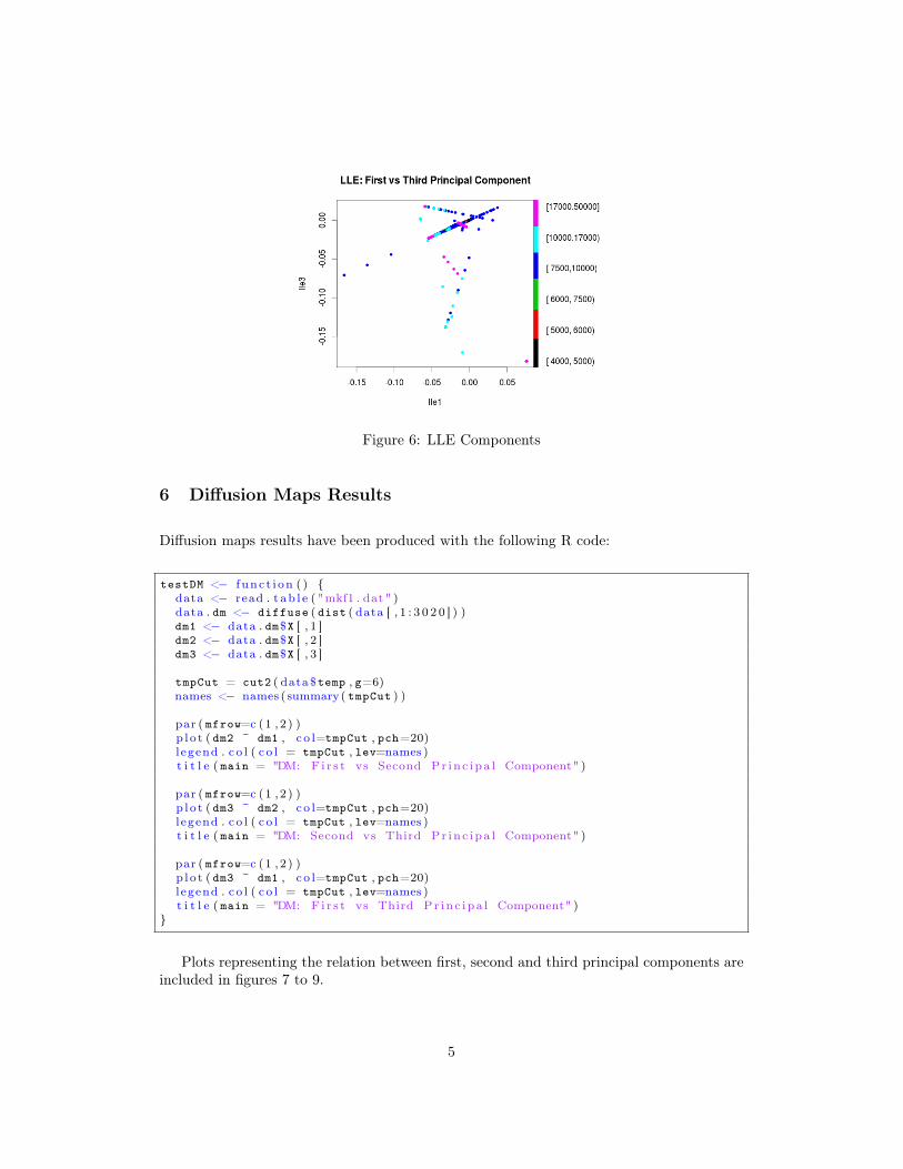
Figure 6: LLE Components

6 Diffusion Maps Results

Diffusion maps results have been produced with the following R code:

testDM <− f unc t i on ( ) {data <− read . t ab l e ( "mkf1 . dat" )data . dm <− diffuse ( dist ( data [ , 1 : 3 0 2 0 ] ) )dm1 <− data . dm$X [ , 1 ]dm2 <− data . dm$X [ , 2 ]dm3 <− data . dm$X [ , 3 ]

tmpCut = cut2 ( data$temp , g=6)names <− names ( summary( tmpCut ) )

par ( mfrow=c (1 , 2 ) )p l o t ( dm2 ~ dm1 , c o l=tmpCut , pch=20)legend . c o l ( c o l = tmpCut , lev=names )t i t l e ( main = "DM: F i r s t vs Second Pr i n c i pa l Component" )

par ( mfrow=c (1 , 2 ) )p l o t ( dm3 ~ dm2 , c o l=tmpCut , pch=20)legend . c o l ( c o l = tmpCut , lev=names )t i t l e ( main = "DM: Second vs Third Pr i n c i p a l Component" )

par ( mfrow=c (1 , 2 ) )p l o t ( dm3 ~ dm1 , c o l=tmpCut , pch=20)legend . c o l ( c o l = tmpCut , lev=names )t i t l e ( main = "DM: F i r s t vs Third Pr i n c i pa l Component" )

}

Plots representing the relation between first, second and third principal components areincluded in figures 7 to 9.

5

Figure 7: DM Components Figure 8: DM Components

Figure 9: DM Components

7 PCA vs LLE

Plots representing the relation between first, second and third principal PCA componentsagainst the first three LLE components respectively, are included in figures 10 to 12.

6

Figure 10: PCA vs LLE Components Figure 11: PCA vs LLE Components

Figure 12: PCA vs LLE Components

8 LLE vs Diffusion Maps

Plots representing the relation between first, second and third principal LLE componentsagainst the first three DM components respectively, are included in figures 13 to 15.

7

Figure 13: LLE vs DM Components Figure 14: LLE vs DM Components

Figure 15: LLE vs DM Components

9 PCA vs Diffusion Maps

Plots representing the relation between first, second and third principal PCA componentsagainst the first three DM components respectively, are included in figures 16 to 18.

8

Figure 16: PCA vs DM Components Figure 17: PCA vs DM Components

Figure 18: PCA vs DM Components

10 Regression Experiment

In this section a cross-validation regression exercise will be completed. We will use supportvector machines (SVM) to perform the regression, with the temperature as the dependentvariable. Three regression models will be constructed, using as independent variables the 5first principal components obtained from PCA, LLE and DM respectively.

Each model will then be tuned to get its optimal parameters, and performance resultswill be presented. R snippets will be included below.

The first thing to do is to read the input data and get the first 5 principal componentsfor each method.

9

data <− read . t ab l e ( "mkf1 . dat" )

data . pc <− prcomp ( data [ , 1 : 3 0 2 0 ] , retx=TRUE , s c a l e=TRUE )pc1 <− data . pc$x [ , 1 ]pc2 <− data . pc$x [ , 2 ]pc3 <− data . pc$x [ , 3 ]pc4 <− data . pc$x [ , 4 ]pc5 <− data . pc$x [ , 5 ]

data . lle <− lle ( as . matrix ( data [ , 1 : 3 0 2 0 ] ) , 5 )lle1 <− data . lle [ , 1 ]lle2 <− data . lle [ , 2 ]lle3 <− data . lle [ , 3 ]lle4 <− data . lle [ , 4 ]lle5 <− data . lle [ , 5 ]

data . dm <− diffuse ( dist ( data [ , 1 : 3 0 2 0 ] ) )dm1 <− data . dm$X [ , 1 ]dm2 <− data . dm$X [ , 2 ]dm3 <− data . dm$X [ , 3 ]dm4 <− data . dm$X [ , 4 ]dm5 <− data . dm$X [ , 5 ]

Three sets of 5 variables have been initialized. Three dataframes are built containingeach of the 5 variables plus the temperature to be predicted by the regression model.

new . data . pc <− data . frame ( pc1 , pc2 , pc3 , pc4 , pc5 , data$temp )new . data . lle <− data . frame ( lle1 , lle2 , lle3 , lle4 , lle5 , data$temp )new . data . dm <− data . frame ( dm1 , dm2 , dm3 , dm4 , dm5 , data$temp )

The next step is to build a train set and a validation set. In order to do so, the data setwill be split into two sets: 80% of the records will be randomly included in the training setand the remaining 20% will correspond to the test set.

n <− nrow (new . data . pc )tindex <− sample (n , round ( n∗ 0 . 8 ) ) # i nd i c e s o f t r a i n i n g samples

xtrain . pc <− new . data . pc [ tindex , ]xtest . pc <− new . data . pc [−tindex , ]

xtrain . lle <− new . data . lle [ tindex , ]xtest . lle <− new . data . lle [−tindex , ]

xtrain . dm <− new . data . dm [ tindex , ]xtest . dm <− new . data . dm [−tindex , ]

We are now ready to perform the regression. Using the tune function, included in theSVM library e1071, we can achieve parameter tuning of the SVM using grid search overthe supplied parameter ranges. The parameters passed to the function are:

• Regression formula: in this case, the outcome is the temperature as a function of therest of variables of the data provided.

• Data: this corresponds to the training set.

10

• Validation set : this corresponds to the test set.

• Gamma: the gamma values to use for the tuning. The range covers from 0.000001 to10.

• Cost : the cost values to use for the tuning. The range covers from 10 to 100.

• Error Function: the error function to minimize for the tuning. For the case of aregression, the root mean squared error function (rmse) is used.

tunemodel . pc <− tune . svm ( data . temp~ . , data=xtrain . pc , validation . x=xtest .←↩pc ,gamma = 10^(−6:1) , cost = 10^(1 :2 ) ,tunecontrol=tune . c on t r o l ( error . fun=rmse ) )

tunemodel . lle <− tune . svm ( data . temp~ . , data=xtrain . lle , validation . x=xtest←↩. lle ,gamma = 10^(−6:1) , cost = 10^(1 :2 ) ,tunecontrol=tune . c on t r o l ( error . fun=rmse ) )

tunemodel . dm <− tune . svm ( data . temp~ . , data=xtrain . dm , validation . x=xtest .←↩dm ,gamma = 10^(−6:1) , cost = 10^(1 :2 ) ,tunecontrol=tune . c on t r o l ( error . fun=rmse ) )

Results are included below. The best performance corresponds to the PCA SVM re-gression model, with an average error of around 2098 K. The worst model, for the dataanalyzed, corresponds to the DM model, with an average error of around 5743 K of tem-perature. Gamma and cost parameters obtained for each model are below.

> tunemodel . pc

Parameter tuning of ’ svm ’ :

− sampling method : 10−fold cross validation

− best parameters :gamma cost

10 100

− best performance : 2098.731

> tunemodel . lle

Parameter tuning of ’ svm ’ :

− sampling method : 10−fold cross validation

− best parameters :gamma cost

1 10

− best performance : 2460.521

> tunemodel . dm

Parameter tuning of ’ svm ’ :

11

− sampling method : 10−fold cross validation

− best parameters :gamma cost

10 10

− best performance : 5743.217

11 Conclusion

Three feature extraction methods have been studied in this assignment.

Principal Component Analysis, Local Linear Embedding and Diffusion Maps have beenused to extract three principal components of the astronomical Kurucz set data. Severalplots comparing the components obtained have been presented.

Finally, a regression exercise using R have been performed to build three SVM modelsbased on the previously obtained principal components.

References

[1] Cosma Shalizi. “Nonlinear Dimensionality Reduction I: Local Linear Embedding”. In:Data Mining Class (2009).

[2] Cosma Shalizi. “Nonlinear Dimensionality Reduction II: Diffusion Maps”. In: Data Min-ing Class (2009).

12

Appendix A R code for the legend.col function

l egend . c o l <− f unc t i on ( co l , lev ) {opar <− parn <− l ength ( c o l )bx <− par ( " usr " )box . cx <− c ( bx [ 2 ] + ( bx [ 2 ] − bx [ 1 ] ) / 1000 ,

bx [ 2 ] + ( bx [ 2 ] − bx [ 1 ] ) / 1000 + ( bx [ 2 ] − bx [ 1 ] ) / 50)box . cy <− c ( bx [ 3 ] , bx [ 3 ] )box . sy <− ( bx [ 4 ] − bx [ 3 ] ) / nxx <− rep ( box . cx , each = 2)

par ( xpd = TRUE )f o r ( i in 1 : n ) {

yy <− c ( box . cy [ 1 ] + ( box . sy ∗ ( i − 1) ) ,box . cy [ 1 ] + ( box . sy ∗ ( i ) ) ,box . cy [ 1 ] + ( box . sy ∗ ( i ) ) ,box . cy [ 1 ] + ( box . sy ∗ ( i − 1) ) )

polygon ( xx , yy , c o l = co l [ i ] , border = co l [ i ] )

}par (new = TRUE )p l o t (0 , 0 , type = "n" ,

ylim = c (1 , 6) ,yaxt = "n" ,ylab = "" ,xaxt = "n" , xlab = "" ,frame . p l o t = FALSE )

ax i s ( side = 4 , las = 2 , tick = FALSE , line = .25 , l a b e l s=lev , at=1:6)par <− opar

}

13