Multi-Compartment T2 Relaxometry Using a Spatially Constrained Multi-Gaussian Model

Multi-Compartment T2 Relaxometry Using a SpatiallyConstrained Multi-Gaussian ModelAshish Raj1*, Sneha Pandya1, Xiaobo Shen1, Eve LoCastro1, Thanh D. Nguyen1, Susan A. Gauthier2

1 Department of Radiology, Weill Cornell Medical College, New York, New York, United States of America, 2 Department of Neurology and Neuroscience, Weill Cornell

Medical College, New York, New York, United States of America

Abstract

The brain’s myelin content can be mapped by T2-relaxometry, which resolves multiple differentially relaxing T2 pools frommulti-echo MRI. Unfortunately, the conventional fitting procedure is a hard and numerically ill-posed problem.Consequently, the T2 distributions and myelin maps become very sensitive to noise and are frequently difficult tointerpret diagnostically. Although regularization can improve stability, it is generally not adequate, particularly at relativelylow signal to noise ratio (SNR) of around 100–200. The purpose of this study was to obtain a fitting algorithm which is ableto overcome these difficulties and generate usable myelin maps from noisy acquisitions in a realistic scan time. To this end,we restrict the T2 distribution to only 3 distinct resolvable tissue compartments, modeled as Gaussians: myelin water, intra/extra-cellular water and a slow relaxing cerebrospinal fluid compartment. We also impose spatial smoothness expectationthat volume fractions and T2 relaxation times of tissue compartments change smoothly within coherent brain regions. Themethod greatly improves robustness to noise, reduces spatial variations, improves definition of white matter fibers, andenhances detection of demyelinating lesions. Due to efficient design, the additional spatial aspect does not cause anincrease in processing time. The proposed method was applied to fast spiral acquisitions on which conventional fittinggives uninterpretable results. While these fast acquisitions suffer from noise and inhomogeneity artifacts, our preliminaryresults indicate the potential of spatially constrained 3-pool T2 relaxometry.

Citation: Raj A, Pandya S, Shen X, LoCastro E, Nguyen TD, et al. (2014) Multi-Compartment T2 Relaxometry Using a Spatially Constrained Multi-GaussianModel. PLoS ONE 9(6): e98391. doi:10.1371/journal.pone.0098391

Editor: Friedemann Paul, Charite University Medicine Berlin, Germany

Received August 5, 2013; Accepted May 2, 2014; Published June 4, 2014

Copyright: � 2014 Raj et al. This is an open-access article distributed under the terms of the Creative Commons Attribution License, which permits unrestricteduse, distribution, and reproduction in any medium, provided the original author and source are credited.

Funding: National MS Society grant #0711009544 partially supported AR, TN and SG. AR was additionally supported by NIH grants 5P41RR02953 and1R01NS075425. The funders had no role in study design, data collection and analysis, decision to publish, or preparation of the manuscript.

Competing Interests: The authors have declared that no competing interests exist.

* E-mail: [email protected]

Introduction

Differential transverse relaxation rate (T2) of water in different

brain tissues enables sensitive estimation of structural changes

[1,2]. Multi-echo T2 relaxometry is an MRI technique in which a

small number of exponentially decaying components is fit to a

series of T2-weighted images obtained at different echo times. The

relative contributions of each tissue compartment is then inferred

non-invasively, including the quantification of the water trapped

between myelin bilayers, called the myelin water fraction (MWF),

a quantitative map of myelin content in each brain voxel. MWF

can be used to assess the integrity of white matter (WM) and it

damage in neurological diseases like multiple sclerosis (MS) [3,4],

epilepsy [5], psychotic disorders [6], and Wallerian degeneration

[7]. MWF has been shown to highly correlate with histological

myelin measurement in animal models [8] and ex vivo brains [9].

Traditionally, clinical assessment of white matter disease is

performed from T2-weighted sequences like Fluid Attenuated

Inversion Recovery (FLAIR) images whose tissue contrast can

frequently be quite high compared to currently available

quantitative T2 methods. However, due to their non-quantitative

nature and lack of anatomic or pathologic specificity, they do not

meet the requirements of the next generation of quantitative brain

imaging applications.

The prevalent fitting method, non-negative least squares

(NNLS) [10], assumes a large number, up to 50 or 100, of

components with known and regularly spaced T2 values, since the

relaxation times of different components in unknown a priori. Far

fewer observations (,20–30 echo times) are available due to scan

time considerations, which yields a highly under-determined and

ill-posed problem whose solution suffers from non-uniqueness,

noise amplification and instability [11]. Tikhonov regularization

[12] of T2 relaxometry [10] added a stabilizing L2 norm penalty

and helps ensure a unique solution, but is still noise-sensitive,

frequently produces visually chaotic and diagnostically uninter-

pretable MWF maps. These challenges - stringent SNR require-

ments (leading to prohibitively long acquisitions or limited brain

coverage), instability of results – greatly impeded the clinical utility

of NNLS. Taking more echoes can improve the situation [11,13]

but is not a viable option due to excessive scan time [14].

The challenges in NNLS-based T2 relaxometry arise not only

from the innate ill-posedness of the inverse problem [15,16], but

also from the introduction of an unnaturally large and biologically

unrealistic number of relaxing components – a highly under-

determined problem that frequently causes the NNLS algorithm to

miss actual peaks in SNR-challenged data [17]. Theoretical

considerations suggest that there is no scope for deducing more

than 2 or 3 T2 components separated by a minimum interval from

15–20 echoes [18]; these criteria are violated by the NNLS

algorithm. The choice then is between a highly underconstrained

but linear estimation problem, and a constrained but highly non-

PLOS ONE | www.plosone.org 1 June 2014 | Volume 9 | Issue 6 | e98391

http://creativecommons.org/licenses/by/4.0/

http://crossmark.crossref.org/dialog/?doi=10.1371/journal.pone.0098391&domain=pdf

linear problem, where only a small number of unknown

compartments are sought to be fit to data.

In this paper, we eschew the underdetermined but linear NNLS

approach in favor of a non-linear formulation that recognizes only

3 distinct T2 compartments in the brain, each exhibiting not a

single T2 but a wide peak distributed within a small disjoint T2

range. This drastically reduces the number of unknowns, greatly

improves the conditioning of the inverse problem and circumvents

the biologically unrealistic and numerically indefensible need for

50 or 100 T2 compartments. A previous comparison between a

similar 3-pool fit and NNLS demonstrated significant improve-

ment in simulations [17]. Our approach is similar, but in addition,

seeks to further improve conditioning by imposing a priori

constraints. We therefore propose a multi-voxel spatial regularization

approach which imposes two constraints:

1. There are only 3 distinct T2 pools in the brain – a fast relaxing

myelin water pool, a slower intra/extra-cellular water pool,

and a very long relaxing cerebrospinal fluid (CSF) pool. Based

on numerous observations of T2 distributions, we model the

first two pools by Gaussian distributions, whose parameters

(mean location, height and variance) are unknown and to be

determined. The long CSF pool is modeled as a single pool

with a single unknown T2 and strength. See Table 1.

2. T2 characteristics of constituent water compartments change

smoothly within coherent brain regions such as healthy WM

while the boundary sharpness between distinctive regions

should also be preserved. These spatial constraints are imposed

separately on each parameter in the above multi-Gaussian

model.

Previously, a single Gaussian distribution was found to

outperform monoexponential models in brain tissue [19] – here

we have extended this to multiple Gaussians. The choice of

Gaussian shape is motivated by simplicity and the fact that shape is

relatively unimportant (see Figure 1, Discussion). For spatial

constraints we adopt the approach first proposed in [14], by

formulating an objective function which penalizes both the fitting

error and non-smooth solutions. Unfortunately, their method is

computationally challenging, taking up to 2 hours per slice, as it

involves joint minimization over multiple voxels, each having

about 50 unknowns. Our formulation has fewer unknowns but

more challenging numerically due to non-linearity, which we solve

using non-linear least squares [20] algorithm. We make several

algorithmic innovations to improve the numerical efficiency. First,

unlike [14] we eschew the explicit computation and storage of

large matrices, instead performing iterative conjugate-gradient-

based searches which are memory-light. We pre-compute the

sparse Jacobian pattern of the non-linear least squares problem,

which greatly speeds up computation. Since our regularization

parameters are spatially invariant we only do the optimization

once, unlike NNLS which requires a separate optimization for

many regularization parameters in order to evaluate the chi-

squared criterion. Due to these reasons our implementation is

around 5 times faster than a local implementation of NNLS.

However, we stress that the main objective of the new method is

not a faster algorithm, but one that overcomes the limitations of ill-

conditioning by utilizing spatial and model-based constraints.

We thoroughly exercise and numerically characterize the

proposed algorithm using a variety of numerical lesion and whole

brain simulations, MR phantoms and in vivo brain data acquired

with the multi-echo spin echo (MESE) sequence. We demonstrate

our method on a small number of normal subjects and a very large

cohort of 154 MS patients, and demonstrate significant improve-

ment over conventional fitting. We also present preliminary results

on a new 3D multi-echo fast T2-prepared spiral imaging sequence

[21], which provides noisy but very fast whole brain coverage and

scan time of 10 min at 3T, making it a clinically feasible

alternative to conventional MESE. While the conventional NNLS

method gives noisier and less reproducible results on all datasets

compared to our method, it is especially problematic on the fast

spiral data, giving noisy, spatially incoherent and unstable MWF

maps, whereas the proposed algorithm continues to produce

clinically useful MWF maps. Thorough statistical analysis of whole

brain variability, lesion detection, and region of interest analysis

over 154 patients are presented.

Theory

T2 RelaxometryGiven MR signals yk in a voxel measured at echo times TEk

(k = 1,…, K), a set i = 1,…,N of discrete sub-components are

hypothesized to exist, each producing an exponentially decaying

signal aiexp(-TEk/T2(i)) with a known T2 constant of T2(i) and an

unknown volume fraction of ai. Assuming a slow exchange regime

[22], this gives:

y(TEk)~XN

i~1

aiexp {TEk

T2(i)

� �z" ð1Þ

or equivalently, y = Ax + e, with Ak,i~exp(� TEk=T2(i)).Vector y is a collection of data yk acquired at echo time TEk, x is a

Table 1. List of parameters to be fitted, per voxel.

Symbol Feature Initial guess Allowable range [lower, upper]

a1 Height of myelin water distribution 0.1 [0, 1]

m1 Mean of myelin water distribution 15 ms [10 ms, 40 ms]

s1 St. dev. of myelin water distribution 10 ms None specified

a2 Height of intra/exra-cellular distribution 0.9 [0, 1]

m2 Mean of intra/exra-cellular distribution 80 ms [60 ms, 200 ms]

s2 St. dev. of intra/exra-cellular distribution 100 ms None specified

hCSF Height of long-T2 (CSF) signal 0 None specified

mCSF Mean of long-T2 (CSF) signal 1800 ms None specified

Their initial guess and allowable range, used during constrained optimization, are also shown.doi:10.1371/journal.pone.0098391.t001

T2 Relaxomtery Using a Multi-Gaussian Model


vector of the unknown ai, and e denotes instrumentation noise.

This system of linear equations is typically under-determined (N.

K) and ill-posed, making a direct inversion either impossible or

prone to extreme noise sensitivity, instability and non-uniqueness

[23]. Tikhonov regularization [12] was proposed to partially

overcome this problem by minimizing the cost function [24]

xx~ argminxx

jjAx{yjj2zlTjjxjj2 x§0 ð2Þ

for each voxel using the non-negative least squares (NNLS)

algorithm. Here lT is a regularization parameter. We follow the

approach and notation of a recent spatially constrained multi-

voxel Bayesian minimization [14]:

xx~ argminxx

jjAex�xx{�yyjj2zlTjjxjj2zmsjjWD �xxjj2 x§0 ð3Þ

where single-voxel quantities x, y are collected in multi-voxel

vectors, and the expanded (block diagonal) matrix Aex is defined

similarly. The last term penalizes spatially non-smooth solutions

via the first-difference operator and corresponds to the convolu-

tion of the T2 distribution image with a high-pass filter. W is a

diagonal weighting matrix which allows for variable penalties

associated with T2 points.

Proposed Multi-Gaussian Spatial RegularizationIn the j-th voxel we wish to determine the following set of

unknown parameters (Table 1):

h(vj)~fa1(j),m1(j),s1(j),a2(j),m2(j),s2(j),hCSF (j),mCSF (j)g

which in turn uniquely determine the T2 distribution as a sum of

two Gaussians and a long-T2 signal:

xj(t)~ (h(vj),t)~a1(j)N(tjm1(j),s1(j))

za2(j)N(tjm2(j),s2(j))zhCSF(j)d(t�mCSF(j))ð4Þ

Each Gaussian is denoted by the shorthand N(.), and T2

distribution is over variable t. The T2 distribution above resulting

from the multi-Gaussian model is evaluated on the 40-point range

of T2 values, and the delta function above turns into a discrete

delta. Collecting multi-voxel parameters in the vector h = {h (vj),

j = 1,…, Nv}, and relating the Gaussian parameters to the resulting

T2 distribution by x = G(h), we minimize

hh~ arg minh

jj�yy{Aexp (h)jj2zlN jjhjj2zmSjjDShjj2 ð5Þ

The 3rd term enforces spatial consistency constraint #2 above,

separately on each parameter of the model, via the first difference

operator matrix DS. The global regularization parameters lN and

mS are unknown a priori and their optimal values are chosen by a

semi-supervised procedure (see Method). Once minimization has

concluded, we obtain the final T2 distribution

xx~ (hh), ð6Þ

Since we model pools explicitly, MWF calculation does not

involve integration:

MWF(vj)~a1(j)

a1(j)za2(j)zhCSF (j)ð7Þ

under the constraint that should be in the range during the

minimization of Eq (6). The operator (hh) is non-linear, hence Eq

Figure 1. Numerical simulations and its effect on decay curve. Numerical simulation of various T2 distributions of roughly equal variancecentered near 20 ms – their effect on the resulting decay curve is minimal. Echo times are the same as those for in vivo MESE scans (omitting thehighest points for ease of visualization).doi:10.1371/journal.pone.0098391.g001



(5) is non-convex. We formulate it as a non-linear least squares

problem by combining all 3 terms into the L2 norm of a single

vector given by

q(h)~

�yy{Aexp (h)

mNh

mSDSh

264

375 , and hh~ arg min

h

q(h)k k2 ð8Þ

Eq (8) is merely a reframing of Eq (5), and is intended to stress

that our chosen approach relies on solving the non-linear least

squares problem (8) rather than the general problem (5), and takes

advantage of the 2-norm structure available to us. This approach

can take advantage of the fact that at each iteration, the

minimization problem is a least squares problem around a local

Jacobian J(h)~Lq(h)=L(h)which is quickly solved by precondi-

tioned conjugate gradients algorithm.

Methods

Simulating healthy brain MWFA synthetic MRI brain image and its white, gray and CSF

probabilistic masks obtained from the Montreal Neurological

Institute (MNI) were used to simulate multi-echo T2 data, each

tissue class having a unique T2 signature. The myelin fraction was

set at 14.5% for pure white matter, 4.5% for pure gray matter, and

0% for CSF. The myelin, intra/extra and long-T2 pools were

simulated as Gaussians centered at 25 ms and 100 ms, respec-

tively, and the CSF peak was set at 1800 ms. These pure T2

components were weighted by the probabilistic masks to get the

actual components. Additive white Gaussian noise was introduced

at SNR level varying from 100 to 1000; SNR is defined for this

purpose with respect to the signal at first echo.

Doped water phantom experiments10 test tubes filled with water doped with varying concentrations

of Gadolinium and MnCl2 were scanned using the MESE

sequence at 1.5T over 8 slices and processed using the propsoed

algorithm. The nominal T2 relaxation times were measured by

fitting a single exopnential onto the averaged signal curves from all

voxels in each test tube.

Human ImagingHuman study with full informed consent was approved by Weill

Cornell Medical College Institutional Review Board. Consent was

obtained both in oral and written form with detailed documen-

tation. Spin echo T2 data were obtained from 2 healthy volunteers

at 1.5T, and a recent whole brain 3D T2prep spiral scans [21] at

both 1.5T and 3T GE HDxt scanner. The imaging parameters

were: Spin echo: axial FOV = 30 cm, matrix size = 2566128

(interpolated to 2566256), partial phase FOV factor = 0.6, slice

thickness = 5 mm, number of slices = 12, TR = 2500 ms, echo

spacing = 5 ms, number of TEs = 32 (5, 10–310 ms (10 ms step)),

scan time = 38 min. 3D T2prep spiral: axial FOV = 24–30 cm,

matrix size = 1926192 (interpolated to 2566256), slice thickness

= 5 mm, number of slices = 32, TR = 2500 ms, flip angle = 10u,number of TEs = 15–26, scan time = 10–26 min. Two end slices

were discarded to account for imperfect slab excitation profile.

Skull (very short T2) and fluid (very long T2) signals were removed

using BrainSuite v09.

Next, a large study of 154 MS patients was undertaken at 3T

under the 3D T2prep spiral sequence. This cohort was used in this

paper for the purpose of obtaining whole brain statistics and

assessment of variability – a detailed study of pathological

discrimination on MS will be carried out in future work. To this

end, a regional parcellation was imposed on T2 images using the

labeled Freesurfer atlas [25] using a recently developed pipeline in

our laboratory [26]. Regional averages of MWF for gray matter

and adjoining white matter regions were computed and their

histograms created. A few of these patients were chosen, on the

basis of visually apparent focal WM hyperintensities, for a

preliminary neurological assessment of demyelinating WM lesions

for the purpose of illustrating the lesion discrimination ability of

the algorithm. T2-weighted volumes and where available, FLAIR

volumes were co-registered to their MWF maps. Hyperintense

focal lesions were manually segmented on the co-registered

volumes under a neurologist’s (SAG) supervision. These lesion

masks were mapped onto MWF maps, and voxel-level statistics

were computed.

Implementation of Multi-Gaussian Spatially ConstrainedT2 Relaxometry

The list of 8 parameters are shown in Table 1, along with initial

guess and allowable range, which were chosen based on prior

experience. Forty T2 points logarithmically spaced over a range of

5–300 ms were chosen for the T2 distribution. Multi-voxel data

fitting was implemented using the iterative lsqnonlin algorithm

[20] in MATLAB version R2011b running on a Windows 7 64-bit

platform and Intel core 2 Duo processor with 2.2 GHz, 4 GB

memory. All voxels in the 3D volume were solved for at once,

presenting a very large minimization problem necessitating

considerable effort over efficient algorithm design. Since the

Jacobian J(h) is not expressible in closed form, it needs to be

estimated at each iteration from first differences over 8?NV

variables – a daunting memory requirement. Fortunately, J(h) is

highly sparse due to the structure of q(h), and its sparsity pattern

was pre-computed and passed to lsqnonlin. Memory require-

ments for storing voxel neighborhood system and Jacobian was

minimized by using sparse data types and a rewrite of the vendor-

supplied lsqnonlin-related functions involving pre-allocating

some large arrays. The final code was able to achieve 10–20

times speed improvement over a direct call to lsqnonlin.

Optimization of regularization parametersUnfortunately choice of regularization parameter greatly affects

the outcome, hence our NNLS implementation evaluated the chi-

square criterion [24] at 100 lTs spaced logarithmically within

[1021, … , 1025] for each voxel, and one that gave residual norm

between 102.0%–102.5% of the non-regularized residual norm

was selected, as specified in previous NNLS reports [13].

Unfortunately, this problem is even more acute for the proposed

approach due to strong non-linearity, hence we developed a novel

algorithm design which greatly reduces parameter dependence by

incorporating the chi-squared criterion within the minimization

itself. At each iteration we rescale the prior penalties such that the

ratios

cN~lN hk k2

�yy{Aexp (h)�� 2

, cS~mS DShk k2

�yy{Aexp (h)�� 2

are held constant throughout the minimization, as follows. We

start with l0N and m0

S and at each iteration n we introduce the

following rescaling:



lnN~(1{d)ln{1

N zdcN �yy{Aexp (hn)�� 2

hnk k2

mnS~(1{d)mn{1

S zdcS �yy{Aexp (hn)�� 2

DShnk k2

The 2nd term is the fully rescaled version which maintains

constant, but in order to reduce the potential for instability or

oscillations, we introduce a small step size to prevent large

discontinuous jumps. This approach completely obviates the need

for testing large ranges of regularization. We tested all cases with

the same prior ratios cN = 0.1, cS = 0.1 and this gave consistent

results across subjects, however in some cases slight tweaks to these

presets produced somewhat better results.

Regional Statistical AnalysisMasks of WM and GM tissue classes were obtained using SPM8

software [27] by co-registering the 10 MS subjects’ T2 images to

T1, then to the T1 template from the Montreal Neurological

Institute (MNI). These transformations are applied to the

computed MWF maps. Spatially unbiased whole brain regional

analysis was performed by parcellating the cortex into 68 regions

using pre-labeled MNI atlas. Mean MWF values are computed for

each region, split further into the cortical ribbon and adjacent

white matter. From these mean ROI values, intra-class coefficient

of variance (COV) was computed and between all region pairs a

two-tailed paired-sample t-test was used to assess p-values, with

p,0.05 considered statistically significant.

Results

Brain Simulation ResultOur purpose was to quantify error rate and to explore the

blurring effect of spatial regularization at tissue boundaries. MWF

maps in Figure 2 indicate higher accuracy and less noise using our

technique. The relative mean square errors

rMSE~

PNv

j~1

(MWFtrue(j){MWFa lg(j))2

PNv

j~1

MWFtrue(j)2

of MWFs is also shown,

where NV is the total number of voxels, and MWFtrue and MWFalg

are the true and estimated MWF. There is little evidence of edge

Figure 2. MWF maps generated by simulation of MESE data using brain phantom. Brain phantom (A) was used to simulate MESE data, andrMSE was calculated at different SNRs (B). The corresponding MWF maps are shown in C at SNR = 100, 500, 1000 (top to bottom).doi:10.1371/journal.pone.0098391.g002



blurring, in fact we see higher tissue contrast than conventional

map. Figure S1 and S2 in File S1 characterizes the effect of spatial

regularization parameter mS at various SNR levels, exhibiting the

typical U-shaped behavior: low mS gives too much noise, high mS

too much smoothing; an intermediate value provides the best

numerical and visual compromise – here this is achieved at

mS = 0.01. The corresponding MWF maps visually reinforce this

impression. Contrary to expectation, the highest mS did not

produce the smoothest image, probably due to the realization of a

different local minimum of the non-convex cost. Note that this

simulation was not designed to investigate intra-tissue spatial

variations; although it is possible to construct numerical phantoms

for this purpose, we feel this is best investigated via in vivo data.

Further, the use of 3 pools in the simulation might appear to

inherently favor the multi-Gaussian model, but the comparison

with conventional NNLS, which is agnostic to the number of

pools, is still valid – the experiment was designed precisely to test

the additional benefit of applying a realistic multi-pool model.

MESE doped water phantom results at 1.5TFigure 3 shows the 5th echo image (40 ms), the average within

each test tube of our MWF, and their measured T2 in parentheses.

Note that this doped water phantom does not produce multiple

pools – only differentially shortened single T2 pool. Thus, the

purpose of this experiment is to assess accuracy and bias when the

multi-pool assumption is violated. Clearly, our algorithm achieved

quite good accuracy on this data, yet a small bias exists which is

more prominent for T2 values close to the 40 ms myelin cutoff.

In vivo MRI ResultsNumerical convergence shows a classic pattern (Figure S3 in

File S1). Only 20 iterations appear sufficient, and further iterations

do not appreciably reduce the cost or image appearance. We

chose 50 iterations for all cases. The processing times of 9 slices of

size 1926192 pixels were approximately 4 hours with the

conventional method and 25 minutes with the spatial constrained

method. For 8 slices of size 2566256 pixels, the processing times

were approximately 6 hours with conventional and 1.2 hours with

spatial algorithm.

Healthy MESE dataFigure 4 shows proposed MWF maps from a healthy subject’s

MESE scan, demonstrating a clear reduction in noise, improved

spatial coherence and depiction of WM structures compared to

NNLS. The proposed map encompasses a much larger area of

WM, including frontal and lateral projections fibers which were

silent on the conventional map. As an anatomic reference, the

bottom row shows T2-prep spiral images at 50 ms. Table 2

summarizes MWF measured on the whole brain and at selected

WM ROIs of normal subjects. At least 20 voxels were used in each

ROI for computing these statistics. The last two rows show ROI

comparison with published literature: voxel-based analysis (VBA)

[28] and multi-voxel Bayesian (MVB) [14]. Although a gold

standard is not available, our values are within the published range

and seem to roughly match NNLS.

Healthy T2prep spiral dataFigure 5 shows processed MWF maps from T2prep spiral scans

of a healthy volunteer, which has a different appearance compared

Figure 3. MESE experiment using test tubes. MESE experiment at1.5T on 10 test tubes filled with water doped with varyingconcentrations of Gd and MnCl2, hence varying T2 times measuredby single exopnential fit. Raw MR signal intensities of a middle slice ofthe 5th echo (40 ms) are shown using idicated color scale (arbitraryscanner units). The text arrows show the average MWF estimated by thepropsoed algorithm within each test tube and its nominal T2 inparentheses. The ‘‘true’’ MWF would be 100% for the two right-mosttubes, and 0% for the rest. These results indicated good accuracy of ouragorithm on MESE data.doi:10.1371/journal.pone.0098391.g003

Figure 4. MWF maps of healthy MESE scans acquired at 1.5T.MWF computed from healthy in vivo anisotropic MESE scans acquired at1.5T. Conventional reconstruction (top), spatial constrained reconstruc-tion (middle) and anatomical T2 FLAIR images (bottom). Twoconsecutive axial slices at the level of thalamus and putamen areshown.doi:10.1371/journal.pone.0098391.g004



to MESE, due to spatial inhomogeneity and other artifacts

introduced by the fast sequence. Although this has made the

NNLS method practically unusable, our approach is able to

retrieve anatomically faithful myelin maps from this data.

However, there is upward bias in GM, which should be lower

than depicted (see Discussion). The values in WM, however, are in

line with reported numbers, as indicated in Table 2. Figure 6

shows another example with similar characteristics, but it

additionally illustrates an oversized effect of T2 shortening induced

by iron deposition in the basal ganglia (see Discussion). The

difference in MWF between whole brain WM and GM was

significant in all subjects (p,0.001) for both methods, indicating

good tissue differentiation. Corresponding COV data (Table 3)

shows greatly reduced variability from our algorithm, reinforcing

the earlier visual impression of smooth, noise-free maps. Figure 7

shows typical T2 decay curves from WM, GM and iron-rich deep

Table 2. MWF of selected WM ROI obtained with proposed and conventional methods, from both MESE and spiral sequences.

Genu of Corpus Callosum Splenium of Corpus Callosum Internal capsules

Conventional: MESE 1.5T 18.162.5 18.361.6 8.8964.9

MultiGaussian: MESE 1.5T 18.564.0 16.862.1 10.864.0

Conventional: T2prep spiral 3T 24.465.1 18.461.6 18.163.0

MultiGaussian: T2prep spiral 3T 19.760.9 17.660.8 18.361.5

VBA 10.2±0.2 14.4±0.2 17.2±0.2

MVB: FSE 1.5T 16.7±1.8 14.6±3.1 14.2±1.5

The last two rows show comparison with published literature: VBA [28] and MVB [14].doi:10.1371/journal.pone.0098391.t002

Figure 5. MWF maps of healthy 3D T2prep adiabatic spiralbrain scan acquired at 1.5T. Two axial slices of MWF computed fromthe second healthy in vivo 3D T2prep adiabatic spiral brain scanacquired at 1.5T, with conventional reconstruction (top), spatialconstrained reconstruction (middle) and anatomical T2 weightedimages (bottom).doi:10.1371/journal.pone.0098391.g005

Figure 6. MWF maps of another healthy 3D T2prep adiabaticspiral brain scan. Another healthy brain 3D T2prep adiabatic spiralexample, with MWF (top) and T2-weighted image (bottom) of twoadjacent axial slices.doi:10.1371/journal.pone.0098391.g006



GM and their estimated T2 distributions – they show expected

behavior, with fast initial decay in WM (and iron rich nuclei).

T2prep spiral data of MS patientsThe example in Figure 8 displays exquisite depiction of

periventricular WM injury (arrows). The NNLS map was

uninterpretable like Figure 4 and is not shown. There was

however, a prominent anterior-posterior spatial gradient. Figure 9

shows an MS example with both small, focal lesions and diffuse

ones, along with T2 weighted images at 60 ms which are

hyperintense in lesions. Another example of MS lesions is in

Figure S4 in File S1, with external validation of lesion location and

extent derived from coregistered FLAIR data. Visually, our

method differentiated lesions more clearly than the noisy NNLS

maps. Spatial smoothing did not obscure small lesions. Table 4

shows p-values from student’s t-test between normal WM and

lesions (drawn manually from FLAIR under a neurologist’s

supervision) of MWF from 3 MS patients – our approach has

higher detectability of demyelinating lesions.

Whole brain and regional MWF StatisticsWhole brain statistics across all 154 MS patients is shown in

Figure 10. Histograms of the distribution of white matter and gray

matter MWF are shown for both the proposed and conventional

NNLS methods. It is clear that there is high statistical separation

between white and gray in our results, much more so compared to

the conventional method. Statistical significance (p-values) is noted

in caption. Regional averages of MWF of the smaller sample of

10 MS patients for 84 gray matter regions from the Freesurfer

atlas and adjoining white matter regions are presented in

Figure 11: histogram of regional MWF averaged across all

subjects (A), histogram of whole brain GM and WM over all

subjects (B), and COV between different regions for all 154 MS

patients. The latter was quite small (0.1–0.2), which indicates

consistent and spatially homogeneous estimates of MWF. Note

that although both Figures 10 and 11 appear to show MWF

statistics of GM and WM regions, the former is evaluated on all

voxels, while the latter on regions. In either case the histograms

show good separation between white and gray matter, compared

to the conventional NNLS method. Despite upward bias in GM

MWF from our algorithm, the statistical separation of the MWF

distribution in WM and GM is very good, with p,0.01.

Discussion

Summary and impact of main resultsThis study demonstrates that physically realistic multi-Gaussian

modeling and spatial constraints can overcome the limitations of

conventional NNLS. The algorithm is fast due to efficient iterative,

low-memory design. The method was thoroughly exercised and

numerically characterized using a variety of experiments: numer-

ical lesion and whole brain simulations to assess spatial coherence

Figure 7. Examination of elevated MWF, relaxation curves and T2 distribution. Detailed investigation of elevated MWF in deep graymatter. Relaxation curves for three brain areas are shown on the middle panel: WM, GM and deep brain GM – these areas are denoted by circles onthe MWF map generated from spatial constrained method (left panel). Dark red circle indicates the WM area, blue indicates the GM area, and greenindicates the GM with fast relaxation rate area. The fitted T2 distribution from each region is shown in the right panel - curves correspond to the ROIaveragedoi:10.1371/journal.pone.0098391.g007

Table 3. Comparisons of Mean Coefficient of Variance (COV) of MWF obtained for the T2prep spiral sequence in various ROIsbetween proposed and conventional methods.

Region Conventional COV Spatial COV

Whole brain WM 0.84 0.14

Whole brain GM 1.14 0.24

Genu of corpus callosum 0.21 0.05

Splenium of corpus callosum 0.09 0.05

Internal capsule 0.17 0.08

doi:10.1371/journal.pone.0098391.t003



and edge preservation; doped water phantom to assess accuracy

and bias in single pools where the model assumptions are violated;

two different in vivo sequences - spin echo and T2-prep spiral; two

scanner field strengths – 1.5T and 3T; and both healthy and

disease. In particular, our disease cohort was very large, consisting

of 154 MS patients. Although any given experiment only tells a

partial story, the combined impact of all these experiments

presents a robust picture of our algorithm compared with currently

available alternatives. Simulated and MRI data show visually and

numerically improved MWF measurements, less noise, greater

spatial consistency, faithful resolution of small WM feature, higher

WM/GM differentiation, and higher lesion detectability. The

variability in MWF (COV) is substantially reduced. White matter

coverage is significantly larger, including frontal and lateral

projection fibers which are frequently silent in NNLS. In MS

patients the visual depiction and statistical discrimination of lesions

is substantially enhanced.

Our work provides a clear path to practical utility in applying

quantitative relaxometry in the clinic, as compared to traditional

visual assessment on FLAIR images, which are not quantitative.

Our algorithm has the potential to produce quality whole brain

myelin maps in under 10 minutes when applied to fast but noisy

T2 prep spiral sequences on which NNLS fails. The spiral results

meet the clinical goal of whole brain MWF maps in under 10

minutes scan time, and can be invaluable in diagnosis, prognosis

and longitudinal monitoring of efficacy of treatment-induced

remyelination. Fast processing time could enhance clinical and

routine applicability – however this was not the focus of current

work. Implementation on high-end multi-core server hardware

could potentially reduce processing time to just a few minutes –

which would open up several interesting clinical applications

which are currently impeded due to overly long execution time of

existing algorithms. While simulation, phantom and in vivo results

on conventional MESE scans indicate little bias, our MWF maps

from fast spiral scans show upward bias in GM and spatial

inhomogeneity, which merit further effort in sequence design. A

modest level of residual bias, where a non-zero myelin fraction is

reported when there is none, is expected behavior for model- and

constraint-based methods when the model assumptions are

violated severely.

Model JustificationThree pools. What if there are more than 3 compartments,

for instance a slowly relaxing component between 300 ms and

800 ms [29]. Our model already allows for a long-T2 component,

which could, if required by the data, conform to this intermediate

compartment. Our algorithm design could easily accommodate a

fourth compartment, but we think it inadvisable. Due to scan time

limitations, sampling echo times higher than 300 ms is practically

difficult. This limits the number of compartments above 300 ms

that can be reliably discerned. Even if more echoes could be

acquired, numerical conditioning of the inverse problem imposes

stringent limits on the maximum number of compartments that

can be reliably estimated [18]. In terms of biophysics, we find no

strong justification or clinical interpretation of four compartments.

Gaussian peak shape. Although our method can easily

accommodate any parsimoniously parameterized peak shape, the

choice of Gaussian was motivated by simplicity, ubiquity and prior

reports [19]; specifically we eschewed prior use of log-Gaussians

[2] for computational reasons. What if the data preferred other

shapes, or worse, require arbitrary model-free shapes? Certainly,

one of the main attractions of full spectrum T2 relaxometry is its

ability to deduce arbitrary, non-discrete T2 distributions [13]. A

relatively under-appreciated factor is poor numerical conditioning,

which leads to a very large number of possible T2 distributions all

fit the multi-echo data equally well, hence small differences in the

shape profile will be simply invisible to the data. This is illustrated

in Figure 1, which shows 3 differently shaped but roughly equally

Figure 8. Illustration of demyelinating lesion in MWF map of aMS patient. Two axial slices of proposed MWF map of a MS patient.Note the excellent depiction of demyelinating lesions (arrows) andimproved definition of callosal and peripheral white matter.doi:10.1371/journal.pone.0098391.g008

Figure 9. MWF maps of MS patient using conventional andspatially constrained method. MWF maps computed from in vivoMS patient scan. Top to bottom are MWF maps from conventionalmethod, spatial constrained method and T2-weighted image at 60 ms.Arrows in T2 of point to small, focal lesions, externally confirmed onFLAIR. These lesions are well delineated on the spatial map but not onconventional map.doi:10.1371/journal.pone.0098391.g009



dispersed distributions centered near 20 ms and their decay

curves: Gaussian, log-Gaussian and Laplacian. The decay curves

for these disparate peaks are strikingly similar and the discrepancy

between them vanishingly small. Given typical levels of MR noise

and artifacts, there is no hope for successfully estimating the

precise shape of the true T2 distribution beyond low-order

statistics like mean and variance, for which Gaussians are the

canonical distribution. Worse, regularization can itself greatly

influence the estimated distribution, making anything beyond the

second moment operationally suspect.

Spatial constraints. These may potentially blur edges and

small lesions or other pathology, but this can be prevented by a

conservative choice of regularization parameter. On the contrary,

spatial constraints can improve the definition of small lesions by

preventing noise from occluding the lesion, as shown later by our

results on demyelinating diseases. Additive noise model. In this

work we have assumed Gaussian white additive noise, but a strong

case can be made for Rician noise, especially in late echoes which

have generally low signal levels. However, as is well-known, such

models result in more challenging objective functions, necessitating

more advanced minimization strategies which may not be

amenable to least squares formulation used here. Given that

spatial constraints already increase the numerical complexity of

our approach manifold, we chose to stay with the Gaussian

assumption in the interest of computational cost. This is in keeping

with the vast majority of prior work in this area, where Gaussian

assumption is routinely and successfully employed even in cases

where it might be sub-optimal.

Comparison with related approachesModels involving 2 or 3 pure relaxing T2 components already

exist [17], but here we accommodated more realistic dispersed

Gaussian distributions to capture micro-environmental heteroge-

neity within tissue compartments. The information contained in

peak dispersion is lost in pure multicompartment models,

including those fitted to steady-state acquisitions like mcDESPOT

[30,31]. When applied to fast T2prep spiral data, our algorithm

can provide a compelling alternative to mcDESPOT in terms of

scan time but in addition handles dispersed peaks. Other

alternatives for myelin quantification, like T2* [32] or magneti-

zation transfer [33] provide complimentary information regarding

multiple tissue compartments, but due to differing mechanisms

and pathological specificity they should be considered substitutes

for multi-compartment T2 modeling.

Unlike the whole brain coverage we demonstrate, previous T2

relaxometry studies of MS are generally reported on selected slices

[33,34], hence preclude the quantification of diffuse or systemic

pathologies. Our processing time is roughly 5 times shorter than

local implementation of NNLS, increasing its routine clinical

applicability. Significantly shorter processing time has been

reported for NNLS [15] using more powerful hardware and

parallel processing techniques, but the above comparison remains

valid because presumably our method too could benefit similarly

from hardware and parallelization. Our MWF maps have similar

range as prior reports [10,14,16], but better visual quality in terms

of smoothness and delineation of brain structures. The mean

MWF values of major WM structures (Table 2) are consistent with

the literature [3,10,15,28], but our numbers are generally higher,

e.g. in the genu of corpus callosum and in deep gray matter. There

is also discrepancy in the internal capsule specific to MESE results,

where both conventional and multi-Gaussian MWF values are low

compared to all other data. We do not fully understand the reason,

but note that the occlusion with basal ganglia makes ROI drawing

difficult and operator dependent. There is no unanimity in the true

value of MWF in normal brain tissue, hence it is difficult to assess

accuracy on in vivo human data. In any case, absolute agreement

in MWF numbers between studies is probably unrealistic due to

differences in hardware, study subjects, pulse sequence, etc.

Exchange between compartments might affect MWF. Interesting-

ly, our results are similar to mcDESPOT [30,31], both numer-

ically and visually; in fact our numbers are generally intermediate

between NNLS and mcDESPOT. Since both mcDESPOT and

our multi-Gaussian approaches rely on pre-defining the number of

distinct pools, this might perhaps explain the similarity in their

visual appearance, and their distinct appearance compared to

NNLS methods which are non-parametric. Until a clear in vivo

gold standard emerges for human tissue, we must rely on statistical

Table 4. P-values of MWF difference between normal WM and WM lesion detected by two methods.

P-value

Conventional Spatial

Patient 1 0.15 0.023

Patient 2 0.041 ,0.001

Patient 3 0.067 0.042

doi:10.1371/journal.pone.0098391.t004

Figure 10. Histogram of MWF for all the subjects and t-testbetween WM and GM. Histogram from different subjects of MWFaveraged over all regions. A t-test between the WM and GM groupsyielded p,1026 for multi-Gaussian and p = 0.0121 for conventionalalgorithm.doi:10.1371/journal.pone.0098391.g010



separation (rather than absolute MWF values) between WM,

lesions and GM as the most practical way to assess clinical utility,

as has been observed in various mcDESPOT studies. Our results

are statistically very sensitive in detecting demyelinating lesions

(Table 4) – much more so than NNLS – irrespective of the actual

MWF values each method reports. Gray/white contrast is also

well-preserved (Figure 10). Since COV values in Table 3 were

computed over voxels, they are higher than some prior reports

which used ROI averages [35].

Spatial constraints are prevalent in image processing [36–38]

and MRI reconstruction [39,40], but rare in T2 relaxometry.

Spatially smoothed versions of conventionally obtained T2/T2*

distributions were proposed as ‘‘reference distributions’’ and

deviations from this was penalized [41] [42]. These approaches

do not amount to a truly spatially constrained approach, because

the inverse problem is still solved voxel-wise. They are unlikely to

fundamentally solve the problem of ill-posedness, because the

noise comes from the fitting process itself and must therefore be

resolved during the fitting process by incorporating spatial

constraints directly into the solution -e.g. see [39,40]. Another

potential problem is that the ‘‘reference distribution’’ obtained by

NNLS can itself be inaccurate or uninformative (as shown in some

of our examples), hence any estimate relying on this reference is

prone to inappropriate bias and obliteration of genuine spatial

variations. Our implementation of this approach failed on our

spiral data and is not shown here. Since the T2 distribution of each

voxel is given by a small number of tissue classes, it can be

assumed to be sparse in the T2 range of interest, i.e. 5 ms to

300 ms. Therefore there is potential for using sparse reconstruc-

tion algorithms on this problem. Although this was not the focus of

the current work, we were able to perform preliminary

implementation and testing of sparse algorithms on this problem,

by imposing and solving for L1-norm regularization terms. The

details and results are contained in Supplementary Information S5

in File S1. The results contain therein are unimpressive, and

suggest that a direct application of sparse reconstruction methods

is likely to be unsuccessful. Our reasoning is that since sparsity is

applicable on a single voxel basis, the sparse algorithm must be run

one voxel at a time, hence by itself sparsity may not be not

sufficient to overcome the ill-posedness of the problem. This is why

our proposed approach favors both a model-based restriction to 3

classes, as well as additional spatial constraints. In contrast, our

approach imposes weaker but realistic spatial coherence con-

straints.

The spatially constrained optimization proposed here is similar

to our prior work [14], but the additional novelty here is regarding

a constrained model along T2. Thus our method has far fewer

degrees of freedom, where we have traded an unconstrained but

quadratic cost function with guaranteed global minimum for a

highly constrained but non-convex cost whose minimization is

challenging. The risk of entrapment within inappropriate local

minima and undesirable sensitivity to initial guess exist, but are

Figure 11. Histogram and COV of regional MWF, histogram averaged over all regions. (A) Histogram of regional MWF of each ROIaveraged over 10 MS subjects. MWF in WM has a higher distribution than GM, and the two are statistically well separated, with p,0.001 from astudent’s t-test between the WM and GM regions (B) Histogram from different subjects of MWF averaged over all regions. A t-test between the WMand GM groups yielded p,0.001. (C) COV of regional MWF for each subject, indicating low variability in regional variations in both WM and GM.doi:10.1371/journal.pone.0098391.g011



outweighed by considerable gains, like unique solutions, better

conditioning, and noise resistance. Our processing time and

memory usage are a fraction of [14]. The MR sequence used

herein is also quite different from that used to evaluate [14]. Given

the difference in methodology and data acquisition, a comparison

with [14] is unlikely to be relevant or useful, hence it is not shown

in this paper. Instead we have directed our comparisons against

the current benchmark method, NNLS, which is both widely used

and well characterized.

Limitations and future workOur 3T spiral results suffer from apparent bias in GM, where

we report higher numbers than previously reported. We attribute

this to the spiral sequence rather than algorithmic issues, since the

bias is not appreciable in simulations (Figure 2), phantom (Figure 3)

or in vivo (Figure 4) MESE data. All MR acquisitions employed

equal spacing between refocusing pulses to minimize the buildup

of unwanted stimulated echoes [43] by maintaining a consistent

refocusing efficiency across the excited 3D volume. Yet, T2-prep

spiral acquisitions exhibit significant spatial gradient caused by B0

inhomogeneity, B1 bias and flip angle error; they have propagated

to computed MWF maps. Our spiral maps also show heightened

MWF in the basal ganglia compared to other reports. T2

shortening induced by iron deposition [44][45], is known to relate

linearly with R2 [44,46,47]. Our MWF results suggest specific

shortening of extra-cellular T2 into the myelin range, heightening

apparent MWF which should not be considered myelin-related.

Although this paper is not concerned with sequence design, we

recognize that its limitations can affect clinical applications. We

intend to implement parallel imaging to further reduce scan time

and achieve isotropic voxel size, and consider more sophisticated

composite and adiabatic pulses which minimize inhomogeneity

artifacts.

Certainly, bias and gradient issues result from the tradeoffs

involved in speedy spiral acquisitions, but it is possible that the

non-linear nature of our constrained model might be exacerbating

it. Our approach requires explicitly fitting a fast and a slower

relaxing component, hence in the presence of noise or artifacts

could be more predisposed to finding a myelin signal even when

one may not be present. We will consider other penalty functions

to prevent this. Bayesian model order selection will be imple-

mented to determine whether the data supports multiple peaks or

single peaks. The proposed algorithm can be improved in other

ways: replacing global, spatially invariant high-pass filter in the

spatial term with locally adaptive smoothness penalties might

better preserve tissue boundary. Plans to exploit edge-preserving

spatial priors [48] are ongoing and will be submitted separately.

Supporting Information

File S1 Contains Figure S1, rMSE of MWF computed using

proposed method on brain simulation with different mS at SNR =

100 and 300 (mN = 0.013). The optimal value was found at 0.01 for

both noise levels. Figure S2, Visual results for spatial constrained

(mN = 0.013) on brain simulation at SNR of 100 (top) and 300

(bottom), where mS = 0.0001, 0.001, 0.01, 0.02, 0.1, respectively,

from left to right. The ones within red boxes provide the best

visual and numerical result, and show that the optimal value of this

parameter is not overly sensitive to SNR. Figure S3, Convergence

of the proposed algorithm. Left: MWF maps computed after 20,

30, 80 and 100 iterations on an in vivo example. Right: The

numerical convergence of the cost function shows a classic pattern,

whereby convergence is reached at 20 iterations, and further

iterations do not appreciably reduce the cost. Although MWF

maps begin looking reasonable in as few as 20 iterations, we chose

30 iterations to provide a margin of error. Figure S4, MWF maps

computed from another in vivo MS patient scan. Top to bottom are

MWF maps from conventional method, spatial constrained

method and FLAIR images. Arrows in FLAIR images point to

lesions. Figure S5, Left to right, single axial slice of a MS patient

showing A] T2-weighted image, B] MWF map from conventional

NNLS method, C] MWF map from spatially constrained Gaussian

method, and D] MWF map reconstructed from sparse L1-

regularized method.

(DOCX)

Acknowledgments

We thank Kyoko Fujimoto and Dushyant Kumar for help with analysis

and programming.

Author Contributions

Conceived and designed the experiments: AR SP XS EL TDN SAG.

Performed the experiments: TDN SAG. Analyzed the data: AR SP TDN

SAG. Contributed reagents/materials/analysis tools: SP EL TDN. Wrote

the paper: AR. Designed the algorithm used in analysis: AR. Designed the

software used in analysis: SP EL.

References

1. Laule C, Vavasour IM, Kolind SH, Li DKB, Traboulsee TL, et al. (2007)

Magnetic resonance imaging of myelin. Neurotherapeutics: the journal of the

American Society for Experimental NeuroTherapeutics 4: 460–484.

2. MacKay A, Laule C, Vavasour I, Bjarnason T, Kolind S, et al. (2006) Insights

into brain microstructure from the T2 distribution. Magnetic resonance imaging

24: 515–525.

3. Laule C, Vavasour IM, Moore GRW, Oger J, Li DKB, et al. (2004) Water

content and myelin water fraction in multiple sclerosis. A T2 relaxation study.

Journal of neurology 251: 284–293.

4. Neema M, Goldberg-Zimring D, Guss ZD, Healy BC, Guttmann CRG, et al.

(2009) 3 T MRI relaxometry detects T2 prolongation in the cerebral normal-

appearing white matter in multiple sclerosis. NeuroImage 46: 633–641.

5. Jackson GD, Connelly A, Duncan JS, Grunewald RA, Gadian DG (1993)

Detection of hippocampal pathology in intractable partial epilepsy: increased

sensitivity with quantitative magnetic resonance T2 relaxometry. Neurology 43:

1793–1799.

6. Wood SJ, Cocchi L, Proffitt T-M, McConchie M, Jackson GD, et al. (2010)

Neuroprotective effects of ethyl-eicosapentaenoic acid in first episode psychosis:

a longitudinal T2 relaxometry pilot study. Psychiatry research 182: 180–182.

7. Does MD, Snyder RE (1996) Multiexponential T2 relaxation in degenerating

peripheral nerve. Magnetic resonance in medicine: official journal of the Society

of Magnetic Resonance in Medicine/Society of Magnetic Resonance in

Medicine 35: 207–213.

8. Gareau PJ, Rutt BK, Karlik SJ, Mitchell JR (2000) Magnetization transfer and

multicomponent T2 relaxation measurements with histopathologic correlation

in an experimental model of MS. Journal of magnetic resonance imaging: JMRI

11: 586–595.

9. Laule C, Kozlowski P, Leung E, Li DKB, Mackay AL, et al. (2008) Myelin water

imaging of multiple sclerosis at 7 T: correlations with histopathology. Neuro-

Image 40: 1575–1580.

10. Whittall KP, MacKay AL, Graeb DA, Nugent RA, Li DK, et al. (1997) In vivo

measurement of T2 distributions and water contents in normal human brain.

Magnetic resonance in medicine: official journal of the Society of Magnetic

Resonance in Medicine/ Society of Magnetic Resonance in Medicineociety of

Magnetic Resonance in Medicine 37: 34–43.

11. Graham SJ, Stanchev PL, Bronskill MJ (1996) Criteria for analysis of

multicomponent tissue T2 relaxation data. Magnetic resonance in medicine:

official journal of the Society of Magnetic Resonance in Medicine/Society of

Magnetic Resonance in Medicine 35: 370–378.

12. Tychonoff AN, Arsenin VY (1977) Solution of Ill-posed Problems. New York:

Winston.

13. Whittall KP, Bronskill MJ, Henkelman RM (1991) Investigation of analysis

techniques for complicated NMR relaxation data. Journal of Magnetic

Resonance (1969) 95: 221–234.

14. Kumar D, Nguyen TD, Gauthier SA, Raj A (2012) Bayesian algorithm using

spatial priors for multiexponential T2 relaxometry from multiecho spin echo

MRI. Magnetic resonance in medicine: official journal of the Society of



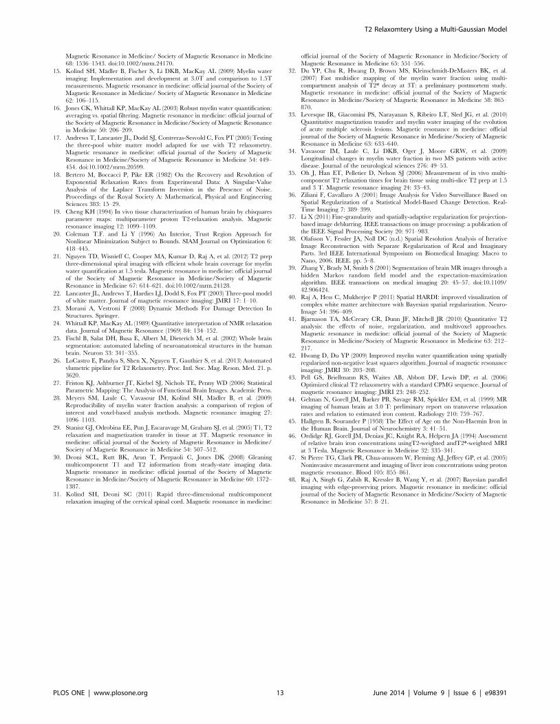
Magnetic Resonance in Medicine/ Society of Magnetic Resonance in Medicine

68: 1536–1543. doi:10.1002/mrm.24170.

15. Kolind SH, Madler B, Fischer S, Li DKB, MacKay AL (2009) Myelin water

imaging: Implementation and development at 3.0T and comparison to 1.5T

measurements. Magnetic resonance in medicine: official journal of the Society of

Magnetic Resonance in Medicine/ Society of Magnetic Resonance in Medicine

62: 106–115.

16. Jones CK, Whittall KP, MacKay AL (2003) Robust myelin water quantification:

averaging vs. spatial filtering. Magnetic resonance in medicine: official journal of

the Society of Magnetic Resonance in Medicine/Society of Magnetic Resonance

in Medicine 50: 206–209.

17. Andrews T, Lancaster JL, Dodd SJ, Contreras-Sesvold C, Fox PT (2005) Testing

the three-pool white matter model adapted for use with T2 relaxometry.


Resonance in Medicine/Society of Magnetic Resonance in Medicine 54: 449–

454. doi:10.1002/mrm.20599.

18. Bertero M, Boccacci P, Pike ER (1982) On the Recovery and Resolution of

Exponential Relaxation Rates from Experimental Data: A Singular-Value

Analysis of the Laplace Transform Inversion in the Presence of Noise.

Proceedings of the Royal Society A: Mathematical, Physical and Engineering

Sciences 383: 15–29.

19. Cheng KH (1994) In vivo tissue characterization of human brain by chisquares

parameter maps: multiparameter proton T2-relaxation analysis. Magnetic

resonance imaging 12: 1099–1109.

20. Coleman T.F. and Li Y (1996) An Interior, Trust Region Approach for

Nonlinear Minimization Subject to Bounds. SIAM Journal on Optimization 6:

418–445.

21. Nguyen TD, Wisnieff C, Cooper MA, Kumar D, Raj A, et al. (2012) T2 prep

three-dimensional spiral imaging with efficient whole brain coverage for myelin

water quantification at 1.5 tesla. Magnetic resonance in medicine: official journal

of the Society of Magnetic Resonance in Medicine/Society of Magnetic

Resonance in Medicine 67: 614–621. doi:10.1002/mrm.24128.

22. Lancaster JL, Andrews T, Hardies LJ, Dodd S, Fox PT (2003) Three-pool model

of white matter. Journal of magnetic resonance imaging: JMRI 17: 1–10.

23. Morassi A, Vestroni F (2008) Dynamic Methods For Damage Detection In

Structures. Springer.

24. Whittall KP, MacKay AL (1989) Quantitative interpretation of NMR relaxation

data. Journal of Magnetic Resonance (1969) 84: 134–152.

25. Fischl B, Salat DH, Busa E, Albert M, Dieterich M, et al. (2002) Whole brain

segmentation: automated labeling of neuroanatomical structures in the human

brain. Neuron 33: 341–355.

26. LoCastro E, Pandya S, Shen X, Nguyen T, Gauthier S, et al. (2013) Automated

vlumetric pipeline for T2 Relaxometry. Proc. Intl. Soc. Mag. Reson. Med. 21. p.

3620.

27. Friston KJ, Ashburner JT, Kiebel SJ, Nichols TE, Penny WD (2006) Statistical

Parametric Mapping: The Analysis of Functional Brain Images. Academic Press.

28. Meyers SM, Laule C, Vavasour IM, Kolind SH, Madler B, et al. (2009)

Reproducibility of myelin water fraction analysis: a comparison of region of

interest and voxel-based analysis methods. Magnetic resonance imaging 27:

1096–1103.

29. Stanisz GJ, Odrobina EE, Pun J, Escaravage M, Graham SJ, et al. (2005) T1, T2

relaxation and magnetization transfer in tissue at 3T. Magnetic resonance in

medicine: official journal of the Society of Magnetic Resonance in Medicine/

Society of Magnetic Resonance in Medicine 54: 507–512.

30. Deoni SCL, Rutt BK, Arun T, Pierpaoli C, Jones DK (2008) Gleaning

multicomponent T1 and T2 information from steady-state imaging data.



1387.

31. Kolind SH, Deoni SC (2011) Rapid three-dimensional multicomponent

relaxation imaging of the cervical spinal cord. Magnetic resonance in medicine:

official journal of the Society of Magnetic Resonance in Medicine/Society of

Magnetic Resonance in Medicine 65: 551–556.32. Du YP, Chu R, Hwang D, Brown MS, Kleinschmidt-DeMasters BK, et al.

(2007) Fast multislice mapping of the myelin water fraction using multi-

compartment analysis of T2* decay at 3T: a preliminary postmortem study.Magnetic resonance in medicine: official journal of the Society of Magnetic

Resonance in Medicine/Society of Magnetic Resonance in Medicine 58: 865–870.

33. Levesque IR, Giacomini PS, Narayanan S, Ribeiro LT, Sled JG, et al. (2010)

Quantitative magnetization transfer and myelin water imaging of the evolutionof acute multiple sclerosis lesions. Magnetic resonance in medicine: official

journal of the Society of Magnetic Resonance in Medicine/Society of MagneticResonance in Medicine 63: 633–640.

34. Vavasour IM, Laule C, Li DKB, Oger J, Moore GRW, et al. (2009)Longitudinal changes in myelin water fraction in two MS patients with active

disease. Journal of the neurological sciences 276: 49–53.

35. Oh J, Han ET, Pelletier D, Nelson SJ (2006) Measurement of in vivo multi-component T2 relaxation times for brain tissue using multi-slice T2 prep at 1.5

and 3 T. Magnetic resonance imaging 24: 33–43.36. Ziliani F, Cavallaro A (2001) Image Analysis for Video Surveillance Based on

Spatial Regularization of a Statistical Model-Based Change Detection. Real-

Time Imaging 7: 389–399.37. Li X (2011) Fine-granularity and spatially-adaptive regularization for projection-

based image deblurring. IEEE transactions on image processing: a publication ofthe IEEE Signal Processing Society 20: 971–983.

38. Olafsson V, Fessler JA, Noll DC (n.d.) Spatial Resolution Analysis of IterativeImage Reconstruction with Separate Regularization of Real and Imaginary

Parts. 3rd IEEE International Symposium on Biomedical Imaging: Macro to

Nano, 2006. IEEE. pp. 5–8.39. Zhang Y, Brady M, Smith S (2001) Segmentation of brain MR images through a

hidden Markov random field model and the expectation-maximizationalgorithm. IEEE transactions on medical imaging 20: 45–57. doi:10.1109/

42.906424.

40. Raj A, Hess C, Mukherjee P (2011) Spatial HARDI: improved visualization ofcomplex white matter architecture with Bayesian spatial regularization. Neuro-

Image 54: 396–409.41. Bjarnason TA, McCreary CR, Dunn JF, Mitchell JR (2010) Quantitative T2

analysis: the effects of noise, regularization, and multivoxel approaches.Magnetic resonance in medicine: official journal of the Society of Magnetic


217.42. Hwang D, Du YP (2009) Improved myelin water quantification using spatially

regularized non-negative least squares algorithm. Journal of magnetic resonanceimaging: JMRI 30: 203–208.

43. Pell GS, Briellmann RS, Waites AB, Abbott DF, Lewis DP, et al. (2006)

Optimized clinical T2 relaxometry with a standard CPMG sequence. Journal ofmagnetic resonance imaging: JMRI 23: 248–252.

44. Gelman N, Gorell JM, Barker PB, Savage RM, Spickler EM, et al. (1999) MRimaging of human brain at 3.0 T: preliminary report on transverse relaxation

rates and relation to estimated iron content. Radiology 210: 759–767.45. Hallgren B, Sourander P (1958) The Effect of Age on the Non-Haemin Iron in

the Human Brain. Journal of Neurochemistry 3: 41–51.

46. Ordidge RJ, Gorell JM, Deniau JC, Knight RA, Helpern JA (1994) Assessmentof relative brain iron concentrations usingT2-weighted andT2*-weighted MRI

at 3 Tesla. Magnetic Resonance in Medicine 32: 335–341.47. St Pierre TG, Clark PR, Chua-anusorn W, Fleming AJ, Jeffrey GP, et al. (2005)

Noninvasive measurement and imaging of liver iron concentrations using proton

magnetic resonance. Blood 105: 855–861.48. Raj A, Singh G, Zabih R, Kressler B, Wang Y, et al. (2007) Bayesian parallel

imaging with edge-preserving priors. Magnetic resonance in medicine: officialjournal of the Society of Magnetic Resonance in Medicine/Society of Magnetic

Resonance in Medicine 57: 8–21.



Multi-Compartment T2 Relaxometry Using a Spatially Constrained Multi-Gaussian Model

Documents

Transcript of Multi-Compartment T2 Relaxometry Using a Spatially Constrained Multi-Gaussian Model