Magnetic properties of nanoparticles useful for SQUID relaxometry in biomedical applications

Magnetic Properties of Nanoparticles Useful for SQUIDRelaxometry in Biomedical Applications

H. C. Bryanta,c,*, Natalie L. Adolphia,d, Dale L. Huberb, Danielle L. Fegana, Todd C.Monsonb, Trace E. Tessiera, and Edward R. FlynnaaSenior Scientific LLC, 11109 Country Club NE, Albuquerque, New Mexico, 87111bSandia National Laboratories, P. O. Box 5800, Albuquerque, New Mexico, 87185cDepartment of Physics and Astronomy, University of New Mexico, Albuquerque, New Mexico87131dDepartment of Biochemistry and Molecular Biology, University of New Mexico, Albuquerque,New Mexico 87131

AbstractWe use dynamic susceptometry measurements to extract semiempirical temperature-dependent,255 to 400 K, magnetic parameters that determine the behavior of single-core nanoparticles usefulfor SQUID relaxometry in biomedical applications. Volume susceptibility measurements weremade in 5K degree steps at nine frequencies in the 0.1 – 1000 Hz range, with a 0.2 mT amplitudeprobe field. The saturation magnetization (Ms) and anisotropy energy density (K) derived from thefitting of theoretical susceptibility to the measurements both increase with decreasing temperature;good agreement between the parameter values derived separately from the real and imaginarycomponents is obtained. Characterization of the Néel relaxation time indicates that theconventional prefactor, 0.1 ns, is an upper limit, strongly correlated with the anisotropy energydensity. This prefactor decreases substantially for lower temperatures, as K increases. We find,using the values of the parameters determined from the real part of the susceptibilitymeasurements at 300 K, that SQUID relaxometry measurements of relaxation and excitationcurves on the same sample are well described.

KeywordsMagnetic nanoparticle; A. C. susceptometry; Magnetorelaxometry; Langevin function; Néelrelaxation; Magnetite

1. IntroductionMagnetic nanoparticles show much promise in labeling cancer cells or other pathologicalstructures that then may be detected by SQUID (Superconducting Quantum Interference

© 2010 Elsevier B.V. All rights reserved.*Corresponding author. Tel.: +1 505 243-1058, [email protected] (H. C. Bryant).Publisher's Disclaimer: This is a PDF file of an unedited manuscript that has been accepted for publication. As a service to ourcustomers we are providing this early version of the manuscript. The manuscript will undergo copyediting, typesetting, and review ofthe resulting proof before it is published in its final citable form. Please note that during the production process errors may bediscovered which could affect the content, and all legal disclaimers that apply to the journal pertain.

NIH Public AccessAuthor ManuscriptJ Magn Magn Mater. Author manuscript; available in PMC 2012 March 1.

Published in final edited form as:J Magn Magn Mater. 2011 March 1; 323(6): 767–774. doi:10.1016/j.jmmm.2010.10.042.

NIH

-PA Author Manuscript

NIH


NIH


Device) relaxometry. The critical magnetic properties for this application are relaxationtimes and spontaneous magnetization.

In order to label biological structures magnetically for detection by SQUID relaxometry, thenanoparticles with their coatings of specific antibodies must be undetectable when notfirmly attached to the target object. That is, when the particles of interest are free to reorientin their suspending fluid, they should have relaxation times much shorter than theobservation time; however, if rotation of the nanocrystal is hindered by its attachmentthrough antibody-antigen interactions with the target structure, the relaxation time can becomparable to the SQUID observation time, typically of the order of a second [1]. In theformer case, the relaxation time for rotation in a fluid is very short for hydrodynamic radiitypical of the particles considered, rendering them invisible to the SQUID system. In thelatter case, when rotation of the crystal lattice of the particle is hindered, the magneticmoment of the single domain nanocrystal, typically a few hundred thousand Bohrmagnetons in magnetite, reorients with characteristic relaxation times first discussed by Néel[2]. The Néel time is of critical importance because its exponential dependence on particlevolume severely limits the sizes of the particles that are suitable for SQUID relaxometry. Aswe shall see below, the "SQUID window", the material-dependent size range for whichSQUIDs can sense the decaying magnetism from relaxing nanoparticles, is only about 2 nmwide centered on a diameter of 26 nm at room temperature, for the magnetite particlesdiscussed here.

In our analysis we do not consider interactions among nanoparticles [3] although we modifythe Langevin function to reflect the disorienting effects of anisotropy with a random easyaxis distribution of an ensemble of fixed particles. After briefly discussing the theoreticalmodels, we describe the fitting of our predictions to results of a susceptibility study of thenanoparticle properties from 255 to 400 K. We then report observations of these sameparticles under SQUID relaxometry, at room temperature and three different magnetic fieldpulse durations, comparing with predictions from the parameters determined from thedynamic susceptibility analysis. We shall use SI units throughout.

2. Material and methods2.1 Nanoparticles

The nanoparticles discussed in this paper were supplied by Ocean NanoTech (SpringdaleAR,USA), designated Ocean SHP 30 lot DE4G. These magnetite particles were suspendedin water with an iron content measured by the phenanthroline assay to be 28.8 mg [Fe] perml. Ten µl of suspension were pipetted onto a cotton swab "Q Tip" (Unilever, Trumbull, CT,USA), and were allowed to dry in zero applied field. We assume the particles are firmlyattached to the cotton fibers so that the crystal lattices themselves cannot rotate in responseto an applied field. This cotton swab was our primary sample for the measurements reportedin this paper. Since Fe3O4 is 0.7235 Fe by weight, we find the mass of magnetitenanoparticles in the sample to be 398 µg. From TEM images (Tecnai G2 F30 at 300kV, FEICorporation, Hillsboro, OR, USA), a distribution of Feret1 diameters of the particles wasdetermined using the program, ImageJ (produced through an NIH grant and available on theinternet). The distribution peaked at 25 nm with a full width at half maximum (FWHM) of 4nm.

1The Feret diameter is the largest caliper measurement that could be made on the TEM image of the particle. A caliper measurementis the distance between two parallel planes each just touching the surface of the object.

Bryant et al.

J Magn Magn Mater. Author manuscript; available in PMC 2012 March 1.

NIH


NIH


NIH


2.2 SusceptometryWe determined the induced magnetic moment of the Q Tip sample at 9 frequencies and 30temperatures, using an MPMS-7 SQUID magnetometer (Quantum Design, San Diego, CA,USA), with a palladium reference sample for calibration. The software associated with theapparatus presents the magnetic moment results in emu (erg/Gauss). These numbers convertto volume susceptibility in the emu system by dividing the magnetic moment by theamplitude of the driving field (2 Oe) and by the total volume of the magnetite, 7.56 × 10−5

cc (398 µg at a density of 5.24 g/cc) in the sample. We converted the resulting(dimensionless emu) volume susceptibilities into (dimensionless rationalized MKS) volumesusceptibilities by multiplying the former by 4π.

2.3 SQUID relaxometryThe SQUID relaxometry measurement technique and apparatus used for the measurementsreported here has been described in detail elsewhere [4,5]. Briefly, the nanoparticle sampleis magnetized using a applied DC magnetic field pulse ranging from 0–4 mT in amplitudeand 0.3 – 1.5 s in duration. Beginning at 50 ms after the end of the field pulse, the decayingsample magnetization is measured for 2 s using a 7-channel SQUID array.

3. Theoretical model3.1 Néel relaxation, anisotropy and field effects

Néel relaxation is principally governed by the coupling energy of the collective electron spinwith special directions in the crystal lattice. This anisotropy energy can also havecontributions from the morphology of the nanoparticle such as shape and surface anisotropy[6]. Configurational anisotropy has been studied in single and pseudo-single domain grainsof magnetite and the effects are comparable to magnetocrystalline anisotropy [7]. In thetreatment below, we shall include, as is commonly done in this field, the anisotropy energydensity in a single parameter K (J/m3), and treat magnetite as a uniaxial crystal, ignoring thefact that its magnetocrystalline anisotropy is triaxial(cubic) [8]. This approach tounderstanding the particle is therefore semiempirical in an attempt to restrict parameters toas few as possible for a reasonable description of the magnetic behavior for biomedicalapplications.

The Néel relaxation time is affected by the strength of the applied magnetic field. We shallrepresent the relaxation time [5,9] in the presence of an applied field by

(1)

where ν is the particle volume, β = (1−B/BK)α and BK = 2K / Ms is the switching field. Forthe relaxometry data we use α = 3/2, consistent with the theoretical work of Victora [10].Ms, B, k and T are the spontaneous magnetization (J/Tm2), applied field (Tesla), Boltzmann'sconstant (1.38×10−23 J/K) and absolute temperature (K) respectively. For susceptibilitymeasurements (section 4) the field-reduction in the time constant is negligible, but it must betaken into account for relaxometry measurements (section 5) that require much higher fields(4 mT). In our modeling, we leave τ0, treated solely as a function of temperature, to be fitwith the susceptibility data (section 4)

3.2 The modified Langevin functionThe equilibrium polar angle θ of alignment of a dipole with an applied field is determined bya balance between the torque exerted on the dipole by the field and the disorienting effect of

Bryant et al.


NIH


NIH


NIH


https://www.researchgate.net/publication/236671462_An_Introduction_to_the_Theory_of_Ferromagnetism?el=1_x_8&enrichId=rgreq-5d52a1b92d36048fff6b5705ddc4e613-XXX&enrichSource=Y292ZXJQYWdlOzUxMDczMjEzO0FTOjEwMzg1OTY3ODYxMzUwOEAxNDAxNzczNDg1Mzc2

thermal fluctuations. When these two effects are the only agents present, the average valueof cosθ is the Langevin function L [10].

However, when the dipole is a single domain nanoparticle, fixed so the crystal cannot rotate,anisotropy can hinder alignment with the external field. In this case the particle energy usedin deriving the Langevin function may be replaced by

(2)

to form a distribution function including anisotropy [11,12], where the unit vectors, ê, b̂, n̂,denote the directions of the magnetic moment, the applied field and the anisotropy axis,respectively,

(3)

where Z(σ, ξ) = ∫exp(−U / kT)dê, with σ = Kν / kT and ξ = Ms νB / kT).

The expectation value of the orientation of the magnetic moment with the applied field B isthen given by

(4)

We shall refer to this expression as the "modified Langevin function", for which theLangevin function L is the limiting case when σ = 0.

The distribution function plays different roles in the susceptibility and relaxometrymeasurements. The modified Langevin function may be numerically computed using aformula generated by Yasumori, Reinen and Selwood [13] for an isotropic distribution offixed anisotropy axes. The ratio of the modified L to L, displayed in Fig. 1 in a form usefulin modeling our data, is consistent numerically with Fig. 1 of Bentivegna et al [14].

3.2 Dynamic susceptibility modelRaikher and Stepanov [12] have treated the theory of dynamic susceptibility ofnanoparticles; we refer the reader to their discussion and insights, starting with thedistribution function W(ê) defined above. In the susceptibility case, the alignment of theparticle's magnetic moment with the applied B can be treated as a perturbation to its energyU (Eq. 2). Their Eq. 40 gives the real and imaginary, linear, dynamic susceptibilities forhindered nanoparticles (assumed uniformly spherical of diameter D and volume ν, withrandomly frozen anisotropy axes), leading in our case to

(5)

and

(6)

Bryant et al.


NIH


NIH


NIH


where

(7)

For large σ, S2 ≅ 1−3/ 2σ, [12] although we used the numerical integration (Eq.7) to allowfor any unexpected small values of σ.

The relaxation time, based on the work of Bessais, Ben Jaffel and Dormann [15], suggestedby Raikher and Stepanov [12],

(8)

is a modification of Eq.1. N is the number of nanoparticles per unit volume, given by thereciprocal of the mean volume, discussed below, derived from the measured distribution ofparticle diameters, w(D).

3.4 Moment observed by relaxometryIn relaxometry, a relatively strong DC magnetic pulse is applied to the nanoparticle sample,and the subsequent collective magnetic moment is measured as a function of time after thepulse is switched off. Here we describe the response using a modification of the MomentSuperposition Model (MSM) [16,17,18]. The observed induced magnetic moment and itssubsequent decay arise from the mechanisms represented below. The square pulse ofstrength B is applied for a time tp, and the magnetic moment M(t) of the sample is given at atime t after the pulse is turned off.

(9)

where n is the number of particles in the sample, μ = νMs is the magnetic moment of aparticle of diameter D. L(σ, ξ) is the modified Langevin function discussed above(3.2). The"Néel factor" is given by g(tp) = 1−exp(−tp / τN), and τ is just τN with the applied field off (β= 1). We replace τ0 with τ0σ(1+;σ / 4)−5 / 2, consistent with Eq. (8)

4. Susceptibility measurements4.1 The size distribution

Fig. 2 displays the distribution of Feret diameters of the sample measured by TEM, about2600 particles. A sub sample of these particles was analyzed by the program ImageJ. Thereis evidence that the particles tend to be less round as the Feret diameter increases between20 and 30 nm. Although we assume spherical particles in our models, the circularity (4πarea/perimeter2), for example, for a Feret diameter of 25 nm in our sample is around 0.77. Acircle is 1.

4.2 The number densityUsing the measured probability distribution w(D) of Feret diameters (Fig.2) and ignoringany departure from sphericity, we find the average particle volume in our sample,

Bryant et al.


NIH


NIH


NIH


(10)

From the total volume of magnetite in the sample (section 2.2), we estimate the number ofnanoparticles on the cotton swab sample as n = 9.4×1012. We take the volume V of thesample to be just the total volume of the particles themselves, so that V = nν ̄. Consequently,the number density N in Eqs.(5) and (6) reduces to 1/ν̄, and n does not enter into our modeleven though it determines the strength of the total dipole moment measured by themagnetometer.

4.3 Comparison with modelThe model for the susceptibility was fitted to the measurements, Fig. 3a,b, by adjusting thevalues of the three temperature-dependent parameters (K, MS, τ0) to minimize the rmsdifferences between the modeled and measured quantities, for each of the 30 temperaturesfor which the real and imaginary susceptibilities were measured. In our fitting we ignoredthe possibility that these three parameters could depend upon the particle size. The real andimaginary parts were treated separately and the outcomes can be compared for consistency.Each 3-paramenter curve fit contained 9 data points corresponding to the 9 frequencies. Thenumerical work was done using Matlab, and representative samples are shown in Fig. 4a,b.

4.4 The anatomy of susceptibilityRepresentative kernels contributing to the model computation are examined to see whereeach value arises in the nanoparticle distribution. By "kernel" we refer to the frequency-dependent integrand at a given temperature of Eqs. (5) or (6) for the real or imaginary part,respectively. To compute these functions of D we use the parameters obtained by making abest fit to the data at each temperature.

As T decreases, the cluster of kernels for each T moves progressively toward the smalldiameter side of the distribution. For the real parts each kernel extends down to the smallestdiameters, whereas for the imaginary parts each kernel is confined to a rather narrow rangeof sizes. Thus, for the real part, the T=400 K measurement is sensitive to the entiredistribution, and the T=255 K cluster is influenced only by the small diameter particles. Wewould therefore expect results in the low temperature regions for the real part to be lessrobust than for the high temperature regions since the modeling is patterned by only thelower wing of the distribution where the statistics are relatively poor. The kernelsconstituting the imaginary fits also will reflect the poor statistics on the small side of the sizedistribution. In fact, our fits for both real and imaginary parts do show increasingfluctuations below 300 K.

4.5 Fitted parametersThe susceptibility model (Eqs. 5 and 6) is compared with the measured values at the ninefrequencies for each temperature and the parameters Ms, K and τ0 are adjusted to give thebest fit to the these data points. As the three parameters are assumed to be temperaturedependent, the fit at each temperature is made independent of any other. Any sizedependence of these parameters has been ignored.

Fig. 6 presents the resulting estimates for the three parameters used in our model. In all threecases the parameters determined from the real and imaginary susceptibilities are much moreconsistent with each other for temperatures above 300 K than for those below.

Bryant et al.


NIH


NIH


NIH


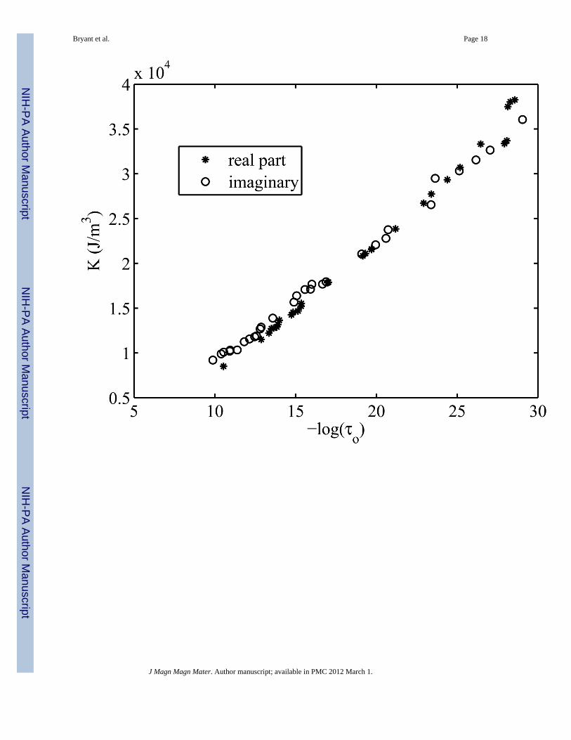
4.6 The correlation between K and logτ0Although the variability of the fitted parameters K and logτ0 shown in Fig. 6b and 6c islarge, the correlation between the variations is strong. Fig 7a shows that there is an abruptthreshold just above 10 for −logτ0. For T greater than about 300 K the ratio of these twoparameters agrees well for the real and imaginary contributions.

In SQUID relaxometry applications (section 5) the size range of nanoparticles shouldcorrespond to a relaxation time of about 1 second. In that case logτ ≈ 0, allowing us via Eq.(1) to find the effective particle diameter (see discussion following Eq 1 in Chantrell et al[3]),

(11)

Consequently, it is the ratio − K / logτ0 that determines the required diameter for SQUIDrelaxometry, the SQUID window, an example of which we treat in section 5. See Fig. 7b.

4.7. A closer look at the fits at 300KWe examine more closely the fits to the susceptibility data at 300 K, the temperature regionof interest in biomedical applications. At this temperature our best fits correspond to a K of2.67×104 and 2.21×104 J/m3 for real and imaginary, respectively, which is about twice thatof the bulk value of magnetite, 1.35×104 J/m3. The accompanying fit for the log of τ0,usually taken as −10, yields −22.9 and −20.0, giving a ratio −K / logτ0 of 1.17×103 and1.11×104 J/m3 that, when multiplied by 10, would be well within the usually accepted rangefor K. In spite of the strong correlation between logτ0 and K, we cannot simply"renormalize" logτ0 back to −10, however, since in this case the fit to the data is muchworse. The rms difference between the model and the measurements (dimensionless) at 300K is 0.057, and the average over all T is 0.062 with a standard deviation of 0.024. In section5 we use these parameters to successfully fit relaxometry data taken on the same sample. Ifwe use τn instead of τ10, set S2 =1, and rerun the real part fit at 300 K, we get somewhatdifferent values for the parameters (−logτ0 increases by about 7%), but the goodness of fit isessentially unchanged.

5.0. SQUID Relaxometry Measurements5.1 Experimental method

Here we apply the model discussed above (3.4), as well as the susceptibility results (4.5,4.7), to the understanding of measurements done on the same Ocean 30 DE4G nanoparticlesin SQUID relaxometry. The sample was the same cotton swab as used in the susceptibilitymeasurements. For these observations the sample is subjected to pulsed magnetic fieldsranging in strength up to 4 mT. The pulsed fields rise abruptly to a constant amplitude andare terminated abruptly after a fixed duration, with a quench time of a few ms. Datacollection begins when the lingering effects of the applied pulsed field and associatedtransients are essentially undetectable, 50 ms past the switch-off, by a SQUID array abovethe sample. The sample and the SQUID array lie along the axis of a Helmholtz pair, with thesample centered between the two coils. The apparatus is described in more detail elsewhere[4,5].

We examine the responses of the sample of tethered nanoparticles to fields of three pulsedurations, 0.3, 0.75 and 1.5 seconds, comparing to the model the measured decay(relaxation) of the induced moment of the sample as a function of the time after switch-off.

Bryant et al.


NIH


NIH


NIH


We also examine the excitation curves for the three cases, namely, the induced moment (50ms after the pulse is switched off) as a function of the pulsed field strength.

The two sets of data, consisting of three curves each, can be modeled with Eq.(9). In thedecay case we have the magnetic field produced by the decaying magnetic moment from theparticles as measured by the SQUID array, Bs(t), vs. time, ranging up to two seconds afterthe pulse is switched off, and, in the excitation case, we have the magnetic moment of thesample M(t) at t = 50 ms (after the field is switched off) vs. the strength of the pulsed field.

5.2 The modelTo model these data we use the cubic spline fit to the size distribution w(D) for the OceanSHP 30 DE4G sample (Fig. 2) discussed above. We define the "SQUID window" as the sizerange of a particular lot of nanoparticles for which the time constants will allow the SQUIDsto pick up a measurable signal from the relaxation of the particles after the alignment pulseis switched off (Fig.7b). The amplitude for the maximum signal we can expect with theabove-described apparatus is proportional to

(12)

The initial induced moment from a sample of n particles is

(13)

The total magnetic moment of the sample is

(14)

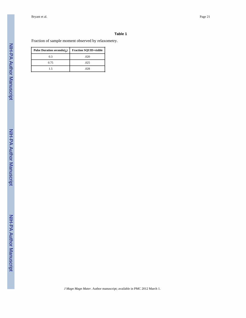
The fraction of the magnetic moment that will be SQUID-visible is then just the ratio ofthese two quantities for the largest pulsed field amplitude used in the excitationmeasurements. See Table 1.

5.3 ResultsFig. 8 presents the SQUID measurements of a) relaxation and b) excitation of the sample ofmagnetite nanoparticles for three different pulse durations compared with the model results,using parameters determined for 300 K. The data shown are plotted for α = 3/2. This valueappears optimal for Fig 8b, but for Fig 8a the optimal value is near α = 2. The modelpredictions were normalized by one fitted constant for 8a and one for 8b. As mentioned insection 4.7, the introduction of Eq.(8) does not affect the overall goodness of fit. It does,however, increase the most favorable diameter from around 25 nm to 26.5 nm.

5.4 Determination of the number of particles

The model moment prediction for the single nanoparticle, , produces amodel data set,yi, for a set of pulsed fields and pulse durations. The measured data setcorresponding to the model set is di. The predicted value for di is nyi, where n is the numberof particles. A least squares fit yields

(15)

Bryant et al.


NIH


NIH


NIH


For the data and the models to which they are compared in Fig 8b, we find n is 1.9×1013.Earlier this sample, a cotton tip, on which fluid containing the suspended particles had beenallowed to evaporate, was estimated (section 4.2) to contain 9.4×1012 particles.

6. ConclusionWe have been able to model the response of a sample of nanoparticles to an acsusceptometry measurement and, fitting the model to the observation, extract values as afunction of temperature of three parameters important to understanding the magneticbehavior, MS, K and logτ0. In the same spirit, with the values of the parameters extractedfrom the susceptibility measurements, we fit results of a SQUID relaxometry study of thesame sample of particles at 300 K for three pulse durations. We have introduced a modifiedLangevin function to include the influence of K on the equilibrium alignment of the momentof a constrained particle with the applied field. Although the use of this semiempiricalapproach produces reasonable fits to the data, understanding the interplay between ratherlarge values of K and the extremely low, seemingly unphysical, values of τ0 requires furtherstudy.

AcknowledgmentsThanks to James R. O'Brien of Quantum Design and Andrew Wang and John Dixon of Ocean Nanotech for theirhelp and kind advice. Thanks also to Richard Larson, Kimberly Butler and Maureen Flynn for their interest andsupport. Comments from Sara Majetich were very helpful. Comments from an anonymous referee substantiallyimproved this paper.

Senior Scientific, LLC, acknowledges the support of the National Institutes of Health under grants R44AI066765,R44CA096154, R44CA105742, and R44CA123785. This work was performed, in part, at the Center for IntegratedNanotechnologies, a U.S. Department of Energy, Office of Basic Energy Sciences user facility. Sandia NationalLaboratories is a multi-program laboratory operated by Sandia Corporation, a Lockheed-Martin Company, for theU. S. Department of Energy under Contract No. DE-AC04-94AL85000. Natalie Adolphi acknowledges equityinterests in nanoMR and ABQMR; nanoMR and ABQMR did not sponsor this research.

References1. Weitschies W, Koetitz R, Bunte T, Trahms L. Pharm. Pharmacol. Lett. 1997; 7:1–4.2. Néel L. Adv. Phys. 1955; 4:191.3. Chantrell RW, Walmsley N, Gore J, Maylin M. Phys. Rev. 2000; B 63 024410-1-14.4. Adolphi NL, Huber DL, Jaetao JE, Bryant HC, Lavato DM, Fegan DL, Venturini EL, Monson TC,

Tessier TE, Hathaway HJ, Bergemann C, Larson RS, Flynn ER. J. Magn. Magn. Mater. 2009;321:1459–1464. [PubMed: 20161153]

5. Flynn ER, Bryant HC. Phys. Med. Biol. 2005; 50:1273–1293. [PubMed: 15798322]6. Aharoni, Amikam. Introduction to the Theory of Ferromagnetism. Oxford; 1996.7. Williams W, Muxworthy AR, Paterson GA. J. Geophys. Res. 2006; 111:1–9. B12S13. [PubMed:

20411040]8. Aragón, Ricardo. Phys Rev B. 1992; 46:5334–5338.9. Majetich SA, Sachen M. J. Phys. D: Appl. Phys. 2006; 39:R407–R422.10. Mayer, JE.; Mayer, MG. Statistical Mechanics. London: John Wiley; 1940. p. 34711. Raikher, Yu. L. J Magn. Magn. Matter. 1983; 39:11–13.12. Raikher, Yu. L.; Stepanov, VI. Phys. Rev. B. 1997; 55:15005–15017.13. Yasumori I, Reinen D, Selwood PW. J. Appl. Phys. 1963; 34:3544–3549. eq. 13.14. Bentivegna F, Ferré J, Nývlt M, Jamet JP, Imhof D, Canva M, Brun A, Veillet P, Višňovský Š,

Chaput F, Boilot JP. J. Appl. Phys. 1998; 83:7776–7788.15. Bessais L, Jaffel L. Ben, Dormann JL. Phys. Rev. B. 1992; 45:7805–7815.16. Chantrell RW, Hoon SR, Tanner BK. J. Magn. Magn. Matter. 1983; 38:133–141.

Bryant et al.


NIH


NIH


NIH


https://www.researchgate.net/publication/236671462_An_Introduction_to_the_Theory_of_Ferromagnetism?el=1_x_8&enrichId=rgreq-5d52a1b92d36048fff6b5705ddc4e613-XXX&enrichSource=Y292ZXJQYWdlOzUxMDczMjEzO0FTOjEwMzg1OTY3ODYxMzUwOEAxNDAxNzczNDg1Mzc2

17. Eberbeck D, Hartwig S, Steinhoff U, Trahms L. Magnetohydrodynamics. 2003; 39:77–83.18. Ludwig F, Heim E, Schilling M. J. Appl. Phys. 2007; 101 113909-1-10.

Bryant et al.


NIH


NIH


NIH


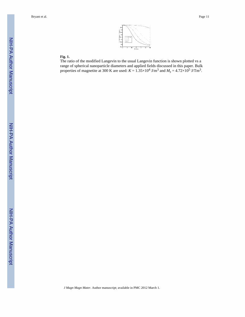
Fig. 1.The ratio of the modified Langevin to the usual Langevin function is shown plotted vs arange of spherical nanoparticle diameters and applied fields discussed in this paper. Bulkproperties of magnetite at 300 K are used: K = 1.35×104 J/m3 and Ms = 4.72×105 J/Tm3.

Bryant et al.


NIH


NIH


NIH


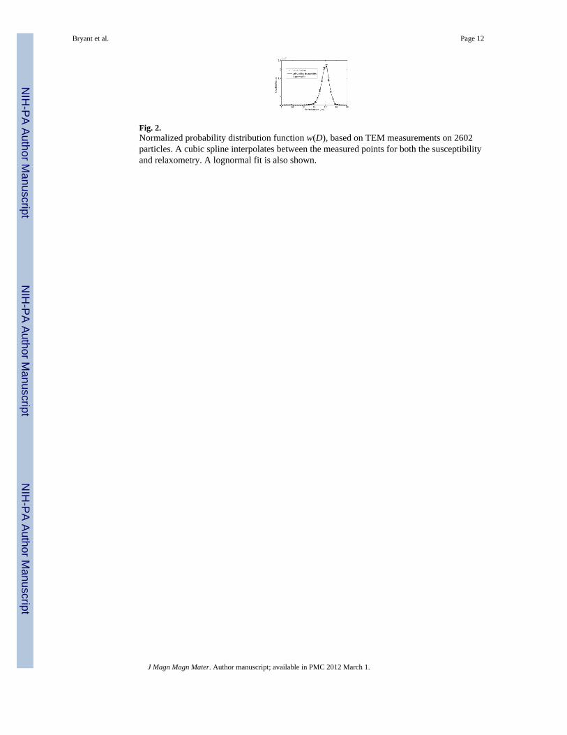
Fig. 2.Normalized probability distribution function w(D), based on TEM measurements on 2602particles. A cubic spline interpolates between the measured points for both the susceptibilityand relaxometry. A lognormal fit is also shown.

Bryant et al.


NIH


NIH


NIH


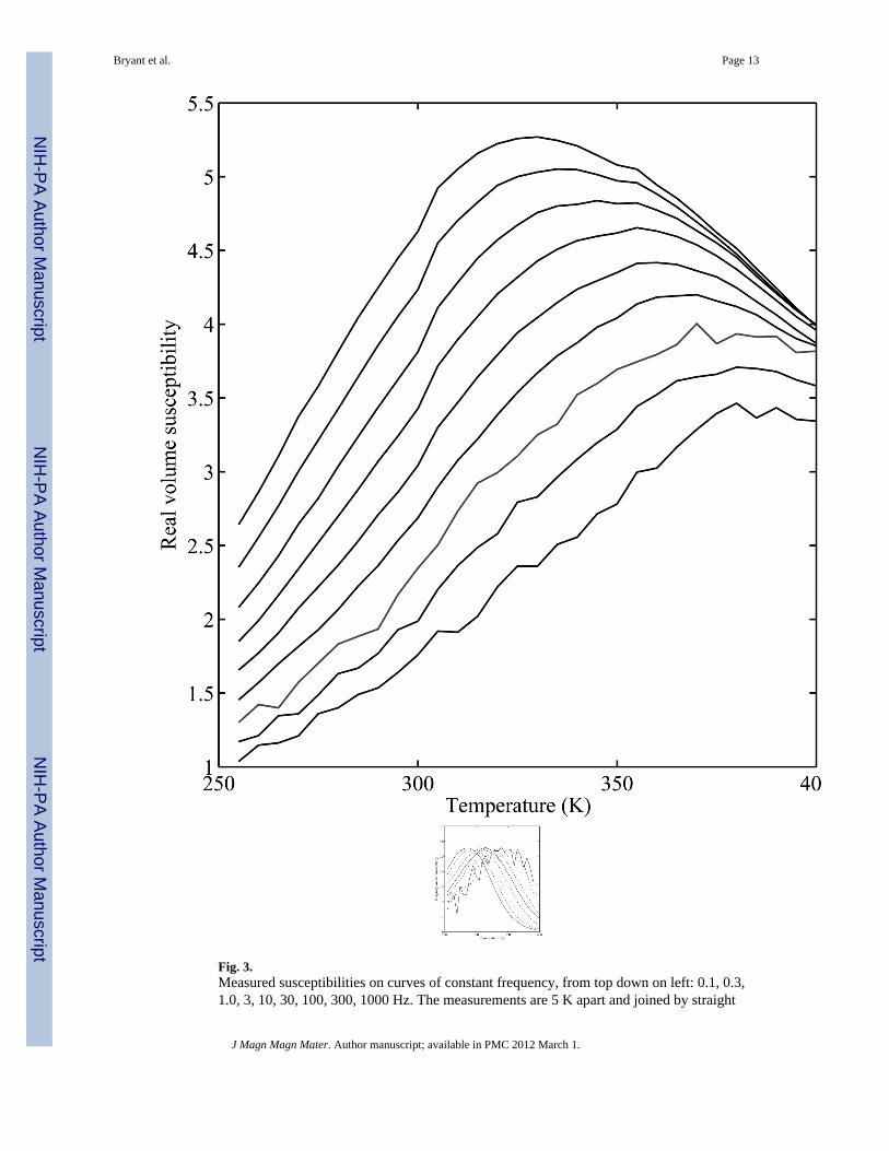
Fig. 3.Measured susceptibilities on curves of constant frequency, from top down on left: 0.1, 0.3,1.0, 3, 10, 30, 100, 300, 1000 Hz. The measurements are 5 K apart and joined by straight

Bryant et al.


NIH


NIH


NIH


lines. The ordinates are volume susceptibility in rationalized MKS. (a) Real part. (b)Imaginary part.

Bryant et al.


NIH


NIH


NIH


Fig.4.Representative samples of fitted constant temperature curves for susceptibility. The 3parameters in the model, Ms, K and τ0, are adjusted for each temperature to give the best fitto the 9 frequency points. (a) Real part for temperatures starting right bottom up: 260 to 350K in 10 K increments. (b) Imaginary part for 290 K, diamonds, 300 K, circles, 310 K,squares. There is relatively more noise in the imaginary than the real measurements becausethe signals are an order of magnitude smaller. All 30 constant T data sets were fit in thismanner.

Bryant et al.


NIH


NIH


NIH


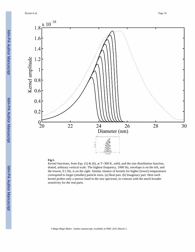
Fig.5.Kernel functions, from Eqs. (5) & (6), at T=300 K, solid, and the size distribution function,dotted, arbitrary vertical scale. The highest frequency, 1000 Hz, envelope is on the left, andthe lowest, 0.1 Hz, is on the right. Similar clusters of kernels for higher (lower) temperaturescorrespond to larger (smaller) particle sizes. (a) Real part. (b) Imaginary part. Here eachkernel probes only a narrow band in the size spectrum, in contrast with the much broadersensitivity for the real parts.

Bryant et al.


NIH


NIH


NIH


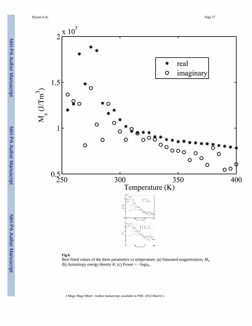
Fig.6.Best fitted values of the three parameters vs temperature. (a) Saturated magnetization, Ms.(b) Anisotropy energy density K. (c) Power = −logτ0.

Bryant et al.


NIH


NIH


NIH


Bryant et al.


NIH


NIH


NIH


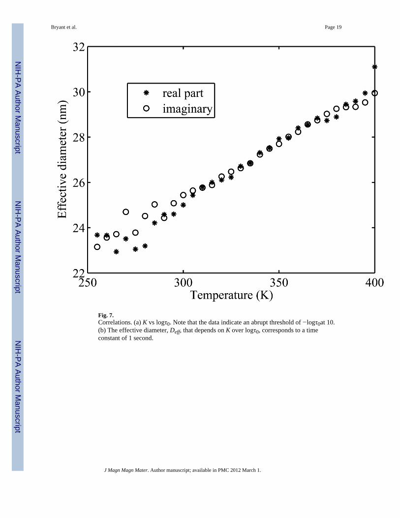
Fig. 7.Correlations. (a) K vs logτ0. Note that the data indicate an abrupt threshold of −logτ0at 10.(b) The effective diameter, Deff, that depends on K over logτ0, corresponds to a timeconstant of 1 second.

Bryant et al.


NIH


NIH


NIH


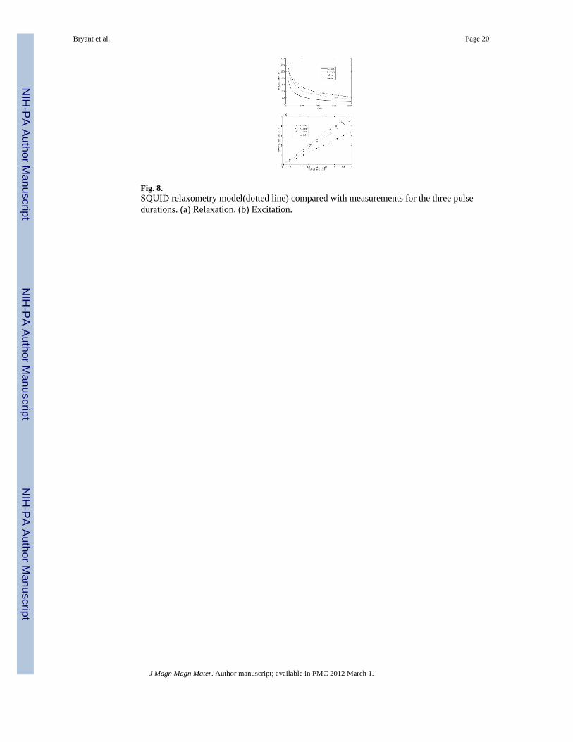
Fig. 8.SQUID relaxometry model(dotted line) compared with measurements for the three pulsedurations. (a) Relaxation. (b) Excitation.

Bryant et al.


NIH


NIH


NIH


NIH


NIH


NIH


Bryant et al.

Table 1

Fraction of sample moment observed by relaxometry.

Pulse Duration seconds(tp) Fraction SQUID-visible

0.3 .020

0.75 .025

1.5 .028


Magnetic properties of nanoparticles useful for SQUID relaxometry in biomedical applications

Documents

Transcript of Magnetic properties of nanoparticles useful for SQUID relaxometry in biomedical applications