Oracle® Data Mining - API Guide
650
Oracle® Data Mining API Guide 18c E91362-07 May 2021
-
Upload
khangminh22 -
Category
Documents
-
view
0 -
download
0
Transcript of Oracle® Data Mining - API Guide
Oracle® Data MiningAPI Guide
18cE91362-07May 2021

Oracle Data Mining API Guide, 18c
E91362-07
Copyright © 2005, 2021, Oracle and/or its affiliates.
Primary Author: Sarika Surampudi
This software and related documentation are provided under a license agreement containing restrictions onuse and disclosure and are protected by intellectual property laws. Except as expressly permitted in yourlicense agreement or allowed by law, you may not use, copy, reproduce, translate, broadcast, modify, license,transmit, distribute, exhibit, perform, publish, or display any part, in any form, or by any means. Reverseengineering, disassembly, or decompilation of this software, unless required by law for interoperability, isprohibited.
The information contained herein is subject to change without notice and is not warranted to be error-free. Ifyou find any errors, please report them to us in writing.
If this is software or related documentation that is delivered to the U.S. Government or anyone licensing it onbehalf of the U.S. Government, then the following notice is applicable:
U.S. GOVERNMENT END USERS: Oracle programs (including any operating system, integrated software,any programs embedded, installed or activated on delivered hardware, and modifications of such programs)and Oracle computer documentation or other Oracle data delivered to or accessed by U.S. Governmentend users are "commercial computer software" or "commercial computer software documentation" pursuantto the applicable Federal Acquisition Regulation and agency-specific supplemental regulations. As such,the use, reproduction, duplication, release, display, disclosure, modification, preparation of derivative works,and/or adaptation of i) Oracle programs (including any operating system, integrated software, any programsembedded, installed or activated on delivered hardware, and modifications of such programs), ii) Oraclecomputer documentation and/or iii) other Oracle data, is subject to the rights and limitations specified in thelicense contained in the applicable contract. The terms governing the U.S. Government’s use of Oracle cloudservices are defined by the applicable contract for such services. No other rights are granted to the U.S.Government.
This software or hardware is developed for general use in a variety of information management applications.It is not developed or intended for use in any inherently dangerous applications, including applications thatmay create a risk of personal injury. If you use this software or hardware in dangerous applications, then youshall be responsible to take all appropriate fail-safe, backup, redundancy, and other measures to ensure itssafe use. Oracle Corporation and its affiliates disclaim any liability for any damages caused by use of thissoftware or hardware in dangerous applications.
Oracle and Java are registered trademarks of Oracle and/or its affiliates. Other names may be trademarks oftheir respective owners.
Intel and Intel Inside are trademarks or registered trademarks of Intel Corporation. All SPARC trademarks areused under license and are trademarks or registered trademarks of SPARC International, Inc. AMD, Epyc,and the AMD logo are trademarks or registered trademarks of Advanced Micro Devices. UNIX is a registeredtrademark of The Open Group.
This software or hardware and documentation may provide access to or information about content, products,and services from third parties. Oracle Corporation and its affiliates are not responsible for and expresslydisclaim all warranties of any kind with respect to third-party content, products, and services unless otherwiseset forth in an applicable agreement between you and Oracle. Oracle Corporation and its affiliates will notbe responsible for any loss, costs, or damages incurred due to your access to or use of third-party content,products, or services, except as set forth in an applicable agreement between you and Oracle.
Contents
Preface
Audience xxii
Documentation Accessibility xxii
Diversity and Inclusion xxii
Related Resources xxiii
Conventions xxiii
Part I Introductions
1 Introduction to Oracle Data Mining
1.1 About Oracle Data Mining 1-1
1.2 Data Mining in the Database Kernel 1-1
1.3 Data Mining in Oracle Exadata 1-2
1.4 About Partitioned Model 1-3
1.5 Interfaces to Oracle Data Mining 1-3
1.5.1 PL/SQL API 1-3
1.5.2 SQL Functions 1-4
1.5.3 Oracle Data Miner 1-5
1.5.4 Predictive Analytics 1-5
1.6 Overview of Database Analytics 1-6
2 Oracle Data Mining Basics
2.1 Mining Functions 2-1
2.1.1 Supervised Data Mining 2-1
2.1.1.1 Supervised Learning: Testing 2-2
2.1.1.2 Supervised Learning: Scoring 2-2
2.1.2 Unsupervised Data Mining 2-2
2.1.2.1 Unsupervised Learning: Scoring 2-3
2.2 Algorithms 2-3
2.2.1 Oracle Data Mining Supervised Algorithms 2-4
iii
2.2.2 Oracle Data Mining Unsupervised Algorithms 2-5
2.3 Data Preparation 2-6
2.3.1 Oracle Data Mining Simplifies Data Preparation 2-6
2.3.2 Case Data 2-7
2.3.2.1 Nested Data 2-7
2.3.3 Text Data 2-7
2.4 In-Database Scoring 2-8
2.4.1 Parallel Execution and Ease of Administration 2-8
2.4.2 SQL Functions for Model Apply and Dynamic Scoring 2-8
Part II Mining Functions
3 Regression
3.1 About Regression 3-1
3.1.1 How Does Regression Work? 3-1
3.1.1.1 Linear Regression 3-2
3.1.1.2 Multivariate Linear Regression 3-3
3.1.1.3 Regression Coefficients 3-3
3.1.1.4 Nonlinear Regression 3-3
3.1.1.5 Multivariate Nonlinear Regression 3-4
3.1.1.6 Confidence Bounds 3-4
3.2 Testing a Regression Model 3-4
3.2.1 Regression Statistics 3-4
3.2.1.1 Root Mean Squared Error 3-4
3.2.1.2 Mean Absolute Error 3-5
3.3 Regression Algorithms 3-5
4 Classification
4.1 About Classification 4-1
4.2 Testing a Classification Model 4-2
4.2.1 Confusion Matrix 4-2
4.2.2 Lift 4-3
4.2.2.1 Lift Statistics 4-3
4.2.3 Receiver Operating Characteristic (ROC) 4-4
4.2.3.1 The ROC Curve 4-4
4.2.3.2 Area Under the Curve 4-5
4.2.3.3 ROC and Model Bias 4-5
4.2.3.4 ROC Statistics 4-5
4.3 Biasing a Classification Model 4-6
iv

4.3.1 Costs 4-6
4.3.1.1 Costs Versus Accuracy 4-6
4.3.1.2 Positive and Negative Classes 4-6
4.3.1.3 Assigning Costs and Benefits 4-7
4.3.2 Priors and Class Weights 4-8
4.4 Classification Algorithms 4-8
5 Anomaly Detection
5.1 About Anomaly Detection 5-1
5.1.1 One-Class Classification 5-1
5.1.2 Anomaly Detection for Single-Class Data 5-2
5.1.3 Anomaly Detection for Finding Outliers 5-2
5.2 Anomaly Detection Algorithm 5-3
6 Clustering
6.1 About Clustering 6-1
6.1.1 How are Clusters Computed? 6-1
6.1.2 Scoring New Data 6-2
6.1.3 Hierarchical Clustering 6-2
6.1.3.1 Rules 6-2
6.1.3.2 Support and Confidence 6-2
6.2 Evaluating a Clustering Model 6-2
6.3 Clustering Algorithms 6-2
7 Association
7.1 About Association 7-1
7.1.1 Association Rules 7-1
7.1.2 Market-Basket Analysis 7-1
7.1.3 Association Rules and eCommerce 7-2
7.2 Transactional Data 7-2
7.3 Association Algorithm 7-3
8 Feature Selection and Extraction
8.1 Finding the Best Attributes 8-1
8.2 About Feature Selection and Attribute Importance 8-2
8.2.1 Attribute Importance and Scoring 8-2
8.3 About Feature Extraction 8-2
8.3.1 Feature Extraction and Scoring 8-3
v
8.4 Algorithms for Attribute Importance and Feature Extraction 8-3
9 Time Series
9.1 About Time Series 9-1
9.2 Choosing a Time Series Model 9-1
9.3 Time Series Statistics 9-2
9.3.1 Conditional Log-Likelihood 9-2
9.3.2 Mean Square Error (MSE) and Other Error Measures 9-3
9.3.3 Irregular Time Series 9-4
9.3.4 Build Apply 9-4
9.4 Time Series Algorithm 9-4
Part III Algorithms
10
Apriori
10.1 About Apriori 10-1
10.2 Association Rules and Frequent Itemsets 10-2
10.2.1 Antecedent and Consequent 10-2
10.2.2 Confidence 10-2
10.3 Data Preparation for Apriori 10-2
10.3.1 Native Transactional Data and Star Schemas 10-2
10.3.2 Items and Collections 10-2
10.3.3 Sparse Data 10-3
10.3.4 Improved Sampling 10-3
10.3.4.1 Sampling Implementation 10-4
10.4 Calculating Association Rules 10-4
10.4.1 Itemsets 10-4
10.4.2 Frequent Itemsets 10-5
10.4.3 Example: Calculating Rules from Frequent Itemsets 10-6
10.4.4 Aggregates 10-7
10.4.5 Example: Calculating Aggregates 10-8
10.4.6 Including and Excluding Rules 10-8
10.4.7 Performance Impact for Aggregates 10-9
10.5 Evaluating Association Rules 10-9
10.5.1 Support 10-9
10.5.2 Minimum Support Count 10-9
10.5.3 Confidence 10-10
10.5.4 Reverse Confidence 10-10
vi
10.5.5 Lift 10-10
11
CUR Matrix Decomposition
11.1 About CUR Matrix Decomposition 11-1
11.2 Singular Vectors 11-1
11.3 Statistical Leverage Score 11-2
11.4 Column (Attribute) Selection and Row Selection 11-2
11.5 CUR Matrix Decomposition Algorithm Configuration 11-3
12
Decision Tree
12.1 About Decision Tree 12-1
12.1.1 Decision Tree Rules 12-1
12.1.1.1 Confidence and Support 12-2
12.1.2 Advantages of Decision Trees 12-3
12.1.3 XML for Decision Tree Models 12-3
12.2 Growing a Decision Tree 12-3
12.2.1 Splitting 12-4
12.2.2 Cost Matrix 12-5
12.2.3 Preventing Over-Fitting 12-5
12.3 Tuning the Decision Tree Algorithm 12-5
12.4 Data Preparation for Decision Tree 12-6
13
Expectation Maximization
13.1 About Expectation Maximization 13-1
13.1.1 Expectation Step and Maximization Step 13-1
13.1.2 Probability Density Estimation 13-1
13.2 Algorithm Enhancements 13-2
13.2.1 Scalability 13-2
13.2.2 High Dimensionality 13-3
13.2.3 Number of Components 13-3
13.2.4 Parameter Initialization 13-3
13.2.5 From Components to Clusters 13-3
13.3 Configuring the Algorithm 13-4
13.4 Data Preparation for Expectation Maximization 13-4
14
Explicit Semantic Analysis
14.1 About Explicit Semantic Analysis 14-1
14.1.1 Scoring with ESA 14-2
vii
14.1.2 Scoring Large ESA Models 14-2
14.2 ESA for Text Mining 14-2
14.3 Data Preparation for ESA 14-3
14.4 Terminologies in Explicit Semantic Analysis 14-3
15
Exponential Smoothing
15.1 About Exponential Smoothing 15-1
15.1.1 Exponential Smoothing Models 15-1
15.1.2 Simple Exponential Smoothing 15-2
15.1.3 Models with Trend but No Seasonality 15-2
15.1.4 Models with Seasonality but No Trend 15-2
15.1.5 Models with Trend and Seasonality 15-3
15.1.6 Prediction Intervals 15-3
15.2 Data Preparation for Exponential Smoothing Models 15-3
15.2.1 Input Data 15-4
15.2.2 Accumulation 15-4
15.2.3 Missing Value 15-4
15.2.4 Prediction 15-5
15.2.5 Parallellism by Partition 15-5
16
Generalized Linear Models
16.1 About Generalized Linear Models 16-1
16.2 GLM in Oracle Data Mining 16-2
16.2.1 Interpretability and Transparency 16-2
16.2.2 Wide Data 16-2
16.2.3 Confidence Bounds 16-2
16.2.4 Ridge Regression 16-3
16.2.4.1 Configuring Ridge Regression 16-3
16.2.4.2 Ridge and Confidence Bounds 16-4
16.2.4.3 Ridge and Data Preparation 16-4
16.3 Scalable Feature Selection 16-4
16.3.1 Feature Selection 16-4
16.3.1.1 Configuring Feature Selection 16-4
16.3.1.2 Feature Selection and Ridge Regression 16-5
16.3.2 Feature Generation 16-5
16.3.2.1 Configuring Feature Generation 16-5
16.4 Tuning and Diagnostics for GLM 16-5
16.4.1 Build Settings 16-5
16.4.2 Diagnostics 16-6
viii
16.4.2.1 Coefficient Statistics 16-6
16.4.2.2 Global Model Statistics 16-6
16.4.2.3 Row Diagnostics 16-7
16.5 GLM Solvers 16-7
16.6 Data Preparation for GLM 16-7
16.6.1 Data Preparation for Linear Regression 16-8
16.6.2 Data Preparation for Logistic Regression 16-8
16.6.3 Missing Values 16-9
16.7 Linear Regression 16-9
16.7.1 Coefficient Statistics for Linear Regression 16-10
16.7.2 Global Model Statistics for Linear Regression 16-10
16.7.3 Row Diagnostics for Linear Regression 16-11
16.8 Logistic Regression 16-11
16.8.1 Reference Class 16-11
16.8.2 Class Weights 16-11
16.8.3 Coefficient Statistics for Logistic Regression 16-11
16.8.4 Global Model Statistics for Logistic Regression 16-12
16.8.5 Row Diagnostics for Logistic Regression 16-12
17
k-Means
17.1 About k-Means 17-1
17.1.1 Oracle Data Mining Enhanced k-Means 17-1
17.1.2 Centroid 17-1
17.2 k-Means Algorithm Configuration 17-2
17.3 Data Preparation for k-Means 17-2
18
Minimum Description Length
18.1 About MDL 18-1
18.1.1 Compression and Entropy 18-1
18.1.1.1 Values of a Random Variable: Statistical Distribution 18-2
18.1.1.2 Values of a Random Variable: Significant Predictors 18-2
18.1.1.3 Total Entropy 18-2
18.1.2 Model Size 18-2
18.1.3 Model Selection 18-2
18.1.4 The MDL Metric 18-3
18.2 Data Preparation for MDL 18-3
ix
19
Naive Bayes
19.1 About Naive Bayes 19-1
19.1.1 Advantages of Naive Bayes 19-3
19.2 Tuning a Naive Bayes Model 19-3
19.3 Data Preparation for Naive Bayes 19-3
20
Neural Network
20.1 About Neural Network 20-1
20.1.1 Neuron and activation function 20-1
20.1.2 Loss or Cost function 20-2
20.1.3 Forward-Backward Propagation 20-2
20.1.4 Optimization Solver 20-2
20.1.5 Regularization 20-2
20.1.6 Convergence Check 20-3
20.1.7 LBFGS_SCALE_HESSIAN 20-3
20.1.8 NNET_HELDASIDE_MAX_FAIL 20-3
20.2 Data Preparation for Neural Network 20-3
20.3 Neural Network Algorithm Configuration 20-4
20.4 Scoring with Neural Network 20-5
21
Non-Negative Matrix Factorization
21.1 About NMF 21-1
21.1.1 Matrix Factorization 21-1
21.1.2 Scoring with NMF 21-2
21.1.3 Text Mining with NMF 21-2
21.2 Tuning the NMF Algorithm 21-2
21.3 Data Preparation for NMF 21-3
22
O-Cluster
22.1 About O-Cluster 22-1
22.1.1 Partitioning Strategy 22-1
22.1.1.1 Partitioning Numerical Attributes 22-2
22.1.1.2 Partitioning Categorical Attributes 22-2
22.1.2 Active Sampling 22-2
22.1.3 Process Flow 22-2
22.1.4 Scoring 22-3
22.2 Tuning the O-Cluster Algorithm 22-3
22.3 Data Preparation for O-Cluster 22-3
x

22.3.1 User-Specified Data Preparation for O-Cluster 22-4
23
R Extensibility
23.1 Oracle Data Mining with R Extensibility 23-1
23.2 Scoring with R 23-2
23.3 About Algorithm Meta Data Registration 23-2
23.3.1 Algorithm Meta Data Registration 23-2
24
Random Forest
24.1 About Random Forest 24-1
24.2 Building a Random Forest 24-1
24.3 Scoring with Random Forest 24-2
25
Singular Value Decomposition
25.1 About Singular Value Decomposition 25-1
25.1.1 Matrix Manipulation 25-1
25.1.2 Low Rank Decomposition 25-2
25.1.3 Scalability 25-2
25.2 Configuring the Algorithm 25-3
25.2.1 Model Size 25-3
25.2.2 Performance 25-3
25.2.3 PCA scoring 25-3
25.3 Data Preparation for SVD 25-4
26
Support Vector Machines
26.1 About Support Vector Machines 26-1
26.1.1 Advantages of SVM 26-1
26.1.2 Advantages of SVM in Oracle Data Mining 26-2
26.1.2.1 Usability 26-2
26.1.2.2 Scalability 26-2
26.1.3 Kernel-Based Learning 26-2
26.2 Tuning an SVM Model 26-3
26.3 Data Preparation for SVM 26-3
26.3.1 Normalization 26-4
26.3.2 SVM and Automatic Data Preparation 26-4
26.4 SVM Classification 26-4
26.4.1 Class Weights 26-4
26.5 One-Class SVM 26-5
xi

26.6 SVM Regression 26-5
Part IV Using the Data Mining API
27
Data Mining With SQL
27.1 Highlights of the Data Mining API 27-1
27.2 Example: Targeting Likely Candidates for a Sales Promotion 27-2
27.3 Example: Analyzing Preferred Customers 27-3
27.4 Example: Segmenting Customer Data 27-5
27.5 Example : Building an ESA Model with a Wiki Dataset 27-6
28
About the Data Mining API
28.1 About Mining Models 28-1
28.2 Data Mining Data Dictionary Views 28-2
28.2.1 ALL_MINING_MODELS 28-2
28.2.2 ALL_MINING_MODEL_ATTRIBUTES 28-3
28.2.3 ALL_MINING_MODEL_PARTITIONS 28-4
28.2.4 ALL_MINING_MODEL_SETTINGS 28-5
28.2.5 ALL_MINING_MODEL_VIEWS 28-6
28.2.6 ALL_MINING_MODEL_XFORMS 28-7
28.3 Data Mining PL/SQL Packages 28-7
28.3.1 DBMS_DATA_MINING 28-8
28.3.2 DBMS_DATA_MINING_TRANSFORM 28-8
28.3.2.1 Transformation Methods inDBMS_DATA_MINING_TRANSFORM 28-9
28.3.3 DBMS_PREDICTIVE_ANALYTICS 28-9
28.4 Data Mining SQL Scoring Functions 28-10
29
Preparing the Data
29.1 Data Requirements 29-1
29.1.1 Column Data Types 29-2
29.1.2 Data Sets for Classification and Regression 29-2
29.1.3 Scoring Requirements 29-2
29.2 About Attributes 29-3
29.2.1 Data Attributes and Model Attributes 29-3
29.2.2 Target Attribute 29-4
29.2.3 Numericals, Categoricals, and Unstructured Text 29-5
29.2.4 Model Signature 29-5
xii

29.2.5 Scoping of Model Attribute Name 29-6
29.2.6 Model Details 29-6
29.3 Using Nested Data 29-7
29.3.1 Nested Object Types 29-7
29.3.2 Example: Transforming Transactional Data for Mining 29-8
29.4 Using Market Basket Data 29-10
29.4.1 Example: Creating a Nested Column for Market Basket Analysis 29-10
29.5 Using Retail Analysis Data 29-11
29.5.1 Example: Calculating Aggregates 29-12
29.6 Handling Missing Values 29-12
29.6.1 Examples: Missing Values or Sparse Data? 29-13
29.6.1.1 Sparsity in a Sales Table 29-13
29.6.1.2 Missing Values in a Table of Customer Data 29-13
29.6.2 Missing Value Treatment in Oracle Data Mining 29-13
29.6.3 Changing the Missing Value Treatment 29-15
30
Transforming the Data
30.1 About Transformations 30-1
30.2 Preparing the Case Table 30-2
30.2.1 Creating Nested Columns 30-2
30.2.2 Converting Column Data Types 30-2
30.2.3 Text Transformation 30-2
30.2.4 About Business and Domain-Sensitive Transformations 30-3
30.3 Understanding Automatic Data Preparation 30-3
30.3.1 Binning 30-3
30.3.2 Normalization 30-4
30.3.3 How ADP Transforms the Data 30-4
30.4 Embedding Transformations in a Model 30-5
30.4.1 Specifying Transformation Instructions for an Attribute 30-5
30.4.1.1 Expression Records 30-6
30.4.1.2 Attribute Specifications 30-7
30.4.2 Building a Transformation List 30-7
30.4.2.1 SET_TRANSFORM 30-7
30.4.2.2 The STACK Interface 30-8
30.4.2.3 GET_MODEL_TRANSFORMATIONS andGET_TRANSFORM_LIST 30-8
30.4.3 Transformation Lists and Automatic Data Preparation 30-9
30.4.4 Oracle Data Mining Transformation Routines 30-9
30.4.4.1 Binning Routines 30-9
30.4.4.2 Normalization Routines 30-10
30.4.4.3 Outlier Treatment 30-11
xiii

30.4.4.4 Routines for Outlier Treatment 30-11
30.5 Understanding Reverse Transformations 30-12
31
Creating a Model
31.1 Before Creating a Model 31-1
31.2 The CREATE_MODEL Procedure 31-1
31.2.1 Choosing the Mining Function 31-2
31.2.2 Choosing the Algorithm 31-3
31.2.3 Supplying Transformations 31-4
31.2.3.1 Creating a Transformation List 31-5
31.2.3.2 Transformation List and Automatic Data Preparation 31-5
31.2.4 About Partitioned Model 31-5
31.2.4.1 Partitioned Model Build Process 31-6
31.2.4.2 DDL in Partitioned model 31-6
31.2.4.3 Partitioned Model scoring 31-7
31.3 Specifying Model Settings 31-8
31.3.1 Specifying Costs 31-9
31.3.2 Specifying Prior Probabilities 31-10
31.3.3 Specifying Class Weights 31-10
31.3.4 Model Settings in the Data Dictionary 31-11
31.3.5 Specifying Mining Model Settings for R Model 31-12
31.3.5.1 ALGO_EXTENSIBLE_LANG 31-12
31.3.5.2 RALG_BUILD_FUNCTION 31-13
31.3.5.3 RALG_DETAILS_FUNCTION 31-15
31.3.5.4 RALG_SCORE_FUNCTION 31-16
31.3.5.5 RALG_WEIGHT_FUNCTION 31-19
31.3.5.6 Registered R Scripts 31-20
31.3.5.7 R Model Demonstration Scripts 31-20
31.4 Model Detail Views 31-20
31.4.1 Model Detail Views for Association Rules 31-21
31.4.2 Model Detail View for Frequent Itemsets 31-26
31.4.3 Model Detail View for Transactional Itemsets 31-27
31.4.4 Model Detail View for Transactional Rule 31-28
31.4.5 Model Detail Views for Classification Algorithms 31-29
31.4.6 Model Detail Views for Decision Tree 31-30
31.4.7 Model Detail Views for Generalized Linear Model 31-32
31.4.8 Model Detail Views for Naive Bayes 31-40
31.4.9 Model Detail Views for Neural Network 31-41
31.4.10 Model Detail Views for Random Forest 31-42
31.4.11 Model Detail View for Support Vector Machine 31-43
xiv
31.4.12 Model Detail Views for Clustering Algorithms 31-44
31.4.13 Model Detail Views for Expectation Maximization 31-47
31.4.14 Model Detail Views for k-Means 31-51
31.4.15 Model Detail Views for O-Cluster 31-52
31.4.16 Model Detail Views for CUR Matrix Decomposition 31-54
31.4.17 Model Detail Views for Explicit Semantic Analysis 31-55
31.4.18 Model Detail Views for Exponential Smoothing Models 31-57
31.4.19 Model Detail Views for Non-Negative Matrix Factorization 31-59
31.4.20 Model Detail Views for Singular Value Decomposition 31-60
31.4.21 Model Detail View for Minimum Description Length 31-63
31.4.22 Model Detail View for Binning 31-64
31.4.23 Model Detail Views for Global Information 31-64
31.4.24 Model Detail View for Normalization and Missing Value Handling 31-66
32
Scoring and Deployment
32.1 About Scoring and Deployment 32-1
32.2 Using the Data Mining SQL Functions 32-2
32.2.1 Choosing the Predictors 32-2
32.2.2 Single-Record Scoring 32-3
32.3 Prediction Details 32-4
32.3.1 Cluster Details 32-4
32.3.2 Feature Details 32-5
32.3.3 Prediction Details 32-5
32.3.4 GROUPING Hint 32-7
32.4 Real-Time Scoring 32-8
32.5 Dynamic Scoring 32-8
32.6 Cost-Sensitive Decision Making 32-10
32.7 DBMS_DATA_MINING.Apply 32-12
33
Mining Unstructured Text
33.1 About Unstructured Text 33-1
33.2 About Text Mining and Oracle Text 33-1
33.3 Data Preparation for Text Features 33-2
33.4 Creating a Model that Includes Text Mining 33-2
33.5 Creating a Text Policy 33-4
33.6 Configuring a Text Attribute 33-5
xv
34
Administrative Tasks for Oracle Data Mining
34.1 Installing and Configuring a Database for Data Mining 34-1
34.1.1 About Installation 34-1
34.1.2 Enabling or Disabling a Database Option 34-2
34.1.3 Database Tuning Considerations for Data Mining 34-2
34.2 Upgrading or Downgrading Oracle Data Mining 34-3
34.2.1 Pre-Upgrade Steps 34-3
34.2.1.1 Dropping Models Created in Java 34-3
34.2.1.2 Dropping Mining Activities Created in Oracle Data Miner Classic 34-3
34.2.2 Upgrading Oracle Data Mining 34-4
34.2.2.1 Using Database Upgrade Assistant to Upgrade Oracle DataMining 34-4
34.2.2.2 Using Export/Import to Upgrade Data Mining Models 34-5
34.2.3 Post Upgrade Steps 34-6
34.2.4 Downgrading Oracle Data Mining 34-7
34.3 Exporting and Importing Mining Models 34-7
34.3.1 About Oracle Data Pump 34-7
34.3.2 Options for Exporting and Importing Mining Models 34-8
34.3.3 Directory Objects for EXPORT_MODEL and IMPORT_MODEL 34-9
34.3.4 Using EXPORT_MODEL and IMPORT_MODEL 34-10
34.3.5 EXPORT and IMPORT Serialized Models 34-12
34.3.6 Importing From PMML 34-12
34.4 Controlling Access to Mining Models and Data 34-12
34.4.1 Creating a Data Mining User 34-12
34.4.1.1 Granting Privileges for Data Mining 34-14
34.4.2 System Privileges for Data Mining 34-14
34.4.3 Object Privileges for Mining Models 34-15
34.5 Auditing and Adding Comments to Mining Models 34-16
34.5.1 Adding a Comment to a Mining Model 34-16
34.5.2 Auditing Mining Models 34-17
35
The Data Mining Sample Programs
35.1 About the Data Mining Sample Programs 35-1
35.2 Installing the Data Mining Sample Programs 35-2
35.3 The Data Mining Sample Data 35-3
Part V Oracle Data Mining API Reference
xvi

36
PL/SQL Packages
36.1 DBMS_DATA_MINING 36-1
36.1.1 Using DBMS_DATA_MINING 36-1
36.1.1.1 DBMS_DATA_MINING Overview 36-2
36.1.1.2 DBMS_DATA_MINING Security Model 36-3
36.1.1.3 DBMS_DATA_MINING — Mining Functions 36-4
36.1.2 DBMS_DATA_MINING — Model Settings 36-5
36.1.2.1 DBMS_DATA_MINING — Algorithm Names 36-5
36.1.2.2 DBMS_DATA_MINING — Automatic Data Preparation 36-6
36.1.2.3 DBMS_DATA_MINING — Mining Function Settings 36-8
36.1.2.4 DBMS_DATA_MINING — Global Settings 36-13
36.1.2.5 DBMS_DATA_MINING — Algorithm Settings:ALGO_EXTENSIBLE_LANG 36-16
36.1.2.6 DBMS_DATA_MINING — Algorithm Settings: CUR MatrixDecomposition 36-18
36.1.2.7 DBMS_DATA_MINING — Algorithm Settings: Decision Tree 36-19
36.1.2.8 DBMS_DATA_MINING — Algorithm Settings: ExpectationMaximization 36-20
36.1.2.9 DBMS_DATA_MINING — Algorithm Settings: Explicit SemanticAnalysis 36-23
36.1.2.10 DBMS_DATA_MINING — Algorithm Settings: ExponentialSmoothing 36-24
36.1.2.11 DBMS_DATA_MINING — Algorithm Settings: GeneralizedLinear Models 36-28
36.1.2.12 DBMS_DATA_MINING — Algorithm Settings: k-Means 36-31
36.1.2.13 DBMS_DATA_MINING — Algorithm Settings: Naive Bayes 36-32
36.1.2.14 DBMS_DATA_MINING — Algorithm Settings: Neural Network 36-33
36.1.2.15 DBMS_DATA_MINING — Algorithm Settings: Non-NegativeMatrix Factorization 36-35
36.1.2.16 DBMS_DATA_MINING — Algorithm Settings: O-Cluster 36-36
36.1.2.17 DBMS_DATA_MINING — Algorithm Settings: Random Forest 36-36
36.1.2.18 DBMS_DATA_MINING — Algorithm Constants and Settings:Singular Value Decomposition 36-37
36.1.2.19 DBMS_DATA_MINING — Algorithm Settings: Support VectorMachine 36-39
36.1.3 DBMS_DATA_MINING — Solver Settings 36-40
36.1.3.1 DBMS_DATA_MINING — Solver Settings: ADMM 36-41
36.1.3.2 DBMS_DATA_MINING — Solver Settings: LBFGS 36-41
36.1.4 DBMS_DATA_MINING Datatypes 36-42
36.1.4.1 Deprecated Types 36-43
36.1.5 Summary of DBMS_DATA_MINING Subprograms 36-48
36.1.5.1 ADD_COST_MATRIX Procedure 36-51
36.1.5.2 ADD_PARTITION Procedure 36-53
xvii
36.1.5.3 ALTER_REVERSE_EXPRESSION Procedure 36-54
36.1.5.4 APPLY Procedure 36-58
36.1.5.5 COMPUTE_CONFUSION_MATRIX Procedure 36-61
36.1.5.6 COMPUTE_CONFUSION_MATRIX_PART Procedure 36-67
36.1.5.7 COMPUTE_LIFT Procedure 36-74
36.1.5.8 COMPUTE_LIFT_PART Procedure 36-79
36.1.5.9 COMPUTE_ROC Procedure 36-85
36.1.5.10 COMPUTE_ROC_PART Procedure 36-89
36.1.5.11 CREATE_MODEL Procedure 36-94
36.1.5.12 CREATE_MODEL2 Procedure 36-98
36.1.5.13 Create Model Using Registration Information 36-100
36.1.5.14 DROP_ALGORITHM Procedure 36-100
36.1.5.15 DROP_PARTITION Procedure 36-101
36.1.5.16 DROP_MODEL Procedure 36-101
36.1.5.17 EXPORT_MODEL Procedure 36-102
36.1.5.18 EXPORT_SERMODEL Procedure 36-105
36.1.5.19 FETCH_JSON_SCHEMA Procedure 36-106
36.1.5.20 GET_ASSOCIATION_RULES Function 36-107
36.1.5.21 GET_FREQUENT_ITEMSETS Function 36-112
36.1.5.22 GET_MODEL_COST_MATRIX Function 36-114
36.1.5.23 GET_MODEL_DETAILS_AI Function 36-116
36.1.5.24 GET_MODEL_DETAILS_EM Function 36-117
36.1.5.25 GET_MODEL_DETAILS_EM_COMP Function 36-119
36.1.5.26 GET_MODEL_DETAILS_EM_PROJ Function 36-121
36.1.5.27 GET_MODEL_DETAILS_GLM Function 36-122
36.1.5.28 GET_MODEL_DETAILS_GLOBAL Function 36-126
36.1.5.29 GET_MODEL_DETAILS_KM Function 36-127
36.1.5.30 GET_MODEL_DETAILS_NB Function 36-129
36.1.5.31 GET_MODEL_DETAILS_NMF Function 36-131
36.1.5.32 GET_MODEL_DETAILS_OC Function 36-133
36.1.5.33 GET_MODEL_SETTINGS Function 36-135
36.1.5.34 GET_MODEL_SIGNATURE Function 36-136
36.1.5.35 GET_MODEL_DETAILS_SVD Function 36-138
36.1.5.36 GET_MODEL_DETAILS_SVM Function 36-140
36.1.5.37 GET_MODEL_DETAILS_XML Function 36-143
36.1.5.38 GET_MODEL_TRANSFORMATIONS Function 36-145
36.1.5.39 GET_TRANSFORM_LIST Procedure 36-148
36.1.5.40 IMPORT_MODEL Procedure 36-151
36.1.5.41 IMPORT_SERMODEL Procedure 36-156
36.1.5.42 JSON Schema for R Extensible Algorithm 36-157
36.1.5.43 REGISTER_ALGORITHM Procedure 36-161
xviii

36.1.5.44 RANK_APPLY Procedure 36-162
36.1.5.45 REMOVE_COST_MATRIX Procedure 36-165
36.1.5.46 RENAME_MODEL Procedure 36-166
36.2 DBMS_DATA_MINING_TRANSFORM 36-167
36.2.1 Using DBMS_DATA_MINING_TRANSFORM 36-167
36.2.1.1 DBMS_DATA_MINING_TRANSFORM Overview 36-168
36.2.1.2 DBMS_DATA_MINING_TRANSFORM Security Model 36-170
36.2.1.3 DBMS_DATA_MINING_TRANSFORM Datatypes 36-171
36.2.1.4 DBMS_DATA_MINING_TRANSFORM Constants 36-173
36.2.2 DBMS_DATA_MINING_TRANSFORM Operational Notes 36-174
36.2.2.1 DBMS_DATA_MINING_TRANSFORM — About TransformationLists 36-176
36.2.2.2 DBMS_DATA_MINING_TRANSFORM — About Stacking andStack Procedures 36-179
36.2.2.3 DBMS_DATA_MINING_TRANSFORM — Nested DataTransformations 36-180
36.2.3 Summary of DBMS_DATA_MINING_TRANSFORM Subprograms 36-184
36.2.3.1 CREATE_BIN_CAT Procedure 36-186
36.2.3.2 CREATE_BIN_NUM Procedure 36-187
36.2.3.3 CREATE_CLIP Procedure 36-189
36.2.3.4 CREATE_COL_REM Procedure 36-190
36.2.3.5 CREATE_MISS_CAT Procedure 36-192
36.2.3.6 CREATE_MISS_NUM Procedure 36-193
36.2.3.7 CREATE_NORM_LIN Procedure 36-194
36.2.3.8 DESCRIBE_STACK Procedure 36-196
36.2.3.9 GET_EXPRESSION Function 36-198
36.2.3.10 INSERT_AUTOBIN_NUM_EQWIDTH Procedure 36-199
36.2.3.11 INSERT_BIN_CAT_FREQ Procedure 36-203
36.2.3.12 INSERT_BIN_NUM_EQWIDTH Procedure 36-207
36.2.3.13 INSERT_BIN_NUM_QTILE Procedure 36-211
36.2.3.14 INSERT_BIN_SUPER Procedure 36-213
36.2.3.15 INSERT_CLIP_TRIM_TAIL Procedure 36-217
36.2.3.16 INSERT_CLIP_WINSOR_TAIL Procedure 36-220
36.2.3.17 INSERT_MISS_CAT_MODE Procedure 36-223
36.2.3.18 INSERT_MISS_NUM_MEAN Procedure 36-225
36.2.3.19 INSERT_NORM_LIN_MINMAX Procedure 36-228
36.2.3.20 INSERT_NORM_LIN_SCALE Procedure 36-230
36.2.3.21 INSERT_NORM_LIN_ZSCORE Procedure 36-232
36.2.3.22 SET_EXPRESSION Procedure 36-234
36.2.3.23 SET_TRANSFORM Procedure 36-237
36.2.3.24 STACK_BIN_CAT Procedure 36-238
36.2.3.25 STACK_BIN_NUM Procedure 36-240
xix

36.2.3.26 STACK_CLIP Procedure 36-242
36.2.3.27 STACK_COL_REM Procedure 36-244
36.2.3.28 STACK_MISS_CAT Procedure 36-246
36.2.3.29 STACK_MISS_NUM Procedure 36-248
36.2.3.30 STACK_NORM_LIN Procedure 36-250
36.2.3.31 XFORM_BIN_CAT Procedure 36-252
36.2.3.32 XFORM_BIN_NUM Procedure 36-254
36.2.3.33 XFORM_CLIP Procedure 36-257
36.2.3.34 XFORM_COL_REM Procedure 36-259
36.2.3.35 XFORM_EXPR_NUM Procedure 36-260
36.2.3.36 XFORM_EXPR_STR Procedure 36-262
36.2.3.37 XFORM_MISS_CAT Procedure 36-265
36.2.3.38 XFORM_MISS_NUM Procedure 36-267
36.2.3.39 XFORM_NORM_LIN Procedure 36-269
36.2.3.40 XFORM_STACK Procedure 36-271
36.3 DBMS_PREDICTIVE_ANALYTICS 36-273
36.3.1 Using DBMS_PREDICTIVE_ANALYTICS 36-273
36.3.1.1 DBMS_PREDICTIVE_ANALYTICS Overview 36-274
36.3.1.2 DBMS_PREDICTIVE_ANALYTICS Security Model 36-274
36.3.2 Summary of DBMS_PREDICTIVE_ANALYTICS Subprograms 36-274
36.3.2.1 EXPLAIN Procedure 36-275
36.3.2.2 PREDICT Procedure 36-277
36.3.2.3 PROFILE Procedure 36-279
37
Data Dictionary Views
37.1 ALL_MINING_MODELS 37-1
37.2 ALL_MINING_MODEL_ATTRIBUTES 37-3
37.3 ALL_MINING_MODEL_PARTITIONS 37-5
37.4 ALL_MINING_MODEL_SETTINGS 37-5
37.5 ALL_MINING_MODEL_VIEWS 37-6
37.6 ALL_MINING_MODEL_XFORMS 37-7
38
SQL Scoring Functions
38.1 CLUSTER_DETAILS 38-1
38.2 CLUSTER_DISTANCE 38-5
38.3 CLUSTER_ID 38-7
38.4 CLUSTER_PROBABILITY 38-10
38.5 CLUSTER_SET 38-12
38.6 FEATURE_COMPARE 38-15
xx

38.7 FEATURE_DETAILS 38-17
38.8 FEATURE_ID 38-20
38.9 FEATURE_SET 38-22
38.10 FEATURE_VALUE 38-25
38.11 ORA_DM_PARTITION_NAME 38-28
38.12 PREDICTION 38-29
38.13 PREDICTION_BOUNDS 38-33
38.14 PREDICTION_COST 38-35
38.15 PREDICTION_DETAILS 38-38
38.16 PREDICTION_PROBABILITY 38-43
38.17 PREDICTION_SET 38-46
xxi

Preface
This preface contains the following topics:
• Audience
• Documentation Accessibility
• Diversity and Inclusion
• Related Resources
• Conventions
AudienceThis guide is intended for application developers and database administrators who arefamiliar with SQL programming and Oracle Database administration and who have abasic understanding of data mining concepts.
Documentation AccessibilityFor information about Oracle's commitment to accessibility, visit theOracle Accessibility Program website at http://www.oracle.com/pls/topic/lookup?ctx=acc&id=docacc.
Access to Oracle Support
Oracle customers that have purchased support have access to electronic supportthrough My Oracle Support. For information, visit http://www.oracle.com/pls/topic/lookup?ctx=acc&id=info or visit http://www.oracle.com/pls/topic/lookup?ctx=acc&id=trsif you are hearing impaired.
Diversity and InclusionOracle is fully committed to diversity and inclusion. Oracle respects and valueshaving a diverse workforce that increases thought leadership and innovation. Aspart of our initiative to build a more inclusive culture that positively impacts ouremployees, customers, and partners, we are working to remove insensitive terms fromour products and documentation. We are also mindful of the necessity to maintaincompatibility with our customers' existing technologies and the need to ensurecontinuity of service as Oracle's offerings and industry standards evolve. Because ofthese technical constraints, our effort to remove insensitive terms is ongoing and willtake time and external cooperation.
Preface
xxii

Related ResourcesFor more information, see these Oracle resources:
• Oracle Public Cloud
http://cloud.oracle.com
• Oracle Data Mining Concepts
• Oracle Data Mining User’s Guide
• Oracle Database PL/SQL Packages and Types Reference
• Oracle Database Reference
ConventionsThe following text conventions are used in this document:
Convention Meaning
boldface Boldface type indicates graphical user interface elementsassociated with an action, or terms defined in text or the glossary.
italic Italic type indicates book titles, emphasis, or placeholder variablesfor which you supply particular values.
monospace Monospace type indicates commands within a paragraph, URLs,code in examples, text that appears on the screen, or text that youenter.
Preface
xxiii
Part IIntroductions
Part I presents an introduction to Oracle Data Mining. The first chapter is a general,high-level overview for those who are new to data mining technology.
Part I contains the following chapters:
• Introduction to Oracle Data Mining
• Oracle Data Mining Basics
1Introduction to Oracle Data Mining
Introduces Oracle Data Mining to perform a variety of mining tasks.
• About Oracle Data Mining
• Data Mining in the Database Kernel
• Oracle Data Mining with R Extensibility
• Data Mining in Oracle Exadata
• About Partitioned Model
• Interfaces to Oracle Data Mining
• Overview of Database Analytics
1.1 About Oracle Data MiningUnderstand the uses of Oracle Data Mining and learn about different miningtechniques.
Oracle Data Mining provides a powerful, state-of-the-art data mining capability withinOracle Database. You can use Oracle Data Mining to build and deploy predictiveand descriptive data mining applications, to add intelligent capabilities to existingapplications, and to generate predictive queries for data exploration.
Oracle Data Mining offers a comprehensive set of in-database algorithms forperforming a variety of mining tasks, such as classification, regression, anomalydetection, feature extraction, clustering, and market basket analysis. The algorithmscan work on standard case data, transactional data, star schemas, and text and otherforms of unstructured data. Oracle Data Mining is uniquely suited to the mining of verylarge data sets.
Oracle Data Mining is one of the two components of the Oracle Advanced AnalyticsOption of Oracle Database Enterprise Edition. The other component is Oracle REnterprise, which integrates R, the open-source statistical environment, with OracleDatabase. Together, Oracle Data Mining and Oracle R Enterprise constitute acomprehensive advanced analytics platform for big data analytics.
Related Topics
• Oracle R Enterprise Documentation Library
1.2 Data Mining in the Database KernelLearn about implementation of Data Mining.
Oracle Data Mining is implemented in the Oracle Database kernel. Data Miningmodels are first class database objects. Oracle Data Mining processes use built-in
1-1

features of Oracle Database to maximize scalability and make efficient use of systemresources.
Data mining within Oracle Database offers many advantages:
• No Data Movement: Some data mining products require that the data be exportedfrom a corporate database and converted to a specialized format for mining. WithOracle Data Mining, no data movement or conversion is needed. This makesthe entire mining process less complex, time-consuming, and error-prone, and itallows for the mining of very large data sets.
• Security: Your data is protected by the extensive security mechanisms of OracleDatabase. Moreover, specific database privileges are needed for different datamining activities. Only users with the appropriate privileges can define, manipulate,or apply mining model objects.
• Data Preparation and Administration: Most data must be cleansed, filtered,normalized, sampled, and transformed in various ways before it can be mined. Upto 80% of the effort in a data mining project is often devoted to data preparation.Oracle Data Mining can automatically manage key steps in the data preparationprocess. Additionally, Oracle Database provides extensive administrative tools forpreparing and managing data.
• Ease of Data Refresh: Mining processes within Oracle Database have readyaccess to refreshed data. Oracle Data Mining can easily deliver mining resultsbased on current data, thereby maximizing its timeliness and relevance.
• Oracle Database Analytics: Oracle Database offers many features for advancedanalytics and business intelligence. Oracle Data Mining can easily be integratedwith other analytical features of the database, such as statistical analysis andOLAP.
• Oracle Technology Stack: You can take advantage of all aspects of Oracle'stechnology stack to integrate data mining within a larger framework for businessintelligence or scientific inquiry.
• Domain Environment: Data mining models have to be built, tested, validated,managed, and deployed in their appropriate application domain environments.Data mining results may need to be post-processed as part of domain specificcomputations (for example, calculating estimated risks and response probabilities)and then stored into permanent repositories or data warehouses. With OracleData Mining, the pre- and post-mining activities can all be accomplished within thesame environment.
• Application Programming Interfaces: The PL/SQL API and SQL languageoperators provide direct access to Oracle Data Mining functionality in OracleDatabase.
Related Topics
• Overview of Database Analytics
1.3 Data Mining in Oracle ExadataUnderstand scoring in Oracle Exadata.
Scoring refers to the process of applying a data mining model to data to generatepredictions. The scoring process may require significant system resources. Vastamounts of data may be involved, and algorithmic processing may be very complex.
Chapter 1Data Mining in Oracle Exadata
1-2

With Oracle Data Mining, scoring can be off-loaded to intelligent Oracle ExadataStorage Servers where processing is extremely performant.
Oracle Exadata Storage Servers combine Oracle's smart storage software andOracle's industry-standard Sun hardware to deliver the industry's highest databasestorage performance. For more information about Oracle Exadata, visit the OracleTechnology Network.
Related Topics
• http://www.oracle.com/us/products/database/exadata/index.htm
1.4 About Partitioned ModelIntroduces partitioned model to organise and represent multiple models.
Oracle Data Mining supports building of a persistent Oracle Data Mining partitionedmodel. A partitioned model organizes and represents multiple models as partitions ina single model entity, enabling a user to easily build and manage models tailored toindependent slices of data. Persistent means that the partitioned model has an on-diskrepresentation. The product manages the organization of the partitioned model andsimplifies the process of scoring the partitioned model. You must include the partitioncolumns as part of the USING clause when scoring.
The partition names, key values, and the structure of the partitioned model are visiblein the ALL_MINING_MODEL_PARTITIONS view.
Related Topics
• Oracle Database Reference
• Oracle Data Mining User’s Guide
1.5 Interfaces to Oracle Data MiningThe programmatic interfaces to Oracle Data Mining are PL/SQL for building andmaintaining models and a family of SQL functions for scoring. Oracle Data Mining alsosupports a graphical user interface, which is implemented as an extension to OracleSQL Developer.
Oracle Predictive Analytics, a set of simplified data mining routines, is built on top ofOracle Data Mining and is implemented as a PL/SQL package.
1.5.1 PL/SQL APIThe Oracle Data Mining PL/SQL API is implemented in the DBMS_DATA_MINING PL/SQLpackage, which contains routines for building, testing, and maintaining data miningmodels. A batch apply operation is also included in this package.
The following example shows part of a simple PL/SQL script for creating an SVMclassification model called SVMC_SH_Clas_sample. The model build uses weights,specified in a weights table, and settings, specified in a settings table. The weightsinfluence the weighting of target classes. The settings override default behavior. Themodel uses Automatic Data Preparation (prep_auto_on setting). The model is trainedon the data in mining_data_build_v.
Chapter 1About Partitioned Model
1-3
Example 1-1 Creating a Classification Model
----------------------- CREATE AND POPULATE A CLASS WEIGHTS TABLE ------------CREATE TABLE svmc_sh_sample_class_wt ( target_value NUMBER, class_weight NUMBER);INSERT INTO svmc_sh_sample_class_wt VALUES (0,0.35);INSERT INTO svmc_sh_sample_class_wt VALUES (1,0.65);COMMIT;----------------------- CREATE AND POPULATE A SETTINGS TABLE ------------------CREATE TABLE svmc_sh_sample_settings ( setting_name VARCHAR2(30), setting_value VARCHAR2(4000));INSERT INTO svmc_sh_sample_settings (setting_name, setting_value) VALUES (dbms_data_mining.algo_name, dbms_data_mining.algo_support_vector_machines);INSERT INTO svmc_sh_sample_settings (setting_name, setting_value) VALUES (dbms_data_mining.svms_kernel_function, dbms_data_mining.svms_linear);INSERT INTO svmc_sh_sample_settings (setting_name, setting_value) VALUES (dbms_data_mining.clas_weights_table_name, 'svmc_sh_sample_class_wt');INSERT INTO svmc_sh_sample_settings (setting_name, setting_value) VALUES (dbms_data_mining.prep_auto, dbms_data_mining.prep_auto_on);END;/------------------------ CREATE THE MODEL -------------------------------------BEGIN DBMS_DATA_MINING.CREATE_MODEL( model_name => 'SVMC_SH_Clas_sample', mining_function => dbms_data_mining.classification, data_table_name => 'mining_data_build_v', case_id_column_name => 'cust_id', target_column_name => 'affinity_card', settings_table_name => 'svmc_sh_sample_settings');END;/
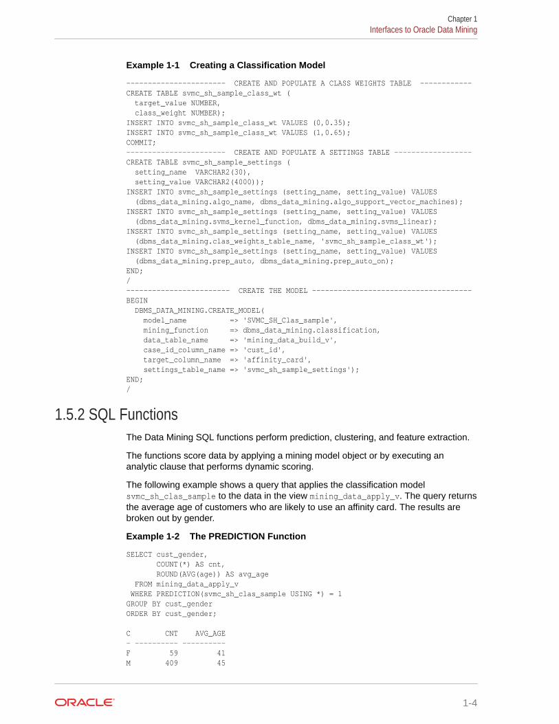
1.5.2 SQL FunctionsThe Data Mining SQL functions perform prediction, clustering, and feature extraction.
The functions score data by applying a mining model object or by executing ananalytic clause that performs dynamic scoring.
The following example shows a query that applies the classification modelsvmc_sh_clas_sample to the data in the view mining_data_apply_v. The query returnsthe average age of customers who are likely to use an affinity card. The results arebroken out by gender.
Example 1-2 The PREDICTION Function
SELECT cust_gender, COUNT(*) AS cnt, ROUND(AVG(age)) AS avg_age FROM mining_data_apply_v WHERE PREDICTION(svmc_sh_clas_sample USING *) = 1GROUP BY cust_genderORDER BY cust_gender;
C CNT AVG_AGE- ---------- ----------F 59 41M 409 45
Chapter 1Interfaces to Oracle Data Mining
1-4
Related Topics
• In-Database Scoring
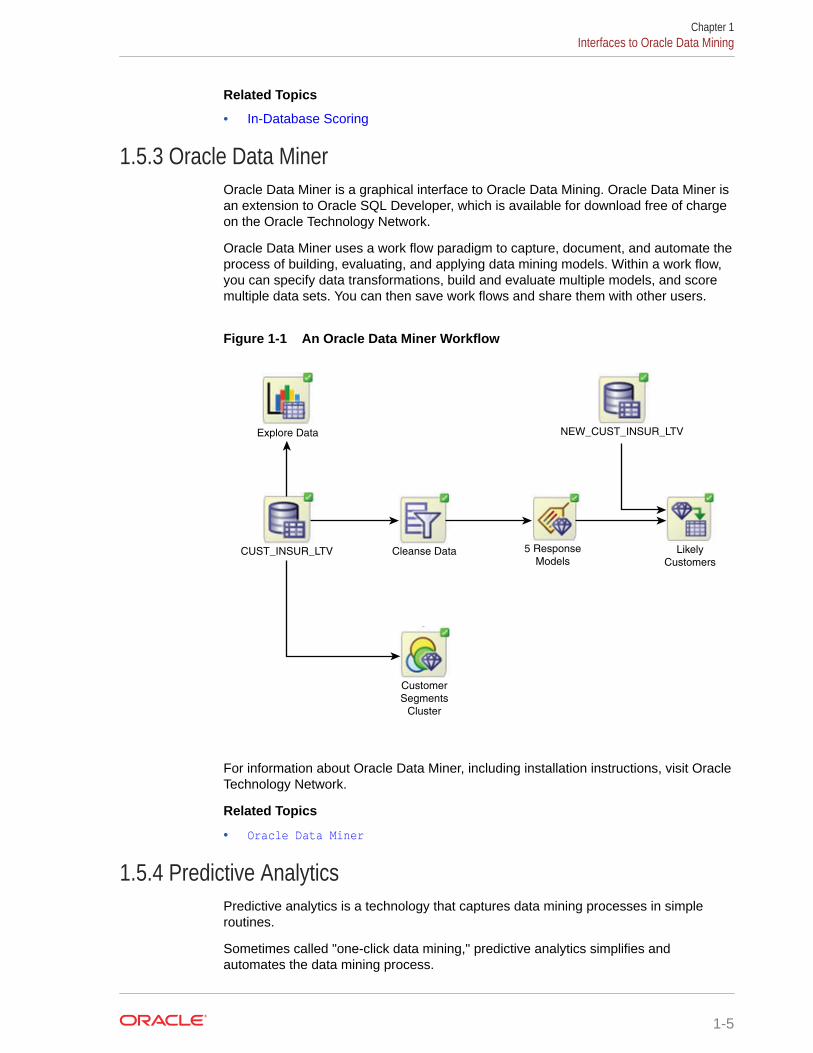
1.5.3 Oracle Data MinerOracle Data Miner is a graphical interface to Oracle Data Mining. Oracle Data Miner isan extension to Oracle SQL Developer, which is available for download free of chargeon the Oracle Technology Network.
Oracle Data Miner uses a work flow paradigm to capture, document, and automate theprocess of building, evaluating, and applying data mining models. Within a work flow,you can specify data transformations, build and evaluate multiple models, and scoremultiple data sets. You can then save work flows and share them with other users.
Figure 1-1 An Oracle Data Miner Workflow
NEW_CUST_INSUR_LTVExplore Data
CUST_INSUR_LTV
Customer
Segments
Cluster
Cleanse Data 5 Response
ModelsLikely
Customers
For information about Oracle Data Miner, including installation instructions, visit OracleTechnology Network.
Related Topics
• Oracle Data Miner
1.5.4 Predictive AnalyticsPredictive analytics is a technology that captures data mining processes in simpleroutines.
Sometimes called "one-click data mining," predictive analytics simplifies andautomates the data mining process.
Chapter 1Interfaces to Oracle Data Mining
1-5
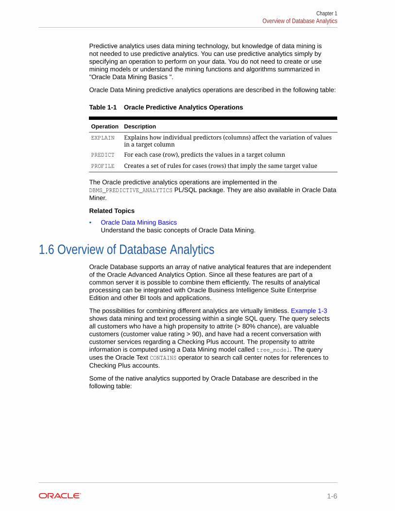
Predictive analytics uses data mining technology, but knowledge of data mining isnot needed to use predictive analytics. You can use predictive analytics simply byspecifying an operation to perform on your data. You do not need to create or usemining models or understand the mining functions and algorithms summarized in"Oracle Data Mining Basics ".
Oracle Data Mining predictive analytics operations are described in the following table:
Table 1-1 Oracle Predictive Analytics Operations
Operation Description
EXPLAIN Explains how individual predictors (columns) affect the variation of valuesin a target column
PREDICT For each case (row), predicts the values in a target column
PROFILE Creates a set of rules for cases (rows) that imply the same target value
The Oracle predictive analytics operations are implemented in theDBMS_PREDICTIVE_ANALYTICS PL/SQL package. They are also available in Oracle DataMiner.
Related Topics
• Oracle Data Mining BasicsUnderstand the basic concepts of Oracle Data Mining.
1.6 Overview of Database AnalyticsOracle Database supports an array of native analytical features that are independentof the Oracle Advanced Analytics Option. Since all these features are part of acommon server it is possible to combine them efficiently. The results of analyticalprocessing can be integrated with Oracle Business Intelligence Suite EnterpriseEdition and other BI tools and applications.
The possibilities for combining different analytics are virtually limitless. Example 1-3shows data mining and text processing within a single SQL query. The query selectsall customers who have a high propensity to attrite (> 80% chance), are valuablecustomers (customer value rating > 90), and have had a recent conversation withcustomer services regarding a Checking Plus account. The propensity to attriteinformation is computed using a Data Mining model called tree_model. The queryuses the Oracle Text CONTAINS operator to search call center notes for references toChecking Plus accounts.
Some of the native analytics supported by Oracle Database are described in thefollowing table:
Chapter 1Overview of Database Analytics
1-6
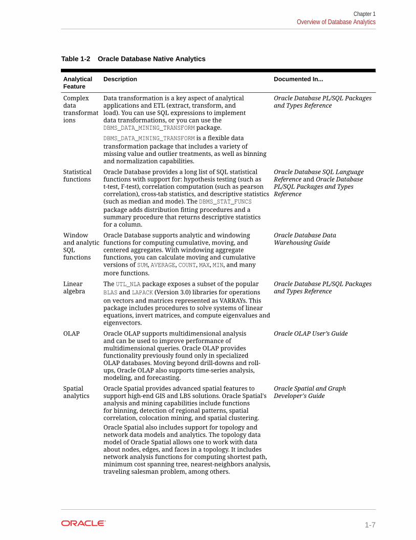
Table 1-2 Oracle Database Native Analytics
AnalyticalFeature
Description Documented In...
Complexdatatransformations
Data transformation is a key aspect of analyticalapplications and ETL (extract, transform, andload). You can use SQL expressions to implementdata transformations, or you can use theDBMS_DATA_MINING_TRANSFORM package.
DBMS_DATA_MINING_TRANSFORM is a flexible datatransformation package that includes a variety ofmissing value and outlier treatments, as well as binningand normalization capabilities.
Oracle Database PL/SQL Packagesand Types Reference
Statisticalfunctions
Oracle Database provides a long list of SQL statisticalfunctions with support for: hypothesis testing (such ast-test, F-test), correlation computation (such as pearsoncorrelation), cross-tab statistics, and descriptive statistics(such as median and mode). The DBMS_STAT_FUNCSpackage adds distribution fitting procedures and asummary procedure that returns descriptive statisticsfor a column.
Oracle Database SQL LanguageReference and Oracle DatabasePL/SQL Packages and TypesReference
Windowand analyticSQLfunctions
Oracle Database supports analytic and windowingfunctions for computing cumulative, moving, andcentered aggregates. With windowing aggregatefunctions, you can calculate moving and cumulativeversions of SUM, AVERAGE, COUNT, MAX, MIN, and manymore functions.
Oracle Database DataWarehousing Guide
Linearalgebra
The UTL_NLA package exposes a subset of the popularBLAS and LAPACK (Version 3.0) libraries for operationson vectors and matrices represented as VARRAYs. Thispackage includes procedures to solve systems of linearequations, invert matrices, and compute eigenvalues andeigenvectors.
Oracle Database PL/SQL Packagesand Types Reference
OLAP Oracle OLAP supports multidimensional analysisand can be used to improve performance ofmultidimensional queries. Oracle OLAP providesfunctionality previously found only in specializedOLAP databases. Moving beyond drill-downs and roll-ups, Oracle OLAP also supports time-series analysis,modeling, and forecasting.
Oracle OLAP User’s Guide
Spatialanalytics
Oracle Spatial provides advanced spatial features tosupport high-end GIS and LBS solutions. Oracle Spatial'sanalysis and mining capabilities include functionsfor binning, detection of regional patterns, spatialcorrelation, colocation mining, and spatial clustering.Oracle Spatial also includes support for topology andnetwork data models and analytics. The topology datamodel of Oracle Spatial allows one to work with dataabout nodes, edges, and faces in a topology. It includesnetwork analysis functions for computing shortest path,minimum cost spanning tree, nearest-neighbors analysis,traveling salesman problem, among others.
Oracle Spatial and GraphDeveloper's Guide
Chapter 1Overview of Database Analytics
1-7

Table 1-2 (Cont.) Oracle Database Native Analytics
AnalyticalFeature
Description Documented In...
Text Mining Oracle Text uses standard SQL to index, search, andanalyze text and documents stored in the Oracledatabase, in files, and on the web. Oracle Text alsosupports automatic classification and clustering ofdocument collections. Many of the analytical features ofOracle Text are layered on top of Oracle Data Miningfunctionality.
Oracle Text ApplicationDeveloper's Guide
Example 1-3 SQL Query Combining Oracle Data Mining and Oracle Text
SELECT A.cust_name, A.contact_info FROM customers A WHERE PREDICTION_PROBABILITY(tree_model, 'attrite' USING A.*) > 0.8 AND A.cust_value > 90 AND A.cust_id IN (SELECT B.cust_id FROM call_center B WHERE B.call_date BETWEEN '01-Jan-2005' AND '30-Jun-2005' AND CONTAINS(B.notes, 'Checking Plus', 1) > 0);
Chapter 1Overview of Database Analytics
1-8
2Oracle Data Mining Basics
Understand the basic concepts of Oracle Data Mining.
• Mining Functions
• Algorithms
• Data Preparation
• In-Database Scoring
2.1 Mining FunctionsIntroduces the concept of data mining functions.
A basic understanding of data mining functions and algorithms is required for usingOracle Data Mining.
Each data mining function specifies a class of problems that can be modeled andsolved. Data mining functions fall generally into two categories: supervised andunsupervised. Notions of supervised and unsupervised learning are derived from thescience of machine learning, which has been called a sub-area of artificial intelligence.
Artificial intelligence refers to the implementation and study of systems that exhibitautonomous intelligence or behavior of their own. Machine learning deals withtechniques that enable devices to learn from their own performance and modify theirown functioning. Data mining applies machine learning concepts to data.
Related Topics
• Algorithms
2.1.1 Supervised Data MiningSupervised learning is also known as directed learning. The learning process isdirected by a previously known dependent attribute or target. Directed data miningattempts to explain the behavior of the target as a function of a set of independentattributes or predictors.
Supervised learning generally results in predictive models. This is in contrast tounsupervised learning where the goal is pattern detection.
The building of a supervised model involves training, a process whereby the softwareanalyzes many cases where the target value is already known. In the training process,the model "learns" the logic for making the prediction. For example, a model that seeksto identify the customers who are likely to respond to a promotion must be trained byanalyzing the characteristics of many customers who are known to have responded ornot responded to a promotion in the past.
2-1

2.1.1.1 Supervised Learning: TestingSeparate data sets are required for building (training) and testing some predictivemodels. The build data (training data) and test data must have the same columnstructure. Typically, one large table or view is split into two data sets: one for buildingthe model, and the other for testing the model.
The process of applying the model to test data helps to determine whether the model,built on one chosen sample, is generalizable to other data. In particular, it helps toavoid the phenomenon of overfitting, which can occur when the logic of the model fitsthe build data too well and therefore has little predictive power.
2.1.1.2 Supervised Learning: ScoringApply data, also called scoring data, is the actual population to which a model isapplied. For example, you might build a model that identifies the characteristics ofcustomers who frequently buy a certain product. To obtain a list of customers whoshop at a certain store and are likely to buy a related product, you might apply themodel to the customer data for that store. In this case, the store customer data is thescoring data.
Most supervised learning can be applied to a population of interest. The principalsupervised mining techniques, Classification and Regression, can both be used forscoring.
Oracle Data Mining does not support the scoring operation for Attribute Importance,another supervised function. Models of this type are built on a population of interest toobtain information about that population; they cannot be applied to separate data. Anattribute importance model returns and ranks the attributes that are most important inpredicting a target value.
Oracle Data Mining supports the supervised data mining functions described in thefollowing table:
Table 2-1 Oracle Data Mining Supervised Functions
Function Description Sample Problem
Attribute Importance Identifies the attributes that aremost important in predicting a targetattribute
Given customer response to an affinitycard program, find the most significantpredictors
Classification Assigns items to discrete classes andpredicts the class to which an itembelongs
Given demographic data about a set ofcustomers, predict customer response toan affinity card program
Regression Approximates and forecastscontinuous values
Given demographic and purchasingdata about a set of customers, predictcustomers' age
2.1.2 Unsupervised Data MiningUnsupervised learning is non-directed. There is no distinction between dependent andindependent attributes. There is no previously-known result to guide the algorithm inbuilding the model.
Chapter 2Mining Functions
2-2
Unsupervised learning can be used for descriptive purposes. It can also be used tomake predictions.
2.1.2.1 Unsupervised Learning: ScoringIntroduces unsupervised learning, supported scoring operations, and unsupervisedOracle Data Mining functions.
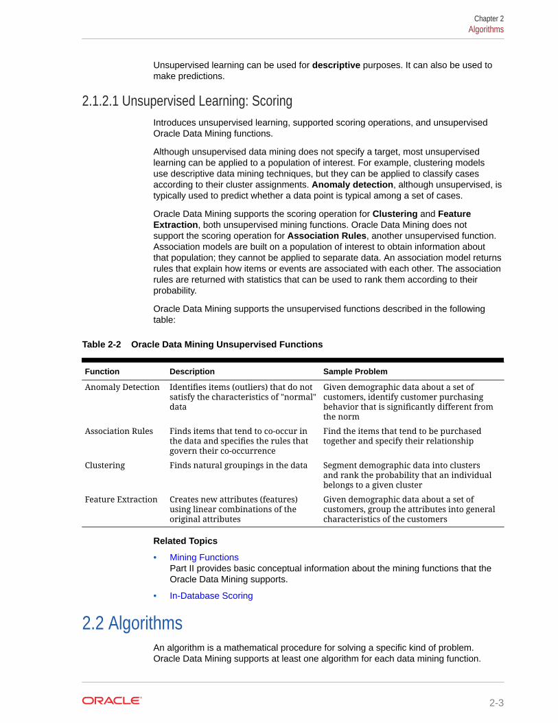
Although unsupervised data mining does not specify a target, most unsupervisedlearning can be applied to a population of interest. For example, clustering modelsuse descriptive data mining techniques, but they can be applied to classify casesaccording to their cluster assignments. Anomaly detection, although unsupervised, istypically used to predict whether a data point is typical among a set of cases.
Oracle Data Mining supports the scoring operation for Clustering and FeatureExtraction, both unsupervised mining functions. Oracle Data Mining does notsupport the scoring operation for Association Rules, another unsupervised function.Association models are built on a population of interest to obtain information aboutthat population; they cannot be applied to separate data. An association model returnsrules that explain how items or events are associated with each other. The associationrules are returned with statistics that can be used to rank them according to theirprobability.
Oracle Data Mining supports the unsupervised functions described in the followingtable:
Table 2-2 Oracle Data Mining Unsupervised Functions
Function Description Sample Problem
Anomaly Detection Identifies items (outliers) that do notsatisfy the characteristics of "normal"data
Given demographic data about a set ofcustomers, identify customer purchasingbehavior that is significantly different fromthe norm
Association Rules Finds items that tend to co-occur inthe data and specifies the rules thatgovern their co-occurrence
Find the items that tend to be purchasedtogether and specify their relationship
Clustering Finds natural groupings in the data Segment demographic data into clustersand rank the probability that an individualbelongs to a given cluster
Feature Extraction Creates new attributes (features)using linear combinations of theoriginal attributes
Given demographic data about a set ofcustomers, group the attributes into generalcharacteristics of the customers
Related Topics
• Mining FunctionsPart II provides basic conceptual information about the mining functions that theOracle Data Mining supports.
• In-Database Scoring
2.2 AlgorithmsAn algorithm is a mathematical procedure for solving a specific kind of problem.Oracle Data Mining supports at least one algorithm for each data mining function.
Chapter 2Algorithms
2-3

For some functions, you can choose among several algorithms. For example, OracleData Mining supports four classification algorithms.
Each data mining model is produced by a specific algorithm. Some data miningproblems can best be solved by using more than one algorithm. This necessitatesthe development of more than one model. For example, you might first use a featureextraction model to create an optimized set of predictors, then a classification model tomake a prediction on the results.
2.2.1 Oracle Data Mining Supervised AlgorithmsOracle Data Mining supports the supervised data mining algorithms described in thefollowing table. The algorithm abbreviations are used throughout this manual.
Table 2-3 Oracle Data Mining Algorithms for Supervised Functions
Algorithm Function Description
Decision Tree Classification Decision trees extract predictive information in the form of human-understandable rules. The rules are if-then-else expressions; theyexplain the decisions that lead to the prediction.
Explicit SemanticAnalysis
Classification Explicit Semantic Analysis (ESA) is designed to make predictionsfor text data. This algorithm can address use cases with hundredsof thousands of classes. In Oracle Database 12c Release 2, ESA wasintroduced as Feature Extraction algorithm.
ExponentialSmoothing
Time Series Exponential Smoothing (ESM) provides forecasts for time seriesdata. Forecasts are made for each time period within a user-specified forecast window. ESM provides a total of 14 different timeseries models, including all the most popular estimates of trend andseasonal effects. Choice of model is controlled by user settings. ESMprovides confidence bounds on its forecasts.
Generalized LinearModels
Classificationand Regression
Generalized Linear Models (GLM) implement logistic regressionfor classification of binary targets and linear regression forcontinuous targets. GLM classification supports confidence boundsfor prediction probabilities. GLM regression supports confidencebounds for predictions.
MinimumDescription Length
AttributeImportance
Minimum Description Length (MDL) is an information theoreticmodel selection principle. MDL assumes that the simplest, mostcompact representation of data is the best and most probableexplanation of the data.
Naive Bayes Classification Naive Bayes makes predictions using Bayes' Theorem, whichderives the probability of a prediction from the underlyingevidence, as observed in the data.
Neural Network Classificationand Regression
Neural Network in Machine Learning is an artificial algorithminspired from biological neural network and is used to estimate orapproximate functions that depend on a large number of generallyunknown inputs. Neural Network is designed for Classification andRegression.
Random Forest Classification Random Forest is a powerful machine learning algorithm.RandomForest algorithm builds a number of decision tree models andpredicts using the ensemble of trees.
Chapter 2Algorithms
2-4
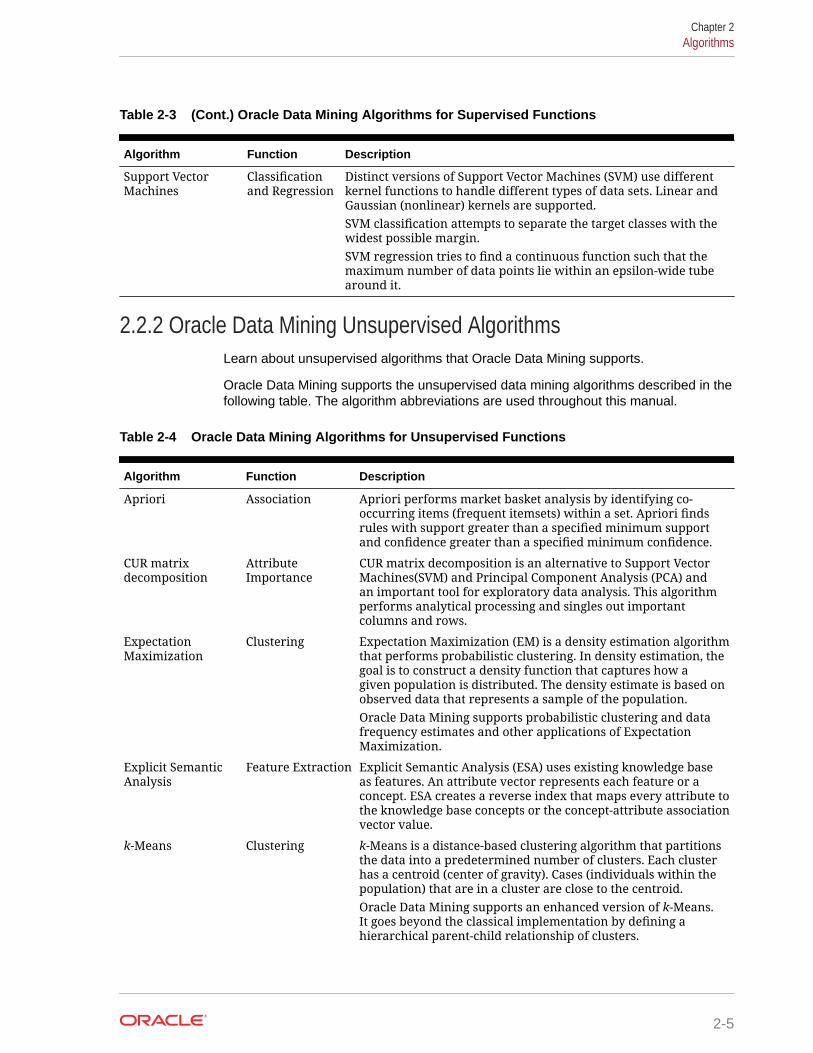
Table 2-3 (Cont.) Oracle Data Mining Algorithms for Supervised Functions
Algorithm Function Description
Support VectorMachines
Classificationand Regression
Distinct versions of Support Vector Machines (SVM) use differentkernel functions to handle different types of data sets. Linear andGaussian (nonlinear) kernels are supported.SVM classification attempts to separate the target classes with thewidest possible margin.SVM regression tries to find a continuous function such that themaximum number of data points lie within an epsilon-wide tubearound it.
2.2.2 Oracle Data Mining Unsupervised AlgorithmsLearn about unsupervised algorithms that Oracle Data Mining supports.
Oracle Data Mining supports the unsupervised data mining algorithms described in thefollowing table. The algorithm abbreviations are used throughout this manual.
Table 2-4 Oracle Data Mining Algorithms for Unsupervised Functions
Algorithm Function Description
Apriori Association Apriori performs market basket analysis by identifying co-occurring items (frequent itemsets) within a set. Apriori findsrules with support greater than a specified minimum supportand confidence greater than a specified minimum confidence.
CUR matrixdecomposition
AttributeImportance
CUR matrix decomposition is an alternative to Support VectorMachines(SVM) and Principal Component Analysis (PCA) andan important tool for exploratory data analysis. This algorithmperforms analytical processing and singles out importantcolumns and rows.
ExpectationMaximization
Clustering Expectation Maximization (EM) is a density estimation algorithmthat performs probabilistic clustering. In density estimation, thegoal is to construct a density function that captures how agiven population is distributed. The density estimate is based onobserved data that represents a sample of the population.Oracle Data Mining supports probabilistic clustering and datafrequency estimates and other applications of ExpectationMaximization.
Explicit SemanticAnalysis
Feature Extraction Explicit Semantic Analysis (ESA) uses existing knowledge baseas features. An attribute vector represents each feature or aconcept. ESA creates a reverse index that maps every attribute tothe knowledge base concepts or the concept-attribute associationvector value.
k-Means Clustering k-Means is a distance-based clustering algorithm that partitionsthe data into a predetermined number of clusters. Each clusterhas a centroid (center of gravity). Cases (individuals within thepopulation) that are in a cluster are close to the centroid.Oracle Data Mining supports an enhanced version of k-Means.It goes beyond the classical implementation by defining ahierarchical parent-child relationship of clusters.
Chapter 2Algorithms
2-5
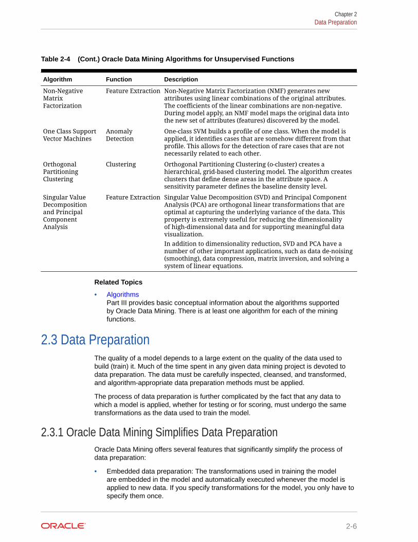
Table 2-4 (Cont.) Oracle Data Mining Algorithms for Unsupervised Functions
Algorithm Function Description
Non-NegativeMatrixFactorization
Feature Extraction Non-Negative Matrix Factorization (NMF) generates newattributes using linear combinations of the original attributes.The coefficients of the linear combinations are non-negative.During model apply, an NMF model maps the original data intothe new set of attributes (features) discovered by the model.
One Class SupportVector Machines
AnomalyDetection
One-class SVM builds a profile of one class. When the model isapplied, it identifies cases that are somehow different from thatprofile. This allows for the detection of rare cases that are notnecessarily related to each other.
OrthogonalPartitioningClustering
Clustering Orthogonal Partitioning Clustering (o-cluster) creates ahierarchical, grid-based clustering model. The algorithm createsclusters that define dense areas in the attribute space. Asensitivity parameter defines the baseline density level.
Singular ValueDecompositionand PrincipalComponentAnalysis
Feature Extraction Singular Value Decomposition (SVD) and Principal ComponentAnalysis (PCA) are orthogonal linear transformations that areoptimal at capturing the underlying variance of the data. Thisproperty is extremely useful for reducing the dimensionalityof high-dimensional data and for supporting meaningful datavisualization.In addition to dimensionality reduction, SVD and PCA have anumber of other important applications, such as data de-noising(smoothing), data compression, matrix inversion, and solving asystem of linear equations.
Related Topics
• AlgorithmsPart III provides basic conceptual information about the algorithms supportedby Oracle Data Mining. There is at least one algorithm for each of the miningfunctions.
2.3 Data PreparationThe quality of a model depends to a large extent on the quality of the data used tobuild (train) it. Much of the time spent in any given data mining project is devoted todata preparation. The data must be carefully inspected, cleansed, and transformed,and algorithm-appropriate data preparation methods must be applied.
The process of data preparation is further complicated by the fact that any data towhich a model is applied, whether for testing or for scoring, must undergo the sametransformations as the data used to train the model.
2.3.1 Oracle Data Mining Simplifies Data PreparationOracle Data Mining offers several features that significantly simplify the process ofdata preparation:
• Embedded data preparation: The transformations used in training the modelare embedded in the model and automatically executed whenever the model isapplied to new data. If you specify transformations for the model, you only have tospecify them once.
Chapter 2Data Preparation
2-6
• Automatic Data Preparation (ADP): Oracle Data Mining supports an automateddata preparation mode. When ADP is active, Oracle Data Mining automaticallyperforms the data transformations required by the algorithm. The transformationinstructions are embedded in the model along with any user-specifiedtransformation instructions.
• Automatic management of missing values and sparse data: Oracle Data Mininguses consistent methodology across mining algorithms to handle sparsity andmissing values.
• Transparency: Oracle Data Mining provides model details, which are a view ofthe attributes that are internal to the model. This insight into the inner detailsof the model is possible because of reverse transformations, which map thetransformed attribute values to a form that can be interpreted by a user. Wherepossible, attribute values are reversed to the original column values. Reversetransformations are also applied to the target of a supervised model, thus theresults of scoring are in the same units as the units of the original target.
• Tools for custom data preparation: Oracle Data Mining provides many commontransformation routines in the DBMS_DATA_MINING_TRANSFORM PL/SQL package.You can use these routines, or develop your own routines in SQL, or both. TheSQL language is well suited for implementing transformations in the database. Youcan use custom transformation instructions along with ADP or instead of ADP.
2.3.2 Case DataMost data mining algorithms act on single-record case data, where the information foreach case is stored in a separate row. The data attributes for the cases are stored inthe columns.
When the data is organized in transactions, the data for one case (one transaction) isstored in many rows. An example of transactional data is market basket data. With thesingle exception of Association Rules, which can operate on native transactional data,Oracle Data Mining algorithms require single-record case organization.
2.3.2.1 Nested DataOracle Data Mining supports attributes in nested columns. A transactional table can becast as a nested column and included in a table of single-record case data. Similarly,star schemas can be cast as nested columns. With nested data transformations,Oracle Data Mining can effectively mine data originating from multiple sources andconfigurations.
2.3.3 Text DataPrepare and transform unstructured text data for data mining.
Oracle Data Mining interprets CLOB columns and long VARCHAR2 columns automaticallyas unstructured text. Additionally, you can specify columns of short VARCHAR2, CHAR,BLOB, and BFILE as unstructured text. Unstructured text includes data items suchas web pages, document libraries, Power Point presentations, product specifications,emails, comment fields in reports, and call center notes.
Oracle Data Mining uses Oracle Text utilities and term weighting strategies totransform unstructured text for mining. In text transformation, text terms are extractedand given numeric values in a text index. The text transformation process is
Chapter 2Data Preparation
2-7
configurable for the model and for individual attributes. Once transformed, the textcan by mined with a data mining algorithm.
Related Topics
• Preparing the Data
• Transforming the Data
• Mining Unstructured Text
2.4 In-Database ScoringScoring is the application of a data mining algorithm to new data. In traditional datamining, models are built using specialized software on a remote system and deployedto another system for scoring. This is a cumbersome, error-prone process open tosecurity violations and difficulties in data synchronization.
With Oracle Data Mining, scoring is easy and secure. The scoring engine and the databoth reside within the database. Scoring is an extension to the SQL language, so theresults of mining can easily be incorporated into applications and reporting systems.
2.4.1 Parallel Execution and Ease of AdministrationAll Oracle Data Mining scoring routines support parallel execution for scoring largedata sets.
In-database scoring provides performance advantages. All Oracle Data Mining scoringroutines support parallel execution, which significantly reduces the time required forexecuting complex queries and scoring large data sets.
In-database mining minimizes the IT effort needed to support data mining initiatives.Using standard database techniques, models can easily be refreshed (re-created) onmore recent data and redeployed. The deployment is immediate since the scoringquery remains the same; only the underlying model is replaced in the database.
Related Topics
• Oracle Database VLDB and Partitioning Guide
2.4.2 SQL Functions for Model Apply and Dynamic ScoringIn Oracle Data Mining, scoring is performed by SQL language functions. Understandthe different ways involved in SQL function scoring.
The functions perform prediction, clustering, and feature extraction. The functions canbe invoked in two different ways: By applying a mining model object (Example 2-1),or by executing an analytic clause that computes the mining analysis dynamically andapplies it to the data (Example 2-2). Dynamic scoring, which eliminates the need for amodel, can supplement, or even replace, the more traditional data mining methodologydescribed in "The Data Mining Process".
In Example 2-1, the PREDICTION_PROBABILITY function applies the modelsvmc_sh_clas_sample, created in Example 1-1, to score the data inmining_data_apply_v. The function returns the ten customers in Italy who are mostlikely to use an affinity card.
Chapter 2In-Database Scoring
2-8

In Example 2-2, the functions PREDICTION and PREDICTION_PROBABILITY usethe analytic syntax (the OVER () clause) to dynamically score the data inmining_data_apply_v. The query returns the customers who currently do not havean affinity card with the probability that they are likely to use.
Example 2-1 Applying a Mining Model to Score Data
SELECT cust_id FROM (SELECT cust_id, rank() over (order by PREDICTION_PROBABILITY(svmc_sh_clas_sample, 1 USING *) DESC, cust_id) rnk FROM mining_data_apply_v WHERE country_name = 'Italy')WHERE rnk <= 10ORDER BY rnk;
CUST_ID---------- 101445 100179 100662 100733 100554 100081 100344 100324 100185 101345
Example 2-2 Executing an Analytic Function to Score Data
SELECT cust_id, pred_prob FROM (SELECT cust_id, affinity_card, PREDICTION(FOR TO_CHAR(affinity_card) USING *) OVER () pred_card, PREDICTION_PROBABILITY(FOR TO_CHAR(affinity_card),1 USING *) OVER () pred_prob FROM mining_data_build_v)WHERE affinity_card = 0AND pred_card = 1ORDER BY pred_prob DESC;
CUST_ID PRED_PROB---------- --------- 102434 .96 102365 .96 102330 .96 101733 .95 102615 .94 102686 .94 102749 .93 . . . 101656 .51
Chapter 2In-Database Scoring
2-9

Part IIMining Functions
Part II provides basic conceptual information about the mining functions that theOracle Data Mining supports.
Mining functions represent a class of mining problems that can be solved using datamining algorithms.
Part II contains these chapters:
• Regression
• Classification
• Anomaly Detection
• Clustering
• Association
• Feature Selection and Extraction
• Time Series
Note:
The term mining function has no relationship to a SQL language function.
Related Topics
• AlgorithmsPart III provides basic conceptual information about the algorithms supportedby Oracle Data Mining. There is at least one algorithm for each of the miningfunctions.
• Oracle Database SQL Language Reference

3Regression
Learn how to predict a continuous numerical target through Regression - thesupervised mining function.
• About Regression
• Testing a Regression Model
• Regression Algorithms
Related Topics
• Oracle Data Mining BasicsUnderstand the basic concepts of Oracle Data Mining.
3.1 About RegressionRegression is a data mining function that predicts numeric values along a continuum.Profit, sales, mortgage rates, house values, square footage, temperature, or distancecan be predicted using Regression techniques. For example, a Regression model canbe used to predict the value of a house based on location, number of rooms, lot size,and other factors.
A Regression task begins with a data set in which the target values are known. Forexample, a Regression model that predicts house values can be developed based onobserved data for many houses over a period of time. In addition to the value, thedata can track the age of the house, square footage, number of rooms, taxes, schooldistrict, proximity to shopping centers, and so on. House value can be the target, theother attributes are the predictors, and the data for each house constitutes a case.
In the model build (training) process, a Regression algorithm estimates the valueof the target as a function of the predictors for each case in the build data. Theserelationships between predictors and target are summarized in a model, which canthen be applied to a different data set in which the target values are unknown.
Regression models are tested by computing various statistics that measure thedifference between the predicted values and the expected values. The historical datafor a Regression project is typically divided into two data sets: one for building themodel, the other for testing the model.
Regression modeling has many applications in trend analysis, business planning,marketing, financial forecasting, time series prediction, biomedical and drug responsemodeling, and environmental modeling.
3.1.1 How Does Regression Work?You do not need to understand the mathematics used in regression analysis todevelop and use quality regression models for data mining. However, it is helpful tounderstand a few basic concepts.
3-1

Regression analysis seeks to determine the values of parameters for a function thatcause the function to best fit a set of data observations that you provide. The followingequation expresses these relationships in symbols. It shows that regression is theprocess of estimating the value of a continuous target (y) as a function (F) of one ormore predictors (x1 , x2 , ..., xn), a set of parameters (θ1 , θ2 , ..., θn), and a measure oferror (e).
y = F(x,θ) + e
The predictors can be understood as independent variables and the target as adependent variable. The error, also called the residual, is the difference between theexpected and predicted value of the dependent variable. The regression parametersare also known as regression coefficients.
The process of training a regression model involves finding the parameter values thatminimize a measure of the error, for example, the sum of squared errors.
There are different families of regression functions and different ways of measuring theerror.
3.1.1.1 Linear RegressionA linear regression technique can be used if the relationship between the predictorsand the target can be approximated with a straight line.
Regression with a single predictor is the easiest to visualize. Simple linear regressionwith a single predictor is shown in the following figure:
Figure 3-1 Linear Regression With a Single Predictor
Y
X
error
error
Linear regression with a single predictor can be expressed with the following equation.
y = θ2x + θ1 + e
The regression parameters in simple linear regression are:
Chapter 3About Regression
3-2

• The slope of the line (2) — the angle between a data point and the regression line
• The y intercept (1) — the point where x crosses the y axis (x = 0)
3.1.1.2 Multivariate Linear RegressionThe term multivariate linear regression refers to linear regression with two or morepredictors (x1, x2, …, xn). When multiple predictors are used, the regression linecannot be visualized in two-dimensional space. However, the line can be computedsimply by expanding the equation for single-predictor linear regression to include theparameters for each of the predictors.
y = θ1 + θ2x1 + θ3x2 + ..... θn xn-1 + e
3.1.1.3 Regression CoefficientsIn multivariate linear regression, the regression parameters are often referred to ascoefficients. When you build a multivariate linear regression model, the algorithmcomputes a coefficient for each of the predictors used by the model. The coefficientis a measure of the impact of the predictor x on the target y. Numerous statistics areavailable for analyzing the regression coefficients to evaluate how well the regressionline fits the data.
3.1.1.4 Nonlinear RegressionOften the relationship between x and y cannot be approximated with a straight line. Inthis case, a nonlinear regression technique can be used. Alternatively, the data can bepreprocessed to make the relationship linear.
Nonlinear regression models define y as a function of x using an equation that is morecomplicated than the linear regression equation. In the following figure, x and y have anonlinear relationship.
Figure 3-2 Nonlinear Regression With a Single Predictor
Y
X
error
error
Chapter 3About Regression
3-3

3.1.1.5 Multivariate Nonlinear RegressionThe term multivariate nonlinear regression refers to nonlinear regression with twoor more predictors (x1, x2, …, xn). When multiple predictors are used, the nonlinearrelationship cannot be visualized in two-dimensional space.
3.1.1.6 Confidence BoundsA Regression model predicts a numeric target value for each case in the scoring data.In addition to the predictions, some Regression algorithms can identify confidencebounds, which are the upper and lower boundaries of an interval in which thepredicted value is likely to lie.
When a model is built to make predictions with a given confidence, the confidenceinterval is produced along with the predictions. For example, a model predictsthe value of a house to be $500,000 with a 95% confidence that the value isbetween $475,000 and $525,000.
3.2 Testing a Regression ModelA regression model is tested by applying it to test data with known target values andcomparing the predicted values with the known values.
The test data must be compatible with the data used to build the model and must beprepared in the same way that the build data was prepared. Typically the build dataand test data come from the same historical data set. A percentage of the records isused to build the model; the remaining records are used to test the model.
Test metrics are used to assess how accurately the model predicts these knownvalues. If the model performs well and meets the business requirements, it can thenbe applied to new data to predict the future.
3.2.1 Regression StatisticsThe Root Mean Squared Error and the Mean Absolute Error are commonly usedstatistics for evaluating the overall quality of a regression model. Different statisticsmay also be available depending on the regression methods used by the algorithm.
3.2.1.1 Root Mean Squared ErrorThe Root Mean Squared Error (RMSE) is the square root of the average squareddistance of a data point from the fitted line.
This SQL expression calculates the RMSE.
SQRT(AVG((predicted_value - actual_value) * (predicted_value - actual_value)))
This formula shows the RMSE in mathematical symbols. The large sigma characterrepresents summation; j represents the current predictor, and n represents the numberof predictors.
Chapter 3Testing a Regression Model
3-4

Figure 3-3 Room Mean Squared Error
RMSE = 1n
n
j = 1
( y j - ŷ
j ) 2
3.2.1.2 Mean Absolute ErrorThe Mean Absolute Error (MAE) is the average of the absolute value of the residuals(error). The MAE is very similar to the RMSE but is less sensitive to large errors.
This SQL expression calculates the MAE.
AVG(ABS(predicted_value - actual_value))
This formula shows the MAE in mathematical symbols. The large sigma characterrepresents summation; j represents the current predictor, and n represents the numberof predictors.
Figure 3-4 Mean Absolute Error
MAE = 1n
n
j = 1
| y j - ŷ
j |
3.3 Regression AlgorithmsOracle Data Mining supports three algorithms for Regression Generalized LinearModels (GLM), Neural Network (NN), and Support Vector Machines (SVM).
Generalized Linear Models (GLM) and Support Vector Machines (SVM) algorithmsare particularly suited for mining data sets that have very high dimensionality (manyattributes), including transactional and unstructured data.
• Generalized Linear Models (GLM)
GLM is a popular statistical technique for linear modeling. Oracle Data Miningimplements GLM for Regression and for binary classification. GLM providesextensive coefficient statistics and model statistics, as well as row diagnostics.GLM also supports confidence bounds.
• Neural Network
Neural networks are powerful algorithms that can learn arbitrary nonlinearregression functions.
• Support Vector Machines (SVM)
SVM is a powerful, state-of-the-art algorithm for linear and nonlinear Regression.Oracle Data Mining implements SVM for Regression, classification, and anomaly
Chapter 3Regression Algorithms
3-5

detection. SVM Regression supports two kernels: the Gaussian kernel fornonlinear Regression, and the linear kernel for Linear Regression.
Note:
Oracle Data Mining uses linear kernel SVM as the default Regressionalgorithm.
Related Topics
• Generalized Linear ModelsLearn how to use Generalized Linear Models (GLM) statistical technique for Linearmodeling.
• Support Vector MachinesLearn how to use Support Vector Machines, a powerful algorithm based onstatistical learning theory.
• Neural NetworkLearn about Neural Network for Regression and Classification mining functions.
Chapter 3Regression Algorithms
3-6

4Classification
Learn how to predict a categorical target through Classification - the supervised miningfunction.
• About Classification
• Testing a Classification Model
• Biasing a Classification Model
• Classification Algorithms
Related Topics
• Oracle Data Mining BasicsUnderstand the basic concepts of Oracle Data Mining.
4.1 About ClassificationClassification is a data mining function that assigns items in a collection to targetcategories or classes. The goal of classification is to accurately predict the target classfor each case in the data. For example, a classification model can be used to identifyloan applicants as low, medium, or high credit risks.
A classification task begins with a data set in which the class assignments are known.For example, a classification model that predicts credit risk can be developed basedon observed data for many loan applicants over a period of time. In addition to thehistorical credit rating, the data might track employment history, home ownership orrental, years of residence, number and type of investments, and so on. Credit ratingis the target, the other attributes are the predictors, and the data for each customerconstitutes a case.
Classifications are discrete and do not imply order. Continuous, floating-point valuesindicate a numerical, rather than a categorical, target. A predictive model with anumerical target uses a regression algorithm, not a classification algorithm.
The simplest type of classification problem is binary classification. In binaryclassification, the target attribute has only two possible values: for example, high creditrating or low credit rating. Multiclass targets have more than two values: for example,low, medium, high, or unknown credit rating.
In the model build (training) process, a classification algorithm finds relationshipsbetween the values of the predictors and the values of the target. Differentclassification algorithms use different techniques for finding relationships. Theserelationships are summarized in a model, which can then be applied to a differentdata set in which the class assignments are unknown.
Classification models are tested by comparing the predicted values to known targetvalues in a set of test data. The historical data for a classification project is typicallydivided into two data sets: one for building the model; the other for testing the model.
4-1
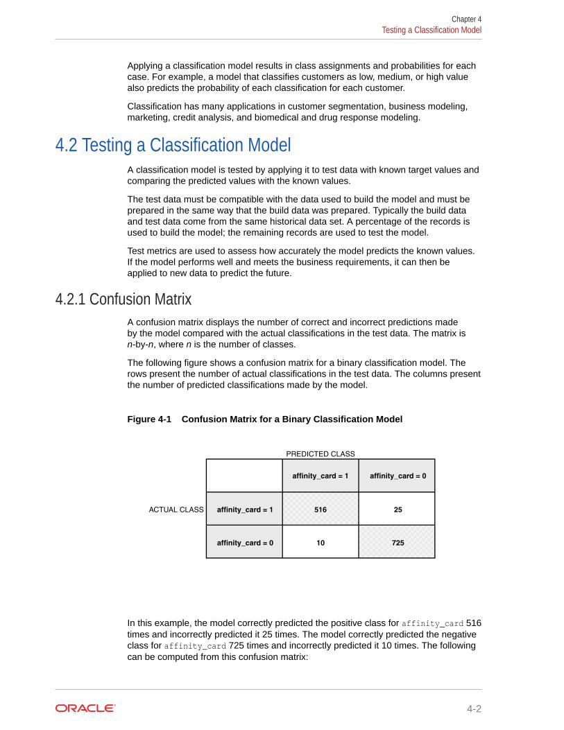
Applying a classification model results in class assignments and probabilities for eachcase. For example, a model that classifies customers as low, medium, or high valuealso predicts the probability of each classification for each customer.
Classification has many applications in customer segmentation, business modeling,marketing, credit analysis, and biomedical and drug response modeling.
4.2 Testing a Classification ModelA classification model is tested by applying it to test data with known target values andcomparing the predicted values with the known values.
The test data must be compatible with the data used to build the model and must beprepared in the same way that the build data was prepared. Typically the build dataand test data come from the same historical data set. A percentage of the records isused to build the model; the remaining records are used to test the model.
Test metrics are used to assess how accurately the model predicts the known values.If the model performs well and meets the business requirements, it can then beapplied to new data to predict the future.
4.2.1 Confusion MatrixA confusion matrix displays the number of correct and incorrect predictions madeby the model compared with the actual classifications in the test data. The matrix isn-by-n, where n is the number of classes.
The following figure shows a confusion matrix for a binary classification model. Therows present the number of actual classifications in the test data. The columns presentthe number of predicted classifications made by the model.
Figure 4-1 Confusion Matrix for a Binary Classification Model
PREDICTED CLASS
ACTUAL CLASS
affinity_card = 1 affinity_card = 0
72510affinity_card = 0
25516affinity_card = 1
In this example, the model correctly predicted the positive class for affinity_card 516times and incorrectly predicted it 25 times. The model correctly predicted the negativeclass for affinity_card 725 times and incorrectly predicted it 10 times. The followingcan be computed from this confusion matrix:
Chapter 4Testing a Classification Model
4-2

• The model made 1241 correct predictions (516 + 725).
• The model made 35 incorrect predictions (25 + 10).
• There are 1276 total scored cases (516 + 25 + 10 + 725).
• The error rate is 35/1276 = 0.0274.
• The overall accuracy rate is 1241/1276 = 0.9725.
4.2.2 LiftLift measures the degree to which the predictions of a classification model are betterthan randomly-generated predictions.
Lift applies to binary classification only, and it requires the designation of a positiveclass. If the model itself does not have a binary target, you can compute lift bydesignating one class as positive and combining all the other classes together as onenegative class.
Numerous statistics can be calculated to support the notion of lift. Basically, lift canbe understood as a ratio of two percentages: the percentage of correct positiveclassifications made by the model to the percentage of actual positive classificationsin the test data. For example, if 40% of the customers in a marketing survey haveresponded favorably (the positive classification) to a promotional campaign in the pastand the model accurately predicts 75% of them, the lift is obtained by dividing .75by .40. The resulting lift is 1.875.
Lift is computed against quantiles that each contain the same number of cases. Thedata is divided into quantiles after it is scored. It is ranked by probability of the positiveclass from highest to lowest, so that the highest concentration of positive predictions isin the top quantiles. A typical number of quantiles is 10.
Lift is commonly used to measure the performance of response models in marketingapplications. The purpose of a response model is to identify segments of thepopulation with potentially high concentrations of positive responders to a marketingcampaign. Lift reveals how much of the population must be solicited to obtain thehighest percentage of potential responders.
Related Topics
• Positive and Negative ClassesDiscusses the importance of positive and negative classes in a confusion matrix.
4.2.2.1 Lift StatisticsLearn the different Lift statistics that Oracle Data Mining can compute.
Oracle Data Mining computes the following lift statistics:
• Probability threshold for a quantile n is the minimum probability for the positivetarget to be included in this quantile or any preceding quantiles (quantiles n-1,n-2,..., 1). If a cost matrix is used, a cost threshold is reported instead. The costthreshold is the maximum cost for the positive target to be included in this quantileor any of the preceding quantiles.
• Cumulative gain is the ratio of the cumulative number of positive targets to thetotal number of positive targets.
Chapter 4Testing a Classification Model
4-3

• Target density of a quantile is the number of true positive instances in thatquantile divided by the total number of instances in the quantile.
• Cumulative target density for quantile n is the target density computed over thefirst n quantiles.
• Quantile lift is the ratio of the target density for the quantile to the target densityover all the test data.
• Cumulative percentage of records for a quantile is the percentage of all casesrepresented by the first n quantiles, starting at the end that is most confidentlypositive, up to and including the given quantile.
• Cumulative number of targets for quantile n is the number of true positiveinstances in the first n quantiles.
• Cumulative number of nontargets is the number of actually negative instancesin the first n quantiles.
• Cumulative lift for a quantile is the ratio of the cumulative target density to thetarget density over all the test data.
Related Topics
• Costs
4.2.3 Receiver Operating Characteristic (ROC)ROC is a metric for comparing predicted and actual target values in a classificationmodel.
ROC, like Lift, applies to Binary Classification and requires the designation of apositive class.
You can use ROC to gain insight into the decision-making ability of the model. Howlikely is the model to accurately predict the negative or the positive class?
ROC measures the impact of changes in the probability threshold. The probabilitythreshold is the decision point used by the model for classification. The defaultprobability threshold for binary classification is 0.5. When the probability of a predictionis 50% or more, the model predicts that class. When the probability is less than 50%,the other class is predicted. (In multiclass classification, the predicted class is the onepredicted with the highest probability.)
Related Topics
• Positive and Negative ClassesDiscusses the importance of positive and negative classes in a confusion matrix.
4.2.3.1 The ROC CurveROC can be plotted as a curve on an X-Y axis. The false positive rate is placed onthe X axis. The true positive rate is placed on the Y axis.
The top left corner is the optimal location on an ROC graph, indicating a high truepositive rate and a low false positive rate.
Chapter 4Testing a Classification Model
4-4
4.2.3.2 Area Under the CurveThe area under the ROC curve (AUC) measures the discriminating ability of a binaryclassification model. The larger the AUC, the higher the likelihood that an actualpositive case is assigned, and a higher probability of being positive than an actualnegative case. The AUC measure is especially useful for data sets with unbalancedtarget distribution (one target class dominates the other).
4.2.3.3 ROC and Model BiasThe ROC curve for a model represents all the possible combinations of values in itsconfusion matrix.
Changes in the probability threshold affect the predictions made by the model. Forinstance, if the threshold for predicting the positive class is changed from 0.5 to 0.6,then fewer positive predictions are made. This affects the distribution of values in theconfusion matrix: the number of true and false positives and true and false negativesdiffer.
You can use ROC to find the probability thresholds that yield the highest overallaccuracy or the highest per-class accuracy. For example, if it is important to you toaccurately predict the positive class, but you don't care about prediction errors for thenegative class, then you can lower the threshold for the positive class. This can biasthe model in favor of the positive class.
A cost matrix is a convenient mechanism for changing the probability thresholds formodel scoring.
Related Topics
• Costs
4.2.3.4 ROC StatisticsOracle Data Mining computes the following ROC statistics:
• Probability threshold: The minimum predicted positive class probability resultingin a positive class prediction. Different threshold values result in different hit ratesand different false alarm rates.
• True negatives: Negative cases in the test data with predicted probabilities strictlyless than the probability threshold (correctly predicted).
• True positives: Positive cases in the test data with predicted probabilities greaterthan or equal to the probability threshold (correctly predicted).
• False negatives: Positive cases in the test data with predicted probabilities strictlyless than the probability threshold (incorrectly predicted).
• False positives: Negative cases in the test data with predicted probabilitiesgreater than or equal to the probability threshold (incorrectly predicted).
• True positive fraction: Hit rate. (true positives/(true positives + false negatives))
• False positive fraction: False alarm rate. (false positives/(false positives + truenegatives))
Chapter 4Testing a Classification Model
4-5
4.3 Biasing a Classification ModelCosts, prior probabilities, and class weights are methods for biasing classificationmodels.
4.3.1 CostsA cost matrix is a mechanism for influencing the decision making of a model. A costmatrix can cause the model to minimize costly misclassifications. It can also cause themodel to maximize beneficial accurate classifications.
For example, if a model classifies a customer with poor credit as low risk, this error iscostly. A cost matrix can bias the model to avoid this type of error. The cost matrix canalso be used to bias the model in favor of the correct classification of customers whohave the worst credit history.
ROC is a useful metric for evaluating how a model behaves with different probabilitythresholds. You can use ROC to help you find optimal costs for a given classifiergiven different usage scenarios. You can use this information to create cost matrices toinfluence the deployment of the model.
4.3.1.1 Costs Versus AccuracyCompares Cost matrix and Confusion matrix for costs and accuracy to evaluate modelquality.
Like a confusion matrix, a cost matrix is an n-by-n matrix, where n is the number ofclasses. Both confusion matrices and cost matrices include each possible combinationof actual and predicted results based on a given set of test data.
A confusion matrix is used to measure accuracy, the ratio of correct predictions to thetotal number of predictions. A cost matrix is used to specify the relative importanceof accuracy for different predictions. In most business applications, it is important toconsider costs in addition to accuracy when evaluating model quality.
Related Topics
• Confusion Matrix
4.3.1.2 Positive and Negative ClassesDiscusses the importance of positive and negative classes in a confusion matrix.
The positive class is the class that you care the most about. Designation of a positiveclass is required for computing Lift and ROC.
In the confusion matrix, in the following figure, the value 1 is designated as thepositive class. This means that the creator of the model has determined that it is moreimportant to accurately predict customers who increase spending with an affinity card(affinity_card=1) than to accurately predict non-responders (affinity_card=0). Ifyou give affinity cards to some customers who are not likely to use them, there islittle loss to the company since the cost of the cards is low. However, if you overlookthe customers who are likely to respond, you miss the opportunity to increase yourrevenue.
Chapter 4Biasing a Classification Model
4-6

Figure 4-2 Positive and Negative Predictions
PREDICTED CLASS
ACTUAL CLASS
affinity_card = 1 affinity_card = 0
725
(true negative)
10
(false positive)affinity_card = 0
25
(false negative)
516
(true positive)affinity_card = 1
The true and false positive rates in this confusion matrix are:
• False positive rate — 10/(10 + 725) =.01
• True positive rate — 516/(516 + 25) =.95
Related Topics
• LiftLift measures the degree to which the predictions of a classification model arebetter than randomly-generated predictions.
• Receiver Operating Characteristic (ROC)ROC is a metric for comparing predicted and actual target values in a classificationmodel.
4.3.1.3 Assigning Costs and BenefitsIn a cost matrix, positive numbers (costs) can be used to influence negative outcomes.Since negative costs are interpreted as benefits, negative numbers (benefits) can beused to influence positive outcomes.
Suppose you have calculated that it costs your business $1500 when you do notgive an affinity card to a customer who can increase spending. Using the model withthe confusion matrix shown in Figure 4-2, each false negative (misclassification ofa responder) costs $1500. Misclassifying a non-responder is less expensive to yourbusiness. You estimate that each false positive (misclassification of a non-responder)only costs $300.
You want to keep these costs in mind when you design a promotion campaign. Youestimate that it costs $10 to include a customer in the promotion. For this reason, youassociate a benefit of $10 with each true negative prediction, because you can simplyeliminate those customers from your promotion. Each customer that you eliminaterepresents a savings of $10. In your cost matrix, you specify this benefit as -10, anegative cost.
The following figure shows how you would represent these costs and benefits in a costmatrix:
Chapter 4Biasing a Classification Model
4-7
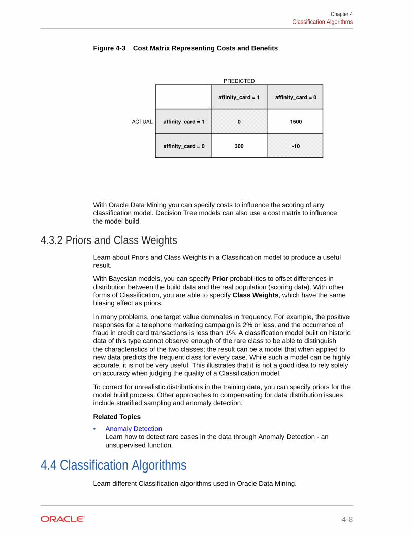
Figure 4-3 Cost Matrix Representing Costs and Benefits
PREDICTED
ACTUAL
affinity_card = 1 affinity_card = 0
-10300affinity_card = 0
15000affinity_card = 1
With Oracle Data Mining you can specify costs to influence the scoring of anyclassification model. Decision Tree models can also use a cost matrix to influencethe model build.
4.3.2 Priors and Class WeightsLearn about Priors and Class Weights in a Classification model to produce a usefulresult.
With Bayesian models, you can specify Prior probabilities to offset differences indistribution between the build data and the real population (scoring data). With otherforms of Classification, you are able to specify Class Weights, which have the samebiasing effect as priors.
In many problems, one target value dominates in frequency. For example, the positiveresponses for a telephone marketing campaign is 2% or less, and the occurrence offraud in credit card transactions is less than 1%. A classification model built on historicdata of this type cannot observe enough of the rare class to be able to distinguishthe characteristics of the two classes; the result can be a model that when applied tonew data predicts the frequent class for every case. While such a model can be highlyaccurate, it is not be very useful. This illustrates that it is not a good idea to rely solelyon accuracy when judging the quality of a Classification model.
To correct for unrealistic distributions in the training data, you can specify priors for themodel build process. Other approaches to compensating for data distribution issuesinclude stratified sampling and anomaly detection.
Related Topics
• Anomaly DetectionLearn how to detect rare cases in the data through Anomaly Detection - anunsupervised function.
4.4 Classification AlgorithmsLearn different Classification algorithms used in Oracle Data Mining.
Chapter 4Classification Algorithms
4-8

Oracle Data Mining provides the following algorithms for classification:
• Decision Tree
Decision trees automatically generate rules, which are conditional statements thatreveal the logic used to build the tree.
• Explicit Semantic Analysis
Explicit Semantic Analysis (ESA) is designed to make predictions for text data.This algorithm can address use cases with hundreds of thousands of classes.
• Naive Bayes
Naive Bayes uses Bayes' Theorem, a formula that calculates a probability bycounting the frequency of values and combinations of values in the historical data.
• Generalized Linear Models (GLM)
GLM is a popular statistical technique for linear modeling. Oracle Data Miningimplements GLM for binary classification and for regression. GLM providesextensive coefficient statistics and model statistics, as well as row diagnostics.GLM also supports confidence bounds.
• Random Forest
Random Forest is a powerful and popular machine learning algorithm that bringssignificant performance and scalability benefits.
• Support Vector Machines (SVM)
SVM is a powerful, state-of-the-art algorithm based on linear and nonlinearregression. Oracle Data Mining implements SVM for binary and multiclassclassification.
Note:
Oracle Data Mining uses Naive Bayes as the default classification algorithm.
Related Topics
• Decision TreeLearn how to use Decision Tree algorithm. Decision Tree is one of theClassification algorithms that the Oracle Data Mining supports.
• Explicit Semantic AnalysisLearn how to use Explicit Semantic Analysis (ESA) as an unsupervised algorithmfor Feature Extraction function and as a supervised algorithm for Classification.
• Naive BayesLearn how to use Naive Bayes Classification algorithm that the Oracle Data Miningsupports.
• Generalized Linear ModelsLearn how to use Generalized Linear Models (GLM) statistical technique for Linearmodeling.
• Random ForestLearn how to use Random Forest as a classification algorithm.
Chapter 4Classification Algorithms
4-9

• Support Vector MachinesLearn how to use Support Vector Machines, a powerful algorithm based onstatistical learning theory.
Chapter 4Classification Algorithms
4-10

5Anomaly Detection
Learn how to detect rare cases in the data through Anomaly Detection - anunsupervised function.
• About Anomaly Detection
• Anomaly Detection Algorithm
Related Topics
• Oracle Data Mining BasicsUnderstand the basic concepts of Oracle Data Mining.
See Also:
• Campos, M.M., Milenova, B.L., Yarmus, J.S., "Creation and Deploymentof Data Mining-Based Intrusion Detection Systems in Oracle Database10g"
Oracle Data Mining
5.1 About Anomaly DetectionThe goal of anomaly detection is to identify cases that are unusual within data that isseemingly homogeneous. Anomaly detection is an important tool for detecting fraud,network intrusion, and other rare events that can have great significance but are hardto find.
Anomaly detection can be used to solve problems like the following:
• A law enforcement agency compiles data about illegal activities, but nothing aboutlegitimate activities. How can a suspicious activity be flagged?
The law enforcement data is all of one class. There are no counter-examples.
• An insurance agency processes millions of insurance claims, knowing that a verysmall number are fraudulent. How can the fraudulent claims be identified?
The claims data contains very few counter-examples. They are outliers.
5.1.1 One-Class ClassificationLearn about Anomaly Detection as one-class Classification in training data.
Anomaly detection is a form of Classification. Anomaly detection is implemented asone-class Classification, because only one class is represented in the training data.An anomaly detection model predicts whether a data point is typical for a given
5-1

distribution or not. An atypical data point can be either an outlier or an example ofa previously unseen class.
Normally, a Classification model must be trained on data that includes both examplesand counter-examples for each class so that the model can learn to distinguishbetween them. For example, a model that predicts the side effects of a medicationmust be trained on data that includes a wide range of responses to the medication.
A one-class classifier develops a profile that generally describes a typical case inthe training data. Deviation from the profile is identified as an anomaly. One-classclassifiers are sometimes referred to as positive security models, because they seek toidentify "good" behaviors and assume that all other behaviors are bad.
Note:
Solving a one-class classification problem can be difficult. The accuracyof one-class classifiers cannot usually match the accuracy of standardclassifiers built with meaningful counterexamples.
The goal of anomaly detection is to provide some useful information whereno information was previously attainable. However, if there are enough of the"rare" cases so that stratified sampling produce a training set with enoughcounter examples for a standard classification model, then that is generally abetter solution.
Related Topics
• About Classification
5.1.2 Anomaly Detection for Single-Class DataIn single-class data, all the cases have the same classification. Counter-examples,instances of another class, are hard to specify or expensive to collect. For instance,in text document classification, it is easy to classify a document under a giventopic. However, the universe of documents outside of this topic can be very largeand diverse. Thus, it is not feasible to specify other types of documents as counter-examples.
Anomaly detection can be used to find unusual instances of a particular type ofdocument.
5.1.3 Anomaly Detection for Finding OutliersOutliers are cases that are unusual because they fall outside the distribution that isconsidered normal for the data. For example, census data shows a median householdincome of $70,000 and a mean household income of $80,000, but one or twohouseholds have an income of $200,000. These cases can probably be identified asoutliers.
The distance from the center of a normal distribution indicates how typical a givenpoint is with respect to the distribution of the data. Each case can be ranked accordingto the probability that it is either typical or atypical.
Chapter 5About Anomaly Detection
5-2

The presence of outliers can have a deleterious effect on many forms of data mining.You can use Anomaly Detection to identify outliners before mining the data.
5.2 Anomaly Detection AlgorithmLearn about One-Class Support Vector Machines (SVM) for Anomaly Detection.
Oracle Data Mining supports One-Class Support Vector Machines (SVM) for AnomalyDetection. When used for Anomaly Detection, SVM classification does not use atarget.
Related Topics
• One-Class SVM
Chapter 5Anomaly Detection Algorithm
5-3
6Clustering
Learn how to discover natural groupings in the data through Clustering - theunsupervised mining function.
• About Clustering
• Evaluating a Clustering Model
• Clustering Algorithms
Related Topics
• Oracle Data Mining BasicsUnderstand the basic concepts of Oracle Data Mining.
6.1 About ClusteringClustering analysis finds clusters of data objects that are similar to one another. Themembers of a cluster are more like each other than they are like members of otherclusters. Different clusters can have members in common. The goal of clusteringanalysis is to find high-quality clusters such that the inter-cluster similarity is low andthe intra-cluster similarity is high.
Clustering, like classification, is used to segment the data. Unlike classification,clustering models segment data into groups that were not previously defined.Classification models segment data by assigning it to previously-defined classes,which are specified in a target. Clustering models do not use a target.
Clustering is useful for exploring data. You can use Clustering algorithms to findnatural groupings when there are many cases and no obvious groupings.
Clustering can serve as a useful data-preprocessing step to identify homogeneousgroups on which you can build supervised models.
You can also use Clustering for Anomaly Detection. Once you segment the data intoclusters, you find that some cases do not fit well into any clusters. These cases areanomalies or outliers.
6.1.1 How are Clusters Computed?There are several different approaches to the computation of clusters. Oracle DataMining supports the following methods:
• Density-based: This type of clustering finds the underlying distribution of the dataand estimates how areas of high density in the data correspond to peaks in thedistribution. High-density areas are interpreted as clusters. Density-based clusterestimation is probabilistic.
• Distance-based: This type of clustering uses a distance metric to determinesimilarity between data objects. The distance metric measures the distance
6-1
between actual cases in the cluster and the prototypical case for the cluster. Theprototypical case is known as the centroid.
• Grid-based: This type of clustering divides the input space into hyper-rectangularcells and identifies adjacent high-density cells to form clusters.
6.1.2 Scoring New DataAlthough clustering is an unsupervised mining function, Oracle Data Mining supportsthe scoring operation for clustering. New data is scored probabilistically.
6.1.3 Hierarchical ClusteringThe clustering algorithms supported by Oracle Data Mining perform hierarchicalclustering. The leaf clusters are the final clusters generated by the algorithm. Clustershigher up in the hierarchy are intermediate clusters.
6.1.3.1 RulesRules describe the data in each cluster. A rule is a conditional statement that capturesthe logic used to split a parent cluster into child clusters. A rule describes theconditions for a case to be assigned with some probability to a cluster.
6.1.3.2 Support and ConfidenceSupport and confidence are metrics that describe the relationships betweenclustering rules and cases. Support is the percentage of cases for which the ruleholds. Confidence is the probability that a case described by this rule is actuallyassigned to the cluster.
6.2 Evaluating a Clustering ModelSince known classes are not used in clustering, the interpretation of clusters canpresent difficulties. How do you know if the clusters can reliably be used for businessdecision making?
Oracle Data Mining clustering models support a high degree of model transparency.You can evaluate the model by examining information generated by the clusteringalgorithm: for example, the centroid of a distance-based cluster. Moreover, becausethe clustering process is hierarchical, you can evaluate the rules and other informationrelated to each cluster's position in the hierarchy.
6.3 Clustering AlgorithmsLearn different Clustering algorithms used in Oracle Data Mining.
Oracle Data Mining supports these Clustering algorithms:
• Expectation Maximization
Expectation Maximization is a probabilistic, density-estimation Clusteringalgorithm.
• k-Means
Chapter 6Evaluating a Clustering Model
6-2
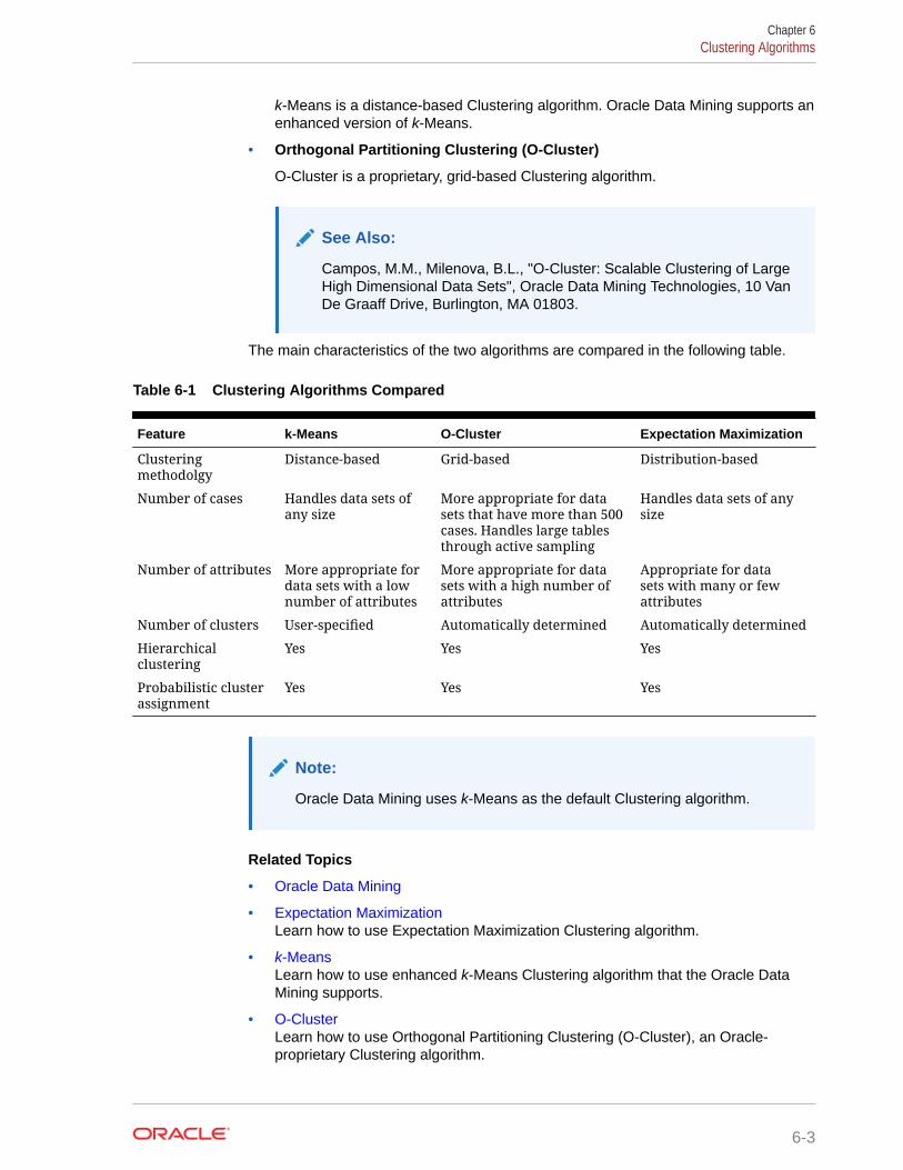
k-Means is a distance-based Clustering algorithm. Oracle Data Mining supports anenhanced version of k-Means.
• Orthogonal Partitioning Clustering (O-Cluster)
O-Cluster is a proprietary, grid-based Clustering algorithm.
See Also:
Campos, M.M., Milenova, B.L., "O-Cluster: Scalable Clustering of LargeHigh Dimensional Data Sets", Oracle Data Mining Technologies, 10 VanDe Graaff Drive, Burlington, MA 01803.
The main characteristics of the two algorithms are compared in the following table.
Table 6-1 Clustering Algorithms Compared
Feature k-Means O-Cluster Expectation Maximization
Clusteringmethodolgy
Distance-based Grid-based Distribution-based
Number of cases Handles data sets ofany size
More appropriate for datasets that have more than 500cases. Handles large tablesthrough active sampling
Handles data sets of anysize
Number of attributes More appropriate fordata sets with a lownumber of attributes
More appropriate for datasets with a high number ofattributes
Appropriate for datasets with many or fewattributes
Number of clusters User-specified Automatically determined Automatically determined
Hierarchicalclustering
Yes Yes Yes
Probabilistic clusterassignment
Yes Yes Yes
Note:
Oracle Data Mining uses k-Means as the default Clustering algorithm.
Related Topics
• Oracle Data Mining
• Expectation MaximizationLearn how to use Expectation Maximization Clustering algorithm.
• k-MeansLearn how to use enhanced k-Means Clustering algorithm that the Oracle DataMining supports.
• O-ClusterLearn how to use Orthogonal Partitioning Clustering (O-Cluster), an Oracle-proprietary Clustering algorithm.
Chapter 6Clustering Algorithms
6-3
7Association
Learn how to discover Association Rules through Association - an unsupervisedmining function.
• About Association
• Transactional Data
• Association Algorithm
Related Topics
• Oracle Data Mining BasicsUnderstand the basic concepts of Oracle Data Mining.
7.1 About AssociationAssociation is a data mining function that discovers the probability of the co-occurrence of items in a collection. The relationships between co-occurring items areexpressed as Association Rules.
7.1.1 Association RulesThe results of an Association model are the rules that identify patterns of associationwithin the data. Oracle Data Mining does not support the scoring operation forassociation modeling.
Association Rules can be applied as follows:
Support: How often do these items occur together in the data?Confidence: How frequently the consequent occurs in transactions that contain theantecedent.Value: How much business value is connected to item associations
7.1.2 Market-Basket AnalysisAssociation rules are often used to analyze sales transactions. For example, it is notedthat customers who buy cereal at the grocery store often buy milk at the same time.In fact, association analysis find that 85% of the checkout sessions that include cerealalso include milk. This relationship can be formulated as the following rule:
Cereal implies milk with 85% confidence
This application of association modeling is called market-basket analysis. It isvaluable for direct marketing, sales promotions, and for discovering business trends.Market-basket analysis can also be used effectively for store layout, catalog design,and cross-sell.
7-1
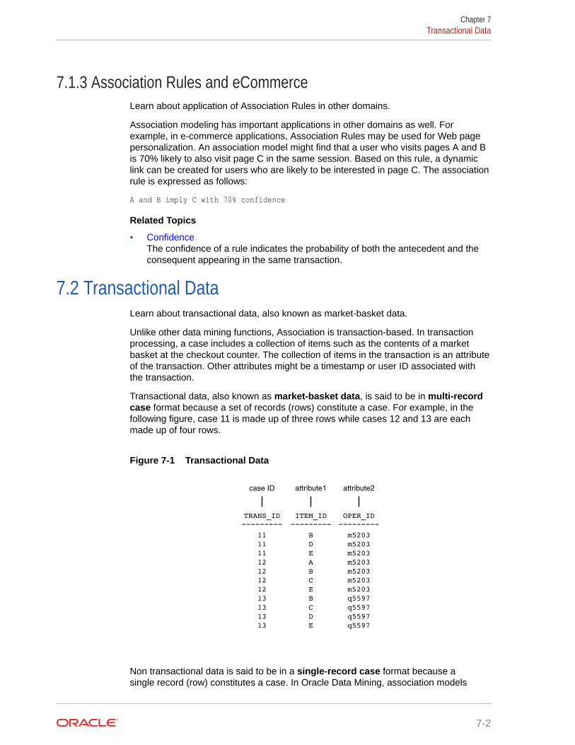
7.1.3 Association Rules and eCommerceLearn about application of Association Rules in other domains.
Association modeling has important applications in other domains as well. Forexample, in e-commerce applications, Association Rules may be used for Web pagepersonalization. An association model might find that a user who visits pages A and Bis 70% likely to also visit page C in the same session. Based on this rule, a dynamiclink can be created for users who are likely to be interested in page C. The associationrule is expressed as follows:
A and B imply C with 70% confidence
Related Topics
• ConfidenceThe confidence of a rule indicates the probability of both the antecedent and theconsequent appearing in the same transaction.
7.2 Transactional DataLearn about transactional data, also known as market-basket data.
Unlike other data mining functions, Association is transaction-based. In transactionprocessing, a case includes a collection of items such as the contents of a marketbasket at the checkout counter. The collection of items in the transaction is an attributeof the transaction. Other attributes might be a timestamp or user ID associated withthe transaction.
Transactional data, also known as market-basket data, is said to be in multi-recordcase format because a set of records (rows) constitute a case. For example, in thefollowing figure, case 11 is made up of three rows while cases 12 and 13 are eachmade up of four rows.
Figure 7-1 Transactional Data
attribute2
OPER_ID---------
m5203m5203m5203m5203m5203m5203m5203q5597q5597q5597q5597
attribute1
ITEM_ID---------
BDEABCEBCDE
case ID
TRANS_ID---------
1111111212121213131313
Non transactional data is said to be in a single-record case format because asingle record (row) constitutes a case. In Oracle Data Mining, association models
Chapter 7Transactional Data
7-2

can be built using either transactional or non transactional or two-dimensional dataformats. If the data is non transactional, it is possible to transform to a nestedcolumn to make it transactional before association mining activities can be performed.Transactional format is the usual format but, the Association Rules model doesaccept two-dimensional input format. For non transactional input format, each distinctcombination of the content in all columns other than the case ID column is treated as aunique item.
Related Topics
• Oracle Data Mining User’s Guide
• Data Preparation for Apriori
7.3 Association AlgorithmOracle Data Mining uses the Apriori algorithm to calculate association rules for itemsin frequent itemsets.
Chapter 7Association Algorithm
7-3
8Feature Selection and Extraction
Learn how to perform Feature Selection, Feature Extraction, and Attribute Importance.
Oracle Data Mining supports attribute importance as a supervised mining function andfeature extraction as an unsupervised mining function.
• Finding the Best Attributes
• About Feature Selection and Attribute Importance
• About Feature Extraction
Related Topics
• Oracle Data Mining BasicsUnderstand the basic concepts of Oracle Data Mining.
8.1 Finding the Best AttributesSometimes too much information can reduce the effectiveness of data mining. Someof the columns of data attributes assembled for building and testing a model do notcontribute meaningful information to the model. Some do actually detract from thequality and accuracy of the model.
For example, you want to collect a great deal of data about a given populationbecause you want to predict the likelihood of a certain illness within this group. Someof this information, perhaps much of it, has little or no effect on susceptibility to theillness. It is possible that attributes such as the number of cars per household do nothave effect whatsoever.
Irrelevant attributes add noise to the data and affect model accuracy. Noise increasesthe size of the model and the time and system resources needed for model buildingand scoring.
Data sets with many attributes can contain groups of attributes that are correlated.These attributes actually measure the same underlying feature. Their presencetogether in the build data can skew the logic of the algorithm and affect the accuracy ofthe model.
Wide data (many attributes) generally presents processing challenges for data miningalgorithms. Model attributes are the dimensions of the processing space used bythe algorithm. The higher the dimensionality of the processing space, the higher thecomputation cost involved in algorithmic processing.
To minimize the effects of noise, correlation, and high dimensionality, some form ofdimension reduction is sometimes a desirable preprocessing step for data mining.Feature selection and extraction are two approaches to dimension reduction.
• Feature selection: Selecting the most relevant attributes
• Feature extraction: Combining attributes into a new reduced set of features
8-1

8.2 About Feature Selection and Attribute ImportanceFinding the most significant predictors is the goal of some data mining projects. Forexample, a model might seek to find the principal characteristics of clients who pose ahigh credit risk.
Oracle Data Mining supports the Attribute Importance mining function, which ranksattributes according to their importance in predicting a target. Attribute importancedoes not actually perform feature selection since all the predictors are retained in themodel. In true feature selection, the attributes that are ranked below a given thresholdof importance are removed from the model.
Feature selection is useful as a preprocessing step to improve computationalefficiency in predictive modeling. Oracle Data Mining implements feature selectionfor optimization within the Decision Tree algorithm and within Naive Bayes whenAutomatic Data Preparation (ADP) is enabled. Generalized Linear Model (GLM) canbe configured to perform feature selection as a preprocessing step.
8.2.1 Attribute Importance and ScoringOracle Data Mining does not support the scoring operation for attribute importance.The results of attribute importance are the attributes of the build data ranked accordingto their predictive influence. The ranking and the measure of importance can be usedin selecting training data for classification models.
8.3 About Feature ExtractionFeature Extraction is an attribute reduction process. Unlike feature selection, whichselects and retains the most significant attributes, Feature Extraction actuallytransforms the attributes. The transformed attributes, or features, are linearcombinations of the original attributes.
The Feature Extraction process results in a much smaller and richer set of attributes.The maximum number of features can be user-specified or determined by thealgorithm. By default, the algorithm determines it.
Models built on extracted features can be of higher quality, because fewer and moremeaningful attributes describe the data.
Feature Extraction projects a data set with higher dimensionality onto a smallernumber of dimensions. As such it is useful for data visualization, since a complexdata set can be effectively visualized when it is reduced to two or three dimensions.
Some applications of Feature Extraction are latent semantic analysis, datacompression, data decomposition and projection, and pattern recognition. FeatureExtraction can also be used to enhance the speed and effectiveness of supervisedlearning.
Feature Extraction can be used to extract the themes of a document collection,where documents are represented by a set of key words and their frequencies. Eachtheme (feature) is represented by a combination of keywords. The documents in thecollection can then be expressed in terms of the discovered themes.
Chapter 8About Feature Selection and Attribute Importance
8-2
8.3.1 Feature Extraction and ScoringOracle Data Mining supports the scoring operation for feature extraction. As anunsupervised mining function, feature extraction does not involve a target. Whenapplied, a feature extraction model transforms the input into a set of features.
8.4 Algorithms for Attribute Importance and FeatureExtraction
Understand the algorithms used for Attribute Importance and Feature Extraction.
Oracle Data Mining supports the following algorithms for Attribute Importance:
• Minimum Description Length
• CUR matrix decomposition
Oracle Data Mining supports these feature extraction algorithms:
• Explicit Semantic Analysis (ESA).
• Non-Negative Matrix Factorization (NMF).
• Singular Value Decomposition (SVD) and Prediction Component Analysis(PCA).
Note:
Oracle Data Mining uses NMF as the default feature extraction algorithm.
Related Topics
• CUR Matrix DecompositionLearn how to use CUR decomposition based algorithm for attribute importance.
• Explicit Semantic AnalysisLearn how to use Explicit Semantic Analysis (ESA) as an unsupervised algorithmfor Feature Extraction function and as a supervised algorithm for Classification.
• Minimum Description LengthLearn how to use Minimum Description Length, the supervised technique forcalculating Attribute Importance.
• Non-Negative Matrix FactorizationLearn how to use Non-Negative Matrix Factorization (NMF), the unsupervisedalgorithm, that the Oracle Data Mining uses for Feature Extraction.
• Singular Value DecompositionLearn how to use Singular Value Decomposition, an unsupervised algorithm forFeature Extraction.
Chapter 8Algorithms for Attribute Importance and Feature Extraction
8-3

9Time Series
Learn about Time Series as an Oracle Data Mining Regression function.
• About Time Series
• Choosing a Time Series Model
• Time Series Statistics
• Time Series Algorithm
9.1 About Time SeriesTime Series is a new data mining function that forecasts target value based solely ona known history of target values. It is a specialized form of Regression, known in theliterature as auto-regressive modeling.
The input to time series analysis is a sequence of target values. A case id columnspecifies the order of the sequence. The case id can be of type NUMBER or a datetype (date, datetime, timestamp with timezone, or timestamp with local timezone).Regardless of case id type, the user can request that the model include trend,seasonal effects or both in its forecast computation. When the case id is a datetype, the user must specify a time interval (for example, month) over which the targetvalues are to be aggregated, along with an aggregation procedure (for example, sum).Aggregation is performed by the algorithm prior to constructing the model.
The time series model provide estimates of the target value for each step of atime window that can include up to 30 steps beyond the historical data. Like otherRegression models, Time Series models compute various statistics that measure thegoodness of fit to historical data.
Forecasting is a critical component of business and governmental decision making.It has applications at the strategic, tactical and operation level. The following are theapplications of forecasting:
• Projecting return on investment, including growth and the strategic effect ofinnovations
• Addressing tactical issues such as projecting costs, inventory requirements andcustomer satisfaction
• Setting operational targets and predicting quality and conformance with standards
Related Topics
• RegressionLearn how to predict a continuous numerical target through Regression - thesupervised mining function.
9.2 Choosing a Time Series ModelLearn how to select a Time Series model.
9-1
Time Series data may contain patterns that can affect predictive accuracy. Forexample, during a period of economic growth, there may be an upward trend in sales.Sales may increase in specific seasons (bathing suits in summer). To accommodatesuch series, it can be useful to choose a model that incorporates trend, seasonaleffects, or both.
Trend can be difficult to estimate, when you must represent trend by a single constant.For example, if there is a grow rate of 10%, then after 7 steps, the value doubles.Local growth rates, appropriate to a few time steps can easily approach such levels,but thereafter drop. Damped trend models can more accurately represent such data,by reducing cumulative trend effects. Damped trend models can better representvariability in trend effects over the historical data. Damped trend models are a goodchoice when the data have significant, but variable trend.
Since modeling attempts to reduce error, how error is measured can affect modelpredictions. For example, data that exhibit a wide range of values may be betterrepresented by error as fraction of level. An error of a few hundred feet in themeasurement of the height of a mountain may be equivalent to an error of an inchor two in the measurement of the height of a child. Errors that are measured relativeto value are called multiplicative errors. Errors that are the same across values arecalled additive errors. If there are multiplicative effects in the model, then the errortype is multiplicative. If there are no explicit multiplicative effects, error type is leftto user specification. The type need not be the same across individual effects. Forexample, trend can be additive while seasonality is multiplicative. This particular mixedtype effect combination defines the popular Holt-Winters model.
Note:
Multiplicative error is not an appropriate choice for data that contain zerosor negative values. Thus, when the data contains such values, it is bestnot to choose a model with multiplicative effects or to set error type to bemultiplicative.
9.3 Time Series StatisticsLearn to evaluate model quality by applying commonly used statistics.
As with other Regression functions, there are commonly used statistics for evaluatingthe overall model quality. An expert user can also specify one of these figures of meritas criterion to optimize by the model build process. Choosing an optimization criterionis not required because model-specific defaults are available.
9.3.1 Conditional Log-LikelihoodLog-likelihood is a figure of merit often used as an optimization criterion for modelsthat provide probability estimates for predictions which depend on the values of themodel’s parameters.
The model probability estimates for the actual values in the training data then yieldsan estimate of the likelihood of the parameter values. Parameter values that yield highprobabilities for the observed target values have high likelihood, and therefore indicatea good model. The calculation of log-likelihood depends on the form of the model.
Chapter 9Time Series Statistics
9-2

Conditional log-likelihood breaks the parameters into two groups. One group isassumed to be correct and the other is assumed the source of any errors. Conditionallog-likelihood is the log-likelihood of the latter group conditioned on the former group.For example, Exponential Smoothing models (ESMs) make an estimate of the initialmodel state. The conditional log-likelihood of an ESM is conditional on that initialmodel state (assumed to be correct). The ESM conditional log-likelihood is as follows:
where et is the error at time t and k(x(t-1) ) is 1 for ESM models with additive errorsand is the estimated level at the previous time step in models with multiplicative error.
9.3.2 Mean Square Error (MSE) and Other Error MeasuresAnother time series figure of merit, that can also be used as an optimization criterion,is Mean Square Error (MSE).
The mean square error is computed as:
where the error at time t is the difference between the actual and model one stepahead forecast value at time t for models with additive error and that difference dividedby the one-step ahead forecast for models with multiplicative error.
Note:
These "forecasts" are for over periods already observed and part of the inputtime series.
Since time series models can forecast for each of multiple steps ahead, time seriescan measure the error associated with such forecasts. Average Mean Square Error(AMSE), another figure of merit, does exactly that. For each period in the input timeseries, it computes a multi-step forecast, computes the error of those forecasts andaverages the errors. AMSE computes the individual errors exactly as MSE doestaking cognizance of error type (additive or multiplicative). The number of steps, k,is determined by the user (default 3). The formula is as follows:
Chapter 9Time Series Statistics
9-3

Other figure of merit relatives of MSE include the Residual Standard Error (RMSE),which is the square root of MSE, and the Mean Absolute Error (MAE) which is theaverage of the absolute value of the errors.
9.3.3 Irregular Time SeriesIrregular time series are time series data where the time intervals between observedvalues are not equally spaced.
One common practice is for the time intervals between adjacent steps to be equallyspaced. However, it is not always convenient or realistic to force such spacing on timeseries. Irregular time series do not make the assumption that time series are equallyspaced, but instead use the case id’s date and time values to compute the intervalsbetween observed values. Models are constructed directly on the observed valueswith their observed spacing. Oracle time series analysis handles irregular time series.
9.3.4 Build ApplyLearn about build and apply operations of Time Series function.
Many of the Oracle Data Mining functions have separate build and apply operations,because you can construct and potentially apply a model to many different sets ofinput data. However, time series input consists of the target value history only. Thus,there is only one set of appropriate input data. When new data arrive, good practicedictates that a new model be built. Since the model is only intended to be used once,the model statistics and forecasts are produced during model build and are availablethrough the model views.
9.4 Time Series AlgorithmOracle Data Mining uses the algorithm Exponential Smoothing to forecast from timeseries data.
Related Topics
• Exponential SmoothingLearn about Exponential Smoothing.
Chapter 9Time Series Algorithm
9-4

Part IIIAlgorithms
Part III provides basic conceptual information about the algorithms supported byOracle Data Mining. There is at least one algorithm for each of the mining functions.
Part III contains these chapters:
• Apriori
• CUR Matrix Decomposition
• Decision Tree
• Expectation Maximization
• Explicit Semantic Analysis
• Exponential Smoothing
• Generalized Linear Models
• k-Means
• Minimum Description Length
• Naive Bayes
• Neural Network
• Non-Negative Matrix Factorization
• O-Cluster
• R Extensibility
• Random Forest
• Singular Value Decomposition
• Support Vector Machines
Related Topics
• Mining FunctionsPart II provides basic conceptual information about the mining functions that theOracle Data Mining supports.
10Apriori
Learn how to calculate Association Rules using Apriori algorithm.
• About Apriori
• Association Rules and Frequent Itemsets
• Data Preparation for Apriori
• Calculating Association Rules
• Evaluating Association Rules
Related Topics
• AssociationLearn how to discover Association Rules through Association - an unsupervisedmining function.
10.1 About AprioriLearn about Apriori.
An association mining problem can be decomposed into the following subproblems:
• Find all combinations of items in a set of transactions that occur with a specifiedminimum frequency. These combinations are called frequent itemsets.
• Calculate rules that express the probable co-occurrence of items within frequentitemsets.
Apriori calculates the probability of an item being present in a frequent itemset, giventhat another item or items is present.
Association rule mining is not recommended for finding associations involving rareevents in problem domains with a large number of items. Apriori discovers patternswith frequencies above the minimum support threshold. Therefore, to find associationsinvolving rare events, the algorithm must run with very low minimum support values.However, doing so potentially explodes the number of enumerated itemsets, especiallyin cases with a large number of items. This increases the execution time significantly.Classification or Anomaly Detection is more suitable for discovering rare events whenthe data has a high number of attributes.
The build process for Apriori supports parallel execution.
Related Topics
• Example: Calculating Rules from Frequent ItemsetsExample to calculating rules from Frequent itemsets.
• Oracle Database VLDB and Partitioning Guide
10-1
10.2 Association Rules and Frequent ItemsetsThe Apriori algorithm calculates rules that express probabilistic relationships betweenitems in frequent itemsets. For example, a rule derived from frequent itemsetscontaining A, B, and C might state that if A and B are included in a transaction, then Cis likely to also be included.
An association rule states that an item or group of items implies the presence ofanother item with some probability. Unlike decision tree rules, which predict a target,association rules simply express correlation.
10.2.1 Antecedent and ConsequentThe IF component of an association rule is known as the antecedent. The THENcomponent is known as the consequent. The antecedent and the consequent aredisjoint; they have no items in common.
Oracle Data Mining supports association rules that have one or more items in theantecedent and a single item in the consequent.
10.2.2 ConfidenceRules have an associated confidence, which is the conditional probability that theconsequent occurs given the occurrence of the antecedent. You can specify theminimum confidence for rules.
10.3 Data Preparation for AprioriAssociation models are designed to use transactional data. In transactional data, thereis a one-to-many relationship between the case identifier and the values for each case.Each case ID/value pair is specified in a separate record (row).
10.3.1 Native Transactional Data and Star SchemasLearn about storage format of transactional data.
Transactional data may be stored in native transactional format, with a non-uniquecase ID column and a values column, or it may be stored in some other configuration,such as a star schema. If the data is not stored in native transactional format, it mustbe transformed to a nested column for processing by the Apriori algorithm.
Related Topics
• Transactional DataLearn about transactional data, also known as market-basket data.
• Oracle Data Mining User’s Guide
10.3.2 Items and CollectionsIn transactional data, a collection of items is associated with each case. The collectiontheoretically includes all possible members of the collection. For example, all productscan theoretically be purchased in a single market-basket transaction. However, in
Chapter 10Association Rules and Frequent Itemsets
10-2
actuality, only a tiny subset of all possible items are present in a given transaction; theitems in the market-basket represent only a small fraction of the items available forsale in the store.
10.3.3 Sparse DataLearn about missing items through sparsity.
Missing items in a collection indicate sparsity. Missing items may be present with anull value, or they may simply be missing.
Nulls in transactional data are assumed to represent values that are known but notpresent in the transaction. For example, three items out of hundreds of possible itemsmight be purchased in a single transaction. The items that were not purchased areknown but not present in the transaction.
Oracle Data Mining assumes sparsity in transactional data. The Apriori algorithm isoptimized for processing sparse data.
Note:
Apriori is not affected by Automatic Data Preparation.
Related Topics
• Oracle Data Mining User’s Guide
10.3.4 Improved SamplingAssociation Rules (AR) can use a good sample size with performance guarantee,based on the work of Riondato and Upfal.
The AR algorithm computes the sample size by the following inputs:
• d-index of the dataset
• Absolute error ε
• Confidence level γ
d-index is defined as the maximum integer d such that the dataset contains at least dtransactions of length d at the minimum. It is the upper bound of Vapnik-Chervonenkis(VC) dimension. The AR algorithm computes d-index of the dataset by scanning thelength of all transactions in the dataset.
Users specify absolute error ε and confidence level γ parameters. A large d-index,small AR support, small ε or large γ can cause a large sample size. The sample sizetheoretically guarantees that the absolute error of both the support and confidence ofthe approximated AR (from sampling) is less than ε compared to the exact AR withprobability (or confidence level) at least γ. In this document this sample size is calledAR-specific sample size.
Chapter 10Data Preparation for Apriori
10-3
10.3.4.1 Sampling ImplementationThe sample size is only computed when users turn on the sampling (ODMS_SAMPLING isset as ODMS_SAMPLING_ENABLE) and do not specify the sample size (ODMS_SAMPLE_SIZEis unspecified).
Usage Notes
1. If ODMS_SAMPLING is unspecified or set as ODMS_SAMPLING_DISABLE, the sampling isnot performed for AR and the exact AR is obtained.
2. If ODMS_SAMPLING is set as ODMS_SAMPLING_ENABLE and if ODMS_SAMPLE_SIZEis specified as positive integer number then the user-specified sample size(ODMS_SAMPLE_SIZE) is utilized. The sampling is performed in the general datapreparation stage before the AR algorithm. The AR-specific sample size is notcomputed. The approximated AR is obtained.
3. If ODMS_SAMPLING is set as ODMS_SAMPLING_ENABLE and ODMS_SAMPLE_SIZE isnot specified, the AR-specified sample size is computed and then sampling isperformed in the AR algorithm. The approximated AR is obtained.
Note:
If the computed AR-specific sample size is larger than or equal to thetotal transaction size in the dataset, the sampling is not performed andthe exact AR is obtained.
If users do not have a good idea on the choice of sample size for AR, it is suggestedto leave ODMS_SAMPLE_SIZE unspecified, only specify proper values for samplingparameters and let AR algorithm compute the suitable AR-specific sample size.
Related Topics
• Oracle Database PL/SQL Packages and Types Reference
10.4 Calculating Association RulesThe first step in association analysis is the enumeration of itemsets. An itemset is anycombination of two or more items in a transaction.
10.4.1 ItemsetsLearn about itemsets.
The maximum number of items in an itemset is user-specified. If the maximum istwo, then all the item pairs are counted. If the maximum is greater than two, then allthe item pairs, all the item triples, and all the item combinations up to the specifiedmaximum are counted.
The following table shows the itemsets derived from the transactions shown in thefollowing example, assuming that maximum number of items in an itemset is set to 3.
Chapter 10Calculating Association Rules
10-4

Table 10-1 Itemsets
Transaction Itemsets
11 (B,D) (B,E) (D,E) (B,D,E)
12 (A,B) (A,C) (A,E) (B,C) (B,E) (C,E) (A,B,C) (A,B,E) (A,C,E) (B,C,E)
13 (B,C) (B,D) (B,E) (C,D) (C,E) (D,E) (B,C,D) (B,C,E) (B,D,E) (C,D,E)
Example 10-1 Sample Transactional Data
TRANS_ID ITEM_ID--------- -------------------11 B11 D11 E12 A12 B12 C12 E13 B13 C13 D13 E
10.4.2 Frequent ItemsetsLearn about Frequent Itemsets and Support.
Association rules are calculated from itemsets. If rules are generated from all possibleitemsets, there can be a very high number of rules and the rules may not be verymeaningful. Also, the model can take a long time to build. Typically it is desirableto only generate rules from itemsets that are well-represented in the data. Frequentitemsets are those that occur with a minimum frequency specified by the user.
The minimum frequent itemset Support is a user-specified percentage that limits thenumber of itemsets used for association rules. An itemset must appear in at least thispercentage of all the transactions if it is to be used as a basis for rules.
The following table shows the itemsets from Table 10-1 that are frequent itemsets withsupport > 66%.
Table 10-2 Frequent Itemsets
Frequent Itemset Transactions Support
(B,C) 2 of 3 67%
(B,D) 2 of 3 67%
(B,E) 3 of 3 100%
(C,E) 2 of 3 67%
(D,E) 2 of 3 67%
(B,C,E) 2 of 3 67%
(B,D,E) 2 of 3 67%
Chapter 10Calculating Association Rules
10-5

Related Topics
• AprioriLearn how to calculate Association Rules using Apriori algorithm.
10.4.3 Example: Calculating Rules from Frequent ItemsetsExample to calculating rules from Frequent itemsets.
The following tables show the itemsets and frequent itemsets that were calculatedin "Association". The frequent itemsets are the itemsets that occur with a minimumsupport of 67%; at least 2 of the 3 transactions must include the itemset.
Table 10-3 Itemsets
Transaction Itemsets
11 (B,D) (B,E) (D,E) (B,D,E)
12 (A,B) (A,C) (A,E) (B,C) (B,E) (C,E) (A,B,C) (A,B,E) (A,C,E) (B,C,E)
13 (B,C) (B,D) (B,E) (C,D) (C,E) (D,E) (B,C,D) (B,C,E) (B,D,E) (C,D,E)
Table 10-4 Frequent Itemsets with Minimum Support 67%
Itemset Transactions Support
(B,C) 12 and 13 67%
(B,D) 11 and 13 67%
(B,E) 11, 12, and 13 100%
(C,E) 12 and 13 67%
(D,E) 11 and 13 67%
(B,C,E) 12 and 13 67%
(B,D,E) 11 and 13 67%
A rule expresses a conditional probability. Confidence in a rule is calculated by dividingthe probability of the items occurring together by the probability of the occurrence ofthe antecedent.
For example, if B (antecedent) is present, what is the chance that C (consequent) isalso present? What is the confidence for the rule "IF B, THEN C"?
As shown in Table 10-3:
• All 3 transactions include B (3/3 or 100%)
• Only 2 transactions include both B and C (2/3 or 67%)
• Therefore, the confidence of the rule "IF B, THEN C" is 67/100 or 67%.
The following table the rules that can be derived from the frequent itemsets inTable 10-4.
Chapter 10Calculating Association Rules
10-6

Table 10-5 Frequent Itemsets and Rules
Frequent Itemset Rules prob(antecedent andconsequent) / prob(antecedent)
Confidence
(B,C) (If B then C)(If C then B)
67/10067/67
67%100%
(B,D) (If B then D)(If D then B)
67/10067/67
67%100%
(B,E) (If B then E)(If E then B)
100/100100/100
100%100%
(C,E) (If C then E)(If E then C)
67/6767/100
100%67%
(D,E) (If D then E)I(f E then D)
67/6767/100
100%67%
(B,C,E) (If B and C thenE)(If B and E thenC)(If C and E thenB)
67/6767/10067/67
100%67%100%
(B,D,E) (If B and D thenE)(If B and E thenD)(If D and E thenB)
67/6767/10067/67
100%67%100%
If the minimum confidence is 70%, ten rules are generated for these frequent itemsets.If the minimum confidence is 60%, sixteen rules are generated.
Tip:
Increase the minimum confidence if you want to decrease the build time forthe model and generate fewer rules.
Related Topics
• AssociationLearn how to discover Association Rules through Association - an unsupervisedmining function.
10.4.4 AggregatesAggregates refer to the quantities associated with each item that the user opts forAssociation Rules Model to aggregate.
Chapter 10Calculating Association Rules
10-7
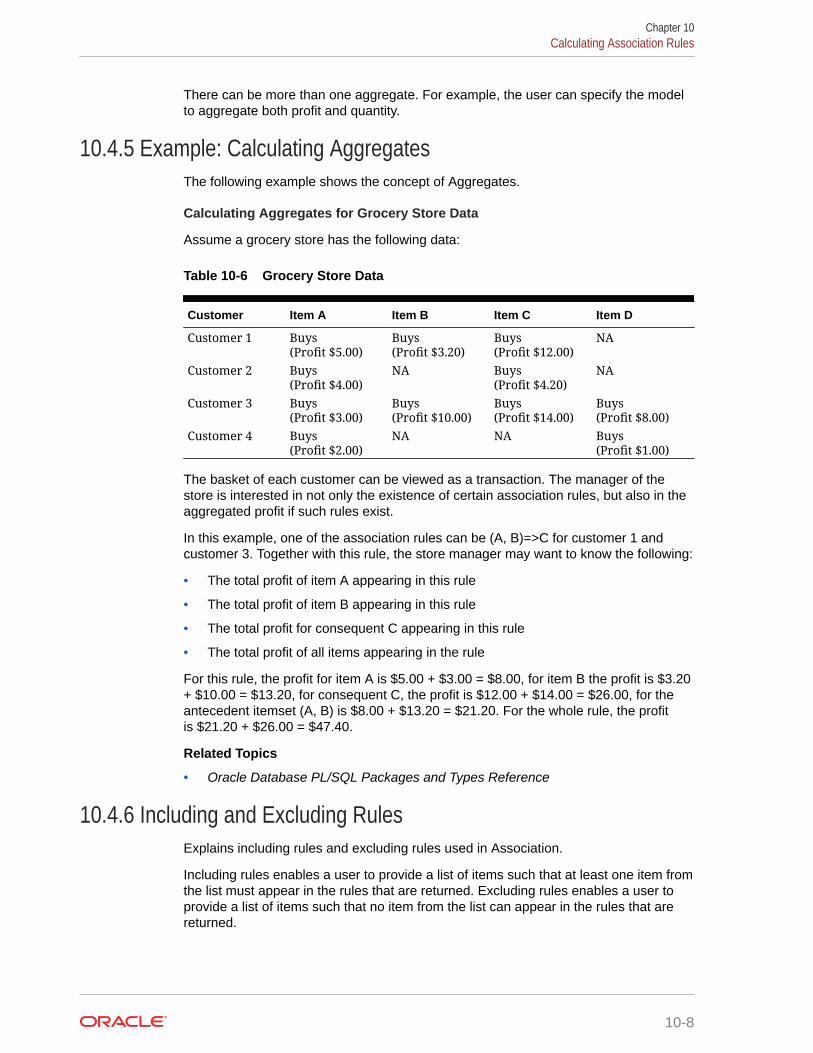
There can be more than one aggregate. For example, the user can specify the modelto aggregate both profit and quantity.
10.4.5 Example: Calculating AggregatesThe following example shows the concept of Aggregates.
Calculating Aggregates for Grocery Store Data
Assume a grocery store has the following data:
Table 10-6 Grocery Store Data
Customer Item A Item B Item C Item D
Customer 1 Buys(Profit $5.00)
Buys(Profit $3.20)
Buys(Profit $12.00)
NA
Customer 2 Buys(Profit $4.00)
NA Buys(Profit $4.20)
NA
Customer 3 Buys(Profit $3.00)
Buys(Profit $10.00)
Buys(Profit $14.00)
Buys(Profit $8.00)
Customer 4 Buys(Profit $2.00)
NA NA Buys(Profit $1.00)
The basket of each customer can be viewed as a transaction. The manager of thestore is interested in not only the existence of certain association rules, but also in theaggregated profit if such rules exist.
In this example, one of the association rules can be (A, B)=>C for customer 1 andcustomer 3. Together with this rule, the store manager may want to know the following:
• The total profit of item A appearing in this rule
• The total profit of item B appearing in this rule
• The total profit for consequent C appearing in this rule
• The total profit of all items appearing in the rule
For this rule, the profit for item A is $5.00 + $3.00 = $8.00, for item B the profit is $3.20+ $10.00 = $13.20, for consequent C, the profit is $12.00 + $14.00 = $26.00, for theantecedent itemset (A, B) is $8.00 + $13.20 = $21.20. For the whole rule, the profitis $21.20 + $26.00 = $47.40.
Related Topics
• Oracle Database PL/SQL Packages and Types Reference
10.4.6 Including and Excluding RulesExplains including rules and excluding rules used in Association.
Including rules enables a user to provide a list of items such that at least one item fromthe list must appear in the rules that are returned. Excluding rules enables a user toprovide a list of items such that no item from the list can appear in the rules that arereturned.
Chapter 10Calculating Association Rules
10-8

Note:
Since each association rule includes both antecedent and consequent, a setof including or excluding rules can be specified for antecedent while anotherset of including or excluding rules can be specified for consequent. Includingor excluding rules can also be defined for the association rule.
Related Topics
• Oracle Data Mining User’s Guide
• Oracle Database PL/SQL Packages and Types Reference
10.4.7 Performance Impact for AggregatesAggregate function requires more memory usage and longer execution time.
For each item, the user may supply several columns to aggregate. It requires morememory to buffer the extra data and more time to compute the aggregate values.
10.5 Evaluating Association RulesMinimum support and confidence are used to influence the build of an associationmodel. Support and confidence are also the primary metrics for evaluating the qualityof the rules generated by the model. Additionally, Oracle Data Mining supports lift forassociation rules. These statistical measures can be used to rank the rules and hencethe usefulness of the predictions.
10.5.1 SupportThe support of a rule indicates how frequently the items in the rule occur together. Forexample, cereal and milk might appear together in 40% of the transactions. If so, thefollowing rules each have a support of 40%:
cereal implies milkmilk implies cereal
Support is the ratio of transactions that include all the items in the antecedent andconsequent to the number of total transactions.
Support can be expressed in probability notation as follows:
support(A implies B) = P(A, B)
10.5.2 Minimum Support CountMinimum support Count defines minimum threshold in transactions that each rule mustsatisfy.
When the number of transactions is unknown, the support percentage thresholdparameter can be tricky to set appropriately. For this reason, support can also beexpressed as a count of transactions, with the greater of the two thresholds beingused to filter out infrequent itemsets. The default is 1 indicating that this criterion is notapplied.
Chapter 10Evaluating Association Rules
10-9

Related Topics
• Association Rules
• Oracle Data Mining User’s Guide
• Frequent ItemsetsLearn about Frequent Itemsets and Support.
10.5.3 ConfidenceThe confidence of a rule indicates the probability of both the antecedent and theconsequent appearing in the same transaction.
Confidence is the conditional probability of the consequent given the antecedent. Forexample, cereal appears in 50 transactions; 40 of the 50 might also include milk. Therule confidence is:
cereal implies milk with 80% confidence
Confidence is the ratio of the rule support to the number of transactions that includethe antecedent.
Confidence can be expressed in probability notation as follows.
confidence (A implies B) = P (B/A), which is equal to P(A, B) / P(A)
Related Topics
• Confidence
• Frequent ItemsetsLearn about Frequent Itemsets and Support.
10.5.4 Reverse ConfidenceThe Reverse Confidence of a rule is defined as the number of transactions in whichthe rule occurs divided by the number of transactions in which the consequent occurs.
Reverse Confidence eliminates rules that occur because the consequent is frequent.The default is 0.
Related Topics
• Confidence
• Example: Calculating Rules from Frequent ItemsetsExample to calculating rules from Frequent itemsets.
• Oracle Data Mining User’s Guide
• Oracle Database PL/SQL Packages and Types Reference
10.5.5 LiftBoth support and confidence must be used to determine if a rule is valid. However,there are times when both of these measures may be high, and yet still produce a rulethat is not useful. For example:
Chapter 10Evaluating Association Rules
10-10

Convenience store customers who buy orange juice also buy milk with a 75% confidence. The combination of milk and orange juice has a support of 30%.
This at first sounds like an excellent rule, and in most cases, it would be. It hashigh confidence and high support. However, what if convenience store customers ingeneral buy milk 90% of the time? In that case, orange juice customers are actuallyless likely to buy milk than customers in general.
A third measure is needed to evaluate the quality of the rule. Lift indicates the strengthof a rule over the random co-occurrence of the antecedent and the consequent, giventheir individual support. It provides information about the improvement, the increase inprobability of the consequent given the antecedent. Lift is defined as follows.
(Rule Support) /(Support(Antecedent) * Support(Consequent))
This can also be defined as the confidence of the combination of items divided bythe support of the consequent. So in our milk example, assuming that 40% of thecustomers buy orange juice, the improvement would be:
30% / (40% * 90%)
which is 0.83 – an improvement of less than 1.
Any rule with an improvement of less than 1 does not indicate a real cross-sellingopportunity, no matter how high its support and confidence, because it actually offersless ability to predict a purchase than does random chance.
Tip:
Decrease the maximum rule length if you want to decrease the build time forthe model and generate simpler rules.
Tip:
Increase the minimum support if you want to decrease the build time for themodel and generate fewer rules.
Chapter 10Evaluating Association Rules
10-11
11CUR Matrix Decomposition
Learn how to use CUR decomposition based algorithm for attribute importance.
• About CUR Matrix Decomposition
• Singular Vectors
• Statistical Leverage Score
• Column (Attribute) Selection and Row Selection
• CUR Matrix Decomposition Algorithm Configuration
11.1 About CUR Matrix DecompositionCUR matrix decomposition is a low-rank matrix decomposition algorithm that isexplicitly expressed in a small number of actual columns and/or actual rows of datamatrix.
CUR matrix decomposition was developed as an alternative to Singular ValueDecomposition (SVD) and Principal Component Analysis (PCA). CUR matrixdecomposition selects columns and rows that exhibit high statistical leverage orlarge influence from the data matrix. By implementing the CUR matrix decompositionalgorithm, a small number of most important attributes and/or rows can be identifiedfrom the original data matrix. Therefore, CUR matrix decomposition is an importanttool for exploratory data analysis. CUR matrix decomposition can be applied to avariety of areas and facilitates Regression, Classification, and Clustering.
Related Topics
• Data Preparation for SVDLearn about preparing the data for Singular Value Decomposition (SVD).
11.2 Singular VectorsSingular Value Decomposition (SVD) is the first step in CUR matrix decomposition.
SVD returns left and right singular vectors for calculating column and row leveragescores. Perform SVD on the following matrix:
A ε Rmxn
The matrix is factorized as follows:
A=UΣVT
where U = [u1 u2...um] and V = [v1 v2...vn] are orthogonal matrices.
Σ is a diagonal m × n matrix with non-negative real numbers σ1,...,σρ on thediagonal, where ρ = min {m,n} and σξ is the ξth singular value of A.
11-1

Let uξ and vξ be the ξth left and right singular vector of A, the jth column of A can thusbe approximated by the top k singular vectors and corresponding singular values as:
where vξj is the jth coordinate of the ξth right singular vector.
11.3 Statistical Leverage ScoreThe statistical leverage scores represent the column (or attribute) and row importance.
The normalized statistical leverage scores for all columns are computed from the top kright singular vectors as follows:
where k is called rank parameter and j = 1,...,n. Given that πj>=0 and
, these scores form a probability distribution over the n columns.
Similarly, the normalized statistical leverage scores for all rows are computed from thetop k left singular vectors as:
where i = 1,...,m.
11.4 Column (Attribute) Selection and Row SelectionColumn (Attribute) selection and Row selection is the final stage in CUR matrixdecomposition.
Attribute selection: Selects attributes with high leverage scores and reports theirnames, scores (as importance) and ranks (by importance).
Row selection: Selects rows with high leverage scores and reports their names, scores(as importance) and ranks (by importance).
Chapter 11Statistical Leverage Score
11-2

1. CUR matrix decomposition first selects the jth column (or attribute) of A withprobability pj= min {1,cπj} for all j ε {1,...,n}
2. If users enable row selection, select ith row of A with probability p�i = min {1,rπ�i}for all i ε {1,...,m}
3. Report the name (or ID) and leverage score (as importance) for all selectedattributes (if row importance is disabled) or for all selected attributes and rows(if row importance is enabled).
c is the approximated (or expected) number of columns that users want to select, and ris the approximated (or expected) number of rows that users want to select.
To realize column and row selections, you need to calculate the probability to selecteach column and row.
Calculate the probability for each column as follows:
pj = min {1,cπj}
Calculate the probability for each row as follows:
p�i = min{1, cπ�i}.
A column or row is selected if the probability is greater than some threshold.
11.5 CUR Matrix Decomposition Algorithm ConfigurationLearn about configuring CUR Matrix Decomposition algorithm.
Example 11-1 Example
In this example you will understand how to build a CUR Matrix Decompositionalgorithm. When the settings table is created and populated with CUR MatrixDecomposition related settings, insert a row in the settings table to specify thealgorithm.
INSERT INTO SETTINGS_TABLE (setting_name, setting_value) VALUES('ALGO_NAME', 'ALGO_CUR_DECOMPOSITION');
Build the model as follows:
BEGINDBMS_DATA_MINING.CREATE_MODEL(model_name => 'model-name',mining_function => dbms_data_mining.attribute_importance,data_table_name => 'test_table',case_id_column_name => 'id',settings_table_name => 'settings_table');END;/
Chapter 11CUR Matrix Decomposition Algorithm Configuration
11-3
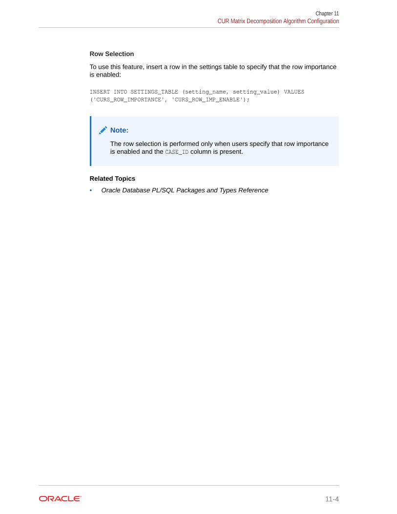
Row Selection
To use this feature, insert a row in the settings table to specify that the row importanceis enabled:
INSERT INTO SETTINGS_TABLE (setting_name, setting_value) VALUES ('CURS_ROW_IMPORTANCE', 'CURS_ROW_IMP_ENABLE');
Note:
The row selection is performed only when users specify that row importanceis enabled and the CASE_ID column is present.
Related Topics
• Oracle Database PL/SQL Packages and Types Reference
Chapter 11CUR Matrix Decomposition Algorithm Configuration
11-4

12Decision Tree
Learn how to use Decision Tree algorithm. Decision Tree is one of the Classificationalgorithms that the Oracle Data Mining supports.
• About Decision Tree
• Growing a Decision Tree
• Tuning the Decision Tree Algorithm
• Data Preparation for Decision Tree
Related Topics
• ClassificationLearn how to predict a categorical target through Classification - the supervisedmining function.
12.1 About Decision TreeThe Decision Tree algorithm, like Naive Bayes, is based on conditional probabilities.Unlike Naive Bayes, decision trees generate rules. A rule is a conditional statementthat can be understood by humans and used within a database to identify a set ofrecords.
In some applications of data mining, the reason for predicting one outcome oranother may not be important in evaluating the overall quality of a model. In others,the ability to explain the reason for a decision can be crucial. For example, aMarketing professional requires complete descriptions of customer segments to launcha successful marketing campaign. The Decision Tree algorithm is ideal for this type ofapplication.
Use Decision Tree rules to validate models. If the rules make sense to a subject matterexpert, then this validates the model.
12.1.1 Decision Tree RulesIntroduces Decision Tree rules.
Oracle Data Mining supports several algorithms that provide rules. In addition todecision trees, clustering algorithms provide rules that describe the conditions sharedby the members of a cluster, and association rules provide rules that describeassociations between attributes.
Rules provide model transparency, a window on the inner workings of the model.Rules show the basis for the model's predictions. Oracle Data Mining supports ahigh level of model transparency. While some algorithms provide rules, all algorithmsprovide model details. You can examine model details to determine how thealgorithm handles the attributes internally, including transformations and reverse
12-1

transformations. Transparency is discussed in the context of data preparation and inthe context of model building in Oracle Data Mining User’s Guide.
The following figure shows a rule generated by a Decision Tree model. This rulecomes from a decision tree that predicts the probability that customers increasespending if given a loyalty card. A target value of 0 means not likely to increasespending; 1 means likely to increase spending.
Figure 12-1 Sample Decision Tree Rule
The rule shown in the figure represents the conditional statement:
IF (current residence > 3.5 and has college degree and is single) THEN predicted target value = 0
This rule is a full rule. A surrogate rule is a related attribute that can be used at applytime if the attribute needed for the split is missing.
Related Topics
• Understanding Reverse Transformations
• Model Detail Views for Decision Tree
• ClusteringLearn how to discover natural groupings in the data through Clustering - theunsupervised mining function.
• AssociationLearn how to discover Association Rules through Association - an unsupervisedmining function.
12.1.1.1 Confidence and SupportConfidence and support are properties of rules. These statistical measures can beused to rank the rules and hence the predictions.
Support: The number of records in the training data set that satisfy the rule.
Confidence: The likelihood of the predicted outcome, given that the rule has beensatisfied.
For example, consider a list of 1000 customers (1000 cases). Out of all the customers,100 satisfy a given rule. Of these 100, 75 are likely to increase spending, and 25
Chapter 12About Decision Tree
12-2
are not likely to increase spending. The support of the rule is 100/1000 (10%). Theconfidence of the prediction (likely to increase spending) for the cases that satisfythe rule is 75/100 (75%).
12.1.2 Advantages of Decision TreesLearn about the advantages of Decision Tree.
The Decision Tree algorithm produces accurate and interpretable models withrelatively little user intervention. The algorithm can be used for both binary andmulticlass classification problems.
The algorithm is fast, both at build time and apply time. The build process for DecisionTree supports parallel execution. (Scoring supports parallel execution irrespective ofthe algorithm.)
Decision Tree scoring is especially fast. The tree structure, created in the model build,is used for a series of simple tests, (typically 2-7). Each test is based on a singlepredictor. It is a membership test: either IN or NOT IN a list of values (categoricalpredictor); or LESS THAN or EQUAL TO some value (numeric predictor).
Related Topics
• Oracle Database VLDB and Partitioning Guide
12.1.3 XML for Decision Tree ModelsLearn about generating XML representation of Decision Tree models.
You can generate XML representing a Decision Tree model; the generated XMLsatisfies the definition specified in the Data Mining Group Predictive Model MarkupLanguage (PMML) version 2.1 specification.
Related Topics
• http://www.dmg.org
12.2 Growing a Decision TreePredicting a target value by a sequence of questions to form or grow a Decision Tree.
A Decision Tree predicts a target value by asking a sequence of questions. At a givenstage in the sequence, the question that is asked depends upon the answers to theprevious questions. The goal is to ask questions that, taken together, uniquely identifyspecific target values. Graphically, this process forms a tree structure.
Chapter 12Growing a Decision Tree
12-3

Figure 12-2 Sample Decision Tree
0: 1120
1: 380
0: 143
1: 31
0: 595
1: 19
0: 738
1: 50
0: 382
1: 330
0: 315
1: 151
0: 67
1: 179
0: 118
1: 119
0: 197
1: 32
Marital status
Education Education
Residence Score = 0;
prob = 8218
Score = 0;
prob = 9690
Score = 1;
prob = 7276
Score = 0;
prob = 8613
Score = 0;
prob = 5988
0
3
874
65
2
1
The figure is a Decision Tree with nine nodes (and nine corresponding rules). Thetarget attribute is binary: 1 if the customer increases spending, 0 if the customer doesnot increase spending. The first split in the tree is based on the CUST_MARITAL_STATUSattribute. The root of the tree (node 0) is split into nodes 1 and 3. Married customersare in node 1; single customers are in node 3.
The rule associated with node 1 is:
Node 1 recordCount=712,0 Count=382, 1 Count=330CUST_MARITAL_STATUS isIN "Married",surrogate:HOUSEHOLD_SIZE isIn "3""4-5"
Node 1 has 712 records (cases). In all 712 cases, the CUST_MARITAL_STATUS attributeindicates that the customer is married. Of these, 382 have a target of 0 (not likely toincrease spending), and 330 have a target of 1 (likely to increase spending).
12.2.1 SplittingDuring the training process, the Decision Tree algorithm must repeatedly find themost efficient way to split a set of cases (records) into two child nodes. Oracle DataMining offers two homogeneity metrics, gini and entropy, for calculating the splits.The default metric is gini.
Homogeneity metrics asses the quality of alternative split conditions and select theone that results in the most homogeneous child nodes. Homogeneity is also calledpurity; it refers to the degree to which the resulting child nodes are made up ofcases with the same target value. The objective is to maximize the purity in the childnodes. For example, if the target can be either yes or no (does or does not increasespending), the objective is to produce nodes where most of the cases either increasespending or most of the cases do not increase spending.
Chapter 12Growing a Decision Tree
12-4

12.2.2 Cost MatrixLearn about Cost Matrix for Decision Tree.
All classification algorithms, including Decision Tree, support a cost-benefit matrix atapply time. You can use the same cost matrix for building and scoring a Decision Treemodel, or you can specify a different cost/benefit matrix for scoring.
Related Topics
• Costs
• Priors and Class WeightsLearn about Priors and Class Weights in a Classification model to produce auseful result.
12.2.3 Preventing Over-FittingIn principle, Decision Tree algorithms can grow each branch of the tree just deeplyenough to perfectly classify the training examples. While this is sometimes areasonable strategy, in fact it can lead to difficulties when there is noise in the data, orwhen the number of training examples is too small to produce a representative sampleof the true target function. In either of these cases, this simple algorithm can producetrees that over-fit the training examples. Over-fit is a condition where a model is ableto accurately predict the data used to create the model, but does poorly on new datapresented to it.
To prevent over-fitting, Oracle Data Mining supports automatic pruning andconfigurable limit conditions that control tree growth. Limit conditions prevent furthersplits once the conditions have been satisfied. Pruning removes branches that haveinsignificant predictive power.
12.3 Tuning the Decision Tree AlgorithmFine tune the Decision Tree algorithm with various parameters.
The Decision Tree algorithm is implemented with reasonable defaults for splitting andtermination criteria. However several build settings are available for fine tuning.
You can specify a homogeneity metric for finding the optimal split condition for a tree.The default metric is gini. The entropy metric is also available.
Settings for controlling the growth of the tree are also available. You can specify themaximum depth of the tree, the minimum number of cases required in a child node,the minimum number of cases required in a node in order for a further split to bepossible, the minimum number of cases in a child node, and the minimum number ofcases required in a node in order for a further split to be possible.
The training data attributes are binned as part of the algorithm's data preparation. Youcan alter the number of bins used by the binning step. There is a trade-off between thenumber of bins used and the time required for the build.
Related Topics
• Oracle Database PL/SQL Packages and Types Reference
Chapter 12Tuning the Decision Tree Algorithm
12-5
12.4 Data Preparation for Decision TreeLearn how to prepare data for Decision Tree.
The Decision Tree algorithm manages its own data preparation internally. It does notrequire pretreatment of the data. Decision Tree is not affected by Automatic DataPreparation.
Related Topics
• Preparing the Data
• Transforming the Data
Chapter 12Data Preparation for Decision Tree
12-6

13Expectation Maximization
Learn how to use Expectation Maximization Clustering algorithm.
• About Expectation Maximization
• Algorithm Enhancements
• Configuring the Algorithm
• Data Preparation for Expectation Maximization
Related Topics
• ClusteringLearn how to discover natural groupings in the data through Clustering - theunsupervised mining function.
13.1 About Expectation MaximizationExpectation Maximization (EM) estimation of mixture models is a popular probabilitydensity estimation technique that is used in a variety of applications. OracleData Mining uses EM to implement a distribution-based clustering algorithm (EM-clustering).
13.1.1 Expectation Step and Maximization StepExpectation Maximization is an iterative method. It starts with an initial parameterguess. The parameter values are used to compute the likelihood of the current model.This is the Expectation step. The parameter values are then recomputed to maximizethe likelihood. This is the Maximization step. The new parameter estimates are usedto compute a new expectation and then they are optimized again to maximize thelikelihood. This iterative process continues until model convergence.
13.1.2 Probability Density EstimationIn density estimation, the goal is to construct a density function that captures how agiven population is distributed. In probability density estimation, the density estimate isbased on observed data that represents a sample of the population. Areas of high datadensity in the model correspond to the peaks of the underlying distribution.
Density-based clustering is conceptually different from distance-based clustering(for example k-Means) where emphasis is placed on minimizing inter-cluster andmaximizing the intra-cluster distances. Due to its probabilistic nature, density-basedclustering can compute reliable probabilities in cluster assignment. It can also handlemissing values automatically.
13-1
13.2 Algorithm EnhancementsAlthough Expectation Maximization (EM) is well established as a distribution-basedclustering algorithm, it presents some challenges in its standard form. The OracleData Mining implementation includes significant enhancements, such as scalableprocessing of large volumes of data and automatic parameter initialization. Thestrategies that Oracle Data Mining uses to address the inherent limitations of EMclustering are described further in this section.
Note:
The EM abbreviation is used here to refer to EM-clustering.
Limitations of Standard Expectation Maximization:
• Scalability: EM has linear scalability with the number of records and attributes. Thenumber of iterations to convergence tends to increase with growing data size (bothrows and columns). EM convergence can be slow for complex problems and canplace a significant load on computational resources.
• High dimensionality: EM has limited capacity for modeling high dimensional (wide)data. The presence of many attributes slows down model convergence, and thealgorithm becomes less able to distinguish between meaningful attributes andnoise. The algorithm is thus compromised in its ability to find correlations.
• Number of components: EM typically requires the user to specify the number ofcomponents. In most cases, this is not information that the user can know inadvance.
• Parameter initialization: The choice of appropriate initial parameter values canhave a significant effect on the quality of the model. Initialization strategies thathave been used for EM have generally been computationally expensive.
• From components to clusters: EM model components are often treated asclusters. This approach can be misleading since cohesive clusters are oftenmodeled by multiple components. Clusters that have a complex shape need tobe modeled by multiple components.
13.2.1 ScalabilityExpectation Maximization (EM) in Oracle Data Mining, uses database parallelprocessing to achieve excellent scalability.
The Oracle Data Mining implementation of Expectation Maximization (EM) usesdatabase parallel processing to achieve excellent scalability. EM computationsnaturally lend themselves to row parallel processing, and the partial results are easilyaggregated. The parallel implementation efficiently distributes the computationallyintensive work across slave processes and then combines the partial results toproduce the final solution.
Related Topics
• Oracle Database VLDB and Partitioning Guide
Chapter 13Algorithm Enhancements
13-2
13.2.2 High DimensionalityThe Oracle Data Mining implementation of Expectation Maximization (EM) canefficiently process high-dimensional data with thousands of attributes. This is achievedthrough a two-fold process:
• The data space of single-column (not nested) attributes is analyzed for pair-wisecorrelations. Only attributes that are significantly correlated with other attributesare included in the EM mixture model. The algorithm can also be configured torestrict the dimensionality to the M most correlated attributes.
• High-dimensional (nested) numerical data that measures events of similar type isprojected into a set of low-dimensional features that are modeled by EM. Someexamples of high-dimensional, numerical data are: text, recommendations, geneexpressions, and market basket data.
13.2.3 Number of ComponentsTypical implementations of Expectation Maximization (EM) require the user to specifythe number of model components. This is problematic because users do not generallyknow the correct number of components. Choosing too many or too few componentscan lead to over-fitting or under-fitting, respectively.
When model search is enabled, the number of EM components is automaticallydetermined. The algorithm uses a held-aside sample to determine the correct numberof components, except in the cases of very small data sets when Bayesian InformationCriterion (BIC) regularization is used.
13.2.4 Parameter InitializationChoosing appropriate initial parameter values can have a significant effect on thequality of the solution. Expectation Maximization (EM) is not guaranteed to convergeto the global maximum of the likelihood function but may instead converge to a localmaximum. Therefore different initial parameter values can lead to different modelparameters and different model quality.
In the process of model search, the EM model is grown independently. As newcomponents are added, their parameters are initialized to areas with poor distributionfit.
13.2.5 From Components to ClustersExpectation Maximization (EM) model components are often treated as clusters.However, this approach can be misleading. Cohesive clusters are often modeledby multiple components. The shape of the probability density function used in EMeffectively predetermines the shape of the identified clusters. For example, Gaussiandensity functions can identify single peak symmetric clusters. Clusters of morecomplex shape need to be modeled by multiple components.
Ideally, high density areas of arbitrary shape must be interpreted as single clusters.To accomplish this, the Oracle Data Mining implementation of EM builds a componenthierarchy that is based on the overlap of the individual components' distributions.Oracle Data Mining EM uses agglomerative hierarchical clustering. Componentdistribution overlap is measured using the Bhattacharyya distance function. Choosing
Chapter 13Algorithm Enhancements
13-3
an appropriate cutoff level in the hierarchy automatically determines the number ofhigh-level clusters.
The Oracle Data Mining implementation of EM produces an assignment of themodel components to high-level clusters. Statistics like means, variances, modes,histograms, and rules additionally describe the high-level clusters. The algorithm canbe configured to either produce clustering assignments at the component level or atthe cluster level.
13.3 Configuring the AlgorithmConfigure Expectation Maximization (EM).
In Oracle Data Mining, Expectation Maximization (EM) can effectively model very largedata sets (both rows and columns) without requiring the user to supply initializationparameters or specify the number of model components. While the algorithm offersreasonable defaults, it also offers flexibility.
The following list describes some of the configurable aspects of EM:
• Whether or not independent non-nested column attributes are included in themodel. The choice is system-determined by default.
• Whether to use Bernoulli or Gaussian distribution for numerical attributes. Bydefault, the algorithm chooses the most appropriate distribution, and individualattributes may use different distributions. When the distribution is user-specified, itis used for all numerical attributes.
• Whether the convergence criterion is based on a held-aside data set oron Bayesian Information Criterion (BIC). The convergence criterion is system-determined by default.
• The percentage improvement in the value of the log likelihood function that isrequired to add a new component to the model. The default percentage is 0.001.
• Whether to define clusters as individual components or groups of components.Clusters are associated to groups of components by default.
• The maximum number of components in the model. If model search is enabled,the algorithm determines the number of components based on improvementsin the likelihood function or based on regularization (BIC), up to the specifiedmaximum.
• Whether the linkage function for the agglomerative clustering step uses thenearest distance within the branch (single linkage), the average distance within thebranch (average linkage), or the maximum distance within the branch (completelinkage). By default the algorithm uses single linkage.
Related Topics
• DBMS_DATA_MINING - Global Settings
• DBMS_DATA_MINING - Algorithm Settings: Expectation Maximization
13.4 Data Preparation for Expectation MaximizationLearn how to prepare data for Expectation Maximization (EM).
If you use Automatic Data Preparation (ADP), you do not need to specify additionaldata preparation for Expectation Maximization. ADP normalizes numerical attributes
Chapter 13Configuring the Algorithm
13-4

(in non-nested columns) when they are modeled with Gaussian distributions. ADPapplies a topN binning transformation to categorical attributes.
Missing value treatment is not needed since Oracle Data Mining algorithms handlemissing values automatically. The Expectation Maximization algorithm replacesmissing values with the mean in single-column numerical attributes that are modeledwith Gaussian distributions. In other single-column attributes (categoricals andnumericals modeled with Bernoulli distributions), NULLs are not replaced; they aretreated as a distinct value with its own frequency count. In nested columns, missingvalues are treated as zeros.
Related Topics
• Oracle Data Mining User’s Guide
Chapter 13Data Preparation for Expectation Maximization
13-5
14Explicit Semantic Analysis
Learn how to use Explicit Semantic Analysis (ESA) as an unsupervised algorithm forFeature Extraction function and as a supervised algorithm for Classification.
• About Explicit Semantic Analysis
• ESA for Text Mining
• Data Preparation for ESA
Related Topics
• Feature Selection and ExtractionLearn how to perform Feature Selection, Feature Extraction, and AttributeImportance.
14.1 About Explicit Semantic AnalysisIn Oracle database 12c Release 2, Explicit Semantic Analysis (ESA) was introducedas an unsupervised algorithm used by Oracle Data Mining for Feature Extraction.Starting from Oracle Database 18c, ESA is enhanced as a supervised algorithm forClassification.
As a Feature Extraction algorithm, ESA does not discover latent features but insteaduses explicit features represented in an existing knowledge base. As a FeatureExtraction algorithm, ESA is mainly used for calculating semantic similarity of textdocuments and for explicit topic modeling. As a Classification algorithm, ESA isprimarily used for categorizing text documents. Both the Feature Extraction andClassification versions of ESA can be applied to numeric and categorical input dataas well.
The input to ESA is a set of attributes vectors. Every attribute vector is associated witha concept. The concept is a feature in the case of Feature Extraction or a target classin the case of Classification. For Feature Extraction, only one attribute vector may beassociated with any feature. For Classification, the training set may contain multipleattribute vectors associated with any given target class. These rows related to onetarget class are aggregated into one by the ESA algorithm.
The output of ESA is a sparse attribute-concept matrix that contains the mostimportant attribute-concept associations. The strength of the association is capturedby the weight value of each attribute-concept pair. The attribute-concept matrix isstored as a reverse index that lists the most important concepts for each attribute.
Note:
For Feature Extraction the ESA algorithm does not project the originalfeature space and does not reduce its dimensionality. ESA algorithm filtersout features with limited or uninformative set of attributes.
14-1

The scope of Classification tasks that ESA handles is different than the Classificationalgorithms such as Naive Bayes and Support Vector Machines. ESA can performlarge scale Classification with the number of distinct classes up to hundreds ofthousands. The large scale classification requires gigantic training data sets with someclasses having significant number of training samples whereas others are sparselyrepresented in the training data set.
14.1.1 Scoring with ESALearn to score with Explicit Semantic Analysis (ESA).
A typical Feature Extraction application of ESA is to identify the most relevantfeatures of a given input and score their relevance. Scoring an ESA model producesdata projections in the concept feature space. If an ESA model is built from anarbitrary collection of documents, then each one is treated as a feature. It isthen easy to identify the most relevant documents in the collection. The featureextraction functions are: FEATURE_DETAILS, FEATURE_ID, FEATURE_SET, FEATURE_VALUE,and FEATURE_COMPARE.
A typical Classification application of ESA is to predict classes of a given documentand estimate the probabilities of the predictions. As a Classification algorithm, ESAimplements the following scoring functions: PREDICTION, PREDICTION_PROBABILITY,PREDICTION_SET, PREDICTION_DETAILS, PREDICTION_COST.
Related Topics
• Oracle Data Mining User’s Guide
• Oracle Database SQL Language Reference
14.1.2 Scoring Large ESA ModelsBuilding an Explicit Semantic Analysis (ESA) model on a large collection of textdocuments can result in a model with many features or titles. The model informationfor scoring is loaded into System Global Area (SGA) as a shared (shared pool size)library cache object. Different SQL predictive queries can reference this object. Whenthe model size is large, it is necessary to set the SGA parameter in the database to asufficient size that accommodates large objects.
If the SGA is too small, the model may need to be re-loaded every time it is referencedwhich is likely to lead to performance degradation.
14.2 ESA for Text MiningLearn how Explicit Semantic Analysis (ESA) can be used for Text mining.
Explicit knowledge often exists in text form. Multiple knowledge bases are availableas collections of text documents. These knowledge bases can be generic, forexample, Wikipedia, or domain-specific. Data preparation transforms the text intovectors that capture attribute-concept associations. ESA is able to quantify semanticrelatedness of documents even if they do not have any words in common. Thefunction FEATURE_COMPARE can be used to compute semantic relatedness.
Related Topics
• Oracle Database SQL Language Reference
Chapter 14ESA for Text Mining
14-2
14.3 Data Preparation for ESAAutomatic Data Preparation normalizes input vectors to a unit length for ExplicitSemantic Analysis (ESA).
When there are missing values in columns with simple data types (not nested), ESAreplaces missing categorical values with the mode and missing numerical values withthe mean. When there are missing values in nested columns, ESA interprets them assparse. The algorithm replaces sparse numeric data with zeros and sparse categoricaldata with zero vectors. The Oracle Data Mining data preparation transforms the inputtext into a vector of real numbers. These numbers represent the importance of therespective words in the text.
14.4 Terminologies in Explicit Semantic AnalysisDiscusses the terms associated with Explicit Semantic Analysis (ESA).
Multi-target Classification
The training items in these large scale classifications belong to several classes. Thegoal of classification in such case is to detect possible multiple target classes forone item. This kind of classification is called multi-target classification. The targetcolumn for ESA-based classification is extended. Collections are allowed as targetcolumn values. The collection type for the target in ESA-based classification isORA_MINING_VARCHAR2_NT.
Large-scale classification
Large-scale classification applies to ontologies that contain gigantic numbers ofcategories, usually ranging in tens or hundreds of thousands. This large-scaleclassification also requires gigantic training datasets which are usually unbalanced,that is, some classes may have significant number of training samples whereasothers may be sparsely represented in the training dataset. Large-scale classificationnormally results in multiple target class assignments for a given test case.
Topic modeling
Topic modelling refers to derivation of the most important topics of a document. Topicmodeling can be explicit or latent. Explicit topic modeling results in the selection ofthe most relevant topics from a pre-defined set, for a given document. Explicit topicshave names and can be verbalized. Latent topic modeling identifies a set of latenttopics characteristic for a collection of documents. A subset of these latent topics isassociated with every document under examination. Latent topics do not have verbaldescriptions or meaningful interpretation.
Related Topics
• Oracle Database PL/SQL Packages and Types Reference
Chapter 14Data Preparation for ESA
14-3

15Exponential Smoothing
Learn about Exponential Smoothing.
• About Exponential Smoothing
• Data Preparation for Exponential Smoothing Models
15.1 About Exponential SmoothingExponential Smoothing methods are widely used for forecasting.
Exponential Smoothing methods have been widely used in forecasting for over half acentury. It has applications at the strategic, tactical, and operation level. For example,at a strategic level, forecasting is used for projecting return on investment, growth andthe effect of innovations. At a tactical level, forecasting is used for projecting costs,inventory requirements, and customer satisfaction. At an operational level, forecastingis used for setting targets and predicting quality and conformance with standards.
In its simplest form, Exponential Smoothing is a moving average method with a singleparameter which models an exponentially decreasing effect of past levels on futurevalues. With a variety of extensions, Exponential Smoothing covers a broader class ofmodels than competitors, such as the Box-Jenkins auto-regressive integrated movingaverage (ARIMA) approach. Oracle Data Mining implements Exponential Smoothingusing a state of the art state space method that incorporates a single source of error(SSOE) assumption which provides theoretical and performance advantages.
Exponential Smoothing is extended to the following:
• A matrix of models that mix and match error type (additive or multiplicative), trend(additive, multiplicative, or none), and seasonality (additive, multiplicative, or none)
• Models with damped trends.
• Models that directly handle irregular time series and time series with missingvalues.
Note:
For more information, see Ord, J.K., et al, Time Series Forecasting: TheCase for the Single Source of Error State Space Approach, Working Paper,Department of Econometrics and Business Statistics, Monash University,VIC 3800, Australia, April 2, 2005.
15.1.1 Exponential Smoothing ModelsExponential Smoothing models are a broad class of forecasting models that areintuitive, flexible, and extensible.
15-1

Members of this class include simple, single parameter models that predict the futureas a linear combination of a previous level and a current shock. Extensions caninclude parameters for linear or non-linear trend, trend damping, simple or complexseasonality, related series, various forms of non-linearity in the forecasting equations,and handling of irregular time series.
Exponential Smoothing assumes that a series extends infinitely into the past, butthat influence of past on future, decays smoothly and exponentially fast. The smoothrate of decay is expressed by one or more smoothing constants. The smoothingconstants are parameters that the model estimates. The assumption is madepractical for modeling real world data by using an equivalent recursive formulation thatis only expressed in terms of an estimate of the current level based on prior historyand a shock to that estimate dependent on current conditions only.The procedurerequires an estimate for the time period just prior to the first observation, thatencapsulates all prior history. This initial observation is an additional model parameterwhose value is estimated by the modeling procedure.
Components of ESM such as trend and seasonality extensions, can have an additiveor multiplicative form. The simpler additive models assume that shock, trend, andseasonality are linear effects within the recursive formulation.
15.1.2 Simple Exponential SmoothingSimple Exponential Smoothing assumes the data fluctuates around a stationary mean,with no trend or seasonal pattern.
In simple exponential smoothing model, each forecast (smoothed value) is computedas the weighted average of the previous observations, where the weights decreaseexponentially depending on the value of smoothing constant α. Values of thesmoothing constant, α, near one, put almost all weight on the most recentobservations. Values of α near zero allows the distant past observations to have alarge influence.
15.1.3 Models with Trend but No SeasonalityThe preferred form of additive (linear) trend is sometimes called Holt’s method ordouble exponential smoothing.
Models with trend add a smoothing parameter γ and optionally a damping parameterφ. The damping parameter smoothly dampens the influence of past linear trend onfuture estimates of level, often improving accuracy.
15.1.4 Models with Seasonality but No TrendWhen the time series average does not change over time (stationary), but is subject toseasonal fluctuations, the appropriate model has seasonal parameters but no trend.
Seasonal fluctuations are assumed to balance out over periods of length m, where mis the number of seasons, For example, m=4 might be used when the input data areaggregated quarterly. For models with additive errors, the seasonal parameters mustsum to zero. For models with multiplicative errors, the product of seasonal parametersmust be one.
Chapter 15About Exponential Smoothing
15-2
15.1.5 Models with Trend and SeasonalityHolt and Winters introduced both trend and seasonality in Exponential SmoothingModel(ESM). The original model, also known as Holt-Winters or triple exponentialsmoothing, considered an additive trend and multiplicative seasonality. Extensionsinclude models with various combinations of additive and multiplicative trend,seasonality and error, with and without trend damping.
15.1.6 Prediction IntervalsTo compute prediction intervals, Exponential Smoothing Model (ESM) is divided intothree classes.
The simplest class is the class of linear models, which include, among others, simpleESM, Holt’s method, and additive Holt-Winters. Class 2 models (multiplicative error,additive components) make an approximate correction for violations of the Normalityassumption. Class 3 modes use a simple simulation approach to calculate predictionintervals.
15.2 Data Preparation for Exponential Smoothing ModelsLearn about preparing the data for Exponential Smoothing Model.
To build an ESM model, you must supply the following :
• Input data
• An aggregation level and method, if the case id is a date type
• Partitioning column, if the data are partitioned
In addition, for a greater control over the build process, the user may optionally specifymodel build parameters, all of which have defaults:
• Model
• Error type
• Optimization criterion
• Forecast Window
• Confidence level for forecast bounds
• Missing value handling
• Whether the input series is evenly spaced
Related Topics
• Oracle Data Mining User’s Guide
See Also:
The Exponential Smoothing Model settings are described in OracleDatabase PL/SQL Packages and Types Reference.
Chapter 15Data Preparation for Exponential Smoothing Models
15-3

15.2.1 Input DataTime Series analysis, requires ordered input data. Hence, each data row must consistof an [index, value] pair, where the index specifies the ordering.
When the CREATE_MODEL procedure is used to initiate an Exponential Smoothing(ESM) model build, the CASE_ID_COLUMN_NAME specifies the column used to computethe indices of the input and the TARGET_COLUMN_NAME specifies the column used tocompute the observed time series values. The time column bears Oracle number, orOracle date, timestamp, timestamp with time zone, or timestamp with local time zone.The input time series are sorted according to the values of CASE_ID (time label). Thecase id column cannot contain missing values. The value column can contain missingvalues indicated as NULL. ESM also supports partitioned models and in such cases,the input table contains an extra column specifying the partition. All [index, value]pairs with the same partition ID form one complete time series. Exponential Smoothingconstructs models for each partition independently, although all models use the samemodel settings.
Properties of the data can result in a warning message or settings are ignored.Settings are ignored when If the user specifies a model with either multiplicativetrend, multiplicative seasonality or both and the data contains values Yt<= 0, then themodel type is set to the default. If the series contain fewer values than the number ofuser-specified seasons, then the seasonality specifications are ignored with a warning.
15.2.2 AccumulationFor Exponential Smoothing algorithms, the accumulation procedure is applied whenthe column is a date type (date, datetime, timestamp, timestamp with timezone, ortimestamp with local timezone).
The case id can be a NUMBER column whose sort index represents the position of thevalue in the time series sequence of values. The case id column can also be a datetype. A date type is accumulated in accordance with a user specified accumulationwindow. Regardless of type, the case id is used to transform the column into anequally spaced time series. No accumulation is applied for a case id of type NUMBER. Asan example, consider a time series about promotion events. The time column containsthe date of each event, and the dates can be unequally spaced. The user must specifythe spacing interval, which is the spacing of the accumulated or transformed equallyspaced time series. In the example, if the user specifies the interval to be month, thenan equally spaced time series with profit for each calendar month is generated fromthe original time series. Setting EXSM_INTERVAL is used to specify the spacing interval.The user must also specify a value for EXSM_ACCUMULATE, for example, EXSM_ACCU_MAX,in which case the equally spaced monthly series would contain the maximum profitover all events that month as the observed time series value.
15.2.3 Missing ValueInput time series can contain missing values. A NULL entry in the target columnindicates a missing value. When the time column is of the type datetime,the accumulation procedure can also introduce missing values. The settingEXSM_SETMISSING can be used to specify how to handle missing values. The specialvalue EXSM_MISS_AUTO indicates that, if the series contains missing values it is to betreated as an irregular time series.
Chapter 15Data Preparation for Exponential Smoothing Models
15-4

Note:
Missing value handling setting must be compatible with model setting,otherwise an error is thrown.
15.2.4 PredictionExponential Smoothing Model (ESM) can be applied to make predictions by specifyingthe prediction window.
Setting EXSM_PREDICTION_STEP can be used to specify the prediction window.The prediction window is expressed in terms of number of intervals (settingEXSM_INTERVAL), when the time column is of the type datetime. If the time columnis a number then the prediction window is the number of steps to forecast. Regardlessof whether the time series is regular or irregular, EXSM_PREDICTION_STEP specifies theprediction window.
15.2.5 Parallellism by PartitionOracle Advanced Analytics supports parallellism by partition.
For example, a user can choose PRODUCT_ID as one partition column and can generateforecasts for different products in a model build. Although a distinct smoothingmodel is built for each partition, all partitions share the same model settings. Forexample, if setting EXSM_MODEL is set to EXSM_SIMPLE, all partition models will be simpleexponential smoothing models. Time series from different partitions can be distributedto different processes and processed in parallel. The model for each time series is builtserially.
Chapter 15Data Preparation for Exponential Smoothing Models
15-5

16Generalized Linear Models
Learn how to use Generalized Linear Models (GLM) statistical technique for Linearmodeling.
Oracle Data Mining supports GLM for Regression and Binary Classification.
• About Generalized Linear Models
• GLM in Oracle Data Mining
• Scalable Feature Selection
• Tuning and Diagnostics for GLM
• GLM Solvers
• Data Preparation for GLM
• Linear Regression
• Logistic Regression
Related Topics
• RegressionLearn how to predict a continuous numerical target through Regression - thesupervised mining function.
• ClassificationLearn how to predict a categorical target through Classification - the supervisedmining function.
16.1 About Generalized Linear ModelsIntroduces Generalized Linear Models (GLM).
GLM include and extend the class of linear models.
Linear models make a set of restrictive assumptions, most importantly, that the target(dependent variable y) is normally distributed conditioned on the value of predictorswith a constant variance regardless of the predicted response value. The advantageof linear models and their restrictions include computational simplicity, an interpretablemodel form, and the ability to compute certain diagnostic information about the qualityof the fit.
Generalized linear models relax these restrictions, which are often violated in practice.For example, binary (yes/no or 0/1) responses do not have same variance acrossclasses. Furthermore, the sum of terms in a linear model typically can have very largeranges encompassing very negative and very positive values. For the binary responseexample, we would like the response to be a probability in the range [0,1].
Generalized linear models accommodate responses that violate the linear modelassumptions through two mechanisms: a link function and a variance function. Thelink function transforms the target range to potentially -infinity to +infinity so that thesimple form of linear models can be maintained. The variance function expresses the
16-1
variance as a function of the predicted response, thereby accommodating responseswith non-constant variances (such as the binary responses).
Oracle Data Mining includes two of the most popular members of the GLM family ofmodels with their most popular link and variance functions:
• Linear regression with the identity link and variance function equal to theconstant 1 (constant variance over the range of response values).
• Logistic regression with the logit link and binomial variance functions.
Related Topics
• Linear Regression
• Linear Regression
• Logistic Regression
16.2 GLM in Oracle Data MiningGeneralized Linear Models (GLM) is a parametric modeling technique. Parametricmodels make assumptions about the distribution of the data. When the assumptionsare met, parametric models can be more efficient than non-parametric models.
The challenge in developing models of this type involves assessing the extent to whichthe assumptions are met. For this reason, quality diagnostics are key to developingquality parametric models.
16.2.1 Interpretability and TransparencyLearn how to interpret, and understand data transparency through model details andglobal details.
Oracle Data Mining Generalized Linear Models (GLM) are easy to interpret. Eachmodel build generates many statistics and diagnostics. Transparency is also a keyfeature: model details describe key characteristics of the coefficients, and globaldetails provide high-level statistics.
Related Topics
• Tuning and Diagnostics for GLM
16.2.2 Wide DataOracle Data Mining Generalized Linear Model (GLM) is uniquely suited for handlingwide data. The algorithm can build and score quality models that use a virtuallylimitless number of predictors (attributes). The only constraints are those imposed bysystem resources.
16.2.3 Confidence BoundsPredict confidence bounds through Generalized Linear Models (GLM).
GLM have the ability to predict confidence bounds. In addition to predicting a bestestimate and a probability (Classification only) for each row, GLM identifies an intervalwherein the prediction (Regression) or probability (Classification) lies. The width of
Chapter 16GLM in Oracle Data Mining
16-2

the interval depends upon the precision of the model and a user-specified confidencelevel.
The confidence level is a measure of how sure the model is that the true value lieswithin a confidence interval computed by the model. A popular choice for confidencelevel is 95%. For example, a model might predict that an employee's income is $125K,and that you can be 95% sure that it lies between $90K and $160K. Oracle DataMining supports 95% confidence by default, but that value can be configured.
Note:
Confidence bounds are returned with the coefficient statistics. You can alsouse the PREDICTION_BOUNDS SQL function to obtain the confidence bounds ofa model prediction.
Related Topics
• Oracle Database SQL Language Reference
16.2.4 Ridge RegressionUnderstand the use of Ridge regression for singularity (exact multicollinearity) in data.
The best regression models are those in which the predictors correlate highly withthe target, but there is very little correlation between the predictors themselves.Multicollinearity is the term used to describe multivariate regression with correlatedpredictors.
Ridge regression is a technique that compensates for multicollinearity. Oracle DataMining supports ridge regression for both Regression and Classification miningfunctions. The algorithm automatically uses ridge if it detects singularity (exactmulticollinearity) in the data.
Information about singularity is returned in the global model details.
Related Topics
• Global Model Statistics for Linear Regression
• Global Model Statistics for Logistic Regression
16.2.4.1 Configuring Ridge RegressionConfigure Ridge Regression through build settings.
You can choose to explicitly enable ridge regression by specifying a build setting forthe model. If you explicitly enable ridge, you can use the system-generated ridgeparameter or you can supply your own. If ridge is used automatically, the ridgeparameter is also calculated automatically.
The configuration choices are summarized as follows:
• Whether or not to override the automatic choice made by the algorithm regardingridge regression
Chapter 16GLM in Oracle Data Mining
16-3
• The value of the ridge parameter, used only if you specifically enable ridgeregression.
Related Topics
• Oracle Database SQL Language Reference
16.2.4.2 Ridge and Confidence BoundsModels built with Ridge Regression do not support confidence bounds.
Related Topics
• Confidence BoundsPredict confidence bounds through Generalized Linear Models (GLM).
16.2.4.3 Ridge and Data PreparationLearn about preparing data for Ridge Regression.
When Ridge Regression is enabled, different data preparation is likely to producedifferent results in terms of model coefficients and diagnostics. Oracle recommendsthat you enable Automatic Data Preparation for Generalized Linear Models, especiallywhen Ridge Regression is used.
Related Topics
• Data Preparation for GLMLearn about preparing data for Generalized Linear Models (GLM).
16.3 Scalable Feature SelectionOracle Data Mining supports a highly scalable and automated version of featureselection and generation for Generalized Linear Models. This capability can enhancethe performance of the algorithm and improve accuracy and interpretability. Featureselection and generation are available for both Linear Regression and binary LogisticRegression.
16.3.1 Feature SelectionFeature selection is the process of choosing the terms to be included in the model.The fewer terms in the model, the easier it is for human beings to interpret itsmeaning. In addition, some columns may not be relevant to the value that the model istrying to predict. Removing such columns can enhance model accuracy.
16.3.1.1 Configuring Feature SelectionFeature selection is a build setting for Generalized Linear Models. It is not enabled bydefault. When configured for feature selection, the algorithm automatically determinesappropriate default behavior, but the following configuration options are available:
• The feature selection criteria can be AIC, SBIC, RIC, or α-investing. When thefeature selection criteria is α-investing, feature acceptance can be either strict orrelaxed.
• The maximum number of features can be specified.
Chapter 16Scalable Feature Selection
16-4

• Features can be pruned in the final model. Pruning is based on t-statistics forlinear regression or wald statistics for logistic regression.
16.3.1.2 Feature Selection and Ridge RegressionFeature selection and ridge regression are mutually exclusive. When feature selectionis enabled, the algorithm can not use ridge.
Note:
If you configure the model to use both feature selection and ridge regression,then you get an error.
16.3.2 Feature GenerationFeature generation is the process of adding transformations of terms into the model.Feature generation enhances the power of models to fit more complex relationshipsbetween target and predictors.
16.3.2.1 Configuring Feature GenerationLearn about configuring Feature Generation.
Feature generation is only possible when feature selection is enabled. Featuregeneration is a build setting. By default, feature generation is not enabled.
The feature generation method can be either quadratic or cubic. By default, thealgorithm chooses the appropriate method. You can also explicitly specify the featuregeneration method.
The following options for feature selection also affect feature generation:
• Maximum number of features
• Model pruning
Related Topics
• Oracle Database PL/SQL Packages and Types Reference
16.4 Tuning and Diagnostics for GLMThe process of developing a Generalized Linear Model typically involves a number ofmodel builds. Each build generates many statistics that you can evaluate to determinethe quality of your model. Depending on these diagnostics, you may want to trychanging the model settings or making other modifications.
16.4.1 Build SettingsSpecify the build settings for Generalized Linear Model (GLM).
You can use specify build settings.
Additional build settings are available to:
Chapter 16Tuning and Diagnostics for GLM
16-5

• Control the use of ridge regression.
• Specify the handling of missing values in the training data.
• Specify the target value to be used as a reference in a logistic regression model.
Related Topics
• Ridge RegressionUnderstand the use of Ridge regression for singularity (exact multicollinearity) indata.
• Data Preparation for GLMLearn about preparing data for Generalized Linear Models (GLM).
• Logistic Regression
• Oracle Database PL/SQL Packages and Types Reference
16.4.2 DiagnosticsGeneralized Linear Models generate many metrics to help you evaluate the quality ofthe model.
16.4.2.1 Coefficient StatisticsLearn about coeffficient statistics for Linear and Logistic Regression.
The same set of statistics is returned for both linear and logistic regression, butstatistics that do not apply to the mining function are returned as NULL.
Coefficient statistics are returned by the Model Detail Views for Generalized LinearModel.
Related Topics
• Coefficient Statistics for Linear Regression
• Coefficient Statistics for Logistic Regression
• Oracle Data Mining User’s Guide
16.4.2.2 Global Model StatisticsLearn about high-level statistics describing the model.
Separate high-level statistics describing the model as a whole, are returned for linearand logistic regression. When ridge regression is enabled, fewer global details arereturned.
Global statistics are returned by the Model Detail Views for Generalized Linear Model.
Related Topics
• Global Model Statistics for Linear Regression
• Global Model Statistics for Logistic Regression
• Ridge RegressionUnderstand the use of Ridge regression for singularity (exact multicollinearity) indata.
• Oracle Data Mining User’s Guide
Chapter 16Tuning and Diagnostics for GLM
16-6
16.4.2.3 Row DiagnosticsGenerate row-statistics by configuring Generalized Linear Models (GLM).
GLM to generate per-row statistics by specifying the name of a diagnostics table in thebuild setting GLMS_DIAGNOSTICS_TABLE_NAME.
GLM requires a case ID to generate row diagnostics. If you provide the name of adiagnostic table but the data does not include a case ID column, an exception israised.
Related Topics
• Row Diagnostics for Linear Regression
• Row Diagnostics for Logistic Regression
16.5 GLM SolversLearn about the different solvers for Generalized Liner Models (GLM).
The GLM algorithm supports four different solvers: Cholesky, QR, StochasticGradient Descent (SGD),and Alternating Direction Method of Multipliers (ADMM)(on top of L-BFGS). The Cholesky and QR solvers employ classical decompositionapproaches. The Cholesky solver is faster compared to the QR solver but less stablenumerically. The QR solver handles better rank deficient problems without the help ofregularization.
The SGD and ADMM (on top of L-BFGS) solvers are best suited for large scale data.The SGD solver employs the stochastic gradient descent optimization algorithm whileADMM (on top of L-BFGS) uses the Broyden-Fletcher-Goldfarb-Shanno optimizationalgorithm within an Alternating Direction Method of Multipliers framework. The SGDsolver is fast but is sensitive to parameters and requires suitable scaled data toachieve good convergence. The L-BFGS algorithm solves unconstrained optimizationproblems and is more stable and robust than SGD. Also, L-BFGS uses ADMM inconjunction, which, results in an efficient distributed optimization approach with lowcommunication cost.
Related Topics
• DBMS_DATA_MINING - Algorithm Settings: Neural Network
• DBMS_DATA_MINING — Algorithm Settings: Generalized Linear Models
• DBMS_DATA_MINING — Algorithm Settings: ADMM
• DBMS_DATA_MINING — Algorithm Settings: LBFGS
16.6 Data Preparation for GLMLearn about preparing data for Generalized Linear Models (GLM).
Automatic Data Preparation (ADP) implements suitable data transformations for bothlinear and logistic regression.
Chapter 16GLM Solvers
16-7

Note:
Oracle recommends that you use Automatic Data Preparation with GLM.
Related Topics
• Oracle Data Mining User’s Guide
16.6.1 Data Preparation for Linear RegressionLearn about Automatic Data Preparation (ADP) for Generalized Linear Model (GLM).
When Automatic Data Preparation (ADP) is enabled, the algorithm chooses atransformation based on input data properties and other settings. The transformationcan include one or more of the following for numerical data: subtracting the mean,scaling by the standard deviation, or performing a correlation transformation (Neter, et.al, 1990). If the correlation transformation is applied to numeric data, it is also appliedto categorical attributes.
Prior to standardization, categorical attributes are exploded into N-1 columns whereN is the attribute cardinality. The most frequent value (mode) is omitted during theexplosion transformation. In the case of highest frequency ties, the attribute values aresorted alpha-numerically in ascending order, and the first value on the list is omittedduring the explosion. This explosion transformation occurs whether or not ADP isenabled.
In the case of high cardinality categorical attributes, the described transformations(explosion followed by standardization) can increase the build data size because theresulting data representation is dense. To reduce memory, disk space, and processingrequirements, use an alternative approach. Under these circumstances, the VIFstatistic must be used with caution.
Related Topics
• Ridge and Data PreparationLearn about preparing data for Ridge Regression.
• Oracle Data Mining User’s Guide
See Also:
• Neter, J., Wasserman, W., and Kutner, M.H., "Applied Statistical Models",Richard D. Irwin, Inc., Burr Ridge, IL, 1990.
16.6.2 Data Preparation for Logistic RegressionCategorical attributes are exploded into N-1 columns where N is the attributecardinality. The most frequent value (mode) is omitted during the explosiontransformation. In the case of highest frequency ties, the attribute values are sortedalpha-numerically in ascending order and the first value on the list is omitted during
Chapter 16Data Preparation for GLM
16-8

the explosion. This explosion transformation occurs whether or not Automatic DataPreparation (ADP) is enabled.
When ADP is enabled, numerical attributes are scaled by the standard deviation. Thismeasure of variability is computed as the standard deviation per attribute with respectto the origin (not the mean) (Marquardt, 1980).
See Also:
Marquardt, D.W., "A Critique of Some Ridge Regression Methods:Comment", Journal of the American Statistical Association, Vol. 75, No. 369 ,1980, pp. 87-91.
16.6.3 Missing ValuesWhen building or applying a model, Oracle Data Mining automatically replaces missingvalues of numerical attributes with the mean and missing values of categoricalattributes with the mode.
You can configure a Generalized Linear Models to override the default treatmentof missing values. With the ODMS_MISSING_VALUE_TREATMENT setting, you can causethe algorithm to delete rows in the training data that have missing values insteadof replacing them with the mean or the mode. However, when the model is applied,Oracle Data Mining performs the usual mean/mode missing value replacement. Asa result, it is possible that the statistics generated from scoring does not match thestatistics generated from building the model.
If you want to delete rows with missing values in the scoring the model, you mustperform the transformation explicitly. To make build and apply statistics match, youmust remove the rows with NULLs from the scoring data before performing the applyoperation. You can do this by creating a view.
CREATE VIEW viewname AS SELECT * from tablename WHERE column_name1 is NOT NULL AND column_name2 is NOT NULL AND column_name3 is NOT NULL .....
Note:
In Oracle Data Mining, missing values in nested data indicate sparsity, notvalues missing at random.
The value ODMS_MISSING_VALUE_DELETE_ROW is only valid for tables withoutnested columns. If this value is used with nested data, an exception is raised.
16.7 Linear RegressionLinear regression is the Generalized Linear Models’ Regression algorithm supportedby Oracle Data Mining. The algorithm assumes no target transformation and constantvariance over the range of target values.
Chapter 16Linear Regression
16-9

16.7.1 Coefficient Statistics for Linear RegressionGeneralized Linear Model Regression models generate the following coefficientstatistics:
• Linear coefficient estimate
• Standard error of the coefficient estimate
• t-value of the coefficient estimate
• Probability of the t-value
• Variance Inflation Factor (VIF)
• Standardized estimate of the coefficient
• Lower and upper confidence bounds of the coefficient
16.7.2 Global Model Statistics for Linear RegressionGeneralized Linear Model Regression models generate the following statistics thatdescribe the model as a whole:
• Model degrees of freedom
• Model sum of squares
• Model mean square
• Model F statistic
• Model F value probability
• Error degrees of freedom
• Error sum of squares
• Error mean square
• Corrected total degrees of freedom
• Corrected total sum of squares
• Root mean square error
• Dependent mean
• Coefficient of variation
• R-Square
• Adjusted R-Square
• Akaike's information criterion
• Schwarz's Baysian information criterion
• Estimated mean square error of the prediction
• Hocking Sp statistic
• JP statistic (the final prediction error)
• Number of parameters (the number of coefficients, including the intercept)
• Number of rows
Chapter 16Linear Regression
16-10

• Whether or not the model converged
• Whether or not a covariance matrix was computed
16.7.3 Row Diagnostics for Linear RegressionFor Linear Regression, the diagnostics table has the columns described in thefollowing table. All the columns are NUMBER, except the CASE_ID column, whichpreserves the type from the training data.
Table 16-1 Diagnostics Table for GLM Regression Models
Column Description
CASE_ID Value of the case ID column
TARGET_VALUE Value of the target column
PREDICTED_VALUE Value predicted by the model for the target
HAT Value of the diagonal element of the hat matrix
RESIDUAL Measure of error
STD_ERR_RESIDUAL Standard error of the residual
STUDENTIZED_RESIDUAL Studentized residual
PRED_RES Predicted residual
COOKS_D Cook's D influence statistic
16.8 Logistic RegressionBinary Logistic Regression is the Generalized Linear Model Classification algorithmsupported by Oracle Data Mining. The algorithm uses the logit link function and thebinomial variance function.
16.8.1 Reference ClassYou can use the build setting GLMS_REFERENCE_CLASS_NAME to specify the target valueto be used as a reference in a binary logistic regression model. Probabilities areproduced for the other (non-reference) class. By default, the algorithm chooses thevalue with the highest prevalence. If there are ties, the attributes are sorted alpha-numerically in an ascending order.
16.8.2 Class WeightsYou can use the build setting CLAS_WEIGHTS_TABLE_NAME to specify the name of a classweights table. Class weights influence the weighting of target classes during the modelbuild.
16.8.3 Coefficient Statistics for Logistic RegressionGeneralized Linear Model Classification models generate the following coefficientstatistics:
Chapter 16Logistic Regression
16-11

• Name of the predictor
• Coefficient estimate
• Standard error of the coefficient estimate
• Wald chi-square value of the coefficient estimate
• Probability of the Wald chi-square value
• Standardized estimate of the coefficient
• Lower and upper confidence bounds of the coefficient
• Exponentiated coefficient
• Exponentiated coefficient for the upper and lower confidence bounds of thecoefficient
16.8.4 Global Model Statistics for Logistic RegressionGeneralized Linear Model Classification models generate the following statistics thatdescribe the model as a whole:
• Akaike's criterion for the fit of the intercept only model
• Akaike's criterion for the fit of the intercept and the covariates (predictors) model
• Schwarz's criterion for the fit of the intercept only model
• Schwarz's criterion for the fit of the intercept and the covariates (predictors) model
• -2 log likelihood of the intercept only model
• -2 log likelihood of the model
• Likelihood ratio degrees of freedom
• Likelihood ratio chi-square probability value
• Pseudo R-square Cox an Snell
• Pseudo R-square Nagelkerke
• Dependent mean
• Percent of correct predictions
• Percent of incorrect predictions
• Percent of ties (probability for two cases is the same)
• Number of parameters (the number of coefficients, including the intercept)
• Number of rows
• Whether or not the model converged
• Whether or not a covariance matrix was computed.
16.8.5 Row Diagnostics for Logistic RegressionFor Logistic Regression, the diagnostics table has the columns described in thefollowing table. All the columns are NUMBER, except the CASE_ID and TARGET_VALUEcolumns, which preserve the type from the training data.
Chapter 16Logistic Regression
16-12
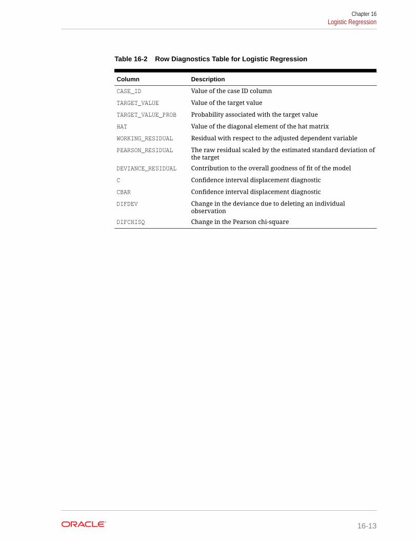
Table 16-2 Row Diagnostics Table for Logistic Regression
Column Description
CASE_ID Value of the case ID column
TARGET_VALUE Value of the target value
TARGET_VALUE_PROB Probability associated with the target value
HAT Value of the diagonal element of the hat matrix
WORKING_RESIDUAL Residual with respect to the adjusted dependent variable
PEARSON_RESIDUAL The raw residual scaled by the estimated standard deviation ofthe target
DEVIANCE_RESIDUAL Contribution to the overall goodness of fit of the model
C Confidence interval displacement diagnostic
CBAR Confidence interval displacement diagnostic
DIFDEV Change in the deviance due to deleting an individualobservation
DIFCHISQ Change in the Pearson chi-square
Chapter 16Logistic Regression
16-13
17k-Means
Learn how to use enhanced k-Means Clustering algorithm that the Oracle Data Miningsupports.
• About k-Means
• k-Means Algorithm Configuration
• Data Preparation for k-Means
Related Topics
• ClusteringLearn how to discover natural groupings in the data through Clustering - theunsupervised mining function.
17.1 About k-MeansThe k-Means algorithm is a distance-based clustering algorithm that partitions the datainto a specified number of clusters.
Distance-based algorithms rely on a distance function to measure the similaritybetween cases. Cases are assigned to the nearest cluster according to the distancefunction used.
17.1.1 Oracle Data Mining Enhanced k-MeansOracle Data Mining implements an enhanced version of the k-Means algorithm withthe following features:
• Distance function: The algorithm supports Euclidean and Cosine distancefunctions. The default is Euclidean.
• Scalable Parallel Model build: The algorithm uses a very efficient methodof initialization based on Bahmani, Bahman, et al. "Scalable k-means++."Proceedings of the VLDB Endowment 5.7 (2012): 622-633.
• Cluster properties: For each cluster, the algorithm returns the centroid, ahistogram for each attribute, and a rule describing the hyperbox that enclosesthe majority of the data assigned to the cluster. The centroid reports the mode forcategorical attributes and the mean and variance for numerical attributes.
This approach to k-Means avoids the need for building multiple k-Means models andprovides clustering results that are consistently superior to the traditional k-Means.
17.1.2 CentroidThe centroid represents the most typical case in a cluster. For example, in a data setof customer ages and incomes, the centroid of each cluster would be a customer of
17-1

average age and average income in that cluster. The centroid is a prototype. It doesnot necessarily describe any given case assigned to the cluster.
The attribute values for the centroid are the mean of the numerical attributes and themode of the categorical attributes.
17.2 k-Means Algorithm ConfigurationLearn about configuring k-means algorithm.
The Oracle Data Mining enhanced k-Means algorithm supports several build-timesettings. All the settings have default values. There is no reason to override thedefaults unless you want to influence the behavior of the algorithm in some specificway.
You can configure k-Means by specifying the following considerations:
• Number of clusters
• Distance Function. The default distance function is Euclidean.
Related Topics
• Oracle Database PL/SQL Packages and Types Reference
17.3 Data Preparation for k-MeansLearn about preparing data for k-means algorithm.
Normalization is typically required by the k-Means algorithm. Automatic DataPreparation performs normalization for k-Means. If you do not use ADP, you mustnormalize numeric attributes before creating or applying the model.
When there are missing values in columns with simple data types (not nested),k-Means interprets them as missing at random. The algorithm replaces missingcategorical values with the mode and missing numerical values with the mean.
When there are missing values in nested columns, k-Means interprets them as sparse.The algorithm replaces sparse numerical data with zeros and sparse categorical datawith zero vectors.
Related Topics
• Oracle Database PL/SQL Packages and Types Reference
• Preparing the Data
• Transforming the Data
Chapter 17k-Means Algorithm Configuration
17-2
18Minimum Description Length
Learn how to use Minimum Description Length, the supervised technique forcalculating Attribute Importance.
• About MDL
• Data Preparation for MDL
Related Topics
• About Feature Selection and Attribute Importance
18.1 About MDLIntroduces Minimum Description Length (MDL) algorithm.
MDL is an information theoretic model selection principle. It is an important concept ininformation theory (the study of the quantification of information) and in learning theory(the study of the capacity for generalization based on empirical data).
MDL assumes that the simplest, most compact representation of the data is the bestand most probable explanation of the data. The MDL principle is used to build OracleData Mining attribute importance models.
The build process for attribute importance supports parallel execution.
Related Topics
• Oracle Database VLDB and Partitioning Guide
18.1.1 Compression and EntropyData compression is the process of encoding information using fewer bits than whatthe original representation uses. The MDL Principle is based on the notion that theshortest description of the data is the most probable. In typical instantiations of thisprinciple, a model is used to compress the data by reducing the uncertainty (entropy)as discussed below. The description of the data includes a description of the modeland the data as described by the model.
Entropy is a measure of uncertainty. It quantifies the uncertainty in a random variableas the information required to specify its value. Information in this sense is definedas the number of yes/no questions known as bits (encoded as 0 or 1) that mustbe answered for a complete specification. Thus, the information depends upon thenumber of values that variable can assume.
For example, if the variable represents the sex of an individual, then the numberof possible values is two: female and male. If the variable represents the salaryof individuals expressed in whole dollar amounts, then the values can be in therange $0-$10B, or billions of unique values. Clearly it takes more information to specifyan exact salary than to specify an individual's sex.
18-1

18.1.1.1 Values of a Random Variable: Statistical DistributionInformation (the number of bits) depends on the statistical distribution of the valuesof the variable as well as the number of values of the variable. If we are judicious inthe choice of Yes/No questions, then the amount of information for salary specificationcannot be as much as it first appears. Most people do not have billion dollar salaries.If most people have salaries in the range $32000-$64000, then most of the time,it requires only 15 questions to discover their salary, rather than the 30 required, ifevery salary from $0-$1000000000 were equally likely. In the former example, if thepersons were known to be pregnant, then their sex is known to be female. There is nouncertainty, no Yes/No questions need be asked. The entropy is 0.
18.1.1.2 Values of a Random Variable: Significant PredictorsSuppose that for some random variable there is a predictor that when its values areknown reduces the uncertainty of the random variable. For example, knowing whethera person is pregnant or not, reduces the uncertainty of the random variable sex-of-individual. This predictor seems like a valuable feature to include in a model. Howabout name? Imagine that if you knew the name of the person, you would also knowthe person's sex. If so, the name predictor would seemingly reduce the uncertaintyto zero. However, if names are unique, then what was gained? Is the person namedSally? Is the person named George?... We would have as many Yes/No predictorsin the name model as there are people. Therefore, specifying the name model wouldrequire as many bits as specifying the sex of each person.
18.1.1.3 Total EntropyFor a random variable, X, the total entropy is defined as minus the Probability(X)multiplied by the log to the base 2 of the Probability(X). This can be shown to be thevariable's most efficient encoding.
18.1.2 Model SizeMinimum Description Length (MDL) takes into consideration the size of the modelas well as the reduction in uncertainty due to using the model. Both model sizeand entropy are measured in bits. For our purposes, both numeric and categoricalpredictors are binned. Thus the size of each single predictor model is the number ofpredictor bins. The uncertainty is reduced to the within-bin target distribution.
18.1.3 Model SelectionMinimum Description Length (MDL) considers each attribute as a simple predictivemodel of the target class. Model selection refers to the process of comparing andranking the single-predictor models.
MDL uses a communication model for solving the model selection problem. In thecommunication model there is a sender, a receiver, and data to be transmitted.
These single predictor models are compared and ranked with respect to the MDLmetric, which is the relative compression in bits. MDL penalizes model complexity toavoid over-fit. It is a principled approach that takes into account the complexity of thepredictors (as models) to make the comparisons fair.
Chapter 18About MDL
18-2

18.1.4 The MDL MetricAttribute importance uses a two-part code as the metric for transmitting each unit ofdata. The first part (preamble) transmits the model. The parameters of the model arethe target probabilities associated with each value of the prediction.
For a target with j values and a predictor with k values, ni (i= 1,..., k) rows per value,there are Ci, the combination of j-1 things taken ni-1 at a time possible conditionalprobabilities. The size of the preamble in bits can be shown to be Sum(log2(Ci)), wherethe sum is taken over k. Computations like this represent the penalties associated witheach single prediction model. The second part of the code transmits the target valuesusing the model.
It is well known that the most compact encoding of a sequence is the encoding thatbest matches the probability of the symbols (target class values). Thus, the model thatassigns the highest probability to the sequence has the smallest target class valuetransmission cost. In bits, this is the Sum(log2(pi)), where the pi are the predictedprobabilities for row i associated with the model.
The predictor rank is the position in the list of associated description lengths, smallestfirst.
18.2 Data Preparation for MDLLearn about preparing data for Minimum Description Length (MDL).
Automatic Data Preparation performs supervised binning for MDL. Supervised binninguses decision trees to create the optimal bin boundaries. Both categorical andnumerical attributes are binned.
MDL handles missing values naturally as missing at random. The algorithm replacessparse numerical data with zeros and sparse categorical data with zero vectors.Missing values in nested columns are interpreted as sparse. Missing values incolumns with simple data types are interpreted as missing at random.
If you choose to manage your own data preparation, keep in mind that MDL usuallybenefits from binning. However, the discriminating power of an attribute importancemodel can be significantly reduced when there are outliers in the data and externalequal-width binning is used. This technique can cause most of the data to concentratein a few bins (a single bin in extreme cases). In this case, quantile binning is a bettersolution.
Related Topics
• Preparing the Data
• Transforming the Data
Chapter 18Data Preparation for MDL
18-3

19Naive Bayes
Learn how to use Naive Bayes Classification algorithm that the Oracle Data Miningsupports.
• About Naive Bayes
• Tuning a Naive Bayes Model
• Data Preparation for Naive Bayes
Related Topics
• ClassificationLearn how to predict a categorical target through Classification - the supervisedmining function.
19.1 About Naive BayesLearn about Naive Bayes algorithm.
The Naive Bayes algorithm is based on conditional probabilities. It uses Bayes'theorem, a formula that calculates a probability by counting the frequency of valuesand combinations of values in the historical data.
Bayes' theorem finds the probability of an event occurring given the probability ofanother event that has already occurred. If B represents the dependent event and Arepresents the prior event, Bayes' theorem can be stated as follows.
Note:
Prob(B given A) = Prob(A and B)/Prob(A)
To calculate the probability of B given A, the algorithm counts the number of caseswhere A and B occur together and divides it by the number of cases where A occursalone.
Example 19-1 Use Bayes' Theorem to Predict an Increase in Spending
Suppose you want to determine the likelihood that a customer under 21 increasesspending. In this case, the prior condition (A) is "under 21," and the dependentcondition (B) is "increase spending."
If there are 100 customers in the training data and 25 of them are customers under 21who have increased spending, then:
Prob(A and B) = 25%
If 75 of the 100 customers are under 21, then:
19-1

Prob(A) = 75%
Bayes' theorem predicts that 33% of customers under 21 are likely to increasespending (25/75).
The cases where both conditions occur together are referred to as pairwise. InExample 19-1, 25% of all cases are pairwise.
The cases where only the prior event occurs are referred to as singleton. InExample 19-1, 75% of all cases are singleton.
A visual representation of the conditional relationships used in Bayes' theorem isshown in the following figure.
Figure 19-1 Conditional Probabilities in Bayes' Theorem
A and B
B
A
P(A) = 3/4
P(B) = 2/4
P(A and B) = P(AB) = 1/4
P(A B) = P(AB) / P(B) = (1/4) / (2/4) = 1/2
P(B A) = P(AB) / P(A) = (1/4) / (3/4) = 1/3
For purposes of illustration, Example 19-1 and Figure 19-1 show a dependent eventbased on a single independent event. In reality, the Naive Bayes algorithm mustusually take many independent events into account. In Example 19-1, factors such asincome, education, gender, and store location might be considered in addition to age.
Naive Bayes makes the assumption that each predictor is conditionally independent ofthe others. For a given target value, the distribution of each predictor is independentof the other predictors. In practice, this assumption of independence, even whenviolated, does not degrade the model's predictive accuracy significantly, and makesthe difference between a fast, computationally feasible algorithm and an intractableone.
Sometimes the distribution of a given predictor is clearly not representative of thelarger population. For example, there might be only a few customers under 21 in thetraining data, but in fact there are many customers in this age group in the widercustomer base. To compensate for this, you can specify prior probabilities whentraining the model.
Related Topics
• Priors and Class WeightsLearn about Priors and Class Weights in a Classification model to produce auseful result.
Chapter 19About Naive Bayes
19-2
19.1.1 Advantages of Naive BayesLearn about the advantages of Naive Bayes.
The Naive Bayes algorithm affords fast, highly scalable model building and scoring. Itscales linearly with the number of predictors and rows.
The build process for Naive Bayes supports parallel execution. (Scoring supportsparallel execution irrespective of the algorithm.)
Naive Bayes can be used for both binary and multiclass classification problems.
Related Topics
• Oracle Database VLDB and Partitioning Guide
19.2 Tuning a Naive Bayes ModelIntroduces about probability calculation of pairwise occurrences and percentage ofsingleton occurrences.
Naive Bayes calculates a probability by dividing the percentage of pairwiseoccurrences by the percentage of singleton occurrences. If these percentages arevery small for a given predictor, they probably do not contribute to the effectiveness ofthe model. Occurrences below a certain threshold can usually be ignored.
The following build settings are available for adjusting the probability thresholds. Youcan specify:
• The minimum percentage of pairwise occurrences required for including apredictor in the model.
• The minimum percentage of singleton occurrences required for including apredictor in the model .
The default thresholds work well for most models, so you need not adjust thesesettings.
Related Topics
• Oracle Database PL/SQL Packages and Types Reference
19.3 Data Preparation for Naive BayesLearn about preparing the data for Naive Bayes.
Automatic Data Preparation performs supervised binning for Naive Bayes. Supervisedbinning uses decision trees to create the optimal bin boundaries. Both categorical andnumeric attributes are binned.
Naive Bayes handles missing values naturally as missing at random. The algorithmreplaces sparse numerical data with zeros and sparse categorical data with zerovectors. Missing values in nested columns are interpreted as sparse. Missing values incolumns with simple data types are interpreted as missing at random.
If you choose to manage your own data preparation, keep in mind that Naive Bayesusually requires binning. Naive Bayes relies on counting techniques to calculateprobabilities. Columns must be binned to reduce the cardinality as appropriate.
Chapter 19Tuning a Naive Bayes Model
19-3
Numerical data can be binned into ranges of values (for example, low, medium, andhigh), and categorical data can be binned into meta-classes (for example, regionsinstead of cities). Equi-width binning is not recommended, since outliers cause mostof the data to concentrate in a few bins, sometimes a single bin. As a result, thediscriminating power of the algorithms is significantly reduced
Related Topics
• Preparing the Data
• Transforming the Data
Chapter 19Data Preparation for Naive Bayes
19-4

20Neural Network
Learn about Neural Network for Regression and Classification mining functions.
• About Neural Network
• Data Preparation for Neural Network
• Neural Network Algorithm Configuration
• Scoring with Neural Network
20.1 About Neural NetworkNeural Network in Oracle Data Mining is designed for mining functions likeClassification and Regression.
In machine learning, an artificial neural network is an algorithm inspired from biologicalneural network and is used to estimate or approximate functions that depend on alarge number of generally unknown inputs. An artificial neural network is composed ofa large number of interconnected neurons which exchange messages between eachother to solve specific problems. They learn by examples and tune the weights ofthe connections among the neurons during the learning process. Neural Network iscapable of solving a wide variety of tasks such as computer vision, speech recognition,and various complex business problems.
Related Topics
• RegressionLearn how to predict a continuous numerical target through Regression - thesupervised mining function.
• ClassificationLearn how to predict a categorical target through Classification - the supervisedmining function.
20.1.1 Neuron and activation functionNeurons are the building blocks of a Neural Network.
A neuron takes one or more inputs having different weights and has an output whichdepends on the inputs. The output is achieved by adding up inputs of each neuronwith weights and feeding the sum into the activation function.
A Sigmoid function is usually the most common choice for activation function but othernon-linear functions, piecewise linear functions or step functions are also used. Thefollowing are some examples of activation functions:
• Logistic Sigmoid function
• Linear function
• Tanh function
20-1

• Arctan function
• Bipolar sigmoid function
20.1.2 Loss or Cost functionA loss function or cost function is a function that maps an event or values of one ormore variables onto a real number intuitively representing some "cost" associated withthe event.
An optimization problem seeks to minimize a loss function. The form of loss function ischosen based on the nature of the problem and mathematical needs.
The following are the different loss functions for different scenarios:
• Binary classification: cross entropy function.
• Multi-class classification: softmax function.
• Regression: squared error function.
20.1.3 Forward-Backward PropagationUnderstand forward-backward propagation.
Forward propagation computes the loss function value by weighted summing theprevious layer neuron values and applying activation functions. Backward propagationcalculates the gradient of a loss function with respect to all the weights in the network.The weights are initialized with a set of random numbers uniformly distributed withina region specified by user (by setting weights boundaries), or region defined by thenumber of nodes in the adjacent layers (data driven). The gradients are fed to anoptimization method which in turn uses them to update the weights, in an attempt tominimize the loss function.
20.1.4 Optimization SolverUnderstand optimization solver.
An optimization solver is used to search for the optimal solution of the loss function tofind the extreme value (maximum or minimum) of the loss (cost) function.
Oracle Data Mining implements Limited-memory Broyden–Fletcher–Goldfarb–Shanno(L-BFGS) together with line search. L-BFGS is a Quasi-Newton method. This methoduses rank-one updates specified by gradient evaluations to approximate Hessianmatrix. This method only needs limited amount of memory. L-BFGS is used to findthe descent direction and line search is used to find the appropriate step size. Thenumber of historical copies kept in L-BFGS solver is defined by LBFGS_HISTORY_DEPTH.When the number of iterations is smaller than the history depth, the Hessian computedby L-BFGS is accurate. When the number of iterations is larger than the history depth,the Hessian computed by L-BFGS is an approximation. Therefore, the history depthcannot be too small or too large as the computation can be too slow. Typically, thevalue is between 3 and 10.
20.1.5 RegularizationUnderstand regularization.
Chapter 20About Neural Network
20-2

Regularization refers to a process of introducing additional information to solvean ill-posed problem or to prevent over-fitting. Ill-posed or over-fitting can occurwhen a statistical model describes random error or noise instead of the underlyingrelationship. Typical regularization techniques include L1-norm regularization, L2-normregularization, and held-aside.
Held-aside is usually used for large training date set whereas L1-norm regularizationand L2-norm regularization are mostly used for small training date set.
20.1.6 Convergence CheckThis checks if the optimal solution has been reached and if the iterations of theoptimization has come to an end.
In L-BFGS solver, the convergence criteria includes maximum number of iterations,infinity norm of gradient, and relative error tolerance. For held-aside regularization, theconvergence criteria checks the loss function value of the test data set, as well as thebest model learned so far. The training is terminated when the model becomes worsefor a specific number of iterations (specified by NNET_HELDASIDE_MAX_FAIL), or the lossfunction is close to zero, or the relative error on test data is less than the tolerance.
20.1.7 LBFGS_SCALE_HESSIANDefines LBFGS_SCALE_HESSIAN.
It specifies how to set the initial approximation of the inverse Hessian at the beginningof each iteration. If the value is set to be LBFGS_SCALE_HESSIAN_ENABLE, then weapproximate the initial inverse Hessian with Oren-Luenberger scaling. If it is set tobe LBFGS_SCALE_HESSIAN_DISABLE, then we use identity as the approximation of theinverse Hessian at the beginning of each iteration.
Related Topics
• Oracle Database PL/SQL Packages and Types Reference
20.1.8 NNET_HELDASIDE_MAX_FAILDefines NNET_HELDASIDE_MAX_FAIL.
Validation data (held-aside) is used to stop training early if the network performance onthe validation data fails to improve or remains the same for NNET_HELDASIDE_MAX_FAILepochs in a row.
Related Topics
• Oracle Database PL/SQL Packages and Types Reference
20.2 Data Preparation for Neural NetworkLearn about preparing data for Neural Network.
The algorithm automatically "explodes" categorical data into a set of binary attributes,one per category value. Oracle Data Mining algorithms automatically handle missingvalues and therefore, missing value treatment is not necessary.
Chapter 20Data Preparation for Neural Network
20-3

The algorithm automatically replaces missing categorical values with the mode andmissing numerical values with the mean. Neural Network requires the normalization ofnumeric input. The algorithm uses z-score normalization. The normalization occursonly for two-dimensional numeric columns (not nested). Normalization places thevalues of numeric attributes on the same scale and prevents attributes with a largeoriginal scale from biasing the solution. Neural Network scales the numeric values innested columns by the maximum absolute value seen in the corresponding columns.
Related Topics
• Preparing the Data
• Transforming the Data
20.3 Neural Network Algorithm ConfigurationLearn about configuring Neural Network algorithm.
Specify Nodes Per Layer
INSERT INTO SETTINGS_TABLE (setting_name, setting_value) VALUES ('NNET_NODES_PER_LAYER', '2,3');
Specify Activation Functions Per Layer
INSERT INTO SETTINGS_TABLE (setting_name, setting_value) VALUES ('NNET_ACTIVATIONS', ' ' ' NNET_ACTIVATIONS_TANH ' ', ' ' NNET_ACTIVATIONS_LOG_SIG ' ' ');
Example 20-1 Example
In this example you will understand how to build a Neural Network. When the settingstable is created and populated, insert a row in the settings table to specify thealgorithm.
INSERT INTO SETTINGS_TABLE (setting_name, setting_value) VALUES ('ALGO_NAME', 'ALGO_NEURAL_NETWORK');
Build the model as follows:
BEGINDBMS_DATA_MINING.CREATE_MODEL(model_name => 'model-name',mining_function => dbms_data_mining.classification/regression,data_table_name => 'test_table',case_id_column_name => 'case_id',target_column_name => 'test_target',settings_table_name => 'settings_table');END;/
Chapter 20Neural Network Algorithm Configuration
20-4
20.4 Scoring with Neural NetworkLearn to score with Neural Network.
Scoring with Neural Network is the same as any other Classificationor Regression algorithm. The following functions are supported:PREDICTION, PREDICTION_PROBABILITY, PREDICTION_COST, PREDICTION_SET, andPREDICTION_DETAILS.
Related Topics
• Oracle Database SQL Language Reference
Chapter 20Scoring with Neural Network
20-5
21Non-Negative Matrix Factorization
Learn how to use Non-Negative Matrix Factorization (NMF), the unsupervisedalgorithm, that the Oracle Data Mining uses for Feature Extraction.
• About NMF
• Tuning the NMF Algorithm
• Data Preparation for NMF
Related Topics
• Feature Selection and ExtractionLearn how to perform Feature Selection, Feature Extraction, and AttributeImportance.
See Also:
Paper "Learning the Parts of Objects by Non-Negative Matrix Factorization"by D. D. Lee and H. S. Seung in Nature (401, pages 788-791, 1999)
21.1 About NMFNon-Negative Matrix Factorization is a state of the art feature extraction algorithm.NMF is useful when there are many attributes and the attributes are ambiguousor have weak predictability. By combining attributes, NMF can produce meaningfulpatterns, topics, or themes.
Each feature created by NMF is a linear combination of the original attribute set. Eachfeature has a set of coefficients, which are a measure of the weight of each attributeon the feature. There is a separate coefficient for each numerical attribute and for eachdistinct value of each categorical attribute. The coefficients are all non-negative.
21.1.1 Matrix FactorizationNon-Negative Matrix Factorization uses techniques from multivariate analysis andlinear algebra. It decomposes the data as a matrix M into the product of two lowerranking matrices W and H. The sub-matrix W contains the NMF basis; the sub-matrixH contains the associated coefficients (weights).
The algorithm iteratively modifies of the values of W and H so that their productapproaches M. The technique preserves much of the structure of the original data andguarantees that both basis and weights are non-negative. The algorithm terminateswhen the approximation error converges or a specified number of iterations isreached.
21-1

The NMF algorithm must be initialized with a seed to indicate the starting point for theiterations. Because of the high dimensionality of the processing space and the fact thatthere is no global minimization algorithm, the appropriate initialization can be critical inobtaining meaningful results. Oracle Data Mining uses a random seed that initializesthe values of W and H based on a uniform distribution. This approach works well inmost cases.
21.1.2 Scoring with NMFLearn about scoring with Non-Negative Matrix Factorization (NMF).
NMF can be used as a pre-processing step for dimensionality reduction inClassification, Regression, Clustering, and other mining tasks. Scoring an NMF modelproduces data projections in the new feature space. The magnitude of a projectionindicates how strongly a record maps to a feature.
The SQL scoring functions for feature extraction support NMF models. When thefunctions are invoked with the analytical syntax, the functions build and applya transient NMF model. The feature extraction functions are: FEATURE_DETAILS,FEATURE_ID, FEATURE_SET, and FEATURE_VALUE.
Related Topics
• Oracle Data Mining User’s Guide
21.1.3 Text Mining with NMFLearn about mining text with Non-Negative Matrix Factorization (NMF).
NMF is especially well-suited for text mining. In a text document, the same word canoccur in different places with different meanings. For example, "hike" can be appliedto the outdoors or to interest rates. By combining attributes, NMF introduces context,which is essential for explanatory power:
• "hike" + "mountain" -> "outdoor sports"
• "hike" + "interest" -> "interest rates"
Related Topics
• Oracle Data Mining User’s Guide
21.2 Tuning the NMF AlgorithmLearn about configuring parameters for Non-Negative Matrix Factorization (NMF).
Oracle Data Mining supports five configurable parameters for NMF. All of them havedefault values which are appropriate for most applications of the algorithm. The NMFsettings are:
• Number of features. By default, the number of features is determined by thealgorithm.
• Convergence tolerance. The default is .05.
• Number of iterations. The default is 50.
• Random seed. The default is -1.
Chapter 21Tuning the NMF Algorithm
21-2

• Non-negative scoring. You can specify whether negative numbers must be allowedin scoring results. By default they are allowed.
Related Topics
• Oracle Database PL/SQL Packages and Types Reference
21.3 Data Preparation for NMFLearn about preparing the date for Non-Negative Matrix Factorization (NMF).
Automatic Data Preparation normalizes numerical attributes for NMF.
When there are missing values in columns with simple data types (not nested), NMFinterprets them as missing at random. The algorithm replaces missing categoricalvalues with the mode and missing numerical values with the mean.
When there are missing values in nested columns, NMF interprets them as sparse.The algorithm replaces sparse numerical data with zeros and sparse categorical datawith zero vectors.
If you choose to manage your own data preparation, keep in mind that outlierscan significantly impact NMF. Use a clipping transformation before binning ornormalizing. NMF typically benefits from normalization. However, outliers with min-maxnormalization cause poor matrix factorization. To improve the matrix factorization, youneed to decrease the error tolerance. This in turn leads to longer build times.
Related Topics
• Preparing the Data
• Transforming the Data
Chapter 21Data Preparation for NMF
21-3

22O-Cluster
Learn how to use Orthogonal Partitioning Clustering (O-Cluster), an Oracle-proprietaryClustering algorithm.
• About O-Cluster
• Tuning the O-Cluster Algorithm
• Data Preparation for O-Cluster
Related Topics
• ClusteringLearn how to discover natural groupings in the data through Clustering - theunsupervised mining function.
See Also:
Campos, M.M., Milenova, B.L., "Clustering Large Databases with Numericand Nominal Values Using Orthogonal Projections", Oracle Data MiningTechnologies, Oracle Corporation.
Oracle Data Mining
22.1 About O-ClusterO-Cluster is a fast, scalable grid-based clustering algorithm well-suited for mininglarge, high-dimensional data sets. The algorithm can produce high quality clusterswithout relying on user-defined parameters.
The objective of O-Cluster is to identify areas of high density in the data and separatethe dense areas into clusters. It uses axis-parallel uni-dimensional (orthogonal) dataprojections to identify the areas of density. The algorithm looks for splitting points thatresult in distinct clusters that do not overlap and are balanced in size.
O-Cluster operates recursively by creating a binary tree hierarchy. The number ofleaf clusters is determined automatically. The algorithm can be configured to limit themaximum number of clusters.
22.1.1 Partitioning StrategyPartitioning strategy refers to the process of discovering areas of density in theattribute histograms. The process differs for numerical and categorical data. Whenboth are present in the data, the algorithm performs the searches separately and thencompares the results.
22-1

In choosing a partition, the algorithm balances two objectives: finding well separatedclusters, and creating clusters that are balanced in size. The following paragraphsdetail how partitions for numerical and categorical attributes are identified.
22.1.1.1 Partitioning Numerical AttributesTo find the best valid cutting plane, O-Cluster searches the attribute histograms forbins of low density (valleys) between bins of high density (peaks). O-Cluster attemptsto find a pair of peaks with a valley between them where the difference between thepeak and valley histogram counts is statistically significant.
A sensitivity level parameter specifies the lowest density that may be considered apeak. Sensitivity is an optional parameter for numeric data. It may be used to filter thesplitting point candidates.
22.1.1.2 Partitioning Categorical AttributesCategorical values do not have an intrinsic order associated with them. Therefore it isimpossible to apply the notion of histogram peaks and valleys that is used to partitionnumerical values.
Instead the counts of individual values form a histogram. Bins with large counts areinterpreted as regions with high density. The clustering objective is to separate thesehigh-density areas and effectively decrease the entropy (randomness) of the data.
O-Cluster identifies the histogram with highest entropy along the individual projections.Entropy is measured as the number of bins above sensitivity level. O-Cluster placesthe two largest bins into separate partitions, thereby creating a splitting predicate. Theremainder of the bins are assigned randomly to the two resulting partitions.
22.1.2 Active SamplingThe O-Cluster algorithm operates on a data buffer of a limited size. It uses an activesampling mechanism to handle data sets that do not fit into memory.
After processing an initial random sample, O-Cluster identifies cases that are of nofurther interest. Such cases belong to frozen partitions where further splitting is highlyunlikely. These cases are replaced with examples from ambiguous regions wherefurther information (additional cases) is needed to find good splitting planes andcontinue partitioning. A partition is considered ambiguous if a valid split can only befound at a lower confidence level.
Cases associated with frozen partitions are marked for deletion from the buffer. Theyare replaced with cases belonging to ambiguous partitions. The histograms of theambiguous partitions are updated and splitting points are reevaluated.
22.1.3 Process FlowThe O-Cluster algorithm evaluates possible splitting points for all projections in apartition, selects the best one, and splits the data into two new partitions. Thealgorithm proceeds by searching for good cutting planes inside the newly createdpartitions. Thus, O-Cluster creates a binary tree structure that divides the input spaceinto rectangular regions with no overlaps or gaps.
The main processing stages are:
Chapter 22About O-Cluster
22-2

1. Load the buffer. Assign all cases from the initial buffer to a single active rootpartition.
2. Compute histograms along the orthogonal uni-dimensional projections for eachactive partition.
3. Find the best splitting points for active partitions.
4. Flag ambiguous and frozen partitions.
5. When a valid separator exists, split the active partition into two new activepartitions and start over at step 2.
6. Reload the buffer after all recursive partitioning on the current buffer is completed.Continue loading the buffer until either the buffer is filled again, or the end of thedata set is reached, or until the number of cases is equal to the data buffer size.
Note:
O-Cluster requires at most one pass through the data
22.1.4 ScoringThe clusters discovered by O-Cluster are used to generate a Bayesian probabilitymodel that can be used to score new data. The generated probability model isa mixture model where the mixture components are represented by a product ofindependent normal distributions for numerical attributes and multinomial distributionsfor categorical attributes.
22.2 Tuning the O-Cluster AlgorithmLearn about configuring build settings for O-Cluster.
The O-Cluster algorithm supports two build-time settings. Both settings have defaultvalues. There is no reason to override the defaults unless you want to influence thebehavior of the algorithm in some specific way.
You can configure O-Cluster by specifying any of the following:
• Buffer size — Size of the processing buffer.
• Sensitivity factor — A fraction that specifies the peak density required forseparating a new cluster.
Related Topics
• Active Sampling
• Partitioning Strategy
• Oracle Database PL/SQL Packages and Types Reference
22.3 Data Preparation for O-ClusterLearn about preparing the data for O-Cluster.
Chapter 22Tuning the O-Cluster Algorithm
22-3

Automatic Data Preparation bins numerical attributes for O-Cluster. It uses aspecialized form of equi-width binning that computes the number of bins per attributeautomatically. Numerical columns with all nulls or a single value are removed. O-Cluster handles missing values naturally as missing at random.
Note:
O-Cluster does not support nested columns, sparse data, or unstructuredtext.
Related Topics
• Preparing the Data
• Transforming the Data
22.3.1 User-Specified Data Preparation for O-ClusterLearn about preparing the user-specified data for O-Cluster.
Keep the following in mind if you choose to prepare the data for O-Cluster:
• O-Cluster does not necessarily use all the input data when it builds a model. Itreads the data in batches (the default batch size is 50000). It only reads anotherbatch if it believes, based on statistical tests, that uncovered clusters can still exist.
• Binary attributes must be declared as categorical.
• Automatic equi-width binning is highly recommended. The bin identifiers areexpected to be positive consecutive integers starting at 1.
• The presence of outliers can significantly impact clustering algorithms. Use aclipping transformation before binning or normalizing. Outliers with equi-widthbinning can prevent O-Cluster from detecting clusters. As a result, the wholepopulation appears to fall within a single cluster.
Related Topics
• Oracle Database PL/SQL Packages and Types Reference
Chapter 22Data Preparation for O-Cluster
22-4
23R Extensibility
Learn how to built analytics model and scored in R with ease. R extensible algorithmsare enhanced to support and register additional algorithms for SQL users andgraphical user interface users.
• Oracle Data Mining with R Extensibility
• Scoring with R
• About Algorithm Meta Data Registration
23.1 Oracle Data Mining with R ExtensibilityLearn how you can use Oracle Data Mining to build, score, and view Oracle DataMining models as well as R models.
The Oracle Data Mining framework is enhanced extending the data mining algorithmset with algorithms from the open source R ecosystem. Oracle Data Mining isimplemented in the Oracle Database kernel. The mining models are Database schemaobjects. With the extensibility enhancement, the data mining framework can build,score, and view both Oracle Data Mining models and R models.
Registration of R scripts
The R engine on the database server executes the R scripts to build, score, and viewR models. These R scripts must be registered with the database beforehand by aprivileged user with rqAdmin role. You must first install Oracle R Enterprise to registerthe R scripts.
Functions of Oracle Data Mining with R Model
The following functions are supported for an R model:
• Oracle Data Mining DBMS_DATA_MINING package is enhanced to support R model.For example, CREATE_MODEL and DROP_MODEL.
• MODEL VIEW to get the R model details about a single model and a partitionedmodel.
• Oracle Data Mining SQL functions are enhanced to operate with the R modelfunctions. For example, PREDICTION and CLUSTER_ID.
R model extensibility supports the following data mining functions:
• Association
• Attribute Importance
• Regression
• Classification
• Clustering
• Feature Extraction
23-1
23.2 Scoring with RLearn how to build and score with R Mining model.
For more information, see Oracle Data Mining User’s Guide
23.3 About Algorithm Meta Data RegistrationAlgorithm Meta Data Registration allows for a uniform and consistent approach ofregistering new algorithm functions and their settings.
Users have the ability to add new R-based algorithms through the registration process.The new algorithms appear as available within Oracle R Enterprise and within theappropriate mining functions. Based on the registration meta data, the settings page isdynamically rendered. The advantages are as follows:
• Manage R-based algorithms more easily
• Easy to specify R-based algorithm for model build
• Clean individual properties in JSON structure
• Share R-based algorithm across user
Algorithm meta data registration extends the mining model capability of Oracle DataMining.
Related Topics
• Oracle Database PL/SQL Packages and Types Reference
• FETCH_JSON_SCHEMA Procedure
• REGISTER_ALGORITHM Procedure
• JSON Schema for R Extensible Algorithm
23.3.1 Algorithm Meta Data RegistrationAlgorithm Meta Data Registration allows for a uniform and consistent approach ofregistering new algorithm functions and their settings.
User have the ability to add new algorithms through the registration process. Thenew algorithms can appear as available within Oracle Data Mining R within theirappropriate mining functions. Based on the registration meta data, the settings pageis dynamically rendered. Algorithm meta data registration extends the mining modelcapability of Oracle Data Mining.
Related Topics
• Oracle Database PL/SQL Packages and Types Reference
• FETCH_JSON_SCHEMA Procedure
• REGISTER_ALGORITHM Procedure
• JSON Schema for R Extensible Algorithm
Chapter 23Scoring with R
23-2

24Random Forest
Learn how to use Random Forest as a classification algorithm.
• About Random Forest
• Building a Random Forest
• Scoring with Random Forest
Related Topics
• Feature Selection and ExtractionLearn how to perform Feature Selection, Feature Extraction, and AttributeImportance.
24.1 About Random ForestRandom Forest is a classification algorithm used by Oracle Data Mining. The algorithmbuilds an ensemble (also called forest) of trees.
The algorithm builds a number of decision tree models and predicts using theensemble. An individual decision tree is built by choosing a random sample from thetraining data set as the input. At each node of the tree, only a random sample ofpredictors is chosen for computing the split point. This introduces variation in the dataused by the different trees in the forest. The parameters RFOR_SAMPLING_RATIO andRFOR_MTRY are used to specify the sample size and number of predictors chosen ateach node. Users can use ODMS_RANDOM_SEED to set the random seed value beforerunning the algorithm.
Related Topics
• Decision TreeLearn how to use Decision Tree algorithm. Decision Tree is one of theClassification algorithms that the Oracle Data Mining supports.
• Splitting
• Data Preparation for Decision TreeLearn how to prepare data for Decision Tree.
24.2 Building a Random ForestThe Random Forest is built upon existing infrastructure and Application ProgrammingInterfaces (APIs) of Oracle Data Mining.
The model is built by specifying parameters in the existing APIs. The scoring isperformed using the same SQL queries and APIs as the existing Classificationalgorithms. Oracle Data Mining implements a variant of Classical Random Forestalgorithm. This implementation supports big data sets. The implementation of thealgorithm differs in the following ways:
24-1

• Oracle Data Mining does not support bagging and instead provides samplingwithout replacement
• Users have the ability to specify the depth of the tree. Trees are not built tomaximum depth.
Example 24-1 Example
In this example you will understand how to build a Random Forest. When the settingstable is created and populated, insert a row in the settings table to specify thealgorithm and the variant.
INSERT INTO SETTINGS_TABLE (setting_name, setting_value) VALUES('ALGO_NAME', 'ALGO_RANDOM_FOREST');
Build the model as follows:
BEGIN DBMS_DATA_MINING.CREATE_MODEL(model_name => ‘model-name',mining_function => dbms_data_mining.classification,data_table_name => 'test_table',case_id_column_name => '',target_column_name => 'test_target',settings_table_name => 'settings_table');END;/
24.3 Scoring with Random ForestLearn to score with Random Forest.
Scoring with Random Forest is the same as any other Classification algorithm.The following functions are supported: PREDICTION, PREDICTION_PROBABILITY,PREDICTION_COST, PREDICTION_SET, and PREDICTION_DETAILS.
Related Topics
• Oracle Database SQL Language Reference
Chapter 24Scoring with Random Forest
24-2

25Singular Value Decomposition
Learn how to use Singular Value Decomposition, an unsupervised algorithm forFeature Extraction.
• About Singular Value Decomposition
• Configuring the Algorithm
• Data Preparation for SVD
Related Topics
• Feature Selection and ExtractionLearn how to perform Feature Selection, Feature Extraction, and AttributeImportance.
25.1 About Singular Value DecompositionSingular Value Decomposition (SVD) and the closely-related Principal ComponentAnalysis (PCA) are well established feature extraction methods that have a wide rangeof applications. Oracle Data Mining implements SVD as a feature extraction algorithmand PCA as a special scoring method for SVD models.
SVD and PCA are orthogonal linear transformations that are optimal at capturingthe underlying variance of the data. This property is very useful for reducingthe dimensionality of high-dimensional data and for supporting meaningful datavisualization.
SVD and PCA have a number of important applications in addition to dimensionalityreduction. These include matrix inversion, data compression, and the imputation ofunknown data values.
25.1.1 Matrix ManipulationSingular Value Decomposition (SVD) is a factorization method that decomposes arectangular matrix X into the product of three matrices:
Figure 25-1 Matrix Manipulation
X = USV'
The U matrix consists of a set of 'left' orthonormal basesThe S matrix is a diagonal matrixThe V matrix consists of set of 'right' orthonormal bases
25-1

The values in S are called singular values. They are non-negative, and theirmagnitudes indicate the importance of the corresponding bases (components). Thesingular values reflect the amount of data variance captured by the bases. The firstbasis (the one with largest singular value) lies in the direction of the greatest datavariance. The second basis captures the orthogonal direction with the second greatestvariance, and so on.
SVD essentially performs a coordinate rotation that aligns the transformed axes withthe directions of maximum variance in the data. This is a useful procedure under theassumption that the observed data has a high signal-to-noise ratio and that a largevariance corresponds to interesting data content while a lower variance corresponds tonoise.
SVD makes the assumption that the underlying data is Gaussian distributed and canbe well described in terms of means and covariances.
25.1.2 Low Rank DecompositionTo reduce dimensionality, Singular Value Decomposition (SVD) keeps lower-orderbases (the ones with the largest singular values) and ignores higher-order bases(the ones with the smallest singular values). The rationale behind this strategy is thatthe low-order bases retain the characteristics of the data that contribute most to itsvariance and are likely to capture the most important aspects of the data.
Given a data set X (nxm), where n is the number of rows and m is the numberof attributes, a low-rank SVD uses only k components (k <= min(m, n)). In typicalimplementations of SVD, the value of k requires a visual inspection of the rankedsingular values associated with the individual components. In Oracle Data Mining,SVD automatically estimates the cutoff point, which corresponds to a significant dropin the explained variance.
SVD produces two sets of orthonormal bases (U and V). Either of these bases can beused as a new coordinate system. In Oracle Data Mining SVD, V is the new coordinatesystem, and U represents the projection of X in this coordinate system. The algorithmcomputes the projection of new data as follows:
Figure 25-2 Computing Projection of New Data
X = XVkS
k
-1~
where X (nxk) is the projected data in the reduced data space, defined by the first kcomponents, and Vk and Sk define the reduced component set.
25.1.3 ScalabilityIn Oracle Data Mining, Singular Value Decomposition (SVD) can process data setswith millions of rows and thousands of attributes. Oracle Data Mining automaticallyrecommends an appropriate number of features, based on the data, for dimensionalityreduction.
SVD has linear scalability with the number of rows and cubic scalability with thenumber of attributes when a full decomposition is computed. A low-rank decompositionis typically linear with the number of rows and linear with the number of columns. The
Chapter 25About Singular Value Decomposition
25-2

scalability with the reduced rank depends on how the rank compares to the number ofrows and columns. It can be linear when the rank is significantly smaller or cubic whenit is on the same scale.
25.2 Configuring the AlgorithmLearn about configuring Singular Value Decomposition (SVD).
Several options are available for configuring the SVD algorithm. Among them aresettings to control model size and performance, and whether to score with SVDprojections or Principal Component Analysis (PCA) projections.
Related Topics
• Oracle Database PL/SQL Packages and Types Reference
25.2.1 Model SizeThe U matrix in Singular Value Decomposition has as many rows as the number ofrows in the build data. To avoid creating a large model, the U matrix persists only whenan algorithm-specific setting is enabled. By default the U matrix does not persist.
25.2.2 PerformanceSingular Value Decomposition can use approximate computations to improveperformance. Approximation may be appropriate for data sets with many columns.An approximate low-rank decomposition provides good solutions at a reasonablecomputational cost. The quality of the approximation is dependent on thecharacteristics of the data.
25.2.3 PCA scoringLearn about configuring Singular Value Decomposition (SVD) to perform PrincipalComponent Analysis (PCA) projections.
SVD models can be configured to perform PCA projections. PCA is closely relatedto SVD. PCA computes a set of orthonormal bases (principal components) that areranked by their corresponding explained variance. The main difference between SVDand PCA is that the PCA projection is not scaled by the singular values. The PCAprojection to the new coordinate system is given by:
Figure 25-3 PCA Projection Calculation
X = XVk
~
where
X
(nxk) is the projected data in the reduced data space, defined by the first kcomponents, and Vk defines the reduced component set.
Chapter 25Configuring the Algorithm
25-3
Related Topics
• Oracle Database PL/SQL Packages and Types Reference
25.3 Data Preparation for SVDLearn about preparing the data for Singular Value Decomposition (SVD).
Oracle Data Mining implements SVD for numerical data and categorical data.
When the build data is scored with SVD, Automatic Data Preparation does nothing.When the build data is scored with Principal Component Analysis (PCA), AutomaticData Preparation shifts the numerical data by mean.
Missing value treatment is not needed, because Oracle Data Mining algorithms handlemissing values automatically. SVD replaces numerical missing values with the meanand categorical missing values with the mode. For sparse data (missing values innested columns), SVD replaces missing values with zeros.
Related Topics
• Preparing the Data
• Transforming the Data
Chapter 25Data Preparation for SVD
25-4

26Support Vector Machines
Learn how to use Support Vector Machines, a powerful algorithm based on statisticallearning theory.
Oracle Data Mining implements Support Vector Machines for Classification,Regression, and Anomaly Detection.
• About Support Vector Machines
• Tuning an SVM Model
• Data Preparation for SVM
• SVM Classification
• One-Class SVM
• SVM Regression
Related Topics
• RegressionLearn how to predict a continuous numerical target through Regression - thesupervised mining function.
• Anomaly DetectionLearn how to detect rare cases in the data through Anomaly Detection - anunsupervised function.
• Oracle Data Mining
See Also:
Milenova, B.L., Yarmus, J.S., Campos, M.M., "Support Vector Machinesin Oracle Database 10g: Removing the Barriers to Widespread Adoptionof Support Vector Machines", Proceedings of the 31st VLDB Conference,Trondheim, Norway, 2005.
26.1 About Support Vector MachinesSupport Vector Machine (SVM) is a powerful, state-of-the-art algorithm with strongtheoretical foundations based on the Vapnik-Chervonenkis theory. SVM has strongregularization properties. Regularization refers to the generalization of the model tonew data.
26.1.1 Advantages of SVMOracle Data Mining SVM implementation includes two types of solvers, an InteriorPoint Method (IPM) solver and a Sub-Gradient Descent (SGD) solver. The IPM solver
26-1
provides stable and accurate solutions, however, it may not be able to handle data ofhigh dimensionality. For high-dimensional and/or large data, for example, text, ratings,and so on, the SGD solver is a better choice. Both solvers have highly scalableparallel implementations and can handle large volumes of data.
26.1.2 Advantages of SVM in Oracle Data MiningOracle Data Mining has its own proprietary implementation of Support VectorMachines (SVM), which exploits the many benefits of the algorithm whilecompensating for some of the limitations inherent in the SVM framework. Oracle DataMining SVM provides the scalability and usability that are needed in a productionquality data mining system.
26.1.2.1 UsabilityExplains usability for Support Vector Machines (SVM) in Oracle Data Mining.
Usability is a major enhancement, because SVM has often been viewed as a tool forexperts. The algorithm typically requires data preparation, tuning, and optimization.Oracle Data Mining minimizes these requirements. You do not need to be an expert tobuild a quality SVM model in Oracle Data Mining. For example:
• Data preparation is not required in most cases.
• Default tuning parameters are generally adequate.
Related Topics
• Data Preparation for SVM
• Tuning an SVM ModelLearn about configuring settings for Support Vector Machines (SVM).
26.1.2.2 ScalabilityLearn how to scale the data for Support Vector Machines (SVM).
When dealing with very large data sets, sampling is often required. However, samplingis not required with Oracle Data Mining SVM, because the algorithm itself usesstratified sampling to reduce the size of the training data as needed.
Oracle Data Mining SVM is highly optimized. It builds a model incrementally byoptimizing small working sets toward a global solution. The model is trained untilconvergence on the current working set, then the model adapts to the new data. Theprocess continues iteratively until the convergence conditions are met. The Gaussiankernel uses caching techniques to manage the working sets.
Related Topics
• Kernel-Based LearningLearn about kernal-based functions to transform the input data for Support VectorMachines (SVM).
26.1.3 Kernel-Based LearningLearn about kernal-based functions to transform the input data for Support VectorMachines (SVM).
Chapter 26About Support Vector Machines
26-2

SVM is a kernel-based algorithm. A kernel is a function that transforms the input datato a high-dimensional space where the problem is solved. Kernel functions can belinear or nonlinear.
Oracle Data Mining supports linear and Gaussian (nonlinear) kernels.
In Oracle Data Mining, the linear kernel function reduces to a linear equation on theoriginal attributes in the training data. A linear kernel works well when there are manyattributes in the training data.
The Gaussian kernel transforms each case in the training data to a point in ann-dimensional space, where n is the number of cases. The algorithm attempts toseparate the points into subsets with homogeneous target values. The Gaussiankernel uses nonlinear separators, but within the kernel space it constructs a linearequation.
Note:
Active Learning is not relevant in Oracle Database 12c Release 2 and later.A setting similar to Active Learning is ODMS_SAMPLING.
Related Topics
• Oracle Database PL/SQL Packages and Types Reference
26.2 Tuning an SVM ModelLearn about configuring settings for Support Vector Machines (SVM).
SVM have built-in mechanisms that automatically choose appropriate settings basedon the data. You may need to override the system-determined settings for somedomains.
Settings pertain to regression, classification, and anomaly detection unless otherwisespecified.
Related Topics
• Oracle Database PL/SQL Packages and Types Reference
26.3 Data Preparation for SVMThe SVM algorithm operates natively on numeric attributes. SVM uses z-scorenormalization on numeric attributes. The normalization occurs only for two-dimensionalnumeric columns (not nested). The algorithm automatically "explodes" categoricaldata into a set of binary attributes, typically one per category value. For example,a character column for marital status with values married or single is transformed totwo numeric attributes: married and single. The new attributes can have the value 1(true) or 0 (false).
When there are missing values in columns with simple data types (not nested), SVMinterprets them as missing at random. The algorithm automatically replaces missingcategorical values with the mode and missing numerical values with the mean.
Chapter 26Tuning an SVM Model
26-3

When there are missing values in the nested columns, SVM interprets them as sparse.The algorithm automatically replaces sparse numerical data with zeros and sparsecategorical data with zero vectors.
26.3.1 NormalizationSupport Vector Machines require the normalization of numeric input. Normalizationplaces the values of numeric attributes on the same scale and prevents attributeswith a large original scale from biasing the solution. Normalization also minimizes thelikelihood of overflows and underflows.
26.3.2 SVM and Automatic Data PreparationLearn about treating and transforming data manually or through Automatic DataPreparation (ADP) for Support Vector Machines (SVM).
The SVM algorithm automatically handles missing value treatment and thetransformation of categorical data, but normalization and outlier detection must behandled by Automatic Data Preparation (ADP) or prepared manually. ADP performsmin-max normalization for SVM.
Note:
Oracle recommends that you use Automatic Data Preparation with SVM. Thetransformations performed by ADP are appropriate for most models.
Related Topics
• Oracle Data Mining User’s Guide
26.4 SVM ClassificationSupport Vector Machines (SVM) Classification is based on the concept of decisionplanes that define decision boundaries. A decision plane is one that separatesbetween a set of objects having different class memberships. SVM finds the vectors("support vectors") that define the separators giving the widest separation of classes.
SVM classification supports both binary, multiclass, and multitarget Classification.Multitarget alllows multiple class labels to be associated with a single row. The targettype is a collection of type ORA_MINING_VARCHAR2_NT.
Related Topics
• Oracle Database PL/SQL Packages and Types Reference
26.4.1 Class WeightsLearn when to implement class weights to a data in Support Vector Machines (SVM).
In SVM classification, weights are a biasing mechanism for specifying the relativeimportance of target values (classes).
Chapter 26SVM Classification
26-4

SVM models are automatically initialized to achieve the best average prediction acrossall classes. However, if the training data does not represent a realistic distribution, youcan bias the model to compensate for class values that are under-represented. If youincrease the weight for a class, then the percent of correct predictions for that classmust increase.
Related Topics
• Priors and Class WeightsLearn about Priors and Class Weights in a Classification model to produce auseful result.
26.5 One-Class SVMOracle Data Mining uses Support Vector Machines (SVM) as the one-class classifierfor anomaly detection. When SVM is used for anomaly detection, it has theclassification mining function but no target.
One-class SVM models, when applied, produce a prediction and a probability for eachcase in the scoring data. If the prediction is 1, the case is considered typical. If theprediction is 0, the case is considered anomalous. This behavior reflects the fact thatthe model is trained with normal data.
You can specify the percentage of the data that you expect to be anomalous withthe SVMS_OUTLIER_RATE build setting. If you have some knowledge that the number of"suspicious" cases is a certain percentage of your population, then you can set theoutlier rate to that percentage. The model approximately identifies that many "rare"cases when applied to the general population.
26.6 SVM RegressionLearn how to use epsilon-insensitivity loss function to solve regression problems inSupport Vector Machines (SVM).
SVM uses an epsilon-insensitive loss function to solve regression problems.
SVM regression tries to find a continuous function such that the maximum numberof data points lie within the epsilon-wide insensitivity tube. Predictions falling withinepsilon distance of the true target value are not interpreted as errors.
The epsilon factor is a regularization setting for SVM regression. It balances themargin of error with model robustness to achieve the best generalization to new data.
Related Topics
• Tuning an SVM ModelLearn about configuring settings for Support Vector Machines (SVM).
Chapter 26One-Class SVM
26-5
Part IVUsing the Data Mining API
Learn how to use Oracle Data Mining application programming interface.
• Data Mining With SQL
• About the Data Mining API
• Preparing the Data
• Transforming the Data
• Creating a Model
• Scoring and Deployment
• Mining Unstructured Text
• Administrative Tasks for Oracle Data Mining
• The Data Mining Sample Programs

27Data Mining With SQL
Learn how to solve business problems using the Oracle Data Mining applicationprogramming interface (API).
• Highlights of the Data Mining API
• Example: Targeting Likely Candidates for a Sales Promotion
• Example: Analyzing Preferred Customers
• Example: Segmenting Customer Data
• Example : Building an ESA Model with a Wiki Dataset
27.1 Highlights of the Data Mining APILearn about the advantages of Data Mining application programming interface (API).
Data mining is a valuable technology in many application domains. It has becomeincreasingly indispensable in the private sector as a tool for optimizing operations andmaintaining a competitive edge. Data mining also has critical applications in the publicsector and in scientific research. However, the complexities of data mining applicationdevelopment and the complexities inherent in managing and securing large stores ofdata can limit the adoption of data mining technology.
Oracle Data Mining is uniquely suited to addressing these challenges. The datamining engine is implemented in the Database kernel, and the robust administrativefeatures of Oracle Database are available for managing and securing the data. Whilesupporting a full range of data mining algorithms and procedures, the API also hasfeatures that simplify the development of data mining applications.
The Oracle Data Mining API consists of extensions to Oracle SQL, the nativelanguage of the Database. The API offers the following advantages:
• Scoring in the context of SQL queries. Scoring can be performed dynamically orby applying data mining models.
• Automatic Data Preparation (ADP) and embedded transformations.
• Model transparency. Algorithm-specific queries return details about the attributesthat were used to create the model.
• Scoring transparency. Details about the prediction, clustering, or feature extractionoperation can be returned with the score.
• Simple routines for predictive analytics.
• A workflow-based graphical user interface (GUI) within Oracle SQL Developer.You can download SQL Developer free of charge from the following site:
Oracle Data Miner
27-1

Note:
A set of sample data mining programs ship with Oracle Database. Theexamples in this manual are taken from these samples.
Related Topics
• The Data Mining Sample ProgramsDescribes the data mining sample programs that ship with Oracle Database.
• Oracle Data Mining Concepts
27.2 Example: Targeting Likely Candidates for a SalesPromotion
This example targets customers in Brazil for a special promotion that offers couponsand an affinity card.
The query uses data on marital status, education, and income to predict the customerswho are most likely to take advantage of the incentives. The query applies a decisiontree model called dt_sh_clas_sample to score the customer data.
Example 27-1 Predict Best Candidates for an Affinity Card
SELECT cust_id FROM mining_data_apply_v WHERE PREDICTION(dt_sh_clas_sample USING cust_marital_status, education, cust_income_level ) = 1 AND country_name IN 'Brazil';
CUST_ID---------- 100404 100607 101113
The same query, but with a bias to favor false positives over false negatives, is shownhere.
SELECT cust_id FROM mining_data_apply_v WHERE PREDICTION(dt_sh_clas_sample COST MODEL USING cust_marital_status, education, cust_income_level ) = 1 AND country_name IN 'Brazil';
CUST_ID---------- 100139 100163 100275 100404 100607 101113
Chapter 27Example: Targeting Likely Candidates for a Sales Promotion
27-2
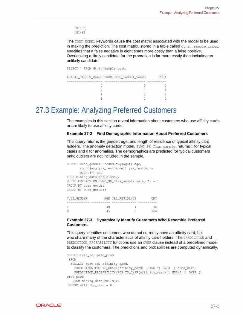
101170 101463
The COST MODEL keywords cause the cost matrix associated with the model to be usedin making the prediction. The cost matrix, stored in a table called dt_sh_sample_costs,specifies that a false negative is eight times more costly than a false positive.Overlooking a likely candidate for the promotion is far more costly than including anunlikely candidate.
SELECT * FROM dt_sh_sample_cost; ACTUAL_TARGET_VALUE PREDICTED_TARGET_VALUE COST------------------- ---------------------- ---------- 0 0 0 0 1 1 1 0 8 1 1 0
27.3 Example: Analyzing Preferred CustomersThe examples in this section reveal information about customers who use affinity cardsor are likely to use affinity cards.
Example 27-2 Find Demographic Information About Preferred Customers
This query returns the gender, age, and length of residence of typical affinity cardholders. The anomaly detection model, SVMO_SH_Clas_sample, returns 1 for typicalcases and 0 for anomalies. The demographics are predicted for typical customersonly; outliers are not included in the sample.
SELECT cust_gender, round(avg(age)) age, round(avg(yrs_residence)) yrs_residence, count(*) cntFROM mining_data_one_class_vWHERE PREDICTION(SVMO_SH_Clas_sample using *) = 1GROUP BY cust_genderORDER BY cust_gender; CUST_GENDER AGE YRS_RESIDENCE CNT------------ ---------- ------------- ----------F 40 4 36M 45 5 304
Example 27-3 Dynamically Identify Customers Who Resemble PreferredCustomers
This query identifies customers who do not currently have an affinity card, butwho share many of the characteristics of affinity card holders. The PREDICTION andPREDICTION_PROBABILITY functions use an OVER clause instead of a predefined modelto classify the customers. The predictions and probabilities are computed dynamically.
SELECT cust_id, pred_prob FROM (SELECT cust_id, affinity_card, PREDICTION(FOR TO_CHAR(affinity_card) USING *) OVER () pred_card, PREDICTION_PROBABILITY(FOR TO_CHAR(affinity_card),1 USING *) OVER () pred_prob FROM mining_data_build_v) WHERE affinity_card = 0
Chapter 27Example: Analyzing Preferred Customers
27-3
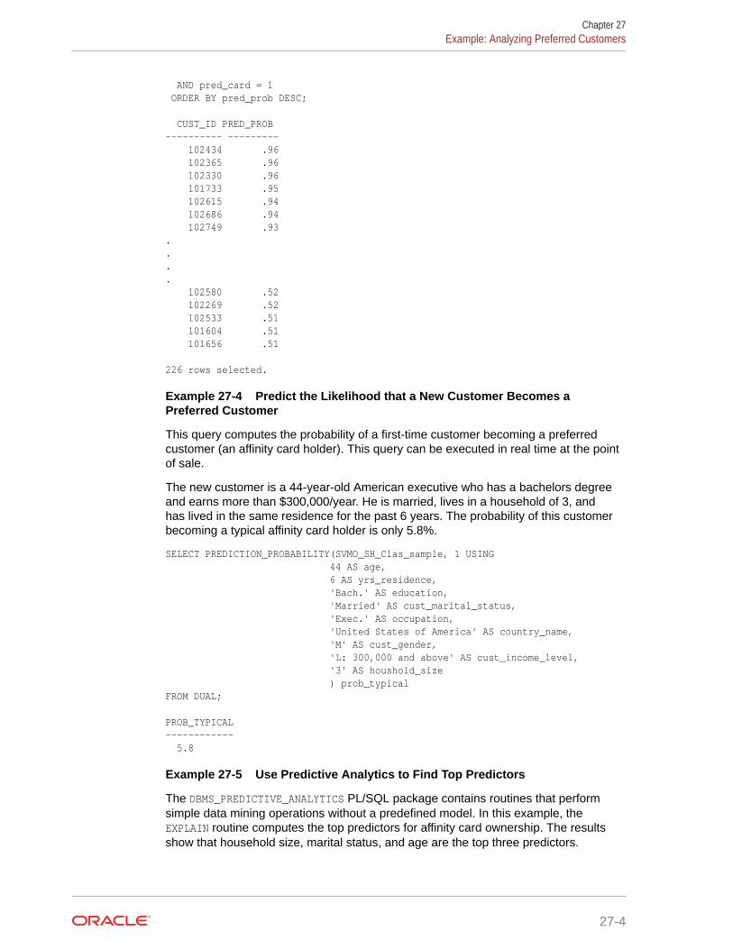
AND pred_card = 1 ORDER BY pred_prob DESC;
CUST_ID PRED_PROB---------- --------- 102434 .96 102365 .96 102330 .96 101733 .95 102615 .94 102686 .94 102749 .93.... 102580 .52 102269 .52 102533 .51 101604 .51 101656 .51 226 rows selected.
Example 27-4 Predict the Likelihood that a New Customer Becomes aPreferred Customer
This query computes the probability of a first-time customer becoming a preferredcustomer (an affinity card holder). This query can be executed in real time at the pointof sale.
The new customer is a 44-year-old American executive who has a bachelors degreeand earns more than $300,000/year. He is married, lives in a household of 3, andhas lived in the same residence for the past 6 years. The probability of this customerbecoming a typical affinity card holder is only 5.8%.
SELECT PREDICTION_PROBABILITY(SVMO_SH_Clas_sample, 1 USING 44 AS age, 6 AS yrs_residence, 'Bach.' AS education, 'Married' AS cust_marital_status, 'Exec.' AS occupation, 'United States of America' AS country_name, 'M' AS cust_gender, 'L: 300,000 and above' AS cust_income_level, '3' AS houshold_size ) prob_typicalFROM DUAL; PROB_TYPICAL------------ 5.8
Example 27-5 Use Predictive Analytics to Find Top Predictors
The DBMS_PREDICTIVE_ANALYTICS PL/SQL package contains routines that performsimple data mining operations without a predefined model. In this example, theEXPLAIN routine computes the top predictors for affinity card ownership. The resultsshow that household size, marital status, and age are the top three predictors.
Chapter 27Example: Analyzing Preferred Customers
27-4

BEGIN DBMS_PREDICTIVE_ANALYTICS.EXPLAIN( data_table_name => 'mining_data_test_v', explain_column_name => 'affinity_card', result_table_name => 'cust_explain_result');END;/
SELECT * FROM cust_explain_result WHERE rank < 4; ATTRIBUTE_NAME ATTRIBUTE_SUBNAME EXPLANATORY_VALUE RANK------------------------ -------------------- ----------------- ----------HOUSEHOLD_SIZE .209628541 1CUST_MARITAL_STATUS .199794636 2AGE .111683067 3
27.4 Example: Segmenting Customer DataThe examples in this section use an Expectation Maximization clustering model tosegment the customer data based on common characteristics.
Example 27-6 Compute Customer Segments
This query computes natural groupings of customers and returns the number ofcustomers in each group.
SELECT CLUSTER_ID(em_sh_clus_sample USING *) AS clus, COUNT(*) AS cnt FROM mining_data_apply_vGROUP BY CLUSTER_ID(em_sh_clus_sample USING *)ORDER BY cnt DESC; CLUS CNT---------- ---------- 9 311 3 294 7 215 12 201 17 123 16 114 14 86 19 64 15 56 18 36
Example 27-7 Find the Customers Who Are Most Likely To Be in the LargestSegment
The query in Example 27-6 shows that segment 9 has the most members. Thefollowing query lists the five customers who are most likely to be in segment 9.
SELECT cust_idFROM (SELECT cust_id, RANK() over (ORDER BY prob DESC, cust_id) rnk_clus2 FROM (SELECT cust_id, ROUND(CLUSTER_PROBABILITY(em_sh_clus_sample, 9 USING *),3) prob FROM mining_data_apply_v))WHERE rnk_clus2 <= 5ORDER BY rnk_clus2; CUST_ID
Chapter 27Example: Segmenting Customer Data
27-5
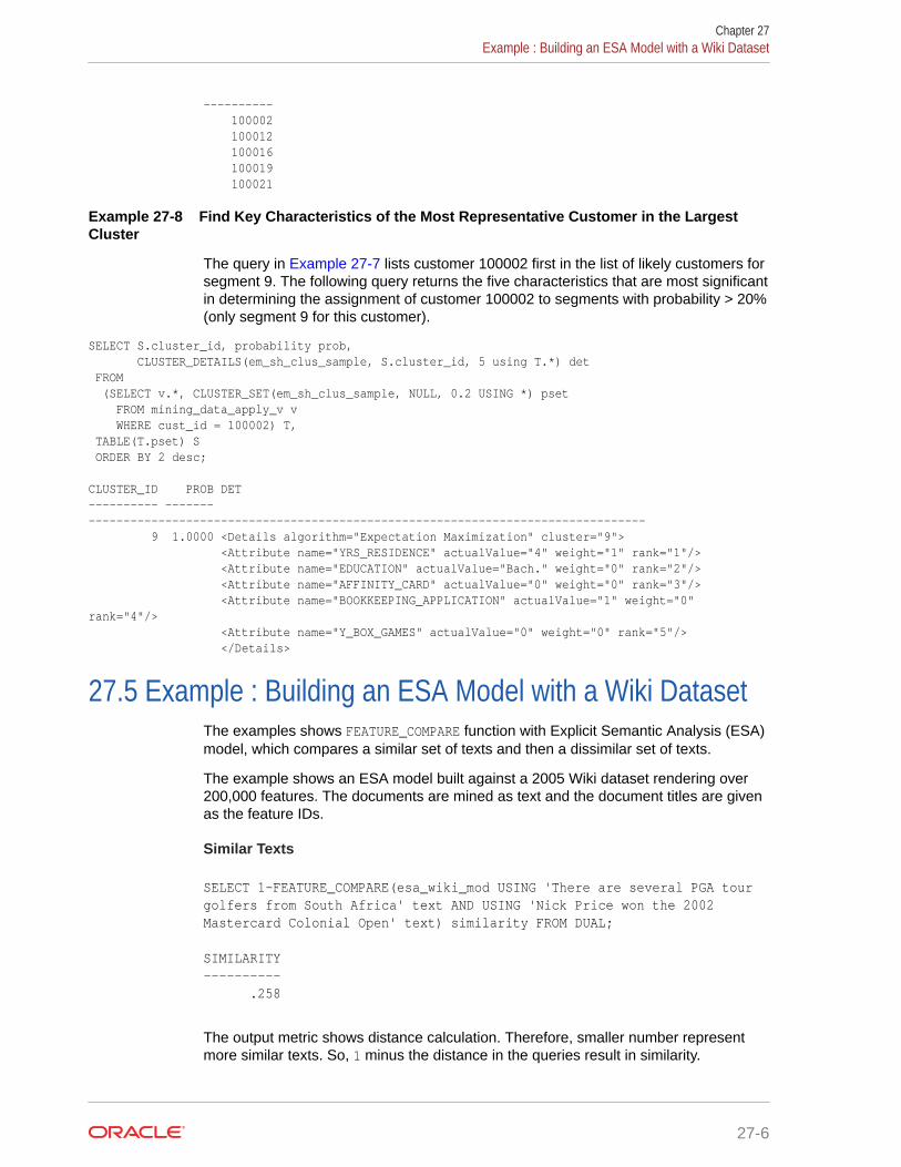
---------- 100002 100012 100016 100019 100021
Example 27-8 Find Key Characteristics of the Most Representative Customer in the LargestCluster
The query in Example 27-7 lists customer 100002 first in the list of likely customers forsegment 9. The following query returns the five characteristics that are most significantin determining the assignment of customer 100002 to segments with probability > 20%(only segment 9 for this customer).
SELECT S.cluster_id, probability prob, CLUSTER_DETAILS(em_sh_clus_sample, S.cluster_id, 5 using T.*) det FROM (SELECT v.*, CLUSTER_SET(em_sh_clus_sample, NULL, 0.2 USING *) pset FROM mining_data_apply_v v WHERE cust_id = 100002) T, TABLE(T.pset) S ORDER BY 2 desc; CLUSTER_ID PROB DET---------- ------- -------------------------------------------------------------------------------- 9 1.0000 <Details algorithm="Expectation Maximization" cluster="9"> <Attribute name="YRS_RESIDENCE" actualValue="4" weight="1" rank="1"/> <Attribute name="EDUCATION" actualValue="Bach." weight="0" rank="2"/> <Attribute name="AFFINITY_CARD" actualValue="0" weight="0" rank="3"/> <Attribute name="BOOKKEEPING_APPLICATION" actualValue="1" weight="0" rank="4"/> <Attribute name="Y_BOX_GAMES" actualValue="0" weight="0" rank="5"/> </Details>
27.5 Example : Building an ESA Model with a Wiki DatasetThe examples shows FEATURE_COMPARE function with Explicit Semantic Analysis (ESA)model, which compares a similar set of texts and then a dissimilar set of texts.
The example shows an ESA model built against a 2005 Wiki dataset rendering over200,000 features. The documents are mined as text and the document titles are givenas the feature IDs.
Similar Texts
SELECT 1-FEATURE_COMPARE(esa_wiki_mod USING 'There are several PGA tour golfers from South Africa' text AND USING 'Nick Price won the 2002 Mastercard Colonial Open' text) similarity FROM DUAL;
SIMILARITY---------- .258
The output metric shows distance calculation. Therefore, smaller number representmore similar texts. So, 1 minus the distance in the queries result in similarity.
Chapter 27Example : Building an ESA Model with a Wiki Dataset
27-6
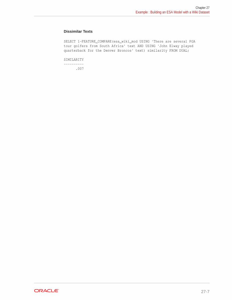
Dissimilar Texts
SELECT 1-FEATURE_COMPARE(esa_wiki_mod USING 'There are several PGA tour golfers from South Africa' text AND USING 'John Elway played quarterback for the Denver Broncos' text) similarity FROM DUAL;
SIMILARITY---------- .007
Chapter 27Example : Building an ESA Model with a Wiki Dataset
27-7
28About the Data Mining API
Overview of the Oracle Data Mining application programming interface (API)components.
• About Mining Models
• Data Mining Data Dictionary Views
• Data Mining PL/SQL Packages
• Data Mining SQL Scoring Functions
28.1 About Mining ModelsMining models are database schema objects that perform data mining.
As with all schema objects, access to mining models is controlled by databaseprivileges. Models can be exported and imported. They support comments, and theycan be tracked in the Database auditing system.
Mining models are created by the CREATE_MODEL procedure in the DBMS_DATA_MININGPL/SQL package. Models are created for a specific mining function, and they usea specific algorithm to perform that function. Mining function is a data mining termthat refers to a class of mining problems to be solved. Examples of mining functionsare: regression, classification, attribute importance, clustering, anomaly detection, andfeature extraction. Oracle Data Mining supports one or more algorithms for eachmining function.
Note:
Most types of mining models can be used to score data. However, it ispossible to score data without applying a model. Dynamic scoring andpredictive analytics return scoring results without a user-supplied model.They create and apply transient models that are not visible to you.
Related Topics
• Dynamic Scoring
• DBMS_PREDICTIVE_ANALYTICSUnderstand the routines of DBMS_PREDICTIVE_ANALYTICS package.
• Creating a ModelExplains how to create data mining models and query model details.
• Administrative Tasks for Oracle Data MiningExplains how to perform administrative tasks related to Oracle Data Mining.
28-1

28.2 Data Mining Data Dictionary ViewsLists Oracle Data Mining data dictionary views.
The data dictionary views for Oracle Data Mining are listed in the following table. Adatabase administrator (DBA) and USER versions of the views are also available.
Table 28-1 Data Dictionary Views for Oracle Data Mining
View Name Description
ALL_MINING_MODELS Provides information about all accessible mining models
ALL_MINING_MODEL_ATTRIBUTES
Provides information about the attributes of allaccessible mining models
ALL_MINING_MODEL_PARTITIONS
Provides information about the partitions of allaccessible partitioned mining models
ALL_MINING_MODEL_SETTINGS
Provides information about the configuration settings forall accessible mining models
ALL_MINING_MODEL_VIEWS Provides information about the model views for allaccessible mining models
ALL_MINING_MODEL_XFORMS Provides the user-specified transformations embedded inall accessible mining models.
28.2.1 ALL_MINING_MODELSDescribes an example of ALL_MINING_MODELS and shows a sample query.
The following example describes ALL_MINING_MODELS and shows a sample query.
Example 28-1 ALL_MINING_MODELS
describe ALL_MINING_MODELS Name Null? Type ----------------------------------------- -------- ---------------------------- OWNER NOT NULL VARCHAR2(128) MODEL_NAME NOT NULL VARCHAR2(128) MINING_FUNCTION VARCHAR2(30) ALGORITHM VARCHAR2(30) CREATION_DATE NOT NULL DATE BUILD_DURATION NUMBER MODEL_SIZE NUMBER PARTITIONED VARCHAR2(3) COMMENTS VARCHAR2(4000)
The following query returns the models accessible to you that use the Support VectorMachine algorithm.
SELECT mining_function, model_name FROM all_mining_models WHERE algorithm = 'SUPPORT_VECTOR_MACHINES' ORDER BY mining_function, model_name;
Chapter 28Data Mining Data Dictionary Views
28-2

MINING_FUNCTION MODEL_NAME ------------------------- -------------------- CLASSIFICATION PART2_CLAS_SAMPLE CLASSIFICATION PART_CLAS_SAMPLE CLASSIFICATION SVMC_SH_CLAS_SAMPLE CLASSIFICATION SVMO_SH_CLAS_SAMPLE CLASSIFICATION T_SVM_CLAS_SAMPLE REGRESSION SVMR_SH_REGR_SAMPLE
Related Topics
• Creating a ModelExplains how to create data mining models and query model details.
• Oracle Database Reference
28.2.2 ALL_MINING_MODEL_ATTRIBUTESDescribes an example of ALL_MINING_MODEL_ATTRIBUTES and shows a sample query.
The following example describes ALL_MINING_MODEL_ATTRIBUTES and shows a samplequery. Attributes are the predictors or conditions that are used to create models andscore data.
Example 28-2 ALL_MINING_MODEL_ATTRIBUTES
describe ALL_MINING_MODEL_ATTRIBUTES Name Null? Type ----------------------------------------- -------- ---------------------------- OWNER NOT NULL VARCHAR2(128) MODEL_NAME NOT NULL VARCHAR2(128) ATTRIBUTE_NAME NOT NULL VARCHAR2(128) ATTRIBUTE_TYPE VARCHAR2(11) DATA_TYPE VARCHAR2(106) DATA_LENGTH NUMBER DATA_PRECISION NUMBER DATA_SCALE NUMBER USAGE_TYPE VARCHAR2(8) TARGET VARCHAR2(3) ATTRIBUTE_SPEC VARCHAR2(4000)
The following query returns the attributes of an SVM classification model namedT_SVM_CLAS_SAMPLE. The model has both categorical and numerical attributes andincludes one attribute that is unstructured text.
SELECT attribute_name, attribute_type, target FROM all_mining_model_attributes WHERE model_name = 'T_SVM_CLAS_SAMPLE' ORDER BY attribute_name;
ATTRIBUTE_NAME ATTRIBUTE_TYPE TAR ------------------------- -------------------- --- AFFINITY_CARD CATEGORICAL YES AGE NUMERICAL NO BOOKKEEPING_APPLICATION NUMERICAL NO BULK_PACK_DISKETTES NUMERICAL NO COMMENTS TEXT NO COUNTRY_NAME CATEGORICAL NO CUST_GENDER CATEGORICAL NO CUST_INCOME_LEVEL CATEGORICAL NO
Chapter 28Data Mining Data Dictionary Views
28-3

CUST_MARITAL_STATUS CATEGORICAL NO EDUCATION CATEGORICAL NO FLAT_PANEL_MONITOR NUMERICAL NO HOME_THEATER_PACKAGE NUMERICAL NO HOUSEHOLD_SIZE CATEGORICAL NO OCCUPATION CATEGORICAL NO OS_DOC_SET_KANJI NUMERICAL NO PRINTER_SUPPLIES NUMERICAL NO YRS_RESIDENCE NUMERICAL NO Y_BOX_GAMES NUMERICAL NO
Related Topics
• About the Data Mining APIOverview of the Oracle Data Mining application programming interface (API)components.
• Oracle Database Reference
28.2.3 ALL_MINING_MODEL_PARTITIONSDescribes an example of ALL_MINING_MODEL_PARTITIONS and shows a sample query.
The following example describes ALL_MINING_MODEL_PARTITIONS and shows a samplequery.
Example 28-3 ALL_MINING_MODEL_PARTITIONS
describe ALL_MINING_MODEL_PARTITIONS Name Null? Type ----------------------------------------- -------- ---------------------------- OWNER NOT NULL VARCHAR2(128) MODEL_NAME NOT NULL VARCHAR2(128) PARTITION_NAME VARCHAR2(128) POSITION NUMBER COLUMN_NAME NOT NULL VARCHAR2(128) COLUMN_VALUE VARCHAR2(4000)
The following query returns the partition names and partition key values for twopartitioned models. Model PART2_CLAS_SAMPLE has a two column partition key withsystem-generated partition names.
SELECT model_name, partition_name, position, column_name, column_value FROM all_mining_model_partitions ORDER BY model_name, partition_name, position;
MODEL_NAME PARTITION_ POSITION COLUMN_NAME COLUMN_VALUE -------------------- ---------- -------- -------------------- --------------- PART2_CLAS_SAMPLE DM$$_P0 1 CUST_GENDER F PART2_CLAS_SAMPLE DM$$_P0 2 CUST_INCOME_LEVEL HIGH PART2_CLAS_SAMPLE DM$$_P1 1 CUST_GENDER F PART2_CLAS_SAMPLE DM$$_P1 2 CUST_INCOME_LEVEL LOW
Chapter 28Data Mining Data Dictionary Views
28-4

PART2_CLAS_SAMPLE DM$$_P2 1 CUST_GENDER F PART2_CLAS_SAMPLE DM$$_P2 2 CUST_INCOME_LEVEL MEDIUM PART2_CLAS_SAMPLE DM$$_P3 1 CUST_GENDER M PART2_CLAS_SAMPLE DM$$_P3 2 CUST_INCOME_LEVEL HIGH PART2_CLAS_SAMPLE DM$$_P4 1 CUST_GENDER M PART2_CLAS_SAMPLE DM$$_P4 2 CUST_INCOME_LEVEL LOW PART2_CLAS_SAMPLE DM$$_P5 1 CUST_GENDER M PART2_CLAS_SAMPLE DM$$_P5 2 CUST_INCOME_LEVEL MEDIUM PART_CLAS_SAMPLE F 1 CUST_GENDER F PART_CLAS_SAMPLE M 1 CUST_GENDER M PART_CLAS_SAMPLE U 1 CUST_GENDER U
Related Topics
• Oracle Database Reference
28.2.4 ALL_MINING_MODEL_SETTINGSDescribes an example of ALL_MINING_MODEL_SETTINGS and shows a sample query.
The following example describes ALL_MINING_MODEL_SETTINGS and shows a samplequery. Settings influence model behavior. Settings may be specific to an algorithm orto a mining function, or they may be general.
Example 28-4 ALL_MINING_MODEL_SETTINGS
describe ALL_MINING_MODEL_SETTINGS Name Null? Type ----------------------------------------- -------- ---------------------------- OWNER NOT NULL VARCHAR2(128) MODEL_NAME NOT NULL VARCHAR2(128) SETTING_NAME NOT NULL VARCHAR2(30) SETTING_VALUE VARCHAR2(4000) SETTING_TYPE VARCHAR2(7)
The following query returns the settings for a model named SVD_SH_SAMPLE. The modeluses the Singular Value Decomposition algorithm for feature extraction.
SELECT setting_name, setting_value, setting_type FROM all_mining_model_settings WHERE model_name = 'SVD_SH_SAMPLE' ORDER BY setting_name;
SETTING_NAME SETTING_VALUE SETTING ------------------------------ ------------------------------ ------- ALGO_NAME ALGO_SINGULAR_VALUE_DECOMP INPUT ODMS_MISSING_VALUE_TREATMENT ODMS_MISSING_VALUE_AUTO DEFAULT ODMS_SAMPLING ODMS_SAMPLING_DISABLE DEFAULT
Chapter 28Data Mining Data Dictionary Views
28-5
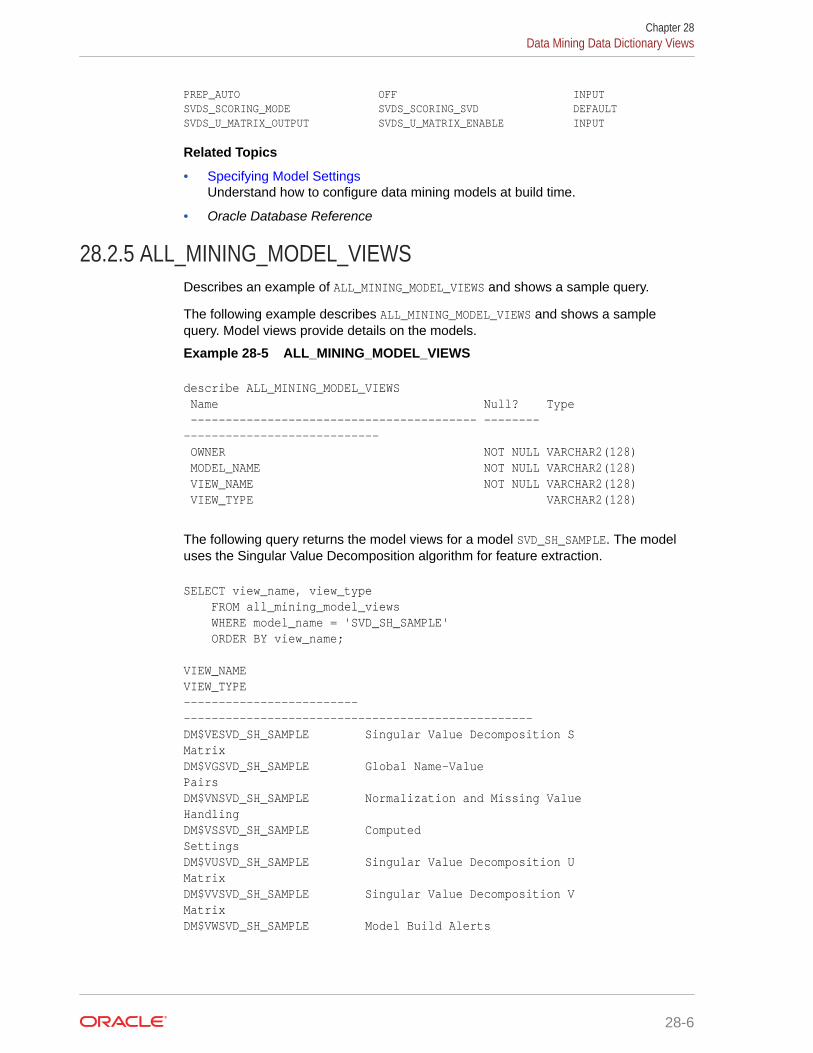
PREP_AUTO OFF INPUT SVDS_SCORING_MODE SVDS_SCORING_SVD DEFAULT SVDS_U_MATRIX_OUTPUT SVDS_U_MATRIX_ENABLE INPUT
Related Topics
• Specifying Model SettingsUnderstand how to configure data mining models at build time.
• Oracle Database Reference
28.2.5 ALL_MINING_MODEL_VIEWSDescribes an example of ALL_MINING_MODEL_VIEWS and shows a sample query.
The following example describes ALL_MINING_MODEL_VIEWS and shows a samplequery. Model views provide details on the models.
Example 28-5 ALL_MINING_MODEL_VIEWS
describe ALL_MINING_MODEL_VIEWS Name Null? Type ----------------------------------------- -------- ---------------------------- OWNER NOT NULL VARCHAR2(128) MODEL_NAME NOT NULL VARCHAR2(128) VIEW_NAME NOT NULL VARCHAR2(128) VIEW_TYPE VARCHAR2(128)
The following query returns the model views for a model SVD_SH_SAMPLE. The modeluses the Singular Value Decomposition algorithm for feature extraction.
SELECT view_name, view_type FROM all_mining_model_views WHERE model_name = 'SVD_SH_SAMPLE' ORDER BY view_name;
VIEW_NAME VIEW_TYPE ------------------------- -------------------------------------------------- DM$VESVD_SH_SAMPLE Singular Value Decomposition S Matrix DM$VGSVD_SH_SAMPLE Global Name-Value Pairs DM$VNSVD_SH_SAMPLE Normalization and Missing Value Handling DM$VSSVD_SH_SAMPLE Computed Settings DM$VUSVD_SH_SAMPLE Singular Value Decomposition U Matrix DM$VVSVD_SH_SAMPLE Singular Value Decomposition V Matrix DM$VWSVD_SH_SAMPLE Model Build Alerts
Chapter 28Data Mining Data Dictionary Views
28-6
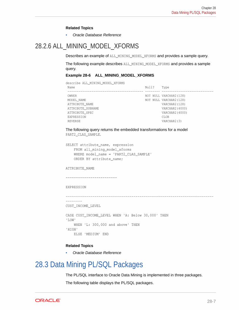
Related Topics
• Oracle Database Reference
28.2.6 ALL_MINING_MODEL_XFORMSDescribes an example of ALL_MINING_MODEL_XFORMS and provides a sample query.
The following example describes ALL_MINING_MODEL_XFORMS and provides a samplequery.
Example 28-6 ALL_MINING_MODEL_XFORMS
describe ALL_MINING_MODEL_XFORMS Name Null? Type ----------------------------------------- -------- ---------------------------- OWNER NOT NULL VARCHAR2(128) MODEL_NAME NOT NULL VARCHAR2(128) ATTRIBUTE_NAME VARCHAR2(128) ATTRIBUTE_SUBNAME VARCHAR2(4000) ATTRIBUTE_SPEC VARCHAR2(4000) EXPRESSION CLOB REVERSE VARCHAR2(3)
The following query returns the embedded transformations for a modelPART2_CLAS_SAMPLE.
SELECT attribute_name, expression FROM all_mining_model_xforms WHERE model_name = 'PART2_CLAS_SAMPLE' ORDER BY attribute_name;
ATTRIBUTE_NAME ------------------------- EXPRESSION --------------------------------------------------------------------------------CUST_INCOME_LEVEL CASE CUST_INCOME_LEVEL WHEN 'A: Below 30,000' THEN 'LOW' WHEN 'L: 300,000 and above' THEN 'HIGH' ELSE 'MEDIUM' END
Related Topics
• Oracle Database Reference
28.3 Data Mining PL/SQL PackagesThe PL/SQL interface to Oracle Data Mining is implemented in three packages.
The following table displays the PL/SQL packages.
Chapter 28Data Mining PL/SQL Packages
28-7

Table 28-2 Data Mining PL/SQL Packages
Package Name Description
DBMS_DATA_MINING Routines for creating and managing mining models
DBMS_DATA_MINING_TRANSFORM Routines for transforming the data for mining
DBMS_PREDICTIVE_ANALYTICS Routines that perform predictive analytics
Related Topics
• DBMS_DATA_MINING
• DBMS_DATA_MINING_TRANSFORM
• DBMS_PREDICTIVE_ANALYTICS
28.3.1 DBMS_DATA_MININGUnderstand the routines of DBMS_DATA_MINING package.
The DBMS_DATA_MINING package contains routines for creating mining models, forperforming operations on mining models, and for querying mining models. Thepackage includes routines for:
• Creating, dropping, and performing other DDL operations on mining models
• Obtaining detailed information about model attributes, rules, and other informationinternal to the model (model details)
• Computing test metrics for classification models
• Specifying costs for classification models
• Exporting and importing models
• Building models using Oracle's native algorithms as well as algorithms written in R
Related Topics
• Oracle Database PL/SQL Packages and Types Reference
28.3.2 DBMS_DATA_MINING_TRANSFORMUnderstand the routines of DBMS_DATA_MINING_TRANSFORM package.
The DBMS_DATA_MINING_TRANSFORM package contains routines that perform datatransformations such as binning, normalization, and outlier treatment. The packageincludes routines for:
• Specifying transformations in a format that can be embedded in a mining model.
• Specifying transformations as relational views (external to mining model objects).
• Specifying distinct properties for columns in the build data. For example, youcan specify that the column must be interpreted as unstructured text, or that thecolumn must be excluded from Automatic Data Preparation.
Chapter 28Data Mining PL/SQL Packages
28-8
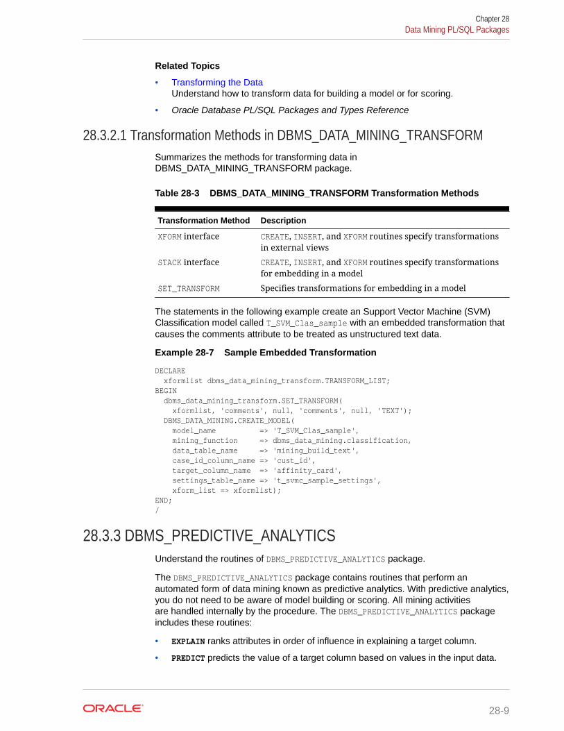
Related Topics
• Transforming the DataUnderstand how to transform data for building a model or for scoring.
• Oracle Database PL/SQL Packages and Types Reference
28.3.2.1 Transformation Methods in DBMS_DATA_MINING_TRANSFORMSummarizes the methods for transforming data inDBMS_DATA_MINING_TRANSFORM package.
Table 28-3 DBMS_DATA_MINING_TRANSFORM Transformation Methods
Transformation Method Description
XFORM interface CREATE, INSERT, and XFORM routines specify transformationsin external views
STACK interface CREATE, INSERT, and XFORM routines specify transformationsfor embedding in a model
SET_TRANSFORM Specifies transformations for embedding in a model
The statements in the following example create an Support Vector Machine (SVM)Classification model called T_SVM_Clas_sample with an embedded transformation thatcauses the comments attribute to be treated as unstructured text data.
Example 28-7 Sample Embedded Transformation
DECLARE xformlist dbms_data_mining_transform.TRANSFORM_LIST;BEGIN dbms_data_mining_transform.SET_TRANSFORM( xformlist, 'comments', null, 'comments', null, 'TEXT'); DBMS_DATA_MINING.CREATE_MODEL( model_name => 'T_SVM_Clas_sample', mining_function => dbms_data_mining.classification, data_table_name => 'mining_build_text', case_id_column_name => 'cust_id', target_column_name => 'affinity_card', settings_table_name => 't_svmc_sample_settings', xform_list => xformlist);END;/
28.3.3 DBMS_PREDICTIVE_ANALYTICSUnderstand the routines of DBMS_PREDICTIVE_ANALYTICS package.
The DBMS_PREDICTIVE_ANALYTICS package contains routines that perform anautomated form of data mining known as predictive analytics. With predictive analytics,you do not need to be aware of model building or scoring. All mining activitiesare handled internally by the procedure. The DBMS_PREDICTIVE_ANALYTICS packageincludes these routines:
• EXPLAIN ranks attributes in order of influence in explaining a target column.
• PREDICT predicts the value of a target column based on values in the input data.
Chapter 28Data Mining PL/SQL Packages
28-9
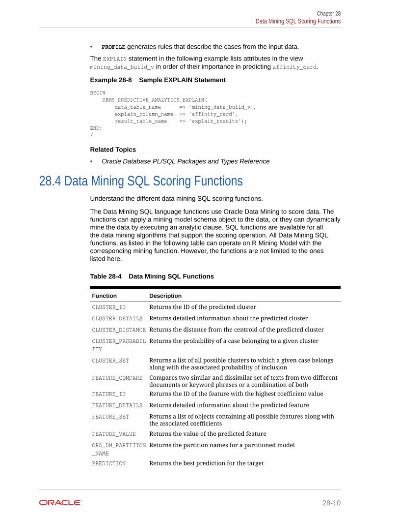
• PROFILE generates rules that describe the cases from the input data.
The EXPLAIN statement in the following example lists attributes in the viewmining_data_build_v in order of their importance in predicting affinity_card.
Example 28-8 Sample EXPLAIN Statement
BEGIN DBMS_PREDICTIVE_ANALYTICS.EXPLAIN( data_table_name => 'mining_data_build_v', explain_column_name => 'affinity_card', result_table_name => 'explain_results'); END; /
Related Topics
• Oracle Database PL/SQL Packages and Types Reference
28.4 Data Mining SQL Scoring FunctionsUnderstand the different data mining SQL scoring functions.
The Data Mining SQL language functions use Oracle Data Mining to score data. Thefunctions can apply a mining model schema object to the data, or they can dynamicallymine the data by executing an analytic clause. SQL functions are available for allthe data mining algorithms that support the scoring operation. All Data Mining SQLfunctions, as listed in the following table can operate on R Mining Model with thecorresponding mining function. However, the functions are not limited to the oneslisted here.
Table 28-4 Data Mining SQL Functions
Function Description
CLUSTER_ID Returns the ID of the predicted cluster
CLUSTER_DETAILS Returns detailed information about the predicted cluster
CLUSTER_DISTANCE Returns the distance from the centroid of the predicted cluster
CLUSTER_PROBABILITY
Returns the probability of a case belonging to a given cluster
CLUSTER_SET Returns a list of all possible clusters to which a given case belongsalong with the associated probability of inclusion
FEATURE_COMPARE Compares two similar and dissimilar set of texts from two differentdocuments or keyword phrases or a combination of both
FEATURE_ID Returns the ID of the feature with the highest coefficient value
FEATURE_DETAILS Returns detailed information about the predicted feature
FEATURE_SET Returns a list of objects containing all possible features along withthe associated coefficients
FEATURE_VALUE Returns the value of the predicted feature
ORA_DM_PARTITION_NAME
Returns the partition names for a partitioned model
PREDICTION Returns the best prediction for the target
Chapter 28Data Mining SQL Scoring Functions
28-10

Table 28-4 (Cont.) Data Mining SQL Functions
Function Description
PREDICTION_BOUNDS
(GLM only) Returns the upper and lower bounds of the intervalwherein the predicted values (linear regression) or probabilities(logistic regression) lie.
PREDICTION_COST Returns a measure of the cost of incorrect predictions
PREDICTION_DETAILS
Returns detailed information about the prediction
PREDICTION_PROBABILITY
Returns the probability of the prediction
PREDICTION_SET Returns the results of a classification model, including thepredictions and associated probabilities for each case
The following example shows a query that returns the results of the CLUSTER_IDfunction. The query applies the model em_sh_clus_sample, which finds groups ofcustomers that share certain characteristics. The query returns the identifiers of theclusters and the number of customers in each cluster.
Example 28-9 CLUSTER_ID Function
-- -List the clusters into which the customers in this-- -data set have been grouped.--SELECT CLUSTER_ID(em_sh_clus_sample USING *) AS clus, COUNT(*) AS cnt FROM mining_data_apply_vGROUP BY CLUSTER_ID(em_sh_clus_sample USING *)ORDER BY cnt DESC;
SQL> -- List the clusters into which the customers in thisSQL> -- data set have been grouped.SQL> --SQL> SELECT CLUSTER_ID(em_sh_clus_sample USING *) AS clus, COUNT(*) AS cnt 2 FROM mining_data_apply_v 3 GROUP BY CLUSTER_ID(em_sh_clus_sample USING *) 4 ORDER BY cnt DESC; CLUS CNT---------- ---------- 9 311 3 294 7 215 12 201 17 123 16 114 14 86 19 64 15 56 18 36
Related Topics
• Scoring and DeploymentExplains the scoring and deployment features of Oracle Data Mining.
Chapter 28Data Mining SQL Scoring Functions
28-11

• Oracle Database SQL Language Reference
Chapter 28Data Mining SQL Scoring Functions
28-12

29Preparing the Data
Learn how to create a table or view that can be used to build a model.
• Data Requirements
• About Attributes
• Using Nested Data
• Using Market Basket Data
• Using Retail Analysis Data
• Handling Missing Values
29.1 Data RequirementsUnderstand how data is stored and viewed for data mining.
Data mining activities require data that is defined within a single table or view. Theinformation for each record must be stored in a separate row. The data records arecommonly called cases. Each case can optionally be identified by a unique case ID.The table or view itself can be referred to as a case table.
The CUSTOMERS table in the SH schema is an example of a table that could be used formining. All the information for each customer is contained in a single row. The caseID is the CUST_ID column. The rows listed in the following example are selected fromSH.CUSTOMERS.
Note:
Oracle Data Mining requires single-record case data for all types of modelsexcept association models, which can be built on native transactional data.
Example 29-1 Sample Case Table
SQL> select cust_id, cust_gender, cust_year_of_birth, cust_main_phone_number from sh.customers where cust_id < 11;
CUST_ID CUST_GENDER CUST_YEAR_OF_BIRTH CUST_MAIN_PHONE_NUMBER------- ----------- ---- ------------- -------------------------1 M 1946 127-379-89542 F 1957 680-327-14193 M 1939 115-509-33914 M 1934 577-104-27925 M 1969 563-667-77316 F 1925 682-732-72607 F 1986 648-272-61818 F 1964 234-693-8728
29-1
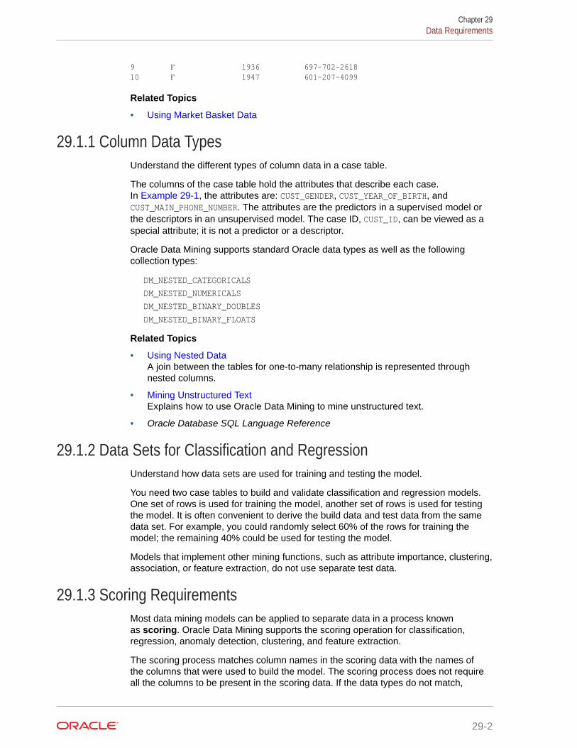
9 F 1936 697-702-261810 F 1947 601-207-4099
Related Topics
• Using Market Basket Data
29.1.1 Column Data TypesUnderstand the different types of column data in a case table.
The columns of the case table hold the attributes that describe each case.In Example 29-1, the attributes are: CUST_GENDER, CUST_YEAR_OF_BIRTH, andCUST_MAIN_PHONE_NUMBER. The attributes are the predictors in a supervised model orthe descriptors in an unsupervised model. The case ID, CUST_ID, can be viewed as aspecial attribute; it is not a predictor or a descriptor.
Oracle Data Mining supports standard Oracle data types as well as the followingcollection types:
DM_NESTED_CATEGORICALS
DM_NESTED_NUMERICALS
DM_NESTED_BINARY_DOUBLES
DM_NESTED_BINARY_FLOATS
Related Topics
• Using Nested DataA join between the tables for one-to-many relationship is represented throughnested columns.
• Mining Unstructured TextExplains how to use Oracle Data Mining to mine unstructured text.
• Oracle Database SQL Language Reference
29.1.2 Data Sets for Classification and RegressionUnderstand how data sets are used for training and testing the model.
You need two case tables to build and validate classification and regression models.One set of rows is used for training the model, another set of rows is used for testingthe model. It is often convenient to derive the build data and test data from the samedata set. For example, you could randomly select 60% of the rows for training themodel; the remaining 40% could be used for testing the model.
Models that implement other mining functions, such as attribute importance, clustering,association, or feature extraction, do not use separate test data.
29.1.3 Scoring RequirementsMost data mining models can be applied to separate data in a process knownas scoring. Oracle Data Mining supports the scoring operation for classification,regression, anomaly detection, clustering, and feature extraction.
The scoring process matches column names in the scoring data with the names ofthe columns that were used to build the model. The scoring process does not requireall the columns to be present in the scoring data. If the data types do not match,
Chapter 29Data Requirements
29-2

Oracle Data Mining attempts to perform type coercion. For example, if a column calledPRODUCT_RATING is VARCHAR2 in the training data but NUMBER in the scoring data, OracleData Mining effectively applies a TO_CHAR() function to convert it.
The column in the test or scoring data must undergo the same transformations as thecorresponding column in the build data. For example, if the AGE column in the builddata was transformed from numbers to the values CHILD, ADULT, and SENIOR, thenthe AGE column in the scoring data must undergo the same transformation so that themodel can properly evaluate it.
Note:
Oracle Data Mining can embed user-specified transformation instructionsin the model and reapply them whenever the model is applied. When thetransformation instructions are embedded in the model, you do not need tospecify them for the test or scoring data sets.
Oracle Data Mining also supports Automatic Data Preparation (ADP). WhenADP is enabled, the transformations required by the algorithm are performedautomatically and embedded in the model along with any user-specifiedtransformations.
See Also:
Transforming the Data for more information on automatic and embeddeddata transformations
29.2 About AttributesAttributes are the items of data that are used in data mining. In predictive models,attributes are the predictors that affect a given outcome. In descriptive models,attributes are the items of information being analyzed for natural groupings orassociations. For example, a table of employee data that contains attributes such asjob title, date of hire, salary, age, gender, and so on.
29.2.1 Data Attributes and Model AttributesData attributes are columns in the data set used to build, test, or score a model.Model attributes are the data representations used internally by the model.
Data attributes and model attributes can be the same. For example, a column calledSIZE, with values S, M, and L, are attributes used by an algorithm to build a model.Internally, the model attribute SIZE is most likely be the same as the data attribute fromwhich it was derived.
On the other hand, a nested column SALES_PROD, containing the sales figures for agroup of products, does not correspond to a model attribute. The data attribute canbe SALES_PROD, but each product with its corresponding sales figure (each row in thenested column) is a model attribute.
Chapter 29About Attributes
29-3

Transformations also cause a discrepancy between data attributes and modelattributes. For example, a transformation can apply a calculation to two data attributesand store the result in a new attribute. The new attribute is a model attribute that hasno corresponding data attribute. Other transformations such as binning, normalization,and outlier treatment, cause the model's representation of an attribute to be differentfrom the data attribute in the case table.
Related Topics
• Using Nested DataA join between the tables for one-to-many relationship is represented throughnested columns.
• Transforming the DataUnderstand how to transform data for building a model or for scoring.
See Also:
29.2.2 Target AttributeUnderstand what a target means in data mining and understand the different targetdata types.
The target of a supervised model is a special kind of attribute. The target columnin the training data contains the historical values used to train the model. The targetcolumn in the test data contains the historical values to which the predictions arecompared. The act of scoring produces a prediction for the target.
Clustering, Feature Extraction, Association, and Anomaly Detection models do not usea target.
Nested columns and columns of unstructured data (such as BFILE, CLOB, or BLOB)cannot be used as targets.
Table 29-1 Target Data Types
Mining Function Target Data Types
Classification VARCHAR2, CHAR
NUMBER, FLOAT
BINARY_DOUBLE, BINARY_FLOAT, ORA_MINING_VARCHAR2_NT
Regression NUMBER, FLOAT
BINARY_DOUBLE, BINARY_FLOAT
You can query the *_MINING_MODEL_ATTRIBUTES view to find the target for a givenmodel.
Related Topics
• ALL_MINING_MODEL_ATTRIBUTESDescribes an example of ALL_MINING_MODEL_ATTRIBUTES and shows a samplequery.
Chapter 29About Attributes
29-4

• Oracle Database PL/SQL Packages and Types Reference
29.2.3 Numericals, Categoricals, and Unstructured TextExplains numeric, categorical, and unstructured text attributes.
Model attributes are numerical, categorical, or unstructured (text). Data attributes,which are columns in a case table, have Oracle data types, as described in "ColumnData Types".
Numerical attributes can theoretically have an infinite number of values. Thevalues have an implicit order, and the differences between them are alsoordered. Oracle Data Mining interprets NUMBER, FLOAT, BINARY_DOUBLE, BINARY_FLOAT,DM_NESTED_NUMERICALS, DM_NESTED_BINARY_DOUBLES, and DM_NESTED_BINARY_FLOATSas numerical.
Categorical attributes have values that identify a finite number of discrete categoriesor classes. There is no implicit order associated with the values. Some categoricalsare binary: they have only two possible values, such as yes or no, or male or female.Other categoricals are multi-class: they have more than two values, such as small,medium, and large.
Oracle Data Mining interprets CHAR and VARCHAR2 as categorical by default, howeverthese columns may also be identified as columns of unstructured data (text). OracleData Mining interprets columns of DM_NESTED_CATEGORICALS as categorical. Columnsof CLOB, BLOB, and BFILE always contain unstructured data.
The target of a classification model is categorical. (If the target of a classificationmodel is numeric, it is interpreted as categorical.) The target of a regression modelis numerical. The target of an attribute importance model is either categorical ornumerical.
Related Topics
• Column Data TypesUnderstand the different types of column data in a case table.
• Mining Unstructured TextExplains how to use Oracle Data Mining to mine unstructured text.
29.2.4 Model SignatureThe model signature is the set of data attributes that are used to build a model.Some or all of the attributes in the signature must be present for scoring. The modelaccounts for any missing columns on a best-effort basis. If columns with the samenames but different data types are present, the model attempts to convert the datatype. If extra, unused columns are present, they are disregarded.
The model signature does not necessarily include all the columns in the build data.Algorithm-specific criteria can cause the model to ignore certain columns. Othercolumns can be eliminated by transformations. Only the data attributes actually usedto build the model are included in the signature.
The target and case ID columns are not included in the signature.
Chapter 29About Attributes
29-5
29.2.5 Scoping of Model Attribute NameThe model attribute name consists of two parts: a column name, and a subcolumnname.
column_name[.subcolumn_name]
The column_name component is the name of the data attribute. It is present in all modelattribute names. Nested attributes and text attributes also have a subcolumn_namecomponent as shown in the following example.
Example 29-2 Model Attributes Derived from a Nested Column
The nested column SALESPROD has three rows.
SALESPROD(ATTRIBUTE_NAME, VALUE)--------------------------------((PROD1, 300), (PROD2, 245), (PROD3, 679))
The name of the data attribute is SALESPROD. Its associated model attributes are:
SALESPROD.PROD1SALESPROD.PROD2SALESPROD.PROD3
29.2.6 Model DetailsModel details reveal information about model attributes and their treatment by thealgorithm. Oracle recommends that users leverage the model detail views for therespective algorithm.
Transformation and reverse transformation expressions are associated with modelattributes. Transformations are applied to the data attributes before the algorithmicprocessing that creates the model. Reverse transformations are applied to the modelattributes after the model has been built, so that the model details are expressed in theform of the original data attributes, or as close to it as possible.
Reverse transformations support model transparency. They provide a view of the datathat the algorithm is working with internally but in a format that is meaningful to a user.
Deprecated GET_MODEL_DETAILS
There is a separate GET_MODEL_DETAILS routine for each algorithm. Starting fromOracle Database 12c Release 2, the GET_MODEL_DETAILS are deprecated. Oraclerecommends to use Model Detail Views for the respective algorithms.
Related Topics
• Model Detail ViewsThe GET_* interfaces are replaced by model views, and Oracle recommends thatusers leverage the views instead.
Chapter 29About Attributes
29-6
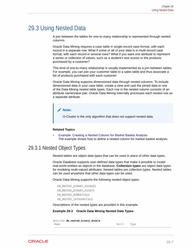
29.3 Using Nested DataA join between the tables for one-to-many relationship is represented through nestedcolumns.
Oracle Data Mining requires a case table in single-record case format, with eachrecord in a separate row. What if some or all of your data is in multi-record caseformat, with each record in several rows? What if you want one attribute to representa series or collection of values, such as a student's test scores or the productspurchased by a customer?
This kind of one-to-many relationship is usually implemented as a join between tables.For example, you can join your customer table to a sales table and thus associate alist of products purchased with each customer.
Oracle Data Mining supports dimensioned data through nested columns. To includedimensioned data in your case table, create a view and cast the joined data to oneof the Data Mining nested table types. Each row in the nested column consists of anattribute name/value pair. Oracle Data Mining internally processes each nested row asa separate attribute.
Note:
O-Cluster is the only algorithm that does not support nested data.
Related Topics
• Example: Creating a Nested Column for Market Basket AnalysisThe example shows how to define a nested column for market basket analysis.
29.3.1 Nested Object TypesNested tables are object data types that can be used in place of other data types.
Oracle Database supports user-defined data types that make it possible to modelreal-world entities as objects in the database. Collection types are object data typesfor modeling multi-valued attributes. Nested tables are collection types. Nested tablescan be used anywhere that other data types can be used.
Oracle Data Mining supports the following nested object types:
DM_NESTED_BINARY_DOUBLES
DM_NESTED_BINARY_FLOATS
DM_NESTED_NUMERICALS
DM_NESTED_CATEGORICALS
Descriptions of the nested types are provided in this example.
Example 29-3 Oracle Data Mining Nested Data Types
describe dm_nested_binary_double Name Null? Type ----------------------------------------- -------- ----------------------------
Chapter 29Using Nested Data
29-7
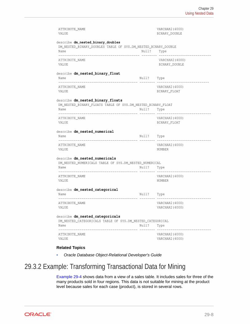
ATTRIBUTE_NAME VARCHAR2(4000) VALUE BINARY_DOUBLE
describe dm_nested_binary_doubles DM_NESTED_BINARY_DOUBLES TABLE OF SYS.DM_NESTED_BINARY_DOUBLE Name Null? Type ------------------------------------------ -------- --------------------------- ATTRIBUTE_NAME VARCHAR2(4000) VALUE BINARY_DOUBLE
describe dm_nested_binary_float Name Null? Type ----------------------------------------- -------- --------------------------- ATTRIBUTE_NAME VARCHAR2(4000) VALUE BINARY_FLOAT describe dm_nested_binary_floats DM_NESTED_BINARY_FLOATS TABLE OF SYS.DM_NESTED_BINARY_FLOAT Name Null? Type ----------------------------------------- -------- ---------------------------- ATTRIBUTE_NAME VARCHAR2(4000) VALUE BINARY_FLOAT
describe dm_nested_numerical Name Null? Type ----------------------------------------- -------- ---------------------------- ATTRIBUTE_NAME VARCHAR2(4000) VALUE NUMBER describe dm_nested_numericals DM_NESTED_NUMERICALS TABLE OF SYS.DM_NESTED_NUMERICAL Name Null? Type ----------------------------------------- -------- ---------------------------- ATTRIBUTE_NAME VARCHAR2(4000) VALUE NUMBER
describe dm_nested_categorical Name Null? Type ----------------------------------------- -------- ---------------------------- ATTRIBUTE_NAME VARCHAR2(4000) VALUE VARCHAR2(4000) describe dm_nested_categoricals DM_NESTED_CATEGORICALS TABLE OF SYS.DM_NESTED_CATEGORICAL Name Null? Type ----------------------------------------- -------- ---------------------------- ATTRIBUTE_NAME VARCHAR2(4000) VALUE VARCHAR2(4000)
Related Topics
• Oracle Database Object-Relational Developer's Guide
29.3.2 Example: Transforming Transactional Data for MiningExample 29-4 shows data from a view of a sales table. It includes sales for three of themany products sold in four regions. This data is not suitable for mining at the productlevel because sales for each case (product), is stored in several rows.
Chapter 29Using Nested Data
29-8
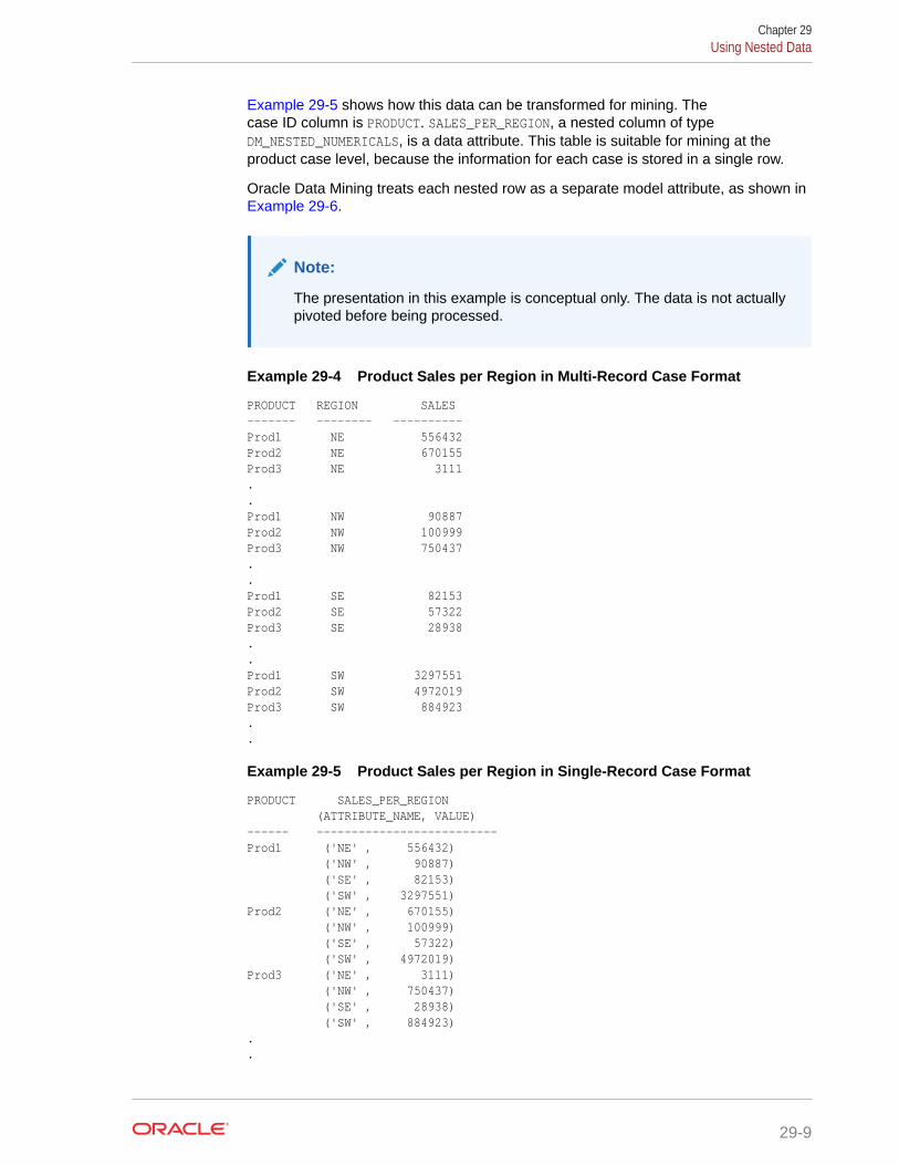
Example 29-5 shows how this data can be transformed for mining. Thecase ID column is PRODUCT. SALES_PER_REGION, a nested column of typeDM_NESTED_NUMERICALS, is a data attribute. This table is suitable for mining at theproduct case level, because the information for each case is stored in a single row.
Oracle Data Mining treats each nested row as a separate model attribute, as shown inExample 29-6.
Note:
The presentation in this example is conceptual only. The data is not actuallypivoted before being processed.
Example 29-4 Product Sales per Region in Multi-Record Case Format
PRODUCT REGION SALES------- -------- ----------Prod1 NE 556432Prod2 NE 670155Prod3 NE 3111..Prod1 NW 90887Prod2 NW 100999Prod3 NW 750437..Prod1 SE 82153Prod2 SE 57322Prod3 SE 28938..Prod1 SW 3297551Prod2 SW 4972019Prod3 SW 884923..
Example 29-5 Product Sales per Region in Single-Record Case Format
PRODUCT SALES_PER_REGION (ATTRIBUTE_NAME, VALUE)------ --------------------------Prod1 ('NE' , 556432) ('NW' , 90887) ('SE' , 82153) ('SW' , 3297551)Prod2 ('NE' , 670155) ('NW' , 100999) ('SE' , 57322) ('SW' , 4972019)Prod3 ('NE' , 3111) ('NW' , 750437) ('SE' , 28938) ('SW' , 884923)..
Chapter 29Using Nested Data
29-9
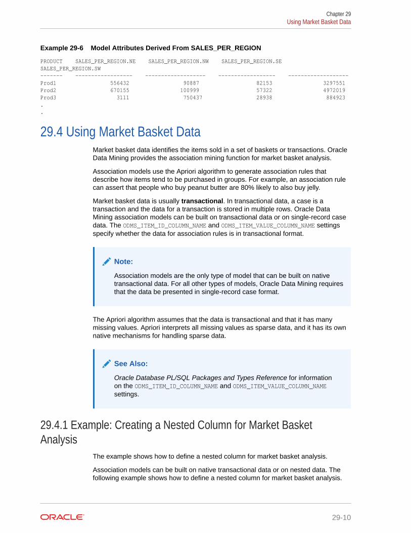
Example 29-6 Model Attributes Derived From SALES_PER_REGION
PRODUCT SALES_PER_REGION.NE SALES_PER_REGION.NW SALES_PER_REGION.SE SALES_PER_REGION.SW ------- ------------------ ------------------- ------------------ -------------------Prod1 556432 90887 82153 3297551Prod2 670155 100999 57322 4972019Prod3 3111 750437 28938 884923..
29.4 Using Market Basket DataMarket basket data identifies the items sold in a set of baskets or transactions. OracleData Mining provides the association mining function for market basket analysis.
Association models use the Apriori algorithm to generate association rules thatdescribe how items tend to be purchased in groups. For example, an association rulecan assert that people who buy peanut butter are 80% likely to also buy jelly.
Market basket data is usually transactional. In transactional data, a case is atransaction and the data for a transaction is stored in multiple rows. Oracle DataMining association models can be built on transactional data or on single-record casedata. The ODMS_ITEM_ID_COLUMN_NAME and ODMS_ITEM_VALUE_COLUMN_NAME settingsspecify whether the data for association rules is in transactional format.
Note:
Association models are the only type of model that can be built on nativetransactional data. For all other types of models, Oracle Data Mining requiresthat the data be presented in single-record case format.
The Apriori algorithm assumes that the data is transactional and that it has manymissing values. Apriori interprets all missing values as sparse data, and it has its ownnative mechanisms for handling sparse data.
See Also:
Oracle Database PL/SQL Packages and Types Reference for informationon the ODMS_ITEM_ID_COLUMN_NAME and ODMS_ITEM_VALUE_COLUMN_NAMEsettings.
29.4.1 Example: Creating a Nested Column for Market BasketAnalysis
The example shows how to define a nested column for market basket analysis.
Association models can be built on native transactional data or on nested data. Thefollowing example shows how to define a nested column for market basket analysis.
Chapter 29Using Market Basket Data
29-10
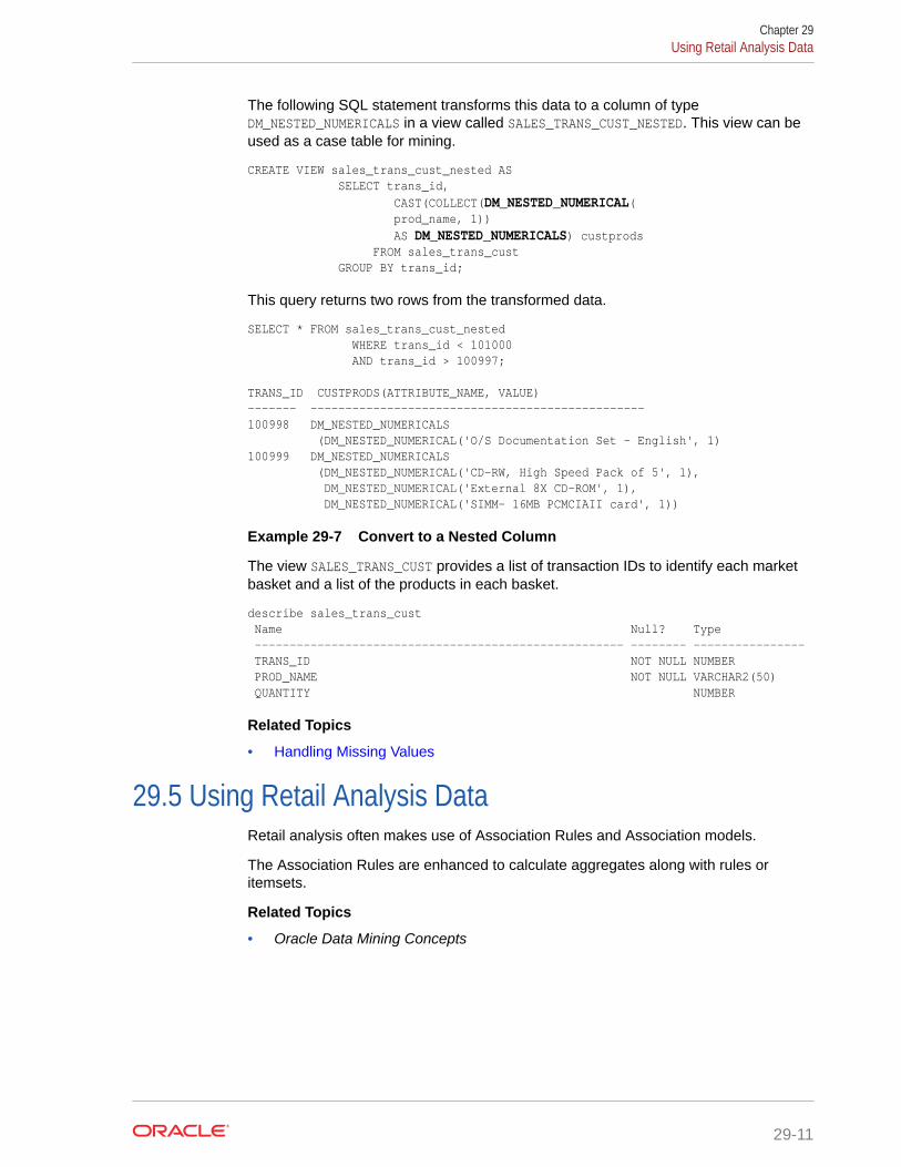
The following SQL statement transforms this data to a column of typeDM_NESTED_NUMERICALS in a view called SALES_TRANS_CUST_NESTED. This view can beused as a case table for mining.
CREATE VIEW sales_trans_cust_nested AS SELECT trans_id, CAST(COLLECT(DM_NESTED_NUMERICAL( prod_name, 1)) AS DM_NESTED_NUMERICALS) custprods FROM sales_trans_cust GROUP BY trans_id;
This query returns two rows from the transformed data.
SELECT * FROM sales_trans_cust_nested WHERE trans_id < 101000 AND trans_id > 100997; TRANS_ID CUSTPRODS(ATTRIBUTE_NAME, VALUE)------- ------------------------------------------------100998 DM_NESTED_NUMERICALS (DM_NESTED_NUMERICAL('O/S Documentation Set - English', 1)100999 DM_NESTED_NUMERICALS (DM_NESTED_NUMERICAL('CD-RW, High Speed Pack of 5', 1), DM_NESTED_NUMERICAL('External 8X CD-ROM', 1), DM_NESTED_NUMERICAL('SIMM- 16MB PCMCIAII card', 1))
Example 29-7 Convert to a Nested Column
The view SALES_TRANS_CUST provides a list of transaction IDs to identify each marketbasket and a list of the products in each basket.
describe sales_trans_cust Name Null? Type ----------------------------------------------------- -------- ---------------- TRANS_ID NOT NULL NUMBER PROD_NAME NOT NULL VARCHAR2(50) QUANTITY NUMBER
Related Topics
• Handling Missing Values
29.5 Using Retail Analysis DataRetail analysis often makes use of Association Rules and Association models.
The Association Rules are enhanced to calculate aggregates along with rules oritemsets.
Related Topics
• Oracle Data Mining Concepts
Chapter 29Using Retail Analysis Data
29-11

29.5.1 Example: Calculating AggregatesThe following example shows the concept of Aggregates.
Calculating Aggregates for Grocery Store Data
Assume a grocery store has the following data:
Table 29-2 Grocery Store Data
Customer Item A Item B Item C Item D
Customer 1 Buys(Profit $5.00)
Buys(Profit $3.20)
Buys(Profit $12.00)
NA
Customer 2 Buys(Profit $4.00)
NA Buys(Profit $4.20)
NA
Customer 3 Buys(Profit $3.00)
Buys(Profit $10.00)
Buys(Profit $14.00)
Buys(Profit $8.00)
Customer 4 Buys(Profit $2.00)
NA NA Buys(Profit $1.00)
The basket of each customer can be viewed as a transaction. The manager of thestore is interested in not only the existence of certain association rules, but also in theaggregated profit if such rules exist.
In this example, one of the association rules can be (A, B)=>C for customer 1 andcustomer 3. Together with this rule, the store manager may want to know the following:
• The total profit of item A appearing in this rule
• The total profit of item B appearing in this rule
• The total profit for consequent C appearing in this rule
• The total profit of all items appearing in the rule
For this rule, the profit for item A is $5.00 + $3.00 = $8.00, for item B the profit is $3.20+ $10.00 = $13.20, for consequent C, the profit is $12.00 + $14.00 = $26.00, for theantecedent itemset (A, B) is $8.00 + $13.20 = $21.20. For the whole rule, the profitis $21.20 + $26.00 = $47.40.
Related Topics
• Oracle Database PL/SQL Packages and Types Reference
29.6 Handling Missing ValuesOracle Data Mining distinguishes between sparse data and data that containsrandom missing values. The latter means that some attribute values are unknown.Sparse data, on the other hand, contains values that are assumed to be known,although they are not represented in the data.
A typical example of sparse data is market basket data. Out of hundreds or thousandsof available items, only a few are present in an individual case (the basket ortransaction). All the item values are known, but they are not all included in the basket.Present values have a quantity, while the items that are not represented are sparse(with a known quantity of zero).
Chapter 29Handling Missing Values
29-12

Oracle Data Mining interprets missing data as follows:
• Missing at random: Missing values in columns with a simple data type (not nested)are assumed to be missing at random.
• Sparse: Missing values in nested columns indicate sparsity.
29.6.1 Examples: Missing Values or Sparse Data?The examples in this section illustrate how Oracle Data Mining identifies data as eithersparse or missing at random.
29.6.1.1 Sparsity in a Sales TableA sales table contains point-of-sale data for a group of products that are sold inseveral stores to different customers over a period of time. A particular customer buysonly a few of the products. The products that the customer does not buy do not appearas rows in the sales table.
If you were to figure out the amount of money a customer has spent for each product,the unpurchased products have an inferred amount of zero. The value is not randomor unknown; it is zero, even though no row appears in the table.
Note that the sales data is dimensioned (by product, stores, customers, and time) andare often represented as nested data for mining.
Since missing values in a nested column always indicate sparsity, you must ensurethat this interpretation is appropriate for the data that you want to mine. For example,when trying to mine a multi-record case data set containing movie ratings from usersof a large movie database, the missing ratings are unknown (missing at random), butOracle Data Mining treats the data as sparse and infer a rating of zero for the missingvalue.
29.6.1.2 Missing Values in a Table of Customer DataA table of customer data contains demographic data about customers. The case IDcolumn is the customer ID. The attributes are age, education, profession, gender,house-hold size, and so on. Not all the data is available for each customer. Anymissing values are considered to be missing at random. For example, if the ageof customer 1 and the profession of customer 2 are not present in the data, thatinformation is simply unknown. It does not indicate sparsity.
Note that the customer data is not dimensioned. There is a one-to-one mappingbetween the case and each of its attributes. None of the attributes are nested.
29.6.2 Missing Value Treatment in Oracle Data MiningMissing value treatment depends on the algorithm and on the nature of the data(categorical or numerical, sparse or missing at random). Missing value treatment issummarized in the following table.
Chapter 29Handling Missing Values
29-13

Note:
Oracle Data Mining performs the same missing value treatment whether ornot Automatic Data Preparation is being used.
Table 29-3 Missing Value Treatment by Algorithm
MissingData
EM, GLM, NMF, k-Means, SVD,SVM
DT, MDL, NB, OC Apriori
NUMERICALmissing atrandom
The algorithm replacesmissing numerical values withthe mean.For Expectation Maximization(EM), the replacement onlyoccurs in columns thatare modeled with Gaussiandistributions.
The algorithm handlesmissing valuesnaturally as missing atrandom.
The algorithminterprets allmissing data assparse.
CATEGORICAL missingat random
Genelized Linear Models(GLM), Non-Negative MatrixFactorization (NMF), k-Means,and Support Vector Machine(SVM) replaces missingcategorical values with themode.Singular Value Decomposition(SVD) does not supportcategorical data.EM does not replace missingcategorical values. EM treatsNULLs as a distinct value withits own frequency count.
The algorithm handlesmissing valuesnaturally as missingrandom.
The algorithminterprets allmissing data assparse.
NUMERICALsparse
The algorithm replaces sparsenumerical data with zeros.
O-Cluster does notsupport nested dataand therefore does notsupport sparse data.Decision Tree (DT),Minimum DescriptionLength (MDL), andNaive Bayes (NB)and replace sparsenumerical data withzeros.
The algorithmhandles sparsedata.
CATEGORICAL sparse
All algorithms except SVDreplace sparse categorical datawith zero vectors. SVD doesnot support categorical data.
O-Cluster does notsupport nested dataand therefore does notsupport sparse data. DT,MDL, and NB replacesparse categorical datawith the special valueDM$SPARSE.
The algorithmhandles sparsedata.
Chapter 29Handling Missing Values
29-14

29.6.3 Changing the Missing Value TreatmentTransform the missing data as sparse or missing at random.
If you want Oracle Data Mining to treat missing data as sparse instead of missing atrandom or missing at random instead of sparse, transform it before building the model.
If you want missing values to be treated as sparse, but Oracle Data Mining interpretsthem as missing at random, you can use a SQL function like NVL to replace thenulls with a value such as "NA". Oracle Data Mining does not perform missing valuetreatment when there is a specified value.
If you want missing nested attributes to be treated as missing at random, you cantransform the nested rows into physical attributes in separate columns — as long asthe case table stays within the 1000 column limitation imposed by the Database. Fill inall of the possible attribute names, and specify them as null. Alternatively, insert rowsin the nested column for all the items that are not present and assign a value such asthe mean or mode to each one.
Related Topics
• Oracle Database SQL Language Reference
Chapter 29Handling Missing Values
29-15

30Transforming the Data
Understand how to transform data for building a model or for scoring.
• About Transformations
• Preparing the Case Table
• Understanding Automatic Data Preparation
• Embedding Transformations in a Model
• Understanding Reverse Transformations
30.1 About TransformationsUnderstand how you can transform data by using Automatic Data Preparation (ADP)and embedded data transformation.
A transformation is a SQL expression that modifies the data in one or more columns.Data must typically undergo certain transformations before it can be used to builda model. Many data mining algorithms have specific transformation requirements.Before data can be scored, it must be transformed in the same way that the trainingdata was transformed.
Oracle Data Mining supports Automatic Data Preparation (ADP), which automaticallyimplements the transformations required by the algorithm. The transformations areembedded in the model and automatically executed whenever the model is applied.
If additional transformations are required, you can specify them as SQL expressionsand supply them as input when you create the model. These transformations areembedded in the model just as they are with ADP.
With automatic and embedded data transformation, most of the work of datapreparation is handled for you. You can create a model and score multiple data sets injust a few steps:
1. Identify the columns to include in the case table.
2. Create nested columns if you want to include transactional data.
3. Write SQL expressions for any transformations not handled by ADP.
4. Create the model, supplying the SQL expressions (if specified) and identifying anycolumns that contain text data.
5. Ensure that some or all of the columns in the scoring data have the same nameand type as the columns used to train the model.
Related Topics
• Scoring Requirements
30-1
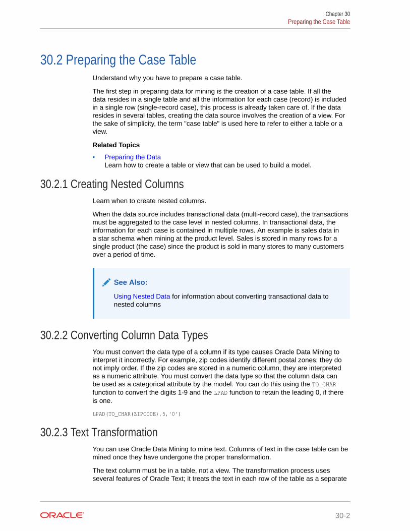
30.2 Preparing the Case TableUnderstand why you have to prepare a case table.
The first step in preparing data for mining is the creation of a case table. If all thedata resides in a single table and all the information for each case (record) is includedin a single row (single-record case), this process is already taken care of. If the dataresides in several tables, creating the data source involves the creation of a view. Forthe sake of simplicity, the term "case table" is used here to refer to either a table or aview.
Related Topics
• Preparing the DataLearn how to create a table or view that can be used to build a model.
30.2.1 Creating Nested ColumnsLearn when to create nested columns.
When the data source includes transactional data (multi-record case), the transactionsmust be aggregated to the case level in nested columns. In transactional data, theinformation for each case is contained in multiple rows. An example is sales data ina star schema when mining at the product level. Sales is stored in many rows for asingle product (the case) since the product is sold in many stores to many customersover a period of time.
See Also:
Using Nested Data for information about converting transactional data tonested columns
30.2.2 Converting Column Data TypesYou must convert the data type of a column if its type causes Oracle Data Mining tointerpret it incorrectly. For example, zip codes identify different postal zones; they donot imply order. If the zip codes are stored in a numeric column, they are interpretedas a numeric attribute. You must convert the data type so that the column data canbe used as a categorical attribute by the model. You can do this using the TO_CHARfunction to convert the digits 1-9 and the LPAD function to retain the leading 0, if thereis one.
LPAD(TO_CHAR(ZIPCODE),5,'0')
30.2.3 Text TransformationYou can use Oracle Data Mining to mine text. Columns of text in the case table can bemined once they have undergone the proper transformation.
The text column must be in a table, not a view. The transformation process usesseveral features of Oracle Text; it treats the text in each row of the table as a separate
Chapter 30Preparing the Case Table
30-2

document. Each document is transformed to a set of text tokens known as terms,which have a numeric value and a text label. The text column is transformed to anested column of DM_NESTED_NUMERICALS.
30.2.4 About Business and Domain-Sensitive TransformationsUnderstand why you need to transform data according to business problems.
Some transformations are dictated by the definition of the business problem. Forexample, you want to build a model to predict high-revenue customers. Since yourrevenue data for current customers is in dollars you need to define what "high-revenue" means. Using some formula that you have developed from past experience,you can recode the revenue attribute into ranges Low, Medium, and High beforebuilding the model.
Another common business transformation is the conversion of date information intoelapsed time. For example, date of birth can be converted to age.
Domain knowledge can be very important in deciding how to prepare the data. Forexample, some algorithms produce unreliable results if the data contains values thatfall far outside of the normal range. In some cases, these values represent errors orabnormalities. In others, they provide meaningful information.
Related Topics
• Outlier Treatment
30.3 Understanding Automatic Data PreparationUnderstand data transformation using Automatic Data Preparation (ADP).
Most algorithms require some form of data transformation. During the model buildprocess, Oracle Data Mining can automatically perform the transformations requiredby the algorithm. You can choose to supplement the automatic transformationswith additional transformations of your own, or you can choose to manage all thetransformations yourself.
In calculating automatic transformations, Oracle Data Mining uses heuristics thataddress the common requirements of a given algorithm. This process results inreasonable model quality in most cases.
Binning, normalization, and outlier treatment are transformations that are commonlyneeded by data mining algorithms.
Related Topics
• Oracle Database PL/SQL Packages and Types Reference
30.3.1 BinningBinning, also called discretization, is a technique for reducing the cardinality ofcontinuous and discrete data. Binning groups related values together in bins to reducethe number of distinct values.
Binning can improve resource utilization and model build response time dramaticallywithout significant loss in model quality. Binning can improve model quality bystrengthening the relationship between attributes.
Chapter 30Understanding Automatic Data Preparation
30-3

Supervised binning is a form of intelligent binning in which important characteristicsof the data are used to determine the bin boundaries. In supervised binning, the binboundaries are identified by a single-predictor decision tree that takes into account thejoint distribution with the target. Supervised binning can be used for both numericaland categorical attributes.
30.3.2 NormalizationNormalization is the most common technique for reducing the range of numerical data.Most normalization methods map the range of a single variable to another range (often0,1).
30.3.3 How ADP Transforms the DataThe following table shows how ADP prepares the data for each algorithm.
Table 30-1 Oracle Data Mining Algorithms With ADP
Algorithm Mining Function Treatment by ADP
Apriori Association Rules ADP has no effect on association rules.
DecisionTree
Classification ADP has no effect on Decision Tree. Data preparation is handled bythe algorithm.
ExpectationMaximization
Clustering Single-column (not nested) numerical columns that are modeledwith Gaussian distributions are normalized with outlier-sensitivenormalization. ADP has no effect on the other types of columns.
GLM Classification andRegression
Numerical attributes are normalized with outlier-sensitivenormalization.
k-Means Clustering Numerical attributes are normalized with outlier-sensitivenormalization.
MDL Attribute Importance All attributes are binned with supervised binning.
NaiveBayes
Classification All attributes are binned with supervised binning.
NMF Feature Extraction Numerical attributes are normalized with outlier-sensitivenormalization.
O-Cluster Clustering Numerical attributes are binned with a specialized form of equi-width binning, which computes the number of bins per attributeautomatically. Numerical columns with all nulls or a single valueare removed.
SVD Feature Extraction Numerical attributes are normalized with outlier-sensitivenormalization.
SVM Classification, AnomalyDetection, andRegression
Numerical attributes are normalized with outlier-sensitivenormalization.
Chapter 30Understanding Automatic Data Preparation
30-4
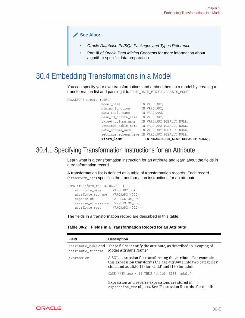
See Also:
• Oracle Database PL/SQL Packages and Types Reference
• Part III of Oracle Data Mining Concepts for more information aboutalgorithm-specific data preparation
30.4 Embedding Transformations in a ModelYou can specify your own transformations and embed them in a model by creating atransformation list and passing it to DBMS_DATA_MINING.CREATE_MODEL.
PROCEDURE create_model( model_name IN VARCHAR2, mining_function IN VARCHAR2, data_table_name IN VARCHAR2, case_id_column_name IN VARCHAR2, target_column_name IN VARCHAR2 DEFAULT NULL, settings_table_name IN VARCHAR2 DEFAULT NULL, data_schema_name IN VARCHAR2 DEFAULT NULL, settings_schema_name IN VARCHAR2 DEFAULT NULL, xform_list IN TRANSFORM_LIST DEFAULT NULL);
30.4.1 Specifying Transformation Instructions for an AttributeLearn what is a transformation instruction for an attribute and learn about the fields ina transformation record.
A transformation list is defined as a table of transformation records. Each record(transform_rec) specifies the transformation instructions for an attribute.
TYPE transform_rec IS RECORD ( attribute_name VARCHAR2(30), attribute_subname VARCHAR2(4000), expression EXPRESSION_REC, reverse_expression EXPRESSION_REC, attribute_spec VARCHAR2(4000));
The fields in a transformation record are described in this table.
Table 30-2 Fields in a Transformation Record for an Attribute
Field Description
attribute_name andattribute_subname
These fields identify the attribute, as described in "Scoping ofModel Attribute Name"
expression A SQL expression for transforming the attribute. For example,this expression transforms the age attribute into two categories:child and adult:[0,19) for 'child' and [19,) for adult
CASE WHEN age < 19 THEN 'child' ELSE 'adult'
Expression and reverse expressions are stored inexpression_rec objects. See "Expression Records" for details.
Chapter 30Embedding Transformations in a Model
30-5
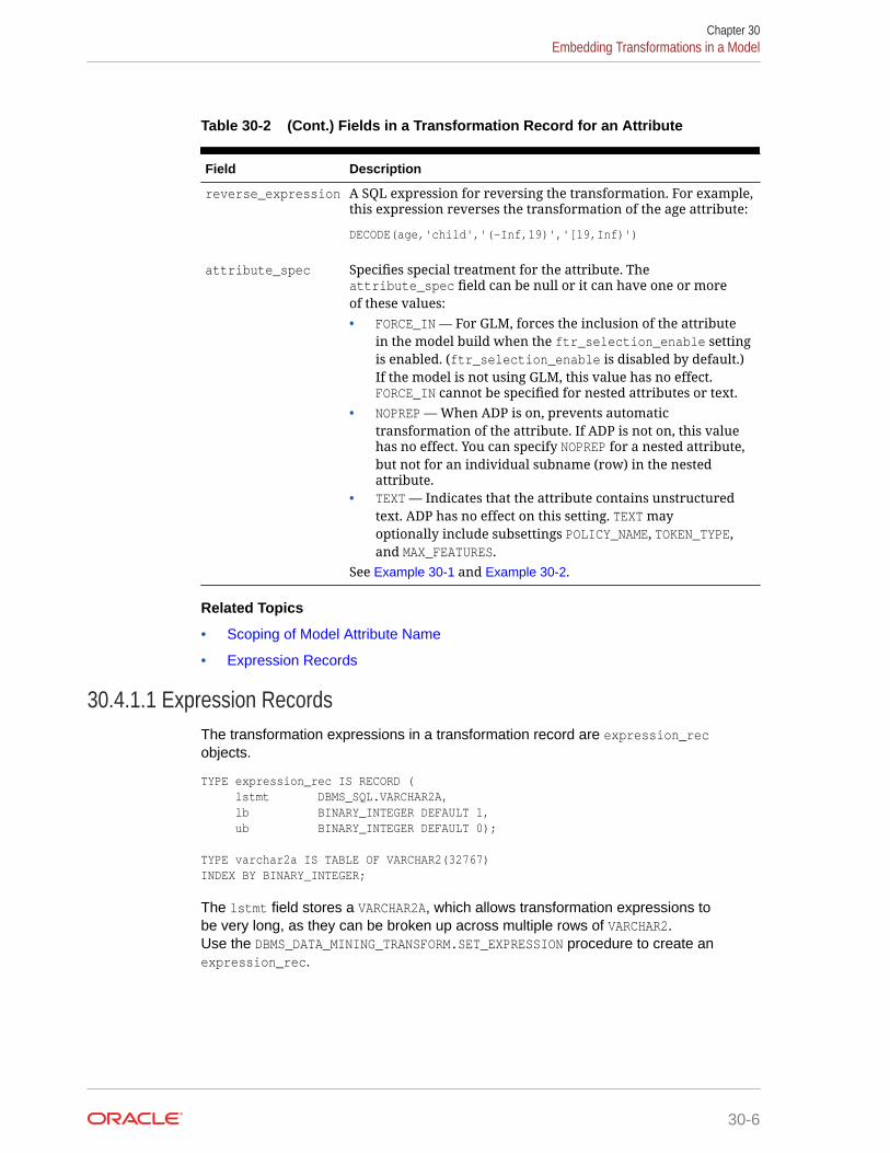
Table 30-2 (Cont.) Fields in a Transformation Record for an Attribute
Field Description
reverse_expression A SQL expression for reversing the transformation. For example,this expression reverses the transformation of the age attribute:
DECODE(age,'child','(-Inf,19)','[19,Inf)')
attribute_spec Specifies special treatment for the attribute. Theattribute_spec field can be null or it can have one or moreof these values:• FORCE_IN — For GLM, forces the inclusion of the attribute
in the model build when the ftr_selection_enable settingis enabled. (ftr_selection_enable is disabled by default.)If the model is not using GLM, this value has no effect.FORCE_IN cannot be specified for nested attributes or text.
• NOPREP — When ADP is on, prevents automatictransformation of the attribute. If ADP is not on, this valuehas no effect. You can specify NOPREP for a nested attribute,but not for an individual subname (row) in the nestedattribute.
• TEXT — Indicates that the attribute contains unstructuredtext. ADP has no effect on this setting. TEXT mayoptionally include subsettings POLICY_NAME, TOKEN_TYPE,and MAX_FEATURES.
See Example 30-1 and Example 30-2.
Related Topics
• Scoping of Model Attribute Name
• Expression Records
30.4.1.1 Expression RecordsThe transformation expressions in a transformation record are expression_recobjects.
TYPE expression_rec IS RECORD ( lstmt DBMS_SQL.VARCHAR2A, lb BINARY_INTEGER DEFAULT 1, ub BINARY_INTEGER DEFAULT 0);
TYPE varchar2a IS TABLE OF VARCHAR2(32767)INDEX BY BINARY_INTEGER;
The lstmt field stores a VARCHAR2A, which allows transformation expressions tobe very long, as they can be broken up across multiple rows of VARCHAR2.Use the DBMS_DATA_MINING_TRANSFORM.SET_EXPRESSION procedure to create anexpression_rec.
Chapter 30Embedding Transformations in a Model
30-6

30.4.1.2 Attribute SpecificationsLearn how to define the characteristics specific to an attribute through attributespecification.
The attribute specification in a transformation record defines characteristics that arespecific to this attribute. If not null, the attribute specification can include valuesFORCE_IN, NOPREP, or TEXT, as described in Table 30-2.
Example 30-1 An Attribute Specification with Multiple Keywords
If more than one attribute specification keyword is applicable, you can provide themin a comma-delimited list. The following expression is the specification for an attributein a GLM model. Assuming that the ftr_selection_enable setting is enabled, thisexpression forces the attribute to be included in the model. If ADP is on, automatictransformation of the attribute is not performed.
"FORCE_IN,NOPREP"
Example 30-2 A Text Attribute Specification
For text attributes, you can optionally specify subsettings POLICY_NAME, TOKEN_TYPE,and MAX_FEATURES. The subsettings provide configuration information that is specific totext transformation. In this example, the transformation instructions for the text contentare defined in a text policy named my_policy with token type is THEME. The maximumnumber of extracted features is 3000.
"TEXT(POLICY_NAME:my_policy)(TOKEN_TYPE:THEME)(MAX_FEATURES:3000)"
Related Topics
• Configuring a Text AttributeLearn how to identify a column as a text attribute and provide transformationinstructions for any text attribute.
30.4.2 Building a Transformation ListA transformation list is a collection of transformation records. When a newtransformation record is added, it is appended to the top of the transformation list.You can use any of the following methods to build a transformation list:
• The SET_TRANFORM procedure in DBMS_DATA_MINING_TRANSFORM
• The STACK interface in DBMS_DATA_MINING_TRANSFORM
• The GET_MODEL_TRANSFORMATIONS and GET_TRANSFORM_LIST functions inDBMS_DATA_MINING
30.4.2.1 SET_TRANSFORMThe SET_TRANSFORM procedure adds a single transformation record to a transformationlist.
DBMS_DATA_MINING_TRANSFORM.SET_TRANSFORM ( xform_list IN OUT NOCOPY TRANSFORM_LIST, attribute_name VARCHAR2, attribute_subname VARCHAR2, expression VARCHAR2,
Chapter 30Embedding Transformations in a Model
30-7
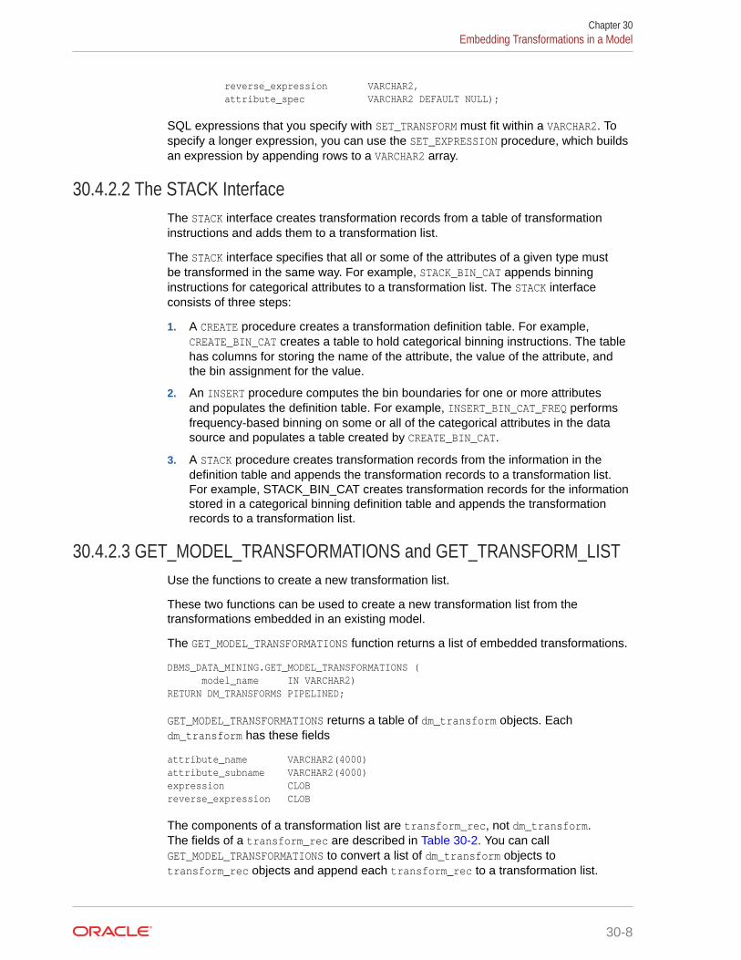
reverse_expression VARCHAR2, attribute_spec VARCHAR2 DEFAULT NULL);
SQL expressions that you specify with SET_TRANSFORM must fit within a VARCHAR2. Tospecify a longer expression, you can use the SET_EXPRESSION procedure, which buildsan expression by appending rows to a VARCHAR2 array.
30.4.2.2 The STACK InterfaceThe STACK interface creates transformation records from a table of transformationinstructions and adds them to a transformation list.
The STACK interface specifies that all or some of the attributes of a given type mustbe transformed in the same way. For example, STACK_BIN_CAT appends binninginstructions for categorical attributes to a transformation list. The STACK interfaceconsists of three steps:
1. A CREATE procedure creates a transformation definition table. For example,CREATE_BIN_CAT creates a table to hold categorical binning instructions. The tablehas columns for storing the name of the attribute, the value of the attribute, andthe bin assignment for the value.
2. An INSERT procedure computes the bin boundaries for one or more attributesand populates the definition table. For example, INSERT_BIN_CAT_FREQ performsfrequency-based binning on some or all of the categorical attributes in the datasource and populates a table created by CREATE_BIN_CAT.
3. A STACK procedure creates transformation records from the information in thedefinition table and appends the transformation records to a transformation list.For example, STACK_BIN_CAT creates transformation records for the informationstored in a categorical binning definition table and appends the transformationrecords to a transformation list.
30.4.2.3 GET_MODEL_TRANSFORMATIONS and GET_TRANSFORM_LISTUse the functions to create a new transformation list.
These two functions can be used to create a new transformation list from thetransformations embedded in an existing model.
The GET_MODEL_TRANSFORMATIONS function returns a list of embedded transformations.
DBMS_DATA_MINING.GET_MODEL_TRANSFORMATIONS ( model_name IN VARCHAR2)RETURN DM_TRANSFORMS PIPELINED;
GET_MODEL_TRANSFORMATIONS returns a table of dm_transform objects. Eachdm_transform has these fields
attribute_name VARCHAR2(4000)attribute_subname VARCHAR2(4000)expression CLOBreverse_expression CLOB
The components of a transformation list are transform_rec, not dm_transform.The fields of a transform_rec are described in Table 30-2. You can callGET_MODEL_TRANSFORMATIONS to convert a list of dm_transform objects totransform_rec objects and append each transform_rec to a transformation list.
Chapter 30Embedding Transformations in a Model
30-8

DBMS_DATA_MINING.GET_TRANSFORM_LIST ( xform_list OUT NOCOPY TRANSFORM_LIST, model_xforms IN DM_TRANSFORMS);
See Also:
"DBMS_DATA_MINING_TRANSFORM Operational Notes","SET_TRANSFORM Procedure", "CREATE_MODEL Procedure", and"GET_MODEL_TRANSFORMATIONS Function" in Oracle DatabasePL/SQL Packages and Types Reference
30.4.3 Transformation Lists and Automatic Data PreparationIf you enable ADP and you specify a transformation list, the transformation list isembedded with the automatic, system-generated transformations. The transformationlist is executed before the automatic transformations.
If you enable ADP and do not specify a transformation list, only the automatictransformations are embedded in the model.
If ADP is disabled (the default) and you specify a transformation list, your customtransformations are embedded in the model. No automatic transformations areperformed.
If ADP is disabled (the default) and you do not specify a transformation list, notransformations is embedded in the model. You have to transform the training, test,and scoring data sets yourself if necessary. You must take care to apply the sametransformations to each data set.
30.4.4 Oracle Data Mining Transformation RoutinesLearn about transformation routines.
Oracle Data Mining provides routines that implement various transformationtechniques in the DBMS_DATA_MINING_TRANSFORM package.
Related Topics
• Oracle Database SQL Language Reference
30.4.4.1 Binning RoutinesExplains Binning techniques in Oracle Data Mining.
A number of factors go into deciding a binning strategy. Having fewer values typicallyleads to a more compact model and one that builds faster, but it can also lead to someloss in accuracy.
Model quality can improve significantly with well-chosen bin boundaries. For example,an appropriate way to bin ages is to separate them into groups of interest, such aschildren 0-13, teenagers 13-19, youth 19-24, working adults 24-35, and so on.
The following table lists the binning techniques provided by Oracle Data Mining:
Chapter 30Embedding Transformations in a Model
30-9

Table 30-3 Binning Methods in DBMS_DATA_MINING_TRANSFORM
Binning Method Description
Top-N Most FrequentItems
You can use this technique to bin categorical attributes.You specify the number of bins. The value that occurs mostfrequently is labeled as the first bin, the value that appearswith the next frequency is labeled as the second bin, and soon. All remaining values are in an additional bin.
Supervised Binning Supervised binning is a form of intelligent binning, wherebin boundaries are derived from important characteristicsof the data. Supervised binning builds a single-predictordecision tree to find the interesting bin boundaries withrespect to a target. It can be used for numerical orcategorical attributes.
Equi-Width Binning You can use equi-width binning for numerical attributes.The range of values is computed by subtracting theminimum value from the maximum value, then the rangeof values is divided into equal intervals. You can specify thenumber of bins or it can be calculated automatically. Equi-width binning must usually be used with outlier treatment.
Quantile Binning Quantile binning is a numerical binning technique.Quantiles are computed using the SQL analytic functionNTILE. The bin boundaries are based on the minimumvalues for each quantile. Bins with equal left and rightboundaries are collapsed, possibly resulting in fewer binsthan requested.
Related Topics
• Routines for Outlier Treatment
30.4.4.2 Normalization RoutinesLearn about Normalization routines in Oracle Data Mining.
Most normalization methods map the range of a single attribute to another range,typically 0 to 1 or -1 to +1.
Normalization is very sensitive to outliers. Without outlier treatment, most values aremapped to a tiny range, resulting in a significant loss of information.
Table 30-4 Normalization Methods in DBMS_DATA_MINING_TRANSFORM
Transformation Description
Min-Max Normalization This technique computes the normalization of an attributeusing the minimum and maximum values. The shift is theminimum value, and the scale is the difference between themaximum and minimum values.
Scale Normalization This normalization technique also uses the minimum andmaximum values. For scale normalization, shift = 0, andscale = max{abs(max), abs(min)}.
Chapter 30Embedding Transformations in a Model
30-10

Table 30-4 (Cont.) Normalization Methods inDBMS_DATA_MINING_TRANSFORM
Transformation Description
Z-Score Normalization This technique computes the normalization of an attributeusing the mean and the standard deviation. Shift is themean, and scale is the standard deviation.
Related Topics
• Routines for Outlier Treatment
30.4.4.3 Outlier TreatmentA value is considered an outlier if it deviates significantly from most other values inthe column. The presence of outliers can have a skewing effect on the data and caninterfere with the effectiveness of transformations such as normalization or binning.
Outlier treatment methods such as trimming or clipping can be implemented tominimize the effect of outliers.
Outliers represent problematic data, for example, a bad reading due to the abnormalcondition of an instrument. However, in some cases, especially in the business arena,outliers are perfectly valid. For example, in census data, the earnings for some of therichest individuals can vary significantly from the general population. Do not treat thisinformation as an outlier, since it is an important part of the data. You need domainknowledge to determine outlier handling.
30.4.4.4 Routines for Outlier TreatmentOutliers are extreme values, typically several standard deviations from the mean. Tominimize the effect of outliers, you can Winsorize or trim the data.
Winsorizing involves setting the tail values of an attribute to some specified value.For example, for a 90% Winsorization, the bottom 5% of values are set equal to theminimum value in the 5th percentile, while the upper 5% of values are set equal to themaximum value in the 95th percentile.
Trimming sets the tail values to NULL. The algorithm treats them as missing values.
Outliers affect the different algorithms in different ways. In general, outliers causedistortion with equi-width binning and min-max normalization.
Table 30-5 Outlier Treatment Methods in DBMS_DATA_MINING_TRANSFORM
Transformation Description
Trimming This technique trims the outliers in numeric columns bysorting the non-null values, computing the tail values basedon some fraction, and replacing the tail values with nulls.
Windsorizing This technique trims the outliers in numeric columns bysorting the non-null values, computing the tail values basedon some fraction, and replacing the tail values with somespecified value.
Chapter 30Embedding Transformations in a Model
30-11

30.5 Understanding Reverse TransformationsUnderstand why you need reverse transformations.
Reverse transformations ensure that information returned by the model is expressed ina format that is similar to or the same as the format of the data that was used to trainthe model. Internal transformation are reversed in the model details and in the resultsof scoring.
Some of the attributes used by the model correspond to columns in the build data.However, because of logic specific to the algorithm, nested data, and transformations,some attributes donot correspond to columns.
For example, a nested column in the training data is not interpreted as an attribute bythe model. During the model build, Oracle Data Mining explodes nested columns, andeach row (an attribute name/value pair) becomes an attribute.
Some algorithms, for example Support Vector Machines (SVM) and GeneralizedLinear Models (GLM), only operate on numeric attributes. Any non-numeric columnin the build data is exploded into binary attributes, one for each distinct value in thecolumn (SVM). GLM does not generate a new attribute for the most frequent value inthe original column. These binary attributes are set to one only if the column value forthe case is equal to the value associated with the binary attribute.
Algorithms that generate coefficients present challenges in regards to interpretabilityof results. Examples are SVM and Non-Negative Matrix Factorization (NMF). Thesealgorithms produce coefficients that are used in combination with the transformedattributes. The coefficients are relevant to the data on the transformed scale, not theoriginal data scale.
For all these reasons, the attributes listed in the model details donot resemble thecolumns of data used to train the model. However, attributes that undergo embeddedtransformations, whether initiated by Automatic Data Preparation (ADP) or by a user-specified transformation list, appear in the model details in their pre-transformedstate, as close as possible to the original column values. Although the attributes aretransformed when they are used by the model, they are visible in the model details in aform that can be interpreted by a user.
Related Topics
• ALTER_REVERSE_EXPRESSION Procedure
• GET_MODEL_TRANSFORMATIONS Function
• Model Detail ViewsThe GET_* interfaces are replaced by model views, and Oracle recommends thatusers leverage the views instead.
Chapter 30Understanding Reverse Transformations
30-12

31Creating a Model
Explains how to create data mining models and query model details.
• Before Creating a Model
• The CREATE_MODEL Procedure
• Specifying Model Settings
• Model Detail Views
31.1 Before Creating a ModelExplains the preparation steps before creating a model.
Models are database schema objects that perform data mining. TheDBMS_DATA_MINING PL/SQL package is the API for creating, configuring, evaluating,and querying mining models (model details).
Before you create a model, you must decide what you want the model to do. Youmust identify the training data and determine if transformations are required. Youcan specify model settings to influence the behavior of the model behavior. Thepreparation steps are summarized in the following table.
Table 31-1 Preparation for Creating a Mining Model
Preparation Step Description
Choose the mining function See "Choosing the Mining Function"
Choose the algorithm See "Choosing the Algorithm"
Identify the build (training) data See "Preparing the Data"
For classification models, identify the test data See "Data Sets for Classification and Regression"
Determine your data transformation strategy See " Transforming the Data"
Create and populate a settings tables (if needed) See "Specifying Model Settings"
Related Topics
• About Mining ModelsMining models are database schema objects that perform data mining.
• DBMS_DATA_MININGUnderstand the routines of DBMS_DATA_MINING package.
31.2 The CREATE_MODEL ProcedureThe CREATE_MODEL procedure in the DBMS_DATA_MINING package uses the specifieddata to create a mining model with the specified name and mining function. The modelcan be created with configuration settings and user-specified transformations.
31-1
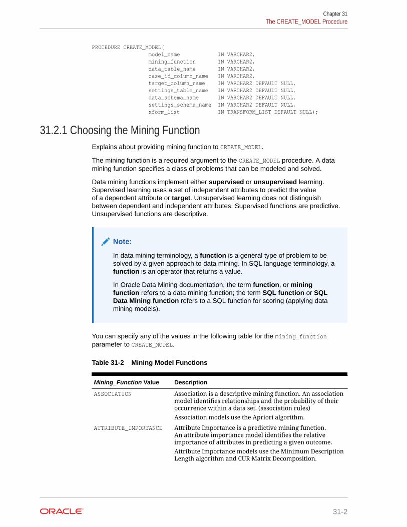
PROCEDURE CREATE_MODEL( model_name IN VARCHAR2, mining_function IN VARCHAR2, data_table_name IN VARCHAR2, case_id_column_name IN VARCHAR2, target_column_name IN VARCHAR2 DEFAULT NULL, settings_table_name IN VARCHAR2 DEFAULT NULL, data_schema_name IN VARCHAR2 DEFAULT NULL, settings_schema_name IN VARCHAR2 DEFAULT NULL, xform_list IN TRANSFORM_LIST DEFAULT NULL);
31.2.1 Choosing the Mining FunctionExplains about providing mining function to CREATE_MODEL.
The mining function is a required argument to the CREATE_MODEL procedure. A datamining function specifies a class of problems that can be modeled and solved.
Data mining functions implement either supervised or unsupervised learning.Supervised learning uses a set of independent attributes to predict the valueof a dependent attribute or target. Unsupervised learning does not distinguishbetween dependent and independent attributes. Supervised functions are predictive.Unsupervised functions are descriptive.
Note:
In data mining terminology, a function is a general type of problem to besolved by a given approach to data mining. In SQL language terminology, afunction is an operator that returns a value.
In Oracle Data Mining documentation, the term function, or miningfunction refers to a data mining function; the term SQL function or SQLData Mining function refers to a SQL function for scoring (applying datamining models).
You can specify any of the values in the following table for the mining_functionparameter to CREATE_MODEL.
Table 31-2 Mining Model Functions
Mining_Function Value Description
ASSOCIATION Association is a descriptive mining function. An associationmodel identifies relationships and the probability of theiroccurrence within a data set. (association rules)Association models use the Apriori algorithm.
ATTRIBUTE_IMPORTANCE Attribute Importance is a predictive mining function.An attribute importance model identifies the relativeimportance of attributes in predicting a given outcome.Attribute Importance models use the Minimum DescriptionLength algorithm and CUR Matrix Decomposition.
Chapter 31The CREATE_MODEL Procedure
31-2

Table 31-2 (Cont.) Mining Model Functions
Mining_Function Value Description
CLASSIFICATION Classification is a predictive mining function. Aclassification model uses historical data to predict acategorical target.Classification models can use Naive Bayes, Neural Network,Decision Tree, Logistic Regression, Random Forest, SupportVector Machines, or Explicit Semantic Analysis. The defaultis Naive Bayes.The classification function can also be used for anomalydetection. In this case, the SVM algorithm with a null targetis used (One-Class SVM).
CLUSTERING Clustering is a descriptive mining function. A clusteringmodel identifies natural groupings within a data set.Clustering models can use k-Means, O-Cluster, orExpectation Maximization. The default is k-Means.
FEATURE_EXTRACTION Feature Extraction is a descriptive mining function. Afeature extraction model creates a set of optimizedattributes.Feature extraction models can use Non-Negative MatrixFactorization, Singular Value Decomposition (which canalso be used for Principal Component Analysis) or ExplicitSemantic Analysis. The default is Non-Negative MatrixFactorization.
REGRESSION Regression is a predictive mining function. A regressionmodel uses historical data to predict a numerical target.Regression models can use Support Vector Machines orLinear Regression. The default is Support Vector Machine.
TIME_SERIES Time series is a predictive mining function. A time seriesmodel forecasts the future values of a time-ordered seriesof historical numeric data over a user-specified timewindow. Time series models use the Exponential Smoothingalgorithm. The default is Exponential Smoothing.
Related Topics
• Oracle Data Mining Concepts
31.2.2 Choosing the AlgorithmLearn about providing the algorithm settings for a model.
The ALGO_NAME setting specifies the algorithm for a model. If you use the defaultalgorithm for the mining function, or if there is only one algorithm available for themining function, you do not need to specify the ALGO_NAME setting. Instructions forspecifying model settings are in "Specifying Model Settings".
Table 31-3 Data Mining Algorithms
ALGO_NAME Value Algorithm Default? Mining Model Function
ALGO_AI_MDL Minimum Description Length — attribute importance
Chapter 31The CREATE_MODEL Procedure
31-3

Table 31-3 (Cont.) Data Mining Algorithms
ALGO_NAME Value Algorithm Default? Mining Model Function
ALGO_APRIORI_ASSOCIATION_RULES
Apriori — association
ALGO_CUR_DECOMPOSITION CUR Decomposition Attribute Importance
ALGO_DECISION_TREE Decision Tree — classification
ALGO_EXPECTATION_MAXIMIZATION
Expectation Maximization
ALGO_EXPLICIT_SEMANTIC_ANALYS
Explicit Semantic Analysis — feature extractionclassification
ALGO_EXPONENTIAL_SMOOTHING Exponential Smoothing — time series
ALGO_EXTENSIBLE_LANG Language used for extensiblealgorithm
— All mining functions aresupported
ALGO_GENERALIZED_LINEAR_MODEL
Generalized Linear Model — classification andregression
ALGO_KMEANS k-Means yes clustering
ALGO_NAIVE_BAYES Naive Bayes yes classification
ALGO_NEURAL_NETWORK Neural Network — classification
ALGO_NONNEGATIVE_MATRIX_FACTOR
Non-Negative Matrix Factorization yes feature extraction
ALGO_O_CLUSTER O-Cluster — clustering
ALGO_RANDOM_FOREST Random Forest — classification
ALGO_SINGULAR_VALUE_DECOMP Singular Value Decomposition(can also be used for PrincipalComponent Analysis)
— feature extraction
ALGO_SUPPORT_VECTOR_MACHINES
Support Vector Machine yes default regressionalgorithmregression, classification,and anomaly detection(classification with notarget)
Related Topics
• Specifying Model SettingsUnderstand how to configure data mining models at build time.
• Oracle Data Mining Concepts
31.2.3 Supplying TransformationsYou can optionally specify transformations for the build data in the xform_listparameter to CREATE_MODEL. The transformation instructions are embedded in themodel and reapplied whenever the model is applied to new data.
Chapter 31The CREATE_MODEL Procedure
31-4
31.2.3.1 Creating a Transformation ListThe following are the ways to create a transformation list:
• The STACK interface in DBMS_DATA_MINING_TRANSFORM.
The STACK interface offers a set of pre-defined transformations that you can applyto an attribute or to a group of attributes. For example, you can specify supervisedbinning for all categorical attributes.
• The SET_TRANSFORM procedure in DBMS_DATA_MINING_TRANSFORM.
The SET_TRANSFORM procedure applies a specified SQL expression to a specifiedattribute. For example, the following statement appends a transformationinstruction for country_id to a list of transformations called my_xforms. Thetransformation instruction divides country_id by 10 before algorithmic processingbegins. The reverse transformation multiplies country_id by 10.
dbms_data_mining_transform.SET_TRANSFORM (my_xforms, 'country_id', NULL, 'country_id/10', 'country_id*10');
The reverse transformation is applied in the model details. If country_id is thetarget of a supervised model, the reverse transformation is also applied to thescored target.
31.2.3.2 Transformation List and Automatic Data PreparationUnderstand the interaction between transformation list and Automatic DataPreparation (ADP).
The transformation list argument to CREATE_MODEL interacts with the PREP_AUTO setting,which controls ADP:
• When ADP is on and you specify a transformation list, your transformationsare applied with the automatic transformations and embedded in the model.The transformations that you specify are executed before the automatictransformations.
• When ADP is off and you specify a transformation list, your transformations areapplied and embedded in the model, but no system-generated transformations areperformed.
• When ADP is on and you do not specify a transformation list, the system-generated transformations are applied and embedded in the model.
• When ADP is off and you do not specify a transformation list, no transformationsare embedded in the model; you must separately prepare the data sets you usefor building, testing, and scoring the model.
Related Topics
• Embedding Transformations in a Model
• Oracle Database PL/SQL Packages and Types Reference
31.2.4 About Partitioned ModelIntroduces partitioned model to organise and represent multiple models.
Chapter 31The CREATE_MODEL Procedure
31-5
Oracle Data Mining supports building of a persistent Oracle Data Mining partitionedmodel. A partitioned model organizes and represents multiple models as partitions ina single model entity, enabling a user to easily build and manage models tailored toindependent slices of data. Persistent means that the partitioned model has an on-diskrepresentation. The product manages the organization of the partitioned model andsimplifies the process of scoring the partitioned model. You must include the partitioncolumns as part of the USING clause when scoring.
The partition names, key values, and the structure of the partitioned model are visiblein the ALL_MINING_MODEL_PARTITIONS view.
Related Topics
• Oracle Database Reference
• Oracle Data Mining User’s Guide
31.2.4.1 Partitioned Model Build ProcessTo build a Partitioned Model, Oracle Data Mining requires a partitioning key. Thepartition key is set through a build setting in the settings table.
The partitioning key is a comma-separated list of one or more columns (up to 16)from the input data set. The partitioning key horizontally slices the input data basedon discrete values of the partitioning key. That is, partitioning is performed as listvalues as opposed to range partitioning against a continuous value. The partitioningkey supports only columns of the data type NUMBER and VARCHAR2.
During the build process the input data set is partitioned based on the distinct valuesof the specified key. Each data slice (unique key value) results in its own modelpartition. This resultant model partition is not separate and is not visible to you asa standalone model. The default value of the maximum number of partitions forpartitioned models is 1000 partitions. You can also set a different maximum partitionsvalue. If the number of partitions in the input data set exceed the defined maximum,Oracle Data Mining throws an exception.
The Partitioned Model organizes features common to all partitions and the partitionspecific features. The common features consist of the following metadata:
• The model name
• The mining function
• The mining algorithm
• A super set of all mining model attributes referenced by all partitions (signature)
• A common set of user-defined column transformations
• Any user-specified or default build settings that are interpreted as global. Forexample, the Auto Data Preparation (ADP) setting
31.2.4.2 DDL in Partitioned modelPartitioned models are maintained through the following DDL operations:
• Drop model or drop partition
• Add partition
Chapter 31The CREATE_MODEL Procedure
31-6
31.2.4.2.1 Drop Model or Drop PartitionOracle Data Mining supports dropping a single model partition for a given partitionname.
If only a single partition remains, you cannot explicitly drop that partition. Instead,you must either add additional partitions prior to dropping the partition or you maychoose to drop the model itself. When dropping a partitioned model, all partitionsare dropped in a single atomic operation. From a performance perspective, Oraclerecommends DROP_PARTITION followed by an ADD_PARTITION instead of leveraging theREPLACE option due to the efficient behavior of the DROP_PARTITION option.
31.2.4.2.2 Add PartitionOracle Data Mining supports adding a single partition or multiple partitions to anexisting partitioned model.
The addition occurs based on the input data set and the name of the existingpartitioned model. The operation takes the input data set and the existing partitionedmodel as parameters. The partition keys are extracted from the input data set and themodel partitions are built against the input data set. These partitions are added to thepartitioned model. In the case where partition keys for new partitions conflict with theexisting partitions in the model, you can select from the following three approaches toresolve the conflicts:
• ERROR: Terminates the ADD operation without adding any partitions.
• REPLACE: Replaces the existing partition for which the conflicting keys are found.
• IGNORE: Eliminates the rows having the conflicting keys.
If the input data set contains multiple keys, then the operation creates multiplepartitions. If the total number of partitions in the model increases to more than theuser-defined maximum specified when the model was created, then you get an error.The default threshold value for the number of partitions is 1000.
31.2.4.3 Partitioned Model scoringLearn about scoring of a partitioned model.
The scoring of the partitioned model is the same as that of the non-partitioned model.The syntax of the data mining function remains the same but is extended to providean optional hint to you. The optional hint can impact the performance of a query whichinvolves scoring a partitioned model.
For scoring a partitioned model, the signature columns used during the build for thepartitioning key must be present in the scoring data set. These columns are combinedto form a unique partition key. The unique key is then mapped to a specific underlyingmodel partition, and the identified model partition is used to score that row.
The partitioned objects that are necessary for scoring are loaded on demand duringthe query execution and are aged out depending on the System Global Area (SGA)memory.
Related Topics
• Oracle Database SQL Language Reference
Chapter 31The CREATE_MODEL Procedure
31-7

31.3 Specifying Model SettingsUnderstand how to configure data mining models at build time.
Numerous configuration settings are available for configuring data mining models atbuild time. To specify settings, create a settings table with the columns shown in thefollowing table and pass the table to CREATE_MODEL.
Table 31-4 Settings Table Required Columns
Column Name Data Type
setting_name VARCHAR2(30)
setting_value VARCHAR2(4000)
Example 31-1 creates a settings table for an Support Vector Machine (SVM)Classification model. Since SVM is not the default classifier, the ALGO_NAME settingis used to specify the algorithm. Setting the SVMS_KERNEL_FUNCTION to SVMS_LINEARcauses the model to be built with a linear kernel. If you do not specify the kernelfunction, the algorithm chooses the kernel based on the number of attributes in thedata.
Some settings apply generally to the model, others are specific to an algorithm. Modelsettings are referenced in Table 31-5 and Table 31-6.
Table 31-5 General Model Settings
Settings Description
Mining function settings See "Mining Function Settings" in Oracle Database PL/SQL Packages andTypes Reference
Algorithm names See "Algorithm Names" in Oracle Database PL/SQL Packages and TypesReference
Global modelcharacteristics
See "Global Settings" in Oracle Database PL/SQL Packages and TypesReference
Automatic DataPreparation
See "Automatic Data Preparation" in Oracle Database PL/SQL Packages andTypes Reference
Table 31-6 Algorithm-Specific Model Settings
Algorithm Description
CUR Matrix Decomposition See "DBMS_DATA_MINING —Algorithm Settings: CUR MatrixDecomposition"in Oracle Database PL/SQL Packages and Types Reference
Decision Tree See "DBMS_DATA_MINING —Algorithm Settings: Decision Tree" in OracleDatabase PL/SQL Packages and Types Reference
Expectation Maximization See "DBMS_DATA_MINING —Algorithm Settings: Expectation Maximization"in Oracle Database PL/SQL Packages and Types Reference
Explicit Semantic Analysis See “DBMS_DATA_MINING —Algorithm Settings: Explicit Semantic Analysis”in Oracle Database PL/SQL Packages and Types Reference
Chapter 31Specifying Model Settings
31-8

Table 31-6 (Cont.) Algorithm-Specific Model Settings
Algorithm Description
Exponential Smoothing See "DBMS_DATA_MINING —Algorithm Settings: Exponential SmoothingModels" in Oracle Database PL/SQL Packages and Types Reference
Generalized Linear Models See "DBMS_DATA_MINING —Algorithm Settings: Generalized Linear Models"in Oracle Database PL/SQL Packages and Types Reference
k-Means See "DBMS_DATA_MINING —Algorithm Settings: k-Means" in OracleDatabase PL/SQL Packages and Types Reference
Naive Bayes See "Algorithm Settings: Naive Bayes" in Oracle Database PL/SQL Packagesand Types Reference
Neural Network See "DBMS_DATA_MINING —Algorithm Settings: Neural Network" in OracleDatabase PL/SQL Packages and Types Reference
Non-Negative MatrixFactorization
See "DBMS_DATA_MINING —Algorithm Settings: Non-Negative MatrixFactorization" in Oracle Database PL/SQL Packages and Types Reference
O-Cluster See "Algorithm Settings: O-Cluster" in Oracle Database PL/SQL Packages andTypes Reference
Random Forest See "DBMS_DATA_MINING — Algorithm Settings: Random Forest" in OracleDatabase PL/SQL Packages and Types Reference
Singular ValueDecomposition
See "DBMS_DATA_MINING —Algorithm Settings: Singular ValueDecomposition" in Oracle Database PL/SQL Packages and Types Reference
Support Vector Machine See "DBMS_DATA_MINING —Algorithm Settings: Support Vector Machine" inOracle Database PL/SQL Packages and Types Reference
Example 31-1 Creating a Settings Table for an SVM Classification Model
CREATE TABLE svmc_sh_sample_settings ( setting_name VARCHAR2(30), setting_value VARCHAR2(4000));
BEGIN INSERT INTO svmc_sh_sample_settings (setting_name, setting_value) VALUES (dbms_data_mining.algo_name, dbms_data_mining.algo_support_vector_machines); INSERT INTO svmc_sh_sample_settings (setting_name, setting_value) VALUES (dbms_data_mining.svms_kernel_function, dbms_data_mining.svms_linear); COMMIT;END;/
Related Topics
• Oracle Database PL/SQL Packages and Types Reference
31.3.1 Specifying CostsSpecify a cost matrix table to build a Decision Tree model.
The CLAS_COST_TABLE_NAME setting specifies the name of a cost matrix table to beused in building a Decision Tree model. A cost matrix biases a classification model tominimize costly misclassifications. The cost matrix table must have the columns shownin the following table:
Chapter 31Specifying Model Settings
31-9
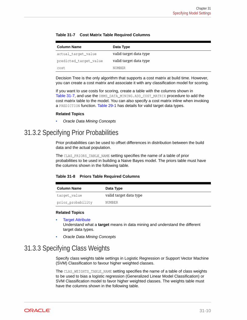
Table 31-7 Cost Matrix Table Required Columns
Column Name Data Type
actual_target_value valid target data type
predicted_target_value valid target data type
cost NUMBER
Decision Tree is the only algorithm that supports a cost matrix at build time. However,you can create a cost matrix and associate it with any classification model for scoring.
If you want to use costs for scoring, create a table with the columns shown inTable 31-7, and use the DBMS_DATA_MINING.ADD_COST_MATRIX procedure to add thecost matrix table to the model. You can also specify a cost matrix inline when invokinga PREDICTION function. Table 29-1 has details for valid target data types.
Related Topics
• Oracle Data Mining Concepts
31.3.2 Specifying Prior ProbabilitiesPrior probabilities can be used to offset differences in distribution between the builddata and the actual population.
The CLAS_PRIORS_TABLE_NAME setting specifies the name of a table of priorprobabilities to be used in building a Naive Bayes model. The priors table must havethe columns shown in the following table.
Table 31-8 Priors Table Required Columns
Column Name Data Type
target_value valid target data type
prior_probability NUMBER
Related Topics
• Target AttributeUnderstand what a target means in data mining and understand the differenttarget data types.
• Oracle Data Mining Concepts
31.3.3 Specifying Class WeightsSpecify class weights table settings in Logistic Regression or Support Vector Machine(SVM) Classification to favour higher weighted classes.
The CLAS_WEIGHTS_TABLE_NAME setting specifies the name of a table of class weightsto be used to bias a logistic regression (Generalized Linear Model Classification) orSVM Classification model to favor higher weighted classes. The weights table musthave the columns shown in the following table.
Chapter 31Specifying Model Settings
31-10

Table 31-9 Class Weights Table Required Columns
Column Name Data Type
target_value valid target data type
class_weight NUMBER
Related Topics
• Target AttributeUnderstand what a target means in data mining and understand the differenttarget data types.
• Oracle Data Mining Concepts
31.3.4 Model Settings in the Data DictionaryExplains about ALL/USER/DBA_MINING_MODEL_SETTINGS in data dictionary view.
Information about mining model settings can be obtained from the data dictionaryview ALL/USER/DBA_MINING_MODEL_SETTINGS. When used with the ALL prefix, this viewreturns information about the settings for the models accessible to the current user.When used with the USER prefix, it returns information about the settings for the modelsin the user's schema. The DBA prefix is only available for DBAs.
The columns of ALL_MINING_MODEL_SETTINGS are described as follows and explainedin the following table.
SQL> describe all_mining_model_settings Name Null? Type ----------------------------------------- -------- ---------------------------- OWNER NOT NULL VARCHAR2(30) MODEL_NAME NOT NULL VARCHAR2(30) SETTING_NAME NOT NULL VARCHAR2(30) SETTING_VALUE VARCHAR2(4000) SETTING_TYPE VARCHAR2(7)
Table 31-10 ALL_MINING_MODEL_SETTINGS
Column Description
owner Owner of the mining model.
model_name Name of the mining model.
setting_name Name of the setting.
setting_value Value of the setting.
setting_type INPUT if the value is specified by a user. DEFAULT if the value issystem-generated.
The following query lists the settings for the Support VectorMachine (SVM) Classification model SVMC_SH_CLAS_SAMPLE. The ALGO_NAME,CLAS_WEIGHTS_TABLE_NAME, and SVMS_KERNEL_FUNCTION settings are user-specified.These settings have been specified in a settings table for the model.
Chapter 31Specifying Model Settings
31-11
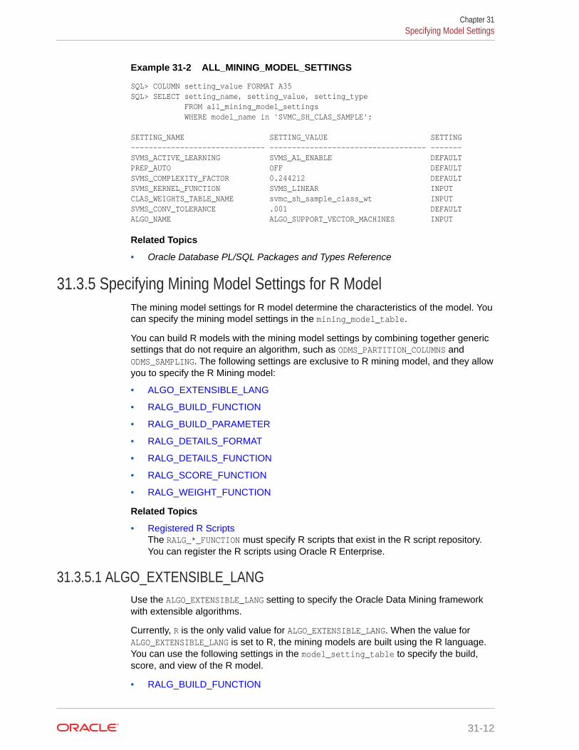
Example 31-2 ALL_MINING_MODEL_SETTINGS
SQL> COLUMN setting_value FORMAT A35SQL> SELECT setting_name, setting_value, setting_type FROM all_mining_model_settings WHERE model_name in 'SVMC_SH_CLAS_SAMPLE'; SETTING_NAME SETTING_VALUE SETTING------------------------------ ----------------------------------- -------SVMS_ACTIVE_LEARNING SVMS_AL_ENABLE DEFAULTPREP_AUTO OFF DEFAULTSVMS_COMPLEXITY_FACTOR 0.244212 DEFAULTSVMS_KERNEL_FUNCTION SVMS_LINEAR INPUTCLAS_WEIGHTS_TABLE_NAME svmc_sh_sample_class_wt INPUTSVMS_CONV_TOLERANCE .001 DEFAULTALGO_NAME ALGO_SUPPORT_VECTOR_MACHINES INPUT
Related Topics
• Oracle Database PL/SQL Packages and Types Reference
31.3.5 Specifying Mining Model Settings for R ModelThe mining model settings for R model determine the characteristics of the model. Youcan specify the mining model settings in the mining_model_table.
You can build R models with the mining model settings by combining together genericsettings that do not require an algorithm, such as ODMS_PARTITION_COLUMNS andODMS_SAMPLING. The following settings are exclusive to R mining model, and they allowyou to specify the R Mining model:
• ALGO_EXTENSIBLE_LANG
• RALG_BUILD_FUNCTION
• RALG_BUILD_PARAMETER
• RALG_DETAILS_FORMAT
• RALG_DETAILS_FUNCTION
• RALG_SCORE_FUNCTION
• RALG_WEIGHT_FUNCTION
Related Topics
• Registered R ScriptsThe RALG_*_FUNCTION must specify R scripts that exist in the R script repository.You can register the R scripts using Oracle R Enterprise.
31.3.5.1 ALGO_EXTENSIBLE_LANGUse the ALGO_EXTENSIBLE_LANG setting to specify the Oracle Data Mining frameworkwith extensible algorithms.
Currently, R is the only valid value for ALGO_EXTENSIBLE_LANG. When the value forALGO_EXTENSIBLE_LANG is set to R, the mining models are built using the R language.You can use the following settings in the model_setting_table to specify the build,score, and view of the R model.
• RALG_BUILD_FUNCTION
Chapter 31Specifying Model Settings
31-12

• RALG_BUILD_PARAMETER
• RALG_DETAILS_FUNCTION
• RALG_DETAILS_FORMAT
• RALG_SCORE_FUNCTION
• RALG_WEIGHT_FUNCTION
Related Topics
• Registered R ScriptsThe RALG_*_FUNCTION must specify R scripts that exist in the R script repository.You can register the R scripts using Oracle R Enterprise.
31.3.5.2 RALG_BUILD_FUNCTIONUse the RALG_BUILD_FUNCTION to specify the name of an existing registered R scriptfor R algorithm mining model build.
You must specify both RALG_BUILD_FUNCTION and ALGO_EXTENSIBLE_LANG in themodel_setting_table. The R script defines an R function that has the first inputargument of data.frame for training data, and it returns an R model object. The firstdata argument is mandatory. The RALG_BUILD_FUNCTION can accept additional modelbuild parameters.
Note:
The valid inputs for input parameters are numeric and string scalar datatypes.
Example 31-3 Example of RALG_BUILD_FUNCTION
This example shows how to specify the name of the R script MY_LM_BUILD_SCRIPT thatis used to build the model in the model_setting_table.
Begininsert into model_setting_table values(dbms_data_mining.ralg_build_function,'MY_LM_BUILD_SCRIPT');End;/
The R script MY_LM_BUILD_SCRIPT defines an R function that builds the LM model.You must register the script MY_LM_BUILD_SCRIPT in the R script repository whichuses the existing ORE security restrictions. You can use Oracle R Enterprise APIsys.rqScriptCreate to register the script. Oracle R Enterprise requires the RQADMINrole to register R scripts.
For example:
Beginsys.rqScriptCreate('MY_LM_BUILD_SCRIPT', 'function(data, formula, model.frame) {lm(formula = formula, data=data, model = as.logical(model.frame)}');
Chapter 31Specifying Model Settings
31-13

End;/
For Clustering and Feature Extraction mining function model build, the R attributesdm$nclus and dm$nfeat must be set on the return R model to indicate the number ofclusters and features respectively.
The R script MY_KM_BUILD_SCRIPT defines an R function that builds the k-Means modelfor Clustering. R attribute dm$nclus is set with the number of clusters for the returnClustering model.
'function(dat) {dat.scaled <- scale(dat) set.seed(6543); mod <- list() fit <- kmeans(dat.scaled, centers = 3L) mod[[1L]] <- fit mod[[2L]] <- attr(dat.scaled, "scaled:center") mod[[3L]] <- attr(dat.scaled, "scaled:scale") attr(mod, "dm$nclus") <- nrow(fit$centers) mod}'
The R script MY_PCA_BUILD_SCRIPT defines an R function that builds the PCA model.R attribute dm$nfeat is set with the number of features for the return feature extractionmodel.
'function(dat) { mod <- prcomp(dat, retx = FALSE) attr(mod, "dm$nfeat") <- ncol(mod$rotation) mod}'
Related Topics
• RALG_BUILD_PARAMETERThe RALG_BUILD_FUNCTION input parameter specifies a list of numeric and stringscalar values in SQL SELECT query statement format.
• Registered R ScriptsThe RALG_*_FUNCTION must specify R scripts that exist in the R script repository.You can register the R scripts using Oracle R Enterprise.
31.3.5.2.1 RALG_BUILD_PARAMETERThe RALG_BUILD_FUNCTION input parameter specifies a list of numeric and string scalarvalues in SQL SELECT query statement format.
Example 31-4 Example of RALG_BUILD_PARAMETER
The RALG_BUILD_FUNCTION input parameters must be a list of numeric and string scalarvalues. The input parameters are optional.
The syntax of the parameter is:
'SELECT value parameter name ...FROM dual'
Chapter 31Specifying Model Settings
31-14

This example shows how to specify a formula for the input argument'formula' and a numeric value zero for input argument 'model.frame' usingthe RALG_BUILD_PARAMETER. These input arguments must match with the functionsignature of the R script used in RALG_BUILD_FUNCTION Parameter.
Begininsert into model_setting_table values(dbms_data_mining.ralg_build_parameter, 'select ''AGE ~ .'' as "formula", 0 as "model.frame" from dual');End;/
Related Topics
• RALG_BUILD_FUNCTIONUse the RALG_BUILD_FUNCTION to specify the name of an existing registered Rscript for R algorithm mining model build.
31.3.5.3 RALG_DETAILS_FUNCTIONThe RALG_DETAILS_FUNCTION specifies the R model metadata that is returned in thedata.frame.
Use the RALG_DETAILS_FUNCTION to specify an existing registered R script thatgenerates model information. The specified R script defines an R function thatcontains the first input argument for the R model object. The output of the Rfunction must be a data.frame. The columns of the data.frame are defined byRALG_DETAILS_FORMAT, and can contain only numeric or string scalar types.
Example 31-5 Example of RALG_DETAILS_FUNCTION
This example shows how to specify the name of the R script MY_LM_DETAILS_SCRIPT inthe model_setting_table. This script defines the R function that is used to provide themodel information.
Begininsert into model_setting_table values(dbms_data_mining.ralg_details_function, 'MY_LM_DETAILS_SCRIPT');End;/
In the R script repository, the script MY_LM_DETAILS_SCRIPT is registered as:
'function(mod) data.frame(name=names(mod$coefficients), coef=mod$coefficients)'
Related Topics
• Registered R ScriptsThe RALG_*_FUNCTION must specify R scripts that exist in the R script repository.You can register the R scripts using Oracle R Enterprise.
• RALG_DETAILS_FORMATUse the RALG_DETAILS_FORMAT parameter to specify the names and column typesin the model view. It is a string that contains a SELECT query to specify a list of
Chapter 31Specifying Model Settings
31-15
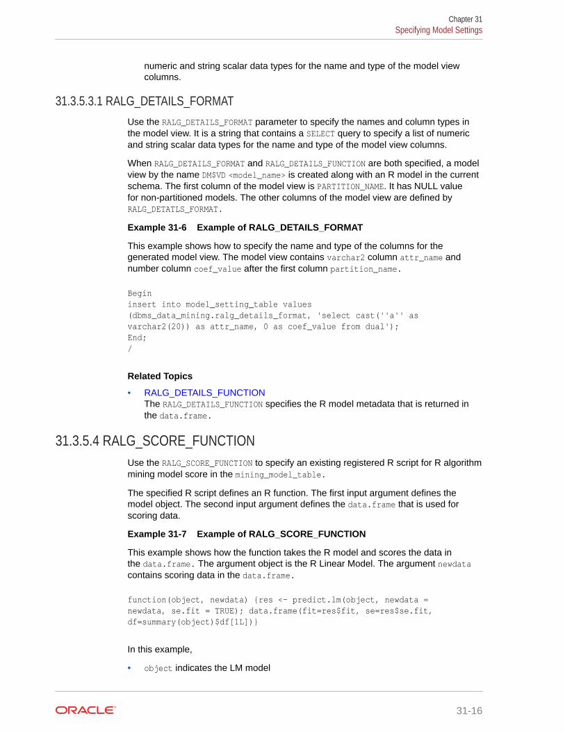
numeric and string scalar data types for the name and type of the model viewcolumns.
31.3.5.3.1 RALG_DETAILS_FORMATUse the RALG_DETAILS_FORMAT parameter to specify the names and column types inthe model view. It is a string that contains a SELECT query to specify a list of numericand string scalar data types for the name and type of the model view columns.
When RALG_DETAILS_FORMAT and RALG_DETAILS_FUNCTION are both specified, a modelview by the name DM$VD <model_name> is created along with an R model in the currentschema. The first column of the model view is PARTITION_NAME. It has NULL valuefor non-partitioned models. The other columns of the model view are defined byRALG_DETATLS_FORMAT.
Example 31-6 Example of RALG_DETAILS_FORMAT
This example shows how to specify the name and type of the columns for thegenerated model view. The model view contains varchar2 column attr_name andnumber column coef_value after the first column partition_name.
Begininsert into model_setting_table values(dbms_data_mining.ralg_details_format, 'select cast(''a'' as varchar2(20)) as attr_name, 0 as coef_value from dual');End;/
Related Topics
• RALG_DETAILS_FUNCTIONThe RALG_DETAILS_FUNCTION specifies the R model metadata that is returned inthe data.frame.
31.3.5.4 RALG_SCORE_FUNCTIONUse the RALG_SCORE_FUNCTION to specify an existing registered R script for R algorithmmining model score in the mining_model_table.
The specified R script defines an R function. The first input argument defines themodel object. The second input argument defines the data.frame that is used forscoring data.
Example 31-7 Example of RALG_SCORE_FUNCTION
This example shows how the function takes the R model and scores the data inthe data.frame. The argument object is the R Linear Model. The argument newdatacontains scoring data in the data.frame.
function(object, newdata) {res <- predict.lm(object, newdata = newdata, se.fit = TRUE); data.frame(fit=res$fit, se=res$se.fit, df=summary(object)$df[1L])}
In this example,
• object indicates the LM model
Chapter 31Specifying Model Settings
31-16
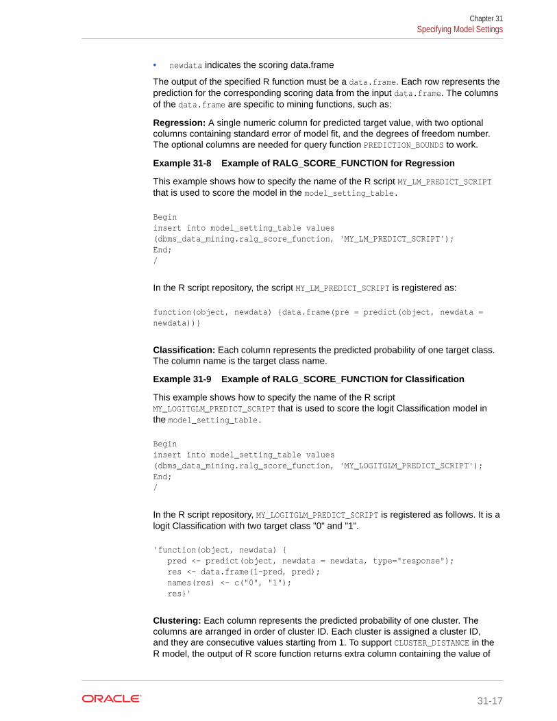
• newdata indicates the scoring data.frame
The output of the specified R function must be a data.frame. Each row represents theprediction for the corresponding scoring data from the input data.frame. The columnsof the data.frame are specific to mining functions, such as:
Regression: A single numeric column for predicted target value, with two optionalcolumns containing standard error of model fit, and the degrees of freedom number.The optional columns are needed for query function PREDICTION_BOUNDS to work.
Example 31-8 Example of RALG_SCORE_FUNCTION for Regression
This example shows how to specify the name of the R script MY_LM_PREDICT_SCRIPTthat is used to score the model in the model_setting_table.
Begininsert into model_setting_table values(dbms_data_mining.ralg_score_function, 'MY_LM_PREDICT_SCRIPT');End;/
In the R script repository, the script MY_LM_PREDICT_SCRIPT is registered as:
function(object, newdata) {data.frame(pre = predict(object, newdata = newdata))}
Classification: Each column represents the predicted probability of one target class.The column name is the target class name.
Example 31-9 Example of RALG_SCORE_FUNCTION for Classification
This example shows how to specify the name of the R scriptMY_LOGITGLM_PREDICT_SCRIPT that is used to score the logit Classification model inthe model_setting_table.
Begininsert into model_setting_table values(dbms_data_mining.ralg_score_function, 'MY_LOGITGLM_PREDICT_SCRIPT');End;/
In the R script repository, MY_LOGITGLM_PREDICT_SCRIPT is registered as follows. It is alogit Classification with two target class "0" and "1".
'function(object, newdata) { pred <- predict(object, newdata = newdata, type="response"); res <- data.frame(1-pred, pred); names(res) <- c("0", "1"); res}'
Clustering: Each column represents the predicted probability of one cluster. Thecolumns are arranged in order of cluster ID. Each cluster is assigned a cluster ID,and they are consecutive values starting from 1. To support CLUSTER_DISTANCE in theR model, the output of R score function returns extra column containing the value of
Chapter 31Specifying Model Settings
31-17

the distance to each cluster in order of cluster ID after the columns for the predictedprobability.
Example 31-10 Example of RALG_SCORE_FUNCTION for Clustering
This example shows how to specify the name of the R scriptMY_CLUSTER_PREDICT_SCRIPT that is used to score the model in themodel_setting_table.
Begininsert into model_setting_table values(dbms_data_mining.ralg_score_function, 'MY_CLUSTER_PREDICT_SCRIPT');End;/
In the R script repository, the script MY_CLUSTER_PREDICT_SCRIPT is registered as:
'function(object, dat){ mod <- object[[1L]]; ce <- object[[2L]]; sc <- object[[3L]]; newdata = scale(dat, center = ce, scale = sc); centers <- mod$centers; ss <- sapply(as.data.frame(t(centers)), function(v) rowSums(scale(newdata, center=v, scale=FALSE)^2)); if (!is.matrix(ss)) ss <- matrix(ss, ncol=length(ss)); disp <- -1 / (2* mod$tot.withinss/length(mod$cluster)); distr <- exp(disp*ss); prob <- distr / rowSums(distr); as.data.frame(cbind(prob, sqrt(ss)))}'
Feature Extraction: Each column represents the coefficient value of one feature. Thecolumns are arranged in order of feature ID. Each feature is assigned a feature ID,and they are consecutive values starting from 1.
Example 31-11 Example of RALG_SCORE_FUNCTION for Feature Extraction
This example shows how to specify the name of the R scriptMY_FEATURE_EXTRACTION_SCRIPT that is used to score the model in themodel_setting_table.
Begininsert into model_setting_table values(dbms_data_mining.ralg_score_function, 'MY_FEATURE_EXTRACTION_SCRIPT');End;/
In the R script repository, the script MY_FEATURE_EXTRACTION_SCRIPT is registered as:
'function(object, dat) { as.data.frame(predict(object, dat)) }'
The function fetches the centers of the features from the R model, and computesthe feature coefficient based on the distance of the score data to the correspondingfeature center.
Chapter 31Specifying Model Settings
31-18

Related Topics
• Registered R ScriptsThe RALG_*_FUNCTION must specify R scripts that exist in the R script repository.You can register the R scripts using Oracle R Enterprise.
31.3.5.5 RALG_WEIGHT_FUNCTIONUse the RALG_WEIGHT_FUNCTION to specify the name of an existing registered R scriptthat computes weight or contribution for each attribute in scoring. The specifiedR script is used in the query function PREDICTION_DETAILS to evaluate attributecontribution.
The specified R script defines an R function containing the first input argument formodel object, and the second input argument of data.frame for scoring data. Whenthe mining function is Classification, Clustering, or Feature Extraction, the target classname or cluster ID or feature ID is passed by the third input argument to compute theweight for that particular class or cluster or feature. The script returns a data.framecontaining the contributing weight for each attribute in a row. Each row corresponds tothat input scoring data.frame.
Example 31-12 Example of RALG_WEIGHT_FUNCTION
This example shows how to specify the name of the R scriptMY_PREDICT_WEIGHT_SCRIPT that computes weight or contribution of R model attributesin the model_setting_table.
Begininsert into model_setting_table values(dbms_data_mining.ralg_weight_function, 'MY_PREDICT_WEIGHT_SCRIPT');End;/
In the R script repository, the script MY_PREDICT_WEIGHT_SCRIPT for Regression isregistered as:
'function(mod, data) { coef(mod)[-1L]*data }'
In the R script repository, the script MY_PREDICT_WEIGHT_SCRIPT for logit Classificationis registered as:
'function(mod, dat, clas) { v <- predict(mod, newdata=dat, type = "response"); v0 <- data.frame(v, 1-v); names(v0) <- c("0", "1"); res <- data.frame(lapply(seq_along(dat), function(x, dat) { if(is.numeric(dat[[x]])) dat[,x] <- as.numeric(0) else dat[,x] <- as.factor(NA); vv <- predict(mod, newdata = dat, type = "response"); vv = data.frame(vv, 1-vv); names(vv) <- c("0", "1"); v0[[clas]] / vv[[clas]]}, dat = dat)); names(res) <- names(dat); res}'
Chapter 31Specifying Model Settings
31-19
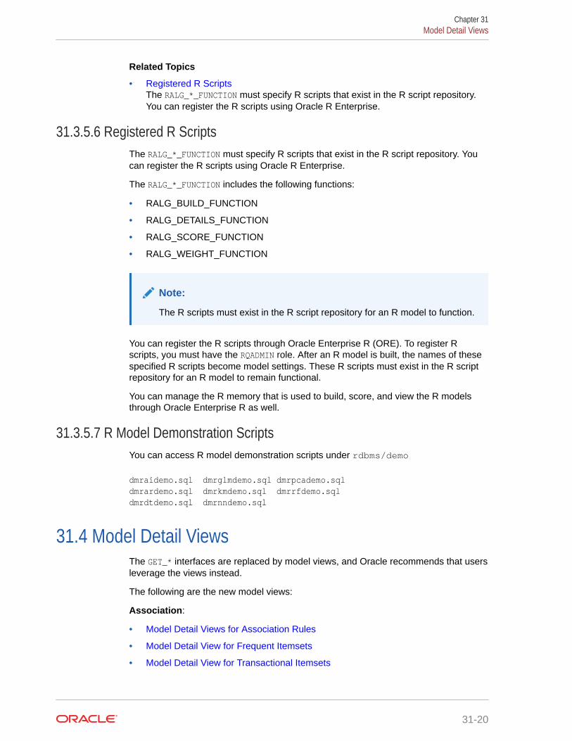
Related Topics
• Registered R ScriptsThe RALG_*_FUNCTION must specify R scripts that exist in the R script repository.You can register the R scripts using Oracle R Enterprise.
31.3.5.6 Registered R ScriptsThe RALG_*_FUNCTION must specify R scripts that exist in the R script repository. Youcan register the R scripts using Oracle R Enterprise.
The RALG_*_FUNCTION includes the following functions:
• RALG_BUILD_FUNCTION
• RALG_DETAILS_FUNCTION
• RALG_SCORE_FUNCTION
• RALG_WEIGHT_FUNCTION
Note:
The R scripts must exist in the R script repository for an R model to function.
You can register the R scripts through Oracle Enterprise R (ORE). To register Rscripts, you must have the RQADMIN role. After an R model is built, the names of thesespecified R scripts become model settings. These R scripts must exist in the R scriptrepository for an R model to remain functional.
You can manage the R memory that is used to build, score, and view the R modelsthrough Oracle Enterprise R as well.
31.3.5.7 R Model Demonstration ScriptsYou can access R model demonstration scripts under rdbms/demo
dmraidemo.sql dmrglmdemo.sql dmrpcademo.sqldmrardemo.sql dmrkmdemo.sql dmrrfdemo.sqldmrdtdemo.sql dmrnndemo.sql
31.4 Model Detail ViewsThe GET_* interfaces are replaced by model views, and Oracle recommends that usersleverage the views instead.
The following are the new model views:
Association:
• Model Detail Views for Association Rules
• Model Detail View for Frequent Itemsets
• Model Detail View for Transactional Itemsets
Chapter 31Model Detail Views
31-20

• Model Detail View for Transactional Rule
Classification, Regression, and Anomaly Detection:
• Model Detail Views for Classification Algorithms
• Model Detail Views for CUR Matrix Decomposition
• Model Detail Views for Decision Tree
• Model Detail Views for Generalized Linear Model
• Model Detail Views for Naive Bayes
• Model Detail Views for Neural Network
• Model Detail Views for Random Forest
• Model Detail View for Support Vector Machine
Clustering:
• Model Detail Views for Clustering Algorithms
• Model Detail Views for Expectation Maximization
• Model Detail Views for k-Means
• Model Detail Views for O-Cluster
Feature Extraction:
• Model Detail Views for Explicit Semantic Analysis
• Model Detail Views for Non-Negative Matrix Factorization
• Model Detail Views for Singular Value Decomposition
Feature Selection:
• Model Detail View for Minimum Description Length
Data Preparation and Other:
• Model Detail View for Binning
• Model Detail Views for Global Information
• Model Detail View for Normalization and Missing Value Handling
Time Series:
Model Detail Views for Exponential Smoothing Models
31.4.1 Model Detail Views for Association RulesModel detail views for Association Rules describe the rule view for Association Rules.Oracle recommends that users leverage the model details views instead of theGET_ASSOCIATION_RULES function.
The rule view DM$VRmodel_name describes the generated rules for Association Rules.Depending on the settings of the model, the rule view has different set of columns.Settings ODMS_ITEM_ID_COLUMN_NAME and ODMS_ITEM_VALUE_COLUMN_NAME determinehow each item is defined. If ODMS_ITEM_ID_COLUMN_NAME is set, the input formatis called transactional input, otherwise, the input format is called 2-Dimensionalinput. With transactional input, if setting ODMS_ITEM_VALUE_COLUMN_NAME is not set,each item is defined by ITEM_NAME, otherwise, each item is defined by ITEM_NAME
Chapter 31Model Detail Views
31-21

and ITEM_VALUE. With 2-Dimensional input, each item is defined by ITEM_NAME,ITEM_SUBNAME and ITEM_VALUE. Setting ASSO_AGGREGATES specifies the columns toaggregate, which is displayed in the view.
Note:
Setting ASSO_AGGREGATES is not allowed for 2-dimensional input.
The following shows the views with different settings.
Transactional Input Without ASSO_AGGREGATES Setting
When setting ITEM_NAME (ODMS_ITEM_ID_COLUMN_NAME) is set and ITEM_VALUE(ODMS_ITEM_VALUE_COLUMN_NAME) is not set, the following is the view. Here theconsequent item is defined with only name field. If ITEM_VALUE setting is also set,the view will have one extra column CONSEQUENT_VALUE to specify the value field.
Name Type ----------------------------------------- ---------------------------- PARTITION_NAME VARCHAR2(128) RULE_ID NUMBER RULE_SUPPORT NUMBER RULE_CONFIDENCE NUMBER RULE_LIFT NUMBER RULE_REVCONFIDENCE NUMBER ANTECEDENT_SUPPORT NUMBER NUMBER_OF_ITEMS NUMBER CONSEQUENT_SUPPORT NUMBER CONSEQUENT_NAME VARCHAR2(4000) ANTECEDENT SYS.XMLTYPE
Table 31-11 Rule View Columns for Transactional Inputs
Column Name Description
PARTITION_NAME A partition in a partitioned model to retrieve details
RULE_ID Identifier of the rule
RULE_SUPPORT The number of transactions that satisfy the rule.
RULE_CONFIDENCE The likelihood of a transaction satisfying the rule.
RULE_LIFT The degree of improvement in the prediction over random chance whenthe rule is satisfied.
RULE_REVCONFIDENCE The number of transactions in which the rule occurs divided by thenumber of transactions in which the consequent occurs.
ANTECEDENT_SUPPORT The ratio of the number of transactions that satisfy the antecedent to thetotal number of transactions.
NUMBER_OF_ITEMS The total number of attributes referenced in the antecedent andconsequent of the rule.
CONSEQUENT_SUPPORT The ratio of the number of transactions that satisfy the consequent tothe total number of transactions.
Chapter 31Model Detail Views
31-22

Table 31-11 (Cont.) Rule View Columns for Transactional Inputs
Column Name Description
CONSEQUENT_NAME Name of the consequent
CONSEQUENT_VALUE Value of the consequent when setting Item_value(ODMS_ITEM_VALUE_COLUMN_NAME) is set with TYPE as numerical, theview has a CONSEQUENT_VALUE column.
When setting Item_value (ODMS_ITEM_VALUE_COLUMN_NAME) is set withTYPE as categorical, the view has a CONSEQUENT_VALUE column.
ANTECEDENT The antecedent is described as an itemset. At the itemset level, itspecifies the number of aggregates, and if not zero, the names of thecolumns to be aggregated (as well as the mapping to ASSO_AGG*). Theitemset contains >= 1 items.
• When setting ODMS_ITEM_VALUE_COLUMN_NAME is not set, each itemis defined by item_name. As an example, assume the antecedentcontains one item B, it is represented as follows:
<itemset NUMAGGR="0"><item><item_name>B</item_name></item></itemset>
As another example, assume the antecedent contains two items, Aand C, it is represented as follows:
<itemset NUMAGGR="0"><item><item_name>A</item_name></item><item><item_name>C</item_name></item></itemset>
• When setting ODMS_ITEM_VALUE_COLUMN_NAME is set, each item isdefined by item_name and item_value. As an example, assume theantecedent contains two items, (name A, value 1) and (name C,value 1), then it is represented as follows:
<itemset NUMAGGR="0"><item><item_name>A</item_name><item_value>1</item_value></item><item><item_name>C</item_name><item_value>1</item_value></item></itemset>
Transactional Input With ASSO_AGGREGATES Setting
Similar to the view without aggregates setting, there are three cases:
• Rule view when ODMS_ITEM_ID_COLUMN_NAME is set and Item_value(ODMS_ITEM_VALUE_COLUMN_NAME) is not set.
• Rule view when ODMS_ITEM_ID_COLUMN_NAME is set and Item_value(ODMS_ITEM_VALUE_COLUMN_NAME) is set with TYPE as numerical, the view has aCONSEQUENT_VALUE column.
• Rule view when ODMS_ITEM_ID_COLUMN_NAME is set and Item_value(ODMS_ITEM_VALUE_COLUMN_NAME) is set with TYPE as categorical, the view has aCONSEQUENT_VALUE column.
For example, refer “Example: Calculating Aggregates” in Oracle Data MiningConcepts.
Chapter 31Model Detail Views
31-23

The view reports two sets of aggregates results:
1. ANT_RULE_PROFIT refers to the total profit for the antecedent itemset with respectto the rule, the profit for each individual item of the antecedent itemset is shownin the ANTECEDENT(XMLtype) column, CON_RULE_PROFIT refers to the total profit forthe consequent item with respect to the rule.
In the example, for rule (A, B) => C, the rule itemset (A, B, C) occurs in thetransactions of customer 1 and customer 3. The ANT_RULE_PROFIT is $21.20,The ANTECEDENT is shown as follow, which tells that item A has profit 5.00 +3.00 = $8.00 and item B has profit 3.20 + 10.00 = $13.20, which sum up toANT_RULE_PROFIT.
<itemset NUMAGGR="1" ASSO_AGG0="profit"><item><item_name>A</item_name><ASSO_AGG0>8.0E+000</ASSO_AGG0></item><item><item_name>B</item_name><ASSO_AGG0>1.32E+001</ASSO_AGG0></item></itemset> The CON_RULE_PROFIT is 12.00 + 14.00 = $26.00
2. ANT_PROFIT refers to the total profit for the antecedent itemset, while CON_PROFITrefers to the total profit for the consequent item. The difference betweenCON_PROFIT and CON_RULE_PROFIT (the same applies to ANT_PROFIT andANT_RULE_PROFIT) is that CON_PROFIT counts all profit for the consequent itemacross all transactions where the consequent occurs, while CON_RULE_PROFIT onlycounts across transactions where the rule itemset occurs.
For example, item C occurs in transactions for customer 1, 2 and 3, CON_PROFITis 12.00 + 4.20 + 14.00 = $30.20, while CON_RULE_PROFIT only counts transactionsfor customer 1 and 3 where the rule itemset (A, B, C) occurs.
Similarly, ANT_PROFIT counts all transactions where itemset (A, B) occurs, whileANT_RULE_PROFIT counts only transactions where the rule itemset (A, B, C) occurs.In this example, by coincidence, both count transactions for customer 1 and 3, andhave the same value.
Example 31-13 Examples
The following example shows the view when setting ASSO_AGGREGATES specifiescolumn profit and column sales to be aggregated. In this example, ITEM_VALUE columnis not specified.
Name Type ----------------------------------------- ---------------------------- PARTITION_NAME VARCHAR2(128) RULE_ID NUMBER RULE_SUPPORT NUMBER RULE_CONFIDENCE NUMBER RULE_LIFT NUMBER RULE_REVCONFIDENCE NUMBER ANTECEDENT_SUPPORT NUMBER NUMBER_OF_ITEMS NUMBER CONSEQUENT_SUPPORT NUMBER CONSEQUENT_NAME VARCHAR2(4000) ANTECEDENT SYS.XMLTYPE ANT_RULE_PROFIT BINARY_DOUBLE CON_RULE_PROFIT BINARY_DOUBLE ANT_PROFIT BINARY_DOUBLE CON_PROFIT BINARY_DOUBLE
Chapter 31Model Detail Views
31-24
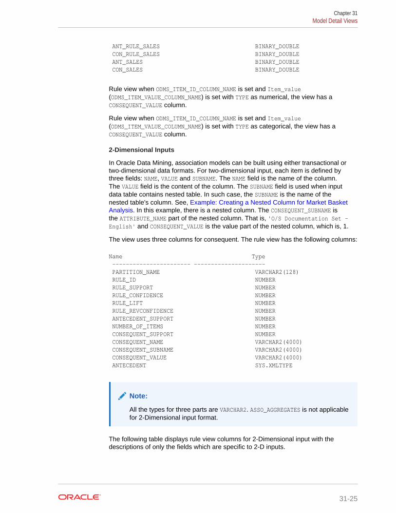
ANT_RULE_SALES BINARY_DOUBLE CON_RULE_SALES BINARY_DOUBLE ANT_SALES BINARY_DOUBLE CON_SALES BINARY_DOUBLE
Rule view when ODMS_ITEM_ID_COLUMN_NAME is set and Item_value(ODMS_ITEM_VALUE_COLUMN_NAME) is set with TYPE as numerical, the view has aCONSEQUENT_VALUE column.
Rule view when ODMS_ITEM_ID_COLUMN_NAME is set and Item_value(ODMS_ITEM_VALUE_COLUMN_NAME) is set with TYPE as categorical, the view has aCONSEQUENT_VALUE column.
2-Dimensional Inputs
In Oracle Data Mining, association models can be built using either transactional ortwo-dimensional data formats. For two-dimensional input, each item is defined bythree fields: NAME, VALUE and SUBNAME. The NAME field is the name of the column.The VALUE field is the content of the column. The SUBNAME field is used when inputdata table contains nested table. In such case, the SUBNAME is the name of thenested table's column. See, Example: Creating a Nested Column for Market BasketAnalysis. In this example, there is a nested column. The CONSEQUENT_SUBNAME isthe ATTRIBUTE_NAME part of the nested column. That is, 'O/S Documentation Set -English' and CONSEQUENT_VALUE is the value part of the nested column, which is, 1.
The view uses three columns for consequent. The rule view has the following columns:
Name Type ----------------------- --------------------- PARTITION_NAME VARCHAR2(128) RULE_ID NUMBER RULE_SUPPORT NUMBER RULE_CONFIDENCE NUMBER RULE_LIFT NUMBER RULE_REVCONFIDENCE NUMBER ANTECEDENT_SUPPORT NUMBER NUMBER_OF_ITEMS NUMBER CONSEQUENT_SUPPORT NUMBER CONSEQUENT_NAME VARCHAR2(4000) CONSEQUENT_SUBNAME VARCHAR2(4000) CONSEQUENT_VALUE VARCHAR2(4000) ANTECEDENT SYS.XMLTYPE
Note:
All the types for three parts are VARCHAR2. ASSO_AGGREGATES is not applicablefor 2-Dimensional input format.
The following table displays rule view columns for 2-Dimensional input with thedescriptions of only the fields which are specific to 2-D inputs.
Chapter 31Model Detail Views
31-25

Table 31-12 Rule View for 2-Dimensional Input
Column Name Description
CONSEQUENT_SUBNAME For two-dimensional inputs, CONSEQUENT_SUBNAME is used fornested column in the input data table.
CONSEQUENT_VALUE Value of the consequent when setting Item_value is set withTYPE as numerical, the view has a CONSEQUENT_VALUE column.
When setting Item_value is set with TYPE as categorical, theview has a CONSEQUENT_VALUE column.
ANTECEDENT The antecedent is described as an itemset. The itemsetcontains >= 1 items. Each item is defined using ITEM_NAME,ITEM_SUBNAME, and ITEM_VALUE:
As an example, assuming that this is not a nested table input,and the antecedent contains one item: (name ADDR, value MA).The antecedent (XMLtype) is as follows:
<itemset NUMAGGR="0"><item><item_name>ADDR</item_name><item_subname></item_subname><item_value>MA</item_value></item></itemset>
For 2-Dimensional input with nested table, the subname fieldis filled.
Global Detail for Association Rules
A single global detail is produced by an Association model. The following tabledescribes a global detail returned for Association Rules model.
Table 31-13 Global Detail for Association Rules
Name Description
ITEMSET_COUNT The number of itemsets generated
MAX_SUPPORT The maximum support
NUM_ROWS The total number of rows used in the build
RULE_COUNT The number of association rules in the model generated
TRANSACTION_COUNT The number of the transactions in input data
31.4.2 Model Detail View for Frequent ItemsetsModel detail view for Frequent Itemsets describes the frequent itemsets view.Oracle recommends that you leverage model details view instead of theGET_FREQUENT_ITEMSETS function.
The frequent itemsets view DM$VImodel_name has the following schema:
Name Type ------------- ------------------ PARTITION_NAME VARCHAR2 (128)
Chapter 31Model Detail Views
31-26

ITEMSET_ID NUMBER SUPPORT NUMBER NUMBER_OF_ITEMS NUMBER ITEMSET SYS.XMLTYPE
Table 31-14 Frequent Itemsets View
Column Name Description
PARTITION_NAME A partition in a partitioned model
ITEMSET_ID Itemset identifier
SUPPORT Support of the itemset
NUMBER_OF_ITEMS Number of items in the itemset
ITEMSET Frequent itemsetThe structure of the SYS.XMLTYPE column itemset isthe same as the corresponding Antecedent column ofthe rule view.
31.4.3 Model Detail View for Transactional ItemsetsModel detail view for Transactional Itemsets describes the transactional itemsets view.Oracle recommends that users leverage the model details views.
For the very common case of transactional data without aggregates,DM$VTmodel_name view provides the itemsets information in transactional format. Thisview can help improve performance for some queries as compared to the view with theXML column. The transactional itemsets view has the following schema:
Name Type ----------------- ----------------- PARTITION_NAME VARCHAR2(128) ITEMSET_ID NUMBER ITEM_ID NUMBER SUPPORT NUMBER NUMBER_OF_ITEMS NUMBER ITEM_NAME VARCHAR2(4000)
Table 31-15 Transactional Itemsets View
Column Name Description
PARTITION_NAME A partition in a partitioned model
ITEMSET_ID Itemset identifier
ITEM_ID Item identifier
SUPPORT Support of the itemset
NUMBER_OF_ITEMS Number of items in the itemset
ITEM_NAME The name of the item
Chapter 31Model Detail Views
31-27
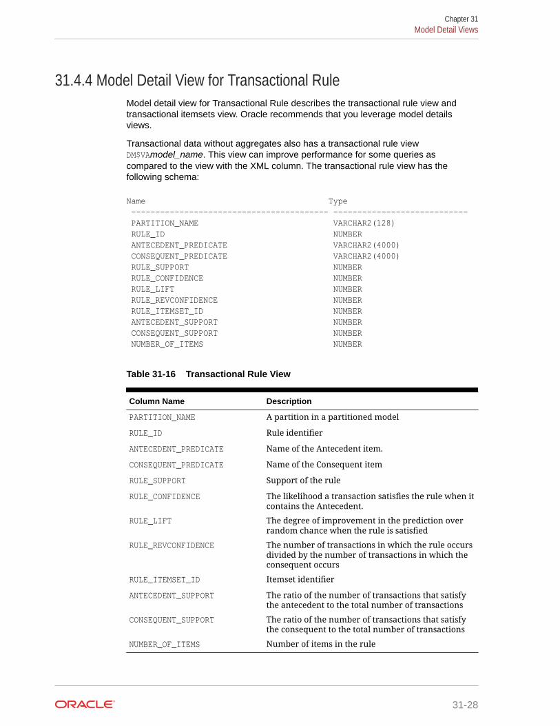
31.4.4 Model Detail View for Transactional RuleModel detail view for Transactional Rule describes the transactional rule view andtransactional itemsets view. Oracle recommends that you leverage model detailsviews.
Transactional data without aggregates also has a transactional rule viewDM$VAmodel_name. This view can improve performance for some queries ascompared to the view with the XML column. The transactional rule view has thefollowing schema:
Name Type ----------------------------------------- ---------------------------- PARTITION_NAME VARCHAR2(128) RULE_ID NUMBER ANTECEDENT_PREDICATE VARCHAR2(4000) CONSEQUENT_PREDICATE VARCHAR2(4000) RULE_SUPPORT NUMBER RULE_CONFIDENCE NUMBER RULE_LIFT NUMBER RULE_REVCONFIDENCE NUMBER RULE_ITEMSET_ID NUMBER ANTECEDENT_SUPPORT NUMBER CONSEQUENT_SUPPORT NUMBER NUMBER_OF_ITEMS NUMBER
Table 31-16 Transactional Rule View
Column Name Description
PARTITION_NAME A partition in a partitioned model
RULE_ID Rule identifier
ANTECEDENT_PREDICATE Name of the Antecedent item.
CONSEQUENT_PREDICATE Name of the Consequent item
RULE_SUPPORT Support of the rule
RULE_CONFIDENCE The likelihood a transaction satisfies the rule when itcontains the Antecedent.
RULE_LIFT The degree of improvement in the prediction overrandom chance when the rule is satisfied
RULE_REVCONFIDENCE The number of transactions in which the rule occursdivided by the number of transactions in which theconsequent occurs
RULE_ITEMSET_ID Itemset identifier
ANTECEDENT_SUPPORT The ratio of the number of transactions that satisfythe antecedent to the total number of transactions
CONSEQUENT_SUPPORT The ratio of the number of transactions that satisfythe consequent to the total number of transactions
NUMBER_OF_ITEMS Number of items in the rule
Chapter 31Model Detail Views
31-28
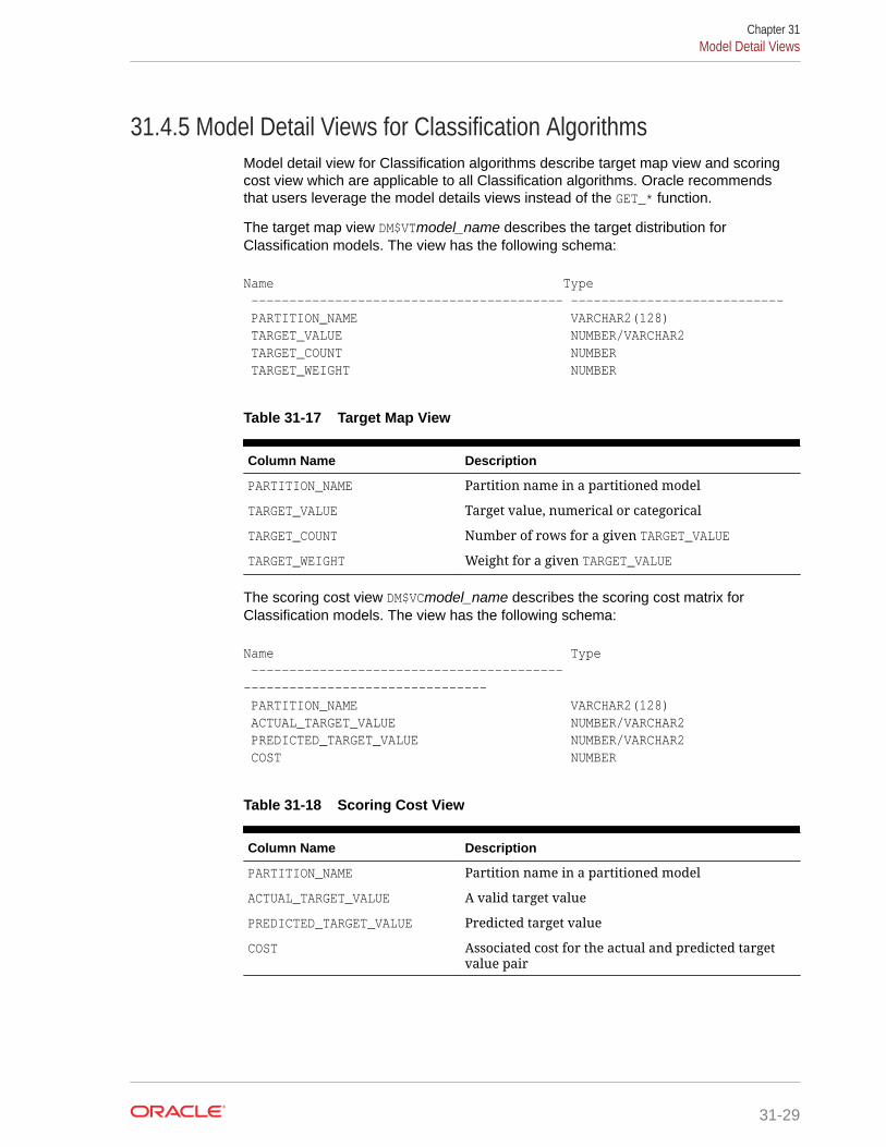
31.4.5 Model Detail Views for Classification AlgorithmsModel detail view for Classification algorithms describe target map view and scoringcost view which are applicable to all Classification algorithms. Oracle recommendsthat users leverage the model details views instead of the GET_* function.
The target map view DM$VTmodel_name describes the target distribution forClassification models. The view has the following schema:
Name Type ----------------------------------------- ---------------------------- PARTITION_NAME VARCHAR2(128) TARGET_VALUE NUMBER/VARCHAR2 TARGET_COUNT NUMBER TARGET_WEIGHT NUMBER
Table 31-17 Target Map View
Column Name Description
PARTITION_NAME Partition name in a partitioned model
TARGET_VALUE Target value, numerical or categorical
TARGET_COUNT Number of rows for a given TARGET_VALUE
TARGET_WEIGHT Weight for a given TARGET_VALUE
The scoring cost view DM$VCmodel_name describes the scoring cost matrix forClassification models. The view has the following schema:
Name Type ----------------------------------------- -------------------------------- PARTITION_NAME VARCHAR2(128) ACTUAL_TARGET_VALUE NUMBER/VARCHAR2 PREDICTED_TARGET_VALUE NUMBER/VARCHAR2 COST NUMBER
Table 31-18 Scoring Cost View
Column Name Description
PARTITION_NAME Partition name in a partitioned model
ACTUAL_TARGET_VALUE A valid target value
PREDICTED_TARGET_VALUE Predicted target value
COST Associated cost for the actual and predicted targetvalue pair
Chapter 31Model Detail Views
31-29
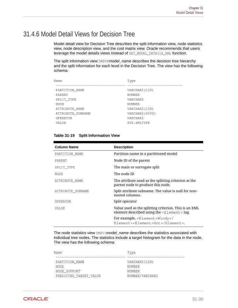
31.4.6 Model Detail Views for Decision TreeModel detail view for Decision Tree describes the split information view, node statisticsview, node description view, and the cost matrix view. Oracle recommends that usersleverage the model details views instead of GET_MODEL_DETAILS_XML function.
The split information view DM$VPmodel_name describes the decision tree hierarchyand the split information for each level in the Decision Tree. The view has the followingschema:
Name Type ---------------------------------- --------------------------- PARTITION_NAME VARCHAR2(128) PARENT NUMBER SPLIT_TYPE VARCHAR2 NODE NUMBER ATTRIBUTE_NAME VARCHAR2(128) ATTRIBUTE_SUBNAME VARCHAR2(4000) OPERATOR VARCHAR2 VALUE SYS.XMLTYPE
Table 31-19 Split Information View
Column Name Description
PARTITION_NAME Partition name in a partitioned model
PARENT Node ID of the parent
SPLIT_TYPE The main or surrogate split
NODE The node ID
ATTRIBUTE_NAME The attribute used as the splitting criterion at theparent node to produce this node.
ATTRIBUTE_SUBNAME Split attribute subname. The value is null for non-nested columns.
OPERATOR Split operator
VALUE Value used as the splitting criterion. This is an XMLelement described using the <Element> tag.
For example, <Element>Windy</Element><Element>Hot</Element>.
The node statistics view DM$VImodel_name describes the statistics associated withindividual tree nodes. The statistics include a target histogram for the data in the node.The view has the following schema:
Name Type ---------------------------------- ---------------------------- PARTITION_NAME VARCHAR2(128) NODE NUMBER NODE_SUPPORT NUMBER PREDICTED_TARGET_VALUE NUMBER/VARCHAR2
Chapter 31Model Detail Views
31-30

TARGET_VALUE NUMBER/VARCHAR2 TARGET_SUPPORT NUMBER
Table 31-20 Node Statistics View
Parameter Description
PARTITION_NAME Partition name in a partitioned model
NODE The node ID
NODE_SUPPORT Number of records in the training set that belong tothe node
PREDICTED_TARGET_VALUE Predicted Target value
TARGET_VALUE A target value seen in the training data
TARGET_SUPPORT The number of records that belong to the node andhave the value specified in the TARGET_VALUE column
Higher level node description can be found in DM$VOmodel_name view. TheDM$VOmodel_name has the following schema:
ame Type ---------------------------------- ---------------------------- PARTITION_NAME VARCHAR2(128) NODE NUMBER NODE_SUPPORT NUMBER PREDICTED_TARGET_VALUE NUMBER/VARCHAR2 PARENT NUMBER ATTRIBUTE_NAME VARCHAR2(128) ATTRIBUTE_SUBNAME VARCHAR2(4000) OPERATOR VARCHAR2 VALUE SYS.XMLTYPE
Table 31-21 Node Description View
Parameter Description
PARTITION_NAME Partition name in a partitioned model
NODE The node ID
NODE_SUPPORT Number of records in the training set that belong tothe node
PREDICTED_TARGET_VALUE Predicted Target value
PARENT The ID of the parent
ATTRIBUTE_NAME Specifies the attribute name
ATTRIBUTE_SUBNAME Specifies the attribute subname
OPERATOR Attribute predicate operator - a conditional operatortaking the following values:IN, = , <>, < , >, <=, and >=
Chapter 31Model Detail Views
31-31

Table 31-21 (Cont.) Node Description View
Parameter Description
VALUE Value used as the description criterion. This is anXML element described using the <Element> tag.
For example, <Element>Windy</Element><Element>Hot</Element>.
The DM$VMmodel_name view describes the cost matrix used by the Decision Treebuild. The DM$VMmodel_name view has the following schema:
Name Type ----------------------------------------- -------------------------------- PARTITION_NAME VARCHAR2(128) ACTUAL_TARGET_VALUE NUMBER/VARCHAR2 PREDICTED_TARGET_VALUE NUMBER/VARCHAR2 COST NUMBER
Table 31-22 Cost Matrix View
Parameter Description
PARTITION_NAME Partition name in a partitioned model
ACTUAL_TARGET_VALUE Valid target value
PREDICTED_TARGET_VALUE Predicted Target value
COST Associated cost for the actual and predicted targetvalue pair
The following table describes the global view for Decision Tree.
Table 31-23 Decision Tree Statistics Information In Model Global View
Name Description
NUM_ROWS The total number of rows used in the build
31.4.7 Model Detail Views for Generalized Linear ModelModel details views for Generalized Linear Model (GLM) describes the model detailsview and row diagnostic view for Linear and Logistic Regression. Oracle recommendsthat users leverage model details views than the GET_MODEL_DETAILS_GLM function.
The model details view DM$VDmodel_name describes the final model information forboth Linear Regression models and Logistic Regression models.
For Linear Regression, the view DM$VDmodel_name has the following schema:
Name Type ---------------------------------- ----------------------------
Chapter 31Model Detail Views
31-32

PARTITION_NAME VARCHAR2(128) ATTRIBUTE_NAME VARCHAR2(128) ATTRIBUTE_SUBNAME VARCHAR2(4000) ATTRIBUTE_VALUE VARCHAR2(4000) FEATURE_EXPRESSION VARCHAR2(4000) COEFFICIENT BINARY_DOUBLE STD_ERROR BINARY_DOUBLE TEST_STATISTIC BINARY_DOUBLE P_VALUE BINARY_DOUBLE VIF BINARY_DOUBLE STD_COEFFICIENT BINARY_DOUBLE LOWER_COEFF_LIMIT BINARY_DOUBLE UPPER_COEFF_LIMIT BINARY_DOUBLE
For Logistic Regression, the view DM$VDmodel_name has the following schema:
Name Type ---------------------------------- ---------------------------- PARTITION_NAME VARCHAR2(128) TARGET_VALUE NUMBER/VARCHAR2 ATTRIBUTE_NAME VARCHAR2(128) ATTRIBUTE_SUBNAME VARCHAR2(4000) ATTRIBUTE_VALUE VARCHAR2(4000) FEATURE_EXPRESSION VARCHAR2(4000) COEFFICIENT BINARY_DOUBLE STD_ERROR BINARY_DOUBLE TEST_STATISTIC BINARY_DOUBLE P_VALUE BINARY_DOUBLE STD_COEFFICIENT BINARY_DOUBLE LOWER_COEFF_LIMIT BINARY_DOUBLE UPPER_COEFF_LIMIT BINARY_DOUBLE EXP_COEFFICIENT BINARY_DOUBLE EXP_LOWER_COEFF_LIMIT BINARY_DOUBLE EXP_UPPER_COEFF_LIMIT BINARY_DOUBLE
Table 31-24 Model View for Linear and Logistic Regression Models
Column Name Description
PARTITION_NAME The name of a feature in the model
TARGET_VALUE Valid target value
ATTRIBUTE_NAME The attribute name when there is no subname, or first part ofthe attribute name when there is a subname. ATTRIBUTE_NAMEis the name of a column in the source table or view. If thecolumn is a non-nested, numeric column, then ATTRIBUTE_NAMEis the name of the mining attribute. For the intercept,ATTRIBUTE_NAME is null. Intercepts are equivalent to the biasterm in SVM models.
Chapter 31Model Detail Views
31-33

Table 31-24 (Cont.) Model View for Linear and Logistic Regression Models
Column Name Description
ATTRIBUTE_SUBNAME Nested column subname. The value is null for non-nestedcolumns.When the nested column is numeric, the miningattribute is identified by the combination ATTRIBUTE_NAME- ATTRIBUTE_SUBNAME. If the column is not nested,ATTRIBUTE_SUBNAME is null. If the attribute is an intercept, boththe ATTRIBUTE_NAME and the ATTRIBUTE_SUBNAME are null.
ATTRIBUTE_VALUE A unique value that can be assumed by a categoricalcolumn or nested categorical column. For categoricalcolumns, a mining attribute is identified by a uniqueATTRIBUTE_NAME.ATTRIBUTE_VALUE pair. For nested categoricalcolumns, a mining attribute is identified by the combination:ATTRIBUTE_NAME.ATTRIBUTE_SUBNAME.ATTRIBUTE_VALUE. Fornumerical attributes, ATTRIBUTE_VALUE is null.
FEATURE_EXPRESSION The feature name constructed by the algorithm when featureselection is enabled. If feature selection is not enabled, thefeature name is simply the fully-qualified attribute name(attribute_name.attribute_subname if the attribute is in a nestedcolumn). For categorical attributes, the algorithm constructs afeature name that has the following form:fully-qualified_attribute_name.attribute_valueWhen feature generation is enabled, a term in the modelcan be a single mining attribute or the product of up to3 mining attributes. Component mining attributes can berepeated within a single term. If feature generation is notenabled or, if feature generation is enabled, but no multiplecomponent terms are discovered by the CREATE model process,then FEATURE_EXPRESSION is null.
Note:
In 12c Release 2, the algorithmdoes not subtract the mean fromnumerical components.
COEFFICIENT The estimated coefficient.
STD_ERROR Standard error of the coefficient estimate.
TEST_STATISTIC For Linear Regression, the t-value of the coefficient estimate.For Logistic Regression, the Wald chi-square value of thecoefficient estimate.
P_VALUE Probability of the TEST_STATISTIC under the (NULL) hypothesisthat the term in the model is not statistically significant. A lowprobability indicates that the term is significant, while a highprobability indicates that the term can be better discarded. Usedto analyze the significance of specific attributes in the model.
VIF Variance Inflation Factor. The value is zero for the intercept. ForLogistic Regression, VIF is null.
Chapter 31Model Detail Views
31-34

Table 31-24 (Cont.) Model View for Linear and Logistic Regression Models
Column Name Description
STD_COEFFICIENT Standardized estimate of the coefficient.
LOWER_COEFF_LIMIT Lower confidence bound of the coefficient.
UPPER_COEFF_LIMIT Upper confidence bound of the coefficient.
EXP_COEFFICIENT Exponentiated coefficient for Logistic Regression. For linearregression, EXP_COEFFICIENT is null.
EXP_LOWER_COEFF_LIMIT Exponentiated coefficient for lower confidence bound of thecoefficient for Logistic Regression. For Linear Regression,EXP_LOWER_COEFF_LIMIT is null.
EXP_UPPER_COEFF_LIMIT Exponentiated coefficient for upper confidence bound of thecoefficient for Logistic Regression. For Linear Regression,EXP_UPPER_COEFF_LIMIT is null.
The row diagnostic view DM$VAmodel_name describes row level information for bothLinear Regression models and Logistic Regression models. For Linear Regression,the view DM$VAmodel_name has the following schema:
Name Type ---------------------------------- ---------------------------- PARTITION_NAME VARCHAR2(128) CASE_ID NUMBER/VARHCAR2, DATE, TIMESTAMP, TIMESTAMP WITH TIME ZONE, TIMESTAMP WITH LOCAL TIME ZONE TARGET_VALUE BINARY_DOUBLE PREDICTED_TARGET_VALUE BINARY_DOUBLE Hat BINARY_DOUBLE RESIDUAL BINARY_DOUBLE STD_ERR_RESIDUAL BINARY_DOUBLE STUDENTIZED_RESIDUAL BINARY_DOUBLE PRED_RES BINARY_DOUBLE COOKS_D BINARY_DOUBLE
Table 31-25 Row Diagnostic View for Linear Regression
Column Name Description
PARTITION_NAME Partition name in a partitioned model
CASE_ID Name of the case identifier
TARGET_VALUE The actual target value as taken from the input row
PREDICTED_TARGET_VALUE The model predicted target value for the row
HAT The diagonal element of the n*n (n=number of rows) that theHat matrix identifies with a specific input row. The modelpredictions for the input data are the product of the Hat matrixand vector of input target values. The diagonal elements (Hatvalues) represent the influence of the ith row on the ith fittedvalue. Large Hat values are indicators that the ith row is a pointof high leverage, a potential outlier.
Chapter 31Model Detail Views
31-35

Table 31-25 (Cont.) Row Diagnostic View for Linear Regression
Column Name Description
RESIDUAL The difference between the predicted and actual target value fora specific input row.
STD_ERR_RESIDUAL The standard error residual, sometimes called the Studentizedresidual, re-scales the residual to have constant variance acrossall input rows in an effort to make the input row residualscomparable. The process multiplies the residual by square rootof the row weight divided by the product of the model meansquare error and 1 minus the Hat value.
STUDENTIZED_RESIDUAL Studentized deletion residual adjusts the standard errorresidual for the influence of the current row.
PRED_RES The predictive residual is the weighted square of the deletionresiduals, computed as the row weight multiplied by the squareof the residual divided by 1 minus the Hat value.
COOKS_D Cook's distance is a measure of the combined impact of the ith
case on all of the estimated regression coefficients.
For Logistic Regression, the view DM$VAmodel_name has the following schema:
Name Type ---------------------------------- ---------------------------- PARTITION_NAME VARCHAR2(128) CASE_ID NUMBER/VARHCAR2, DATE, TIMESTAMP, TIMESTAMP WITH TIME ZONE, TIMESTAMP WITH LOCAL TIME ZONE TARGET_VALUE NUMBER/VARCHAR2 TARGET_VALUE_PROB BINARY_DOUBLE Hat BINARY_DOUBLE WORKING_RESIDUAL BINARY_DOUBLE PEARSON_RESIDUAL BINARY_DOUBLE DEVIANCE_RESIDUAL BINARY_DOUBLE C BINARY_DOUBLE CBAR BINARY_DOUBLE DIFDEV BINARY_DOUBLE DIFCHISQ BINARY_DOUBLE
Table 31-26 Row Diagnostic View for Logistic Regression
Column Name Description
PARTITION_NAME Partition name in a partitioned model
CASE_ID Name of the case identifier
TARGET_VALUE The actual target value as taken from the input row
TARGET_VALUE_PROB Model estimate of the probability of the predicted target value.
Chapter 31Model Detail Views
31-36

Table 31-26 (Cont.) Row Diagnostic View for Logistic Regression
Column Name Description
Hat The Hat value concept from Linear Regression is extendedto Logistic Regression by multiplying the Linear RegressionHat value by the variance function for Logistic Regression,the predicted probability multiplied by 1 minus the predictedprobability.
WORKING_RESIDUAL The working residual is the residual of the working response.The working response is the response on the linearized scale.For Logistic Regression it has the form: the ith row residualdivided by the variance of the ith row prediction. The varianceof the prediction is the predicted probability multiplied by 1minus the predicted probability.WORKING_RESIDUAL is the difference between the workingresponse and the linear predictor at convergence.
PEARSON_RESIDUAL The Pearson residual is a re-scaled version of the workingresidual, accounting for the weight. For Logistic Regression,the Pearson residual multiplies the residual by a factor that iscomputed as square root of the weight divided by the varianceof the predicted probability for the ith row.RESIDUAL is 1 minus the predicted probability of the actualtarget value for the row.
DEVIANCE_RESIDUAL The DEVIANCE_RESIDUAL is the contribution to the modeldeviance of the ith observation. For Logistic Regression it has theform the square root of 2 times the log(1 + e^eta) - eta forthe non-reference class and -square root of 2 time the log (1 +eta) for the reference class, where eta is the linear prediction(the prediction as if the model were a Linear Regression).
C Measures the overall change in the fitted logits due to thedeletion of the ith observation for all points including the onedeleted (the ith point). It is computed as the square of thePearson residual multiplied by the Hat value divided by thesquare of 1 minus the Hat value.Confidence interval displacement diagnostics that providesscalar measure of the influence of individual observations.
CBAR C and CBAR are extensions of Cooks’ distance for LogisticRegression. CBAR measures the overall change in the fitted logitsdue to the deletion of the ith observation for all points excludingthe one deleted (the ith point). It is computed as the square ofthe Pearson residual multiplied by the Hat value divided by (1minus the Hat value)Confidence interval displacement diagnostic which measuresthe influence of deleting an individual observation.
DIFDEV A statistic that measures the change in deviance that occurswhen an observation is deleted from the input. It is computed asthe square of the deviance residual plus CBAR.
DIFCHISQ A statistic that measures the change in the Pearson chi-squarestatistic that occurs when an observation is deleted from theinput. It is computed as CBAR divided by the Hat value.
Chapter 31Model Detail Views
31-37
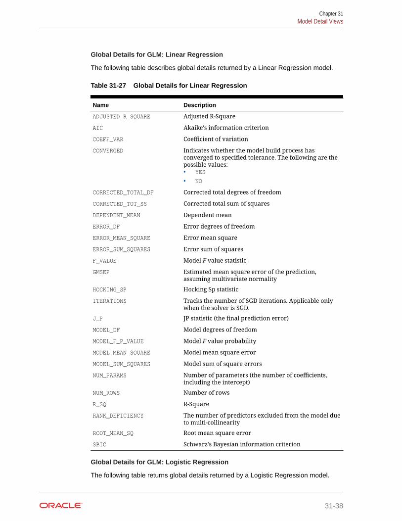
Global Details for GLM: Linear Regression
The following table describes global details returned by a Linear Regression model.
Table 31-27 Global Details for Linear Regression
Name Description
ADJUSTED_R_SQUARE Adjusted R-Square
AIC Akaike's information criterion
COEFF_VAR Coefficient of variation
CONVERGED Indicates whether the model build process hasconverged to specified tolerance. The following are thepossible values:• YES
• NO
CORRECTED_TOTAL_DF Corrected total degrees of freedom
CORRECTED_TOT_SS Corrected total sum of squares
DEPENDENT_MEAN Dependent mean
ERROR_DF Error degrees of freedom
ERROR_MEAN_SQUARE Error mean square
ERROR_SUM_SQUARES Error sum of squares
F_VALUE Model F value statistic
GMSEP Estimated mean square error of the prediction,assuming multivariate normality
HOCKING_SP Hocking Sp statistic
ITERATIONS Tracks the number of SGD iterations. Applicable onlywhen the solver is SGD.
J_P JP statistic (the final prediction error)
MODEL_DF Model degrees of freedom
MODEL_F_P_VALUE Model F value probability
MODEL_MEAN_SQUARE Model mean square error
MODEL_SUM_SQUARES Model sum of square errors
NUM_PARAMS Number of parameters (the number of coefficients,including the intercept)
NUM_ROWS Number of rows
R_SQ R-Square
RANK_DEFICIENCY The number of predictors excluded from the model dueto multi-collinearity
ROOT_MEAN_SQ Root mean square error
SBIC Schwarz's Bayesian information criterion
Global Details for GLM: Logistic Regression
The following table returns global details returned by a Logistic Regression model.
Chapter 31Model Detail Views
31-38
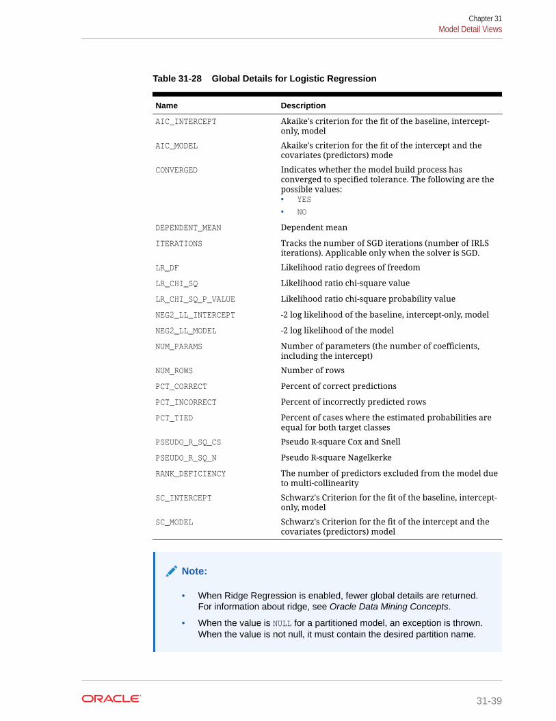
Table 31-28 Global Details for Logistic Regression
Name Description
AIC_INTERCEPT Akaike's criterion for the fit of the baseline, intercept-only, model
AIC_MODEL Akaike's criterion for the fit of the intercept and thecovariates (predictors) mode
CONVERGED Indicates whether the model build process hasconverged to specified tolerance. The following are thepossible values:• YES
• NO
DEPENDENT_MEAN Dependent mean
ITERATIONS Tracks the number of SGD iterations (number of IRLSiterations). Applicable only when the solver is SGD.
LR_DF Likelihood ratio degrees of freedom
LR_CHI_SQ Likelihood ratio chi-square value
LR_CHI_SQ_P_VALUE Likelihood ratio chi-square probability value
NEG2_LL_INTERCEPT -2 log likelihood of the baseline, intercept-only, model
NEG2_LL_MODEL -2 log likelihood of the model
NUM_PARAMS Number of parameters (the number of coefficients,including the intercept)
NUM_ROWS Number of rows
PCT_CORRECT Percent of correct predictions
PCT_INCORRECT Percent of incorrectly predicted rows
PCT_TIED Percent of cases where the estimated probabilities areequal for both target classes
PSEUDO_R_SQ_CS Pseudo R-square Cox and Snell
PSEUDO_R_SQ_N Pseudo R-square Nagelkerke
RANK_DEFICIENCY The number of predictors excluded from the model dueto multi-collinearity
SC_INTERCEPT Schwarz's Criterion for the fit of the baseline, intercept-only, model
SC_MODEL Schwarz's Criterion for the fit of the intercept and thecovariates (predictors) model
Note:
• When Ridge Regression is enabled, fewer global details are returned.For information about ridge, see Oracle Data Mining Concepts.
• When the value is NULL for a partitioned model, an exception is thrown.When the value is not null, it must contain the desired partition name.
Chapter 31Model Detail Views
31-39

Related Topics
• Oracle Database PL/SQL Packages and Types Reference
• Model Detail Views for Global InformationModel detail views for Global Information describes global statistics view, alertview, and computed settings view. Oracle recommends that users leverage themodel details views instead of GET_MODEL_DETAILS_GLOBAL function.
31.4.8 Model Detail Views for Naive BayesModel Detail Views for Naive Bayes describes prior view and result view.Oracle recommends that users leverage the model details views instead of theGET_MODEL_DETAILS_NB function.
The prior view DM$VPmodel_name describes the priors of the targets for Naïve Bayes.The view has the following schema:
Name Type ----------------------------------------- ---------------------------- PARTITION_NAME VARCHAR2(128) TARGET_NAME VARCHAR2(128) TARGET_VALUE NUMBER/VARCHAR2 PRIOR_PROBABILITY BINARY_DOUBLE COUNT NUMBER
Table 31-29 Prior View for Naive Bayes
Column Name Description
PARTITION_NAME The name of a feature in the model
TARGET_NAME Name of the target column
TARGET_VALUE Target value, numerical or categorical
PRIOR_PROBABILITY Prior probability for a given TARGET_VALUE
COUNT Number of rows for a given TARGET_VALUE
The Naïve Bayes result view DM$VVmodel_view describes the conditional probabilitiesof the Naïve Bayes model. The view has the following schema:
Name Type ----------------------------------------- ---------------------------- PARTITION_NAME VARCHAR2(128) TARGET_NAME VARCHAR2(128) TARGET_VALUE NUMBER/VARCHAR2 ATTRIBUTE_NAME VARCHAR2(128) ATTRIBUTE_SUBNAME VARCHAR2(4000) ATTRIBUTE_VALUE VARCHAR2(4000) CONDITIONAL_PROBABILITY BINARY_DOUBLE COUNT NUMBER
Chapter 31Model Detail Views
31-40

Table 31-30 Result View for Naive Bayes
Column Name Description
PARTITION_NAME The name of a feature in the model
TARGET_NAME Name of the target column
TARGET_VALUE Target value, numerical or categorical
ATTRIBUTE_NAME Column name
ATTRIBUTE_SUBNAME Nested column subname. The value is null for non-nested columns.
ATTRIBUTE_VALUE Mining attribute value for the columnATTRIBUTE_NAME or the nested columnATTRIBUTE_SUBNAME (if any).
CONDITIONAL_PROBABILITY Conditional probability of a mining attribute for agiven target
COUNT Number of rows for a given mining attribute and agiven target
The following table describes the global view for Naive Bayes.
Table 31-31 Naive Bayes Statistics Information In Model Global View
Name Description
NUM_ROWS The total number of rows used in the build
31.4.9 Model Detail Views for Neural NetworkModel Detail Views for Neural Network describes the weights of the neurons: inputlayer and hidden layers. Oracle recommends that users leverage the model detailsviews.
Neural Network algorithm has the following views:
Weights: DM$VAmodel_name
The view DM$VAmodel_name has the following schema:
Name Type ---------------------- ----------------------- PARTITION_NAME VARCHAR2(128) LAYER NUMBER IDX_FROM NUMBER ATTRIBUTE_NAME VARCHAR2(128) ATTRIBUTE_SUBNAME VARCHAR2(4000) ATTRIBUTE_VALUE VARCHAR2(4000) IDX_TO NUMBER TARGET_VALUE NUMBER/VARCHAR2 WEIGHT BINARY_DOUBLE
Chapter 31Model Detail Views
31-41

Table 31-32 Weights View
Column Name Description
PARTITION_NAME Partition name in a partitioned model
LAYER Layer ID, 0 as an input layer
IDX_FROM Node index that the weight connects from (attributeid for input layer)
ATTRIBUTE_NAME Attribute name (only for the input layer)
ATTRIBUTE_SUBNAME Attribute subname. The value is null for non-nestedcolumns.
ATTRIBUTE_VALUE Categorical attribute value
IDX_TO Node index that the weights connects to
TARGET_VALUE Target value. The value is null for regression.
WEIGHT Value of the weight
The view DM$VGmodel_name is a pre-existing view. The following name-value pairs areadded to the view.
Table 31-33 Neural Networks Statistics Information In Model Global View
Name Description
CONVERGED Indicates whether the model build process hasconverged to specified tolerance. The following arethe possible values:• YES
• NO
ITERATIONS Number of iterations
LOSS_VALUE Loss function value (if it is withNNET_REGULARIZER_HELDASIDE regularization, it isthe loss function value on test data)
NUM_ROWS Number of rows in the model (or partitioned model)
31.4.10 Model Detail Views for Random ForestModel Detail Views for Random Forest describes variable importance measures andstatistics in global view. Oracle recommends that users leverage the model detailsviews.
Random Forest algorithm has the following statistics views:
• Variable importance statistics DM$VAmodel_name
• Random Forest statistics in model global view DM$VGmodel_name
Chapter 31Model Detail Views
31-42
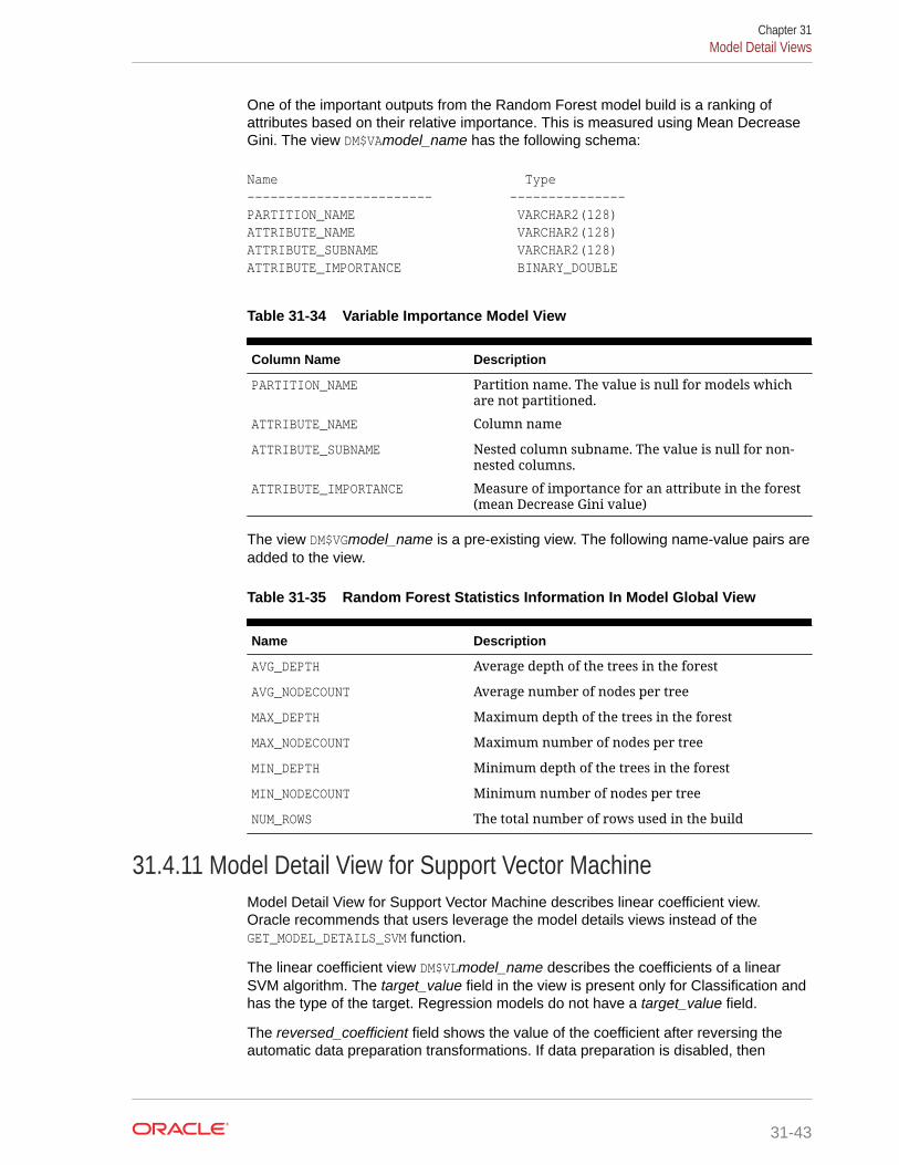
One of the important outputs from the Random Forest model build is a ranking ofattributes based on their relative importance. This is measured using Mean DecreaseGini. The view DM$VAmodel_name has the following schema:
Name Type ------------------------ --------------- PARTITION_NAME VARCHAR2(128) ATTRIBUTE_NAME VARCHAR2(128) ATTRIBUTE_SUBNAME VARCHAR2(128) ATTRIBUTE_IMPORTANCE BINARY_DOUBLE
Table 31-34 Variable Importance Model View
Column Name Description
PARTITION_NAME Partition name. The value is null for models whichare not partitioned.
ATTRIBUTE_NAME Column name
ATTRIBUTE_SUBNAME Nested column subname. The value is null for non-nested columns.
ATTRIBUTE_IMPORTANCE Measure of importance for an attribute in the forest(mean Decrease Gini value)
The view DM$VGmodel_name is a pre-existing view. The following name-value pairs areadded to the view.
Table 31-35 Random Forest Statistics Information In Model Global View
Name Description
AVG_DEPTH Average depth of the trees in the forest
AVG_NODECOUNT Average number of nodes per tree
MAX_DEPTH Maximum depth of the trees in the forest
MAX_NODECOUNT Maximum number of nodes per tree
MIN_DEPTH Minimum depth of the trees in the forest
MIN_NODECOUNT Minimum number of nodes per tree
NUM_ROWS The total number of rows used in the build
31.4.11 Model Detail View for Support Vector MachineModel Detail View for Support Vector Machine describes linear coefficient view.Oracle recommends that users leverage the model details views instead of theGET_MODEL_DETAILS_SVM function.
The linear coefficient view DM$VLmodel_name describes the coefficients of a linearSVM algorithm. The target_value field in the view is present only for Classification andhas the type of the target. Regression models do not have a target_value field.
The reversed_coefficient field shows the value of the coefficient after reversing theautomatic data preparation transformations. If data preparation is disabled, then
Chapter 31Model Detail Views
31-43
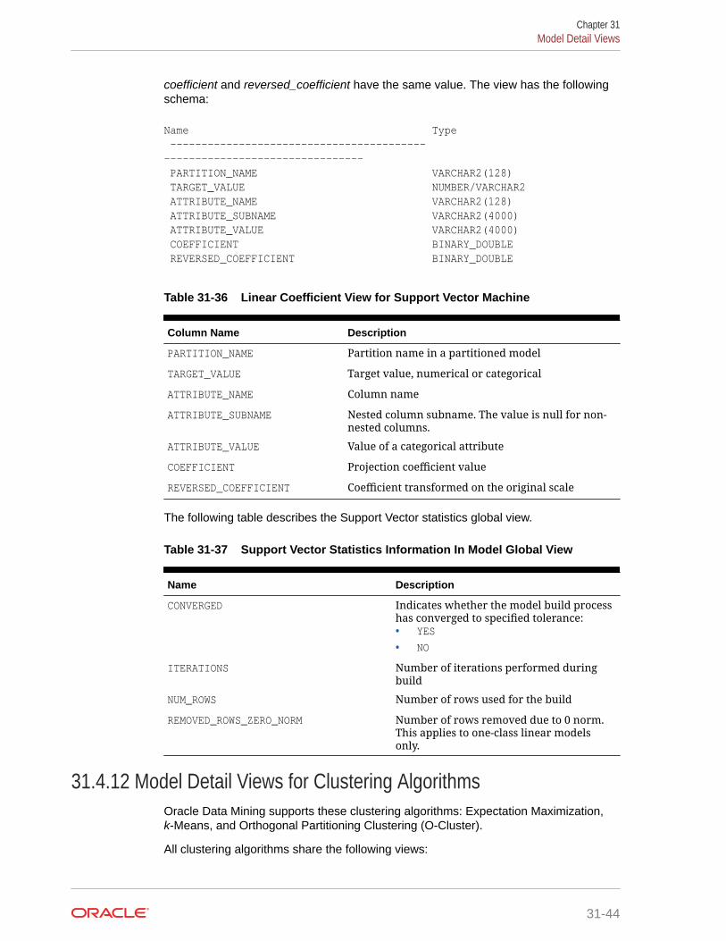
coefficient and reversed_coefficient have the same value. The view has the followingschema:
Name Type ----------------------------------------- -------------------------------- PARTITION_NAME VARCHAR2(128) TARGET_VALUE NUMBER/VARCHAR2 ATTRIBUTE_NAME VARCHAR2(128) ATTRIBUTE_SUBNAME VARCHAR2(4000) ATTRIBUTE_VALUE VARCHAR2(4000) COEFFICIENT BINARY_DOUBLE REVERSED_COEFFICIENT BINARY_DOUBLE
Table 31-36 Linear Coefficient View for Support Vector Machine
Column Name Description
PARTITION_NAME Partition name in a partitioned model
TARGET_VALUE Target value, numerical or categorical
ATTRIBUTE_NAME Column name
ATTRIBUTE_SUBNAME Nested column subname. The value is null for non-nested columns.
ATTRIBUTE_VALUE Value of a categorical attribute
COEFFICIENT Projection coefficient value
REVERSED_COEFFICIENT Coefficient transformed on the original scale
The following table describes the Support Vector statistics global view.
Table 31-37 Support Vector Statistics Information In Model Global View
Name Description
CONVERGED Indicates whether the model build processhas converged to specified tolerance:• YES
• NO
ITERATIONS Number of iterations performed duringbuild
NUM_ROWS Number of rows used for the build
REMOVED_ROWS_ZERO_NORM Number of rows removed due to 0 norm.This applies to one-class linear modelsonly.
31.4.12 Model Detail Views for Clustering AlgorithmsOracle Data Mining supports these clustering algorithms: Expectation Maximization,k-Means, and Orthogonal Partitioning Clustering (O-Cluster).
All clustering algorithms share the following views:
Chapter 31Model Detail Views
31-44

• Cluster description DM$VDmodel_name
• Attribute statistics DM$VAmodel_name
• Histogram statistics DM$VHmodel_name
• Rule statistics DM$VRmodel_name
The cluster description view DM$VDmodel_name describes cluster level informationabout a clustering model. The view has the following schema:
Name Type ---------------------------------- ---------------------------- PARTITION_NAME VARCHAR2(128) CLUSTER_ID NUMBER CLUSTER_NAME NUMBER/VARCHAR2 RECORD_COUNT NUMBER PARENT NUMBER TREE_LEVEL NUMBER LEFT_CHILD_ID NUMBER RIGHT_CHILD_ID NUMBER
Table 31-38 Cluster Description View for Clustering Algorithm
Column Name Description
PARTITION_NAME Partition name in a partitioned model
CLUSTER_ID The ID of a cluster in the model
CLUSTER_NAME Specifies the label of the cluster
RECORD_COUNT Specifies the number of records
PARENT The ID of the parent
TREE_LEVEL Specifies the number of splits from the root
LEFT_CHILD_ID The ID of the child cluster on the left side of the split
RIGHT_CHILD_ID The ID of the child cluster on the right side of thesplit
The attribute view DM$VAmodel_name describes attribute level information about aClustering model. The values of the mean, variance, and mode for a particular clustercan be obtained from this view. The view has the following schema:
Name Type ---------------------------------- ---------------------------- PARTITION_NAME VARCHAR2(128) CLUSTER_ID NUMBER CLUSTER_NAME NUMBER/VARCHAR2 ATTRIBUTE_NAME VARCHAR2(128) ATTRIBUTE_SUBNAME VARCHAR2(4000) MEAN BINARY_DOUBLE VARIANCE BINARY_DOUBLE MODE_VALUE VARCHAR2(4000)
Chapter 31Model Detail Views
31-45

Table 31-39 Attribute View for Clustering Algorithm
Column Name Description
PARTITION_NAME A partition in a partitioned model
CLUSTER_ID The ID of a cluster in the model
CLUSTER_NAME Specifies the label of the cluster
ATTRIBUTE_NAME Specifies the attribute name
ATTRIBUTE_SUBNAME Specifies the attribute subname
MEAN The field returns the average value of a numericattribute
VARIANCE The variance of a numeric attribute
MODE_VALUE The mode is the most frequent value of a categoricalattribute
The histogram view DM$VHmodel_name describes histogram level information about aClustering model. The bin information as well as bin counts can be obtained from thisview. The view has the following schema:
Name Type ---------------------------------- ---------------------------- PARTITION_NAME VARCHAR2(128) CLUSTER_ID NUMBER CLUSTER_NAME NUMBER/VARCHAR2 ATTRIBUTE_NAME VARCHAR2(128) ATTRIBUTE_SUBNAME VARCHAR2(4000) BIN_ID NUMBER LOWER_BIN_BOUNDARY BINARY_DOUBLE UPPER_BIN_BOUNDARY BINARY_DOUBLE ATTRIBUTE_VALUE VARCHAR2(4000) COUNT NUMBER
Table 31-40 Histogram View for Clustering Algorithm
Column Name Description
PARTITION_NAME A partition in a partitioned model
CLUSTER_ID The ID of a cluster in the model
CLUSTER_NAME Specifies the label of the cluster
ATTRIBUTE_NAME Specifies the attribute name
ATTRIBUTE_SUBNAME Specifies the attribute subname
BIN_ID Bin ID
LOWER_BIN_BOUNDARY Numeric lower bin boundary
UPPER_BIN_BOUNDARY Numeric upper bin boundary
ATTRIBUTE_VALUE Categorical attribute value
COUNT Histogram count
Chapter 31Model Detail Views
31-46
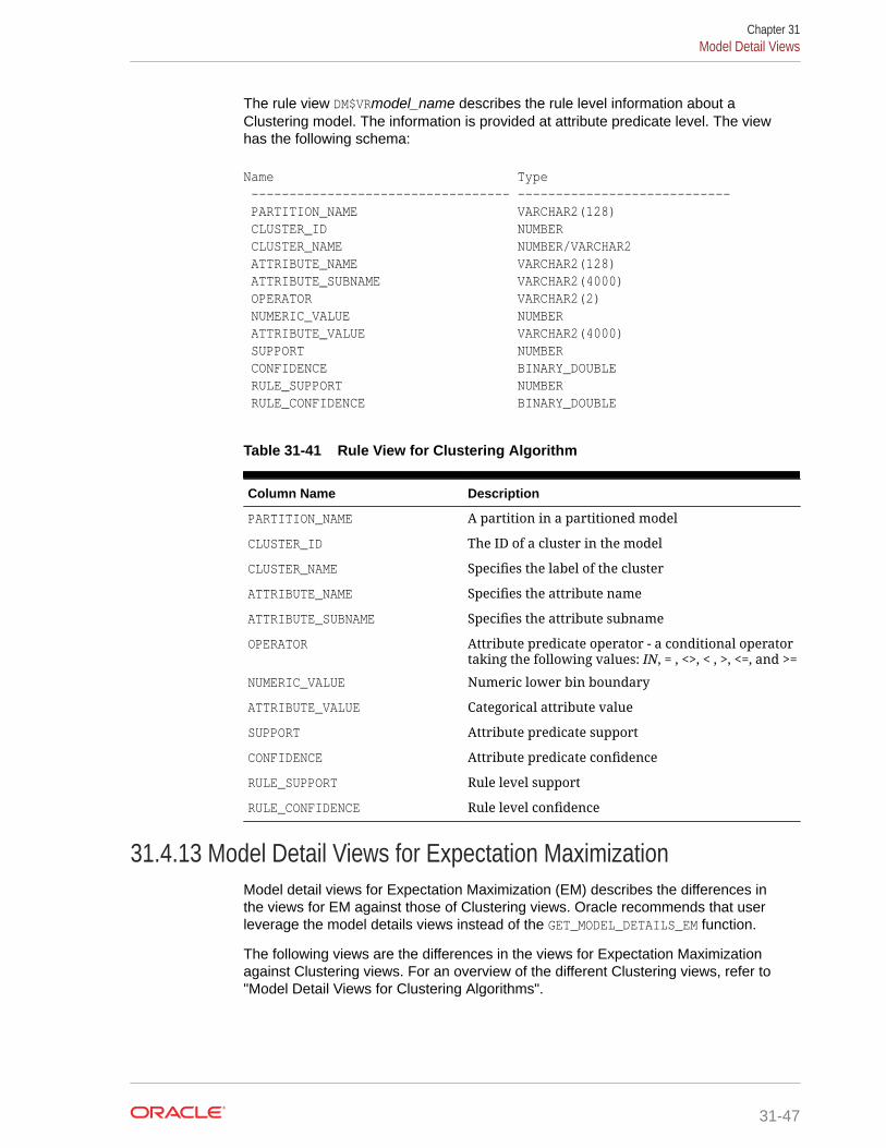
The rule view DM$VRmodel_name describes the rule level information about aClustering model. The information is provided at attribute predicate level. The viewhas the following schema:
Name Type ---------------------------------- ---------------------------- PARTITION_NAME VARCHAR2(128) CLUSTER_ID NUMBER CLUSTER_NAME NUMBER/VARCHAR2 ATTRIBUTE_NAME VARCHAR2(128) ATTRIBUTE_SUBNAME VARCHAR2(4000) OPERATOR VARCHAR2(2) NUMERIC_VALUE NUMBER ATTRIBUTE_VALUE VARCHAR2(4000) SUPPORT NUMBER CONFIDENCE BINARY_DOUBLE RULE_SUPPORT NUMBER RULE_CONFIDENCE BINARY_DOUBLE
Table 31-41 Rule View for Clustering Algorithm
Column Name Description
PARTITION_NAME A partition in a partitioned model
CLUSTER_ID The ID of a cluster in the model
CLUSTER_NAME Specifies the label of the cluster
ATTRIBUTE_NAME Specifies the attribute name
ATTRIBUTE_SUBNAME Specifies the attribute subname
OPERATOR Attribute predicate operator - a conditional operatortaking the following values: IN, = , <>, < , >, <=, and >=
NUMERIC_VALUE Numeric lower bin boundary
ATTRIBUTE_VALUE Categorical attribute value
SUPPORT Attribute predicate support
CONFIDENCE Attribute predicate confidence
RULE_SUPPORT Rule level support
RULE_CONFIDENCE Rule level confidence
31.4.13 Model Detail Views for Expectation MaximizationModel detail views for Expectation Maximization (EM) describes the differences inthe views for EM against those of Clustering views. Oracle recommends that userleverage the model details views instead of the GET_MODEL_DETAILS_EM function.
The following views are the differences in the views for Expectation Maximizationagainst Clustering views. For an overview of the different Clustering views, refer to"Model Detail Views for Clustering Algorithms".
Chapter 31Model Detail Views
31-47
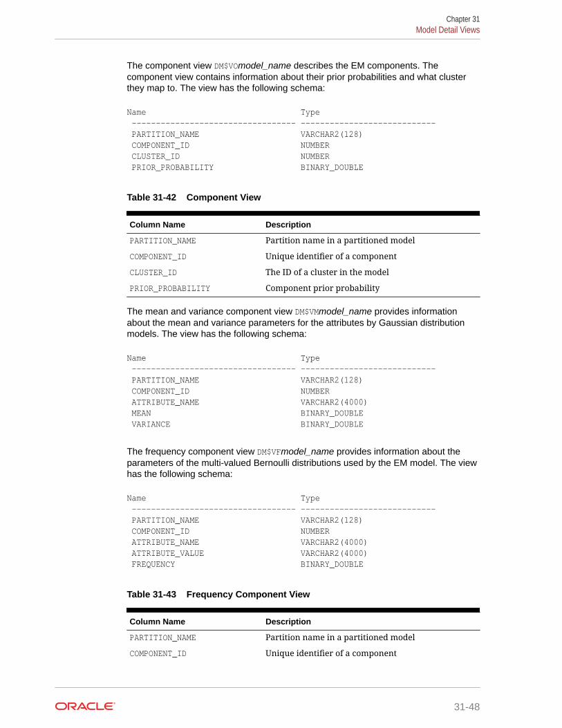
The component view DM$VOmodel_name describes the EM components. Thecomponent view contains information about their prior probabilities and what clusterthey map to. The view has the following schema:
Name Type ---------------------------------- ---------------------------- PARTITION_NAME VARCHAR2(128) COMPONENT_ID NUMBER CLUSTER_ID NUMBER PRIOR_PROBABILITY BINARY_DOUBLE
Table 31-42 Component View
Column Name Description
PARTITION_NAME Partition name in a partitioned model
COMPONENT_ID Unique identifier of a component
CLUSTER_ID The ID of a cluster in the model
PRIOR_PROBABILITY Component prior probability
The mean and variance component view DM$VMmodel_name provides informationabout the mean and variance parameters for the attributes by Gaussian distributionmodels. The view has the following schema:
Name Type ---------------------------------- ---------------------------- PARTITION_NAME VARCHAR2(128) COMPONENT_ID NUMBER ATTRIBUTE_NAME VARCHAR2(4000) MEAN BINARY_DOUBLE VARIANCE BINARY_DOUBLE
The frequency component view DM$VFmodel_name provides information about theparameters of the multi-valued Bernoulli distributions used by the EM model. The viewhas the following schema:
Name Type ---------------------------------- ---------------------------- PARTITION_NAME VARCHAR2(128) COMPONENT_ID NUMBER ATTRIBUTE_NAME VARCHAR2(4000) ATTRIBUTE_VALUE VARCHAR2(4000) FREQUENCY BINARY_DOUBLE
Table 31-43 Frequency Component View
Column Name Description
PARTITION_NAME Partition name in a partitioned model
COMPONENT_ID Unique identifier of a component
Chapter 31Model Detail Views
31-48

Table 31-43 (Cont.) Frequency Component View
Column Name Description
ATTRIBUTE_NAME Column name
ATTRIBUTE_VALUE Categorical attribute value
FREQUENCY The frequency of the multivalued Bernoullidistribution for the attribute/value combinationspecified by ATTRIBUTE_NAME and ATTRIBUTE_VALUE.
For 2-Dimensional columns, EM provides an attribute ranking similar to that ofAttribute Importance. This ranking is based on a rank-weighted average overKullback–Leibler divergence computed for pairs of columns. This unsupervisedAttribute Importance is shown in the DM$VImodel_name view and has the followingschema:
Name Type ----------------------------------------- ---------------------------- PARTITION_NAME VARCHAR2(128) ATTRIBUTE_NAME VARCHAR2(128) ATTRIBUTE_IMPORTANCE_VALUE BINARY_DOUBLE ATTRIBUTE_RANK NUMBER
Table 31-44 2–Dimensional Attribute Ranking for Expectation Maximization
Column Name Description
PARTITION_NAME Partition name in a partitioned model
ATTRIBUTE_NAME Column name
ATTRIBUTE_IMPORTANCE_VALUE Importance value
ATTRIBUTE_RANK An attribute rank based on the importance value
The pairwise Kullback–Leibler divergence is reported in the DM$VBmodel_nameview. This metric evaluates how much the observed joint distribution of two attributesdiverges from the expected distribution under the assumption of independence. Thatis, the higher the value, the more dependent the two attributes are. The dependencyvalue is scaled based on the size of the grid used for each pairwise computation. Thatensures that all values fall within the [0; 1] range and are comparable. The view hasthe following schema:
Name Type ----------------------------------------- ---------------------------- PARTITION_NAME VARCHAR2(128) ATTRIBUTE_NAME_1 VARCHAR2(128) ATTRIBUTE_NAME_2 VARCHAR2(128) DEPENDENCY BINARY_DOUBLE
Chapter 31Model Detail Views
31-49
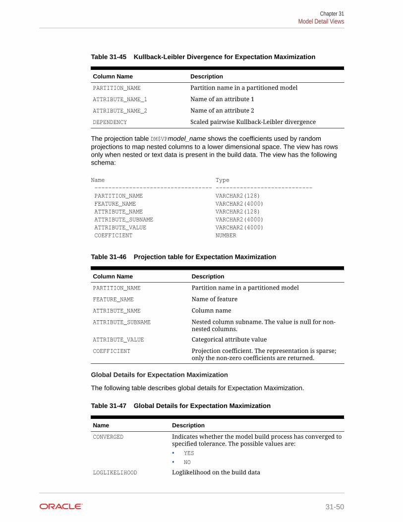
Table 31-45 Kullback-Leibler Divergence for Expectation Maximization
Column Name Description
PARTITION_NAME Partition name in a partitioned model
ATTRIBUTE_NAME_1 Name of an attribute 1
ATTRIBUTE_NAME_2 Name of an attribute 2
DEPENDENCY Scaled pairwise Kullback-Leibler divergence
The projection table DM$VPmodel_name shows the coefficients used by randomprojections to map nested columns to a lower dimensional space. The view has rowsonly when nested or text data is present in the build data. The view has the followingschema:
Name Type ---------------------------------- ---------------------------- PARTITION_NAME VARCHAR2(128) FEATURE_NAME VARCHAR2(4000) ATTRIBUTE_NAME VARCHAR2(128) ATTRIBUTE_SUBNAME VARCHAR2(4000) ATTRIBUTE_VALUE VARCHAR2(4000) COEFFICIENT NUMBER
Table 31-46 Projection table for Expectation Maximization
Column Name Description
PARTITION_NAME Partition name in a partitioned model
FEATURE_NAME Name of feature
ATTRIBUTE_NAME Column name
ATTRIBUTE_SUBNAME Nested column subname. The value is null for non-nested columns.
ATTRIBUTE_VALUE Categorical attribute value
COEFFICIENT Projection coefficient. The representation is sparse;only the non-zero coefficients are returned.
Global Details for Expectation Maximization
The following table describes global details for Expectation Maximization.
Table 31-47 Global Details for Expectation Maximization
Name Description
CONVERGED Indicates whether the model build process has converged tospecified tolerance. The possible values are:• YES
• NO
LOGLIKELIHOOD Loglikelihood on the build data
Chapter 31Model Detail Views
31-50

Table 31-47 (Cont.) Global Details for Expectation Maximization
Name Description
NUM_COMPONENTS Number of components produced by the model
NUM_CLUSTERS Number of clusters produced by the model
NUM_ROWS Number of rows used in the build
RANDOM_SEED The random seed value used for the model build
REMOVED_COMPONENTS The number of empty components excluded from the model
Related Topics
• Model Detail Views for Clustering AlgorithmsOracle Data Mining supports these clustering algorithms: ExpectationMaximization, k-Means, and Orthogonal Partitioning Clustering (O-Cluster).
31.4.14 Model Detail Views for k-MeansModel detail views for k-Means (KM) describes cluster description view andscoring view. Oracle recommends that you leverage model details view instead ofGET_MODEL_DETAILS_KM function.
This section describes the differences in the views for k-Means against the Clusteringviews. For an overview of the different views, refer to "Model Detail Views forClustering Algorithms". For k-Means, the cluster description view DM$VDmodel_namehas an additional column:
Name Type ---------------------------------- ---------------------------- DISPERSION BINARY_DOUBLE
Table 31-48 Cluster Description for k-Means
Column Name Description
DISPERSION A measure used to quantify whether a set ofobserved occurrences are dispersed compared to astandard statistical model.
The scoring view DM$VCmodel_name describes the centroid of each leaf clusters:
Name Type ---------------------------------- ---------------------------- PARTITION_NAME VARCHAR2(128) CLUSTER_ID NUMBER CLUSTER_NAME NUMBER/VARCHAR2 ATTRIBUTE_NAME VARCHAR2(128) ATTRIBUTE_SUBNAME VARCHAR2(4000) ATTRIBUTE_VALUE VARCHAR2(4000) VALUE BINARY_DOUBLE
Chapter 31Model Detail Views
31-51
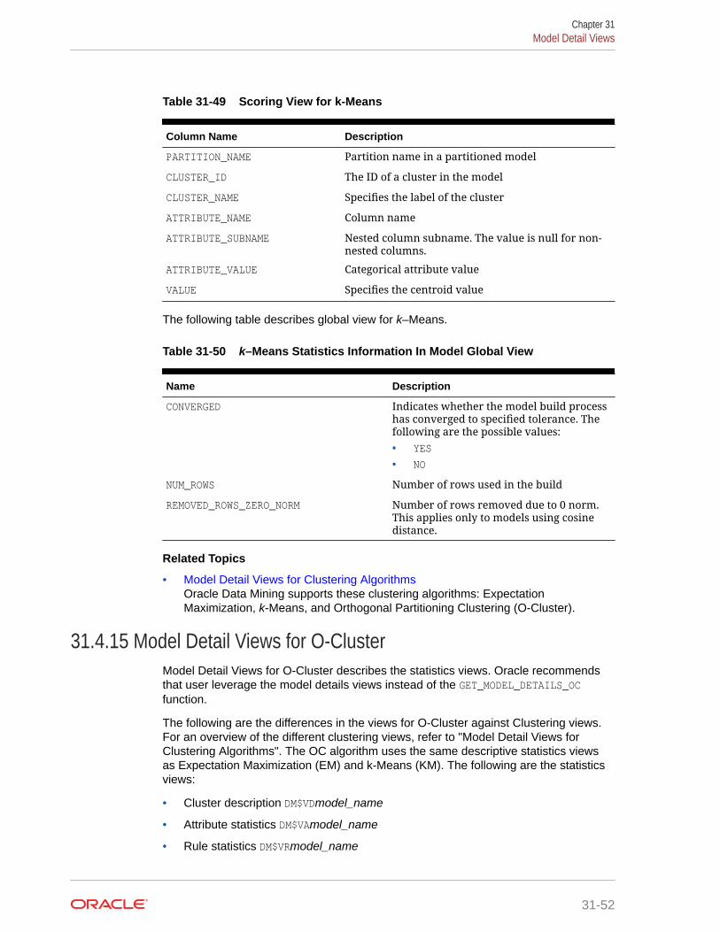
Table 31-49 Scoring View for k-Means
Column Name Description
PARTITION_NAME Partition name in a partitioned model
CLUSTER_ID The ID of a cluster in the model
CLUSTER_NAME Specifies the label of the cluster
ATTRIBUTE_NAME Column name
ATTRIBUTE_SUBNAME Nested column subname. The value is null for non-nested columns.
ATTRIBUTE_VALUE Categorical attribute value
VALUE Specifies the centroid value
The following table describes global view for k–Means.
Table 31-50 k–Means Statistics Information In Model Global View
Name Description
CONVERGED Indicates whether the model build processhas converged to specified tolerance. Thefollowing are the possible values:• YES
• NO
NUM_ROWS Number of rows used in the build
REMOVED_ROWS_ZERO_NORM Number of rows removed due to 0 norm.This applies only to models using cosinedistance.
Related Topics
• Model Detail Views for Clustering AlgorithmsOracle Data Mining supports these clustering algorithms: ExpectationMaximization, k-Means, and Orthogonal Partitioning Clustering (O-Cluster).
31.4.15 Model Detail Views for O-ClusterModel Detail Views for O-Cluster describes the statistics views. Oracle recommendsthat user leverage the model details views instead of the GET_MODEL_DETAILS_OCfunction.
The following are the differences in the views for O-Cluster against Clustering views.For an overview of the different clustering views, refer to "Model Detail Views forClustering Algorithms". The OC algorithm uses the same descriptive statistics viewsas Expectation Maximization (EM) and k-Means (KM). The following are the statisticsviews:
• Cluster description DM$VDmodel_name
• Attribute statistics DM$VAmodel_name
• Rule statistics DM$VRmodel_name
Chapter 31Model Detail Views
31-52

• Histogram statistics DM$VHmodel_name
The Cluster description view DM$VDmodel_name describes the O-Cluster components.The cluster description view has additional fields that specify the split predicate. Theview has the following schema:
Name Type ---------------------------------- ---------------------------- ATTRIBUTE_NAME VARCHAR2(128) ATTRIBUTE_SUBNAME VARCHAR2(4000) OPERATOR VARCHAR2(2) VALUE SYS.XMLTYPE
Table 31-51 Description View
Column Name Description
ATTRIBUTE_NAME Column name
ATTRIBUTE_SUBNAME Nested column subname. The value is null for non-nested columns.
OPERATOR Split operator
VALUE List of split values
The structure of the SYS.XMLTYPE is as follows:
<Element>splitval1</Element>
The OC algorithm uses a histogram view DM$VHmodel_name with a different schemathan EM and k-Means (KM). The view has the following schema:
Name Type ---------------------------------- ---------------------------- PARTITON_NAME VARCHAR2(128) CLUSTER_ID NUMBER ATTRIBUTE_NAME VARCHAR2(128) ATTRIBUTE_SUBNAME VARCHAR2(4000) BIN_ID NUMBER LABEL VARCHAR2(4000) COUNT NUMBER
Table 31-52 Histogram Component View
Column Name Description
PARTITION_NAME Partition name in a partitioned model
CLUSTER_ID Unique identifier of a component
ATTRIBUTE_NAME Column name
ATTRIBUTE_SUBNAME Nested column subname. The value is null for non-nested columns.
BIN_ID Unique identifier
Chapter 31Model Detail Views
31-53

Table 31-52 (Cont.) Histogram Component View
Column Name Description
LABEL Bin label
COUNT Bin histogram count
The following table describes the global view for O-Cluster.
Table 31-53 O-Cluster Statistics Information In Model Global View
Name Description
NUM_ROWS The total number of rows used in the build
Related Topics
• Model Detail Views for Clustering AlgorithmsOracle Data Mining supports these clustering algorithms: ExpectationMaximization, k-Means, and Orthogonal Partitioning Clustering (O-Cluster).
31.4.16 Model Detail Views for CUR Matrix DecompositionModel Detail Views for CUR matrix decomposition describe scores and ranks ofattributes and rows.
CUR matrix decomposition algorithm has the following views:
Attribute importance and rank: DM$VCmodel_name
Row importance and rank: DM$VRmodel_name
Global statistics: DM$VG
The Attribute Importance and Rank view DM$VCmodel_name has the following schema:
Name Type ----------------- ----------------- PARTITION_NAME VARCHAR2(128) ATTRIBUTE_NAME VARCHAR2(128) ATTRIBUTE_SUBNAME VARCHAR2(4000) ATTRIBUTE_VALUE VARCHAR2(4000) ATTRIBUTE_IMPORTANCE NUMBER ATTRIBUTE_RANK NUMBER
Table 31-54 Attribute Importance and Rank View
Column Name Description
PARTITION_NAME Partition name in a partitioned model
ATTRIBUTE_NAME Attribute name
ATTRIBUTE_SUBNAME Attribute subname. The value is null for non-nestedcolumns.
Chapter 31Model Detail Views
31-54

Table 31-54 (Cont.) Attribute Importance and Rank View
Column Name Description
ATTRIBUTE_VALUE Value of the attribute
ATTRIBUTE_IMPORTANCE Attribute leverage score
ATTRIBUTE_RANK Attribute rank based on leverage score
The view DM$VRmodel_name exposes the leverage scores and ranks of all selectedrows through a view. This view is created when users decide to perform rowimportance and the CASE_ID column is present. The view has the following schema:
Name Type --------------------- ------------------------ PARTITION_NAME VARCHAR2(128) CASE_ID Original cid data types, including NUMBER, VARCHAR2, DATE, TIMESTAMP, TIMESTAMP WITH TIME ZONE, TIMESTAMP WITH LOCAL TIME ZONE ROW_IMPORTANCE NUMBER ROW_RANK NUMBER
Table 31-55 Row Importance and Rank View
Column Name Description
PARTITION_NAME Partition name in a partitioned model
CASE_ID Case ID. The supported case ID types are the same asthat supported for GLM, SVD, and ESA algorithms.
ROW_IMPORTANCE Row leverage score
ROW_RANK Row rank based on leverage score
The following table describes global statistics for CUR Matrix Decomposition.
Table 31-56 CUR Matrix Decomposition Statistics Information In Model GlobalView.
Name Description
NUM_COMPONENTS Number of SVD components (SVD rank)
NUM_ROWS Number of rows used in the model build
31.4.17 Model Detail Views for Explicit Semantic AnalysisModel Detail Views for Explicit Semantic Analysis (ESA) describes attribute statisticsview and feature view. Oracle recommends that users leverage the model details view.
ESA algorithm has the following views:
Chapter 31Model Detail Views
31-55
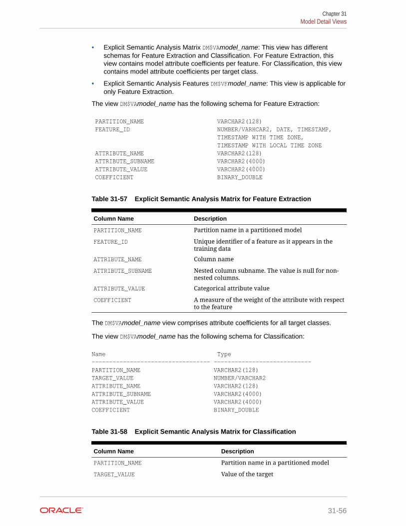
• Explicit Semantic Analysis Matrix DM$VAmodel_name: This view has differentschemas for Feature Extraction and Classification. For Feature Extraction, thisview contains model attribute coefficients per feature. For Classification, this viewcontains model attribute coefficients per target class.
• Explicit Semantic Analysis Features DM$VFmodel_name: This view is applicable foronly Feature Extraction.
The view DM$VAmodel_name has the following schema for Feature Extraction:
PARTITION_NAME VARCHAR2(128) FEATURE_ID NUMBER/VARHCAR2, DATE, TIMESTAMP, TIMESTAMP WITH TIME ZONE, TIMESTAMP WITH LOCAL TIME ZONE ATTRIBUTE_NAME VARCHAR2(128) ATTRIBUTE_SUBNAME VARCHAR2(4000) ATTRIBUTE_VALUE VARCHAR2(4000) COEFFICIENT BINARY_DOUBLE
Table 31-57 Explicit Semantic Analysis Matrix for Feature Extraction
Column Name Description
PARTITION_NAME Partition name in a partitioned model
FEATURE_ID Unique identifier of a feature as it appears in thetraining data
ATTRIBUTE_NAME Column name
ATTRIBUTE_SUBNAME Nested column subname. The value is null for non-nested columns.
ATTRIBUTE_VALUE Categorical attribute value
COEFFICIENT A measure of the weight of the attribute with respectto the feature
The DM$VAmodel_name view comprises attribute coefficients for all target classes.
The view DM$VAmodel_name has the following schema for Classification:
Name Type---------------------------------- ----------------------------PARTITION_NAME VARCHAR2(128)TARGET_VALUE NUMBER/VARCHAR2ATTRIBUTE_NAME VARCHAR2(128)ATTRIBUTE_SUBNAME VARCHAR2(4000)ATTRIBUTE_VALUE VARCHAR2(4000)COEFFICIENT BINARY_DOUBLE
Table 31-58 Explicit Semantic Analysis Matrix for Classification
Column Name Description
PARTITION_NAME Partition name in a partitioned model
TARGET_VALUE Value of the target
Chapter 31Model Detail Views
31-56

Table 31-58 (Cont.) Explicit Semantic Analysis Matrix for Classification
Column Name Description
ATTRIBUTE_NAME Column name
ATTRIBUTE_SUBNAME Nested column subname. The value is nullfor non-nested columns.
ATTRIBUTE_VALUE Categorical attribute value
COEFFICIENT A measure of the weight of the attributewith respect to the feature
The view DM$VFmodel_name has a unique row for every feature in one view. Thisfeature is helpful if the model was pre-built and the source training data are notavailable. The view has the following schema:
Name Type ---------------------------------- ---------------------------- PARTITION_NAME VARCHAR2(128) FEATURE_ID NUMBER/VARHCAR2, DATE, TIMESTAMP, TIMESTAMP WITH TIME ZONE, TIMESTAMP WITH LOCAL TIME ZONE
Table 31-59 Explicit Semantic Analysis Features for Explicit Semantic Analysis
Column Name Description
PARTITION_NAME Partition name in a partitioned model
FEATURE_ID Unique identifier of a feature as it appears in thetraining data
The following table describes the global view for Explicit Semantic Analysis.
Table 31-60 Explicit Semantic Analysis Statistics Information In Model GlobalView
Name Description
NUM_ROWS The total number of input rows
REMOVED_ROWS_BY_FILTERS Number of rows removed by filters
31.4.18 Model Detail Views for Exponential Smoothing ModelsModel Detail Views for Exponential Smoothing Model (ESM) describes the views formodel output and global information. Oracle recommends that users leverage themodel details views.
Exponential Smoothing Model algorithm has the following views:
Model output: DM$VPmodel_name
Model global information: DM$VGmodel_name
Chapter 31Model Detail Views
31-57

Model output: This view gives the result of ESM model. The output has a set ofrecords such as partition, CASE_ID, value, prediction, lower, upper, and so on andordered by partition and CASE_ID (time). Each partition has a separate smoothingmodel. For a given partition, for each time (CASE_ID) point that the input time seriescovers, the value is the observed or accumulated value at the time point, and theprediction is the one-step-ahead forecast at that time point. For each time point (futureprediction) beyond the range of input time series, the value is NULL, and the predictionis the model forecast for that time point. Lower and upper are the lower bound andupper bound of the user specified confidence interval for the prediction.
Model global Information: This view gives the global information of the modelalong with the estimated smoothing constants, the estimated initial state, and globaldiagnostic measures.
Depending on the type of model, the global diagnostics include some or all of thefollowing for Exponential Smoothing.
Table 31-61 Exponential Smoothing Model Statistics Information In ModelGlobal View
Name Description
–2 LOG-LIKELIHOOD Negative log-likelihood of model
ALPHA Smoothing constant
AIC Akaike information criterion
AICC Corrected Akaike information criterion
AMSE Average mean square error over user-specified time window
BETA Trend smoothing constant
BIC Bayesian information criterion
GAMMA Seasonal smoothing constant
INITIAL LEVEL Model estimate of value one time intervalprior to start of observed series
INITIAL SEASON i Model estimate of seasonal effect forseason i one time interval prior to start ofobserved series
INITIAL TREND Model estimate of trend one time intervalprior to start of observed series
MAE Model mean absolute error
MSE Model mean square error
PHI Damping parameter
STD Model standard error
SIGMA Model standard deviation of residuals
Chapter 31Model Detail Views
31-58
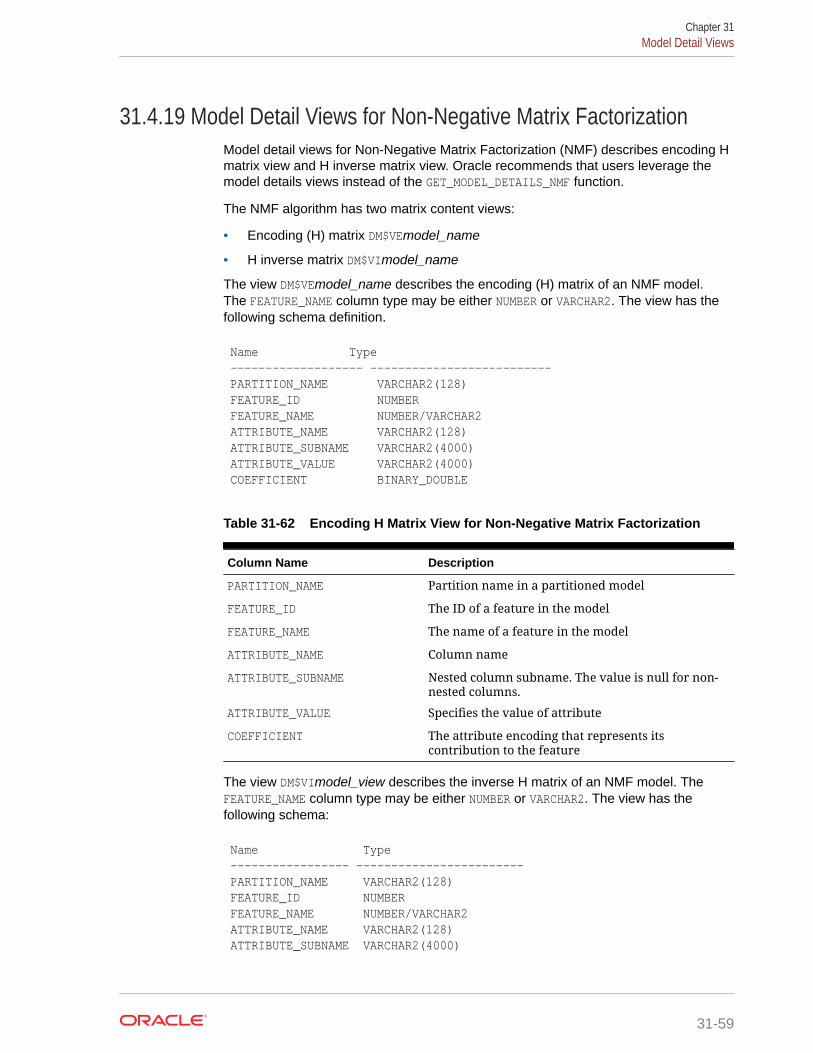
31.4.19 Model Detail Views for Non-Negative Matrix FactorizationModel detail views for Non-Negative Matrix Factorization (NMF) describes encoding Hmatrix view and H inverse matrix view. Oracle recommends that users leverage themodel details views instead of the GET_MODEL_DETAILS_NMF function.
The NMF algorithm has two matrix content views:
• Encoding (H) matrix DM$VEmodel_name
• H inverse matrix DM$VImodel_name
The view DM$VEmodel_name describes the encoding (H) matrix of an NMF model.The FEATURE_NAME column type may be either NUMBER or VARCHAR2. The view has thefollowing schema definition.
Name Type ------------------- -------------------------- PARTITION_NAME VARCHAR2(128) FEATURE_ID NUMBER FEATURE_NAME NUMBER/VARCHAR2 ATTRIBUTE_NAME VARCHAR2(128) ATTRIBUTE_SUBNAME VARCHAR2(4000) ATTRIBUTE_VALUE VARCHAR2(4000) COEFFICIENT BINARY_DOUBLE
Table 31-62 Encoding H Matrix View for Non-Negative Matrix Factorization
Column Name Description
PARTITION_NAME Partition name in a partitioned model
FEATURE_ID The ID of a feature in the model
FEATURE_NAME The name of a feature in the model
ATTRIBUTE_NAME Column name
ATTRIBUTE_SUBNAME Nested column subname. The value is null for non-nested columns.
ATTRIBUTE_VALUE Specifies the value of attribute
COEFFICIENT The attribute encoding that represents itscontribution to the feature
The view DM$VImodel_view describes the inverse H matrix of an NMF model. TheFEATURE_NAME column type may be either NUMBER or VARCHAR2. The view has thefollowing schema:
Name Type ----------------- ------------------------ PARTITION_NAME VARCHAR2(128) FEATURE_ID NUMBER FEATURE_NAME NUMBER/VARCHAR2 ATTRIBUTE_NAME VARCHAR2(128) ATTRIBUTE_SUBNAME VARCHAR2(4000)
Chapter 31Model Detail Views
31-59

ATTRIBUTE_VALUE VARCHAR2(4000) COEFFICIENT BINARY_DOUBLE
Table 31-63 Inverse H Matrix View for Non-Negative Matrix Factorization
Column Name Description
PARTITION_NAME Partition name in a partitioned model
FEATURE_ID The ID of a feature in the model
FEATURE_NAME The name of a feature in the model
ATTRIBUTE_NAME Column name
ATTRIBUTE_SUBNAME Nested column subname. The value is null for non-nested columns.
ATTRIBUTE_VALUE Specifies the value of attribute
COEFFICIENT The attribute encoding that represents itscontribution to the feature
The following table describes the global statistics for Non-Negative MatrixFactorization.
Table 31-64 Non-Negative Matrix Factorization Statistics Information In ModelGlobal View
Name Description
CONV_ERROR Convergence error
CONVERGED Indicates whether the model build processhas converged to specified tolerance. Thefollowing are the possible values:• YES
• NO
ITERATIONS Number of iterations performed duringbuild
NUM_ROWS Number of rows used in the build inputdataset
SAMPLE_SIZE Number of rows used by the build
31.4.20 Model Detail Views for Singular Value DecompositionModel detail views for Singular Value Decomposition (SVD) describes S Matrixview, right-singular vectors view, and left-singular vector view. Oracle recommendsthat users leverage the model details views instead of the GET_MODEL_DETAILS_SVDfunction.
The DM$VEmodel_name view leverages the fact that each singular value in theSVD model has a corresponding principal component in the associated PrincipalComponents Analysis (PCA) model to relate a common set of information for bothclasses of models. For a SVD model, it describes the content of the S matrix. WhenPCA scoring is selected as a build setting, the variance and percentage cumulative
Chapter 31Model Detail Views
31-60

variance for the corresponding principal components are shown as well. The view hasthe following schema:
Name Type ---------------------------------- ---------------------------- PARTITION_NAME VARCHAR2(128) FEATURE_ID NUMBER FEATURE_NAME NUMBER/VARCHAR2 VALUE BINARY_DOUBLE VARIANCE BINARY_DOUBLE PCT_CUM_VARIANCE BINARY_DOUBLE
Table 31-65 S Matrix View
Column Name Description
PARTITION_NAME Partition name in a partitioned model
FEATURE_ID The ID of a feature in the model
FEATURE_NAME The name of a feature in the model
VALUE The matrix entry value
VARIANCE The variance explained by a component. Thiscolumn is only present for SVD models withsetting dbms_data_mining.svds_scoring_mode setto dbms_data_mining.svds_scoring_pca
This column is non-null only if the build datais centered, either manually or because of thefollowing setting:dbms_data_mining.prep_auto isset to dbms_data_mining.prep_auto_on.
PCT_CUM_VARIANCE The percent cumulative variance explained by thecomponents thus far. The components are ranked bythe explained variance in descending order.This column is only present for SVD models withsetting dbms_data_mining.svds_scoring_mode setto dbms_data_mining.svds_scoring_pca
This column is non-null only if the build datais centered, either manually or because of thefollowing setting:dbms_data_mining.prep_auto isset to dbms_data_mining.prep_auto_on.
The SVD DM$VVmodel_view describes the right-singular vectors of SVD model. For aPCA model it describes the principal components (eigenvectors). The view has thefollowing schema:
Name Type ---------------------------------- ---------------------------- PARTITION_NAME VARCHAR2(128) FEATURE_ID NUMBER FEATURE_NAME NUMBER/VARCHAR2 ATTRIBUTE_NAME VARCHAR2(128) ATTRIBUTE_SUBNAME VARCHAR2(4000)
Chapter 31Model Detail Views
31-61

ATTRIBUTE_VALUE VARCHAR2(4000) VALUE BINARY_DOUBLE
Table 31-66 Right-singular Vectors of Singular Value Decomposition
Column Name Description
PARTITION_NAME Partition name in a partitioned model
FEATURE_ID The ID of a feature in the model
FEATURE_NAME The name of a feature in the model
ATTRIBUTE_NAME Column name
ATTRIBUTE_SUBNAME Nested column subname. The value is null for non-nested columns.
ATTRIBUTE_VALUE Categorical attribute value. For numerical attributes,ATTRIBUTE_VALUE is null.
VALUE The matrix entry value
The view DM$VUmodel_name describes the left-singular vectors of a SVD model. Fora PCA model, it describes the projection of the data in the principal components. Thisview does not exist unless the settings dbms_data_mining.svds_u_matrix_output isset to dbms_data_mining.svds_u_matrix_enable. The view has the following schema:
Name Type ---------------------------------- ---------------------------- PARTITION_NAME VARCHAR2(128) CASE_ID NUMBER/VARHCAR2, DATE, TIMESTAMP, TIMESTAMP WITH TIME ZONE, TIMESTAMP WITH LOCAL TIME ZONE FEATURE_ID NUMBER FEATURE_NAME NUMBER/VARCHAR2 VALUE BINARY_DOUBLE
Table 31-67 Left-singular Vectors of Singular Value Decomposition orProjection Data in Principal Components
Column Name Description
PARTITION_NAME Partition name in a partitioned model
CASE_ID Unique identifier of the row in the build datadescribed by the U matrix projection.
FEATURE_ID The ID of a feature in the model
FEATURE_NAME The name of a feature in the model
VALUE The matrix entry value
Global Details for Singular Value Decomposition
The following table describes a global detail for Singular Value Decomposition.
Chapter 31Model Detail Views
31-62

Table 31-68 Global Details for Singular Value Decomposition
Name Description
NUM_COMPONENTS Number of features (components) produced by the model
NUM_ROWS The total number of rows used in the build
SUGGESTED_CUTOFF Suggested cutoff that indicates how many of the topcomputed features capture most of the variance in themodel. Using only the features below this cutoff would bea reasonable strategy for dimensionality reduction.
Related Topics
• Oracle Database PL/SQL Packages and Types Reference
31.4.21 Model Detail View for Minimum Description LengthModel detail view for Minimum Description Length (for calculating AttributeImportance) describes Attribute Importance view. Oracle recommends that usersleverage the model details views instead of the GET_MODEL_DETAILS_AI function.
The Attribute Importance view DM$VAmodel_name describes the Attribute Importanceas well as the Attribute Importance rank. The view has the following schema:
Name Type ----------------------------------------- ---------------------------- PARTITION_NAME VARCHAR2(128) ATTRIBUTE_NAME VARCHAR2(128) ATTRIBUTE_SUBNAME VARCHAR2(4000) ATTRIBUTE_IMPORTANCE_VALUE BINARY_DOUBLE ATTRIBUTE_RANK NUMBER
Table 31-69 Attribute Importance View for Minimum Description Length
Column Name Description
PARTITION_NAME Partition name in a partitioned model
ATTRIBUTE_NAME Column name
ATTRIBUTE_SUBNAME Nested column subname. The value is null for non-nested columns.
ATTRIBUTE_IMPORTANCE_VALUE Importance value
ATTRIBUTE_RANK Rank based on importance
The following table describes the global view for Minimum Description Length.
Table 31-70 Minimum Description Length Statistics Information In ModelGlobal View
Name Description
NUM_ROWS The total number of rows used in the build
Chapter 31Model Detail Views
31-63
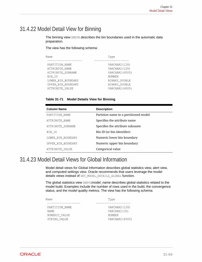
31.4.22 Model Detail View for BinningThe binning view DM$VB describes the bin boundaries used in the automatic datapreparation.
The view has the following schema:
Name Type -------------------- -------------------- PARTITION_NAME VARCHAR2(128) ATTRIBUTE_NAME VARCHAR2(128) ATTRIBUTE_SUBNAME VARCHAR2(4000) BIN_ID NUMBER LOWER_BIN_BOUNDARY BINARY_DOUBLE UPPER_BIN_BOUNDARY BINARY_DOUBLE ATTRIBUTE_VALUE VARCHAR2(4000)
Table 31-71 Model Details View for Binning
Column Name Description
PARTITION_NAME Partition name in a partitioned model
ATTRIBUTE_NAME Specifies the attribute name
ATTRIBUTE_SUBNAME Specifies the attribute subname
BIN_ID Bin ID (or bin identifier)
LOWER_BIN_BOUNDARY Numeric lower bin boundary
UPPER_BIN_BOUNDARY Numeric upper bin boundary
ATTRIBUTE_VALUE Categorical value
31.4.23 Model Detail Views for Global InformationModel detail views for Global Information describes global statistics view, alert view,and computed settings view. Oracle recommends that users leverage the modeldetails views instead of GET_MODEL_DETAILS_GLOBAL function.
The global statistics view DM$VGmodel_name describes global statistics related to themodel build. Examples include the number of rows used in the build, the convergencestatus, and the model quality metrics. The view has the following schema:
Name Type ------------------- -------------------- PARTITION_NAME VARCHAR2(128) NAME VARCHAR2(30) NUMERIC_VALUE NUMBER STRING_VALUE VARCHAR2(4000)
Chapter 31Model Detail Views
31-64

Table 31-72 Global Statistics View
Column Name Description
PARTITION_NAME Partition name in a partitioned model
NAME Name of the statistic
NUMERIC_VALUE Numeric value of the statistic
STRING_VALUE Categorical value of the statistic
The alert view DM$VWmodel_name lists alerts issued during the model build. The viewhas the following schema:
Name Type ------------------- ---------------------- PARTITION_NAME VARCHAR2(128) ERROR_NUMBER BINARY_DOUBLE ERROR_TEXT VARCHAR2(4000)
Table 31-73 Alert View
Column Name Description
PARTITION_NAME Partition name in a partitioned model
ERROR_NUMBER Error number (valid when event is Error)
ERROR_TEXT Error message
The computed settings view DM$VSmodel_name lists the algorithm computed settings.The view has the following schema:
Name Type ----------------- -------------------- PARTITION_NAME VARCHAR2(128) SETTING_NAME VARCHAR2(30) SETTING_VALUE VARCHAR2(4000)
Table 31-74 Computed Settings View
Column Name Description
PARTITION_NAME Partition name in a partitioned model
SETTING_NAME Name of the setting
SETTING_VALUE Value of the setting
Chapter 31Model Detail Views
31-65
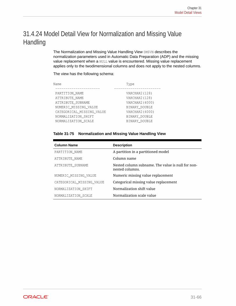
31.4.24 Model Detail View for Normalization and Missing ValueHandling
The Normalization and Missing Value Handling View DM$VN describes thenormalization parameters used in Automatic Data Preparation (ADP) and the missingvalue replacement when a NULL value is encountered. Missing value replacementapplies only to the twodimensional columns and does not apply to the nested columns.
The view has the following schema:
Name Type ---------------------- ----------------------- PARTITION_NAME VARCHAR2(128) ATTRIBUTE_NAME VARCHAR2(128) ATTRIBUTE_SUBNAME VARCHAR2(4000) NUMERIC_MISSING_VALUE BINARY_DOUBLE CATEGORICAL_MISSING_VALUE VARCHAR2(4000) NORMALIZATION_SHIFT BINARY_DOUBLE NORMALIZATION_SCALE BINARY_DOUBLE
Table 31-75 Normalization and Missing Value Handling View
Column Name Description
PARTITION_NAME A partition in a partitioned model
ATTRIBUTE_NAME Column name
ATTRIBUTE_SUBNAME Nested column subname. The value is null for non-nested columns.
NUMERIC_MISSING_VALUE Numeric missing value replacement
CATEGORICAL_MISSING_VALUE Categorical missing value replacement
NORMALIZATION_SHIFT Normalization shift value
NORMALIZATION_SCALE Normalization scale value
Chapter 31Model Detail Views
31-66

32Scoring and Deployment
Explains the scoring and deployment features of Oracle Data Mining.
• About Scoring and Deployment
• Using the Data Mining SQL Functions
• Prediction Details
• Real-Time Scoring
• Dynamic Scoring
• Cost-Sensitive Decision Making
• DBMS_DATA_MINING.Apply
32.1 About Scoring and DeploymentScoring is the application of models to new data. In Oracle Data Mining, scoring isperformed by SQL language functions.
Predictive functions perform Classification, Regression, or Anomaly detection.Clustering functions assign rows to clusters. Feature Extraction functions transformthe input data to a set of higher order predictors. A scoring procedure is also availablein the DBMS_DATA_MINING PL/SQL package.
Deployment refers to the use of models in a target environment. Once the modelshave been built, the challenges come in deploying them to obtain the best results, andin maintaining them within a production environment. Deployment can be any of thefollowing:
• Scoring data either for batch or real-time results. Scores can include predictions,probabilities, rules, and other statistics.
• Extracting model details to produce reports. For example: clustering rules,decision tree rules, or attribute rankings from an Attribute Importance model.
• Extending the business intelligence infrastructure of a data warehouse byincorporating mining results in applications or operational systems.
• Moving a model from the database where it was built to the database where itused for scoring (export/import)
Oracle Data Mining supports all of these deployment scenarios.
32-1
Note:
Oracle Data Mining scoring operations support parallel execution. Whenparallel execution is enabled, multiple CPU and I/O resources are appliedto the execution of a single database operation.
Parallel execution offers significant performance improvements, especiallyfor operations that involve complex queries and large databases typicallyassociated with decision support systems (DSS) and data warehouses.
Related Topics
• Oracle Database VLDB and Partitioning Guide
• Oracle Data Mining Concepts
• Exporting and Importing Mining ModelsYou can export data mining models to flat files to back up work in progress or tomove models to a different instance of Oracle Database Enterprise Edition (suchas from a development database to a test database).
32.2 Using the Data Mining SQL FunctionsLearn about the benefits of SQL functions in data mining.
The data mining SQL functions provide the following benefits:
• Models can be easily deployed within the context of existing SQL applications.
• Scoring operations take advantage of existing query execution functionality. Thisprovides performance benefits.
• Scoring results are pipelined, enabling the rows to be processed without requiringmaterialization.
The data mining functions produce a score for each row in the selection. The functionscan apply a mining model schema object to compute the score, or they can scoredynamically without a pre-defined model, as described in "Dynamic Scoring".
Related Topics
• Dynamic Scoring
• Scoring Requirements
• Table 28-4
• Oracle Database SQL Language Reference
32.2.1 Choosing the PredictorsThe data mining functions support a USING clause that specifies which attributes to usefor scoring. You can specify some or all of the attributes in the selection and you canspecify expressions. The following examples all use the PREDICTION function to findthe customers who are likely to use an affinity card, but each example uses a differentset of predictors.
The query in Example 32-1 uses all the predictors.
Chapter 32Using the Data Mining SQL Functions
32-2

The query in Example 32-2 uses only gender, marital status, occupation, and incomeas predictors.
The query in Example 32-3 uses three attributes and an expression as predictors. Theprediction is based on gender, marital status, occupation, and the assumption that allcustomers are in the highest income bracket.
Example 32-1 Using All Predictors
SELECT cust_gender, COUNT(*) AS cnt, ROUND(AVG(age)) AS avg_age FROM mining_data_apply_v WHERE PREDICTION(dt_sh_clas_sample USING *) = 1 GROUP BY cust_gender ORDER BY cust_gender; C CNT AVG_AGE- ---------- ----------F 25 38M 213 43
Example 32-2 Using Some Predictors
SELECT cust_gender, COUNT(*) AS cnt, ROUND(AVG(age)) AS avg_age FROM mining_data_apply_v WHERE PREDICTION(dt_sh_clas_sample USING cust_gender,cust_marital_status, occupation, cust_income_level) = 1 GROUP BY cust_gender ORDER BY cust_gender; C CNT AVG_AGE- ---------- ----------F 30 38M 186 43
Example 32-3 Using Some Predictors and an Expression
SELECT cust_gender, COUNT(*) AS cnt, ROUND(AVG(age)) AS avg_age FROM mining_data_apply_v WHERE PREDICTION(dt_sh_clas_sample USING cust_gender, cust_marital_status, occupation, 'L: 300,000 and above' AS cust_income_level) = 1 GROUP BY cust_gender ORDER BY cust_gender; C CNT AVG_AGE- ---------- ----------F 30 38M 186 43
32.2.2 Single-Record ScoringThe data mining functions can produce a score for a single record, as shown inExample 32-4 and Example 32-5.
Example 32-4 returns a prediction for customer 102001 by applying the classificationmodel NB_SH_Clas_sample. The resulting score is 0, meaning that this customer isunlikely to use an affinity card.
Chapter 32Using the Data Mining SQL Functions
32-3

Example 32-5 returns a prediction for 'Affinity card is great' as the comments attributeby applying the text mining model T_SVM_Clas_sample. The resulting score is 1,meaning that this customer is likely to use an affinity card.
Example 32-4 Scoring a Single Customer or a Single Text Expression
SELECT PREDICTION (NB_SH_Clas_Sample USING *) FROM sh.customers where cust_id = 102001; PREDICTION(NB_SH_CLAS_SAMPLEUSING*)----------------------------------- 0
Example 32-5 Scoring a Single Text Expression
SELECT PREDICTION(T_SVM_Clas_sample USING 'Affinity card is great' AS comments)FROM DUAL; PREDICTION(T_SVM_CLAS_SAMPLEUSING'AFFINITYCARDISGREAT'ASCOMMENTS)----------------------------------------------------------------- 1
32.3 Prediction DetailsPrediction details are XML strings that provide information about the score. Detailsare available for all types of scoring: clustering, feature extraction, classification,regression, and anomaly detection. Details are available whether scoring is dynamic orthe result of model apply.
The details functions, CLUSTER_DETAILS, FEATURE_DETAILS, and PREDICTION_DETAILSreturn the actual value of attributes used for scoring and the relative importance ofthe attributes in determining the score. By default, the functions return the five mostimportant attributes in descending order of importance.
32.3.1 Cluster DetailsFor the most likely cluster assignments of customer 100955 (probability of assignment> 20%), the query in the following example produces the five attributes that havethe most impact for each of the likely clusters. The clustering functions apply anExpectation Maximization model named em_sh_clus_sample to the data selected frommining_data_apply_v. The "5" specified in CLUSTER_DETAILS is not required, becausefive attributes are returned by default.
Example 32-6 Cluster Details
SELECT S.cluster_id, probability prob, CLUSTER_DETAILS(em_sh_clus_sample, S.cluster_id, 5 USING T.*) det FROM (SELECT v.*, CLUSTER_SET(em_sh_clus_sample, NULL, 0.2 USING *) pset FROM mining_data_apply_v v WHERE cust_id = 100955) T, TABLE(T.pset) S ORDER BY 2 DESC; CLUSTER_ID PROB DET---------- ----- ---------------------------------------------------------------------------- 14 .6761 <Details algorithm="Expectation Maximization" cluster="14">
Chapter 32Prediction Details
32-4
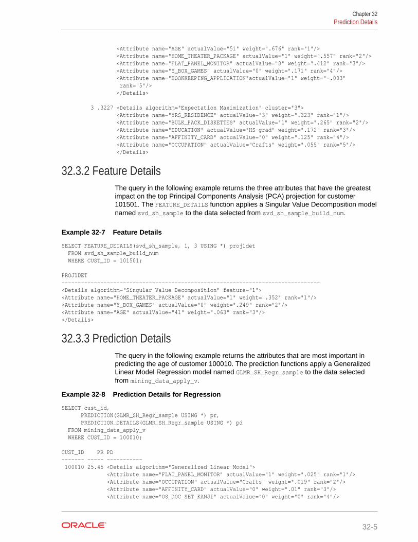
<Attribute name="AGE" actualValue="51" weight=".676" rank="1"/> <Attribute name="HOME_THEATER_PACKAGE" actualValue="1" weight=".557" rank="2"/> <Attribute name="FLAT_PANEL_MONITOR" actualValue="0" weight=".412" rank="3"/> <Attribute name="Y_BOX_GAMES" actualValue="0" weight=".171" rank="4"/> <Attribute name="BOOKKEEPING_APPLICATION"actualValue="1" weight="-.003" rank="5"/> </Details> 3 .3227 <Details algorithm="Expectation Maximization" cluster="3"> <Attribute name="YRS_RESIDENCE" actualValue="3" weight=".323" rank="1"/> <Attribute name="BULK_PACK_DISKETTES" actualValue="1" weight=".265" rank="2"/> <Attribute name="EDUCATION" actualValue="HS-grad" weight=".172" rank="3"/> <Attribute name="AFFINITY_CARD" actualValue="0" weight=".125" rank="4"/> <Attribute name="OCCUPATION" actualValue="Crafts" weight=".055" rank="5"/> </Details>
32.3.2 Feature DetailsThe query in the following example returns the three attributes that have the greatestimpact on the top Principal Components Analysis (PCA) projection for customer101501. The FEATURE_DETAILS function applies a Singular Value Decomposition modelnamed svd_sh_sample to the data selected from svd_sh_sample_build_num.
Example 32-7 Feature Details
SELECT FEATURE_DETAILS(svd_sh_sample, 1, 3 USING *) proj1det FROM svd_sh_sample_build_num WHERE CUST_ID = 101501; PROJ1DET--------------------------------------------------------------------------------<Details algorithm="Singular Value Decomposition" feature="1"><Attribute name="HOME_THEATER_PACKAGE" actualValue="1" weight=".352" rank="1"/><Attribute name="Y_BOX_GAMES" actualValue="0" weight=".249" rank="2"/><Attribute name="AGE" actualValue="41" weight=".063" rank="3"/></Details>
32.3.3 Prediction DetailsThe query in the following example returns the attributes that are most important inpredicting the age of customer 100010. The prediction functions apply a GeneralizedLinear Model Regression model named GLMR_SH_Regr_sample to the data selectedfrom mining_data_apply_v.
Example 32-8 Prediction Details for Regression
SELECT cust_id, PREDICTION(GLMR_SH_Regr_sample USING *) pr, PREDICTION_DETAILS(GLMR_SH_Regr_sample USING *) pd FROM mining_data_apply_v WHERE CUST_ID = 100010; CUST_ID PR PD------- ----- ----------- 100010 25.45 <Details algorithm="Generalized Linear Model"> <Attribute name="FLAT_PANEL_MONITOR" actualValue="1" weight=".025" rank="1"/> <Attribute name="OCCUPATION" actualValue="Crafts" weight=".019" rank="2"/> <Attribute name="AFFINITY_CARD" actualValue="0" weight=".01" rank="3"/> <Attribute name="OS_DOC_SET_KANJI" actualValue="0" weight="0" rank="4"/>
Chapter 32Prediction Details
32-5
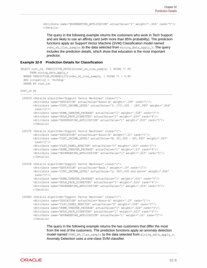
<Attribute name="BOOKKEEPING_APPLICATION" actualValue="1" weight="-.004" rank="5"/> </Details>
The query in the following example returns the customers who work in Tech Supportand are likely to use an affinity card (with more than 85% probability). The predictionfunctions apply an Support Vector Machine (SVM) Classification model namedsvmc_sh_clas_sample. to the data selected from mining_data_apply_v. The queryincludes the prediction details, which show that education is the most importantpredictor.
Example 32-9 Prediction Details for Classification
SELECT cust_id, PREDICTION_DETAILS(svmc_sh_clas_sample, 1 USING *) PD FROM mining_data_apply_v WHERE PREDICTION_PROBABILITY(svmc_sh_clas_sample, 1 USING *) > 0.85 AND occupation = 'TechSup' ORDER BY cust_id; CUST_ID PD------- --------------------------------------------------------------------------------------- 100029 <Details algorithm="Support Vector Machines" class="1"> <Attribute name="EDUCATION" actualValue="Assoc-A" weight=".199" rank="1"/> <Attribute name="CUST_INCOME_LEVEL" actualValue="I: 170\,000 - 189\,999" weight=".044" rank="2"/> <Attribute name="HOME_THEATER_PACKAGE" actualValue="1" weight=".028" rank="3"/> <Attribute name="BULK_PACK_DISKETTES" actualValue="1" weight=".024" rank="4"/> <Attribute name="BOOKKEEPING_APPLICATION" actualValue="1" weight=".022" rank="5"/> </Details> 100378 <Details algorithm="Support Vector Machines" class="1"> <Attribute name="EDUCATION" actualValue="Assoc-A" weight=".21" rank="1"/> <Attribute name="CUST_INCOME_LEVEL" actualValue="B: 30\,000 - 49\,999" weight=".047" rank="2"/> <Attribute name="FLAT_PANEL_MONITOR" actualValue="0" weight=".043" rank="3"/> <Attribute name="HOME_THEATER_PACKAGE" actualValue="1" weight=".03" rank="4"/> <Attribute name="BOOKKEEPING_APPLICATION" actualValue="1" weight=".023" rank="5"/> </Details> 100508 <Details algorithm="Support Vector Machines" class="1"> <Attribute name="EDUCATION" actualValue="Bach." weight=".19" rank="1"/> <Attribute name="CUST_INCOME_LEVEL" actualValue="L: 300\,000 and above" weight=".046" rank="2"/> <Attribute name="HOME_THEATER_PACKAGE" actualValue="1" weight=".031" rank="3"/> <Attribute name="BULK_PACK_DISKETTES" actualValue="1" weight=".026" rank="4"/> <Attribute name="BOOKKEEPING_APPLICATION" actualValue="1" weight=".024" rank="5"/> </Details> 100980 <Details algorithm="Support Vector Machines" class="1"> <Attribute name="EDUCATION" actualValue="Assoc-A" weight=".19" rank="1"/> <Attribute name="FLAT_PANEL_MONITOR" actualValue="0" weight=".038" rank="2"/> <Attribute name="HOME_THEATER_PACKAGE" actualValue="1" weight=".026" rank="3"/> <Attribute name="BULK_PACK_DISKETTES" actualValue="1" weight=".022" rank="4"/> <Attribute name="BOOKKEEPING_APPLICATION" actualValue="1" weight=".02" rank="5"/> </Details>
The query in the following example returns the two customers that differ the mostfrom the rest of the customers. The prediction functions apply an anomaly detectionmodel named SVMO_SH_Clas_sample to the data selected from mining_data_apply_v.Anomaly Detection uses a one-class SVM classifier.
Chapter 32Prediction Details
32-6

Example 32-10 Prediction Details for Anomaly Detection
SELECT cust_id, pd FROM (SELECT cust_id, PREDICTION_DETAILS(SVMO_SH_Clas_sample, 0 USING *) pd, RANK() OVER (ORDER BY prediction_probability( SVMO_SH_Clas_sample, 0 USING *) DESC, cust_id) rnk FROM mining_data_one_class_v) WHERE rnk <= 2 ORDER BY rnk;
CUST_ID PD---------- ----------------------------------------------------------------------------------- 102366 <Details algorithm="Support Vector Machines" class="0"> <Attribute name="COUNTRY_NAME" actualValue="United Kingdom" weight=".078" rank="1"/> <Attribute name="CUST_MARITAL_STATUS" actualValue="Divorc." weight=".027" rank="2"/> <Attribute name="CUST_GENDER" actualValue="F" weight=".01" rank="3"/> <Attribute name="HOUSEHOLD_SIZE" actualValue="9+" weight=".009" rank="4"/> <Attribute name="AGE" actualValue="28" weight=".006" rank="5"/> </Details> 101790 <Details algorithm="Support Vector Machines" class="0"> <Attribute name="COUNTRY_NAME" actualValue="Canada" weight=".068" rank="1"/> <Attribute name="HOUSEHOLD_SIZE" actualValue="4-5" weight=".018" rank="2"/> <Attribute name="EDUCATION" actualValue="7th-8th" weight=".015" rank="3"/> <Attribute name="CUST_GENDER" actualValue="F" weight=".013" rank="4"/> <Attribute name="AGE" actualValue="38" weight=".001" rank="5"/> </Details>
32.3.4 GROUPING HintData mining functions consist of SQL functions such as PREDICTION*, CLUSTER*,FEATURE*, and ORA_DM_*. The GROUPING hint is an optional hint which applies to datamining scoring functions when scoring partitioned models.
This hint results in partitioning the input data set into distinct data slices so thateach partition is scored in its entirety before advancing to the next partition. However,parallelism by partition is still available. Data slices are determined by the partitioningkey columns used when the model was built. This method can be used with any datamining function against a partitioned model. The hint may yield a query performancegain when scoring large data that is associated with many partitions but maynegatively impact performance when scoring large data with few partitions on largesystems. Typically, there is no performance gain if you use the hint for single rowqueries.
Enhanced PREDICTION Function Command Format
<prediction function> ::= PREDICTION <left paren> /*+ GROUPING */ <prediction model> [ <comma> <class value> [ <comma> <top N> ] ] USING <mining attribute list> <right paren>
The syntax for only the PREDICTION function is given but it is applicable to any Datamining function where PREDICTION, CLUSTERING, and FEATURE_EXTRACTION scoringfunctions occur.
Chapter 32Prediction Details
32-7

Example 32-11 Example
SELECT PREDICTION(/*+ GROUPING */my_model USING *) pred FROM <input table>;
Related Topics
• Oracle Database SQL Language Reference
32.4 Real-Time ScoringOracle Data Mining SQL functions enable prediction, clustering, and feature extractionanalysis to be easily integrated into live production and operational systems. Becausemining results are returned within SQL queries, mining can occur in real time.
With real-time scoring, point-of-sales database transactions can be mined. Predictionsand rule sets can be generated to help front-line workers make better analyticaldecisions. Real-time scoring enables fraud detection, identification of potentialliabilities, and recognition of better marketing and selling opportunities.
The query in the following example uses a Decision Tree model nameddt_sh_clas_sample to predict the probability that customer 101488 uses an affinitycard. A customer representative can retrieve this information in real time when talkingto this customer on the phone. Based on the query result, the representative can offeran extra-value card, since there is a 73% chance that the customer uses a card.
Example 32-12 Real-Time Query with Prediction Probability
SELECT PREDICTION_PROBABILITY(dt_sh_clas_sample, 1 USING *) cust_card_prob FROM mining_data_apply_v WHERE cust_id = 101488;
CUST_CARD_PROB-------------- .72764
32.5 Dynamic ScoringThe Data Mining SQL functions operate in two modes: by applying a pre-definedmodel, or by executing an analytic clause. If you supply an analytic clause instead of amodel name, the function builds one or more transient models and uses them to scorethe data.
The ability to score data dynamically without a pre-defined model extends theapplication of basic embedded data mining techniques into environments wheremodels are not available. Dynamic scoring, however, has limitations. The transientmodels created during dynamic scoring are not available for inspection or fine tuning.Applications that require model inspection, the correlation of scoring results with themodel, special algorithm settings, or multiple scoring queries that use the same model,require a predefined model.
The following example shows a dynamic scoring query. The example identifies therows in the input data that contain unusual customer age values.
Chapter 32Real-Time Scoring
32-8

Example 32-13 Dynamic Prediction
SELECT cust_id, age, pred_age, age-pred_age age_diff, pred_det FROM (SELECT cust_id, age, pred_age, pred_det, RANK() OVER (ORDER BY ABS(age-pred_age) DESC) rnk FROM (SELECT cust_id, age, PREDICTION(FOR age USING *) OVER () pred_age, PREDICTION_DETAILS(FOR age ABS USING *) OVER () pred_det FROM mining_data_apply_v))WHERE rnk <= 5;
CUST_ID AGE PRED_AGE AGE_DIFF PRED_DET------- ---- ---------- -------- -------------------------------------------------------------- 100910 80 40.6686505 39.33 <Details algorithm="Support Vector Machines"> <Attribute name="HOME_THEATER_PACKAGE" actualValue="1" weight=".059" rank="1"/> <Attribute name="Y_BOX_GAMES" actualValue="0" weight=".059" rank="2"/> <Attribute name="AFFINITY_CARD" actualValue="0" weight=".059" rank="3"/> <Attribute name="FLAT_PANEL_MONITOR" actualValue="1" weight=".059" rank="4"/> <Attribute name="YRS_RESIDENCE" actualValue="4" weight=".059" rank="5"/> </Details> 101285 79 42.1753571 36.82 <Details algorithm="Support Vector Machines"> <Attribute name="HOME_THEATER_PACKAGE" actualValue="1" weight=".059" rank="1"/> <Attribute name="HOUSEHOLD_SIZE" actualValue="2" weight=".059" rank="2"/> <Attribute name="CUST_MARITAL_STATUS" actualValue="Mabsent" weight=".059" rank="3"/> <Attribute name="Y_BOX_GAMES" actualValue="0" weight=".059" rank="4"/> <Attribute name="OCCUPATION" actualValue="Prof." weight=".059" rank="5"/> </Details> 100694 77 41.0396722 35.96 <Details algorithm="Support Vector Machines"> <Attribute name="HOME_THEATER_PACKAGE" actualValue="1" weight=".059" rank="1"/> <Attribute name="EDUCATION" actualValue="< Bach." weight=".059" rank="2"/> <Attribute name="Y_BOX_GAMES" actualValue="0" weight=".059" rank="3"/> <Attribute name="CUST_ID" actualValue="100694" weight=".059" rank="4"/> <Attribute name="COUNTRY_NAME" actualValue="United States of America" weight=".059" rank="5"/> </Details> 100308 81 45.3252491 35.67 <Details algorithm="Support Vector Machines"> <Attribute name="HOME_THEATER_PACKAGE" actualValue="1" weight=".059" rank="1"/> <Attribute name="Y_BOX_GAMES" actualValue="0" weight=".059" rank="2"/> <Attribute name="HOUSEHOLD_SIZE" actualValue="2" weight=".059" rank="3"/> <Attribute name="FLAT_PANEL_MONITOR" actualValue="1" weight=".059" rank="4"/>
Chapter 32Dynamic Scoring
32-9
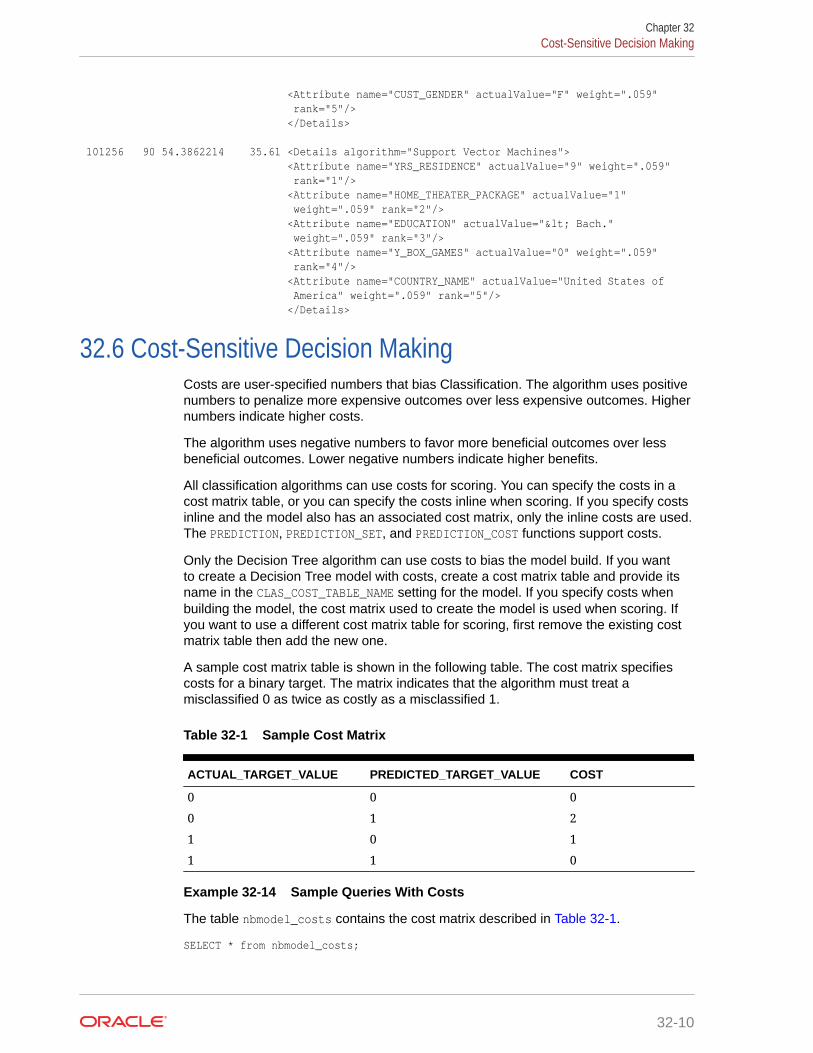
<Attribute name="CUST_GENDER" actualValue="F" weight=".059" rank="5"/> </Details> 101256 90 54.3862214 35.61 <Details algorithm="Support Vector Machines"> <Attribute name="YRS_RESIDENCE" actualValue="9" weight=".059" rank="1"/> <Attribute name="HOME_THEATER_PACKAGE" actualValue="1" weight=".059" rank="2"/> <Attribute name="EDUCATION" actualValue="< Bach." weight=".059" rank="3"/> <Attribute name="Y_BOX_GAMES" actualValue="0" weight=".059" rank="4"/> <Attribute name="COUNTRY_NAME" actualValue="United States of America" weight=".059" rank="5"/> </Details>
32.6 Cost-Sensitive Decision MakingCosts are user-specified numbers that bias Classification. The algorithm uses positivenumbers to penalize more expensive outcomes over less expensive outcomes. Highernumbers indicate higher costs.
The algorithm uses negative numbers to favor more beneficial outcomes over lessbeneficial outcomes. Lower negative numbers indicate higher benefits.
All classification algorithms can use costs for scoring. You can specify the costs in acost matrix table, or you can specify the costs inline when scoring. If you specify costsinline and the model also has an associated cost matrix, only the inline costs are used.The PREDICTION, PREDICTION_SET, and PREDICTION_COST functions support costs.
Only the Decision Tree algorithm can use costs to bias the model build. If you wantto create a Decision Tree model with costs, create a cost matrix table and provide itsname in the CLAS_COST_TABLE_NAME setting for the model. If you specify costs whenbuilding the model, the cost matrix used to create the model is used when scoring. Ifyou want to use a different cost matrix table for scoring, first remove the existing costmatrix table then add the new one.
A sample cost matrix table is shown in the following table. The cost matrix specifiescosts for a binary target. The matrix indicates that the algorithm must treat amisclassified 0 as twice as costly as a misclassified 1.
Table 32-1 Sample Cost Matrix
ACTUAL_TARGET_VALUE PREDICTED_TARGET_VALUE COST
0 0 0
0 1 2
1 0 1
1 1 0
Example 32-14 Sample Queries With Costs
The table nbmodel_costs contains the cost matrix described in Table 32-1.
SELECT * from nbmodel_costs;
Chapter 32Cost-Sensitive Decision Making
32-10

ACTUAL_TARGET_VALUE PREDICTED_TARGET_VALUE COST------------------- ---------------------- ---------- 0 0 0 0 1 2 1 0 1 1 1 0
The following statement associates the cost matrix with a Naive Bayes model callednbmodel.
BEGIN dbms_data_mining.add_cost_matrix('nbmodel', 'nbmodel_costs');END;/
The following query takes the cost matrix into account when scoringmining_data_apply_v. The output is restricted to those rows where a prediction of1 is less costly then a prediction of 0.
SELECT cust_gender, COUNT(*) AS cnt, ROUND(AVG(age)) AS avg_age FROM mining_data_apply_v WHERE PREDICTION (nbmodel COST MODEL USING cust_marital_status, education, household_size) = 1 GROUP BY cust_gender ORDER BY cust_gender; C CNT AVG_AGE- ---------- ----------F 25 38M 208 43
You can specify costs inline when you invoke the scoring function. If you specify costsinline and the model also has an associated cost matrix, only the inline costs are used.The same query is shown below with different costs specified inline. Instead of the "2"shown in the cost matrix table (Table 32-1), "10" is specified in the inline costs.
SELECT cust_gender, COUNT(*) AS cnt, ROUND(AVG(age)) AS avg_age FROM mining_data_apply_v WHERE PREDICTION (nbmodel COST (0,1) values ((0, 10), (1, 0)) USING cust_marital_status, education, household_size) = 1 GROUP BY cust_gender ORDER BY cust_gender; C CNT AVG_AGE- ---------- ----------F 74 39M 581 43
The same query based on probability instead of costs is shown below.
SELECT cust_gender, COUNT(*) AS cnt, ROUND(AVG(age)) AS avg_age FROM mining_data_apply_v WHERE PREDICTION (nbmodel USING cust_marital_status, education, household_size) = 1 GROUP BY cust_gender ORDER BY cust_gender; C CNT AVG_AGE- ---------- ----------
Chapter 32Cost-Sensitive Decision Making
32-11

F 73 39M 577 44
Related Topics
• Example 27-1
32.7 DBMS_DATA_MINING.ApplyThe APPLY procedure in DBMS_DATA_MINING is a batch apply operation that writes theresults of scoring directly to a table.
The columns in the table are mining function-dependent.
Scoring with APPLY generates the same results as scoring with the SQL scoringfunctions. Classification produces a prediction and a probability for each case;clustering produces a cluster ID and a probability for each case, and so on. Thedifference lies in the way that scoring results are captured and the mechanisms thatcan be used for retrieving them.
APPLY creates an output table with the columns shown in the following table:
Table 32-2 APPLY Output Table
Mining Function Output Columns
classification CASE_ID
PREDICTION
PROBABILITY
regression CASE_ID
PREDICTION
anomaly detection CASE_ID
PREDICTION
PROBABILITY
clustering CASE_ID
CLUSTER_ID
PROBABILITY
feature extraction CASE_ID
FEATURE_ID
MATCH_QUALITY
Since APPLY output is stored separately from the scoring data, it must be joined to thescoring data to support queries that include the scored rows. Thus any model that isused with APPLY must have a case ID.
A case ID is not required for models that is applied with SQL scoring functions.Likewise, storage and joins are not required, since scoring results are generated andconsumed in real time within a SQL query.
The following example illustrates Anomaly Detection with APPLY. The query of theAPPLY output table returns the ten first customers in the table. Each has a a probabilityfor being typical (1) and a probability for being anomalous (0).
Chapter 32DBMS_DATA_MINING.Apply
32-12

Example 32-15 Anomaly Detection with DBMS_DATA_MINING.APPLY
EXEC dbms_data_mining.apply ('SVMO_SH_Clas_sample','svmo_sh_sample_prepared', 'cust_id', 'one_class_output');
SELECT * from one_class_output where rownum < 11; CUST_ID PREDICTION PROBABILITY---------- ---------- ----------- 101798 1 .567389309 101798 0 .432610691 102276 1 .564922469 102276 0 .435077531 102404 1 .51213544 102404 0 .48786456 101891 1 .563474346 101891 0 .436525654 102815 0 .500663683 102815 1 .499336317
Related Topics
• Oracle Database PL/SQL Packages and Types Reference
Chapter 32DBMS_DATA_MINING.Apply
32-13

33Mining Unstructured Text
Explains how to use Oracle Data Mining to mine unstructured text.
• About Unstructured Text
• About Text Mining and Oracle Text
• Data Preparation for Text Features
• Creating a Model that Includes Text Mining
• Creating a Text Policy
• Configuring a Text Attribute
33.1 About Unstructured TextData mining algorithms act on data that is numerical or categorical. Numerical datais ordered. It is stored in columns that have a numeric data type, such as NUMBERor FLOAT. Categorical data is identified by category or classification. It is stored incolumns that have a character data type, such as VARCHAR2 or CHAR.
Unstructured text data is neither numerical nor categorical. Unstructured text includesitems such as web pages, document libraries, Power Point presentations, productspecifications, emails, comment fields in reports, and call center notes. It has beensaid that unstructured text accounts for more than three quarters of all enterprise data.Extracting meaningful information from unstructured text can be critical to the successof a business.
33.2 About Text Mining and Oracle TextUnderstand what is text mining and oracle text.
Text mining is the process of applying data mining techniques to text terms, alsocalled text features or tokens. Text terms are words or groups of words that havebeen extracted from text documents and assigned numeric weights. Text terms are thefundamental unit of text that can be manipulated and analyzed.
Oracle Text is a Database technology that provides term extraction, word and themesearching, and other utilities for querying text. When columns of text are present inthe training data, Oracle Data Mining uses Oracle Text utilities and term weightingstrategies to transform the text for mining. Oracle Data Mining passes configurationinformation supplied by you to Oracle Text and uses the results in the model creationprocess.
Related Topics
• Oracle Text Application Developer's Guide
33-1
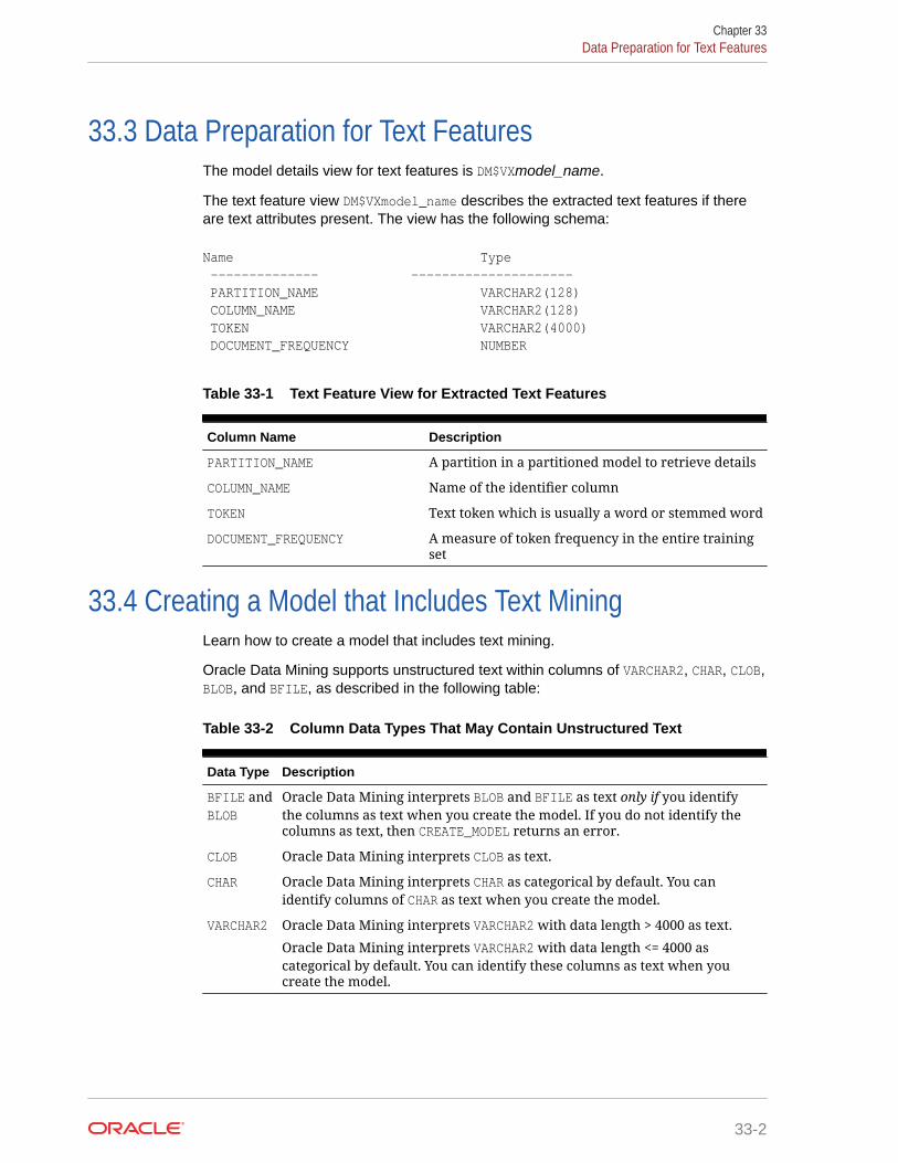
33.3 Data Preparation for Text FeaturesThe model details view for text features is DM$VXmodel_name.
The text feature view DM$VXmodel_name describes the extracted text features if thereare text attributes present. The view has the following schema:
Name Type -------------- --------------------- PARTITION_NAME VARCHAR2(128) COLUMN_NAME VARCHAR2(128) TOKEN VARCHAR2(4000) DOCUMENT_FREQUENCY NUMBER
Table 33-1 Text Feature View for Extracted Text Features
Column Name Description
PARTITION_NAME A partition in a partitioned model to retrieve details
COLUMN_NAME Name of the identifier column
TOKEN Text token which is usually a word or stemmed word
DOCUMENT_FREQUENCY A measure of token frequency in the entire trainingset
33.4 Creating a Model that Includes Text MiningLearn how to create a model that includes text mining.
Oracle Data Mining supports unstructured text within columns of VARCHAR2, CHAR, CLOB,BLOB, and BFILE, as described in the following table:
Table 33-2 Column Data Types That May Contain Unstructured Text
Data Type Description
BFILE andBLOB
Oracle Data Mining interprets BLOB and BFILE as text only if you identifythe columns as text when you create the model. If you do not identify thecolumns as text, then CREATE_MODEL returns an error.
CLOB Oracle Data Mining interprets CLOB as text.
CHAR Oracle Data Mining interprets CHAR as categorical by default. You canidentify columns of CHAR as text when you create the model.
VARCHAR2 Oracle Data Mining interprets VARCHAR2 with data length > 4000 as text.
Oracle Data Mining interprets VARCHAR2 with data length <= 4000 ascategorical by default. You can identify these columns as text when youcreate the model.
Chapter 33Data Preparation for Text Features
33-2

Note:
Text is not supported in nested columns or as a target in supervised datamining.
The settings described in the following table control the term extraction process fortext attributes in a model. Instructions for specifying model settings are in "SpecifyingModel Settings".
Table 33-3 Model Settings for Text
Setting Name Data Type Setting Value Description
ODMS_TEXT_POLICY_NAME
VARCHAR2(4000)
Name of anOracle Text policyobject created withCTX_DDL.CREATE_POLICY
Affects how individual tokens areextracted from unstructured text. See"Creating a Text Policy".
ODMS_TEXT_MAX_FEATURES
INTEGER 1 <= value <= 100000 Maximum number of features touse from the document set (acrossall documents of each text column)passed to CREATE_MODEL.
Default is 3000.
A model can include one or more text attributes. A model with text attributes can alsoinclude categorical and numerical attributes.
To create a model that includes text attributes:
1. Create an Oracle Text policy object..
2. Specify the model configuration settings that are described in "Table 33-3".
3. Specify which columns must be treated as text and, optionally, provide texttransformation instructions for individual attributes.
4. Pass the model settings and text transformation instructions toDBMS_DATA_MINING.CREATE_MODEL.
Note:
All algorithms except O-Cluster can support columns of unstructuredtext.
The use of unstructured text is not recommended for association rules(Apriori).
Related Topics
• Specifying Model SettingsUnderstand how to configure data mining models at build time.
Chapter 33Creating a Model that Includes Text Mining
33-3

• Creating a Text PolicyAn Oracle Text policy specifies how text content must be interpreted. You canprovide a text policy to govern a model, an attribute, or both the model andindividual attributes.
• Configuring a Text AttributeLearn how to identify a column as a text attribute and provide transformationinstructions for any text attribute.
• Embedding Transformations in a Model
33.5 Creating a Text PolicyAn Oracle Text policy specifies how text content must be interpreted. You can providea text policy to govern a model, an attribute, or both the model and individualattributes.
If a model-specific policy is present and one or more attributes have their own policies,Oracle Data Mining uses the attribute policies for the specified attributes and themodel-specific policy for the other attributes.
The CTX_DDL.CREATE_POLICY procedure creates a text policy.
CTX_DDL.CREATE_POLICY( policy_name IN VARCHAR2, filter IN VARCHAR2 DEFAULT NULL, section_group IN VARCHAR2 DEFAULT NULL, lexer IN VARCHAR2 DEFAULT NULL, stoplist IN VARCHAR2 DEFAULT NULL, wordlist IN VARCHAR2 DEFAULT NULL);
The parameters of CTX_DDL.CREATE_POLICY are described in the following table.
Table 33-4 CTX_DDL.CREATE_POLICY Procedure Parameters
Parameter Name Description
policy_name Name of the new policy object. Oracle Text policies and text indexesshare the same namespace.
filter Specifies how the documents must be converted to plain text forindexing. Examples are: CHARSET_FILTER for character sets andNULL_FILTER for plain text, HTML and XML.
For filter values, see "Filter Types" in Oracle Text Reference.
section_group Identifies sections within the documents. For example,HTML_SECTION_GROUP defines sections in HTML documents.
For section_group values, see "Section Group Types" in Oracle TextReference.Note: You can specify any section group that is supported by CONTEXTindexes.
lexer Identifies the language that is being indexed. For example,BASIC_LEXER is the lexer for extracting terms from text in languagesthat use white space delimited words (such as English and mostwestern European languages).For lexer values, see "Lexer Types" in Oracle Text Reference.
Chapter 33Creating a Text Policy
33-4

Table 33-4 (Cont.) CTX_DDL.CREATE_POLICY Procedure Parameters
Parameter Name Description
stoplist Specifies words and themes to exclude from term extraction. Forexample, the word "the" is typically in the stoplist for Englishlanguage documents.The system-supplied stoplist is used by default.See "Stoplists" in Oracle Text Reference.
wordlist Specifies how stems and fuzzy queries must be expanded. A stemdefines a root form of a word so that different grammatical formshave a single representation. A fuzzy query includes commonmisspellings in the representation of a word.See "BASIC_WORDLIST" in Oracle Text Reference.
Related Topics
• Oracle Text Reference
33.6 Configuring a Text AttributeLearn how to identify a column as a text attribute and provide transformationinstructions for any text attribute.
As shown in Table 33-2, you can identify columns of CHAR,shorter VARCHAR2 (<=4000),BFILE, and BLOB as text attributes. If CHAR and shorter VARCHAR2 columns arenot explicitly identified as unstructured text, then CREATE_MODEL processes them ascategorical attributes. If BFILE and BLOB columns are not explicitly identified asunstructured text, then CREATE_MODEL returns an error.
To identify a column as a text attribute, supply the keyword TEXT in anAttribute specification. The attribute specification is a field (attribute_spec) in atransformation record (transform_rec). Transformation records are components oftransformation lists (xform_list) that can be passed to CREATE_MODEL.
Note:
An attribute specification can also include information that is not related totext. Instructions for constructing an attribute specification are in "EmbeddingTransformations in a Model".
You can provide transformation instructions for any text attribute by qualifying the TEXTkeyword in the attribute specification with the subsettings described in the followingtable.
Chapter 33Configuring a Text Attribute
33-5

Table 33-5 Attribute-Specific Text Transformation Instructions
SubsettingName
Description Example
BIGRAM A sequence of two adjacent elements froma string of tokens, which are typicallyletters, syllables, or words. Here, NORMAL tokens are mixed with theirbigrams.
(TOKEN_TYPE:BIGRAM)
POLICY_NAME Name of an Oracle Text policy objectcreated with CTX_DDL.CREATE_POLICY
(POLICY_NAME:my_policy)
STEM_BIGRAM Here, STEM tokens are extracted first andthen stem bigrams are formed.
(TOKEN_TYPE:STEM_BIGRAM)
SYNONYM Oracle Data Mining supports synonyms.The following is an optional parameter:<thesaurus> where <thesaurus> is thename of the thesaurus defining synonyms.If SYNONYM is used without this parameter,then the default thesaurus is used.
(TOKEN_TYPE:SYNONYM)
(TOKEN_TYPE:SYNONYM[NAMES])
TOKEN_TYPE The following values are supported:
NORMAL (the default)STEM
THEME
See "Token Types in an Attribute Specification"
(TOKEN_TYPE:THEME)
MAX_FEATURES Maximum number of features to use fromthe attribute.
(MAX_FEATURES:3000)
Note:
The TEXT keyword is only required for CLOB and longer VARCHAR2 (>4000)when you specify transformation instructions. The TEXT keyword is alwaysrequired for CHAR, shorter VARCHAR2, BFILE, and BLOB — whether or not youspecify transformation instructions.
Tip:
You can view attribute specifications in the data dictionary viewALL_MINING_MODEL_ATTRIBUTES, as shown in Oracle Database Reference.
Token Types in an Attribute Specification
When stems or themes are specified as the token type, the lexer preference for thetext policy must support these types of tokens.
The following example adds themes and English stems to BASIC_LEXER.
Chapter 33Configuring a Text Attribute
33-6

BEGIN CTX_DDL.CREATE_PREFERENCE('my_lexer', 'BASIC_LEXER'); CTX_DDL.SET_ATTRIBUTE('my_lexer', 'index_stems', 'ENGLISH'); CTX_DDL.SET_ATTRIBUTE('my_lexer', 'index_themes', 'YES');END;
Example 33-1 A Sample Attribute Specification for Text
This expression specifies that text transformation for the attribute must use the textpolicy named my_policy. The token type is THEME, and the maximum number offeatures is 3000.
"TEXT(POLICY_NAME:my_policy)(TOKEN_TYPE:THEME)(MAX_FEATURES:3000)"
Related Topics
• Embedding Transformations in a Model
• Specifying Transformation Instructions for an AttributeLearn what is a transformation instruction for an attribute and learn about the fieldsin a transformation record.
• Oracle Database PL/SQL Packages and Types Reference
• ALL_MINING_MODEL_ATTRIBUTES
Chapter 33Configuring a Text Attribute
33-7

34Administrative Tasks for Oracle DataMining
Explains how to perform administrative tasks related to Oracle Data Mining.
• Installing and Configuring a Database for Data Mining
• Upgrading or Downgrading Oracle Data Mining
• Exporting and Importing Mining Models
• Controlling Access to Mining Models and Data
• Auditing and Adding Comments to Mining Models
34.1 Installing and Configuring a Database for Data MiningLearn how to install and configure a database for Data Mining.
• About Installation
• Enabling or Disabling a Database Option
• Database Tuning Considerations for Data Mining
34.1.1 About InstallationOracle Data Mining is a component of the Oracle Advanced Analytics option to OracleDatabase Enterprise Edition.
To install Oracle Database, follow the installation instructions for your platform. Choosea Data Warehousing configuration during the installation.
Oracle Data Miner, the graphical user interface to Oracle Data Mining, is an extensionto Oracle SQL Developer. Instructions for downloading SQL Developer and installingthe Data Miner repository are available on the Oracle Technology Network.
To perform data mining activities, you must be able to log on to the Oracle database,and your user ID must have the database privileges described in Example 34-7.
Related Topics
• Oracle Data Miner
See Also:
Install and Upgrade page of the Oracle Database online documentationlibrary for your platform-specific installation instructions: Oracle Database18c Release
34-1

34.1.2 Enabling or Disabling a Database OptionLearn how you can enable or disable Oracle Advanced Analytics option after theinstallation.
The Oracle Advanced Analytics option is enabled by default during installation ofOracle Database Enterprise Edition. After installation, you can use the command-lineutility chopt to enable or disable a database option. For instructions, see "Enablingand Disabling Database Options After Installation" in the installation guide for yourplatform.
Related Topics
• Oracle Database Installation Guide for Linux
• Oracle Database Installation Guide for Microsoft Windows
34.1.3 Database Tuning Considerations for Data MiningUnderstand the Database tuning considerations for Data Mining.
DBAs managing production databases that support Oracle Data Mining must followstandard administrative practices as described in Oracle Database Administrator’sGuide.
Building data mining models and batch scoring of mining models tend to put a DSS-like workload on the system. Single-row scoring tends to put an OLTP-like workload onthe system.
Database memory management can have a major impact on data mining. Thecorrect sizing of Program Global Area (PGA) memory is very important for modelbuilding, complex queries, and batch scoring. From a data mining perspective, theSystem Global Area (SGA) is generally less of a concern. However, the SGA mustbe sized to accommodate real-time scoring, which loads models into the sharedcursor in the SGA. In most cases, you can configure the database to managememory automatically. To do so, specify the total maximum memory size in the tuningparameter MEMORY_TARGET. With automatic memory management, Oracle Databasedynamically exchanges memory between the SGA and the instance PGA as neededto meet processing demands.
Most data mining algorithms can take advantage of parallel execution when it isenabled in the database. Parameters in INIT.ORA control the behavior of parallelexecution.
Related Topics
• Oracle Database Administrator’s Guide
• Scoring and DeploymentExplains the scoring and deployment features of Oracle Data Mining.
• Oracle Database Administrator’s Guide
• Part I Database Performance Fundamentals
• Tuning Database Memory
• Oracle Database VLDB and Partitioning Guide
Chapter 34Installing and Configuring a Database for Data Mining
34-2

34.2 Upgrading or Downgrading Oracle Data MiningUnderstand how to upgrade and downgrade Oracle Data Mining.
• Pre-Upgrade Steps
• Upgrading Oracle Data Mining
• Post Upgrade Steps
• Downgrading Oracle Data Mining
34.2.1 Pre-Upgrade StepsBefore upgrading, you must drop any data mining models that were created in Javaand any mining activities that were created in Oracle Data Miner Classic (the earlierversion of Oracle Data Miner).
Caution:
In Oracle Database 12c, Oracle Data Mining does not support a Java API,and Oracle Data Miner Classic cannot run against Oracle Database 12c .
34.2.1.1 Dropping Models Created in JavaIf your 10g or 11g database contains models created in Java, use theDBMS_DATA_MINING.DROP_MODEL routine to drop the models before upgrading thedatabase.
34.2.1.2 Dropping Mining Activities Created in Oracle Data Miner ClassicIf your database contains mining activities from Oracle Data Miner Classic, delete themining activities and drop the repository before upgrading the database. Follow thesesteps:
1. Use the Data Miner Classic user interface to delete the mining activities.
2. In SQL*Plus or SQL Developer, drop these tables:
DM4J$ACTIVITIESDM4J$RESULTSDM4J$TRANSFORMS
and these views:
DM4J$MODEL_RESULTS_VDM4J$RESULTS_STATE_V
There must be no tables or views with the prefix DM4J$ in any schema in the databaseafter you complete these steps.
Chapter 34Upgrading or Downgrading Oracle Data Mining
34-3

34.2.2 Upgrading Oracle Data MiningLearn how to upgrade Oracle Data Mining.
After you complete the "Pre-Upgrade Steps", all models and mining metadata are fullyintegrated with the Oracle Database upgrade process whether you are upgradingfrom 11g or from 10g releases.
Upgraded models continue to work as they did in prior releases. Both upgradedmodels and new models that you create in the upgraded environment can make use ofthe new mining functionality introduced in the new release.
To upgrade a database, you can use Database Upgrade Assistant (DBUA) or you canperform a manual upgrade using export/import utilities.
Related Topics
• Pre-Upgrade Steps
• Oracle Database Upgrade Guide
34.2.2.1 Using Database Upgrade Assistant to Upgrade Oracle Data MiningOracle Database Upgrade Assistant provides a graphical user interface that guidesyou interactively through the upgrade process.
On Windows platforms, follow these steps to start the Upgrade Assistant:
1. Go to the Windows Start menu and choose the Oracle home directory.
2. Choose the Configuration and Migration Tools menu.
3. Launch the Upgrade Assistant.
On Linux platforms, run the DBUA utility to upgrade Oracle Database.
34.2.2.1.1 Upgrading from Release 10gIn Oracle Data Mining 10g, data mining metadata and PL/SQL packages are stored inthe DMSYS schema. In Oracle Data Mining 11g and 12c, DMSYS no longer exists; datamining metadata objects are stored in SYS.
When Oracle Database 10g is upgraded to 12c, all data mining metadata objectsand PL/SQL packages are migrated from DMSYS to SYS. The DMSYS schema and itsassociated objects are removed after a successful migration. When DMSYS is removed,the SYS.DBA_REGISTRY view no longer lists Oracle Data Mining as a component.
After upgrading to Oracle Database 12c, you can no longer switch to the Data MiningScoring Engine (DMSE). The Scoring Engine does not exist in Oracle Database 11g or12c.
34.2.2.1.2 Upgrading from Release 11gIf you upgrade Oracle Database 11g to Oracle Database 12c, and the database waspreviously upgraded from Oracle Database 10g, then theDMSYS schema may still bepresent. If the upgrade process detects DMSYS, it displays a warning message anddrops DMSYS during the upgrade.
Chapter 34Upgrading or Downgrading Oracle Data Mining
34-4

34.2.2.2 Using Export/Import to Upgrade Data Mining ModelsIf required, you can you can use a less automated approach to upgrading data miningmodels. You can export the models created in a previous version of Oracle Databaseand import them into an instance of Oracle Database 12c.
Caution:
Do not import data mining models that were created in Java. They are notsupported in Oracle Database 12c.
34.2.2.2.1 Export/Import Release 10g Data Mining ModelsFollow the instructions for exporting and importing Data Mining models.
To export models from an instance of Oracle Database 10g to a dump file, follow theinstructions in "Exporting and Importing Mining Models". Before importing the modelsfrom the dump file, run the DMEIDMSYS script to create the DMSYS schema in OracleDatabase 12c.
SQL>CONNECT / as sysdba;SQL>@ORACLE_HOME\RDBMS\admin\dmeidmsys.sqlSQL>EXIT;
Note:
The TEMP tablespace must already exist in the Oracle Database 12gdatabase. The DMEIDMSYS script uses the TEMP and SYSAUX tablespaces tocreate the DMSYS schema.
To import the dump file into the Oracle Database 12c database:
%ORACLE_HOME\bin\impdp system\<password> dumpfile=<dumpfile_name> directory=<directory_name> logfile=<logfile_name> .....SQL>CONNECT / as sysdba;SQL>EXECUTE dmp_sys.upgrade_models();SQL>ALTER SYSTEM FLUSH SHARED_POOL;SQL>ALTER SYSTEM FLUSH BUFFER_CACHE;SQL>EXIT;
The upgrade_models script migrates all data mining metadata objects and PL/SQLpackages from DMSYS to SYS and then drops DMSYS before upgrading the models.
ALTER SYSTEM Statement
You can flush the Database Smart Flash Cache by issuing an ALTER SYSTEM FLUSHFLASH_CACHE statement. Flushing the Database Smart Flash Cache can be useful ifyou need to measure the performance of rewritten queries or a suite of queries fromidentical starting points.
Chapter 34Upgrading or Downgrading Oracle Data Mining
34-5

Related Topics
• Exporting and Importing Mining ModelsYou can export data mining models to flat files to back up work in progress or tomove models to a different instance of Oracle Database Enterprise Edition (suchas from a development database to a test database).
34.2.2.2.2 Export/Import Release 11g Data Mining ModelsTo export models from an instance of Oracle Database 11g to a dump file, follow theinstructions in Exporting and Importing Mining Models.
Caution:
Do not import data mining models that were created in Java. They are notsupported in Oracle Database 12c.
To import the dump file into the Oracle Database 12c database:
%ORACLE_HOME\bin\impdp system\<password> dumpfile=<dumpfile_name> directory=<directory_name> logfile=<logfile_name> .....SQL>CONNECT / as sysdba;SQL>EXECUTE dmp_sys.upgrade_models();SQL>ALTER SYSTEM flush shared_pool;SQL>ALTER SYSTEM flush buffer_cache;SQL>EXIT;
ALTER SYSTEM Statement
You can flush the Database Smart Flash Cache by issuing an ALTER SYSTEM FLUSHFLASH_CACHE statement. Flushing the Database Smart Flash Cache can be useful ifyou need to measure the performance of rewritten queries or a suite of queries fromidentical starting points.
34.2.3 Post Upgrade StepsPerform steps to view the upgraded database.
After upgrading the database, check the DBA_MINING_MODELS view in the upgradeddatabase. The newly upgraded mining models must be listed in this view.
After you have verified the upgrade and confirmed that there is no need to downgrade,you must set the initialization parameter COMPATIBLE to 12.1.
Note:
The CREATE MINING MODEL privilege must be granted to Data Mining useraccounts that are used to create mining models.
Chapter 34Upgrading or Downgrading Oracle Data Mining
34-6
Related Topics
• Creating a Data Mining UserExplains how to create a Data Mining user.
• Controlling Access to Mining Models and DataUnderstand how to create a Data Mining user and grant necessary privileges.
34.2.4 Downgrading Oracle Data MiningBefore downgrading the Oracle Database 12c database back to the previous version,ensure that no Singular Value Decomposition models or Expectation Maximizationmodels are present. These algorithms are only available in Oracle Database 12c. Usethe DBMS_DATA_MINING.DROP_MODEL routine to drop these models before downgrading.If you do not do this, the database downgrade process terminates.
Issue the following SQL statement in SYS to verify the downgrade:
SQL>SELECT o.name FROM sys.model$ m, sys.obj$ o WHERE m.obj#=o.obj# AND m.version=2;
34.3 Exporting and Importing Mining ModelsYou can export data mining models to flat files to back up work in progress or to movemodels to a different instance of Oracle Database Enterprise Edition (such as from adevelopment database to a test database).
All methods for exporting and importing models are based on Oracle Data Pumptechnology.
The DBMS_DATA_MINING package includes the EXPORT_MODEL and IMPORT_MODELprocedures for exporting and importing individual mining models. EXPORT_MODEL andIMPORT_MODEL use the export and import facilities of Oracle Data Pump.
• About Oracle Data Pump
• Options for Exporting and Importing Mining Models
• Directory Objects for EXPORT_MODEL and IMPORT_MODEL
• Using EXPORT_MODEL and IMPORT_MODEL
• EXPORT and IMPORT Serialized Models
• Importing From PMML
Related Topics
• EXPORT_MODEL
• IMPORT_MODEL
34.3.1 About Oracle Data PumpOracle Data Pump consists of two command-line clients and two PL/SQL packages.The command-line clients, expdp and impdp, provide an easy-to-use interface to theData Pump export and import utilities. You can use expdp and impdp to export andimport entire schemas or databases.
Chapter 34Exporting and Importing Mining Models
34-7

The Data Pump export utility writes the schema objects, including the tables andmetadata that constitute mining models, to a dump file set. The Data Pump importutility retrieves the schema objects, including the model tables and metadata, from thedump file set and restores them in the target database.
expdp and impdp cannot be used to export/import individual mining models.
See Also:
Oracle Database Utilities for information about Oracle Data Pump and theexpdp and impdp utilities
34.3.2 Options for Exporting and Importing Mining ModelsLists options for exporting and importing mining models.
Options for exporting and importing mining models are described in the following table.
Table 34-1 Export and Import Options for Oracle Data Mining
Task Description
Export orimport a fulldatabase
(DBA only) Use expdp to export a full database and impdp to import a full database. Allmining models in the database are included.
Export orimport aschema
Use expdp to export a schema and impdp to import a schema. All mining models in theschema are included.
Export orimportindividualmodels within adatabase
Use DBMS_DATA_MINING.EXPORT_MODEL to export individual models andDBMS_DATA_MINING.IMPORT_MODEL to import individual models. These procedures canexport and import a single mining model, all mining models, or mining models thatmatch specific criteria.By default, IMPORT_MODEL imports models back into the schema from which they wereexported. You can specify the schema_remap parameter to import models into a differentschema. You can specify tablespace_remap with schema_remap to import models into aschema that uses a different tablespace.You may need special privileges in the database to import models into adifferent schema. These privileges are granted by the EXP_FULL_DATABASE andIMP_FULL_DATABASE roles, which are only available to privileged users (such as SYS or auser with the DBA role). You do not need these roles to export or import models withinyour own schema.To import models, you must have the same database privileges as the user who createdthe dump file set. Otherwise, a DBA with full system privileges must import the models.
Chapter 34Exporting and Importing Mining Models
34-8

Table 34-1 (Cont.) Export and Import Options for Oracle Data Mining
Task Description
Export orimportindividualmodels to orfrom a remotedatabase
Use a database link to export individual models to a remote database or importindividual models from a remote database. A database link is a schema object in onedatabase that enables access to objects in a different database. The link must be createdbefore you execute EXPORT_MODEL or IMPORT_MODEL.
To create a private database link, you must have the CREATE DATABASE LINK systemprivilege. To create a public database link, you must have the CREATE PUBLIC DATABASELINK system privilege. Also, you must have the CREATE SESSION system privilege onthe remote Oracle Database. Oracle Net must be installed on both the local and remoteOracle Databases.
Related Topics
• IMPORT_MODEL Procedure
• EXPORT_MODEL Procedure
• Oracle Database SQL Language Reference
34.3.3 Directory Objects for EXPORT_MODEL and IMPORT_MODELLearn how to use directory objects to identify the location of the dump file set.
EXPORT_MODEL and IMPORT_MODEL use a directory object to identify the location of thedump file set. A directory object is a logical name in the database for a physicaldirectory on the host computer.
To export data mining models, you must have write access to the directory object andto the file system directory that it represents. To import data mining models, you musthave read access to the directory object and to the file system directory. Also, thedatabase itself must have access to file system directory. You must have the CREATEANY DIRECTORY privilege to create directory objects.
The following SQL command creates a directory object named dmuser_dir. The filesystem directory that it represents must already exist and have shared read/writeaccess rights granted by the operating system.
CREATE OR REPLACE DIRECTORY dmuser_dir AS '/dm_path/dm_mining';
The following SQL command gives user dmuser both read and write access todmuser_dir.
GRANT READ,WRITE ON DIRECTORY dmuser_dir TO dmuser;
Related Topics
• Oracle Database SQL Language Reference
Chapter 34Exporting and Importing Mining Models
34-9
34.3.4 Using EXPORT_MODEL and IMPORT_MODELThe examples illustrate various export and import scenarios with EXPORT_MODEL andIMPORT_MODEL.
The examples use the directory object dmdir shown in Example 34-1 and twoschemas, dm1 and dm2. Both schemas have data mining privileges. dm1 has twomodels. dm2 has one model.
SELECT owner, model_name, mining_function, algorithm FROM all_mining_models; OWNER MODEL_NAME MINING_FUNCTION ALGORITHM---------- -------------------- -------------------- --------------------------DM1 EM_SH_CLUS_SAMPLE CLUSTERING EXPECTATION_MAXIMIZATIONDM1 DT_SH_CLAS_SAMPLE CLASSIFICATION DECISION_TREEDM2 SVD_SH_SAMPLE FEATURE_EXTRACTION SINGULAR_VALUE_DECOMP
Example 34-1 Creating the Directory Object
-- connect as system userCREATE OR REPLACE DIRECTORY dmdir AS '/scratch/dmuser/expimp';GRANT READ,WRITE ON DIRECTORY dmdir TO dm1;GRANT READ,WRITE ON DIRECTORY dmdir TO dm2;SELECT * FROM all_directories WHERE directory_name IN 'DMDIR';
OWNER DIRECTORY_NAME DIRECTORY_PATH---------- -------------------------- ----------------------------------------SYS DMDIR /scratch/dmuser/expimp
Example 34-2 Exporting All Models From DM1
-- connect as dm1BEGIN dbms_data_mining.export_model ( filename => 'all_dm1', directory => 'dmdir');END;/
A log file and a dump file are created in /scratch/dmuser/expimp, the physicaldirectory associated with dmdir. The name of the log file is dm1_exp_11.log. The nameof the dump file is all_dm101.dmp.
Example 34-3 Importing the Models Back Into DM1
The models that were exported in Example 34-2 still exist in dm1. Since an import doesnot overwrite models with the same name, you must drop the models before importingthem back into the same schema.
BEGIN dbms_data_mining.drop_model('EM_SH_CLUS_SAMPLE'); dbms_data_mining.drop_model('DT_SH_CLAS_SAMPLE'); dbms_data_mining.import_model( filename => 'all_dm101.dmp', directory => 'DMDIR');END;/SELECT model_name FROM user_mining_models;
Chapter 34Exporting and Importing Mining Models
34-10

MODEL_NAME------------------------------DT_SH_CLAS_SAMPLEEM_SH_CLUS_SAMPLE
Example 34-4 Importing Models Into a Different Schema
In this example, the models that were exported from dm1 in Example 34-2 are importedinto dm2. The dm1 schema uses the example tablespace; the dm2 schema uses thesysaux tablespace.
-- CONNECT as sysdba BEGIN dbms_data_mining.import_model ( filename => 'all_d101.dmp', directory => 'DMDIR', schema_remap => 'DM1:DM2', tablespace_remap => 'EXAMPLE:SYSAUX');END;/-- CONNECT as dm2SELECT model_name from user_mining_models; MODEL_NAME--------------------------------------------------------------------------------SVD_SH_SAMPLEEM_SH_CLUS_SAMPLEDT_SH_CLAS_SAMPLE
Example 34-5 Exporting Specific Models
You can export a single model, a list of models, or a group of models that share certaincharacteristics.
-- Export the model named dt_sh_clas_sampleEXECUTE dbms_data_mining.export_model ( filename => 'one_model', directory =>'DMDIR', model_filter => 'name in (''DT_SH_CLAS_SAMPLE'')');-- one_model01.dmp and dm1_exp_37.log are created in /scratch/dmuser/expimp
-- Export Decision Tree modelsEXECUTE dbms_data_mining.export_model( filename => 'algo_models', directory => 'DMDIR', model_filter => 'ALGORITHM_NAME IN (''DECISION_TREE'')');-- algo_model01.dmp and dm1_exp_410.log are created in /scratch/dmuser/expimp
-- Export clustering models EXECUTE dbms_data_mining.export_model( filename =>'func_models', directory => 'DMDIR', model_filter => 'FUNCTION_NAME = ''CLUSTERING''');-- func_model01.dmp and dm1_exp_513.log are created in /scratch/dmuser/expimp
Related Topics
• Oracle Database PL/SQL Packages and Types Reference
Chapter 34Exporting and Importing Mining Models
34-11

34.3.5 EXPORT and IMPORT Serialized ModelsFrom Oracle Database Release 18c onwards, EXPORT_SERMODEL and IMPORT_SERMODELprocedures are available to export and import serialized models.
The serialized format allows the models to be moved to another platform (outside thedatabase) for scoring. The model is exported in a BLOB that can be saved in a BFILE.The import routine takes the serialized content in the BLOB and the name of the modelto be created with the content.
Related Topics
• EXPORT_SERMODEL Procedure
• IMPORT_SERMODEL Procedure
34.3.6 Importing From PMMLYou can import Regression models represented in Predictive Model Markup Language(PMML).
PMML is an XML-based standard specified by the Data Mining Group (http://www.dmg.org). Applications that are PMML-compliant can deploy PMML-compliantmodels that were created by any vendor. Oracle Data Mining supports the corefeatures of PMML 3.1 for regression models.
You can import regression models represented in PMML. The models must be of typeRegressionModel, either linear regression or binary logistic regression.
Related Topics
• Oracle Database PL/SQL Packages and Types Reference
34.4 Controlling Access to Mining Models and DataUnderstand how to create a Data Mining user and grant necessary privileges.
• Creating a Data Mining User
• System Privileges for Data Mining
• Object Privileges for Mining Models
34.4.1 Creating a Data Mining UserExplains how to create a Data Mining user.
A Data Mining user is a database user account that has privileges for performing datamining activities. Example 34-6 shows how to create a database user. Example 34-7shows how to assign data mining privileges to the user.
Chapter 34Controlling Access to Mining Models and Data
34-12

Note:
To create a user for the Data Mining sample programs, you must run twoconfiguration scripts as described in "The Data Mining Sample Programs".
Example 34-6 Creating a Database User in SQL*Plus
1. Log in to SQL*Plus with system privileges.
Enter user-name: sys as sysdba Enter password: password
2. To create a user named dmuser, type these commands. Specify a password ofyour choosing.
CREATE USER dmuser IDENTIFIED BY password DEFAULT TABLESPACE USERS TEMPORARY TABLESPACE TEMP QUOTA UNLIMITED ON USERS;Commit;
The USERS and TEMP tablespace are included in the pre-configured database thatOracle ships with the database media. USERS is used mostly by demo users; itis appropriate for running the sample programs described in "The Data MiningSample Programs". TEMP is the temporary tablespace that is shared by mostdatabase users.
Note:
Tablespaces for Data Mining users must be assigned according tostandard DBA practices, depending on system load and systemresources.
3. To login as dmuser, type the following.
CONNECT dmuserEnter password: password
Related Topics
• The Data Mining Sample ProgramsDescribes the data mining sample programs that ship with Oracle Database.
See Also:
Oracle Database SQL Language Reference for the complete syntax of theCREATE USER statement
Chapter 34Controlling Access to Mining Models and Data
34-13

34.4.1.1 Granting Privileges for Data MiningYou must have the CREATE MINING MODEL privilege to create models in your ownschema. You can perform any operation on models that you own. This includesapplying the model, adding a cost matrix, renaming the model, and dropping themodel.
The GRANT statements in the following example assign a set of basic data miningprivileges to the dmuser account. Some of these privileges are not required for allmining activities, however it is prudent to grant them all as a group.
Additional system and object privileges are required for enabling or restricting specificmining activities.
Example 34-7 Privileges Required for Data Mining
GRANT CREATE MINING MODEL TO dmuser;GRANT CREATE SESSION TO dmuser;GRANT CREATE TABLE TO dmuser;GRANT CREATE VIEW TO dmuser;GRANT EXECUTE ON CTXSYS.CTX_DDL TO dmuser;
READ or SELECT privileges are required for data that is not in your schema. Forexample, the following statement grants SELECT access to the sh.customers table.
GRANT SELECT ON sh.customers TO dmuser;
34.4.2 System Privileges for Data MiningLearn different privileges to control operations on mining models.
A system privilege confers the right to perform a particular action in the database or toperform an action on a type of schema objects. For example, the privileges to createtablespaces and to delete the rows of any table in a database are system privileges.
You can perform specific operations on mining models in other schemas if you havethe appropriate system privileges. For example, CREATE ANY MINING MODEL enablesyou to create models in other schemas. SELECT ANY MINING MODEL enables you toapply models that reside in other schemas. You can add comments to models if youhave the COMMENT ANY MINING MODEL privilege.
To grant a system privilege, you must either have been granted the system privilegewith the ADMIN OPTION or have been granted the GRANT ANY PRIVILEGE systemprivilege.
The system privileges listed in the following table control operations on mining models.
Table 34-2 System Privileges for Data Mining
System Privilege Allows you to....
CREATE MINING MODEL Create mining models in your own schema.
CREATE ANY MINING MODEL Create mining models in any schema.
ALTER ANY MINING MODEL Change the name or cost matrix of any mining modelin any schema.
Chapter 34Controlling Access to Mining Models and Data
34-14
Table 34-2 (Cont.) System Privileges for Data Mining
System Privilege Allows you to....
DROP ANY MINING MODEL Drop any mining model in any schema.
SELECT ANY MINING MODEL Apply a mining model in any schema, also view modeldetails in any schema.
COMMENT ANY MINING MODEL Add a comment to any mining model in any schema.)
AUDIT_ADMIN role Generate an audit trail for any mining model inany schema. (See Oracle Database Security Guide fordetails.)
Example 34-8 Grant System Privileges for Data Mining
The following statements allow dmuser to score data and view model details in anyschema as long as SELECT access has been granted to the data. However, dmuser canonly create models in the dmuser schema.
GRANT CREATE MINING MODEL TO dmuser;GRANT SELECT ANY MINING MODEL TO dmuser;
The following statement revokes the privilege of scoring or viewing model details inother schemas. When this statement is executed, dmuser can only perform data miningactivities in the dmuser schema.
REVOKE SELECT ANY MINING MODEL FROM dmuser;
Related Topics
• Adding a Comment to a Mining Model
• Oracle Database Security Guide
34.4.3 Object Privileges for Mining ModelsAn object privilege confers the right to perform a particular action on a specific schemaobject. For example, the privilege to delete rows from the SH.PRODUCTS table is anexample of an object privilege.
You automatically have all object privileges for schema objects in your own schema.You can grant object privilege on objects in your own schema to other users or roles.
The object privileges listed in the following table control operations on specific miningmodels.
Table 34-3 Object Privileges for Mining Models
Object Privilege Allows you to....
ALTER MINING MODEL Change the name or cost matrix of the specified mining modelobject.
SELECT MININGMODEL
Apply the specified mining model object and view its modeldetails.
Chapter 34Controlling Access to Mining Models and Data
34-15
Example 34-9 Grant Object Privileges on Mining Models
The following statements allow dmuser to apply the model testmodel to the salestable, specifying different cost matrixes with each apply. The user dmuser can alsorename the model testmodel. The testmodel model and sales table are in the shschema, not in the dmuser schema.
GRANT SELECT ON MINING MODEL sh.testmodel TO dmuser;GRANT ALTER ON MINING MODEL sh.testmodel TO dmuser;GRANT SELECT ON sh.sales TO dmuser;
The following statement prevents dmuser from renaming or changing the cost matrix oftestmodel. However, dmuser can still apply testmodel to the sales table.
REVOKE ALTER ON MINING MODEL sh.testmodel FROM dmuser;
34.5 Auditing and Adding Comments to Mining ModelsMining model objects support SQL COMMENT and AUDIT statements.
34.5.1 Adding a Comment to a Mining ModelComments can be used to associate descriptive information with a database object.You can associate a comment with a mining model using a SQL COMMENT statement.
COMMENT ON MINING MODEL schema_name.model_name IS string;
Note:
To add a comment to a model in another schema, you must have theCOMMENT ANY MINING MODEL system privilege.
To drop a comment, set it to the empty '' string.
The following statement adds a comment to the model DT_SH_CLAS_SAMPLE in yourown schema.
COMMENT ON MINING MODEL dt_sh_clas_sample IS 'Decision Tree model predicts promotion response';
You can view the comment by querying the catalog view USER_MINING_MODELS.
SELECT model_name, mining_function, algorithm, comments FROM user_mining_models;
MODEL_NAME MINING_FUNCTION ALGORITHM COMMENTS----------------- ---------------- -------------- -----------------------------------------------DT_SH_CLAS_SAMPLE CLASSIFICATION DECISION_TREE Decision Tree model predicts promotion response
To drop this comment from the database, issue the following statement:
COMMENT ON MINING MODEL dt_sh_clas_sample '';
Chapter 34Auditing and Adding Comments to Mining Models
34-16
See Also:
• Table 34-2
• Oracle Database SQL Language Reference for details about SQLCOMMENT statements
34.5.2 Auditing Mining ModelsThe Oracle Database auditing system is a powerful, highly configurable tool fortracking operations on schema objects in a production environment. The auditingsystem can be used to track operations on data mining models.
Note:
To audit mining models, you must have the AUDIT_ADMIN role.
Unified auditing is documented in Oracle Database Security Guide. However, the fullunified auditing system is not enabled by default. Instructions for migrating to unifiedauditing are provided in Oracle Database Upgrade Guide.
See Also:
• "Auditing Oracle Data Mining Events" in Oracle Database Security Guidefor details about auditing mining models
• "Monitoring Database Activity with Auditing" in Oracle Database SecurityGuide for a comprehensive discussion of unified auditing in OracleDatabase
• "About the Unified Auditing Migration Process for Oracle Database"in Oracle Database Upgrade Guide for information about migrating tounified auditing
• Oracle Database Upgrade Guide
Chapter 34Auditing and Adding Comments to Mining Models
34-17
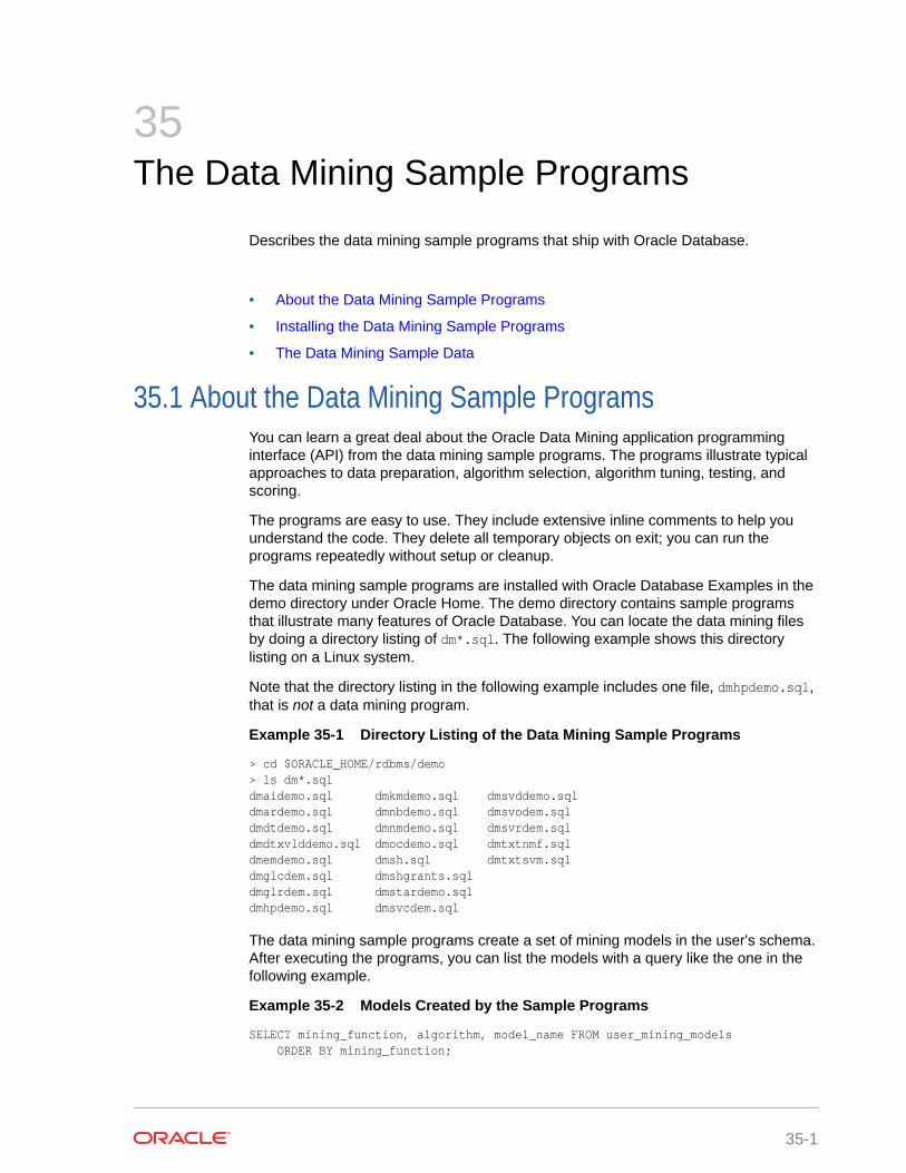
35The Data Mining Sample Programs
Describes the data mining sample programs that ship with Oracle Database.
• About the Data Mining Sample Programs
• Installing the Data Mining Sample Programs
• The Data Mining Sample Data
35.1 About the Data Mining Sample ProgramsYou can learn a great deal about the Oracle Data Mining application programminginterface (API) from the data mining sample programs. The programs illustrate typicalapproaches to data preparation, algorithm selection, algorithm tuning, testing, andscoring.
The programs are easy to use. They include extensive inline comments to help youunderstand the code. They delete all temporary objects on exit; you can run theprograms repeatedly without setup or cleanup.
The data mining sample programs are installed with Oracle Database Examples in thedemo directory under Oracle Home. The demo directory contains sample programsthat illustrate many features of Oracle Database. You can locate the data mining filesby doing a directory listing of dm*.sql. The following example shows this directorylisting on a Linux system.
Note that the directory listing in the following example includes one file, dmhpdemo.sql,that is not a data mining program.
Example 35-1 Directory Listing of the Data Mining Sample Programs
> cd $ORACLE_HOME/rdbms/demo> ls dm*.sqldmaidemo.sql dmkmdemo.sql dmsvddemo.sql dmardemo.sql dmnbdemo.sql dmsvodem.sql dmdtdemo.sql dmnmdemo.sql dmsvrdem.sql dmdtxvlddemo.sql dmocdemo.sql dmtxtnmf.sql dmemdemo.sql dmsh.sql dmtxtsvm.sqldmglcdem.sql dmshgrants.sql dmglrdem.sql dmstardemo.sql dmhpdemo.sql dmsvcdem.sql
The data mining sample programs create a set of mining models in the user's schema.After executing the programs, you can list the models with a query like the one in thefollowing example.
Example 35-2 Models Created by the Sample Programs
SELECT mining_function, algorithm, model_name FROM user_mining_models ORDER BY mining_function;
35-1
MINING_FUNCTION ALGORITHM MODEL_NAME------------------------------ ------------------------------ -------------------ASSOCIATION_RULES APRIORI_ASSOCIATION_RULES AR_SH_SAMPLECLASSIFICATION GENERALIZED_LINEAR_MODEL GLMC_SH_CLAS_SAMPLECLASSIFICATION SUPPORT_VECTOR_MACHINES T_SVM_CLAS_SAMPLECLASSIFICATION SUPPORT_VECTOR_MACHINES SVMC_SH_CLAS_SAMPLECLASSIFICATION SUPPORT_VECTOR_MACHINES SVMO_SH_CLAS_SAMPLECLASSIFICATION NAIVE_BAYES NB_SH_CLAS_SAMPLECLASSIFICATION DECISION_TREE DT_SH_CLAS_SAMPLECLUSTERING EXPECTATION_MAXIMIZATION EM_SH_CLUS_SAMPLECLUSTERING O_CLUSTER OC_SH_CLUS_SAMPLECLUSTERING KMEANS KM_SH_CLUS_SAMPLECLUSTERING KMEANS DM_STAR_CLUSTERFEATURE_EXTRACTION SINGULAR_VALUE_DECOMP SVD_SH_SAMPLEFEATURE_EXTRACTION NONNEGATIVE_MATRIX_FACTOR NMF_SH_SAMPLEFEATURE_EXTRACTION NONNEGATIVE_MATRIX_FACTOR T_NMF_SAMPLEREGRESSION SUPPORT_VECTOR_MACHINES SVMR_SH_REGR_SAMPLEREGRESSION GENERALIZED_LINEAR_MODEL GLMR_SH_REGR_SAMPLE
35.2 Installing the Data Mining Sample ProgramsLearn how to install Data Mining sample programs.
The data mining sample programs require:
• Oracle Database Enterprise Edition with the Advanced Analytics option
• Oracle Database sample schemas
• Oracle Database Examples
• A data mining user account
• Execution of dmshgrants.sql by a system administrator
• Execution of dmsh.sql by the data mining user
Follow these steps to install the data mining sample programs:
1. Install or obtain access to Oracle Database 12c Enterprise Edition with theAdvanced Analytics option. To install the Database, see the installation instructionsfor your platform at Oracle Database 18c Release.
2. Ensure that the sample schemas are installed in the database. The sampleschemas are installed by default with Oracle Database. See Oracle DatabaseSample Schemasfor details about the sample schemas.
3. Verify that Oracle Database Examples has been installed with the database, orinstall it locally. Oracle Database Examples loads the Database sample programsinto the rdbms/demo directory under Oracle home. See Oracle Database ExamplesInstallation Guide for installation instructions.
4. Verify that a data mining user account has been created, or create it yourself if youhave administrative privileges. See "Creating a Data Mining User".
5. Ask your system administrator to run dmshgrants.sql, or run it yourself if youhave administrative privileges. dmshgrants grants the privileges that are requiredfor running the sample programs. These include SELECT access to tables in the SHschema as described in "The Data Mining Sample Data" and the system privilegeslisted in the following table.
Pass the name of the data mining user to dmshgrants.
Chapter 35Installing the Data Mining Sample Programs
35-2

SQL> CONNECT sys / as sysdbaEnter password: sys_passwordConnected.SQL> @ $ORACLE_HOME/rdbms/demo/dmshgrants dmuser
Table 35-1 System Privileges Granted by dmshgrants.sql to the DataMining User
Privilege Allows the data mining user to
CREATE SESSION log in to a database session
CREATE TABLE create tables, such as the settings tables forCREATE_MODEL
CREATE VIEW create views, such as the views of tables in the SHschema
CREATE MINING MODEL create data mining models
EXECUTE ONctxsys.ctx_ddl
execute procedures in the ctxsys.ctx_ddl PL/SQLpackage; required for text mining
6. Connect to the database as the data mining user and run dmsh.sql. This scriptcreates views of the sample data in the schema of the data mining user.
SQL> CONNECT dmuserEnter password: dmuser_passwordConnected.SQL> @ $ORACLE_HOME/rdbms/demo/dmsh
Related Topics
• Oracle Database Sample Schemas
• Oracle Database Examples Installation Guide
• Creating a Data Mining UserExplains how to create a Data Mining user.
35.3 The Data Mining Sample DataThe data used by the sample data mining programs is based on these tables in the SHschema:
SH.CUSTOMERS SH.SALES SH.PRODUCTS SH.SUPPLEMENTARY_DEMOGRAPHICSSH.COUNTRIES
The dmshgrants script grants SELECT access to the tables in SH. The dmsh.sql scriptcreates views of the SH tables in the schema of the data mining user. The views aredescribed in the following table:
Table 35-2 The Data Mining Sample Data
View Name Description
MINING_DATA Joins and filters data
Chapter 35The Data Mining Sample Data
35-3

Table 35-2 (Cont.) The Data Mining Sample Data
View Name Description
MINING_DATA_BUILD_V Data for building models
MINING_DATA_TEST_V Data for testing models
MINING_DATA_APPLY_V Data to be scored
MINING_BUILD_TEXT Data for building models that include text
MINING_TEST_TEXT Data for testing models that include text
MINING_APPLY_TEXT Data, including text columns, to be scored
MINING_DATA_ONE_CLASS_V
Data for anomaly detection
The association rules program creates its own transactional data.
Chapter 35The Data Mining Sample Data
35-4
Part VOracle Data Mining API Reference
Learn about Oracle Data Mining PL/SQL packages, data dictionary views, and datamining SQL scoring functions.
• PL/SQL Packages
• Data Dictionary Views
• SQL Scoring Functions
36PL/SQL Packages
Learn how to create, evaluate, and query data mining models through Data MiningPL/SQL packages.
• DBMS_DATA_MINING
• DBMS_DATA_MINING_TRANSFORM
• DBMS_PREDICTIVE_ANALYTICS
36.1 DBMS_DATA_MININGThe DBMS_DATA_MINING package is the application programming interface for creating,evaluating, and querying data mining models.
This chapter contains the following topics:
• Overview
• Security Model
• Mining Functions
• Model Settings
• Solver Settings
• Datatypes
• Summary of DBMS_DATA_MINING Subprograms
See Also:
• Oracle Data Mining Concepts
• Oracle Data Mining User’s Guide
• DBMS_DATA_MINING_TRANSFORM
• DBMS_PREDICTIVE_ANALYTICS
36.1.1 Using DBMS_DATA_MININGThis section contains topics that relate to using the DBMS_DATA_MINING package.
• Overview
• Security Model
• Mining Functions
• Model Settings
36-1
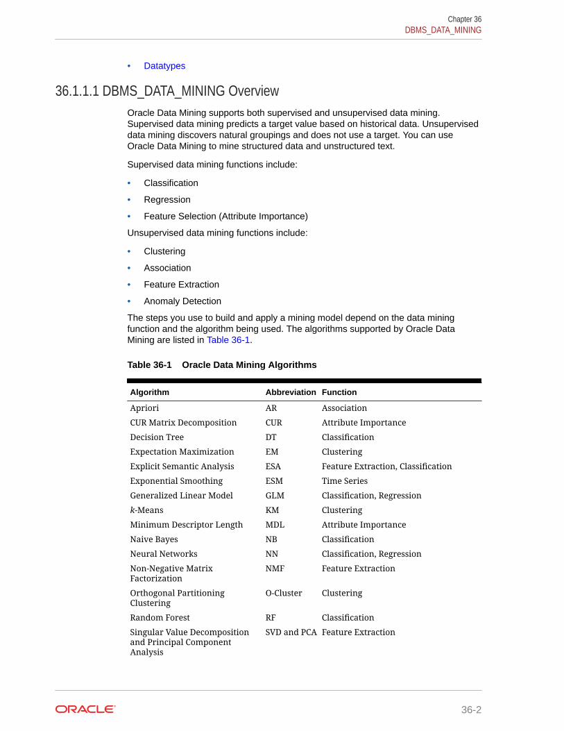
• Datatypes
36.1.1.1 DBMS_DATA_MINING OverviewOracle Data Mining supports both supervised and unsupervised data mining.Supervised data mining predicts a target value based on historical data. Unsuperviseddata mining discovers natural groupings and does not use a target. You can useOracle Data Mining to mine structured data and unstructured text.
Supervised data mining functions include:
• Classification
• Regression
• Feature Selection (Attribute Importance)
Unsupervised data mining functions include:
• Clustering
• Association
• Feature Extraction
• Anomaly Detection
The steps you use to build and apply a mining model depend on the data miningfunction and the algorithm being used. The algorithms supported by Oracle DataMining are listed in Table 36-1.
Table 36-1 Oracle Data Mining Algorithms
Algorithm Abbreviation Function
Apriori AR Association
CUR Matrix Decomposition CUR Attribute Importance
Decision Tree DT Classification
Expectation Maximization EM Clustering
Explicit Semantic Analysis ESA Feature Extraction, Classification
Exponential Smoothing ESM Time Series
Generalized Linear Model GLM Classification, Regression
k-Means KM Clustering
Minimum Descriptor Length MDL Attribute Importance
Naive Bayes NB Classification
Neural Networks NN Classification, Regression
Non-Negative MatrixFactorization
NMF Feature Extraction
Orthogonal PartitioningClustering
O-Cluster Clustering
Random Forest RF Classification
Singular Value Decompositionand Principal ComponentAnalysis
SVD and PCA Feature Extraction
Chapter 36DBMS_DATA_MINING
36-2

Table 36-1 (Cont.) Oracle Data Mining Algorithms
Algorithm Abbreviation Function
Support Vector Machine SVM Classification, Regression, AnomalyDetection
Oracle Data Mining supports more than one algorithm for the classification, regression,clustering, and feature extraction mining functions. Each of these mining functions hasa default algorithm, as shown in Table 36-2.
Table 36-2 Oracle Data Mining Default Algorithms
Mining Function Default Algorithm
Classification Naive Bayes
Clustering k-Means
Feature Extraction Non-Negative Matrix Factorization
Feature Selection Minimum Descriptor Length
Regression Support Vector Machine
36.1.1.2 DBMS_DATA_MINING Security ModelThe DBMS_DATA_MINING package is owned by user SYS and is installed as part ofdatabase installation. Execution privilege on the package is granted to public. Theroutines in the package are run with invokers' rights (run with the privileges of thecurrent user).
The DBMS_DATA_MINING package exposes APIs that are leveraged by the Oracle DataMining component of the Advanced Analytics Option. Users who wish to create miningmodels in their own schema require the CREATE MINING MODEL system privilege. Userswho wish to create mining models in other schemas require the CREATE ANY MININGMODEL system privilege.
Users have full control over managing models that exist within their own schema.Additional system privileges necessary for managing data mining models in otherschemas include ALTER ANY MINING MODEL, DROP ANY MINING MODEL, SELECT ANYMINING MODEL, COMMENT ANY MINING MODEL, and AUDIT ANY.
Individual object privileges on mining models, ALTER MINING MODEL and SELETMINING MODEL, can be used to selectively grant privileges on a model to a differentuser.
See Also:
Oracle Data Mining User's Guide for more information about the securityfeatures of Oracle Data Mining
Chapter 36DBMS_DATA_MINING
36-3

36.1.1.3 DBMS_DATA_MINING — Mining FunctionsA data mining function refers to the methods for solving a given class of data miningproblems.
The mining function must be specified when a model is created. (SeeCREATE_MODEL Procedure.)
Table 36-3 Mining Functions
Value Description
ASSOCIATION Association is a descriptive mining function. An associationmodel identifies relationships and the probability of theiroccurrence within a data set.Association models use the Apriori algorithm.
ATTRIBUTE_IMPORTANCE Attribute importance is a predictive mining function,also known as feature selection. An attribute importancemodel identifies the relative importance of an attribute inpredicting a given outcome.Attribute importance models can use Minimum DescriptionLength, or CUR Matrix Decomposition. Minimum DescriptionLength is the default.
CLASSIFICATION Classification is a predictive mining function. A classificationmodel uses historical data to predict a categorical target.Classification models can use: Naive Bayes, Decision Tree,Logistic Regression, or Support Vector Machine. The defaultis Naive Bayes.The classification function can also be used for anomalydetection. In this case, the SVM algorithm with a null targetis used (One-Class SVM).
CLUSTERING Clustering is a descriptive mining function. A clusteringmodel identifies natural groupings within a data set.Clustering models can use k-Means, O-Cluster, or ExpectationMaximization. The default is k-Means.
FEATURE_EXTRACTION Feature Extraction is a descriptive mining function. A featureextraction model creates an optimized data set on which tobase a model.Feature extraction models can use Explicit SemanticAnalysis, Non-Negative Matrix Factorization, Singular ValueDecomposition, or Principal Component Analysis. Non-Negative Matrix Factorization is the default.
REGRESSION Regression is a predictive mining function. A regressionmodel uses historical data to predict a numerical target.Regression models can use Support Vector Machine or LinearRegression. The default is Support Vector Machine.
TIME_SERIES Time series is a predictive mining function. A time seriesmodel forecasts the future values of a time-ordered seriesof historical numeric data over a user-specified timewindow. Time series models use the Exponential Smoothingalgorithm.
Chapter 36DBMS_DATA_MINING
36-4
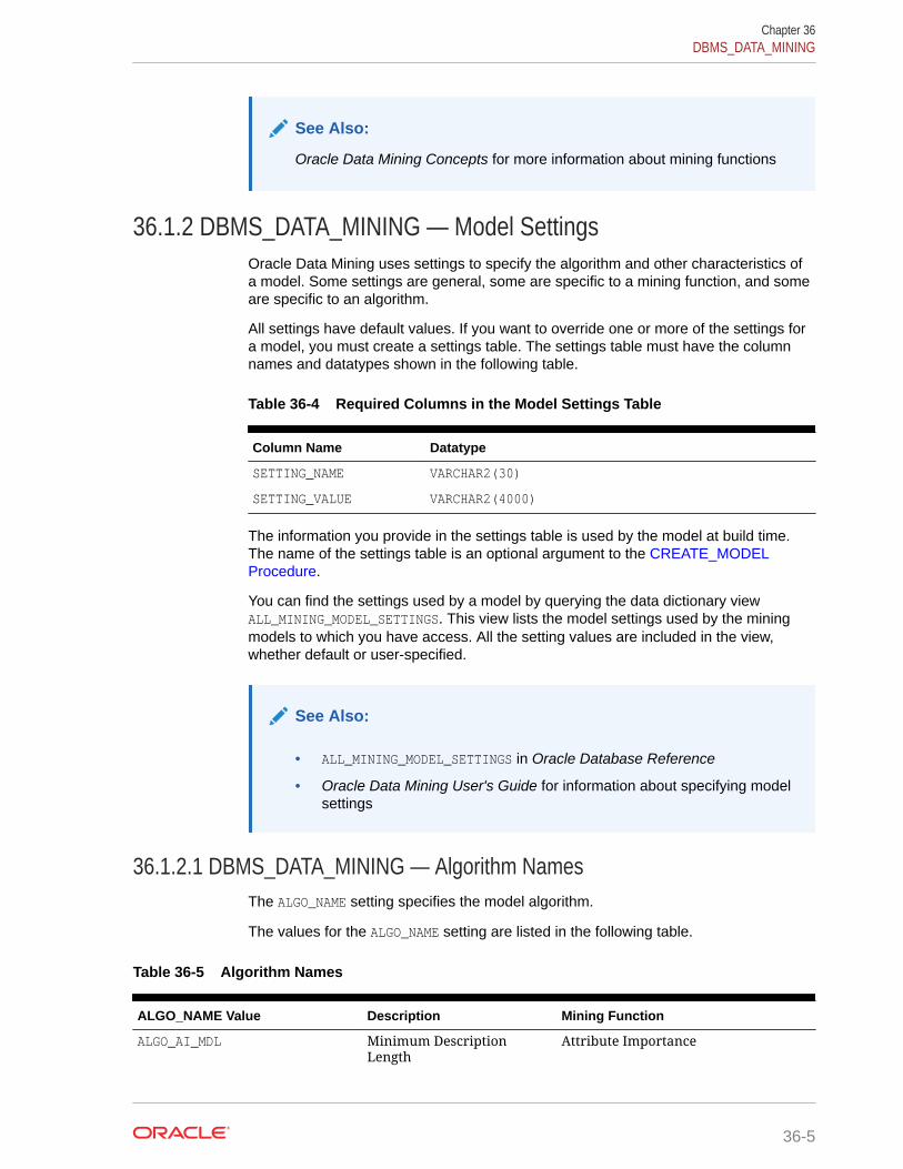
See Also:
Oracle Data Mining Concepts for more information about mining functions
36.1.2 DBMS_DATA_MINING — Model SettingsOracle Data Mining uses settings to specify the algorithm and other characteristics ofa model. Some settings are general, some are specific to a mining function, and someare specific to an algorithm.
All settings have default values. If you want to override one or more of the settings fora model, you must create a settings table. The settings table must have the columnnames and datatypes shown in the following table.
Table 36-4 Required Columns in the Model Settings Table
Column Name Datatype
SETTING_NAME VARCHAR2(30)
SETTING_VALUE VARCHAR2(4000)
The information you provide in the settings table is used by the model at build time.The name of the settings table is an optional argument to the CREATE_MODELProcedure.
You can find the settings used by a model by querying the data dictionary viewALL_MINING_MODEL_SETTINGS. This view lists the model settings used by the miningmodels to which you have access. All the setting values are included in the view,whether default or user-specified.
See Also:
• ALL_MINING_MODEL_SETTINGS in Oracle Database Reference
• Oracle Data Mining User's Guide for information about specifying modelsettings
36.1.2.1 DBMS_DATA_MINING — Algorithm NamesThe ALGO_NAME setting specifies the model algorithm.
The values for the ALGO_NAME setting are listed in the following table.
Table 36-5 Algorithm Names
ALGO_NAME Value Description Mining Function
ALGO_AI_MDL Minimum DescriptionLength
Attribute Importance
Chapter 36DBMS_DATA_MINING
36-5

Table 36-5 (Cont.) Algorithm Names
ALGO_NAME Value Description Mining Function
ALGO_APRIORI_ASSOCIATION_RULES
Apriori Association Rules
ALGO_CUR_DECOMPOSITION CUR Decomposition Attribute Importance
ALGO_DECISION_TREE Decision Tree Classification
ALGO_EXPECTATION_MAXIMIZATION Expectation Maximization Clustering
ALGO_EXPLICIT_SEMANTIC_ANALYS Explicit Semantic Analysis Feature ExtractionClassification
ALGO_EXPONENTIAL_SMOOTHING Exponential Smoothing Time Series
ALGO_EXTENSIBLE_LANG Language used for extensiblealgorithm
All mining functions supported
ALGO_GENERALIZED_LINEAR_MODEL Generalized Linear Model Classification, Regression; also FeatureSelection and Generation
ALGO_KMEANS Enhanced k_Means Clustering
ALGO_NAIVE_BAYES Naive Bayes Classification
ALGO_NEURAL_NETWORK Neural Network Classification
ALGO_NONNEGATIVE_MATRIX_FACTOR
Non-Negative MatrixFactorization
Feature Extraction
ALGO_O_CLUSTER O-Cluster Clustering
ALGO_RANDOM_FOREST Random Forest Classification
ALGO_SINGULAR_VALUE_DECOMP Singular ValueDecomposition
Feature Extraction
ALGO_SUPPORT_VECTOR_MACHINES Support Vector Machine Classification and Regression
See Also:
Oracle Data Mining Concepts for information about algorithms
36.1.2.2 DBMS_DATA_MINING — Automatic Data PreparationOracle Data Mining supports fully Automatic Data Preparation (ADP), user-directedgeneral data preparation, and user-specified embedded data preparation. The PREP_*settings enable the user to request fully automated or user-directed general datapreparation. By default, fully Automatic Data Preparation (PREP_AUTO_ON) is enabled.
When you enable Automatic Data Preparation, the model uses heuristics totransform the build data according to the requirements of the algorithm. Insteadof fully Automatic Data Preparation, the user can request that the data be shiftedand/or scaled with the PREP_SCALE* and PREP_SHIFT* settings. The transformationinstructions are stored with the model and reused whenever the model is applied.Refer to Model Detail Views, Oracle Data Mining User’s Guide.
Chapter 36DBMS_DATA_MINING
36-6
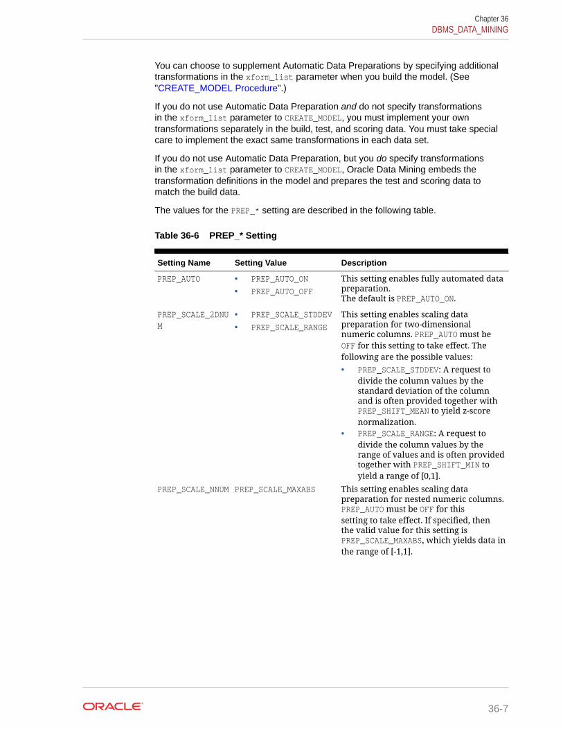
You can choose to supplement Automatic Data Preparations by specifying additionaltransformations in the xform_list parameter when you build the model. (See"CREATE_MODEL Procedure".)
If you do not use Automatic Data Preparation and do not specify transformationsin the xform_list parameter to CREATE_MODEL, you must implement your owntransformations separately in the build, test, and scoring data. You must take specialcare to implement the exact same transformations in each data set.
If you do not use Automatic Data Preparation, but you do specify transformationsin the xform_list parameter to CREATE_MODEL, Oracle Data Mining embeds thetransformation definitions in the model and prepares the test and scoring data tomatch the build data.
The values for the PREP_* setting are described in the following table.
Table 36-6 PREP_* Setting
Setting Name Setting Value Description
PREP_AUTO • PREP_AUTO_ON
• PREP_AUTO_OFF
This setting enables fully automated datapreparation.The default is PREP_AUTO_ON.
PREP_SCALE_2DNUM
• PREP_SCALE_STDDEV
• PREP_SCALE_RANGE
This setting enables scaling datapreparation for two-dimensionalnumeric columns. PREP_AUTO must beOFF for this setting to take effect. Thefollowing are the possible values:• PREP_SCALE_STDDEV: A request to
divide the column values by thestandard deviation of the columnand is often provided together withPREP_SHIFT_MEAN to yield z-scorenormalization.
• PREP_SCALE_RANGE: A request todivide the column values by therange of values and is often providedtogether with PREP_SHIFT_MIN toyield a range of [0,1].
PREP_SCALE_NNUM PREP_SCALE_MAXABS This setting enables scaling datapreparation for nested numeric columns.PREP_AUTO must be OFF for thissetting to take effect. If specified, thenthe valid value for this setting isPREP_SCALE_MAXABS, which yields data inthe range of [-1,1].
Chapter 36DBMS_DATA_MINING
36-7
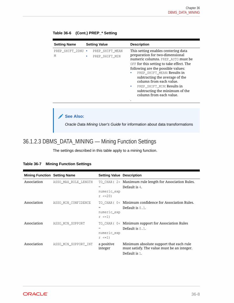
Table 36-6 (Cont.) PREP_* Setting
Setting Name Setting Value Description
PREP_SHIFT_2DNUM
• PREP_SHIFT_MEAN
• PREP_SHIFT_MIN
This setting enables centering datapreparation for two-dimensionalnumeric columns. PREP_AUTO must beOFF for this setting to take effect. Thefollowing are the possible values:• PREP_SHIFT_MEAN: Results in
subtracting the average of thecolumn from each value.
• PREP_SHIFT_MIN: Results insubtracting the minimum of thecolumn from each value.
.
See Also:
Oracle Data Mining User's Guide for information about data transformations
36.1.2.3 DBMS_DATA_MINING — Mining Function SettingsThe settings described in this table apply to a mining function.
Table 36-7 Mining Function Settings
Mining Function Setting Name Setting Value Description
Association ASSO_MAX_RULE_LENGTH TO_CHAR( 2<=numeric_expr <=20)
Maximum rule length for Association Rules.Default is 4.
Association ASSO_MIN_CONFIDENCE TO_CHAR( 0<=numeric_expr <=1)
Minimum confidence for Association Rules.Default is 0.1.
Association ASSO_MIN_SUPPORT TO_CHAR( 0<=numeric_expr <=1)
Minimum support for Association RulesDefault is 0.1.
Association ASSO_MIN_SUPPORT_INT a positiveinteger
Minimum absolute support that each rulemust satisfy. The value must be an integer.Default is 1.
Chapter 36DBMS_DATA_MINING
36-8

Table 36-7 (Cont.) Mining Function Settings
Mining Function Setting Name Setting Value Description
Association ASSO_MIN_REV_CONFIDENCE
TO_CHAR( 0<=numeric_expr <=1)
Sets the Minimum Reverse Confidence thateach rule should satisfy.The Reverse Confidence of a rule is defined asthe number of transactions in which the ruleoccurs divided by the number of transactionsin which the consequent occurs.The value is real number between 0 and 1.The default is 0.
Association ASSO_IN_RULES NULL Sets Including Rules applied for eachassociation rule: it specifies the list of itemsthat at least one of them must appear in eachreported association rule, either as antecedentor as consequent. It is a comma separatedstring containing the list of including items.If not set, the default behavior is, the filteringis not applied.
Association ASSO_EX_RULES NULL Sets Excluding Rules applied for eachassociation rule: it specifies the list ofitems that none of them can appear ineach reported Association Rules. It is acomma separated string containing the list ofexcluding items. No rule can contain any itemin the list.The default is NULL.
Association ASSO_ANT_IN_RULES NULL Sets Including Rules for the antecedent: itspecifies the list of items that at least oneof them must appear in the antecedent partof each reported association rule. It is acomma separated string containing the list ofincluding items. The antecedent part of eachrule must contain at least one item in the list.The default is NULL.
Association ASSO_ANT_EX_RULES NULL Sets Excluding Rules for the antecedent:it specifies the list of items that none ofthem can appear in the antecedent partof each reported association rule. It is acomma separated string containing the list ofexcluding items. No rule can contain any itemin the list in its antecedent part.The default is NULL.
Association ASSO_CONS_IN_RULES NULL Sets Including Rules for the consequent: itspecifies the list of items that at least oneof them must appear in the consequent partof each reported association rule. It is acomma separated string containing the list ofincluding items. The consequent of each rulemust be an item in the list.The default is NULL.
Chapter 36DBMS_DATA_MINING
36-9
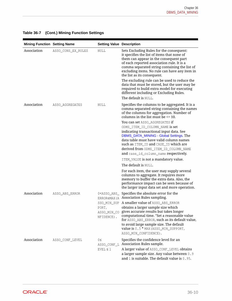
Table 36-7 (Cont.) Mining Function Settings
Mining Function Setting Name Setting Value Description
Association ASSO_CONS_EX_RULES NULL Sets Excluding Rules for the consequent:it specifies the list of items that none ofthem can appear in the consequent partof each reported association rule. It is acomma separated string containing the list ofexcluding items. No rule can have any item inthe list as its consequent.The excluding rule can be used to reduce thedata that must be stored, but the user may berequired to build extra model for executingdifferent including or Excluding Rules.The default is NULL.
Association ASSO_AGGREGATES NULL Specifies the columns to be aggregated. It is acomma separated string containing the namesof the columns for aggregation. Number ofcolumns in the list must be <= 10.You can set ASSO_AGGREGATES ifODMS_ITEM_ID_COLUMN_NAME is setindicating transactional input data. SeeDBMS_DATA_MINING - Global Settings. Thedata table must have valid column namessuch as ITEM_ID and CASE_ID which arederived from ODMS_ITEM_ID_COLUMN_NAMEand case_id_column_name respectively.
ITEM_VALUE is not a mandatory value.
The default is NULL.
For each item, the user may supply severalcolumns to aggregate. It requires morememory to buffer the extra data. Also, theperformance impact can be seen because ofthe larger input data set and more operation.
Association ASSO_ABS_ERROR 0<ASSO_ABS_ERROR≤MAX(ASSO_MIN_SUPPORT,ASSO_MIN_CONFIDENCE).
Specifies the absolute error for theAssociation Rules sampling.A smaller value of ASSO_ABS_ERRORobtains a larger sample size whichgives accurate results but takes longercomputational time. "Set a reasonable valuefor ASSO_ABS_ERROR, such as its default value,to avoid large sample size. The defaultvalue is 0.5 * MAX(ASSO_MIN_SUPPORT,ASSO_MIN_CONFIDENCE).
Association ASSO_CONF_LEVEL 0≤ASSO_CONF_LEVEL ≤ 1
Specifies the confidence level for anAssociation Rules sample.A larger value of ASSO_CONF_LEVEL obtainsa larger sample size. Any value between 0.9and 1 is suitable. The default value is 0.95.
Chapter 36DBMS_DATA_MINING
36-10
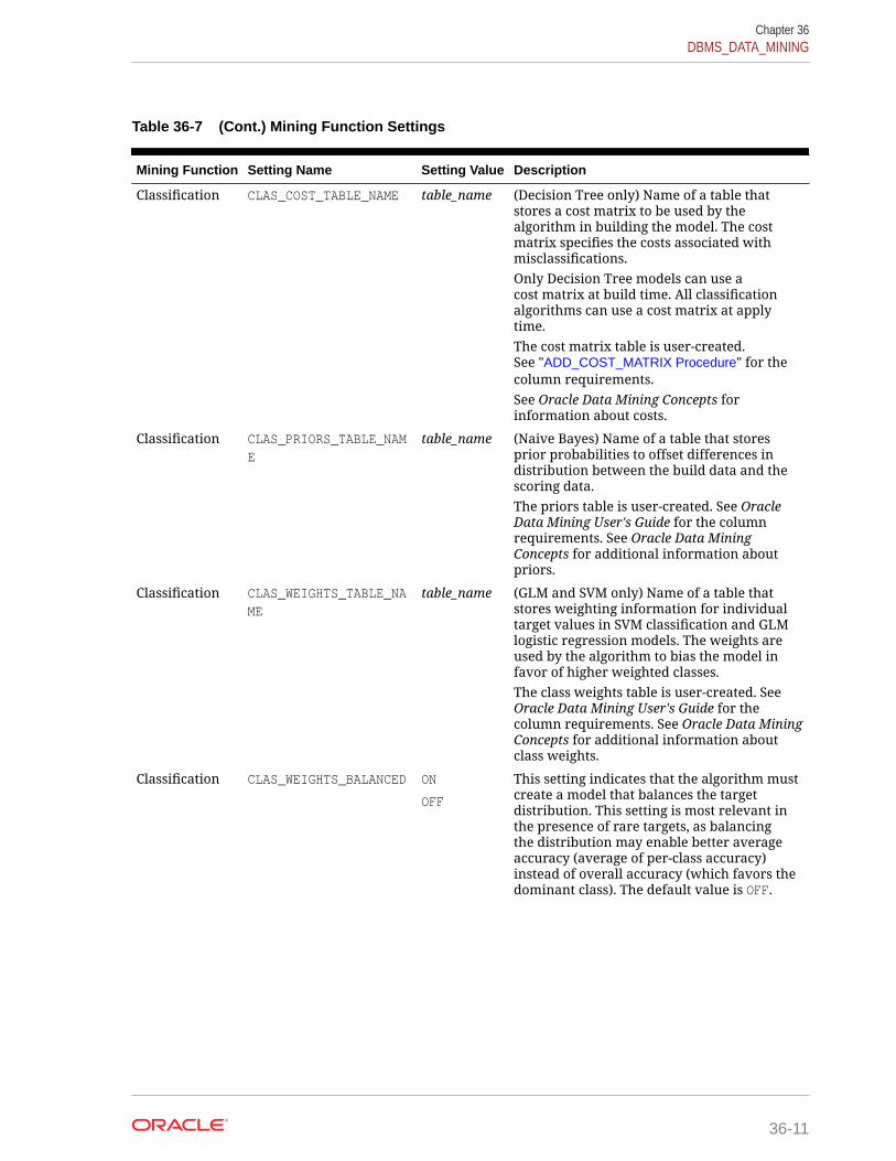
Table 36-7 (Cont.) Mining Function Settings
Mining Function Setting Name Setting Value Description
Classification CLAS_COST_TABLE_NAME table_name (Decision Tree only) Name of a table thatstores a cost matrix to be used by thealgorithm in building the model. The costmatrix specifies the costs associated withmisclassifications.Only Decision Tree models can use acost matrix at build time. All classificationalgorithms can use a cost matrix at applytime.The cost matrix table is user-created.See "ADD_COST_MATRIX Procedure" for thecolumn requirements.See Oracle Data Mining Concepts forinformation about costs.
Classification CLAS_PRIORS_TABLE_NAME
table_name (Naive Bayes) Name of a table that storesprior probabilities to offset differences indistribution between the build data and thescoring data.The priors table is user-created. See OracleData Mining User's Guide for the columnrequirements. See Oracle Data MiningConcepts for additional information aboutpriors.
Classification CLAS_WEIGHTS_TABLE_NAME
table_name (GLM and SVM only) Name of a table thatstores weighting information for individualtarget values in SVM classification and GLMlogistic regression models. The weights areused by the algorithm to bias the model infavor of higher weighted classes.The class weights table is user-created. SeeOracle Data Mining User's Guide for thecolumn requirements. See Oracle Data MiningConcepts for additional information aboutclass weights.
Classification CLAS_WEIGHTS_BALANCED ON
OFF
This setting indicates that the algorithm mustcreate a model that balances the targetdistribution. This setting is most relevant inthe presence of rare targets, as balancingthe distribution may enable better averageaccuracy (average of per-class accuracy)instead of overall accuracy (which favors thedominant class). The default value is OFF.
Chapter 36DBMS_DATA_MINING
36-11

Table 36-7 (Cont.) Mining Function Settings
Mining Function Setting Name Setting Value Description
Classification CLAS_MAX_SUP_BINS For DecisionTree:2 <= anumber<=2147483647
For RandomForest:2 <= anumber<=254
This parameter specifies the maximumnumber of bins for each attribute.Default value is 32.
See, DBMS_DATA_MINING — Automatic DataPreparation
Clustering CLUS_NUM_CLUSTERS TO_CHAR( numeric_expr>=1)
Maximum number of leaf clusters generatedby a clustering algorithm. The algorithm mayreturn fewer clusters, depending on the data.Enhanced k-Means usually produces theexact number of clusters specified byCLUS_NUM_CLUSTERS, unless there are fewerdistinct data points.Expectation Maximization (EM) may returnfewer clusters than the number specifiedby CLUS_NUM_CLUSTERS depending on thedata. The number of clusters returned byEM cannot be greater than the numberof components, which is governed byalgorithm-specific settings. (See ExpectationMaximization Settings for Learning table)Depending on these settings, there may befewer clusters than components. If componentclustering is disabled, the number of clustersequals the number of components.For EM, the default value ofCLUS_NUM_CLUSTERS is system-determined.For k-Means and O-Cluster, the default is 10.
FeatureExtraction
FEAT_NUM_FEATURES TO_CHAR( numeric_expr>=1)
Number of features to be extracted by afeature extraction model.The default is estimated from the data by thealgorithm. If the matrix rank is smaller thanthis number, fewer features will be returned.For CUR Matrix Decomposition, theFEAT_NUM_FEATURES value is same as theCURS_SVD_RANK value.
See Also:
Oracle Data Mining Concepts for information about mining functions
Chapter 36DBMS_DATA_MINING
36-12
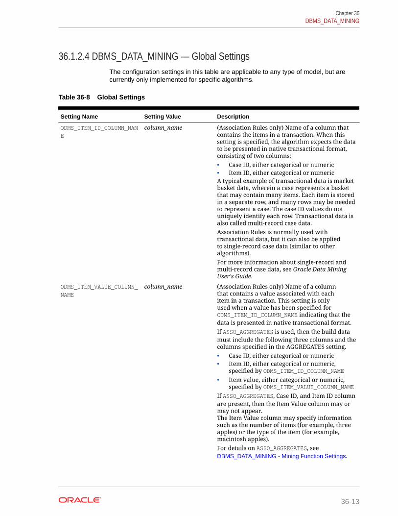
36.1.2.4 DBMS_DATA_MINING — Global SettingsThe configuration settings in this table are applicable to any type of model, but arecurrently only implemented for specific algorithms.
Table 36-8 Global Settings
Setting Name Setting Value Description
ODMS_ITEM_ID_COLUMN_NAME
column_name (Association Rules only) Name of a column thatcontains the items in a transaction. When thissetting is specified, the algorithm expects the datato be presented in native transactional format,consisting of two columns:• Case ID, either categorical or numeric• Item ID, either categorical or numericA typical example of transactional data is marketbasket data, wherein a case represents a basketthat may contain many items. Each item is storedin a separate row, and many rows may be neededto represent a case. The case ID values do notuniquely identify each row. Transactional data isalso called multi-record case data.Association Rules is normally used withtransactional data, but it can also be appliedto single-record case data (similar to otheralgorithms).For more information about single-record andmulti-record case data, see Oracle Data MiningUser's Guide.
ODMS_ITEM_VALUE_COLUMN_NAME
column_name (Association Rules only) Name of a columnthat contains a value associated with eachitem in a transaction. This setting is onlyused when a value has been specified forODMS_ITEM_ID_COLUMN_NAME indicating that thedata is presented in native transactional format.If ASSO_AGGREGATES is used, then the build datamust include the following three columns and thecolumns specified in the AGGREGATES setting.• Case ID, either categorical or numeric• Item ID, either categorical or numeric,
specified by ODMS_ITEM_ID_COLUMN_NAME• Item value, either categorical or numeric,
specified by ODMS_ITEM_VALUE_COLUMN_NAMEIf ASSO_AGGREGATES, Case ID, and Item ID columnare present, then the Item Value column may ormay not appear.The Item Value column may specify informationsuch as the number of items (for example, threeapples) or the type of the item (for example,macintosh apples).For details on ASSO_AGGREGATES, seeDBMS_DATA_MINING - Mining Function Settings.
Chapter 36DBMS_DATA_MINING
36-13

Table 36-8 (Cont.) Global Settings
Setting Name Setting Value Description
ODMS_MISSING_VALUE_TREATMENT
ODMS_MISSING_VALUE_MEAN_MODE
ODMS_MISSING_VALUE_DELETE_ROW
ODMS_MISSING_VALUE_AUTO
Indicates how to treat missing values inthe training data. This setting does notaffect the scoring data. The default value isODMS_MISSING_VALUE_AUTO.
ODM_MISSING_VALUE_MEAN_MODE replaces missingvalues with the mean (numeric attributes)or the mode (categorical attributes) both atbuild time and apply time where appropriate.ODMS_MISSING_VALUE_AUTO performs differentstrategies for different algorithms.When ODMS_MISSING_VALUE_TREATMENT is set toODMS_MISSING_VALUE_DELETE_ROW, the rows inthe training data that contain missing values aredeleted. However, if you want to replicate thismissing value treatment in the scoring data, thenyou must perform the transformation explicitly.The value ODMS_MISSING_VALUE_DELETE_ROW isapplicable to all algorithms.
ODMS_ROW_WEIGHT_COLUMN_NAME
column_name (GLM only) Name of a column in the training datathat contains a weighting factor for the rows. Thecolumn datatype must be NUMBER.Row weights can be used as a compactrepresentation of repeated rows, as in the designof experiments where a specific configuration isrepeated several times. Row weights can also beused to emphasize certain rows during modelconstruction. For example, to bias the modeltowards rows that are more recent and awayfrom potentially obsolete data.
ODMS_TEXT_POLICY_NAME The name of an OracleText POLICY createdusingCTX_DDL.CREATE_POLICY.
Affects how individual tokens are extracted fromunstructured text.For details about CTX_DDL.CREATE_POLICY, seeOracle Text Reference.
ODMS_TEXT_MAX_FEATURES 1 <= value Maximum number of distinct features, across alltext attributes, to use from a document set passedto CREATE_MODEL. The default is 3000. ESA has thedefault value of 300000.
ODMS_TEXT_MIN_DOCUMENTS Non-negative value This is a text processing setting the controls howin how many documents a token needs to appearto be used as a feature.The default is 1. ESA has default of 3.
Chapter 36DBMS_DATA_MINING
36-14
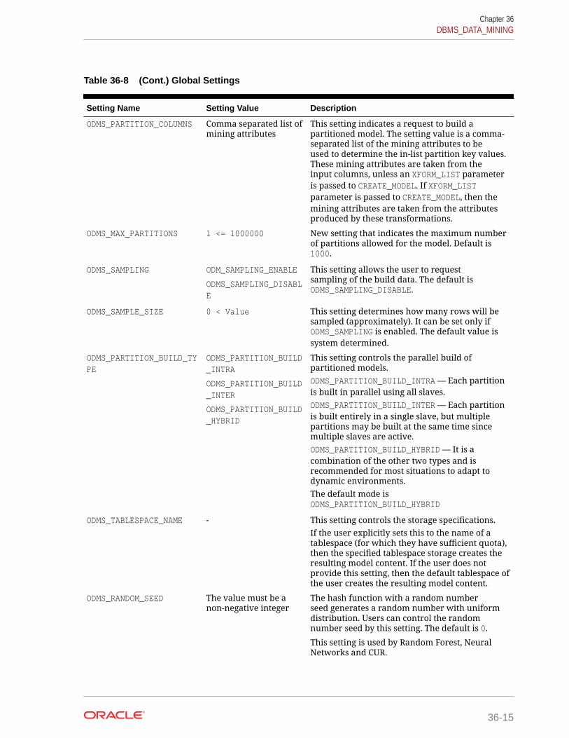
Table 36-8 (Cont.) Global Settings
Setting Name Setting Value Description
ODMS_PARTITION_COLUMNS Comma separated list ofmining attributes
This setting indicates a request to build apartitioned model. The setting value is a comma-separated list of the mining attributes to beused to determine the in-list partition key values.These mining attributes are taken from theinput columns, unless an XFORM_LIST parameteris passed to CREATE_MODEL. If XFORM_LISTparameter is passed to CREATE_MODEL, then themining attributes are taken from the attributesproduced by these transformations.
ODMS_MAX_PARTITIONS 1 <= 1000000 New setting that indicates the maximum numberof partitions allowed for the model. Default is1000.
ODMS_SAMPLING ODM_SAMPLING_ENABLE
ODMS_SAMPLING_DISABLE
This setting allows the user to requestsampling of the build data. The default isODMS_SAMPLING_DISABLE.
ODMS_SAMPLE_SIZE 0 < Value This setting determines how many rows will besampled (approximately). It can be set only ifODMS_SAMPLING is enabled. The default value issystem determined.
ODMS_PARTITION_BUILD_TYPE
ODMS_PARTITION_BUILD_INTRA
ODMS_PARTITION_BUILD_INTER
ODMS_PARTITION_BUILD_HYBRID
This setting controls the parallel build ofpartitioned models.ODMS_PARTITION_BUILD_INTRA — Each partitionis built in parallel using all slaves.ODMS_PARTITION_BUILD_INTER — Each partitionis built entirely in a single slave, but multiplepartitions may be built at the same time sincemultiple slaves are active.ODMS_PARTITION_BUILD_HYBRID — It is acombination of the other two types and isrecommended for most situations to adapt todynamic environments.The default mode isODMS_PARTITION_BUILD_HYBRID
ODMS_TABLESPACE_NAME - This setting controls the storage specifications.If the user explicitly sets this to the name of atablespace (for which they have sufficient quota),then the specified tablespace storage creates theresulting model content. If the user does notprovide this setting, then the default tablespace ofthe user creates the resulting model content.
ODMS_RANDOM_SEED The value must be anon-negative integer
The hash function with a random numberseed generates a random number with uniformdistribution. Users can control the randomnumber seed by this setting. The default is 0.
This setting is used by Random Forest, NeuralNetworks and CUR.
Chapter 36DBMS_DATA_MINING
36-15

Table 36-8 (Cont.) Global Settings
Setting Name Setting Value Description
ODMS_DETAILS • ODMS_ENABLE
• ODMS_DISABLE
This setting reduces the space that is used whilecreating a model, especially a partitioned model.The default value is ODMS_ENABLE.
When the setting is ODMS_ENABLE, it creates modeltables and views when the model is created. Youcan query the model with SQL. When the settingis ODMS_DISABLE, model views are not created andtables relevant to model details are not createdeither.The reduction in the space depends on the model.Reduction on the order of 10x can be achieved.
See Also:
Oracle Data Mining Concepts for information about GLM
Oracle Data Mining Concepts for information about Association Rules
Oracle Data Mining User's Guide for information about mining unstructuredtext
36.1.2.5 DBMS_DATA_MINING — Algorithm Settings:ALGO_EXTENSIBLE_LANG
The settings listed in the following table configure the behavior of the mining modelwith an Extensible algorithm. The mining model is built in R language.
The RALG_*_FUNCTION specifies the R script that is used to build, score, and viewan R model and must be registered in the Oracle R Enterprise script repository. TheR scripts are registered through Oracle R Enterprise with special privileges. WhenALGO_EXTENSIBLE_LANG is set to R in the MINING_MODEL_SETTING table, the miningmodel is built in the R language. After the R model is built, the names of the R scriptsare recorded in MINING_MODEL_SETTING table in the SYS schema. The scripts mustexist in the script repository for the R model to function. The amount of R memoryused to build, score, and view the R model through these R scripts can be controlledby Oracle R Enterprise.
All algorithm-independent DBMS_DATA_MINING subprograms can operate on an Rmodel for mining functions such as Association, Attribute Importance, Classification,Clustering, Feature Extraction, and Regression.
The supported DBMS_DATA_MINING subprograms include, but are not limited, to thefollowing:
• ADD_COST_MATRIX Procedure
• COMPUTE_CONFUSION_MATRIX Procedure
• COMPUTE_LIFT Procedure
Chapter 36DBMS_DATA_MINING
36-16

• COMPUTE_ROC Procedure
• CREATE_MODEL Procedure
• DROP_MODEL Procedure
• EXPORT_MODEL Procedure
• GET_MODEL_COST_MATRIX Function
• IMPORT_MODEL Procedure
• REMOVE_COST_MATRIX Procedure
• RENAME_MODEL Procedure
Table 36-9 ALGO_EXTENSIBLE_LANG Settings
Setting Name Setting Value Description
RALG_BUILD_FUNCTION R_BUILD_FUNCTION_SCRIPT_NAME
Specifies the name of an existingregistered R script for R algorithmmining model build function. The Rscript defines an R function for thefirst input argument for training dataand returns an R model object. ForClustering and Feature Extraction miningfunction model build, the R attributesdm$nclus and dm$nfeat must be seton the R model to indicate the numberof clusters and features respectively.The RALG_BUILD_FUNCTION must be setalong with ALGO_EXTENSIBLE_LANG in themodel_setting_table.
RALG_BUILD_PARAMETER SELECT valueparam_name, ...FROM DUAL
Specifies a list of numeric and string scalarfor optional input parameters of the modelbuild function.
RALG_SCORE_FUNCTION R_SCORE_FUNCTION_SCRIPT_NAME
Specifies the name of an existing registeredR script to score data. The script returns adata.frame containing the correspondingprediction results. The setting is usedto score data for mining functions suchas Regression, Classification, Clustering,and Feature Extraction. This setting doesnot apply to Association and AttributeImportance functions
RALG_WEIGHT_FUNCTION R_WEIGHT_FUNCTION_SCRIPT_NAME
Specifies the name of an existing registeredR script for R algorithm that computes theweight (contribution) for each attribute inscoring. The script returns a data.framecontaining the contributing weight foreach attribute in a row. This functionsetting is needed for PREDICTION_DETAILSSQL function.
RALG_DETAILS_FUNCTION R_DETAILS_FUNCTION_SCRIPT_NAME
Specifies the name of an existing registeredR script for R algorithm that produces themodel information. This setting is requiredto generate a model view.
Chapter 36DBMS_DATA_MINING
36-17

Table 36-9 (Cont.) ALGO_EXTENSIBLE_LANG Settings
Setting Name Setting Value Description
RALG_DETAILS_FORMAT SELECT type_valuecolumn_name, ... FROMDUAL
Specifies the SELECT query for the list ofnumeric and string scalars for the outputcolumn type and the column name ofthe generated model view. This setting isrequired to generate a model view.
See Also:
Oracle Data Mining User’s Guide
36.1.2.6 DBMS_DATA_MINING — Algorithm Settings: CUR MatrixDecomposition
The following settings affects the behavior of the CUR Matrix Decomposition algorithm.
The following settings configure the behavior of the CUR Matrix Decompositionalgorithm.
Table 36-10 CUR Matrix Decomposition Settings
Setting Name Setting Value Description
CURS_APPROX_ATTR_NUM
The value must be apositive integer
Defines the approximate number of attributes to be selected.The default value is the number of attributes.
CURS_ROW_IMPORTANCE
CURS_ROW_IMP_ENABLE
CURS_ROW_IMP_DISABLE
Defines the flag indicating whether or not to perform rowselection.The default value is CURS_ROW_IMP_DISABLE.
CURS_APPROX_ROW_NUM
The value must be apositive integer
Defines the approximate number of rows to be selected. Thisparameter is only used when users decide to perform rowselection (CURS_ROW_IMP_ENABLE).
The default value is the total number of rows.
CURS_SVD_RANK The value must be apositive integer
Defines the rank parameter used in the column/rowleverage score calculation.If users do not provide an input value, the value isdetermined by the system.
See Also:
Oracle Data Mining Concepts
Chapter 36DBMS_DATA_MINING
36-18

36.1.2.7 DBMS_DATA_MINING — Algorithm Settings: Decision TreeThese settings configure the behavior of the Decision Tree algorithm. Note that theDecision Tree settings are also used to configure the behavior of Random Forest as itconstructs each individual Decision Tree.
Table 36-11 Decision Tree Settings
Setting Name Setting Value Description
TREE_IMPURITY_METRIC TREE_IMPURITY_ENTROPY
TREE_IMPURITY_GINI
Tree impurity metric for Decision Tree.Tree algorithms seek the best test question forsplitting data at each node. The best splitter andsplit value are those that result in the largestincrease in target value homogeneity (purity) forthe entities in the node. Purity is measured inaccordance with a metric. Decision trees canuse either gini (TREE_IMPURITY_GINI) or entropy(TREE_IMPURITY_ENTROPY) as the purity metric. Bydefault, the algorithm uses TREE_IMPURITY_GINI.
TREE_TERM_MAX_DEPTH For Decision Tree:2<= a number <=20
For Random Forest:2<= a number <=100
Criteria for splits: maximum tree depth (themaximum number of nodes between the root andany leaf node, including the leaf node).For Decision Tree the default is 7.
For Random Forest the default is 16.
TREE_TERM_MINPCT_NODE 0<= a number<=10 The minimum number of training rows in a nodeexpressed as a percentage of the rows in thetraining data.Default is 0.05, indicating 0.05%.
TREE_TERM_MINPCT_SPLIT
0 < a number <=20 Minimum number of rows required to considersplitting a node expressed as a percentage of thetraining rows.Default is 0.1, indicating 0.1%.
TREE_TERM_MINREC_NODE a number>=0 Minimum number of rows in a node.Default is 10.
TREE_TERM_MINREC_SPLIT
a number > 1 Criteria for splits: minimum number of records ina parent node expressed as a value. No split isattempted if number of records is below this value.Default is 20.
See Also:
Oracle Data Mining Concepts for information about Decision Tree
Chapter 36DBMS_DATA_MINING
36-19
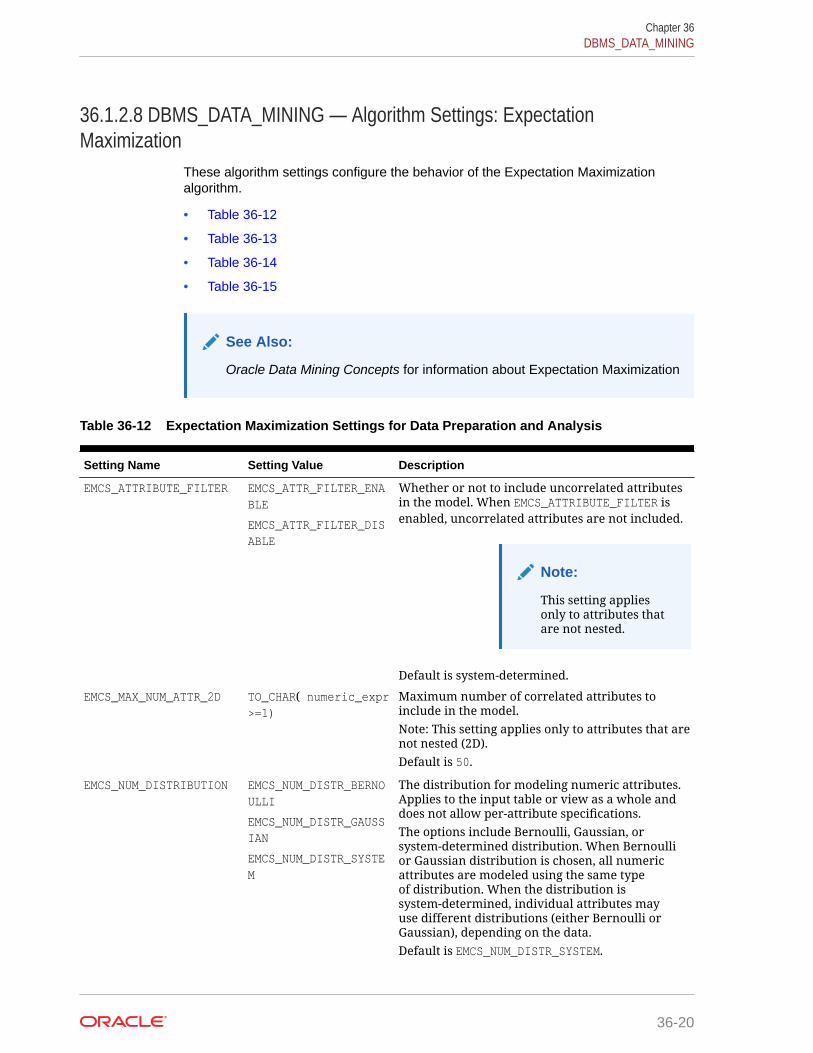
36.1.2.8 DBMS_DATA_MINING — Algorithm Settings: ExpectationMaximization
These algorithm settings configure the behavior of the Expectation Maximizationalgorithm.
• Table 36-12
• Table 36-13
• Table 36-14
• Table 36-15
See Also:
Oracle Data Mining Concepts for information about Expectation Maximization
Table 36-12 Expectation Maximization Settings for Data Preparation and Analysis
Setting Name Setting Value Description
EMCS_ATTRIBUTE_FILTER EMCS_ATTR_FILTER_ENABLE
EMCS_ATTR_FILTER_DISABLE
Whether or not to include uncorrelated attributesin the model. When EMCS_ATTRIBUTE_FILTER isenabled, uncorrelated attributes are not included.
Note:
This setting appliesonly to attributes thatare not nested.
Default is system-determined.
EMCS_MAX_NUM_ATTR_2D TO_CHAR( numeric_expr>=1)
Maximum number of correlated attributes toinclude in the model.Note: This setting applies only to attributes that arenot nested (2D).Default is 50.
EMCS_NUM_DISTRIBUTION EMCS_NUM_DISTR_BERNOULLI
EMCS_NUM_DISTR_GAUSSIAN
EMCS_NUM_DISTR_SYSTEM
The distribution for modeling numeric attributes.Applies to the input table or view as a whole anddoes not allow per-attribute specifications.The options include Bernoulli, Gaussian, orsystem-determined distribution. When Bernoullior Gaussian distribution is chosen, all numericattributes are modeled using the same typeof distribution. When the distribution issystem-determined, individual attributes mayuse different distributions (either Bernoulli orGaussian), depending on the data.Default is EMCS_NUM_DISTR_SYSTEM.
Chapter 36DBMS_DATA_MINING
36-20

Table 36-12 (Cont.) Expectation Maximization Settings for Data Preparation and Analysis
Setting Name Setting Value Description
EMCS_NUM_EQUIWIDTH_BINS
TO_CHAR( 1<numeric_expr <=255)
Number of equi-width bins that will be used forgathering cluster statistics for numeric columns.Default is 11.
EMCS_NUM_PROJECTIONS TO_CHAR( numeric_expr>=1)
Specifies the number of projections that will beused for each nested column. If a column hasfewer distinct attributes than the specified numberof projections, the data will not be projected. Thesetting applies to all nested columns.Default is 50.
EMCS_NUM_QUANTILE_BINS TO_CHAR( 1<numeric_expr <=255)
Specifies the number of quantile bins that willbe used for modeling numeric columns withmultivalued Bernoulli distributions.Default is system-determined.
EMCS_NUM_TOPN_BINS TO_CHAR( 1<numeric_expr <=255)
Specifies the number of top-N bins that willbe used for modeling categorical columns withmultivalued Bernoulli distributions.Default is system-determined.
Table 36-13 Expectation Maximization Settings for Learning
Setting Name Setting Value Description
EMCS_CONVERGENCE_CRITERION
EMCS_CONV_CRIT_HELDASIDE
EMCS_CONV_CRIT_BIC
The convergence criterion for EM. Theconvergence criterion may be based on a held-aside data set, or it may be Bayesian InformationCriterion.Default is system determined.
EMCS_LOGLIKE_IMPROVEMENT
TO_CHAR( 0 <numeric_expr < 1)
When the convergence criterionis based on a held-aside dataset (EMCS_CONVERGENCE_CRITERION =EMCS_CONV_CRIT_HELDASIDE), this setting specifiesthe percentage improvement in the value of thelog likelihood function that is required for addinga new component to the model.Default value is 0.001.
EMCS_NUM_COMPONENTS TO_CHAR( numeric_expr>=1)
Maximum number of components in themodel. If model search is enabled, thealgorithm automatically determines the numberof components based on improvements in thelikelihood function or based on regularization, upto the specified maximum.The number of components must be greater thanor equal to the number of clusters.Default is 20.
EMCS_NUM_ITERATIONS TO_CHAR( numeric_expr>=1)
Specifies the maximum number of iterations inthe EM algorithm.Default is 100.
Chapter 36DBMS_DATA_MINING
36-21

Table 36-13 (Cont.) Expectation Maximization Settings for Learning
Setting Name Setting Value Description
EMCS_MODEL_SEARCH EMCS_MODEL_SEARCH_ENABLE
EMCS_MODEL_SEARCH_DISABLE (default).
This setting enables model search in EM wheredifferent model sizes are explored and a best sizeis selected.The default is EMCS_MODEL_SEARCH_DISABLE.
EMCS_REMOVE_COMPONENTS EMCS_REMOVE_COMPS_ENABLE (default)
EMCS_REMOVE_COMPS_DISABLE
This setting allows the EM algorithm to remove asmall component from the solution.The default is EMCS_REMOVE_COMPS_ENABLE.
EMCS_RANDOM_SEED Non-negative integer This setting controls the seed of the randomgenerator used in EM. The default is 0.
Table 36-14 Expectation Maximization Settings for Component Clustering
Setting Name Setting Value Description
EMCS_CLUSTER_COMPONENTS EMCS__CLUSTER_COMP_ENABLE
EMCS_CLUSTER_COMP_DISABLE
Enables or disables the grouping of EMcomponents into high-level clusters. Whendisabled, the components themselves are treatedas clusters.When component clustering is enabled, modelscoring through the SQL CLUSTER functionwill produce assignments to the higher levelclusters. When clustering is disabled, the CLUSTERfunction will produce assignments to the originalcomponents.Default is EMCS_CLUSTER_COMP_ENABLE.
EMCS_CLUSTER_THRESH TO_CHAR( numeric_expr >=1)
Dissimilarity threshold that controls the clusteringof EM components. When the dissimilaritymeasure is less than the threshold, thecomponents are combined into a single cluster.A lower threshold may produce more clustersthat are more compact. A higher threshold mayproduce fewer clusters that are more spread out.Default is 2.
EMCS_LINKAGE_FUNCTION EMCS_LINKAGE_SINGLE
EMCS_LINKAGE_AVERAGE
EMCS_LINKAGE_COMPLETE
Allows the specification of a linkage function forthe agglomerative clustering step.EMCS_LINKAGE_SINGLE uses the nearest distancewithin the branch. The clusters tend to be largerand have arbitrary shapes.EMCS_LINKAGE_AVERAGE uses the average distancewithin the branch. There is less chaining effectand the clusters are more compact.EMCS_LINKAGE_COMPLETE uses the maximumdistance within the branch. The clusters aresmaller and require strong component overlap.Default is EMCS_LINKAGE_SINGLE.
Chapter 36DBMS_DATA_MINING
36-22

Table 36-15 Expectation Maximization Settings for Cluster Statistics
Setting Name Setting Value Description
EMCS_CLUSTER_STATISTICS EMCS_CLUS_STATS_ENABLE
EMCS_CLUS_STATS_DISABLE
Enables or disables the gathering of descriptivestatistics for clusters (centroids, histograms, andrules). When statistics are disabled, model size isreduced, and GET_MODEL_DETAILS_EM only returnstaxonomy (hierarchy) and cluster counts.Default is EMCS_CLUS_STATS_ENABLE.
EMCS_MIN_PCT_ATTR_SUPPORT TO_CHAR( 0 <numeric_expr < 1)
Minimum support required for including anattribute in the cluster rule. The support is thepercentage of the data rows assigned to a clusterthat must have non-null values for the attribute.Default is 0.1.
36.1.2.9 DBMS_DATA_MINING — Algorithm Settings: Explicit SemanticAnalysis
Explicit Semantic Analysis (ESA) is a useful technique for extracting meaningful andinterpretable features.
The settings listed in the following table configure the ESA values.
Table 36-16 Explicit Semantic Analysis Settings
Setting Name Setting Value Description
ESAS_VALUE_THRESHOLD Non-negative number This setting thresholds a small valuefor attribute weights in the transformedbuild data. The default is 1e-8.
ESAS_MIN_ITEMS Text input 100
Non-text input is 0
This setting determines the minimumnumber of non-zero entries that need tobe present in an input row. The defaultis 100 for text input and 0 for non-textinput.
ESAS_TOPN_FEATURES A positive integer This setting controls the maximumnumber of features per attribute. Thedefault is 1000.
See Also:
Oracle Data Mining Concepts for information about Explicit SemanticAnalysis.
Chapter 36DBMS_DATA_MINING
36-23

36.1.2.10 DBMS_DATA_MINING — Algorithm Settings: Exponential SmoothingExponential Smoothing (ESM) is a useful technique for extracting meaningful andinterpretable features.
The settings listed in the following table configure Exponential Smoothing values.
Chapter 36DBMS_DATA_MINING
36-24

Table 36-17 Exponential Smoothing Settings
Setting Name Setting Value Description
EXSM_MODEL It can take valuein set {EXSM_SIMPLE,EXSM_SIMPLE_MULT,EXSM_HOLT,EXSM_HOLT_DMP,EXSM_MUL_TRND,EXSM_MULTRD_DMP,EXSM_SEAS_ADD,EXSM_SEAS_MUL,EXSM_HW, EXSM_HW_DMP,EXSM_HW_ADDSEA,EXSM_DHW_ADDSEA,EXSM_HWMT,EXSM_HWMT_DMP}
This setting specifies the model.EXSM_SIMPLE: Simple exponentialsmoothing model is applied.EXSM_SIMPLE_MULT: Simple exponentialsmoothing model with multiplicativeerror is applied.EXSM_HOLT: Holt linear exponentialsmoothing model is applied.EXSM_HOLT_DMP: Holt linear exponentialsmoothing model with damped trend isapplied.EXSM_MUL_TRND: Exponential smoothingmodel with multiplicative trend isapplied.EXSM_MULTRD_DMP: Exponentialsmoothing model with multiplicativedamped trend is applied.EXSM_SEAS_ADD: Exponential smoothingwith additive seasonality, but no trend,is applied.EXSM_SEAS_MUL: Exponential smoothingwith multiplicative seasonality, but notrend, is applied.EXSM_HW: Holt-Winters triple exponentialsmoothing model, additive trend,multiplicative seasonality is applied.EXSM_HW_DMP: Holt-Wintersmultiplicative exponential smoothingmodel with damped trend, additivetrend, multiplicative seasonality isapplied.EXSM_HW_ADDSEA: Holt-Winters additiveexponential smoothing model, additivetrend, additive seasonality is applied.EXSM_DHW_ADDSEA: Holt-Winters additiveexponential smoothing model withdamped trend, additive trend, additiveseasonality is applied.EXSM_HWMT: Holt-Winters multiplicativeexponential smoothing model withmultiplicative trend, multiplicativetrend, multiplicative seasonality isapplied.EXSM_HWMT_DMP: Holt-Wintersmultiplicative exponential smoothingmodel with damped multiplicativetrend, multiplicative trend,multiplicative seasonality is applied.The default value is EXSM_SIMPLE.
Chapter 36DBMS_DATA_MINING
36-25
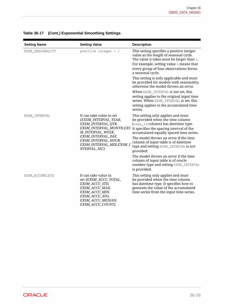
Table 36-17 (Cont.) Exponential Smoothing Settings
Setting Name Setting Value Description
EXSM_SEASONALITY positive integer > 1 This setting specifies a positive integervalue as the length of seasonal cycle.The value it takes must be larger than 1.For example, setting value 4 means thatevery group of four observations formsa seasonal cycle.This setting is only applicable and mustbe provided for models with seasonality,otherwise the model throws an error.When EXSM_INTERVAL is not set, thissetting applies to the original input timeseries. When EXSM_INTERVAL is set, thissetting applies to the accumulated timeseries.
EXSM_INTERVAL It can take value in set{EXSM_INTERVAL_YEAR,EXSM_INTERVAL_QTR,EXSM_INTERVAL_MONTH,EXSM_INTERVAL_WEEK,EXSM_INTERVAL_DAY,EXSM_INTERVAL_HOUR,EXSM_INTERVAL_MIN,EXSM_INTERVAL_SEC}
This setting only applies and mustbe provided when the time column(case_id column) has datetime type.It specifies the spacing interval of theaccumulated equally spaced time series.The model throws an error if the timecolumn of input table is of datetimetype and setting EXSM_INTERVAL is notprovided.The model throws an error if the timecolumn of input table is of oraclenumber type and setting EXSM_INTERVALis provided.
EXSM_ACCUMULATE It can take value inset {EXSM_ACCU_TOTAL,EXSM_ACCU_STD,EXSM_ACCU_MAX,EXSM_ACCU_MIN,EXSM_ACCU_AVG,EXSM_ACCU_MEDIAN,EXSM_ACCU_COUNT}.
This setting only applies and mustbe provided when the time columnhas datetime type. It specifies how togenerate the value of the accumulatedtime series from the input time series.
Chapter 36DBMS_DATA_MINING
36-26
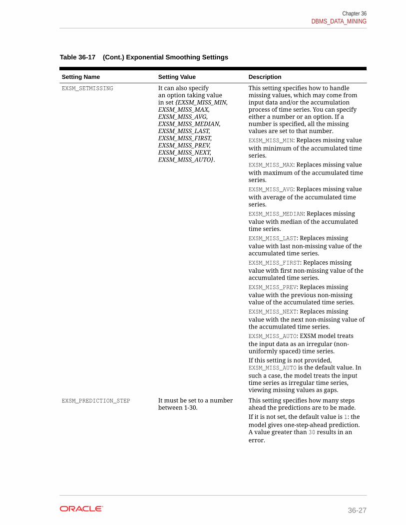
Table 36-17 (Cont.) Exponential Smoothing Settings
Setting Name Setting Value Description
EXSM_SETMISSING It can also specifyan option taking valuein set {EXSM_MISS_MIN,EXSM_MISS_MAX,EXSM_MISS_AVG,EXSM_MISS_MEDIAN,EXSM_MISS_LAST,EXSM_MISS_FIRST,EXSM_MISS_PREV,EXSM_MISS_NEXT,EXSM_MISS_AUTO}.
This setting specifies how to handlemissing values, which may come frominput data and/or the accumulationprocess of time series. You can specifyeither a number or an option. If anumber is specified, all the missingvalues are set to that number.EXSM_MISS_MIN: Replaces missing valuewith minimum of the accumulated timeseries.EXSM_MISS_MAX: Replaces missing valuewith maximum of the accumulated timeseries.EXSM_MISS_AVG: Replaces missing valuewith average of the accumulated timeseries.EXSM_MISS_MEDIAN: Replaces missingvalue with median of the accumulatedtime series.EXSM_MISS_LAST: Replaces missingvalue with last non-missing value of theaccumulated time series.EXSM_MISS_FIRST: Replaces missingvalue with first non-missing value of theaccumulated time series.EXSM_MISS_PREV: Replaces missingvalue with the previous non-missingvalue of the accumulated time series.EXSM_MISS_NEXT: Replaces missingvalue with the next non-missing value ofthe accumulated time series.EXSM_MISS_AUTO: EXSM model treatsthe input data as an irregular (non-uniformly spaced) time series.If this setting is not provided,EXSM_MISS_AUTO is the default value. Insuch a case, the model treats the inputtime series as irregular time series,viewing missing values as gaps.
EXSM_PREDICTION_STEP It must be set to a numberbetween 1-30.
This setting specifies how many stepsahead the predictions are to be made.If it is not set, the default value is 1: themodel gives one-step-ahead prediction.A value greater than 30 results in anerror.
Chapter 36DBMS_DATA_MINING
36-27

Table 36-17 (Cont.) Exponential Smoothing Settings
Setting Name Setting Value Description
EXSM_CONFIDENCE_LEVEL It must be a number between0 and 1, exclusive.
This setting specifies the desiredconfidence level for prediction.The lower and upper bounds of thespecified confidence interval is reported.If this setting is not specified, the defaultconfidence level is 95%.
EXSM_OPT_CRITERION It takes value inset {EXSM_OPT_CRIT_LIK,EXSM_OPT_CRIT_MSE,EXSM_OPT_CRIT_AMSE,EXSM_OPT_CRIT_SIG,EXSM_OPT_CRIT_MAE}.
This setting specifies the desiredoptimization criterion. The optimizationcriterion is useful as a diagnostic forcomparing models' fit to the same data.EXSM_OPT_CRIT_LIK: Minus twice thelog-likelihood of a model.EXSM_OPT_CRIT_MSE: Mean square errorof a model.EXSM_OPT_CRIT_AMSE: Average meansquare error over user-specified timewindow.EXSM_OPT_CRIT_SIG: Model's standarddeviation of residuals.EXSM_OPT_CRIT_MAE: Mean absoluteerror of a model.The default value isEXSM_OPT_CRIT_LIK.
EXSM_NMSE positive integer This setting specifies the length ofthe window used in computing theerror metric average mean square error(AMSE).
See Also:
Oracle Data Mining Concepts for information about ESM.
36.1.2.11 DBMS_DATA_MINING — Algorithm Settings: Generalized LinearModels
The settings listed in the following table configure the behavior of Generalized LinearModels
Table 36-18 DBMS_DATA_MINING GLM Settings
Setting Name Setting Value Description
GLMS_CONF_LEVEL TO_CHAR(0<numeric_expr <1)
The confidence level for coefficient confidenceintervals.The default confidence level is 0.95.
Chapter 36DBMS_DATA_MINING
36-28
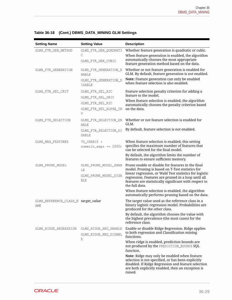
Table 36-18 (Cont.) DBMS_DATA_MINING GLM Settings
Setting Name Setting Value Description
GLMS_FTR_GEN_METHOD GLMS_FTR_GEN_QUADRATIC
GLMS_FTR_GEN_CUBIC
Whether feature generation is quadratic or cubic.When feature generation is enabled, the algorithmautomatically chooses the most appropriatefeature generation method based on the data.
GLMS_FTR_GENERATION GLMS_FTR_GENERATION_ENABLE
GLMS_FTR_GENERATION_DISABLE
Whether or not feature generation is enabled forGLM. By default, feature generation is not enabled.Note: Feature generation can only be enabledwhen feature selection is also enabled.
GLMS_FTR_SEL_CRIT GLMS_FTR_SEL_AIC
GLMS_FTR_SEL_SBIC
GLMS_FTR_SEL_RIC
GLMS_FTR_SEL_ALPHA_INV
Feature selection penalty criterion for adding afeature to the model.When feature selection is enabled, the algorithmautomatically chooses the penalty criterion basedon the data.
GLMS_FTR_SELECTION GLMS_FTR_SELECTION_ENABLE
GLMS_FTR_SELECTION_DISABLE
Whether or not feature selection is enabled forGLM.By default, feature selection is not enabled.
GLMS_MAX_FEATURES TO_CHAR(0 <numeric_expr <= 2000)
When feature selection is enabled, this settingspecifies the maximum number of features thatcan be selected for the final model.By default, the algorithm limits the number offeatures to ensure sufficient memory.
GLMS_PRUNE_MODEL GLMS_PRUNE_MODEL_ENABLE
GLMS_PRUNE_MODEL_DISABLE
Prune enable or disable for features in the finalmodel. Pruning is based on T-Test statistics forlinear regression, or Wald Test statistics for logisticregression. Features are pruned in a loop until allfeatures are statistically significant with respect tothe full data.When feature selection is enabled, the algorithmautomatically performs pruning based on the data.
GLMS_REFERENCE_CLASS_NAME
target_value The target value used as the reference class in abinary logistic regression model. Probabilities areproduced for the other class.By default, the algorithm chooses the value withthe highest prevalence (the most cases) for thereference class.
GLMS_RIDGE_REGRESSION GLMS_RIDGE_REG_ENABLE
GLMS_RIDGE_REG_DISABLE
Enable or disable Ridge Regression. Ridge appliesto both regression and Classification miningfunctions.When ridge is enabled, prediction bounds arenot produced by the PREDICTION_BOUNDS SQLfunction.Note: Ridge may only be enabled when featureselection is not specified, or has been explicitlydisabled. If Ridge Regression and feature selectionare both explicitly enabled, then an exception israised.
Chapter 36DBMS_DATA_MINING
36-29
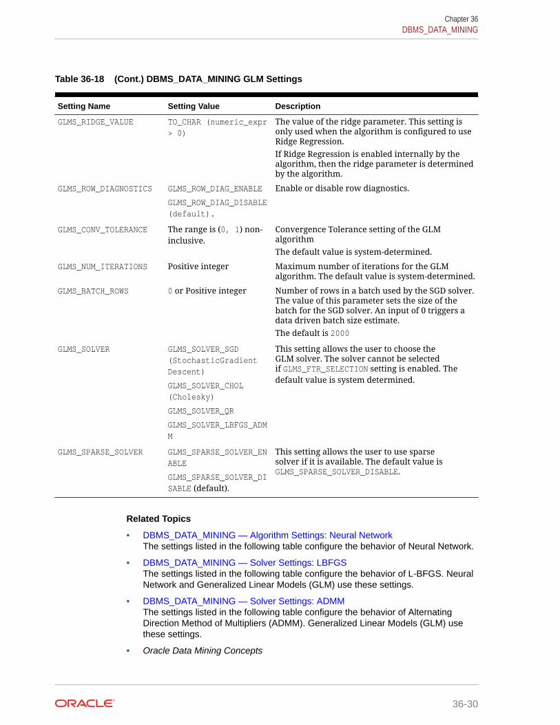
Table 36-18 (Cont.) DBMS_DATA_MINING GLM Settings
Setting Name Setting Value Description
GLMS_RIDGE_VALUE TO_CHAR (numeric_expr> 0)
The value of the ridge parameter. This setting isonly used when the algorithm is configured to useRidge Regression.If Ridge Regression is enabled internally by thealgorithm, then the ridge parameter is determinedby the algorithm.
GLMS_ROW_DIAGNOSTICS GLMS_ROW_DIAG_ENABLE
GLMS_ROW_DIAG_DISABLE(default).
Enable or disable row diagnostics.
GLMS_CONV_TOLERANCE The range is (0, 1) non-inclusive.
Convergence Tolerance setting of the GLMalgorithmThe default value is system-determined.
GLMS_NUM_ITERATIONS Positive integer Maximum number of iterations for the GLMalgorithm. The default value is system-determined.
GLMS_BATCH_ROWS 0 or Positive integer Number of rows in a batch used by the SGD solver.The value of this parameter sets the size of thebatch for the SGD solver. An input of 0 triggers adata driven batch size estimate.The default is 2000
GLMS_SOLVER GLMS_SOLVER_SGD(StochasticGradientDescent)
GLMS_SOLVER_CHOL(Cholesky)
GLMS_SOLVER_QR
GLMS_SOLVER_LBFGS_ADMM
This setting allows the user to choose theGLM solver. The solver cannot be selectedif GLMS_FTR_SELECTION setting is enabled. Thedefault value is system determined.
GLMS_SPARSE_SOLVER GLMS_SPARSE_SOLVER_ENABLE
GLMS_SPARSE_SOLVER_DISABLE (default).
This setting allows the user to use sparsesolver if it is available. The default value isGLMS_SPARSE_SOLVER_DISABLE.
Related Topics
• DBMS_DATA_MINING — Algorithm Settings: Neural NetworkThe settings listed in the following table configure the behavior of Neural Network.
• DBMS_DATA_MINING — Solver Settings: LBFGSThe settings listed in the following table configure the behavior of L-BFGS. NeuralNetwork and Generalized Linear Models (GLM) use these settings.
• DBMS_DATA_MINING — Solver Settings: ADMMThe settings listed in the following table configure the behavior of AlternatingDirection Method of Multipliers (ADMM). Generalized Linear Models (GLM) usethese settings.
• Oracle Data Mining Concepts
Chapter 36DBMS_DATA_MINING
36-30

See Also:
Oracle Data Mining Concepts for information about GLM.
36.1.2.12 DBMS_DATA_MINING — Algorithm Settings: k-MeansThe settings listed in the following table configure the behavior of the k-Meansalgorithm.
Table 36-19 k-Means Settings
Setting Name Setting Value Description
KMNS_CONV_TOLERANCE TO_CHAR(0<numeric_expr<1) Minimum Convergence Tolerance for k-Means.The algorithm iterates until the minimumConvergence Tolerance is satisfied or until themaximum number of iterations, specified inKMNS_ITERATIONS, is reached.
Decreasing the Convergence Toleranceproduces a more accurate solution but mayresult in longer run times.The default Convergence Tolerance is 0.001.
KMNS_DISTANCE KMNS_COSINE
KMNS_EUCLIDEAN
Distance function for k-Means.The default distance function isKMNS_EUCLIDEAN.
KMNS_ITERATIONS TO_CHAR(positive_numeric_expr)
Maximum number of iterations for k-Means.The algorithm iterates until either themaximum number of iterations is reached orthe minimum Convergence Tolerance, specifiedin KMNS_CONV_TOLERANCE, is satisfied.
The default number of iterations is 20.
KMNS_MIN_PCT_ATTR_SUPPORT
TO_CHAR(0<=numeric_expr<=1)
Minimum percentage of attribute values thatmust be non-null in order for the attributeto be included in the rule description for thecluster.If the data is sparse or includes many missingvalues, a minimum support that is too high cancause very short rules or even empty rules.The default minimum support is 0.1.
KMNS_NUM_BINS TO_CHAR(numeric_expr>0) Number of bins in the attribute histogramproduced by k-Means. The bin boundaries foreach attribute are computed globally on theentire training data set. The binning methodis equi-width. All attributes have the samenumber of bins with the exception of attributeswith a single value that have only one bin.The default number of histogram bins is 11.
Chapter 36DBMS_DATA_MINING
36-31
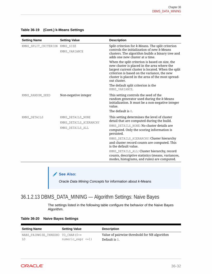
Table 36-19 (Cont.) k-Means Settings
Setting Name Setting Value Description
KMNS_SPLIT_CRITERION KMNS_SIZE
KMNS_VARIANCE
Split criterion for k-Means. The split criterioncontrols the initialization of new k-Meansclusters. The algorithm builds a binary tree andadds one new cluster at a time.When the split criterion is based on size, thenew cluster is placed in the area where thelargest current cluster is located. When the splitcriterion is based on the variance, the newcluster is placed in the area of the most spread-out cluster.The default split criterion is theKMNS_VARIANCE.
KMNS_RANDOM_SEED Non-negative integer This setting controls the seed of therandom generator used during the k-Meansinitialization. It must be a non-negative integervalue.The default is 0.
KMNS_DETAILS KMNS_DETAILS_NONE
KMNS_DETAILS_HIERARCHY
KMNS_DETAILS_ALL
This setting determines the level of clusterdetail that are computed during the build.KMNS_DETAILS_NONE: No cluster details arecomputed. Only the scoring information ispersisted.KMNS_DETAILS_HIERARCHY: Cluster hierarchyand cluster record counts are computed. Thisis the default value.KMNS_DETAILS_ALL: Cluster hierarchy, recordcounts, descriptive statistics (means, variances,modes, histograms, and rules) are computed.
See Also:
Oracle Data Mining Concepts for information about k-Means
36.1.2.13 DBMS_DATA_MINING — Algorithm Settings: Naive BayesThe settings listed in the following table configure the behavior of the Naive BayesAlgorithm.
Table 36-20 Naive Bayes Settings
Setting Name Setting Value Description
NABS_PAIRWISE_THRESHOLD
TO_CHAR(0<=numeric_expr <=1)
Value of pairwise threshold for NB algorithmDefault is 0.
Chapter 36DBMS_DATA_MINING
36-32

Table 36-20 (Cont.) Naive Bayes Settings
Setting Name Setting Value Description
NABS_SINGLETON_THRESHOLD
TO_CHAR(0<=numeric_expr <=1)
Value of singleton threshold for NB algorithmDefault value is 0.
See Also:
Oracle Data Mining Concepts for information about Naive Bayes
36.1.2.14 DBMS_DATA_MINING — Algorithm Settings: Neural NetworkThe settings listed in the following table configure the behavior of Neural Network.
Table 36-21 DBMS_DATA_MINING Neural Network Settings
Setting Name Setting Value Description
NNET_HIDDEN_LAYERS Non-negative integer Defines the topology by number of hidden layers.The default value is 1.
NNET_NODES_PER_LAYER A list of positive integers Defines the topology by number of nodes perlayer. Different layers can have different numberof nodes.The value should be non-negative integers andcomma separated. For example, '10, 20, 5'.The setting values must be consistent withNNET_HIDDEN_LAYERS. The default number ofnodes per layer is the number of attributes or 50(if the number of attributes > 50).
Chapter 36DBMS_DATA_MINING
36-33
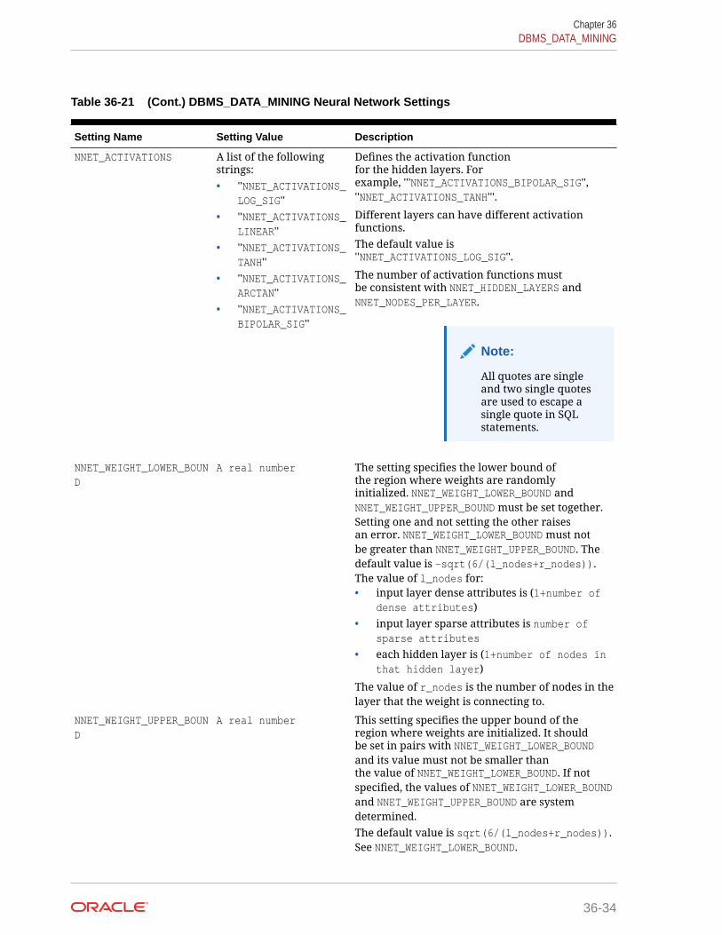
Table 36-21 (Cont.) DBMS_DATA_MINING Neural Network Settings
Setting Name Setting Value Description
NNET_ACTIVATIONS A list of the followingstrings:• ''NNET_ACTIVATIONS_
LOG_SIG''• ''NNET_ACTIVATIONS_
LINEAR''• ''NNET_ACTIVATIONS_
TANH''• ''NNET_ACTIVATIONS_
ARCTAN''• ''NNET_ACTIVATIONS_
BIPOLAR_SIG''
Defines the activation functionfor the hidden layers. Forexample, '''NNET_ACTIVATIONS_BIPOLAR_SIG'',''NNET_ACTIVATIONS_TANH'''.
Different layers can have different activationfunctions.The default value is''NNET_ACTIVATIONS_LOG_SIG''.
The number of activation functions mustbe consistent with NNET_HIDDEN_LAYERS andNNET_NODES_PER_LAYER.
Note:
All quotes are singleand two single quotesare used to escape asingle quote in SQLstatements.
NNET_WEIGHT_LOWER_BOUND
A real number The setting specifies the lower bound ofthe region where weights are randomlyinitialized. NNET_WEIGHT_LOWER_BOUND andNNET_WEIGHT_UPPER_BOUND must be set together.Setting one and not setting the other raisesan error. NNET_WEIGHT_LOWER_BOUND must notbe greater than NNET_WEIGHT_UPPER_BOUND. Thedefault value is –sqrt(6/(l_nodes+r_nodes)).The value of l_nodes for:• input layer dense attributes is (1+number of
dense attributes)• input layer sparse attributes is number of
sparse attributes
• each hidden layer is (1+number of nodes inthat hidden layer)
The value of r_nodes is the number of nodes in thelayer that the weight is connecting to.
NNET_WEIGHT_UPPER_BOUND
A real number This setting specifies the upper bound of theregion where weights are initialized. It shouldbe set in pairs with NNET_WEIGHT_LOWER_BOUNDand its value must not be smaller thanthe value of NNET_WEIGHT_LOWER_BOUND. If notspecified, the values of NNET_WEIGHT_LOWER_BOUNDand NNET_WEIGHT_UPPER_BOUND are systemdetermined.The default value is sqrt(6/(l_nodes+r_nodes)).See NNET_WEIGHT_LOWER_BOUND.
Chapter 36DBMS_DATA_MINING
36-34

Table 36-21 (Cont.) DBMS_DATA_MINING Neural Network Settings
Setting Name Setting Value Description
NNET_ITERATIONS Positive integer This setting specifies the maximum number ofiterations in the Neural Network algorithm.The default value is 200.
NNET_TOLERANCE TO_CHAR(0<numeric_expr <1)
Defines the convergence tolerance setting of theNeural Network algorithm.The default value is 0.000001.
NNET_REGULARIZER NNET_REGULARIZER_NONE
NNET_REGULARIZER_L2
NNET_REGULARIZER_HELDASIDE
Regularization setting for Neural Networkalgorithm. If the total number of trainingrows is greater than 50000, the defaultis NNET_REGULARIZER_HELDASIDE. If the totalnumber of training rows is less than or equal to50000, the default is NNET_REGULARIZER_NONE.
NNET_HELDASIDE_RATIO 0 <= numeric_expr <=1 Define the held ratio for the held-aside method.The default value is 0.25.
NNET_HELDASIDE_MAX_FAIL
The value must be apositive integer.
With NNET_REGULARIZER_HELDASIDE, the trainingprocess is stopped early if the networkperformance on the validation data failsto improve or remains the same forNNET_HELDASIDE_MAX_FAIL epochs in a row.
The default value is 6.
NNET_REG_LAMBDA TO_CHAR(numeric_expr>=0)
Defines the L2 regularization parameterlambda. This can not be set together withNNET_REGULARIZER_HELDASIDE.
The default value is 1.
Related Topics
• DBMS_DATA_MINING — Solver Settings: LBFGSThe settings listed in the following table configure the behavior of L-BFGS. NeuralNetwork and Generalized Linear Models (GLM) use these settings.
See Also:
Oracle Data Mining Concepts for information about Neural Network.
36.1.2.15 DBMS_DATA_MINING — Algorithm Settings: Non-Negative MatrixFactorization
The settings listed in the following table configure the behavior of the Non-NegativeMatrix Factorization algorithm.
You can query the data dictionary view *_MINING_MODEL_SETTINGS (using the ALL,USER, or DBA prefix) to find the setting values for a model. See Oracle DatabaseReference for information about *_MINING_MODEL_SETTINGS.
Chapter 36DBMS_DATA_MINING
36-35
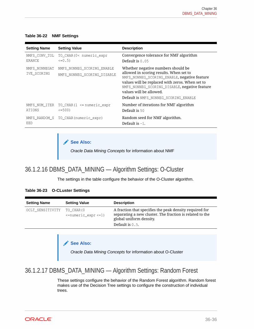
Table 36-22 NMF Settings
Setting Name Setting Value Description
NMFS_CONV_TOLERANCE
TO_CHAR(0< numeric_expr<=0.5)
Convergence tolerance for NMF algorithmDefault is 0.05
NMFS_NONNEGATIVE_SCORING
NMFS_NONNEG_SCORING_ENABLE
NMFS_NONNEG_SCORING_DISABLE
Whether negative numbers should beallowed in scoring results. When set toNMFS_NONNEG_SCORING_ENABLE, negative featurevalues will be replaced with zeros. When set toNMFS_NONNEG_SCORING_DISABLE, negative featurevalues will be allowed.Default is NMFS_NONNEG_SCORING_ENABLE
NMFS_NUM_ITERATIONS
TO_CHAR(1 <= numeric_expr<=500)
Number of iterations for NMF algorithmDefault is 50
NMFS_RANDOM_SEED
TO_CHAR(numeric_expr) Random seed for NMF algorithm.Default is –1.
See Also:
Oracle Data Mining Concepts for information about NMF
36.1.2.16 DBMS_DATA_MINING — Algorithm Settings: O-ClusterThe settings in the table configure the behavior of the O-Cluster algorithm.
Table 36-23 O-CLuster Settings
Setting Name Setting Value Description
OCLT_SENSITIVITY TO_CHAR(0<=numeric_expr <=1)
A fraction that specifies the peak density required forseparating a new cluster. The fraction is related to theglobal uniform density.Default is 0.5.
See Also:
Oracle Data Mining Concepts for information about O-Cluster
36.1.2.17 DBMS_DATA_MINING — Algorithm Settings: Random ForestThese settings configure the behavior of the Random Forest algorithm. Random forestmakes use of the Decision Tree settings to configure the construction of individualtrees.
Chapter 36DBMS_DATA_MINING
36-36
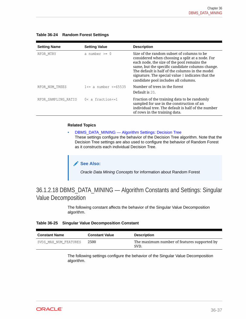
Table 36-24 Random Forest Settings
Setting Name Setting Value Description
RFOR_MTRY a number >= 0 Size of the random subset of columns to beconsidered when choosing a split at a node. Foreach node, the size of the pool remains thesame, but the specific candidate columns change.The default is half of the columns in the modelsignature. The special value 0 indicates that thecandidate pool includes all columns.
RFOR_NUM_TREES 1<= a number <=65535 Number of trees in the forestDefault is 20.
RFOR_SAMPLING_RATIO 0< a fraction<=1 Fraction of the training data to be randomlysampled for use in the construction of anindividual tree. The default is half of the numberof rows in the training data.
Related Topics
• DBMS_DATA_MINING — Algorithm Settings: Decision TreeThese settings configure the behavior of the Decision Tree algorithm. Note that theDecision Tree settings are also used to configure the behavior of Random Forestas it constructs each individual Decision Tree.
See Also:
Oracle Data Mining Concepts for information about Random Forest
36.1.2.18 DBMS_DATA_MINING — Algorithm Constants and Settings: SingularValue Decomposition
The following constant affects the behavior of the Singular Value Decompositionalgorithm.
Table 36-25 Singular Value Decomposition Constant
Constant Name Constant Value Description
SVDS_MAX_NUM_FEATURES 2500 The maximum number of features supported bySVD.
The following settings configure the behavior of the Singular Value Decompositionalgorithm.
Chapter 36DBMS_DATA_MINING
36-37

Table 36-26 Singular Value Decomposition Settings
Setting Name Setting Value Description
SVDS_U_MATRIX_OUTPUT
SVDS_U_MATRIX_ENABLE
SVDS_U_MATRIX_DISABLE
Indicates whether or not to persist the U Matrix produced bySVD.The U matrix in SVD has as many rows as the number ofrows in the build data. To avoid creating a large model, theU matrix is persisted only when SVDS_U_MATRIX_OUTPUT isenabled.When SVDS_U_MATRIX_OUTPUT is enabled, the build datamust include a case ID. If no case ID is present and the Umatrix is requested, then an exception is raised.Default is SVDS_U_MATRIX_DISABLE.
SVDS_SCORING_MODE SVDS_SCORING_SVD
SVDS_SCORING_PCA
Whether to use SVD or PCA scoring for the model.When the build data is scored with SVD, the projections willbe the same as the U matrix. When the build data is scoredwith PCA, the projections will be the product of the U and Smatrices.Default is SVDS_SCORING_SVD.
SVDS_SOLVER SVDS_SOLVER_TSSVD
SVDS_SOLVER_TSEIGEN
SVDS_SOLVER_SSVD
SVDS_SOLVER_STEIGEN
This setting indicates the solver to be used for computingSVD of the data. In the case of PCA, the solver settingindicates the type of SVD solver used to compute the PCAfor the data. When this setting is not specified the solvertype selection is data driven. If the number of attributesis greater than 3240, then the default wide solver is used.Otherwise, the default narrow solver is selected.The following are the group of solvers:• Narrow data solvers: for matrices with up to 11500
attributes (TSEIGEN) or up to 8100 attributes (TSSVD).• Wide data solvers: for matrices up to 1 million
attributes.For narrow data solvers:• Tall-Skinny SVD uses QR computation TSVD
(SVDS_SOLVER_TSSVD)• Tall-Skinny SVD uses eigenvalue computation, TSEIGEN
(SVDS_SOLVER_TSEIGEN), is the default solver for narrowdata.
For wide data solvers:• Stochastic SVD uses QR computation SSVD
(SVDS_SOLVER_SSVD), is the default solver for wide datasolvers.
• Stochastic SVD uses eigenvalue computations, STEIGEN(SVDS_SOLVER_STEIGEN).
SVDS_TOLERANCE Range [0, 1] This setting is used to prune features. Define the minimumvalue the eigenvalue of a feature as a share of the firsteigenvalue to not to prune. Default value is data driven.
SVDS_RANDOM_SEED Range [0 -4,294,967,296]
The random seed value is used for initializing the samplingmatrix used by the Stochastic SVD solver. The default is 0.The SVD Solver must be set to SSVD or STEIGEN.
Chapter 36DBMS_DATA_MINING
36-38

Table 36-26 (Cont.) Singular Value Decomposition Settings
Setting Name Setting Value Description
SVDS_OVER_SAMPLING Range [1, 5000]. This setting is configures the number of columns in thesampling matrix used by the Stochastic SVD solver. Thenumber of columns in this matrix is equal to the requestednumber of features plus the oversampling setting. The SVDSolver must be set to SSVD or STEIGEN.
SVDS_POWER_ITERATIONS
Range [0, 20]. The power iteration setting improves the accuracy of theSSVD solver. The default is 2. The SVD Solver must be set toSSVD or STEIGEN.
See Also:
Oracle Data Mining Concepts
36.1.2.19 DBMS_DATA_MINING — Algorithm Settings: Support VectorMachine
The settings listed in the following table configure the behavior of the Support VectorMachine algorithm.
Table 36-27 SVM Settings
Setting Name Setting Value Description
SVMS_COMPLEXITY_FACTOR
TO_CHAR(numeric_expr >0)
Regularization setting that balances the complexity ofthe model against model robustness to achieve goodgeneralization on new data. SVM uses a data-drivenapproach to finding the complexity factor.Value of complexity factor for SVM algorithm (bothClassification and Regression).Default value estimated from the data by the algorithm.
SVMS_CONV_TOLERANCE TO_CHAR(numeric_expr >0)
Convergence tolerance for SVM algorithm.Default is 0.0001.
SVMS_EPSILON TO_CHAR(numeric_expr >0)
Regularization setting for regression, similar tocomplexity factor. Epsilon specifies the allowableresiduals, or noise, in the data.Value of epsilon factor for SVM regression.Default is 0.1.
SVMS_KERNEL_FUNCTION SVMS_GAUSSIAN
SVMS_LINEAR
Kernel for Support Vector Machine. Linear or Gaussian.The default value is SVMS_LINEAR.
SVMS_OUTLIER_RATE TO_CHAR(0<numeric_expr <1)
The desired rate of outliers in the training data. Valid forOne-Class SVM models only (Anomaly Detection).Default is 0.01.
Chapter 36DBMS_DATA_MINING
36-39
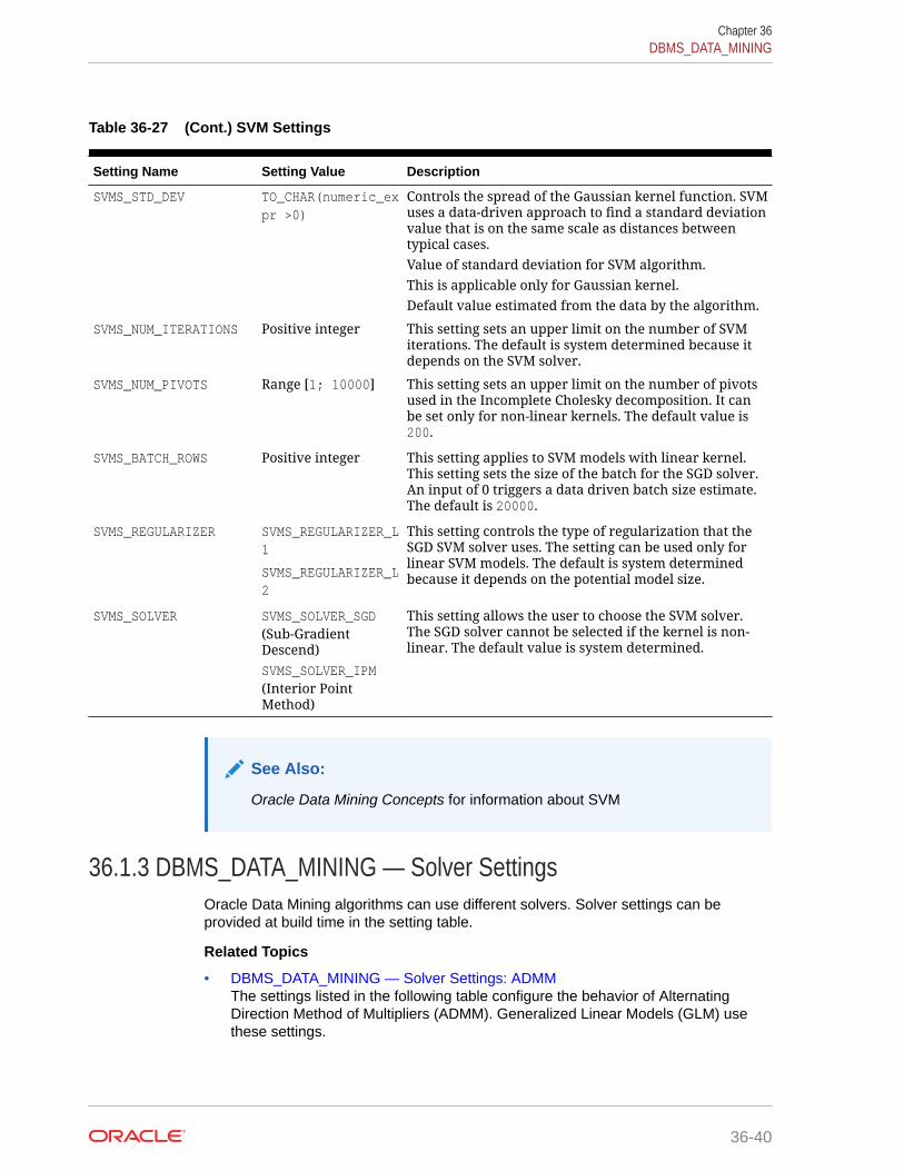
Table 36-27 (Cont.) SVM Settings
Setting Name Setting Value Description
SVMS_STD_DEV TO_CHAR(numeric_expr >0)
Controls the spread of the Gaussian kernel function. SVMuses a data-driven approach to find a standard deviationvalue that is on the same scale as distances betweentypical cases.Value of standard deviation for SVM algorithm.This is applicable only for Gaussian kernel.Default value estimated from the data by the algorithm.
SVMS_NUM_ITERATIONS Positive integer This setting sets an upper limit on the number of SVMiterations. The default is system determined because itdepends on the SVM solver.
SVMS_NUM_PIVOTS Range [1; 10000] This setting sets an upper limit on the number of pivotsused in the Incomplete Cholesky decomposition. It canbe set only for non-linear kernels. The default value is200.
SVMS_BATCH_ROWS Positive integer This setting applies to SVM models with linear kernel.This setting sets the size of the batch for the SGD solver.An input of 0 triggers a data driven batch size estimate.The default is 20000.
SVMS_REGULARIZER SVMS_REGULARIZER_L1
SVMS_REGULARIZER_L2
This setting controls the type of regularization that theSGD SVM solver uses. The setting can be used only forlinear SVM models. The default is system determinedbecause it depends on the potential model size.
SVMS_SOLVER SVMS_SOLVER_SGD(Sub-GradientDescend)SVMS_SOLVER_IPM(Interior PointMethod)
This setting allows the user to choose the SVM solver.The SGD solver cannot be selected if the kernel is non-linear. The default value is system determined.
See Also:
Oracle Data Mining Concepts for information about SVM
36.1.3 DBMS_DATA_MINING — Solver SettingsOracle Data Mining algorithms can use different solvers. Solver settings can beprovided at build time in the setting table.
Related Topics
• DBMS_DATA_MINING — Solver Settings: ADMMThe settings listed in the following table configure the behavior of AlternatingDirection Method of Multipliers (ADMM). Generalized Linear Models (GLM) usethese settings.
Chapter 36DBMS_DATA_MINING
36-40
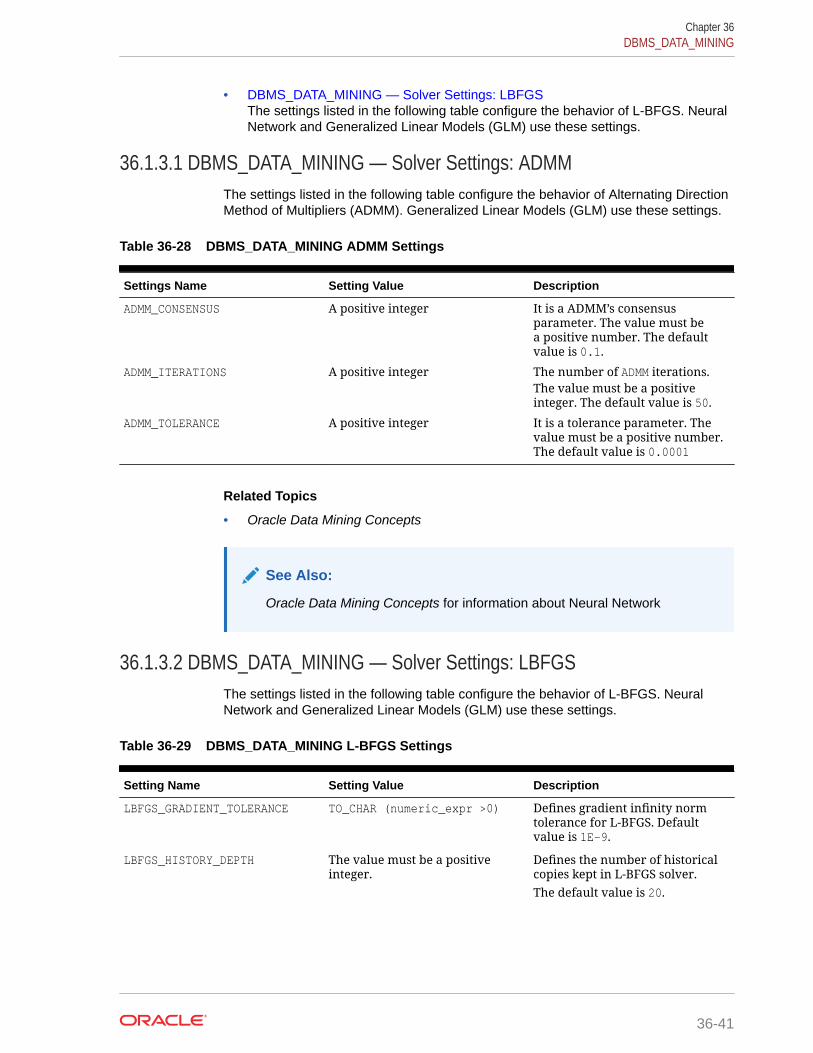
• DBMS_DATA_MINING — Solver Settings: LBFGSThe settings listed in the following table configure the behavior of L-BFGS. NeuralNetwork and Generalized Linear Models (GLM) use these settings.
36.1.3.1 DBMS_DATA_MINING — Solver Settings: ADMMThe settings listed in the following table configure the behavior of Alternating DirectionMethod of Multipliers (ADMM). Generalized Linear Models (GLM) use these settings.
Table 36-28 DBMS_DATA_MINING ADMM Settings
Settings Name Setting Value Description
ADMM_CONSENSUS A positive integer It is a ADMM’s consensusparameter. The value must bea positive number. The defaultvalue is 0.1.
ADMM_ITERATIONS A positive integer The number of ADMM iterations.The value must be a positiveinteger. The default value is 50.
ADMM_TOLERANCE A positive integer It is a tolerance parameter. Thevalue must be a positive number.The default value is 0.0001
Related Topics
• Oracle Data Mining Concepts
See Also:
Oracle Data Mining Concepts for information about Neural Network
36.1.3.2 DBMS_DATA_MINING — Solver Settings: LBFGSThe settings listed in the following table configure the behavior of L-BFGS. NeuralNetwork and Generalized Linear Models (GLM) use these settings.
Table 36-29 DBMS_DATA_MINING L-BFGS Settings
Setting Name Setting Value Description
LBFGS_GRADIENT_TOLERANCE TO_CHAR (numeric_expr >0) Defines gradient infinity normtolerance for L-BFGS. Defaultvalue is 1E-9.
LBFGS_HISTORY_DEPTH The value must be a positiveinteger.
Defines the number of historicalcopies kept in L-BFGS solver.The default value is 20.
Chapter 36DBMS_DATA_MINING
36-41
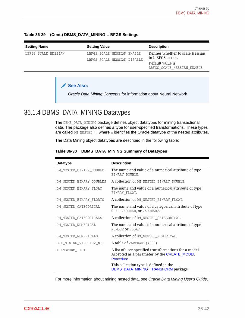
Table 36-29 (Cont.) DBMS_DATA_MINING L-BFGS Settings
Setting Name Setting Value Description
LBFGS_SCALE_HESSIAN LBFGS_SCALE_HESSIAN_ENABLE
LBFGS_SCALE_HESSIAN_DISABLE
Defines whether to scale Hessianin L-BFGS or not.Default value isLBFGS_SCALE_HESSIAN_ENABLE.
See Also:
Oracle Data Mining Concepts for information about Neural Network
36.1.4 DBMS_DATA_MINING DatatypesThe DBMS_DATA_MINING package defines object datatypes for mining transactionaldata. The package also defines a type for user-specified transformations. These typesare called DM_NESTED_n, where n identifies the Oracle datatype of the nested attributes.
The Data Mining object datatypes are described in the following table:
Table 36-30 DBMS_DATA_MINING Summary of Datatypes
Datatype Description
DM_NESTED_BINARY_DOUBLE The name and value of a numerical attribute of typeBINARY_DOUBLE.
DM_NESTED_BINARY_DOUBLES A collection of DM_NESTED_BINARY_DOUBLE.
DM_NESTED_BINARY_FLOAT The name and value of a numerical attribute of typeBINARY_FLOAT.
DM_NESTED_BINARY_FLOATS A collection of DM_NESTED_BINARY_FLOAT.
DM_NESTED_CATEGORICAL The name and value of a categorical attribute of typeCHAR, VARCHAR, or VARCHAR2.
DM_NESTED_CATEGORICALS A collection of DM_NESTED_CATEGORICAL.
DM_NESTED_NUMERICAL The name and value of a numerical attribute of typeNUMBER or FLOAT.
DM_NESTED_NUMERICALS A collection of DM_NESTED_NUMERICAL.
ORA_MINING_VARCHAR2_NT A table of VARCHAR2(4000).
TRANSFORM_LIST A list of user-specified transformations for a model.Accepted as a parameter by the CREATE_MODELProcedure.
This collection type is defined in theDBMS_DATA_MINING_TRANSFORM package.
For more information about mining nested data, see Oracle Data Mining User's Guide.
Chapter 36DBMS_DATA_MINING
36-42

Note:
Starting from Oracle Database 12c Release 2, *GET_MODEL_DETAILS aredeprecated and are replaced with Model Detail Views. See Oracle DataMining User’s Guide.
36.1.4.1 Deprecated TypesThis topic contains tables listing deprecated types.
The DBMS_DATA_MINING package defines object datatypes for storing information aboutmodel attributes. Most of these types are returned by the table functions GET_n, wheren identifies the type of information to return. These functions take a model name asinput and return the requested information as a collection of rows.
For a list of the GET functions, see "Summary of DBMS_DATA_MINING Subprograms".
All the table functions use pipelining, which causes each row of output to bematerialized as it is read from model storage, without waiting for the generation ofthe complete table object. For more information on pipelined, parallel table functions,consult the Oracle Database PL/SQL Language Reference.
Table 36-31 DBMS_DATA_MINING Summary of Deprecated Datatypes
Datatype Description
DM_CENTROID The centroid of a cluster.
DM_CENTROIDS A collection of DM_CENTROID. A member of DM_CLUSTER.
DM_CHILD A child node of a cluster.
DM_CHILDREN A collection of DM_CHILD. A member of DM_CLUSTER.
DM_CLUSTER A cluster. A cluster includes DM_PREDICATES,DM_CHILDREN, DM_CENTROIDS, and DM_HISTOGRAMS. Italso includes a DM_RULE.
See also, DM_CLUSTER Fields.
DM_CLUSTERS A collection of DM_CLUSTER. Returnedby GET_MODEL_DETAILS_KM Function,GET_MODEL_DETAILS_OC Function, andGET_MODEL_DETAILS_EM Function.
See also, DM_CLUSTER Fields.
DM_CONDITIONAL The conditional probability of an attribute in a NaiveBayes model.
DM_CONDITIONALS A collection of DM_CONDITIONAL. Returned byGET_MODEL_DETAILS_NB Function.
DM_COST_ELEMENT The actual and predicted values in a cost matrix.
DM_COST_MATRIX A collection of DM_COST_ELEMENT. Returned byGET_MODEL_COST_MATRIX Function.
DM_EM_COMPONENT A component of an Expectation Maximization model.
Chapter 36DBMS_DATA_MINING
36-43
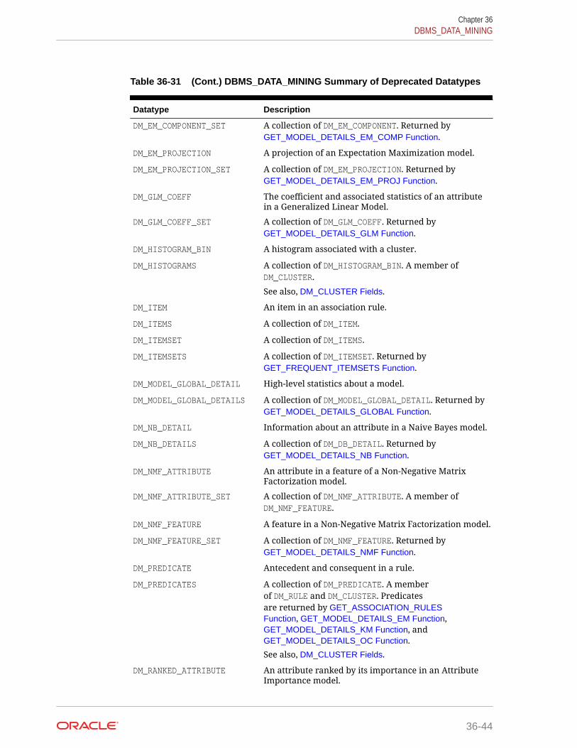
Table 36-31 (Cont.) DBMS_DATA_MINING Summary of Deprecated Datatypes
Datatype Description
DM_EM_COMPONENT_SET A collection of DM_EM_COMPONENT. Returned byGET_MODEL_DETAILS_EM_COMP Function.
DM_EM_PROJECTION A projection of an Expectation Maximization model.
DM_EM_PROJECTION_SET A collection of DM_EM_PROJECTION. Returned byGET_MODEL_DETAILS_EM_PROJ Function.
DM_GLM_COEFF The coefficient and associated statistics of an attributein a Generalized Linear Model.
DM_GLM_COEFF_SET A collection of DM_GLM_COEFF. Returned byGET_MODEL_DETAILS_GLM Function.
DM_HISTOGRAM_BIN A histogram associated with a cluster.
DM_HISTOGRAMS A collection of DM_HISTOGRAM_BIN. A member ofDM_CLUSTER.
See also, DM_CLUSTER Fields.
DM_ITEM An item in an association rule.
DM_ITEMS A collection of DM_ITEM.
DM_ITEMSET A collection of DM_ITEMS.
DM_ITEMSETS A collection of DM_ITEMSET. Returned byGET_FREQUENT_ITEMSETS Function.
DM_MODEL_GLOBAL_DETAIL High-level statistics about a model.
DM_MODEL_GLOBAL_DETAILS A collection of DM_MODEL_GLOBAL_DETAIL. Returned byGET_MODEL_DETAILS_GLOBAL Function.
DM_NB_DETAIL Information about an attribute in a Naive Bayes model.
DM_NB_DETAILS A collection of DM_DB_DETAIL. Returned byGET_MODEL_DETAILS_NB Function.
DM_NMF_ATTRIBUTE An attribute in a feature of a Non-Negative MatrixFactorization model.
DM_NMF_ATTRIBUTE_SET A collection of DM_NMF_ATTRIBUTE. A member ofDM_NMF_FEATURE.
DM_NMF_FEATURE A feature in a Non-Negative Matrix Factorization model.
DM_NMF_FEATURE_SET A collection of DM_NMF_FEATURE. Returned byGET_MODEL_DETAILS_NMF Function.
DM_PREDICATE Antecedent and consequent in a rule.
DM_PREDICATES A collection of DM_PREDICATE. A memberof DM_RULE and DM_CLUSTER. Predicatesare returned by GET_ASSOCIATION_RULESFunction, GET_MODEL_DETAILS_EM Function,GET_MODEL_DETAILS_KM Function, andGET_MODEL_DETAILS_OC Function.
See also, DM_CLUSTER Fields.
DM_RANKED_ATTRIBUTE An attribute ranked by its importance in an AttributeImportance model.
Chapter 36DBMS_DATA_MINING
36-44

Table 36-31 (Cont.) DBMS_DATA_MINING Summary of Deprecated Datatypes
Datatype Description
DM_RANKED_ATTRIBUTES A collection of DM_RANKED_ATTRIBUTE. Returned byGET_MODEL_DETAILS_AI Function.
DM_RULE A rule that defines a conditional relationship.The rule can be one of the association rules returned byGET_ASSOCIATION_RULES Function, or it can be a ruleassociated with a cluster in the collection of clustersreturned by GET_MODEL_DETAILS_KM Function andGET_MODEL_DETAILS_OC Function.
See also, DM_CLUSTER Fields.
DM_RULES A collection of DM_RULE. Returned byGET_ASSOCIATION_RULES Function.
See also, DM_CLUSTER Fields.
DM_SVD_MATRIX A factorized matrix S, V, or U returned by a SingularValue Decomposition model.
DM_SVD_MATRIX_SET A collection of DM_SVD_MATRIX. Returned byGET_MODEL_DETAILS_SVD Function.
DM_SVM_ATTRIBUTE The name, value, and coefficient of an attribute in aSupport Vector Machine model.
DM_SVM_ATTRIBUTE_SET A collection of DM_SVM_ATTRIBUTE. Returned byGET_MODEL_DETAILS_SVM Function. Also a member ofDM_SVM_LINEAR_COEFF.
DM_SVM_LINEAR_COEFF The linear coefficient of each attribute in a SupportVector Machine model.
DM_SVM_LINEAR_COEFF_SET A collection of DM_SVM_LINEAR_COEFF. Returned byGET_MODEL_DETAILS_SVM Function for an SVM modelbuilt using the linear kernel.
DM_TRANSFORM The transformation and reverse transformationexpressions for an attribute.
DM_TRANSFORMS A collection of DM_TRANSFORM. Returned byGET_MODEL_TRANSFORMATIONS Function.
Return Values for Clustering Algorithms
The table contains description of DM_CLUSTER return value columns, nested tablecolumns, and rows.
Chapter 36DBMS_DATA_MINING
36-45

Table 36-32 DM_CLUSTER Return Values for Clustering Algorithms
Return Value Description
DM_CLUSTERS A set of rows of type DM_CLUSTER. The rows have the followingcolumns:
(id NUMBER, cluster_id VARCHAR2(4000), record_count NUMBER, parent NUMBER, tree_level NUMBER, dispersion NUMBER, split_predicate DM_PREDICATES, child DM_CHILDREN, centroid DM_CENTROIDS, histogram DM_HISTOGRAMS, rule DM_RULE)
DM_PREDICATE The antecedent and consequent columns each return nested tablesof type DM_PREDICATES. The rows, of type DM_PREDICATE, have thefollowing columns:
(attribute_name VARCHAR2(4000), attribute_subname VARCHAR2(4000), conditional_operator CHAR(2)/*=,<>,<,>,<=,>=*/, attribute_num_value NUMBER, attribute_str_value VARCHAR2(4000), attribute_support NUMBER, attribute_confidence NUMBER)
DM_CLUSTER Fields
The following table describes DM_CLUSTER fields.
Table 36-33 DM_CLUSTER Fields
Column Name Description
id Cluster identifier
cluster_id The ID of a cluster in the model
record_count Specifies the number of records
parent Parent ID
tree_level Specifies the number of splits from the root
dispersion A measure used to quantify whether a set of observedoccurrences are dispersed compared to a standardstatistical model.
Chapter 36DBMS_DATA_MINING
36-46

Table 36-33 (Cont.) DM_CLUSTER Fields
Column Name Description
split_predicate The split_predicate column of DM_CLUSTER returns anested table of type DM_PREDICATES. Each row, of typeDM_PREDICATE, has the following columns:
(attribute_name VARCHAR2(4000), attribute_subname VARCHAR2(4000), conditional_operator CHAR(2) /*=,<>,<,>,<=,>=*/, attribute_num_value NUMBER, attribute_str_value VARCHAR2(4000), attribute_support NUMBER, attribute_confidence NUMBER)
Note: The Expectation Maximization algorithm uses allthe fields except dispersion and split_predicate.
child The child column of DM_CLUSTER returns a nestedtable of type DM_CHILDREN. The rows, of type DM_CHILD,have a single column of type NUMBER, which containsthe identifiers of each child.
centroid The centroid column of DM_CLUSTER returns a nestedtable of type DM_CENTROIDS. The rows, of typeDM_CENTROID, have the following columns:
(attribute_name VARCHAR2(4000), attribute_subname VARCHAR2(4000), mean NUMBER, mode_value VARCHAR2(4000), variance NUMBER)
histogram The histogram column of DM_CLUSTER returns anested table of type DM_HISTOGRAMS. The rows, of typeDM_HISTOGRAM_BIN, have the following columns:
(attribute_name VARCHAR2(4000), attribute_subname VARCHAR2(4000), bin_id NUMBER, lower_bound NUMBER, upper_bound NUMBER, label VARCHAR2(4000), count NUMBER)
Chapter 36DBMS_DATA_MINING
36-47

Table 36-33 (Cont.) DM_CLUSTER Fields
Column Name Description
rule The rule column of DM_CLUSTER returns a single row oftype DM_RULE. The columns are:
(rule_id INTEGER, antecedent DM_PREDICATES, consequent DM_PREDICATES, rule_support NUMBER, rule_confidence NUMBER, rule_lift NUMBER, antecedent_support NUMBER, consequent_support NUMBER, number_of_items INTEGER)
Usage Notes
• The table function pipes out rows of type DM_CLUSTER. For information on DataMining datatypes and piped output from table functions, see "Datatypes".
• For descriptions of predicates (DM_PREDICATE) and rules (DM_RULE), seeGET_ASSOCIATION_RULES Function.
36.1.5 Summary of DBMS_DATA_MINING SubprogramsThis table summarizes the subprograms included in the DBMS_DATA_MINING package.
The GET_* interfaces are replaced by model views. Oracle recommends that usersleverage model detail views instead. For more information, refer to “Model DetailViews” in Oracle Data Mining User’s Guide and "Static Data Dictionary Views:ALL_ALL_TABLES to ALL_OUTLINES" in Oracle Database Reference.
Table 36-34 DBMS_DATA_MINING Package Subprograms
Subprogram Purpose
ADD_COST_MATRIX Procedure Adds a cost matrix to a classification model
ADD_PARTITION Procedure Adds single or multiple partitions in an existingpartition model
ALTER_REVERSE_EXPRESSIONProcedure
Changes the reverse transformation expression toan expression that you specify
APPLY Procedure Applies a model to a data set (scores the data)
COMPUTE_CONFUSION_MATRIXProcedure
Computes the confusion matrix for a classificationmodel
COMPUTE_CONFUSION_MATRIX_PART Procedure
Computes the evaluation matrix for partitionedmodels
COMPUTE_LIFT Procedure Computes lift for a classification model
COMPUTE_LIFT_PART Procedure Computers lift for partitioned models
COMPUTE_ROC Procedure Computes Receiver Operating Characteristic (ROC)for a classification model
Chapter 36DBMS_DATA_MINING
36-48
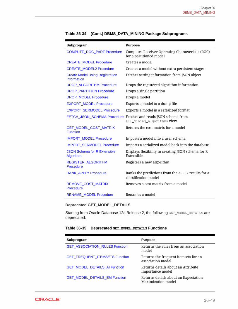
Table 36-34 (Cont.) DBMS_DATA_MINING Package Subprograms
Subprogram Purpose
COMPUTE_ROC_PART Procedure Computes Receiver Operating Characteristic (ROC)for a partitioned model
CREATE_MODEL Procedure Creates a model
CREATE_MODEL2 Procedure Creates a model without extra persistent stages
Create Model Using RegistrationInformation
Fetches setting information from JSON object
DROP_ALGORITHM Procedure Drops the registered algorithm information.
DROP_PARTITION Procedure Drops a single partition
DROP_MODEL Procedure Drops a model
EXPORT_MODEL Procedure Exports a model to a dump file
EXPORT_SERMODEL Procedure Exports a model in a serialized format
FETCH_JSON_SCHEMA Procedure Fetches and reads JSON schema fromall_mining_algorithms view
GET_MODEL_COST_MATRIXFunction
Returns the cost matrix for a model
IMPORT_MODEL Procedure Imports a model into a user schema
IMPORT_SERMODEL Procedure Imports a serialized model back into the database
JSON Schema for R ExtensibleAlgorithm
Displays flexibility in creating JSON schema for RExtensible
REGISTER_ALGORITHMProcedure
Registers a new algorithm
RANK_APPLY Procedure Ranks the predictions from the APPLY results for aclassification model
REMOVE_COST_MATRIXProcedure
Removes a cost matrix from a model
RENAME_MODEL Procedure Renames a model
Deprecated GET_MODEL_DETAILS
Starting from Oracle Database 12c Release 2, the following GET_MODEL_DETAILS aredeprecated:
Table 36-35 Deprecated GET_MODEL_DETAILS Functions
Subprogram Purpose
GET_ASSOCIATION_RULES Function Returns the rules from an associationmodel
GET_FREQUENT_ITEMSETS Function Returns the frequent itemsets for anassociation model
GET_MODEL_DETAILS_AI Function Returns details about an AttributeImportance model
GET_MODEL_DETAILS_EM Function Returns details about an ExpectationMaximization model
Chapter 36DBMS_DATA_MINING
36-49

Table 36-35 (Cont.) Deprecated GET_MODEL_DETAILS Functions
Subprogram Purpose
GET_MODEL_DETAILS_EM_COMP Function Returns details about the parameters of anExpectation Maximization model
GET_MODEL_DETAILS_EM_PROJ Function Returns details about the projects of anExpectation Maximization model
GET_MODEL_DETAILS_GLM Function Returns details about a Generalized LinearModel
GET_MODEL_DETAILS_GLOBAL Function Returns high-level statistics about a model
GET_MODEL_DETAILS_KM Function Returns details about a k-Means model
GET_MODEL_DETAILS_NB Function Returns details about a Naive Bayes model
GET_MODEL_DETAILS_NMF Function Returns details about a Non-NegativeMatrix Factorization model
GET_MODEL_DETAILS_OC Function Returns details about an O-Cluster model
GET_MODEL_SETTINGS Function Returns the settings used to build the givenmodelThis function is replaced with USER/ALL/DBA_MINING_MODEL_SETTINGS
GET_MODEL_SIGNATURE Function Returns the list of columns from the buildinput tableThis function is replaced with USER/ALL/DBA_MINING_MODEL_ATTRIBUTES
GET_MODEL_DETAILS_SVD Function Returns details about a Singular ValueDecomposition model
GET_MODEL_DETAILS_SVM Function Returns details about a Support VectorMachine model with a linear kernel
GET_MODEL_TRANSFORMATIONSFunction
Returns the transformations embedded ina modelThis function is replaced with USER/ALL/DBA_MINING_MODEL_XFORMS
GET_MODEL_DETAILS_XML Function Returns details about a Decision Treemodel
GET_TRANSFORM_LIST Procedure Converts between two differenttransformation specification formats
Related Topics
• Oracle Data Mining User’s Guide
• Oracle Database Reference
Chapter 36DBMS_DATA_MINING
36-50

36.1.5.1 ADD_COST_MATRIX ProcedureThe ADD_COST_MATRIX procedure associates a cost matrix table with a Classificationmodel. The cost matrix biases the model by assigning costs or benefits to specificmodel outcomes.
The cost matrix is stored with the model and taken into account when the model isscored.
You can also specify a cost matrix inline when you invoke a Data Mining SQL functionfor scoring. To view the scoring matrix for a model, query the DM$VC prefixed modelview. Refer to Model Detail View for Classification Algorithm.
To obtain the default scoring matrix for a model, query the DM$VC prefixedmodel view. To remove the default scoring matrix from a model, use theREMOVE_COST_MATRIX procedure. See "GET_MODEL_COST_MATRIX Function" and"REMOVE_COST_MATRIX Procedure".
See Also:
• "Biasing a Classification Model" in Oracle Data Mining Concepts formore information about costs
• Oracle Database SQL Language Reference for syntax of inline costmatrix
• Oracle Data Mining User’s Guide
Syntax
DBMS_DATA_MINING.ADD_COST_MATRIX ( model_name IN VARCHAR2, cost_matrix_table_name IN VARCHAR2, cost_matrix_schema_name IN VARCHAR2 DEFAULT NULL); partition_name IN VARCHAR2 DEFAULT NULL);
Parameters
Table 36-36 ADD_COST_MATRIX Procedure Parameters
Parameter Description
model_name Name of the model in the form [schema_name.]model_name.If you do not specify a schema, then your own schema isassumed.
cost_matrix_table_name
Name of the cost matrix table (described in Table 36-37).
cost_matrix_schema_name
Schema of the cost matrix table. If no schema is specified,then the current schema is used.
partition_name Name of the partition in a partitioned model
Chapter 36DBMS_DATA_MINING
36-51
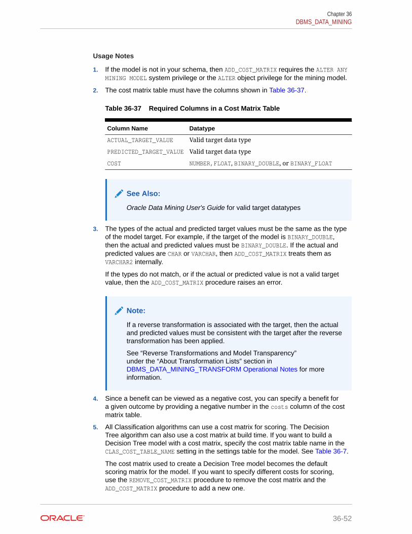
Usage Notes
1. If the model is not in your schema, then ADD_COST_MATRIX requires the ALTER ANYMINING MODEL system privilege or the ALTER object privilege for the mining model.
2. The cost matrix table must have the columns shown in Table 36-37.
Table 36-37 Required Columns in a Cost Matrix Table
Column Name Datatype
ACTUAL_TARGET_VALUE Valid target data type
PREDICTED_TARGET_VALUE Valid target data type
COST NUMBER,FLOAT, BINARY_DOUBLE, or BINARY_FLOAT
See Also:
Oracle Data Mining User's Guide for valid target datatypes
3. The types of the actual and predicted target values must be the same as the typeof the model target. For example, if the target of the model is BINARY_DOUBLE,then the actual and predicted values must be BINARY_DOUBLE. If the actual andpredicted values are CHAR or VARCHAR, then ADD_COST_MATRIX treats them asVARCHAR2 internally.
If the types do not match, or if the actual or predicted value is not a valid targetvalue, then the ADD_COST_MATRIX procedure raises an error.
Note:
If a reverse transformation is associated with the target, then the actualand predicted values must be consistent with the target after the reversetransformation has been applied.
See “Reverse Transformations and Model Transparency”under the “About Transformation Lists” section inDBMS_DATA_MINING_TRANSFORM Operational Notes for moreinformation.
4. Since a benefit can be viewed as a negative cost, you can specify a benefit fora given outcome by providing a negative number in the costs column of the costmatrix table.
5. All Classification algorithms can use a cost matrix for scoring. The DecisionTree algorithm can also use a cost matrix at build time. If you want to build aDecision Tree model with a cost matrix, specify the cost matrix table name in theCLAS_COST_TABLE_NAME setting in the settings table for the model. See Table 36-7.
The cost matrix used to create a Decision Tree model becomes the defaultscoring matrix for the model. If you want to specify different costs for scoring,use the REMOVE_COST_MATRIX procedure to remove the cost matrix and theADD_COST_MATRIX procedure to add a new one.
Chapter 36DBMS_DATA_MINING
36-52
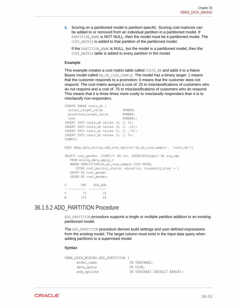
6. Scoring on a partitioned model is partition-specific. Scoring cost matrices canbe added to or removed from an individual partition in a partitioned model. IfPARTITION_NAME is NOT NULL, then the model must be a partitioned model. TheCOST_MATRIX is added to that partition of the partitioned model.
If the PARTITION_NAME is NULL, but the model is a partitioned model, then theCOST_MATRIX table is added to every partition in the model.
Example
This example creates a cost matrix table called COSTS_NB and adds it to a NaiveBayes model called NB_SH_CLAS_SAMPLE. The model has a binary target: 1 meansthat the customer responds to a promotion; 0 means that the customer does notrespond. The cost matrix assigns a cost of .25 to misclassifications of customers whodo not respond and a cost of .75 to misclassifications of customers who do respond.This means that it is three times more costly to misclassify responders than it is tomisclassify non-responders.
CREATE TABLE costs_nb ( actual_target_value NUMBER, predicted_target_value NUMBER, cost NUMBER);INSERT INTO costs_nb values (0, 0, 0);INSERT INTO costs_nb values (0, 1, .25);INSERT INTO costs_nb values (1, 0, .75);INSERT INTO costs_nb values (1, 1, 0);COMMIT; EXEC dbms_data_mining.add_cost_matrix('nb_sh_clas_sample', 'costs_nb'); SELECT cust_gender, COUNT(*) AS cnt, ROUND(AVG(age)) AS avg_age FROM mining_data_apply_v WHERE PREDICTION(nb_sh_clas_sample COST MODEL USING cust_marital_status, education, household_size) = 1 GROUP BY cust_gender ORDER BY cust_gender; C CNT AVG_AGE- ---------- ----------F 72 39M 555 44
36.1.5.2 ADD_PARTITION ProcedureADD_PARTITION procedure supports a single or multiple partition addition to an existingpartitioned model.
The ADD_PARTITION procedure derives build settings and user-defined expressionsfrom the existing model. The target column must exist in the input data query whenadding partitions to a supervised model.
Syntax
DBMS_DATA_MINING.ADD_PARTITION ( model_name IN VARCHAR2, data_query IN CLOB, add_options IN VARCHAR2 DEFAULT ERROR);
Chapter 36DBMS_DATA_MINING
36-53

Parameters
Table 36-38 ADD_PARTITION Procedure Parameters
Parameter Description
model_name Name of the model in the form [schema_name.]model_name. If you do notspecify a schema, then your own schema is used.
data_query An arbitrary SQL statement that provides data to the model build. The usermust have privilege to evaluate this query.
add_options Allows users to control the conditional behavior of ADD for cases whererows in the input dataset conflict with existing partitions in the model. Thefollowing are the possible values:• REPLACE: Replaces the existing partition for which the conflicting keys
are found.• ERROR: Terminates the ADD operation without adding any partitions.• IGNORE: Eliminates the rows having the conflicting keys.
Note:
For better performance, Oracle recommendsusing DROP_PARTITION followed by theADD_PARTITION instead of using the REPLACEoption.
36.1.5.3 ALTER_REVERSE_EXPRESSION ProcedureThis procedure replaces a reverse transformation expression with an expression thatyou specify. If the attribute does not have a reverse expression, the procedure createsone from the specified expression.
You can also use this procedure to customize the output of clustering, featureextraction, and anomaly detection models.
Syntax
DBMS_DATA_MINING.ALTER_REVERSE_EXPRESSION ( model_name VARCHAR2, expression CLOB, attribute_name VARCHAR2 DEFAULT NULL, attribute_subname VARCHAR2 DEFAULT NULL);
Parameters
Table 36-39 ALTER_REVERSE_EXPRESSION Procedure Parameters
Parameter Description
model_name Name of the model in the form [schema_name.]model_name. Ifyou do not specify a schema, your own schema is used.
Chapter 36DBMS_DATA_MINING
36-54
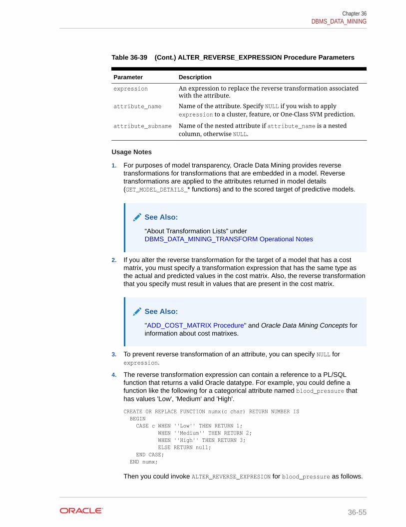
Table 36-39 (Cont.) ALTER_REVERSE_EXPRESSION Procedure Parameters
Parameter Description
expression An expression to replace the reverse transformation associatedwith the attribute.
attribute_name Name of the attribute. Specify NULL if you wish to applyexpression to a cluster, feature, or One-Class SVM prediction.
attribute_subname Name of the nested attribute if attribute_name is a nestedcolumn, otherwise NULL.
Usage Notes
1. For purposes of model transparency, Oracle Data Mining provides reversetransformations for transformations that are embedded in a model. Reversetransformations are applied to the attributes returned in model details(GET_MODEL_DETAILS_* functions) and to the scored target of predictive models.
See Also:
“About Transformation Lists” underDBMS_DATA_MINING_TRANSFORM Operational Notes
2. If you alter the reverse transformation for the target of a model that has a costmatrix, you must specify a transformation expression that has the same type asthe actual and predicted values in the cost matrix. Also, the reverse transformationthat you specify must result in values that are present in the cost matrix.
See Also:
"ADD_COST_MATRIX Procedure" and Oracle Data Mining Concepts forinformation about cost matrixes.
3. To prevent reverse transformation of an attribute, you can specify NULL forexpression.
4. The reverse transformation expression can contain a reference to a PL/SQLfunction that returns a valid Oracle datatype. For example, you could define afunction like the following for a categorical attribute named blood_pressure thathas values 'Low', 'Medium' and 'High'.
CREATE OR REPLACE FUNCTION numx(c char) RETURN NUMBER IS BEGIN CASE c WHEN ''Low'' THEN RETURN 1; WHEN ''Medium'' THEN RETURN 2; WHEN ''High'' THEN RETURN 3; ELSE RETURN null; END CASE; END numx;
Then you could invoke ALTER_REVERSE_EXPRESION for blood_pressure as follows.
Chapter 36DBMS_DATA_MINING
36-55

EXEC dbms_data_mining.alter_reverse_expression( '<model_name>', 'NUMX(blood_pressure)', 'blood_pressure');
5. You can use ALTER_REVERSE_EXPRESSION to label clusters produced by clusteringmodels and features produced by feature extraction.
You can use ALTER_REVERSE_EXPRESSION to replace the zeros and ones returnedby anomaly-detection models. By default, anomaly-detection models labelanomalous records with 0 and all other records with 1.
See Also:
Oracle Data Mining Concepts for information about anomaly detection
Examples
1. In this example, the target (affinity_card) of the model CLASS_MODEL ismanipulated internally as yes or no instead of 1 or 0 but returned as 1s and 0swhen scored. The ALTER_REVERSE_EXPRESSION procedure causes the target valuesto be returned as TRUE or FALSE.
The data sets MINING_DATA_BUILD and MINING_DATA_TEST are included with theOracle Data Mining sample programs. See Oracle Data Mining User's Guide forinformation about the sample programs.
DECLARE v_xlst dbms_data_mining_transform.TRANSFORM_LIST; BEGIN dbms_data_mining_transform.SET_TRANSFORM(v_xlst, 'affinity_card', NULL, 'decode(affinity_card, 1, ''yes'', ''no'')', 'decode(affinity_card, ''yes'', 1, 0)'); dbms_data_mining.CREATE_MODEL( model_name => 'CLASS_MODEL', mining_function => dbms_data_mining.classification, data_table_name => 'mining_data_build', case_id_column_name => 'cust_id', target_column_name => 'affinity_card', settings_table_name => NULL, data_schema_name => 'dmuser', settings_schema_name => NULL, xform_list => v_xlst ); END;/SELECT cust_income_level, occupation, PREDICTION(CLASS_MODEL USING *) predict_response FROM mining_data_test WHERE age = 60 AND cust_gender IN 'M' ORDER BY cust_income_level; CUST_INCOME_LEVEL OCCUPATION PREDICT_RESPONSE------------------------------ --------------------- --------------------A: Below 30,000 Transp. 1E: 90,000 - 109,999 Transp. 1E: 90,000 - 109,999 Sales 1G: 130,000 - 149,999 Handler 0G: 130,000 - 149,999 Crafts 0H: 150,000 - 169,999 Prof. 1J: 190,000 - 249,999 Prof. 1
Chapter 36DBMS_DATA_MINING
36-56

J: 190,000 - 249,999 Sales 1 BEGIN dbms_data_mining.ALTER_REVERSE_EXPRESSION ( model_name => 'CLASS_MODEL', expression => 'decode(affinity_card, ''yes'', ''TRUE'', ''FALSE'')', attribute_name => 'affinity_card');END;/column predict_response oncolumn predict_response format a20SELECT cust_income_level, occupation, PREDICTION(CLASS_MODEL USING *) predict_response FROM mining_data_test WHERE age = 60 AND cust_gender IN 'M' ORDER BY cust_income_level; CUST_INCOME_LEVEL OCCUPATION PREDICT_RESPONSE------------------------------ --------------------- --------------------A: Below 30,000 Transp. TRUEE: 90,000 - 109,999 Transp. TRUEE: 90,000 - 109,999 Sales TRUEG: 130,000 - 149,999 Handler FALSEG: 130,000 - 149,999 Crafts FALSEH: 150,000 - 169,999 Prof. TRUEJ: 190,000 - 249,999 Prof. TRUEJ: 190,000 - 249,999 Sales TRUE
2. This example specifies labels for the clusters that result from the sh_clus model.The labels consist of the word "Cluster" and the internal numeric identifier for thecluster.
BEGIN dbms_data_mining.ALTER_REVERSE_EXPRESSION( 'sh_clus', '''Cluster ''||value');END;/ SELECT cust_id, cluster_id(sh_clus using *) cluster_id FROM sh_aprep_num WHERE cust_id < 100011 ORDER by cust_id; CUST_ID CLUSTER_ID------- ------------------------------------------------ 100001 Cluster 18 100002 Cluster 14 100003 Cluster 14 100004 Cluster 18 100005 Cluster 19 100006 Cluster 7 100007 Cluster 18 100008 Cluster 14 100009 Cluster 8 100010 Cluster 8
Chapter 36DBMS_DATA_MINING
36-57

36.1.5.4 APPLY ProcedureThe APPLY procedure applies a mining model to the data of interest, and generates theresults in a table. The APPLY procedure is also referred to as scoring.
For predictive mining functions, the APPLY procedure generates predictions in a targetcolumn. For descriptive mining functions such as Clustering, the APPLY processassigns each case to a cluster with a probability.
In Oracle Data Mining, the APPLY procedure is not applicable to Association modelsand Attribute Importance models.
Note:
Scoring can also be performed directly in SQL using the Data Miningfunctions. See
• "Data Mining Functions" in Oracle Database SQL Language Reference
• "Scoring and Deployment" in Oracle Data Mining User's Guide
Syntax
DBMS_DATA_MINING.APPLY ( model_name IN VARCHAR2, data_table_name IN VARCHAR2, case_id_column_name IN VARCHAR2, result_table_name IN VARCHAR2, data_schema_name IN VARCHAR2 DEFAULT NULL);
Parameters
Table 36-40 APPLY Procedure Parameters
Parameter Description
model_name Name of the model in the form[schema_name.]model_name. If you do not specify aschema, then your own schema is used.
data_table_name Name of table or view containing the data to be scored
case_id_column_name Name of the case identifier column
result_table_name Name of the table in which to store apply results
data_schema_name Name of the schema containing the data to be scored
Usage Notes
1. The data provided for APPLY must undergo the same preprocessing as the dataused to create and test the model. When you use Automatic Data Preparation, thepreprocessing required by the algorithm is handled for you by the model: both atbuild time and apply time. (See "Automatic Data Preparation".)
2. APPLY creates a table in the user's schema to hold the results. The columns arealgorithm-specific.
Chapter 36DBMS_DATA_MINING
36-58

The columns in the results table are listed in Table 36-41 through Table 36-45. Thecase ID column name in the results table will match the case ID column nameprovided by you. The type of the incoming case ID column is also preserved inAPPLY output.
Note:
Make sure that the case ID column does not have the same name asone of the columns that will be created by APPLY. For example, whenapplying a Classification model, the case ID in the scoring data must notbe PREDICTION or PROBABILITY (See Table 36-41).
3. The datatype for the PREDICTION, CLUSTER_ID, and FEATURE_ID output columns isinfluenced by any reverse expression that is embedded in the model by the user.If the user does not provide a reverse expression that alters the scored valuetype, then the types will conform to the descriptions in the following tables. See"ALTER_REVERSE_EXPRESSION Procedure".
4. If the model is partitioned, the result_table_name can contain results fromdifferent partitions depending on the data from the input data table. An additionalcolumn called PARTITION_NAME is added to the result table indicating the partitionname that is associated with each row.
For a non-partitioned model, the behavior does not change.
Classification
The results table for Classification has the columns described in Table 36-41. Ifthe target of the model is categorical, the PREDICTION column will have a VARCHAR2datatype. If the target has a binary type, the PREDICTION column will have the binarytype of the target.
Table 36-41 APPLY Results Table for Classification
Column Name Datatype
Case ID column name Type of the case ID
PREDICTION Type of the target
PROBABILITY BINARY_DOUBLE
Anomaly Detection
The results table for Anomaly Detection has the columns described in Table 36-42.
Table 36-42 APPLY Results Table for Anomaly Detection
Column Name Datatype
Case ID column name Type of the case ID
PREDICTION NUMBER
PROBABILITY BINARY_DOUBLE
Regression
Chapter 36DBMS_DATA_MINING
36-59

The results table for Regression has the columns described in APPLY Procedure.
Table 36-43 APPLY Results Table for Regression
Column Name Datatype
Case ID column name Type of the case ID
PREDICTION Type of the target
Clustering
Clustering is an unsupervised mining function, and hence there are no targets. Theresults of an APPLY procedure will contain simply the cluster identifier corresponding toa case, and the associated probability. The results table has the columns described inTable 36-44.
Table 36-44 APPLY Results Table for Clustering
Column Name Datatype
Case ID column name Type of the case ID
CLUSTER_ID NUMBER
PROBABILITY BINARY_DOUBLE
Feature Extraction
Feature Extraction is also an unsupervised mining function, and hence there are notargets. The results of an APPLY procedure will contain simply the feature identifiercorresponding to a case, and the associated match quality. The results table has thecolumns described in Table 36-45.
Table 36-45 APPLY Results Table for Feature Extraction
Column Name Datatype
Case ID column name Type of the case ID
FEATURE_ID NUMBER
MATCH_QUALITY BINARY_DOUBLE
Examples
This example applies the GLM Regression model GLMR_SH_REGR_SAMPLE to thedata in the MINING_DATA_APPLY_V view. The APPLY results are output of the tableREGRESSION_APPLY_RESULT.
SQL> BEGIN DBMS_DATA_MINING.APPLY ( model_name => 'glmr_sh_regr_sample', data_table_name => 'mining_data_apply_v', case_id_column_name => 'cust_id', result_table_name => 'regression_apply_result'); END; /
Chapter 36DBMS_DATA_MINING
36-60
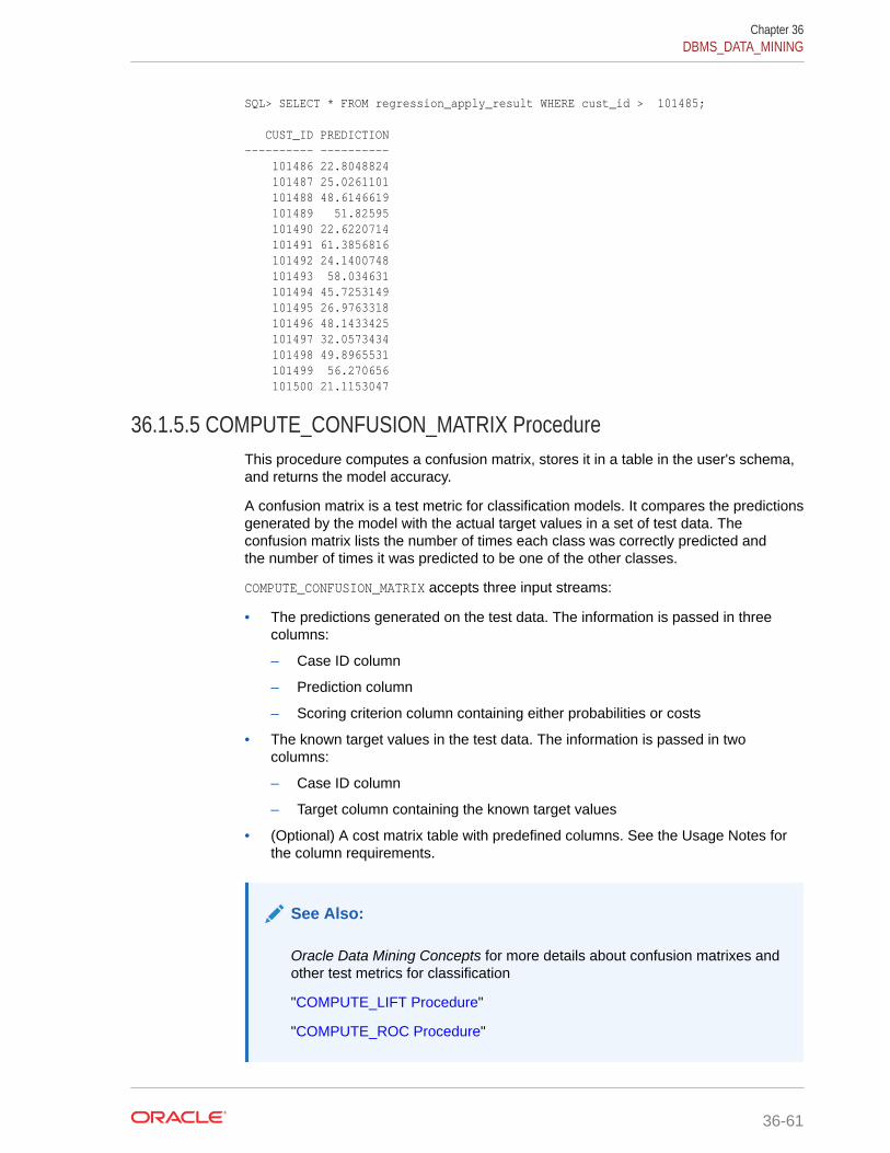
SQL> SELECT * FROM regression_apply_result WHERE cust_id > 101485; CUST_ID PREDICTION---------- ---------- 101486 22.8048824 101487 25.0261101 101488 48.6146619 101489 51.82595 101490 22.6220714 101491 61.3856816 101492 24.1400748 101493 58.034631 101494 45.7253149 101495 26.9763318 101496 48.1433425 101497 32.0573434 101498 49.8965531 101499 56.270656 101500 21.1153047
36.1.5.5 COMPUTE_CONFUSION_MATRIX ProcedureThis procedure computes a confusion matrix, stores it in a table in the user's schema,and returns the model accuracy.
A confusion matrix is a test metric for classification models. It compares the predictionsgenerated by the model with the actual target values in a set of test data. Theconfusion matrix lists the number of times each class was correctly predicted andthe number of times it was predicted to be one of the other classes.
COMPUTE_CONFUSION_MATRIX accepts three input streams:
• The predictions generated on the test data. The information is passed in threecolumns:
– Case ID column
– Prediction column
– Scoring criterion column containing either probabilities or costs
• The known target values in the test data. The information is passed in twocolumns:
– Case ID column
– Target column containing the known target values
• (Optional) A cost matrix table with predefined columns. See the Usage Notes forthe column requirements.
See Also:
Oracle Data Mining Concepts for more details about confusion matrixes andother test metrics for classification
"COMPUTE_LIFT Procedure"
"COMPUTE_ROC Procedure"
Chapter 36DBMS_DATA_MINING
36-61

Syntax
DBMS_DATA_MINING.COMPUTE_CONFUSION_MATRIX ( accuracy OUT NUMBER, apply_result_table_name IN VARCHAR2, target_table_name IN VARCHAR2, case_id_column_name IN VARCHAR2, target_column_name IN VARCHAR2, confusion_matrix_table_name IN VARCHAR2, score_column_name IN VARCHAR2 DEFAULT 'PREDICTION', score_criterion_column_name IN VARCHAR2 DEFAULT 'PROBABILITY', cost_matrix_table_name IN VARCHAR2 DEFAULT NULL, apply_result_schema_name IN VARCHAR2 DEFAULT NULL, target_schema_name IN VARCHAR2 DEFAULT NULL, cost_matrix_schema_name IN VARCHAR2 DEFAULT NULL, score_criterion_type IN VARCHAR2 DEFAULT 'PROBABILITY');
Parameters
Table 36-46 COMPUTE_CONFUSION_MATRIX Procedure Parameters
Parameter Description
accuracy Output parameter containing the overallpercentage accuracy of the predictions.
apply_result_table_name Table containing the predictions.
target_table_name Table containing the known target values from thetest data.
case_id_column_name Case ID column in the apply results table. Mustmatch the case identifier in the targets table.
target_column_name Target column in the targets table. Contains theknown target values from the test data.
confusion_matrix_table_name Table containing the confusion matrix. The tablewill be created by the procedure in the user'sschema.The columns in the confusion matrix table aredescribed in the Usage Notes.
score_column_name Column containing the predictions in the applyresults table.The default column name is PREDICTION, which isthe default name created by the APPLY procedure(See "APPLY Procedure").
Chapter 36DBMS_DATA_MINING
36-62
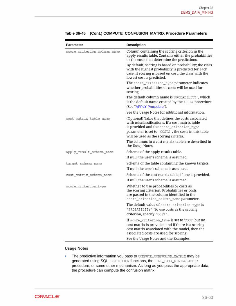
Table 36-46 (Cont.) COMPUTE_CONFUSION_MATRIX Procedure Parameters
Parameter Description
score_criterion_column_name Column containing the scoring criterion in theapply results table. Contains either the probabilitiesor the costs that determine the predictions.By default, scoring is based on probability; the classwith the highest probability is predicted for eachcase. If scoring is based on cost, the class with thelowest cost is predicted.The score_criterion_type parameter indicateswhether probabilities or costs will be used forscoring.The default column name is 'PROBABILITY', whichis the default name created by the APPLY procedure(See "APPLY Procedure").
See the Usage Notes for additional information.
cost_matrix_table_name (Optional) Table that defines the costs associatedwith misclassifications. If a cost matrix tableis provided and the score_criterion_typeparameter is set to 'COSTS', the costs in this tablewill be used as the scoring criteria.The columns in a cost matrix table are described inthe Usage Notes.
apply_result_schema_name Schema of the apply results table.If null, the user's schema is assumed.
target_schema_name Schema of the table containing the known targets.If null, the user's schema is assumed.
cost_matrix_schema_name Schema of the cost matrix table, if one is provided.If null, the user's schema is assumed.
score_criterion_type Whether to use probabilities or costs asthe scoring criterion. Probabilities or costsare passed in the column identified in thescore_criterion_column_name parameter.
The default value of score_criterion_type is'PROBABILITY'. To use costs as the scoringcriterion, specify 'COST'.
If score_criterion_type is set to 'COST' but nocost matrix is provided and if there is a scoringcost matrix associated with the model, then theassociated costs are used for scoring.See the Usage Notes and the Examples.
Usage Notes
• The predictive information you pass to COMPUTE_CONFUSION_MATRIX may begenerated using SQL PREDICTION functions, the DBMS_DATA_MINING.APPLYprocedure, or some other mechanism. As long as you pass the appropriate data,the procedure can compute the confusion matrix.
Chapter 36DBMS_DATA_MINING
36-63

• Instead of passing a cost matrix to COMPUTE_CONFUSION_MATRIX, you can use ascoring cost matrix associated with the model. A scoring cost matrix can beembedded in the model or it can be defined dynamically when the model isapplied. To use a scoring cost matrix, invoke the SQL PREDICTION_COST function topopulate the score criterion column.
• The predictions that you pass to COMPUTE_CONFUSION_MATRIX are in a table or viewspecified in apply_result_table_name.
CREATE TABLE apply_result_table_name AS ( case_id_column_name VARCHAR2, score_column_name VARCHAR2, score_criterion_column_name VARCHAR2);
• A cost matrix must have the columns described in Table 36-47.
Table 36-47 Columns in a Cost Matrix
Column Name Datatype
actual_target_value Type of the target column in the build data
predicted_target_value
Type of the predicted target in the test data. The type of thepredicted target must be the same as the type of the actualtarget unless the predicted target has an associated reversetransformation.
cost BINARY_DOUBLE
See Also:
Oracle Data Mining User's Guide for valid target datatypes
Oracle Data Mining Concepts for more information about cost matrixes
• The confusion matrix created by COMPUTE_CONFUSION_MATRIX has the columnsdescribed in Table 36-48.
Table 36-48 Columns in a Confusion Matrix
Column Name Datatype
actual_target_value Type of the target column in the build data
predicted_target_value
Type of the predicted target in the test data. The type ofthe predicted target is the same as the type of the actualtarget unless the predicted target has an associated reversetransformation.
value BINARY_DOUBLE
See Also:
Oracle Data Mining Concepts for more information about confusionmatrixes
Chapter 36DBMS_DATA_MINING
36-64
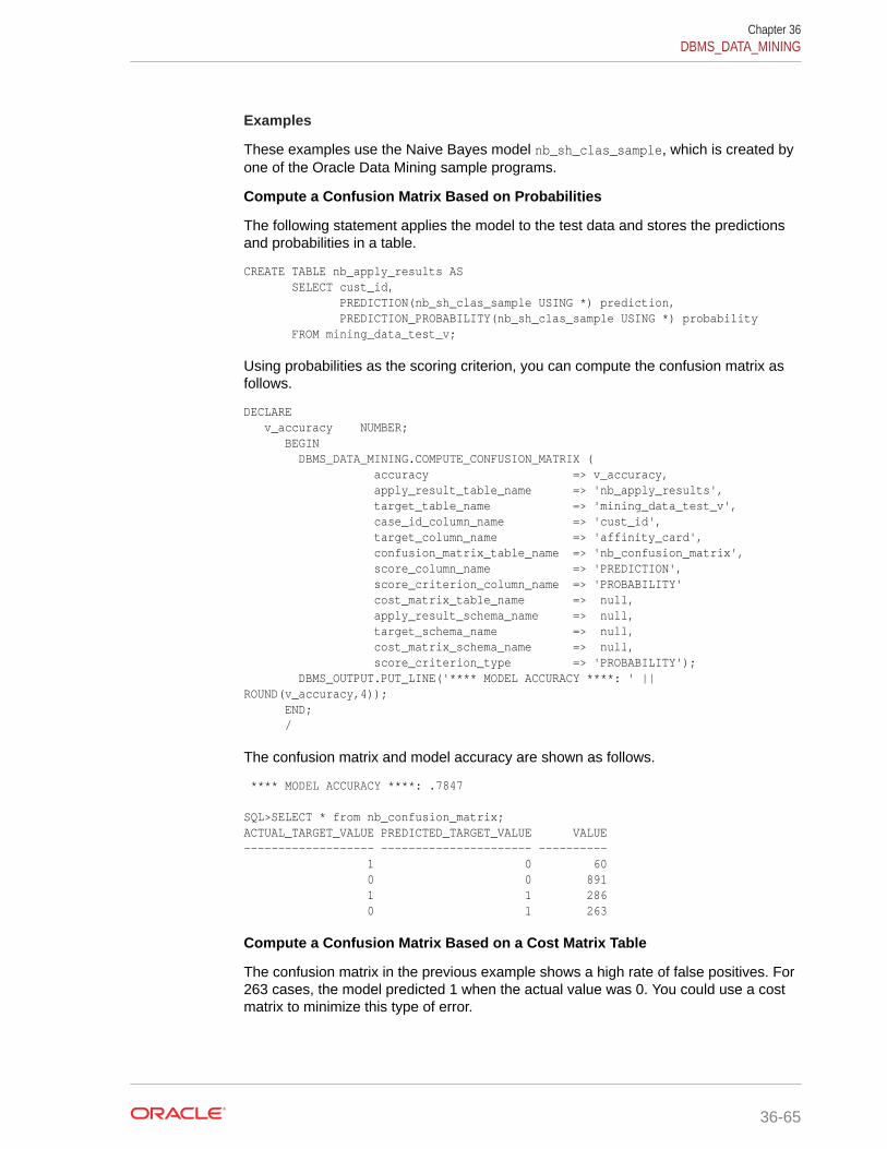
Examples
These examples use the Naive Bayes model nb_sh_clas_sample, which is created byone of the Oracle Data Mining sample programs.
Compute a Confusion Matrix Based on Probabilities
The following statement applies the model to the test data and stores the predictionsand probabilities in a table.
CREATE TABLE nb_apply_results AS SELECT cust_id, PREDICTION(nb_sh_clas_sample USING *) prediction, PREDICTION_PROBABILITY(nb_sh_clas_sample USING *) probability FROM mining_data_test_v;
Using probabilities as the scoring criterion, you can compute the confusion matrix asfollows.
DECLARE v_accuracy NUMBER; BEGIN DBMS_DATA_MINING.COMPUTE_CONFUSION_MATRIX ( accuracy => v_accuracy, apply_result_table_name => 'nb_apply_results', target_table_name => 'mining_data_test_v', case_id_column_name => 'cust_id', target_column_name => 'affinity_card', confusion_matrix_table_name => 'nb_confusion_matrix', score_column_name => 'PREDICTION', score_criterion_column_name => 'PROBABILITY' cost_matrix_table_name => null, apply_result_schema_name => null, target_schema_name => null, cost_matrix_schema_name => null, score_criterion_type => 'PROBABILITY'); DBMS_OUTPUT.PUT_LINE('**** MODEL ACCURACY ****: ' || ROUND(v_accuracy,4)); END; /
The confusion matrix and model accuracy are shown as follows.
**** MODEL ACCURACY ****: .7847
SQL>SELECT * from nb_confusion_matrix;ACTUAL_TARGET_VALUE PREDICTED_TARGET_VALUE VALUE------------------- ---------------------- ---------- 1 0 60 0 0 891 1 1 286 0 1 263
Compute a Confusion Matrix Based on a Cost Matrix Table
The confusion matrix in the previous example shows a high rate of false positives. For263 cases, the model predicted 1 when the actual value was 0. You could use a costmatrix to minimize this type of error.
Chapter 36DBMS_DATA_MINING
36-65

The cost matrix table nb_cost_matrix specifies that a false positive is 3 times morecostly than a false negative.
SQL> SELECT * from nb_cost_matrix;ACTUAL_TARGET_VALUE PREDICTED_TARGET_VALUE COST------------------- ---------------------- ---------- 0 0 0 0 1 .75 1 0 .25 1 1 0
This statement shows how to generate the predictions using APPLY.
BEGIN DBMS_DATA_MINING.APPLY( model_name => 'nb_sh_clas_sample', data_table_name => 'mining_data_test_v', case_id_column_name => 'cust_id', result_table_name => 'nb_apply_results'); END;/
This statement computes the confusion matrix using the cost matrix table. The scorecriterion column is named 'PROBABILITY', which is the name generated by APPLY.
DECLARE v_accuracy NUMBER; BEGIN DBMS_DATA_MINING.COMPUTE_CONFUSION_MATRIX ( accuracy => v_accuracy, apply_result_table_name => 'nb_apply_results', target_table_name => 'mining_data_test_v', case_id_column_name => 'cust_id', target_column_name => 'affinity_card', confusion_matrix_table_name => 'nb_confusion_matrix', score_column_name => 'PREDICTION', score_criterion_column_name => 'PROBABILITY', cost_matrix_table_name => 'nb_cost_matrix', apply_result_schema_name => null, target_schema_name => null, cost_matrix_schema_name => null, score_criterion_type => 'COST'); DBMS_OUTPUT.PUT_LINE('**** MODEL ACCURACY ****: ' || ROUND(v_accuracy,4)); END; /
The resulting confusion matrix shows a decrease in false positives (212 instead of263).
**** MODEL ACCURACY ****: .798
SQL> SELECT * FROM nb_confusion_matrix;ACTUAL_TARGET_VALUE PREDICTED_TARGET_VALUE VALUE------------------- ---------------------- ---------- 1 0 91 0 0 942 1 1 255 0 1 212
Compute a Confusion Matrix Based on Embedded Costs
Chapter 36DBMS_DATA_MINING
36-66

You can use the ADD_COST_MATRIX procedure to embed a cost matrix in a model. Theembedded costs can be used instead of probabilities for scoring. This statement addsthe previously-defined cost matrix to the model.
BEGIN DBMS_DATA_MINING.ADD_COST_MATRIX ('nb_sh_clas_sample', 'nb_cost_matrix');END;/
The following statement applies the model to the test data using the embedded costsand stores the results in a table.
CREATE TABLE nb_apply_results AS SELECT cust_id, PREDICTION(nb_sh_clas_sample COST MODEL USING *) prediction, PREDICTION_COST(nb_sh_clas_sample COST MODEL USING *) cost FROM mining_data_test_v;
You can compute the confusion matrix using the embedded costs.
DECLARE v_accuracy NUMBER; BEGIN DBMS_DATA_MINING.COMPUTE_CONFUSION_MATRIX ( accuracy => v_accuracy, apply_result_table_name => 'nb_apply_results', target_table_name => 'mining_data_test_v', case_id_column_name => 'cust_id', target_column_name => 'affinity_card', confusion_matrix_table_name => 'nb_confusion_matrix', score_column_name => 'PREDICTION', score_criterion_column_name => 'COST', cost_matrix_table_name => null, apply_result_schema_name => null, target_schema_name => null, cost_matrix_schema_name => null, score_criterion_type => 'COST'); END; /
The results are:
**** MODEL ACCURACY ****: .798
SQL> SELECT * FROM nb_confusion_matrix;ACTUAL_TARGET_VALUE PREDICTED_TARGET_VALUE VALUE------------------- ---------------------- ---------- 1 0 91 0 0 942 1 1 255 0 1 212
36.1.5.6 COMPUTE_CONFUSION_MATRIX_PART ProcedureThe COMPUTE_CONFUSION_MATRIX_PART procedure computes a confusion matrix, storesit in a table in the user's schema, and returns the model accuracy.
COMPUTE_CONFUSION_MATRIX_PART provides support to computation of evaluationmetrics per-partition for partitioned models. For non-partitioned models, refer toCOMPUTE_CONFUSION_MATRIX Procedure.
Chapter 36DBMS_DATA_MINING
36-67
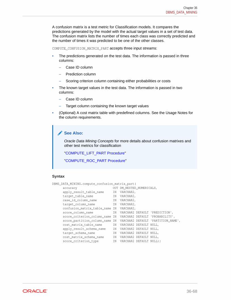
A confusion matrix is a test metric for Classification models. It compares thepredictions generated by the model with the actual target values in a set of test data.The confusion matrix lists the number of times each class was correctly predicted andthe number of times it was predicted to be one of the other classes.
COMPUTE_CONFUSION_MATRIX_PART accepts three input streams:
• The predictions generated on the test data. The information is passed in threecolumns:
– Case ID column
– Prediction column
– Scoring criterion column containing either probabilities or costs
• The known target values in the test data. The information is passed in twocolumns:
– Case ID column
– Target column containing the known target values
• (Optional) A cost matrix table with predefined columns. See the Usage Notes forthe column requirements.
See Also:
Oracle Data Mining Concepts for more details about confusion matrixes andother test metrics for classification
"COMPUTE_LIFT_PART Procedure"
"COMPUTE_ROC_PART Procedure"
Syntax
DBMS_DATA_MINING.compute_confusion_matrix_part( accuracy OUT DM_NESTED_NUMERICALS, apply_result_table_name IN VARCHAR2, target_table_name IN VARCHAR2, case_id_column_name IN VARCHAR2, target_column_name IN VARCHAR2, confusion_matrix_table_name IN VARCHAR2, score_column_name IN VARCHAR2 DEFAULT 'PREDICTION', score_criterion_column_name IN VARCHAR2 DEFAULT 'PROBABILITY', score_partition_column_name IN VARCHAR2 DEFAULT 'PARTITION_NAME', cost_matrix_table_name IN VARCHAR2 DEFAULT NULL, apply_result_schema_name IN VARCHAR2 DEFAULT NULL, target_schema_name IN VARCHAR2 DEFAULT NULL, cost_matrix_schema_name IN VARCHAR2 DEFAULT NULL, score_criterion_type IN VARCHAR2 DEFAULT NULL);
Chapter 36DBMS_DATA_MINING
36-68

Parameters
Table 36-49 COMPUTE_CONFUSION_MATRIX_PART Procedure Parameters
Parameter Description
accuracy Output parameter containing the overallpercentage accuracy of the predictionsThe output argument is changed from NUMBER toDM_NESTED_NUMERICALS
apply_result_table_name Table containing the predictions
target_table_name Table containing the known target values from thetest data
case_id_column_name Case ID column in the apply results table. Mustmatch the case identifier in the targets table.
target_column_name Target column in the targets table. Contains theknown target values from the test data.
confusion_matrix_table_name Table containing the confusion matrix. The tablewill be created by the procedure in the user'sschema.The columns in the confusion matrix table aredescribed in the Usage Notes.
score_column_name Column containing the predictions in the applyresults table.The default column name is PREDICTION, which isthe default name created by the APPLY procedure(See "APPLY Procedure").
score_criterion_column_name Column containing the scoring criterion in theapply results table. Contains either the probabilitiesor the costs that determine the predictions.By default, scoring is based on probability; the classwith the highest probability is predicted for eachcase. If scoring is based on cost, then the class withthe lowest cost is predicted.The score_criterion_type parameter indicateswhether probabilities or costs will be used forscoring.The default column name is PROBABILITY, which isthe default name created by the APPLY procedure(See "APPLY Procedure").
See the Usage Notes for additional information.
score_partition_column_name (Optional) Parameter indicating the column whichcontains the name of the partition. This columnslices the input test results such that each partitionhas independent evaluation matrices computed.
Chapter 36DBMS_DATA_MINING
36-69
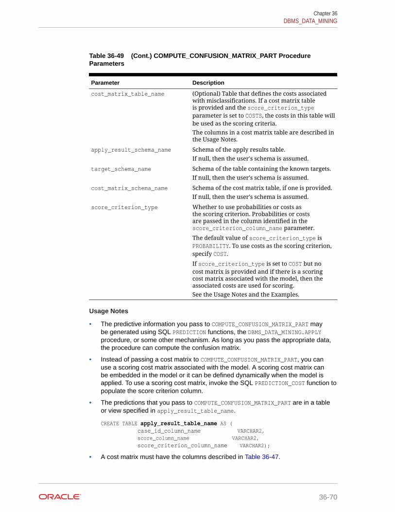
Table 36-49 (Cont.) COMPUTE_CONFUSION_MATRIX_PART ProcedureParameters
Parameter Description
cost_matrix_table_name (Optional) Table that defines the costs associatedwith misclassifications. If a cost matrix tableis provided and the score_criterion_typeparameter is set to COSTS, the costs in this table willbe used as the scoring criteria.The columns in a cost matrix table are described inthe Usage Notes.
apply_result_schema_name Schema of the apply results table.If null, then the user's schema is assumed.
target_schema_name Schema of the table containing the known targets.If null, then the user's schema is assumed.
cost_matrix_schema_name Schema of the cost matrix table, if one is provided.If null, then the user's schema is assumed.
score_criterion_type Whether to use probabilities or costs asthe scoring criterion. Probabilities or costsare passed in the column identified in thescore_criterion_column_name parameter.
The default value of score_criterion_type isPROBABILITY. To use costs as the scoring criterion,specify COST.
If score_criterion_type is set to COST but nocost matrix is provided and if there is a scoringcost matrix associated with the model, then theassociated costs are used for scoring.See the Usage Notes and the Examples.
Usage Notes
• The predictive information you pass to COMPUTE_CONFUSION_MATRIX_PART maybe generated using SQL PREDICTION functions, the DBMS_DATA_MINING.APPLYprocedure, or some other mechanism. As long as you pass the appropriate data,the procedure can compute the confusion matrix.
• Instead of passing a cost matrix to COMPUTE_CONFUSION_MATRIX_PART, you canuse a scoring cost matrix associated with the model. A scoring cost matrix canbe embedded in the model or it can be defined dynamically when the model isapplied. To use a scoring cost matrix, invoke the SQL PREDICTION_COST function topopulate the score criterion column.
• The predictions that you pass to COMPUTE_CONFUSION_MATRIX_PART are in a tableor view specified in apply_result_table_name.
CREATE TABLE apply_result_table_name AS ( case_id_column_name VARCHAR2, score_column_name VARCHAR2, score_criterion_column_name VARCHAR2);
• A cost matrix must have the columns described in Table 36-47.
Chapter 36DBMS_DATA_MINING
36-70

Table 36-50 Columns in a Cost Matrix
Column Name Datatype
actual_target_value Type of the target column in the test data
predicted_target_value
Type of the predicted target in the test data. The type of thepredicted target must be the same as the type of the actualtarget unless the predicted target has an associated reversetransformation.
cost BINARY_DOUBLE
See Also:
Oracle Data Mining User's Guide for valid target datatypes
Oracle Data Mining Concepts for more information about cost matrixes
• The confusion matrix created by COMPUTE_CONFUSION_MATRIX_PART has thecolumns described in Table 36-48.
Table 36-51 Columns in a Confusion Matrix Part
Column Name Datatype
actual_target_value Type of the target column in the test data
predicted_target_value
Type of the predicted target in the test data. The type ofthe predicted target is the same as the type of the actualtarget unless the predicted target has an associated reversetransformation.
value BINARY_DOUBLE
See Also:
Oracle Data Mining Concepts for more information about confusionmatrixes
Examples
These examples use the Naive Bayes model nb_sh_clas_sample, which is created byone of the Oracle Data Mining sample programs.
Compute a Confusion Matrix Based on Probabilities
The following statement applies the model to the test data and stores the predictionsand probabilities in a table.
CREATE TABLE nb_apply_results AS SELECT cust_id, PREDICTION(nb_sh_clas_sample USING *) prediction, PREDICTION_PROBABILITY(nb_sh_clas_sample USING *) probability FROM mining_data_test_v;
Chapter 36DBMS_DATA_MINING
36-71

Using probabilities as the scoring criterion, you can compute the confusion matrix asfollows.
DECLARE v_accuracy NUMBER; BEGIN DBMS_DATA_MINING.COMPUTE_CONFUSION_MATRIX_PART ( accuracy => v_accuracy, apply_result_table_name => 'nb_apply_results', target_table_name => 'mining_data_test_v', case_id_column_name => 'cust_id', target_column_name => 'affinity_card', confusion_matrix_table_name => 'nb_confusion_matrix', score_column_name => 'PREDICTION', score_criterion_column_name => 'PROBABILITY' score_partition_column_name => 'PARTITION_NAME' cost_matrix_table_name => null, apply_result_schema_name => null, target_schema_name => null, cost_matrix_schema_name => null, score_criterion_type => 'PROBABILITY'); DBMS_OUTPUT.PUT_LINE('**** MODEL ACCURACY ****: ' || ROUND(v_accuracy,4)); END; /
The confusion matrix and model accuracy are shown as follows.
**** MODEL ACCURACY ****: .7847
SELECT * FROM NB_CONFUSION_MATRIX;ACTUAL_TARGET_VALUE PREDICTED_TARGET_VALUE VALUE------------------- ---------------------- ---------- 1 0 60 0 0 891 1 1 286 0 1 263
Compute a Confusion Matrix Based on a Cost Matrix Table
The confusion matrix in the previous example shows a high rate of false positives. For263 cases, the model predicted 1 when the actual value was 0. You could use a costmatrix to minimize this type of error.
The cost matrix table nb_cost_matrix specifies that a false positive is 3 times morecostly than a false negative.
SELECT * from NB_COST_MATRIX;ACTUAL_TARGET_VALUE PREDICTED_TARGET_VALUE COST------------------- ---------------------- ---------- 0 0 0 0 1 .75 1 0 .25 1 1 0
This statement shows how to generate the predictions using APPLY.
BEGIN DBMS_DATA_MINING.APPLY( model_name => 'nb_sh_clas_sample', data_table_name => 'mining_data_test_v', case_id_column_name => 'cust_id',
Chapter 36DBMS_DATA_MINING
36-72

result_table_name => 'nb_apply_results'); END;/
This statement computes the confusion matrix using the cost matrix table. The scorecriterion column is named 'PROBABILITY', which is the name generated by APPLY.
DECLARE v_accuracy NUMBER; BEGIN DBMS_DATA_MINING.COMPUTE_CONFUSION_MATRIX_PART ( accuracy => v_accuracy, apply_result_table_name => 'nb_apply_results', target_table_name => 'mining_data_test_v', case_id_column_name => 'cust_id', target_column_name => 'affinity_card', confusion_matrix_table_name => 'nb_confusion_matrix', score_column_name => 'PREDICTION', score_criterion_column_name => 'PROBABILITY', score_partition_column_name => 'PARTITION_NAME' cost_matrix_table_name => 'nb_cost_matrix', apply_result_schema_name => null, target_schema_name => null, cost_matrix_schema_name => null, score_criterion_type => 'COST'); DBMS_OUTPUT.PUT_LINE('**** MODEL ACCURACY ****: ' || ROUND(v_accuracy,4)); END; /
The resulting confusion matrix shows a decrease in false positives (212 instead of263).
**** MODEL ACCURACY ****: .798
SELECT * FROM NB_CONFUSION_MATRIX;ACTUAL_TARGET_VALUE PREDICTED_TARGET_VALUE VALUE------------------- ---------------------- ---------- 1 0 91 0 0 942 1 1 255 0 1 212
Compute a Confusion Matrix Based on Embedded Costs
You can use the ADD_COST_MATRIX procedure to embed a cost matrix in a model. Theembedded costs can be used instead of probabilities for scoring. This statement addsthe previously-defined cost matrix to the model.
BEGIN DBMS_DATA_MINING.ADD_COST_MATRIX ('nb_sh_clas_sample', 'nb_cost_matrix');END;/
The following statement applies the model to the test data using the embedded costsand stores the results in a table.
CREATE TABLE nb_apply_results AS SELECT cust_id, PREDICTION(nb_sh_clas_sample COST MODEL USING *) prediction, PREDICTION_COST(nb_sh_clas_sample COST MODEL USING *) cost FROM mining_data_test_v;
Chapter 36DBMS_DATA_MINING
36-73

You can compute the confusion matrix using the embedded costs.
DECLARE v_accuracy NUMBER; BEGIN DBMS_DATA_MINING.COMPUTE_CONFUSION_MATRIX_PART ( accuracy => v_accuracy, apply_result_table_name => 'nb_apply_results', target_table_name => 'mining_data_test_v', case_id_column_name => 'cust_id', target_column_name => 'affinity_card', confusion_matrix_table_name => 'nb_confusion_matrix', score_column_name => 'PREDICTION', score_criterion_column_name => 'COST', score_partition_column_name => 'PARTITION_NAME' cost_matrix_table_name => null, apply_result_schema_name => null, target_schema_name => null, cost_matrix_schema_name => null, score_criterion_type => 'COST'); END; /
The results are:
**** MODEL ACCURACY ****: .798
SELECT * FROM NB_CONFUSION_MATRIX;ACTUAL_TARGET_VALUE PREDICTED_TARGET_VALUE VALUE------------------- ---------------------- ---------- 1 0 91 0 0 942 1 1 255 0 1 212
36.1.5.7 COMPUTE_LIFT ProcedureThis procedure computes lift and stores the results in a table in the user's schema.
Lift is a test metric for binary classification models. To compute lift, one of thetarget values must be designated as the positive class. COMPUTE_LIFT compares thepredictions generated by the model with the actual target values in a set of test data.Lift measures the degree to which the model's predictions of the positive class are animprovement over random chance.
Lift is computed on scoring results that have been ranked by probability (or cost)and divided into quantiles. Each quantile includes the scores for the same number ofcases.
COMPUTE_LIFT calculates quantile-based and cumulative statistics. The number ofquantiles and the positive class are user-specified. Additionally, COMPUTE_LIFT acceptsthree input streams:
• The predictions generated on the test data. The information is passed in threecolumns:
– Case ID column
– Prediction column
Chapter 36DBMS_DATA_MINING
36-74
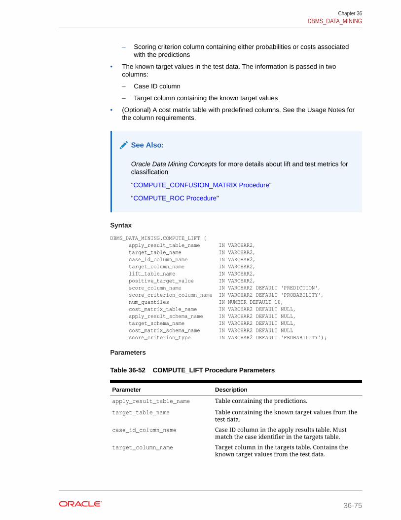
– Scoring criterion column containing either probabilities or costs associatedwith the predictions
• The known target values in the test data. The information is passed in twocolumns:
– Case ID column
– Target column containing the known target values
• (Optional) A cost matrix table with predefined columns. See the Usage Notes forthe column requirements.
See Also:
Oracle Data Mining Concepts for more details about lift and test metrics forclassification
"COMPUTE_CONFUSION_MATRIX Procedure"
"COMPUTE_ROC Procedure"
Syntax
DBMS_DATA_MINING.COMPUTE_LIFT ( apply_result_table_name IN VARCHAR2, target_table_name IN VARCHAR2, case_id_column_name IN VARCHAR2, target_column_name IN VARCHAR2, lift_table_name IN VARCHAR2, positive_target_value IN VARCHAR2, score_column_name IN VARCHAR2 DEFAULT 'PREDICTION', score_criterion_column_name IN VARCHAR2 DEFAULT 'PROBABILITY', num_quantiles IN NUMBER DEFAULT 10, cost_matrix_table_name IN VARCHAR2 DEFAULT NULL, apply_result_schema_name IN VARCHAR2 DEFAULT NULL, target_schema_name IN VARCHAR2 DEFAULT NULL, cost_matrix_schema_name IN VARCHAR2 DEFAULT NULL score_criterion_type IN VARCHAR2 DEFAULT 'PROBABILITY');
Parameters
Table 36-52 COMPUTE_LIFT Procedure Parameters
Parameter Description
apply_result_table_name Table containing the predictions.
target_table_name Table containing the known target values from thetest data.
case_id_column_name Case ID column in the apply results table. Mustmatch the case identifier in the targets table.
target_column_name Target column in the targets table. Contains theknown target values from the test data.
Chapter 36DBMS_DATA_MINING
36-75

Table 36-52 (Cont.) COMPUTE_LIFT Procedure Parameters
Parameter Description
lift_table_name Table containing the lift statistics. The table will becreated by the procedure in the user's schema.The columns in the lift table are described in theUsage Notes.
positive_target_value The positive class. This should be the class ofinterest, for which you want to calculate lift.If the target column is a NUMBER, you can usethe TO_CHAR() operator to provide the value as astring.
score_column_name Column containing the predictions in the applyresults table.The default column name is 'PREDICTION', which isthe default name created by the APPLY procedure(See "APPLY Procedure").
score_criterion_column_name Column containing the scoring criterion in theapply results table. Contains either the probabilitiesor the costs that determine the predictions.By default, scoring is based on probability; the classwith the highest probability is predicted for eachcase. If scoring is based on cost, the class with thelowest cost is predicted.The score_criterion_type parameter indicateswhether probabilities or costs will be used forscoring.The default column name is 'PROBABILITY', whichis the default name created by the APPLY procedure(See "APPLY Procedure").
See the Usage Notes for additional information.
num_quantiles Number of quantiles to be used in calculating lift.The default is 10.
cost_matrix_table_name (Optional) Table that defines the costs associatedwith misclassifications. If a cost matrix tableis provided and the score_criterion_typeparameter is set to 'COST', the costs will be used asthe scoring criteria.The columns in a cost matrix table are described inthe Usage Notes.
apply_result_schema_name Schema of the apply results table.If null, the user's schema is assumed.
target_schema_name Schema of the table containing the known targets.If null, the user's schema is assumed.
cost_matrix_schema_name Schema of the cost matrix table, if one is provided.If null, the user's schema is assumed.
Chapter 36DBMS_DATA_MINING
36-76
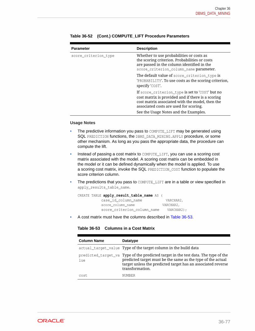
Table 36-52 (Cont.) COMPUTE_LIFT Procedure Parameters
Parameter Description
score_criterion_type Whether to use probabilities or costs asthe scoring criterion. Probabilities or costsare passed in the column identified in thescore_criterion_column_name parameter.
The default value of score_criterion_type is'PROBABILITY'. To use costs as the scoring criterion,specify 'COST'.
If score_criterion_type is set to 'COST' but nocost matrix is provided and if there is a scoringcost matrix associated with the model, then theassociated costs are used for scoring.See the Usage Notes and the Examples.
Usage Notes
• The predictive information you pass to COMPUTE_LIFT may be generated usingSQL PREDICTION functions, the DBMS_DATA_MINING.APPLY procedure, or someother mechanism. As long as you pass the appropriate data, the procedure cancompute the lift.
• Instead of passing a cost matrix to COMPUTE_LIFT, you can use a scoring costmatrix associated with the model. A scoring cost matrix can be embedded inthe model or it can be defined dynamically when the model is applied. To usea scoring cost matrix, invoke the SQL PREDICTION_COST function to populate thescore criterion column.
• The predictions that you pass to COMPUTE_LIFT are in a table or view specified inapply_results_table_name.
CREATE TABLE apply_result_table_name AS ( case_id_column_name VARCHAR2, score_column_name VARCHAR2, score_criterion_column_name VARCHAR2);
• A cost matrix must have the columns described in Table 36-53.
Table 36-53 Columns in a Cost Matrix
Column Name Datatype
actual_target_value Type of the target column in the build data
predicted_target_value
Type of the predicted target in the test data. The type of thepredicted target must be the same as the type of the actualtarget unless the predicted target has an associated reversetransformation.
cost NUMBER
Chapter 36DBMS_DATA_MINING
36-77

See Also:
Oracle Data Mining Concepts for more information about cost matrixes
• The table created by COMPUTE_LIFT has the columns described in Table 36-54
Table 36-54 Columns in a Lift Table
Column Name Datatype
quantile_number NUMBER
probability_threshold NUMBER
gain_cumulative NUMBER
quantile_total_count NUMBER
quantile_target_count NUMBER
percent_records_cumulative NUMBER
lift_cumulative NUMBER
target_density_cumulative NUMBER
targets_cumulative NUMBER
non_targets_cumulative NUMBER
lift_quantile NUMBER
target_density NUMBER
See Also:
Oracle Data Mining Concepts for details about the information in the lifttable
• When a cost matrix is passed to COMPUTE_LIFT, the cost threshold is returned inthe probability_threshold column of the lift table.
Examples
This example uses the Naive Bayes model nb_sh_clas_sample, which is created byone of the Oracle Data Mining sample programs.
The example illustrates lift based on probabilities. For examples that showcomputation based on costs, see "COMPUTE_CONFUSION_MATRIX Procedure".
The following statement applies the model to the test data and stores the predictionsand probabilities in a table.
CREATE TABLE nb_apply_results AS SELECT cust_id, t.prediction, t.probability FROM mining_data_test_v, TABLE(PREDICTION_SET(nb_sh_clas_sample USING *)) t;
Using probabilities as the scoring criterion, you can compute lift as follows.
Chapter 36DBMS_DATA_MINING
36-78
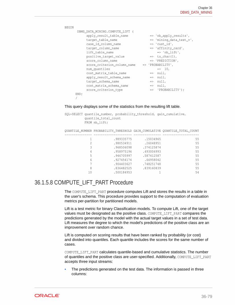
BEGIN DBMS_DATA_MINING.COMPUTE_LIFT ( apply_result_table_name => 'nb_apply_results', target_table_name => 'mining_data_test_v', case_id_column_name => 'cust_id', target_column_name => 'affinity_card', lift_table_name => 'nb_lift', positive_target_value => to_char(1), score_column_name => 'PREDICTION', score_criterion_column_name => 'PROBABILITY', num_quantiles => 10, cost_matrix_table_name => null, apply_result_schema_name => null, target_schema_name => null, cost_matrix_schema_name => null, score_criterion_type => 'PROBABILITY'); END; /
This query displays some of the statistics from the resulting lift table.
SQL>SELECT quantile_number, probability_threshold, gain_cumulative, quantile_total_count FROM nb_lift;
QUANTILE_NUMBER PROBABILITY_THRESHOLD GAIN_CUMULATIVE QUANTILE_TOTAL_COUNT --------------- --------------------- --------------- -------------------- 1 .989335775 .15034965 55 2 .980534911 .26048951 55 3 .968506098 .374125874 55 4 .958975196 .493006993 55 5 .946705997 .587412587 55 6 .927454174 .66958042 55 7 .904403627 .748251748 55 8 .836482525 .839160839 55 10 .500184953 1 54
36.1.5.8 COMPUTE_LIFT_PART ProcedureThe COMPUTE_LIFT_PART procedure computes Lift and stores the results in a table inthe user's schema. This procedure provides support to the computation of evaluationmetrics per-partition for partitioned models.
Lift is a test metric for binary Classification models. To compute Lift, one of the targetvalues must be designated as the positive class. COMPUTE_LIFT_PART compares thepredictions generated by the model with the actual target values in a set of test data.Lift measures the degree to which the model's predictions of the positive class are animprovement over random chance.
Lift is computed on scoring results that have been ranked by probability (or cost)and divided into quantiles. Each quantile includes the scores for the same number ofcases.
COMPUTE_LIFT_PART calculates quantile-based and cumulative statistics. The numberof quantiles and the positive class are user-specified. Additionally, COMPUTE_LIFT_PARTaccepts three input streams:
• The predictions generated on the test data. The information is passed in threecolumns:
Chapter 36DBMS_DATA_MINING
36-79

– Case ID column
– Prediction column
– Scoring criterion column containing either probabilities or costs associatedwith the predictions
• The known target values in the test data. The information is passed in twocolumns:
– Case ID column
– Target column containing the known target values
• (Optional) A cost matrix table with predefined columns. See the Usage Notes forthe column requirements.
See Also:
Oracle Data Mining Concepts for more details about Lift and test metrics forclassification
"COMPUTE_LIFT Procedure"
"COMPUTE_CONFUSION_MATRIX Procedure"
"COMPUTE_CONFUSION_MATRIX_PART Procedure"
"COMPUTE_ROC Procedure"
"COMPUTE_ROC_PART Procedure"
Syntax
DBMS_DATA_MINING.COMPUTE_LIFT_PART ( apply_result_table_name IN VARCHAR2, target_table_name IN VARCHAR2, case_id_column_name IN VARCHAR2, target_column_name IN VARCHAR2, lift_table_name IN VARCHAR2, positive_target_value IN VARCHAR2, score_column_name IN VARCHAR2 DEFAULT 'PREDICTION', score_criterion_column_name IN VARCHAR2 DEFAULT 'PROBABILITY', score_partition_column_name IN VARCHAR2 DEFAULT 'PARTITION_NAME', num_quantiles IN NUMBER DEFAULT 10, cost_matrix_table_name IN VARCHAR2 DEFAULT NULL, apply_result_schema_name IN VARCHAR2 DEFAULT NULL, target_schema_name IN VARCHAR2 DEFAULT NULL, cost_matrix_schema_name IN VARCHAR2 DEFAULT NULL, score_criterion_type IN VARCHAR2 DEFAULT NULL);
Parameters
Table 36-55 COMPUTE_LIFT_PART Procedure Parameters
Parameter Description
apply_result_table_name Table containing the predictions
Chapter 36DBMS_DATA_MINING
36-80
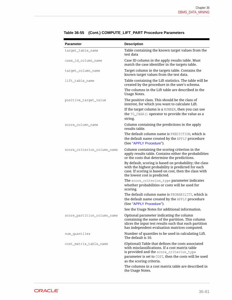
Table 36-55 (Cont.) COMPUTE_LIFT_PART Procedure Parameters
Parameter Description
target_table_name Table containing the known target values from thetest data
case_id_column_name Case ID column in the apply results table. Mustmatch the case identifier in the targets table.
target_column_name Target column in the targets table. Contains theknown target values from the test data.
lift_table_name Table containing the Lift statistics. The table will becreated by the procedure in the user's schema.The columns in the Lift table are described in theUsage Notes.
positive_target_value The positive class. This should be the class ofinterest, for which you want to calculate Lift.If the target column is a NUMBER, then you can usethe TO_CHAR() operator to provide the value as astring.
score_column_name Column containing the predictions in the applyresults table.The default column name is PREDICTION, which isthe default name created by the APPLY procedure(See "APPLY Procedure").
score_criterion_column_name Column containing the scoring criterion in theapply results table. Contains either the probabilitiesor the costs that determine the predictions.By default, scoring is based on probability; the classwith the highest probability is predicted for eachcase. If scoring is based on cost, then the class withthe lowest cost is predicted.The score_criterion_type parameter indicateswhether probabilities or costs will be used forscoring.The default column name is PROBABILITY, which isthe default name created by the APPLY procedure(See "APPLY Procedure").
See the Usage Notes for additional information.
score_partition_column_name Optional parameter indicating the columncontaining the name of the partition. This columnslices the input test results such that each partitionhas independent evaluation matrices computed.
num_quantiles Number of quantiles to be used in calculating Lift.The default is 10.
cost_matrix_table_name (Optional) Table that defines the costs associatedwith misclassifications. If a cost matrix tableis provided and the score_criterion_typeparameter is set to COST, then the costs will be usedas the scoring criteria.The columns in a cost matrix table are described inthe Usage Notes.
Chapter 36DBMS_DATA_MINING
36-81

Table 36-55 (Cont.) COMPUTE_LIFT_PART Procedure Parameters
Parameter Description
apply_result_schema_name Schema of the apply results tableIf null, then the user's schema is assumed.
target_schema_name Schema of the table containing the known targetsIf null, then the user's schema is assumed.
cost_matrix_schema_name Schema of the cost matrix table, if one is providedIf null, then the user's schema is assumed.
score_criterion_type Whether to use probabilities or costs asthe scoring criterion. Probabilities or costsare passed in the column identified in thescore_criterion_column_name parameter.
The default value of score_criterion_type isPROBABILITY. To use costs as the scoring criterion,specify COST.
If score_criterion_type is set to COST but nocost matrix is provided and if there is a scoringcost matrix associated with the model, then theassociated costs are used for scoring.See the Usage Notes and the Examples.
Usage Notes
• The predictive information you pass to COMPUTE_LIFT_PART may be generatedusing SQL PREDICTION functions, the DBMS_DATA_MINING.APPLY procedure, orsome other mechanism. As long as you pass the appropriate data, the procedurecan compute the Lift.
• Instead of passing a cost matrix to COMPUTE_LIFT_PART, you can use a scoringcost matrix associated with the model. A scoring cost matrix can be embeddedin the model or it can be defined dynamically when the model is applied. To usea scoring cost matrix, invoke the SQL PREDICTION_COST function to populate thescore criterion column.
• The predictions that you pass to COMPUTE_LIFT_PART are in a table or viewspecified in apply_results_table_name.
CREATE TABLE apply_result_table_name AS ( case_id_column_name VARCHAR2, score_column_name VARCHAR2, score_criterion_column_name VARCHAR2);
• A cost matrix must have the columns described in Table 36-53.
Table 36-56 Columns in a Cost Matrix
Column Name Datatype
actual_target_value Type of the target column in the test data
Chapter 36DBMS_DATA_MINING
36-82
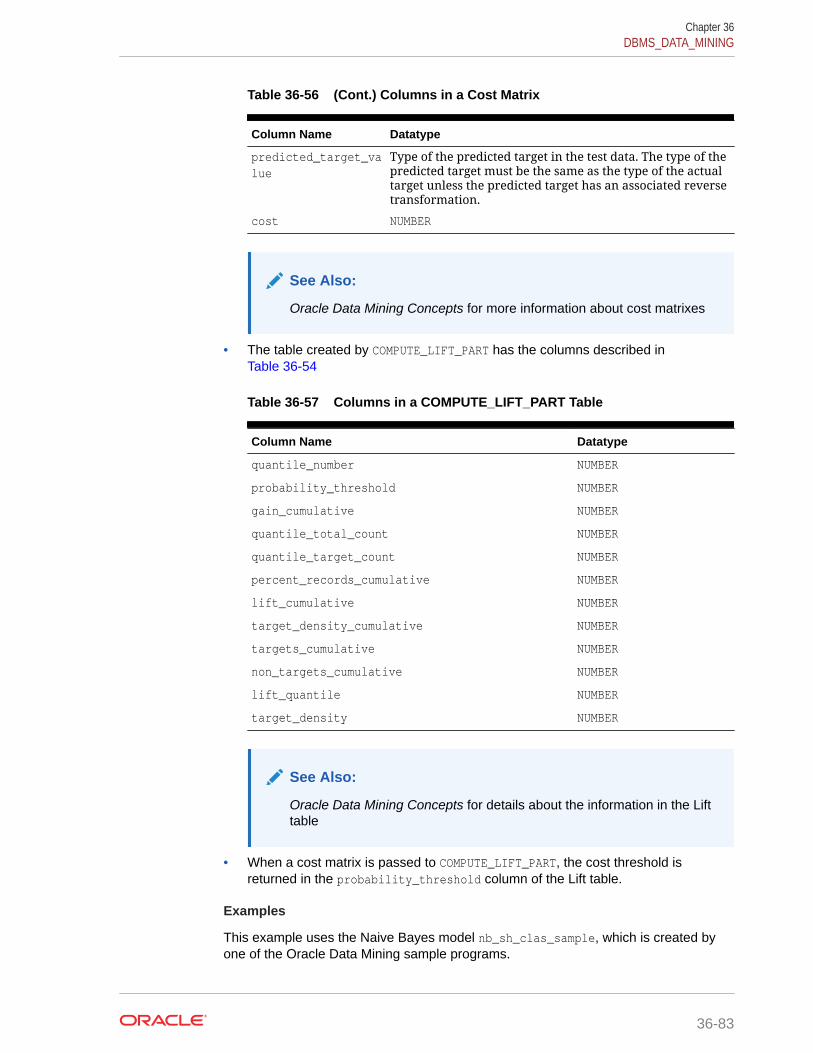
Table 36-56 (Cont.) Columns in a Cost Matrix
Column Name Datatype
predicted_target_value
Type of the predicted target in the test data. The type of thepredicted target must be the same as the type of the actualtarget unless the predicted target has an associated reversetransformation.
cost NUMBER
See Also:
Oracle Data Mining Concepts for more information about cost matrixes
• The table created by COMPUTE_LIFT_PART has the columns described inTable 36-54
Table 36-57 Columns in a COMPUTE_LIFT_PART Table
Column Name Datatype
quantile_number NUMBER
probability_threshold NUMBER
gain_cumulative NUMBER
quantile_total_count NUMBER
quantile_target_count NUMBER
percent_records_cumulative NUMBER
lift_cumulative NUMBER
target_density_cumulative NUMBER
targets_cumulative NUMBER
non_targets_cumulative NUMBER
lift_quantile NUMBER
target_density NUMBER
See Also:
Oracle Data Mining Concepts for details about the information in the Lifttable
• When a cost matrix is passed to COMPUTE_LIFT_PART, the cost threshold isreturned in the probability_threshold column of the Lift table.
Examples
This example uses the Naive Bayes model nb_sh_clas_sample, which is created byone of the Oracle Data Mining sample programs.
Chapter 36DBMS_DATA_MINING
36-83

The example illustrates Lift based on probabilities. For examples that showcomputation based on costs, see "COMPUTE_CONFUSION_MATRIX Procedure".
For a partitioned model example, see "COMPUTE_CONFUSION_MATRIX_PARTProcedure".
The following statement applies the model to the test data and stores the predictionsand probabilities in a table.
CREATE TABLE nb_apply_results AS SELECT cust_id, t.prediction, t.probability FROM mining_data_test_v, TABLE(PREDICTION_SET(nb_sh_clas_sample USING *)) t;
Using probabilities as the scoring criterion, you can compute Lift as follows.
BEGIN DBMS_DATA_MINING.COMPUTE_LIFT_PART ( apply_result_table_name => 'nb_apply_results', target_table_name => 'mining_data_test_v', case_id_column_name => 'cust_id', target_column_name => 'affinity_card', lift_table_name => 'nb_lift', positive_target_value => to_char(1), score_column_name => 'PREDICTION', score_criterion_column_name => 'PROBABILITY', score_partition_column_name => 'PARTITITON_NAME', num_quantiles => 10, cost_matrix_table_name => null, apply_result_schema_name => null, target_schema_name => null, cost_matrix_schema_name => null, score_criterion_type => 'PROBABILITY');END;/
This query displays some of the statistics from the resulting Lift table.
SELECT quantile_number, probability_threshold, gain_cumulative, quantile_total_count FROM nb_lift;
QUANTILE_NUMBER PROBABILITY_THRESHOLD GAIN_CUMULATIVE QUANTILE_TOTAL_COUNT --------------- --------------------- --------------- -------------------- 1 .989335775 .15034965 55 2 .980534911 .26048951 55 3 .968506098 .374125874 55 4 .958975196 .493006993 55 5 .946705997 .587412587 55 6 .927454174 .66958042 55 7 .904403627 .748251748 55 8 .836482525 .839160839 55 10 .500184953 1 54
Chapter 36DBMS_DATA_MINING
36-84
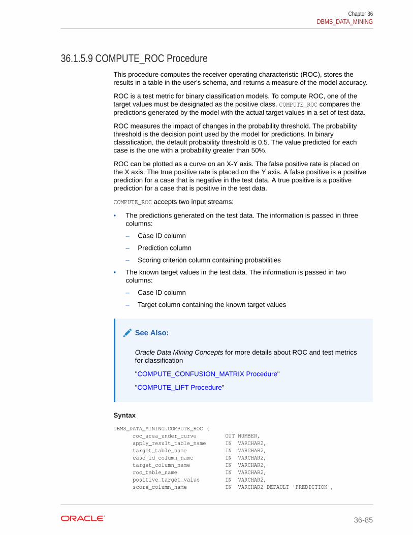
36.1.5.9 COMPUTE_ROC ProcedureThis procedure computes the receiver operating characteristic (ROC), stores theresults in a table in the user's schema, and returns a measure of the model accuracy.
ROC is a test metric for binary classification models. To compute ROC, one of thetarget values must be designated as the positive class. COMPUTE_ROC compares thepredictions generated by the model with the actual target values in a set of test data.
ROC measures the impact of changes in the probability threshold. The probabilitythreshold is the decision point used by the model for predictions. In binaryclassification, the default probability threshold is 0.5. The value predicted for eachcase is the one with a probability greater than 50%.
ROC can be plotted as a curve on an X-Y axis. The false positive rate is placed onthe X axis. The true positive rate is placed on the Y axis. A false positive is a positiveprediction for a case that is negative in the test data. A true positive is a positiveprediction for a case that is positive in the test data.
COMPUTE_ROC accepts two input streams:
• The predictions generated on the test data. The information is passed in threecolumns:
– Case ID column
– Prediction column
– Scoring criterion column containing probabilities
• The known target values in the test data. The information is passed in twocolumns:
– Case ID column
– Target column containing the known target values
See Also:
Oracle Data Mining Concepts for more details about ROC and test metricsfor classification
"COMPUTE_CONFUSION_MATRIX Procedure"
"COMPUTE_LIFT Procedure"
Syntax
DBMS_DATA_MINING.COMPUTE_ROC ( roc_area_under_curve OUT NUMBER, apply_result_table_name IN VARCHAR2, target_table_name IN VARCHAR2, case_id_column_name IN VARCHAR2, target_column_name IN VARCHAR2, roc_table_name IN VARCHAR2, positive_target_value IN VARCHAR2, score_column_name IN VARCHAR2 DEFAULT 'PREDICTION',
Chapter 36DBMS_DATA_MINING
36-85

score_criterion_column_name IN VARCHAR2 DEFAULT 'PROBABILITY', apply_result_schema_name IN VARCHAR2 DEFAULT NULL, target_schema_name IN VARCHAR2 DEFAULT NULL);
Parameters
Table 36-58 COMPUTE_ROC Procedure Parameters
Parameter Description
roc_area_under_the_curve Output parameter containing the area under theROC curve (AUC). The AUC measures the likelihoodthat an actual positive will be predicted as positive.The greater the AUC, the greater the flexibility ofthe model in accommodating trade-offs betweenpositive and negative class predictions. AUC can beespecially important when one target class is rareror more important to identify than another.
apply_result_table_name Table containing the predictions.
target_table_name Table containing the known target values from thetest data.
case_id_column_name Case ID column in the apply results table. Mustmatch the case identifier in the targets table.
target_column_name Target column in the targets table. Contains theknown target values from the test data.
roc_table_name Table containing the ROC output. The table will becreated by the procedure in the user's schema.The columns in the ROC table are described in theUsage Notes.
positive_target_value The positive class. This should be the class ofinterest, for which you want to calculate ROC.If the target column is a NUMBER, you can use theTO_CHAR() operator to provide the value as a string.
score_column_name Column containing the predictions in the applyresults table.The default column name is 'PREDICTION', which isthe default name created by the APPLY procedure(See "APPLY Procedure").
score_criterion_column_name Column containing the scoring criterion in theapply results table. Contains the probabilities thatdetermine the predictions.The default column name is 'PROBABILITY', whichis the default name created by the APPLY procedure(See "APPLY Procedure").
apply_result_schema_name Schema of the apply results table.If null, the user's schema is assumed.
target_schema_name Schema of the table containing the known targets.If null, the user's schema is assumed.
Chapter 36DBMS_DATA_MINING
36-86

Usage Notes
• The predictive information you pass to COMPUTE_ROC may be generated using SQLPREDICTION functions, the DBMS_DATA_MINING.APPLY procedure, or some othermechanism. As long as you pass the appropriate data, the procedure can computethe receiver operating characteristic.
• The predictions that you pass to COMPUTE_ROC are in a table or view specified inapply_results_table_name.
CREATE TABLE apply_result_table_name AS ( case_id_column_name VARCHAR2, score_column_name VARCHAR2, score_criterion_column_name VARCHAR2);
• The table created by COMPUTE_ROC has the columns shown in Table 36-59.
Table 36-59 COMPUTE_ROC Output
Column Datatype
probability BINARY_DOUBLE
true_positives NUMBER
false_negatives NUMBER
false_positives NUMBER
true_negatives NUMBER
true_positive_fraction NUMBER
false_positive_fraction NUMBER
See Also:
Oracle Data Mining Concepts for details about the output of COMPUTE_ROC
• ROC is typically used to determine the most desirable probability threshold. Thiscan be done by examining the true positive fraction and the false positive fraction.The true positive fraction is the percentage of all positive cases in the testdata that were correctly predicted as positive. The false positive fraction is thepercentage of all negative cases in the test data that were incorrectly predicted aspositive.
Given a probability threshold, the following statement returns the positivepredictions in an apply result table ordered by probability.
SELECT case_id_column_name FROM apply_result_table_name WHERE probability > probability_threshold ORDER BY probability DESC;
• There are two approaches to identifying the most desirable probability threshold.Which approach you use depends on whether or not you know the relative cost ofpositive versus negative class prediction errors.
Chapter 36DBMS_DATA_MINING
36-87

If the costs are known, you can apply the relative costs to the ROC table tocompute the minimum cost probability threshold. Suppose the relative cost ratio is:Positive Class Error Cost / Negative Class Error Cost = 20. Then execute a querylike this.
WITH cost AS ( SELECT probability_threshold, 20 * false_negatives + false_positives cost FROM ROC_table GROUP BY probability_threshold), minCost AS ( SELECT min(cost) minCost FROM cost) SELECT max(probability_threshold)probability_threshold FROM cost, minCost WHERE cost = minCost;
If relative costs are not well known, you can simply scan the values in theROC table (in sorted order) and make a determination about which of thedisplayed trade-offs (misclassified positives versus misclassified negatives) ismost desirable.
SELECT * FROM ROC_table ORDER BY probability_threshold;
Examples
This example uses the Naive Bayes model nb_sh_clas_sample, which is created byone of the Oracle Data Mining sample programs.
The following statement applies the model to the test data and stores the predictionsand probabilities in a table.
CREATE TABLE nb_apply_results AS SELECT cust_id, t.prediction, t.probability FROM mining_data_test_v, TABLE(PREDICTION_SET(nb_sh_clas_sample USING *)) t;
Using the predictions and the target values from the test data, you can compute ROCas follows.
DECLARE v_area_under_curve NUMBER;BEGIN DBMS_DATA_MINING.COMPUTE_ROC ( roc_area_under_curve => v_area_under_curve, apply_result_table_name => 'nb_apply_results', target_table_name => 'mining_data_test_v', case_id_column_name => 'cust_id', target_column_name => 'mining_data_test_v', roc_table_name => 'nb_roc', positive_target_value => '1', score_column_name => 'PREDICTION', score_criterion_column_name => 'PROBABILITY'); DBMS_OUTPUT.PUT_LINE('**** AREA UNDER ROC CURVE ****: ' || ROUND(v_area_under_curve,4));END;/
Chapter 36DBMS_DATA_MINING
36-88
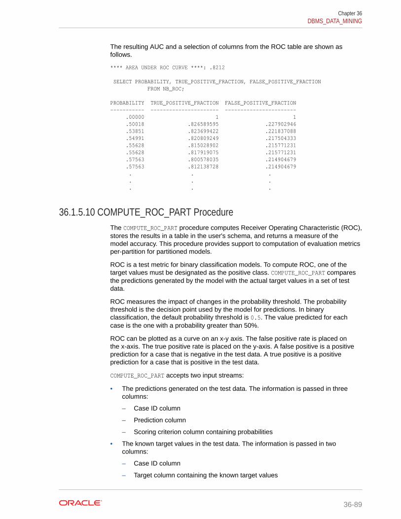
The resulting AUC and a selection of columns from the ROC table are shown asfollows.
**** AREA UNDER ROC CURVE ****: .8212
SELECT PROBABILITY, TRUE_POSITIVE_FRACTION, FALSE_POSITIVE_FRACTION FROM NB_ROC; PROBABILITY TRUE_POSITIVE_FRACTION FALSE_POSITIVE_FRACTION----------- ---------------------- ----------------------- .00000 1 1 .50018 .826589595 .227902946 .53851 .823699422 .221837088 .54991 .820809249 .217504333 .55628 .815028902 .215771231 .55628 .817919075 .215771231 .57563 .800578035 .214904679 .57563 .812138728 .214904679 . . . . . . . . .
36.1.5.10 COMPUTE_ROC_PART ProcedureThe COMPUTE_ROC_PART procedure computes Receiver Operating Characteristic (ROC),stores the results in a table in the user's schema, and returns a measure of themodel accuracy. This procedure provides support to computation of evaluation metricsper-partition for partitioned models.
ROC is a test metric for binary classification models. To compute ROC, one of thetarget values must be designated as the positive class. COMPUTE_ROC_PART comparesthe predictions generated by the model with the actual target values in a set of testdata.
ROC measures the impact of changes in the probability threshold. The probabilitythreshold is the decision point used by the model for predictions. In binaryclassification, the default probability threshold is 0.5. The value predicted for eachcase is the one with a probability greater than 50%.
ROC can be plotted as a curve on an x-y axis. The false positive rate is placed onthe x-axis. The true positive rate is placed on the y-axis. A false positive is a positiveprediction for a case that is negative in the test data. A true positive is a positiveprediction for a case that is positive in the test data.
COMPUTE_ROC_PART accepts two input streams:
• The predictions generated on the test data. The information is passed in threecolumns:
– Case ID column
– Prediction column
– Scoring criterion column containing probabilities
• The known target values in the test data. The information is passed in twocolumns:
– Case ID column
– Target column containing the known target values
Chapter 36DBMS_DATA_MINING
36-89
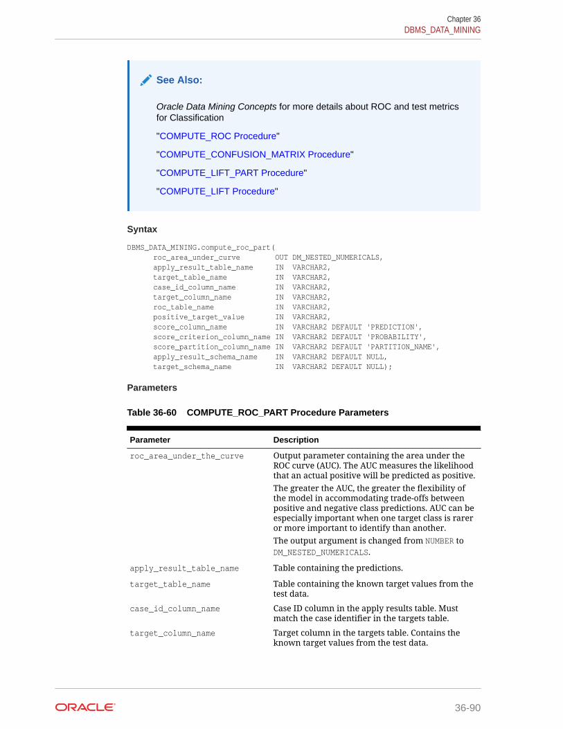
See Also:
Oracle Data Mining Concepts for more details about ROC and test metricsfor Classification
"COMPUTE_ROC Procedure"
"COMPUTE_CONFUSION_MATRIX Procedure"
"COMPUTE_LIFT_PART Procedure"
"COMPUTE_LIFT Procedure"
Syntax
DBMS_DATA_MINING.compute_roc_part( roc_area_under_curve OUT DM_NESTED_NUMERICALS, apply_result_table_name IN VARCHAR2, target_table_name IN VARCHAR2, case_id_column_name IN VARCHAR2, target_column_name IN VARCHAR2, roc_table_name IN VARCHAR2, positive_target_value IN VARCHAR2, score_column_name IN VARCHAR2 DEFAULT 'PREDICTION', score_criterion_column_name IN VARCHAR2 DEFAULT 'PROBABILITY', score_partition_column_name IN VARCHAR2 DEFAULT 'PARTITION_NAME', apply_result_schema_name IN VARCHAR2 DEFAULT NULL, target_schema_name IN VARCHAR2 DEFAULT NULL);
Parameters
Table 36-60 COMPUTE_ROC_PART Procedure Parameters
Parameter Description
roc_area_under_the_curve Output parameter containing the area under theROC curve (AUC). The AUC measures the likelihoodthat an actual positive will be predicted as positive.The greater the AUC, the greater the flexibility ofthe model in accommodating trade-offs betweenpositive and negative class predictions. AUC can beespecially important when one target class is rareror more important to identify than another.The output argument is changed from NUMBER toDM_NESTED_NUMERICALS.
apply_result_table_name Table containing the predictions.
target_table_name Table containing the known target values from thetest data.
case_id_column_name Case ID column in the apply results table. Mustmatch the case identifier in the targets table.
target_column_name Target column in the targets table. Contains theknown target values from the test data.
Chapter 36DBMS_DATA_MINING
36-90

Table 36-60 (Cont.) COMPUTE_ROC_PART Procedure Parameters
Parameter Description
roc_table_name Table containing the ROC output. The table will becreated by the procedure in the user's schema.The columns in the ROC table are described in theUsage Notes.
positive_target_value The positive class. This should be the class ofinterest, for which you want to calculate ROC.If the target column is a NUMBER, then you can usethe TO_CHAR() operator to provide the value as astring.
score_column_name Column containing the predictions in the applyresults table.The default column name is PREDICTION, which isthe default name created by the APPLY procedure(See "APPLY Procedure").
score_criterion_column_name Column containing the scoring criterion in theapply results table. Contains the probabilities thatdetermine the predictions.The default column name is PROBABILITY, which isthe default name created by the APPLY procedure(See "APPLY Procedure").
score_partition_column_name Optional parameter indicating the column whichcontains the name of the partition. This columnslices the input test results such that each partitionhas independent evaluation matrices computed.
apply_result_schema_name Schema of the apply results table.If null, then the user's schema is assumed.
target_schema_name Schema of the table containing the known targets.If null, then the user's schema is assumed.
Usage Notes
• The predictive information you pass to COMPUTE_ROC_PART may be generated usingSQL PREDICTION functions, the DBMS_DATA_MINING.APPLY procedure, or someother mechanism. As long as you pass the appropriate data, the procedure cancompute the receiver operating characteristic.
• The predictions that you pass to COMPUTE_ROC_PART are in a table or view specifiedin apply_results_table_name.
CREATE TABLE apply_result_table_name AS ( case_id_column_name VARCHAR2, score_column_name VARCHAR2, score_criterion_column_name VARCHAR2);
• The COMPUTE_ROC_PART table has the following columns:
Chapter 36DBMS_DATA_MINING
36-91
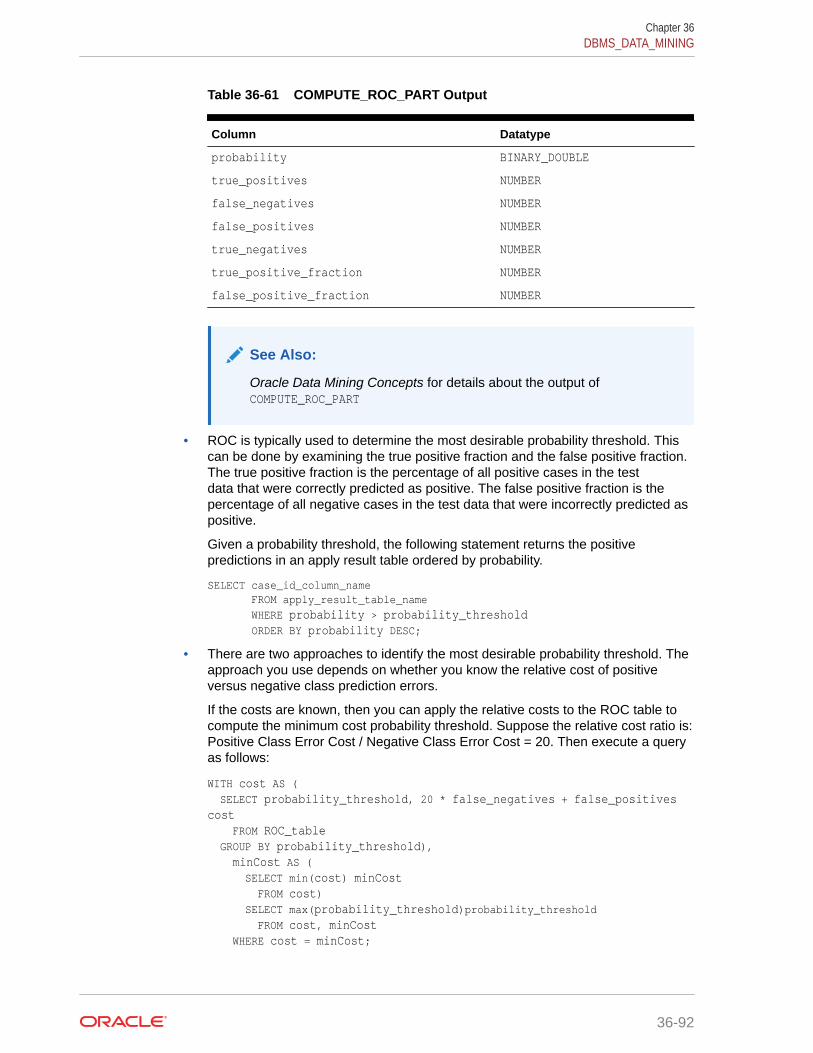
Table 36-61 COMPUTE_ROC_PART Output
Column Datatype
probability BINARY_DOUBLE
true_positives NUMBER
false_negatives NUMBER
false_positives NUMBER
true_negatives NUMBER
true_positive_fraction NUMBER
false_positive_fraction NUMBER
See Also:
Oracle Data Mining Concepts for details about the output ofCOMPUTE_ROC_PART
• ROC is typically used to determine the most desirable probability threshold. Thiscan be done by examining the true positive fraction and the false positive fraction.The true positive fraction is the percentage of all positive cases in the testdata that were correctly predicted as positive. The false positive fraction is thepercentage of all negative cases in the test data that were incorrectly predicted aspositive.
Given a probability threshold, the following statement returns the positivepredictions in an apply result table ordered by probability.
SELECT case_id_column_name FROM apply_result_table_name WHERE probability > probability_threshold ORDER BY probability DESC;
• There are two approaches to identify the most desirable probability threshold. Theapproach you use depends on whether you know the relative cost of positiveversus negative class prediction errors.
If the costs are known, then you can apply the relative costs to the ROC table tocompute the minimum cost probability threshold. Suppose the relative cost ratio is:Positive Class Error Cost / Negative Class Error Cost = 20. Then execute a queryas follows:
WITH cost AS ( SELECT probability_threshold, 20 * false_negatives + false_positives cost FROM ROC_table GROUP BY probability_threshold), minCost AS ( SELECT min(cost) minCost FROM cost) SELECT max(probability_threshold)probability_threshold FROM cost, minCost WHERE cost = minCost;
Chapter 36DBMS_DATA_MINING
36-92
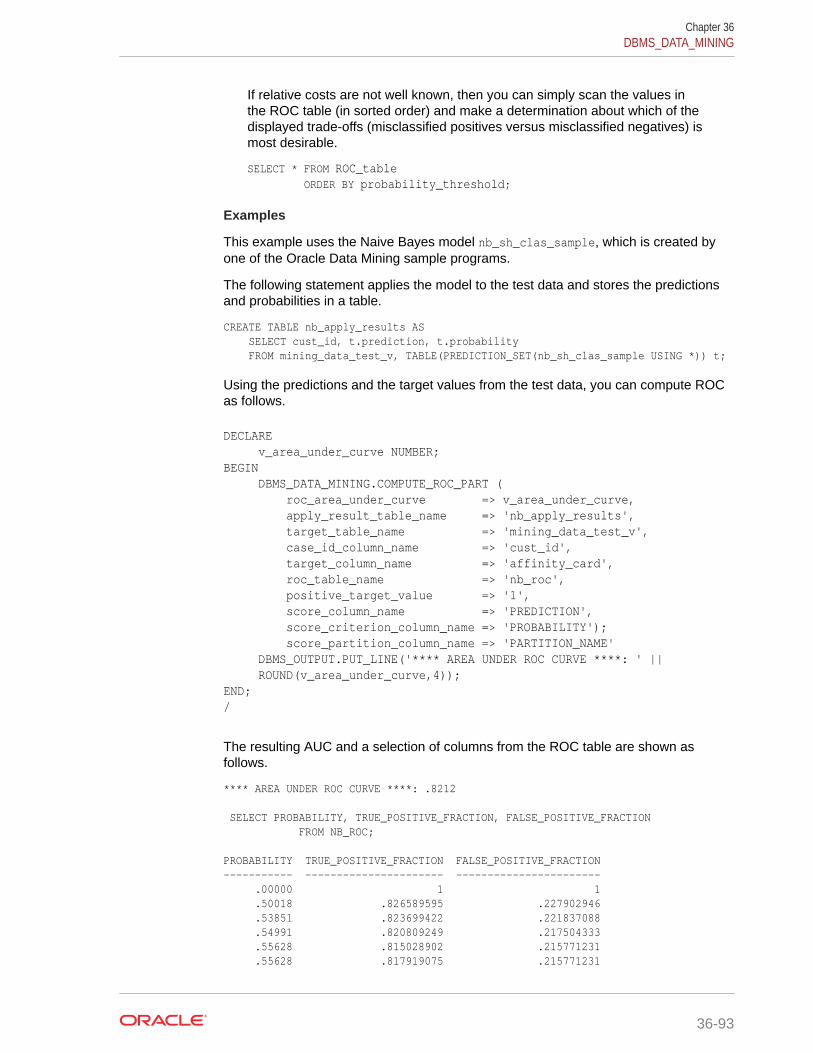
If relative costs are not well known, then you can simply scan the values inthe ROC table (in sorted order) and make a determination about which of thedisplayed trade-offs (misclassified positives versus misclassified negatives) ismost desirable.
SELECT * FROM ROC_table ORDER BY probability_threshold;
Examples
This example uses the Naive Bayes model nb_sh_clas_sample, which is created byone of the Oracle Data Mining sample programs.
The following statement applies the model to the test data and stores the predictionsand probabilities in a table.
CREATE TABLE nb_apply_results AS SELECT cust_id, t.prediction, t.probability FROM mining_data_test_v, TABLE(PREDICTION_SET(nb_sh_clas_sample USING *)) t;
Using the predictions and the target values from the test data, you can compute ROCas follows.
DECLARE v_area_under_curve NUMBER;BEGIN DBMS_DATA_MINING.COMPUTE_ROC_PART ( roc_area_under_curve => v_area_under_curve, apply_result_table_name => 'nb_apply_results', target_table_name => 'mining_data_test_v', case_id_column_name => 'cust_id', target_column_name => 'affinity_card', roc_table_name => 'nb_roc', positive_target_value => '1', score_column_name => 'PREDICTION', score_criterion_column_name => 'PROBABILITY'); score_partition_column_name => 'PARTITION_NAME' DBMS_OUTPUT.PUT_LINE('**** AREA UNDER ROC CURVE ****: ' || ROUND(v_area_under_curve,4));END;/
The resulting AUC and a selection of columns from the ROC table are shown asfollows.
**** AREA UNDER ROC CURVE ****: .8212
SELECT PROBABILITY, TRUE_POSITIVE_FRACTION, FALSE_POSITIVE_FRACTION FROM NB_ROC; PROBABILITY TRUE_POSITIVE_FRACTION FALSE_POSITIVE_FRACTION----------- ---------------------- ----------------------- .00000 1 1 .50018 .826589595 .227902946 .53851 .823699422 .221837088 .54991 .820809249 .217504333 .55628 .815028902 .215771231 .55628 .817919075 .215771231
Chapter 36DBMS_DATA_MINING
36-93
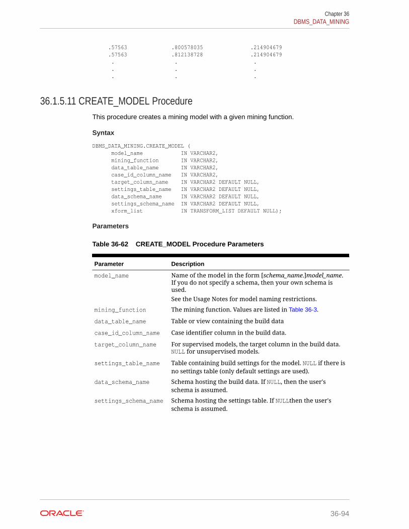
.57563 .800578035 .214904679 .57563 .812138728 .214904679 . . . . . . . . .
36.1.5.11 CREATE_MODEL ProcedureThis procedure creates a mining model with a given mining function.
Syntax
DBMS_DATA_MINING.CREATE_MODEL ( model_name IN VARCHAR2, mining_function IN VARCHAR2, data_table_name IN VARCHAR2, case_id_column_name IN VARCHAR2, target_column_name IN VARCHAR2 DEFAULT NULL, settings_table_name IN VARCHAR2 DEFAULT NULL, data_schema_name IN VARCHAR2 DEFAULT NULL, settings_schema_name IN VARCHAR2 DEFAULT NULL, xform_list IN TRANSFORM_LIST DEFAULT NULL);
Parameters
Table 36-62 CREATE_MODEL Procedure Parameters
Parameter Description
model_name Name of the model in the form [schema_name.]model_name.If you do not specify a schema, then your own schema isused.See the Usage Notes for model naming restrictions.
mining_function The mining function. Values are listed in Table 36-3.
data_table_name Table or view containing the build data
case_id_column_name Case identifier column in the build data.
target_column_name For supervised models, the target column in the build data.NULL for unsupervised models.
settings_table_name Table containing build settings for the model. NULL if there isno settings table (only default settings are used).
data_schema_name Schema hosting the build data. If NULL, then the user'sschema is assumed.
settings_schema_name Schema hosting the settings table. If NULLthen the user'sschema is assumed.
Chapter 36DBMS_DATA_MINING
36-94
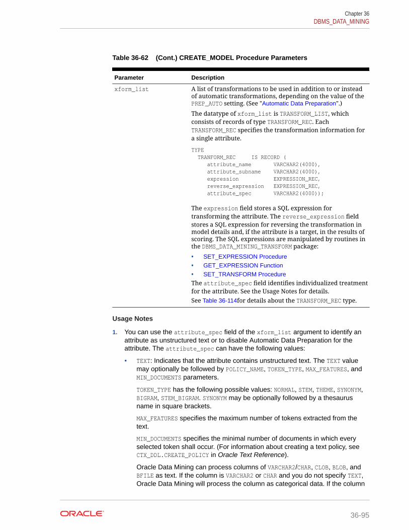
Table 36-62 (Cont.) CREATE_MODEL Procedure Parameters
Parameter Description
xform_list A list of transformations to be used in addition to or insteadof automatic transformations, depending on the value of thePREP_AUTO setting. (See "Automatic Data Preparation".)
The datatype of xform_list is TRANSFORM_LIST, whichconsists of records of type TRANSFORM_REC. EachTRANSFORM_REC specifies the transformation information fora single attribute.
TYPE TRANFORM_REC IS RECORD ( attribute_name VARCHAR2(4000), attribute_subname VARCHAR2(4000), expression EXPRESSION_REC, reverse_expression EXPRESSION_REC, attribute_spec VARCHAR2(4000));
The expression field stores a SQL expression fortransforming the attribute. The reverse_expression fieldstores a SQL expression for reversing the transformation inmodel details and, if the attribute is a target, in the results ofscoring. The SQL expressions are manipulated by routines inthe DBMS_DATA_MINING_TRANSFORM package:
• SET_EXPRESSION Procedure• GET_EXPRESSION Function• SET_TRANSFORM ProcedureThe attribute_spec field identifies individualized treatmentfor the attribute. See the Usage Notes for details.See Table 36-114for details about the TRANSFORM_REC type.
Usage Notes
1. You can use the attribute_spec field of the xform_list argument to identify anattribute as unstructured text or to disable Automatic Data Preparation for theattribute. The attribute_spec can have the following values:
• TEXT: Indicates that the attribute contains unstructured text. The TEXT valuemay optionally be followed by POLICY_NAME, TOKEN_TYPE, MAX_FEATURES, andMIN_DOCUMENTS parameters.
TOKEN_TYPE has the following possible values: NORMAL, STEM, THEME, SYNONYM,BIGRAM, STEM_BIGRAM. SYNONYM may be optionally followed by a thesaurusname in square brackets.
MAX_FEATURES specifies the maximum number of tokens extracted from thetext.
MIN_DOCUMENTS specifies the minimal number of documents in which everyselected token shall occur. (For information about creating a text policy, seeCTX_DDL.CREATE_POLICY in Oracle Text Reference).
Oracle Data Mining can process columns of VARCHAR2/CHAR, CLOB, BLOB, andBFILE as text. If the column is VARCHAR2 or CHAR and you do not specify TEXT,Oracle Data Mining will process the column as categorical data. If the column
Chapter 36DBMS_DATA_MINING
36-95

is CLOB, then Oracle Data Mining will process it as text by default (You do notneed to specify it as TEXT. However, you do need to provide an Oracle TextPolicy in the settings). If the column is BLOB or BFILE, you must specify it asTEXT, otherwise CREATE_MODEL will return an error.
If you specify TEXT for a nested column or for an attribute in a nested column,CREATE_MODEL will return an error.
• NOPREP: Disables ADP for the attribute. When ADP is OFF, the NOPREP value isignored.
You can specify NOPREP for a nested column, but not for an attribute in anested column. If you specify NOPREP for an attribute in a nested column whenADP is on, CREATE_MODEL will return an error.
2. You can obtain information about a model by querying the Data Dictionary views.
ALL/USER/DBA_MINING_MODELSALL/USER/DBA_MINING_MODEL_ATTRIBUTESALL/USER/DBA_MINING_MODEL_SETTINGSALL/USER/DBA_MINING_MODEL_VIEWSALL/USER/DBA_MINING_MODEL_PARTITIONSALL/USER/DBA_MINING_MODEL_XFORMS
You can obtain information about model attributes by querying the model detailsthrough model views. Refer to Oracle Data Mining User’s Guide.
3. The naming rules for models are more restrictive than the naming rules for mostdatabase schema objects. A model name must satisfy the following additionalrequirements:
• It must be 123 or fewer characters long.
• It must be a nonquoted identifier. Oracle requires that nonquoted identifierscontain only alphanumeric characters, the underscore (_), dollar sign ($),and pound sign (#); the initial character must be alphabetic. Oracle stronglydiscourages the use of the dollar sign and pound sign in nonquoted literals.
Naming requirements for schema objects are fully documented in OracleDatabase SQL Language Reference.
4. To build a partitioned model, you must provide additional settings.
The setting for partitioning columns are as follows:
INSERT INTO settings_table VALUES (‘ODMS_PARTITION_COLUMNS’, ‘GENDER, AGE’);
To set user-defined partition number for a model, the setting is as follows:
INSERT INTO settings_table VALUES ('ODMS_MAX_PARTITIONS’, '10’);
The default value for maximum number of partitions is 1000.
5. By passing an xform_list to CREATE_MODEL, you can specify a list oftransformations to be performed on the input data. If the PREP_AUTO setting isON, the transformations are used in addition to the automatic transformations.If the PREP_AUTO setting is OFF, the specified transformations are the onlyones implemented by the model. In both cases, transformation definitions areembedded in the model and executed automatically whenever the model is
Chapter 36DBMS_DATA_MINING
36-96
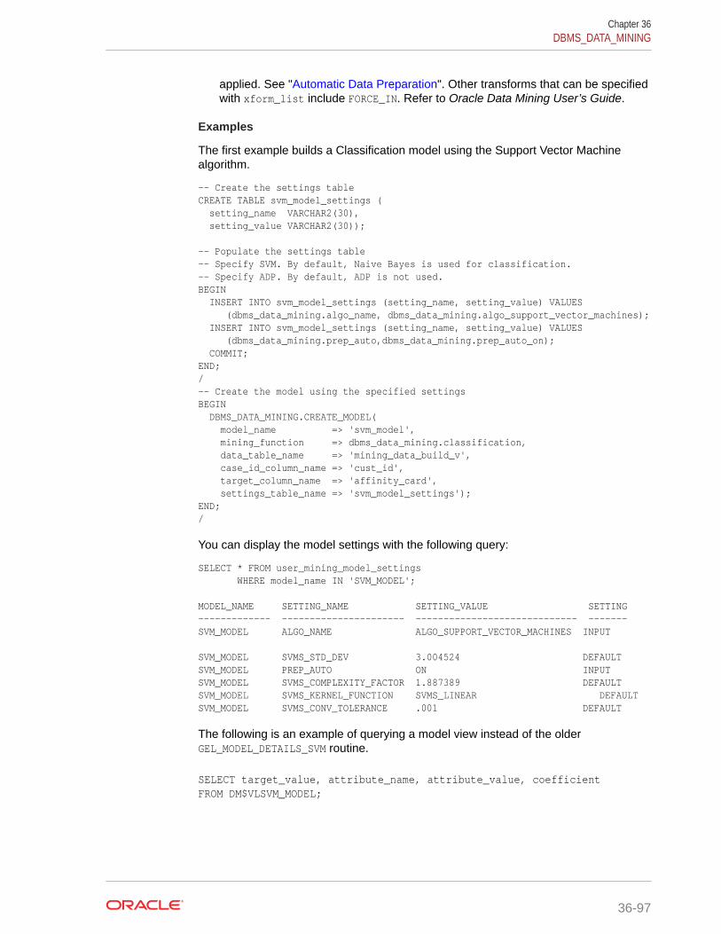
applied. See "Automatic Data Preparation". Other transforms that can be specifiedwith xform_list include FORCE_IN. Refer to Oracle Data Mining User’s Guide.
Examples
The first example builds a Classification model using the Support Vector Machinealgorithm.
-- Create the settings table CREATE TABLE svm_model_settings ( setting_name VARCHAR2(30), setting_value VARCHAR2(30));
-- Populate the settings table-- Specify SVM. By default, Naive Bayes is used for classification.-- Specify ADP. By default, ADP is not used.BEGIN INSERT INTO svm_model_settings (setting_name, setting_value) VALUES (dbms_data_mining.algo_name, dbms_data_mining.algo_support_vector_machines); INSERT INTO svm_model_settings (setting_name, setting_value) VALUES (dbms_data_mining.prep_auto,dbms_data_mining.prep_auto_on); COMMIT;END;/-- Create the model using the specified settings BEGIN DBMS_DATA_MINING.CREATE_MODEL( model_name => 'svm_model', mining_function => dbms_data_mining.classification, data_table_name => 'mining_data_build_v', case_id_column_name => 'cust_id', target_column_name => 'affinity_card', settings_table_name => 'svm_model_settings');END;/
You can display the model settings with the following query:
SELECT * FROM user_mining_model_settings WHERE model_name IN 'SVM_MODEL';
MODEL_NAME SETTING_NAME SETTING_VALUE SETTING------------- ---------------------- ----------------------------- -------SVM_MODEL ALGO_NAME ALGO_SUPPORT_VECTOR_MACHINES INPUT
SVM_MODEL SVMS_STD_DEV 3.004524 DEFAULTSVM_MODEL PREP_AUTO ON INPUTSVM_MODEL SVMS_COMPLEXITY_FACTOR 1.887389 DEFAULTSVM_MODEL SVMS_KERNEL_FUNCTION SVMS_LINEAR DEFAULTSVM_MODEL SVMS_CONV_TOLERANCE .001 DEFAULT
The following is an example of querying a model view instead of the olderGEL_MODEL_DETAILS_SVM routine.
SELECT target_value, attribute_name, attribute_value, coefficient FROM DM$VLSVM_MODEL;
Chapter 36DBMS_DATA_MINING
36-97

The second example creates an Anomaly Detection model. Anomaly Detection usesSVM Classification without a target. This example uses the same settings tablecreated for the SVM Classification model in the first example.
BEGIN DBMS_DATA_MINING.CREATE_MODEL( model_name => 'anomaly_detect_model', mining_function => dbms_data_mining.classification, data_table_name => 'mining_data_build_v', case_id_column_name => 'cust_id', target_column_name => null, settings_table_name => 'svm_model_settings');END;/
This query shows that the models created in these examples are the only ones in yourschema.
SELECT model_name, mining_function, algorithm FROM user_mining_models; MODEL_NAME MINING_FUNCTION ALGORITHM---------------------- -------------------- ------------------------------SVM_MODEL CLASSIFICATION SUPPORT_VECTOR_MACHINESANOMALY_DETECT_MODEL CLASSIFICATION SUPPORT_VECTOR_MACHINES
This query shows that only the SVM Classification model has a target.
SELECT model_name, attribute_name, attribute_type, target FROM user_mining_model_attributes WHERE target = 'YES'; MODEL_NAME ATTRIBUTE_NAME ATTRIBUTE_TYPE TARGET------------------ --------------- ----------------- ------SVM_MODEL AFFINITY_CARD CATEGORICAL YES
36.1.5.12 CREATE_MODEL2 ProcedureThe CREATE_MODEL2 procedure is an alternate procedure to the CREATE_MODELprocedure, which enables creating a model without extra persistence stages. In theCREATE_MODEL procedure, the input is a table or a view and if such an object is notalready present, the user must create it. By using the CREATE_MODEL2 procedure, theuser does not need to create such transient database objects.
Syntax
DBMS_DATA_MINING.CREATE_MODEL2 ( model_name IN VARCHAR2, mining_function IN VARCHAR2, data_query IN CLOB, set_list IN SETTING_LIST, case_id_column_name IN VARCHAR2 DEFAULT NULL, target_column_name IN VARCHAR2 DEFAULT NULL, xform_list IN TRANSFORM_LIST DEFAULT NULL);
Chapter 36DBMS_DATA_MINING
36-98
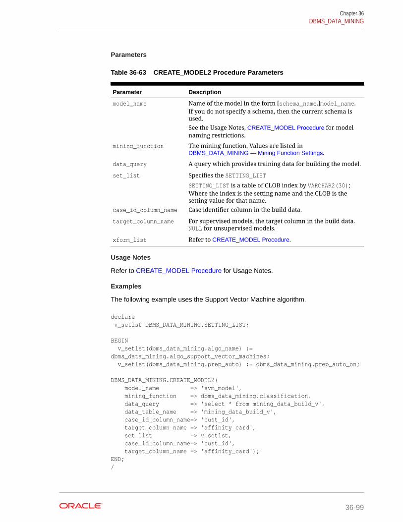
Parameters
Table 36-63 CREATE_MODEL2 Procedure Parameters
Parameter Description
model_name Name of the model in the form [schema_name.]model_name.If you do not specify a schema, then the current schema isused.See the Usage Notes, CREATE_MODEL Procedure for modelnaming restrictions.
mining_function The mining function. Values are listed inDBMS_DATA_MINING — Mining Function Settings.
data_query A query which provides training data for building the model.
set_list Specifies the SETTING_LIST
SETTING_LIST is a table of CLOB index by VARCHAR2(30);Where the index is the setting name and the CLOB is thesetting value for that name.
case_id_column_name Case identifier column in the build data.
target_column_name For supervised models, the target column in the build data.NULL for unsupervised models.
xform_list Refer to CREATE_MODEL Procedure.
Usage Notes
Refer to CREATE_MODEL Procedure for Usage Notes.
Examples
The following example uses the Support Vector Machine algorithm.
declare v_setlst DBMS_DATA_MINING.SETTING_LIST;
BEGIN v_setlst(dbms_data_mining.algo_name) := dbms_data_mining.algo_support_vector_machines; v_setlst(dbms_data_mining.prep_auto) := dbms_data_mining.prep_auto_on; DBMS_DATA_MINING.CREATE_MODEL2( model_name => 'svm_model', mining_function => dbms_data_mining.classification, data_query => 'select * from mining_data_build_v', data_table_name => 'mining_data_build_v', case_id_column_name=> 'cust_id', target_column_name => 'affinity_card', set_list => v_setlst, case_id_column_name=> 'cust_id', target_column_name => 'affinity_card');END;/
Chapter 36DBMS_DATA_MINING
36-99

36.1.5.13 Create Model Using Registration InformationCreate model function fetches the setting information from JSON object.
Usage Notes
If an algorithm is registered, user can create model using the registered algorithmname. Since all R scripts and default setting values are already registered, providingthe value through the setting table is not necessary. This makes the use of thisalgorithm easier.
Examples
The first example builds a Classification model using the GLM algorithm.
CREATE TABLE GLM_RDEMO_SETTINGS_CL ( setting_name VARCHAR2(30), setting_value VARCHAR2(4000)); BEGIN INSERT INTO GLM_RDEMO_SETTINGS_CL VALUES ('ALGO_EXTENSIBLE_LANG', 'R'); INSERT INTO GLM_RDEMO_SETTINGS_CL VALUES (dbms_data_mining.ralg_registration_algo_name, 't1'); INSERT INTO GLM_RDEMO_SETTINGS_CL VALUES (dbms_data_mining.odms_formula, 'AGE + EDUCATION + HOUSEHOLD_SIZE + OCCUPATION'); INSERT INTO GLM_RDEMO_SETTINGS_CL VALUES ('RALG_PARAMETER_FAMILY', 'binomial(logit)' ); END; / BEGIN DBMS_DATA_MINING.CREATE_MODEL( model_name => 'GLM_RDEMO_CLASSIFICATION', mining_function => dbms_data_mining.classification, data_table_name => 'mining_data_build_v', case_id_column_name => 'CUST_ID', target_column_name => 'AFFINITY_CARD', settings_table_name => 'GLM_RDEMO_SETTINGS_CL'); END; /
36.1.5.14 DROP_ALGORITHM ProcedureThis function is used to drop the registered algorithm information.
Syntax
DBMS_DATA_MINING.DROP_ALGORITHM (algorithm_name IN VARCHAR2(30), cascade IN BOOLEAN default FALSE)
Chapter 36DBMS_DATA_MINING
36-100
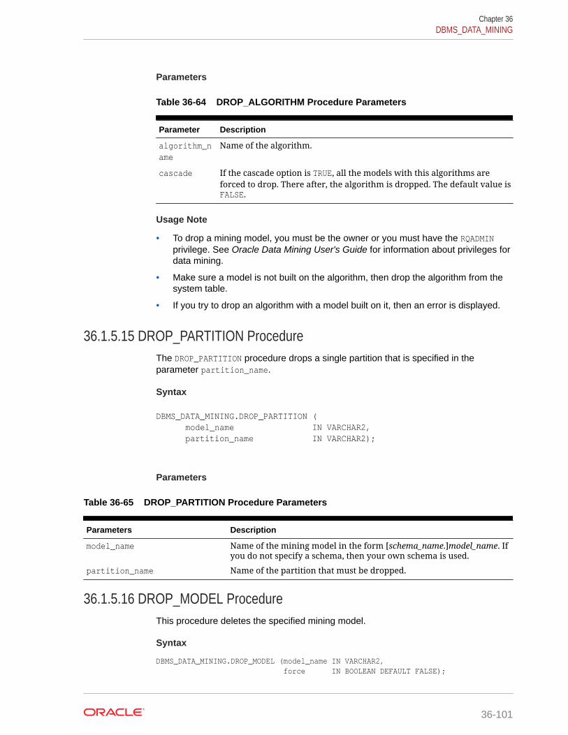
Parameters
Table 36-64 DROP_ALGORITHM Procedure Parameters
Parameter Description
algorithm_name
Name of the algorithm.
cascade If the cascade option is TRUE, all the models with this algorithms areforced to drop. There after, the algorithm is dropped. The default value isFALSE.
Usage Note
• To drop a mining model, you must be the owner or you must have the RQADMINprivilege. See Oracle Data Mining User's Guide for information about privileges fordata mining.
• Make sure a model is not built on the algorithm, then drop the algorithm from thesystem table.
• If you try to drop an algorithm with a model built on it, then an error is displayed.
36.1.5.15 DROP_PARTITION ProcedureThe DROP_PARTITION procedure drops a single partition that is specified in theparameter partition_name.
Syntax
DBMS_DATA_MINING.DROP_PARTITION ( model_name IN VARCHAR2, partition_name IN VARCHAR2);
Parameters
Table 36-65 DROP_PARTITION Procedure Parameters
Parameters Description
model_name Name of the mining model in the form [schema_name.]model_name. Ifyou do not specify a schema, then your own schema is used.
partition_name Name of the partition that must be dropped.
36.1.5.16 DROP_MODEL ProcedureThis procedure deletes the specified mining model.
Syntax
DBMS_DATA_MINING.DROP_MODEL (model_name IN VARCHAR2, force IN BOOLEAN DEFAULT FALSE);
Chapter 36DBMS_DATA_MINING
36-101
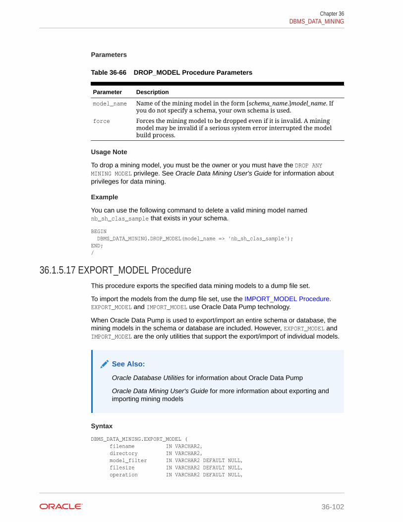
Parameters
Table 36-66 DROP_MODEL Procedure Parameters
Parameter Description
model_name Name of the mining model in the form [schema_name.]model_name. Ifyou do not specify a schema, your own schema is used.
force Forces the mining model to be dropped even if it is invalid. A miningmodel may be invalid if a serious system error interrupted the modelbuild process.
Usage Note
To drop a mining model, you must be the owner or you must have the DROP ANYMINING MODEL privilege. See Oracle Data Mining User's Guide for information aboutprivileges for data mining.
Example
You can use the following command to delete a valid mining model namednb_sh_clas_sample that exists in your schema.
BEGIN DBMS_DATA_MINING.DROP_MODEL(model_name => 'nb_sh_clas_sample');END;/
36.1.5.17 EXPORT_MODEL ProcedureThis procedure exports the specified data mining models to a dump file set.
To import the models from the dump file set, use the IMPORT_MODEL Procedure.EXPORT_MODEL and IMPORT_MODEL use Oracle Data Pump technology.
When Oracle Data Pump is used to export/import an entire schema or database, themining models in the schema or database are included. However, EXPORT_MODEL andIMPORT_MODEL are the only utilities that support the export/import of individual models.
See Also:
Oracle Database Utilities for information about Oracle Data Pump
Oracle Data Mining User's Guide for more information about exporting andimporting mining models
Syntax
DBMS_DATA_MINING.EXPORT_MODEL ( filename IN VARCHAR2, directory IN VARCHAR2, model_filter IN VARCHAR2 DEFAULT NULL, filesize IN VARCHAR2 DEFAULT NULL, operation IN VARCHAR2 DEFAULT NULL,
Chapter 36DBMS_DATA_MINING
36-102
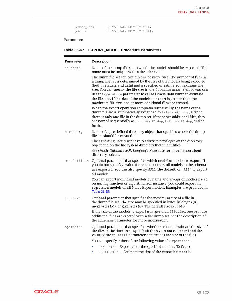
remote_link IN VARCHAR2 DEFAULT NULL, jobname IN VARCHAR2 DEFAULT NULL);
Parameters
Table 36-67 EXPORT_MODEL Procedure Parameters
Parameter Description
filename Name of the dump file set to which the models should be exported. Thename must be unique within the schema.The dump file set can contain one or more files. The number of files ina dump file set is determined by the size of the models being exported(both metadata and data) and a specified or estimated maximum filesize. You can specify the file size in the filesize parameter, or you canuse the operation parameter to cause Oracle Data Pump to estimatethe file size. If the size of the models to export is greater than themaximum file size, one or more additional files are created.When the export operation completes successfully, the name of thedump file set is automatically expanded to filename01.dmp, even ifthere is only one file in the dump set. If there are additional files, theyare named sequentially as filename02.dmp, filename03.dmp, and soforth.
directory Name of a pre-defined directory object that specifies where the dumpfile set should be created.The exporting user must have read/write privileges on the directoryobject and on the file system directory that it identifies.See Oracle Database SQL Language Reference for information aboutdirectory objects.
model_filter Optional parameter that specifies which model or models to export. Ifyou do not specify a value for model_filter, all models in the schemaare exported. You can also specify NULL (the default) or 'ALL' to exportall models.You can export individual models by name and groups of models basedon mining function or algorithm. For instance, you could export allregression models or all Naive Bayes models. Examples are provided inTable 36-68.
filesize Optional parameter that specifies the maximum size of a file inthe dump file set. The size may be specified in bytes, kilobytes (K),megabytes (M), or gigabytes (G). The default size is 50 MB.If the size of the models to export is larger than filesize, one or moreadditional files are created within the dump set. See the description ofthe filename parameter for more information.
operation Optional parameter that specifies whether or not to estimate the size ofthe files in the dump set. By default the size is not estimated and thevalue of the filesize parameter determines the size of the files.
You can specify either of the following values for operation:
• 'EXPORT' — Export all or the specified models. (Default)• 'ESTIMATE' — Estimate the size of the exporting models.
Chapter 36DBMS_DATA_MINING
36-103

Table 36-67 (Cont.) EXPORT_MODEL Procedure Parameters
Parameter Description
remote_link Optional parameter that specifies the name of a database link to aremote system. The default value is NULL. A database link is a schemaobject in a local database that enables access to objects in a remotedatabase. When you specify a value for remote_link, you can exportthe models in the remote database. The EXP_FULL_DATABASE role isrequired for exporting the remote models. The EXP_FULL_DATABASEprivilege, the CREATE DATABASE LINK privilege, and other privilegesmay also be required.
jobname Optional parameter that specifies the name of the export job. Bydefault, the name has the form username_exp_nnnn, where nnnn isa number. For example, a job name in the SCOTT schema might beSCOTT_exp_134.
If you specify a job name, it must be unique within the schema. Themaximum length of the job name is 30 characters.A log file for the export job, named jobname.log, is created in the samedirectory as the dump file set.
Usage Notes
The model_filter parameter specifies which models to export. You can list themodels by name, or you can specify all models that have the same mining functionor algorithm. You can query the USER_MINING_MODELS view to list the models in yourschema.
SQL> describe user_mining_models Name Null? Type ----------------------------------------- -------- ---------------------------- MODEL_NAME NOT NULL VARCHAR2(30) MINING_FUNCTION VARCHAR2(30) ALGORITHM VARCHAR2(30) CREATION_DATE NOT NULL DATE BUILD_DURATION NUMBER MODEL_SIZE NUMBER COMMENTS VARCHAR2(4000)
Examples of model filters are provided in Table 36-68.
Table 36-68 Sample Values for the Model Filter Parameter
Sample Value Meaning
'mymodel' Export the model named mymodel
'name= ''mymodel''' Export the model named mymodel
'name IN (''mymodel2'',''mymodel3'')' Export the models named mymodel2and mymodel3
'ALGORITHM_NAME = ''NAIVE_BAYES''' Export all Naive Bayes models. SeeTable 36-5 for a list of algorithm names.
'FUNCTION_NAME =''CLASSIFICATION''' Export all classification models. SeeTable 36-3 for a list of mining functions.
Chapter 36DBMS_DATA_MINING
36-104
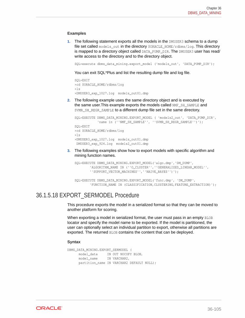
Examples
1. The following statement exports all the models in the DMUSER3 schema to a dumpfile set called models_out in the directory $ORACLE_HOME/rdbms/log. This directoryis mapped to a directory object called DATA_PUMP_DIR. The DMUSER3 user has read/write access to the directory and to the directory object.
SQL>execute dbms_data_mining.export_model ('models_out', 'DATA_PUMP_DIR');
You can exit SQL*Plus and list the resulting dump file and log file.
SQL>EXIT>cd $ORACLE_HOME/rdbms/log>ls>DMUSER3_exp_1027.log models_out01.dmp
2. The following example uses the same directory object and is executed bythe same user.This example exports the models called NMF_SH_SAMPLE andSVMR_SH_REGR_SAMPLE to a different dump file set in the same directory.
SQL>EXECUTE DBMS_DATA_MINING.EXPORT_MODEL ( 'models2_out', 'DATA_PUMP_DIR', 'name in (''NMF_SH_SAMPLE'', ''SVMR_SH_REGR_SAMPLE'')');SQL>EXIT>cd $ORACLE_HOME/rdbms/log>ls>DMUSER3_exp_1027.log models_out01.dmp DMUSER3_exp_924.log models2_out01.dmp
3. The following examples show how to export models with specific algorithm andmining function names.
SQL>EXECUTE DBMS_DATA_MINING.EXPORT_MODEL('algo.dmp','DM_DUMP', 'ALGORITHM_NAME IN (''O_CLUSTER'',''GENERALIZED_LINEAR_MODEL'', ''SUPPORT_VECTOR_MACHINES'',''NAIVE_BAYES'')'); SQL>EXECUTE DBMS_DATA_MINING.EXPORT_MODEL('func.dmp', 'DM_DUMP', 'FUNCTION_NAME IN (CLASSIFICATION,CLUSTERING,FEATURE_EXTRACTION)');
36.1.5.18 EXPORT_SERMODEL ProcedureThis procedure exports the model in a serialized format so that they can be moved toanother platform for scoring.
When exporting a model in serialized format, the user must pass in an empty BLOBlocator and specify the model name to be exported. If the model is partitioned, theuser can optionally select an individual partition to export, otherwise all partitions areexported. The returned BLOB contains the content that can be deployed.
Syntax
DBMS_DATA_MINING.EXPORT_SERMODEL ( model_data IN OUT NOCOPY BLOB, model_name IN VARCHAR2, partition_name IN VARCHAR2 DEFAULT NULL);
Chapter 36DBMS_DATA_MINING
36-105
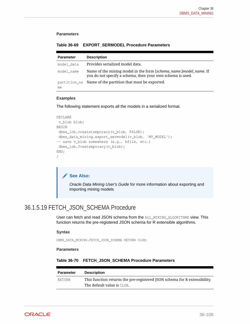
Parameters
Table 36-69 EXPORT_SERMODEL Procedure Parameters
Parameter Description
model_data Provides serialized model data.
model_name Name of the mining model in the form [schema_name.]model_name. Ifyou do not specify a schema, then your own schema is used.
partition_name
Name of the partition that must be exported.
Examples
The following statement exports all the models in a serialized format.
DECLARE v_blob blob;BEGIN dbms_lob.createtemporary(v_blob, FALSE); dbms_data_mining.export_sermodel(v_blob, 'MY_MODEL');-- save v_blob somewhere (e.g., bfile, etc.) dbms_lob.freetemporary(v_blob);END;/
See Also:
Oracle Data Mining User's Guide for more information about exporting andimporting mining models
36.1.5.19 FETCH_JSON_SCHEMA ProcedureUser can fetch and read JSON schema from the ALL_MINING_ALGORITHMS view. Thisfunction returns the pre-registered JSON schema for R extensible algorithms.
Syntax
DBMS_DATA_MINING.FETCH_JSON_SCHEMA RETURN CLOB;
Parameters
Table 36-70 FETCH_JSON_SCHEMA Procedure Parameters
Parameter Description
RETURN This function returns the pre-registered JSON schema for R extensibility.The default value is CLOB.
Chapter 36DBMS_DATA_MINING
36-106
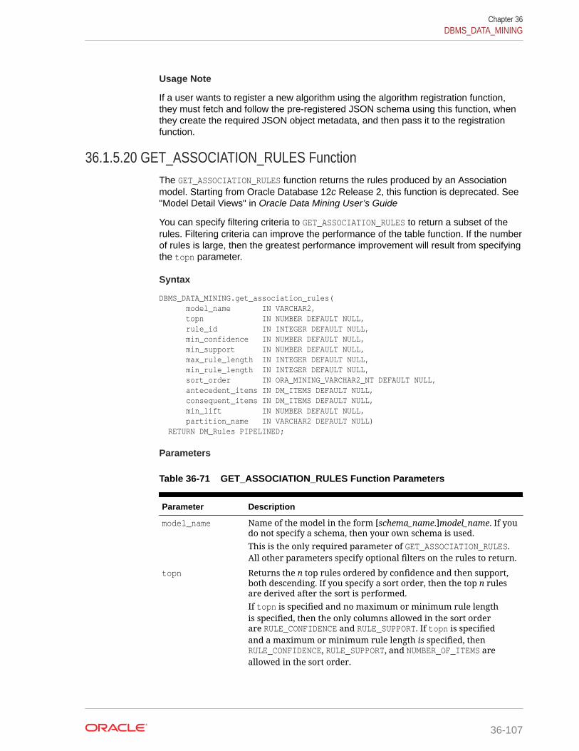
Usage Note
If a user wants to register a new algorithm using the algorithm registration function,they must fetch and follow the pre-registered JSON schema using this function, whenthey create the required JSON object metadata, and then pass it to the registrationfunction.
36.1.5.20 GET_ASSOCIATION_RULES FunctionThe GET_ASSOCIATION_RULES function returns the rules produced by an Associationmodel. Starting from Oracle Database 12c Release 2, this function is deprecated. See"Model Detail Views" in Oracle Data Mining User’s Guide
You can specify filtering criteria to GET_ASSOCIATION_RULES to return a subset of therules. Filtering criteria can improve the performance of the table function. If the numberof rules is large, then the greatest performance improvement will result from specifyingthe topn parameter.
Syntax
DBMS_DATA_MINING.get_association_rules( model_name IN VARCHAR2, topn IN NUMBER DEFAULT NULL, rule_id IN INTEGER DEFAULT NULL, min_confidence IN NUMBER DEFAULT NULL, min_support IN NUMBER DEFAULT NULL, max_rule_length IN INTEGER DEFAULT NULL, min_rule_length IN INTEGER DEFAULT NULL, sort_order IN ORA_MINING_VARCHAR2_NT DEFAULT NULL, antecedent_items IN DM_ITEMS DEFAULT NULL, consequent_items IN DM_ITEMS DEFAULT NULL, min_lift IN NUMBER DEFAULT NULL, partition_name IN VARCHAR2 DEFAULT NULL) RETURN DM_Rules PIPELINED;
Parameters
Table 36-71 GET_ASSOCIATION_RULES Function Parameters
Parameter Description
model_name Name of the model in the form [schema_name.]model_name. If youdo not specify a schema, then your own schema is used.This is the only required parameter of GET_ASSOCIATION_RULES.All other parameters specify optional filters on the rules to return.
topn Returns the n top rules ordered by confidence and then support,both descending. If you specify a sort order, then the top n rulesare derived after the sort is performed.If topn is specified and no maximum or minimum rule lengthis specified, then the only columns allowed in the sort orderare RULE_CONFIDENCE and RULE_SUPPORT. If topn is specifiedand a maximum or minimum rule length is specified, thenRULE_CONFIDENCE, RULE_SUPPORT, and NUMBER_OF_ITEMS areallowed in the sort order.
Chapter 36DBMS_DATA_MINING
36-107

Table 36-71 (Cont.) GET_ASSOCIATION_RULES Function Parameters
Parameter Description
rule_id Identifier of the rule to return. If you specify a value for rule_id,do not specify values for the other filtering parameters.
min_confidence Returns the rules with confidence greater than or equal to thisnumber.
min_support Returns the rules with support greater than or equal to thisnumber.
max_rule_length Returns the rules with a length less than or equal to this number.Rule length refers to the number of items in the rule (SeeNUMBER_OF_ITEMS in Table 36-72). For example, in the rule A=>B(if A, then B), the number of items is 2.If max_rule_length is specified, then the NUMBER_OF_ITEMScolumn is permitted in the sort order.
min_rule_length Returns the rules with a length greater than or equal to thisnumber. See max_rule_length for a description of rule length.
If min_rule_length is specified, then the NUMBER_OF_ITEMScolumn is permitted in the sort order.
sort_order Sorts the rules by the values in one or more of the returnedcolumns. Specify one or more column names, each followed by ASCfor ascending order or DESC for descending order. (See Table 36-72for the column names.)For example, to sort the result set in descending order first by theNUMBER_OF_ITEMS column, then by the RULE_CONFIDENCE column,you must specify:ORA_MINING_VARCHAR2_NT('NUMBER_OF_ITEMS DESC','RULE_CONFIDENCE DESC')
If you specify topn, the results will vary depending on the sortorder.By default, the results are sorted by Confidence in descendingorder, then by Support in descending order.
antecedent_items Returns the rules with these items in the antecedent.
consequent_items Returns the rules with this item in the consequent.
min_lift Returns the rules with lift greater than or equal to this number.
partition_name Specifies a partition in a partitioned model.
Return Values
The object type returned by GET_ASSOCIATION_RULES is described in Table 36-72. Fordescriptions of each field, see the Usage Notes.
Chapter 36DBMS_DATA_MINING
36-108
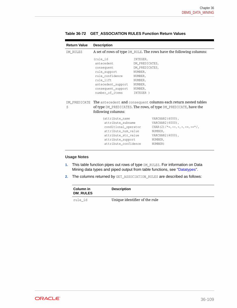
Table 36-72 GET_ASSOCIATION RULES Function Return Values
Return Value Description
DM_RULES A set of rows of type DM_RULE. The rows have the following columns:
(rule_id INTEGER, antecedent DM_PREDICATES, consequent DM_PREDICATES, rule_support NUMBER, rule_confidence NUMBER, rule_lift NUMBER, antecedent_support NUMBER, consequent_support NUMBER, number_of_items INTEGER )
DM_PREDICATES
The antecedent and consequent columns each return nested tablesof type DM_PREDICATES. The rows, of type DM_PREDICATE, have thefollowing columns:
(attribute_name VARCHAR2(4000), attribute_subname VARCHAR2(4000), conditional_operator CHAR(2)/*=,<>,<,>,<=,>=*/, attribute_num_value NUMBER, attribute_str_value VARCHAR2(4000), attribute_support NUMBER, attribute_confidence NUMBER)
Usage Notes
1. This table function pipes out rows of type DM_RULES. For information on DataMining data types and piped output from table functions, see "Datatypes".
2. The columns returned by GET_ASSOCIATION_RULES are described as follows:
Column inDM_RULES
Description
rule_id Unique identifier of the rule
Chapter 36DBMS_DATA_MINING
36-109

Column inDM_RULES
Description
antecedent The independent condition in the rule. When this conditionexists, the dependent condition in the consequent also exists.The condition is a combination of attribute values calleda predicate (DM_PREDICATE). The predicate specifies acondition for each attribute. The condition may specifyequality (=), inequality (<>), greater than (>), less than (<),greater than or equal to (>=), or less than or equal to (<=) agiven value.Support and Confidence for each attribute conditionin the antecedent is returned in the predicate. Supportis the number of transactions that satisfy the antecedent.Confidence is the likelihood that a transaction will satisfy theantecedent.Note: The occurence of the attribute as a DM_PREDICATEindicates the presence of the item in the transaction.The actual value for attribute_num_value orattribute_str_value is meaningless. For example, thefollowing predicate indicates that 'Mouse Pad' is present inthe transaction even though the attribute value is NULL.
DM_PREDICATE('PROD_NAME', 'Mouse Pad', '= ', NULL, NULL, NULL, NULL))
consequent The dependent condition in the rule. This condition existswhen the antecedent exists.The consequent, like the antecedent, is a predicate(DM_PREDICATE).
Support and confidence for each attribute condition inthe consequent is returned in the predicate. Support isthe number of transactions that satisfy the consequent.Confidence is the likelihood that a transaction will satisfy theconsequent.
rule_support The number of transactions that satisfy the rule.
rule_confidence The likelihood of a transaction satisfying the rule.
rule_lift The degree of improvement in the prediction over randomchance when the rule is satisfied.
antecedent_support The ratio of the number of transactions that satisfy theantecedent to the total number of transactions.
consequent_support The ratio of the number of transactions that satisfy theconsequent to the total number of transactions.
number_of_items The total number of attributes referenced in the antecedentand consequent of the rule.
Examples
The following example demonstrates an Association model build followed by severalinvocations of the GET_ASSOCIATION_RULES table function:
-- prepare a settings table to override default settingsCREATE TABLE market_settings ASSELECT * FROM TABLE(DBMS_DATA_MINING.GET_DEFAULT_SETTINGS)
Chapter 36DBMS_DATA_MINING
36-110
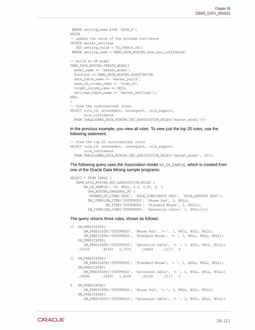
WHERE setting_name LIKE 'ASSO_%';BEGIN-- update the value of the minimum confidenceUPDATE market_settings SET setting_value = TO_CHAR(0.081) WHERE setting_name = DBMS_DATA_MINING.asso_min_confidence;
-- build an AR model DBMS_DATA_MINING.CREATE_MODEL( model_name => 'market_model', function => DBMS_DATA_MINING.ASSOCIATION, data_table_name => 'market_build', case_id_column_name => 'item_id', target_column_name => NULL, settings_table_name => 'market_settings');END;/-- View the (unformatted) rules SELECT rule_id, antecedent, consequent, rule_support, rule_confidence FROM TABLE(DBMS_DATA_MINING.GET_ASSOCIATION_RULES('market_model'));
In the previous example, you view all rules. To view just the top 20 rules, use thefollowing statement.
-- View the top 20 (unformatted) rulesSELECT rule_id, antecedent, consequent, rule_support, rule_confidence FROM TABLE(DBMS_DATA_MINING.GET_ASSOCIATION_RULES('market_model', 20));
The following query uses the Association model AR_SH_SAMPLE, which is created fromone of the Oracle Data Mining sample programs:
SELECT * FROM TABLE ( DBMS_DATA_MINING.GET_ASSOCIATION_RULES ( 'AR_SH_SAMPLE', 10, NULL, 0.5, 0.01, 2, 1, ORA_MINING_VARCHAR2_NT ( 'NUMBER_OF_ITEMS DESC', 'RULE_CONFIDENCE DESC', 'RULE_SUPPORT DESC'), DM_ITEMS(DM_ITEM('CUSTPRODS', 'Mouse Pad', 1, NULL), DM_ITEM('CUSTPRODS', 'Standard Mouse', 1, NULL)), DM_ITEMS(DM_ITEM('CUSTPRODS', 'Extension Cable', 1, NULL))));
The query returns three rules, shown as follows:
13 DM_PREDICATES( DM_PREDICATE('CUSTPRODS', 'Mouse Pad', '= ', 1, NULL, NULL, NULL), DM_PREDICATE('CUSTPRODS', 'Standard Mouse', '= ', 1, NULL, NULL, NULL)) DM_PREDICATES( DM_PREDICATE('CUSTPRODS', 'Extension Cable', '= ', 1, NULL, NULL, NULL)) .15532 .84393 2.7075 .18404 .3117 2 11 DM_PREDICATES( DM_PREDICATE('CUSTPRODS', 'Standard Mouse', '= ', 1, NULL, NULL, NULL)) DM_PREDICATES( DM_PREDICATE('CUSTPRODS', 'Extension Cable', '= ', 1, NULL, NULL, NULL)) .18085 .56291 1.8059 .32128 .3117 1 9 DM_PREDICATES( DM_PREDICATE('CUSTPRODS', 'Mouse Pad', '= ', 1, NULL, NULL, NULL)) DM_PREDICATES( DM_PREDICATE('CUSTPRODS', 'Extension Cable', '= ', 1, NULL, NULL, NULL))
Chapter 36DBMS_DATA_MINING
36-111
.17766 .55116 1.7682 .32234 .3117 1
See Also:
Table 36-72 for the DM_RULE column data types.
Oracle Data Mining User's Guide for information about the sample programs.
Oracle Data Mining User’s Guide for Model Detail Views.
36.1.5.21 GET_FREQUENT_ITEMSETS FunctionThe GET_FREQUENT_ITEMSETS function returns a set of rows that represent the frequentitemsets from an Association model. Starting from Oracle Database 12c Release 2,this function is deprecated. See "Model Detail Views" in Oracle Data Mining User’sGuide.
For a detailed description of frequent itemsets, consult Oracle Data Mining Concepts.
Syntax
DBMS_DATA_MINING.get_frequent_itemsets( model_name IN VARCHAR2, topn IN NUMBER DEFAULT NULL, max_itemset_length IN NUMBER DEFAULT NULL, partition_name IN VARCHAR2 DEFAULT NULL) RETURN DM_ItemSets PIPELINED;
Parameters
Table 36-73 GET_FREQUENT_ITEMSETS Function Parameters
Parameter Description
model_name Name of the model in the form [schema_name.]model_name. Ifyou do not specify a schema, then your own schema is used.
topn When not NULL, return the top n rows ordered by support indescending order
max_itemset_length Maximum length of an item set.
partition_name Specifies a partition in a partitioned model.
Note:
The partition_name columnsapplies only when the model ispartitioned.
Chapter 36DBMS_DATA_MINING
36-112

Return Values
Table 36-74 GET_FREQUENT_ITEMSETS Function Return Values
Return Value Description
DM_ITEMSETS A set of rows of type DM_ITEMSET. The rows have the following columns:
(partition_name VARCHAR2(128)itemsets_id NUMBER,items DM_ITEMS,support NUMBER,number_of_items NUMBER)
Note:
The partition_name columns applies onlywhen the model is partitioned.
The items column returns a nested table of type DM_ITEMS. The rowshave type DM_ITEM:
(attribute_name VARCHAR2(4000),attribute_subname VARCHAR2(4000),attribute_num_value NUMBER,attribute_str_value VARCHAR2(4000))
Usage Notes
This table function pipes out rows of type DM_ITEMSETS. For information on Data Miningdatatypes and piped output from table functions, see "Datatypes".
Examples
The following example demonstrates an Association model build followed by aninvocation of GET_FREQUENT_ITEMSETS table function from Oracle SQL.
-- prepare a settings table to override default settingsCREATE TABLE market_settings AS
SELECT *
FROM TABLE(DBMS_DATA_MINING.GET_DEFAULT_SETTINGS) WHERE setting_name LIKE 'ASSO_%';BEGIN-- update the value of the minimum confidenceUPDATE market_settings SET setting_value = TO_CHAR(0.081) WHERE setting_name = DBMS_DATA_MINING.asso_min_confidence;
/* build a AR model */DBMS_DATA_MINING.CREATE_MODEL( model_name => 'market_model', function => DBMS_DATA_MINING.ASSOCIATION, data_table_name => 'market_build', case_id_column_name => 'item_id',
Chapter 36DBMS_DATA_MINING
36-113
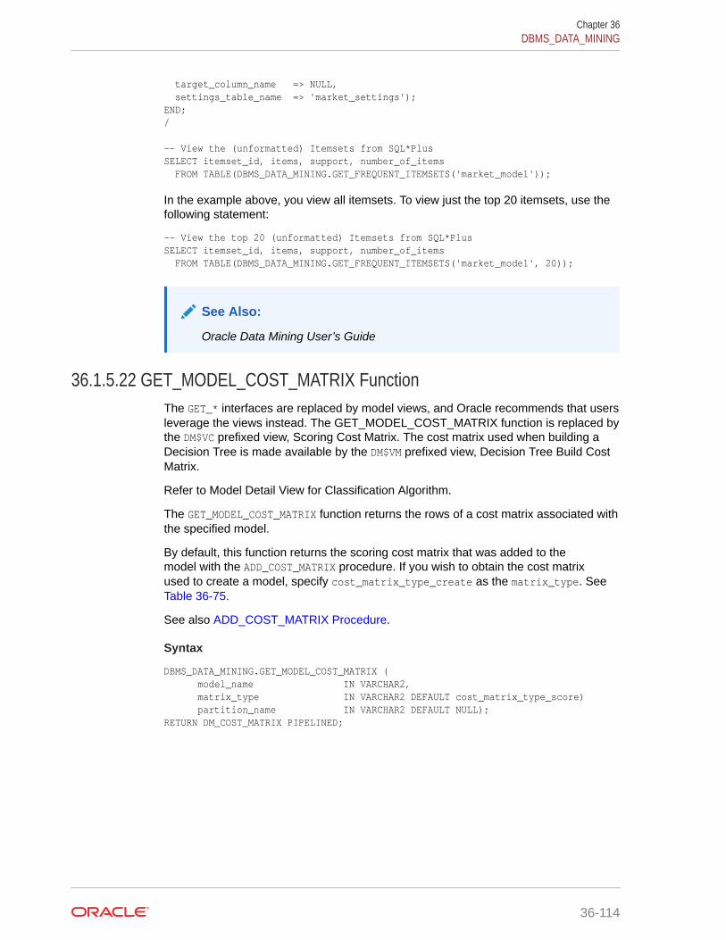
target_column_name => NULL, settings_table_name => 'market_settings');END;/
-- View the (unformatted) Itemsets from SQL*PlusSELECT itemset_id, items, support, number_of_items FROM TABLE(DBMS_DATA_MINING.GET_FREQUENT_ITEMSETS('market_model'));
In the example above, you view all itemsets. To view just the top 20 itemsets, use thefollowing statement:
-- View the top 20 (unformatted) Itemsets from SQL*PlusSELECT itemset_id, items, support, number_of_items FROM TABLE(DBMS_DATA_MINING.GET_FREQUENT_ITEMSETS('market_model', 20));
See Also:
Oracle Data Mining User’s Guide
36.1.5.22 GET_MODEL_COST_MATRIX FunctionThe GET_* interfaces are replaced by model views, and Oracle recommends that usersleverage the views instead. The GET_MODEL_COST_MATRIX function is replaced bythe DM$VC prefixed view, Scoring Cost Matrix. The cost matrix used when building aDecision Tree is made available by the DM$VM prefixed view, Decision Tree Build CostMatrix.
Refer to Model Detail View for Classification Algorithm.
The GET_MODEL_COST_MATRIX function returns the rows of a cost matrix associated withthe specified model.
By default, this function returns the scoring cost matrix that was added to themodel with the ADD_COST_MATRIX procedure. If you wish to obtain the cost matrixused to create a model, specify cost_matrix_type_create as the matrix_type. SeeTable 36-75.
See also ADD_COST_MATRIX Procedure.
Syntax
DBMS_DATA_MINING.GET_MODEL_COST_MATRIX ( model_name IN VARCHAR2, matrix_type IN VARCHAR2 DEFAULT cost_matrix_type_score) partition_name IN VARCHAR2 DEFAULT NULL);RETURN DM_COST_MATRIX PIPELINED;
Chapter 36DBMS_DATA_MINING
36-114
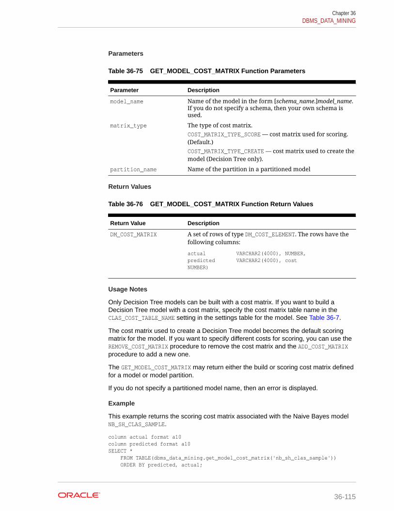
Parameters
Table 36-75 GET_MODEL_COST_MATRIX Function Parameters
Parameter Description
model_name Name of the model in the form [schema_name.]model_name.If you do not specify a schema, then your own schema isused.
matrix_type The type of cost matrix.COST_MATRIX_TYPE_SCORE — cost matrix used for scoring.(Default.)COST_MATRIX_TYPE_CREATE — cost matrix used to create themodel (Decision Tree only).
partition_name Name of the partition in a partitioned model
Return Values
Table 36-76 GET_MODEL_COST_MATRIX Function Return Values
Return Value Description
DM_COST_MATRIX A set of rows of type DM_COST_ELEMENT. The rows have thefollowing columns:
actual VARCHAR2(4000), NUMBER, predicted VARCHAR2(4000), cost NUMBER)
Usage Notes
Only Decision Tree models can be built with a cost matrix. If you want to build aDecision Tree model with a cost matrix, specify the cost matrix table name in theCLAS_COST_TABLE_NAME setting in the settings table for the model. See Table 36-7.
The cost matrix used to create a Decision Tree model becomes the default scoringmatrix for the model. If you want to specify different costs for scoring, you can use theREMOVE_COST_MATRIX procedure to remove the cost matrix and the ADD_COST_MATRIXprocedure to add a new one.
The GET_MODEL_COST_MATRIX may return either the build or scoring cost matrix definedfor a model or model partition.
If you do not specify a partitioned model name, then an error is displayed.
Example
This example returns the scoring cost matrix associated with the Naive Bayes modelNB_SH_CLAS_SAMPLE.
column actual format a10column predicted format a10SELECT * FROM TABLE(dbms_data_mining.get_model_cost_matrix('nb_sh_clas_sample')) ORDER BY predicted, actual;
Chapter 36DBMS_DATA_MINING
36-115
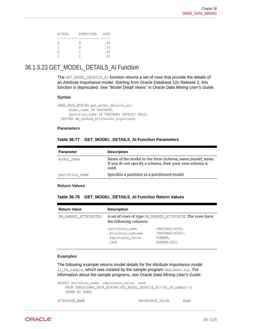
ACTUAL PREDICTED COST---------- ---------- -----0 0 .001 0 .750 1 .251 1 .00
36.1.5.23 GET_MODEL_DETAILS_AI FunctionThe GET_MODEL_DETAILS_AI function returns a set of rows that provide the details ofan Attribute Importance model. Starting from Oracle Database 12c Release 2, thisfunction is deprecated. See "Model Detail Views" in Oracle Data Mining User’s Guide.
Syntax
DBMS_DATA_MINING.get_model_details_ai( model_name IN VARCHAR2, partition_name IN VARCHAR2 DEFAULT NULL) RETURN dm_ranked_attributes pipelined;
Parameters
Table 36-77 GET_MODEL_DETAILS_AI Function Parameters
Parameter Description
model_name Name of the model in the form [schema_name.]model_name.If you do not specify a schema, then your own schema isused.
partition_name Specifies a partition in a partitioned model.
Return Values
Table 36-78 GET_MODEL_DETAILS_AI Function Return Values
Return Value Description
DM_RANKED_ATTRIBUTES A set of rows of type DM_RANKED_ATTRIBUTE. The rows havethe following columns:
(attribute_name VARCHAR2(4000, attribute_subname VARCHAR2(4000), importance_value NUMBER, rank NUMBER(38))
Examples
The following example returns model details for the Attribute Importance modelAI_SH_sample, which was created by the sample program dmaidemo.sql. Forinformation about the sample programs, see Oracle Data Mining User's Guide.
SELECT attribute_name, importance_value, rank FROM TABLE(DBMS_DATA_MINING.GET_MODEL_DETAILS_AI('AI_SH_sample')) ORDER BY RANK; ATTRIBUTE_NAME IMPORTANCE_VALUE RANK
Chapter 36DBMS_DATA_MINING
36-116

---------------------------------------- ---------------- ----------HOUSEHOLD_SIZE .151685183 1CUST_MARITAL_STATUS .145294546 2YRS_RESIDENCE .07838928 3AGE .075027496 4Y_BOX_GAMES .063039952 5EDUCATION .059605314 6HOME_THEATER_PACKAGE .056458722 7OCCUPATION .054652937 8CUST_GENDER .035264741 9BOOKKEEPING_APPLICATION .019204751 10PRINTER_SUPPLIES 0 11OS_DOC_SET_KANJI -.00050013 12FLAT_PANEL_MONITOR -.00509564 13BULK_PACK_DISKETTES -.00540822 14COUNTRY_NAME -.01201116 15CUST_INCOME_LEVEL -.03951311 16
36.1.5.24 GET_MODEL_DETAILS_EM FunctionThe GET_MODEL_DETAILS_EM function returns a set of rows that provide statistics aboutthe clusters produced by an Expectation Maximization model. Starting from OracleDatabase 12c Release 2, this function is deprecated. See "Model Detail Views" inOracle Data Mining User’s Guide.
By default, the EM algorithm groups components into high-level clusters, andGET_MODEL_DETAILS_EM returns only the high-level clusters with their hierarchies.Alternatively, you can configure EM model to disable the grouping of componentsinto high-level clusters. In this case, GET_MODEL_DETAILS_EM returns the componentsthemselves as clusters with their hierarchies. See Table 36-12.
Syntax
DBMS_DATA_MINING.get_model_details_em( model_name VARCHAR2, cluster_id NUMBER DEFAULT NULL, attribute VARCHAR2 DEFAULT NULL, centroid NUMBER DEFAULT 1, histogram NUMBER DEFAULT 1, rules NUMBER DEFAULT 2, attribute_subname VARCHAR2 DEFAULT NULL, topn_attributes NUMBER DEFAULT NULL, partition_name IN VARCHAR2 DEFAULT NULL) RETURN dm_clusters PIPELINED;
Parameters
Table 36-79 GET_MODEL_DETAILS_EM Function Parameters
Parameter Description
model_name Name of the model in the form [schema_name.]model_name.If you do not specify a schema, then your own schema isused.
cluster_id The ID of a cluster in the model. When a valid cluster IDis specified, only the details of this cluster are returned.Otherwise, the details for all clusters are returned.
Chapter 36DBMS_DATA_MINING
36-117
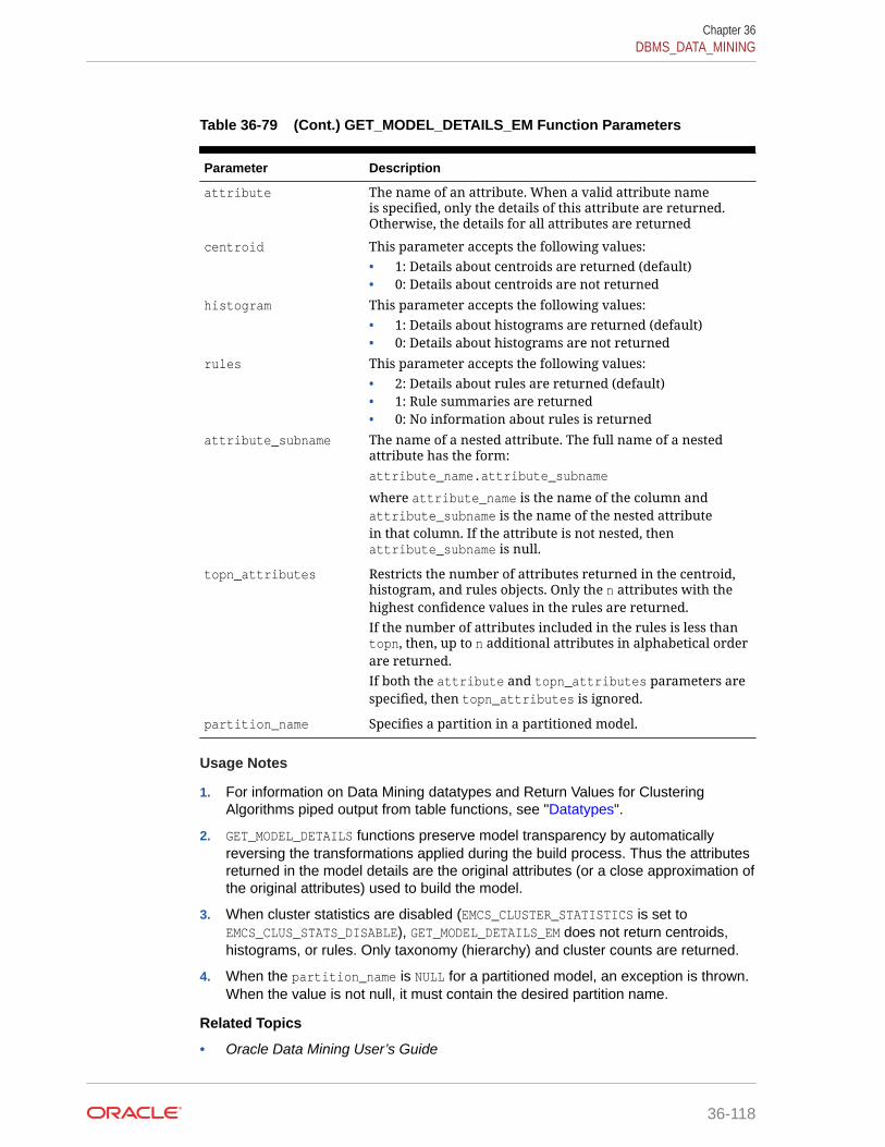
Table 36-79 (Cont.) GET_MODEL_DETAILS_EM Function Parameters
Parameter Description
attribute The name of an attribute. When a valid attribute nameis specified, only the details of this attribute are returned.Otherwise, the details for all attributes are returned
centroid This parameter accepts the following values:• 1: Details about centroids are returned (default)• 0: Details about centroids are not returned
histogram This parameter accepts the following values:• 1: Details about histograms are returned (default)• 0: Details about histograms are not returned
rules This parameter accepts the following values:• 2: Details about rules are returned (default)• 1: Rule summaries are returned• 0: No information about rules is returned
attribute_subname The name of a nested attribute. The full name of a nestedattribute has the form:attribute_name.attribute_subname
where attribute_name is the name of the column andattribute_subname is the name of the nested attributein that column. If the attribute is not nested, thenattribute_subname is null.
topn_attributes Restricts the number of attributes returned in the centroid,histogram, and rules objects. Only the n attributes with thehighest confidence values in the rules are returned.If the number of attributes included in the rules is less thantopn, then, up to n additional attributes in alphabetical orderare returned.If both the attribute and topn_attributes parameters arespecified, then topn_attributes is ignored.
partition_name Specifies a partition in a partitioned model.
Usage Notes
1. For information on Data Mining datatypes and Return Values for ClusteringAlgorithms piped output from table functions, see "Datatypes".
2. GET_MODEL_DETAILS functions preserve model transparency by automaticallyreversing the transformations applied during the build process. Thus the attributesreturned in the model details are the original attributes (or a close approximation ofthe original attributes) used to build the model.
3. When cluster statistics are disabled (EMCS_CLUSTER_STATISTICS is set toEMCS_CLUS_STATS_DISABLE), GET_MODEL_DETAILS_EM does not return centroids,histograms, or rules. Only taxonomy (hierarchy) and cluster counts are returned.
4. When the partition_name is NULL for a partitioned model, an exception is thrown.When the value is not null, it must contain the desired partition name.
Related Topics
• Oracle Data Mining User’s Guide
Chapter 36DBMS_DATA_MINING
36-118
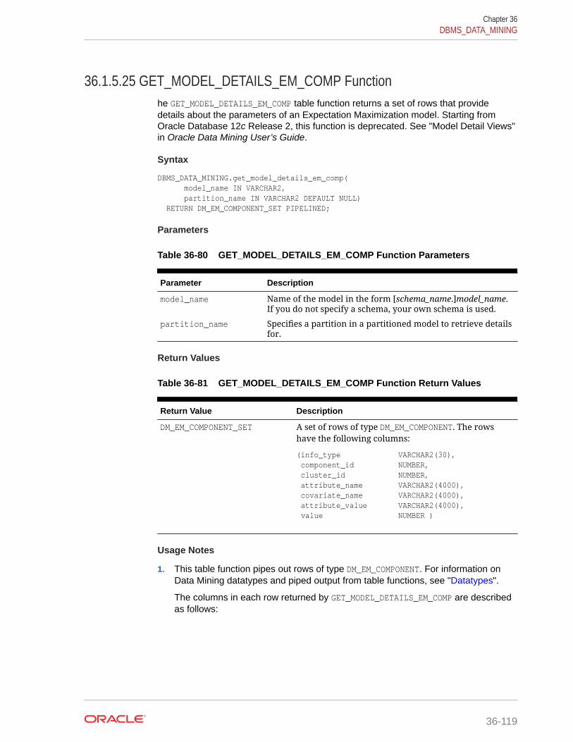
36.1.5.25 GET_MODEL_DETAILS_EM_COMP Functionhe GET_MODEL_DETAILS_EM_COMP table function returns a set of rows that providedetails about the parameters of an Expectation Maximization model. Starting fromOracle Database 12c Release 2, this function is deprecated. See "Model Detail Views"in Oracle Data Mining User’s Guide.
Syntax
DBMS_DATA_MINING.get_model_details_em_comp( model_name IN VARCHAR2, partition_name IN VARCHAR2 DEFAULT NULL) RETURN DM_EM_COMPONENT_SET PIPELINED;
Parameters
Table 36-80 GET_MODEL_DETAILS_EM_COMP Function Parameters
Parameter Description
model_name Name of the model in the form [schema_name.]model_name.If you do not specify a schema, your own schema is used.
partition_name Specifies a partition in a partitioned model to retrieve detailsfor.
Return Values
Table 36-81 GET_MODEL_DETAILS_EM_COMP Function Return Values
Return Value Description
DM_EM_COMPONENT_SET A set of rows of type DM_EM_COMPONENT. The rowshave the following columns:
(info_type VARCHAR2(30), component_id NUMBER, cluster_id NUMBER, attribute_name VARCHAR2(4000), covariate_name VARCHAR2(4000), attribute_value VARCHAR2(4000), value NUMBER )
Usage Notes
1. This table function pipes out rows of type DM_EM_COMPONENT. For information onData Mining datatypes and piped output from table functions, see "Datatypes".
The columns in each row returned by GET_MODEL_DETAILS_EM_COMP are describedas follows:
Chapter 36DBMS_DATA_MINING
36-119
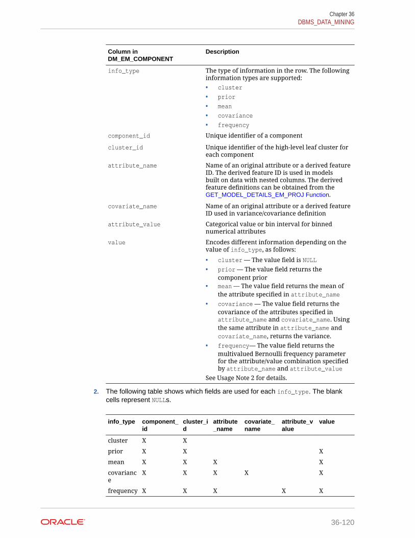
Column inDM_EM_COMPONENT
Description
info_type The type of information in the row. The followinginformation types are supported:• cluster
• prior
• mean
• covariance
• frequency
component_id Unique identifier of a component
cluster_id Unique identifier of the high-level leaf cluster foreach component
attribute_name Name of an original attribute or a derived featureID. The derived feature ID is used in modelsbuilt on data with nested columns. The derivedfeature definitions can be obtained from theGET_MODEL_DETAILS_EM_PROJ Function.
covariate_name Name of an original attribute or a derived featureID used in variance/covariance definition
attribute_value Categorical value or bin interval for binnednumerical attributes
value Encodes different information depending on thevalue of info_type, as follows:
• cluster — The value field is NULL• prior — The value field returns the
component prior• mean — The value field returns the mean of
the attribute specified in attribute_name• covariance — The value field returns the
covariance of the attributes specified inattribute_name and covariate_name. Usingthe same attribute in attribute_name andcovariate_name, returns the variance.
• frequency— The value field returns themultivalued Bernoulli frequency parameterfor the attribute/value combination specifiedby attribute_name and attribute_value
See Usage Note 2 for details.
2. The following table shows which fields are used for each info_type. The blankcells represent NULLs.
info_type component_id
cluster_id
attribute_name
covariate_name
attribute_value
value
cluster X X
prior X X X
mean X X X X
covariance
X X X X X
frequency X X X X X
Chapter 36DBMS_DATA_MINING
36-120
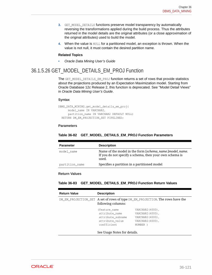
3. GET_MODEL_DETAILS functions preserve model transparency by automaticallyreversing the transformations applied during the build process. Thus the attributesreturned in the model details are the original attributes (or a close approximation ofthe original attributes) used to build the model.
4. When the value is NULL for a partitioned model, an exception is thrown. When thevalue is not null, it must contain the desired partition name.
Related Topics
• Oracle Data Mining User’s Guide
36.1.5.26 GET_MODEL_DETAILS_EM_PROJ FunctionThe GET_MODEL_DETAILS_EM_PROJ function returns a set of rows that provide statisticsabout the projections produced by an Expectation Maximization model. Starting fromOracle Database 12c Release 2, this function is deprecated. See "Model Detail Views"in Oracle Data Mining User’s Guide.
Syntax
DBMS_DATA_MINING.get_model_details_em_proj( model_name IN VARCHAR2, partition_name IN VARCHAR2 DEFAULT NULL) RETURN DM_EM_PROJECTION_SET PIPELINED;
Parameters
Table 36-82 GET_MODEL_DETAILS_EM_PROJ Function Parameters
Parameter Description
model_name Name of the model in the form [schema_name.]model_name.If you do not specify a schema, then your own schema isused.
partition_name Specifies a partition in a partitioned model
Return Values
Table 36-83 GET_MODEL_DETAILS_EM_PROJ Function Return Values
Return Value Description
DM_EM_PROJECTION_SET A set of rows of type DM_EM_PROJECTION. The rows have thefollowing columns:
(feature_name VARCHAR2(4000), attribute_name VARCHAR2(4000), attribute_subname VARCHAR2(4000), attribute_value VARCHAR2(4000), coefficient NUMBER )
See Usage Notes for details.
Chapter 36DBMS_DATA_MINING
36-121
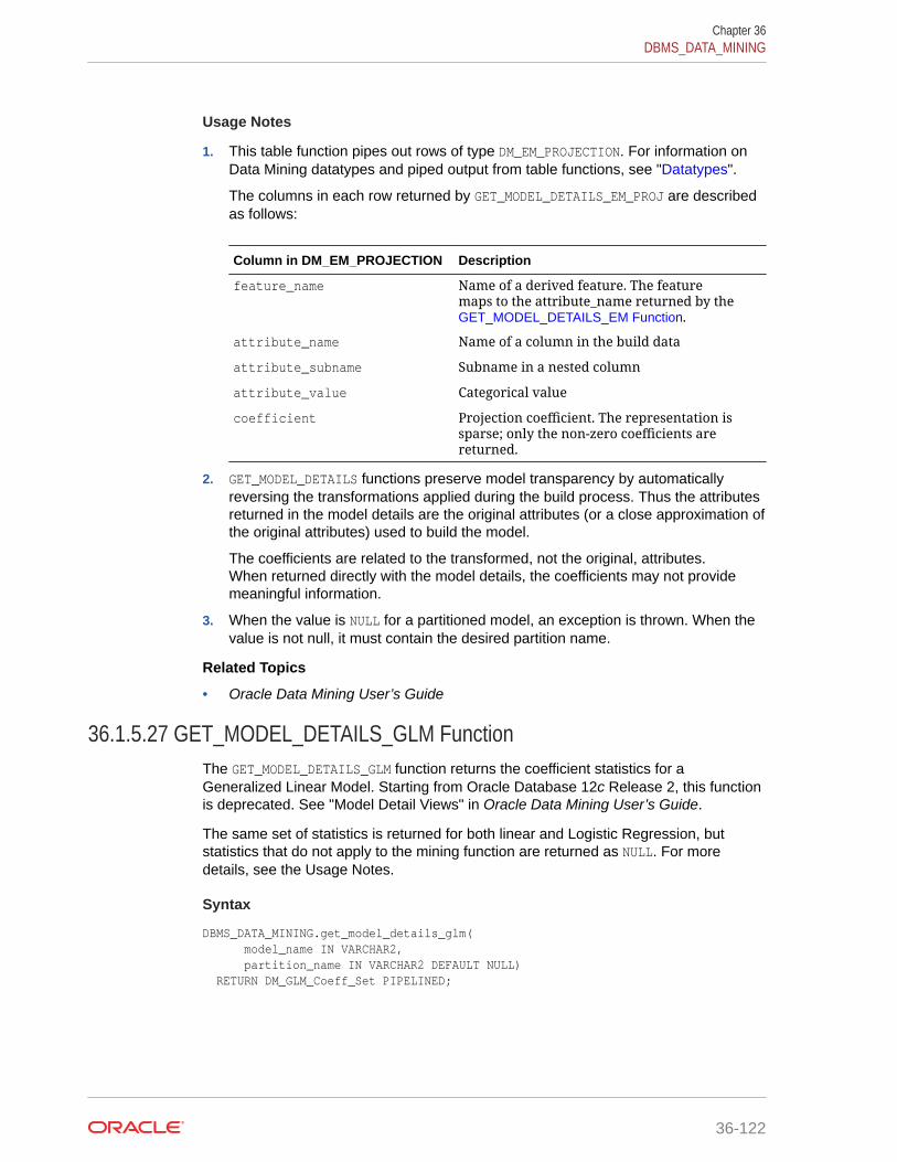
Usage Notes
1. This table function pipes out rows of type DM_EM_PROJECTION. For information onData Mining datatypes and piped output from table functions, see "Datatypes".
The columns in each row returned by GET_MODEL_DETAILS_EM_PROJ are describedas follows:
Column in DM_EM_PROJECTION Description
feature_name Name of a derived feature. The featuremaps to the attribute_name returned by theGET_MODEL_DETAILS_EM Function.
attribute_name Name of a column in the build data
attribute_subname Subname in a nested column
attribute_value Categorical value
coefficient Projection coefficient. The representation issparse; only the non-zero coefficients arereturned.
2. GET_MODEL_DETAILS functions preserve model transparency by automaticallyreversing the transformations applied during the build process. Thus the attributesreturned in the model details are the original attributes (or a close approximation ofthe original attributes) used to build the model.
The coefficients are related to the transformed, not the original, attributes.When returned directly with the model details, the coefficients may not providemeaningful information.
3. When the value is NULL for a partitioned model, an exception is thrown. When thevalue is not null, it must contain the desired partition name.
Related Topics
• Oracle Data Mining User’s Guide
36.1.5.27 GET_MODEL_DETAILS_GLM FunctionThe GET_MODEL_DETAILS_GLM function returns the coefficient statistics for aGeneralized Linear Model. Starting from Oracle Database 12c Release 2, this functionis deprecated. See "Model Detail Views" in Oracle Data Mining User’s Guide.
The same set of statistics is returned for both linear and Logistic Regression, butstatistics that do not apply to the mining function are returned as NULL. For moredetails, see the Usage Notes.
Syntax
DBMS_DATA_MINING.get_model_details_glm( model_name IN VARCHAR2, partition_name IN VARCHAR2 DEFAULT NULL) RETURN DM_GLM_Coeff_Set PIPELINED;
Chapter 36DBMS_DATA_MINING
36-122
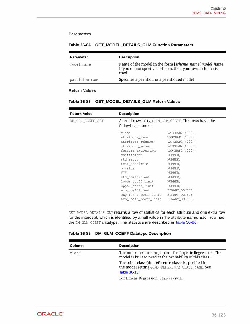
Parameters
Table 36-84 GET_MODEL_DETAILS_GLM Function Parameters
Parameter Description
model_name Name of the model in the form [schema_name.]model_name.If you do not specify a schema, then your own schema isused.
partition_name Specifies a partition in a partitioned model
Return Values
Table 36-85 GET_MODEL_DETAILS_GLM Return Values
Return Value Description
DM_GLM_COEFF_SET A set of rows of type DM_GLM_COEFF. The rows have thefollowing columns:
(class VARCHAR2(4000), attribute_name VARCHAR2(4000), attribute_subname VARCHAR2(4000), attribute_value VARCHAR2(4000), feature_expression VARCHAR2(4000), coefficient NUMBER, std_error NUMBER, test_statistic NUMBER, p_value NUMBER, VIF NUMBER, std_coefficient NUMBER, lower_coeff_limit NUMBER, upper_coeff_limit NUMBER, exp_coefficient BINARY_DOUBLE, exp_lower_coeff_limit BINARY_DOUBLE, exp_upper_coeff_limit BINARY_DOUBLE)
GET_MODEL_DETAILS_GLM returns a row of statistics for each attribute and one extra rowfor the intercept, which is identified by a null value in the attribute name. Each row hasthe DM_GLM_COEFF datatype. The statistics are described in Table 36-86.
Table 36-86 DM_GLM_COEFF Datatype Description
Column Description
class The non-reference target class for Logistic Regression. Themodel is built to predict the probability of this class.The other class (the reference class) is specified inthe model setting GLMS_REFERENCE_CLASS_NAME. SeeTable 36-18.
For Linear Regression, class is null.
Chapter 36DBMS_DATA_MINING
36-123
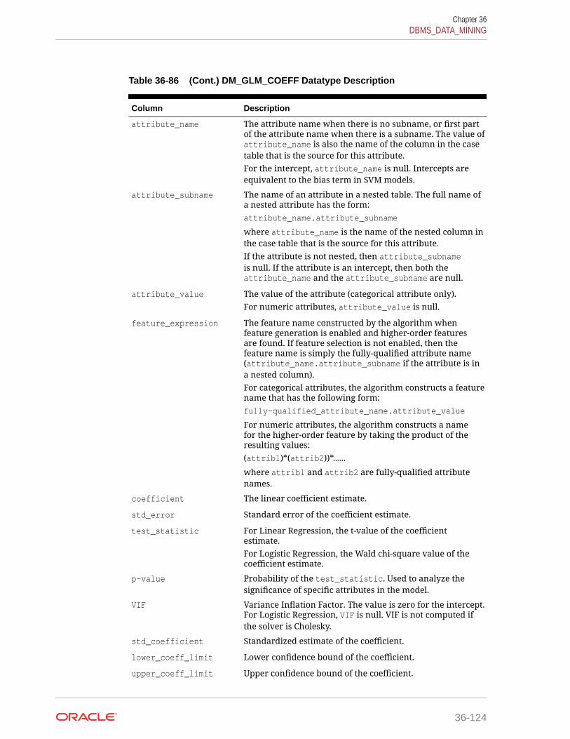
Table 36-86 (Cont.) DM_GLM_COEFF Datatype Description
Column Description
attribute_name The attribute name when there is no subname, or first partof the attribute name when there is a subname. The value ofattribute_name is also the name of the column in the casetable that is the source for this attribute.For the intercept, attribute_name is null. Intercepts areequivalent to the bias term in SVM models.
attribute_subname The name of an attribute in a nested table. The full name ofa nested attribute has the form:attribute_name.attribute_subname
where attribute_name is the name of the nested column inthe case table that is the source for this attribute.If the attribute is not nested, then attribute_subnameis null. If the attribute is an intercept, then both theattribute_name and the attribute_subname are null.
attribute_value The value of the attribute (categorical attribute only).For numeric attributes, attribute_value is null.
feature_expression The feature name constructed by the algorithm whenfeature generation is enabled and higher-order featuresare found. If feature selection is not enabled, then thefeature name is simply the fully-qualified attribute name(attribute_name.attribute_subname if the attribute is ina nested column).For categorical attributes, the algorithm constructs a featurename that has the following form:fully-qualified_attribute_name.attribute_value
For numeric attributes, the algorithm constructs a namefor the higher-order feature by taking the product of theresulting values:(attrib1)*(attrib2))*......
where attrib1 and attrib2 are fully-qualified attributenames.
coefficient The linear coefficient estimate.
std_error Standard error of the coefficient estimate.
test_statistic For Linear Regression, the t-value of the coefficientestimate.For Logistic Regression, the Wald chi-square value of thecoefficient estimate.
p-value Probability of the test_statistic. Used to analyze thesignificance of specific attributes in the model.
VIF Variance Inflation Factor. The value is zero for the intercept.For Logistic Regression, VIF is null. VIF is not computed ifthe solver is Cholesky.
std_coefficient Standardized estimate of the coefficient.
lower_coeff_limit Lower confidence bound of the coefficient.
upper_coeff_limit Upper confidence bound of the coefficient.
Chapter 36DBMS_DATA_MINING
36-124

Table 36-86 (Cont.) DM_GLM_COEFF Datatype Description
Column Description
exp_coefficient Exponentiated coefficient for Logistic Regression. For LinearRegression, exp_coefficient is null.
exp_lower_coeff_limit Exponentiated coefficient for lower confidence bound of thecoefficient for Logistic Regression. For Linear Regression,exp_lower_coeff_limit is null.
exp_upper_coeff_limit Exponentiated coefficient for upper confidence boundof the coefficient for Logistic Regression. For LinearRegression, exp_lower_coeff_limit is null.
Usage Notes
Not all statistics are necessarily returned for each coefficient. Statistics will be null if:
• They do not apply to the mining function. For example, exp_coefficient does notapply to Linear Regression.
• They cannot be computed from a theoretical standpoint. For information on ridgeregression, see Table 36-18.
• They cannot be computed because of limitations in system resources.
• Their values would be infinity.
• When the value is NULL for a partitioned model, an exception is thrown. When thevalue is not null, it must contain the desired partition name.
Examples
The following example returns some of the model details for the GLMRegression model GLMR_SH_Regr_sample, which was created by the sample programdmglrdem.sql. For information about the sample programs, see Oracle Data MiningUser's Guide.
SET line 120SET pages 99column attribute_name format a30column attribute_subname format a20column attribute_value format a20col coefficient format 990.9999col std_error format 990.9999SQL> SELECT * FROM(SELECT attribute_name, attribute_value, coefficient, std_error FROM DM$VDGLMR_SH_REGR_SAMPLE order by 1,2)WHERE rownum < 11;
ATTRIBUTE_NAME ATTRIBUTE_VALUE COEFFICIENT STD_ERROR------------------------------ -------------------- ----------- ---------AFFINITY_CARD -0.5797 0.5283BOOKKEEPING_APPLICATION -0.4689 3.8872BULK_PACK_DISKETTES -0.9819 2.5430COUNTRY_NAME Argentina -1.2020 1.1876COUNTRY_NAME Australia -0.0071 5.1146COUNTRY_NAME Brazil 5.2931 1.9233COUNTRY_NAME Canada 4.0191 2.4108COUNTRY_NAME China 0.8706 3.5889
Chapter 36DBMS_DATA_MINING
36-125

COUNTRY_NAME Denmark -2.9822 3.1803COUNTRY_NAME France -1.1044 7.1811
Related Topics
• Oracle Data Mining User’s Guide
36.1.5.28 GET_MODEL_DETAILS_GLOBAL FunctionThe GET_MODEL_DETAILS_GLOBAL function returns statistics about the model as awhole. Starting from Oracle Database 12c Release 2, this function is deprecated. See"Model Detail Views" in Oracle Data Mining User’s Guide.
Global details are available for Generalized Linear Models, Association Rules,Singular Value Decomposition, and Expectation Maximization. There are new Globalmodel views which show global information for all algorithms. Oracle recommends thatusers leverage the views instead. Refer to Model Details View Global.
Syntax
DBMS_DATA_MINING.get_model_details_global( model_name IN VARCHAR2, partition_name IN VARCHAR2 DEFAULT NULL) RETURN DM_model_global_details PIPELINED;
Parameters
Table 36-87 GET_MODEL_DETAILS_GLOBAL Function Parameters
Parameter Description
model_name Name of the model in the form [schema_name.]model_name.If you do not specify a schema, then your own schema isused.
partition_name Specifies a partition in a partitioned model.
Return Values
Table 36-88 GET_MODEL_DETAILS_GLOBAL Function Return Values
Return Value Description
DM_MODEL_GLOBAL_DETAILS A collection of rows of typeDM_MODEL_GLOBAL_DETAIL. The rows have thefollowing columns:
(global_detail_name VARCHAR2(30), global_detail_value NUMBER)
Examples
The following example returns the global model details for the GLM Regression modelGLMR_SH_Regr_sample, which was created by the sample program dmglrdem.sql. Forinformation about the sample programs, see Oracle Data Mining User's Guide.
SELECT * FROM TABLE(dbms_data_mining.get_model_details_global(
Chapter 36DBMS_DATA_MINING
36-126
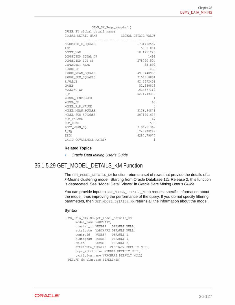
'GLMR_SH_Regr_sample'))ORDER BY global_detail_name;GLOBAL_DETAIL_NAME GLOBAL_DETAIL_VALUE------------------------------ -------------------ADJUSTED_R_SQUARE .731412557AIC 5931.814COEFF_VAR 18.1711243CORRECTED_TOTAL_DF 1499CORRECTED_TOT_SS 278740.504DEPENDENT_MEAN 38.892ERROR_DF 1433ERROR_MEAN_SQUARE 49.9440956ERROR_SUM_SQUARES 71569.8891F_VALUE 62.8492452GMSEP 52.280819HOCKING_SP .034877162J_P 52.1749319MODEL_CONVERGED 1MODEL_DF 66MODEL_F_P_VALUE 0MODEL_MEAN_SQUARE 3138.94871MODEL_SUM_SQUARES 207170.615NUM_PARAMS 67NUM_ROWS 1500ROOT_MEAN_SQ 7.06711367R_SQ .743238288SBIC 6287.79977VALID_COVARIANCE_MATRIX 1
Related Topics
• Oracle Data Mining User’s Guide
36.1.5.29 GET_MODEL_DETAILS_KM FunctionThe GET_MODEL_DETAILS_KM function returns a set of rows that provide the details of ak-Means clustering model. Starting from Oracle Database 12c Release 2, this functionis deprecated. See "Model Detail Views" in Oracle Data Mining User’s Guide.
You can provide input to GET_MODEL_DETAILS_KM to request specific information aboutthe model, thus improving the performance of the query. If you do not specify filteringparameters, then GET_MODEL_DETAILS_KM returns all the information about the model.
Syntax
DBMS_DATA_MINING.get_model_details_km( model_name VARCHAR2, cluster_id NUMBER DEFAULT NULL, attribute VARCHAR2 DEFAULT NULL, centroid NUMBER DEFAULT 1, histogram NUMBER DEFAULT 1, rules NUMBER DEFAULT 2, attribute_subname VARCHAR2 DEFAULT NULL, topn_attributes NUMBER DEFAULT NULL, partition_name VARCHAR2 DEFAULT NULL) RETURN dm_clusters PIPELINED;
Chapter 36DBMS_DATA_MINING
36-127

Parameters
Table 36-89 GET_MODEL_DETAILS_KM Function Parameters
Parameter Description
model_name Name of the model in the form [schema_name.]model_name. If youdo not specify a schema, then your own schema is used.
cluster_id The ID of a cluster in the model. When a valid cluster ID isspecified, only the details of this cluster are returned. Otherwisethe details for all clusters are returned.
attribute The name of an attribute. When a valid attribute name isspecified, only the details of this attribute are returned. Otherwise,the details for all attributes are returned
centroid This parameter accepts the following values:• 1: Details about centroids are returned (default)• 0: Details about centroids are not returned
histogram This parameter accepts the following values:• 1: Details about histograms are returned (default)• 0: Details about histograms are not returned
rules This parameter accepts the following values:• 2: Details about rules are returned (default)• 1: Rule summaries are returned• 0: No information about rules is returned
attribute_subname
The name of a nested attribute. The full name of a nested attributehas the form:attribute_name.attribute_subname
where attribute_name is the name of the column andattribute_subname is the name of the nested attribute in thatcolumn.If the attribute is not nested, attribute_subname is null.
topn_attributes Restricts the number of attributes returned in the centroid,histogram, and rules objects. Only the n attributes with the highestconfidence values in the rules are returned.If the number of attributes included in the rules is less thantopn, then up to n additional attributes in alphabetical order arereturned.If both the attribute and topn_attributes parameters arespecified, then topn_attributes is ignored.
partition_name Specifies a partition in a partitioned model.
Usage Notes
1. The table function pipes out rows of type DM_CLUSTERS. For information on DataMining datatypes and Return Value for Clustering Algorithms piped output fromtable functions, see "Datatypes".
2. When the value is NULL for a partitioned model, an exception is thrown. When thevalue is not null, it must contain the desired partition name.
Chapter 36DBMS_DATA_MINING
36-128
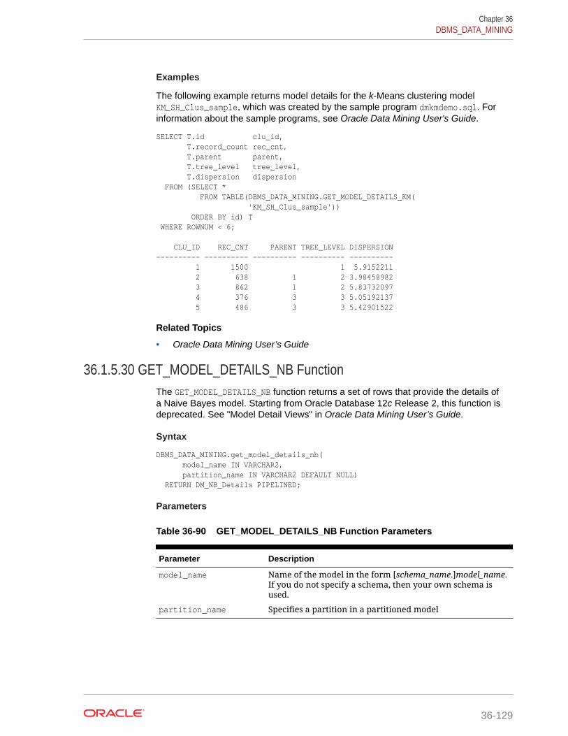
Examples
The following example returns model details for the k-Means clustering modelKM_SH_Clus_sample, which was created by the sample program dmkmdemo.sql. Forinformation about the sample programs, see Oracle Data Mining User's Guide.
SELECT T.id clu_id, T.record_count rec_cnt, T.parent parent, T.tree_level tree_level, T.dispersion dispersion FROM (SELECT * FROM TABLE(DBMS_DATA_MINING.GET_MODEL_DETAILS_KM( 'KM_SH_Clus_sample')) ORDER BY id) T WHERE ROWNUM < 6; CLU_ID REC_CNT PARENT TREE_LEVEL DISPERSION---------- ---------- ---------- ---------- ---------- 1 1500 1 5.9152211 2 638 1 2 3.98458982 3 862 1 2 5.83732097 4 376 3 3 5.05192137 5 486 3 3 5.42901522
Related Topics
• Oracle Data Mining User’s Guide
36.1.5.30 GET_MODEL_DETAILS_NB FunctionThe GET_MODEL_DETAILS_NB function returns a set of rows that provide the details ofa Naive Bayes model. Starting from Oracle Database 12c Release 2, this function isdeprecated. See "Model Detail Views" in Oracle Data Mining User’s Guide.
Syntax
DBMS_DATA_MINING.get_model_details_nb( model_name IN VARCHAR2, partition_name IN VARCHAR2 DEFAULT NULL) RETURN DM_NB_Details PIPELINED;
Parameters
Table 36-90 GET_MODEL_DETAILS_NB Function Parameters
Parameter Description
model_name Name of the model in the form [schema_name.]model_name.If you do not specify a schema, then your own schema isused.
partition_name Specifies a partition in a partitioned model
Chapter 36DBMS_DATA_MINING
36-129
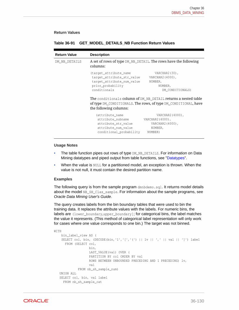
Return Values
Table 36-91 GET_MODEL_DETAILS_NB Function Return Values
Return Value Description
DM_NB_DETAILS A set of rows of type DM_NB_DETAIL. The rows have the followingcolumns:
(target_attribute_name VARCHAR2(30), target_attribute_str_value VARCHAR2(4000), target_attribute_num_value NUMBER, prior_probability NUMBER, conditionals DM_CONDITIONALS)
The conditionals column of DM_NB_DETAIL returns a nested tableof type DM_CONDITIONALS. The rows, of type DM_CONDITIONAL, havethe following columns:
(attribute_name VARCHAR2(4000), attribute_subname VARCHAR2(4000), attribute_str_value VARCHAR2(4000), attribute_num_value NUMBER, conditional_probability NUMBER)
Usage Notes
• The table function pipes out rows of type DM_NB_DETAILS. For information on DataMining datatypes and piped output from table functions, see "Datatypes".
• When the value is NULL for a partitioned model, an exception is thrown. When thevalue is not null, it must contain the desired partition name.
Examples
The following query is from the sample program dmnbdemo.sql. It returns model detailsabout the model NB_SH_Clas_sample. For information about the sample programs, seeOracle Data Mining User's Guide.
The query creates labels from the bin boundary tables that were used to bin thetraining data. It replaces the attribute values with the labels. For numeric bins, thelabels are (lower_boundary,upper_boundary]; for categorical bins, the label matchesthe value it represents. (This method of categorical label representation will only workfor cases where one value corresponds to one bin.) The target was not binned.
WITH bin_label_view AS ( SELECT col, bin, (DECODE(bin,'1','[','(') || lv || ',' || val || ']') label FROM (SELECT col, bin, LAST_VALUE(val) OVER ( PARTITION BY col ORDER BY val ROWS BETWEEN UNBOUNDED PRECEDING AND 1 PRECEDING) lv, val FROM nb_sh_sample_num) UNION ALL SELECT col, bin, val label FROM nb_sh_sample_cat
Chapter 36DBMS_DATA_MINING
36-130

), model_details AS ( SELECT T.target_attribute_name tname, NVL(TO_CHAR(T.target_attribute_num_value,T.target_attribute_str_value)) tval, C.attribute_name pname, NVL(L.label, NVL(C.attribute_str_value, C.attribute_num_value)) pval, T.prior_probability priorp, C.conditional_probability condp FROM TABLE(DBMS_DATA_MINING.GET_MODEL_DETAILS_NB('NB_SH_Clas_sample')) T, TABLE(T.conditionals) C, bin_label_view L WHERE C.attribute_name = L.col (+) AND (NVL(C.attribute_str_value,C.attribute_num_value) = L.bin(+)) ORDER BY 1,2,3,4,5,6 ) SELECT tname, tval, pname, pval, priorp, condp FROM model_details WHERE ROWNUM < 11;
TNAME TVAL PNAME PVAL PRIORP CONDP-------------- ---- ------------------------- ------------- ------- -------AFFINITY_CARD 0 AGE (24,30] .6500 .1714AFFINITY_CARD 0 AGE (30,35] .6500 .1509AFFINITY_CARD 0 AGE (35,40] .6500 .1125AFFINITY_CARD 0 AGE (40,46] .6500 .1134AFFINITY_CARD 0 AGE (46,53] .6500 .1071AFFINITY_CARD 0 AGE (53,90] .6500 .1312AFFINITY_CARD 0 AGE [17,24] .6500 .2134AFFINITY_CARD 0 BOOKKEEPING_APPLICATION 0 .6500 .1500AFFINITY_CARD 0 BOOKKEEPING_APPLICATION 1 .6500 .8500AFFINITY_CARD 0 BULK_PACK_DISKETTES 0 .6500 .3670
Related Topics
• Oracle Data Mining User’s Guide
36.1.5.31 GET_MODEL_DETAILS_NMF FunctionThe GET_MODEL_DETAILS_NMF function returns a set of rows that provide the details of aNon-Negative Matrix Factorization model. Starting from Oracle Database 12c Release2, this function is deprecated. See "Model Detail Views" in Oracle Data Mining User’sGuide.
Syntax
DBMS_DATA_MINING.get_model_details_nmf( model_name IN VARCHAR2, partition_name VARCHAR2 DEFAULT NULL) RETURN DM_NMF_Feature_Set PIPELINED;
Parameters
Table 36-92 GET_MODEL_DETAILS_NMF Function Parameters
Parameter Description
model_name Name of the model in the form [schema_name.]model_name. If youdo not specify a schema, then your own schema is used.
Chapter 36DBMS_DATA_MINING
36-131

Table 36-92 (Cont.) GET_MODEL_DETAILS_NMF Function Parameters
Parameter Description
partition_name Specifies a partition in a partitioned model
Return Values
Table 36-93 GET_MODEL_DETAILS_NMF Function Return Values
Return Value Description
DM_NMF_FEATURE_SET
A set of rows of DM_NMF_FEATURE. The rows have the followingcolumns:
(feature_id NUMBER, mapped_feature_id VARCHAR2(4000), attribute_set DM_NMF_ATTRIBUTE_SET)
The attribute_set column of DM_NMF_FEATURE returns anested table of type DM_NMF_ATTRIBUTE_SET. The rows, of typeDM_NMF_ATTRIBUTE, have the following columns:
(attribute_name VARCHAR2(4000), attribute_subname VARCHAR2(4000), attribute_value VARCHAR2(4000), coefficient NUMBER)
Usage Notes
• The table function pipes out rows of type DM_NMF_FEATURE_SET. For information onData Mining datatypes and piped output from table functions, see "Datatypes".
• When the value is NULL for a partitioned model, an exception is thrown. When thevalue is not null, it must contain the desired partition name.
Examples
The following example returns model details for the feature extraction modelNMF_SH_Sample, which was created by the sample program dmnmdemo.sql. Forinformation about the sample programs, see Oracle Data Mining User's Guide.
SELECT * FROM (SELECT F.feature_id, A.attribute_name, A.attribute_value, A.coefficient FROM TABLE(DBMS_DATA_MINING.GET_MODEL_DETAILS_NMF('NMF_SH_Sample')) F, TABLE(F.attribute_set) AORDER BY feature_id,attribute_name,attribute_value) WHERE ROWNUM < 11; FEATURE_ID ATTRIBUTE_NAME ATTRIBUTE_VALUE COEFFICIENT--------- ----------------------- ---------------- ------------------- 1 AFFINITY_CARD .051208078859308 1 AGE .0390513260041573 1 BOOKKEEPING_APPLICATION .0512734004239326
Chapter 36DBMS_DATA_MINING
36-132
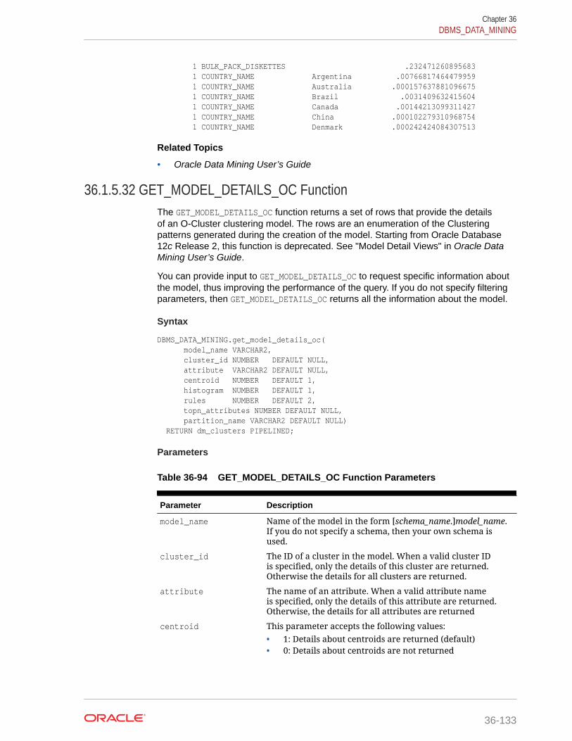
1 BULK_PACK_DISKETTES .232471260895683 1 COUNTRY_NAME Argentina .00766817464479959 1 COUNTRY_NAME Australia .000157637881096675 1 COUNTRY_NAME Brazil .0031409632415604 1 COUNTRY_NAME Canada .00144213099311427 1 COUNTRY_NAME China .000102279310968754 1 COUNTRY_NAME Denmark .000242424084307513
Related Topics
• Oracle Data Mining User’s Guide
36.1.5.32 GET_MODEL_DETAILS_OC FunctionThe GET_MODEL_DETAILS_OC function returns a set of rows that provide the detailsof an O-Cluster clustering model. The rows are an enumeration of the Clusteringpatterns generated during the creation of the model. Starting from Oracle Database12c Release 2, this function is deprecated. See "Model Detail Views" in Oracle DataMining User’s Guide.
You can provide input to GET_MODEL_DETAILS_OC to request specific information aboutthe model, thus improving the performance of the query. If you do not specify filteringparameters, then GET_MODEL_DETAILS_OC returns all the information about the model.
Syntax
DBMS_DATA_MINING.get_model_details_oc( model_name VARCHAR2, cluster_id NUMBER DEFAULT NULL, attribute VARCHAR2 DEFAULT NULL, centroid NUMBER DEFAULT 1, histogram NUMBER DEFAULT 1, rules NUMBER DEFAULT 2, topn_attributes NUMBER DEFAULT NULL, partition_name VARCHAR2 DEFAULT NULL) RETURN dm_clusters PIPELINED;
Parameters
Table 36-94 GET_MODEL_DETAILS_OC Function Parameters
Parameter Description
model_name Name of the model in the form [schema_name.]model_name.If you do not specify a schema, then your own schema isused.
cluster_id The ID of a cluster in the model. When a valid cluster IDis specified, only the details of this cluster are returned.Otherwise the details for all clusters are returned.
attribute The name of an attribute. When a valid attribute nameis specified, only the details of this attribute are returned.Otherwise, the details for all attributes are returned
centroid This parameter accepts the following values:• 1: Details about centroids are returned (default)• 0: Details about centroids are not returned
Chapter 36DBMS_DATA_MINING
36-133
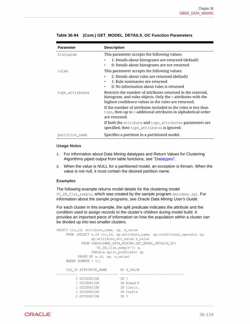
Table 36-94 (Cont.) GET_MODEL_DETAILS_OC Function Parameters
Parameter Description
histogram This parameter accepts the following values:• 1: Details about histograms are returned (default)• 0: Details about histograms are not returned
rules This parameter accepts the following values:• 2: Details about rules are returned (default)• 1: Rule summaries are returned• 0: No information about rules is returned
topn_attributes Restricts the number of attributes returned in the centroid,histogram, and rules objects. Only the n attributes with thehighest confidence values in the rules are returned.If the number of attributes included in the rules is less thantopn, then up to n additional attributes in alphabetical orderare returned.If both the attribute and topn_attributes parameters arespecified, then topn_attributes is ignored.
partition_name Specifies a partition in a partitioned model.
Usage Notes
1. For information about Data Mining datatypes and Return Values for ClusteringAlgorithms piped output from table functions, see "Datatypes".
2. When the value is NULL for a partitioned model, an exception is thrown. When thevalue is not null, it must contain the desired partition name.
Examples
The following example returns model details for the clustering modelOC_SH_Clus_sample, which was created by the sample program dmocdemo.sql. Forinformation about the sample programs, see Oracle Data Mining User's Guide.
For each cluster in this example, the split predicate indicates the attribute and thecondition used to assign records to the cluster's children during model build. Itprovides an important piece of information on how the population within a cluster canbe divided up into two smaller clusters.
SELECT clu_id, attribute_name, op, s_value FROM (SELECT a.id clu_id, sp.attribute_name, sp.conditional_operator op, sp.attribute_str_value s_value FROM TABLE(DBMS_DATA_MINING.GET_MODEL_DETAILS_OC( 'OC_SH_Clus_sample')) a, TABLE(a.split_predicate) sp ORDER BY a.id, op, s_value) WHERE ROWNUM < 11; CLU_ID ATTRIBUTE_NAME OP S_VALUE----------- -------------------- --------------------------------- 1 OCCUPATION IN ? 1 OCCUPATION IN Armed-F 1 OCCUPATION IN Cleric. 1 OCCUPATION IN Crafts 2 OCCUPATION IN ?
Chapter 36DBMS_DATA_MINING
36-134

2 OCCUPATION IN Armed-F 2 OCCUPATION IN Cleric. 3 OCCUPATION IN Exec. 3 OCCUPATION IN Farming 3 OCCUPATION IN Handler
Related Topics
• Oracle Data Mining User’s Guide
36.1.5.33 GET_MODEL_SETTINGS FunctionThe GET_MODEL_SETTINGS function returns the settings used to build the given model.Starting from Oracle Database 12c Release 2, this function is deprecated. See"Static Data Dictionary Views: ALL_ALL_TABLES to ALL_OUTLINES" in Oracle DatabaseReference.
Syntax
FUNCTION get_model_settings(model_name IN VARCHAR2) RETURN DM_Model_Settings PIPELINED;
Parameters
Table 36-95 GET_MODEL_SETTINGS Function Parameters
Parameter Description
model_name Name of the model in the form [schema_name.]model_name.If you do not specify a schema, then your own schema isused.
Return Values
Table 36-96 GET_MODEL_SETTINGS Function Return Values
Return Value Description
DM_MODEL_SETTINGS A set of rows of type DM_MODEL_SETTINGS. The rows have thefollowing columns:
DM_MODEL_SETTINGS TABLE OF SYS.DM_MODEL_SETTING Name Type ---------------------- -------------------- SETTING_NAME VARCHAR2(30) SETTING_VALUE VARCHAR2(4000)
Usage Notes
1. This table function pipes out rows of type DM_MODEL_SETTINGS. For informationon Data Mining datatypes and piped output from table functions, see"DBMS_DATA_MINING Datatypes".
2. The setting names/values include both those specified by the user and anydefaults assigned by the build process.
Chapter 36DBMS_DATA_MINING
36-135

Examples
The following example returns model model settings for an example Naive Bayesmodel.
SETTING_NAME SETTING_VALUE------------------------------ ------------------------------ALGO_NAME ALGO_NAIVE_BAYESPREP_AUTO ONODMS_MAX_PARTITIONS 1000NABS_SINGLETON_THRESHOLD 0CLAS_WEIGHTS_BALANCED OFFNABS_PAIRWISE_THRESHOLD 0ODMS_PARTITION_COLUMNS GENDER,Y_BOX_GAMESODMS_MISSING_VALUE_TREATMENT ODMS_MISSING_VALUE_AUTOODMS_SAMPLING ODMS_SAMPLING_DISABLE
9 rows selected.
Related Topics
• Oracle Database Reference
36.1.5.34 GET_MODEL_SIGNATURE FunctionThe GET_MODEL_SIGNATURE function returns the list of columns from the build inputtable that were used by the build process to train the model. Starting from OracleDatabase 12c Release 2, this function is deprecated. See "Static Data DictionaryViews: ALL_ALL_TABLES to ALL_OUTLINES" in Oracle Database Reference.
Syntax
FUNCTION get_model_signature (model_name IN VARCHAR2)RETURN DM_Model_Signature PIPELINED;
Parameters
Table 36-97 GET_MODEL_SIGNATURE Function Parameters
Parameter Description
model_name Name of the model in the form [schema_name.]model_name.If you do not specify a schema, then your own schema isused.
Chapter 36DBMS_DATA_MINING
36-136
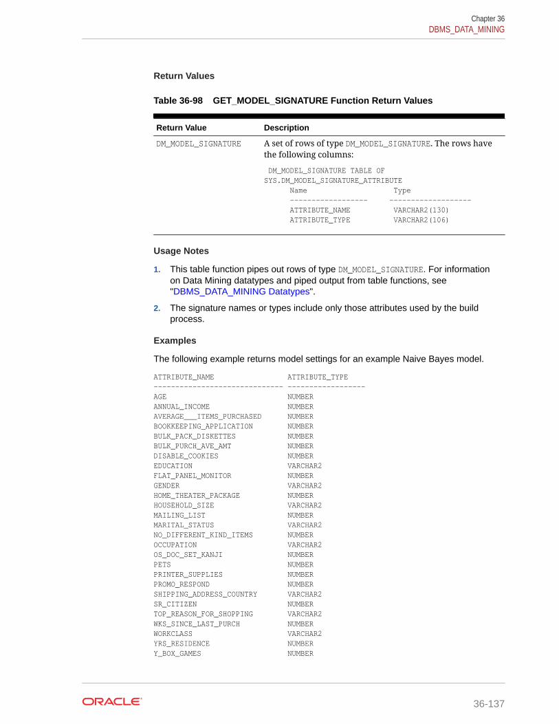
Return Values
Table 36-98 GET_MODEL_SIGNATURE Function Return Values
Return Value Description
DM_MODEL_SIGNATURE A set of rows of type DM_MODEL_SIGNATURE. The rows havethe following columns:
DM_MODEL_SIGNATURE TABLE OF SYS.DM_MODEL_SIGNATURE_ATTRIBUTE Name Type ------------------ ------------------- ATTRIBUTE_NAME VARCHAR2(130) ATTRIBUTE_TYPE VARCHAR2(106)
Usage Notes
1. This table function pipes out rows of type DM_MODEL_SIGNATURE. For informationon Data Mining datatypes and piped output from table functions, see"DBMS_DATA_MINING Datatypes".
2. The signature names or types include only those attributes used by the buildprocess.
Examples
The following example returns model settings for an example Naive Bayes model.
ATTRIBUTE_NAME ATTRIBUTE_TYPE------------------------------ ------------------AGE NUMBERANNUAL_INCOME NUMBERAVERAGE___ITEMS_PURCHASED NUMBERBOOKKEEPING_APPLICATION NUMBERBULK_PACK_DISKETTES NUMBERBULK_PURCH_AVE_AMT NUMBERDISABLE_COOKIES NUMBEREDUCATION VARCHAR2FLAT_PANEL_MONITOR NUMBERGENDER VARCHAR2HOME_THEATER_PACKAGE NUMBERHOUSEHOLD_SIZE VARCHAR2MAILING_LIST NUMBERMARITAL_STATUS VARCHAR2NO_DIFFERENT_KIND_ITEMS NUMBEROCCUPATION VARCHAR2OS_DOC_SET_KANJI NUMBERPETS NUMBERPRINTER_SUPPLIES NUMBERPROMO_RESPOND NUMBERSHIPPING_ADDRESS_COUNTRY VARCHAR2SR_CITIZEN NUMBERTOP_REASON_FOR_SHOPPING VARCHAR2WKS_SINCE_LAST_PURCH NUMBERWORKCLASS VARCHAR2YRS_RESIDENCE NUMBERY_BOX_GAMES NUMBER
Chapter 36DBMS_DATA_MINING
36-137
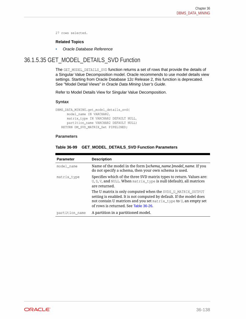
27 rows selected.
Related Topics
• Oracle Database Reference
36.1.5.35 GET_MODEL_DETAILS_SVD FunctionThe GET_MODEL_DETAILS_SVD function returns a set of rows that provide the details ofa Singular Value Decomposition model. Oracle recommends to use model details viewsettings. Starting from Oracle Database 12c Release 2, this function is deprecated.See "Model Detail Views" in Oracle Data Mining User’s Guide.
Refer to Model Details View for Singular Value Decomposition.
Syntax
DBMS_DATA_MINING.get_model_details_svd( model_name IN VARCHAR2, matrix_type IN VARCHAR2 DEFAULT NULL, partition_name VARCHAR2 DEFAULT NULL) RETURN DM_SVD_MATRIX_Set PIPELINED;
Parameters
Table 36-99 GET_MODEL_DETAILS_SVD Function Parameters
Parameter Description
model_name Name of the model in the form [schema_name.]model_name. If youdo not specify a schema, then your own schema is used.
matrix_type Specifies which of the three SVD matrix types to return. Values are:U, S, V, and NULL. When matrix_type is null (default), all matricesare returned.The U matrix is only computed when the SVDS_U_MATRIX_OUTPUTsetting is enabled. It is not computed by default. If the model doesnot contain U matrices and you set matrix_type to U, an empty setof rows is returned. See Table 36-26.
partition_name A partition in a partitioned model.
Chapter 36DBMS_DATA_MINING
36-138

Return Values
Table 36-100 GET_MODEL_DETAILS_SVD Function Return Values
Return Value Description
DM_SVD_MATRIX_SET A set of rows of type DM_SVD_MATRIX. The rows have thefollowing columns:
(matrix_type CHAR(1), feature_id NUMBER, mapped_feature_id VARCHAR2(4000), attribute_name VARCHAR2(4000), attribute_subname VARCHAR2(4000), case_id VARCHAR2(4000), value NUMBER, variance NUMBER, pct_cum_variance NUMBER)
See Usage Notes for details.
Usage Notes
1. This table function pipes out rows of type DM_SVD_MATRIX. For information on DataMining datatypes and piped output from table functions, see "Datatypes".
The columns in each row returned by GET_MODEL_DETAILS_SVD are described asfollows:
Column inDM_SVD_MATRIX_SET
Description
matrix_type The type of matrix. Possible values are S, V, andU. This field is never null.
feature_id The feature that the matrix entry refers to.
mapped_feature_id A descriptive name for the feature.
attribute_name Column name in the V matrix component bases.This field is null for the S and U matrices.
attribute_subname Subname in the V matrix component bases. Thisis relevant only in the case of a nested column.This field is null for the S and U matrices.
case_id Unique identifier of the row in the build datadescribed by the U matrix projection. This field isnull for the S and V matrices.
value The matrix entry value.
Chapter 36DBMS_DATA_MINING
36-139

Column inDM_SVD_MATRIX_SET
Description
variance The variance explained by a component.It is non-null only for S matrix entries.This column is non-null only for Smatrix entries and for SVD models withsetting dbms_data_mining.svds_scoring_modeset to dbms_data_mining.svds_scoring_pcaand the build data is centered,either manually or because the settingdbms_data_mining.prep_auto is set todbms_data_mining.prep_auto_on.
pct_cum_variance The percent cumulative variance explained bythe components thus far. The components areranked by the explained variance in descendingorder.This column is non-null only for Smatrix entries and for SVD models withsetting dbms_data_mining.svds_scoring_modeset to dbms_data_mining.svds_scoring_pcaand the build data is centered,either manually or because the settingdbms_data_mining.prep_auto is set todbms_data_mining.prep_auto_on.
2. The output of GET_MODEL_DETAILS is in sparse format. Zero values are notreturned. Only the diagonal elements of the S matrix, the non-zero coefficientsin the V matrix bases, and the non-zero U matrix projections are returned.
There is one exception: If the data row does not produce non-zero U Matrixprojections, the case ID for that row is returned with NULL for the feature_id andvalue. This is done to avoid losing any records from the original data.
3. GET_MODEL_DETAILS functions preserve model transparency by automaticallyreversing the transformations applied during the build process. Thus the attributesreturned in the model details are the original attributes (or a close approximation ofthe original attributes) used to build the model.
4. When the value is NULL for a partitioned model, an exception is thrown. When thevalue is not null, it must contain the preferred partition name.
Related Topics
• Oracle Data Mining User’s Guide
36.1.5.36 GET_MODEL_DETAILS_SVM FunctionThe GET_MODEL_DETAILS_SVM function returns a set of rows that provide the details ofa linear Support Vector Machine (SVM) model. If invoked for nonlinear SVM, it returnsORA-40215. Starting from Oracle Database 12c Release 2, this function is deprecated.See "Model Detail Views" in Oracle Data Mining User’s Guide.
In linear SVM models, only nonzero coefficients are stored. This reduces storage andspeeds up model loading. As a result, if an attribute is missing in the coefficient listreturned by GET_MODEL_DETAILS_SVM, then the coefficient of this attribute should beinterpreted as zero.
Chapter 36DBMS_DATA_MINING
36-140
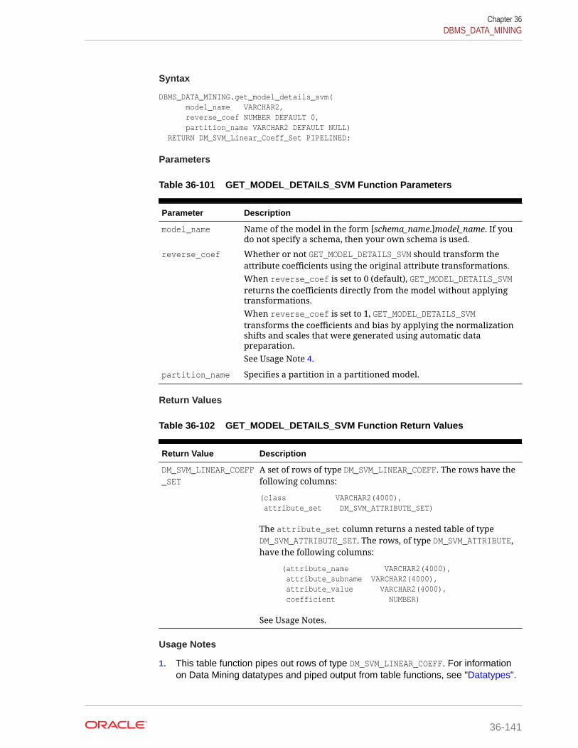
Syntax
DBMS_DATA_MINING.get_model_details_svm( model_name VARCHAR2, reverse_coef NUMBER DEFAULT 0, partition_name VARCHAR2 DEFAULT NULL) RETURN DM_SVM_Linear_Coeff_Set PIPELINED;
Parameters
Table 36-101 GET_MODEL_DETAILS_SVM Function Parameters
Parameter Description
model_name Name of the model in the form [schema_name.]model_name. If youdo not specify a schema, then your own schema is used.
reverse_coef Whether or not GET_MODEL_DETAILS_SVM should transform theattribute coefficients using the original attribute transformations.When reverse_coef is set to 0 (default), GET_MODEL_DETAILS_SVMreturns the coefficients directly from the model without applyingtransformations.When reverse_coef is set to 1, GET_MODEL_DETAILS_SVMtransforms the coefficients and bias by applying the normalizationshifts and scales that were generated using automatic datapreparation.See Usage Note 4.
partition_name Specifies a partition in a partitioned model.
Return Values
Table 36-102 GET_MODEL_DETAILS_SVM Function Return Values
Return Value Description
DM_SVM_LINEAR_COEFF_SET
A set of rows of type DM_SVM_LINEAR_COEFF. The rows have thefollowing columns:
(class VARCHAR2(4000), attribute_set DM_SVM_ATTRIBUTE_SET)
The attribute_set column returns a nested table of typeDM_SVM_ATTRIBUTE_SET. The rows, of type DM_SVM_ATTRIBUTE,have the following columns:
(attribute_name VARCHAR2(4000), attribute_subname VARCHAR2(4000), attribute_value VARCHAR2(4000), coefficient NUMBER)
See Usage Notes.
Usage Notes
1. This table function pipes out rows of type DM_SVM_LINEAR_COEFF. For informationon Data Mining datatypes and piped output from table functions, see "Datatypes".
Chapter 36DBMS_DATA_MINING
36-141

2. The class column of DM_SVM_LINEAR_COEFF contains Classification target values.For SVM Regression models, class is null. For each Classification target value,a set of coefficients is returned. For Binary Classification, one-class Classification,and Regression models, only a single set of coefficients is returned.
3. The attribute_value column in DM_SVM_ATTRIBUTE_SET is used for categoricalattributes.
4. GET_MODEL_DETAILS functions preserve model transparency by automaticallyreversing the transformations applied during the build process. Thus the attributesreturned in the model details are the original attributes (or a close approximation ofthe original attributes) used to build the model.
The coefficients are related to the transformed, not the original, attributes.When returned directly with the model details, the coefficients may not providemeaningful information. If you want GET_MODEL_DETAILS_SVM to transform thecoefficients such that they relate to the original attributes, set the reverse_coefparameter to 1.
5. When the value is NULL for a partitioned model, an exception is thrown. When thevalue is not null, it must contain the desired partition name.
Examples
The following example returns model details for the SVM Classification modelSVMC_SH_Clas_sample, which was created by the sample program dmsvcdem.sql. Forinformation about the sample programs, see Oracle Data Mining User's Guide.
WITH mod_dtls AS ( SELECT * FROM TABLE(DBMS_DATA_MINING.GET_MODEL_DETAILS_SVM('SVMC_SH_Clas_sample')) ), model_details AS ( SELECT D.class, A.attribute_name, A.attribute_value, A.coefficient FROM mod_dtls D, TABLE(D.attribute_set) A ORDER BY D.class, ABS(A.coefficient) DESC ) SELECT class, attribute_name aname, attribute_value aval, coefficient coeff FROM model_details WHERE ROWNUM < 11; CLASS ANAME AVAL COEFF---------- ------------------------- ------------------------- -----1 -2.851 BOOKKEEPING_APPLICATION 1.111 OCCUPATION Other -.941 HOUSEHOLD_SIZE 4-5 .881 CUST_MARITAL_STATUS Married .821 YRS_RESIDENCE .761 HOUSEHOLD_SIZE 6-8 -.741 OCCUPATION Exec. .711 EDUCATION 11th -.711 EDUCATION Masters .63
Related Topics
• Oracle Data Mining User’s Guide
Chapter 36DBMS_DATA_MINING
36-142
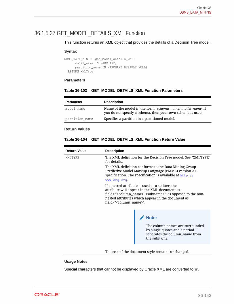
36.1.5.37 GET_MODEL_DETAILS_XML FunctionThis function returns an XML object that provides the details of a Decision Tree model.
Syntax
DBMS_DATA_MINING.get_model_details_xml( model_name IN VARCHAR2, partition_name IN VARCHAR2 DEFAULT NULL) RETURN XMLType;
Parameters
Table 36-103 GET_MODEL_DETAILS_XML Function Parameters
Parameter Description
model_name Name of the model in the form [schema_name.]model_name. Ifyou do not specify a schema, then your own schema is used.
partition_name Specifies a partition in a partitioned model.
Return Values
Table 36-104 GET_MODEL_DETAILS_XML Function Return Value
Return Value Description
XMLTYPE The XML definition for the Decision Tree model. See "XMLTYPE"for details.The XML definition conforms to the Data Mining GroupPredictive Model Markup Language (PMML) version 2.1specification. The specification is available at http://www.dmg.org.
If a nested attribute is used as a splitter, theattribute will appear in the XML document asfield="'<column_name>'.<subname>", as opposed to the non-nested attributes which appear in the document asfield="<column_name>".
Note:
The column names are surroundedby single quotes and a periodseparates the column_name fromthe subname.
The rest of the document style remains unchanged.
Usage Notes
Special characters that cannot be displayed by Oracle XML are converted to '#'.
Chapter 36DBMS_DATA_MINING
36-143

Examples
The following statements in SQL*Plus return the details of the Decision Tree modeldt_sh_clas_sample. This model is created by the program dmdtdemo.sql, one of thesample data mining programs provided with Oracle Database Examples.
Note: The """ characters you will see in the XML output are a result of SQL*Plusbehavior. To display the XML in proper format, cut and past it into a file and open thefile in a browser.
column dt_details format a320SELECT dbms_data_mining.get_model_details_xml('dt_sh_clas_sample') AS DT_DETAILSFROM dual;
DT_DETAILS--------------------------------------------------------------------------------<PMML version="2.1"> <Header copyright="Copyright (c) 2004, Oracle Corporation. All rights reserved."/> <DataDictionary numberOfFields="9"> <DataField name="AFFINITY_CARD" optype="categorical"/> <DataField name="AGE" optype="continuous"/> <DataField name="BOOKKEEPING_APPLICATION" optype="continuous"/> <DataField name="CUST_MARITAL_STATUS" optype="categorical"/> <DataField name="EDUCATION" optype="categorical"/> <DataField name="HOUSEHOLD_SIZE" optype="categorical"/> <DataField name="OCCUPATION" optype="categorical"/> <DataField name="YRS_RESIDENCE" optype="continuous"/> <DataField name="Y_BOX_GAMES" optype="continuous"/> </DataDictionary> <TreeModel modelName="DT_SH_CLAS_SAMPLE" functionName="classification" splitCharacteristic="binarySplit"> <Extension name="buildSettings"> <Setting name="TREE_IMPURITY_METRIC" value="TREE_IMPURITY_GINI"/> <Setting name="TREE_TERM_MAX_DEPTH" value="7"/> <Setting name="TREE_TERM_MINPCT_NODE" value=".05"/> <Setting name="TREE_TERM_MINPCT_SPLIT" value=".1"/> <Setting name="TREE_TERM_MINREC_NODE" value="10"/> <Setting name="TREE_TERM_MINREC_SPLIT" value="20"/> <costMatrix> <costElement> <actualValue>0</actualValue> <predictedValue>0</predictedValue> <cost>0</cost> </costElement> <costElement> <actualValue>0</actualValue> <predictedValue>1</predictedValue> <cost>1</cost> </costElement> <costElement> <actualValue>1</actualValue> <predictedValue>0</predictedValue> <cost>8</cost> </costElement> <costElement> <actualValue>1</actualValue>
Chapter 36DBMS_DATA_MINING
36-144
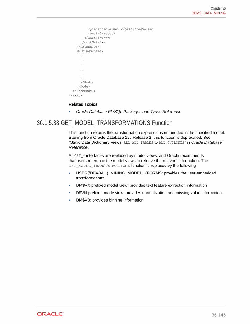
<predictedValue>1</predictedValue> <cost>0</cost> </costElement> </costMatrix> </Extension> <MiningSchema> . . . . . . </Node> </Node> </TreeModel></PMML>
Related Topics
• Oracle Database PL/SQL Packages and Types Reference
36.1.5.38 GET_MODEL_TRANSFORMATIONS FunctionThis function returns the transformation expressions embedded in the specified model.Starting from Oracle Database 12c Release 2, this function is deprecated. See"Static Data Dictionary Views: ALL_ALL_TABLES to ALL_OUTLINES" in Oracle DatabaseReference.
All GET_* interfaces are replaced by model views, and Oracle recommendsthat users reference the model views to retrieve the relevant information. TheGET_MODEL_TRANSFORMATIONS function is replaced by the following:
• USER(/DBA/ALL)_MINING_MODEL_XFORMS: provides the user-embeddedtransformations
• DM$VX prefixed model view: provides text feature extraction information
• D$VN prefixed mode view: provides normalization and missing value information
• DM$VB: provides binning information
Chapter 36DBMS_DATA_MINING
36-145

See Also:
“About Transformation Lists” in DBMS_DATA_MINING_TRANSFORMOperational Notes
"GET_TRANSFORM_LIST Procedure"
"CREATE_MODEL Procedure"
"ALL_MINING_MODEL_XFORMS" in Oracle Database Reference
"DBA_MINING_MODEL_XFORMS" in Oracle Database Reference
"USER_MINING_MODEL_XFORMS" in Oracle Database Reference
Model Details View for Binning
Normalization and Missing Value Handling
Data Preparation for Text Features
Syntax
DBMS_DATA_MINING.get_model_transformations( model_name IN VARCHAR2, partition_name IN VARCHAR2 DEFAULT NULL) RETURN DM_Transforms PIPELINED;
Parameters
Table 36-105 GET_MODEL_TRANSFORMATIONS Function Parameters
Parameter Description
model_name Indicates the name of the model in the form[schema_name.]model_name. If you do not specify a schema, thenyour own schema is used.
partition_name Specifies a partition in a partitioned model
Return Values
Table 36-106 GET_MODEL_TRANSFORMATIONS Function Return Value
Return Value Description
DM_TRANSFORMS The transformation expressions embedded in model_name.
The DM_TRANSFORMS type is a table of DM_TRANSFORM objects. EachDM_TRANSFORM has these fields:
attribute_name VARCHAR2(4000)attribute_subname VARCHAR2(4000)expression CLOBreverse_expression CLOB
Chapter 36DBMS_DATA_MINING
36-146

Usage Notes
When Automatic Data Preparation (ADP) is enabled, both automatic and user-definedtransformations may be associated with an attribute. In this case, the user-definedtransformations are evaluated before the automatic transformations.
When invoked for a partitioned model, the partition_name parameter must bespecified.
Examples
In this example, several columns in the SH.CUSTOMERS table are used to create a NaiveBayes model. A transformation expression is specified for one of the columns. Themodel does not use ADP.
CREATE OR REPLACE VIEW mining_data AS SELECT cust_id, cust_year_of_birth, cust_income_level,cust_credit_limit FROM sh.customers;
describe mining_data Name Null? Type -------------------------------------- -------- -------------------------- CUST_ID NOT NULL NUMBER CUST_YEAR_OF_BIRTH NOT NULL NUMBER(4) CUST_INCOME_LEVEL VARCHAR2(30) CUST_CREDIT_LIMIT NUMBER CREATE TABLE settings_nb( setting_name VARCHAR2(30), setting_value VARCHAR2(30));BEGIN INSERT INTO settings_nb (setting_name, setting_value) VALUES (dbms_data_mining.algo_name, dbms_data_mining.algo_naive_bayes); INSERT INTO settings_nb (setting_name, setting_value) VALUES (dbms_data_mining.prep_auto, dbms_data_mining.prep_auto_off); COMMIT;END;/DECLARE mining_data_xforms dbms_data_mining_transform.TRANSFORM_LIST; BEGIN dbms_data_mining_transform.SET_TRANSFORM ( xform_list => mining_data_xforms, attribute_name => 'cust_year_of_birth', attribute_subname => null, expression => 'cust_year_of_birth + 10', reverse_expression => 'cust_year_of_birth - 10'); dbms_data_mining.CREATE_MODEL ( model_name => 'new_model', mining_function => dbms_data_mining.classification, data_table_name => 'mining_data', case_id_column_name => 'cust_id', target_column_name => 'cust_income_level', settings_table_name => 'settings_nb', data_schema_name => nulL, settings_schema_name => null, xform_list => mining_data_xforms ); END; /SELECT attribute_name, TO_CHAR(expression), TO_CHAR(reverse_expression)
Chapter 36DBMS_DATA_MINING
36-147
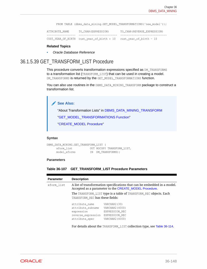
FROM TABLE (dbms_data_mining.GET_MODEL_TRANSFORMATIONS('new_model'));
ATTRIBUTE_NAME TO_CHAR(EXPRESSION) TO_CHAR(REVERSE_EXPRESSION)------------------ ------------------------ ----------------------------- CUST_YEAR_OF_BIRTH cust_year_of_birth + 10 cust_year_of_birth - 10
Related Topics
• Oracle Database Reference
36.1.5.39 GET_TRANSFORM_LIST ProcedureThis procedure converts transformation expressions specified as DM_TRANSFORMSto a transformation list (TRANSFORM_LIST) that can be used in creating a model.DM_TRANSFORMS is returned by the GET_MODEL_TRANSFORMATIONS function.
You can also use routines in the DBMS_DATA_MINING_TRANSFORM package to construct atransformation list.
See Also:
“About Transformation Lists” in DBMS_DATA_MINING_TRANSFORM
"GET_MODEL_TRANSFORMATIONS Function"
"CREATE_MODEL Procedure"
Syntax
DBMS_DATA_MINING.GET_TRANSFORM_LIST ( xform_list OUT NOCOPY TRANSFORM_LIST, model_xforms IN DM_TRANSFORMS);
Parameters
Table 36-107 GET_TRANSFORM_LIST Procedure Parameters
Parameter Description
xform_list A list of transformation specifications that can be embedded in a model.Accepted as a parameter to the CREATE_MODEL Procedure.
The TRANSFORM_LIST type is a table of TRANSFORM_REC objects. EachTRANSFORM_REC has these fields:
attribute_name VARCHAR2(30)attribute_subname VARCHAR2(4000)expression EXPRESSION_RECreverse_expression EXPRESSION_RECattribute_spec VARCHAR2(4000)
For details about the TRANSFORM_LIST collection type, see Table 36-114.
Chapter 36DBMS_DATA_MINING
36-148
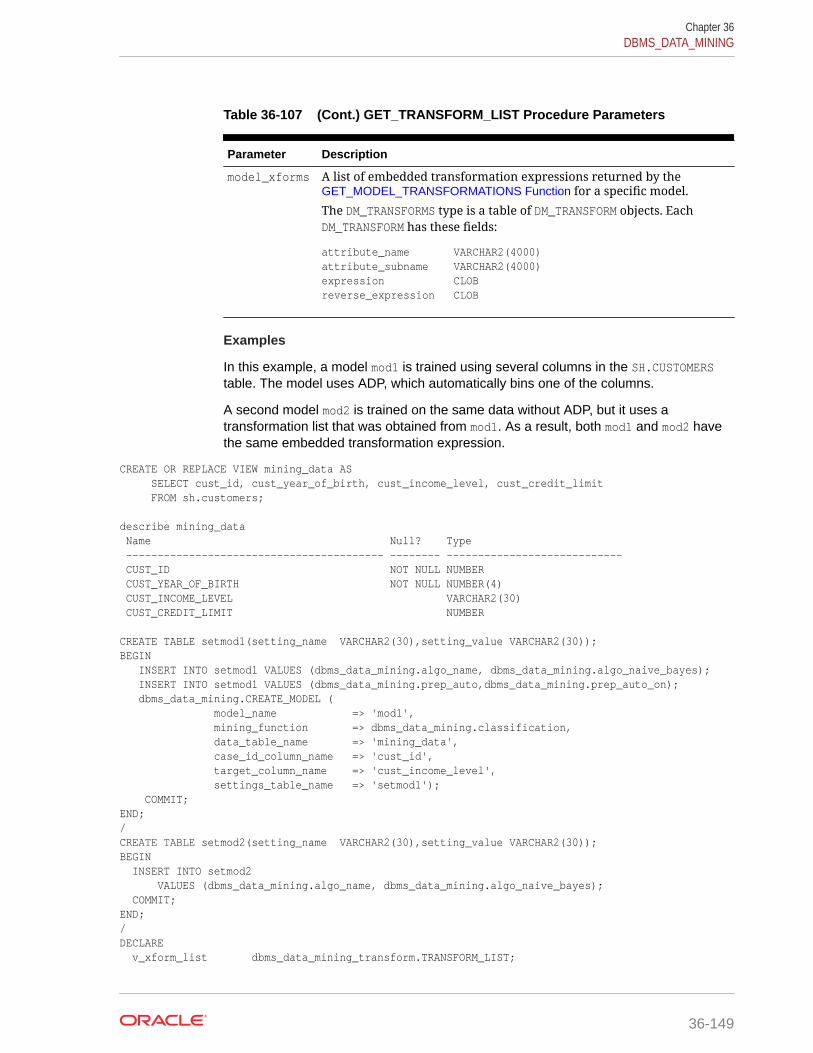
Table 36-107 (Cont.) GET_TRANSFORM_LIST Procedure Parameters
Parameter Description
model_xforms A list of embedded transformation expressions returned by theGET_MODEL_TRANSFORMATIONS Function for a specific model.
The DM_TRANSFORMS type is a table of DM_TRANSFORM objects. EachDM_TRANSFORM has these fields:
attribute_name VARCHAR2(4000)attribute_subname VARCHAR2(4000)expression CLOBreverse_expression CLOB
Examples
In this example, a model mod1 is trained using several columns in the SH.CUSTOMERStable. The model uses ADP, which automatically bins one of the columns.
A second model mod2 is trained on the same data without ADP, but it uses atransformation list that was obtained from mod1. As a result, both mod1 and mod2 havethe same embedded transformation expression.
CREATE OR REPLACE VIEW mining_data AS SELECT cust_id, cust_year_of_birth, cust_income_level, cust_credit_limit FROM sh.customers; describe mining_data Name Null? Type ----------------------------------------- -------- ---------------------------- CUST_ID NOT NULL NUMBER CUST_YEAR_OF_BIRTH NOT NULL NUMBER(4) CUST_INCOME_LEVEL VARCHAR2(30) CUST_CREDIT_LIMIT NUMBER
CREATE TABLE setmod1(setting_name VARCHAR2(30),setting_value VARCHAR2(30));BEGIN INSERT INTO setmod1 VALUES (dbms_data_mining.algo_name, dbms_data_mining.algo_naive_bayes); INSERT INTO setmod1 VALUES (dbms_data_mining.prep_auto,dbms_data_mining.prep_auto_on); dbms_data_mining.CREATE_MODEL ( model_name => 'mod1', mining_function => dbms_data_mining.classification, data_table_name => 'mining_data', case_id_column_name => 'cust_id', target_column_name => 'cust_income_level', settings_table_name => 'setmod1'); COMMIT;END;/CREATE TABLE setmod2(setting_name VARCHAR2(30),setting_value VARCHAR2(30));BEGIN INSERT INTO setmod2 VALUES (dbms_data_mining.algo_name, dbms_data_mining.algo_naive_bayes); COMMIT;END;/DECLARE v_xform_list dbms_data_mining_transform.TRANSFORM_LIST;
Chapter 36DBMS_DATA_MINING
36-149

dmxf DM_TRANSFORMS;BEGIN EXECUTE IMMEDIATE 'SELECT dm_transform(attribute_name, attribute_subname,expression, reverse_expression) FROM TABLE(dbms_data_mining.GET_MODEL_TRANSFORMATIONS (''mod1''))' BULK COLLECT INTO dmxf; dbms_data_mining.GET_TRANSFORM_LIST ( xform_list => v_xform_list, model_xforms => dmxf); dbms_data_mining.CREATE_MODEL( model_name => 'mod2', mining_function => dbms_data_mining.classification, data_table_name => 'mining_data', case_id_column_name => 'cust_id', target_column_name => 'cust_income_level', settings_table_name => 'setmod2', xform_list => v_xform_list);END;/
-- Transformation expression embedded in mod1SELECT TO_CHAR(expression) FROM TABLE (dbms_data_mining.GET_MODEL_TRANSFORMATIONS('mod1'));
TO_CHAR(EXPRESSION)--------------------------------------------------------------------------------CASE WHEN "CUST_YEAR_OF_BIRTH"<1915 THEN 0 WHEN "CUST_YEAR_OF_BIRTH"<=1915 THEN 0WHEN "CUST_YEAR_OF_BIRTH"<=1920.5 THEN 1 WHEN "CUST_YEAR_OF_BIRTH"<=1924.5 THEN 2....5 THEN 29 WHEN "CUST_YEAR_OF_BIRTH" IS NOT NULL THEN 30 END
-- Transformation expression embedded in mod2SELECT TO_CHAR(expression) FROM TABLE (dbms_data_mining.GET_MODEL_TRANSFORMATIONS('mod2'));
TO_CHAR(EXPRESSION)--------------------------------------------------------------------------------CASE WHEN "CUST_YEAR_OF_BIRTH"<1915 THEN 0 WHEN "CUST_YEAR_OF_BIRTH"<=1915 THEN 0WHEN "CUST_YEAR_OF_BIRTH"<=1920.5 THEN 1 WHEN "CUST_YEAR_OF_BIRTH"<=1924.5 THEN 2....5 THEN 29 WHEN "CUST_YEAR_OF_BIRTH" IS NOT NULL THEN 30 END
-- Reverse transformation expression embedded in mod1SELECT TO_CHAR(reverse_expression)FROM TABLE (dbms_data_mining.GET_MODEL_TRANSFORMATIONS('mod1'));
TO_CHAR(REVERSE_EXPRESSION)--------------------------------------------------------------------------------DECODE("CUST_YEAR_OF_BIRTH",0,'( ; 1915), [1915; 1915]',1,'(1915; 1920.5]',2,'(1920.5; 1924.5]',3,'(1924.5; 1928.5]',4,'(1928.5; 1932.5]',5,'(1932.5; 1936.5]',6...8,'(1987.5; 1988.5]',29,'(1988.5; 1989.5]',30,'(1989.5; )',NULL,'NULL') -- Reverse transformation expression embedded in mod2SELECT TO_CHAR(reverse_expression) FROM TABLE (dbms_data_mining.GET_MODEL_TRANSFORMATIONS('mod2'));
Chapter 36DBMS_DATA_MINING
36-150

TO_CHAR(REVERSE_EXPRESSION)--------------------------------------------------------------------------------DECODE("CUST_YEAR_OF_BIRTH",0,'( ; 1915), [1915; 1915]',1,'(1915; 1920.5]',2,'(1920.5; 1924.5]',3,'(1924.5; 1928.5]',4,'(1928.5; 1932.5]',5,'(1932.5; 1936.5]',6...8,'(1987.5; 1988.5]',29,'(1988.5; 1989.5]',30,'(1989.5; )',NULL,'NULL')
36.1.5.40 IMPORT_MODEL ProcedureThis procedure imports one or more data mining models. The procedure isoverloaded. You can call it to import mining models from a dump file set, or you cancall it to import a single mining model from a PMML document.
Import from a dump file set
You can import mining models from a dump file set that was created by theEXPORT_MODEL Procedure. IMPORT_MODEL and EXPORT_MODEL use Oracle DataPump technology to export to and import from a dump file set.
When Oracle Data Pump is used directly to export/import an entire schema ordatabase, the mining models in the schema or database are included. EXPORT_MODELand IMPORT_MODEL export/import mining models only.
Import from PMML
You can import a mining model represented in Predictive Model Markup Language(PMML). The model must be of type RegressionModel, either linear regression orbinary logistic regression.
PMML is an XML-based standard specified by the Data Mining Group (http://www.dmg.org). Applications that are PMML-compliant can deploy PMML-compliantmodels that were created by any vendor. Oracle Data Mining supports the corefeatures of PMML 3.1 for regression models.
See Also:
Oracle Data Mining User's Guide for more information about exporting andimporting mining models
Oracle Database Utilities for information about Oracle Data Pump
http://www.dmg.org/faq.html for more information about PMML
Syntax
Imports a mining model from a dump file set:
DBMS_DATA_MINING.IMPORT_MODEL ( filename IN VARCHAR2, directory IN VARCHAR2, model_filter IN VARCHAR2 DEFAULT NULL, operation IN VARCHAR2 DEFAULT NULL, remote_link IN VARCHAR2 DEFAULT NULL,
Chapter 36DBMS_DATA_MINING
36-151

jobname IN VARCHAR2 DEFAULT NULL, schema_remap IN VARCHAR2 DEFAULT NULL, tablespace_remap IN VARCHAR2 DEFAULT NULL);
Imports a mining model from a PMML document:
DBMS_DATA_MINING.IMPORT_MODEL ( model_name IN VARCHAR2, pmmldoc IN XMLTYPE strict_check IN BOOLEAN DEFAULT FALSE);
Parameters
Table 36-108 IMPORT_MODEL Procedure Parameters
Parameter Description
filename Name of the dump file set from which the models should beimported. The dump file set must have been created by theEXPORT_MODEL procedure or the expdp export utility of Oracle DataPump.The dump file set can contain one or more files. (Refer to"EXPORT_MODEL Procedure" for details.) If the dump file setcontains multiple files, you can specify 'filename%U' insteadof listing them. For example, if your dump file set contains 3files, archive01.dmp, archive02.dmp, and archive03.dmp, you canimport them by specifying 'archive%U'.
directory Name of a pre-defined directory object that specifies where thedump file set is located. Both the exporting and the importing usermust have read/write access to the directory object and to the filesystem directory that it identifies.Note: The target database must have also have read/write access tothe file system directory.
model_filter Optional parameter that specifies one or more models to import. Ifyou do not specify a value for model_filter, all models in the dumpfile set are imported. You can also specify NULL (the default) or 'ALL'to import all models.The value of model_filter can be one or more model names. Thefollowing are valid filters.
'mymodel1''name IN (''mymodel2'',''mymodel3'')'
The first causes IMPORT_MODEL to import a single model namedmymodel1. The second causes IMPORT_MODEL to import two models,mymodel2 and mymodel3.
operation Optional parameter that specifies whether to import the models orthe SQL statements that create the models. By default, the models areimported.You can specify either of the following values for operation:
• 'IMPORT' — Import the models (Default)• 'SQL_FILE'— Write the SQL DDL for creating the models to a
text file. The text file is named job_name.sql and is located inthe dump set directory.
Chapter 36DBMS_DATA_MINING
36-152
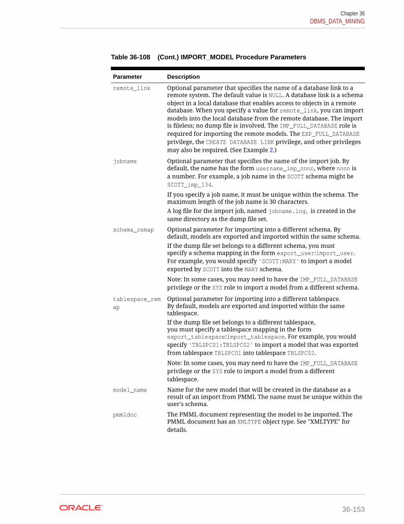
Table 36-108 (Cont.) IMPORT_MODEL Procedure Parameters
Parameter Description
remote_link Optional parameter that specifies the name of a database link to aremote system. The default value is NULL. A database link is a schemaobject in a local database that enables access to objects in a remotedatabase. When you specify a value for remote_link, you can importmodels into the local database from the remote database. The importis fileless; no dump file is involved. The IMP_FULL_DATABASE role isrequired for importing the remote models. The EXP_FULL_DATABASEprivilege, the CREATE DATABASE LINK privilege, and other privilegesmay also be required. (See Example 2.)
jobname Optional parameter that specifies the name of the import job. Bydefault, the name has the form username_imp_nnnn, where nnnn isa number. For example, a job name in the SCOTT schema might beSCOTT_imp_134.
If you specify a job name, it must be unique within the schema. Themaximum length of the job name is 30 characters.A log file for the import job, named jobname.log, is created in thesame directory as the dump file set.
schema_remap Optional parameter for importing into a different schema. Bydefault, models are exported and imported within the same schema.If the dump file set belongs to a different schema, you mustspecify a schema mapping in the form export_user:import_user.For example, you would specify 'SCOTT:MARY' to import a modelexported by SCOTT into the MARY schema.
Note: In some cases, you may need to have the IMP_FULL_DATABASEprivilege or the SYS role to import a model from a different schema.
tablespace_remap
Optional parameter for importing into a different tablespace.By default, models are exported and imported within the sametablespace.If the dump file set belongs to a different tablespace,you must specify a tablespace mapping in the formexport_tablespace:import_tablespace. For example, you wouldspecify 'TBLSPC01:TBLSPC02' to import a model that was exportedfrom tablespace TBLSPC01 into tablespace TBLSPC02.
Note: In some cases, you may need to have the IMP_FULL_DATABASEprivilege or the SYS role to import a model from a differenttablespace.
model_name Name for the new model that will be created in the database as aresult of an import from PMML The name must be unique within theuser's schema.
pmmldoc The PMML document representing the model to be imported. ThePMML document has an XMLTYPE object type. See "XMLTYPE" fordetails.
Chapter 36DBMS_DATA_MINING
36-153

Table 36-108 (Cont.) IMPORT_MODEL Procedure Parameters
Parameter Description
strict_check Whether or not an error occurs when the PMML document containssections that are not part of core PMML (for example, Output orTargets). Oracle Data Mining supports only core PMML; any non-corefeatures may affect the scoring representation.If the PMML does not strictly conform to core PMML andstrict_check is set to TRUE, then IMPORT_MODEL returns an error.If strict_check is FALSE (the default), then the error is suppressed.The model may be imported and scored.
Examples
1. This example shows a model being exported and imported within the schemadmuser2. Then the same model is imported into the dmuser3 schema. The dmuser3user has the IMP_FULL_DATABASE privilege. The dmuser2 user has been assignedthe USER2 tablespace; dmuser3 has been assigned the USER3 tablespace.
SQL> connect dmuser2Enter password: dmuser2_passwordConnected.SQL> select model_name from user_mining_models; MODEL_NAME------------------------------NMF_SH_SAMPLESVMO_SH_CLAS_SAMPLESVMR_SH_REGR_SAMPLE
-- export the model called NMF_SH_SAMPLE to a dump file in same schemaSQL>EXECUTE DBMS_DATA_MINING.EXPORT_MODEL ( filename =>'NMF_SH_SAMPLE_out', directory =>'DATA_PUMP_DIR', model_filter => 'name = ''NMF_SH_SAMPLE''');
-- import the model back into the same schemaSQL>EXECUTE DBMS_DATA_MINING.IMPORT_MODEL ( filename => 'NMF_SH_SAMPLE_out01.dmp', directory => 'DATA_PUMP_DIR', model_filter => 'name = ''NMF_SH_SAMPLE''');
-- connect as different user-- import same model into that schemaSQL> connect dmuser3Enter password: dmuser3_passwordConnected.SQL>EXECUTE DBMS_DATA_MINING.IMPORT_MODEL ( filename => 'NMF_SH_SAMPLE_out01.dmp', directory => 'DATA_PUMP_DIR', model_filter => 'name = ''NMF_SH_SAMPLE''', operation =>'IMPORT', remote_link => NULL, jobname => 'nmf_imp_job', schema_remap => 'dmuser2:dmuser3', tablespace_remap => 'USER2:USER3');
Chapter 36DBMS_DATA_MINING
36-154

The following example shows user MARY importing all models from a dump file,model_exp_001.dmp, which was created by user SCOTT. User MARY has beenassigned a tablespace named USER2; user SCOTT was assigned the tablespaceUSERS when the models were exported into the dump file model_exp_001.dmp.Thedump file is located in the file system directory mapped to a directory object calledDM_DUMP. If user MARY does not have IMP_FULL_DATABASE privileges, IMPORT_MODELwill raise an error.
-- import all modelsDECLARE file_name VARCHAR2(40);BEGIN file_name := 'model_exp_001.dmp'; DBMS_DATA_MINING.IMPORT_MODEL( filename=> 'file_name', directory=>'DM_DUMP', schema_remap=>'SCOTT:MARY', tablespace_remap=>'USERS:USER2'); DBMS_OUTPUT.PUT_LINE( 'DBMS_DATA_MINING.IMPORT_MODEL of all models from SCOTT done!');END;/
2. This example shows how the user xuser could import the model dmuser.r1modfrom a remote database. The SQL*Net connection alias for the remote databaseis R1DB. The user xuser is assigned the SYSAUX tablespace; the user dmuser isassigned the TBS_1 tablespace.
CONNECT / AS SYSDBA;GRANT CREATE DATABASE LINK TO xuser; GRANT imp_full_database TO xuser;CONNECT xuser/xuserpassword CREATE DATABASE LINK dmuser_link CONNECT TO dmuser IDENTIFIED BY dmuserpassword USING 'R1DB';EXEC dbms_data_mining.import_model ( NULL, 'DMUSER_DIR', 'R1MOD', remote_link => 'DMUSER_LINK', schema_remap => 'DMUSER:XUSER', tablespace_remap => 'TBS_1:SYSAUX' );SELECT name FROM dm_user_models; NAME-----------------------------------------------------------------------------R1MOD
3. This example shows how a PMML document called SamplePMML1.xml could beimported from a location referenced by directory object PMMLDIR into the schema ofthe current user. The imported model will be called PMMLMODEL1.
BEGIN dbms_data_mining.import_model ('PMMLMODEL1', XMLType (bfilename ('PMMLDIR', 'SamplePMML1.xml'), nls_charset_id ('AL32UTF8') ));END;
Related Topics
• Oracle Database PL/SQL Packages and Types Reference
Chapter 36DBMS_DATA_MINING
36-155
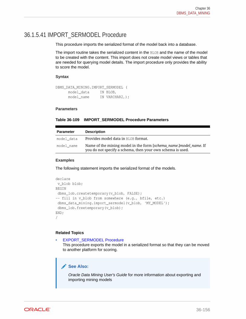
36.1.5.41 IMPORT_SERMODEL ProcedureThis procedure imports the serialized format of the model back into a database.
The import routine takes the serialized content in the BLOB and the name of the modelto be created with the content. This import does not create model views or tables thatare needed for querying model details. The import procedure only provides the abilityto score the model.
Syntax
DBMS_DATA_MINING.IMPORT_SERMODEL ( model_data IN BLOB, model_name IN VARCHAR2,);
Parameters
Table 36-109 IMPORT_SERMODEL Procedure Parameters
Parameter Description
model_data Provides model data in BLOB format.
model_name Name of the mining model in the form [schema_name.]model_name. Ifyou do not specify a schema, then your own schema is used.
Examples
The following statement imports the serialized format of the models.
declare v_blob blob;BEGIN dbms_lob.createtemporary(v_blob, FALSE);-- fill in v_blob from somewhere (e.g., bfile, etc.) dbms_data_mining.import_sermodel(v_blob, 'MY_MODEL'); dbms_lob.freetemporary(v_blob);END;/
Related Topics
• EXPORT_SERMODEL ProcedureThis procedure exports the model in a serialized format so that they can be movedto another platform for scoring.
See Also:
Oracle Data Mining User's Guide for more information about exporting andimporting mining models
Chapter 36DBMS_DATA_MINING
36-156
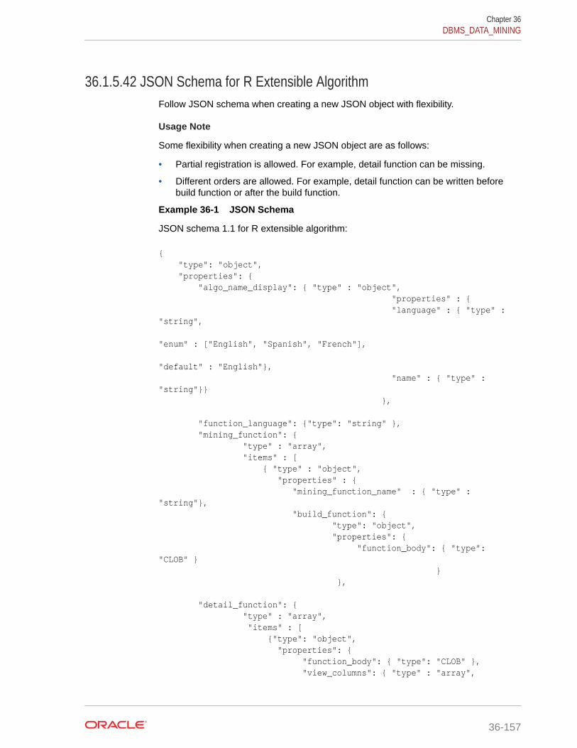
36.1.5.42 JSON Schema for R Extensible AlgorithmFollow JSON schema when creating a new JSON object with flexibility.
Usage Note
Some flexibility when creating a new JSON object are as follows:
• Partial registration is allowed. For example, detail function can be missing.
• Different orders are allowed. For example, detail function can be written beforebuild function or after the build function.
Example 36-1 JSON Schema
JSON schema 1.1 for R extensible algorithm:
{ "type": "object", "properties": { "algo_name_display": { "type" : "object", "properties" : { "language" : { "type" : "string", "enum" : ["English", "Spanish", "French"], "default" : "English"}, "name" : { "type" : "string"}} },
"function_language": {"type": "string" }, "mining_function": { "type" : "array", "items" : [ { "type" : "object", "properties" : { "mining_function_name" : { "type" : "string"}, "build_function": { "type": "object", "properties": { "function_body": { "type": "CLOB" } } },
"detail_function": { "type" : "array", "items" : [ {"type": "object", "properties": { "function_body": { "type": "CLOB" }, "view_columns": { "type" : "array",
Chapter 36DBMS_DATA_MINING
36-157
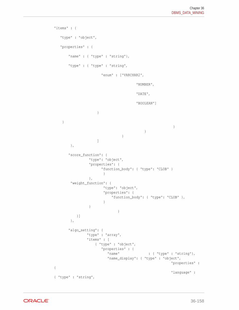
"items" : { "type" : "object", "properties" : { "name" : { "type" : "string"}, "type" : { "type" : "string", "enum" : ["VARCHAR2", "NUMBER", "DATE", "BOOLEAN"] } } } } } ] },
"score_function": { "type": "object", "properties": { "function_body": { "type": "CLOB" } } }, "weight_function": { "type": "object", "properties": { "function_body": { "type": "CLOB" }, } } } }] },
"algo_setting": { "type" : "array", "items" : [ { "type" : "object", "properties" : { "name" : { "type" : "string"}, "name_display": { "type" : "object", "properties" : { "language" : { "type" : "string",
Chapter 36DBMS_DATA_MINING
36-158
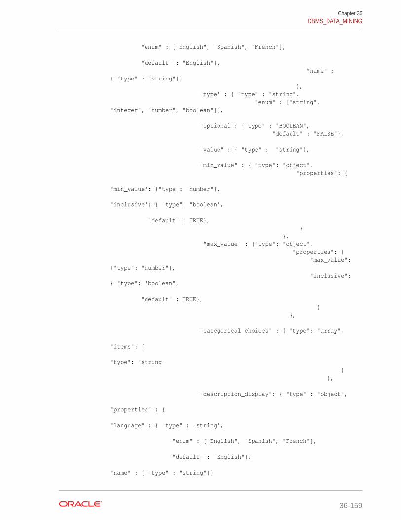
"enum" : ["English", "Spanish", "French"], "default" : "English"}, "name" : { "type" : "string"}} }, "type" : { "type" : "string", "enum" : ["string", "integer", "number", "boolean"]},
"optional": {"type" : "BOOLEAN", "default" : "FALSE"}, "value" : { "type" : "string"},
"min_value" : { "type": "object", "properties": { "min_value": {"type": "number"}, "inclusive": { "type": "boolean", "default" : TRUE}, } }, "max_value" : {"type": "object", "properties": { "max_value": {"type": "number"}, "inclusive": { "type": "boolean", "default" : TRUE}, } },
"categorical choices" : { "type": "array", "items": { "type": "string" } },
"description_display": { "type" : "object", "properties" : { "language" : { "type" : "string", "enum" : ["English", "Spanish", "French"], "default" : "English"}, "name" : { "type" : "string"}}
Chapter 36DBMS_DATA_MINING
36-159

} } } ] } }}
Example 36-2 JSON object example
The following is an JSON object example that must be passed to the registrationprocedure:
{ "algo_name_display" : {"English", "t1"}, "function_language" : "R", "mining_function" : { "mining_function_name" : "CLASSIFICATION", "build_function" : {"function_body": "function(dat, formula, family) { set.seed(1234); mod <- glm(formula = formula, data=dat, family= eval(parse(text=family))); mod}"}, "score_function" : { "function_body": "function(mod, dat) { res <- predict(mod, newdata = dat, type=''response ''); res2=data.frame(1-res, res); res2}"}} }, "algo_setting" : [{"name" : "dbms_data_mining.odms_m issing_value_treatment", "name_display" : {"English", "dbms_data_mining.odms_missing_value _treatment"}, "type" : "string", "optional" : "TRUE", "value" : "dbms_data_mining.odms_missing_value_mean_mode", "categorical choices" : [ "dbms_data_mining.odms_missing_value_mean_mode", "dbms_data_mining.odms_missing_value_auto", "dbms_data_mining.odms_missing_value_delete_row"], "description" : {"English",
Chapter 36DBMS_DATA_MINING
36-160

"how to treat missing values"} }, {"name" : "RALG_PARAMETER_FAMILY", "name_display" : {"English", "RALG_PARAMETER_FAMILY"}, "type" : "string", "optional" : "TRUE", "value" : "", "description" : {"English", "R family parameter in build function"} }], }
36.1.5.43 REGISTER_ALGORITHM ProcedureUser can register a new algorithm by providing algorithm name, mining function, andall other algorithm metadata to this function.
Syntax
DBMS_DATA_MINING.REGISTER_ALGORITHM ( algorithm_name IN VARCHAR2, algorithm_metadata IN CLOB, algorithm_description IN VARCHAR2 DEFAULT NULL);
Parameters
Table 36-110 REGISTER_ALGORITHM Procedure Parameters
Parameter Description
algorithm_name Name of the algorithm.
algorithm_metadata Metadata of the algorithm.
algorithm_description Description of the algorithm.
Usage Notes
The registration procedure performs the following:
• Checks whether algorithm_metadata has correct JSON syntax.
• Checks whether the input JSON object follows the predefined JSON schema.
• Checks whether current user has RQADMIN privilege.
• Checks duplicate algorithms such that the same algorithm is not registered twice.
• Checks for missing entries. For example, algorithm name, algorithm type,metadata, and build function.
Register Algorithms After the JSON Object Is Created
SQL users can register new algorithms by following the given procedure:
Chapter 36DBMS_DATA_MINING
36-161
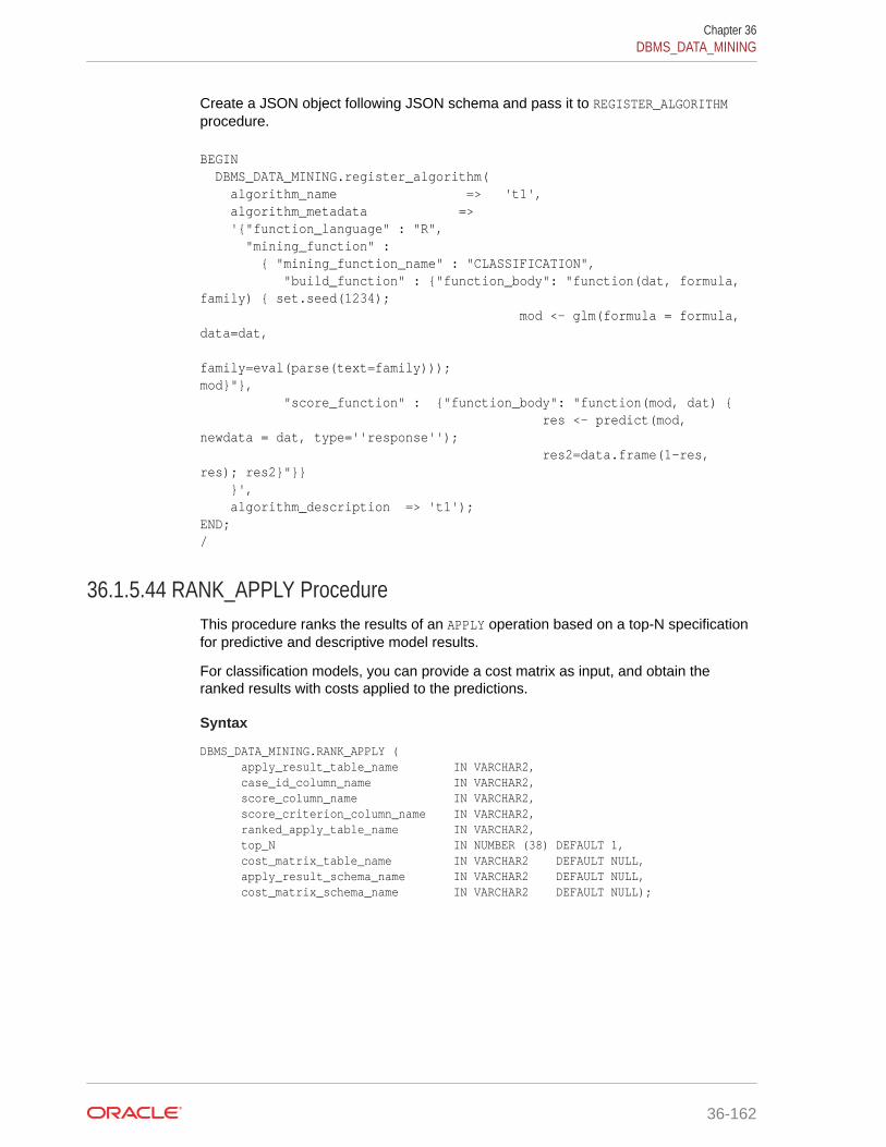
Create a JSON object following JSON schema and pass it to REGISTER_ALGORITHMprocedure.
BEGIN DBMS_DATA_MINING.register_algorithm( algorithm_name => 't1', algorithm_metadata => '{"function_language" : "R", "mining_function" : { "mining_function_name" : "CLASSIFICATION", "build_function" : {"function_body": "function(dat, formula, family) { set.seed(1234); mod <- glm(formula = formula, data=dat, family=eval(parse(text=family))); mod}"}, "score_function" : {"function_body": "function(mod, dat) { res <- predict(mod, newdata = dat, type=''response''); res2=data.frame(1-res, res); res2}"}} }', algorithm_description => 't1');END;/
36.1.5.44 RANK_APPLY ProcedureThis procedure ranks the results of an APPLY operation based on a top-N specificationfor predictive and descriptive model results.
For classification models, you can provide a cost matrix as input, and obtain theranked results with costs applied to the predictions.
Syntax
DBMS_DATA_MINING.RANK_APPLY ( apply_result_table_name IN VARCHAR2, case_id_column_name IN VARCHAR2, score_column_name IN VARCHAR2, score_criterion_column_name IN VARCHAR2, ranked_apply_table_name IN VARCHAR2, top_N IN NUMBER (38) DEFAULT 1, cost_matrix_table_name IN VARCHAR2 DEFAULT NULL, apply_result_schema_name IN VARCHAR2 DEFAULT NULL, cost_matrix_schema_name IN VARCHAR2 DEFAULT NULL);
Chapter 36DBMS_DATA_MINING
36-162

Parameters
Table 36-111 RANK_APPLY Procedure Parameters
Parameter Description
apply_result_table_name
Name of the table or view containing the results of an APPLYoperation on the test data set (see Usage Notes)
case_id_column_name Name of the case identifier column. This must be the sameas the one used for generating APPLY results.
score_column_name Name of the prediction column in the apply results table
score_criterion_column_name
Name of the probability column in the apply results table
ranked_apply_result_tab_name
Name of the table containing the ranked apply results
top_N Top N predictions to be considered from the APPLY resultsfor precision recall computation
cost_matrix_table_name
Name of the cost matrix table
apply_result_schema_name
Name of the schema hosting the APPLY results table
cost_matrix_schema_name
Name of the schema hosting the cost matrix table
Usage Notes
You can use RANK_APPLY to generate ranked apply results, based on a top-N filter andalso with application of cost for predictions, if the model was built with costs.
The behavior of RANK_APPLY is similar to that of APPLY with respect to other DDL-likeoperations such as CREATE_MODEL, DROP_MODEL, and RENAME_MODEL. The proceduredoes not depend on the model; the only input of relevance is the apply resultsgenerated in a fixed schema table from APPLY.
The main intended use of RANK_APPLY is for the generation of the final APPLY resultsagainst the scoring data in a production setting. You can apply the model against testdata using APPLY, compute various test metrics against various cost matrix tables, anduse the candidate cost matrix for RANK_APPLY.
The schema for the apply results from each of the supported algorithms is listed insubsequent sections. The case_id column will be the same case identifier column asthat of the apply results.
Classification Models — NB and SVM
For numerical targets, the ranked results table will have the definition as shown:
(case_id VARCHAR2/NUMBER,prediction NUMBER,probability NUMBER,cost NUMBER,rank INTEGER)
Chapter 36DBMS_DATA_MINING
36-163
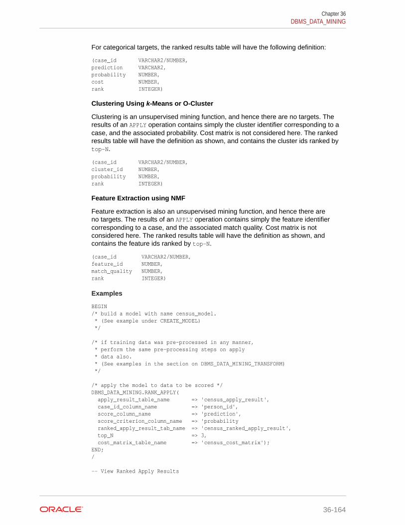
For categorical targets, the ranked results table will have the following definition:
(case_id VARCHAR2/NUMBER,prediction VARCHAR2,probability NUMBER,cost NUMBER,rank INTEGER)
Clustering Using k-Means or O-Cluster
Clustering is an unsupervised mining function, and hence there are no targets. Theresults of an APPLY operation contains simply the cluster identifier corresponding to acase, and the associated probability. Cost matrix is not considered here. The rankedresults table will have the definition as shown, and contains the cluster ids ranked bytop-N.
(case_id VARCHAR2/NUMBER,cluster_id NUMBER,probability NUMBER,rank INTEGER)
Feature Extraction using NMF
Feature extraction is also an unsupervised mining function, and hence there areno targets. The results of an APPLY operation contains simply the feature identifiercorresponding to a case, and the associated match quality. Cost matrix is notconsidered here. The ranked results table will have the definition as shown, andcontains the feature ids ranked by top-N.
(case_id VARCHAR2/NUMBER,feature_id NUMBER,match_quality NUMBER,rank INTEGER)
Examples
BEGIN/* build a model with name census_model. * (See example under CREATE_MODEL) */
/* if training data was pre-processed in any manner, * perform the same pre-processing steps on apply * data also. * (See examples in the section on DBMS_DATA_MINING_TRANSFORM) */
/* apply the model to data to be scored */DBMS_DATA_MINING.RANK_APPLY( apply_result_table_name => 'census_apply_result', case_id_column_name => 'person_id', score_column_name => 'prediction', score_criterion_column_name => 'probability ranked_apply_result_tab_name => 'census_ranked_apply_result', top_N => 3, cost_matrix_table_name => 'census_cost_matrix');END;/
-- View Ranked Apply Results
Chapter 36DBMS_DATA_MINING
36-164
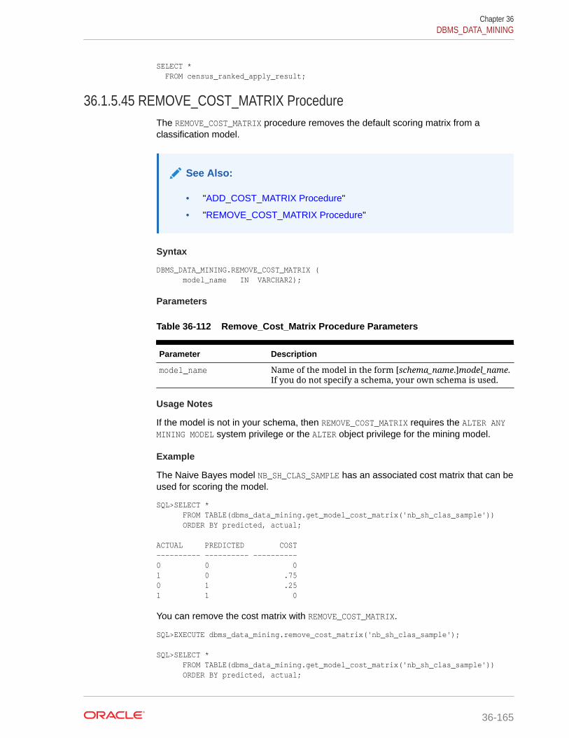
SELECT * FROM census_ranked_apply_result;
36.1.5.45 REMOVE_COST_MATRIX ProcedureThe REMOVE_COST_MATRIX procedure removes the default scoring matrix from aclassification model.
See Also:
• "ADD_COST_MATRIX Procedure"
• "REMOVE_COST_MATRIX Procedure"
Syntax
DBMS_DATA_MINING.REMOVE_COST_MATRIX ( model_name IN VARCHAR2);
Parameters
Table 36-112 Remove_Cost_Matrix Procedure Parameters
Parameter Description
model_name Name of the model in the form [schema_name.]model_name.If you do not specify a schema, your own schema is used.
Usage Notes
If the model is not in your schema, then REMOVE_COST_MATRIX requires the ALTER ANYMINING MODEL system privilege or the ALTER object privilege for the mining model.
Example
The Naive Bayes model NB_SH_CLAS_SAMPLE has an associated cost matrix that can beused for scoring the model.
SQL>SELECT * FROM TABLE(dbms_data_mining.get_model_cost_matrix('nb_sh_clas_sample')) ORDER BY predicted, actual; ACTUAL PREDICTED COST---------- ---------- ----------0 0 01 0 .750 1 .251 1 0
You can remove the cost matrix with REMOVE_COST_MATRIX.
SQL>EXECUTE dbms_data_mining.remove_cost_matrix('nb_sh_clas_sample');
SQL>SELECT * FROM TABLE(dbms_data_mining.get_model_cost_matrix('nb_sh_clas_sample')) ORDER BY predicted, actual;
Chapter 36DBMS_DATA_MINING
36-165

no rows selected
36.1.5.46 RENAME_MODEL ProcedureThis procedure changes the name of the mining model indicated by model_name tothe name that you specify as new_model_name.
If a model with new_model_name already exists, then the procedure optionallyrenames new_model_name to versioned_model_name before renaming model_nameto new_model_name.
The model name is in the form [schema_name.]model_name. If you do not specifya schema, your own schema is used. For mining model naming restrictions, see theUsage Notes for "CREATE_MODEL Procedure".
Syntax
DBMS_DATA_MINING.RENAME_MODEL ( model_name IN VARCHAR2, new_model_name IN VARCHAR2, versioned_model_name IN VARCHAR2 DEFAULT NULL);
Parameters
Table 36-113 RENAME_MODEL Procedure Parameters
Parameter Description
model_name Model to be renamed.
new_model_name New name for the model model_name.
versioned_model_name New name for the model new_model_name if it alreadyexists.
Usage Notes
If you attempt to rename a model while it is being applied, then the model will berenamed but the apply operation will return indeterminate results.
Examples
1. This example changes the name of model census_model to census_model_2012.
BEGIN DBMS_DATA_MINING.RENAME_MODEL( model_name => 'census_model', new_model_name => 'census_model_2012');END;/
2. In this example, there are two classification models in the user's schema:clas_mod, the working model, and clas_mod_tst, a test model. The RENAME_MODELprocedure preserves clas_mod as clas_mod_old and makes the test model thenew working model.
SELECT model_name FROM user_mining_models;MODEL_NAME-------------------------------------------------------------------
Chapter 36DBMS_DATA_MINING
36-166
CLAS_MODCLAS_MOD_TST
BEGIN DBMS_DATA_MINING.RENAME_MODEL( model_name => 'clas_mod_tst', new_model_name => 'clas_mod', versioned_model_name => 'clas_mod_old');END;/
SELECT model_name FROM user_mining_models;MODEL_NAME-------------------------------------------------------------------CLAS_MODCLAS_MOD_OLD
36.2 DBMS_DATA_MINING_TRANSFORMDBMS_DATA_MINING_TRANSFORM implements a set of transformations that are commonlyused in data mining.
This chapter contains the following topics:
• Overview
• Operational Notes
• Security Model
• Datatypes
• Constants
• Summary of DBMS_DATA_MINING_TRANSFORM Subprograms
See Also:
• DBMS_DATA_MINING
• Oracle Data Mining User's Guide
36.2.1 Using DBMS_DATA_MINING_TRANSFORMThis section contains topics that relate to using the DBMS_DATA_MINING_TRANSFORMpackage.
• Overview
• Operational Notes
• Security Model
• Datatypes
• Constants
Chapter 36DBMS_DATA_MINING_TRANSFORM
36-167

36.2.1.1 DBMS_DATA_MINING_TRANSFORM OverviewA transformation is a SQL expression that modifies the data in one or more columns.
Data must typically undergo certain transformations before it can be used tobuild a mining model. Many data mining algorithms have specific transformationrequirements.
Data that will be scored must be transformed in the same way as the data that wasused to create (train) the model.
External or Embedded Transformations
DBMS_DATA_MINING_TRANSFORM offers two approaches to implementing transformations.For a given model, you can either:
• Create a list of transformation expressions and pass it to the CREATE_MODELProcedure
or
• Create a view that implements the transformations and pass the name of the viewto the CREATE_MODEL Procedure
If you create a transformation list and pass it to CREATE_MODEL, the transformationexpressions are embedded in the model and automatically implemented whenever themodel is applied.
If you create a view, the transformation expressions are external to the model. You willneed to re-create the transformations whenever you apply the model.
Note:
Embedded transformations significantly enhance the model's usability whilesimplifying the process of model management.
Automatic Transformations
Oracle Data Mining supports an Automatic Data Preparation (ADP) mode. When ADPis enabled, most algorithm-specific transformations are automatically embedded. Anyadditional transformations must be explicitly provided in an embedded transformationlist or in a view.
If ADP is enabled and you create a model with a transformation list, bothsets of transformations are embedded. The model will execute the user-specifiedtransformations from the transformation list before executing the automatictransformations specified by ADP.
Within a transformation list, you can selectively disable ADP for individual attributes.
Chapter 36DBMS_DATA_MINING_TRANSFORM
36-168
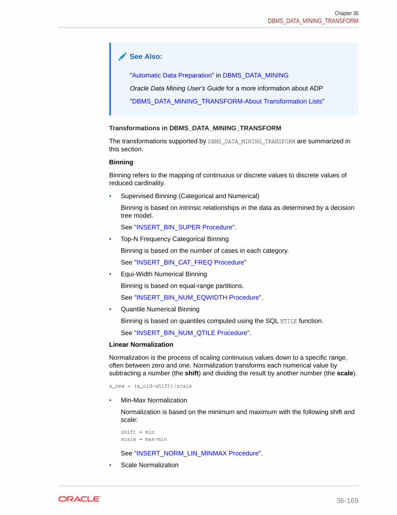
See Also:
"Automatic Data Preparation" in DBMS_DATA_MINING
Oracle Data Mining User's Guide for a more information about ADP
"DBMS_DATA_MINING_TRANSFORM-About Transformation Lists"
Transformations in DBMS_DATA_MINING_TRANSFORM
The transformations supported by DBMS_DATA_MINING_TRANSFORM are summarized inthis section.
Binning
Binning refers to the mapping of continuous or discrete values to discrete values ofreduced cardinality.
• Supervised Binning (Categorical and Numerical)
Binning is based on intrinsic relationships in the data as determined by a decisiontree model.
See "INSERT_BIN_SUPER Procedure".
• Top-N Frequency Categorical Binning
Binning is based on the number of cases in each category.
See "INSERT_BIN_CAT_FREQ Procedure"
• Equi-Width Numerical Binning
Binning is based on equal-range partitions.
See "INSERT_BIN_NUM_EQWIDTH Procedure".
• Quantile Numerical Binning
Binning is based on quantiles computed using the SQL NTILE function.
See "INSERT_BIN_NUM_QTILE Procedure".
Linear Normalization
Normalization is the process of scaling continuous values down to a specific range,often between zero and one. Normalization transforms each numerical value bysubtracting a number (the shift) and dividing the result by another number (the scale).
x_new = (x_old-shift)/scale
• Min-Max Normalization
Normalization is based on the minimum and maximum with the following shift andscale:
shift = minscale = max-min
See "INSERT_NORM_LIN_MINMAX Procedure".
• Scale Normalization
Chapter 36DBMS_DATA_MINING_TRANSFORM
36-169

Normalization is based on the minimum and maximum with the following shift andscale:
shift = 0 scale = max{abs(max), abs(min)}
See "INSERT_NORM_LIN_SCALE Procedure".
• Z-Score Normalization
Normalization is based on the mean and standard deviation with the following shiftand scale:
shift = mean scale = standard_deviation
See "INSERT_NORM_LIN_ZSCORE Procedure".
Outlier Treatment
An outlier is a numerical value that is located far from the rest of the data. Outliers canartificially skew the results of data mining.
• Winsorizing
Outliers are replaced with the nearest value that is not an outlier.
See "INSERT_CLIP_WINSOR_TAIL Procedure"
• Trimming
Outliers are set to NULL.
See "INSERT_CLIP_TRIM_TAIL Procedure".
Missing Value Treatment
Missing data may indicate sparsity or it may indicate that some values are missingat random. DBMS_DATA_MINING_TRANSFORM supports the following transformations forminimizing the effects of missing values:
• Missing numerical values are replaced with the mean.
See "INSERT_MISS_NUM_MEAN Procedure".
• Missing categorical values are replaced with the mode.
See "INSERT_MISS_CAT_MODE Procedure".
Note:
Oracle Data Mining also has default mechanisms for handling missing data.See Oracle Data Mining User's Guide for details.
36.2.1.2 DBMS_DATA_MINING_TRANSFORM Security ModelThe DBMS_DATA_MINING_TRANSFORM package is owned by user SYS and is installed aspart of database installation. Execution privilege on the package is granted to public.
Chapter 36DBMS_DATA_MINING_TRANSFORM
36-170
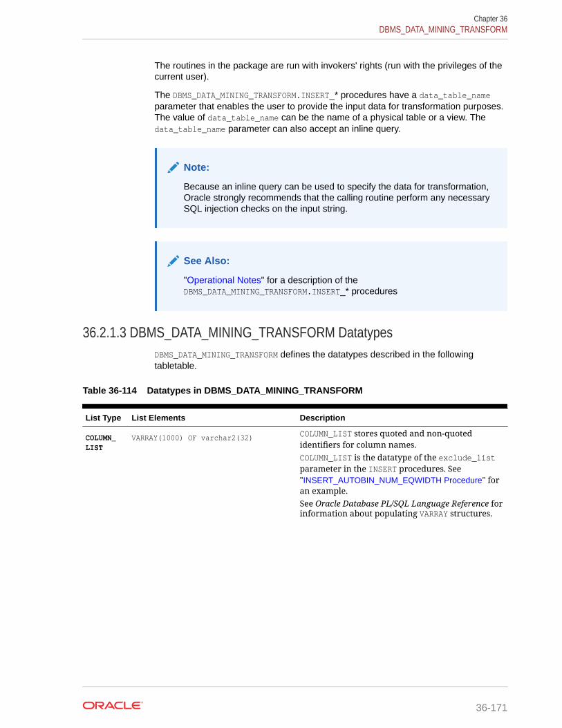
The routines in the package are run with invokers' rights (run with the privileges of thecurrent user).
The DBMS_DATA_MINING_TRANSFORM.INSERT_* procedures have a data_table_nameparameter that enables the user to provide the input data for transformation purposes.The value of data_table_name can be the name of a physical table or a view. Thedata_table_name parameter can also accept an inline query.
Note:
Because an inline query can be used to specify the data for transformation,Oracle strongly recommends that the calling routine perform any necessarySQL injection checks on the input string.
See Also:
"Operational Notes" for a description of theDBMS_DATA_MINING_TRANSFORM.INSERT_* procedures
36.2.1.3 DBMS_DATA_MINING_TRANSFORM DatatypesDBMS_DATA_MINING_TRANSFORM defines the datatypes described in the followingtabletable.
Table 36-114 Datatypes in DBMS_DATA_MINING_TRANSFORM
List Type List Elements Description
COLUMN_LIST
VARRAY(1000) OF varchar2(32) COLUMN_LIST stores quoted and non-quotedidentifiers for column names.COLUMN_LIST is the datatype of the exclude_listparameter in the INSERT procedures. See"INSERT_AUTOBIN_NUM_EQWIDTH Procedure" foran example.See Oracle Database PL/SQL Language Reference forinformation about populating VARRAY structures.
Chapter 36DBMS_DATA_MINING_TRANSFORM
36-171

Table 36-114 (Cont.) Datatypes in DBMS_DATA_MINING_TRANSFORM
List Type List Elements Description
DESCRIBE_LIST
DBMS_SQL.DESC_TAB2
TYPE desc_tab2 IS TABLE OF desc_rec2 INDEX BY BINARY_INTEGER
TYPE desc_rec2 IS RECORD (col_type BINARY_INTEGER := 0,col_max_len BINARY_INTEGER := 0,col_name VARCHAR2(32767):= '',col_name_len BINARY_INTEGER := 0,col_schema_name VARCHAR2(32) := '',col_schema_name_len BINARY_INTEGER := 0,col_precision BINARY_INTEGER := 0,col_scale BINARY_INTEGER := 0,col_charsetid BINARY_INTEGER := 0,col_charsetform BINARY_INTEGER := 0,col_null_ok BOOLEAN := TRUE);
DESCRIBE_LIST describes the columns of thedata table after the transformation list has beenapplied. A DESCRIBE_LIST is returned by theDESCRIBE_STACK Procedure.
The DESC_TAB2 and DESC_REC2 types are definedin the DBMS_SQL package. See "DESC_REC2 RecordType".The col_type field of DESC_REC2 identifies thedatatype of the column. The datatype is expressedas a numeric constant that represents a built-indatatype. For example, a 1 indicates a variablelength character string. The codes for Oracle built-in datatypes are listed in Oracle Database SQLLanguage Reference. The codes for the Oracle DataMining nested types are described in "Constants".
The col_name field of DESC_REC2 identifies thecolumn name. It may be populated with a columnname, an alias, or an expression. If the columnname is a SELECT expression, it may be very long.If the expression is longer than 30 bytes, it cannotbe used in a view unless it is given an alias.
Chapter 36DBMS_DATA_MINING_TRANSFORM
36-172
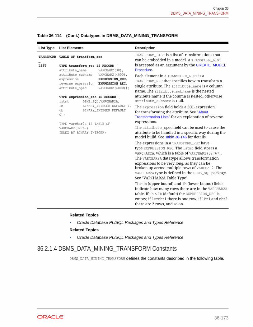
Table 36-114 (Cont.) Datatypes in DBMS_DATA_MINING_TRANSFORM
List Type List Elements Description
TRANSFORM_LIST
TABLE OF transform_rec
TYPE transform_rec IS RECORD (attribute_name VARCHAR2(30),attribute_subname VARCHAR2(4000),expression EXPRESSION_REC,reverse_expression EXPRESSION_REC,attribute_spec VARCHAR2(4000));
TYPE expression_rec IS RECORD (lstmt DBMS_SQL.VARCHAR2A,lb BINARY_INTEGER DEFAULT 1,ub BINARY_INTEGER DEFAULT 0);
TYPE varchar2a IS TABLE OF VARCHAR2(32767)INDEX BY BINARY_INTEGER;
TRANSFORM_LIST is a list of transformations thatcan be embedded in a model. A TRANSFORM_LISTis accepted as an argument by the CREATE_MODELProcedure.
Each element in a TRANSFORM_LIST is aTRANSFORM_REC that specifies how to transform asingle attribute. The attribute_name is a columnname. The attribute_subname is the nestedattribute name if the column is nested, otherwiseattribute_subname is null.
The expression field holds a SQL expressionfor transforming the attribute. See "AboutTransformation Lists" for an explanation of reverseexpressions.The attribute_spec field can be used to cause theattribute to be handled in a specific way during themodel build. See Table 36-146 for details.
The expressions in a TRANSFORM_REC havetype EXPRESSION_REC. The lstmt field stores aVARCHAR2A, which is a table of VARCHAR2(32767).The VARCHAR2A datatype allows transformationexpressions to be very long, as they can bebroken up across multiple rows of VARCHAR2. TheVARCHAR2A type is defined in the DBMS_SQL package.See "VARCHAR2A Table Type".The ub (upper bound) and lb (lower bound) fieldsindicate how many rows there are in the VARCHAR2Atable. If ub < lb (default) the EXPRESSION_REC isempty; if lb=ub=1 there is one row; if lb=1 and ub=2there are 2 rows, and so on.
Related Topics
• Oracle Database PL/SQL Packages and Types Reference
Related Topics
• Oracle Database PL/SQL Packages and Types Reference
36.2.1.4 DBMS_DATA_MINING_TRANSFORM ConstantsDBMS_DATA_MINING_TRANSFORM defines the constants described in the following table.
Chapter 36DBMS_DATA_MINING_TRANSFORM
36-173
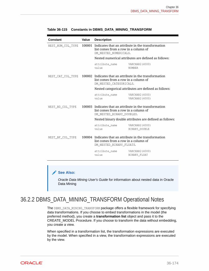
Table 36-115 Constants in DBMS_DATA_MINING_TRANSFORM
Constant Value Description
NEST_NUM_COL_TYPE 100001 Indicates that an attribute in the transformationlist comes from a row in a column ofDM_NESTED_NUMERICALS.
Nested numerical attributes are defined as follows:
attribute_name VARCHAR2(4000)value NUMBER
NEST_CAT_COL_TYPE 100002 Indicates that an attribute in the transformationlist comes from a row in a column ofDM_NESTED_CATEGORICALS.
Nested categorical attributes are defined as follows:
attribute_name VARCHAR2(4000)value VARCHAR2(4000)
NEST_BD_COL_TYPE 100003 Indicates that an attribute in the transformationlist comes from a row in a column ofDM_NESTED_BINARY_DOUBLES.
Nested binary double attributes are defined as follows:
attribute_name VARCHAR2(4000)value BINARY_DOUBLE
NEST_BF_COL_TYPE 100004 Indicates that an attribute in the transformationlist comes from a row in a column ofDM_NESTED_BINARY_FLOATS.
attribute_name VARCHAR2(4000)value BINARY_FLOAT
See Also:
Oracle Data Mining User's Guide for information about nested data in OracleData Mining
36.2.2 DBMS_DATA_MINING_TRANSFORM Operational NotesThe DBMS_DATA_MINING_TRANSFORM package offers a flexible framework for specifyingdata transformations. If you choose to embed transformations in the model (thepreferred method), you create a transformation list object and pass it to theCREATE_MODEL Procedure. If you choose to transform the data without embedding,you create a view.
When specified in a transformation list, the transformation expressions are executedby the model. When specified in a view, the transformation expressions are executedby the view.
Chapter 36DBMS_DATA_MINING_TRANSFORM
36-174

Transformation Definitions
Transformation definitions are used to generate the SQL expressions that transformthe data. For example, the transformation definitions for normalizing a numeric columnare the shift and scale values for that data.
With the DBMS_DATA_MINING_TRANSFORM package, you can call procedures to computethe transformation definitions, or you can compute them yourself, or you can do both.
Transformation Definition Tables
DBMS_DATA_MINING_TRANSFORM provides INSERT procedures that computetransformation definitions and insert them in transformation definition tables. You canmodify the values in the transformation definition tables or populate them yourself.
XFORM routines use populated definition tables to transform data in external views.STACK routines use populated definition tables to build transformation lists.
To specify transformations based on definition tables, follow these steps:
1. Use CREATE routines to create transformation definition tables.
The tables have columns to hold the transformation definitions for a given typeof transformation. For example, the CREATE_BIN_NUM Procedure creates adefinition table that has a column for storing data values and another column forstoring the associated bin identifiers.
2. Use INSERT routines to compute and insert transformation definitions in the tables.
Each INSERT routine uses a specific technique for computing the transformationdefinitions. For example, the INSERT_BIN_NUM_EQWIDTH Procedure computesbin boundaries by identifying the minimum and maximum values then setting thebin boundaries at equal intervals.
3. Use STACK or XFORM routines to generate transformation expressions based on theinformation in the definition tables:
• Use STACK routines to add the transformation expressions to a transformationlist. Pass the transformation list to the CREATE_MODEL Procedure. Thetransformation expressions will be assembled into one long SQL query andembedded in the model.
• Use XFORM routines to execute the transformation expressions within a view.The transformations will be external to the model and will need to be re-created whenever the model is applied to new data.
Transformations Without Definition Tables
STACK routines are not the only method for adding transformation expressions to atransformation list. You can also build a transformation list without using definitiontables.
To specify transformations without using definition tables, follow these steps:
1. Write a SQL expression for transforming an attribute.
2. Write a SQL expression for reversing the transformation.(See "Reverse Transformations and Model Transparency" in"DBMS_DATA_MINING_TRANSFORM-About Transformation Lists".)
Chapter 36DBMS_DATA_MINING_TRANSFORM
36-175

3. Determine whether or not to disable ADP for the attribute. By default ADPis enabled for the attribute if it is specified for the model. (See "DisablingAutomatic Data Preparation" in "DBMS_DATA_MINING_TRANSFORM - AboutTransformation Lists".)
4. Specify the SQL expressions and ADP instructions in a call to theSET_TRANSFORM Procedure, which adds the information to a transformationlist.
5. Repeat steps 1 through 4 for each attribute that you wish to transform.
6. Pass the transformation list to the CREATE_MODEL Procedure. Thetransformation expressions will be assembled into one long SQL query andembedded in the model.
Note:
SQL expressions that you specify with SET_TRANSFORM must fit withina VARCHAR2. To specify a longer expression, you can use theSET_EXPRESSION Procedure. With SET_EXPRESSION, you can build anexpression by appending rows to a VARCHAR2 array.
About Stacking
Transformation lists are built by stacking transformation records. Transformation listsare evaluated from bottom to top. Each transformation expression depends on theresult of the transformation expression below it in the stack.
Related Topics
• CREATE_MODEL ProcedureThis procedure creates a mining model with a given mining function.
• DBMS_DATA_MINING_TRANSFORM — About Transformation ListsThe elements of a transformation list are transformation records. Eachtransformation record provides all the information needed by the model formanaging the transformation of a single attribute.
• DBMS_DATA_MINING_TRANSFORM — About Stacking and Stack ProceduresTransformation lists are built by stacking transformation records. Transformationlists are evaluated from bottom to top. Each transformation expression depends onthe result of the transformation expression below it in the stack.
• DBMS_DATA_MINING_TRANSFORM — Nested Data TransformationsThe CREATE routines create transformation definition tables that include twocolumns, col and att, for identifying attributes. The column col holds the name ofa column in the data table. If the data column is not nested, then att is null, andthe name of the attribute is col. If the data column is nested, then att holds thename of the nested attribute, and the name of the attribute is col.att.
36.2.2.1 DBMS_DATA_MINING_TRANSFORM — About Transformation ListsThe elements of a transformation list are transformation records. Eachtransformation record provides all the information needed by the model for managingthe transformation of a single attribute.
Each transformation record includes the following fields:
Chapter 36DBMS_DATA_MINING_TRANSFORM
36-176

• attribute_name — Name of the column of data to be transformed
• attribute_subname — Name of the nested attribute if attribute_name is a nestedcolumn, otherwise NULL
• expression — SQL expression for transforming the attribute
• reverse_expression — SQL expression for reversing the transformation
• attribute_spec — Identifies special treatment for the attribute during the modelbuild. See Table 36-146 for details.
See Also:
• Table 36-114 for details about the TRANSFORM_LIST and TRANSFORM_RECobject types
• SET_TRANSFORM Procedure
• CREATE_MODEL Procedure
Reverse Transformations and Model Transparency
An algorithm manipulates transformed attributes to train and score a model. Thetransformed attributes, however, may not be meaningful to an end user. For example,if attribute x has been transformed into bins 1 — 4, the bin names 1, 2 , 3, and 4 aremanipulated by the algorithm, but a user is probably not interested in the model detailsabout bins 1 — 4 or in predicting the numbers 1 — 4.
To return original attribute values in model details and predictions, you can provide areverse expression in the transformation record for the attribute. For example, if youspecify the transformation expression 'log(10, y)' for attribute y, you could specifythe reverse transformation expression 'power(10, y)'.
Reverse transformations enable model transparency. They make internal processingtransparent to the user.
Note:
STACK procedures automatically reverse normalization transformations, butthey do not provide a mechanism for reversing binning, clipping, or missingvalue transformations.
You can use the DBMS_DATA_MINING.ALTER_REVERSE_EXPRESSION procedureto specify or update reverse transformations expressions for an existingmodel.
Chapter 36DBMS_DATA_MINING_TRANSFORM
36-177
See Also:
Table 36-114
"ALTER_REVERSE_EXPRESSION Procedure"
"Summary of DBMS_DATA_MINING Subprograms" for links to the modeldetails functions
Disabling Automatic Data Preparation
ADP is controlled by a model-specific setting (PREP_AUTO). The PREP_AUTO settingaffects all model attributes unless you disable it for individual attributes.
If ADP is enabled and you set attribute_spec to NOPREP, only the transformations thatyou specify for that attribute will be evaluated. If ADP is enabled and you do not setattribute_spec to NOPREP, the automatic transformations will be evaluated after thetransformations that you specify for the attribute.
If ADP is not enabled for the model, the attribute_spec field of the transformationrecord is ignored.
See Also:
"Automatic Data Preparation" for information about the PREP_AUTO setting
Adding Transformation Records to a Transformation List
A transformation list is a stack of transformation records. When a new transformationrecord is added, it is appended to the top of the stack. (See "About Stacking" fordetails.)
When you use SET_TRANSFORM to add a transformation record to a transformation list,you can specify values for all the fields in the transformation record.
When you use STACK procedures to add transformation records to a transformationlist, only the transformation expression field is populated. For normalizationtransformations, the reverse transformation expression field is also populated.
You can use both STACK procedures and SET_TRANSFORM to build one transformationlist. Each STACK procedure call adds transformation records for all the attributesin a specified transformation definition table. Each SET_TRANSFORM call adds atransformation record for a single attribute.
Chapter 36DBMS_DATA_MINING_TRANSFORM
36-178

36.2.2.2 DBMS_DATA_MINING_TRANSFORM — About Stacking and StackProcedures
Transformation lists are built by stacking transformation records. Transformation listsare evaluated from bottom to top. Each transformation expression depends on theresult of the transformation expression below it in the stack.
Stack Procedures
STACK procedures create transformation records from the information in transformationdefinition tables. For example STACK_BIN_NUM builds a transformation record for eachattribute specified in a definition table for numeric binning. STACK procedures stack thetransformation records as follows:
• If an attribute is specified in the definition table but not in the transformationlist, the STACK procedure creates a transformation record, computes the reversetransformation (if possible), inserts the transformation and reverse transformationin the transformation record, and appends the transformation record to the top ofthe transformation list.
• If an attribute is specified in the transformation list but not in the definition table,the STACK procedure takes no action.
• If an attribute is specified in the definition table and in the transformation list, theSTACK procedure stacks the transformation expression from the definition table ontop of the transformation expression in the transformation record and updates thereverse transformation. See Table 36-114and Example 36-6.
Example 36-3 Stacking a Clipping Transformation
This example shows how STACK_CLIP Procedure would add transformation recordsto a transformation list. Note that the clipping transformations are not reversed inCOL1 and COL2 after stacking (as described in "Reverse Transformations and ModelTransparency" in "DBMS_DATA_MINING_TRANSFORM-About Transformation Lists").
Refer to:
• CREATE_CLIP Procedure — Creates the definition table
• INSERT_CLIP_TRIM_TAIL Procedure — Inserts definitions in the table
• INSERT_CLIP_WINSOR_TAIL Procedure — Inserts definitions in the table
• Table 36-114 — Describes the structure of the transformation list (TRANSFORM_LISTobject)
Assume a clipping definition table populated as follows.
col att lcut lval rcut rval
COL1 null -1.5 -1.5 4.5 4.5
COL2 null 0 0 1 1
Assume the following transformation list before stacking.
-------------------------transformation record #1:-------------------------
Chapter 36DBMS_DATA_MINING_TRANSFORM
36-179
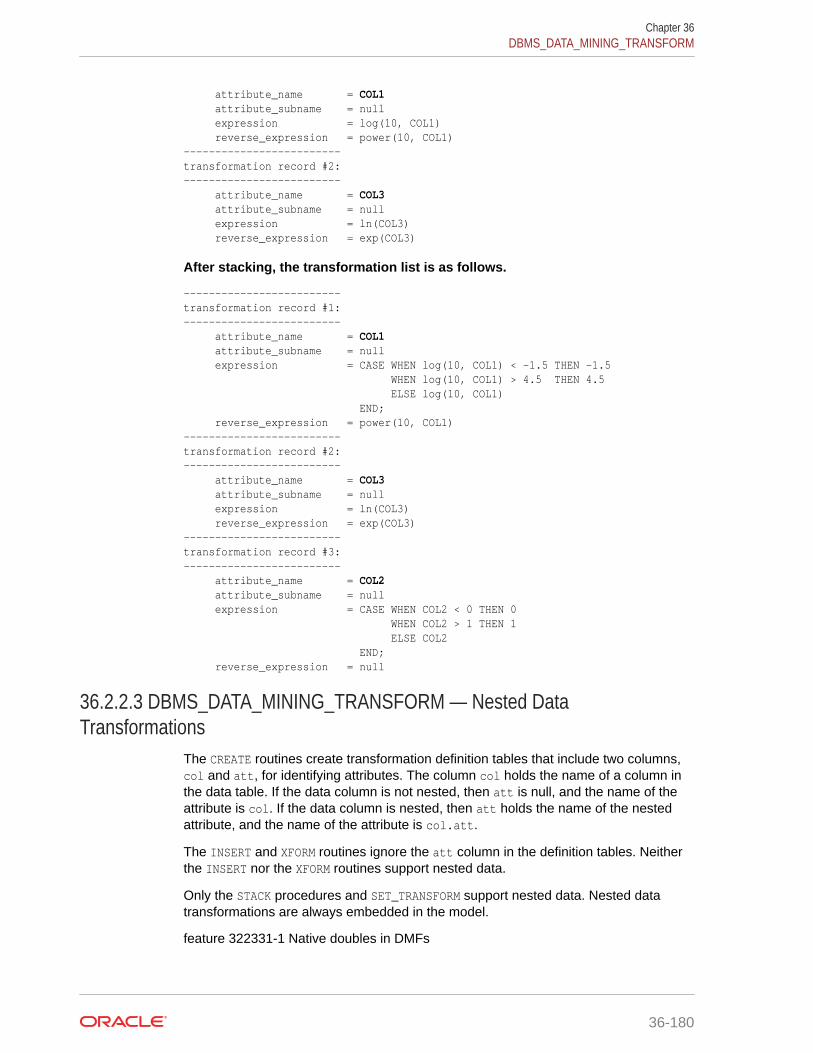
attribute_name = COL1 attribute_subname = null expression = log(10, COL1) reverse_expression = power(10, COL1)-------------------------transformation record #2:------------------------- attribute_name = COL3 attribute_subname = null expression = ln(COL3) reverse_expression = exp(COL3)
After stacking, the transformation list is as follows.
-------------------------transformation record #1:------------------------- attribute_name = COL1 attribute_subname = null expression = CASE WHEN log(10, COL1) < -1.5 THEN -1.5 WHEN log(10, COL1) > 4.5 THEN 4.5 ELSE log(10, COL1) END; reverse_expression = power(10, COL1)-------------------------transformation record #2:------------------------- attribute_name = COL3 attribute_subname = null expression = ln(COL3) reverse_expression = exp(COL3)-------------------------transformation record #3:------------------------- attribute_name = COL2 attribute_subname = null expression = CASE WHEN COL2 < 0 THEN 0 WHEN COL2 > 1 THEN 1 ELSE COL2 END; reverse_expression = null
36.2.2.3 DBMS_DATA_MINING_TRANSFORM — Nested DataTransformations
The CREATE routines create transformation definition tables that include two columns,col and att, for identifying attributes. The column col holds the name of a column inthe data table. If the data column is not nested, then att is null, and the name of theattribute is col. If the data column is nested, then att holds the name of the nestedattribute, and the name of the attribute is col.att.
The INSERT and XFORM routines ignore the att column in the definition tables. Neitherthe INSERT nor the XFORM routines support nested data.
Only the STACK procedures and SET_TRANSFORM support nested data. Nested datatransformations are always embedded in the model.
feature 322331-1 Native doubles in DMFs
Chapter 36DBMS_DATA_MINING_TRANSFORM
36-180

Nested columns in Oracle Data Mining can have the following types:
DM_NESTED_NUMERICALSDM_NESTED_CATEGORICALSDM_NESTED_BINARY_DOUBLESDM_NESTED_BINARY_FLOATS
See Also:
"Constants"
Oracle Data Mining User's Guide for details about nested attributes in OracleData Mining
Specifying Nested Attributes in a Transformation Record
A transformation record (TRANSFORM_REC) includes two fields, attribute_name andattribute_subname, for identifying the attribute. The field attribute_name holdsthe name of a column in the data table. If the data column is not nested, thenattribute_subname is null, and the name of the attribute is attribute_name. Ifthe data column is nested, then attribute_subname holds the name of the nestedattribute, and the name of the attribute is attribute_name.attribute_subname.
Transforming Individual Nested Attributes
You can specify different transformations for different attributes in a nested column,and you can specify a default transformation for all the remaining attributes in thecolumn. To specify a default nested transformation, specify null in the attribute_namefield and the name of the nested column in the attribute_subname field as shown inExample 36-4. Note that the keyword VALUE is used to represent the value of a nestedattribute in a transformation expression.
Example 36-4 Transforming a Nested Column
The following statement transforms two of the nested attributes in COL_N1. AttributeATTR1 is transformed with normalization; Attribute ATTR2 is set to null, which causesattribute removal transformation (ATTR2 is not used in training the model). All theremaining attributes in COL_N1 are divided by 10.
DECLARE stk dbms_data_mining_transform.TRANSFORM_LIST;BEGIN dbms_data_mining_transform.SET_TRANSFORM( stk,'COL_N1', 'ATTR1', '(VALUE - (-1.5))/20', 'VALUE *20 + (-1.5)'); dbms_data_mining_transform.SET_TRANSFORM( stk,'COL_N1', 'ATTR2', NULL, NULL); dbms_data_mining_transform.SET_TRANSFORM( stk, NULL, 'COL_N1', 'VALUE/10', 'VALUE*10');END;/
The following SQL is generated from this statement.
CAST(MULTISET(SELECT DM_NESTED_NUMERICAL( "ATTRIBUTE_NAME", DECODE("ATTRIBUTE_NAME",
Chapter 36DBMS_DATA_MINING_TRANSFORM
36-181

'ATTR1', ("VALUE" - (-1.5))/20, "VALUE"/10)) FROM TABLE("COL_N1") WHERE "ATTRIBUTE_NAME" IS NOT IN ('ATTR2')) AS DM_NESTED_NUMERICALS)
If transformations are not specified for COL_N1.ATTR1 and COL_N1.ATTR2, then thedefault transformation is used for all the attributes in COL_N1, and the resulting SQLdoes not include a DECODE.
CAST(MULTISET(SELECT DM_NESTED_NUMERICAL( "ATTRIBUTE_NAME", "VALUE"/10) FROM TABLE("COL_N1")) AS DM_NESTED_NUMERICALS)
Since DECODE is limited to 256 arguments, multiple DECODE functions are nested tosupport an arbitrary number of individual nested attribute specifications.
Adding a Nested Column
You can specify a transformation that adds a nested column to the data, as shown inExample 36-5.
Example 36-5 Adding a Nested Column to a Transformation List
DECLARE v_xlst dbms_data_mining_transform.TRANSFORM_LIST; BEGIN dbms_data_mining_transform.SET_TRANSFORM(v_xlst, 'YOB_CREDLIM', NULL, 'dm_nested_numericals( dm_nested_numerical( ''CUST_YEAR_OF_BIRTH'', cust_year_of_birth), dm_nested_numerical( ''CUST_CREDIT_LIMIT'', cust_credit_limit))', NULL); dbms_data_mining_transform.SET_TRANSFORM( v_xlst, 'CUST_YEAR_OF_BIRTH', NULL, NULL, NULL); dbms_data_mining_transform.SET_TRANSFORM( v_xlst, 'CUST_CREDIT_LIMIT', NULL, NULL, NULL); dbms_data_mining_transform.XFORM_STACK( v_xlst, 'mining_data', 'mining_data_v');END;/
set long 2000SELECT text FROM user_views WHERE view_name IN 'MINING_DATA_V'; TEXT---------------------------------------------------------------------------------SELECT "CUST_ID","CUST_POSTAL_CODE",dm_nested_numericals( dm_nested_numerical( 'CUST_YEAR_OF_BIRTH', cust_year_of_birth), dm_nested_numerical( 'CUST_CREDIT_LIMIT', cust_credit_limit)) "YOB_CREDLIM" FROM mining_data SELECT * FROM mining_data_v WHERE cust_id = 104500; CUST_ID CUST_POSTAL_CODE YOB_CREDLIM(ATTRIBUTE_NAME, VALUE)
Chapter 36DBMS_DATA_MINING_TRANSFORM
36-182

------- ---------------- --------------------------------------------------------- 104500 68524 DM_NESTED_NUMERICALS(DM_NESTED_NUMERICAL( 'CUST_YEAR_OF_BIRTH', 1962), DM_NESTED_NUMERICAL('CUST_CREDIT_LIMIT', 15000))
Stacking Nested Transformations
Example 36-6 shows how the STACK_NORM_LIN Procedure would addtransformation records for nested column COL_N to a transformation list.
Refer to:
• CREATE_NORM_LIN Procedure — Creates the definition table
• INSERT_NORM_LIN_MINMAX Procedure — Inserts definitions in the table
• INSERT_NORM_LIN_SCALE Procedure — Inserts definitions in the table
• INSERT_NORM_LIN_ZSCORE Procedure — Inserts definitions in the table
• Table 36-114 — Describes the structure of the transformation list
Example 36-6 Stacking a Nested Normalization Transformation
Assume a linear normalization definition table populated as follows.
col att shift scale
COL_N ATT2 0 20
null COL_N 0 10
Assume the following transformation list before stacking.
-------------------------transformation record #1:------------------------- attribute_name = COL_N attribute_subname = ATT1 expression = log(10, VALUE) reverse_expression = power(10, VALUE)-------------------------transformation record #2:------------------------- attribute_name = null attribute_subname = COL_N expression = ln(VALUE) reverse_expression = exp(VALUE)
After stacking, the transformation list is as follows.
-------------------------transformation record #1:------------------------- attribute_name = COL_N attribute_subname = ATT1 expression = (log(10, VALUE) - 0)/10 reverse_expression = power(10, VALUE*10 + 0)-------------------------transformation record #2:-------------------------
Chapter 36DBMS_DATA_MINING_TRANSFORM
36-183

attribute_name = NULL attribute_subname = COL_N expression = (ln(VALUE)- 0)/10 reverse_expression = exp(VALUE *10 + 0)-------------------------transformation record #3:------------------------- attribute_name = COL_N attribute_subname = ATT2 expression = (ln(VALUE) - 0)/20 reverse_expression = exp(VALUE * 20 + 0)
36.2.3 Summary of DBMS_DATA_MINING_TRANSFORMSubprograms
This table lists the DBMS_DATA_MINING_TRANSFORM subprograms in alphabetical orderand briefly describes them.
Table 36-116 DBMS_DATA_MINING_TRANSFORM Package Subprograms
Subprogram Purpose
CREATE_BIN_CAT Procedure Creates a transformation definition table forcategorical binning
CREATE_BIN_NUM Procedure Creates a transformation definition table for numericalbinning
CREATE_CLIP Procedure Creates a transformation definition table for clipping
CREATE_COL_REM Procedure Creates a transformation definition table for columnremoval
CREATE_MISS_CAT Procedure Creates a transformation definition table forcategorical missing value treatment
CREATE_MISS_NUM Procedure Creates a transformation definition table for numericalmissing values treatment
CREATE_NORM_LIN Procedure Creates a transformation definition table for linearnormalization
DESCRIBE_STACK Procedure Describes the transformation list
GET_EXPRESSION Function Returns a VARCHAR2 chunk from a transformationexpression
INSERT_AUTOBIN_NUM_EQWIDTH Procedure
Inserts numeric automatic equi-width binningdefinitions in a transformation definition table
INSERT_BIN_CAT_FREQProcedure
Inserts categorical frequency-based binning definitionsin a transformation definition table
INSERT_BIN_NUM_EQWIDTHProcedure
Inserts numeric equi-width binning definitions in atransformation definition table
INSERT_BIN_NUM_QTILEProcedure
Inserts numeric quantile binning expressions in atransformation definition table
INSERT_BIN_SUPER Procedure Inserts supervised binning definitions in numericaland categorical transformation definition tables
INSERT_CLIP_TRIM_TAILProcedure
Inserts numerical trimming definitions in atransformation definition table
Chapter 36DBMS_DATA_MINING_TRANSFORM
36-184
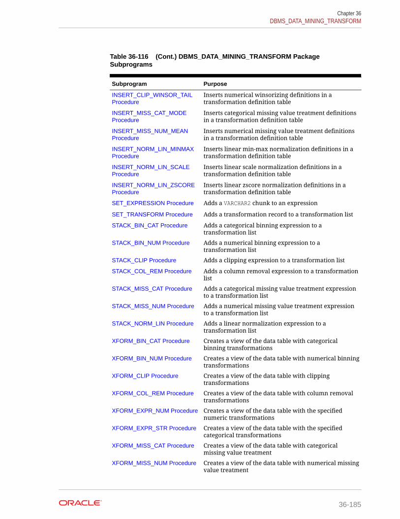
Table 36-116 (Cont.) DBMS_DATA_MINING_TRANSFORM PackageSubprograms
Subprogram Purpose
INSERT_CLIP_WINSOR_TAILProcedure
Inserts numerical winsorizing definitions in atransformation definition table
INSERT_MISS_CAT_MODEProcedure
Inserts categorical missing value treatment definitionsin a transformation definition table
INSERT_MISS_NUM_MEANProcedure
Inserts numerical missing value treatment definitionsin a transformation definition table
INSERT_NORM_LIN_MINMAXProcedure
Inserts linear min-max normalization definitions in atransformation definition table
INSERT_NORM_LIN_SCALEProcedure
Inserts linear scale normalization definitions in atransformation definition table
INSERT_NORM_LIN_ZSCOREProcedure
Inserts linear zscore normalization definitions in atransformation definition table
SET_EXPRESSION Procedure Adds a VARCHAR2 chunk to an expression
SET_TRANSFORM Procedure Adds a transformation record to a transformation list
STACK_BIN_CAT Procedure Adds a categorical binning expression to atransformation list
STACK_BIN_NUM Procedure Adds a numerical binning expression to atransformation list
STACK_CLIP Procedure Adds a clipping expression to a transformation list
STACK_COL_REM Procedure Adds a column removal expression to a transformationlist
STACK_MISS_CAT Procedure Adds a categorical missing value treatment expressionto a transformation list
STACK_MISS_NUM Procedure Adds a numerical missing value treatment expressionto a transformation list
STACK_NORM_LIN Procedure Adds a linear normalization expression to atransformation list
XFORM_BIN_CAT Procedure Creates a view of the data table with categoricalbinning transformations
XFORM_BIN_NUM Procedure Creates a view of the data table with numerical binningtransformations
XFORM_CLIP Procedure Creates a view of the data table with clippingtransformations
XFORM_COL_REM Procedure Creates a view of the data table with column removaltransformations
XFORM_EXPR_NUM Procedure Creates a view of the data table with the specifiednumeric transformations
XFORM_EXPR_STR Procedure Creates a view of the data table with the specifiedcategorical transformations
XFORM_MISS_CAT Procedure Creates a view of the data table with categoricalmissing value treatment
XFORM_MISS_NUM Procedure Creates a view of the data table with numerical missingvalue treatment
Chapter 36DBMS_DATA_MINING_TRANSFORM
36-185

Table 36-116 (Cont.) DBMS_DATA_MINING_TRANSFORM PackageSubprograms
Subprogram Purpose
XFORM_NORM_LIN Procedure Creates a view of the data table with linearnormalization transformations
XFORM_STACK Procedure Creates a view of the transformation list
36.2.3.1 CREATE_BIN_CAT ProcedureThis procedure creates a transformation definition table for categorical binning.
The columns are described in the following table.
Table 36-117 Columns in a Transformation Definition Table for CategoricalBinning
Name Datatype Description
col VARCHAR2(30) Name of a column of categorical data.If the column is not nested, the column name is also theattribute name. For information about attribute names, seeOracle Data Mining User's Guide.
att VARCHAR2(4000) The attribute subname if col is a nested column.
If col is nested, the attribute name is col.att. If col is notnested, att is null.
val VARCHAR2(4000) Values of the attribute
bin VARCHAR2(4000) Bin assignments for the values
Syntax
DBMS_DATA_MINING_TRANSFORM.CREATE_BIN_CAT ( bin_table_name IN VARCHAR2, bin_schema_name IN VARCHAR2 DEFAULT NULL );
Parameters
Table 36-118 CREATE_BIN_CAT Procedure Parameters
Parameter Description
bin_table_name Name of the transformation definition table to be created
bin_schema_name Schema of bin_table_name. If no schema is specified, the currentschema is used.
Usage Notes
1. See Oracle Data Mining User's Guide for details about categorical data.
2. See "Nested Data Transformations" for information about transformation definitiontables and nested data.
Chapter 36DBMS_DATA_MINING_TRANSFORM
36-186
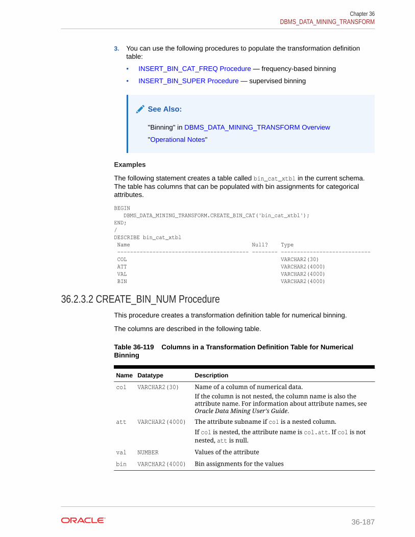
3. You can use the following procedures to populate the transformation definitiontable:
• INSERT_BIN_CAT_FREQ Procedure — frequency-based binning
• INSERT_BIN_SUPER Procedure — supervised binning
See Also:
"Binning" in DBMS_DATA_MINING_TRANSFORM Overview
"Operational Notes"
Examples
The following statement creates a table called bin_cat_xtbl in the current schema.The table has columns that can be populated with bin assignments for categoricalattributes.
BEGIN DBMS_DATA_MINING_TRANSFORM.CREATE_BIN_CAT('bin_cat_xtbl');END;/DESCRIBE bin_cat_xtbl Name Null? Type ----------------------------------------- -------- ---------------------------- COL VARCHAR2(30) ATT VARCHAR2(4000) VAL VARCHAR2(4000) BIN VARCHAR2(4000)
36.2.3.2 CREATE_BIN_NUM ProcedureThis procedure creates a transformation definition table for numerical binning.
The columns are described in the following table.
Table 36-119 Columns in a Transformation Definition Table for NumericalBinning
Name Datatype Description
col VARCHAR2(30) Name of a column of numerical data.If the column is not nested, the column name is also theattribute name. For information about attribute names, seeOracle Data Mining User's Guide.
att VARCHAR2(4000) The attribute subname if col is a nested column.
If col is nested, the attribute name is col.att. If col is notnested, att is null.
val NUMBER Values of the attribute
bin VARCHAR2(4000) Bin assignments for the values
Chapter 36DBMS_DATA_MINING_TRANSFORM
36-187

Syntax
DBMS_DATA_MINING_TRANSFORM.CREATE_BIN_NUM ( bin_table_name IN VARCHAR2, bin_schema_name IN VARCHAR2 DEFAULT NULL );
Parameters
Table 36-120 CREATE_BIN_NUM Procedure Parameters
Parameter Description
bin_table_name Name of the transformation definition table to be created
bin_schema_name Schema of bin_table_name. If no schema is specified, the currentschema is used.
Usage Notes
1. See Oracle Data Mining User's Guide for details about numerical data.
2. See "Nested Data Transformations" for information about transformation definitiontables and nested data.
3. You can use the following procedures to populate the transformation definitiontable:
• INSERT_AUTOBIN_NUM_EQWIDTH Procedure — automatic equi-widthbinning
• INSERT_BIN_NUM_EQWIDTH Procedure — user-specified equi-widthbinning
• INSERT_BIN_NUM_QTILE Procedure — quantile binning
• INSERT_BIN_SUPER Procedure — supervised binning
See Also:
"Binning" in DBMS_DATA_MINING_TRANSFORM Overview
"Operational Notes"
Examples
The following statement creates a table called bin_num_xtbl in the current schema.The table has columns that can be populated with bin assignments for numericalattributes.
BEGIN DBMS_DATA_MINING_TRANSFORM.CREATE_BIN_NUM('bin_num_xtbl');END;/ DESCRIBE bin_num_xtbl Name Null? Type ----------------------------------------- -------- ---------------------------- COL VARCHAR2(30)
Chapter 36DBMS_DATA_MINING_TRANSFORM
36-188

ATT VARCHAR2(4000) VAL NUMBER BIN VARCHAR2(4000)
36.2.3.3 CREATE_CLIP ProcedureThis procedure creates a transformation definition table for clipping or winsorizing tominimize the effect of outliers.
The columns are described in the following table.
Table 36-121 Columns in a Transformation Definition Table for Clipping orWinsorizing
Name Datatype Description
col VARCHAR2(30) Name of a column of numerical data.If the column is not nested, the column name is also theattribute name. For information about attribute names, seeOracle Data Mining User's Guide.
att VARCHAR2(4000) The attribute subname if col is a nested column ofDM_NESTED_NUMERICALS. If col is nested, the attribute nameis col.att.
If col is not nested, att is null.
lcut NUMBER The lowest typical value for the attribute.If the attribute values were plotted on an xy axis, lcutwould be the left-most boundary of the range of valuesconsidered typical for this attribute.Any values to the left of lcut are outliers.
lval NUMBER Value assigned to an outlier to the left of lcut
rcut NUMBER The highest typical value for the attributeIf the attribute values were plotted on an xy axis, rcutwould be the right-most boundary of the range of valuesconsidered typical for this attribute.Any values to the right of rcut are outliers.
rval NUMBER Value assigned to an outlier to the right of rcut
Syntax
DBMS_DATA_MINING_TRANSFORM.CREATE_CLIP ( clip_table_name IN VARCHAR2, clip_schema_name IN VARCHAR2 DEFAULT NULL );
Parameters
Table 36-122 CREATE_CLIP Procedure Parameters
Parameter Description
clip_table_name Name of the transformation definition table to be created
clip_schema_name Schema of clip_table_name. If no schema is specified, thecurrent schema is used.
Chapter 36DBMS_DATA_MINING_TRANSFORM
36-189

Usage Notes
1. See Oracle Data Mining User's Guide for details about numerical data.
2. See "Nested Data Transformations" for information about transformation definitiontables and nested data.
3. You can use the following procedures to populate the transformation definitiontable:
• INSERT_CLIP_TRIM_TAIL Procedure — replaces outliers with nulls
• INSERT_CLIP_WINSOR_TAIL Procedure — replaces outliers with an averagevalue
See Also:
"Outlier Treatment" in DBMS_DATA_MINING_TRANSFORM Overview
"Operational Notes"
Examples
The following statement creates a table called clip_xtbl in the current schema.The table has columns that can be populated with clipping instructions for numericalattributes.
BEGIN DBMS_DATA_MINING_TRANSFORM.CREATE_CLIP('clip_xtbl');END;/ DESCRIBE clip_xtbl Name Null? Type ----------------------------------------- -------- ---------------------------- COL VARCHAR2(30) ATT VARCHAR2(4000) LCUT NUMBER LVAL NUMBER RCUT NUMBER RVAL NUMBER
36.2.3.4 CREATE_COL_REM ProcedureThis procedure creates a transformation definition table for removing columns from thedata table.
The columns are described in the following table.
Chapter 36DBMS_DATA_MINING_TRANSFORM
36-190
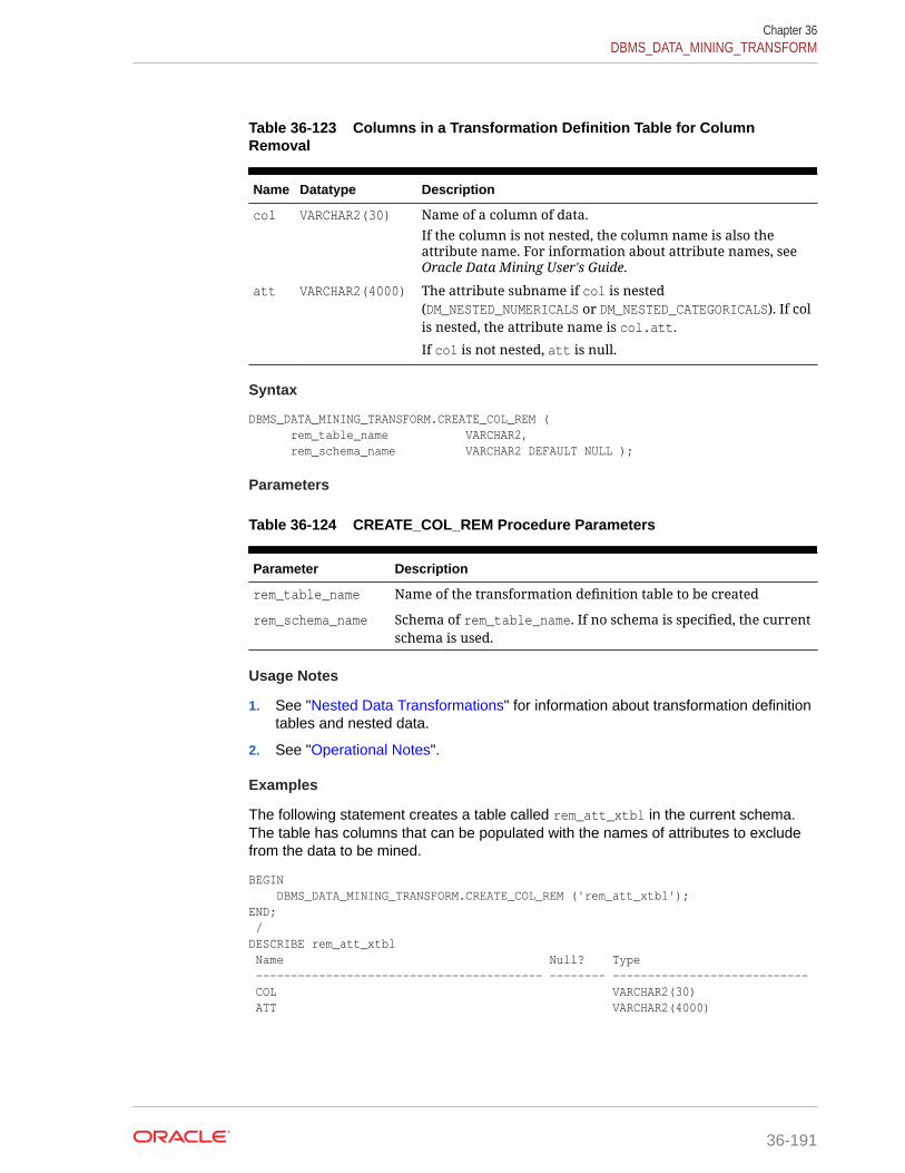
Table 36-123 Columns in a Transformation Definition Table for ColumnRemoval
Name Datatype Description
col VARCHAR2(30) Name of a column of data.If the column is not nested, the column name is also theattribute name. For information about attribute names, seeOracle Data Mining User's Guide.
att VARCHAR2(4000) The attribute subname if col is nested(DM_NESTED_NUMERICALS or DM_NESTED_CATEGORICALS). If colis nested, the attribute name is col.att.
If col is not nested, att is null.
Syntax
DBMS_DATA_MINING_TRANSFORM.CREATE_COL_REM ( rem_table_name VARCHAR2, rem_schema_name VARCHAR2 DEFAULT NULL );
Parameters
Table 36-124 CREATE_COL_REM Procedure Parameters
Parameter Description
rem_table_name Name of the transformation definition table to be created
rem_schema_name Schema of rem_table_name. If no schema is specified, the currentschema is used.
Usage Notes
1. See "Nested Data Transformations" for information about transformation definitiontables and nested data.
2. See "Operational Notes".
Examples
The following statement creates a table called rem_att_xtbl in the current schema.The table has columns that can be populated with the names of attributes to excludefrom the data to be mined.
BEGIN DBMS_DATA_MINING_TRANSFORM.CREATE_COL_REM ('rem_att_xtbl');END; /DESCRIBE rem_att_xtbl Name Null? Type ----------------------------------------- -------- ---------------------------- COL VARCHAR2(30) ATT VARCHAR2(4000)
Chapter 36DBMS_DATA_MINING_TRANSFORM
36-191

36.2.3.5 CREATE_MISS_CAT ProcedureThis procedure creates a transformation definition table for replacing categoricalmissing values.
The columns are described in the following table.
Table 36-125 Columns in a Transformation Definition Table for CategoricalMissing Value Treatment
Name Datatype Description
col VARCHAR2(30) Name of a column of categorical data.If the column is not nested, the column name is also theattribute name. For information about attribute names, seeOracle Data Mining User's Guide.
att VARCHAR2(4000) The attribute subname if col is a nested column ofDM_NESTED_CATEGORICALS. If col is nested, the attributename is col.att.
If col is not nested, att is null.
val VARCHAR2(4000) Replacement for missing values in the attribute
Syntax
DBMS_DATA_MINING_TRANSFORM.CREATE_MISS_CAT ( miss_table_name IN VARCHAR2, miss_schema_name IN VARCHAR2 DEFAULT NULL );
Parameters
Table 36-126 CREATE_MISS_CAT Procedure Parameters
Parameter Description
miss_table_name Name of the transformation definition table to be created
miss_schema_name Schema of miss_table_name. If no schema is specified, thecurrent schema is used.
Usage Notes
1. See Oracle Data Mining User's Guide for details about categorical data.
2. See "Nested Data Transformations" for information about transformation definitiontables and nested data.
3. You can use the INSERT_MISS_CAT_MODE Procedure to populate thetransformation definition table.
Chapter 36DBMS_DATA_MINING_TRANSFORM
36-192

See Also:
"Missing Value Treatment" in DBMS_DATA_MINING_TRANSFORMOverview
"Operational Notes"
Examples
The following statement creates a table called miss_cat_xtbl in the current schema.The table has columns that can be populated with values for missing data incategorical attributes.
BEGIN
DBMS_DATA_MINING_TRANSFORM.CREATE_MISS_CAT('miss_cat_xtbl');END;/ DESCRIBE miss_cat_xtbl Name Null? Type ----------------------------------------- -------- ---------------------------- COL VARCHAR2(30) ATT VARCHAR2(4000) VAL VARCHAR2(4000)
36.2.3.6 CREATE_MISS_NUM ProcedureThis procedure creates a transformation definition table for replacing numericalmissing values.
The columns are described in Table 36-127.
Table 36-127 Columns in a Transformation Definition Table for NumericalMissing Value Treatment
Name Datatype Description
col VARCHAR2(30) Name of a column of numerical data.If the column is not nested, the column name is also theattribute name. For information about attribute names, seeOracle Data Mining User's Guide.
att VARCHAR2(4000) The attribute subname if col is a nested column ofDM_NESTED_NUMERICALS. If col is nested, the attribute nameis col.att.
If col is not nested, att is null.
val NUMBER Replacement for missing values in the attribute
Syntax
DBMS_DATA_MINING_TRANSFORM.CREATE_MISS_NUM ( miss_table_name IN VARCHAR2, miss_schema_name IN VARCHAR2 DEFAULT NULL );
Chapter 36DBMS_DATA_MINING_TRANSFORM
36-193
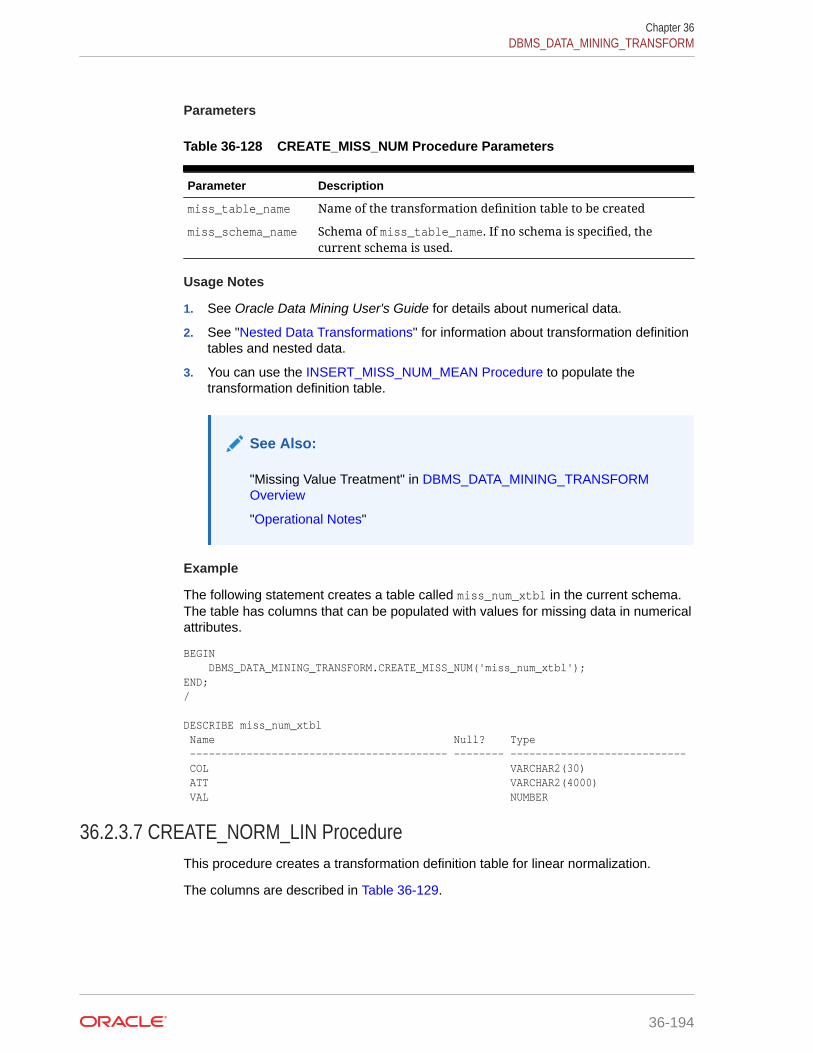
Parameters
Table 36-128 CREATE_MISS_NUM Procedure Parameters
Parameter Description
miss_table_name Name of the transformation definition table to be created
miss_schema_name Schema of miss_table_name. If no schema is specified, thecurrent schema is used.
Usage Notes
1. See Oracle Data Mining User's Guide for details about numerical data.
2. See "Nested Data Transformations" for information about transformation definitiontables and nested data.
3. You can use the INSERT_MISS_NUM_MEAN Procedure to populate thetransformation definition table.
See Also:
"Missing Value Treatment" in DBMS_DATA_MINING_TRANSFORMOverview
"Operational Notes"
Example
The following statement creates a table called miss_num_xtbl in the current schema.The table has columns that can be populated with values for missing data in numericalattributes.
BEGIN DBMS_DATA_MINING_TRANSFORM.CREATE_MISS_NUM('miss_num_xtbl');END;/ DESCRIBE miss_num_xtbl Name Null? Type ----------------------------------------- -------- ---------------------------- COL VARCHAR2(30) ATT VARCHAR2(4000) VAL NUMBER
36.2.3.7 CREATE_NORM_LIN ProcedureThis procedure creates a transformation definition table for linear normalization.
The columns are described in Table 36-129.
Chapter 36DBMS_DATA_MINING_TRANSFORM
36-194

Table 36-129 Columns in a Transformation Definition Table for LinearNormalization
Name Datatype Description
col VARCHAR2(30) Name of a column of numerical data.If the column is not nested, the column name is also theattribute name. For information about attribute names, seeOracle Data Mining User's Guide.
att VARCHAR2(4000) The attribute subname if col is a nested column ofDM_NESTED_NUMERICALS. If col is nested, the attribute nameis col.att.
If col is not nested, att is null.
shift NUMBER A constant to subtract from the attribute values
scale NUMBER A constant by which to divide the shifted values
Syntax
DBMS_DATA_MINING_TRANSFORM.CREATE_NORM_LIN ( norm_table_name IN VARCHAR2, norm_schema_name IN VARCHAR2 DEFAULT NULL );
Parameters
Table 36-130 CREATE_NORM_LIN Procedure Parameters
Parameter Description
norm_table_name Name of the transformation definition table to be created
norm_schema_name Schema of norm_table_name. If no schema is specified, thecurrent schema is used.
Usage Notes
1. See Oracle Data Mining User's Guide for details about numerical data.
2. See "Nested Data Transformations" for information about transformation definitiontables and nested data.
3. You can use the following procedures to populate the transformation definitiontable:
• INSERT_NORM_LIN_MINMAX Procedure — Uses linear min-maxnormalization
• INSERT_NORM_LIN_SCALE Procedure — Uses linear scale normalization
• INSERT_NORM_LIN_ZSCORE Procedure — Uses linear zscorenormalization
Chapter 36DBMS_DATA_MINING_TRANSFORM
36-195

See Also:
"Linear Normalization" in DBMS_DATA_MINING_TRANSFORMOverview
"Operational Notes"
Examples
The following statement creates a table called norm_xtbl in the current schema. Thetable has columns that can be populated with shift and scale values for normalizingnumerical attributes.
BEGIN DBMS_DATA_MINING_TRANSFORM.CREATE_NORM_LIN('norm_xtbl');END;/ DESCRIBE norm_xtbl Name Null? Type ----------------------------------------- -------- ---------------------------- COL VARCHAR2(30) ATT VARCHAR2(4000) SHIFT NUMBER SCALE NUMBER
36.2.3.8 DESCRIBE_STACK ProcedureThis procedure describes the columns of the data table after a list of transformationshas been applied.
Only the columns that are specified in the transformation list are transformed. Theremaining columns in the data table are included in the output without changes.
To create a view of the data table after the transformations have been applied, use theXFORM_STACK Procedure.
Syntax
DBMS_DATA_MINING_TRANSFORM.DESCRIBE_STACK ( xform_list IN TRANSFORM_LIST, data_table_name IN VARCHAR2, describe_list OUT DESCRIBE_LIST, data_schema_name IN VARCHAR2 DEFAULT NULL);
Parameters
Table 36-131 DESCRIBE_STACK Procedure Parameters
Parameter Description
xform_list A list of transformations. See Table 36-114 for a description of theTRANSFORM_LIST object type.
data_table_name Name of the table containing the data to be transformed
Chapter 36DBMS_DATA_MINING_TRANSFORM
36-196

Table 36-131 (Cont.) DESCRIBE_STACK Procedure Parameters
Parameter Description
describe_list Descriptions of the columns in the data table after thetransformations specified in xform_list have been applied. SeeTable 36-114 for a description of the DESCRIBE_LIST object type.
data_schema_name Schema of data_table_name. If no schema is specified, thecurrent schema is used.
Usage Notes
See "Operational Notes" for information about transformation lists and embeddedtransformations.
Examples
This example shows the column name and datatype, the column name length, andthe column maximum length for the view dmuser.cust_info after the transformationlist has been applied. All the transformations are user-specified. The results ofDESCRIBE_STACK do not include one of the columns in the original table, because theSET_TRANSFORM procedure sets that column to NULL.
CREATE OR REPLACE VIEW cust_info AS SELECT a.cust_id, c.country_id, c.cust_year_of_birth, CAST(COLLECT(DM_Nested_Numerical( b.prod_name, 1)) AS DM_Nested_Numericals) custprods FROM sh.sales a, sh.products b, sh.customers c WHERE a.prod_id = b.prod_id AND a.cust_id=c.cust_id and a.cust_id between 100001 AND 105000 GROUP BY a.cust_id, country_id, cust_year_of_birth; describe cust_info Name Null? Type ----------------------------------------- -------- ---------------------------- CUST_ID NOT NULL NUMBER COUNTRY_ID NOT NULL NUMBER CUST_YEAR_OF_BIRTH NOT NULL NUMBER(4) CUSTPRODS SYS.DM_NESTED_NUMERICALS DECLARE cust_stack dbms_data_mining_transform.TRANSFORM_LIST; cust_cols dbms_data_mining_transform.DESCRIBE_LIST;BEGIN dbms_data_mining_transform.SET_TRANSFORM (cust_stack, 'country_id', NULL, 'country_id/10', 'country_id*10'); dbms_data_mining_transform.SET_TRANSFORM (cust_stack, 'cust_year_of_birth', NULL, NULL, NULL); dbms_data_mining_transform.SET_TRANSFORM (cust_stack, 'custprods', 'Mouse Pad', 'value*100', 'value/100'); dbms_data_mining_transform.DESCRIBE_STACK( xform_list => cust_stack, data_table_name => 'cust_info', describe_list => cust_cols); dbms_output.put_line('===='); for i in 1..cust_cols.COUNT loop
Chapter 36DBMS_DATA_MINING_TRANSFORM
36-197

dbms_output.put_line('COLUMN_NAME: '||cust_cols(i).col_name); dbms_output.put_line('COLUMN_TYPE: '||cust_cols(i).col_type); dbms_output.put_line('COLUMN_NAME_LEN: '||cust_cols(i).col_name_len); dbms_output.put_line('COLUMN_MAX_LEN: '||cust_cols(i).col_max_len); dbms_output.put_line('===='); END loop;END;/====COLUMN_NAME: CUST_IDCOLUMN_TYPE: 2COLUMN_NAME_LEN: 7COLUMN_MAX_LEN: 22====COLUMN_NAME: COUNTRY_IDCOLUMN_TYPE: 2COLUMN_NAME_LEN: 10COLUMN_MAX_LEN: 22====COLUMN_NAME: CUSTPRODSCOLUMN_TYPE: 100001COLUMN_NAME_LEN: 9COLUMN_MAX_LEN: 40====
36.2.3.9 GET_EXPRESSION FunctionThis function returns a row from a VARCHAR2 array that stores a transformationexpression. The array is built by calls to the SET_EXPRESSION Procedure.
The array can be used for specifying SQL expressions that are too long to be usedwith the SET_TRANSFORM Procedure.
Syntax
DBMS_DATA_MINING_TRANSFORM.GET_EXPRESSION ( expression IN EXPRESSION_REC, chunk_num IN PLS_INTEGER DEFAULT NULL); RETURN VARCHAR2;
Parameters
Table 36-132 GET_EXPRESSION Function Parameters
Parameter Description
expression An expression record (EXPRESSION_REC) that specifies atransformation expression or a reverse transformation expression foran attribute. Each expression record includes a VARCHAR2 array andindex fields for specifying upper and lower boundaries within thearray.There are two EXPRESSION_REC fields within a transformation record(TRANSFORM_REC): one for the transformation expression; the otherfor the reverse transformation expression.See Table 36-114 for a description of the EXPRESSION_REC type.
chunk A VARCHAR2 chunk (row) to be appended to expression.
Chapter 36DBMS_DATA_MINING_TRANSFORM
36-198
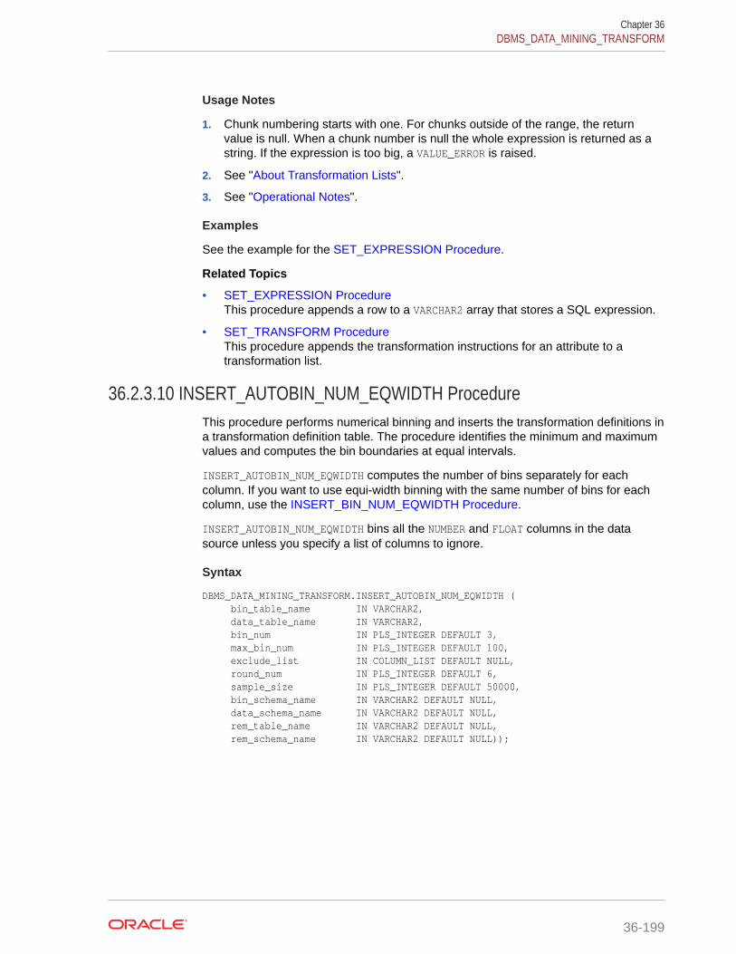
Usage Notes
1. Chunk numbering starts with one. For chunks outside of the range, the returnvalue is null. When a chunk number is null the whole expression is returned as astring. If the expression is too big, a VALUE_ERROR is raised.
2. See "About Transformation Lists".
3. See "Operational Notes".
Examples
See the example for the SET_EXPRESSION Procedure.
Related Topics
• SET_EXPRESSION ProcedureThis procedure appends a row to a VARCHAR2 array that stores a SQL expression.
• SET_TRANSFORM ProcedureThis procedure appends the transformation instructions for an attribute to atransformation list.
36.2.3.10 INSERT_AUTOBIN_NUM_EQWIDTH ProcedureThis procedure performs numerical binning and inserts the transformation definitions ina transformation definition table. The procedure identifies the minimum and maximumvalues and computes the bin boundaries at equal intervals.
INSERT_AUTOBIN_NUM_EQWIDTH computes the number of bins separately for eachcolumn. If you want to use equi-width binning with the same number of bins for eachcolumn, use the INSERT_BIN_NUM_EQWIDTH Procedure.
INSERT_AUTOBIN_NUM_EQWIDTH bins all the NUMBER and FLOAT columns in the datasource unless you specify a list of columns to ignore.
Syntax
DBMS_DATA_MINING_TRANSFORM.INSERT_AUTOBIN_NUM_EQWIDTH ( bin_table_name IN VARCHAR2, data_table_name IN VARCHAR2, bin_num IN PLS_INTEGER DEFAULT 3, max_bin_num IN PLS_INTEGER DEFAULT 100, exclude_list IN COLUMN_LIST DEFAULT NULL, round_num IN PLS_INTEGER DEFAULT 6, sample_size IN PLS_INTEGER DEFAULT 50000, bin_schema_name IN VARCHAR2 DEFAULT NULL, data_schema_name IN VARCHAR2 DEFAULT NULL, rem_table_name IN VARCHAR2 DEFAULT NULL, rem_schema_name IN VARCHAR2 DEFAULT NULL));
Chapter 36DBMS_DATA_MINING_TRANSFORM
36-199

Parameters
Table 36-133 INSERT_AUTOBIN_NUM_EQWIDTH Procedure Parameters
Parameter Description
bin_table_name Name of the transformation definition table for numericalbinning. You can use the CREATE_BIN_NUM Procedure to createthe definition table. The following columns are required:
COL VARCHAR2(30)VAL NUMBERBIN VARCHAR2(4000)
CREATE_BIN_NUM creates an additional column, ATT, which may beused for specifying nested attributes. This column is not used byINSERT_AUTOBIN_NUM_EQWIDTH.
data_table_name Name of the table containing the data to be transformed
bin_num Minimum number of bins. If bin_num is 0 or NULL, it is ignored.
The default value of bin_num is 3.
max_bin_num Maximum number of bins. If max_bin_num is 0 or NULL, it isignored.The default value of max_bin_num is 100.
exclude_list List of numerical columns to be excluded from the binningprocess. If you do not specify exclude_list, all numericalcolumns in the data source are binned.The format of exclude_list is:
dbms_data_mining_transform.COLUMN_LIST('col1','col2', ...'coln')
round_num Specifies how to round the number in the VAL column of thetransformation definition table.When round_num is positive, it specifies the most significantdigits to retain. When round_num is negative, it specifies the leastsignificant digits to remove. In both cases, the result is roundedto the specified number of digits. See the Usage Notes for anexample.The default value of round_num is 6.
sample_size Size of the data sample. If sample_size is less than the totalnumber of non-NULL values in the column, then sample_size isused instead of the SQL COUNT function in computing the numberof bins. If sample_size is 0 or NULL, it is ignored. See the UsageNotes.The default value of sample_size is 50,000.
bin_schema_name Schema of bin_table_name. If no schema is specified, the currentschema is used.
data_schema_name Schema of data_table_name. If no schema is specified, thecurrent schema is used.
Chapter 36DBMS_DATA_MINING_TRANSFORM
36-200

Table 36-133 (Cont.) INSERT_AUTOBIN_NUM_EQWIDTH Procedure Parameters
Parameter Description
rem_table_name Name of a transformation definition table for columnremoval. The table must have the columns described in"CREATE_COL_REM Procedure".
INSERT_AUTOBIN_NUM_EQWIDTH ignores columns with all nulls oronly one unique value. If you specify a value for rem_table_name,these columns are removed from the mining data. If you do notspecify a value for rem_table_name, these unbinned columnsremain in the data.
rem_schema_name Schema of rem_table_name. If no schema is specified, the currentschema is used.
Usage Notes
1. See Oracle Data Mining User's Guide for details about numerical data.
2. INSERT_AUTOBIN_NUM_EQWIDTH computes the number of bins for a column basedon the number of non-null values (COUNT), the maximum (MAX), the minimum (MIN),the standard deviation (STDDEV), and the constant C=3.49/0.9:
N=floor(power(COUNT,1/3)*(max-min)/(c*dev))
If the sample_size parameter is specified, it is used instead of COUNT.
See Oracle Database SQL Language Reference for information about the COUNT,MAX, MIN, STDDEV, FLOOR, and POWER functions.
3. INSERT_AUTOBIN_NUM_EQWIDTH uses absolute values to compute the number ofbins. The sign of the parameters bin_num, max_bin_num, and sample_size has noeffect on the result.
4. In computing the number of bins, INSERT_AUTOBIN_NUM_EQWIDTH evaluates thefollowing criteria in the following order:
a. The minimum number of bins (bin_num)
b. The maximum number of bins (max_bin_num)
c. The maximum number of bins for integer columns, calculated as the numberof distinct values in the range max-min+1.
5. The round_num parameter controls the rounding of column values in thetransformation definition table, as follows:
For a value of 308.162:when round_num = 1 result is 300when round_num = 2 result is 310when round_num = 3 result is 308when round_num = 0 result is 308.162when round_num = -1 result is 308.16when round_num = -2 result is 308.2
Examples
In this example, INSERT_AUTOBIN_NUM_EQWIDTH computes the bin boundaries forthe cust_year_of_birth column in sh.customers and inserts the transformations
Chapter 36DBMS_DATA_MINING_TRANSFORM
36-201

in a transformation definition table. The STACK_BIN_NUM Procedure creates atransformation list from the contents of the definition table. The CREATE_MODELProcedure embeds the transformation list in a new model called nb_model.
The transformation and reverse transformation expressions embedded in nb_modelare returned by the GET_MODEL_TRANSFORMATIONS Function.
CREATE OR REPLACE VIEW mining_data AS SELECT cust_id, cust_year_of_birth, cust_postal_code FROM sh.customers; DESCRIBE mining_data Name Null? Type ----------------------------- -------- ---------------------------- CUST_ID NOT NULL NUMBER CUST_YEAR_OF_BIRTH NOT NULL NUMBER(4) CUST_POSTAL_CODE NOT NULL VARCHAR2(10) BEGIN dbms_data_mining_transform.CREATE_BIN_NUM( bin_table_name => 'bin_tbl'); dbms_data_mining_transform.INSERT_AUTOBIN_NUM_EQWIDTH ( bin_table_name => 'bin_tbl', data_table_name => 'mining_data', bin_num => 3, max_bin_num => 5, exclude_list => dbms_data_mining_transform.COLUMN_LIST('cust_id'));END;/
set numwidth 4column val offSELECT col, val, bin FROM bin_tbl ORDER BY val ASC; COL VAL BIN------------------------- ---- -----CUST_YEAR_OF_BIRTH 1913CUST_YEAR_OF_BIRTH 1928 1CUST_YEAR_OF_BIRTH 1944 2CUST_YEAR_OF_BIRTH 1959 3CUST_YEAR_OF_BIRTH 1975 4CUST_YEAR_OF_BIRTH 1990 5
DECLARE year_birth_xform dbms_data_mining_transform.TRANSFORM_LIST;BEGIN dbms_data_mining_transform.STACK_BIN_NUM ( bin_table_name => 'bin_tbl', xform_list => year_birth_xform); dbms_data_mining.CREATE_MODEL( model_name => 'nb_model', mining_function => dbms_data_mining.classification, data_table_name => 'mining_data', case_id_column_name => 'cust_id', target_column_name => 'cust_postal_code', settings_table_name => null, data_schema_name => null, settings_schema_name => null, xform_list => year_birth_xform);END;
Chapter 36DBMS_DATA_MINING_TRANSFORM
36-202
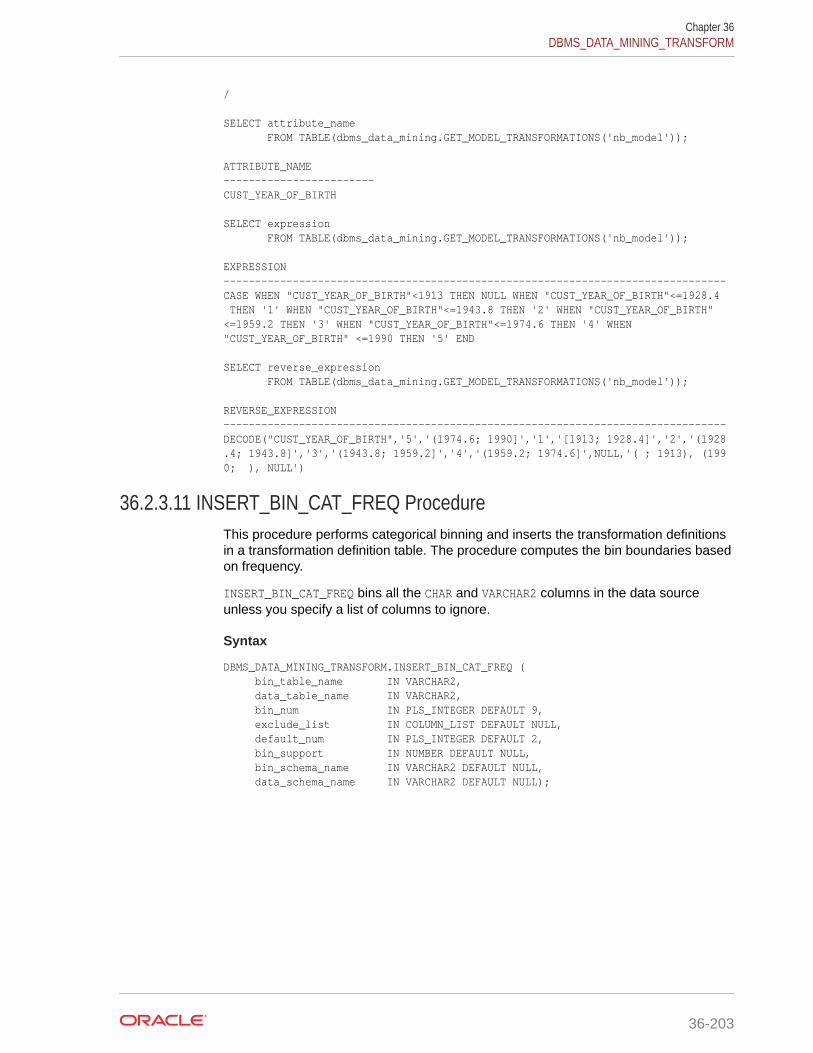
/ SELECT attribute_name FROM TABLE(dbms_data_mining.GET_MODEL_TRANSFORMATIONS('nb_model')); ATTRIBUTE_NAME------------------------CUST_YEAR_OF_BIRTH SELECT expression FROM TABLE(dbms_data_mining.GET_MODEL_TRANSFORMATIONS('nb_model')); EXPRESSION--------------------------------------------------------------------------------CASE WHEN "CUST_YEAR_OF_BIRTH"<1913 THEN NULL WHEN "CUST_YEAR_OF_BIRTH"<=1928.4 THEN '1' WHEN "CUST_YEAR_OF_BIRTH"<=1943.8 THEN '2' WHEN "CUST_YEAR_OF_BIRTH"<=1959.2 THEN '3' WHEN "CUST_YEAR_OF_BIRTH"<=1974.6 THEN '4' WHEN"CUST_YEAR_OF_BIRTH" <=1990 THEN '5' END SELECT reverse_expression FROM TABLE(dbms_data_mining.GET_MODEL_TRANSFORMATIONS('nb_model')); REVERSE_EXPRESSION--------------------------------------------------------------------------------DECODE("CUST_YEAR_OF_BIRTH",'5','(1974.6; 1990]','1','[1913; 1928.4]','2','(1928.4; 1943.8]','3','(1943.8; 1959.2]','4','(1959.2; 1974.6]',NULL,'( ; 1913), (1990; ), NULL')
36.2.3.11 INSERT_BIN_CAT_FREQ ProcedureThis procedure performs categorical binning and inserts the transformation definitionsin a transformation definition table. The procedure computes the bin boundaries basedon frequency.
INSERT_BIN_CAT_FREQ bins all the CHAR and VARCHAR2 columns in the data sourceunless you specify a list of columns to ignore.
Syntax
DBMS_DATA_MINING_TRANSFORM.INSERT_BIN_CAT_FREQ ( bin_table_name IN VARCHAR2, data_table_name IN VARCHAR2, bin_num IN PLS_INTEGER DEFAULT 9, exclude_list IN COLUMN_LIST DEFAULT NULL, default_num IN PLS_INTEGER DEFAULT 2, bin_support IN NUMBER DEFAULT NULL, bin_schema_name IN VARCHAR2 DEFAULT NULL, data_schema_name IN VARCHAR2 DEFAULT NULL);
Chapter 36DBMS_DATA_MINING_TRANSFORM
36-203

Parameters
Table 36-134 INSERT_BIN_CAT_FREQ Procedure Parameters
Parameter Description
bin_table_name Name of the transformation definition table for categoricalbinning. You can use the CREATE_BIN_CAT Procedure to create thedefinition table.The following columns are required:
COL VARCHAR2(30)VAL VARCHAR2(4000)BIN VARCHAR2(4000)
CREATE_BIN_CAT creates an additional column, ATT, which may beused for specifying nested attributes. This column is not used byINSERT_BIN_CAT_FREQ.
data_table_name Name of the table containing the data to be transformed
bin_num The number of bins to fill using frequency-based binning Thetotal number of bins will be bin_num+1. The additional bin is thedefault bin. Classes that are not assigned to a frequency-based binwill be assigned to the default bin.The default binning order is from highest to lowest: the mostfrequently occurring class is assigned to the first bin, the secondmost frequently occurring class is assigned to the second bin, andso on.You can reverse the binning order by specifying a negativenumber for bin_num. The negative sign causes the binning orderto be from lowest to highest.If the total number of distinct values (classes) in the column is lessthan bin_num, then a separate bin will be created for each valueand the default bin will be empty.If you specify NULL or 0 for bin_num, no binning is performed.
The default value of bin_num is 9.
exclude_list List of categorical columns to be excluded from the binningprocess. If you do not specify exclude_list, all categoricalcolumns in the data source are binned.The format of exclude_list is:
dbms_data_mining_transform.COLUMN_LIST('col1','col2', ...'coln')
default_num The number of class occurrences (rows of the same class) requiredfor assignment to the default binBy default, default_num is the minimum number of occurrencesrequired for assignment to the default bin. For example, ifdefault_num is 3 and a given class occurs only once, it will notbe assigned to the default bin. You can change the occurrencerequirement from minimum to maximum by specifying a negativenumber for default_num. For example, if default_num is -3 and agiven class occurs only once, it will be assigned to the default bin,but a class that occurs four or more times will not be included.If you specify NULL or 0 for default_bin, there are norequirements for assignment to the default bin.The default value of default_num is 2.
Chapter 36DBMS_DATA_MINING_TRANSFORM
36-204

Table 36-134 (Cont.) INSERT_BIN_CAT_FREQ Procedure Parameters
Parameter Description
bin_support The number of class occurrences (rows of the same class)required for assignment to a frequency-based bin. bin_supportis expressed as a fraction of the total number of rows.By default, bin_support is the minimum percentage required forassignment to a frequency-based bin. For example, if there aretwenty rows of data and you specify.2 for bin_support, thenthere must be four or more occurrences of a class (.2*20) inorder for it to be assigned to a frequency-based bin. You canchange bin_support from a minimum percentage to a maximumpercentage by specifying a negative number for bin_support. Forexample, if there are twenty rows of data and you specify -.2 forbin_support, then there must be four or less occurrences of aclass in order for it to be assigned to a frequency-based bin.Classes that occur less than a positive bin_support or more than anegative bin_support will be assigned to the default bin.
If you specify NULL or 0 for bin_support, then there is no supportrequirement for frequency-based binning.The default value of bin_support is NULL.
bin_schema_name Schema of bin_table_name. If no schema is specified, the currentschema is used.
data_schema_name Schema of data_table_name. If no schema is specified, thecurrent schema is used.
Usage Notes
1. See Oracle Data Mining User's Guide for details about categorical data.
2. If values occur with the same frequency, INSERT_BIN_CAT_FREQ assigns them indescending order when binning is from most to least frequent, or in ascendingorder when binning is from least to most frequent.
Examples
1. In this example, INSERT_BIN_CAT_FREQ computes the bin boundaries for thecust_postal_code and cust_city columns in sh.customers and inserts thetransformations in a transformation definition table. The STACK_BIN_CATProcedure creates a transformation list from the contents of the definition table,and the CREATE_MODEL Procedure embeds the transformation list in a newmodel called nb_model.
The transformation and reverse transformation expressions embedded innb_model are returned by the GET_MODEL_TRANSFORMATIONS Function.
CREATE OR REPLACE VIEW mining_data AS SELECT cust_id, cust_year_of_birth, cust_postal_code, cust_city FROM sh.customers; DESCRIBE mining_data Name Null? Type ------------------------------------- -------- ----------------------------- CUST_ID NOT NULL NUMBER
Chapter 36DBMS_DATA_MINING_TRANSFORM
36-205
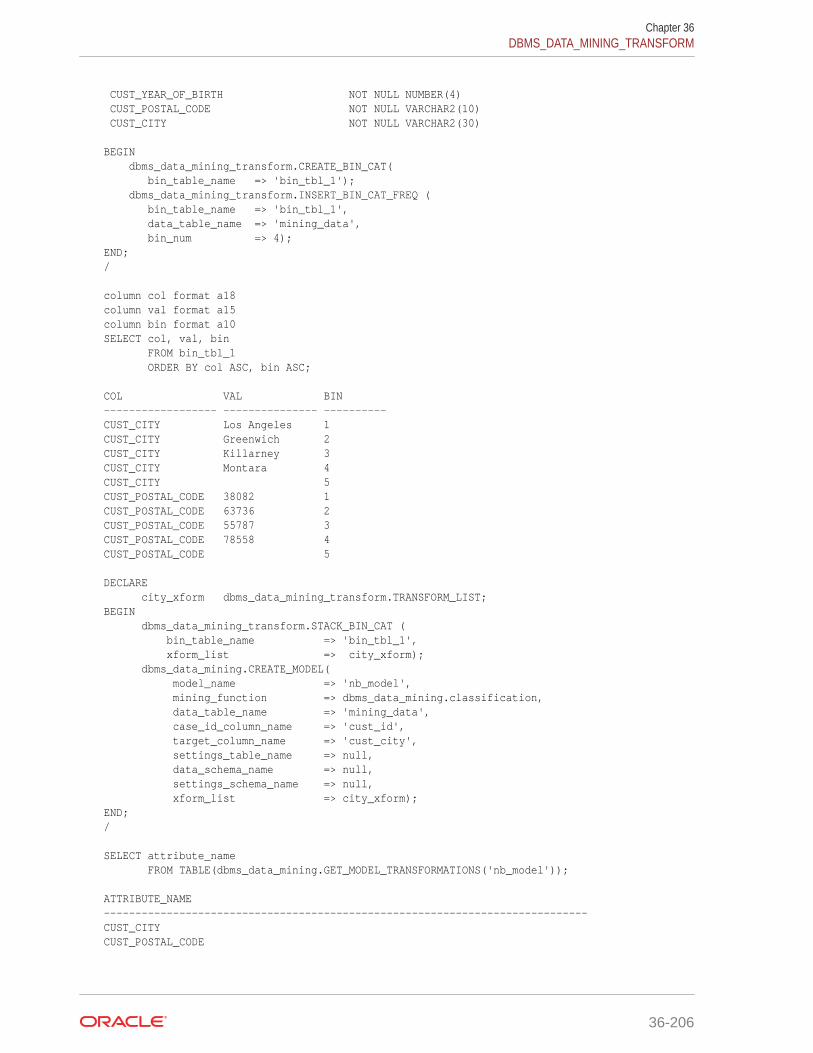
CUST_YEAR_OF_BIRTH NOT NULL NUMBER(4) CUST_POSTAL_CODE NOT NULL VARCHAR2(10) CUST_CITY NOT NULL VARCHAR2(30) BEGIN dbms_data_mining_transform.CREATE_BIN_CAT( bin_table_name => 'bin_tbl_1'); dbms_data_mining_transform.INSERT_BIN_CAT_FREQ ( bin_table_name => 'bin_tbl_1', data_table_name => 'mining_data', bin_num => 4);END;/ column col format a18column val format a15column bin format a10SELECT col, val, bin FROM bin_tbl_1 ORDER BY col ASC, bin ASC; COL VAL BIN------------------ --------------- ----------CUST_CITY Los Angeles 1CUST_CITY Greenwich 2CUST_CITY Killarney 3CUST_CITY Montara 4CUST_CITY 5CUST_POSTAL_CODE 38082 1CUST_POSTAL_CODE 63736 2CUST_POSTAL_CODE 55787 3CUST_POSTAL_CODE 78558 4CUST_POSTAL_CODE 5 DECLARE city_xform dbms_data_mining_transform.TRANSFORM_LIST;BEGIN dbms_data_mining_transform.STACK_BIN_CAT ( bin_table_name => 'bin_tbl_1', xform_list => city_xform); dbms_data_mining.CREATE_MODEL( model_name => 'nb_model', mining_function => dbms_data_mining.classification, data_table_name => 'mining_data', case_id_column_name => 'cust_id', target_column_name => 'cust_city', settings_table_name => null, data_schema_name => null, settings_schema_name => null, xform_list => city_xform);END;/ SELECT attribute_name FROM TABLE(dbms_data_mining.GET_MODEL_TRANSFORMATIONS('nb_model')); ATTRIBUTE_NAME-----------------------------------------------------------------------------CUST_CITYCUST_POSTAL_CODE
Chapter 36DBMS_DATA_MINING_TRANSFORM
36-206
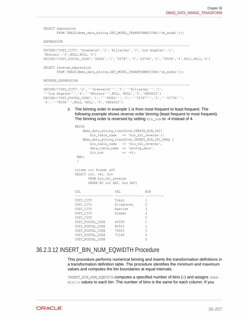
SELECT expression FROM TABLE(dbms_data_mining.GET_MODEL_TRANSFORMATIONS('nb_model')); EXPRESSION-----------------------------------------------------------------------------DECODE("CUST_CITY",'Greenwich','2','Killarney','3','Los Angeles','1','Montara','4',NULL,NULL,'5')DECODE("CUST_POSTAL_CODE",'38082','1','55787','3','63736','2','78558','4',NULL,NULL,'5')
SELECT reverse_expression FROM TABLE(dbms_data_mining.GET_MODEL_TRANSFORMATIONS('nb_model'));
REVERSE_EXPRESSION-----------------------------------------------------------------------------DECODE("CUST_CITY",'2','''Greenwich''','3','''Killarney''','1','''Los Angeles''','4','''Montara''',NULL,'NULL','5','DEFAULT')DECODE("CUST_POSTAL_CODE",'1','''38082''','3','''55787''','2','''63736''','4','''78558''',NULL,'NULL','5','DEFAULT')
2. The binning order in example 1 is from most frequent to least frequent. Thefollowing example shows reverse order binning (least frequent to most frequent).The binning order is reversed by setting bin_num to -4 instead of 4.
BEGIN dbms_data_mining_transform.CREATE_BIN_CAT( bin_table_name => 'bin_tbl_reverse'); dbms_data_mining_transform.INSERT_BIN_CAT_FREQ ( bin_table_name => 'bin_tbl_reverse', data_table_name => 'mining_data', bin_num => -4); END; / column col format a20SELECT col, val, bin FROM bin_tbl_reverse ORDER BY col ASC, bin ASC; COL VAL BIN-------------------- --------------- ----------CUST_CITY Tokyo 1CUST_CITY Sliedrecht 2CUST_CITY Haarlem 3CUST_CITY Diemen 4CUST_CITY 5CUST_POSTAL_CODE 49358 1CUST_POSTAL_CODE 80563 2CUST_POSTAL_CODE 74903 3CUST_POSTAL_CODE 71349 4CUST_POSTAL_CODE 5
36.2.3.12 INSERT_BIN_NUM_EQWIDTH ProcedureThis procedure performs numerical binning and inserts the transformation definitions ina transformation definition table. The procedure identifies the minimum and maximumvalues and computes the bin boundaries at equal intervals.
INSERT_BIN_NUM_EQWIDTH computes a specified number of bins (n) and assigns (max-min)/n values to each bin. The number of bins is the same for each column. If you
Chapter 36DBMS_DATA_MINING_TRANSFORM
36-207

want to use equi-width binning, but you want the number of bins to be calculated on aper-column basis, use the INSERT_AUTOBIN_NUM_EQWIDTH Procedure.
INSERT_BIN_NUM_EQWIDTH bins all the NUMBER and FLOAT columns in the data sourceunless you specify a list of columns to ignore.
Syntax
DBMS_DATA_MINING_TRANSFORM.INSERT_BIN_NUM_EQWIDTH ( bin_table_name IN VARCHAR2, data_table_name IN VARCHAR2, bin_num IN PLS_INTEGER DEFAULT 10, exclude_list IN COLUMN_LIST DEFAULT NULL, round_num IN PLS_INTEGER DEFAULT 6, bin_schema_name IN VARCHAR2 DEFAULT NULL, data_schema_name IN VARCHAR2 DEFAULT NULL);
Parameters
Table 36-135 INSERT_BIN_NUM_EQWIDTH Procedure Parameters
Parameter Description
bin_table_name Name of the transformation definition table for numericalbinning. You can use the CREATE_BIN_NUM Procedure to createthe definition table. The following columns are required:
COL VARCHAR2(30)VAL NUMBERBIN VARCHAR2(4000)
CREATE_BIN_NUM creates an additional column, ATT, which maybe used for specifying nested attributes. This column is not usedby INSERT_BIN_NUM_EQWIDTH.
data_table_name Name of the table containing the data to be transformed
bin_num Number of bins. No binning occurs if bin_num is 0 or NULL.
The default number of bins is 10.
exclude_list List of numerical columns to be excluded from the binningprocess. If you do not specify exclude_list, all numericalcolumns in the data source are binned.The format of exclude_list is:
dbms_data_mining_transform.COLUMN_LIST('col1','col2', ...'coln')
round_num Specifies how to round the number in the VAL column of thetransformation definition table.When round_num is positive, it specifies the most significantdigits to retain. When round_num is negative, it specifies the leastsignificant digits to remove. In both cases, the result is roundedto the specified number of digits. See the Usage Notes for anexample.The default value of round_num is 6.
bin_schema_name Schema of bin_table_name. If no schema is specified, the currentschema is used.
Chapter 36DBMS_DATA_MINING_TRANSFORM
36-208
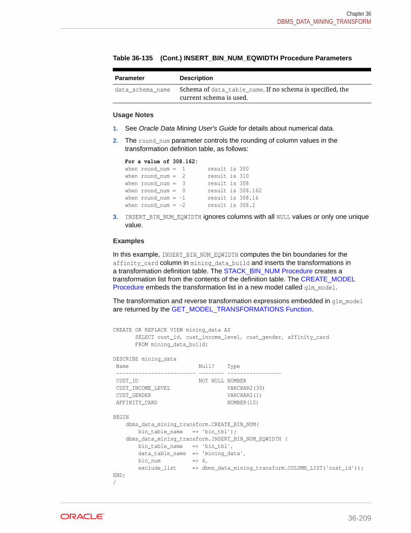
Table 36-135 (Cont.) INSERT_BIN_NUM_EQWIDTH Procedure Parameters
Parameter Description
data_schema_name Schema of data_table_name. If no schema is specified, thecurrent schema is used.
Usage Notes
1. See Oracle Data Mining User's Guide for details about numerical data.
2. The round_num parameter controls the rounding of column values in thetransformation definition table, as follows:
For a value of 308.162:when round_num = 1 result is 300when round_num = 2 result is 310when round_num = 3 result is 308when round_num = 0 result is 308.162when round_num = -1 result is 308.16when round_num = -2 result is 308.2
3. INSERT_BIN_NUM_EQWIDTH ignores columns with all NULL values or only one uniquevalue.
Examples
In this example, INSERT_BIN_NUM_EQWIDTH computes the bin boundaries for theaffinity_card column in mining_data_build and inserts the transformations ina transformation definition table. The STACK_BIN_NUM Procedure creates atransformation list from the contents of the definition table. The CREATE_MODELProcedure embeds the transformation list in a new model called glm_model.
The transformation and reverse transformation expressions embedded in glm_modelare returned by the GET_MODEL_TRANSFORMATIONS Function.
CREATE OR REPLACE VIEW mining_data AS SELECT cust_id, cust_income_level, cust_gender, affinity_card FROM mining_data_build; DESCRIBE mining_data Name Null? Type ------------------------- -------- ----------------- CUST_ID NOT NULL NUMBER CUST_INCOME_LEVEL VARCHAR2(30) CUST_GENDER VARCHAR2(1) AFFINITY_CARD NUMBER(10) BEGIN dbms_data_mining_transform.CREATE_BIN_NUM( bin_table_name => 'bin_tbl'); dbms_data_mining_transform.INSERT_BIN_NUM_EQWIDTH ( bin_table_name => 'bin_tbl', data_table_name => 'mining_data', bin_num => 4, exclude_list => dbms_data_mining_transform.COLUMN_LIST('cust_id'));END;/
Chapter 36DBMS_DATA_MINING_TRANSFORM
36-209
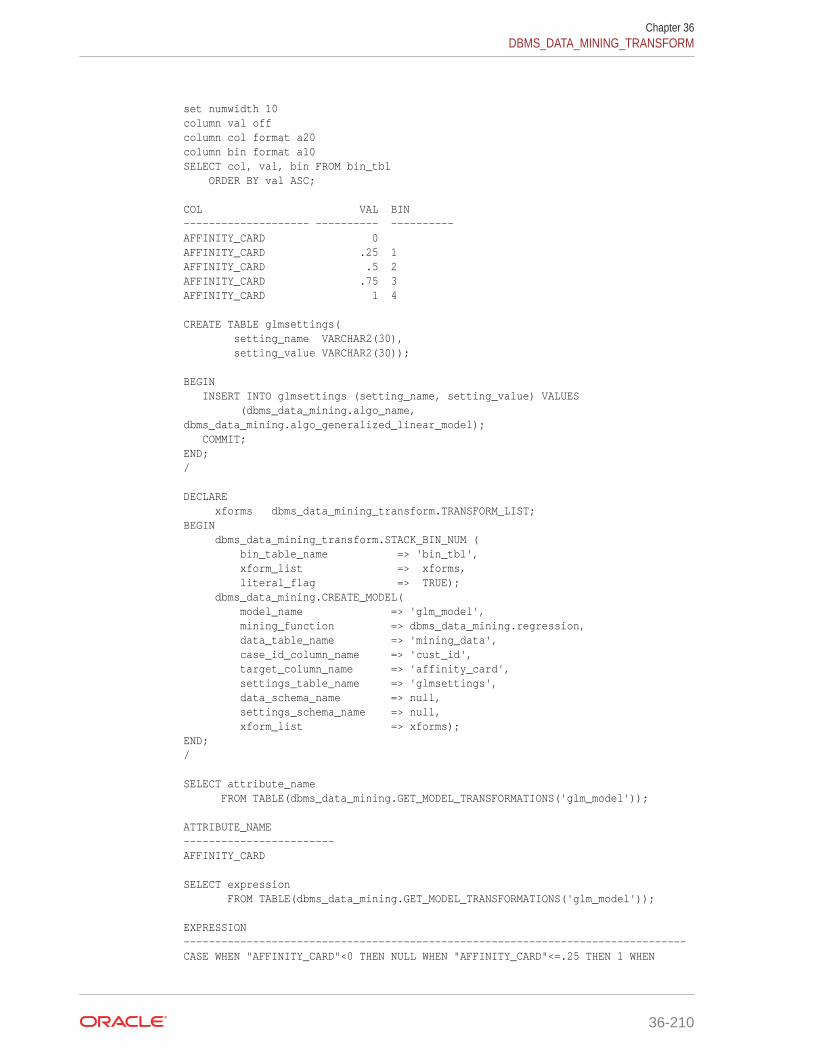
set numwidth 10column val offcolumn col format a20column bin format a10SELECT col, val, bin FROM bin_tbl ORDER BY val ASC; COL VAL BIN-------------------- ---------- ----------AFFINITY_CARD 0AFFINITY_CARD .25 1AFFINITY_CARD .5 2AFFINITY_CARD .75 3AFFINITY_CARD 1 4 CREATE TABLE glmsettings( setting_name VARCHAR2(30), setting_value VARCHAR2(30)); BEGIN INSERT INTO glmsettings (setting_name, setting_value) VALUES (dbms_data_mining.algo_name, dbms_data_mining.algo_generalized_linear_model); COMMIT;END;/ DECLARE xforms dbms_data_mining_transform.TRANSFORM_LIST;BEGIN dbms_data_mining_transform.STACK_BIN_NUM ( bin_table_name => 'bin_tbl', xform_list => xforms, literal_flag => TRUE); dbms_data_mining.CREATE_MODEL( model_name => 'glm_model', mining_function => dbms_data_mining.regression, data_table_name => 'mining_data', case_id_column_name => 'cust_id', target_column_name => 'affinity_card', settings_table_name => 'glmsettings', data_schema_name => null, settings_schema_name => null, xform_list => xforms);END;/ SELECT attribute_name FROM TABLE(dbms_data_mining.GET_MODEL_TRANSFORMATIONS('glm_model')); ATTRIBUTE_NAME------------------------AFFINITY_CARD SELECT expression FROM TABLE(dbms_data_mining.GET_MODEL_TRANSFORMATIONS('glm_model')); EXPRESSION--------------------------------------------------------------------------------CASE WHEN "AFFINITY_CARD"<0 THEN NULL WHEN "AFFINITY_CARD"<=.25 THEN 1 WHEN
Chapter 36DBMS_DATA_MINING_TRANSFORM
36-210
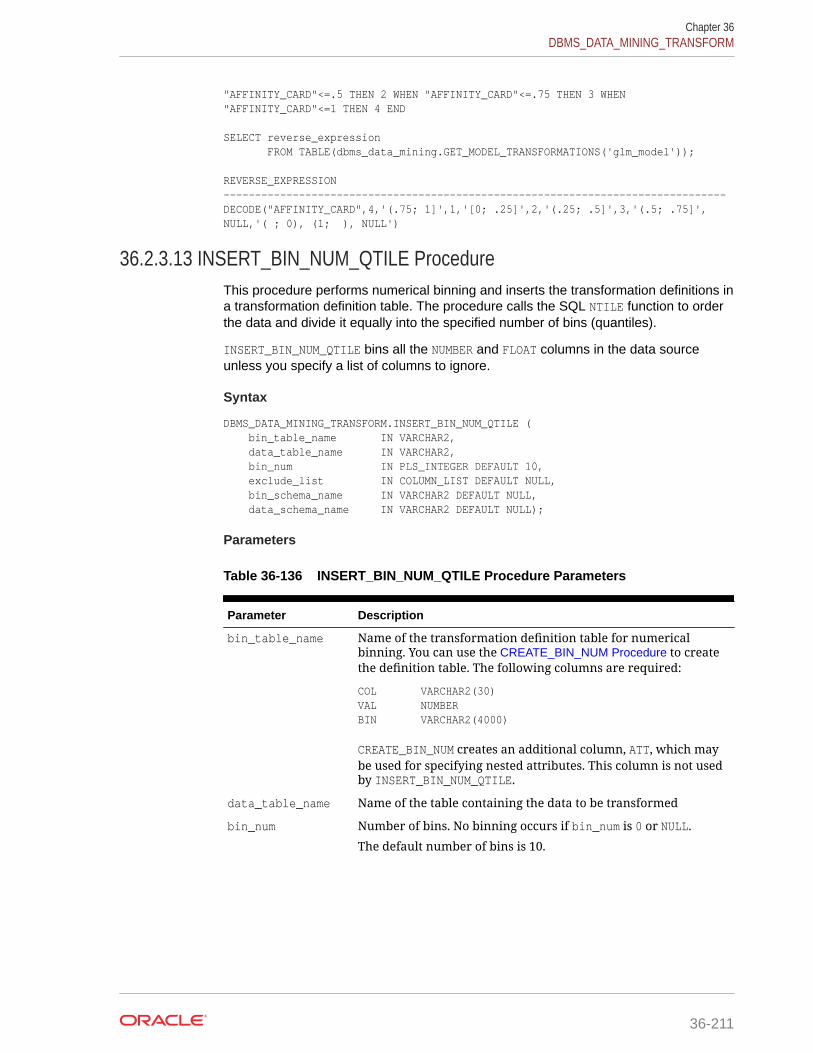
"AFFINITY_CARD"<=.5 THEN 2 WHEN "AFFINITY_CARD"<=.75 THEN 3 WHEN"AFFINITY_CARD"<=1 THEN 4 END SELECT reverse_expression FROM TABLE(dbms_data_mining.GET_MODEL_TRANSFORMATIONS('glm_model')); REVERSE_EXPRESSION--------------------------------------------------------------------------------DECODE("AFFINITY_CARD",4,'(.75; 1]',1,'[0; .25]',2,'(.25; .5]',3,'(.5; .75]',NULL,'( ; 0), (1; ), NULL')
36.2.3.13 INSERT_BIN_NUM_QTILE ProcedureThis procedure performs numerical binning and inserts the transformation definitions ina transformation definition table. The procedure calls the SQL NTILE function to orderthe data and divide it equally into the specified number of bins (quantiles).
INSERT_BIN_NUM_QTILE bins all the NUMBER and FLOAT columns in the data sourceunless you specify a list of columns to ignore.
Syntax
DBMS_DATA_MINING_TRANSFORM.INSERT_BIN_NUM_QTILE ( bin_table_name IN VARCHAR2, data_table_name IN VARCHAR2, bin_num IN PLS_INTEGER DEFAULT 10, exclude_list IN COLUMN_LIST DEFAULT NULL, bin_schema_name IN VARCHAR2 DEFAULT NULL, data_schema_name IN VARCHAR2 DEFAULT NULL);
Parameters
Table 36-136 INSERT_BIN_NUM_QTILE Procedure Parameters
Parameter Description
bin_table_name Name of the transformation definition table for numericalbinning. You can use the CREATE_BIN_NUM Procedure to createthe definition table. The following columns are required:
COL VARCHAR2(30)VAL NUMBERBIN VARCHAR2(4000)
CREATE_BIN_NUM creates an additional column, ATT, which maybe used for specifying nested attributes. This column is not usedby INSERT_BIN_NUM_QTILE.
data_table_name Name of the table containing the data to be transformed
bin_num Number of bins. No binning occurs if bin_num is 0 or NULL.
The default number of bins is 10.
Chapter 36DBMS_DATA_MINING_TRANSFORM
36-211
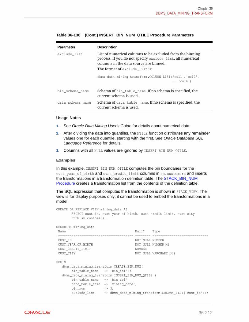
Table 36-136 (Cont.) INSERT_BIN_NUM_QTILE Procedure Parameters
Parameter Description
exclude_list List of numerical columns to be excluded from the binningprocess. If you do not specify exclude_list, all numericalcolumns in the data source are binned.The format of exclude_list is:
dbms_data_mining_transform.COLUMN_LIST('col1','col2', ...'coln')
bin_schema_name Schema of bin_table_name. If no schema is specified, thecurrent schema is used.
data_schema_name Schema of data_table_name. If no schema is specified, thecurrent schema is used.
Usage Notes
1. See Oracle Data Mining User's Guide for details about numerical data.
2. After dividing the data into quantiles, the NTILE function distributes any remaindervalues one for each quantile, starting with the first. See Oracle Database SQLLanguage Reference for details.
3. Columns with all NULL values are ignored by INSERT_BIN_NUM_QTILE.
Examples
In this example, INSERT_BIN_NUM_QTILE computes the bin boundaries for thecust_year_of_birth and cust_credit_limit columns in sh.customers and insertsthe transformations in a transformation definition table. The STACK_BIN_NUMProcedure creates a transformation list from the contents of the definition table.
The SQL expression that computes the transformation is shown in STACK_VIEW. Theview is for display purposes only; it cannot be used to embed the transformations in amodel.
CREATE OR REPLACE VIEW mining_data AS SELECT cust_id, cust_year_of_birth, cust_credit_limit, cust_city FROM sh.customers; DESCRIBE mining_data Name Null? Type --------------------------------------- -------- ----------------------------- CUST_ID NOT NULL NUMBER CUST_YEAR_OF_BIRTH NOT NULL NUMBER(4) CUST_CREDIT_LIMIT NUMBER CUST_CITY NOT NULL VARCHAR2(30) BEGIN dbms_data_mining_transform.CREATE_BIN_NUM( bin_table_name => 'bin_tbl'); dbms_data_mining_transform.INSERT_BIN_NUM_QTILE ( bin_table_name => 'bin_tbl', data_table_name => 'mining_data', bin_num => 3, exclude_list => dbms_data_mining_transform.COLUMN_LIST('cust_id'));
Chapter 36DBMS_DATA_MINING_TRANSFORM
36-212

END;/ set numwidth 8column val offcolumn col format a20column bin format a10SELECT col, val, bin FROM bin_tbl ORDER BY col ASC, val ASC; COL VAL BIN-------------------- -------- ----------CUST_CREDIT_LIMIT 1500CUST_CREDIT_LIMIT 3000 1CUST_CREDIT_LIMIT 9000 2CUST_CREDIT_LIMIT 15000 3CUST_YEAR_OF_BIRTH 1913CUST_YEAR_OF_BIRTH 1949 1CUST_YEAR_OF_BIRTH 1965 2CUST_YEAR_OF_BIRTH 1990 3 DECLARE xforms dbms_data_mining_transform.TRANSFORM_LIST;BEGIN dbms_data_mining_transform.STACK_BIN_NUM ( bin_table_name => 'bin_tbl', xform_list => xforms); dbms_data_mining_transform.XFORM_STACK ( xform_list => xforms, data_table_name => 'mining_data', xform_view_name => 'stack_view');END;/ set long 3000SELECT text FROM user_views WHERE view_name in 'STACK_VIEW'; TEXT--------------------------------------------------------------------------------SELECT "CUST_ID",CASE WHEN "CUST_YEAR_OF_BIRTH"<1913 THEN NULL WHEN "CUST_YEAR_OF_BIRTH"<=1949 THEN '1' WHEN "CUST_YEAR_OF_BIRTH"<=1965 THEN '2' WHEN "CUST_YEAR_OF_BIRTH"<=1990 THEN '3' END "CUST_YEAR_OF_BIRTH",CASE WHEN "CUST_CREDIT_LIMIT"<1500 THEN NULL WHEN "CUST_CREDIT_LIMIT"<=3000 THEN '1' WHEN "CUST_CREDIT_LIMIT"<=9000 THEN '2' WHEN "CUST_CREDIT_LIMIT"<=15000 THEN '3' END "CUST_CREDIT_LIMIT","CUST_CITY" FROM mining_data
36.2.3.14 INSERT_BIN_SUPER ProcedureThis procedure performs numerical and categorical binning and inserts thetransformation definitions in transformation definition tables. The procedure computesbin boundaries based on intrinsic relationships between predictors and a target.
INSERT_BIN_SUPER uses an intelligent binning technique known as supervisedbinning. It builds a single-predictor decision tree and derives the bin boundaries fromsplits within the tree.
INSERT_BIN_SUPER bins all the VARCHAR2, CHAR, NUMBER, and FLOAT columns in the datasource unless you specify a list of columns to ignore.
Chapter 36DBMS_DATA_MINING_TRANSFORM
36-213
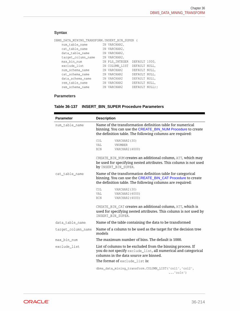
Syntax
DBMS_DATA_MINING_TRANSFORM.INSERT_BIN_SUPER ( num_table_name IN VARCHAR2, cat_table_name IN VARCHAR2, data_table_name IN VARCHAR2, target_column_name IN VARCHAR2, max_bin_num IN PLS_INTEGER DEFAULT 1000, exclude_list IN COLUMN_LIST DEFAULT NULL, num_schema_name IN VARCHAR2 DEFAULT NULL, cat_schema_name IN VARCHAR2 DEFAULT NULL, data_schema_name IN VARCHAR2 DEFAULT NULL, rem_table_name IN VARCHAR2 DEFAULT NULL, rem_schema_name IN VARCHAR2 DEFAULT NULL);
Parameters
Table 36-137 INSERT_BIN_SUPER Procedure Parameters
Parameter Description
num_table_name Name of the transformation definition table for numericalbinning. You can use the CREATE_BIN_NUM Procedure to createthe definition table. The following columns are required:
COL VARCHAR2(30)VAL VNUMBERBIN VARCHAR2(4000)
CREATE_BIN_NUM creates an additional column, ATT, which maybe used for specifying nested attributes. This column is not usedby INSERT_BIN_SUPER.
cat_table_name Name of the transformation definition table for categoricalbinning. You can use the CREATE_BIN_CAT Procedure to createthe definition table. The following columns are required:
COL VARCHAR2(30)VAL VARCHAR2(4000)BIN VARCHAR2(4000)
CREATE_BIN_CAT creates an additional column, ATT, which isused for specifying nested attributes. This column is not used byINSERT_BIN_SUPER.
data_table_name Name of the table containing the data to be transformed
target_column_name Name of a column to be used as the target for the decision treemodels
max_bin_num The maximum number of bins. The default is 1000.
exclude_list List of columns to be excluded from the binning process. Ifyou do not specify exclude_list, all numerical and categoricalcolumns in the data source are binned.The format of exclude_list is:
dbms_data_mining_transform.COLUMN_LIST('col1','col2', ...'coln')
Chapter 36DBMS_DATA_MINING_TRANSFORM
36-214

Table 36-137 (Cont.) INSERT_BIN_SUPER Procedure Parameters
Parameter Description
num_schema_name Schema of num_table_name. If no schema is specified, thecurrent schema is used.
cat_schema_name Schema of cat_table_name. If no schema is specified, thecurrent schema is used.
data_schema_name Schema of data_table_name. If no schema is specified, thecurrent schema is used.
rem_table_name Name of a column removal definition table. The table musthave the columns described in "CREATE_COL_REM Procedure".You can use CREATE_COL_REM to create the table. See UsageNotes.
rem_schema_name Schema of rem_table_name. If no schema is specified, thecurrent schema is used.
Usage Notes
1. See Oracle Data Mining User's Guide for details about numerical and categoricaldata.
2. Columns that have no significant splits are not binned. You can remove theunbinned columns from the mining data by specifying a column removal definitiontable. If you do not specify a column removal definition table, the unbinnedcolumns remain in the mining data.
3. See Oracle Data Mining Concepts to learn more about decision trees in OracleData Mining
Examples
In this example, INSERT_BIN_SUPER computes the bin boundaries for predictors ofcust_credit_limit and inserts the transformations in transformation definition tables.One predictor is numerical, the other is categorical. (INSERT_BIN_SUPER determinesthat the cust_postal_code column is not a significant predictor.) STACK procedurescreate transformation lists from the contents of the definition tables.
The SQL expressions that compute the transformations are shown in the viewsMINING_DATA_STACK_NUM and MINING_DATA_STACK_CAT. The views are for displaypurposes only; they cannot be used to embed the transformations in a model.
CREATE OR REPLACE VIEW mining_data AS SELECT cust_id, cust_year_of_birth, cust_marital_status, cust_postal_code, cust_credit_limit FROM sh.customers; DESCRIBE mining_data Name Null? Type -------------------------------- -------- ------------------------------------ CUST_ID NOT NULL NUMBER CUST_YEAR_OF_BIRTH NOT NULL NUMBER(4) CUST_MARITAL_STATUS VARCHAR2(20) CUST_POSTAL_CODE NOT NULL VARCHAR2(10) CUST_CREDIT_LIMIT NUMBER
Chapter 36DBMS_DATA_MINING_TRANSFORM
36-215
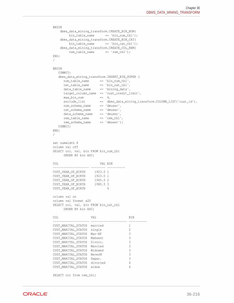
BEGIN dbms_data_mining_transform.CREATE_BIN_NUM( bin_table_name => 'bin_num_tbl'); dbms_data_mining_transform.CREATE_BIN_CAT( bin_table_name => 'bin_cat_tbl'); dbms_data_mining_transform.CREATE_COL_REM( rem_table_name => 'rem_tbl');END;/ BEGIN COMMIT; dbms_data_mining_transform.INSERT_BIN_SUPER ( num_table_name => 'bin_num_tbl', cat_table_name => 'bin_cat_tbl', data_table_name => 'mining_data', target_column_name => 'cust_credit_limit', max_bin_num => 4, exclude_list => dbms_data_mining_transform.COLUMN_LIST('cust_id'), num_schema_name => 'dmuser', cat_schema_name => 'dmuser', data_schema_name => 'dmuser', rem_table_name => 'rem_tbl', rem_schema_name => 'dmuser'); COMMIT;END;/ set numwidth 8column val offSELECT col, val, bin FROM bin_num_tbl ORDER BY bin ASC; COL VAL BIN-------------------- -------- ----------CUST_YEAR_OF_BIRTH 1923.5 1CUST_YEAR_OF_BIRTH 1923.5 1CUST_YEAR_OF_BIRTH 1945.5 2CUST_YEAR_OF_BIRTH 1980.5 3CUST_YEAR_OF_BIRTH 4 column val oncolumn val format a20SELECT col, val, bin FROM bin_cat_tbl ORDER BY bin ASC; COL VAL BIN-------------------- -------------------- ----------CUST_MARITAL_STATUS married 1CUST_MARITAL_STATUS single 2CUST_MARITAL_STATUS Mar-AF 3CUST_MARITAL_STATUS Mabsent 3CUST_MARITAL_STATUS Divorc. 3CUST_MARITAL_STATUS Married 3CUST_MARITAL_STATUS Widowed 3CUST_MARITAL_STATUS NeverM 3CUST_MARITAL_STATUS Separ. 3CUST_MARITAL_STATUS divorced 4CUST_MARITAL_STATUS widow 4 SELECT col from rem_tbl;
Chapter 36DBMS_DATA_MINING_TRANSFORM
36-216

COL--------------------CUST_POSTAL_CODE DECLARE xforms_num dbms_data_mining_transform.TRANSFORM_LIST; xforms_cat dbms_data_mining_transform.TRANSFORM_LIST; BEGIN dbms_data_mining_transform.STACK_BIN_NUM ( bin_table_name => 'bin_num_tbl', xform_list => xforms_num); dbms_data_mining_transform.XFORM_STACK ( xform_list => xforms_num, data_table_name => 'mining_data', xform_view_name => 'mining_data_stack_num'); dbms_data_mining_transform.STACK_BIN_CAT ( bin_table_name => 'bin_cat_tbl', xform_list => xforms_cat); dbms_data_mining_transform.XFORM_STACK ( xform_list => xforms_cat, data_table_name => 'mining_data', xform_view_name => 'mining_data_stack_cat'); END; / set long 3000SELECT text FROM user_views WHERE view_name IN 'MINING_DATA_STACK_NUM'; TEXT--------------------------------------------------------------------------------SELECT "CUST_ID",CASE WHEN "CUST_YEAR_OF_BIRTH"<1923.5 THEN '1' WHEN "CUST_YEAR_OF_BIRTH"<=1923.5 THEN '1' WHEN "CUST_YEAR_OF_BIRTH"<=1945.5 THEN '2' WHEN "CUST_YEAR_OF_BIRTH"<=1980.5 THEN '3' WHEN "CUST_YEAR_OF_BIRTH" IS NOT NULL THEN '4'END "CUST_YEAR_OF_BIRTH","CUST_MARITAL_STATUS","CUST_POSTAL_CODE","CUST_CREDIT_LIMIT" FROM mining_data SELECT text FROM user_views WHERE view_name IN 'MINING_DATA_STACK_CAT'; TEXT--------------------------------------------------------------------------------SELECT "CUST_ID","CUST_YEAR_OF_BIRTH",DECODE("CUST_MARITAL_STATUS",'Divorc.','3','Mabsent','3','Mar-AF','3','Married','3','NeverM','3','Separ.','3','Widowed','3','divorced','4','married','1','single','2','widow','4') "CUST_MARITAL_STATUS","CUST_POSTAL_CODE","CUST_CREDIT_LIMIT" FROM mining_data
36.2.3.15 INSERT_CLIP_TRIM_TAIL ProcedureThis procedure replaces numeric outliers with nulls and inserts the transformationdefinitions in a transformation definition table.
INSERT_CLIP_TRIM_TAIL computes the boundaries of the data based on a specifiedpercentage. It removes the values that fall outside the boundaries (tail values) fromthe data. If you wish to replace the tail values instead of removing them, use theINSERT_CLIP_WINSOR_TAIL Procedure.
INSERT_CLIP_TRIM_TAIL clips all the NUMBER and FLOAT columns in the data sourceunless you specify a list of columns to ignore.
Chapter 36DBMS_DATA_MINING_TRANSFORM
36-217
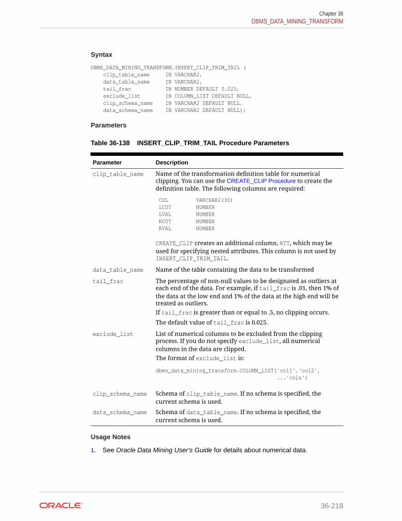
Syntax
DBMS_DATA_MINING_TRANSFORM.INSERT_CLIP_TRIM_TAIL ( clip_table_name IN VARCHAR2, data_table_name IN VARCHAR2, tail_frac IN NUMBER DEFAULT 0.025, exclude_list IN COLUMN_LIST DEFAULT NULL, clip_schema_name IN VARCHAR2 DEFAULT NULL, data_schema_name IN VARCHAR2 DEFAULT NULL);
Parameters
Table 36-138 INSERT_CLIP_TRIM_TAIL Procedure Parameters
Parameter Description
clip_table_name Name of the transformation definition table for numericalclipping. You can use the CREATE_CLIP Procedure to create thedefinition table. The following columns are required:
COL VARCHAR2(30) LCUT NUMBER LVAL NUMBER RCUT NUMBER RVAL NUMBER
CREATE_CLIP creates an additional column, ATT, which may beused for specifying nested attributes. This column is not used byINSERT_CLIP_TRIM_TAIL.
data_table_name Name of the table containing the data to be transformed
tail_frac The percentage of non-null values to be designated as outliers ateach end of the data. For example, if tail_frac is .01, then 1% ofthe data at the low end and 1% of the data at the high end will betreated as outliers.If tail_frac is greater than or equal to .5, no clipping occurs.
The default value of tail_frac is 0.025.
exclude_list List of numerical columns to be excluded from the clippingprocess. If you do not specify exclude_list, all numericalcolumns in the data are clipped.The format of exclude_list is:
dbms_data_mining_transform.COLUMN_LIST('col1','col2', ...'coln')
clip_schema_name Schema of clip_table_name. If no schema is specified, thecurrent schema is used.
data_schema_name Schema of data_table_name. If no schema is specified, thecurrent schema is used.
Usage Notes
1. See Oracle Data Mining User's Guide for details about numerical data.
Chapter 36DBMS_DATA_MINING_TRANSFORM
36-218
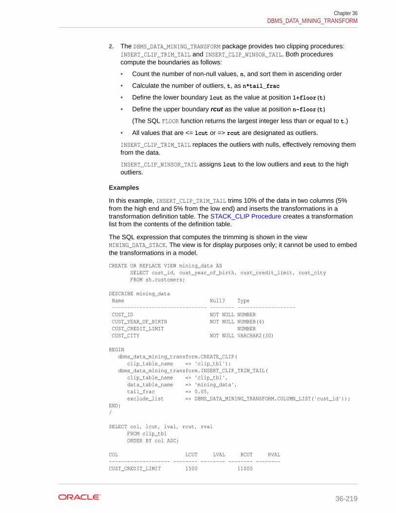
2. The DBMS_DATA_MINING_TRANSFORM package provides two clipping procedures:INSERT_CLIP_TRIM_TAIL and INSERT_CLIP_WINSOR_TAIL. Both procedurescompute the boundaries as follows:
• Count the number of non-null values, n, and sort them in ascending order
• Calculate the number of outliers, t, as n*tail_frac
• Define the lower boundary lcut as the value at position 1+floor(t)
• Define the upper boundary rcut as the value at position n-floor(t)
(The SQL FLOOR function returns the largest integer less than or equal to t.)
• All values that are <= lcut or => rcut are designated as outliers.
INSERT_CLIP_TRIM_TAIL replaces the outliers with nulls, effectively removing themfrom the data.
INSERT_CLIP_WINSOR_TAIL assigns lcut to the low outliers and rcut to the highoutliers.
Examples
In this example, INSERT_CLIP_TRIM_TAIL trims 10% of the data in two columns (5%from the high end and 5% from the low end) and inserts the transformations in atransformation definition table. The STACK_CLIP Procedure creates a transformationlist from the contents of the definition table.
The SQL expression that computes the trimming is shown in the viewMINING_DATA_STACK. The view is for display purposes only; it cannot be used to embedthe transformations in a model.
CREATE OR REPLACE VIEW mining_data AS SELECT cust_id, cust_year_of_birth, cust_credit_limit, cust_city FROM sh.customers; DESCRIBE mining_data Name Null? Type ------------------------------- -------- ------------------- CUST_ID NOT NULL NUMBER CUST_YEAR_OF_BIRTH NOT NULL NUMBER(4) CUST_CREDIT_LIMIT NUMBER CUST_CITY NOT NULL VARCHAR2(30)
BEGIN dbms_data_mining_transform.CREATE_CLIP( clip_table_name => 'clip_tbl'); dbms_data_mining_transform.INSERT_CLIP_TRIM_TAIL( clip_table_name => 'clip_tbl', data_table_name => 'mining_data', tail_frac => 0.05, exclude_list => DBMS_DATA_MINING_TRANSFORM.COLUMN_LIST('cust_id'));END;/ SELECT col, lcut, lval, rcut, rval FROM clip_tbl ORDER BY col ASC; COL LCUT LVAL RCUT RVAL-------------------- -------- -------- -------- --------CUST_CREDIT_LIMIT 1500 11000
Chapter 36DBMS_DATA_MINING_TRANSFORM
36-219

CUST_YEAR_OF_BIRTH 1934 1982 DECLARE xforms dbms_data_mining_transform.TRANSFORM_LIST;BEGIN dbms_data_mining_transform.STACK_CLIP ( clip_table_name => 'clip_tbl', xform_list => xforms); dbms_data_mining_transform.XFORM_STACK ( xform_list => xforms, data_table_name => 'mining_data', xform_view_name => 'mining_data_stack'); END; / set long 3000SELECT text FROM user_views WHERE view_name IN 'MINING_DATA_STACK'; TEXT--------------------------------------------------------------------------------SELECT "CUST_ID",CASE WHEN "CUST_YEAR_OF_BIRTH" < 1934 THEN NULL WHEN "CUST_YEAR_OF_BIRTH" > 1982 THEN NULL ELSE "CUST_YEAR_OF_BIRTH" END "CUST_YEAR_OF_BIRTH",CASE WHEN "CUST_CREDIT_LIMIT" < 1500 THEN NULL WHEN "CUST_CREDIT_LIMIT" > 11000 THEN NULL ELSE "CUST_CREDIT_LIMIT" END "CUST_CREDIT_LIMIT","CUST_CITY" FROM mining_data
36.2.3.16 INSERT_CLIP_WINSOR_TAIL ProcedureThis procedure replaces numeric outliers with the upper or lower boundary values. Itinserts the transformation definitions in a transformation definition table.
INSERT_CLIP_WINSOR_TAIL computes the boundaries of the data based on a specifiedpercentage. It replaces the values that fall outside the boundaries (tail values)with the related boundary value. If you wish to set tail values to null, use theINSERT_CLIP_TRIM_TAIL Procedure.
INSERT_CLIP_WINSOR_TAIL clips all the NUMBER and FLOAT columns in the data sourceunless you specify a list of columns to ignore.
Syntax
DBMS_DATA_MINING_TRANSFORM.INSERT_CLIP_WINSOR_TAIL ( clip_table_name IN VARCHAR2, data_table_name IN VARCHAR2, tail_frac IN NUMBER DEFAULT 0.025, exclude_list IN COLUMN_LIST DEFAULT NULL, clip_schema_name IN VARCHAR2 DEFAULT NULL, data_schema_name IN VARCHAR2 DEFAULT NULL);
Chapter 36DBMS_DATA_MINING_TRANSFORM
36-220
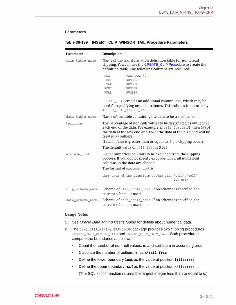
Parameters
Table 36-139 INSERT_CLIP_WINSOR_TAIL Procedure Parameters
Parameter Description
clip_table_name Name of the transformation definition table for numericalclipping. You can use the CREATE_CLIP Procedure to create thedefinition table. The following columns are required:
COL VARCHAR2(30) LCUT NUMBER LVAL NUMBER RCUT NUMBER RVAL NUMBER
CREATE_CLIP creates an additional column, ATT, which may beused for specifying nested attributes. This column is not used byINSERT_CLIP_WINSOR_TAIL.
data_table_name Name of the table containing the data to be transformed
tail_frac The percentage of non-null values to be designated as outliers ateach end of the data. For example, if tail_frac is .01, then 1% ofthe data at the low end and 1% of the data at the high end will betreated as outliers.If tail_frac is greater than or equal to .5, no clipping occurs.
The default value of tail_frac is 0.025.
exclude_list List of numerical columns to be excluded from the clippingprocess. If you do not specify exclude_list, all numericalcolumns in the data are clipped.The format of exclude_list is:
dbms_data_mining_transform.COLUMN_LIST('col1','col2', ...'coln')
clip_schema_name Schema of clip_table_name. If no schema is specified, thecurrent schema is used.
data_schema_name Schema of data_table_name. If no schema is specified, thecurrent schema is used.
Usage Notes
1. See Oracle Data Mining User's Guide for details about numerical data.
2. The DBMS_DATA_MINING_TRANSFORM package provides two clipping procedures:INSERT_CLIP_WINSOR_TAIL and INSERT_CLIP_TRIM_TAIL. Both procedurescompute the boundaries as follows:
• Count the number of non-null values, n, and sort them in ascending order
• Calculate the number of outliers, t, as n*tail_frac
• Define the lower boundary lcut as the value at position 1+floor(t)
• Define the upper boundary rcut as the value at position n-floor(t)
(The SQL FLOOR function returns the largest integer less than or equal to t.)
Chapter 36DBMS_DATA_MINING_TRANSFORM
36-221

• All values that are <= lcut or => rcut are designated as outliers.
INSERT_CLIP_WINSOR_TAIL assigns lcut to the low outliers and rcut to the highoutliers.
INSERT_CLIP_TRIM_TAIL replaces the outliers with nulls, effectively removing themfrom the data.
Examples
In this example, INSERT_CLIP_WINSOR_TAIL winsorizes 10% of the data in two columns(5% from the high end, and 5% from the low end) and inserts the transformations in atransformation definition table. The STACK_CLIP Procedure creates a transformationlist from the contents of the definition table.
The SQL expression that computes the transformation is shown in the viewMINING_DATA_STACK. The view is for display purposes only; it cannot be used to embedthe transformations in a model.
CREATE OR REPLACE VIEW mining_data AS SELECT cust_id, cust_year_of_birth, cust_credit_limit, cust_city FROM sh.customers;
describe mining_data Name Null? Type ---------------------------------------- -------- ------------- CUST_ID NOT NULL NUMBER CUST_YEAR_OF_BIRTH NOT NULL NUMBER(4) CUST_CREDIT_LIMIT NUMBER CUST_CITY NOT NULL VARCHAR2(30) BEGIN dbms_data_mining_transform.CREATE_CLIP( clip_table_name => 'clip_tbl'); dbms_data_mining_transform.INSERT_CLIP_WINSOR_TAIL( clip_table_name => 'clip_tbl', data_table_name => 'mining_data', tail_frac => 0.05, exclude_list => DBMS_DATA_MINING_TRANSFORM.COLUMN_LIST('cust_id'));END;/
SELECT col, lcut, lval, rcut, rval FROM clip_tbl ORDER BY col ASC;COL LCUT LVAL RCUT RVAL------------------------------ -------- -------- -------- --------CUST_CREDIT_LIMIT 1500 1500 11000 11000CUST_YEAR_OF_BIRTH 1934 1934 1982 1982
DECLARE xforms dbms_data_mining_transform.TRANSFORM_LIST;BEGIN dbms_data_mining_transform.STACK_CLIP ( clip_table_name => 'clip_tbl', xform_list => xforms);dbms_data_mining_transform.XFORM_STACK ( xform_list => xforms, data_table_name => 'mining_data', xform_view_name => 'mining_data_stack');END;/
Chapter 36DBMS_DATA_MINING_TRANSFORM
36-222

set long 3000SQL> SELECT text FROM user_views WHERE view_name IN 'MINING_DATA_STACK'; TEXT--------------------------------------------------------------------------------SELECT "CUST_ID",CASE WHEN "CUST_YEAR_OF_BIRTH" < 1934 THEN 1934 WHEN "CUST_YEAR_OF_BIRTH" > 1982 THEN 1982 ELSE "CUST_YEAR_OF_BIRTH" END "CUST_YEAR_OF_BIRTH",CASE WHEN "CUST_CREDIT_LIMIT" < 1500 THEN 1500 WHEN "CUST_CREDIT_LIMIT" > 11000 THEN 11000 ELSE "CUST_CREDIT_LIMIT" END "CUST_CREDIT_LIMIT","CUST_CITY" FROM mining_data
36.2.3.17 INSERT_MISS_CAT_MODE ProcedureThis procedure replaces missing categorical values with the value that occurs mostfrequently in the column (the mode). It inserts the transformation definitions in atransformation definition table.
INSERT_MISS_CAT_MODE replaces missing values in all VARCHAR2 and CHAR columns inthe data source unless you specify a list of columns to ignore.
Syntax
DBMS_DATA_MINING_TRANSFORM.INSERT_MISS_CAT_MODE ( miss_table_name IN VARCHAR2, data_table_name IN VARCHAR2, exclude_list IN COLUMN_LIST DEFAULT NULL, miss_schema_name IN VARCHAR2 DEFAULT NULL, data_schema_name IN VARCHAR2 DEFAULT NULL);
Parameters
Table 36-140 INSERT_MISS_CAT_MODE Procedure Parameters
Parameter Description
miss_table_name Name of the transformation definition table for categoricalmissing value treatment. You can use the CREATE_MISS_CATProcedure to create the definition table. The following columns arerequired:
COL VARCHAR2(30) VAL VARCHAR2(4000)
CREATE_MISS_CAT creates an additional column, ATT, which maybe used for specifying nested attributes. This column is not usedby INSERT_MISS_CAT_MODE.
data_table_name Name of the table containing the data to be transformed
exclude_list List of categorical columns to be excluded from missing valuetreatment. If you do not specify exclude_list, all categoricalcolumns are transformed.The format of exclude_list is:
dbms_data_mining_transform.COLUMN_LIST('col1','col2', ...'coln')
Chapter 36DBMS_DATA_MINING_TRANSFORM
36-223

Table 36-140 (Cont.) INSERT_MISS_CAT_MODE Procedure Parameters
Parameter Description
miss_schema_name Schema of miss_table_name. If no schema is specified, the currentschema is used.
data_schema_name Schema of data_table_name. If no schema is specified, the currentschema is used.
Usage Notes
1. See Oracle Data Mining User's Guide for details about categorical data.
2. If you wish to replace categorical missing values with a value other than the mode,you can edit the transformation definition table.
See Also:
Oracle Data Mining User's Guide for information about default missingvalue treatment in Oracle Data Mining
Example
In this example, INSERT_MISS_CAT_MODE computes missing value treatment forcust_city and inserts the transformation in a transformation definition table. TheSTACK_MISS_CAT Procedure creates a transformation list from the contents of thedefinition table.
The SQL expression that computes the transformation is shown in the viewMINING_DATA_STACK. The view is for display purposes only; it cannot be used to embedthe transformations in a model.
CREATE OR REPLACE VIEW mining_data AS SELECT cust_id, cust_year_of_birth, cust_city FROM sh.customers; describe mining_data Name Null? Type -------------------------------- -------- ---------------- CUST_ID NOT NULL NUMBER CUST_YEAR_OF_BIRTH NOT NULL NUMBER(4) CUST_CITY NOT NULL VARCHAR2(30) BEGIN dbms_data_mining_transform.create_miss_cat( miss_table_name => 'missc_tbl'); dbms_data_mining_transform.insert_miss_cat_mode( miss_table_name => 'missc_tbl', data_table_name => 'mining_data');END;/
SELECT stats_mode(cust_city) FROM mining_data; STATS_MODE(CUST_CITY)
Chapter 36DBMS_DATA_MINING_TRANSFORM
36-224

------------------------------Los Angeles
SELECT col, val from missc_tbl;
COL VAL------------------------------ ------------------------------CUST_CITY Los Angeles
DECLARE xforms dbms_data_mining_transform.TRANSFORM_LIST;BEGIN dbms_data_mining_transform.STACK_MISS_CAT ( miss_table_name => 'missc_tbl', xform_list => xforms); dbms_data_mining_transform.XFORM_STACK ( xform_list => xforms, data_table_name => 'mining_data', xform_view_name => 'mining_data_stack');END;/ set long 3000SELECT text FROM user_views WHERE view_name IN 'MINING_DATA_STACK'; TEXT--------------------------------------------------------------------------------SELECT "CUST_ID","CUST_YEAR_OF_BIRTH",NVL("CUST_CITY",'Los Angeles') "CUST_CITY" FROM mining_data
36.2.3.18 INSERT_MISS_NUM_MEAN ProcedureThis procedure replaces missing numerical values with the average (the mean) andinserts the transformation definitions in a transformation definition table.
INSERT_MISS_NUM_MEAN replaces missing values in all NUMBER and FLOAT columns inthe data source unless you specify a list of columns to ignore.
Syntax
DBMS_DATA_MINING_TRANSFORM.INSERT_MISS_NUM_MEAN ( miss_table_name IN VARCHAR2, data_table_name IN VARCHAR2, exclude_list IN COLUMN_LIST DEFAULT NULL, round_num IN PLS_INTEGER DEFAULT 6, miss_schema_name IN VARCHAR2 DEFAULT NULL, data_schema_name IN VARCHAR2 DEFAULT NULL);
Chapter 36DBMS_DATA_MINING_TRANSFORM
36-225
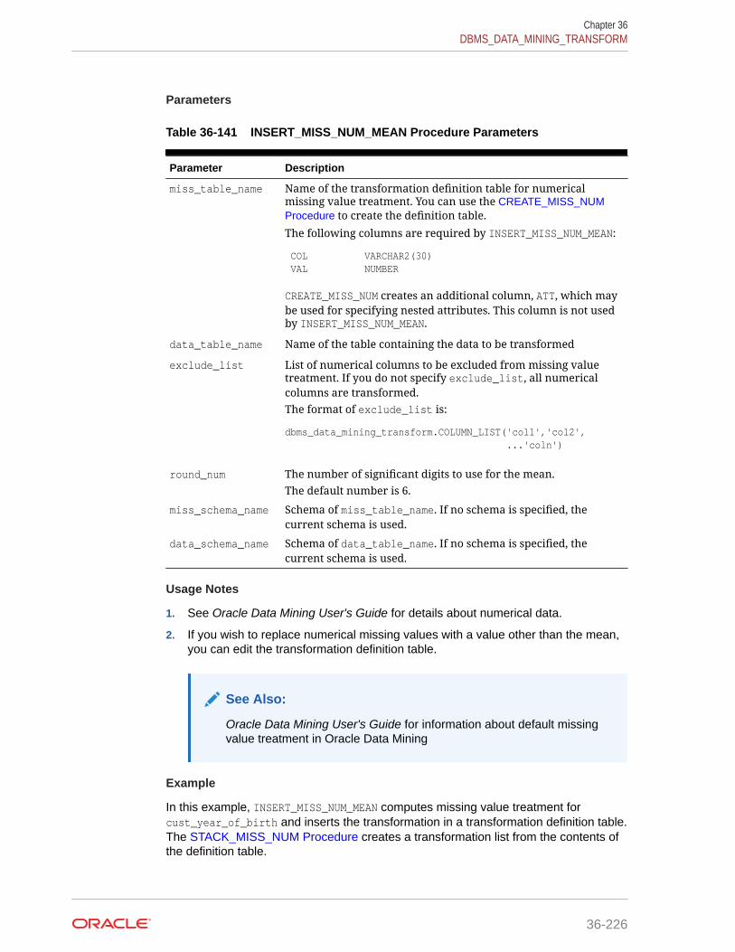
Parameters
Table 36-141 INSERT_MISS_NUM_MEAN Procedure Parameters
Parameter Description
miss_table_name Name of the transformation definition table for numericalmissing value treatment. You can use the CREATE_MISS_NUMProcedure to create the definition table.
The following columns are required by INSERT_MISS_NUM_MEAN:
COL VARCHAR2(30) VAL NUMBER
CREATE_MISS_NUM creates an additional column, ATT, which maybe used for specifying nested attributes. This column is not usedby INSERT_MISS_NUM_MEAN.
data_table_name Name of the table containing the data to be transformed
exclude_list List of numerical columns to be excluded from missing valuetreatment. If you do not specify exclude_list, all numericalcolumns are transformed.The format of exclude_list is:
dbms_data_mining_transform.COLUMN_LIST('col1','col2', ...'coln')
round_num The number of significant digits to use for the mean.The default number is 6.
miss_schema_name Schema of miss_table_name. If no schema is specified, thecurrent schema is used.
data_schema_name Schema of data_table_name. If no schema is specified, thecurrent schema is used.
Usage Notes
1. See Oracle Data Mining User's Guide for details about numerical data.
2. If you wish to replace numerical missing values with a value other than the mean,you can edit the transformation definition table.
See Also:
Oracle Data Mining User's Guide for information about default missingvalue treatment in Oracle Data Mining
Example
In this example, INSERT_MISS_NUM_MEAN computes missing value treatment forcust_year_of_birth and inserts the transformation in a transformation definition table.The STACK_MISS_NUM Procedure creates a transformation list from the contents ofthe definition table.
Chapter 36DBMS_DATA_MINING_TRANSFORM
36-226
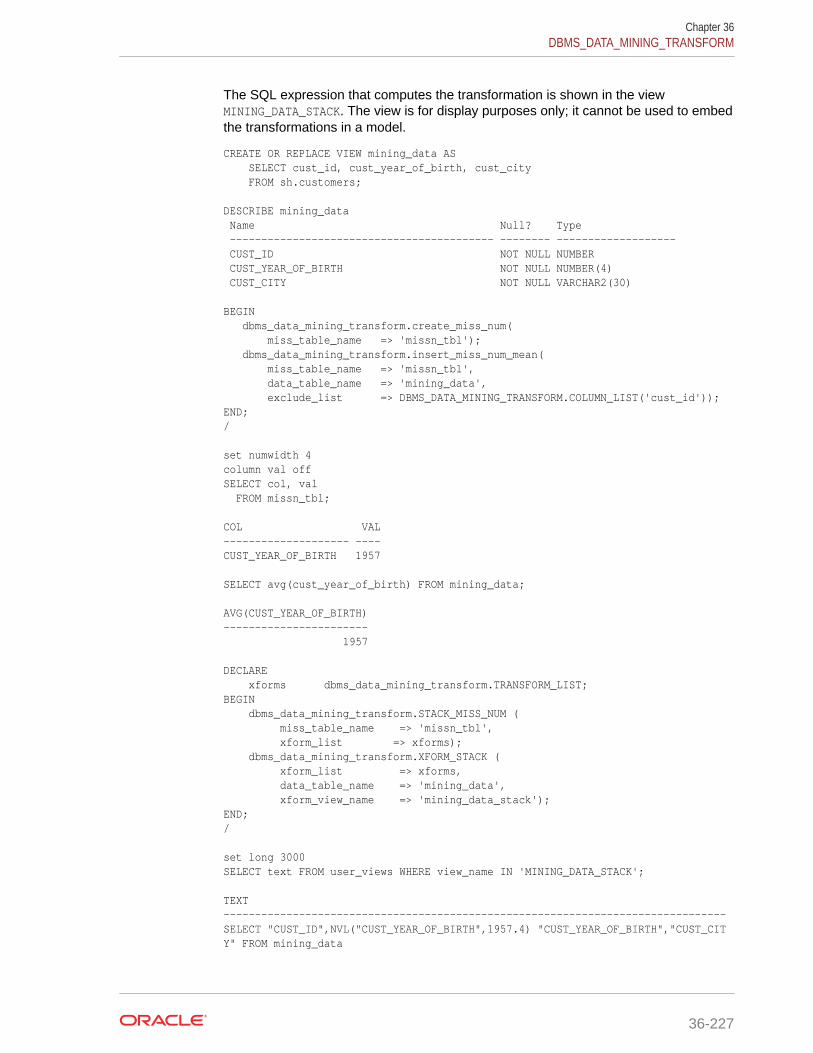
The SQL expression that computes the transformation is shown in the viewMINING_DATA_STACK. The view is for display purposes only; it cannot be used to embedthe transformations in a model.
CREATE OR REPLACE VIEW mining_data AS SELECT cust_id, cust_year_of_birth, cust_city FROM sh.customers;
DESCRIBE mining_data Name Null? Type ------------------------------------------ -------- ------------------- CUST_ID NOT NULL NUMBER CUST_YEAR_OF_BIRTH NOT NULL NUMBER(4) CUST_CITY NOT NULL VARCHAR2(30) BEGIN dbms_data_mining_transform.create_miss_num( miss_table_name => 'missn_tbl'); dbms_data_mining_transform.insert_miss_num_mean( miss_table_name => 'missn_tbl', data_table_name => 'mining_data', exclude_list => DBMS_DATA_MINING_TRANSFORM.COLUMN_LIST('cust_id'));END;/ set numwidth 4column val offSELECT col, val FROM missn_tbl; COL VAL-------------------- ----CUST_YEAR_OF_BIRTH 1957 SELECT avg(cust_year_of_birth) FROM mining_data; AVG(CUST_YEAR_OF_BIRTH)----------------------- 1957 DECLARE xforms dbms_data_mining_transform.TRANSFORM_LIST;BEGIN dbms_data_mining_transform.STACK_MISS_NUM ( miss_table_name => 'missn_tbl', xform_list => xforms); dbms_data_mining_transform.XFORM_STACK ( xform_list => xforms, data_table_name => 'mining_data', xform_view_name => 'mining_data_stack');END;/ set long 3000SELECT text FROM user_views WHERE view_name IN 'MINING_DATA_STACK'; TEXT--------------------------------------------------------------------------------SELECT "CUST_ID",NVL("CUST_YEAR_OF_BIRTH",1957.4) "CUST_YEAR_OF_BIRTH","CUST_CITY" FROM mining_data
Chapter 36DBMS_DATA_MINING_TRANSFORM
36-227

36.2.3.19 INSERT_NORM_LIN_MINMAX ProcedureThis procedure performs linear normalization and inserts the transformation definitionsin a transformation definition table.
INSERT_NORM_LIN_MINMAX computes the minimum and maximum values from the dataand sets the value of shift and scale as follows:
shift = minscale = max - min
Normalization is computed as:
x_new = (x_old - shift)/scale
INSERT_NORM_LIN_MINMAX rounds the value of scale to a specified number ofsignificant digits before storing it in the transformation definition table.
INSERT_NORM_LIN_MINMAX normalizes all the NUMBER and FLOAT columns in the datasource unless you specify a list of columns to ignore.
Syntax
DBMS_DATA_MINING_TRANSFORM.INSERT_NORM_LIN_MINMAX ( norm_table_name IN VARCHAR2, data_table_name IN VARCHAR2, exclude_list IN COLUMN_LIST DEFAULT NULL, round_num IN PLS_INTEGER DEFAULT 6, norm_schema_name IN VARCHAR2 DEFAULT NULL, data_schema_name IN VARCHAR2 DEFAULT NULL);
Parameters
Table 36-142 INSERT_NORM_LIN_MINMAX Procedure Parameters
Parameter Description
norm_table_name Name of the transformation definition table for linearnormalization. You can use the CREATE_NORM_LIN Procedure tocreate the definition table. The following columns are required:
COL VARCHAR2(30) SHIFT NUMBER SCALE NUMBER
CREATE_NORM_LIN creates an additional column, ATT, which maybe used for specifying nested attributes. This column is not usedby INSERT_NORM_LIN_MINMAX.
data_table_name Name of the table containing the data to be transformed
exclude_list List of numerical columns to be excluded from normalization.If you do not specify exclude_list, all numerical columns aretransformed.The format of exclude_list is:
dbms_data_mining_transform.COLUMN_LIST('col1','col2', ...'coln')
Chapter 36DBMS_DATA_MINING_TRANSFORM
36-228

Table 36-142 (Cont.) INSERT_NORM_LIN_MINMAX Procedure Parameters
Parameter Description
round_num The number of significant digits to use for the minimum andmaximum. The default number is 6.
norm_schema_name Schema of norm_table_name. If no schema is specified, thecurrent schema is used.
data_schema_name Schema of data_table_name. If no schema is specified, thecurrent schema is used.
Usage Notes
See Oracle Data Mining User's Guide for details about numerical data.
Examples
In this example, INSERT_NORM_LIN_MINMAX normalizes the cust_year_of_birthcolumn and inserts the transformation in a transformation definition table. TheSTACK_NORM_LIN Procedure creates a transformation list from the contents of thedefinition table.
The SQL expression that computes the transformation is shown in the viewMINING_DATA_STACK. The view is for display purposes only; it cannot be used to embedthe transformations in a model.
CREATE OR REPLACE VIEW mining_data AS SELECT cust_id, cust_gender, cust_year_of_birth FROM sh.customers;
describe mining_data Name Null? Type ------------------------------------ -------- ---------------- CUST_ID NOT NULL NUMBER CUST_GENDER NOT NULL CHAR(1) CUST_YEAR_OF_BIRTH NOT NULL NUMBER(4) BEGIN dbms_data_mining_transform.CREATE_NORM_LIN( norm_table_name => 'norm_tbl'); dbms_data_mining_transform.INSERT_NORM_LIN_MINMAX( norm_table_name => 'norm_tbl', data_table_name => 'mining_data', exclude_list => dbms_data_mining_transform.COLUMN_LIST( 'cust_id'), round_num => 3);END;/ SELECT col, shift, scale FROM norm_tbl; COL SHIFT SCALE------------------------------ ---------- ----------CUST_YEAR_OF_BIRTH 1910 77
DECLARE xforms dbms_data_mining_transform.TRANSFORM_LIST;BEGIN dbms_data_mining_transform.STACK_NORM_LIN (
Chapter 36DBMS_DATA_MINING_TRANSFORM
36-229
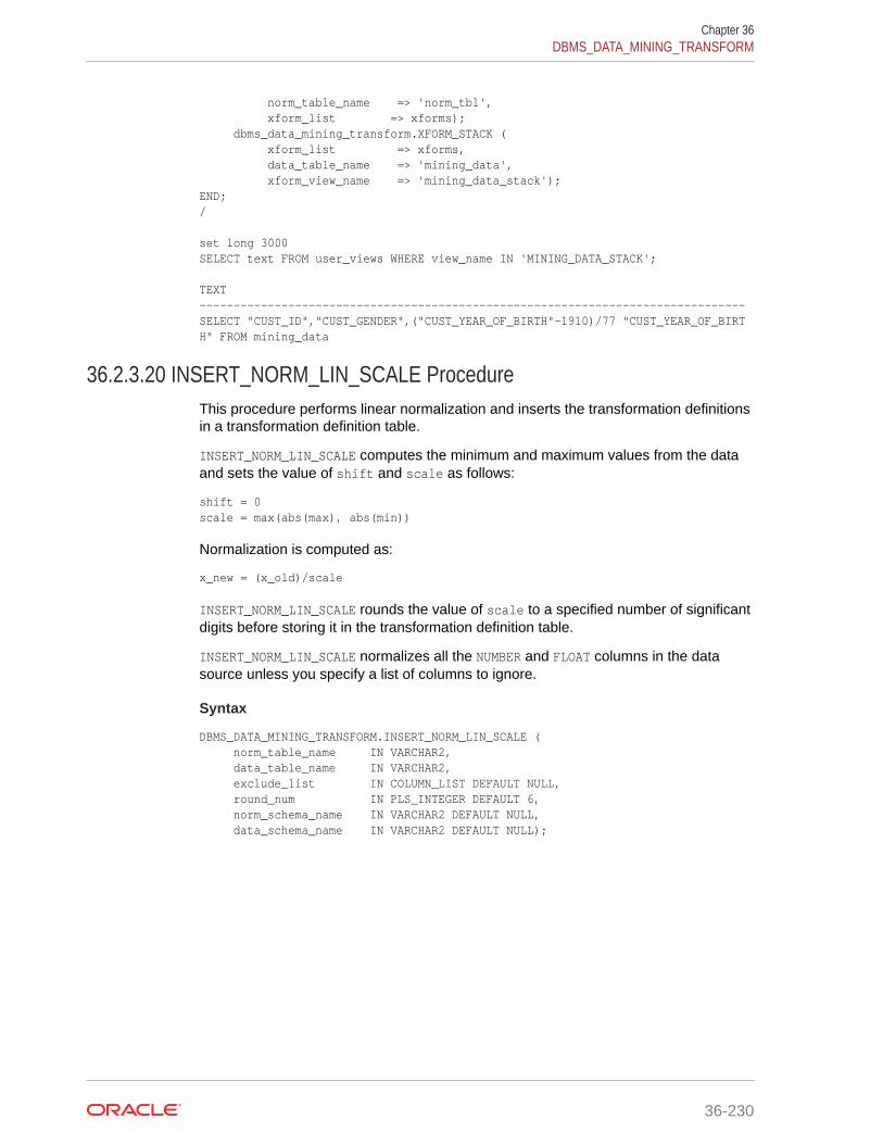
norm_table_name => 'norm_tbl', xform_list => xforms); dbms_data_mining_transform.XFORM_STACK ( xform_list => xforms, data_table_name => 'mining_data', xform_view_name => 'mining_data_stack');END;/ set long 3000SELECT text FROM user_views WHERE view_name IN 'MINING_DATA_STACK'; TEXT--------------------------------------------------------------------------------SELECT "CUST_ID","CUST_GENDER",("CUST_YEAR_OF_BIRTH"-1910)/77 "CUST_YEAR_OF_BIRTH" FROM mining_data
36.2.3.20 INSERT_NORM_LIN_SCALE ProcedureThis procedure performs linear normalization and inserts the transformation definitionsin a transformation definition table.
INSERT_NORM_LIN_SCALE computes the minimum and maximum values from the dataand sets the value of shift and scale as follows:
shift = 0scale = max(abs(max), abs(min))
Normalization is computed as:
x_new = (x_old)/scale
INSERT_NORM_LIN_SCALE rounds the value of scale to a specified number of significantdigits before storing it in the transformation definition table.
INSERT_NORM_LIN_SCALE normalizes all the NUMBER and FLOAT columns in the datasource unless you specify a list of columns to ignore.
Syntax
DBMS_DATA_MINING_TRANSFORM.INSERT_NORM_LIN_SCALE ( norm_table_name IN VARCHAR2, data_table_name IN VARCHAR2, exclude_list IN COLUMN_LIST DEFAULT NULL, round_num IN PLS_INTEGER DEFAULT 6, norm_schema_name IN VARCHAR2 DEFAULT NULL, data_schema_name IN VARCHAR2 DEFAULT NULL);
Chapter 36DBMS_DATA_MINING_TRANSFORM
36-230

Parameters
Table 36-143 INSERT_NORM_LIN_SCALE Procedure Parameters
Parameter Description
norm_table_name Name of the transformation definition table for linearnormalization. You can use the CREATE_NORM_LIN Procedure tocreate the definition table. The following columns are required:
COL VARCHAR2(30) SHIFT NUMBER SCALE NUMBER
CREATE_NORM_LIN creates an additional column, ATT, which maybe used for specifying nested attributes. This column is not usedby INSERT_NORM_LIN_SCALE.
data_table_name Name of the table containing the data to be transformed
exclude_list List of numerical columns to be excluded from normalization.If you do not specify exclude_list, all numerical columns aretransformed.The format of exclude_list is:
dbms_data_mining_transform.COLUMN_LIST('col1','col2', ...'coln')
round_num The number of significant digits to use for scale. The defaultnumber is 6.
norm_schema_name Schema of norm_table_name. If no schema is specified, thecurrent schema is used.
data_schema_name Schema of data_table_name. If no schema is specified, thecurrent schema is used.
Usage Notes
See Oracle Data Mining User's Guide for details about numerical data.
Examples
In this example, INSERT_NORM_LIN_SCALE normalizes the cust_year_of_birthcolumn and inserts the transformation in a transformation definition table. TheSTACK_NORM_LIN Procedure creates a transformation list from the contents of thedefinition table.
The SQL expression that computes the transformation is shown in the viewMINING_DATA_STACK. The view is for display purposes only; it cannot be used to embedthe transformations in a model.
CREATE OR REPLACE VIEW mining_data AS SELECT cust_id, cust_gender, cust_year_of_birth FROM sh.customers;
DESCRIBE mining_data Name Null? Type ---------------------------------- -------- ------------------ CUST_ID NOT NULL NUMBER
Chapter 36DBMS_DATA_MINING_TRANSFORM
36-231

CUST_GENDER NOT NULL CHAR(1) CUST_YEAR_OF_BIRTH NOT NULL NUMBER(4) BEGIN dbms_data_mining_transform.CREATE_NORM_LIN( norm_table_name => 'norm_tbl'); dbms_data_mining_transform.INSERT_NORM_LIN_SCALE( norm_table_name => 'norm_tbl', data_table_name => 'mining_data', exclude_list => dbms_data_mining_transform.COLUMN_LIST( 'cust_id'), round_num => 3); END; / SELECT col, shift, scale FROM norm_tbl; COL SHIFT SCALE-------------------- ----- -----CUST_YEAR_OF_BIRTH 0 1990 DECLARE xforms dbms_data_mining_transform.TRANSFORM_LIST;BEGIN dbms_data_mining_transform.STACK_NORM_LIN ( norm_table_name => 'norm_tbl', xform_list => xforms); dbms_data_mining_transform.XFORM_STACK ( xform_list => xforms, data_table_name => 'mining_data', xform_view_name => 'mining_data_stack');END;/ set long 3000SELECT text FROM user_views WHERE view_name IN 'MINING_DATA_STACK'; TEXT--------------------------------------------------------------------------------SELECT "CUST_ID","CUST_GENDER",("CUST_YEAR_OF_BIRTH"-0)/1990 "CUST_YEAR_OF_BIRTH" FROM mining_data
36.2.3.21 INSERT_NORM_LIN_ZSCORE ProcedureThis procedure performs linear normalization and inserts the transformation definitionsin a transformation definition table.
INSERT_NORM_LIN_ZSCORE computes the mean and the standard deviation from thedata and sets the value of shift and scale as follows:
shift = meanscale = stddev
Normalization is computed as:
x_new = (x_old - shift)/scale
INSERT_NORM_LIN_ZSCORE rounds the value of scale to a specified number ofsignificant digits before storing it in the transformation definition table.
Chapter 36DBMS_DATA_MINING_TRANSFORM
36-232
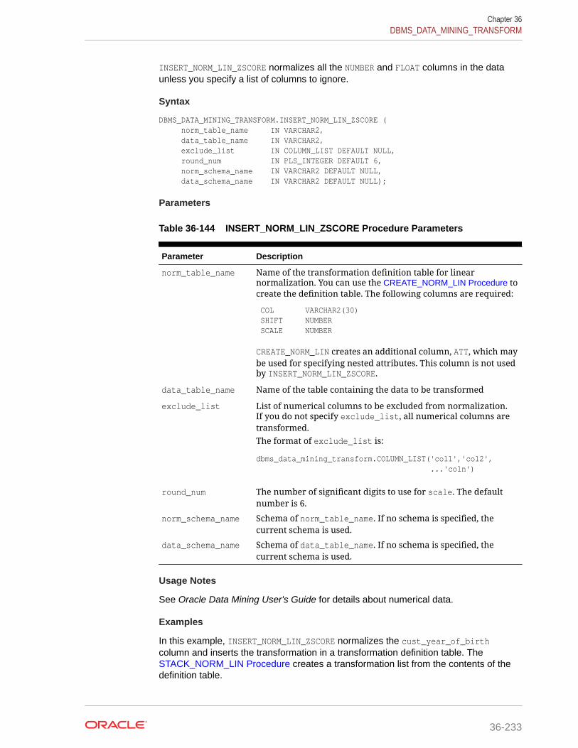
INSERT_NORM_LIN_ZSCORE normalizes all the NUMBER and FLOAT columns in the dataunless you specify a list of columns to ignore.
Syntax
DBMS_DATA_MINING_TRANSFORM.INSERT_NORM_LIN_ZSCORE ( norm_table_name IN VARCHAR2, data_table_name IN VARCHAR2, exclude_list IN COLUMN_LIST DEFAULT NULL, round_num IN PLS_INTEGER DEFAULT 6, norm_schema_name IN VARCHAR2 DEFAULT NULL, data_schema_name IN VARCHAR2 DEFAULT NULL);
Parameters
Table 36-144 INSERT_NORM_LIN_ZSCORE Procedure Parameters
Parameter Description
norm_table_name Name of the transformation definition table for linearnormalization. You can use the CREATE_NORM_LIN Procedure tocreate the definition table. The following columns are required:
COL VARCHAR2(30) SHIFT NUMBER SCALE NUMBER
CREATE_NORM_LIN creates an additional column, ATT, which maybe used for specifying nested attributes. This column is not usedby INSERT_NORM_LIN_ZSCORE.
data_table_name Name of the table containing the data to be transformed
exclude_list List of numerical columns to be excluded from normalization.If you do not specify exclude_list, all numerical columns aretransformed.The format of exclude_list is:
dbms_data_mining_transform.COLUMN_LIST('col1','col2', ...'coln')
round_num The number of significant digits to use for scale. The defaultnumber is 6.
norm_schema_name Schema of norm_table_name. If no schema is specified, thecurrent schema is used.
data_schema_name Schema of data_table_name. If no schema is specified, thecurrent schema is used.
Usage Notes
See Oracle Data Mining User's Guide for details about numerical data.
Examples
In this example, INSERT_NORM_LIN_ZSCORE normalizes the cust_year_of_birthcolumn and inserts the transformation in a transformation definition table. TheSTACK_NORM_LIN Procedure creates a transformation list from the contents of thedefinition table.
Chapter 36DBMS_DATA_MINING_TRANSFORM
36-233
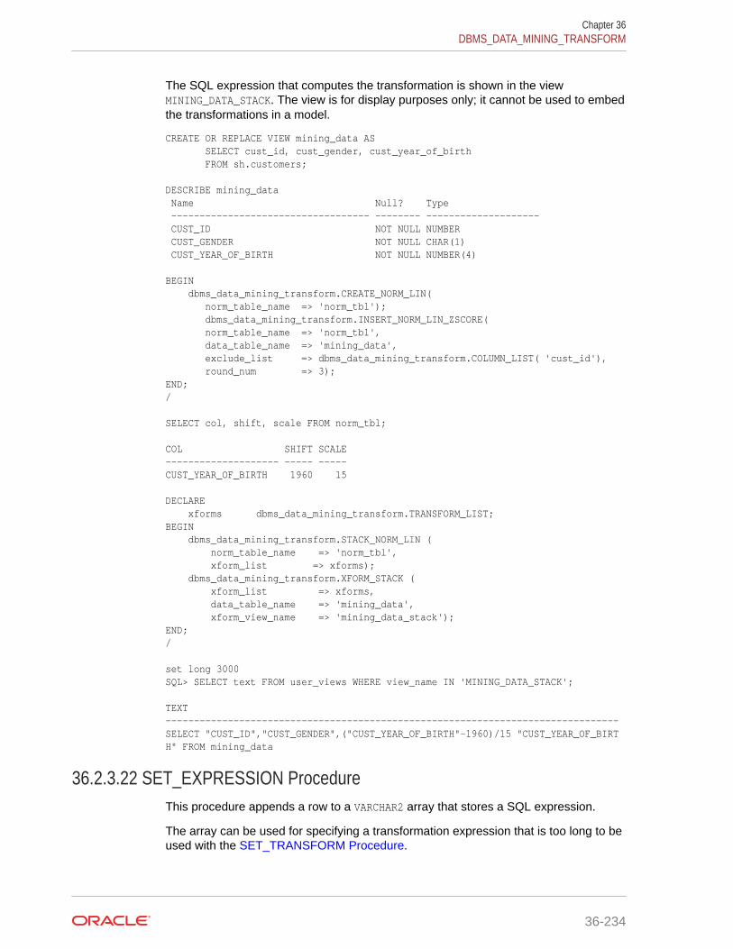
The SQL expression that computes the transformation is shown in the viewMINING_DATA_STACK. The view is for display purposes only; it cannot be used to embedthe transformations in a model.
CREATE OR REPLACE VIEW mining_data AS SELECT cust_id, cust_gender, cust_year_of_birth FROM sh.customers; DESCRIBE mining_data Name Null? Type ----------------------------------- -------- -------------------- CUST_ID NOT NULL NUMBER CUST_GENDER NOT NULL CHAR(1) CUST_YEAR_OF_BIRTH NOT NULL NUMBER(4) BEGIN dbms_data_mining_transform.CREATE_NORM_LIN( norm_table_name => 'norm_tbl'); dbms_data_mining_transform.INSERT_NORM_LIN_ZSCORE( norm_table_name => 'norm_tbl', data_table_name => 'mining_data', exclude_list => dbms_data_mining_transform.COLUMN_LIST( 'cust_id'), round_num => 3);END;/ SELECT col, shift, scale FROM norm_tbl; COL SHIFT SCALE-------------------- ----- -----CUST_YEAR_OF_BIRTH 1960 15 DECLARE xforms dbms_data_mining_transform.TRANSFORM_LIST;BEGIN dbms_data_mining_transform.STACK_NORM_LIN ( norm_table_name => 'norm_tbl', xform_list => xforms); dbms_data_mining_transform.XFORM_STACK ( xform_list => xforms, data_table_name => 'mining_data', xform_view_name => 'mining_data_stack');END;/ set long 3000SQL> SELECT text FROM user_views WHERE view_name IN 'MINING_DATA_STACK'; TEXT--------------------------------------------------------------------------------SELECT "CUST_ID","CUST_GENDER",("CUST_YEAR_OF_BIRTH"-1960)/15 "CUST_YEAR_OF_BIRTH" FROM mining_data
36.2.3.22 SET_EXPRESSION ProcedureThis procedure appends a row to a VARCHAR2 array that stores a SQL expression.
The array can be used for specifying a transformation expression that is too long to beused with the SET_TRANSFORM Procedure.
Chapter 36DBMS_DATA_MINING_TRANSFORM
36-234

The GET_EXPRESSION Function returns a row in the array.
When you use SET_EXPRESSION to build a transformation expression, you must build acorresponding reverse transformation expression, create a transformation record, andadd the transformation record to a transformation list.
Syntax
DBMS_DATA_MINING_TRANSFORM.SET_EXPRESSION ( expression IN OUT NOCOPY EXPRESSION_REC, chunk VARCHAR2 DEFAULT NULL);
Parameters
Table 36-145 SET_EXPRESSION Procedure Parameters
Parameter Description
expression An expression record (EXPRESSION_REC) that specifies a transformationexpression or a reverse transformation expression for an attribute.Each expression record includes a VARCHAR2 array and index fields forspecifying upper and lower boundaries within the array.There are two EXPRESSION_REC fields within a transformation record(TRANSFORM_REC): one for the transformation expression; the other forthe reverse transformation expression.See Table 36-114 for a description of the EXPRESSION_REC type.
chunk A VARCHAR2 chunk (row) to be appended to expression.
Notes
1. You can pass NULL in the chunk argument to SET_EXPRESSION to clear the previouschunk. The default value of chunk is NULL.
2. See "About Transformation Lists".
3. See "Operational Notes".
Examples
In this example, two calls to SET_EXPRESSION construct a transformation expressionand two calls construct the reverse transformation.
Note:
This example is for illustration purposes only. It shows how SET_EXPRESSIONappends the text provided in chunk to the text that already exists inexpression. The SET_EXPRESSION procedure is meant for constructing verylong transformation expressions that cannot be specified in a VARCHAR2argument to SET_TRANSFORM.
Similarly while transformation lists are intended for embedding in a model,the transformation list v_xlst is shown in an external view for illustrationpurposes.
Chapter 36DBMS_DATA_MINING_TRANSFORM
36-235

CREATE OR REPLACE VIEW mining_data AS SELECT cust_id, cust_year_of_birth, cust_postal_code, cust_credit_limit FROM sh.customers; DECLARE v_expr dbms_data_mining_transform.EXPRESSION_REC; v_rexp dbms_data_mining_transform.EXPRESSION_REC; v_xrec dbms_data_mining_transform.TRANSFORM_REC; v_xlst dbms_data_mining_transform.TRANSFORM_LIST := dbms_data_mining_transform.TRANSFORM_LIST(NULL);BEGIN dbms_data_mining_transform.SET_EXPRESSION( EXPRESSION => v_expr, CHUNK => '("CUST_YEAR_OF_BIRTH"-1910)'); dbms_data_mining_transform.SET_EXPRESSION( EXPRESSION => v_expr, CHUNK => '/77'); dbms_data_mining_transform.SET_EXPRESSION( EXPRESSION => v_rexp, CHUNK => '"CUST_YEAR_OF_BIRTH"*77'); dbms_data_mining_transform.SET_EXPRESSION( EXPRESSION => v_rexp, CHUNK => '+1910'); v_xrec := null; v_xrec.attribute_name := 'CUST_YEAR_OF_BIRTH'; v_xrec.expression := v_expr; v_xrec.reverse_expression := v_rexp; v_xlst.TRIM; v_xlst.extend(1); v_xlst(1) := v_xrec; dbms_data_mining_transform.XFORM_STACK ( xform_list => v_xlst, data_table_name => 'mining_data', xform_view_name => 'v_xlst_view'); dbms_output.put_line('===='); FOR i IN 1..v_xlst.count LOOP dbms_output.put_line('ATTR: '||v_xlst(i).attribute_name); dbms_output.put_line('SUBN: '||v_xlst(i).attribute_subname); FOR j IN v_xlst(i).expression.lb..v_xlst(i).expression.ub LOOP dbms_output.put_line('EXPR: '||v_xlst(i).expression.lstmt(j)); END LOOP; FOR j IN v_xlst(i).reverse_expression.lb.. v_xlst(i).reverse_expression.ub LOOP dbms_output.put_line('REXP: '||v_xlst(i).reverse_expression.lstmt(j)); END LOOP; dbms_output.put_line('===='); END LOOP; END;/====ATTR: CUST_YEAR_OF_BIRTHSUBN:EXPR: ("CUST_YEAR_OF_BIRTH"-1910)EXPR: /77REXP: "CUST_YEAR_OF_BIRTH"*77REXP: +1910====
Chapter 36DBMS_DATA_MINING_TRANSFORM
36-236

36.2.3.23 SET_TRANSFORM ProcedureThis procedure appends the transformation instructions for an attribute to atransformation list.
Syntax
DBMS_DATA_MINING_TRANSFORM.SET_TRANSFORM ( xform_list IN OUT NOCOPY TRANSFORM_LIST, attribute_name VARCHAR2, attribute_subname VARCHAR2, expression VARCHAR2, reverse_expression VARCHAR2, attribute_spec VARCHAR2 DEFAULT NULL);
Parameters
Table 36-146 SET_TRANSFORM Procedure Parameters
Parameter Description
xform_list A transformation list. See Table 36-114for a description of theTRANSFORM_LIST object type.
attribute_name Name of the attribute to be transformed
attribute_subname Name of the nested attribute if attribute_name is a nestedcolumn, otherwise NULL.
expression A SQL expression that specifies the transformation of theattribute.
reverse_expression A SQL expression that reverses the transformation forreadability in model details and in the target of a supervisedmodel (if the attribute is a target)
attribute_spec One or more keywords that identify special treatment for theattribute during model build. Values are:• NOPREP — When ADP is on, prevents automatic
transformation of the attribute. If ADP is not on, this valuehas no effect.
• TEXT — Causes the attribute to be treated as unstructuredtext data
• FORCE_IN — Forces the inclusion of the attribute in themodel build. Applies only to GLM models with featureselection enabled (ftr_selection_enable = yes). Featureselection is disabled by default.If the model is not using GLM with feature selection, thisvalue has no effect.See "Specifying Transformation Instructions for anAttribute" in Oracle Data Mining User's Guide for moreinformation about attribute_spec.
Usage Notes
1. See the following relevant sections in "Operational Notes":
• About Transformation Lists
Chapter 36DBMS_DATA_MINING_TRANSFORM
36-237
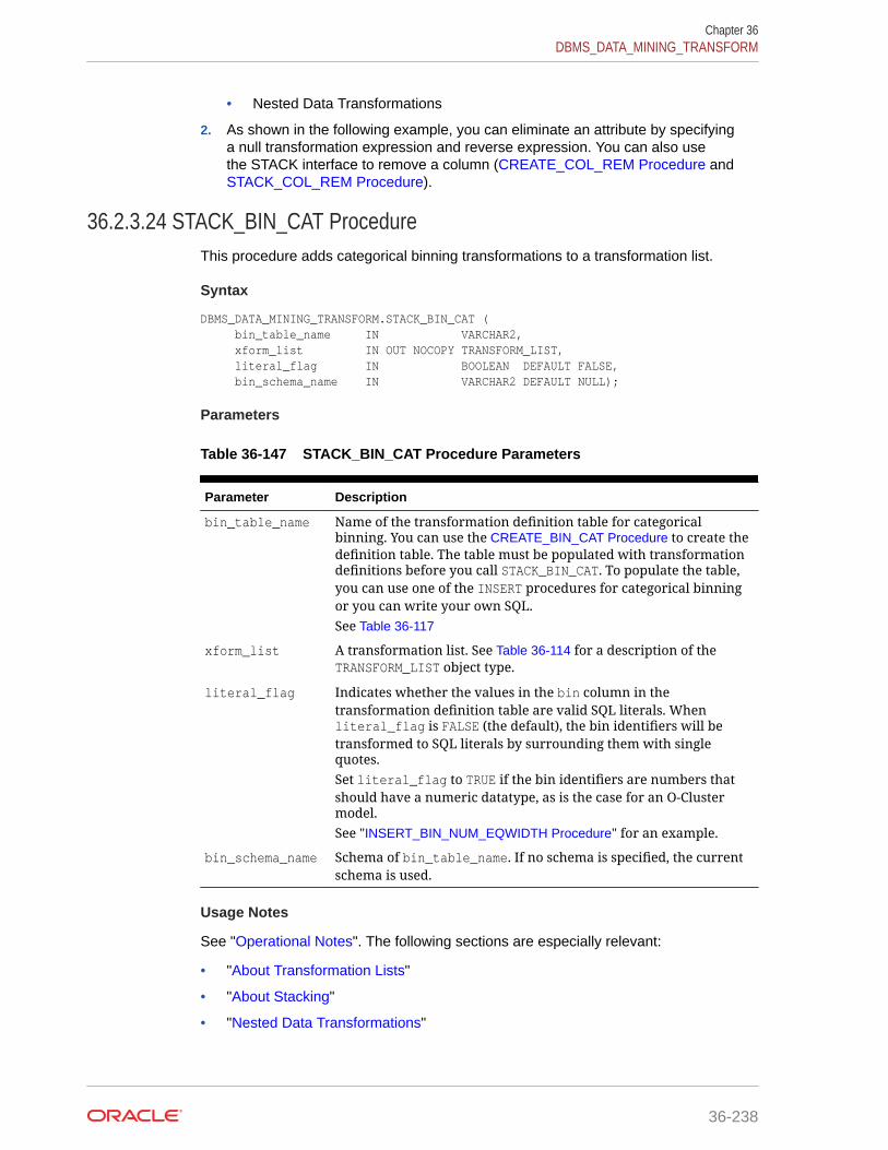
• Nested Data Transformations
2. As shown in the following example, you can eliminate an attribute by specifyinga null transformation expression and reverse expression. You can also usethe STACK interface to remove a column (CREATE_COL_REM Procedure andSTACK_COL_REM Procedure).
36.2.3.24 STACK_BIN_CAT ProcedureThis procedure adds categorical binning transformations to a transformation list.
Syntax
DBMS_DATA_MINING_TRANSFORM.STACK_BIN_CAT ( bin_table_name IN VARCHAR2, xform_list IN OUT NOCOPY TRANSFORM_LIST, literal_flag IN BOOLEAN DEFAULT FALSE, bin_schema_name IN VARCHAR2 DEFAULT NULL);
Parameters
Table 36-147 STACK_BIN_CAT Procedure Parameters
Parameter Description
bin_table_name Name of the transformation definition table for categoricalbinning. You can use the CREATE_BIN_CAT Procedure to create thedefinition table. The table must be populated with transformationdefinitions before you call STACK_BIN_CAT. To populate the table,you can use one of the INSERT procedures for categorical binningor you can write your own SQL.See Table 36-117
xform_list A transformation list. See Table 36-114 for a description of theTRANSFORM_LIST object type.
literal_flag Indicates whether the values in the bin column in thetransformation definition table are valid SQL literals. Whenliteral_flag is FALSE (the default), the bin identifiers will betransformed to SQL literals by surrounding them with singlequotes.Set literal_flag to TRUE if the bin identifiers are numbers thatshould have a numeric datatype, as is the case for an O-Clustermodel.See "INSERT_BIN_NUM_EQWIDTH Procedure" for an example.
bin_schema_name Schema of bin_table_name. If no schema is specified, the currentschema is used.
Usage Notes
See "Operational Notes". The following sections are especially relevant:
• "About Transformation Lists"
• "About Stacking"
• "Nested Data Transformations"
Chapter 36DBMS_DATA_MINING_TRANSFORM
36-238
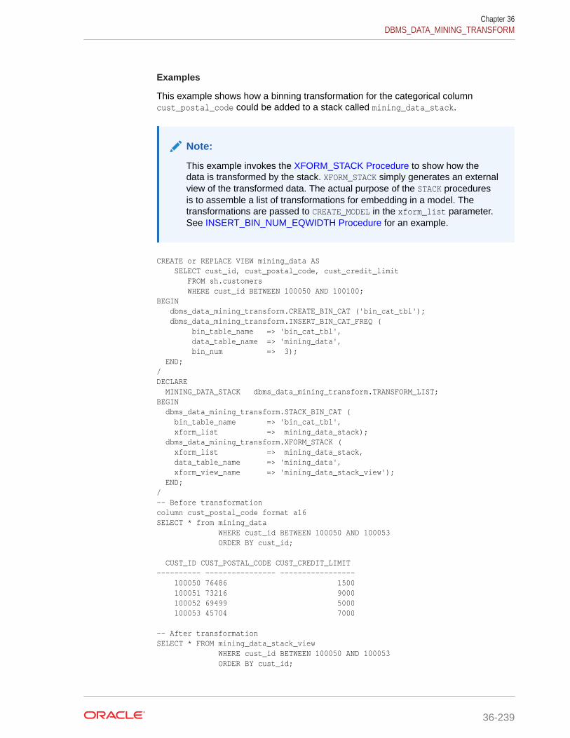
Examples
This example shows how a binning transformation for the categorical columncust_postal_code could be added to a stack called mining_data_stack.
Note:
This example invokes the XFORM_STACK Procedure to show how thedata is transformed by the stack. XFORM_STACK simply generates an externalview of the transformed data. The actual purpose of the STACK proceduresis to assemble a list of transformations for embedding in a model. Thetransformations are passed to CREATE_MODEL in the xform_list parameter.See INSERT_BIN_NUM_EQWIDTH Procedure for an example.
CREATE or REPLACE VIEW mining_data AS SELECT cust_id, cust_postal_code, cust_credit_limit FROM sh.customers WHERE cust_id BETWEEN 100050 AND 100100;BEGIN dbms_data_mining_transform.CREATE_BIN_CAT ('bin_cat_tbl'); dbms_data_mining_transform.INSERT_BIN_CAT_FREQ ( bin_table_name => 'bin_cat_tbl', data_table_name => 'mining_data', bin_num => 3); END;/DECLARE MINING_DATA_STACK dbms_data_mining_transform.TRANSFORM_LIST;BEGIN dbms_data_mining_transform.STACK_BIN_CAT ( bin_table_name => 'bin_cat_tbl', xform_list => mining_data_stack); dbms_data_mining_transform.XFORM_STACK ( xform_list => mining_data_stack, data_table_name => 'mining_data', xform_view_name => 'mining_data_stack_view'); END;/-- Before transformationcolumn cust_postal_code format a16SELECT * from mining_data WHERE cust_id BETWEEN 100050 AND 100053 ORDER BY cust_id;
CUST_ID CUST_POSTAL_CODE CUST_CREDIT_LIMIT---------- ---------------- ----------------- 100050 76486 1500 100051 73216 9000 100052 69499 5000 100053 45704 7000
-- After transformationSELECT * FROM mining_data_stack_view WHERE cust_id BETWEEN 100050 AND 100053 ORDER BY cust_id;
Chapter 36DBMS_DATA_MINING_TRANSFORM
36-239
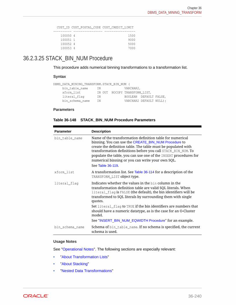
CUST_ID CUST_POSTAL_CODE CUST_CREDIT_LIMIT---------- ---------------- ----------------- 100050 4 1500 100051 1 9000 100052 4 5000 100053 4 7000
36.2.3.25 STACK_BIN_NUM ProcedureThis procedure adds numerical binning transformations to a transformation list.
Syntax
DBMS_DATA_MINING_TRANSFORM.STACK_BIN_NUM ( bin_table_name IN VARCHAR2, xform_list IN OUT NOCOPY TRANSFORM_LIST, literal_flag IN BOOLEAN DEFAULT FALSE, bin_schema_name IN VARCHAR2 DEFAULT NULL);
Parameters
Table 36-148 STACK_BIN_NUM Procedure Parameters
Parameter Description
bin_table_name Name of the transformation definition table for numericalbinning. You can use the CREATE_BIN_NUM Procedure tocreate the definition table. The table must be populated withtransformation definitions before you call STACK_BIN_NUM. Topopulate the table, you can use one of the INSERT procedures fornumerical binning or you can write your own SQL.See Table 36-119.
xform_list A transformation list. See Table 36-114 for a description of theTRANSFORM_LIST object type.
literal_flag Indicates whether the values in the bin column in thetransformation definition table are valid SQL literals. Whenliteral_flag is FALSE (the default), the bin identifiers will betransformed to SQL literals by surrounding them with singlequotes.Set literal_flag to TRUE if the bin identifiers are numbers thatshould have a numeric datatype, as is the case for an O-Clustermodel.See "INSERT_BIN_NUM_EQWIDTH Procedure" for an example.
bin_schema_name Schema of bin_table_name. If no schema is specified, the currentschema is used.
Usage Notes
See "Operational Notes". The following sections are especially relevant:
• "About Transformation Lists"
• "About Stacking"
• "Nested Data Transformations"
Chapter 36DBMS_DATA_MINING_TRANSFORM
36-240

Examples
This example shows how a binning transformation for the numerical columncust_credit_limit could be added to a stack called mining_data_stack.
Note:
This example invokes the XFORM_STACK Procedure to show how thedata is transformed by the stack. XFORM_STACK simply generates an externalview of the transformed data. The actual purpose of the STACK proceduresis to assemble a list of transformations for embedding in a model. Thetransformations are passed to CREATE_MODEL in the xform_list parameter.See INSERT_BIN_NUM_EQWIDTH Procedure for an example.
CREATE OR REPLACE VIEW mining_data AS SELECT cust_id, cust_postal_code, cust_credit_limit FROM sh.customers WHERE cust_id BETWEEN 100050 and 100100;BEGIN dbms_data_mining_transform.create_bin_num ('bin_num_tbl'); dbms_data_mining_transform.insert_bin_num_qtile ( bin_table_name => 'bin_num_tbl', data_table_name => 'mining_data', bin_num => 5, exclude_list => dbms_data_mining_transform.COLUMN_LIST('cust_id'));END;/DECLARE MINING_DATA_STACK dbms_data_mining_transform.TRANSFORM_LIST;BEGIN dbms_data_mining_transform.STACK_BIN_CAT ( bin_table_name => 'bin_num_tbl', xform_list => mining_data_stack); dbms_data_mining_transform.XFORM_STACK ( xform_list => mining_data_stack, data_table_name => 'mining_data', xform_view_name => 'mining_data_stack_view');END;/-- Before transformationSELECT cust_id, cust_postal_code, ROUND(cust_credit_limit) FROM mining_data WHERE cust_id BETWEEN 100050 AND 100055 ORDER BY cust_id;CUST_ID CUST_POSTAL_CODE ROUND(CUST_CREDIT_LIMIT)------- ----------------- -------------------------100050 76486 1500100051 73216 9000 100052 69499 5000100053 45704 7000100055 74673 11000100055 74673 11000
-- After transformationSELECT cust_id, cust_postal_code, ROUND(cust_credit_limit) FROM mining_data_stack_view WHERE cust_id BETWEEN 100050 AND 100055
Chapter 36DBMS_DATA_MINING_TRANSFORM
36-241

ORDER BY cust_id;CUST_ID CUST_POSTAL_CODE ROUND(CUST_CREDIT_LIMITT)------- ---------------- -------------------------100050 76486 100051 73216 2100052 69499 1100053 45704 100054 88021 3100055 74673 3
36.2.3.26 STACK_CLIP ProcedureThis procedure adds clipping transformations to a transformation list.
Syntax
DBMS_DATA_MINING_TRANSFORM.STACK_CLIP ( clip_table_name IN VARCHAR2, xform_list IN OUT NOCOPY TRANSFORM_LIST, clip_schema_name IN VARCHAR2 DEFAULT NULL);
Parameters
Table 36-149 STACK_CLIP Procedure Parameters
Parameter Description
clip_table_name Name of the transformation definition table for clipping.Youcan use the CREATE_CLIP Procedure to create the definitiontable. The table must be populated with transformationdefinitions before you call STACK_CLIP. To populate thetable, you can use one of the INSERT procedures for clippingor you can write your own SQL.See Table 36-121
xform_list A transformation list. See Table 36-114 for a description ofthe TRANSFORM_LIST object type.
clip_schema_name Schema of clip_table_name. If no schema is specified, thecurrent schema is used.
Usage Notes
See DBMS_DATA_MINING_TRANSFORM Operational Notes. The following sectionsare especially relevant:
• “About Transformation Lists”
• “About Stacking”
• “Nested Data Transformations”
Examples
This example shows how a clipping transformation for the numerical columncust_credit_limit could be added to a stack called mining_data_stack.
Chapter 36DBMS_DATA_MINING_TRANSFORM
36-242
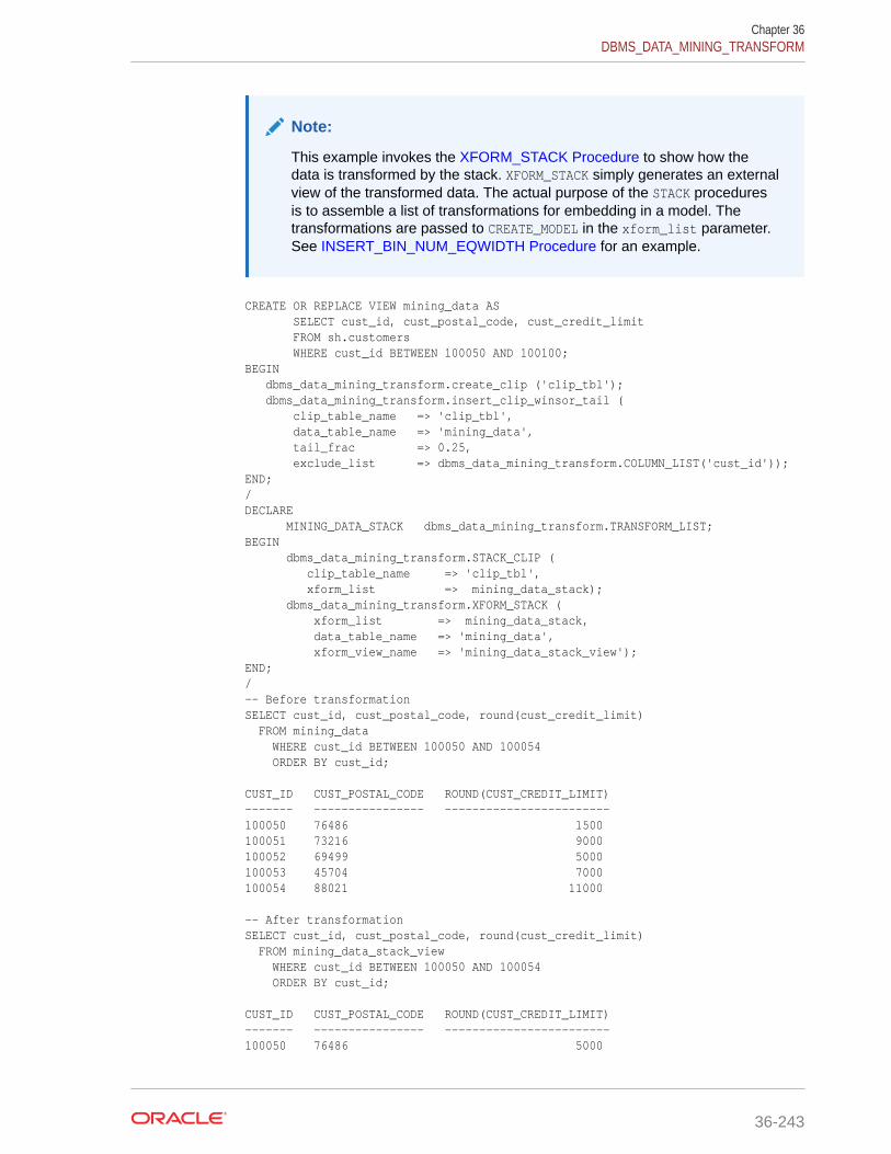
Note:
This example invokes the XFORM_STACK Procedure to show how thedata is transformed by the stack. XFORM_STACK simply generates an externalview of the transformed data. The actual purpose of the STACK proceduresis to assemble a list of transformations for embedding in a model. Thetransformations are passed to CREATE_MODEL in the xform_list parameter.See INSERT_BIN_NUM_EQWIDTH Procedure for an example.
CREATE OR REPLACE VIEW mining_data AS SELECT cust_id, cust_postal_code, cust_credit_limit FROM sh.customers WHERE cust_id BETWEEN 100050 AND 100100;BEGIN dbms_data_mining_transform.create_clip ('clip_tbl'); dbms_data_mining_transform.insert_clip_winsor_tail ( clip_table_name => 'clip_tbl', data_table_name => 'mining_data', tail_frac => 0.25, exclude_list => dbms_data_mining_transform.COLUMN_LIST('cust_id'));END;/DECLARE MINING_DATA_STACK dbms_data_mining_transform.TRANSFORM_LIST;BEGIN dbms_data_mining_transform.STACK_CLIP ( clip_table_name => 'clip_tbl', xform_list => mining_data_stack); dbms_data_mining_transform.XFORM_STACK ( xform_list => mining_data_stack, data_table_name => 'mining_data', xform_view_name => 'mining_data_stack_view');END;/-- Before transformationSELECT cust_id, cust_postal_code, round(cust_credit_limit) FROM mining_data WHERE cust_id BETWEEN 100050 AND 100054 ORDER BY cust_id; CUST_ID CUST_POSTAL_CODE ROUND(CUST_CREDIT_LIMIT)------- ---------------- ------------------------ 100050 76486 1500 100051 73216 9000 100052 69499 5000 100053 45704 7000 100054 88021 11000 -- After transformationSELECT cust_id, cust_postal_code, round(cust_credit_limit) FROM mining_data_stack_view WHERE cust_id BETWEEN 100050 AND 100054 ORDER BY cust_id; CUST_ID CUST_POSTAL_CODE ROUND(CUST_CREDIT_LIMIT)------- ---------------- ------------------------100050 76486 5000
Chapter 36DBMS_DATA_MINING_TRANSFORM
36-243
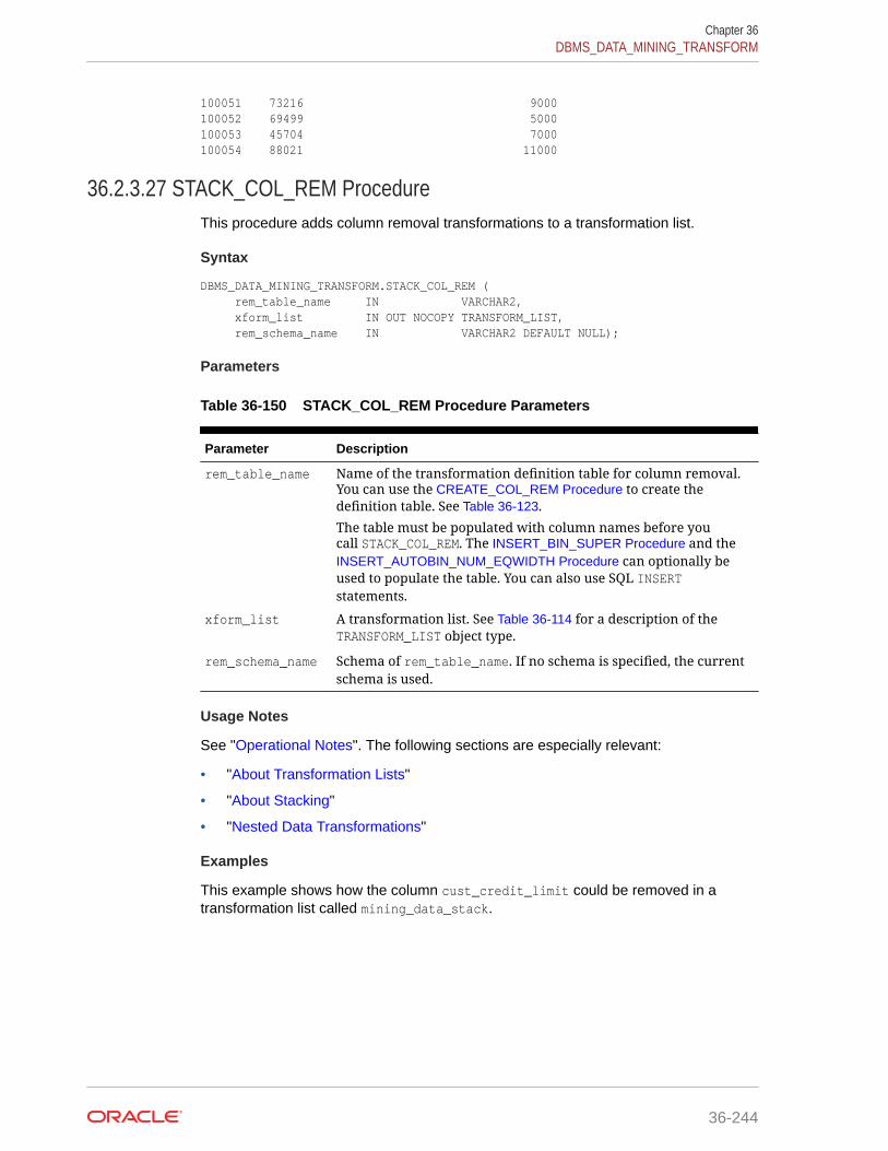
100051 73216 9000100052 69499 5000100053 45704 7000100054 88021 11000
36.2.3.27 STACK_COL_REM ProcedureThis procedure adds column removal transformations to a transformation list.
Syntax
DBMS_DATA_MINING_TRANSFORM.STACK_COL_REM ( rem_table_name IN VARCHAR2, xform_list IN OUT NOCOPY TRANSFORM_LIST, rem_schema_name IN VARCHAR2 DEFAULT NULL);
Parameters
Table 36-150 STACK_COL_REM Procedure Parameters
Parameter Description
rem_table_name Name of the transformation definition table for column removal.You can use the CREATE_COL_REM Procedure to create thedefinition table. See Table 36-123.
The table must be populated with column names before youcall STACK_COL_REM. The INSERT_BIN_SUPER Procedure and theINSERT_AUTOBIN_NUM_EQWIDTH Procedure can optionally beused to populate the table. You can also use SQL INSERTstatements.
xform_list A transformation list. See Table 36-114 for a description of theTRANSFORM_LIST object type.
rem_schema_name Schema of rem_table_name. If no schema is specified, the currentschema is used.
Usage Notes
See "Operational Notes". The following sections are especially relevant:
• "About Transformation Lists"
• "About Stacking"
• "Nested Data Transformations"
Examples
This example shows how the column cust_credit_limit could be removed in atransformation list called mining_data_stack.
Chapter 36DBMS_DATA_MINING_TRANSFORM
36-244

Note:
This example invokes the XFORM_STACK Procedure to show how thedata is transformed by the stack. XFORM_STACK simply generates an externalview of the transformed data. The actual purpose of the STACK proceduresis to assemble a list of transformations for embedding in a model. Thetransformations are passed to CREATE_MODEL in the xform_list parameter.See INSERT_BIN_NUM_EQWIDTH Procedure for an example.
CREATE OR REPLACE VIEW mining_data AS SELECT cust_id, country_id, cust_postal_code, cust_credit_limit FROM sh.customers; BEGIN dbms_data_mining_transform.create_col_rem ('rem_tbl');END;/
INSERT into rem_tbl VALUES (upper('cust_postal_code'), null); DECLARE MINING_DATA_STACK dbms_data_mining_transform.TRANSFORM_LIST;BEGIN dbms_data_mining_transform.stack_col_rem ( rem_table_name => 'rem_tbl', xform_list => mining_data_stack); dbms_data_mining_transform.XFORM_STACK ( xform_list => mining_data_stack, data_table_name => 'mining_data', xform_view_name => 'mining_data_stack_view');END;/ SELECT * FROM mining_data WHERE cust_id BETWEEN 100050 AND 100051 ORDER BY cust_id; CUST_ID COUNTRY_ID CUST_POSTAL_CODE CUST_CREDIT_LIMIT------- ---------- ---------------- -----------------100050 52773 76486 1500100051 52790 73216 9000 SELECT * FROM mining_data_stack_view WHERE cust_id BETWEEN 100050 AND 100051 ORDER BY cust_id; CUST_ID COUNTRY_ID CUST_CREDIT_LIMIT------- ---------- -----------------100050 52773 1500100051 52790 9000
Chapter 36DBMS_DATA_MINING_TRANSFORM
36-245

36.2.3.28 STACK_MISS_CAT ProcedureThis procedure adds categorical missing value transformations to a transformation list.
Syntax
DBMS_DATA_MINING_TRANSFORM.STACK_MISS_CAT ( miss_table_name IN VARCHAR2, xform_list IN OUT NOCOPY TRANSFORM_LIST, miss_schema_name IN VARCHAR2 DEFAULT NULL);
Parameters
Table 36-151 STACK_MISS_CAT Procedure Parameters
Parameter Description
miss_table_name Name of the transformation definition table for categoricalmissing value treatment. You can use the CREATE_MISS_CATProcedure to create the definition table. The table must bepopulated with transformation definitions before you callSTACK_MISS_CAT. To populate the table, you can use theINSERT_MISS_CAT_MODE Procedure or you can write your ownSQL.See Table 36-125.
xform_list A transformation list. See Table 36-114 for a description of theTRANSFORM_LIST object type.
miss_schema_name Schema of miss_table_name. If no schema is specified, thecurrent schema is used.
Usage Notes
See "Operational Notes". The following sections are especially relevant:
• "About Transformation Lists"
• "About Stacking"
• "Nested Data Transformations"
Examples
This example shows how the missing values in the column cust_marital_statuscould be replaced with the mode in a transformation list called mining_data_stack.
Note:
This example invokes the XFORM_STACK Procedure to show how thedata is transformed by the stack. XFORM_STACK simply generates an externalview of the transformed data. The actual purpose of the STACK proceduresis to assemble a list of transformations for embedding in a model. Thetransformations are passed to CREATE_MODEL in the xform_list parameter.See INSERT_BIN_NUM_EQWIDTH Procedure for an example.
Chapter 36DBMS_DATA_MINING_TRANSFORM
36-246
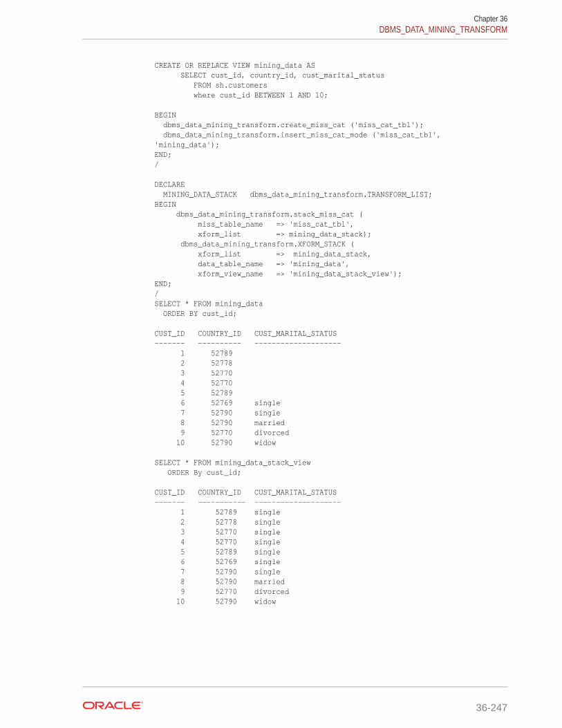
CREATE OR REPLACE VIEW mining_data AS SELECT cust_id, country_id, cust_marital_status FROM sh.customers where cust_id BETWEEN 1 AND 10; BEGIN dbms_data_mining_transform.create_miss_cat ('miss_cat_tbl'); dbms_data_mining_transform.insert_miss_cat_mode ('miss_cat_tbl', 'mining_data');END;/ DECLARE MINING_DATA_STACK dbms_data_mining_transform.TRANSFORM_LIST;BEGIN dbms_data_mining_transform.stack_miss_cat ( miss_table_name => 'miss_cat_tbl', xform_list => mining_data_stack); dbms_data_mining_transform.XFORM_STACK ( xform_list => mining_data_stack, data_table_name => 'mining_data', xform_view_name => 'mining_data_stack_view');END;/SELECT * FROM mining_data ORDER BY cust_id; CUST_ID COUNTRY_ID CUST_MARITAL_STATUS------- ---------- -------------------- 1 52789 2 52778 3 52770 4 52770 5 52789 6 52769 single 7 52790 single 8 52790 married 9 52770 divorced 10 52790 widow SELECT * FROM mining_data_stack_view ORDER By cust_id; CUST_ID COUNTRY_ID CUST_MARITAL_STATUS------- ----------- -------------------- 1 52789 single 2 52778 single 3 52770 single 4 52770 single 5 52789 single 6 52769 single 7 52790 single 8 52790 married 9 52770 divorced 10 52790 widow
Chapter 36DBMS_DATA_MINING_TRANSFORM
36-247
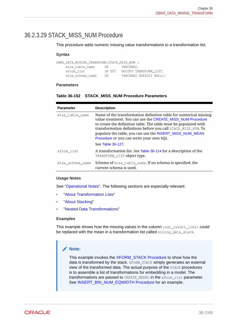
36.2.3.29 STACK_MISS_NUM ProcedureThis procedure adds numeric missing value transformations to a transformation list.
Syntax
DBMS_DATA_MINING_TRANSFORM.STACK_MISS_NUM ( miss_table_name IN VARCHAR2, xform_list IN OUT NOCOPY TRANSFORM_LIST, miss_schema_name IN VARCHAR2 DEFAULT NULL);
Parameters
Table 36-152 STACK_MISS_NUM Procedure Parameters
Parameter Description
miss_table_name Name of the transformation definition table for numerical missingvalue treatment. You can use the CREATE_MISS_NUM Procedureto create the definition table. The table must be populated withtransformation definitions before you call STACK_MISS_NUM. Topopulate the table, you can use the INSERT_MISS_NUM_MEANProcedure or you can write your own SQL.
See Table 36-127.
xform_list A transformation list. See Table 36-114 for a description of theTRANSFORM_LIST object type.
miss_schema_name Schema of miss_table_name. If no schema is specified, thecurrent schema is used.
Usage Notes
See "Operational Notes". The following sections are especially relevant:
• "About Transformation Lists"
• "About Stacking"
• "Nested Data Transformations"
Examples
This example shows how the missing values in the column cust_credit_limit couldbe replaced with the mean in a transformation list called mining_data_stack.
Note:
This example invokes the XFORM_STACK Procedure to show how thedata is transformed by the stack. XFORM_STACK simply generates an externalview of the transformed data. The actual purpose of the STACK proceduresis to assemble a list of transformations for embedding in a model. Thetransformations are passed to CREATE_MODEL in the xform_list parameter.See INSERT_BIN_NUM_EQWIDTH Procedure for an example.
Chapter 36DBMS_DATA_MINING_TRANSFORM
36-248

describe mining_data Name Null? Type ----------------------------------------------------- -------- ----- CUST_ID NOT NULL NUMBER CUST_CREDIT_LIMIT NUMBER
BEGIN dbms_data_mining_transform.create_miss_num ('miss_num_tbl'); dbms_data_mining_transform.insert_miss_num_mean ('miss_num_tbl','mining_data');END;/SELECT * FROM miss_num_tbl; COL ATT VAL-------------------- ----- ------CUST_ID 5.5CUST_CREDIT_LIMIT 185.71 DECLARE MINING_DATA_STACK dbms_data_mining_transform.TRANSFORM_LIST; BEGIN dbms_data_mining_transform.STACK_MISS_NUM ( miss_table_name => 'miss_num_tbl', xform_list => mining_data_stack); dbms_data_mining_transform.XFORM_STACK ( xform_list => mining_data_stack, data_table_name => 'mining_data', xform_view_name => 'mining_data_stack_view');END;/-- Before transformationSELECT * FROM mining_data ORDER BY cust_id;CUST_ID CUST_CREDIT_LIMIT------- ----------------- 1 100 2 3 200 4 5 150 6 400 7 150 8 9 100 10 200 -- After transformationSELECT * FROM mining_data_stack_view ORDER BY cust_id;CUST_ID CUST_CREDIT_LIMIT------- ----------------- 1 100 2 185.71 3 200 4 185.71 5 150 6 400 7 150 8 185.71
Chapter 36DBMS_DATA_MINING_TRANSFORM
36-249

9 100 10 200
36.2.3.30 STACK_NORM_LIN ProcedureThis procedure adds linear normalization transformations to a transformation list.
Syntax
DBMS_DATA_MINING_TRANSFORM.STACK_NORM_LIN ( norm_table_name IN VARCHAR2, xform_list IN OUT NOCOPY TRANSFORM_LIST, norm_schema_name IN VARCHAR2 DEFAULT NULL);
Parameters
Table 36-153 STACK_NORM_LIN Procedure Parameters
Parameter Description
norm_table_name Name of the transformation definition table for linearnormalization. You can use the CREATE_NORM_LIN Procedure tocreate the definition table. The table must be populated withtransformation definitions before you call STACK_NORM_LIN.Topopulate the table, you can use one of the INSERT procedures fornormalization or you can write your own SQL.See Table 36-129.
xform_list A transformation list. See Table 36-114 for a description of theTRANSFORM_LIST object type.
norm_schema_name Schema of norm_table_name. If no schema is specified, thecurrent schema is used.
Usage Notes
See "Operational Notes". The following sections are especially relevant:
• "About Transformation Lists"
• "About Stacking"
• "Nested Data Transformations"
Examples
This example shows how the column cust_credit_limit could be normalized in atransformation list called mining_data_stack.
Chapter 36DBMS_DATA_MINING_TRANSFORM
36-250

Note:
This example invokes the XFORM_STACK Procedure to show how thedata is transformed by the stack. XFORM_STACK simply generates an externalview of the transformed data. The actual purpose of the STACK proceduresis to assemble a list of transformations for embedding in a model. Thetransformations are passed to CREATE_MODEL in the xform_list parameter.See INSERT_BIN_NUM_EQWIDTH Procedure for an example.
CREATE OR REPLACE VIEW mining_data AS SELECT cust_id, country_id, cust_postal_code, cust_credit_limit FROM sh.customers;BEGIN dbms_data_mining_transform.create_norm_lin ('norm_lin_tbl'); dbms_data_mining_transform.insert_norm_lin_minmax ( norm_table_name => 'norm_lin_tbl', data_table_name => 'mining_data', exclude_list => dbms_data_mining_transform.COLUMN_LIST('cust_id', 'country_id'));END;/SELECT * FROM norm_lin_tbl;COL ATT SHIFT SCALE-------------------- ----- ------ ------CUST_CREDIT_LIMIT 1500 13500
DECLARE MINING_DATA_STACK dbms_data_mining_transform.TRANSFORM_LIST;BEGIN dbms_data_mining_transform.stack_norm_lin ( norm_table_name => 'norm_lin_tbl', xform_list => mining_data_stack); dbms_data_mining_transform.XFORM_STACK ( xform_list => mining_data_stack, data_table_name => 'mining_data', xform_view_name => 'mining_data_stack_view');END;/SELECT * FROM mining_data WHERE cust_id between 1 and 10 ORDER BY cust_id;CUST_ID COUNTRY_ID CUST_POSTAL_CODE CUST_CREDIT_LIMIT------- ---------- -------------------- ----------------- 1 52789 30828 9000 2 52778 86319 10000 3 52770 88666 1500 4 52770 87551 1500 5 52789 59200 1500 6 52769 77287 1500 7 52790 38763 1500 8 52790 58488 3000 9 52770 63033 3000 10 52790 52602 3000 SELECT * FROM mining_data_stack_view WHERE cust_id between 1 and 10 ORDER BY cust_id;
Chapter 36DBMS_DATA_MINING_TRANSFORM
36-251

CUST_ID COUNTRY_ID CUST_POSTAL_CODE CUST_CREDIT_LIMIT------- ---------- -------------------- ----------------- 1 52789 30828 .55556 2 52778 86319 .62963 3 52770 88666 0 4 52770 87551 0 5 52789 59200 0 6 52769 77287 0 7 52790 38763 0 8 52790 58488 .11111 9 52770 63033 .11111 10 52790 52602 .11111
36.2.3.31 XFORM_BIN_CAT ProcedureThis procedure creates a view that implements the categorical binning transformationsspecified in a definition table. Only the columns that are specified in the definition tableare transformed; the remaining columns from the data table are present in the view,but they are not changed.
Syntax
DBMS_DATA_MINING_TRANSFORM.XFORM_BIN_CAT ( bin_table_name IN VARCHAR2, data_table_name IN VARCHAR2, xform_view_name IN VARCHAR2, literal_flag IN BOOLEAN DEFAULT FALSE, bin_schema_name IN VARCHAR2 DEFAULT NULL, data_schema_name IN VARCHAR2 DEFAULT NULL, xform_schema_name IN VARCHAR2 DEFAULT NULL);
Parameters
Table 36-154 XFORM_BIN_CAT Procedure Parameters
Parameter Description
bin_table_name Name of the transformation definition table for categoricalbinning. You can use the CREATE_BIN_CAT Procedure tocreate the definition table. The table must be populated withtransformation definitions before you call XFORM_BIN_CAT. Topopulate the table, you can use one of the INSERT procedures forcategorical binning or you can write your own SQL.See Table 36-117.
data_table_name Name of the table containing the data to be transformed.
xform_view_name Name of the view to be created. The view presents columnsin data_table_name with the transformations specified inbin_table_name.
Chapter 36DBMS_DATA_MINING_TRANSFORM
36-252
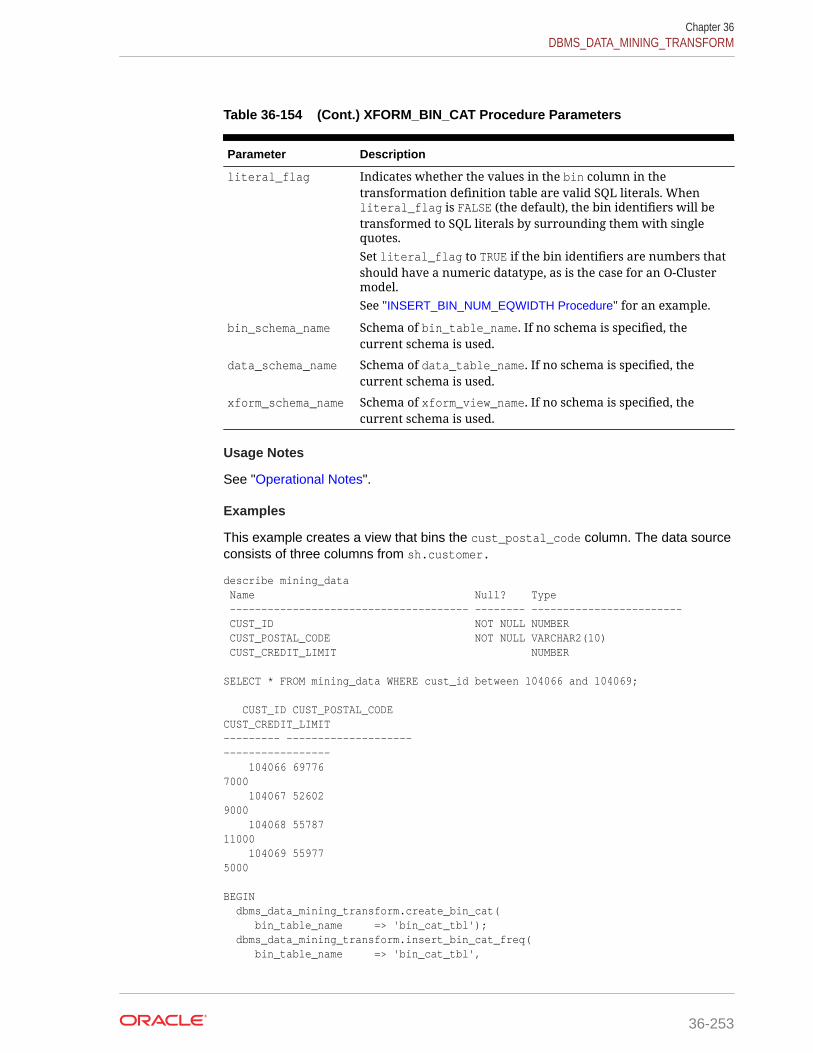
Table 36-154 (Cont.) XFORM_BIN_CAT Procedure Parameters
Parameter Description
literal_flag Indicates whether the values in the bin column in thetransformation definition table are valid SQL literals. Whenliteral_flag is FALSE (the default), the bin identifiers will betransformed to SQL literals by surrounding them with singlequotes.Set literal_flag to TRUE if the bin identifiers are numbers thatshould have a numeric datatype, as is the case for an O-Clustermodel.See "INSERT_BIN_NUM_EQWIDTH Procedure" for an example.
bin_schema_name Schema of bin_table_name. If no schema is specified, thecurrent schema is used.
data_schema_name Schema of data_table_name. If no schema is specified, thecurrent schema is used.
xform_schema_name Schema of xform_view_name. If no schema is specified, thecurrent schema is used.
Usage Notes
See "Operational Notes".
Examples
This example creates a view that bins the cust_postal_code column. The data sourceconsists of three columns from sh.customer.
describe mining_data Name Null? Type -------------------------------------- -------- ------------------------ CUST_ID NOT NULL NUMBER CUST_POSTAL_CODE NOT NULL VARCHAR2(10) CUST_CREDIT_LIMIT NUMBER SELECT * FROM mining_data WHERE cust_id between 104066 and 104069; CUST_ID CUST_POSTAL_CODE CUST_CREDIT_LIMIT --------- -------------------- ----------------- 104066 69776 7000 104067 52602 9000 104068 55787 11000 104069 55977 5000 BEGIN dbms_data_mining_transform.create_bin_cat( bin_table_name => 'bin_cat_tbl'); dbms_data_mining_transform.insert_bin_cat_freq( bin_table_name => 'bin_cat_tbl',
Chapter 36DBMS_DATA_MINING_TRANSFORM
36-253
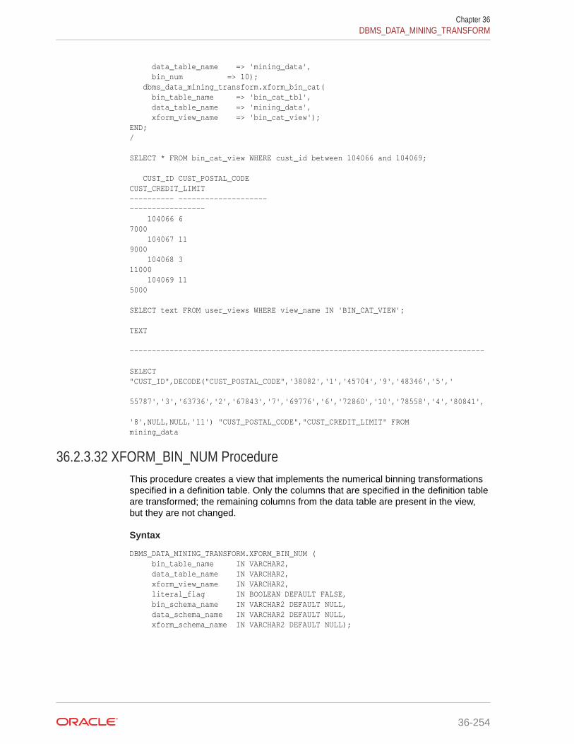
data_table_name => 'mining_data', bin_num => 10); dbms_data_mining_transform.xform_bin_cat( bin_table_name => 'bin_cat_tbl', data_table_name => 'mining_data', xform_view_name => 'bin_cat_view');END;/ SELECT * FROM bin_cat_view WHERE cust_id between 104066 and 104069; CUST_ID CUST_POSTAL_CODE CUST_CREDIT_LIMIT ---------- -------------------- ----------------- 104066 6 7000 104067 11 9000 104068 3 11000 104069 11 5000 SELECT text FROM user_views WHERE view_name IN 'BIN_CAT_VIEW'; TEXT -------------------------------------------------------------------------------- SELECT "CUST_ID",DECODE("CUST_POSTAL_CODE",'38082','1','45704','9','48346','5',' 55787','3','63736','2','67843','7','69776','6','72860','10','78558','4','80841', '8',NULL,NULL,'11') "CUST_POSTAL_CODE","CUST_CREDIT_LIMIT" FROM mining_data
36.2.3.32 XFORM_BIN_NUM ProcedureThis procedure creates a view that implements the numerical binning transformationsspecified in a definition table. Only the columns that are specified in the definition tableare transformed; the remaining columns from the data table are present in the view,but they are not changed.
Syntax
DBMS_DATA_MINING_TRANSFORM.XFORM_BIN_NUM ( bin_table_name IN VARCHAR2, data_table_name IN VARCHAR2, xform_view_name IN VARCHAR2, literal_flag IN BOOLEAN DEFAULT FALSE, bin_schema_name IN VARCHAR2 DEFAULT NULL, data_schema_name IN VARCHAR2 DEFAULT NULL, xform_schema_name IN VARCHAR2 DEFAULT NULL);
Chapter 36DBMS_DATA_MINING_TRANSFORM
36-254

Parameters
Table 36-155 XFORM_BIN_NUM Procedure Parameters
Parameter Description
bin_table_name Name of the transformation definition table for numericalbinning. You can use the CREATE_BIN_NUM Procedure tocreate the definition table. The table must be populated withtransformation definitions before you call XFORM_BIN_NUM. Topopulate the table, you can use one of the INSERT procedures fornumerical binning or you can write your own SQL.See "Table 36-119".
data_table_name Name of the table containing the data to be transformed
xform_view_name Name of the view to be created. The view presents columnsin data_table_name with the transformations specified inbin_table_name.
literal_flag Indicates whether the values in the bin column in thetransformation definition table are valid SQL literals. Whenliteral_flag is FALSE (the default), the bin identifiers will betransformed to SQL literals by surrounding them with singlequotes.Set literal_flag to TRUE if the bin identifiers are numbers thatshould have a numeric datatype, as is the case for an O-Clustermodel.See "INSERT_BIN_NUM_EQWIDTH Procedure" for an example.
bin_schema_name Schema of bin_table_name. If no schema is specified, thecurrent schema is used.
data_schema_name Schema of data_table_name. If no schema is specified, thecurrent schema is used.
xform_schema_name Schema of xform_view_name. If no schema is specified, thecurrent schema is used.
Usage Notes
See "Operational Notes".
Examples
This example creates a view that bins the cust_credit_limit column. The datasource consists of three columns from sh.customer.
describe mining_data Name Null? Type -------------------------------------- -------- ------------------------ CUST_ID NOT NULL NUMBER CUST_POSTAL_CODE NOT NULL VARCHAR2(10) CUST_CREDIT_LIMIT NUMBER column cust_credit_limit offSELECT * FROM mining_data WHERE cust_id between 104066 and 104069; CUST_ID CUST_POSTAL_CODE CUST_CREDIT_LIMIT
Chapter 36DBMS_DATA_MINING_TRANSFORM
36-255

--------- ------------------ -------------------- 104066 69776 7000 104067 52602 9000 104068 55787 11000 104069 55977 5000 BEGIN dbms_data_mining_transform.create_bin_num( bin_table_name => 'bin_num_tbl'); dbms_data_mining_transform.insert_autobin_num_eqwidth( bin_table_name => 'bin_num_tbl', data_table_name => 'mining_data', bin_num => 5, max_bin_num => 10, exclude_list => dbms_data_mining_transform.COLUMN_LIST('cust_id')); dbms_data_mining_transform.xform_bin_num( bin_table_name => 'bin_num_tbl', data_table_name => 'mining_data', xform_view_name => 'mining_data_view');END;/describe mining_data_view Name Null? Type ------------------------------------ -------- ------------------------ CUST_ID NOT NULL NUMBER CUST_POSTAL_CODE NOT NULL VARCHAR2(10) CUST_CREDIT_LIMIT VARCHAR2(2) col cust_credit_limit oncol cust_credit_limit format a25SELECT * FROM mining_data_view WHERE cust_id between 104066 and 104069; CUST_ID CUST_POSTAL_CODE CUST_CREDIT_LIMIT ---------- -------------------- ------------------------- 104066 69776 5 104067 52602 6 104068 55787 8 104069 55977 3 set long 2000SELECT text FROM user_views WHERE view_name IN 'MINING_DATA_VIEW'; TEXT -------------------------------------------------------------------------------- SELECT "CUST_ID","CUST_POSTAL_CODE",CASE WHEN "CUST_CREDIT_LIMIT"<1500 THEN NULL WHEN "CUST_CREDIT_LIMIT"<=2850 THEN '1' WHEN "CUST_CREDIT_LIMIT"<=4200 THEN
Chapter 36DBMS_DATA_MINING_TRANSFORM
36-256

'2' WHEN "CUST_CREDIT_LIMIT"<=5550 THEN '3' WHEN "CUST_CREDIT_LIMIT"<=6900 THEN '4' WHEN "CUST_CREDIT_LIMIT"<=8250 THEN '5' WHEN "CUST_CREDIT_LIMIT"<=9600 THEN '6' WHEN "CUST_CREDIT_LIMIT"<=10950 THEN '7' WHEN "CUST_CREDIT_LIMIT"<=12300 THEN ' 8' WHEN "CUST_CREDIT_LIMIT"<=13650 THEN '9' WHEN "CUST_CREDIT_LIMIT"<=15000 THEN '10' END "CUST_CREDIT_LIMIT" FROM mining_data
36.2.3.33 XFORM_CLIP ProcedureThis procedure creates a view that implements the clipping transformations specifiedin a definition table. Only the columns that are specified in the definition table aretransformed; the remaining columns from the data table are present in the view, butthey are not changed.
Syntax
DBMS_DATA_MINING_TRANSFORM.XFORM_CLIP ( clip_table_name IN VARCHAR2, data_table_name IN VARCHAR2, xform_view_name IN VARCHAR2, clip_schema_name IN VARCHAR2 DEFAULT NULL, data_schema_name IN VARCHAR2,DEFAULT NULL, xform_schema_name IN VARCHAR2,DEFAULT NULL);
Parameters
Table 36-156 XFORM_CLIP Procedure Parameters
Parameter Description
clip_table_name Name of the transformation definition table for clipping. You canuse the CREATE_CLIP Procedure to create the definition table.The table must be populated with transformation definitionsbefore you call XFORM_CLIP. To populate the table, you can useone of the INSERT procedures for clipping you can write yourown SQL.See Table 36-121.
data_table_name Name of the table containing the data to be transformed
xform_view_name Name of the view to be created. The view presents columnsin data_table_name with the transformations specified inclip_table_name.
clip_schema_name Schema of clip_table_name. If no schema is specified, thecurrent schema is used.
data_schema_name Schema of data_table_name. If no schema is specified, thecurrent schema is used.
xform_schema_name Schema of xform_view_name. If no schema is specified, thecurrent schema is used.
Chapter 36DBMS_DATA_MINING_TRANSFORM
36-257
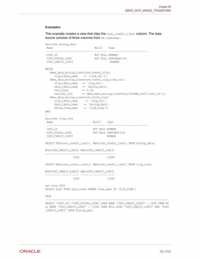
Examples
This example creates a view that clips the cust_credit_limit column. The datasource consists of three columns from sh.customer.
describe mining_data Name Null? Type ------------------------------ -------- ------------------------- CUST_ID NOT NULL NUMBER CUST_POSTAL_CODE NOT NULL VARCHAR2(10) CUST_CREDIT_LIMIT NUMBER BEGIN dbms_data_mining_transform.create_clip( clip_table_name => 'clip_tbl'); dbms_data_mining_transform.insert_clip_trim_tail( clip_table_name => 'clip_tbl', data_table_name => 'mining_data', tail_frac => 0.05, exclude_list => dbms_data_mining_transform.COLUMN_LIST('cust_id')); dbms_data_mining_transform.xform_clip( clip_table_name => 'clip_tbl', data_table_name => 'mining_data', xform_view_name => 'clip_view');END;/describe clip_view Name Null? Type ----------------------------- -------- -------------------------- CUST_ID NOT NULL NUMBER CUST_POSTAL_CODE NOT NULL VARCHAR2(10) CUST_CREDIT_LIMIT NUMBER SELECT MIN(cust_credit_limit), MAX(cust_credit_limit) FROM mining_data; MIN(CUST_CREDIT_LIMIT) MAX(CUST_CREDIT_LIMIT)---------------------- ---------------------- 1500 15000 SELECT MIN(cust_credit_limit), MAX(cust_credit_limit) FROM clip_view; MIN(CUST_CREDIT_LIMIT) MAX(CUST_CREDIT_LIMIT)---------------------- ---------------------- 1500 11000 set long 2000SELECT text FROM user_views WHERE view_name IN 'CLIP_VIEW'; TEXT--------------------------------------------------------------------------------SELECT "CUST_ID","CUST_POSTAL_CODE",CASE WHEN "CUST_CREDIT_LIMIT" < 1500 THEN NULL WHEN "CUST_CREDIT_LIMIT" > 11000 THEN NULL ELSE "CUST_CREDIT_LIMIT" END "CUST_CREDIT_LIMIT" FROM mining_data
Chapter 36DBMS_DATA_MINING_TRANSFORM
36-258

36.2.3.34 XFORM_COL_REM ProcedureThis procedure creates a view that implements the column removal transformationsspecified in a definition table. Only the columns that are specified in the definition tableare removed; the remaining columns from the data table are present in the view.
Syntax
DBMS_DATA_MINING_TRANSFORM.XFORM_COL_REM ( rem_table_name IN VARCHAR2, data_table_name IN VARCHAR2, xform_view_name IN VARCHAR2, rem_schema_name IN VARCHAR2 DEFAULT NULL, data_schema_name IN VARCHAR2 DEFAULT NULL, xform_schema_name IN VARCHAR2 DEFAULT NULL);
Parameters
Table 36-157 XFORM_COL_REM Procedure Parameters
Parameter Description
rem_table_name Name of the transformation definition table for columnremoval. You can use the CREATE_COL_REM Procedure tocreate the definition table. See Table 36-123.
The table must be populated with column names beforeyou call XFORM_COL_REM. The INSERT_BIN_SUPER Procedureand the INSERT_AUTOBIN_NUM_EQWIDTH Procedure canoptionally be used to populate the table. You can also useSQL INSERT statements.
data_table_name Name of the table containing the data to be transformed
xform_view_name Name of the view to be created. The view presents thecolumns in data_table_name that are not specified inrem_table_name.
rem_schema_name Schema of rem_table_name. If no schema is specified, thecurrent schema is used.
data_schema_name Schema of data_table_name. If no schema is specified, thecurrent schema is used.
xform_schema_name Schema of xform_view_name. If no schema is specified, thecurrent schema is used.
Usage Notes
See "Operational Notes".
Examples
This example creates a view that includes all but one column from the table customersin the current schema.
describe customers Name Null? Type ----------------------------------------- -------- ---------------------------- CUST_ID NOT NULL NUMBER
Chapter 36DBMS_DATA_MINING_TRANSFORM
36-259
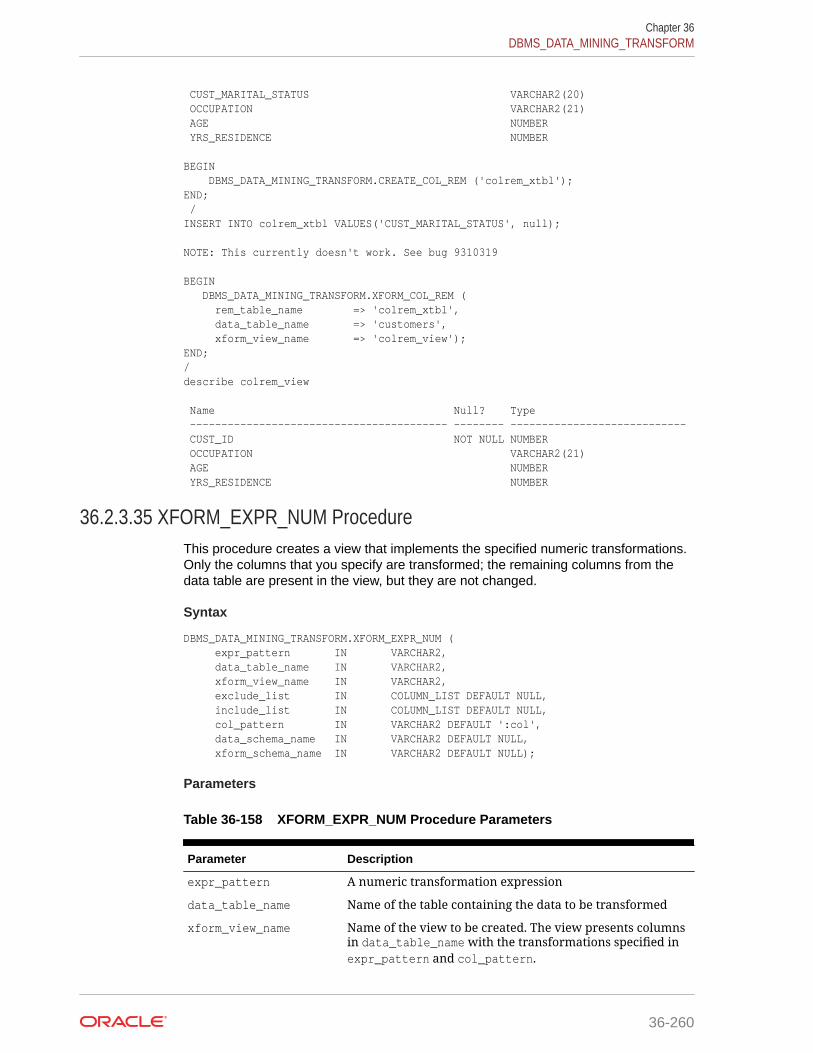
CUST_MARITAL_STATUS VARCHAR2(20) OCCUPATION VARCHAR2(21) AGE NUMBER YRS_RESIDENCE NUMBER
BEGIN DBMS_DATA_MINING_TRANSFORM.CREATE_COL_REM ('colrem_xtbl');END; /INSERT INTO colrem_xtbl VALUES('CUST_MARITAL_STATUS', null);
NOTE: This currently doesn't work. See bug 9310319
BEGIN DBMS_DATA_MINING_TRANSFORM.XFORM_COL_REM ( rem_table_name => 'colrem_xtbl', data_table_name => 'customers', xform_view_name => 'colrem_view');END;/describe colrem_view
Name Null? Type ----------------------------------------- -------- ---------------------------- CUST_ID NOT NULL NUMBER OCCUPATION VARCHAR2(21) AGE NUMBER YRS_RESIDENCE NUMBER
36.2.3.35 XFORM_EXPR_NUM ProcedureThis procedure creates a view that implements the specified numeric transformations.Only the columns that you specify are transformed; the remaining columns from thedata table are present in the view, but they are not changed.
Syntax
DBMS_DATA_MINING_TRANSFORM.XFORM_EXPR_NUM ( expr_pattern IN VARCHAR2, data_table_name IN VARCHAR2, xform_view_name IN VARCHAR2, exclude_list IN COLUMN_LIST DEFAULT NULL, include_list IN COLUMN_LIST DEFAULT NULL, col_pattern IN VARCHAR2 DEFAULT ':col', data_schema_name IN VARCHAR2 DEFAULT NULL, xform_schema_name IN VARCHAR2 DEFAULT NULL);
Parameters
Table 36-158 XFORM_EXPR_NUM Procedure Parameters
Parameter Description
expr_pattern A numeric transformation expression
data_table_name Name of the table containing the data to be transformed
xform_view_name Name of the view to be created. The view presents columnsin data_table_name with the transformations specified inexpr_pattern and col_pattern.
Chapter 36DBMS_DATA_MINING_TRANSFORM
36-260

Table 36-158 (Cont.) XFORM_EXPR_NUM Procedure Parameters
Parameter Description
exclude_list List of numerical columns to exclude. If NULL, no numericalcolumns are excluded.The format of exclude_list is:
dbms_data_mining_transform.COLUMN_LIST('col1','col2', ...'coln')
include_list List of numeric columns to include. If NULL, all numericcolumns are included.The format of include_list is:
dbms_data_mining_transform.COLUMN_LIST('col1','col2', ...'coln')
col_pattern The value within expr_pattern that will be replaced with acolumn name. The value of col_pattern is case-sensitive.
The default value of col_pattern is ':col'
data_schema_name Schema of data_table_name. If no schema is specified, thecurrent schema is used.
xform_schema_name Schema of xform_view_name. If no schema is specified, thecurrent schema is used.
Usage Notes
1. The XFORM_EXPR_NUM procedure constructs numeric transformation expressionsfrom the specified expression pattern (expr_pattern) by replacing everyoccurrence of the specified column pattern (col_pattern) with an actual columnname.
XFORM_EXPR_NUM uses the SQL REPLACE function to construct the transformationexpressions.
REPLACE (expr_pattern,col_pattern,'"column_name"') || '"column_name"'
If there is a column match, then the replacement is made in the transformationexpression; if there is not a match, then the column is used without transformation.
See:
Oracle Database SQL Language Reference for information about theREPLACE function
2. Because of the include and exclude list parameters, the XFORM_EXPR_NUM andXFORM_EXPR_STR procedures allow you to easily specify individual columns fortransformation within large data sets. The other XFORM_* procedures support anexclude list only. In these procedures, you must enumerate every column that youdo not want to transform.
3. See "Operational Notes"
Chapter 36DBMS_DATA_MINING_TRANSFORM
36-261

Examples
This example creates a view that transforms the datatype of numeric columns.
describe customers Name Null? Type ----------------------------------- -------- ------------------------ CUST_ID NOT NULL NUMBER CUST_MARITAL_STATUS VARCHAR2(20) OCCUPATION VARCHAR2(21) AGE NUMBER YRS_RESIDENCE NUMBER
BEGIN DBMS_DATA_MINING_TRANSFORM.XFORM_EXPR_NUM( expr_pattern => 'to_char(:col)', data_table_name => 'customers', xform_view_name => 'cust_nonum_view', exclude_list => dbms_data_mining_transform.COLUMN_LIST( 'cust_id'), include_list => null, col_pattern => ':col');END;/describe cust_nonum_view Name Null? Type ----------------------------------- -------- ------------------------ CUST_ID NOT NULL NUMBER CUST_MARITAL_STATUS VARCHAR2(20) OCCUPATION VARCHAR2(21) AGE VARCHAR2(40) YRS_RESIDENCE VARCHAR2(40)
36.2.3.36 XFORM_EXPR_STR ProcedureThis procedure creates a view that implements the specified categoricaltransformations. Only the columns that you specify are transformed; the remainingcolumns from the data table are present in the view, but they are not changed.
Syntax
DBMS_DATA_MINING_TRANSFORM.XFORM_EXPR_STR ( expr_pattern IN VARCHAR2, data_table_name IN VARCHAR2, xform_view_name IN VARCHAR2, exclude_list IN COLUMN_LIST DEFAULT NULL, include_list IN COLUMN_LIST DEFAULT NULL, col_pattern IN VARCHAR2 DEFAULT ':col', data_schema_name IN VARCHAR2 DEFAULT NULL, xform_schema_name IN VARCHAR2 DEFAULT NULL);
Parameters
Table 36-159 XFORM_EXPR_STR Procedure Parameters
Parameter Description
expr_pattern A character transformation expression
data_table_name Name of the table containing the data to be transformed
Chapter 36DBMS_DATA_MINING_TRANSFORM
36-262

Table 36-159 (Cont.) XFORM_EXPR_STR Procedure Parameters
Parameter Description
xform_view_name Name of the view to be created. The view presents columnsin data_table_name with the transformations specified inexpr_pattern and col_pattern.
exclude_list List of categorical columns to exclude. If NULL, no categoricalcolumns are excluded.The format of exclude_list is:
dbms_data_mining_transform.COLUMN_LIST('col1','col2', ...'coln')
include_list List of character columns to include. If NULL, all charactercolumns are included.The format of include_list is:
dbms_data_mining_transform.COLUMN_LIST('col1','col2', ...'coln')
col_pattern The value within expr_pattern that will be replaced with acolumn name. The value of col_pattern is case-sensitive.
The default value of col_pattern is ':col'
data_schema_name Schema of data_table_name. If no schema is specified, thecurrent schema is used.
xform_schema_name Schema of xform_view_name. If no schema is specified, thecurrent schema is used.
Usage Notes
1. The XFORM_EXPR_STR procedure constructs character transformation expressionsfrom the specified expression pattern (expr_pattern) by replacing everyoccurrence of the specified column pattern (col_pattern) with an actual columnname.
XFORM_EXPR_STR uses the SQL REPLACE function to construct the transformationexpressions.
REPLACE (expr_pattern,col_pattern,'"column_name"') || '"column_name"'
If there is a column match, then the replacement is made in the transformationexpression; if there is not a match, then the column is used without transformation.
See:
Oracle Database SQL Language Reference for information about theREPLACE function
2. Because of the include and exclude list parameters, the XFORM_EXPR_STR andXFORM_EXPR_NUM procedures allow you to easily specify individual columns for
Chapter 36DBMS_DATA_MINING_TRANSFORM
36-263

transformation within large data sets. The other XFORM_* procedures support anexclude list only. In these procedures, you must enumerate every column that youdo not want to transform.
3. See "Operational Notes"
Examples
This example creates a view that transforms character columns to upper case.
describe customers Name Null? Type ----------------------------------- -------- ------------------------ CUST_ID NOT NULL NUMBER CUST_MARITAL_STATUS VARCHAR2(20) OCCUPATION VARCHAR2(21) AGE NUMBER YRS_RESIDENCE NUMBER
SELECT cust_id, cust_marital_status, occupation FROM customers WHERE cust_id > 102995 ORDER BY cust_id desc; CUST_ID CUST_MARITAL_STATUS OCCUPATION------- -------------------- --------------------- 103000 Divorc. Cleric. 102999 Married Cleric. 102998 Married Exec. 102997 Married Exec. 102996 NeverM Other BEGIN DBMS_DATA_MINING_TRANSFORM.XFORM_EXPR_STR( expr_pattern => 'upper(:col)', data_table_name => 'customers', xform_view_name => 'cust_upcase_view');END;/describe cust_upcase_view Name Null? Type ----------------------------- -------- -------------------- CUST_ID NOT NULL NUMBER CUST_MARITAL_STATUS VARCHAR2(20) OCCUPATION VARCHAR2(21) AGE NUMBER YRS_RESIDENCE NUMBER SELECT cust_id, cust_marital_status, occupation FROM cust_upcase_view WHERE cust_id > 102995 ORDER BY cust_id desc; CUST_ID CUST_MARITAL_STATUS OCCUPATION------- -------------------- --------------------- 103000 DIVORC. CLERIC. 102999 MARRIED CLERIC. 102998 MARRIED EXEC. 102997 MARRIED EXEC. 102996 NEVERM OTHER
Chapter 36DBMS_DATA_MINING_TRANSFORM
36-264
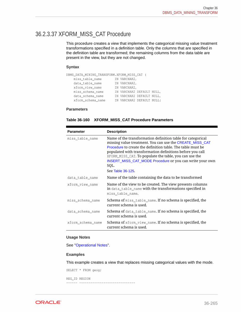
36.2.3.37 XFORM_MISS_CAT ProcedureThis procedure creates a view that implements the categorical missing value treatmenttransformations specified in a definition table. Only the columns that are specified inthe definition table are transformed; the remaining columns from the data table arepresent in the view, but they are not changed.
Syntax
DBMS_DATA_MINING_TRANSFORM.XFORM_MISS_CAT ( miss_table_name IN VARCHAR2, data_table_name IN VARCHAR2, xform_view_name IN VARCHAR2, miss_schema_name IN VARCHAR2 DEFAULT NULL, data_schema_name IN VARCHAR2 DEFAULT NULL, xform_schema_name IN VARCHAR2 DEFAULT NULL;
Parameters
Table 36-160 XFORM_MISS_CAT Procedure Parameters
Parameter Description
miss_table_name Name of the transformation definition table for categoricalmissing value treatment. You can use the CREATE_MISS_CATProcedure to create the definition table. The table must bepopulated with transformation definitions before you callXFORM_MISS_CAT. To populate the table, you can use theINSERT_MISS_CAT_MODE Procedure or you can write your ownSQL.See Table 36-125.
data_table_name Name of the table containing the data to be transformed
xform_view_name Name of the view to be created. The view presents columnsin data_table_name with the transformations specified inmiss_table_name.
miss_schema_name Schema of miss_table_name. If no schema is specified, thecurrent schema is used.
data_schema_name Schema of data_table_name. If no schema is specified, thecurrent schema is used.
xform_schema_name Schema of xform_view_name. If no schema is specified, thecurrent schema is used.
Usage Notes
See "Operational Notes".
Examples
This example creates a view that replaces missing categorical values with the mode.
SELECT * FROM geog;
REG_ID REGION------ ------------------------------
Chapter 36DBMS_DATA_MINING_TRANSFORM
36-265

1 NE 2 SW 3 SE 4 SW 5 6 NE 7 NW 8 NW 9 10 11 SE 12 SE 13 NW 14 SE 15 SE SELECT STATS_MODE(region) FROM geog;
STATS_MODE(REGION)------------------------------SE BEGIN DBMS_DATA_MINING_TRANSFORM.CREATE_MISS_CAT('misscat_xtbl'); DBMS_DATA_MINING_TRANSFORM.INSERT_MISS_CAT_MODE ( miss_table_name => 'misscat_xtbl', data_table_name => 'geog' );END;/
SELECT col, val FROM misscat_xtbl;
COL VAL---------- ----------REGION SE BEGIN DBMS_DATA_MINING_TRANSFORM.XFORM_MISS_CAT ( miss_table_name => 'misscat_xtbl', data_table_name => 'geog', xform_view_name => 'geogxf_view');END;/
SELECT * FROM geogxf_view;
REG_ID REGION------ ------------------------------ 1 NE 2 SW 3 SE 4 SW 5 SE 6 NE 7 NW 8 NW 9 SE 10 SE 11 SE 12 SE 13 NW
Chapter 36DBMS_DATA_MINING_TRANSFORM
36-266

14 SE 15 SE
36.2.3.38 XFORM_MISS_NUM ProcedureThis procedure creates a view that implements the numerical missing value treatmenttransformations specified in a definition table. Only the columns that are specified inthe definition table are transformed; the remaining columns from the data table arepresent in the view, but they are not changed.
Syntax
DBMS_DATA_MINING_TRANSFORM.XFORM_MISS_NUM ( miss_table_name IN VARCHAR2, data_table_name IN VARCHAR2, xform_view_name IN VARCHAR2, miss_schema_name IN VARCHAR2 DEFAULT NULL, data_schema_name IN VARCHAR2 DEFAULT NULL, xform_schema_name IN VARCHAR2 DEFAULT NULL;
Parameters
Table 36-161 XFORM_MISS_NUM Procedure Parameters
Parameter Description
miss_table_name Name of the transformation definition table for numericalmissing value treatment. You can use the CREATE_MISS_NUMProcedure to create the definition table. The table must bepopulated with transformation definitions before you callXFORM_MISS_NUM. To populate the table, you can use theINSERT_MISS_NUM_MEAN Procedure or you can write yourown SQL.See Table 36-127.
data_table_name Name of the table containing the data to be transformed
xform_view_name Name of the view to be created. The view presents columnsin data_table_name with the transformations specified inmiss_table_name.
miss_schema_name Schema of miss_table_name. If no schema is specified, thecurrent schema is used.
data_schema_name Schema of data_table_name. If no schema is specified, thecurrent schema is used.
xform_schema_name Schema of xform_view_name. If no schema is specified, thecurrent schema is used.
Usage Notes
See "Operational Notes".
Examples
This example creates a view that replaces missing numerical values with the mean.
Chapter 36DBMS_DATA_MINING_TRANSFORM
36-267
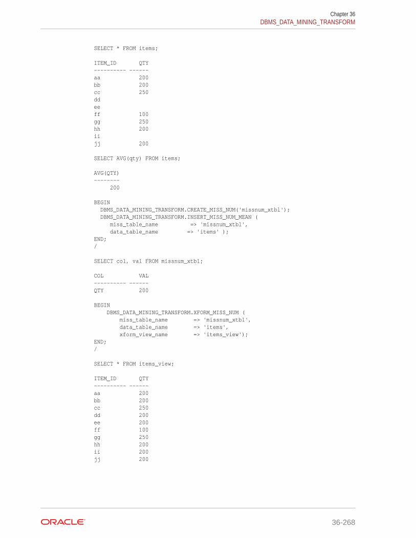
SELECT * FROM items; ITEM_ID QTY---------- ------aa 200bb 200cc 250ddeeff 100gg 250hh 200iijj 200 SELECT AVG(qty) FROM items; AVG(QTY)-------- 200 BEGIN DBMS_DATA_MINING_TRANSFORM.CREATE_MISS_NUM('missnum_xtbl'); DBMS_DATA_MINING_TRANSFORM.INSERT_MISS_NUM_MEAN ( miss_table_name => 'missnum_xtbl', data_table_name => 'items' );END;/ SELECT col, val FROM missnum_xtbl; COL VAL---------- ------QTY 200 BEGIN DBMS_DATA_MINING_TRANSFORM.XFORM_MISS_NUM ( miss_table_name => 'missnum_xtbl', data_table_name => 'items', xform_view_name => 'items_view');END;/ SELECT * FROM items_view; ITEM_ID QTY---------- ------aa 200bb 200cc 250dd 200ee 200ff 100gg 250hh 200ii 200jj 200
Chapter 36DBMS_DATA_MINING_TRANSFORM
36-268

36.2.3.39 XFORM_NORM_LIN ProcedureThis procedure creates a view that implements the linear normalizationtransformations specified in a definition table. Only the columns that are specifiedin the definition table are transformed; the remaining columns from the data table arepresent in the view, but they are not changed.
Syntax
DBMS_DATA_MINING_TRANSFORM.XFORM_NORM_LIN ( norm_table_name IN VARCHAR2, data_table_name IN VARCHAR2, xform_view_name IN VARCHAR2, norm_schema_name IN VARCHAR2 DEFAULT NULL, data_schema_name IN VARCHAR2 DEFAULT NULL, xform_schema_name IN VARCHAR2 DEFAULT NULL);
Parameters
Table 36-162 XFORM_NORM_LIN Procedure Parameters
Parameter Description
norm_table_name Name of the transformation definition table for linearnormalization. You can use the CREATE_NORM_LIN Procedureto create the definition table. The table must be populated withtransformation definitions before you call XFORM_NORM_LIN. Topopulate the table, you can use one of the INSERT proceduresfor normalization or you can write your own SQL.See Table 36-125.
data_table_name Name of the table containing the data to be transformed
xform_view_name Name of the view to be created. The view presents columnsin data_table_name with the transformations specified inmiss_table_name.
norm_schema_name Schema of miss_table_name. If no schema is specified, thecurrent schema is used.
data_schema_name Schema of data_table_name. If no schema is specified, thecurrent schema is used.
xform_schema_name Schema of xform_view_name. If no schema is specified, thecurrent schema is used.
Usage Notes
See "Operational Notes".
Examples
This example creates a view that normalizes the cust_year_of_birth andcust_credit_limit columns. The data source consists of three columns fromsh.customer.
CREATE OR REPLACE VIEW mining_data AS SELECT cust_id, cust_year_of_birth, cust_credit_limit FROM sh.customers;
Chapter 36DBMS_DATA_MINING_TRANSFORM
36-269

describe mining_data Name Null? Type -------------------------------------- -------- -------------------------- CUST_ID NOT NULL NUMBER CUST_YEAR_OF_BIRTH NOT NULL NUMBER(4) CUST_CREDIT_LIMIT NUMBER SELECT * FROM mining_data WHERE cust_id > 104495 ORDER BY cust_year_of_birth; CUST_ID CUST_YEAR_OF_BIRTH CUST_CREDIT_LIMIT-------- ------------------ ----------------- 104496 1947 3000 104498 1954 10000 104500 1962 15000 104499 1970 3000 104497 1976 3000 BEGIN dbms_data_mining_transform.CREATE_NORM_LIN( norm_table_name => 'normx_tbl'); dbms_data_mining_transform.INSERT_NORM_LIN_MINMAX( norm_table_name => 'normx_tbl', data_table_name => 'mining_data', exclude_list => dbms_data_mining_transform.COLUMN_LIST( 'cust_id'), round_num => 3);END;/ SELECT col, shift, scale FROM normx_tbl; COL SHIFT SCALE ------------------------------ -------- -------- CUST_YEAR_OF_BIRTH 1910 77 CUST_CREDIT_LIMIT 1500 13500 BEGIN DBMS_DATA_MINING_TRANSFORM.XFORM_NORM_LIN ( norm_table_name => 'normx_tbl', data_table_name => 'mining_data', xform_view_name => 'norm_view');END;/ SELECT * FROM norm_view WHERE cust_id > 104495 ORDER BY cust_year_of_birth; CUST_ID CUST_YEAR_OF_BIRTH CUST_CREDIT_LIMIT-------- ------------------ ----------------- 104496 .4805195 .1111111 104498 .5714286 .6296296 104500 .6753247 1 104499 .7792208 .1111111 104497 .8571429 .1111111 set long 2000SQL> SELECT text FROM user_views WHERE view_name IN 'NORM_VIEW'; TEXT
Chapter 36DBMS_DATA_MINING_TRANSFORM
36-270

---------------------------------------------------------------------------SELECT "CUST_ID",("CUST_YEAR_OF_BIRTH"-1910)/77 "CUST_YEAR_OF_BIRTH",("CUST_CREDIT_LIMIT"-1500)/13500 "CUST_CREDIT_LIMIT" FROM mining_data
36.2.3.40 XFORM_STACK ProcedureThis procedure creates a view that implements the transformations specified by thestack. Only the columns and nested attributes that are specified in the stack aretransformed. Any remaining columns and nested attributes from the data table appearin the view without changes.
To create a list of objects that describe the transformed columns, use theDESCRIBE_STACK Procedure.
See Also:
"Overview"
Oracle Data Mining User's Guide for more information about data miningattributes
Syntax
DBMS_DATA_MINING_TRANSFORM.XFORM_STACK ( xform_list IN TRANSFORM_list, data_table_name IN VARCHAR2, xform_view_name IN VARCHAR2, data_schema_name IN VARCHAR2 DEFAULT NULL, xform_schema_name IN VARCHAR2 DEFAULT NULL);
Parameters
Table 36-163 XFORM_STACK Procedure Parameters
Parameter Description
xform_list The transformation list. See Table 36-114 for a description of theTRANSFORM_LIST object type.
data_table_name Name of the table containing the data to be transformed
xform_view_name Name of the view to be created. The view applies thetransformations in xform_list to data_table_name.
data_schema_name Schema of data_table_name. If no schema is specified, thecurrent schema is used.
xform_schema_name Schema of xform_view_name. If no schema is specified, thecurrent schema is used.
Usage Notes
See "Operational Notes". The following sections are especially relevant:
• "About Transformation Lists"
Chapter 36DBMS_DATA_MINING_TRANSFORM
36-271
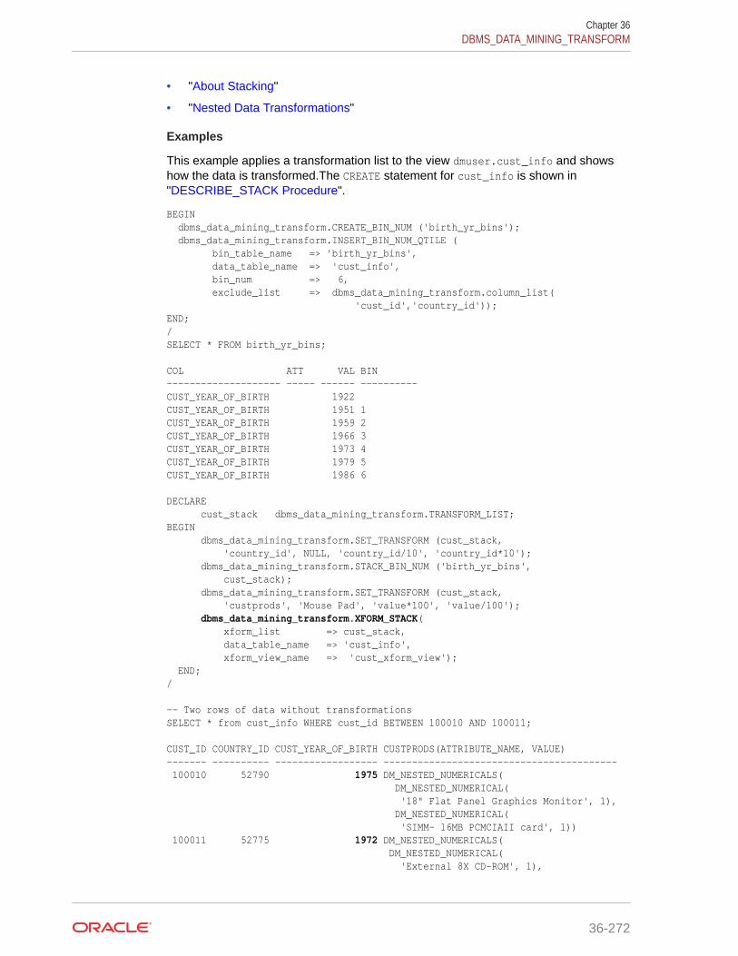
• "About Stacking"
• "Nested Data Transformations"
Examples
This example applies a transformation list to the view dmuser.cust_info and showshow the data is transformed.The CREATE statement for cust_info is shown in"DESCRIBE_STACK Procedure".
BEGIN dbms_data_mining_transform.CREATE_BIN_NUM ('birth_yr_bins'); dbms_data_mining_transform.INSERT_BIN_NUM_QTILE ( bin_table_name => 'birth_yr_bins', data_table_name => 'cust_info', bin_num => 6, exclude_list => dbms_data_mining_transform.column_list( 'cust_id','country_id'));END;/SELECT * FROM birth_yr_bins;
COL ATT VAL BIN-------------------- ----- ------ ----------CUST_YEAR_OF_BIRTH 1922CUST_YEAR_OF_BIRTH 1951 1CUST_YEAR_OF_BIRTH 1959 2CUST_YEAR_OF_BIRTH 1966 3CUST_YEAR_OF_BIRTH 1973 4CUST_YEAR_OF_BIRTH 1979 5CUST_YEAR_OF_BIRTH 1986 6
DECLARE cust_stack dbms_data_mining_transform.TRANSFORM_LIST;BEGIN dbms_data_mining_transform.SET_TRANSFORM (cust_stack, 'country_id', NULL, 'country_id/10', 'country_id*10'); dbms_data_mining_transform.STACK_BIN_NUM ('birth_yr_bins', cust_stack); dbms_data_mining_transform.SET_TRANSFORM (cust_stack, 'custprods', 'Mouse Pad', 'value*100', 'value/100'); dbms_data_mining_transform.XFORM_STACK( xform_list => cust_stack, data_table_name => 'cust_info', xform_view_name => 'cust_xform_view'); END;/
-- Two rows of data without transformationsSELECT * from cust_info WHERE cust_id BETWEEN 100010 AND 100011;
CUST_ID COUNTRY_ID CUST_YEAR_OF_BIRTH CUSTPRODS(ATTRIBUTE_NAME, VALUE)------- ---------- ------------------ ----------------------------------------- 100010 52790 1975 DM_NESTED_NUMERICALS( DM_NESTED_NUMERICAL( '18" Flat Panel Graphics Monitor', 1), DM_NESTED_NUMERICAL( 'SIMM- 16MB PCMCIAII card', 1)) 100011 52775 1972 DM_NESTED_NUMERICALS( DM_NESTED_NUMERICAL( 'External 8X CD-ROM', 1),
Chapter 36DBMS_DATA_MINING_TRANSFORM
36-272

DM_NESTED_NUMERICAL( 'Mouse Pad', 1), DM_NESTED_NUMERICAL( 'SIMM- 16MB PCMCIAII card', 1), DM_NESTED_NUMERICAL( 'Keyboard Wrist Rest', 1), DM_NESTED_NUMERICAL( '18" Flat Panel Graphics Monitor', 1), DM_NESTED_NUMERICAL( 'O/S Documentation Set - English', 1))
-- Same two rows of data with transformationsSELECT * FROM cust_xform_view WHERE cust_id BETWEEN 100010 AND 100011; CUST_ID COUNTRY_ID C CUSTPRODS(ATTRIBUTE_NAME, VALUE)------- ---------- - -------------------------------------------------------- 100010 5279 5 DM_NESTED_NUMERICALS( DM_NESTED_NUMERICAL( '18" Flat Panel Graphics Monitor', 1), DM_NESTED_NUMERICAL( 'SIMM- 16MB PCMCIAII card', 1)) 100011 5277.5 4 DM_NESTED_NUMERICALS( DM_NESTED_NUMERICAL( 'External 8X CD-ROM', 1), DM_NESTED_NUMERICAL( 'Mouse Pad', 100), DM_NESTED_NUMERICAL( 'SIMM- 16MB PCMCIAII card', 1), DM_NESTED_NUMERICAL( 'Keyboard Wrist Rest', 1), DM_NESTED_NUMERICAL( '18" Flat Panel Graphics Monitor', 1), DM_NESTED_NUMERICAL( 'O/S Documentation Set - English', 1))
36.3 DBMS_PREDICTIVE_ANALYTICSData mining can discover useful information buried in vast amounts of data. However,it is often the case that both the programming interfaces and the data mining expertiserequired to obtain these results are too complex for use by the wide audiences thatcan obtain benefits from using Oracle Data Mining.
The DBMS_PREDICTIVE_ANALYTICS package addresses both of these complexities byautomating the entire data mining process from data preprocessing through modelbuilding to scoring new data. This package provides an important tool that makes datamining possible for a broad audience of users, in particular, business analysts.
This chapter contains the following topics:
• Overview
• Security Model
• Summary of DBMS_PREDICTIVE_ANALYTICS Subprograms
36.3.1 Using DBMS_PREDICTIVE_ANALYTICSThis section contains topics that relate to using the DBMS_PREDICTIVE_ANALYTICSpackage.
Chapter 36DBMS_PREDICTIVE_ANALYTICS
36-273

• Overview
• Security Model
36.3.1.1 DBMS_PREDICTIVE_ANALYTICS OverviewDBMS_PREDICTIVE_ANALYTICS automates parts of the data mining process.
Data mining, according to a commonly used process model, requires the followingsteps:
1. Understand the business problem.
2. Understand the data.
3. Prepare the data for mining.
4. Create models using the prepared data.
5. Evaluate the models.
6. Deploy and use the model to score new data.
DBMS_PREDICTIVE_ANALYTICS automates parts of step 3 — 5 of this process.
Predictive analytics procedures analyze and prepare the input data, create and testmining models using the input data, and then use the input data for scoring. Theresults of scoring are returned to the user. The models and supporting objects are notpreserved after the operation completes.
36.3.1.2 DBMS_PREDICTIVE_ANALYTICS Security ModelThe DBMS_PREDICTIVE_ANALYTICS package is owned by user SYS and is installed aspart of database installation. Execution privilege on the package is granted to public.The routines in the package are run with invokers' rights (run with the privileges of thecurrent user).
The DBMS_PREDICTIVE_ANALYTICS package exposes APIs which are leveraged by theOracle Data Mining option. Users who wish to invoke procedures in this packagerequire the CREATE MINING MODEL system privilege (as well as the CREATE TABLE andCREATE VIEW system privilege).
36.3.2 Summary of DBMS_PREDICTIVE_ANALYTICS SubprogramsThis table lists and briefly describes the DBMS_PREDICTIVE_ANALYTICS packagesubprograms.
Table 36-164 DBMS_PREDICTIVE_ANALYTICS Package Subprograms
Subprogram Purpose
EXPLAIN Procedure Ranks attributes in order of influence in explaining a targetcolumn.
PREDICT Procedure Predicts the value of a target column based on values in theinput data.
PROFILE Procedure Generates rules that identify the records that have the sametarget value.
Chapter 36DBMS_PREDICTIVE_ANALYTICS
36-274

36.3.2.1 EXPLAIN ProcedureThe EXPLAIN procedure identifies the attributes that are important in explaining thevariation in values of a target column.
The input data must contain some records where the target value is known (not NULL).These records are used by the procedure to train a model that calculates the attributeimportance.
Note:
EXPLAIN supports DATE and TIMESTAMP datatypes in addition to the numeric,character, and nested datatypes supported by Oracle Data Mining models.
Data requirements for Oracle Data Mining are described in Oracle DataMining User's Guide.
The EXPLAIN procedure creates a result table that lists the attributes in order of theirexplanatory power. The result table is described in the Usage Notes.
Syntax
DBMS_PREDICTIVE_ANALYTICS.EXPLAIN ( data_table_name IN VARCHAR2, explain_column_name IN VARCHAR2, result_table_name IN VARCHAR2, data_schema_name IN VARCHAR2 DEFAULT NULL);
Parameters
Table 36-165 EXPLAIN Procedure Parameters
Parameter Description
data_table_name Name of input table or view
explain_column_name Name of the column to be explained
result_table_name Name of the table where results are saved
data_schema_name Name of the schema where the input table or view residesand where the result table is created. Default: the currentschema.
Usage Notes
The EXPLAIN procedure creates a result table with the columns described inTable 36-166.
Chapter 36DBMS_PREDICTIVE_ANALYTICS
36-275

Table 36-166 EXPLAIN Procedure Result Table
Column Name Datatype Description
ATTRIBUTE_NAME VARCHAR2(30) Name of a column in the input data; all columns except theexplained column are listed in the result table.
EXPLANATORY_VALUE NUMBER Value indicating how useful the column is for determining thevalue of the explained column. Higher values indicate greaterexplanatory power. Value can range from 0 to 1.An individual column's explanatory value is independent ofother columns in the input table. The values are based on howstrong each individual column correlates with the explainedcolumn. The value is affected by the number of records in theinput table, and the relations of the values of the column to thevalues of the explain column.An explanatory power value of 0 implies there is nouseful correlation between the column's values and theexplain column's values. An explanatory power of 1 impliesperfect correlation; such columns should be eliminated fromconsideration for PREDICT. In practice, an explanatory powerequal to 1 is rarely returned.
RANK NUMBER Ranking of explanatory power. Rows with equal values forexplanatory_value have the same rank. Rank values are notskipped in the event of ties.
Example
The following example performs an EXPLAIN operation on theSUPPLEMENTARY_DEMOGRAPHICS table of Sales History.
--Perform EXPLAIN operation BEGIN DBMS_PREDICTIVE_ANALYTICS.EXPLAIN( data_table_name => 'supplementary_demographics', explain_column_name => 'home_theater_package', result_table_name => 'demographics_explain_result'); END; / --Display results SELECT * FROM demographics_explain_result;
ATTRIBUTE_NAME EXPLANATORY_VALUE RANK---------------------------------------- ----------------- ----------Y_BOX_GAMES .524311073 1YRS_RESIDENCE .495987246 2HOUSEHOLD_SIZE .146208506 3AFFINITY_CARD .0598227 4EDUCATION .018462703 5OCCUPATION .009721543 6FLAT_PANEL_MONITOR .00013733 7PRINTER_SUPPLIES 0 8OS_DOC_SET_KANJI 0 8BULK_PACK_DISKETTES 0 8BOOKKEEPING_APPLICATION 0 8COMMENTS 0 8CUST_ID 0 8
Chapter 36DBMS_PREDICTIVE_ANALYTICS
36-276
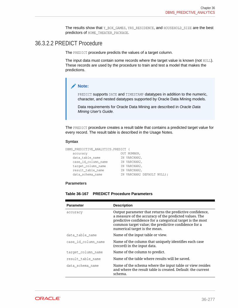
The results show that Y_BOX_GAMES, YRS_RESIDENCE, and HOUSEHOLD_SIZE are the bestpredictors of HOME_THEATER_PACKAGE.
36.3.2.2 PREDICT ProcedureThe PREDICT procedure predicts the values of a target column.
The input data must contain some records where the target value is known (not NULL).These records are used by the procedure to train and test a model that makes thepredictions.
Note:
PREDICT supports DATE and TIMESTAMP datatypes in addition to the numeric,character, and nested datatypes supported by Oracle Data Mining models.
Data requirements for Oracle Data Mining are described in Oracle DataMining User's Guide.
The PREDICT procedure creates a result table that contains a predicted target value forevery record. The result table is described in the Usage Notes.
Syntax
DBMS_PREDICTIVE_ANALYTICS.PREDICT ( accuracy OUT NUMBER, data_table_name IN VARCHAR2, case_id_column_name IN VARCHAR2, target_column_name IN VARCHAR2, result_table_name IN VARCHAR2, data_schema_name IN VARCHAR2 DEFAULT NULL);
Parameters
Table 36-167 PREDICT Procedure Parameters
Parameter Description
accuracy Output parameter that returns the predictive confidence,a measure of the accuracy of the predicted values. Thepredictive confidence for a categorical target is the mostcommon target value; the predictive confidence for anumerical target is the mean.
data_table_name Name of the input table or view.
case_id_column_name Name of the column that uniquely identifies each case(record) in the input data.
target_column_name Name of the column to predict.
result_table_name Name of the table where results will be saved.
data_schema_name Name of the schema where the input table or view residesand where the result table is created. Default: the currentschema.
Chapter 36DBMS_PREDICTIVE_ANALYTICS
36-277

Usage Notes
The PREDICT procedure creates a result table with the columns described inTable 36-168.
Table 36-168 PREDICT Procedure Result Table
Column Name Datatype Description
Case ID columnname
VARCHAR2 orNUMBER
The name of the case ID column in the input data.
PREDICTION VARCHAR2 orNUMBER
The predicted value of the target column for thegiven case.
PROBABILITY NUMBER For classification (categorical target), theprobability of the prediction. For regressionproblems (numerical target), this column containsNULL.
Note:
Make sure that the name of the case ID column is not 'PREDICTION' or'PROBABILITY'.
Predictions are returned for all cases whether or not they contained target values inthe input.
Predicted values for known cases may be interesting in some situations. For example,you could perform deviation analysis to compare predicted values and actual values.
Example
The following example performs a PREDICT operation and displays the first 10predictions. The results show an accuracy of 79% in predicting whether each customerhas an affinity card.
--Perform PREDICT operation DECLARE v_accuracy NUMBER(10,9); BEGIN DBMS_PREDICTIVE_ANALYTICS.PREDICT( accuracy => v_accuracy, data_table_name => 'supplementary_demographics', case_id_column_name => 'cust_id', target_column_name => 'affinity_card', result_table_name => 'pa_demographics_predict_result'); DBMS_OUTPUT.PUT_LINE('Accuracy = ' || v_accuracy); END; /
Accuracy = .788696903
--Display resultsSELECT * FROM pa_demographics_predict_result WHERE rownum < 10;
Chapter 36DBMS_PREDICTIVE_ANALYTICS
36-278

CUST_ID PREDICTION PROBABILITY---------- ---------- ----------- 101501 1 .834069848 101502 0 .991269965 101503 0 .99978311 101504 1 .971643388 101505 1 .541754127 101506 0 .803719133 101507 0 .999999303 101508 0 .999999987 101509 0 .999953074
36.3.2.3 PROFILE ProcedureThe PROFILE procedure generates rules that describe the cases (records) from theinput data.
For example, if a target column CHURN has values 'Yes' and 'No', PROFILE generatesa set of rules describing the expected outcomes. Each profile includes a rule, recordcount, and a score distribution.
The input data must contain some cases where the target value is known (not NULL).These cases are used by the procedure to build a model that calculates the rules.
Note:
PROFILE does not support nested types or dates.
Data requirements for Oracle Data Mining are described in Oracle DataMining User's Guide.
The PROFILE procedure creates a result table that specifies rules (profiles) and theircorresponding target values. The result table is described in the Usage Notes.
Syntax
DBMS_PREDICTIVE_ANALYTICS.PROFILE ( data_table_name IN VARCHAR2, target_column_name IN VARCHAR2, result_table_name IN VARCHAR2, data_schema_name IN VARCHAR2 DEFAULT NULL);
Parameters
Table 36-169 PROFILE Procedure Parameters
Parameter Description
data_table_name Name of the table containing the data to be analyzed.
target_column_name Name of the target column.
result_table_name Name of the table where the results will be saved.
Chapter 36DBMS_PREDICTIVE_ANALYTICS
36-279
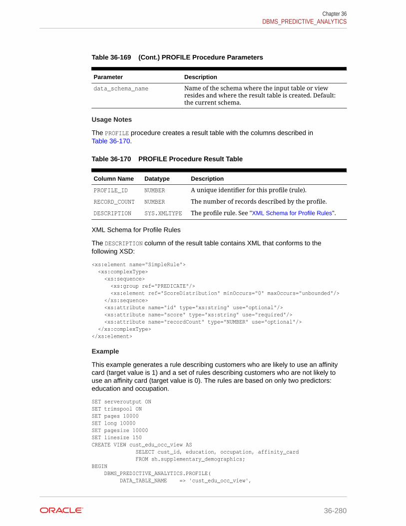
Table 36-169 (Cont.) PROFILE Procedure Parameters
Parameter Description
data_schema_name Name of the schema where the input table or viewresides and where the result table is created. Default:the current schema.
Usage Notes
The PROFILE procedure creates a result table with the columns described inTable 36-170.
Table 36-170 PROFILE Procedure Result Table
Column Name Datatype Description
PROFILE_ID NUMBER A unique identifier for this profile (rule).
RECORD_COUNT NUMBER The number of records described by the profile.
DESCRIPTION SYS.XMLTYPE The profile rule. See "XML Schema for Profile Rules".
XML Schema for Profile Rules
The DESCRIPTION column of the result table contains XML that conforms to thefollowing XSD:
<xs:element name="SimpleRule"> <xs:complexType> <xs:sequence> <xs:group ref="PREDICATE"/> <xs:element ref="ScoreDistribution" minOccurs="0" maxOccurs="unbounded"/> </xs:sequence> <xs:attribute name="id" type="xs:string" use="optional"/> <xs:attribute name="score" type="xs:string" use="required"/> <xs:attribute name="recordCount" type="NUMBER" use="optional"/> </xs:complexType></xs:element>
Example
This example generates a rule describing customers who are likely to use an affinitycard (target value is 1) and a set of rules describing customers who are not likely touse an affinity card (target value is 0). The rules are based on only two predictors:education and occupation.
SET serveroutput ONSET trimspool ONSET pages 10000SET long 10000SET pagesize 10000SET linesize 150CREATE VIEW cust_edu_occ_view AS SELECT cust_id, education, occupation, affinity_card FROM sh.supplementary_demographics;BEGIN DBMS_PREDICTIVE_ANALYTICS.PROFILE( DATA_TABLE_NAME => 'cust_edu_occ_view',
Chapter 36DBMS_PREDICTIVE_ANALYTICS
36-280

TARGET_COLUMN_NAME => 'affinity_card', RESULT_TABLE_NAME => 'profile_result');END;/
This example generates eight rules in the result table profile_result. Seven of therules suggest a target value of 0; one rule suggests a target value of 1. The scoreattribute on a rule identifies the target value.
This SELECT statement returns all the rules in the result table.
SELECT a.profile_id, a.record_count, a.description.getstringval() FROM profile_result a;
This SELECT statement returns the rules for a target value of 0.
SELECT * FROM profile_result t WHERE extractvalue(t.description, '/SimpleRule/@score') = 0;
The eight rules generated by this example are displayed as follows.
<SimpleRule id="1" score="0" recordCount="443"> <CompoundPredicate booleanOperator="and"> <SimpleSetPredicate field="OCCUPATION" booleanOperator="isIn"> <Array type="string">"Armed-F" "Exec." "Prof." "Protec." </Array> </SimpleSetPredicate> <SimpleSetPredicate field="EDUCATION" booleanOperator="isIn"> <Array type="string">"< Bach." "Assoc-V" "HS-grad" </Array> </SimpleSetPredicate> </CompoundPredicate> <ScoreDistribution value="0" recordCount="297" /> <ScoreDistribution value="1" recordCount="146" /> </SimpleRule>
<SimpleRule id="2" score="0" recordCount="18"> <CompoundPredicate booleanOperator="and"> <SimpleSetPredicate field="OCCUPATION" booleanOperator="isIn"> <Array type="string">"Armed-F" "Exec." "Prof." "Protec." </Array> </SimpleSetPredicate> <SimpleSetPredicate field="EDUCATION" booleanOperator="isIn"> <Array type="string">"10th" "11th" "12th" "1st-4th" "5th-6th" "7th-8th" "9th" "Presch." </Array> </SimpleSetPredicate> </CompoundPredicate> <ScoreDistribution value="0" recordCount="18" /> </SimpleRule>
<SimpleRule id="3" score="0" recordCount="458"> <CompoundPredicate booleanOperator="and"> <SimpleSetPredicate field="OCCUPATION" booleanOperator="isIn"> <Array type="string">"Armed-F" "Exec." "Prof." "Protec." </Array> </SimpleSetPredicate> <SimpleSetPredicate field="EDUCATION" booleanOperator="isIn"> <Array type="string">"Assoc-A" "Bach." </Array> </SimpleSetPredicate>
Chapter 36DBMS_PREDICTIVE_ANALYTICS
36-281
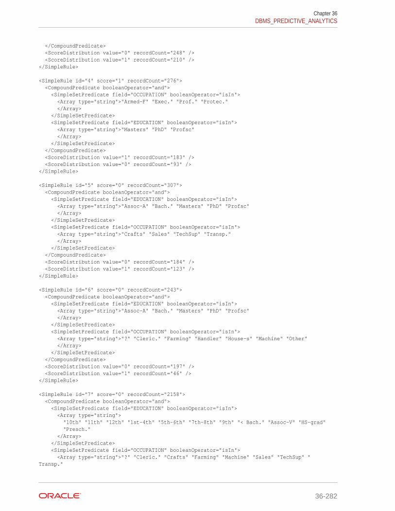
</CompoundPredicate> <ScoreDistribution value="0" recordCount="248" /> <ScoreDistribution value="1" recordCount="210" /> </SimpleRule>
<SimpleRule id="4" score="1" recordCount="276"> <CompoundPredicate booleanOperator="and"> <SimpleSetPredicate field="OCCUPATION" booleanOperator="isIn"> <Array type="string">"Armed-F" "Exec." "Prof." "Protec." </Array> </SimpleSetPredicate> <SimpleSetPredicate field="EDUCATION" booleanOperator="isIn"> <Array type="string">"Masters" "PhD" "Profsc" </Array> </SimpleSetPredicate> </CompoundPredicate> <ScoreDistribution value="1" recordCount="183" /> <ScoreDistribution value="0" recordCount="93" /> </SimpleRule>
<SimpleRule id="5" score="0" recordCount="307"> <CompoundPredicate booleanOperator="and"> <SimpleSetPredicate field="EDUCATION" booleanOperator="isIn"> <Array type="string">"Assoc-A" "Bach." "Masters" "PhD" "Profsc" </Array> </SimpleSetPredicate> <SimpleSetPredicate field="OCCUPATION" booleanOperator="isIn"> <Array type="string">"Crafts" "Sales" "TechSup" "Transp." </Array> </SimpleSetPredicate> </CompoundPredicate> <ScoreDistribution value="0" recordCount="184" /> <ScoreDistribution value="1" recordCount="123" /> </SimpleRule>
<SimpleRule id="6" score="0" recordCount="243"> <CompoundPredicate booleanOperator="and"> <SimpleSetPredicate field="EDUCATION" booleanOperator="isIn"> <Array type="string">"Assoc-A" "Bach." "Masters" "PhD" "Profsc" </Array> </SimpleSetPredicate> <SimpleSetPredicate field="OCCUPATION" booleanOperator="isIn"> <Array type="string">"?" "Cleric." "Farming" "Handler" "House-s" "Machine" "Other" </Array> </SimpleSetPredicate> </CompoundPredicate> <ScoreDistribution value="0" recordCount="197" /> <ScoreDistribution value="1" recordCount="46" /> </SimpleRule>
<SimpleRule id="7" score="0" recordCount="2158"> <CompoundPredicate booleanOperator="and"> <SimpleSetPredicate field="EDUCATION" booleanOperator="isIn"> <Array type="string"> "10th" "11th" "12th" "1st-4th" "5th-6th" "7th-8th" "9th" "< Bach." "Assoc-V" "HS-grad" "Presch." </Array> </SimpleSetPredicate> <SimpleSetPredicate field="OCCUPATION" booleanOperator="isIn"> <Array type="string">"?" "Cleric." "Crafts" "Farming" "Machine" "Sales" "TechSup" " Transp."
Chapter 36DBMS_PREDICTIVE_ANALYTICS
36-282
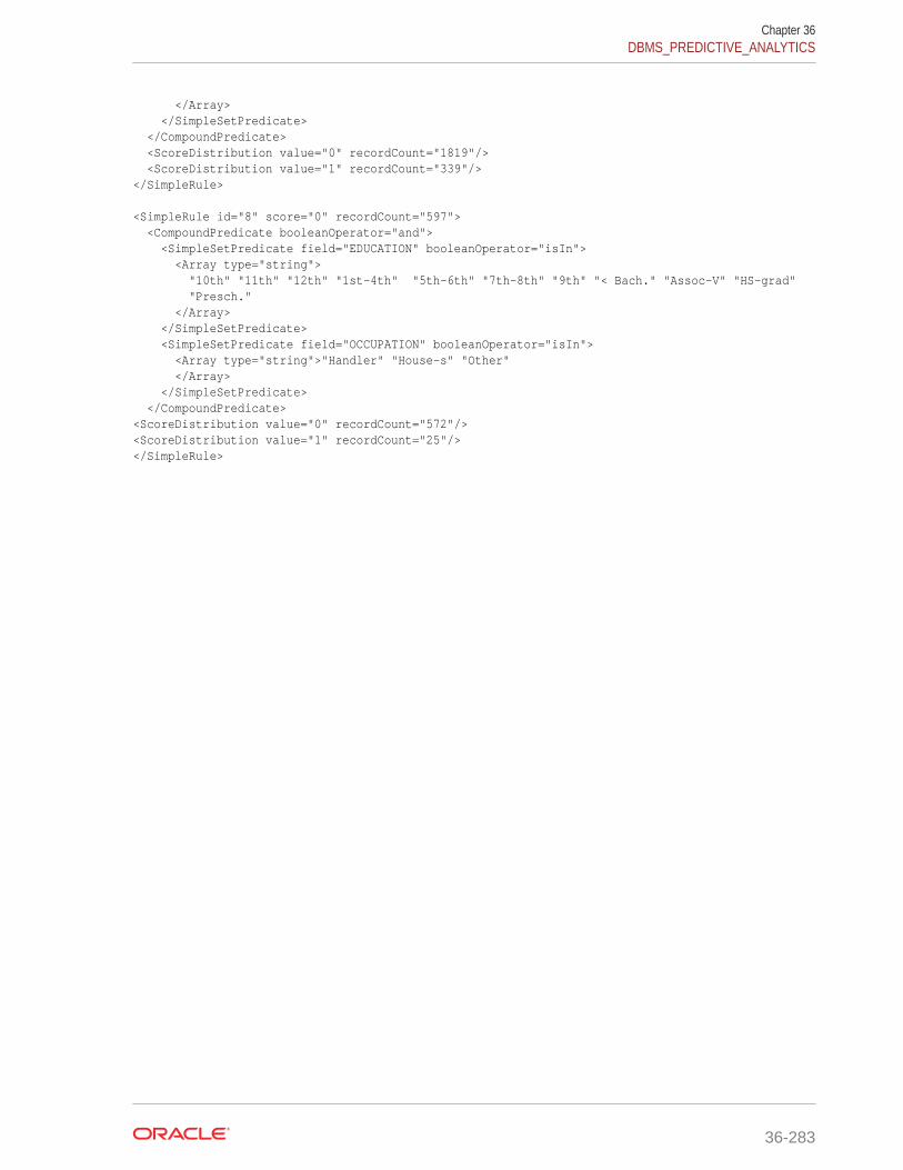
</Array> </SimpleSetPredicate> </CompoundPredicate> <ScoreDistribution value="0" recordCount="1819"/> <ScoreDistribution value="1" recordCount="339"/></SimpleRule>
<SimpleRule id="8" score="0" recordCount="597"> <CompoundPredicate booleanOperator="and"> <SimpleSetPredicate field="EDUCATION" booleanOperator="isIn"> <Array type="string"> "10th" "11th" "12th" "1st-4th" "5th-6th" "7th-8th" "9th" "< Bach." "Assoc-V" "HS-grad" "Presch." </Array> </SimpleSetPredicate> <SimpleSetPredicate field="OCCUPATION" booleanOperator="isIn"> <Array type="string">"Handler" "House-s" "Other" </Array> </SimpleSetPredicate> </CompoundPredicate><ScoreDistribution value="0" recordCount="572"/><ScoreDistribution value="1" recordCount="25"/></SimpleRule>
Chapter 36DBMS_PREDICTIVE_ANALYTICS
36-283

37Data Dictionary Views
The information in the data dictionary tables can be viewed through data dictionaryviews. The data mining related dictionary views are listed in this chapter.
• ALL_MINING_MODELS
• ALL_MINING_MODEL_ATTRIBUTES
• ALL_MINING_MODEL_PARTITIONS
• ALL_MINING_MODEL_SETTINGS
• ALL_MINING_MODEL_VIEWS
• ALL_MINING_MODEL_XFORMS
37.1 ALL_MINING_MODELSALL_MINING_MODELS describes the mining models accessible to the current user.
Mining models are schema objects created by Oracle Data Mining.
Related Views
• DBA_MINING_MODELS describes all mining models in the database.
• USER_MINING_MODELS describes the mining models owned by the current user. Thisview does not display the OWNER column.
Column Datatype NULL Description
OWNER VARCHAR2(128) NOT NULL Owner of the mining model
MODEL_NAME VARCHAR2(128) NOT NULL Name of the mining model
MINING_FUNCTION VARCHAR2(30) NOT NULL Function of the mining model. The functionidentifies the class of problems that can besolved by this model. The mining function isspecified when the model is built:• CLASSIFICATION
• REGRESSION
• CLUSTERING
• FEATURE_EXTRACTION
• ASSOCIATION_RULES
• ATTRIBUTE_IMPORTANCE
37-1

Column Datatype NULL Description
ALGORITHM VARCHAR2(30) NOT NULL Algorithm used by the model. Each miningfunction has a default algorithm. The defaultcan be overridden with a model setting (see*_MINING_MODEL_SETTINGS):
• CUR_DECOMPOSITION
• NAIVE_BAYES
• DECISION_TREE
• EXPLICIT_SEMANTIC_ANALYS
• EXPONENTIAL_ SMOOTHING
• SUPPORT_VECTOR_MACHINES
• KMEANS
• O_CLUSTER
• NONNEGATIVE_MATRIX_FACTOR
• NEURAL_NETWORK
• GENERALIZED_LINEAR_MODEL
• APRIORI_ASSOCIATION_RULES
• MINIMUM_DESCRIPTION_LENGTH
• EXPECTATION_MAXIMIZATION
• RANDOM_FOREST
• SINGULAR_VALUE_DECOMP
• R_EXTENSIBLE
ALGORITHM_TYPE VARCHAR2(10) NOT NULL Algorithm type of the model
CREATION_DATE DATE NOT NULL Date that the model was created
BUILD_DURATION NUMBER NOT NULL Time (in seconds) of the model build process
MODEL_SIZE NUMBER NOT NULL Size of the model (in megabytes)
PARTITIONED VARCHAR2(3) NOT NULL Indicates whether the model is partitioned ornot. Possible values:• YES: The model is partitioned.• NO: The model is not partitioned
COMMENTS VARCHAR2(4000) NOT NULL Comment applied to the model with a SQLCOMMENT statement
Related Topics
• DBA_MINING_MODEL
• USER_MINING_MODELS
See Also:
• Oracle Data Mining User’s Guide for information about mining modelschema objects
• Oracle Data Mining Concepts for an introduction to Data Mining
Chapter 37ALL_MINING_MODELS
37-2

37.2 ALL_MINING_MODEL_ATTRIBUTESALL_MINING_MODEL_ATTRIBUTES describes the attributes of the mining modelsaccessible to the current user. Only the attributes in the model signature are includedin this view. The attributes in the model signature correspond to the columns in thetraining data that were used to build the model.Mining models are schema objects created by Oracle Data Mining.
Related Views
• DBA_MINING_MODEL_ATTRIBUTES describes the attributes of all mining models in thedatabase.
• USER_MINING_MODEL_ATTRIBUTES describes the attributes of the mining modelsowned by the current user. This view does not display the OWNER column.
Column Datatype NULL Description
OWNER VARCHAR2(128) NOT NULL Owner of the mining model
MODEL_NAME VARCHAR2(128) NOT NULL Name of the mining model
ATTRIBUTE_NAME VARCHAR2(128) NOT NULL Name of the attribute
ATTRIBUTE_TYPE VARCHAR2(11) – Logical type of the attribute. The type isidentified during the model build or applyprocess:• NUMERICAL: Numeric data• CATEGORICAL: Character data• TEXT: Unstructured text data• PARTITION: The input signature column is
used for the partitioning key• MIXED: The input signature column takes
on more than one attribute type.This is due to user-defined embeddedtransformations that allow an inputcolumn to be transformed into multipleindependent mining attributes, includingmining attributes of different types.
DATA_TYPE VARCHAR2(106) – Data type of the attribute
DATA_LENGTH NUMBER – Length of the data type
DATA_PRECISION NUMBER – Precision of a fixed point number. Precision,which is the total number of significantdecimal digits, is represented as p in the datatype NUMBER(p,s).
DATA_SCALE NUMBER – Scale of a fixed point number. Scale, which isthe number of digits from the decimal to theleast significant digit, is represented as s in thedata type NUMBER(p,s).
Chapter 37ALL_MINING_MODEL_ATTRIBUTES
37-3

Column Datatype NULL Description
USAGE_TYPE VARCHAR2(8) – Indicates whether the attribute was usedto construct the model (ACTIVE) or not(INACTIVE). Some attributes may be eliminatedby transformations or algorithmic processing.The *_MINING_MODEL_ATTRIBUTES view only liststhe attributes used by the model, therefore thevalue of this column is always ACTIVE.
TARGET VARCHAR2(3) – Indicates whether the attribute is the target ofa predictive model (YES) or not (NO). The targetdescribes the result that is produced when themodel is applied.
ATTRIBUTE_SPEC VARCHAR2(4000) – One or more keywords that identify specialtreatment for the attribute during model build.Values are:• FORCE_IN: (GLM only) When feature
selection is enabled, forces the inclusion ofthe attribute in the model build. Featureselection is disabled by default. If themodel is not using GLM with featureselection enabled, this value is ignored.
• NOPREP: When ADP is on, preventsautomatic transformation of the attribute.If ADP is OFF, this value is ignored.
• TEXT: Causes the attribute to betreated as unstructured text data. TheTEXT value supports three subsettings:POLICY_NAME, MAX_FEATURES, TOKEN_TYPE, andMIN_DOCUMENTS. Subsettings are specifiedas name:value pairs within parentheses.For example: (POLICY_NAME:mypolicy)(MAX_FEATURES:2000)(TOKEN_TYPE:THEME).See Oracle Data Mining User’s Guide fordetails.
• NULL: The ATTRIBUTE_SPEC for this attributeis NULL.
ATTRIBUTE_SPEC is a parameter to thePL/SQL procedureDBMS_DATA_MINING_TRANSFORM.SET_TRANSFOR
M. See Oracle Database PL/SQL Packagesand Types Reference for details.
Related Topics
• DBA_MINING_MODEL_ATTRIBUTES
• USER_MINING_MODEL_ATTRIBUTES
See Also:
Oracle Data Mining User’s Guide
Chapter 37ALL_MINING_MODEL_ATTRIBUTES
37-4
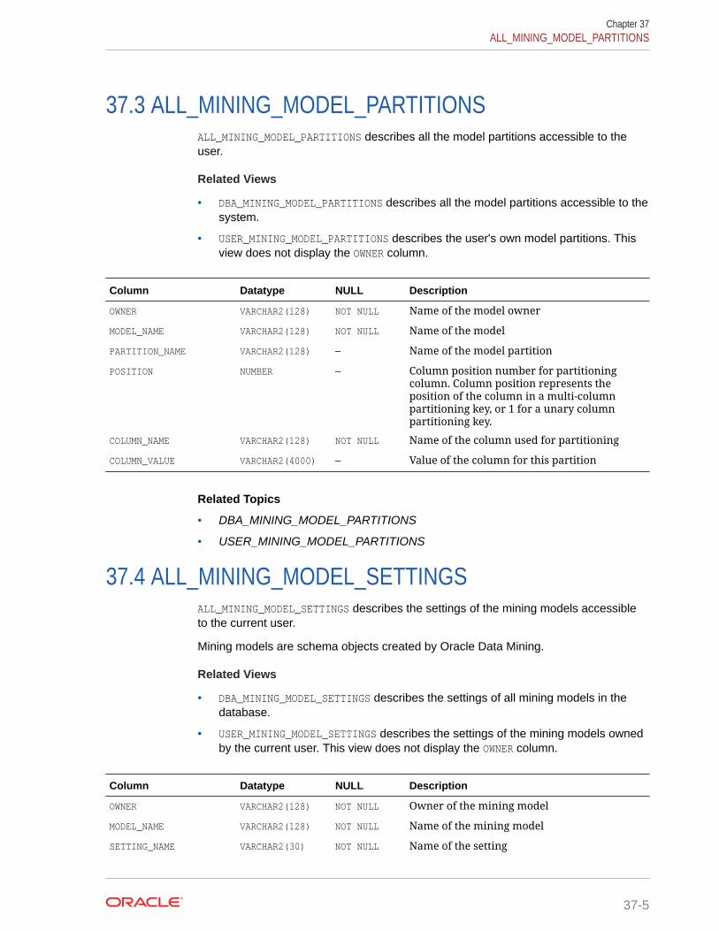
37.3 ALL_MINING_MODEL_PARTITIONSALL_MINING_MODEL_PARTITIONS describes all the model partitions accessible to theuser.
Related Views
• DBA_MINING_MODEL_PARTITIONS describes all the model partitions accessible to thesystem.
• USER_MINING_MODEL_PARTITIONS describes the user's own model partitions. Thisview does not display the OWNER column.
Column Datatype NULL Description
OWNER VARCHAR2(128) NOT NULL Name of the model owner
MODEL_NAME VARCHAR2(128) NOT NULL Name of the model
PARTITION_NAME VARCHAR2(128) – Name of the model partition
POSITION NUMBER – Column position number for partitioningcolumn. Column position represents theposition of the column in a multi-columnpartitioning key, or 1 for a unary columnpartitioning key.
COLUMN_NAME VARCHAR2(128) NOT NULL Name of the column used for partitioning
COLUMN_VALUE VARCHAR2(4000) – Value of the column for this partition
Related Topics
• DBA_MINING_MODEL_PARTITIONS
• USER_MINING_MODEL_PARTITIONS
37.4 ALL_MINING_MODEL_SETTINGSALL_MINING_MODEL_SETTINGS describes the settings of the mining models accessibleto the current user.
Mining models are schema objects created by Oracle Data Mining.
Related Views
• DBA_MINING_MODEL_SETTINGS describes the settings of all mining models in thedatabase.
• USER_MINING_MODEL_SETTINGS describes the settings of the mining models ownedby the current user. This view does not display the OWNER column.
Column Datatype NULL Description
OWNER VARCHAR2(128) NOT NULL Owner of the mining model
MODEL_NAME VARCHAR2(128) NOT NULL Name of the mining model
SETTING_NAME VARCHAR2(30) NOT NULL Name of the setting
Chapter 37ALL_MINING_MODEL_PARTITIONS
37-5

Column Datatype NULL Description
SETTING_VALUE VARCHAR2(4000) – Value of the setting
SETTING_TYPE VARCHAR2(7) – Indicates whether the default value (DEFAULT)or a user-specified value (INPUT) is used by themodel
Related Topics
• DBA_MINING_MODEL_SETTINGS
• USER_MINING_MODEL_SETTINGS
See Also:
Oracle Database PL/SQL Packages and Types Reference for descriptions ofmodel settings
37.5 ALL_MINING_MODEL_VIEWSALL_MINING_MODEL_VIEWS provides a description of all the model views accessible tothe user.
Related Views
• DBA_MINING_MODEL_VIEWS provides a description of all the model views in thedatabase.
• USER_MINING_MODEL_VIEWS provides a description of the user's own model views.This view does not display the OWNER column.
Column Datatype NULL Description
OWNER VARCHAR2(128) NOT NULL Owner of the model view
MODEL_NAME VARCHAR2(128) NOT NULL Name of the model to which model viewsbelongs
VIEW_NAME VARCHAR2(128) NOT NULL Name of the model view
VIEW_TYPE VARCHAR2(128) – Type of the model view
Related Topics
• DBA_MINING_MODEL_VIEWS
• USER_MINING_MODEL_VIEWS
See Also:
"USER_MINING_MODEL_VIEWS" in Oracle Data Mining User’s Guide
Chapter 37ALL_MINING_MODEL_VIEWS
37-6
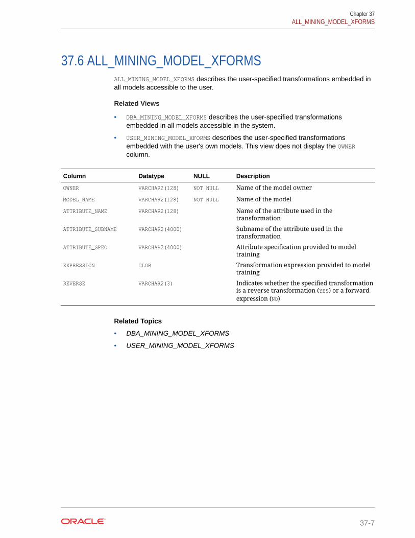
37.6 ALL_MINING_MODEL_XFORMSALL_MINING_MODEL_XFORMS describes the user-specified transformations embedded inall models accessible to the user.
Related Views
• DBA_MINING_MODEL_XFORMS describes the user-specified transformationsembedded in all models accessible in the system.
• USER_MINING_MODEL_XFORMS describes the user-specified transformationsembedded with the user's own models. This view does not display the OWNERcolumn.
Column Datatype NULL Description
OWNER VARCHAR2(128) NOT NULL Name of the model owner
MODEL_NAME VARCHAR2(128) NOT NULL Name of the model
ATTRIBUTE_NAME VARCHAR2(128) Name of the attribute used in thetransformation
ATTRIBUTE_SUBNAME VARCHAR2(4000) Subname of the attribute used in thetransformation
ATTRIBUTE_SPEC VARCHAR2(4000) Attribute specification provided to modeltraining
EXPRESSION CLOB Transformation expression provided to modeltraining
REVERSE VARCHAR2(3) Indicates whether the specified transformationis a reverse transformation (YES) or a forwardexpression (NO)
Related Topics
• DBA_MINING_MODEL_XFORMS
• USER_MINING_MODEL_XFORMS
Chapter 37ALL_MINING_MODEL_XFORMS
37-7

38SQL Scoring Functions
Data Mining functions are single-row functions that use Oracle Data Mining to scoredata. The functions can apply a mining model schema object to the data, or they candynamically mine the data by executing an analytic clause.
• CLUSTER_DETAILS
• CLUSTER_DISTANCE
• CLUSTER_ID
• CLUSTER_PROBABILITY
• CLUSTER_SET
• FEATURE_COMPARE
• FEATURE_DETAILS
• FEATURE_ID
• FEATURE_SET
• FEATURE_VALUE
• ORA_DM_PARTITION_NAME
• PREDICTION
• PREDICTION_BOUNDS
• PREDICTION_COST
• PREDICTION_DETAILS
• PREDICTION_PROBABILITY
• PREDICTION_SET
38.1 CLUSTER_DETAILSSyntax
cluster_details::=
CLUSTER_DETAILS (
schema .
model
, cluster_id
, topN
DESC
ASC
ABS
mining_attribute_clause )
38-1

Analytic Syntax
cluster_details_analytic::=
CLUSTER_DETAILS ( INTO n
, cluster_id
, topN
DESC
ASC
ABS
mining_attribute_clause ) OVER ( mining_analytic_clause )
mining_attribute_clause::=
USING
*
schema .
table . *
expr
AS alias
,
mining_analytic_clause::=
query_partition_clause order_by_clause
See Also:
"Analytic Functions" for information on the syntax, semantics, and restrictionsof mining_analytic_clause
Purpose
CLUSTER_DETAILS returns cluster details for each row in the selection. The return valueis an XML string that describes the attributes of the highest probability cluster or thespecified cluster_id.
Chapter 38CLUSTER_DETAILS
38-2
topN
If you specify a value for topN, the function returns the N attributes that most influencethe cluster assignment (the score). If you do not specify topN, the function returns the5 most influential attributes.
DESC, ASC, or ABS
The returned attributes are ordered by weight. The weight of an attribute expressesits positive or negative impact on cluster assignment. A positive weight indicates anincreased likelihood of assignment. A negative weight indicates a decreased likelihoodof assignment.
By default, CLUSTER_DETAILS returns the attributes with the highest positive weights(DESC). If you specify ASC, the attributes with the highest negative weights are returned.If you specify ABS, the attributes with the greatest weights, whether negative orpositive, are returned. The results are ordered by absolute value from highest tolowest. Attributes with a zero weight are not included in the output.
Syntax Choice
CLUSTER_DETAILS can score the data in one of two ways: It can apply a mining modelobject to the data, or it can dynamically mine the data by executing an analytic clausethat builds and applies one or more transient mining models. Choose Syntax orAnalytic Syntax:
• Syntax — Use the first syntax to score the data with a pre-defined model. Supplythe name of a clustering model.
• Analytic Syntax — Use the analytic syntax to score the data without apre-defined model. Include INTO n, where n is the number of clusters tocompute, and mining_analytic_clause, which specifies if the data should bepartitioned for multiple model builds. The mining_analytic_clause supports aquery_partition_clause and an order_by_clause. (See "analytic_clause::=".)
The syntax of the CLUSTER_DETAILS function can use an optional GROUPING hint whenscoring a partitioned model. See GROUPING Hint.
mining_attribute_clause
mining_attribute_clause identifies the column attributes to use as predictors forscoring. When the function is invoked with the analytic syntax, these predictors arealso used for building the transient models. The mining_attribute_clause behavesas described for the PREDICTION function. (See "mining_attribute_clause".)
See Also:
• Oracle Data Mining User's Guide for information about scoring.
• Oracle Data Mining Concepts for information about clustering.
Chapter 38CLUSTER_DETAILS
38-3
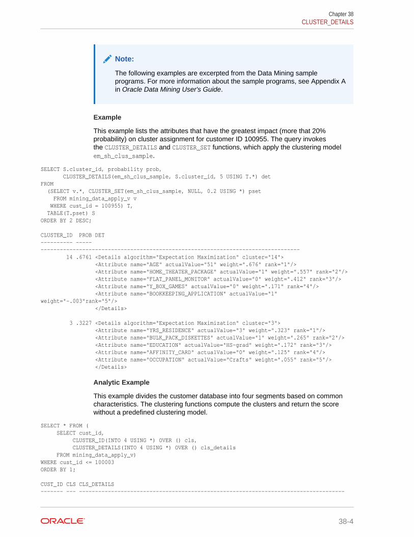
Note:
The following examples are excerpted from the Data Mining sampleprograms. For more information about the sample programs, see Appendix Ain Oracle Data Mining User's Guide.
Example
This example lists the attributes that have the greatest impact (more that 20%probability) on cluster assignment for customer ID 100955. The query invokesthe CLUSTER_DETAILS and CLUSTER_SET functions, which apply the clustering modelem_sh_clus_sample.
SELECT S.cluster_id, probability prob, CLUSTER_DETAILS(em_sh_clus_sample, S.cluster_id, 5 USING T.*) detFROM (SELECT v.*, CLUSTER_SET(em_sh_clus_sample, NULL, 0.2 USING *) pset FROM mining_data_apply_v v WHERE cust_id = 100955) T, TABLE(T.pset) SORDER BY 2 DESC; CLUSTER_ID PROB DET---------- ----- --------------------------------------------------------------------------------- 14 .6761 <Details algorithm="Expectation Maximization" cluster="14"> <Attribute name="AGE" actualValue="51" weight=".676" rank="1"/> <Attribute name="HOME_THEATER_PACKAGE" actualValue="1" weight=".557" rank="2"/> <Attribute name="FLAT_PANEL_MONITOR" actualValue="0" weight=".412" rank="3"/> <Attribute name="Y_BOX_GAMES" actualValue="0" weight=".171" rank="4"/> <Attribute name="BOOKKEEPING_APPLICATION" actualValue="1" weight="-.003"rank="5"/> </Details> 3 .3227 <Details algorithm="Expectation Maximization" cluster="3"> <Attribute name="YRS_RESIDENCE" actualValue="3" weight=".323" rank="1"/> <Attribute name="BULK_PACK_DISKETTES" actualValue="1" weight=".265" rank="2"/> <Attribute name="EDUCATION" actualValue="HS-grad" weight=".172" rank="3"/> <Attribute name="AFFINITY_CARD" actualValue="0" weight=".125" rank="4"/> <Attribute name="OCCUPATION" actualValue="Crafts" weight=".055" rank="5"/> </Details>
Analytic Example
This example divides the customer database into four segments based on commoncharacteristics. The clustering functions compute the clusters and return the scorewithout a predefined clustering model.
SELECT * FROM ( SELECT cust_id, CLUSTER_ID(INTO 4 USING *) OVER () cls, CLUSTER_DETAILS(INTO 4 USING *) OVER () cls_details FROM mining_data_apply_v)WHERE cust_id <= 100003ORDER BY 1; CUST_ID CLS CLS_DETAILS------- --- -----------------------------------------------------------------------------------
Chapter 38CLUSTER_DETAILS
38-4

100001 5 <Details algorithm="K-Means Clustering" cluster="5"> <Attribute name="FLAT_PANEL_MONITOR" actualValue="0" weight=".349" rank="1"/> <Attribute name="BULK_PACK_DISKETTES" actualValue="0" weight=".33" rank="2"/> <Attribute name="CUST_INCOME_LEVEL" actualValue="G: 130\,000 - 149\,999" weight=".291" rank="3"/> <Attribute name="HOME_THEATER_PACKAGE" actualValue="1" weight=".268" rank="4"/> <Attribute name="Y_BOX_GAMES" actualValue="0" weight=".179" rank="5"/> </Details>
100002 6 <Details algorithm="K-Means Clustering" cluster="6"> <Attribute name="CUST_GENDER" actualValue="F" weight=".945" rank="1"/> <Attribute name="CUST_MARITAL_STATUS" actualValue="NeverM" weight=".856" rank="2"/> <Attribute name="HOUSEHOLD_SIZE" actualValue="2" weight=".468" rank="3"/> <Attribute name="AFFINITY_CARD" actualValue="0" weight=".012" rank="4"/> <Attribute name="CUST_INCOME_LEVEL" actualValue="L: 300\,000 and above" weight=".009" rank="5"/> </Details> 100003 7 <Details algorithm="K-Means Clustering" cluster="7"> <Attribute name="CUST_MARITAL_STATUS" actualValue="NeverM" weight=".862" rank="1"/> <Attribute name="HOUSEHOLD_SIZE" actualValue="2" weight=".423" rank="2"/> <Attribute name="HOME_THEATER_PACKAGE" actualValue="0" weight=".113" rank="3"/> <Attribute name="AFFINITY_CARD" actualValue="0" weight=".007" rank="4"/> <Attribute name="CUST_ID" actualValue="100003" weight=".006" rank="5"/> </Details>
38.2 CLUSTER_DISTANCESyntax
cluster_distance::=
CLUSTER_DISTANCE (
schema .
model
, cluster_id
mining_attribute_clause )
Analytic Syntax
cluster_distance_analytic::=
CLUSTER_DISTANCE ( INTO n
, cluster_id
mining_attribute_clause )
OVER ( mining_analytic_clause )
Chapter 38CLUSTER_DISTANCE
38-5

mining_attribute_clause::=
USING
*
schema .
table . *
expr
AS alias
,
mining_analytic_clause::=
query_partition_clause order_by_clause
See Also:
"Analytic Functions" for information on the syntax, semantics, and restrictionsof mining_analytic_clause
Purpose
CLUSTER_DISTANCE returns a cluster distance for each row in the selection. The clusterdistance is the distance between the row and the centroid of the highest probabilitycluster or the specified cluster_id. The distance is returned as BINARY_DOUBLE.
Syntax Choice
CLUSTER_DISTANCE can score the data in one of two ways: It can apply a miningmodel object to the data, or it can dynamically mine the data by executing an analyticclause that builds and applies one or more transient mining models. Choose Syntax orAnalytic Syntax:
• Syntax — Use the first syntax to score the data with a pre-defined model. Supplythe name of a clustering model.
• Analytic Syntax — Use the analytic syntax to score the data without apre-defined model. Include INTO n, where n is the number of clusters tocompute, and mining_analytic_clause, which specifies if the data should bepartitioned for multiple model builds. The mining_analytic_clause supports aquery_partition_clause and an order_by_clause. (See "analytic_clause::=".)
The syntax of the CLUSTER_DISTANCE function can use an optional GROUPING hint whenscoring a partitioned model. See GROUPING Hint.
mining_attribute_clause
mining_attribute_clause identifies the column attributes to use as predictors forscoring. When the function is invoked with the analytic syntax, this data is also
Chapter 38CLUSTER_DISTANCE
38-6
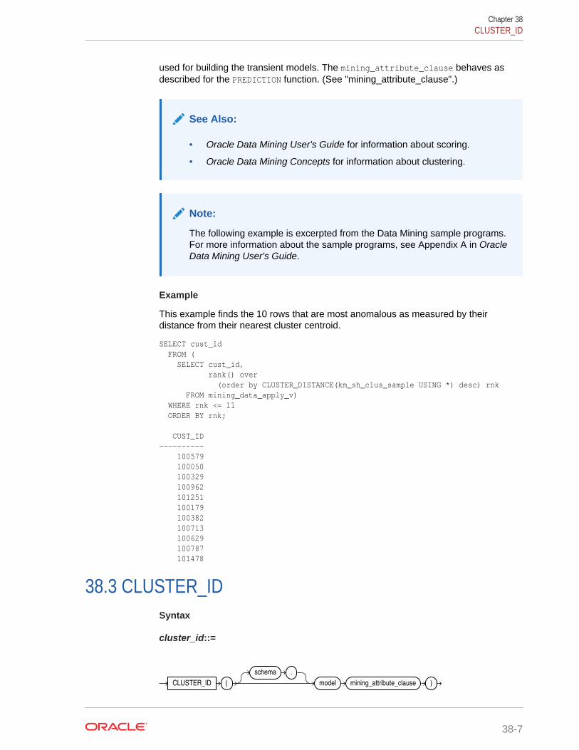
used for building the transient models. The mining_attribute_clause behaves asdescribed for the PREDICTION function. (See "mining_attribute_clause".)
See Also:
• Oracle Data Mining User's Guide for information about scoring.
• Oracle Data Mining Concepts for information about clustering.
Note:
The following example is excerpted from the Data Mining sample programs.For more information about the sample programs, see Appendix A in OracleData Mining User's Guide.
Example
This example finds the 10 rows that are most anomalous as measured by theirdistance from their nearest cluster centroid.
SELECT cust_id FROM ( SELECT cust_id, rank() over (order by CLUSTER_DISTANCE(km_sh_clus_sample USING *) desc) rnk FROM mining_data_apply_v) WHERE rnk <= 11 ORDER BY rnk; CUST_ID---------- 100579 100050 100329 100962 101251 100179 100382 100713 100629 100787 101478
38.3 CLUSTER_IDSyntax
cluster_id::=
CLUSTER_ID (
schema .
model mining_attribute_clause )
Chapter 38CLUSTER_ID
38-7

Analytic Syntax
cluster_id_analytic::=
CLUSTER_ID ( INTO n mining_attribute_clause ) OVER ( mining_analytic_clause )
mining_attribute_clause::=
USING
*
schema .
table . *
expr
AS alias
,
mining_analytic_clause::=
query_partition_clause order_by_clause
See Also:
"Analytic Functions" for information on the syntax, semantics, and restrictionsof mining_analytic_clause
Purpose
CLUSTER_ID returns the identifier of the highest probability cluster for each row in theselection. The cluster identifier is returned as an Oracle NUMBER.
Syntax Choice
CLUSTER_ID can score the data in one of two ways: It can apply a mining model objectto the data, or it can dynamically mine the data by executing an analytic clause thatbuilds and applies one or more transient mining models. Choose Syntax or AnalyticSyntax:
• Syntax — Use the first syntax to score the data with a pre-defined model. Supplythe name of a clustering model.
• Analytic Syntax — Use the analytic syntax to score the data without apre-defined model. Include INTO n, where n is the number of clusters tocompute, and mining_analytic_clause, which specifies if the data should bepartitioned for multiple model builds. The mining_analytic_clause supports aquery_partition_clause and an order_by_clause. (See "analytic_clause::=".)
Chapter 38CLUSTER_ID
38-8

The syntax of the CLUSTER_ID function can use an optional GROUPING hint when scoringa partitioned model. See GROUPING Hint.
mining_attribute_clause
mining_attribute_clause identifies the column attributes to use as predictors forscoring. When the function is invoked with the analytic syntax, these predictors arealso used for building the transient models. The mining_attribute_clause behavesas described for the PREDICTION function. (See "mining_attribute_clause".)
See Also:
• Oracle Data Mining User's Guide for information about scoring.
• Oracle Data Mining Concepts for information about clustering.
Note:
The following examples are excerpted from the Data Mining sampleprograms. For more information about the sample programs, see Appendix Ain Oracle Data Mining User's Guide.
Example
The following example lists the clusters into which the customers inmining_data_apply_v have been grouped.
SELECT CLUSTER_ID(km_sh_clus_sample USING *) AS clus, COUNT(*) AS cnt FROM mining_data_apply_v GROUP BY CLUSTER_ID(km_sh_clus_sample USING *) ORDER BY cnt DESC;
CLUS CNT---------- ---------- 2 580 10 216 6 186 8 115 19 110 12 101 18 81 16 39 17 38 14 34
Analytic Example
This example divides the customer database into four segments based on commoncharacteristics. The clustering functions compute the clusters and return the scorewithout a predefined clustering model.
SELECT * FROM ( SELECT cust_id, CLUSTER_ID(INTO 4 USING *) OVER () cls,
Chapter 38CLUSTER_ID
38-9

CLUSTER_DETAILS(INTO 4 USING *) OVER () cls_details FROM mining_data_apply_v)WHERE cust_id <= 100003ORDER BY 1; CUST_ID CLS CLS_DETAILS------- --- ----------------------------------------------------------------------------- 100001 5 <Details algorithm="K-Means Clustering" cluster="5"> <Attribute name="FLAT_PANEL_MONITOR" actualValue="0" weight=".349" rank="1"/> <Attribute name="BULK_PACK_DISKETTES" actualValue="0" weight=".33" rank="2"/> <Attribute name="CUST_INCOME_LEVEL" actualValue="G: 130\,000 - 149\,999" weight=".291" rank="3"/> <Attribute name="HOME_THEATER_PACKAGE" actualValue="1" weight=".268" rank="4"/> <Attribute name="Y_BOX_GAMES" actualValue="0" weight=".179" rank="5"/> </Details>
100002 6 <Details algorithm="K-Means Clustering" cluster="6"> <Attribute name="CUST_GENDER" actualValue="F" weight=".945" rank="1"/> <Attribute name="CUST_MARITAL_STATUS" actualValue="NeverM" weight=".856" rank="2"/> <Attribute name="HOUSEHOLD_SIZE" actualValue="2" weight=".468" rank="3"/> <Attribute name="AFFINITY_CARD" actualValue="0" weight=".012" rank="4"/> <Attribute name="CUST_INCOME_LEVEL" actualValue="L: 300\,000 and above" weight=".009" rank="5"/> </Details> 100003 7 <Details algorithm="K-Means Clustering" cluster="7"> <Attribute name="CUST_MARITAL_STATUS" actualValue="NeverM" weight=".862" rank="1"/> <Attribute name="HOUSEHOLD_SIZE" actualValue="2" weight=".423" rank="2"/> <Attribute name="HOME_THEATER_PACKAGE" actualValue="0" weight=".113" rank="3"/> <Attribute name="AFFINITY_CARD" actualValue="0" weight=".007" rank="4"/> <Attribute name="CUST_ID" actualValue="100003" weight=".006" rank="5"/> </Details>
38.4 CLUSTER_PROBABILITYSyntax
cluster_probability::=
CLUSTER_PROBABILITY (
schema .
model
, cluster_id
mining_attribute_clause )
Analytic Syntax
cluster_prob_analytic::=
CLUSTER_PROBABILITY ( INTO n
, cluster_id
mining_attribute_clause )
OVER ( mining_analytic_clause )
Chapter 38CLUSTER_PROBABILITY
38-10

mining_attribute_clause::=
USING
*
schema .
table . *
expr
AS alias
,
mining_analytic_clause::=
query_partition_clause order_by_clause
See Also:
"Analytic Functions" for information on the syntax, semantics, and restrictionsof mining_analytic_clause
Purpose
CLUSTER_PROBABILITY returns a probability for each row in the selection. Theprobability refers to the highest probability cluster or to the specified cluster_id. Thecluster probability is returned as BINARY_DOUBLE.
Syntax Choice
CLUSTER_PROBABILITY can score the data in one of two ways: It can apply a miningmodel object to the data, or it can dynamically mine the data by executing an analyticclause that builds and applies one or more transient mining models. Choose Syntax orAnalytic Syntax:
• Syntax — Use the first syntax to score the data with a pre-defined model. Supplythe name of a clustering model.
• Analytic Syntax — Use the analytic syntax to score the data without apre-defined model. Include INTO n, where n is the number of clusters tocompute, and mining_analytic_clause, which specifies if the data should bepartitioned for multiple model builds. The mining_analytic_clause supports aquery_partition_clause and an order_by_clause. (See "analytic_clause::=".)
The syntax of the CLUSTER_PROBABILITY function can use an optional GROUPING hintwhen scoring a partitioned model. See GROUPING Hint.
mining_attribute_clause
mining_attribute_clause identifies the column attributes to use as predictors forscoring. When the function is invoked with the analytic syntax, these predictors are
Chapter 38CLUSTER_PROBABILITY
38-11
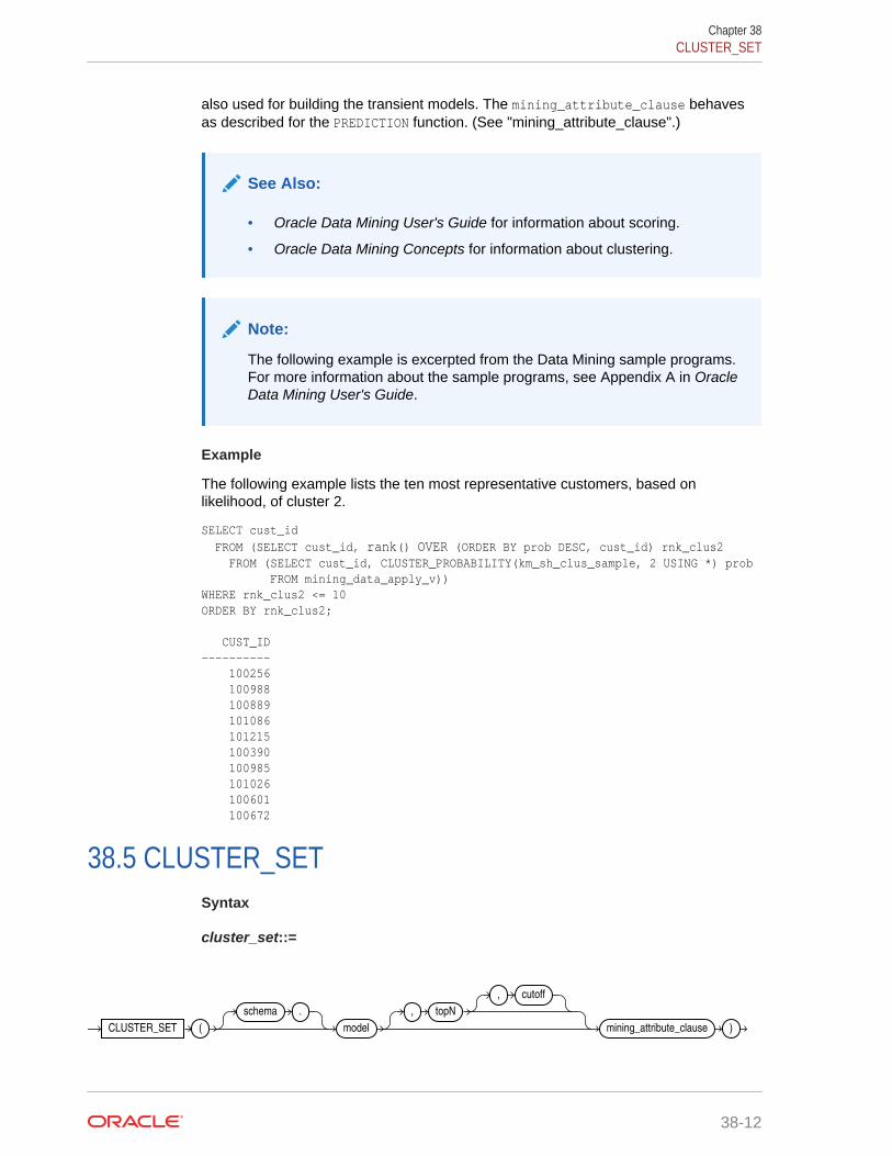
also used for building the transient models. The mining_attribute_clause behavesas described for the PREDICTION function. (See "mining_attribute_clause".)
See Also:
• Oracle Data Mining User's Guide for information about scoring.
• Oracle Data Mining Concepts for information about clustering.
Note:
The following example is excerpted from the Data Mining sample programs.For more information about the sample programs, see Appendix A in OracleData Mining User's Guide.
Example
The following example lists the ten most representative customers, based onlikelihood, of cluster 2.
SELECT cust_id FROM (SELECT cust_id, rank() OVER (ORDER BY prob DESC, cust_id) rnk_clus2 FROM (SELECT cust_id, CLUSTER_PROBABILITY(km_sh_clus_sample, 2 USING *) prob FROM mining_data_apply_v))WHERE rnk_clus2 <= 10ORDER BY rnk_clus2; CUST_ID---------- 100256 100988 100889 101086 101215 100390 100985 101026 100601 100672
38.5 CLUSTER_SETSyntax
cluster_set::=
CLUSTER_SET (
schema .
model
, topN
, cutoff
mining_attribute_clause )
Chapter 38CLUSTER_SET
38-12

Analytic Syntax
cluster_set_analytic::=
CLUSTER_SET ( INTO n
, topN
, cutoff
mining_attribute_clause )
OVER ( mining_analytic_clause )
mining_attribute_clause::=
USING
*
schema .
table . *
expr
AS alias
,
mining_analytic_clause::=
query_partition_clause order_by_clause
See Also:
"Analytic Functions" for information on the syntax, semantics, and restrictionsof mining_analytic_clause
Purpose
CLUSTER_SET returns a set of cluster ID and probability pairs for each row in theselection. The return value is a varray of objects with field names CLUSTER_IDand PROBABILITY. The cluster identifier is an Oracle NUMBER; the probability isBINARY_DOUBLE.
topN and cutoff
You can specify topN and cutoff to limit the number of clusters returned by thefunction. By default, both topN and cutoff are null and all clusters are returned.
• topN is the N most probable clusters. If multiple clusters share the Nth probability,then the function chooses one of them.
Chapter 38CLUSTER_SET
38-13

• cutoff is a probability threshold. Only clusters with probability greater than orequal to cutoff are returned. To filter by cutoff only, specify NULL for topN.
To return up to the N most probable clusters that are greater than or equal to cutoff,specify both topN and cutoff.
Syntax Choice
CLUSTER_SET can score the data in one of two ways: It can apply a mining model objectto the data, or it can dynamically mine the data by executing an analytic clause thatbuilds and applies one or more transient mining models. Choose Syntax or AnalyticSyntax:
• Syntax — Use the first syntax to score the data with a pre-defined model. Supplythe name of a clustering model.
• Analytic Syntax — Use the analytic syntax to score the data without apre-defined model. Include INTO n, where n is the number of clusters tocompute, and mining_analytic_clause, which specifies if the data should bepartitioned for multiple model builds. The mining_analytic_clause supports aquery_partition_clause and an order_by_clause. (See "analytic_clause::=".)
The syntax of the CLUSTER_SET function can use an optional GROUPING hint whenscoring a partitioned model. See GROUPING Hint.
mining_attribute_clause
mining_attribute_clause identifies the column attributes to use as predictors forscoring. When the function is invoked with the analytic syntax, these predictors arealso used for building the transient models. The mining_attribute_clause behavesas described for the PREDICTION function. (See "mining_attribute_clause".)
See Also:
• Oracle Data Mining User's Guide for information about scoring.
• Oracle Data Mining Concepts for information about clustering.
Note:
The following example is excerpted from the Data Mining sample programs.For more information about the sample programs, see Appendix A in OracleData Mining User's Guide.
Example
This example lists the attributes that have the greatest impact (more that 20%probability) on cluster assignment for customer ID 100955. The query invokesthe CLUSTER_DETAILS and CLUSTER_SET functions, which apply the clustering modelem_sh_clus_sample.
SELECT S.cluster_id, probability prob, CLUSTER_DETAILS(em_sh_clus_sample, S.cluster_id, 5 USING T.*) det
Chapter 38CLUSTER_SET
38-14

FROM (SELECT v.*, CLUSTER_SET(em_sh_clus_sample, NULL, 0.2 USING *) pset FROM mining_data_apply_v v WHERE cust_id = 100955) T, TABLE(T.pset) SORDER BY 2 DESC; CLUSTER_ID PROB DET---------- ----- ------------------------------------------------------------------------------ 14 .6761 <Details algorithm="Expectation Maximization" cluster="14"> <Attribute name="AGE" actualValue="51" weight=".676" rank="1"/> <Attribute name="HOME_THEATER_PACKAGE" actualValue="1" weight=".557" rank="2"/> <Attribute name="FLAT_PANEL_MONITOR" actualValue="0" weight=".412" rank="3"/> <Attribute name="Y_BOX_GAMES" actualValue="0" weight=".171" rank="4"/> <Attribute name="BOOKKEEPING_APPLICATION" actualValue="1" weight="-.003"rank="5"/> </Details> 3 .3227 <Details algorithm="Expectation Maximization" cluster="3"> <Attribute name="YRS_RESIDENCE" actualValue="3" weight=".323" rank="1"/> <Attribute name="BULK_PACK_DISKETTES" actualValue="1" weight=".265" rank="2"/> <Attribute name="EDUCATION" actualValue="HS-grad" weight=".172" rank="3"/> <Attribute name="AFFINITY_CARD" actualValue="0" weight=".125" rank="4"/> <Attribute name="OCCUPATION" actualValue="Crafts" weight=".055" rank="5"/> </Details>
38.6 FEATURE_COMPARESyntax
feature_compare::=
FEATURE_COMPARE (
schema .
model mining_attribute_clause AND mining_attribute_clause )
mining_attribute_clause::=
USING
*
schema .
table . *
expr
AS alias
,
Purpose
The FEATURE_COMPARE function uses a Feature Extraction model to compare twodifferent documents, including short ones such as keyword phrases or two attributelists, for similarity or dissimilarity. The FEATURE_COMPARE function can be used withFeature Extraction algorithms such as Singular Value Decomposition (SVD), Principal
Chapter 38FEATURE_COMPARE
38-15
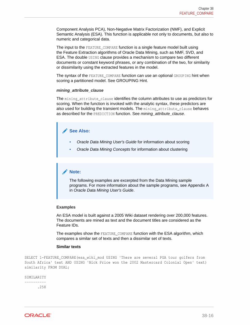
Component Analysis PCA), Non-Negative Matrix Factorization (NMF), and ExplicitSemantic Analysis (ESA). This function is applicable not only to documents, but also tonumeric and categorical data.
The input to the FEATURE_COMPARE function is a single feature model built usingthe Feature Extraction algorithms of Oracle Data Mining, such as NMF, SVD, andESA. The double USING clause provides a mechanism to compare two differentdocuments or constant keyword phrases, or any combination of the two, for similarityor dissimilarity using the extracted features in the model.
The syntax of the FEATURE_COMPARE function can use an optional GROUPING hint whenscoring a partitioned model. See GROUPING Hint.
mining_attribute_clause
The mining_attribute_clause identifies the column attributes to use as predictors forscoring. When the function is invoked with the analytic syntax, these predictors arealso used for building the transient models. The mining_attribute_clause behavesas described for the PREDICTION function. See mining_attribute_clause.
See Also:
• Oracle Data Mining User's Guide for information about scoring
• Oracle Data Mining Concepts for information about clustering
Note:
The following examples are excerpted from the Data Mining sampleprograms. For more information about the sample programs, see Appendix Ain Oracle Data Mining User's Guide.
Examples
An ESA model is built against a 2005 Wiki dataset rendering over 200,000 features.The documents are mined as text and the document titles are considered as theFeature IDs.
The examples show the FEATURE_COMPARE function with the ESA algorithm, whichcompares a similar set of texts and then a dissimilar set of texts.
Similar texts
SELECT 1-FEATURE_COMPARE(esa_wiki_mod USING 'There are several PGA tour golfers from South Africa' text AND USING 'Nick Price won the 2002 Mastercard Colonial Open' text) similarity FROM DUAL;
SIMILARITY---------- .258
Chapter 38FEATURE_COMPARE
38-16

The output metric shows the results of a distance calculation. Therefore, a smallernumber represents more similar texts. So 1 minus the distance in the queriesrepresents a document similarity metric.
Dissimilar texts
SELECT 1-FEATURE_COMPARE(esa_wiki_mod USING 'There are several PGA tour golfers from South Africa' text AND USING 'John Elway played quarterback for the Denver Broncos' text) similarity FROM DUAL;
SIMILARITY---------- .007
38.7 FEATURE_DETAILSSyntax
feature_details::=
FEATURE_DETAILS (
schema .
model
, feature_id
, topN
DESC
ASC
ABS
mining_attribute_clause )
Analytic Syntax
feature_details_analytic::=
FEATURE_DETAILS ( INTO n
, feature_id
, topN
DESC
ASC
ABS
mining_attribute_clause ) OVER ( mining_analytic_clause )
Chapter 38FEATURE_DETAILS
38-17
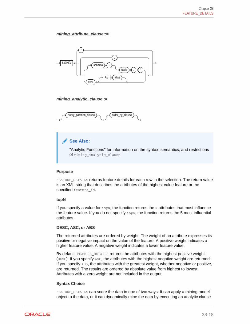
mining_attribute_clause::=
USING
*
schema .
table . *
expr
AS alias
,
mining_analytic_clause::=
query_partition_clause order_by_clause
See Also:
"Analytic Functions" for information on the syntax, semantics, and restrictionsof mining_analytic_clause
Purpose
FEATURE_DETAILS returns feature details for each row in the selection. The return valueis an XML string that describes the attributes of the highest value feature or thespecified feature_id.
topN
If you specify a value for topN, the function returns the N attributes that most influencethe feature value. If you do not specify topN, the function returns the 5 most influentialattributes.
DESC, ASC, or ABS
The returned attributes are ordered by weight. The weight of an attribute expresses itspositive or negative impact on the value of the feature. A positive weight indicates ahigher feature value. A negative weight indicates a lower feature value.
By default, FEATURE_DETAILS returns the attributes with the highest positive weight(DESC). If you specify ASC, the attributes with the highest negative weight are returned.If you specify ABS, the attributes with the greatest weight, whether negative or positive,are returned. The results are ordered by absolute value from highest to lowest.Attributes with a zero weight are not included in the output.
Syntax Choice
FEATURE_DETAILS can score the data in one of two ways: It can apply a mining modelobject to the data, or it can dynamically mine the data by executing an analytic clause
Chapter 38FEATURE_DETAILS
38-18

that builds and applies one or more transient mining models. Choose Syntax orAnalytic Syntax:
• Syntax — Use the first syntax to score the data with a pre-defined model. Supplythe name of a feature extraction model.
• Analytic Syntax — Use the analytic syntax to score the data without apre-defined model. Include INTO n, where n is the number of features toextract, and mining_analytic_clause, which specifies if the data should bepartitioned for multiple model builds. The mining_analytic_clause supports aquery_partition_clause and an order_by_clause. (See "analytic_clause::=".)
The syntax of the FEATURE_DETAILS function can use an optional GROUPING hint whenscoring a partitioned model. See GROUPING Hint.
mining_attribute_clause
mining_attribute_clause identifies the column attributes to use as predictors forscoring. When the function is invoked with the analytic syntax, these predictors arealso used for building the transient models. The mining_attribute_clause behavesas described for the PREDICTION function. (See "mining_attribute_clause".)
See Also:
• Oracle Data Mining User's Guide for information about scoring.
• Oracle Data Mining Concepts for information about feature extraction.
Note:
The following examples are excerpted from the Data Mining sampleprograms. For more information about the sample programs, see Appendix Ain Oracle Data Mining User's Guide.
Example
This example uses the feature extraction model nmf_sh_sample to score the data.The query returns the three features that best represent customer 100002 and theattributes that most affect those features.
SELECT S.feature_id fid, value val, FEATURE_DETAILS(nmf_sh_sample, S.feature_id, 5 using T.*) det FROM (SELECT v.*, FEATURE_SET(nmf_sh_sample, 3 USING *) fset FROM mining_data_apply_v v WHERE cust_id = 100002) T, TABLE(T.fset) SORDER BY 2 DESC; FID VAL DET---- ------ ------------------------------------------------------------------------------------ 5 3.492 <Details algorithm="Non-Negative Matrix Factorization" feature="5"> <Attribute name="BULK_PACK_DISKETTES" actualValue="1" weight=".077" rank="1"/> <Attribute name="OCCUPATION" actualValue="Prof." weight=".062" rank="2"/>
Chapter 38FEATURE_DETAILS
38-19
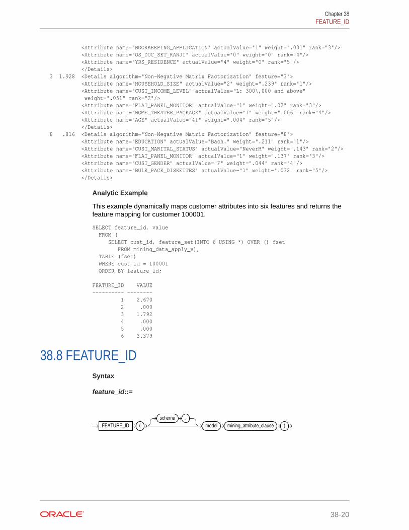
<Attribute name="BOOKKEEPING_APPLICATION" actualValue="1" weight=".001" rank="3"/> <Attribute name="OS_DOC_SET_KANJI" actualValue="0" weight="0" rank="4"/> <Attribute name="YRS_RESIDENCE" actualValue="4" weight="0" rank="5"/> </Details> 3 1.928 <Details algorithm="Non-Negative Matrix Factorization" feature="3"> <Attribute name="HOUSEHOLD_SIZE" actualValue="2" weight=".239" rank="1"/> <Attribute name="CUST_INCOME_LEVEL" actualValue="L: 300\,000 and above" weight=".051" rank="2"/> <Attribute name="FLAT_PANEL_MONITOR" actualValue="1" weight=".02" rank="3"/> <Attribute name="HOME_THEATER_PACKAGE" actualValue="1" weight=".006" rank="4"/> <Attribute name="AGE" actualValue="41" weight=".004" rank="5"/> </Details> 8 .816 <Details algorithm="Non-Negative Matrix Factorization" feature="8"> <Attribute name="EDUCATION" actualValue="Bach." weight=".211" rank="1"/> <Attribute name="CUST_MARITAL_STATUS" actualValue="NeverM" weight=".143" rank="2"/> <Attribute name="FLAT_PANEL_MONITOR" actualValue="1" weight=".137" rank="3"/> <Attribute name="CUST_GENDER" actualValue="F" weight=".044" rank="4"/> <Attribute name="BULK_PACK_DISKETTES" actualValue="1" weight=".032" rank="5"/> </Details>
Analytic Example
This example dynamically maps customer attributes into six features and returns thefeature mapping for customer 100001.
SELECT feature_id, value FROM ( SELECT cust_id, feature_set(INTO 6 USING *) OVER () fset FROM mining_data_apply_v), TABLE (fset) WHERE cust_id = 100001 ORDER BY feature_id; FEATURE_ID VALUE---------- -------- 1 2.670 2 .000 3 1.792 4 .000 5 .000 6 3.379
38.8 FEATURE_IDSyntax
feature_id::=
FEATURE_ID (
schema .
model mining_attribute_clause )
Chapter 38FEATURE_ID
38-20
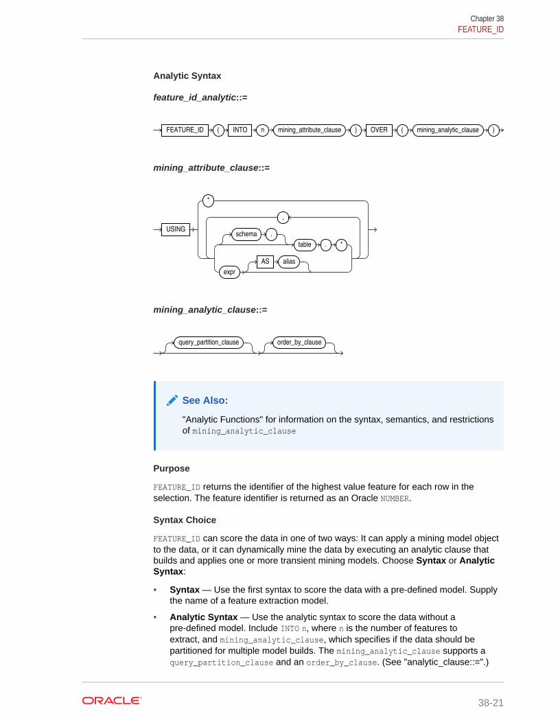
Analytic Syntax
feature_id_analytic::=
FEATURE_ID ( INTO n mining_attribute_clause ) OVER ( mining_analytic_clause )
mining_attribute_clause::=
USING
*
schema .
table . *
expr
AS alias
,
mining_analytic_clause::=
query_partition_clause order_by_clause
See Also:
"Analytic Functions" for information on the syntax, semantics, and restrictionsof mining_analytic_clause
Purpose
FEATURE_ID returns the identifier of the highest value feature for each row in theselection. The feature identifier is returned as an Oracle NUMBER.
Syntax Choice
FEATURE_ID can score the data in one of two ways: It can apply a mining model objectto the data, or it can dynamically mine the data by executing an analytic clause thatbuilds and applies one or more transient mining models. Choose Syntax or AnalyticSyntax:
• Syntax — Use the first syntax to score the data with a pre-defined model. Supplythe name of a feature extraction model.
• Analytic Syntax — Use the analytic syntax to score the data without apre-defined model. Include INTO n, where n is the number of features toextract, and mining_analytic_clause, which specifies if the data should bepartitioned for multiple model builds. The mining_analytic_clause supports aquery_partition_clause and an order_by_clause. (See "analytic_clause::=".)
Chapter 38FEATURE_ID
38-21

The syntax of the FEATURE_ID function can use an optional GROUPING hint when scoringa partitioned model. See GROUPING Hint.
mining_attribute_clause
mining_attribute_clause identifies the column attributes to use as predictors forscoring. When the function is invoked with the analytic syntax, these predictors arealso used for building the transient models. The mining_attribute_clause behavesas described for the PREDICTION function. (See "mining_attribute_clause".)
See Also:
• Oracle Data Mining User's Guide for information about scoring.
• Oracle Data Mining Concepts for information about feature extraction.
Note:
The following example is excerpted from the Data Mining sample programs.For more information about the sample programs, see Appendix A in OracleData Mining User's Guide.
Example
This example lists the features and corresponding count of customers in a data set.
SELECT FEATURE_ID(nmf_sh_sample USING *) AS feat, COUNT(*) AS cnt FROM nmf_sh_sample_apply_prepared GROUP BY FEATURE_ID(nmf_sh_sample USING *) ORDER BY cnt DESC, feat DESC;
FEAT CNT---------- ---------- 7 1443 2 49 3 6 6 1 1 1
38.9 FEATURE_SETSyntax
feature_set::=
FEATURE_SET (
schema .
model
, topN
, cutoff
mining_attribute_clause )
Chapter 38FEATURE_SET
38-22
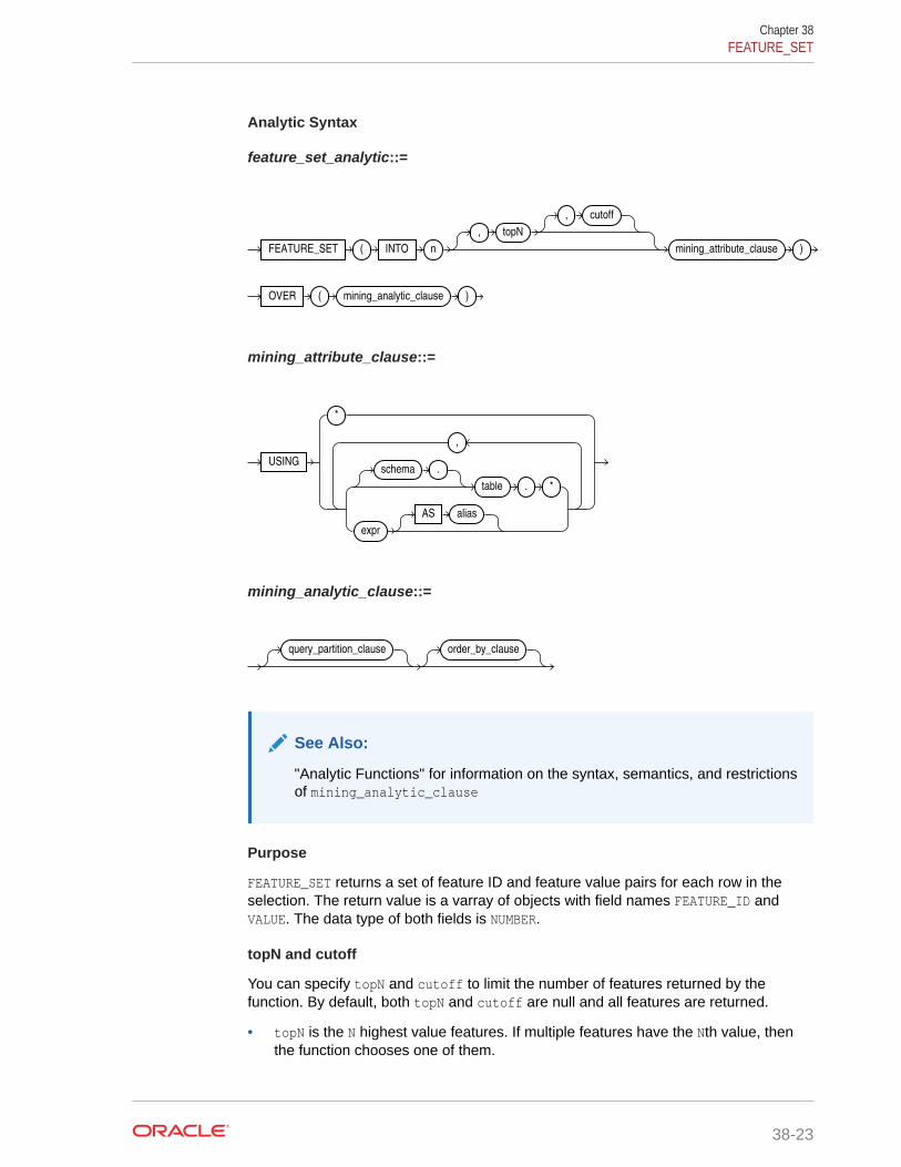
Analytic Syntax
feature_set_analytic::=
FEATURE_SET ( INTO n
, topN
, cutoff
mining_attribute_clause )
OVER ( mining_analytic_clause )
mining_attribute_clause::=
USING
*
schema .
table . *
expr
AS alias
,
mining_analytic_clause::=
query_partition_clause order_by_clause
See Also:
"Analytic Functions" for information on the syntax, semantics, and restrictionsof mining_analytic_clause
Purpose
FEATURE_SET returns a set of feature ID and feature value pairs for each row in theselection. The return value is a varray of objects with field names FEATURE_ID andVALUE. The data type of both fields is NUMBER.
topN and cutoff
You can specify topN and cutoff to limit the number of features returned by thefunction. By default, both topN and cutoff are null and all features are returned.
• topN is the N highest value features. If multiple features have the Nth value, thenthe function chooses one of them.
Chapter 38FEATURE_SET
38-23

• cutoff is a value threshold. Only features that are greater than or equal to cutoffare returned. To filter by cutoff only, specify NULL for topN.
To return up to N features that are greater than or equal to cutoff, specify both topNand cutoff.
Syntax Choice
FEATURE_SET can score the data in one of two ways: It can apply a mining model objectto the data, or it can dynamically mine the data by executing an analytic clause thatbuilds and applies one or more transient mining models. Choose Syntax or AnalyticSyntax:
• Syntax — Use the first syntax to score the data with a pre-defined model. Supplythe name of a feature extraction model.
• Analytic Syntax — Use the analytic syntax to score the data without apre-defined model. Include INTO n, where n is the number of features toextract, and mining_analytic_clause, which specifies if the data should bepartitioned for multiple model builds. The mining_analytic_clause supports aquery_partition_clause and an order_by_clause. (See "analytic_clause::=".)
The syntax of the FEATURE_SET function can use an optional GROUPING hint whenscoring a partitioned model. See GROUPING Hint.
mining_attribute_clause
mining_attribute_clause identifies the column attributes to use as predictors forscoring. When the function is invoked with the analytic syntax, these predictors arealso used for building the transient models. The mining_attribute_clause behavesas described for the PREDICTION function. (See "mining_attribute_clause".)
See Also:
• Oracle Data Mining User's Guide for information about scoring.
• Oracle Data Mining Concepts for information about feature extraction.
Note:
The following example is excerpted from the Data Mining sample programs.For more information about the sample programs, see Appendix A in OracleData Mining User's Guide.
Example
This example lists the top features corresponding to a given customer record anddetermines the top attributes for each feature (based on coefficient > 0.25).
WITHfeat_tab AS (SELECT F.feature_id fid, A.attribute_name attr,
Chapter 38FEATURE_SET
38-24

TO_CHAR(A.attribute_value) val, A.coefficient coeff FROM TABLE(DBMS_DATA_MINING.GET_MODEL_DETAILS_NMF('nmf_sh_sample')) F, TABLE(F.attribute_set) A WHERE A.coefficient > 0.25),feat AS (SELECT fid, CAST(COLLECT(Featattr(attr, val, coeff)) AS Featattrs) f_attrs FROM feat_tabGROUP BY fid),cust_10_features AS (SELECT T.cust_id, S.feature_id, S.value FROM (SELECT cust_id, FEATURE_SET(nmf_sh_sample, 10 USING *) pset FROM nmf_sh_sample_apply_prepared WHERE cust_id = 100002) T, TABLE(T.pset) S)SELECT A.value, A.feature_id fid, B.attr, B.val, B.coeff FROM cust_10_features A, (SELECT T.fid, F.* FROM feat T, TABLE(T.f_attrs) F) B WHERE A.feature_id = B.fidORDER BY A.value DESC, A.feature_id ASC, coeff DESC, attr ASC, val ASC;
VALUE FID ATTR VAL COEFF-------- ---- ------------------------- ------------------------ ------- 6.8409 7 YRS_RESIDENCE 1.3879 6.8409 7 BOOKKEEPING_APPLICATION .4388 6.8409 7 CUST_GENDER M .2956 6.8409 7 COUNTRY_NAME United States of America .2848 6.4975 3 YRS_RESIDENCE 1.2668 6.4975 3 BOOKKEEPING_APPLICATION .3465 6.4975 3 COUNTRY_NAME United States of America .2927 6.4886 2 YRS_RESIDENCE 1.3285 6.4886 2 CUST_GENDER M .2819 6.4886 2 PRINTER_SUPPLIES .2704 6.3953 4 YRS_RESIDENCE 1.2931 5.9640 6 YRS_RESIDENCE 1.1585 5.9640 6 HOME_THEATER_PACKAGE .2576 5.2424 5 YRS_RESIDENCE 1.0067 2.4714 8 YRS_RESIDENCE .3297 2.3559 1 YRS_RESIDENCE .2768 2.3559 1 FLAT_PANEL_MONITOR .2593
38.10 FEATURE_VALUESyntax
feature_value::=
FEATURE_VALUE (
schema .
model
, feature_id
mining_attribute_clause )
Chapter 38FEATURE_VALUE
38-25
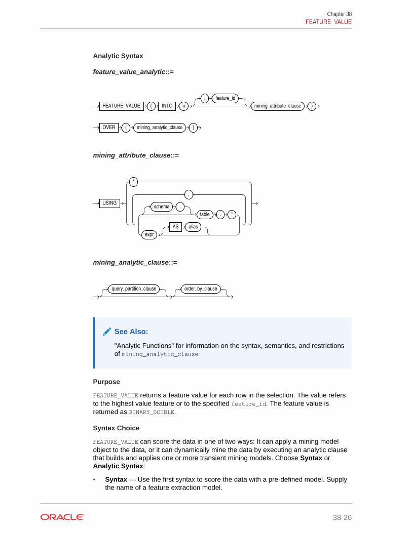
Analytic Syntax
feature_value_analytic::=
FEATURE_VALUE ( INTO n
, feature_id
mining_attribute_clause )
OVER ( mining_analytic_clause )
mining_attribute_clause::=
USING
*
schema .
table . *
expr
AS alias
,
mining_analytic_clause::=
query_partition_clause order_by_clause
See Also:
"Analytic Functions" for information on the syntax, semantics, and restrictionsof mining_analytic_clause
Purpose
FEATURE_VALUE returns a feature value for each row in the selection. The value refersto the highest value feature or to the specified feature_id. The feature value isreturned as BINARY_DOUBLE.
Syntax Choice
FEATURE_VALUE can score the data in one of two ways: It can apply a mining modelobject to the data, or it can dynamically mine the data by executing an analytic clausethat builds and applies one or more transient mining models. Choose Syntax orAnalytic Syntax:
• Syntax — Use the first syntax to score the data with a pre-defined model. Supplythe name of a feature extraction model.
Chapter 38FEATURE_VALUE
38-26

• Analytic Syntax — Use the analytic syntax to score the data without apre-defined model. Include INTO n, where n is the number of features toextract, and mining_analytic_clause, which specifies if the data should bepartitioned for multiple model builds. The mining_analytic_clause supports aquery_partition_clause and an order_by_clause. (See "analytic_clause::=".)
The syntax of the FEATURE_VALUE function can use an optional GROUPING hint whenscoring a partitioned model. See GROUPING Hint.
mining_attribute_clause
mining_attribute_clause identifies the column attributes to use as predictors forscoring. When the function is invoked with the analytic syntax, this data is alsoused for building the transient models. The mining_attribute_clause behaves asdescribed for the PREDICTION function. (See "mining_attribute_clause".)
See Also:
• Oracle Data Mining User's Guide for information about scoring.
• Oracle Data Mining Concepts for information about feature extraction.
Note:
The following example is excerpted from the Data Mining sample programs.For more information about the sample programs, see Appendix A in OracleData Mining User's Guide.
Example
The following example lists the customers that correspond to feature 3, ordered bymatch quality.
SELECT * FROM (SELECT cust_id, FEATURE_VALUE(nmf_sh_sample, 3 USING *) match_quality FROM nmf_sh_sample_apply_prepared ORDER BY match_quality DESC) WHERE ROWNUM < 11;
CUST_ID MATCH_QUALITY---------- ------------- 100210 19.4101627 100962 15.2482251 101151 14.5685197 101499 14.4186292 100363 14.4037396 100372 14.3335148 100982 14.1716545 101039 14.1079914 100759 14.0913761 100953 14.0799737
Chapter 38FEATURE_VALUE
38-27

38.11 ORA_DM_PARTITION_NAMESyntax
ORA_DM_PARTITION_NAME (
schema .
model mining_attribute_clause )
mining_attribute_clause::=
USING
*
schema .
table . *
expr
AS alias
,
Purpose
ORA_DM_PARTITION_NAME is a single row function that works along with other existingfunctions. This function returns the name of the partition associated with the input row.When ORA_DM_PARTITION_NAME is used on a non-partitioned model, the result is NULL.
The syntax of the ORA_DM_PARTITION_NAME function can use an optional GROUPING hintwhen scoring a partitioned model. See GROUPING Hint.
mining_attribute_clause
The mining_attribute_clause identifies the column attributes to use as predictors forscoring. When the function is invoked with the analytic syntax, these predictors arealso used for building the transient models. The mining_attribute_clause behavesas described for the PREDICTION function. See mining_attribute_clause.
See Also:
• Oracle Data Mining User's Guide for information about scoring
• Oracle Data Mining Concepts for information about clustering
Note:
The following examples are excerpted from the Data Mining sampleprograms. For more information about the sample programs, see Appendix Ain Oracle Data Mining User's Guide.
Chapter 38ORA_DM_PARTITION_NAME
38-28

Example
SELECT prediction(mymodel using *) pred, ora_dm_partition_name(mymodel USING *) pname FROM customers;
38.12 PREDICTIONSyntax
prediction::=
PREDICTION (
grouping_hint schema .
model
cost_matrix_clause
mining_attribute_clause )
Analytic Syntax
prediction_analytic::=
PREDICTION (OF ANOMALY
FOR expr
cost_matrix_clause
mining_attribute_clause )
OVER ( mining_analytic_clause )
cost_matrix_clause::=
COST
MODEL
AUTO
( class_value
,
) VALUES ( ( cost_value
,
)
,
)
mining_attribute_clause::=
USING
*
schema .
table . *
expr
AS alias
,
Chapter 38PREDICTION
38-29

mining_analytic_clause::=
query_partition_clause order_by_clause
See Also:
"Analytic Functions" for information on the syntax, semantics, and restrictionsof mining_analytic_clause
Purpose
PREDICTION returns a prediction for each row in the selection. The data type ofthe returned prediction depends on whether the function performs Regression,Classification, or Anomaly Detection.
• Regression: Returns the expected target value for each row. The data type of thereturn value is the data type of the target.
• Classification: Returns the most probable target class (or lowest cost targetclass, if costs are specified) for each row. The data type of the return value isthe data type of the target.
• Anomaly Detection: Returns 1 or 0 for each row. Typical rows are classified as 1.Rows that differ significantly from the rest of the data are classified as 0.
cost_matrix_clause
Costs are a biasing factor for minimizing the most harmful kinds of misclassifications.You can specify cost_matrix_clause for Classification or Anomaly Detection. Costsare not relevant for Regression. The cost_matrix_clause behaves as described for"PREDICTION COST".
Syntax Choice
PREDICTION can score data in one of two ways: It can apply a mining model objectto the data, or it can dynamically score the data by executing an analytic clause thatbuilds and applies one or more transient mining models. Choose Syntax or AnalyticSyntax:
• Syntax: Use this syntax to score the data with a pre-defined model. Supply thename of a model that performs Classification, Regression, or Anomaly Detection.
• Analytic Syntax: Use the analytic syntax to score the data without apre-defined model. The analytic syntax uses mining_analytic_clause ,which specifies if the data should be partitioned for multiple model builds.The mining_analytic_clause supports a query_partition_clause and anorder_by_clause. (See "analytic_clause::=".)
– For Regression, specify FOR expr, where expr is an expression that identifies atarget column that has a numeric data type.
– For Classification, specify FOR expr, where expr is an expression that identifiesa target column that has a character data type.
Chapter 38PREDICTION
38-30

– For Anomaly Detection, specify the keywords OF ANOMALY.
The syntax of the PREDICTION function can use an optional GROUPING hint when scoringa partitioned model. See GROUPING Hint.
mining_attribute_clause
mining_attribute_clause identifies the column attributes to use as predictors forscoring.
• If you specify USING *, all the relevant attributes present in the input row are used.
• If you invoke the function with the analytic syntax, the mining_attribute_clauseis used both for building the transient models and for scoring.
• It you invoke the function with a pre-defined model, the mining_attribute_clauseshould include all or some of the attributes that were used to create the model.The following conditions apply:
– If mining_attribute_clause includes an attribute with the same name but adifferent data type from the one that was used to create the model, then thedata type is converted to the type expected by the model.
– If you specify more attributes for scoring than were used to create the model,then the extra attributes are silently ignored.
– If you specify fewer attributes for scoring than were used to create the model,then scoring is performed on a best-effort basis.
See Also:
• Oracle Data Mining User's Guide for information about scoring.
• Oracle Data Mining Concepts for information about predictive datamining.
• Appendix C in Oracle Database Globalization Support Guide for thecollation derivation rules, which define the collation assigned to thereturn value of PREDICTION when it is a character value
Note:
The following examples are excerpted from the Data Mining sampleprograms. For more information about the sample programs, see Appendix Ain Oracle Data Mining User's Guide.
Example
In this example, the model dt_sh_clas_sample predicts the gender and age ofcustomers who are most likely to use an affinity card (target = 1). The PREDICTIONfunction takes into account the cost matrix associated with the model and uses maritalstatus, education, and household size as predictors.
SELECT cust_gender, COUNT(*) AS cnt, ROUND(AVG(age)) AS avg_age FROM mining_data_apply_v
Chapter 38PREDICTION
38-31
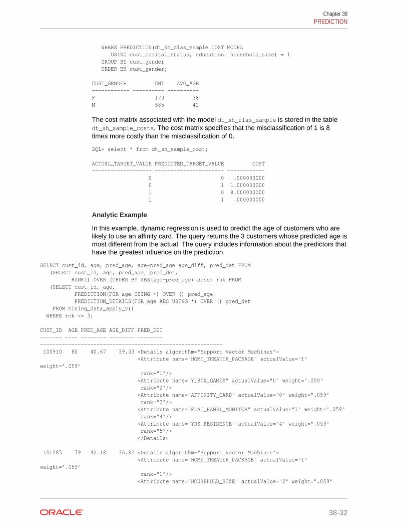
WHERE PREDICTION(dt_sh_clas_sample COST MODEL USING cust_marital_status, education, household_size) = 1 GROUP BY cust_gender ORDER BY cust_gender; CUST_GENDER CNT AVG_AGE------------ ---------- ----------F 170 38M 685 42
The cost matrix associated with the model dt_sh_clas_sample is stored in the tabledt_sh_sample_costs. The cost matrix specifies that the misclassification of 1 is 8times more costly than the misclassification of 0.
SQL> select * from dt_sh_sample_cost; ACTUAL_TARGET_VALUE PREDICTED_TARGET_VALUE COST------------------- ---------------------- ------------ 0 0 .000000000 0 1 1.000000000 1 0 8.000000000 1 1 .000000000
Analytic Example
In this example, dynamic regression is used to predict the age of customers who arelikely to use an affinity card. The query returns the 3 customers whose predicted age ismost different from the actual. The query includes information about the predictors thathave the greatest influence on the prediction.
SELECT cust_id, age, pred_age, age-pred_age age_diff, pred_det FROM (SELECT cust_id, age, pred_age, pred_det, RANK() OVER (ORDER BY ABS(age-pred_age) desc) rnk FROM (SELECT cust_id, age, PREDICTION(FOR age USING *) OVER () pred_age, PREDICTION_DETAILS(FOR age ABS USING *) OVER () pred_det FROM mining_data_apply_v)) WHERE rnk <= 3; CUST_ID AGE PRED_AGE AGE_DIFF PRED_DET------- ---- -------- -------- -------- ---------------------------------------------------------- 100910 80 40.67 39.33 <Details algorithm="Support Vector Machines"> <Attribute name="HOME_THEATER_PACKAGE" actualValue="1" weight=".059" rank="1"/> <Attribute name="Y_BOX_GAMES" actualValue="0" weight=".059" rank="2"/> <Attribute name="AFFINITY_CARD" actualValue="0" weight=".059" rank="3"/> <Attribute name="FLAT_PANEL_MONITOR" actualValue="1" weight=".059" rank="4"/> <Attribute name="YRS_RESIDENCE" actualValue="4" weight=".059" rank="5"/> </Details> 101285 79 42.18 36.82 <Details algorithm="Support Vector Machines"> <Attribute name="HOME_THEATER_PACKAGE" actualValue="1" weight=".059" rank="1"/> <Attribute name="HOUSEHOLD_SIZE" actualValue="2" weight=".059"
Chapter 38PREDICTION
38-32
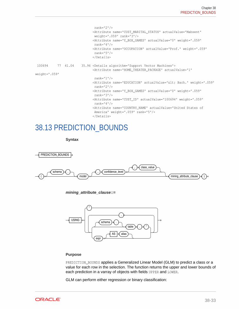
rank="2"/> <Attribute name="CUST_MARITAL_STATUS" actualValue="Mabsent" weight=".059" rank="3"/> <Attribute name="Y_BOX_GAMES" actualValue="0" weight=".059" rank="4"/> <Attribute name="OCCUPATION" actualValue="Prof." weight=".059" rank="5"/> </Details> 100694 77 41.04 35.96 <Details algorithm="Support Vector Machines"> <Attribute name="HOME_THEATER_PACKAGE" actualValue="1" weight=".059" rank="1"/> <Attribute name="EDUCATION" actualValue="< Bach." weight=".059" rank="2"/> <Attribute name="Y_BOX_GAMES" actualValue="0" weight=".059" rank="3"/> <Attribute name="CUST_ID" actualValue="100694" weight=".059" rank="4"/> <Attribute name="COUNTRY_NAME" actualValue="United States of America" weight=".059" rank="5"/> </Details>
38.13 PREDICTION_BOUNDSSyntax
PREDICTION_BOUNDS
(
schema .
model
, confidence_level
, class_value
mining_attribute_clause )
mining_attribute_clause::=
USING
*
schema .
table . *
expr
AS alias
,
Purpose
PREDICTION_BOUNDS applies a Generalized Linear Model (GLM) to predict a class or avalue for each row in the selection. The function returns the upper and lower bounds ofeach prediction in a varray of objects with fields UPPER and LOWER.
GLM can perform either regression or binary classification:
Chapter 38PREDICTION_BOUNDS
38-33
• The bounds for regression refer to the predicted target value. The data type ofUPPER and LOWER is the data type of the target.
• The bounds for binary classification refer to the probability of either the predictedtarget class or the specified class_value. The data type of UPPER and LOWER isBINARY_DOUBLE.
If the model was built using ridge regression, or if the covariance matrix is found to besingular during the build, then PREDICTION_BOUNDS returns NULL for both bounds.
confidence_level is a number in the range (0,1). The default value is 0.95. You canspecify class_value while leaving confidence_level at its default by specifying NULLfor confidence_level.
The syntax of the PREDICTION_BOUNDS function can use an optional GROUPING hintwhen scoring a partitioned model. See GROUPING Hint.
mining_attribute_clause
mining_attribute_clause identifies the column attributes to use as predictors forscoring. This clause behaves as described for the PREDICTION function. (Note that thereference to analytic syntax does not apply.) See "mining_attribute_clause".
See Also:
• Oracle Data Mining User's Guide for information about scoring
• Oracle Data Mining Concepts for information about Generalized LinearModels
Note:
The following example is excerpted from the Data Mining sample programs.For more information about the sample programs, see Appendix A in OracleData Mining User's Guide.
Example
The following example returns the distribution of customers whose ages are predictedwith 98% confidence to be greater than 24 and less than 46.
SELECT count(cust_id) cust_count, cust_marital_status FROM (SELECT cust_id, cust_marital_status FROM mining_data_apply_v WHERE PREDICTION_BOUNDS(glmr_sh_regr_sample,0.98 USING *).LOWER > 24 AND PREDICTION_BOUNDS(glmr_sh_regr_sample,0.98 USING *).UPPER < 46) GROUP BY cust_marital_status; CUST_COUNT CUST_MARITAL_STATUS-------------- -------------------- 46 NeverM 7 Mabsent 5 Separ.
Chapter 38PREDICTION_BOUNDS
38-34
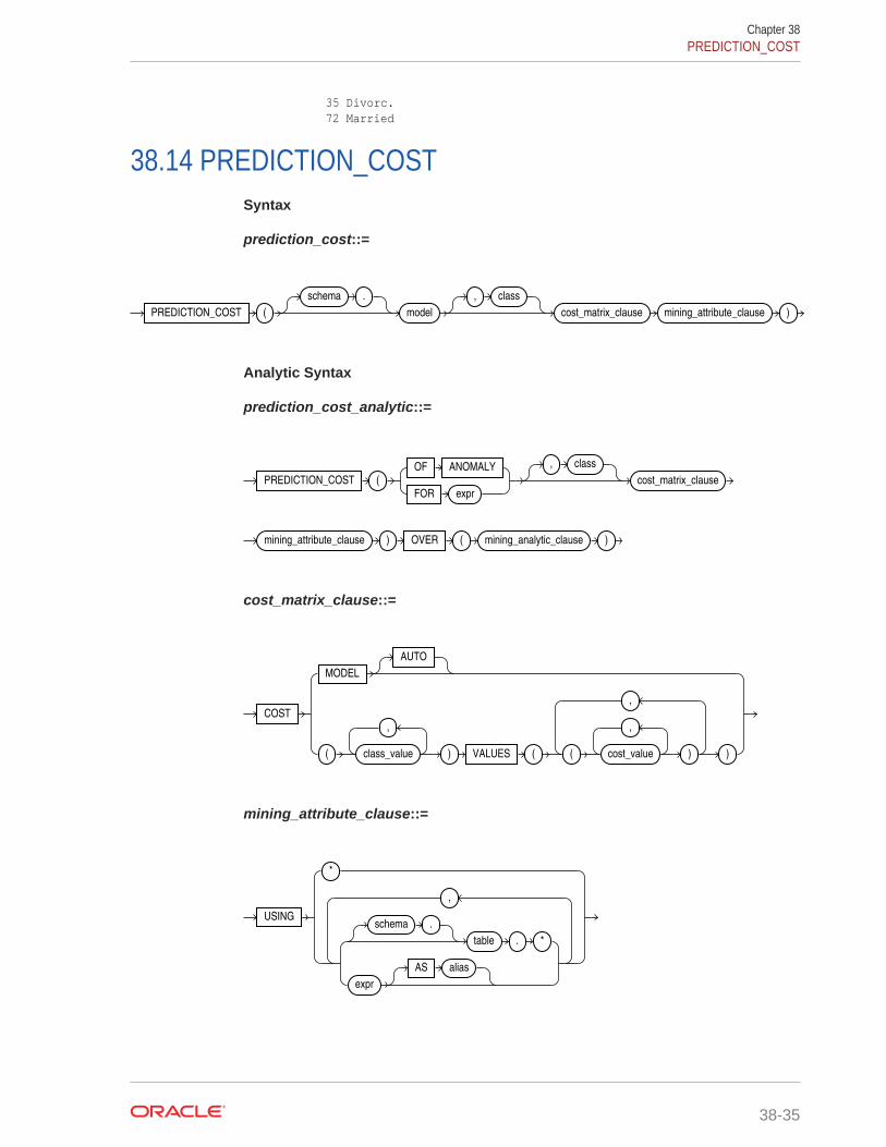
35 Divorc. 72 Married
38.14 PREDICTION_COSTSyntax
prediction_cost::=
PREDICTION_COST (
schema .
model
, class
cost_matrix_clause mining_attribute_clause )
Analytic Syntax
prediction_cost_analytic::=
PREDICTION_COST (OF ANOMALY
FOR expr
, class
cost_matrix_clause
mining_attribute_clause ) OVER ( mining_analytic_clause )
cost_matrix_clause::=
COST
MODEL
AUTO
( class_value
,
) VALUES ( ( cost_value
,
)
,
)
mining_attribute_clause::=
USING
*
schema .
table . *
expr
AS alias
,
Chapter 38PREDICTION_COST
38-35
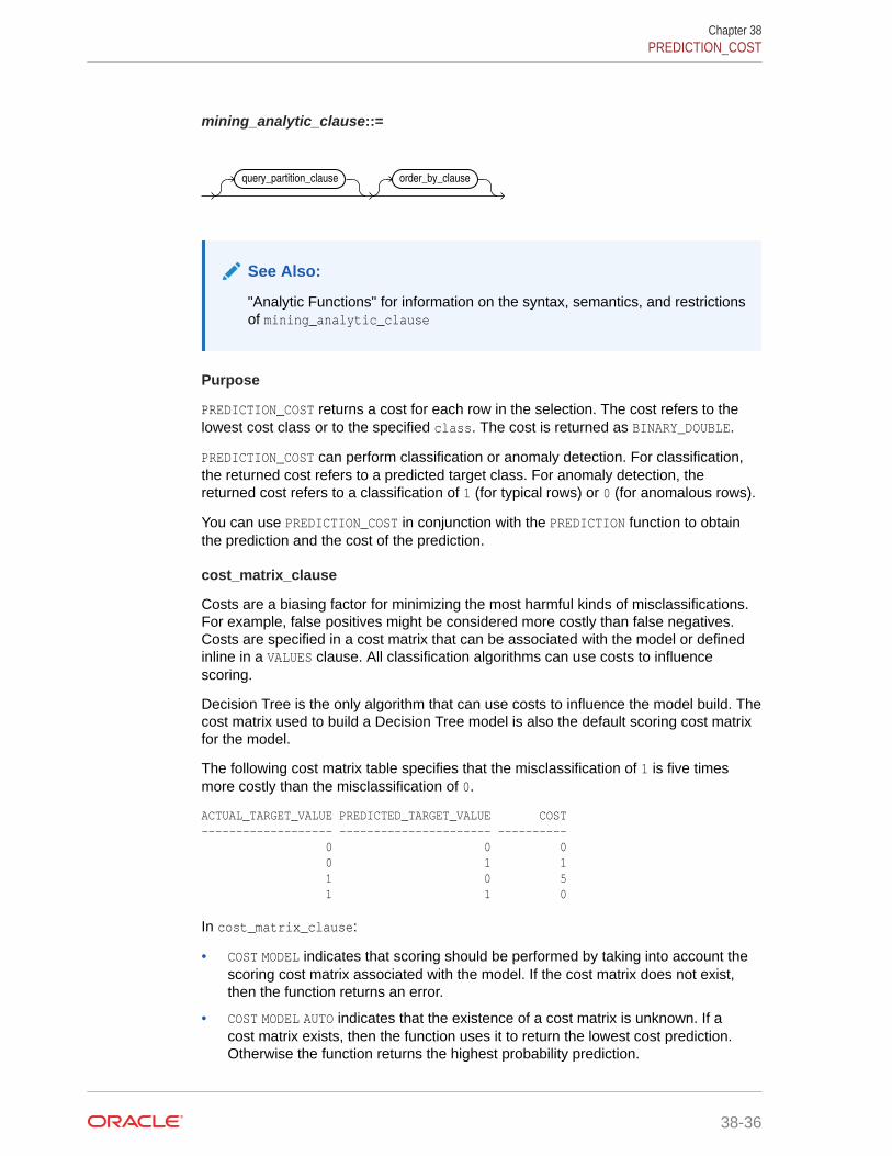
mining_analytic_clause::=
query_partition_clause order_by_clause
See Also:
"Analytic Functions" for information on the syntax, semantics, and restrictionsof mining_analytic_clause
Purpose
PREDICTION_COST returns a cost for each row in the selection. The cost refers to thelowest cost class or to the specified class. The cost is returned as BINARY_DOUBLE.
PREDICTION_COST can perform classification or anomaly detection. For classification,the returned cost refers to a predicted target class. For anomaly detection, thereturned cost refers to a classification of 1 (for typical rows) or 0 (for anomalous rows).
You can use PREDICTION_COST in conjunction with the PREDICTION function to obtainthe prediction and the cost of the prediction.
cost_matrix_clause
Costs are a biasing factor for minimizing the most harmful kinds of misclassifications.For example, false positives might be considered more costly than false negatives.Costs are specified in a cost matrix that can be associated with the model or definedinline in a VALUES clause. All classification algorithms can use costs to influencescoring.
Decision Tree is the only algorithm that can use costs to influence the model build. Thecost matrix used to build a Decision Tree model is also the default scoring cost matrixfor the model.
The following cost matrix table specifies that the misclassification of 1 is five timesmore costly than the misclassification of 0.
ACTUAL_TARGET_VALUE PREDICTED_TARGET_VALUE COST------------------- ---------------------- ---------- 0 0 0 0 1 1 1 0 5 1 1 0
In cost_matrix_clause:
• COST MODEL indicates that scoring should be performed by taking into account thescoring cost matrix associated with the model. If the cost matrix does not exist,then the function returns an error.
• COST MODEL AUTO indicates that the existence of a cost matrix is unknown. If acost matrix exists, then the function uses it to return the lowest cost prediction.Otherwise the function returns the highest probability prediction.
Chapter 38PREDICTION_COST
38-36

• The VALUES clause specifies an inline cost matrix for class_value. For example,you could specify that the misclassification of 1 is five times more costly than themisclassification of 0 as follows:
PREDICTION (nb_model COST (0,1) VALUES ((0, 1),(1, 5)) USING *)
If a model that has a scoring cost matrix is invoked with an inline cost matrix, thenthe inline costs are used.
See Also:
Oracle Data Mining User's Guide for more information about cost-sensitive prediction.
Syntax Choice
PREDICTION_COST can score the data in one of two ways: It can apply a mining modelobject to the data, or it can dynamically mine the data by executing an analytic clausethat builds and applies one or more transient mining models. Choose Syntax orAnalytic Syntax:
• Syntax — Use the first syntax to score the data with a pre-defined model. Supplythe name of a model that performs classification or anomaly detection.
• Analytic Syntax — Use the analytic syntax to score the data withouta pre-defined model. The analytic syntax uses mining_analytic_clause ,which specifies if the data should be partitioned for multiple model builds.The mining_analytic_clause supports a query_partition_clause and anorder_by_clause. (See "analytic_clause::=".)
– For classification, specify FOR expr, where expr is an expression that identifiesa target column that has a character data type.
– For anomaly detection, specify the keywords OF ANOMALY.
The syntax of the PREDICTION_COST function can use an optional GROUPING hint whenscoring a partitioned model. See GROUPING Hint.
mining_attribute_clause
mining_attribute_clause identifies the column attributes to use as predictors forscoring. When the function is invoked with the analytic syntax, these predictors arealso used for building the transient models. The mining_attribute_clause behavesas described for the PREDICTION function. (See "mining_attribute_clause".)
See Also:
• Oracle Data Mining User's Guide for information about scoring.
• Oracle Data Mining Concepts for information about classification withcosts
Chapter 38PREDICTION_COST
38-37

Note:
The following example is excerpted from the Data Mining sample programs.For more information about the sample programs, see Appendix A in OracleData Mining User's Guide.
Example
This example predicts the ten customers in Italy who would respond to the leastexpensive sales campaign (offering an affinity card).
SELECT cust_id FROM (SELECT cust_id,rank() OVER (ORDER BY PREDICTION_COST(DT_SH_Clas_sample, 1 COST MODEL USING *) ASC, cust_id) rnk FROM mining_data_apply_v WHERE country_name = 'Italy') WHERE rnk <= 10 ORDER BY rnk; CUST_ID---------- 100081 100179 100185 100324 100344 100554 100662 100733 101250 101306
38.15 PREDICTION_DETAILSSyntax
prediction_details::=
PREDICTION_DETAILS (
schema .
model
, class_value
, topN
DESC
ASC
ABS
mining_attribute_clause )
Chapter 38PREDICTION_DETAILS
38-38

Analytic Syntax
prediction_details_analytic::=
PREDICTION_DETAILS (OF ANOMALY
FOR expr
, class_value
, topN
DESC
ASC
ABS
mining_attribute_clause ) OVER ( mining_analytic_clause )
mining_attribute_clause::=
USING
*
schema .
table . *
expr
AS alias
,
mining_analytic_clause::=
query_partition_clause order_by_clause
See Also:
"Analytic Functions" for information on the syntax, semantics, and restrictionsof mining_analytic_clause
Purpose
PREDICTION_DETAILS returns prediction details for each row in the selection. The returnvalue is an XML string that describes the attributes of the prediction.
For regression, the returned details refer to the predicted target value. Forclassification and anomaly detection, the returned details refer to the highestprobability class or the specified class_value.
Chapter 38PREDICTION_DETAILS
38-39

topN
If you specify a value for topN, the function returns the N attributes that have the mostinfluence on the prediction (the score). If you do not specify topN, the function returnsthe 5 most influential attributes.
DESC, ASC, or ABS
The returned attributes are ordered by weight. The weight of an attribute expressesits positive or negative impact on the prediction. For regression, a positive weightindicates a higher value prediction; a negative weight indicates a lower valueprediction. For classification and anomaly detection, a positive weight indicates ahigher probability prediction; a negative weight indicates a lower probability prediction.
By default, PREDICTION_DETAILS returns the attributes with the highest positive weight(DESC). If you specify ASC, the attributes with the highest negative weight are returned.If you specify ABS, the attributes with the greatest weight, whether negative or positive,are returned. The results are ordered by absolute value from highest to lowest.Attributes with a zero weight are not included in the output.
Syntax Choice
PREDICTION_DETAILS can score the data in one of two ways: It can apply a miningmodel object to the data, or it can dynamically mine the data by executing an analyticclause that builds and applies one or more transient mining models. Choose Syntax orAnalytic Syntax:
• Syntax — Use the first syntax to score the data with a pre-defined model. Supplythe name of a model that performs classification, regression, or anomaly detection.
• Analytic Syntax — Use the analytic syntax to score the data withouta pre-defined model. The analytic syntax uses mining_analytic_clause,which specifies if the data should be partitioned for multiple model builds.The mining_analytic_clause supports a query_partition_clause and anorder_by_clause. (See "analytic_clause::=".)
– For classification, specify FOR expr, where expr is an expression that identifiesa target column that has a character data type.
– For regression, specify FOR expr, where expr is an expression that identifies atarget column that has a numeric data type.
– For anomaly detection, specify the keywords OF ANOMALY.
The syntax of the PREDICTION_DETAILS function can use an optional GROUPING hintwhen scoring a partitioned model. See GROUPING Hint.
mining_attribute_clause
mining_attribute_clause identifies the column attributes to use as predictors forscoring. When the function is invoked with the analytic syntax, these predictors arealso used for building the transient models. The mining_attribute_clause behavesas described for the PREDICTION function. (See "mining_attribute_clause".)
Chapter 38PREDICTION_DETAILS
38-40

See Also:
• Oracle Data Mining User's Guide for information about scoring.
• Oracle Data Mining Concepts for information about predictive datamining.
Note:
The following examples are excerpted from the Data Mining sampleprograms. For more information about the sample programs, see Appendix Ain Oracle Data Mining User's Guide.
Example
This example uses the model svmr_sh_regr_sample to score the data. The queryreturns the three attributes that have the greatest influence on predicting a highervalue for customer age.
SELECT PREDICTION_DETAILS(svmr_sh_regr_sample, null, 3 USING *) prediction_details FROM mining_data_apply_v WHERE cust_id = 100001; PREDICTION_DETAILS---------------------------------------------------------------------------------------<Details algorithm="Support Vector Machines"><Attribute name="CUST_MARITAL_STATUS" actualValue="Widowed" weight=".361" rank="1"/><Attribute name="CUST_GENDER" actualValue="F" weight=".14" rank="2"/><Attribute name="HOME_THEATER_PACKAGE" actualValue="1" weight=".135" rank="3"/></Details>
Analytic Syntax
This example dynamically identifies customers whose age is not typical for the data.The query returns the attributes that predict or detract from a typical age.
SELECT cust_id, age, pred_age, age-pred_age age_diff, pred_det FROM (SELECT cust_id, age, pred_age, pred_det, RANK() OVER (ORDER BY ABS(age-pred_age) DESC) rnk FROM (SELECT cust_id, age, PREDICTION(FOR age USING *) OVER () pred_age, PREDICTION_DETAILS(FOR age ABS USING *) OVER () pred_det FROM mining_data_apply_v)) WHERE rnk <= 5; CUST_ID AGE PRED_AGE AGE_DIFF PRED_DET------- --- -------- -------- ------------------------------------------------------------------ 100910 80 40.67 39.33 <Details algorithm="Support Vector Machines"> <Attribute name="HOME_THEATER_PACKAGE" actualValue="1" weight=".059" rank="1"/> <Attribute name="Y_BOX_GAMES" actualValue="0" weight=".059" rank="2"/> <Attribute name="AFFINITY_CARD" actualValue="0" weight=".059" rank="3"/>
Chapter 38PREDICTION_DETAILS
38-41
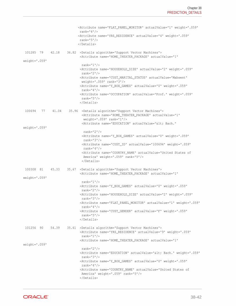
<Attribute name="FLAT_PANEL_MONITOR" actualValue="1" weight=".059" rank="4"/> <Attribute name="YRS_RESIDENCE" actualValue="4" weight=".059" rank="5"/> </Details> 101285 79 42.18 36.82 <Details algorithm="Support Vector Machines"> <Attribute name="HOME_THEATER_PACKAGE" actualValue="1" weight=".059" rank="1"/> <Attribute name="HOUSEHOLD_SIZE" actualValue="2" weight=".059" rank="2"/> <Attribute name="CUST_MARITAL_STATUS" actualValue="Mabsent" weight=".059" rank="3"/> <Attribute name="Y_BOX_GAMES" actualValue="0" weight=".059" rank="4"/> <Attribute name="OCCUPATION" actualValue="Prof." weight=".059" rank="5"/> </Details> 100694 77 41.04 35.96 <Details algorithm="Support Vector Machines"> <Attribute name="HOME_THEATER_PACKAGE" actualValue="1" weight=".059" rank="1"/> <Attribute name="EDUCATION" actualValue="< Bach." weight=".059" rank="2"/> <Attribute name="Y_BOX_GAMES" actualValue="0" weight=".059" rank="3"/> <Attribute name="CUST_ID" actualValue="100694" weight=".059" rank="4"/> <Attribute name="COUNTRY_NAME" actualValue="United States of America" weight=".059" rank="5"/> </Details> 100308 81 45.33 35.67 <Details algorithm="Support Vector Machines"> <Attribute name="HOME_THEATER_PACKAGE" actualValue="1" weight=".059" rank="1"/> <Attribute name="Y_BOX_GAMES" actualValue="0" weight=".059" rank="2"/> <Attribute name="HOUSEHOLD_SIZE" actualValue="2" weight=".059" rank="3"/> <Attribute name="FLAT_PANEL_MONITOR" actualValue="1" weight=".059" rank="4"/> <Attribute name="CUST_GENDER" actualValue="F" weight=".059" rank="5"/> </Details> 101256 90 54.39 35.61 <Details algorithm="Support Vector Machines"> <Attribute name="YRS_RESIDENCE" actualValue="9" weight=".059" rank="1"/> <Attribute name="HOME_THEATER_PACKAGE" actualValue="1" weight=".059" rank="2"/> <Attribute name="EDUCATION" actualValue="< Bach." weight=".059" rank="3"/> <Attribute name="Y_BOX_GAMES" actualValue="0" weight=".059" rank="4"/> <Attribute name="COUNTRY_NAME" actualValue="United States of America" weight=".059" rank="5"/> </Details>
Chapter 38PREDICTION_DETAILS
38-42

38.16 PREDICTION_PROBABILITYSyntax
prediction_probability::=
PREDICTION_PROBABILITY (
schema .
model
, class
mining_attribute_clause )
Analytic Syntax
prediction_prob_analytic::=
PREDICTION_PROBABILITY (OF ANOMALY
FOR expr
, class
mining_attribute_clause )
OVER ( mining_analytic_clause )
mining_attribute_clause::=
USING
*
schema .
table . *
expr
AS alias
,
mining_analytic_clause::=
query_partition_clause order_by_clause
See Also:
"Analytic Functions" for information on the syntax, semantics, and restrictionsof mining_analytic_clause
Chapter 38PREDICTION_PROBABILITY
38-43

Purpose
PREDICTION_PROBABILITY returns a probability for each row in the selection. Theprobability refers to the highest probability class or to the specified class. The datatype of the returned probability is BINARY_DOUBLE.
PREDICTION_PROBABILITY can perform classification or anomaly detection. Forclassification, the returned probability refers to a predicted target class. For anomalydetection, the returned probability refers to a classification of 1 (for typical rows) or 0(for anomalous rows).
You can use PREDICTION_PROBABILITY in conjunction with the PREDICTION function toobtain the prediction and the probability of the prediction.
Syntax Choice
PREDICTION_PROBABILITY can score the data in one of two ways: It can apply a miningmodel object to the data, or it can dynamically mine the data by executing an analyticclause that builds and applies one or more transient mining models. Choose Syntax orAnalytic Syntax:
• Syntax — Use the first syntax to score the data with a pre-defined model. Supplythe name of a model that performs classification or anomaly detection.
• Analytic Syntax — Use the analytic syntax to score the data withouta pre-defined model. The analytic syntax uses mining_analytic_clause,which specifies if the data should be partitioned for multiple model builds.The mining_analytic_clause supports a query_partition_clause and anorder_by_clause. (See "analytic_clause::=".)
– For classification, specify FOR expr, where expr is an expression that identifiesa target column that has a character data type.
– For anomaly detection, specify the keywords OF ANOMALY.
The syntax of the PREDICTION_PROBABILITY function can use an optional GROUPING hintwhen scoring a partitioned model. See GROUPING Hint.
mining_attribute_clause
mining_attribute_clause identifies the column attributes to use as predictors forscoring. When the function is invoked with the analytic syntax, these predictors arealso used for building the transient models. The mining_attribute_clause behavesas described for the PREDICTION function. (See "mining_attribute_clause".)
See Also:
• Oracle Data Mining User's Guide for information about scoring.
• Oracle Data Mining Concepts for information about predictive datamining.
Chapter 38PREDICTION_PROBABILITY
38-44

Note:
The following examples are excerpted from the Data Mining sampleprograms. For information about the sample programs, see Appendix A inOracle Data Mining User's Guide.
Example
The following example returns the 10 customers living in Italy who are most likely touse an affinity card.
SELECT cust_id FROM ( SELECT cust_id FROM mining_data_apply_v WHERE country_name = 'Italy' ORDER BY PREDICTION_PROBABILITY(DT_SH_Clas_sample, 1 USING *) DESC, cust_id) WHERE rownum < 11; CUST_ID---------- 100081 100179 100185 100324 100344 100554 100662 100733 101250 101306
Analytic Example
This example identifies rows that are most atypical in the data inmining_data_one_class_v. Each type of marital status is considered separately sothat the most anomalous rows per marital status group are returned.
The query returns three attributes that have the most influence on the determinationof anomalous rows. The PARTITION BY clause causes separate models to be built andapplied for each marital status. Because there is only one record with status Mabsent,no model is created for that partition (and no details are provided).
SELECT cust_id, cust_marital_status, rank_anom, anom_det FROM (SELECT cust_id, cust_marital_status, anom_det, rank() OVER (PARTITION BY CUST_MARITAL_STATUS ORDER BY ANOM_PROB DESC,cust_id) rank_anom FROM (SELECT cust_id, cust_marital_status, PREDICTION_PROBABILITY(OF ANOMALY, 0 USING *) OVER (PARTITION BY CUST_MARITAL_STATUS) anom_prob, PREDICTION_DETAILS(OF ANOMALY, 0, 3 USING *) OVER (PARTITION BY CUST_MARITAL_STATUS) anom_det FROM mining_data_one_class_v )) WHERE rank_anom < 3 order by 2, 3;
CUST_ID CUST_MARITAL_STATUS RANK_ANOM ANOM_DET------- ------------------- ----------
Chapter 38PREDICTION_PROBABILITY
38-45

-----------------------------------------------------------102366 Divorc. 1 <Details algorithm="Support Vector Machines" class="0"> <Attribute name="COUNTRY_NAME" actualValue="United Kingdom" weight=".069" rank="1"/> <Attribute name="AGE" actualValue="28" weight=".013" rank="2"/> <Attribute name="YRS_RESIDENCE" actualValue="4" weight=".006" rank="3"/> </Details>
101817 Divorc. 2 <Details algorithm="Support Vector Machines" class="0"> <Attribute name="YRS_RESIDENCE" actualValue="8" weight=".018" rank="1"/> <Attribute name="EDUCATION" actualValue="PhD" weight=".007" rank="2"/> <Attribute name="CUST_INCOME_LEVEL" actualValue="K: 250\,000 - 299\,999" weight=".006" rank="3"/> </Details> 101713 Mabsent 1 101790 Married 1 <Details algorithm="Support Vector Machines" class="0"> <Attribute name="COUNTRY_NAME" actualValue="Canada" weight=".063" rank="1"/> <Attribute name="EDUCATION" actualValue="7th-8th" weight=".011" rank="2"/> <Attribute name="HOUSEHOLD_SIZE" actualValue="4-5" weight=".011" rank="3"/> </Details>. . .
38.17 PREDICTION_SETSyntax
prediction_set::=
PREDICTION_SET (
schema .
model
, bestN
, cutoff
cost_matrix_clause
mining_attribute_clause )
Chapter 38PREDICTION_SET
38-46
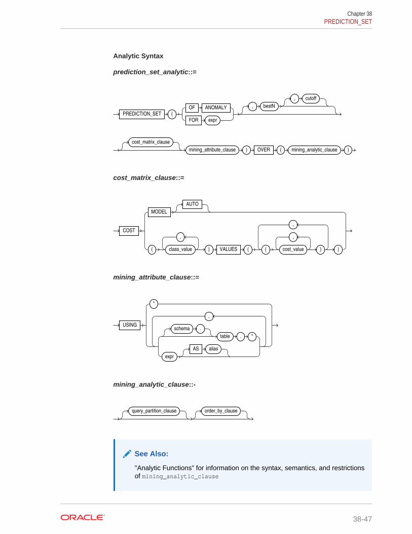
Analytic Syntax
prediction_set_analytic::=
PREDICTION_SET (OF ANOMALY
FOR expr
, bestN
, cutoff
cost_matrix_clause
mining_attribute_clause ) OVER ( mining_analytic_clause )
cost_matrix_clause::=
COST
MODEL
AUTO
( class_value
,
) VALUES ( ( cost_value
,
)
,
)
mining_attribute_clause::=
USING
*
schema .
table . *
expr
AS alias
,
mining_analytic_clause::-
query_partition_clause order_by_clause
See Also:
"Analytic Functions" for information on the syntax, semantics, and restrictionsof mining_analytic_clause
Chapter 38PREDICTION_SET
38-47
Purpose
PREDICTION_SET returns a set of predictions with either probabilities or costs foreach row in the selection. The return value is a varray of objects with field namesPREDICTION_ID and PROBABILITY or COST. The prediction identifier is an Oracle NUMBER;the probability and cost fields are BINARY_DOUBLE.
PREDICTION_SET can perform classification or anomaly detection. For classification, thereturn value refers to a predicted target class. For anomaly detection, the return valuerefers to a classification of 1 (for typical rows) or 0 (for anomalous rows).
bestN and cutoff
You can specify bestN and cutoff to limit the number of predictions returned by thefunction. By default, both bestN and cutoff are null and all predictions are returned.
• bestN is the N predictions that are either the most probable or the least costly. Ifmultiple predictions share the Nth probability or cost, then the function choosesone of them.
• cutoff is a value threshold. Only predictions with probability greater than or equalto cutoff, or with cost less than or equal to cutoff, are returned. To filter bycutoff only, specify NULL for bestN. If the function uses a cost_matrix_clausewith COST MODEL AUTO, then cutoff is ignored.
You can specify bestN with cutoff to return up to the N most probable predictions thatare greater than or equal to cutoff. If costs are used, specify bestN with cutoff toreturn up to the N least costly predictions that are less than or equal to cutoff.
cost_matrix_clause
You can specify cost_matrix_clause as a biasing factor for minimizing the mostharmful kinds of misclassifications. cost_matrix_clause behaves as described for"PREDICTION_COST ".
Syntax Choice
PREDICTION_SET can score the data in one of two ways: It can apply a mining modelobject to the data, or it can dynamically mine the data by executing an analytic clausethat builds and applies one or more transient mining models. Choose Syntax orAnalytic Syntax:
• Syntax — Use the first syntax to score the data with a pre-defined model. Supplythe name of a model that performs classification or anomaly detection.
• Analytic Syntax — Use the analytic syntax to score the data withouta pre-defined model. The analytic syntax uses mining_analytic_clause,which specifies if the data should be partitioned for multiple model builds.The mining_analytic_clause supports a query_partition_clause and anorder_by_clause. (See "analytic_clause::=".)
– For classification, specify FOR expr, where expr is an expression that identifiesa target column that has a character data type.
– For anomaly detection, specify the keywords OF ANOMALY.
The syntax of the PREDICTION_SET function can use an optional GROUPING hint whenscoring a partitioned model. See GROUPING Hint.
Chapter 38PREDICTION_SET
38-48

mining_attribute_clause
mining_attribute_clause identifies the column attributes to use as predictors forscoring. When the function is invoked with the analytic syntax, these predictors arealso used for building the transient models. The mining_attribute_clause behavesas described for the PREDICTION function. (See "mining_attribute_clause".)
See Also:
• Oracle Data Mining User's Guide for information about scoring.
• Oracle Data Mining Concepts for information about predictive datamining.
Note:
The following example is excerpted from the Data Mining sample programs.For more information about the sample programs, see Appendix A in OracleData Mining User's Guide.
Example
This example lists the probability and cost that customers with ID less than 100006 willuse an affinity card. This example has a binary target, but such a query is also usefulfor multiclass classification such as low, medium, and high.
SELECT T.cust_id, S.prediction, S.probability, S.cost FROM (SELECT cust_id, PREDICTION_SET(dt_sh_clas_sample COST MODEL USING *) pset FROM mining_data_apply_v WHERE cust_id < 100006) T, TABLE(T.pset) SORDER BY cust_id, S.prediction; CUST_ID PREDICTION PROBABILITY COST---------- ---------- ------------ ------------ 100001 0 .966183575 .270531401 100001 1 .033816425 .966183575 100002 0 .740384615 2.076923077 100002 1 .259615385 .740384615 100003 0 .909090909 .727272727 100003 1 .090909091 .909090909 100004 0 .909090909 .727272727 100004 1 .090909091 .909090909 100005 0 .272357724 5.821138211 100005 1 .727642276 .272357724
Chapter 38PREDICTION_SET
38-49