
Oxygen Relationships in Streams
206
Oxygen Relationships in Streams Proceedings of a Seminar sponsored by the Water Supply and Water Pol- lution Program of the Sanitary Engineering Center, October 30 - November 1, 1957 U. S. DEPARTMENT OF HEALTH, EDUCATION, AND WELFARE Public Health Service Bureau of State Services Division of Sanitary Engineering Services Robert A. Taft Sanitary Engineering Center Cincinnati 26, Ohio March 1958
-
Upload
khangminh22 -
Category
Documents
-
view
0 -
download
0
Transcript of Oxygen Relationships in Streams

Oxygen Relationships in Streams
Proceedings of a Seminar sponsored by the Water Supply and Water Pol-lution Program of the Sanitary Engineering Center, October 30 - November 1, 1957
U. S. DEPARTMENT OF HEALTH, EDUCATION, AND WELFARE Public Health Service
Bureau of State Services Division of Sanitary Engineering Services
Robert A. Taft Sanitary Engineering Center Cincinnati 26, Ohio
March 1958


OXYGEN RELATIONSHIPS IN STREAMS
DEDICATION
These Proceedings are dedicated to Harold W. Streeter, Sanitary Engineering Director (Retired), who contri-buted so much to the initial studies that led to the mathematical understanding of oxygen relationships in streams.


OXYGEN RELATIONSHIPS IN STREAMS V
Foreword
HARRY G. HANSON, Director Robert A. Taft Sanitary Engineering Center
Dissolved oxygen relationships have long been of basic importance in the water environment. In fact, they have been perhaps the single most Important set of relationships -- except possible bacteriological re-lationships -- with respect to maintenance of water quality in the last half century. It is likely that the oxygen balance will continue to be significant even as we move from a period of primary concern with domestic wastes into a period of greater concern with complex in-dustrial wastes.
This is the first national seminar sponsored by the Public Health Service on dissolved oxygen relationships. It is intended to serve as a forum for scientific discussions. As such it provides an opportunity for ex-change of views between scientists; for summarizing our present state of knowledge; and for identifying unsolved problems. In addition, this seminar constitutes a recognition of the contribution made by such pioneers as Streeter, Phelps, Hoskins, Theriault, Kehr, Butterfield, Purdy, Ruchhoft and many others. We are honored to have a foremost representative of these pioneers, Mr. Streeter, as a participant in this Seminar.
The summary of current knowledge, concepts and status that emerges from these discussions should serve as a valuable reference for those concerned with the oxygen resources in streams and other aquatic en-vironments.
The Seminar was developed and sponsored by the Water Supply and Water Pollution Program specifically, Mr. W. W. Towne, Chief, Water Pollution Control; Dr. A. F. Bartsch, Biologist; Dr. E. C. Tsivoglou, In Charge, Radioactivity Studies in Water Quality Management; Mr. F. W. Kittrell, In Charge, Stream Sanitation Studies; and Mr. R. Porges, In Charge, Waste Treatment Studies.
The collection of papers contained herein was assembled and organized by Mr. R. Porges. Editorial review of papers and of formal written dis-cussions was kept to a minimum. Informal remarks were reviewed by the speakers. In view of this procedure and to expedite publication, printing proceeded without proof of printed text by the authors.
These published Proceedings are furnished as a part of the research, technical assistance and technical training services of the Sanitary Engineering Center. We hope they will be useful to engineers and scientists in public agencies, universities, industry, and other institu-tions -- and that they will contribute to forward progress in waste treatment and stream improvement.


OXYGEN RELATIONSHIPS IN STREAMS VII
Pr e f ace
BERNARD B. BERGER, Chief, Water Supply and Water Pollution Program Robert A. Taft Sanitary Engineering Center
Our main purpose in holding this Seminar is to stop and take note of where we stand with respect to our ability to make optimum use of our streams' dissolved oxygen resource. There is clearly no better way to take stock of our position than to confer with our colleagues from States, universities, industry, and consulting agencies who, like us, are in-terested in this matter. We feel very fortunate that we have here engineers and allied scientists who are among the foremost in the Nation in appraising a stream's ability to accept a putrescible waste. We are also fortunate that we have participants, and you are all in-cluded, who look "loaded for bear" so to speak.
As a Federal agency having some responsibility for disseminating the results of research relating to the prevention and control of water pol-lution, the Public Health Service has a particular interest in improving communications with our fellow workers. Experience indicates that the customary methods of communication often fail in permitting an affective transfer of knowledge. It is safe to say, I believe, that some of the information to be considered here at this Seminar will not have been offered for the first time. In spite of this, I predict that much will be new to all of us, and that presentation of this information in an in-formal atmosphere in which "give and take" in discussion is promoted, will give it special meaning and impact.
As an agency that must have the latest and best knowledge available for use in its day-to-day activities, the Center has a special interest in the information and views that will be presented here. It is reasonable to believe that our field engineering services and our research programs will be affected by what is discussed at the Seminar.
Too few opportunities are provided for informal, fruitful discussion of important developments in our general field. Many of our sanitary engineering practices, both long established and newly proposed, will bear close scrutiny by persons who use them. We will all benefit by re-evaluation of such practices in an atmosphere that encourages free exchange of information and opinions. We are sure that such an atmos-phere exists here, and we look forward to a stimulating, provocative, and profitable three-day experience.
A seminar Proceedings will be prepared which will include the papers presented and their discussion, both formal and informal. It is ex-pected that a wide demand for these Proceedings will be experienced. What is said here today and in the next two days, therefore, may in-fluence the thinking and practice of many of our co-workers in water pollution control. I urge that you not be restrained by the knowledge that what you say here will be recorded. Each participant will have an opportunity to edit his questions and remarks.

•

OXYGEN RELATIONSHIPS IN STREAMS
Contents Page
First Session 1
The Use of Stream Data in Administration of Pollution Abatement Programs - A. F. Dappert 3
Discussion - K. H. Spies 10
Informal Discussion 13
Dissolved Oxygen Requirements for Fishes - C. M. Tarzwell 15
Discussion - L. E. Perry 21
Informal Discussion 22
The Oxygen Sag and Dissolved Oxygen Relationships in Streams - H. W. Streeter 25
Discussion - M. LeBosquet, Jr. 28
Informal Discussion 30
Second Session 33
The Measurement and Calculation of Stream Reaeration Ratio - D. J. O'Connor 35
Discussion - E. A. Pearson 43
Informal Discussion 45
Significance of Organic Sludge Deposits - C. J. Velz 47
Discussion - E. W. Moore 58
Informal Discussion 60
Oxidation, Reaeration, and Mixing in the Thames Estuary - A. L. H. Gameson and M. J. Barrett 63
Discussion - H. E. Langley, Jr. 91
Informal Discussion 93
Third Session 95
Mixing and Diffusion of Wastes in Streams - H. A. Thomas, Jr. 97
Discussion - T. R. Camp 103
Informal Discussion 104
Effects of Impoundments on Oxygen Resources - M. A. Churchill 107
Discussion - C. H. Hull 124
Informal Discussion 130
Fourth Session 131
Representative Sampling and Analytical Methods in Stream Studies- P. D. Haney and J. Schmidt 133
Informal Discussion 141
Application of Stream Data to Waste Treatment Design - G. J. Schroepfer 143
Discussion - E. C. Tsivoglou 151
Informal Discussion 156
Algae and Their Effects on Dissolved Oxygen and Biochemical Oxygen Demand - T. F. Wisniewski 157
Discussion - A. F. Bartsch 177
Informal Discussion 180
Areas for Future Study - A Panel Discussion 181
W. W. Towne, Cb,airman 181 K. H. Spies 183 E. A. Pearson 184 G. J. Schroepfer 185 F. W. Kittrell 186
Closing Remarks - W. W. Towne 189
Roster of Attendance 190


OXYGEN RELATIONSHIPS IN STREAMS 1
First Session
Presiding
B. B. Berger, Chief, Water Supply and Water Pollution Program, Robert A. Taft Sanitary Engineering Center
The Use of Stream Data in Administration of Pollution Abatement Programs
A. F. Dappert, Executive Secretary, Water Pollution Program, New York State Department of Health
Discussion
K. H. Spies, Deputy Sanitary Engineer, Oregon State Board of Health and State Sanitary Authority
Dissolved Oxygen Requirements for Fishes
C. M. Tarzwell, Chief of Aquatic Biology, Robert A. Taft Sanitary Engineering Center
Discussion
L. E. Perry, Biologist, U. S. Department of Interior, Fish and Wildlife Service
The Oxygen Sag and Dissolved Oxygen Relationships in Streams
H. W. Streeter, Sanitary Engineer Director (Retired), U. S. Public Health Service
Discussion
M. LeBosquet, Jr., Sanitary Engineer Director, U. S. Public Health Service


The Use of Stream Data in Administration of Pollution' Abatement Programs
A. F. DAPPERT, Executive Secretary
New York State Water Pollution Control Board
3
This discussion will not be of a profound na-ture. In fact it will be characterized by such a quality of unprofoundness as to raise a ques-tion as to whether it should be dignified as part of any seminar discussion.
Some thirty-seven years ago, when the mind was more alert and more avid and interested in the search for knowledge and the solution of various kinds of hypothetical problems in meticulous detail, I had the fortunate op-portunity of being led in my educational pur-suits by a professor at the University of Illinois whom I have always regarded as among the best. He had the faculty of guiding a student through the most intricate maze of theory and technical considerations and when one became sufficiently confused he seemed to be able to unscramble the eggs and plough through to the solution of a problem by the use of short cuts, the application of a little plain arithmetic instead of calculus and, when all was said and done, to temper the answer with a little dose of common judgement. Most of you, I am sure, know him or know of him. He was Professor Babbitt. For the past several years he has been serving in a con-sulting capacity to Brazilian engineering schools in connection with their programs of training.
In those days, as I recall, we had not yet heard very much about the studies of Streeter and Phelps in relation to oxygen sag curves, rates of deoxygenation and reaeration and so on or, if we had, we were too dumb to under-stand it. In determining degrees of treatment
needed under varying conditions of stream flow, we were pretty much guided by the old concept developed around the turn of the century in terms of so many second feet of stream flow required per 1,000 population.
Later in 1926-27 I had the opportunity of re-ceiving some excellent training under Pro-fessor Fair at Harvard. Even in those days I seemed to have retained sufficient mental alertness to follow somewhat his tours through the intricate processes of theory and practice, or in any event I somehow managed to pass his courses. That was some 30 years ago. By that time, in relation to determining de-grees of sewage treatment needed under varying conditions of stream flow, we seemed to have passed from the general concept of so many second feet per 1,000 population to the more scientific concept of oxygen balances, oxygen sags, rates of deoxygenation, rates of reaeration, population equivalents, B.O.D. loadings, K coefficients, some complicated formulae, at least upon first glance, and so on.
A lot happens in thirty years. Mental pro-cesses slow down. A man passes more or less from a student stage into administra-tive responsibilities with little time to explore problems in an academic way. The trickle of technical and allied literature has turned into a flood which can be measured in tons. Time available for constructive thinking has been reduced by astronomical proportions, the demands for services have increased by leaps and bounds and the technical personnel available to assist has been reduced by about

4 OXYGEN RELATIONSHIPS IN STREAMS
the proportion that work loads have in-creased.
From my own point of view therefore, the metamorphosis which has taken place during the past 30 years has left me far behind in technical ability to approach any problem with any true scientific or academic spirit. Most decisions have to be made hurriedly without ability to fully explore all of their ramifications and these decisions generally are made out of a background of general ex-perience with the application of a degree of judgment plus the use now and then of a little simple arithmetic. I have long since passed the point of being able to read highly tech-nical articles in the Sewage and Industrial Wastes Journal or other journals and under-stand them. I think, in the main, I can still get the drift of some of their conclusions but that is about all. Certainly my knowledge of calculus and gamma and beta functions has long since diminished to the zero point.
I have mentioned these matters by way of in-troduction simply to make it clear to you that this will be no profound discussion and that I would have to bow out if you elected to query me on anything remotely resembling any kind of a mathematical formula or equation beyond possibly what might be considered in the realm of simple arithmetic.
We are concerned here with the use of stream data in the administration of pollution abate-ment programs. There are three aspects of this subject that merit discussion at least from the New York State point of view. These are, (1) stream data in relation to classi-fication of waters, (2) stream data in relation to approval of plans for sewage and waste treatment facilities and, (3) stream data in relation to special problems.
Stream Data in Relation To Classification of Waters
The New York Water Pollution Control Law requires that consideration be given to stream data in advance of classifications and that waters be classified before the Water Pol-lution Control Board has legal authority to require abatement of any pollution.
With respect to classifications the law says (Quote):
(1)
It is recognized that, due to variable factors, no single standard of quality and purity of the waters is applicable to all waters of the state or to different segments of the same waters.
(2) In order to attain the objectives of this article, the board after proper study, and after conducting public hearing upon due notice, shall group the designated waters of the state into classes. Such classification shall be made in accord-ance with considerations of best usage in the interest of the public and with regard to the considerations mentioned in subdivision three hereof.
(3) In adopting the classification of waters and the standards of purity and quality above mentioned, consideration shall be given to:
(a) the size, depth, surface area cov-ered, volume, direction and rate of flow, stream gradient and tem-perature of the water;
(b) the character of the district bor-dering said waters and its peculiar suitability for the particular uses, and with a view to conserving the value of the same and encouraging the most appropriate use of lands bordering said waters, for resi-dential, agricultural, industrial or recreational purposes;
(c) the uses which have been made, are being made or may be made, of said waters for transportation, do-mestic and industrial consumption, bathing, fishing and fish culture, fire prevention, the disposal of sew-age, industrial wastes and other wastes, or other uses within this state, and, at the discretion of the board, any such uses in another state or interstate waters flowing through or originating in this state;
(d) the extent of present defilement or fouling of said waters which has already occurred or resulted from past discharges therein. (End Quote)
It is to be noted that in respect to the classi-fication of waters we are concerned with stream data of all kinds and in no sense limited to stream flows. We are concerned with recognition of those uses of waters, past, present and future, which will be in the best public interest and considered in the light of such things as flows; temperatures; other hydrologic factors; bordering land usages; past, present and future water usages; and the extent of existing pollution.
It is to be emphasized that in classifying waters the law requires the board to consider all of these matters. The law does not specify to what degree all of these various factors must be considered - only that they shall be considered.
STREAM DATA - POLLUTION - ADMINISTRATION 5
To conform with the requirements of the law we have concluded that all of our survey work preliminary to classification of waters should be pointed to obtaining information in re-lation to all of these factors and that data bearing upon these factors should be presented in our published survey reports to furnish proof that they have all been considered.
Our field surveys are made by a team of engineers and chemists supplemented by op-eration of a mobile field laboratory as well as central laboratory service. This team collects the data in relation to the several considerations I have mentioned and these are summarized or tabulated in our reports.
I have here, byway of example, our published report on Skaneateles Creek Drainage Basin. I shall go through it and point out in some detail the various items which can be classi-fied as within the category of stream data.
On page 9 is given a historical sketch of the area leading up to use of the lake as a water supply for the City of Syracuse. This has a definite bearing upon the matter of its classi-fication. Past studies are discussed on pages 9 and 10, all of which have some bearing on classification of the lake. The peculiarities of flows in Skaneateles Creek in respect to regulation of release water from the lake are discussed on pages 11 and 12. Description of the basin, water and land uses, present water uses, potential future uses are dis-cussed in some detail on pages 12 to 14 and all of this discussion relates definitely to the matter of classification. The material pre-sented on pages 14 to 17 is primarily related to the consideration of the extent of present defilement.
The detailed results of our sampling pro-gram are tabulated on pages 19 to 22.
Data relating to uses of waters for municipal and industrial waste discharges are given on page 23.
Population distribution is outlined on page 24 and significant flow data are given on pages 24 and 25.
Graphs are included on pages 27 to 39 to illustrate the results of the analytical survey in respect to dissolved oxygen, coliform density, biochemical oxygen demand, hard-ness, alkalinity and pH.
We would not contend that our sampling pro-gram, as carried on in this particular study, was any comprehensive affair but we think
we carried on sufficient work to satisfy the requirements of the law in respect to con-sideration of the extent of existing defilement.
I now call your attention to the Table of Re-commended Classifications on page 18 where-in are recorded under appropriate columns our judgment on the basis of all known facts we are able to develop, with reference to character of the district, the condition of the waters, present primary usages, the best usage and significant comments. In propos-ing recommended classifications we made a detailed study in cooperation with the Con-servation Department as to which streams should be considered trout fishing streams. In the case of this particular basin this was not particularly complicated but in other larger basins involving hundreds of streams the exploration in this respect between trout and non-trout streams involves considerable work.
I believe this is enough to say relative to the use of stream data bearing upon our classi-fication procedures. The data we collect in respect to the various required considerations are by no means exhaustive but, so far, they have been sufficient to meet the requirements of our law.
Stream Data in Relation To Approval of Plans For Sewage and Waste Treatment Facilities
If I were inclined to be an academician, I would undertake to explain, for example, the oxygen sag curve and the formulae by means of which it is derived and as set forth in the 7th Edition of Professor Babbitt's book "Sew-age and Sewage Treatment". In these for-mulae in respect to any particular problem, all we need to know, in order to determine the dissolved oxygen deficit at a particular point in a stream, are the values for such factors as time of flow, initial dissolved oxygen deficit, initial first stage B.O.D., IC1, K2, Da, Cm, Cs, Cw, Qs, Qw, and T. In the text book it is stated that in most dilu-tion problems it is possible to measure or estimate all of these factors except one of them and then solve for the unknown in the formula.
Far be it from me to decry such a theoretical and scientific approach to the problem of determining how much treatment is required for a sewage or waste to maintain the con-ditions which are desired in any given stream. There are occasional cases where such an approach is needed when, perhaps, rule of

OXYGEN RELATIONSHIPS IN STREAMS
thumb methods and the background of experi-ence and judgment are not sufficiently reliable to reach a sound decision. We have been con-fronted with occasional problems when I would have given my left arm for the services of a Streeter or a Phelps or a LeBosquet.
Where is the manpower to carry out this sci-entific approach to the solution of each such problem that is presented to us? And how do we apply these formulae and various factors to many situations which involve dry streams? And how much judgment goes into the assump-tion of reasonable values for some of the factors in these formulae?
In our office we pass upon about 1,000 plans for sewers and sewage and waste treatment facilities each year. These reviews are made by a small staff of engineers. The plans Involve sewer extensions, intercepting sew-ers, new sewer systems including treatment works, new or modified sewage and waste treatment plants, and so on. They involve plans for disposal systems to serve large municipalities and industries, plans for dis-posal systems to serve medium to small mu-nicipalities and industries, schools, hotels, camps and similar institutions and down even to plans for disposal systems to serve in-dividual homes on public water supply water-sheds which are protected by rules and regu-lations. In most cases, except for sewer extensions and the like, we are confronted with the problem of determining what kind and what degree of sewage and waste treat-ment is required in each instance. In reaching these decisions, we are compelled by the force of circumstances to rely on rule of thumb procedures and our background of ex-perience and engineering judgment. Naturally we make some mistakes but in all of our permits we leave the road open to require additional treatment, if and when it becomes necessary.
We strive to obtain initial installations which will serve their purposes satisfactorily for many years in the future and in the main we believe we are doing so.
Certainly in relation to review of plans for any proposed sewage or waste treatment plant which is to discharge either into ground or surface waters we make use of stream data. In many cases the stream data are meager or not available so we are thrown into the guess-estimating business.
Perhaps a few examples will serve to illus-trate how we use stream data when we are reviewing a set of plans.
Example No. 1
We have plans for a school sewage disposal system to discharge into a small stream which has been assigned a "D" classification. The specifications for Class "D" require suffi-cient treatment to effectively remove floating solids, settleable solids and sludge deposits and to maintain at least 3 parts per million oxygen in the stream. There are no flow records for this stream.
The architect for this school has proposed properly designed units based upon the new school's capacity of 1,000 pupils. The school will be in operation for a period each year extending from about the middle of September until the middle of June. During the summer season it will have some limited use by the school staff, occasional use by community groups and so on. The architect has pro-posed an adequate size septic tank followed by an adequate covered sand filter.
Those are the essential facts that we know at the time the plans are placed under review. These plans came to us after a preliminary review by a county sanitary engineer who felt, In view of the fact the sewage load would be light in the summer season when the flow in the stream would be low, that the proposed treatment facilities possibly would be all right although he regarded the case as a bor-derline situation.
Since in this example we are dealing with a classified stream, we could not approve the plans unless we actually believed that the proposed facilities would be sufficient. The county sanitary engineer was slightly in doubt but he does not have the responsibility for affixing his name to any official approval. As Secretary for the Water Pollution Control Board I have that responsibility and I would violate the provisions of our law if I were to approve plans for any system which I believe would result in an effluent which would con-travene the standards established for the stream.
After receipt of these plans we needed answers to a few questions. What is the flow in the stream during periods of low flow? Does the stream become dry during the summer sea-son? Does the School Board have sufficient monies in its budget to construct any additional units? Through what character of district does the stream flow? If only the septic tank and covered sand filters are constructed, will nuisance conditions develop in the stream sufficient to give rise to complaints?

STREAM DATA - POLLUTION - ADMINISTRATION 7
We go to the U.S.G.S. topographic map and scale off the watershed as approximately 1 1/2 square miles. We know from general experience throughout the state for water-sheds of 50 or 100 square miles we could count generally on having low summer flows on the order of about 0.1 second feet per square mile. However we know this is only a rough approximation and has no application to such a small watershed. Our first judg-ment then is that we are dealing with a stream which will be dry for extended periods of time. But how dry and for what periods of time?
The county engineer tells us that he thinks there is some flow in the stream even during the summer months but that he did not make any particular inquiries on this point.
In this situation if we could be assured of about 0.1 to 0.2 second feet in the stream during the summer months, we would be will-ing to approve the plans. But if the stream is dry, particularly during a portion of the time when the school is in full operation, we doubt that the proposed treatment would be sufficient. Perhaps it would be for a few years but, in time, we feel that objectionable conditions might result.
We requested further information through the County Health Department. The county engi-neer made a canvass of some local residents and got information to the effect that the stream generally was dry from about the middle of June until late October. He also re-ported that the stream into which the discharge was to be made flowed in close proximity to three homes but generally was fairly well Isolated from residential development.
In the midst of these considerations and be-fore we had approved the plans, the architect believing on the strength of his conversations with the county engineer that we probably would approve the facilities he had proposed, had proceeded with the taking of bids on the new school. Favorable bids were received and the School Board was anxious to award contracts. If there was to be a hold-up be-cause we had not yet approved plans for the sewage treatment plant, the chances were that if the job had to be readvertised, less favorable bids would be forthcoming and the cost to the school district would be materi-ally increased. We instructed the architect to proceed with the award of the contract for the school building including the septic tank but, for the time being, to eliminate the sand filter from the first contract.
Later we met with the architect. To meet our requirements we called for revised plans for the treatment plant to include the following units: septic tank, recirculating trickling filter, secondary settling tank and covered sand filters. We were satisfied that these units would provide adequate treatment for an effluent to be discharged to a dry stream. In respect to our approval of plans therefore we had meticulously complied with the re-quirements of our law. However, our law leaves it to the discretion of our Board as to whether all of these units should be con-structed at one and the same time.
The School Board had in its current budget only enough money to cover cost of construct-ing the septic tank and sand filters. Accord-ingly, we readily went along with this schedule but we certainly have the school authorities well committed to some future construction if conditions do develop in the stream to re-quire it.
Example No. 2
Many years ago the City of Syracuse purchased water rights to Skaneateles Lake from down-stream users on the outlet. This included the Village of Skaneateles. The Water Power and Control Commission in its decision permitted the City to take up to 58 million gallons per day for water supply purposes but required that sufficient dilution water be released to provide adequate dilution for the sewage of the Village of Skaneateles. This was calcu-lated on the basis of 7 second feet per 1,000 population in the village. The village has a present population of about 2, 300.
I refer you now to Tables 8 and 9 on pages 24 and 25 of the published report. Table 9 shows that from 1946 to 1954 the City was consist-ently below the release requirements as specified in the decision. The reason of course was the urgent need by the City for more water during the summer season and the City took it notwithstanding the release require-ment. This precipitated many complaints from the villages and industries along Skanea-teles outlet who were becoming well aware of the fact that before long the Water Pollution Control Board would be after them to provide needed treatment of sewage and industrial wastes.
The City a year or so ago made application to the Water Power and Control Commission for revision of its former decision to permit reduction in the required amount of release water to around 5 million gallons per day.

OXYGEN RELATIONSHIPS IN STREAMS
Prior to its application the City had worked out an arrangement with the village under which the City would build a sewage plant for the village and in return the village would not oppose its application for reduction in the release requirement.
The City conferred with us relative to plans for a treatment plant to serve the village. The outlet has been assigned to Class"D" re-quiring effective removal of floating solids, settleable solids and sludge deposits and maintenance of dissolved oxygen at or above the level of 3 parts per million in the stream. Some of the stream flow is lost to the grotind through the stream bed. The City did some concrete grouting work to stop this but still quit a volume is lost to the ground.
The question was - What degree of treatment should the City provide for Skaneateles?
I refer now to Table 7 which shows the ac-curate flow data for the releases made to the stream during our sampling period. These are substantially what the future picture will be if Syracuse is granted the permission it has requested. This is the approximate con-dition which can be expected to prevail in the future and rather uniformly during the dry season of each year, namely, a flow from the lake to the stream of around 5 million gallons per day and below the village a loss of about 2 million gallons per day through the stream bed.
Going back to the old "turn of the century" concept, we might say that for an effective primary treatment plant effluent we would need for 2,300 people in the village a mini-mum flow in the stream of about 8 second feet or about 5 million gallons per day. Except for the 2 million gallons daily which are lost through the stream bed, this is about the amount of water we will have entering the stream if permission is granted to the City. However, below the village the flow in the stream during the summer will be only around 3 million gallons per day. In view of this, if we had no other data to contradict this we might conclude that effective primary treat-ment for the village would be insufficient. Or more appropriately perhaps we might request the services of a LeBosquet to help us out in our analysis of the problem.
In this particular case the City did not want to pay the extra expense of a secondary type plant. By this time our report had been pub-lished. The City flashed the data of Table 8 and the graph on page 29 upon us. This graph
shows, as you will note, even with the un-treated sewage of the village and the other sources of pollution going into the stream there was no oxygen sag to a level below 4.5 parts per million at a time when the flow in the stream below the leaky stream bed section was less than 4 million gallons daily.
There was never any argument about this mat-ter with the City and we approved plans for a primary type plant but with forewarning that more treatment may be required in the future, etc.
Example No. 3
We use a very rough method generally in cal-culating dilution requirements and in most situations we are dealing with relatively small flowing streams.
Take a stream, for example, with a minimum summer flow of 2 second feet. Take a sewer district that into serve 2,000 people. Assume the stream is classified or in all probability will be classified as "C" which requires that dissolved oxygen shall be maintained at or above 4 parts per million. We will have available in the stream say 4 parts per million of oxygen for oxidation purposes. Say the expected B.O.D. is 200 parts per million and assume a primary effluent will be 100 parts per million.
The sewage flow will be 200,000 gallons per day or 0.2 million gallons. The B.O.D. of the effluent in pounds will be 100x8.3 x 0.2 =166 pounds per day.
The oxygen available in the stream will be 2x 0.646 x 8.3 x 4 = about 43 pounds per day. This rough calculation which ignores reaera-tion entirely indicates that primary treatment would be insufficient.
Suppose in relation to this example we now consider a type of secondary treatment plant which would produce an effluent containing 20 instead of 100 parts per million. The B.O.D. of the effluent in pounds per day would be about 33 and the oxygen available in the stream would be 43 pounds per day so this type of secondary treatment would be sufficient to maintain at least 4 parts per million of oxygen in the stream.
Admittedly such a method is very rough but it can serve as a good guide and it is quick. After all, in relation to any problem, there are a good many assumptions which have to be made. How fast will a community grow, for example?

STREAM DATA - POLLUTION - ADMINISTRATION 9
Consulting engineers look over previous population figures and project curves into the future to arrive at a probable population 20 years hence. In some cases, as with new developments, there are no previous popu-lation data to serve as a guide. The consulting engineers engage in quite a bit of speculative thinking in this regard but only the test of time will prove whether or not they have been reasonably correct or way off base in their estimates.
Every sewage treatment plant is either under-designed or over-designed. We try to keep the under-designed plants to a minimum so, generally, we expect to get some over-design in plants so that they may serve their purpose for 30 or more years, instead of the 20 years which may have been considered as the pro-bably useful life of the structure. So what is the difference if we seem a little unscientific In analyzing these various problems through use of rough methods and application of judg-ment based on quite a few years of experience?
Stream Data in Relation to Special Problems
In this discussion I have used the term "stream data" in a broad sense to include about any factor that one might want to consider in rela-tion to any pollutional problem. These factors go far beyond those related to stream flows. They include, in addition to the several divers matters I have mentioned, the matter of pat-terns of flow.
In certain cases knowledge of the patterns of flow is of supreme importance and knowledge of volume of flow is a somewhat insignificant matter. I can illustrate this by two examples. Example No. 1 The Niagara River flows on the average about 230,000 second feet, which represents a tremendous amount of diluting water. Even at half this figure it would still be a lot of water.
The Niagara forms two branches as it flows around Grand Island-the East Branch and the West Branch or Chippewa or Emerald Chan-nel. The Emerald Channel or West Branch is water of excellent quality. The water of the East Branch formerly was heavily polluted and still is polluted to some extent although we have made great strides in cleaning up its pollution.
Several public water supplies are still taken from the East Branch - Tonawanda, North Tonawanda and Lockport. The policy of our Department for many years has been against the approval of any more water supplies taken
from the East Branch and this still remains the policy even though we know that we are well on the road to great improvement in river quality through pollution abatement measures. If we were operating in the 1900's we would probably take Metcalf and Eddy's figures, add up the population tributary to sewers dis-charging into the river and compare this with the 230,000 second feet available for dilution and say this looks all right so no treatment is needed. Evidently in past years somebody must have rationalized the problem along these lines because sewers were constructed without treatment works to serve many thou-sands of people and this condition prevailed until along in the 1930's when the first treat-ment plant along the Niagara Frontier was constructed at Niagara Falls. Since that time additional plants have been installed so now, except for combined sewer relief overflows, we have no municipal sewage discharges going into the river without treatment.
Many years ago the Department of Health made detailed studies of the East Branch of the Niagara River and determined that under the normal and usually prevailing patterns of flow from a pollutional standpoint the river was horizontally stratified. That is, normal-ly, pollution hugged very closely to the east shore of the East Branch and under normal circumstances the various water supply in-takes which were located westward in the East Branch several hundred feet from shore would be little affected by this pollution.
This was an interesting determination but the trouble was that the studies did not go far enough. Even though all of the cities taking water from the East Branch had installed water filtration plants there were innumerable occurrences of bad tastes in these water sup-plies due to phenols and other substances and, on occasions, there would be water-borne outbreaks of one kind or another. The last one was in 1933 when Niagara Falls had some 20,000 cases of gastro-enteritis which occur-red when the chlorine demand of the water exceeded the water plants chlorinating capac-ity by about tenfold.
That was the year when we began to learn something about slugs of pollution. The one that occurred in 1933 was traced as far as Kingston, Ontario near the outlet of Lake Ontario. So now, in addition to knowing some-thing about the horizontal stratification of the East Branch, we know also that we cannot depend on this stratification as a 100 percent measure of protection for these water sup-plies.

10 OXYGEN RELATIONSHIPS IN STREAMS
These facts, of course, have determined Department policy with respect to any new water supplies from the East Branch and also have entered very much in the Water Pollu-tion Control Board's program of classifying this river. Because of these facts, it was necessary to draw up specifications for a Special Class"A" which has been assigned to this river and which clearly recognize these peculiarities with respect to East Branch flows.
Example No. 2
During the past summer in connection with our classification survey of the Lake Ontario Drainage Basin, we have been carrying on a rather extensive program of sampling along the shore front of Rochester. Our studies have also embraced the release of bottle floats from three different locations-a point some miles westerly of Rochester, at a point on
Genesee River near its mouth, and in the effluent of the main sewage treatment works of the City.
The purpose of these studios is to develop if possible the patterns of flow from these three principal sources of pollution. We are concerned principally upon these patterns of flow as they may affect several water supply intakes and several bathing beaches.
Without going into details I have simply men-tioned this as an example of the use we shall make of flow data in relation to certain special problems in the Rochester area that are of a major nature and concerning which we must obtain much more information in order to visualize some practical solutions. The mat-ter of the pollution of bathing beaches in vicinity of Rochester has been widely publi-cized and has certainly stirred up a public furore in that area.
DISCUSSION KENNETH H. SPIES, Deputy State Sanitary Engineer
Oregon State Board of Health
In his paper Mr. A. F. Dappert has discus-sed in some detail how and to what extent stream data are used by the New York State Water Pollution Control Board in the admin-istration of its pollution abatement program. He has pointed out that because of certain re-quirements in the New York law stream data are used particularly in relation to the classi-fication of waters, in determining the degree of sewage or waste treatment required as a basis for review and approval of plans, and in solving special sewage and waste disposal problems.
All states, of course, do not have identical pollution control laws or the same statutory requirements for administration of their re-spective water pollution control programs. From this standpoint, therefore, the uses which are made of stream data may vary slightly from state to state. For example, all state laws do not require that their streams be classified before steps can be taken to abate existing sources of pollution. Such is the case in Oregon where the law requires that the natural purity of all the public waters in the state shall be preserved for the protection of public health, for the conservation of aquat-ic life, for the recreational enjoyment of the people, and for the general welfare of the state. No exceptions are provided for in this law. This law is explicit as to policy but general as to how said policy shall be carried out or administered. For this reason the
Oregon State Sanitary Authority has thus far not attempted to adopt any detailed or com-prehensive system of stream classification. Instead it has established, as required by law, general standards of purity for all the • public waters of the state.
In Oregon, therefore, stream data are used first of all to determine if the water quality of any particular stream conforms to said general standards of purity and is otherwise in accordance with the state's public policy. If the water quality does not meet these re-quirements, then the stream data are used as the basis for determining the pollution abatement needs.
In Oregon, as in the majority of the other states, the official pollution control agency has the responsibility for reviewing and ap-proving project plans and specifications. It follows the practice of attempting to utilize as much as possible the natural capacity of the receiving stream to assimilate pollution without creating detrimental effects. In order to determine the degree of treatment required for each project it is therefore necessary to estimate the natural or self-purification ca-pacity of the receiving stream. Although the job of the pollution control agency would probably be simplified if this natural capacity did not have to be utilized, it is doubtful if the time will ever come when we can afford not to utilize it. There are, of course, cer-

STREAM DATA - POLLUTION - ADMINISTRATION 11
tam n interests, at least in the State of Oregon, who argue that all sewage and industrial wastes should be given complete treatment such that their effluents would be of a quality equal to or even better than that of the re-ceiving stream, regardless of the size, nature of flow, or uses made of the latter.
Mr. Dappert has made mention of the various scientific methods which have been developed for estimating the natural or self-purification capacity of streams. He stated that because of an inadequately sized staff and for other reasons short cuts are generally taken by his department in making such estimates or de-terminations. The State of New York is cer-tainly not alone in that respect. Practically all state pollution control agencies have con-siderably more work than they can handle and therefore do not always have the time to make all of the preliminary investigations neces-sary for using these scientific methods. Calculating the natural or sell-purification capacity is under the best of conditions far from being an exact science. Too many varia-bles are involved. Every estimate, however, should be as accurate as possible. Further-more, it should be based on several para-meters rather than just on dissolved oxygen. More will be said about that later.
In Oregon, because of our limited staff, we too have to resort to the use of simplified methods for calculating allowable pollution loadsbasedon oxygen demand. In most cases we feel that we have sufficient knowledge of the stream conditions to make a reasonably accurate estimate of the self-purification factor (f = k2/Iti). Fairly reliable data re-garding critical stream flow, water tempera-ture, nature of flow and upstream BOD loadings are usually available.
Under our present stream purity standards the minimum allowable dissolved oxygen con-centration in all cases is set at 5.0 parts per million. It is entirely possible, however, that we may have to revise this in the near future because the fisheries biologists have recently informed us that in waters which are used for the spawning of certain species of fish dissolved oxygen concentrations of as much as 7.0 or 8.0 ppm are believed necessary. On the other hand, in the lower sections of some of our streams where there is little or no fish propagation taking place we may be able to get by with concentrations as low as 3.0 ppm and still not cause any injury. If this revision is made it will in a sense be a start toward stream classification.
In these remarks no attempt will be made to
discuss the subject of how the natural stream capacity should or can best be allocated when two or more sources of pollution are involved except to state that we usually assume that for each source of pollution the initial oxygen de-ficit is equal to the maximum allowable deficit. In some cases this provides an extra factor of safety.
The use of stream data for the purpose under discussion requires a great deal of judgment and common sense. All major factors which affect the oxygen balance must be considered. The lower Willamette River in Oregon pro-vides a rather interesting example of a pol-lution problem in which these points are especially pertinent. These particular waters at the present time, within a distance of 85 miles, receive pollution loadings from 11 public sewerage works each consisting of primary sewage treatment plants one of which includes a large flow of cannery wastes. There are also 4 sulphite pulp mills and several individual outfall sewers, the latter having no treatment facilities. These individual sewers are located along the City of Portland water-front within the lower 15 miles of the river. The lower 26 miles are affected by tidal action and, because of the water depth, are subject to sludge deposits during part of the year. Sludge deposits are also possible in the next 24 miles upstream above a dam and natural falls.
All of the 11 primary sewage treatment plants have been built since 1949 when the first cal-culations of allowable pollution loads for this portion of the river were made. In the mean-time the population equivalent of the sewage and waste loadings handled by these 11 systems has increased more than enough to offset completely the reduction in pollution effected by only primary treatment. At the same time the production of wastes from the 4 pulp mills has increased more than 25 per-cent. This increased load offsets a big share of the reduction effected by impoundment and barging of the concentrated spent sulphite liquors, the efficiency of which during the low stream period this past summer reached a maximum of 70 percent. Under such conditions any technique that is used for determining the degree of sewage or waste treatment required must include a good crys-tal ball for estimating future loads.
Another important factor in connection with the Willamette River pollution problem is the nitrogen deficiency of the pulp mill wastes which incidentally are the major pollutant. Because of this deficiency the rate constant "le' is likely to change materially as the flow

12 OXYGEN RELATIONSHIPS IN STREAMS
of wastes progresses downstream. Research studies have disclosed further that in the ab-sence of sufficient nutrients a decrease in the organic loading may result in an increase in the rate constant. As a consequence, a reduction in the organic loading does not necessarily result in a corresponding re-duction in oxygen demand.
One other factor which should be mentioned relative to the Willamette River problem is the pollution load from sewers along the City of Portland waterfront. Whereas it was pre-viously expected that the flows from all sewers within the city would be intercepted and re-moved completely from the basin, recent studies have disclosed that a large number of sewers are still discharging significant quan-tities of untreated sewage and industrial wastes from waterfront properties. Many of these were previouslyunknown and therefore they were not included in the original cal-culations.
In Oregon we have found from experience that there are other parameters besides dissolved oxygen which must be taken into consideration when attempting to estimate allowable pollu-tion loads or to determine the degree of treatment required. One of our major pro-blems has been the wastes from the lumber and wood products industries, particularly pulp mills. In addition to exerting a high demand for dissolved oxygen, pulp mill wastes can also create toxic conditions, result in deposition of solids sufficient to smother bottom fish food organisms, produce prolific slime growths, or even cause an odor nuisance from the river water itself.
In 1949 a Kraft pulp mill was built on the McKenzie River which is a beautiful cold water stream having a most valuable sport and com-mercial fishery. The initial capacity of the mill was 150 tons per day. Special provisions were made to reduce the toxic constituents, settleable solids and oxygen demand of the wastes. As a consequence no pollution was caused in the receiving stream which has a minimum flow of about 1300 cfs and a maxi-mum temperature of 18° C. (The water temperature during the summer normally will be from 14° to 17° C.) Later the capacity of the mill was increased to approximately 400 tons per day but no additional provisions were made to reduce or control the waste loading. In spite of the increase in mill capacity there has thus far been no significant effect upon
the dissolved oxygen content of the down-stream water. In fact, the lowest DO recorded during the past 7 years is 8.4 ppm and general-ly it is well above 9.0 ppm. There has, however, been a most significant change in the aquatic environment of the downstream waters. This change has consisted of an ex-tremely prolific growth of bacterial slimes and algae which forms a heavy blanket over a fairly extensive section of the river bottom. These growths have crowded out most of the normal aquatic insects and other bottom organisms thereby altering greatly the food supply for valuable sport and commercial fish life. Biological studies have shown that on a wet volume basis these growths 1/2 mile below the mill outfall will on occasion be as much as 300 times the normal growth in the upstream waters. The full effect of these conditions on the sport and commercial fishery has not yet been determined.
In addition to the problem of slime growth these particular pulp mill wastes have also caused obnoxious odors from the downstream waters which have been a serious public nui-sance to riparian home owners. The odors are reportedly caused by very minute con-centrations of organic sulfides. Fortunately, additional waste treatment was provided by the company this past summer which abated or at least alleviated this odor nuisance. The slime problem, however, remains to be solved. This and other similar experiences have shown the value of the aquatic biologist to any water pollution control program par-ticularly where industrial wastes are in-volved. As a consequence, all surveys conducted by the Oregon State Sanitary Au-thority of rivers and coastal waters which may be considered as possible sites for new pulp mills now include comprehensive biological studies.
With practically all cities and industries in the state now having at least some degree of sewage or waste treatment, stream surveys are being used primarily as a monitoring de-vice or for determining the effectiveness of existing pollution control works. Such surveys are extremely helpful in promoting proper operation and maintenance of sewage and waste treatment facilities. Unless a close check is maintained on the condition of the downstream waters, it is only human nature for the plant operators to use the by-pass sewer on the slightest excuse.

STREAM DATA - POLLUTION - ADMINISTRATION 13
INFORMAL DISCUSSION B. B. Berger: The two papers you have
just heard are now open for discussion. Let me urge you again to feel free to ask ques-tions that occur to you. I assure you that you will have the chance to edit your ques-tions and remarks.
W. E. Long: I have two questions I would like to ask Mr. Dappert. First one: on his larger streams, does he have any specified stream flow that he uses for design criteria of waste treatment works?
A. F. Dappert: We operate on a princi-ple of using the minimum consecutive 7-day low flow with a return frequency of once in 10 years.
W. E. Long: The second question is: after you calculate or estimate the assimi-lating capacity of the stream, how do you allocate it to the various users along the stream?
A. F. Dappert: That is a good $64,000 question. We don't. But disregarding the principle of reaeration, our calculation will leave us some reserve capacity. How much, we don't know.
M. LeBosquet: How do you describe the minimum dissolved oxygen standard? Is the standard an individual result or is it an aver-age over a period such as 24 hours?
A. F. Dappert: The standard is 3 parts per million and that is the minimum, for one second.
B. B. Berger: How much confidence do you attach to the consulting engineers' pre-dictions particularly in regard to the demand of the waste on the dissolved oxygen resource of the stream?
A. F. Dappert: That depends on the con-sulting engineer. We have some consulting engineers in which we certainly have the greatest confidence and others who are cer-tainly inexperienced in the field, but licensed as professional engineers and do designing work, and so on. Those people have to have a great deal of guidance.
T. R. Camp: Mr. Dappert stated that he had to examine and approve hundreds of sets of plans a year. Why? Wouldn't it be better, if the law permits, to put the burden of per-formance on the designer, and simply give him the objective, that is, the allowable pol-
lution load? If that were done, you could direct all of your attention to the stream and not the treatment plant.
A. F. Dappert: I don't know. The law is the law. We are operating under the law. As I have pointed out, in New York State we have professional engineers licensed under the law. He can get the job if he is licensed. I admit there are a good many engineers that know very little about sewage and waste treatment, and to just turn over to them the problem of not polluting the stream, I think could be very dangerous.
E. A. Pearson: I would like to direct my comment to Mr. Spies. You mentioned in the stream pollution investigation by your agency, that biological evaluations were made of the stream. Will you describe specifically what biological.evaluations were conducted? Were they quantitative or qualitative?
K. H. Spies: Both quantitative and quali-tative. Quantitative to the best of our ability. A certain segment of the stream bottom is sampled and the organisms countedand iden-tified, and the measurement made, at least by wet volume basis. Our biologists have attempted to work out a scheme of deter-mining the aquatic condition of a given river. It should be borne in mind that you can't use the same basis for all streams.
E. A. Pearson: Are only the bottom or-ganisms evaluated?
K. H. Spies: No, fish life, insects, all types of life are evaluated. Mr. Chairman, might I speak on that other question that was raised about consulting engineers? I have often thought it might be a lot better, as far as Oregon is concerned, if we could have our laws changed to place the responsibility on the consulting engineer as Mr. Camp has suggested. I believe the California water pol-lution control agency has done this. In Oregon we spend a lot of time and the taxpayers money reviewing these plans and suggesting changes but we do not have an adequate staff to go out in the field and inspect construction. I doubt if there is one installation in a hundred that is built in conformance with the approved plans.
J. C. Morris: Mr. Dappert, in view of the zoning and classification used for various stream systems in your State, does your agency do anything to monitor or appraise routinely discharges to the streams or their effects on the stream and if so, what sampling frequency do you find is necessary?

14 OXYGEN RELATIONSHIPS IN STREAMS
A. F. Dappert: No, not at this time. We do not have sufficient staff, but it is recognized that we will need some kind of a monitoring system.
B. B. Berger: I should like to put this question to our educators. How do you justify the use of highly refined procedures for pre-dicting the waste demand on the stream's dissolved oxygen in view of the regulatory agency's rule-of-thumb approach to this matter?
T. R. Camp: I am no longer an educator, but I used to be. I am going to speak now, however, from the viewpoint of the designing engineer. Most of us should have courage enough to work towards the objective of our projects rather than simply to comply with what the regulatory agency thinks is the ob-jective. The objective is to abate pollution. If we don't compute how much abatement is needed, the project may be a failure as has been the case all too frequently. I ddn't see any other way to compute the allowable pol-lution load except by rational methods such as exemplified by Mr. Streeter's technique.
E. W. Moore: I think the word refined has been confusedwith the word complicated. It is the hope eventually that we can get the mathematical methods sufficiently well work-ed out that they won't necessarily be com-plicated and therefore, by obviating the necessity of so much field work, they will actually save time and money. We have not yet arrived at this point and may never do so, but we still hope that we can make it.
G. A. Fthame: I would like to say that this thing the educators call the "rule of thumb" is not being put on us by choice but by necessity. I can give you another situation
where we can use Mr. Streeter's develop-ment and necessarily long field work involved but in the meantime, if a man comes in and wants to know how much waste can be dis-charged, we must give an answer.
P. D. Haney: I speak also as a former educator. I think that students encountering these problems in water pollution for the first time gain a great deal by actually making computations even if the professor has to as-sume some values of k
1 and k2. When a student
gets through with one of these problems, he has some idea that there is such a thing as reaeration and deoxygenation and that the oxygen curve sags to a minimum and then tends to go up again. He can't always find that precise sag in practice, but at least he has some qualitative ideas of the factors in-volved. I am all in favor of retaining the mathematical approach.
E. A. Pearson: I would just like to make one further comment regarding this general question. I agree with all the remarks that these educators and speakers have said, but I also want to comment on the point that in this discussion our pollution and abatement effort is directed toward dissolved oxygen considerations. I would say that on the West coast, other than for a few specific areas, most of the stream pollution problems can't be resolved by dissolved oxygen considera-tions. It is the effect of the wastes on the environment. Oxygen is no longer a problem. If you consider the problem complex of eval-uating the situation in respect to oxygen characteristics, or however you want to eval-uate it, wait until you face the problem of evaluating quantitatively the biological ef-fects, ecological effects, or presumed toxic effects. This is where it really gets involved.

Dissolved Oxygen Requirements for Fishes
CLARENCE M. TARZWELL, Chief of Aquatic Biology Water Supply and Water Pollution Program Robert A. Taft Sanitary Engineering Center
15
Since the dawn of history man has congre-gated along water courses and has thrown unwanted materials into streams to be carried away and removed from his sight. The ad-vances of civilization and the progress of man has been marked, among other things, by his increasing ability to pollute his streams and other water. Among the many results of this practice has been the reduction or depletion of the dissolved oxygen in the water and a de-crease in value or destruction of valuable aquatic resources. This has been strongly resented by those who depend on aquatic organisms for their livelihood or sport and their voice has been one of the strongest and most insistent for pollution abatement. This group has, over the years, consistently fought for legislation to control the discharge of wastes into our waters so that dissolved Oxygen and other requirements of aquatic life are maintained at suitable levels. Those discharging wastes into our waters have also expressed a desire to know what conditions must be maintained in the streams in order that they may know the amount of waste which can be added to the stream without being judged in violation of the law.
While there is wide agreement on the need for criteria or standards of water quality, there is no general agreement as to just what these criteria should be or how they should be applied. Some criteria have been set with-out the main objectives being clearly in mind and without a knowledge of the habitat require-ments of the organisms which it is desired to protect. Adequate water quality criteria
cannot be established on the basis of expedi-ency, opinion, or compromise. They must be based on a knowledge of habitat require-ments if their objective is to be realized. The objective of such criteria is the preservation or restoration of the aquatic resource. The prime essential in the attainment of this objective is provision or restoration of environmental conditions essential to and favorable for aquatic life. The provision of environmental conditions essential for the survival, growth, reproduction, and well be-ing of aquatic organisms presupposes a know-ledge of the environmental requirements of those organisms. If these requirements are known and understood, criteria can be set up which will achieve the objective. Without such' knowledge the objective cannot be attained. Dissolved oxygen criteria for fishes and their food organisms must be based on a knowledge of the amount of dissolved oxygen required by the various species at different stages in their life history. If these criteria are to serve their purpose they must insure that D.O. con-centrations are favorable at all times and not merely sublethal. Since a fish can be killed only once, habitat conditions must not reach lethal levels for even short periods. Further, provisions must be made to insure adequate D.O. levels at those periods when the D.O. requirements of the fish are the highest; i.e., during the development of the eggs and fry.
In the setting of oxygen criteria the following should be taken into consideration: the re-quirements of the different species and of the different life history stages, the requirements

16 OXYGEN RELATIONSHIPS IN STREAMS
of the food organisms, and the effects of other factors in the environment, such as temperature, pH, CO2, and other dissolved gases and solids on the amount of oxygen re-quired. It is believed that D.O. criteria should be expressed as p.p.m. and should specify the lowest allowable level. Oxygen criteria should not be expressed as average D.O. values. Averages are indefinite, mis-leading, and ususable since it is the extremes which are governing. Criteria expressed as percent of saturation are also unsatisfactory as the solubility of oxygen in water decreases with increase in temperature whereas the re-quirements of the fish increase with a rise In temperature. In the setting of oxygen criteria consideration must be given to sea-sonal and diurnalvariations in D.O. levels in a stream. Field studies in Lytle Creek and other streams of southwest Ohio (1) (2) (3) (4) have indicated diurnal fluctuations of as much as 18 p.p.m. Seasonal variations and requirements are also important.
It is apparent that the setting of D.O. criteria for aquatic life is a difficult procedure. Final criteria for all species must await a knowledge of the environmental requirements of those species. Much research is still needed to obtain all the information essential for the solution of this problem. While this goal is far from attainment our present knowledge is quite large and pertinent studies are being carried on by several groups. Biologists of the Robert A. Taft Sanitary Engineering Center are carrying out investigations on several phases of this problem in cooperation with the Department of Game and Fish Man-agement of Oregon State College at Corvallis, Oregon. Very good work is being done in Canada at the University of Toronto, and at the Nanaimo Laboratory in British Columbia. Notable research is in progress at Dr. Southgate's Laboratory at Stevenage, Eng-lknd, and some fine studies have been made in Germany and in Russia.
It is believed that the establishment of D.O. criteria should not await the completion of all studies on D.O. requirements of fishes and other aquatic organisms. A great deal of data on this subject is now available and it is believed that if it is wisely analyzed and ap-plied it can be of great value in the maintenance of a satisfactory environment, in the protec-tion of fish life and in the production of a suitable crop.
On the basis of our present knowledge and experiences tentative criteria can be estab-lished now with the idea that they will be altered, modified, completely changed, or
eliminated when so indicated by more com-plete and better data. Gross pollution exists and there is great immediate need for us to apply existing knowledge toward the abate-ment of this problem at once.
In the setting of these tentative criteria for dissolved oxygen all data should be evaluated and consideration given to all known envi-ronmental factors which affect the oxygen re-quirements of fish. There are a host of environmental and other conditions which influence or determine the solubility of oxygen in water, the amount of dissolved oxygen favorable to fish life, and the minimum amount needed for existence. In fresh waters, temperature is the most important factor af-fecting the solubility of oxygen. Dissolved solids are rarely present in sufficient amounts to have an appreciable influence. Several environmental conditions may influence the optimum amount of oxygen required by fish or interfere with the obtaining of oxygen by the fish or may change or increase their mini-mum need for oxygen. Among these are temperature, pH, CO2, and dissolved solids.
Temperature increases within the range fa-vorable to fish are accompanied by a progres-sively higher metabolic rate and a continuous increase in the oxygen uptake. Wiebe and Fuller (5) found that at 25° C. the oxygen consumption of largemouth black bass was 282 percent of that at 15° C. At 20° C. it was 177 percent of the consumption at 15° C. This is in accord with the van't Hoff law which states that for any chemical change the rate of reaction is increased between 2- and 3-fold for every 10° C. increase in temperature. Temperature is of outstanding importance in the determination of environmental require-ments since the oxygen consumption increases as temperature rises whereas solubility of oxygen decreases. Because the annual range in temperature of streams of the temperate region may be as much as 28° C., oxygen consumption at peak temperatures may be severalfold what it is at minimum tempera-tures, whereas at peak stream or lake temperatures the water will hold only about half as much oxygen as it does at minimum temperatures. Graham (6) found that for speckled trout the rate of oxygen uptake in-creased with increasing temperature up to the ultimate upper lethal temperature, if suf-ficient oxygen were available. Water con-taining less than 75 percent of the air saturation level of oxygen reduced the activity of speckled trout at all temperatures, and above 20° C. (68° F.) fully saturated water is required to allow the full scope of activities.

D.O. REQUIREMENTS FOR FISHES 17
Several other investigators have also found that the oxygen requirements of fishes be-come greater with increases in temperature (7) (8) (9).
Temperature also markedly affects dissolved oxygen concentrations which are lethal to various species of fish. Burdick (10) found that smallmouth bass died in 5 to 9 hours at oxygen concentrations of 0.7 p.p.m. to 1.17 p.p.m. at temperatures of 52° F. to 72° F. There was also some variation in the turn-over time for different species of fishes. At 55° F. and oxygen concentrations of 1 to 2 p.p.m. the turnover times were as follows: brook trout 1-3/4 hours; brown trout, 2-1/2 hours; and rainbow trout, 3 hours. At 69 ° F. to 71 ° F. these fishes turned over in ap-proximately the same time at oxygen con-centrations of 2.3 to 3.4 p.p.m.
Several other environmental factors also interfere with oxygen uptake or increase the oxygen requirements of fishes. High and low pH levels interfere with the ability of fishes to absorb oxygen from the water. High CO2 concentrations interfere with the utilization of dissolved oxygen. Fry and Black (11) found that the common sucker, with its CO2 sensitive blood, was unable to remove oxygen from water containing CO; tensions which did not hinder the respiration of bullheads, the latter possessing blood with a very low sensitivity to CO2. Under pollutional con-ditions fish generally require more oxygen (12) (13) (14). At low dissolved oxygen levels fish succumb to concentrations of toxic materials which they can tolerate at high dissolved oxygen levels.
Many studies have been made in attempts to determine the lowest D.O. levels tolerated by different species of fish. Gutsell (15) re-ported that some brook trout could endure, for a short period, an oxygen concentration as low as 1.2 p.p.m.; however, some asphyxia-tion occurred at a D.O. content of 2.5 p.p.m. Smallmouth black bass lived for a time at 0.4 p.p.m. D.O. Wiebe (16) found that some fish can withstand sudden wide changes in the concentration of oxygen and that they can live in water supersaturated with oxygen. The in-crease in D.O. was followed by a slowing down of the respiratory movements. Fry (17) states that at 49° F. the ultimate minimal tolerance of brook trout for dissolved oxygen Is 0.9 p.p.m. Gardner and King (18) reported the asphyxial level of trout to be 1.1 p.p.m. D.O. at 6.5° C. and 3.4 p.p.m. at 25° C. Thompson (19) on the basis of field studies, reported that carp and buffalo lived in water having 2.2 p.p.m. D.O. However, he found
a variety of fishes only when there was over 4 p.p.m. of oxygen and the greatest variety of fishes were present when the D.O. was 9 p.p.m. He found that fish died overnight in water con-taining less than 2 p.p.m. D.O. Ellis reported (20) that goldfish, perch, catfish, and other species of freshwater fisheswhen maintained in water of constant flow, composition, and temperature (20° to 25° C.) showed respira-tory compensation in both volume and rate when the dissolved oxygen was reduced to slightly below 5 p.p.m.
In addition to those environmental conditions which influence the oxygen requirement, there are several physical, chemical, and physio-logical conditions which influence the ability of fish to extract oxygen from the water, its need for oxygen, and its ability to resist low oxygen levels. First, it must be realized that ability to extract oxygen from the water and to resist low D.O. levels varies with the species. It is well known that dogfish, carp, and gar can survive at much lower D.O. levels than trout and several other fishes. Some fishes are more efficient in the ex-traction of oxygen or their blood is not as sensitive to the presence of CO2.
The amount of oxygen required by fishes is determined in part by activity. It is generally recognized that a man lying in bed does not breathe as deeply or require as much oxygen as one digging a ditch. It has been reported that from two to four times as much oxygen is required by a fish when it is active as when it is quiescent (6) (8)(17). Under actual stream conditions a fish must maintain its position against the current, find, pursue, and catch its food, avoid its enemies, and reproduce. All these activities require oxygen in such amounts that D.O. levels at which the fish can just survive are unsatisfactory. Age, size, and season are also of importance. In general, fry and younger fish have a higher metabolic rate and require more oxygen than adults (21) (22). Because of increased activity and their physiological condition fish require more oxygen at the spawning season. Studies carried out in our laboratories indicate that the minimum D.O. level which can be resisted by a species of fish varies throughout the year and further, the physical condition of fish is of outstanding importance in determin-ing requirements and the minimum level tolerated. An actively feeding, rapidly grow-ing fish requires considerably more oxygen than one which feeds very little. Since growth Is rapid in the fry to fingerling stage it is expected that for many species D.O. require-ments will be higher at this period. Eggs deposited in bottom materials require higher

18 OXYGEN RELATIONSHIPS IN STREAMS
D.O. concentrations than do adult fish. Since the current through the bottom materials is slow, the amount of water flowing by the eggs per unit of time is small and thus it must contain more D.O. to provide needed require-ments.
Through acclimation, resistance to low D.O. levels may be increased. Fry (17) reports that through acclimation the lethal dissolved oxygen level can be reduced to about one-half the corresponding value for trout accustomed to air-saturated water. Lower dissolved oxygen levels can be tolerated for considera-ble periods through an increase in respiration rate and volume of water pumped, reduced activity and food consumption, and an increase in blood haemoglobin (23) (24). By means of such adaptation fishes may live for considera-ble periods at reduced oxygen concentrations without apparent harm. This does not mean, however, that they can complete their life cycle at such levels. Further, ability to live more or less indefinitely at low oxygen levels does not mean that some of their physiological processes have not been altered so that their well being and growth are adversely affected. It has been reported (25) that the bullhead is unable to become acclimated to increased temperature when D.O. levels are low whereas it becomes rapidly acclimated at normal D.O. levels. Dissolved oxygen levels adequate for growth, reproduction, normal activities, and well being are considerably higher than levels which can be tolerated for extended periods through acclimation and compensation.
Studies of the oxygen requirements of fishes fall into two categories: laboratory investi-gations, where as many as possible of the variables are controlled, the factor under study is varied, and the effects on fishes directly observed for a relatively short period; and field studies, where the variable in question is measured in different sections of the stream and is related to the fish popu-lation in various areas. Both types of study have certain advantages and disadvantages. It is very difficult to relate laboratory results to field conditions, while in the field studies, factors other than the variable in question (dissolved oxygen concentration) might have a bearingupon results. It is believed that the best approach is to carry on both laboratory and field studies so that they supplement each other. In the interpretation of laboratory findings, it must be recognized that fish are usually held under favorable conditions and it is necessary to realize that all findings are not applicable to natural conditions.
The Lytle Creek studies (3) and other field
studies have indicated dissolved oxygen con-centrations at which fish and their food supply can maintain themselves. Twenty-four hour studies were made on Lytle Creek at all sea-sons of the year at selected stations to determine D.O., CO2, pH, and temperature. Such studies or a continuous record of dis-solved oxygen are essential for investigations of D.O. requirements as there are great diurnal and seasonal variations in oxygen concentration. Fish populations and growth rate studies were made over a two-year period (26) (27) in order to relate them to environ-mental conditions and their seasonal varia-tions in different portions of the stream. Uncontrolled variables encountered in stream studies usually make it difficult to be certain that differences in fish populations are caused by oxygen concentration alone. However, it is believed that variations in oxygen concen-tration were the important variable in Lytle Creek since fish appeared first in the riffles of the upper zone of recovery and were found first in the pools much farther downstream. Since fish were not present in the pool im-mediately below the riffles or between them, it is believed this difference is due to D.O. as other limiting factors probably would not change so rapidly. In streams having a con-siderable biological oxygen demand there are marked differences in D.O. in the pools and riffles. In studying a section of the Scioto River, it was found that the D.O. at the tail of a large pool was 0.1 p.p.m. while about 200 yards downstream, water which had passed over a wide shallow riffle on one side of the stream contained 5.6 p.p.m. oxygen. Some 20 feet from the riffle in the main flow of the river there was 2.5 p.p.m. of oxygen.
In streams polluted with organic wastes, toxic material such as HO, NH3, and CH4 may be formed by anaerobic decomposition. The HO may escape or be fairly rapidly used by certain bacteria such as Beggiotoa, Thio-thrix, and Sphaerotilus. Usually much of the NH3 is converted to NO3 and both of these materials are rapidly utilized by the dense growths of algae in the recovery zone (4). Most of the CH4, which is not very toxic, escapes as a gas. Thus, while toxic materials may be formed, it is possible that they do not exert a marked effect on the fish.
Determination of the oxygen requirements of fishes and establishment of suitable dissolved oxygen criteria are especially difficult tasks. A great many studies have been made of the oxygen requirements of fishes. Investigators have not always used a uniform approach. In fact, there has been great diversity in the species studied, the conditions under which

D.O. REQUIREMENTS FOR FISHES 19
they were studied, the experimental methods used, the objectives of the study, the caliber of the investigation, and the interpretation of results. Consequently, data obtained have varied widely and have not always been in agreement. Short time studies carried out In aquaria at low temperatures with resist-ant fishes which are not fed indicate only that certain fishes can survive very low concen-trations of dissolved oxygen for limited periods. It should be recognized that these levels are not adequate for normal existence or completion of the life history of all the important fishes. In setting water quality criteria for the protection of aquatic life, it must be recognized that mere survival is not enough and that the minimum dissolved oxygen level should be one suitable for the continuous maintenance of a satisfactory fish crop. Minimum D.O. levels at which some species of fish can, through adaptation, resist death by asphyxiation for a time are not ade-quate for completion of the normal life cycle. Oxygen levels must be continuously adequate for the general well being of the fish and the maintenance of fish food organisms.
Findings in Lytle Creek have indicated that in a stream section in which the oxygen con-centration is usually above 5 p.p.m., the occurrence of concentrations below 5 p.p.m., but not below 3 p.p.m. for a few hours, does not have an adverse affect upon a well rounded warm water fish population. Minnows and other coarse fishes were found in the section where minimum D.O. levels dropped to 2 p.p.m. or slightly below. On the basis of these studies and other pertinent data it is believed that for a well rounded warm water fish population, dissolved oxygen concentra-tions must not be below 5 p.p.m. for more than 8 hours of any 24-hour period and at no
References
1. Gaufin, Arden R. and Clarence M. Tarzwell. Aquatic invertebrates as in-dicators of stream pollution. P.H.R. 67 (1): 57-64 (1952).
2. Gaufin, Arden R. and Clarence M. Tarzwell. Environmental changes in a polluted stream during winter. AM. Mid. Nat., 54: 78-88. (1955).
3. Tarzwell, Clarence M. and Arden R. Gaufin. Some important effects of pol-lution often disregarded in stream surveys. Proc. Eighth Ind. Waste Conf., Purdue Univ., Eng. Bull. Ser., 83: 295-316. (1953).
time should they be below 3 p.p.m. For the maintenance of a coarse fish population dis-solved oxygen concentrations should not be below 5 p.p.m. for more than 8 hours of any 24-hour period, and at no time should they be below 2 p.p.m.
The salmonoid fishes are not usually found in streams where minimum dissolved oxygen concentrations are lower than 4 to 5 p.p.m. For normal feeding and adequate growth at least 5 p.p.m. dissolved oxygen are required. Successful development of eggs and fry re-quire a minimum of 6 p.p.m., while for the full range of activity for brook trout and per-haps for other members of the family, 7.6 p.p.m. are required at 15° C. and full air saturation at 20° C. and above (17). It is believed, therefore, that for good salmonoid production dissolved oxygen concentrations should not be less than 6 p.p.m.
However, it may be lower at certain tunes and in certain sections of the stream; namely, during periods when eggs and fry are not developing and in areas where the fish do not live permanently but are used only during migration. Salmonoid fishes have been found in areas where minimum D.O. levels drop to 4 to 5 p.p.m. Further, Salmonoids can sur-vive for short periods even lower D.O. concentrations 1.5 to 2 p.p.m., but it must be realized that such levels are not satisfactory for continued existence. Warm water species have been found to live for considerable periods during cold weather at low D.O. levels, 1 to 2 p.p.m., but they have not completed their life history at such levels. For con-tinued existence and well being it is believed that the objective should be to maintain D.O. levels at the higher concentrations stated previously.
4. Gaufin, Arden R. and Clarence M. Tarzwell. Aquatic macro-invertebrate communities as indicators of organic pol-lution in Lytle Creek. Sew. Ind. Wastes, 28 (7): 906-924. (1956).
5. Wiebe, A. H. and Arno 0. Fuller. The oxygen consumption of largemouth black bass (Huro floridana) fingerlings Trans. Am. Fish. Soc., 63: 208-214. (1934).
6. Graham, J. M. Some effects of tempera-ture and oxygen pressure on the meta-bolism and activity of the speckled trout, Salvelinus fontinalis. Can. J. Res. D 27: 270-288. (1949).

OXYGEN RELATIONSHIPS IN STREAMS 20
7. Chapman, W. M. The oxygen consumption of salmon and steelhead trout. Wash. Dept. Fish., Biol. Rept. 37A: 1-22. (1938)
8. Fry, F. E. J. and J. S. Hart. The relation of temperature to oxygen consumption in the goldfish. Biol. Bull., 94: 66-77 (1948).
9. Wells, N. A. The influence of tempera-ture on the respiratory metabolism of the Pacific killifish, Fundulus parvipinnis, due to size, season, and continued con-stant temperature. Physiol. Zool, 8: 318-336 (1935).
10. Burdick, G. E., Morris Lipschuetz, Howard F. Dean, and Earl F. Harris. Lethal oxygen concentrations for trout and smallmouth bass. N.Y. Fish and Game J., Jan.: 84-97 (1954).
11. Fry, F. E. J. and E. C. Black. The in-fluence of carbon dioxide on the utilization of oxygen by certain species of fish in Algonquin Park, Ontario. Anat. Rec. 72 (Supplement 1938):47 (1938).
12. Wiebe, A. H., A. M. McGavock, A. C. Fuller, and 11. C. Markus. The ability of fresh-water fish to extract oxygen at different hydrogen-ion concentrations. Physiol. Zool., 7: 435-448 (1934).
13. Downing, K. M. The influence of dis-solved oxygen concentration on the toxicity of potassium cyanide to rainbow trout. Jour. Exp. Biol., 31; 161-164 (1954).
14. Townsend, L. D. and H. Cheyne. The influence of hydrogen-ion concentration on the minimum dissolved oxygen tolera-tion of the silver salmon, Oncorhynchus kisutch (Walbaum), Ecol., 25: 461-466 (1944).
15. Gutsell, James S. Influence of certain water conditions, expecially dissolved gases ontrout. Ecology, 10: 77-96(1929).
16. Wiebe, A. H. Notes on the exposure of several species of fish to sudden changes in the hydrogen-ion concentration of the water and to an atmosphere of pure oxygen. Trans. Am. Fish. Soc., 61: 216-224. (1931).
17. Fry, F. E. J. Some environmental rela-tions of the speckled trout (Salvelinus fontinalis). Rept. Proc. N. E. Atlantic Fish. Con. (1951).
18. Gardner, J. A. and G. King. Respira-tory exchange in freshwater fish. IV. Further comparison of goldfish and trout. Biochem. J., 16: 729-735. (1922).
19. Thompson, D. H. Some observations on the oxygen requirements of fishes in the Illinois River. Bull. Nat. Hist. Sur., 15, Art. 7: 423-437. (1925).
20. Ellis, M. M. Water purity standards for fresh water fishes. U. S. Fish and Wild-life Service. Special Sci. Rept. 2, Mimeo. (1944).
21. Packard, W. H. The effect of carbohydra-tes on resistance to lack of oxygen. Amer-J. Physiol., 18: 164-180. (1907).
22. Privolnev, T. I. Critical pressure of oxygen in water for various ages of the young, Salmo salar. Doklady. Akad. Nauk. SSSR, Vol. 58, p. 1197. (1947). Chem. Abs., 46:4685. (1952).
23. Black, E. C. Respiration in fishes. Publ. Ont. Fish. Res. Lab., 71:91-111. (1951).
24. Ellis, M. M. The detection and measure-ment of stream pollution. Bull. Bur. Fish., 48 (22): 365-437. (1937).
25. Brett, J. R. Rate of gain of heat-tolerance In Goldfish (Carassius attratus). Univ. of Toronto Studies, Biol. Ser. No. 53. Pub. Ont. Fish. Res. Lab. No. 64: 1-28. (1946).
26. Katz, Max and Arden R. Gaufin. The effects of sewage pollution on the fish population of a midwestern stream. Trans. Am. Fish. Soc., 82 (1952): 156-165. (1953).
27. Katz, Max and W. Charles Howard. The length and growth of 0-year class creek chubs in relation to domestic pollution. Trans. Am. Fish. Soc., 84 (1954): 228-238. (1955).

D.O. REQUIREMENTS FOR FISHES 21
DISCUSSION L. EDWARD PERRY, Biologist U.S. Fish and Wildlife Service
I am pleased with the suggestions that Dr. Tarzwell has made on standards for oxygen in waters inhabited by fish. These recommen-dations are excellent.
Standards for oxygen should be respected conscientiously because of the complex nature of oxygen requirements. Too frequently there is a tendency to treat these requirements lightly. The lower end of the tolerance range of fish is often accepted because of conven-ience, whereas we should strive toward the upper end and ensure adequate survival. It is too easy to let the oxygen content drop be-low standard for a brief period where we believe it will not last long and the fish will be able to adjust themselves. Also, fish are considered to be a renewable resource, and if they are lost during an emergency, the re-source will recover. We are often inclined to overlook some of the desired standards that are recommended and adopt lower ones merely for convenience.
In the Northwest where I have been working with salmon in recent years, we are proud of our water resources, the fish they pro-duce, and the high standards we are trying to maintain. The Columbia River salmon and steelhead fishery is estimated to be worth $17,500,000 annually, at the wholesale level. A recent study reported the salmon and steel-head fishery of the State of Washington to be worth several hundred million dollars a year. Hence, there is a big responsibility in main-taining satisfactory conditions for salmon and steelhead.
The habits of salmon require transportation through many miles of stream as they migrate as adults to spawning areas in the upper tribu-tary streams or return as young to the ocean. Thus, the streams are used for transportation as well as rearing and reproduction. Often we assume that fish can pass through dis-turbed areas without much difficulty and high standard need be maintained only on the spawning ground. True, the requirements on spawning grounds should be high, but equal care must be maintained in setting standards for transportationwater, although the oxygen requirement need not be quite as high. We have observed that disturbances in streams may affect the taste or odor and fish are in-clined to avoid such changes. As a result, they will stay below or pass through in smaller numbers. The homing instinct of salmon and steelhead is not fully understood, but undoubt-edly chemical changes do affect it.
Also, it appears that dissolved oxygen content of water may influence the migratory path of salmon. Dr. Doudoroff at Oregon State Col-lege has shown that fish will avoid water with low oxygen content.
Mr. Pearson of California has said that we have a bigger problem of toxic pollutants in California than low oxygen. This is probably true because of the general high quality of the water supplies; however, some serious pro-blems of low oxygen do exist. We may have problems of low oxygen, even in natural spawning beds. Actually a hatchery has its greatest value in producing a high hatch--perhaps even 98 percent in some hatcheries, whereas natural hatch may be only 25 to 50 percent.
There are good indications that successful hatching requires a minimum of 7 p.p.m. of dissolved oxygen in the stream, hence I would suggest to Dr. Tarzwell that for recommenda-tions in the Northwest this higher figure be adopted instead of 6 p.p.m. where there is spawning of trout and salmon.
Dr. Tarzwell said that Dr. Doudoroff's work indicates a breaking point for the hatching of eggs around 6 p.p.m., but careful examination of the experimental data will reveal that a truly suitable hatch of salmon eggs is obtained only when the oxygen is around 9 or 10 p.p.m.
We recently have encountered a problem that lends additional weight to our feeling that dis-solved oxygen standards should be considered seriously. On the Sacramento River, in the heart of the spawning area of a large run of Chinook salmon, a pulp and paper mill is planned. A survey reported that the river in the neighborhood below Shasta Dam is suitable for three pulp mills--without regard to the concentrated spawning of salmon. Because of the critical requirements of developing eggs in the gravel, any lax standards for oxygen in this area added to toxic effluents may result in serious depletion of the salmon of the Sacramento River. We are deeply concerned with the future of this area.
These suggested oxygen standards we have discussed are much higher than you are ac-customed to having in most streams, and they are not necessary in all streams, but they do illustrate requirements typical of the Northwest.

22 OXYGEN RELATIONSHIPS IN STREAMS
INFORMAL DISCUSSION R. H. Holtje: Dr. Tarzwell and Dr. Perry
both touched on the combined effect of D.O. plus velocity. Do we know enough about the combination of the two factors to incorporate the knowledge into criteria? If we do incor-porate them, we would have to have different criteria for each range of velocities.
C. M. Tarzwell: When I spoke of veloc-ity, I was speaking of velocity and flow around the fish eggs. If the velocity of flow is greater, it supplies more oxygen per unit of time for the eggs. We do not know enough about the relationship of D.O. and velocity to incorpor-ate it into criteria.
G. A. Rhame: From a practical admin-istrative standpoint, assuming the fish can accommodate to different D.O. levels, at what rate can they stand change in D.O.?
C. M. Tarzwell: Fish can withstand wide and fairly rapid changes in D.O. In nature changes are as great as 10 p.p.m. in 12 hours.
G. A. Rhame: You mentioned certain low-er limits that you maintained for 8 hours. How much time did you allow to make that change from one level to the other?
C. M. Tarzwell: That is the normal fluc-tuation which occurs in a 24 hour period.
G. A. Rhame: If you have changes in water released from a power dam, or some-thing like that, it gets to be an actual change to near zero.
C. M. Tarzwell: Well, if the change is in that range that has been indicated as favor-able, I don't think you would have any trouble. If it goes to zero it is of course lethal. We have stated that for game fishes, the D.O. should not be below 3 p.p.m.
R. S. Ingols: The observation is that the fish live below the dams while the D.O. comes out of the dam at 0 p.p.m. for several days at a time.
C. M. Tarzwell: It was not zero where the fish were living for any length of time. We have no record of fish living at zero oxygen; they cannot do it.
T. R. Camp: One of the things that bothers me a great deal on the question of pollution and fish is that we are dealing primarily with the bottom of the oxygen sag or curve. When
you speak of spawning, it is my understanding that this occurs upstream. Now the ques-tion I want to raise is how low can we go at the bottom of the oxygen sag and still have fish that can go through that into regions of greater oxygen content?
C. M. Tarzwell: In our investigation at Oregon State College we have investigated the avoidance reactions of some fishes to low oxygen. We find that there is very definite avoidance of low oxygen, so even though fish might be able to live for a time at low oxygen levels, if they avoid it, it is just the same as excluding them from that area. I am unable to give you data on the avoidance reaction of the warm water species but I do know that a considerable number of species will with-stand 2 p.p.m. for a certain length of time. Carp have been held for quite a while at 1 p.p.m. However, for a well rounded warm water species we have suggested that the level shall not go below 3 p.p.m. and it shall not go below 5 p.p.m. for more than 8 hours out of any 24 hour period. If this was not stated there might be instances where the level was kept at 3 p.p.m. all the time, by a certain adjustment of the flow. This is un-desirable because these species cannot com-plete their life history at such levels. They can go through, but if there is a strong cur-rent to fight, they cannot fight that current for any length of time at a low oxygen level. They might go down easier than they could go up.
T. R. Camp: Is it necessary for brook trout to go through, or do they stay in the up-per regions all the time?
C. M. Tarzwell: The larger brook trout usually drop down into the bigger waters but of course, they do not drop down into the larger warm rivers. They usually but not always go up into the headwaters to spawn. Brook trout require for spawning gravel in which there is spring seepage. They lay their eggs in the fall, and the water must not get too cold. So they dig their nests in gravel areas where there is spring seepage. Brown trout usually do the same thing. The rain-bows do not.
T. R. Camp: I have one more question. Is it realistic to classify the upper region of a stream for trout, below which there is pol-lution, which according to the classification Is allowed to go down to 1 p.p.m. D.0.?
C. M. Tarzwell: Many of our streams are classified that way by nature. The upper portions are trout streams, the lower portions
D.O. REQUIREMENTS FOR FISHES 23
are bass streams or even coarse fish streams, because of the temperature and other factors. When the stream gets larger the shade is re-moved, they are far removed from the source of spring water and the temperature rises to a point at which they are not satisfactory for trout, and it ceases to be a trout stream. If you have migratory trout, like the rainbow, which come up either from the ocean or the Great Lakes, you can't have oxygen blocks which prevent them from getting up to lay their eggs. This is quite important.
T. R. Camp: How many fish are there that go up from the ocean to the streams to spawn?
C. M. Tarzwell: There are a number of them: the Atlantic and Pacific salmons, the shad, the striped bass and several others. There are blocks in some of our eastern rivers. There has been an oxygen block in the Savannah River. It occurs usually in the early fall when the shad are coming down, not when they are going up. Due to the large spring flows the block is usually not present when the adults are moving up to spawn. Blocks are present however during most of the year in some eastern streams.
T. R. Camp: Then should not standards specify the kind of fish you are trying to pre-serve?
C. M. Tarzwell: Yes. That is what I was trying to do. I spoke of coarse fish, warm water fish, and cold water fish.
G. A. Rhame: The question I have may not be in your field, but I would like your comment on it. That has to do with the tech-nique involved in measuring D.O. We in South Carolina have a lot of swamp water. In the summer time it gets hot and has a lot of color and organic matter and we use the sodium azide method of determining D.O. We have begun to suspect that there is a little some-thing wrong with that, because lots of times we have fish living in waters where they are supposed to be dead.
C. M. Tarzwell: Would you like to clear up that question, Mr. Burdick?
G. E. Burdick: We use a sample blank procedure somewhat similar to that recom-mended by Ellis or the A.S.T.M. Boiler Water Procedure which is an alkaline iodide sample blank procedure which corrects for iodine demand and also corrects for any iodine re-lease which sometimes occurs.
While I am up here, can I ask one ques-tion? If you have a minimum figure, at low
flow and high temperature condition of a stream, of 5 p.p.m., what would be the antici-pated oxygen level of that stream during the spawning period of trout, spawning and egg raising?
B. B. Berger: I think, Dr. Burdick, we should defer that question until tomorrow when the subjects to be discussed should provide an appropriate opportunity to con-sider it.
E. A. Pearson: I have a couple of com-ments, some remarks Dr. Perry made disturbed me a little bit. In part because I was raised in the Northwest, and partly be-cause I think his remarks might give an erroneous impression to people who might not be acquainted with the problem.
First, I would like to ask, in the form of a question and a comment, dowe have enough Information to assess the level of oxygen con-centration required for egg productivity; that Is hatchability? To my knowledge there have been only two studies in this general area with only cursory or preliminary data in to date. I would think it would be a little bit premature to suggest that for hatching sal-mon eggs it requires 9 p.p.m. of D.O. I could cite several hatcheries in the State of Wash-ington that hatch salmon eggs., and I know for a fact that the water that they use does not contain 9 p.p.m. of D.O. Now, I am not saying that these hatcheries get 99.9% hatchability of their eggs. I haven't seen the hatchery that does.
A second comment is with respect to the recommendation of 7 p.p.m. of D.O. for all the waters of the Pacific Northwest, as re-lated to the needs of salmonoid fishes. First of all, if we did not have any pollution at all in the Northwest, and we know that we do, we could not maintain 7 p.p.m. in all the waters. In fact we can start with the Pacific Ocean. You will find the occurrence of upwelling due to oceanic phenomena, that results in deoxy-genated water on that northern coastal shelf, in fact it extends all the way from California to Alaska. Upwelled water characteristic of the ocean waters may have a D.O. concen-tration at times for days that will be about 5 p.p.m., and sometimes less than 2 or 3 p.p.m. And I am not talking about single sample. I am talking about large ocean water masses. Certainly we could not attribute these conditions to pollution. We have to assess directly the effect of a given D.O. level on a local situation. There may be areas, spawning or other, that need 7 p.p.m. But certainly not all waters of the Pacific North-west.

24 OXYGEN RELATIONSHIPS IN STREAMS
I was asked regarding the California problem and potential site for the location of a pulp mill on the Sacramento River near a spawning area. As I understand it, it is not at all certain that the pulp mill will locate there. After reviewing the preliminary draft of the Water Pollution Control Board's re-quirements for that site, I think the industry is considering waste disposal in the area of a Sputnik.
C. M. Tarzwell: Do you care to make any comment, Dr. Perry?
L. E. Perry: Briefly. When I suggest 9 p.p.m. in spawning areas, I realize that we do not have the experimental data necessary to definitely establish this level. As far as 7 p.p.m. is concerned, I classify that as an immediate general requirement for spawning areas of salmon and trout. Of course, there are occasions when water is warmer and 7 p.p.m. is not possible. You have to adjust your standard because of natural conditions, but this would seldom occur in spawning areas. I would say that 7 p.p.m. should generally be the minimum. I also realize that not all hatcheries are operating with the success that we desire. Many hatcheries have been built on poor water supplies, although the value of the hatchery depends on the water supply. The kind we desire will produce 98% hatch. I am glad to hear about the Sacramento River.
K. H. Spies: I am not alarmed about the 7 p.p.m., because we have that much now in the spawning areas, but I did not get the answer to Mr. Camp's question about what minimum could we have downstream below a spawning area so as to get the migratory fish through. I am particularly concerned about the Willamette River, as that is our major problem, and one of the incentives for getting adequate sewage and waste treatment in that basin will be to attempt to restore or at least build up the fall run of Chinook salmon. What minimum oxygen will we strive for in the Portland Harbor, which is the lower end of that river, to get those fish through?
C. M. Tarzwell: I cannot answer that question. We do not know at the present time. However, again I would like to say that in our avoidance tests at Oregon State College, we found up to 95% avoidance of low oxygen levels by some salmon. Some species, of course, just blundered right in; rainbow trout did not seem to avoid it. It varied with the species. But the subject is going to require more study. I cannot give you a definite answer on it.
C. N. Sawyer: I am just wondering how many of these fish know that there is such a thing as oxygen sag and that on the other side of the sag there is a happy hunting ground, or spawning place. It seems to me that we need some guideposts in the river, for these fish, that read "Hold your breath for a little while and keep swimming".
C. M. Tarzwell: With the salmon this probably does not apply. They have that great biological urge to go upstream, and they will go against almost any odds. But for other fish! think perhaps that question is very perti-nent, because some of them are not so migratory and don't have that urge.
T. R. Camp: It seems to me that what is developing out of this discussion is that probably there are two or three standards necessary - one for the hot, dry weather flow in the summer through which the fish don't have to pass, another one for the fall, and another for the spring when the water is cooler and the sag is not so low.
C. M. Tarzwell: We discussed the three groups - the salmonoids, the warm water game fishes and the coarse fishes. Some of them are not very migratory. Most of the salmonoids are migratory, and the salmon are outstandingly migratory. We have sug-gested different standards for the different groups. Many of our salmon streams have, of course, become too warm at certain sea-sons. The fish come up and spawn when the temperatures are suitable and at that time, of course, the oxygen is at the best level. If I have notdone so, there is something I would like to make clear. As biologists we are asked to determine the D.O. requirements of fishes. This we are attempting to do. The figures I have given today are the best we can suggest based upon our present knowledge and experi-ence. We believe these are the requirements of the fish and we are recommending levels which we believe are needed by the fish. Whether or not these recommendations be-come legal criteria will be upto the adminis-trators. It may be that they will decide that they will only try to meet the requirements of coarse fish or they may decide that in certain sections they cannot maintain conditions suitable for fish. Our function is to determine the environmental conditions necessary for good fish production. We may recommend but as research men we are not in the ad-ministrative field. In the long run it will be the public majority that will decide what is wanted.

The Oxygen Sag and Dissolved Oxygen Relationships in Streams
H. W. STREETER, Sanitary Engineer Director (Retired) U. S. Public Health Service
25
The relationships of oxygen in sewage-pol-luted streams are shaped largely by changes resulting from the oxygen sag, which re-presents the resultant of two opposing forces, each governed by a different set of conditions. One of these forces seeks to deoxygenate the stream water in order to satisfy its oxygen demand. The other is aimed to reoxygenate the stream up to the level of D.O. saturation at the prevailing temperature of the stream and the partial gas pressure of the overlaying atmosphere. Both processes proceed as a time function in accordance with definite laws. Deoxygenation in each unit of time is proportional to the remaining concentration of unoxidized substance, measured in terms of oxidizability. Reoxygenation, or reaera-tion, in each unit of time is proportional to the remaining degree of unsaturation of dis-solved oxygen in the stream water, or in other words, to the oxygen saturation defi-ciency. The resultant of these two opposed actions, one tending to lower the dissolved oxygen content of the stream water and the other, to raise it toward the oxygen-satura-tion level, forms the oxygen-sag curve, which on a time scale is shaped like an inverted bow, usually with its descending limb up-stream toward the source of pollution, and its ascending limb downstream following the minimum point of the curve, where deoxy-genation and reaeration are momentarily in balance with each other.
Expressed mathematically, this resultant action maybe written in differential form as:
dD —= KiL - K2D (1) dt in which L represents the momentary oxygen demand and D the oxygen saturation defi-ciency, both at any time t, and Ki and K2 coefficients defining, respectively, the pro-portionate rates of deoxygenation and reaera-tion.
When the common logarithmic base (10) is used for ordinary computations, the inte-grated form of this differential equation is:
kiLa -kit -k2t-r
-k2t (2) Dt- (10 -10 1 Da •
10 k2 - ki where La is the initial B.O.D.,
Da is the initial D.O. saturation deficiency, and k1= 0.434 K1, and k2 -=- 0.434 K2.
In applying the oxygen-sag equation to practi-cal situations, the assignment of proper values to the coefficients ki and k2 is a mat-ter of major importance. The coefficient k1 Is a measure of the composite rate of deoxy-genation between two given points in a stream; hence it should be based on the total oxygen demand exerted on the stream between these points including that of any organic sludge de-posits, if present. If this total quantity be represented by Xt, and the observed B.O.D. at the lower point by LB, then:
[ LB 1
LB + Xt og k1--
-- l t (3)

26 OXYGEN RELATIONSHIPS IN STREAMS
The measurement of Xt may involve terminal observation of B.O.D. at the upper station A and the lower station B, the latter being cor-rected for the affect of inflow. In this case:
k1= --1 log L
A
(4) t
Equation (4) may be applicable also to situa-tions in which the initial B.O.D. LA may be reduced in the stream at the standard "laboratory" rate as given by the B.O.D. test at 20 degrees C. corrected to the stream temperature and time of flow between points A and B. In this case k1 may be corrected to the stream temperature by using the rela-tion k1./k20 = 1.047 (T - 20), T being the stream temperature.
The assignment of a proper value to the reaeration coefficient k2 presents sometimes a difficult problem, as rates of reaeration vary widely with flow conditions (stream depths, velocities and turbulence) and to some extent with temperature.
If the total oxygen demand Xt exerted in the stream between two points is known, then the amount of reaeration rm may be calculated from the relation:
rm = Xt (DA - DB) . ( 5)
Where DA and DB are the observed D.O. satu-ration deficiencies at the upper and lower stations, respectively. Then k2 will be given approximately by the relation:
k2— 2.3 Dm (6)
Where Dm is the mean oxygen saturation de-ficit and rm the amount of reaeration, both in parts per million.
An indirect method of calculating k2 would involve the use of the oxygen-sag equation (2), with all terms except k2 known. Trial values of k2 are assumed and corresponding values Dt are calculated, La, Da, and k1 being de-termined from actual measurements. From a plot of the assumedvalues of k2 against the calculated values of Dt, a value of k2 cor-responding to the observed oxygen deficiency DB at the lower station (corrected for inflow) Is taken. This value should be a very close approximation to the true value of k2 for the conditions assumed, as equation (2) will be satisfied. Ordinarily, not more than three trial calculations are necessary to trace a curve from which a proper value of k2 may be derived. In making these calculations, La, Da and Dt maybe expressed in parts per
million or pounds per day, though all should of course be expressed in the same units.
Recently in an analysis of the mechanism of reaeration in natural streams, O'Connor and Dobbins have made a notable contribution to the subject. In their paper, the basic theory of turbulent flow has been utilized to explain many phenomena occuring in natural and arti-ficial waterways. Turbulent flow theory, both isotropic and non-isotropic, has furnished the basis for a theoretical derivation of the re-aeration coefficient. Calculated and observed values of the coefficient show marked agree-ment. It is possible that many of the difficul-ties and uncertainties that have heretofore been encountered in the derivation of proper values for the reaeration coefficient k2 will be resolved. Their study appears to mark a distinct step in advance toward an improved understanding of this complex phenomenon.
Ordinarily it is assumed that in most streams normal conditions affecting rates of reaera-tion will prevail; that is to say that rates of surface absorption of oxygen from the atmos-phere will be influenced by conditions of turbulence, D.O. deficiency and temperature. Under some conditions, however, rates of surface reaeration may be retarded by the presence of substances which alter the sur-face tension. Among these are oils, soaps, and detergents. The retarding effects of such substances may be material, and high concen-trations of sewage containing mixtures of various detergents can produce similar ef-fects. In some experiments conducted several years ago in a stream-flow channel at the Cincinnati station of the U.S.P.H.S., it was found that surface rates of reaeration were retarded up to 60 percent by vegetable oil and gasoline, mineral oil and gasoline, mixed fatty acids, and soap in different concentra-tions. Mixtures of sewage ranging from 4 to 24 percent showed retarded rates varying from 35 to 55 percent. Recent reports of the British Water Pollution Research Board have revealed similar retarding effects of surface-active agents. Although these substances are not ordinarily present in high concentrations, the effect of oil spills especially can be ap-preciable, and the increasing use of deter-gents both in the home and in some industries may result in serious problems in this re-spect.
The influence of organic sludge deposits on the trend of the oxygen sag curve maybe very considerable. As this subject is to be covered in another part of this program, it will only

THE OXYGEN SAG AND D.O. RELATIONSHIPS IN STREAMS 27
be mentioned here. In some cases these ef-fects may be enhanced when organic deposits are stored on the channel bottom during the winter, when their rate of decomposition is retarded. In the spring, when the temperature rises and decomposition is accelerated, the cummulative effect is sometimes very great, and may greatly affect the course of the sag curve, In streams with an increased spring flow, the accumulated deposits maybe flush-ed out, in which case their effects may not be prolonged, though intensified during the period of their action.
Because of the difficulties involved in the direct application of the oxygen sag formula, several notable efforts to simplify the cal-culation of oxygen relationships in stream have been made. To mention only a few, the studies of Akerlindh, Churchill, Fair and Moore, and LeBosquet and Tsivoglou have been especially noteworthy. These studies have been aimed in some cases to obviate the necessity of determining values of ki and k2 observationally, and of using the time func-tion, which involved laborious measurements of flow velocities in the stream. Wherever the B.O.D. load is concentrated at a single point, simplified methods have been labor-saving and sufficiently accurate for practical purposes. In many situations, however, where a succession of B.O.D. loads along a stream may require adjustments in the load conditions affecting deoxygenation, the origi-nal oxygen sag formula, with possible modi-fication suggested byvarious workers, offers a ready means of making these adjustments. In practice, a point-to-point application of the formula can be made, adjusting the value of La for new B.O.D. loads, and using the resi-dual L value from the next point above as the basis of adjustment. The value of Da would in each case represent that which has been computed from the next point upstream. In some cases the value of k2 would be adjusted to take account of any change in conditions affecting rates of reaeration.
This method has been used by the author in estimating oxygen profiles throughout the length of the Ohio River, where accurate time-of-flow data are available, and is being followed in similar estimates for the Monon-gahela River, where fairly accurate time data are alsoavailable. In order to facilitate computations, use has been made of nomo-graphs developed a few years ago and pub-lished in the Sewage Works Journal in September, 1949. The method has been ap-
plied especially to low-flow conditions of summer, which in general are most critical. For purposes of estimate, it appears to be sufficiently accurate for practical purposes, and it offers complete flexibility with respect to time, temperature and flow conditions. With the added aid of improved methods of determining the reaeration coefficient k2 which have resulted from the recent work oi Messrs. O'Connor and Dobbins, the accuracy of these estimates should be measurably en-hanced.
With reference to the deoxygenation coef-ficient kl, there is considerable evidence that in the absence of complicating elements, such as organic sludge deposits, or attached growths of oxidizing bacteria, these rates tend to follow a "normal" course in the stream with k1 approximately 0.1 at 20 degrees C. and increasing or decreasing with rise or fall in temperature. Although the extent of change in k1 with temperature has been variously re-ported by different investigators, values of 0, the temperature coefficient ranging from 1.047 to 1.065, have not been widely divergent. In small, shallow streams, oxidation rates tend to be higher than in the larger rivers, and observed values of k1 have been corres-pondingly higher. As to whether these ob-servedly higher rates are actual, or whether they represent storage and slower oxidation of organic materials on the side and bottom of such streams, where attached growths often are prevalent, is a question for study. In his book Stream Sanitation, the late Professor Phelps showed that an apparently rapid rate of oxidation in water flowing through an experimental channel, judging from the observed decrease in B.O.D. in measured-times of flow, was due largely to storage of oxidizable material which settled to the bot-tom, and its subsequent slow oxidation at about the "normal" rate.
In this brief review, nothing new has been added to present knowledge of the subject; in fact, the author is not certain as to whether he has indeed kept pace with current progress. His aim has been to promote discussion, and thus bring out new ideas bearing on the inter-pretation and application of the oxygen sag curve. With all of its variations in form as observed in numerous streams, the curve remains fundamentally sound in principle and useful in practice. It is hoped that the dis-cussion of this paper will bring out both its weaknesses and its practical usefulness as a tool in estimating the capacities of streams for self-purification.

28 OXYGEN RELATIONSHIPS IN STREAMS
DISCUSSION M. LeBOSQUET, JR., Assistant Chief Water Supply and Water Pollution Control Branch
In 1925, with the publication of Public Health Bulletin 146, Mr. H. W. Streeter, Sanitary Engineer Director and former Officer-in-Charge of the Public Health Service Research Center in Cincinnati, gave the sanitary en-gineering profession a base for a mathemati-cal approach to the determination of the natural self-purification capacity of a stream as regards oxygen-depleting pollution. It is good that he has been able to repeat that role for this seminar.
Many scientific papers have been presented which have dealt with the approach by Mr. Streeter and with refinements and variatio-to that approach. However, there have la( .n relatively few papers presenting the practic.... results stemming from the application of Mr. Streeter's oxygen sag formula. Over the years I have had a number of occasions to use the oxygen sag formula in the solution of pro-blems of water pollution control and water quality management. As time and resources have not always been available for exhaustive computations, a simplified approach to dis-solved oxygen computations has sometimes been used. Today, I plan to supplement Mr. Streeter's excellent basic paper by describ-ing the simplified method of dissolved oxygen computations and by outlining some experi-ences in the use of the oxygen sag formula.
Simplified Dissolved Oxygen Computations
From an observation of the oxygen sag for-mula, it can be concluded that in situations where there is no initial deficit in oxygen saturation, the critical deficit measured in pounds of oxygen below saturation at the minimum point on the oxygen sag curve below a source of pollution will be constant with a constant pollution load, despite moderate variations in stream flow and variations in temperature. Please note that I qualify the temperature variations for which this holds as "moderate". One would hesitate to esti-mate summer conditions on the basis of winter stream sampling results. The derivation of the statement is the subject of a paper by the writer and Dr. E. C. Tsivoglou (Sewage and Industrial Wastes, Vol. 22, No. 8, August, 1950), and need not be repeated here. As pointed out in that paper, the statement means that if oxygen deficit below saturation is plot-ted against the reciprocal of the flow, a straight line will result, thus making possible a least squares analysis of observational re-sults.
The writer and Dr. Tsivoglou, in developing the simplified approach, were fortunate in having the consulting advice of Mr. Streeter. We felt that convincing Mr. Streeter that the approach was sound was a prerequisite to publication. The fact that correlation coef-ficients of 0.90 and above'were obtained on specific situations was helpful to our case.
As stated, this simplified approach is speci-fically applicable in situations where there is no initial dissolved oxygen deficit or where the initial dissolved oxygen deficit is of a• minor nature. However, if consideration is being given to an entire stream section with repeated sources of pollution and a common percentage reduction in pollution will be re-quired by all contributors, the method is applicable with a reasonable degree of ac-curacy. In such cases, the control program will reduce the initial dissolved oxygen deficit at the lower sources of pollution by the per-centage pollution reduction to be required of all pollution sources, including upstream sources. There are situations where the use of the oxygen sag formula, regardless of what adaptation is used, will not apply. I refer to small streams which may be a series of pools separated by small ripples and where algae increase the supply of available oxygen through photosynthesis. In addition, this particular simplified method will not normally take into account the oxygen demand of sludge deposits. It has been my observation that where sludge deposits are a problem, the level of oxygen under similar flow conditions will drop as the summer proceeds or as the time from the spring freshets increases. If the problem is to estimate treatment require-ments which will include elimination of sludge deposits, it is best to place greatest weight on early summer stream dissolved oxygen results which reflect minimum sludge de-posit conditions after the spring freshets of eastern streams, rather than late summer results which may reflect maximum sludge deposit conditions.
Determination of Degree of Treatment
One of the principal problems which a dis-solved oxygen sag analysis attempts to solve Is determination of the percent of treatment that should be applied to a source of pollution, or a series of sources of pollution, in order that the dissolved oxygen at the critical point maybe raised toa pre-determined objective.

THE OXYGEN SAG AND D.O. RELATIONSHIPS IN STREAMS 29
Field data and a number of basic decisions and estimates which constitute the basis for design are prerequisites to the analysis. These are: (1) the critical design flow, (2) the critical design temperature, (3) the dissolved oxygen objective, (4) the estimated future growth of the community or source of pol-lution, and (5) the analytical and stream flow results from which the critical dissolved oxygen deficit in pounds can be computed. The actual computations as applied to the Cincinnati Pool, and set forth in the paper by the writer and Dr. Tsivoglou, can best be used to illustrate the 1949 computation details.
Basis for Design
Critical design flow (Q) 6,300 c.f.s. Critical design temperature 25°C or 77°F Dissolved oxygen objective (DO) 4.0 p.p.m.
(Saturation of 25°C is 8.38 p.p.m. and design dissolved oxygen deficit De is therefore 4.38 p.p.m.)
Growth 26 percent (Estimate by City of Cincinnati from 1940 to 1970)
From curve, 1/Q (data of 1939) for deficit of 4.38 p.p.m. is .071 (Q in 1,000 c.f.s.) or Q= 14,000 c.f.s.
Computations
DO deficit (1940) Dc in pounds= Dc in p.p.m. x Flow in c.f.s. x Conversion Constant = Pounds 4.38 x 14,000 x 5.4 = 331, 000 De in pounds for 1970= 33-1, 000 x 1.26 = 417, 000 Permissible De in pounds 4.38 x 6,300 x 5.4 =149,000
Percent treatment= 417, 000 - 149,000
417 000 x
100 = 64.3, use 65% , Recognizing that the full 65 percent treatment would not be required at all times, the Ohio River Valley Water Sanitation Commission worded the treatment requirement as follows:
(a) Substantially complete removal of settleable solids; and
(b) Removal of not less than forty-five per cent of the total suspended solids; and, in addition
(c) Reduction by 65 percent of the bio-chemical oxygen demand of organic wastes, subject, however, to the limitation that whenever conditions permit, such lesser degree of re-duction, but not lower than 35 per cent, may be applied to such wastes
if as a result there will be no impair-ment in the Cincinnati Pool of a water quality standard of 4.0 parts per mil-lion of dissolved oxygen at the bottom of the oxygen sag in the Ohio River below Cincinnati.
For the information of the water pollution control administrator, it would be desirable to prepare a chart in which dissolved oxygen is plotted against percent purification or, better yet, dissolved oxygen is plotted against cost of treatment. This would enable the ad-ministrator to adopt a water quality objective with full knowledge of the cost of each addi-tional part per million of dissolved oxygen requested.
Effect of Increased Flow
Oxygen conditions can be improved either by increasing the degree of treatment or by in-creasing stream flow through the use of an equalizing reservoir. It is possible, there-fore, to equate the value of increased flow in terms of the cost of the alternate method of accomplishing the same objective. It should, of course, be pointed out that increased flow is no substitute for treatment works as ob-jectionable conditions due to sludge deposits and to floating sewage solids and scum are not improved to an appreciable extent by flow increases. The technique of evaluating low flow increases in terms of the alternate costs of higher degrees of treatment has been prac-ticed by the Public Health Service in reports to the Corps of Engineers on reservoir pro-jects since a number of studies in 1940.
Effect of Canalization
In estimating oxygen conditions in a canal which has been converted from a flowing stream, the basic characteristics, including such things as deoxygenation and reaeration coefficients, have been altered. Future dis-solved oxygen conditions in the canalized stream must be based, therefore, on esti-mates of the changes in the coefficients of the oxygen sag equation. As a check in a study of this nature, the records of the Minneapolis-St. Paul Sanitary District were analyzed before and after the construction of the Hast-ings Dam. This is one of the few instances where adequate analytical results were col-lected both prior to and following completion of the canalization project. In this case, it was determined that in order to maintain the same dissolved oxygen after canalization that occurred prior to canalization, it was neces-sary to have the flow increased by 25% or to in-crease the degree of treatment a like amount.

30 OXYGEN RELATIONSHIPS IN STREAMS
Estimate of Future Conditions
Computations made in 1929 involved the esti-mate of dissolved oxygen conditions in the Connecticut River over future years due to increased pollution resulting from population and industrial growth. The results of this computation are buried deep in the records of the Supreme Court case of the State of Connecticut vs. the Commonwealth of Massa-chusetts protesting the use of water from Connecticut River tributaries for the water supply of the Boston Metropolitan District Water Supply Commission. The estimates follow:
Equivalent Population % D.O. D.O.
Year Estimate Saturation P.P.M.
1929 750,000 56 4.9 1940 900, 000 50 4.4 1950 1, 080, 000 45 3.96 1960 1, 290, 000 41 3.61 1970 1, 540,000 37 3.26 Mahoning River (Ohio) Studies
In 1942, in connection with the then proposed Berlin Reservoir on Mahoning River, certain studies were made to predict future conditions in the Mahoning River following construction of the reservoir. This problem was com-plicated by the fact that the Mahoning River is used very largely for cooling water and temperatures up to 50°F. in excess of normal are experienced. In this situation, an in-creased flow had a double effect: first, in
furnishing diluting water as would be the case in any equalizing reservoir but second, in re-ducing the temperature. Because of this doubly beneficial effect of increased stream flow, the increase could be demonstrated to have a substantial value. The methods used in the temperature computations of this par-ticular study were published in the June 1946 Proceedings of the New England Water Works Association.
Conclusion
We have much to thank Mr. Streeter for in his development of the fundamentals of the oxygen sag. I have tried to indicate to you that this is a valuable tool which can be utilized to solve some of the practical problems of the pollution control agency and the water re-source developer. As far as the simplified approach is concerned, there are shortcom-ings which we recognize. However, often these are shortcomings not so much of the simplified approach as of the oxygen sag equation itself which cannot be expected, for example, to reflect the effect of dissolved oxygen resulting from the photosynthetic action of algae. I conclude with the comment that though we may conduct extensive sampling programs and may devote days to mathe-matical computations and analysis, it is always good to convert the final answer into the old-time terms—dilution ratio in cubic feet per second per thousand of population—and find that our answer will stand up under a check for reasonableness.
INFORMAL DISCUSSION G. A. Rhame: I am wondering about the
simplified dissolved oxygen computation method. How did you derive that point?
M. LeBosquet: The derivation is des-cribed in Sewage and Industrial Wastes, Vol. 22, page 1054, August 1950. In brief, the derivation indicates that in the case of a con-stant pollution load, the dissolved oxygen deficit below saturation, measured in pounds, is constant at the critical point (minimum oxygen point) below a point of pollution des-pite variations in temperature and quantity of stream flow. However, the critical point will move downstream with either an increase In flow or a decrease in temperature. It is also true that a 50 percent reduction in pol-lution will reduce the dissolved oxygen deficit 50 percent in situations where sludge deposits are not a major factor.
T. F. Wisniewski: Would that apply in the case of a narrow temperature range?
M. LeBosquet: I would say that the con-stant deficit in pounds would apply reasonably well over a moderate temperature range of perhaps 20°F.
B. B. Berger: May I ask Dr. Burdick to repeat his earlier question to which he got no answer?
G. E. Burdick: Of course. In a stream with a high temperature oxygen level of 5 p.p.m., what would be the anticipated dis-solved oxygen level in a northeastern state during the spawning season for trout which is late Fall, possible early spring? This not only involves a temperature change from 68-70°F. to maybe in the range of 35-36°F., but also involves increased flow.

THE OXYGEN SAG AND D.O. RELATIONSHIPS IN STREAMS 31
M. LeBosquet: Because of decreased temperature the critical or minimum dis-solved oxygen level would increase. The magnitude of the increase would be equal to the difference in saturation values at the two temperatures. However, a correction for a 32°F. difference in temperature is asking quite a lot. Increased flow would also in-crease the dissolved oxygen level. For example, if the flow were doubled, the dis-solved oxygen deficit or the difference between saturation and the existing oxygen level would be halved. It is because of this inverse re-lation that I have plotted the reciprocal of the flow (1/Q) against D.O. deficit.
A. F. Dappert: I would like to ask one question. Maurice, would you describe this method as using the "rule of thumb" method?
M. LeBosquet: It certainly is rapid and simple to use. Let me cite a recent applica-tion. The other day the Bureau of the Budget wanted to know what effect an additional 1,000 c.f.s. diversion of water from Lake Michigan would have on conditions in the Illinois Water-way. This was in connection with H. R. 2 of the 85th Congress which would authorize such an increased diversion. I asked Ralph Holtje, who is present at this meeting, to estimate the effect on oxygen conditions. He came back in a short time and stated that low sum-mer oxygen levels would be increased by an estimated 1.6 p.p.m. When I asked him how he got the figure, he showed me one of these curves. In answer to your question, I don't believe I would call the method "rule of thumb." The method has a sound basis and it would be difficult in any reasonable time to improve on Ralph Holtje's estimate.
A. L. H. Gameson: One of the things we are at present studying at the Water Pollution Research Laboratory is the reaeration which takes place at weirs. There are a number of weirs to be found in many British rivers, generally with a fall of 3-4 ft. They arise from the requirements of flood control, navi-gation, and operation of mills. Their direct effect on the oxygen balance of rivers is of such importance that we have reached the conclusion that the reaeration taking place at the weirs is sometimes as greatas the reae-ration between successive weirs which may be a mile or two apart.
In field observations and using a small experimental weir, we have found (as would be expected) that in a given system the oxygen deficiency below the weir is proportional to the deficiency above the weir. The ratio of
these deficiencies we term the deficit ratio: if there were no aeration occurring at the weir the ratio would be unity, while if the defi-ciency at the head of the weir were twice as great as that at the foot the deficit ratio would be 2. This ratio is found to depend mainly on the type of weir and the height through which the water falls; other factors which affect the ratio to a lesser degree are the quality and temperature of the water, and the depth of water into which it falls. Surprisingly enough the rate of discharge over the weir seems to have little effect on the deficit ratio. For a typical weir with a free fall, the relation be-tween this ratio and the height of the fall is roughly that shown in the accompanying figure; for a sewage effluent the slope would be rather less, and for pure water rather greater. Thus, if the oxygen deficiency immediately upstream of a weir of this type having a fall of 6-1/2 ft. is 8 p.p.m., then the oxygen added will be 4 p.p.m. Clearly in a river with such a high oxygen deficiency this addition of 4 p.p.m. will be of very great benefit. If the water does not fall freely but clings to the face of the weir, the amount of reaeration is greatly reduced. Consequently, where there is a loss of hydraulic head in a polluted river it is of great importance that the best use should be made of it.
—
2'4
22
20
8 1
I 6
14
12
1-0 0 1 2 3 4 5 6 7 8 9 1
HEIGHT Ot3
Figure 1
M. LeBosquet: C ould I comment on this ? We have weirs in this country too, but a very curious system is used of putting the water down through a power turbine and letting it discharge below the weir very gently.
A. L. II. Gameson: Yes, there is far more utilization of hydraulic power over here than in Britian where the available head is

32 OXYGEN RELATIONSHIPS IN STREAMS
generally so much less. Unless special pro-vision is made, much possible reaeration is lost by passing the water through a turbine or mill wheel.
T. R. Camp: I want to thank Mr. Gam e son for a splendid idea. Now we know how to design the effluent conduits from treatment plants so as to recover dissolved oxygen.
M. LeBosquet: I might say also that weirs are helpful in the Red River of the North in this country which, in the winter, is a closed conduit. Occasional weirs not only have the reaeration effect that Mr. Game son has men-tioned, but also the weirs open the stream to the atmosphere so that you get a double effect.
J. M. Bolton: In using the curve, what number would you use for the flow of the stream?
M. LeBosquet: This is a minimum design flow which in the case of New York experience would be a 7-day flow presumably in the sum-mer, which would return once every 10 years. We have used similar design flows in studies for the Corps of Engineers, U.S. Army. The report to the Corps of Engineers will usually specify flows desired or required for each month of the year. The Corps of Engineers may then go through their calculation and re-port that the flows can be provided every year in the past except, for example, 1934. As a result of this experience, I usually put in an escape clause to the flow specification providing that flows can be reduced to 80% of those specified providing this does not happen more than one year in every 10 years. That takes care of that unusual drought which I do not think can be provided for in any case. If a 20% reduction in flow would result in a major fish kill, it would be important that a safe flow be provided at all times. However, in a highly polluted stream a 20% re-duction in flow might result in creation of a
slight nuisance for a few days. This might be tolerated.
G. J. Schroepfer: I would just like to make the comment that the simplification you present may have limited application. I do not think you use it on a $20-30 million pro-ject because of the fact that some of the in-fluencing variables such as temperature and Incoming dissolved oxygen are not included. In a particular situation you must consider too many variables that may vary widely. The use of Streeter's basic equations is not very laborious particularly with the use of nomo-graphs and calculators.
M. LeBosquet: I concur. I think some of the shortcomings you mentioned, however, are not shortcomings of this approach but shortcomings of the oxygen sag formula. I also agree that you would not spend $20-30 million on the basis of a short simplified ap-proach. You would go very thoroughly into your calculations. You might make a very thorough computation and then utilize the simplified method in making a correction for slight changes in flow estimates or oxygen standards.
B. B. Berger: Gentlemen, I think we can say that we have set a satisfactory framework for the Seminar. The responsibilities and practices of state sanitary engineers have been described. Their position vis-a-vis sanitary engineers, educators and consulting engineers has been discussed. As could have been predicted, engineers present have urged that dissolved oxygen requirements proposed for fish protection be realistic since a portion of the stream's dissolved oxygen resource should be available for waste assimilation. The basic, classical concept for determina-tion of oxygen sag has been presented. I think we are agreed that we have had very stimulating meeting.

OXYGEN RELATIONSHIPS IN STREAMS 33
Second Session
Presiding
T. R. Camp, Consulting Engineer; Camp, Dresser and McKee
The Measurement and Calculation of Stream Reaeration Ratio
D. J. O'Connor, Associate Professor C. E., Manhattan College
Discussion
E. A. Pearson, Associate Professor of Sanitary Engineering, University of California
Significance of Organic Sludge Deposits
C. J. Velz, Professor, Sanitary Engineering, University of Michigan
Discussion
E. W. Moore, Lecturer In Sanitary Chemistry, Harvard University
Oxidation, Reaeration and Mixing in the Thames Estuary
A. L. H. Gameson, Physical Chemist, Water Pollution Research Laboratory and
M. J. Barrett, Water Pollution Research Laboratory (Stevenage,England)
Discussion
H. E. Langley, Jr., Sanitary Engineer, Arthur D. Little Inc.


The Measurement and Calculation of Stream Reaerati on Ratio
D. J. O'CONNOR, Associate Professor Civil Engineering Department
Manhattan College
35
Introduction
The purpose of this paper is to discuss vari-ous methods which may be employed in the determination of the stream reaeration coef-ficient. By definition, this coefficient is the time rate of change of the dissolved oxygen deficit and is usually referred to as the volu-metric coefficient, K2. The first part of this paper is a review of previous work; the second part deals with the determination of the reae-ration coefficient by means of the theoretical formulae; and the third part, with its deter-mination by means of the relationships, defining the oxygen balance in streams. Perti-nent laboratory and field data are presented. Areas, in which future research is required or planned, are also indicated.
Review of Previous Work
The reaeration coefficient has been defined for natural rivers by a theoretical develop-ment, in which fundamental turbulence parameters have been taken into account (1). The relationship, in a fundamental form, is as follows:
1/2 1/2 K L [ v
2 H
in which
K2= reaeration coefficient, base "e"
DL= coefficient of diffusion of oxygen in water
H = average depth
v = vertical velocity fluctuation
1 = mixing length.
The ratio of the vertical velocity fluctuation and the mixing length is the rate of surface renewal and pertains to the surface layer of the river exposed to the atmosphere. In the case of nonisotropic turbulence, this ratio is equal to the velocity gradient at the surface. Differentiating the equation defining the loga-rithmic velocity distribution in open channels and substituting in equation (1), the reaera-tion coefficient becomes
1/2
K _ DL • [Ha
2- H
in which
g = gravity constant
s = slope of energy gradient.
K = von "Carman constant
For practical usage, equation (1) reduces to:
D 1/2 1/4 s k2= 480 L
(3) 5/4
(1)
1/4
EK I I] 1/2
(2)
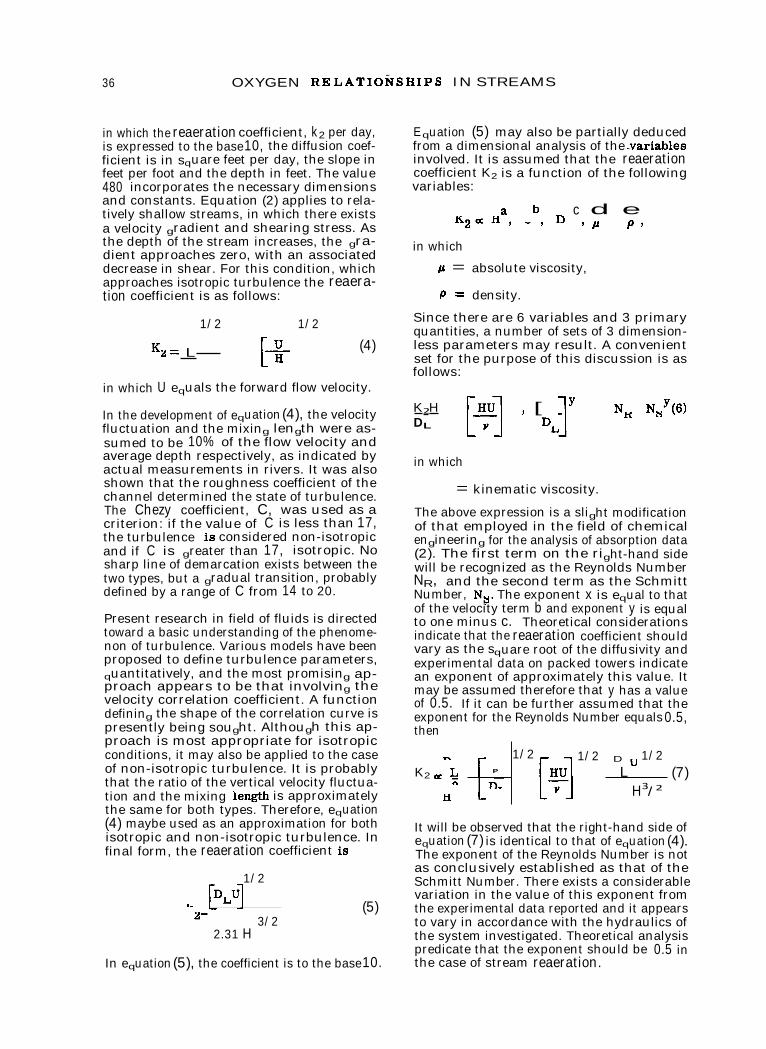
36 OXYGEN RELATIORSHIPS IN STREAMS
in which the reaeration coefficient, k2 per day, is expressed to the base 10, the diffusion coef-ficient is in square feet per day, the slope in feet per foot and the depth in feet. The value 480 incorporates the necessary dimensions and constants. Equation (2) applies to rela-tively shallow streams, in which there exists a velocity gradient and shearing stress. As the depth of the stream increases, the gra-dient approaches zero, with an associated decrease in shear. For this condition, which approaches isotropic turbulence the reaera-tion coefficient is as follows:
Equation (5) may also be partially deduced from a dimensional analysis of the _variables involved. It is assumed that the reaeration coefficient K2 is a function of the following variables:
K2ΠHa , b c d e
7 ••• 7 D , IL p,
in which
A = absolute viscosity,
p= density.
1/2
K2= L
1/2
• [±1 (4)
Since there are 6 variables and 3 primary quantities, a number of sets of 3 dimension-less parameters may result. A convenient set for the purpose of this discussion is as follows:
in which U equals the forward flow velocity.
In the development of equation (4), the velocity fluctuation and the mixing length were as-sumed to be 10% of the flow velocity and average depth respectively, as indicated by actual measurements in rivers. It was also shown that the roughness coefficient of the channel determined the state of turbulence. The Chezy coefficient, C, was used as a criterion: if the value of C is less than 17, the turbulence is considered non-isotropic and if C is greater than 17, isotropic. No sharp line of demarcation exists between the two types, but a gradual transition, probably defined by a range of C from 14 to 20.
Present research in field of fluids is directed toward a basic understanding of the phenome-non of turbulence. Various models have been proposed to define turbulence parameters, quantitatively, and the most promising ap-proach appears to be that involving the velocity correlation coefficient. A function defining the shape of the correlation curve is presently being sought. Although this ap-proach is most appropriate for isotropic conditions, it may also be applied to the case of non-isotropic turbulence. It is probably that the ratio of the vertical velocity fluctua-tion and the mixing -length is approximately the same for both types. Therefore, equation (4) maybe used as an approximation for both isotropic and non-isotropic turbulence. In final form, the reaeration coefficient is
1/2 [DLU]
k
2-
- 3/2
2.31 H
In equation (5), the coefficient is to the base 10.
K2H [HU1 , [
]Y
Nwx NQY(6)
DL DL
"
in which
= kinematic viscosity.
The above expression is a slight modification of that employed in the field of chemical engineering for the analysis of absorption data (2). The first term on the right-hand side will be recognized as the Reynolds Number NR, and the second term as the Schmitt Number, Ns. The exponent x is equal to that of the velocity term b and exponent y is equal to one minus c. Theoretical considerations indicate that the reaeration coefficient should vary as the square root of the diffusivity and experimental data on packed towers indicate an exponent of approximately this value. It may be assumed therefore that y has a value of 0.5. If it can be further assumed that the exponent for the Reynolds Number equals 0.5, then
K2 „,,DL
H
2
P
1/2 1/2 [HU]
v
D u 1/2 L (7) [
DL H3/2
It will be observed that the right-hand side of equation (7) is identical to that of equation (4). The exponent of the Reynolds Number is not as conclusively established as that of the Schmitt Number. There exists a considerable variation in the value of this exponent from the experimental data reported and it appears to vary in accordance with the hydraulics of the system investigated. Theoretical analysis predicate that the exponent should be 0.5 in the case of stream reaeration.
(5)

0
00 LEGEND
C) CLARION RIVER
O LITTLE TENNESSEE
® WATAUGA RIVER C) SCIOTO RIVER
(:S) 14DLSTON RIVER
• FRENCH BOARD
® ILLINOIS RIVER
0 OHIO RIVER ® SAN DIEGO BAY
OBSERVED k. 0.1 LO 10.0
STREAM REAERATION - MEASUREMENT AND CALCULATION 37
In order to show that equation (5) may apply to the non-isotropic case, as well as the iso-tropic, Table 1 is presented. The rivers, which data are indicated in the table, are characterized by a state of non-isotropic tur-bulence, as determined by the criteria dis-cussed above. The observed values of the reaeration coefficient are given and compared to those calculated by equations (3) non-isotropic and (5) isotropic.
Table 1 Reaeration Coefficients
River Observed Calculated
Non-isotropic Isotropic
Clarion 4.8 5.4 5.8 1.9 2.1 1.4
Tenn. 1.05 0.84 0.80 0.72 0.75 0.72
Ohio 11 - 19 0.21 0.30 0.24 23 - 65 0.28 0.30 0.28 77- 88 0.19 0.17 0.15
104 - 349 0.20 0.28 0.31
That the isotropic formula may be used for both cases is indicated by this comparison. Although the non-isotropic values in general agree more closely with the observed, the difference between the isotropic and non-isotropic would be considered insignificant in most practical cases.
Figure 1 shows the comparison between the observed values of the reaeration coefficient
COMPARISON OF THE CALCULATED AND OBSERVED REAERATION COEFFICIENTS
Figure 1
and the values, as calculated by the isotropic formula, of all the available data. In addition the data of the rivers originally presented (1), there are also included value s from the Scioto (3), Little Tennessee, Watauga, Holston and French Broad Rivers (4). The data from the last four rivers are particularly significant in that they represent cases of reaeration, free of the influence of deaeration by organic mat-ter. The water was initially deaerated by vir-tue of the fact that it was discharged from a reservoir. The measurement of the reaera-tion coefficient is therefore not influenced by the complication of oxygen demands of pol-lution.
Only in the case of the Little Tennessee River were depth measurements available. In the other cases, values of the depth were comput-ed by the continuity equation, knowing the flow velocity and width. Appreciating this proce-dure gives only an approximation of the depth, the reaeration coefficient must be regarded in the same light. The observed values re-ported were darkness values,— i.e.,not in-fluenced by algae. On two of these rivers - the Watauga and the Little Tennessee—the effect of algae was pronounced during daylight hours. It is emphasized that the theoretical development (equations 3 & 5) made no at-tempt to account for this source of oxygen. Any comparison between the theoretical equations and reported data is not valid if algae are present. This factor should be taken into account separately, both in practice and theory. The reported values were therefore those measured when sunlight was not present and the reaeration was due to oxygen transfer-red from the atmosphere through the water surface.
Determination of Reaeration Coefficient
A. Reaeration Formula
Inspection of equation (5) indicates that know-ledge of the depth, velocity and diffusivity are necessary for the calculationof the reae-ration coefficient. The depth referred to in this equation is the ratio of the volume to the surface area of a particular stretch of river or of the cross-sectional area to the width at any particular station. It is obvious that a representative value of the depth must be used In order to arrive at a representative value of the reaeration coefficient. In any river stretch, this value of the depthwill vary from station to station. The extent of its variation depends upon the roughness of the channel and is most pronounced under low flood con-ditions. Figure 2 presents the statistical

0.5 1 2 5 10 20 30 40 50 GO 70 50 90 95 9955 95.5
DEPT
H-FT
. EQ
UA
L TO
OR
LES
S TH
AN
1000
PROBABILITY ■ 95% OF MEASURED MEAN FALLING WITHIN INDICATED % OF TRUE MEAN
0.0 0.1 0.2 0.3 0.4 05 COEFFICIENT OF VARIATION
38 OXYGEN RELATIONSHIPS IN STREAMS
analysis of data, taken from actual stream surveys, showing typicalvariations of depths from station to station. The Wabash River data was taken from the measured cross-sections reported (5); the Clarion River depths from U. S. Corps of Engineers Maps and the Codorus values from field measurements of a survey, with which the writer was associa-ted. This figure shows the actual data and the computed lines of best fit, based on a normal distribution. That a normal distribution is re-presentative of these data may be seen from the agreement between the observed and com-puted values. It is significant that a wide range of depths can be expected in some cases, as is evidenced by the Wabash River data. The question arises then: How many cross-sections are required to insure for a given probability that the measured mean will fall within a given percent of the true mean? A particular distribution, Student's distribu-tion, may be used to answer this question. Based on this distribution, at a probability of 95%, Figure 3 indicates the number of samples required for a range of coefficients of variation, so that the measured mean will fall within a given percent of the true mean. For example, assume that there were 20 cross-sections taken of a stretch of river and therefore 20 values of depth were available. From a statistical analysis of the depth data, the standard deviation and the coefficient of variation maybe computed. For a coefficient of variation of 0.20 and 'a sample number of 20, it may be seen from Figure 3 that the measured mean would be within 10% of the true mean with a probability of 95%. Although this statistic may be applied to any variable which is subject to a normal distribution, it is particularly significant in reference to a variable which is raised to a power greater than 1, such as the depth in reaeration for-mula.
% FREQUENCY OF OCCURRENCE TYPICAL DEPTH VARIATIONS
Figure 2
Figure 3
Table 2 presents a summary of the statistical analysis of the depth data indicated on Figure 2.
Table 2
Mean Depths and Variations
Wabash Codorus Clarion
Mean depth - ft. 5.3 1.2 2.1
Standard Deviation 2.0 0.28 0.33
Coefficient of Variation 0.38 0.23 0.13
Number of Samples available 147 11 17
% Variation for Probability =-95% 6 15 7
In addition, Table 2 indicates the number of samples which were taken in each survey. Based on this number, there is also indicated the % that the measured mean will fall with-in the true mean. From these examples, it is evident that appreciable variation can be in-troduced, if account is not taken of this factor of sufficient samples.
The effect of various constituents on the reae-ration coefficient has been recognized. Vari-ous data are available indicating the reduction In reaeration which is generally associated with solutions other than pure water (6) (7). This condition has also been observed in bubble aeration (8) (9). In this case, however, the effect is twofold in that various con-stituents not only influence on the transfer

60 20
0 1 0 20 30 40 50
(I WATER Kt • 0.37 PER MR. 0 WASTE Kt • 0.32 PER HR.
RATIO • 0.87
60
50
40
30
DE
FIC
IT- S
SAT
UR
AT
ION
100
90
80
70
STREAM REAERATION - MEASUREMENT AND CALCULATION 39
coefficient, but also the size of the bubble and therefore the ratio of the interfacial area to the volume. In the case of natural streams the ratio of the surface area to the volume is a constant for a given flow condition. The ef-fect of the majority of wastes substances on the reaeration coefficient is reflected by their influence on the diffusivity. Waste con-stituents, such as surface-active substances, concentrate at the liquid-air interface and ap-parently create a barrier to the diffusion of oxygen. At the interface a thin layer exists through which the diffusion is molecular in nature and below which the eddy diffusion controls. Since substances such as surface-active agents concentrate at the interface, the molecular diffusion is hindered. The magni-tude of this influence is a function of con-centration of the waste substance and, at relatively low concentrations, the reported reductions in reaeration rate are significant. Research is presently being conducted to investigate the effect of various substances on the reaeration coefficient. Equation (6) or some modification of it may provide a means of correlating such data.
It is also possible that some substances may influence the turbulence characteristics, in-asmuch as they influence the viscosity of the solution. Ultimately, turbulent energy dissi-pates itself by the mechanisms of viscous action and thus any change in viscosity may effect the turbulence parameters which in turn control the interfacial renewal rate. Con-sequently, substances which alter the vis-cosity can influence the reaeration coefficient In two ways: by the probable effect on the coefficient of diffusion and by the possible ef-fect on the rate of surface renewal.
It is further significant that some waste con-stituents are responsible for a decrease in oxygen saturation value. In reporting reaera-tion coefficients, account should be first taken of this factor. Since a saturation value of dissolved oxygen is employed in all cal-culations of reaeration values, it may account partially or wholly for differences in the re-ported values between pure water and waste waters. Small differences in the saturation values (in the order of 0.5 p.p.m.), can have a significant effect on the calculated coef-ficient, particularly at the higher concentra-tions of dissolved oxygen. This factor is also being investigated at the present time.
In order to account for these factors in any practical case, field or laboratory measure-ments must be employed. Analysis of actual survey data automatically accounts for these factors. Reaeration coefficients thus deter-mined are representative of the flow and waste
conditions at the time of the survey; however, it is difficult to extrapolate this information to other flows and waste conditions. The follow-ing laboratory procedure is suggested as a means of determining these effects in a given case over any desired range of conditions. The laboratory procedure involves the meas-urement of the reaeration coefficient under conditions of turbulence, comparable to that of the river. Such a laboratory apparatus would consist of a grid oscillating vertically in the fluid, creating a uniform degree of turbulence. The procedure involves meas-urement of the reaeration coefficients in pure water and in the waste solution. The coef-ficient in the waste solution should be measured for a range of anticipated dilutions with the river water. The solutions are ini-tially deaerated and samples withdrawn for dissolved oxygen determination at predeter-mined intervals over the test period. The period of time over which measurements are made should be short enough so that oxygen demands are insignificant. The initial con-centration of the waste and its rate of oxidation determines the limit of test period. Depending upon the time requirements, the degree of agitation can be established in order to reach any desired degree of saturation. A typical example is shown in Figure 4, comparing the reaeration rates of pure water and a particu-lar waste. It is pertinent to note that this test measures the overall effect of the factors dis-cussed above.
TIME
EFFECT OF WASTE CHARACTERISTICS ON REAERATION COEFFICIENTS
Figure 4

40 OXYGEN RELATIONSHIPS IN STREAMS
B. Oxygen Sag Equation
The differential equation which describes the combined action of deoxygenation and reaera-tion has been presented in the work of Streeter and Phelps (10):
dD = KO, - K2D dt (8)
in which
dD=time rate of change of the dissolved dt oxygen deficit
L = concentration of the organic matter
D = dissolved oxygen deficit
K1= deoxygenation coefficient
K2= reaeration coefficient.
The integrated form of equation (8) is used in the analysis of the dissolved oxygen balance in a polluted river. It may also be used to determine the reaeration coefficient. All other terms being known, the reaeration coefficient can be solved for by trial and error. The observedvalues of this coefficient shown in Figure (1) were determined in this fashion, with the exception of those in Tennessee River drainage area. In this case, since no BOD was present (L = o) equation (8) reduces to
D dt 2 •
Equation (9) integrates to
Dt = Doe - Krit
in which
Dt = deficit after time "t"
Do= initial deficit.
A graphical solution of equation (10) was employed in Figure 4 in calculating the coef-ficients for the pure water and the waste solution.
Under certain conditions, less laborious and more exact solutions of the reaeration coef-ficient can be made rather than using the integrated form of equation (8). The general condition required for this solution is that the
time rate of change of the dissolved oxygen deficit is zero. This condition is realized in the following:
1. When dissolved oxygen is zero for a short stretch.
The only limitation in this regard is that con-ditions are not anaerobic and they probably will not be if the distance is short enough. This condition is furthermore significant in that no estimation has to be made of the deoxygenation coefficient, Kl. Since the dissolved oxygen is zero, the amount of oxygen transferred is a constant and also a maxi-mum and equal to
K2D = K2C5 . (11)
The deficit is equal to the saturation value Cs for the case of zero dissolved oxygen. It follows that this condition limits the oxida-tion of organic matter to a reaction which is linear in time or distance. The quantity of oxygen transferred equals that utilized for oxidation, which is equal to
La - Li;) L (12) T
La= ultimate BOD at upstream station.
Lb = ultimate BOD at downstream station.
T = time of travel between stations.
Equating (11) and (12) ,
K2Cs = 7
and therefore
- -F Tt2
— e;
Equation (11) may be used if conditions are not anaerobic and the organic matter is being removed by oxidation and not by other pro-cesses such as settling, volatilization, im-mediate reactions, etc. K2 in equation (13) is expressed to base "e".
2. At the critical point.
At the location of the minimum dissolved oxy-gen concentration in the stream, the rate of
(9)
(10)
(13)

KiLc = K2Dc
KiLc =.—_ Dc
or
K2
(14)
DIS
SO
LVED
OXYG
EN
PPM
2 0
BOD5-DAy= 130 PPM
TEMPERATURE= 32°C
UPTAKE= 2.5 PPM/HR
8
7
6
5
4
3
2
•
THE OXYGEN SAG AND D.O. RELATIONSHIPS IN STREAMS 41
change equals zero and equation (8) redtices to
in which values refer to those at the critical point.
In equation (14), as well as equation (8) the rate of oxidation of the organic matter has been expressed as a first-order reaction, which appears to be sufficiently representa-tive in most cases. Thomas (11) however, has shown that a"bimolecular" formation for the BOD should be considered under certain conditions. The rate of deoxygenation is re-presented by the following expression:
dL 2 dt Lo
= - (15)
At the minimum dissolved oxygen location, equation (15) may be equated to rate of reaera-tion, resulting in
K2 KbLc
2
LoDc
(16)
in which
Lc= ultimate BOD at critical point
Lo= ultimate BOD at the point of dis-charge.
3. When the dissolved oxygen is present.
Under a steady-state condition of flow and waste the time rate of change of the dissolved oxygen deficit is zero at a particular location. In this case, a relationship similar to equa-tion (14) results. In order to eliminate the necessity for determining K1 and L, a simpli-fied procedure for measuring the oxygen up-take may be employed. KO., equals the rate of oxygen utilization and may be measured directly, in manner similar to that employed with a sample of activated sludge (12).
The river sample is aerated and the drop-off of oxygen is recorded, polarographically. The sample is sealed and no aeration is permit-ted to occur during this period. Agitation is effected by means of a magnetic stirrer. The time over which this test is conducted de-pends upon the concentration of the organic matter and its rate of oxidation. A typical
example is shown in Figure 5. The oxygen uptake rate, R, is equal to the slope of the line which defines the oxygen drop-off. As-suming this rate is the same as that in the stream, then
K2D = KiL = R (17)
or
K2 = -fr • (18)
D, as above, is the dissolved oxygen deficit determined from field measurements of the dissolved oxygen at the particular location. It is believed this procedure offers a relatively simple and accurate means of determining the reaeration coefficient in natural streams.
TIME - HOURS
TYPICAL UPTAKE VALUE
Figure 5
Conclusion
Various methods have been reviewed concern-ing the determination of the stream reaeration coefficient. Additional data has been present-ed to substantiate the theoretical reaeration formulae. The effects of waste constituents on reaeration rates have been discussed and laboratory procedures have been suggested to measure these effects. Criteria have been presented to evaluate the probable variation of reaeration coefficients as determined ana-lytically.

OXYGEN RELATIONSHIPS IN STREAMS 42
References
1. O'Connor, D. J. and W. E. Dobbins. Mechanism of reaeration in natural streams. J. of San. Engr. Div., American Society of Civil Engineers.
2. Sherwood, T. K. and R. D. Pigford. Ab-sorption and Extraction. McGraw-Hill Book Co., 2nd Ed., New York. (1952).
3. Kehr, R. W. and Others. A study of the pollution and natural purification of the Scioto River. Pub. Hlth. Bull. 276. (1941).
4. Churchill, M. A. Effect of storage im-poundments on water quality. J. of San. Engr. Div., American Society of Civil Engineers, 83. (1957).
5. Ohio River Valley Water Sanitation Commission. Wabash River pollution - abatement needs. Published by the Com-mission, Cincinnati, Ohio. (1950).
6. Kehr. R. W. Measures of stream oxida-tion - effect of sewage on reaeration. Sewage Works Jour., 10:228. (1938).
7. Department of Scientific and Industrial Research. Water Pollution Research, 195. H. M. Stationery Office, London.
8. Ippen, A. T., L. G. Campbell and C. E. Carver, Jr. The determination of oxygen absorption in aeration processes. Tech. Rept. No. 7. Hydrodynamics Laboratory, M.I.T. (May 1952).
9. Eckenfelder, Jr. W.W., L. W. Raymond and D. T. Lauria. Effect of various organic substances on oxygen absorp-tion efficiency. Sewage and Industrial Wastes, 28. (1956).
10. Streeter, H. W. and E. B. Phelps. Pub. Hlth. Bull. 146. U. S. Public Health Service. (1925).
11. Thomas, Jr., H. A. Notes on step method of oxygen sag calculations. As presented at E. H. C Cincimiati, Ohio. (July, 1953).
12. Eckenfelder, Jr., W. W. Aeration effi-ciency and design. Sewage and Industrial Waste Journal, 24: 1221. (1952).

STREAM REAERATION - MEASUREMENT AND CALCULATION 43
DISCUSSION •
ERMAN A. PEARSON, Associate Professor Sanitary Engineering University of California
Dr. O'Connor deserves a great deal of credit for his excellent paper dealing with theoretical aspects of stream reaeration coefficients and the practical problems of field measurement or evaluation associated therewith.
Several aspects of his presentation are worthy of considerable elaboration and discussion. In the theoretical development of the expres-sion for k2, a fundamental assumption is made that the reaeration coefficient is proportional to the square root of the ratio of vertical velocity fluctuation to mixing. length. The basic question is whether or not the ratio of velocity fluctuation to mixing length re-presents the best estimate of the rate of surface renewal. A second assumption is that the velocity fluctuation is equal to one tenth the mean horizontal velocity. Similarly, the mixing length is assumed to be on the average one tenth of the average stream depth. It is convenient mathematically to allow both constants of proportionality to cancel out in the development of the expression for k2 and permit direct substitution of mean velocity and depth for fluctuating velocity and mixing length. However, this appears tobe an over-simplification of the phenomena. Although Kalinske (1) reported that the largest mean eddy-scale found in the Mississippi River was 0.1d where d is the depth of the river, there is considerable question as to its general applicability.
The vertical velocity fluctuation is not defined specifically but it is assumed that reference Is to the standard deviation of the vertical velocity fluctuation. Again the assumption that the velocity fluctuation is 10 percent of thp mean flow velocity appears to be open to question. Kalinske (2) has reportedvalues of cr, the standard deviation of the fluctuating
horizontal velocity in normal turbulent flow in channels, to be as much as 33 percent of the mean velocity near the boundaries. The maxi-mum fluctuating component would be at about 3 a or equal to 100 percent of the mean hori-zontal velocity component. While the maxi-mum vertical fluctuating velocity component may not be nearly this great, it appears that as a minimum it would be at least 20 percent of the mean.
The assumption that a Chezy coefficient, C, of less than 17 represents non-isotropic flow condition whereas a Chezy C greater than 17 indicates isotropic flow has little supporting evidence.
Reference is made to the "Schmitt" number as a parameter of the reaeration coefficient. It is presumed that the name "Schmitt" re-presents a typographical error and reference Is intended to the "Schmidt" number.
With reference to Table 1 it would be of in-terest to compare the methods employed for computation of the reaeration coefficient in the "observed" column with the expressions used to compute the non-isotropic and iso-tropic reaeration coefficients in order to assess the validity of the comparison.
In the opinion of the writer and also concluded by Gameson (3) and others, one of the most important factors affecting the rate of reaera-tion of a stream or estuary is the turbulence of the surface or the rate of renewal of the surface film. Therefore, it would be highly desirable if a better or more direct measure of the surface renewal phenomenon were available than the assumed fluctuating velo-city-mixing length ratio. Questions about the validity of the latter ratio as a measure of surface renewal have already been raised.
Recent work by Brooks (4), Pearson (5) (6) (7) and others concerned with the prediction of waste concentrations in receiving waters have employed a Fickian diffusion model to describe mathematically the dispersion of pollutants. The differential equation for the phenomenon is as follows:
k C
t where C = concentration of waste or tracer t = time x = space coordinate k = coefficient of eddy diffusivity.
The coefficient of eddy diffusion is really a measure of horizontal turbulence or disper-sion effected by fluctuating velocity com-ponents and eddy systems. It is a direct measure of the rate of dispersion of a tracer and as such should be proportional to rate of surface renewal. Moreover, the coefficient of eddy diffusivity is frequently determined by measurement of the rate of surface dispersion of a dye spot or stream (8). If the coefficient of lateral eddy diffusivity is determined on the surface by measurement of dye patches or trajectories, this should give a fairly
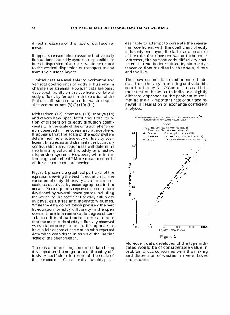
44 OXYGEN RELATIONSHIPS IN STREAMS
direct measure of the rate of surface re-newal.
It appears reasonable to assume that velocity fluctuations and eddy systems responsible for lateral dispersion of a tracer would be related to the vertical dispersion or transport to and from the surface layers.
Limited data are available for horizontal and vertical coefficients of eddy diffusivity in channels or streams. However data are being developed rapidly on the coefficient of lateral eddy diffusivity for use in the solution of the Fickian diffusion equation for waste disper-sion computations (8) (9) (10) (11).
Richardson (12), Stommel (13), Inouye (14) and others have speculated about the varia-tion of dispersion or eddy diffusion coeffi-cients with the scale of the diffusion phenome-non observed in the ocean and atmosphere. It appears that the scale of the eddy system determines the effective eddy diffusivity coef-ficient. In streams and channels the boundary configuration and roughness will determine the limiting value of the eddy or effective dispersion system. However, what is the limiting scale effect? More measurements of these phenomena are needed.
Figure 1 presents a graphical portrayal of the equation showing the best fit equation for the variation of eddy diffusivity as a function of scale as observed by oceanographers in the ocean. Plotted points represent recent data developed by several investigators including the writer for the coefficient of eddy diffusivity in bays, estuaries and laboratory flumes. While the data do not follow precisely the best fit equation for eddy diffusivity in the open ocean, there is a remarkable degree of cor-relation. It is of particular interest to note that the magnitude of eddy diffusivity observed In two laboratory flume studies appears to have a fair degree of correlation with reported data when considered in terms of the limiting scale of the phenomenon.
There is an increasing amount of data being developed on the magnitude of the eddy dif-fusivity coefficient in terms of the scale of the phenomenon. Consequently it would appear
desirable to attempt to correlate the reaera-tion coefficient with the coefficient of eddy diffusivity employing the latter as'a measure of the rate of surface renewal or turbulence. Moreover, the surface eddy diffusivity coef-ficient is readily determined by simple dye tracer or float studies in channels, rivers and the like.
The above comments are not intended to de-tract from the very interesting and valuable contribution by Dr. O'Connor. Instead it is the intent of the writer to indicate a slightly different approach to the problem of esti-mating the all-important rate of surface re-newal in reaeration or exchange coefficient analyses.
MAGNITUDE OF EDDY DIFFUSIVITY COEFFICIENTS (16) Plotted Points Represent Recent Data
CODE X Gunnarson Santa Monica Bay (8) • Moon et al Texas Gulf Coast (9) 0 Pearson Port Angeles Harbi3r (15) 12 Harleman l'x 1-1/2' x 32 Lucite Flume (11) Lt Orlob 1, x3'x 24' Flume, Sand Bottom (10)
10
10
B /
10-3
o 4 0.1 1.0
1 10
1 100 1000 10000
LENGTH SCALE -feet
Figure I
Moreover, data developed of the type indi-cated would be of considerable value in problem areas concerned with the mixing and dispersion of wastes in rivers, lakes and estuaries.
103
2

STREAM REAERATION - MEASUREMENT AND CALCULATION 45
References
1. Kaiinske, A. A. Application of statistical theory to velocity and suspended sedi-ment measurements in rivers. Trans. A.G.U., 26:261-265. (1945).
2. ICalinske, A. A. The role of turbulence in river hydraulics. Proc. Second Hy-draulics Conference Bull. 27. (1943).
3. Gameson, A. L. H. and W. S. Preddy. Factors affecting the concentration of dissolved oxygen in the Thames Estuary.
4. Brooks, N. H. Report on methods of analysis of the performance of ocean out-fall diffusers with application to the proposed Hyperion Ouffall. For Hyperion Enginners, City of Los Angeles. 36 pages. (1956).
5. Pearson, E. A. Preliminary report on special design considerations for Hy-perion Sewage Treatment Plant. For Richard R. Kennedy, Member Board of Consultants, City of Los Angeles. 52 pages. (Feb. 1956).
6. Pearson, E. A. and A. L. Gram. Rational design of submarine waste dispersion systems. Pre-publication manuscript - soon to be published.
7. Pearson, E. A. Submarine waste disposal installations. Proc. Sixth International Conference on Coastal Engineering. (Dec. 1957).
8. Gunnarson, C. G. Sewage disposal in Santa Monica Bay. Proc ASCE, 84:1534-1 to 1534-27. (Feb. 1958).
9. Moon, F. W., C. L. Bretschneider and D. W. Hood. A method for measuring eddy diffusion in coastal embayments. Institute of Marine Science IV:14-21. (July 1957).
10. Orlobb, G. T. Unpublished research - private communication. (Oct. 1957).
11. Harlemen, D. R. F. Unpublished re-search - priviledged communication. (Feb. 1958).
12. Richardson, L. F. and H. Stommel. Notes on eddy diffusion on the sea. Jour. of Meteorology, 5:238-240. (1948).
13. Stommel, H. Horizontal diffusion due to oceanic turbulence. Jour. of Marine Re-search, 8:199-225. (1949).
14. Inouye, Eiich. Eddy diffusion coefficient in the sea. ICaguka Tisiki, 20(11). (1950).
15. Pearson, E. A. Unpublished investiga-tions. (Sept. 1957).
16. Pearson, E. A. An Investigation of the Efficacy of Submarine Outfall Disposal of Sewage and Sludge. Publication No. 14, California Water Pollution Control Board. (Dec. 1955).
INFORMAL DISCUSSION H. A. Thomas, Jr.: I want to make some
remarks about your paper, Don, and I trust you won't interpret them as destructive criti-cism. You know my opinion is that your work is highly commendable. You showed a graph in which you had plotted K2 by your formula versus the K2 which you called "observed'. As I recollect from my previous computations, there is something like a 30% discrepancy between what you have called the "calculated" K2 and the "observed" K2. It is important I believe to examine this point and to try to assess the practical implication of the data exhibited on this graph.
It is a foible of language to call one K2 an "observed" value and one a "calculated" value. Both derive from theories. The Streeter-Phelps formulation is a theory. By
substituting measured BOD and DO values in this formula a value (or values) of K2 may be calculated. The same thing is true of your formula; measurements are made of certain quantities and a K2 is calculated.
There is an analogy here to computing the roughness coefficient n of a reach of a river (1) by the Kutter formula, and (2) by the Manning formula. Both formulas represent theories of open channel flow. In order to tahi the channel friction coefficient in each case, use is made of certain measurements of depth, hydraulic radius, slope and dis-charge. In both cases an n-value is obtained. In general these n-values differ numerically. Pairs of n-values thus obtained for several different streams exhibit strong correlation; that is, if a stream has a high n-value by the

46 OXYGEN RELATIONSHIPS IN STREAMS
Manning formula, it is likely to have a high n-value by the Kutter formula. The values will not be identical because the formulas are dif-ferent. The point here is that it would be doing violence to the language to refer to the n-values calculated by, say, the Manning formula as "calculated" and those of the Kut-ter formula as "observed'. Both have the same conceptual status; both are computed from theoretical formulations using stream measurements. Precisely the same situation obtains with the K2 values obtained by the Streeter-Phelps formulation and those by the O'Connor-Dobbins formulation.
It is relevant to point out that a high cor-relation does not necessarily exclude the possibility that both formulations are wrong. Generally, however, high correlation tends to bolster the validity of both formu-lations, and we may adopt the simpler formulation particularly if it entails field measurements that are easy to make with requisite precision. In the present case there Is no doubt that your formulation is to be pre-ferred and accordingly it should be regarded
an an important forward step in the theory of analysis of oxygen balance in streams.
D. J. O'Connor: (Ed. Mr. O'Connor dis-cussed the comments made by H. A. Thomas, Jr., and indicated some of the assumptions made.)
G. A. Rhame: This thing has been very educational. Why do you spend all your time computing this, that and the other when you take your K1 very much for granted, and then measure oxygen utilization in a quiet bottle when the stream is turbulent?
D. J. O'Connor: I forgot to mention--there is a magnetic stirrer.
W. E. Dobbins: Are you attempting to screen parameters? Most of mathematical developments to date indicate some sort of mathematical discordance.
E. A. Pearson: (Ed. Mr. Pearson dis-cussed collection and methods of analyzing field data.)

Significance of Organic Sludge Deposits
C. J. VELZ, Professor, Sanitary Engineering
University of Michigan
47
It is a pleasure to appear before this dis-tinguished group and to talk about sludge deposits and their effect on dissolved oxygen. I haven't prepared a paper and therefore may do some rambling. I think that sludge de-posits can be generally classified as producing very unsightly conditions in the streams, in-cluding sludge boils. Also, of course, sludge deposits can produce abnormalities in de-pression of the dissolved oxygen profile. The degree of this abnormality depends upon a number of conditions which I will try to illus-trate. We might think of sludge as arising from three types of deposits; the normal being that which is associatedwith settleable solids contained in sewage or wastes. We also can have sludge deposits associated with floc-culation or coagulation which might take place in the stream. These do not occur as fre-quently as the first type. A third type we might think of as associated with biological extraction and accumulation.
Before going into the subject matter perhaps it would be desirable to take you out on the river through the medium of a little strip movie which I clipped from some film which we took in the field. I believe a much better impression of the river is obtained by going down the river in a boat, than surveying it from the laboratory window or from bridges. If you will bear with me I will show you the effects of some sludge deposits as we have observed them on a number of rivers we have been studying. These are actual shots of dif-ferent river conditions pieced together.--(Color film)
You will notice some sludge boils occurring here and floating sludge that has come to the surface after deposit in pool areas behind dams. It gets to be an unsightly mess after a while, with settled organics becoming gas, entrained, rising to the surface as gobs, float-ing, and redepositing. This doesn't show clearly but actually there are gas bubbles dis-charging to the atmosphere and sludge boils shooting up to the surface.---Here all colors of the rainbow are seen, growths which have established themselves on the floating sludge particles that have come to the surface.---In this shot you get some idea of what flows by in the form of fresh settleable solids, by plac-ing a thin white metal sheet about a foot underneath the surface and then photographing the passing stream. You can see what flows in a river at times and is the source of sludge deposit. And of course as these deposits settle, digestion releases gas to the atmos-phere. This shows what happens to the shore line in a pool area behind dams where velocity slows up. It is quite a spectrum in color in part due to oil entrainment. Shove a paddle In the deposit, which is 6 or 7 feet deep at this zone, and a violent release of H2S is ob-served. These are actual gas bubbles breaking from the water surface overlying the deposit area extending over extensive reaches of the pool. You can see those bubbles breaking and really gas escaping to the atmosphere. In a sense part of the debt is being paid by the at-mosphere in addition to that being paid by D.O. in the river water. These are not rain drops; it is actual gasification. One source of deposits, as I mentioned, is

48 OXYGEN RELATIONSHIPS IN STREAMS
biological growths that can extract B.O.D. and then settle in quiescent areas or attach themselves to the bottom. Perhaps you can see these growths in this shot, largely Sphaerotilus accumulations attached to the stone which has the effect of settleable solids deposits. Also in the flowing stream notice the lacy-like material passing over the sub-merged white metal sheet. It is like excess activated sludge.
Here you see sludge deposit induced by iron waste flocculation entraining suspended and colloidal matter resulting in a substantial sludge deposit area. The wastes themselves may be free of settleable solids, but on hit-ting the water form this fine chemical floc in the form of clouds that you see over the sub-merged metal sheet. I thought this short color film would give you a little view of what takes place in the river physically.
To determine the potentialities for sludge deposits and get at the quantitative determi-nation of their effect upon D.O. of the river I think it is essential to get a definition of the physical and hydraulic character of the river channel along its course. We think that the simplest way to get at this, and also to pro-vide the information for reaeration, is fre-quent channel cross-sections. We like to take a cross-section of the channel every 500 ft.
along its entire course. This sounds like a large order, and used to be large order, but today with modern echo sound devices which cost a little over $1,000 one can in 3 - 4 days cross-section 40 - 50 miles of river at 500 foot intervals and have in the process a record of each section. These plots of cross-sections can be planimete red directly giving end areas, mean depths, channel volumes, surface areas, etc., and you have all the physical facts that are necessary for a quantitative computation, not only for sludge deposits but for deoxygenation and reaeration. These data then can be used for computing the all-important time of passage down the course of the river by a simple process of displace-ment of the occupied channel volume by the run off that flows to the sections. (Shows slide of time of passage curves).
We think such time of passage curves are an essential part of stream analysis work. If cumulative time of passage from cross-sec-tion to cross-section is plotted against river mileage the flow pattern along the entire course is defined and the slope of this curve at any point gives the velocity of that point. We feel that 0.6 ft. per second is about the critical velocity at which organics will deposit and ac-cumulate. To rescour accumulations of de-posits may require a velocity of the order of 1.0 - 1.5 ft. per second depending upon activity
• 0 0
To
20
0 0
VELO ITT • FT / SEC
s.
." 0 Ns'
0
• 0 r a to . • ultra DE T AREAS POTENTIAL SLOSS DEPOSIT Afg•S
7 "—TV" [21
JP4 c5, ,,,,
S ,0
. 0 ... .O. ..7
4, .0.• E
O ,O 4, #*
0 O. 0 4 •
cf
ALETM NATIONAL COUNCIL FOR STREAM IMPRO (NEST
PULP. PAPER a pAPERBOARO INDUSTRIES •H ...... . .H..
TIME OF PASSAGE ..... TO WES. WV AT r aa■ous Hmems
UNIVERSITY OF MICHIGAN. SCHOOL OF PUIILM HEALTH STREAM ANALYSIS RESEARCH PROJECT
_
SG OS GO SS SA SS
NILES ASO. THE NOD, H
Figure 1

DA
YS
FR
OM
MILE
POIN
T
- 0
SIGNIFICANCE OF ORGANIC SLUDGE DEPOSITS 49
of decomposition and compaction of accumula-tions. A nest of velocity slopes are conveni-ently laid off on the time of passage graph and translating the 0.6 ft. per second slope along the time of passage curves for a range in runoffs identifies areas of potential sludge deposit. Each runoff, of course, has its own time of passage curve and each channel cross-section must be adjusted by means of stage rating curves to the new regime of runoff. Identifying the reaches of river where the slope is 0.6 or less provides a very fine method of determining where and at what runoff one can potentially expect sludge de-posits. Similarly investigating for slopes of 1.0 - 1.5 ft. per second gives the runoff level at which scour can be expected.
Here three deposit areas are identified. There is no question of the deposit area in the low velocity pool area but two other very signifi-cant deposit areas were discovered by this process and later were confirmed in the field.
A series of small dams creating pools in which velocity very definitely slows below 0.6 ft. per second and a whole series of deposit areas are indicated. Depending upon runoff level some areas are bypassed and redistribution occurs by scour from one to another.
The question of the effect of sludge deposits on dissolved oxygen and methods for its quantitative measurement requires the under-standing of the relationship between accumu-lation of the deposits and the demand from these accumulations. If following a scouring freshet, there is opportunity for only one day's deposit to accumulate the effect upon the dissolved oxygen profile is very little.
However, if you have 40 or 50 days' accumu-lation in the deposit area then the effect is quite pronounced -- quite dramatic. There-fore, it is important that we appreciate the relationship between accumulations and de-mand.
40
70
VELOCITY - FT/SEC -Ad
— e
- 1
--.;"
004
- -
Is DEPOSIT AREAS AREAS in •
- -
,
00
All
.04 0., .... CITI S I I
...,. c Aw _.... :
CP.
24.
MIAMI RIVER
TIME OF PASSAGE FROM DAYTON TO POINTS DOWNSTREAM
AT RUNOFFS OF 240, 400, AND 965 CFS (DAYTON GAGE) ''' ....././
:
. _. 1 , . . H. 64 62 60 711 75 74 72 10 52 42 40 55
MILES ABOVE THE MOUTH
Slide-time of passage curve for three run-off levels on the Miami River
0
TI M
E O
F PA
SSA
GE IN
10 '■:1":.
00
Figure 2

50 OXYGEN RELATIONSHIPS IN STREAMS
Ld 2 le ( I - ICY") .3
WHERE
L d THE CUMULATIVE BOD IN POUNDS
THE B 0.D ADDED TO THE DEPOSIT IN LBS. PER DAY
k THE SPECIFIC RATE OF OXIDATION OF THE DEPOSIT
t THE TIME OF ACCUMULATION IN DAYS
Slide referring to Mr. Streeter's original formulation
Figure 3 The equation which shows the relationships between the daily deposit, the accumula-tion, and the demand from the accumulation has been expressed by Streeter in this form. Here, LD is cumulative BOD in pounds in the deposit area, PD is the BOD added to the deposit area per day in pounds, and leis what I like to think of as the rate of eating from the pile or the rate of satisfaction on a semi-anaerobic basis in the sludge de-posit area, and t' here is not time of passage down the channel but rather the time of ac-cumulation, the period over which the daily deposits had an opportunity to accumulate. Of course, ultimately one reaches a condition of equilibrium, so that what is added per day to the pile is eaten from the accumulation. Then there is no change in the level of accumu-lation, and that usually representS the maximum demand. The demand, of course, at any other level other than the equilibrium level of accumulation will be much less than that under equilibrium conditions and will have much less effect on the dissolved oxygen of the overflowing stream. (Next slide please)
SLUDGE ACCUMULATION AND DEMAND
lc' 0.03, Teeperature 250 C
Time in
Days
Accumulation as a Percentage of the HOD of
the Daily Deposit
Daily Demand from the Accumulation as a Percentage of the DOD of the Daily Deposit
2 187 12.9 3 271 18.7 4 350 24.1 5 425 29.2 10 724 49.9 20 1,088 74.9
30 1,267 87.4
40 1,559 93.7 so 1,404 96.8 so 1,417 98.4 70 1,458 99.2 80 1,444 99.6 90 1,447 99.0
Ultimate 1,450 100.0
Figure 4
If we have only two days of accumulation (expressing demand and accumulation as the percentage of the BOD added per day to the deposit area),we find that we would accumu-late 187% of one day's load that would be added to the sludge pile while the demand, or amount eating from that much accumulation would constitute only 13% of what was added per day. Gradually accumulation builds up: at 50 days we have about 14 times the BOD added per day accumulated in the pile, and then eating from this accumulation at the semi-anaerobic rate would result in a demand on dissolved oxygen of 96.8% of what was added per day. Ultimately, one reaches a point of equilibrium where the pile from which the organisms are eating is large enough so that, in eating from the accumulated pile, they eat from it per day exactly what has been added to it per day, and we are at equilibrim. But, at any intermediate level of accumulation below equilibrium, it is quite important to emphasize that the daily demand from sludge deposits will be less than the daily BOD de-posited because the bugs are eating from a smaller pile. Keep in mind, that the effect upon the D.O. profile depends not only upon the fact that deposits potentially can occur but also upon the length of the period over which deposits have an opportunity to accumu-late without interruption.
Now, the next question involved is how do we get a method for quantitatively evaluating sludge deposits in a specific river situation? First of all, we believe that the best way to get at a quantitative measure of how much is going to be involved in sludge deposits is to measure at the sources the BOD fraction in settleable solids form. This usually is not done, but we think should be routine. If one ran a total BOD of the sewage or wastes and then allowed another sample to stand for an hour and ran BOD of the supernatant, the difference will give a pretty good measure of the BOD in settleable solids form subject to deposit. Since the sludge problem is so im-portant serious study should be given to standard procedure for inclusion in the next edition of Standard Methods. The BOD in settleable solids form at the various sources (speaking figuratively) gives you the size of the "truck load" picked up at each source.
The second problem is to determine how much of the "truck load" from each source is con-sumed while in transit from the source to the deposit area and what remains to be dumped into the sludge deposit pile. To determine this you need to know the time of passage down the river from each source to the sludge deposit area. With this, you know how much

4' DEEp
STA. A 60,000 (C. a D.) 40,000 (S.S.)
cpS
STA. A 200 60.0 01.0 _ ui ...___ 1Ltt
a: - 1 00 8.-- 2 -23.2 ---- -- _ — oi BO= 0 X 60 I- _
STA. B
1-; 4
5.
80: 60- 40- 20-
----- --
COMPUTED DO. PROFILE
— 20
1 0 3
o.a
■11-
ASS. LIAB. RUNOFF 80.0 I 6.7 (S.S)
REA 23.3 33. 3 (SLUDGE) +1-6T3 31.4 (C.8 D.) -81.4 -81.4 +21.9
94.2 - 232 %
1 00
DEEp
1.0 do.
0
100 -80 - 60 - 40 - 20
0
40
STA. C
COLLOIDAL 8 DISSOLVED -- — FRACTION
SETTLEABLE SOLIDS FRACTION
INTEGRATION OF POLLUTION LOADS
STA.!) 200 68.6
30.4
DAILY SLUDOE 33.3- DEPOSIT
1 2 PASSAGE IN DAYS FROM STA. A
ST D
550 CFS
le STA. B 40,000 (C. a D.) 1 0,000 (S.S.)
co 4 STA. C
DAM
—100 — 80 — 60
40
20
10
--- ------ - -425 • • .126
12:11 44.6 33.3
- 5.4 -11.3
SIGNIFICANCE OF ORGANIC SLUDGE DEPOSITS 51
of the original "truck load" the bugs are going to eat in transit, the remainder then con-stitutes the size of the daily load added to the sludge pile.
A third factor we need to know, of course, is the size of the accumulated pile. This depends upon how many days since the last freshet scour they have been hauling "truck loads" down to the deposit area. Now, if I may have the next slide, (Figure 5).
First, let us take the settleable solids fraction, and as shown on the lower portion of the slide, integrate on semi-log paper the two loads down the river at the time of pas-sage that prevailed for the given runoff pattern. You start the integration at"A" with 40,000 P.E. at a slope associated with aerobic rate of satisfaction (for this case k of .126 at 25° C), arriving at industry "B" after a time of passage of 0.5 days, with 34,600 left on the "truck load." Then you dump in another
INFLUENCE OF DAM AND SLUDGE DEPOSITS
Figure 5
I might illustrate to you a simple procedure which we have devised to arrive at this. To arrive at this, I am referring you first to the upper portion of the graph, illustrating a simplified situation of a town at Station "A" contributing 100,000 population equivalents to the river of which BOD in settleable solids form was determined at its source as 40,000 P.E. and 60,000 P.E. as colloidal and dis-solved. Down the river at Station "B" is an industry, where again determined at the source, the settleable solids fraction of BOD is 10,000 P.E. and the colloidal and dissolved 40,000. Now we break the problem into two parts, considering the settleable solids frac-tion separate from the colloidal and dissolved.
10,000 from industry "B", raising to 44,600 P.E. the combined load is then integrated down the river to the deposit area behind the dam. While in transit the "bugs" are eating and we end up at the deposit area behind the dam with 33,300 P.E. remaining from the combined initial "truck loads" of 10,000 and 40,000. This 33,300 is now (figuratively speaking) dumped behind the dam and con-stitutes the size of the daily deposit added to the sludge area. Integrating on semi-log paper the settleable solids fraction of BOD, independent of the colloidal and the dissolved fraction, affords a very simple graphical method of determining the size of the daily contribution to the sludge pile.

52 OXYGEN RELATIONSHIPS IN STREAMS
The graph also shows the independent integra-tion of the colloidal and dissolved fraction of BOD. The liabilities then can be combined as: (1) BOD of settleable solids fraction paid in transit, (2) BOD of colloidal and dissolved fraction paid in transit, and (3) the demand exercised from the sludge deposit accumu-lation. Striking a balance with the oxygen assets from reaeration and from tributary runoff gives the resultant DO profile.
Coming back to consideration of the demand from sludge deposits, the question that still remains before us is, "How large is the ac-cumulated pile?" This depends now on the hydraulics of the river with reference to de-posit and scour associated with the preceding runoff hydrograph, the continuity of the sew-age and waste discharges, and of course, on the rate at which the "bugs" eat from the pile.
The rate of eating under the semi-anaerobic conditions in the sludge pile, with end pro-ducts leaching into the overflowing stream, which we have found to check out remarkably well, is that initially suggested by Streeter at k' of 0.03 at 25° C. This amounts to about 6.9% per day of what is left from the preced-ing day. In other words the "bugs" in the sludge pile eat only about 7% per day, and, as we have seen previously from the equation, at equilibrium the pile would accumulate a BOD load 14.5 times that of the BOD load added to the pile per day.
Perhaps of more importance than the rate of eating is the nature of the past prevailing hy-drograph. If the hydrograph remains low so that the velocity through the sludge deposit area remains below 0.6 feet per second for 40 - 50 days, the pile builds up approaching equilibrium. If a scour intervenes with a freshet the pile might be completely flushed. If it is desired to check an observed D.O. stream condition for which only a few days of prior accumulation has been possible, then, one must integrate the amount of ac-cumulation in the pile to the particular day on which D.O.'s were observed. I have illus-trated a simple procedure for determining the size of the pile and the demand at levels below equilibrium in the following slides.
In order to avoid the mathematical difficulties of manipulating Streeter's equation, it is as-sumed that each day's "truck load" residual is added to the pile as a slug rather than con-tinuously. Taking a simple case of uninter-rupted depositing with daily BOD load of unity, and rate of eating at k' of 0.03 the accumula-tion chronologically in days, is illustrated by
Case I. (Figure 6).
SLUDGE ACCUMULATION AND DEMAND
CASES I 8 2 .
003 c. 25.0
TIME OF ACCUMULATION IN OATS
Figure 6
Starting at the beginning of the first day and adding, say 1 pound, the "bugs" eat 7% per day leaving at the end of the first day a resi-dual accumulation in the pile of 0.93 pounds, the beginning of the second day the "truckload" adds 1 pound and the accumulation jumps to 1.93, then on the second day the "bugs" eat 7% of this, reducing the pile to 1.80 pounds, and so on, day after day for 50-60 days until the pile builds up to somewhat over 14 times the daily addition at which time the "bugs" eating at 7% per day just eat off 1 pound, the amount added per day, and we are at equili-brium, as indicated at A - B on the slide. At some intermediate level, say after 10 days, the accumulation is about 7-1/2 times the daily addition and the demand for this 10th day is 7% of 7-1/2 pounds or only 0.5 pound which is only 1/2 of the BOD which has been deposited in the form of settleable solids that day. Thus the demand on any day at which ac-cumulation is below equilibrium depends upon the level of accumulation on that day.
Referring back to the illustration where we found that the daily addition to the sludge pile was equivalent to 33, 300 P.E., at equilibrium accumulation the pile would contain 14.5 x 33,300 or about 483,000 P.E. The "bugs" eating from this at 6.9% per day would exer-cise a daily demand on the overflowing D.O. equivalent to the complete satisfaction of the daily load added.

Fi• RESVOn0 - in11.,1171C -.4- DE NWT..
50 60 110 210 50 •0
TIME IN DAYS
Figure 7
4
5
3
20
10
,
0
9
7
6 Te----EGOILIDA1101 DEPOSITING FLOOD AND DIAN RUNOFF
DESALT,. IN COMPLETE SOOD11-..
E 6
: 5
4 0 •
3
3
9 90 10 20 SO 40 50 60
TIME IN OATS
Figure 8
SIGNIFICANCE OF ORGANIC SLUDGE DEPOSITS 53
Taking the next slide, Case 3, (Figure 7) if at equilibrium accumulation such as at"A" depositing was interrupted by an increase in runoff sufficient to by-pass the deposit area
SLUDGE ACCUMULATION AND DEMAND
CASE 3
for several days, the bugs continuing to eat would reduce the pile from 14.5 pounds at equilibrium to about 4 pounds at B and the demand on D.O. from eating would fall from
SLUDGE ACCUMULATION AND DEMAND
CASE 4
1 pound per day to 0.27 pound on the day at point B. If the hydrograph declined, per-mitting depositing to resume the accumulation would again build up and daily the demand from eating from a larger pile would increase day by day. (Next Slide, Case 4) (Figure 8)
One might conceive that the sludge pile was completely at equilibrium accumulation level. Then, suddenly a freshet occurred and the entire deposit was flushed, then you'd have to build up again the accumulation before you'd have the total effects felt on the overflowing dissolved oxygen. (Next slide, Case 5) (Figure 9)
SLUDGE ACCUMULATION AND DEMAND
CASE 5
20 30 40 60
TINE IN DAYS
Figure 9
You might also conceive of a situation where toward the fall of the year, after a dry period of 40 days or so of low flow, the sludge pile would reach equilibrium accumulation and then very cold weather set in causing the "bugs" to stop eating. Then what was added to the pile per day simply accumulated build-ing up a super equilibrium level such that when warm weather set in again you would have an abnormally heavy demand on the dis-solved oxygen, greater than that equivalent to the daily addition to the pile. This, of course, would only temporarily prevail and gradually it would work down to equilibrium level for the temperatures involved. Fortun-ately, this usually would not occur because spring freshets would flush winter accumu-lation before warm weather would occur.

.0
60
50
40
30
•C Loop ISNIUM AOTAMMO 4110/1 MMUI1412—
20
TUB 60*WI C ToomimmuM 2CCUMOLIT1OM IR S LT5s 600
TE AAAAAA LIME TO 15.0 02.
7
6
25°C
54 OXYGEN RELATIONSHIPS IN STREAMS A
CC
UM
UL
AT
ED
PO
UN
DS
OF
80
0
IN SL
UDG
(Next slide, Case 6) (Figure 10)
SLUDGE ACCUMULATION AND DEMAND
CASE 6
2 • 0 03 AT 25°C
10 20 30 40 50 60
TIME IN DAYS
Figure 10
This case is the converse, where a sudden drop in temperature would slow the rate of eating and temporarily the demand would be less than that of the daily addition to the pile until the new equilibrium accumulation level for the lower temperature was obtained.
The procedure in computing dissolved oxygen profile, where sludge deposits are involved, is illustrated by the next slide. We, in our procedure, try to simplify this by breaking down the various demands and various assets into separate steps. This is the same slide we saw before and as mentioned we had a daily contribution to the sludge pile of 33, 300 popu-lation equivalent. Let us assume that the sludge had an opportunity to accumulate for 40 or 50 days, coming very close to equilibrium such that the demand from the sludge pile would be equivalent to 33, 300, just equal to that which is added to the pile per day. The other demands exercised by the settleable solids fraction would constitute the amount that was eaten from the "truck load" in transit. In other words, the normal rate of satisfaction of BOD of the settleable solids in transit in the flowing stream, is obtained by taking the dif-ferentials from the integration down to the deposit area at "C"; (40-34.6) or 5.4 and (44.6-33.3) or 11.3 making a total satisfied In transit in this stretch of 16.7. Then we integrate down to "C" the 60,000 and 40,000
colloidal and dissolved fractions which re-main in transit in a flowing stream and taking the differentials "A" to "B" and "B" to "C" we get 31.4 satisfied from the colloidal and dissolved fraction. Or adding these three demands together (16.7 SS + 33.3 sludge at equilibrium + 31.4 C & D) gives 81.4 thousand population equivalents as the total demand upon the dissolved oxygen in the reach "A" to "C". Our assets are the dissolved oxygen contained in the runoff as it enters the area plus reaeration, giving us a total down to the dam at "C" of 103.3 thousand. Subtract from this that which was paid off, and we have a balance of cash on hand of 21.9 thousand. Dividing this by what could be in the stream at saturation and we find that the dissolved oxygen under these conditions would fall to about 23% of saturation at the dam. As you can readily see, 33.3 thousand population equivalents from sludge deposit at equilibrium constitutes in itself about a third of the satu-ration value and is one of the major factors responsible for the sharp drop in the sag curve.
I have selected from some of our river studies a few conditions which illustrate actual ab-normalities encountered due to sludge de-posits. (Next slide) This shows the dissolved oxygen profile of the Kalamazoo River below the city of Kalamazoo, Michigan (Figure 11).
KALAMAZOO RIVER
COMPARISON OF NORMAL D.O. PROFILE WITH
DISTORTED PROFILE DUE TO SLUDGE DEPOSITS
MILE 2011.111 •110VE TME MONTM
Figure 11
The upper curve is the computed normal dis-solved oxygen profile for the prevailing loads if there were no sludge deposits involved. The lower curve shows the computed and ob-served distortion to the otherwise normal dissolved oxygen profile by virtue of sludge deposits. The sag at Mile 58 is the result of deposits behind dams and was expected, but
BO
70
60
50
40
20
•

100
80
SA
TUR
ATI
ON
_ 60
40
• 20
0
SIGNIFICANCE OF ORGANIC SLUDGE DEPOSITS 55
nobody expected the sag at Mile 72. In study-ing the channel cross-sections and the time of passage curve very definitely velocities less than 0.6 of afoot per second were indicated at Mile 72. The reason for it we discovered in tracingback the history. Years ago dredging took place in this section of the channel for navigation which was later abandoned. When we went in the field to check this particular short reach of river it was found to be filled with sludge. Prior to the river D.O. sampling survey there was opportunity for deposits to approach equilibrium which exercised a heavy demand on the D.O. of the overflowing water inducing the sharp sags. The compute4 D.O. profile allowing for sludge at equilibrium was in close agreement with the observed. (Next slide) (Figure 12)
Of course, the runoff is somewhat higher for Curve A than B, but the real factor producing the relative high D.O. profile was the short opportunity for sludge accumulation. The computed profile "A" allowing for 8 days' accumulation also was in close agreement with observed river D.O. taken under these con-ditions. Now, if one projects the computation at 400 cubic feet per second and makes the assumptions that low flow prevails for suf-ficient period to approach equilibrium sludge accumulation then quite a dramatic drop in the D.O. profile takes place as shown by curve
• B with a succession of dips in the D.O. pro- file quite definitely associated with the sludge deposit areas.
Some tricky things can take place with sludge
MIAMI RIVER
COMPUTED DISSOLVED OXYGEN INFLUENCE OF DROUGHT FLOW AND SLUDGE
1949 POLLUTION LOADS
c:It PO' SO-05 4.‘)11 ‘00.04
■.V° tSC .00 ON* st,:t%
#‘ °
çO 4.`
PROFILES ACCUMULATION
I 1 11
P P, R.-- SLUDGE DEPOSIT AREAS i
CURVE A: 965 CFS CURVE B: 400 C FS
1 , ■ 1 ■ I I I I ■ ■ ■ ■
' ( DAYTON GAGE), 25C, 8 DAYS SLUDGE ACCUMULATION
( DAYTON GAGE), 25 C, SLUDGE ACCUMULATION AT EQUILIBRIUM
. ■ ■
\ N 11 CURVE
..
...k —Q-1.10)/E C SAME AS-Til-TRCEPT
CURVE A
SO,ADS BYPASSING AREA I DEPOSI TING IN AREA 2
, „„... 1 lir
. •
A Iv AI C;JR VE B V
, . . • , , ,, , , ,,,,,,„
E. Ill. POLLUTION LOADS ( 1949)
zoMILES ABOVE THE MOUTH
Figure 12
This shows a complicated dissolved oxygen deposits, particularly in a river of this type. profile on the Miami River, and you recall Hydraulics of the river may be such that at the time of passage curve that I previously certain runoff levels one deposit area maybe showed you. At the top of the graph are the by-passed and deposits from several sources locations where the hydraulics of the channel accumulate in the slower moving pools down would permit sludge deposits to occur and the stream. Also with successive flushings accumulate. Quite dramatically different from small freshets one can get a redistri- dissolved oxygen profiles occur, as contrast- bution of the sludge deposit to complicate ing curves A and B, depending upon the level interpretation of observed river readings. of accumulation in those deposit areas. Curve A reflects the D.O. profile where only 8 days I have one case of sludge deposit that relates of accumulation took place following a freshet to biological extractions and accumulations, which was sufficient to scour everything out. a phenomenon that worries many of us these
100
80
60
40
20
0
D.O.
%,
SATU
RA
TIO
N

5,00Q,
7,000 r .1 5,000"
4,900
4,600
4,400
4,200
4,000
3,800
3,600
3,400
3,200
3,000
1 2,800
2,600
2,400
1,200
2,000
,600
,600
1,400
1,200
,000
600 hi..
600
400
200
DAILY HYDROGRAPH - 1951
RI V
IDRAINA
GJR VE !OK DR AINA
ODS
VE B
FEIR
JI
CUR Ve A (SH DED FALLING F
69
NG ON ER SO.M1
RIV;-:14 3Q,
C LIF
10 15 20 25 5 10 15 20 25 10 15 20 25 5 10 1 20 25 20 2 5 10 15 20 25 5 10 15 20 2 JUNE JULY AUGUST SEPTEMBER OCTOBER NOVEMBER DECEMBER
Figure 13
,ACKSON AREA - 40
N ON JAME
AREA u 3
3E
RU
I 3,000
I 1,000
9,000
7,000
5,000'
5,000
4,800
• ,600
• ,400
4,200
• ,000
3,800
3 GOO
3,400
3,200
3 000
2,900
2 SOO
2 400
2,200
2 ma ,100
GOO,
,400
20O
I 000
800,
600,
400,
2002
20
56 OXYGEN RELATIONSHIPS IN STREAMS
days. We made an extensive study of the upper James River in Virginia where bio-logical extractions and accumulations were involved and for which almost daily observed D.O.'s and BOD of the river were available for a three year period. This illustrates what happens to D.O. profile depending again upon the level of accumulation of sludge deposit. (Next slide) (Figure 13)
provided over 50 days' opportunity to accum,p-late. The next slide shows the observed and computed dissolved oxygen profiles for these two situations. (Figure 14)
The upper curve, solid line, represents the computed dissolved oxygen profile for the prolonged period of sludge accumulation ap-proaching equilibrium level, such that what
Fl.
!
JUNE 5 10 15 20 25
JULY AUGUST 5 10 15 20 25 5 10 15 20 25
SEPTEMBER OCTOBER NOVEMBER 5 10 15 20 25 5 10 15 20 25 5 10 15 20 25
. 17,0000
DECEMBER 1 5.500 5 10 15 20 25 •
This indicates the hydrograph of runoff preceding two sampling periods that were selected to illustrate the influence of sludge accumulation. A freshet of a very high magni-tude that just scoured everything absolutely clean occurred in mid-June followed by a rapid decline. A sampling period, June 26-30, was selected to reflect a short period for sludge accumulation which, from the hy-draulics, we figured was about a mean time of 10 days. The second period selected, August 5-10 at about the same runoff level,
was extracted and deposited per day was paid off per day. This represents the worst demand on D.O. and there is a sharp sag approaching exhaustion.
The solid circle represent the mean observed D.O. values and the open circles represent the maximum and minimum observed dis-solved oxygen values. There is a remarkably good check between the independently com-puted results and the actual observed conditions of dissolved oxygen in the stream.
1 7,000
i 5,000
I 3,000
,000
9,000

(it 6 6 6 0
•
6.— seu.pn., Stations-4 66' d6
• •
FIG. 15-A
Augyst 6-10, 1951, Proceeded by Prolonged Per M !od of ological Extraction and Accumulation.
. . . . . . I
1 -
1 1 I
100
90
80
! 70
60
n 50
• 40
8 e 30
20
10
0
100
• 90
• 80
70 !,
60 u
50
40 •
SO J
20
10
0
so
0
O I
20
10
SIGNIFICANCE OF ORGANIC SLUDGE DEPOSITS 57
JAC.KSON-UPPER JAMES RIVERS
COMPARISON OF COMPUTED AND OBSFIVED DISSOLVED OXYGEN PI.OFILES
...00veted D.O. Profile Observed D.O. Average minim,. Y111 Surveys
Covington Rayon Terrace Clifton Forge
Dunlap Cr. Potts Creek
Iron Gate
Eagle Rook
Craig. Cr.
corpasture
100
90
80
g 70
p 60
A so
40
j30
III, _ de d 6 6 _ _ I t ! I t
1 1 1 1 1 i 1.,. . I ,
6 110 di
1 , . . 1 1 1 1 I I I I I I 1 6
. _ _ '\--g----......--------1-- FIG. 15-13
_ June 26-29, 1951, Proceeded by Short Period of Biological Extraction and Accumulation.
-
...
-
i -
-
-
...
1 1 1 1 f I 1 1 1 1 1 1 1 1 1 1 1 1 1 1 1 1 1 1 1 I I I 1 / 1 1 1 I 1 1 1 1 1 1
,-
0
,
25 20 15 10
MILES
Jaokson Fiver
5 0
FROM JUNCTION JACKSON AND COMPASTURE
5 10
James River
15
e
Figure 14
Now in contrast, the lower curve represents the computed and observed D.O. profile for the short period of about 10 days of opportunity to accumulate sludge, and a radically dif-ferent D.O. profile results. Since the load, runoff and temperature were very similar for these two situations, the difference in level of the two profiles is due to the difference in size of the sludge pile, the one 10 days' ac-cumulation and the other over 50 days. Again it will be noted that the theoretical computed D.O. profile, allowing for 10 days' accumu-lation, is in good agreement with the observed D.O.'s.
If I may interpose at this point, the real test of any technique of computing dissolved oxygen profile is the consistency with which one can check independently against observed stream conditions without using in the computations the BOD or the D.O.'s of the river survey. If you can consistently reproduce observed dissolved oxygen profile under a wide variety of loads and runoff employing basic measur-able parameters such as time of passage,
depth, surface area, etc., that is the real test of any theory of stream analysis.
In closing, a.word with respect to the much maligned BOD rate and its wide variation fre-quently reported in the literature. The observed drop in BOD between two river sampling stations does not always mean that this represented the rate of eating (k,) in transit between the stations. A very im-portant factor that we feel is frequently lost sight of in river studies in determining so called k, from observed river data is the possibility of sludge deposit and accumula-tion introducing a false idea of the rate of eating. A large fraction of the removal of BOD maybe depositing, not eating, and proof of this is evident in the above illustrations. While we were getting the same removal of BOD in these reaches during the "short" and the "prolonged", the demand on the dissolved oxygen, however, was not the same as the BOD removed in both cases as evidenced by the marked difference in the D.O. profile levels.

58 OXYGEN RELATIONSHIPS IN STREAMS
DISCUSSION E. W. MOORE, Lecturer in Sanitary Chemistry, Harvard University
The paper is an outstanding example of how much can be accomplished by combining the mathematics of hydrology, which is substan-tially that of probability, with those of the biochemical decomposition of organic matter, Imperfect as the latter may appear at present. Successful prediction of oxygen profiles in a given stream shows that the inconstancies of the "constants" in our B.O.D., oxygen sag, and benthal demand equations are not such as to render these equations useless, as some have claimed. It is only when we attempt to apply the"constants" obtained from one study of one stream to another quite different sit-uation that trouble is encountered.
In sanitary engineering research, we can generally avail ourselves of two ways of ap-proaching a problem: the "field" approach, in which nature sets up the experiments for us, and we act only as observers; and the laboratory approach in which we attempt to set up controlled expreiments that will in part duplicate natural conditions. Although no piece of research is ever exclusively one or the other, Professor Velz's study rep-resents primarily the field approach. The outstanding advantage of this approach is that no one will ever question whether the results obtained "will apply in practice", - they are "practice". The only thing that can be ques-tioned is one's analysis of what the results may mean. The limitations of the "field" ap-proach are two: nature is capricious about the duration of her experiments and is prone to terminate them, or drastically alter the conditions without notice; also she tends to put into the system many more variables than one likes to cope with. These two limi-tations force us to rely heavily on mass data and statistical methods if any precision is desired. They also make it difficult to get at fundemental relationships.
The "laboratory" approach does not have these defects, at least not to such a degree, but it suffers from many others, such as the near impossibility of reproducing natural conditions, and the difficulty of applying the results obtained from the simpler laboratory systems to the more complex conditions in nature. If our "constants" are not constant in the laboratory they are even less so when we try to transfer them to the field.
In the study of the processes taking place in deposits, either natural or pollutional, on the bottom of streams, both approaches have something to offer. Since Prof. Velz has so
ably demonstrated the value and applicability of the first approach, perhaps this discussion may complement his study by indicating what has been done and might be done with the second.
Three laboratory studies, eachusing a some-what different technique, come to mind. A recent, brief experimental study by Oldaker (1) collected samples of bottom sediments from a stream, and measured their oxygen uptake over a period of ten days in a War-burg respiremeter. He found that oxygen up-take per unit of volatile matter varied con-siderably, - by a factor of almost five for the ten day demand - and, as might be ex-pected, that the material deposited nearest the sources of pollution gave the highest up-take per unit of volatile matter.
Calvert, Parker, and Southgate (2) stored sediments from the Mersey River and its estuary under sea water, with no attempt to replenish the oxygen in this water, and meas-ured the change in organic carbon over sev-eral months. Some of the sediments, which were relatively free of pollution, actually gained rather than lost organic carbon over the period, due to the action of autotrophic bacteria.
Fair, Moore, and Thomas (3) attempted to come closer to actual stream conditions by passing a steady flow of water containing oxygen over samples of sewage sludges weighted with washed clay and natural river deposits, in a closed system, measuring the uptake in situ, and also collecting and measuring any gas produced by anaerobic action. Considerable experimental difficulty was encountered, some of which could be ob-viated by the use of better equipment now available, especially devices for maintaining small steady flows. However, many inter-esting results were obtained.
The decomposition processes that go on in deposited sediments represent a merging and conflict of aerobic and anaerobic process at an indefinite and fluctuating boundary, which may under various conditions be either out-side the deposit in the overlying water, or in the deposit itself at varying depths. (See Vallentyne, Am. Scientist 3 (esp. p 241)(June 1957) The proportion of the total decompo-sition which takes place aerobically depends on two factors: the rate of demand of the or-ganic matter of the deposit - fresh material is more active - , and the depth of the deposit.

SIGNIFICANCE OF ORGANIC SLUDGE DEPOSITS 59
Only in shallow deposits is the oxygen-de-manding potentiality of the organic matter fully realized: it may amount to as much as lmg. of 02 per mg. of volatile material, ex-erted at the first-order rate of about 20% per day at 25°C (k=0.1). In a highly anaerobic deposit it was found to be as low as 0.1 mg. of 02 per mg. of volatile material, exerted' at a rate of 1% per day (k=0.0044). Streeter's value of k=0.03 for sediments under natural conditions, represents a compromise between the two processes. The oxygen demand over a unit area of deposit tended to vary as the square root of the volatile solids per unit area, or, substantially, as the square root of the depth of the deposit for similar mater-ials.
Under aerobic conditions, organic carbon goes to CO2 and under anaerobic conditions to CH4 and CO2. The CO2 in our experiments was dissolved in the flowing water, but the CH4 has to be trapped and measured. Even the thinnest layers and most inert deposits produced some methane, indicating that a part of the potential oxygen demand was be-ing destroyed anaerobically, The thicker de-posits and the sewage sludges produced con-siderable quantities of methane over the 200 day duration of the experiments. As would be expected, sewage sludges seeded with di-gested sludge substantially completed their methane production in 50 days.
In the experiments, organic nitrogen from both sewage sludges and river deposits was decomposed and entered the flowing water in soluble forms. In deep deposits of sewage sludges as much as 61% of the total organic nitrogen of the sludge was liberated to the flowing water as ammonia and this was the predominant form in which nitrogen was re-leased. Of course, this would produce a de-layed oxygen demand in a stream. On the other hand, the more stabilized river de-posits gave up only 1 to 2 per cent of their
total organic nitrogen to the water, and much of this was in the form of nitrate, as nitri-fying bacteria had become established in them. Temperature had a profound effect on these bacteria: at 10°C, 4/5 of the cumula-tive nitrogen transfer was as ammonia and the rest as nitrate, but at 17.5° and 25 °C the proportions were nearly reversed. In all cases, nitrogen evolution from the sample appeared to be completed more quickly (in 50 to 70 days) than the oxidation of the car-bonaceous material, as the sludges and muds continued to remove oxygen from the water even after 360 days of flow.
Iron was also released to the flowing water, apparently by reduction to ferrous iron in the anaerobic portions of the deposit, and leach-ing of the iron in this soluble form to the water. About 20% to 30% of the total iron of the material escaped to the water during the course of the experiment, a higher propor-tion being released by the sewage solids than by the river muds. The iron incidentally provided visual evidence of the existence of an aerobic - anaerobic boundary within the deposits. As the experiment progressed, a visible red iron oxide band appeared near the surface of the deposit and moved slowly downward. In this area, oxygen diffusing downward into the mud met ferrous iron dif-fusing out, with the expected result. Prob-ably many other mineral exchanges go on be-tween the deposits and the overlying water.
Enough has been said to indicate the impor-tance of deposition in streams, and the sub-sequent behavior of the deposits. Professor Velz has indicated an efficient technique by which the effects of such deposits on the D.O. profile of the stream may be estimated. It is to be hoped that he will continue and enlarge his studies, and the others will be stimulated to work on this and other exchanges between the stream and its floor, both in the field and in the laboratory.
References
1. Calvert, Parker and Southgate. W.P.R.B. Tech. Paper #7 (1938)
2. Fair, et al. Sewage Works Journal, 13:270-307, 756-799, and 1209-1228. (1941).
3. Oldaker, Sanitalk 3:8 (April, May, June 1957).

60 OXYGEN RELATI'ONSHIPS IN STREAMS
INFORMAL DISCUSSION C. N. Sawyer: I think the thing of greatest interest to me in Professor Velz 's paper con-cerns the excellent correlation shown between the calculated B.O.D. in the waste entering the stream and that exerted in the stream as measured by dissolved oxygen conditions. I believe a lot.of our thinking has been confus-ed in this area because of false concepts re-lating to the end results of anaerobic versus aerobic decomposition in sludge banks. It is generally held that anaerobic decomposition produces methane, the methane escapes to the atmosphere, and a portion of the B.O.D. is not exerted. This is true if the water above is anaerobic, but, if the water above is aero-bic, the methane serves as bacterial food and Is converted into carbon dioxide and wate As a result, the net effect on the stream _ the same as though all decomposition had occurred aerobically.
C. J. Velz: Even when one approaches zero dissolved oxygen, you do not always get gas-ification of bubbles to the atmosphere. As I see these situations actually occurring in the body of a river, and watch them, I cannot help but be impressed with the constant in-terchange that is going on from top to bottom under decomposition of fresh deposits. Try-ing to simulate this situation in a laboratory, to get at a rate of eating as described, is pretty rough. When you weight sludge with something to keep it there, you have gotten away from what is going on in a stream. How to set up experiment in laboratory similar to situation where there is constantly dropping and boiling of sludge is quite a problem, and has quite a bearing on the integrated over-all rate of eating. It is not easy. Our feeling is, that in large pools the deposits that remain permanently along the bottom do not exer-cise significant demand on D.O. along the stream. Fresh deposits can account for a big drop in D.O., providing you take into ac-count the level or time the sludge might have had to accumulate in the pool.
In evaluating corrective measures where sludge deposition is involved, I think it would be obvious that one should design for the equilibrium condition; the intermediate con-ditions with sludge accumulation below equi-librium level are for the purposes of inter-preting observed river data. The exact rate of eating is not as important as prolonged opportunity for accumulation, because ulti-mately you are going to build up to equilib-rium. If you are at equilibrium, you are going to eat off the pile the amount that was added per day to the pile.
I would like to see a standard procedure for measurement developed of how big is the "truck load" of solids going to the river as this is an important factor in determining how much is down there in the pile. Standard Methods Committee ought to tackle this prob-
.lem. We ought to have standard procedure for determining the settleable solids fraction of the B.O.D. Suspended solids and volatile solids as such are of little value in comput-ing the D.O. profile. To get at it quantitatively the easiest way is to measure the fraction of B.O.D. in settleable form at the source of pollution. Perhaps the simple approach for a Standard Methods procedure would be to prescribe a definite period of sedimentation before running B.O.D. of the supernatant.
C. M. Tarzwell: Sludge deposits usually form during periods of low water, when water is clearing. In general D.O. is not a problem at this time as photosynthetic activity sup-plies sufficient oxygen for fish life. Thus, oxygen trouble does not usually come at per-iods of low water. The trouble comes when we have rain which raises the level of the river and mixes up and transports sludge deposits. These materials exert a great oxy-gen demand and we have a fish kill. This is a critical time. If you want to prevent a fish kill you are going to have to prevent sludge deposits.
R. S. Ingols: I would like to substantiate Dr? Tarzwell's comment. I have seen fish kills on a river when the flow was at least five or six times the minimum velocity, when there was scour of the slime growths, not sludge deposits. During the scour of the slime there was poor distribution of the soluble organic matter because of the velocity. In this mix-ture of slime organisms and organic matter in a narrow section of the river, fish could be seen dying. It is not the periods of ac-cumulation but the periods of scour that cause fish kills.
D. J. O'Connor; Aerobic conditions occur in sludge deposits.
E. W. Moore: In our experiments previously referred to, the presence of visible iron ox-ide boundaries within the sludge deposits gave evidence of the penetration of dissolved oxygen into the upper layers of the deposit. These layers moved down as decomposition progressed.
G. J. Schroepfer: Do you know of any situa-tion where significant sludge deposits occurr-ed when good sedimentation has been pro-vided to sewage and wastes prior to dis-charge?

SIGNIFICANCE OF ORGANIC SLUDGE DEPOSITS 61
C. J. Velz: Of course, growth situation oc-curs where you have raw sewage or raw waste, containing settleable solids. If these are removed by sedimentation prior to dis-charge you can do a tremendous job in im-proving conditions in the stream. It has been our experience that where settleable solids are removed by sedimentation you greatly improve the sludge deposit problem, but of course there is no such thing as 100% removal of settleable solids.
E. A. Pearson: When given a range of values, you observe for at least equilibrium condi-tions in streams, for oxygen utilized, and for weight of sludge deposits in pounds per acre.
C. J. Velz: No attempt is made to measure on an area or volumetric basis in the river. It is entirely based upon B.O.D. per day. How much is the wagon load? Whether spread thick or thin, we do not take into account. In considering the effects of sludge deposit, time of passage is also a factor, where time of passage is short and the reach of river is short, a sharp drop in D.O. occurs with sludge deposit. However, for a longtime of passage through a short pool, not much difference in D.O. profile would occur over that normally expected in flowing through the pool. In long pools with a long time of passage you might get a sharp dip at the upper end and then an
. improvement in the lower end.


Oxidation, Reaeration, and Mixing in the Thames Estuary
A. L. H. GAMESON and M. J. BARRETT,
Water Pollution Research Laboratory, Stevenage, England
63
INTRODUCTION
During the past few years a considerable amount of work has been carried out at the British Water Pollution Research Laboratory on the self-purification of rivers and estu-aries. Most of this has already been pub-lished in British technical journals which, however, some workers in America may not have seen; in the present paper some of the methods that have been used are outlined, the work done on the Thames Estuary is discuss-ed in some detail, and the factors which af-fect the rate of reaeration are examined.
The Water Pollution Research Laboratory
The Water Pollution Research Laboratory was set up in 1927 by the Department of Scientific and Industrial Research (a Government body) to assist in solving problems of pollution. Its duties are to carry out research on the treat-ment of water, sewage and industrial efflu-ents, and on the effects of all types of pol-luting substances when discharged to natural waters; and to advise industry, local author-ities, and others, on methods by which pol-lution can best be avoided. It works in close contact with other laboratories of the Depart-ment, with other Government Departments in Great Britain, and those in Northern Ireland and the Commonwealth, and with municipal authorities, water undertakings, and indus-try. The staff includes chemists, biologists, and physicists, and at the present time the total staff numbers about 95 of which some 65 are actually engaged in technical work.
Abstracts of articles on subjects relating to water pollution, selected from literature published in many countries, are published monthly (1) and a report by the Director on the work of the Laboratory appears annually (2); since 1943 the Director of Water Pollu-tion Research has been Dr. B.A. Southgate.
Work on estuaries
The Laboratory has carried out three major surveys of polluted estuaries. The first was of the Tees (3) (1929-33) where the main ob-jects of the investigation were to study vary-ing physical and chemical conditions and the types and distribution of animal and plant life, with special reference to the effects of discharges of sewage and industrial wastes. The second was of the Mersey (4) (1933-36) where the effect of the discharge of large volumes of untreated sewage on the deposition of solid matter in the estuary was examined. Thirdly, since 1949 a survey of the Thames Estuary has been in progress; the field work was completed in 1954 and the final report is now being written (5) - this work is the sub-ject of the present paper.
Work on fresh-water streams
For about 4 years now a small team - num-bering, on the average, some 4 workers - has been engaged on the study of fresh-water streams, and it is hoped that when the work on the Thames is finished that being done on streams will be intensified. Little quantita-tive work has previously been carried out in

64 OXYGEN RELATIONSHIPS IN STREAMS
Britain on the factors which determine the distribution of dissolved oxygen in polluted streams. The work so far done by the Lab-oratory has followed roughly the following course. First a channel carrying sewage ef-fluent was studied, and an attempt was made, using the methods due to Streeter and Phelps (6), to calculate the distribution of oxygen in It from a knowledge of the dimensions of the channel and the pollutional load which it re-ceived. It was found, however, that the ef-fect of benthal deposits was all-important, and so it was decided that a more simple system should be studied. The river then chosen was one which received a good quality effluent with a discharge of the same order as that of the river upstream of the outfall.
It was soon found (7) that the complications introduced by the simultaneous diurnal vari-ations in the temperature, load, flow, and oxygen content of the effluent, together with those in the photosynthetic production of oxy-gen, made it virtually impossible to distin-guish between the effects of the various fact-ors. It was then decided to isolate, so far as possible, the factors concerned in the oxygen balance and to study them separately; those so far studied are re-aeration and, to some extent, photosynthesis.
After a few words on methods of analysis, and on values to be used for the solubility of oxygen, some details of the work on the Thames Estuary are given.
DETERMINATION OF DISSOLVED OXYGEN Winkler Method (Alsterberg Modification)
It is customary at the W.P.R.L. to use Winkler 's method of determining dissolved oxygen (8); generally the alkaline iodide so-lution contains sodium azide, and this modi-fication (due to Alsterberg (9)) is invariably used when there is the possibility of any in-terference by small amounts of nitrite. Some notes on the determination of dissolved oxy-gen were published (10) by the staff of the W.P.R.L. in 1953.
Detection of end-point
As a general rule starch is used in detecting the end-point in the titration of iodine with sodium thiosulphate. An exception to this is In the presence of more than about 2 p.p.m. of surface-active agents, or when any other colouring matter obscures the end-point when this is detected by visual methods; another Is when the sample size is so small that it is necessary to use thiosulphate solution weak-er than N/160. In such cases the end-point
Is detected amperometrically (11).
For work on rivers we use 4-oz. sampling bottles and titrate 100 ml. with N/80 thio-sulphate; for experiments in the laboratory it has generally been found convenient to use 2 oz. bottles, and to titrate 50 ml. against N/160 thiosulphate. In certain experiments, where only small quantities of water could be removed from the system, half-ounce bottles have been used; in such experiments 10 ml. have been titrated with N/400 thiosulphate (N/800 thiosulphate being found to be insuf-ficiently stable) and the titration made amp-erometrically. All thiosulphate solutions are standardized daily against iodate.
Comparison with gasometric method
To check that the titrimetric methods give the right values for dissolved oxygen a gas-ometric method of determination was devel-oped. Both in distilled water and in sea water the two methods gave values which agreed within the limits of experimental error (12).
Dissolved Oxygen Recording Apparatus
In many river surveys it is desirable to be able to follow the changes in dissolved oxygen which take place from hour to hour over a period of days; it is then a great advantage if the dissolved oxygen can be recorded contin-uously and automatically. An apparatus which carries out the modified Winkler method mechanically has been developed at the W.P. R.L. (13). A sample of water is pumped through the apparatus every 10 min., the usual reagents are added through valves, and the titration with thiosulphate is replaced by measurement of the optical density of the liberated iodine by means of a photoelectric cell; the result is recorded on a chart.
The instrument has been tested in the labor-atory and in the field, and has been found to work satisfactorily even in the sewage ef-fluent channel. Unfortunately the apparatus is both cumbersome and costly and it is un-likely that the Laboratory will make much use of this type of apparatus in the future.
Dropping-Mercury Electrode
Another type of recording apparatus is being developed at the Laboratory (14); this is a dropping-mercury electrode system and is based on the method developed previously by Ingols (15) and Fdyn (16). The instrument shows great promise, and it is hoped that it will prove to be a very useful tool - particu-

OXIDATION, REAERATION, MIXING - THAMES ESTUARY 65
larly in prolonged surveys of rivers. At present the recording is done photographic-ally, and the temperature and level of the water are simultaneously obtained.
Settled Sewage
The dissolved oxygen content of settled sew-age is occasionally of interest. Some work is now being done at the Laboratory on this sub-ject, using various modifications of the Wink-ler method that have been proposed from time to time; so far it appears that a modification due to Ohle (17) is the most satisfactory.
SOLUBILITY OF ATMOSPHERIC OXYGEN
In almost any work involving figures for the concentration of dissolved oxygen a value is required for the solubility. For many years it has been customary to use the results of measurements made by Fox (18, 19), but dur-ing some experiments on reaeration made in 1948-49, Mr. G.A. Truesdale, at the W.P.R. L., found that if Fox's solubility figures were used when plotting the logarithm of the defi-ciency against time, straight lines were not obtained. Eventually a new series of satura-tion values was determined; the first com-munication was made to Nature (20), and the detailed results were published by Truesdale, Downing and Lowden, in 1955, in the Journal of A plied Chemistry (21). The results of these experiments may be expressed by the formula
Cs=14.161 - 0.3943T +0.007714T2 -0.0000646T3 - S(0.0841 - 0.00256T ± 0.000037414), .............................. (1)
where Cs is the solubility, in p.p.m. of oxy-gen in water of salinity S parts per thousand and temperature T°C., exposed to an atmos-phere of wet CO2-free air at a pressure of 760 mm. Hg. This equation follows the form used by Fox.
More recently a simpler equation has been derived (22):
475 - 2.65S (2) Cs 33.5+T This equation is sufficiently accurate for most purposes. The figures obtained from these equations must be multiplied by the ratio of the prevailing barometric pressure to the standard pressure of 760 mm. Hg.
The probable accuracy of the two equations has been examined in a recent paper (23) where a third equation (of intermediate com-plexity) is also given. These new solubility figures have been supported by Mortimer (24) in Britain, Schmassmann (25) in Switzer-land, and Richards (26) in America; the de-
partures from the values found by Fox are shown in Fig. 1.
. \
\ — \
\ \
tkRE ‘
W ER
‘.
— — —CeUrte calculate:I from Fats 00ta
• • • Data of Truesdak,Downing and Lowden
—Curve.calculated from Equation
\
\ •
\
\ . ■ N.. •
'N.
N. N. •
•
N.
N.
•
N N...
• ..... ■ •
N.. ■ N..
■ ... N.. .N.
.....
•• .... N. 4
,•-..........
0 10 20 30 TEMPERATURE ( -0
Fig. 1. Solubility of oxygen in pure water and sea water (salinity 30g./1000g.) exposed to an atmosphere of wet, CO2-free air at a pres-sure of 760 mm. Hg.
RATE OF REAERATION
In calculating the distribution of dissolved oxygen in any particular system, one of the factors which must be known is the rate of reaeration. Until about five years ago, prac-tically no work on this subject had been done in Britain, and the work carried out in Amer-ica did not seem to be relevant to this task. Accordingly, an appreciable part of our pro-gramme has been concerned with the deter-mination of the rate of reaeration of water in different systems. The Overall Absorption Coefficient, K
The rate of reaeration, in terms of change of concentration per unit time, is proportional to the oxygen deficiency in the water, and the constant of proportionality is generally known to us as the overall absorption coefficient, and denoted by K (in American literature the symbol usually adapted is K2). While this coefficient is the one required in reaeration calculations, values found in one system are not readily applicable to those to be expected in another. It is not a fundamental unit: it does not measure the rate of transfer of oxy-gen through the surface, but only the change in concentration this transfer produces.
If in two systems, containing water of the same quality, the turbulence in the surface layers is identical and the water is well mix-ed, it may be assumed that when the oxygen deficiency is the same in both systems the
14
12
6

66 OXYGEN RELATIONSHIPS IN STREAMS
rate of solution - in terms of the transfer of mass of oxygen through the surface - will also be the same. But if in one case the depth is twice as great as in the other, the rate of change of concentration in the deep water will be only half as great as in the shallow. Con-sequently a more fundamental measure of the rate of reaeration is one which takes into account the depth of the water.
The Exchange Coefficient, f
By multiplying the absorption coefficient by the aeration depth, z, one obtains the coef-ficient f, introduced by Adeney (27) as the exit coefficient but which we now prefer to term the exchange coefficient.
f = zK .................................... (3)
This is the same as the liquid-film coefficient of Lewis and Whitman (29) for sparingly sol-uble gases - denoted by KL in American work.
The aeration depth of a body of water of uni-form oxygen content is the volume divided by the area of the air-water interface, or at any point in a river the cross-sectional area divided by the surface width. There are two cases where it is difficult to determine the value of z: one is when there is pronounced stratification so that the oxygen entering the water is not distributed through the whole bulk; and the other is when the surface of the water is not smooth, thus making it difficult to measure the surface area - in this case it Is often convenient to work with nominal val-ues of f in which the width (or area) of the undisturbed surface is used.
The units generally adopted for K are hr.-1 or day-1, and those for f, cm./hr. It has been shown (28) that cm/hr. is the same as
p.p.m. deficit, hr. - a unit which is clearly one of mass transfer.
Measurement of Reaeration
There are several ways of measuring, or estimating, the rate of reaeration of water, but each of them has some disadvantage when the system being studied is a large body of flowing water. After describing briefly var-ious methods that have from time to time been used, the calculation of the average rate of reaeration in the Thames Estuary will be described.
The method generally used in the Laboratory is that which may be termed the "disturbed equilibrium" method. In this the level of
oxygenation is artificially changed, either chemically or by physical means, and the course of reaeration is followed. This as-sumes that other processes which affect the oxygen content are unaffected by the change In the oxygen tension.
A totally different method is to enclose part of the water surface under a gas tent and to measure the amount of oxygen escaping from the tent into the water. This has the serious drawback that the apparatus itself disturbs the surface of the water and is thus liable to give the wrong answer. Under certain con-ditions, however, this method is valuable.
Methods of indirect calculationwhich require a knowledge of the rate of oxidation appear to be those most used in the United States, but in our work it was thought best to try to measure the rates of reaeration and oxida-tion by more direct methods, rather than to calculate one from the other.
In the Thames survey the most suitable meth-od turned out to be that using the oxygen bal-ance. In this, the average net rate of utiliza-tion of dissolved oxygen was equated to the average net rate of oxygen demand, and also to the average rate of supply of oxygen. By considering all the sources of oxygen and of pollution over a length of some 60 miles an average value was obtained for the exchange coefficient. This method is generally likely to be applicable only when observations ex-tend over a whole year since it is assumed that the total amounts of available oxygen and of ultimate oxygen demand in the reach con-sidered can be taken as the same at the end of the period as at the beginning.
Finally, when all else fails, or when it is not practicable to make actual measurements, a very rough idea of the magnitude of the ex-change coefficient may be obtained from vis-ual inspection and comparison with systems for which the coefficient has been determined. In some circumstances this maybe sufficient to rule out the importance of reaeration; al-ternatively, it may indicate that some meas-urement must be made.
BALANCE OF OXYGEN IN THE THAMES ESTUARY
The insanitary condition of the Thames Es-tuary during recent years has caused some concern, and since 1949 the Water Pollution Research Laboratory has been studying this problem which is, of course, one of excess-ive pollution. Under normal summer condi-tions of flow and temperature, the water in the middle reaches of the estuary becomes

• I "COUTHER I, 0 UTFAL L 20
TILBUR
OXIDATION, REAERATION, MIXING - THAMES ESTUARY 67
anaerobic, and under the worst conditions the escape of hydrogen sulphide to the atmos-phere constitutes a public nuisance to those who live on or near the river. In addition to its objectionable smell this gas tarnishes certain metals and discolours lead-based paints, while below the water-line the sul-phide in solution leads to the rapid corrosion of metals. The problem is no fresh one: 100 years ago conditions were probably as bad; in those days all London's sewage was discharged in the crude state, finding its way to the estuary by any conyenient route, and conditions were at their worst in the cities of London and Westminster. Ninety years ago, the condi-tion was alleviated by the introduction of a new sewerage system which discharged the sewage (still untreated) from two outfalls - one on each side of the estuary - some 10 or 15 miles downstream of the previous centre of pollution (see map - Fig. 2). It was not long before the residents in the vicinity of the
NORTHERN \ OUTFALL
i"---atUNT Y •F
ondary treatment to over 250 of the 370 mil-lion gallons of sewage that enter daily from the L.C.C.'s works.
An appreciable part of the Laboratory's sur-vey of the Thames was devoted to finding out at what rate oxygen was being used in the estuary. This was done in three ways: by considering the net rate of entry of polluting matter and its capacity for taking up oxygen; by examining the sources of the oxygen used in this process and the rate at which it is made available; and finally by considering the degree of pollution of the estuary and the rate of oxicPAtion in it. A preliminary report on this work was published in 1954 (30) and a more detailed account appeared two years later (31).
Sources of Pollution
The first stage was to examine all the dis-charges which entered the estuary. In this work we were helped by the Port of London
SOUTHEN SO
LONDON
• TON 20
EIR Fig. 2. Map of Thames Estuary. Figures show distances along
navigable channel in miles from London Bridge.
new outfalls started to complain and, as a result, since 1889 all the sewage has received treatment by settlement before discharge to the estuary. It was not until about 1935 that any further treatment was given to the sew-age; by the outbreak of war (1939) about 50 of the 370 million gallons* daily entering the estuary were receiving treatment in an acti-vated-sludge plant. The London County Coun-cil (who are responsible for the treatment of the sewage)have kept a continual check of the condition of the water of the estuary and at no time during the 70 years or so for which records are available has the estuary been in a healthy state - the average oxygen con-tent at the sag curve minimum never exceed-ing 25 per cent of saturation under average summer conditions. By 1947 an anaerobic zone was persisting throughout the summer months and after a further six years the po-sition had worsened to such an extent that 20 or 30 miles of the estuary were entirely de-void of a measurable concentration of dis-solved oxygen for the greater part of the year. Work is now in progress to give sec-
* Throughout the paper U.S. gallons are used; 1 U.S. gallon= 0.8 Imperial gallon.
Authority who are the conservators of the estuarine waters; from an examination of their records it was decided which of the dis-charges could be immediately neglected, and the sources of all the others were visited by staff of the Laboratory during 1952-53 when samples were taken and analysed for B.O.D., ammoniacal nitrogen, and other factors. Es-timates were also made of the flow where the Information available had been insufficient.
Sewage works
The two major sources of pollution are the sewage outfalls of the London County Council referred to above. That which drains the north side of greater London had, at the time of the Laboratory's survey, an average dis-charge of about 190 m.g.d. of settled sewage with a B.O.D. of 270 p.p.m., and 50 m.g.d. of activated-sludge. plant effluent with a B.O.D. of 80 p.p.m. - the total load on the estuary from this works amounting to some 270 tons* of 5-day B.O.D. per day. The Southern Out-fall takes the sewage from a smaller area
* Short tons of 2000 pounds are used through-out the paper.

68 OXYGEN RELATIONSHIPS IN STREAMS
and one that has fewer industries; the aver-age discharge is about 120 m.g.d., the B.O.D. about 180 p.p.m., and the polluting load in terms of the B.O.D. some 85 tons per day. Other sewage works discharging to the mid-dle reaches of the estuary contribute a fur-ther 50 m.g.d. with a load of 37 tons B.O.D. per day, while at the upper end of the estuary the West Middlesex works at Modgen dis-charges 100 m.g.d. with a B.O.D. which dur-ing 1945-54 averaged 18 p.p.m. giving a cor-responding load of some 7 tons per day. The total discharge of sewage effluent to the es-tuary amounts to some 540 m.g.d. with a load averaging, in 1949-54, 370 toneleB.O.D. per day.
Storm water At times of heavy, or even moderate, rain-fall intensity, storm water from the combined sewerage system enters the estuary at as many as 20 points within a distance of 20 miles in the central reaches of the estuary. The estimation of the effect of this essen-tially spasmodic discharge required the sampling of storm water over a period of about a year. Although the sampling was in-complete - not all discharges being sampled throughout each storm - it was nevertheless possible to make a reasonable estimate of the average rate of discharge of pollution to the estuary in storm water. From this it was concluded that about 9 tons of B.O.D. is daily added to the estuary; of course, there may be no discharge of storm water for several months on end, while on a single day the load to the estuary may exceed 200 tons of B.O.D.
Industrial effluents There are not many industries which dis-charge their effluents direct to the estuary since nearly all the waste waters from the factories in the London area enter the sewers of the L.C.C. However, a number of such discharges do exist and of these the more Important are paper mills, gas works, and a distillery. Their total load to the estuary at the time of the survey amounted to about 49 tons B.O.D. per day.
To reduce atmospheric pollution the flue gases at two of the Thames-side power sta-tions are washed with water taken from the estuary; before return to the estuary this ef-fluent is aerated, but the net effect of the whole process is to deplete the estuary of some 4 tons of oxygen per day under average working conditions.
Fresh-water discharges Discharges of fresh water to the estuary also
add organic matter. The B.O.D. of the water of the Upper Thames passing over Teddington Weir (which forms the upper limit of the es-tuary) generally lies between 2 and 5 p.p.m. The various tributaries which discharge di-rect to the estuary add about the same amount of B.O.D. as does the upper river, and the total from all such discharges averages about 34 tons B.O.D. per day.
The sea
Solid matter is continually entering the es-tuary in suspension in the various discharges of fresh water, sewage, and industrial ef-fluents. Large quantities of material are removed by dredging by the Port of London Authority so as to maintain the navigable channel in the estuary and to keep the docks in service. The major part of the dredging spoil is dumped in the mouth of the estuary some 20 miles beyond Southend (as is the sludge from the L.C.C.'s works). On com-paring the masses of solid matter known to be entering and leaving the estuary, and making an approximate allowance for the decomposition of solids within the estuary, it is found that there is a large discrepancy that suggests the entry of solid matter from the sea. Neither the quantity nor the compo-sition of this is known, but it is possible that some of the material dumped at the mouth of the estuary returns to the middle reaches (32). It has not been found possible to make any reliable estimate of the oxygen demand of the material returning to the estuary and in the calculations that have been made it has been thought best to ignore this factor; it was found later, however, by comparison of observed and predicted curves for the dis-tribution of dissolved oxygen of the estuary under a w ide range of conditions that thedis-tribution of oxygen was unlikely to be influ-enced greatly by the presence of organic matter brought in from the sea.
Other sources
There appear to be no other important sources of pollution - although small amounts will enter the estuary in discharges from shipping, from the spilling of material being transfer-red to and from vessels in the docks and es-tuary, and even a small amount by deposition and absorption from the polluted atmosphere.
The Ultimate Oxygen Demand (U.O.D.)
The total B.O.D. load added daily to the es-tuary is estimated to run to some 470 tons; but the total capacity of this material to take up oxygen is not represented by the B.O.D.

1- 8 ci
OXIDATION, REAERATION, MIXING - THAME,S ESTUARY 69
Long-term experiments of the B.O.D. type, and measurements of oxygen uptake in res-pirometers (33), have shown that the total ultimate uptake of oxygen is well represented by the relation
U.O.D. = 2.7C +4.6N .............. (4)
where U.O.D. is the ultimate oxygen demand, C is the content of organic carbon, and N the total oxidizable nitrogen - organic plus am-moniacal. This relation is based on the as-sumptions that all the carbon is oxidized to carbon dioxide and that all the nitrogen passes from ammonia to nitrate; the validity of this relationship is considered in greater detail in a paper to be published shortly (34).
The relation between the ultimate oxygen demand and the 5-day B.O.D. is not a simple one; for instance, consider the uptake of oxy-gen by the sample shown in Fig. 3. The U.O.D.
'
1.-
I / /
'I 10 1 5 20
TIME (days)
Fig. 3. Uptake of oxygen by a mixture of sew-age effluent, estuary water, and sea water, at 20°C.
is calculated to be 160 p.p.m.; the uptake in the first 5 days was 50 p.p.m., giving a U.O.D./B.O.D. ratio of 3.2 Had the sample been kept aerated and the examination start-ed some time later, the remaining uptake of oxygen would have been represented by the same curve but with the origin of the axes of the graph moved to some point along the curve. Thus, if the respirometer readings had started five days later the uptake in the first five days may be expected to have been 12 p.p.m. and the U.O.D. 110 p.p.m., giving a ratio of about 9.5. If this procedure is carried out at intervals of 2-1/2 days for the first 35 days, the relation between the U.O.D./ B.O.D. ratio and the time of putting on the sample is that shown by Fig. 4.
0 5 10 15 20 25 30 35
TIME (days)
Fig. 4. Ratio of remaining ultimate oxygen demand to the uptake in 5 days, at different times after the start of the experiment shown in Fig. 3.
It is not to be expected, in practice, that the course of purification of a sewage passing through a sewage works will be the same as that occurring in a respirometer. Neverthe-less, the U.O.D./B.O.D. ratio will vary dur-ing the course of treatment in some such manner as shown in Fig. 4.
Clearly, it is very important to know whether or not nitrification has occurred in the sam-ples for which B.O.D. figures have been ob-tained. As it happened none of the effluents discharging to the Thames was found to nitrify during incubation so that the relation between U.O.D. and B.O.D. was not as complicated as it might have been.
This method of calculating ultimate oxygen demand was introduced into the Thames work only in the later stages, and nearly all the data for the pollutional loading of the estuary was in terms of the 5-day B.O.D.; in any case, the authorities concerned with the larger sewage discharges were able to provide de-tailed average figures for the B.O.D. but had • little information from which the U.O.D. could be derived. Accordingly, it was necessary to examine the relation between the B.O.D. and the U.O.D. for at least the major sources of pollution. Over 100 samples of the various effluents from the Northern Outfall, Southern Outfall and Modgen works were obtained and the U.O.D. calculated from the results of analyses made at the W.P.R.L.; these were compared with the B.O.D. figures supplied by the authority taking the samples. Alter this the average figures for B.O.D. were convert-ed to averages of U.O.D., and the loading of ultimate oxygen demand was estimated for each discharge.
12
10

70 OXYGEN RELATIONSHIPS IN STREAMS
Loss of Polluting Matter
Effects of deposition
Much of the solid organic matter that enters the estuary settles to the bed, and although a proportion of it later passes into suspension again there is a continual accumulation of this material on the bed from where it is eventually removed in the course of dredging. Even before it is physically lost from the system in this way, it has ceased to exert its full influence on the oxygen economy of the estuary, and in considering the oxygen balance as a whole, allowance must be made for this loss of oxidizable material. Details of the volumes of material dredged from the estuary and docks were provided by the Port of London Authority, and a large number of samples of bottom deposits and dredging spoil, taken by the Laboratory during the course of the Thames survey, were examined for the contents of carbon and nitrogen; in this way it was possible to estimate the ul-timate oxygen demand of all the organic mat-ter lost by dredging. In making this calcula-tion it was necessary to consider average conditions over a period of 30 years, since, although the rate of deposition may remain steady -and it is the deposition that removes the oxidizable matter from the system - the rate at which the deposited material is dred-ged depends on economic and other factors. The estimated rate of removal of U.O.D. was 347 tons per day.
Loss to the sea
Not all the oxidizable matter which remains In solution or suspension is oxidized before it passes out to the estuary as a result of the effects of the fresh-water flow and tidal mix-ing. For the purpose of this work the seaward limit of the estuary has been taken as 42-1/2 miles below London Bridge (a point which lies off Southend) and it has been calculated that some 134 tons per day of U.O.D. is lost under average conditions by displacement and mixing through this boundary of the estuary. The method of calculating this depends on the application of the mixing theory described later.
Sources of Oxygen
The second stage in the calculation of the oxygen balance was to examine all the sourc-es of the oxygen that is available for the oxi-dation of organic matter in the estuary. Most of this oxygen entering the estuary does so from the air above it, but some also enters in solution in the water of the Upper Thames
and other fresh water discharges, and from the sea. The effects of photosynthesis must also be examined, and the availability of oxy-gen from the reduction of chemical compounds containing oxygen is another factor of some importance.
Exchange with atmosphere
The rate of uptake of oxygen by any body of water is proportional to the oxygen deficiency and to the area of the air/water surface. The total rate for the whole estuary may be writ-ten in the form
ff (Cs - C)y dx,
where C, Cs, y are the concentration of dis-solved oxygen, the solubility, and the surface width respectively, at a distance x from the head of the estuary; f is the exchange coef-ficient defined earlier in this paper. The in-tegration is carried out from the head of the estuary at Teddington Weir to the seaward boundary off Southend. It was assumed that none of these three factors varies substan-tially over the width of the estuary; it has been found that, except under certain condi-tions for the upper reaches of the estuary, neither ,the oxygen content nor the solubility changes appreciably over a cross-section, but the magnitude of the exchange coefficient will not necessarily be the same near the bank as in mid-stream, since it is dependent on the degree of turbulence of the water.
During the course of the survey of the Thames a direct method of measuring the rate of so-lution of oxygen was developed. This method, which is described later, did not prove to be very satisfactory, but the experiments indi-cated that the probable value of f was of the order of 10 cm./hr.
Since there was apparently no suitable method for the direct determination of the exchange coefficient it was assumed, as a working hy-pothesis, that its average value was the same at all points in the estuary. One purpose of the calculations on the oxygen balance was therefore to give a figure for the exchange coefficient. The total rate of entry of oxygen from the atmosphere was thus taken to be
f
f (cs -c)y dx
and the integral could be evaluated from the available chemical and hydrographic data. In this way it was found that the average rate of atmospheric oxygen during 1950-53 was 132 f tons per day, where f is the average ex-change coefficient over the whole estuary ex-pressed in cm./hr. .Later in this account,

OXIDATION, REAERATION, MIXING - THAMES ESTUARY 71
when all the other sources of oxygen have been examined, and the balance completed, a value will be derived for the magnitude of f.
Fresh-water discharges
The oxygen content of the water entering the estuary over Teddington Weir is generally close to the saturation value, so that the rate of addition of oxygen is roughly proportional to the discharge over the weir. The average rate during 1950-53 is estimated to have been 77 tons per day while the tributaries contrib-uted a further 7 tons daily.
The sea
The seaward displacement of water past Southend causes oxygen to be lost from the estuary. However, since the concentration of oxygen is greater on the seaward side of the boundary than a few miles landward, the effect of the longitudinal mixing due to tidal action is to give a net gain of oxygen from the sea. Calculation of the rate of entry of oxygen in this way requires a knowledge of the mixing theory developed later, but under average conditions the gain in oxygen by mixing across the boundary at Southend is very nearly the same as the loss by dis-placement.
Photosynthesis
In the late spring and early summer there is generally a high concentration of dissolved oxygen in the outer parts of the estuary (35) and it is at this time of the year that the largest concentrations of phytoplankton are to be found. Thus, during June, July, and August 1952, the total number of cells per ml. found 40 miles below London Bridge, were 4000, 700, and 10 respectively; 20 miles upstream the corresponding figures were 4500, 5500, and 2000 and in September the number had fallen to 400. On occasions there is appreciable super-saturation of the un-polluted water lying some 20 miles beyond Southend and formerly super-saturation was also found as far upstream as Southend. Sim-ilarly, at the upper end of the estuary, in the first few miles below Teddington Weir, dis-solved oxygen concentrations as high as 150 per cent of the air-saturation values have occurred.
It is clear, therefore, that the effects of pho-tosynthesis may be of great importance in the oxygen balance. The net effect over the year will depend on the ultimate fate of the decay-ing phytoplankton organisms; if they are com-pletely oxidized before drifting out of the
estuary the net effect of photosynthesis will be small, but if they fall to the bed and are removed by dredging, or are covered up so that oxygen. cannot reach them, or if they pass out of the estuary in suspension, then the net effect during the year would be a gain in oxygen. The fate of the plankton is still uncertain, but from the distribution of phy-toplankton cells along the estuary it appears that the effect of the transfer across the sea-ward boundary is likely to be negligible from July to February; during the spring and early summer there may be a net transfer that is appreciable.
Nitrate and sulphate
Under certain conditions, which are examin-ed in more detail later, nitrate and sulphate present in the water are reduced by bacterial action; the oxygen does not appear to pass Into solution but is directly utilized in oxi-dizing carbonaceous organic matter. Calcu-lation of the amounts of oxygen made avail-able by this means is difficult, but from a consideration of the nitrate concentration in the estuary - using date for 1950-53 supplied by the Port of London Authority and for 1953-54 from the W.P.R.L. surveys "- it was esti-mated that on the average the reduction of nitrate during the former period supplied about 62 tons of oxygen daily.
The sulphate is reduced to sulphide, of which some escapes to the atmosphere as hydrogen sulphide, and some is removed in the mater-ial dredged from the estuary; in either case this represents a net gain in oxygen. The remainder of the sulphide is either oxidized to sulphate or to elementary sulphur which may be lost from the estuary by dredging or possibly by displacement. Even a rough es-timate of the oxygen made available from sulphate is very difficult, but from calcula-tions based on the data available for the con-centration of sulphide in solution, for the rate of escape of hydrogen sulphide from water, and from figures for the contents of free sulphur and of sulphide found in mud deposits, it has been estimated that during 1950-53 the average rate at which oxygen was made available from sulphate amounted to some 34 tons per day.
Degree of Pollution
The final stage in calculating the average net rate of utilization of oxygen in the estuary is from the degree of pollution. Oxidizable matter is present in the estuary in three forms: in solution, in suspension, and in mud

72 OXYGEN RELATIONSHIPS IN STREAMS
deposits; but it can pass from one form to another - as when suspended matter is de-posited around slack water and eroded during the ebb and flood of the tide, and when solid matter during oxidation gives rise to soluble products. The fate of the oxidizable matter Is that either it is oxidized, is removed by dredging, escapes to the atmosphere, or is washed out of the estuary. If the rate of oxi-dation in each form is known, and the masses Involved can be found, then it should be poss-ible to calculate the average net rate of util-ization of oxygen.
Oxidation of dissolved matter.
It has been assumed in this approximate calculation that the rate of oxidation is pro-portional to the concentration of oxidizable material present, and is independent of the concentration of dissolved oxygen - provided only that there is spine dissolved oxygen present. Experimental work at the Labora-tory gave an average value of 0.23 day-1 for the rate-constant of oxidation at 20°C. - a figure which agrees with values found by Phelps (36) and Theriault (37); the tempera-ture coefficient of the rate-constant was tak-en as given by Gotaas (38). It has been nec-essary to estimate the degree of pollution from B.O.D. data, since no data for the U.O.D. of the estuary water were available. All the samples to which the B.O.D. figures relate were taken at a depth of 6 ft. in mid-stream; these samples will have contained suspended matter, and it is necessary to subtrsact from the B.O.D. that portion of it which is due to the suspended matter. From results of a large number of B.O.D. tests, carried out on filtered and unfiltered samples, a relation has been found between the average B.O.D. attributable to the suspended solids and the position in the estuary from which they came. Using this relation the B.O.D. of the dissolved substances in the water has been estimated; the average rate of uptake of oxygen by the dissolved matter during 1950-53 was esti-mated to be about 710 tons per day.
In these rough calculations it was assumed that throughout the anaerobic zone oxygen was being utilized at the same rate as it was supplied from the air and by the reduction of sulphate. Estimation of this quetity requires a knowledge of the exchange coefficient, and the value that has been used is the one that is later derived in the concluding part of the work on the oxygen balance, It is also as-sumed that this oxygen is used in oxidizing only dissolved matter.
Oxidation of suspended matter
It is still uncertain whether or not this pro-cess takes place exponentially with a rate-constant of the same order as that for dis-solved matter. If the diffusion of oxygen into the solid material is a limiting factor the rate may be nearly steady for several days; also, it may depend on particle size and hence probably on the concentration of suspended solids. As mentioned above, the available figures for B.O.D. refer to samples taken 6 ft. below the surface in mid-stream, but there is a large variation in concentration of suspended solids over any cross-section; the pattern changes rapidly throughout the tidal cycle and is not the same in successive cycles. Since an appreciable proportion of the oxygen demand lies in the suspended matter it is clear that without a large amount of information about variations in concentra-tion of suspended solids it would not be poss-ible to obtain a reliable estimate for the rate of uptake of oxygen in this manner.
From the examination of all the data which were available for the B.O.D. associated with the suspended matter, and for the variations In the concentration of suspended solids over cross-sections throughout the estuary, it was concluded that the average rate of uptake of oxygen by the suspended matter during 1950- 53 amounted to about 353 tons per day.
Oxidation of deposited matter
The rate of uptake of oxygen by Thames mud has been measured in the Laboratory and in situ. In both experiments the method used was to pass freshwater of known oxygen con-tent over the surface of the mud, and to measure the rate of flow and the decrease in oxygen content of the water leaving the appa-ratus. The four laboratory experiments on mud from the middle and lower reaches of the estuary, each made at three different temperatures, showed the rate of uptake to be dependent on temperature - the rate being roughly doubled for each rise of 10°C. in the temperature. Three experiments made in the tidal basin at Tilbury gave values close to 0.2 lb. oxygen per 1000 sq. ft. mud surface per day at roughly 20°C. - this is the same value as was obtained in the Laboratory in the same temperature range.
Although only a little work has been done on this subject, the consistency of the results of experiments on mud from different parts of the estuary, and the comparison of laboratory and field experiments, suggest that the fig-ure given above is a suitable one to use in the

OXIDATION, REAERATION, MIXING - THAMES ESTUARY 73
calculations. From an examination of the area of the mud deposits in the estuary it was then calculated that during 1950-53 the average rate of uptake of oxygen by the mud deposits, when the supernatant water was not anaerobic, amounted to approximately 9 tons per day. This figure is so small that even a large percentage error in determining it would have but a small effect on the calcula-tions of the oxygen balance. At some points in the estuary, however, liquid mud is found which is likely to take up oxygen at a con-siderably greater rate; the effects of this will have been neglected in the present calcula-tions.
The Oxygen Balance
The various sources of oxygen and pollution have been considered above, and details are shown in Table 1. The figures in the first part of the table are in terms of the U.O.D. load.
I. From the sources of pollution Sewage effluents 1129 Storm water 26 Industrial discharges 130 Fresh-water discharges 95 Other sources 4
Total known gains 1384 Loss to the sea 134 Loss by deposition 347
Total known losses 481 Calculated net rate of
utilization of oxygen 903 H. From the sources of oxygen
Exchange with atmosphere 132f Fresh-water discharges 84 Exchange with sea 7 Nitrate and sulphate 96
Total 187+1321 III. From the degree of pollution
Rate of uptake by Dissolved substances 710 Suspended matter 353 Mud deposits 9 Total 1072
Table 1. Factors in the balance of oxygen in the Thames Estuary during 1950-53. Calcu-lations of average net rate of utilization of oxygen, all figures in tons of oxygen per day.
Before arriving at an estimate for f from this table it is of interest to note which of the various quantities that come into this calcu-lation are the least reliable.
In the sources of pollution there is consider-able uncertainty in the value to be used for
the ultimate oxygen demand of some of the discharges -although it is thought that for the major discharges the figures are fairly re-liable. A far more uncertain quantity is the rate of loss of oxidizable matter resulting from deposition, and the ultimate oxygen de-mand of this material. The entry of material from the sea and the loss of U.O.D. by the oxidation and subsequent reduction of nitro-genous compounds are also unknown quan-tities.
Among the sources of oxygen that are un-certain perhaps the most important is photo-synthesis, although it is believed that over any period of 12 months the net effect will not be very great. The oxygen made available by the reduction of sulphate is another very doubtful quantity.
Finally, in the calculations made from the degree of pollution, the variations in concen-tration of suspended solids over the cross-section, the neglecting of effects of liquid mud, and uncertanties 4n the rate of oxidation of the material in the estuary, make this probably the least certain of the estimates of the rate of utilization of oxygen.
The exchange coefficient
We now have three estimates of the same quantity: from the sources of pollution - 903 tons per day; from the degree of pollution - 1072 tons per day; and from the sources of oxygen - 187+ 132f tons per day. Equating the figures for the rate of utilization of oxy-gen, as obtained from the estimates made by examining the sources of oxygen and of pollu-tion, a figure of 5.4 cm./hr. is obtained. If the results of the calculations on the degree of pollution are used instead of those of the sources of pollution, the figure obtained for the exchange coefficient is 6.7 cm./hr. The discrepancy between these two results is not great when the various sources of error in-volved in the calculations are taken into ac-count, and it is reasonable to suppose that the true value for the average exchange co-efficient throughout the estuary is not very far from 6 cm.hr.
Use of 3-hour B.O.D.
As the oxygen content of the water in the es-tuary changes little from day to day (allowing for movement by tides)the rate at which oxy-gen is utilized by the water must be approxi-mately equal to the rate of entry of oxygen brought about by mixing, photosynthesis, and

74 OXYGEN RELATIONSHIPS IN STREAMS
solution from the air; provided that the oxy-gen content of the water is not zero, sulphide Is absent, and any reduction or oxidation occurring during the test is the same as in the estuary. If therefore it is possible to measure the rate of utilization of oxygen in this way, and to allow for mixing and photo-synthesis, it is possible to calculate the rate of entry. This may be considered as a local-ized calculation of the oxygen balance.
During 1953-54 more than 300 samples were taken from various points in the estuary and examined for their 3-hour B.O.D. The aver-age rate of oxidation over a period of 3 hours is probably within a few per cent of the rate of oxidation at the beginning of the period, so that no appreciable error arises throughusing the average value. Large errors, however, do arise from two other sources.
All the samples were taken at a depth of 6 ft. and consequently will not represent the aver-age rate of oxidation over the cross-section (this is the same difficulty as was referred to earlier). Also, since the uptake in 3 hours is often less than 0.3 p.p.m. the errors aris-ing in analysis can contribute proportionally large errors to the apparent B.O.D. Effects of photosynthesis have been greatly reduced by considering only the determinations made during the winter months and by applying corrections deduced from the difference be-tween the 3-hour B.O.D.'s obtained from samples incubated in the light and those in-cubated in total darkness. It may be men-tioned that all samples were initially aerated by shaking in a measuring cylinder, and that during the 3 hours the bottles were kept in a bucket of water taken from the estuary.
The importance of mixing is difficult to assess, and it was decided that the cor-rection that needed to be applied would be so slight as not to justify the considerable amount of work required to calculate it. All the 3-hour B.O.D. values for the upper part of the estuary had to be corrected to allow for the seaward displacement of water by the fresh-water flow.
After making these various corrections and other minor adjustments, the mean value obtained from this large set of data gave the value for the exchange coefficient equal to 6.7 cm./hr., a figure which is in surprising-ly good agreement with those found from the oxygen balance in the estuary as a whole.
GASOMETRIC MEASUREMENT OF REAERATION
It is convenient at this point to examine the method that was developed (39) for measur-ing directly the rate of entry of oxygen to the wate; of the estuary.
Principles
A tent of polythene sheeting stretched over a metal framework and supported by a system of floats, was placed on the water so as to enclose about 1 sq. ft. of the surface. The walls of the tent extended several inches be-low the surface to reduce the possibility of their rising clear of the water under rough conditions. A number of such tents have been constructed, some square and some circular, and a typical one is shown in Fig. 5. The tent Is allowed to float on the surface of the water for a period of a few hours, and by measur-ing the initial and final volumes and oxygen content of the air, the amount of oxygen en-tering the water can be found. From the barometric pressure and from the tempera-ture and salinity of the water the solubility of oxygen is calculated, and from measure-ments of the dissolved oxygen content of the water near the tent the oxygen deficit is found. Knowing also the area of the surface enclosed by the tent, the rate of entry in g/cm2., p.p.m., h r. is calculated - this, as mentioned above, is the exchange coefficient in cm./hr.
Fig. 5. Tent for measuring transfer of oxygen through a water surface.
An experiment was made to check that the polythene membrane was not so permeable

OXIDATION, REAERATION, MIXING - THAMES ESTUARY 75
to oxygen that it would affect the accuracy of the experiments. The value obtained for the permeability was
0.115 x 10⁻⁹
cm.3 cm./cm.2, sec., cm. Hg;
this is of the same order as found by Brubaker and Kammermeyer (40), who found the figure to be 0.306 instead of 0.115. Taking the ex-perimental value of permeability and consid-ering a typical type of tent used, it is found that the permeability of the tent membrane will give an error of only about 1 per cent in the value obtained for the exchange coefficient under average conditions.
Limitations
A fundamental difficulty in the way of this direct measurement of the rate of solution of atmospheric oxygen is that when some con-straint, however slight, is put upon a body of water, or the atmosphere immediately above it, the motion of the water is affected to some degree. There is sufficient play in these tents to keep the inside pressure near to atmos-pheric, but some damping of the waves does occur. To avoid jerking of the tent and set-ting up false waves, the framework should be light and flexible and the floats should be as near to the edge of the tent as possible, so that the tent and framework rest on the same section of a wave and move together. In prac-tice it is often difficult to prevent the tents from drifting into the banks of a river or into any other obstruction, but if a tent is con-trolled by means of an attached string, con-ditions inside the tent are likely to differ from those outside.
Under rough conditions there is always the possibility that the side of the tent may be-come clear of the water, but the longer the skirt of the tent the greater is likely to 'be
the difference in the degree of turbulence at the surface inside and outside the tent.
Experiments in Quiescent Conditions
It was essential that the accuracy of the method should be studied, but it could not of course be tested under conditions exactly comparable with those occurring in an estu-ary. The effect of wind, for example, is ex-tremely difficult to reproduce satisfactorily on the laboratory scale - as are waves with the multiplicity of wave lengths and frequen-cies that occur in an estuary. To check the validity of the method under ideal conditions a tent was used in a 200-gallon tank 5 ft. long and 2-1/2 ft. wide. The water was deoxygen-ated by bubbling nitrogen through it, and the tent, containing a measured volume of gas, was left for several hours. During this period samples of water were taken at regular in-tervals and their oxygen content measured. At the end of the period the volume and com-position of the gas remaining in the tent were determined. From these figures the rate of solution of oxygen was calculated in two dif-ferent ways. In the first experiment the water was slowly stirred by a propeller type stirrer, and the gas contained in the tent was air. In the second experiment oxygen-free nitrogen was put in the tent to find out whether the rate of transfer of oxygen from solution into the gas phase was the same as the reverse process. In a third experiment an attempt was made to create waves on the surface of the water in the tank, by causing a small sub-merged baffle, fitted at one end of the tank, to move up and down with a regular motion. The results of these measurements, given in Table 2, indicated that the tent method was reasonably accurate for water moving slowly but undisturbed by waves, but pointed clearly to the need for more information about its accuracy on water disturbed by waves.
Experiment No.
Type of disturbance imparted to water
Gas contained
in tent
Exchange coefficient (cm./hr.) -
(a) Gasometric
method
(b) Disturbed-
equilibrium method
1
2
Slow movement produced by propeller-type stirrer
Air 2.9 2.9
Nitrogen 2.9 2.5
3 Waves of varying sizes up to 1-1/2 in. Air 11.8 17.2
Table 2. Comparison of values for the ex-change coefficient obtained by (a) gasometric method (b) disturbed equilibrium method

76 OXYGEN RELATIONSHIPS IN STREAMS
Experiments in a Wave Tank
Further experiments were made in a tank 64 ft. long and 4 ft. wide, filled with fresh water to a depth of 3 ft. Waves could be gen-erated at one end of this tank by a large baffle mounted in a vertical plane and moved back-wards and forwards with a frequency and amplitude which could be varied to give waves of almost any character. It was possible to produce a nearly uniform disturbance over nearly the whole length of the tank.
The water in the tank was de-oxygenated by adding catalysed sodium sulphite, and mixing was assisted by vigorous streams of nitrogen passed through the water. The exchange co-efficient was calculated by the disturbed-equilibrium method and also by the use of three tents placed on the water tied loosely to prevent them from drifting. It was found that the two methods gave very different re-sults. In five experiments where the exchange coefficient (as found from the changes in oxy-gen content of the water) varied between 11 and 42 cm./hr. the tents gave values that varied between two and three times as great. In two further experiments, with a smooth regular swell and an exchange coefficient of about 8 cm./hr., the values given by the tents were only half those found by the other method.
The conclusion from the experiments with the two different types of tank, was that the meth-od is capable of giving reasonably reliable results for water undisturbed by waves, but that when the rate of entry of oxygen is con-trolled mainly by the amount of wave disturb-ance, then the reliability will depend on the size of the tent and the form of the waves. It is probable that the method exaggerates the variation in the rate , of entry caused by changes in wave height.
Experiments in the Thames Estuary
As was mentioned previously, the gasometric method of measuring reaeration was devel-oped during the survey of the Thames Estuary. In 1952-54 a large number of measurements were made, both on the estuary and on the calmer waters of a dock and Tilbury tidal basin. The 67 results obtained in the estuary gave values ranging from 3.2 to 23.2 cm./hr. with a mean value of 10.4 cm./hr., and the 10 values found in the experiments in the dock and tidal basin varied between 1.1 and 2.8 cm./hr. with a mean value of 2.3 cm./hr. The majority of the experiments in the estu-ary were made in the middle and lower reaches, since in the upper parts there were
difficulties arising from the congestion of river traffic. While no great reliance can be placed on the results obtained, the average value of f in the lower reaches, where there is generally greater disturbance of the sur-face by waves, may well be nearly as high as 10 cm./hr.
FACTORS AFFECTING
THE RATE OF REAERATION
During the course of the Thames survey, Information was required on the cause of the deterioration in the condition of the water during recent years; there did not appear to have been any substantial change in the pollu-tional loading, but anaerobic conditions had persisted in the summer months only since about 1947. Accordingly, the various factors which it was thought might affect the rate of reaeration were examined in the Laboratory, and, where possible, experiments were also made in conditions nearer to those existing in the estuary. These various factors will now be considered very briefly.
Turbulence
The turbulence of the surface layers of the water is one of the most important factors in reaeration. The theoretical importance of this factor has been studied in considerable detail by O'Connor and Dobbins (41) and no comparable work has been done in Britain.
Wind and waves
It was mentioned above that in the experi-ments using air tents on the Thames Estuary there was adistinct correlation between wind speed and exchange coefficient, and between wave height and exchange coefficient. It was found that the value obtained for the exchange coefficient increased by about 1 cm./hr. for each m.p.h. increase in the wind speed, and, although there is reason to doubt the accuracy of this relation (owing to limitations in the gasometric method of measuring exchange coefficients), when it is used in calculating the changes in oxygen content that would be expected to follow a gale, the results are in surprisingly good agreement with those act-ually observed.
Some further work has also been carried out on the effects of wind velocity and wave height both in the Laboratory and in large tanks; these experiments have already been report-ed in detail (42, 43).

SO-
8, 70
16°
5°
w 40 1re a 3 30.
u
1005 1 2 5 0 20 50
INITIAL EXCHANGE COEFFICIENT 100 200 500 (cm./nr)
OXIDATION, REAERATION, MIXING THAMES ESTUARY 77
Stirring
A large amount of work has been done on the variations of exchange coefficient that may be produced by stirring water in a beaker, tank, or other vessel (42).
Velocity of flow
Streeter, Wright and Kehr found a linear re-lationship between the velocity of water flow-ing in a channel and the rate of reaeration. More recently, the same type of relationship has been found in experiments made in a fast-flowing stream (28) and in experiments made at the Water Pollution Research Laboratory, using a small half-round channel (44).
Temperature
The effect of temperature on the rate of solu-tion of oxygen has been examined by a number of workers; a summary is included in a paper recently prepared at the W.P.R.L. (45).
Laboratory experiments
In experiments in which water was stirred slowly, it was found that the exchange coef-ficient varied linearly with the temperature over the range 5° - 35°C. (42). The average value found for the temperature coefficient was 2.5 per cent (of the value at 15°C.) per °C.
fresh water (7), but the work that has been done on this factor is not very detailed.
Surface-Active Agents
Very small quantities of surface-active mat-ter are found to produce an appreciable low-ering of the rate of reaeration of water. It is difficult to summarize the results of the ex-perimental work (42, 28, 44, 49) since there is no doubt that the effect depends not only on the concentration and type of surface-active matter, but also on the absolute mag-nitude of the exchange coefficient; it appears also that the method of agitating the water in producing the higher rates of reaeration is also of some importance.
The addition of synthetic anionic detergents to clean tap water flowing in a small channel have shown significant reductions in the rate of •reareation in as low concentrations as 0.1 p.p.m. (44) (expressed in terms of Manoxol O.T. as standard (50). The effect appears to increase very roughly in proportion to the logarithm of the concentration up to approxi-mately 1 p.p.m.; thereafter increasing the concentration to 100 p.p.m. seems to have very little further effect. The variation of the effect of 1 p.p.m. in flowing water with the magnitude of the exchange coefficient is shown in Fig. 6 (44).
Flowing water
Streeter, Wright and Kehr (46) found that the temperature coefficient of f was 4.7 per cent per °C. but recent work at the Laboratory (45) has shown a value of about 1.5 for water flowing in a small channel. These experi-ments seem to be satisfactory and the reason for this marked, and important, discrepancy Is unknown. It may be noted that the more recent value is supported on theoretical grounds by O'Connor and Dobbins (41) who have shown that this factor should have a temperature coefficient of 1.6 per cent per °C at 20°C.
Weirs
The reaeration takingplace at weirs has been studied (47) at the Laboratory, and work on an experimental weir system (48) has given a value of about 2% (of the value at 15°C.) per °C for reaeration produced.
Salinity
In seawater the exchange coefficient appears to be roughly 7 per cent less than that of
Fig. 6. Reduction in rate of reaeration in tap water flowing in a small channel produced by synthetic detergents with a concentration of 1 p.p.m. surface-active matter.
Settled Sewage
Experiments in the small channel (44) have confirmed the results of Kehr (51) who found that the addition of settled detergent-free sewage to clean water produced reductions of up to 60 per cent in the exchange coefficient (see Fig. 7).

'78 OXYGEN RELATIONSHIPS IN STREAMS
X sewn, o sommr • Wit 09310
X
•
u
o
1-6
1
x o
002 005 01 02 05 2 5
10 20 50 CONCENTRATION OF DETERGENT—FREE SETTLED SEWAGE
(per cent)
Fig. 7. Reduction in rate of reaeration in tap water flowing in a small channel produced by detergent-free settled sewage.
When detergents are added to water already containing up to 4 per cent settled sewage they bring about a further reduction in the rate of reaeration when this is low, but in higher concentrations of settled sewage and at high rates of reaeration the addition of de-tergents seems to have no further effect.
These effects have also been studied in other surface-aeration systems (49).
Sewage Effluents
Similar experiments with the effluents from a small percolating filter and from an acti-vated-sludge plant, both treating detergent-free sewage have shown that the presence of sewage effluent reduces the exchange coef-ficient (44, 49). With 10 per cent of sewage effluent in flowing water, the maximum re-duction was found when the clean-water value of the exchange coefficient was about 5 cm./ hr.; the reduction then amounted to nearly 30 per cent.
In concentrations of up to 30 per cent sewage effluent the addition of detergents produced almost as great an effect as in clean water.
Other Contaminants
The effects of a foam suppressor (52) and of thin films of oil (42) and cetyl alcohol (53) " have also been examined.
Relevance to Thames
When the distributions of temperature, salin-ity, surface-active agents, settled sewage, and sewage effluents along the Thames Estu-ary are taken into account, it is concluded that their net effect on the exchange coeffi-cient will not cause it to vary by more than
10 per cent over a distance of 50 miles. The effects of variations in wave height with posi-tions in the estuary is likely to be far more Important, but there are insufficient data on the distribution of wave height and of the effect of wave height on reaeration for cal-culation to be possible.
It is thought that the introduction of the wide-spread use of household detergents around 1949 has contributed to the deterioration in condition of the estuary in recent years. There is not enough information available to make it possible to carry out calculations of the oxygen balance for a period say 30 years ago and thus to conclude whether the exchange coefficient has changed substantially.
TIDAL MIXING
An effluent entering a fresh-water stream will spread out as the result of mixing, but it is generally found that the average disper-sion is small in comparison with the displace-ment. In an estuary, however, the reverse is true: in a period of one tidal cycle the centre of gravity of an effluent discharged may be displaced only a fraction of a mile towards the sea, while it is dispersed over a distance of many miles. In streamflow calculations the dispersion can generally be neglected, but to treat an estuary in the same way would give results that might be valueless.
The Thames Estuary is only slightly strati-fied - the differences in salinity between the water of the surface and that near the bed are never anywhere large; similarly there is little variation over the width. This lack of stratification makes all the calculations much simpler than would otherwise have been the case.
Representation of Mixing
All the calculations involving effects of mix-ing in the Thames have been based on the theory developed by Mr. W.S. Preddy at the Laboratory in 1949. This theory has already been published in some detail (54), and short-er accounts have also appeared (31, 55); the full account of it will appear in the final re-port on the Thames Survey (5).
The water which, at the beginning of a tidal cycle, was at some particular point in the estuary, will have spread out by the end of the cycle. Suppose that a proportion Pi is then downstream of the initial position, P2 upstream, and that the remainder (1-P1-P2) returns to the immediate neighbourhood of
6 w 3
z 2
6 10

9 0 9
(a)
27 miles 6 27 miles
(b)
OXIDATION, REAERATION, MIXING - THAMES ESTUARY 79
the initial position (it is not necessary at this stage to define what is meant by "the immed-iate neighbourhood"). If the mixing is intense, P1 and P2 will each be of the order of 1/2. and 1-P1,132 will be small; if there is no mixing both P1 and P2 will be equal to zero.
The actual distribution at the end of one tidal cycle is not known, nor is it practicable to determine it. No attempt has been made to determine the effects of mixing for any but average tidal conditions, since the method of calculation was to be used only for calculating the equilibrium state of the estuary under different sets of steady conditions. Changes In the salinity, temperature and oxygen con-tent of a body of water the size of the Thames occur slowly - except for the effects of gales, tidal surges, and sudden increases in the fresh-water flow. Consequently, even if the distribution of the water dispersed from any point during one tidal cycle is not known, it will generally be satisfactory if the distri-bution after a number of cycles is known with reasonable accuracy.
If the water at a particular point in the estu-ary is mixed according to any particular dis-tribution for one tide, and is then mixed again after a further period of one tide according to the same distribution, the distribution for two tidal cycles is obtained. It is found that for a symmetrical distribution (P1=P2) the distributions after only three cycles are al-most identical when starting from quite dif-ferent types of distribution - provided that they have the same dispersion, as measured by the second moment of the distribution. This is similar to the way that the normal error curve is approached by a binomial as the integer increases. It was thus necessary to choose the form of representation that would be most suitable: by this is meant that it would be likely to approach the true dis-tribution rapidly on repeated mixing, and would still be of a form that could readily be used in the tedious numerical calculation that such work entails.
The mean tidal excursion throughout nearly the whole of the Thames Estuary is between 8 and 9 miles under average tidal conditions. Some of the water may travel very much fur-ther than this, but it is probably a reasonable working hypothesis to assume that each of the proportions P1 and P2 will be spread over only about two-thirds of the mean distance of tidal flow. To facilitate subsequent calcula-tions it was found convenient to work with a representation of the mixing during a period of two tides, and since the dispersion will increase as the square root of the number of
mixes, a suitable value to choose for the mixing length was 9 miles.
The representation finally arrived at was that shown in Fig. 8(a). After a time of two tides a proportion P1 of the water originally at 0 is assumed to be spread uniformly throughout the distance of 9 miles downstream, and the proportion P2 uniformly upstream; the re-mainder (1-P1-P2) returns to, or remains in, the immediate vicinity of 0. When P1 = P2= 1/2, the distribution after a further two periods of two tides is that shown in Fig. 8(b).
Fig. 8. Representation of dispersion of water by tidal mixing.
(a) Assumed distribution, after two tidal cycles, of water initially at 0.
(b) Distribution after six tides when P1= P2 = 1/2.
Asymmetry of mixing
The mixing in the estuary must, in general, be asymmetric and P1 greater than P2. If P1 and P2 were equal all along the estuary then it can be shown that this would lead to a net transfer of water upstream due to mixing alone, which is clearly impossible.
Evaluation of Mixing Constants
The evaluation of the mixing constants (which will vary from point to point in the estuary) Is made from two conditions of continuity that must apply to the system. These are that under equilibrium conditions of tidal and fresh-water flow there is no net transfer of either salt or water across any boundary due to mixing alone. From these two conditions and the equations to which they lead, it fol-lows that two, and only two, arbitrary con-stants can be determined for the mixing dis-tribution for each point in the estuary. These constants are P1 and P2. If, on deriving a set of mixing constants and then checking their validity by calculating the distribution of salinity along the estuary under conditions of flow differing from those for which the constants were derived, it were found that the observed and predicted salinities did not

80 OXYGEN RELATIONSHIPS IN STREAMS
agree, this would suggest that either the rec-tangular representation of Fig. 8(a) was en-tirely inadequate or that the values of 9 miles chosen for the mixing lengths were unsuitable.
During a period of two tides the amount of salt transferred upstream past any point due to the mixing back of water from an element of length8x at a distance x milks downstream of the point, (x <9), will be x SAP2 8x, where S is the salinity, A the cross-sectional area of the estuary, and P2 the upstream mixing constant at the point x. The total net transfer of salt upstream by mixing during 2n tides will then be
- S 1 [r
9 n
AP2(9 - x) dx 9 jo 1
n
SAP1(9 -I-x) clad
If during this time of 2n tides the total amount of salt discharged to the estuary above the point considered is Z, and the increase in the total salt content to the estuary .above the point is m, and the loss of salt past the point as a result of the displacement by fresh water is QS, then the expression above must be equal to QS -f- m - Z. Writing S for
the average salt concentration
and QS for the average product of n
flow (-LZ QS), putting APi = X,
equating the two expressions der and dividing through by n, gives
[J 9 Šy9 - x)dx-f-f
-9 o ŠX(9
QS + (m - Z)/n ..........
The corresponding condition that net transfer of water through section by mixing alone is
Jo Y(9 - x)dx Jo X(9 -Fx)dx - o ....... (6)
Sources of data
In calculating X and Y (and hence P1 and P2), use was made of figures for the salinity of the estuary during 1948 that had been obtain-ed by the London County Council in the course of their regular sampling and analysis of the water. The total fresh-water flow past each point in the estuary was found from data of
the flow of the Upper Thames, of the tribu-taries, and of the various discharges that had been studied in the course of the survey. The period chosen for the evaluation of the mixing proportions was from 1st „January to 18th December, and it was found that the value of m was so small that it could be neg-lected in comparison with the other terms of Equation 5; seaward of London Bridge the total addition of salt to the estuary above the point considered could also be neglected. In the upper-most reaches, however, Z could not be estimated sufficiently accurately owing to incomplete information about discharges con-taining salt; accordingly it was impossible to obtain the mixing constants for this part of the estuary.
Method of solving Equations 5 and 6
Numerical methods of successive approxi-mation have to be used in solving Equations 5 and 6 for which there is no algebraic solu-tion. Consider three points in the estuary separated by distances of 9 miles, and let the values of X and Y at these points be indicated by use of the subscripts -1, 0, 1 in order seaward. As a first approximation, X, Y, and S may be considered as linear functions of distance within the range of the mixing length of 9 miles, so that their values at a distance x seaward of the middle point will be
Xo - (X.4 - Xo) x/9 for -9 < x < 0, Y= Yo - (Yi - Y0) x/9 for 0 x <9,
and §= b+ cx for -9
where b and c are constants.
Substituting in Equations 5 and 6, neglecting the term (m - Z)/n, and simplifying gives
Yi Yo X0 + X_i = 4š/27c .............. (7) and
Y1 +2(Y0 - X0) - X 1= 0 ...................... (8)
These two equations will apply wherever (m - Z)/n may be neglected, and approximate solutions may be obtained by relaxation meth-ods; as a first approximate solution, values of X and Y can be taken corresponding to P1 and P2 each being equal to 1/2.
Only approximate solutions of Equations 7 and 8 are required since they themselves are only approximate. Greater accuracy can be obtained by expressing the variables as quad-ratic functions of distance and constructing equations which are similar to Equations 7 and 8 (but more complex) and then applying relaxation methods. The evaluation of X and
1 S), 1
salinity and
and AP2 =Y,
ived above,
x)cbd =
(5) '
there is no any cross-

BELOW LONDON BRIDGE
(!) 1)
DISTANCE
so
11 10- 09- 041- 07-:\
0•5-
04 -
IN17 NW PROPORTIONS DISPI-PCEMENT 01.4 ro mums 1....1d.,/
OXIDATION, REAERATION, MIXING - THAMES ESTUARY 81
Y was a very slow process and the amount of labour involved imposed a practical limit on the accuracy which could be attaine
Results
In Fig. 9 are shown the calculated values for P1 and P2 which were derived at intervals of 1 mile throughout the estuary. It is seen that there are large variations in both the mixing constants, but that everywhere the values appear reasonable. Pi+ P2 is the measure of the amount of mixing that takes place and it has a maximum value of about 0.9 around 25 miles below London Bridge. Everywhere P1 is greater than 1)2.
Fig. 9. Calculated values of the mixing pro-portions P1, P2, and 1 - P1 - P2 for the Thames Estuary and of the displacement due to mixing.
Also shown in Fig. 9 is the seaward displace-ment resulting from mixing and which is additional to the movement caused by the fresh-water flow. This seaward movement is, in places, more than 1 mile a day; in the lower reaches it is very much greater than the movement caused by the fresh water, so that the period of retention of substances within the estuary is very much less than it would be if it were determined solely by the flow of land water.
Verification of Mixing Equations
Once values of X and Y are known, it is pos-sible to calculate the changes in the distribu-tion of salinity occurring over a period, given only the initial distribution and the flows of fresh water during that period. Comparison between predicted and observed values may thus be used in verifying the accuracy of the mixing constants. In Fig. 10(a) and (b), Curve 1 shows the salinities which were observed on a particular day preceding a large change in the flow of the Upper Thames. In Fig. 10(a) the flow at Teddington was increasing at the time when the readings of Curve 1 were taken
and in Fig. 10(b) it was decreasing. Curves 2 are the salinities to be expected two weeks later, found by calculating the salinity changes for each interval of two tides during the fort-night - using the mixing constants previously derived and the figures for fresh-water flow during the period. The crosses in these fig-ures refer to the salinity data of the London County Council at about the time to which Curves 2 refer; as readings are seldom taken throughout the estuary on a single day the determined values do not correspond exactly with the conditions assumed for the calculated curves. The agreement between the observed and predicted salinity distributions is as good as can be expected; a similar calculation of the average distribution throughout 1946 also gave satisfactory results. It was concluded from these graphs that the values found for the mixing constants were likely to be suf-ficiently accurate for the purposes for which they would be used.
o o Observed salinity on one day -- -
-5(110°111 am through ploltcdpornts
-Curve predicted for 14 days later
" CSMi
dar
sr
itgA
cc 2 daYs
(a) Flow increasing b) Flow decreasing •
- •
• / SI - A
Ii:
_ / II
x
_
-
,
/
-
/
_ ,0 c 30 SO
MILES BELOW LONDON o
BRI
a 40 AT HALF TIDE
Fig. 10. Observed and predicted changes in salinity during a period of two weeks when fresh-water flow was changing rapidly.
ESTUARINE SAG CURVES
Principles of Calculation
Consider the movement of an effluent that is discharged at some point in an estuary; it will be displaced toward the sea by the flow of land water; it will move up and down the estuary as the result of the rise and fall of the tide; and it will continually be dispersed as a result of tidal mixing. While all this is taking place the effluent is constantly taking up oxygen from the water, and as a conse-quence of the lowering of the oxygen tension in the water the rate of entry of atmospheric oxygen increases. The effects of several ef-fluents are additive - provided that none of them causes the system anywhere to become anaerobic, or brings about conditions under which substances containing oxygen are re-duced. In what follows it is sufficient to con-sider a single discharge.
3

82 OXYGEN RELATIONSHIPS IN STREAMS
In calculating the oxygen deficiency due to a discharge it is necessary to carry out the work in two stages: in the first the distribu-tion of ultimate oxygen demand under equil-librium conditions is found, then the oxygen deficiency in equilibrium with this distribu-tion is calculated. U.O.D. curve
The entry, oxidation, displacement, and mix-ing of the effluent are all continuous process-es, and any method of calculation must treat them either simultaneously or else in such a way that the results obtained will not differ appreciably from those that would have been given by treatingithem simultaneously. There is of course no true equilibrium in the sys-tem, as, although under standard tidal condi-tions the distribution of U.O.D. will be the same at the same instant in successive tidal cycles, the distribution at different states of the tide will not be exactly the same even when all the positions are adjusted to half-tide conditions. However, this difference will generally be slight, and all calculations that are made refer to average conditions over the average tidal cycle adjusted to half-tide.
Consider now the changes which occur in the distribution of the U.O.D. associated with this effluent during the period of two tides - a period which will be denoted by T. During this time the water of. the estuary receives further additions of the effluent, is displaced toward the sea by the entry of landwater, and part of the U.O.D. is lost by oxidation. (It is assumed that none of the effluent is lost by deposition.) These three processes can be treated, in effect, simultaneously. The mix-ing occurring during the time T, however, has to be treated separately, so that the cal-culation of the distribution of U.O.D. involves two operations: the calculation of the effects firstly of addition, decay, and displacement, and secondly of mixing. Both calculations refer only to changes in the distribution oc-curring during a period of two tides, so that if the calculations are being made from first principles, that is if the effluent is discharg-ed to a previously unpolluted estuary, the time taken for equilibrium to be attained may be a very large number of tidal cycles, and the number of iterations required of these two stages in the calculations will be corres-pondingly great. Much labour is saved by taking the distribution that is thought likely to exist under equilibrium conditions; the nearer this assumed distribution is to the one to be calculated the less will be the work required. Similarly, by making intelligent guesses it is possible to use a new assumed
curve before each iteration is carried out, and so further shorten the work.
During the time T the water will be displaced by the flows of the Upper Thames and other discharges. If, at half-tide, the volume of water lying upstream of a point a distance x from the head of the estuary is V, then after two tides this water will have been displaced to some point x + A x for which the half -tide volume is V+ V, where AV is the total dis-charge during that time from all points up-stream of x + å x. The displacement Ax can be calculated from a knowledge of the cross-sectional area of the estuary and the rates of entry of fresh water.
While being displaced, the organic matter is being oxidized, and if the value of the rate-constant of oxidation, k, remains unchanged, the U.O.D. will be reduced from some value U0 to u e kT . But this expression will not be complete if the body of water concerned receives additional organic matter during the displacement; the U.O.D. added by the dis-charge must be distributed throughout the volume of water to which it is discharged. In practice, this is done by dividing the mass of the U.O.D. discharged during two tides by the volume of water passing the outfall between high water and low water as the result of the tidal oscillation. The rate of increase in U.O.D. at any point, due to the incoming material, will be denoted by I.
Between the times t and t+8t since the be-ginning of the period T, the entry of fresh material will• increase the U.O.D. by I 8t, where I refers to the half -tide position of the water at time t. During the remainder of the period this increase is reduced by oxidation to I at e-ker-0, and the total increase in U.O.D. due to the addition during displace-ment will be given by integrating this expres-sion. Adding the effect of oxidation of the material present at the start of the time T, the calculated U.O.D., +A x, at the dis- placed position is given by
fo T e-k(T-t) U' =Uxe-kT 2E+ åx
where Ux was the value of the assumed curve at the start of the displacement.
In the Thames work the integral in Equation 9 has been evaluated numerically by dividing the displacement, A x miles, into n intervals of one mile and a remainder of a fraction of a mile. Values of I were found for each mile in calculating the distribution of the incom-ing effluent through the tidal excursion. If ti
dt .. (9)

OXIDATION, REAERATION, MIXING - THAMES ESTUARY 83
is the time taken by the water in passing through the i'th mile from x, and tIL t the time from x to x+Ax, then Equation 9 may be represented in numerical form, with suffi-cient accuracy, by
U'x+ xe-kT+ I. t.
i=1
exp (-k (ti/2 r=i+1
t+ t,))
+ In+1
tn t
e .................... (10)
where the divisors of 2 in two of the expo-nents allow for the fact that, on the average, the material entering in any reach has its centre of gravity half way along the reach.
When the displacement is less than one mile the summation terms vanish, tn, becomes T, and In-Fibecomes Ii; the equation then re-duces to
- U e-kT
+I T e-kT/2 U'x _F Ax _ x 1 (11)
The change in the distribution of U.O.D due to the mixing of the water must now be cal-culated. According to the representation of mixing developed above, the water at a point after mixing is composed of water which previously lay within 9 miles on either side of the point. The contribution to the U.O.D. at x, made by the water which mixes back from the section of the estuary below this
1 R9 point, is —Jo A UtP
2 ds, where subscripts s s
o,s refer to distances from x, and U' is the U.O.D. before mixing, that is, as given by Equation 10. The contribution from upstream is similarly derived, and the contribution from the water that is considered not to have moved is U'0(1-P1-P2). Putting X =APi and Y AP2, the U.O.D. after mixing is then given by
9 fo U' Y ds+ 9 U'co (A-X-Y)01
......................................................... (12)
Equation 12 (like Equation 9) has to be modi-fied so that a sufficiently accurate numerical solution can be obtained; the form that has been used is
-1 1
°-18A RU'-9 -9 X + 2 Ui Xi -F
i= _8
8 -F(U o Y0 2 Uti Yi U'8 Y9)-F
i =1
+18 U'o (A- X -Y)0] .............. (13)
A reasonable way in which to obtain the equi-librium distribution of U.O.D. would be to apply Equation 10 to the initial assumed dis-tribution (starting at each mile-point in turn throughout the estuary), plot the values ob-tained for U' against the displaced position, read off from the curve at the mile-points, use the values so obtained in Equation 13 (which must also be applied at each mile), and so arrive at the end of the first complete iteration. Then,starting from a new assumed curve, make further iterations until the dif-ference between the curve before and after iteration is so slight that it is judged that the equilibrium distribution has been obtained with sufficient accuracy. However, the pro-cess of mixing is a continuous one, and it is no more correct to consider the displacement to take place before the mixing than it is to consider the mixing to take place before the displacement; in fact, both orders are wrong and the true state of affairs lies somewhere between these two extremes. Since the U.O.D. curve is later used in deriving the curve for oxygen deficiency, it was thought that the error in the latter curve would be minimized by making one calculation with the mixing first and the other with the displacement first. In obtaining the U.O.D. curve the values of
x found from Equation 10 were put into Equation 13 at the undisplaced positions (x), and after applying the mixing equation the values of IA% were plotted at the displaced positions (x -1-,i x). Later, in producing the deficiency curves the method first described was used.
Oxygen-deficiency curve
Having derived the equilibrium curve for U.O.D. this must now be used in calculating the corresponding curve for oxygen defi-ciency. The method is essentially the same as for the U.O.D. curve; starting with an as-sumed curve for the deficiency, the changes that occur in the time of two tides due to dis-placement, oxidation, and reaeration are cal-culated, then the water is mixed in accord-ance with the mixing theory and this completes the first iteration; the method of approaching
[ U' X ds+

84 OXYGEN RELATIONSHIPS IN STREAMS
equilibrium conditions by successive itera-tions is also the same.
Let the initially assumed value of the oxygeh deficiency at some point in the estuary be Wx; then if no oxidation were occurring the deficiency after time T would have been re-
duced to Wx 2 (- fn
T z- dt) as the result
of reaeration, where f and z are the re-spective values of the exchange coefficient and aeration depth applying to the water when it has travelled for a time t since the begin-ning of the displacement.
However, during the displacement the water has been losing oxygen ov3ing to oxidation. At time t after the start of the displacement the U.O.D. has a value Ut given hy the equilibrium U.O.D. curve already derived. In the short Interval from t to t 8 the oxygen taken up will be k Ut 8 t and the proportion of this additional depletion of oxygen that will not be made good by reaeration during the rest of
the displacement will be exp(-fT -f
dt). In-- t z
tegration of the product of these two express-ions over the whole displacement then gives the net removal of oxygen by oxidation after allowing for reaeration.
The calculated value of the oxygen deficit at the end of the displacement is therefore
Wx' +Aix =Wx t_V (-.10 dt)+
r T T .10 k Ut exp (-f dt) dt ...............(14)
t z Once again a numerical form is required for the evaluation of the integrals, and the form of this equation that is now being used in the calculations is
Wx? +A x. Wx exp. (-f( ti/zi tn ,/zn+.0)-1- i=1
k Ui ti exp (-1(4/2zi+ i=1
'+Z tr/zr tn,/zn r=i+1
k Un, tn, exp (-ftn,/2zn+i) ........... (15)
where all the subscripts have the same sig-nificance as in Equation 10; U1 and Un, are read from the equilibrium U.O.D. curve at the mid-point of the mile, or fraction of a mile, to which they refer.
When the displacement is less than one mile, the summation terms vanish, tn , becomes T, Zn+i becomes Z1 , and Un , becomes Un , (the value of U at the point in -the first mile which lies half-way along the displacement, and when x is=ewxacetly_fTo/nze mile Un, is identical with U
1); hence for x less than one mile
Equation 15 reduces to
W' x+Ax x 1+ k U T e-fT/2zi o'
................................(16) The change in distribution of oxygen defi-ciency due to the mixing of the water is cal-culated in exactly the same way as for the U.O.D. curve, only the mixing equation (12) is replaced by
1 9 f W' X dk -Ff W'Y dx +
—o -9 0
-I- 9 W; (A - X - Y)c] ....................(17)
The numerical form of this equation follows immediately from Equation 13 by replacing each U by a W. It may be noted that in the mixing equations the symbols U'2, W'2, for instance, refer to the values of U', W', 2 miles downstream of the origin; whereas in Equation 15, U2 refers to the mid-point of the second mile, that is 1-1/2 miles downstream of the origin.
By the iterative application of Equation 15 and the numerical form of Equation 17 the equilibrium distribution of oxygen deficiency is approached.
It will be evident that this method of calcu-lation is very laborious and time-consuming, and that intelligent anticipation of the move-ments of the curves can save many iterations. Although some use was made of the electron-ic computer at the National Physical Labora-tory, nearly all the calculations have, been carried out manually on automatic or semi-automatic machines.
Correction for anaerobic conditions
It sometimes happens that the oxygen defi-ciency calculated in the way described above exceeds the solubility of dissolved oxygen under the conditions to which the calculations refer. Further calculations must then be made before the oxygen distribution can be found. In a zone where the estuary is anaer-obic, the rate of biochemical oxidation is limited by the rate of solution of oxygen. The oxygen demand thus tends to accumulate in this zone until the concentration has reached a level at which the rate of removal to other parts of the estuary by mixing is equal to the rate of accumulation.
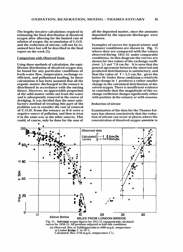
•
•
/ • I.. • /
10 20
• •
••
•
:4
OXIDATION, REAERATION, MIXING - THAMES ESTUARY 85
•
•
The lengthy iterative calculations required in estimating the final distribution of dissolved oxygen after allowing for the limited rate of solution of oxygen, the accumulation of U.O.D. and the reduction of nitrate, will not be ex-amined here but will be described in the final report on the work (5).
Comparison with Observed Data
Using these methods of calculation, the equi-librium distribution of dissolved oxygen may be found for any particular conditions of fresh-water flow, temperature, exchange co-efficient, and pollutional loading, In these calculations it has been assumed that all the organic matter discharged to the estuary is distributed in accordance with the mixing theory. However, an appreciable proportion of the solid matter settles out from the water and is subsequently removed in the course of dredging. It was decided that the most satis-factory method of treating this part of the problem was to consider the rate of removal of U.O.D. from the estuary as if it were a negative source of pollution, and then to treat it in the same way as the other sources. This could, of course, only be done for the sum of
•
100
•
0 — 80-•
•
u 60
5 Vx 40
n20 In
0
0
all the deposited matter, since the amounts deposited by the separate discharges were unknown.
Examples of curves for typical winter and summer conditions are shown in Fig. 11 where they are compared with the values observed during 1951-55 under comparable conditions. In this diagram the curves are shown for two values of the exchange coeffi-cient: 5.5 and '7.0 cm./hr. It is seen that the general agreement between the observed and predicted distributions is satisfactory, and that the value of f = 5.5 cm./hr. gives the better fit. Under these Conditions a relatively large change in f produces a rather smaller change in the calculated distribution of dis-solved oxygen. There is insufficient evidence to conclude that the magnitude of the ex-change coefficient changes significantly either with position in the estuary or with seasons.
Reduction of nitrate
Examination of the data for the Thames Est-uary has shown conclusively that the reduc-tion of nitrate can occur at places where the concentration of dissolved oxygen amolInts to
•
•
• •• (
8•
1. •oil
_sr
10 Above Below
Observed data • • Calculated [--1 5.5am/hr. curves -- 1=7.0cm/hr.
30 40
•
MILES FROM LONDON BRIDGE Fig. 11. Individual oxygen figures for 1951-55 comparedwith calculated curves for 1950-53. All positions adjusted to half-tide conditions.
(a) Observed: flow at Teddington 3100 to 4400 m.g.d., temperature at London Bridge 5° to 10°C. Calculated: flow 3750 m.g.d., temperature 5°C.
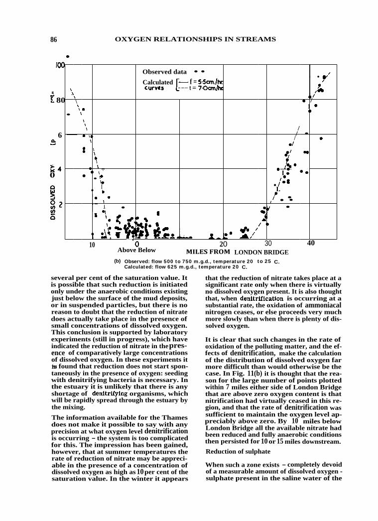
;"( 4 0
a
86 OXYGEN RELATIONSHIPS IN STREAMS
100
.15. 80
6 CL
•■■••■•
•
\
•\ ■
Observed data • • Calculated [-- f = 5-5cm./hc curves --- t = 7.0cmjhr
. • Iv
P f /db
1
/
•
\ \ ■ ‘
_____.
•
\ ■ \
\ • /
/
• 1
•
/ • •
■ • • •
•
\ \ • ■ 1
/ • ./ e/
IF/ r
• .-4 I •
/ •
• /, • 8 I.
P / • / • •
I.
• •
•
• • l
•
. P I. I • •
1.41 1 • I i •
I Pi 6- 1 ■P • _... ■• is. ara I -I'
1 :11, 41P1F VII;
11 .,-- %
1482,•i.....• I ■
• 0 /
at . -IL/
../ 4•4
/1110
•
10 4— 0 20 30 40 Above Below MILES FROM LONDON BRIDGE
(b) Observed: flow 500 to 750 m.g.d., temperature 20° to 25°C. Calculated: flow 625 m.g.d., temperature 20°C.
several per cent of the saturation value. It is possible that such reduction is initiated only under the anaerobic conditions existing just below the surface of the mud deposits, or in suspended particles, but there is no reason to doubt that the reduction of nitrate does actually take place in the presence of small concentrations of dissolved oxygen. This conclusion is supported by laboratory experiments (still in progress), which have indicated the reduction of nitrate in the pres-ence of comparatively large concentrations of dissolved oxygen. In these experiments it Fs found that reduction does not start spon-taneously in the presence of oxygen: seeding with denitrifying bacteria is necessary. In the estuary it is unlikely that there is any shortage of denitrifying organisms, which will be rapidly spread through the estuary by the mixing.
The information available for the Thames does not make it possible to say with any precision at what oxygen level denitrification is occurring - the system is too complicated for this. The impression has been gained, however, that at summer temperatures the rate of reduction of nitrate may be appreci-able in the presence of a concentration of dissolved oxygen as high as 10 per cent of the saturation value. In the winter it appears
that the reduction of nitrate takes place at a significant rate only when there is virtually no dissolved oxygen present. It is also thought that, when denitrification is occurring at a substantial rate, the oxidation of ammoniacal nitrogen ceases, or else proceeds very much more slowly than when there is plenty of dis-solved oxygen.
It is clear that such changes in the rate of oxidation of the polluting matter, and the ef-fects of denitrification, make the calculation of the distribution of dissolved oxygen far more difficult than would otherwise be the case. In Fig. 11(b) it is thought that the rea-son for the large number of points plotted within 7 miles either side of London Bridge that are above zero oxygen content is that nitrification had virtually ceased in this re-gion, and that the rate of denitrification was sufficient to maintain the oxygen level ap-preciably above zero. By 10 miles below London Bridge all the available nitrate had been reduced and fully anaerobic conditions then persisted for 10 or 15 miles downstream.
Reduction of sulphate
When such a zone exists - completely devoid of a measurable amount of dissolved oxygen - sulphate present in the saline water of the

1933 1935 1936 1934 1932
6000
400a
2000
0
Low water H igh water -- —
OXIDATION, REAERATION, MIXING - THAMES ESTUARY 87
estuary is reduced, giving rise to sulphide (56). It appears from the Laboratory's sur-veys that sulphide is never to be found in solution in the presence of any significant amounts of either dissolved oxygen or ni-trate, and so it has been concluded that in order to avoid all nuisance from the produc-tion of sulphide it is only necessary to ensure that there is always some dissolved oxygen or some nitrate present at every point in the estuary.
Effects of flow and temperature
It is evident from Fig. 11 that the condition of the estuary is very much worse in the summer than in the winter. This might be attributed either to differences in tempera-ture or to differences in fresh-water flow. While the mixing theory was being developed a fairly detailed statistical analysis was made of the large amount of data made avail-able by the London County Council relating to the oxygen content of the water in the estuary. From this it was concluded that the effect of fresh-water flow was of far greater import-ance than that of temperature. An example of the data that led to this conclusion is shown In Fig. 12, where monthly averages of the temperature and oxygen content of the water off Northern Outfall are compared with the
corresponding figures for the flow at Tedd-ington; the temperature scale has been in-verted to make the comparison more conven-ient. It is seen that normally during the winter - when the temperature falls and the flow rises - the oxygen .content increases, but that in the exceptionally dry winter of 1933-34, when the flow hardly exceeded the normal summer value, the oxygen content of the estuary at this point did not rise much above 10 per cent of saturation, although the temperature curve for that winter is perfect-ly normal.
It is only comparatively recently that it has been realized that the conclusions drawn from the statistical work are incomplete, since the condition of the water should be judged by its content of nitrate as well as by that of dissolved oxygen. The effect of tem-perature is much less marked when the con-dition of the water is roughly that at which denitrification can take place. Since the re-duction of nitrate occurs more readily at higher temperatures, the adverse effects of temperature on the condition of the estuary is largely masked by oxygen being made available by denitrification. Thus it was found that although when the general level of the sag curve minimum was around 10 per cent of saturation the effect of temperature
Fig. 12. Four-weekly averages of oxygen content and temperature off Northern Outfall and of flow at Teddington, July 1932 to July 1936.

88 OXYGEN RELATIONSHIPS IN STREAMS
could hardly be discerned, as soon as anaer-obic conditions became frequent the length of the anaerobic zone was dependent on the tem-perature - once an anaerobic zone exists, all the available nitrate from the upper estuary has been reduced and, for a given fresh-water flow, roughly the same amount of oxy-gen will have been made available at all times of the year.
Application of Methods
By comparing the observed and predicted data for dissolved oxygen under various con-ditions, of which Fig. 11 shows two examples, It was concluded that the methods that have been used were fairly satisfactory. It was then possible to use these methods for pre-dicting what changes could be expected in the distribution of dissolved oxygen if certain changes were made in the factors that affect the oxygen concentration.
Oxygen depletion by unit polluting load
For example, curves were calculated to show the effect of adding polluting matter at a rate of 10 tons U.O.D. per day at various points in
the estuary. A separate calculation is re-quired for each point of input, exchange co-efficient, flow, and temperature. The oxy-gen depletion caused by U.O.D. loads other than 10 tons per day is found by simple pro-portion. In Fig. 13 are shown some of the curves for different flows and temperatures relating to inputs at two different points in the estuary.
To find the effect of adding any particular load to the sources of pollution already exist-ing it is only necessary to subtract from the observed distribution of dissolved oxygen the depletion calculated from curves such as shown in Fig. 13; but this addition can be made only if the oxygen content of the water is nowhere zero and the total polluting load does not reduce the oxygen content sufficient-ly to affect the reduction of nitrate. It is evident from Fig. 11 that under the conditions that have existed in the estuary during the past few years, curves such as those shown in Fig. 13 cannot be applied directly to the sag curve. Under these conditions it is nec-essary to make the further complicated iter-ative calculations mentioned above, so as to determine the extent of the anaerobic zone
I Li
1-8
h6
1-4
12
/ •
0.
\ .
I I i FLOW AT TEDDINGTON (m.g.d.) 170 SOO 1500
TEMPERATURE OF WATER(.) 24 20 20 INPUT AT LONDON BRIDGE -0 -0---0—
INPUT 20 MILES BELOW LONDON BRIDGE ..........
.
. . .
4
. . 4
0, ,
, ,
,. . , . , • . •
... to .3,..
1 /
........... ..- .•
/ /
•• • • •
• • . ..._
.... - ..
— . ...
10 0 10 20 30 Above Below MILES FROM LONDON BRIDGE Fig. 13. Oxygen deficit, at half-tide, produced by steady input of 10 tons U.O.D. per day at two points in the estuary, under certain equilibrium conditions of flow and temperature.
40
OXIDATION, REAERATION, MIXING - THAMES ESTUARY 89
and to calculate the shape of the sag curve; if the condition of the estuary were improved sufficiently, the curves such as shown in Fig. 13 could be applied directly.
Other estuaries The methods that have been used in the sur-vey of the Thames Estuary are probably ap-plicable to any other estuary in which there is little or no stratification. Where there is pronounced stratification the method would have to be modified and might become un-workable.
The calculations have taken a very long time, but this has been largely due to the time taken in developing a satisfactory theory and apply-ing it to the particular conditions in the Thames Estuary. If another estuary were
tackled in the same way the work involved, although great, would probably not require such an expenditure of time and labour as did the survey of the Thames.
Distribution of temperature
Essentially the same methods based on the mixing theory have been used in calculating the effects of heated discharges on the dis-tribution of temperature in the estuary. A full account of this work will be published shortly (57).
ACKNOWLEDGEMENT
This paper is published by permission of the Department of Screntific and Industrial Re-search, Great Britain.
References
1. Water Pollution Abstracts. Published monthly, H. M. Stationery Office, London.
2. Department of Scientific and Industrial Research. Reports of Water Pollution Research Board. Published annually, H. M. Stationery Office, London.
3. Department of Scientific and Industrial Research, 1935. Survey of the river Tees. Part II. The estuary - chemical and biological. Water Pollution Re-search Technical Paper No. 5. H. M. Stationery Office, London.
4. Department of Scientific and Industrial Research, 1937. Effect of discharge of crude sewage into the estuary of the river Mersey on the amount and hardness of the deposit in the estuary. Water Pollution Research Technical Paper No. 7. H.M. Stationery Office, London.
5. Department of Scientific and Industrial Research. (In preparation.)
6. Streeter, LW., and Phelps, E. B., 1925. A study of the pollution and natural puri-fication of the Ohio River, III. Publ. Hlth. Bull., Wash., No. 146.
7. Department of Scientific and Industrial Research, 1956. Water Pollution Re-search 1955. H. M. Stationery Office, London.
8. Winkler, L. W., 1886. Die Bestimmung des im Wasser gelBsten Sauerstoffes. Ber. dtsch. chem. Ges., 21, 2843.
9. Alsterberg, G., 1925. Methoden fUr Bestimmung von im Wasser gelOsten Sauerstoff bei Gegenwart von Salpetri-gersgure. Biochem. Z., 159, 36.
10. Staff of the Water Pollution Research Laboratory, 1953. Some notes on the determination of dissolved oxygen. Water Sanit. Engr., 4 48.
11. Knowles, G.' and LOwden, G. F., 1953.
Methods for detecting the endpoint in the titration of iodine with thiosulphate. Analyst, 78, 159.
12. Wheatland, A.B., and Smith, L. J., 1955. Gasometric determination of dissolved oxygen in pure and saline water as a check of titrimetric methods. J. appl. Chem.,
144.
13. Briggs, R., Knowles, G., and Scragg, L. J., 1954. A continuous recorder for dissolved oxygen in water. Analyst, 79, 744.
14. Briggs, R., Dyke, G. V., and Knowles, G. Analyst (in the press).
15. Ingols, R. S., 1941. Determination of dissolved oxygen by the dropping mercury electrode. Sewage Wks J., 13, 1097.
16. Fyn, E., 1955. Continuous oxygen re-cording in sea-water. Fiskerkiir. Skr. HavundersOk., 11, No. 3.

90
17.
OXYGEN RELATIONSHIPS IN STREAMS
Ohle, W., 1953. Die chemishe und die elektrochemische Bestimmung des mole-kular ffelOsten Sauerstoffes der Bin-nengewasser. Mitt. in Ver. Limnol. No. 3.
18. Fox, C. J. J., 1909. Coefficients of absorption of nitrogen and oxygen in distilled water and sea-water, and of atmospheric carbon dioxide in sea-water. Trans. Faraday Soc., • 68.
19. Whipple, G. C., and Whipple, M. C., 1911. Solubility of oxygen in sea-water. J. Amer. Chem. Soc., 33, 362.
20. Truesdale, G. A., and Downing, A. L., 1954. Solubility of oxygen in water. Nature, Lond., 173, 1236.
21. Truesdale, G. A., Downing, A. L., and Lowden, G. F., 1955. The solubility of oxygen in pure water and sea-water. J. appl. Chem., 5, 53.
22. Gameson, A. L. H., and Robertson, K. G., 1955. The solubility of oxygen in pure water and sea-water. J. appl. Chem., 5, 502.
23. Truesdale, G. A., and Gameson, A. L. H., 1957. The solubility of oxygen in saline water. J. Cons. int. Explor. Mer., 22, 163.
24. Mortimer, C. H., 1956. The oxygen con-tent of air-saturated fresh waters, and aids in calculating percentage saturation. Mitt. int. Ver. Limnol., No. 6.
25. Sclunassmann, H., 1956. Determination of the oxygen saturation concentration. Schweiz. Z. Hydrol., 18, 144.
26. Richards, F. A., and Corwin, N., 1956. Some oceanographic applications of re-cent determinations of the solubility of oxygen in sea-water. Limnol. & Ocean-ogr., 1, No. 4, 263.
27. Adeney, W. E., and Becker, H. G., 1919. Determination of atmospheric oxygen in water. Phil. Mag., 38, 317.
28. Gameson, A. L. H., Truesdale, G. A., and Downing, A. L., 1955. Reaeration studies in a lakeland beck. J. Instn Wat. Engrs, 9, 571.
29. Lewis, W. K., and Whitman, W. G., 1924. Principles of gas absorption. Industr. Engng Chem., 16, 1215.
30. Gameson, A. L. H., 1954. L'auto-epura-tion dans les estuaires. Bull. Centre belge Et. Document. Eaux, No. 24, 71.
31. Gameson, A. L. H., and Preddy, W. S., 1956. Factors affecting the concentra-tion of dissolved oxygen in the Thames Estuary. J. Inst. Sewage Purif., Part 4, 322.
32. Inglis, C. C., and Allen, F. H. The regimen of the Thames Estuary as af-fected by currents, salinities, and river flow. Presented to Institution of Civil Engineers, May, 1957.
33. Wheatland, A. B., and Lloyd, R., 1955. A respirometer for the study of the oxygen demand of polluted water and sewage. Lab. Pract., 4, 6.
34. Gameson, A. L. H., and Wheatland, A. B. (In preparation.)
35. Butler, W., and Coste, J. H., 1923. Sea-sonal variations in the dissolved oxygen content of the water of the Thames Estu-ary. Biochem. J., 17, 49.
36. Phelps, E. B., 1944. Stream Sanitation. John Wiley & Sons Inc.
37. Theriault, E. J., 1927. The oxygen de-mand of polluted waters. U. S. Publ. Hlth Bull., No. 1'73.
38. Gotaas, H. B., 1948. Effect of tempera-ture on biochemical oxidation of sewage. Sewage Wks J., 20, 441.
39. Department of Scientific and Industrial Research, 1954. Water Pollution Re-search 1953. H. M. Stationery Office, London.
40. Brubaker, D. W., and ICammermeyer, K., 1953. Flow of gases through plastic membranes. Industr. Engng Chem., 45, 1148.
41. O'Connor, D. J., and Dobbins, W. E., 1956. The mechanism of reaeration in natural streams. Proc. Amer. Soc.Civ. Engrs., 82, SA6, Paper No. 1115.
42. Downing, A. L., and Truesdale, G. A., 1955. Some factors affecting the rate of solution of oxygen in water. J. appl. Chem., 5, 570.
43. Department of Scientific and Industrial Research, 1955. Water Pollution Re-search 1954. H. M. Stationery Office, London.

OXIDATION, REAERATION, MIXING - THAMES ESTUARY 91
44. Gameson, A. L. H., Truesdale, G. A., and Varley, R. A., 1956. Some factors affecting the aeration of flowing water. Wat. Sanit. Engr, 6, 52.
45. Truesdale, G. A., and Vandyke, K. G., 1958. The effect of temperature on the aeration of flowing water. Wat. Waste Treatm. J., 7, 9.
46. Streeter, H. W., Wright, C. T., and Kehr, R. W., 1936. Measures of natural oxidation in polluted streams M. Sew-age Wks J., 8, 282.
47. Gameson, A. L. H., 1957. Weirs and the aeration of rivers. J. Instn Wat. Engrs. 11, No. 6, 477.
48. Gameson, A. L. H., Vandyke, K. G. and Ogden, C. G. The effect of temperature on aeration at weirs. (In preparation.)
49. Downing, A. L., Melbourne, K. V., and Bruce, A. M. The effect of contaminants on the rate of aeration of water. J. appl. Chem. (In the press.)
50. Longwell, J., and Maniece, W. D., 1955. Determination of anionic detergents in sewage, sewage effluents and river waters. Analyst, 80, 167. •
51. Kehr, R. W., 1938. Measures of natural oxidation in polluted streams IV. Sewage Wks J., 10, 228.
52. Downing, A. L., and Melbourne, K. V., 1956. The effect of foam-suppressor on the aeratipn of polluted water. Wat. Sanit. Engr, 6, 148.
53. Downing, A. L., and Melbourne, K. V., 1957. Chemical conservation of water. J. Instn Wat. Engrs, 11, 438.
54. Preddy, W. S., 1954. The mixing and movement of water in the estuary of the Thames. J. Mar. biol. Ass. U.K., 33, 645.
55. Southgate, B. A., and Preddy, W. S., 1952. Discharge of sewage and industrial wastes to estuaries. J. R. sanit. Inst., 72, 424.
56. Wheatland, A. B., 1954. Factors affect-ing the formation and oxidation of sul-phides in a polluted estuary. J. Hyg., Camb., 52, 194.
57. Gameson, A. L. H., Hall, H., and Preddy, W. S., 1957. The effects of heated dis-charges on the temperature of the Thames Estuary. The Engineer, Lond. 204, 816.
DISCUSSION if. E. LANGELY, JR. Arthur D. Little, Incorporated
The group at the Water Pollution Research Laboratory in Britain have used a direct method employing oxygen balances for evalua-ting the exchange coefficient for reaeration in the Thames Estuary. The calculated oxygen sag curves for average summer and winter conditions show relatively good agreement with observed dissolved oxygen values. There are two points in the report that require further discussion however, the mechanism involved in the oxidation of suspended mat-ter and the use of nitrate and sulfate as a source of oxygen.
The oxygen relationships in a polluted stream or estuary depend fundamentally on the micro-organisms in the water. Many different groups of microorganisms are present in any natural water course but the bacteria play the most Important role in stream purification. These microorganisms use pollutional matter as a source of food. The stabilization of organic matter and the exertion of oxygen demand in streams are principally a result of their metabolism.
Bacterial Metabolism
The organic matter used by the bacteria must be in solution and of a molecular size small enough to diffuse through the cell wall as all synthesis and energy reactions take place inside the bacterial cell. Part of this organic matter is used for synthesizing bacterial protoplasm and the rest is oxidized for energy.
Before suspended organic matter can be used by the cell, it must be put into solution. This is accomplished by extracellular enzymes excreted into the surrounding solution by the bacteria. These enzymes break down the suspended organic matter and large dissolved molecules through a series of hydrolysis reactions. The rate of oxidation of suspended matter in a stream therefore, must depend on the rate of enzymatic hydrolysis of this material and not on the diffusion of oxygen Into the solid particles.
Stabilization of Organic Pollutants
The stabilization of organic matter is brought

92 OXYGEN RELATIONSHIPS IN STREAMS
about by the energy reactions of the micro-organisms. These are oxidation-reduction reactions carried out by enzymes within the cell. Organic matter is oxidized indirectly by enzymes through a series of dehydro-genation and hydration reactions and not by direct addition of oxygen. The hydrogen re-moved is transferred through enzyme systems to the material acting as the hydrogen ac-ceptor which is reduced. McKinney and Conway (1) have reported on the mechanisms involved in bacterial oxidation under both aerobic and anaerobic conditions and have shown that hydrogen acceptors are utilized in the following order:
1. Dissolved Oxygen
2. Nitrate
3. Sulfate
4. No Oxygen.
The amount of energy derived by the micro-organisms utilizing these hydrogen acceptors decreases in the same order.
Microorganism Predominance
A mixed microbiological population will adapt itself to utilize the food source available. The species that predominate can use the food at the fastest rate and this metabolic activity requires the greatest amount of energy. The predominating species therefore, will be the ones capable of using the hydrogen acceptor yielding the greatest amount of energy to the cell per unit of organic matter oxidized.
Nitrate Reduction
The organisms that can utilize both dissolved oxygen and nitrate as hydrogen acceptors will always use dissolved oxygen as long as it is available to provide the greatest amount of energy for their metabolism. As dissolved oxygen is depleted, these organisms shift their enzyme systems to the utilization of nitrate reducing it to nitrogen gas. The shift to nitrate reduction is accompanied by a de-crease in energy yield to the organism and occurs only when the dissolved oxygen con-centration reaches a limiting value some-where between zero and a few tenths of a p.p.m. depending on the concentration of nitrate.
The use of nitrate as a hydrogen acceptor by microorganisms to satisfy their energy
requirements should not be confused with the reduction of nitrate to. ammonia by some organisms to provide a source of nitrogen for cellular protein. When nitrate is the sole source of nitrogen, these organisms will re-duce nitrate at any dissolved oxygen concen-tration as this reduction is a synthetic process. In a stream with other sources of nitrogen available, this reaction would be insignificant.
Sulfate Reduction
When all dissolved oxygen and nitrate are re-moved from solution, facultative organisms and other anaerobic organisms oxidize organic matter in a higher energy state and reduce organic matter in a lower energy state with a net yield of energy to the cells. This results in only a partial stabilization or organic matter. Two specialized groups of strictly anaerobic organisms exist that can utilize these organic end products. One group oxidizes them utilizing sulfate as the hydrogen acceptor reducing it to sulfide. The other group reduces carbon dioxide and the organic end products to form methane. Sulfate re-duction yields higher energy than methane formation, but in either case, energy yields are low in comparison with nitrate.
Swaimary
Microorganism stabilize organic matter in a polluted stream by oxidizing it inside the cell. Since all organic matter entering the cell must be in solution, the rate of oxidation of sus-pended matter must depend on the rate of solution of this material by enzymatic hydrolysis and not on the diffusion of oxygen into the solid particles. The oxidative pro-cess involves the transfer of hydrogen to a hydrogen acceptor and the organisms al-ways use the hydrogen accepted yielding the greatest amount of energy to the cell as long as it is available. The depletion of the oxygen resources in streams occurs in the following sequence, 1) dissolved oxygen, 2) nitrate, and 3) sulfate. Thus a stream that always contains some dissolved oxygen or nitrate will be free of nuisance problems due to hydrogen sulfide and methane production.
References
1. McKinney, R. E. and R. A. Conway. Chemical oxygen in biological waste treatment. Sewage and Ind. Wastes, 29: 1097. (1957).

OXIDATION, REAERATION, MIXING - THAMES ESTUARY 93
INFORMAL DISCUSSION A. L. H. Gameson: Concerning the oxi-
dation of solid matter, I agree that "the rate of oxidation of suspended matter in a stream .......... must depend on the rate of enzymatic hydrolysis of this material and not on the dif-fusion of oxygen into the solid particles". Nevertheless, the uncertainty about the rate of oxidation remains.
In the reduction of nitrate, from the data available for the Thames, it appears that the maximum oxygen concentration at which denitrification occurs depends on the tem-perature -nitrate being more readily reduced under aerobic conditions in the summer than in the winter. We have not observed any effect of the concentration of nitrate on this limiting oxygen concentration.
E. A. Pearson: What is the effect of photosynthesis in the Thames?
A. L. H. Gameson: This aspect is dealt with in the published paper but had not been included in my verbal presentation.
M. LeBosquet: Has direct aeration of
the estuary water ever been used as a practical solution to the pollution problem?
A. L. H. Gameson: Direct aeration has never, so far as I am aware, been used in the Thames Estuary, but at the two electri-city generating stations where the washing of flue gases is practiced, and which conse-quently discharge sulphite to the estuary, the effluent receives some aeration and this re-duces the polluting load reaching the Thames. At the present time the practicability of aerating the condenser water passing through some of the larger power stations is being examined.
T. R. Camp: Has any consideration been given to discharging the main sewage effluents further downstream?
A. L. H. Gameson: A hundred years ago, when a Royal Commission was examining the disposal of sewage from the Metropolis, there was a proposal that the sewer outialls should be sited about 20 miles downstream of the positions finally adopted. Another proposal was that the sewage from both the north and south sides of the river should be discharged to the North Sea on the Essex coast. I under-stand that it is now considered uneconomical to move the positions of the outfalls.


OXYGEN RELATIONSHIPS IN STREAMS 95
Third Session
Presiding
E. W. Moore, Lecturer In Sanitary Chemistry, Harvard University
Mixing and Diffusion of Wastes in Streams
H. A. Thomas, Jr., Professor of Sanitary Engineering, Harvard University
Discussion
T. R. Camp, Consulting Engineer; Camp, Dresser and McKee
Effects of Impoundments on Oxygen Resources
M. A. Churchill, Chief, Stream Pollution Control Section, Tennessee Valley Authority
Discussion
C. H. Hull, Consulting Engineer, Sheppard T. Powell Company

),
.

Mixing and Diffusion of Wastes in Streams
HAROLD A. THOMAS, JR. Professor of Civil and Sanitary Engineering
Harvard University
97
1. Definitions
Longitudinal mixing is a kinematic effect in "one-dimensional" fluid flow systems in which the various portions of the flow take different times to traverse a given reach of the stream.
Shortcircuiting is a form of longitudinal mixing in which a portion of the flow travels through the reach in a time in-terval substantially shorter than the mean time.
Mean flow time or theoretical detention period is the volume of liquid in the reach divided by the mean rate of flow or dis-charge. This is the arithmetic mean travel time of the water molecules. In unsteady flow systems the theoretical detention period is the temporal mean volume of the reach divided by the tempo-ral mean discharge.
Flow-through time distribution is a graph (table or formula) indicating the time of traverse of each portion of the flow. Such distributions are usually described and interpreted statistically. They may be given in the form of a frequency distri-bution or a cumulative frequency distri-bution of flow times.
Tracer is a substance such as a dye, salt, float, or radio-isotope added to the flow and identified in samples from down-stream stations. It is presumed to behave
kinetically in the fluid in a manner similar to the fluid particles themselves.
Radial, lateral, and vertical mixing may occur in the flow and affect or be affected by longitudinal mixing.
H. Causes of Longitudinal Mixing. Longi-tudinal mixing of flow in the passage of fluids through streams, conduits, tanks, and lakes is the result of several factors acting separately or in combination.
A. Major Factors
1. The non-uniform distribution of velocity caused by the curvature of and shear at the solid bounda-ries of the flow;
2. Eddy diffusion engendered by the turbulence of the moving stream;
3. Irregular displacements, convec-tion, and mixing due to wind and to density differences.
B. Minor Factors
1. Mixing and convection from boats, pumps, sludge removal mecha-nisms, anaerobic sludge flotation, etc.
2. Non-consumptive water uses; for example, cooling water returned to the stream.

98 OXYGEN RELATIONSHIPS IN STREAMS
3. Molecular diffusion.
4. Non-uniform flow times associ-ated with non-uniform irrotational (potential) flow. In absence of dif-fusion (molecular or eddy) and lateral mixing, longitudinal dis-persion occurs when stream lines have different mean velocities.
M. Effects of Longitudinal Mixing
A. Major. Longitudinal mixing may greatly affect the degree of treat-ment or self-purification of fluids containing pollution, the removal of which proceeds primarily in accord-ance with a time-dependent process. Example: radioactive isotopes not affected by physical, chemical, or biochemical processes but subject only to nuclear decay.
B. Minor. Affects (or is correlated with) degree of treatment or self-purifica-tion of processes, e.g. BOD, settling, and coliform-dieaway that are in part, at least, time-dependent. Even with processes that depend primarily upon contact rather than time, the degree of treatment or removal maybe cor-related with longitudinal mixing para-meters since these maybe indicative of the opportunity for and frequency of contact between the fluid and boundaries or particles on (or in) which purification or stabilization takes place.
IV. Experimental Methods. The principal techniques are patterned after the Allen salt-velocity method: a slug or cloud of salt (tracer) solution is abruptly injected into the flow, and measurements are made at a downstream station or stations of the time of travel of various portions of the tracer cloud.
A. Salts (1) (7) (8) (15) B. Dyes (11) (12) C. Radio-tracers (2) (6) (10) (13) Other techniques involve use of floats, temperature, and pH measurements.
V. Parameters Descriptive of Longitudinal Mixing
A. Average flow-time: Mean, median, and mode of observed flow-through time distributions. In dye tests, the average of the time of appearance of the first and last trace is sometimes used.
The term "actual flow time" usually refers to the time abscissa of the cen-troid of the flow-through distribution. This parameter is often of limited value and may be misleading since the amount of tracer "recovered" at the downstream station may be con-siderably smaller than that added. The difference depends upon the ade-quacy of the tracer, the sensitivity of the detection techniques, and the frequency and duration of sampling. In steady flow, by definition, no com-pletely "dead" space can exist. There may, of course, exist relatively stag-nant zones in the reach that may trap part of the flow and release it slowly at concentrations below the threshold of detection.
The term "volumetric efficiency" calculated as the observed mean flow time divided by the theoretical deten-tion period has sometimes been used as a parameter describing longitudi-nal mixing. It is a defective para-meter in that its magnitude as mea-sured on a given flow system depends to a large extent upon the tracer used and the sensing technique employed.
B. Measures of Dispersion: The spread of the tracer cloud maybe described by the standard deviation, semi-interquartile range, decile range or the time interval between the first and last traces of the tracer cloud. The value of these descriptive parameters is dependent upon the adequacy of the tracer (degree of ab-sorption, sensitivity of detection) and the sampling program. Various methods are used to adjust the ob-servations so as to correct for in-complete recovery of the tracer slug.
C. Flow-times Relative to the Modal Flow-time: A simple method of des-cription of flow-through time distri-butions that is relatively independent of imperfections of the tracer and sampling technique is the following:
1. Find the modal concentration and time (t2).
2. Divide the modal concentration by four and locate the times before (t1) and after (t3) the modal time on the flow-through distribution corresponding to this concentra-tion.
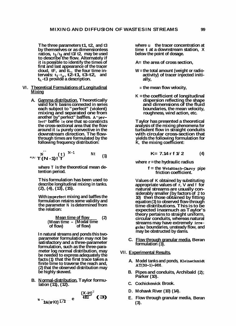
MIXING AND DIFFUSION OF WASTES IN STREAMS 99
The three parameters t1, t2, and t3 by themselves or as dimensionless ratios, t1/t2 and t3/t2, may be used to describe the flow. Alternately if it is possible to identify the times of first and last appearance of the tracer cloud, tF, and tL, the four time in-tervals: ti-tF, t2-t1, t3-t2, and tL-t3 provide a description.
VI. Theoretical Formulations of Longitudinal Mixing
A. Gamma distribution. Theoretically valid for N basins connected in series each subject to "perfect" (violent) mixing and separated one from another by"perfect" baffles. A"per-feet" baffle is one that so constricts the cross-sectional area that the flow around it is purely convective in the downstream direction. The flow-through times are formulated by the following frequency distribution:
where u the tracer concentration at time t at a downstream station, X below the point of dosage.
A= the area of cross section,
W = the total amount (weight or radio-activity) of tracer injected initi-ally,
= the mean flow velocity,
K =the coefficient of longitudinal dispersion reflecting the shape and dimensions of the fluid boundaries, the mean velocity, roughness, wind action, etc.
Taylor has presented a theoretical analysis of the mixing phenomena for turbulent flow in straight conduits with circular cross-section that yields the following formulation for K, the mixing coefficient:
N-1 1"/
NN
( t ) T(N-1)! T
Nt (1) K= 7.14 r f 1/2 (4)
where T is the theoretical mean de-tention period.
This formulation has been used to describe longitudinal mixing in tanks. (2), (4), (13), (15).
With imperfect mixing and baffles the formulation retains some validity and the parameter N is determined from the relation:
Mean time of flow (2) (Mean time - (Modal time of flow) of flow)
In natural streams and ponds this two-parameter formulation may not be satisfactory and a three-parameter formulation, such as the three-para-meter log normal distribution, may be needed to express adequately the facts (1) that the first trace takes a finite time to traverse the reach and, (2) that the observed distribution may be highly skewed.
B. Normal-distribution. Taylor formu-lation (11), (12).
(X-i-rt)2 -4-Kr- (3) U - e 2A(7r Kt) 1/2
where r =the hydraulic radius f = the Weishbach-Darcy pipe
friction coefficient.
Values of K obtained by substituting appropriate values of r, V and f for natural streams are usually con-siderably smaller (by factors of 2 to 10) then those obtained by fitting equation (3) to observed flow-through time distributions. This is to be expected inasmuch as Taylor's theory pertains to straight uniform, circular conduits, whereas natural streams may have extremely irre-gular boundaries, unsteady flow, and may be obstructed by dams.
C. Flow through granular media. Beran formulation (3).
VII. Experimental Results.
A. Model tanks and ponds, Kleinschmidt AT(30-1)-966.
B. Pipes and conduits, Archibald (2); Parker (10).
C. Cochickewick Brook.
D. Mohawk River (10) (14).
E. Flow through granular media, Beran (3).

TABLE 1. Results of Various Tracer Tests, Cochichewick Brook Dosing Pt. to Station 8 Time abscissa, hours *
Run No.
Radio- isotope
Date Dosed
Average Disch.
cfs
Coef. of Var. of Disch. in %
mc Dosed mc Rec Sta. 8
% Rec. Oak Ridge figs. Sta. 8
t1
t3
t4
6 Rb86 4/4/56 6.44 25.8 49.0 42.0 85.7 19 31 89 58 8 Rb86 5/2/55 4.17 44.6 29.8 32.2 108.1 26 32 145 128 9 Rb86 5/23/55 3.23 13.0 14.1 10.1 71.7 44 50 64 56 10 Rb86 6/6/55 6.15 33.2 49.0 26.7 54.4 42 24 54 36 11 Rb86 6/13/55 4.37 8.70 38.2 27.9 73.1 27 45 75 74 12 Rb86 7/11/55 3.93 47.6 36.3 25.8 71.2 52 57 87 25 13 Rb86 8/1/55 2.91 81.1 28.3 18.1 64.0 40 72 88 42 14 Rb86 8/22/55 4.09 60.4 28.8 18.4 64.0 40 64 144 56 15 Rb86 9/12/55 8.09 27.3 13.7 10.8 79.1 64 71 78 44 17 Sr89 12/20/55 9.89 28.2 33.1 29.0 87.5 22 41 101 25 20 Rb86 2/14/56 16.70 9.2 44.9 52.7 117.5 3 11 34 37 26 CePr 144 6/4/56 8.43 41.8 5.5 5.0 90.6 14 13 14 55 28 Sr89 7/2/56 7.25 47.9 36.1 24.6 68.3 40 55 80 14
* t1 = time of first trace to time at 25% peak concentration t2 = time 25% peak concentration to time of peak t3 = time of peak to time 25% peak concentr ation t4 = time of 25% peak concentration to time of last trace
October 1957
0
OX
YG
EN
RE
LA
TIO
NS
HIP
S IN
ST
RE
AM
S

MIXING AND DIFFUSION OF WASTES IN STREAMS 101
TABLE 2 - Radioactive Tracer Data, Constant Flow Tests *
Distance (feet)
Theoretical Mode First trace time of flow, (percent- (percentage T (seconds) age of T) of T)
Average time
(percent- age of T)
Height of mode
(1) (2) (3) (4) (5) (6)
(a) Reynolds Number = 14,210
21.4 10.2 103.8 73.1 139.0 1.36 36.5 17.1 95.4 73.3 101.2 60.9 28.3 92.9 82.2 108.2 1.28 75.6 34.0 93.9 82.5 100.0 1.17 94.0 44.3 98.4 89.4 100.0 0.89
(b) Reynolds Number = 7,490
31.3 27.8 56.2 45.9 78.6 44.8 39.4 69.1 55.4 80.1 53.4 46.9 72.1 63.0 86.0 78.2 68.7 77.1 69.9 84.2
(c) Reynolds Number = 218
21.4 69.4 57.7 39.0 84.7 5.30 36.5 116.5 60.1 38.6 67.6 2.80 60.9 195.5 70.3 38.3 60.4 75.6 219.4 54.8 44.2 57.9 1.06 94.0 292.6 56.8 46.4 70.9
* Thomas and Archibald TASCE 117 839 (1952)

TABLE 3. Results of Tracer Test, Mohawk River, August 9-18, 1954
% of initial dose (4.5 curies) passing
Station River Time of Mean Observed Observed Corrected Corrected Coefficient miles observed flow- peak for for of from peak time, activity- nuclear nuclear longitudinal
KAPL hr hr concentra- decay decay and dispersion,. outfall tion for self- K, ft/sec 4
dpm/liter purification
(1) (2) (3) (4) (5) (6) (7) (8) (8)
1CAPL 0.0 0.0 0.0 - 100 100 100
Vischer Ferry Dam 1.7 34.0 35.1 2900 58.2 62.1 100 14
Buoy 49 2.8 48.7 50.9 1200 50.4 54.2 100 49
Buoy 18B 7.5 118.5 118.5 450 19.7 24.5 100 67
Coheos Water Treatment Plant 13.0 217* 3.3* 100
* Extrapolated value.
OX
YG
EN
RE
LA
TIO
NS
HIP
S IN
ST
RE
AM
S
I■L 0

MIXING AND DIFFUSION OF WASTES IN STREAMS 103
References
1. Allen, C. M. and E. A. Taylor. The salt-velocity method of water measurement. Trans. Amer. Soc. of Mech. Engr., 45: 285. (1923).
2. Archibald, R. S. Radioactive tracers in flow tests. Jour. Boston Soc. of Civ. Engrs., 37:49-116. (1950).
3. Beran, M. J. The dispersion of soluble matter in flow through granular media. Jour. of Chem. Physics, 27:270-274 (July, 1957)
4. Camp, T. R. Sedimentation and the design of settling tanks. Trans. Amer. Soc. of Civ. Engrs. 111:931-34. (1946).
5. Glover, R. E. The dispersion of dissolved or suspended materials in flowing streams. Rept. U. S. Geol. Survey. Den-ver, Colorado. (June 1956).
6. Huiswaard, P. J. and C. G. Bell, Jr. Model study of the fate of pollution in a tidal estuary. Rept. Project AT(11-1)- 353. Dept. of C. E., Technological Insti-tute, Northwestern University. (Jan. 1957).
7. Mason, M. A. Contribution to a study of the Allen salt-velocity method of water measurement. Jour. Boston Soc. of Civ. Engrs., 27:207. (1940).
8. Morrill, A. B. Sedimentation basin re-search and design. Jour. Amer. Wat. Wks. Assn., 24:1442. (1932).
9. Nejedly, A. and J. Pelz. Effect of stream flow upon the course of self-purification of streams. (Abstract in Engliph). V§z-kumn§ 4tav vodohospodL(sky, Praha-Podbaba cislo 4. (1957).
10. Parker, F. L. Mechanisms of Dilution of Radio-contaminants in Streams. The iss, Harvard University. (1955).
11. Taylor, G. I. Dispersion of matter in turbulent flow through a pipe. Proc. of Roy. Soc. Series A 220:446-468. (1954).
12. Taylor, G. I. Dispersion of soluble mat-ter in solvent flowing slowly through a tube. Proc. Roy. Soc. Series A 219:186-203. (1953).
13. Thomas, Jr., H. A. and R. S. Archibald. Longitudinal mixing measured by radio-active tracers. Trans. Amer. Soc. of Civ. Engrs., 117:839-56. (1952).
14. Thomas, Jr., H. A. Radioactive tracers as tools in sanitary engineering research. Proc. of International Conference in Geneva. Vol. 15. (Aug. 1955).
15. Thomas, Jr., H. A. and J. E. McKee. Longitudinal mixing in aeration tanks. Sewage Works Jour., 16:42-55. (1944).
DISCUSSION THOMAS R. CAMP, Consulting Engineer Camp, Dresser, and McKee
(ED: Mr. Camp presented a formal discus-sion of Professor Thomas's paper. He emphasized that lateral and vertical mixing
were often as important as longitudinal mixing and he cited specific cases where this pheno-menon occurred.)

104 OXYGEN RELATIONSHIPS IN STREAMS
INFORMAL DISCUSSION M. D. Sinkoff: I would like to direct a
question to Professor Thomas. Is there any advantage in applying a tracer in a slug rather than in a continuous dose and then cutting it off instantaneously and operating with the resultant curve?
H. A. Thomas, Jr.: We do it both ways; particularly in sewers the way you described has some merits.
E. A. Pearson: I would like to ask Pro-fessor Thomas if he has any special reason why he chose to call the IC in his expressions or in the formulations of Taylor the coeffi-cient of longitudinal dispersion. Isn't this the same K we have described as the coefficient of eddy diffusion?
H. A. Thomas, Jr.: No.
E. A. Pearson: How does it differ?
H. A. Thomas, Jr.: There are cases in which the geometry is very simple where they are identical. In other cases, common in in-land waterways, they are not because of ir-regularities in the boundary of the flow such as dams. In the streams we have investigated, the flow patterns are complex and the aniso-trophy of turbulence is marked because of the irregular outline of the solid boundaries of the flow. As a result, the mixing process is very complicated. Fortunately, however, the practical assessment of the overall degree of mixing is simple since it is incorporated In the longitudinal mixing coefficient, K, which is proportional to the standard devia-tion of the temporal distribution of the tracer cloud.
Now the eddy diffusion coefficient is a different thing entirely. As defined in ele-mentary texts it is simply the ratio of the shear stress at a point in the fluid divided by the mean velocity gradient at this point in a direction normal to that of the velocity vector. As such it is merely a local parameter. In rivers we have found that it varies markedly from point to point in the flow. The eddy dif-fusion coefficient only grovides a measure of mixing intensity at a point in the flow, but it does not give a measure of the overall degree of mixing in the entire stream. The longitu-dinal mixing coefficient does this since it re-presents the effective average of the mixing at all points.
E. A. Pearson: I think maybe there is a little bit of longitudinal dispersion in our analysis. Oceanographers have been measur-ing this type of dispersion probably longer than anyone and they use K and call it eddy diffusivity. It concludes all the factors that are included in your expression. The oceano-graphic literature includes expressions of the type that you credit to Taylor or the solution of the general diffusion equation that I put on the board. These predate Taylor's equation by many years. In the general oceanographic field they have been concerned with dispersion phenomena, laterally as well as vertically. They chose to use the term eddy diffusivity.
H. A. Thomas, Jr.: In oceans, K and the eddy diffusion coefficient may for certain purposes be taken as the same thing; in rivers they are not the same thing. In oceans it, the mixing process, is fairly simple; in rivers It is much more complicated. It is true that if you knew the special and temporal distri-bution of the local diffusion coefficients throughout the river you could compute the overall effect by an appropriate method of averaging these. In effect this is precisely what is done by the tracer test and the calcu-lation of the coefficient K. The eddy diffusion coefficient is a local parameter; the longitu-din2l mixing coefficient indicates the overall effect.
D. J. O'Connor: You commented that in one case lateral mixing inhibited longitudinal mixing. Am I correct in that statement?
H. A. Thomas, Jr.: I did give a case where lateral mixing inhibited longitudinal mixing. Taylor has discussed this mechanism in considerable detail.
D. J. O'Connor: Could we apply that idea or case to a river where pollutants would hug the shore?
H. A. Thomas, Jr.: What is needed is a fundamental study of lateral and vertical mix-ing and a good place for such a study would be at Vicksburg. One object of the study would be to study methods, economical engineering methods, to foster the spread - to do as Mr. Camp said - to get better diffusion. On the other hand, we should study methodsfor pre-venting lateral diffusion in the case of the Detroit River where one can use a relatively unpolluted section of the flow for water sup-ply. We ought to make a thorough study of a practical and inexpensive engineering method for controlling lateral and vertical mixing.

MIXING AND DIFFUSION OF WASTES IN STREAMS 105
R. S. Ingols: I have been working with a situation where the consulting engineer has been directed by one of the other members of this audience, to provide lateral mixing for an effluent into a shallow, broad river in order to accomplish lateral mixing. It has been found that at extremely low flows there is little mixing in the river, pollution hugs the shore and slime extends many miles down-stream. At intermediate flows the pollution disperses across the river to an extent that no evidence of sewage fungus reaches three miles downstream. At extremely high flows - some 25-35" greater depth of flow - there is again very little lateral mixing. The designing engineer has been instructed to obtain lateral mixing at all flow values.
L. L. Falk: This is more of a comment than it is a question but it will wind up with a question that will be legal. I am just wonder-ing if some of us in the field of dispersion in streams might be overlooking a whole field of effort and work that has been done in the problem of dispersion from stacks. I refer principally to the work of C. H. Bosanquet and 0. G. Sutton in England. It seems to me that all of their theoretical approach might certainly have some application here. It is true that we have much more severe boundary conditions in the stream than we do in the air where we might deal only with the boundary imposed by the ground and perhaps the bound-ary imposed by temperature inversions. Mr. Thomas, has any consideration been given, as far as you know, to the work of these men as it might apply to dispersion in streams?
H. A. Thomas, Jr.: Yes. These are gen-erally similar phenomena. The differential equations are not different, but there are marked differences in the geometry of flows. The geometry is much more complicated in streams. Our real need, though, is not for more theory; we need more facts so as to delineate the parameters more precisely. I don't think there are available any oceano-graphers or new equations to elucidate stream sanitation problems. We do need more data pertaining to longitudinal mixing coefficients. Eddy diffusion coefficients are different; they do not have a direct application in the mea-surement of the overall mixing process in in-land waterways.
E. A. Pearson: I question that last state-ment. In fact, recent work that I am familiar with indicates that they are probably of the same order of magnitude if you consider the scale.
D. J. O'Connor: (Ed: O'Connor discussed Sutton's and Ftichardson's theories.)
H. A. Thomas, Jr.: Richardson's diffu-sion formulation is a particularly unsatis-factory one to use to formulate mixing phenomena in lakes.
E. W. Moore: Are there any other ques-tions?
B. Kaplan: Mr. Camp, I had reason recently to contact representatives of the Department of Conservation in reference to tidal studies they had been making out on Long Island Sound. They have run into a problem very similar to yours toward trying to esti-mate the total tidal volume. They described their experimental procedure and I believe it would be of interest to you or to the people who are doing Pork of this type. They had used current meters, which are used fre-quently in laboratories and placed to the full depth of river to be examined. They were then able to plot a complete velocity profile of the type you developed here. The current meter would rotate at the velocity at the depth indicated. In placing this meter at various locations, a complete velocity profile could be picked up.
T. R. Camp: How were the velocity meters supported?
B. Kaplan: They operated from a boat and for certain conditions they had, I think, rigged up some sort of support. I believe they had also developed a device for counting the rotations.
T. R. Camp: I wonder if the effect of the boat would not be to destroy the very thing we are trying to measure. I think if you had a current meter that is supported in some way so that it does not interfere with what you are trying to measure, results would be better.
C. H. Hull: We have tried this very thing with current meters and we can get an ap-parent measurable current in a bucket of water by just moving the meter up and down very slightly. There is a significant error involved in vertical motion of the meter.
E. A. Pearson: Just one point of infor-mation regarding the current problem. The State of California is currently negotiating a contract for about $10,000, for a complete review of continuous current monitoring systems for monitoring currents between a lower limit of a tenth of a knot and a maxi-mum of about three knots. The monitoring system should measure and record on a continuous or semi-continuous basis both
106 OXYGEN RELATIONSHIPS IN STREAMS
current strength and direction at multi-depths. They are to be evaluated for ocean or large lake studies and should provide a record of current strength and direction that can be evaluated and interpreted on a statis-tical basis.
M. A. Churchill: We have had this same problem in the Tennessee Valley. The thing that we developed was a "float" anchored to the bottom by three sloping cables in such a manner that the float could not move up and would not go down. The current meter was supported with a cable below the float. That way, we thought, it worked all right.
C. M. Proctor: At the Eleventh General Assembly of the International Union of Geodesy and Geophysics, Toronto, September 1957, Dr. J. H. Carruthers described a rather cute little device for estimating currents in a steady state condition. He had a bottle about half full of slow setting agar with a little com-pass needle floating on the surface of the agar. This was let down on a wire and left until the agar solidified. The angle of the agar surface and the position of the compass needle would indicate the orientation of the bottle when the
agar solidified. From this information, cur-rent velocity could be estimated.
C. J. Velz: We had some experience on Lake Michigan in tracing currents. The staff developed an ingenious device of taking a gal-lon bottle of dye to which dynamite caps are attached, submerged at desired depth and exploded, then the trace of the dye could be followed and timed from the air or by boat over reasonable periods of time. This gave a good indication of the direction andvelocity of current at different levels of water depth.
T. R. Camp: By floating it at a different depth?
C. J. Velz: Yes.
E. W. Moore: Any further comments? Mr. Gameson,
A. L. H. Gameson: I presume that t1 and t3 refer to the times when the concentration minus background is half the modal concen-tration minus background. If the background Is not subtracted, the values of t1 and t3 will depend on the concentration of the tracer used.

Effects of Impoundments on
Oxygen Resources
M. A. CHURCHILL, Chief, Stream Pollution Control Section Division of Health and Safety Tennessee Valley Authority
107
Introduction
Since the trend toward more and more con-servation of water is certain to continue in this country, and in some other countries of the world, more and more reservoirs will be formed to store water during times of excess flow for release during periods of low flow. When water is stored in reservoirs, changes occur in practically all aspects of water quality. The current discussion is concerned with, and is limited to, the effects of reser; voirs on oxygen resources. A previous paper; from which some of the illustrations herein have been taken, has presented the more general picture.
The data presented herein were obtained from selected observations made on reser-voirs of the TVA system throughout a period of many years. Deep, multi-purpose storage impoundments, with power intakes deep in the pools, exert different influences on oxygen concentrations in the stored and released waters than do shallower, single-purpose reservoirs with intakes near the water sur-face. The effects on oxygen resources of both types of reservoirs are illustrated herein and general principles applicable to each are dis-cussed.
At the end of the paper density underflows are discussed. A formula is given for computing the velocity of such underflows. The height to which such an undercurrent might rise on the face of a submerged weir or dam is also discussed.
Reservoir Hydraulics
To understand what follows concerning oxygen concentrations in water stored in and released from various types of impoundments, it is necessary to review the mechanics of flow, or water movement, through the reservoirs. The influence of water temperature is very important in these considerations and con-sequently temperature influences are dealt with in considerable detail.
Figure 1 shows the thermal situation in Cherokee Reservoir on March 1, 1945. Cherokee Reservoir is located on the Holston River above Knoxville, Tennessee. It has full-pool volume of 1, 565, 400 acre-feet and a full-pool depth at the dam of 150 feet. It is a multi-purpose storage pool with power intakes deep in the pool as shown by Figure 1. On March 1, 1945, there was little thermal stra-tification in the pool, as the isotherms Indicate. Flow through the power Wakes dur-ing such isothermous periods is drawn from the entire cross-section of the pool, as the flow-net theory would indicate.
As spring advances, the warmer inflows from the tributaries, and the increased direct heating of the lake waters by the sun, produce
1. M. A. Churchill, "Effects of Storage Im-poundments on Water Quality, "Journal of the Sanitary Engineering Division, American Society of Civil Engineers, Vol. 83, No. SA1, February 1957.

108 OXYGEN RELATIONSHIPS IN STREAMS
the thermally stratified situation shown by Figure 2 for June 6, 1945. The warm upper strata, the epilimnion, is separated by the thermocline, which shows rapid changes in temperature with depth, from the colder waters of the hypolimnion below. Wind and diurnal temperature changes mix and aerate the waters of the warm epilimnion. Algae also help in keeping oxygen concentrations high in the epilimnion. The thermocline marks the lower limit of the mixing effect. Below the thermocline, the waters of the hypolimnion are cut off from oxygen of the atmosphere and are also below the depths at which most algae produce oxygen. Consequently, as sum-mer progresses, waters of the hypolimnion are slowly deoxygenated by the residual bio-chemical oxygen demand (B.O.D.) of materials originally carried by the water into the pool, and by the oxygen demand of deal algal cells settling into the lower strata from the epili-mnion. In addition, some oxygen-demanding materials settle into the lower levels from turbid inflows to the lake.
`During thermally-stratified periods, flow through the power intakes is drawn from the hypolimnion exclusively, since the warmer waters of the epilimnion simply float on the cooler, more dense waters below, just as would oil on water. Since draft from the pool is through the deep intakes, the warmer water from above settle downward to occupy the space vacated by the colder discharged water. Water velocities in the hypolimnion, induced by the draft, are of course very low, excepting close to the intake. Water is dis-charged according to its temperature (den-sity), the coldest (most dense) water at or above the intake level going out first. In this way, water many miles upstream from the dam maybe discharged ahead of water at the dam stored only 50 feet or so above the in-take elevation but having a temperature several degrees warmer than that at the intake elevation. As shown by Figure 2, the cold water trapped below the intake level cannot be discharged (unless the sluices were opened) since its density keeps it at the lowest eleva-tion possible. Naturally, some mixing of this water with the overlying moving water takes place at the interface, but even so the water in the low pocket is changed very slowly.
Figure 3, showing thermal conditions on September 8, 1945, shows the waters of the hypolimnion, as the hypolimnion existed on June 6, have been discharged from the pool. On September 8, the thermocline was at the intake level. Very little cold, or cool, water from the previous winter still remained in the pool on September 8.
Oxygen concentrations in the discharged water begin to drop as soon as a thermocline begins to form in the spring and, of course, continue to recede until all the water of the hypolimnion is gone. When well-oxygenated water from the epilimnion is available to the intake, oxygen concentrations in the outflow increase abruptly, as will be shown later. (Figure 21).
On October 18, 1945, Figure 4 shows the ef-fect in Cherokee Reservoir of then-cooler inflows from upstream. The tributary river inflows are, of course, cooled more quickly than the great mass of reservoir water and consequently these cooler inflows move into, and through, the pool along the bottom as a density underflow. Such underflows move, by gravity, quite slowly along the old river chan-nel, most of them having velocities of a few tenths of a foot per second. With a velocity of 0.25 foot per second, some 12 days would be required to pass through a pool 50 miles long. For a given volume of inflow, the velocity of the underflow is increased as the density difference of the two waters is in-creased, and as the slope of the river bed is Increased.
Density underflows continue in the fall of the year until the pooled waters are cooled by vertical circulation to such an extent there is little if any difference between the tempera-ture of the inflowing and the pooled waters. For the latitudes of the Tennessee Valley, the pools are essentially isothermous from the middle of December to about the end of March or the middle of April. During this period the isothermous water offers little resistance to wind-induced mixing and, consequently, oxygen concentrations in the pool are very high.
A somewhat different presentation of thermal stratification in a very deep pool is shown by Figure 5. Fontana Reservoir, on the Little Tennessee River, has a full-pool volume of 1,444,300 acre-feet and a depth at the dam of 440 feet. The upper line of Figure 5 shows the variation in pool level throughout the year 1946. Note the power intake is located nearly 200 feet above the bottom of this very deep pool. Note also that water in the deep pocket below the elevation of the intake remains at winter temperature throughout the year.
In contrast to the situation where discharge Is through a deep power intake is the flow pattern through a single-purpose pool with a high-level intake. Parksville Reservoir, on Ocoee River, has a full-pool volume of 91,300 acre-feet and a depth at the dam of only 120 feet. As shown by the water levels for both

EFFECTS OF IMPOUNDMENTS ON OXYGEN RESOURCES 109
1946 and 1947 in Figure 6, this pool is main-tained essentially full the year round. Although the pool is relatively shallow, flow takes place during the summer months through the upper 60 feet of water only, as proven by the fact that winter-temperature water exists In the pool below a depth of 60 feet all year long. Obviously, the depth to the intake in a reservoir fixes the flow pattern through the pool that will exist during the warmer months of the year. With the water flowing through the upper layers during the summer period, oxygen concentrations in the outflow from Parksville are high all year.
Observed D.O. Concentrations
Now that the basic flow patterns through re-servoirs have been illustrated, a series of charts is presented concerning dissolved oxygen concentrations in the reservoirs them-selves, and in the outflows therefrom.
First, however, Figure 7 is shown to illus-trate for the case of Cherokee Reservoir, the magnitude of the BOD load carried into the pool in the main tributary stream, and also the BOD load passing out of the pool. The long-term BOD curves shown indicate the 30-day demand of the inflow is over twice that of the outflow. There is very little pollution discharged directly to this pool. One might be inclined to wonder why, after such long storage in the pool as the water discharged in late summer is given, there is any signi-ficant BOD remaining. The answer seems to be composed of two parts: (1) dead algal cells and other settleable materials are continually added to the deep waters, and (2) the second, or nitrification, stage of the BOD apparently does not move forward to completion in the lower levels of the reservoir itself due to low residual oxygen concentrations in the water, and possible due to very low concentrations df the nitrifying bacteria, Nitrosomonas and Nitrobacter.
Dissolved oxygen concentrations in Cherokee Reservoir in late September and early October of 1943 (two years after Cherokee closure) are shown in Figure 8. Note concentrations are high in the upper layers but drop off abruptly just above and at the intake level.
Figures 9, 10, and 11 show results of weekly D.O. determinations made during 1956 on water samples collected from the power pen-stocks of Cherokee, Norris, and Fontana Dams, respectively. Of particular interest is a comparison of the time of occurrence of the minimum D.O. concentration in the out-flow. Note that for Cherokee the low point
was reached about mid-August, for Norris It was reached at the end of September, and for Fontana it did not occur until the end of October. Thermal stratification is estab-lished in each of these pools at about the same time in the spring. While it is true that the pollution load to Cherokee is somewhat heavier than to Norris and Fontana, there is another factor that is believed to be the con-trolling reason for the progressively later occurrence of the minimum D.O. values. This factor is depth of water over the power intake during the late spring and summer months. For Cherokee this depth was about 100-110 feet, for Norris it was 140-150 feet, and for Fontana it was approximately 230 feet. Now, if it can be assumed (no actual obser-vations have been made) that algal growth is roughly the same per square foot of pool surface for each of the three pools, then it follows that the algal contribution of organic matter to each cubic foot of water below the surface strata is progressively less for the deeper pools. If, as has been advanced by some workers and as seems reasonable, algal growth is greater per square foot of pool surface in shallower bodies of water, then there is all the more reason for algal contributions of organic matter to be less per cubic foot of water in the deeper pools.
Thermal stratification and D. 0. concentra-tions in a main-river reservoir are shown for August 8-9, 1956, by Figures 12 and 13. The sloping isotherms of Figure 12 are due to the fact that inflow to Watts Bar Reservoir from both Fort Loudoun Reservoir and from Clinch River is colder than is normal for local un-regulated streams at that time of year. This colder inflow passes through the downstream half of Watts Bar as a density underflow in-asmuch as the power intakes at the dam are near the bottom. Of special interest is the decrease in D. 0. concentrations, below a depth of 20 feet, in the reach from about Mile 560 on downstream to Watts Bar Dam. Known pollution loads coming downstream to this reach and the insignificant loads contributed directly to this reach seem to be far from sufficient (bottom-deposit effects have not been evaluated yet) to produce the observed decrease in D.O. concentrations in the 20,000 cfs of water flowing there. Here again algal contributions of organic matter would seem to be the only answer. The still surface waters of the warm epilimnion overlying this reach are supersaturated with oxygen, thus indi-cating prolific algal growths.
1. J. R. Vallentyne, "Principles of Modern Limnology," American Scientist, June 1956.
110 OXYGEN RELATIONSHIPS IN STREAMS
It is apparent that more attention needs to be paid to algal quantitative influences on dis-solved oxygen in reservoirs.
Figures 14 and 15 shows thermal and D. 0. conditions in the Watauga arm of Boone Re-servoir on July 14-15 and October 22, 1953. Boone Reservoir is located on South Holston and Watauga Rivers in northeastern Tennes-see. Full-pool volume is 196,700 acre-feet, and the water depth at the dam is 120 feet. Figure 14 shows the upper end of the Watauga arm to be horizontally stratified on July 14, except in the extreme upper end. The sloping isotherms here are produced by cold water released from the lower levels of a large storage impoundment located upstream on the Watauga River. Figure 14 also shows D. 0. concentrations to be zero, or nearly so, below a:depth of about 50 feet. This D. 0. situation results from a fairly heavy load of industrial waste discharged to the Watauga River a few miles above Boone Reservoir. The inflow on July 14 was entering the pool, according to Its density level, some 20 to 30 feet below the surface. This density interflow is discussed below in more detail.
On October 22, the stratification, flow pat-tern, and D. 0. situation was entirely different from that existing on July14-15, as shown by Figure 15. On October 22, the inflow from upstream was colder and thus more dense than any water in the Watauga arm and, therefore, it flowed into and through the pool along the old river channel as a density underflow. Thermal stratification in the water above the underflow was very weak during the daylight hours of observation, and probably was non-existent at night.
The July interflow mentioned above was ob-served in some detail by using electrical resistance as a means of identifying and fol-lowing a particular mass of water as it flowed into the pool from upstream. Figures 16, 17, and 18 show the progressive movement of a mass of water having a relatively low resist-ance (meaning the concentrations of ionized pollutants was greater) as it entered the pool on July 12, flowed downstream along the bot-tom until it encountered colder, denser water it could not displace at about Mile 11, and consequently detached itself from the bottom on July 14 and moved downstream toward the dam at a depth of about 20 feet below the surface.
Another illustration of how the position of the intakes in the dam controls the pattern of flow during the warmer months of the year is given by Figure 19. Cheoah Reservoir in western North Carolina is a short, deep rela-tively small reservoir on the Little Tennessee River. Water enters Cheoah Reservoir from Fontana Reservoir immediately upstream. In spite of the fact that the inflow from Fontana is always relatively cool, a deep pocket of "dead" water remains below intake level in the lower end of Cheoah Reservoir.
Reaeration in Open Channels below Storage Impoundments
A number of D. 0. observations have been made on water in open channels below im-poundments in the Tennessee Valley. Some of these observations are presented herein. Perhaps the most interesting fact evidenced by all these data is the great river distance required for reasonably complete reaeration of sizable flows.
The D. 0. pattern of October 22 shows the rather unusual situation of higher D. 0. values near the bottom of the pool than in the upper levels. The inflow was polluted, but still high in D. 0. at the head of the pool. Naturally, as it moved fairly slowly through the pool along the bottom the oxygen demand of the pollution began to show its effect on D. 0. con-centrations. At a point 11 miles below the head of the pool oxygen concentrations in the underflow were down to less than 4 ppm. Above the underflow, vertical circulation was pro-ceeding, at least during the nights, at so rapid a rate (due to a sudden drop in atmos-pheric temperatures a few days prior to October 22) that surface aeration could not keep up with the rate at which low-oxygen water from mid-depth was being brought to the surface. This is a rather unusual situation and one not observed very often.
The observed data shown by Figure 20 were obtained below a series of impoundments, the dam for the most downstream one of the series being located at Mile 8, shown at the left edge of Figure 20, on South Fork Holston River. As indicated, the water discharged from this dam in May 1954 had a D. 0. concentration just over 3 ppm. As this water flowed down-stream at a low flow of about 400 cfs it picked up oxygen quite rapidly and at Mile 4.7 con-tained over 6 ppm. Just downstream from Mile 4.7 an industrial city discharges wastes with a population equivalent of approximately half a million people. This load of approxi-mately 1250 population equivalents per cis resulted in essentially complete D. 0. ex- . haustion at Mile 0.5. At the mouth of the South Fork high-oxygen inflow from North Fork raised oxygen levels below the junction mate-rially. When flow from the dam at Mile 8

EFFECTS OF IMPOUNDMENTS ON OXYGEN RESOURCES 111
was in the neighborhood of 3500 cfs in May, the pollution load added below Mile 4.7 hardly slowed up the rate of reaeration.
In both July and October 1954, D. 0. concen-trations in the water leaving the dam werc about 1 ppm. After the pollution load was added to a flow of 400 cfs, all D. O. was natu-rally exhausted quite promptly. However, when the flow was 3500 cfs in both July and October, oxygen concentrations continued to rise in view of the relatively low load of ap-proximately 140 population equivalents per cfs, and the high oxygen deficit existing. Since the channel of South Fork is quite steep and rough in this reach, reae ration is appreciable.
Reaeration in 50 miles of the lower Holston River below Cherokee Dam is shown in Fig-ure 21 for all flow and temperature conditions existing during the year April 1945 through March 1946. The slope of the river channel naturally varies considerably from reach to reach but the over-all slope in this 50-mile section is about 2.2 feet per mile. When oxygen concentrations in the released water were near zero during August, reaeration in the 50 miles of open channel flow produced oxygen concentrations at the lower end of 6 to 8 ppm. However, even these relatively high values were significantly below satura-tion concentrations for the water tempera-tures observed at the lower end of the reach.
Figure 22 shows the rate and extent of re-aeration observed throughout some 27 miles of the lower Holston River during periods of controlled steady flow. At 3300 cfs the in-crease in dissolved oxygen concentrations was approximately 5 ppm, whereas under greater oxygen deficits the increase for 13,600 cfs flow was slightly less than 3 ppm. However, in terms of total pounds of oxygen picked up by the water in flowing through this 27 miles of river channel, the higher flows picked up over twice as much as the lower flows. This might be expected from the greater oxygen deficit existing for the higher flows but, on the other hand, the time of flow for the higher flows was naturally materially less.
Data on reaeration in the lower reaches of the French Broad River below Douglas Dam are shown for a period of a year by Figure 23. The slope of this 25-mile reach of river is also about 2.2 feet per mile. Starting from Douglas Dam with concentrations about 1 ppm, approximately 4 ppm D. 0. were picked up by the 8000± cfs in 25 miles of open channel flow during mid-August 1945. D.O. concen-trations at the lower end of the reach were
materially less than saturation throughout all the warmer months of the year.
Figure 24 shows observed reaeration below Douglas Dam for periods of steady flow throughout the 18-mile reach under obser-vation. Here again the lower flows showed the greater increase in parts per million. In terms of pounds of oxygen picked up in the reach, there was very little difference be-tween that picked up by 3700 cfs and by 16,800 cfs. In this case, however, the oxygen de-ficits at the dam for the higher flows were considerably less than for the lower flows.
Reaeration in the Clinch River below Norris Dam for steady flows in July 1957 is shown by Figure 25. Saturation deficits were not very great during these observations and so naturally the oxygen increase was relatively small for both 3100 and 5900 cfs. The slope of Clinch River through the observed reach is approximately 1.9 feet per mile.
Can High-Oxygen Water Be Drawn from a Stratified Single-Purpose Impoundment Hav-ing a Low-Levenntake?
This discussion would not be complete with-out some consideration being given to single-purpose, constant-head, power reservoirs built Just downstream from large storage reservoirs. In such a relatively small reser-voir, having but little pool-level variation, a submerged darn might be built around the intake area (if the intakes were low) in an at-tempt to force flow through the upper strata of the small pool. This scheme can be suc-cessful if water velocities for the water moving through the main body of the pool are kept very low. If relatively high velocities (anything over about 0.5 foot per second) are allowed during the spring and summer, the colder water nearer the bottom will be gradu-ally mixed with the overflowing warmer water and carried out of the pool. Subsequent inflow will then tend to pass through the downstream portion of the pool as a density underflow since the colder water will no longer be present to force the inflow into the upper levels only.
If a density underflow does develop, it will have a tendency to flow up and over the sub-merged dam and pass out of the pool without much more oxygen in it, and possibly even less, than it had when it was discharged from the storage reservoir upstream. Obviously the height to which the underflow will rise at the submerged dam is important in such con-siderations since the dam maybe overtopped.

112 OXYGEN RELATIONSHIPS IN STREAMS
The following discussion illustrates how this height of rise can be computed, or at least estimated, for a particular situation.
A density underflow of cold water moves by gravity along the old stream bed of a river, underneath the warmer mass of overlying still water. The velocity of this underflow can be computed from the following formula. This formula was derived in 1945 and field checked by observations on underflows through Fort Loudoun Reservoir.1
AS(w2 -w1) w
2 0.221 32.2
(0'0032 ± 0.237'
Re 8 1/2
WPT -1-0.453w2n2RB
-1/3WPB
V = velocity of underflow
A = cross sectional area of underflowing stream
S = mean slope of river bed
w1 = specific weight of lighter, still water, in pounds per cubic foot
w2 = specific weight of heavier, moving water, in pounds per cubic foot
Re = Reynolds Number of the flow
WBr = average width of top surface of under-flowing stream, in feet
WPB = wetted perimeter of moving stream, ex-cluding top surface
n = Manning coefficient of channel roughness A REi= hydraulic radius= for the moving
stratum 'B
Following suggestions made by the late S. M. Woodward, formerly Chief Water Control Planning Engineer, .and Honorary Member, American Society of Civil Engineers, the formula can be simplified to some extent by using a Manning coefficient of roughness for the "roughness" existing at the interface be-tween the moving and still waters.
1. M. A. Churchill, "Velocity of Density Underflows in Reservoirs," unpublished in-ternal TVA report, June 22, 1945.
1/2 2.2ASR
1/3B (w2-w1)
V= w2(14WPT± niSVPB)
in which:
nT= Manning coefficient of roughness for the interface
nB= Manning coefficient of channel roughness, as ordinarily used
In the case of Fort Loudoun Reservoir, the two most accurate determinations of this nT coefficient yielded values of 0.015 and 0.017.
To use this formula in an actual situation for a specified inflow, it is necessary to assume a velocity of underflow and then after insert-ing in the formula the various hydraulic values consistent with the inflow rate in ds and this assumed velocity, solve the formula for V to see if the assumed velocity checks out. Successive approximations will soon yield the true velocity.
When the underflowing water reaches the sub-merged dam, it will rise up the face of the dam some unknown distance, d, measured from the upper surface of the underflow. For purposes of illustration in computing the height of rise, assume 11) the lighter water has a temperature 20°C and thus weighs 62.3161 pounds per cubic foot, (2) the heavier water has a temperature of 15°C and thus weighs 62.3721 pounds per cubic foot, and (3) the velocity of underflow is 0.5 foot per sec-ond. A liquid moving at 0.5 foot per second has a velocity head of V2 or 0.25 = 0.003882
2g 64.4 foot. This is the height the underflow would rise in air, but in this case the underflow rises in a liquidalmost as heavy as the mov-ing liquid itself. Multiplying 0.003882 foot times 62.3721 pounds per cubic foot yields 0.2421 pounds per square foot. This is the static pressure under 0.003882 foot of the heavier water. To develop this much dif-ferential pressure between the two liquids liTice 0.2421 by the difference in the specific weights of the two quir-i I:777w 0.0560 in this case, and get 4.3 feet as the height of rise, d, of the underflow at the dam.
The formula for computing d is thus:
V2w2
d- w2 w1
v=

100 00 HOLSTON RIVER MILE 70 eo so
HOLSTON RIVER MILE 70 80 90 100 110
1NTMES
SLUICE
920
WATER TEMPERATURES IN CHEROKEE RESERVOIR SEPT. 8. 1945
DEGREES C
SPILLWAY 1043
INTAKE DEGREES C
SLUICE
TOP OF 1075 GATES
WATER TEMPERATURES IN CHEROKEE RESERVOIR MARCH 1 1945
Figure 1
TOP OF 1075 GATES
SPILLWAY 1043 040
g 1.000
Figure 3
110 110 TOP OF 1075 GATES
;PILLWAY 1043 1.040
5 1.000
SLUICE
INTAKES 920
HOLSTON RIVER MLE 70 ao so
DEGREES C.
HOLSTON RIVER MILE 70 ao so loo
TOP OF 1075 GATES MIIMINIIIIMEMMENO=1
SPILLWAY 1043 1040
INTMES
SLUICE
DEGREES C
EFFECTS OF IMPOUNDMENTS ON OXYGEN RESOURCES 113
The formula clearly indicates that the height of rise will increase as (1) the velocity of tuiderflow increases, and (2) the density dif-ference decreases. These two factors tend to oppose each other, however, since for a given situation, greater density differences are required to produce greater velocities of underflow. When density differences are due to differences in dissolved and suspended solids concentrations, as well as thermal differences, considerably higher velocities of stable flow (without significant mixing) can be produced.
If the submerged dam is high enough to pre-vent overtopping under the most extreme (but possible) limits of those factors which in-crease the height of rise, then it naturally follows thatwater will be discharged primari-ly from the surface strata.
Acknowledgements
A considerable portion of the temperature data presented herein was obtained by per-sonnel of the Hydraulic Data Branch, TVA, under the direction of Mr. A. S. Fry. Most of the earlier data on dissolved oxygen concentrations in, and downstream from, Cherokee and Douglas Reservoirs, were ob-tained under the direction of Mr. F. W. Kittrell, at that time, Chief, Stream Sani-tation Section, TVA.
The paper was written under the general direction of Dr. F. E. Gartrell, Assistant Director of Health, and of Mr. C. M. Davidson, Chief, Environmental Hygiene Branch. Spe-cial acknowledgement is due Mr. R. A. Buckingham, Public Health Engineer, Stream Pollution Control Section, for supervision of the preparation of the figures included in this paper.
WATER TEMPERATURES IN CHEROKEE RESERVOIR JUNE 6.1945
Figure 2
WATER TEMPERATURES IN CHEROKEE RESERVOIR OCTOBER 18.1945
Figure 4

ELEV
ATIO
N-FE
ET A
BOVE
MSL
WATER TEMP t 1700
1660
1620
1580
1540
1500
1420- -12 --•
, 1646 • BOTTOM AT ELEV. 1280-8 ' 1380
840 LiJ 820- < 800 - z - 180-
760 740-
1946 840
I-I 820 1- 800 - z - 780
760 -
740 -
16. \ 24_ - •• :\12 \ '• \20 _ :20/
\. •••- _;
• \ \
114 OXYGEN RELATIONSHIPS IN STREAMS
JAN MAR MAY JUL SEP NOV THERMAL STRATIFICATION IN FONTANA RESERVOIR AT DAM
SHOWING EFFECT OF LOW-LEVEL POWER INTAKES
FIGURE 5
1947 JAN FEB MAR APR MAY JUN JUL AUG SEP OCT NOV DEC
THERMAL STRATIFICATION IN PARKSVILLE RESERVOIR AT DAM SHOWING EFFECT OF HIGH-LEVEL POWER INTAKES
FIGURE 6

CHEROKEE DAM
TOP OF 1.075 GATES
HOLSTON RIVER MILE 70 80 90
PARTS PER MILLION
EFFECTS OF IMPOUNDMENTS ON OXYGEN RESOURCES 115
10
8
2
0
6
- A ---- --. •••-•_;
.N.........
-------
*-
_
•-•
... :.4-;
4--
---
- .----- - -----_-•- ----•-•--•-•-•=,--
.-_-"2-..-:--•_-
\ • ••?.. •?* .
'-'
-
... /
,fr,..,....r.,..• •-•i:'/ xog„......
;(/ 7-
31 ..
INFLOW-HOLSTON RIVER MILE 104.2
a_cl- 4
ci ci 2
OUTFLOW-HOLSTON RIVER MILE 52 0
. • • . - • • -- -----
00 5 10 15 20 25 30
TIME -DAYS EFFECT OF CHEROKEE RESERVOIR
ON LONG-TERM 6.0.0.-
I952
Figure 7
DISSOLVED OXYGEN IN CHEROKEE RESERVOIR SEPT-OCT 1943
Figure 8

116 OXYGEN RELATIONSHIPS IN STREAMS
12 10 8 6 4 2 0
24 20 16 12 8
0
12 10
8 6 4
2 0
24 20
16 12 5 4 0
12
10 8
6 4 2 0
24 20 16 12 8 4 0
12 10 8 6
4
2
0 24
16 12
0
12 10 8
6 4
2
0 24
20
16
12
8 4
12 10 8
6
4
2
24
20.
16
8
4
0
-20
-8 -4
. •
DISSOLVED OXYGEN - PPM
. •
- - - - 7
. •
TEMPERATURE -
. •
•
I
. .
-
- -
JAN FEB MAR APR MAY JUN JUL AUG SEP CHEROKEE DAM — 1956
Figure 9
OCT NOV DEC
•
. .
DISSOLVED OXYGEN - PPM
TEMPERATURE -
. •
. • . •
JAN FEB MAR APR MAY JUN JUL AUG SEP NORRIS DAM — 1956
Figure 10
OCT NOV DEC
• • . . • • • • • •
• • • ...
DISSOLVED OXYGEN - PPM . •
•
_
TEMPERATURE -
. • . • . • • • • • • • • .
. •
JAN FEB MAR APR MAY JUN JUL AUG SEP OCT NOV DEC FONTANA DAM — 1956
Figure 11

RIVER CLINCH
WATTS BAR DAM TENNESSEE
8 7 6
FT. LOUDOUN DAM RIVER MILE
3
4.9 AVERAGE Do.
DISSOLVED OXYGEN - PPM
WATTS BAR RESERVOIR SURFACE ELEVATION-740 FT. ABOVE IASL
AUGUST. 8-9.1956
EFFECTS OF IMPOUNDMENTS ON OXYGEN RESOURCES 117
CLINCH RIVER
WATTS BAR DAM FT. LOUDOUN DAN TENNESSEE RIVER MILE
3 3, ,
-•
28"-- ,, , , • / I ...••• ..-- ..... ...- ...- • 27" ........_„.•••• / / ..••• • ..-- .....,
/ ....
Pa ....- ••••• ''''''
.........- •••"' ---. .... 6....
...••• ••••• ...•••
• ••••••• /
.••••• ...... ta. 20 ..... 1 ....• ....... i
....... ...... ,/ ./... a. ta
- - - - - - - - - - - - - - - - - - - - - - - - - - - - -23-----....:\ . - - - - - - - - - ----------- ----..„....., j t- • ..--
o • \ • / ..,/
22.3 AVERAGE TEI/P-
•
TEMPERATURE - *C
WATTS BAR RESERVOIR SURFACE ELEVATION-740 FT ABOVE IASL
AUGUST. 8-9.1956
Figure 12
Figure 13
.
40

1385o
0 1340 4:C
al 1300
1260 1385
TEMP. X 7/14/53
5 I0
10 15
4 1340 ••••"'
1300 TO'
WATAUGA RIVER MILE 5 10 15
0.0.-PPM 7/14-15/53
D.O. AND TEMPERATURE WATAUGA ARM-BOONE RES.
Figure 14
1260
D.0 -PPM 10/22/53
D.O. AND TEMPERATURE WATAUGA ARM-BOONE RES.
Figure 15
1300
1260
1340
118 OXYGEN RELATIONSHIPS IN STREAMS
1385
0 1340
t.L.1 Lû 1300
WATAUGA RIVER MILE 5 10 15
0/A. 20
9 2.uw '-s . . 1
5
15 TEMP X 10/22/53
•
1260 13850 10 15

13854 WATAUGA RIVER MILE
8 10 12 14
Ii p■-■■■
6
14 WATAUGA RIVER MILE
8 10 12
6 14 12 10 1385 1
4
10 13
12 z 12 0 1340
d -13 .12: 9 RESISTANCE-1000 OHMS JULY 14.1953
TUESDAY II
8 .
13854 6 Ö 10 12 14
4
8
II
INTERFLOW INTO BOONE RES. Figure 16
RESISTANCE-1000 OHMS JULY 13.1953
MONDAY
1340
-J
13 RESISTANCE-1000 OHMS
JULY 10.1953 FRIDAY
1340
-J LLI
1300
RESISTANCE-1000 OHMS JULY 12.1953
SUNDAY
14
EFFECTS OF IMPOUNDMENTS ON OXYGEN RESOURCES 119
13001-- INTERFLOW INTO BOONE RES. Figure 17

12 14 4 13851
9
Prri' 1076-
PO/ RESISTANCE-1000 OHMS JULY 16, 1953
THURSDAY 1300
10
WATAUGA RIVER MILE
13854 6 8 10 12 14
LA
1300 1—
8
RESISTANCE-1000 OHMS JULY 15.1953 WEDNESDAY
II
TW. WW1,' All• II
120 OXYGEN RELATIONSHIPS IN STREAMS
INTERFLOW INTO BOONE RES.
Figure 18

9/20/55
INTAKE 275
25
INTAKE - 1200
0 1150
1.2.1 1100
LITTLE TENNESSEE RIVER MILE CHEOAH FONTANA
514 53 55 57 59 61
INTAKE -1275
TEMP. *C 6/30/55
INTAKE 12-7_
1250
INTAKE-
D.0.-PPM 6/30/55
INTAKE -315 1250-
INTAKE 1200
1150
1100
6
NO
RTH
FO
RK
ON MILEAGE
• — MAY • — JULY • — OCTOBER
a. a. 6
222
X4 0
2.2
02
5 A
0 4 2 SOUTH FORK
141 139 137 135 133 131 MILEAGE ON HOLSTON RIVER
j
EFFECTS OF IMPOUNDMENTS ON OXYGEN RESOURCES 121
LITTLE TENNESSEE RIVER MILE CHEOAH FONTANA
514 53 55 57 59 61
THERMAL STRATIFICATION & D. 0. CONCENTRATIONS CHEOAH RESERVOIR -1955
Figure 19
— LOW FLOW, 400• C FS AT MILE 4.7 D.O. PROFILES FOR TYPICAL -- HIGH FLOW, 390G•C FS Ai' MILE 4.7 HIGH AND LOW FLOWS
BELOW KINGSPORT -1954
Figure 20

0
30
0 L" 30
CY V)
122 OXYGEN RELATIONSHIPS IN STREAMS
Ei 2
15
0 a IHR 1 a 4 ilk 1 NM is ilLa ara. 4,1
APR. JUNE AUG. OCT DEC JAN. MAR. 1945 1946
REAERATION IN 50 MILES OF HOLSTON RIVER BELOW CHEROKEE DAM
Figure 21
HOLSTON RIVER MILE
REAERATION BELOW CHEROKEE DAM JUL Y — AUGUST, 1957
Figure 22

30
30
15
0 APR JUNE ' AUG OCT 1 DEC 11 JAN MAR 1945 1946
EFFECTS OF IMPOUNDMENTS ON OXYGEN RESOURCES 123
DIS
SO
LVED
OX
YG
EN -
PP
M
I I ■
.......................... MILE 7.5 (SATURATION ••••••••••• .................................
I .....
DOUGLAS PENSTOCK-MILE 32.2 -
T—
REAERATION IN 25 MILES OF FRENCH BROAD RIVER BELOW DOUGLAS DAM
Figure 23
8 ^ 0
6
2
• 30 20 10 FRENCH BROAD RIVER MILE
REAERATION BELOW DOUGLAS DAM AUGUST-SEPTEMBER, 1957
Figure 24
4
2
0
4
6
8
SA
TUR
ATI
ON
DEF
ICIT
- P
PM

CLINCH RIVER MILE
3100 CF
sop c FS
80 70 60
REAERATION BELOW NORRIS DAM JULY - 1957
8 a_ a_
6
4
2
DIS
SO
LVED
OX
YG
EN
0
2
4
6
SA
TUR
ATI
ON
DEF
ICIT
- PP
M
124 OXYGEN RELATIONSHIPS IN STREAMS
Figure 25
DISCUSSION C. H. HULL, Research Associate Department of Sanitary Engineering and Water Resources The Johns Hopkins University
Mr. Churchill has outlined the various principles involved in the deoxygenation and reoxygenation in impoundments. After such an explanation, it is most difficult to say any-thing that would clarify or add to his presenta-tion. Therefore, my remarks will be very limited with respect to the principles control-ling oxygen in reservoirs, and instead will be directed more toward the downstream effects and possible solutions of the problems associated with deoxygenation in reservoirs.
I would like to mention two factors which have interested me for some time, but which in my opinion have not been given adequate attention, at least by the sanitary engineering profes-sion. The first of these is on the credit side of the oxygen-balance ledger. This factor is photosynthetic oxygen production by phytop-lankton. I am convinced that in many reser-voirs, photosynthesis plays a very important part - often a major part - in the reaeration of reservoir waters. Mr. Churchill has re-cognized this source of oxygen and has mentioned it in earlier papers. Many obser-vations of supersaturated dissolved-oxygen values have been recorded in impoundments and other relatively quiescent bodies of water. It is true, of course, that these high oxygen values normally occur only during daylight hours on clear sunny days. But certainly,
under such conditions, there can be no atmos-pheric reaeration. With supersaturated dis-solved-oxygen values in the surface waters, the net transfer of oxygen across the air-water interface must be in the upward direction. At the same time, however, the high oxygen concentrations near the surface provide a sharp gradient of dissolved-oxygen decreasing in the downward direction. This increases considerably the driving force for downward movement of oxygen by diffusion and mixing.
In 1949, during a pollution survey of Baltimore Harbor, it was found by light and dark bottle measurements that approximately twenty-three pounds of oxygen per ava per day were produced by photosynthesis-14 While I have doubt concerning the accuracy of light and dark bottle experiments, this finding is indi-cative of the significance of photosynthesis as a source of oxygen. My lack of faith in the light and dark bottle tedlnique stems from work reported by Harvy, 2/ indicating that the size of bottles used has a significant effect on the results.
The relative amounts of photosynthetically produced oxygen and the portions which are lost to the atmosphere and stored in the water are unknowns which should be of considerable

EFFECTS OF IMPOUNDMENTS ON OXYGEN RESOURCES 125
importance and interest to sanitary engineers. Public Health Service engineers and others have been involved in recent years in studies of sewage oxidation ponds, which depend primarily on photosynthesis as a source of oxygen. The Public Health Service has been quite active in the study of this method of waste disposal.
Another area of interest in photosynthetic oxygen production is related to current ex-periments in the reduction of reservoir evaporation using a monomolecular layer of hexadecanol. The question has been raised concerning the effect of this material on the atmospheric reaeration capability of reser-voirs. No less important is the relation between a hexadecanol surface film and the rate of loss of oxygen from supersaturated waters. The loss of one source of oxygen may be compensated by increased retention of oxygen from the other source. Of course, it must not be assumed that hexadecanol effects either atmospheric or photosynthetic reaera-tion. We need to know.
I think it is well to point out that the Streeter-Phelps formulation of the dissolved-oxygen sag, though a useful tool, is not a complete theory of oxygen relationships in streams. The theoretical considerations behind the formula do not include photosynthesis, which, In my opinion, cannot be ignored. This has not been too serious in the past because the effects of photosynthesis and respiration have been hidden in deoxygenation and reoxygena-tion coefficients, k1 and k2, which are determined empirically from field observa-tions. Thus it has been possible to obtain fair agreement between observed and calcu-lated "theoretical" oxygen-sag curves. (This is the "autocorrelation" mentioned by Dr. Thomas in his discussion yesterday of Dr. O'Connor's paper.)
If Dr. O'Connor and Dr. Pearson succeed in giving us a method for the determination of theoretically correct k2 values which exclude photosynthetic reaeration, then it is quite possible that we will no longer be able to obtain reasonable agreement between the ob-served and calculated sag curves. It will then be necessary to modify the Streeter-Phelps formula to include photosynthetic reaeration for we will then have no place to include this effect in the present formula.
It is my belief that photosynthesis is the prin-cipal cause of the widely varying k2 values which are commonly found in analyzing stream data. I repeat, the Streeter-Phelps oxygen
sag formula is a useful tool in the determina-tion of pollution abatement requirements, but in its present form it is not theoretically cor-rect. It is useful only because the empirically determined constants include photosynthetic and other obscure effects. The formula is therefore an empirical approximation of the theoretical oxygen sag.
There is still much to be learned by the study of photosynthesis as related to the oxygen re-sources of our streams and impoundments. Let us hope that this subject will receive more attention in the near future.
The second item which is not generally con-sidered in studies of impoundments is the removal of oxygen from the water during ebul-lition of gases from bottom deposits of organic materials. This is on the debit side of the oxygen-balance ledger. I am not referring to the so-called benthal biochemical oxygen demand. I refer to the purely physical pro-cess of oxygen removal from the water by absorption into the gas bubbles through the gas-water interface. Probably most of you have observed these bubbles breaking the surface in streams and impoundments during the warm season. We know that these bubbles are the results of anaerobic processes, and therefore do not contain oxygen as they first start their rise from the bottom. We also know that a liquid solution of any gas in con-tact with a space will lose the dissolved gas until equilibrium is reached between the par-tial pressure of the gas in the space and the gas in the solution. As the initial partial pres-sure of oxygen in the bubble is zero, there is an effective "vacuum deaerator" set up in each bubble which removes oxygen from the surrounding water.
We should be curious as to the importance of this physical process in the deoxygenation of the hypolimnion waters of impoundments. Perhaps it is insignificant. Perhaps it is partially responsible for the very low dis-solved-oxygen concentrations observed in the bottom waters of deep impoundments. Again, we need to know.
Potential Corrective Measures
The problem associated with oxygen-depleted waters in reservoirs is becoming widely re- cognized. Churchill.3-/ Ingo's Kittrell§1, and others have presented papers calling at-tention to this problem as related to water quality and water uses in streams below im-poundments: Now that the problem has been recognized, it is to be hoped that more attention will be

126 OXYGEN RELATIONSHIPS IN STREAMS
directed toward remedies. As a matter of fact, potential corrective measures have been and are now being considered, and some of these have been studied and tried in models and in field experiments.
One of the reasons for interest in the dis-solved-oxygen concentration of water re-leased from a reservoir is that the ability of the stream to assimilate wastes is determined in part by that concentration. Other conditions being equal (flow, temperature, residual BOD) the assimilative capacity of a stream below an impoundment is a function of a dis-solved-oxygen concentration.
A useful concept is the reduction of waste-assimilative capacity caused by an impound-ment, calculated in terms of biochemical oxygen demand (BOD). The reduction of BOD capacity could be considered the equivalent BOD waste load contributed by the impound-ment. Ingolsii has suggested a somewhat different concept in which the reduction of D. 0. is called the "equivalent BOD," that BOD which is numerically equal to the D. 0. drop caused by the impoundment. For rea-sons that will be explained later, I have found it more "useful to equate the D. O. drop to the drop in BOD capacity below the impoundment. In the latter concept, it is important to note that, in general, the D. O. drop is not numeri-cally equal to the BOD-capacity drop. Factors other than D. 0. also determine the BOD capacity. These factors are included auto-matically if some method of oxygen-sag analysis is used, such as the Streeter-Phelps formula/ ,or the statistical method of Churchill /, te determine the BOD capacity for both pre- and post-impoundment con-ditions. These values are then compared to give the BOD-capacity difference attributable to the impoundment. By assigning an equiva-lent BOD load to an impoundment, a pollution control agency can treat the impoundment as a source of pollution and determine pollution-abatement requirements comparable to the abatement measures required of actual wastes sources, both municipal and industrial.
A necessary adjunct of this concept is the use of a pre-impoundment "design" flow, that stream flow which would be used by a control agency in the absence of the impoundment, in determining the stream's waste assimilative capacity and the degree of waste treatment required. Lack of time prevents a full dis-cussion of "design" flows as criteria for waste-treatment requirements. Suffice it to say that a design-flow concept is necessary where stream standards, as opposed to ef-fluent standards, are used in the determina-tion of pollution-abatement requirements.
The design flow may be the minimum daily flow having a recurrence interval of five years, or it may be the minimum seven-con-secutive-day flow with recurrence interval of ten years, or it may be some other flow based on similar statistical criteria. It should be mentioned that many control agencies have not officially adopted design-flow criteria, and that among those which have, there is little uniformity. Whatever flow criterion would be used for waste treatment design in a given stream without upstream impound-ment should serve as the basis for computing the equivalent BOD load attributed to the im-poundment. The minimum flow of record or the monthly average or annual average flow is meaningless unless such would be the design flow in the absence of upstream impound-ments.
Once the equivalent BOD load of an impound-ment is determined, its share of pollution abatement measures can be prescribed as a required reduction in its equivalent load. It should be remembered that the equivalent BOD load of the impoundment is assumed to be the drop in BOD capacity of the stream below the impoundment resulting from a re-duction of dissolved oxygen. Therefore, in prescribing a reduction in equivalent BOD load, the control agency would be calling for a restoration of BOD capacity.
There are two general methods by which the BOD capacity below an impoundment can be restored. The first of these is augmentation of the design flow by additional releases of water stored in the impoundment. The second method, obviously, is the restoration by artificial means of the dissolved-oxygen mixing by reason of the impoundment. Of course, a combination of these two methods might also be used.
In the flow-augmentation method, the pounds of oxygen available for waste stabilization is increased in proportion to the additional flow released, assuming, of course, that there is some available dissolved-oxygen in the water released. By available oxygen is meant the oxygen above the concentration set by the con-trol agency as the minimum allowable value in the stream. For example, if a D. 0. of 4 ppm is set as the minimum allowable after assimilation of downstream wastes, then only that D. 0. above 4 ppm in the discharge from the impoundment is "available" oxygen. at should be noted that any oxygen added to the stream by natural reaeration between the dam and the minimum oxygen sag point is also "available".)

EFFECTS OF IMPOUNDMENTS ON OXYGEN RESOURCES 127
In the flow-augmentation method, there is another beneficial effect of the increment of flow above the design flow. This is the dilu-tion effect of the added flow which also provides BOD assimilative capacity. This extra dilution has the effect of increasing significantly the BOD capacity above that cal-culated on the basis of available dissolved-oxygen. This is one good reason for not equating numerically the equivalent BOD load to the D. O. drop caused by the impoundment. In using one of the methods of oxygen-sag analysis, the dilution effect is accounted for automatically. The dilution effect can be ex-plained simply by referring to the BOD reaction rate. This rate is proportional to the concentration of BOD remaining unsatisfied at any given time. Dilution with unpolluted water, even if it is low in D. 0., reduces the concentration of BOD and thereby slows the BOD reaction rate (in ppm per day) in the stream. This allows the reaeration rate of the stream to catch the deoxygenation rate sooner, causing a higher D. 0. at the mini-mum sag point. In this connection, it is interesting to note that it is theoretically possible, with sufficient water, to provide unlimited BOD capacity by dilution alone, assuming no available oxygen in the discharge from an impoundment. This means simply that with enough dilution, the oxygen profile will not sag below the concentration found at the point of introduction of a BOD waste load.
Low-flow augmentation from reservoirs has usually been considered as a means of pro-viding an increase in waste-assimilative capacity as a potential benefit to downstream sources of pollution. The benefit is computed in terms of monetary savings in the construc-tion and operation of waste-treatment facili-ties. The reduced treatment requirements result from the increased dilution provided during critical low-flow periods. The concept of treating impoundments as polluters because of low D. 0. concentrations in the discharge appears to be relatively new.
The second general method of restoring BOD capacity below an impoundment, that of adding oxygen artifically, has been considered by several investigators in recent years. Several potential ways of accomplishing this have been proposed, and some techniques proposed pri-marily for other purposes might prove useful in this application.
One of the most frequently suggested tech-niques for adding oxygen to the water discharged from a re dervoir involves pumping air into the tailrace immOiately downstream from the dam. Tyler/ reports that this
scheme was tried with some success in the Flambeau River in Wisconsin, an open stream not unlike those found below many impound-ments. The efficiency of air absorption was reportedly very low, as would be expected from experience in activated sludge plants. I have been informed unofficially that this in-stallation is still operated during the warm critical period of the year.
This compressed air method has been tested in a pilot plant using oxygen-deficient water from the tailrace below an impoundment on the Roanoke River in North Carolina. These tests also showed low efficiency of oxygen up-take. The tests indicated that it would be possible technically to add oxygen to the tur-bine discharge for relatively low flows. However, for the large flows from a peaking hydroelectric power plant, the quantity of oxygen necessary to raise D. 0. concentra-tions significantly would require an unreason-ably large installation of air compressors. Therefore, it is not practical to use this method in cases where the D. 0. concentra-tions of the discharge water is below the minimum allowable value. Its value as a potential corrective measure is probably limited to flows of a few hundred cfs.
A method closely related to application of compressed air to the tailrace water is that of supplying air to the water in the turbine on the theory that turbulence and longer retention of the air will increase the efficiency of oxygen absorption. An opportunity to study this scheme is afforded by the existence of vacuum breakers as standard equipment on many tur-bine installations. These devices are provided on large turbines designed for high discharge rates to prevent extremely low pressure that would develop at low discharge rates. The vacuum breakers are spring loaded and open automatically at low discharge to admit air from the atmosphere. The reaeration capa-bility of these devices has been studied at a hydroelectric plant on the Roanoke River. It has been found that the vacuum-breaker operation does indeed add a significant amount of D. 0. at low discharge rates when the initial D. 0. is relatively low. The benefit of this aeration can be obtained at times by splitting the total off-peak discharge between two tur-bines to provide a flow rate through each turbine which will cause automatic vacuum-breaker operation. At other times
'
the total off-peak discharge is low enough to permit vacuum-breaker operation with a single tur-bine.
The splitting of flows to obtain vacuum-breaker operation results in considerable loss

128 OXYGEN RELATIONSHIPS IN STREAMS
of power. Also, it raises a serious question of possible damage to the turbines, which are not designed to operate for extended periods with vacuum breakers open. The economic aspects of this technique are at present un-known.
In 1954, the Public Health Service investi-gated the effects of air ducts installed in flood-controLtpnnels at Fort Randall Dam in South Dakota-1 . With the tunnels operating, air supplied through the ducts is reported to have caused supersaturated D. 0. concen-trations in the stream below the impoundment.
Another technique using compressed air would call for application of the air in the reservoir. This method was tested in 1953 in two water-supply reservoirs in Los _Angeles. In these tests, reported by Derby0/ , an attempt was made to lift the oxygen-deficient bottom water by air entrainment. According to Derby, "Water was moved in large volumes but it tended to fall back to the deep zone. Insuffi-cient horizontal circulation prevented com-plete success, but the thermocline was definitely lowered in both reservoirs."
This technique was proposed by Streiff in 1955 for a different purpose.1.1i In this case the compressed air would also cause an artificial turnover of the stratified reservoir, but the aim was temperature reduction at the surface to reduce evaporation rather than aeration of the low - D. 0. hypolimnion water. However, Streiff s scheme, in accomplishing the former purpose, would automatically accomplish the later.
More recently, Riddickill reported field tests of this technique in a reservoir of rela-tively small size at Ossining, New York. It Is reported that with only eight horsepower to supply the compressed air at a depth of only seven and a half feet below the surface, the twenty-eight foot deep reservoir was com-pletely circulated and stratification was eliminated. "Before and After" D. 0. verti-cals showed a considerable gain of oxygen, which was attributed mainly to the exposure of oxygen-deficient water from below the thermocline to the atmosphere at the surface during continuous circulation. It is interesting that relatively little of the D. 0. pickup was credited to the oxygen supplied in the com-pressed air.
The technique using compressed air to induce vertical circulation has been used in impound-ments to keep trash removed from the trash racks in front of turbine intakes. It has also
been used successfully to prevent icing in navigation channels and in logging ponds.
A different method of mixing hypolimnion and epilimnion waters was reported in 1952 by Hooper, Ball, and Tanner.W An experi-ment in artificial circulation was performed In a small Michigan lake by pumping water from near the bottom, at a depth of 39 feet, and discharging it onto a barge from which it overflowed back into the surface waters of the lake. The experiment was reported to be completely effective in mixing the cold bot-tom water, at 51°F, with the warm surface water at 78°F. At the start of the ten-day pumping period, the D. 0. was zero below the 34 foot depth, and the D. 0. of the epili-mnion was about 8 ppm down to a depth of 27 feet. Measurements after the pumping period showed a deeper thermocline, with water containing 8 ppm as deep as 35 feet. D. 0. concentrations of 2 ppm were found as deep as 40 feet.
A completely different method of improving the D. 0. concentration of reservoir dis-charges has received considerable attention in recent years. This method is simply the selection of water from the epilimnion for discharge through the turbines or other outlet. The why's and why-not' s of this technique have consumed a large share of my own timg and interest for the last three years. It has sur-prised me to find that the workability of this method has becomeithe subject of controversy. Mr. Churchill's observations show quite clearly that in thermally stratified reser-voirs, low-level intakes select water from the deep layers of a reservoir, intermediate-level intakes select water from intermediate layers and high-level intakes select water from high levels in the reservoir. Of course, it is recognized that under certain circum-stances, such as wide fluctuations of surface elevation, the selection of surface water may not be practical. However, it is difficult to understand the persistence in the apparent belief that the method is not workable general-ly.
Garstka, Timlin and Moran11/have cited two studies 15/16J which have led them to the conclusion that the selective withdrawal of surface water is hydrodynamically unwork-able. I must confess that I have not yet studied the references cited, but the titles indicate that the findings are based on theoretical and model investigations, rather than on studies of full-scale installations. In the face of Mr. Churchill's observations in actual reservoirs, I find it difficult to place much credence in

EFFECTS OF IMPOUNDMENTS ON OXYGEN RESOURCES 129
theoretical or model studies which indicate that water must be funneled to an intake from all levels of a reservoir in accordance with the classical flow net. Bear in mind that we are talking about stratified reservoirs. The flow-net theory is based on an assumption of uniform density.
Many of you are aware of the recent installa-tion of a submerged weir around the turbine intakes of a hydroelectric power plant on the Roanoke River in North Carolina. The weir extends from the bottom of the reservoir up-ward to an elevation 25 feet below the normal pool elevation. The company which owns and operated the plant adopted this measure for the purpose of selecting high-level, high-D.O. water for discharge through the turbines. The thermal density difference between the upper and lower layers of water is depended upon to make the weir function in retaining
the deeper water while selecting the upper layers of water above the crest of the weir for withdrawal. During the past summer an intensive field survey was conducted to deter-mine the effectiveness of this measure. Several agencies participated in this work, and a joint report of the survey is now under preparation. A great mass of data was col-lected and this information has not yet been analyzed completely. However, I believe it is safe to say that the study will show that such a scheme is hydrodynamically workable.
Mr. Churchill has performed a notable service in studying and reporting the oxygen relation-ship of impoundments. The problem of low concentrations of dissolved-oxygen which he has clarified justifies concern. However, the problem is by no means hopeless. Sessions such as this should go far in stimulating the search for workable solutions.
References
1. Hull, C. H. Photosynthetic Oxygen Pro-duction in Baltimore Harbor, Master's Thesis. The Johns Hopkins University. (1950).
2. Harvey, H. W. The Chemistry and Fer-tility of Sea Water. Cambridge Univ. Press, New York.
3. Churchill, M. A. Effects of storage im-poundments on water quality. J. San. Engr. Div. Proc. ASCE, Proc. Paper 1171. (Feb. 1957).
4. Ingols, Robert S. Pollutional effects of hydraulic power generation. J. of F.S.I.W.A., 29 (3):292. (Mar. 1957).
5. Kittrell, F. W. Deoxygenating effects of reservoirs. P.H.S. (mimeo.) (1957).
6. Streeter, H. W. and E. B. Phelps. A study of the pollution and natural purifi-cation of the Ohio River. III. Factors concerned in the phenomena of oxidation and reaeration. Pub. Health Bull. No. 146. (1925).
7. Churchill, M. A. How much pollution can a stream assimilate. Public Works, p. 96. (June 1956).
8. Tyler, R. G. Polluted streams cleated up by aeration. Civil Engineering, 16. (Aug. 1946).
9. Central Missouri river water quality in-vestigation 1954. U. S. Dept. of Health,
Education, and Welfare, P.H.S., Mis-souri Drainage Basin Office. (Aug. 1955).
10. Derby, Ray L. Chlorination of deep re-servoirs for taste and odor control. J.A.W.W.A., 48 (7): 777. (July 1956).
11. Streiff, Abraham. Compressed air ver-sus drought. Compressed Air Magazine, 60 (8): 232-235. (Aug. 1955).
12. Riddick, Thomas M. Forced circulation of reservoir waters. Water and Sewage Works, 104 (6): 231. (June 1957).
13. Hooper, F. F., R. C. Ball and H. A. Tanner. An experiment in artificial cir-culation of a small Michigan lake. Trans. Amer. Fish. Soc., 82. (1952).
14. Garstka, W. V., W. T. Timlin and L. 0. Moran. Water storage reservoir eva-poration reduction. Presented at meeting of American Society of Civil Engineers, New York, October 15, 1957.
15. Garstka, W. V., H. B. Phillips, I. E. Allen and D. J. Herbert. Withdrawing water from Lake Mead. Water-Loss In-vestigations, Lake Mead Studies, Geolo-gical Survey, Professional Paper 298. (1957).
16. Schuster, J. C. Hydraulic model study of stratified flow over a weir. U. S. Bureau of Reclamation Hydraulic Lab. Rept. No. Hyd. -425. (1956).

130 OXYGEN RELATIONSHIPS IN STREAMS
INFORMAL DISCUSSION • I would like to ask a question, if
I may. What happens with the passage of years? Do you have any information on that? Do conditions remain as the first year or do they improve thereafter?
M. A. Churchill: The very first year you do get the worst effect. We cannot clear all the organic matter off the bottom and sides of the reservoir. We do clear trees and debris above a minimum pool level. But even so, weeds and the grass grow back before the pool is filled. The first year you do get pretty foul water coming out, but after the first winter or so, conditions are improved.
• Mr. Churchill, do you by chance make manganese and iron determinations?
M. A. Churchill: We have. I refer you to one of my papers that came out in the February 1957 issue of the ASCE Proceedings. One very well known method of long standing for minimizing iron and manganese difficulties is an intake tower with gates at various ele-vations. I asked our design engineers whether
such a tower would be feasible as an intake structure for power turbines.
• What were the answers?
M. A. Churchill: The cost would be ex-cessive.
T. F. Wisniewski: How about introducing vacuum breakers to the penstocks?
• Well, it is just a physical im- possibility to get enough air through such vents to add any significant amount of oxygen at the higher flows. Also, the efficiency of the turbine would be reduced.
• We have been working along these lines for three years. This year we have switched over to venting of the turbines. Auxi-liary vents have been installed.
T. F. Wisniewski: What is their magni-tude of flow?
• Up to 4,000 cfs per turbine.
E. W. Moore: In view of no other ques-tions, this session stands adjourned.

OXYGEN RELATIONSHIPS IN STREAMS 131
Fourth Session
Presiding
R. E. Fuhrman, Executive Secretary - Editor, Federation of Sewage and Industrial Wastes Association
Representative Sampling and Analytical Methods in Stream Studies
P. D. Haney, Consulting Engineer, Black & Veatch and
J. Schmidt, Consulting Engineer, Black & Veatch
Application of Stream Data to Waste Treatment Design
G. J. Schroepfer, Professor of Sanitary Engineering ,University of Minnesota
Discussion
E. C. Tsivoglou, Senior Sanitary Engineer, Robert A. Taft Sanitary Engineering Center
Algae and Their Effects on Dissolved Oxygen and Biochemical Oxygen Demand
T. F. Wisniewski, Director, Wisconsin Committee on Water Pollution
Discussion
A. F. Bartsch, Biologist, Robert A. Taft Sanitary Engineering Center
Areas for Future Study
A Panel Discussion by W. W. Towne (Chairman), K. H. Spies, E. A. Pearson, G. J. Schroepfer, F. W. Kittrell
Closing Remarks
W. W. Towne, Chief, Water Pollution Control, Robt. A. Taft Sanitary Engineering Center


Representative Sampling and Analytical Methods in Stream Studies
PAUL D. HANEY and JOHN SCHMIDT Consulting Engineers - Black and Veatch
133
Introduction
Louis Klein (1) in his excellent book titled Aspects of River Pollution states that while river surveys may be carried out for a num-ber of reasons, whatever the purpose in view, the detection and identification of the pollu-tants, followed by quantitative methods to determine the extent of pollution must con-stitute a fundamental feature of the survey. Obviously Klein is referring to the basic im-portance of sampling and analysis. These phases of a water pollution survey are cer-tainly the cornerstones of the investigation.
Hardy Cross (2) in speaking of structural engineering has stated:
"Most literature in the structural field deals with strength and stability for the very good reason, not always obvious to the amateur, that if a structure is not sufficiently strong, it makes little difference what other attributes it has. One might almost say that its strength is essential and otherwise unimportant."
By analogy these statements could be applied to the topic under discussion - sampling and analysis. Unless this feature of the survey Is thoroughly and accurately done, what fol-lows will not stand up. If the program of sampling is not carefully thought out and analyses accurately conducted, no matter how the data are manipulated graphically and mathematically and no matter how elegantly the report of findings is presented, the end result will be"structurallr' weak. The basic
information from which all else is derived must be sound in order to produce a sound finished product. We do not imply that the raw data obtained from a program of sampling and analysis should not be subjected to much study by appropriate statistical methods and that a great deal of time and effort should not be spent on interpretation and presenta-tion. Rather, we are emphasizing the dif-ficulties inherent in building something structurally solid out of poor material. While those charged with responsibility for water pollution control activities cannot look upon themselves as dedicated solely to the task of data collection, they do have the duty of pro-viding a sound factual basis on which to build their programs.
Sampling
The assembly of reliable water quality data begins with sampling. A sample, by defini-tion, should be representative for it is presented as evidence of the quality of the body of water from which it was obtained. It does not take much in the way of deliberation to reach the conclusion that the term "sample" means much more than a small volume of water contained in a glass bottle even though the bottle may be glass-stoppered and made of special glass. Unfortunately bottles of water are often submitted to chemists and other analysts that bear little resemblance to "samples" in the true sense of the word. About the only good that can derive from the analysis of such specimens is the opportunity given laboratory personnel to practice their

134 OXYGEN RELATIONSHIPS IN STREAMS
techniques. They are not likely to enjoy this activity, however; and "management" will most certainly hear from them. One of the fundamental rules for the care and feeding of chemists, bacteriologists and biologists is that they not be burdened with the job of pro-ducing a mass of accurate but useless analytical data. Klein (1) provides some succinct comments on this point. He quotes Webber as follows:
" 'The actual collection of the water sample is a matter of considerable importance, more especially as this is often done by laymen with little knowledge of such matters. There can be few responsible chemists who have riot received a grubby bottle filled with dirty water late on a Friday afternoon, accompanied by a vague note dated the previous Saturday. On opening the"sample", it may reek to high heaven of cough mixture, "Evening in Paris", or gin. Such efforts are completely useless.' "
Doubtlessly many here, particularly those who have been associated with state health departments, have had similar experiences. One of the authors recalls the consequences of one gross sampling mistake. The situation Involved the performance of a certain aerator with respect to the removal of sulfide from water. The aerator manufacturer's repre-sentative carefully collected a two-liter water sample and sent same to a laboratory some 700 miles away. Eventually the sample was analyzed and surprisingly enough there was about one part per million of sulfide re-maining. Based on this information the manufacturer guaranteed that the aerator would remove 100% of the sulfide. The aerator was installed and the state health department was asked to perform the acceptance tests. Field tests for sulfide indicated that the raw water contained about 15 parts per million of sulfide and that the aerator achieved a re-duction of about 20%. There followed much conferring and letter writing but none of this had any influence on the performance of the aerator and eventually it was dismantled.
It is far easier to talk about sampling than it is to do it. A dominant aspect of a sampling program is the fact that sampling is hard work. There is no escape from this and the attendant expense. An important goal, there-fore should be the conduct of the sampling in such a way that it will lead to results that bear some reasonable relationship to the time, effort and money expended. As has been emphasized by a number of authors, notably Velz (3), in order to achieve results com-mensurate with effort the sampling program
needs to be carefully designed. The first things that have to be settled are, of course, the basic purposes of the survey. What are the problems that make the survey necessary? About 20 years ago Hoskins (4) emphasized the importance of clear-cut objectives. In his brief but informative paper on the organiza-tion and conduct of water pollution studies, he says:
"Surveys to determine the sanitary condition of polluted streams may be undertaken for any one or a combination of several purposes. The nature of the organization required to conduct such a survey, as well as the survey itself, is, then, very largely dependent upon the kind of information desired. It is there-fore highly essential that a clear and complete statement of the objectives be agreed upon first; then the plans for the survey can be built around these requirements."
Once over-all survey stategy has been agreed upon, a tactical plan can be developed. The stream sampling program is a major phase of this plan.
Study of various sections of Standard Methods (5) will provide valuable informa-tion about samples of various types. Special procedures for collection, storage, and pre-servation are described in Standard Methods but obviously no single book, or shelf of books, can specify detailed instructions for every situation. It is very necessary that the person who is to collect the sample have a thorough understanding of the correct techniques and precautions. The advice of the chemist, bacteriologist, or biologist who will work with the samples should be obtained early in the planning stages of the study.
Poets, in particular, have written of rivers as though they were endowed with human characteristics and there is a good deal of truth in their writings. Streams can be will-ful, stubborn, secretive things and like people they seen) to take great delight in confounding the experts. Velz (3) has referred to the dynamic nature of streams and to the fact that they are subject to wide variations in time as well as from place to place along their course. Velz (3) has also presented an excellent sum-mary of the major factors that affect stream sampling. These include:
(1) Sampling as related to the daily ht-drograph. TTF—faell peira sampling is during a period of steady runoff after the establishment of a stable river regime.

SAMPLING AND ANALYTICAL METHODS IN STREAM STUDIES 135
(2) Sampling in relation to sources of pollution and tributaries. This is especially important because it in-volves the problem of mixing of polluted waste water and tributary stream flow with the waters of the river being investigated. Care must be taken to locate sampling stations far enough below sources of pollution to insure reasonable mixing. If there Is doubt about mixing, as there often is, variability should be checked by multiple sampling points across the stream. A recent survey of the Mis-sissippi River (6) provides some exemplary data. In this instance phenol concentrations varied from approximately 50 parts per billion near both shores to practically zero in mid-stream (7). Attention is called to the influence of water tem-peratures on mixing. A significant temperature difference between two streams of water may result in ver-tical stratification. The same thing can occur when the density of one stream is substantially greater than that of another. This type of stratifi-cation has been observed in streams polluted by salt water.
(3) Sampling in relation to physical characteristics and river develop-ments. Width of river, depth, and flow-regulation influence the design of a sampling program. Hydroe-lectric plants are particularly trou-blesome because of the radical daily and weekly flow patterns they pro-duce. Velz (3) and Ingols (8) have both presented discussions of this problem and it is now under study by the U. S. Public Health Service.
(4) Sampling in relation waste dis- charge. laustries are particularly troublesome in this respect. They can exhibit wide daily, weekly, and seasonal fluctuations.
(5) Abnormalities in natural purifica-tion. The Velz (3) discussion in-cludes the effects of immediate oxygen demand, sludge deposits, biological absorption on the stream bed and algae (7). These factors complicate oxygen relationships enormously and probably are re-sponsible for some of the erratic results obtained in some surveys.
The number of samples required to establish a reasonably accurate picture of the stream behavior cannot be determined by any formula known to the authors. The problem posed by the question - How many samples? - cannot be solved rapidly and easily. Probably an Individual possessing good statistical sense In combination with considerable experience in stream sanitation could make some quick, educated guesses as to the required number of samples. Such estimates could serve as a good basis for further study and argument. Advice of this nature should be obtained, if at all possible, in connection with sampling program planning. In general any temptation to secure broad coverage by the establish-ment of a large number of sampling stations should be resisted. Invariably this leads to inadequate coverage of individual stations and results that are unreliable. Unless there is good reason for departing from it the guiding principle should be that stated by Velz (3): - "A few locations with sufficient number of samples to define results in terms of statistical significance . . . ."
We should add the comment that sampling station location may be influenced somewhat by stations established in connection with earlier surveys.
With regard to the intensity of sampling at a particular station it is suggested that con-centrated sampling during a short period of time is likely to produce more useful results than extended periodic sampling.
To return momentarily to the question of the number of samples required, the authors of this discussion want the record to show that we have a little more than theoretical know-ledge of the problems involved in sampling Our own experience has told us that the very practical considerations of available man-power, time, money and a multiplicity of physical obstacles will place a ceiling on any sampling program. This frequently is the answer to the question as to why more samples were not obtained. Scientific criteria often have to be tempered by practical considera-tions of time and money. However, this lends emphasis to the previously expressed thought that careful preliminary planning is necessary to insure best use of the sampling resources available.
Some mention should be made of the two broad sample classifications; that is, grab samples and composite samples. Composites find their greatest field of usefulness in con-nection with correlative studies of pollution loads but they are also of value in stream

136 OXYGEN RELATIONSHIPS IN STREAMS
work. They have been used advantageously in connection with mineral analyses. An obvious word of caution regarding composite samples is in order. It should be understood that the act of compositing automatically masks the quality abnormalities in the stream being sampled. Often these variations are of as much, or more, interest than the average value given by the composite. Grab samples, as the name suggests, are manually - col-lected single portions of water. Analytical results on grab samples indicate concentra-tion of the constituents at the time and place of sample collection. Frequent grab samples at the same station will show variations in quality as a function of time. It must be re-membered that any reasonable size of sample represents a negligible fraction of the total flow. However, in subsequent computations, we may apply the total flow figure to the re-sults of the analysis. Based on the volume of the original sample the multiplier is enor-mous. If this sample and others like it are not representative, no amount of mathemati-cal manipulation can avoid large discrepan-cies in the final results of the survey. Such discrepancies lead to a most inconvenient state of affairs that probably will require several pages of report text to explain.
Having emphasized the importance of securing truly representative samples, we might ex-amine briefly a situation where survey pur-poses are better served if the sample obtained is representative of only part of the total flow of the stream. Such could arise where mixing does not occur readily and pollution is strati-fied horizontally or vertically. Assume the pollution hugs the shoreline. The operator of a downstream water plant having a shore in-take will not be nearly as much concerned with the pounds per day or average parts per million of, say phenol, in the water passing his plant as he will be in the concentration of phenol in the water at the intake structure. This touches upon a corollary problem as-sociated, not so much with sampling, as with the reporting of results of analyses. This concerns the use and abuse of averages. These things called "averages" are both convenient and dangerous and they alone could be made the topic of an interesting discussion. There are many good books that treat averages and other measures of central tendency. However, anyone interested in undertaking a study of these and other interesting statistical para-meters might well begin with Professor Fair's (9) chapter on "Mathematical Aspects of Sewage Research" which appeared in the Federation publication Modern Sewage Dis-posal.
The stream sanitation staff of the Tennessee Valley Authority (3) (10) have used a scheme involving identification of a water mass as it travels downstream. It is our impression, subject to correction, that one way in which this was done was by introducing salt and identifying the salt slug by conductivity mea-surements. Samples for the usual analyses were collected from the same water mass at successive down-river stations. Data of this kind should be quite valuable in determining the effects of a definite quantity of pollution on water quality and the fate of polluting materials as they travel downstream.
Churchill and Buckingham (11) (12), also of the Tennessee Valley Authority, have deve-loped a new approach to the determination of a stream's capacity to assimilate organic pol-lution. This method is based on "multiple correlation of all the principal factors pro-ducing and controlling the extent of the dissolved oxygen sag below a source of pol-lution." These factors are BOD load, stream flow and water temperature. A salient feature of Churchill's approach is elimination of the need for long-term BOD and time-of-flow determinations. Application requires a mini-mum of sampling stations and samples. It is hoped that this method can be tested on a number of streams for it appears to offer a welcome opportunity for reduction in the labor and expense associated with stream surveys.
While the importance of careful survey plan-ning has been repeatedly stressed it is recognized that many stream investigations have to be conducted on an emergency basis. The personnel of state water pollution con-trol agencies are all too aware of this and probably have learned more about emergency surveys than they care to know. Timing is all important in such cases and planning if any must be done while enroute to the scene of the difficulty. The main consideration is to get the samples; probably there will be no second chance. The choice may lie between some data and no data and some specific knowledge is always better than none. Gener-ally water pollution emergencies are caused by "slugs" of waste material. If the "slug" is missed results will be inconclusive and speculation cannot replace evidence. In de-termining what is to be done under emergency conditions there is no acceptable substitute for experience. Water works operators, fishermen and other water users along the stream can often be helpful. Reliable indi-viduals should be alerted and their assistance requested. In any emergency operation of this type good communication between field

SAMPLING AND ANALYTICAL METHODS IN STREAM STUDIES 137
men and central or district offices are, of course, highly desirable. It is not unlikely that the pollution that results in a water quality emergency will also result in legal action. When a case goes to court the whole matter is in the hands of another profession and the game is played according to their long-established rules. It is well to have some advance information regarding these rules, particularly as regards the handling of samples, and reporting the results of analysis. In general the legal pitfalls seem to increase about as the square of the number of people who handle the sample from the time of collection until analyzed and reported.
Several years ago Don Bloodgood (13) pre-sented an interesting paper titled "Legal Indices of Stream Pollution" in which he presented summaries of a number of court actions involving stream pollution. Little if any mention was made of the common para-meters of pollution dissolved oxygen, BOD and coliform bacteria. However, judicial notice was taken of stream properties such as "objectionable solids or slimes upon a river's bottom or banks", "scum on the water surface" "discoloring of the stream" "pol- lution with ............ small quantities of oil." These and other characteristics such as odors, dead fish, and taste in drinking water are the criteria by which the public and most of the legal profession measure water pol-lution. Any of these may be a "cause of action." The public, judges attorneys and juries can readily understand these simple criteria. While most of them are not readily subject to quantitative measurement, they can be made to serve very useful purposes. Photography sometimes offers a means of making an easily understandable record of of-fensive stream conditions. One carefully composed well-documented photograph-par-ticularly if it is in color - may be worth a hundred dissolved oxygen samples insofar as securing public support or influencing a jury Is concerned. A photograph is, in a sense, a sample for it may be "presented for inspection or shown as evidence of the quality of the whole."
Sampling Equipment
Technical considerations demand sampling equipment tailored to the work to be done and many ingenious sampling devices have been built and are in every-day use. However, a good deal of supplementary equipment ranging from boats to waders is often re-quired. This should receive careful consid-eration also. The role of the sampler is not an easy one and he may feel that he is up
against a bitter struggle in an imperfect world. This is not conducive to much interest or enthusiasm. Both of these are traits worth cultivating. All reasonable equipment re-quirements should receive careful considera-tion.
Sampling apparatus ranges from fairly simple manual devices to rather complex mechani-cally-operated equipment. We are all familiar with the dissolved oxygen sampler pictured in each edition of Standard Methods (5). Less familiar are some of the devices used by biologists and oceanographers. Even if the authors of this discussion were thoroughly familiar with the functioning and application of the many sampling devices that have been described in the literature, we would not have time to talk about them. We can, however, suggest a few sources of what we believe to be good information on the subject of sampling equipment. These include besides Standard Methods (5) the well known Ohio River Re-port of the U. S. Public Health Service, (14) ai-V-papers by Black (15) on the sampling of Industrial wastes and Thomas, Kleinschmidt and Parker (16) on an integrating sampler. Recently Tsivoglou, Harward, and Ingram (17) have described sampling devices found useful in connection with stream surveys for ratioactive waste control.
Doubtlessly the authors of this discussion have overlooked other valuable descriptions of sampling equipment. Information about sampling devices is scattered throughout the literature of science and engineering. In ad-dition many workable devices are in daily use whose descriptions have never been published. A worthwhile project would be to assemble published and unpublished data, photographs and drawings of samplers suited to various water sanitation studies. Such a publication would, we believe, be of real assistance to all who are concerned with water pollution control problems.
Analytical Methods
Lord Kelvin is supposed to have said: "When you can measure what you are speaking about and express it in numbers you know something about it and when you cannot measure it, when you cannot express it in numbers, your knowledge is of a meagre and unsatisfactory kind." (18) Lord Kelvin may never have ap-plied his considerable talents to water pollu-tion surveys and the problems of analysis associated with them, but his remarks are pertinent to these subjects, nonetheless. Laboratory analyses are major sources of Information in water pollution surveys. Little
138 OXYGEN RELATIONSHIPS IN STREAMS
progress was made until laboratory personnel developed techniques for expressing water quality data in terms of numbers and the search for improved methods for obtaining more and better numbers goes on from day to day.
The first standard manual on the laboratory examination of water was published in 1905 under the name Standard Methods of Water Analysis. Since then nine other editions have been published and the name has been changed to Standard Methods for the Examination of Water, SeWage, and Industrial Wastes (5). As stated in the preface to the tenth edition each new edition"can represent only another stage of progress. To some extent, standard methods must be out-of-date by the time they are published." However, we believe all will agree that the current edition is a remarkedly well-prepared and useful publication.
The laboratory procedures that are particu-larly pertinent to this conference; namely, the dissolved oxygen test and the BOD deter-mination, are very satisfactorily presented in the current edition of Standard Methods; attention is called to the common sources of error; measures of the precision of results are given. It should be noted that the direc-tions and precautions stated in very brief form in Standard Methods represent the summation of a great deal of knowledge. To achieve full benefit of this knowledge it is necessary that directions given be followed consistently and carefully. Unless the cir-cumstances are exceptional short-cuts are not recommended. In general deviations should be matters of necessity and not merely of convenience.
Of the common tests made in connection with stream surveys the BOD determination pro-bably causes the most difficulties. Simple in concept, the test presents considerable dif-ficulties in practice. One prominent source of trouble is unsatisfactory dilution water; another, is improper seeding. An example of the importance of seeding material has been discussed by Ettinger, Lishka and Kroner (19) in connection with work conducted here at the Sanitary Engineering Center on the pol-lutional characteristics of specific organic materials. Studies of pyridine and related compounds indicated that these materials are "aerobically attacked in dilute solutions by microorganisms." However, the BOD of these compounds may not be observed in the absence of proper seeding organisms. Nor-mally stale sewage is used as seed but this was not at all satisfactory as seed material in the case of pyridine compounds. On the
other hand polluted river waters apparently contained an abundance of appropriate seed material. Such a situation can, of course, lead to large discrepancies between waste loads as measured at the source and the actual load applied to the stream. Obviously, re-sults of this kind are going to be somewhat difficult to interpret and explain to cities, industries and fishermen.
Thus far in stream sanitation we have dealt with rather non-specific measures of pol-lution such as BOD, oxygen sag, pH, color and threshold odor. While the authors do not minimize the continuing importance of these "collective parameters" we believe that one key to long range progress lies in the develop-ment of improved methods for the detection and study of specific compounds. Examples of work of this kind are the previously men-tioned studies (19) on pyridine and related compounds and the carbon filter work (20) now under way here at the Center. Parenthe-tically, attention is called to the fact that the carbon filter, as currently used for research studies, (20) at the Sanitary Engineering Center represents a sampling device that to a degree combines the functions concentrating and compositing. It offers a means of de-tecting and identifying classes of compounds that occur in concentrations far below the threshold of normal analytical methods.
Probably there is no one here who believes that the BOD test, useful as it is, is a uni-versal assay method and that when the B0D's are run and reported there has been a com-plete assessment of the pollution potential of a waste. If there is anyone anywhere who is unwilling to look further he should recall Hamlet's admonition: "There are more things in heaven and earth, Horatio, than are dreamt of in our philosphy."
Ettinger (21) has recently discussed the im-portance of chemical pollutants that persist in a stream. For such materials the stream has virtually no self-purification capacity within the usual meaning of the term. Pol-lutants of this kind produce permanent water quality damage. They exhibit little or no BOD and dilution provides the only means of re-ducing their concentration. Obviously BOD tests alone may not provide a satisfactory evaluation of the pollution characteristics of a complex waste. We must not, in our en-thusiasm for the study of oxygen relations, overlook the damaging materials, organic and inorganic, that have no or very little ef-fect on these relations but which may have a profound influence on water quality.

SAMPLING AND ANALYTICAL METHODS IN STREAM STUDIES 139
In 1949 the firm of Camp, Dresser and McKee submitted a report to the Sanitary Water Board, Pennsylvania Department of Health on Clarion River pollution abatement studies (22). The results of this comprehensive in-vestigation make very interesting and worth-while reading. Especially pertinent to today's discussion are certain recommendations, quoted as follows:
"In our judgment it will be much more diffi-cult to insure the proper and continuous use of the pollution-abatement facilities recom-mended in this report than it will be to induce the industries to provide the facilities. It is essential, therefore, after the works re-commended in this report have been con-structed that the Sanitary Water Board have effective means for insuring continuous and satisfactory use of these works. Periodic inspection and river sample analyses will not suffice because of the probability of sporadic overflows or dumpings of strong industrial wastes. In order to detect such pollution one or more continuous recording stations are necessary to obtain continuous records of the dissolved-oxygen and BOD content of the river waters. Apparatus satisfactory for these purposes has not yet been developed ready for installation. Por-tions of the equipment are available but research and development will be required before a complete station can be designed. We recommend ............ the necessary re- search and development and the construction of one or more stations on the Clarion River
11
McKee (23) made a similar recommendation In 1952 when he stated that "efforts be made to encourage the development of continuous recorders by which various criteria of water quality in streams can be measured and re-corded." Hoak (24) has reiterated the necessity for continuous water-quality re-corders.
To dwell at length on the great value of equip-ment of this kind is to emphasize the obvious. Significant progress has been made. Levine, Warren, Tsivoglou and Walker have reported on the continuous measurement of dissolved oxygen in water. (25) Quite recently Levine and Kleinschmidt (26) have published results of further development work. It is essential
that work along these lines continue and at a more rapid pace.
If recent-past and current trends in analysis could be characterized by one word, this would be "instrumentation." Formerly the chemist worked with relatively simple volu-metric, gravimetric, and colorimetric equip-ment. Now many laboratories possess a variety of complex instruments that have vastly extended the efficiency, sensitivity and scope of analytical activities. Entirely new fields of analysis have also been developed. It is fortunate that research and development in analysis have moved forward fairly rapidly for we are constantly confronted with new problems in the water pollution field. These stem from more intensive use of water re-sources for many purposes including waste disposal, greater industrial activity and technological progress, the like of which we have not seen before. New industries that deal with substances that did not exist or were little more than laboratory curiosities ten to twenty years ago have developed and are developing. It seems that nearly every issue of Chemical and Engineering News and In-dustrial and Engineering Chemistry contain news of the use of unusual chemicals. A re-cent article (27) discusses the industrial health hazards associated with boron, tita-nium, molybdenum, zirconium, germanium, columbium and vanadium. Another (28) mentions some of the difficulties associated with fluorine-derived chemicals used in rocket-propellant combinations. These in-clude oxygen difluoride, nitrogen trifluoride, chlorine trifluoride and bromine pentafluo-ride. The authors do not suggest that these specific materials are causing or will ever cause water pollution problems. They are cited merely in an attempt to lend support to the previous statement relative to the rapid-ity of technological change. This much is certain: we shall encounter many new com-pounds of one kind or another, possibly on a tonnage-production basis, in the future. The potential of simple chemistry; that is, the kind of chemistry associated with the electron shells of atoms, is obviously large. Now that we have begun to tamper with the nucleus of the atom we have entered a truly new field where the opportunities for technological advancement are very great indeed. We have no choice but to concern ourselves with these new developments while retaining our interest in improved application of existing knowledge.
140 OXYGEN RELATIONSHIPS IN STREAMS
References
1. Klein, Louis. Aspects of River Pollution. Academic Press, New York. (1957).
2. Cross, Hardy. Engineers and Ivory Tow-ers. McGraw-Hill, New York. (1952).
3. Velz, C. J. Sampling for effective evalu-ation of stream pollution. Sewage and Industrial Wastes, 22:666. (1950).
4. Hoskins, J. K. Planning the organization and conduct of stream pollution surveys. P. H. R. 53:729. (May 6, 1938).
5. Standard Methods for the Examination of Water, Sewage and Industrial Wastes. 10th ed. American Public Health As-sociation, New York. (1955).
6. Mississippi River Water Pollution In-vestigation. Bi-State Development Agen-cy, St. Louis, Mo. (1954).
7. Haney, Paul D. Water pollution control policy. Proc. Amer. Soc. Civil Engrs. 79: Separate No. 335. (November 1953).
8. Ingols, Robert S. Pollutional effects of hydraulic power generation. Sewage and Industrial Wastes, 29:292. (1957).
9. Fair, Gordon M. Mathematical aspects of sewage research. Modern Sewage Disposal. Federation of Sewage and Industrial Wastes Association, Wash-ington, D. C. (1938).
10. Clark, Robert N. Discussion of sampling for effective evaluation of stream pol-lution. Sewage and Industrial Wastes, 22:683. (1950).
11.. Churchill, M. A. Analysis of a stream's capacity for assimilating pollution. Sew-age and Industrial Wastes, 26:887. (1954).
12. Churchill, M. A. and R. A. Buckingham. Statistical method for analysis of stream purification capacity. Sewage and Indus-trial Wastes, 28:517. (1956).
13. Bloodgood, Don E. Legal indices of stream pollution. Sewage Works Journal, 21:711. (1949).
14. Ohio River Pollution Control. Report of the United States Public Health Service. Part H, Supp. House Doc. 266, 78th Cong., 1st Session, U. S. Goyernment Printing Office, Washington, D. C. (1944).
15. Black, Hayse H. Procedures for sampl-ing and measuring industrial wastes. Sewage and Industrial Wastes, 24:45. (1952).
16. Thomas, Harold A., R. S. Kleinschmidt end Frank L. Parker. An integrating water sampler. Sewage and Industrial Wastes, 23:1493. (1951).
17. Tsivoglou, E. C., E. D. Harward and W. M. Ingram. Stream surveys for radio-active waste control. Jour. Am. Water Works Assoc. 49:750. (1957).
18. Crumpler, T. B. and J. H. Yoe. Chemical Computations and Errors. John Wiley & Sons, New York. (1940).
19. Ettinger, M. B., R. J. Lishka and R. C. Kroner. Persistence of pyridine bases in polluted water. Ind. and Engr. Chem. 46:791. (1954).
20. Rosen, A. A., F. M. Middleton and N. W. Taylor. Identification of anionic syn-thetic detergents in foams and surface waters. Jour. Am. Water Works Assoc. 48:1321. (1956).
21. Ettinger, M. B. Biochemical oxidation characteristics of stream-pollutant or-ganics. Ind. and Engr. Chem. 48:256. (1956).
22. Camp, Dresser and McKee. Clarion River Pollution Abatement. Penna. De-partment of Health, Harrisburg. (1949).
23. McKee, J. E. Water Quality Criteria Pub. No. 3. State Water Pollution Con-trol Board, Sacramento, Calif. (1952).
24. Hoak, R. D. Stream pollution control in theory and practice. Water and Sewage Works, 99:426. (1952).
25. Levine, H. S., W. V. Warren, E. C. Tsivoglou and W. W. Walker. Continuous measurement of dissolved oxygen. Anal. Chem. 28:343. (1956).
26. Levine, H. S. and R. S. Kleinschmidt. Principles and problems in development of a dissolved oxygen analyzer. Sewage and Industrial Wastes, 29:856. (1957).
27. Schrenk, H. H. Industrial hygiene of metals of recent industrial importance. Ind. and Engr. Chem. 49:87A. (1957).
28. Gall, John F. Fluorine-derived chemi-cals as liquid propellants. Ind. and Engr. Chem. 49:1331. (1957).

SAMPLING AND ANALYTICAL METHODS IN STREAM STUDIES 141
INFORMAL DISCUSSION R. E. Fuhrman: Thank you Mr. Haney,
any questions? T. R. Camp: Recent surveys of the Detroit
River indicated that a satisfactory water in-take could be constructed in the middle of the river so as to minimize the extent of water pollution. The question arises as to whether a similar lateral distribution might not also apply to these organics being obtained from the Ohio River by the carbon filter technique. Is there any evidence that they are not con-centrated in this same fashion? Anyone know?
M. B. Ettinger: One of the disadvantages of the carbon filter technique is that it is cum-bersome and expensive. So far we have not felt that studies of the type suggested by Mr. Camp compare favorably in productivity with alternate uses of the same resources.
C. N. Sawyer: I would just like to press this issue a bit farther, Paul, if I may. I presume that the condition you describe is below cities. Have investigations been made on the Mississippi, upstream of these cities, to find out whether similar relationships hold there? I think you will recall, Dr. Hoak has evidence which indicates that phenols, or many of them, are not necessarily due to the gas liquors, etc., but may be of natural origin. I am wondering if a similar picture has been observed in the cases of your cities.
P.. D. Haney: I have been away from the Mississippi Study for so long that I can't answer that question. I will say though that there is ample evidence there was a lot of phenol -- based on survey of sources of pol-lution. Also, I am sure that below that metropolitan area the phenol concentration is substantially greater than that above.
C. N. Sawyer: I have one other question. It concerns BOD determinations. After you collect these beautiful samples and bring them Into the laboratory, how would you instruct your chemist to run the BOD's, in a dark or light incubator?
P. D. Haney: We instruct our chemist to use the dark incubator inasmuch as that is the only kindwe have. We have whipped the dilu-tion water problem finally. I think everyone has to go through the wringer in starting up a new laboratory.
A. L. H. Gameson: I would like to raise the question of the solubility of dissolved oxygen. In any accurate work on the calcula-tion of oxygen relationships in streams where reaeration is an important factor it is es-sential that the correct solubility figures be
used. This subject is discussed in my paper with Mr. Barrett(l) (although I did not mention it when presenting it yesterday). Truesdale, Downing and Lowden(2) deter-mined the solubility values between 0° and 40° during 1954 and found appreciable differences from the accepted values of Fox.
C. N. Sawyer: About what percent?
A. L. H. Gameson: About 3 to 4 percent for temperatures up to 25° C. Similar work has been carried out using sea water, and in 1956 some of the values were checked(3).
T. R. Camp: Your new values are less?
A. L. H. Gameson: That is so. It is per-haps relevant to mention that Rake straw and Emmel(4) found a similar discrepancy in Fox's values for the solubility of nitrogen in sea water.
C. N. Sawyer: If I am not mistaken this was described by W. A. Moore in his work done here at the Center and reported in the Sewage Works Journal about 1936 or 1938 in conjunction with reaeration studies by R. W. Kehr. He observed this depression of the solubility of oxygen. We have worked in the presence of surfactants at 15 ppm levels. We have not been able to obtain the regular satu-ration value that we would obtain in their absence.
A. L. H. Gameson: We have not examined this in any detail but I had obtained the im-pression that surfactants had no appreciable effect on the solubility.
C. J. Velz: Were these experiments done in distilled water or just tap water?
A. L. H. Gameson: Distilled water and sea water only, but experiments with weirs have shown that the new values may be used for tap water and clean river water without appreciable error.
C. J. Vein: I think Dr. Gameson has sort of given us a little push in this country in terms of the originality with which he ap-proached some of their problems. They take nothing for granted over there and it is rather refreshing to have somebody attack this thing with such a fresh point of view. This gives us all a kind of little jolt.
A. L. H. Gameson: It isverykind of you to say so. If we have shown some originality I think it is partly because we were so far behind! The methods adopted in this country did not seem to us to be applicable to British rivers where the physical characteristics fluctuate so greatly from time to time and place to place.

142 OXYGEN RELATIONSHIPS IN STREAMS
R. C. Eck: With respect to the sampling equipment you have mentioned, I would like to know if there has been developed, or if there is work toward developing, an improved sampling device which might incorporate the portability of the pump type sampler and the accuracy and compositing of the scoop type sampler. This relates back to our help short-age problems. If we can find something to replace the sampler maybe we can put up with our help shortage. (Ed. Considerable discussion ensued by Mr. Haney, Mr. Eck, Mr. Camp, and others con-cerning sampling and recording devices. It was concluded that much benefit would derive from a compilation, possibly by the Public Health Service, of existing methods and in-formation, for widespread distribution.)
C. H. Hull: I have some unofficial in-formation that Dr. Dave Garrett, Department of Oceanography at the Johns Hopkins Univer-sity, has been developing a dissolved oxygen recorder and I think he is very close to having the thing in a workable condition. This in-strument, I think, has an advantage over the one being developed here in that it has a very important time of response, a matter of a few minutes.
M. B. Ettinger: We are in the oxygen analyzer business essentially because our complacency was distrubed by a gently applied needle and the principal wielder of this needle was Mr. Haney when he was on the staff here. He kept asking for an oxygen analyzer that would serve as a basis for a superior survey, something he could put on a boat and tow up, down and across the river. We started out primarily hunting for a survey instrument and, as you know, we have hunted diligently but we have not been very effective so far.
There are two types of approaches that are under consideration. Mr. Hull has indi-cated one type of approach. This was pushed awhile back by Beckman Instruments and they had essentially a polarographic setup with an electrode covered by a membrane, polye-thylene in most cases. There are two distinct disadvantages that I could see. First, the signal from the instrument drifted with time. There was another difficulty, namely some-thing on the order of 5° C. drift per degree
References
1. Gameson, A. L. H. and M. J. Barrett. Oxidation, Reaeration and Mixing in the Thames Estuary.
2. Truesdale, G. A., A. L. Downing and G. F. Lowden. J. Appl. Chem. 5. (1955).
centigrade in the signal from the instrument. In other words, if it moves 10 feet up and down and the temperature changes 10
0, the
reading will indicate 60 percent difference in oxygen when there is no difference. There is another development which is essentially the same combination of instruments by ICanwishe and Garrett. They soak the instrument and keep it soaked so that the time drift has finally leveled out and it stays stable. Through the courtesy of Professor Morris, I have seen their other development which is a thermistor that is put in series with the electrodes and the thermistor is planned to permit control of the effect of temperature. Adjustment will not be fast because the thermistor is covered with 1/4" of plastic. I think this instrument is going to have a lot of merit. At the present time I have been told by Dr. ICanwishe that the instrument requires reasonable frequent re-calibration to stay in tune. This means that someone will have to sit on it or have it re-calibrated every now and then which is a disadvantage.
The instrument that we are shooting at now is not going to have rapid resolution time. It is going to be running 15-20 minutes behind. On the other hand, if the bugs are out of it, it is going to be the sort of thing that you plop down in an oxygen station and change the chart once every two or three days. As you can see, Mr. Camp is calling for a patient, reliable, continuous, monitor rather than something a high-priced man sits on in a river.
My analysis of the situation is that there are two things we are aiming towards now, namely a good basis for a permanent moni-toring station and a good basis for a survey and scanning instrument. It would be desira-ble to have one instrument which would serve both purposes. At this time it looks to me like we may have an instrument that will serve each function but not one which will satisfy both needs.
G. A. Rhame: We already have a reliable survey instrument. The difficulty is in keep-ing it in continuous operation. What we need is someone to work on the care and nurture of the sample taker so that he can sit up and take samples all night.
3. Truesdale, G. A. and A. L. H. Gameson. J. Cons. in Explor. Mer. 22: 163. (1957). -
4. Rakestraw' N. and L. Emmel. J. Phys.
Chem. 42: 1211. (1938).

Application of Stream Data to Waste Treatment Plant Design
GEORGE J. SCHROEPFER, Professor of Sanitary Engineering University of Minnesota
143
I. Introduction Your speaker has decided to present this sub-ject by using the Minneapolis - St. Paul - Mississippi River problem as an illustrative application. This meeting is very timely from the standpoint of your speaker because his staff is now engaged in a five-year cooperative research project with the Minneapolis - St. Paul Sanitary District to analyze the thirty-year record of river analytical data and to employ this data in determining degree of treatment requirements for the years 1980 and 2000. To date only the first part of the study has been completed. Your speaker came here with more questions than answers to the second portion of the investigation. Some of the mental question marks have disappeared as a result of this very excellent meeting. Thirty years ago this speaker made a similar analysis of the Mississippi River Problem, but then had less than ten samples per station to work with. The calculations came out beautifully and the analysis appeared very simple. However with 34,800 river samples analyzed for the years 1926 to 1955 inclusive, the solutions are not as clear-cut and straightforward. To assist in the analysis, the ten determinations for each sample were put on IBM cards from which the information can be transferred to magnetic tape if this is found necessary or desirable. The availability of this mass of data permits a statistical ap-proach to this problem involving the inter-action of a number of influencing factors. The illustrative material which is included is extracted from the first volume of a series of
reports to be prepared under the title, "Pol-lution and Recovery Characteristics of the Mississippi River". Acknowledgement is made to the Minneapolis - St. Paul Sanitary District and its Chief Engineer and Superin-tendent Kerwin L. Mick for the use of this material. To assist in orientation Fig. 1 is presented which shows the location of sampl-ing stations employed in this 90-mile stretch.
SAMPLING STATIONS
Figure 1
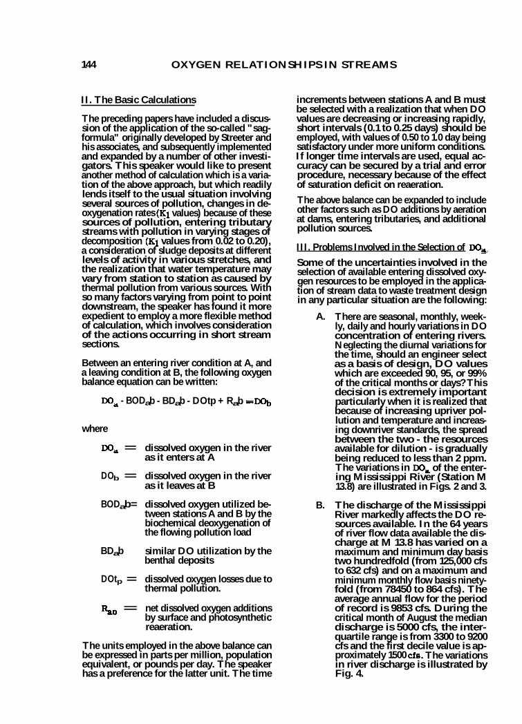
144 OXYGEN RELATIONSHIPS IN STREAMS
II. The Basic Calculations
The preceding papers have included a discus-sion of the application of the so-called "sag-formula" originally developed by Streeter and his associates, and subsequently implemented and expanded by a number of other investi-gators. This speaker would like to present another method of calculation which is a varia-tion of the above approach, but which readily lends itself to the usual situation involving several sources of pollution, changes in de-oxygenation rates (K1 values) because of these sources of pollution, entering tributary streams with pollution in varying stages of decomposition (K1 values from 0.02 to 0.20), a consideration of sludge deposits at different levels of activity in various stretches, and the realization that water temperature may vary from station to station as caused by thermal pollution from various sources. With so many factors varying from point to point downstream, the speaker has found it more expedient to employ a more flexible method of calculation, which involves consideration of the actions occurring in short stream sections.
Between an entering river condition at A, and a leaving condition at B, the following oxygen balance equation can be written:
D0a - BODab - BDab - DOtp + Rab L.D0b
where
D0a = dissolved oxygen in the river as it enters at A
DOb = dissolved oxygen in the river as it leaves at B
BODab= dissolved oxygen utilized be-tween stations A and B by the biochemical deoxygenation of the flowing pollution load
BDab similar DO utilization by the benthal deposits
DOtp = dissolved oxygen losses due to thermal pollution.
Rab = net dissolved oxygen additions by surface and photosynthetic reaeration.
The units employed in the above balance can be expressed in parts per million, population equivalent, or pounds per day. The speaker has a preference for the latter unit. The time
increments between stations A and B must be selected with a realization that when DO values are decreasing or increasing rapidly, short intervals (0.1 to 0.25 days) should be employed, with values of 0.50 to 1.0 day being satisfactory under more uniform conditions. If longer time intervals are used, equal ac-curacy can be secured by a trial and error procedure, necessary because of the effect of saturation deficit on reaeration.
The above balance can be expanded to include other factors such as DO additions by aeration at dams, entering tributaries, and additional pollution sources.
III. Problems Involved in the Selection of D0a Some of the uncertainties involved in the selection of available entering dissolved oxy-gen resources to be employed in the applica-tion of stream data to waste treatment design in any particular situation are the following:
A. There are seasonal, monthly, week-ly, daily and hourly variations in DO concentration of entering rivers. Neglecting the diurnal variations for the time, should an engineer select as a basis of design, DO values which are exceeded 90, 95, or 99% of the critical months or days? This decision is extremely important particularly when it is realized that because of increasing upriver pol-lution and temperature and increas-ing downriver standards, the spread between the two - the resources available for dilution - is gradually being reduced to less than 2 ppm. The variations in DO a of the enter-ing Mississippi River (Station M 13.8) are illustrated in Figs. 2 and 3.
B. The discharge of the Mississippi River markedly affects the DO re-sources available. In the 64 years of river flow data available the dis-charge at M 13.8 has varied on a maximum and minimum day basis two hundredfold (from 125,000 cfs to 632 cfs) and on a maximum and minimum monthly flow basis ninety-fold (from 78450 to 864 cfs). The average annual flow for the period of record is 9853 cfs. During the critical month of August the median discharge is 5000 cfs, the inter-quartile range is from 3300 to 9200 cfs and the first decile value is ap-proximately 1500 cfs. The variations in river discharge is illustrated by Fig. 4.

MS
04 N 5.4
6
•
2
0 115 1 5 10 20 30 40 50 GO 10 NO 110 85 90 910
% PROBABILITY OF OCCURRENCE
NOTE. AVERAGE MOIFINLY 0.0. VALUES USED (1842-1968)
DISSOLVED OXYGEN FREQUENCY DISTRIBUTION
ABOVE MSSD TREATMENT PLANT
Figure 2
strAinumm Irard111111EIMINVI 1111111111011111111110001 11/1111111ENIMMII 1111SEEEDMIE111
11 0 N MONTH Of THE YEAR MONTHLY DO OF MISSISSIPPI RIVER AT
Miao a M13.8 (1942-35)
Figure 3
STREAM DATA APPLIED TO WASTE TREATMENT PLANT DESIGN 145
INEM11111111111111M
I
.OS
CHAR
OE IN
CUB
IC F
EE
T PE
R S
ECO
ND
to
•
• •
w
to
.1
4*
.1 V
5.
ammo's =INIIMIIIII621111111111M•11111111111111
WillIMMIMINIII
MIIIIN
solhonum
PrniNN/I■•••111111■111■1&■•1111•1■IL■ WiMIMEERINE■MOMM3:51111■ME 1111-
IMF/fivini. 111MUMICIOIIIIMMIIIMIEMOIN I. IMMEILMIRM=MEEn■TIMEM 9°
NA a INN=NIIMIN
El raminimmew.w.:=■Ego WARISKISIETZMNIME
am
II mig mrdnio:
MEAN
.
MONTH N J J • s o m 0 OF THE YEAR Jr A A MISSISSIPPI RIVER AT M138 (1892-1955)
DISCHARGE FREQUENCY VS MONTHS
Figure 4
C. Along with the variations in DO con-tent and river discharge there has been a significant increase in river temperature caused by thermal pol-lution from various sources. These Increases are most important at critical lower discharges as illus-trated by Fig. 5. At median August flows of 5000 cfs an indicated in-crease of 4°C in water temperature (in flowing through the Twin Cities) at present thermal pollution levels Is very important in its effect on de-composition rates and DO saturation values. From power production sources alone, it has been estimated that by 1980, the thermal input will be 3.5 times the 1955 level, reaching a value of six times the present amount by the year 2000. Planned location of power plants to take advantage of natural cooling, and other develop-ments in the technology of power pro-duction may reduce the indicated effects of this factor. In considering temperature effects on the dilution capacity of a river the uncertainties In the validity of the DO saturation values at different temperatures as determined by Fox more than fifty

4
3 (213)
( 1 Inditores Sir Tompsratui 4
(23.1)
2 (Mgt it .4.51
1 (20.91
.1 22.91 10000 20,000 30,000 40,000
DISCHARGE IN CUBIC FEET PER SECOND
AT M 13.8
INC
RE
AS
E (M
0-48
-M13
.8)-
°C.
146 OXYGEN RELATIONSHIPS IN STREAMS
years ago (as presented in current Standard Methods) and which for the first time were openly raised at this meeting, are extremely important. Since only 1 to 2 ppm of DO may be available for dilution purposes an uncertainty of 0.4 ppm at critical summer temperatures becomes sig-nificant. This also raises the ques-tion, assuming the Fox - Standard Method values are shown to be in error, whether many of the studies and standards concerning fish and aquatic life which appear to have been based on these values, are also in doubt.
TEMPERATURE INCREASE FROM M 0-4.8 TO Ni3.13 VS. DISCHARGE, AUGUST, 1949-55
Figure 5
D. The status of entering pollutional load and the uncertainty of upriver community growth must be reckoned with in determining the entering river quality (D0a). The accuracy of prediction for a particular situa-tion is perhaps several-fold better than other factors involved in river assimilation studies. The tendency towards increase in upriver pollu-tional load in this situation is illus-trated by Fig. 6.
E. The above statements are presented to indicate the problems involved in determination of the factors involved in an engineering decision on degree
of treatment of this one element of dilution capacity, viz., the entering river conditions from a resource and pollutional standpoint.
MISSISSIPPI RIVER AT M 0-4.8 (1926 - 55) SOD VS. TIME
Figure 6
IV. Problems Involved in the Determination of BODab
A. The demand exerted between two stretches of a river is affected by many factors. The first in time se-quence is the BOD exerted by the entering river. For the entering river in this case (M 13.8) the five day BODvalues for a 14-year period of record are shown in Fig. 7.
B. Next is the demand exerted by added pollutional increments from down-river communities. In this case this is exemplified by the data in Fig. 8 on an annual increase basis, and in Figs. 9 and 10 on a monthly variation basis. To the variations in uncer-tainty based on past records must be added the questionable growth in population and industrial activity (of the wet and dry type) in central and suburban areas.

18138
JAvuAR
0 115 1 2 5 10 20 30 40 50 60 70 BO 98 93 98 99
%PROBABILITY OF OCCURRENCE
18
14
12
10
B 0
D IN
PPM
6
•
2
STREAM DATA APPLIED TO WASTE TREATMENT PLANT DESIGN 147
MEAN B 0 D FREQUENCY DISTRIBUTION ABOVE MSS!) PLANT (1942-1955)
Figure 7
AVERAGE MONTHLY BOO OF INFLUENT AND EFFLUENT MINNEAPOLIS- ST. PAUL SANITARY DISTRICT
SEWAGE TREAMENT PLANT
Figure 9
V I I , ,A - EZEMMII r ALL
I 1 i )N 1 1 I
1USA
NDS
OF
POUN
D!
AIN i I ry; I 1 1 1 , 1
1 1 , 1 r
IIAI
1939 1941 1943 1945 1947 1949 1961 953
YEARS
MINNEAPOUS -ST. PAUL SANITARY DISTRICT SEWAGE TREATMENT PLANT
JANUARY AVERAGE DAILY B 0 D OF IN FLUENT
Figure 8
SOUTH ST. PAUL SEWAGE TREATMENT PLANT AVERAGE MONTHLY SOD OF EFFLUENT
Figure 10

148 OXYGEN RELATIONSHIPS IN STREAMS
C. A characteristic of the deoxygenation constant (K) is its inconstancy. At a temperature of 20°C, the K value can vary for this particular situation from a value of 0.02 to 0.06 for an entering river, to 0.22 for the aver-age effluent of a primary treatment plant (variations from 0.14 for Sun-days and holidays to 0.23 for week-days, as illustrated by Table I). It
should also be recognized that the deoxygenation constants of plant effluents from intermediate and secondary treatment are materially different from those which result from primary treatment.
D. Avery important factor in the calcu-lations concerning deoxygenation and reaeration is the flow time between
Table I
20°C Velocity Constants for Minneapolis-St. Paul Sewage Effluent
Moment 1-3-5
Moment 1-3-5-10
Computation of k by time ratios
1.1.2 la OA LA LACI
Thu. JULY 4, '57 .133 102.4 .176 .137 .098 FRI. JULY 5 .235 118.1 .278 .242 .188 Sat. JULY 6 .270 101.8 .270 .270 .274 Sun. JULY 7 .138 51.8 .061 .118 .220 MAN. JULY 8 .302 96.6 .406 .314 .190 Tue. JULY 9 .246 127.9 .290 .254 .196 WED. JULY 10 .241 126.6 .264 .245 .208 THU. JULY 11 .240 115.2 .242 .241 .236 FRI. JULY 12 .236 118.1 .248 .238 .218 Sat. JULY 13 .186 99.5 .200 .188 .174 Sun. JULY 14 .110 91.2 .093 .102 .120 Mon. JULY 15 .192 114.6 .225 .198 .162 Tue. JULY 16 .185 97.9 .102 142.4 .157 .179 .118 .218 .058 Wed. JULY 17 .216 122.1 .122 165.7 .222 .217 .146 .208 .074 THU. JULY 18 .274 104.4 .198 119.7 .283 .278 .221 .262 .132 Fri. JULY 19 .258 82.0 .147 107.0 .276 .260 .176 .232 .084 Sat. JULY 20 .086 64.3 .100 58.3 .01 .054 .073 .188 .086 Sun. JULY 21 .01 .044 55.4 .01 .01 .01 .011 .114 MON. JULY 22 .217 102.9 .151 123.4 .264 .224 .184 .168 .110 Tue. JULY 23 .217 129.7 .192 137.4 .215 .216 .199 -49 .164 Wed. JULY 24 .247 120.1 .205 130.0 .245 .246 .218 .244 .158 THU. JULY 25 .246 117.0 .217 126.6 .259 .264 .231 .267 .163 Fri. JULY 26 .281 109.6 .212 123.2 .276 .279 .234 .286 .144 Sat. JULY 27 .210 94.7 .199 97.0 .167 .210 .194 .266 .177 SUN. JULY 28 .158 82.8 .144 86.6 .152 .154 .147 .164 .133 MON. JULY 29 .254 113.1 .201 124.9 .257 .254 .218 .246 .150 TUE. JULY 30 .250 102.7 .165 124.2 .255 .250 .188 .245 .105 Wed. JULY 31 .220 95.7 .203 99.4 .185 .213 .201 .270 .171
Thu. Aug. 1, '57 .232 90.7 .201 97.1 .208 .228 .206 .265 .161 Fri. Aug. 2 .184 77.3 .112 101.1 .197 .187 .133 .174 .075 Sat. Aug. 3 .178 73.3 .144 81.8 .149 .172 .148 .212 .114 Sun. Aug. 4 .140 57.0 .117 63.6 .089 .126 .115 .190 .095 Mon. Aug. 5 .264 99.1 .199 111.7 .297 .270 .226 .230 .145 Tue. Aug. 6 .237 116.4 .183 133.6 .240 .237 .200 .228 .137 Wed. Aug. 7 .258 114.2 .175 136.0 .227 .253 .192 .302 .108 Thu. Aug. 8 .217 116.9 .183 126.2 .223 .218 .194 .211 .150 Fri. Aug. 9 .242 109.7 .191 122.0 .215 .239 .200 .280 .138
All values .221 102.7 .169 114.1 .223 .216 .182 .218 .126 Sunday & Holidays .136 77.0 .1.30 75.1 .114 .127 .131 .158 .114 Weekdays .235 107.0 .173 117.7 .241 .230 .186 .228 .127

MUM
INE=N5PM=1313EIC=3:11 =11111111/11111111Williailidilll 111•111111MIKILVIMMIEIMII MINMEMMINIIIM111111111 MIIIIIIIMIN=M11111111TIM= 11111111111/11WHISIMIRIIIMIPI
800 NEWISIIIINNOINI 1.11111.EIM 20 ==11111W101/111E=1:NZ 11/110111/2212121■11M11111M 11111141111111MIMMINIIIIIPF --------
- --
-
0- 37.8 Jan211 29 - 30 - 31 F.3.1 - 2 - 3 - • 5 - I (Tuesday) (Tunas, FLOW TIME IN DAYS
30 25 2
20
25
3 C 0
0 10 25 2
STREAM DATA APPLIED TO WASTE TREATMENT PLANT DESIGN 149
adjacent stations. This is an uncer-tain calculation since effective cross-sectional areas are indefinite. The use of tracers can be an effect-ive tool, as suggested by Figs. 11 and 12 wherein BOD and N were employ-ed. These tracers indicated close correlation with the results of pre-vious judgment determination (as early as 1934) of the effective cross-sectional areas.
MISSISSIPPI RIVER FLOW TIME — MINIMUM BOO BASIS
Figure 11
calculation of this pollutional source is made uncertain because of the interacting effects of benthal decomposition and physical and photosynthetic reaeration effects.
VI. The DO Losses Due to Thermal Pollution (DOtp)
The effect of this factor on DO losses has al-ready been discussed, as well as its effect on deoxygenation rates.
, °
1 t i
AO
, IIIIIIII=ZraN:ATs
:
LO
115711111
1111111111 MOM 111111 IIIERW111111111111
- I, 11111 .EirdilhINSIVII
Ir ' ,AM I ii raratol W....Irv"-, NOE IM
&LOW ;1.3.00/ TIME IN DAYS 3 IT.-.4
3
MISSISSIPPI RIVER FLOW TIME — MINIMUM TOTAL NITROGEN BASIS
Figure 12
E. The very important effect of water temperature on DO content has been mentioned. The effect of tempera-ture on deoxygenation rates remains Indefinite. In the light of recent de-velopments, it is suggested that additional data are necessary to accurately reappraise this pollution factor.
V. The Determination of the Benthal Deposit Load (BODab)
This element of deoxygenation is a subtraction from the oxygen resources available. Its magnitude will vary with river velocity and cross sectional characteristics, prior degree of sewage treatment, and other factors. The
VII. Net Dissolved Oxygenation Additions by Surface and Photosynthetic Reaeration (Rab)
Assuming the benthal effects are negligible, the relative effects of surface and photosyn-thetic reaeration can be evaluated. The speaker prefers to use the parameter of pounds of reaeration per 1000 square feet per day, with values for this situation at 50% satu-ration and 20°C, of between 1.5 to 2.0 being indicated.
VIII. The Selection of Minimum DOh Values
The decision on the standards of the receiving waters has a profound effect on the cost of remedial measures since at elevated summer

150 OXYGEN RELATIONSHIPS IN STREAMS
temperatures only 1 to 2 ppm of oxygen re-sources may be available for dilution pur-poses. With an incoming river DO content as low as 6 ppm during the summer, the selec-tion of a 5 ppm standard results in only one-half the oxygen resources being available as compared to a 4 ppm standard.
The variation in dissolved oxygen caused by photosynthetic action, illustrated in Fig. 13 for an upriver station and in Fig. 14 for a downriver station, raises the question of whether standards should be based on mini-mum hourly or average daily conditions, or should they allow for some variation for a specified period of time during the day as was suggested for the Ohio River. This requires continuous sampling which is extremely ex-pensive and makes necessary the early availability of an automatic sampling and re-cording device.
D.O.
. o
—
re
to
» to
el
• • S
V;
JUNI ,JUL'A AUG,
AUG.
1935
1934 M
il
JULY 25-26,1931 .
111116h,
__ h ME"
arpr
lialW
1.
11
111
1.
EIWAVINIEI
--MEN ■ - 10
2 • 6 8 10 12 2 • 6 9 N) 12
AM PM
TIME OF DAY
D.O. DIURNAL VARIATION 1934-1935 M 0-4.8
Figure 13
The speaker would like to make a summary remark concerning the suggestion which was made at this meeting that reae ration and dam aeration be neglected in river and stream dilution capacity calculations, and that instead these recovery elements be considered as a factor of safety. The unsoundness of this reasoning is illustrated by the following state-ments. In the local situation which has been described, the median five-day BOD of the entering river is 2 ppm (this is a reasonable value). The flow time in the critical pool below the point of plant effluent addition from the metropolitan area is about five days under low flow conditions. With an entering river DO content of 6 ppm, and an assumed DO standard of 4 ppm, there would not be available a pound of DO for dilution of the effluent of the sewage plants of the metropolitan area. Necessarily the addition of thousands of pounds of DO by aeration and reaeration must be considered.
SUBMERGED BOTTLE STUDY. SEPT. 5-6 M 30.5
Figure 14

STREAM DATA APPLIED TO WASTE TREATMENT PLANT DESIGN 151
DISCUSSION E. C. TSIVOGLOU, In Charge Radioactivity Studies in Water Quality Management
Watching Professor Schroepfer present his data I was again impressed by the fact that it is easy to make computations and predictions when there is very little data available. But the larger the mass of available data, the more complex the problem seems to become!
The tremendous amount of information on k1 values was especially impressive, as were the light and dark bottle experiments. One question was suggested by the k1 data: there seemed to be a relationship between the magnitude of k1 and the river temperature. It is assumed that all samples were incubated at 20°C. Yet in January the k1 values were in the neighborhood of 0.11, while in August and September they were down to about 0.04. They seemed to correlate in this fashion with river temperature, and at the moment I can-not guess why. Perhaps I missed something in Professor Schroepfer's talk -- perhaps there is some interesting explanation.
It is especially interesting to see these light and dark bottle experiments going on in the incubation of river B.O.D.'s. Because from just the small amount of work we have done here at the Center, and from the hints that we have seen in the literature, it appears that river algae and photosynthesis may have more effect on the B.O.D. determination than we have realized.
During recent months we have observed another effect that ties in with Paul Haney's earlier remarks about accuracy and signifi-cant figures, and with the major question of whether the oxygen sag (or any simple equa-tion) really applies to this problem of stream self-purification.
Within the past four months we have seen at least three cases in which applying the sag equation to stream data in the usual fashion has resulted in a negative computed value of k2, the reoxygenation velocity constant. (By "usual fashion" I mean that for a particular reach we find everything else and then com-pute k2 according to the sag equation. This computed k2 is in reality a somewhat dubious figure because by the very nature of the com-putation it contains an error sufficient to compensate for any and all other errors that may have crept into the computation because of nonrepresentative sampling, faulty B.O.D. determination, algae, sludge demands, etc.)
These negative k2 values indicate, then, that even though the stream is deficient in dis-solved oxygen, it is still giving some oxygen off to the atmosphere! At first glance, this may appear to discredit the basic oxygen sag theory. Similar differences between obser-vation and theory have caused others to question the validity or at least the usefulness of the oxygen sag equation.
However, a closer look at our observed data Indicates a good reason why our k2 values turned out to be negative. One thing was con-sistent in all three cases that I have mentioned, and that was that we were dealing with very low B.O.D.'s. For example, at an upstream station we had 2.10 p.p.m. of ultimate first stage B.O.D., while the B.O.D. at the down-stream station was 1.90 p.p.m. Our compu-tation for k2, then, was based on a B.O.D. change of 0.20 p.p.m. between sampling stations. Numerical values of D.O. at these stations were, of course, rather high, and there was similarly little D.O. change between the stations.
Now in the first place, although I have a great deal of respect for the practical value of the B.O.D. test, I do not believe that it really is that sensitive! Secondly, there is the very relevant question of the time of flow between sampling stations, and how this relates to hourly fluctuations of B.O.D. and D.O. We found, for example, that the B.O.D. at one station did vary some on an hourly basis. Such variations can easily account for ob-served differences of 0.20 p.p.m. or more of B.O.D. and/or D. 0. So that these two ques-tions of sensitivity of the B.O.D. test and obtaining truly representative samples make this B.O.D. difference of 0.20 p.p.m. that we have "observed" a pretty hard thing to pin down. It is not a precise figure. Our ob-served data, rather than the oxygen sag theory, is open to question.
This kind of computation is not a fair test of any theory. We have known for some time that the sag equation is most satisfactory in pro-blems where a pronounced D. 0. sag actually occurs; many errors become magnified out of proportion, and our predictions are corres-pondingly undependable, in problems where there is no appreciable sag. The oxygen sag equation has been a very good theoretical basis for practical waste treatment plant design, when it has been used judiciously.

152 OXYGEN RELATIONSHIPS IN STREAMS
No theory can be expected to withstand the test of observed data that is incorrect or nonrepresentative or not sufficiently precise.
The following figures illustrate some inter-esting aspects of these questions of precision and certain errors of measurement and interpretation.
The first figure shows the results of a few computations on the question of how errors in k1 affect computed degrees of sewage treat-ment. After all, that is our goal, to predict the degree of sewage treatment necessary to meet some particular D.O. objective in a given stream, under a specific set of circum-stances. For example, we wanted to know just how much effect in terms of required waste treatment is likely to result if an error of 50 percent is made in the estimate of the ILI value. A great deal more could be done to generalize the work, but the graph indicates the trend of results. As indicated in Figure 1, the con-ditions of computation were: a minimum D.O. objective of 5.0 p.p.m., an initial deficit of 2.0 p.p.m., temperature of 25°C., the absence of significant sludge demands, and a "true" k1 value of 0.15/day. Computations were made by the oxygen sag equation. A pollution load, La, of 25 p.p.m. was used.
® t(5)
, = CONSTANT
k T = -= = CONSUNT I'
0 C CONSTANT
L(5) = CONSTANT k2 = CONSTANT
CONST
ON_ C JE
jfT On
(1)
rg
5.0. OSJECTIVE INITIAL T = 25°C. NO SLONE
= 5.0 p.o.e. DEFICIT = 2.0 ppd..
05P03115 Ai (Imm)--,-0.15111AT
.05 .10 • .20 .25 ki
EFFECT* OF ki ON REQUIRED DEGREE OF WASTE TREATMENT 9ACCORDING TO OXYGEN SAG EQUATION)
Figure 1
Now Curve A looks like the most extreme variation of required degree of treatmentvs. lg. The conditions of computation were that k2 and La were constants. From this curve, we find that for the "true" value k1 = 0.15/day, 64 percent B.O.D. removal by waste treatment is needed to meet our D.O. objective at the
critical point of the sag curve. But suppose that we had made a mistake and assumed k1 = 0.10/day; in this case we would have predicted a required degree of treatment of 50 percent B.O.D. removal, or somewhat less than the "true" 64 percent. On the other hand, suppose we had erred on the high side and used k1 = 0.20/day; we would then have re-quired 71 percent B.O.D. removal instead of the correct 64 percent.
However, Curve A is most probably not the governing relation. It is based on a constant k2 value, which is probably a good enough as-sumption for practical purposes. But it also asstimes a constant La, the ultimate first stage B.O.D., which is probably not a good assumption. More probably, the actual data would have included a set of 5-day B.O.D.'s, and these would be corrected to La's on the basis of the selected value of kl. Hence the assumed conditions for Curve B are more likely to suit the practical case -- that is, k2 constant, and the 5-day B.O.D., L(5), constant. Curve B is therefore our most likely relation.
From Curve B, it appears that the effect of errors in k1 on required degree of treatment is relatively small. For example, had we selected k1 = 0.10/day instead of 0.15/day, we would have required 59 or 60 percent B.O.D. removal instead of 64 percent. Had we assumed 1(1= 0.20/day, the required B.O.D. removal would have been 68 percent. Hence a relatively large error in ki (after all, we usually report k1 to three or four decimal places) results in a fairly small error in design. Most of us can probably agree that a number of sources of error are present in predicting waste treatment needs, and a design that is correct within 10 percent is about as precise as we can hope to be, anyway.
Curves C and D of Figure 1 are included as theoretical cases, rather than as practical probabilities. Curve C assumes that the error in ki is balanced by an error in k2 such that f = k2/k1 remains constant. It also assumes La constant, which we have seen to be unlike-ly. Curve D represents the condition of k2 and L(5) constant. Neither of these curves Indicates any really significant variation of required percent B.O.D. removal with ki.
The whole point of the matter is that we must look also at the final computations - the idea of how much waste treatment we need - and examine these in the light of the errors that may be involved in such things as observed B.O.D.'s, D.O.'s, velocity constants, etc.
1 03
so
60
20
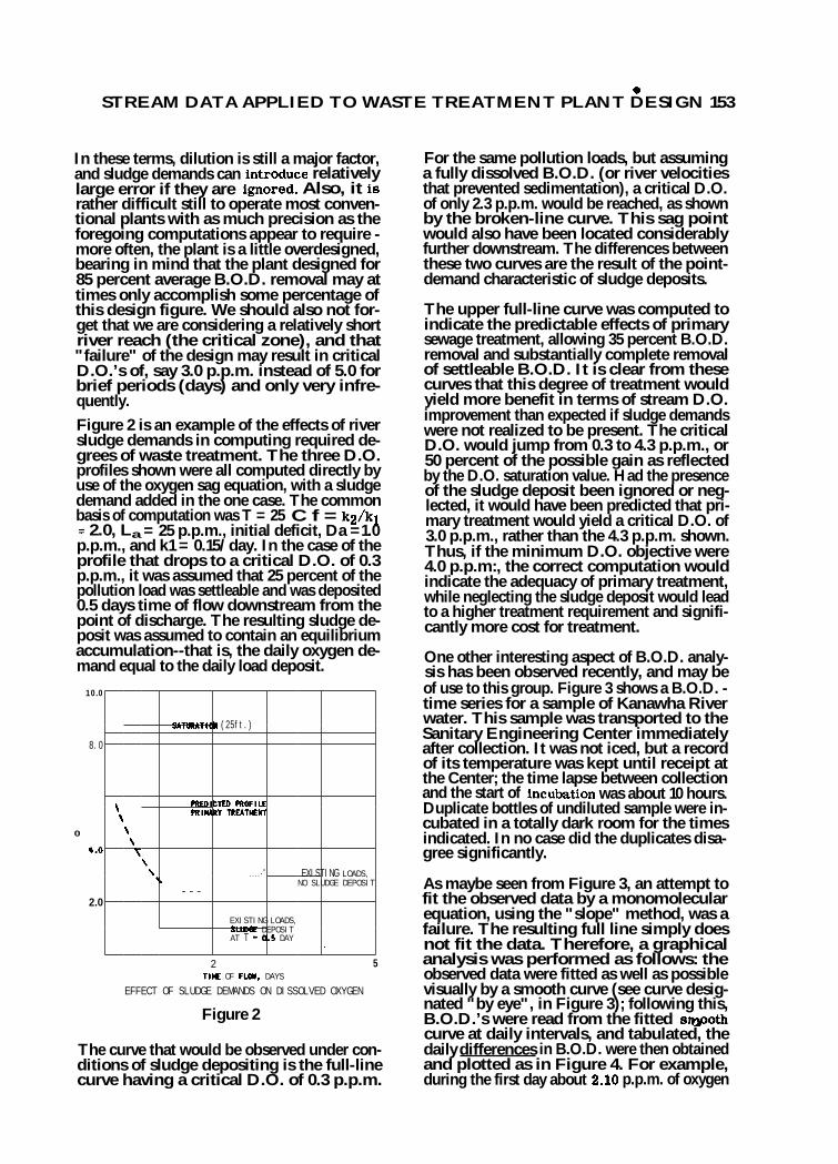
I STREAM DATA APPLIED TO WASTE TREATMENT PLANT DESIGN 153
In these terms, dilution is still a major factor, and sludge demands can introduce relatively large error if they are ignored. Also, it is rather difficult still to operate most conven-tional plants with as much precision as the foregoing computations appear to require - more often, the plant is a little overdesigned, bearing in mind that the plant designed for 85 percent average B.O.D. removal may at times only accomplish some percentage of this design figure. We should also not for-get that we are considering a relatively short river reach (the critical zone), and that "failure" of the design may result in critical D.O.'s of, say 3.0 p.p.m. instead of 5.0 for brief periods (days) and only very infre-quently. Figure 2 is an example of the effects of river sludge demands in computing required de-grees of waste treatment. The three D.O. profiles shown were all computed directly by use of the oxygen sag equation, with a sludge demand added in the one case. The common basis of computation was T = 25°C f = k2/k1 = 2.0, La = 25 p.p.m., initial deficit, Da =1.0 p.p.m., and k1 = 0.15/day. In the case of the profile that drops to a critical D.O. of 0.3 p.p.m., it was assumed that 25 percent of the pollution load was settleable and was deposited 0.5 days time of flow downstream from the point of discharge. The resulting sludge de-posit was assumed to contain an equilibrium accumulation--that is, the daily oxygen de-mand equal to the daily load deposit.
SATURATION (25ft.)
‘ \ \ \
PREDICTED PROFILE TREATIENT PRIMARY
\ \ \ N.
---
....-" EXISTING LOADS, DEPOSIT NO SLUDGE
EXISTING LOADS,
DAY ,
SLUDGE DEPOSIT AT T . 0,6
2 5 TIIE OF FLOW, DAYS
EFFECT OF SLUDGE DEMANDS ON DISSOLVED OXYGEN
Figure 2
The curve that would be observed under con-ditions of sludge depositing is the full-line curve having a critical D.O. of 0.3 p.p.m.
For the same pollution loads, but assuming a fully dissolved B.O.D. (or river velocities that prevented sedimentation), a critical D.O. of only 2.3 p.p.m. would be reached, as shown by the broken-line curve. This sag point would also have been located considerably further downstream. The differences between these two curves are the result of the point-demand characteristic of sludge deposits.
The upper full-line curve was computed to indicate the predictable effects of primary sewage treatment, allowing 35 percent B.O.D. removal and substantially complete removal of settleable B.O.D. It is clear from these curves that this degree of treatment would yield more benefit in terms of stream D.O. improvement than expected if sludge demands were not realized to be present. The critical D.O. would jump from 0.3 to 4.3 p.p.m., or 50 percent of the possible gain as reflected by the D.O. saturation value. Had the presence of the sludge deposit been ignored or neg-lected, it would have been predicted that pri-mary treatment would yield a critical D.O. of 3.0 p.p.m., rather than the 4.3 p.p.m. shown. Thus, if the minimum D.O. objective were 4.0 p.p.m:, the correct computation would indicate the adequacy of primary treatment, while neglecting the sludge deposit would lead to a higher treatment requirement and signifi-cantly more cost for treatment.
One other interesting aspect of B.O.D. analy-sis has been observed recently, and may be of use to this group. Figure 3 shows a B.O.D. - time series for a sample of Kanawha River water. This sample was transported to the Sanitary Engineering Center immediately after collection. It was not iced, but a record of its temperature was kept until receipt at the Center; the time lapse between collection and the start of incubation was about 10 hours. Duplicate bottles of undiluted sample were in-cubated in a totally dark room for the times indicated. In no case did the duplicates disa-gree significantly.
As maybe seen from Figure 3, an attempt to fit the observed data by a monomolecular equation, using the "slope" method, was a failure. The resulting full line simply does not fit the data. Therefore, a graphical analysis was performed as follows: the observed data were fitted as well as possible visually by a smooth curve (see curve desig-nated "by eye", in Figure 3); following this, B.O.D.'s were read from the fitted stypoth curve at daily intervals, and tabulated, the daily differences in B.O.D. were then obtained and plotted as in Figure 4. For example, during the first day about 2.10 p.p.m. of oxygen
10.0
8.0
0
4.0
2.0

0 154 OXYGEN RELATIONSHIPS IN STREAMS
LOPE" METRO ---- "--"nm-c.--
! BY
p.m. T= 0.071
La = 4.86 p
....-- 7:
•••• ..•• .... , .....
f
kl = 0.60 Va = 1.80 p p.m.
- / /
/ /
----."-d•-• - - - - - -
o = AVERAGE OF DUPLICATE BOTTLES
2 8 10 12 14 TIME 1 N DAYS
KANAWHA RIVER - SAMPLE NO.II-X, MARCH, 1956 Figure 3
B.O.
D., p.p.m.
8.0
6.0
4.0
2.0
were used; by the end of the second day a total of about 3.0 p.p.m. had been used, or a dif-ference of 0.9 p.p.m. during the second day, and so forth. The graph in Figure 4 resulted.
If the reaction were monomolecular, the data of Figure 4 would have been arrayed in a straight line. Clearly, then, the reaction was not simple monomolecular, as is generally assumed in the basic B.O.D. equation. How-ever, it can be seen from Figure 4 that we have a straight line fit of the data following the third or fourth day. This suggested a somewhat more complex reaction having a monomolecular base, so to speak. A straight line was fitted to these latter day data, and extrapolated to time zero as shown. Then the differences between this line and the observed data (1.32, 0.24, 0.07, 0.02 p.p.m.) were plot-ted as a separate process, as shown in Figure 5. A straight line resulted, as can be seen from Figure 5. For each of the straight lines shown in Figures 4 and 5 a ki value, or slope, was determined separately by use of the simple monomo-lecular equation. In other words, the two processes were treated as independent mono-molecular reactions. Having determined the velocity constants, the ultimate first-stage B.O.D.'s were determined by solution of two simultaneous equations of the form:
(t)= Lai x 10-k11t
+ La2 x 10-1112t (1)
where kii and 1E12 are the B.O.D. velocity constants for the two reactions, Lai and La2 are the corresponding ultimate first stage de-mands, and the y (t) are the observed B.O.D. '5. Substitution into equation (1) of two sets (y, t) results in two equations in which the only un-knowns are Lai and La2, and these may then be found by simultaneous solution. For exam-ple, in order that the test data reflect both reactions, one might use the observed y's at t =1 or 2 and t = 7 or 8 days. In the case shown, the data indicate a quite rapid (k = 0.6/day) and a relatively slow (k.= 0.07/day) reaction. The rapid reaction ac-counts for 27 percent of the total B.O.D. (6.66 p.p.m.), or 1.80 p.p.m. ultimate first-stage demand. The two separate reactions are shown in Figure 3 as broken lines. The sum-mation of these two curves produces the resultant observed curve. These data, then, appear to indicate that two quite independent simple monomolecular re-actions make up the observed complex B.O.D. - time curve of Figure 3. No single monomolecular curve could be expected to fit the data. The two-component reaction found here appears to fit the observed data quite well throughout the entire 13 days of obser-vation.
Four other Kanawha River samples from dif-ferent locations showed the same type of two-component reaction. In two cases, the two

0
o
I 1.32
.... w T N. 0.24 \ ■ \
NI6.07 N
\ kto--0.02
\
k - 0.071
0
0 0
0
3.0
2.0
DAILY DIFFERENCE IN D.O.D., D.
D.I6
1.0 0.9 0.8 0.7
0.6
0.5
0.4
03
0.2
0.1
2.0
001
1 .0 0.8
0.6
0.4
a 0 3 C.
c; 0.2
0.04
0.03
0.02
k - 0.60
0
STREAM DATA APPLIED TO WASTE TREATMENT PLANT DESIGN 155
2 4 6 10 12 0 2 4 TINE IN DAYS TIME IN DAYS
KANAWHA RIVER - SAMPLE NO. II-X
Figure 4
component curves did not fit together so smoothly, and a pronounced hump in the ob-served curve occurred on the second or third day, as the faster reaction approached com-pletion and the slower process became pre-dominant. Such a break in the observed curve is commonly taken as a sign of nitrification, but in these cases it was actually the result of superposition of two first stage reactions.
These results seem to be in general agree-ment with present knowledge of the B.O.D. reaction. For example, the observed k1 of 0.60/day is in keeping with recently ob-served reaction velocity constants for ac-climated seeds. The Kanawha River receives a variety of domestic and comples industrial wastes for which acclimated seeds might well
KANAWHA RIVER - SAMPLE NO. II-X
Figure 5
be expected to develop in the river. Nothing in the B.O.D. theory implies that two such separate reactions cannot proceed at the same time or would be mutually exclusive. These results simply implement present methods of analysis and interpretation, and support the existing basic theory of the monomolecular process. It seems probably that in reality such multicomponent reactions occur much more frequently than we realize. This is quite in keeping with the basic biological theory of the reaction, and is one rational explanation of the oft-noted failure of the simple B.O.D. equation to fit a specific set of data. Since the more rapid process is essentially com-pleted in a little over a day, it is easily missed entirely, and this may explain why it is not much more frequently observed.

156 OXYGEN RELATIONSHIPS IN STREAMS
INFORMAL DISCUSSION R. E. Fuhrman: Thank you Profes.sor
Schroepfer. Any questions?
F. C. Larson: I have been working on K2 factors. I would like to have some dis-dussion from someone else in the audience in regard to negative K2 values. I would like to know what seems to be wrong with the concept of placing the observed values in the oxygen sag equation and coming out with a negative K2.
E. C. Tsivoglou: As I indicated in my preceding discussion I believe the negative K2's are due primarily to the fact that we are dealing with numbers that are not much larger than the errors introduced in the determina-tions. For instance, in the case Professor Larson refers to, the BOD's were quite low - ultimate BOD in range of 2 ppm - and the observed differences in DO were low. In other words, we are computing figures that are unrealistic in that the information put into the oxygen sag is not sufficiently accurate.
C. J.. Velz : We owe Professor Schroepfer a vote of thanks for providing us with some very interesting information. I am particu-larly interested in knowing, George, if you tried Lee's method of computing some of these K values. I think Lee has made significant contributions in computing K values which a lot of us are missing. In using some of the rigid mathematical methods of computing K, a small deviation in differences between two BOD's can produce considerable variation in
the computed K rate which is not really a measure of K. Lee's method allows much more flexibility in evaluating whether devia-tions are truly out of line. In our experience with Lee's method we get much more con-sistent values in K1. His method is presented as a discussion in "Sewage & Industrial Wastes", vol. 23, #2, pp. 164-6, February 1951. The other point I would like to make, in addition to what Dr. Tsivoglou pointed out here that in refinement of reaeration we may be getting too far away from engineering deci-sions, is that we have another important decision to make with respect to treatment namely, "What drought probability are we going to protect against?" This is to me a really basic problem and ought to be answered in the last analyses not only in terms of eco-nomic evaluation but in terms of what we want to do with our rivers. We are inclined to make our standards and decisions without considering the over-all water problem. The decision to protect against the once-in-twenty-year, or once-in-ten-year, or once-in-five-year drought may imply treatment requirements ranging all the way from pri-mary to complete. Technical refinements in BOD and reaeration are desirable, but I think the great need is to carry our analyses over into the engineering economics.of this problem. If we don't, while we are fussing with "grace notes" others will take over the job from us.
R. E. Fuhrman: Thank you, Professor Velz. I am sorry that we have our time limited. May I again express thanks for each presentation. We will now adjourn until 11 o'clock.

Algae and Their Effects on Dissolved Oxygen and Biochemical Oxygen Demand*
T. F. WISNIEWSKI. Director Wisconsin Committee on Water Pollution
157
During 1955 and 1956, cooperative state-in-dustry stream studies were conducted jointly by the Committee on Water Pollution and the Sulphite Pulp Manufacturers' Research League, Incorporated.
These studies conducted with assistance of personnel from pulp and paper mills located on the rivers investigated were directed to-wards the evaluation of stream loading and purification capacity. Bulletin WP-101 issued March 15, 1956 detailed the results of studies in 1955, and Bulletin WP-103 is a detailed report on the studies made in 1956.
As the studies progressed, it became apparent that it would be necessary to evaluate the ef-fect of algae on the purification capacity of a stream. Attempts to evaluate this effect were made in 1956 in conjunction with the cross-section surveys of the Fox River.
The Fox River forms one of the major drain-age basins of the state, the stream and its tributaries draining a total of 6, 520 square miles. The section studied is the lower ex-tremity of the basin from Lake Winnebago to Green Bay, containing 6% of the drainage basin area but having 83% of the total fall.
The rapid descent of the river in the 39-mile stretch studies, plus the vast storage system backed up by dams located at Neenah and Menasha which create a flowage area of 297 square miles at elevation 750, both make available the important water powers found on the lower Fox River. Plentiful water and
power has made possible the development of the lower Fox River as it now exists result-ing in the greatest concentration of the pulp and paper industry in the state, as well as population concentration per stream mile. Hydro-electric developments along this sec-tion make use of the majority of river fall creating a series of river run pools utilizing the 166 feet of fall in the 39-mile distance from Neenah-Menasha to Green Bay. The elimination of all fast water reaches has thus reduced opportunity for natural reaeration of the stream as well as the capacity for puri-fication of wastes.
The U.S. Geological Survey has maintained a river gaging station on the lower Fox River for the past 40 years at Rapid Croche Dam at mile 19.3 on the stream. The station at this point intercepts the drainage from 6,150 square miles of the drainage area. The dura-tion curve values indicate that the stream at this point will exhibit a discharge of 1, 250 cubic feet per second or more 95% of the time. The 50% discharge value is 3,610 cubic feet per second.
Sources of pollutional wastes of man-made origin discharged to the stream over the sec-tion studied are derived from two major
* Abstracted from Evaluation of Stream Load-ing and Purification Capacity, Supplement No. 1, Committee on Water Pollution Bul-letin No. WP 103 by Lueck, B. F., Scott, R. H., Wiley, A. J. and Wisniewski, T. F. (March 1, 1957).

158 OXYGEN RELATIONSHIPS IN STREAMS
sources. These are wastes, treated and untreated, from the pulp and paper and other industries, and treated sanitary sewage.
Several additional sources of organic and Inorganic matter reach the stream and can be expected to have material effect upon the total loading assimilated. These other sources have up to this time received little, if any, study or evaluation as to their actual importance in the over-all picture of stream pollution.
The following sources probably have a greater effect on stream conditions than has hereto-fore been realized.
1. Large tonnages of organic matter pro-duced by algae grown in the "blooms" on upstream lakes and in quiet waters behind dams along the Fox River.
2. Settled organic and inorganic solids derived from fibrous materials, from algal blooms in prior years, from silt deposited by soil erosion, from ex-tensive weed beds, from fungus growths which may be quite heavy in some waters, and from storm water drainage.
3. Drainage from farm lands heavily fertilized with the more concentrated chemical fertilizers common to mod-ern practices in diversified agricul-ture may also be indirectly important In accelerating growth of algae and increasing their abundance.
The effect of algae in streams is recognized as having some significance, but there is little Information available in the literature on these effects. The preliminary planning for this phase of work, therefore, was complicated due to the lack of specific points of departure based upon previous work by other investi-gators. The algal load, in relation to oxida-tion ponds, has been investigated by the University of California group at Berkeley covering some aspects of the dissolved oxygen balance under controlled experimental con-ditions and with certain cultures. In the studies of "Biological and Chemical Aspects of Organic Waste Lagoons" by Dr. A. F. Bartsch of the Robert A. Taft Sanitary Engi-neering Center, some attention was given to dissolved oxygen production by algae. Little information was available regarding stream work and algal load in relation to the influence of algae as it either increased or decreased the oxygen demand load while the process of waste stabilization was taking place.
It was early recognized that efforts in this regard needed to be limited to restricted areas of inquiry, and that information gained in the preliminary phases would not be any complete answer to a problem whichwill require more extensive investigation. The experimental work and conclusions drawn therefrom are not presented, therefore, with any assump-tion that the problem associated with algal growth and death in the flowing stream is answered, rather additional questions are posed. Neither is the data without significance as it may stimulate others to undertake work along this avenue of experimentation, and does give several points for additional study if later opportunity permits.
The main questions for which answers were sought by the preliminary experimental work were:
1. What influence, if any, does the pres-ence of algae have on the laboratory B.O.D. determination?
2. What influence, if any, do increasing amounts of algae have on the labora-tory B.O.D. value?
3. What difference occurs in oxygen usage rates between samples contain-ing algae which are incubated in the dark and the light?
4. What influence, if any, does the pres-ence of dead or decomposed algal cells have on the B.O.D. determination?
Considering the questions above, it is ap-parent that three principal variables are introduced into the normal B.O.D. reaction in attempting to solve these problems. The pres-ence of algae, or experimentally increasing the amounts of algae, supposes that such pre-sence or addition will be reflected in an in-creasing B.O.D. It is not reasonable to presume otherwise, considering that added organic matter is thus present to enter into the reaction. However, the presence of algae in the sample incubated in the dark may affect the B.O.D. value in two ways: (1) by direct addition of organic matter capable of aerobic bacterial decomposition thus adding to the normal B.O.D., and (2) the respiration of the live cells thus utilizing the dissolved oxygen in the dilution water, resulting in an added apparent B.O.D. These two variables, due to the presence of algae, could be effective in increasing the B.O.D. value of any sample in-cubated without light in the normal manner, each, or both together, contributing to added oxygen usage measurable by the determina-tion. A value is thus obtained consisting of a

ALGAE AND THEIR EFFECTS ON D.O. AND B.O.D. 159
true B.O.D. due to the stabilization of decom-posable organic matter and an added B.O.D. due to cell respiration. The thirdvariable in the B.O.D. reaction in the presence of algae results from the introduction of the photosyn-thetic effect when incubation is carried out under light. Presuming the vast majority of algal cell material to be in a live state, cell respiration under conditions of incubation permitting photo synthesis results in produc-tion of oxygen. At the same time, the normal B.O.D. reaction is also continuing under these conditions. As a result, from the experi-mental laboratory standpoint, if sufficient oxygen is produced to result in a net gain, ,it must be assumed that sufficient living cells are present to produce oxygen in excess of that required for the normal B.O.D. requirements of aerobic bacterial stabilization.
Biological Determinations
Concentrated algae samples were obtained July 25, 1956 and again on August 8, 1956 from Station A in the Menasha Channel at mileage designation 38.5, at Station B from Rapid Croche Dam at mileage designation 19.5, and Station C above the De Pere Dam at mileage designation 7.0. The concentrated algae samples were obtained by centrifuging 50 gallons of river water at 12,000 r.p.m., and suspending the residue in one gallon of algae free water. A blender was employed in re-suspending the algae. An aliquot sample of this 50 to 1 concentration was used for biological analyses.
Ten c.c.'s of the concentrated samples equivalent to 500 c.c.'s of raw water were centrifuged at an approximate speed of 2,000 r.p.m. in a constable tube. The cell pack or cell volume as calculated on a raw water basis was as follows:
Station
A
Cell Pack (c.c. per liter)
July 25
.068
.058
.036
August 8
.086
.066
.045
The samples displayed color stratification in the constable tube. The upper white layer was composed principally of single blue-green cells and small fragments of blue-green colo-nies with few celled green colonies and small single-celled green species in lesser num-bers. A middle light green layer was princi-pally blue-green colonies and many-celled fragments or larger fragments of these fila-ments of Aphanizomenon, Anabaena, and Gleotrichia. There were numerous single
blue-green cells and some colonial greens with a few diatoms. The lower dark layer was still predominantly blue-green algae, due to their abundance in the sample, but the diatoms were heavily concentrated. The large-celled Lyngbya birgei and the dinofla-gellate Ceratium was most concentrated in this layer.
The packed cells or residue from the con-stable tubes were washed in distilled water and were dried and ignited on a platinum dish. The following results were obtained:
MS. dry wSt./1, Mg. Ash/L Mg. Vol. Sol./L Station 7-25 8-8 7-25 8-8 7-25 8-8
A 9.8 14.6 4.4 6.8 5.4 7.8 10.6 14.4 5.4 4.6 5.2 9.8 4.8 6.4 2.0 2.8 2.8 3.6
Algae counts were made from the concentrated material obtained from the three stations. The results of the counts appear in Table I.
A review of the biological analyses indicates the following:
1. It would appear that lake algae as re-presented by Sample A is undergoing a change under/Fox River conditions. Certain normal lake residents such as Anabaena,, Aphanizomenon and Microcystis are reduced under river conditions and possibly die. Blue-green algae as a whole are reduced under river conditions and some species are eliminated.
2. Green algae and diatoms, which are normally found more abundantly in flowing water, become increased under river conditions. In the green algae, in particular, several new species are added under flowingwater conditions. Although smaller in actual size, they no doubt replace the blue-green algae which have died or de-creased.
3. Station B would appear to represent a transition zone between two algal communities. Station A is representa-tive of typical lake algae, whereas Station C is representative of stream algae with considerable numbers of lake contaminants.
4. The process of centrifuging and re-suspending broke up many algal cells as principally noted in the unidentified single cells of blue-green algae (pro-bably Microcystis) and the single cells of 1Kirchneriella(?). If these had been
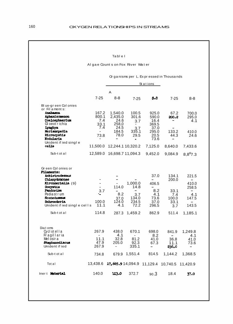
160 OXYGEN RELATIONSHIPS IN STREAMS
TABLE I
ALGAE COUNTS ON FOX RIVER WATER
ORGANISMS PER L. EXPRESSED IN THOUSANDS
7-25
STATIONS
7-25 8-8
A
8-8 7-25 8-8
BLUE-GREEN COLONIES OR FILAMENTS:
ANABAENA 167.2 1,540.0 100.5 925.0 67.2 700.0 APHANIZOMENON 800.1 2,435.0 301.6 590.0 203.2 295.0 COELOSPHAERIUM 7.4 24.6 3.7 16.4 - 4.1 GLOEOTRICHIA 33.1 258,0 - 369.5 LARNSBYS 7.4 24.5 3.7 37.0 - MERISMOPEDIA - 184.5 335.1 295.0 133.2 410.0 MICROCYSTIS 73.8 78.0 29.5 20.5 44.3 24.6 MODULARIA - - . 73.6 - UNIDENTIFIED SINGLE CELLS 11,500.0 12,244.1 10,320.2 7,125.0 8,640.0 7,433.6
SUB-TOTAL 12,589.0 16,698.7 11,094.3 9,452.0 9,084.9 8,867.3
GREEN COLONIES OR FILAMENTS:
ANKISTRODESMUS - 37.0 134.1 221.5 CHLEUNYTTOMONAS - - - - 200.0 - KIRCHNERIELLA (9) - - 1,000.0 406.5 410.0 OOCYSTIS - 114.0 14.8 - 258.5 PANDORINA 3.7 - - 8.2 33.1 - PEDIASTRUM .- 8.2 3.7 4.1 7.4 4.1 SCENEDESMUS 37.0 134.0 73.6 100.0 147.5 SCHROEDERIA 100.0 124.0 234.5 37.0 33.1 - UNIDENTIFIED SINGLE CELLS 11.1 4.1 72.2 296.5 3.7 143.5
SUB-TOTAL 114.8 287.3 1,459.2 862.9 511.4 1,185.1
DIATOMS CYCLOTELLA 267.9 438.0 670.1 698.0 841.9 1,249.8 FRAGILLARIA - 4.1 - 8.2 - 4.1 MELOSIRA 11.1 32.8 81.2 41.0 36.8 41.0 STEPHANODISCUS 47.9 205.0 92.3 67.3 11.1 73.6 UNIDENTIFIED 267.9 - 335.1 - 236.0 -
SUB-TOTAL 734.8 679.9 1,551.4 814.5 1,144.2 1,368.5
TOTAL 13,438.6 17,665.9 14,094.9 11,129.4 10,740.5 11,420.9
INERT MATERIAL 140.0 123.0 372.7 90.3 18.4 37.0

ALGAE AND THEIR EFFECTS ON D.O. AND B.O.D. 161
permitted to remain as colonies, the counts would have been lower, but should have been in direct proportion.
5. Casual observation of the three samples revealed that the greatest concentration of cells, volume-wise, was Microcystis and Aphanizomenon.
6. The cell pack or cell volume drops off directly from Station A, through Sta-tion B, to Station C. From the algae counts on July 25, it would appear that Station B has more cells than Station A, and Station C has less than either A or B. This is brought about by the in-creased cell count of green algae at Station B. Blue-green colonies are uniformly larger in size than green colonies, therefore, it is logical that at Station B the total count remains high whereas the cell pack or cell volume becomes reduced From the samples collected on August 8, Sta-tion A displays the greatest number of cells, whereas Stations B and C are similar. There is a descending order of abundance of blue-green forms and an ascending order of abundance of green forms and diatoms.
7. The volatile solids, or the amount of organic material which would deter-mine algal quantity remains fairly constant for Stations A and B. The samples from Station C contain about half the volatile solids of Stations A and B.
8. On July 25, the abundance of inert material as determined both by micro-scopic examination and fixed solids determination was greatest from the sample at Station B, and dropped off markedly in the sample taken from Station C. On August 8, the quantity of inert material showed a steady de-cline from Station A through Station B to Station C.
Effects of Algae
All data relative to the examination of the ef-fect of algae on the B.O.D. reaction is tabu-lated in the Appendix.
Table 2, of the Appendix shows the data obtained under experimental conditions while the algal solids content of the incubated samples are progressively increased. The concentration values were arrived at by de-termination and calculation. The suspended
solids increases both vertically and hori-zontally for any single original concentration. Duplicate samples of each dilution were also incubated under continuous light, the data obtained showing as negative B.O.D. or dis-solved oxygen gain, in the higher concentra-tion sequences.
The data recorded in Table 3 is related directly to that shown in Table 2. This shows the analytical values obtained upon determination of the suspended solids concen-tration in the samples as received, and the corresponding sample as the 50-1 concentrate obtained by centrifuging the solids from the river water.
Tables 4 and 5 of the Appendix show the rate of oxidation data obtained upon dark and light incubation of duplicate samples run under the conditions shown. The "as received' sample was that taken directly from the river at the individual station. The centrifuged sample was obtained by centrifuging 50 gal-lons of river water in obtaining 50-1 concen-trate. Thus the centrifuged sample had very nearly all of the suspended material removed.
Influence of Live Algae on B.O.D.
Differentiation of the soluble and suspended solids B.O.D. load is shown in the curves in Figures 3 and 4 which are derived from data tabulated in Tables 4 and 5 of the Appendix, and relate to material obtained at Stations A, B, and C. In this case the increasing B.O.D., graphed against time, shows an increased demand of the normal sample as compared with the soluble B.O.D. load. In all cases the total B.O.D. is greater than the soluble B.O.D., which one would expect. How-ever, while the normal B.O.D. at Station A (Lake Winnebago water) and Station C are very nearly the same on the 5-day basis on both surveys, the increased normal B.O.D. and the increased soluble B.O.D. at Station B, due presumably to addition of wastes to the stream, is clearly evident. It is also ap-parent that a significant portion of the B.O.D. at this station, due to suspended matter, is lost by the time Station C is reached either by conversion of suspended matter to soluble B.O.D., which remains the same, or by separation by sedimentation from the stream flow.
While the differences between normal samples and centrifuged samples very easily demon-strate the apparent effect of added B.O.D. due to algae and suspended matter, it must be understood that no distinction is here made between true B.O.D. and algal respiration.

162 OXYGEN RELATIONSHIPS IN STREAMS
Consequently, what appears as a difference in B.O.D. values may in part be the added value of cell respiration, and certainly this should be recognized as a significant facto' in interpreting such data. Data relative to the rate of respiration (k) of the algal cells is found in the tables in Tables 4 and 5 under the heading of light-dark incubation. After incubation of the samples from Stations A, B, and C for seven days under light conditions, an increase in algal growth was noted. The greatest portion of the solu-ble B.O.D. having been satisfied, the samples were subjected to seven additional days of dark incubation to obtain the rate data given under the light-dark heading. In all cases except for the sample from Station B of August 8, the rate is within the range of .04 to .07.
The Influence of Dead Algal Cells on B.O.D. The data. relative to the B.O.D. values of auto-claved samples, as compared to normal B.O.D. data is contained in Table 1 of the Appendix, and graphed in Figures 1 and 2. The purpose of autoclaving duplicate com-posite samples from these two survey runs at cross-section Stations 5, 5A and 6 which lie between Stations A and C, was to deter-mine if possible the B.O.D. value of added "available" organic matter from decompos-ing algae. While it is appreciated that the situation is in no way parallel to actual stream conditions, and that such B.O.D. added to the stream would be available at a much slower rate, the data is of interest from an experimental standpoint. The rate constants, shown by the autoclaved samples, compared to the normal B.O.D. values show conflicting results. The July survey samples show a decreased rate con-stant on autoclaving, indicating greater resistance to oxidation. September values show increasing values indicating more easily oxidized materials available. The July survey found very little algae in the stream as com-pared to the September survey. The lowered rates of oxidation upon autoclaving the July samples may have resulted from heat coagula-tion of colloidal solids, thus reducing the amount of readily available oxidizable materi-al even though the ultimate B.O.D. was practi-cally the same in both cases. The lower rate constants of the normal B.O.D. of the Septem-ber samples maybe due to an inhibiting effect of high algal concentrations, or to the absence of industrial wastes of an easily oxidizable nature in the stream over the Labor Day week-end shutdown. The relatively low rate con-stants for the September survey normal samples would increase upon autoclaving
which would remove any inhibitory effect of live algae, and presumably make available a relatively greater amount of oxidizable mat-ter. In spite of the variation in rate constants between the normal and autoclaved long-term B.O.D.'s, it is evident that autoclaving such samples does not greatly affect the ultimate B.O.D., these values being nearly the same on all samples tested. On the long-term basis, it thus appears that the slow oxygen con-sumption of live algae respiration is no greater than aerobic bacterial oxidation of dead algal cell material.
The Influence of Increasing Algal Concentra-tions on the B.O.D.
The only work completed in 1956 which furnishes information regarding the effect of varying algal concentrations on the B.O.D. is that contained in Table 2 of the Appendix, under the heading of dark incubation. The suspended solids concentrations shown in the left-hand column were arrived at both by actual determination and by calculation on the basis of dilution factors, using the analytical values shown in Table 3 of the Appendix. It was intended that this phase of the experi-mental work might show some correlation of ratio between 5-day B.O.D. values and algal solids concentration. This objective was ac-complished in part. In Table 2 the algal solids concentration for any single station increases both vertically and horizontally. The zero sus-pended solids sample is centrifuge effluent while the fourth sample down in the vertical column for each station is the raw water sample obtained directly from the stream. The remaining samples and suspended solids concentrations were made up from the 50 to 1 concentrate from the centrifuge.
Considering the vertical data and the three dilutions of any single solids concentration, a trend of increasing B.O.D. values is ap-parent. The 25% and 50% concentrations were a combination of centrifuge effluent and centrifuge solids with added dilution water. The 100% concentrations consist only of centrifuge solids and centrifuge effluent. For the purpose of deriving a solids to B.O.D. ratio, the 100% concentration was employed because the rate of increase is mOre uniform, and each sample contains only river water with increasing amounts of suspended solids. Making use of this data and volatile solids derived from analyses in Table 3 of the Appendix, the ratio of the 5-day B.O.D. of suspended matter to the volatile suspended matter has been determined. These ratios have been graphed as shown in Figure 6.

ALGAE AND THEIR EFFECTS ON D.O. AND B.O.D. 163
While some inconsistencies are apparent, a reasonable uniformity exists. For example, at Station C on August 9 the ratios for the various concentrations are well grouped along the average curve. The one exception to this uniform grouping occurs at Station A on August 8 where two values were obtained. The lower concentrations displayed a larger ratio than the higher concentrations of algal solids.
Ratio of 5-day B.O.D. to Volatile Suspended Solids
Station 7/25/56 8/8-9/56
A .23 .40 & .23 .20 .31 .19 .34
It is noted that fairly uniform ratios exist irrespective of the location at which samples were collected.
Similar data derived from cross—section stream surveys on September 3 with the mills down and an abundance of algae in the stream show ratios of .27, .21, and .22 at Stations 5, 5A, and 6 between Stations A and C.
The Influence of Photosynthesis on the B.O.D.
That phase of the experimental work con-cerned with the effect of light on the B.O.D. incubation was devoted to sample material obtained at Stations A, B, and C. The samples were incubated as duplicates of those used for normal dark incubation but were exposed to 300 foot-candle light intensity at the water surface of the temperature-controlled im-mersion incubator.
The analytical data obtained from this experi-mental work appears in Table 2, 4 and 5 of the Appendix. Graphs which are drawn from the data appear in Figures 3 to 5. We have already discussed the results obtained upon increasing the concentration of algae and its relation to the B.O.D. under normal dark Incubation. Table 2 of the Appendix shows the data obtained from analyses of duplicate samples incubated in the light for 5 days. The value shown as "negative" B.O.D. is actually oxygen gain, due to photosynthetic activity by algae in supplying oxygen to the system at a greater rate than the B.O.D. reaction utilized available dissolved oxygen. The negative B.O.D. for any given solids con-centration may thus be compared with a similar solids concentration and dilution undergoing normal dark incubation in arriving at a net dissolved oxygen gain for the sample under conditions of continuous illumination.
The results obtained are quite inconsistent and fail to follow any logical pattern that might be expected to result. If the amount of excess oxygen developedwas a function of the algal solids concentration, the dissolved oxy-gen (negative B.O.D.) should have increased both vertically and horizontally Actually, the vertical data shows some of this picture, however, with marked inconsistencies and extreme differences. For example, at Sta-tion C on July 25, the 25% sample mixture shows that at 2.8 parts per million of algal solids, 3.4 parts per million D.O. were developed in five days. At 11 parts per mil-lion algal solids, the dissolved oxygen in-creased to 7.9 parts per million, while at 13.7 parts per million solids, the dissolved oxygen was 18.4 parts per million. Little relationship is thus expressed by the data which allows any conclusion from a quanti-tative standpoint.
The same inconsistencies are apparent in the horizontal data comparing the 25%, 50% and 100% concentrations of the separate suspend-ed solids samples. While it is generally true that increased solids concentration results in an increase in dissolved oxygen over that used by the B.O.D. within the system, there Is no consistent relationship quantitatively. For example, the 30 parts per million sus-pended solids sample at Station B on August 8 showed negative B.O.D.'s of 5.8, 7.6, and 3.1 parts per million for the 25%, 50%, and 100% concentrations of the original suspension. The variation in solids is fourfold, yet the highest concentration develops less dissolved oxygen than the lowest concentration. It can generally be stated that the 50% concentration shows an increase in dissolved oxygen as compared to the 25% concentration. However, the 100% concentration is almost always less than the 50% value, and frequently less than the 25% value in the higher suspended solids samples. Several possible explanations are available but do not answer the problem with-out further experimental work.
The results would be divorced from the possibility of contaminated dilution water furnishing B.O.D. Factors related to cell environment and activity maybe responsible. While similar illumination intensities are assumed for all samples
' practically speak-
ing, this was not achieved under the procedure employed. Refraction, reflection, and dif-fraction of the light rays certainly offered opportunity for differences of light intensity from bottle to bottle in the incubator and from point to point within the bottle. The circulation
' suspension and agitation of cell
that at occurred during the incubation

164 OXYGEN RELATIONSHIPS IN STREAMS
period which would allow all live algal cell material to obtain the minimum necessary light intensity for maximum activity is un-known. The data may indicate that for the 100% concentrations, the usable number of cells for maximum dissolved oxygen produc-tion has been exceeded. However, the same decrease in production frequently occurs in the lower suspended solids values at the 100% concentration. It is not likely that the nutri-ents in the water become limiting since the centrifuge effluent would contain the rich nutrient materials typical of a stream re-ceiving the discharge of sewage effluents and industrial wastes. While nutrient deficiency may have otherwise exerted some effect at Station A, assuming the tie-up of available phosphorus, nitrogen and other elements due to the growth of algae in Lake Winnebago, all bottles received the same amount of nutrient salts. It is also possible that a toxic effect contained in the algal suspension itself serves to reduce the activity of the increas-ingly concentrated incubated culture. Future work in this phase of investigation should in-clude steps to assure uniform light, agitation perhaps by magnetic stirring, and analysis of nutrients remaining after incubation.
While the quantitative results are difficult to interpret in a logical sense, it may be observ-ed that for each survey there is an increasing activity in dissolved oxygen production, re-lated to suspended solids concentration, as we move downstream. Thus, for example, on July25 at Station A, the 19 parts per mil-lion suspension at 25% concentration develop-ed 6.9 parts per million of dissolved oxygen. At Station B the 19.1 parts per million sus-pension at 25% concentration shows 11.6 parts per million dissolved oxygen, while the 13.7 parts per million suspension in the same concentration at Station C shows 18.4 parts per million dissolved oxygen. The same re-lationship exists during the August survey for any selected similar suspended solids con-centration at the separate stations. These results indicate an increasing oxygen pro-duction potential as we move downstream, caused by a developing, young and vigorously growing culture of green algae and diatoms capable of a higher photosynthetic rate than the lake types sampled at Station A. Coincident with development of types typical of flowing waters, as shown by the algal count and identification work, the possible nutrient defi-ciency in trace elements of Lake Winnebago water should no longer be a barrier to rapid growth and development due to the nutrient rich environment created by treated sewage effluents and industrial wastes discharged to the stream. As a result, the lower reaches
of the river containing the lowest dissolved oxygen concentrations have the advantage of the greatest reaeration rate from the atmos-phere, and a greatly increased potential yield of dissolved oxygen through photosynthetic activity from algal growth.
The graphs, Figures 3-5, show the results obtained from the rate of oxidation data, tabulated in Tables 4 and 5 of the Ap-pendix, demonstrating the effect of light on the B.O.D. determination. Curves numbered 1 in Figures 3 and 4 show the dark incubation as normal rising curves having the lowest values at Stations A and C on both surveys. In contrast, duplicate samples incubated in the light, curves No. 3, show a positive oxy-gen balance soon after the start of incubation. The concentration of dissolved oxygen con-tinues to increase up to the end of the test period of the July survey, and reaches an equilibrium point or slight decrease from the maximum concentration on the August survey as shown in the data in Table 5.
In considering the magnitude of the dissolved oxygen concentration shown in Tables 2, 4 and 5 for those samples incubated under light conditions, it is apparent that some samples became supersaturated with dis-solved oxygen. Saturation at the 20°C. incubation temperature is 9.17 parts per mil-lion oxygen in equilibrium with the atmos-phere. The data in Table 2 shows dissolved oxygen concentrations of 18 to 23 parts per million, far above saturation, while data recorded in Table 4 and 5 show many concentrations above saturation. The validity of these results was questioned, it being be-lieved that manipulation in drawing and fixing the long-term samples or fixing the 5-day samples would provide opportunity for dis-solved oxygen loss. It was reasonable to assume that actual values were probably higher than the determined values by some unknown factor. However, plotting of the long-term excess dissolved oxygen data re-sults in a smooth curve, as shown in Figures 3 and 4, a uniformity which would not be a logi-cal sequence if uncontrolled dissolved oxygen loss was occurring. It is thus demonstrated that under conditions existing in a closed system, that while the solution was super-saturated with respect to air, with respect to oxygen added through photo synthesis, supersaturation was not reached. Thus, lake and stream waters supporting heavy algal growths are sometimes supersaturated with oxygen in relation to the atmosphere, but not in respect to pure oxygen formed within the system.

ALGAE AND THEIR EFFECTS ON D.O. AND B.O.D. 165
Of interest also are those results obtained from the long-term light incubation of centri-fuge effluent as shown in Tables 4 and 5. Consideration of the data shows that with the exception of Station A on August 8, samples eventually developed a positive oxygen balance within the test period. Again Station C is indi-cated as the location of greatest photosyn-thetic activity due both to the afore-mentioned increased oxygen production of the green algal types, plus the fact that such forms, being smaller, are less efficiently separated from the stream water by centrifuging. It is ap-parent also that under the experimental conditions prevailing that relatively few algal cells are needed to develop an oxygen produc-tion rate exceeding the soluble B.O.D. demand, the rate of oxygen production and usage reaching an equilibrium point within 2 or 3 days after which a gross gain in dissolved oxygen occurs.
The curves shown in Figure 5 are composites of the data in Tables 4 and 5 combining on one graph for each survey the data obtained at Stations A, B, and C under the long-term incubation procedure. Results are graphed for the normal long-term dark incubation, as contrasted with those obtained under light conditions.
The negative B.O.D. values (excess oxygen) show the increasingly active algal culture developed in the stream in a precise relation-ship to the stream location. Both surveys showed increased oxygen production progres-sing from Station A to Station C with Station B intermediate. The data indicates that under the experimental conditions employed, the net gain in dissolved oxygen due to photo-synthesis in all cases exceeded the oxygen utilization rate in the B.O.D. reaction. The net gain in dissolved oxygen is represented by the curves below the zero B.O.D. level. The gross gain in dissolved oxygen is that value represented by the net gain plus the B.O.D. value for any time interval selected. For example, the net gain at Station B on August 8 at 5 days is 7.9 parts per million dissolved oxygen, while the gross amount produced amounts to about 16.1 parts per million.
Summary
1. The oxidation rate obtained by the re-spiration of live algae in the absence of light was determined to be much lower than the rate obtained by the biological oxidation of
the dead cells. This was indicated by the com-parison of the oxidation rates as determined on the "as received" basis and after "auto-claving".
2. The ultimate B.O.D. of live algae was determined to be practically the same as for dead algae. This was obtained by comparison of ultimate B.O.D. values from normal and autoclaved samples.
3. In the determination of the 5-day B.O.D. in the algal concentration studies, dilution of the sample with distilled water produced abnormally high variations in the B.0 . D.
4. A linear relationship was found to exist between the 5-day B.O.D. of suspended mat-ter and volatile suspended solids concentra-tion.
5. Oxygen is produced by live algae in a closed bottle in continuous light (300 foot-candles) at a definite rate. This production rate appears to be sufficient, under experi-mental conditions, to exceed the rate of oxy-gen usage in the B.O.D. reactions, resulting In a significant net gain in dissolved oxygen.
6. Centrifuged river water seems well clarified for macroanalytical purposes but retains sufficient algae to provide seed for luxuriant growth in three or four days under continuous light.
7. The type of algae in the river changes from source to mouth. At the source (Lake Winnebago) the blue-green genera character-istic of still waters predominated. Near the mouth, the green algae characteristic of moving waters predominated.
The subject headings under which the algal work has been discussed each contain suf-ficient avenues of investigation to occupy many hours of planning and research. The purpose of the present work was not intended to furnish any complete answer to any phase of the work involved, but it does point the way to needed experimental investigations. Many unanswered problems remain from this work. Modifications in technique used in Investigating the separate problems are indi-cated. Only by a continued active interest by many investigators will the true role of algae in its relation to water pollution and stream purification be eventually determined.

166 OXYGEN RELATIONSHIPS IN STREAMS
References
1. Lueck, B. F., R. H. Scott, A. J. Wiley and T. F. Wisniewski. Report WP 103 State Committee on Water Pollution, Madison, Wisconsin. (March 1, 1957).
2. Bartsch, A. F. Biological and chemical aspects of organic waste lagoons, land
disposal of liquid wastes. University of Wisconsin Extension Publication. Engi-neering Institute on Industrial Wastes. (1956).
3. Allen, M. B. General features of algal growth in sewage oxidation ponds. Cali-fornia State Water Pollution Control Board, Publication No. 13. (1955).
APPENDIX
Table 1 Rate of Oxidation Data (20°C) on Cross-Section Sampling
Rate of Oxidation Data (20°C) on Cross-Section Sampling
Station No. 5 Above Kaukauna A.M. July 26, 1956
Station No. 5 Above Kaukauna A.M. Sept. 3, 1956
As Received Centrifuged Autoclaved . Time B.O.D. Time B.O.D. Time B.O.D.
As Received Centrifuged Autoclaved pa_ye p. p.m. Dan p,pn. p_ays. rime B.O.D. Time B.O.D. Time B.O.D. Days p.p.m. Days p.p.m. Days p.p.m. .75 2.05 .76 1.15 .99 1.54
1.70 3.59 1.70 1.76 2.02 4.59
2.73 4.63 2.73 2.54 3.00 7.08
3.72 5.63 3.71 2.97 4.03 8.30 No. Data - Sample Contaminated 4.75 7.07 4.74 3.10 5.14 9.42
5.86 8.26 5.85 3.36 6.00 10.24
8.73 8.95 8.72 3.49 6.99 10.73
k ..0698 k =.1887 k =.0868
L =13.43 L=3.63 L = 14.66
Immediately Immediately Station No. 5A Below Kaukauna P.M. July 28, 1958 Station No. 5A Below Kaukauna P.M. Sept. 3, 1958
.65 2.21 .65 1.19 1.00 1.92 1.07 1.95 1.09 .83 1.00 1.80
1.57 4.07 1.57 2.40 2.03 4.32? 2.02 3.53 2.03 1.79 2.02 4.68
2.60 .5.44 2.60 4.07? 3.01 4.79 3.05 4.75 3.05 2.97 3.02 7.30
3.58 6.35 3.58 4.16 3.99 5.67 4.04 5.86 4.04 3.37 4.02 8.59
4.55 7.40 4.55 4.55 5.00 6.53 5.05 7.00 5.05 3.75 5.12 9.66
5.55 7.81 5.55 4.76 6.00 7.41 6.16 8.35 6.15 3.98 6.01 10.48
6.56 8.32 6.57 4.76 6.98 7.81 7.04 9.16 7.03 4.09 6.97 10.93
k= .1443 k = .1940 k=.0898 k =.0398 k =.1793 k =.1145
L=9.33 L= 5.17 L =10.22 L=19.37 L=4.42 L=13.15
Station No. 6 Below Kaukauna A.M. July 27, 1956 Station No. 6 Below Kaukauna A.M. Sept. 4, 1956
.71 1.28 .71 .90 1.08 1.49 .79 1.82 .79 1.12 1.03 2.76
1.79 2.50 1.79 1.43 2.03 2.58 1.83 3.40 1.82 2.08 2.01 5.55
2.73 3.38 2.73 1.83 3.05 3.45 2.82 4.62 2.81 2.79 3.02 8.18
3.74 4.25 3.74 2.11 4.06 4.32 3.81 5.69 3.80 3.28 4.11 9.66
4.75 4.93 4.76 2.45 5.08 4.94 4.92 6.99 4.90 3.79 5.00 10.53
5.77 5.04 5.79 3.42? 6.03 5.35 5.80 7.97 5.79 3.89 5.97 11.22
6.73 5.39 6.74 3.34? 7.00 5.48 6.77 8.75 6.76 3.92 6.96 11.78
k = .1133 k = .1622 k = .0939 k = .0579 k = .1488 k = .1377
L = 6.64 L = 2.87 L= 7.34 L =14.70 L = 4.48 L = 13.25

ALGAE AND THEIR EFFECTS ON D.O. AND B.O.D. 167
Table 2
5 Day B.O.D. (20°C) on Algae Studies
July 25, 1956 August 8-9, 1956
Suspended Solids in Sample p.p.m.
Dark Incubation Station A
p.p.m. of
Light Incubation Station A
Suspended Solids in Sample p.p.m.
Dark Incubation Station A
Light Incubation Station A
5 Day B.O.D. Concentration
Incubated Sample
5 Day B.O.D. p.p.m. Concentration of Incubated Sample
5 Day B.O.D. p.p.m. Concentration of Incubated Sample
5 Day B.O.D. p.p.m. Concentration of Incubated Sample
25% 50% 100% 25% 50% 100% 25% 50% 100% 25% 50% 100%
.0 3.4 2.5 .9 2.0 1.9 .4 .0 5.0 3.1 1.3 4.2 1.3 .9
2.4 3.3 2.5 1.0 1.6 .9 -2.9 4.1 6.2 4.0 2.4 4.6 .7 .0
4.8 3.9 2.5 1.6 .2 -1.2 -2.5 8.2 5.8 5.0 3.6 - .4 -1.4 - .7
11.5 5.3 3.8 2.5 .4 -2.8 -3.0 13.7 8.4 8.6 5.5 4.4 1.7 -3.7
14.2 4.7 4.3 3.3 -1.1 -5.3 -2.5 24.5 11.9 8.2 4.8 -1.0 -5.8 -4.7
19.0 5.9 5.4 4.0 -6.9 -6.2 -3.3 32.6 13.4 10.1 5.8 -5.9 -5.4 -3.0
23.8 6.6 5.9 3.9 -5.9 -5.9 -4.6 40.8 16.8 10.9 6.7 -4.0 -4.9 -2.3
21.2 * 12.5 13.2 5.1 -3.4 -2.5 -3.7
Station B Station B Station B Station B
.0 - 4.2 3.3 1.2 1.2 .2 .0 11.5 7.1 6.0 9.1 5.1 4.1
3.2 7.0 7.7 3.9 2.0 -4.9 -2.0 3.0 9.5 9.2 6.7 4.8 2.0 - .5
6.4 5.7 5.3 4.5 -2.5 -2.2 -3.7 6.0 10.5 8.9 6.8 - .1 -1.0 -2.8
12.2 8.9 6.2 4.8 1.4 -2.5 -6.6 17.6 24.4 10.7 - 9.5 -8.9 -6.3
19.1 8.4 7.8 5.1 -11.6 -11.1 -7.5 18.0 13.8 10.8 - -7.1 -8.8 -6.7
25.4 8.8 7.9 6.1 -8.1 -12.7 -8.1 24.0 18.0 11.7 - -5.0 -6.8 -5.3
31.8 9.6 9.0 6.0 -18.2 -13.1 -9.2 30.0 17.4 13.0 - -5.8 -7.6 -3.1
9.8 * 17.8 10.4 - 4.4 -1.2 -4.4
Station C Station C Station C Station C
'.0 - 2.0 3.0 6.1 .4 .2 .0 7.0 3.9 2.6 4.0 - .1 -2.4
1.4 4.0 3.4 2.9 .4 - .1 -3.3 1.8 5.8 3.9 3.1 -4.0 -6.2 -6.4
2.8 4.7 7.2 3.2 -3.4 -5.2 -4.4 3.5 8.0 4.5 4.0 -5.8 -10.0 -8.9
6.6 6.8 4.6 4.0 -15.5 -13.3 -11.2 8.9 11.5 6.1 4.5 -8.1 -15.7 -11.0
8.3 6.0 5.3 4.5 -6.2 -11.6 -8.4 10.5 9.5 7.2 5.4 -13.6 -15.9 -12.4
11.0 7.2 6.0 - -7.9 -14.3 -10.3 14.0 10.3 8.3 5.7 -13.8 -16.7 -9.8
13.7 6.3 6.4 6.1 -18.4 -14.0 -5.1 17.5 11.3 8.7 6.1 -23.8 -22.9 -16.9
8.3 * 7.6 6.7 5.7 -6.6 -7.7 -6.7
* Algae collected in plankton net instead of by centrifuge

168 OXYGEN RELATIONSHIPS IN STREAMS
Table 3
Suspended Solids Data on Algae Studies
Station Date
Suspended Solids
Sample P.P.M.
Fixed Suspended
Solids
A 7-25-56 As Received 11 4
A 7-25-56 Concentrated 50-1 475 180
7-25-56 As Received 12 4
7-25-56 Concentrated 50-1 635 295
7-25-56 As Received 6 .4
7-25-56 Concentrated 50-1 275 60
A 8- 8-56 As Received 14 2
A 8- 8-56 Concentrated 50-1 815 320
8- 8-56 As Received 17 3
8- 8-56 Concentrated 50-1 600 220
8- 9-56 As Received 9 2
8- 9-56 Concentrated 50-1 350 85
Solids Collected in Plankton Net
A 8- 8-56 Concentrated 50-1 424 112
B 8- 8-56 Concentrated 50-1 196 44
C 8- 9-56 Concentrated 50-1 166 22

ALGAE AND THEIR EFFECTS ON D.O. AND B.O.D. 169
Table 4
Rate of Oxidation Data (20°C) on Algae Studies
Station A Menasha Water Plant July 25, 1956
Dark Incubation Light Incubation Light-Dark Incubation * As Received Centrifuged As Received Centrifuged As Received Time B.O.D. Time B.O.D. Time B.O.D. Time B.O.D. Time B.O.D. Days p.p.m. Days p.p.m. Days p.p.m. Days p.p.m. Days p.p.m.
.76 .63 .76 .28 .71 - .64 .71 .39 .98 1.54
1.73 1.16 1.73 .44 1.69 -1.53 1.69 .59 1.95 2.38
2.77 1.58 2.77 .46 2.74 -2.73 2.74 .54 2.90 3.38
3.79 .62 3.76 -3.71 3.76 .52 3.98 4.35
4.74 .75 4.76 -4.06 4.76 .39 4.89 5.02 Sample Lost
5.74 .92 5.76 -4.57 5.77 - .08 5.90 5.95
6.74 .97 6.77 -4.83 6.77 - .82
k = .1572 k = .0352 k =.0562
L: 2.51 L = 2.36 L = 10.90
Station B Rapid Croche Headrace July 25, 1956
.67 1.76 .67 .44 .63 .85 .63 .54 .98 2.20
1.64 2.96 1.70 1.45 1.61 .39 1.61 1.26 1.95 4.14
2.69 3.84 2.74 2.09 2.67 -1.57 2.67 1.50 2.90 5.99
3.70 4.76 3.76 3.17 7 3.68 -4.40 3.68 1.47 3.98 7.65 Centrifuged
4.65 5.53 4.71 3.04 7 4.68 -8.26 4.69 1.63 4.89 8.80
5.66 6.24 5.72 3.09 5.69 -10.31 5.70 .88 5.90 10.45
6.66 6.80 6.72 3.24 6.69 -11.13 6.70 - .44
k =.0903 k = .1281 k = .0502
L =9.01 L = 3.80 L= 21.04
Station C Osen Milling Co. Headrace July 25, 1956
.65 .95 .65 .53 .51 - .16 .54 .28 .98 1.78
1.60 1.81 1.60 1.22 1.51 -1.39 1.50 .93 1.94 3.63
2.62 2.48 2.83 1.78 2.55 -4.76 2.56 1.15 2.89 5.30
9.67 3.04 3.67 2.30 3.56 -8.94 3.56 .95 3.97 6.72 Centrifuged
4.60 3.63 4.60 2.66 4.57 -10.60 4.58 .68 4.88 7.86
5.60 3.91 5.60 3.36 ? 5.58 -11.56 5.58 .76 5.89 9.32
6.60 4.47 6.81 3.05 6.58 -11.62 6.58 -2.14 6.90 10.43
k = .1021 k = .0989 *After seven days of "light" incubation, these k = .0418 samples were subjected to seven days of "dark"
L = 5.49 L = 4.00 incubation. L = 21.57

170 OXYGEN RELATIONSHIPS IN STREAMS
Table 5
Rate of Oxidation Data (20°C) on Algae Studies
Station A Menasha Water Plant August 8, 1956
Dark Incubation Light Incubation Light-Dark Incubation * As Received Centrifuged As Received Centrifuged As Received Centrifuged
Time B.O.D. Days p.p.m.
Time Days
B.O.D. Time B.O.D. Time B.O.D. .1: 11. Days 2,p,L..n.
Time B.O.D. Dan 2.1,m.
Time Days
B.O.D. p,p_g_n.
.92 1.26 .91 .40 .91 -1.04 .90 .36 1.01 1.01 1.01 .38
1.93 2.52 1.92 .72 1.89 -1.77 1.88 .54 1.96 2.09 1.96 .57
2.90 3.47 2.89 .95 2.88 -2.47 2.87 .69 2.93 3.25 2.93 .88
3.86 4.23 3.85 1.40 3.83 -2.78 3.82 .79 3.98 4.22 3.98 1.05
4.91 4.86 4.90 1.56 4.89 -2.80 4.88 .77 4.96 5.02 4.96 1.20
5.93 5.35 5.92 1.78 5.89 -2.73 5.88 .83 5.96 5.83 5.96 1.47
6.90 5.77 6.89 1.94 6.94 -1.94 6.93 .57 6.96 6.40 6.96 1.47
k =.0983 ' k = .0654 k -..0535 k = .0718
L =7.24 L = 3.03 L= 11.57 L= 2.23
Station B Rapid Croche Headrace August 8, 1956
.81 3.17 .83 1.90 .80 .70 .82 1.81 1.01 2.83
1.82 4.56 1.84 3.18 1.78 - .74 1.80 3.17 1.96 5.38
2.79 5.87 2.81 4.12 2.77 -3.71 2.79 4.00 2.93 7.36
3.75 6.90 3.77 4.42 3.72 -5.88 3.74 4.18 3.98 9.03
4.80 8.00 4.82 4.96 4.78 -7.71 4.80 3.34 4.96 10.25
5.82 8.97 5.84 5.38 5.78 -8.29 5.80 1.72 5.96 11.18
6.79 9.77 6.81 5.74 6.83 -8.06 6.85 -1.70 6.96 11.98
k =.1027 k =.1559 k = .1011
L = 12.00 L = 6.14 L = 14.92
Station C Osen Milling Co. Headrace August 9, 1956
.93 1.36 .92 1.19 .89 - .11 .88 .56 .97 2.70
1.90 2.34 1.89 2.27 1.88 -3.46 1.87 1.11 1.94 5.03
2.86 3.05 2.85 3.43 2.83 -6.00 2.82 1.19 2.99 8.74
3.91 3.81 3.90 4.57 3.89 -8.83 3.88 .35 3.97 8.26
4.97 4.42 4.92 5.70 4.89 -10.46 4.88 - .84 4.97 9.99
5.94 4.85 5.89 7.34 5.94 -11.36 5.93 -3.19 5.97 11.06
6.98 5.17 6.93 8.18 6.93 -12.09 6.92 -5.54 6.97 12.42
k =.1072 k = .0092 *After seven days of "light" incubation, these 'k = .0681 ? samples were subjected to seven days of "dark"
L = 6.27 L = 58.56 incubation. L= 18.17

B.O.
D.
Rate of Oxidation Cceparison (20°C) on Cross Section Studies
Station 5A 7-27-56
k .0898 Autoclaved L 10.2
k .1111.3 Az Received L 9.3
k .1940 Centrifuged L 5.2 1
4 2
10 9
Time - 2030
Rate of Oxidation Comparison (20°
C) oo Cr...
Bretton Stoll..
nett= 6 7-27-56
k .0939 Autoclaved L • 7.3
I .1133 As Received L 6.6
k .1622 Centrifuged L . 2.9
1
10
Time
ALGAE AND THEIR EFFECTS ON D.O. AND B.O.D. 171
Figure 1

172 OXYGEN RELATIONSHIPS IN STREAMS
RATE OF OXIDNTION COMPARISON (20°C) ON CROSS SECTION STUDIES
STATION 5 9-3-56
K• .0868 - -- AUTOCLAVED L 14.7
K .0698 AN RECEIVED L 13.4
K - .1887 - — - CENTRIFUGED L . 3.6
ROTE OF OXIDATION ONUMULSON (20°C) ON CROSS SECTION STUDIES
STATION 5A 9-3-56
K .1145 — — — AUTOCLAVED 1.13.2
K• .0398 AA RECEIVED L 19.4
K .1793 — - — CENTRIFUGED L 4.4
4 2 13
.0.D
. P.P
..
TIRE - DAYS 6 TIME - DEANS
2
RATE OF OXIDATION COSSERISON (20°C) ON CROSS SECTION STUDIES
STATION 6 9-4-56
K . .1377 AUTOCLAVED L 13.3
K . .0579 AS RECEIVED L 14.7
K• .1488 1 CENTRIFUGED L 4.5
1
10
TIME - MR.
FIGURE 2

B.O
.D. P
.P.•
2
0
.2
Rate of Oxidation Comparison on Algae Similes
Station B 745-56
18 —
10 —
14 —
1. As Received; incubated in dark
2. Centrifuged; incubated in dark
3. As Received; incubated in light
12 —
10 —
B.O.D. of Suspended Matter u and Algae
4 —
B.O.D. of Soluble Matter
-4 Excess D.O. Produced in Continuous Light
-10
-12
-14
-16
.18
0 2 6 1 I
1 I 1
0 12 14 Time - Days
1 1 2
of Su ed Matter
Station C 7.25.56
1. As Received; incubated In dark
2. Centrifuged; incubated in dark
3. As Received; incubated in light
18
16
14
1 1
B.O.D. of Soluble Matter
Mmes. D.O. Produced in Continumm Light
1 I ti Time - Days
1 1 1 1 1 10 12 LII
.6
10
8
-14
-16
ALGAE AND THEIR EFFECTS ON D.O. AND B.O.D. 173
Rate of Oxidation Comparieon on Algae Studiee
Station A 7-25-56
1. M Received; incubated in dark
2. Centrifuged; incubated in dark
3. As Received; incubated in light
I 1 1 1 I 1 I I I
6 8 10 12 1 Time - Days
18
16
14
Rate of Csidation Comparison on Algae Studies
Figure 3

Tilbe DARE
16
14
12
10
8
B.O.D. p.p..
0
1. AS RECEIVED; INCUBATED IN DARK
2. CENTRIFUGED; INCUBATED IN DARK
3. AS RECEIVED; INCUBATED IN LIGHT
B.O.D. OF SUSPENDED MATTER AND ALGAE
18
16
16
12
10
8
6
16
2 13.0.0. OF SOLUBLE SLATER
BRAES. D.O. P 8000 IN CON-TINUOUS LI; LIT
1 1 1 1 1 1 1 1 6 10 12
2 .2
-6
-6
-10
-12
-16
16
-1/3
0 1 11.
4 2
0
4 "2
-8
-10
-12
174 OXYGEN RELATIONSHIPS IN STREAMS
acte OF AID DAT 1 ON COMPARISON ON ALA. StUdia RATE OF OXIDATION Comparieon ON ALGA. STUDIES
STATION A 8.8-56 STATION 13 8-6-56
1. AN RECEIVED; INCUBATED IN DARK
2. CENTRIFUGED; INCUBATED IN DARK
3. AS RECEIVED; INCUBATED IN LIGHT
^
1 1 1 I 1 1 1 1 1 1 1 1 2 I. 6 8 10 12
TIME - Dsys
RATE OF OXIDATION Comparieon ON ALGAE STUDIES
STATION C 8-9-56 LE
16
18
1. AS RECEIVED; INCUBATED IN DARK
2. Centrifugee; INCUBATED IN DARK
3. AS RECEIVED; INCUBATED IN LIGHT
12
10
0 1 1 1 1 1 1 1 1 10 12
TIME - DAYS
Figure 4
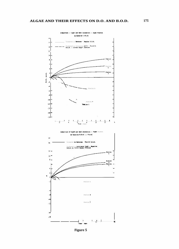
12 —
Station L
Station A
.2 —
Station B -Station C
Incubated in Darkness - Regular B.O.D. 11
Incubated in Continuous Light - Negative 8.0.0. is ibvess Oxygen Produced
Station
B.O
.1.
p.p..
-12
8 -
-16
-16
-18
ALGAE AND THEIR EFFECTS ON D.O. AND B.O.D. 175
Comparison of Light and Dark Incubation on Algae Studies
As Received 7-25-56
I I I1
1 i i 4
1 1 I i 1 I 2 6 a 10 12
Tian - Days
Comparison of Light and Dark Incubation on Algae Studies
Am ./Received 8-8.56 and 8-9-56
18
16
— Incubated in Continuous Light . Negative B.O.D. is Excess Cmygen Produced
4
Incubated 111 NAM.. Regular B.O.D.
0.4
12
108
4
2
0
Station A
Station B
-2
-6
-8
-10Station C
-12
-16
-18
2 ' Time - DV.
I I I10 -• It
Figure 5

5-DAY B.O.D. (20°C) ON ALGAE STULIES
RETIO - 5-8.5 B.O.D. OF SUSPENDED METTER TO VOLATILE SUSPENDED POTTER
STATION A
R 7-25-56
---0 8_8_56
5-DAY B.O.D. (20°C) ON ALGAE STUDIES
RATIO - 5 -DAY B.O.D. OF SUSPENDED MATTER TO VOLATILE SUMPENDED MATTER
STATION B
X 7-25-56
----0 8-8-56
6
Z CY
><
0/ O /
./
7 VOLATILE SUSPENDED SOLIDS - P.P.M.
12 1. 20 VOLATILE SUSPENDED SOLIDS P.P.M.
1 1 1 1 1 1 1 1 1 1
176 OXYGEN RELATIONSHIPS IN STREAMS
5-DAY B.O.D. (20°C) ON ALGAE STUDIES
RATIO - 5 -8.1 B.O.D. OF SUSPENDED MATTER TO VOLATILE SUSPENDED METTER
STATION C
)( 7-25-56
- 0 8-9-568
7
6
0 5 0.
3
2
1
8 12 16 20 24 28 VOLATILE SUSPENDED SOLIDS - p.p.m.
FIGURE 6

SEWAGE + DEAD ALGAE
-0.15, L.-7.79
It-GENAGE + LIVING ALGAE -
161-0.11, La-6.95
SEWAGE -0.14, L.-3.32
It-- DEAD ALGAE
LIVING ALGAE
10
ALGAE AND THEIR EFFECTS ON D.O. AND B.O.D. 177
DISCUSSION A. F. BARTSCH, Biologist Water Supply and Water Pollution Program
The information presented by Mr. Wisniewski represents an interestingly new approach to a problem that has been neglected for a long time. It seems appropriate that this work should have been done in Wisconsin because in that State especially there has long been an interest in algae as they relate to artificial eutrophication involving sewage plant efflu-ents, chemical algal control, and effects of algae upon stream conditions. There is reason to believe that water resource problems that accompany intense algal production will grow in prominence throughout the country as levels of available algal nutrients increase and many water areas become improved algal habitats as a result of impoundment.
He points out that there are two principal areas of algal influence on which better in-formation is needed; the part algae play in determining the assimilation capacity of streams and the effect of algae present in the sample upon the laboratory B.O.D. Field and laboratory data are presented in refer-ence to both areas of interest.
Although the Fox River in Wisconsin appar-ently brought the algal problem into sharp focus because of the large tonnages of algae entering it from Lake Winnebago, this type of situation is not typical of that usually found in rivers. Here, the algae reaching the river originated in a different type of habitat, are less suited to existence in the river and die off downstream. In October of 1946 (Mackenthun, et. al. 1948) a more intensified situation of this kind occurred in the Yahara River in Wisconsin where tremendous quanti-ties of algal entered from Lake Kegonsa, decomposed in passing downstream, and caused oxygen depletion with resulting death of tons of fish.
More commonly the algae in rivers are less numerous than in the two situations cited. Moreover, algae found in rivers typically are produced therein and therefore are in closer harmony with that type of habitat. They are likely to affect both the oxygen relations in the stream and the course of the B.O.D. re-action with less violence than under the circumstances cited above.
Results of limited studies here are generally in close agreement with the Wisconsin results. They are presented in reference to the same questions that were stated by Wisniewski.
1. What influence, if any, does the presence of algae have on the laboratory B.O.D. determination?
In one case, this question has been approached by removing algae from samples and compar-ing the B.O.D. response with that of samples containing algae. Unaltered samples from waste stabilization ponds commonly have B.O.D. of about 25 ppm whereas others that have been filtered to remove the algae have values between 6 and 7. Another approach has been to add known quantities of algae (Chlorella variegata) to samples made up with 0.5% settled sewage and then determining the B.O.D. in the standard manner. Figure 1 shows the course of the B.O.D. reaction with a sample containing 1.2 million cells/ml. The algal cells contributed to the total B.O.D. to the extent of about 0.2 ppm/million cells.
B.O.D., ppm
3
t, DAYS
INFLUENCE OF ALGAE ON B.O.D.
Figure 1
2. What influence, if any, do increasing amounts of algae have on the laboratory B.O.D. value?

5
D.O.D. 2- -(-NEAN D.O.D.
7
NEAN 0.07
0 2 5 8 iii 2 5 8 II
AN NOON PH
INFLUENCE OF DIFFUSED DAYLIGHT ON B.O.D. SAMPLE CONTAINING ALGAE - AUGUST 26, 1955
1 1 1
178 OXYGEN RELATIONSHIPS IN STREAMS
To obtain information on this question, B.O.D. samples were prepared so that one contained the phytoplankton removed from 20 volumes of Ohio River water, the other the quantity removed from 40 volumes. These are re-ferenced to as "x algae" and "2x algae" in Figure 2 which shows, as does the Wisconsin work, that increasing amounts of algae re-sult in increasing B.O.D. When dead Chlorella cells from laboratory cultures were added to samples in relative quantities of 1, 10 and 66, the resulting B.O.D. values were 3.21, 3.73 and 7.74 ppm respectively. A similar result occurred with living cells. These results agree with the Fox River data which show that B.O.D. concentrations increase with increas-ing suspended solids, largely algae, in the sample.
2 9 5 t, DAYS
INFLUENCE OF QUANTITY OF ALGAE ON 8.0.0. AUGUST 25, 1055
Figure 2
3. What difference occurs in oxygen usage rates between samples containing algae which are incubated in the dark and the light?
The influence of algal photosynthesis on the B.O.D. of samples incubated in the light is well shown by the Wisconsin data. With con-tinuous illumination, there was generally an excess of D.O. in the sample. It is also im-portant to follow the fluctuating course of the D.O. levels, and therefore the indicated B.O.D. also, when the samples are exposed to the daily changing light intensities found in nature. Results of such exposure are shown in Figure 3 for a sample containing Ohio River algae. When replicates were incubated in the dark for 19 hours the mean B.O.D. was 2.77 ppm; but with natural light, it was only 1.15 ppm. Furthermore, if all the samples had been processed at noon, the mean B.O.D. of
the illuminated samples would have been 0.55 ppm., but that of the ones in the dark would have been 2.10 ppm -- a difference of 400%1 Obviously, incubation in neither continuous light nor continuous darkness can yield in-structive results in relation to natural con-ditions in streams.
2
I. I
z .;
Figure 3
4. What influence, if any, does the presence of dead or decomposed algal cells have on the B.O.D. determination?
Samples from the Fox River were processed to determine the influence of dead cells. July samples that were autoclaved to kill the algae showed a decreased rate constant whereas September samples had an increased constant as compared with unautoclaved material.
Figure 1 shows the course of the B.O.D. re-action with living algae together with that for the same quantity of algae killed by raising the temperature to 70° C. It was concluded from the Wisconsin work that autoclaving the samples (i.e. having dead algal material present) does not greatly affect the ultimate B.O.D. This is suggested to some extent by the curves in Figure 1 also. It is agreed that the slow oxygen consumption in algal respira-tion is no greater than aerobic bacterial oxidation of dead algal cell material.
Various approaches have been made to assess the influence of algal photo-synthesis upon D.O. resources in streams. In the Wisconsin work this was done through use of "instruc-tive" B.O.D.'s such as those described. Another approach is that of Odum (1956, 57) which interrelates existing oxygen concentra-tion, provision of oxygen from inflow, atmos-phere and photosynthesis, and loss through

RESPIRATORY USE AND D.O. PRODUCTION AT THREE DEPTHS
9 II 1 3 5 7 AM NOON PM
2
0
9.0
4 • • 8 5 0.
8.0
4 O. 0.5
0.0
D.O. CONCENTRATION IN RIVER
(OCTOBER 2, 1957)
(OCTOBER 3, 1957)
ALGAE AND THEIR EFFECTS ON D.O. AND B.O.D. 179
2 9 4 5 a DEPTH, FEET
LIGHT PENETRATION THROUGH NATURAL WATERS
Figure 4
total respiration. A third approach involves the use of "light and dark bottle" tests to measure photosynthesis and respiration simultaneously.
Because, in general, all appreciable photo-synthesis occurs in the surface layer that absorbs 99% of the light (euphotic zone), it is important to measure and evaluate water transparency in connection with oxygen re-lations. This characteristic mayvary widely as indicated in Figure 4 which shows light penetration in three bodies of water. In the euphotic zone of the Ohio River on October 3, 1957, light and dark bottle tests indicated oxygen production of 57 pounds per acre per day and respiratory use of 45 pounds per acre per day -- a P/R ratio of 1.3. As shown in Figure 5, the rate of oxygen production varies with time of day in relation to momentary
DISSOLVED OXYGEN RELATIONS IN OHIO RIVER (REACH II, BROMLEY) OCT. 3, 1957
Figure 5

180 OXYGEN RELATIONSHIPS IN STREAMS
Intensity of solar radiation and decreases also with depth in response to impaired light penetration. The influence of photosynthesis on D.O. concentration in the river was ob-scured by an abnormal flow pattern on Octo-ber 3. Conditions shown for October 2 were more typical. Similar tests in a raw sewage pond at Lemmon, South Dakota on August 10, 1955 showed production of 183 pounds and respiratory use of 130 pounds per acre per day -- a P/R ratio of 1.4.
It is apparent from these ratios that the oxy-gen provided by algal photosynthesis is not a free gift obtained at no cost. As long as P/R. ratios are in the neighborhood of 1.5, high daytime oxygen production by dense algal populations will be accompanied by rapid respiratory use that persists around the clock. In rivers this typically results in mild noctur-nal depressions in D.O., but in sewage ponds it may bring about oxygen exhaustion lasting several hours.
Acknowledgment
The writer wishes to acknowledge the con-tinuing efforts of his fellow workers, E. C. Tsivoglou, W. M. Ingram, T. E. Maloney and D. G. Ballinger, in connection with this sub-ject. Without their joint interest, the data reported here could not have been obtained.
References
1. Mackenthtm, R. M., E. F. Herman and A. F. Bartsch. A heavy mortality of fishes resulting from the decomposition of algae in the Yahara River, Wisconsin. Trans. Amer. Fish. Soc. 75:175-180. 1945 (Published 1948).
2. Odum, H. T. Primary production in flowing waters. Limnology and Oceano-graphy 1:102-117. (1956).
3. Odum , H. T. Primary production meas- urements in eleven Florida springs and a marine turtle-grass community. Limnology and Oceanography 2:85-97. (1957).
INFORMAL DISCUSSION R. E. Fuhrman: Any comments on this
subject which we have had presented so fully here?
C. M. Weiss: The revised saturation values for oxygen in water are available, in the literature published in this country, in a very useful fashion. Richards and Corwin, in a paper entitled "Some oceanographic ap-plications of recent determinations of the solubility of oxygen in seawater," Limnology and Oceanography, October 1956, included a nomograph for determining saturation values of oxygen at various temperatures and chlo-rinities. This nomograph is based on the new oxygen saturation values as determined by Truesdale, Downing and Lowden, J. Applied Chemistry 5:53, 1955. The chlorinity scale of the nomograph extends to zero chlorinity and thus the nomograph can be used directly for saturation values of oxygen in freshwater.
C. N. Sawyer: lam certainly happy this information has been presented here by Ted
and Fritz. I would like to mention that the National Institutes of Health are sponsoring a research program at the University of Wis-consin on this particular topic and I believe the investigator carrying on that work, Dr. Fitzgerald, is here in the group. I would like to ask him if he has any comment to make.
R. E. F'uhrman: Is Dr. Fitzgerald present?
G. P. Fitzgerald: I can't make a com-ment because I have only run one BOD test in my life and that was last week. I prefer to keep quiet until I learn how algae affect BOD measurements.
R. E. Fuhrman: Thank you. We respect and admire your approach. If there are no other comments on this, gentlemen, I would like to express the appreciation of those who are presentand have been present this morn-ing and to all those who presented the morning papers and discussions.

Areas for Future Study
A Panel Discussion
181
W. W. TO'WNE, Chairman, Chief, Water Pollution Control Water Supply and Water Pollution Program
The personnel here at the Center who have been responsible for developing this seminar fully realize there are many deficiencies in our knowledge of stream sanitation of which oxygen relationships are only one. Therefore, It was felt that in closing the discussions on this subject it would be well to point out areas for future study not only within the field under discussion here, but in the broader field of general stream sanitation. In so doing we• should consider the entire field without re-gard to the persons or institutions that should undertake such studies. These latter ques-tions are details that can be worked out once the needs have been established and agreed upon by the profession as a whole. We have asked people from various areas of the country representing various professional activities to lead this discussion. Most of them are, of course, well known to this group. In fact, they have already contributed to previous ses-sions. I would hope that their comments might stimulate expressions from the group as a whole and if they, or you, have any specific comments that might relate to the general problem or to the activities here at the Center, we would surely welcome your suggestions as to how this service might be made more effective.
Before proceeding with the panel discussion I would like to call your attention to a re-issue, now available, of Public Health Bulletin No. 146"A Study of the Pollution and Natural Purification of the Ohio River - III" by H. W. Streeter, Sanitary Engineer and E. B. Phelps, Consultant (1925). This bulletin contains the original work leading to the development of the formulation of oxidation and reaeration phenomena in streams, reprinted in 1958 by the U. S. Department of Health, Education, and Welfare; and also to a nomograph (Figure 1) that has been developed by Mr. and Mrs. T. A. Wastler for the graphical solution of the oxygen sag equation. Mr. Wastler is a chemist in the Water Pollution Control section here at the Center and Mrs. Wastler, a chemist in her own right, has been called upon to assist us from time to time during emergencies.
Iwould like to call first upon Mr. Spies and I hope that he will present some of the particular needs of the regulatory agencies and how re-search might help to better solve their problems. Mr. Spies will be followed by Professor Pearson, Professor Schroepfer and Mr. Kittrell.

13 4 5 La Da
7
10
0.3
0.14
0.10
0.09
0.07
.08
•100
2.0 b a t. 1.2 1.5
1.0 cks
0.6 1.0
0.4
0.5 0.9 as
40 0.7
OA
0.2 0.18
/01.tte:44:1
At 41444:00,, , 0.16 if,
0.12 .+Aok
0.
0.06 Tr
Illak \,‘
/a 08
.7 4
0,1 I a W .6; 1 '
V. ,d111MA
Afr fir . 4yde■ • e**0‘1
///,';'ij , 7 ■■•*1 ...4..-_.„.... ., .41/diegib. ■01110.- 1
,', AgStirrift.-41116.. x'
1
0.05
0.045
0.04
0.035
003
0.30 Dt • 3.0 ppm
k (2) To find: k2 t i t 0.25 k, .01 100 1.0 (a) Calculate : La/D0 • 10.0/2.0 .5.0
60 080 Dt/La = 3.0/10.0.0.3 0.20 40 0.60 (b ) Find k it • 0.07 by passing line C through k, • 0.1 and
Dt/La .02 0.50 t • 0.7 on the straight line nomograph. ao
0.40 (c) Pass line A through La/ Da • 5.0 and Dt/ La • 0.3 0.15 10 0.30 intersecting kit • 0.07.
6 (d ) Read f • 1.2 on f -scale at point of intersection of line A and kit • 0.07 1 k2 • k, f =1.2 x 0.1 • 0.12
(3) To find : Dc and tc 0.10 2 (a) Pass line B through La/Da • 5.0 tangent to
f • 1.2 curve. (b) Read Dc/La • 0.41 on Dt/La scale ( Dc •10.0x 0.41=4.1 ppm )
0.6 0.4 006 (c) Read kitc • 0.31 on k it scale at point of tangency
0.2 0.05 tc • 0. 31/0.10 • 3.1 days ) 0.2
0.05 0.04
Computed and Drawn by T.A. Wristlet. and N.D. Wastler
GRAPHICAL SOLUTION OF THE OXYGEN SAG EQUATION
Di. , La 00-o _ 10-fko) +Do ID- fltit Where f • -•- k,
f -I k
Example of use of Chart :
(I) Given : Da • 2.0 ppm k, • 0.10 per day La •10.0 ppm t • 0.7 day
0.025
0.02
0.015
141 • 0.01
OX
YG
EN
RE
LA
TIO
NS
HIP
S I
N S
TR
EA
MS

AREAS FOR FUTURE STUDY 183
K. H. SPIES, Deputy State Sanitary Engineer Oregon State Board of Health
In the remarks which I made the other day I mentioned that one of our water pollution control problems in Oregon is in connection with slime growths resulting from the dis-charge of certain types of industrial wastes. Thus far we have been unable to find much Information in the literature regarding stream conditions which are likely to cause such growths, how much dilution may be required to prevent this growth, or to what extent such slime growths damage or otherwise affect a normal aquatic environment. Research studies should be undertaken to supply the answers to these questions.
Another problem facing us in Oregon is ex-cessive turbidity caused by sand and gravel mining operations, by other types of mining operations in the mountain areas, and by soil erosion resulting primarily from timber harvesting and road construction. It would be of considerable help to water pollution control agencies if research could be con-ducted to determine the damaging effects, if any, of excessive turbidity on the aquatic environment and to establish a basis for re-commending permissible turbidity limits.
To obtain some of this information the State of Oregon through its Natural Resources Committee has started a special comprehen-sive survey and study of one of our smaller watersheds. The purpose of this special pro-ject is to determine the effects upon the water quality of the various types of operations which are normally conducted on our water-sheds. It is hoped that information will also be obtained for developing ways of controlling certain operations so that stream pollution can be prevented. This research study is just getting underway and it is expected that it vill be continued for several years.
Being a coastal state we are also interested in the possible toxic effects of various pol-lutants upon shellfish and other marine life. Recently we had an industry propose the installation of a Kraft pulp mill on a tidal estuary which during the summer time re-ceives very little fresh water dilution. This particular estuary constitutes a valuable sport and commercial fishery including the propa-gation of oysters. We were unable to find much definite information regarding the pos-sible effects of Kraft mill wastes upon such waters. In our opinion, therefore, more research is needed in this particular field.
I do not want to give the impression that in
Oregon we are concerned only with the pro-tection of fish life. We are also concerned with the protection of public health. With regard to waters which are used for swimming it seems that there are almost 48 different standards being used by the 48 states. In my opinion it would be most helpful if, through research studies, a uniform maximum permissible bacterial limit for bathing waters could be adopted by all of the states.
Another subject of current interest in our state is the use of raw sewage lagoons or stabili-zation ponds as they are sometimes called. City officials and others in our state have learned about their economy and successful use in other sections of the country and are requesting that they be permitted to use them in Oregon. In the western part of our state we have climatic conditions which are con-siderably different from those in the Middle West and other areas where oxidation ponds have thus far been used so widely. We have long periods of cloudy weather and heavy rainfall, particularly during the winter months which might detrimentally affect the operation of this type of sewage disposal. We are making plans now to undertake a research study in cooperation with the Public Health Service and the State of Washington which we hope will determine whether or not the raw sewage lagoon can be used successfully under such climatic conditions.
Another field where we would like to see some disinterested party conduct research is in connection with the many special patented pro-ceases which are developed primarily by the equipment companies for the treatment and disposal of sewage. One example is the so-called rated or long-time aeration process which has been developed for small installa-tions. The results obtained from recent installations of this type of process in Oregon have not been nearly as good as we had ex-pected in view of reports which had previously been made to us. It would, therefore, be our recommendation that some agency such as the Public Health Service make thorough investigations of all such processes so that reliable information could be made available to all official water pollution control agencies regarding their possible uses.
It is our hope that work will continue toward the development of automatic and continuous sampling devices as an aid in monitoring stream conditions. It is hoped further that

184 OXYGEN RELATIONSHIPS IN STREAMS
these devices when developed will be reliable and rugged and that they will not require a specially trained person to service them.
The last research need which I want to mention is in connection with the possible toxic effects caused by the wastes from new industrial pro-cesses. I have in mind a pollution problem which confronted us recently in connection with the wastes from a new plant which pro-duces zirconium. Preliminary studies have indicated that certain constituents in this
plant's wastes have very seriously affected the biological processes in the treatment plant serving the city sewer system into which said wastes are discharged. The ef-ficiency of both the separate sludge digester and the trickling filter has been materially reduced due to the toxic effects of these wastes. As long as we have new industrial processes being developed, there is going to be a need for research to provide the answers for the waste disposal problems which will be created as a result of such developments.
E. A. PEARSON, Associate Professor, Sanitary Engineering University of California
I have not been able to resolve why I was selected for this panel; particularly with the collection of experts we have here. About all I cando is to give you some impressions that I have gained from this seminar and I am not going to try to outline the manifold research areas that might be of interest.
First of all, one fact that impressed me greatly was the amount of activity and interest In rather fundamental aspects of many pro-blems in our field, not only by people in universities but also by people in industry, by consulting engineers, and by representa-tives of regulatory agencies. Then too I was impressed generally by the gross differences that exist in the approach of regulatory agencies with respect to scientific or techni-cal concepts apart from political, administra-tive or legal aspects of their problems. There appears to be considerable need for a sound technical or fundamental approach to many problems. I was also impressed by signifi-cant differences in the approach of people interested in basic problems; people in universities as well as in other agencies doing fundamental research or basic engineering Investigation. Again, I was impressed by the need for a fundamentally conceived approach in research and engineering investigations. Even thoughan investigation maybe of afield character, there is no reason why it cannot be as fundam entally conceived and designed as a basic research investigation.
I have been reminded again in my experience here as well as previously of the need for a closer liaison or working relationship be-tween scientific, technical and administrative or regulatory people in the field. I think an Interchange or interflow of information and ideas in these areas is direly needed; not only to orient research to solve some of the
many problems, but also to provide data for the regulatory agencies so that they gradually can improve the "armchair" or "rule of thumb" type of problem solving. All too fre-quently we are forced to such solutions be-cause of insufficient data. If we do not conduct more research and develop a more objective and scientific basis for the work we do, we may find someone else may be effecting the solutions to our problems. We may find that the solution to our problems will be reduced to a completely political or non-technical basis or that the work will be done by people who are presumed to be more competent in the subject area than we are. I think even as administrators in regulatory agencies or as technical people we have some complex pro-blems to resolve and we need more basic data and more investigation to resolve them.
In California as elsewhere we have had con-siderable political pressure from various groups interested in pollution abatement. For example, in the southern part of the state, pressure has been brought to bear to study problems that may not be as important as some of the problems that we have com-pletely ignored or that have not merited any significant investigation. Recently, the Cali-fornia legislature approved in principle and funded the first year of a half a million dollar investigation of a single marine plant, Macrocystis, the giant kelp. One half of the study is to be devoted to ecological aspects, the other half devoted to the effect of waste discharge on the plant. Now I do not mean to imply that such a study should not be made, however, if one-half million dollars can be justified for the study of a single marine plant, certainly we can justify a little more basic investigation on some of the other as-pects of our water pollution and water re-sources problems.

AREAS FOR FUTURE STUDY 185
With respect to specific aspects of this Seminar, certainly I think we all appreciate the opportunity to express our interest and concern in the general subject area. A few things have been pointed out that appear fairly clear. First with respect to describing what happens in receiving waters when wastes are discharged and the role of physical processes such as turbulence. There is need for addi-tional work in resolving this phenomenon, at least to the point of quantitatively characteriz-ing, within the limits of engineering precision, the effect of turbulence in our streams not only as it relates to aeration, but also as it relates to sedimentation, \ sediment transport, and resuspension of bottom sediments. These are all related to the oxygen sag or balance as well as to other physical, chemical and biological effects. With due respect to the classic work of Streeter and Phelps, I think there is a need for a good reappraisal. of general oxygen sag relationships and compu-tation procedures with due consideration for and quantitation of the many variables which exist. I was particularly heartened to learn of the approach to the problem presented by Prof. Schroepfer where he has conducted a materials or oxygen balance on a reach of a stream in an attempt to quantitate the many variables involved. This appears to be a fundamental approach to the overall evaluation of the oxygen resources in a stream. Cer-tainly more of this caliber of work is needed. The work in the Thames estuary related by Mr. Gameson is another commendable exam-ple. There is not only a need for further study of oxygen relationships in streams but also a need for better methodology for quanti-tative description of the biological effects of waste discharge. Quantitative description of the biota within the limits of engineering pre-cision are needed so that we can evaluate or predict the effect, good or bad, of waste dis-charge; not just related to oxygen concentra-tions, but all effects, presumed adverse or toxic effects, or on occasion, beneficial effects. What appears to be needed is a
realistic measure of the biological producti-vity of a stream or lake. In some cases, this maybe measured by the light and dark bottle technique. However, this is only one approach to the problem. What is really needed is a quantitative, and I emphasize the word quanti-tative description of the biota so that evalua-tion of the effect of waste discharge can be based upon data and fact rather than on feel-ing and emotion. Lastly, I would like to emphasize the need for a more thorough evaluation of the physical, chemical and biological characteristics of estuarine waters, not only the marine biota but also quantitative descriptions of the phy-sical processes of estuaries. The work in England is an excellent example of one ap-proach to this problem and other approaches have been employed in this country. This problem has been studied to some extent by physical oceanographers; however, sanitary engineers have devoted little attention to this subject. Flushing or exchange theories for estuaries are still very vague and open to question and I think work is needed to resolve the problem in terms of mixing character-istics and residence time. Again quantitation of pollutional effects, oxygen productivity from photosynthetic activity, and oxygen de-mand from sediments and bottom deposits are needed. Certainly these problems merit in-creased investigative effort and quantitative analysis beyond the level that they have re-ceived in the past. I was glad to be responsible in part for a re-commendation to our State which was adopted by the State Water Pollution Control Board that the San Francisco Bay estuary be studied to the extent of about $400,000 in the next three years. The studies will be devoted primarily to a physical, chemical and biolo-gical evaluation of conditions existing in the estuary. I believe much more of this type of activity is needed and I think it should develop at a far greater rate than it has in the past. I thank you.
GEORGE J. SCHROEPFER Professor of Sanitary Engineering University of Minnesota
This is an unfortunate position to be in; all of the remarks I intended to make have been covered quite well. I would like first to pay a compliment to the group here at the Center. I've attended a great many meetings but I think this is one of the best ones I've attended. The planners of the meeting have either con-sciously or accidentally created a rather favorable balance between the progressive
thinking of the young minds and the very neces-sary judgment of the experienced practitioner or the advisor who has to interpret the re-sults of the new developments in the knowledge and in the art.
I also have the comment that even in the ad-vanced stage of communication we have developed in this country there is such a long

186 OXYGEN RELATIONSHIPS IN STREAMS
(b)
(c)
interval between the time when an investi-gator conceives an idea and proves it by research and the time when it is actually accepted and employed in practice. There should be some way of shortening that time. The three important avenues of needed in-vestigation, in my opinion are the following:
(a) A study of the effects of, and re-medies for, thermal pollution.
The reappraisal of the mechanism of deoxygenation and the effect of temperature on rates.
The importance of the availability of a continuous recording DO device since up to now our knowledge of water course conditions from the standpoint of the theme of this seminar, is meager indeed.
F. W. KITTRELL, In Charge Stream Sanitation Studies, Water Pollution Control Water Supply and Water Pollution Program
The usual method for determination of re-aeration capacities of streams traditionally has assumed that we can establish the magni-tudes and rates of exertion of oxygen demand with acceptable accuracy. When there are errors in the evaluation of oxygen demand factors, comparable errors are reflected in the computed reaeration capacities. I suspect that significant deficiencies are involved in oxygen demand data and basic assumptions regarding the nature of the reaction more often than we realize. Although this is a dissolved oxygen seminar my remarks regarding future work needed will have to do exclusively with deficiencies in knowledge of oxygen de-mand than of dissolved oxygen.
First I want to make a prediction regarding the very promising work on determination of reaeration in streams, relatively uncompli-cated by oxygen demand, being done by Churchill and his associates. The success of this work will confirm, or permit revision of O'Connors formulas and will allow the computation of reaeration capacities of streams on the basis of their physical characteristics with some assurance. I pre-dict that this will lead to a new and reverse order of computing oxygen relationships in streams. I believe that we will first establish reaeration capacities on the basis of physical measurements and proceed from there to compute what the oxygen demand is doing. I am confident that this reverse approach will lead to solution of some of the oxygen demand problems that have been puzzling many of us for so long.
I suspect that second stage oxygen demand may be a more important factor in some of our puzzling B.O.D. results than generally is realized. In 1948 Ruchhoft, Placak and Ettinger published an interesting and signifi-cant paper in Sewage Works Journal. They made parallel determinations, at frequent time intervals, of B.O.D. and nitrites on a
large number of incubated samples. When plotted against time the B.O.D.'s gave the er-ratic curves with which many of us are all too familiar. With monotonous, not irregular, frequency individual points occurred above the curve that was indicated by the majority of re-sults. The high points were found to represent individual bottles in which significant nitrites were found. When the oxygen necessary to form the nitrites was subtracted from the B.O.D.'s the high points fell into line with other results. The authors concluded that the apparently erratic results were due to nitrification which occurred, without parti-cular pattern, in some incubated bottles, and not in others, at any given series of ob-servations.
They found that some bottles yielded nitrites as early as the first or second day after in-cubation started while other bottles in the same series might not contain nitrites for 10 or more days after incubation started. They concluded that some bottles filled from a given sample initially received sufficient nitrifying organisms to cause nitrification, while other bottles filled from the same sample failed to receive sufficient seeding organisms to produce nitrification.
The implications of these findings in regard to laboratory determination of B.O.D. are ob-vious. Aiittle thought extends their implica-tions to the possibilities in the stream itself. A stream develops the necessary seeding organisms to attack any material subject to biological attack if the material is discharged regularly to the stream. Where nitrogenous material is discharged to a stream the stream will develop nitrifying organisms. There is no especial reason to assume that the seeding will wait for a spot 10 days time of water travel downstream to develop. The paper cited shows, on the contrary, that nitrification may be well established in one to two days after dilution of the sewage. It appears that

AREAS FOR FUTURE STUDY 187
the necessary source of nitrifiers may be-come established in a stream a very short distance below a nitrogenous waste discharge and that nitrification, or second stage B.O.D., may start in far less than the classical 10 days. I agree with the author's conclusion, expressed in 1948, that this subject needs more investigation. It appears rather obvious that second stage B.O.D. inevitably is present in sewage sludge deposits. The laws of sedimentation are not selective with respect to whether a settleable material will produce first or second stage B.O.D. Fair, Moore and Thomas published a series of articles on laboratory studies of sludge deposits in Sewage Works Journal in 1941. These articles dealt, among other things, with the fate of nitrogen compounds in sludge deposits. In spite of the availability of this background information I can not re-call any published material that included consideration of second stage B.O.D. in com-putations involving sludge deposits. I have been equally as guilty of this omission as anyone. This, also, is a subject which I be-lieve needs future investigation.
The second stage B.O.D. of sludge deposits probably has a parallel in the organic matter absorbed from the flowing water by biological organisms attached to the bed of the stream. Those organisms are not selective between the first and second stage material that they absorb. I would like to illustrate this point with an extreme example for emphasis. The highly polluted stream involved was small, shallow and swift. It was ideal for develop-ment of large quantities of attached biological growths. Long terms B.O.D. curves were developed from 24 hour composite samples taken 0.1 miles and 2.6 miles below the source of waste. The first stage B.O.D. at the up-stream station, A, was 222 ppm. At the downstream station, B, the first stage B.O.D. was 20 ppm. The time of water travel was approximately 12 hours. If we compute the stream coefficient, ki, by the classical method, using first stage B.O.D.'s only, we obtain a value of 2.0. The second stage B.O.D. at station A was 407 ppm, and that at B was 40 ppm. If we use these values in place of those for first stage B.O. D.' s we also get a stream k1 of essentially 2.0. Let's carry the mathematical manipulations a step farther, however, and use the two sets of B.O.D.'s to compute the stream reaeration coefficient, k2, by the classical method. The first stage B.O.D.'s yield a k2 of about 6, while the second stage values yield one of nearly 12. I place no confidence, myself, in the quantitative exactness of these values; but I do submit that they indicate something
we need to know more about. I do not believe we can ignore second stage B.O.D. in stream sections where biological organisms absorb significant portions of the organic matter. The foregoing data may be used to illustrate another deficiency in our knowledge of B.O.D. reactions in streams. The difference in the first stage values between stations A and B was 202 ppm and for the second stage values the difference was 367 ppm. Regardless of which value you are willing to accept as re-presentative of actual conditions, one or the other must represent B.O.D. that was either satisfied or stored in the stream section. I cannot accept a conclusion that the portion that was absorbed or stored in the living bodies of biological growths in the stream exerted a demand on the D.O. of the flowing water of the same magnitude and at the same rate that it was absorbed by the growths. I question whether all of the absorbed B.O.D. ever exerts a demand on the stream D.O. equivalent to the original B.O.D. that was ab-sorbed. Until we can determine what fraction of the absorbed B.O.D. is actually exerted on the dissolved oxygen of the stream we cannot compute a reliable reaeration coef-ficient. Earlier I pointed out that this was a small stream and it obviously was not typical of a majority of the streams with which we deal. It does, however, reveal rather dramatically certain phenomena which I be-lieve occur in varying degrees in all streams. Although the effects of these phenomena un-doubtedly are minor in large, slow flowing streams I believe a better understanding of their effects in the smaller streams would help us in our interpretation of the results of surveys on a variety of streams.
The Ruchhoft, Placak and Ettinger paper pre-viously quoted included another factor worthy of note. They determined B.O.D. rates on many samples through the usual daily obser-vations for 10 days. They obtained the usual range of k's from a few hundredths to nearly 0.3. Using the same samples, but at some-what higher concentrations to permit obser-vation at hourly intervals for the first day, they obtained rates for the first day only, of 0.4 to 2.3. There is evidence in numerous streams that rates of oxygen demand im-mediately below a source of waste discharge are more rapid than those farther down-stream. In other words, the rate at which oxygen demand is exerted in a stream may not be represented by the classical straight line on semi-logarithmic paper. The rate may, rather, continuously diminish on pro-ceeding downstream. This is not something we should continue to wonder about. We should find out.


Closing Remarks
W. W. TOWNE, Chief Water Pollution Control
Water Supply and Water Pollution Program
Mr. Harry G. Hanson, who welcomed you to this meeting, has been called out of town and I am sure that he would want to thank all of you for your active participation in this en-deavor. Any measure of success of this or other similar meetings can be attributed to both those appearing on the program and the audience. I am sure that the number of participants and the interest shown by all in this conference has far exceeded any ex-pectations of those of us who assisted in the development of the program.
I would also like to state that we plan to publish the proceedings of this seminar and hope that this maybe the first of many meet-ings dealing with the several problems to maintaining the quality of the surface waters of the Nation at a level essential for the many water uses of our expanding economy.
Again on behalf of Mr. Hanson, thank you and come back.
189

Roster of Attendance
190
Aderholdt, D. F., Laboratory Director, Virginia Water Control Board, Rich-mond, Virginia
Allen, H. L. Jr., Graduate Student, University of Tennessee, Knoxville, Tennessee
Al-Sarraf, M. A., Graduate Student, University of Tennessee, Knoxville, Tennessee
Bartsch, A. F., Biologist, Robt. A. Taft Sanitary Engineering Center, Cincinnati, Ohio
Baumann, E. R., Professor, Civil Engineering, Iowa State College, Ames, Iowa
Becher, A. E. Jr., S. A. Sanitary Engineer, Robt. A. Taft Sanitary Engineering Center, Cincinnati, Ohio
Belkov, Sylvin, District Engineer, Maryland Water Pollution Control Com-mission, Baltimore, Maryland
Bendixen, T. W., Soil Scientist, Robt. A. Taft Sanitary Engineering Center, Cincinnati, Ohio
Berger, Bernard B., Chief, WS & WP Program, Robt. A. Taft Sani-tary Engineering Center, Cincinnati, Ohio
Bielo, Robert, Regional Manager, Pennsylvania Fish Commission, Harris-burg, Pennsylvania
Bishop, William, Instructor, Case Instittite of Technology, Cleveland, Ohio
Black, Hayse H., Industrial Waste Consultant, Robt. A. Taft Sanitary Engineering Center, Cincinnati, Ohio
Bolton John M., Sanitary Engineer, Alabama State Health Department, Mont-gomery, Alabama
Borchardt, J. A., Associate Professor, University of Michigan, Ann Arbor, Michigan
Bramer, Henry C., Fellow, Mellon Institute of Industrial Research, Pittsburgh, Pennsylvania
Brown, Roy L., Assistant Sanitary Engineer, Bureau of Sanitary Eng. Virginia State Health Dept., Richmond, Virginia
Burdick, G. E., Sr. Aquatic Biologist, N. Y. Conservation Department, Albany, New York
Camp, Thomas R., Consulting Engineer, Camp, Dresser & McKee, Boston, Massachusetts
Cassanos, J. G., San. Engr. Consultant, National Research Council, Woburn, Massachusetts
Churchill, M. A., Chief, Stream Pollution Control Sec., Ten-nessee Valley Authority, Chattanooga, Tennessee
Clark, J. W., Professor, New Mexico A & M, State College, New Mexico
Cleary, E. J., Executive Director, ORSANCO, Cincinnati, Ohio
Cohen, J. M., Chemist, Robt. A. Taft Sanitary Engineering Center, Cincinnati, Ohio
Coughlin, F. J., Assoc, Director, Product Dept., The Proctor & Gamble Co., Cincinnati, Ohio
Courchaine, R. J. Sanitary Engineer, Mich. Water Resources Comm., Lansing, Michigan
Cross, William P., Hydraulic Engineer, U. S. Geological Survey, Columbus, Ohio
Dappert, A. F., Executive Secretary, Water Pollution Program, New York State Dept. of Health, Albany, New York
Davis, R. V., Engineer, Va. State Water Control Board, Rich-mond, Virginia
Davison, Robert, Sanitary Biologist — Bacteriologist, Sewage Disposal Section, City of Cincinnati, Cincinnati, Ohio
Dearwater, J. R. S. A. Sanitary Engineer, Robt. A. Taft banitary Engineering Center, Cincinnati, Ohio

191
Dobbins, William E., Professor of Sanitary Engineering, New York University, New York, New York
Eck, Russell C., Chief, Water Pollution Section, Indiana State Board of Health, Indianapolis, Indiana
Eldridge, Warren E., Chemist, Robt. A. Taft Sanitary Engineering Center, Cincinnati, Ohio
Ettinger, M. B., Chief, Chemistry & Physics, Robt,A. Taft Sani-tary Engineering Center, Cincinnati, Ohio
Eubanks, C. E., Graduate Student, University of Tennessee, Knoxville, Tennessee
Falk, Lloyd L., Waste Consultant, E. I. duPont De Nemours & Co., Wilming-ton, Delaware
Feldmuth, Guillermo, Biochemist, National University of Engineering, Lima, Peru
Fitzgerald, George P., Research Associate, University of Wisconsin, Madison, Wis-consin
Fuhrman, R. E., Exec. Secy. - Editor, Federation of Sewage & Industrial Wastes Association, Washington, D. C.
Gameson, A. L. H., Physical Chemist, Dept. of Scientific &Industrial Research, Water Pollution Research Laboratory, Stevenage, Herts, England
Garrett, George B., Assistant Sanitary Engi-neer, Ohio Dept. of Health, Columbus, Ohio
Gebhard, LloydW., Assistant Regional Engi-neer, U.S.P.H.S. Region M, Charlottes-ville, Virginia
Gerber, Robert A., Sanitary Engineer, Miss. State Board of Health, Jackson, Mississippi
Glynn, R. S., Director San. Research, Assn. American Railroads, Chicago, Illinois
Groche, Dieter, Depl.-Ing., Stuttgart, Germany
Grime, Werner N., Associate Professor, Georgia Institute of Technology, Atlanta, Georgia.
Hamlin, W. G., Sanitary Engineer, A. M. Kinney, Inc., Cincinnati, Ohio
Haney, Paul D., Consulting Engineer, Black & Veatch, Kansas City, Missouri
Hanson, H. G., Director, Robt. A. Taft Sanitary Engineering Center, Cincinnati, Ohio
Harris, John W., Chief, Savannah Harbor Investigations, Savan-nah District, Corps of Engineers, Savannah, Georgia
Henderson, Croswell, Aquatic Biologist, Robt. A. Taft Sanitary Engineering Center, Cincinnati, Ohio
Hert, Oral H., Sanitary Engineer, Indiana State Board of Health, Indiana-polis, Indiana
Hirth, Carl R., Chemist, Robt. A. Taft Sanitary Engineering Center, Cincinnati, Ohio
Holtje, Ralph H., Public Health Engineer, Public Health Service, Washington, D.C.
Horning, William, A., Sanitarian (Biologist), Robt. A. Taft Sanitary Engineering Center, Cincinnati, Ohio
Hull, C. H., Consulting Engineer, Sheppard T. Powell Company, Baltimore, Maryland
Hyde, R. T., Information Officer, Robt. A. Taft Sanitary Engineering Center, Cincinnati, Ohio
Ingols, R. S., Professor, Georgia Institute of Technology, Atlanta, Georgia
Jackson, H. W., Biologist, Robt. A. Taft Sanitary Engineering Center, Cincinnati, Ohio
Jente, R. C., Assistant Director Product Quality, Monsanto Chemical Co., St. Louis, Missouri
Kaplan, Bernard, Assistant Prof. Civil Eng., The City College of N. Y., New York, New York

192
Kinney, John E., Consulting Engineer, Ann Arbor, Michigan
Kittrell, F. W., Sanitary Engineer, U.S.P.H.S., Robt. A. Taft, Sanitary Engi-neering Center, Cincinnati, Ohio
Kohler, Walter, Assistant Chief Sewerage Section, Pennsylvania Dept. of Health, Harrisburg, Pennsylvania
Krieger, Herman L., Chemist, Robt. A. Taft Sanitary Engineering Center, Cincinnati, Ohio
Landon, Paul E. Jr., Sanitary Engineer, Greeley & Hansen, Chicago, Illinois
Langley, Harold E. Jr., Sanitary Engineer, Arthur D. Little, Inc., Cambridge, Massachusetts
Larson, F.C., Associate Professor, University of Tennessee, Knoxville, Tennessee
LeBosquet, Maurice Jr., Sanitary Engineer Director, U.S.P.H.S., Washington, D.C.
Lerner, Guy E., District Engineer, Maryland Water Pollution Control Com-mission, Baltimore, Maryland
Long, Wilbur E. Jr., Chief, Pollution Control Section, Div. of Water Pollution Control, N. C. State Board of Health, Raleigh, North Carolina
Ludzack, F. J., Chemist, Robt. A. Taft Sanitary Engineering Center, Cincinnati, Ohiq
Mathews, W. C., Development Chemist, Mead Corporation, Chillicothe, Ohio
McDermott, G. N., Sanitary Engineer, Robt. A. Taft Sanitary Engineering Center Cincinnati, Ohio
McLean, John E., Sanitary Engineer, Robt. A. Taft Sanitary Engineering Center, Cincinnati, Ohio
Megregian, Stephen, Chemist Consultant, Robt. A. Taft Sanitary Engineering Center Cincinnati, Ohio
Meredith, James C., Assistant Sanitary Engineer, Robt. A. Taft Sanitary Engi-neering Center, Cincinnati, Ohio
Montanan, F. W., Sanitary Engineer, ORSANCO, Cincinnati, Ohio
Moore, Edward W., Lecturer In Sanitary Chemistry, Harvard University, Cam-bridge, Massachusetts
Moore, W. Allen, Chemist, Robt. A. Taft Sanitary Engineering Center, Cincinnati, Ohio
Morris, J. Carrell, Associate Professor, Harvard University, Cambridge, Massa-chusetts
Morris, James M. Jr., Senior Hydraulic Engineer, Calif. Dept. of Water Re-sources, Sacramento, California
Moss, H. V., Director-Product Quality, Monsanto Chemical Co., St. Louis, Mis-souri
Msarsa, Maurice G., Graduate Student, University of Tennessee, Knoxville, Tennessee
Murray, William C., Sanitary Engineer, Corps of Engineers, Norfolk, Virginia
Muss, David L., Assistant Professor, City College of New York, New York, New York
Myers, Charles S., Sr. Chemist, Pennsylvania Dept. of Health, Harris-burg, Pennsylvania
O'Connor, Donald J., Associate Professor C. E., Manhattan College, New York, New York
0/Melia, Charles R., Teaching Fellow, University of Michigan, Ann Arbor, Michigan
Paessler, A. H., Executive Secretary, Va. State Water Control Board, Rich-mond, Virginia
Palange, R. C., Assistant Chief, WS & WP Program, Robt. A. Taft Sani-tary Engineering Center, Cincinnati, Ohio
Pearson, Erman A., Assoc. Prof. Sanitary Engineering, University of California, Berkeley, California
Perry, Edward L., U.S. Dept. of Interior, Fish & Wildlife Service, Washington, D. C.
Peters, Reinhardt E., Hydraulic Engineer, Corps of Engineers, Norfolk, Virginia

193
Pierce, Robert W., District Engineer, Maryland Water Pollution Control Com-mission, Baltimore, Maryland
Porges, Ralph, In Charge, Waste Treatment Studies, Robt. A. Taft Sanitary Engineering Center, Cincinnati, Ohio
Proctor, C. M., Consultant, Robt. A. Taft Sanitary Engineering Center, Cincinnati, Ohio
Rennerfelt, Jan, Research Engineer, The Waste Water Laboratory of the Swedish Forest Industries, StockholM, Sweden
Rhame, G. A., Engineer-Chemist, S. C. Water Pollution Control Authority, State Board of Health, Columbia, South Carolina
Richards, John E., Assistant Sanitary Engi-neer, Ohio Dept. of Health, Worthington, Ohio
Ristroph, J. D., Superintendent , Production Results, Virginia Electric & Power Co., Richmond, Virginia
Robeck, Gordon G., Sr. Sanitary Engineer, Robt. A. Taft Sanitary Engineering Center, Cincinnati, Ohio
Robertson, D. A. Jr., Sanitary Engineer, ORSANCO, Cincinnati, Ohio
Ruland, W. E., Civil Engineer, Mobile District Office, U. S. Army Engi-neers, Mobile, Alabama
Ryckman, D. W., Assoc. Professor San. Engr. , Washington University, St. Louis, Mis-souri
Saiger, Howard F., District Engineer, Kansas State Board of Health, Wichita, Kansas
Sawyer, Clair N., Associate, Metcalf & Eddy, Boston, Massachusetts
Schliekelman, R. J., Public Health Engineer, Iowa State Health Department, Des Moines, Iowa
Schott, Fred, Research Engineer, Mead Corporation, Chillicothe, Ohio
Schroepfer, G. J., Prof. San. Engineering, University of Minnesota, Minneapolis, Minnesota
Schultheis, Jack, Maryland Water Pollution Control Commission, Baltimore, Mary-land
Setter, L. R., Chemist, Robt. A. Taft Sanitary Engineering Center, Cincinnati, Ohio
Shadix, Carl N., Chemist, Robt. A. Taft Sanitary Engineering Center, Cincinnati, Ohio
Shay, J. R., P. H. Engineer, Iowa State Department of Health, Des Moines, Iowa
Shearer, S. David, Assistant Sanitary Engi-neer, Robt. A. Taft Sanitary Engineer-ing Center, Cincinnati, Ohio
Sheffield, C. W., Sanitary Engineer, Robt. A. Taft Sanitary Engineering Center, Cincinnati, Ohio
Sinkoff, Morton D., Sanitary Engineer, Robt. A. Taft Sanitary Engineering Center, Cincinnati, Ohio
Spies, Kenneth H., Deputy State Sanitary Engineer, Oregon State Board of Health and State Sanitary Authority, Portland, Oregon
Streeter, H. W., San. Eng. Dir. (Retired), U.S.P.H.S., Cincinnati, Ohio
Struzeski, E. J. Jr., Assistant San. Engineer, Robt. A. Taft Sanitary Engineering Center, Cincinnati, Ohio
Sutherland, J. R., Regional Engineer, Va. State Dept. of Health, Norfolk, Vir-ginia
Swanberg, Stacy C., Scientist I., Nebraska Dept. of Health, Lincoln, Nebraska
Tarzwell, Clarence M., Chief of Aquatic Bio-logy, Robt. A. Taft Sanitary Engineering Center, Cincinnati, Ohio
Thomas, H. A. Jr., Prof. Sanitary Engineer-ing, Harvard University, Cambridge, Massachusetts
Topping, Herbert E., Hydraulic Engineer, Corps of Engineers, U. S. Army South Atlantic Division, Atlanta, Georgia
Towne, W. W., Chief, Water Pollution Control, Robt. A. Taft Sanitary Engineering Center, Cincinnati, Ohio

194
Tsivoglou, E. C., Sr. Sanitary Engineer, Robt. A. Taft Sanitary Engineering Center, Cincinnati, Ohio
Vanderhoof, Richard A., Public Health Engi-neer, Robt. A. Taft Sanitary Engineering Center, Cincinnati, Ohio
Velz, C. J., Chr. Env. Health, University of Michigan, Ann Arbor, Michigan
Walton, Graham, Sr. San. Eng., Robt. A. Taft Sanitary Engineering Center, Cincinnati, Ohio
Wastler, Nancy D. Mrs., Chemist, Robt. A. Taft Sanitary Engineering Center, Cincinnati, Ohio
Wastler, T. A., Sanitarian, Robt. A. Taft Sanitary Engineering Center, Cincinnati, Ohio
Weaver, P. J., Proctor & Gamble Co., Cincinnati, Ohio
Weiss, Charles M., Assoc. Prof. Sanitary Science, Department Sanitary Eng., University of North Carolina, Chapel Hill, North Carolina
Wieters, Alfred H., Public Health Service, Washington, D. C.
Williams, Ned E., Hydraulic Engineer, Ohio Division of Water, Columbus, Ohio
Wisniewski, Theo. F., Director, Wisconsin Committee on Water Pollution, Madison, Wisconsin
Witt, Vicente, Research Assistant, University of Michigan, Ann Arbor, Michigan
Womack, James D., Assistant Research Bac-teriologist, University of Tennessee, Knoxville, Tennessee
Woodward, R. L., Chief, Water Supply, Robt. A. Taft Sanitary Engineering Center, Cincinnati, Ohio
Wright, Bern, Acting Executive Secretary, W. Va. State Water Commission, Charleston, W. Virginia
Yarborough, Keith A., Instructor in Sanitary Engineering, University of lllinois, Champaign, Illinois
Young, Lewis A., Assistant Regional Engi-neer, Public Health Service, Region IV, Atlanta, Georgia


a