Thermodynamics of spin S=1/2 antiferromagnetic uniform and alternating-exchange Heisenberg chains

arX

iv:c

ond-

mat

/000

3271

v2 [

cond

-mat

.str

-el]

23

Mar

200

0

Thermodynamics of spin S = 1/2 antiferromagnetic uniform

and alternating-exchange Heisenberg chains

D. C. JohnstonAmes Laboratory and Department of Physics and Astronomy, Iowa State University, Ames, Iowa 50011

R. K. KremerMax-Planck-Institut fur Festkorperforschung, Heisenbergstrasse 1, Postfach 800665, D-70569 Stuttgart, Germany

M. TroyerInstitute for Solid State Physics, University of Tokyo, Roppongi 7-22-1, Tokyo 106, Japan

and Theoretische Physik, Eidgenossische Technische Hochschule-Zurich, CH-8093 Zurich, Switzerland

X. WangInstitut Romand de Recherche Numerique en Physique des Materiaux, IN-Ecublens, CH-1015 Lausanne, Switzerland

A. KlumperUniversitat zu Koln, Institut fur Theoretische Physik, Zulpicher Strasse 77, D-50937, Germany

S. L. Bud’ko, A. F. Panchula,∗ and P. C. CanfieldAmes Laboratory and Department of Physics and Astronomy, Iowa State University, Ames, Iowa 50011

(To be published in Physical Review B)

The magnetic susceptibility χ∗(t) and specific heat C(t) versus temperature t of the spin S = 1/2antiferromagnetic (AF) alternating-exchange (J1 and J2) Heisenberg chain are studied for the entirerange 0 ≤ α ≤ 1 of the alternation parameter α ≡ J2/J1 (J1, J2 ≥ 0, J2 ≤ J1, t = kBT/J1,χ∗ = χJ1/Ng2µ2

B). For the uniform chain (α = 1), the high-accuracy χ∗(t) and C(t) Bethe ansatzdata of Klumper and Johnston (unpublished) are shown to agree very well at low t with the respectiveexact theoretical low-t logarithmic correction predictions of Lukyanov, Nucl. Phys. B 522, 533(1998). Accurate (∼ 10−7) independent empirical fits to the respective data are obtained over tranges spanning 25 orders of magnitude, 5 × 10−25 ≤ t ≤ 5, which contain extrapolations to therespective exact t = 0 limits. The infinite temperature entropy calculated using our C(t) fit functionis within 8 parts in 108 of the exact value ln 2. Quantum Monte Carlo (QMC) simulations andtransfer-matrix density-matrix renormalization group (TMRG) calculations of χ∗(α, t) are presentedfor 0.002 ≤ t ≤ 10 and 0.05 ≤ α ≤ 1, and an accurate (2 × 10−4) two-dimensional (α, t) fit to thecombined data is obtained for 0.01 ≤ t ≤ 10 and 0 ≤ α ≤ 1. From the low-t TMRG data, the spingap ∆(α) is extracted for 0.8 ≤ α ≤ 0.995 and compared with previous results, and a fit functionis formulated for 0 ≤ α ≤ 1 by combining these data with literature data. We infer from our datathat the asymptotic critical regime near the uniform chain limit is only entered for α >

∼ 0.99. Weexamine in detail the theoretical predictions of Bulaevskii, Sov. Phys. Solid State 11, 921 (1969),for χ∗(α, t) and compare them with our results. To illustrate the application and utility of ourtheoretical results, we model our experimental χ(T ) and specific heat Cp(T ) data for NaV2O5 singlecrystals in detail. The χ(T ) data above the spin dimerization temperature Tc ≈ 34K are not inquantitative agreement with the prediction for the S = 1/2 uniform Heisenberg chain, but canbe explained if there is a moderate ferromagnetic interchain coupling and/or if J changes with T .Fitting the χ(T ) data using our χ∗(α, t) fit function, we obtain the sample-dependent spin gap andrange ∆(T = 0)/kB = 103(2) K, alternation parameter δ(0) ≡ (1 − α)/(1 + α) = 0.034(6) andaverage exchange constant J(0)/kB = 640(80) K. The δ(T ) and ∆(T ) are derived from the data. Aspin pseudogap with magnitude ≈ 0.4 ∆(0) is consistently found just above Tc, which decreases withincreasing temperature. From our Cp(T ) measurements on two crystals, we infer that the magneticspecific heat at low temperatures T <

∼ 15K is too small to be resolved experimentally, and that thespin entropy at Tc is too small to account for the entropy of the transition. A quantitative analysisindicates that at Tc, at least 77 % of the entropy change due to the transition at Tc and associatedorder parameter fluctuations arise from the lattice and/or charge degrees of freedom and less than23 % from the spin degrees of freedom.

PACS numbers: 75.40.Cx, 75.20.Ck, 75.10.Jm, 75.50.Ee

1

http://arXiv.org/abs/cond-mat/0003271v2

I. INTRODUCTION

An antiferromagnetic alternating-exchange Heisenbergchain is one in which nearest-neighbor spins in the chaininteract via a Heisenberg interaction, but with two anti-ferromagnetic (AF) exchange constants J2 ≤ J1, J1, J2 ≥0 which alternate from bond to bond along the chain;the alternation parameter is α ≡ J2/J1. Here we willbe concerned with the magnetic susceptibility χ andspecific heat C versus temperature T of alternating-exchange chains consisting of spins S = 1/2. The uni-form AF Heisenberg chain is one limit of the alternat-ing chain in which the two exchange constants are equal(α = 1, J1 = J2 ≡ J). At the other limit is the iso-lated dimer in which one of the exchange constants iszero (α = 0). The present work is a combined theo-retical and experimental study of χ(T ) and C(T ) of theS = 1/2 AF alternating-exchange chain over the entirerange 0 ≤ α ≤ 1 of the alternation parameter, with theemphasis on the regime α <∼ 1 at and close to the uniformchain limit. This latter regime is relevant for compoundsshowing second order spin dimerization transitions withdecreasing T . The present work was originally motivatedby our desire to accurately extract the temperature de-pendent energy gap ∆(T ) for magnetic excitations, the“spin gap”, from experimental χ(T ) data for the S = 1/2chain/two-leg ladder compound NaV2O5 below its spindimerization temperature Tc ≈ 34K. We found that ex-isting theory for the alternating-exchange chain was in-sufficient to accomplish this goal. In the present work wecritically examine the predictions of previous theory, per-form the required additional theoretical calculations, andthen apply the results to extract ∆(T ) at T <∼ Tc from ourχ(T ) data for NaV2O5 single crystals. We have extendedthe original goal so that we also include theoretical andexperimental studies of C(T ) and how this quantity re-lates to χ(T ). In the remainder of this introduction webriefly review the prior theoretical results pertaining toχ(T ) and C(T ) of the uniform and alternating-exchangechain to place our work in the proper context. We thenreview the experimental and theoretical background onNaV2O5 and describe the plan for the rest of the paper.

A. Theory

The χ(T ) and C(T ) of both limits of the S = 1/2AF alternating-exchange Heisenberg chain are known ex-actly. For the dimer, the χ(T ) is given by the exactEq. (8a) below and the exact C(T ) is also easily calcu-lated. The χ(T ) and C(T ) of the uniform chain for T >∼0.4J/kB (kB is Boltzmann’s constant) were estimatedfrom calculations for chains with ≤ 11 spins by Bonnerand Fisher in 1964;1 they extended their results by ex-trapolating to T = 0, and in the case of χ(T ) to the exactT = 0 value.2 The exact solution for χ(T ) of the uniformchain was obtained using the Bethe ansatz in 1994 by

Eggert, Affleck and Takahashi, and compared with theirlow-T results from conformal field theory.3 They found,remarkably, that χ(T → 0) has infinite slope. Their nu-merical χ(T ) values are up to ∼ 10% larger than theBonner-Fisher extrapolation for T <∼ 0.25J/kB (for acomparison of the two predictions, see Fig. 8.1 in Ref. 4).Their conformal field theory calculations showed that theleading order correction to the zero temperature limitis of the form χ(T ) = χ(0){1 + 1/[2 ln(T0/T )]}, wherethe value of the scaling temperature T0 is not predictedby the field theory. Such log terms are called “logarith-mic corrections” in the literature. One of us recentlypresented numerical Bethe ansatz calculations of χ(T )with a higher absolute accuracy for χ(T ) estimated tobe 1 × 10−7,5 and showed that the data are consistentwith the above field theory prediction, with an additionalhigher order logarithmic correction, over the temperaturerange 5 × 10−25 ≤ kBT/J <∼ 10−3. Corresponding C(T )calculations were also carried out, and logarithmic cor-rections were studied for this quantity as well.5 Lukyanovhas recently presented an exact theory for χ(T ) and C(T )at low T , including the exact value of T0.

6 In the presentwork, we compare the very recent numerical Bethe ansatzresults of Klumper and Johnston5 with the predictions ofLukyanov’s theory and find agreement for χ(T ) to highaccuracy (≤ 1×10−6) over a temperature range spanning18 orders of magnitude, 5 × 10−25 ≤ kBT/J ≤ 5 × 10−7;the agreement in the lower part of this temperaturesrange is much better, O(10−7). For C(T ), the logarith-mic correction in Lukyanov’s theory is insufficient to de-scribe the Bethe ansatz data sufficiently accurately evenat very low temperatures, so we derive the next two log-arithmic corrections from the Bethe ansatz C(T ) data.For various applications, it would be desirable to havefits to the χ(T ) and C(T ) Bethe ansatz data which ex-tend to higher temperatures. We describe the formula-tion and implementation of fit functions, incorporatingthe influence of the logarithmic correction terms, whichyield extremely precise fits to the data for both quan-tities over the entire 25 decades in temperature of thecalculations, 5 × 10−25 ≤ kBT/J ≤ 5.

The χ(T ) in the intermediate regime 0 < α < 1has been investigated analytically in the Hartree-Fockapproximation7 and using numerical techniques.8,9 Ofparticular interest here is the regime α <∼ 1, close tothe uniform limit, which is the regime relevant to mate-rials exhibiting a dimerization transition with decreasingT such as occurs in materials exhibiting a spin-Peierlstransition. There are no accurate theoretical predictionsavailable for χ(T ) of the alternating-exchange Heisenbergchain in this regime, which is the property usually used toinitially characterize the occurrence of such a transitionexperimentally. To address this deficiency and to alsocover a more extended α range, we carried out extensivequantum Monte Carlo (QMC) simulations and transfer-matrix density-matrix renormalization group (TMRG)calculations10,11 of χ(T ) for 0.05 ≤ α ≤ 1 over the tem-perature range 0.002 ≤ kBT/J1 ≤ 10.

2

An interesting issue is how the spin gap ∆ evolveswith alternation parameter α as the uniform limit is ap-proached, α → 1. Because the uniform chain is a gaplessquantum-critical system, the introduction of alternatingexchange along the chain has been theoretically predictedto yield a nonanalytic ∆(α) behavior for α → 1. We de-rive ∆(α) by fitting our low-t TMRG χ(T ) data by anexpression which we formulated. The ∆(α) results arecompared with those of previous numerical calculationsand with the theoretical prediction. We infer from ourdata that the asymptotic critical regime is only enteredfor α >∼ 0.99.

In order to be optimally useful for accurately modelingexperimental χ(T ) data for alternating-exchange chaincompounds, our QMC and TMRG χ(α, T ) results mustfirst be accurately fitted by a continuous function of bothα and T . We will introduce a general fit function whicheventually proves capable of fitting these combined datafor the alternating-exchange Heisenberg chain very accu-rately. We first fit the χ(T ) of the uniform chain andisolated dimer using this function and then use the ob-tained fitting parameters as end-point parameters in thefit to our combined QMC and TMRG data for interme-diate values of α. The final fit function is a single two-dimensional function of α and T for 0 ≤ α ≤ 1 which canbe used to extract the (possibly temperature-dependent)alternation parameter, exchange constants and spin gapfrom experimental χ(T ) data for compounds for whichthe S = 1/2 AF alternating-exchange Heisenberg chainHamiltonian is appropriate. Our fit function will also beuseful as a reference for χ(T ) calculated from other re-lated S = 1/2 Hamiltonians such as that incorporatingthe spin-phonon interaction for spin-Peierls systems.

B. NaV2O5

Vanadium oxides show a remarkable variety of elec-tronic behaviors. For example, the metallic fcc normal-spinel structure compound LiV2O4 shows local moment-like behaviors above ∼ 50K, crossing over to heavyfermion behaviors below ∼ 10K.12 On the other hand,the d1 compound CaV2O5 has a two-leg trellis-ladder-layer structure13 in which all of the V atoms are crystallo-graphically equivalent and is a Mott-Hubbard insulator.The χ(T ) shows a spin-gap ∆/kB ≈ 660K arising fromstrong coupling of the V S = 1/2 spins across a rung.13

Modeling of χ(T ) by QMC simulations confirmed thatthis compound consists magnetically of V2 dimers, withan intradimer AF exchange constant J/kB ≈ 665K andwith very weak interdimer interactions.14

The compound NaV2O5 can also be formed. Thecrystal structure was initially reported in 1975 toconsist of two-leg ladders as in CaV2O5, but in anon-centrosymmetric (acentric) structure (space groupP21mn) in which charge segregation occurs such that oneleg of each ladder consists of V+4 and the other of crystal-

lographically inequivalent V+5 ions.15 However, recentlyfive different crystal structure investigations showed thatthe structure is actually centrosymmetric (space groupPmmn), with all V atoms crystallographically equivalentat room temperature,16–20 so that (static) charge seg-regation between the V atoms does not, in fact, occur.This result is consistent with 51V NMR investigationswhich showed the presence of only one type of V atomat room temperature.21,22 This compound is thus for-mally a mixed-valent d0.5 system, which has been con-sidered in a one-electon-band picture to be a quarter-filled ladder compound.17,23 We note that from mod-eling optical excitations in the energy range 4 meV–4 eV, Damascelli and coworkers initially concluded thatthe room-temperature structure of NaV2O5 is acentric;24

their analysis was consistent with the V atoms on a rungof a ladder having oxidation states of 4.1 and 4.9, respec-tively. However, this group subsequently explained thatlength- and/or time-scale-of-measurement issues may beinvolved in their interpretation, such that charge dispro-portionation between V atoms may only occur locallyand possibly dynamically, which could then be consistentwith the (average long-range) crystal structure refine-ments and NMR measurements.25 Theoretical supportfor this scenario was provided by Nishimoto and Ohta.26

Factor group analyses of the possible IR- and Raman-active phonon modes and comparisons with experimentalobservations at room temperature are consistent with thecentrosymmetric space group for the compound.25,27–29

A first-principles electronic structure study based on thedensity functional method within the generalized gradi-ent approximation showed that the total energy of thecentric structure is about 1.0 eV/(formula unit) lowerthan that of the acentric structure,30 consistent with therecent structural studies.

One might expect that the hole-doping which occursupon replacing Ca in CaV2O5 by Na would result inmetallic properties for NaV2O5, because of the nonin-tegral oxidation state of the V cations and of the crystal-lographic equivalence of these atoms. However, NaV2O5

is a semiconductor.31 This has been explained by the for-mation of d1 V-O-V molecular clusters on the rungs of thetwo-leg ladders, again resulting in a Mott-Hubbard insu-lator due to the on-site Coulomb repulsion,17,32 where inthis case a “site” is a V-O-V molecular cluster. Thus anonintegral oxidation state and crystallographic equiva-lence of transition metal atoms in a compound are notsufficient to guarantee metallic character simply by sym-metry; all nearest-neighbor pairs, triplets, ..., of transi-tion metal atoms must also be crystallographically equiv-alent, which is not the case in NaV2O5, since a V2 pairon a rung is not crystallographically equivalent to oneon a leg in the two-leg ladders. In contrast, all V atomsand pairs of V atoms in mixed-valent fcc LiV2O4 arerespectively crystallographically equivalent, resulting inmetallic character as demanded by symmetry.

The V-O-V rung molecular clusters which are coupledalong the ladder direction in NaV2O5 may be consid-

3

ered to form an effective S = 1/2 one-dimensional (1D)chain.17,23,32 Experimental support for this picture, of-ten quoted in the literature, is that the magnetic sus-ceptibility (above Tc, see below) is in agreement withthe Bonner-Fisher prediction for the S = 1/2 Heisenbergchain, as reported by Isobe and Ueda.33 Angle-resolvedphotoemission spectroscopy (ARPES) measurements onNaV2O5 by Kobayashi et al.34 showed that the electronicstructure is essentially 1D, despite the ostensibly 2D na-ture of the trellis layer, with dispersion in the oxygen andcopper bands (below the Fermi energy) occurring only inthe ladder direction (b-axis). Interestingly, the dispersionin the lowest binding energy part of the occupied Cu Hub-bard band showed a lattice periodicity of 2b, which mayreflect dynamical short-range AF and/or crystallographicordering in the ladder direction. Temperature-dependentARPES measurements on Na0.96V2O5 by the same groupfrom 120 to 300K showed evidence for the predicted spin-charge separation in 1D magnetic systems.35

A phase transition occurs in NaV2O5 at a critical tem-perature Tc ≈ 33–36K, below which the spin suscep-tibility χspin → 0 as T → 0 and a lattice distortionoccurs.33,36,37 The lattice distortion results in a super-cell with lattice parameters 2a× 2b× 4c.36 Therefore thetransition was initially characterized as a possible spin-Peierls transition, which by definition is driven by mag-netoelastic (spin-phonon) coupling, and in which thereis no change in the charge/spin distribution within therungs/V-O-V molecular clusters. The superstructure inthe a and c directions, perpendicular to the V chainswhich run in the b direction, would be a result of thephasing of the distortions in adjacent chains/ladders. Inthis interpretation, and within the adiabatic approxima-tion (discussed later), one would expect that the mag-netic properties above Tc should be close to those of theS = 1/2 Heisenberg uniform chain, and of an S = 1/2alternating-exchange Heisenberg chain below Tc.

It has become clear, however, that the phase transi-tion occurring at Tc in NaV2O5 is accompanied by chargeordering, in contrast to a classic spin-Peierls transition.Therefore, the magnetoelastic coupling may only play asecondary role, and the spin gap may be a secondaryorder parameter. In particular, 51V NMR experimentsshowed the presence of (inequivalent) V+4 and V+5 be-low Tc, whereas only one V species was present aboveTc.

22 This result is consistent with the solution of the su-perstructure below Tc by Ludecke and co-workers19 usingsynchrotron x-ray diffraction. Ludecke et al. found thatthere are modulated and unmodulated chains of V atomsbelow Tc, tentatively assigned to magnetic and nonmag-netic chains. One interpretation of the results is that thed1 V+4 cations segregate into alternate two-leg ladderswhich are isolated from each other within the V2O3 trellislayer by intervening two-leg ladders containing only non-magnetic V+5.19 The anomalous strong increase in thethermal conductivity below Tc may also be due to chargeordering.38 From ultrasonic measurements of shear andlongitudinal elastic constants, Schwenk and co-workers

have suggested that the charge ordering is of the zig-zagtype within each ladder.39 In each of these scenarios forcharge ordering, static charge disproportionation occurssuch that 1/2 of the V atoms have oxidation state +4and the other half +5, consistent with the average for-mal oxidation state of +4.5 in the compound.

Koppen et al.40 have concluded from thermal expan-sion measurements that the phase transition at Tc ac-tually consists intrinsically of two closely-spaced phasetransitions separated by <∼ 1K, where the upper transi-tion is thermodynamically of second order whereas thelower one is first order. However, a double transitionwas not found in their specific heat measurements on thesame crystal, which they attributed to the 50mK tem-perature oscillations required by their ac measurementtechnique which were thought to broaden the two tran-sitions and render them indistinguishable.

The nature of the possible charge ordering pattern hasbeen studied theoretically by several groups. Seo andFukuyama41 predicted (at T = 0) a static zig-zag chainof V+4 ions on each two-leg ladder, with an interpene-trating zig-zag chain of V+5 ions. They proposed thatpairs of V+4 spins, one each on adjacent ladders, wouldform spin singlets, resulting in the observed spin gap. Asimilar zig-zag charge configuration in each ladder was in-ferred by Mostovoy and Khomskii,42 with subsequent ex-perimental support by Smirnov et al.,43 and by Gros andValenti.44 Motivated in part by the above thermal expan-sion measurement results of Koppen et al.,40 Thalmeierand Fulde45 proposed that the charge ordering transitionwould result in one linear chain of V+4 and one linearchain of V+5 on each two-leg ladder, thereby then al-lowing a conventional spin-Peierls transition to occur ata slightly lower temperature, resulting in a double tran-sition as reported by Koppen et al.40 A similar picturewas put forward by Nishimoto and Ohta.23 Thalmeierand Yaresko46 have extensively discussed the linear-chainand zig-zag scenarios for charge ordering, and in additionhave considered the alternating two-leg ladder charge or-dering pattern of the type suggested by Ludecke et al.19

They point out that in both the linear and zig-zag pat-terns, a secondary spin-Peierls dimerization or spin ex-change anisotropy (in spin space) may be necessary togive a spin gap, whereas the two-leg ladder ordering hasa spin gap even with no lattice distortion. Thalmeier andYaresko describe the characteristic signatures of each ofthe charge-ordered models to be compared with experi-mental inelastic neutron scattering measurements. Rieraand Poilblanc have discussed the influence of electron-phonon coupling on the derived charge- and spin-orderphase diagrams.47

We have carried out χ(T ) measurements from 2 to750K on single crystals of NaV2O5 along the ladder (baxis) direction to further characterize and clarify the na-ture of the magnetic interactions and ordering below andabove Tc. We find that the magnetic properties aboveTc are not accurately described by the S = 1/2 Heisen-berg uniform chain prediction with a T -independent J ,

4

although a mean-field ferromagnetic interchain couplingcan explain these data. Using our theoretical χ(α, T )fit function for the AF alternating-exchange chain be-low Tc, we find that δ(0) ≡ (1 − α)/(1 + α) = 0.034(6)and that the zero-temperature spin-gap of NaV2O5 is∆(0)/kB = 103(2)K. The δ(T ) and ∆(T ) below Tc areextracted. A spin pseudogap is found to occur above Tc

with a rather large magnitude. From our specific heatmeasurements on two crystals, we find that the magneticspecific heat at low temperatures T <∼ 15K is too smallto be resolved experimentally, and that the spin entropyat Tc is too small to account for the entropy of the tran-sition. A quantitative analysis shows that at least 77%of the entropy change at Tc due to the transition(s) andassociated order parameter fluctuations must arise fromthe lattice and/or charge degrees of freedom and less than23% from the spin degrees of freedom.

C. Plan of the paper

The rest of the paper is organized as follows. Ournotation for the Heisenberg spin Hamiltonian and forthe reduced susceptibility, temperature and spin gapare given immediately in Sec. II. Some general fea-tures of the high-temperature series expansion (HTSE)for χ(T ) and C(T ) of S = 1/2 Heisenberg spin latticesand the low-temperature limits of these quantities forone-dimensional (1D) systems with a spin gap are thengiven. We then specialize to the S = 1/2 AF alternating-exchange Heisenberg chain in Sec. II C, where we discussthe HTSEs, the spin gap and the one-magnon dispersionrelations E(∆, k). In the latter subsection, we derivea one-parameter approximation for E(∆, k) which cor-rectly extrapolates to the α → 0 limit and which we willneed in order to later fit the TMRG χ(T ) data to extract∆(α). We also show that the expressions for the low-Tlimits of both χ(T ) and C(T ) depend only on the spingap (in addition to T ). In Sec. III, we discuss overallfeatures of the χ(T ) and C(T ) for the uniform chain andthen focus on the low-T behavior. The explicit formsof the logarithmic corrections previously found for χ(T )are first discussed. We show that a low-T expansion ofthe theory of Lukyanov6 gives the same first two correc-tions, and in addition gives the next higher-order term.We then compare the Bethe ansatz χ(T ) results5 directlywith the theory with no adjustable parameters or approx-imations. Logarithmic corrections are also found to beimportant to accurately describe the Bethe ansatz data5

for C(T ). We show that the lowest order correction isnot sufficient to fit the data, and we derive the next twohigher-order corrections by fitting the data at very lowtemperatures.

General features of our scheme to fit numerical χ(T )data are described in Sec. IVA, followed by a fit to theexact χ(T ) for the antiferromagnetic Heisenberg dimerand two fits to the numerical χ(T ) data5 for the uni-

form chain. Due to the special requirements of, and con-straints on, the two-dimensional fit function necessary toaccurately fit χ(α, T ) data for the alternating-exchangechain over large ranges of both α and T , a separate sec-tion, Sec. IVE, is devoted to formulating and discussingthis fit function. Using a fit function similar to thatused to fit numerical χ(T ) data, in the next section anextremely accurate and precise fit is obtained over 25decades in temperature to the Bethe ansatz C(T ) data.5

Our QMC and TMRG χ(T ) data for the alternating-exchange chain are presented and fitted in Sec. V, usingas end-point parameters those determined for the uni-form chain and the dimer, respectively. The spin gap∆(α) is extracted for 0.8 ≤ α ≤ 0.995 by fitting theTMRG χ(α, T ) data at low temperatures in Sec. VI. Sec-tion VII contains a comparison of our numerical resultswith previous work. The ∆(α) values are compared withprevious numerical results and with the theoretical pre-diction for the asymptotic critical behavior in Sec. VII A.Our χ(T ) calculations are shown in Sec. VII B to be ingood agreement with the previous numerical results ofBarnes and Riera9 for 0.2 ≤ α ≤ 0.8. The numericalcalculations of Bulaevskii7 have been extensively used inthe past by experimentalists to fit the χ(T ) of spin-Peierlscompounds, but up to now a detailed analysis of the pre-dictions of this theory has not been given. We presentsuch an analysis in Sec. VII C and compare our resultswith these predictions.

We begin the experimental part of the paper by study-ing the anisotropic magnetic susceptibility of a high qual-ity NaV2O5 single crystal in Sec. VIII A, where literaturedata on the anisotropy of the g factor and Van Vlecksusceptibility are compared with our results. In the fol-lowing sections we illustrate the utility and applicationof many of the theoretical results derived and presentedpreviously in the paper. In Sec. VIII B we present ex-perimental χ(T ) data for single crystals of NaV2O5 andmodel these data in detail in Sec. VIII C using our QMCand TMRG χ(T ) data fit function for the AF alternating-exchange Heisenberg chain. We show that qualitativelyand quantitatively new information about the tempera-ture dependences of the spin dimerization parameter andspin gap below Tc can be obtained from our modeling.This analysis also shows that spin dimerization fluctu-ations and a spin pseudogap are present above Tc, andwe quantitatively determine their magnitudes. Our spe-cific heat measurements of NaV2O5 single crystals andour extensive modeling of these data are presented inSec. VIII D, where we obtain quantitative limits on therelative contributions of the lattice, spin and charge de-grees of freedom to the change in the entropy due to thetransition at Tc and to associated order parameter fluctu-ations. A summary and concluding discussion are givenin Sec. IX.

5

II. THEORY

In this paper we will only be concerned with the spinS = 1/2 antiferromagnetic (AF) Heisenberg Hamiltonian

H =∑

<ij>

JijSi · Sj , (1)

where Jij is the Heisenberg exchange interaction betweenspins Si and Sj and the sum is over unique exchangebonds. A Jij > 0 corresponds to AF coupling, whereasJij < 0 refers to ferromagnetic coupling. Note that mag-netic nearest neighbors Sj of a given spin Si in Eq. (1)need not be crystallographic nearest neighbors. A mag-netic nearest neighbor of a given spin is any other spinwith which the given spin has an exchange interaction.

For notational convenience, we define the reduced spinsusceptibilities χ∗ and χ∗, reduced temperatures t and tand reduced spin gaps ∆∗ and ∆∗ as

χ∗ ≡ χJmax

Ng2µ2B

, χ∗ ≡ χJ

Ng2µ2B

, (2)

t ≡ kBT

Jmax, t ≡ kBT

J, (3)

∆∗ ≡ ∆

Jmax, ∆∗ ≡ ∆

J, (4)

where Jmax and J are, respectively, the largest and aver-age exchange constants in the system, N is the number ofspins, g is the spectroscopic splitting factor appropriateto the direction of the applied magnetic field relative tothe crystallographic axes, and µB is the Bohr magneton.

A. High-temperature series expansions for the spinsusceptibility and magnetic specific heat

For any Heisenberg spin lattice (in any dimension) inwhich the spins are magnetically equivalent, i.e. whereeach spin has identical magnetic coordination spheres,the first three to four terms of the exact quantum me-chanical high temperature series expansion of χ∗(t) havethe same form, with a particularly simple form if theseries is inverted.4 For S = 1/2, one obtains4,48,49

1

4χ∗t=

∞∑

n=0

dn

tn, (5a)

d0 = 1, d1 =1

4Jmax

∑

j

Jij , d2 =1

8Jmax2

∑

j

J2ij ,

(5b)

d3 =1

24Jmax3

∑

j

J3ij . (5c)

Equation (5b) is universal, but Eq. (5c) holds only forspin lattices which are not geometrically frustrated forAF ordering and in which the magnetic and crystallo-graphic nearest neighbors of a given spin are the same.Geometrically frustrated lattices typically contain closedtriangular exchange paths within the spin lattice struc-ture, such as in the 2D triangular lattice or in the 3DB sublattices of the fcc AB2O4 oxide normal-spinel andA2B2O7 oxide pyrochlore structures. The uniform andalternating-exchange chains considered in this paper arenot geometrically frustrated, and the magnetic and crys-tallographic nearest neighbors of a given spin are thesame. It has been found4 that the terms to O(1/t3) onthe right-hand-side of Eq. (5a) are sufficient to quite ac-curately describe the susceptibilities of a variety of non-frustrated zero-, one-, and two-dimensional S = 1/2 AFHeisenberg spin lattices to surprisingly low temperaturest <∼ 1. Higher order dn/tn terms with n ≥ 4 are de-pendent on the structure and dimensionality of the spinlattice. The Weiss temperature θ in the Curie-Weiss lawχ(T ) = C/(T − θ) is given by the universal expressionθ = −d1J

max/kB.Because the spin susceptibility and the magnetic con-

tribution C(T ) to the specific heat can both be expressed,via the fluctuation-dissipation theorem and the Heisen-berg Hamiltonian, respectively, in terms of the spin-spincorrelation functions, there is a close relationship be-tween these two quantities.50 In particular, just as thereis a universal expression for the first three to four HTSEterms for χ(T ) of a Heisenberg spin lattice as discussedabove, a universal expression for the first one to twoHTSE terms for C(T ) of such a spin lattice exists andis given for S = 1/2 by4,48,49

C(t)

NkB=

3

32

[

∑

j J2ij

t2Jmax2 +

∑

j J3ij

2t3Jmax3 + O( 1

t4

)

]

. (6)

The sums are over all magnetic nearest-neighbor bondsof any given spin Si. The first term is universal but thesecond term holds only for geometrically nonfrustratedspin lattices in which the crystallographic and magneticnearest-neighbors of any given spin are the same. Higherorder terms all depend on the structure and dimension-ality of the spin lattice.

A common misconception is that C = 0 if the magneticsusceptibility of a local-moment system obeys the Curie-Weiss law. This is only true classically. For Heisenbergspin lattices, one can easily show that the Weiss tem-perature θ in the Curie-Weiss law arises from the firstHTSE term [O(1/t)] of the magnetic nearest-neighborspin-spin correlation function, which is the same quan-tity that the first HTSE term of C(t) arises from.4 Thus,e.g., for S = 1/2 Heisenberg spin lattices at temperaturest ≫ 1 at which the Curie-Weiss law holds, the magneticspecific heat is given by the universal first term of Eq. (6).

6

B. Low-temperature limit of the spin susceptibilityand specific heat of 1D systems with a spin gap

Magnetic susceptibility. For one-dimensional (1D)S = 1/2 Heisenberg spin systems with a spin gap such asthe S = 1/2 two-leg ladder (and the alternating-exchangechain), Troyer, Tsunetsugu, and Wurtz51 derived a gen-eral expression for χ∗(t) which approximately takes intoaccount kinematic magnon interactions, given by

χ∗(t) =1

t

z(t)

1 + 3z(t), (7a)

z(t) =1

π

∫ π

0

e−εk/t d(ka) , (7b)

where εk ≡ E(k)/Jmax, E(k) is the nondegenerate one-magnon (triplet) dispersion relation (the Zeeman degen-eracy is already accounted for) and a is the (average)distance between spins. This expression is exact in boththe low- and high-temperature limits. For the isolateddimer, for which εk = ∆∗ = 1, Eq. (7a) is exact at alltemperatures. Inserting z(t) = e−1/t for the dimer intoEq. (7a) yields the correct result

χ∗(t) =e−1/t

t

1

1 + 3 e−1/t, (dimer) (8a)

χ∗(t → 0) =e−1/t

t. (8b)

The χ∗(t) in Eq. (8a) for the antiferromagnetic Heisen-berg dimer is plotted in Fig. 1; the fit shown in the figurewill be presented and discussed later in Sec. IVB.

At low temperatures t ≪ ∆∗ and t ≪ one-magnonbandwidth/Jmax, and for a dispersion relation with aparabolic dependence on wave vector k near the bandminimum

εk ≡ E(k)

Jmax= ∆∗ + c∗(ka)2 , (9)

one can replace εk in Eq. (7b) by the approximation (9)and replace the upper limit of the integral in Eq. (7b) by∞, yielding z(t) = e−∆∗/t

√t/(2

√πc∗). Substituting this

result into Eq. (7a) gives the low-t limit51

χ∗(t → 0) =A

tγe−∆∗/t , (10a)

A =1

2√

πc∗, γ =

1

2. (10b)

This result is correct for any 1D S = 1/2 Heisenberg spinsystem with a spin gap and with a nondegenerate (ex-cluding Zeeman degeneracy) lowest-lying excited tripletmagnon band which is parabolic at the band minimum.

0.00

0.05

0.10

0.15

0.20

0 1 2 3 4 5

χJ/N

g2µ B

2

kBT/J

(a)

Fit

AF Heisenberg Dimer

-6

-4

-2

0

2

4

6

0.01 0.1 1 10F

it D

evia

tion

(10−8

)k

BT/J

(b)

FIG. 1. (a) Magnetic susceptibility χ (◦) versus tempera-ture T for the spin S = 1/2 Heisenberg dimer with antifer-romagnetic exchange constant J . The fit from Sec. IV B isshown by the solid curve. (b) Semilog plot of the fit deviationvs T . The lines connecting the points in (b) are guides to theeye.

On the other hand, the low-temperature limit of χ∗(t)for the isolated dimer in Eq. (8b) is of the same formas Eq. (10a), but with γ = 1. Thus, for 1D systemsconsisting essentially of dimers which are weakly coupledto each other, a crossover from γ = 1 to γ = 1/2 isexpected with decreasing t.

The parameters A and γ can be determined if veryaccurate χ∗(t) and ∆∗ data are available. Taking thelogarithm of Eq. (10a) yields the low-t prediction

ln[χ∗(t)] +∆∗

t= lnA − γ ln t , (11a)

so plotting the left-hand-side vs ln t allows these twoparameters to be determined. Alternatively, assumingγ = 1/2, one can obtain estimates of A and ∆∗ usingEq. (10a), according to

− ln(χ∗√

t) = − lnA +∆∗

t(11b)

and/or

− ∂ ln(χ∗√

t)

∂(1/t)= ∆∗. (11c)

7

Specific heat. The low-t limit of the magnetic contri-bution C(T ) to the specific heat for the same model51 iscalculated to be

C(t → 0)

NkB=

3

2

( ∆∗

πc∗

)1/2(∆∗

t

)3/2

×[

1 +t

∆∗+

3

4

( t

∆∗

)2]

e−∆∗/t . (12)

Note that, in addition to the ratio t/∆∗ = kBT/∆of the thermal energy to the spin gap, the magnitudeof χ∗ in Eqs. (10) is determined by the actual value ofthe curvature c∗ at the triplet one-magnon band mini-mum, whereas the magnitude of C in Eq. (12) dependsonly on the ratio of c∗ to ∆∗. These formulas have beenapplied in the literature to model experimental data foralternating-exchange chain and two-leg spin ladder com-pounds. However, with one exception52 to our knowl-edge, these modeling studies have not recognized that theprefactor parameter and the spin gap are not indepen-dently adjustable parameters. For a given spin lattice,they are in fact uniquely related to each other. Their re-lationship for the S = 1/2 two-leg Heisenberg ladder wasstudied in Ref. 52. For the alternating-exchange chain,we estimate the relationship between c∗ and ∆∗ below inSec. II C 3.

C. Alternating-exchange chain

The S = 1/2 AF alternating-exchange Heisenbergchain Hamiltonian is written in three equivalent waysas53

H =∑

i

J1S→

2i−1 · S→

2i + J2S→

2i · S→

2i+1 (13a)

=∑

i

J1S→

2i−1 · S→

2i + αJ1S→

2i · S→

2i+1 (13b)

=∑

i

J(1 + δ)S→

2i−1 · S→

2i + J(1 − δ)S→

2i · S→

2i+1 , (13c)

where

J1 = J(1 + δ) =2J

1 + α, (14a)

α =J2

J1=

1 − δ

1 + δ, (14b)

δ =J1

J− 1 =

J1 − J2

2J=

1 − α

1 + α, (14c)

J =J1 + J2

2= J1

1 + α

2, (14d)

with AF couplings J1 ≥ J2 ≥ 0, 0 ≤ (α, δ) ≤ 1.The uniform undimerized chain corresponds to α =1, δ = 0, J1 = J2 = J . The form of the Hamiltonianin Eq. (13c) is most appropriate for chains showing a

second-order dimerization transition at Tc with decreas-ing T . If the exchange modulation δ ≪ 1 (α ∼ 1), the(average) J below Tc can be identified with the exchangecoupling in the high-T undimerized state.

In spin-Peierls systems, the spin-phonon interactioncauses a lattice dimerization to occur below the spin-Peierls transition temperature, together with a spin-gapdue to the formation of spin singlets on the dimers.The Hamiltonian can be mapped onto the spin Hamil-tonian (13) (with renormalized exchange constants) onlyin the adiabatic parameter regime, in which the relevantphonon energy is much smaller than J . If such a map-ping cannot be made, dynamical phonon effects (quan-tum mechanical fluctuations) become important and theχ(T ) can be significantly different from that predictedfrom Hamiltonian (13).54–56 This issue will be discussedfurther when modeling the χ(T ) data for NaV2O5 inSec. VIII B.

1. High-temperature series expansions

Magnetic Susceptibility. For the alternating-exchangechain, according to our definition one has Jmax = J1.Then using the definition for α in Eq. (14b), the dn HTSEcoefficients in Eqs. (5b) and (5c) become

d0 = 1, d1 =1 + α

4, d2 =

1 + α2

8, d3 =

1 + α3

24. (15)

One can change variables from α and J1 in χ∗(α, t) to δand J in χ∗(δ, t) using Eqs. (14) which give

t =t

1 + δ, (16a)

χ∗(δ, t) =1

1 + δχ∗

(1 − δ

1 + δ,

t

1 + δ

)

. (16b)

We write the resulting HTSE for the inverse of χ∗(δ, t)as

1

4χ∗ t=

∞∑

n=0

dn

tn , (17a)

where we find

d0 = 1, d1 =1

2, d2 =

1 + δ2

4, d3 =

1 + 3δ2

12. (17b)

An important feature of this HTSE of χ∗(δ, t) is that itis an even (analytic) function of δ for any finite temper-ature. This constraint must be true in general and notjust for the terms listed,5 because χ∗(δ, t) cannot dependon the sign of δ = (J1 − J2)/(2J): the Hamiltonian inEq. (13c) is invariant upon such a sign change. Physi-cally, a negative δ would simply correspond to relabelingall Si → Si+1, which cannot change the physical prop-erties. We will use this constraint that χ∗(δ, t) must be

8

an even function of δ to help formulate our fitting func-tion (after a change back in variables) for our QMC andTMRG χ∗(α, t) calculations for the alternating-exchangechain. This constraint is important because it allows afit function for χ∗(α, t) to be formulated which is accu-rate for α <∼ 1 (δ ≪ 1), a parameter regime relevantto compounds exhibiting second-order spin-dimerizationtransitions with decreasing temperature.

Magnetic specific heat. Using Jmax = J1 and α =J2/J1, the general HTSE expression in Eq. (6) yieldsthe two lowest-order HTSE terms for the magnetic spe-cific heat C(T ) of the S = 1/2 AF alternating-exchangeHeisenberg chain as

C(t)

NkB=

3

32

[1 + α2

t2+

1 + α3

2t3+ O

( 1

t4

)]

. (18)

2. Spin gap

The spin gap ∆∗(α) of the alternating-exchange chainwas determined to high (≤ 1%) accuracy for 0 ≤ α ≤ 0.9,in α increments of 0.1, using multiprecision methods byBarnes, Riera, and Tennant (BRT).53 They found thattheir calculations could be parametrized well by

∆∗(α) ≡ ∆(α)

J1≈ (1 − α)3/4(1 + α)1/4 , (19a)

∆∗(δ) ≡ ∆(δ)

J≈ 2δ3/4 . (19b)

The same ∆∗(δ) was found in numerical calculationsby Ladavac et al.57 for 0.01 ≤ δ ≤ 1, whereas calculationsfor 0.03 ≤ δ ≤ 0.06 by Augier et al.58 yielded somewhatsmaller values of ∆∗ than predicted by Eq. (19b). Theasymptotic critical behavior of ∆∗ as the uniform limitis approached (α → 1, δ → 0) has been given5,59–61 as

∆∗(δ) ∝ δ2/3

| ln δ|1/2; (20)

thus the parametrization in Eq. (19b) evidently indicatesthat the fitted data do not reside within the asymp-totic critical regime. Alternatively, Barnes, Riera, andTennant53 suggested that Eq. (20) may not be the cor-rect form for the asymptotic critical behavior. On theother hand, Uhrig et al.62 fitted their T = 0 densitymatrix renormalization group (DMRG) calculations of∆∗(δ) for 0.004 ≤ δ ≤ 0.1 to a power-law behavior with-out the log correction and obtained ∆∗ ≈ 1.57 δ0.65. Wewill further discuss the above spin gap calculation resultslater in Sec. VII A after deriving our own ∆∗(α) valuesfrom our TMRG χ∗(α, t) data in Sec. VI.

0.0

0.4

0.8

1.2

1.6

0.0 0.2 0.4 0.6 0.8 1.0

E(α

,k)/

J 1

ka/π

Dispersion Relations for Alternating Chain

α = 0.00.20.40.6

0.81.0

Dashed Curves:Barnes, Riera & Tennant (1999)5th Order Series

E(α,k)/J1 = [∆*(α)2 + f2(α) sin2(ka)]1/2

FIG. 2. Dispersion relations E(α, k) for the S = 1/2 an-tiferromagnetic alternating-exchange Heisenberg chain. Thedashed curves for alternation parameters α = 0, 0.2, 0.4, 0.6and 0.8 are the dimer series expansion results of Barnes, Ri-era and Tennant (Ref. 53), the solid curves for these α valuesare from our expression given in the figure and in Eqs. (23),and the solid curve for α = 1 is the known exact result forthe uniform chain, which by construction is the same for theexpression in the figure at this α value.

3. One-magnon dispersion relations

Barnes, Riera, and Tennant have computed the dimerseries expansion of the dispersion relation ε(α, k) ≡E(α, k)/J1 for the one-magnon (S = 1) energy E(α, k)vs wave vector k along the chain for the lowest-lying one-magnon band, up to fifth order in α,53 which we writeas

ε(α, k) =

∞∑

n=0

an(α) cos(2nka) , (21)

where a is the (average) spin-spin distance, which is 1/2the lattice repeat distance along the chain in the dimer-ized state. Plots of ε(α, k) for α = 0, 0.2, 0.4, 0.6, and0.8 up to fifth order in α, as given in Fig. 4 of Ref. 53,are shown as the dashed curves in Fig. 2. The curvesare symmetric about ka = π/2, so the same spin gap∆∗(α) =

∑

∞

n=0 an(α) occurs at ka = 0 and π. This fifth-order approximation yields ∆∗(α) values for α ≤ 0.9 inrather close agreement with BRTs’ results discussed inthe previous section. For a dimer series expansion we ex-pect the average energy of the one-magnon band statesto be nearly independent of α, i.e.,

1

π

∫ π

0

ε(α, ka) d(ka) = 1 . (22)

Indeed, upon inserting BRTs’ fifth order expansion coef-ficients into Eq. (21) and the result into Eq. (22), we findthat this sum rule is satisfied to within 1% for 0 ≤ α ≤ 1.

Also shown as a solid curve in Fig. 2 is the exact resultε(k) = (π/2)| sin(ka)| for the uniform chain (α = 1).63

This ε(k) has a cusp with infinite curvature (at ka = 0

9

0.0

0.4

0.8

1.2

1.6

0.0 0.2 0.4 0.6 0.8 1.0

f

∆* or α

E/J1 = [∆* 2 + f2 sin2(ka)]1/2

f(∆* )

f(α) if ∆* = (1 − α)3/4(1 + α)1/4

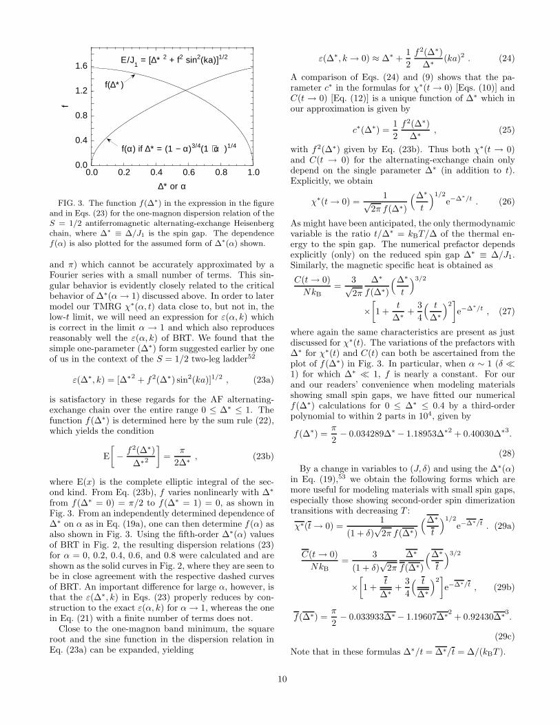
FIG. 3. The function f(∆∗) in the expression in the figureand in Eqs. (23) for the one-magnon dispersion relation of theS = 1/2 antiferromagnetic alternating-exchange Heisenbergchain, where ∆∗ ≡ ∆/J1 is the spin gap. The dependencef(α) is also plotted for the assumed form of ∆∗(α) shown.

and π) which cannot be accurately approximated by aFourier series with a small number of terms. This sin-gular behavior is evidently closely related to the criticalbehavior of ∆∗(α → 1) discussed above. In order to latermodel our TMRG χ∗(α, t) data close to, but not in, thelow-t limit, we will need an expression for ε(α, k) whichis correct in the limit α → 1 and which also reproducesreasonably well the ε(α, k) of BRT. We found that thesimple one-parameter (∆∗) form suggested earlier by oneof us in the context of the S = 1/2 two-leg ladder52

ε(∆∗, k) = [∆∗2 + f2(∆∗) sin2(ka)]1/2 , (23a)

is satisfactory in these regards for the AF alternating-exchange chain over the entire range 0 ≤ ∆∗ ≤ 1. Thefunction f(∆∗) is determined here by the sum rule (22),which yields the condition

E

[

− f2(∆∗)

∆∗2

]

=π

2∆∗, (23b)

where E(x) is the complete elliptic integral of the sec-ond kind. From Eq. (23b), f varies nonlinearly with ∆∗

from f(∆∗ = 0) = π/2 to f(∆∗ = 1) = 0, as shown inFig. 3. From an independently determined dependence of∆∗ on α as in Eq. (19a), one can then determine f(α) asalso shown in Fig. 3. Using the fifth-order ∆∗(α) valuesof BRT in Fig. 2, the resulting dispersion relations (23)for α = 0, 0.2, 0.4, 0.6, and 0.8 were calculated and areshown as the solid curves in Fig. 2, where they are seen tobe in close agreement with the respective dashed curvesof BRT. An important difference for large α, however, isthat the ε(∆∗, k) in Eqs. (23) properly reduces by con-struction to the exact ε(α, k) for α → 1, whereas the onein Eq. (21) with a finite number of terms does not.

Close to the one-magnon band minimum, the squareroot and the sine function in the dispersion relation inEq. (23a) can be expanded, yielding

ε(∆∗, k → 0) ≈ ∆∗ +1

2

f2(∆∗)

∆∗(ka)2 . (24)

A comparison of Eqs. (24) and (9) shows that the pa-rameter c∗ in the formulas for χ∗(t → 0) [Eqs. (10)] andC(t → 0) [Eq. (12)] is a unique function of ∆∗ which inour approximation is given by

c∗(∆∗) =1

2

f2(∆∗)

∆∗, (25)

with f2(∆∗) given by Eq. (23b). Thus both χ∗(t → 0)and C(t → 0) for the alternating-exchange chain onlydepend on the single parameter ∆∗ (in addition to t).Explicitly, we obtain

χ∗(t → 0) =1√

2π f(∆∗)

(∆∗

t

)1/2

e−∆∗/t . (26)

As might have been anticipated, the only thermodynamicvariable is the ratio t/∆∗ = kBT/∆ of the thermal en-ergy to the spin gap. The numerical prefactor dependsexplicitly (only) on the reduced spin gap ∆∗ ≡ ∆/J1.Similarly, the magnetic specific heat is obtained as

C(t → 0)

NkB=

3√2π

∆∗

f(∆∗)

(∆∗

t

)3/2

×[

1 +t

∆∗+

3

4

( t

∆∗

)2]

e−∆∗/t , (27)

where again the same characteristics are present as justdiscussed for χ∗(t). The variations of the prefactors with∆∗ for χ∗(t) and C(t) can both be ascertained from theplot of f(∆∗) in Fig. 3. In particular, when α ∼ 1 (δ ≪1) for which ∆∗ ≪ 1, f is nearly a constant. For ourand our readers’ convenience when modeling materialsshowing small spin gaps, we have fitted our numericalf(∆∗) calculations for 0 ≤ ∆∗ ≤ 0.4 by a third-orderpolynomial to within 2 parts in 104, given by

f(∆∗) =π

2− 0.034289∆∗ − 1.18953∆∗2 + 0.40030∆∗3.

(28)

By a change in variables to (J, δ) and using the ∆∗(α)in Eq. (19),53 we obtain the following forms which aremore useful for modeling materials with small spin gaps,especially those showing second-order spin dimerizationtransitions with decreasing T :

χ∗(t → 0) =1

(1 + δ)√

2π f(∆∗)

(∆∗

t

)1/2

e−∆∗/t . (29a)

C(t → 0)

NkB=

3

(1 + δ)√

2π

∆∗

f(∆∗)

(∆∗

t

)3/2

×[

1 +t

∆∗+

3

4

( t

∆∗

)2]

e−∆∗/t , (29b)

f(∆∗) =π

2− 0.033933∆∗ − 1.19607∆∗

2+ 0.92430∆∗

3.

(29c)

Note that in these formulas ∆∗/t = ∆∗/t = ∆/(kBT ).

10

III. THEORY: S = 1/2 UNIFORM HEISENBERGCHAIN

A. Magnetic spin susceptibility

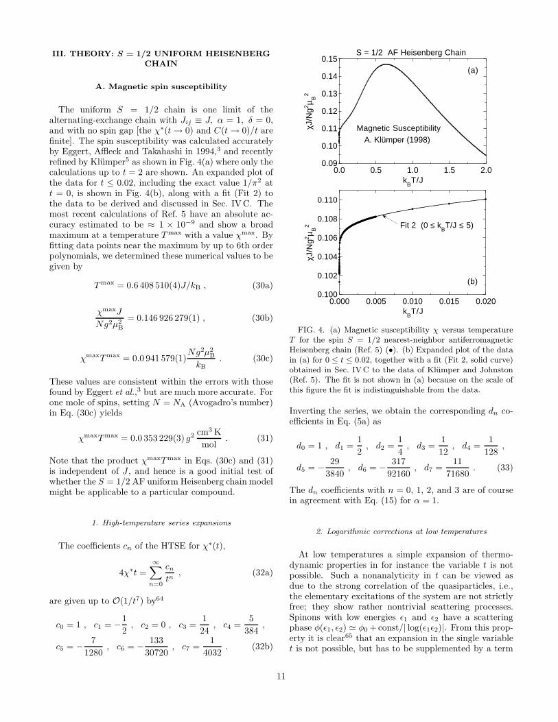
The uniform S = 1/2 chain is one limit of thealternating-exchange chain with Jij ≡ J, α = 1, δ = 0,and with no spin gap [the χ∗(t → 0) and C(t → 0)/t arefinite]. The spin susceptibility was calculated accuratelyby Eggert, Affleck and Takahashi in 1994,3 and recentlyrefined by Klumper5 as shown in Fig. 4(a) where only thecalculations up to t = 2 are shown. An expanded plot ofthe data for t ≤ 0.02, including the exact value 1/π2 att = 0, is shown in Fig. 4(b), along with a fit (Fit 2) tothe data to be derived and discussed in Sec. IVC. Themost recent calculations of Ref. 5 have an absolute ac-curacy estimated to be ≈ 1 × 10−9 and show a broadmaximum at a temperature T max with a value χmax. Byfitting data points near the maximum by up to 6th orderpolynomials, we determined these numerical values to begiven by

T max = 0.6 408 510(4)J/kB , (30a)

χmaxJ

Ng2µ2B

= 0.146 926 279(1) , (30b)

χmaxT max = 0.0 941 579(1)Ng2µ2

B

kB. (30c)

These values are consistent within the errors with thosefound by Eggert et al.,3 but are much more accurate. Forone mole of spins, setting N = NA (Avogadro’s number)in Eq. (30c) yields

χmaxT max = 0.0 353 229(3) g2 cm3 K

mol. (31)

Note that the product χmaxT max in Eqs. (30c) and (31)is independent of J , and hence is a good initial test ofwhether the S = 1/2 AF uniform Heisenberg chain modelmight be applicable to a particular compound.


The coefficients cn of the HTSE for χ∗(t),

4χ∗t =

∞∑

n=0

cn

tn, (32a)

are given up to O(1/t7) by64

c0 = 1 , c1 = −1

2, c2 = 0 , c3 =

1

24, c4 =

5

384,

c5 = − 7

1280, c6 = − 133

30720, c7 =

1

4032. (32b)

0.09

0.10

0.11

0.12

0.13

0.14

0.15

0.0 0.5 1.0 1.5 2.0

χJ/N

g2µ B

2

kBT/J

(a)

S = 1/2 AF Heisenberg Chain

A. Klümper (1998)Magnetic Susceptibility

0.100

0.102

0.104

0.106

0.108

0.110

0.000 0.005 0.010 0.015 0.020χJ

/Ng2

µ B2

kBT/J

(b)

Fit 2 (0 ≤ kBT/J ≤ 5)

FIG. 4. (a) Magnetic susceptibility χ versus temperatureT for the spin S = 1/2 nearest-neighbor antiferromagneticHeisenberg chain (Ref. 5) (•). (b) Expanded plot of the datain (a) for 0 ≤ t ≤ 0.02, together with a fit (Fit 2, solid curve)obtained in Sec. IVC to the data of Klumper and Johnston(Ref. 5). The fit is not shown in (a) because on the scale ofthis figure the fit is indistinguishable from the data.

Inverting the series, we obtain the corresponding dn co-efficients in Eq. (5a) as

d0 = 1 , d1 =1

2, d2 =

1

4, d3 =

1

12, d4 =

1

128,

d5 = − 29

3840, d6 = − 317

92160, d7 =

11

71680. (33)

The dn coefficients with n = 0, 1, 2, and 3 are of coursein agreement with Eq. (15) for α = 1.

2. Logarithmic corrections at low temperatures

At low temperatures a simple expansion of thermo-dynamic properties in for instance the variable t is notpossible. Such a nonanalyticity in t can be viewed asdue to the strong correlation of the quasiparticles, i.e.,the elementary excitations of the system are not strictlyfree; they show rather nontrivial scattering processes.Spinons with low energies ǫ1 and ǫ2 have a scatteringphase φ(ǫ1, ǫ2) ≃ φ0 +const/| log(ǫ1ǫ2)|. From this prop-erty it is clear65 that an expansion in the single variablet is not possible, but has to be supplemented by a term

11

1/ log(t). Although being very intuitive, this physicalpicture on the basis of scattering processes of spinonshas not played any important role in the investigation oflogarithmic corrections until recently.5

Logarithmic dependencies of physical quantities havebeen known for the spin-1/2 Heisenberg chain for a ratherlong time. Usually, a quantum chain with critical cou-plings leads to critical correlations only in the thermo-dynamic limit 1/L = 0 and at T = 0, where L is thelength of the chain. If one of these conditions is not metthe physical properties receive nonanalytic contributionsin terms of 1/L or T . From the renormalization grouppoint of view the existence of logarithmic corrections isreflected by the perturbation of the (critical) fixed pointHamiltonian by some marginal operator. Such operatorsusually exist only for isotropic systems.

The investigation of the size dependence of energy lev-els of critical quantum chains was started more thana decade ago. For the isotropic spin-1/2 Heisenbergchain, expansions in 1/L and additional logarithmic cor-rections (1/L logL etc.) were found in lattice approaches(Bethe ansatz66–68) as well as in field theory [RG studyof the Wess-Zumino-Witten (WZW) model with topolog-ical term k = 1 (Refs. 61,69,70)].

Many of these earlier results are still relevant for theissues discussed in this section due to an equivalence ofmany-particle systems at T = 0, 1/L > 0 (groundstateproperties of finite chains) and those at T > 0, 1/L = 0(thermodynamics of the bulk). This leads to asymp-totic series where T and 1/L play very similar roles. Toour knowledge the first explicit report on log(T ) correc-tions in the magnetic susceptibility resulting in an infiniteslope at T = 0 was given in Ref. 3. Including higher orderterms, the asymptotic expansion χ∗

lt(t) for χ∗(t) is3,5,65,71

χ∗

lt(t) =1

π2

[

1 +1

2L − ln(

L + 12

)

(2L)2+ · · ·

]

, (34a)

=1

π2

[

1 +1

2L − lnL(2L)2

− 1

(2L)3+ · · ·

]

, (34b)

L ≡ ln(t0/t) , (34c)

where t0 is a nonuniversal (undetermined) parameter. InRef. 3 the field theoretical prediction on the basis of theWZW model was compared with the results of thermody-namic Bethe ansatz calculations and showed convincingagreement in an intermediate temperature regime. Usingup to the first logarithmic correction term in Eq. (34a),Eggert, Affleck, and Takahashi estimated t0 ≈ 7.7,3 so atlow temperatures t <∼ 0.01 the parameter L ≫ 1.

A general feature of field theoretical and lattice ap-proaches is their restriction to “low” and “high” temper-atures, respectively. Field theoretical studies suffer athigh temperatures from the neglect of (infinitely many)irrelevant operators. Lattice studies show convergence

problems at low temperatures as increasingly larger sys-tems have to be studied in order to avoid finite-size ef-fects. In addition, the comparison of field theory andlattice results can only verify or falsify the universal as-pects of an asymptotic expansion. Non-universal quanti-ties like t0 which derive from some coupling constant ofa marginal or irrelevant operator (undetermined withinthe field theory) can at best be fitted as done in Ref. 3.

The latter problem of determining the couplingconstants in an effective field theory was solved byLukyanov6 who used a bosonic representation of theHeisenberg chain. The coupling constants were fixed bya comparison of the susceptibility data χ(T = 0, h) ob-tained by him with Bethe ansatz calculations for mag-netic field h at T = 0. Eventually, the χ(T > 0, h = 0)data could be calculated without any need of a fit pa-rameter.

Lukyanov6 obtained the following analytical low-temperature expansion of χ∗(t),

χ∗

lt,g(t) =1

π2

{

1 +g

2+

3g3

32+ O(g4)

+

√3

πt2[1 + O(g)]

}

, (35a)

where g obeys the transcendental equation

1

2lng +

1

g= L (35b)

or equivalently

√g e1/g =

t0t

, (35c)

with a unique value of t0 given by

t0 =

√

π

2eγ+(1/4) ≈ 2.866 257 058 , (35d)

where γ ≈ 0.577 215 665 is Euler’s constant. Lukyanovshowed that his χ∗

lt,g(t) is in agreement with the numer-

ical data of Eggert, Affleck and Takahashi3 at low tem-peratures t ≥ 0.003.

In the following, we will compare high-accuracy nu-merical Bethe ansatz calculations carried out to muchlower temperatures by Klumper and Johnston5 with thistheory6 in some detail because this theory is exact atlow temperatures with no adjustable parameters. Thecalculations of Ref. 5 are based on lattice studies, how-ever without suffering from the usual shortcomings. Bymeans of a lattice path integral representation of the fi-nite temperature Heisenberg chain and the formulationof a suitable quantum transfer matrix (both quite analo-gous to the numerical TMRG calculations presented laterin this paper) a set of numerically well-posed expressionsfor the free energy was derived. In more physical termsthe method can be understood as an application of the

12

familiar though often rather vague concept of quasipar-ticles to a quantitative description of the many particlesystem valid for all temperatures T and magnetic fieldvalues h.5 The work can be understood as an evaluationof the full scattering theory of spinons and antispinons.5

Our iterative solution of Eq. (35b) yields the expansion

g =1

L

{

1 − lnL2L +

(lnL)2 − lnL(2L)2

+ O[

1

(2L)3

]}

. (36)

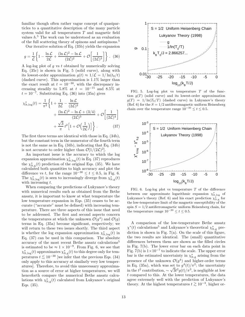
A log-log plot of g vs t obtained by numerically solvingEq. (35c) is shown in Fig. 5 (solid curve), along withits lowest-order approximation g(t) ≈ 1/L = 1/ ln(t0/t)(dashed curve). This approximation is 1.1% larger thanthe exact result at t = 10−30, with the discrepancy in-creasing steadily to 5.8% at t = 10−15 and 8.5% att = 10−7. Substituting Eq. (36) into (35a) gives

χ∗

lt,log(t) =1

π2

{

1 +1

2L − lnL(2L)2

+(lnL)2 − lnL + (3/4)

(2L)3+ O

[

1

(2L)4

]

+

√3

πt2

[

1 + O( 1

2L)]

}

. (37)

The first three terms are identical with those in Eq. (34b),but the constant term in the numerator of the fourth termis not the same as in Eq. (34b), indicating that Eq. (34b)is not accurate to order higher than O[1/(2L)2].

An important issue is the accuracy to which the logexpansion approximation χ∗

lt,log(t) in Eq. (37) reproduces

the χ∗

lt,g(t) prediction of the original Eqs. (35). We havecalculated both quantities to high accuracy and plot thedifference vs t, for the range 10−30 ≤ t ≤ 0.5, in Fig. 6.The χ∗

lt,log(t) is seen to increasingly diverge from χ∗

lt,g(t)with increasing t.

When comparing the predictions of Lukyanov’s theorywith numerical results such as obtained from the Betheansatz, it is important to know at what temperature thelow temperature expansion in Eqs. (35) ceases to be ac-curate (“accurate” must be defined) with increasing tem-perature. There are three aspects of this issue that needto be addressed. The first and second aspects concernthe temperatures at which the unknown O(g4) and O(g)terms in Eq. (35a) become significant, respectively; wewill return to these two issues shortly. The third aspectis whether the log expansion approximation χ∗

lt,log(t) in

Eq. (37) can be used in this comparison. The absoluteaccuracy of the most recent Bethe ansatz calculations5

is estimated to be ≈ 1 × 10−9. From Fig. 6, we see thatχ∗

lt,log(t) approximates χ∗

lt,g(t) to this degree only for tem-

peratures t <∼ 10−30 [we infer that the previous Eqs. (34)only apply to this accuracy at similarly very low temper-atures]. Therefore, to avoid this unnecessary approxima-tion as a source of error at higher temperatures, we willhenceforth compare the numerical Bethe ansatz calcu-lations with χ∗

lt,g(t) calculated from Lukyanov’s original

Eqs. (35).

0.01

0.1

1

-30 -25 -20 -15 -10 -5 0

g1/ln(T

0/T)g

log10

(kBT/J)

Lukyanov Theory (1998)

S = 1/2 Uniform Heisenberg Chain

kBT

0/J = 2.866257...

FIG. 5. Log-log plot vs temperature T of the func-tion g(T ) (solid curve) and its lowest-order approximationg(T ) = 1/ ln(T0/T ) (dashed curve) in Lukyanov’s theory(Ref. 6) for the S = 1/2 antiferromagnetic uniform Heisenbergchain over the temperature range 10−30 ≤ t ≤ 0.5.

10-8

10-7

10-6

10-5

10-4

10-3

-30 -25 -20 -15 -10 -5 0

χ*lt,

log −

χ* lt,

g

log10

(kBT/J)



FIG. 6. Log-log plot vs temperature T of the differencebetween our approximate logarithmic expansion χ∗

lt,log ofLukyanov’s theory (Ref. 6) and his exact prediction χ∗

lt,g forthe low-temperature limit of the magnetic susceptibility of thespin S = 1/2 antiferromagnetic uniform Heisenberg chain, forthe temperature range 10−30 ≤ t ≤ 0.5.

A comparison of the low-temperature Bethe ansatzχ∗(t) calculations5 and Lukyanov’s theoretical χ∗

lt,g pre-

diction is shown in Fig. 7(a). On the scale of this figure,the two results are identical. The (small) quantitativedifferences between them are shown as the filled circlesin Fig. 7(b). The lower error bar on each data point inFig. 7(b) is 1×10−7 to indicate the scale. The upper errorbar is the estimated uncertainty in χ∗

lt,g arising from the

presence of the unknown O(g4) and higher-order termsin Eq. (35a), which was set to g4(t)/π2; the uncertainty

in the t2 contribution, ∼√

3t2g(t)/π3, is negligible at lowt compared to this. At the lower temperatures, the dataagree extremely well with the prediction of Lukyanov’stheory. At the highest temperatures t >∼ 10−3, higher or-

13

0.102

0.104

0.106

0.108

0.110

0.112

-25 -20 -15 -10 -5 0

χ *

log10

(kBT/J)

Lukyanov χ*lt,g

Theory (1998)


Klümper χ* Data (1998)

(a)

-25

-20

-15

-10

-5

0

5

10

-25 -20 -15 -10 -5 0

(χ*−

χ* lt,

g) (1

0−7)

log10

(kBT/J)

(b)

FIG. 7. Semilog plots vs temperature T at low T of (a)numerical Bethe ansatz magnetic susceptibility (χ∗) data forthe S = 1/2 uniform Heisenberg chain (Ref. 5) (•) and theprediction χ∗

lt,g (solid curve) of Lukyanov’s theory (Ref. 6),and (b) the difference between these two results (•). In (b),the upper error bar is the estimated uncertainty in χ∗

lt,g (seetext).

der tn terms also become important, as inferred from ourempirical fits (Fits 1 and 2) below to the numerical data.

Irrespective of the uncertainties in the theoretical pre-diction at high temperatures just discussed, we can safelyconclude directly from Fig. 7(b) that the Bethe ansatzχ∗(t) data5 are in agreement with the exact theory ofLukyanov6 to within an absolute accuracy of 1 × 10−6

(relative accuracy ≈ 10 ppm) over a temperature rangespanning 18 orders of magnitude from t = 5 × 10−25 tot = 5× 10−7. The agreement is much better than this atthe lower temperatures.

B. Magnetic specific heat

The magnetic specific heat C of the S = 1/2 AF uni-form Heisenberg chain was recently calculated to high ac-curacy by Klumper and Johnston over the temperaturerange 5 × 10−25 ≤ kBT/J ≤ 5.5 The accuracy is esti-mated to be 3 × 10−10C(t). The results for T ≤ 2J/kB

are shown in Fig. 8(a). The initial T dependence is ap-proximately (see below) linear, and is given exactly in

0.0

0.1

0.2

0.3

0.0 0.5 1.0 1.5 2.0

C/N

k B

kBT/J

A. Klümper (1998)

S = 1/2 AF Uniform Heisenberg Chain

Specific Heat

(a)

0.0

0.2

0.4

0.6

0.8

1.0

0.0 0.5 1.0 1.5 2.0C

J/N

k B2 T

kBT/J

(b)

FIG. 8. (a) Specific heat C vs temperature T (•) for theS = 1/2 antiferromagnetic uniform Heisenberg chain (Ref. 5).(b) Specific heat coefficient C/T vs T from the data in (a).The area under the curve in (b) from T = 0 to T = 5J/kB is99.4% of ln 2.

the t = 0 limit by

C(t → 0)

NkB=

2

3t . (38)

The data show a maximum with a value Cmax at a tem-perature T max

C . By fitting 3–7 data points in the vicinityof the maximum by up to 6th order polynomials, thesevalues were found to be

kBT maxC

J= 0.48 028 487(1) ,

(39)

Cmax

NkB= 0.3 497 121 235(2) .

The electronic specific heat coefficient C(T )/T is plot-ted vs temperature in Fig. 8(b). As expected fromEq. (38), the data approach the value (2/3)Nk2

B/J fort → 0. The initial deviation from this constant valueis positive and approximately (see below) quadratic int. The data exhibit a smooth maximum with a value(C/T )max at a temperature T max

C/T , values which we deter-

mined by fitting polynomials to the data in the vicinityof the peak to be

14

0.0

0.2

0.4

0.6

0.8

1.0

0.0 0.5 1.0 1.5 2.0

S/(

Nk B

ln2)

kBT/J

A. Klümper (1998)


Entropy

FIG. 9. Entropy S vs temperature T for the S = 1/2antiferromagnetic uniform Heisenberg chain, obtained fromthe data in Fig. 8(b). The entropy is normalized byS(T = ∞) = NkB ln 2.

kBT maxC/T

J= 0.30 716 996(2) ,

(40)

(C/T )maxJ

Nk2B

= 0.8 973 651 576(5) .

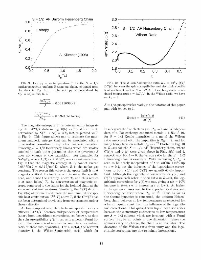
The magnetic entropy S(T ) is determined by integrat-ing the C(T )/T data in Fig. 8(b) vs T and the result,normalized by S(T → ∞) = NkB ln 2, is plotted vs Tin Fig. 9. This figure allows one to estimate the max-imum magnetic entropy that can be associated with adimerization transition or any other magnetic transitioninvolving S = 1/2 Heisenberg chains which are weaklycoupled to each other [assuming that the (average) Jdoes not change at the transition]. For example, forNaV2O5 where kBTc/J ≈ 0.057, one can estimate fromFig. 9 that the magnetic entropy at Tc cannot exceed0.056R ln 2 = 0.32J/molK, where R is the molar gasconstant. The reason this value is the upper limit is thatmagnetic critical fluctuations will increase the specificheat, and hence the entropy, above Tc and thus reduceit at (and below) Tc, by conservation of magnetic en-tropy, compared to the values for the isolated chain at thesame reduced temperatures. Similarly, the C(T ) data inFig. 8(a) allow one to estimate the minimum lattice spe-cific heat contribution C lat(T ) above Tc if the C lat(T ) hasnot been determined previously from experiments and/ortheory directly.

At low temperatures, the electronic specific heat co-efficient C(T )/T becomes independent of temperature(apart from logarithmic corrections, see below), as doesthe spin susceptibility χ∗(t), just as in a metal (Fermi liq-uid). Therefore it is of interest to compute a normalizedratio of these two quantities. For a metal, the relevantquantity is the Wilson-Sommerfeld ratio, which for

1.8

2.0

2.2

2.4

2.6

2.8

3.0

0.0 0.1 0.2 0.3 0.4 0.5

4π2 χ *

(t)t

/[3

C(t

)]

t

Wilson Ratio


FIG. 10. The Wilson-Sommerfeld ratio RW = 4π2χ∗(t)t/[3C(t)] between the spin susceptibility and electronic specificheat coefficient for the S = 1/2 AF Heisenberg chain vs re-duced temperature t = kBT/J . In the Wilson ratio, we haveset kB = 1.

S = 1/2 quasiparticles reads, in the notation of this paperand with kB set to 1,

RW(t) =4π2χ∗(t)t

3C(t). (41)

In a degenerate free electron gas, RW = 1 and is indepen-dent of t. For exchange-enhanced metals 1 < RW

<∼ 10,for S = 1/2 Kondo impurities in a metal the Wilsonratio associated with the impurities is RW = 2, and formany heavy fermion metals RW ∼ 2.72 Plotted in Fig. 10is RW(t) for the S = 1/2 AF Heisenberg chain, whereC(t)/t and χ∗(t) were given above in Figs. 8(b) and 4,respectively. For t → 0, the Wilson ratio for the S = 1/2Heisenberg chain is exactly 2. With increasing t, RW isseen to be nearly independent of t to within ±10% upto t ≈ 0.4, but the influence of the logarithmic correc-tions to both χ(T ) and C(T ) are quantitatively impor-tant. Although the logarithmic corrections for χ(T ) andC(T ) oppose each other in their ratio in RW(t), the log-arithmic corrections for χ(t) win out, giving a net ∼ 10%increase in RW(t) with increasing t at low t. At highert, the system crosses over to the expected local momentHeisenberg behavior where RW ∝ t2. Thus as far asthe thermodynamics is concerned, the uniform Heisen-berg chain behaves at low temperatures as expected fora Fermi liquid, apart from the influence of the logarith-mic corrections. This quasi-Fermi liquid behavior arisesbecause the elementary excitations at low temperaturesare S = 1/2 spinons which are fermions with a Fermisurface (i.e., Fermi points in one dimension). Since thespinons carry no charge, the chain is an insulator. Thedeviation of the Wilson ratio from unity and the loga-rithmic corrections are due to spinon interactions.

15


The HTSE for the specific heat of a spin S AF uniformHeisenberg chain is49

C(T )

NkB=

x2

3t2

[

1 +∞∑

n=1

cn(x)

tn

]

, (42a)

x = S(S + 1) , t =kBT

J, (42b)

c1 =1

2, c2 =

1

15(3 − 8x − 3x2) ,

c3 =1

36(3 − 16x − 4x2) ,

c4 =1

5040(192 − 1432x + 1123x2 + 800x3 + 160x4) ,

c5 =1

21600(414 − 3768x + 6635x2 + 2624x3 + 480x4) .

(42c)

Specializing Eqs. (42) to S = 1/2 (x = 3/4) then gives

C(T )

NkB=

3

16t2

[

1 +∞∑

n=1

cn

tn

]

, (43a)

c1 =1

2, c2 = c3 = − 5

16, c4 =

7

256, c5 =

917

7680.

(43b)

The two C(T ) HTSE terms of order 1/t2 and 1/t3 inEqs. (43) are in agreement with the general expressionfor the two lowest-order HTSE expansion terms for C(T )of the S = 1/2 alternating-exchange Heisenberg chain inEq. (18) with alternation parameter α = 1.

In a later section, the Bethe ansatz C(T ) data5 willbe fitted to obtain a function accurately representing theC(T ) of the S = 1/2 AF uniform Heisenberg chain. Inorder that we are not required to change our fitting equa-tions from those we use for fitting magnetic susceptibilitydata, the coefficients for the series inverted from that inEq. (43a) are required. We obtain

C(T )

NkB=

3

16t2

[

1 +∞∑

n=1

dn

tn

]

−1

, (44a)

d1 = −1

2, d2 =

9

16, d3 = −1

8, d4 =

7

128, d5 =

7

1920.

(44b)

0.00

0.01

0.02

0.03

0.04

0.00 0.02 0.04 0.06 0.08 0.10

(C/t)-2/3(C/t)-(2/3)[1+(3/8)g3](C/t)-(2/3)[1+(3/8)g3+a

4g4]

(C/t)-(2/3)[1+(3/8)g3+a4g4+a

5g5]

∆C/t

t

Logarithmic Specific Heat Corrections

(a)

a4 = 1.5374(3)

a5 = 3.125(11)

0.0000

0.0002

0.0004

0.0006

0.0008

0.0010

0.0012

0.000 0.001 0.002 0.003 0.004 0.005

∆C/t

t

(b)

FIG. 11. (a) Difference ∆C/t between the electronic spe-cific heat coefficient from the Bethe ansatz data (Ref. 5) andthe nominal coefficient of 2/3 (top data set), plotted vs re-duced temperature t. Moving down the figure, successive datasets show the influence of correcting for cumulative logarith-mic correction terms. (b) Expanded plots at low tempera-tures. The reduced temperature is t = kBT/J and we haveset N = kB = 1. In both (a) and (b), the lines connecting thedata points are guides to the eye.

2. Low-temperature logarithmic corrections

At first sight, from Fig. 8 there appear to be no singu-larities in the temperature dependence of the specific heatfor the S = 1/2 AF uniform Heisenberg chain. However,if the electronic specific heat coefficient C(T )/T is exam-ined in detail, one sees anomalous behavior at low tem-peratures. Shown as the top curve in Fig. 11(a) is a plotof the difference between the electronic specific heat co-efficient and its zero-temperature value, ∆C(t)/NkBt ≡[C(t) − (2/3)t]/(NkBt) for 0 ≤ t ≤ 0.1 [compare withFig. 8(b)]. From this figure, there is still nothing par-ticularly strange about the data. However, upon furtherexpanding the plot to study the range 0 ≤ t ≤ 0.005 asshown in Fig. 11(b), we see that ∆C/NkBt is developingan infinite slope as t → 0. This is the signature of theexistence of logarithmic corrections to the specific heatat temperatures t ≪ 1, just as it was for the magneticsusceptibility.

16

-40

-30

-20

-10

0

-30 -25 -20 -15 -10 -5 0

log 1

0[(C

lt,lo

g − C

lt,g)/

(Nk B

)]

log10

(kBT/J)



FIG. 12. Log-log plot vs temperature T of the dif-ference between our approximate logarithmic expansionClt,log/(NkB) of Lukyanov’s theory (Ref. 6) and his exactprediction Clt,g/(NkB) for the low-temperature limit of themagnetic specific heat of the spin S = 1/2 antiferromag-netic uniform Heisenberg chain, for the temperature range10−30 ≤ t ≤ 0.5.

Klumper,5 Lukyanov,6 and others have found a log-arithmic correction to the low-t limit in Eq. (38).Lukyanov’s exact asymptotic expansion for the free en-ergy per spin in zero magnetic field is

f = −J ln 2 − (kBT )2

3J

[

1 +3

8g3 + O(g4)

]

− 33/2(kBT )4

10πJ3[1 + O(g)] , (45)

where g(t/t0) and t0 are the same as given in Eqs. (35b)and (35d), respectively, and where g(t) was plotted inFig. 5. The specific heat at constant volume is calculatedusing C = −T∂2f/∂T 2, yielding

Clt,g(T )

NkB=

2kBT

3J

[

1 +3

8g3 + O(g4)

]

+2(35/2)

5π

(kBT

J

)3

[1 + O(g)] . (46)

This formula shows that the electronic specific heat co-efficient C(T )/T increases quadradically with T at lowT (after subtracting the logarithmic corrections). Thenumerical prefactor of the t3 term is 1.98478 · · ·. If theapproximate expansion for g(L) in Eq. (36) is substitutedinto Eq. (46), one obtains

Clt,log(T )

NkB=

2kBT

3J

{

1 +3

(2L)3+ O

[ 1

(2L)4

]

}

+2(35/2)

5π

(kBT

J

)3[

1 + O( 1

2L)]

, (47)

where the prefactor 3/8 in the logarithmic correctionterm was found independently by Klumper,5 confirming

0

5

10

15

20

25

0.0001 0.001 0.01

∆C/N

k B (

10−7

)

kBT/J


Specific Heat

∆C = C − (2/3)NkB

2T/J

∆C = C − Clt,g

FIG. 13. Semilog plot vs temperature T of the difference∆C = C −Clt,g (•) between the Bethe ansatz numerical spe-cific heat C(T ) data (Ref. 5) and Lukyanov’s theory (Ref. 6)[Clt,g(T )] for the spin S = 1/2 antiferromagnetic uniformHeisenberg chain at low temperatures. The error bar on eachdata point is an estimated uncertainty in the theory due tohigher order correction terms that were not calculated. Alsoshown is the deviation ∆C = C − (2/3)Nk2

BT/J (◦) of thenumerical data from the T → 0 limit of C(T ).

Refs. 61 and 68. The difference between Clt,log(T ) andClt,g(T ) is plotted vs temperature in Fig. 12, where thedifference becomes > 10−10 only for t >∼ 10−5.

Shown in Fig. 13 is the deviation ∆C/NkB (•) of theBethe ansatz data5 from Lukyanov’s theoretical predic-tion in Eq. (46). For temperatures t <∼ 10−4, the agree-ment is better than 10−8. At higher temperatures, theuncertainty in the theoretical prediction due to the un-known O(g4) and higher order correction terms becomesan important factor in the comparison. The length ofthe error bar on each data point in Fig. 13 has arbitrar-ily been set to (4/3)tg4(t) [cf. Eq. (46)]; the O(g) uncer-tainty in the T 3 term is negligible compared to this. Alsoplotted in Fig. 13 is the deviation of the numerical datafrom the extrapolated linear low-T behavior (◦). A com-parison of the two data sets indicates that the O(g3) log-arithmic correction term is responsible for at least mostof this latter difference for temperatures t <∼ 0.001.

A more rigorous evaluation of the influence of theabove logarithmic correction term is obtained by correct-ing for it in the plot of ∆C/t vs t, as shown by the sec-ond curve from the top in each of Figs. 11(a) and 11(b).From the latter figure, we infer that although subtractingthis correction term from the data helps to remove thezero-temperature singularity, a singularity is still presentbut with reduced amplitude. This means that additionallogarithmic correction terms are important, within theaccuracy and precision of the data. Another indicationof this is shown in Fig. 14, where we have plotted ∆C/t3

vs t. According to Eq. (46), after accounting for thelogarithmic correction term(s), the result should be in-dependent of t at low t. Instead, both before and afteraccounting for the log correction term, there is a strong

17

0

2

4

6

8

10

0.00 0.05 0.10 0.15 0.20 0.25 0.30

{C-(2t/3)}/t3

{C-(2t/3)[1+(3/8)g3]}/t3

{C-(2t/3)[1+(3/8)g3+a4g4]}/t3

{C-(2t/3)[1+(3/8)g3+a4g4+a

5g5]}/t3

∆ C/t3

t


a4 = 1.5374(3), a

5 = 3.125(11)

FIG. 14. Coefficient ∆C/t3 of the expected t2 dependenceof the electronic specific heat coefficient at low temperatures(top data set). Moving down the figure, successive data setsshow the influence of correcting for cumulative logarithmiccorrection terms. If all logarithmic corrections were accountedfor, the data would become independent of t for t → 0.Here, the reduced temperature is t = kBT/J and we haveset N = kB = 1. The lines connecting the data points areguides to the eye.

upturn at low temperatures although the strength of theupturn is smaller after subtracting the influence of thelog correction term.

The numerical Bethe ansatz specific heat data5 aresufficiently accurate and precise that we can estimatethe coefficients of the next two logarithmic correction(g4, g5) terms in Eq. (46) from these data as fol-lows. From Eq. (46), if we plot the numerical data as[C(t)/(NkBt) − (2/3)(1 + 3g3/8)]/g4 vs g at low tem-peratures, where the t3 term can be neglected, and fitthe lowest t data by a straight line, the y intercept forg → 0 gives the coefficient of the g4 term and the slopegives the coefficient of the g5 term. This plot is givenin Fig. 15. This type of plot places extreme demands onthe accuracy of the data. Even so, we see that the datafollow the required linear behavior even at the lowesttemperatures. We fitted a straight line to the data fromt = 5 × 10−25 up to a maximum temperature tmax. Thefit parameters and rms deviation held nearly constant fortmax = 5× 10−15 (11 data points) up to tmax = 5× 10−8

(18 data points), but both quantities changed rapidlyupon further increasing tmax. The fit for tmax = 5×10−8

is shown as the straight line in Fig. 15, along with thefit parameters. From the parameters of the fit [after ac-counting for the prefactor of 2/3 in Eq. (46)], we includeour estimated coefficients in Eq. (46) explicitly as

Clt,g(T )

NkB=

2kBT

3J

[

1 +3

8g3 + a4g

4 + a5g5 + O(g6)

]

+2(35/2)

5π

(kBT

J

)3

[1 + O(g)] , (48a)

0.9

1.0

1.1

1.2

1.3

1.4

1.5

1.6

0.00 0.02 0.04 0.06 0.08 0.10 0.12 0.14

{(C/t)-(2/3)[1+(3/8)g3]}/g4

Fit

(∆C

/t)/

g4

g


Fit: 1.0249(2) + 2.083(7) g

Fit range: 0.017 ≤ g ≤ 0.052

(5 x 10−25 ≤ t ≤ 5 x 10−8)

FIG. 15. Plot showing the estimation of the coefficients ofthe O(g4) and O(g5) logarithmic correction terms in Eq. (46)for the magnetic specific heat of the S = 1/2 AF uniformHeisenberg chain. The reduced temperature is t = kBT/Jand we have set N = kB = 1.

a4 = 1.5374(3) , a5 = 3.125(11) . (48b)

The influences of these g4 and g5 logarithmic correc-tion terms on the data in Figs. 11 and 14 are shown asthe two additional data sets in each figure, where ac-counting for these two terms is seen to largely removethe remaining singular behavior as t → 0. From Fig. 14,we can now estimate that the coefficient of the t3 termin Eq. (48) is a little larger than 2, contrary to the ex-act value 1.98478· · ·. The magnitude of this difference isabout as expected from the O(g) logarithmic correctionto the t3 term, since g(t ∼ 0.1) ∼ 0.1. The remainingupturn at low temperatures in Fig. 14 is due to residuallogarithmic corrections which are not accounted for.

If the approximate expansion for g(L) in Eq. (36) isinserted into Eq. (48a), one obtains

Clt,g

NkB=

2kBT

3J

{

1 +3

(2L)3− 9 ln(L) − 16a4

(2L)4

+lnL[18 ln(L) − 64a4 − 9] + 32a5

(2L)5+ O

[ 1

(2L)6

]

}

+2(35/2)

5π

(kBT

J

)3[

1 + O( 1

2L)]

. (49)

IV. FITS TO χ∗(t) AND C(t) OF HEISENBERGSPIN LATTICES

A. General χ∗(t) fit considerations

The general expression we use to fit theoretical numer-ical χ∗(t) data for S = 1/2 Heisenberg spin lattices is

χ∗(t) =e−∆∗

fit/t

4tP(q)

(r) (t) , (50a)

18

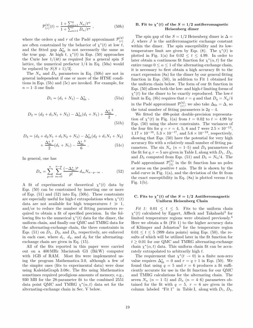
P(q)(r) (t) =

1 +∑q

n=1 Nn/tn

1 +∑r

n=1 Dn/tn, (50b)

where the orders q and r of the Pade approximant P(q)(r)

are often constrained by the behavior of χ∗(t) at low t,and the fitted gap ∆∗

fit is not necessarily the same asthe true gap. At high t, χ∗(t) in Eqs. (50) approachesthe Curie law 1/(4t) as required [for a general spin Slattice, the numerical prefactor 1/4 in Eq. (50a) wouldbe replaced by S(S + 1)/3].

The Nn and Dn parameters in Eq. (50b) are not ingeneral independent if one or more of the HTSE condi-tions in Eqs. (5b) and (5c) are invoked. For example, forn = 1–3 one finds

D1 = (d1 + N1) − ∆∗

fit , (51a)

D2 = (d2 + d1N1 + N2) − ∆∗

fit(d1 + N1) +∆∗

fit2

2,

(51b)

D3 = (d3 + d2N1 + d1N2 + N3) − ∆∗

fit(d2 + d1N1 + N2)

+∆∗

fit2

2(d1 + N1) −

∆∗

fit3

6. (51c)

In general, one has

Dn =

n∑

p=0

n−p∑

m=0

(−∆∗

fit)p

p!dmNn−p−m . (52)

A fit of experimental or theoretical χ∗(t) data byEqs. (50) can be constrained by inserting one or moreof Eqs. (51) and (52) into Eq. (50b). These constraintsare especially useful for high-t extrapolations when χ∗(t)data are not available for high temperatures t ≫ 1,and/or to reduce the number of fitting parameters re-quired to obtain a fit of specified precision. In the fol-lowing fits to the numerical χ∗(t) data for the dimer, theuniform chain, and finally our QMC and TMRG data forthe alternating-exchange chain, the three constraints inEqs. (51) on D1, D2, and D3, respectively, are enforcedin each case, where d1, d2, and d3 for the alternating-exchange chain are given in Eq. (15).

All of the fits reported in this paper were carriedout on a 400MHz Macintosh G3 (B&W) computerwith 1GB of RAM. Most fits were implemented us-ing the program Mathematica 3.0, although a few ofthe simpler ones (fits to experimental data) were doneusing KaleidaGraph 3.08c. The fits using Mathematicasometimes required prodigious amounts of memory, e.g.,930 MB for the 28-parameter fit to the combined 2551data point QMC and TMRG χ∗(α, t) data set for thealternating-exchange chain in Sec. V below.

B. Fit to χ∗(t) of the S = 1/2 antiferromagneticHeisenberg dimer

The spin gap of the S = 1/2 Heisenberg dimer is ∆ =J , where J is the antiferromagnetic exchange constantwithin the dimer. The spin susceptibility and its low-temperature limit are given by Eqs. (8). The χ∗(t) isplotted in Fig. 1(a) for 0.02 ≤ t ≤ 4.99. In order tolater obtain a continuous fit function for χ∗(α, t) for theentire range 0 ≤ α ≤ 1 of the alternating-exchange chain,it is necessary to first obtain a high accuracy fit to theexact expression (8a) for the dimer by our general fittingfunction in Eqs. (50), in addition to Fit 1 obtained forthe uniform chain below. The form of our fit function inEqs. (50) allows both the low- and high-t limiting forms ofχ∗(t) for the dimer to be exactly reproduced. The low-tlimit in Eq. (8b) requires that r = q and that Dq = Nq/4

in the Pade approximant P(q)(r) ; we also take ∆fit = ∆, so

the total number of fitting parameters is 2q − 4.We fitted the 498-point double-precision representa-

tion of χ∗(t) in Fig. 1(a) from t = 0.02 to t = 4.99 byEqs. (50) using the above constraints. The variances ofthe four fits for q = r = 4, 5, 6 and 7 were 2.5 × 10−13,1.17 × 10−16, 5.3 × 10−17, and 5.6 × 10−19, respectively,showing that Eqs. (50) have the potential for very highaccuracy fits with a relatively small number of fitting pa-rameters. The six Nn (n = 1–5) and D4 parameters ofthe fit for q, r = 5 are given in Table I, along with D1, D2,and D3 computed from Eqs. (51) and D5 = N5/4. The

Pade approximant P(5)(5) in the fit function has no poles

or zeros on the positive t axis. The fit is shown by thesolid curve in Fig. 1(a), and the deviation of the fit fromthe exact susceptibility in Eq. (8a) is plotted versus t inFig. 1(b).

C. Fits to χ∗(t) of the S = 1/2 AntiferromagneticUniform Heisenberg Chain

Fit 1: 0.01 ≤ t ≤ 5. Fits to the uniform chainχ∗(t) calculated by Eggert, Affleck and Takahashi3 forlimited temperature regions were obtained previously.4

Here we obtain a fit (Fit 1) to the higher accuracy dataof Klumper and Johnston5 for the temperature region0.01 ≤ t ≤ 5 (999 data points) using Eqs. (50), the re-sults of which will be utilized later in the fit function fort ≥ 0.01 for our QMC and TMRG alternating-exchangechain χ∗(α, t) data. This uniform chain fit can be accu-rately extrapolated to arbitrarily high t.

The requirement that χ∗(t → 0) is a finite non-zerovalue requires ∆∗

fit = 0 and r = q + 1 in Eqs. (50). Wefound that using q = 5 and r = 6 produces a fit suffi-ciently accurate for use in the fit function for our QMCand TMRG calculations for the alternating chain. Theseven Nn (n = 1–5) and Dn (n = 4–6) parameters ob-tained for the fit with q = 5, r = 6 are given in thecolumn labeled “Fit 1” in Table I, along with D1, D2,

19

-15

-10

-5

0

5

10

0.01 0.1 1 10

Fit

1 D

evia

tion

(10−6

)

kBT/J


FIG. 16. Semilog plot vs temperature T of the deviation ofFit 1 from the magnetic susceptibility calculations of Klumperand Johnston (Ref. 5) for the S = 1/2 uniform antiferromag-netic Heisenberg chain.

and D3 computed from Eqs. (51). The Pade approxi-

mant P(5)(6) in the fit function has no poles or zeros on the

positive t axis. The deviation of the fit from the data isplotted in Fig. 16. The variance of the fit is 2.97×10−12,and the relative rms deviation of the fit from the data inthe fitted t region is 14.5 ppm. Extrapolation of the fitto higher temperatures is very accurate.

TABLE I. Fitted parameters for χ∗(t) of the S = 1/2 antiferromagnetically coupled Heisenberg dimer (α = 0) [Eqs. (50)with ∆∗

fit = 1] and χ∗(t) and C(t) [Eqs. (54)] for the uniform chain (α = 1). χ∗(t) Fit 1 for the uniform chain (0.01 ≤ t ≤ 5)[Eqs. (50) with ∆∗

fit = 0] uses powers of 1/t only, whereas χ∗(t) Fit 2 (0 ≤ t ≤ 5) [Eqs. (53)] also incorporates logarithmiccorrection terms.

parameter χ∗(α = 0) χ∗(α = 1) Fit 1 χ∗(α = 1) Fit 2 C(α = 1)

N1 0.6342798982 −0.053837836 −0.240262331211 −0.018890951426N2 0.1877696166 0.097401365 0.451187371598 0.024709724025N3 0.03360361730 0.014467437 0.0125889356883 −0.0037086264240N4 0.003861106893 0.0013925193 0.0357903808997 0.0030159975962N5 0.0002733142974 0.00011393434 0.00801840643283 −0.00037946929995N6 0.00182319434072 0.000042683893992N7 0.0000533189078137N8 0.000184003448334N81 1.423476309767N82 0.341607132329t1 5.696020642244D1 −0.1157201018 0.44616216 0.259737668789 −0.51889095143D2 0.08705969295 0.32048245 0.581056205993 0.59657583453D3 0.005631366688 0.13304199 0.261450372018 −0.15117343936D4 0.001040886574 0.037184126 0.142680453011 0.074445241148D5 0.00006832857434 0.0028136088 0.0572246926066 −0.0024804135233D6 0.00026467628 0.0176410851952 −0.00053631174698D7 0.00390435823809 0.00082005310111D8 0.000119767935536 −0.00010820401214D9 0.000011991365422a1 −0.000015933393a2 0.013021564a3 0.0043275575a4 49.422168a5 0.00040160786a6 325.22706

The quality of Fit 1 does not approach the limitationimposed by the absolute accuracy of the data (1×10−9).For an ideal fit, the variance is expected to be ∼ 10−18

and the relative rms deviation ∼ 0.01 ppm. As can beinferred from Fit 2 in the following section, the reasonthat Fit 1 cannot be optimized to this extent is due tothe t = 0 critical point and associated logarithmic di-vergence in the slope of χ∗(t) as t → 0; this divergencecannot be fitted accurately by a finite polynomial or Padeapproximant. We attempted to improve the accuracy ofthe fit over the same temperature range 0.01 ≤ t ≤ 5 by

replacing the Pade approximant P(5)(6) in the fit function

by P(6)(7) , which incorporates two additional fitting param-

eters. The variance improved somewhat to 2.18 × 10−12

and the relative rms deviation improved slightly to 12.2ppm, but the Pade approximant developed a pole at1/t = 129.23, and hence this fit was discarded. Althoughthe temperature at which this pole occurs is below thefitted temperature range, as a general rule we cannot al-low poles in the fit function at low temperatures becauseof problems that can occur when using the fit functionto model experimental data which include data at tem-peratures lying below the fitted temperature range of thefit function. In fact, we will encounter this situation fre-quently in modeling experimental data later. For exam-

20

ple, for NaV2O5, t = 0.01 corresponds to an absolutetemperature T ≈ 7K, whereas the experimental dataand modeling extend down to ≈ 2K.

Fit 2: 0 ≤ t ≤ 5. We can greatly improve the accu-racy of the fit compared to that of Fit 1, and extend thefit to t = 0, by restricting the high-temperature limit ofthe fit and using in the fit function one or more low-temperature logarithmic correction terms discussed inSec. III A 2. In particular, in this section we obtain avery high precision fit (Fit 2) to the exact t = 0 valueand to the calculations of Klumper and Johnston5 overthe entire temperature range 5×10−25 ≤ t ≤ 5 of the cal-culations. We do not use this fit in our formulation of thefit function for the alternating-exchange chain. However,Fit 2 will be generally useful for evaluating the accuracyof other theoretical calculations of χ∗(t) for the uniformchain, such as our TMRG calculations to be presentedbelow, and for modeling appropriate experimental χ(T )data whose scaled upper temperature limit is below t = 5.

We initially formulated a fit function utilizing a mod-ified Pade approximant in which the last term of thenumerator and/or denominator contained the χ∗

lt,log ex-

pansion in Eq. (37), such that the low-temperature ex-pansion of the fit function yielded χ∗

lt,log to lowest or-

ders in t. The best fit to the data from t = 5 × 10−25

to 2.5 (777 data points) was unsatisfactory, with a vari-ance v = 2.4 × 10−11 and a relative rms deviationσrms = 45ppm. Allowing an arbitrary t2 coefficient inplace of the exact value

√3/π3 yielded an improved fit

with v = 1.1 × 10−12 and σrms = 9.6 ppm. However,this fit was still unsatisfactory, given the high absoluteaccuracy (1 × 10−9) of the data. From these results itbecame clear that a fit function which can fit the datato much higher accuracy over such a large temperaturerange would indeed have to include an expression χ∗

log(t)containing logarithmic correction terms, but where theform and/or coefficient of one or more of these termswould have to be empirically determined by trial anderror. This process yielded the formulation we now de-scribe.

The χ∗

log(t) function is incorporated into our fit func-

tion in Eqs. (50) as follows. As in Fit 1, the finite valueof χ∗(0) requires ∆fit = 0 in Eq. (50a) and r = q + 1

in the Pade approximant P(q)(r) (t) in Eq. (50b). Since the

two terms highest order in 1/t in P(q)(r) (t) (one each in the

numerator and denominator) dominate the fit as t → 0and become small for t >∼ 1, relative to the other termsin the numerator and denominator, respectively, we in-corporate χ∗

log(t) into the last term in the numerator of

a modified P(q)(r) (t). Trial fits showed that to obtain the

optimum accuracy of the fit required q = 8 and r = 9.Our final fit function for Fit 2 is

χ∗(t) =( 1

4t

) 1 +[∑7

n=1 Nn/tn]

+ 4N8χ∗

log(t)/t8

1 +[∑8

n=1 Dn/tn]

+ N8/t9,

(53a)

-10

-5

0

5

10

-25 -20 -15 -10 -5 0

Fit

2 D

evia

tion

(10−8

)

log10

(kBT/J)

(a)


Deviation of Fit 2 fromdata of Klümper (1998)

Magnetic Susceptibility:

σrms

= 9.92 x 10−9

-10

-5

0

5

10

-4 -3 -2 -1 0 1F

it 2

Dev

iatio

n (1

0−8)

log10

(kBT/J)

(b)

FIG. 17. (a) Semilog plot of the absolute deviation of Fit 2(0 ≤ t ≤ 4) from the magnetic susceptibility calculations ofKlumper and Johnston (Ref. 5) versus temperature T . (b)Expanded plot of the data in (a) at the higher temperatures.

χ∗

log(t) =1

π2

[

1 +1

2L − ln(

L + 12

)

− N81

(2L)2+

N82

(2L)3

]

,

(53b)

L ≡ ln(t1/t) , (53c)

subject to the three constraints on D1, D2, and D3 inEqs. (51) which are required by the HTSE. Two of thefour logarithmic correction terms in Eq. (53b) are identi-cal to the first two such terms in Eq. (34a). By construc-tion, the exact χ∗(0) = 1/π2 is fitted exactly.

We fitted all of the numerical χ∗(t) data,5 calculatedover the range 5 × 10−25 ≤ t ≤ 5 (1119 data points),by Eqs. (53). The 19 fitting parameters of the fit func-tion (53), which are Nn (n = 1–8), Dn (n = 4–8),N81, N82 and t1, are given in the column labeled “Fit 2”in Table I, along with D1, D2, and D3 computed fromEqs. (51). The data to parameter ratio is 59. The denom-inator of the modified Pade approximant in Eq. (53a) hasno zeros for any real positive t. The fit is shown in thelow-temperature region 0 ≤ t ≤ 0.02 in Fig. 4(b) [overthe larger t range plotted in Fig. 4(a), the fit is indis-tinguishable from the data and is therefore not plottedthere].

21

The deviation of Fit 2 from the numerical data for10−25 ≤ t ≤ 5 is plotted vs log10 t in Fig. 17(a), andan expanded plot at the higher temperatures is shown inFig. 17(b). Due to a logarithmic divergence in χ∗

log(t) at

t = t1 = 5.696, Fit 2 should not be used (e.g., for mod-eling experimental data) at temperatures t >∼ 5. Thevariance of the fit is 9.8×10−17, and the relative rms de-viation is σrms = 0.087ppm. These values are both muchsmaller than for Fit 1 above. The relatively large numberof fitting parameters in Fit 2 is justified a posteriori bythe extremely high quality of the fit over a temperaturerange spanning 25 orders of magnitude.

D. Fit to C(t) for the S = 1/2 antiferromagneticuniform Heisenberg chain

The logarithmic corrections to the magnetic spe-cific heat C(t) at low temperatures, discussed above inSec. III B 2, do not pose as serious a problem for fittingthe data as for χ∗(t), because the strength of these logcorrections is much smaller for C(t) than for χ∗(t). Inaddition, since here we fit C(t), and not the electronicspecific heat coefficient C(t)/t, the influence of the logcorrections is ameliorated by the multiplicative leadingorder t1 dependence of C(t). Even so, in order to obtainthe optimum fit to the highly accurate Bethe ansatz C(t)data,5 we found it necessary to take the influence of thelogarithmic corrections into account.

Our fit to the Bethe ansatz C(t) data,5 some of whichwere shown previously in Fig. 8(a), was carried out intwo stages. First, the data from t = 0.01 to the maxi-mum temperature t = 5 of the calculations were fitted

by the Pade approximant P(q)(r) in Eq. (50b) with a pref-

actor 3/(16t2) to satisfy the HTSE in Eqs. (44) to lowest

order in 1/t. The orders q and r of P(q)(r) were chosen to

satisfy r = q + 3 so that C(t → 0) ∝ t. To obtain afit of the required accuracy (see the fit deviations givenbelow) we found that q = 6 and r = 9 are of sufficientlyhigh order. Due to the presence of the log corrections atvery low t, we did not require the parameters N6 and D9

to yield the exact coefficient γ = 2/3 in the expressionC(t)/NkB = γt, in a low-t expansion of the fit function.We also found that to obtain the best fit, only the oneadditional HTSE constraint (on D1) in Eq. (51a) (with∆∗

fit = 0) could be used. It was quite difficult to findthe region in parameter space in which the absolute min-imum in the variance of the fit resided; the initial startingparameters usually flowed to regions with local varianceminima in them with much larger values (by two to fourorders of magnitude) than the smallest variance weultimately found. Then the deviation of the fit from allthe data for 5×10−25 ≤ t ≤ 5 was computed. The fit de-viations for t ≥ 0.01 were very small [O(10−8)], but thelog corrections which become most important at lower

-6

-4

-2

0

2

4

6

10-6 10-5 10-4 10-3 10-2 10-1 100 101

Fit

Dev

iatio

n (1

0−8)

kBT/J


Specific heat: deviation of fit from data

Fit Region: 5 x 10−25 ≤ kBT/J ≤ 5

rms deviation = 1.34 x 10−8

FIG. 18. Semilog plot of the absolute deviation of the fit(10−25 ≤ kBT/J ≤ 5) from the specific heat calculations ofKlumper and Johnston (Ref. 5) in Fig. 8(a) versus temper-ature T . The fit deviation is negligible at low temperaturesT ≤ 10−6J/kB. The lines connecting the data points areguides to the eye.

temperatures resulted in fit deviations at t < 0.01 anorder of magnitude larger. We therefore fitted the fit de-viation versus t for 0 < t ≤ 0.1 by a separate empiricallydetermined function F (t), so the net fit function consistsof the Pade approximant fit function minus the fit func-tion to the low-t fit deviations. In the final fitting cyclesthe two functions were refined simultaneously.

Our final fit function for C(t) in the range 0 ≤ t ≤ 5 is

C(t)

NkB=

3

16t2P(6)

(9) (t) − F (t) , (54a)

P(6)(9) (t) =

1 +[∑6

n=1 Nn/tn]

1 +[∑9

n=1 Dn/tn] , (54b)

F (t) = a1t sin( 2π

a2 + a3t

)

e−a4t + a5t e−a6t , (54c)

subject to the constraint on D1 in Eq. (51a) whichis required by the HTSE. By construction, the exactC(0) = 0 is fitted exactly. The 20 fitting parameters,Nn (n = 1 − 6), Dn (n = 2 − 9) and an (n = 1 − 6), aregiven in Table I, together with the constrained parameterD1 computed from Eq. (51a) with ∆∗

fit = 0 and d1 givenin Eq. (44b). The deviation of the fit from the data isshown in a semilog plot vs temperature in Fig. 18. Themaximum deviations of ≈ ±4 × 10−8 occur at t ≈ 0.3.The absolute rms deviation of the fit from all the data(1119 data points), which extend over the temperature

22

range 5 × 10−25 ≤ t ≤ 5, is 1.34 × 10−8, and the rela-tive rms deviation for 0.01 ≤ t ≤ 5 (999 data points) is0.50ppm.

At high temperatures, our C(t) fit function reducesby construction to the lowest order 1/t2 and 1/t3 termsof the HTSE of C(t) in Eqs. (44), so extrapolation ofour C(t) fit function to arbitrarily higher temperaturesshould be very accurate (see Fig. 18). In particular, eventhough our fit was to C(t) and hence not optimized asa fit to the electronic specific heat coefficient C(t)/t, themagnetic entropy S at t = ∞ computed from our C(t)fit function is

S(t = ∞)

NkB≡

∫

∞

0

C(t)

NkB tdt = 0.693 147 235 , (55)

which is the same as the exact value ln 2 = 0.693 147 181to within 8 parts in 108. This agreement reflects well onour fit function, and of course also strongly confirms thehigh accuracy of the Bethe ansatz C(t) data.5

E. Fit function for the S = 1/2 AFalternating-exchange Heisenberg chain χ∗(α, t)

Here we formulate a single two-dimensional (α, t) func-tion to accurately fit numerical calculations of χ∗(α, t) forthe S = 1/2 alternating-exchange Heisenberg chain forthe entire range 0 ≤ α ≤ 1, and for the entire tempera-ture range t ≥ 0.01 over which our Fit 1 for χ∗(t) of theuniform chain is most accurate, subject to four generalrequirements as follows. (i) The HTSE of the χ∗(α, t)fit function must give the correct result to O(1/t4), assatisfied by the fit functions for the dimer and uniformchain (Fit 1) susceptibilities above, so that the fit can beaccurately extrapolated to higher temperatures. (ii) Werequire the χ∗(α, t) fit function to become identical withthose found above for the isolated dimer and for the uni-form chain (Fit 1) when α = 0 and α = 1, respectively.As discussed above in Sec. II C, at any finite temperature,χ∗(δ, t) in the variables δ and t is an even (analytic) func-tion of δ. Therefore, as a minimum accommodation ofthis fact, (iii) we require that the fit function for χ∗(α, t),when transformed to the form χ∗(δ, t), must have theproperty ∂χ∗(δ, t)/∂δ|δ=0 = 0 at all finite temperatures.This requirement is clearly the minimum necessary in or-der to accurately interpolate the fit vs α for α → 1 ateach t, and to thereby accurately model the susceptibilityof materials which are in or near this limit. Finally, theQMC and TMRG calculations of χ∗(α, t) to be presentedbelow are sufficiently accurate and cover sufficiently largeranges of α and t with sufficient resolution that (iv) werequire the nonanalytic energy gap ∆(α) [see Eqs. (19)and (20)] to be included in the fit function in order to fitthe data for α <∼ 1 at t ≪ 1, so as to avoid the alternatenecessity of including high-order power series in α and tin the fit function. We note that according to Eq. (19b)or (20), ∂∆∗(δ)/∂δ|δ=0 = ∞. The major obstacle we

faced in formulating the fit function for χ∗(α, t) was tosimultaneously satisfy both requirements (iii) and (iv),which at first sight seem to require mutually exclusiveforms for the fit function.

We found that these four requirements can all be sat-isfied by an extension of the form of the fit function inEqs. (50) which was used above for the isolated dimerand for the uniform chain Fit 1. This extension consistsof using a modified Pade approximant Pm

(7)(8) in the fit

function in place of the former P(q)(r) . The fit function is

χ∗(α, t) =e−∆∗

fit(α)/t

4tPm

(7)(8)(α, t) , (56a)

Pm(7)(8)(α, t) =

[∑6

n=0 Nn/tn] + (N71α + N72α2)(∆∗

0/t)y/t7

[∑7

n=0 Dn/tn] + (D81α + D82α2)(∆∗

0/t)ze(∆∗

0−∆∗

fit)/t/t8

,

(56b)

∆∗

fit(α) = 1 − 1

2α − 2α2 +

3

2α3 , (56c)

∆∗

0(α) = (1 − α)3/4(1 + α)1/4

+ g1α(1 − α) + g2α2(1 − α)2 , (56d)

N0 = D0 = 1 , (56e)

Nn(α) =4

∑

m=0

Nnmαm (n = 1 − 6) , (56f)

Dn(α) =

4∑

m=0

Dnmαm (n = 1 − 7) . (56g)

To satisfy requirement (i), D1(α), D2(α), and D3(α)are determined from the N1(α), N2(α), and N3(α) fittingparameters according to the three constraints in Eqs. (51)demanded by the HTSE. In order to satisfy requirement(ii), the {Nn0, Dn0} parameters are set to be identicalwith those determined above for the dimer, and we re-quire {Nn(1), Dn(1)} to be identical with the correspond-ing fit parameters determined above in Fit 1 for the uni-form chain. In order to satisfy requirement (iii), the Nnm

and Dnm coefficients must satisfy

4∑

m=0

(n − 2m)(Nnm or Dnm) = 0 , (57)

so that no δ1 term appears in the Taylor series expan-sions in δ of the transformed {Nn(δ), Dn(δ)}. These var-ious constraints on the {Nnm, Dnm} parameters reduce

23

the number of independent fitting parameters withinthis set from 50 to 20. Together with the parametersN71, N72, N81, N82, y, z in Eq. (56b) and g1, g2 inEq. (56d), the total number of independent fitting pa-rameters in the fit function is 28.

The quantity ∆∗

fit(α) in the exponential prefactor to

Pm(7)(8) in Eq. (56a) cannot be set equal to the true non-

analytic gap ∆∗(α), because this prefactor affects the fitat all t, and would not allow requirement (iii) above to befulfilled. In addition, the nonanalytic critical behavior of∆∗(α → 1) in practice only becomes manifest in χ∗(α, t)at low temperatures t ≪ 1. Therefore, we separated thespin gap into an analytic part ∆∗

fit(α) which goes into theargument of the exponential prefactor in Eq. (56a), anda nonanalytic part ∆∗

0(α) [satisfying requirement (iv)]which is placed into the argument of the exponential in

the last term of the denominator of Pm(7)(8) in Eq. (56b)

and which therefore only becomes important at low tem-peratures. The first two terms of ∆∗

fit(α) (to order α1)in Eq. (56c) are the first two terms of the exact dimerseries expansion up to O(α9) given by Barnes, Riera andTennant53 for the AF alternating-exchange chain, andthe last two are included so that ∂∆∗

fit(δ)/∂δ|δ=0 = 0,in accordance with requirement (iii). The nonanalytic∆∗

0(α) in Eq. (56d) contains the behavior in Eq. (19a)proposed by Barnes, Riera, and Tennant,53 plus two an-alytic terms which are included to adjust the α depen-dence for α → 1 but which make no contribution at α = 0or α = 1. Provided that the inequality y, z > 4/3 is sat-isfied by the powers y and z in Eq. (56b), the last term

in each of the numerator and denominator of Pm(7)(8)(α, t),

when transformed to the variables (δ, t), has a partialderivative with respect to δ which is zero at δ = 0.

We have now shown that at δ = 0 (α = 1), the par-tial derivative of each part of χ∗(δ, t) with respect to δis zero (if y, z > 4/3, which is confirmed in the actualfit later). Hence, the entire fit function has the prop-erty ∂χ∗(δ, t)/∂δ|δ=0 = 0 at all finite temperatures, thussatisfying requirement (iii), despite the fact that the fitfunction contains the nonanalytic ∆∗

0(α) as required byrequirement (iv).

At the lowest temperatures, the last term in each of

the numerator and denominator of Pm(7)(8) in Eq. (56b)

should dominate the fit, together with the exponential

prefactor to Pm(7)(8) in Eq. (56a), so in this limit our fit

function for 0 < α < 1 becomes

χ∗(α, t → 0) =N71α + N72α

2

4(D81α + D82α2)

[∆∗

0(α)

t

]y−z

e−∆∗

0(α)/t .

(58)

This expression has the form of Eq. (10a) (with γ = y−z)as required in the low-t limit. In fact, the forms of thelast term in each of the numerator and denominator ofPm

(7)(8) were designed to result in the form of Eq. (10a) in

the low-t limit, with ∆∗

0 and t entering the prefactor only

as their ratio as in Eq. (26), in addition to being consis-tent with requirements (iii) and (iv). One might expectthe fitted y and z powers to satisfy y− z = γ = 1/2 as inEq. (10b). However, if a fit of χ∗(t) data by Eq. (10a) isnot carried out completely within the low-t limit, an ef-fective exponent γ ∼ 1 is often inferred [see, e.g., Eq. (70)and subsequent discussion, and Fig. 36 below]. Similarly,since many of our calculated χ∗(α, t) data sets for differ-ent α in the fitted temperature range t ≥ 0.01 are not,or do not contain extensive data, in the low-t limit, wedid not impose the constraint y − z = 1/2. On the basisof the above discussion we expect the actual fitted valuesof y and z to yield y − z ∼ 1. In fact, as will be seenin the next section, our fitted parameters y and z givey − z = 1.14.

V. QMC AND TMRG χ∗(α, T ) CALCULATIONSAND FIT FOR THE S = 1/2 AF

ALTERNATING-EXCHANGE HEISENBERGCHAIN

QMC simulations of χ∗(α, t) were carried out on S =1/2 alternating-exchange chains containing 100 spins forα = 0.05, 0.1, 0.15, . . . , 0.9, 0.92, 0.94, 0.96, 0.97,0.98, and 0.99 in various temperature ranges spanned by0.01 ≤ t ≤ 4.

Complementary TMRG calculations of χ∗(α, t) of S =1/2 alternating-exchange chains were carried out for α =0.80, 0.82, ..., 0.96, 0.97, 0.98, 0.99, 0.995 and 1, wherethe number of states kept was m = 150 or 256. Thecalculations were carried out for temperatures given by1/t = 0.1, 0.2, ..., (1/t)max, with (1/t)max <∼ 500 increas-ing with increasing α, and comprised a total of 22 370(α, t) parameter combinations. The details of the calcu-lational method are given in Refs. 10 and 11. It shouldbe noted that the TMRG calculations by their nature areexplicitly in the thermodynamic limit.

The reason for doing TMRG calculations for the uni-form chain (α = 1) was to enable comparison of the re-sults with the values5 computed with the Bethe ansatzwhich have a high absolute accuracy of 1 × 10−9. Thiscomparison was done using the above very accurate andprecise Fit 2 for the Bethe ansatz data. The relative devi-ation of the TMRG data from Fit 2 is shown in Fig. 19(a),and an expanded plot for the higher temperature regiont ≥ 0.01 is shown in Fig. 19(b). This comparison in-dicates that the accuracy of the TMRG calculations forboth m = 150 and 256 in the range t ≥ 0.01 is betterthan 0.1%, which is the same as the estimate10 madepreviously for m = 80. However, the accuracy of thesecalculations deteriorates rapidly at lower t, to about 3%at the lowest temperatures t ≈ 0.002 for m = 150.

Since the TMRG calculations extend close to the t = 0limit for most of the above-stated α values, the spin gapscan be estimated from these data. Comparisons withprevious work can then be made of the dependenceof the spin gap on α. An important question, not yet

24

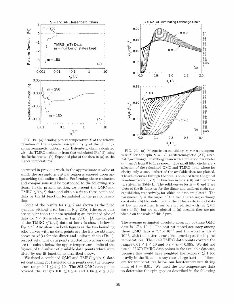
-4

-3

-2

-1

0

1

0.001 0.01 0.1 1 10

Rel

ativ

e D

evia

tion

(%)

kBT/J

(a)

m = 256

m = 150

TMRG χ(T) Datam = number of states kept


-0.10

-0.05

0.00

0.05

0.01 0.1 1 10

Rel

ativ

e D

evia

tion

(%)

kBT/J

(b)

m = 256

m = 150

FIG. 19. (a) Semilog plot vs temperature T of the relativedeviation of the magnetic susceptibility χ of the S = 1/2antiferromagnetic uniform spin Heisenberg chain calculatedwith the TMRG technique from that calculated (Ref. 5) usingthe Bethe ansatz. (b) Expanded plot of the data in (a) at thehigher temperatures.

answered in previous work, is the approximate α value atwhich the asymptotic critical region is entered upon ap-proaching the uniform limit. Performing these estimatesand comparisons will be postponed to the following sec-tions. In the present section, we present the QMC andTMRG χ∗(α, t) data and obtain a fit to these combineddata by the fit function formulated in the previous sec-tion.

Some of the results for t ≤ 2 are shown as the filledsymbols without error bars in Fig. 20(a) (the error barsare smaller than the data symbols); an expanded plot ofdata for t ≤ 0.4 is shown in Fig. 20(b). [A log-log plotof the TMRG χ∗(α, t) data at low t is shown below inFig. 27.] Also shown in both figures as the two boundingsolid curves with no data points are the fits we obtainedabove to χ∗(t) for the dimer and uniform chain (Fit 1),respectively. The data points plotted for a given α valueare the subset below the upper temperature limits of thefigures, of the subset of available data points which werefitted by our fit function as described below.

We fitted a combined QMC and TMRG χ∗(α, t) dataset containing 2551 selected data points over the temper-ature range 0.01 ≤ t ≤ 10. The 802 QMC data pointscovered the ranges 0.01 <∼ t ≤ 4 and 0.05 ≤ α ≤ 0.99.

0.00

0.05

0.10

0.15

0.20

0.0 0.5 1.0 1.5 2.0

χJ1/N

g2µ B

2

kBT/J

1

α =00.10.20.30.40.50.60.70.80.90.960.9951

α = 0

α = 1

S = 1/2 AF Alternating-Exchange Chain

(a)

0.00

0.05

0.10

0.15

0.0 0.1 0.2 0.3 0.4

χJ1/N

g2µ B

2

kBT/J

1

α =00.20.30.40.50.60.70.80.860.880.90.920.940.960.970.980.990.9951

α = 0

α = 1

(b)

FIG. 20. (a) Magnetic susceptibility χ versus tempera-ture T for the spin S = 1/2 antiferromagnetic (AF) alter-nating-exchange Heisenberg chain with alternation parameterα = J2/J1 from 0 to 1, as shown. The small filled circles are aselection of the calculated QMC and TMRG data, where forclarity only a small subset of the available data are plotted.The set of curves through the data is obtained from the globaltwo-dimensional (α, t) fit function in Eqs. (56) with parame-ters given in Table II. The solid curves for α = 0 and 1 areplots of the fit function for the dimer and uniform chain sus-ceptibilities, respectively, for which no data are plotted. Theparameter J1 is the larger of the two alternating exchangeconstants. (b) Expanded plot of the fit for a selection of dataat low temperatures. Error bars are plotted with the QMCdata in (b), but are not plotted in (a) because they are notvisible on the scale of this figure.

The average estimated absolute accuracy of these QMCdata is 1.7 × 10−4. The best estimated accuracy amongthese QMC data is 7.7 × 10−6 and the worst is 1.5 ×10−3, with the better accuracies occurring at the highesttemperatures. The 1749 TMRG data points covered theranges 0.01 ≤ t ≤ 10 and 0.8 ≤ α ≤ 0.995. We did notuse all 22 370 TMRG data points in the available data set,because this would have weighted the region α <∼ 1 tooheavily in the fit, and in any case a large fraction of theseare for temperatures below our low-temperature fittinglimit of t = 0.01. We used the low-temperature datato determine the spin gaps as described in the following

25

section.We fitted this χ∗(α, t) data set by Eqs. (56), with the

constraints on the parameters discussed above. Obtain-ing a reliable 28-parameter two-dimensional fit to thesedata over the full above-cited ranges of t and α, withno poles in the fit, posed a very difficult challenge. Theparticular choice of starting parameters and the detailedsequence of refinements were found to be important toavoiding poles in the final fit. Since there are a total of28 parameters in the fit function for 2551 data points,the data to parameter ratio is 91. The number of fittingparameters seems large, until it is realized that we are si-multaneously fitting χ∗(t) data for 29 different α values,so on average a χ∗(t) data set for a given α value is fit-ted by a single parameter. A weighting function was notincluded during the variance minimization, because wewere interested in obtaining a fit which treated all thedata points the same on an absolute scale; this choiceoptimizes the fit for use in modeling experimental data.

The parameters of the fit are given in Table II, wherewe have also included the constrained parameters forcompleteness and for ease of implementation of our fitfunction by the reader. From Eqs. (51), the constrainedparameters D2 and D3 contain products of the third-order (in α) polynomial ∆∗

fit with itself and/or withthe fourth-order N1 fitting polynomial, so D2 and D3

are of seventh and tenth-order, respectively. The two-dimensional fit is shown as the set of solid curves inFig. 20. The variance of the fit is v = 3.77 × 10−8.The absolute rms deviation

√v ≈ 1.9 × 10−4 is about

the same as the average estimated accuracy of the QMCdata noted above, indicating that the fit function is ap-propriate and that the fit is a reliable representation of

TABLE II. Parameters in the fit function [Eqs. (56)] for χ∗(α, t) of the S = 1/2 antiferromagnetic alternating-exchangeHeisenberg chain. Note that D2 and D3 are respectively of seventh and tenth order in α.

parameter m = 0 m = 1 m = 2 m = 3 m = 4

N1m 0.63427990 −2.06777217 −0.70972219 4.89720885 −2.80783223N2m 0.18776962 −2.84847225 5.96899688 −3.85145137 0.64055849N3m 0.033603617 −0.757981757 4.137970390 −6.100241386 2.701116573N4m 0.0038611069 0.5750352896 −2.3359243110 2.934083364 −1.1756629304N5m 0.00027331430 −0.10724895512 0.40345647304 −0.48608843641 0.18972153852N6m 0 0.00578123759 −0.02313572892 0.02892774508 −0.01157325374N7m 2.59870347×10−7 −2.39236193×10−7

D1m −0.11572010 −1.31777217 1.29027781 3.39720885 −2.80783223D2m 0.08705969 −1.44693321 5.09401919 −10.51861382 8.97655318

5.75312680 (m = 5) −11.83647774 (m = 6) 4.21174835 (m = 7)D3m 0.00563137 0.65986015 −1.38069533 −0.09849603 7.54214913

−22.31810507 (m = 5) 27.60773633 (m = 6) −6.39966673 (m = 7)−15.69691721 (m = 8) 13.37035665 (m = 9) −3.15881126 (m = 10)

D4m 0.0010408866 0.1008789796 −0.9188446197 1.6052570070 −0.7511481272D5m 0.0000683286 −0.1410232710 0.6939435034 −0.9608700949 0.4106951428D6m 0 0.0367159872 −0.1540749976 0.1982667100 −0.0806430233D7m 0 −0.00314381636 0.01140642324 −0.01338139741 0.00511879053D8m 1.25124679×10−7 −1.03824523×10−7

g1 g2 y z

0.38658545 −0.20727806 4.69918784 3.55692695

-20

-15

-10

-5

0

5

10

15

20

0.01 0.1 1 10

Fit

Dev

iatio

n (1

0−4)

kBT/J

1


σrms

= 2.5 x 10−4

QMC data (a)

-10

-5

0

5

10

15

0.01 0.1 1 10

Fit

Dev

iatio

n (1

0−4)

kBT/J

1

σrms

= 1.6 x 10−4

TMRG data(b)

FIG. 21. Deviation in absolute units of the fit function forthe magnetic susceptibility χ∗ versus temperature T for thespin S = 1/2 antiferromagnetic (AF) alternating-exchangeHeisenberg chain, with alternation parameter α = J2/J1

from 0.05 to 0.995, from the QMC data (a) and TMRG data(b). The parameter J1 is the larger of the two alternatingexchange constants. The absolute rms deviations of the re-spective data from the fit are given in the figures. The fitfunction is given in Eqs. (56) with the parameters in Table II.

26

-10

-5

0

5

10

α = 0.98

Fit Function Deviations from L = 400, 800 QMC Data

L = 400L = 800

-15-10-505

1015

Fit

Dev

iatio

n (1

0−4)

α = 0.985

-10

0

10

20

30

α = 0.99

-100

1020304050

0.0 0.1 0.2 0.3 0.4

kBT/J

1

α = 0.995

FIG. 22. Deviation in absolute units of the fit function forthe magnetic susceptibility χ∗ versus temperature T for thespin S = 1/2 antiferromagnetic (AF) alternating-exchangeHeisenberg chain, from L = 400 (•) and L = 800 (opensquares) QMC data for α = 0.98, 0.985, 0.99 and 0.995.The only significant deviation is at the lowest temperatureT = 0.01J/kB. The fit function is given in Eqs. (56) with theparameters in Table II.

the data. The fit deviations from the 802 QMC and1749 TMRG data are shown separately in Figs. 21(a)and 21(b), respectively. A comparison of the two figuresshows that the TMRG data are, on average, significantlymore precise at a given temperature.

After the parameters in the present χ∗(α, t) fit functionwere finalized, as a check on the accuracy of the fit func-tion for α values close to the uniform limit, we carried outQMC χ∗(t) simulations for alternating-exchange chainsof length L = 400 and 800, factors of four and eight longerthan the chains for which QMC data were combined withTMRG data to determine the fit function, respectively.The simulations were carried out for α = 0.98, 0.985, 0.99,and 0.995 at temperatures 0.01 ≤ t ≤ 4. Overall, the fitfunction was found to be in extremely good agreementwith the QMC data. For 0.4 ≤ t ≤ 4, the χ∗(α, t) fitfunction agreed with the simulation data to within about±5 × 10−5 or better. The deviations of the fit functionfrom the data for 0.01 ≤ t ≤ 0.4 are shown in Fig. 22,along with the error bars on the QMC data. As can beseen from the figure, the only significant deviation of thefit function from the QMC data in this t range is at thelowest temperature t = 0.01 for each of the four α

0.00

0.02

0.04

0.06

0.08

0.10

0.12

0.14

0.16

0.0 0.5 1.0 1.5 2.0

χJ/N

g2µ B

2

kBT/J

δ =00.00250.0050.010.020.030.040.050.10.20.30.40.50.60.70.80.91

δ = 0

δ = 1


(a)

0.00

0.02

0.04

0.06

0.08

0.10

0.12

0.14

0.0 0.1 0.2 0.3 0.4

χJ/N

g2µ B

2

kBT/J

δ =00.00250.0050.010.020.030.040.050.10.20.30.40.50.60.70.80.91

δ = 0(b)

FIG. 23. (a) Magnetic susceptibility χ versus tempera-ture T for the spin S = 1/2 antiferromagnetic alternat-ing-exchange Heisenberg chain with values of alternation pa-rameter δ from 0 to 1 as shown, where χ is scaled by 1/J andT by J in contrast to Fig. 20. The parameter J = J1/(1+δ) isthe average of the two exchange constants J1 and J2 alternat-ing along the chain. (b) Expanded plot at low temperatures.These χ∗(δ, t) plots were generated using our two-dimensionalχ∗(α, t) fit function which was converted to the variables (δ, t)using Eq. (16b).

values. Because the fit deviations at this temperatureremain upon increasing the length of the simulated chainfrom L = 400 to L = 800, these fit deviations are mostlikely due to inaccuracies in the fit function, as expectedat this lowest fitted temperature.

For compounds showing spin-Peierls or other types ofsecond-order spin dimerization transitions, it is more ap-propriate to scale χ by 1/J and T by J , where J is theaverage of J1 and J2, in which case the appropriate al-ternation parameter is δ rather than α. It is straight-forward to convert our χ∗(α, t) fit function to the formχ∗(δ, t), where t ≡ kBT/J , using Eq. (16b). We havedone this and plot the χ∗(δ, t) fit function versus tem-perature for a series of δ values in Fig. 23(a). An ap-pealing monotonic progression of χ∗(δ, t) with increasingδ is seen in Fig. 23(a); an expanded plot at lower tem-peratures is shown in Fig. 23(b). This formulation of thefit function allows accurate estimates to be made of thetemperature-dependent spin gap in compounds exhibit-

27

ing spin-dimerization transitions, provided that the near-est neighbor S = 1/2 AF alternating-exchange Heisen-berg model is appropriate to them. An illustration ofthe procedure and the results to be gained will be givenlater when we model the χ(T ) data for NaV2O5.

VI. SPIN GAP FROM TMRG χ∗(α, t)

According to Eq. (11c), if highly precise χ∗(t) data inthe low-t limit are available, the spin gap ∆∗ can in prin-ciple be computed directly from the derivative of thesedata with respect to inverse temperature. However, ingeneral the maximum temperature of the low-t limit re-gion is ill defined since it depends on how precise andaccurate the data are and the accuracy to which ∆∗ isto be determined. Therefore, in practice one could de-fine a temperature-dependent effective spin gap ∆∗

eff fromEq. (11c) as

∆∗

eff(t) = −∂ ln(χ∗√

t)

∂(1/t), (59)

and then try to ascertain ∆∗ from the extrapolated zero-temperature limit ∆∗ = limt→0 ∆∗

eff(t). Using Eq. (11b)would be less desirable and precise because a fit of thistype typically averages ∆∗

eff(t) over a rather large tem-perature range.

An overview of ∆∗

eff(α, t) determined from our TMRGχ∗(α, t) data for 0.8 ≤ α ≤ 0.995 using Eq. (59) is shownin Fig. 24(a). At the lowest temperatures, and for αnot too close to 1, the ∆∗

eff(α, t) data do approach a con-stant value with decreasing t, confirming the applicabilityof Eqs. (10) and prior assumptions and hence Eqs. (11)and (59) to the alternating chain, and the approximatevalues of ∆∗(α) can be estimated from the figure. Closerinspection reveals that ∆∗

eff(α, t) shows a weak maximumbefore decreasing by ≈ 1

2% to ∆∗ as t → 0, as illustratedin Fig. 24(b) for α = 0.8. For this among other rea-sons, we will not use Eq. (59) to extract the spin gapsfrom our TMRG χ∗(α, t) data. On the other hand, weneed to know whether such behavior is expected, sinceit could conceivably arise from systematic errors in theTMRG calculations. Therefore, in the next section westudy the ∆∗

eff(α, t) expected at low temperatures for thealternating-exchange chain. As part of this study, we for-mulate and discuss the fit function which we will use inSec. VI B to extract ∆∗(α) from our TMRG χ∗(α, t) dataat low temperatures.

A. Effective spin gap ∆∗

eff(∆∗, t) for thealternating-exchange chain

From our definition of ∆∗

eff in Eq. (59), a discussion ofhow this quantity varies with t at low t requires an inde-pendent estimate of χ∗(α, t) for the alternating-exchange

0.0

0.1

0.2

0.3

0.4

0.00 0.05 0.10 0.15 0.20 0.25 0.30

∆*ef

f

t

α = 0.800.820.840.860.880.900.920.940.960.970.980.990.995


TMRG data

(a)

0.33

0.34

0.35

0.00 0.02 0.04 0.06 0.08 0.10

∆*ef

ft

(b)

α = 0.8

256 states kept

FIG. 24. (a) Overview of the effective spin gap ∆∗

eff(α, t)vs temperature t for the S = 1/2 AF alternating-exchangeHeisenberg chain, derived from our TMRG χ∗(α, t) data usingthe definition in Eq. (59), where α = J2/J1 is the alternationparameter. (b) Expanded plot of ∆∗

eff(t) for α = 0.8 at lowtemperatures from (a).

chain, which must include at least the leading order cor-rection to the low-t limit in Eqs. (10). As a first attempt,we used the general expression for χ∗(t) in Eqs. (7), whichrequires as input the one-magnon dispersion relation ε(k)for the alternating chain. For this we used the explicitε(∆∗, k) for 0 ≤ α ≤ 1 in Eqs. (23) that we presentedand discussed previously. The resultant χ∗(t) is plottedfor eleven ∆∗ values in Fig. 25(a), where the results aredesignated by χ∗(1) in the figure. Although χ∗(1)(∆∗, t)is exact in both the low- and high-t limits, the resultsare only qualitatively correct at intermediate tempera-tures, as can be seen by comparing Fig. 25(a) with theQMC and TMRG data and fit in Fig. 20. Troyer, Tsunet-sugu and Wurtz51 obtained a very good fit of χ∗(1)(∆∗, t)to QMC χ∗(t) simulation data over a large temperaturerange for the S = 1/2 two-leg Heisenberg ladder withspatially isotropic exchange; however, they assumed aε(∆∗, k) in the fit function which was later found to beinaccurate over much of the Brillouin zone.

We formulated an approximation [designated as χ∗(2)]which is more accurate in the low-temperature range, andwhich we will use in the next section as a fit function tofit our TMRG χ∗(t) data at low t to extract ∆∗(α). Thefunction χ∗(2) was obtained by summing the susceptibil-ities of isolated dimers with a distribution of singlet-trip-

28

0.00

0.05

0.10

0.15

0.20

0.25

0.30

0.35

0.0 0.2 0.4 0.6 0.8 1.0

χ(1) J 1

/Ng2

µ B2

kBT/J

1

∆/J1

0.050.10.150.20.250.30.40.50.60.81

dimer


(a)

0.00

0.05

0.10

0.15

0.20

0.0 0.2 0.4 0.6 0.8 1.0

χ(2) J 1

/Ng2

µ B2

kBT/J

1

∆/J1

0.050.10.150.20.250.30.40.50.60.81

dimer

(b)

FIG. 25. Magnetic susceptibilities χ(1) (a) and χ(2) (b) vstemperature T for the spin S = 1/2 antiferromagnetic alter-nating-exchange Heisenberg chain, calculated using two dif-ferent approximations for χ∗(t), respectively (see text). Notethe different scales for the ordinates in (a) and (b).

let energy gaps given by our one-parameter dispersionrelation ε(∆∗, k) for 0 ≤ ∆∗ ≤ 1 in Eqs. (23), whichtakes into account the interdimer interactions. Thus fromEq. (8a) we simply obtain

χ∗(2)(∆∗, t) =1

πt

∫ π

0

dk

3 + eε(∆∗,k)/t. (60)

Note that we make no assumptions here about the formof the function ∆∗(α), since only ∆∗ appears in the ex-pression. This χ∗(2)(∆∗, t) is exact in both the low-and high-t limits, as is χ∗(1)(∆∗, t), and both repro-duce χ∗(t) for the isolated dimer (∆∗ = 1) exactly, butχ∗(2)(∆∗, t) is more accurate at intermediate tempera-tures for α <∼ 1 as shown in Fig. 25(b). In addition, by

comparing χ∗(1)(∆∗, t) and χ∗(2)(∆∗, t) with the TMRGχ∗(α, t) calculations at low t, we found that the low-tcorrections to the low-t limit in Eqs. (10) are much moreaccurately given by χ∗(2)(t) than by χ∗(1)(t). We willtherefore not discuss χ∗(1)(t) further here.

At low temperatures, the approximation χ∗(2)(∆∗, t) isexpected to accurately describe the leading-order t cor-rections to the low-t limit only as long as the averagenumber of magnons nm occupying a state near the min-imum in the one-magnon band is much less than unity.Using the expression for the boson occupation number

0.95

0.96

0.97

0.98

0.99

1.00

1.01

1.02

1.03

0.00 0.05 0.10 0.15 0.20 0.25 0.30

∆ eff(T

)/∆

kBT /∆

∆/J1

0.050.10.150.20.250.30.40.50.60.81

dimer(∆/J

1 = 1)


∆/J1 = 0.8

∆/J1 = 0.05

FIG. 26. Effective spin gap ∆eff , defined in Eq. (59)and computed using Eq. (60), vs reduced temperaturekBT/∆ = t/∆∗ for the S = 1/2 antiferromagnetic al-ternating-exchange Heisenberg chain for various values of∆∗ ≡ ∆/J1, where t = kBT/J1. A limiting behavior is seenfor ∆∗ → 0, for which the maximum in ∆eff(kBT/∆) occurs atkBT/∆ ≈ 0.14. The linear in T behavior of ∆eff(kBT/∆ → 0)for the isolated dimer (∆∗ = 1) is due to the identically zerowidth of the one-magnon dispersion relation for this ∆∗ value.

for this case,

nm =1

e∆∗/t − 1, (61)

yields t/∆∗ = 0.22 and 0.42 for nm = 0.01 and 0.1, re-spectively. Thus, when fitting our low-t TMRG χ∗(α, t)data by the fit function χ∗(2)(∆∗, t) in the following sec-tion, we expect χ∗(2)(∆∗, t) to be sufficiently accurateonly for t/∆∗ <∼ 0.4. For this reason, our fits will belimited to this maximum scaled temperature.

We have computed ∆eff(∆∗, T )/∆ from χ∗(2)(∆∗, t) inEq. (60), using the definition in Eq. (59), and plot theresults vs kBT/∆ in Fig. 26. For the dimer (∆∗ = 1),one finds analytically that ∆eff(T )/∆ = 1 − 2kBT/∆ tolowest order in T . On the other hand, for 0 < ∆∗ < 1,the initial dependence is positive and quadratic in T , anda maximum is seen in ∆eff(T )/∆, which for ∆∗ <∼ 0.4occurs at t/∆∗ ≡ kBT/∆ ≈ 0.14 with a height of ≈ 0.5%.This height is quantitatively consistent with the data inFig. 24(b) derived from the TMRG χ∗(t) for α = 0.8.Thus the weak maximum seen in that figure is not aspurious effect.

B. Fits to the low-t TMRG χ∗(α, t) data

We were tempted to fit ∆∗

eff(α, t) derived from the low-t TMRG χ∗(α, t) data, as discussed above, to obtainthe spin gaps ∆∗(α, t). However, this procedure wouldhave weighted the χ∗(α, t) data in an ill advised way.We therefore decided to do conventional fits of the low-tχ∗(α, t) data by the fit function χ∗(2)(∆∗, t) in Eq. (60).For a given α, this is a one-parameter (∆∗) fit function

29

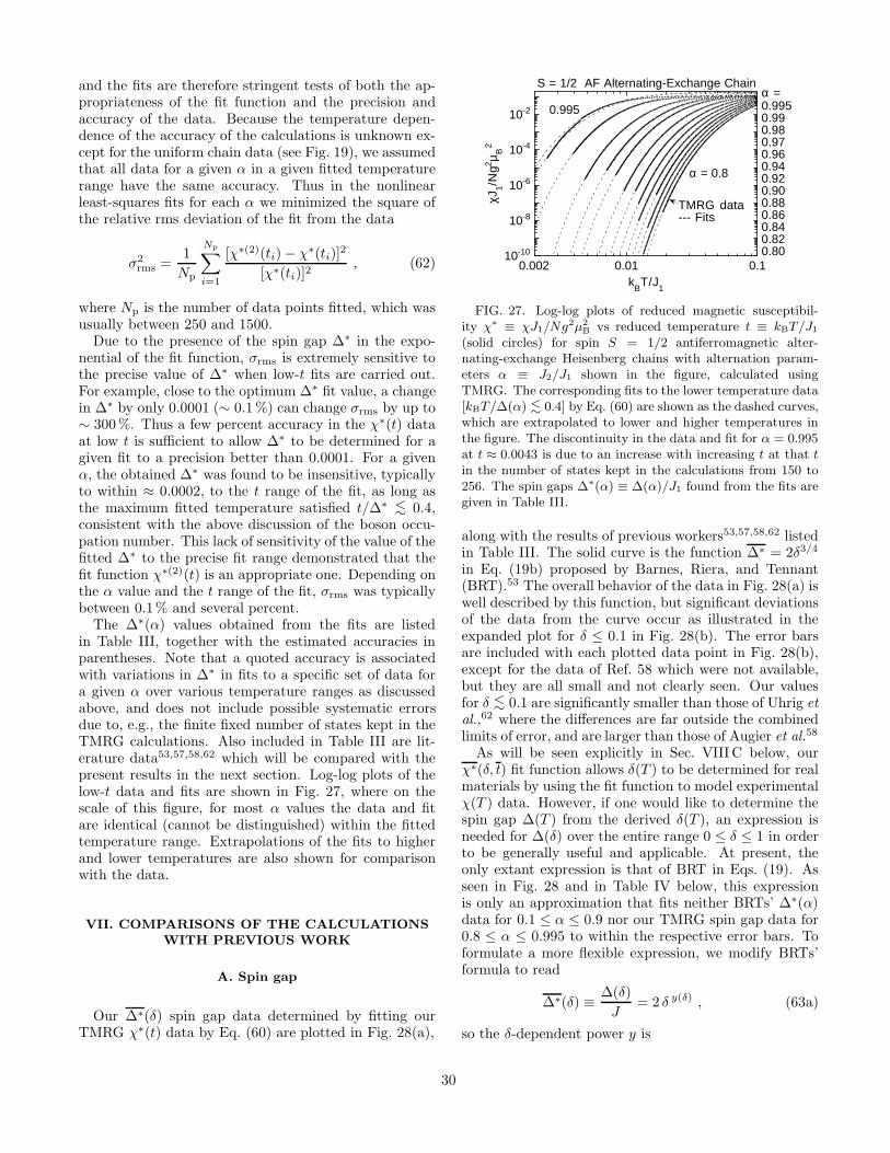
and the fits are therefore stringent tests of both the ap-propriateness of the fit function and the precision andaccuracy of the data. Because the temperature depen-dence of the accuracy of the calculations is unknown ex-cept for the uniform chain data (see Fig. 19), we assumedthat all data for a given α in a given fitted temperaturerange have the same accuracy. Thus in the nonlinearleast-squares fits for each α we minimized the square ofthe relative rms deviation of the fit from the data

σ2rms =

1

Np

Np∑

i=1

[χ∗(2)(ti) − χ∗(ti)]2

[χ∗(ti)]2, (62)

where Np is the number of data points fitted, which wasusually between 250 and 1500.

Due to the presence of the spin gap ∆∗ in the expo-nential of the fit function, σrms is extremely sensitive tothe precise value of ∆∗ when low-t fits are carried out.For example, close to the optimum ∆∗ fit value, a changein ∆∗ by only 0.0001 (∼ 0.1 %) can change σrms by up to∼ 300%. Thus a few percent accuracy in the χ∗(t) dataat low t is sufficient to allow ∆∗ to be determined for agiven fit to a precision better than 0.0001. For a givenα, the obtained ∆∗ was found to be insensitive, typicallyto within ≈ 0.0002, to the t range of the fit, as long asthe maximum fitted temperature satisfied t/∆∗ <∼ 0.4,consistent with the above discussion of the boson occu-pation number. This lack of sensitivity of the value of thefitted ∆∗ to the precise fit range demonstrated that thefit function χ∗(2)(t) is an appropriate one. Depending onthe α value and the t range of the fit, σrms was typicallybetween 0.1% and several percent.

The ∆∗(α) values obtained from the fits are listedin Table III, together with the estimated accuracies inparentheses. Note that a quoted accuracy is associatedwith variations in ∆∗ in fits to a specific set of data fora given α over various temperature ranges as discussedabove, and does not include possible systematic errorsdue to, e.g., the finite fixed number of states kept in theTMRG calculations. Also included in Table III are lit-erature data53,57,58,62 which will be compared with thepresent results in the next section. Log-log plots of thelow-t data and fits are shown in Fig. 27, where on thescale of this figure, for most α values the data and fitare identical (cannot be distinguished) within the fittedtemperature range. Extrapolations of the fits to higherand lower temperatures are also shown for comparisonwith the data.

VII. COMPARISONS OF THE CALCULATIONSWITH PREVIOUS WORK

A. Spin gap

Our ∆∗(δ) spin gap data determined by fitting ourTMRG χ∗(t) data by Eq. (60) are plotted in Fig. 28(a),

10-10

10-8

10-6

10-4

10-2

0.01 0.1

χJ1/N

g2 µ B2

kBT/J

1

α =0.9950.990.980.970.960.940.920.900.880.860.840.820.80


α = 0.8

0.995

TMRG data--- Fits

0.002

FIG. 27. Log-log plots of reduced magnetic susceptibil-ity χ∗ ≡ χJ1/Ng2µ2

B vs reduced temperature t ≡ kBT/J1

(solid circles) for spin S = 1/2 antiferromagnetic alter-nating-exchange Heisenberg chains with alternation param-eters α ≡ J2/J1 shown in the figure, calculated usingTMRG. The corresponding fits to the lower temperature data[kBT/∆(α) <

∼ 0.4] by Eq. (60) are shown as the dashed curves,which are extrapolated to lower and higher temperatures inthe figure. The discontinuity in the data and fit for α = 0.995at t ≈ 0.0043 is due to an increase with increasing t at that tin the number of states kept in the calculations from 150 to256. The spin gaps ∆∗(α) ≡ ∆(α)/J1 found from the fits aregiven in Table III.

along with the results of previous workers53,57,58,62 listedin Table III. The solid curve is the function ∆∗ = 2δ3/4

in Eq. (19b) proposed by Barnes, Riera, and Tennant(BRT).53 The overall behavior of the data in Fig. 28(a) iswell described by this function, but significant deviationsof the data from the curve occur as illustrated in theexpanded plot for δ ≤ 0.1 in Fig. 28(b). The error barsare included with each plotted data point in Fig. 28(b),except for the data of Ref. 58 which were not available,but they are all small and not clearly seen. Our valuesfor δ <∼ 0.1 are significantly smaller than those of Uhrig etal.,62 where the differences are far outside the combinedlimits of error, and are larger than those of Augier et al.58

As will be seen explicitly in Sec. VIII C below, ourχ∗(δ, t) fit function allows δ(T ) to be determined for realmaterials by using the fit function to model experimentalχ(T ) data. However, if one would like to determine thespin gap ∆(T ) from the derived δ(T ), an expression isneeded for ∆(δ) over the entire range 0 ≤ δ ≤ 1 in orderto be generally useful and applicable. At present, theonly extant expression is that of BRT in Eqs. (19). Asseen in Fig. 28 and in Table IV below, this expressionis only an approximation that fits neither BRTs’ ∆∗(α)data for 0.1 ≤ α ≤ 0.9 nor our TMRG spin gap data for0.8 ≤ α ≤ 0.995 to within the respective error bars. Toformulate a more flexible expression, we modify BRTs’formula to read

∆∗(δ) ≡ ∆(δ)

J= 2 δ y(δ) , (63a)

so the δ-dependent power y is

30

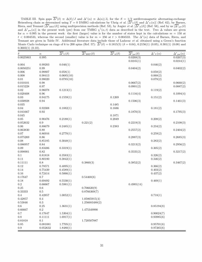
TABLE III. Spin gaps ∆∗(δ) ≡ ∆(δ)/J and ∆∗(α) ≡ ∆(α)/J1 for the S = 1/2 antiferromagnetic alternating-exchangeHeisenberg chain as determined using T = 0 DMRG calculations by Uhrig et al. [∆∗

U(δ) and ∆∗

U(α)] (Ref. 62), by Barnes,Riera, and Tennant [∆∗

BRT(δ)] using multiprecision methods (Ref. 53), by Augier et al. [∆∗A(δ)] (Ref. 58), and by us [∆∗

pw(δ)and ∆∗

pw(α)] in the present work (pw) from our TMRG χ∗(α, t) data as described in the text. Two ∆ values are givenfor α = 0.995 in the present work: the first (larger) value is for the number of states kept in the calculations m = 150 att < 0.004533, whereas the second (smaller) value is for m = 256 at t > 0.004533. The ∆∗(α) data of Barnes, Riera, andTennant are given in Table IV. Additional literature data include those of Ladavac et al. obtained using a Green’s functionMonte Carlo technique on rings of 6 to 200 spins (Ref. 57): ∆∗(δ) = 0.1815(5) (δ = 0.04), 0.2156(1) (0.05), 0.301(1) (0.08) and0.3603(1) (0.10).

δ α ∆∗U(δ) ∆∗

BRT(δ) ∆∗A(δ) ∆∗

pw(δ) ∆∗

U(α) ∆∗

pw(α)

0.0025063 0.995 0.0268(3) 0.0267(3)0.0245(1) 0.0244(1)

0.004 0.99203 0.046(1) 0.046(2)0.0050251 0.99 0.0404(2) 0.0402(2)0.006 0.98807 0.058(1) 0.058(2)0.008 0.98413 0.0685(10) 0.068(2)0.01 0.98020 0.0785(10) 0.078(2)0.010101 0.98 0.0667(2) 0.0660(2)0.015228 0.97 0.0901(2) 0.0887(2)0.02 0.96078 0.1213(1) 0.119(2)0.020408 0.96 0.1116(4) 0.1094(4)0.03 0.94175 0.1559(1) 0.1269 0.151(2)0.030928 0.94 0.1506(3) 0.1461(3)0.035 0.14850.04 0.92308 0.1882(1) 0.1686 0.181(2)0.041667 0.92 0.1870(3) 0.1795(3)0.045 0.18710.05 0.90476 0.2188(1) 0.2049 0.208(2)0.052632 0.9 0.221(2) 0.2219(3) 0.2108(3)0.06 0.88679 0.2485(1) 0.2383 0.234(2)0.063830 0.88 0.2557(2) 0.2404(2)0.07 0.86916 0.2770(1) 0.259(2)0.075269 0.86 0.2887(3) 0.2685(3)0.08 0.85185 0.3048(1) 0.282(2)0.086957 0.84 0.3213(2) 0.2956(2)0.09 0.83486 0.3319(1) 0.305(2)0.098901 0.82 0.3535(2) 0.3217(2)0.1 0.81818 0.3583(1) 0.326(2)0.11 0.80180 0.3842(1) 0.346(2)0.11111 0.8 0.3860(3) 0.3852(2) 0.3467(2)0.12 0.78571 0.4095(1) 0.366(2)0.14 0.75439 0.4589(1) 0.403(2)0.16 0.72414 0.5066(1) 0.437(2)0.17647 0.7 0.54468(6)0.18 0.69492 0.5530(1) 0.469(1)0.2 0.66667 0.5981(1) 0.4985(14)0.25 0.6 0.706620(9)0.33333 0.5 0.8766369(7)0.4 0.42857 1.0052(1) 0.718(1)0.42857 0.4 1.05865915(4)0.53846 0.3 1.256683488(2)0.6 0.25 1.3631(1) 0.85194(8)0.66667 0.2 1.4753499900.7 0.17647 1.5304(1) 0.90024(7)0.8 0.11111 1.6917(1) 0.93985(6)0.81818 0.1 1.7205078870.85 0.081081 1.7705(1) 0.95701(6)0.9 0.052632 1.8480(1) 0.97265(6)

31

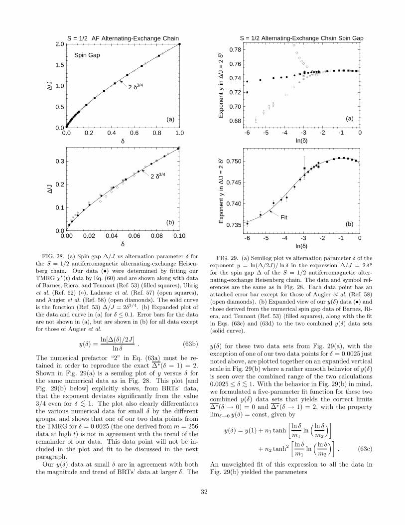
0.0

0.5

1.0

1.5

2.0

0.0 0.2 0.4 0.6 0.8 1.0

∆/J

δ


(a)

2 δ3/4

Spin Gap

0.0

0.1

0.2

0.3

0.00 0.02 0.04 0.06 0.08 0.10

∆/J

δ

(b)

2 δ3/4

FIG. 28. (a) Spin gap ∆/J vs alternation parameter δ forthe S = 1/2 antiferromagnetic alternating-exchange Heisen-berg chain. Our data (•) were determined by fitting ourTMRG χ∗(t) data by Eq. (60) and are shown along with dataof Barnes, Riera, and Tennant (Ref. 53) (filled squares), Uhriget al. (Ref. 62) (◦), Ladavac et al. (Ref. 57) (open squares),and Augier et al. (Ref. 58) (open diamonds). The solid curveis the function (Ref. 53) ∆/J = 2δ3/4. (b) Expanded plot ofthe data and curve in (a) for δ ≤ 0.1. Error bars for the dataare not shown in (a), but are shown in (b) for all data exceptfor those of Augier et al.

y(δ) =ln[∆(δ)/2J ]

ln δ. (63b)

The numerical prefactor “2” in Eq. (63a) must be re-tained in order to reproduce the exact ∆∗(δ = 1) = 2.Shown in Fig. 29(a) is a semilog plot of y versus δ forthe same numerical data as in Fig. 28. This plot [andFig. 29(b) below] explicitly shows, from BRTs’ data,that the exponent deviates significantly from the value3/4 even for δ <∼ 1. The plot also clearly differentiatesthe various numerical data for small δ by the differentgroups, and shows that one of our two data points fromthe TMRG for δ = 0.0025 (the one derived from m = 256data at high t) is not in agreement with the trend of theremainder of our data. This data point will not be in-cluded in the plot and fit to be discussed in the nextparagraph.

Our y(δ) data at small δ are in agreement with boththe magnitude and trend of BRTs’ data at larger δ. The

0.68

0.70

0.72

0.74

0.76

0.78

-6 -5 -4 -3 -2 -1 0

Exp

onen

t y

in ∆

/J =

2 δ

y

ln(δ)

S = 1/2 Alternating-Exchange Chain Spin Gap

(a)

0.735

0.740

0.745

0.750

-6 -5 -4 -3 -2 -1 0

Exp

onen

t y

in ∆

/J =

2 δ

y

ln(δ)

(b)Fit

FIG. 29. (a) Semilog plot vs alternation parameter δ of theexponent y = ln(∆/2J)/ ln δ in the expression ∆/J = 2 δy

for the spin gap ∆ of the S = 1/2 antiferromagnetic alter-nating-exchange Heisenberg chain. The data and symbol ref-erences are the same as in Fig. 28. Each data point has anattached error bar except for those of Augier et al. (Ref. 58)(open diamonds). (b) Expanded view of our y(δ) data (•) andthose derived from the numerical spin gap data of Barnes, Ri-era, and Tennant (Ref. 53) (filled squares), along with the fitin Eqs. (63c) and (63d) to the two combined y(δ) data sets(solid curve).

y(δ) for these two data sets from Fig. 29(a), with theexception of one of our two data points for δ = 0.0025 justnoted above, are plotted together on an expanded verticalscale in Fig. 29(b) where a rather smooth behavior of y(δ)is seen over the combined range of the two calculations0.0025 ≤ δ <∼ 1. With the behavior in Fig. 29(b) in mind,we formulated a five-parameter fit function for these twocombined y(δ) data sets that yields the correct limits∆∗(δ → 0) = 0 and ∆∗(δ → 1) = 2, with the propertylimδ→0 y(δ) = const, given by

y(δ) = y(1) + n1 tanh

[

ln δ

m1ln

( ln δ

m2

)

]

+ n2 tanh2

[

ln δ

m1ln

( ln δ

m2

)

]

. (63c)

An unweighted fit of this expression to all the data inFig. 29(b) yielded the parameters

32

0.0

0.1

0.2

0.00 0.02 0.04 0.06 0.08 0.10

∆ /J

δ2/3/ | lnδ |1/2


Spin Gap

∆/J = 3.3 δ2/3/ | lnδ |1/2

FIG. 30. Spin gap ∆/J vs δ2/3/| ln δ|1/2 obtained from thedata in Fig. 28. The straight line passes through the originwith slope 3.3.

y(1) = 0.74922 , n1 = 0.00776 , n2 = −0.00685 ,

m1 = 3.3297 , m2 = −2.2114 , (63d)

so that

limδ→0

y(δ) = y(1) − n1 + n2 = 0.7346 . (64)

The fit is plotted as the solid curve in Fig. 29(b). Ascan be seen from the figure, our data are fitted to withinour error bars. In addition, when the y(δ) fit function inEqs. (63c) and (63d) is inserted into Eq. (63a), the pre-dicted values of ∆∗(δ) are in agreement with each of thevalues of BRT at larger δ to within 0.0001, which is suffi-cient for modeling experimental data. The δ = 0 limit ofy(δ) in Eq. (64) is in agreement with the theoretical ef-fective value y(0) = 0.72(3), which was obtained withoutthe log correction term by Singh and Weihong73 froman eleventh-order dimer series expansion of the tripletdispersion relation. We will use Eqs. (63) to compute∆(T ) from the experimentally derived δ(T ) for NaV2O5

in Sec. VIII C below.In order to test the critical behavior prediction ∆∗ =

Aδ2/3/| ln δ|1/2 in Eq. (20), which need only hold in theasymptotic critical regime δ → 0 in contrast to the fitfunction for 0 ≤ δ ≤ 1 in Eqs. (63), in Fig. 30 is plot-ted ∆/J vs δ2/3/| ln δ|1/2 in the region δ <∼ 0.06 for thesame data and symbols as in Fig. 28. A proportional-ity appears to be developing in our data for δ <∼ 0.005,as shown by the straight line with slope A = 3.3 pass-ing through the origin of the figure, suggesting that theasymptotic critical regime begins with decreasing δ be-low δ ∼ 0.005 (α >∼ 0.99). High-accuracy ∆∗(δ) datafor δ <∼ 0.001 are needed to test this conjecture. FromFig. 30, the slope 3.3 of the line drawn is evidently alower limit of the prefactor A within the actual asymp-totic critical regime.

0.00

0.05

0.10

0.15

0.20

0.0 0.5 1.0 1.5 2.0

χJ1/N

g2 µ B2

kBT/J

1


α = 0.2

QMC & TMRG Data Fit

0.40.6

0.8

Symbols: Lanczos CalculationsBarnes & Riera (1994)

(a)

0.7

-4

-2

0

2

4

6

0.0 0.5 1.0 1.5 2.0

Dev

iatio

n (1

0−4)

kBT/J

1

(b)

to 2.0 x 10−3 at t = 0.05

FIG. 31. (a) Magnetic susceptibility χ versus tempera-ture T for the spin S = 1/2 antiferromagnetic alternat-ing-exchange Heisenberg chain with alternation parameterα = 0.2, 0.4, 0.6, 0.7 and 0.8 (symbols), calculated by Barnesand Riera (Ref. 9) using the Lanczos technique. Our χ∗(t) fitfunction as in Fig. 20 (solid curves) for the same α values isshown for comparison. (b) Deviation of the data of Barnesand Riera from our fit function vs T .

B. Numerical χ∗(α, t) results

Barnes and Riera previously carried out exact diag-onalizations of Hamiltonian (13) for S = 1/2 alternat-ing chains of length up to 16 spins using the Lanczostechnique.9 Their computed χ∗(t) values for α = 0.2,0.4, 0.6, 0.7, and 0.8 were extrapolated to the bulk limitand the results are shown as the symbols in Fig. 31(a).Our fit function as in Fig. 20 for the same α valuesis plotted as the solid curves in Fig. 31(a), which areseen to be in good overall agreement with the calcula-tions of Barnes and Riera. The deviations of the dataof Barnes and Riera from our fit function are plottedvs temperature in Fig. 31(b). The average deviation oftheir data from our fit function is very small for each dataset: −0.41, +0.33, −0.40, −0.26, and +0.79 × 10−4 forα = 0.2, 0.4, 0.6, 0.7, and 0.8, respectively. The absoluterms deviations σrms of their data from our fit function for

33

α = 0.2, 0.4, 0.6, 0.7, and 0.8 are (in units of 10−4) 1.73,1.43, 0.73, 0.78, and 3.76, respectively. We conclude thattheir data are in good quantitative agreement with ourdata and fit, with the exception of their data point forα = 0.8 at their lowest temperature t = 0.05.

C. Bulaevskii Theory

Bulaevskii7 calculated χ∗(t) analytically in theHartree-Fock approximation. He first obtained an in-tegral equation for the magnon spectrum E(k):

ε(k) ≡ E(k)

J1=

1

2

[

√

1 + α2 − 2α cos k

+C1 + αC2 − (αC1 + C2) cos k√

1 + α2 − 2α cos k

]

, (65)

C1(t) =1

π

∫ π

0

dk1 − α cos k√

1 + α2 − 2α cosktanh

ε(k)

2t,

(66)

C2(t) =1

π

∫ π

0

dkα2 − α cos k√

1 + α2 − 2α cosktanh

ε(k)

2t,

where k is measured in units of 2π/d. d ≡ 1 is the latticerepeat distance along the chain, which is twice the aver-age distance between spins. He then expressed χ∗(t) interms of ε(k):

χ∗(t) ≡ F (t)

2 + (1 + α)F (t),

(67)

F (t) =1

2πt

∫ π

0

dk

cosh2[ε(k)/(2t)].

At t = 0 and α 6= 0, from Eqs. (66) we obtain

C1(α) =1

π

{

(1 + α)E

[

4α

(1 + α)2

]

+ (1 − α)K

[

4α

(1 + α)2

]}

,

(68)

C2(α) =1

π

{

(1 + α)E

[

4α

(1 + α)2

]

− (1 − α)K

[

4α

(1 + α)2

]}

,

where K(y) and E(y) are, respectively, the complete el-liptic integrals of the first and second kinds. The disper-sion relations versus α at t = 0 are obtained by insertingEqs. (68) into (65) and a selection of results is shown inFig. 32. From Eqs. (65) and (68), at t = 0 the spin-gap∆k=0(α) at k = 0 is given by

0.0

0.2

0.4

0.6

0.8

1.0

1.2

1.4

1.6

0.0 0.5 1.0 1.5 2.0

E(k

)/J 1

k/π

α =0.10.20.30.40.50.60.70.8

0.90.95

T = 0

0.186

0.187

0.188

0.189

0.190

0.191

0 0.01 0.02 0.03

α = 0.9, T = 0

FIG. 32. Dispersion relations E(k) at temperature T = 0from Bulaevskii’s theory (Ref. 7) in Eqs. (65) and (68) for tenvalues of the alternation parameter α. The inset shows anexpanded plot near k = 0 of E(k) for α = 0.9.

∆k=0(α) =1 − α

2

{

1 +2(1 − α)

πK

[

4α

(1 + α)2

]

}

. (69)

This expression gives the actual spin-gap for 0 < α ≤0.79. However, for 0.79 <∼ α < 1, the minimum in thedispersion relation does not occur at k = 0, as illustratedin an expanded plot of E(k) for α = 0.9 in the inset toFig. 32. The wave vector kG at which the minimum spingap ∆B occurs is plotted versus α in Fig. 33(b). The ∆B

from Bulaevskii’s theory at t = 0 is plotted versus α asthe solid curve in Fig. 33(a), and a few representative val-ues are given in Table IV. The predictions of Bulaevskii’stheory are in very good agreement with those of Barnes,Riera, and Tennant53 for α <∼ 0.3, but the agreement be-comes progressively worse as α increases further. FromEqs. (65) and (66), E(k) is temperature dependent. Inaddition, in the range 0.79 <∼ α < 1 for which kG 6= 0at t = 0, we find that kG depends on t, as shown inFig. 34. From Fig. 34, kG → 0 at t ≈ 0.083, 0.122, 0.131,0.125, and 0.111 for α = 0.8, 0.85, 0.9, 0.95, and 0.99,respectively.

We computed χ∗(t) by inserting ε(k) in Eq. (65) intoEqs. (66), numerically solving the latter two simultaneousequations for C1 and C2 at each t, and then inserting theresulting ε(k) into Eqs. (67). The progression of χ∗(t)with increasing α from 0.001 to 0.99 is shown in Fig. 35.As noted by Bulaevskii,7 the values of χ∗ at the maximaare too large and the temperatures at which these occurare too small by ∼ 5–10% (compare Fig. 35 with Fig. 20).

At low temperatures 0.033 ≤ t ≤ 1/4, Bulaevskii fittedχ∗(α, t), calculated from Eqs. (67), by the two-parameterform

34

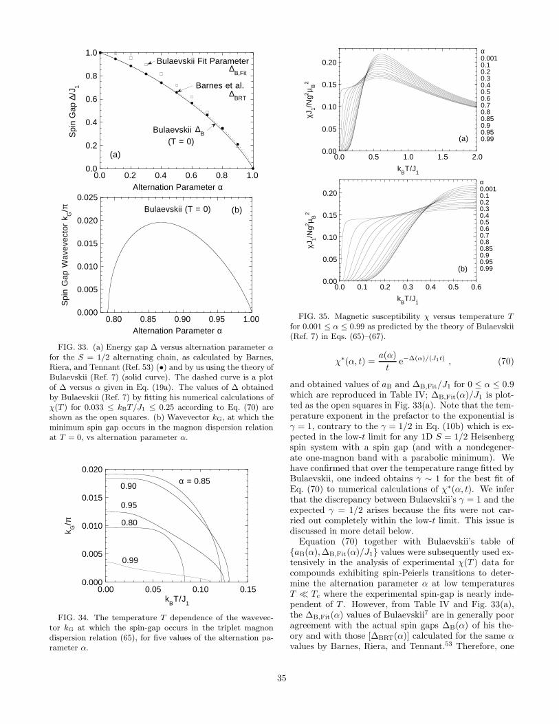
0.0

0.2

0.4

0.6

0.8

1.0

0.0 0.2 0.4 0.6 0.8 1.0

Spi

n G

ap ∆

/J1

Alternation Parameter α

Bulaevskii

Barnes et al.

(T = 0)

(a)

Bulaevskii Fit Parameter∆

B,Fit

∆BRT

∆B

0.000

0.005

0.010

0.015

0.020

0.025

0.80 0.85 0.90 0.95 1.00

Spi

n G

ap W

avev

ecto

r k G

/π

Alternation Parameter α

Bulaevskii (T = 0) (b)

FIG. 33. (a) Energy gap ∆ versus alternation parameter αfor the S = 1/2 alternating chain, as calculated by Barnes,Riera, and Tennant (Ref. 53) (•) and by us using the theory ofBulaevskii (Ref. 7) (solid curve). The dashed curve is a plotof ∆ versus α given in Eq. (19a). The values of ∆ obtainedby Bulaevskii (Ref. 7) by fitting his numerical calculations ofχ(T ) for 0.033 ≤ kBT/J1 ≤ 0.25 according to Eq. (70) areshown as the open squares. (b) Wavevector kG, at which theminimum spin gap occurs in the magnon dispersion relationat T = 0, vs alternation parameter α.

0.000

0.005

0.010

0.015

0.020

0.00 0.05 0.10 0.15

k G/π

kBT/J

1

0.80

α = 0.85

0.95

0.99

0.90

FIG. 34. The temperature T dependence of the wavevec-tor kG at which the spin-gap occurs in the triplet magnondispersion relation (65), for five values of the alternation pa-rameter α.

0.00

0.05

0.10

0.15

0.20

0.0 0.5 1.0 1.5 2.0

χJ1/N

g2µ B

2

kBT/J

1

α0.0010.10.20.30.40.50.60.70.80.850.90.950.99(a)

0.00

0.05

0.10

0.15

0.20

0.0 0.1 0.2 0.3 0.4 0.5 0.6

χJ1/N

g2 µ B2

kBT/J

1

α0.0010.10.20.30.40.50.60.70.80.850.90.950.99(b)

FIG. 35. Magnetic susceptibility χ versus temperature Tfor 0.001 ≤ α ≤ 0.99 as predicted by the theory of Bulaevskii(Ref. 7) in Eqs. (65)–(67).

χ∗(α, t) =a(α)

te−∆(α)/(J1t) , (70)

and obtained values of aB and ∆B,Fit/J1 for 0 ≤ α ≤ 0.9which are reproduced in Table IV; ∆B,Fit(α)/J1 is plot-ted as the open squares in Fig. 33(a). Note that the tem-perature exponent in the prefactor to the exponential isγ = 1, contrary to the γ = 1/2 in Eq. (10b) which is ex-pected in the low-t limit for any 1D S = 1/2 Heisenbergspin system with a spin gap (and with a nondegener-ate one-magnon band with a parabolic minimum). Wehave confirmed that over the temperature range fitted byBulaevskii, one indeed obtains γ ∼ 1 for the best fit ofEq. (70) to numerical calculations of χ∗(α, t). We inferthat the discrepancy between Bulaevskii’s γ = 1 and theexpected γ = 1/2 arises because the fits were not car-ried out completely within the low-t limit. This issue isdiscussed in more detail below.

Equation (70) together with Bulaevskii’s table of{aB(α), ∆B,Fit(α)/J1} values were subsequently used ex-tensively in the analysis of experimental χ(T ) data forcompounds exhibiting spin-Peierls transitions to deter-mine the alternation parameter α at low temperaturesT ≪ Tc where the experimental spin-gap is nearly inde-pendent of T . However, from Table IV and Fig. 33(a),the ∆B,Fit(α) values of Bulaevskii7 are in generally pooragreement with the actual spin gaps ∆B(α) of his the-ory and with those [∆BRT(α)] calculated for the same αvalues by Barnes, Riera, and Tennant.53 Therefore, one

35

should consider the ∆B,Fit parameters as fitting param-eters only, with no direct relation to the actual spin gap.

According to Eq. (8a) for χ∗(t) of the isolated dimerwhich is a zero-dimensional spin system, the form ofχ∗(t) in Eq. (70) with γ = 1 is correct for α = 0 andt → 0. On the other hand, for one-dimensional spin sys-tems such as the two-leg spin ladder (and the alternating-exchange chain) at temperatures kBT ≪ ∆ and kBT ≪one-magnon bandwidth, Eqs. (10) apply, with γ = 1/2,assuming that the triplet one-magnon dispersion rela-tion E(k) is parabolic at the minimum. In this case oneexpects γ = 1/2 at sufficiently low t for any finite α.Thus, in the temperature region of validity of Eq. (10a),a plot of the left-hand-side of Eq. (11a) vs lnt shouldgive a straight line with slope −γ. Shown in Fig. 36 aresuch plots, obtained using our χ∗(α, t) calculated fromBulaevskii’s theory as described above, for α = 0.001to 0.99. For α = 0.001, a crossover is clearly evident fromγ = 1 to γ = 1/2 with decreasing t. The other curves alsoexhibit signs of a crossover, with γ ≈ 1/2 at the lowesttemperatures, with the exception of the curve for α = 0.8.For this α value, which is just above the value α ≈ 0.79 atwhich kG becomes nonzero at t = 0 [see Fig. 33(b)], the γat the lowest t is intermediate between the values of 1/2and 1, and the assumption of a parabolic form for E(k) atthe band minimum is evidently not satisfied (see Fig. 32).In fact, Troyer, Tsunetsugu and Wurtz51 calculated thelow-t limit of χ∗(t) for 1D systems with general dispersionrelation ε(k) = ∆∗ + c∗|ka|n, where k is the deviation ofthe wave vector from that at the band minimum. Theyfound the same form χ∗(t) = (An/tγ) exp(−∆∗/t) as forthe parabolic case n = 2, but where γ = 1−(1/n). Thus,e.g., γ = 2/3 and 3/4 for n = 3 and 4, respectively. Thisrange of γ is consistent with the slope of the data at thelowest temperatures for α = 0.8 in Fig. 36.

The predictions of Bulaevskii’s theory for χ∗(t) fromFig. 35 are compared with our χ∗(α, t) fit function (solid

TABLE IV. Prefactor a and spin-gap ∆ describing the low-temperature spin susceptibility in Eq. (70) of the S = 1/2alternating chain with alternation parameter α [and δ = (1 − α)/(1 + α), see Eqs. (13)]. Fit parameters given by Bulaevskii(Ref. 7) (aB, ∆B,Fit) that he obtained by fitting to his low-t χ∗(t) calculations using Eq. (70) are shown. We obtained theactual spin gap values ∆B/J1 in Bulaevskii’s theory by numerically solving Eqs. (65) and (66). Also included are the accuratecalculations of the spin gap ∆BRT/J1 by Barnes, Riera, and Tennant (Ref. 53), which are compared with numerical values oftheir approximate form ∆(α)/J1 ≈ (1 − α)3/4(1 + α)1/4 [Eq. (19a)].

α δ aB ∆B,Fit/J1 ∆B/J1 ∆BRT/J1 (1 − α)3/4(1 + α)1/4

0.0 1 1 1 1 1 10.1 0.81818 0.980 0.995 0.946245 0.946279339 0.946300.2 0.66667 0.873 0.954 0.884911 0.885209996 0.885350.3 0.53846 0.733 0.897 0.815791 0.816844275(1) 0.817160.4 0.42857 0.582 0.818 0.738504 0.74106141(3) 0.741560.5 0.33333 0.427 0.720 0.652443 0.6574777(5) 0.658040.6 0.25 0.346 0.617 0.556661 0.565296(7) 0.565690.7 0.17647 0.224 0.484 0.449626 0.46298(5) 0.462860.8 0.11111 0.138 0.345 0.328631 0.3474(3) 0.346410.9 0.05263 0.076 0.193 0.186319 0.2098(17) 0.208781.0 0 0 0 0

-2

0

2

4

6

8

-10 -8 -6 -4 -2 0

ln[χ

*(t)

e∆

*(t)

/t ]

ln(t)

slope = −1

slope = −1/2

α =0.0010.10.20.30.50.70.80.90.950.99

FIG. 36. Log-log plot of χ∗(t) e∆∗(t)/t at low t ver-sus reduced temperature t for 0.001 ≤ α ≤ 0.99 [seeEq. (11a)] as predicted by the theory of Bulaevskii (Ref. 7) inEqs. (65)–(67).

curves) for α = 0.2, 0.4, 0.6, 0.8 and 0.99 (as in Fig. 20) inFig. 37, where the Bulaevskii prediction for each of theseα values is shown as the corresponding dashed curve.The disagreement between the two calculations becomesprogressively more severe as temperature decreases andas the uniform chain limit is approached with increas-ing α. Therefore, the accuracies of the α and J1 valuespreviously extracted from experimental data at low Tfor compounds with α <∼ 1 using Bulaevskii’s theory areunclear. Our χ∗(α, t) fit function now provides a muchmore accurate and reliable means of extracting exchangeconstants and spin gaps from experimental χ(T ) data.

36

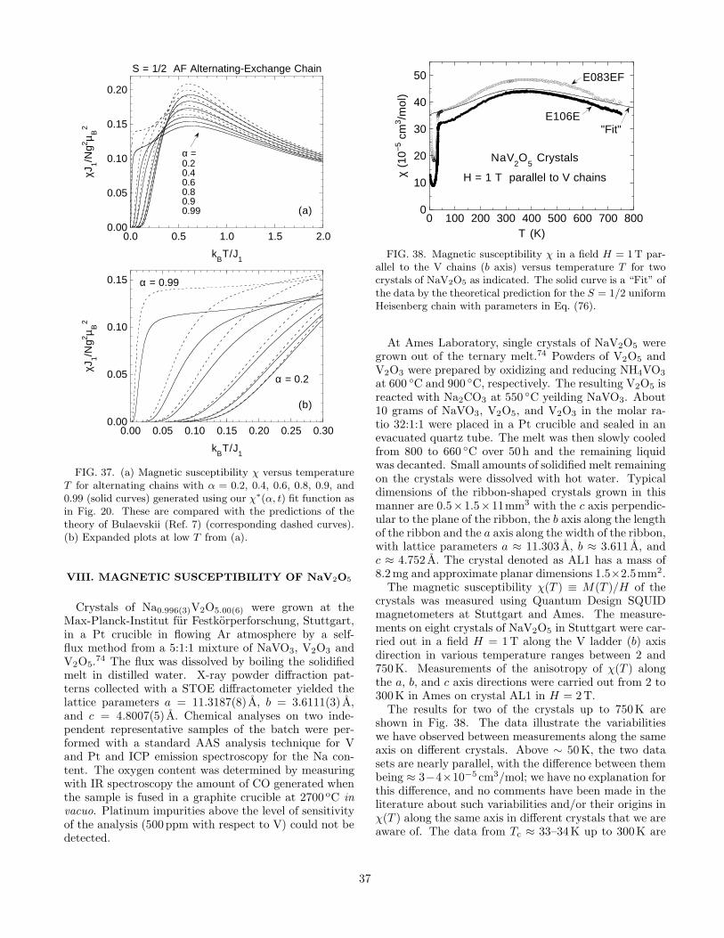
0.00

0.05

0.10

0.15

0.20

0.0 0.5 1.0 1.5 2.0

χ J1/N

g2 µ B2

kBT/J

1

(a)

α =0.20.40.60.80.90.99


0.00

0.05

0.10

0.15

0.00 0.05 0.10 0.15 0.20 0.25 0.30

χ J1/N

g2 µ B2

kBT/J

1

(b)

α = 0.2

α = 0.99

FIG. 37. (a) Magnetic susceptibility χ versus temperatureT for alternating chains with α = 0.2, 0.4, 0.6, 0.8, 0.9, and0.99 (solid curves) generated using our χ∗(α, t) fit function asin Fig. 20. These are compared with the predictions of thetheory of Bulaevskii (Ref. 7) (corresponding dashed curves).(b) Expanded plots at low T from (a).

VIII. MAGNETIC SUSCEPTIBILITY OF NaV2O5

Crystals of Na0.996(3)V2O5.00(6) were grown at theMax-Planck-Institut fur Festkorperforschung, Stuttgart,in a Pt crucible in flowing Ar atmosphere by a self-flux method from a 5:1:1 mixture of NaVO3, V2O3 andV2O5.

74 The flux was dissolved by boiling the solidifiedmelt in distilled water. X-ray powder diffraction pat-terns collected with a STOE diffractometer yielded thelattice parameters a = 11.3187(8) A, b = 3.6111(3) A,and c = 4.8007(5) A. Chemical analyses on two inde-pendent representative samples of the batch were per-formed with a standard AAS analysis technique for Vand Pt and ICP emission spectroscopy for the Na con-tent. The oxygen content was determined by measuringwith IR spectroscopy the amount of CO generated whenthe sample is fused in a graphite crucible at 2700 oC invacuo. Platinum impurities above the level of sensitivityof the analysis (500 ppm with respect to V) could not bedetected.

0

10

20

30

40

50

0 100 200 300 400 500 600 700 800

χ (1

0−5 c

m3 /m

ol)

T (K)

NaV2O

5 Crystals

H = 1 T parallel to V chains

E083EF

E106E"Fit"

FIG. 38. Magnetic susceptibility χ in a field H = 1T par-allel to the V chains (b axis) versus temperature T for twocrystals of NaV2O5 as indicated. The solid curve is a “Fit” ofthe data by the theoretical prediction for the S = 1/2 uniformHeisenberg chain with parameters in Eq. (76).

At Ames Laboratory, single crystals of NaV2O5 weregrown out of the ternary melt.74 Powders of V2O5 andV2O3 were prepared by oxidizing and reducing NH4VO3

at 600 ◦C and 900 ◦C, respectively. The resulting V2O5 isreacted with Na2CO3 at 550 ◦C yeilding NaVO3. About10 grams of NaVO3, V2O5, and V2O3 in the molar ra-tio 32:1:1 were placed in a Pt crucible and sealed in anevacuated quartz tube. The melt was then slowly cooledfrom 800 to 660 ◦C over 50 h and the remaining liquidwas decanted. Small amounts of solidified melt remainingon the crystals were dissolved with hot water. Typicaldimensions of the ribbon-shaped crystals grown in thismanner are 0.5×1.5×11mm3 with the c axis perpendic-ular to the plane of the ribbon, the b axis along the lengthof the ribbon and the a axis along the width of the ribbon,with lattice parameters a ≈ 11.303 A, b ≈ 3.611 A, andc ≈ 4.752 A. The crystal denoted as AL1 has a mass of8.2mg and approximate planar dimensions 1.5×2.5mm2.

The magnetic susceptibility χ(T ) ≡ M(T )/H of thecrystals was measured using Quantum Design SQUIDmagnetometers at Stuttgart and Ames. The measure-ments on eight crystals of NaV2O5 in Stuttgart were car-ried out in a field H = 1T along the V ladder (b) axisdirection in various temperature ranges between 2 and750K. Measurements of the anisotropy of χ(T ) alongthe a, b, and c axis directions were carried out from 2 to300K in Ames on crystal AL1 in H = 2T.

The results for two of the crystals up to 750K areshown in Fig. 38. The data illustrate the variabilitieswe have observed between measurements along the sameaxis on different crystals. Above ∼ 50K, the two datasets are nearly parallel, with the difference between thembeing ≈ 3−4×10−5 cm3/mol; we have no explanation forthis difference, and no comments have been made in theliterature about such variabilities and/or their origins inχ(T ) along the same axis in different crystals that we areaware of. The data from Tc ≈ 33–34K up to 300K are

37

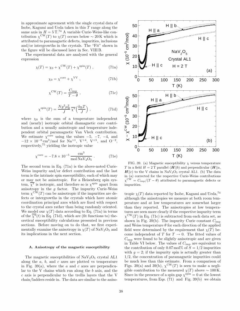
in approximate agreement with the single crystal data ofIsobe, Kagumi and Ueda taken in this T range along thesame axis in H = 5 T.74 A variable Curie-Weiss-like con-tribution χCW(T ) to χ(T ) occurs below ∼ 20K which isattributed to paramagnetic defects, impurities, inclusionsand/or intergrowths in the crystals. The “Fit” shown inthe figure will be discussed later in Sec. VIII B.

The experimental data are analyzed with the generalexpression

χ(T ) = χ0 + χCW(T ) + χspin(T ) , (71a)

χ0 = χcore + χVV , (71b)

χCW(T ) =Cimp

T − θ, (71c)

χspin(T ) =Ng2µ2

B

Jχ∗

(kBT

J

)

, (71d)

where χ0 is the sum of a temperature independentand (nearly) isotropic orbital diamagnetic core contri-bution and a usually anisotropic and temperature inde-pendent orbital paramagnetic Van Vleck contribution.We estimate χcore using the values −5, −7, −4, and−12 × 10−6 cm3/mol for Na+1, V+4, V+5, and O−2,respectively,75 yielding the isotropic value

χcore = −7.8 × 10−5 cm3

mol NaV2O5. (71e)

The second term in Eq. (71a) is the above-noted Curie-Weiss impurity and/or defect contribution and the lastterm is the intrinsic spin susceptibility, each of which mayor may not be anisotropic. For a Heisenberg spin sys-tem, χ∗ is isotropic, and therefore so is χspin apart fromanisotropy in the g factor. The impurity Curie-Weissterm χCW(T ) can be anisotropic if the impurities are de-fects or intergrowths in the crystals which have atomiccoordination principal axes which are fixed with respectto the crystal axes rather than being randomly oriented.We model our χ(T ) data according to Eq. (71a) in termsof the χ∗(t) in Eq. (71d), which are (fit functions to) the-oretical susceptibility calculations presented in previoussections. Before moving on to do that, we first experi-mentally examine the anisotropy in χ(T ) of NaV2O5 andits implications in the next section.

A. Anisotropy of the magnetic susceptibility

The magnetic susceptibilities of NaV2O5 crystal AL1along the a, b, and c axes are plotted vs temperaturein Fig. 39(a), where the a and c axes are perpendicu-lar to the V chains which run along the b axis, and thec axis is perpendicular to the trellis layers that the Vchain/ladders reside in. The data are similar to the aniso-

0

10

20

30

40

50

0 50 100 150 200 250 300

χ (1

0−5 c

m3/m

ol)

T (K)

(a)

Crystal AL1

NaV2O

5

H || b

H || c

H = 2 T

H || a

H || c

0

10

20

30

40

50

0 50 100 150 200 250 300

χ −

χCW

(10

−5 c

m3/m

ol)

T (K)

(b)

H || b

H || c

H || a

H || c

FIG. 39. (a) Magnetic susceptibility χ versus temperatureT in a field H = 2 T parallel (H ||b) and perpendicular (H ||a,H ||c) to the V chains in NaV2O5 crystal AL1. (b) The datain (a) corrected for the respective Curie-Weiss contributionsχCW = Cimp/(T − θ) attributed to paramagnetic defects orimpurities.

tropic χ(T ) data reported by Isobe, Kagami and Ueda,74

although the anisotropies we measure at both room tem-perature and at low temperatures are somewhat largerthan they reported. The anisotropies at low tempera-tures are seen more clearly if the respective impurity termχCW(T ) in Eq. (71c) is subtracted from each data set, asshown in Fig. 39(b). The impurity Curie constant Cimp

and Weiss temperature θ for each direction of the appliedfield were determined by the requirement that χ(T ) be-come independent of T for T → 0. The fitted values ofCimp were found to be slightly anisotropic and are givenin Table VI below. The values of Cimp are equivalent tothe contribution of only 0.07mol% of S = 1/2 impuritieswith g = 2; if the impurity spin is actually greater than1/2, the concentration of paramagnetic impurities couldbe much less than this estimate. From a comparison ofFigs. 39(a) and 39(b), χCW(T ) is seen to make a negli-gible contribution to the measured χ(T ) above ∼ 100K.Since in the presence of a spin gap χspin = 0 at the lowesttemperatures, from Eqs. (71) and Fig. 39(b) we obtain

38

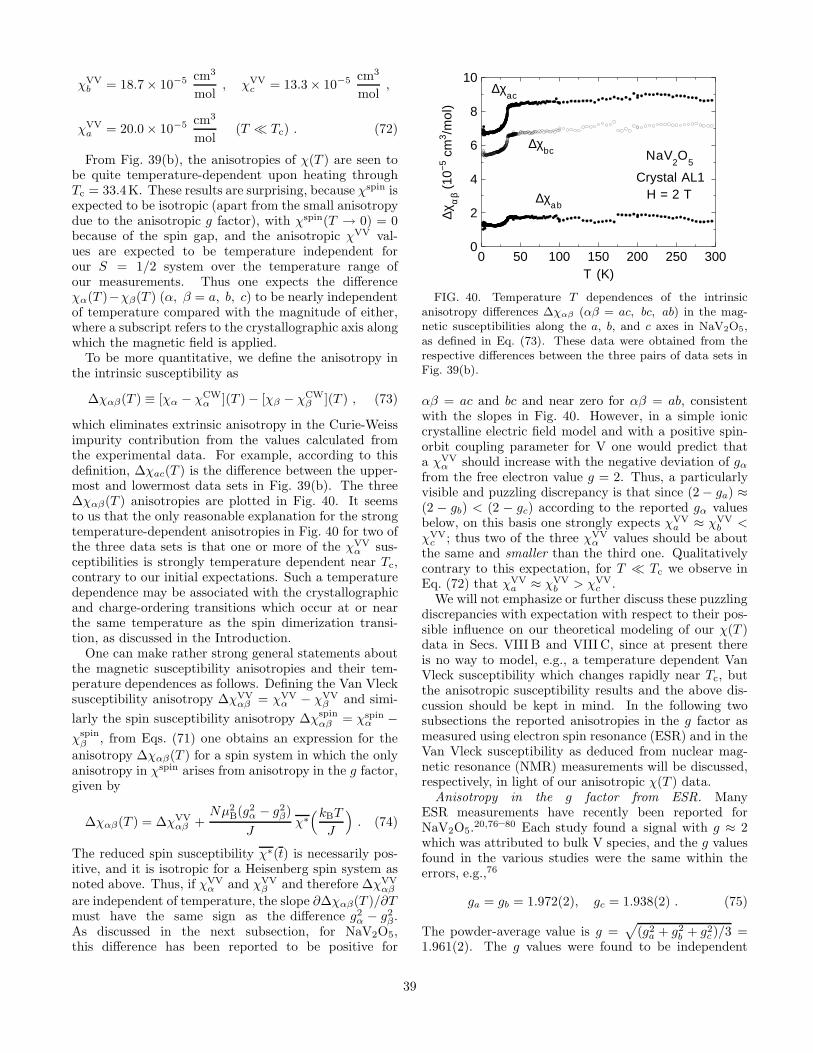
χVVb = 18.7 × 10−5 cm3

mol, χVV

c = 13.3 × 10−5 cm3

mol,

χVVa = 20.0 × 10−5 cm3

mol(T ≪ Tc) . (72)

From Fig. 39(b), the anisotropies of χ(T ) are seen tobe quite temperature-dependent upon heating throughTc = 33.4K. These results are surprising, because χspin isexpected to be isotropic (apart from the small anisotropydue to the anisotropic g factor), with χspin(T → 0) = 0because of the spin gap, and the anisotropic χVV val-ues are expected to be temperature independent forour S = 1/2 system over the temperature range ofour measurements. Thus one expects the differenceχα(T )−χβ(T ) (α, β = a, b, c) to be nearly independentof temperature compared with the magnitude of either,where a subscript refers to the crystallographic axis alongwhich the magnetic field is applied.

To be more quantitative, we define the anisotropy inthe intrinsic susceptibility as

∆χαβ(T ) ≡ [χα − χCWα ](T ) − [χβ − χCW

β ](T ) , (73)

which eliminates extrinsic anisotropy in the Curie-Weissimpurity contribution from the values calculated fromthe experimental data. For example, according to thisdefinition, ∆χac(T ) is the difference between the upper-most and lowermost data sets in Fig. 39(b). The three∆χαβ(T ) anisotropies are plotted in Fig. 40. It seemsto us that the only reasonable explanation for the strongtemperature-dependent anisotropies in Fig. 40 for two ofthe three data sets is that one or more of the χVV

α sus-ceptibilities is strongly temperature dependent near Tc,contrary to our initial expectations. Such a temperaturedependence may be associated with the crystallographicand charge-ordering transitions which occur at or nearthe same temperature as the spin dimerization transi-tion, as discussed in the Introduction.

One can make rather strong general statements aboutthe magnetic susceptibility anisotropies and their tem-perature dependences as follows. Defining the Van Vlecksusceptibility anisotropy ∆χVV

αβ = χVVα − χVV

β and simi-

larly the spin susceptibility anisotropy ∆χspinαβ = χspin

α −χspin

β , from Eqs. (71) one obtains an expression for the

anisotropy ∆χαβ(T ) for a spin system in which the onlyanisotropy in χspin arises from anisotropy in the g factor,given by

∆χαβ(T ) = ∆χVVαβ +

Nµ2B(g2

α − g2β)

Jχ∗

(kBT

J

)

. (74)

The reduced spin susceptibility χ∗(t) is necessarily pos-itive, and it is isotropic for a Heisenberg spin system asnoted above. Thus, if χVV

α and χVVβ and therefore ∆χVV

αβ

are independent of temperature, the slope ∂∆χαβ(T )/∂Tmust have the same sign as the difference g2

α − g2β.

As discussed in the next subsection, for NaV2O5,this difference has been reported to be positive for

0

2

4

6

8

10

0 50 100 150 200 250 300

∆χα

β (10

−5 c

m3 /m

ol)

T (K)

Crystal AL1

NaV2O

5

H = 2 T

∆χbc

∆χac

∆χab

FIG. 40. Temperature T dependences of the intrinsicanisotropy differences ∆χαβ (αβ = ac, bc, ab) in the mag-netic susceptibilities along the a, b, and c axes in NaV2O5,as defined in Eq. (73). These data were obtained from therespective differences between the three pairs of data sets inFig. 39(b).

αβ = ac and bc and near zero for αβ = ab, consistentwith the slopes in Fig. 40. However, in a simple ioniccrystalline electric field model and with a positive spin-orbit coupling parameter for V one would predict thata χVV

α should increase with the negative deviation of gα

from the free electron value g = 2. Thus, a particularlyvisible and puzzling discrepancy is that since (2 − ga) ≈(2 − gb) < (2 − gc) according to the reported gα valuesbelow, on this basis one strongly expects χVV

a ≈ χVVb <

χVVc ; thus two of the three χVV

α values should be aboutthe same and smaller than the third one. Qualitativelycontrary to this expectation, for T ≪ Tc we observe inEq. (72) that χVV

a ≈ χVVb > χVV

c .We will not emphasize or further discuss these puzzling

discrepancies with expectation with respect to their pos-sible influence on our theoretical modeling of our χ(T )data in Secs. VIII B and VIII C, since at present thereis no way to model, e.g., a temperature dependent VanVleck susceptibility which changes rapidly near Tc, butthe anisotropic susceptibility results and the above dis-cussion should be kept in mind. In the following twosubsections the reported anisotropies in the g factor asmeasured using electron spin resonance (ESR) and in theVan Vleck susceptibility as deduced from nuclear mag-netic resonance (NMR) measurements will be discussed,respectively, in light of our anisotropic χ(T ) data.

Anisotropy in the g factor from ESR. ManyESR measurements have recently been reported forNaV2O5.

20,76–80 Each study found a signal with g ≈ 2which was attributed to bulk V species, and the g valuesfound in the various studies were the same within theerrors, e.g.,76

ga = gb = 1.972(2), gc = 1.938(2) . (75)

The powder-average value is g =√

(g2a + g2

b + g2c )/3 =

1.961(2). The g values were found to be independent

39

of T down to 20K, which is below Tc. From all thesemeasurements, there is no indication that the S = 1/2Heisenberg Hamiltonian is not appropriate to the spinsystem in NaV2O5. Unfortunately, given the sensitivityof the ESR technique, we cannot be certain that theseESR results are representative of the bulk spin speciesin NaV2O5, because no quantitative measurements ofthe concentration of spin species observed in these mea-surements were reported. Although the (uncalibrated)ESR intensity versus temperature measurements approx-imately mirror the bulk susceptibility behavior in most(but not all) of these studies, it is still possible that thesignal arises from a minority spin species that is cou-pled to the bulk spin system. An interesting relatedissue which has not been discussed in the literature iswhy the presumed bulk S = 1/2 species in NaV2O5 areobservable to low temperatures T <∼ 0.03J/kB by ESR,where the AF exchange constant is J/kB ∼ 580K (seebelow), whereas the bulk Cu+2 spins 1/2 in the high-Tc

cuprates are not observable by ESR up to 1100K, whichis ≈ 0.7J/kB where J/kB ≈ 1600K is only a factor of 2.8larger.4

In Ref. 21 the authors estimated the χVV values us-ing the reported anisotropic g values obtained fromESR measurements, obtaining χVV

a = χVVb = 2.4 ×

10−5 cm3/mol and χVVc = 6.6 × 10−5 cm3/mol, which

were stated to be in agreement with the values from theirK-χ analysis discussed in the following subsection. Thesevalues do not agree with our T = 0 values in Eq. (72).In addition, from the χVV values of Ohama et al.,21 oneobtains ∆χVV

ca = ∆χVVcb = 4.2×10−5 cm3/mol, which are

similar in magnitude but opposite in sign to our data inEq. (72). If the strong change in each of ∆χac and ∆χbc

below Tc in Fig. 40 is due to a respective ∆χVVαβ which

is strongly temperature dependent in this temperaturerange, an effect similar to that reported to occur fromNMR measurements discussed in the next subsection, itis hard to understand why this change is not reflected ina distinct change in the reported temperature dependentanisotropy of the g values at Tc if these g-value measure-ments are recording the characteristics of the bulk phase.

Anisotropy in the Van Vleck susceptibility from NMR.

From a so-called K-χ analysis using NMR paramagneticnuclear resonance shift K(T ) data, combined with χ(T )measurements, under certain assumptions χVV can beobtained if K is proportional to χ, with T as an im-plicit parameter. In this way, χVV values have beenobtained by Ohama and coworkers for NaV2O5 using23Na (Ref. 81) and 51V (Ref. 21) NMR measurementson the same aligned powder sample. The former 23Nastudy yielded χVV

b = 23 × 10−5 cm3/mol below Tc and16×10−5 cm3/mol above Tc, corresponding to a decreaseof 7× 10−5 cm3/mol at Tc. Their low temperature valueis quite similar to our value in Eq. (72).

The 51V NMR study,21 carried out above Tc, yieldedχVV

b = 2(1) × 10−5 cm3/mol, roughly an order of mag-nitude smaller than obtained in the authors’ first study(no comment was made about this discrepancy), and in

addition gave χVVa = 1(1) × 10−5 cm3/mol and χVV

c =4(1) × 10−5 cm3/mol. These values are significantlysmaller than our values. We note that a K-χ anal-ysis on the d1 V+4 compound VO2 yielded χVV =6.5 × 10−5 cm3/mol.82

B. Modeling the susceptibility of NaV2O5 above Tc

Turning now to the experimental χ(T ) data in Fig. 38,we have T max ≈ 370K. Assuming the validity of theHamiltonian (1), Eq. (30a) for the uniform Heisenbergchain yields the exchange constant J/kB ≈ 580K. Thenthe gb value in Eq. (75) and our χ0 values at T = 0in Table VI below, together with Eqs. (31) and (71),predict that the measured χmax ∼ 40 × 10−5 cm3/mol,which is similar to the measured values of ≈ 44 and48 × 10−5 cm3/mol for the two crystals in Fig. 38, re-spectively. We therefore proceeded to try to fit the databy the uniform chain model. The “Fit”, shown as thesolid curve in Fig. 38, is a plot of Eqs. (71), with χ∗(t)being the susceptibility of the uniform chain (Fit 2 above)and with the parameters

χ0 = 8 × 10−5 cm3

mol, Cimp = 0,

(76)

g = 1.972 ,J

kB= 580 K . (“Fit”)

This “Fit” is not really a fit, since we just set the gand J values to those estimated above and then set χ0

so that the calculated curve is in the vicinity of thedata, because no small change in the parameters canbring the theory in agreement with the data. It is clearthat adjusting χ0 further will not improve the agree-ment, nor will including a nonzero impurity Curie con-stant Cimp. However, the shapes of the curve and thedata are similar, so the agreement can be improved con-siderably (not shown) by simultaneously decreasing χ0

to ≈ −10 × 10−5 cm3/mol, which is not possible physi-cally according to Eqs. (71) because it would require theVan Vleck susceptibility to be negative, and increasingg to the unphysically large value of ≈ 2.4, while keep-ing J constant. These results are in disagreement withthe conclusion of Isobe and Ueda who found that theBonner-Fisher prediction1 fitted their powder suscepti-bility data from 50 to 700K very well assuming g = 2.33

We can only note that their χ(T ) data have not beenquantitatively reproduced in either their31,74 or others’subsequent measurements on NaV2O5, including ours,and that the Bonner-Fisher prediction is not accurate attemperatures below ∼ J/(4kB) ≈ 145K as discussed inthe Introduction.

Lohmann et al.77 and Hemberger et al.79 also previ-ously concluded that the χ(T ) of NaV2O5 is not de-scribed (below 250K) by the prediction for the S = 1/2

40

Heisenberg chain, based on their fits by the Bonner-Fisher prediction1 to their χ(T ) deduced from ESR mea-surements up to 650K. They suggested that additionalexchange couplings may be required to explain the ob-served χ(T ). We consider this possibility here by mod-eling the influence of possible interchain spin coupling.Because there are no accurate and generally applicablenumerical calculations for this case that we are awareof, we utilize the following simple molecular field theory(MFT) prediction for the spin susceptibility4,14

1

χ∗(t)=

1

χ∗

chain(t)+

z′J ′

J, (77)

where χ∗

chain(t) is the reduced spin susceptibility of theisolated quantum S = 1/2 uniform Heisenberg chain (ourFit 2 above). The parameter z′ is the effective number ofspins on other chains to which a spin in a given chain iscoupled with effective (or average) exchange constant J ′.To be consistent with our sign convention for the intra-chain exchange constant J , J ′ is positive for AF interac-tions and negative for ferromagnetic (FM) interactions.Equation (77) is very accurate when |z′J ′/J | ≪ 1.4,14

We fitted the χ(T ) data above 50K for the two crys-tals in Fig. 38 by Eqs. (71) and (77), where we fixedgb = 1.972 and Cimp = 0 and allowed χ0, J and the prod-uct z′J ′ to vary. Very good fits were obtained, for whichthe fitting parameters are given in Table V. The fits areplotted as the solid curves in Fig. 41. For the parame-ters of the two crystals taken together, the fitted J/kB

= 584(9)K is the same as deduced above (580K) fromthe temperature of the maximum in χ(T ), and the fittedχ0 = 1.4(16)× 10−5 cm3/mol is similar to our results atlow temperatures in Fig. 39(b). A moderately large andnegative (FM) interchain coupling z′J ′/J = −1.26(5)was obtained. This coupling is sufficiently strong thatlong-range magnetic ordering might be expected, butwhich is not observed, possibly due to magnetic frustra-tion effects. If the present mean-field interchain couplinganalysis is correct, this interchain coupling should be ev-ident in the magnon dispersion relations observable byinelastic magnetic neutron scattering measurements. In-deed, moderately strong dispersions of 1.4meV in each oftwo bands perpendicular to the chains have in fact beenobserved by Yosihama et al.83 in such measurements onsingle crystals. It remains to be seen whether the mag-nitude and sign of the interchain exchange coupling thatwe infer in the mean-field analysis are consistent with thedispersion relations deduced from the neutron scatteringdata.

An alternative and/or additional mechanism whichcan produce a strong deviation of the measured χ(T )of a uniform chain compound from that predicted forHeisenberg uniform and alternating chains is the spin-phonon interaction.54–56,84–86 At low T this interactioncan lead to a spin-Peierls transition and can stronglymodify χ(T ) above Tc from that expected for the Heisen-berg chain.54,56 Sandvik, Singh, and Campbell carried

0

10

20

30

40

50

0 100 200 300 400 500 600 700 800

χ (1

0−5 c

m3 /m

ol)

T (K)

NaV2O

5 Crystals


E083EF

E106EMFT Fits50-750 K

FIG. 41. Fits of the magnetic susceptibility χ vs temper-ature T from 50K to 750 K for the two crystals in Fig. 38by Eqs. (71) with Cimp = 0, g = 1.972 and the spin suscep-tibility χspin given by the molecular field theory (MFT) pre-diction (77) for coupled quantum S = 1/2 uniform Heisenberchains. The fits are shown as the solid curves and the fit pa-rameters are given in Table V. The fits overlap the data sothey are difficult to see; consequently they have been extrap-olated to higher and lower temperatures to show where theyare.

out a detailed QMC investigation of a spin-Peierls modelin which the spin 1/2 interactions were modified by thepresence of dynamical (quantum mechanical) dispersion-less Einstein phonons.54 For particular values of the spin-phonon coupling constant and phonon frequency, theyfound that the effective exchange constant Jeff decreasesstrongly with increasing T , and at T = 0 is about 27.3%larger than the bare J . Perhaps surprisingly, they foundhowever that if the bare g factor is reduced by ≈ 7%and the bare J by ≈ 18% in the χ∗(t) predicted for theHeisenberg model, this model was then in good agree-ment with their QMC simulations for temperatures aboveTc. A recent important extensive study of many finite-temperature properties of the same model using QMCsimulations was carried out by Kuhne and Low.56 Theyfound that for not too low temperatures, the suscepti-bilities for various Einstein phonon frequencies and spin-phonon coupling constants can all be scaled onto a uni-versal curve, given by that for the uniform Heisenbergchain, using only a suitably defined effective exchangeconstant Jeff > J . Contrary to the result of Ref. 54, theyfound that a rescaling of the g factor was not necessary.

TABLE V. Fit parameters for the magnetic susceptibilityof two NaV2O5 crystals according to Eq. (71) with Cimp = 0,g = 1.972 and the spin susceptibility χspin given by the molec-ular field theory expression (77) for coupled quantum S = 1/2uniform Heisenberg chains.

χ0 J/kB z′J ′/J

crystal(

10−5 cm3

mol

)

(K)

E083EF +2.8(2) 577(2) −1.28(3)E106E −0.1(1) 592(1) −1.23(2)

41

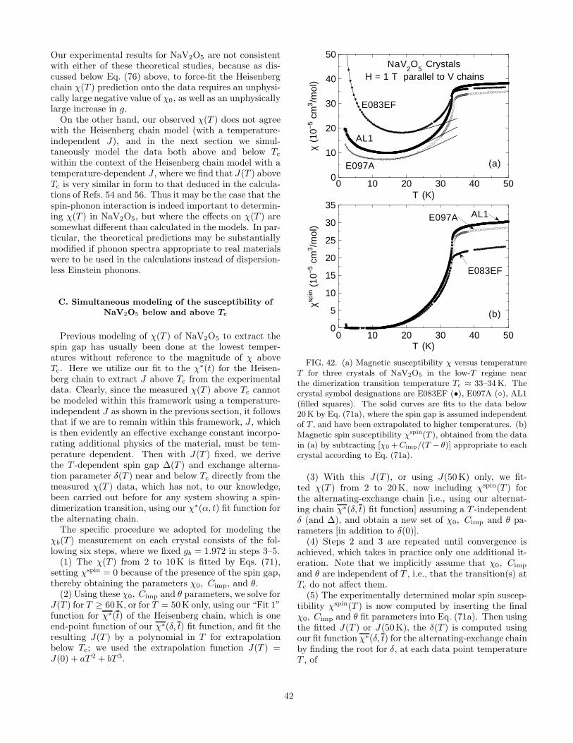
Our experimental results for NaV2O5 are not consistentwith either of these theoretical studies, because as dis-cussed below Eq. (76) above, to force-fit the Heisenbergchain χ(T ) prediction onto the data requires an unphysi-cally large negative value of χ0, as well as an unphysicallylarge increase in g.

On the other hand, our observed χ(T ) does not agreewith the Heisenberg chain model (with a temperature-independent J), and in the next section we simul-taneously model the data both above and below Tc

within the context of the Heisenberg chain model with atemperature-dependent J , where we find that J(T ) aboveTc is very similar in form to that deduced in the calcula-tions of Refs. 54 and 56. Thus it may be the case that thespin-phonon interaction is indeed important to determin-ing χ(T ) in NaV2O5, but where the effects on χ(T ) aresomewhat different than calculated in the models. In par-ticular, the theoretical predictions may be substantiallymodified if phonon spectra appropriate to real materialswere to be used in the calculations instead of dispersion-less Einstein phonons.

C. Simultaneous modeling of the susceptibility ofNaV2O5 below and above Tc

Previous modeling of χ(T ) of NaV2O5 to extract thespin gap has usually been done at the lowest temper-atures without reference to the magnitude of χ aboveTc. Here we utilize our fit to the χ∗(t) for the Heisen-berg chain to extract J above Tc from the experimentaldata. Clearly, since the measured χ(T ) above Tc cannotbe modeled within this framework using a temperature-independent J as shown in the previous section, it followsthat if we are to remain within this framework, J , whichis then evidently an effective exchange constant incorpo-rating additional physics of the material, must be tem-perature dependent. Then with J(T ) fixed, we derivethe T -dependent spin gap ∆(T ) and exchange alterna-tion parameter δ(T ) near and below Tc directly from themeasured χ(T ) data, which has not, to our knowledge,been carried out before for any system showing a spin-dimerization transition, using our χ∗(α, t) fit function forthe alternating chain.

The specific procedure we adopted for modeling theχb(T ) measurement on each crystal consists of the fol-lowing six steps, where we fixed gb = 1.972 in steps 3–5.

(1) The χ(T ) from 2 to 10K is fitted by Eqs. (71),setting χspin = 0 because of the presence of the spin gap,thereby obtaining the parameters χ0, Cimp, and θ.

(2) Using these χ0, Cimp and θ parameters, we solve forJ(T ) for T ≥ 60K, or for T = 50K only, using our “Fit 1”function for χ∗(t) of the Heisenberg chain, which is oneend-point function of our χ∗(δ, t) fit function, and fit theresulting J(T ) by a polynomial in T for extrapolationbelow Tc; we used the extrapolation function J(T ) =J(0) + aT 2 + bT 3.

0

10

20

30

40

50

0 10 20 30 40 50

χ (1

0−5 c

m3/m

ol)

T (K)

NaV2O

5 Crystals

(a)


E083EF

AL1

E097A

0

5

10

15

20

25

30

35

0 10 20 30 40 50

χspin (

10−5

cm

3/m

ol)

T (K)

(b)

AL1E097A

E083EF

FIG. 42. (a) Magnetic susceptibility χ versus temperatureT for three crystals of NaV2O5 in the low-T regime nearthe dimerization transition temperature Tc ≈ 33–34 K. Thecrystal symbol designations are E083EF (•), E097A (◦), AL1(filled squares). The solid curves are fits to the data below20K by Eq. (71a), where the spin gap is assumed independentof T , and have been extrapolated to higher temperatures. (b)Magnetic spin susceptibility χspin(T ), obtained from the datain (a) by subtracting [χ0 + Cimp/(T − θ)] appropriate to eachcrystal according to Eq. (71a).

(3) With this J(T ), or using J(50K) only, we fit-ted χ(T ) from 2 to 20K, now including χspin(T ) forthe alternating-exchange chain [i.e., using our alternat-ing chain χ∗(δ, t) fit function] assuming a T -independentδ (and ∆), and obtain a new set of χ0, Cimp and θ pa-rameters [in addition to δ(0)].

(4) Steps 2 and 3 are repeated until convergence isachieved, which takes in practice only one additional it-eration. Note that we implicitly assume that χ0, Cimp

and θ are independent of T , i.e., that the transition(s) atTc do not affect them.

(5) The experimentally determined molar spin suscep-tibility χspin(T ) is now computed by inserting the finalχ0, Cimp and θ fit parameters into Eq. (71a). Then usingthe fitted J(T ) or J(50K), the δ(T ) is computed usingour fit function χ∗(δ, t) for the alternating-exchange chainby finding the root for δ, at each data point temperatureT , of

42

450

500

550

600

650

700

750

0 50 100 150 200 250 300

J/k B

(K

)

T (K)

NaV2O

5 Crystals E083EF

E097AAL1

FIG. 43. Exchange constant J versus temperature T forthe three crystals of NaV2O5 in Fig. 42 in the temperatureregime T ≥ 60K which is above the dimerization temperatureTc ≈ 34K. The solid curves are polynomial fits to the databetween 60 and 150 K for the respective samples, which areextrapolated to T = 0 as shown.

χspinb (T ) =

NAg2bµ2

B

Jb(T )χ∗

[

δ,kBT

Jb(T )

]

. (78)

(6) In a separate step not associated with the fitting pro-cedure in steps 1–5, the spin gap ∆(T ) is computed fromδ(T ) determined in step 5 using an independently knownfunction ∆∗(δ) ≡ ∆(δ)/J and our J(T ) or J(50K). Weused our ∆∗(δ) fit function in Eqs. (63) for this purpose.

We measured χb(T ) for nine different crystals from fourdifferent batches of NaV2O5 and now present illustrativeresults obtained in each of the above modeling steps2 to 4 (final iteration), 5 and 6 for three representativecrystals. We will follow in graphical form the data mod-eling through successive steps for these three crystals toshow how differences in one property between the crys-tals may or may not propagate through the next step(s)

TABLE VI. Fitted parameters in Eqs. (71), using the χ∗(α, t) fit function (50) for the alternating-exchange chain, obtainedby fitting the χ(T ) data in the range 2–20 K for nine crystals of NaV2O5, for an assumed g factor of 1.972. If an arror bar isnot given for J(0), this value is J(50 K) which was determined from a single data point near 50 K. The spin gap ∆(0) is not afitted parameter, but is rather computed from the fitted alternation parameter δ(0) using Eqs. (63). Similarly, the alternationparameter α(0) is computed from δ(0) using Eq. (14b). Note that all three measurements for crystal AL1 were carried out ina field of 2T, whereas all the other crystals were measured in a field of 1T.

Crystal χ0 Cimp −θ J(0)/kB δ(0) α(0) ∆(0)/kB(

10−5 cm3

mol

) (

10−3 cm3 Kmol

)

(K) (K) (K)

E082E 6.82(4) 1.123(5) 0.46(1) 710(4) 0.0287(2) 0.9442(4) 101.1(10)E083B 4.56(9) 0.81(1) 0.30(5) 654(3) 0.0327(3) 0.9366(6) 102.6(13)E083EF 11.2(1) 1.11(1) 0.43(4) 723(2) 0.0279(4) 0.9458(8) 100.8(14)E083G 6.55(3) 1.112(3) 0.45(1) 688 0.0298(1) 0.9421(2) 100.7(2)E083H 4.24(3) 0.780(3) 0.33(1) 650 0.0332(2) 0.9357(4) 102.9(5)E083I 4.18(6) 0.946(7) 0.32(2) 657 0.0329(4) 0.9363(8) 103.3(9)E097A 5.92(3) 0.170(3) 0.25(4) 589(2) 0.0389(2) 0.9251(4) 104.6(6)E106E 5.67(8) 0.134(8) 0.31(1) 662(2) 0.0332(5) 0.9358(9) 104.8(13)AL1 (H ||a) 12.22(6) 0.221(7) 0.46(6) 598(1) 0.0366(3) 0.9294(6) 101.5(8)AL1 (H ||b) 10.94(6) 0.240(7) 0.46(6) 607(1) 0.0352(3) 0.9320(6) 100.4(8)AL1 (H ||c) 5.49(7) 0.298(8) 0.75(7) 635(1) 0.0337(4) 0.9348(7) 101.7(9)

of the analysis, but we present the fitting parameters forall of the crystals in Table VI.

The measured χ(T ) data below 50K for the three crys-tals are shown in Fig. 42(a), where the fits below 20K instep 4 are shown as the solid curves with parameters inTable VI. Crystals E097A and AL1 are seen to have muchlower levels of paramagnetic impurities than E083EF, asreflected in the impurity Curie constant, i.e., the magni-tude of the impurity Curie-Weiss upturn at low T . Bysubtracting the χ0 and impurity Curie-Weiss terms fromthe data, the spin susceptibility χspin(T ) is obtained foreach crystal as shown in Fig. 42(b). These data showgood consistency below Tc for the three crystals, despitethe differences in the χ0 values, the magnitudes of theCurie-Weiss impurity term and in the χ(T ) above Tc.The J(T ) determined for the three crystals in step 2 areshown up to 300K in Fig. 43. J is found to decreaseby ∼ 10–20% upon increasing T from 60 to 300K, whichwhen T is scaled by J is similar to the fractional decreasepredicted by Sandvik et al.54 due to the spin-phonon in-teraction. It is noteworthy that crystal E083EF, with byfar the highest level of paramagnetic defects and/or im-purities, also has the largest J(T ) and the largest changein J with T .

Figures 44(a) and 44(b) show the spin dimerization pa-rameter δ(T ) and spin gap ∆(T ) determined for each ofthe three crystals in the final modeling steps 5 and 6,respectively. Several features of these data are of note.First, there is a rather large variation in the dimeriza-tion parameter, δ(0) = 0.028–0.040, between the threecrystals, despite the fact that Tc = 33–34K is nearly thesame for the different crystals; the most impure crystalE083EF has the smallest δ(0), as might have been ex-pected. Despite this variability, these δ(0) values are allsignificantly smaller than the three values reported forvarious samples by different groups as determined usingdifferent techniques, which are listed in Table VII along

43

0.00

0.01

0.02

0.03

0.04

15 20 25 30 35 40 45 50

Alte

rnat

ion

Par

amet

er δ

T (K)

NaV2O

5 Crystals

(a)

E083EF

AL1

E097A

0

20

40

60

80

100

120

15 20 25 30 35 40 45 50

∆ /k B

(K

)

T (K)

(b)

E083EFAL1

E097A

FIG. 44. Alternation parameter δ (a) and spin gap ∆ (b)versus temperature T below 50 K for the three crystals ofNaV2O5 in Fig. 42. The nonzero δ and ∆ above the tran-sition temperature ∼ 33–34 K are presumed to arise fromspin dimerization fluctuations and concurrent spin gap fluc-tuations, respectively.

with other related information.22,27,33,36,37,40,57,76–79,81,87–89 On the other hand, the

TABLE VII. Exchange constant J , spin gap ∆, and alternation parameter δ for NaV2O5 at the temperature(s) T asdetermined by the listed method for the sample with transition temperature Tc. The literature reference is given in the lastcolumn. Method abbreviations: χ, magnetic susceptibility; Neutrons, neutron scattering; NMR, nuclear magnetic resonance;ESR, electron spin resonance; Cp, specific heat; Raman, Raman light scattering.

sample Tc (K) J/kB (K) T (K) ∆/kB (K) δ Method Ref.

Powder none 529 350 χ 87Powder 33.9 560 35–700 χ 33Powder 35.3 7 114 Neutrons 36Aligned powder 10–20 98 23Na NMR 81Crystals 33 441 2–30 85(15) χ 37Crystal 35 560 2–34 92(20) 0.10(2) ESR, χ 76Crystal 33.5 560 15–30 100(2) 0.107 ESR 77Crystal 34 578 250–650 100 ESR, χ 79Crystal 32.7,33.0 1.8–12 84(10) Cp 40Crystal 5 88(2) Raman 27Crystal 35 10–35 85(20) ESR 78Crystal 34 455 15 0.047 Raman 57Crystal 4.2 94 ESR 88Crystals 33 7–15 67(5) Cp 89Aligned powder 34.0 11–20 108 51V NMR 22Powder 34.0 491 4–30 77 χ 20

corresponding range of ∆(0)/kB = 103(2)K for the threecrystals is fractionally much smaller than that of δ(0).We infer that some of the discrepancies between the ∆(0)values in Table VII reported for NaV2O5 by differentgroups may arise from differences in, e.g., the types ofmeasurements which are used to determine ∆(0) and inthe different analyses of those data, rather than fromdifferent ∆(0) values in the samples. The variability inδ(0) between the crystals in Fig. 44(a), compared withthe lack of much variability in ∆(0) in Fig. 44(b), evi-dently arises because δ must be combined with J to ob-tain ∆, and the variations in the first two parametersmust largely cancel. Thus, not surprisingly, the low-Tχspin(T ) is governed by the spin gap ∆ and not by δ orJ separately.

The δ(T ) data for our best crystals show very sharp,nearly vertical increases with decreasing T at Tc. We can-not extract a precise critical exponent β from our δ(T )data due to the large temperature-dependent backgroundabove Tc, to be discussed shortly. However, rough fits be-low Tc by the expression δ(T ) ∼ (1−T/Tc)

β gave β valuesconsistent with the values β = 0.25(10) (Ref. 90) from in-frared reflectivity measurements, 0.34(8) (Ref. 91) fromsound velocity measurements along the chain axis and0.35(8) (Ref. 40) from thermal expansion measurementsalong that axis. We note that these values are a factorof two larger than the value of ∼ 0.15 (Ref. 92) inferredfrom x-ray diffuse scattering measurements.

The data in Figs. 44(a) and 44(b) clearly show the exis-tence of spin dimerization fluctuations and a spin pseudo-gap above Tc for each crystal, respectively, irrespectiveof the crystal quality as judging from the Curie-Weissimpurity term in the low-T χ(T ), with magnitudes justabove Tc of about 20% and 40% of δ(0) and ∆(0),respectively. This is a robust result, which was obtained

44

for each of the nine crystals we measured, which doesnot depend on the precise value of J [and resultantχspin(T, δ = 0)] or the details of how J is determinedabove Tc, or even on the detailed formulation of theχ∗(α, t) fit function for the alternating-exchange chain.For example, setting J to be a constant, equal to thevalue at 50K, yields nearly the same ∆(T ) near Tc as de-termined using a T -dependent J . Similarly, deleting theimpurity Curie-Weiss term in the fit to the data above Tc

changes the derived χ0 and J(T ) or J(50K) somewhatas well as the detailed temperature dependence of thepseudogap ∆(T ) above Tc but has little influence on themagnitude of ∆ near Tc. Further, in a previous version ofthe QMC and TMRG χ∗(α, t) fit function (not otherwisediscussed in this paper), we did not enforce the require-ment (iii) in Sec. IVE that the transformed χ∗(δ, t) sat-isfy ∂χ∗(δ, t)/∂δ|δ=0 = 0, and the same fluctuation effectsabove Tc were found using that fit function as using thepresent one, although these fluctuations were somewhatreduced in magnitude compared to the present results.Finally, these fluctuations are observable directly in themeasured χ(T ) data in Fig. 42(a) as a rounding of thesusceptibility curves above Tc.

From Fig. 44, the fluctuation effects persist up to hightemperatures T > 50K, although the fluctuation am-plitudes decrease with increasing T . Precursor effectsabove Tc have been reported in x-ray diffuse scatter-ing measurements92 up to ∼ 90K, in ultrasonic soundvelocity91 and optical absorption24,25,93 measurementsup to ∼ 70K, and in specific heat measurements79,94 upto ∼ 40–50K, so it is not surprising that spin dimer-ization parameter fluctuations in Fig. 44(a), and a spinpseudogap in Fig. 44(b) reflecting fluctuations in the spingap, are found above Tc.

D. Specific heat of NaV2O5

In order to correlate the magnetic effects discussedabove in NaV2O5 with thermal effects, we have carriedout specific heat vs temperature Cp(T ) measurements onthe same crystal AL1, and a crystal E097 from the samebatch as E097A, for which χ(T ) data were presented andmodeled above. The results from 2 K to 50K for crystalsE097 and AL1 are shown in Fig. 45(a). Over this tem-perature range, the Cp(T ) data for the two crystals agreeextremely well, except in the range 33.0–34.2K, i.e., inthe vicinity of the transitions as will be discussed shortly.The shapes of the specific heat anomalies at Tc are notmean-field-like specific heat jumps as observed in, e.g.,conventional superconductors, but instead are λ-shapedanomalies. Thus, any attempt to define a (mean-field)“specific heat jump at Tc” is fraught with ambiguity.These shapes are retained in plots of Cp(T )/T vs T asshown in Fig. 46(a). This λ shape has been observedpreviously, and variously attributed to fluctuation effectsor a possible smeared-out first order transition. In view

10

15

20

25

30

35

40

32.0 32.5 33.0 33.5 34.0 34.5 35.0C

p (J/

mol

K)

T (K)

AL1

E097

(b)

0

5

10

15

20

25

30

35

40

0 10 20 30 40 50

Cp (

J/m

ol K

)

T (K)

NaV2O

5 Crystals

AL1

E097

(a)

0

20

40

60

80

100

32.0 32.5 33.0 33.5 34.0 34.5 35.0

d(χ

T)/

dT (

10−4

cm

3 /mol

)

T (K)

AL1

E097A

(c)E106E

FIG. 45. (a) Specific heat Cp vs temperature T for NaV2O5

crystals E097 and AL1. (b) Expanded plots of the data in thevicinity of the transition temperatures of the two crystals. (c)Temperature derivative of χT vs T for the same crystal AL1as in (a) and (b) plus data for crystals E097A (from the samebatch as E097) and E106E. The lines connecting the datapoints are guides to the eye.

of the coupled structural, charge-ordering and spindimerization transitions at Tc in NaV2O5 as discussedin the Introduction, their relative contributions to thespecific heat anomalies are not clear, if indeed their con-tributions can be uniquely distinguished.

Expanded plots of Cp(T ) and Cp(T )/T versus T ,shown in Figs. 45(b) and 46(b), respectively, reveal asharp high peak at 33.4K for crystal AL1, which isslightly split by ≈ 0.1K in spite of the fact that theoverall height of the anomaly is much larger than pre-

45

400

500

600

700

800

900

1000

1100

30 31 32 33 34 35 36

Cp/T

(m

J/m

ol K

2 )

T (K)

AL1

E097

(b)

0

200

400

600

800

1000

0 10 20 30 40 50

Cp/T

(m

J/m

ol K

2 )

T (K)

NaV2O

5 Crystals

AL1

E097

(a)

FIG. 46. (a) Specific heat Cp divided by temperature Tversus T for NaV2O5 crystals E097 and AL1. (b) Expandedplots of the data in the vicinity of the transition temperaturesof the two crystals. The lines connecting the data points forcrystal AL1 are guides to the eye.

viously reported for any crystal of NaV2O5. Two peaksare also observed for crystal E097, at 33.4K and 33.8K,which are more widely separated than for crystal AL1.From Fig. 46(b), the entropy under the anomaly(ies) foreach crystal is about the same (see below). Comparingthese results with the δ(T ) and ∆(T ) data in Fig. 44,the larger splitting of the Cp(T ) peak for crystal E097does not result in any major difference in the magneticorder parameter properties between the two crystals, al-though the transition onset is slightly rounded for crystalE097A compared to AL1. By using the Fisher relation,50

∂[χ(T )T ]/∂T ∼ C(T ) where C(T ) is the magnetic con-tribution to the specific heat, one obtains results whichshow the same features near Tc as does the specific heat,as shown in Fig. 45(c). Thus, careful scrutiny of the mag-netic properties can reveal the fine detail observed in thespecific heat near Tc. In particular, this comparison sug-gests that both anomalies in the specific heat near Tc

for each crystal are associated with and/or reflected bymagnetic effects.

The splitting of the transition into two apparent transi-tions that we report here was previously observed in ther-mal expansion, but not seen in their specific heat, mea-surements of a crystal by Koppen et al.40 The detailedorigin of the transition splitting, and more fundamentally

whether the splitting is instrinsic to ideal crystallograph-ically ordered NaV2O5, remain to be clarified. An essen-tial feature that any explanation must account for is thatthe temperature splitting between the two transitions ina crystal varies from crystal to crystal.

Modeling. In this section we will only consider themodel utilized above for analyzing our χ(T ) data, inwhich NaV2O5 consists, effectively, of isolated S = 1/2uniform or (below Tc) alternating-exchange Heisenbergchains, where the (average) exchange constant J shows,at most, only a smooth and relatively small change belowTc. For reasons which will become clear below, unfortu-nately we cannot use our specific heat data to extractdetailed information about the magnetic subsystem inNaV2O5. However, other types of important informationabout the thermodynamics will be derived using variousof the theoretical results presented and discussed previ-ously in this paper.

There have been two reports40,89 deriving the spingap from Cp(T ) data at T <∼ 15K. We first discussthe limits of this type of analysis. Using J(0)/kB =600K, δ(0) = 0.040, and ∆/kB = 100K (see Table VI),Eqs. (29b) and (29c) predict that the magnetic specificheat C(T ) in the dimerized phase at low temperaturesT ≪ (∆/kB, Tc) is

C(T ) = 1.0J

mol K

(100

T

)3/2

×[

1 +T

100+

3

4

( T

100

)2]

e−100/T , (79)

with T in units of K. Equation (79) predicts thatC(15 K) = 0.026J/molK, which is about 40 timessmaller than the observed Cp(15 K) ≈ 1 J/molK (whichmust therefore be due to the lattice contribution) andhence is unresolvable at such low temperatures. Withinthis model, we must therefore conclude that the previ-ous estimates of the spin gap based upon modeling thelow temperature specific heat were most likely artifactsof modeling the lattice specific heat. This can happenif one does not utilize the fact that the prefactor to theactivated exponential term of the magnetic contributionC(T ) is not an independently adjustable parameter, butis rather determined by the spin gap itself as we havepreviously demonstrated and emphasized in Sec. II C 3.

A related question is whether the entropy associatedwith the transition(s) at Tc can be associated solely withthe magnetic subsystem. The minimum possible esti-mate of the entropy of the transition is obtained from theCp(T )/T vs T data in Fig. 46(b) by drawing a horizontalline from the data at the Cp(T )/T minimum at ≈ 35.0K,just above Tc, to the data that the line intersects withbelow Tc at ≈ 30.6K, and then computing the area be-tween the line and the peak(s) above the line. In thisway we obtain a value of 0.397 J/molK for crystal E097and 0.375 J/molK for crystal AL1. On the other hand,the maximum magnetic entropy of the S = 1/2 uniformchain subsystem at Tc, using rough values J/kB = 600K

46

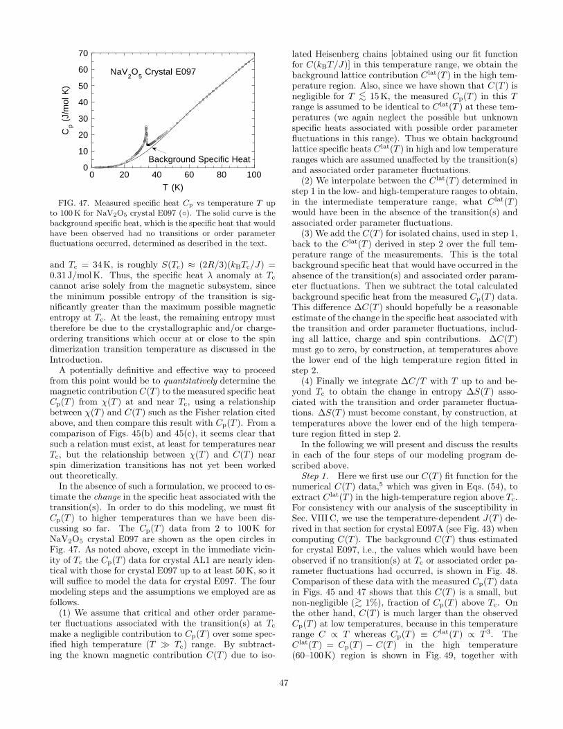
0

10

20

30

40

50

60

70

0 20 40 60 80 100

Cp (

J/m

ol K

)

T (K)

NaV2O

5 Crystal E097

Background Specific Heat

FIG. 47. Measured specific heat Cp vs temperature T upto 100 K for NaV2O5 crystal E097 (◦). The solid curve is thebackground specific heat, which is the specific heat that wouldhave been observed had no transitions or order parameterfluctuations occurred, determined as described in the text.

and Tc = 34K, is roughly S(Tc) ≈ (2R/3)(kBTc/J) =0.31J/molK. Thus, the specific heat λ anomaly at Tc

cannot arise solely from the magnetic subsystem, sincethe minimum possible entropy of the transition is sig-nificantly greater than the maximum possible magneticentropy at Tc. At the least, the remaining entropy musttherefore be due to the crystallographic and/or charge-ordering transitions which occur at or close to the spindimerization transition temperature as discussed in theIntroduction.

A potentially definitive and effective way to proceedfrom this point would be to quantitatively determine themagnetic contribution C(T ) to the measured specific heatCp(T ) from χ(T ) at and near Tc, using a relationshipbetween χ(T ) and C(T ) such as the Fisher relation citedabove, and then compare this result with Cp(T ). From acomparison of Figs. 45(b) and 45(c), it seems clear thatsuch a relation must exist, at least for temperatures nearTc, but the relationship between χ(T ) and C(T ) nearspin dimerization transitions has not yet been workedout theoretically.

In the absence of such a formulation, we proceed to es-timate the change in the specific heat associated with thetransition(s). In order to do this modeling, we must fitCp(T ) to higher temperatures than we have been dis-cussing so far. The Cp(T ) data from 2 to 100K forNaV2O5 crystal E097 are shown as the open circles inFig. 47. As noted above, except in the immediate vicin-ity of Tc the Cp(T ) data for crystal AL1 are nearly iden-tical with those for crystal E097 up to at least 50K, so itwill suffice to model the data for crystal E097. The fourmodeling steps and the assumptions we employed are asfollows.

(1) We assume that critical and other order parame-ter fluctuations associated with the transition(s) at Tc

make a negligible contribution to Cp(T ) over some spec-ified high temperature (T ≫ Tc) range. By subtract-ing the known magnetic contribution C(T ) due to iso-

lated Heisenberg chains [obtained using our fit functionfor C(kBT/J)] in this temperature range, we obtain thebackground lattice contribution C lat(T ) in the high tem-perature region. Also, since we have shown that C(T ) isnegligible for T <∼ 15K, the measured Cp(T ) in this Trange is assumed to be identical to C lat(T ) at these tem-peratures (we again neglect the possible but unknownspecific heats associated with possible order parameterfluctuations in this range). Thus we obtain backgroundlattice specific heats C lat(T ) in high and low temperatureranges which are assumed unaffected by the transition(s)and associated order parameter fluctuations.

(2) We interpolate between the C lat(T ) determined instep 1 in the low- and high-temperature ranges to obtain,in the intermediate temperature range, what C lat(T )would have been in the absence of the transition(s) andassociated order parameter fluctuations.

(3) We add the C(T ) for isolated chains, used in step 1,back to the C lat(T ) derived in step 2 over the full tem-perature range of the measurements. This is the totalbackground specific heat that would have occurred in theabsence of the transition(s) and associated order param-eter fluctuations. Then we subtract the total calculatedbackground specific heat from the measured Cp(T ) data.This difference ∆C(T ) should hopefully be a reasonableestimate of the change in the specific heat associated withthe transition and order parameter fluctuations, includ-ing all lattice, charge and spin contributions. ∆C(T )must go to zero, by construction, at temperatures abovethe lower end of the high temperature region fitted instep 2.

(4) Finally we integrate ∆C/T with T up to and be-yond Tc to obtain the change in entropy ∆S(T ) asso-ciated with the transition and order parameter fluctua-tions. ∆S(T ) must become constant, by construction, attemperatures above the lower end of the high tempera-ture region fitted in step 2.

In the following we will present and discuss the resultsin each of the four steps of our modeling program de-scribed above.

Step 1. Here we first use our C(T ) fit function for thenumerical C(T ) data,5 which was given in Eqs. (54), toextract C lat(T ) in the high-temperature region above Tc.For consistency with our analysis of the susceptibility inSec. VIII C, we use the temperature-dependent J(T ) de-rived in that section for crystal E097A (see Fig. 43) whencomputing C(T ). The background C(T ) thus estimatedfor crystal E097, i.e., the values which would have beenobserved if no transition(s) at Tc or associated order pa-rameter fluctuations had occurred, is shown in Fig. 48.Comparison of these data with the measured Cp(T ) datain Figs. 45 and 47 shows that this C(T ) is a small, butnon-negligible (>∼ 1%), fraction of Cp(T ) above Tc. Onthe other hand, C(T ) is much larger than the observedCp(T ) at low temperatures, because in this temperaturerange C ∝ T whereas Cp(T ) ≡ C lat(T ) ∝ T 3. TheC lat(T ) = Cp(T ) − C(T ) in the high temperature(60–100K) region is shown in Fig. 49, together with

47

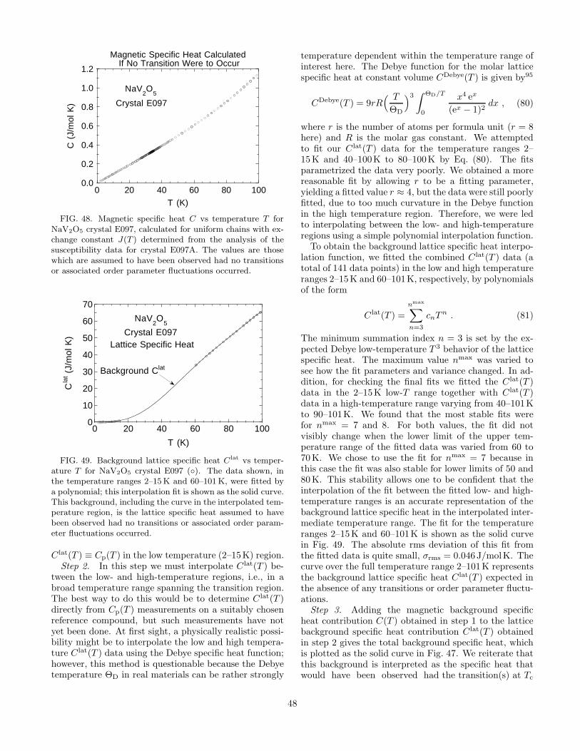
0.0

0.2

0.4

0.6

0.8

1.0

1.2

0 20 40 60 80 100

C (

J/m

ol K

)

T (K)

NaV2O

5

Crystal E097

Magnetic Specific Heat Calculated If No Transition Were to Occur

FIG. 48. Magnetic specific heat C vs temperature T forNaV2O5 crystal E097, calculated for uniform chains with ex-change constant J(T ) determined from the analysis of thesusceptibility data for crystal E097A. The values are thosewhich are assumed to have been observed had no transitionsor associated order parameter fluctuations occurred.

0

10

20

30

40

50

60

70

0 20 40 60 80 100

Cla

t (J/

mol

K)

T (K)

NaV2O

5

Crystal E097Lattice Specific Heat

Background Clat

FIG. 49. Background lattice specific heat Clat vs temper-ature T for NaV2O5 crystal E097 (◦). The data shown, inthe temperature ranges 2–15 K and 60–101 K, were fitted bya polynomial; this interpolation fit is shown as the solid curve.This background, including the curve in the interpolated tem-perature region, is the lattice specific heat assumed to havebeen observed had no transitions or associated order param-eter fluctuations occurred.

C lat(T ) ≡ Cp(T ) in the low temperature (2–15K) region.Step 2. In this step we must interpolate C lat(T ) be-

tween the low- and high-temperature regions, i.e., in abroad temperature range spanning the transition region.The best way to do this would be to determine Clat(T )directly from Cp(T ) measurements on a suitably chosenreference compound, but such measurements have notyet been done. At first sight, a physically realistic possi-bility might be to interpolate the low and high tempera-ture C lat(T ) data using the Debye specific heat function;however, this method is questionable because the Debyetemperature ΘD in real materials can be rather strongly

temperature dependent within the temperature range ofinterest here. The Debye function for the molar latticespecific heat at constant volume CDebye(T ) is given by95

CDebye(T ) = 9rR( T

ΘD

)3∫ ΘD/T

0

x4 ex

(ex − 1)2dx , (80)

where r is the number of atoms per formula unit (r = 8here) and R is the molar gas constant. We attemptedto fit our C lat(T ) data for the temperature ranges 2–15K and 40–100K to 80–100K by Eq. (80). The fitsparametrized the data very poorly. We obtained a morereasonable fit by allowing r to be a fitting parameter,yielding a fitted value r ≈ 4, but the data were still poorlyfitted, due to too much curvature in the Debye functionin the high temperature region. Therefore, we were ledto interpolating between the low- and high-temperatureregions using a simple polynomial interpolation function.

To obtain the background lattice specific heat interpo-lation function, we fitted the combined C lat(T ) data (atotal of 141 data points) in the low and high temperatureranges 2–15K and 60–101K, respectively, by polynomialsof the form

C lat(T ) =

nmax

∑

n=3

cnT n . (81)

The minimum summation index n = 3 is set by the ex-pected Debye low-temperature T 3 behavior of the latticespecific heat. The maximum value nmax was varied tosee how the fit parameters and variance changed. In ad-dition, for checking the final fits we fitted the C lat(T )data in the 2–15K low-T range together with C lat(T )data in a high-temperature range varying from 40–101Kto 90–101K. We found that the most stable fits werefor nmax = 7 and 8. For both values, the fit did notvisibly change when the lower limit of the upper tem-perature range of the fitted data was varied from 60 to70K. We chose to use the fit for nmax = 7 because inthis case the fit was also stable for lower limits of 50 and80K. This stability allows one to be confident that theinterpolation of the fit between the fitted low- and high-temperature ranges is an accurate representation of thebackground lattice specific heat in the interpolated inter-mediate temperature range. The fit for the temperatureranges 2–15K and 60–101K is shown as the solid curvein Fig. 49. The absolute rms deviation of this fit fromthe fitted data is quite small, σrms = 0.046J/molK. Thecurve over the full temperature range 2–101K representsthe background lattice specific heat C lat(T ) expected inthe absence of any transitions or order parameter fluctu-ations.

Step 3. Adding the magnetic background specificheat contribution C(T ) obtained in step 1 to the latticebackground specific heat contribution C lat(T ) obtainedin step 2 gives the total background specific heat, whichis plotted as the solid curve in Fig. 47. We reiterate thatthis background is interpreted as the specific heat thatwould have been observed had the transition(s) at Tc

48

-0.5

0.0

0.5

1.0

1.5

2.0

2.5

3.0

0 10 20 30 40 50 60

∆ S (

J/m

ol K

)

T (K)

(b)∆S(60 K) = 2.28 J/mol K

0

4

8

12

16

0 10 20 30 40 50 60

∆ C (

J/m

ol K

)

T (K)

NaV2O

5 (a)

Crystal E097

FIG. 50. Temperature T dependence of the change in thespecific heat ∆C (a) and in the entropy ∆S (b) in NaV2O5

crystal E097 due to the transition(s) at Tc ≈ 34 K as well as tocrystallographic, magnetic and charge order parameter fluc-tuations associated with this (these) transition(s). The occur-rances of negative ∆C and ∆S values at low temperatures arereal effects due to loss of magnetic specific heat and magneticentropy, respectively, at these temperatures due to the open-ing of the spin gap at Tc. By construction, ∆C(T > 60K) = 0and ∆S(T > 60K) = constant. The actual order parameterfluctuation effects likely extend to temperatures higher than60 K.

and associated order parameter fluctuations not oc-curred. The difference ∆C between the measured Cp(T )and the total background specific heat is plotted versustemperature in Fig. 50(a). As would have been qualita-tively anticipated, ∆C is negative below about 16K dueto the loss of magnetic specific heat at low temperaturesarising from the opening of the spin gap at Tc. This nega-tive ∆C does not arise from a problem in our polynomialinterpolation C lat(T ) fit function or from our C(T ) func-tion; these functions are both positive for all T > 0. Sincethe magnetic background contribution is proportional toT and the lattice background contribution [which is as-sumed not to change below 15K due to the occurrence ofthe transition(s)] is proportional to T 3 at low T , open-ing a spin gap at Tc must necessarily lead to a negative∆C at sufficiently low temperatures since the magneticcontribution then becomes exponentially small there.

Step 4. Finally, we can compute the change ∆S in thetotal entropy of the system versus temperature due to thetransition(s) and associated order parameter fluctuationsby integrating ∆C(T ) from step 3 according to ∆S(T ) =∫ T

0 [∆C(T )/T ] dT . The result is shown in Fig. 50(b). Theentropy change is negative below about 22K, due to theloss of magnetic entropy at low temperatures associatedwith the loss of magnetic specific heat as just discussed.From conservation of magnetic entropy, this lost entropymust reappear at higher temperatures.

By construction, step 2 requires that ∆C(T > 60K)= 0 and consequently ∆S(T > 60K) = const. Thisrequirement is not desirable, but we had to enforce itto ensure that the ∆C(T ) and ∆S(T ) derived at lowertemperatures were accurate. Since the effects of the or-der parameter fluctuations are likely to continue to bepresent at temperatures higher than 60K, the ∆C(T )and ∆S(T ) at temperatures at and near 60K in Fig. 50are lower limits.

The net change in the entropy at 60K in Fig. 50(b) dueto the occurrence of the transition(s) at Tc ≈ 34K andassociated order parameter fluctuations above and belowTc is ∆S(60K) = 2.28 J/molK. This is far larger thanthe maximum possible change ∆Smax

mag = 0.556J/molKin the magnetic entropy at this temperature obtainedfrom Fig. 48, where this value is just the maximum pos-sible entropy of the magnetic subsystem at this temper-ature, confirming our qualitative conclusion above basedon very rough arguments. In particular, our quanti-tative analysis indicates that at least 76% of the en-tropy change at 60K must arise from the lattice andcharge degrees of freedom, and only a minor fraction(< 24%) from the magnetic degrees of freedom. Simi-larly, at Tc = 33.7K, we obtain ∆S = 1.38J/molK and∆Smax

mag = 0.311J/molK, yielding ∆Smaxmag/∆S ≤ 23% at

Tc.As a closing remark for this section, it is clear from

Fig. 50 and the discussion in the above two paragraphsthat ∆C and ∆S do not saturate to their respectivehigh temperature limiting values until a temperature ofat least 60K is reached, which is almost twice Tc. Thepresent analysis of the thermal behavior of NaV2O5 thuslends strong support to our independent analysis and in-terpretation of our magnetic susceptibility data for thiscompound in Sec. VIII C.

IX. SUMMARY AND CONCLUDINGDISCUSSION

We have shown that the high-accuracy numericalBethe ansatz calculations of the magnetic susceptibil-ity χ∗(t) for the S = 1/2 uniform Heisenberg chain byKlumper and Johnston5 are in excellent agreement withthe theory of Lukyanov6 over 18 decades of temperatureat low temperatures. An independent high precision em-pirical fit to these data was obtained over 25 decades of

49

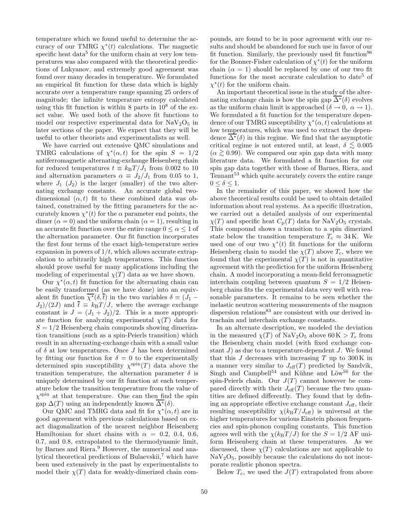
temperature which we found useful to determine the ac-curacy of our TMRG χ∗(t) calculations. The magneticspecific heat data5 for the uniform chain at very low tem-peratures was also compared with the theoretical predic-tions of Lukyanov, and extremely good agreement wasfound over many decades in temperature. We formulatedan empirical fit function for these data which is highlyaccurate over a temperature range spanning 25 orders ofmagnitude; the infinite temperature entropy calculatedusing this fit function is within 8 parts in 108 of the ex-act value. We used both of the above fit functions tomodel our respective experimental data for NaV2O5 inlater sections of the paper. We expect that they will beuseful to other theorists and experimentalists as well.

We have carried out extensive QMC simulations andTMRG calculations of χ∗(α, t) for the spin S = 1/2antiferromagnetic alternating-exchange Heisenberg chainfor reduced temperatures t ≡ kBT/J1 from 0.002 to 10and alternation parameters α ≡ J2/J1 from 0.05 to 1,where J1 (J2) is the larger (smaller) of the two alter-nating exchange constants. An accurate global two-dimensional (α, t) fit to these combined data was ob-tained, constrained by the fitting parameters for the ac-curately known χ∗(t) for the α parameter end points, thedimer (α = 0) and the uniform chain (α = 1), resulting inan accurate fit function over the entire range 0 ≤ α ≤ 1 ofthe alternation parameter. Our fit function incorporatesthe first four terms of the exact high-temperature seriesexpansion in powers of 1/t, which allows accurate extrap-olation to arbitrarily high temperatures. This functionshould prove useful for many applications including themodeling of experimental χ(T ) data as we have shown.

Our χ∗(α, t) fit function for the alternating chain canbe easily transformed (as we have done) into an equiv-alent fit function χ∗(δ, t) in the two variables δ ≡ (J1 −J2)/(2J) and t ≡ kBT/J , where the average exchangeconstant is J = (J1 + J2)/2. This is a more appropri-ate function for analyzing experimental χ(T ) data forS = 1/2 Heisenberg chain compounds showing dimeriza-tion transitions (such as a spin-Peierls transition) whichresult in an alternating-exchange chain with a small valueof δ at low temperatures. Once J has been determinedby fitting our function for δ = 0 to the experimentallydetermined spin susceptibility χspin(T ) data above thetransition temperature, the alternation parameter δ isuniquely determined by our fit function at each temper-ature below the transition temperature from the value ofχspin at that temperature. One can then find the spingap ∆(T ) using an independently known ∆∗(δ).

Our QMC and TMRG data and fit for χ∗(α, t) are ingood agreement with previous calculations based on ex-act diagonalization of the nearest neighbor HeisenbergHamiltonian for short chains with α = 0.2, 0.4, 0.6,0.7, and 0.8, extrapolated to the thermodynamic limit,by Barnes and Riera.9 However, the numerical and ana-lytical theoretical predictions of Bulaevskii,7 which havebeen used extensively in the past by experimentalists tomodel their χ(T ) data for weakly-dimerized chain com-

pounds, are found to be in poor agreement with our re-sults and should be abandoned for such use in favor of ourfit function. Similarly, the previously used fit function96

for the Bonner-Fisher calculation of χ∗(t) for the uniformchain (α = 1) should be replaced by one of our two fitfunctions for the most accurate calculation to date5 ofχ∗(t) for the uniform chain.

An important theoretical issue in the study of the alter-nating exchange chain is how the spin gap ∆∗(δ) evolvesas the uniform chain limit is approached (δ → 0, α → 1).We formulated a fit function for the temperature depen-dence of our TMRG susceptibility χ∗(α, t) calculations atlow temperatures, which was used to extract the depen-dence ∆∗(δ) in this regime. We find that the asymptoticcritical regime is not entered until, at least, δ <∼ 0.005(α >∼ 0.99). We compared our spin gap data with manyliterature data. We formulated a fit function for ourspin gap data together with those of Barnes, Riera, andTennant53 which quite accurately covers the entire range0 ≤ δ ≤ 1.

In the remainder of this paper, we showed how theabove theoretical results could be used to obtain detailedinformation about real systems. As a specific illustration,we carried out a detailed analysis of our experimentalχ(T ) and specific heat Cp(T ) data for NaV2O5 crystals.This compound shows a transition to a spin dimerizedstate below the transition temperature Tc ≈ 34K. Weused one of our two χ∗(t) fit functions for the uniformHeisenberg chain to model the χ(T ) above Tc, where wefound that the experimental χ(T ) is not in quantitativeagreement with the prediction for the uniform Heisenbergchain. A model incorporating a mean-field ferromagneticinterchain coupling between quantum S = 1/2 Heisen-berg chains fits the experimental data very well with rea-sonable parameters. It remains to be seen whether theinelastic neutron scattering measurements of the magnondispersion relations83 are consistent with our derived in-trachain and interchain exchange constants.

In an alternate description, we modeled the deviationin the measured χ(T ) of NaV2O5 above 60K > Tc fromthe Heisenberg chain model (with fixed exchange con-stant J) as due to a temperature-dependent J . We foundthat this J decreases with increasing T up to 300K ina manner very similar to Jeff(T ) predicted by Sandvik,Singh and Campbell54 and Kuhne and Low56 for thespin-Peierls chain. Our J(T ) cannot however be com-pared directly with their Jeff(T ) because the two quan-tities are defined differently. They found that by defin-ing an appropriate effective exchange constant Jeff , theirresulting susceptibility χ(kBT/Jeff) is universal at thehigher temperatures for various Einstein phonon frequen-cies and spin-phonon coupling constants. This functionagrees well with the χ(kBT/J) for the S = 1/2 AF uni-form Heisenberg chain at these temperatures. As wediscussed, these χ(T ) calculations are not applicable toNaV2O5, possibly because the calculations do not incor-porate realistic phonon spectra.

Below Tc, we used the J(T ) extrapolated from above

50

60K and our global χ∗(α, t) fit function for the alter-nating Heisenberg chain to determine the temperature-dependent alternation parameter δ(T ), and then the spingap ∆(T ) from δ(T ), directly from the χ(T ) data. Wefind that the ∆(0)/kB values for nine single crystals ofNaV2O5 are in the range 103(2)K. This result is inagreement, within the errors, with many previous anal-yses of data from various types of measurements forthis compound by other groups. However, our valuesof δ(0) = 0.034(6) for various crystals are significantlysmaller than previous estimates. We note that the twoestimates with δ(0) ≈ 0.1 in Table VII were obtainedusing Bulaevskii’s theory7 for the alternating-exchangechain, which we have shown is not accurate at low tem-peratures in the relevant alternation parameter range.

The dispersion of two one-magnon branches perpen-dicular to the chains observed in the neutron scatteringmeasurements has been recently explained quantitativelyby Gros and Valenti assuming that a zig-zag charge or-dering transition occurs at Tc.

44 They also predict thatδ(0) ∼ 0.034. This is within our range of δ(0) values inspite of the fact that we assumed that J(T ) is either con-stant or increases slightly with decreasing T below Tc,contrary to their prediction that J decreases below Tc.Gros and Valenti made no predictions for χ(T ), δ(T ),∆(T ) or C(T ), so comparisons with our results for thesequantities are not possible. We note that Klumper, Rau-pach, and Schonfeld85 obtained a good fit to the χ(T )data below Tc for the spin-Peierls compound CuGeO3

within the context of a spin-Peierls model containingfrustrating second-neighbor interactions and static spin-phonon coupling.

We discovered that ∆(T ) [and δ(T )] of NaV2O5 doesnot go to zero at Tc, indicating the existence of a spinpseudogap above Tc with a large magnitude just aboveTc of ≈ 40% of ∆(0); the pseudogap is present up toat least 50K with a magnitude decreasing with increas-ing T above Tc. To our knowledge, this pseudogap hasnot been reported previously, and there are as yet notheoretical predictions for the magnitude or tempera-ture dependence of this pseudogap. The pseudogap isstrongly reminiscent of the spin pseudogap derived byone of us using χ(T ) measurements above the transitiontemperature of inorganic quasi-one-dimensional chargedensity wave compounds,97 as predicted theoretically byLee, Rice, and Anderson98 long before those observationswere made. Similar to that case, in the present systemone may think of the pseudogap as the rms fluctuationin the spin gap above Tc, with an associated reductionin the magnon density of states at low energy. In thisinterpretation, the pseudogap in NaV2O5 should be ob-servable in high resolution quasielastic neutron scatter-ing and other spectroscopic measurements probing thelow energy magnetic excitations.

Finally, we carried out an extensive modeling studyof our specific heat data for NaV2O5 crystals, using thesame model that we used to analyze our susceptibilitydata. The most important part of this study is that we

have been able to determine a limit on the relative con-tributions of the magnetic and lattice/charge degrees offreedom to the entropy associated with the transition(s)at Tc. We find that at least 77% of the change in theentropy at Tc must arise from the lattice and/or chargedegrees of freedom, to which the spin degrees of freedommust of course be coupled, and that the spin degrees offreedom themselves contribute less than 23% of this en-tropy change. Our results also indicate that order param-eter fluctuation effects are important in the specific heatup to at least 60K, strongly confirming the above simi-lar and independent conclusion based on our modeling ofour magnetic susceptibility data for the same crystals.

ACKNOWLEDGMENTS

We thank E. Brucher and C. Lin for help with thesample preparation, and C. Song for assistance withLaue x-ray diffraction measurements. We are grate-ful to S. Eggert and T. Barnes for providing the nu-merical χ∗(t) calculation results for the uniform chainin Ref. 3 and the alternating chain in Ref. 9, respec-tively, and to D. Poilblanc and G. S. Uhrig for send-ing us their ∆∗(δ) data in Refs. 58 and 62, respectively.We are grateful to M. Greven and X. Zotos for help-ful discussions, and to A. A. Zvyagin for helpful corre-spondence. One of us (D.C.J.) thanks the Max-Planck-Institut fur Festkorperforschung, Stuttgart, where thiswork was started, for kind hospitality. Ames Labora-tory is operated for the U.S. Department of Energy byIowa State University under Contract No. W-7405-Eng-82. The work at Ames was supported by the Direc-tor for Energy Research, Office of Basic Energy Sci-ences. The QMC program was written in C++ usinga parallelizing Monte Carlo library developed by one ofthe authors.99 The QMC simulations by M.T. were per-formed on the Hitachi SR2201 massively parallel com-puter of the University of Tokyo and on the IBM SP-2 ofthe Competence Center for Computational Chemistry ofETH Zurich. X.W. acknowledges Swiss National Fund-ing Grant No. 20-49486.96. A.K. acknowledges financialsupport by the Deutsche Forschungsgemeinschaft underGrant No. Kl 645/3 and support by the research programof the Sonderforschungsbereich 341, Koln-Aachen-Julich.

∗ Present address: Department of Applied Physics, StanfordUniversity, Stanford, California 94305.

1 J. C. Bonner and M. E. Fisher, Phys. Rev. 135, A640(1964).

2 R. B. Griffiths, Phys. Rev. 133, A768 (1964); C. N. Yangand C. P. Yang, Phys. Rev. 150, 327 (1966).

3 S. Eggert, I. Affleck, and M. Takahashi, Phys. Rev. Lett.73, 332 (1994).

51

4 D. C. Johnston, in Handbook of Magnetic Materials, editedby K. H. J. Buschow, (Elsevier, Amsterdam, 1997), Vol. 10,Chap. 1, pp. 1–237.

5 A. Klumper, Eur. Phys. J. B 5, 677 (1998); A. Klumperand D. C. Johnston, cond-mat/0002140 (unpublished).

6 S. Lukyanov, cond-mat/9712314 (unpublished); Nucl.Phys. B 522, 533 (1998).

7 L. N. Bulaevskii, Fiz. Tverd. Tela 11, 1132 (1969) [Sov.Phys. Solid State 11, 921 (1969)].

8 J. C. Bonner, H. W. J. Blote, J. W. Bray, and I. S. Jacobs,J. Appl. Phys. 50, 1810 (1979). According to the primaryauthor, their numerical χ∗(α, t) data for the alternating-exchange chain are no longer available, so we cannot makeprecise comparisons of our calculations with theirs.

9 T. Barnes and J. Riera, Phys. Rev. B 50, 6817 (1994).10 X. Wang and T. Xiang, Phys. Rev. B 56, 5061 (1997);

T. Xiang, ibid. 58, 9142 (1998).11 T. Xiang and X. Wang, in Lecture Notes in Physics: Den-

sity Matrix Renormalization, edited by I. Peschel, X. Wang,M. Kaulke, and H. Karen (Springer, Berlin, 1999), Vol. 528,Chap. 5.

12 S. Kondo, D. C. Johnston, C. A. Swenson, F. Borsa,A. V. Mahajan, L. L. Miller, T. Gu, A. I. Goldman,M. B. Maple, D. A. Gajewski, E. J. Freeman, N. R.Dilley, R. P. Dickey, J. Merrin, K. Kojima, G. M. Luke,Y. J. Uemura, O. Chmaissem, and J. D. Jorgensen, Phys.Rev. Lett. 78, 3729 (1997).

13 M. Onoda and N. Nishiguchi, J. Solid State Chem. 127,359 (1996).

14 S. Miyahara, M. Troyer, D. C. Johnston, and K. Ueda, J.Phys. Soc. Jpn. 67, 3918 (1998).

15 P. A. Carpy and J. Galy, Acta Crystallogr., Sect. B: Struct.Crystallogr. Cryst. Chem. 31, 1481 (1975).

16 H. G. von Schnering, Yu. Grin, M. Kaupp, M. Somer,R. K. Kremer, O. Jepsen, T. Chatterji, and M. Weiden,Z. Kristallogr. 213, 246 (1998).

17 H. Smolinski, C. Gros, W. Weber, U. Peuchert, G. Roth,M. Weiden, and C. Geibel, Phys. Rev. Lett. 80, 5164(1998).

18 A. Meetsma, J. L. de Boer, A. Damascelli, J. Jegoudez,A. Revcolevschi, and T. T. M. Palstra, cond-mat/9806081v2 (unpublished); Acta Crystallogr., Sect. C: Cryst. Struct.Commun. 54, 1558 (1998).

19 J. Ludecke, A. Jobst, S. van Smaalen, E. Morre, C. Geibel,and H.-G. Krane, Phys. Rev. Lett. 82, 3633 (1999).

20 M. Onoda and T. Kagami, J. Phys.: Condens. Matter 11,3475 (1999).

21 T. Ohama, H. Yasuoka, M. Isobe, and Y. Ueda, J. Phys.Soc. Jpn. 66, 3008 (1997).

22 T. Ohama, H. Yasuoka, M. Isobe, and Y. Ueda, Phys. Rev.B 59, 3299 (1999).

23 S. Nishimoto and Y. Ohta, J. Phys. Soc. Jpn. 67, 2996(1998).

24 A. Damascelli, D. van der Marel, M. Gruninger, C. Presura,and T. T. M. Palstra, Phys. Rev. Lett. 81, 918(1998); A. Damascelli, D. Van der Marel, J. Jegoudez,G. Dhalenne, and A. Revcolevschi, Physica B 259–261,978 (1999).

25 A. Damascelli, C. Presura, D. van der Marel, J. Jegoudez,and A. Revcolevschi, cond-mat/9906042 (unpublished);

Phys. Rev. B 61, 2535 (2000).26 S. Nishimoto and Y. Ohta, J. Phys. Soc. Jpn. 67, 3679

(1998); 67, 4010 (1998).27 P. Lemmens, M. Fischer, G. Els, G. Guntherodt, A. S.

Mishchenko, M. Weiden, R. Hauptmann, C. Geibel, andF. Steglich, Phys. Rev. B 58, 14 159 (1998).

28 Z. V. Popovic, M. J. Konstantinovic, R. Gajic, V. Popov,Y. S. Raptis, A. N. Vasil’ev, M. Isobe, and Y. Ueda, J.Phys.: Condens. Matter 10, L513 (1998); Solid State Com-mun. 110, 381 (1999).

29 M. N. Popova, A. B. Sushkov, S. A. Golubchik,B. N. Mavrin, V. N. Denisov, B. Z. Malkin, A. I. Iskhakova,M. Isobe, and Y. Ueda, cond-mat/9807369 (unpublished);Zh. Eksp. Teor. Fiz. 115, 2170 (1999) [JETP 88, 1186(1999)].

30 N. Katoh, T. Miyazaki, and T. Ohno, Phys. Rev. B 59,R12 723 (1999).

31 M. Isobe and Y. Ueda, J. Alloys Compd. 262–263, 180(1997).

32 P. Horsch and F. Mack, Eur. Phys. J. B 5, 367 (1998).33 M. Isobe and Y. Ueda, J. Phys. Soc. Jpn. 65, 1178 (1996).34 K. Kobayashi, T. Mizokawa, A. Fujimori, M. Isobe, and

Y. Ueda, Phys. Rev. Lett. 80, 3121 (1998).35 K. Kobayashi, T. Mizokawa, A. Fujimori, M. Isobe,

Y. Ueda, T. Tohyama, and S. Maekawa, cond-mat/9808334v2 (unpublished); Phys. Rev. Lett. 82, 803 (1999).

36 Y. Fujii, H. Nakao, T. Yosihama, M. Nishi, K. Nakajima,K. Kakurai, M. Isobe, Y. Ueda, and H. Sawa, J. Phys. Soc.Jpn. 66, 326 (1997).

37 M. Weiden, R. Hauptmann, C. Geibel, F. Steglich, M.Fischer, P. Lemmens, and G. Guntherodt, Z. Phys. B 103,1 (1997).

38 A. N. Vasil’ev, V. V. Pryadun, D. I. Khomskii,G. Dhalenne, A. Revcolevschi, M. Isobe, and Y. Ueda,Phys. Rev. Lett. 81, 1949 (1998); V. V. Pryadun,A. N. Vasil’ev, G. Dhalenne, A. Revcolevschi, M. Isobe,and Y. Ueda, Physica B 259–261, 990 (1999).

39 H. Schwenk, S. Zherlitsyn, B. Luthi, E. Morre, andC. Geibel, cond-mat/9904346 (unpublished); Phys. Rev. B60, 9194 (1999).

40 M. Koppen, D. Pankert, R. Hauptmann, M. Lang,M. Weiden, C. Geibel, and F. Steglich, Phys. Rev. B 57,8466 (1998).

41 H. Seo and H. Fukuyama, J. Phys. Soc. Jpn. 67, 2602(1998); see also H. Fukuyama, cond-mat/9812294 (unpub-lished).

42 M. V. Mostovoy and D. I. Khomskii, cond-mat/9806215(unpublished); Solid State Commun. 113, 159 (2000).

43 A. I. Smirnov, M. N. Popova, A. B. Sushkov,S. A. Golubchik, D. I. Khomskii, M. V. Mostovoy,A. N. Vasil’ev, M. Isobe, and Y. Ueda, cond-mat/9808165v2 (unpublished); Phys. Rev. B 59, 14 546 (1999).

44 C. Gros and R. Valenti, cond-mat/9809154 v2 (unpub-lished); Phys. Rev. Lett. 82, 976 (1999).

45 P. Thalmeier and P. Fulde, Europhys. Lett. 44, 242 (1998).46 P. Thalmeier and A. N. Yaresko, cond-mat/9904443 (un-

published).47 J. Riera and D. Poilblanc, Phys. Rev. B 59, 2667 (1999).48 D. C. Johnston (unpublished).49 G. S. Rushbrooke and P. J. Wood, Mol. Phys. 1, 257 (1958).

52

http://arXiv.org/abs/cond-mat/0002140












50 M. E. Fisher, Philos. Mag. 7, 1731 (1962).51 M. Troyer, H. Tsunetsugu, and D. Wurtz, Phys. Rev. B

50, 13 515 (1994). Equations (28) and (39) in this paperare incorrect.

52 D. C. Johnston, Phys. Rev. B 54, 13 009 (1996).53 T. Barnes, J. Riera, and D. A. Tennant, cond-mat/9801224

(unpublished); Phys. Rev. B 59, 11 384 (1999).54 A. W. Sandvik, R. R. P. Singh, and D. K. Campbell,

cond-mat/9706046 (unpublished); Phys. Rev. B 56, 14 510(1997).

55 G. Wellein, H. Fehski, and A. P. Kampf, Phys. Rev. Lett.81, 3956 (1998).

56 R. W. Kuhne and U. Low, cond-mat/9905337 (unpub-lished); Phys. Rev. B 60, 12 125 (1999).

57 K. Ladavac, M. J. Konstantinovic, A. Belic, Z. V. Popovic,A. N. Vasil’ev, M. Isobe, and Y. Ueda, cond-mat/9806258(unpublished); M. J. Konstantinovic, K. Ladavac, A. Belic,Z. V. Popovic, A. N. Vasil’ev, M. Isobe, and Y. Ueda, J.Phys.: Condens. Matter 11, 2103 (1999).

58 D. Augier, D. Poilblanc, S. Haas, A. Delia, and E. Dagotto,Phys. Rev. B 56, R5732 (1997).

59 M. C. Cross and D. Fisher, Phys. Rev. B 19, 402 (1979).60 J. L. Black and V. J. Emery, Phys. Rev. B 23, 429 (1981).61 I. Affleck, D. Gepner, H. J. Schulz, and T. Ziman, J. Phys.

A 22, 511 (1989).62 G. S. Uhrig, F. Schonfeld, M. Laukamp, and E. Dagotto,

Eur. Phys. J. B 7, 67 (1999).63 J. des Cloizeaux and J. J. Pearson, Phys. Rev. 128, 2131

(1962).64 T. Obokata, I. Ono, and T. Oguchi, J. Phys. Soc. Jpn. 23,

516 (1967).65 W. McRae and O. P. Sushkov, Phys. Rev. B 58, 62 (1998).66 F. Woynarovich and H.-P. Eckle, J. Phys. A 20, L97 (1987).67 K. Nomura, Phys. Rev. B 48, 16 814 (1993).68 M. Karbach and K.-H. Mutter, J. Phys. A 28, 4469 (1995).69 J. L. Cardy, J. Phys. A 19, L1093 (1986); 20, 5039 (E)

(1987).70 A. W. W. Ludwig and J. L. Cardy, Nucl. Phys. B 285

[FS19], 687 (1987).71 Y. J. Kim, M. Greven, U.-J. Wiese, and R. J. Birgeneau,

Eur. Phys. J. B 4, 291 (1998), and cited references.72 See, e.g., D. C. Johnston, C. A. Swenson, and S. Kondo,

Phys. Rev. B 59, 2627 (1999).73 R. R. P. Singh and Z. Weihong, cond-mat/9811028 v2 (un-

published); Phys. Rev. B 59, 9911 (1999).74 M. Isobe, C. Kagami, and Y. Ueda, J. Crystal Growth 181,

314 (1997).75 P. W. Selwood, Magnetochemistry, 2nd ed. (Interscience,

New York, 1956), p. 78.76 A. N. Vasil’ev, A. I. Smirnov, M. Isobe, and Y. Ueda, Phys.

Rev. B 56, 5065 (1997).77 M. Lohmann, A. Loidl, M. Klemm, G. Obermeier, and S.

Horn, Solid State Commun. 104, 649 (1997).78 S. Schmidt, W. Palme, B. Luthi, M. Weiden, R. Haupt-

mann, and C. Geibel, Phys. Rev. B 57, 2687 (1998).

79 J. Hemberger, M. Lohmann, M. Nicklas, A. Loidl,M. Klemm, G. Obermeier, and S. Horn, Europhys. Lett.42, 661 (1998); M. Lohmann, J. Hemberger, M. Nicklas,A. Loidl, M. Klemm, G. Obermeier, and S. Horn, PhysicaB 259–261, 983 (1999).

80 W. Palme, S. Schmidt, B. Luthi, J. P. Boucher,M. Weiden, R. Hauptmann, C. Geibel, A. Revcolevschi,and G. Dhalenne, Physica B 246–247, 32 (1998).

81 T. Ohama, M. Isobe, H. Yasuoka, and Y. Ueda, J. Phys.Soc. Jpn. 66, 545 (1997).

82 J. P. Pouget, P. Lederer, D. W. Schreiber, H. Launois,D. Wohlleben, A. Casalot, and G. Villeneuve, J. Phys.Chem. Solids 33, 1961 (1972).

83 T. Yosihama, M. Nishi, K. Nakajima, K. Kakurai, Y. Fujii,M. Isobe, C. Kagami, and Y. Ueda, J. Phys. Soc. Jpn. 67,744 (1998).

84 D. Augier and D. Poilblanc, Eur. Phys. J. B 1, 19 (1998).85 A. Klumper, R. Raupach, and F. Schonfeld, cond-

mat/9809224 (unpublished); Phys. Rev. B 59, 3612 (1999).86 R. J. Bursill, R. H. McKenzie, and C. J. Hamer, cond-

mat/9812409 (unpublished); Phys. Rev. Lett. 83, 408(1999).

87 F. Mila, P. Millet, and J. Bonvoisin, Phys. Rev. B 54,11 925 (1996).

88 S. Luther, H. Nojiri, M. Motokawa, M. Isobe, and Y. Ueda,J. Phys. Soc. Jpn. 67, 3715 (1998).

89 W. Schnelle, Yu. Grin, and R. K. Kremer, Phys. Rev. B59, 73 (1999).

90 D. Smirnov, P. Millet, J. Leotin, D. Poilblanc, J. Riera,D. Augier, and P. Hansen, Phys. Rev. B 57, R11 035(1998).

91 P. Fertey, M. Poirier, M. Castonguay, J. Jegoudez, andA. Revcolevschi, Phys. Rev. B 57, 13 698 (1998).

92 S. Ravy, J. Jegoudez, and A. Revcolevschi, cond-mat/9808313 v2 (unpublished); Phys. Rev. B 59, R681(1999).

93 D. Smirnov, J. Leotin, P. Millet, J. Jegoudez, andA. Revcolevschi, Physica B 259–261, 992 (1999).

94 D. K. Powell, J. W. Brill, Z. Zeng, and M. Greenblatt,Phys. Rev. B 58, R2937 (1998).

95 C. Kittel, Introduction to Solid State Physics, 4th ed. (Wi-ley, New York, 1971), Chap. 6.

96 W. E. Estes, D. P. Gavel, W. E. Hatfield, andD. J. Hodgson, Inorg. Chem. 17, 1415 (1978); W. E.Hatfield, J. Appl. Phys. 52, 1985 (1981).

97 D. C. Johnston, Phys. Rev. Lett. 52, 2049 (1984); SolidState Commun. 56, 439 (1985); D. C. Johnston, M. Maki,and G. Gruner, ibid. 53, 5 (1985); D. C. Johnston,J. P. Stokes, and R. A. Klemm, J. Magn. Magn. Mater.54–57, 1317 (1986).

98 P. A. Lee, T. M. Rice, and P. W. Anderson, Phys. Rev.Lett. 31, 462 (1973).

99 M. Troyer, B. Ammon, and E. Heeb, in Lecture Notes in

Computer Science, edited by D. Caromel et al. (SpringerVerlag, Berlin, 1998), Vol. 1505.

53












Thermodynamics of spin S=1/2 antiferromagnetic uniform and alternating-exchange Heisenberg chains

Documents

Transcript of Thermodynamics of spin S=1/2 antiferromagnetic uniform and alternating-exchange Heisenberg chains