Shape-induced anisotropy in antiferromagnetic nanoparticles

O. Gomonay n, S. Kondovych, V. LoktevNational Technical University of Ukraine “KPI”, ave Peremogy, 37, 03056 Kyiv, Ukraine

a r t i c l e i n f o

Article history:Received 20 August 2013Received in revised form25 October 2013Available online 11 November 2013

Keywords:AntiferromagnetDomain structureNanoparticleShape effect

a b s t r a c t

High fraction of the surface atoms considerably enhances the influence of size and shape on the magneticand electronic properties of nanoparticles. Shape effects in ferromagnetic nanoparticles are wellunderstood and allow us to set and control the parameters of a sample that affect its magneticanisotropy during production. In the present paper we study the shape effects in the other widely usedmagnetic materials – antiferromagnets, – which possess vanishingly small or zero macroscopicmagnetization. We take into account the difference between the surface and bulk magnetic anisotropyof a nanoparticle and show that the effective magnetic anisotropy depends on the particle shape andcrystallographic orientation of its faces. The corresponding shape-induced contribution to the magneticanisotropy energy is proportional to the particle volume, depends on magnetostriction, and can causeformation of equilibrium domain structure. Crystallographic orientation of the nanoparticle surfacedetermines the type of domain structure. The proposed model allows us to predict the magneticproperties of antiferromagnetic nanoparticles depending on their shape and treatment.

& 2013 Elsevier B.V. All rights reserved.

1. Introduction

Magnetic nanoparticles (NP) are widely used as constitutiveelements for the information technology (e.g. memory cells, spinvalves, magnetic field controllers etc.). To drive and control themagnetic state of a particle and values of critical fields andcurrents, we can use not only internal properties of magneticmaterial, but also shape and size of the sample. As for ferromag-netic (FM) particles, shape effects allow us to tailor theeffective magnetic anisotropy and critical field values duringproduction.

On the other hand, nowadays technologies use antiferromag-netic (AFM) nanoparticles along with (or sometimes instead of)FM ones. Experiments with AFM particles show that the reductionof size to tens of nanometres leads to noticeable changes ofproperties compared to the bulk samples: an increase of latticeparameters in the magnetically ordered phase [1–3]; an increaseof the magnetic anisotropy [4]; a pronounced decrease of AFMRfrequency [5]. Some of the finite size effects could be caused by theshape and faces orientations of nanoparticle. For example, accordingto the Néel predictions [6,7], small AFM particles exhibit uncom-pensated magnetic moment with the size- and shape-dependentvalue [8,9]. Recent experiments with rather large (100–500 nmsize) AFM particles [10–12] discovered the shape effects similar tothe shape-induced phenomena in FM materials: (i) switching of

AFM vector from crystallographic to particle easy-axis with anincrease of aspect ratio; (ii) correlation between the type ofdomain structure and such parameters as aspect ratio of thesample and orientation of faces.

However, the mechanism of the finite-size and shape effects inAFM nanoparticles is still an open issue.

Shape effects in AFM particles could, in principle, originate froma weak ferromagnetic moment [13] thus reducing the differencebetween AFM and FM systems to quantitative one. On the otherhand, AFMs show some peculiar features (like exchange enhance-ment, gap in the magnon spectra, coupling to the external magneticfield) that have no counterparts in FMs.

Understanding the mechanisms of the shape effects specific toAFM ordered systems is crucial for optimizing and finetuning theproperties of AFM-based devices and clarifying the fundamentalquestions whether the shape effects reside in AFM with vanish-ingly small macroscopic magnetization, and which of peculiar AFMproperties might depend on the particle shape. For this purposewe investigate the finite-size and shape effects in AFM particles,regardless of their macroscopic magnetization, combining twopreviously shown statements: (i) the shape effects in AFM materialsmay originate from the long-range fields of “magnetoelastic” chargesdue to spontaneous magnetostriction below the Néel temperature(so-called destressing fields) [14]; (ii) “magnetoelastic” chargesmay arise from the surface magnetic anisotropy [15]. We considerthe particles with the characteristic size below the several criticallengths of monodomainization (which, for convenience, arereferred to as “nanoparticles” though their dimensions could alsofall into submicron–micron range).

Contents lists available at ScienceDirect

journal homepage: www.elsevier.com/locate/jmmm

Journal of Magnetism and Magnetic Materials

0304-8853/$ - see front matter & 2013 Elsevier B.V. All rights reserved.http://dx.doi.org/10.1016/j.jmmm.2013.11.003

n Corresponding author. Tel.: þ380 44 406 83 55.E-mail addresses: helen.gomonay@gmail.com, homo@pti.kpi.ua (O. Gomonay).

Journal of Magnetism and Magnetic Materials 354 (2014) 125–135

The basic idea is to consider a priori the surface and bulkproperties as different: to distinguish the constants of surface andbulk magnetic anisotropy and, as a consequence, equilibrium orien-tation of AFM vectors at the surface and in the bulk. Up to ourknowledge, M.I. Kaganov [16] was first who pointed out the role ofthe surface magnetic anisotropy effects on spin-flop transitions inmagnetic materials, considering the magnetic moment at the surfaceas an additional parameter. This idea was then generalized to accountfor surface exchange interactions and was applied to description ofvarious inhomogeneous states at a nanoscale range, includingvortices and twisted phases [17–19]. In our work we further developthis approach introducing into model the magnetoelastic coupling,which, as we believe, noticeably affects the properties of thenanosized AFM particle. We show that due to the long-range natureof magnetoelastic and elastic forces, the surface anisotropy contri-butes to the magnetic energy of the sample. This contribution isproportional to the particle volume, depends on the aspect ratio andcrystallographic orientation of the sample faces, and affects equili-brium (single- and multi-domain) state of AFM nanoparticle. Theproposed approach requires consistent description of the magneticand elastic subsystems of AFM particles and thus differs from thewell-known formalism for the FM [20].

2. Model

To describe the equilibrium magnetic state of a NP we need tointroduce at least three additional (in comparisonwith bulk samples)parameters that characterize: (i) shape, (ii) size, and (iii) orientationof sample faces.

We consider a thin flat rectangular particle (thickness h⪡boa,Fig. 1), typical for experimental studies (see, e.g., [12]). The thicknessh of a particle is, however, large enough to ensure an AFM ordering(i.e. significantly larger than the magnetic correlation length).

The sample surface (see Fig. 1b) consists of four faces with thenormal vectors nj ¼ ð cos ψ j; sin ψ jÞ, j¼ 1;…;4 (x, y are parallel tocrystallographic axes). We disregard the upper and lower faces(z¼Z¼const) as they do not contribute to the effects discussedbelow. Equations that define the surface are (ZA ½0;h�, X, Y areparallel to the particle edges):

X ¼ a=2; YA ½�b=2; b=2�; n1 ¼ ð1;0Þ; ψ1 ¼ψ ;

Y ¼ b=2; XA ½�a=2; a=2�; n2 ¼ ð0;1Þ; ψ2 ¼ψþπ=2;X ¼ �a=2; YA ½�b=2; b=2�; n3 ¼ ð�1;0Þ; ψ3 ¼ψþπ;Y ¼ �b=2; XA ½�a=2; a=2�; n4 ¼ ð0; �1Þ; ψ4 ¼ψþ3π=2: ð1Þ

For such a model, the additional external (in thermodynamicsense) parameters of the NP are: (i) aspect ratio a/b (defines theshape), (ii) width b (defines characteristic size), and (iii) angle ψ(defines the orientation of the surfaces).

We consider a typical collinear AFM with two equivalent sub-latticesM1 andM2; the Néel (or AFM) vector L¼M1�M2 plays a role

of the order parameter. Far below the critical point the magnitude ofthe AFM vector is fixed (we assume jLj ¼ 1).

To obtain equilibrium distribution LðrÞ for the NP of givenshape and size, we minimize the total energy W which includesseveral terms of different nature. First of all, we may consider thesurface as a separate magnetic phase [21–23] with a small butfinite thickness δsur (narrow peripheral region S of thickness δsur inFig. 2) and thus distinguish the bulk, Wbulk, and the surface, Wsur,contributions:

W ¼WbulkþWsur: ð2ÞThen, we can also distinguish different contributions to the

bulk energy, Wbulk, the most important are those that describe themagnetic anisotropy, wanis, exchange, wexch, and magnetoelastic,wm�e coupling. We assume that the bulk magnetic anisotropycorresponds to tetragonal symmetry with two equivalent easydirections in the NP plane (x or y in Fig. 1b) and model respectivecontribution to the energy density as follows:

wanis ¼ 12 K J L

2z �K ? ðL4x þL4yÞ; ð3Þ

where K J≫K ? 40 are the phenomenologic anisotropy constants.Exchange interactions (responsible for inhomogeneous distri-

bution of the Néel vector inside the sample) give rise to a gradientterm

wexch ¼ 12αð∇LÞ2; ð4Þ

where α is a phenomenological constant. Competition betweenthe exchange coupling (4) and magnetic anisotropy (3) defines thecharacteristic size ξDW of the domain wall (DW): ξDW ¼ ð1=2Þffiffiffiffiffiffiffiffiffiffiffiffiffiα=K ?

p.

Magnetoelastic coupling in AFM materials can be pronounced(compared with FM ones) due to the presence of strong crystalfield and, as a result, strong spin–orbit coupling (like in oxidesLaFeO3 or NiO). In the simplest case of the elastically isotropic

Fig. 1. Sample (a) and orientation of the Néel vector L (b) with respect to crystal axes (x,y) and sample edges (X,Y).

Fig. 2. Space distribution of AFM vector (arrows) in a single domain (a) andmultidomain (b) states.

O. Gomonay et al. / Journal of Magnetism and Magnetic Materials 354 (2014) 125–135126

material, the density of magnetoelastic energy is:

wm�e ¼ λisoL2Truþ2λanis½ðL � L�1

3 IÞðu�13 I Tr uÞ�; ð5Þ

where u is the strain tensor, I is the identity matrix, constantsλiso and λanis describe isotropic and shear magnetostriction,respectively.

Final expression for the bulk energy is thus given by

Wbulk ¼ZVðwanisþwexchþwm�eþwelasÞ dV ; ð6Þ

where welas is the elastic energy density (see, e.g. [24]), V¼abh isthe NP volume, all other terms are defined above.

At last, let us focus on the magnetic surface energy Wsur which isof crucial importance for our model and needs special discussion.Experiments with the nanoscale AFM particles reveal a significantdifference between the magnetic ordering and hence the magneticproperties of the surface from those of the bulk. In particular,depending on the material, treatment, and other technologicalfactors, the NP surface may lack the long-range magnetic structure(paramagnetic or spin glass [23,25]), or may have different type ofordering (e.g. multi- vs. two-sublatteral in the bulk [26]), or differenteasy axis/axes. We consider the last case and assume, for the sake ofsimplicity, that the easy magnetic axis at the surface is perpendicularto the normal n; then, expression for the magnetic surface energytakes the form:

Wsur ¼ Ksur∮S ðLnÞ2 dS¼ Ksur ∑4

j ¼ 1

ZSjðLnjÞ2 dS; ð7Þ

where Ksur40 is a phenomenological constant. Wsur obviouslydepends on orientation of edges: angles ψj, or, equivalently, vectorsnj (see (1)).

It is instructive to compare the specific surface magneticanisotropy Ksur=δsur with the magnetic anisotropy constant K ? :they have the same order of value (Ksur=δsurpK ? ), if the brokenexchange bonds play the main role in formation of the surfaceproperties; while in the case of dominating dipole-dipole interac-tions Ksur=δsur can be much greater than K ? [13].

It should be stresses, that, in principle, all introduced phenom-enological constants fall into two categories: internal [27] (indexed“in”) and superficial (indexed “sur”); interactions of both types cancontribute to the shape effects. However, in our model wedistinguish only between the magnetic constants Ksur=δsur andK ? , taking this difference as the most important.

The expression (2) for the NP energy is the functional over thefield variables LðrÞ (the AFM vector) and uðrÞ (the displacementvector). We reduce the number of independent variables to threeassuming that: (i) vector L lies within the xy plane and can beparametrized by a single angle φ (see Fig. 1b because of a strongeasy-plane anisotropy (K J≫K ? ); (ii) strain component uzz in arather thin plate (h≫a;b) can be considered as homogeneous andthus can be excluded from consideration (see [24]). The standardminimum conditions generate the set of differential equations forone magnetic, φðrÞ, and two elastic, uxðrÞ, uyðrÞ variables in thebulk:

�αΔφþK ? sin 4φþ2λanis½�ðuxx�uyyÞ sin 2φþ2uxy cos 2φ� ¼ 0;

ð8Þ

Δuxþνeff∇x div u¼ �ðλanis=μÞ½∇x cos 2φþ∇y sin 2φ�; ð9Þ

Δuyþνeff∇y div u¼ �ðλanis=μÞ½∇x sin 2φ�∇y cos 2φ�: ð10Þ

Here, operators Δ and div are two-dimensional, νeff � ð1þνÞ=ð1�νÞ is the effective Poisson ratio (instead of 3-dimensional ν[24]), μ is the shear modulus.

Equations for the AFM vector at the j-th face (variables φðjÞsur,

see (1))

�Ksur sin 2ðφðjÞsurþψ jÞþαðnj∇ÞφðjÞ

sur ¼ 0 ð11Þ

could be considered as the boundary conditions. They differ fromthe standard boundary conditions for AFMs (see, e.g., [28,29]) dueto the presence of the additional surface term with Ksur.

In the limit Ksur-0 the solutions of Eqs. (9), (10), (11) are wellknown: the AFM vector LðrÞ ¼ const lies along one of the easy axes(φin ¼ 0 or π=2), the displacement vector uðrÞ generates thehomogeneous field of the magnetically-induced strain:

uð0Þxx �uð0Þ

yy ¼ �λanisμ

cos 2φin; uð0Þxy ¼ �λanis

2μsin 2φin: ð12Þ

In the massive (infinite) samples the spontaneous striction (12)causes magnetoelastic gap in the spin-wave spectrum (in assump-tion of “frozen” lattice), but does not affect the equilibriumorientation of the AFM vector (all the magnetostrictive terms in(8) cancel out, eliminating the shape effect).

For the finite-size samples with nonzero surface anisotropy(Ksura0) the easy direction at least in some near-surface regionsunavoidably differs from that in the bulk and so, the spatialdistribution of the AFM vector should be non-uniform. As a result,the sources of the displacement field – the nonzero gradientterms, or “magnetoelastic charges” – appear in the r.h.s of Eqs.(9) and (10). In the following section we discuss this issue in moredetail.

3. Shape-induced anisotropy

The consistent theory of shape effects in AFMs should accountfor the long-range elastic and magnetoelastic interactions and thusshould rest upon the complete set of Eqs. (8)–(10). However, thedisplacement field uðrÞ can be formally excluded from considera-tion once the Green tensor Gjkðr; r′Þ for Eqs. (9) and (10) is known(see Appendix A). In this case the spatial distribution of the AFMvector LðrÞ should minimize the energy functional

W ½LðrÞ� ¼ZVðwmagþwexchÞ dVþWsurþWadd; ð13Þ

which includes the additional term of magnetoelastic nature:

Wadd ¼2λ2anisμ

ZV

ZV∇m½LjðrÞLmðrÞ�Gkjðr; r′Þ∇′

l Lkðr′ÞLlðr′Þ½ � dV dV ′

þ2λ2anisμ

∮S∮S LjðrsurÞLmðrsurÞGkjðrsur; r′surÞLkðr′surÞLlðr′surÞ dSm dS′l:

ð14ÞAnalysis of the Exp. (14) shows that any inhomogeneous

distribution LðrÞ gives nonzero, generally positive contribution toenergyWadd. Due to the “Coulomb-like” nature of the elastic forces(Gjkðr; r′Þp1=jr�r′j) this contribution scales as sample volume V.In addition, nonlocality of the Wadd term turns Eqs. (8) to integro-differential ones and thus complicates the problem.

In the present paper we propose the simplified approach to solveEqs. (8)–(10) using the following peculiar features of antiferromagnets.

First, we consider the magnetostriction of AFMs as a secondaryorder parameter which means that in the thermodynamic limit (inneglection of boundary conditions) the homogeneous spontaneousstrains (12) preserve the symmetry of the magnetically ordered stateand orientation of the easy axis. In addition, though usually themagnetoelastic energy is comparable (up to the order of value) to the4-th order magnetic anisotropy (i.e. to K ? constant), it can be muchless than the uniaxial magnetic anisotropy. Thus, assuming stronguniaxial surface anisotropy Ksur≫K ?δsur, we can disregard theinfluence of magnetoelastic strains on equilibrium orientation of

O. Gomonay et al. / Journal of Magnetism and Magnetic Materials 354 (2014) 125–135 127

AFM vector at the surface. However, this assumption does not restrictthe relation between Ksur and the characteristic DW energy sDW ,because sDW p

ffiffiffiffiffiffiffiffiffiK ? J

palat≫K ?δsur (where J≫K ? characterizes the

exchange coupling, alat is the lattice constant, and we used thefollowing relations: αp Ja2lat, δsurpalat).

Second, we propose the following hierarchy of characteristiclength scales: the width of magnetic inhomogeneity is much lessthan the sample size, ξDW⪡a;b, but much greater than interatomicdistance, ξDW≫alat (due to exchange enhancement); the width ofelastic inhomogeneity has interatomic scale and thus is much lessthan ξDW . Note, that the value of ξDW in nanoparticles with thelarge fraction of the surface atoms can be much smaller than thatfor the bulk samples due to variation of magnetoelastic andexchange coupling (see, e.g. [30]). Thus, inequality ξDW⪡a; b keepstrue in a wide range of the sample dimensions down to tens ofnanometers (below this range applicability of the continual modelis questionable).

Thus, within the above approximations, equilibrium orientationof the AFM vector at the surface results mainly from competition ofthe magnetic interactions: surface magnetic anisotropy and inho-mogeneous exchange coupling, once the bulk vector Lin is fixed.Orientation of Lin, in turn, is defined by interplay between the bulkmagnetic anisotropy and magnetostrictive contribution induced byspatial rotation of AFM vector in the thin (pξDW ) near-surfaceregion (see Fig. 3). So, the effective shape-induced magneticanisotropy and equilibrium distribution of AFM vector could bedetermined self-consistently according to the following procedure:(i) to calculate Lsur starting from some (initially unknown) “seed”

distribution of the AFM vector Lin in the NP bulk; (ii) to substitutethus defined seed distribution into equations for the displacementvector and to determine the corresponding field sources (magne-toelastic charges); (iii) to calculate charge-induced average strainswhose contribution into free energy is proportional to the samplevolume; (iv) to define the effective magnetic anisotropy whichaccounts for the average strains and calculate Lin.

Note, that the form of the seed distribution (and hence the freevariable of the structure) is different for a single- and a multi-domain states. In the first case Lin is homogeneous within the bulkbut can deflect from the magnetic easy axis, so, φin is theappropriate free variable. In the second case we assume, inanalogy with FM, that AFM vector within each of the domains isfixed and parallel to one of two equivalent easy axes; then, freevariable coincides with the fraction of type-I (or type-II) domains.

3.1. Seed distribution and magnetoelastic charges

In the simplest case of a single-domain state (Fig. 2a), there aretwo homogeneous regions: the “shell” (of the thickness δsur) andthe core. An equilibrium value φin inside the core is fixed, constant(as Δφin ¼ 0), but unknown (in some cases discussed belowφin ¼ 0 or π=2 that corresponds to one of the easy axes). Wecalculate the value φðjÞ

sur at the surface from Eq. (11) with account ofthe standard expression for the domain wall profile:

sin 2ðφðξÞ�φinÞ ¼ 2ξDWdφdξ

¼ 1coshððξ�ξ0Þ=ξDW Þ: ð15Þ

Face normals generate the set of variables ξ¼ ð7X�a=2Þ;ð7Y�b=2Þ of the local coordinate system (see the inset inFig. 3b). Position ξ0 of the DW center is calculated from theboundary conditions (see below). In (15) we neglect the possibledifference between the DW width ξDW ¼ ð1=2Þ

ffiffiffiffiffiffiffiffiffiffiffiffiffiα=K ?

pin the near-

surface region and in the core.Substituting (15) in (11), we obtain the following equation

for φðjÞsur:

tan 2φðjÞsur ¼

Ksur sin 2ψ jþsDW sin 2φin

sDW cos 2φin�Ksur cos 2ψ j; ð16Þ

where sDW ¼ ffiffiffiffiffiffiffiffiffiffiffiαK ?

p ¼ 2ξDWK ? is the characteristic energy of thedomain wall. The values φðjÞ

sur at the opposite faces coincide:φð1Þ

sur ¼φð3Þsur, φ

ð2Þsur ¼φð4Þ

sur (see (1)).Analysis of Exp. (16) shows that the AFM vector at the surface

can be either parallel to the edge: φðjÞsur ¼ψ j, as shown in Fig. 2 (in

the limit of large surface anisotropy, Ksur≫sDW ), or coincide withthe bulk AFM vector: φðjÞ

sur ¼φin (for the vanishing surface energy,Ksur⪡sDW ). In the last case the surface influence and, correspond-ingly, shape effects disappear.

Note that the surface DW is “incomplete”: in general, DWcenter is located outside the sample (see Fig. 3b) and its coordinateξðjÞ0 depends on the surface anisotropy

ξðjÞ0 ¼ ξDW sinh�1 Ksur sin 2ψ jþsDW sin 2φin

sDW cos 2φin�Ksur cos 2ψ j: ð17Þ

In a single-domain nanoparticle the AFM vector rotates from Lsurto Lin in a narrow, almost zero-width (rξDW⪡a; b) region and so,we can model the spatial dependence of LðrÞ with a step-likefunction. Within this approximation, r.h.s. of Eqs. (9) and (10)are nontrivial only at the surface; this fact makes it possible touse a homogeneous form of these equations for the bulk region ofthe NP:

Δuþνeff∇div u¼ 0 ð18Þ

Fig. 3. Distribution of the Néel vector in the vicinity of Y¼b/2 face, multidomainstate. (a) Periodic (period d) domain structure, double arrows indicate orientationof AFM vectors inside domains and in the near-surface region (shaded horizontalstripe). (b) Space dependence of LxðξÞ (solid line) calculated from (15) provided thatφin ¼ 0. The horizontal line defines the center ξ0 of a virtual full domain wall(dotted line). Shaded vertical bar indicates the position of surface region. Directionof DW normal coincides with the axis ξ of the local coordinate system (inset).

O. Gomonay et al. / Journal of Magnetism and Magnetic Materials 354 (2014) 125–135128

with the following boundary conditions for the displacementvector:

ðn � ∇Þusurþνeffn div usur ¼ nQm�e

: ð19ÞIn (19) we introduced the tensor of magnetoelastic charges asfollows:

Qm�e � �λanis

μLsur � Lsur�Lin � Lin½ �: ð20Þ

For a rectangular-shaped sample the charges at the opposite edgescoincide: Q

m�eðn1Þ ¼ Qm�eðn3Þ, Q

m�eðn2Þ ¼ Qm�eðn4Þ. We can

express all the components of the Qm�e

tensor in terms of twonontrivial combinations, Qm�e

1 �Qm�eXX �Qm�e

YY and Qm�e2 � 2Qm�e

XY(in X, Y coordinates).

From definition (20) and the relations (16) it follows that

Qm�e1 ðn1;2Þ ¼

λanisμ

cos 2ðφinþψ Þ� sDW cos 2ðφinþψ Þ8KsurffiffiffiffiffiffiffiffiffiffiffiffiffiffiffiffiffiffiffiffiffiffiffiffiffiffiffiffiffiffiffiffiffiffiffiffiffiffiffiffiffiffiffiffiffiffiffiffiffiffiffiffiffiffiffiffiffiffiffiffiffiffiffiffiffiffiffiffiffiffiffiffiffiffiffiffiffiffiffiffiffiK2sur82KsursDW cos 2ðφinþψ Þþs2DW

q0B@

1CA;

ð21Þand

Qm�e2 ðn1;2Þ ¼

λanisμ

sin 2ðφinþψ Þ 1� sDWffiffiffiffiffiffiffiffiffiffiffiffiffiffiffiffiffiffiffiffiffiffiffiffiffiffiffiffiffiffiffiffiffiffiffiffiffiffiffiffiffiffiffiffiffiffiffiffiffiffiffiffiffiffiffiffiffiffiffiffiffiffiffiffiffiffiffiffiffiffiffiffiffiffiffiffiffiffiffiffiffiK2sur82KsursDW cos 2ðφinþψ Þþs2DW

q0B@

1CA:

ð22ÞMagnetoelastic charges (20) (as well as (21), (22)) are similar to

“magnetostatic charges” at the surface of FMs but have another,magnetoelastic, nature (i.e. depend on magnetostriction), anddepend on the surface magnetic anisotropy Ksur. Magnetoelasticcharges disappear in the limiting case of small surface anisotropyKsur⪡sDW and reach the maximum possible value when Ksur≫sDW(as illustrated in Fig. 4). Like magnetostatic, magnetoelastic chargesdepend on the crystallographic orientation of the sample faces andvanish for those parts of the surface where Lin JLsur. From Eqs. (18),(19) it follows that magnetoelastic charges produce long-range(decaying as 1/r2) elastic fields, which, in turn, lead to the “destres-sing” effects (similar to “demagnetizing” effects in FMs).

Another way to interpret the formation of magnetoelasticcharges presents itself in terms of incompatibility of seed sponta-neous deformations at the surface and in the bulk. To this end,sufficient condition for charges to appear stems from the differ-ence between the surface and bulk values of any physical quantity:magnetic (e.g. nonmagnetic or paramagnetic surface), magnetoe-lastic, or elastic (e.g. rigid shell).

3.2. Average strains and shape-induced anisotropy

At the next, (iii), stage of the algorithm we solve Eqs. (18), (19)for the displacement vector which, in a general case, generatesnon-uniform field of additional (compared with (12)) elasticdeformations. However, the main contribution to the magneticanisotropy comes from the shear strains averaged over the samplevolume ðlabeled as⟨⋯⟩Þ :

⟨uXX�uYY ⟩¼ � π1þνeff

½Qm�e1 ðn2ÞþQm�e

1 ðn1Þ� 1þνeff J2ab

� �h in

� J1ab

� �½Qm�e

1 ðn1Þ�Qm�e1 ðn2Þ�

o; ð23Þ

2⟨uXY ⟩¼ �π ½Qm�e2 ðn2ÞþQm�e

2 ðn1Þ� 1� νeff1þνeff

J2ab

� �� ��

� J1ab

� �½Qm�e

2 ðn1Þ�Qm�e2 ðn2Þ�

o; ð24Þ

where J1ða=bÞ, J2ða=bÞ are the dimensionless shape functions of theaspect ratio a/b (see Fig. 5):

J1ab

� �¼ 2π

arctanab�arctan

baþ a4b

ln 1þb2

a2

!� b4a

ln 1þa2

b2

� " #;

ð25Þ

J2ab

� �¼ 4π

baln 1þa2

b2

� þabln 1þb2

a2

!" #: ð26Þ

Note that J2ða=bÞ ¼ J2ðb=aÞ; J1ða=bÞ ¼ � J1ðb=aÞ, so, J1ð1Þ ¼ 0 for asquare (a¼b); in the opposite limiting case of high aspect ratio(a≫b) J1ð1Þ-1, J2ð1Þ-0.

Substituting Exps. (21), (22), (23), and (24) into Eq. (8) wearrive at the following equation for magnetic variable:

K ? sin 4φinþKsh2 sin 2ðφinþψ ÞþKsh

4 sin 4ðφinþψ Þ ¼ 0; ð27Þ

where we introduce the shape-dependent coefficients Ksh2 , Ksh

4 ,and take into account that Δφ¼ 0. In the limiting (and practically

Fig. 4. Magnetoelastic charges Qm�e (in λanis=μ units) vs. surface constant Ksur

calculated for single-domain state, ψ ¼ π=4. Inset shows the charge distributionover the particles edges. Arrows indicate orientation of AFM vector at the surfaceand in the bulk.

Fig. 5. Form-factors J1ða=bÞ, J2ða=bÞ vs aspect ratio a/b. Arrows show the pointswhere the functions J1 (a/b¼1) and Ksh

4 (a=b� 16) change the sign.

O. Gomonay et al. / Journal of Magnetism and Magnetic Materials 354 (2014) 125–135 129

important) case Ksur≫sDW

Ksh2 ¼ 2 Km�eJ1

ab

� �; Ksh

4 ¼ Km�e 2J2ab

� ��1

h i; Km�e � 4πνeffλ

2anis

ð1þνeff Þμ:

ð28ÞIn a general case the coefficients Ksh

2 and Ksh4 depend on the

constant Ksur of surface magnetic anisotropy and vanish whenKsur⪡sDW (see Appendix B).

Eq. (27) for the magnetic variables φin can be treated as theminimum condition for the effective energy density of the sample

weff �Weff

V¼ �1

4½K ? cos 4φinþ2Ksh

2 cos 2ðφinþψ ÞþKsh4 cos 4ðφinþψ Þ�;

ð29Þwhich, apart from the magnetic anisotropy, includes contributionsfrom magnetoelastic and surface forces (the underlined terms). Thelast two terms in (29) cause the shape effects in AFM nanoparticle.To illustrate this result we consider some typical cases.

Let the sample edges be parallel to the easy magnetic axes(ψ ¼ 0). In this case, as follows from (27) and (29), the term withKsh2 removes degeneracy of states φin ¼ 0 and φin ¼ π=2. This term is

equivalent to uniaxial anisotropy, which selects the state with thecollinear orientation of AFM vectors at the surface and in the bulk asenergetically favorable. This means that the AFM vector is parallel tothe long edge of the rectangle: if a4b, then Ksh

2 40 and LJX(φin ¼ 0). The second shape-induced term with Ksh

4 renormalizesthe “bare” magnetic anisotropy constant, K ?-K ? þKsh

4 ; however,this effect makes no influence on the orientation of the AFM vector.For the square sample (a¼b) the shape-induced correction has thesame sign as K ? (Ksh

4 40) and thus does not affect equilibriumorientation of the AFM vector. The change of Ksh

4 sign appears for thesamples with large aspect ratio (a=b� 16, see Fig. 5), where uniaxialanisotropy governs the orientation of the AFM vector, and shape-induced renormalization of K ? is insignificant.

The role of the terms with Ksh4 becomes noticeable when the

faces (edges) of the square (a¼b) sample are cut at the angleψ ¼ π=4 (i.e. along the “hard” magnetic axes). In this case theuniaxial anisotropy vanishes, Ksh

2 ¼ 0 and the effective magneticanisotropy constant decreases: K ?-K ? �Ksh

4 . Assuming that K ?and Ksh

4 have the same (spin-orbit) nature, we conclude that theshape can change the direction of the easy axes (if K ? oKsh

4 ) orentirely compensate the 4-th order magnetic anisotropy (ifK ? � Ksh

4 ), as it was recently observed in the experiments [12].

4. Multidomain state, destressing energy and critical size

In the multidomain state the seed distribution can, in principle,model the domains and domain boundaries both in the bulk andat the surface. To simplify the problem we assume that distribu-tion of the AFM vector LsurðrÞ within each face is homogeneousand Lsur aligns due to the surface anisotropy (Ksur≫sDW ), as shownin Fig. 3a. In this case, orientation of the AFM vector and,correspondingly, angle φ, can take one of two values within thebulk: φI

in ¼ 0 or φIIin ¼ π=2 (domains of two types, I and II). At the

surface φð1Þsur ¼φð3Þ

sur and φð2Þsur ¼φð4Þ

sur.Magnetoelastic charges appear near the surface (due to the

difference between Lsur and Lin) and at the domain walls in thebulk (due to the difference between LIin and LIIin). The total chargeof the full domain wall is zero because of the perfect compensationof the charges with opposite signs. So, the field of internal chargesdecreases rapidly with distance (as 1/r6, due to Coulomb-likenature of the “elastic” forces) and can be neglected.

Near-surface domain structure generates two types of the charges,Q

m�eI and Q

meII , corresponding to two types of the domains with LIin

and LIIin (see Eq. (20)). Thus, distribution of Qm�eI;II is space-dependent.

We consider the simplest case of the stripe domain structure (seediscussion of possible generalization below) and model it as

Qm�eðηjÞ ¼ ⟨Q

m�ej ⟩þðQm�e

I �Qm�eII Þf ðηjÞ: ð30Þ

Here ηj is a local coordinate parallel to the j-th edge of the sample (forexample, η2 ¼ �X in Fig. 3), and f ðηjÞ is a periodic function with zeromean value: f ðηjþdÞ ¼ f ðηjÞ, ⟨f ðηjÞ⟩¼ 0; d is a domain structureperiod.

In the case of the fine domain structure, d⪡b; a, the averagedvalue ⟨Q

mej ⟩ is independent of j and coincides with that averaged

over the particle volume. As in the single-domain state, theeffective contribution from the averaged charges to the magneticenergy density is similar to (29):

wdestr ¼ �14 2Ksh

2 ⟨ cos 2ðφinþψ Þ⟩þKsh4 ½⟨ cos 2ðφinþψ Þ⟩2�⟨ sin 2ðφinþψ Þ⟩2�

n o:

ð31Þ

The term with Ksh2 corresponds to the uniaxial shape-induced

anisotropy. The second term, with Ksh4 , depends nonlinearly on the

domain fraction and is analogous to the demagnetization energyof FM. Previously [14] we named this contribution as destressingenergy, since it determines the equilibrium domain structure inthe presence of the external fields (in the defectless samples).

We estimate the energy contribution of the second term in (30)using the analogy between the theory of elasticity and electro-(magneto-)statics: the total field of the alternating charge dis-tribution with zero average decays exponentially into the sampleat distances d: ujpexpð�jX7a=2j=dÞ; expð�jY7b=2j=dÞ. Thecorresponding contribution to the total energy density can easilybe obtained by analogy with the well-known Kittel expressions forFMs (formulae (54), (63) in [20]):

wnear� sur ¼ AμðQm�eI �Q

m�eII Þ2Sd

Vð32Þ

where A is a factor of the order of unity, S is the surface area.Comparison of (32) and (31) shows that wnear� sur=wdestrpd=ℓ⪡1

(where ℓ is the characteristic size sample). However, contributionwnear� sur, though small, defines the details of the domain structure(period, number of domains, orientation and shape of DW). Also, asin the case of FM, a period of the equilibrium domain structure isdetermined by the competition between the energy (32) (whichincreases with d increase) and the total DW energy density wbound ¼sDWℓS=ðVdÞ (which decreases with d increase). An optimal value dopt(up to an unessential numerical factor) is

dopt �ffiffiffiffiffiffiffiffiffiffiffiffiffiffiffiffiffiffiffiffiffiffiffiffiffiffiffiffiffiffiffiffiffiffiffiffiffiffiffi

ℓsDW

μðQm�eI �Q

m�eII Þ2

s: ð33Þ

The period dopt of the domain structure defines the critical NPsize ℓcr, below which the formation of AFM domains becomesenergetically unfavorable:

ℓcr ¼ dopt ¼sDW

μðQm�eI �Q

m�eII Þ2

: ð34Þ

Let us compare expressions (33), (34) with the similar expres-sions for the FM samples for two limiting cases.

Strong surface anisotropy, Ksur≫sDW . In this case, Qm�eI

��Q

m�eII Þpλanis=μ and

ℓcr ¼ dopt ¼sDW

λ2anis=μp

sDWK ?

pξDW : ð35Þ

Here we used the fact that the magnetic anisotropy in the AFMhas the same nature as the magnetoelastic energy, resulting in

K ? pλ2anis=μ.

O. Gomonay et al. / Journal of Magnetism and Magnetic Materials 354 (2014) 125–135130

Weak surface anisotropy, Ksur≫sDW . In this case ðQm�eI

�Qm�eII ÞpλanisKsur=ðsDWμÞ, and so,

ℓcr ¼ dopt ¼sDWλ2anis=μ

sDWKsur

� 2

pξDWsDWKsur

� 2

≫ξDW : ð36Þ

Thus, in AFMs, as opposed to FMs, the domain size and thecritical particle size depend on the properties of the surface (inthis particular case – on the magnetic surface anisotropy). In thepresence of strong surface anisotropy the characteristic size of thedomain is of the same order of magnitude as the DW width.A similar result is obtained in the FMs, provided that the magneticanisotropy is of the same order as the shape anisotropy. In thelimiting case of zero surface magnetic anisotropy the criticalparticle size tends to infinity, in agreement with the expectedabsence of the shape effects in the large AFM samples (thermo-dynamic limit).

We emphasize that, in contrast to FMs, the equilibrium struc-ture of AFMs is formed by the orientational domains only (theangle between vectors L in neighboring domains o1801). Thetranslational 1801 domains in collinear AFMs (that have opposite Ldirections) are physically indistinguishable and should be identi-fied by the presence of the interfaces. This problem is out of thescope of the paper.

5. Domain structure of bulk samples

The above model predicts the occurrence of the domains inarbitrarily large (bulk) samples, provided that Ksura0. Contribu-tion of the magnetoelastic charges to the surface energy isproportional to the sample volume and competes with theanisotropy energy in samples of any size. On the other hand,increasing the characteristic size of the sample, we can reduce theinfluence of surface on the local properties up to the thermo-dynamic limit. Thus, we can question the existence of the uppercritical size, above which the sample can be considered as single-domain. To find a rigorous answer, we need to solve a complicatedproblem, which is beyond the scope of our work; we confineourselves to a few physical considerations.

Formally, we may move to the case of physically large samples (tothe thermodynamic limit) in two ways: either as limKsur-0 limℓ-1,or in the other order limℓ-1 limKsur-0. In the first case, the surfaceleads to the shape effects and the domain structure formation.Increasing the sample size, and thus the domain size, we obtainlarge homogeneous regions, in which the influence of domain wallsand the surface can be neglected (this issue is discussed in detailbelow). In the second case, we exclude the surface from considera-tion and get the homogeneous throughout the sample solution (12),which corresponds to the energy minimum. The domain structure isabsent and the size of the sample is not important as a thermo-dynamic parameter.

We emphasize that our estimates of the domain structure period(33) and lower critical sample size (34) are based on the simplifiedKittel's model of striped domain structure with one characteristicperiod. While the optimal period is less than or equal to the criticalsample size (34), such choice of seed distribution seems reasonable.However, if the sample size (and dopt) increases, the contribution ofthe charges Q

meI;II to the energy grows. At the same time, energy can be

decreased by the branching (fractalization) of the domain structure:the surface of “large” domain stimulates formation of small domainsinside. Similar structures were observed in ferromagnetic and ferroe-lastic materials (such as martensites, in which deformation is theprimary order parameter [31]). In [32] authors show that the scaleinvariance of the two-dimensional Laplace equation causes the fractalnature of the ferromagnetic and intermediate state superconducting

structures. In our case, assuming the Coulomb nature of the elasticforces, we can also expect that the system of Eqs. (18) contains asimilar (probably more difficult) fractal solution. We suppose that amulti-domain hierarchical structure, which contains ever smallerregions with various orientations of the AFM vector, may also appearin large AFM samples. This leads us to the following conclusions.

First, for large ℓ we need to adjust the estimate (33) for thedomain structure period dopt. Indeed, the total length of thedomain walls in the fractal structure increases with the domainsize d as dDH , where DH is the Hausdorf fractal dimension. Thus, thetotal energy of the domain walls changes as wboundpℓdDH �2

(similar estimate for multiferroic BiFeO3 was made in [33]), andthe optimal domain size is doptpℓ1=ð3�DH Þ. For the striped domainsDH¼1, which yields (33); for branching structures, obviously,DH41, and the dependence doptðℓÞ is stronger. Second, in thefractal structure the ratio of the surface energy to the bulk energydecreases with increasing ℓ slower than 1=ℓ, indicating theimportant role of the surface in large samples.

Finally, we note that branching domain structure also allowstransition to thermodynamic limit: as we have already noted, forperiodic structures the field of magnetoelastic charges is screenedover distances of the order of dopt from the surface. Thus, even inmultidomain sample the local magnetic properties of homoge-neous regions (such as orientation of AFM vector, AFMR frequen-cies, susceptibility, etc.) depend on the internal (bulk) parametersonly, and the role of the surface energy is insignificant.

Let us discuss another, practical, approach to the concept of theupper critical dimension. Imagine that initially the multidomainsample is transferred to a single-domain, homogeneous state(without DWs) by an external field. The question is: will thedomain structure appear after the field is switched off? As in thecase of the FM materials, the answer depends on various para-meters, including the size of the sample, and the magnitude of theDW formation activation barrier Ubar. As we have already noted,the domain formation starts at the surface – from edges or verticesof the particle, depending on the crystallographic orientation ofthe surface. The domain nucleus creates the elastic stress field;energy density of this field decreases with distance (in analogywith the elastic energy of dislocation field) as ½ðQmeÞ2=μ�ln r=r0 (r0is a characteristic size of the order of the nucleus curvature radius).If Ubar4 ½ðQmeÞ2=μ�, then the domain walls preferably form in areaswhere the field of magnetoelastic charges located at the oppositeedges add constructively. Hence, we estimate the upper criticalsize of the sample: ℓup

cr pr0 exp Ubarμ=ðQmeÞ2. In small particles,ℓoℓup

cr , the interaction of charges located at the opposite edges issufficient for the DW formation. If ℓ4ℓup

cr , the sample may remainin the metastable single-domain state.

6. Discussion

We proposed the model that takes account of the magneticsurface anisotropy and magnetoelastic coupling and predictsthe additional shape-dependent magnetic anisotropy in AFM. Thesurface anisotropy selects one of the easy magnetic axes as energe-tically favorable, while magnetoelastic long-range interactions trans-fer the influence of the surface on the entire NP bulk. Formally, themodel describes such effects using the tensor of magnetoelasticcharges (20) localized at the NP surface. The developed theory shouldappropriately describe the magnetic behavior of AFM particles withthe pronounced magnetostriction, like NiO, α-Fe2O3 (hematite),Cr2O3, LaFeO3, low-doped La2� xSrxCuO4, etc. (see Table 1). Moreover,analysis of various experiments with these materials gives clearevidences of different shape-induced effects which we discuss in thissection.

O. Gomonay et al. / Journal of Magnetism and Magnetic Materials 354 (2014) 125–135 131

Shape-induced magnetic anisotropy manifests itself in twoways: (i) as uniaxial anisotropy, which splits energy of otherwisedegenerated equilibrium orientations of AFM vector; (ii) as a“demagnetizing” (destressing) factor, which promotes formationof a certain domain type.

The first effect occurs when the shape-imposed easy axis isperpendicular to the “proper” easy magnetic axis of the crystal (e.g., induced by an external magnetic field). The constants ofintrinsic and shape-induced magnetic anisotropy are of oppositesigns; so, there is a critical aspect ratio a/b, at which spin–floptransition of the AFM vector takes place. Such a behavior wasobserved in the rectangular-shaped stripes of LaFeO3, in which theeffective magnetic field was induced by the exchange couplingwith underlying FM layer [10]. In particular, in the wide (b¼ 1 μm)stripes with small aspect ratio the AFM vector was oriented alongthe field-defined easy magnetic axis, while in the thin(b¼200 nm) stripes with the large aspect ratio AFM vector wasparallel to the long edge of the sample, perpendicular to easy axis.At intermediate value bp 500 nm (critical aspect ratio), thestripes demonstrated AFM domain structure that may originatedue to the balance of shape-induced and proper magnetic aniso-tropies in the “spin-flop” point.

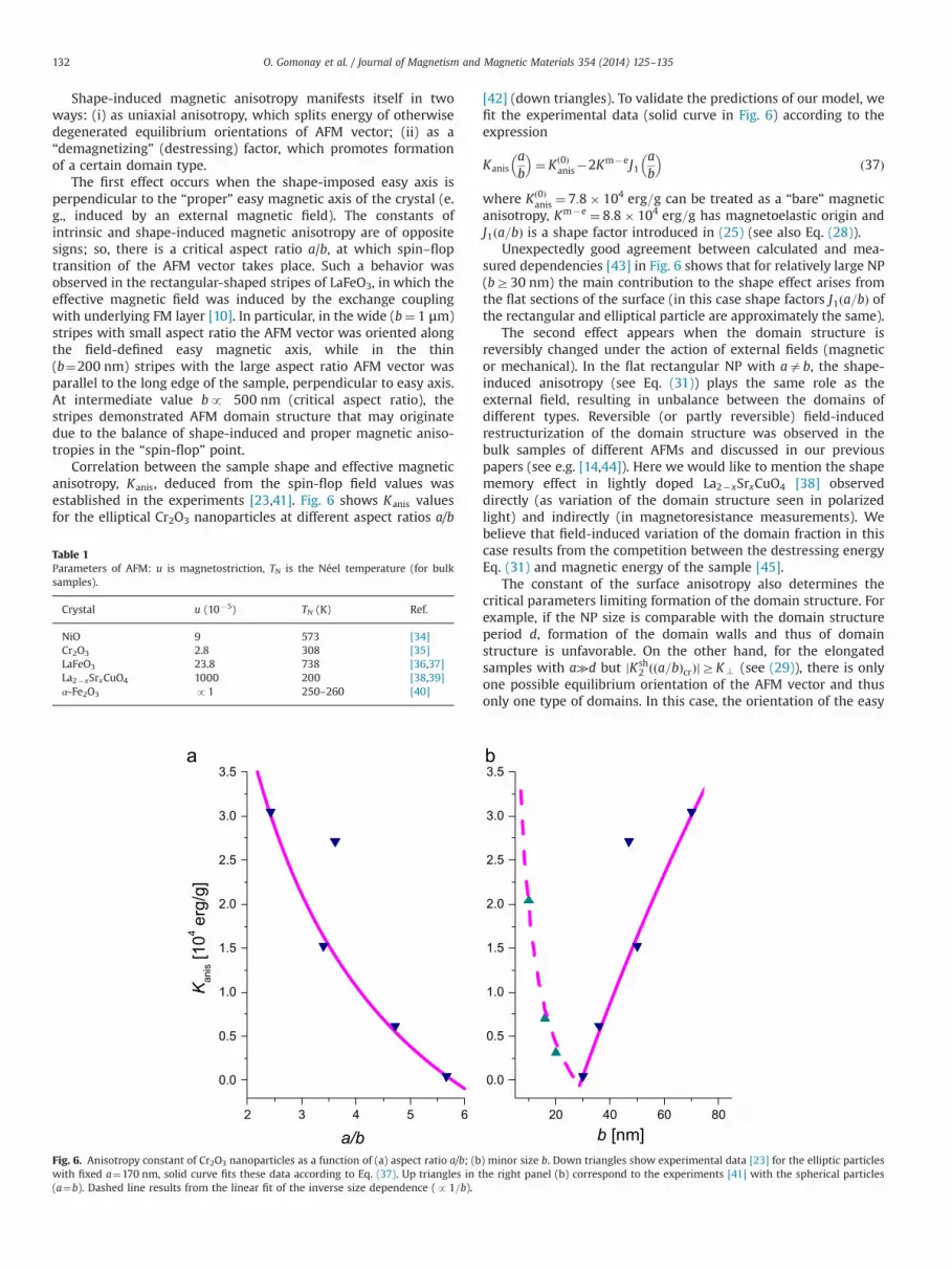
Correlation between the sample shape and effective magneticanisotropy, Kanis, deduced from the spin-flop field values wasestablished in the experiments [23,41]. Fig. 6 shows Kanis valuesfor the elliptical Cr2O3 nanoparticles at different aspect ratios a/b

[42] (down triangles). To validate the predictions of our model, wefit the experimental data (solid curve in Fig. 6) according to theexpression

Kanisab

� �¼ K ð0Þ

anis�2Km�eJ1ab

� �ð37Þ

where K ð0Þanis ¼ 7:8� 104 erg=g can be treated as a “bare” magnetic

anisotropy, Km�e ¼ 8:8� 104 erg=g has magnetoelastic origin andJ1ða=bÞ is a shape factor introduced in (25) (see also Eq. (28)).

Unexpectedly good agreement between calculated and mea-sured dependencies [43] in Fig. 6 shows that for relatively large NP(bZ30 nm) the main contribution to the shape effect arises fromthe flat sections of the surface (in this case shape factors J1ða=bÞ ofthe rectangular and elliptical particle are approximately the same).

The second effect appears when the domain structure isreversibly changed under the action of external fields (magneticor mechanical). In the flat rectangular NP with aab, the shape-induced anisotropy (see Eq. (31)) plays the same role as theexternal field, resulting in unbalance between the domains ofdifferent types. Reversible (or partly reversible) field-inducedrestructurization of the domain structure was observed in thebulk samples of different AFMs and discussed in our previouspapers (see e.g. [14,44]). Here we would like to mention the shapememory effect in lightly doped La2�xSrxCuO4 [38] observeddirectly (as variation of the domain structure seen in polarizedlight) and indirectly (in magnetoresistance measurements). Webelieve that field-induced variation of the domain fraction in thiscase results from the competition between the destressing energyEq. (31) and magnetic energy of the sample [45].

The constant of the surface anisotropy also determines thecritical parameters limiting formation of the domain structure. Forexample, if the NP size is comparable with the domain structureperiod d, formation of the domain walls and thus of domainstructure is unfavorable. On the other hand, for the elongatedsamples with a≫d but jKsh

2 ðða=bÞcrÞjZK ? (see (29)), there is onlyone possible equilibrium orientation of the AFM vector and thusonly one type of domains. In this case, the orientation of the easy

Fig. 6. Anisotropy constant of Cr2O3 nanoparticles as a function of (a) aspect ratio a/b; (b) minor size b. Down triangles show experimental data [23] for the elliptic particleswith fixed a¼170 nm, solid curve fits these data according to Eq. (37). Up triangles in the right panel (b) correspond to the experiments [41] with the spherical particles(a¼b). Dashed line results from the linear fit of the inverse size dependence (p1=b).

Table 1Parameters of AFM: u is magnetostriction, TN is the Néel temperature (for bulksamples).

Crystal u (10�5) TN (K) Ref.

NiO 9 573 [34]Cr2O3 2.8 308 [35]LaFeO3 23.8 738 [36,37]La2� xSrxCuO4 1000 200 [38,39]α-Fe2O3 p1 250–260 [40]

O. Gomonay et al. / Journal of Magnetism and Magnetic Materials 354 (2014) 125–135132

axis depends not only on ratio a/b, but also on the angle ψ, whichdetermines the orientations of the sample edges. So, the control ofthe AFM particles shape allows us not only to create single-domainsamples, but also to drive the magnetic ordering direction.

The magnetoelastic charge-based formalism allows us to predict,at least qualitatively, the morphology of the domain structuredepending on the size of the NP and crystallographic orientationsof its edges. Note that charge contribution increases the energydensity of NP compared with the case of an infinite crystal.So, charge-less (or zero mean) configuration is more favorable, asin FMs. If the NP edges are parallel to the crystallographic axes, thesurface charges disappear in the structure that shown in Fig. 7a, –when the domain of a certain type grows from the edge into the bulkas far as possible. This type of the domain growth was observedexperimentally in [12]; the authors named it “edge effect”. Edgeeffect disappears if sample edges are rotated at angle ψ ¼ π=4 withrespect to easy magnetic axes. Really, in this geometry chargevanishes only in average (due to formation of the domain structurethat is periodic along the edge, Fig. 7b). In this case, we assume thatdomain formation starts from the vertices of the rectangle, and thesurface tension stresses can play a significant role in this process.A detailed discussion of this issue is beyond the scope of this paper.

The explicit form of the shape-induced anisotropy constants(28), (29) depends on the magnetic properties of the surface. Inour model we suggest that the magnetic ordering at the surfacesomehow differs from that in the bulk, e.g. by orientation of easyaxis (see (1)). However, it is possible to generalize the model andconsider other typical situations: e.g., the surface of the sample isparamagnetic, unlike the bulk. In this case, we expect that thenonmagnetic shell will impose additional stresses (that result fromincompatibility between magnetostriction of the core and zerostrain at the surface) in the particle, which for large (multidomain)samples could show up in the destressing energy (similar to (31)).In the single-domain particles these stresses could result in theincrease of the observed magnetostriction compared to the bulksamples, as it was experimentally found in NiO [1,46] and Cr2O3

[41] nanoparticles.It is necessary to mention another contribution into shape-

induced anisotropy ignored in our model. Namely, inhomogeneousdistribution of AFM vectors (and/or elastic strains) at the surfacecan give rise to the “Laplas”-like stress proportional to thecurvature of the surface. In the spherical-shaped particles the roleof Laplas stress grows with a decrease of particle size. In particular,Fig. 6b illustrates this fact using as an example the size depen-dence of the effective anisotropy Kanis of small (br30 nm) Cr2O3

particles. Experimental data [41] (up triangles) are rather wellfitted with the inverse dependence Kanisp1=b (dashed curve).In the rectangular samples additional Laplas stresses may appearin the vicinity of the apexes.

Note that we have considered the ideal, i.e. defectless, sample,eliminating the energy of twin boundaries and disclinations (thelatter inevitably arise in the areas of convergence of three or more

domains), and neglecting peculiarities of the AFM vector distribu-tion near the vertices of the rectangle. Certainly, these factorsshould influence the domain structure formation and the effectivemagnetic anisotropy of the sample. However, we assume that onlythe surface relates the internal magnetic properties of NP and itsform. We have shown that the shape effects can be caused by thelong-range fields of non-magnetic nature – elastic forces – and sothey should appear in the “pure” AFM samples (without FMmoment as well). The effects described above should be morepronounced in the small (up to few critical lengths) samples: in thiscase, the formation of the magnetic structure is determined mainlyby the surface and the influence of the defects can be neglected.

The developed model can be applied to AFM particles whosedimensions are large enough to admit micromagnetic description.Typical thickness of the surface layer can be estimated as 1–3 nm(see, e.g., [47,48]), the minimal domain size observed in 12 nmparticles of NiO was as small as 4 nm [49]. So, the model candescribe, at least qualitatively, the particles even within thenanoscale range (i.e. 10–100 nm), however, below 100 nm themodel should be generalized to account for the surface curvature,as explained above.

The proposed model is suitable for description of the bit-patterned media with AFM layer widely used in informationtechnologies (see, e.g. [50–55]). Typical element has a submicron(down to 200 nm) size, rectangular shape and usually is wellseparated from the neighbors, so, it can be viewed as an alone-standing AFM particle considered above. On the other hand, suchmultilayered systems pose new interesting and nontrivial pro-blems related to competition of shape effects resulted from bothFM and AFM layers, interparticle interaction through the elasti-cally soft substrate, etc.

In conclusion, the results obtained show that the shape can be usedas a technological factor which allows us to drive, control and set theproperties of antiferromagnetic nano- and submicron-sized samples.

The work is performed under the program of fundamentalResearch Department of Physics and Astronomy, National Academyof Sciences of Ukraine, and supported in part by a grant of Ministry ofEducation and Science of Ukraine (N 2466-f).

Appendix A. Green tensor method for the displacement fieldcalculation

Assuming that we know the distribution of the AFM vector LðrÞ,let us examine Eqs. (9)–(10) for the elastic subsystem. Thecorresponding boundary conditions at the surface are:

1þνeff1�3νeff

n div uþnxð∇xux�∇yuyÞþnyð∇xuyþ∇yuxÞnxð∇xuyþ∇yuxÞ�nyð∇xux�∇yuyÞ

!

¼ �2λanisμ

LsurðLsurnÞ: ðA:1Þ

Fig. 7. Multidomain state of the nanoparticle with edges parallel (a) or at an angle 451 (b) relative to crystal axes. Arrows outside the rectangle indicate the orientation of theNéel vector at the surface.

O. Gomonay et al. / Journal of Magnetism and Magnetic Materials 354 (2014) 125–135 133

To simplify, we skip the terms that describe the isotropicmagnetostriction (as insignificant for further discussion).

We denote the bulk forces vector by

f ¼ �∇x cos 2φþ∇y sin 2φ∇x sin 2φ�∇y cos 2φ

!; ðA:2Þ

and the surface tension tensor (of the magnetostrictive nature) by2ðλanis=μÞLsur � Lsur.

Let the functions Gkjðr; r′Þ (k; j¼ x; y) be the solutions of theequation:

ΔGkjðr; r′Þþνeff∇k∇lGljðr; r′Þ ¼ �δkjδðr�r′Þ; ðA:3Þ

with the following boundary conditions:

ðn;∇ÞGkjðrsur; r′Þþνeff nk∇lGljðrsur; r′Þþnl∇kGljðrsur; r′Þ �¼ 0: ðA:4Þ

Here, δkj is the Kronecker symbol, δðr�r′Þ is the Dirac delta-function, n is the surface normal in point rsur.

The functions Gkjðr; r′Þ coincide with Green tensor for isotropicmedium with fixed stresses (accurate within constants). In thiscase, we can represent the displacement vector as follows:

ujðrÞ ¼ �2λanisμ

ZVGkjðr; r′Þ∇′

l½Lkðr′ÞLlðr′Þ� dV ′

�2λanisμ

∮SGkjðr; r′surÞLkðr′surÞLlðr′surÞ dS′l ðA:5Þ

Substituting (A.5) into energy expression (6) and taking intoaccount boundary conditions (A.4), we obtain elastic and magne-toelastic energy contributions:

Wadd ¼2λ2anisμ

ZV

ZV∇m½LjðrÞLmðrÞ�Gkjðr; r′Þ∇′

l½Lkðr′ÞLlðr′Þ� dV dV ′

þ2λ2anisμ

∮S∮S LjðrsurÞLmðrsurÞGkjðrsur; r′surÞLkðr′surÞLlðr′surÞ dSm dS′l:

ðA:6Þ

Appendix B. Shape-induced contribution into the magneticenergy for an arbitrary constant Ksur

In the general case, magnetoelastic charges (21) and (22)depend on the ratio s� sDW=Ksur, which we took as a unit whenobtained Eqs. (28) and (29). Here, we generalize these expressionsfor arbitrary values of s.

Substituting (21), (22) and (23), (24) into Eq. (8), we obtainexpressions (27), where coefficients Ksh

2 , Ksh4 depend on variables

φðinÞ:

Ksh2 ¼ Km�e J1

ab

� �Λþ þΛ�ΛþΛ�

� 1þνeff J2ab

� �� �Λþ �Λ�ΛþΛ�

� �; ðB:1Þ

Ksh4 ¼ Km�e 2J2

ab

� ��1

� �1�sðΛþ þΛ� Þ

2ΛþΛ�

� � J1

ab

� �sðΛþ �Λ� Þ2ΛþΛ�

� �:

ðB:2ÞHere,

Λ7 �ffiffiffiffiffiffiffiffiffiffiffiffiffiffiffiffiffiffiffiffiffiffiffiffiffiffiffiffiffiffiffiffiffiffiffiffiffiffiffiffiffiffiffiffiffiffiffiffiffiffiffiffiffiffiffi172s cos 2ðφinþψ Þþs2

q: ðB:3Þ

In the limiting case of the small magnetic anisotropy (s≫1)both shape-dependent constants vanish:

Ksh2 ¼ Km�eJ1

ab

� �2s-0; Ksh

4 ¼ �Km�eJ1ab

� � cos 2ðφinþψ Þs

-0:

ðB:4Þ

Eq. (27) may perform as the minimum condition for theeffective energy:

weff ¼ �14K ? cos 4φin�

12sKm�e J1

ab

� �ðΛþ �Λ� Þ

hþ 1þνeff J2

ab

� �� �ðΛþ þΛ� Þ

i

� 112s

Km�e 2J2ab

� ��1

� �3 s cos 4ðφinþψ Þþ2ðΛ� þΛþ Þ3� �h

�2J1ab

� �ðΛ� �Λþ Þ3

i: ðB:5Þ

References

[1] M. Petrik, B. Harbrecht, in: 26 European Crystallographic Meeting Darmstard,Germany, 2010, pp. FA5–MS41–P11.

[2] M. Petrik, B. Harbrecht, Z. Kristallogr. Proc. 1 (2011) 253.[3] X.G. Zheng, H. Kubozono, H. Yamada, K. Kato, Y. Ishiwata, C.N. Xu, Nat.

Nanotechnol. 3 (2008) 724.[4] M. Petrik, B. Harbrecht, Z. Anorgan. Allgem. Chem. 636 (2010) 2049.[5] C. Bahl, L.T. Kuhn, K. Lefmann, P.-A. Lindgard, S. Morup, Phys. B: Condens.

Matter 385–386 (1) (2006) 398.[6] L. Néel, C.R. Hebd Séan. Acad. Sci. 328 (1949) 664.[7] L. Néel, Low-temperature physics, in: C. de Witt, B. Dreyfus, P.-G. de Gennes

(Eds.), Summer School of theoretical physics, les houches (1961) Théorie despropriétés magnétiques des grains fins antiferromagnétiques: superparamag-nétisme et superantiferromagnétisme, Gordon & Breach, New York, New York,1962, p. 413.

[8] R.H. Kodama, A.E. Berkowitz, E.J. McNiff Jr., S. Foner, Phys. Rev. Lett. 77 (1996) 394.[9] S. Morup, C. Frandsen, F. Bodker, S.N. Klausen, K. Lefmann, P.-A. Lindgard,

M.F. Hansen, in: P. Gutlich, B.W. Fitzsimmons, R. Ruffer, H. Spiering (Eds.),Mossbauer Spectroscopy, Springer, Netherlands, 2003, pp. 347–357.

[10] E. Folven, A. Scholl, S.T. Young, A. Retterer, J.E. Boschker, T. Tybell, Y. Takamura,J.K. Grepstad, Nano Lett. 12 (2012) 2386.

[11] E. Folven, A. Scholl, A. Young, S.T. Retterer, J.E. Boschker, T. Tybell, Y. Takamura,J.K. Grepstad, Phys. Rev. B 84 (2011) 220410.

[12] E. Folven, T. Tybell, A. Scholl, A. Young, S.T. Retterer, Y. Takamura, J.K. Grepstad,Nano Lett. 10 (2010) 4578.

[13] D.A. Garanin, H. Kachkachi, Phys. Rev. Lett. 90 (2003) 065504.[14] H.V. Gomonay, V.M. Loktev, Phys. Rev. B 75 (2007) 174439.[15] H. Gomonay, I. Kornienko, V. Loktev, Condens. Matter Phys. 13 (2010) 23701.[16] M.I. Kaganov, Sov. Phys. JETP 52 (1980) 779.[17] A.N. Bogdanov, U.K. Rößler, Phys. Rev. B 68 (2003) 012407.[18] A.N. Bogdanov, U.K. Rößler, Phys. Rev. Lett. 87 (2001) 037203.[19] A. Bogdanov, U. Rossler, K.-H. Muller, J. Magn. Magn. Mat. 238 (2002) 155.[20] C. Kittel, Rev. Mod. Phys. 21 (1949) 541.[21] N. Pérez, P. Guardia, A.G. Roca, M.P. Morales, C.J. Serna, O. Iglesias, F. Bartolomé,

L.M. García, X. Batlle, A. Labarta, Nanotechnology 19 (2008) 5704.[22] R.N. Bhowmik, R. Nagarajan, R. Ranganathan, Phys. Rev. B 69 (2004) 054430.[23] D. Tobia, E. Winkler, R.D. Zysler, M. Granada, H.E. Troiani, Phys. Rev. B 78

(2008) 104412.[24] L.D. Landau, E.M. Lifshits, 4th ed.,Theory of elasticity, course of theoretical

physics, vol. 7, Fizmatgiz, Moscow, 1987, p. 246.[25] S.K. Mishra, V. Subrahmanyam, Int. J. Mod. Phys. B 25 (2011) 2507.[26] R.H. Kodama, S.A. Makhlouf, A.E. Berkowitz, Phys. Rev. Lett. 79 (1997) 1393.[27] The values of the internal constants in NPs could differ significantly (by

several times or even orders) from those for the bulk samples [1,3,56], wherethe role of the surface is negligible.

[28] V. Gann, A. Zhukov, Sov. Solid State Physics 22 (1980) 3188.[29] E.A. Brener, V.I. Marchenko, Phys. Rev. Lett. 97 (2006) 067204.[30] M. Petrik, B. Harbrecht, Solid State Phenom. 170 (2011) 244.[31] M. Nishida, T. Hara, M. Matsuda, S. Ii, Mater. Sci. Eng.: A 481–482 (2008) 18.[32] E.D. Belokolos, J. Phys. A: Math. General 34 (2001) 2331.[33] G. Catalan, H. Béa, S. Fusil, M. Bibes, P. Paruch, A. Barthélémy, J.F. Scott, Phys.

Rev. Lett. 100 (2008) 027602.[34] T. Yamada, S. Saito, Y. Shimomura, J. Phys. Soc. Jpn. 21 (1966) 672.[35] K.L. Dudko, V.V. Eremenko, L.M. Semenenko, Physica Status Solidi (b) 43 (1971) 471.[36] S.C. Abrahams, R.L. Barns, J.L. Bernstei, Solid State Commun. 10 (1972) 379.[37] D. Treves, J. Appl. Phys. 36 (1965).[38] A.N. Lavrov, S. Komiya, Y. Ando, Nature 418 (2002) 385.[39] A. Nabialek, P. Komorowski, M.U. Gutowska, M.A. Balbashov, J.N. G?recka,

H. Szymczak, O.A. Mironov, Supercond. Sci. Technol. 10 (1997) 786.[40] R.A. Voskanya, R.Z. Levitin, V.A. Shchurov, Sov. Phys. JETP 27 (1968) 423.[41] D. Tobia, E. De Biasi, M. Granada, H.E. Troiani, G. Zampieri, E. Winkler,

R.D. Zysler, J. Appl. Phys. 108 (2010) 104303.[42] Originally, in [23] Kanis was measured as a function of synthesis temperature

whose value correlates with the minor size b of the nanoparticles. The majoraxis kept approximately constant value 170 nm.

[43] At large b-a the particle can split into multidomain state. In this caseapproximation (37) should be corrected.

[44] E.V. Gomonaj, V.M. Loktev, Phys. Rev. B 64 (2001) 064406.

O. Gomonay et al. / Journal of Magnetism and Magnetic Materials 354 (2014) 125–135134

[45] In the experiments [38] shape memory effect was observed below and abovethe Néel point. In the latter case expression for destressing energy should bewritten in terms of strains, not AFM vectors.

[46] M. Petrik, B. Harbrecht, Z. Anorgan. Allgem. Chem. 634 (2008) 2069.[47] J. Ma, K. Chen, Phys. Lett. A 377 (2013) 2216.[48] J.F.K. Cooper, A. Ionescu, R.M. Langford, K.R.A. Ziebeck, C.H.W. Barnes, R. Gruar,

C. Tighe, J.A. Darr, N.T.K. Thanh, B. Ouladdiaf, J. Appl. Phys. 114 (2013) 083906.[49] S. Klausen, P.-A. Lindgard, K. Lefmann, F. Bodker, S. Morup, Phys. Status Solidi

A 189 (2002) 1039.[50] A. Moser, K. Takano, D.T. Margulies, M. Albrecht, Y. Sonobe, Y. Ikeda, S. Sun,

E.E. Fullerton, J. Phys. D: Appl. Phys. 35 (2002) R157.

[51] S. Maat, K. Takano, S.S.P. Parkin, E.E. Fullerton, Phys. Rev. Lett. 87 (2001)087202.

[52] Y. Takamura, R.V. Chopdekar, A. Scholl, A. Doran, J.A. Liddle, B. Harteneck,Y. Suzuki, Nano Lett. 6 (2006) 1287.

[53] I.L. Prejbeanu, S. Bandiera, J. Alvarez-Hérault, R.C. Sousa, B. Dieny, J.-P. Nozíres,J. Phys. D: Appl. Phys. 46 (2013) 074002.

[54] T. Hasegawa, T. Tomioka, Y. Kondo, H. Yamane, S. Ishio, J. Appl. Phys. 111 (2012) 07.[55] A.D. Lamirand, M.M. Soares, A.Y. Ramos, H.C.N. Tolentino, M. De Santis,

J.C. Cezar, A. de Siervo, M. Jamet, Phys. Rev. B 88 (2013) 140401.[56] Z.H. Sun, X.Y. Song, F.X. Yin, L.X. Sun, X.K. Yuan, X.M. Liu, J. Phys. D: Appl. Phys.

42 (2009) 122004.

O. Gomonay et al. / Journal of Magnetism and Magnetic Materials 354 (2014) 125–135 135