arX

iv:c

ond-

mat

/950

6052

v1 1

2 Ju

n 19

95

Scaling Theory of Antiferromagnetic

Heisenberg Ladder Models

Naomichi Hatano∗ and Yoshihiro NishiyamaDepartment of Physics, University of Tokyo, Hongo 7-3-1, Bunkyo-ku, Tokyo 113, Japan

Abstract

The S = 1/2 antiferromagnetic Heisenberg model on multi-leg ladders is investigated.Criticality of the ground-state transition is explored by means of finite-size scaling. Theladders with an even number of legs and those with an odd number of legs are distinguishedclearly. In the former, the energy gap opens up as ∆E ∼ J⊥, where J⊥ is the strength ofthe antiferromagnetic inter-chain coupling. In the latter, the critical phase with the centralcharge c = 1 extends over the whole region of J⊥ > 0.

1 Introduction

Understanding of the ground-state criticality of one-dimensional quantum system has been enrichedgreatly in the past decade. One of the important breakthroughs was finite-size scaling based on theconformal field theory [1]; see [2] for a review. Nowadays many attempts on generalization for higher-dimensional systems are in progress. One of them is the study of coupled chains. The Heisenbergladder models are particularly of interest. The two-dimensional Heisenberg model might be exploredas the limiting case of the ladder models. In addition, actual substances which realize the laddermodels have been developed experimentally: Sr2n−2Cu2nO4n−2, for example [3].

The Hamiltonian of the S = 1/2 Heisenberg ladder models is given by

H ≡ Hleg + Hrung, (1.1)

where

Hleg ≡ JL−1∑

x=0

nl∑

y=1

~Sx,y · ~Sx+1,y, (1.2)

Hrung ≡ J⊥L−1∑

x=0

nl−1∑

y=1

~Sx,y · ~Sx,y+1. (1.3)

In the present paper we treat the antiferromagnetic case, J > 0 and J⊥ > 0. Each component of thespins is defined by

Sµ =1

2σµ (µ = x, y, z), (1.4)

where {σµ} are the Pauli matrices. We define S± ≡ Sx± iSy. We impose periodic boundary conditionsonly in the x direction:

~SL,y = ~S0,y for y = 1, 2, . . . , nl. (1.5)

Hereafter the system size L is even.In the present paper, we focus on the ground-state criticality of the ladder models. It was conjec-

tured [4] that the ladder models with even nl and those with odd nl behave quite differently from each

∗Address from April 1995 to March 1996: Lyman Laboratory of Physics, Harvard University, Cambridge, Mas-

other; for J⊥ = 1, the former is massive, while the latter is massless. Here we discuss the criticalityfor arbitrary positive J⊥ and for general nl.

It is well known that the antiferromagnetic Heisenberg chain (J⊥/J = 0) is massless [5]. Manyquestions arise when we introduce the inter-chain coupling Hrung: It has been quite controversial [6-9]whether the system with nl = 2 becomes massive for any positive J⊥, or there exists a critical pointat a finite value of J⊥; It has not been clarified whether the massless phase for odd nl extends overthe whole region of J⊥ > 0, or a massive phase exists in the region 0 < J⊥ < 1; The universality ofthe massless phase has not been discussed either.

The purpose of the present paper is to answer the above questions on the basis of finite-sizescaling theory. We introduce our scaling ansatz in section 2.1. The ansatz yields useful conclusionsimmediately. In particular, we conclude that the whole region of J⊥ > 0 is controlled by the stablefixed point at J⊥/J = ∞. Thus we distinguish the systems with even nl and those with odd nl clearly:the former is massive for any J⊥, while the latter is critical with the central charge c = 1 for any J⊥.We present some results for even nl and for odd nl in sections 2.2 and 2.3, respectively. We particularlyshow estimation of critical amplitudes. We give numerical confirmation of the scaling ansatz in section2.1. In addition to that, we confirm the ansatz by means of perturbation theory in section 3.

2 Finite-size scaling of the energy gap

In this section, we introduce the finite-size scaling form of the energy gap. We numerically confirmthe scaling ansatz. We present our conclusions drawn from the ansatz.

2.1 General arguments

The central scaling ansatz of the present paper is written in the form

∆E(L) ≃J

L∆(x) = J⊥

∆(x)

xwith x ≡

LJ⊥J

, (2.1)

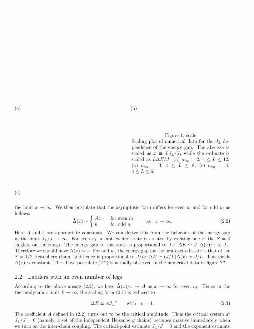
where ∆E is the energy gap between the ground state and the first excited state, and ∆ denotes therelevant scaling function. We show, in figure ??, numerical data obtained by the Lanczos method [10].The data are scaled well over a finite region of x (namely 0 ≤ x ≤ 5) for nl = 2, 4, and over the wholeregion of x for nl = 3. We confirm the scaling form (2.1) by means of perturbation theory in section 3.

The ansatz (2.1) implies that the inter-chain coupling is a relevant operator. The coupling Hrung

drives the system away from the point J⊥/J = 0, and makes the system renormalized to the limitJ⊥/J → ∞ as L → ∞; see figure ??. Thus the fixed point at J⊥/J = ∞ controls the whole phase ofthe region J⊥ > 0. Apart from correction to scaling, the thermodynamic limit L → ∞ is equivalentto the limit J⊥/J → ∞.

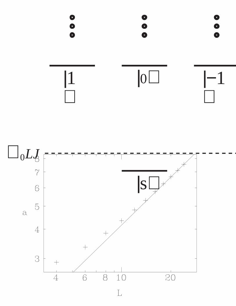
We can thereby understand the difference between the systems with even nl and those with oddnl. For even nl, the spins on each rung form an S = 0 singlet in the limit J⊥/J → ∞. The system atthe fixed point J⊥/J = ∞ is the S = 0 chain with the energy gap of the order of J⊥ [11]. For odd nl,on the other hand, the spins on each rung form an S = 1/2 doublet in the limit J⊥/J → ∞. In thefirst-order perturbation of J , we have the same energy spectrum as of the S = 1/2 Heisenberg chain.(See section 2.3 for details.) Hence the system at the fixed point J⊥/J = ∞ is the S = 1/2 Heisenbergchain, which is massless, or critical. Thus the whole phase of J⊥ > 0 for even (odd) nl is controlled bythe massive S = 0 (massless S = 1/2) Heisenberg chain.

In order to argue asymptotic behavior of the scaling function ∆(x), we can exploit the two limitsJ⊥/J → ∞ and L → ∞. In the thermodynamic limit L → ∞, we must have non-divergent value of

˜

(a) (b)

(c)

Figure 1: scaleScaling plot of numerical data for the J⊥ de-pendence of the energy gap. The abscissa isscaled as x ≡ LJ⊥/J , while the ordinate isscaled as L∆E/J : (a) nleg = 2, 4 ≤ L ≤ 12;(b) nleg = 3, 4 ≤ L ≤ 8; (c) nleg = 4,4 ≤ L ≤ 6.

the limit x → ∞. We then postulate that the asymptotic form differs for even nl and for odd nl asfollows:

∆(x) ∼

{

Ax for even nlb for odd nl

as x→ ∞. (2.2)

Here A and b are appropriate constants. We can derive this from the behavior of the energy gapin the limit J⊥/J → ∞. For even nl, a first excited state is created by exciting one of the S = 0singlets on the rungs. The energy gap to this state is proportional to J⊥: ∆E ≃ J⊥∆(x)/x ∝ J⊥.Therefore we should have ∆(x) ∼ x. For odd nl, the energy gap for the first excited state is that of theS = 1/2 Heisenberg chain, and hence is proportional to J/L: ∆E ≃ (J/L)∆(x) ∝ J/L. This yields∆(x) ∼ constant. The above postulate (2.2) is actually observed in the numerical data in figure ??.

2.2 Ladders with an even number of legs

According to the above ansatz (2.2), we have ∆(x)/x → A as x → ∞ for even nl. Hence in thethermodynamic limit L→ ∞, the scaling form (2.1) is reduced to

∆E ≃ AJ⊥ν with ν = 1. (2.3)

The coefficient A defined in (2.2) turns out to be the critical amplitude. Thus the critical system atJ⊥/J = 0 (namely, a set of the independent Heisenberg chains) becomes massive immediately whenwe turn on the inter-chain coupling. The critical-point estimate J⊥/J = 0 and the exponent estimate

Figure 2: renomThe conjectured renormalization-flow diagramfor the Heisenberg ladders. The fixed pointJ⊥/J = 0 is unstable with respect to theinter-chain coupling. The stable fixed pointat J⊥/J = ∞ is described by the massiveS = 0 chain for even nleg, and by the mass-less S = 1/2 chain for odd nleg. We therebyconclude that the whole phase of J⊥ > 0 ismassive for even nleg and is critical for oddnleg.

Let us estimate the critical amplitude A for nl = 2. We utilize the following general finite-sizescaling form for one-dimensional quantum ground-state phase transitions [12]:

L∆E(L)

J≃

Ax+D+e−Cx in the disordered phase,B at the critical point,D−e−Cx in the ordered phase.

(2.4)

Here x ≡ L|ε|ν denotes the relevant scaling variable with ε being the distance from the critical point;x = LJ⊥/J in the present case. The coefficient A gives the critical amplitude in (2.3). The coefficientC, on the other hand, gives the critical amplitude of the correlation length: ξ−1 ≃ C(J⊥/J)ν . Weintroduced in [12] the amplitude relation

A/C = vs, (2.5)

where vs is the sound velocity. The coefficient B is predicted from the conformal field theory asB = vsπη, where η is Fisher’s correlation exponent [13]. For the Hamiltonian (1.1) with J⊥/J = 0,the Bethe-ansatz solution [14] gives

η = 1 and vs =π

2; (2.6)

hence we haveA

C=π

2= 1.570796 · · · and B =

π2

2= 4.934802 · · · . (2.7)

The coefficients D+ and D− may have weak x dependence [12].The asymptotic behavior in (2.2) for even nl is consistent with the scaling form (2.4) in the disor-

dered phase. We can employ our previous analysis in [12], where we showed for the one-dimensionalquantum Potts model that a good estimator of the amplitude A is given by

AminL ≡ min

x>0

(

L∆E/J

x

)

. (2.8)

(If the data followed the scaling form (2.4) completely, the quantity L∆E/(Jx) would converge to Aexponentially as x → ∞. However, there appears the minimum in practice, probably because somecorrection to scaling [12].) The estimator (2.8) may converge to A exponentially [12] in the form

AminL ≃ A+ c1 exp(−c2L). (2.9)

We calculated AminL for the data in figure ?? (a), and fitted the results to the form (2.9); see figure ??.

We thereby have the estimate A = 0.47(1) and hence 1/C = vs/A = 3.34(7) for nl = 2. (The error of

(a) (b)

Figure 3: fitEstimation of the critical amplitude A for nleg = 2 as was done in [12]. (a) The quantity L∆E/(Jx)versus x for L = 12, for example. The estimator (2.8) is obtained as Amin

12 = 0.505 · · ·, which isindicated by the dotted lines. (b) The values of the estimator (2.8) are fitted to the form (2.9). Thesolid line shows the best fit Amin

L ≃ 0.468 + 0.505 exp(−0.218L).

the estimate A was evaluated through the least-squares fitting to the form (2.9).) Namely, we have

∆E ≃ 0.47J⊥ and ξ ≃ 3.34J

J⊥(2.10)

as L → ∞ and near J⊥/J ∼ 0. These explain the following estimates in [4] quite well: ∆E = 0.504Jand ξ = 3.19(1) for nl = 2 and J⊥/J = 1. Although it is unnecessary that the critical behavior (2.10)near J⊥/J ∼ 0 is observed even for J⊥/J = 1, we see in figure 2 of [7] that correction to (2.10) maybe quite small in the region J⊥/J ≤ 1.

Incidentally, the energy gap is ∆E = J⊥ for nl = 2 in the limit J⊥/J → ∞, where the system isreduced to a set of independent dimers. A crossover from the behavior (2.10) to the behavior ∆E = J⊥may occur in the region J⊥/J > 1.

If we naively apply the same analysis as above to the data for nl = 4 with L = 2, 4 and 6, weobtain the tentative estimates

A ≃ 0.27 and C−1 = vs/A ≃ 5.8. (2.11)

Though there may be some errors in these estimates, the values (2.10) and (2.11) are fairly consistentwith the scaling hypothesis ξ ∝ nl [4].

2.3 Ladders with an odd number of legs

For odd nl, we can see in figure ?? that the scaling region is quite wide. We may naturally assumethat the scaling form (2.1) with (2.2) is valid for any value of L and J⊥/J . Thus we have the followingremarkable conclusion: for any positive J⊥, the energy gap in the thermodynamic limit L→ ∞ behavesas

∆E

J≃

b

L, (2.12)

where the amplitude b is the coefficient defined in (2.2). Note that this amplitude is independent ofJ by definition. In other words, the energy spectrum in the thermodynamic limit for any positive

J⊥ is identical to that for J⊥/J → ∞, or the spectrum of the S = 1/2 antiferromagnetic Heisenbergchain. We thus conclude that the whole phase of J⊥ > 0 for odd nl is a critical phase with the centralcharge c = 1. Note that the central charge is c = nl for J⊥/J = 0, because we have nl systems of c = 1at this point.

We can obtain the value of the amplitude b by considering the limit J⊥/J → ∞. For this purpose,we first describe how to obtain explicitly the effective Hamiltonian of the S = 1/2 Heisenberg chain inthe limit J⊥/J → ∞.

In the very limit of J⊥/J = ∞, or J/J⊥ = 0, the Hamiltonian is reduced to Hrung; the rungs areindependent of each other. The ground state of the whole system is the direct product of the groundstate of each rung. On each rung, an odd number of spins are coupled with the antiferromagneticinteraction J⊥. Hence two ground states of each rung are degenerate with S = 1/2 and Sz = ±1/2.We express the states on the xth rung as |+x〉 and |−x〉. The ground states of the whole system havethe 2L-fold degeneracy. This degeneracy is lift up in the first-order perturbation of J/J⊥, or Hleg. Wecalculate the first-order perturbation for degenerate states by writing down the secular equation:

∣

∣

∣H − λI∣

∣

∣ = 0. (2.13)

Here the matrix I denotes the identity operator. The first-order energy is denoted by λ. The matrixH is a 2L × 2L matrix which represents the operator Hleg in the subspace of the degenerate ground

states. For example, one of the diagonal elements of H is given by

〈−1 −2 +3 −4 · · ·|Hleg |−1 −2 +3 −4 · · ·〉

= JL−1∑

x=0

nl∑

y=1

〈−1 −2 +3 −4 · · ·| ~Sx,y · ~Sx+1,y |−1 −2 +3 −4 · · ·〉

= Jnl∑

y=1

(

〈−1|Sz1,y |−1〉 〈−2|S

z2,y |−2〉 + 〈−2|S

z2,y |−2〉 〈+3|S

z3,y |+3〉 + · · ·

)

, (2.14)

and one of the nonzero off-diagonal elements is given by

〈−1 −2 +3 −4 · · ·| Hleg |−1 +2 −3 −4 · · ·〉 =J

2

nl∑

y=1

〈−2|S−2,y |+2〉 〈+3|S

+3,y |−3〉 . (2.15)

It is apparent that the secular equation (2.13) is equivalent to the eigenvalue equation for theS = 1/2 Heisenberg chain:

Heff = Jeff

L−1∑

x=0

~Sx · ~Sx+1. (2.16)

We can see in (2.14) that the effective coupling Jeff is given by

Jeff = Jnl∑

y=1

(

〈+|Szy |+〉)2. (2.17)

We show numerical results for Jeff in figure ??. The value of Jeff is generally close to unity but increasesmonotonically. In particular, Jeff = J for nl = 3 [11]. For large nl, the matrix element in (2.17) maydepend on nl as [2]

〈+|Szy |+〉 ∼ nl−β/ν = nl

−1/2. (2.18)

Hence we may have Jeff ∼ O(nl0).

As we mentioned in (2.4) and (2.7), it is known [14] for the antiferromagnetic Heisenberg chainwith the coupling Jeff that the energy gap behaves as

∆E ≃vsπη

J =π2Jeff

. (2.19)

Figure 4: JeffThe effective coupling Jeff for odd nleg in thelimit J⊥/J → ∞. The values were calculatednumerically on the basis of (2.17).

Figure 5: spectrumA schematic view of the low-lying energy spec-trum of the S = 1/2 antiferromagnetic Heisen-berg chain.

Comparing this with (2.12), we arrive at the conclusion

b ≡ limx→∞

∆(x) = vsπηJeff

J=π2

2

Jeff

J. (2.20)

3 Perturbational derivation of the scaling ansatz

In this section, we describe a perturbational calculation which yields the scaling form (2.1). This wasbriefly reported in [8].

3.1 Zeroth order of J⊥/J

Let us first describe the energy spectrum for J⊥/J = 0. At this point, we have nl number of theS = 1/2 Heisenberg chains independent of each other. The spectrum of each chain is given [14] asfigure ??. Let |sy〉 denote the singlet ground state of the yth leg, and let |My〉 = {|1y〉 , |0y〉 , |−1y〉}denote the triplet of the first excited states. The energy of the singlet ground state is written in theform

Es ≃ ǫ0LJ −vsπc

6LJ =

(

ǫ0L−π2

12L

)

J as L→ ∞, (3.1)

where ǫ0 = 1/4 − ln 2 is the exact ground-state energy density [5], vs = π/2 is the sound velocity asbefore, and c = 1 denotes the central charge. The energy gap to the triplet states is given by

∆E ≃vsπη

J =π2

J as L → ∞, (3.2)

where η = 1 is Fisher’s correlation exponent as before.The ground state of the whole system is given by the direct product of the singlet states as

∣

∣

∣ψ(0)gs

⟩

=nl⊗

y=1

|sy〉 (3.3)

with the energy

Egs ≃ nl

(

ǫ0L−π2

12L

)

J. (3.4)

The first excited states have the 3nl-fold degeneracy:

∣

∣

∣ψ(0)ex

⟩

= |My1〉 ⊗

nl⊗

y=1

y 6=y1

|sy〉

(M = 0,±1 and y1 = 1, 2, · · · , nl). (3.5)

The energy gap to these excited states is the same as in (3.2).

3.2 First-order perturbation of J⊥/J

Now we calculate the first-order perturbation with respect to Hrung. The first-order energy of theground state is given by

E(1)gs =

⟨

ψ(0)gs

∣

∣

∣Hrung

∣

∣

∣ψ(0)gs

⟩

= J⊥L−1∑

x=0

nl−1∑

y=1

〈sy| ~Sx,y |sy〉 · 〈sy+1| ~Sx,y+1 |sy+1〉 = 0, (3.6)

because we have〈s|Szx |s〉 = 〈s|S±

x |s〉 = 0. (3.7)

In order to obtain the first-order energy of the excited state, we have to construct the secularequation, because the zeroth-order first excited states are degenerate. We concentrate on the sector∑

yMy = 1. The ground state of this sector gives the perturbed first excited state, because theperturbed energy spectrum would be similar to that in figure ?? owing to the SU(2) symmetry. Thefollowing nl states are of this sector:

|(y1)〉 ≡ |1y1〉 ⊗

nl⊗

y=1

y 6=y1

|sy〉

(y1 = 1, 2, · · · , nl). (3.8)

We immediately have〈(y1)|Hrung |(y2)〉 = 0 unless |y1 − y2| = 1. (3.9)

The nonzero matrix elements are

〈(y + 1)| Hrung |(y)〉 =J⊥2

L−1∑

x=0

〈sy|S−x,y |1y〉 〈1y+1|S

+x,y+1 |sy+1〉 = J⊥a

(y = 1, 2, · · · , nl − 1) (3.10)

and their conjugates. Here the coefficient a is defined by

a ≡L

2

∣

∣

∣〈s|S−x |1〉

∣

∣

∣

2(3.11)

(The x dependence of the matrix element 〈s|S−x |1〉 appears only in the phase factor in the form eikx,

and hence the absolute value is independent of x.) The secular equation for the first-order energy ofthe excited state is thereby written in the form

∣

∣

∣

∣

∣

∣

∣

∣

∣

∣

∣

∣

∣

∣

−E(1)ex J⊥a 0J⊥a −E(1)

ex J⊥a

J⊥a. . .

. . .. . .

. . . J⊥a0 J⊥a −E(1)

ex

∣

∣

∣

∣

∣

∣

∣

∣

∣

∣

∣

∣

∣

∣

= 0. (3.12)

This is equivalent to the one-dimensional tight-binding model under the free boundary condition; thetriplet state hops from a leg to a neighboring leg with the hopping amplitude J⊥a. This model isexactly solvable [15]. The zeroth-order wave function and the first-order energy are obtained in theforms

∣

∣

∣ψ(0)ex

⟩

=

√

2

nl

nl∑

y=1

sin(

mπ

nl + 1y)

|(y)〉 , (3.13)

E(1)ex = −2J⊥a cos

mπ

nl + 1, (3.14)

for m = 1, 2, · · · , nl. The state with m = 1 gives the lowest energy.We thereby obtain the energy gap up to the first order of J⊥/J as

∆E ≃J

L

(

π2

2− 2xa cos

π

nl + 1

)

, (3.15)

where x ≡ LJ⊥/J as before.We are in position to estimate the size dependence of the coefficient a. In the following we show

analytically and numerically that a = O(L0).We first show that the coefficient a is proportional to the transverse susceptibility of the Heisenberg

chain. Let us consider the Hamiltonian with a transverse field at the origin:

∆eH ≡ JL−1∑

i=0

~Si · ~Si+1 − γSx0 . (3.16)

After the standard calculation, we have

χ00 ≡∂

∂γ〈Sx0 〉γ

∣

∣

∣

∣

∣

γ=0

=∑

ψn(6=ψgs)

|〈ψn|Sx0 |ψgs〉|

2

∆En(3.17)

=∫ ∞

0dτ 〈Sx0S

x0 (τ)〉0 , (3.18)

where the angular brackets 〈· · ·〉γ denote the expectation value with respect to the ground state of(3.16), ∆En is the excitation energy of the excited state |ψn〉, and

Sx0 (τ) ≡ e−τ∆eHSx0 eτ∆eH. (3.19)

The most dominant of the excited states |ψn〉 is |S = 1, Sz = ±1〉 with the energy gap (3.2), or ∆E ∼L−1. Hence the expression (3.17) is approximately rewritten as

χ ≃4a. (3.20)

Figure 6: coeffThe size dependence of the quantity a appearsto be of the form a ∼ (lnL)ω. The solidline connects the last two data points with theslope ω ≃ 0.68.

On the other hand, a field-theoretic description [16] yields

〈Sx0Sx0 (τ)〉0 ∼

1

τ. (3.21)

Thus the expression (3.18) is a dimensionless quantity: χ00 = O(L0). We thus arrive at the conclusiona = O(L0). There may be logarithmic corrections to this size dependence.

We also calculated the coefficient a in (3.11) numerically for L ≤ 24; see figure ??. The logarithmicplot reveals that the coefficient actually behaves as

a ∼ (lnL)0.68 = O(L0). (3.22)

3.3 Order estimation of higher-order perturbations

We next derive the approximate second-order energy of the ground state. The second-order perturba-tion is given by the formula

E(2)gs = −

∑

ψn(6=ψgs)

|〈ψn| Hrung |ψgs〉|2

∆En. (3.23)

The most dominant excited states are the 3(nl − 1) states

|ψn〉 =

|0y10y1+1〉|1y1 − 1y1+1〉|−1y11y1+1〉

⊗

nl⊗

y=1

y 6=y1,y1+1

|sy〉

(3.24)

with y1 = 1, 2, · · · , nl − 1. The energy gap ∆En to these states is twice as large as in (3.2):

∆En ≃π2J

L. (3.25)

The numerator of (3.23) gives the factor a2 for each of the states (3.24). Hence the second-order energyof the ground state is

E(2)gs ≃ −

3(nl − 1)a2

π2

(

LJ⊥J

)2 J

L. (3.26)

Although it is complicated to calculate the second-order energy of the first excited state (3.13), wecan see that the size dependence is the same as in (3.26):

E(2) ∼ a2(

LJ⊥)2 J

. (3.27)

We thereby have

∆E ≃J

L

[

π2

2+ α1ax+ α2 (ax)2

]

, (3.28)

where x ≡ LJ⊥/J , and α1 and α2 are constants. Since a is of the order of L0, the expression (3.28) isconsistent with the scaling form (2.1).

It is generally difficult to calculate higher-order perturbation explicitly. However, it is possible toestimate the size dependence roughly [17]. The kth-order energy is approximately given by

E(k) ∼∑

{ψ}

〈ψgs|Hrung |ψ1〉 〈ψ2|Hrung |ψ3〉 · · · 〈ψk−1|Hrung |ψgs〉

× [(∆E1) (∆E2) · · · (∆Ek−1)]−1 . (3.29)

We may estimate the dimensionality of the operator Hrung at LJ⊥ × [~S]2 ∼ J⊥, because the magnetic

operator ~S of the antiferromagnetic Heisenberg chain has the dimensionality [~S] = L−β/ν = L−1/2 [2].(This rough estimate is consistent with the estimation a = O(L0).) On the other hand, each energydenominator ∆E is of the order of J/L, because the Heisenberg chain is critical. We thereby have therough estimate

E(k) ∼ J⊥k(

J

L

)−(k−1)

=J

L

(

LJ⊥J

)k

. (3.30)

Hence the energy gap may be given by the form

∆E ∼J

L

∑

k

αkxk (3.31)

with appropriate coefficients {αk}. This is consistent with the scaling ansatz (2.1).We have not confirmed that the above perturbational expansion is convergent. However, the

numerical results in figure ?? do suggest that the series converges at least over a finite region ofx = LJ⊥/J .

4 Summary

In the present paper, we introduced the finite-size scaling form of the energy gap of the antiferromag-netic Heisenberg ladder models:

∆E(L)/J ≃ L−1∆(LJ⊥/J). (4.1)

We confirmed this scaling form numerically as well as by means of perturbation theory. On the basisof the scaling theory, we discussed the criticality of the ladder models in a unified way. The differencebetween the ladders with even nl and with odd nl was attributed to the different asymptotic behaviorof the scaling function in the limit LJ⊥/J → ∞.

For even nl, the energy gap develops in the form ∆E ∼ J⊥. The whole region of J⊥ > 0 is adisordered phase with a unique ground state. (This ground state is reduced to a set of independentsinglets in the limit J⊥/J → ∞.) We estimated for nl = 2 the critical amplitude of the energy gapand the correlation length around the critical point J⊥/J = 0.

For odd nl, on the other hand, the whole region of J⊥ > 0 is the critical line. The energygap vanishes in the form ∆E ∼ L−1 for any J⊥. The critical line is controlled by the S = 1/2antiferromagnetic Heisenberg chain which is obtained in the limit J⊥/J → ∞. The central charge ofthe phase is hence unity.

Acknowledgments

The authors are grateful to Dr A Terai for helpful discussions. The numerical calculations wereperformed on the super-computer HITAC S3800/480 of the Computer Centre, University of Tokyoand on the work-station HP Apollo 9000/735 of the Suzuki group, Department of Physics, Universityof Tokyo.

References

[1] Cardy J L 1984 J. Phys. A: Math. Gen. 17 L385-7[2] Cardy J L 1987 Phase Transitions and Critical Phenomena vol 11 ed C Domb and J L Lebowitz

(New York: Academic) pp 55-126[3] Takano M, Hiroi Z, Azuma M and Takeda Y 1992 Mechanisms of Superconductivity JJAP Ser. 7

(Tokyo: JJAP) p 3[4] White S R, Noack R M and Scalapino D J 1994 Phys. Rev. Lett. 73 886-9[5] Bethe H A 1931 Z. Phys. 71 205-26[6] Dagotto E, Riera J and Scalapino D 1992 Phys. Rev. B 45 5744-7[7] Barnes T, Dagotto E, Riera J and Swanson E S 1993 Phys. Rev. B 47 3196-203[8] Nishiyama Y, Hatano N and Suzuki M 1995 J. Phys. Soc. Japan 64 No. 6[9] Terai A 1995 private communication

[10] Lanczos C 1950 J. Res. NBS 45 255-82[11] Reigrotzki M, Tsunetsugu H and Rice T M 1994 J. Phys.: Condens. Matter 6 9235-45[12] Hatano N, Nishiyama Y and Suzuki M 1994 J. Phys. A: Math. Gen. 27 6077-89[13] Fisher M E 1964 J. Math. Phys. 5 944-62[14] Alcaraz F C, Barber M N and Batchelor M T 1988 Ann. Phys. (N. Y.) 182 280-343[15] Matsubara F and Katsura S 1973 Prog. Theor. Phys. 49 367-8[16] Luther A and Peschel I 1975 Phys. Rev. B 12 3908-17[17] Hatano N 1995 J. Phys. Soc. Japan 64 1529-51

0 ∞

∋0LJ

|1⟩

|−1⟩

|0⟩

|s⟩