Fermi-bose transmutation: From semiflexible polymers to superstrings
40
ANNALS OF PHYSICS 202, 186-225 (1990) Fermi-Bose Transmutation: From Semiflexible Polymers to Superstrings ARKADY L. KHOLODENKO 375H. L. Hunter Laboratories. Clemson University, Clemson, South Carolina 29634-1905 Received May 18, 1989; revised January 30, 1990 It is demonstrated that all known results for the conformational properties of semiflexible polymers can be reproduced exactly with the help of a Euclidean version of Dirac’s propagator. Obtained single chain results are further generalized to the case of monodisperse solutions of semiflexible polymers. Flory’s results for this case are reproduced exactly at the mean field saddle point level of approximation to the functional integral which is a direct extension of the results proposed earlier for the fully flexible chains. A new purely geometrical derivation of the path integral for the Dirac’s propagator describing semiflexible polymer chains is presented and subsequently generalized to the case of semiflexible surfaces. This generalization indicates that statistical properties of semiflexible surfaces are being described by the heterotic superstring of the type conjectured by Polyakov. % 1990 Academic Press, Inc. 1. INTRODUCTION AND SUMMARY Recently I have initiated a program of systematic reformulation of classical equilibrium statistical mechanics into the field-theoretic path integral form [l-6]. The need for such reformulation comes from the consideration of the following sequence of problems. Begin with statistical mechanics of interacting point-like particles. Consider then the situation when these particles are offinite size and have rigid surfaces. Assume, furthermore, that the surfaces of the particles are flexible. Finally, complicate the problem by taking into consideration interacting particles of different topology. While the first two classes of problems have been studied by traditional methods for some time, the third and the fourth class of problems have emerged only quite recently in connection with microemulsions, statistics of knotted polymers such as DNAs, etc. The description of statistical mechanical properties of the above kind of systems is possible on/y in terms of path integrals. To this end, it was necessary first to reformulate the first two classes of problems in a field- theoretic fashion in order then to extend the developed formalism to more complicated problems just described. The formalism developed so far dealt with objects such as fully flexible polymers or microemulsions consisting of droplets which have fully flexible surfaces. This description is rather unrealistic, as will be evident from the results presented in this paper, and can be viewed as a limiting 186 0003-4916/90 $7.50 Copyright rQ 1990 by Academic Press. Inc. All rlghts of reproduction in any form reserved.
-
Upload
independent -
Category
Documents
-
view
0 -
download
0
Transcript of Fermi-bose transmutation: From semiflexible polymers to superstrings
ANNALS OF PHYSICS 202, 186-225 (1990)
Fermi-Bose Transmutation: From Semiflexible Polymers to Superstrings
ARKADY L. KHOLODENKO
375H. L. Hunter Laboratories. Clemson University, Clemson, South Carolina 29634-1905
Received May 18, 1989; revised January 30, 1990
It is demonstrated that all known results for the conformational properties of semiflexible polymers can be reproduced exactly with the help of a Euclidean version of Dirac’s propagator. Obtained single chain results are further generalized to the case of monodisperse solutions of semiflexible polymers. Flory’s results for this case are reproduced exactly at the mean field saddle point level of approximation to the functional integral which is a direct extension of the results proposed earlier for the fully flexible chains. A new purely geometrical derivation of the path integral for the Dirac’s propagator describing semiflexible polymer chains is presented and subsequently generalized to the case of semiflexible surfaces. This generalization indicates that statistical properties of semiflexible surfaces are being described by the heterotic superstring of the type conjectured by Polyakov. % 1990 Academic Press, Inc.
1. INTRODUCTION AND SUMMARY
Recently I have initiated a program of systematic reformulation of classical equilibrium statistical mechanics into the field-theoretic path integral form [l-6]. The need for such reformulation comes from the consideration of the following sequence of problems. Begin with statistical mechanics of interacting point-like particles. Consider then the situation when these particles are offinite size and have rigid surfaces. Assume, furthermore, that the surfaces of the particles are flexible. Finally, complicate the problem by taking into consideration interacting particles of different topology. While the first two classes of problems have been studied by traditional methods for some time, the third and the fourth class of problems have emerged only quite recently in connection with microemulsions, statistics of knotted polymers such as DNAs, etc. The description of statistical mechanical properties of the above kind of systems is possible on/y in terms of path integrals. To this end, it was necessary first to reformulate the first two classes of problems in a field- theoretic fashion in order then to extend the developed formalism to more complicated problems just described. The formalism developed so far dealt with objects such as fully flexible polymers or microemulsions consisting of droplets which have fully flexible surfaces. This description is rather unrealistic, as will be evident from the results presented in this paper, and can be viewed as a limiting
186 0003-4916/90 $7.50 Copyright rQ 1990 by Academic Press. Inc. All rlghts of reproduction in any form reserved.
FERMI-BOSE TRANSMUTATION 187
case of a more general type of model which must take the rigidity effects fully into account.
Recently I have made such an attempt to correct the existing theory. This attempt is documented in a short note [6] in which the main results of the present paper have been announced. The present work can be considered as a detailed exposition and broad generalization of the results announced earlier. Because of the interdisciplinary character of this work, the level of presentation is chosen in such a way as to make it accessible to the readers from different fields.
A simple model of the semiflexible polymers which for the fixed polymer length fi exhibits rigid rod to random coil type of transition has been well-known for some time [7]. Much later it was recognized that the above model is directly related to the Brownian motion on the sphere of unit radius [S, 91. Unlike the case of ordinary Brownian motion described by the easily soluble path integral [lo], the description of the Brownian motion on the sphere so far has been considered as surprisingly difficult when formulated in the path integral language [ 111.
Here the entirely different treatment of the whole problem is proposed based on some ideas of Polyakov [ 12, 131. Following Polyakov, begin with the observation that the computation of the mean square end-to-end distance (R*) for the (non) relativistic scalar bose particle produces the result (R’) a t, which is well-known from the theory of Brownian motion (in case of polymers the role of time t is being played by fi). The same computation for the relativistic fermi particle produces (R2) a t2 (i.e., rigid rod, in case of polymers) as it is conjectured by Polyakov [12]. By analogy with quantum mechanics, it is reasonable to assume that the transition from the relativistic (Fermi) to the nonrelativistic (Bose) limit for the Dirac propagator is ultimately connected with the above rod-to-coil transition. Recently Pavsic [ 141 have explicitly demonstrated that the quantization of the point particle along the paths having extrinsic curvature leads to Dirac’s equation. Because the above quantization problem is directly related to the path integral description of the semiflexible polymers [6 J, the above work by Pavsic provides a strong support to the assertion made above.
This introductory discussion would not be complete without mentioning other facets of the same problem. Recently Stone [ 151 has demonstrated that the path integral description of the spinning particle (molecule) is the same as the above described Brownian motion on the sphere, while Fradkin and Stone have extended the above formalism to the case of the quantum Heisenberg antiferromagnet [16]. The last is ultimately connected with the strong coupling limit of the Hubbard model [17] which is considered to be a likely candidate for explaining the high temperature superconductivity [ 181. Polyakov has recently demonstrated [ 191 how the above antiferromagnetic model leads to Dirac’s equation via the Fermi-Bose transmutation mechanism. His results were broadly generalized to higher (than two) dimensions by Tze and Nam [20]. In the present work the termin Fermi-Bose transmutation is being used in a sense somewhat different from that in Polyakov’s paper [ 191 and is associated with the rigid rod to random coil crossover which is effectively associated with the change in statistics.

188 ARKADY L. KHOLODENKO
This paper is organized as follows. In Section 2 an elementary introduction into the problem of statistical mechanics description of the semiflexible polymer chains is given. It is explained here why this problem is considered to be connected with the Brownian motion on the sphere. In Section 3 rigorous treatments of the above problem are provided for the case of the single polymer chain. The rigorous approaches discussed here include: (a) systematic l/d expansion methods [21] (where d is the dimensionality of the imbedding space). These methods are very similar to l/N expansions for the nonlinear rr models [ 12, 221 and technically are almost the same for both semiflexible polymers [21] and surfaces with rigidity [23, 241. Because of the technical similarity between the description of semiflexible polymers and rigid surfaces the conclusions in both cases are very semilar as well; (b) mapping of the path integrals for semiflexible polymers into a d-component one dimensional Heisenberg model which admits an exact solution [25]; (c) the Ising model reformulation [26] of the same problem for the case of planar random walks with rigidity. The continuum limit of the Ising model reformulation produces a well-known result for a 1 + 1 dimensional Dirac’s propagator. This result is further generalized to spaces of arbitrary dimensionality with the help of the one dimen- sional d-component Potts model.
In Section 4 generalization of the above results to the case of monodisperse solutions of semiflexible polymers is developed as a direct extension of the earlier obtained path integral results for the fully flexible chains. While the latter at the saddle point mean field level produces a well-known Flory-Huggins approxima- tion [4, 51, the former exactly reproduces similar results of Flory [27] for the case of semiflexible polymers.
In my previous work [6] I have demonstrated that extension of the results for the fully flexible polymers to the case of monodisperse microemulsions (e.g., droplets of oil in water) naturally leads to use of the formalism of bosonic strings in noncritical dimensions. These objects, however, are ill-defined for dimensionalities 1 <d-c 25 so that only the semiclassical approximaiton (d + - co) was utilized. In Section 5 I develop a new purely geometrical method of obtaining the Dirac’s propagator for the case of semiflexible polymer chains. This method admits a natural generalization to the case of semiflexible surfaces described as well in this section. If inclusion of rigidity naturally leads to the Dirac’s propagator for a one dimensional object such as the polymer chain, the same arguments for two dimensional objects naturally lead to the heterotic type of superstring in complete agreement with the conjecture made by Polyakov [ 131. The heterotic string formulation of semiflexible surfaces is not unique, however, in fact there are several equioalent possibilities discussed in the main text. The symmetrized “overcomplete” description of the semiflexible surfaces is given in terms of the Neveu-Ramond- Schwarz type of superstring [28].
FERMI-BOSE TRANSMUTATION 189
2. PATH INTEGRAL FOR STIFF POLYMER CHAINS: ELEMENTARY TREATMENT
It is well-known [29], that irrespective of chemical composition beyond some length scale I polymer chains can be modelled by usual random walks so that, if the total length of the polymer is fi, then the properly averaged end-to-end distance (R’) is given by (R’) cc fi (equivalently, if N is the number of effective links (steps), then (R2) = 12N). Evidently, the role of time in a usual Brownian motion is being played by fi. Because of this observation, it is possible to formulate the above polymer model in terms of path integrals [lo]. To this end, one introduces the end-to-end distribution function G(R, fi) so that (R’), for example, is given by
(R2) = (R’),= 1 dR R’G(R, fi)
s dR G(R, 8’) ’ (2.1)
Usually (but not always) one chooses normalization of G such that J dR G(R, &) = 1. The distribution function G(R, A) for a standard Brownian motion is given in terms of path integrals as [lo]
G(R, fi) = I”“‘=” Nr(T)l ew{ - fffi[V(T)l)~ r(O)=0
where
(2.2)
and v=dr/d~, (v.v) =Cf=, uju’. In the above formalism r(z) denotes a spatial position of the chain segment (with respect to the chosen origin) which has a contour position T along the chain which is imbedded in d dimensional space. The combination d/l plays the role of the mass of the particle in the Euclidean version of quantum mechanics [12], so that H,+ is actually a Euclidean action for the nonrelativistic point particle moving in d dimensional space. A straightforward calculation of (2.2) in the spirit of Feynman produces
G(R,fi)Irexp{ -&}. (2.3a)
The result ( R2) = 12N is most easily obtained with the use of Fourier transforms. Choosing the system of units such that d/Z= 1 one obtains
190 ARKADY L. KHOLODENKO
so that (2.1) can be rewritten as
(R2), a $1” WP, fi)l,=o. (2.5)
Here, the isotropy of space is taken into account so that G (p, A) s G(pZ, fi) with p being a conjugate variable to R. Application of Laplace transform to (2.4) produces
-I G(p,s)= ;+s ,
( ) (2.6)
where the Laplace variable s is being a conjugate to 8. For future convenience it is better to consider
WP, s) -= (p2+d-’ 2 (2.7)
with m2 =2s. Written in such form the r.h.s. of Eq. (2.7) can be recognized as a Fourier transform of the Euclidean version of the Kelin-Gordon propagator [30] where the role of mass is being played by the Laplace variable s. Below, in Section 5, it will become apparent that the propagator (2.7) can be obtained from the functional integral of the type [ 12, 3 11
G(R,nz*)=[~~~~))!, exp -pO d { j
h/‘-&6, I
pLgw?t2. (2.8)
Here, the action in the exponent is nothing but the length of the curve [32] so that it is reparametrization-invariant, i.e., it is invariant under the transformations given
r(z
for some functionf(z) such that
4 r(f(t)) (2.9)
1, df = and & > 0. (2.10)
This result is well-known from the differential geometry and is a simple expres- sion of the fact that the total length of the curve is just an invariant scalar. The above reparametrization-invariant description is important when the generalization of the above formalism to the case of stiff polymers and surfaces with rigidity is being developed.
FERMI-BOSE TRANSMUTATION 191
In the case of stiff polymers begin with the elementary analysis. Following Freed [33] one can replace the Hamiltonian (2.3) by the following one
(2.11)
where the tangent vector t = dvjdz and q is some phenomenological rigidity parameter the physical meaning of which is going to be clarified in the subsequent text. From the differential geometry [32] it is known that (t . t ) is the square of the curvature (when the natural parametrization by the length of the curve is chosen). Also, it is known that in the case of natural parametrization (v . v > = 1 (at the classical level) so that effectively one obtains instead of (2.2) the following functional integral
G(v(& v(0)) = j’=“‘“’ v=v(O)
9[v(r)]exp{ -!Joi’m(t-t)ind(v’(r)-l), (2.12)
where v2(r) = (v(z) .v(T)). If the constraint in the functional integral (2.12) could be ignored, one would have the functional integral of the type given by Eqs. (2.2) and (2.3) with obvious replacement r(~) + v(r). Whence, it can be easily computed. The presence of the constraint makes the computation much more complicated so that the necessary details will be presented in Section 3. Here I would like to restrict myself to the approach based on physical intuition being motivated by the work of Doi and Edwards [S]. Going back to (2.12) 1 would like to calculate the averaged value of ([v(r) - v(O)]~)~. The functional integral (2.12) describes the Brownian motion on the d-dimensional sphere of unit radius. If 0 < r $ fi, then the Brownian motion on the sphere is the same as the Brownian motion in the plane, whence the d-constraint can be ignored which immediately produces
(2.13)
i.e., the standard Brownian motion result. Noting that v2 = 1 for all r one obtains from here as well
(2-2v(r).v(0)),=2-2<v(?)-v(O))~=~r, (2.14)
where v(z) . v(0) = (v(z) * v(0)). This immediately produces, upon reexponentiation,
(v(~).v(O))~=exp T > 0. (2.15)
Now (R2) can be obtained in a standard way [8] as
192 ARKADY L. KHOLODENKO
(R2)=s”d?spm’ (v(T).v(T’))~ 0 0
(2.16)
which is the well-known result given in the book by Landau and Lifshitz [7]. The fact that the functional integral (2.12) indeed describes the Brownian motion
on the sphere is nontrivial [34] and, whence, I would like to provide an alternative derivation of the result (2.15) which should convince the reader that, indeed, in the present case we have the Brownian motion on the sphere. Following Yamakawa [35], the distribution function G(v(t), v(O)) can be obtained as a solution of the following diffusion equation
z=dVl G, (2.17)
where V,Z is just the angular portion of the Laplacian (d= 3) for the case of the unit sphere, 6 = l/21. The solution of (2.17) can be easily obtained thus producing the final result
G(O,~,r~O,O,O)=&-(2n+l)exp{-n(n+l)6/r-r’/} n
x P,(cos 0) P,(l), (2.18)
where it was taken into account that the unit vector v on the sphere can be characterized by the polar angles 0 and cp, and that at the moment z =0 the angular position of the vector v was at 0 = cp = 0. Alternatively, 0 and cp are the corresponding angular distances between the vectors v(r) and v(0) on the sphere. Let v in the spherical coordinate system be presented as
v = v,e, + veeg + vqeqp, (2.19)
where e,, e, and eq are mutually orthogonal unit vectors in a spherical system of coordinates and v,, v~, V~ are some functions of 0 and cp. Because of the constraint, v2 = 1, one obtains
v;+v;+v:,=1. (2.20)
If v@ = v, = 0, then vf = 1. With this assumption, one obtains, following Yamakawa [35], the result
V(T) .v(O) = e,(s) .e,(O). (2.21)
Noting that
e,(t) = sin 0 cos fpi + sin 0 sin cpj + cos Ok, (2.22
FERMI-BOSETRANSMUTATION 193
where i, j, k are unit vectors in the Cartesian system of coordinates, produces immediately
V(T). v(0) = cos 0. (2.23)
Taking into account that
dOd~cosOsinOG(O,cp,rlO,O,O)=e-‘“”-”I (2.24)
and comparing this result with Eqs. (2.15), (2.16) one obtains again the result (2.16). Whence, I have demonstrated, though nonrigorously, that the path integral (2.12) indeed describes the Brownian motion on the sphere. Even though, this looks like the end of the discussion, in fact, it is just the beginning for the following reasons. First, I have introduced the phenomenological rigidity parameter q. It is not absolutely clear from the above deriviation how it is related to the microscopic parameters of the polymers such as trans-gauche bending energy, for example [36]. Second, although the averaged velocity correlators given by (2.15) and (2.24) are the same, this does not guarantee that the higher correlators or the partition functions in both cases are the same. Third, the formulation of the problem of stiff chains based on (2.12) is not easily extendable for the case of more complicated situations, e.g., associated with the excluded volume effects [lo] or with the effects of concentration dependence [IS]. Fourth, it is not immediately clear how to extend the above results to the case of surfaces with rigidity which are currently of great interest. Because of this, another method to be developed is described in some detail below.
3. PATH INTEGRALS FOR STIFF POLYMER CHAINS: RIGOROUS APPROACHES
It is not my purpose to give here a detailed list of all rigorous works on stiff polymers. The discussion to be presented below is based on selected results which admit further generalizations to be considered in the subsequent sections.
I begin our discussion with consideration of the nonperturbative saddle point methods, Section 3.1, similar to that used for the case of nonlinear (T model [ 12,221. The reason for this is to show that the steps in such calculations are practically the same for both linear objects such as semiflexible polymers and surfaces with rigidity. Moreover, many of the results of such calculations are the same as well, which is quite remarkable. Because these calculations are not exact, I provide a sketch of the exact calculation, Section 3.2, where the model given by (2.12) is being mapped onto the model of the one dimensional Heisenberg ferromagnet which admits the exact solution. Because the obtained exact solution is not physically illuminating, I provide an alternative exact approach to the problem of stiff chains, Section 3.3, by reformulating it in terms of the Euclidean
194 ARKADY L. KHOLODENKO
version of the Dirac propagator. These results were previously briefly announced in my earlier work [6].
3.1. The Analogy with Nonlinear C-J Model
The nonperturbative treatment for the nonlinear CJ model leading to use of l/N expansion methods is already well documented in the monographs by Polyakov [ 121 and by Zakrjewski [22]. In the present case, instead of l/N type of expansion, l/d type of expansion is being used which is technically almost the same as l/N expansion methods. Because this method is well documented, here I provide only some brief comments which are important for the subsequent development.
Pisarski [21] as well as Ambjorn et al. [37, 381 have considered the model of random walks with curvature-dependent action given by
S=Ij-‘kP(s)ds+m[‘ds (3.1) @I 0 0
where p = 1, 2, 3, . . . . k(s) is the local curvature which in the case of natural parametization is given by k(s) = dm as before. The case p = 1 has been studied by Pisarski while the case p = 2 corresponds to the continuous version of the .one dimensional Heisenberg ferromagnet to be discussed in Section 3.2. The case of arbitrary p is studied in Ref. [37, 381.
In the gauge (v . v) = 1 (natural parametrization) the second term in (3.1) is just a number and, whence, is irrelevant. By analogy with the G model [12] it is necessary to account for the constraint (v . v) = 1 by introducing an auxiliary field o(s) so that the functional integral to be considered is given by
z=s’+im 23[w(r)l j 9Cv(7)1 exp{ -Xv, ol), (3.2) C-iJI
where
(3.3)
Here, unlike in (2.8), I explicitly keep the length of the curve L as an upper limit of the corresponding integrals. This turns out to be essential, at least for the under- standing of the results of l/d methods. I shall concentrate here mainly on the cases p = 1 and p = 2. The cases p = 1 and p = 2 are, in fact, very similar as was already noted by Pisarski. Use of the identity
(3.4)
practically brings the case p = 1 to the case p = 2. Calculation of the functional integral (3.2) with the help of (3.4) proceeds exactly as for the case of the nonlinear
FERMI-BOSE TRANSMUTATION 195
(r model [ 12, 221. Noting that with the use of (3.4) the action S, given by (3.3), is just a quadratic form with respect to the v variable, the integration over this variable can be formally performed producing the final result for the effective Lagrangian as [21]
(3.5)
where
(3.6)
Comparison between these expressions and those which emerge in the large d calculations for rigid strings [23,24] shows complete similarity. Because of this similarity, the subsequent steps in the calculations are practically the same with very similar final results. In particular, it is necessary to represent the fields w and I as o = w,, + &AA= A,, + 62 so that, by analogy with nonlinear 0 model [ 12, 221, the saddle point method applied to (3.2) in the limit d + 00 produces the self- consistent equations for o,, and &. In the case when L -+ co the calculations are particularly simple and one obtains [Zl ]
(3.7)
where CI, = ~((1) (accordingly o! = cr(ci)) is the renormalized macroscopic coupling constant (inverse rigidity) at the scale p (respectively, microscopic rigidity c1 taken at the scale A). Moreover, Pisarski obtains [21]
(V(+v(~‘))F~exp{-o,q (T-T’() (3.9)
to be compared with (2.15), (2.24). The last result clearly demonstrates that the same functional form for the v-v correlator can be obtained from the treatment of very different microscopic models. This feature of rigid random walks was already noted in Ref. [38]. Equation (3.9) represents a typical example of the order parameter correlation function. In the case of surfaces, instead of v = dr(T)/dz one uses [24, 391 ti= &(x)/ax, (i= 1 -D), where D is the intrinsic dimension of the manifold. Calculations done by Peliti and Leibler [40] for surfaces show the same type of order parameter correlator behavior with obvious replacement z -+ x. It is important to note at this point that the low temperature behavior of the two dimensional Heisenberg model is being described by the same correlator [ 12,411 (3.9) (with T -+x replacement) and the same equation for the “mass” (3.7). Such
196 ARKADY L. KHOLODENKO
deep connection between the above two models is naturally explained in the work by Polyakov on Fermi-Bose transmutation [19]. As for the case of the Heisenberg model [12,41-J, one observes in the present case the phenomenon of asymptotic freedom which is indirectly reflected in (3.8): if one starts with whatever magnitude of the microscopic rigidity at the scale /1, one ends up with the renormalized rigidity ~1, which is smaller (p < /i) than the original one and eventually may vanish for some p. This phenomenon is closely related to the phenomenon of crumpling transition for the case of surfaces [40]. Indeed, using Eqs. (3.7)-(3.9), one notes that 0,4’ plays the role of the inverse correlation length cd1 so that as long as the correlation lenth stays finite the fluctuations of the order parameter at scales beyond r are uncorrelated. Following Leibler [40], the surface (the polymer in our case) is crumpled for distances larger than t and is Jlur for the distances less than 5. This phenomenon is very well known in polymer physics [29] where 5 is just a persistence length beyond which polymers can be modeled by the simple random walks. The nature of “crumpling” transition can be also easily understood directly from the analysis of (2.16). Indeed, when q -+ CC one obtains (R’) = g2, i.e., the rigid rod (flat phase), while for q + 0 one obtains ( R2) CC fi, i.e., the random coil (or crumpled phase). The requirement q --* oc, should also be correlated with the size of the chain fi because if fl+ 00 when q -+ co, then it depends which of two limits is taken first. The above analysis is in complete accord with more rigorous analysis by AmbjGrn et al. [38] who also notied that q = co is the point of phase transition and that for any finite q the chain eventually behaves as a random coil (when m-+ co).
I would like to note that the above results, (3.7)-(3.9), were performed under assumption of infinite chain length from the beginning. The finite size effects can be considered as well as is already done by Pisarski [21]. Alternative style of calcula- tions which takes into account finite size effects can be found in Refs. [9,42]. Inspite of rather interesting information obtained by (l/d) nonperturbative methods, the obtained results are not exact, moreover, they are valid only for d -+ co and for very long chains. Fortunately, there is a completely different way to approach the whole problem (at least for the case of p = 2) which I am going to describe below.
3.2, Mapping into the One Dimensional Heisenberg Model: Exact Results
Some time ago, Isacson had shown [34] that the continuum limit of the clasical 3-component one dimensional Heisenberg model describes the Brownian motion on the surface of a sphere. Because the l-d Heisenberg model is known to be exactly solvable, this then makes the problem of diffusion on the sphere exactly solvable too. Here I would like to demonstrate just the opposite: the discretized vesion of the propagator (2.12) is nothing but the above 3-component Heisenberg model. In fact, should I consider, instead of three-dimensional space in (2.12) the space of arbitrary dimensionality d, I would have the case of the d-component Heisenberg model which was solved exactly by Stanley [25] long ago. The discrete version of Eq. (2.12) can be obtained in complete analogy with the usual case of Brownian
FERMI-BOSE TRANSMUTATION 197
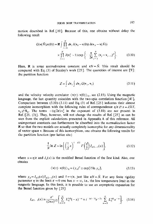
motion described in Ref. [lo]. Because of this, one obtains without delay the following result
x fi S(vf - 1) exp { -2 $ tvjwv,- l12]. (3.10) /= I /=I
Here, K is some normalization constant and EN= fi. This result should be compared with Eq. (3) of Stanley’s work [25]. The quantities of interest are [9]: the partition function
(3.11)
and the velocity-velocity correlator (v(r) . v(O)),, see (2.15). Using the magnetic language, the last quantity coincides with the two-spin correlation function [41]. Comparison between (3.10)-(3.11) and Eq. (3) of Ref. [25] indicates their almost complete isomorphism with the following rules of correspondence q/e 2 x = J/kT, v,s S,. The terms -(~/2e) vz in the exponent of (3.10) are not present in Ref. [25, (3)]. They, however, will not change the results of Ref. [25] as can be seen from the explicit calculations presented in Appendix A of this reference. All unimportant constants can furthermore be absorbed into the normalization factor K so that the two models are actually completely isomorphic for any dimensionality of vector space v. Because of this isomorphism, one obtains the following results for the partition function (per lattice site)
(3.12)
where x = r+ and Z,(x) is the modified Bessel function of the first kind. Also, one obtains
<v(t) .v(O)), = (.vd)’ = exp[z” In yd], (3.13)
where y,= Zd,2(x)/Zd,z- i(x) and r” = T/E, just like EN = I?. For any finite rigidity parameter 9 in the limit E -+ 0 one has x + co, i.e., the low temperature limit in the magnetic language. In this limit, it is possible to use an asymptotic expansion for the Bessel function given by [25]
Y N- Id,,- l(X) - (2n&
[ f, p-,)-n + ir’d- ‘)e-2” f LIp’x-” ) (3.14)
n=O 1

198 ARKADY L. KHOLODENKO
where Lkd’ are defined by means of the recursion relation
L,d’ = Cd- 2J2 - (2n - 1 I2 L’d’ n 8n n-1 (3.15)
with LCd’ = 1. I would like, for the sake of illustration only, to consider the case d= 3 wOhich is the most interesting in polymer physics. In this case LL3’ = 0 for n > 0 and one obtains, using (3.12), (3.14) the following result
-$lnZ=l +i [ln(~(3)/2~1/2)+ln(2?c)-e~2”+ . ..I
This result, unfortunately, turns out to be unsatisfactory from the point of view of polymer physics as can be seen from the treatment presented in my earlier work [6] (see, in particular, Eqs. (16), (18) of Ref. [6]). I have already mentioned at the end of Section 2, as well as after (3.9) that the very different microscopic models can produce practically the same v-v correlator in spite of the fact that the partition function as well as the higher moments, in general, might differ for different models. In the present case, the asymptotic expansion for y, is given by
y,4-(d--1)&+Ll”‘xZ+ ..’ (3.17)
which for d= 3 with the help of (3.13) produces (for E -+ 0)
(v(.?).v(0))G=exp -? = i ‘iI ex+~i
which obviously coincides with (2.15), as expected. The important lesson of the above analysis is the acknowledgment of the fact that (3.18) (or (2.15)) can be obtained by many methods starting from very different microscopic models. One then is left with the decision as to which microscopic model actually represents the reality. I have demonstrated in a brief note [6] that the correct microscopic model is based on the fermionic path integral description of conformational properties of semiflexible polymers. This statement is being clarified in the next subsection and in the following sections.
3.3. Dirac Propagator for Semiflexible Polymers: Exact Results
Recently PavsiE [ 141 has demonstrated that if one starts with the classical action given by (3.1) and proceeds in a usual way (i.e., via Hamiltonian formalism) towards quantization, then the resulting quantum theory naturally produces Dirac’s equation. His computations are done in the Minkowski space while the case of semiflexible polymers actually requires Euclidean formulation as will be demonstrated shortly below. Although the interested reader is encouraged to read PavsiE’s paper, Ref. [ 143, I provide in Section 5 a more direct way to arrive at the
FERMI-BOSE TRANSMUTATION 199
same conclusions as in PavsiE’s paper. For the moment I am just going to accept PavsiE’s result, and use it in order to obtain the necessary results related to polymers.
Begin with the Problem 2-6 in the famous Feynman and Hibbs book [43]. Although the problem was known for quite some time, its explicit solution has become available only recently [26]. In Problem 2-6 the discretized version of the 1 + 1 dimensional Dirac propagator is being discussed. It is quite remarkable that the above problem is directly related to the statistical mechanics of the one dimen- sional Ising model. For the reader’s convenience, I would like to briefly review the statement of the problem as well as its solution in order to indicate how this problem can be further generalized and how it is connected with other similar problems such as the directed walk models of polymers recently considered by Privman et al. [44].
Consider a square lattice which is rotated counterclockwise by a 45” angle so that the axes of some chosen coordinate system go through the diagonals of the initial lattice squares. Following Feynman, I choose the system of units !i = c = 1 to simplify matters. Consider now the motion of a particle on such a lattice. The particle can move straight or change its direction by 90” at the corners of squares of the lattice. In the X-Y plane, the X axis represents space while the Y axis represents time. The particle is allowed to move back and forth along the direction of X axis but only forth along the Y axis direction. Let a = (x,, y,) and b = (x,, yz) be the initial and final points for this type of a walk and let N(R) be the total number of walks of N steps long, starting at a, ending at b, and having exactly R turns along their paths. The lattice propagator is given then by [26,43]
Kzp(a, b) = f N,a(R)(ion)R, (3.19) R=O
where CI and /I correspond to the initial (final) orientations of the walk: to the “right” (+ ) or to the “left” (- ). It is being assumed that the length of each step is E and m represents the ‘bending” weight factor (i.e., each turn is associated with some bending energy: to go straight costs nothing, but to change the direction costs m each time). Usually, one should make an average over the initial positions and sum over the final positions of the walk (as it is done in continuous limit for the Dirac particle [30]), so that the quantity of interest is actually
K(a, b) = 1 &(a, b) p(cc), (3.20)
where p(m) represents the discrete version of the polarization matrix [30]. In the subsequent text I consider only nonpolarized cases so that p( + ) =p( - ) = i and these factors are being absorbed into Kas. With these remarks, I am ready to formulate the statistical mechanics vesion of the above problem following closely Ref. [26].
595!202:1-14
200 ARKADY L. KHOLODENKO
If N, (N-) represents the total number of the steps to the right (left), then one gets N= N, + N_ and M= N, - NM. The time interval t, - t, is given, in view of the above definitions, by
tb - t, = NE (3.21)
while the space interval is given by
x,-X,=M&. (3.22)
Introduce a system of N Ising spins bi, i= 1 -N, and associate the ith step with (TV so that ci = + 1 (- 1) will correspond to the move to the right (left). With such a defined rule for the spins, the “magnetization” is given by
M=N+-N-= i ai. (3.23) i=l
The number of turns R can be easily obtained now as
R=kNf’ (1 -eibi+,). (3.24) ,=I
From Ref. [26] it follows that the propagator (3.19) can actually be written as
&da, b) = Z,,,,(N, M;.d
1’ erp{j~~,‘(oiaj+,-l)), gN-,= ZkI
(3.25)
where j = -i In (km) and the primes near the summation signs indicate that the partition function Z should be actually evaluated under the constraint given by (3.23). Although the partition function with the above constraint can be evaluated, in principle, it is much easier to use the “momentum” representation introduced in the following way
Z,,,,JN, p;j) = 5 e”“Z,,,,(N J4i.d M= -N
(3.26)
Here (01 represents spin summation from a1 to aN-, , as before. Let t = tb - t, and x = x6 - x,, then Z(N, M;j) -+ K (t, x) and, accordingly, Z(N, /.qj) + K( t, p) where the momentum variable p is determined by the relation h4,u = -ipx or
p = -ipE. (3.27)
FERMI-BOSE TRANSMUTATION 201
Use of the transfer matrix methods now produces
Z,,,,(N,~;j)=~=cp+(a,)cp+(o,)+~Ncp-(a,)cp-(o,), (3.28)
where A+ and cp f are eigenvalues and eigenfunctions of the matrix H(ai, gi+, ) given by
H(“i,ai+I)=exp(ScL(ai+ai+I)+j(oiai+,-l)). (3.29)
The eigenfunctions are being properly normalized with the help of the constraint
(3.30)
i, j = +. In actual computations one has to remember that exp( - 2j) = km and p = - ipe. This then produces the matrix
H= 1 - ipc iem
km 1 + ip& >
which has eigenvalues
where
ELI+PZ m2’
(3.31)
(3.32)
(3.33)
With the use of (3.30) eigenfunctions of the matrix (3.31) can be easily obtained as well thus producing the final result
G(P, t) = 1 JL,(t, P) a3 P
(3.34)
where the present result differs from that given in Ref. [26] by the signs of l/E terms which are opposite to that given in that reference because of my choice of the factor (ism)R (versus (-icm)R) in (3.19). Note also that in Ref. [26], m= 1. In arriving at the result (3.34) I have essentially used the fact that N= t/c: and that, accordingly,
iim (1 f. i&mE)” = exp( + im,Q). (3.35) s-to+
If the multidimensional situation is being considered, then one should replace p2 by p2 as can easily be seen from the nonrelativistic limit (p2/m2 + 1) of the above
202 ARKADY L. KHOLODENKO
propagator (3.34). In this limit, Ex 1 + p2/2m2 so that using (3.34) one arrives at the familiar result given in Feynman’s book [43]
G(p, t) N 2&mfeiPzt/2m. (3.36)
For the purposes of the present work, one needs the Euclidean version of the above Dirac propagator. It is obtained in the usual way by making a redefinition fit -+ fi. The choice of signs: “+” or “-” is determined by the further convenience. In particular, to arrive at the result (2.16), I choose the “+” sign. In this case, using (3.34), I obtain
G(p, fi) = 2 cosh(mEI?) + $ sinh(mEN).
The combined use of (2.5) and (3.37) produces now
(3.37)
If one now chooses m = (2&)) i and fi = N $ one obtains back (2.16). It is essential to better understand the meaning of the rigidity parameter q as well
as the need to rescale $. To this end, it is useful to recall that, according to the just described Ising model interpretation of the Dirac’s propagator, the vertical “time” coordinate fi and the actual number of steps (of unit length in suitably chosen system of units) are related between each other as fi= N$ if the underlying lattice is a simple square lattice. The physical meaning of the mass m requires more comments. The next section is entirely devoted to the clarification of the meaning of m. In addition, I am going to demonstrate also that the partition function obtained from the Dirac’s propagator produces the well-known result obtained by Flory [27] many years ago. This is one of the main YeaSOnS why the exact partition function given by (3.16) is not acceptable and why the Dirac’s equation approach to semiflexible polymers is used instead. Another serious reason will become clear from reading Section 5.
The discussion of this section would not be complete without mentioning the connections between the present formulation and that given by Privman et al. [44] for the case of fully directed walks. To arrive at their results, one should consider instead of the one dimensional Ising model the Potts model having d states where d is the number of spatial dimensions, A brief summary of some important technical results related to the Potts model can be found in my earlier work [45].
By analogy with (3.24), one can define a number of turns R as
(3.39)
where the Potts variable ;i. takes the values A= 1, w, . . . . a~~~-‘, o = exp{2zi/2d}.
FERMI-BOSE TRANSMUTATION 203
Equation (3.21) remains the same while (3.23) should be changed to
(3.40) J=i
i = 1 -d, LCi) is equal to one of possible values of 2 which is associated with ith positive spatial direction of the lattice irrespective to the actual position of the jth link. With such defined R and M;, one can now easily obtain the patition function for the general d dimensional fully directed walk. It is given by
The one dimensional Potts model is known to be exactly solvable for arbitrary d [46]. Therefore the problem of fully directed walks is exactly solvable as well [44]. Although it would be of interest to obtain explicitly the exact solution for the present case, I restrict myself to the observation that, due to the fact that (3.36) is straightforwardly generalizable to any dimensions, the multidimensional version of (3.34) is obtained by simple replacement: p’ -+ p’. With these remarks one is ready to discuss the meaning of m as well as the explicit form of the partition function, Z=G (p=O, #).
4. GRAND CANONICAL ENSEMBLE FOR SEMIFLEXIBLE POLYMER SOLUTIONS IN TERMS OF PATH INTEGRALS
Recently, I have developed a new path integral formalism to describe the statisti- cal mechanics properties of solutions of fully flexible polymers [5]. It is quite natural to expect that the already obtained results should be viewed as the limiting case of a more general situation which accounts for the polymer stiffness. Because of this requirement of consistency and complementarity, I would like to remind the reader of some details of the already developed formalism.
Begin with the case of simple fluids. The grand partition function for a classical gas (fluid) placed in an external auxiliary potential U(r) is given by
Z=nto$Qn,
where
(4.1)
Q”=j fi ddrjexp{-P 1 W,-ri)-B i U(r)}, i=O (iii) i=O
204 ARKADY L. KHOLODENKO
fl = (/CT)-’ with T being a temperature and k being a Boltzmann’s constant. I have argued in the previous work that there is not much difference between l-component and 2-component systems: the latter includes the former as a special case when the interaction potentials V(r) are suitably chosen. Because of this one can consider from the beginning a 2-component system. Use of identities (CI = 1,2)
p,(r) = C fW - Cl, (4.2)
along with the account of the constraint
$j dddpl(r) +&)I = 1, (4.4)
where V is the volume of the system, I’= adN and ad= 1 in a suitably chosen system of units, while fi is the total number of cells in the volume V, produces after
(4.5)
some algebra the following result for Z [S],
Z=jD[A] exp {-B j ddW)} =%WN~
where
(4.6)
-- ~Sddrexp{-P(~,-1)J-~lddrexpj-8(rp,-l)). (4.7)
Here, 0, = U, - ,ur with ,LL~ being a chemical potential for the crth component, 1,=&-dexp/?~E,tidNad=1;q=q1,q2.ThematrixVisgivenby
(4.8)
Here and above the explicit spatial dependence is suppressed but is being under- stood. All unimportant for the present, normalization factors are adsorbed into the functional integral measure. The functional integral (4.7) is calculated by use of the saddle point method. Writing cptl = Q, + 6q, and 2 = X + 61 and demanding that the

FERMI-BOSE TRANSMUTATION 205
terms linear in 6qp, and 61 in the exponents of Eqs. (4.5) and (4.6) vanish produces equations for the mean fields (p, and 1 of the following type
(4.9)
and
exp{-fl(cp,--X))+exp{-/?(cp,-X))=l. (4.10)
This result can be simplified because of the following observation. The average density of cx th component can be obtained from the equation
(4.11)
In the saddle point (mean field) approximation this produces the result
p=J”ddrV-1((p-i7). (4.12)
Combining (4.9) and (4.12) produces
P,=exp{-P((P,-4j. (4.13)
The combined use of Eqs. (4.7), (4.9) (4.10), and (4.13) produces the following saddle point approximation for the thermodynamic potential Q,
Q= -$lnZ=Z[@,A]+jd”ri(r). (4.14)
Using the known connection between Q and the free energy F, F = Q + p. N one obtains for the free energy
F= S[@, X] + 1 AL(r) -J &U . p, (4.15)
where it was taken into account that for U = 0, 8 = -p and that j ddrp = N. Straightforward calculation produces
(4.16)
where p=p, and the explicit spatial dependence is suppressed. For the homogeneous density p = n one obtains
206 ARKADY L. KHOLODENKO
PF -= -$n2V,,+2n(l-n) V,,+(1-n)2 V2*] N
+nInn+(l-n)ln(l-n). (4.17)
The last result can be obtained without any path integral methods just with the help of pure thermodynamics and combinatorics by analogy with the Bragg-Williams approximation for ferromagnetism. Therefore I shall call (4.17) the Bragg-Williams lattice-gas approximation. In case of fully flexible polymer solutions, the Bragg-Williams approximation is known as the Flory-Huggins approximation [29]. As I shall demonstrate shortly, a similar approximation exists also for the case of semiflexible polymers and was also discovered by Flory [27]. The Flory-Huggins approximation for the fully flexible polymers can be obtained from the following path integral [S]
(4.18)
where
where ..$ is some normalization factor to be specified below. The matrix V has the same form as in the case of simple fluids with I’,, , Vi, and
V,, being polymer-polymer, polymer-solvent, and solvent-solvent interactions, respectively. I have suppressed the obvious spatial dependence in (4.19). Computa- tion of the functional integral given by (4.18) and (4.19) proceeds in complete analogy with the case of simple fluids with only one additional complication coming from the functional integral nature of the last term in (4.19). Because this complication is also going to be present in the case of semiflexible polymers, I would like to describe the technical matters in some detail. As before, I write ip, = @, + S&xN, A= A + Lin/fi and require the linear in fluctuations terms in the exponents of (4.18), (4.19) to vanish. Taking into account (4.19) one needs to consider the following expansion
FERMI-BOSE TRANSMUTATION 207
x
xG,(R,-r;~-~)i3@(r(z))Go(r-R2;~)+ ... . (4.20)
Here 6@ = 6~, - 6A, Go denotes “free,” in the present case Gaussian, propagator normalized (with the help of K), in such a way that
Z”‘- j”R, jddR2Go(R,-R,;fi)
= v=(fq=JT. (4.21)
Collecting all terms in the exponent of (4.18) (4.19) linear in &p, and 61 and taking into account (4.20) and (4.21) produces after functional differentiation the following saddle point equations for the mean fields Cp, and 2
fiexp(-fiKi% -X))+exp(-p(cp,-A))= 1 (4.23)
to be compared with (4.9), (4.10). I would like to note here that the operation of the functional differentiation when applied to (4.20) is effectively equivalent to the replacing of @(r(r)) with 6(r -r’). This observation along with the choice of normalization for Go such that
s ddR,Go(R, -R, k) = 1 (4.21a)
produces ultimately the results (4.22), (4.23). Note that in the above derivation the actual functional integral representation for Go was nor used. This property is very important when I consider below the generalization of the above results to the case of semiflexible polymers. The rest of the calculations for the fully flexible polymers proceeds in complete analogy with the case of simple fluids, just discussed, so that one arrives at the following anticipated Flory-Huggins result
BF -= -f [n2V,, +2n(l -n) V,,+(l -n)* V,,]
IT 00 + X In : +(l-n)ln(l-n). (4.24)
208 ARKADY L. KHOLODENKO
This result was obtained for the first time with use of path integrals in my previous work [4]. To generalize the above results to the case of solutions of semiflexible polymers, I would like to give an intuitive picture of the lattice model developed by Flory for this case [27]. Following Flory, consider a monodisperse ensemble of semiflexible polymers put on some arbitrary regular lattice with coor- dination number z. Concentrating our attention first on a particular polymer chain modeled by the semiflexible random walk one has the following situation. After a given step is made, for the walker there are two options: (a) to continue going in the same direction (trans); or (b) to change the direction (gauche), pro- vided that the immediate self-reversals are excluded. The first option is weighted with the conditional probability one, while the second is weighted with the factor (z-2) x exp(-E) where the dimensionless(trans-gauche) energy E can be computed quantum mechanically, in principle. After the first such walker has been placed on the lattice, the subsequent walkers should evidently adjust their “behavior” in order not to run into the first walker, etc. The combinatorial details are given by Flory and the reader is urged to read his paper [27]. What is important for us is the fact that he provides the result for the average number of bends (turns) per polymer molecule per effective link given by
R= (z-2)exp(-E)
1 + (z - 2) exp(-E)’ (4.25)
where our R (see (3.24)) corresponds to his f (see (5) of Ref. [27]). I am now going to obtain result (4.25) based on the earlier obtained results presented in Section 3.3. Taking into account (3.27) and neglecting the end effects, the partition function for the single chain, Z = G (p = 0, A), is given by
Z= C exp j $ (a,~~+~-- 1) . 10) i i=l I
(4.26)
It is convenient to now use the dual variables Si = cibi+ i in order to arrive at the final expression for Z. A trivial calculation produces
hlnZ= -j+ln2coshj. (4.27)
The average number of turns per lattice link is given by
iai 1 R= -Zg-+lnZ=2(l-tanhj). (4.28)
If now I choosej= - fln[(z- 2) ePE], then the result (4.25) is reproduced at once. But before I had j= - $ln(sm) (Euclidean version), see so that one obtains cm = (z - 2) eAE. Moreover, because of the relation m = (2 one also knows

FERMI-BOSE TRANSMUTATION 209
now the connection between the macroscopic phenomenological rigidity parameter r] and the microscopic bending energy E.
After these preliminaries, one is ready to extend the above single chain results to the concentration-dependent case. In this situation, I have to replace the functional integral given by (4.18), (4.19) with that appropriate integral for the semiflexible polymers. Evidently, one has to replace only the last term in Eq. (4.19) by the expression which is appropriate for the semiflexible polymers. Because, until now, I have not provided the explicit functional integral form for the Dirac’s propagator (this is goind to be accomplished in part in Section S), I cannot provide here an explicit closed form functional integral for the partition function for the semiflexible polymers. However, in view of (4.20), this actually is not necessary for the present type of calculation. It will become necessary when the generalization for the case of semiflexible surfaces is discussed (see Section 5). For the present purposes, it is convenient to rewrite (4.20) in the alternative equivalent form as follows:
Eq. (4.20) = exp{ -@(q,(r) - X(r))}
8G(O, I?+- j" &o
dzG(O,fi-T)&D(O)G(O,T)+ ... 1 ,
(4.29)
where G(0, fi) = G(p = 0, A) and G(p, fi) is given in (3.37). Collecting the terms proportional to fluctuations of the fields 6~,, 6A and taking functional derivates produces the saddle point equations similar to (4.22), (4.23) where now
p,=2~(1+&m)~“exp(-P~(~,-K)) (4.30)
and
P2=expi-P((P2-J)l (4.31)
as before. In arriving at (4.30) I used Eqs. (4.18), (4.19), and (4.29). From the last equation (with the help of (3.35)), the following result can be obtained,
I
fi dz G(O, #-r) G(O,7) = 2fi[cosh mfi + sinh mfi]
0
= 2fl exp { mA} = lim 2fi( 1 + Em)""". E-O (4.32)
Now replacing the densities in (4.22), (4.23) with that given by (4.30), (4.31) and producing the same type of calculations as for the case of simple fluids produces now the following result for the free energy
PF ,= N
-; [r?V,, +2n(l -n) I/,,+(1 -n)2 V,,]
+ N In N +(l-n)ln(l-n)-nln(l+(z-2)exp(-E)) (4.33) (“1 r>
210 ARKADY L. KHOLODENKO
which coincides exactly with that obtained by Flory [27] (see his Eqs. (2)-(6)) in the limit fi+ cc and note that the interaction term in (4.33) can be rewritten as xrr( 1 -n) + (/?/2)n (V,, - I’,,). Flory’s result is obtained if one chooses p( Vz2 - V,,) = 2.) Based on the results just obtained it is also of interest to obtain the Onsager’s results related to the nematic ordering of rod-like macromolecules [S]. To do so, it is sufficient to go through the following steps. First, by analogy with (4.16), (4.17) one rewrites (4.33) in the inhomogeneous form given by
F=-f/ji?lp+$j(R)ln(X)+$j(l-p)ln(l-p)
-jlpln(l+(z-Z)exp(--E)). (4.34)
Second, it is sufficient to consider just a l-component case for which V,, = - I’,? = - Vzz = I’ (see Ref. [S] for more details). Third, one should assume that the interaction potential V is only angular-dependent. In general, the interaction potential is anticipated to be composed of two parts: one which is only coordinate- dependent (which is used to model the excluded volume effects in case of fully flexible polymers [lo]) and another part which is angular- (or spin-) dependent. This part may or may not contain in addition some spatial dependence as well. Such decomposition is analogous to that used in the Landau theory of Fermi liquids [7]. In the case when only the solutions of rigid rods are of interest, one needs only the potential which is angular-dependent as was already stated. In this case some further simplifications are possible.
Fourth, one assumes in addition that the density D 4 1 and that it can be written in the form
fT=NnY(n), (4.35)
where the angular-dependent function Y(n) is normalized to unity as
i dQ, Y(n) = 1 (4.36)
with n being a unit vector in the direction of the rod. With these simplifications one is ready to rewrite (4.34) in the following form
dQ,Y(n)In Y(n)-ln(l+(z-2)exp(-E))N , I
(4.37)
where U(n,, n,)= -N’V(n,, n2) (usually one takes V(n,, n,)= -26 In, xn2/ with b being the diameter of the rod [S 1). The original Onsager’s result differs from that
FERMI-BOSE TRANSMUTATION 211
given in (4.37) by an unimportant constant: ln( 1 + (Z - 2) exp( -E))N is being replaced by unity. This discrepancy, however, is fictitious and does not affect any of the conclusions of Onsager’s theory [S] because in the rigid rod limit E + co.
Presented path integral formulation of the grand canonical ensemble partition function for the case of semiflexible polymers allows one to study now a variety of other situations not covered by the Flory’s or Onsager’s theories as well as to analyze the fluctuation corrections to the mean field results in a systematic fashion. This is necessary for determination of the stability of the mean field phases as well as for obtaining the critical exponents, etc., in case of possible second order phase transitions.
To develop a similar theory for the case of semiflexible surfaces, more informa- tion is needed. This is the subject of the next section.
5. FROM SEMIFLEXIBLE POLYMERS TO SUPERSTRINGS
In order to further develop the theory, I would first like to provide here an alter- native derivation of PavsiE’s results [ 141 connecting the bosonic formulation of the semiflexible polymers in terms of paths with extrinsic curvature with the fermionic description in terms of Dirac’s propagator. To this end, it is essential to first provide a necessary geometrical background for those readers who are not familiar with the modern differential geometry.
5.1. Some Results from the Differential Geometry of Curves and the Problem of Quantization
A three dimensional curve in Euclidean space can be described in the parametized form by the vector function r(r) such that
r(7) = c x,(7) i$, (5.1) i= 1
where 6, are unit vectors along the positive semiaxes of some Cartesian coordinate system. The length of the curve is given by
where v = dr/d7 (and other notations are given in Section 2). Whence, if the curve is naturally parametrized, just as in the case above, then (v . v) = 1. It is rather an easy exercise to show that the above equation (5.2) is reparametrization invariant [32] as it was already mentioned in Section 2. The curve can be described globally by (5.1) and (5.2), or locally. In the last case one has to define locally the curvature B(7) via
(5.3)
212 ARKADY L.KHOLODENKO
where n is some unit vector. Because of the constraint (v . v) = 1, one concludes that (t . v) = 0, i.e., that II is perpendicular to v. Note also that not only is n the unit vector, but v is also. Because of this, one defines, yet another, unit vector b via
b=vxn=vAn (5.4)
The last equality defines the exterior product A. It is quite remarkable and useful for the present purposes that only for d= 3 do the operations of vector multiplication and exterior product coincide [47]. Define now the torsion T(t) of the curve via
db z= -T(t)n.
THEOREM 5.1. The torsion T(z)for the planar curves is zero [32].
Finally, for the consistency of (5.3)-(5.5) one must require
dn x= -W(z)v+T(z)b. (5.6)
Equations (5.3), (5.5), and (5.6) are known as Serret-Frenet formulas. There is an important.
THEOREM 5.2, A curve in three dimensional space is jii[ly determined b-y 9(z) and T(r) (with accuracy up to its actual location in 3-d space) [32].
Because of the above theorem, the action given by (3.1) does not describe three dimensional curves completely. To correct the situation, Polyakov [13] has proposed considering instead the following action (for the case of Minkowski space of quantum mechanics)
where
C(T)=!;: duv. $x2 [ 1
1 v(t), u=l
v-v(? u)= f(o), u=o
(5.7)
(5.7a)
(5.7b)
with some unspecified vector f(0). Use of (5.3) and natural parameterization produces, instead of (5.7), the following result,

FERMI-BOSE TRANSMUTATION 213
For the case of closed curves on the surface of the unit sphere (v . v) = 1, it can be shown [20] that the last term in (5.7~) can be rewritten as
in accordance with the above cited Theorem 5.2. It can be shown [ 15,201 that, irrespective of the actual parameterization chosen in (5.7b), the r.h.s. of (5.8) is just some integer. Because of that, the exponent of the functional integral which contains action (5.7~) will actually not contain the last term in (5.7~) within the leading classical approximation, because exp{ 2xin) = 1 for n = 0, f 1, . . . . This is, of course, not the case if the next order of approximation is being considered which ultimately results in the fact, that for the closed orbits the functional integral constructed with the help of action S, given by (5.7) leads to Dirac’s propagator [ 131. The situation for the open orbits is considerably more complicated and was discussed in Ref. [48]. The authors of Ref. [48] have obtained the path integral for Dirac’s propagator solely in terms of bosonic-like fields (i.e., without use of Grassmann type of variables) which presents some computational advantages in the case when Monte Carlo simulations are performed, for example.
Here I provide, still another, derivation of Dirac’s propagator because of the following reasons. First, from the usual quantization prescription of Feynman [43] it is known that variation of the action in the exponent of the functional integral should lead to the classical equations of motion. In our case, one has “equations of motion” given by (5.3), (5.5), and (5.6). It is not immediately obvious how to obtain them from action S given by (5.7). Second, (5.7a) is’correct only for the case of closed paths and should be somehow, changed if the paths are open. Third, the account for this situation presented in Ref. [48] does not provide a simple link with (5.3) (5.5) and (5.6) which is essential if generalization to the case of surfaces is to be discussed.
Begin with the observation that Eqs. (5.3), (5.5), and (5.6) can be written in a rather illuminating form as
2 = ,$, b,e,, (5.9)
where ei={v,n,b},ei.e,=6,, i,j=l-3 and (Ib,II is a skew-symmetric matrix given by
(5.10)
Equation (5.9) can be given a physical interpretation. First, because in three dimen- sions the operations x and A are the same [47], one concludes that
ei A ei= -ej A e, (5.11)
214 ARKADY L. KHOLODENKO
i.e., ei can be interpreted as elements of the Grassmann algebra (I do not use here the boldface notations for ei in order to emphasize this fact). Second, Eqs. (5.9) can be rewritten as
where the “magnetic” field Bj is given by: B, = - T, B, = 0, B, = -B and, as usual, summation over repeating indices is assumed here and below. Equation (5.12) can be interpreted in terms of classical mechanics: it describes the precession of a (Grassmann) vector in a magnetic field [49, SO]. Using methods of symplectic geometry [47] one can interpret (5.12) as an equation of motion written in a usual Hamiltonian form if one defines the following Poisson’s bracket [49]
for some arbitrary functions f and g which are some polynomials in ei variables. With such defined Poisson’s bracket Hamiltonian equations of motion can be written in a usual way as
Use of (5.18)-( 5.14) permits one to write our “Hamiltonian” as
H= - ;qikBiqe,. (5.15)
One can also define the spin Sj via
Si = - +iE,,eie, (5.16)
so that [49]
(5.17)
which leads to the usual SU(2) Lie algebra commutation relations for spin. Finally, equations of motion (5.12) can be obtained from the variation of the action given
by
S= i j” df[e,P, + C,e,e,] (5.18)
FERMI-BOSE TRANSMUTATION 215
where ii = de,jdz and C, = E~~B~. Evidently, the imaginary i can be absorbed into t, if desired, so that one should consider instead of action given by (5.7) the following action (Minkowski space)
S’=~~1d~[e~1(r)(v~v)-e(r)m2-i(e,~,+C,e,e,)]. (5.19) 0
The sign *‘-” in front of the Grassmann term in (5.19) is chosen because of the following consideration. When (5.19) is used in the corresponding functional integral one has actually to consider not ST but exp ( -ST}. The sign ‘I-” in front of ST in the exponent compensates the sign “-” in front of the Grassmann term in (5.19).
To arrive at this form of action Eqs. (3.4) and (5.18) were used with p. - m2 as in (2.8) and with e(r) playing the same role as the variable E,* in (3.4). Because this form of the action is similar to that obtained by Polyakov [ 131 (who obtained it by less systematic, more heuristic methods), the rest of the calculations will proceed in a way similar (but not identical!) to that given by Polyakov.
First, following Ref. [Sl], I would like to reinterpret Serret-Fenet formulas for three dimensional curves. Let z. be some point on the curve. Consider the coor- dinate frame (v, n, b) along the curve and project b(z), n(T) onto the plane spanned by b(t,), it. For r -+ z. the velocity vector is projected as an infinitesimal vector and, in this approximation, one can assume that it is zero. Then one has a motion of vectors b(r) and n(r) on the above constructed plane which is described by equations
db z= -T(r)n,
dn dt= UT) b,
(5.5a)
i.e., the motion is determined by a 2 x 2 skew-symmetric matrix obtained from (5.10) by putting C% = 0. Hence, the vectors b and n are rotated about v with the speed of rotation determined by the torsion of the curve. The most important for us is the observation that, at least locally, the three dimensional curve can be thought of as a twisted straight line.
Now, consider the action ST, given by (5.19), in four dimensional Euclidean (or Minkowski) space. One can repeat word for word the arguments presented above. This time, one chooses four-velocity v = dx/dz along the curve and has a hyper- surface spanned by three vectors orthogonal to it. Equations of motion for these vectors are just that given by (5.9), (5.10). This allows one to rewrite the action (5.19) in a different equivalent form. To this end, define a Grassmann vector q~ via
\v= i eifj(t)-Ce, i= 1 i
(5.20)
216 ARKADY L. KHOLODENKO
so that
I choosefi in such a way that
i= I i= 1
j;=c C&
(5.21a)
(5.21b)
Define the operation of “inner” scalar product via
(“fcf,) = h/3 (5.21~)
then
w.\ir-(yf.\ir)=C eikj+CC,ieiei !( >
(5.22) i
also define a unit vector e, which coincides with direction of four-velocity, then
(v4d=O (5.23)
by construction, where the operation ( . ) was defined after (2.3). This can be equivalently rewritten (in Minkowski space) as
yip,, IpY = 0, (5.24)
where
q@,,=diag(-, +, +, +).
With the help of (5.22) one can eliminate C, from the action given by (5.19) at the expense of introducing a new Grassmann-type Lagrangian multiplier x. This then produces
ST=&-s,, (5.25)
where
S1 = g ji dt e(z). (5.26b)
The first term, S,, coincides exactly with that given by Fainberg and Marshakov [52] for the action of a massless spinning Dirac particle while the
FERMI-BOSE TRANSMUTATION 217
second term, Si, needs to be somewhat changed in order to describe correctly the case of a massive Dirac particle. The reasons for this change are explained in Polyakov’s book [ 12, pp. 223-2241 so that the corrected action S, can be written as
s,=; rldz[em2+ill/,ll/,+imX~,], (5.26~)
where, yet another, Grassmann field tj5 is introduced to account for the correct definition of length in superspace. Combined action, (5.26a) and (5.26c), when used in the exponent of the corresponding functional integral [52] ultimately produces the Minkowski space Dirac’s propagator. The reader is also strongly advised to read Ref. [31 J in order to understand better how the final result for the Dirac’s case was obtained. In the above reference, the reader will find detailed computations of the propagator given by (2.8). It is demonstrated there that the Fourier transform of the propagator (2.8) produces the r.h.s. of (2.7) as was already mentioned in Section 2. This concludes the path integral treatment of curves. Below, I consider possible generalizations of these ideas to the case of surfaces.
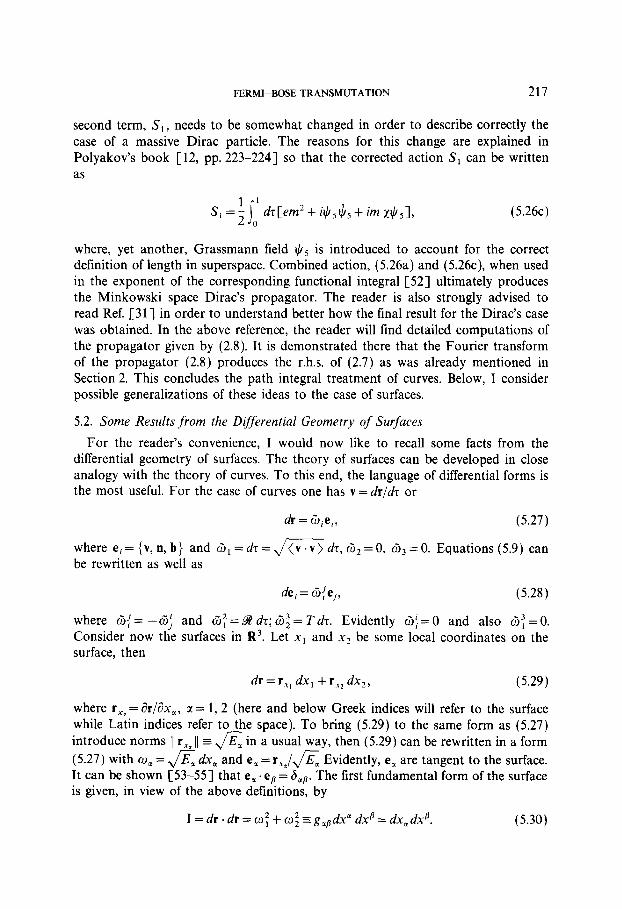
5.2. Some Results from the Differential Geometry of Surfaces
For the reader’s convenience, I would now like to recall some facts from the differential geometry of surfaces. The theory of surfaces can be developed in close analogy with the theory of curves. To this end, the language of differential forms is the most useful. For the case of curves one has v = dr/& or
a? = Gie,, (5.27)
where ei=(v,n,b} and &,=dz=Jmd z, I%* = 0, & = 0. Equations (5.9) can be rewritten as well as
de, = 6;ej, (5.28)
where I@= -&J and ~$=9ddz;(3~=Tdr. Evidently cZ,j=O and also OT=O. Consider now the surfaces in R3. Let x1 and x2 be some local coordinates on the surface. then
dr = rl, dx, + r”* dx,, (5.29)
where rx, = &/ax,, a = 1, 2 (here and below Greek indices will refer to the surface while Latin indices refer to the space). To bring (5.29) to the same form as (5.27) introduce norms 11 rx, 11 G & . m a usual way, then (5.29) can be rewritten in a form (5.27) with o, = & dx, and e, = r-J& Evidently, e, are tangent to the surface. It can be shown [53-551 that e, .ea = 6,,. The first fundamental form of the surface is given, in view of the above definitions, by
I = dr . dr = co: + co: s g,,dx’ dxfl = dx,dx@. (5.30)
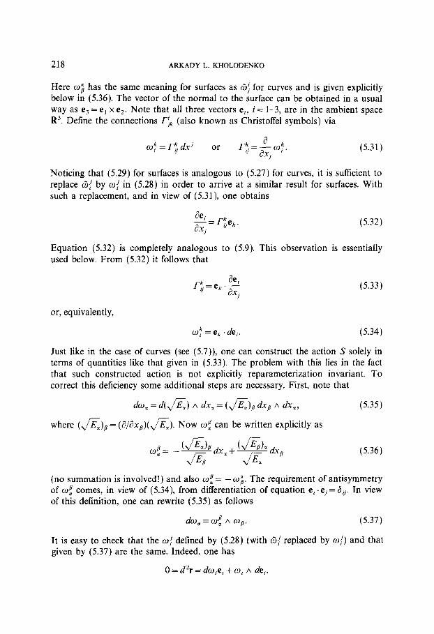
218 ARKADY L. KHOLODENKO
Here c$ has the same meaning for surfaces as 6; for curves and is given explicitly below in (5.36). The vector of the normal to the surface can be obtained in a usual way as e3 = e, x eZ. Note that all three vectors ei, i= 1-3, are in the ambient space R3. Define the connections ri, (also known as Christoffel symbols) via
(5.31)
Noticing that (5.29) for surfaces is analogous to (5.27) for curves, it is sufficient to replace G{ by o/ in (5.28) in order to arrive at a similar result for surfaces. With such a replacement, and in view of (5.31) one obtains
(5.32)
Equation (5.32) is completely analogous to (5.9). This observation is essentially used below. From (5.32) it follows that
rb.=e .!!!S rl k axj (5.33)
or, equivalently,
of = ek. de,. (5.34)
Just like in the case of curves (see (5.7)), one can construct the action S solely in terms of quantities like that given in (5.33). The problem with this lies in the fact that such constructed action is not explicitly reparameterization invariant. To correct this deficiency some additional steps are necessary. First, note that
do, = d(JE,) A dx, = (&& dx, A dx,, (5.35)
where (&Jp = W&&h%. N ow 0: can be written explicitly as
(5.36)
(no summation is involved!) and also wt = -w;. The requirement of antisymmetry of of comes, in view of (5.34), from differentiation of equation ej .ej= 6,. In view of this definition, one can rewrite (5.35) as follows
da, = wf A wg. (5.37)
It is easy to check that the o{ defined by (5.28) (with 6,: replaced by o{) and that given by (5.37) are the same. Indeed, one has
0 = d2r = dwiei + wi A de,.
FERMI-BOSE TRANSMUTATION 219
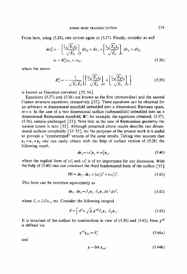
From here, using (5.28), one arrives again at (5.37). Finally, consider as well
(Jq?). dx, A dx, + - [ 1 JEa dx, A dx,
= -Rico, A cop, (5.38)
where the tensor
Rfl= -+-[[~]p+[~],] (5.39)
is known as Gaussian curvature [53, 541. Equations (5.37) and (5.38) are known as the first (torsion-free) and the second
Cartan structure equations, respectively [53]. These equations can be obtained for an arbitrary m dimensional manifold imbedded into n dimensional Riemann space, m <II. In the case of a two dimensional surface (submanifold) imbedded into an n dimensional Reimannian manifold, R”, for example, the equations obtained, (5.37), (5.38), remain unchanged [53]. Note that in the case of Riemannian geometry the torsion tensor is zero [53]. Although presented above results describe two dimen- sional surfaces completely [53-551, for the purposes of the present work it is useful to provide a “symmetrized’ version of the same results. Taking into account that e3 = e, x e2 one can easily obtain with the help of surface version of (5.28) the following result,
de3 = wie, + oie,, (5.40)
where the explicit form of W: and 0: is of no importance for our discussion. With the help of (5.40) one can construct the third fundamental form of the surface [55]
III = de, . de3 = (w:)~ + (co:)~. (5.41)
This form can be rewritten equivalently as
de, . de, = aIe3. ape, dx” dx”, (5.42)
where a, = d/ax,, etc. Consider the following integral
S = s d2x & ga8asle, . a,e,. (5.43)
It is invariant of the surface by construction in view of (5.30) and (5.42). Here g’fl is defined via
Pk’gsy = 6; (5.44a)
and
g = det gmB. (5.44b)
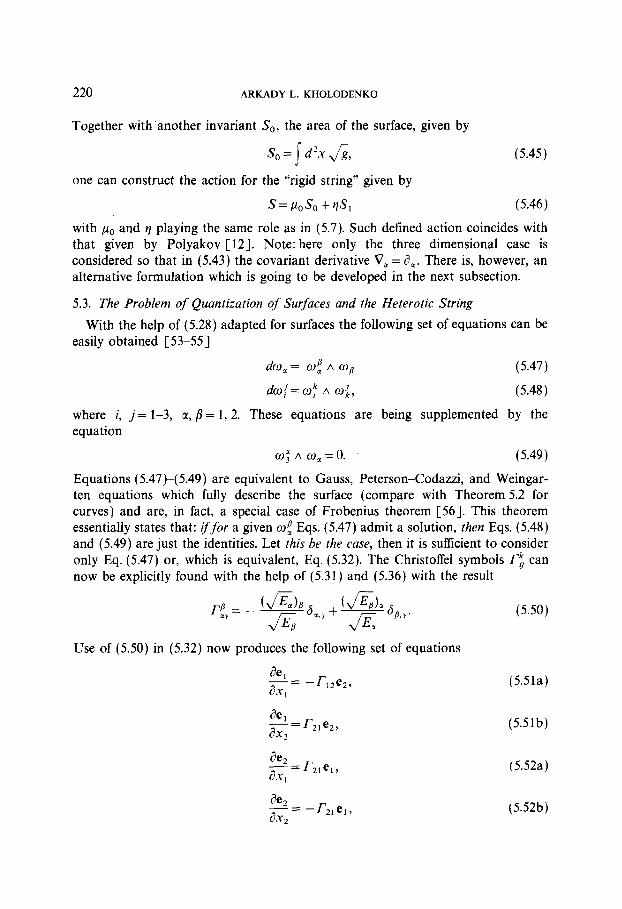
220 ARKADY L. KHOLODENKO
Together with’another invariant S,,, the area of the surface, given by
S,, = j d ‘.x ,/g, (5.45)
one can construct the action for the “rigid string” given by
S=PO&+VSl (5.46)
with p0 and q playing the same role as in (5.7). Such defined action coincides with that given by Polyakov [12]. Note: here only the three dimensional case is considered so that in (5.43) the covariant derivative V, = a,. There is, however, an alternative formulation which is going to be developed in the next subsection.
5.3. The Problem of Quantization of Surfaces and the Heterotic String
With the help of (5.28) adapted for surfaces the following set of equations can be easily obtained [53-551
do,= o&wg (5.47)
do:=w; A o$, (5.48)
where i, j= 1-3, tx, /3 = 1, 2. These equations are being supplemented by the equation
O;Aoll=O. (5.49)
Equations (5.47)-(5.49) are equivalent to Gauss, Peterson-Codazzi, and Weingar- ten equations which fully describe the surface (compare with Theorem 5.2 for curves) and are, in fact, a special case of Frobenius theorem [56]. This theorem essentially states that: iffor a given 0: Eqs. (5.47) admit a solution, then Eqs. (5.48) and (5.49) are just the identities. Let this be the case, then it is sufficient to consider only Eq. (5.47) or, which is equivalent, Eq. (5.32). The Christoffel symbols ri can now be explicitly found with the help of (5.31) and (5.36) with the result
(5.50)
Use of (5.50) in (5.32) now produces the following set of equations
(5.51a) EL-r e
8x1 12 21
$=r,,e,,
2
$=I;,e,,
1
ae,=-, e
ax, 21 I7
(5.52a)
FERMI-BOSE TRANSMUTATION 221
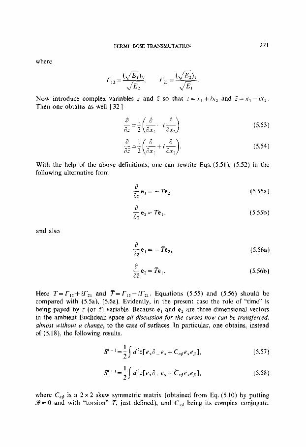
where
Now introduce complex variables z and Z so that z = x1 + ix, and 2 =x1 - LX,. Then one obtains as well [32]
(5.53)
(5.54)
With the help of the above definitions, one can rewrite Eqs. (5.51), (5.52) in the following alternative form
a z
e, = - Te,, (5.55a)
a z
e2= Te,, (5.55b)
and also
a %
e, = - Te,, (5.56a)
a z
e,= Fe,. (5.56b)
Here T = rr2 + iT,, and T= r12 - iT,, . Equations (5.55) and (5.56) should be compared with (5.5a), (5.6a). Evidently, in the present case the role of “time” is being payed by z (or 2) variable. Because e, and e2 are three dimensional vectors in the ambient Euclidean space all discussion for the curves now can be transferred, almost without a change, to the case of surfaces. In particular, one obtains, instead of (5.18), the following results,
SC-)=: d2z[e,dpe,+C,pe,eg], s
(5.57)
sit,=! 2 j d2zCe,a+ e, + Cgge,eSl, (5.58)
where C,, is a 2 x 2 skew symmetric matrix (obtained from Eq. (5.10) by putting 9? = 0 and with “torsion” T, just defined), and C,, being its complex conjugate.
222 ARKADY L. KHOLODENKO
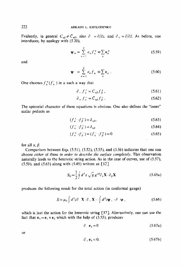
Evidently, in general C,, # C,,, also & = aI&, and a+ = a/a?. As .before, one introduces, by analogy with (5.20),
and
tf_ = i e,f; -Eel a=1 r
One chooses f ,‘(f; ) in a such a way that
a-f:=c,,f;,
a+f;=C,,fp
(5.59)
(5.60)
(5.61)
(5.62)
The spinorial character of these equations is obvious. One also defines the “inner” scalar prducts as
(fLf;)=h,> (5.63)
(f,.f/a=b (5.64)
(fx-;)=(f,.fpf)=O (5.65)
for all ci, p. Comparison between Eqs. (5.51), (5.52), (5.55), and (5.56) indicates that one can
choose either of these in order to describe the surface completely. This observation naturally leads to the heterotic string action. As in the case of curves, use of (5.57), (5.59), and (5.63) along with (5.45) written as [12]
s,=~J~‘~J~ pa,x. a,x (5.45a)
produces the following result for the total action (in conformal gauge)
s=Il,Sd2;a~x.a+x-Sd2zW, .a-v+ (5.66)
which is just the action for the heterotic string [57]. Alternatively, one can use the fact that e3 = e, x e2 which with the help of (5.55), produces
a-e,=0 (5.67a)
or
a+e,=O. (5.67b)
FERMI-BOSE TRANSMUTATION 223
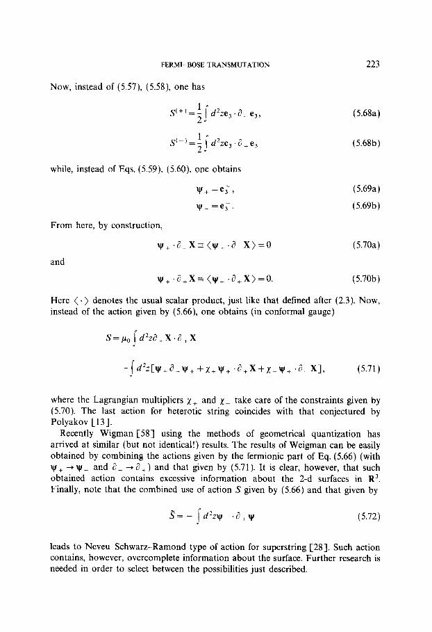
Now, instead of (5.57), (5.58), one has
St-)=; d2ze,.a+e, I
(5.68b)
while, instead of Eqs. (5.59), (5.60), one obtains
w+ =e:,
VI- =e;.
From here, by construction,
W+ .a-x= cw+ 4x)=0 and
\~r, .a+x= (w+ .a+x)=o.
(5.69a)
(5.69b)
(5.70a)
(5.70b)
Here (. ) denotes the usual scalar product, just like that defined after (2.3). Now, instead of the action given by (5.66), one obtains (in conformal gauge)
- d2zrW+a-v+ +x+v+ 4+x+x-v+ +-xi1 I (5.71)
where the Lagrangian multipliers x+ and x- take care of the constraints given by (5.70). The last action for heterotic string coincides with that conjectured by Polyakov [13].
Recently Wigman [58] using the methods of geometrical quantization has arrived at similar (but not identical!) results. The results of Weigman can be easily obtained by combining the actions given by the fermionic part of Eq. (5.66) (with w + + v _ and a _ + a +) and that given by (5.71). It is clear, however, that such obtained action contains excessive information about the 2-d surfaces in R3.
Finally, note that the combined use of action S given by (5.66) and that given by
(5.72)
leads to Neveu-Schwarz-Ramond type of action for superstring [28]. Such action contains, however, overcomplete information about the surface. Further research is needed in order to select between the possibilities just described.
224 ARKADY L. KHOLODENKO
ACKNOWLEDGMENTS
I would like to thank Professor Tze (Virginia Polytechnic Institute) for sending me a copy of Polyakov’s lecture notes. The present work would be impossible without the inspiration taken from these notes. I also would like to thank Professors Kardar (MIT) for providing me preprints of Ref. [SS], Gujrati (University of Akron) and Privman (Clarkson University) for various stimulating discussions which took place during my work on the manuscript. I am especially indebted to Professor Goldschmidt (University of Pittsburgh) for his careful reading of the whole manuscript and numerous comments. Lastly, my special thanks to the unknown referee whose kind generosity helped to improve the scientific quality of the paper. The linancial support of the present work by the Petroleum Research Fund through Grant PRF 19353 AC6 is gratefully acknowledged.
REFERENCES
1. A. KHOLODENKO AND A. BEYERLEIN, Phvs. Rev. A 34 (1986), 3309.
2. A. KHOLODENKO AND A. BEYERLEIN, Phys. Left. A 132 (1988), 347. 3. A. KHOLODENKO, Ph.vs. Let?. A 138 (1989), 13. 4. A. KHOLDENKO AND C. QIAN, Phys. Left. A 138 (1989), 19.
5. A. KHOLODENKO AND C. QIAN, Phys. Rev. B40 (1989), 2477. 6. A. KHOLODENKO, Phys. Lett. A 141 (1989). 351.
7. L. LANDAU AND E. LIFSHITZ, “Statistical Physics. Part I,” Pergamon. Oxford, 1986. 8. M. DOI AND S. EDWARDS, “Theory of Polymer Dynamic?,” Clarendon, London, 1986. 9. C. QIAN AND A. KHOLODENKO, J. Chem. Phys. 89 (1988), 2301.
10. K. FREED, “Renormalization Group Theory of Macromolecules,” Wiley, New York, 1987. 11. H. FUKUTAKA AND T. KASHIWA, Ann. Phys. (N.Y.I 176 (1987), 301. 12. A. POLYAKOV, “Gauge Fields and Strings,” Harwood Academic, New York, 1987. 13. A. POLYAKOV, in “Fields, Strings and Critical Phenomena,” Elsevier, Amsterdam, 1989, in press. 14. M. PAVSI~, Phys. Left. B221 (1989), 264. 15. M. STONE. Nucl. Phys. B 314 (1989), 557. 16. E. FRADKIN AND M. STONE, Phys. Rev. B38 (1988), 7215. 17. A. KHOLODENKO, J. Phys. Condensed Matter 1 (1989). 93. 18. P. ANDERSON, Science 235 (1987), 1196. 19. A. POLYAKOV, Mod. Phys. Left. A 3 (1988), 325. 20. C. TZE AND S. NAM, Ann. Phys. (N.Y.) 193 (1989). 419. 21. R. PISARSKI. Phys. Rev. D 34 (1986), 670. 22. W. ZAKREWSKI, “Low Dimensional Sigma Models,” Hilger, Bristol, 1989. 23. R. PISARSKI, Phys. Rev. D 38 (1988), 578. 24. F. DAVID AND E. GUTTIER, Nucl. Phys. B 295 (1988), 332. 25. E. STANLEY, Phys. Rev. 179 (1969), 570. 26. H. GERSCH, Int. J. Theor. Phys. 20 (1981), 491. 27. P. FOLRY, Proc. R. Sot. London A 234 (1956). 60. 28. M. GREEN, J. SCHWARZ, AND E. WITTEN. “Superstring Theory,” Vols. 1, 2, Cambridge Univ. Press,
New York, 1987. 29. P. DE GENNES, “Scaling Concepts in Polymer Physics,” Cornell Univ. Press, Ithaca, 1979. 30. V. BERESTETSKII. E. LIFSHITZ, AND L. PITAEVSKII, “Quantum Electrodynamics,” Pergamon, Oxford,
1982. 31. A. COHEN, G. MOORE, P. NELSON, AND J. POLCHINSKI. Nucl. Phys. B276 (1986), 143. 32. B. DUBROVIN, A. FORMENKO, AND S. NOVIKOV, “Modern Geometry-Methods and Applications,”
Part 1, Springer-Verlag, New York, 1984. 33. K. FREED, J. Chem. Phys. 56 (1971), 1453. 34. D. ISACSON, J. Marh. Phys. 23 (1982). 138.
FERMI-BOSE TRANSMUTATION 225
35. H. YAMAKAWA, “Modern Theory of Polymer Solutions,” Harper and Row, New York, 1971.
36. P. FLORY, ‘Statistical Mechanics of Chain Molecules,” Wiley, New York, 1969. 37. J. AMBJ~RN, B. DURHUUS. AND T. JONSSON, Europhys. Left. 3 (1987). 1059.
38. J. AMBJ~RN, B. DURHUUS, AND T. JONSSON, J. Ph]x A 21 (1988). 981. 39. F. DAVID, in “Statistical Mechanics of Membranes and Surfaces” (D. Nelson, T. Prian, and
S. Weinberg, Eds.), p. 157, World Scientific, Singapore, 1989. 40. S. LEIBLER in “Statistical Mechanics of Membranes and Surfaces” (D. Nelson, T. Piran, and
S. Weinberg Eds.), p. 45, World Scientific, Singapore, 1989.
41. A. POLYAKOV, Phys. Lett. B 59 (1975), 79. 42. H. KLEINERT, J. Math. Phys. 27 (1986) 3003. 43. R. FEYNMAN AND A. HIBBS, “Quantum Mechanics and Path Integrals,” McGraw-Hill, New York,
1965. 44. V. PRIVMAN AND N. SVRAKI~‘, “Directed Models of Polymers, Interfaces and Clusters: Scaling and
Finite Size Properties,” Lecture Notes in Physics, Vol. 338, Springer-Verlag, New York, 1989. 45. A. KHOLODENKO, J. Stat. Phys. 58 (1990) 355.
46. C. TOMPSON, ‘Classical Equilibrium Statistical Mechanics,” Clarendon, Oxford, 1988. 47. V. ARNOLD, “Mathematical Methods of Classical Mechanics,” Springer-Verlag, New York, 1978.
48. A. ALEKSEEV AND S. SHATASHVILI. Mod. Phys. Lert. A 3 (1988) 1551. 49. F. BEREZIN AND M. MARINOV, Ann. Phys. (N. Y.) 104 (1977) 336. 50. R. CASALBUONI, Nuovo Cinrento 33 (1976) 389.
51. A. MISHCHENKO AND A. FOMENKO. “A Course of DiNerential Geometry and Topology,” Mir, Moscow, 1988.
52. V. FAINBERG AND A. MARSHAKOV, Nucl. Phys. B 306 (1988) 659.
53. S. GOLDBERG, “Curvature and Homology,” Dover, New York, 1982. 54. B. O’NEIL, “Elementary Differential Geometry,” Academic Press, New York, 1966.
55. D. STURUIK, “Lectures on Classical Differential Geometry,” Addison-Wesley, Reading, MA, 1961.
56. N. HICKS, “Notes on Differential Geometry,” Van Nostrand, Princeton, 1965. 57. E. D’HOKER AND D. PHONG. Ret). Mod. Phys. 60 (1988) 917. 58. P. WEIGMANN, Nucl. Phys. B 323 (1989). 311, 330.