Single-phase AC circuits - JC Bose University

Module 4

Single-phase AC circuits

Version 2 EE IIT, Kharagpur

Lesson 15

Solution of Current in AC Series and Parallel

Circuits Version 2 EE IIT, Kharagpur

In the last lesson, two points were described:

1. How to solve for the impedance, and current in an ac circuit, consisting of single element, R / L / C?

2. How to solve for the impedance, and current in an ac circuit, consisting of two elements, R and L / C, in series, and then draw complete phasor diagram?

In this lesson, the solution of currents in simple circuits, consisting of resistance R, inductance L and/or capacitance C connected in series, fed from single phase ac supply, is presented. Then, the circuit with all above components in parallel is taken up. The process of drawing complete phasor diagram with current(s) and voltage drops in the different components is described. The computation of total power and also power consumed in the different components, along with power factor, is explained. One example of series circuit are presented in detail, while the example of parallel circuit will be taken up in the next lesson.

Keywords: Series and parallel circuits, impedance, admittance, power, power factor.

After going through this lesson, the students will be able to answer the following questions;

1. How to compute the total reactance and impedance / admittance, of the series and parallel circuits, fed from single phase ac supply?

2. How to compute the different currents and also voltage drops in the components, both in magnitude and phase, of the circuit?

3. How to draw the complete phasor diagram, showing the currents and voltage drops?

4. How to compute the total power and also power consumed in the different components, along with power factor?

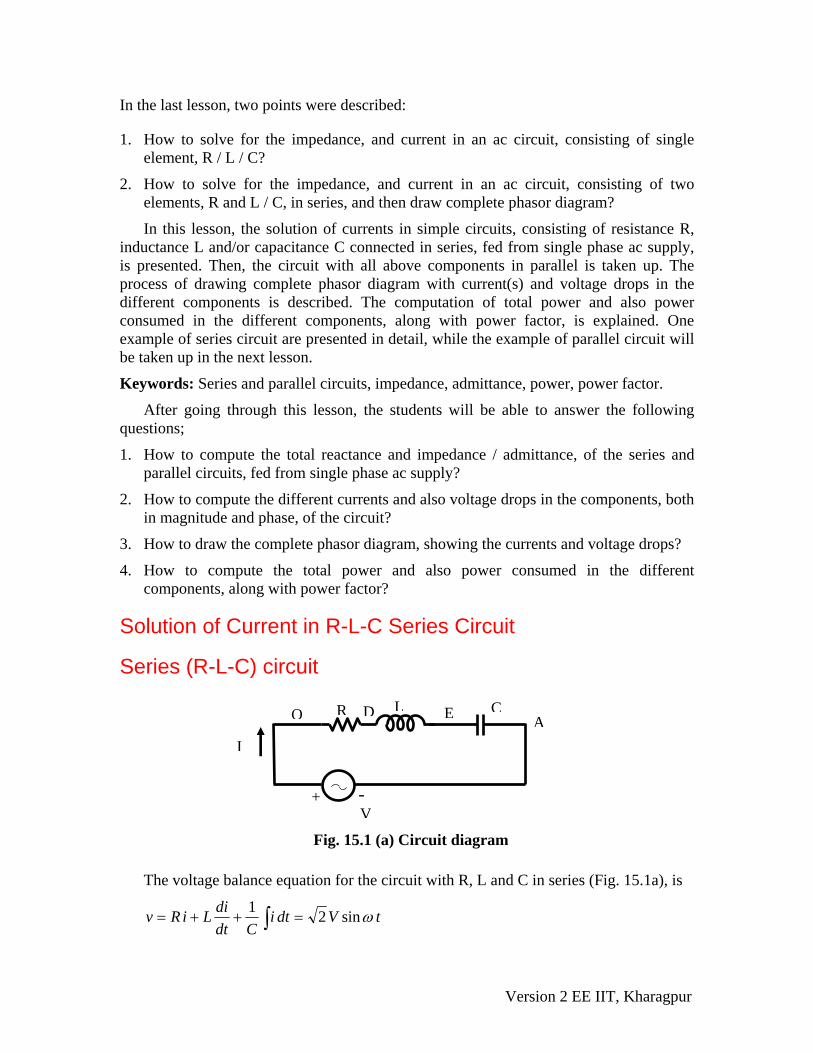
Solution of Current in R-L-C Series Circuit

Series (R-L-C) circuit

+ -V

R L C

Fig. 15.1 (a) Circuit diagram

O D E AI

The voltage balance equation for the circuit with R, L and C in series (Fig. 15.1a), is

tVdtiCdt

diLiRv ωsin21=++= ∫


The current, i is of the form,

)(sin2 φω ±= tIi As described in the previous lesson (#14) on series (R-L) circuit, the current in steady state is sinusoidal in nature. The procedure given here, in brief, is followed to determine the form of current. If the expression for )(sin2 φω −= tIi is substituted in the voltage equation, the equation shown here is obtained, with the sides (LHS & RHS) interchanged.

tV

tICtILtIR

ω

φωωφωωφω

sin2

)(cos2)/1()(cos2)(sin2

=

−⋅−−⋅+−⋅

or tVtICLtIR ωφωωωφω sin2)(cos2)]/1([)(sin2 =−⋅−+−⋅ The steps to be followed to find the magnitude and phase angle of the current I , are same as described there (#14). So, the phase angle is RCL /)]/1([tan 1 ωωφ −= −

and the magnitude of the current is ZVI /= where the impedance of the series circuit is 22 )]/1([ CLRZ ωω −+=

Alternatively, the steps to find the rms value of the current I, using complex form of impedance, are given here. The impedance of the circuit is

⎟⎟⎠

⎞⎜⎜⎝

⎛−+=−+=±∠

CLjRXXjRZ CL ω

ωφ 1)(

where, ( )2222 )/1()( CLRXXRZ CL ωω −+=−+= , and

⎟⎟⎠

⎞⎜⎜⎝

⎛ −=⎟

⎠⎞

⎜⎝⎛ −

= −−

RCL

RXX CL )/1(tantan 11 ωωφ

( ))/1(0

)(00

CLjRjV

XXjRjV

ZVI

CL ωωφφ

−++

=−+

+=

±∠°∠

=∠

−−

∓

2

222

1)(⎟⎟⎠

⎞⎜⎜⎝

⎛−+

=−+

==

CLR

VXXR

VZVI

CL

ωω

Two cases are: (a) Inductive ⎟⎟⎠

⎞⎜⎜⎝

⎛>

CL

ωω 1 , and (b) Capacitive ⎟⎟

⎠

⎞⎜⎜⎝

⎛<

CL

ωω 1 .

(a) Inductive

In this case, the circuit is inductive, as total reactance ( ))/1( CL ωω − is positive, under the condition ( )/1( CL )ωω > . The current lags the voltage by φ (taken as positive), with the voltage phasor taken as reference. The power factor (lagging) is less than 1 (one), as °≤≤° 900 φ . The complete phasor diagram, with the voltage drops across the


components and input voltage (OA), and also current (OB ), is shown in Fig. 15.1b. The voltage phasor is taken as reference, in all cases. It may be observed that

)()]([DA)]([)( ZiVXjiVXjiVRiV OACLCDOC +=+= −= = =using the Kirchoff’s second law relating to the voltage in a closed loop. The phasor diagram can also be drawn with the current phasor as reference, as will be shown in the example given here. The expression for the average power is . The power is only consumed in the resistance, R, but not in inductance/capacitance (L/C), in all three cases.

RIIV 2cos =φ

φ

O D

E

V

Inductive (XL > XC) Fig 15.1 (b) Phasor diagram

I (-jXC)

I (+jXL)

A

B I

I.R

In this case, the circuit is inductive, as total reactance ( ))/1( CL ωω − is positive, under the condition ( )/1( CL )ωω > . The current lags the voltage by φ (positive). The power factor (lagging) is less than 1 (one), as °≤≤° 900 φ . The complete phasor diagram, with the voltage drops across the components and input voltage ( ), and also current ( ), is shown in Fig. 15.1b. The voltage phasor is taken as reference, in all cases. It may be observed that

OA OB

)()]([)]([)( ZiVXjiVXjiVRiV OACDALCDOC ==−=+=+= using the Kirchoff’s second law relating to the voltage in a closed loop. The phasor diagram can also be drawn with the current phasor as reference, as will be shown in the example given here. The expression for the average power is . The power is only consumed in the resistance, R, but not in inductance/capacitance (L/C), in all three cases.

RIIV 2cos =φ


(b) Capacitive

φ O D

E

V

Capacitive (XL < XC) Fig 15.1 (c) Phasor diagram

I (-jXC)

LI(+jX )

A

B I I.R

The circuit is now capacitive, as total reactance ( ))/1( CL ωω − is negative, under the condition ( )/1( CL )ωω < . The current leads the voltage by φ , which is negative as per convention described in the previous lesson. The voltage phasor is taken as reference here. The complete phasor diagram, with the voltage drops across the components and input voltage, and also current, is shown in Fig. 15.1c. The power factor (leading) is less than 1 (one), as °≤≤° 900 φ , φ being negative. The expression for the average power remains same as above.

The third case is resistive, as total reactance )/1( CL ωω − is zero (0), under the condition )/1( CL ωω = . The impedance is 00 jRZ +=°∠ . The current is now at unity power factor ( °= 0φ ), i.e. the current and the voltage are in phase. The complete phasor diagram, with the voltage drops across the components and input (supply) voltage, and also current, is shown in Fig. 15.1d. This condition can be termed as ‘resonance’ in the series circuit, which is described in detail in lesson #17. The magnitude of the impedance in the circuit is minimum under this condition, with the magnitude of the current being maximum. One more point to be noted here is that the voltage drops in the inductance, L and also in the capacitance, C, is much larger in magnitude than the supply voltage, which is same as the voltage drop in the resistance, R. The phasor diagram has been drawn approximately to scale.


+

-

E

O

( )LI j.X

( )CI -j X

I ( )OD OBV , V I.R

Resistive (XL = XC)

Fig. 15.1 (d) Phasor diagram

D, A

It may be observed here that two cases of series (R-L & R-C) circuits, as discussed in

the previous lesson, are obtained in the following way. The first one (inductive) is that of (a), with C very large, i.e. 0/1 ≈Cω , which means that C is not there. The second one (capacitive) is that of (b), with L not being there ( or L 0=Lω ).

Example 15.1 A resistance, R is connected in series with an iron-cored choke coil (r in series with

L). The circuit (Fig. 15.2a) draws a current of 5 A at 240 V, 50 Hz. The voltages across the resistance and the coil are 120 V and 200 V respectively. Calculate,

(a) the resistance, reactance and impedance of the coil, (b) the power absorbed by the coil, and (c) the power factor (pf) of the input current.

I

V

A

L

B

CR

I


D r

Solution

)(OBI = 5 A = 240 V = 50 Hz )(OAVS f fπω 2= The voltage drop across the resistance VRIOCV 120)(1 =⋅=


The resistance, Ω=== 245/120/1 IVR The voltage drop across the coil VZICAV L 200)(2 =⋅=

The impedance of the coil, Ω===+= 405/200/222 IVXrZ LL

From the phasor diagram (Fig. 15.2b),

V1 V2

A

A R L C

E B D

40V, 50 Hz

I

1A

Fig. 15.2(b): Phasor Diagram

556.0600,57000,32

2401202)200()240()120(

2coscos

222222

=

=××

−+=

⋅⋅−+

=∠=OCOA

CAOCOAAOCφ

The power factor (pf) of the input current = )(556.0cos lag=φ The phase angle of the total impedance, °== − 25.56)556.0(cos 1φInput voltage, VZIOAVS 240)( =⋅=

The total impedance of the circuit, Ω===++= 485/240/)( 22 IVXrRZ SL Ω+=°∠=++=∠ )91.3967.26(25.5648)( jXjrRZ Lφ

The total resistance of the circuit, Ω=+=+ 67.2624 rrR The resistance of the coil, Ω=−= 67.20.2467.26r The reactance of the coil, Ω=== 9.392 LfLX L πω

The inductance of the coil, mHHf

XL L 12710127127.05029.39

23 =⋅==

×== −

ππ

The phase angle of the coil, °==== −−− 17.86)067.0(cos)0.40/67.2(cos)/(cos 111

LL Zrφ Ω°∠=+=+=∠ )717.8640)9.3967.2( jXjrZ LLL φ

The power factor (pf) of the coil, )(067.0cos lag=φ

The copper loss in the coil WrI 75.6667.2522 =×==

Example 15.2


An inductive coil, having resistance of 8 Ω and inductance of 80 mH, is connected in series with a capacitance of 100 Fμ across 150 V, 50 Hz supply (Fig. 15.3a). Calculate, (a) the current, (b) the power factor, and (c) the voltages drops in the coil and capaci-tance respectively.

ER L

+

- B

A

ID

V


C

Solution

f = 50 Hz sradf /16.3145022 =×== ππω L = HmH 08.0108080 3 =⋅= − Ω=×== 13.2508.016.314LX l ω

C = FF 610100100 −⋅=μ Ω=⋅×

== − 83.311010016.314

116C

X C ω

R = 8 Ω VOAVS 150)( = The impedance of the coil, Ω°∠=+=+=∠ 34.72375.26)13.250.8( jXjRZ LLL φ The total impedance of the circuit,

Ω°−∠=−=−+=−+=−∠

95.39435.10)7.60.8()83.3113.25(0.8)( 4 jjXXjRZ CLφ

The current drawn from the supply,

AjAZVI )26.902.11(95.39375.1495.39

435.101500

+=°∠=°∠⎟⎟⎠

⎞⎜⎜⎝

⎛=

−∠°∠

=∠φ

φ

The current is, AI 375.14=The power factor (pf) )(767.095.39coscos lead=°== φ D

A EI

I.R

B

IZL I. (jXL)

I. (-jXC)

Fig. 15.3 (b) Phasor diagram


Please note that the current phasor is taken as reference in the phasor diagram (Fig. 15.3b) and also here. The voltage drop in the coil is,

VjVZIV LL

)24.3611.115(34.7214.37934.72)375.26375.14(011

+=°∠=°∠×=∠⋅°∠=∠ φθ

The voltage drop in the capacitance in,

VjVZIV CC

58.4570.9058.4570.90)83.31475.14(022

−=°−∠=°−∠×=−∠⋅°∠=∠ φθ

Solution of Current in Parallel Circuit

Parallel circuit The circuit with all three elements, R, L & C connected in parallel (Fig. 15.4a), is fed to the ac supply. The current from the supply can be computed by various methods, of which two are described here.

C

+

-

V

Fig. 15.4 (a) Circuit diagram.

I

IL

L R

IR IC

First method The current in three branches are first computed and the total current drawn from the supply is the phasor sum of all three branch currents, by using Kirchoff’s first law related to the currents at the node. The voltage phasor (V ) is taken as reference.

All currents, i.e. three branch currents and total current, in steady state, are sinusoidal in nature, as the input (supply voltage is sinusoidal of the form, tVv ωsin2= Three branch currents are obtained by the procedure given in brief. , or RiRv ⋅= tItRVRvi RR ωω sin2sin)/(2/ === , where, )/( RVI R =

Similarly, dtidLv L=

So, is, Li tItLVdttVLdtvLi LL ωωωω cos2cos)]/([2)sin(2)/1()/1( −=−=== ∫∫

)90(sin2 °−= tI L ω


where, )/( LL XVI = with LX L ω=

, from which is obtained as, ∫= dtiCv C)/1( Ci

tItCVtVdtdC

dtvdCi CC ωωωω cos2 cos)(2)sin2( =⋅===

)90(sin2 °+= tIC ω where, )/( Cc XVI = with )/1( CX C ω= Total (supply) current, i is cos2cos2sin2 tItItIiiii CLRCLR ωωω +−=++=

)(sin2cos)(2sin2 φωωω ∓tItIItI CLR =−−= The two equations given here are obtained by expanding the trigonometric form appearing in the last term on RHS, into components of tωcos and tωsin , and then equating the components of tωcos and tωsin from the last term and last but one (previous) . RII =φcos and )(sin CL III −=φ From these equations, the magnitude and phase angle of the total (supply) current are,

22

22 111)()( ⎟⎟⎠

⎞⎜⎜⎝

⎛−+⎟

⎠⎞

⎜⎝⎛⋅=−+=

CLCLR XXR

VIIII

YVCLR

V ⋅=⎟⎟⎠

⎞⎜⎜⎝

⎛−+⎟

⎠⎞

⎜⎝⎛⋅=

22 11 ωω

⎥⎦

⎤⎢⎣

⎡⎟⎟⎠

⎞⎜⎜⎝

⎛−⋅=⎟⎟

⎠

⎞⎜⎜⎝

⎛ −=⎟⎟

⎠

⎞⎜⎜⎝

⎛ −= −−−

Cl

CL

R

CL

XXR

RXX

III 11tan

)/1()/1()/1(

tantan 111φ

⎥⎦

⎤⎢⎣

⎡⎟⎟⎠

⎞⎜⎜⎝

⎛−⋅= − C

LR ω

ω1tan 1

where, the magnitude of the term (admittance of the circuit) is,

2222 11111⎟⎟⎠

⎞⎜⎜⎝

⎛−+⎟

⎠⎞

⎜⎝⎛=⎟⎟

⎠

⎞⎜⎜⎝

⎛−+⎟

⎠⎞

⎜⎝⎛= C

LRXXRY

CL

ωω

Please note that the admittance, which is reciprocal of impedance, is a complex quantity. The angle of admittance or impedance, is same as the phase angle, φ of the current I , with the input (supply) voltage taken as reference phasor, as given earlier.

Alternatively, the steps required to find the rms values of three branch currents and the total (suuply) current, using complex form of impedance, are given here. Three branch currents are

L

VjLj

VXjVIjI

RVII

LLLRR ωω

−===−=°−∠==°∠ 90;0

VCjCj

VXj

VIjIC

CC ωω

=−

=−

==°+∠)/1(

90


Of the three branches, the first one consists of resistance only, the current, is in phase with the voltage (V). In the second branch, the current, lags the voltage by , as there is inductance only, while in the third one having capacitance only, the current,

leads the voltage . All these cases have been presented in the previous lesson.

RI

LI °90

CI °90 The total current is

( ) ⎥⎦

⎤⎢⎣

⎡⎟⎟⎠

⎞⎜⎜⎝

⎛−+=−+=±∠

LCj

RVIIjII LcR ω

ωφ 11

where,

( )⎥⎥⎦

⎤

⎢⎢⎣

⎡⎟⎟⎠

⎞⎜⎜⎝

⎛−+=−+=

2

222 11

LC

RVIIII LCR ω

ω , and

⎥⎦

⎤⎢⎣

⎡⎟⎟⎠

⎞⎜⎜⎝

⎛−=⎟⎟

⎠

⎞⎜⎜⎝

⎛ −= −−

LCR

III

R

LC

ωωφ 1tantan 11

The two cases are as described earlier in series circuit.

(a) Inductive

IC

E

O

D AIR

IL

I

φ

Inductive (IL > IC) Fig. 15.4 (b) Phasor diagram

In this case, the circuit being inductive, the current lags the voltage by φ (positive),

as , i.e. CL II > CL ωω >/1 , or CL ωω /1< .This condition is in contrast to that derived in the case of series circuit earlier. The power factor is less than 1 (one). The complete phasor diagram, with the three branch currents along with total current, and also the voltage, is shown in Fig. 15.4b. The voltage phasor is taken as reference in all cases. It may be observed there that

)()()()( OBICBIDCIODI CLR =++


The Kirchoff’s first law related to the currents at the node is applied, as stated above. The expression for the average power is . The power is only consumed in the resistance, R, but not in inductance/capacitance (L/C), in all three cases.

RVRIIV R /cos 22 ==φ

(b) Capacitive

The circuit is capacitive, as , i.e. LC II > LC ωω /1> , or CL ωω /1> . The current leads the voltage by φ (φ being negative), with the power factor less than 1 (one). The complete phasor diagram, with the three branch currents along with total current, and also the voltage, is shown in Fig. 15.4c.

The third case is resistive, as CL II = , i.e. CL ωω =/1 or CL ωω /1= . This is the same condition, as obtained in the case of series circuit. It may be noted that two currents,

and , are equal in magnitude as shown, but opposite in sign (phase difference being ), and the sum of these currents

LI CI°180 )( CL II + is zero (0). The total current is in

phase with the voltage ( °= 0φ ), with RII = , the power factor being unity. The complete phasor diagram, with the three branch currents along with total current, and also the voltage, is shown in Fig. 15.4d. This condition can be termed as ‘resonance’ in the parallel circuit, which is described in detail in lesson #17. The magnitude of the impedance in the circuit is maximum (i.e., the magnitude of the admittance is minimum) under this condition, with the magnitude of the total (supply) current being minimum.

O

B

E

I

φ D

IC

IR

Capacitive (IL < IC) Fig. 15.4 (c) Phasor diagram

A

V

IL


The circuit with two elements, say R & L, can be solved, or derived with C being large ( or 0=CI 0/1 =Cω ).

+

-

O

L LI (V /( jX )

( )C CI V/(-jX )

( )RI = I V RV

Resistive (IL = IC)

Fig. 15.4 (d) Phasor Diagram

E

D, B

IR

Second method Before going into the details of this method, the term, Admittance must be explained. In the case of two resistance connected in series, the equivalent resistance is the sum of two resistances, the resistance being scalar (positive). If two impedances are connected in series, the equivalent impedance is the sum of two impedances, all impedances being complex. Please note that the two terms, real and imaginary, of two impedances and also the equivalent one, may be positive or negative. This was explained in lesson no. 12. If two resistances are connected in parallel, the inverse of the equivalent resistance is the sum of the inverse of the two resistances. If two impedances are connected in parallel, the inverse of the equivalent impedance is the sum of the inverse of the two impedances. The inverse or reciprocal of the impedance is termed ‘Admittance’, which is complex. Mathematically, this is expressed as

2121

111 YYZZZ

Y +=+==

As admittance (Y) is complex, its real and imaginary parts are called conductance (G) and susceptance (B) respectively. So, BjGY += . If impedance, XjRZ +=∠φ with X being positive, then the admittance is

BjG

XRXj

XRR

XRXjR

XjRXjRXjR

XjRZY

−=+

−+

=

+−

=−+

−=

+=

°∠=−∠

2222

22)()(1

01φ

where,


2222 ;XR

XBXR

RG+

=+

=

Please note the way in which the result of the division of two complex quantities is obtained. Both the numerator and the denominator are multiplied by the complex conjugate of the denominator, so as to make the denominator a real quantity. This has also been explained in lesson no. 12. The magnitude and phase angle of Z and Y are )/(tan; 122 RXXRZ −=+= φ , and

⎟⎠⎞

⎜⎝⎛=⎟

⎠⎞

⎜⎝⎛=

+=+= −−

RX

GB

XRBGY 11

22

22 tantan;1 φ

To obtain the current in the circuit (Fig. 15.4a), the steps are given here. The admittances of the three branches are

Lj

XjZY

RZY

L ω11190;110

22

11 −===°−∠==°∠

CjXjZ

YC

ω=−

==°∠1190

33

The total admittance, obtained by the phasor sum of the three branch admittances, is

BjGL

CjR

YYYY +=⎟⎟⎠

⎞⎜⎜⎝

⎛−+=++=±∠ω

ωφ 11321

where,

⎥⎦

⎤⎢⎣

⎡⎟⎟⎠

⎞⎜⎜⎝

⎛−=

⎥⎥⎦

⎤

⎢⎢⎣

⎡⎟⎟⎠

⎞⎜⎜⎝

⎛−+= −

LCR

LC

RY

ωωφ

ωω 1tan;11 1

2

2 , and

LCBRG ωω /1;/1 −== The total impedance of the circuit is

2222

11BG

BjBG

GBjGY

Z+

−+

=+

=±∠

=∠φ

φ∓

The total current in the circuit is obtained as

φφφ

φ ±∠=±∠⋅°∠=∠

°∠=±∠ )(00 YVYV

ZVI∓

where the magnitude of current is ZVYVI /=⋅= The current is the same as obtained earlier, with the value of Y substituted in the

above equation.

This is best illustrated with an example, which is described in the next lesson.

The solution of the current in the series-parallel circuits will also be discussed there, along with some examples.


Problems 15.1 Calculate the current and power factor (lagging / leading) for the following

circuits (Fig. 15.5a-d), fed from an ac supply of 200 V. Also draw the phasor diagram in all cases.

+

-

200 V

(a)

L R

= 20 Ω

jXL

= j 25 Ω

+

-

R

L

200 V

(c)

C

= 15 Ω

jXL

= j25 Ω

-jXC

=-j20 Ω C

+

-

200 V

(d)

-jXC

= - j25 ΩjXC

- j20 Ω

R =15 Ω

Fig. 15.5

C

+

-

200 V

(b)

R = 25 Ω

- jXC

= -j20 Ω

15.2 A voltage of 200 V is applied to a pure resistor (R), a pure capacitor, C and a lossy inductor coil, all of them connected in parallel. The total current is 2.4 A, while the component currents are 1.5, 2.0 and 1.2 A respectively. Find the total power factor and also the power factor of the coil. Draw the phasor diagram.

15.3 A 200 V. 50Hz supply is connected to a lamp having a rating of 100 V, 200 W, in

series with a pure inductance, L, such that the total power consumed is the same, i.e. 200W. Find the value of L.

A capacitance, C is now connected across the supply. Find value of C, to bring the supply power factor to unity (1.0). Draw the phasor diagram in the second case.

1.(a) Find the value of the load resistance (RL) to be connected in series with a real voltage source (VS + RS in series), such that maximum power is transferred from the above source to the load resistance.

(b) Find the voltage was 8Ω resistance in the circuit shown in Fig. 1(b). 2.(a) Find the Theremin’s equivalent circuit (draw the ckt.) between the terminals A + B, of the circuit shown in Fig. 2(a).


(b) A circuit shown in Fig. 2(b) is supplied at 40V, 50Hz. The two voltages V1 and V2 (magnitude only) is measured as 60V and 25V respectively. If the current, I is measured as 1A, find the values of R, L and C. Also find the power factor of the circuit (R-L-C). Draw the complete phasor diagram.

3.(a) Find the line current, power factor, and active (real) power drawn from 3-phase, 100V, 50Hz, balanced supply in the circuit shown in Fig. 3(a). (b) In the circuit shown in Fig. 3(b), the switch, S is put in position 1 at t = 0. Find ie(t),

t > 0, if vc(0-) = 6V. After the circuit reaches steady state, the switch, S is brought to position 2, at t = T1. Find ic(t), t > T1. Switch the above waveform.

4.(a) Find the average and rms values of the periodic waveform shown in Fig. 4(a).

(b) A coil of 1mH lowing a series resistance of 1Ω is connected in parallel with a capacitor, C and the combination is fed from 100 mV (0.1V), 1 kHz supply (source) having an internal resistance of 10Ω. If the circuit draws power at unity power factor (upf), determine the value of the capacitor, quality factor of the coil, and power drawn by the circuit. Also draw the phasor diagram.


List of Figures

Fig. 15.1 (a) Circuit diagram (R-L-C in series) (b) Phasor diagram – Circuit is inductive ( ) Cl XX > (c) Phasor diagram – Capacitive ( l CX X< ) (d) Phasor diagram – Resistive ( Cl XX = )

Fig. 15.2 (a) Circuit diagram (Ex. 15.1), (b) Phasor diagram

Fig. 15.3 (a) Circuit diagram (Ex. 15.2), (b) Phasor diagram

Fig. 15.4 (a) Circuit diagram (R-L-C in parallel) (b) Phasor diagram – Circuit is inductive ( Cl XX < ) (c) Phasor diagram – Capacitive ( ) Cl XX > (d) Phasor diagram – Resistive ( Cl XX = )


Please note that the current phasor is taken as reference in the phasor diagram (Fig. 15.3b) and also here. The voltage drop in the coil is,

VjVZIV LL

)24.3611.115(34.7214.37934.72)375.26375.14(011

+=°∠=°∠×=∠⋅°∠=∠ φθ

The voltage drop in the capacitance in,

VjVZIV CC

58.4570.9058.4570.90)83.31475.14(022

−=°−∠=°−∠×=−∠⋅°∠=∠ φθ

Solution of Current in Parallel Circuit

Parallel circuit The circuit with all three elements, R, L & C connected in parallel (Fig. 15.4a), is fed to the ac supply. The current from the supply can be computed by various methods, of which two are described here.

C

+

-

V


I

IL

L R

IR IC

First method The current in three branches are first computed and the total current drawn from the supply is the phasor sum of all three branch currents, by using Kirchoff’s first law related to the currents at the node. The voltage phasor (V ) is taken as reference.

All currents, i.e. three branch currents and total current, in steady state, are sinusoidal in nature, as the input (supply voltage is sinusoidal of the form, tVv ωsin2= Three branch currents are obtained by the procedure given in brief. , or RiRv ⋅= tItRVRvi RR ωω sin2sin)/(2/ === , where, )/( RVI R =

Similarly, dtidLv L=

So, is, Li tItLVdttVLdtvLi LL ωωωω cos2cos)]/([2)sin(2)/1()/1( −=−=== ∫∫

)90(sin2 °−= tI L ω


where, )/( LL XVI = with LX L ω=

, from which is obtained as, ∫= dtiCv C)/1( Ci

tItCVtVdtdC

dtvdCi CC ωωωω cos2 cos)(2)sin2( =⋅===

)90(sin2 °+= tIC ω where, )/( Cc XVI = with )/1( CX C ω= Total (supply) current, i is cos2cos2sin2 tItItIiiii CLRCLR ωωω +−=++=

)(sin2cos)(2sin2 φωωω ∓tItIItI CLR =−−= The two equations given here are obtained by expanding the trigonometric form appearing in the last term on RHS, into components of tωcos and tωsin , and then equating the components of tωcos and tωsin from the last term and last but one (previous) . RII =φcos and )(sin CL III −=φ From these equations, the magnitude and phase angle of the total (supply) current are,

22

22 111)()( ⎟⎟⎠

⎞⎜⎜⎝

⎛−+⎟

⎠⎞

⎜⎝⎛⋅=−+=

CLCLR XXR

VIIII

YVCLR

V ⋅=⎟⎟⎠

⎞⎜⎜⎝

⎛−+⎟

⎠⎞

⎜⎝⎛⋅=

22 11 ωω

⎥⎦

⎤⎢⎣

⎡⎟⎟⎠

⎞⎜⎜⎝

⎛−⋅=⎟⎟

⎠

⎞⎜⎜⎝

⎛ −=⎟⎟

⎠

⎞⎜⎜⎝

⎛ −= −−−

Cl

CL

R

CL

XXR

RXX

III 11tan

)/1()/1()/1(

tantan 111φ

⎥⎦

⎤⎢⎣

⎡⎟⎟⎠

⎞⎜⎜⎝

⎛−⋅= − C

LR ω

ω1tan 1

where, the magnitude of the term (admittance of the circuit) is,

2222 11111⎟⎟⎠

⎞⎜⎜⎝

⎛−+⎟

⎠⎞

⎜⎝⎛=⎟⎟

⎠

⎞⎜⎜⎝

⎛−+⎟

⎠⎞

⎜⎝⎛= C

LRXXRY

CL

ωω

Please note that the admittance, which is reciprocal of impedance, is a complex quantity. The angle of admittance or impedance, is same as the phase angle, φ of the current I , with the input (supply) voltage taken as reference phasor, as given earlier.

Alternatively, the steps required to find the rms values of three branch currents and the total (suuply) current, using complex form of impedance, are given here. Three branch currents are

L

VjLj

VXjVIjI

RVII

LLLRR ωω

−===−=°−∠==°∠ 90;0

VCjCj

VXj

VIjIC

CC ωω

=−

=−

==°+∠)/1(

90


Of the three branches, the first one consists of resistance only, the current, is in phase with the voltage (V). In the second branch, the current, lags the voltage by , as there is inductance only, while in the third one having capacitance only, the current,

leads the voltage . All these cases have been presented in the previous lesson.

RI

LI °90

CI °90 The total current is

( ) ⎥⎦

⎤⎢⎣

⎡⎟⎟⎠

⎞⎜⎜⎝

⎛−+=−+=±∠

LCj

RVIIjII LcR ω

ωφ 11

where,

( )⎥⎥⎦

⎤

⎢⎢⎣

⎡⎟⎟⎠

⎞⎜⎜⎝

⎛−+=−+=

2

222 11

LC

RVIIII LCR ω

ω , and

⎥⎦

⎤⎢⎣

⎡⎟⎟⎠

⎞⎜⎜⎝

⎛−=⎟⎟

⎠

⎞⎜⎜⎝

⎛ −= −−

LCR

III

R

LC

ωωφ 1tantan 11

The two cases are as described earlier in series circuit.

(a) Inductive

IC

E

O

D AIR

IL

I

φ

Inductive (IL > IC) Fig. 15.4 (b) Phasor diagram

In this case, the circuit being inductive, the current lags the voltage by φ (positive),

as , i.e. CL II > CL ωω >/1 , or CL ωω /1< .This condition is in contrast to that derived in the case of series circuit earlier. The power factor is less than 1 (one). The complete phasor diagram, with the three branch currents along with total current, and also the voltage, is shown in Fig. 15.4b. The voltage phasor is taken as reference in all cases. It may be observed there that

)()()()( OBICBIDCIODI CLR =++


The Kirchoff’s first law related to the currents at the node is applied, as stated above. The expression for the average power is . The power is only consumed in the resistance, R, but not in inductance/capacitance (L/C), in all three cases.

RVRIIV R /cos 22 ==φ

(b) Capacitive

The circuit is capacitive, as , i.e. LC II > LC ωω /1> , or CL ωω /1> . The current leads the voltage by φ (φ being negative), with the power factor less than 1 (one). The complete phasor diagram, with the three branch currents along with total current, and also the voltage, is shown in Fig. 15.4c.

The third case is resistive, as CL II = , i.e. CL ωω =/1 or CL ωω /1= . This is the same condition, as obtained in the case of series circuit. It may be noted that two currents,

and , are equal in magnitude as shown, but opposite in sign (phase difference being ), and the sum of these currents

LI CI°180 )( CL II + is zero (0). The total current is in

phase with the voltage ( °= 0φ ), with RII = , the power factor being unity. The complete phasor diagram, with the three branch currents along with total current, and also the voltage, is shown in Fig. 15.4d. This condition can be termed as ‘resonance’ in the parallel circuit, which is described in detail in lesson #17. The magnitude of the impedance in the circuit is maximum (i.e., the magnitude of the admittance is minimum) under this condition, with the magnitude of the total (supply) current being minimum.

O

B

E

I

φ D

IC

IR

Capacitive (IL < IC) Fig. 15.4 (c) Phasor diagram

A

V

IL


The circuit with two elements, say R & L, can be solved, or derived with C being large ( or 0=CI 0/1 =Cω ).

+

-

O

L LI (V /( jX )

( )C CI V/(-jX )

( )RI = I V RV

Resistive (IL = IC)

Fig. 15.4 (d) Phasor Diagram

E

D, B

IR

Second method Before going into the details of this method, the term, Admittance must be explained. In the case of two resistance connected in series, the equivalent resistance is the sum of two resistances, the resistance being scalar (positive). If two impedances are connected in series, the equivalent impedance is the sum of two impedances, all impedances being complex. Please note that the two terms, real and imaginary, of two impedances and also the equivalent one, may be positive or negative. This was explained in lesson no. 12. If two resistances are connected in parallel, the inverse of the equivalent resistance is the sum of the inverse of the two resistances. If two impedances are connected in parallel, the inverse of the equivalent impedance is the sum of the inverse of the two impedances. The inverse or reciprocal of the impedance is termed ‘Admittance’, which is complex. Mathematically, this is expressed as

2121

111 YYZZZ

Y +=+==

As admittance (Y) is complex, its real and imaginary parts are called conductance (G) and susceptance (B) respectively. So, BjGY += . If impedance, XjRZ +=∠φ with X being positive, then the admittance is

BjG

XRXj

XRR

XRXjR

XjRXjRXjR

XjRZY

−=+

−+

=

+−

=−+

−=

+=

°∠=−∠

2222

22)()(1

01φ

where,


2222 ;XR

XBXR

RG+

=+

=

Please note the way in which the result of the division of two complex quantities is obtained. Both the numerator and the denominator are multiplied by the complex conjugate of the denominator, so as to make the denominator a real quantity. This has also been explained in lesson no. 12. The magnitude and phase angle of Z and Y are )/(tan; 122 RXXRZ −=+= φ , and

⎟⎠⎞

⎜⎝⎛=⎟

⎠⎞

⎜⎝⎛=

+=+= −−

RX

GB

XRBGY 11

22

22 tantan;1 φ

To obtain the current in the circuit (Fig. 15.4a), the steps are given here. The admittances of the three branches are

Lj

XjZY

RZY

L ω11190;110

22

11 −===°−∠==°∠

CjXjZ

YC

ω=−

==°∠1190

33

The total admittance, obtained by the phasor sum of the three branch admittances, is

BjGL

CjR

YYYY +=⎟⎟⎠

⎞⎜⎜⎝

⎛−+=++=±∠ω

ωφ 11321

where,

⎥⎦

⎤⎢⎣

⎡⎟⎟⎠

⎞⎜⎜⎝

⎛−=

⎥⎥⎦

⎤

⎢⎢⎣

⎡⎟⎟⎠

⎞⎜⎜⎝

⎛−+= −

LCR

LC

RY

ωωφ

ωω 1tan;11 1

2

2 , and

LCBRG ωω /1;/1 −== The total impedance of the circuit is

2222

11BG

BjBG

GBjGY

Z+

−+

=+

=±∠

=∠φ

φ∓

The total current in the circuit is obtained as

φφφ

φ ±∠=±∠⋅°∠=∠

°∠=±∠ )(00 YVYV

ZVI∓

where the magnitude of current is ZVYVI /=⋅= The current is the same as obtained earlier, with the value of Y substituted in the

above equation.

This is best illustrated with an example, which is described in the next lesson.

The solution of the current in the series-parallel circuits will also be discussed there, along with some examples.


In the last lesson, the following points were described:

1. How to compute the total impedance/admittance in series/parallel circuits?

2. How to solve for the current(s) in series/parallel circuits, fed from single phase ac supply, and then draw complete phasor diagram?

3. How to find the power consumed in the circuit and also the different components, and the power factor (lag/lead)?

In this lesson, the computation of impedance/admittance in parallel and series-parallel circuits, fed from single phase ac supply, is presented. Then, the currents, both in magnitude and phase, are calculated. The process of drawing complete phasor diagram is described. The computation of total power and also power consumed in the different components, along with power factor, is explained. Some examples, of both parallel and series-parallel circuits, are presented in detail.

Keywords: Parallel and series-parallel circuits, impedance, admittance, power, power factor.


1. How to compute the impedance/admittance, of the parallel and series-parallel circuits, fed from single phase ac supply?

2. How to compute the different currents and also voltage drops in the components, both in magnitude and phase, of the circuit?

3. How to draw the complete phasor diagram, showing the currents and voltage drops?

4. How to compute the total power and also power consumed in the different components, along with power factor?

This lesson starts with two examples of parallel circuits fed from single phase ac supply. The first example is presented in detail. The students are advised to study the two cases of parallel circuits given in the previous lesson.

Example 16.1

The circuit, having two impedances of Ω+= )158(1 jZ and Ω−= )86(2 jZ in parallel, is connected to a single phase ac supply (Fig. 16.1a), and the current drawn is 10 A. Find each branch current, both in magnitude and phase, and also the supply voltage.


B

I = 10A


A

Z2 = (6 – j8) Ω

Z1 = (8 + j15) Ω I1

I2

Solution

Ω°∠=+=∠ 93.6117)158(11 jZ φ Ω°−∠=−=−∠ 13.5310)86(22 jZ φ AjOCI )010(010)(0 +=°∠=°∠

The admittances, using impedances in rectangular form, are, 13

2211

11 10)9.5168.27(289

158158158

15811 −− Ω⋅−=

−=

+−

=+

=∠

=−∠ jjjjZ

Yφ

φ

1322

2222 10)0.800.60(

10086

8686

8611 −− Ω⋅+=

+=

++

=−

=−∠

=∠ jjjjZ

Yφ

φ

Alternatively, using impedances in polar form, the admittances are,

1311

11

10)9.5168.27(

93.6105882.093.610.17

11

−− Ω⋅−=

°−∠=°∠

=∠

=−∠

j

ZY

φφ

13

2222 10)0.800.60(13.531.0

13.530.1011 −− Ω⋅+=°∠=

°−∠=

−∠=∠ j

ZY

φφ

The total admittance is, 33

21 10)1.2868.87(10)]0.800.60()9.5168.27[( −− ⋅+=⋅++−=+=∠ jjjYYY φ 13 77.171007.92 −− Ω°∠⋅=

The total impedance is,

Ω−=°−∠=°∠⋅

=∠

=−∠ − )315.3343.10(77.1786.1077.171007.92

113 j

YZ

φφ

The supply voltage is VZIVV AB °−∠=°−∠×=−∠⋅°∠=−∠ 77.176.10877.17)86.1010(0)( φφ

Vj )15.3343.103( −=

The branch currents are,

AZVODI °−∠=°+°−∠⎟

⎠⎞

⎜⎝⎛=

∠−∠

=−∠ 7.7939.6)93.6177.17(0.176.108)(

1111 φ

φθ


Aj )286.6143.1( −=

2 2 1 1( ) 0 ( )(10.0 0.0) (1.143 6.286) (8.857 6.286) 10.86 35.36

I OE I I OC OD OC CEj j j A

θ θ∠ = ∠ °− ∠− − = −= + − − = + = ∠ ° A

Alternatively, the current is, 2I

2 22 2

108.6( ) ( 17.77 53.13 ) 10.86 35.36

10.0V

I OE AZ

φθ

φ∠− ⎛ ⎞∠ = = ∠ − °+ ° = ∠⎜ ⎟∠− ⎝ ⎠

°

Aj )285.6857.8( +=

The phasor diagram with the total (input) current as reference is shown in Fig. 16.1b.


53.13°

I2= 10.86

61.90

108.63 V

Ф = 17.8°

I1 = 6.4 A D

θ1 = 79.7°

θ1 = 35.35

O

E

VAB

C I = 10A

Alternative Method

Ω°∠=+=−++=−∠+∠=′∠′ 565.2665.15)714()86()158(2211 jjjZZZ φφφ

Ω−=°−∠=

°−°−°∠⎟⎠⎞

⎜⎝⎛ ×

=′∠′−∠⋅∠

=+⋅

=−∠

)315.3343.10(77.1786.10

)565.2613.5393.61(65.15

0.100.172211

21

21

jZ

ZZZZZZZ

φφφ

φ

The supply voltage is ( ) (10 10.86) 17.77 108.6 17.77

(103.43 33.15)ABV V I Z

j Vφ∠− = ⋅ = × ∠− ° = ∠− °

= −V

The branch currents are,

21 1

1 2

10.0 10.0( ) ( 53.13 26.565 ) 6.39 79.715.65

(1.142 6.286)

×⎛ ⎞∠− = = ∠ − °− ° = ∠− °⎜ ⎟+ ⎝ ⎠= −

ZI OD I AZ Z

j A

θ


2 2 1( ) ( ) (10.0 0.0) (1.142 6.286)(8.858 6.286) 10.862 35.36

I OE I I OC OD OC CE j jj A A

θ∠ = − − = − = + − −= + = ∠ °

Alternatively, the current is, 2I

12 2

1 2

10.0 17.0( ) (61.93 26.565 ) 10.86 35..36

15.65(8.858 6.286)

ZI OE I A

Z Zj A

θ×⎛ ⎞∠ = = ∠ °− ° = ∠⎜ ⎟+ ⎝ ⎠

= +

°

Example 16.2 The power consumed in the inductive load (Fig. 16.2a) is 2.5 kW at 0.71 lagging

power factor (pf). The input voltage is 230 V, 50 Hz. Find the value of the capacitor C, such that the resultant power factor of the input current is 0.866 lagging.

+

- C


I IL

IC

230 V

L O A D

Solution

WKWP 2500105.25.2 3 =⋅== V = 230 V = 50 Hz fThe power factor in the inductive branch is )(71.0cos lagL =φ The phase angle is °≈°== − 4577.44)71.0(cos 1

Lφ( ) 2500cos230cos =⋅=⋅= LLLL IIVP φφ

AV

PIL

L 31.1571.0230

2500cos

=×

==φ

AIAI LLLL 87.1045sin32.15sin;87.1071.031.15cos =°×==×= φφ The current is, LI AjI LL )87.1087.10(4531.15 −=°−∠=−∠ φ The power consumed in the circuit remains same, as the capacitor does not consume

any power, but the reactive power in the circuit changes. The active component of the total current remains same as computed earlier.

AII LL 87.10coscos == φφ The power factor of the current is cos )(866.0 lag=φ The phase angle is °== − 30)866.0(cos 1φThe magnitude of the current is AI 55.12866.0/87.10 == The current is AjI )276.687.10(3055.12 −=°−∠=−∠ φ


The current in the capacitor is

AjjjIII LLC

°∠==−−−=−∠−−∠=°∠

90504.4504.4)87.1087.10()276.687.10(90 φφ

This current is the difference of two reactive currents, AIII LLC 504.487.10276.6sinsin −=−=−=− φφ

The reactance of the capacitor, C is Ω==== 066.51504.4

2302

1

CC I

VCf

Xπ

The capacitor, C is FXf

CC

μππ

33.621033.62066.51502

12

1 6 =⋅=××

== −

The phasor diagram with the input voltage as reference is shown in Fig. 16.2b.

230 V

C

15.3

A

IC4.5 A

φ45°


B

IC

Example 16.3

An inductive load (R in series with L) is connected in parallel with a capacitance C of 12.5 Fμ (Fig. 16.3a). The input voltage to the circuit is 100 V at 31.8 Hz. The phase angle between the two branch currents, ( LII =1 ) and ( CII =2 ) is , and the current in the first branch is . Find the total current, and also the values of R & L.

°120AII L 5.01 ==

A

B

C = 12.5 μF

I2

I

R D L

+

-

100 V


1 = 0.5A I


Solution

f = 31.8 Hz sradf /2008.3122 ≈×== ππω V = 100 V C = AI 5.01 = FF 6105.125.12 −⋅=μ Ω=⋅×== − 400)105.12200/(1)/(1 6CX C ω The current in the branch no. 2 is

AjXjVI C

)25.00.0(9025.090)400/100(90400/0100)/(902

+=°∠=°∠=°−∠°∠=−=°∠

The current in the branch no. 1 is 111 5.0 φφ −∠=−∠I The phase angle between and is 1I 2I °=+° 12090 1φ So, °=°−°= 30901201φ

AjI )25.0433.0(305.0301 −=°−∠=°−∠ The impedance of the branch no. 1 is,

Ω+=°∠=°∠=°−∠°∠=+=∠

)0.1002.173(3020030)5.0/100(30/0)( 111

jIVXjRZ Lφ

Ω= 2.173R Ω== 0.100LX L ω So, mHHXL L 500105005.0200/100/ 3 =⋅==== −ωThe total current is,

AjjjIII

°∠=+=+−=°∠+°−∠=°∠

0433.0)0.0433.0(25.0)25.0433.0(90300 21

The total impedance is,

Ω+=°∠=°∠=°∠°∠=+′=°∠

)0.00.231(00.2310)433.0/100(0/0)0(0

jIVjRZ

The current, I is in phase with the input voltage, V . The total admittance is )90/1()30/1(900 21211 °−∠+°∠=°∠+−∠=°∠ ZZYYY φ The total impedance is )9030/()9030(0 2121 °−∠+°∠°−∠⋅°∠=°∠ ZZZZZ Any of the above values can be easily calculated, and then checked with those

obtained earlier. The phasor diagram is drawn in Fig. 16.3b. Solution of Current in Series-parallel Circuit Series-parallel circuit The circuit, with a branch having impedance , in series with two parallel branches having impedances, and , shown in Fig. , , is connected to a single phase ac supply.

1Z

2Z 3Z

The impedance of the branch, AB is 11 φφ ∠=∠ ZZ ABAB

33

3322

221;1φ

φφ

φ∠

=−∠∠

=−∠Z

YZ

Y


The admittance of the parallel branch, BC is

3322

332211φφ

φφφ∠

+∠

=−∠+−∠=−∠ZZ

YYY BCBC

The impedance of the parallel branch, BC is

( ) ( )3232

3322

3322

33221φφφφ

φφφφ

φφ

+∠∠+∠

=∠⋅∠∠+∠

=−∠

=∠ZZ

ZZZZZZ

YZ

BCBCBCBC

The total impedance of the circuit is BCBCBCBCABABACAC ZZZZZ φφφφφ ∠+∠=∠+∠=∠ 11 The supply current is

ACAC

AC ZVI

φφ

∠°∠

=−∠0

The current in the impedance is 2Z

( )3322

3342 φφ

φφφ

∠+∠∠

−∠=∠ZZ

ZII AC

Thus, the currents, along with the voltage drops, in all branches are calculated. The phasor diagram cannot be drawn for this case now. This is best illustrated with the following examples, where the complete phasor diagram will also be drawn in each case.

30°BA

I = 0.433

0.25 I2

0.5 I1

Z1D

I2 = 0.25


86.6 V

100 V

50 V

Example 16.4

Find the input voltage at 50 Hz to be applied to the circuit shown in Fig. 16.4a, such that the current in the capacitor is 8 A?

I

R1 = 5 Ω L1 = 25.5 mH

R3 = 7 Ω L3 = 38.2 mHBA

R2 = 8 Ω 318 μF

I1

2I = 8A


•• ••

I1

D


Solution

f = 50 Hz sradf /16.3145022 =×== ππω HL 0255.01 = HL 0382.03 = FFC 610318318 −⋅== μ

Ω=×== 80255.016.31411 LX ω Ω=×== 120382.016.31433 LX ω Ω=⋅×== − 10)1031816.314/(1)/(1 6

2 CX ω AjI )08(0802 +=°∠=°∠ Ω°∠=+=+=∠ 58434.9)85(1111 jXjRZ φ Ω°−∠=−=−=−∠ 34.51806.12)108(2222 jXjRZ φ Ω°∠=+=+=∠ 74.5989.13)127(3333 jXjRZ φ

VjVZIVAC

)8064(34.5145.10234.51)806.120.8(0 2222

−=°−∠=°−∠×=−∠⋅°∠=−∠ φφ

Aj

AZ

VI AC

)25.106.3(

34.10986.10)5834.51(434.9

45.102

11

211

−−=

°−∠=°+°−∠⎟⎠⎞

⎜⎝⎛=

∠−∠

=−∠φφ

θ

A

jjjIII°−∠=

−=+++−=°∠+−∠=−∠77.66154.11

)25.104.4()0.00.8()25.106.3(02113 θθ

VjVZIV CBCB

)96.18764.153(03.793.154)74.5977.66()89.13154.11(333

−=°−∠=°+°−∠×=∠⋅−∠=−∠ φθθ

Vj

jjVVV CBCBACABAB

°−∠=−=−+−=−∠+−∠=−∠

44.242.239)96.09764.217()96.18764.153()0.800.64(2 θφθ

The phasor diagram with the branch current, as reference, is shown in Fig. 16.4b. 2I

I1 = 10.86A

58°

51.34°

66.77°

11.15A

I

I2 = 8A

VDB = 154.9V

VAB = 239.2


7.03°

VAD = 102.45 V


Example 16.5

A resistor of 50 in parallel with an inductor of 30 mH, is connected in series with a capacitor, C (Fig. 16.5a). A voltage of 220 V, 50 Hz is applied to the circuit. Find,

Ω

(a) the value of C to give unity power factor, (b) the total current, and (c) the current in the inductor

A


DB

L = 30 mH

R = 50 Ω

230 V 50 Hz

C • •

Solution

= 50 Hz f sradf /16.3145022 =×== ππω Ω= 50R V = 220 V HmHL 03.0103030 3 =⋅== −

Ω=×== 24.9403.016.314LX L ω The admittance, is, ADY

1

3

95.2702264.0

10)61.100.20(24.94

150111

−

−

Ω°−∠=

⋅−=+=+=−∠ jjXjR

Yl

ADAD φ

The impedance, ADZ is,

Ω+=°∠=°−∠=∠=∠

)7.2002.39(95.2717.44)95.2702264.0/(1)/(1

jYZ ADADADAD φφ

The impedance of the branch (DB) is )/(1[ CjXjZ CDB ω−=−= . As the total current is at unity power factor (upf), the total impedance, is resistive only.

ABZ

)7.20(02.399000 CDBADADABAB XjZZjRZ −+=°−∠+∠=+=°∠ φ Equating the imaginary part, Ω== 7.20)/(1 CX c ω The value of the capacitance C is,


FX

CC

μω

8.153108.1537.2016.314

11 6 =⋅=×

== −

So, Ω°∠=+=+=°∠ 002.39)0.002.39(00 jjRZ ABAB The total current is, AjZVI AB °∠=+=°∠=°∠°∠=°∠ 064.5)0.064.5(0)02.39/0.220(0/00 The voltage, is, ADV

Vj

VZIV ADADADAD

)73.1160.220(95.2705.24995.27)17.4464.5(0

+=°∠=°∠×=∠⋅°∠=∠ φφ

The current in the inductor, is, LI

AjAXVI LADADLL

)335.224.1(05.6264.2)9095.27()24.94/05.249(90/

−=°−∠=°−°∠=°∠∠=∠ φθ

The phasor diagram is shown in Fig. 16.5b.

28°

5.64 62°

IL = 2.64 A

IR = 4.98

28°A

D

B

116.7 V

116.7 V

249.0

220 V


(i) (ii)

Example 16.6 In the circuit (Fig. 16.6a) the wattmeter reads 960 W and the ammeter reads 6 A. Calculate the values of nd . LCCS IIIVV ,,,, a CX

jxL = j 8 Ω

VC

IC

C IC

A R2 = 6 Ω

IL

E A

+

-

D

B

R1 = 10 Ω WI


• • •

•


Solution

In this circuit, the power is consumed in two resistance, and only, but not consumed in inductance L, and capacitance C. These two components affect only the reactive power.

1R 2R

P = 960 W I = 6 A Ω=101R Ω= 62R Ω= 8LX Total power is, WIIRIRIP LLL 9606360610)6( 222

22

12 =⋅+=⋅+×=⋅+⋅=

or, WI L 6003609606 2 =−=⋅

So, AI L 106/600 == The impedance of the inductive branch is, Ω°∠=+=+= 13.5310)86(2 jXjRZ LL

The magnitude of the voltage in the inductive branch is, VZIVV LLCDB 1001010 =×=⋅== Assuming as reference, the current, is, °∠= 0100DBV LI

AjAZVI LLDBLL )86(13.531013.53)10/100(/0 −=°−∠=°−∠=∠°∠=−∠ φφ The current, °∠=°−∠°∠==°∠ 90)/(90/0 90 CCDBCC XVXVIjI The total current is )8(6)86(90 −+=+−=°∠+−∠=∠ CCCLL IjIjjIII φφ

So, AII C 6)8()6( 22 =−+=

or, 36)6()8(36 22 ==−+ CI So, AIC 8= The capacitive reactance is, Ω=== 5.128/100/ CDBC IVX

The total current is AjI °∠=+=°∠ 06)06(0 or, it can be written as,

AjjjIII CLL °∠=+=+−=°∠+−∠=°∠ 06)06(8)86(900 φ The voltage is. ADV VjRIjRIVAD )060(0600)106(0)()0(00 11 +=°∠=°∠×=°∠⋅=+⋅°∠=°∠ The voltage, is. ABS VV = VjVVVV DBADABS )0160(00160)10060(000 +=°∠=°∠+=°∠+°∠=°∠= The current, I is in phase with ABS VV = , and also . DBV The total impedance is,

Ω+=

°∠=°∠=°∠°∠=°∠+°∠=°∠)0.067.26(

067.260)6/160(0/0000j

IVZZZ ABDBADAB

The impedance, is, DBZ

Ω+=°∠=°∠=°∠°∠=°∠−°∠=°∠

)0.067.16(067.160)6/100(0/0000

jIVZZZ DBADABDB

Both the above impedances can be easily obtained using the circuit parameters by the method given earlier, and then checked with the above values. The impedance, can DBZ


be obtained by the steps given in Example 16.3. The phasor diagram is shown in Fig. 16.6b.

A B

8 A 53.13° A

I = 6A

60 V

8 A

6 ADAB = 160 V (VO)


Starting with the examples of parallel circuits, the solution of the current in the series-parallel circuit, along with the examples, was taken up in this lesson. The problem of resonance in series and parallel circuits will be discussed in the next lesson. This will complete the module of single phase ac circuits


In the last lesson, the following points were described: 1. How to compute the total impedance in parallel and series-parallel circuits?

2. How to solve for the current(s) in parallel and series-parallel circuits, fed from single phase ac supply, and then draw complete phasor diagram?

3. How to find the power consumed in the circuits and also the different components, and the power factor (lag/lead)?

In this lesson, the phenomenon of the resonance in series and parallel circuits, fed from single phase variable frequency supply, is presented. Firstly, the conditions necessary for resonance in the above circuits are derived. Then, the terms, such as bandwidth and half power frequency, are described in detail. Some examples of the resonance conditions in series and parallel circuits are presented in detail, along with the respective phasor diagrams.

Keywords: Resonance, bandwidth, half power frequency, series and parallel circuits,


1. How to derive the conditions for resonance in the series and parallel circuits, fed from a single phase variable frequency supply?

2. How to compute the bandwidth and half power frequency, including power and power factor under resonance condition, of the above circuits?

3. How to draw the complete phasor diagram under the resonance condition of the above circuits, showing the currents and voltage drops in the different components?

Resonance in Series and Parallel Circuits

Series circuit

C

E L A R D

+

-

I

B

V

frequency (f)


The circuit, with resistance R, inductance L, and a capacitor, C in series (Fig. 17.1a) is connected to a single phase variable frequency ( ) supply. f The total impedance of the circuit is


⎟⎟⎠

⎞⎜⎜⎝

⎛−+=∠

CLjRZ

ωωφ 1

where,

fR

CLC

LRZ πωωωφω

ω 2;)/1(tan;1 12

2 =−

=⎥⎥⎦

⎤

⎢⎢⎣

⎡⎟⎟⎠

⎞⎜⎜⎝

⎛−+= −

The current is

( ) φφ

φ −∠=∠

°∠=−∠ ZV

ZVI /0

where ( )[ ]2122 /1( CLR

VIωω −+

=

The current in the circuit is maximum, if C

Lω

ω 1= .

The frequency under the above condition is

CL

f oo ππ

ω2

12

==

This condition under the magnitude of the current is maximum, or the magnitude of the impedance is minimum, is called resonance. The frequency under this condition with the constant values of inductance L, and capacitance C, is called resonant frequency. If the capacitance is variable, and the frequency, is kept constant, the value of the capacitance needed to produce this condition is

f

LfLC 22 )2(

11πω

==

The magnitude of the impedance under the above condition is RZ = , with the reactance , as the inductive reactance0=X LX l ω= is equal to capacitive reactance

CX C ω/1= . The phase angle is °= 0φ , and the power factor is unity ( 1cos =φ ), which means that the current is in phase with the input (supply) voltage.. So, the magnitude of the current ( )/( RV ) in the circuit is only limited by resistance, R. The phasor diagram is shown in Fig. 17.1b.

The magnitude of the voltage drop in the inductance L/capacitance C (both are equal, as the reactance are equal) is )/1( CILI oo ωω ⋅=⋅ .

The magnification of the voltage drop as a ratio of the input (supply) voltage is

CL

RRLf

RL

Q oo 12===

πω


+

-

E

A

( )LI j.X

( )CI -j X

I ( )AD ABV , V I.R

Fig. 17.1 (b) Phasor Diagram

It is termed as Quality (Q) factor of the coil. The impedance of the circuit with the constant values of inductance L, and capa-

citance C is minimum at resonant frequency ( ), and increases as the frequency is changed, i.e. increased or decreased, from the above frequency. The current is maximum at , and decreases as frequency is changed ( , or

of

off = off > off < ), i.e. . The variation of current in the circuit having a known value of capacitance with a variable frequency supply is shown in Fig. 17.2.

off ≠

Fig. 17.2 Variation of current under variable frequency supply

Cur

rent

(I)

f1 f0 f2

mI 1 V= .R2 2

frequency (f)

(a)

Im = V/ R

small R

large RCur

rent

frequency

(b)

The maximum value of the current is ( ). If the magnitude of the current is reduced to (

RV /2/1 ) of its maximum value, the power consumed in R will be half of that

with the maximum current, as power is RI 2 . So, these points are termed as half power


points. If the two frequencies are taken as and , where and , the band width being given by

1f 2f 2/01 fff Δ−=2/02 fff Δ+= 12 fff −=Δ .

The magnitude of the impedance with the two frequencies is

21

2

00

2

)2/(21)2/(2

⎥⎥⎦

⎤

⎢⎢⎣

⎡⎟⎟⎠

⎞⎜⎜⎝

⎛Δ±

−Δ±+=Cff

LffRZπ

π

As ( CfLf 00 2/12 ππ = ) and the ratio ( 02/ ffΔ ) is small, the magnitude of the reactance of the circuit at these frequencies is )/( 00 ffXX L Δ= . As the current is

( 2/1 ) of its maximum value, the magnitude of the impedance is ( 2 ) of its minimum value (R) at resonant frequency.

So, ( )[ ]21200

2 )/(2 ffXRRZ L Δ+=⋅= From the above, it can be obtained that ( ) RXff L =Δ 00/

or L

RLf

fRX

fRfff

L ππ 22 0

0

0

012 ===−=Δ

The band width is given by )2/(12 LRfff π=−=Δ It can be observed that, to improve the quality factor (Q) of a coil, it must be designed

to have its resistance, R as low as possible. This also results in reduction of band width and losses (for same value of current). But if the resistance, R cannot be decreased, then Q will decrease, and also both band width and losses will increase.

Example 17.1 A constant voltage of frequency, 1 MHz is applied to a lossy inductor (r in series with

L), in series with a variable capacitor, C (Fig. 17.3). The current drawn is maximum, when C = 400 pF; while current is reduced to ( 2/1 ) of the above value, when C = 450 pF. Find the values of r and L. Calculate also the quality factor of the coil, and the bandwidth.

L R

C

+

-

V

f = 1 MHz Fig. 17.3 Circuit diagram

Solution

f = 1 MHz = Hz 610 fπω 2= FpFC 1210400400 −⋅==


rVI /max = as CL XX = Ω=⋅×⋅

== − 39810400102

12

1126ππ Cf

Xc

Ω=== 3982 LfXX CL π HL μπ

34.63102

0.3986 =

⋅=

pFC 4501 = Ω=⋅×⋅

== − 7.35310450102

11261 πCX

( ) Ω+=−+=−+=∠ )3.44()7.3530.398(1 jrjrXXjrZ CLφ

22

max

)3.44(22 +==

⋅==

rV

ZV

rVI

I

From above, 22 )3.44(2 +=⋅ rr or 222 )3.44(2 += rror Ω= 3.44r

The quality factor of the coil is 984.83.440.398===

rXQ L

The band with is

kHz

MHzL

rfff

3.111103.111

1113.0101113.0103983.44

1034.6323.44

23

66612

=⋅=

=⋅=⋅

=⋅×

==−=Δ −−ππ

Parallel circuit The circuit, with resistance R, inductance L, and a capacitor, C in parallel (Fig. 17.4a) is connected to a single phase variable frequency ( ) supply. f The total admittance of the circuit is

C

+

-

B

V

frequency (f)


I

Ic IL

L IR

R

O

⎟⎟⎠

⎞⎜⎜⎝

⎛−+=∠

LCj

RY

ωωφ 11

where,


fL

CRL

CR

Y πωω

ωφω

ω 2;1tan;11 12

2 =⎥⎦

⎤⎢⎣

⎡⎟⎟⎠

⎞⎜⎜⎝

⎛−=

⎥⎥⎦

⎤

⎢⎢⎣

⎡⎟⎟⎠

⎞⎜⎜⎝

⎛−+= −

The impedance is φφ ∠=−∠ YZ /1 The current is φφφφφ ∠=−∠°∠=∠⋅=∠⋅°∠=∠ )/(/0)(0 ZVZVYVYVI

where, ⎥⎥⎦

⎤

⎢⎢⎣

⎡⎟⎟⎠

⎞⎜⎜⎝

⎛−+=

2

2

11L

CR

VIω

ω

The current in the circuit is minimum, if L

Cω

ω 1=

The frequency under the above condition is

CL

f oo ππ

ω2

12

==

+

-

O

L LI (V /( jX ))

( )C CI V/(-jX )

( )RI = I V R


V

This condition under which the magnitude of the total (supply) current is minimum, or the magnitude of the admittance is minimum (which means that the impedance is maximum), is called resonance. It may be noted that, for parallel circuit, the current or admittance is minimum (the impedance being maximum), while for series circuit, the current is maximum (the impedance being minimum). The frequency under this condition with the constant values of inductance L, and capacitance C, is called resonant frequency. If the capacitance is variable, and the frequency, f is kept constant, the value of the capacitance needed to produce this condition is

LfLC 22 )2(

11πω

==

The magnitude of the impedance under the above condition is ( RZ = ), while the

magnitude of the admittance is ( )/1( RGY == ). The reactive part of the admittance is


0=B , as the susceptance (inductive) )/1( LBL ω= is equal to the susceptance (capacitive) CBC ω= . The phase angle is °= 0φ , and the power factor is unity ( 1cos =φ ). The total (supply) current is phase with the input voltage. So, the magnitude of the total current ( )/( RV ) in the circuit is only limited by resistance R. The phasor diagram is shown in Fig. 17.4b.

The magnitude of the current in the inductance, L / capacitance, C (both are equal, as the reactance are equal), is CVLV oo ωω ⋅=)/1( . This may be termed as the circulating current in the circuit with only inductance and capacitance, the magnitude of which is

LCVII CL ==

substituting the value of oo fπω 2= . This circulating current is smaller in magnitude than the input current or the current in the resistance as RLC oo >= )/1( ωω .

The input current increases as the frequency is changed, i.e. increased or decreased from the resonant frequency ( , or off > off < ), i.e. off ≠ .

In the two cases of series and parallel circuits described earlier, all components, including the inductance, are assumed to be ideal, which means that the inductance is lossless, having no resistance. But, in actual case, specially with an iron-cored choke coil, normally a resistance r is assumed to be in series with the inductance L, to take care of the winding resistance and also the iron loss in the core. In an air-cored coil, the winding resistance may be small and no loss occurs in the air core.

An iron-cored choke coil is connected in parallel to capacitance, and the combination is fed to an ac supply (Fig. 17.5a).


I

R

L

IC

IL

+

- C

The total admittance of the circuit is

CjLrLjrCj

LjrYYY ω

ωωω

ω+

+−

=++

=+= 222211

If the magnitude of the admittance is to be minimum, then

222 LrLCω

ωω+

= or 222 LrLCω+

= .

The frequency is


2

21

2r

CLf o

o −==ππ

ω

This is the resonant frequency. The total admittance is 2220Lr

rYω+

=°∠

The total impedance is r

LrZ222

0 ω+=°∠

The total (input) current is

2220)(000000

LrrVYV

ZVYV

ZVI

ω+⋅

=°∠⋅=°∠⎟⎠⎞

⎜⎝⎛=°∠⋅°∠=

°∠°∠

=°∠

This current is at unity power factor with °= 0φ . The total current can be written as ( )CLLLLCLL IIjIIjIjII −+=+−∠=+=°∠ φφφ sincos00

So, the condition is lLC II φsin=

where222222

sin;;Lr

L

LrVICV

XVI LL

CC

ω

ωφω

ω+

=+

=⋅==

From the above, the condition, as given earlier, can be obtained. The total current is LLII φcos= The value, as given here, can be easily obtained. The phasor diagram is shown in Fig.

17.5b. It may also be noted that the magnitude of the total current is minimum, while the magnitude of the impedance is maximum. V D I

A

B

IC

IL

LΦ


Example 17.2

A coil, having a resistance of 15 Ω and an inductance of 0.75 H, is connected in series with a capacitor (Fig. 17.6a. The circuit draws maximum current, when a voltage of 200 V at 50 Hz is applied. A second capacitor is then connected in parallel to the circuit (Fig. 17.6b). What should be its value, such that the combination acts like a non-inductive resistance, with the same voltage (200 V) at 100 Hz? Calculate also the current drawn by the two circuits.


Solution

1f = 50 Hz V = 200 V R = 15 Ω L = 0.75 H From the condition of resonance at 50 Hz in the series circuit,

11111111 2

112CfC

XLfLX CL πωπω =====

So, ( ) ( )

FLf

C μππ

5.13105.1375.0502

12

1 622

11 =⋅=

×⋅== −

The maximum current drawn from the supply is, ARVI 33.1315/200/max ===

2f = 100 Hz sradf /3.62810022 22 =⋅== ππω Ω=⋅⋅== 24.47175.010022 22 ππ LfX L

Ω=⋅⋅⋅

== − .8.117105.131002

12

16

122 ππ Cf

X C

( )Ω°∠=

+=−+=−+=∠57.8775.353

44.35315)8.11724.471(152211 jjXXjRZ CLφ

13

3

1111

10)824.212.0(

57.8710827.257.8775.353

144.35315

11

−−

−

Ω⋅−=

°−∠⋅=°∠

=+

=∠

=−∠

j

jZY

φφ

( )2222 /1 CjZY ω== As the combination is resistive in nature, the total admittance is

223

21 10)824.212.0(00 CjjYYjYY ω+⋅−=+=+=°∠ − From the above expression, 3

222 10824.23.628 −⋅=⋅= CCω

or, FC μ5.4105.43.62810824.2 6

3

2 =⋅=⋅

= −−

The total admittance is 131012.0 −− Ω⋅=YThe total impedance is ( ) Ω=Ω⋅=⋅== − kYZ 33.81033.81012.0/1/1 33 The total current drawn from the supply is

C1

L R

+

C1

•L R

+

-

f2 = 100Hz

Fig. 17.6 (b) Circuit diagram

V = 200 V

I

I1

C2

I2

-

f1 = 50Hz


V = 200 V

•


mAAZVYVI 241024024.01012.0200/ 33 =⋅==⋅×==⋅= −− The phasor diagram for the circuit (Fig. 17.6b) is shown in Fig. 17.6c.

I V

I2

I1

φ1 = 87.6°

Fig. 17.6 (c) Phasor diagram

The condition for resonance in both series and parallel circuits fed from single phase ac supply is described. It is shown that the current drawn from the supply is at unity power factor (upf) in both cases. The value of the capacitor needed for resonant condition with a constant frequency supply, and the resonant frequency with constant value of capacitance, have been derived. Also taken up is the case of a lossy inductance coil in parallel with a capacitor under variable frequency supply, where the total current will be at upf. The quality factor of the coil and the bandwidth of the series circuit with known value of capacitance have been determined. This is the final lesson in this module of single phase ac circuits. In the next module, the circuits fed from three phase ac supply will be described.


Single-phase AC circuits - JC Bose University

Documents

Transcript of Single-phase AC circuits - JC Bose University