Hindawi Publishing CorporationMathematical Problems in EngineeringVolume 2009, Article ID 213857, 13 pagesdoi:10.1155/2009/213857

Research ArticleScaling Properties of a HybridFermi-Ulam-Bouncer Model

Diego F. M. Oliveira,1 Rafael A. Bizao,2 and Edson D. Leonel2

1 Departamento de Fısica, Instituto de Geociencias e Ciencias Exatas, Universidade Estadual Paulista(UNESP), Avenida 24A, 1515 - Bela Vista, 13506-900 Rio Claro, SP, Brazil

2 Departamento de Estatıstica, Matematica Aplicada e Computacao, Instituto de Geociencias e CienciasExatas, Universidade Estadual Paulista (UNESP), Avenida 24A, 1515, Bela Vista,13506-900 Rio Claro, SP, Brazil

Correspondence should be addressed to Diego F. M. Oliveira, dfmo@rc.unesp.br

Received 28 January 2008; Revised 25 July 2008; Accepted 29 September 2008

Recommended by Francesco Pellicano

Some dynamical properties for a one-dimensional hybrid Fermi-Ulam-bouncer model are studiedunder the framework of scaling description. The model is described by using a two-dimensionalnonlinear area preserving mapping. Our results show that the chaotic regime below the lowestenergy invariant spanning curve is scaling invariant and the obtained critical exponents are usedto find a universal plot for the second momenta of the average velocity.

Copyright q 2009 Diego F. M. Oliveira et al. This is an open access article distributed underthe Creative Commons Attribution License, which permits unrestricted use, distribution, andreproduction in any medium, provided the original work is properly cited.

1. Introduction

The investigation of nonlinear dynamical systems has awaken special interest along lastdecades since they can explain and/or predict some phenomena until then incomprehensible.A special class of systems that present nonlinear phenomena and that can be described viarecursive equations is the so-called classical nonlinear billiard problems [1, 2]. Generally,a billiard problem consists of a system in which a point-like particle moves freely insidea bounded region and suffers specular reflections with the boundaries. This system hasbeen extensively studied during several years considering both its classical and quantizedformulation.

It is well known in the literature that the phase space of billiard problems highlydepends on the shape of the boundary. The dynamics of the particle might generate phasespaces of different kinds that can be settled in three different classes of universality including(i) integrable, (ii) ergodic, and (iii) mixed. A typical example of case (i) is the circle billiard, asthe integrability of such a case resembles the angular momentum conservation. Two examples

2 Mathematical Problems in Engineering

of case (ii) are the Bunimovich stadium [3] and the Sinai billiard [4]. In case (iii), the mostimportant property present in the phase space is that chaotic seas, generally surroundingKolmogorov-Arnold-Moser (KAM) islands, are confined by invariant spanning curves [2]sometimes also called as primary KAM tori. Particularly, such curves cross the phase planefrom one side to the other one thus separating different portions of the phase space. Themixed structure in the phase portrait is such that regions of regular motion and regionswith chaotic behavior could coexist together. This property is generic for nondegenerateHamiltonian systems [5]. Some examples of systems with this particular structure are theone-dimensional Fermi-Ulam model [6–12], the bouncer model [13–19], time-dependentpotentials well [20, 21], and many other different problems considering different degreesof freedom.

In this paper, we will consider a 1D model that is described using the formalism ofdiscrete mappings, the so-called hybrid Fermi-Ulam-bouncer model [22, 23]. We are seekingto understand and describe a scaling property present in the chaotic sea of such a model.The model was originally proposed to merge together two different nonlinear problemscommonly studied apart from each other, that is, the Fermi-Ulam model and the bouncermodel. The Fermi-Ulam model (FUM) consists of a classical particle, in the total absenceof any external field, which is confined to bounce between two rigid walls, where one ofthem is fixed and the other one is periodically time varying. The returning mechanism of theparticle for a next collision with the moving wall is due to a reflection with the fixed wall.On the other hand, the bouncer model consists of a classical particle falling in a constantgravitational field and that hits a periodically oscillating wall. The returning mechanism ofthe bouncer model is related to the gravitational field only. Despite the very similar models,the different returning mechanisms of the two models cause profound consequences on thedynamics of the particle [24]. Particularly, depending on the combination of the controlparameters and initial conditions, the average velocity of the particle reaches a constant valuefor sufficient long time in the FUM, while it diverges on the bouncer model. Such a divergencyis basically related to the phenomenon of Fermi acceleration. Therefore, Fermi acceleration(FA) is a phenomenon in which a classical particle acquires unbounded energy from collisionswith a massive moving wall [25, 26]. Applications of FA have acquired a broad interest indifferent fields of physics including plasma physics [27], astrophysics [28, 29], atomic physics[30], optics [31, 32], and even in the well-known time-dependent billiard problems [33, 34].The interesting posed question that should be answered is whether the FA results from thenonlinear dynamics itself considering the complete absence of any imposed random motion.An one-dimensional model exhibiting such a phenomenon, which is modelled by a nonlinearmapping, is the bouncer model. For two-dimensional time-dependent billiards (billiards withmoving boundaries), the answer for this question is not unique and it depends on the kind ofphase space for the corresponding static version of the problem. Therefore, as conjectured byLoskutov et al. [35] (such a conjecture is known in the literature as the LRA conjecture), theregular dynamics for a fixed boundary implies a bound to the energy gained by the bouncingparticle, but the chaotic dynamics of a billiard with a fixed boundary is a sufficient conditionfor FA in the system when a boundary perturbation is introduced. Such a conjecture wasconfirmed in different billiards [36–38]. It was, therefore, observed recently FA in a timevarying elliptical billiard [39]. The oval billiard, however, seems not to exhibit FA for thebreathing case [40].

Thus, the hybrid Fermi-Ulam-bouncer model consists of a classical particle which isconfined in and bouncing elastically between two rigid walls in the presence of a constantgravitational field. Thus, properties that are individually observed in the FUM and bouncer

Mathematical Problems in Engineering 3

model come together and coalesce in the hybrid Fermi-Ulam-bouncer model [22]. As wewill show, the phase space of this model is of mixed kind. Our main goal is to characterizesome properties on the chaotic regime for the region below the first invariant spanning curve,particularly the behavior of the average velocity and the deviation of the average velocity.

This paper is organized as follows. In Section 2, we give all the details needed for theconstruction of the nonlinear mapping. We illustrate some results for the phase space of themodel considering both the simplified and the complete versions of the Fermi-Ulam-bouncermodel. The scaling hypotheses are present and numerical results are discussed in Section 3.Finally, in Section 4, we draw our conclusions.

2. The Model and the Mapping

We discuss in this section all the details needed for the mapping construction. We also presentthe phase space and obtain the positive Lyapunov exponent for the low-energy chaotic sea.The one-dimensional hybrid Fermi-Ulam-bouncer model thus consists of a classical particleconfined to bounce elastically between two rigid walls. One of the walls is assumed to befixed at the position y = l, while the other one moves periodically in time according to theequation yw(t) = ε cos(wt). Here, ε and w denote, respectively, the amplitude of oscillationand the frequency of the moving wall. Additionally, the particle is suffering the action of aconstant gravitational field g ′. As it is so usual in the literature, the dynamics of the particleis described in terms of a two-dimensional nonlinear area preserving map T that gives thevelocity of the particle vn and the corresponding time tn at the instant of the nth impact withthe moving wall, that is, T(vn, tn) = (vn+1, tn+1). Before we write the equations of the mapping,it is convenient to define dimensionless and much more appropriated variables to describethe dynamics of the particle. We define ε = ε/l, g = g ′/(w2l), and Vn = vn/(wl). Finally,we measure the time in terms of φn = wtn. Incorporating this new set of variables in thedynamics, the map is written as

T :

⎧⎨

⎩

Vn+1 = V ∗n + gφc − 2ε sin(φn+1

),

φn+1 =(φn + ΔTn

)mod(2π),

(2.1)

where the expressions for both V ∗n and ΔTn depend on the kind of collision occurs. Thereare three different possible situations, namely (i) multiple collisions, (ii) collisions withoutreflection in the upper wall, and (iii) collisions with reflection in the upper wall. Consideringthe first case, where the particle suffers an impact before leaving the collision zone, which isgiven by the interval y ∈ [−ε, ε], the expressions are V ∗n = −Vn and ΔTn = φc, where φc isobtained as the smallest solution of G(φc) = 0 with φc ∈ (0, 2π]. Such solution is equivalentto the position of the particle being the same as the position of the moving wall. Thus, thetranscendental equation G(φc) is given by

G(φc) = ε cos(φn + φc

)− ε cos

(φn

)− Vnφc +

gφ2c

2. (2.2)

If G(φc) does not have a solution in the interval φc ∈ (0, 2π], the particle leaves thecollision zone without suffering a successive hit. Considering the case (ii), the neededcondition for the particle not colliding with the upper wall after leaving the collision zone is

4 Mathematical Problems in Engineering

Vn ≤√

2g[1 − ε cos(φn)]. In this case, V ∗n =√

V 2n + 2gε[cos(φn) − 1] and ΔTn = φu + φd + φc,

where the auxiliary terms assume the following expressions:

φu =Vng,

φd =

√

V 2n + 2gε[cos(φn) − 1]

g.

(2.3)

The term φc is obtained by solution of F(φc) = 0. Again, considering the condition thatmatches the same position of the moving wall and of the particle. Thus, F(φc) is given by

F(φc

)= ε cos

(φn + φu + φd + φc

)− ε − V ∗nφc +

gφ2c

2. (2.4)

Finally, for the case (iii), where Vn >√

2g[1 − ε cos(φn)], the correspondingexpressions for V ∗n and ΔTn are the same as those of the case (ii). However, the auxiliaryterms, φu and φd, assume the following expressions:

φu =Vn −

√

V 2n − 2g[1 − ε cos(φn)]

g,

φd =

√

V 2n + 2gε[ε cos(φn) − 1] −

√

V 2n − 2g[1 − ε cos(φn)]

g.

(2.5)

The value of φc is obtained from (2.4) using, however, the new expressions for φu and φd.Figure 1(a) shows the phase space for the complete hybrid Fermi-Ulam-bouncer

model generated from (2.1). The control parameters used in Figure 1 are ε= 10−3 and g =5.628 × 10−5. It is easy to see the presence of KAM islands surrounded by a chaotic sea, thatis, limited by an invariant spanning curve. The presence of the invariant spanning curves inthe phase space implies that the particle cannot acquire unlimited energy. To illustrate thebehavior of the average energy, we define

Ej =1

n + 1

n∑

i=0

V 2i,j , (2.6)

and finally obtain the average energy as

E(n, ε) =1M

M∑

j=1

Ej, (2.7)

where M corresponds to an ensemble of different initial conditions.

Mathematical Problems in Engineering 5

6543210

φ

0

0.02

0.04

0.06

0.08

0.1

V

(a)

106104102100

n

10−5

10−4

10−3

10−2

E

(b)

Figure 1: (a) Phase space for the complete hybrid Fermi-Ulam-bouncer model. (b) Behavior of the averageenergy, E, as function of n. The control parameters used in (a) and (b) were ε = 10−3 and g = 5.628 × 10−5.

Figure 1(b) shows the behavior of the average energy, E, as a function of n. We cansee that the energy grows for small n and then, after a changeover, it reaches a regime ofsaturation for large n. The initial velocity was considered fixed as V0 = 2.1ε, while we haveconsidered an ensemble of M = 5000 different initial phases φ0 uniformly distributed inthe interval [0, 2π). Each initial condition was evolved up to 107 iterations. Since the instantof each impact of the particle with the moving wall can only be obtained numerically, thecomputational time for evaluation of (2.7) is very large. As an attempt to reduce the timeconsuming in the numerical simulations, we will discuss in Section 2.1 a simplified versionof the hybrid Fermi-Ulam-bouncer model.

2.1. A Simplified Hybrid Fermi-Ulam-Bouncer Model

In this section, we discuss a simplification used in the model. For the complete model, theinstant of the impact of the particle with the moving wall is obtained via a solution of atranscendental equation, which yields the simulations to be long-time consuming. However,instead of considering solving transcendental equations, we will use a simplification in themodel which is commonly used in the literature [2]. We will suppose that both walls arefixed (one of them is fixed at y = 0 and the other one is fixed at y = l), but that, whenthe particle suffers a collision with one of then (say, with the one at y = 0), the particleexchanges momentum and energy as if the wall was moving. This simplification carries agreat advantage of allowing us to speed up our numerical simulations when compared tothe complete version of the model. Such a simplification also retains the nonlinearity of theproblem. Considering the same dimensionless variables defined for the complete model, themap for the simplified hybrid Fermi-Ulam-bouncer model can be written as

T :

{Vn+1 =

∣∣Vn − 2ε sin

(φn+1

)∣∣,

φn+1 =(φn + ΔTn

)mod(2π).

(2.8)

6 Mathematical Problems in Engineering

The modulus function used in the equation of the velocity on the mapping (2.8) wasintroduced to preserve the particle into the region between the walls. The expressions forΔTn depend on the following conditions:

(1) collision without reflection in the upper wall. Such a condition is verified ifVn ≤

√2g(1 − ε cos(φn)). In this case, the particle rises and decelerates due to the

gravitational field only until reaches instantaneously the rest. Then the particle isaccelerated downward until it collides with the wall at y = 0. Thus, ΔTn is given by

ΔTn =2Vng. (2.9)

(2) Collision with reflection in the upper wall. For such a collision, the condition thatmust be observed is Vn >

√2g(1 − ε cos(φn)). In this case, the particle goes in the

upward direction and hits the upper wall. It is then reflected downward and is alsoaccelerated by the gravitational field. The expression for ΔTn is written as

ΔTn =Vn −

√

V 2n − 2g

g. (2.10)

The mapping (2.8) preserves the phase space measure since that det(J) = ±1.The phase space for the mapping (2.8) is shown in Figure 2(a) for the same control

parameters used in Figure 1. We have also evaluated numerically the positive Lyapunovexponent for the chaotic sea of Figure 2(a). It is well known that the Lyapunov exponent hasgreat applicability as a practical tool that can quantify the average expansion or contractionrate for a small volume of initial conditions. As discussed in [41], the Lyapunov exponentsare defined as

λj = limn→∞

1n

ln∣∣Λj

∣∣, j = 1, 2, (2.11)

where Λj are the eigenvalues of M =∏n

i=1Ji(Vi, φi) and Ji is the Jacobian matrix evaluatedover the orbit (Vi, φi). However, a direct implementation of a computational algorithmto evaluate (2.11) has a severe limitation to obtain M. Even in the limit of short n, thecomponents of M can assume very different orders of magnitude for chaotic orbits andperiodic attractors, yielding impracticable the implementation of the algorithm. In order toavoid such problem, we note that J can be written as J = ΘT, where Θ is an orthogonalmatrix and T is a right triangular matrix. Thus, we rewrite M as M = JnJn−1, . . . , J2Θ1Θ−1

1 J1,where T1 = Θ−1

1 J1. A product of J2Θ1 defines a new J ′2. In a next step, it is easy to show thatM = JnJn−1, . . . , J3Θ2Θ−1

2 J ′2T1. The same procedure can be used to obtain T2 = Θ−12 J ′2, and so

on. Using this procedure, the problem is reduced to evaluate the diagonal elements of Ti:Ti11, T

i22. Finally, the Lyapunov exponents are now given by

λj = limn→∞

1n

n∑

i=1

ln∣∣Tijj

∣∣, j = 1, 2. (2.12)

Mathematical Problems in Engineering 7

6543210

φ

0

0.02

0.04

0.06

0.08

0.1

V

(a)

×10821.510.50

n

0

1.2

1.4

1.6

1.8

2

λ

λ = 1.55(1)

(b)

1e + 06100001001

n

10−6

10−5

10−4

10−3

E

(c)

Figure 2: (a) Phase space generated from iteration of mapping (2.8) for the control parameters ε = 10−3 andg = 5.628 × 10−5. (b) Behavior of the positive Lyapunov exponent of the chaotic sea for the same controlparameters used in (a). The average value obtained was λ = 1.55 ± 0.01, where the error 0.01 correspondsto the standard deviation of the 10 samples. (c) Behavior of the average energy, E, as function of n.

If at least one of the λj is positive, then the orbit is classified as chaotic. Figure 2(b) showsthe behavior of the positive Lyapunov exponent plotted against the number of collisions nwith the wall located at y = 0 for 10 different initial conditions on the chaotic sea. The controlparameters used in the construction of Figure 2 were ε= 10−3 and g = 5.628×10−5. The averageof the positive Lyapunov exponent for the ensemble of the 10-time series gives λ = 1.55±0.01,where the value 0.01 corresponds to the standard deviation of the ten samples. Finally, inFigure 2(c), we present the behavior of the average energy of the particle for the simplifiedmodel.

3. Scaling Analysis

The main goal of this section is to describe a scaling present in the low-energy regime. Wediscuss in full detail the investigation for the simplified and then, at the end of section,we present the corresponding results for the complete version. Thus, we now discuss theprocedures used to obtain the average velocity on the chaotic low-energy region. The averagevelocity (average along an orbit) is defined as

V (n, ε) =1

n + 1

n∑

i=0

Vi. (3.1)

8 Mathematical Problems in Engineering

Since we obtain the average velocity, it is also easy to obtain the deviation of the averagevelocity, sometimes also called as the second momenta of V . It is defined as

ω(n, ε) =1M

M∑

i=1

√

V 2i (n, ε) − Vi

2(n, ε), (3.2)

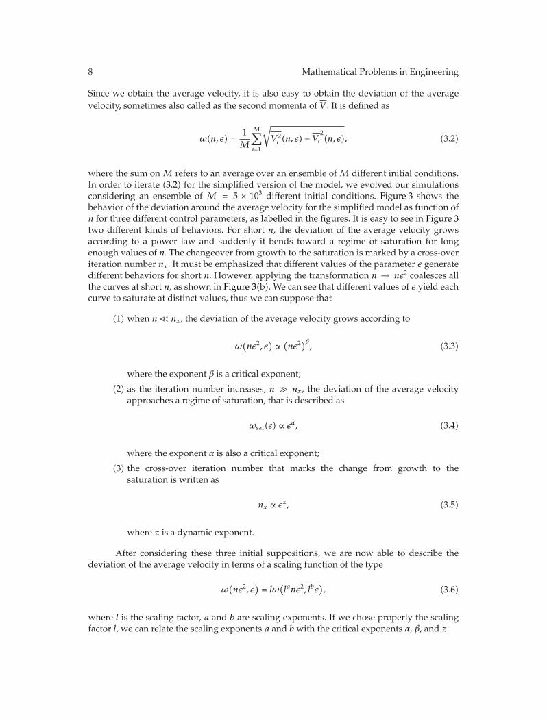
where the sum on M refers to an average over an ensemble of M different initial conditions.In order to iterate (3.2) for the simplified version of the model, we evolved our simulationsconsidering an ensemble of M = 5 × 103 different initial conditions. Figure 3 shows thebehavior of the deviation around the average velocity for the simplified model as function ofn for three different control parameters, as labelled in the figures. It is easy to see in Figure 3two different kinds of behaviors. For short n, the deviation of the average velocity growsaccording to a power law and suddenly it bends toward a regime of saturation for longenough values of n. The changeover from growth to the saturation is marked by a cross-overiteration number nx. It must be emphasized that different values of the parameter ε generatedifferent behaviors for short n. However, applying the transformation n → nε2 coalesces allthe curves at short n, as shown in Figure 3(b). We can see that different values of ε yield eachcurve to saturate at distinct values, thus we can suppose that

(1) when n� nx, the deviation of the average velocity grows according to

ω(nε2, ε

)∝(nε2)β, (3.3)

where the exponent β is a critical exponent;

(2) as the iteration number increases, n nx, the deviation of the average velocityapproaches a regime of saturation, that is described as

ωsat(ε) ∝ εα, (3.4)

where the exponent α is also a critical exponent;

(3) the cross-over iteration number that marks the change from growth to thesaturation is written as

nx ∝ εz, (3.5)

where z is a dynamic exponent.

After considering these three initial suppositions, we are now able to describe thedeviation of the average velocity in terms of a scaling function of the type

ω(nε2, ε

)= lω

(lanε2, lbε

), (3.6)

where l is the scaling factor, a and b are scaling exponents. If we chose properly the scalingfactor l, we can relate the scaling exponents a and b with the critical exponents α, β, and z.

Mathematical Problems in Engineering 9

108106104102

n

10−3

10−2

10−1

ω

ε = 6 × 10−3

ε = 6 × 10−3

ε = 6 × 10−3

(a)

10410210010−210−4

nε2

10−3

10−2

10−1

ω

ε = 6 × 10−3

ε = 6 × 10−3

ε = 6 × 10−3

(b)

Figure 3: (a) Behavior of the deviation of the average velocity for different values of the control parameterε for the simplified model. (b) Their initial collapse after the transformation nε2 for the simplified model.The control parameter g was fixed as g = 5.628 × 10−5.

×10−2

10.40.10.050.02

ε

0.8

2

3

6

×10−2

ωsa

t

Numerical dataBest fit

α = 0.5003(6)

(a)

×10−2

10.40.10.050.02

ε

2

7

20

70

×102

nx

Numerical dataBest fit

z = −0.96(1)

(b)

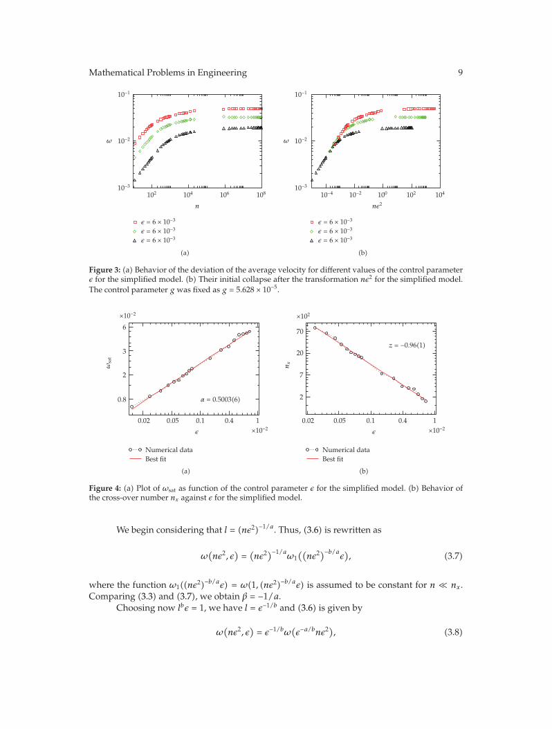
Figure 4: (a) Plot of ωsat as function of the control parameter ε for the simplified model. (b) Behavior ofthe cross-over number nx against ε for the simplified model.

We begin considering that l = (nε2)−1/a. Thus, (3.6) is rewritten as

ω(nε2, ε

)=(nε2)−1/a

ω1((nε2)−b/aε

), (3.7)

where the function ω1((nε2)−b/aε) = ω(1, (nε2)−b/aε) is assumed to be constant for n � nx.Comparing (3.3) and (3.7), we obtain β = −1/a.

Choosing now lbε = 1, we have l = ε−1/b and (3.6) is given by

ω(nε2, ε

)= ε−1/bω

(ε−a/bnε2), (3.8)

10 Mathematical Problems in Engineering

10410210010−210−410−6

nε2

10−4

10−3

10−2

10−1

ω

ε = 6 × 10−4

ε = 2 × 10−4ε = 8 × 10−3

ε = 2 × 10−3

(a)

10610410210010−2

nεz+2

10−2

10−1

100

ω/εα

ε = 6 × 10−4

ε = 2 × 10−4ε = 8 × 10−3

ε = 2 × 10−3

(b)

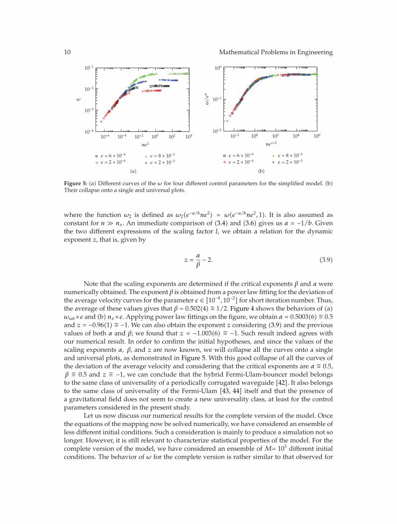
Figure 5: (a) Different curves of the ω for four different control parameters for the simplified model. (b)Their collapse onto a single and universal plots.

where the function ω2 is defined as ω2(ε−a/bnε2) = ω(ε−a/bnε2, 1). It is also assumed asconstant for n nx. An immediate comparison of (3.4) and (3.6) gives us α = −1/b. Giventhe two different expressions of the scaling factor l, we obtain a relation for the dynamicexponent z, that is, given by

z =α

β− 2. (3.9)

Note that the scaling exponents are determined if the critical exponents β and α werenumerically obtained. The exponent β is obtained from a power law fitting for the deviation ofthe average velocity curves for the parameter ε ∈ [10−4, 10−2] for short iteration number. Thus,the average of these values gives that β = 0.502(4) ∼= 1/2. Figure 4 shows the behaviors of (a)ωsat×ε and (b) nx×ε. Applying power law fittings on the figure, we obtain α = 0.5003(6) ∼= 0.5and z = −0.96(1) ∼= −1. We can also obtain the exponent z considering (3.9) and the previousvalues of both α and β; we found that z = −1.003(6) ∼= −1. Such result indeed agrees withour numerical result. In order to confirm the initial hypotheses, and since the values of thescaling exponents α, β, and z are now known, we will collapse all the curves onto a singleand universal plots, as demonstrated in Figure 5. With this good collapse of all the curves ofthe deviation of the average velocity and considering that the critical exponents are α ∼= 0.5,β ∼= 0.5 and z ∼= −1, we can conclude that the hybrid Fermi-Ulam-bouncer model belongsto the same class of universality of a periodically corrugated waveguide [42]. It also belongsto the same class of universality of the Fermi-Ulam [43, 44] itself and that the presence ofa gravitational field does not seem to create a new universality class, at least for the controlparameters considered in the present study.

Let us now discuss our numerical results for the complete version of the model. Oncethe equations of the mapping now be solved numerically, we have considered an ensemble ofless different initial conditions. Such a consideration is mainly to produce a simulation not solonger. However, it is still relevant to characterize statistical properties of the model. For thecomplete version of the model, we have considered an ensemble of M= 103 different initialconditions. The behavior of ω for the complete version is rather similar to that observed for

Mathematical Problems in Engineering 11

10010−210−4

nε2

10−3

10−2

ω

ε = 1 × 10−3

ε = 2 × 10−3

ε = 3 × 10−3

(a)

104102100

nεz+2

10−2

10−1

ω/εα

ε = 1 × 10−3

ε = 2 × 10−3

ε = 3 × 10−3

(b)

Figure 6: (a) Different curves of the ω for three different control parameters for the complete model. (b)Their collapse onto a single and universal plots.

the simplified version of the model. After an extensive simulation, we obtain that the criticalexponents are β = 0.50(2) ∼= 0.5, α = 0.501(3), and z = −0.95(3). Evaluating (3.9), we foundthat z = −1.00(3). These critical exponents also allow us to produce a good collapse of all thecurves of ω onto a single and universal plots, as shown in Figure 6. Thus, we can concludethat the scaling properties are unaffected by considering the simplified or complete versionsof the model.

4. Final Remarks

As a final remark of the present paper, we have studied a simplified and the complete versionof the hybrid Fermi-Ulam-bouncer model considering elastic collisions with the walls. Weshow that the average energy as well as the deviation around the average velocity for chaoticorbits for both the complete and simplified versions of the model exhibit scaling propertieswith the same critical exponents. Moreover, we have shown that there is an analytical relationbetween the critical exponents α, β, and z. Our scaling hypotheses are confirmed by a goodcollapse of all the curves of ω onto a single and universal plot, therefore, confirming that thismodel also belongs to the same class of universality of the Fermi-Ulam model [43], for therange of control parameters studied, and the periodically corrugated waveguide [42].

Acknowledgment

D. F. M. Oliveira and R. A. Bizao are grateful to CNPq; E. D. Leonel thanks FAPESP,FUNDUNESP, and CNPq for financial support.

References

[1] M. V. Berry, “Regularity and chaos in classical mechanics, illustrated by three deformations of acircular ‘billiard’,” European Journal of Physics, vol. 2, no. 2, pp. 91–102, 1981.

12 Mathematical Problems in Engineering

[2] A. J. Lichtenberg and M. A. Lieberman, Regular and Chaotic Dynamics, vol. 38 of Applied MathematicalSciences, Springer, New York, NY, USA, 2nd edition, 1992.

[3] L. A. Bunimovich, “On the ergodic properties of nowhere dispersing billiards,” Communications inMathematical Physics, vol. 65, no. 3, pp. 295–312, 1979.

[4] Y. G. Sinai, “Dynamical systems with elastic reflections,” Russian Mathematical Surveys, vol. 25, no. 2,pp. 137–189, 1970.

[5] A. M. Ozorio de Almeida, Hamiltonian Systems: Chaos and Quantization, Cambridge Monographs onMathematical Physics, Cambridge University Press, Cambridge, UK, 1988.

[6] D. G. Ladeira and J. K. L. da Silva, “Time-dependent properties of a simplified Fermi-Ulam acceleratormodel,” Physical Review E, vol. 73, no. 2, Article ID 026201, 6 pages, 2006.

[7] E. D. Leonel, J. K. L. da Silva, and S. O. Kamphorst, “On the dynamical properties of a Fermiaccelerator model,” Physica A, vol. 331, no. 3-4, pp. 435–447, 2004.

[8] A. K. Karlis, P. K. Papachristou, F. K. Diakonos, V. Constantoudis, and P. Schmelcher, “Hyperacceler-ation in a stochastic Fermi-Ulam model,” Physical Review Letters, vol. 97, no. 19, Article ID 194102, 4pages, 2006.

[9] A. K. Karlis, P. K. Papachristou, F. K. Diakonos, V. Constantoudis, and P. Schmelcher, “Fermiacceleration in the randomized driven Lorentz gas and the Fermi-Ulam model,” Physical Review E,vol. 76, no. 1, Article ID 016214, 17 pages, 2007.

[10] J. V. Jose and R. Cordery, “Study of a quantum Fermi-acceleration model,” Physical Review Letters, vol.56, no. 4, pp. 290–293, 1986.

[11] E. D. Leonel, D. F. M. Oliveira, and R. E. de Carvalho, “Scaling properties of the regular dynamics fora dissipative bouncing ball model,” Physica A, vol. 386, no. 1, pp. 73–78, 2007.

[12] D. F. M. Oliveira and E. D. Leonel, “The Feigenbaum’s δ for a high dissipative bouncing ball model,”Brazilian Journal of Physics, vol. 38, no. 1, pp. 62–64, 2008.

[13] R. M. Everson, “Chaotic dynamics of a bouncing ball,” Physica D, vol. 19, no. 3, pp. 355–383, 1986.[14] P. J. Holmes, “The dynamics of repeated impacts with a sinusoidally vibrating table,” Journal of Sound

and Vibration, vol. 84, no. 2, pp. 173–189, 1982.[15] G. A. Luna-Acosta, “Regular and chaotic dynamics of the damped Fermi accelerator,” Physical Review

A, vol. 42, no. 12, pp. 7155–7162, 1990.[16] T. L. Vincent and A. I. Mees, “Controlling a bouncing ball,” International Journal of Bifurcation and Chaos

in Applied Sciences and Engineering, vol. 10, no. 3, pp. 579–592, 2000.[17] E. D. Leonel and A. L. P. Livorati, “Describing Fermi acceleration with a scaling approach: the Bouncer

model revisited,” Physica A, vol. 387, no. 5-6, pp. 1155–1160, 2008.[18] A. C. J. Luo and R. P. S. Han, “The dynamics of a bouncing ball with a sinusoidally vibrating table

revisited,” Nonlinear Dynamics, vol. 10, no. 1, pp. 1–18, 1996.[19] A. C. J. Luo, “An unsymmetrical motion in a horizontal impact oscillator,” Journal of Vibration and

Acoustics, vol. 124, no. 3, pp. 420–426, 2002.[20] E. D. Leonel and P. V. E. McClintock, “Scaling properties for a classical particle in a time-dependent

potential well,” Chaos, vol. 15, no. 3, Article ID 033701, 7 pages, 2005.[21] J. L. Mateos, “Traversal-time distribution for a classical time-modulated barrier,” Physics Letters A,

vol. 256, no. 2-3, pp. 113–121, 1999.[22] E. D. Leonel and P. V. E. McClintock, “A hybrid Fermi-Ulam-bouncer model,” Journal of Physics A,

vol. 38, no. 4, pp. 823–839, 2005.[23] D. G. Ladeira and E. D. Leonel, “Dynamical properties of a dissipative hybrid Fermi-Ulam-bouncer

model,” Chaos, vol. 17, no. 1, Article ID 013119, 7 pages, 2007.[24] A. J. Lichtenberg, M. A. Lieberman, and R. H. Cohen, “Fermi acceleration revisited,” Physica D, vol.

1, no. 3, pp. 291–305, 1980.[25] S. M. Ulam, “On some statistical properties of dynamical systems,” in Proceedings of the 4th Berkeley

Symposium on Mathematical Statistics and Probability, vol. 3, pp. 315–320, University of California Press,Berkeley, Calif, USA, June-July 1960.

[26] J. M. Hammerseley, “On the dynamical disequilibrium of individual particles,” in Proceedings of the4th Berkeley Symposium on Mathematical Statistics and Probability, vol. 3, p. 79, University of CaliforniaPress, Berkeley, Calif, USA, June-July 1960.

[27] A. V. Milovanov and L. M. Zelenyi, ““Strange” Fermi processes and power-law nonthermal tailsfrom a self-consistent fractional kinetic equation,” Physical Review E, vol. 64, no. 5, Article ID 052101,4 pages, 2001.

Mathematical Problems in Engineering 13

[28] A. Veltri and V. Carbone, “Radiative intermittent events during Fermi’s stochastic acceleration,”Physical Review Letters, vol. 92, no. 14, Article ID 143901, 4 pages, 2004.

[29] K. Kobayakawa, Y. S. Honda, and T. Samura, “Acceleration by oblique shocks at supernova remnantsand cosmic ray spectra around the knee region,” Physical Review D, vol. 66, no. 8, Article ID 083004,11 pages, 2002.

[30] G. Lanzano, E. De Filippo, D. Mahboub, et al., “Fast electron production at intermediate energies:evidence for Fermi shuttle acceleration and for deviations from simple relativistic kinematics,”Physical Review Letters, vol. 83, no. 22, pp. 4518–4521, 1999.

[31] G. L. Gutsev, P. Jena, and R. J. Bartlett, “Two thermodynamically stable states in SiO- and PN-,”Physical Review A, vol. 58, no. 6, pp. 4972–4974, 1998.

[32] A. Steane, P. Szriftgiser, P. Desbiolles, and J. Dalibard, “Phase modulation of atomic de Broglie waves,”Physical Review Letters, vol. 74, no. 25, pp. 4972–4975, 1995.

[33] A. Loskutov and A. B. Ryabov, “Particle dynamics in time-dependent stadium-like billiards,” Journalof Statistical Physics, vol. 108, no. 5-6, pp. 995–1014, 2002.

[34] S. O. Kamphorst and S. P. de Carvalho, “Bounded gain of energy on the breathing circle billiard,”Nonlinearity, vol. 12, no. 5, pp. 1363–1371, 1999.

[35] A. Loskutov, A. B. Ryabov, and L. G. Akinshin, “Properties of some chaotic billiards with time-dependent boundaries,” Journal of Physics A, vol. 33, no. 44, pp. 7973–7986, 2000.

[36] R. E. de Carvalho, F. C. Souza, and E. D. Leonel, “Fermi acceleration on the annular billiard,” PhysicalReview E, vol. 73, no. 6, Article ID 066229, 10 pages, 2006.

[37] A. Yu. Loskutov, A. B. Ryabov, and L. G. Akinshin, “Mechanism of Fermi acceleration in dispersingbilliards with time-dependent boundaries,” Journal of Experimental and Theoretical Physics, vol. 89, no.5, pp. 966–974, 1999.

[38] R. E. de Carvalho, F. C. de Souza, and E. D. Leonel, “Fermi acceleration on the annular billiard: asimplified version,” Journal of Physics A, vol. 39, no. 14, pp. 3561–3573, 2006.

[39] F. Lenz, F. K. Diakonos, and P. Schmelcher, “Tunable Fermi acceleration in the driven ellipticalbilliard,” Physical Review Letters, vol. 100, no. 1, Article ID 014103, 4 pages, 2008.

[40] S. O. Kamphorst, E. D. Leonel, and J. K. L. da Silva, “The presence and lack of Fermi acceleration innonintegrable billiards,” Journal of Physics A, vol. 40, no. 37, pp. F887–F893, 2007.

[41] J.-P. Eckmann and D. Ruelle, “Ergodic theory of chaos and strange attractors,” Reviews of ModernPhysics, vol. 57, no. 3, pp. 617–656, 1985.

[42] E. D. Leonel, “Corrugated waveguide under scaling investigation,” Physical Review Letters, vol. 98, no.11, Article ID 114102, 4 pages, 2007.

[43] E. D. Leonel, P. V. E. McClintock, and J. K. L. da Silva, “Fermi-Ulam accelerator model under scalinganalysis,” Physical Review Letters, vol. 93, no. 1, Article ID 014101, 4 pages, 2004.

[44] J. K. L. da Silva, D. G. Ladeira, E. D. Leonel, P. V. E. McClintock, and S. O. Kamphorst, “Scalingproperties of the Fermi-Ulam accelerator model,” Brazilian Journal of Physics, vol. 36, no. 3A, pp. 700–707, 2006.