
Scaling Mobile Ad Hoc Networks: - Samraksh
123
Page | i Approved for Public Release, Distribution Unlimited Scaling Mobile Ad Hoc Networks: Alternate Semantics for Local Routing Combined with Leveraging Small Amounts of Global Capacity Public Release: Technical Book [Draft Copy - version 0.9] Program: Fixed Wireless at a Distance, Networking Tract Team: The Samraksh Company Advanced Concepts Lab, Advanced Technology Lab, Lockheed Martin Professor P. R. Kumar Disclaimer: The views expressed are those of the author(s) and do not reflect the official policy or position of the Department of Defense or the U.S. Government Primary Investigator: Kenneth W. Parker, Ph.D. Contributors: Mukundan Sridharan, Ph. D. Algorithms and Analysis Prof. P.R. Kumar Capacity & Information Theory Prof. Anish Arora Networking & Stability Herb Greenburg Simulations & Post-Simulation Analysis Prof. Vinod K. Kulathumani Census & Common Operation Picture Danny Patru Android, Simulations & Post-Simulation Analysis Jesse R Brown Click & NS3 Gautam H Thaker Interference Rick Correa Project, Motion Models & Android Chuck Winters Project Version 0.9 7/12/2013
-
Upload
khangminh22 -
Category
Documents
-
view
1 -
download
0
Transcript of Scaling Mobile Ad Hoc Networks: - Samraksh

Page | i Approved for Public Release, Distribution Unlimited
Scaling Mobile Ad Hoc Networks: Alternate Semantics for Local Routing Combined with Leveraging Small Amounts of Global Capacity
Public Release: Technical Book [Draft Copy - version 0.9]
Program: Fixed Wireless at a Distance, Networking Tract
Team: The Samraksh Company Advanced Concepts Lab, Advanced Technology Lab, Lockheed Martin Professor P. R. Kumar
Disclaimer: The views expressed are those of the author(s) and do not reflect the official policy or position of the Department of Defense or the U.S. Government
Primary Investigator: Kenneth W. Parker, Ph.D.
Contributors: Mukundan Sridharan, Ph. D. Algorithms and Analysis
Prof. P.R. Kumar Capacity & Information Theory
Prof. Anish Arora Networking & Stability
Herb Greenburg Simulations & Post-Simulation Analysis
Prof. Vinod K. Kulathumani Census & Common Operation Picture
Danny Patru Android, Simulations & Post-Simulation Analysis
Jesse R Brown Click & NS3
Gautam H Thaker Interference
Rick Correa Project, Motion Models & Android
Chuck Winters Project
Version 0.9 7/12/2013

Page | ii Approved for Public Release, Distribution Unlimited
Foreword

Page | iii Approved for Public Release, Distribution Unlimited
A shockingly large body of failures suggests that Mobile Ad Hoc Networks (MANETs) simply do not scale beyond about 100 nodes. The key difficulty is that the complexity of the network dy-namics becomes overwhelming as the scale of the network grows.
It has been known for about 15 years that the aggregate capacity of multi-hop networks is √𝑛 fold greater than an otherwise equivalent cellular network. This is one of the key motivations for MANETs. However, it was recently discovered that the complexity of maintaining local knowledge of a node’s neighborhood grows ln (𝑛)𝛾 faster than network capacity (for 1 ≤ 𝛾 ≤2). This implies that MANETs can’t scale. Even worse, traditional MANETs require global aware-ness, which is at least 𝑂(𝑛) worse, often 𝑂(𝑛2) worse. Abandoning the traditional radio abstraction, as a node-to-node communication device, in favor of a many-node-to-many-node communication abstraction (network-coding), could increase the aggregate capacity by 𝑂(√𝑛). But in the presence of mobility this seems likely to increase the networking overhead, thereby eroding the gain. More importantly, huge gaps remain between current theory and any practical implementation.
In this project, we have advocated designing systems that only require local network knowledge. The result is not absolutely scalable, but it allows systems to scale to 10s of thousands of nodes. Our position seems to preclude arbitrary point-to-point (P2P) routing. However, many highly scalable Application Specific Networking Patterns (ASNPs) are known to exist; the problem is none of them are fully general. We believe that the desire for a fully general networking abstrac-tion is the endemic flaw with MANET research today. This desire should be actively avoided. Rather, MANET applications should be redesigned to accommodate scaling issues.
Using this approach, we designed, simulated and implemented ASNPs using the ns3-Click modu-lar software router framework. We started with 5 ASNPs that we thought were important: (1) Flooding with Pruning, (2) Emergent Local Groups, (3) Census, (4) Exfiltration and (5) Common Operating Picture. We in no way argue that these are the only ones required in a MANET. In fact, we believe, that we will continue to work on other ASNPs. But, on the other hand we do not think that 100s of ASNPs are needed. Ideally, about 20 ASNPs should be able to support 1000s of applications. We demonstrated that all of these patterns are much more scalable than what has been achieved by current generation MANETs. We have also provided general guidelines for designing scalable ASNPs.
We have summarized existing theoretical results that support our clean-slate approach. We also discovered new theory results during this project (however these results are not published in this book), which provides new lower bounds for the network overhead in MANETs. The new results demonstrate what was always suspected, that no MANET routing protocols can scale in abso-lutely.
We also brought out link layer issues such as discovery and low power MACs and defined a Link Layer API that will serve as our layer of standardization (colloquially called the “waist” of a sys-tem). The narrowness of the link layer makes porting to new hardware especially easy.
We understand that the clean-slate approach could result in a few issues as the framework ma-tures. Probably, the most important of these is that many applications will have to be redesigned to take advantage of the new ASNPs, but on the other hand the new framework will enable even more applications that were not previously possible (or were extremely inefficient). The other potential issue is naming of ASNPs and applications, which is very much solvable.

Page | iv Approved for Public Release, Distribution Unlimited
TABLE OF CONTENTS
Foreword ............................................................................................................................................................... ii
TABLE OF CONTENTS .................................................................................................................................................... iv
TABLE OF FIGURES ....................................................................................................................................................... vii
Part I A Design Framework for Mobile Ad Hoc Networks .................................................................................. 1
Raison D’Etre .................................................................................................................................. 2
Intractable Problems ................................................................................................................................................. 3
Failure of Traditional Formulation ............................................................................................................................ 4
The Alternate Formulation: Application Specific Networking Patterns .................................................................... 5
Link Layer is the “Narrow” Part of the Stack ............................................................................................................. 7
The Hybrid Architecture ............................................................................................................................................ 8
Fake Issues ................................................................................................................................................................ 8
Important Future Issues ............................................................................................................................................ 9
Analysis of the Traditional Solution .............................................................................................. 10
Understanding the Failures in the Current MANETs ............................................................................................... 10
Analysis of Broken Routes ....................................................................................................................................... 12
Analysis of Repair Time Scaling Wall ...................................................................................................................... 14
Design Heuristics ..................................................................................................................................................... 15
The Link Layer, Medium Access Control (MAC), and Neighborhood Discovery .............................. 17
Link Layer Abstraction ............................................................................................................................................. 18
MAC Paradigms Supported ..................................................................................................................................... 19
Low-Power MAC ...................................................................................................................................................... 20
Router Abstraction Layer .............................................................................................................. 25
Requirements of a Router Abstraction .................................................................................................................... 25
Impact of a Router Abstraction ............................................................................................................................... 27
Click as a Software Router ...................................................................................................................................... 29
Application Specific Networking Patterns as Graph Nodes .................................................................................... 31
Linux as a Development Platform ........................................................................................................................... 32
Models and Fidelity ....................................................................................................................... 33
Validation Mechanisms ........................................................................................................................................... 34
Critical Factors for Validation ................................................................................................................................. 35
Scaling in the Presence of Fidelity ........................................................................................................................... 39

Page | v Approved for Public Release, Distribution Unlimited
Part II Example Application Specific Networking Patterns (ASNPs) ................................................................... 40
Flooding With Pruning .................................................................................................................. 41
FwP Background ..................................................................................................................................................... 41
The Algorithm ......................................................................................................................................................... 42
Callbacks ................................................................................................................................................................. 43
Protocol Flow .......................................................................................................................................................... 43
Temporary Disconnections ...................................................................................................................................... 44
Pruning Criteria ....................................................................................................................................................... 44
Regional Pruning ..................................................................................................................................................... 44
Implementation and ns-3 Simulation Results ......................................................................................................... 46
Pattern Remarks ..................................................................................................................................................... 47
Emergent Local Groups ................................................................................................................. 48
Background: Link State Routing ............................................................................................................................. 48
Overview and Theoretical Analysis of NK-LSR ......................................................................................................... 49
Need-to-Know Link State Protocol .......................................................................................................................... 55
Evaluation and Results ............................................................................................................................................ 56
Scalability of NK-LSR ............................................................................................................................................... 59
Pattern Remarks ..................................................................................................................................................... 59
Census........................................................................................................................................... 61
Background: One-Shot Aggregate Querying .......................................................................................................... 62
Census Protocol ....................................................................................................................................................... 63
Census Analytical Bounds ....................................................................................................................................... 65
Census APIs ............................................................................................................................................................. 66
Performance Evaluation .......................................................................................................................................... 67
Pattern Remarks ..................................................................................................................................................... 74
Exfiltration .................................................................................................................................... 75
Background: Tree Based Exfiltration ...................................................................................................................... 75
The Inverse-Wave ................................................................................................................................................... 76
The Algorithm ......................................................................................................................................................... 76
Simulation Results ................................................................................................................................................... 79
Pattern Remarks ..................................................................................................................................................... 83
Common Operating Picture ........................................................................................................... 84
Background: Common Operating Picture and Global Snapshots ........................................................................... 84
The COP Protocol .................................................................................................................................................... 85

Page | vi Approved for Public Release, Distribution Unlimited
COP APIs .................................................................................................................................................................. 89
Important Metrics ................................................................................................................................................... 90
Evaluations and Results .......................................................................................................................................... 90
Pattern Remarks ..................................................................................................................................................... 95
Part III Conclusions and Recommendations .................................................................................................. 96
The Frisson .................................................................................................................................... 97
COP Review ............................................................................................................................................................. 97
Scalable Distance-sensitive Geographic Routing .................................................................................................... 98
Scalable Distance-sensitive Distance Vector Routing ............................................................................................. 99
Scalable Distance-sensitive Probabilistic Routing ................................................................................................. 100
Recommendations ...................................................................................................................... 102
Clean Slate Approach ............................................................................................................................................ 102
Embrace ASNPs ..................................................................................................................................................... 103
Part IV Appendices ...................................................................................................................................... 104
Capacity Theory .......................................................................................................................... 105
Acronyms .................................................................................................................................... 108
References .................................................................................................................................. 110

Page | vii Approved for Public Release, Distribution Unlimited
TABLE OF FIGURES
Figure 1. K2. Often considered the hardest mountain to climb .............................................................................. 2
Figure 2. There is a practical problem with the proposed solution .......................................................................... 3
Figure 3. Spatial reuse in a MANET ........................................................................................................................ 3
Figure 4. Capacity scaling and network layer overhead scaling in MANET ................................................................ 4
Figure 5. Scaling for flooding.................................................................................................................................. 4
Figure 6. The transport and networking layer are combined into Application Specific Networking Patterns (ASNPs)5
Figure 7. Scaling wall for ASNs considered below ................................................................................................... 6
Figure 8. Lowering the waist, not just widening the networking layer. A traditional network on the left compared
to an ASNP-centric network on the left ................................................................................................................... 7
Figure 9. The ‘byzantine fault’ problem in routing .................................................................................................. 8
Figure 10. The range of naming choices for a networking system ........................................................................... 8
Figure 11. The grid network used to study problems in traditional MANETs ......................................................... 10
Figure 12. High percentage of paths are broken in OLSR, even under low mobility ............................................... 11
Figure 13. Expected OLSR NLO growth and scaling ............................................................................................... 11
Figure 14. Initial State of an example network ..................................................................................................... 12
Figure 15. The routing information after the link state change occurs and the after the network has stabilized to its
new routes ........................................................................................................................................................... 12
Figure 16. Broken routes just after the link state change ...................................................................................... 13
Figure 17. A healed but not-yet stabilized network .............................................................................................. 13
Figure 18. Example scenario leading to broken path and region flooded to fix the routes ..................................... 14
Figure 19. Repair Time Scaling Wall ...................................................................................................................... 14
Figure 20. Lowering the waist, not just widening the networking layer. A traditional network on the left compared
to an ASNP-centric network on the left ................................................................................................................. 18
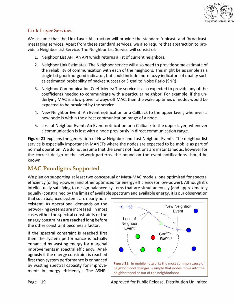
Figure 21. In mobile networks the most common cause of neighborhood changes is simply that nodes move into
the neighborhood or out of the neighborhood ..................................................................................................... 19
Figure 22. Visual intuition for the amount of energy consumed by the radio (bull Elephant), signal processing
(Gorilla) and everything else (Dog). ....................................................................................................................... 21
Figure 23. Classical asynchronous discovery scheme ............................................................................................ 21
Figure 24. Flooding-based cued discovery ............................................................................................................ 22
Figure 25. Limitation of flooding-based cued discovery ........................................................................................ 22
Figure 26. Infrastructure assisted discovery ......................................................................................................... 23
Figure 27. Ingress/Egress integration points provided by ns-3-click ...................................................................... 27
Figure 28: Adding positional support to ns-3-click/Click ........................................................................................ 28

Page | viii Approved for Public Release, Distribution Unlimited
Figure 29: Simple Click router configuration using 3 ASNPs ................................................................................... 30
Figure 30: Click router graph ................................................................................................................................ 31
Figure 31. Effective Communication Range shrinks even with Far Interferers. ...................................................... 36
Figure 32. Testing For Interference at Scale. ........................................................................................................ 36
Figure 33. Illustration of the impact of multi-path on link stability. ....................................................................... 37
Figure 34. Example of multipath in the visual spectrum. ...................................................................................... 37
Figure 35. A fringe pattern corresponding to a high degree of multi-path. ............................................................ 38
Figure 36. Low multi-path environment. .............................................................................................................. 38
Figure 37 Regional Flooding Results ..................................................................................................................... 44
Figure 38 Hop Count Flooding Results .................................................................................................................. 45
Figure 39 Distance Flooding Results ...................................................................................................................... 45
Figure 40. Region of perturbation for a Link Change in a Uniform 2D deployment ................................................. 51
Figure 41. A Random distance-based 100 Node graph generated by uniform random placement in a 2D plane .... 52
Figure 42. Distribution of Node Degree in a random 2D graph .............................................................................. 53
Figure 43. Message Cost vs Link Error Events ...................................................................................................... 53
Figure 44. Bridges are very important for overland connectivity. .......................................................................... 54
Figure 45. Histogram of Cost Networks of Size 100 and 500 and M=7 ................................................................... 54
Figure 46: Average reachability percentage (2 Hz discovery rate) .......................................................................... 57
Figure 47. Communication cost in message per node per second ........................................................................ 58
Figure 48. Communication cost in bits per second per node ................................................................................. 58
Figure 49. Communication cost in bits per second per node (NK-LSR) ................................................................... 59
Figure 50. Average reachability % (NK-LSR) .......................................................................................................... 59
Figure 51. Illustration of the steps involved in a Census operation ....................................................................... 61
Figure 52. Census uses tokens for data ex-filtration by visiting each node. From each node, a token moves to an
unvisited node if available and aggregates data from that node ............................................................................ 63
Figure 53. During token passing phase, the token may be surrounded by an island of visited nodes, i.e., all
neighboring nodes have already been visited. Nodes that have not yet been visited set up a gradient using the set
of visited nodes and attract the token towards them ............................................................................................ 65
Figure 54. Average time to achieve 95% convergence (Trend-line computed by MS Excel) ................................... 68
Figure 55. Average messages until 95% convergence. Token messages include token announcement, requests and
token passing. ...................................................................................................................................................... 69
Figure 56. Convergence pattern for 3 different runs at 4000 nodes with 62 tokens .............................................. 69
Figure 57. Linear growth of gradient messages over time; 4000 nodes with 62 tokens ......................................... 70
Figure 58. Average messages until 95% convergence. Token messages include token announcement, requests and
token passing. ...................................................................................................................................................... 70

Page | ix Approved for Public Release, Distribution Unlimited
Figure 59. Average time to achieve 95% convergence (Trend-line computed by MS Excel) ................................... 71
Figure 60. Growth of gradient messages over time; 4000 nodes with 24 tokens ................................................... 71
Figure 61. Convergence pattern for 3 different runs at 4000 nodes with 24 tokens .............................................. 72
Figure 62. Impact of number of tokens on messages until 95% convergence. N = 250 .......................................... 72
Figure 63. Impact of number of tokens on 95% convergence time. N= 250 ........................................................... 73
Figure 64. Impact of number of tokens on 95% convergence time. N= 500 ........................................................... 73
Figure 65. Impact of number of tokens on messages until 95% convergence. N = 500 .......................................... 74
Figure 66. A spanning tree of the type that might be used in TBE. ........................................................................ 75
Figure 67. The wave structure used in our algorithm. ........................................................................................... 76
Figure 68. Bottlenecks are the only scenario in which a node can lose contact with its elders. .............................. 78
Figure 69. Starting Node Layout and Root Node Designation ................................................................................ 79
Figure 70. Illustration of How Probability of Reaching Root are Calculated. ........................................................... 80
Figure 71. Number of nodes connected to the Root .............................................................................................. 81
Figure 72. Average Number of Hops to the Root .................................................................................................. 81
Figure 73. Average Probability of Reaching Root ................................................................................................... 82
Figure 74. Probability of Reaching Root as a Function of Depth ............................................................................. 82
Figure 75. Temporary Disconnect of Portion of the Network. ............................................................................... 83
Figure 76. Rapid Reconnect from a Disconnected Condition ................................................................................. 83
Figure 77. Distance-based COP illustration ............................................................................................................ 85
Figure 78. Staleness of information in Distance-based COP ................................................................................... 86
Figure 79. Protocol Actions for Distance-based COP .............................................................................................. 88
Figure 80. Spatial distribution of staleness and rate of update .............................................................................. 91
Figure 81. Histogram of Packet Lengths for DS-COP .............................................................................................. 92
Figure 82. Total bytes sent for DS-COP and DI-COP ............................................................................................... 92
Figure 83. Packet-Size Histogram comparing DS-COP and DI-COP.......................................................................... 93
Figure 84 Maximum Expected Staleness for a deterministic DS-COP ..................................................................... 94
Figure 85. Accumulating staleness in DS-COP ........................................................................................................ 94
Figure 86 Staleness versus Distance for DI-COP and DS-COP................................................................................. 95
Figure 87. Staleness of information in Distance-sensitive COP ............................................................................... 97
Figure 88. Geographic Routing -- Graceful rerouting with mobility ...................................................................... 98
Figure 89. The effect of distant sensitive location fidelity on geographic routing. .................................................. 98
Figure 90. Distance-senstive Hop Count based routing fixed the “hole” problem .................................................. 99
Figure 91. Probabilistic Routing can solve the “moving bridge” problem ............................................................. 100
Figure 92. Correct and wrong analogies between network models ...................................................................... 102

Page | 1 Approved for Public Release, Distribution Unlimited
Part I A Design Framework
for Mobile Ad Hoc Networks
Page | 2 Approved for Public Release, Distribution Unlimited
Raison D’Etre
It is often said that right questions are more important than the right answers. But often this is merely a cliché. Perhaps the assertion feels wise because it simultaneously seems contrarian and vaguely intuitive. Too often the assertion can’t be accompanied by with an explanation of why or when it might be true. Perhaps the assertion should be applied to itself. Is it not more important to ask why or when, “Questions are more important than answer”, than to simply know that it is in some sense true?
Even worse, sometimes the assertion is meant to imply that it is more important to think big thoughts than to solve tough problems. This can lead to research that feel more relevant to Star Trek than to an actual operational setting. Alternatively it can lead to development efforts that include every technology at an appropriate Technology Readiness (TR) level with any plausible relevance.
This project is based on the idea that the right question is more important than the right answers in two specific ways:
1. There are a range of problem formula-tions with operational relevance. Some are more tractable than others. For hard problems like scaling of MA-NET (Mobile Ad Hoc Network) it’s helpful to allow tractability to influ-ence problem formulation.
2. When harder problem formulations are tractable they can provide extra operational functionality compared to simpler forms of the problem. How-ever, this is not always the case. Sometimes the simpler problem for-mulation better matches the operational needs. At times the pri-mary advantage of solving the hard problem is to prove that you can. This is the intellectual equivalent of climbing K2 (Figure 1). Getting to the top of K2 is unlikely to address the needs of a operational scenario.
Part-I of the book explicitly and somewhat aggressively address the first point. Part-II addresses the second point in a somewhat oblique manner. The reader is being led to the conclusion that many of the alternative problem formulations are at least as good a fit to operational needs as the classical problem formulation. Part III of the book presents a somewhat surprising conclusion regarding the classical problem formulation and our recommendations for designing scalable MABETs. In Appendices A, we presents a summary of existing theoretical results, a list of acro-nyms used in the book and their expansions can be found in Appendix B and finally the list of
Figure 1. K2. Often considered the hardest mountain to climb

Page | 3 Approved for Public Release, Distribution Unlimited
References in Appendix C. While we discov-ered new and tighter theoretical bounds for the Network Layer Overhead during this pro-ject, we are not able to publish them in this book since they have not be published in other forums yet.
Intractable Problems
When a problem can be stated in less than 20 pages, but remains unsolved in spite of 100’s of millions of dollars of research, the problem is probably intractable. The internet and cheap supercomputing has allowed the invention of Freestyle Chess, where teams of skilled amateurs play chess by exploiting com-puter aided collaboration. Most freestyle chess teams, consisting of talented amateurs with a year or two of practice, are able to vastly outplay even the world champion [1]. Much of research follows a similar pattern. It is unrealistic to expect a few researchers (even if they happen to be “Grandmaster Re-searchers”) to solve problems that have eluded more than a few well organized research teams.
As a result, it seems to us that scaling MANETs beyond a few 100 nodes is for all practical purposes an intractable problem. Several dif-ferent well founded, well organized, research teams have worked on the problem. The pat-tern is well summarized by a quote from one of the top researchers in this area (not affili-ated with us), “Any good graduate student can make a MANET with 5 nodes. A MANET with 25 nodes requires careful attention to engineering subtlety. But making a MANET work at 75 nodes is rocket science”. The DARPA (Defense Advanced Research Program Agency) WNAN (Wireless Network After Next) program succeeded in demonstrating a sys-tem with 103 nodes [2] . Our observation from a distance suggests this represents a world class outcome. It is therefore natural to assume that the desire to make a MANET work for 10K nodes is imposable.
Figure 3. Spatial reuse in a MANET
Figure 2. There is a practical problem with the pro-posed solution

Page | 4 Approved for Public Release, Distribution Unlimited
On very rare occasions someone solves an “intractable” problem, like solving Fermat’s Last Theorem, through dec-ades of deep focus [3]. That is, by solving a problem widely considered intractable, they show that the prob-lem was in fact tractable, notwithstanding the prevailing percep-tions. However, although not common, it is not altogether rare for someone to “solve” an intractable problem by tweaking the problem for-mulation. That is, they do not technical solve the intractable prob-lem, but rather find a tractable problem that can be substituted for
the original one.
This latter approach dominates some areas of Computer Science (CS), where many natural prob-lem formulations are provable Nondeterministic-Polynomial (NP) Complete or NP-Hard, and are “understood” to be provably intractable. In these areas of CS, especially the more advanced examples, algorithm design primarily consists of finding problem formulations that yield a useful, yet tractable, result.
The work reported on here started by assuming that the classical formulation of the MANET could not be scaled to 10K nodes. It then focused on trying to understand the likely root causes of this intractability. Armed with partial knowledge of the root causes of intractability, we then searched for alternate problem formulations that achieve the operational goals of large scale MANETs, and (critically) are tractable at scales of 10K nodes.
Failure of Traditional Formulation
The core promise of Peer-to-Peer Networks (P2PNs) is that by using many short links instead of one long link a significant degree of spatial reuse of the spectrum can be achieved. Figure 3 illustrates the spatial reuse in MANETs. Indeed a large body of research, [4, 5], has shown that for a wide range of plausible scenarios the theoretical capacity of P2PNs is much higher than for comparable tradi-tional shared channel networks. However, many P2PNs scale poorly and the promise remain un-fulfilled. Most MANETs cannot scale beyond 100 nodes [2, 6], some exhibit stability problems be-yond 25 or 30 nodes.
The scaling problem is caused by networking overhead. Traditional MANETs use routing proto-cols that extend Open Shortest Path First (OSPF) and thus require that every change in link-layer connectivity be communicated to a large fraction
Figure 4. Capacity scaling and network layer overhead scaling in MANET
100
101
102
103
104
10-1
100
101
102
103
Network Scale
Norm
aliz
ed N
etw
ork
Capacity
Capacity
NLO
Figure 5. Scaling for flooding
100
102
104
10-2
100
102
Network Scale
Netw
ork
Capacity
Total
Useful

Page | 5 Approved for Public Release, Distribution Unlimited
of network. This leads to two problems: 1) networking overhead grows much faster than network capacity, overwhelming the network (as shown in Figure 4) and 2) delays in propagating network information create timeliness issues, which cause routing inefficiencies and in extreme cases insta-bility
The No Overhead Extreme
On the opposite extreme are designs that maintain zero (non-local) network state. In these cases there is no scaling wall, because there is no routing overhead; however, each packet must dis-cover its destination. In general this requires flooding the entire network for every packet. The efficiency then decreases like 1O n , as shown in Figure 5. For large n the useful capacity is worse than for a shared traditional channel network (i.e., without spatial reuse of the spectrum).
The networking overhead problem is a result of the arbitrary point-to-point formulation of rout-ing (the traditional MANET formulation), and can be avoided for less general or less abstract forms of routing. Many simpler forms of routing, such as flooding, do not have this problem. We are proposing a system that uses many different highly scalable Application Specific Networking Patterns (ASNPs).
In the context of this program, we propose using the long-link as the fallback when non-local point-to-point routing is required. If the collection of ASNPs is rich enough the need to resort to the long-link should be extremely rare.
The Alternate Formulation: Application Specific Networking Pat-terns
In the last decade and half, Wireless Sensor Networks (WSN) have made significant progress and scaled to thousands of nodes. The scalability of WSNs can be attributed to two factors: (i) Typically WSNs are less mobile, and (ii) Most of the traffic in WSNs is local does not need arbi-trary P2P. While the first factor contributes significantly to stability of links and hence to the decrease of Network Layer Overhead, we be-lieve the true reason for WSN scalability is the lack of global P2P routing support. This frees up the channel capacity used by the tradi-tional MANETs for sending link state updates throughout the network,
which caused the capacity scaling wall as shown in Figure 4.
The primary design philosophy we adopt in this project is that the network routing should match the application usage for the network to scale. Thus, we propose a number of Application Specific Network Patterns (ASNPs) instead of a single P2P MANET routing protocol. A useful analogy is
Figure 6. The transport and networking layer are combined into Application Specific Networking Patterns (ASNPs)

Page | 6 Approved for Public Release, Distribution Unlimited
the Application Specific Integrated Circuits (ASIC) used in the hardware design to extract maxi-mum hardware performance, where the performance improvement comes from matching the circuitry to the application. Figure 6 shows the architecture of our new paradigm. In this archi-tecture, what used to be called the network and transport layer in the traditional layered architecture has been combined into the ASNPs.
Application Specific Does Not Mean ‘Each Application on its Own’
Although we call our networking patterns as application specific, it must not be interpreted as each and every application having its own networking pattern or an application programmer now needing to write networking protocols. We envision a large degree of reuse for our ASNPs and imagine ~20 ASNPs supporting thousands of applications. It is not our desire in this project, how-ever, to argue for completeness of ASNPs, that is, to arrive at a set of ASNPs that can support any and all applications imaginable.
Impact of MANET Traffic Patterns on Capacity
Traffic patterns play a significant role in determining whether a P2PN scales to a large number of nodes. Non uniform traffic can compromise scalability, i.e., if hot spots limit total performance, or enhance scalability, i.e., for local traffic. In fact, for O(n) scalability, the traffic pattern must involve a ‘small’ average distance between source and destination nodes [4]. Interestingly, MA-NET applications anticipated for the FCS Brigade Combat Team have been analyzed to have fairly localized traffic patterns [7]. Specifically, the analysis shows that their traffic should satisfy a power law distribution with exponent between 2 and 3, in which case capacity is O(n) scalable, i.e., constant per node capacity is achievable.
Highly Scalable ASNPs
The ASNPs considered here preserve routing efficiency, while only requiring lo-cal, regional, or application sub-network state. This is possible because they sup-port a less general form of routing. In some cases, the network state infor-mation must be distributed to log( )O n nodes in a region of size log( )O n , in other cases this information is distributed only to a fixed number of neighbors. This implies an overhead complexity that is between O n and 2log( )O n n . This is graphed in Figure 7. For this particular example the scaling wall is beyond 10,000 nodes.
A key point is that none of these ASNPs may encapsulate a traditional MANET. The networking overhead problem limits scaling even if data is never sent on the associated network. So if one of the ASNPs is high overhead the entire system will not scale. In essence this reduces to a pro-hibition on arbitrary point-to-point routing. If a scalable form of point-to-point routing is
Figure 7. Scaling wall for ASNs considered below
100
102
104
100
102
Network Scale
Norm
aliz
ed C
apacity
Capacity
Over (min)
Over (max)

Page | 7 Approved for Public Release, Distribution Unlimited
developed, then it should be used to implement a modern MANET, otherwise non-local point-to-point routing must be banned from the ASNPs.
Link Layer is the “Narrow” Part of the Stack
Complexity theorists believe that a robust system needs a point of standardization (colloquially called a ‘waist’). Without standardization it is not possible to mix and match parts in a system. For example, the standardization of parts helped a lot in the production of rifles during the revo-lutionary war [8].
In a traditional network the point of great standardization (called “the waist”) is the networking and transport layers, e.g., TCP/IP. The high degree of standardization in these layers facilitates a greater flexibility both above and below the waist. We are proposing that for most P2PNs, espe-cially MANETs, this is the wrong meta-architecture. The preferred meta-architecture is a collection of ASNPs with greater standardization at link-layer as shown in Figure 8. The choice of Link Layer as the point of standardization is somewhat natural given the need for standardization in the stack. However it is important to remember that we propose to standardize only the se-mantics and the APIs of the link layer and DO NOT propose restricting the protocols or technologies used in the link layer. In general this architecture can work with a large set of link layer technologies, but some of them might need a “shim” layer that provides the APIs needed by the ASNP layer. In Chapter 3 we discuss in detail the Link Layer semantics and architecture.
Figure 8. Lowering the waist, not just widening the networking layer. A traditional network on the left compared to an ASNP-centric network on the left

Page | 8 Approved for Public Release, Distribution Unlimited
The Hybrid Architecture
One of the main differences be-tween the Fixed Wireless network architecture and the MANETs of the past is the infrastructure based Long Link to a Forward Operating Base. This hybrid architecture can be used to increase the robustness of the system and to scale to larger sizes by using the long link in a planned and systematic manner. While the long link does not add much to the capac-ity of the network, it can be used to tame a number of problems in the MANET that can be made easy by a “global” knowledge of the network. For example (as shown in Figure 9), in a mobile MANET a node could move just a short distance back and forth between two locations in such a manner that it could require data packets to be rerouted across a large portion of the network. While such problems may be unsolvable in the MANET, it can be trivially solved using the infrastructure link in the hybrid architecture. In general we see three advantages in the hybrid architecture:
1. Handles a little bit of the difficult traffic. Perhaps P2P traffic.
2. Accommodates design of a more efficient network “broadcast”.
3. Allows the long link to act as a “way out” of Byzantine Problems. (We assume the long link is less Byzantine).
Fake Issues
Application-Network Instance Naming
In traditional systems, the networking abstraction names the nodes. Some, Culler et al [9] in particular, have advocated that this naming concept is critical and should be preserved for P2PNs (even though the details may have to be more like IPv6 and LoWPAN) [9]. In opposition to this point of view many, notably Estrin and Van Jacobson [10] have advocated that the network should name the data (Named Data Networks (NDN)). The ASNP paradigm can support either IPv6 or NDN, but is conceptually in neither camp.
Figure 10. The range of naming choices for a networking system
Ph
ysic
al
No
de
Vir
tual
No
de
Net
wo
rk
Typ
es
Dat
a In
stan
ces
Dat
a Ty
pes
Ap
plic
atio
n-
Net
wo
rk
Inst
ance
s
Ap
plic
atio
n
Inst
ance
s
Ap
plic
atio
n
Typ
es
Figure 9. The ‘byzantine fault’ problem in routing

Page | 9 Approved for Public Release, Distribution Unlimited
The spectrum for the naming choices is illustrated in Figure 10. The coupling of names to nodes strongly reinforces the point-to-point nature of the networking system. Even something as sim-ple as multicast requires an overlay (or the application) to intervene in the process to receive each packet and forwarding it to multiple downstream nodes. In practical systems, because this involves cross layer operations, it may not even be possible to do this at line-rates. We find the argument that naming should be decoupled from the nodes appealing. But NDN seems to be too extreme in the other direction. Any control of the routing may require the creation of route specific data instances (or at least route specific data names).
We take the position that the networking system should name each instance of an ASNP. User applications will thus communicate among themselves via their corresponding instance identifi-ers. Some ASN identifiers will be well known; for instance, a service for discovery the existence of ASN instances (analogous to the Domain Name System (DNS) in TCP/IP) will have associated with it a well-known ASN identifier. The current effort focused on a limited set of ASNPs (namely the 5 presented in Part-II of this book) and has used static naming of the ASNPs. However, we expect that as we continue to evolve the system, we will design an ASPN-based naming architec-ture.
Security
Our current effort does not address security. We believe security is an important aspect of the ASNP based architecture and needs to be addressed in future. However, we assert that security for ASNPs in no more difficult than the traditional wireless networks. In some cases ASNPs can even provide better security and attack isolation than the traditional MANETs, since a lot of the patterns are local and hence a breach can be more easily contained. As the architecture evolves and matures, the security of the system of the system can be addressed and evolved.
Important Future Issues
Stability Issues
In the current effort we have not focused much on issues related to link stability, interference (both self and external) and the inter-play of these factors on the ASNP stability and design. Also, we have mostly ignored co-existence issues between the various ASNPs. However, we believe that such inter-related issues will have an impact on the stability of the links and consequently on the performance of the ASNPs and will need to carefully considered. We will focus on these issues in the future.
Application Redesign
A second real and important issue that needs attention is the redesign of applications to work with the ASNPs. Most of the current generation applications have be design and developed for the traditional paradigm, that is, the internet and with some minor modifications have been adapted for MANETs. However, with ASNPs, application semantics will change, giving a lot more flexibility to the application developers to choose the networking patterns, but a number of con-cepts from the traditional networks, such as node addressed, sockets, security APIs, etc., could change in our architecture. This means most of the applications that already exist for the tradi-tional network will need some redesign and tweaking, while some might have to be thrown away altogether and redeveloped. While this could be seen as additional work, we believe this is also an opportunity to reinvent the applications.

Page | 10 Approved for Public Release, Distribution Unlimited
Analysis of the Traditional Solution
With over a decade of experimentation and research, the mystery behind the inability of MANETs to scale beyond 70-100 nodes has remained unsolved. While theory has pointed to a asymptotic capacity scaling wall for the P2P routing in MANETs, it is not clear that in reality we are even close to this capacity scaling wall. In this subsection we analyze the performance and overhead of tra-ditional MANET routing with a focus on scalability. We study a number of variants of the Link State Routing, including the Optimized Link State Routing (OLSR) –which is considered as the state-of-the-art in MANET routing– to understand the factors affecting the performance of the current generation MANETs.
Understanding the Failures in the Current MANETs
While deploying scalable MANETs have re-mained challenging, the research efforts in the area have continued to present some-what of a mixed picture. Many incremental schemes have been presented with suppos-edly improved performance. In order to understand the problem with the scalability of OLSR we began by simulating a scenario which is known to be not scalable in real de-ployments.
Simulating the Failure Scenario
Specifically we constructed and simulated the standard implementation of the OLSR using network scenarios of size 75-150 nodes, that were known to have encountered performance problems [2]. We constructed a grid network (Figure 11 shows this topology) with varying sizes and introduced random link changes at a rate corresponding to low-to-medium mobility. Alt-hough a grid network is not a very realistic deployment scenario, it allows us to control very precisely the ground truth; that is, the number of neighbors and the rate of change of links, which would be somewhat more difficult to control precisely in a scenario with random mobility. Fur-ther, in order to isolate the effect of Network Layer Overhead (NLO) on scaling, the simulations were done in the absence of any useful data traffic. The expected result of these simulations was that when the network size reached around ~100 nodes, the system would start to fail and the NLO at that point would have reached between 15%-30% of the network capacity, thereby leav-ing very little capacity for useful data traffic. Thus, our definition of the capacity wall for these simulations was NLO reaching 15%-20% of channel capacity.
Figure 11. The grid network used to study problems in traditional MANETs

Page | 11 Approved for Public Release, Distribution Unlimited
Capacity Not the (Current) Problem
Counter to our expectations, for a simulation of 100 nodes the OLSR-NLO did not consume around 15% of the capacity. In fact, the NLO was accounting for around 1% of the physical capac-ity. But further investigation revealed that the routing performance in the network was indeed bad. The real problem turned out to be the percentage of broken paths. OLSR in fact was mini-mizing NLO at the expense of routing performance. To calculate the number of broken paths, we took periodic snapshots of the nodes routing tables every 100 milliseconds and traversed the path derived from the routing table to find the reachability of the nodes between every pair of nodes. Figure 12 shows the plot of the percentage of broken paths with time for OLSR. From the figure the reader can see that around 60% of the paths remain broken almost throughout the entire period of the simulation.
Capacity-Wall of OLSR
The fact that for ~100 nodes the NLO was only 1% of the capacity suggests that the capacity-wall of OLSR is much further away. A pure event based Link State Routing algorithm such as OSPF has a NLO of 𝑶(𝒏𝟐). Due to its use of Multi-Point Relays (MPR) to distribute its LSU updates --instead of pure flooding—OLSR achieves on average a reduction of 𝑶(√𝒏) traffic, although this still depends on the exact topology and connectivity of the network. Thus, extrapolating from the fact that NLO of OLSR grows as 𝑶(𝒏√𝒏) and that the network capacity grows only as 𝑶(√𝒏), the capacity wall is perhaps in the range of 600-1000 nodes (Figure 13 shows this expected growth of OLSR NLO and the scaling wall). But, how
big a MANET OLSR can support cannot be answered without fixing the performance issues in the current standard implementation, as fixing these issues will consume additional capacity.
Figure 13. Expected OLSR NLO growth and scaling
100
101
102
103
104
10-1
100
101
102
103
Network Scale
Norm
aliz
ed N
etw
ork
Capacity
Capacity
Expt. OLSR NLO
Figure 12. High percentage of paths are broken in OLSR, even under low mobility
Pe
rce
nta
ge o
f B
roke
n P
ath
s

Page | 12 Approved for Public Release, Distribution Unlimited
Analysis of Broken Routes
The discovery that capacity is not the root cause of performance problems for MANETs at a scale of 100 nodes suggests that there might be other is-sues involved in scaling of MANETs. The fact that nearly 60% of the paths are broken at most of the time suggests that the basic link-discovery and path repair mechanisms of OLSR do not work very well at a scale of ~100 nodes.
A detailed analysis of the cause strongly suggested the following phenomenon, illustrated by the exam-ple in Figure 14. The optimal routes to a red node are shown for every node in the network. This would be the state of the network after it has stabilized (or ini-tialized). In the actual implementation the routing table contains similar groups for every potential des-tination in the network, but the details rapidly obscure the main points. The path from the green node to the red node is highlighted in yellow.
However, for the purpose of illustration, the red node is moving as shown by the dashed arrow. So it will form a new link and break its current one in the near future. Once that happens the new links state information will flood to the network and the new routes will be as shown in Figure 15.
This can be seen in Figure 16, which shows the net-work shortly after the link state change; the new link information is starting to flood the network (shown as the region in pink stripes), but has only reached a few nodes. By design in any stable state there are no bro-ken routes. In fact, in any stable state every reachable node is optimally reached by following the route in the routing table. Broken routes must be a transient phe-nomenon occurring during transitions between stable states. In the example broken routes must occur dur-ing the transition from Figure 14 to Figure 15.
The result is that the routes for almost all the nodes in the network send packets to a dead-end. In the nor-mal Transmission Control Protocol (TCP) these packets having reached a dead-end would be dropped, the sender would time-out and retry after a randomized delay. Of course, retry will meet with the same fate until the broken route is fixed.
An interesting observation is that on average the bro-ken route will be fixed long before the network has
Figure 15. The routing information after the link state change occurs and the after the network has stabilized to its new routes
Figure 14. Initial State of an example network

Page | 13 Approved for Public Release, Distribution Unlimited
actually stabilized. In general the updated link state information only needs to flood a small region com-pletely surrounding the destination node in order to fix all broken routes. Once that has occurred packets originating from outside the region will follow the old routes until they intersect the region of updated routes, at which point they will follow the updated routes to the correct destination.
This is shown in Figure 17. Here the updated link state information has flooded out just enough to remove the dead-end. Most of the network still has the old routes, but all of the old routes get close enough to the current location of the red node to intersect the region of new routes, and once a packet intersects the region of new routes, it proceeds without problem. Of course, the result is suboptimal. This transient route from the green node to the red node is shown by the greenish-yellow highlight. It is somewhat longer than the routes when the system is stable, either before or after the change.
The Repair Time Scaling Wall
An understanding of this mechanism led to an aug-mentation of the scaling wall theory. The NLO Capacity Scaling Wall seriously limits scalability. However, an-other scaling wall can be sometimes even more limiting.
The elapsed time for a broken route to be fixed grows with network size, while the average stable period for a link depends on the degree (and type) of mobility, but is nearly independent of network scale. As a result as the network grows eventually the “repair” time as-sociated with a link state change becomes more than a few percent of the expected life of the paths in the network (note that the number of paths and their length grows too with network size). At this point a sig-nificant percentage of the network routes will be broken at any given time and the network will fail.
We dubbed this the repair time scaling wall.
Figure 17. A healed but not-yet stabilized net-work
Figure 16. Broken routes just after the link state change

Page | 14 Approved for Public Release, Distribution Unlimited
Analysis of Repair Time Scaling Wall
The Repair Time (RT) of a network is the sum of two components: (i) The link state or neighborhood Dis-covery Time (DT) which is independent of scale, and (ii) The New Path Information Propagation Delay (NPIPD), which grows slowly with scale. The DT is simply the time taken to discover a change in the status of a link. Figure 18 explains NPIPD. When a link is lost it breaks the paths which used that link. When the information about the new path(s) inter-sects the original path, the break is repaired.
RT = DT + NPIPD
Figure 18 shows two scenarios. In the first (the bot-tom figure), the neighborhood service detects the new node position quickly and hence the region to be flooded with new information, so that the new information intersects the old path, is relatively small. The top figure shows a case where the region to be flooded and consequently the NPIPD is much larger. NPIPD is the time taken for the information about a node’s new link status to propagate to all of the node’s previous neighbors. In general this is delay is small and is very close to the neighborhood discovery time. But for large networks and for highly mobile networks it can grow slowly with scale. The growth of NPIPD will be inves-tigated in our future work, however for the purpose of this book we will speculate that it grows as 𝑶(𝐥𝐧(𝒏)𝜶). Thus, the total repair time is dominated by the first component the discovery time
The upper bound on the allowable repair time is the path stability time, which decreases as 𝑶(√𝒏). Since the average hop count of the net-work increases as 𝑶(√𝒏), the stability of a path decreases linearly with the average hop length. And at a certain scale the Repair Time would be equal to or greater than the average path sta-bility time and most of the paths would remain broken. This is the Repair Time Scaling Wall. Figure 19 explains visually the growth of Repair Time and the Path Stability Time.
Factors Affecting Performance of OLSR
From our simulations and analysis, it appears that the somewhat sub-par performance of OLSR is due to a combination of factors. But some of these are features of the protocol, which enable the protocol to work well at lower scales, hence fixing the protocol for large MANETs seem non-trivial.
Figure 18. Example scenario leading to broken path and region flooded to fix the routes
Figure 19. Repair Time Scaling Wall
100
101
102
103
104
10-1
100
101
102
Network Scale
Norm
aliz
ed T
ime
Repair Time
Path Stability Time

Page | 15 Approved for Public Release, Distribution Unlimited
1. Periodic discovery and updates: OLSR is a periodic protocol. The nodes perform discovery using periodic beacons, and also send their link state updates to the MPR nodes periodi-cally. While this is simple to implement, this strategy does not adapt well to networks with different mobility rates and scales. For optimal performance, the neighborhood dis-covery time should be about half of the order of the average link stability time. The standard value of the neighbor discovery beacon period is 2 seconds, and usually at least 3 beacons need to be missed before a neighbor can be declared dead, which means it takes 6 seconds to discover that a one-hop neighbor has moved away.
2. Delayed repair due to MPRs: The key difference between OLSR and other LSR protocols is the use of the Multi-Point Relays (MPRs) for decreasing the amount of NLO traffic. MPRs decrease the number of nodes forwarding the link state updates to about 𝑶(√𝒏), which helps OLSR scale better. But MPRs also contributes to delayed repair in the OLSR. For every node in OLSR at least one of its neighbors is an MPR, which is responsible for for-warding its Link State updates. If a node moves or its MPR moves, it is likely that the node’s Link State update for that period will be missed. In the standard implementation, the Link State update time (called the TC time) is 5 seconds. When a node moves (or if its MPR moves) there is an additional delay for it to choose a new MPR, thus it is likely to miss an update period and consequently take up to 10 seconds for the first update to be send to nodes at 2-hops and beyond. Thus, along with the delay in discovery, it takes up to 6 seconds to discover one-hop neighbors and up to 16 seconds to send updates to 2-hop nodes. The periodicity of discovery and TC messages can be made smaller, but still the basic dynamics of the protocol do not change.
3. More brittle control structures due to MPRs: A standard LSR publishes LSU of each node individually. It uses all nodes in the network to flood LSU messages, which makes the LSU messaging process highly reliable, since there are a large number of paths through which an LSU can travel between any two nodes in the network. The use of MPRs in OLSR re-stricts this structure to an approximate minimum spanning tree. While an update from a particular MPR is in progress, if any of the other MPR moves, then the LSUs of a large number of nodes are likely to not reach many of the nodes. The use of MPR not only restricts the structure on which the LSU updates are sent, but also aggregates updates from several nodes to be sent periodically. Typically each MPR is responsible for publish-ing to and from 𝑶(√𝒏) nodes, if the dead-link between MPR subset is close to the source of the update then a majority of the nodes might not get the update. All of these factors make the LSU update process very brittle in large networks.
The factors mentioned above together result in the poor performance of the OLSR path repair process in networks of medium mobility and medium scale. And since the factors that contrib-uted to the problems are also the factors that make it efficient, fixing OLSR for medium to large scale MANETs is expected to be non-trivial.
Design Heuristics
The analysis of existing MANET solutions leads us to the following general design heuristics that we will use in the design of our patterns.

Page | 16 Approved for Public Release, Distribution Unlimited
Design Goals
1. Minimize Repair Time: One of the reasons for the failure of a large number of paths is the delay in repairing broken paths. If the one-hop and two-hop paths of nodes are fixed quickly, path reachability will be improved. (That is, try to avoid the repair time scaling wall).
2. Minimize traffic induced by link state change: Keep the amount of network state dissemi-nated to the bare minimum needed by a pattern. The more the network state information sent to other nodes, the more the network capacity that is wasted. (That is, try to avoid the capacity scaling wall).
There is a natural tension between these goals, but both goals are necessary if a truly scalable MANET is to be designed. The use of local traffic patterns wherever possible, or at least the design routing patterns that do not require global path information, can make achieving both the goals more tractable.
Repair Strategy
As our Repair Time analysis implies, waiting to repair a broken route has a major impact on path reachability. On the other hand, sub-optimality of the paths does not cost much, especially if they are temporary. Hence, the desired strategy is to quickly repair a broken path, and to then opti-mize the paths more gradually.
Fault Strategy
In a number of MANET protocols, a lot of computation is expended on solving byzantine problems elegantly, which occur rarely. While designing our patterns we will assume that the long link is more reliable than the MANET local links, and will use the long link to solve most of the hard problems. If a pattern has a byzantine problem, we will define and instrument the pattern to detect the problem and, once detected, we will use the long link to intimate or solve the problem.

Page | 17 Approved for Public Release, Distribution Unlimited
The Link Layer, Medium Access Control (MAC), and Neighborhood Discovery
For decades systems theorists have talked about the vertical dimension of a system or ecosystem. A business that produces hardware that only works with its software and software that only works with its hardware is said to be pursuing a strategy of vertical integration. While the PC market in about the year 2000, where Intel produced the chips for virtually all hardware assem-blers and Microsoft provided the Operating System (OS) for almost all applications, is said to be horizontally segmented. The vertical dimension represents the degree of abstraction; high levels of abstraction correspond to higher levels of the system or ecosystem. The horizontal dimension corresponds to the degree of diversity.
Many system theorists, especially complexity theorists like John Doyle, have argued that robust ecosystems require great breadth and that paradoxically great breadth in some layers requires great standardization (or extreme narrowness) in other layers, see [11], [12], [13], [14], & [15]. This narrow part of the system is widely known as the waist of the system. Examples of this theory that seem especially relevant to this document include the proposition that the extreme breadth of internet software is facilitated by the extreme universality and simplicity of the Trans-mission Control Protocol Internet Protocol (TCP/IP), that the breadth of e-commerce is facilitated by the narrowness of the HTML standard, and that the range of Android apps is facilitated by the compactness of the Dalvik.
The best of these arguments are based on rigorous proofs about simplified models, not on anal-ysis of real systems. To be sure the models are designed in good faith to elucidate key features of real systems, which are too complex to rigorously analyze. Like game theory or some parts of evolutionary behaviorism the resulting insights are often powerful, and yet it is hard to know when they apply. Nevertheless, we roughly believe in the applicability of this theory to our de-signs. We suspect that simply broadening the waist of the legacy internet would reduce the potential breadth of other parts of the system. And that this would decrease the economic ro-bustness of the system, making it much less likely to be a viable real world solution. Although much of this document focuses on widening the networking layer, this is only viable in the context of defining some other waist for the ecosystem. The more complete understanding of this work is that it’s about lowering the waist as shown in Figure 20. This section defines that waist.

Page | 18 Approved for Public Release, Distribution Unlimited
Link Layer Abstraction
Lowering the ‘Waist’, not just Broadening the Network Layer
It is important to reiterate that our system has a waist and that the waist is the Link Layer. It is also important to understand that our Waist is not the MAC but the Link Layer in the standard OSI model. The MAC layer is usually about fine gained scheduling to send and receive packets. The Link Layer on the other hand is about Neighbors, that is, the set of nodes with which a node can communicate directly. We also include in our Link Layer Abstraction a neighborhood Discov-ery Service that would be responsible for alerting the layers above, if a new neighbor is available or if an old neighbor is lost.
It is also important to understand that what we propose as the Link Layer is only an abstraction or a set of APIs and not any protocol or a network standard. We plan on supporting at least two different meta-MACs in the system. In fact any of existing MAC and Link Layers can be supported by our system as long as a suitable “shim-layer” is provided with the necessary Link Layer Ab-straction APIs. Each MAC that needs to be supported might require a different shim-layer, although we believe that for most of the existing technologies the shim-layer will in fact be quite thin. A network with heterogeneous MAC/Link Layers, however, might need some redesign of some of the networking patterns to work well.
Figure 20. Lowering the waist, not just widening the networking layer. A traditional network on the left compared to an ASNP-centric network on the left
Applications
TCP
IP
Link & Physical
Application
Link
Physical
ASNPs
Page | 19 Approved for Public Release, Distribution Unlimited
Link Layer Services
We assume that the Link Layer Abstraction will provide the standard ‘unicast’ and ‘broadcast’ messaging services. Apart from these standard services, we also require that abstraction to pro-vide a Neighbor List Service. The Neighbor List Service will consist of:
1. Neighbor List API: An API which returns a list of current neighbors.
2. Neighbor Link Estimates: The Neighbor service will also need to provide some estimate of the reliability of communication with each of the neighbors. This might be as simple as a single bit good/no-good indicator, but could include more fuzzy indicators of quality such as estimated probability of packet success or Signal to Noise Ratio (SNR).
3. Neighbor Communication Coefficients: The service is also expected to provide any of the coefficients needed to communicate with a particular neighbor. For example, if the un-derlying MAC is a low-power always-off MAC, then the wake up times of nodes would be expected to be provided by the service.
4. New Neighbor Event: An Event notification or a Callback to the upper layer, whenever a new node is within the direct communication range of a node.
5. Loss of Neighbor Event: An Event notification or a Callback to the upper layer, whenever a communication is lost with a node previously in direct communication range.
Figure 21 explains the generation of New Neighbor and Lost Neighbor Events. The neighbor list service is especially important in MANETs where the nodes are expected to be mobile as part of normal operation. We do not assume that the Event notifications are instantaneous, however for the correct design of the network patterns, the bound on the event notifications should be known.
MAC Paradigms Supported
We plan on supporting at least two conceptual or Meta-MAC models, one optimized for spectral efficiency (or high-power) and other optimized for energy efficiency (or low-power). Although it’s intellectually satisfying to design balanced systems that are simultaneously (and approximately equally) constrained by the limits of available spectrum and available energy, it is our observation that such balanced systems are nearly non-existent. As operational demands on the networking systems are increased, in most cases either the spectral constraints or the energy constraints are reached long before the other constraint becomes a factor.
If the spectral constraint is reached first then the system performance is actually enhanced by wasting energy for marginal improvements in spectral efficiency. Anal-ogously if the energy constraint is reached first then system performance is enhanced by wasting spectral capacity for improve-ments in energy efficiency. The ASNPs
Figure 21. In mobile networks the most common cause of neighborhood changes is simply that nodes move into the neighborhood or out of the neighborhood
Comm.
Range
New Neighbor
Event
Loss of
Neighbor
Event

Page | 20 Approved for Public Release, Distribution Unlimited
presented throughout this document are designed to work with the two MAC abstractions, a spectrally optimized MAC and an energy optimized MAC.
The Transmitter-Centric Paradigm
When the spectral limitations dominate all other system-level issues, the salient insight is that whenever any transmitter is on, it reduces the aggregate availability of spectrum, however, turn-ing on the receiver uses energy but has no impact on the availability of spectrum. This leads naturally to the design paradigm where every receiver is on all the time, to maximize the chance that something useful might be received, while the core goal of the designer is to reduce the amount of time each transmitter is on to the absolute minimum. This simplification of design goals is empowering. It makes the application of algorithm reasoning more tractable. While this model is simple to design applications for and has high spectral efficiency, it in fact consumes very high energy, since the radio is always in the receiver mode, unless it is transmitting. It has become necessary to name the above model as the “transmitter-centric paradigm”, since alter-natives [16, 17] to this paradigm have emerged in recent years. But until recently it was such a dominant paradigm that it remained unnamed. It still remains the dominant paradigm for most military radio systems. This paradigm is also known as the “high-power” or the “always-on” model.
The Receiver-Centric Paradigm
When the energy limitations dominate other system-level issues, the key insight is to turn of the radio whenever you can. And ideally in this scenario, the radio should be on only if a node is sending or receiving a message. This leads to a design where a priori knowledge of nodes receiv-ing schedule is needed in order to send a message to the node. A transmitter would send a message only if it knows its intended receiver is awake and listening; this is referred to as the “receiver-centric paradigm”. Although it offers huge energy savings, the paradigm is somewhat complex, since each node is required to know the receiving schedules of all its neighbors, before it can start exchanging nodes. Also, a node needs to first discover a particular neighbor before it can know its schedule. This is referred to as the “asynchronous discovery problem”, for which several solutions have been proposed [18, 19, 20] but with essentially the same theoretical bounds. The overall paradigm is also referred to as the “low-power” or the “almost always-off” model. We will discuss this paradigm in detail next.
Low-Power MAC
Need for Low-Power MAC
The need for supporting low-power MACs might not be clear for somebody outside of Wireless Sensor Networks (WSN) and MANETs. Let us consider an example from the WSN universe, a net-work of Unattended Ground Sensors (UGS) designed to detect and track an intruder. Energy analysis of such an application revels the following energy consumption pattern for various mod-ules;
1. Radio Module: ~2 Kilo Joules per day.
2. Signal Processing Module: ~60 Joules per day
3. Everything else: 8 Joules per day

Page | 21 Approved for Public Release, Distribution Unlimited
Figure 22 conveys the scale of energy usage of various modules visually using a human as a ref-erence. The bull elephant being analogous to the radio module, the gorilla being analogous to the signal processing and the dog representing everything else. It is quite clear in such applica-tions that the radio is the biggest consumer of energy and any effort to turn off the radio will go a long way in prolonging the life of the deployment or period of replacement of batteries.
While the UGS example is representative of the issue of energy drain by radio modules, it is not quite definitive. MANETs have a slightly different energy usage profile, which is not as stark as the one presented above. But the basic thesis still stands valid, which is, the limit to a low-power consumption profile of an application is the energy consumption of the radios in the receiver mode. And the way to achieve this is by using a low-power MAC which stays almost always off, except when it actually receives or sends a message.
Neighbor Discovery
One of the complexities of using a low power MAC is that the nodes and their re-ceiving schedules needs to be discovered first, before message exchange can start.
Asynchronous Discovery
A number of schemes have been pro-posed for the problem of discovering neighbors, when their radio is turned off most of the time. Figure 23 shows the classical asynchronous discovery scheme. The idea is to use a special pattern that overlaps itself at least once per cycle, no matter what the offset is. A number of variations of this scheme has been pub-lished [18, 19, 20], where each of them is a small factor with the optimal delay published in
Figure 22. Visual intuition for the amount of energy consumed by the radio (bull Elephant), signal processing (Gorilla) and everything else (Dog).
Figure 23. Classical asynchronous discovery scheme
0 n-1
2n-1n
n^2 - 1n^2 - n

Page | 22 Approved for Public Release, Distribution Unlimited
literature. However, the average and maximum delay for discovery of nodes is too long for MA-NETs which aim for very low power consumption. The energy used in such protocols is represented as radio duty cycle, which is the percentage of time the radio module is on. For these protocols the cycle time is 𝑶(𝒏𝟐), where 1/n is the approximate targeted duty cycle. For example, if a MANET targets a duty cycle of 1%, and each of the transmission/reception slots are 10 milli-seconds long, the maximum discovery time is around 17 minutes.
The discovery time for such protocols is absurdly long for a MANET where nodes are expected to be moving in and out of neighborhood constantly. The other problem with the classical solution is that when the number of nodes in a neighborhood is high (say >15) the probability of collision during the discovery slot starts become significant and needs to considered while implementing the algorithm.
However there are ways to improve the delay of asynchronous discovery, which we will discuss next.
Asynchronous Discovery with Cueing
The average delay in discovering nodes can be improved if we use a cueing mechanism along with the discovery protocol.
Local Cueing based discovery: Figure 24 shows a flood-based cueing mechanism that is used to improve the discovery de-lay. In this scheme, each node floods an “I am here” beacon periodically and this message is flooded for a few hops. This way a node’s ID and its corresponding wake-up schedule can be flooded to a re-gion, before it actually moves into the
region. While this is simple, it works only if the node is already part of the network. For example Figure 25 shows a scenario where two groups of nodes (one in blue and the other in red) are moving towards each other, and while the nodes in each network could be flooding the “I am here” beacons with their respective networks, they cannot communicate with the other network, since they have not been discovered yet. In this case, the nodes will have to fall back on the asynchronous discovery. However, once one of the nodes in the blue network discovers one in red, then subsequently the rest of the nodes can be discovered through flooding. And finally, the mechanism of cueing in-side of a network need not be flooding; while flooding is the simplest, it also con-sumes a lot of messages. A neighborhood summary can be generated by each node periodically and can be gossiped between the nodes in that region.
Infrastructure Assisted discovery:
Figure 25. Limitation of flooding-based cued discovery
Figure 24. Flooding-based cued discovery

Page | 23 Approved for Public Release, Distribution Unlimited
The cueing about a potential neighbor can also be done by centralized infrastructure nodes, such as the Forward Operating Base (FOB). The FOB can collect information about the location of each node periodically and can then send a list of potential neighbor to each node. Figure 26 illustrates this mode of discovery. In the fig-ure the Base intimates the red and blue nodes about possible new nodes in their cor-responding regions and the red and blue nodes in turn communicate with other nodes (already part of network) about the possible new nodes. A node can then start listening for those potential neighbors mes-sages. This drastically reduces the discovery time and the nodes can start communicating almost as soon as they are within radio range of each other. The period at which the FOB updates the nodes can be rather long, like every 10 minutes, as long as the list of poten-tial neighbors is bounded.
Neighbor Reliability Abstraction
The definition of what constitutes a reliable link is somewhat arbitrary. One solution to this issue would be to make the criteria for a reliable link a parameter of the design, to be adjusted as needed. However, in many cases it is natural to define a degree of reliability, which implicitly defines a variable extent to which two nodes are neighbor. And, while in colloquial speech it is natural to refer to a link as 50% reliable, it is somewhat unnatural to refer to a node as a 50% neighbor. However, the linking of these two concepts implies that either both concepts are fuzzy or that both concepts are Boolean.
The design developed in this project will encapsulate the determination about the reliability of a link in a separate policy method. A network administrator will have the ability to change the parameters of neighborhood policy, in situ, or even to switch between entire policy-modules, if multiple policy modules were deployed.
Link Estimation in High Power MACs
Estimating the links will be important for high-power MACs, since they are expected to operate in a regime of healthy congestion. For an always on MAC, a complete lack of congestion is an indication of under-utilized spectrum, while very heavy congestion also leads to wasted spec-trum. Thus, high power MACs are expected to operate in a narrow region of “healthy” competition between nodes for the channel spectrum. However, link utilization under congestion needs careful design and understanding of the physical characteristics of the radio, since conges-tion is known to affect the quality of the links.
Figure 26. Infrastructure assisted discovery
Base

Page | 24 Approved for Public Release, Distribution Unlimited
Link Estimation in Low Power MACs
One of the strengths of low-power MACs is estimating the state of links is very natural and can be done quickly, accurately and with very high efficiency. Once a node has been discovered and its receive schedule is known, messages can be sent periodically to the nodes, without much congestion from other nodes. The receiver-centricity of the MAC decreases the chances of con-gestion to a large extent. However, it is possible that if the network load increases and a low power MAC is used for scenarios of heavy channel utilization, then even for a single receiver a number of senders might compete and collide. In such scenarios, lessons learned for link estima-tion under congestion in high-power MACs can be employed.

Page | 25 Approved for Public Release, Distribution Unlimited
Router Abstraction Layer
Our approach for implementing the Fixed Wireless ASNPs is aimed at enabling a quick transition between a simulation environment and an analogous hardware platform. The approach facili-tates a rapid progression from prototype to field testing with minimal impact to the original design. While there are a variety of ways to evaluate a new protocol or network structure purely in simulation there are assumptions inherent to the environment that may invalidate the results when applied to physical scenarios. Conversely, developing to a particular hardware platform is often too specific and time consuming. To avoid these pitfalls we provide a router layer [21] that abstracts the details of platform operations and allows us to develop to a common infrastructure.
For pure mathematical environments, such as Matlab, there is a lack of simulated network arti-facts that prevent accurate simulation results. Even more robust environments such as the network simulator ns-2 – which has large community support – have artifacts that make it diffi-cult to transition directly to a physical environment [22]. Our approach bridges the gap between simulation and hardware by adapting a software router platform that can operate on hardware as a true router – capable of close to line rates – that also integrates with the ns-3 simulator platform. Here we get the best of both worlds by incorporating the community support and agil-ity of the ns-3 simulator with the ability to run router software on production hardware.
Requirements of a Router Abstraction
At a minimum, we need to support a simulation environment that provides high fidelity results. We utilized the Click framework to provide an open source modular router platform. Click inter-faces with the simulator infrastructure at OSI Layer 2, which is close enough to true IEEE802.3 (Ethernet) and IEEE802.11 (Wi-Fi) so transitioning involves little or no change in data format. In addition to supporting high fidelity simulations using natural packet formats we provide a full custom router implementation for layers 2-4 of the OSI model enabling full control of packet routing from within our framework.
To provide hardware support, we need to support the widely accepted TAP [23] functionality for general operation. It is assumed that, in the general case, it is sufficient to execute a process in non-privileged mode and not have to deploy to a kernel module. This gives us the flexibility to develop to a well-known API without having to support various extensions or modification for each of our desired target platforms. There are advantages to deploying to a kernel module to handle operations such as installing the ASNP-aware router as part of the hardware platform including tighter integration with packet handling routines; performance considerations; and possible integration with environments outside of the Linux/C++ workflow. We discuss when this would be desirable in the following sections.
The goal of the router abstraction is to sever the simulation interface in a way that naturally transitions to a physical model. We do this at the TAP interface. In Linux, it is possible to use TAP from a user level context to handle network packets from the kernel. In our simulation, this is simply a redirection of packets from the host interface within the router (wireless or otherwise)

Page | 26 Approved for Public Release, Distribution Unlimited
to the portion of the network packet flow defined by our software router with minimal changes to the routing logic source code.
There may be situations where this is not possible, for example if we need to run as a kernel module – a mode natively supported by Click – or to integrate more tightly with specific embed-ded platforms it may be the case that we provide specific augmentations to the core router infrastructure to allow it to build as part of the embedded image. In this case the router would handle direct interaction with the networking components of the system instead of indirectly through an API. In the general sense, we will use the TAP interface provided by Linux for com-modity installations and simulation support and only develop a specific integration with a platform to support attractive one-off installations.
In this phase we used the TAP support on Android and cross-compiled Click to allow testing and prototype demonstration on a Google Nexus 7 tablet. We found running as a userspace applica-tion was sufficient to modify packets at the line rates specified by the program. The two main advantages of kernel mode are to provide higher priority execution and to avoid unnecessary copies to userspace. Both are important design considerations for high rate traffic such as wire-line gigabit speeds but for a proof of concept wireless network, we felt userspace Click allowed a quicker turn-around time for developing and porting. The basic process of demonstrating and porting to the Nexus 7 platform consisted of: configuring TAP support in the Android kernel and rebuilding; cross compiling Click to the Android platform, flashing the Android device with the new Click image; and fixing the interface names to match the hardware and not the simulation. Implementing all of these took approximately two weeks of full-time employee effort.

Page | 27 Approved for Public Release, Distribution Unlimited
Impact of a Router Abstraction
As mentioned above, the primary target for the abstraction is the TAP interface of a system. We also consider an interface to the application but this is less critical as, from the router prospective, there are APIs available for handling data flowing toward the network (e.g. Berkeley sockets). The main concern then becomes how our router platform disrupts or affects the simulation en-vironment and/or the target hardware by intercepting packet flow through TAP devices. We consider how a software router augments existing packet handling facilities first for ns-3 then for our hardware choice, the Nexus 7 tablet.
Figure 27. Ingress/Egress integration points provided by ns-3-click

Page | 28 Approved for Public Release, Distribution Unlimited
Simulation Impact
The ns-3 simulator implements an entire networking stack when constructing packets to transmit through the simulated environment. In specific cases (e.g. Linux) it can incorporate the actual data structures used by the host machine when it processes packets natively by copying the header files from the host machine and using them during the simulator build process. This native structure support is helpful in two ways: it allows us to construct ASNPs that use existing infra-structure and it provides a clean separation of the layers of the networking stack for interposing our router software.
Layer 2 is a natural point to want to intercept packet flow in both simulation and hardware. Op-erating at this point avoids the need to manage the physical properties of the radio being used.
/*
* Every Click element is built with a router object so getting
* position information with this interface is as simple as
* router ()->get_position (position);
* or
* router ()->get_position (position, node);
*/
int
Router::get_position(Position& pos, int node = -1) {
#if CLICK_NS
return sim_get_node_position (node, pos);
#elif CLICK_ANDROID
return device_get_gps (pos);
#else
return -1; // unsupported build
#endif
}
/*
* In the simulatormodel there is a type switch which controls message
passing
* between Click and the simulator and the message type SIM_NODE_POSITION
* would be implemented as:
*/
int simclick_cim_command (simclick_node_t *simnode, int cmd, ...) {
// ...
switch (cmd) {
// ...
case SIM_NODE_POSITION:
// ...
Position &p = arg0;
int nodeid = arg1;
// ...
ns3::Vector v =
node->GetObject< ns3::MobilityModel > ()-
>GetPosition ();
p.SetX (v.x);
p.SetY (v.y);
p.SetZ (v.z);
retval = 0;
break;
// ...
}
return retval;
}
Figure 28: Adding positional support to ns-3-click/Click

Page | 29 Approved for Public Release, Distribution Unlimited
In simulation, this enables the simulated models to calculate the interference and energy prop-erties and only concern ourselves with packets that are eventually to be delivered to the host machine. On the Nexus 7 the TAP interface already operates at layer 2 providing essentially the same construct we are utilizing in the simulation.
The mapping of ns-3 packet to true network structures is capable of ingesting packets using a TAP-like interface provided we can address simulated interfaces as opaque devices. With minimal effort, using ns-3 and the ns-3-click project provided infrastructure [24] (see Figure 27) to provide the necessary parts to interpose Click within ns-3, ns-3-click also provides Click timers and timestamp support to drive the ns-3 simulation clock instead of wall time.
With ns-3-click support, the only simulator modifications that are necessary are restricted to those services one would expect on a physical device but are not provided natively by the simu-lation or ns-3-click. One such example is the need to support geographic positional information (see Figure 28); ns-3 provides this information for its nodes but, as it is simply a router, Click is ignorant of these node-specific details. We augment the simulator as described in Figure 28 to support this. Note that the process is not specific to positional data, but generic enough to sup-port any message type needed.
The changes discussed above (ns-3-click, TAP support, ns-3-click extensions) do not impact the fidelity of the simulator as it pertains to modeling physical effects. Since we only handle infor-mation at layer 2 and above we cannot influence the physical environment; we can only modify the performance of routing facilities – which is exactly what we want to measure with our ASNPs.
Hardware Impact
The considerations for hardware are less constrained than those for the simulator as Click was originally designed to build to physical devices. The availability of a TAP interface (included in all of our Phase I target hardware) provides enough to process packets and execute the exact code that is run in simulation. Functionality that had to be introduced to the simulator (see example of node position above) is now available natively from the device and the API for providing this information from the simulation allows us to simply exchange the source of the information transparent to the router.
Click as a Software Router
The Click modular router is a software router platform developed at MIT. Click was used as part of the MIT Roofnet project [25] where madwifi drivers were combined with Atheros chipsets to support routing pure 802.11 frames (as opposed to 802.3 Ethernet) and building of access points with specific policy within Roofnet. In addition to Roofnet, Click has integration with libpcap [26], support for TUN/TAP devices, and the ability to run as a user process or in the Linux kernel as a module.
Click is designed to support decomposing routing processes into Elements that accomplish a very specific task (e.g. computing a TCP checksum). Once these elements have been constructed they can be plugged together to form a directed graph that details how packets move through the router. There are very few limits on how elements plug together allowing for flexible and novel protocol and ASNP construction in a relatively small amount of time. Contributing to the useful-ness of Click is the ability to reuse these elements in many different configurations. Consider, for example, the need to support link state routing (LSR). Several of our ASNPs rely on local LSR to

Page | 30 Approved for Public Release, Distribution Unlimited
accomplish short-range packet routing (e.g. Sentry) but LSR is non-trivial to write so developing an LSR Click element allows for a write once use often model. A side benefit of this model is error containment: if a defect is realized in an implementation there is only one place to fix the prob-lem.
Click router graphs are developed using a domain specific language for describing the relation-ships between elements between source(s) and sink(s). Part of an example configuration is listed in Figure 29 with its resulting Click graph (Figure 30). This graph describes a router that supports three distinct ASNPs on a single device.
Click is developed to an x86 Linux platform almost exclusively with smaller efforts focusing on embedded and Windows platforms. Deploying Click to a non x86 platform requires the support of a cross-compiler – something we needed to develop to install our ASNPs on the Nexus 7 tablets (ARM-based). This process is well documented and involves mostly satisfying dependencies on the target platform during the build process. In all, we spent approximately 2 weeks configuring the cross-compiling tools to build Click for Android.
Considering the integration with ns-3 (through ns-3-click), the ability to easily build for various Linux-based platforms, and the 802.11 support derived from the Roofnet legacy, Click is a natural
FromSimDevice(eth0, SNAPLEN 4096, PROMISC true)
-> cl::Classifier(
12/2222, // Census
12/3333, // Cop
12/4444, // Wave Exfil
-); // Other
// Census pattern
cl[0] -> census::Census (HWADDR eth0:eth) -> ToSimDevice
(eth0);
// Common Operating Picture pattern
cl[1] -> cop::Cop (HWADDR eth0:eth) -> ToSimDevice
(eth0);
// Flood with Pruning pattern
cl[2] -> fwp::PFlood(HWADDR eth0:eth, ROOT true) ->
ToSimDevice (eth0);
// All other packets (destined for us) get delivered to
us
cl[3]
-> Strip (14)
-> CheckIPHeader2
-> MarkIPHeader
-> GetIPAddress(16)
-> ipc :: IPClassifier(dst host eth0:ip, -)
-> output;
ipc[1] -> Discard;
Figure 29: Simple Click router configuration using 3 ASNPs

Page | 31 Approved for Public Release, Distribution Unlimited
choice for a router abstraction. Click supports: TAP through reusable elements that also mas-querade as ns-3 simulation interface adapters; full encapsulation of the networking stack from layer 2 through layer 5; an API for handling higher layer data; and various build targets (user application, kernel module, x86, ARM). These abilities fully cover the needs of our development environment.
Application Specific Networking Patterns as Graph Nodes
The graph shown in Figure 30 exposes the simplicity of inserting elements into a Click router graph – one only needs to define a new element and insert it into the router configuration. This inherently leads to pattern encapsulation when ASNPs are designed and written as Click ele-ments.
Each ASNP is developed as a Click element which provides two specific things: it receives all the benefit of the encapsulation and reuse of Click elements and it is removed from the specifics of the current environment (simulation or hardware). By allowing Click to handle the details of in-terfacing with the environment we can now develop ASNPs in isolation where it makes the most sense (local machine, Nexus 7 device, etc.). And, because the rules for Click graph construction
Figure 30: Click router graph

Page | 32 Approved for Public Release, Distribution Unlimited
allow it, a single ASNP can provide/exclude any or all of the facilities expected from multiple layers of the networking stack.
To identify specifc ASNPs in our graphs we use the Ethertype field of the Ethernet frame header. If you look at Figure 29, the cl::Classifier element handles splitting the flow according to the numbers we’ve assigned to each protocol – in this case 2222, 3333, and 4444 represent the ASNPs Census, COP (Common Operating Picture) and Wave Exfiltration respectively. ASNP coor-dination would be handled similar to how the classifier element works: by taking all packets inbound to the router to maintain global state available to all ASNPs.
An example of the reuse provided by construction of nodes of a graph by way of C++ classes can be seen in our approach to providing Link State Routing (LSR). There are a couple of ASNPs we provide, that rely on local LSR that has been [optionally] modified to a certain extent. In order to avoid writing three versions of LSR we provide a single node (C++ class) that includes the basic LSR implementation. Many of the methods of this class are virtual, allowing subclasses of LSR to override behavior to match requirements.
For example, we provide the Need-to-Know LSR (NK-LSR) pattern which derives from LSR and re-implements only the packet handling for link state announcements; the remainder of the LSR implementation is provided by the base LSR class. The same approach applies for a Sentry pattern (that we experimented with, but are not including in this book) which divides the network into specific groups small enough to not overwhelm LSR and then uses LSR to route locally within those groups. This reuse of not just code, but patterns themselves, lends to an aggregate archi-tecture for ASNP development reusing many of the existing pieces as necessary.
Linux as a Development Platform
All development on this phase has taken place in a Linux environment. This is a natural conse-quence of the tools we are using and the platform we’d like to demonstrate. ns-3 is written in C++ integrated with Python, Click is C++-based with some features written directly in C, and An-droid is a Linux-based operating system with components written mostly in Java with an optional NDK that supports C++.
While there is nothing that inherently prevents these tools from running on a non-Linux platform, there are strong benefits to using Linux. Some direct benefits include3: ns-3 supports Linux native networking architecture through shared use of the existing networking structures; Click supports user level processes as well as building to a kernel module; Android is Linux-based with an NDK for supporting C++ development; and TAP support is available on most Linux distributions. These advantages do not, however, necessarily preclude our solution from running on another plat-form. For example, there is a development track for ns-3 on Windows, Click support for Windows platforms (sans the kernel build), and .NET embedded platforms for a variety of hardware de-vices.
In theory, any system that supports building C++ code and running Python can host the simulator with Click integration. Extending the full simulation-to-hardware solution to a hardware system other than Android (or other Linux platform) would take the bulk of development time. Even with such an effort, the additional support would not invalidate the encapsulation provided by the element-based development approach we utilize.

Page | 33 Approved for Public Release, Distribution Unlimited
Models and Fidelity
MANET validation poses obvious challenges. Are physical layer effects adequately captured, in particular, in the context of the terrain(s) in which the Fixed Wireless at a Distance MANET will be deployed? Is node mobility represented realistically, so that its effect on physical and higher layer network performance is adequately captured? Is the network traffic considered representa-tive of field use? And is the validation performed with the target system platform and MANET realization, or is the surrogate platform used accurate enough to capture implementation details, such as timing?
Simulations offer the most convenient approach to validation, especially since this effort targets MANETs of ~5000 nodes. But it is important to keep in mind that the discrepancy between re-ported simulations and in-field performance has attracted a lot of attention in the context of wireless networks in general and MANETs in particular. The history of MANETs has numerous examples of network protocols which scaled well under simulation, became Internet Standards, and then failed to transition to the field at a scale that was operationally relevant. Key technical reasons for these failures have included waveform details, the relevance of the channel model, inadequate modeling of environmental fading, wireless interference, the applicability of the traf-fic model, the granularity of network protocol implementation and application mobility characteristics, and the consequent lack of visibility into the network overheads, efficiency, avail-ability and effective network capacity.
The takeaway for this effort is that simulation based validation is only as good as the simulator’s ability to model the primary factors affecting the validation with the appropriate level of fidelity. In particular, it is imperative that we deeply consider simulation details noted above while re-maining scalable [27]. This includes determining which details are critical and which can be treated as nuisance factors from the perspective of MANET network scalability. We ask the reader to pause to consider whether the following considerations are critical or nuisance in the context of large Fixed Wireless at a Distance MANETs:
a) The impact of far away (non-local) interference in large scale matters on MANET perfor-mance.
b) The impact of terrain-specific fading on MANET performance, even at small scale.
c) The impact of mobility-specific Doppler fading on MANET performance, in the context of expected mobility patterns.
d) The impact of capturing waveform details on MANET performance.
e) The impact of capturing (ASNP) network implementation on MANET performance.
Here, we first discuss how we chose and designed our simulation environment to accommodate the considerations discussed above. We also discuss our rationale for incorporating real-code implementations of the ASNP realizations in our simulation. We then discuss how and why in Phase 2 of this effort our modeling ought to become increasingly driven by data collected from the terrains of interest.

Page | 34 Approved for Public Release, Distribution Unlimited
Validation Mechanisms
Simulation in the Context of Network Life Cycle
We begin by recalling that our choice of simulation environment has to fit into the entire network design, development, deployment, and evolution lifecycle. This is because clean-slate redesign of the MANET from a point to point abstraction to a collection of ASNPs demands a lifecycle approach that maintains tight coupling between network design, validation, implementation, and in-field operation and maintenance. The failures of standards-based military MANETs after simulations had suggested scalability is a case in point. Hard to predict emergent dynamics and architectural constraints for accommodate legacy systems and interoperability have only exacer-bated the difficulty. To successfully validate, operate, and grow ASNP based network architectures ab initio, a tight coupling between efforts at various stages of the network lifecycle will be core to avoiding many pitfalls.
We therefore decided to reduce the gap between the various lifecycle efforts, by using a frame-work where the same network programs are used in all phases, including Simulation. This is achieved by decomposing the system at the network layer, interposing the Click modular router, and starting with real code for the network layer and above at the prototype stage. Thus, the real code that operates in the field devices at the network layer and above is the same as that which is used for validating the prototype.
Click is an open source routing layer abstraction, which allows for modular incorporation of any ASNP realization during the design phase. Its modularity also allows for incorporation of mecha-nisms for co-existence of multiple (and changing) ASNP realizations and the concomitant resource management. In terms of implementation, it is readily hosted on different radio plat-forms, as it is highly portable to a variety of operating systems ranging from Linux from embedded OSes. It moreover facilitates unit level testing and supports instrumentation for gaining visibility into run time behavior. Click can be integrated at either the user level or in the OS kernel. The latter enjoys better performance, even the former can yield several million packet per second processing if proper I/O libraries are used [28]. From the perspective of validation, it is relevant to note that Click integrates well with high fidelity simulation environments such as ns-3 and EMANE.
Choosing ns-3 for High Fidelity Simulation at Scale
We compared three simulators ―ns-3 [29], Extendable Mobile Ad-hoc Network Emulator (EM-ANE) [30], and QualNet [31] ― along multiple dimensions, including primarily: scalability to many thousands of nodes (and feasibility of distributed simulation); fidelity of modeling interference and fading at the physical layer; fidelity of modeling mobility; availability of candidate radio wave-forms; and ease of integration with the Click modular router so as to simulate with real-code that is designed for target devices.
In sum, we concluded that ns-3 is the preferred choice for targeting large-scale Fixed-Wireless MANETs. Some key factors that led to our choice of ns-3 include: Version 3.14 of ns-3 provides numerous detailed models for propagation loss, fading, and interference. Its user community has contributed substantial and set of extensible mobility models and integrated Click (ns-3-click). Its real-code support is excellent; there is evidence that network emulation with ns-3 has been achieved at scales of 15,000 nodes [32] albeit not in the context of mobile nodes.

Page | 35 Approved for Public Release, Distribution Unlimited
By way of contrast, EMANE’s features include several physical layer models for several military radio waveforms, such as Soldier Radio Waveform (SRW) and Highband Network Radio (HNR), and its excellent support for real-code. It has been shown to work with real-code at scales of ~500-1000 virtual machines. And efforts are underway to scale its emulation to 5000 nodes [33]. Nevertheless, when interference modeling is considered, its core approach is centralized and that severely limits its scalability. Also, Click has yet to be integrated with EMANE.
QualNet has found significant use for military MANET simulation. It is proprietary and expensive. Its main features are its scalability to thousands of nodes and its substantial library of existing protocol models. Given the clean slate context of our work on ASNPs, however, we did not find a compelling reason for preferring it over ns-3.
As one indicator of the resulting performance of our customized ns-3 simulation environment, we note that during Phase I we performed high fidelity ns-3 simulations with real-code at scales of 5000 mobile nodes, with only a single i7 machine with 6-cores and 32GB-main memory. The slow-down was of the order of 1-50x as a function of network size.
Scripting Mobility Models
Although ns-3 support a relatively rich set of motion models, our experience with MANET ops suggested that military operations yield several specific mobility patterns which are not suffi-ciently captured by extant models.
We therefore leveraged BonnMotion [34] for creating a library of parameterized, operationally relevant motion models. BonnMotion is a software package for creating and analyzing scenarios which integrates readily with ns-3 (and other simulators). It provides common academic mobility patterns [35] out of the box but also enabled rapid creation of other scenarios that we regard as relevant to Fixed Wireless. In particular, the models we scripted include “sweep”, “supply logis-tics”, “indoor combat”, “forward operating base normal operating procedures”, “attack preparation”, “fan-out and cover”, and “routing patrol”.
We used these mobility models for some of our ASNP performance evaluation simulations. And we expect these mobility models will be especially useful for Phase II efforts to predict the link-quality experienced by MANET nodes as they move in a much more fine-grain manner than we accommodated in this phase.
Critical Factors for Validation
We now turn to the questions of critical factors for fidelity in large-scale simulations.

Page | 36 Approved for Public Release, Distribution Unlimited
Understanding the Im-pact of Far Interference at Scale in ns-3
Interference at the physical layer is often treated as a local phenomenon in simulations, i.e., considering only interfer-ence from nodes with the radius of communication. Par-ticularly for large scale networks, this tends to materi-ally underestimate the true interference resulting from many potentially far away nodes communicating at the same time.
In Phase I, we verified the importance of distant RF (non-local) interference of simulation with a thought experiment to quantify the effect on throughput between a single sender and receiver pair by n nodes equidistant from the receiver transmitting simultaneously. The interferer nodes were organized in a ring around the receiver, whose radius was grown progressively, see Fig-ure 32. The sender and the receiver were separated by a distance within, but not far from, the cutoff distance where reliable reception is still possible, assuming a Friis wireless propagation model.
Our simulations used the 802.11b PHY layer, with variations to disable carrier sensing, disable RTS/CTS, multiple power levels, and/or changing interference traffic from being unicast to broadcast.
Figure 31 shows how, as the number of interferers grows (ex-ponentially from 1 to 4096), the distance from the receiver at which they have negligible interference grows significantly; in this particular case, many nodes within multiple kilometers are seen to dramatically lower the throughput between the sender and receiver. As another data point, enabling carrier sensing al-lows the distance threshold for negligible interference to reduce somewhat but not substantially.
We note that theoretical models have been devised [36] for the case where the nodes are uniformly placed (rather than equidistant) and carrier sensing is used to deal with interference, yielding an effective signal to interference ratio as a function of number of nodes, node density, source traffic rate, and path loss. Although this ratio is lower bounded as the number of nodes increase, the effect of many hundreds if not thousands of nodes is likewise seen to be significant.
Figure 32. Testing For Interfer-ence at Scale.
Figure 31. Effective Communication Range shrinks even with Far Inter-ferers.

Page | 37 Approved for Public Release, Distribution Unlimited
The findings of this work―that far away interference is material―are consistent with our obser-vation that beyond certain thresholds of node number, density, and traffic, interference can be summarily treated as a noise factor.
Impact of Fading, Especially on Link Stability
In Phase I, we performed detailed analysis of the effect of link stability on various ASNP designs. The fidelity of this analysis was almost uniformly high: the motion models, though ad-hoc, were reasonable; the waveforms were simulated in greater detail than is easily justified; propagation loss models were used were grossly realistic; and actual networking code was used to simulate higher-level protocols.
However, the mapping from the node locations to link states did not account for multi-path, shadowing effects, and other fading resulting from the terrain in which the nodes were moving. Link fluctuations caused by mobility were thus not accounted for.
To illustrate the possible nature of link instability, Figure 33 shows a scenario in which a truck travels behind some build-ings that temporarily block the signal from some other node outside the illustration. The occlusion could cause the net-work to reconfigure when the link disappeared and then to almost immediately reconfigure back to its original state, when the link reappears.
To generalize the example of the moving truck in Figure 33, consider the more familiar experience of light shining through slots in the fence as in Figure 34. Moving through the result-
ing pattern of light and dark regions creates a strobing sensation. Multi-path creates an RF pattern of varying intensities over the landscape and a node moves through this pattern the sig-nal strength fluctuates.
For the case of long distance links, fading of the links occurs on a time scale shorter than a packet interval. But this is aggressively ad-dressed at the physical layer by modern waveforms; specifically with interleavers, channel trackers, equalizers, and Forward Error Correctors (FEC). Even though the degree of multi-path may be high in this case, the impact on networking is not pronounced.
Fluctuations that occur slowly are easily ad-dressed by almost any self-adjusting system. However, fluctuations in the range between a couple of times the packet interval to a few times the network’s relaxation time can directly im-pact the scalability of ASNPs. This is typically the case in MANET links where communication is typically between two ground level nodes at much shorter distance. Even though the resulting degree of multi-path is modest, moving through this environment is more likely to cause fading on the scale that is directly manifest as link fluctuation.
Figure 33. Illustration of the impact of multi-path on link stability.
Figure 34. Example of multipath in the visual spec-trum.

Page | 38 Approved for Public Release, Distribution Unlimited
Unfortunately, these fluctuations are almost never considered in the analysis of MANETs. Since we did not incorporate terrain effects in our (current) simulations either, it is thus pos-sible that our simulations experienced more benign link quality than is likely to occur in practice.
We regard the potential link instability result-ing from multi-path a primary and perhaps the only remaining deep-risk for our validation; all the other risks seem addressable with time, money, project management, and high quality engineering. We therefore propose that a Phase II effort address this in the following manner.
How to Incorporate Relevant Fading Models: ns-3 has several propagation models, includ-ing: a building path loss model, a two-ray Fresnel Zone model, various static loss models, a random model, a couple of range based mod-els, and two urban loss models (i.e., Okumura and Hata). However, none of these models are especially relevant. Even as a group they are applicable to only a small fraction of militarily significant terrains. Even when applicable, they only model average power losses, not the vari-ability of the power losses. Yet the impact on networking is almost entirely a function of the
variability, not the average power. Finally, many of these “glass-top” models assume that the channel is independent from one packet to the next.
Although fading models have been extensively researched for a couple of generations, surpris-ingly little of the published results are relevant to military style mesh networks. There are many reasons for this, but the most significant is that virtually of the research has focused on long range links, where the degree of multi-path tends to be very high. The resulting fringe patterns are kaleidoscopically complex, as illustrated in Figure 35. A node moving through such an environ-ment tends to experience rapid fading on time scales less than the packet duration. This is exactly the type of fading that modern waveforms are optimized to address.
However, in mesh networking, communication is typically between two ground level nodes at much shorter distance; the resulting degree of multi-path is modest and fringe patterns relatively open, as illustrated in Figure 36. Moving through this environment seems more likely to cause fading on the scale that will directly manifest as link flicker.
Towards elucidating issues in a particular ASNP technology with respect to stability of MANET links, rather than using “glass top” fading models, the need seems to be to rapidly construct semi-empirical probabilistic link models for various terrain types, to understand the effects of various
Figure 35. A fringe pattern corresponding to a high degree of multi-path.
Figure 36. Low multi-path environment.

Page | 39 Approved for Public Release, Distribution Unlimited
types of terrain on the networking technology, and to adjust the networking algorithms to be less fragile.
In this section we elaborated the need for Semi-Empirical Probabilistic Link Models (SEP-LM) and we plan on developing such a model as part of our future efforts. However, as stated in Chapter 3, we assume that the neighborhood service provides the ASPNs with an estimation about the reliability of the links that encapsulates multi-path effects from the ASPNs.
Scaling in the Presence of Fidelity
Scaling through MPI
Although our facility for ns-3 simulation on a single computer was good up to 10K nodes, in an-ticipation of adding to the fidelity of modeling link fading, etc., we also attempted in Phase 1 to test the parallel computing version of ns-3, based on Message Passing Interface (MPI). Specifi-cally, our test attempted to verify the fidelity of the ns-3 interference model at scale.
The test however failed even at small scales, as it assigns nodes to processors and then only accounts for interference from other nodes assigned to the same processor. As we proceed to modeling far interference with noise factor approximations, as noted above, it becomes possible to patch MPI-ns-3 in Phase II to achieve large scale with better speedups than we get on a single computer. In other words, efficiency will be achieved by designing an interference model that smoothly transitions from accounting for all the RF detail to using a noise model as the number of interferers exceeds some threshold.

Page | 40 Approved for Public Release, Distribution Unlimited
Part II Example Application Specific Net-
working Patterns (ASNPs)

Page | 41 Approved for Public Release, Distribution Unlimited
Flooding With Pruning
The Flooding with Pruning (FwP) pattern distributes a dataset generated (or aggregated) at a node to all nodes in some “region”. The region is defined by the application at hand through a callback interface to best meet the traffic needs. The definition of the regions is flexible: it can use not only traditional distance mechanisms such as time, hop count, distance, direction (i.e., “the east”), and geographic constraint (i.e., “everyone on the other side of the mountain”), but can also be based on other criteria that the application specifies through an application interface. Conceptually, the dataset is flooded in throughout the region but for efficient realization the ap-plication programmer specifies a customized pruning criterion. The pruning criterion restricts the nodes that get the dataset, and it specification is a function of the dataset or a function of some property of the nodes.
More generally, the pattern provides the application with two functions:
1. Consume: This function is called by the FWP pattern, with the dataset as the function parameter, whenever a packet from a new flood is received by the pattern. The applica-tion can process the received packet using this function.
2. Prune: This function is called by the FWP pattern, with the packet metadata as parame-ters, whenever a packet of a new flood arrives and if the application has the option to retransmit this packet. The application programmer can decide if the packet should be retransmitted or not and if the application programmer decides to retransmit the packet, a modified metadata can be returned to the pattern.
The dataset is numbered so that packets belonging to different floods can be sequenced. Data packets also contain a hop count. Other pruning criteria, including the location of the source of the dataset, time-to-live, etc., can be specified in the optional custom metadata field of data packets. The pattern focuses mainly on delivering the datasets in a large mobile network, accord-ing to the pruning criterion, to the connected nodes during the period of the flood. It thus assumes that in the common case the system consists of a connected set of nodes, albeit the connectivity can change over time, even rapidly, and at all times a few of the nodes may be tem-porarily disconnected from the network.
FwP Background
Information dissemination in wireless networks using flooding and other diffusion wave propa-gation has been studied widely. While flooding is unquestionably the most reliable way of disseminating information in the network, it is also the costliest in terms of messages and energy. Additionally, in wireless networks, uncontrolled flooding can have a substantial negative impact on the residual capacity of the network. Consequently, flooding has been used only when the communication pattern desired is one-to-many or if the network dynamics are so high that any sort of routing/caching are essentially infeasible.

Page | 42 Approved for Public Release, Distribution Unlimited
The Algorithm
Flooding Protocol
A node that has a dataset to send to all other nodes in the region (aka the “flood-source” node) initiates a flood to its immediate neigh-bors. Table 1 shows the format of the packet header that is used in the FwP pattern. The Flood Type specifies the packets belong to the flooding with pruning ASNP and identifies the type of the pruning condition the application has to use. The pruning condition parameters may be explicitly included in the packet header ex-plicitly or implicitly specified in the data portion of the packet. Other mandatory packet fields in-clude:
1. Node ID: Node ID of the flood-source.
2. Flood-Source: Flood ID of the flood-source. This field together with the Flood-Source ID, can uniquely identify a flood.
3. Flood-Source Location: 3-D location of the flood-source.
4. Hop-Count: The number of hops the packet has traveled from the Flood-source to the node at hand.
When any node forwards a packet, it updates the header by replacing the Node ID with its id and by decrementing the hop count. The Opt field indicates if additional optional metadata is speci-fied for a custom prune condition. The metadata is application-specific and can vary across flood instances, depending on the criteria. The flood-source thus broadcasts the dataset along with its ID, location, a hop-count of 1, and any other metadata that is required for the receiving nodes to make the pruning decision in the data section of the packet. The node receiving the broadcast can choose to process, re-transmit or suppress the data packet. If a node chooses to retransmit the dataset, it can optionally update the packet’s metadata.
Suppressing Retransmissions in a Neighborhood
Each node retransmits a dataset packet at most once. Further, each node suppresses its retrans-mission if the packet in hand has been retransmitted enough number of times in its neighborhood, so that all nodes in the region would have received the packet with a high enough probability without this retransmission.
The choice of the “overhearing” threshold to suppress retransmission depends upon the number of nodes in the neighborhood. Based on our previous experience and from current simulations, the value of the Retransmission Suppression Threshold is set by default to 3 for good coverage of the network.
Table 1. The flooding with pruning header
Flood Type
Node ID (16bits) Flood-Source (16b)
X Coordinate (32bits)
Y Coordinate (32bits)
Z Coordinate (32bits)
Hops (10b) OMF (6b)
Data Size (16bits)
{Optional Metadata} – (0-63 Words 2016bits)
Packet Data

Page | 43 Approved for Public Release, Distribution Unlimited
Packet Metadata
The optional metadata header field (24 bytes plus optional metadata) enables the support of custom-specific pruning conditions and their necessary parameters. The option is exercised by setting the optional metadata field (OMF) to 1. Any information that helps the nodes decide whether or not to consume, or retransmit the packet is specified in the header.
Callbacks
Consume Callback
When a node first receives a packet from a new flood, it invokes the Consume function, along with the flood metadata and dataset as the parameters. The application decides how to interpret this data based on the metadata fields, but does not retransmit using this callback. The Consume callback is invoked only the first time a packet is received and not on subsequent receptions.
Prune Callback
When a node receives a packet, it first ascertains whether it has been previously heard at least k times in the neighborhood, for some threshold k. If not, the node calls the Prune function to give the option to the application to decide whether the packet should be retransmitted. The function call passes both the metadata and all the dataset as parameters. If the application decided to retransmit the packet, it returns the metadata to the FwP pattern, optionally modifying the metadata fields. If the return value contains metadata that is a valid, the packet is retransmitted with that metadata by the FwP pattern. On the other hand, if the application decides to suppress the retransmission, it returns a NULL and no retransmission occurs.
Protocol Flow
Each node maintains a list of “active” flood IDs and a list of “inactive” flood IDs. When a node receives a packet, it first checks whether the flood ID is inactive, in which case it ignores the packet. Else, if the flood ID is not known to be active either, it add that ID to the list of active flood IDs, sets the “Retransmission Count” for the flood as 1, and start a randomized “Retrans-mission Suppress Timer”. It then invokes the Consume callback for the application to process the packet. Any new packet arrivals with the same flood ID will result in incrementing the Retrans-mission Count. When the Retransmission Timer expires, the pattern checks the Retransmission Count to determine whether it exceeds the Retransmission Suppression Threshold, in which case the flood ID is added to the inactive list. If the threshold is not exceeded, the Prune application callback is invoked. If the callback returns a valid Metadata, the packet is retransmitted with the
Metadata Prune (Metadata, Dataset)
Void Consume (Metadata, Dataset)

Page | 44 Approved for Public Release, Distribution Unlimited
Metadata; else, if the callback returns a NULL, the retransmission is suppressed, the flood ID is marked as inactive and all further packets of this flood are ignored.
Temporary Disconnections
We now consider the scenario when a few nodes in the network become disconnected from the rest of the network. A node which is disconnected from the network during the flood will miss the data during that flood. If only a small percentage of nodes are affected, we may choose to ignore those nodes. Nodes that are disconnected intermittently will have the opportunity to
receive the data one of two ways: through retransmission from nodes that haven’t reached the retransmission suppression threshold or by other neighborhood nodes that have naturally propagated the flood.
Pruning Criteria
Several pruning techniques are included in our current implementation; however there are a large number of pruning methods that can additionally be implemented using the optional metadata fields. (Implementation of the optional metadata field and the op-tional custom metadata field was relegated to the next phase of the project, and is thus not part of the evaluation discussed later in this chapter.)
Regional Pruning
Regional pruning uses 3-D coordinates as its pruning condition. When a node receives a flood packet, it checks to see if the node is within the region the packet is traversing. Figure 37 shows the results in simulation. The solid nodes re-transmit data, while the hollow nodes suppress data. The nodes send data to the “NorthEast” region. Each node encodes its origin in the 3-D location field of the packet. The simulation shown uses the Manhattan Grid Mobility Model.
Figure 37 Regional Flooding Results

Page | 45 Approved for Public Release, Distribution Unlimited
Hop Count
Hop Count based pruning uses the TTL based field in the packet to decide whether to re-transmit or suppress. When the TTL of a packet is 0, the node suppresses the packet and does not forward it any further. Else, it retransmits the packet, and decrements the packet’s TTL by 1. Figure 38 demonstrates the hop-base flooding with pruning sce-nario. The solid dots represent nodes that retransmit the flood packet when they re-ceive it, and the hollow nodes suppress it. The simulation uses a Manhattan Grid mo-bility model.
Distance Based
Distance based pruning enables a packet flood to reach nodes within a defined radius from the root node at the time of initial transmission. When a node receives a flooded packet, it performs a simple distance calculation to determine how far it is from the flood source. If the distance exceeds the specified radius in the packet, the node suppresses the broadcast. Figure 39 demonstrates the result of flooding within a radius of 250 meters (note that the graph’s coor-dinate system is skewed slightly). The simulation used the Manhattan Grid mobility model.
Custom Pruning
The FwP ASNP allows application developers to create custom pruning conditions that can suite their needs. A short list of examples of cus-tom pruning conditions would include:
Flood to all nodes that have heard a gunshot in the past ten minutes.
Flood to all nodes that have a partic-ular sensor reading such as temperature.
Flood to all nodes that have had con-nectivity to a particular node.
Flood to all nodes that have seen a motion event in the past n seconds.
Flood to all nodes on the other side of a mountain.
To create a custom Flooding with Pruning ASNP, the Application developer would in-sert the custom metadata into the optional metadata portion of the packet and set the
Figure 39 Distance Flooding Results
Figure 38 Hop Count Flooding Results

Page | 46 Approved for Public Release, Distribution Unlimited
Optional Metadata (OMF) field to the number of words in the optional metadata portion of the packet. When the OMF field is 0, there is no custom pruning condition. Else, the size of the custom pruning metadata equals the number of words in the OMF field (up to 63 words or 2016 bits). The ASNP would receive the flooded packet, evaluate it and determine the pruning decision is to be made by the Application. The application would receive the optional metadata and de-cide whether to suppress, consume and/or flood.
Implementation and ns-3 Simulation Results
We implemented and demonstrated FwP with the following four pruning strategies:
Quadrant-base – Flood to all nodes within the root’s quadrant, moving as the node moves. For example, “flood to all nodes northeast of current node location”.
Region – Flood to all nodes within a particular region.
Hop – Flood to all nodes until the packet’s TTL expires.
Distance based – Flood to all nodes within a certain distance.
We used ns-3, Click and ns-click to simulate FwP. We evaluated the pattern using static, random waypoint and the Manhattan Grid mobility patterns provided by BonnMotion.
Table 2 shows a sample output from an ns-3-Click simulation of a FwP pattern. Line 1 shows the Root Node’s (i.e., flood source) Source MAC. Line 2 shows node 506 is at position (2388.09, 1593.92, 0), at time 0.000000. Line 3 shows the node’s FwP stack sends a Flooding with Pruning Packet. Line 4 shows node 501 receiving the packet from root node 506. It processes it and pushes it out to node 16. Eventually node 760 receives the packet and evaluates and decides not to flood it further (prune). This is either because the prune condition has been met or because the node had previously seen the unique flood request 3 times (i.e. it met the Retransmission Suppression Threshold). The flooding then stops.
Table 2 Example output from NS-3 running FwP
Line Output
1 Root Node configured with 00:00:00:00:01:FB
2 [0.000000 node: 506] pos: 2388.097624 1593.920837 0.000000
3 [0.000565 node: 506] > PF [506:66] (root)
4 [0.000814 node: 501] < PF [506:66]
5 [0.000814 node: 501] pos: 2380.400458 1602.011820 0.000000
6 [0.000814 node: 501] flood
7 [0.000814 node: 16] < PF [506:66]
8 [0.000814 node: 16] pos: 2341.088789 1593.071707 0.000000
9 [0.000814 node: 16] flood
10 [0.000814 node: 760] < PF [506:66]
11 [0.000814 node: 760] pos: 2302.573613 1613.444248 0.000000
….. …..
12 [0.000814 node: 760] prune

Page | 47 Approved for Public Release, Distribution Unlimited
Pattern Remarks
Flooding with pruning provides a mechanism to disseminate information that balances the flexi-bility of flooding with the controllability and scalability of selective message passing. It exposes a powerful pruning mechanism for applications to customize pruning strategies based on a vari-ety of mechanisms, including but not limited to sensor readings, distance, and other environmental/temporal criteria.
We were able to validate the basic design of the FwP with several pruning strategies in simula-tion. More theoretical and simulation evaluation is needed to quantify the performance of the algorithm and its various pruning strategies. Additionally, a more in-depth comparison of FwP to its alternatives could help, although these alternatives would tend to be point-solutions or would inadequately address the class of applications where FwP performs well.
The current design of the pattern is best-effort. A modified version of the FwP pattern that guar-antees delivery within (reasonable) finite time will expand the class of applications that can be supported by the pattern.
Lastly, a security evaluation of the callback architecture used to implement the custom pruning criteria needs to be carried out to make sure the pattern meets the security requirements of the overall system.
Overall, we believe FwP provides a powerful data transfer paradigm that materially augments the set of ASNPs that provide scalable MANET routing protocols.

Page | 48 Approved for Public Release, Distribution Unlimited
Emergent Local Groups
The Emergent Local Group Pattern is aimed at supporting a collaborative task between a group of nodes in the network. The task is assumed to “emerge” in the network in a somewhat ad hoc manner. For example, a node that detects an intruder might need to collaborate with other nodes that have detected the intruder. Upon formation, this group of nodes can interact to track the intruder and contain the threat. There are numerous scenarios in military MANET operations where such a pattern could be put to use.
In general, the pattern consists of three phases:
1. Formation: Where one or more nodes “initiate” the construction of a new group.
2. Mission: Upon formation, the nodes communicate in any-to-any fashion within the group to perform their mission.
3. Dissolution/Hibernate: Upon completion of the mission, some or all of the nodes might drop off from the group. Alternatively, the group can go in to a hibernation mode, where they lie dormant waiting for some other event of interest to happen.
In the discussion that follows, we focus primarily on the requirements of the mission phase. For ease of exposition, let’s assume that the group has been formed during network initialization and that the group does not dissolve after the mission is complete, but rather hibernates after the completion of the task. (Our current implementation does not handle addition of new nodes nor dropout of existing nodes from the group: these services will be implemented in future versions of the pattern.)
We realize any-to-any routing with a new link state routing protocol that we call the Need-to-Know-LSR (NK-LSR), which is much more tolerant to network dynamics and is more efficient in terms of the network overhead than the current state of the art link state routing protocol such as the OLSR [37]. The efficiency of our protocol comes from 3 key techniques: (i) limiting the area of link state update to the affected region, that is, conditioning of updates based upon the ne-cessity of the information; (ii) fixing the one-hop neighborhood as soon as possible; and (iii) filtering out unstable links from propagating in the network. By integrating these techniques with a link state routing protocol, we are able to reduce the maximum overhead for propagating a single event in the network to the order of O(log(N) * √𝑁) , rather than the O(N) for protocols such as OLSR. This makes the ELG pattern scale to a much larger network than is handled by any of the current mobile routing algorithms.
Background: Link State Routing
Link State Routing has many inherent advantages over Distance Vector Routing. However due to the high rate of link changes in mobile networks, scaling Link State Routing in MANETs has been a challenge. A number of solutions for scaling LSR have been proposed. These can be categorized [38] as:
1. Efficient dissemination approaches, such as OLSR, TBRPF, and STAR.

Page | 49 Approved for Public Release, Distribution Unlimited
2. Limited dissemination approaches, where overhead is controlled by limiting the space of the update or the rate of update.
Towards scaling performance, algorithms such as OLSR decrease the update traffic, using an ap-proximate Minimum Connected Dominating Set (MCDS) tree and a time-based update, in lieu of the event-based update of the original Link State Routing. Nonetheless, these algorithms still have high error rates, due to the bottleneck created by efficient dissemination techniques or the arbitrary manner in which update traffic is controlled in the limited dissemination techniques. LSR algorithms that retain their event-driven (i.e., link change based) updated but where the dis-semination is controlled based on some network property of the nodes tend to have fewer path errors and to scale better.
We are therefore led to designing NK-LSR to be event-based.
Overview and Theoretical Analysis of NK-LSR
Drawbacks of Current Generation MANET LSRs
Based on the results in the existing literature and in our ns-3/Click simulator experiments, we identify the following causes for the poor performance of the existing Link State Routing proto-cols.
Unnecessary Updates and Wasted Capacity: In most existing proactive MANET routing proto-cols, updates are sent throughout the network in a more or less blind manner, that is, without checking whether the information improves the routing structure. The resulting overhead can reduce available capacity and therefore impede the propagation of useful link state updates.
Periodic Updates: Because of the high rate of link changes in a mobile network, most of the LSR protocols prefer periodic updates of the link state to event-based. While this helps limit the rout-ing overhead, it also results in broken links per node for significant time durations. As the network size increases the periodicity of updates is increased to throttle the overall routing overhead, which results in even more broken links. A large number of data packets might have to be dropped because their immediate next hop is not available, resulting in wasted capacity.
Long Distance Propagation of Transient Links: In a mobile network, at any given time a certain subset of the links are transient. These are temporary links that are formed while a node moves past another. While these links may serve to improve routing with a region, propagating these links across the network to build network wide routing paths is wasteful. In several cases, the link vanishes even before the update has reached the other end of the network. This not only wastes capacity, but a second correction wave needs to be send to mend the broken paths created by the first update wave. Many of the current generation LSR protocols make no attempt to differ-entiate a transient link from a more stable link. Arguably, this is non-trivial and the transient-link detection technique needs to be fine-tuned depending on the specific type of mobility in the network.
Optimality versus Connectivity: In any mobile network of reasonable scale, maintaining a proac-tive global any-to-any routing structure is a non-trivial task. However, many MANET routing protocols choose the forwarding path to be shortest path available to a destination. But optimal paths tend to break sooner in the presence of transient links. Building in some sub-optimality into path selection can prevent a node from choosing a transient but shorter path.

Page | 50 Approved for Public Release, Distribution Unlimited
Need-to-Know LSR: Design Principles
NK-LSR leverages the observations above, so as to eschew drawbacks of the current algorithms, be much more efficient, scale to a much larger network, and deliver close to optimal connectivity under a given mobility. Our design of NK-LSR is based on the following principles:
Conditional Updates: Instead of blindly propagating link-state updates from each node (or a cer-tain subset of nodes as is the case with OLSR) throughout the network, we propagate a link state update only in the region where the update will (or is likely to) affect the routing paths of the nodes. That is, when a node K receives a link state update from a certain source S, it evaluates the result of the update on its own routing table, before propagating the update. If and only if the update from S changes the one or more routing paths of K will K propagate this message. This design decision is based on the observation that a node that is farther away from a source of a link perturbation than K is likely to be unaffected by the perturbation. The decision reduces the number of link update messages drastically in operation, while ensuring that connectivity is not compromised.
Event-based Updates: As described earlier, LSR is based an event based update, where an event is any change in the state of a link, but MANETS adopted periodic updates in order to constrain the number of updates. And this has serious implications for connectivity. In light of this, we have reverted to the event-based update paradigm, so that a link change event detected by a node is published to its immediate neighborhood as soon as it is detected, thereby minimizing the break-age in the network topology.
Bad News Travels Fast, Good News Travels Slow: Also described earlier was network path fluc-tuations resulting from treating transient links like stable links and link breakage events like new link events. In fact, an unstable or a lost link event in a MANET ought to not wait for the next periodic update interval, since potentially many other nodes in the network could be making routing decisions based on this misinformation and the hops travelled by data packets based on such misinformation reduce available capacity. Thus, we prioritize link-breakage event propaga-tion over new link event propagation. A broken link update is sent as soon as detected, while a new link detected is added to the local link table, but an update packet for the event is not sent immediately. The link is evaluated for a period of time (that depends on the mobility of the network) and then an update is sent. This technique also filters the transient-link updates from propagating beyond the immediate neighborhood.
Routing Overhead in Geometric Uniformly Dense Network NK-LSR propagates a link state update from a source only if the update affects its own routing state. In this subsection, we give analytically quantify the overhead of the protocol towards show-ing that such an approach indeed results in drastically decreased overhead.
Theorem 1: In a wireless network with N nodes in a uniform geometric deployment, when the state of a single link changes in the network, the number of nodes with at least a single change in their shortest hop distance(s) is bounded by O(2 R ∗ √N ).
Proof Outline: Consider a 2D network with uniform geometric deployment such as the one pre-sented in Figure 40. Let us assume that N nodes are arranged in a uniform grid and that the transmission range is such that each node is only connected to its immediate neighbors. Consider a link between any two arbitrary nodes a and b, which are within each other’s radio transmission
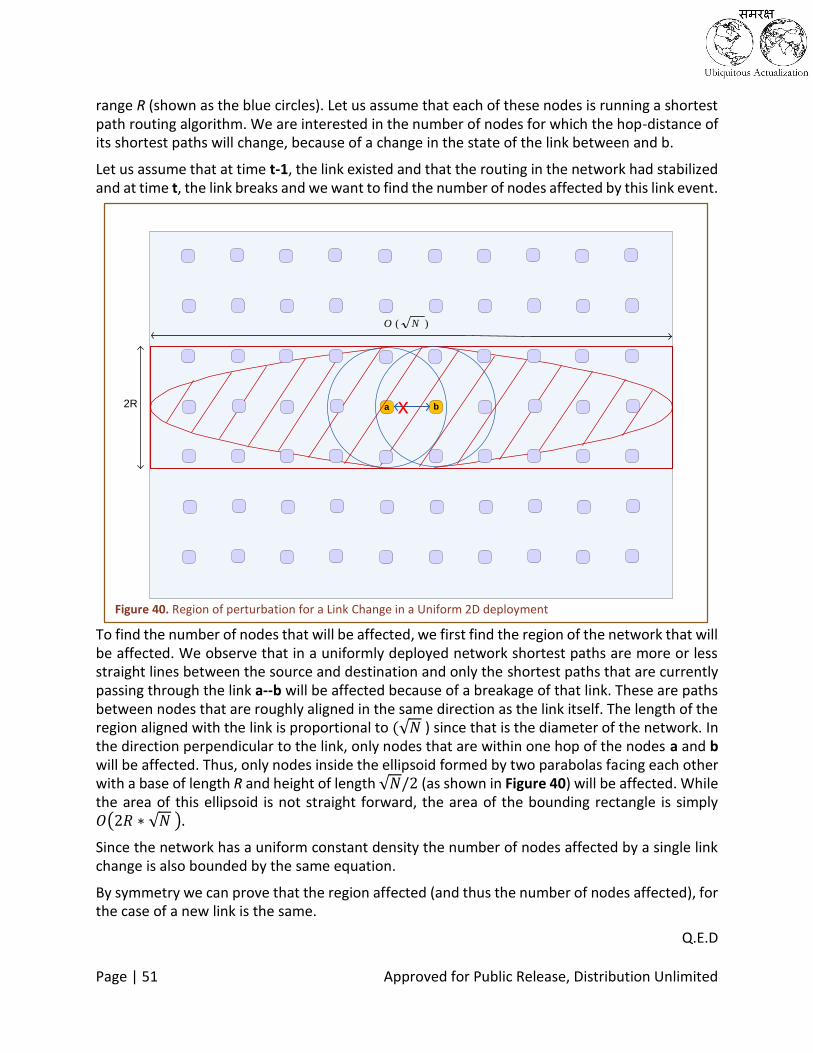
Page | 51 Approved for Public Release, Distribution Unlimited
range R (shown as the blue circles). Let us assume that each of these nodes is running a shortest path routing algorithm. We are interested in the number of nodes for which the hop-distance of its shortest paths will change, because of a change in the state of the link between and b.
Let us assume that at time t-1, the link existed and that the routing in the network had stabilized and at time t, the link breaks and we want to find the number of nodes affected by this link event.
To find the number of nodes that will be affected, we first find the region of the network that will be affected. We observe that in a uniformly deployed network shortest paths are more or less straight lines between the source and destination and only the shortest paths that are currently passing through the link a--b will be affected because of a breakage of that link. These are paths between nodes that are roughly aligned in the same direction as the link itself. The length of the region aligned with the link is proportional to (√𝑁 ) since that is the diameter of the network. In the direction perpendicular to the link, only nodes that are within one hop of the nodes a and b will be affected. Thus, only nodes inside the ellipsoid formed by two parabolas facing each other with a base of length R and height of length √𝑁/2 (as shown in Figure 40) will be affected. While the area of this ellipsoid is not straight forward, the area of the bounding rectangle is simply 𝑂(2𝑅 ∗ √𝑁 ).
Since the network has a uniform constant density the number of nodes affected by a single link change is also bounded by the same equation.
By symmetry we can prove that the region affected (and thus the number of nodes affected), for the case of a new link is the same.
Q.E.D
xa b
)( NO
2R
Figure 40. Region of perturbation for a Link Change in a Uniform 2D deployment

Page | 52 Approved for Public Release, Distribution Unlimited
Corollary 1: In a wireless network with N nodes in uniform geometric deployment and with each node knowing its set of shortest paths, when the state of a single link changes in the network, the new set of shortest paths for all nodes in the network can be computed using O(4 Log(N) ∗ R ∗√N ) bits of routing overhead.
Proof Outline: In a network with N nodes, a single node can be represented in log(N) bits and therefore a link between two nodes can be represented in 2*log(N) bits. Now from Theorem 1, to compute a new set of paths, only 𝑂(2𝑅 ∗ √𝑁 ) nodes need to be updated. Moreover these nodes lie within a contiguous geographic region. Thus it suffices and is possible to send infor-mation about the link state change to only these 𝑂(2𝑅 ∗ √𝑁 ) nodes affected. By sending the new link state of 2 𝐿𝑜𝑔(𝑁) bits to only the nodes in the affected region, it is possible to compute the new shortest paths using only 𝑂(4 Log(𝑁) ∗ 𝑅 ∗ √𝑁 ) bits of overhead.
Q.E.D
Routing Overhead in Probabilistic Uniformly Dense Network
MANET nodes are typically deployed in a non-uniform manner and allowed to move continually. The resultant node spatial deployment is probabilistic, and in this section we will consider the routing overhead under a probabilistic distribution of nodes. For simplicity, we will consider a uniformly random placement of nodes in a 2D plane. However, the results presented in this sec-tion will be similar for any random probabilistic placement.
Varying Node Degrees
A distance based graph formed by a uniform random deployment tends to have a non-uniform connectivity. That is, the number of neighbors that each node has varies quite a bit. Figure 41 shows an example of such a network. The distribution of the node degree in such networks ap-proximates a Gaussian distribution as shown in Fig-ure 42 (for a 1000 node network with average de-gree of 20). The result of such a varying node degree is that the graph has regions of high connectivity and re-gions of low connectivity. This means that not all links are of the same importance for connectivity in the net-work. In regions of high connectivity a link breakage is less costly than in regions of low connectivity.
Figure 41. A Random distance-based 100 Node graph generated by uni-form random placement in a 2D plane

Page | 53 Approved for Public Release, Distribution Unlimited
Edge Betweenness
In graph theory one of the ways this is quantified is by a centrality measure called as the Edge Betweenness. Edge Between-ness is defined as the number times an edge occurs in the shortest path between two nodes of the network. The Between-ness measure is important because it gives the number of nodes that will be affected by a change in the state of that edge in a probabilistic graph.
Estimation of Routing Overhead in Probabilistic Networks
It is non-trivial to get a closed form equation for Edge Betweenness of random graphs. Here we study the cost of changing a single link in the network by simulations, by implementing our NK-LSR algorithm in Matlab. In the simulations, random graphs based on distances between uni-formly random 2D placements of nodes where generated for different network size N and different average node degree M. For each such graph, a sequence of link change events is gen-erated and its effect on the shortest paths studied. To generate a link change, a random link between nodes a and b, which are within the maximum communication distance, is selected and
Figure 43. Message Cost vs Link Error Events
Figure 42. Distribution of Node Degree in a random 2D graph

Page | 54 Approved for Public Release, Distribution Unlimited
its state is reversed. To measure the cost of the link change, first the link change is propagated to all neighbors of a and b. If any of their shortest paths change, they in turn propagate the change to all of their neighbors. The count of all of the nodes which receive a link change is meas-ured as a percentage of the number of nodes in the network and plotted for a sequence of events. The results of the simulation are shown in Figure 43 for networks of various scale, but with similar average degree of 7. As we can see from the result while most of the link changes is propagated only to a small percentage of the network, there are certain link changes which propagate to a large percentage of the network, some even to the whole network.
The Bridge Effect
The phenomenon we see in Figure 43 is due to the non-uniformity of con-nectivity due to varying densities and node degree in the network. Because of this non-uniformity some of the links are more important to the net-work connectivity and hence is part of a large number of shortest paths in the network and hence a change in them will affect a large number of nodes in the network. These links serve a pur-pose similar to that of bridges in a city. In a city a bridge that connects two sides of a river is likely to be part of any route between two points on either side of the river, while roads on the same side of the river are less important. Figure 44 illustrates this point. In reality the instantaneous networks formed by mobile nodes in a MANET are more like a group of islands linked together by a few key bridge links, which are very critical for con-nectivity.
Figure 44. Bridges are very important for overland connectiv-ity.
Figure 45. Histogram of Cost Networks of Size 100 and 500 and M=7
0 10 20 30 40 50 60 70 80 90 1000
100
200
300
400
500
600
700
0 50 100 150 200 250 300 350 400 450 5000
100
200
300
400
500
600

Page | 55 Approved for Public Release, Distribution Unlimited
Plotting the histogram of the cost of the simulations makes this clear. Figure 45 shows the distri-bution of cost for two different network sizes of 100 and 500 and an average neighbor size of 7. The figures show that the distribution is in fact a heavy-tailed distribution, and likely to be a power law. While many values fall below 𝑀2, the cost does not tail off and the tail continues to be of the same size as that of the network, implying that there are at least a few links that affect the entire network.
Growth of the Message Cost with Network Size
The implication of this result is twofold: (1) Since the cost of fixing a single link change in the probabilistic network has a heavy tailed distribution, it is not easy to quantify the cost just using the mean of the distribution. The exact nature of the distribution and the tail need to quantified in order to understand its implications on overhead. (2) Since the heavy tail result from the con-nectivity pattern of the graph, which in turn is affected by the type of node distribution induced by mobility, the node distribution pattern also needs to be understood better to completely quantify the results.
The good news, however, is that the average of the cost is once again in the range of √𝑁 and is very far away from the N, which would be the cost of a complete network broadcast as in a tra-ditional link state routing algorithm.
Table 3 shows the average cost from the simulation as the size of the network increases for the NK-LSR Matlab simulations. The table shows the simulation cost in column 3, and the expected average cost if √𝑁 nodes are affected by each link change in column 4 and the expected average cost if (𝐿𝑜𝑔(𝑁) ∗ √𝑁) nodes are affected. We can see from the table that simulations results are slightly higher than √𝑁, but very much in the same order. This confirms our intuition from the uniform geometric deployment results.
Need-to-Know Link State Protocol
In the previous sections we provided the overview and the intuition for our new routing algo-rithm. Here we describe in detail the actual design of the routing algorithm.
The algorithm exploits the intuition that a node that is far away from a link change is most prob-ably not going to be affected by the change. But instead of limiting the updates arbitrarily in
Table 3. Simulation Cost and Expected Cost
Net-work Size (N)
Ave Neigh-borhood Size (M)
Simulation Cost (% of nodes up-dated)
Expected Cost for 𝑂(√𝑁)
(% of nodes updated)
Expected Cost for
𝑂(𝐿𝑜𝑔(𝑁) ∗ √𝑁)
(% of nodes up-dated)
100 6.8 13.26 10 20
500 7.18 7.37 4.47 12.07
1000 7.17 6.68 3.16 9.48
Page | 56 Approved for Public Release, Distribution Unlimited
space and time as some of the previous LSR algorithms [38], the NK-LSR algorithm finds nodes that are affected by the link change and propagates the changes up to nodes one hop away from the nodes that are affected. Also NK-LSR reverts to the original principle of generating event-based updates in LSR.
Neighbor Discovery
We assume a neighborhood service lets each node detect new nodes in its neighborhood or nodes that are no longer in its neighborhood. This is usually accomplished by a broadcast based heartbeat message sent at some periodic interval, but any discovery mechanism should suffice.
Link State Updates
When a node detects that one or more of its neighbors are no longer linked to it, it sends a Link State Update immediately to all of its neighbors using a broadcast. In contrast, when the node detects that it has a new neighbor, it delays sending the update for α number of periods. The delay is to prevent updates regarding transient links from propagating into the network. Cur-rently we recommend using a value of α=3.
Routing Table Update and Link State Update Propagation
When a node a receives a LSU(c) packet at time t from a neighbor b, about a node c, node a first recomputes its routing table (using the standard shortest path algorithm) with the new infor-mation available in the update. Node a also rebroadcasts LSU(c) but only if the update caused a change in its next hop selection for any destination or if the update made a aware about a new node in the network.
Evaluation and Results
In this section, we present the results of evaluating the NK-LSR protocol in simulation in ns-3. We compare the performance of the NK-LSR with that of a pure Event based link state routing (E-LSR) protocol, where every link update is sent to every node in the network. It must be noted that in terms of network reachability, no other link state protocol can perform better than E-LSR, as long as E-LSR does not exceed capacity (which is the case in our simulations).
Simulation Model We considered a network of N nodes (N=50, 75, 100, 150) with a random initial deployment
in a square area of sides √𝑁 *80m. The nodes move using a Random Waypoint mobility model with velocities between 2-4 m/sec. Communication is based on a constant distance propagation model (unit disk) of radius 180m, since the objective of this simulation is merely to validate our new routing protocol. Using a fixed distance model allows us to estimate the network topology ground truth accurately at any given time. Snapshots of the node locations and their link state tables are taken every 100ms and analyzed. The average neighborhood of each node is approxi-mately equal to 12. The network is observed to be fully connected at all times. Thus the ground truth path reachability is 100%. The number of link changes per second per node is approximately 0.3, irrespective of network size. We analyze the scaling limits for 3 different types of link state routing using simulations in ns-3. (1) The version of link state routing where link state updates are sent periodically by each node, which is referred to here as P-LSR. (2) The version in which link state updates are initiated at a

Page | 57 Approved for Public Release, Distribution Unlimited
node only upon discovery of a neighborhood change (link add/drop) and are forwarded network-wide, which is referred to as E-LSR (event-based). (3) The version where link state updates are initiated at a node only upon discovery of a neighborhood change and are forwarded only if they cause a change in the local routing table, which is NK-LSR.
Metrics Evaluated (1) Percentage of Reachable Paths: The total number of recursively reachable paths in the net-
work is computed using the NK-LSR and E-LSR routing table. The ratio of this number to the total number of ground truth valid paths existing at that time is used to compute this metric.
(2) Message Cost: The total number of Link State Update messages sent in the network (exclud-ing the heartbeat messages used for discovery) during a particular run of the simulation for 100 seconds. Noting that each message could be of different sizes (depending upon the num-ber of link state records sent in each message), we also measure the total number of bits transmitted per second by each node. The size of each link state record in a message is kept at 32 bits.
Evaluation of Reachable Paths
We simulated the three protocols with a 2 Hz discovery rate. For the P-LSR, the network refresh rate is kept at 0.5 Hz. Figure 46 shows the reachability for the three protocols at different net-work sizes.
Evaluation of Message Cost
Figure 47 shows the communication per node incurred by the three protocols. Its shows the cost in terms of messages per second and Figure 48 shows the cost in terms of bits per second.
Figure 46: Average reachability percentage (2 Hz discovery rate)

Page | 58 Approved for Public Release, Distribution Unlimited
From these charts we see that NK-LSR is able to achieve almost the same reachability as P-LSR and E-LSR, at much lower messaging costs. This shows that NK-LSR can scale to a larger number of nodes in comparison with the other two protocols.
The communication cost for E-LSR rises steeply at a scale of 75 nodes. This is because in E-LSR, each event causes a link state packet to be forwarded separately across the network. P-LSR, on the other hand, combines these link state updates in aggregate intervals which are pre-deter-mined. This reduces the cost in comparison with E-LSR, but however the protocol is not reactive to changes in the network. NK-LSR is reactive as well as low in message complexity because of the need-to-know forwarding built into its design.
Figure 48. Communication cost in bits per second per node
Figure 47. Communication cost in message per node per second

Page | 59 Approved for Public Release, Distribution Unlimited
Scalability of NK-LSR To analyze the scalability of NK-LSR, we simulated NK-LSR for network sizes of up to 300 nodes. We see in Figure 46 that reachability for NK-LSR drops to 80% at a heartbeat rate of 2 Hz. For increased heartbeat interval to 0.25 seconds (4 Hz) for networks of 150, 225 and 300 nodes, the average reachability and communication rate are shown in Figure 50 and Figure 49. Figure 49
shows that the communication cost per node in NK-LSR grows as √𝑁.
Pattern Remarks
NK-LSR provides a similar level of connectivity as P-LSR and E-LSR, but using only messages of the order of √𝑁. This implies that NK-LSR scales to a much larger size than the current state of the art routing protocols in MANET. A more through theoretical and simulation evaluation is needed quantify the performance of the algorithm and its many subtle variants. We expect OLSR to have a reachability that is appreciably lower than that of the E-LSR, but at a much lower cost. Hence,
Figure 49. Communication cost in bits per second per node (NK-LSR)
Figure 50. Average reachability % (NK-LSR)

Page | 60 Approved for Public Release, Distribution Unlimited
it is also important to study its performance with OLSR and NK-LSR under same mobility condi-tions. Secondly, the effect of mobility, particularly the rate of change of links, on NK-LSR and in general in a MANET needs to be better understood.
Overall we find that the performance of NK-LSR is superior to any of the existing MANET routing protocols.

Page | 61 Approved for Public Release, Distribution Unlimited
Census
In this Chapter, we focus on the Census, or one-shot aggregate querying, pattern in mobile ad-hoc networks. The objective of Census is to collect information about resources of some type deployed in the network, or to aggregate sensor values, by querying each node in the network, ideally without missing out on any node and without double counting any response. The pattern is designed to work even when the underlying network topology is dynamic and may also be subject to temporary partitioning. Census examples in a military mobile ad-hoc network include counting the available artillery units, ammunition, food, fuel, etc.
A Census query can be sent into the network from any node in the network, to collect some aggregate statistic (such as count, max, sum) of the network nodes. Figure 51 illustrates the sequence of steps involved in a single Census operation. The query specifies a ‘Resource Type’ that is counted. The query is propagated in to the network and the aggregate counts are collected on few nodes. These nodes then send the aggregate counts to the FOB using the long link. The FOB forwards these results to the initiating node again through the long link.
The Census pattern utilizes a token-based counting ap-proach, where only the most recent aggregate information is carried in each token message. When a query is issued from a node, a predetermined number of tokens are initiated in the network to compute the cen-sus. The time to complete the query (the convergence time) depends on the number of to-kens initiated. Tokens are iteratively passed to individual nodes in the network until all nodes have been ‘visited’ and their information has been included into the aggregate count carried by the token. To avoid duplicate counting and at the same time reduce the size of each message, the information about inclusion in the aggregate is stored locally within each node instead on the token. By doing so, each node is able to contribute towards the aggregate exactly once. Once all (or a desired set of nodes) of nodes have been covered, the tokens are exfiltrated using the long link.
For such a query -- which needs to visit every node in order to gather the statistics -- the cost of implementing and the time taken to finish the query are very important. The Census operation on a network with N nodes finishes in O(√𝑁) time and its message cost is proportional to N.
Forward
Operating
Base
T1: Node Initiates Census
T2: Aggregate
values collected at
some of the nodes
T3: Aggregate values
are sent to the FOB
through Long Link
T4: FOB sends the final
count to initiating node
through Long Link
Figure 51. Illustration of the steps involved in a Census operation

Page | 62 Approved for Public Release, Distribution Unlimited
Background: One-Shot Aggregate Querying Tree-based: One-shot querying has been well studied in the context of static, wireless sensor networks, In-network aggregation techniques using spanning trees have been shown to be effi-cient and reliable solutions for the problem [39] [40]. However, in the context of a mobile network, a spanning tree structure is likely to be unstable and could potentially incur a high com-munication overhead for maintenance.
Flooding and diffusion: In complete contrast to a tree-based approach is the unstructured flood-ing based technique in which data from every node is disseminated to every other node. The messaging cost of this solution is high: O(N2), where N is the number of nodes in the network. To reduce this cost, flooding of individual data can be avoided by opportunistically aggregating in-formation before rebroadcasting, and thus essentially diffusing the aggregate information across the network. The hurdle in doing so is that the knowledge of nodes whose information has al-ready been included in the aggregate is needed so as to avoid duplicate counting. This hurdle can potentially be overcome by explicitly including the data from each node in every message as op-posed to only sending the aggregate message. Although the number of messages are reduced in this diffusion based approach, the size of each message is now O(N). Still, we note that the diffu-sion based approach has the property of quick convergence (if the network is connected, the aggregation will complete in O(D) time where D is the diameter of the network).
Relation to random walks: Our proposed approach utilizes a random walk construct on the to-kens to cover the network – however, there are two differences in the proposed approach in comparison to traditional random walks. Firstly, if there are one or more unvisited nodes in the neighborhood of a node that has a token, the token is passed to one of the unvisited nodes picked at random. By contrast, in a canonical random walk, the next node is randomly selected amongst all neighbors. Secondly, when all nodes in the communication range have been visited but there are still unvisited nodes in the network, a gradient is used to pull the token towards unvisited nodes. Thus, the underlying random walk is complemented by a gradient based biasing mecha-nism to avoid potentially unbounded circulation among already visited nodes. With the proposed
biased random walk solution, we observe a convergence time of O(√𝑁) when √𝑁 tokens are used and O(N) when log2(N) tokens are used.
Results on random walks: The biasing of the random walk enables reduction in convergence time as well as messages in comparison to an unbiased pure random walk. The following is a summary of some known bounds on random walks.
(1) It has been shown that the expected cover time (and messages) for a random walk for general graphs with bounded degree is O(N3) and for regular graphs is O(N2) [41, 42, 43]. A speed-up by a factor of k has been shown when k independent random walks are uti-lized in the graph [44]
(2) For random regular graphs, the expected cover time with a single random walk is O(N2) and a speed up by a factor of k can be obtained when k independent random walks are utilized [45] [46]. Note that random regular graphs are those in which the nodes have uniform degree and the set of neighbors are chosen independently for each node from the set of all nodes. However, we note that the flat radio networks being considered in this project cannot be modeled as random regular graphs.

Page | 63 Approved for Public Release, Distribution Unlimited
(3) Of relevance to wireless ad-hoc networks is a study of random walks on random geomet-ric graphs in which nodes are placed uniformly on a unit square and two nodes are connected if and only if their Euclidean distance is less than r. It is shown in [47] that if the communication radius is greater than a certain threshold, then the expected cover time is O(N*log(N)). Specifically, the critical communication radius proven in [47], trans-lates to a node degree of the order of θ(8*log(N)).
(4) A recent experimental study on random walks considered a form of choice, in which the next vertex to move is chosen randomly from a set of unvisited vertices neighboring the current vertex, if any are available, and from a set of visited nodes, only if no unvisited vertices are neighboring the current vertex. This study points to improved cover time when choice is exploited in a random walk [48].
(5) We note also that the expected cover time for random walks has been studied mostly for static networks, cover times in time-varying graphs (relevant for mobile networks) have not been explicitly characterized to the best of our knowledge.
Census Protocol
Overview of the Protocol In Census, data aggregation is performed using token passing. A token acts as a mobile register that is used to gather census from the nodes in the network. A node that currently holds a token includes its information into the aggregate value stored in the token. The token is then passed successively to the other nodes in the network. Thus, at any time t, the value stored in a token is the aggregate computed over all nodes visited by the token until that time. There can be multiple tokens used in the census computation. However, each token is assumed to have a unique iden-tifier and each node can add its information into only one token. Figure 52 illustrates the working of the protocol.
Census consists of three tasks: (1) token creation, which initiating the tokens in the network; (2) token passing, which dic-tates which neighbor should get the token next; and (3) gradient setup, which biases the flow of tokens towards regions of the network with unvisited nodes. We describe each of these components in de-tail in the following subsections. To accomplish these tasks, each node stores three variables: visited, holder and level. visited is a boolean which keeps track of whether a node’s data has been included in the aggregate value stored in a token. Initially, visited=0 at all nodes. When a to-
ken first arrives at a node, visited is set to 1. All nodes in which a token is initiated are marked as visited by default and the token value is initialized to the data at the corresponding node. holder is used to identify nodes that currently hold a token. Each node also participates in a
Figure 52. Census uses tokens for data ex-filtration by visiting each node. From each node, a token moves to an unvisited node if available and aggre-gates data from that node

Page | 64 Approved for Public Release, Distribution Unlimited
gradient setup process to attract tokens towards unvisited nodes. To do so, each node uses the state variable level, where 0 ≤ level ≤ 1. Nodes that are unvisited are at level=1. Nodes that hold a token set level to 0 when they receive a token.
Token Creation Creation of tokens in the network can be done in many ways. We describe one method here. By default, the initiating node creates a token for itself. The request for performing a census is then flooded across the network. Upon receiving a new request for census, each node probabilistically creates a new token. Thus, a minimum of one token exists in the network (created by the root). In addition, if the probability of creating a token is set to p, the expected number of tokens cre-ated in the network is 1+pN where N is the number of nodes that receive a token. Moreover, it is expected that the tokens will be distributed uniformly across the network or the partition of the network that receives the initial flood.
Token Passing To accumulate information in a token, the token has to be propagated to other nodes in the network. This is done as follows. Nodes that currently possess a token add their information into the token and announce the token. A timer Tr is started to accept requests for the token. All nodes with level>0 randomize their response time and accordingly respond to the token an-nouncement along with their current level. Nodes with level>0 are nodes that have either not been visited (level=1) or nodes that have been visited and are now part of a gradient (0 < level < 1). The token holder stores all requests received during time Tr. The replies are sorted based on the level of the requestors and the token is sent to the node with the highest level. When multiple requestors exist with the same level, the token recipient is chosen randomly among that set. Thus if an unvisited node requests a token, the token will be sent to that node. If all nodes that have currently requested the token have been visited, the token is sent to the node with the highest value of level, which is expected to be the node that is closest to an unvisited node. As soon as a token reply has been sent, the node resets holder to 0.
Token Checkpoints and Reliable Token Transfer Reliable token transfer is critical for successful operation. If a token is released by a node, but the intended recipient does not receive the token reply message, the aggregate value computed thus far by the token could be lost. At the same time, if the sending node relies on acknowledgements to release a token, it is possible that the acknowledgement is lost and duplicate tokens are cre-ated. To address this issue, Census uses acknowledgments in conjunction with checkpoints. As soon as a token reply is sent, the sender releases the token (the node resets holder to zero). At the same time, it remains in a wait state for acknowledgements from the recipient. If an acknowl-edgement is not received within a time Ta, the token send message is repeated up to a maximum of K times. If the recipient receives the token multiple times, it simply repeats the acknowledge-ment message. However, if the token sender does not receive the acknowledgement even after K retries, it creates a checkpoint for the token, i.e., the aggregate computed thus far is exfiltrated using the long link along with the token id. It is possible that the token was actually successfully passed, but even in this case the checkpoint will not create duplicate counting. At the same time, the process ensures that data is not lost.

Page | 65 Approved for Public Release, Distribution Unlimited
Gradient Setup During the Census operation a token can be stuck inside a region where all its neighbors have already been visited. To recover from such a scenario, a gradient is setup in the network to attract tokens towards unvisited nodes, i.e., nodes with level=1. This is realized as follows. For nodes with level=1 none of whose neighbors currently hold a token and that have at least one neighboring node with level=0, a gradient setup is initiated by broadcasting a gradient message. Nodes with level=1 learn about neighbors that have level=0 through an underlying beacon mechanism. Nodes with level=0 that receive a gradient message update their level to one half of sender’s level and rebroadcast the gradient message. Thus, gradient broadcasts propagate only till the region where nodes with non-zero level are present, filling up the gap between a unvisited node and other nodes with non-zero levels. Figure 53 illustrates the gradient setup process.
Gradient Refresh To account for node mobility, gradients have to be periodically refreshed. To do so, when a node updates its level from zero to some non-zero value less than 1, it starts a timer proportionate to the new level and when the timer expires it resets its level back to 0. Thus nodes with higher values of level are refreshed slower than nodes with smaller values. This heuristic is based on two reasons. (1) Gradients should preferably not be refreshed before a token is able to climb up a gradient and reach an unvisited node. By refreshing at a rate proportionate to the value of level, a token gets more time to reach closer to the source of the gradient. (2) Nodes that are far away from an unvisited node (i.e., that are closer to the bottom of the gradient) should prevent block-ing of gradient setup from unvisited nodes that are nearby, for extended periods of time.
Termination Note that when all nodes have been visited, the gradient setup will be terminated because the gradient setup is only initiated by nodes that have not been visited. When nodes holding the token get a level 0 reply from all their neighbors for its token announcement broadcast, the holder nodes conclude that all nodes in the network have been visited and they send the aggre-gate information to the initiator node through the Long Link.
Census Analytical Bounds
In this section, we quantify the expected bounds on convergence time and message complexity for Census for scenarios with √𝑁 tokens and log(N) tokens. We state these bounds for mobile, connected networks and, in the following section, we simulate the performance in networks which suffer from temporary disconnections.
Figure 53. During token passing phase, the token may be surrounded by an island of visited nodes, i.e., all neighboring nodes have already been visited. Nodes that have not yet been visited set up a gradi-ent using the set of visited nodes and attract the token towards them

Page | 66 Approved for Public Release, Distribution Unlimited
Theorem 1: The expected convergence time for Census in a connected, mobile network of N nodes with √N tokens is O(N3/4), and with log(N) tokens is O(N/log(N)).
Proof Outline: In a network with √𝑁 tokens, on average, each token is responsible for aggregat-
ing information from O(√𝑁) nodes and these nodes are deployed over a region of expected diameter O(N1/4). Assume that after counting each node in this region, the token travels a worst case distance of O(N1/4). In this case, the expected convergence time for Census in a connected,
mobile network of N nodes with √𝑁 tokens is bounded by O(N3/4).
Theorem 2: The expected convergence time for Census in a connected, mobile network of N nodes with log(N) tokens is O(N/log(N)).
Proof Outline: In a network with log(N) tokens, on average, each token is responsible for aggre-gating information from O(N/log(N)) nodes and these nodes are deployed over a region of expected diameter O((N/log(N))1/2). Assume that after counting each node in this region, the token travels a worst case distance of O((N/log(N))1/2). In this case, the expected convergence time for Census in a connected, mobile network of N nodes with log(N) tokens is bounded by O((N/log(N))3/2) Note that the above results assume the network to be connected. When temporary disconnec-tions are possible, and this occurs continuously, a long tail is possible during counting. Hence, in the simulation results with a random waypoint mobility model, we compute the expected time for 95% convergence. Our experimental results indicate that the 95% convergence times in the simulated networks are lower than the bounds stated above.
Theorem 3: The expected number of gradient messages for Census in a connected, mobile net-work of N nodes with √N tokens is O(N1.25).
Proof Outline: In a network with √𝑁 tokens, the expected length of a gradient emanating from a node is O(N1/4). If all nodes are involved in setting up a gradient, the expected number of gra-dient messages is O(N1.25).
Theorem 4: The expected number of gradient messages for Census in a connected, mobile net-work of N nodes with log(N) tokens is O(N1.5/(log(N))0.5).
Proof Outline: In a network with log(N) tokens, the expected length of a gradient emanating from a node is O((N/log(N))1/2). If all nodes are involved in setting up a gradient, the expected number of gradient messages is O(N1.5/(log(N))0.5).
Census APIs
When the Census Pattern is instantiated on a node, it provides the following APIs through which the application can interact with the pattern:(a) StartCensus, (b) NodeValue, and (c) CensusRe-sults.
StartCensus API:
bool StartCensus (int SourceNodeID, int QueryNumber, Enum ResourceType)

Page | 67 Approved for Public Release, Distribution Unlimited
The StartCensus function call allows a node to initiate a new census in the network. An applica-tion on a node calls the StartCensus API, with the following parameters: (i) SourceNodeID: the ID of the node that is initiating the census so that FOB can return the results to the node. (ii) QueryNumber: A sequence number so that the current Census query can be differentiated from the previous ones. And (iii) ResourceType: This parameter specifies the type of resource that is being counted by the query. This can be a one of a number of predefined resources. The call returns ‘true’ if a new query is initiated successfully, else it returns ‘false’.
NodeValue Callback:
NodeValue is a callback that needs to be implemented by the application that is called by the Census pattern. The callback is provided so that the application can contribute a value to the aggregate that the census pattern is calculating. This API provides information about the origin of the Census, the query number and the resource type parameters, so that the node receiving the query can make a decision about the value. The callback has a Value pointer of type double, which can be set by the application. On returning from the callback the individual Value contrib-uted by the node will be aggregated with the ‘aggregate value’ carried in the token.
CensusResult Callback:
CensusResult is a callback that needs to be implemented by the application that is called by the Census pattern. The function is called when the result of a Census query is returned by the FOB through the Long Link to the node initiating the Census. The API has the query number and the resource type parameters, along with the ‘Result’ provided as a double and a ‘NodeCount’ which gives the number of nodes over which this particular aggregate result has been calculated. The pattern has a built-in mechanism to detect termination of the census and when one or more nodes with a token detect termination, the nodes send the aggregate values to the FOB through the Long Link and the FOB in turn forwards these results to the node initiating the query. It is possible that the CensusResult API is called multiple times, i.e., each time a node with one of the tokens sends a partial result through the FOB.
Performance Evaluation In this section we validate the performance of the Census pattern realization via ns-3 simulations. We simulated for different network scales, from 125 nodes to 5000 nodes, and measured the convergence time to cover 95% of the nodes and network overhead (number of packets sent on the wireless channel). Node mobility was controlled using a random waypoint mobility model with a node speed ranging from 2-4 m/s. A log propagation fading model is used to simulate the wireless channel. We present two sets of results, with varying number of tokens used in the Cen-sus pattern, to show how the convergence and overhead vary with tokens. In the first set of
simulations we use √𝑁 tokens and in the second set we use 2*log2(N) tokens, where N is the
void CensusResult (int QueryNumber, Enum ResourceType, double Result, int
NodeCount)
void NodeValue (int SourceNodeID, int QueryNumber, Enum ResourceType,
double *Value)

Page | 68 Approved for Public Release, Distribution Unlimited
network size. Finally we evaluate the impact of number of tokens ranging from 2 to √𝑁, on the convergence time.
Results for √𝑵 Tokens
In this section, we quantify the performance with √𝑁 tokens. We consider networks of sizes: 125, 250, 500, 1000, 2000, 3000, 4000, and 5000. The corresponding numbers of tokens used in the system are 11, 16, 22, 32, 45, 54, 63 and 71 respectively.
Figure 54 shows the 95% convergence time as a function of the number of nodes. The trend-line shows that the bounds are below the analytical bounds determined in Section 0. Figure 55 shows the gradient setup messages and token messages as a function of the number of nodes. Note that token messages include token transfers, requests and announcements.
Figure 54. Average time to achieve 95% convergence (Trend-line computed by MS Excel)
y = 5.9804x0.4208
0
50
100
150
200
250
0 1000 2000 3000 4000 5000
Tim
e (
seco
nd
s)
Number of nodes
95% ConvergenceTime
Power (95%Convergence Time)

Page | 69 Approved for Public Release, Distribution Unlimited
In Figure 56 and Figure 57, we show the convergence pattern and the growth of gradient setup messages as a function of time for one specific network size, i.e., 4000 nodes and 62 tokens.
Figure 55. Average messages until 95% convergence. Token messages include token an-nouncement, requests and token passing.
0
10000
20000
30000
40000
50000
60000
0 1000 2000 3000 4000 5000
Mes
sage
s
Number of nodes
Gradient messages
Token messages
Linear (Gradient messages)
Linear (Token messages)
Figure 56. Convergence pattern for 3 different runs at 4000 nodes with 62 tokens
0
20
40
60
80
100
120
0 100 200 300 400 500
Co
nve
rgen
ce %
Time (seconds)
Convergence pattern (4000 nodes; 62 tokens)
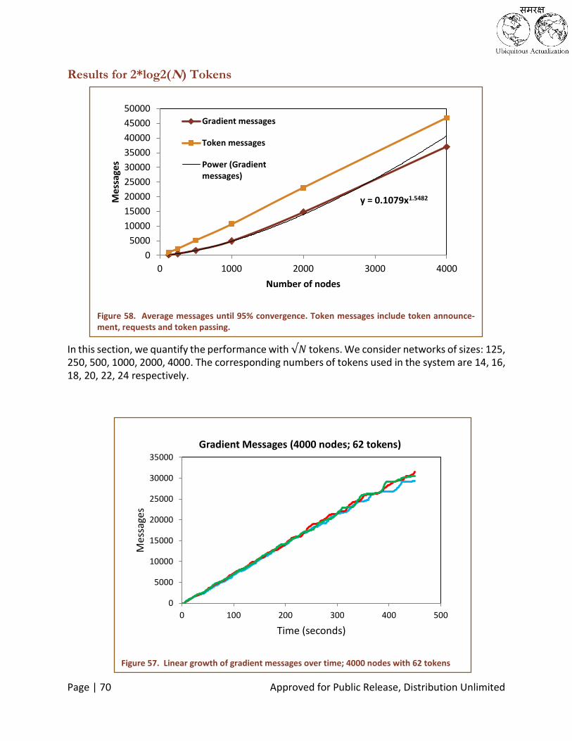
Page | 70 Approved for Public Release, Distribution Unlimited
Results for 2*log2(N) Tokens
In this section, we quantify the performance with √𝑁 tokens. We consider networks of sizes: 125, 250, 500, 1000, 2000, 4000. The corresponding numbers of tokens used in the system are 14, 16, 18, 20, 22, 24 respectively.
Figure 57. Linear growth of gradient messages over time; 4000 nodes with 62 tokens
0
5000
10000
15000
20000
25000
30000
35000
0 100 200 300 400 500
Mes
sage
s
Time (seconds)
Gradient Messages (4000 nodes; 62 tokens)
Figure 58. Average messages until 95% convergence. Token messages include token announce-ment, requests and token passing.
y = 0.1079x1.5482
0
5000
10000
15000
20000
25000
30000
35000
40000
45000
50000
0 1000 2000 3000 4000
Mes
sage
s
Number of nodes
Gradient messages
Token messages
Power (Gradientmessages)

Page | 71 Approved for Public Release, Distribution Unlimited
Figure 59 shows the 95% convergence time as a function of the number of nodes. The trend-line shows that the bounds are less than the analytical bounds determined previously. Figure 58 shows the gradient setup messages and token messages as a function of the number of nodes. Note that token messages include token transfers, requests and announcements.
In Figure 61 and Figure 60, we show the convergence pattern and the growth of gradient setup messages as a function of time for one specific network size, i.e., 4000 nodes and 24 tokens.
Figure 59. Average time to achieve 95% convergence (Trend-line computed by MS Excel)
0
100
200
300
400
500
600
700
0 1000 2000 3000 4000
Tim
e (
seco
nd
s)
Number of nodes
95% ConvergenceTime
Linear (95%Convergence Time)
Figure 60. Growth of gradient messages over time; 4000 nodes with 24 tokens
-5000
0
5000
10000
15000
20000
25000
30000
35000
40000
45000
0 100 200 300 400 500 600
Mes
sage
s
Time (seconds)
Gradient messages (4000 nodes; 24 tokens)

Page | 72 Approved for Public Release, Distribution Unlimited
Impact of Number of Tokens on Convergence Here we show impact of number of tokens on convergence time and messages. Figure 62 shows the impact of number of tokens on gradient setup messages and token related messages. Figure 63 displays the impact of number of tokens on convergence time for network size of 250 nodes.
Figure 61. Convergence pattern for 3 different runs at 4000 nodes with 24 tokens
0
10
20
30
40
50
60
70
80
90
100
0 100 200 300 400 500 600
Co
nve
rgen
ce %
Time (seconds)
Convergence pattern (4000 nodes; 24 tokens)
Figure 62. Impact of number of tokens on messages until 95% convergence. N = 250
y = 9561x-1
0
1000
2000
3000
4000
5000
6000
0 2 4 6 8 10 12 14 16
Mes
sage
s
Number of tokens
Gradient messages
Token messages
Power (Gradient messages)
Linear (Token messages)

Page | 73 Approved for Public Release, Distribution Unlimited
Figure 64 displays the impact of number of tokens on convergence time for network size of 250 nodes. Figure 65 shows the impact of number of tokens on gradient setup messages and token related messages.
Figure 63. Impact of number of tokens on 95% convergence time. N= 250
y = 619.59x-0.835
0
50
100
150
200
250
300
350
400
0 2 4 6 8 10 12 14 16
Tim
e (
seco
nd
s)
Number of tokens
95% ConvergenceTime
Power (95%Convergence Time)
Figure 64. Impact of number of tokens on 95% convergence time. N= 500
y = 1540.5x-0.973
0
50
100
150
200
250
300
4 6 8 10 12 14 16 18 20 22
Tim
e (
seco
nd
s)
Number of nodes
95% Convergence Time

Page | 74 Approved for Public Release, Distribution Unlimited
Pattern Remarks The proposed Census pattern has an observed convergence time of approximately O(√𝑁) when
√𝑁 tokens are used and O(N) when 2*log2(N) tokens are used. The number of token messages grows linearly with number of nodes in both cases. The number of gradient messages grows lin-
early when √𝑁 tokens are used and grow as O(N√𝑁) when log2(N) tokens are used when. Both convergence time and gradient messages fall proportional to the number of tokens used
Figure 65. Impact of number of tokens on messages until 95% convergence. N = 500
y = 30822x-0.99
0
1000
2000
3000
4000
5000
6000
7000
4 6 8 10 12 14 16 18 20 22
Mes
sage
s
Number of tokens
Gradient messages
Token messages

Page | 75 Approved for Public Release, Distribution Unlimited
Exfiltration
This design is based on the many Tree-Based Exfiltration (TBE) patterns documented in the liter-ature [39, 40]. TBE patterns maintain a spanning tree across the network, which can be traversed to the root in order to accomplish exfiltration. When a link-state changes, the spanning tree is updated quickly and ideally with minimal traffic. The pattern that we present here forms a Span-ning Wave instead of a spanning tree, but exfiltration is accomplished by following the wave back to its origin in a manner that is closely analogous to TBE. The advantage of our Inverse-Wave Based Exfiltration (IWBE) is that the dynamics of maintaining the spanning wave in the presence of link state changes are significantly better.
Background: Tree Based Exfiltration
Figure 66 shows a spanning tree of the type that is used in the classic TBE pattern. Each node maintains a parent that is closer to the root than it. If a node moves so that it loses its parent, then it finds a new parent. In contrast, if a parent loses, it has no obligation with respect to the child node. Finding a new parent can be performed by broadcasting a “cry” to any potential neighbors and then evaluating all offers of adoption. A node that changes its parent need not inform its children, likewise a node that acquires new children need not inform its parent.
The parsimony of classic TBE allows the network to scale aggressively. Firstly, most link state changes have no effect on network. Only link state changes that cause the loss of a parent result in networking changes. And secondly, all link networking changes are resolved by coor-dination within the single-hop neighborhood of one of the nodes involved in the link state change. However, this highly scalable form of the algorithm is never proposed in the litera-ture because:
1. It tends to result in long suboptimal paths.
2. It uses only a small fraction of the po-tential links.
Instead TBE algorithms presented in the litera-ture tends to be significantly more complex that are more optimal for static networks. However, because they are more brittle and “heal” less quickly, in the presence of mobility their scaling is good, but not great.
For our purposes the worst problem with TBE is that whenever a parent is lost there is a mo-ment period when a route is completely
Figure 66. A spanning tree of the type that might be used in TBE.
1
1
1
2
2 2
2
3
33
3
3
4
4
5
5
66
7

Page | 76 Approved for Public Release, Distribution Unlimited
broken. If combined with end-to-end retry then this is expected to be the limit on scaling. Our number one design heuristic is to minimize the time to recover from a link state change. IWBE is expected to be dramatically better with regard to this criterion.
The Inverse-Wave
Figure 67 the shows a wave structure that is analogous to the spanning tree shown in Figure 66. The key difference is that nodes may have many parents. In fact because the parent-child analogy is strained, we will abandon it and instead simply refer to generations. Each extra hop between a node and the root place the node in a younger generation. Every node will divide all of its neighbors into three categories: 1) the older generation, 2) its generation, and 3) the younger generation.
Each node forwards each packet to any one of its elders. In the majority case the loss of a single elder due to a link state change simply causes packets to be routed to one of the other elders. If a node loses its last elder and it suddenly finds itself in the younger generation, it may forward to any of its pervious peers. Only if a node loses its last elder and all of its other neighbors are in the younger generation is the route temporarily broken.
The key advantage of IWBE over TBE is that the vast majority of the time the loss of a link state change results in a zero delay repair to the routing service. Link state changes will somewhat regularly cause some of the routes to be momentarily suboptimal. Only a very rare link state change will cause a route to be wrong.
In the next section we will attempt to design the details of the algorithm so that recovery from these rare problems is also handled. The hope is that this will ensure that even at very large scales the amount of traffic taken of-fline by actual routing errors will remain small.
The Algorithm
Link Quality Metric
The neighbor discover-protocol is assumed to provide link quality estimation for every link, denoted at the Link Quality Metric (LQM).
If the discovery protocol knows little or nothing about the link quality it may restrict the values of the LQM to 0 for no link and 1 for a link. More generally the LQM would be a fuzzy number between 0 and 1. The simplest case is likely that the LQM would be an estimate of the probability that a new packet would successfully traverse the link. In more elaborate cases, the probability of
Figure 67. The wave structure used in our algorithm.
1
1
1
2
2
2
3
3
3
4
5 5
6
1
2
2
34
4

Page | 77 Approved for Public Release, Distribution Unlimited
packet success might be adjusted to reduce hot spots or based on the life expectancy of the link.
Choosing an Elder
A node will choose the elder to send a particular packet to by making a completely random choice weighted by the LQM.
Mathematically, assume an ordered list of em neighbors that are elders, each with an LQM of iq
. We will further define the quality density of elders as
1
0
em
i
ie q .
We will also define the cumulative quality sum (analogous to a Cumulative Distribution Func-tion (CDF)) as
k
i
iqk0
)( ,
and the inverse cumulative quality sum as:
)1()(,)(1 kandkk
Then the choice of elder will be k erand 1 .
Link State Changes and Generation Management
Whenever a new neighbor is discovered, the nodes should exchange generations.
If the new neighbor is more than one generation above the node’s current generation, then the node should promote itself to the generation one below its new neighbor.
When a node is promoted to a higher generation, it should exchange generational information with any neighbor that it believes to be more than one generation below its new level. This exchange of generational information shall be lower priority than regular traffic and shall be de-layed by a specified amount (i.e., per hop).
When a connection to an elder is lost, the node should check to see if the reduced value of e has fallen below some threshold. If it has, then it must regress to a generation one below the highest generation for which it has a sufficient quality density.
Whenever a node regresses, it should exchange generational information with all of its new el-ders, in order to ensure that regressions that it doesn’t yet know about have not created a false sense of connection to the root. This exchange of generational information initiated shall be higher priority than regular traffic.
If a node’s generation falls below some threshold, it shall be considered infinitely removed from the root. The exchange of generational information initiated from a node that is infinity removed from the root or sent to a node that is believed to be infinity removed from the root shall be higher priority than regular traffic.
Retries
Each hop is to be acknowledged. If a packet is not acknowledged it is to be retried. However, every retry should randomly re-choose which elder to contact.

Page | 78 Approved for Public Release, Distribution Unlimited
If a packet fails a certain number of times on the same link, then that link shall be considered temporarily down and retries shall continue on any remaining links. If this results in e falling below the specified threshold, then the node shall be considered temporarily disconnected from the higher generation.
However, temporary disconnection shall not be considered the same as an actual link state change. A node that is temporarily disconnected from its elders shall delay a specified amount of time and try again.
Partitioning
In this section we consider what happens when a portion of the network becomes disconnected from the root. When the last connected node loses its last elder, it will regress to a lower gener-ation. This will cause it to exchange generational information with its neighbors, in turn causing them to regress to a lower generation. The chain reaction will rapidly regress the entire discon-nected region beyond the limit at which the entire region is considered disconnected.
Later when the first node is connected to an outside node, the disconnected region will rapidly reorganize itself to exfiltrate through this node.
While the region is disconnected, we expect that there is minimal advantage to routing packets to the last known best exfiltration point only to have them forwarded from that point via the long link.
Bailing Out from Byzantine Behavior
Figure 68 illustrates that any situation in which a node could lose contact with all of its elders might loosely be described as a bottleneck. In this situation the change of the state could have a significant propagation affect to the rest of the network. If the bottleneck is intermittent it could drive thrashing throughout the network.
In general it’s possible to construct a clever adversary that result in nodes that are delayed a long time. In this case we wish to bail out and use the long link.
If a packet has traversed more than some number of hops, it should be forwarded via the long link directly to the root.
A node that has been in the network for longer than a specified du-ration shall be forwarded directly to the root via the long link.
Discovery
The pattern assumes the availability of a discovery service similar to the one outlined in Chapter 3.
Parameters
Maximum Hop Count: If a single packet travels this many hops it shall be
concluded to be in some sort of Byzantine problem.
Maximum Single Link Retry: If a packet attempts to traverse a single link
this many times it shall be considered that the link temporarily down.
Figure 68. Bottlenecks are the only scenario in which a node can lose contact with its elders.
n
n-1
n+1
n-2
n-2
n-2
n+1
n+1

Page | 79 Approved for Public Release, Distribution Unlimited
Minimum Elder Quality Density (Regression): The minimum value of e at which the node should be
considered as being connected to the older generation.
Minimum Elder Quality Density (Promotion): The minimum value of e above the node should be con-
sidered to be connected to this generation.
Maximum Connected Generation: If the nodes generation falls below this level it shall be considered to
have fallen out of the wave. It will be treated like it’s disconnected.
Simulation Results
An initial simulation capability for this pattern was constructed using ns-3. All experiments re-ported here were run using ns-3 to implement the network and click to implement the routing protocol. The click code reported the status of each node every half second. The results reported are based on these samplings. As the sampling is independent of the patterns operations, the results show the nodes of the pattern in all the possible configurations. For the results reported below the initial configuration consisted of an 8x8 grid space 100 meters apart with intermediate nodes placed in the centers for a total of 113 nodes. The initial layout is shown in Figure 69.
Figure 69. Starting Node Layout and Root Node Designation

Page | 80 Approved for Public Release, Distribution Unlimited
Small amounts of jitter are added to the central nodes to cause links to form and break. The root has been placed in the lower left corner to maximize the distance to the farthest node and there-fore the corresponding path lengths.
At each half second the simulation yields the following information:
Position of each node.
Set of Elders, Peers and Children node for each node.
Link Quality Measure (LQM) from each node to each of its elders, peers and children.
The single hop LQM value represents an approximate probability that a packet will successfully traverse that link. From these, individual LQM values are used in the following manner to calcu-late multi-hop probabilities of successful traversals. We designate these value "Probability of Reaching Root" or Prr values.
Figure 70. Illustration of How Probability of Reaching Root are Calculated.

Page | 81 Approved for Public Release, Distribution Unlimited
Given these basic calculations of a node's ability to reach the root, we will discuss various metrics that provide insight into how the pat-tern is performing in this case.
Connectivity to the Root
Initially, we consider any Prr > 0.0 to mean that a node is able to reach the root. With this threshold the pattern does well at maintaining connectivity to the root. Figure 71 shows the number of nodes that have a positive probability of reaching the root by following the tree. It can be seen that almost al-ways there is 100% connectivity with only a few short exceptions.
Path Length to the Root
The pattern tends to discover nodes that are between 100 to 120 meters. At these distances many of the LQM values are well below 1.0 but in this initial study we consider any positive LQM value to be capable of traversing the link successfully. In Figure 72 we show the average hops to the root over the 60 second experiment of the pattern. This result is shown as "Tree Length" in the graph. Also overlaid on this graph are results for average number of hops to the root from nodes if we are to consider nodes within a given distance to be connected. This is a theoretical measurement that is just based on the location of nodes and is not based on ns-3 simulation. We can tell that on average the elder links established and used by the pattern are between 100 to 120 meters. This is a result of pattern's primary mechanism that attempts to reduce the number of hops to the root. This behavior causes it to choose an elder with any positive LQM that will cause the number of hops to reduce.
Figure 71. Number of nodes connected to the Root
Figure 72. Average Number of Hops to the Root
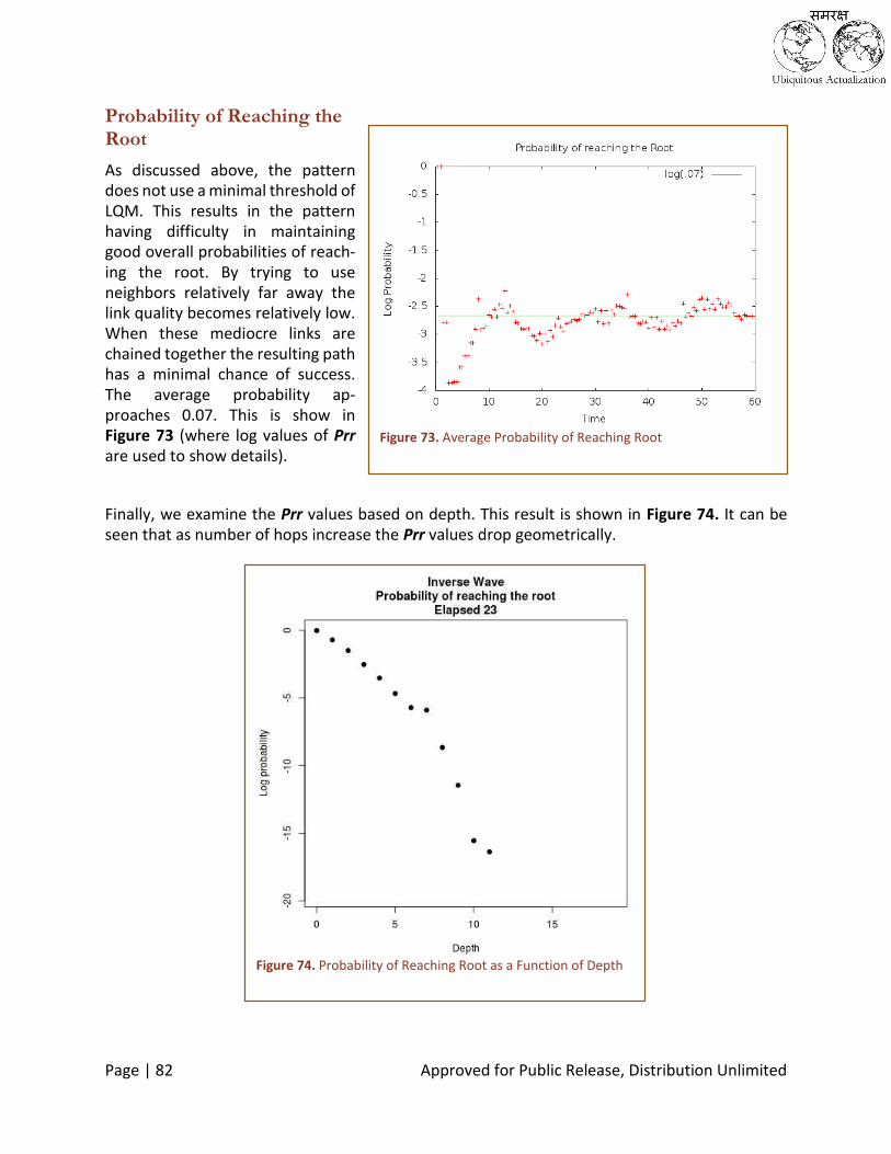
Page | 82 Approved for Public Release, Distribution Unlimited
Probability of Reaching the Root
As discussed above, the pattern does not use a minimal threshold of LQM. This results in the pattern having difficulty in maintaining good overall probabilities of reach-ing the root. By trying to use neighbors relatively far away the link quality becomes relatively low. When these mediocre links are chained together the resulting path has a minimal chance of success. The average probability ap-proaches 0.07. This is show in Figure 73 (where log values of Prr are used to show details).
Finally, we examine the Prr values based on depth. This result is shown in Figure 74. It can be seen that as number of hops increase the Prr values drop geometrically.
Figure 73. Average Probability of Reaching Root
Figure 74. Probability of Reaching Root as a Function of Depth

Page | 83 Approved for Public Release, Distribution Unlimited
Occasional Disconnects
The grid is sparse enough that the average number of parents to a node is less than 3. In particular there are many nodes with only one parent. In Figure 75 the green node numbered 39 had been linked to node number 23 with a link quality of 0.1. When this link dropped, node 39 was temporarily left with no parents. Many of the nodes above it (colored orange) were left with no path to the root but were unaware of it. This entire situation was resolved by the next snapshot (in Figure 76) with node 39 properly attached to nodes 24, 31 and 38.
Pattern Remarks The pattern shows promise in preserving the communication to the root in a mobile environment. However, as it stands, it is fragile as a result of link stability issues. By using a more sophisticated method of choosing elders, it should be able to handle the link sta-bility issues. The pattern is designed to quickly respond to link outages. During boot up the paths are rather long with strong link status. As time progresses, the average length of paths to the root decreases. However, there is a corresponding decrease in the overall link status. Over time, the path length approaches the path length expected when any hop less than 110 meters is allowed.
Figure 76. Rapid Reconnect from a Disconnected Condi-tion
Figure 75. Temporary Disconnect of Portion of the Net-work.

Page | 84 Approved for Public Release, Distribution Unlimited
Common Operating Picture
This chapter describes the scalable Distance-based Common Operating Picture (COP) pattern . We limit our presentation to an initial version of the pattern design, based on distance-based controlled broadcasts. We expect several refinements of this pattern to be documented in the near future.
COP is motivated by the situation where soldiers in the battlefield want to be able to look at a map and see where their fellow soldiers and equipment are deployed. The soldiers want to be able to have a common picture of the battlefield. The current state-of-the-art COP protocols scale to only a few tens of nodes, because of their use of network-wide broadcast. But with the use of distance-based broadcasting in our design, the COP pattern scales to a few hundreds of nodes, if not thousands.
The cost for being able to scale is that the staleness of the state of the map varies with distance. A soldier will be able to see the position of a soldier near him as it was a couple seconds ago but the position of a soldier far away from him will be shown as it was perhaps a few tens of seconds ago. We think this is acceptable for many operational contexts, where it is important to have an up-to-date picture of the immediate environment where a soldier is deployed, while for areas farther away a slightly delayed picture suffices.
In the current version of the COP design, the spatial correlation of locations of nodes in the same region has not been exploited to compress the data exchanged between nodes. We note that the overhead of the COP protocol can be decreased even further or conversely the rate of up-dates for the same level of traffic can be increased by using a location compression mechanism that aggregates over several nodes. We will explore this option in future versions of this pattern.
Background: Common Operating Picture and Global Snapshots
Global state snapshots whether about the location of the nodes or about some sensor values are a fundamental primitive for wireless networks that interact with real environments. While com-municating periodic, consistent and timely global state snapshots has been well studied in distributed systems [49], the problem has not been sufficiently studied in a wireless network. The problem is hard enough in static networks, but close to intractable in a mobile scenario. Con-sistent, timely and uniform snapshots are costly and exceed the capacity of the network in most cases. Some of the approaches used to decrease the cost of global snapshots it to exploit the temporal and spatial correlation of data being shared or to scale the resolution of the data.
For example, in [50], the authors propose a framework for a one time all-to-all broadcast of sen-sor data assuming the data is spatially correlated. This of course does not work when the state being shared is not correlated. However in our case, it is possible to further improve the cost or conversely to increase the rate of update of the distance-sensitive COP by compressing location information from nodes in the same region (i.e., using the spatial correlation of nodes). We will explore this option in the next phase of the project.

Page | 85 Approved for Public Release, Distribution Unlimited
Fractionally cascaded information [51] is a form of distance sensitive resolution that is widely used in computational geometry community for speeding up data structures. Recently, fractional cascading has been used for sensor networks as an efficient storage mechanism [52, 53]. Data is first stored at multiple resolutions across the network, which is then used to efficiently answer aggregate queries about a range of locations without exploring the entire area. [53] The approach uses probabilistic gossip mechanism for creating the multi-resolution data structure and is not really scalable for our continuous update semantics. In COP, by way of contrast, the location in-formation we share with other nodes changes constantly and is therefore generated and consumed on an ongoing basis.
In COP, instead of compressing information using spatial or temporal correlation, we scale the rate of update with distance and there by lower the cost. The idea of distance sensitive rate has also been used in other contexts. For example, Fisheye state routing [54] is a proactive routing protocol that re-duces the frequency of topology updates to distant parts of the network, which is very similar to the way we scale, although Fisheye routing scales traffic in an ad hoc manner. The focus of COP is to deliver ongo-ing all-to-all global snapshots, with a predictable latency that depends on the distance and at overall network cost that is of the same order of network capacity.
The COP Protocol
In a network of wirelessly-communicating, possibly mobile nodes, where each node knows its own location, the Common Operating Picture (COP) pattern tries to provide all the nodes in the network with a common view of the other nodes in the network and their locations, in a scalable manner irrespective of the size of the network. The current design of COP is adapted from the
algorithm in [55] and more generally along the distance sensitive snapshot work in [56].
The specification for a COP pattern is as fol-lows: Each node j should maintain a location table (as shown in Table 4) with one row for every node i in the network, listing:
id for node j
location for node i
timestamp t, at which node i was at the location, and
The timestamp is included because each node only knows its own location intrinsi-cally and the location of other nodes must
d e
m
f g h
i
l
j
k
b ca
d(a,g)≈2 d(b,g)≈1.4 d(c,g)≈2
d(d,g)≈1 d(e,g)≈1
d(f,g)≈1.4 d(h,g)≈1.4
d(i,g)≈1 d(j,g)≈1
d(k,g)≈2 d(m,g)≈2d(l,g)≈1.4
Figure 77. Distance-based COP illustration
Table 4. Example Location Table
Node ID
Loca-tion
Timestamp Parame-ter ν
1 (x1,y1) t1 ν1
2 (x2,y2) t2 ν2
. . . .
j (xj,yj) tj νj
. . . .
N (xN,yN) tN νN

Page | 86 Approved for Public Release, Distribution Unlimited
be learned from messages passed from other nodes. The timestamp indicates when the location information was generated at the source node.
Our implementation maintains an additions field in the table, a parameter ν which indicates the number of times node j has heard about a particular node most recent location with timestamp t. The ν parameter is maintained for efficiency reasons. If j hears of another node’s location mul-tiple times from its neighbors, we don’t want j to use limited network bandwidth to rebroadcast the location data that its neighbors presumably already know about. The parameter ν tracks how many times j has heard about i’s location from its neighbors, and j will only broadcast i’s location if ν is less than some threshold η.
The rate of update of the information to each node will depend on the distance of the node to the source, i.e., the closer two nodes are the faster the update rate between the nodes and the farther they are the slower the update rate. In the current version of the solution, the rate of update scales linearly with the distance between the source and destination.
The solution is push based, that is, each node pushes its location and timestamp periodically to its neighbors, but as this information flows through the network, its rate is scaled linearly at each hop. The information that is sent out by any node in certain period of time depends on the local rate of publishing and the diameter of the network.
In COP, each node periodically publishes its information, namely its location and the current timestamp, to its neighbors at an average rate of r times a second. In each message apart from its own information, a node includes in the most recent information it has about other nodes in the network. The rate which a node J publishes information about another node I is proportion-ate to their distance.
A node will transmit information about it-self in every message, and on average about all of its one-hop neighbors every two messages (r/2 times a second), about all of its two-hop neighbors every three messages (r/3 times a second), about all of its three-hop neighbors every four mes-sages (r /4 times a second), and so on. Figure 77 illustrates how COP would oper-ate in a network where nodes are laid out approximately on a grid one hop-unit square. Lines represent 1-hop connections. The distance from the central node g, Dx,g is shown in the figure. Information about node d distance away will be published by g, in once every d+1 messages.
From a receiver’s perspective, each node receives information about all of its immediate neighbors r times a second, about all of its neigh-bors two hop away r/2 times a second, about all of its neighbors three hops away r/3 times a second and so on. Thus the critical action in the protocol is to decide which node’s information (apart from self-information) should be included in the packet to be published in the current
r
a b
1/r2/r
3/r c
Figure 78. Staleness of information in Distance-based COP

Page | 87 Approved for Public Release, Distribution Unlimited
period. Figure 78 illustrates that the staleness of information about a node scales according to the distance between them. A node r that has an immediate neighbor a receives information from it every period and hence has a staleness of 1/r, whereas a node b that is roughly at twice that distance will have an staleness 2/r, and node c at 3 times the distance will have a staleness of 3/r, and so on and so forth.
Publishing information about neighbors in a deterministic manner based on their distance results in messages of different sizes in different periods. Thus in order to amortize the size of the mes-sages and to keep the average message sizes more or less equal, we randomize the period in which to include the information of a particular node i. Next we provide the exact pseudo-code of the protocol implementation.
Protocol Actions Here we describe the COP protocol as a set of actions performed as a response to protocol events, such as a timer firing or receiving a packet from a neighbor. The COP protocol performs 3 actions: the initialization action performed at the starting of the protocol on a node, a timer action performed each time a timer is fired, and a receive action when new packet is received from one of the neighbors. First let us begin by defining the variables used by the protocol. Let N denote the number of nodes in the network. Let j denote an arbitrary node in the network. j maintains a list other nodes in the network, let’s denote this list as 𝑗. 𝑉. For each node i in the list 𝑗. 𝑉 (i.e. for each node in the network), the node j also maintains its location, denoted by 𝑗. 𝑋𝑖 and the corre-sponding timestamp of the location information 𝑇𝑖 . That is 𝑖. 𝑇𝑖 represents the time on i when i published 𝑗. 𝑋𝑖. A node also keeps track of the number of times it hears the latest Location (lat-est is discovered using the timestamp) about some node i from its neighbors. Let us denote this count maintained by j about 𝑗. 𝑋𝑖 as 𝑗. 𝜈𝑖. Let 𝑟 represent the rate at which nodes publish their location information to their 1-hop neighbors. Also let 𝑗. 𝜆 represent the current timestamp on the node on node j. Please note that 𝑗. 𝜆 need not actually indicate the current time. It suffices if it is a monotonically increasing number incremented each time a node publishes its location. Let 𝜂 represent a parameter that governs the number of times particular location information has been published in a neighborhood. The recommend value of 𝜂 is at least 3, for good perfor-mance. Let 𝑑(𝑖, 𝑗) represent the geographical distance between nodes i and j, and 𝑑ℎ(𝑖, 𝑗) represent the network hop distance between nodes i and j. Initialization: During initialization all the variables defined above are initialized. Also a random-
ized local timer with a periodicity between (1
𝑟∗ 0.5) and (
1
𝑟∗ 1.5) is started. On average the
timer would have a periodicity of 1/𝑟 . Timer Action: Each time the timer is fired on a node j, the node builds a new message 𝑗. 𝑀𝑒𝑠𝑠𝑎𝑔𝑒𝜆and broadcasts this message to all its neighbors. To begin with it first increments the sequence number . 𝜆 . Let us add a new variable 𝑗. 𝑉𝜆 to denote the list of nodes whose location will be published by j in the current interval. To begin with 𝑗. 𝑉𝜆 contains only j . Thus information about itself is broadcast by a node in every interval along with the current sequence number (𝑗. 𝜆) which serves as the timestamp for this record. Next for each node i in the list 𝑗. 𝑉 the node

Page | 88 Approved for Public Release, Distribution Unlimited
i added to 𝑗. 𝑉𝜆 if 𝑑(𝑖, 𝑗) ∗ 𝑟𝑎𝑛𝑑() < 1 and if j has not heard about 𝑗. 𝑋𝑖 already from its neighbors 𝜂 times in the last 𝑑ℎ(𝑖, 𝑗). The condition 𝑑(𝑖, 𝑗) ∗ 𝑟𝑎𝑛𝑑() < 1 will be true approximately once every 𝑑(𝑖, 𝑗) times and hence a node at distance 𝑑(𝑖, 𝑗) will included roughly at the same rate, thereby providing a distance-based update rate. Checking if other nodes have already sent the information 𝜂 times, ensures that information about any node at a distance of k communication hops is broadcast at most 𝜂 times every k intervals in each communication neighborhood. And when j has decided whether or not to include each node in 𝑗. 𝑉 in 𝑗. 𝑉𝜆, 𝑗. 𝑀𝑒𝑠𝑠𝑎𝑔𝑒𝜆 is prepared
Actions on Node: j Variables: 𝑗. 𝑉 : List of nodes in the network 𝑗. 𝑋𝑖 : Location of node I 𝑗. 𝑇𝑖 : Timestamp of i's information 𝑗. 𝜈𝑖 : Counter for i's information 𝑗. 𝜆 : Sequence number of current interval 𝑗. 𝑉𝜆 : Forwarding list for the interval 𝑗. 𝜆 Actions: [A1]:: Initialization 𝑗. 𝑉 = 𝑗; 𝑗. 𝜈𝑖 = 0; 𝑗. 𝜆 = 0;
Timer.Start( 1
𝑟 ∗ (𝑟𝑎𝑛𝑑() + 0.5)) ;
[A2]:: Timer fired j.λ=j.λ+1; j.Vλ =j; ∀ 𝑖 ∈ 𝑗. 𝑉 if (𝑑(𝑖, 𝑗) ∗ 𝑟𝑎𝑛𝑑() < 1) if (𝑗. νI < η) 𝐴𝑑𝑑 𝑖 𝑡𝑜 𝑗. 𝑉𝜆; fi 𝑗. 𝜈𝑖 = 0; fi ∀ 𝑖 ∈ 𝑗. 𝑉λ 𝑆𝑒𝑛𝑑 𝑗. 𝑋𝑖, 𝑗. 𝑇𝑖 [A3]::Receive(𝑖. 𝑉) ∀𝑘 ∈ 𝑖. 𝑉 if ((𝑗. 𝑇𝑘 < 𝑖. 𝑇𝑘)𝑉 (𝑘 ∉ 𝑗. 𝑉))
𝑗. 𝑋𝑘 = 𝑖. 𝑋𝑘; 𝑗. 𝑇𝑘 = 𝑖. 𝑇𝑘; 𝑗. 𝑣𝑘 = 1; fi elseif (𝑗. 𝑇𝑘 == 𝑖. 𝑇𝑘) 𝑗. 𝑣𝑘 = 𝑗. 𝑣𝑘 + 1; fi
Figure 79. Protocol Actions for Distance-based COP

Page | 89 Approved for Public Release, Distribution Unlimited
by including a sequence of (𝑖, 𝑗. 𝑋𝑖, 𝑗. 𝑇𝑖) for all nodes i in the list 𝑗. 𝑉𝜆 and the message is sent out. Receive Action: When a node hears a message, it parses the message for the list of nodes whose location information is included in the message. When the message contains newer (based on the timestamp) information 𝑋𝑖 about some node i, j simply updates 𝑗. 𝑋𝑖 and also reset 𝑗. 𝑣𝑘 to 1. If 𝑋_𝑖 in the message is same as 𝑗. 𝑋𝑖 , then j increments 𝑗. 𝜈𝑖. Together these three actions implement the distance sensitive COP protocol. Figure 79. Protocol Actions for Distance-based COP shows the exact protocol actions as imple-mented in the Click router.
COP APIs
The COP protocol instantiated on a node provides the following two APIs, namely, (a) MapUpdate Callback, and (b) GetMap Query, through which the application can interact with the protocol. The COP protocol maintains the locations of each node in the network along with its last update time. The information about a single node is called a Record. The information maintained by COP is a set of N (the number of nodes in the network) records.
MapUpdate Callback API
Each time the COP protocol receives new information, the protocol calls the MapUpdate function in the application, with the number of new records and a pointer to the records array. The appli-cation programmer can decide how to use this call back. For example, if the application has a visual representation of the locations on an actual map, then, this callback can be used to update the locations of the nodes on the visual map. The main objective of this callback is to provide the information to the end user, with the least amount of delay. Hence delay sensitive operations can be carried out in the callback.
GetMap Query API:
The GetMap is a synchronous API which is used to look up the current state of the COP records which have been updated in the last X seconds. The GetMap takes three parameters: (1) Time period in seconds – the time interval in which the records where updated (or not), (2) a boolen- to specify whether we are looking for records that were updated or not updated in the time period, and (3) a pointer to integer – used indicate the number of records returned by the API. The first parameter specifies the interval to look up the records from current time t to (t-Period) seconds in which the record status changed (or not) and it returns a pointer to the records array. The second parameter specifies if the user is looking for updated records that which got new information in the periods specified or the state records that have not been updated in the period specified. The number of records returned through the pointer is conveyed to the calling function
void MapUpdate (int Number_Of_Records, Records* R)
Records* GetMap (int Period, bool Updated, int* NumerOfRecords)

Page | 90 Approved for Public Release, Distribution Unlimited
through the pointer provided as the second parameter ‘NumberOfRecords’. If the first parame-ter is 0, then the entire table is returned, irrespective of the second parameter.
Important Metrics
Definitions: L1. Staleness S(j,i, t): The staleness S(j, i, t) in the state of node i as possessed by node j at time t
is the time elapsed since the timestamp of the state of i (j.Ti). Thus S(j, i, t) = t - j.Ti .
L2. Maximum Staleness Smax(j, t): This is the mean of the value of S(j, i, t) for all 𝑖 ∈ {1. . 𝑁}, just before a new packet is received. This can be measured in the simulation by calculating the mean of staleness for all nodes in the network, when a new packet is received, but before the packet is processed. Staleness of any node for which information is not available at j should be measured over a long interval, such as 10000 seconds. At the end of the simulation a single value for each
node Smax(j) by averaging I over time.
L3. Network Staleness NS: This is the mean of Maximum Staleness Smax(j) (generated above) for
all nodes in the network 𝑗 ∈ {1. . 𝑁}. This can be measured in the simulation by periodically cal-culating the Network Staleness in the network and then finding the mean of that at the end of the simulation. L4. Snapshot Rate SR(j,i,t): The number of unique location updates from source i received at node j in a time interval of t.
Evaluations and Results
Simulation Parameters:
G1. Staleness versus Distance: We are interested in studying the distribution of Staleness as a function of distance. The Staleness S(j, i, t) computed when a node j receives a new packet is logged on each node and then plotted at the end of the simulation. This is likely to be a large dataset of size N*N*m*r*T, where T is the total simulation time.
G2. Network Staleness versus N: The Network Staleness would increase with N, the number of nodes in the network.
Distance-Insensitive COP
As a way of comparing our results from DS-COP and to show its scaling properties, we simulated a Distance Insensitive COP (DI-COP), along with DS-COP. The difference is in broadcasting strat-egy. Distance Insensitive COP includes information about every node in every packet it transmits.
Examples:
Get the records updated in last 10 seconds:
int num;
Records * r = GetMap(10,true,&num);
Get the records that have not been updated in last 20 seconds:
Records * r = GetMap(20,false,&num);

Page | 91 Approved for Public Release, Distribution Unlimited
On every broadcast time, every node will attempt to broadcast information about every node it knows about, except if that information has already been heard three or more times.
Simulation Scenario
We compare distance-sensitive COP and distance-insensitive COP for networks of nodes 16, 64, 256, 1024, and 4096. See Table 5 for various combina-tions of the scenarios simulated, for which we present the results in this section. Each simulation was run for 40 seconds with nodes broadcasting an average of two times a second. Each simulation was run with both static and mobile nodes. Static nodes were placed in a square grid, spaced 75 meters apart. Mobile nodes were placed the same, but then allowed to move using a Random Way-Point mobil-ity model
Results for a 49 Node Static Network
We first show the results for a 49 node static network, in order to demonstrate the scaling of staleness and snapshot rates with distance. Figure 80 shows the spatial distribution of staleness and the snapshot rate for a 49 node static network. Green circle shows the source of information, blue numbers show average staleness at nodes for the source in green and red numbers show the number of unique snapshot received out of 200 snapshots sent by the source of information in Distance-based COP. Staleness is shown in blue and the number of unique snapshots in red.
Table 5. Simulation variables for examining the effect of distance-sensitivity on COP
Simulation Pa-rameter
Values
Number of nodes
16, 64, 256, 1024, 2096
Mobility Static, Mobile
Simulation time 40 seconds
Distance-sensi-tivity
Sensitive, Not-sensitive
Figure 80. Spatial distribution of staleness and rate of update

Page | 92 Approved for Public Release, Distribution Unlimited
We can see from the figure that, while the staleness increases linearly with distance, the snapshot rate decreases linearly.
Bandwidth Comparison of DS-COP with DI-COP
The results show little if any difference between mobile and static situations with respect to the total bytes transmitted or staleness. By transmitting without regard to distance, distance-insen-sitive COP uses much more bandwidth in larger networks.
Figure 81. Histogram of Packet Lengths for DS-COP
Figure 82. Total bytes sent for DS-COP and DI-COP

Page | 93 Approved for Public Release, Distribution Unlimited
For example, as shown in Figure 82, static DS-COP with 4096 nodes transmits less bytes than DI COP with 1024 nodes and at 1024 nodes, DI-COP transmits approximately ten times more bytes than the distance-sensitive network of the same size.
DS-COPs have a close to “Normal” or “Gaussian” histograms for the size of packets transmitted on the air (as shown in Figure 81). This is expected due to the randomness involved in selecting the nodes to include in the packet. Even though the individual nodes choose to include a node in the packet based on a uniform distribution, when number of such distributions interact, the re-sultant distribution tend to be Gaussian in nature.
The DI-COP on the other hand tends to have a lot of very big packets (as shown in Figure 83), with maximum number of packets being of maximum size since, the DI-COP includes information about all known nodes in the network. In fact any packet that is less than the maximum size is simply a transition effect (an artifact of the relatively small simulation time of 40 seconds), where the network is booting up and the network is only aware of local nodes. As the initial boot up phase gets over the packets reach the maximum size and stay at that size for the rest of the simulation. Figure 83 clearly shows the scaling benefits of using DS-COP over DI-COP as the aver-age packet size saturates quickly in DS-COP.
Figure 83. Packet-Size Histogram comparing DS-COP and DI-COP

Page | 94 Approved for Public Release, Distribution Unlimited
Analysis of Staleness
The tradeoff for band-width parsimony of the DS-COP is staleness. Stale-ness in the distance-sensitive COPs grows as the square of distance while for non-distance-sensitive COPs staleness grows linearly with dis-tance. More accurately, for a DS-COP where the rate of update is scaled linearly with distance, the max staleness is given by
∑ 𝑘𝐷𝑘=1 = 𝐷(𝐷 + 1)/2 ,
where D is the distance between the source of the information and the node where staleness is measured. Figure 84 shows this expected staleness growth with distance. However, such an anal-ysis is valid only for a deterministic version of DS-COP, which transmits a particular nodes information in a specific time slot. For a deterministic DS-COP on average, each node broadcasts information about another node at a time proportional to the distance.
Figure 85 explains the same cumulative staleness effect for period of transmission of .5 seconds. Figure 86 shows the staleness as a function of distance. As we can see while the DI-COP has a linear growth of staleness, the DS-COP has quadratic growth. This is the price for scalability. How-ever, because of the randomness in the implementation the actual staleness is slightly less than what is predicted by the equation (but never-the-less is of order (𝐷2) ) .
Figure 84 Maximum Expected Staleness for a deterministic DS-COP
0
50
100
150
200
250
300
350
0 1000 2000 3000 4000St
ale
ne
ss (
Cu
mu
lati
ve d
ela
y)
Distance
Average Cumulative Delay
Figure 85. Accumulating staleness in DS-COP

Page | 95 Approved for Public Release, Distribution Unlimited
No Difference between Mobile and Static Scenarios
One of the striking results from COP simulations is that there is very little difference between the mobile and static scenarios in terms of the results (for any metric). For example, in Figure 86, while there is a substantial difference between DS-COP and DI-COP staleness, there is no differ-ence between a mobile and static simulation of same size for a DS-COP. However, this is as expected and not a surprise. This is a result of the structure-free dissemination that COP uses.
Pattern Remarks The COP ASNP outlined here is the first truly (and absolutely) scalable design and implementation of the Common Operating Picture Con-Ops to the best of our knowledge. We have implemented and validated the basic protocol. However, the scaling laws under various mobility models and information loads needs further study. Also, the pattern presented here only scales the rate of information disseminated. The other dimensions of scaling, for example, in-formation precision and geographic aggregation needs further investigation.
Figure 86 Staleness versus Distance for DI-COP and DS-COP

Page | 96 Approved for Public Release, Distribution Unlimited
Part III Conclusions and Recommendations
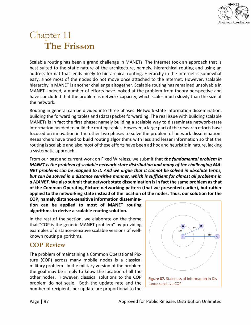
Page | 97 Approved for Public Release, Distribution Unlimited
The Frisson
Scalable routing has been a grand challenge in MANETs. The Internet took an approach that is best suited to the static nature of the architecture, namely, hierarchical routing and using an address format that lends nicely to hierarchical routing. Hierarchy in the Internet is somewhat easy, since most of the nodes do not move once attached to the Internet. However, scalable hierarchy in MANET is another challenge altogether. Scalable routing has remained unsolvable in MANET. Indeed, a number of efforts have looked at the problem from theory perspective and have concluded that the problem is network capacity, which scales much slowly than the size of the network.
Routing in general can be divided into three phases: Network-state information dissemination, building the forwarding tables and (data) packet forwarding. The real issue with building scalable MANETs is in fact the first phase; namely building a scalable way to disseminate network-state information needed to build the routing tables. However, a large part of the research efforts have focused on innovation in the other two phases to solve the problem of network dissemination. Researchers have tried to build routing algorithms with less and lesser information so that the routing is scalable and also most of these efforts have been ad hoc and heuristic in nature, lacking a systematic approach.
From our past and current work on Fixed Wireless, we submit that the fundamental problem in MANET is the problem of scalable network-state distribution and many of the challenging MA-NET problems can be mapped to it. And we argue that it cannot be solved in absolute terms, but can be solved in a distance sensitive manner, which is sufficient for almost all problems in a MANET. We also submit that network state dissemination is in fact the same problem as that of the Common Operating Picture networking pattern (that we presented earlier), but rather applied to the networking state instead of the location of the nodes. Thus, our solution for the COP, namely distance-sensitive information dissemina-tion can be applied to most of MANET routing algorithms to derive a scalable routing solution.
In the rest of the section, we elaborate on the theme that “COP is the generic MANET problem” by providing examples of distance-sensitive scalable versions of well-known routing algorithms.
COP Review
The problem of maintaining a Common Operational Pic-ture (COP) across many mobile nodes is a classical military problem. In the military version of the problem the goal may be simply to know the location of all the other nodes. However, classical solutions to the COP problem do not scale. Both the update rate and the number of recipients per update are proportional to the
r
a b
1/r2/r
3/r c
Figure 87. Staleness of information in Dis-tance-sensitive COP

Page | 98 Approved for Public Release, Distribution Unlimited
size of the network, so the communication load grows as 𝑂(𝑁2). However, the aggregate capac-ity of the network only grows as 𝑂(√𝑁).
The military application of COP motivates a useful redefinition of the problem. A war fighter typically needs high fidelity information about nearby units, but only low fidelity information about distant units. It is natural to relax the consistency constraint as a function of distance. Any scheme that reduces fidelity as a function of distance rapidly enough so that the aggregate com-munication load doesn’t grow faster (with scale) than the capacity of the network will scale
We studied a specific Distant Sensitive COP (DS-COP) algorithm in order to gain further insight. Every node maintains a list of node location for every node in the network (all COP algorithms must do this). Our algorithm then randomly shared some of its information with each of its neighbors. We weighted the random selection criteria of data so that local data was appropri-ately favored. Whenever a node received new location data, it compared that data with the data it already had and kept only the most recent data. This resulted in a distance sensitive loss of temporal fidelity that allowed for scaling to a few 10’s of thousands of nodes. The relaxed fidelity also results in a relaxed maximum staleness of information (as shown in Figure 87) that is also proportional to the distance to the source. Other methods of degrading fidelity with distance, such as spatial approximation or node aggrega-tion, could be included and would generally improve the results.
Scalable Distance-sensitive Geo-graphic Routing
Our DS-COP can be directly used as the location disseminating service for a Geographic Routing (GR) service. In Geographic Routing, messages are routed to a neighbor that is geographically closer to the destination than the current node. This requires that the location of the destination is known to do routing. Overlaying a Geographic Routing service on our DS-COP service creates an arbitrary point-to-point (P2P) routing service. Since our COP service scales the resulting P2P routing also scales. One advantage with geographic
routing is that the messages can be gracefully rerouted to a destination that is moving. As illustrated in Figure 88, Geographic Routing would work as long as the precision of direc-tion towards the destination remains constant or get better, as the message travels towards the destination. If the precision of di-rection decrease, that the message could never “catch up” with the mobile destination.
For DS-COP, the precision of direction to-wards the destination (which is important for GR) is fairly constant (see Figure 89), since the
Figure 89. The effect of distant sensitive location fidel-ity on geographic routing.
Figure 88. Geographic Routing -- Graceful rerout-ing with mobility

Page | 99 Approved for Public Release, Distribution Unlimited
precision of location of the destination increases along the routing path. In MANET the geo-graphic routing could lead to slightly spiral paths, which are only slightly suboptimal (see Figure 88). Unlike wired networks, for MANETs trading routing optimality for networking overhead is a highly desirable system-level trade.
One problem with geographic routing though is that it needs approximately uniform node cov-erage, and may fail if the network has large “holes” or voids. This however is an intrinsic problem with Geographic Routing and is not related to DS-COP. Even with perfect information routing may fail with large holes in the network. Thus, while DS-COP makes Ge-ographic Routing scale, it does not make its problems any worse.
Scalable Distance-sensitive Distance Vector Routing
Our COP ASNP can be applied in general to any information, be it a physical property like temperature or network information like node locations. Using the COP protocol to disseminate the hop-counts of the nodes in the network will yield a distance-sensitive Distance-Vector protocol. Traditional Distance-Vector MANET solu-tions like Destination-Sequenced Distance-Vector (DSDV) protocol do not scale, since they require the nodes to send the distances (hop-counts) to all other nodes in the network. As the number of nodes in network grows, the distance-vector table grows as 𝑂(𝑁) and the total traffic grows as 𝑂(𝑁2).
In the distance sensitive version of this protocol, nodes will ex-change hop-counts about some of their nodes in the network. Which nodes will be included in a particular exchange will be ran-dom and will depend on a probability proportional to their hop-counts. This makes the average number of nodes included in each routing table update more or less constant (as opposed to the 𝑂(𝑁) in the non-distance sensitive case). The COP-like dissemination solves the scaling problem of the traditional distance vector algorithm.
The other advantage of this approach over the COP + Geographic Routing solu-tion is that, DS-DV routing does not suffer from the “hole” problem as shown in Figure 90. In the figure, if Geographic Routing is used, node 2 would act has the “hole” for messages from the right of the network to node 1. However when using hop counts, node 2 would reroute the messages to node 4, since it is closer to node 0 by hop-count.
Figure 90. Distance-senstive Hop Count based routing fixed the “hole” problem
20
1
3 45
Table 6. Example hop-count table of distance-sensitive distance-vector protocol
Node 2 Table
Node Dist Next
0 2 4
1 3 4
2 ~
3 2 4
4 1 ~
5 1 ~

Page | 100 Approved for Public Release, Distribution Unlimited
Scalable Distance-sensitive Prob-abilistic Routing
Another interesting application of COP to net-work state dissemination is to build a probabilistic routing protocol for MANET. Most of the existing protocols treat links and paths as binary events: either a link exists or it doesn’t, and either a path exists or it doesn’t. This is the legacy inherited from the wired Internet, where packet loss and link changes are somewhat rare. But in MANETs the links are more com-
plex. The interplay between phenomena, such as fading, propagation loss, interference, congestion and mobility, makes the state of the links and paths not binary, but probabilistic. A link could have partial reliability and it would be advantageous to build a routing protocol that could explicitly use an estimate of the link reliability.
One way to build such a protocol is to use the probability of a path as the metric, in-stead of the hop count, using which packets are to be routed. Nodes build and maintain routing tables for the probability of reaching every node in the network through every neighbor. The size of such a table would be 𝑶(𝒎𝑵), where m is the average neighbor-hood size and N is the size of the network. Table 7 shows an example routing table of such a protocol. Assuming that we have the link quality probability for each of the neigh-bors, the rest of the table can be updated using Bayes Theorem. Sending the entire routing table throughout the network will be very expensive for such a protocol, but once again we can disseminate the information in a COP like manner, using distance-sensitivity and tune the per node network layer overhead to be a constant.
One of the advantages of such a protocol is, it would solve some of the intermittent link problems (as shown in Figure 91), that the more traditional MANET protocols experience. An intermittent link is one that keeps changing state throughout and never really stabilizing. In such a scenario traditional routing protocols would also keep change the paths continuously and also rerouting large parts of the data traffic. In the example shown in Figure 91, when the link shown in dotted lines changes state, paths for large parts of the network will need to be rerouted. But a probabil-istic protocol can account for instability of the paths and can route only a percentage of the traffic that is proportional to its stability. In general such a protocol can address a class of problems commonly referred to as “Bayesian Problems”.
Each of these examples will have strengths and weaknesses, but as a group they illustrate our core argument, that the core problem to be solved in MANETs is keeping track of the nodes, not
Figure 91. Probabilistic Routing can solve the “moving bridge” problem
Table 7. Example path probability table
Node P(N0) P(N1) P(N2) P(N3)
0 .8 .2 .98 .1
1 .5 .99 ~ ~
2 .1 .8 .85 .88
3 .9 .96 .8 ~
4 .7 .2 ~ ~

Page | 101 Approved for Public Release, Distribution Unlimited
figuring out the optimal route between nodes. This is the COP problem. New and improved solu-tions to the COP problem lead directly to new and improved solutions to the MANET problem. And most MANET solutions can be thought of as a COP service applied to networking data. This perspective immediately reveals why most MANET protocols don’t scale and why a few do.

Page | 102 Approved for Public Release, Distribution Unlimited
Recommendations
Clean Slate Approach
We recommend, based on our past work and current work on the Fixed Wireless program, that a somewhat “Clean Slate Approach” to networking is needed in order to achieve scalable MA-NETs. We suggest this, because we believe that a number of lessons have been mis-learned from experiences with the wired Internet.
False Analogy: Static Network and MANET
MANETs have typically been treated as an extension of the Internet, with essentially the same set of problems. Mobility has often been regarded as an inconvenience that needs to be man-aged. Scalability has been under-addressed as it is, in a sense, a solved issue in the Internet given that the use of a multi-tier hierarchy largely tames the problem. Many variants of protocols have been proposed with the intent to redress issues related to “mobility” and “hierarchy” in MANETs. However, the goals of most of these protocols have remained essentially the same as that of the wired Internet, namely, (i) optimal routing and (ii) load balancing. And thus IP-address based peer to peer routing has persisted. Figure 92 illustrates the correct and wrong analogies (in our opin-ion) that have been made between network models. The bold arrows indicate a tight correlation, while the light dotted arrows indicate a loose correlation between different types of networks.
In fact, the core MANET issues are fundamentally different. The core issues in a MANET are: (i) Network State Knowledge, (ii) Connectivity Maintenance/Repair in the presence of Mobility, and (iii) Scalability.
Knowing Others State is Critical in MANET
As we stated in the Chapter 11 (Frisson), a fundamental issue in MANETs is scalable knowledge of the state of other nodes in the network. In military terms, this is the Common Operating Pic-ture problem, for which the traditional problem formulation does not admit scalable solution. We have shown however that an alternative, distance sensitive, formulation of the problem is solvable in a scalable manner, with a loss of optimality in terms of delay that is proportional to
Figure 92. Correct and wrong analogies between network models
MANets COP
Internet Cellular
MANets COP
Internet Cellular
Wrong
Page | 103 Approved for Public Release, Distribution Unlimited
distance. We have also that the principle of distance sensitive information propagation is generic in nature and can be applied to other problems in the MANET. We therefore recommend that designers focus their efforts on the core problem of network state dissemination and adopt the distance-sensitive propagation of control information as one of the generic ways to design scal-able protocols.
Optimality versus Scalability
It seems that for several problems in MANETs, optimality and scalability cannot be achievable simultaneously. But by sacrificing optimality one can reduce the control overhead to achieve scalability. We suggest that a more appropriate design for MANETs is to aim for scalability. If done properly. One can still achieve near-optimality (or be within a constant factor of it).
Embrace ASNPs We recommend that designers embrace the new ASNP paradigm and abandon the incumbent P2P routing paradigm. While we have presented a few ways of designing scalable P2P routing, the intention was not to suggest that global P2P routing must be or can be used. On the contrary, it was a demonstration of our principles used for designing ASNPs, which when applied to P2P routing, make them more scalable than what has been achieved previously. ASNPs enable an-other dimension of efficiency, as they tailor the control traffic to the needs of application, the locality and pattern of traffic, and the properties of the network. A single P2P routing protocol cannot have the flexibility and adaptation that the ASNP architecture brings.

Page | 104 Approved for Public Release, Distribution Unlimited
Part IV Appendices

Page | 105 Approved for Public Release, Distribution Unlimited
Capacity Theory
Introduction
A significant body of network capacity theory has been worked out, in which a standard definition of network capacity is the sum of all traffic rates in units of data-distance (e.g., bit-meters or gigabyte-miles). In other words, the network capacity captures the maximum achievable rate, over all traffic patterns, all node locations, and all transmission protocols. Its consideration on data-distance as opposed to data alone distinguishes it from the more traditional focus on throughput capacity1.
A well known result [57] states that as the number of network nodes, n, grows, the network capacity of P2P networks increases by 𝑂(√𝑛), assuming the nodes are placed arbitrarily in a fixed (say unit) area. Said another way, the per node capacity decreases as 𝑂(1/√𝑛) as the number of nodes grows. The intuition behind the observation is that as you add nodes to a fixed area, each node can reduce its power in order to communicate over a proportionally smaller area. The result is n nodes communicating at the same rate, but over a distance that is reduced by 𝑂(1/√𝑛).
Of course, if all links in the network are long, in the sense that transmission on any link will inter-ference with transmissions on every other link, then network capacity scales as Θ(1).
Importantly, the observation holds broadly for many other scenarios (excluding a few quasi-pathological ones). In particular, the same result holds in the extended network model where the area grows as the number of nodes grows holding the node density to be constant.2 The details of many specific scenarios are stated in the literature, see [4] for a summary of key results.
Models Sensitivity to Traffic Pattern: Convergecast, Broadcast, and Local Traffic
Traffic patterns play a significant role in determining whether a P2PN scales to a large number of nodes. I.e., assuming that the traffic pattern is not any-to-any node has significant impact on the achievable network capacity. Non uniform traffic can compromise scalability, i.e., if hot spots limit total performance, or enhance scalability, i.e., for local traffic.
Convergecast is an important pattern for many applications. By way of contrast to random peer to peer traffic, El Gamal [58] has shown that in the case of convergecast traffic although the single sink node in the many-to-one channel acts like a bottleneck, as n grows in a fixed area, the transport capacity in an information theoretic model scales not as Θ(1) but as Θ(log (n)). The
1 Considerable confusion results from not being careful in distinguishing throughput capacity from network capac-ity. We will refer to network capacity in this book, unless otherwise specified. 2 In unit area networks where density grows unboundedly, it is sometimes assumed that the attenuation decreases unboundedly as neighbor distances decrease unboundedly. This ignores consideration of the near-field effect. This consideration can be safely ignored in extended network models.

Page | 106 Approved for Public Release, Distribution Unlimited
main idea is to allow every node to distribute its information to closely located nodes, which is efficient given node density, and then those nodes can cooperate to transmit the information to the collector using a beamformer to get the logarithmic increase in the received power, and sub-sequently, the capacity.
A similar idea suffices to show that in a fixed area, broadcast capacity scales not as Θ(1), as shown in [59], but as Θ(log (n)) [60].
Importantly, for achieving O(n) scalability, the traffic pattern must involve a small average dis-tance between source and destination nodes [61]. In other words, strictly local traffic traffic yields perfect scalability. Interestingly, MANET applications anticipated for the FCS Brigade Com-bat Team have been analyzed to have fairly localized traffic patterns [7]. Specifically, the analysis shows that their traffic should satisfy a power law distribution with exponent between 2 and 3, in which case capacity is O(n) scalable, i.e., constant per node capacity is achievable.
Sensitivity to Mobility
Network capacity increases with mobility, the idea being that if delay is discounted then a node’s connectivity over time will increase without necessarily increasing the contention. A well-known two-hop relay protocol has been shown to provide Θ(1) throughput per node, assuming an ideal mobility pattern in which each node uniformly and independently visits all other nodes, the delay in this case being Θ(n).
Other work has shown a tradeoff between delay and throughput, where bounding the delay by a constant D, between Θ(1) and Θ(n), provides a corresponding increase in throughput which is related to the cube-root of D [62, 63, 64].
This tradeoff is important since isolated consideration of capacity tends towards operation in regions where latency is high or the probability of error is high. Also notable is the notion of critical delay capture a lower bound below which node mobility cannot be used to improve the throughput. The critical delay for Brownian motion (likewise, random walks) is Θ(n2), for random waypoint is 𝛩(√𝑛), for IID mobility is Θ(1) [65].
Sensitivity to Connectivity
An interesting corner case is when the connectivity of the network is marginal; in this case, the network needs to have some notion of Delay Tolerance associated with it. It is well known that connectivity to O(log n) nearest neighbors in probabilisitic (Erdos-Renyi) or random geometric graphs is both necessary and sufficient. However, if connectivity is not necessary, but the exist-ence of a giant connected component is sufficient, then connectivity to even 3 nearest neighbors is sufficient.
Sensitivity to Physical Layer Signals
While the early results for network capacity were developed for the geometry-based unit disk protocol model, similar results were later known for the SINR-based physical model, and the channel-based information theoretic models.
In some cases asymptotic capacity results match across the various models, the higher fidelity of the physical layer yields better capacity in other cases, say by allowing antenna sharing for co-herent relaying and interference subtraction or for MIMO beamforming. The literature suggests that in many cases the MIMO radios deliver log( )O n n capacity, in addition to significantly

Page | 107 Approved for Public Release, Distribution Unlimited
larger absolute capacity. However, some of the complexity of the MIMO may spill over into the networking layer, partially exacerbating the network overhead management problem.
Hierarchy
The capacity of two-tier hierarchies (with the higher tier being static, and there sometimes being a bounded ratio between higher tier and lower tier links) and log n-tier hierarchies have also been deeply studied. While we believe that the latter are worth studying for future Fixed Wireless systems we do not elaborate on these in this book
Remarks
There is agreement that network overhead is substantial in MANETs, and as such a proper infor-mation theoretic consideration of network capacity should not ignore the scaling of network overhead. We regard the ratio of network overhead to network capacity as an important metric of MANETs, which Application Specific Networks seek to substantially improve3. The table below summarizes representative ratios for various models.
Fixed Size
Capacity NLO NLO/Capacity
Traditional P2P O n
2
O n
3 2
O n
Long Link — Arbitrary Traffic 1O 2nO 2nO
Long Link — Broadcast O n 2nO O n
Virtual Hierarchy O n
3 2log( )O n n log( )O n n
Application Specific Networking O n
log( )O n n log( )O n
We note here that we discovered new theoretical results for the network overhead related to
neighborhood maintenance in the presence of location uncertainty. However we are not includ-
ing those results as part of this book since they have not been published in other forums yet
3 As our work has shown, NLO/Capacity is not the only consideration. The real-time overhead of routing, relaying,
physical layer cooperation, beamforming, and other sophisticated coordination techniques can affect the stability
of networks, even in cases where the ratio of NLO/Capacity is low.

Page | 108 Approved for Public Release, Distribution Unlimited
Acronyms
Acronym Definition Page
API Application Programming Interface iii
ARM Advanced RISC Machine 30
ASIC Application Specific Integrated Circuits 6
ASNP Application Specific Network Pattern iii
CDF Cumulative Distribution Function 77
COP Common Operating Picture 32
RTS/CTS Request-To-Send/Clear-To-Send 36
DNS Domain Name System 9
DI-COP Distance Insensitive Common Operating Picture 90
DS-COP Distance Sensitive Common Operating Picture 90
DSDV Destination Sequence Distance Vector 99
ELG Emergent Local Group 48
EMANE Extendable Mobile Ad-hoc Network Emulator 35
FCS Future Combat Systems 6
FEC Forward Error Correction 37
FOB Forward Operating Base 23
FwP Flooding with Pruning 41
HNR Highband Network Radio 35
HTML Hyper Text Markup Language 17
IWBE Inverse Wave Based Exfiltration 75
LQM Link Quality Metric 76
LSR Link State Routing 10
LSU Link State Update 11
MAC Medium Access Control 11
MANET Mobile Ad-hoc NETworks 11
MCDS Minimum Connected Dominating Set 49
MIMO Multiple Input Multiple Output Antennas 106
MIT Massachusetts Institute of Technology 29
MPI Message Passing Interface 39
MPR Multi-Point Relays 11
NDK Android Native Development Kit 32
NDN Named Data Networks 8
.NET Microsoft .NET Framework 32
NLO Network Layer Overhead 10
NPIPD New Path Information Propagation Delay 14

Page | 109 Approved for Public Release, Distribution Unlimited
Acronym Definition Page
OLSR Optimized Link State Routing 11
OMF Optional Metadata Field 42
OSI Open Systems Interconnection Model 18
OSPF Open Shortest Path First 4
PHY Physical Layer 36
SEP-LM Semi Empirical Probabilistic Link Model 39
SINR Signal to Interference plus Noise Ratio 106
SNR Signal to Noise Ratio 19
SRW Soldier Radio Waveform 35
STAR Source Tree Adaptive Routing 48
TBE Tree Based Exfiltration 75
TBRPF Topology Broadcast based Reverse-Path Forwarding 48
TCP Transmission Control Protocol 7
TR Technology Readiness 2
TTL Time To Live 45
UGS Unattended Ground Sensors 20
WNAN Wireless Network After Next 3
WSN Wireless Sensor Network 5

Page | 110 Approved for Public Release, Distribution Unlimited
References
[1] "Freestyle Chess," [Online]. Available: http://freestyle-chess.webs.com/. [Accessed 2 April 2013].
[2] J. Redi and R. Ramanathan, "The DARPA WNaN network architecture," in Military Communications
Conference (MILCOM), 2011.
[3] G. Kolata, "At last, shout of 'Eureka!' in age-old math mystery," [Online]. Available:
http://www.nytimes.com/1993/06/24/us/at-last-shout-of-eureka-in-age-old-math-mystery.html.
[Accessed 2 April 2013].
[4] F. Xue and P. R. Kumar, "Scaling laws for ad hoc wireless networks: An information theoretic
approach," Foundations and Trends in Networking , vol. 1, no. 2, pp. 145-270, 2006.
[5] I. D. Chakeres and J. P. Macker, "Mobile ad hoc networking and the IETF -- IETF 69," in ACM
SIGMOBILE Mobile Computing and Communications Review, 2007.
[6] J. G. Andrews, N. Jindal, M. Haenggi, R. Berry, S. A. Jafar, D. Guo, S. Shakkottai, R. W. Heath, M.
Neely, S. Weber and A. Yener, "Rethinking information theory for mobile ad hoc networks," IEEE
Communications Magazine, vol. 46, no. 12, pp. 94-101, 2008.
[7] R. Ramanathan, R. Allan, P. Basu, J. Feinberg, G. Jakllari, V. Kawadia, S. Loos, J. Redi, C. Santivanez
and J. Freebersyse, "Scalability of mobile ad hoc networks: theory vs practice," in Military
Communications Conference, 2010.
[8] "Eli Whitney - firearms and the birth of standardization," [Online]. Available:
http://inventors.about.com/cs/inventorsalphabet/a/machine_2.htm. [Accessed 29 April 2013].
[9] J. Hui and D. Culler, "IP is dead, long live IP for wireless sensor networks," in 6th International
Conference on Embedded Networked Sensor Systems, 2008.
[10] "The Named Data Networking Project," [Online]. Available: http://www.named-data.net/.
[11] D. L. Alderson and J. C. Doyle, "Contrasting views of complexity and their implications for network-
centric infrastructures," Systems, Man, and Cybernetics Society, vol. 40, no. 4, pp. 839 - 852, July
2010.

Page | 111 Approved for Public Release, Distribution Unlimited
[12] J. C. Doyle and M. Csete, "Architecture, constraints, and behavior," Procedings of the National
Academy of Science of United States of America, vol. 108, pp. 15624-15630, 2011.
[13] K. Zhou, J. C. Doyle and K. Glover, Robust and Optimal Control, Prentice Hall, 1995, p. 596.
[14] K. Zhou and J. C. Doyle, Essentials of Robust Control, Prentice Hall, 1997, p. 411.
[15] S. Low, F. Paganini and J. Doyle, "Internet congestion control," Control Systems, vol. 22, no. 1, pp.
28-43, 2002.
[16] K.-H. Kim, Y. Zhu, R. Sivakumar and H.-Y. Hsieh, "A Receiver-Centric Transport Protocol for Mobile
Hosts with Heterogeneous Wireless Interfaces," Wireless Networks, vol. 11, no. 4, pp. 363-382, July
2005.
[17] H. Cao, K. W. Parker and A. Arora, "O-MAC: A receiver centric power management protocol," in
Proceedings of the 2006 14th IEEE International Conference on Network Protocols, Santa Barbara,
California, 2006.
[18] R. Zheng, J. C. Hou and L. Sha, "Asynchronous Wakeup for ad hoc networks," in ACM Symposium
on Mobile Ad Hoc Networking and Computing (MobiHoc), 2003.
[19] P. Dutta and D. Culler, "Practical asynchronous neighbor discovery and rendezvous for mobile
sensing applications," in ACM conference on Embedded Networking sensor Systems (SenSys), 2008.
[20] A. Kandhalu, K. Laskhman and R. Rajkumar, "U-connect: A low-latency energy-efficient
asynchronous neighbor discovery protocol," in 9th International Conference on Information
Processing in Sensor Networks, NewYork, USA, 2010.
[21] E. e. a. Kohler, “The Click modular router,” ACM Transactions on Computer Systems (TOCS), pp.
263-297, 2000.
[22] T. Henderson, “12.2.1 The Packet Class,” 11 November 2011. [Online]. Available:
http://www.isi.edu/nsnam/ns/doc/node132.html. [Accessed 18 March 2013].
[23] "TUN/TAP," [Online]. Available: http://en.wikipedia.org/wiki/TUN/TAP. [Accessed April 2013].
[24] P. L. a. R. M. Suresh, “ns-3-click: click modular router integration for ns-3,” in Proceedings of the
4th International ICST Conference on Simulation Tools and Techniques, 2011.
[25] D. e. a. Aguayo, “MIT roofnet,” in Proceedings of the International Conference on Mobile
Computing and Networking, 2003.

Page | 112 Approved for Public Release, Distribution Unlimited
[26] tcpdump/libpcap, “TCPDUMP/LIBPCAP public repository,” 2010. [Online]. Available:
http://www.tcpdump.org/. [Accessed 18 March 2013].
[27] L. Burbank, W. Kasch and J. and Ward, An Introduction to Network Modeling and Simulation for
the Practicing Engineer, Wiley-IEEE Press, 2011.
[28] L. Rizzo, "Transparent acceleration of software packet forwarding using netmap," in INFOCOM,
Pisa, Italy, 2012.
[29] "NS-3 : Discrete Event Network Simulator," [Online]. Available: http://www.nsnam.org/.
[30] "Extendable Mobile Ad-hoc Network Emulator (EMANE)," [Online]. Available:
http://cs.itd.nrl.navy.mil/work/emane/.
[31] "QualNet: QualNet Simulation Platform," [Online]. Available: http://web.scalable-
networks.com/content/qualnet.
[32] K. Renard, C. Peri and J. Clarke, "A performance and scalability evaluation of the ns-3 distributed
scheduler," in 5th International ICST Conference on Simulation Tools and Techniques, 2012.
[33] B. J. Henz, T. Parker, D. Richie and L. Marvel, "Large scale MANET emulations using U.S. Army
waveforms with application: VoIP," in Military Communications Conference (MILCOM ), 2011.
[34] N. Aschenbruck, R. Ernst, E. Gerhards-Padilla and M. Schwamborn, "BonnMotion: A mobility
scenario generation and analysis tool," in 3rd International ICST Conference on Simulation Tools
and Techniques, 2010.
[35] T. Camp, J. Boleng and V. Davies, "A survey of mobility models for ad hoc network research,"
Wireless Communications & Mobile Computing (WCMC): Special Issue on Mobile Ad Hoc
Networking: Reasearch, Trends and Applications, vol. 2, pp. 483-502, 2002.
[36] R. Hekmat and P. Mieghem, "Interference in wireless multi-hop ad-hoc networks and its effect on
network capacity," Wireless Networks, vol. 10, no. 4, pp. 389-399, 2004.
[37] P. Jacquet, P. Mühlethaler, T. Clausen, A. Laouiti, A. Qayyum and L. Viennot, "Optimized link state
routing protocol for ad hoc networks," in International Multi Topic Conference, IEEE INMIC, 2001.
[38] Cesar A. Santivanez; Ram Ramanathan, "Hazy sighted link state (HSLS) routin: A scalable link state
algorithm," BBN Technical Memorandum No.1301, 2001.
[39] O. Gnawali, R. Fonseca, K. Jamieson, D. Moss and P. Levis, "Collection Tree Protocol," in 7th ACM
Conference on Embedded Networked Sensor Systems, 2009.

Page | 113 Approved for Public Release, Distribution Unlimited
[40] S. Madden, M. Franklin, J. Hellerstein and W. Hong, "TAG: A tiny aggregation service for ad hoc
sensor networks," in ACM/USENIX Symposium on Operating Systems Design and Implementation,
2002.
[41] L. Lovascz, "Random walks on graphs: A survey," Combinatorics, Paul Erdos 80, 1993.
[42] U. Feige, "A tight lower bound for the cover time of random walks on graphs," Random structures
and algorithms, vol. 6, no. 4, pp. 433--438, 1995.
[43] U. Feige, "A tight upper bound on the cover time for random walks on graphs," Random structures
and algorithms, vol. 6, no. 1, pp. 51--54, 1995.
[44] N. Alon, C. Avin, M. Koucky and G. Kozma, "Many random walks are faster than one," in 20th
Annual ACM Symposium on Parallel Algorithms and Architectures (SPAA), 2008.
[45] A. Frieze and C. Cooper, "The cover time of random regular graphs," SIAM Journal of Discrete
Mathematics, vol. 18, no. 4, pp. 728--740, 2005.
[46] C. Cooper, A. Frieze and T. Radik, "Multiple random walks in random regular graphs," SIAM Journal
of Discrete Mathematics, vol. 23, no. 4, pp. 1738--1761, 2009.
[47] G. Ercal and C. Avin, "On the cover time of random geometric graphs," in Automata, Languages,
and Programming, 2005.
[48] C. Avin and B. Krishnamachari, "The power of choice in random walks: An empirical study," in
International Symposium on Modeling, Analysis and Simulation of Wireless Mobile Systems, 2006.
[49] M. Chandy and L. Lamport, "Distributed snapshots: determining global states of distributed
systems," ACM Transactions on Computer Systems, vol. 3, no. 5, pp. 63-75, 1985.
[50] S. D. Servetto, "Sensing lena-massively distributed compression of sensor images," in IEEE
International Conference on Image Processing, 2003.
[51] F. Dehne, A. Ferreira and A. Rau-Chaplin, "Parallel fractional cascading on hypercube
multiprocessors," Computational Geometry Theory and Applications, vol. 2, pp. 144-167, 1992.
[52] J. Gao, L. J. Guibas, J. Hershberger and L. Zhang, "Fractionally cascaded information in a sensor
network," in Information Processing in Sensor Network, 2004.
[53] R. Sarkar, X. Zhu and J. Gao, "Hierarchical spatial gossip for multi-resolution representations in
sensor networks," in Information Processing in Sensor Networks (IPSN), 2007.

Page | 114 Approved for Public Release, Distribution Unlimited
[54] G. Pei, M. Gerla and T.-W. Chen, "Fisheye state routing in mobile ad hoc networks," in ICDCS
Workshop on Wireless Networks, 2000.
[55] V. Kulathumani and Y. Fallah, "An infrastructure-less vehicular traffic information service with
distance-sensitive precision," in IEEE Vehicular Technology Conference (VTC), 2012.
[56] V. Kulathumani and A. Arora, "Distance sensitive snapshots in wireless sensor networks," in
Proceedings of the 11th international conference on Principles of distributed systems, 2007.
[57] P. Gupta and P. R. Kumar, "The capacity of wireless networks," IEEE Transactions on Information
Theory, vol. 46, no. 2, pp. 388-404, 2000.
[58] H. E. Gamal, "On the scaling laws of dense wireless sensor networks: the data gathering channel,"
IEEE Transactions on Information Theory, vol. 51, no. 3, pp. 1229-1234, 2005.
[59] A. Keshavarz-Haddad, V. Ribeiro and R. Riedi, "Broadcast capacity in multihop wireless networks,"
in ACM International Conference on Mobile Computing and Networking (MobiCom 06), NewYork,
NY, 2006.
[60] B. Sirkeci-Mergen and M. Gastpar, "On the broadcast capacity of high density wireless networks,"
in Information Theory and Applications Workshop, San Deigo, CA , 2007.
[61] J. Li, C. Blake, D. S. J. D. Couto, C. Hu, H. I. Lee and R. Morris, "Capacity of ad hoc wireless
networks," in ACM International Conference on Mobile Computing and Networking (MobiCom 01),
2001.
[62] X. Lin and N. Shroff, "Towards achieving the maximum capacity in large mobile wireless networks
under delay constraints," Journal of Communications and Networks, 2004.
[63] M. J. Neely and E. Modiano, "Capacity and delay tradeoffs for ad hoc mobile networks," in
International Conference on Broadband Networks (BROADNETS), 2004.
[64] X. Wang, L. Fu, X. Tian, Y. Bei, Q. Peng, X. Gan, H. Yu and J. Liu, "Converge-cast: On the capacity and
delay tradeoffs," IEEE Transactions on Mobile Computing, vol. 99, no. 1, 2011.
[65] G. Sharma, R. Maxumdar and N. Shroff, "Delay and capacity trade offs in mobile ad hoc networks:
a global perspective," IEEE Transactions on Networking, vol. 15, no. 5, 2007.