1-4244-2575-4/08/$20.00 c©2008 IEEE

Optimal Scaling of Multicommodity Flows in Wireless Ad Hoc Networks:Beyond The Gupta-Kumar Barrier

Shirish Karande §, Zheng Wang §, Hamid Sadjadpour §, J.J. Garcia-Luna-Aceves §,∗§Department of Electrical Engineering and Computer Engineering

University of California, Santa Cruz, 1156 High Street, Santa Cruz, CA 95064, USA∗Palo Alto Research Center (PARC),3333 Coyote Hill Road, Palo Alto, CA 94304, USA

Email: {karandes,wzgold,hamid,jj}@soe.ucsc.edu

Abstract

We establish a tight max-flow min-cut theorem for multi-commodity routing in random geometric graphs. We showthat, as the number of nodes in the network n tends to in-finity, the maximum concurrent flow (MCF) and the min-imum cut-capacity scale as Θ(n2r3(n)/k) for a randomchoice of k ≥ Θ(n) source-destination pairs, where r(n)is the communication range in the network. We exploit thefact, that the MCF in a random geometric graph equalsthe interference-free capacity of an ad-hoc network underthe protocol model, to derive scaling laws for interference-constrained network capacity. We generalize all existingresults reported to date by showing that the per-commoditycapacity of the network scales as Θ(1/r(n)k) for thesingle-packet reception model suggested by Gupta and Ku-mar, and as Θ(nr(n)/k) for the multiple-packet receptionmodel suggested by others. More importantly, we show that,if the nodes in the network are capable of multiple-packettransmission and reception, then it is feasible to achievethe optimal scaling of Θ

(n2r3(n)/k

), despite the pres-

ence of interference. This result provides an improvementof Θ

(nr2(n)

)over the highest achieved capacity reported

to date. In stark contrast to the conventional wisdom thathas evolved from the Gupta-Kumar results, our results showthat the capacity of ad-hoc networks can actually increasewith n while the communication range tends to zero!

1 Introduction

The price, performance and form factors of sensors, pro-cessors, storage elements, and radios today are at a pointthat the age of viable large-scale ad-hoc networks wouldappear to be finally upon us. Alas, Gupta and Kumar’s [8]seminal work cautions us to the contrary. They studied thecapacity of wireless ad-hoc networks with n nodes when re-

ceivers are static, transmit or receive one packet at a time,and the network traffic consists of n unicast sessions. Theirconclusion was a rather negative one: The capacity of ad-hoc networks does not scale with an increase in networksize.

Gupta and Kumar’s analysis [8] applies to the traditionalview of ad hoc networking in which protocols are based ona one-to-one communication paradigm aimed at avoidingmultiple access interference (MAI). However, a number ofrecent advances in cooperative communication and gener-alizations of routing are challenging the long-held view thatavoiding interference is the way to maximize throughput inad hoc networks. For example, network coding (NC) [1]generalizes routing by permitting processing of packets atintermediate nodes. In certain network configurations (re-fer to illustrations in [9, 19]) some nodes can utilize NC toconcurrently transmit multiple packets. Many-to-one andmany-to-many communication is also feasible under a vari-ety of other cooperative techniques [3, 6, 18].

Co-operative protocols that provide performance bene-fits in specific network configurations need not scale wellwith the network size. In particular, Liu et al. [15]proved another disheartening result: NC cannot increasethe throughput order of wireless ad-hoc networks for multi-pair unicast applications under half-duplex communication.However, in a recent challenge, Garcia-Luna-Aceves et al.[6] call for the realization of ad hoc networks that scale byembracing MAI through the use of multi-packet reception(MPR) at the receivers. They show that, if the nodes in thenetwork are capable of MPR, then the order capacity of anetwork with n unicast sessions grows as Θ(r(n)), wherer(n) is the communication range. This represents a gain ofΘ

(nr2(n)

)over the throughput order of Θ(1/nr(n)) re-

ported by Gupta and Kumar.

Interestingly, the prior work on the capacity of wirelessnetworks, which we summarize in Section 2, has focused onwhat is attainable with specific approaches to handle MAI.

No prior work has focused on first establishing what is theoptimal capacity of a wireless network in the absence ofMAI, and then determining whether that capacity is attain-able when MAI is present. This is precisely the focus andoverall contribution of this paper.

Section 3 presents the first contribution of this paper.We model a random network with n nodes, a homoge-neous communication range of r(n), and unicast traffic fork source-destination (S-D) pairs. In the absence of inter-ference, such a network corresponds to a random geometricgraph(RGG) with an edge between any two nodes separatedby a distance less than r(n). We define a combinatorial in-terference model based on RGGs, and use it to express allthe protocol models used in the past and a model that welater use to show that the optimal capacity of a wireless net-work is indeed attainable. We introduce a protocol modelin which nodes have the ability to decode correctly multiplepackets transmitted concurrently from different nodes, andtransmit concurrently multiple packets to different nodes.We refer to this as the multi-packet transmission and recep-tion (MPTR) protocol model.

Section 4 presents the second contribution of this paper,which is the characterization of the optimal interference-free capacity of a wireless network. The task of concur-rently maximizing the data-rate for k S-D pairs is an in-stance of the multi-commodity flow problem. Hence, themaximum concurrent multi-commodity flow-rate (MCF) ina RGG equals the interference free capacity (i.e., the opti-mal capacity) of the network. To derive upper bounds onthe optimal network capacity, we use the fact that the MCFis less than the minimum capacity of a multi-commodity cutfor any arbitrary graph. The max-flow min-cut theorem byFord and Fulkerson [4] establishes that this bound is tightfor a single commodity. However, in general, the min-cutdoes not provide a tight bound on the max-flow [14]. Thebound is known to be tight only for special cases [10], andin general can exhibit a gap of Θ(log n) [14]. We establish atight max-flow min-cut theorem for RGGs for the first time,and show that Θ

(n2r3(n)/k

)is a tight bound on the opti-

mal capacity of a wireless network.

Section 5 presents our third contribution, which consistsof generalizing prior results by Gupta and Kumar and byGarcia-Luna-Aceves et al., and proving that the optimal ca-pacity of wireless networks is attainable in the presence ofMAI. We utilize the max-flow min-cut theorem of Section 4to deduce tight order bounds for the capacity of randomnetworks under various interference models. We show thatthe per-commodity capacity, under the protocol model sug-gested in [8], exhibits a tight order bound of Θ(1/r(n)k). This result generalizes Gupta and Kumar’s result to anyk ≥ Θ(n) S-D pairs. Similarly, we generalize Garcia-Luna-Aceves et al.’s analysis for the MPR protocol model. Weshow that, under the MPR model, the per-commodity ca-

pacity of the network scales as Θ(nr(n)/k), which meansthat it is bounded away from the optimal capacity by a factorof Θ

(nr2(n)

). Furthermore, the analysis in [6] implicitly

assumes the existence of a tight max-flow min-cut theoremfor RGGs; therefore, the results in this paper fill an impor-tant gap in their analysis.

We show that MPTR achieves the optimal capacityof Θ

(n2r3(n)/k

). Hence, MPTR provides a gain of

Θ(nr2(n)

)over MPR and any previously reported feasible

capacity. What is just as striking is that MPTR can achievethe dual objective of increasing capacity and decreasing thetransmission range as n increases. This is in stark contrastto the commonly held view that the capacity of multihopwireless networks cannot increase as the number of nodesincreases. Indeed, our results demonstrate that the capacityof ad-hoc networks can actually increase with n while thecommunication range tends to zero! Section 6 addresses theimpact of our results on the design of protocols for futurewireless ad hoc networks.

2 Related Work

There have been many contributions on the capacitystudy of wireless ad hoc networks, however due to spacelimitations we only mention a few of them that focus on uni-casting. A number of papers have extended the results byGupta and Kumar [8], which showed a gap between the up-per and lower bounds on capacity under the physical model.Franceschetti et al. [5] closed this gap using percolation the-ory. Several techniques aimed at improving the capacity ofwireless ad hoc networks have been analyzed. Grossglauserand Tse [7] demonstrated that a non-vanishing capacity canbe attained at the price of long delivery latencies by tak-ing advantage of long-term storage in mobile nodes. Someworks have demonstrated that changing physical layer as-sumptions such as using multiple channels [13] or MIMOcooperation [17] can change the network capacity.

Ozgur et al. [17] proposed a hierarchical cooperationtechnique based on virtual MIMO to achieve linear capac-ity. They showed that the optimal per-session capacity ofan ad-hoc network is bounded as O(n log n), and a con-stant per-session capacity of Θ(1) is achievable. Our workis significantly different from this work, in terms of the themodel and assumptions used to derive the results. Ozgur et.al. consider the information-theoretic model, and assumethat the network employs heterogenous hop-sizes, at timesrequiring a direct communication between widely separatednodes. In contrast, our work is based on the protocol modeland assumes a homogenous transmission range, which is amore realistic assumption.

Cooperation can be extended to the simultaneous trans-mission and reception at the various nodes in the network,which can result in significant capacity improvement [3].

As we have stated, Garcia-Luna-Aceves et al. [6] showedthat using MPR at the receivers can increase the order ca-pacity of wireless networks subject to unicast traffic.

A generalization of the max-flow min-cut theorem tomultiple commodities is not feasible in arbitrary graphs.However, Leighton and Rao [14] showed that the gap be-tween the max-flow and min-cut is at most Θ(logn). In arecent work, Madan et. al. [16] have utilized the Leightonand Rao’s work to derive bounds for the capacity of ad-hocnetworks. They focus on the special case where k = Θ(n2)and the single packet reception (SPR) model. Our work isinspired by the analysis of Leighton and Rao. Since weare able to deduce a tight max-flow min-cut theorem, ourbounds are tighter than those reported by Madan et al. [16].Furthermore, our work is applicable to a wider variety ofprotocol models and traffic patterns.

3 Preliminaries

3.1 Network Model

For a continuous region R, we use |R| to denote its area.We denote the cardinality of a set S by |S|, and by ‖x− y‖the distance between nodes x and y. Whenever convenient,we utilize the indicator function 1{P}, which is equal to oneif P is true and zero if P is false. Pr(E) represents theprobability of event E. We say that an event E occurs withhigh probability (w.h.p.) as n → ∞ if Pr(E) > (1−(1/n)). We employ the standard order notations O, Ω, and Θ.

We assume a random wireless network with n nodes dis-tributed uniformly in a unit-square. In our model, as n goesto infinity, the density of the network also goes to infin-ity. Therefore, our analysis is applicable to dense networks.Furthermore, we assume a fixed transmission range r(n)for all the nodes in the network. Thus, the network topol-ogy can be characterized using a RGG, which we denote byGr and define next.

Definition 3.1 Random Geometric Graph Gr:We associate a directed graph Gr(Vr , Er) with a wirelessnetwork formed by distributing n nodes uniformly in a unitsquare. We represent the node-set by V = {1, · · · , n}. Letthe locations of these nodes be given by {X1, · · · , Xn}, theedge-set is then E = {(i, j) | ‖Xi − Xj‖ ≤ r(n)} .

While the results in this paper can be extended to undi-rected graphs, it is more convenient for us to use directedgraphs because we use edge-coloring techniques in ourwork. In the case of undirected graphs, the argument shouldbe based on vertices (receivers) rather than edges. Also notethat we permit two edges for a pair of connected verticeswith possibly different capacity in each direction.

We assume that the network operates using a slottedchannel and, in the absence of interference, the data rate

in each time slot for every transmitter-receiver pair is a con-stant of value W bits/slot. Given that W does not changethe order capacity, we normalize its value to 1. Hence, theinterference-free capacity of each edge in Gr is equal to 1.

Gupta and Kumar [8] have proved the following criteriafor the connectivity of Gr.

Lemma 3.2 For a random distribution of n nodes in a unit-square, the graph Gr is connected with high probability asn → ∞, iff. r(n) ≥ rc(n) = Θ(

√log n/n).

In a dense network, interference is the primary constrainton network capacity. Like [16], we describe the interferenceof a network by the following generic model.

Definition 3.3 Combinatorial Interference Model:The interference model for the graph1 G(V, E) is deter-mined by a function I : E → P (E), where P (E) is thepower set of E, i.e., the set of all possible subsets of E. Forevery e ∈ E, I(e) represents an interference set such that, atransmission on edge e is successful if and only if (iff) thereare no concurrent transmissions on any e ∈ I(e). An inter-ference model can be restricted to a sub-graph H(VH , EH)by defining a function IH : EH → P (EH) such thatIH(e) = I(e)

⋂EH .

The various protocol models that have been proposed inthe past can now be expressed as special cases on Gr.

Gupta and Kumar [8] studied a single packet reception(SPR) protocol model under which a transmission fromnode i to receiver j is successful iff ‖Xi − Xj‖ ≤ r(n)and if ‖Xj − Xk‖ ≥ (1 + η)r(n) for any other transmitterk. Here η is a guard-zone that is assumed to be constantfor the entire network. Moreover, all the nodes operate inhalf-duplex mode. The following definition expresses thismodel in terms of the notation we have introduced.

Definition 3.4 Single-Packet Reception (SPR) Model:Let e = (e+, e−) ∈ E, then the interference set for edge eis defined as

ISPR(e) = J(e) − e,

J(e) = {e ∈ Er | ‖Xe+ − Xe−‖ ≤ (1 + η)r(n)} .(1)

Garcia-Luna-Aceves et al. [6] generalized the abovemodel to account for MPR capability at the receivers. Ac-cording to their MPR protocol model a node i can simulta-neously receive all the packets transmitted by nodes withina distance r(n) iff there are no transmitters at a distancegreater than r(n) but less than (1 + η)r(n). Furthermore, ifa node j transmits a packet to node i, then it cannot simulta-neously transmit a packet to any other node in the network.

1Note that Gr denotes a RGG while G represents a general graph.

Definition 3.5 Multi-Packet Reception (MPR) Model:

IMPR(e) = ISPR(e) − (A(e) − B(e)) ∀e ∈ E where

A(e) = {e ∈ Er | ‖Xe+ − Xe−‖ ≤ r(n)} (2)

B(e) ={e ∈ Er | e+ = e+

}(3)

We also consider the case in which nodes have MPRand MPT capabilities, i.e., can decode multiple concurrenttransmissions and can transmit concurrently multiple pack-ets to different nodes. We capture the MPR and MPT capa-bilities with a simple yet representative, multi-packet trans-mission and reception (MPTR) protocol model, which isdefined below.

Definition 3.6 Multi-Packet Transmission and Reception(MPTR) Model:

IMPTR(e) = IMPR(e) − B(e) ∀e ∈ E (4)

It is important to highlight some of the features of theabove model. The MPTR protocol model still restricts thenodes to operate in a half-duplex mode. Moreover, thismodel is identical to the MPR protocol model in terms ofthe nodes that are permitted to transmit within the vicinityof a receiver i, i.e., both models prohibit transmission froma node j such that r(n) < ‖Xi−Xj‖ ≤ (1+η)r(n). Thus,the difference between the MPR and MPTR protocol mod-els stems purely from the fact that, under the MPTR model,a node j transmitting a packet to node i can simultaneouslytransmit packets to other nodes in the network.

We assume that the traffic in the network is generated byunicast communication between k source-destination (S-D)pairs. We associate a rate vector λ = [λ1, · · · , λk] withthese k pairs. We assume the data rate for each S-D pair tobe non-zero. Hence, without loss of generality (w.l.g) therate vector can be written as λ = [fDi, · · · , fDk] wheref ∈ R+ and Di ∈ [1/2, 1] for 1 ≤ i ≤ k.We refer tothe parameter f as the concurrent flow rate and to D =[D1, · · · , Dk] as the demand vector.

Definition 3.7 Feasible Flow Rate:Given k S-D pairs {(s(1), d(1)), . . . , (s(k), d(k))}, a ratevector λ = [fDi, · · · , fDk] is feasible if there exists aspatial and temporal scheme for scheduling transmissionssuch that by operating the network in a multi-hop fashion,and buffering at intermediate nodes when awaiting trans-mission, every source s(i) can send λi bits/sec on averageto the chosen destination d(i). A flow rate f is feasible for ademand vector D = [D1, · · · , Dk] iff λ = [fDi, · · · , fDk]is a feasible rate vector.

Definition 3.8 Capacity of Random Networks:The capacity per commodity of a network is Θ(f(n)) if un-der a random placement of n nodes,a random choice of k

S-D pairs and for an arbitrary demand vector we have:

limn→∞ Pr(cf(n)is feasible flow rate) = 1(5)

lim infn→∞Pr(c′f(n)is infeasible flow rate) < 1(6)

for some c > 0 and c < c′ < +∞.

In the following sections we repeatedly utilize the wellknown Chernoff bounds:

Lemma 3.9 Chernoff Bounds: Consider N i.i.d randomvariables Yi ∈ {0, 1} with p = Pr(Yi = 1). Let Y =∑N

i=1 Yi. Then for every c > 0 there exist 0 < δ1 < 1 andδ2 > 0 such that

Pr (Y ≤ (1 − δ1)Np) < e−cNp (7)

Pr (Y ≥ (1 + δ2)np) < e−cNp (8)

3.2 Graph Theory Results

We review some definitions from graph theory. In partic-ular, note that the task of identifying a feasible flow rate canbe posed as a multi-commodity flow problem, specificallythe k-commodity flow problem.

Definition 3.10 k-Commodity Flow Problem:Consider a directed graph G(V, E) with a capacity functionc : E → [0, 1]. Let {(s(1), d(1)), . . . , (s(k), d(k))) be k S-D pairs, with a demand vector D ∈ [1/2, 1]k. Let f ∈ R+

be a concurrent flow rate. Find flow functions fi : E → R+

for 1 ≤ i ≤ k, which satisfy the following flow constraints:Capacity Constraint : ∀e ∈ E

∑

1≤i≤k

fi(e) ≤ c(e) (9)

Flow Conservation : ∀v = s(i), d(i)∑

e:e+=v

fi(e) =∑

e:e−=v

fi(e) (10)

Demand Satisfaction : 1 ≤ i ≤ k

fDi =∑

e:e+=s(i)

fi(e) −∑

e:e−=s(i)

fi(e)

=∑

e:e−=d(i)

fi(e) −∑

e:e+=d(i)

fi(e) (11)

Flow functions that satisfy the above constraints arecalled feasible. Other inputs to the problem being fixed, aflow rate f is said to feasible iff the above problem has a so-lution. Furthermore, let f∗ be the MCF such that the aboveproblem has a feasible solution. A wireless network canbe represented by an equivalent graph with capacity func-tions determined by the interference. Thus, the MCF in

an equivalent graph can be perceived as the maximum flowthat can be routed in a network. Additionally, if w.h.p. f∗

is the MCF for any graph formed by a random distributionof nodes, sources and destinations, then the capacity of thewireless network is also f∗.

Consider the following additional definitions.

Definition 3.11 Vertex Cut:Given a node set V , a cut is the separation of the vertex setV into two disjoint and exhaustive sets (S, SC). We shalloften reference a cut just by the set S .

Definition 3.12 Multi-commodity Cut Capacity:Given a graph G(V, E), a capacity function c : E → [0, 1]and a cut (S, SC). The multi-commodity cut capacity isdefined as

ΥG,S =∑

e∈E 1[e+∈S,e−∈SC ]c(e)∑i:s(i)∈S,d(i)∈SC Di

(12)

Definition 3.13 Minimum Cut Capacity:Given a graph G(V, E) and capacity function c : E →[0, 1], the minimum multi-commodity cut capacity is definedas

ΥG = minS⊂V

ΥG,S (13)

It is well-known that the minimum cut-capacity providesan upper bound on the maximum flow rate.

Lemma 3.14 For any k-commodity flow f∗ ≤ ΥG

4 Optimal Capacity

We show that for RGGs, the MCF provides a tight ap-proximation of the minimum-cut capacity. This relation-ship implies a tight characterization of the interference-freecapacity of wireless ad-hoc networks with a homogenoustransmission range. Our approach can be summarized asfollows: For a particular demand vector, we provide an up-per bound by showing that there exists a multi-commoditycut in Gr of order O(g(n)) and a lower bound by construct-ing a flow of order Ω(g(n)) in a sub-graph Hr ⊆ Gr. Theseresults along with the following Lemmas prove that the ca-pacity of Hr and Gr has a tight bound Θ(g(n)).

Lemma 4.1 A graph G(V, E) and a sub-graphH(VH , EH) satisfy the following two properties: (a)If f is a feasible flow-rate in H then f is feasible in G; and(b) the capacity of a cut (S, SC) in G is always greaterthan or equal to the capacity of the cut in H .

Proof: To prove Part (a) of the lemma, let fH,i for 1 ≤i ≤ k be the flow functions associated with the feasibleflow of rate f in H . Note that these flow functions satisfy

r(n)r(n)

O(nr(n)2)O(nr(n)2)

SS ScSc

AA

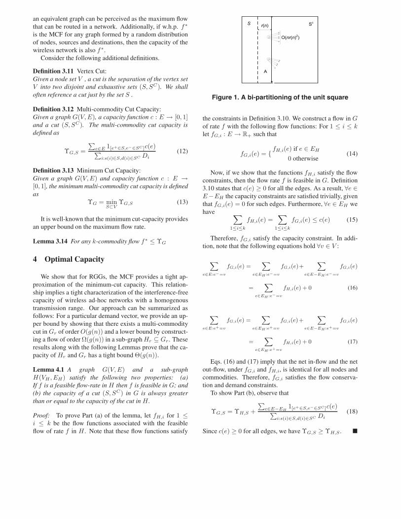
Figure 1. A bi-partitioning of the unit square

the constraints in Definition 3.10. We construct a flow in Gof rate f with the following flow functions: For 1 ≤ i ≤ klet fG,i : E → R+ such that

fG,i(e) = { fH,i(e) if e ∈ EH

0 otherwise(14)

Now, if we show that the functions fH,i satisfy the flowconstraints, then the flow rate f is feasible in G. Definition3.10 states that c(e) ≥ 0 for all the edges. As a result, ∀e ∈E−EH the capacity constraints are satisfied trivially, giventhat fG,i(e) = 0 for such edges. Furthermore, ∀e ∈ EH wehave ∑

1≤i≤k

fH,i(e) =∑

1≤i≤k

fG,i(e) ≤ c(e) (15)

Therefore, fG,i satisfy the capacity constraint. In addi-tion, note that the following equations hold ∀v ∈ V :

X

e∈E:e−=v

fG,i(e) =X

e∈EH :e−=v

fG,i(e)+X

e∈E−EH:e−=v

fG,i(e)

=X

e∈EH :e−=v

fH,i(e) + 0 (16)

X

e∈E:e+=v

fG,i(e) =X

e∈EH :e+=v

fG,i(e)+X

e∈E−EH :e+=v

fG,i(e)

=X

e∈EH :e+=v

fH,i(e) + 0 (17)

Eqs. (16) and (17) imply that the net in-flow and the netout-flow, under fG,i and fH,i, is identical for all nodes andcommodities. Therefore, fG,i satisfies the flow conserva-tion and demand constraints.

To show Part (b), observe that

ΥG,S = ΥH,S +

∑e∈E−EH

1[e+∈S,e−∈SC ]c(e)∑i:s(i)∈S,d(i)∈SC Di

(18)

Since c(e) ≥ 0 for all edges, we have ΥG,S ≥ ΥH,S . �

4.1 Upper Bound

We utilize the following properties of Gr.

Lemma 4.2 If r(n) ≥ rc(n) then w.h.p. graph Gr is suchthat: (a) The minimum vertex degree ∇ ≥ Θ

(nr2(n)

), and

(b) the maximum vertex degree Δ ≤ Θ(nr2(n)

).

Proof: We first show that ∇ ≥ Θ(nr2(n)

). A node v

in Gr is connected to all the nodes in a disk of radius r(n)centered at v . The area of this disk is πr2(n). Given auniformly random distribution of nodes, the probability ofanother node u lying within this disk is πr2(n). Considera random variable Yv,u ∈ {0, 1} which is equal to one iffnode u is connected to node v. The degree of node v canbe written as deg(v) =

∑u∈V −{v} Yv,u. Therefore, the

Chernoff Bound (11) implies that ∀c > 0 there exists a 0 ≤δ ≤ 1 such that

Pr(deg(v) ≤ (1 − δ)nπr2(n)

)< e−cnπr2(n) (19)

From the union bound we obtain

Pr(∇ ≤ (1 − δ)nπr2(n)

)

< nPr(deg(v) ≤ (1 − δ)nπr2(n)

)(20)

Given that r(n) ≥ rc(n) we have r(n) ≥ c1

√log n/n for

some c1 > 0. Therefore, Eqs. (19) and (20) imply that

Pr(∇ ≤ (1 − δ)πnr2(n)

)< ne−cπc1 log n = 1/ncπc1−1

(21)Now, Lemma 3.9 tell us that we can choose c ≥ 2/(πc1))and corresponding 0 < δ1 < 1 such that

Pr(∇ ≥ (1 − δ)πnr2(n)

)> 1 − (1/n) (22)

We use similar arguments to show that Δ ≤ Θ(nr2(n)

)

w.h.p.. This fact follows from Eq. (8), which implies that∀c > 0 there exists a 0 ≤ δ ≤ 1 such that

Pr(deg(v) ≥ (1 + δ1)nπr2(n)

)< e−cnπr2(n) (23)

The union bound and the fact that r(n) ≥ c2

√log n/n im-

plies that

Pr(Δ ≥ (1 + δ)πnr2(n)

)< ne−cπc2 log n (24)

Therefore, there exists a δ2 > 0 s.t

Pr(Δ ≤ (1 + δ2)πnr2(n)

)> 1 − (1/n) (25)

�Consider the cut S described by Figure 1. The cut con-

sists of all the nodes in the rectangular region of a constantarea.

Lemma 4.3 If the network consists of k ≥ Θ(log n) S-Dpairs then w.h.p. a region R of constant area |R| containsΘ(k) sources with destinations outside region R.

Proof: Let Yi ∈ 0, 1 be a random variable that is equal toone iff the ith S-D pair is such that s(i) belongs to region Rand d(i) does not. Under a uniformly random placement ofnodes

Pr (Yi = 1) = |R|(1 − |R|) (26)

The total number of S-D pairs satisfying the required con-dition can be represented by Y =

∑k1 Yi. If k ≥ c log n

the Chernoff Bounds imply the existence of constants c1 =1/(c|R|(1 − |R|)), 0 ≤ δ1 ≤ 1 and δ2 > 0 s.t.

Pr (Y ≥ (1 − δ1)|R|(1 − |R|)k) > 1 − e−c1k|R|(1−|R|)

≥ 1 − e−c1c|R|(1−|R|) log n = 1 − (1/n) (27)

Pr (Y ≤ (1 + δ2)|R|(1 − |R|)k) > 1 − e−c1k|R|(1−|R|)

= 1 − e−c1c|R|(1−|R|) log n = 1 − (1/n) (28)

�Furthermore, consider the subset A in S defined by a

strip of dimension 1× r(n). The total number of vertices inA is Θ(nr(n)) because of the uniform distribution of nodesin the network.

Theorem 4.4 If r(n) ≥ rc(n) and k ≥ Θ(logn), then thecapacity of the cut S is ΥGr,S = O(n2r3(n)/k) w.h.p.

Proof: According to the definition of Gr two nodes areconnected iff they are separated by a distance less than r(n).Consequently, if an edge cuts across S then it has to be in-cident upon a node at a distance less than r(n) from theboundary separating S and SC , i.e. the head of the edgeshould lie in the subset A of dimension r(n) × 1. Further-more, for each node in A the maximum number of edgescutting across the cut is bounded by Δ

∑

e∈E

1[e+∈S,e−∈SC ] ≤ |A|Δ (29)

In the absence of interference c(e) = 1 for all the edges.Hence,

ΥGr,S =

∑e∈Er

1[e+∈S,e−∈SC ]∑i:s(i)∈S,d(i)∈SC Di

≤ |A|Δ∑i:s(i)∈S,d(i)∈SC Di

(30)

According to Lemma 4.3, there exists c1 > 0 s.t. the to-tal number S-D pairs across the cut is c1k. Furthermore,by Definition 3.10 the demand for each pair is at least 1/2.Hence,

ΥGr,S ≤ 2|A|Δc1k

(31)

Lemma 4.2 implies that there exists a c2 > 0 s.t. Δ <c2nr2(n), while uniform distribution of nodes in the net-work implies that there exists a c3 > 0 s.t. |A| ≤ c3nr(n).Hence,

ΥGr,S ≤ 2c2c3n2r3(n)/(c1k) (32)

�Any cut in Gr has a capacity greater than the minimum

cut capacity ΥG. Consequently Theorem 4.5 implies thefollowing Corollary.

Corollary 4.5 If r(n) ≥ rc(n) and k ≥ Θ(log n) then ΥGr

is upper bounded as O(n2r3(n)/k).

4.2 Lower Bound

h =r(n)/3

1

i

l

1 j l

(i, j)th

square-let

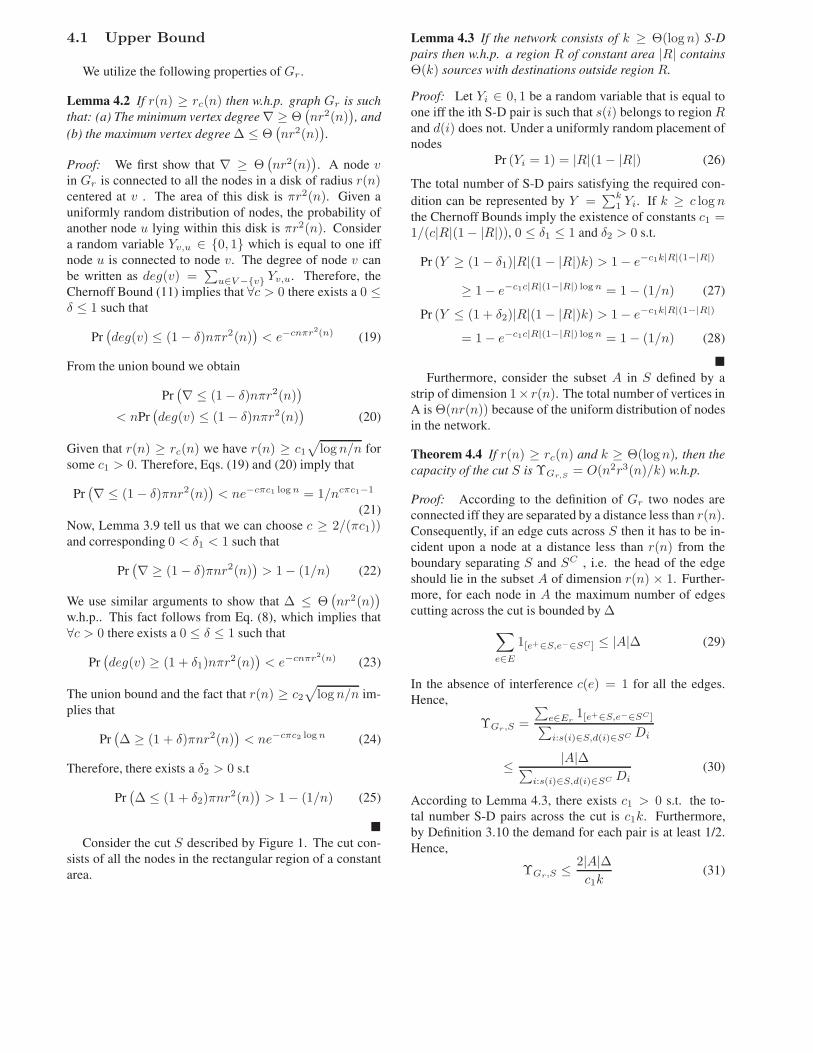
Figure 2. Decomposition of network area intol2 squarelets, each of side-length r(n)/3

To describe a capacity-achieving flow in a more genericsetting, we use an important result from parallel and dis-tributed computing. Consider a mesh of l2 processing unitswith l processors in each row and column. Let each proces-sor be a source and destination of exactly h packets. Theproblem of routing the hl2 packets to their destinations isknown as h × h permutation routing and can be character-ized by the following result [12].

Lemma 4.6 If in a single slot, each processor can trans-mit one packet each to its immediate horizontal and verticalneighbors, then an h×h permutation routing in a l×l meshcan be performed deterministically in hl/2 + o(hl) steps.

We utilize the following corollary that can be readily de-duced from the above Lemma.

Corollary 4.7 If a processor is capable of transmitting atleast η packets to each of its neighbors in each slot, then anh×h permutation routing in a l× l mesh can be performeddeterministically in O(hl/η) steps.

Now consider a sub-graph Hr ⊆ Gr obtained by em-ploying location based constraints on the edge-set. In orderto describe these constraints, we first define a location de-pendent hash function.

Definition 4.8 Index Function ζ:Divide the network area into l2 squarelets [11] of side-length a = r(n)/3 , as shown in Figure 2. Let ζ be afunction that associates an index (i, j) with a squarelet inthe ith column and jth row. Furthurmore, the index as-signed to each squarelet is associated with each vertex inthe squarelet.

We obtain Hr by removing all edges, except those con-necting two nodes in vertically or horizontally adjacentsquarelets. We do not necessarily have to consider Hr inorder to obtain a lower bound on the interference-free ca-pacity. However, the performance bounds for Hr play animportant role when we analyze interference constrainednetworks in Section 5.

Definition 4.9 Geographically Restricted Sub-Graph Hr :The graph Hr(Vr, Er,H) is a sub-graph of Gr with an iden-tical node-set and an edge-set defined as:

Er,H = {e ∈ E | ζ(e−) = (a, b) ⇒ ζ(e+) = (a±1, b±1)}(33)

25%

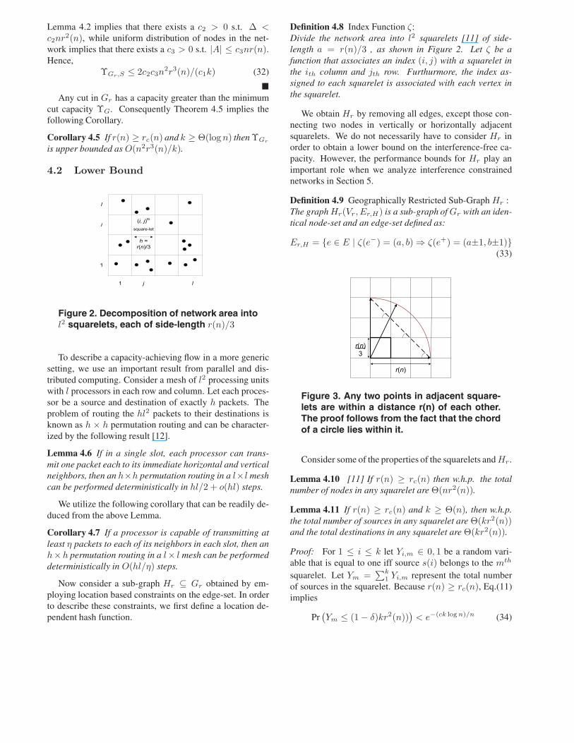
r(n)

r(n)3

Figure 3. Any two points in adjacent square-lets are within a distance r(n) of each other.The proof follows from the fact that the chordof a circle lies within it.

Consider some of the properties of the squarelets and Hr.

Lemma 4.10 [11] If r(n) ≥ rc(n) then w.h.p. the totalnumber of nodes in any squarelet are Θ(nr2(n)).

Lemma 4.11 If r(n) ≥ rc(n) and k ≥ Θ(n), then w.h.p.the total number of sources in any squarelet are Θ(kr2(n))and the total destinations in any squarelet are Θ(kr2(n)).

Proof: For 1 ≤ i ≤ k let Yi,m ∈ 0, 1 be a random vari-able that is equal to one iff source s(i) belongs to the mth

squarelet. Let Ym =∑k

1 Yi,m represent the total numberof sources in the squarelet. Because r(n) ≥ rc(n), Eq.(11)implies

Pr(Ym ≤ (1 − δ)kr2(n))

)< e−(ck log n)/n (34)

The total number of squarelets in a unit square is equal to

(3/r(n)) × (3/r(n)) ≤ c1n/ log n (35)

Therefore, the union bound implies that

Pr(min. no. of nodes in a squarelet < Θ(kr2(n)

)

≤ (total no. of squarelets) × e−(ck log n)/n

≤ (c1n/ logn) × e−(ck log n)/n

= c1/(n(ck/n)−1 log n) (36)

Thus, k ≥ Θ(n) guarantees the required convergence andhence each squarelet has at least Θ(kr2(n)) sources. Theupper bound on the number of sources and the bounds onthe number of destinations can be calculated similarly. �Theorem 4.12 If r(n) ≥ rc(n) and k ≥ Θ(n), then w.h.p.the maximum flow rate f∗

H in Hr is at least Θ(n2r3(n)/k

)

.

Proof: The proof follows from mapping various compo-nents of the above defined problem to the h×h permutationrouting problem. Let us map each squarelet to a processor.Consequently, for the chosen size of squarelets, the networkequates to a mesh of l2 processors with l = 3/r(n). As-sume that each source intends to transmit Di as the ith ele-ment of the demand vector. Because Di ≤ 1, Lemma 4.11implies that the total number of bits to be transmitted to andfrom each squarelet are at most h ≤ ckr2(n). Finally, notethat any two nodes in adjacent squarelets are within a dis-tance r(n). Fig. 3 provides a geometric proof for this fact;an alternative proof can be easily obtained by employing thePythagoras theorem. In each slot, we can send one packetalong each edge between two adjacent squarelets. There-fore, Lemma 4.10 implies that

η = (min. no. of edges between adjacent squarelets)≤ (min. no. of nodes per squarelet)2 ≤ c1n

2r4(n)

Hence, the total number of slots γ required to complete thedesired routing is

γ ≤ (c2hl/η)≤ c2 × (ckr2(n)) × (3/r(n)) × (1/c1n

2r4(n))= (3c2ck/c1n

2r3(n)) (37)

We can repeat the above routing periodically to guaranteea flow rate of f = (1/γ) ≥ Θ(n2r3(n)/k). By definition,the max-flow rate is greater than any other feasible flow rate,and the theorem follows. �

Aggregating the above results we have the followingconclusion.

Theorem 4.13 If r(n) ≥ Θ√

log n/n and k ≥ Θ(n), thenthe max- flow f∗

G in Gr can be approximated tightly by themin-cut capacity Υ∗

Grin Gr. Moreover, the f∗

G and Υ∗Gr

scale as Θ(n2r3(n)/k

).

Proof: Lemma 4.1 implies that f∗G ≥ f∗

H . Hence, theresult follows from the lower bound provided by Theorem4.12 and the upper bound provided by Corollary 4.5. �

Scaling laws for k = Θ(n) have been given special at-tention in the literature. Hence, it is worth stating explicitlythe above results for this scenario.

Corollary 4.14 Consider an ad-hoc network described bya random placement of n nodes in a unit square, withΘ(n) S-D pairs and a homogenous transmission range ofr(n) ≥ Θ(

√log n/n). The interference-free capacity of

the network scales as Θ(nr3(n)

).

5 Interference-Limited Capacity

5.1 General Results

Interference can severely limit the network capacity. Inthis section we obtain scaling laws for the SPR, MPR andMPTR interference models. We primarily focus on deduc-ing lower bounds. Moreover, to facilitate a succinct analy-sis, we develop some additional terminology and establishsome important results.

Recall from Section 3 that, for two different communi-cation schemes A and B (e.g., SPR and MPR) defined inthe same graph, their corresponding interference functionsIA and IB are different.

Definition 5.1 Dual-Interference-Set:Consider an edge set E and an interference set I(e) foran edge e ∈ E, as defined in Definition 3.3. The dualinterference-set for e is defined by F (e) = {e ∈ E | e ∈I(e)}, which is the set of edges that experience a collisionon account of a transmission on edge e.

Definition 5.2 Dual Conflict Graph:Given a graph G(V, E) and an interference function I ,we defined the dual conflict graph as GD(E, ED) , whereED = {(e, e) | e ∈ I(e))}.

Definition 5.3 Total Degree in Dual Conflict Graph:The total degree of each node in a dual conflict graph isequal to |M(e)| where M(e) = I(e)

⋃F (e).

Similar to the work in [16], we have the followingLemma.

Lemma 5.4 Consider a graph G(V, E) and interference I .Let κ = maxe∈E |M(e)| . If f is a feasible flow rate in theabsence of interference, then flow rate fI = f/(1 + κ) isfeasible in presence of interference I .

Proof: In the absence of interference the capacity of eachedge is assumed to be one. However, because of interfer-ence, all edges cannot be activated simultaneously. Let σ

be the minimum frequency with which each edge is acti-vated without causing any interference conflicts. Then, foreach edge we have c(e) ≥ 1/σ.

Observe that κ is the maximum vertex degree of the dualconflict graph GD . It is well known that, if κ is the maxi-mum vertex degree, then κ + 1 colors are sufficient to pro-vide a proper vertex coloring [2]. Thus, we can partition theedge-set E into 1 + κ subsets such that no two edges in thesame subset interfere. Consequently, we can periodicallyactivate these subsets to realize c(e) ≥ 1/(1 + κ) for eachedge. Thus, a feasible flow rate fI = f/(1 + κ) can beobtained by scaling the flow functions associated with f bya factor of 1/(1 + κ). �

The maximum vertex degree does not provide a tightbound on the minimum number of colors required to pro-vide a proper vertex coloring. Hence, in order to analyze awider variety of protocol models, we introduce the conceptof interference clones.

Definition 5.5 Interference Clone:Two edges e1, e2 are said to be interference-clones un-der function I if they satisfy the conditions that M(e1) =M(e2).

Lemma 5.6 Clone Piggy-backing Lemma: Consider agraph G(V, E) along with interference functions IA andIB , then IA and IB are such that:

1. κ = maxe∈E |MA(e)|2. ∀e ∈ E there exists a set MA,B(e) ⊆ MA(e) such that

every edge belonging MA,B(e) is an interference-cloneof e under IB . Further, let μ = mine∈E |MAB(e)|.

If f is a feasible flow rate in G without any interference,fIA = f/(1 + κ) is a feasible flow rate in G under the IA

interference function and κ as its correponding parameter,then fIB = f(1 + μ)/(1 + κ) is feasible in presence ofinterference defined by IB .

Proof: Consider the interference defined by IA. FromLemma 5.4 we know that there exists a conflict free peri-odic schedule which can activate each edge at least onceevery (1 + κ) slots. Let us represent this schedule by anindicator function α(e, τ) which equals one iff edge e is ac-tive in slot τ . Note that the capacity of each edge underschedule α is given by

cα(e) = Στα(e, τ) = 1/(1 + κ). (38)

Now let us use this schedule in the presence of interferenceIB . Observe that, for every e, α allocates a distinct slotfor each edge in MA,B(e)

⋂{e}. Consequently, every edgehas |MA,B(e)| interference clones scheduled in slots dis-tinct from each other and the edge itself. In addition, notethat if an edge is activated in a time slot meant for one of

its interference clones, then it does not lead to any conflict.Therefore, we can define a new conflict-free schedule βsuch that β(e, τ) = 1 iff there exits an e1 ∈ MA,B(e)

⋂{e}such that α(e1, τ) = 1. Given that μ = mine∈E |MAB(e)|,the capacity of each edge under schedule β for interferenceIB , is given by

cβ(e) = Σe1∈MA,BΣτα(e1, τ)

≤ (1 + μ) × (1/(1 + κ)) (39)

Accordingly, a feasible flow of fIB = f(1 + μ)/(1 + κ)can be obtained by scaling all the flow functions associatedwith the inference-free flow by a factor of (1+μ)

(1+κ) . �In the subsequent discussion, we find it convenient to

deduce a bound for a particular interference model and thenshow that it applies to a wider set of models. In order tofacilitate such arguments, we define the following partialorder.

Definition 5.7 Partial Order of Interference Models:An interference function IA is said to be more restrictivethan IB , represented as IA IB , iff every edge satisfiesthe conditions that IB(e) ⊆ IA(e) .

Lemma 5.8 Consider a graph G(V, E) along with inter-ference IA and IB . If IA IB , then a feasible flow rateunder IA remains feasible under IB .

Proof: A conflict free schedule under IA remains conflictfree under IB . Hence we can say that

cA(e) ≤ cB(e) (40)

where cA(e) and cB(e) represent the edge capacities undereach interference model. Therefore, if a particular flow sat-isfies the capacity constraints under IA, it necessarily satis-fies those same constraints under IB . �

5.2 Lower Bounds

Direct analysis of the interference models can be tedious.Hence, for mathematical convenience, we consider the fol-lowing restrictive models. Lemma 5.8 allows us to utilizethe performance limits under these restrictive models to in-directly bind the capacity under the interference models forSPR, MPR and MPTR.

We define a restrictive interference model that introducesmore restrictions (i.e., collisions) on the interference set foreach edge than those strictly dictated by the original in-terference model. We will show that, under this restric-tive model, the order of the lower bound capacity achievesthe upper bound under the original (non-restrictive) inter-ference model.

Definition 5.9 Restricted SPR (RSPR) Model:

IRSPR(e) = W (e) − {e} ∀e ∈ Er,H

where W (e) =⋃

e:ζ(e−)=ζ(e−)

MSPR(e) (41)

Definition 5.10 Restricted MPR (RMPR) Model:

IRMPR(e) = W (e) − U(e) ∀e ∈ Er,H

where U(e) ={e ∈ Er,H | e− = e−

}(42)

Definition 5.11 Restricted MPTR (RMPTR) Model:

IRMPTR(e) = W (e) − V (e) ∀e ∈ Er,H

where V (e) =⋃

e:ζ(e−)=ζ(e−)

U(e) (43)

Consider the following properties of the restricted mod-els.

Lemma 5.12 For the graph Hr, we have a partial orderdefined by (i) ISPR IMPR IMPTR, (ii) IRSPR IRMPR IRMPTR, (iii) ISPR IRSPR (iv) IRMPR IMPR (v) IRMPTR IMPTR

Proof: (Sketch) The proof for the partial orders (i) to (iii)follows directly from the definitions. Partial order (iv) fol-lows from the fact that J(e) ⊆ W (e) and U(e) ⊆ A(e) −B(e). Similarly, the fact that A(e) ⊆ V (e) implies partialorder (v). �

Lemma 5.13 If r(n) ≥ rc(n), then all edgese ∈ Er,H have |M(e)| = Θ

(n2r4(n)

)under

interference described by either of the models:ISPR, IMPR, IMPTR, IRSPR, IRMPR, IRMPTR.

Proof: From Lemma 5.12 we can conclude that RSPRis the most restrictive model, while MPTR is the least re-strictive model. Further note that FRSPR(e) ⊆ W (e) andIMPTR(e) ⊆ MMPTR(e). Hence, it suffices to prove the fol-lowing:

γmax = maxe∈Er,H |W (e)| = O(n2r4(n)) (44)

γmin = mine∈Er,H |IMPTR(e)| = Ω(n2r4(n)) (45)

Recall that a node in Hr is connected to all and only thosenodes that are placed in adjacent squarelets. Hence Lemma4.10 tells us that the degree of each vertex v ∈ Hr isbounded as

4c1nr2(n) ≤ deg(v) ≤ 4c2nr2(n) (46)

Now lets prove the lower bound by considering the modelMPTR. According to Definition 3.6, the transmission onedge e experiences interference from any transmission by

a node v such that r(n) < ‖Xe− − Xv‖ ≤ (1 + η)r(n).Therefore, there exists an annular ring around e− of widthηr(n) such that any transmission from a node in this ringinterferes with e. The area of this annular ring is given by

area of annular ring = η(2 + η)πr2(n) (47)

We have already seen ( Lemma 4.2) that an area ofΘ(r2(n)) contains at least Θ(nr2(n)) nodes. Hence, thereexists a c3 such that

γmin ≥ c3nr2(n) × 4c1nr2(n) (48)

Eq. (48) proves the reqd. lower bound. The proof for theupper bound is obtained with a similar argument. First, letus inspect the transmission along edge e under the SPRmodel. Any transmission from a node in a disk of ra-dius (1 + η)r(n) around e−, interferes with e. More-over, a transmission from e+ interferes with any recep-tion in a disk of radius (1 + η)r(n) around e+. Giventhat ‖Xe+ − Xe−‖ ≤ r(n), there exists a disk of ra-dius (2 + η)r(n) around e− containing all the nodes thatmay have transmission conflicts with e. Further note that asquarelet can be completely inscribed in a circum-circle ofradius (1/3

√2)r(n). Hence, there exists a circle of maxi-

mum radius R = (2 + η + (1/3√

2))r(n) containing all thenodes that may have transmission conflicts with e under themodel RSPR. The area of R is Θ(r2(n)) and hence thereexists a constant c4 such that

γmax = maxe∈Er,H |W (e)|≤ (max. no. of nodes in R) × (max. node degree)

≤ c4n(2 + η + (√

2/6))2r(n)2 × 4c2nr2(n)= O(n2r4(n)) (49)

�Lemma 5.14 Consider the graph Hr with r(n) ≥ rc(n)and k ≥ Θ(n). In such a graph, each edge e hasat least Θ

(nr2(n)

)clones under interference IRMPR and

Θ(n2r4(n)

)clones under interference IRMPTR, such that

these clones interfere with each other and e, under the in-terference IRSPR.

Proof: According to Definitions 5.10 and 5.11, U(e)and V (e) represent the desired set of clones for IRMPR andIRMPTR respectively. Lemma 4.10 implies that there exist c1

and c2 such that

μRMPR = mine∈Er,H |U(e)|≥ min. vertex degree = c1nr2(n) (50)

μRMPTR = mine∈Er,H |V (e)|≥ [mine∈Er,H |U(e)|] × min. nodes per squarelet

≥ c1nr2(n) × c2nr2(n) (51)

�

Theorem 5.15 For r(n) ≥ rc(n) and k ≥ Θ(n), thecapacity of random geometric network is at least: (a)Θ(1/r(n)k) under the SPR model, (b) Θ(nr(n)/k) underthe MPR model, and (c) Θ(n2r3(n)/k) under the MPTRmodel.

Proof: Recall that the capacity of the random network isgreater than the feasible flow rate in Hr. Theorem 4.12shows that a rate of f = c1n

2r3(n)/k is feasible in Hr.Additionally, Lemma 5.13 shows that the size of the largestinterference set under RSPR is at most κ = c2n

2r4(n).Hence, Lemma 5.4 implies that a rate of

fRSPR = f × (1/(1 + κ)) ≥ (c3/r(n)k) (52)

is feasible under the RSPR model. If we take into considera-tion the interference clones, then Lemma 5.6 further impliesthat the rate

fRMPR = f × (1/(1 + κ)) × (1 + μRMPR)≥ (c3/r(n)k) × (c4nr2(n))= (c3c4nr(n)/k) (53)

is feasible under the RMPR model. Similarly, the rate

fRMPTR = f × (1/(1 + κ)) × (1 + μRMPTR)≥ (c3/r(n)k) × (c5n

2r4(n))= (c3c5n

2r3(n)/k) (54)

is feasible under the RMPTR model. Finally, note that afeasible rate under a restricted model is necessarily feasi-ble under the original model. Hence, the result proven inLemma 5.13 completes the proof. �

5.3 Upper Bounds

The interference-free capacity provides an upper boundon the capacity under any model, and Theorem 5.15 alreadyshows that the MPTR model achieves this capacity. How-ever, we need to provide additional arguments to obtain atight bound on the capacity under SPR and MPR. Our argu-ments are similar to [15] and [6], and we briefly sketch theproof of the following result for the sake of completeness.

Theorem 5.16 For r(n) ≥ rc(n) and k ≥ Θ(n), thecapacity of random geometric network is at most: (a)Θ(1/r(n)k) under the SPR model, (b) Θ(nr(n)/k) underthe MPR model, and (c) Θ(n2r3(n)/k) under the MPTRmodel.

Proof: (Sketch) Consider the Cut S in Figure 1. The capac-ity of this cut and hence the network is less than

(no. of transmitters in A) × (max. tranmission per node)(1/2)k

(55)

The total number of transmitters in A is less than the totalnumber of nodes in A. We have already shown that the to-tal number of nodes is Θ(nr(n)). Under the MPTR model,each node can transmit a maximum of Θ(nr2(n)) packets,and under the MPR model each packet trasnmits just a sin-gle packet. This provides the bounds for MPR and MPTR.To obtain the bound for SPR, we note that each transmittersilences all the nodes within an area of Θ(r2(n)). Hence,only Θ(1/r(n)) nodes are capable of transmitting simulta-neously across a cut. Each of these nodes transmits a sin-gle packet and, therefore, the above equation provides thebound for SPR. �

6 Discussion

The results we have presented demonstrate that futuread hoc networks can scale well beyond the Gupta-Kumarcapacity bounds attained when nodes simply try to avoidMAI [8]. First, we showed that the optimal capacity thatany protocol architecture can attain in a wireless networkis Θ

(n2r3(n)/k

). Second, we demonstrated that this ca-

pacity can indeed be attained when nodes embrace MAI astransmitters and receivers, and that a non-vanishing capac-ity is attainable per S-D pair even when information must bedisseminated over multiple hops. Given that the majority ofnodes in an ad hoc network are sources and destinations ofinformation, we frame the rest of our discussion for the im-portant case of k = Θ(n).

The capacity under the SPR model when k = Θ(n)equals Θ(1/nr(n)), which is the well-known Gupta-Kumarresult, and shows that avoiding MAI in the communicationprotocols of ad hoc networks does not scale. Given that to-day’s ad hoc networks are based on interference avoidance,it is clear that massively scalable ad hoc networks cannotexist without substantial changes to the way in which pro-tocols are designed.

0 2 4 6 8 10

x 106

0

5

10

15

20

25

30

35

40

45

n

2η

min

/(lk

max)

mean observed valueminimum observed valuemaximum observed value

0.4 x n0.25

0.8 x n0.25

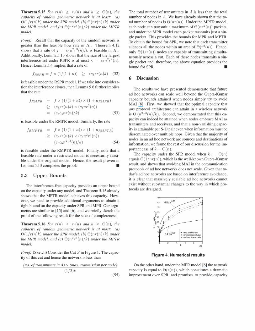
Figure 4. Numerical results

On the other hand, under the MPR model [6] the networkcapacity is equal to Θ(r(n)), which constitutes a dramaticimprovement over SPR, and promises to provide capacity

gains in practice by embracing interference at the receivers.However, to attain a non-vanishing capacity, r(n) must beΘ(1), i.e., use single-hop communication. Unfortunately,this is not feasible in practice, because of the energy thatwould be incurred in transmissions and the complexity re-quired for the receivers to decode a number of transmissionsin the order of the nodes in the network.

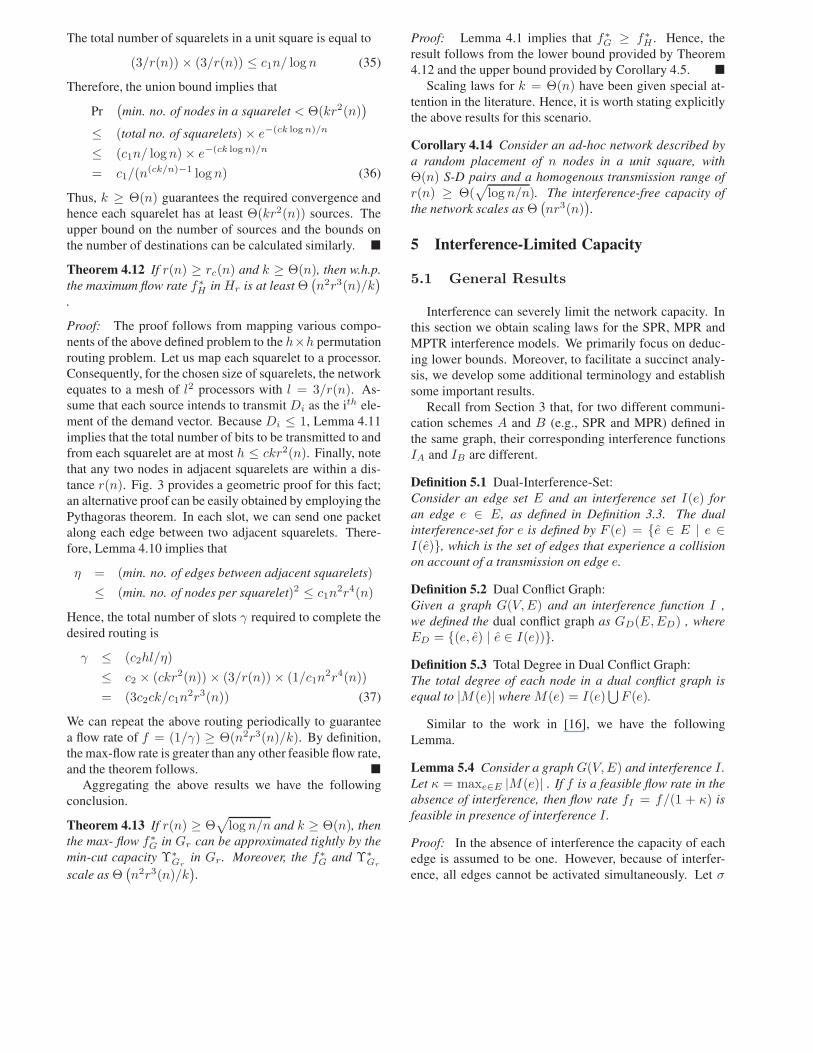
In contrast to the above, MPTR achieves the optimalper-node capacity of Θ(nr3(n)). Thus, any choice ofr(n) = Ω(n−1/3) allows us to increase the per-node ca-pacity of the network with n, while still having multihopcommunication. Moreover, the transmission range and hop-size decreases with n. As per our analysis, the capac-ity of a network is a constant factor of Γ, where Γ =2ηmin/l(kmax), such that ηmin is the minimum number ofedges between any two squarelets, kmax is the maximumnumber of sources or destinations in a single squarelet andl × l is the total number of squarelets. To illustrate this,we numerically evaluated the behavior of Γ as a function ofn. Figure 4 presents the mean, minimum and maximumobserved value of Γ over a thousand network topologiesrandomly generated and in which k = n/2 and r(n) =1/n0.25. Clearly, as n → ∞ we have r(n) → 0. Neverthe-less, the numerical results show that the per-node capacitystill increases as Θ(n0.25).

In closing, we should point out that, while our resultsprovide a completely new outlook on the design of wirelessad hoc networks, much work remains to be done to fully un-derstand their fundamental limits! For example, the resultswe have presented address only unicast traffic; our modelcan be used to study the cases of multicast and broadcastinformation dissemination. We also hope that this papermotivates research on protocol architectures that combinemulti-packet reception and transmission to attain massivelyscalable ad hoc networks.

7 Acknowledgments

This work was partially sponsored by the U.S. Army ResearchOffice under grants W911NF-04-1-0224 and W911NF-05-1-0246,by the National Science Foundation under grant CCF-0729230,by the Defense Advanced Research Projects Agency through AirForce Research Laboratory Contract FA8750-07-C-0169, and bythe Baskin Chair of Computer Engineering. The views and con-clusions contained in this document are those of the authors andshould not be interpreted as representing the official policies, ei-ther expressed or implied, of the U.S. Government.

References

[1] R. Ahlswede, C. Ning, S.-Y. R. Li, and R. W. Yeung. Net-work information flow. IEEE Transactions on InformationTheory, 46(4):1204–1216, 2000.

[2] B. Bollabas. Modern Graph Theory. Springer Verlag, 1998.

[3] R. M. de Moraes, H. R. Sadjadpour, and J. J. Garcia-Luna-Aceves. Many-to-many communication: A new approach forcollaboration in manets. In Proc. of IEEE INFOCOM 2007,Anchorage, Alaska, USA., May 6-12 2007.

[4] L. R. Ford and D. R. Fulkerson. Flows in Networks. Prince-ton Univ. Press, 1962.

[5] M. Franceschetti, O. Dousse, D. Tse, and P. Thiran. Clos-ing the gap in the capacity of wireless networks via perco-lation theory. IEEE Transactions on Information Theory,53(3):1009–1018, 2007.

[6] J. J. Garcia-Luna-Aceves, H. R. Sadjadpour, and Z. Wang.Challenges: Towards truly scalable ad hoc networks. InProc. of ACM MobiCom 2007, Montreal, Quebec, Canada,September 9-14 2007.

[7] M. Grossglauser and D. Tse. Mobility increases the capacityof ad hoc wireless networks. IEEE/ACM Transactions onNetworking, 10(4):477–486, 2002.

[8] P. Gupta and P. R. Kumar. The capacity of wireless networks.IEEE Transactions on Information Theory, 46(2):388–404,2000.

[9] S. Katti, S. Gollakota, and D. Katabi. Embracing wirelessinterference: Analog network coding. In Proc. of ACM SIG-COMM 2007, Kyoto, Japan, August 27-31 2007.

[10] P. Klein, S. A. Plotkin, and S. Rao. Excluded minors, net-work decomposition, and multicommodity flow. In Proc. ofACM symposium on Theory of computing, San Diego, Cali-fornia, USA, May 16-18 1993.

[11] S. Kulkarni and P. Viswanath. A deterministic approach tothroughput scaling wireless networks. IEEE Transactions onInformation Theory, 50(6):1041–1049, 2004.

[12] M. Kunde. Block gossiping on grids and tori: Deterministicsorting and routing match the bisection bound. In Proc. ofEuropean Symp. Algorithms, 1991.

[13] P. Kyasanur and N. Vaidya. Capacity of multi-channel wire-less networks: Impact of number of channels and interfaces.In Proc. of ACM MobiCom 2005, Cologne, Germany, August28-September 2 2005.

[14] T. Leighton and S. Rao. Multicommodity max-flow min-cut theorems and their use in designing approximation algo-rithms. Journal of the ACM, 46(6):787–832, 1999.

[15] J. Liu, D. Goeckel, and D. Towsley. Bounds on the gain ofnetwork coding and broadcasting in wireless networks. InProc. of IEEE INFOCOM 2007, Anchorage, Alaska, USA.,May 6-12 2007.

[16] R. Madan, D. Shah, and O. Leveque. Product multicommod-ity flow in wireless networks. Submitted to IEEE Transac-tions on Information Theory, 2007.

[17] A. Ozgur, O. Leveque, and D. Tse. Hierarchical coopera-tion achieves optimal capacity scaling in ad hoc networks.IEEE Transactions on Information Theory, 53(10):2549–3572, 2007.

[18] S. Toumpis and A. J. Goldsmith. Capacity regions for wire-less ad hoc networks. IEEE Transactions on Wireless Com-munications, 2(4):736–748, 2003.

[19] Y. Wu, P. A. Chou, and S.-Y. Kung. Information exchangein wireless networks with network coding and physical-layerbroadcast. In Proc. of CISS 2005, Baltimore, MD, March16-18 2005.