Robust Data Partitioning for Ad-hoc Query Processing

by Qui T. Nguyen

S.B., Massachusetts Institute of Technology, 2015

Submitted to theDepartment of Electrical Engineering and Computer Sciencein Partial Fulfillment of the Requirements for the Degree of

Master of Engineering in Electrical Engineering and Computer Science

at the

Massachusetts Institute of Technology

September 2015

c© Massachusetts Institute of Technology 2015. All rights reserved.

Author: . . . . . . . . . . . . . . . . . . . . . . . . . . . . . . . . . . . . . . . . . . . . . . . . . . . . . . . . . . . . . . . . . . . . . . . . . . . . . . . . . .Department of Electrical Engineering and Computer Science

August 18, 2015

Certified by: . . . . . . . . . . . . . . . . . . . . . . . . . . . . . . . . . . . . . . . . . . . . . . . . . . . . . . . . . . . . . . . . . . . . . . . . . . . . .Samuel Madden, Professor

August 18, 2015

Accepted by: . . . . . . . . . . . . . . . . . . . . . . . . . . . . . . . . . . . . . . . . . . . . . . . . . . . . . . . . . . . . . . . . . . . . . . . . . . . .Prof. Albert R. Meyer, Chairman, Masters of Engineering Thesis Committee

Robust Data Partitioning for Ad-hoc Query Processing

by Qui T. Nguyen

Submitted to the Department of Electrical Engineering and Computer Science

On August 18, 2015

In Partial Fulfillment of the Requirements for the Degree ofMaster of Engineering in Electrical Engineering and Computer Science

Abstract

Data partitioning can significantly improve query performance in distributed databasesystems. Most proposed data partitioning techniques choose the partitioning based on aparticular expected query workload or use a simple upfront scheme, such as uniform rangepartitioning or hash partitioning on a key. However, these techniques do not adequatelyaddress the case where the query workload is ad-hoc and unpredictable, as in many analyticapplications. The Hyper-Partitioning system aims to fill that gap, by using a novel space-partitioning tree on the space of possible attribute values to define partitions incorporatingall attributes of a dataset. The system creates a robust upfront partitioning tree, designedto benefit all possible queries, and then adapts it over time in response to the actualworkload. This thesis evaluates the robustness of the upfront hyper-partitioning algorithm,describes the implementation of the overall Hyper-Partitioning system, and shows howhyper-partitioning improves the performance of both selection and join queries.

Thesis Supervisor: Samuel MaddenTitle: Professor

2

Acknowledgements

First, I would like to acknowledge Alekh Jindal, Anil Shanbhag, and Aaron Elmore, whoworked tirelessly on this project with me, generously sharing their time, knowledge, andpatience.

I would also like to thank Prof. Samuel Madden, my thesis supervisor, for giving me theopportunity to work on this project and providing guidance and feedback throughout theprocess.

Finally, I am always grateful to my family and friends, who encouraged me to take onthis challenge and supported me along the way.

3

Contents

1 Introduction 6

1.1 Traditional database partitioning . . . . . . . . . . . . . . . . . . . . . . . . 8

1.2 Motivating problem . . . . . . . . . . . . . . . . . . . . . . . . . . . . . . . . 10

1.3 Hyper-partitioning overview . . . . . . . . . . . . . . . . . . . . . . . . . . . 10

1.4 Contributions . . . . . . . . . . . . . . . . . . . . . . . . . . . . . . . . . . . 11

2 Related Work 12

2.1 Workload-aware partitioning . . . . . . . . . . . . . . . . . . . . . . . . . . . 12

2.1.1 Partitioning in HDFS . . . . . . . . . . . . . . . . . . . . . . . . . . . 14

2.2 Multi-attribute database design . . . . . . . . . . . . . . . . . . . . . . . . . 14

2.2.1 Multi-attribute partitioning . . . . . . . . . . . . . . . . . . . . . . . 14

2.2.2 Multi-dimensional indexing . . . . . . . . . . . . . . . . . . . . . . . 15

2.3 Data block skipping . . . . . . . . . . . . . . . . . . . . . . . . . . . . . . . . 15

3 Robust Data Partitioning 17

3.1 Hyper-partitioning tree . . . . . . . . . . . . . . . . . . . . . . . . . . . . . . 18

3.1.1 Tree structure . . . . . . . . . . . . . . . . . . . . . . . . . . . . . . . 18

3.1.2 Partitioning a dataset . . . . . . . . . . . . . . . . . . . . . . . . . . 20

3.1.3 Distinction from k-d tree . . . . . . . . . . . . . . . . . . . . . . . . . 21

3.2 Robust hyper-partitioning algorithm . . . . . . . . . . . . . . . . . . . . . . 24

3.2.1 Balancing partition size . . . . . . . . . . . . . . . . . . . . . . . . . 24

3.2.2 Tree height . . . . . . . . . . . . . . . . . . . . . . . . . . . . . . . . 25

3.2.3 Balancing allocation . . . . . . . . . . . . . . . . . . . . . . . . . . . 25

4 Query Processing with Hyper-Partitioning 27

4.1 Selections . . . . . . . . . . . . . . . . . . . . . . . . . . . . . . . . . . . . . 27

4.2 Joins . . . . . . . . . . . . . . . . . . . . . . . . . . . . . . . . . . . . . . . . 28

4.2.1 Co-partitioning . . . . . . . . . . . . . . . . . . . . . . . . . . . . . . 30

4.2.2 Approximating co-partitioning with hyper-partitioning . . . . . . . . 31

4.2.3 Algorithms for forming rough co-partitionings . . . . . . . . . . . . . 34

4

5 Hyper-Partitioning System 405.1 System overview . . . . . . . . . . . . . . . . . . . . . . . . . . . . . . . . . 405.2 Upfront data partitioner . . . . . . . . . . . . . . . . . . . . . . . . . . . . . 42

5.2.1 Two-phase partitioning . . . . . . . . . . . . . . . . . . . . . . . . . . 435.2.2 Partitioning in parallel . . . . . . . . . . . . . . . . . . . . . . . . . . 445.2.3 Heterogeneous replicas . . . . . . . . . . . . . . . . . . . . . . . . . . 45

5.3 Physical operators . . . . . . . . . . . . . . . . . . . . . . . . . . . . . . . . 46

6 Evaluation 496.1 Robustness of partitioning tree . . . . . . . . . . . . . . . . . . . . . . . . . 49

6.1.1 Definitions . . . . . . . . . . . . . . . . . . . . . . . . . . . . . . . . . 506.1.2 Comparison to k-d tree . . . . . . . . . . . . . . . . . . . . . . . . . . 51

6.2 Query performance . . . . . . . . . . . . . . . . . . . . . . . . . . . . . . . . 536.2.1 Experimental setup . . . . . . . . . . . . . . . . . . . . . . . . . . . . 536.2.2 Selections . . . . . . . . . . . . . . . . . . . . . . . . . . . . . . . . . 536.2.3 Joins . . . . . . . . . . . . . . . . . . . . . . . . . . . . . . . . . . . . 54

6.3 Partitioning overhead . . . . . . . . . . . . . . . . . . . . . . . . . . . . . . . 56

7 Conclusion 58

5

Chapter 1

Introduction

Collecting data is steadily becoming cheaper and easier, leading to ever-larger datasets. This

big data, from wide-ranging sources such as sensors, financial transactions, and software logs,

has the potential to help people uncover new relationships and make more informed decisions,

but only if people can analyze it effectively.

In particular, we would like to design a database system that enables analysts to quickly

explore their datasets. Imagine an analyst considering the logs of every item ordered on a

popular e-commerce website, looking for untapped business opportunities. There is a large

variety of possible queries, and the results of a query may affect future queries. For example,

the analyst might ask which items sell best in a certain time of year, which items sell well

even when there is no discount, or which items are most often returned. If one of these queries

returns interesting results, then the analyst may ask additional related queries; otherwise,

the analyst may try other types of queries. The system should be able to support this type

of ad-hoc, unplanned query workload as efficiently as possible.

Big data poses significant challenges for analysis because of its sheer size. It would take far

too long for a single machine to process hundreds of gigabytes or terabytes of data. Instead,

big datasets are typically stored on multiple machines, in a distributed file system such as

6

Hadoop Distributed File System (HDFS). Then, the multiple machines can work in parallel

to answer queries.

In such a distributed system, the dataset is physically split, or partitioned, between the

machines. It may also be further partitioned on each machine into smaller partitions. The

way these partitions are chosen significantly affects the time any given query will take, and is

therefore an important area of investigation in distributed database design.

Most proposed techniques for data partitioning require a typical query workload. This

workload may be predicted in advance, based on the expected usage of the dataset, or gathered

over time as the database system is used, but either way, these techniques optimize the data

partitioning to suit that particular workload. They do not adequately address the situation

highlighted above, where the business analyst makes ad-hoc queries. In that situation, the

workload cannot be predicted in advance and may change over time.

The Hyper-Partitioning system has been designed to solve this kind of problem. It

aims to create a robust upfront partitioning that can benefit all queries, thus removing the

need for an expected query workload in advance and enabling efficient ad-hoc analysis from

the start. It then adapts the partitioning over time to increase efficiency even further. The

system is currently being investigated by the Database Group at MIT’s Computer Science

and Artificial Intelligence Laboratory.

This thesis will validate the robustness of the upfront hyper-partitioning algorithm,

describe the implementation of the overall Hyper-Partitioning system, and show how

hyper-partitioning improves the performance of queries. 1

1This work was done as part of a team. I was principally responsible for evaluating the robustness ofthe upfront partitioning algorithm, developing the join algorithms for hyper-partitioning, and running theexperiments.

7

1.1 Traditional database partitioning

Database partitioning involves dividing the data in a database into separate physical parts. It

is typically done for three main reasons: to distribute data, to tolerate failures, or to improve

performance. For example, if a dataset is too large to be stored on a single machine, it can be

partitioned into parts to be distributed among a cluster of machines. Each partition might be

stored on a single machine, or stored on multiple machines for fault-tolerance. Partitioning

also goes beyond simply dividing data among machines. The data may be further partitioned

within each machine to improve performance.

A dataset consists of a collection of records, where each record consists of values for some

set of attributes. In partitioning, the partitions are typically formed based on one or more

attributes of the dataset, i.e., each record is mapped to a partition based on some function

applied to its values for those attribute(s). For instance, if the partitioning attribute were

price, each record might be mapped to a partition based on the range its price attribute fell

within. In that case, we would say that the dataset was range-partitioned on price. Another

common type of partitioning is hash partitioning, where each record is mapped to a partition

with a hash function on the attribute values.

Roughly, partitioning improves performance by laying out the data in a more organized

way. If the data system can quickly determine the partition that each data record is located

in, the system can also determine which partitions do not contain any records matching a

given query. The database system can then skip those irrelevant partitions for that query,

allowing it to answer the query more quickly.

More concretely, consider a dataset that is range-partitioned into three partitions on one

attribute, the ID of each data record r. Each partition Pi only contains records with IDs in a

certain range, e.g.

P1 = {r | 0 ≤ r.id < 700}

8

P2 = {r | 700 ≤ r.id < 1200}

P3 = {r | 1200 ≤ r.id < 2000}

Then, given the query ‘r.ID < 1000’ the system only has to read the records in the partitions

whose ranges include IDs less than 1000, namely P1 and P2. It does not have to scan P3.

Without the partitioning given above, the system might have needed to scan the entire

dataset.

In general, if a dataset is partitioned on the same attribute that a query is based on, the

performance of that query improves significantly because the system can use the partition

information to skip partitions that do not match the query. Therefore, deciding which

attributes to partition on, and how records map to partitions, is an important part of

database system design. It becomes even more critical in large database systems, where

scanning the entire dataset for a single query is impractical.

In the most conventional approach, the database is partitioned on a single attribute. This

partitioning attribute would typically be the attribute used by the most time-consuming or

frequent queries. Many more sophisticated techniques for partitioning data have also been

proposed, but they all share a fundamental weakness. Specifically, they all construct the

partitions based on the types of queries that are expected to run, or have run in the past.

Queries outside the expected workload will still perform badly. These types of techniques are

inadequate for the case we are considering, ad-hoc queries, because in this case, the query

workload is not known a priori. We would like to have a data partitioning technique that

can provide performance gains for all types of possible queries, not just queries within some

restricted set.

9

1.2 Motivating problem

To reiterate, the overall problem this thesis targets is ad-hoc query processing, where the

query workload is unknown in advance and may change over time. This kind of query

processing is common in big data analytic applications, because the important features of

a big dataset may not be obvious before the data is analyzed, and these features may shift

as analysts gain a better understanding of the data or external priorities change. Some

examples of big datasets of current interest to researchers are interactions on social networks,

measurements from large-scale scientific surveys, and the economic actions of consumers.

Partitioning datasets can significantly speed up query times, making the analysis of

big data more tractable, but current partitioning techniques depend on an expected query

workload and are therefore unsuitable for ad-hoc analysis. We would like to develop a data

processing system that can improve the performance of queries, like traditional database

partitioning, but is not limited to particular types of queries.

1.3 Hyper-partitioning overview

Our proposed solution is the Hyper-Partitioning system. It aims to support ad-hoc

query processing in two ways: first, by creating an initial robust partitioning that provides

balanced performance improvements for queries on every attribute in a dataset, and second,

by gradually adapting the partitioning in response to the actual workload, to provide better

performance once a particular workload has emerged.

The main idea behind hyper-partitioning is to range-partition the dataset on all of its

attributes at once, into relatively small blocks of data. Each partition would then hold records

that fall into a certain hypercube of the attribute value space. As long as the partitions are

not too small, this should improve the performance of queries on any attribute, fulfilling

our goal of not needing the query workload a priori. The initial partitioning balances the

10

improvements across all attributes, while the adaptive component refines the partitioning to

increase the benefit for frequent types of queries.

In this thesis, I focus on static hyper-partitioning, without the adaptive component. I

show that the upfront hyper-partitioning algorithm creates a robust partitioning, discuss how

the partitions created through hyper-partitioning can be used to speed up query processing,

and evaluate the gains hyper-partitioning provides for upfront query performance.

1.4 Contributions

The contributions of this thesis are:

• We describe how the partitioning created by hyper-partitioning may be used to speed

up queries, particularly joins

• We describe the implementation of the Hyper-Partitioning system and how it can

be integrated into a general data processing system

• We demonstrate the robustness of the upfront hyper-partitioning algorithm

• We evaluate the gains in query performance with hyper-partitioning, for both selections

and joins

11

Chapter 2

Related Work

This thesis focuses on finding a robust, multi-attribute partitioning for a database when no

typical query workload exists, in order to support ad-hoc analytical applications. In this

chapter, I discuss related work in partitioning and ad-hoc query processing.

Note that there are two ways to partition a database: horizontally, into partitions of

records, or vertically, into partitions of attributes. Previous work has considered vertical

partitioning decisions extensively, addressing both the optimal choice of an upfront vertical

partitioning given a typical workload [25, 10, 16], as well as the adaptation of vertical

partitioning in response to the actual workload [15]. Our work, however, uses horizontal

partitioning, so the rest of the discussion about partitioning in this chapter will concentrate

on horizontal partitioning.

2.1 Workload-aware partitioning

A large body of work exists on automatically finding the optimal horizontal partitioning of a

database when a typical query workload is available.

One popular approach is recommending an upfront partitioning that minimizes the

12

estimated cost of an expected query workload. The partitioning advisor can either directly

use the query optimizer of a database system to recommend partitioning plans and estimate

their costs [29], or be more deeply integrated with the optimizer [20]. Other researchers have

also used optimizer-based methods to consider horizontal partitioning decisions together with

other physical design decisions, such as vertical partitioning, indexes, or materialized views

[1, 39].

Another area of work focuses on upfront horizontal partitioning specifically for online

transaction processing (OLTP) workloads, in which queries access fine-grained portions of

data, as opposed to coarse-grained analytical queries. The aim is to minimize the number of

cross-partition transactions, which are the most expensive, especially when the partitions are

on separate machines. One idea is to represent the expected query workload as a graph, and

find good partitionings from partitioning the graph [4]. The graph may be compressed [28], or

the cost model may be extended to consider skew in addition to the number of cross-partition

transactions [26].

Finally, database cracking is a technique that adaptively partitions the dataset and builds

an index [17, 13]. In contrast to the other approaches described above, the dataset is not

partitioned at once upfront. Instead, as queries are processed, the attributes in each query

are used to decide how to split the data into more fine-grained partitions. As a result, the

first few queries do not receive as much benefit [30]. Furthermore, attributes can only be

cracked independently, and the cracking attributes must be chosen in advance.

In our work, the workload is ad-hoc and unpredictable, so there is not a set of typical

queries that we can use to optimize the partitioning. Instead, we attempt to develop an

optimal upfront partitioning with the assumption that all possible queries are equally likely.

13

2.1.1 Partitioning in HDFS

In particular, our work uses HDFS as the storage engine. By default, HDFS partitions

datasets based simply on size, into evenly sized blocks, without regard to the content of

the blocks. Various data processing tools on top of HDFS, e.g. Pig [23], Hive [37], and

Impala [14], add support for attribute-based partitions. These tools just create traditional,

single-attribute partitions, but still give the developer some ability to optimize the data

layout for a workload.

Researchers have also built extensions of HDFS capable of more advanced partitioning,

given information about the query workload. Hadoop++ [5] can co-partition data within

blocks to make joins more efficient, and CoHadoop [7] can co-locate related partitions. We

aim to extend HDFS even further to partition on many attributes at once.

2.2 Multi-attribute database design

When the data of interest is many-dimensional, adding support for multiple attributes to the

database system can significantly speed up query processing.

2.2.1 Multi-attribute partitioning

One approach to incorporating multiple attributes in the database is creating multi-attribute

horizontal partitionings. Like the methods for single-attribute horizontal partitioning, the

following automatic methods require a typical workload, unlike our approach. MAGIC [9]

declusters data using two or more attributes, aiming to balance the work in a given query

workload equally among a set of processors. The resulting partitions are stored in directories

in the file system. In Teradata [35], possible partitioning ranges for each attribute are

extracted from the queries and combined to create a multi-attribute partitioning. Similarly,

multi-dimensional clustering selects the clustering keys from the workload, then uses every

14

unique combination of the values of each clustering key as a cluster [24, 18].

Manual multi-attribute partitioning is possible, as well. The relational database manage-

ment systems Oracle and MySQL support sub-partitioning to create nested partitions on

multiple attributes, although sub-partitions can only be hash partitions, and the order of the

nested attributes must be chosen carefully [34, 33].

2.2.2 Multi-dimensional indexing

Another way to add support for multiple attributes is to add a multi-dimensional index

structure, which speeds up the lookup times for multi-dimensional records.

The database literature covers many different types of multi-dimensional indexes. Some

commonly used indexes include k-d trees [3], R-trees [11], quad-trees [8], and grid files [21].

A database system can simply build one of these multi-dimensional indexes on a dataset and

use it to retrieve records for queries.

Multi-dimensional indexes can also be integrated more deeply with the database system.

SpatialHadoop [6] adds native support for spatial data processing to MapReduce, by par-

titioning the data on each node with a grid file or R-tree index, then using the indexes to

implement spatial operators. MD-HBase [22] transforms a multi-dimensional index into a

one-dimensional key space with Z-ordering, to enable efficient queries on spatio-temporal

data stored in a basic key-value store. The index may be a k-d tree or a quad-tree. So far,

however, these multi-dimensional systems have only been designed to handle two or three

dimensions, while our proposed system is designed to handle many more.

2.3 Data block skipping

Recent systems built for ad-hoc, analytical workloads expedite query processing by supporting

data block skipping. By maintaining some metadata about each block of data, and using it to

15

determine whether or not each block is relevant to a given query, the system can access less

data and avoid excessive random disk access. These blocks are not necessarily attribute-based

partitions. Brighthouse [32] is a column-oriented system that uses size-based blocks and stores

several types of derived metadata about the blocks, such as bitmaps of the values present

and matrices recording relationships between pairs of blocks, to optimize queries. Another

approach is small material aggregates [19], where aggregate values such as the minimum and

maximum are stored for every block of records.

Other systems do use an attribute-based partitioning. Google’s PowerDrill system [12]

partitions the dataset into chunks based on a few chosen attributes to facilitate skipping.

Recently, [36] proposed extracting features from a query workload and using those features to

define data blocks, better fitting the data blocking to the workload to maximize the potential

for skipping. Like these systems, our approach creates data blocks with a partitioning, but

the partitioning is defined on all the attributes, does not require a set workload, and can be

used for other types of queries beyond selections, e.g. joins.

16

Chapter 3

Robust Data Partitioning

This chapter discusses the upfront hyper-partitioning algorithm, which aims to create a robust

partitioning that will benefit all queries equally, well-suited for ad-hoc workloads.

To create such a partitioning, we look to space-partitioning trees, which recursively divide

a multi-dimensional space into non-overlapping regions. If we build a space-partitioning tree

on the value space of all the attributes in a dataset, the regions created by the tree will define

a partitioning of the data. Furthermore, using a tree to define the partitioning is desirable

because we can then use the tree to easily search for specific partitions. For our purposes, we

modified the conventional k-d tree, which is a commonly used space-partitioning tree. We

call this modified tree a hyper-partitioning tree. Our modifications allow the tree to adjust its

partitioning to the number of attributes in the dataset, making the final partitioning more

evenly distributed.

First, I describe the hyper-partitioning tree. Then, I describe the upfront hyper-

partitioning algorithm, which builds a hyper-partitioning tree that will specify a robust,

balanced partitioning of a given set of records. Note that this discussion provides necessary

background for the rest of the thesis, but is not a primary contribution of this work. See [31]

for more details on the hyper-partitioning tree and algorithm.

17

3.1 Hyper-partitioning tree

The hyper-partitioning tree is a generalization of the conventional k-d tree [3]. The structure

of the hyper-partitioning tree remains the same, so this section first describes that structure.

Then, the key difference between the trees, a relaxation of one of the k-d tree’s constraints, is

discussed.

3.1.1 Tree structure

The k-d tree is an extension of the binary search tree to multiple dimensions. Recall that a

binary search tree is a binary tree of nodes, where the nodes have values and are arranged

such that their values satisfy the binary search tree property. In a binary tree, each node has

at most two child nodes, referred to as the right child and the left child. These children may

have children of their own, forming subtrees. One node is defined as the root, from which all

the other subtrees descend. The binary search tree property says that for any node, all of the

values in its left subtree must be less than the node’s value, and all of the values in its right

subtree must be greater. Typically these values are numbers, but they can be from any set of

objects with a defined total ordering.

The binary search tree property makes it possible to efficiently find a node with a certain

value in a binary search tree. Starting at the root, you can traverse the tree towards the

desired node by comparing the search value to the value of the current node and using the

binary search tree property to decide whether to continue searching in the left or the right

child. This will require a number of comparisons no more than the maximum height of the

tree.

The k-d tree extends the binary search tree to enable efficient searching for points in

k-dimensions, rather than just points with a single value. Each node in the k-d tree is

associated not only with a k-dimensional value, but also with a specific dimension called the

18

x = -8 x = -1

y = 2

x = 10

y = 3

x = 5

(a) k-d tree.

x = -8 x = -1

y = 2

x = 10

y = 3

x = 5

(b) k-d tree with buckets correspondingto regions.

10

10

x

y

(c) Regions of xy-space formed by tree.

Figure 3.1: Representations of an example k-d tree in xy-space.

discriminator of that node. Then, the search property is extended as follows:

k-d tree search property. For any node with discriminator dimension i, the

ith dimension of every value in its left subtree must be less than the value of that

node’s ith dimension, and the ith dimension of every value in its right subtree

must be greater.

Thus, each node in the tree splits the k-dimensional space in half with a hyperplane. All

points to the left of the hyperplane belong in the left subtree of that node, and all points to

the right of the hyperplane belong in the right subtree. Together, the hyperplanes combine

to split the k-dimensional space into non-overlapping regions.

Figure 3.1a shows an example of a k-d tree in two dimensions, x and y, and Figure 3.1c

19

is a visualization of how that tree splits the xy space. In two dimensions, the splitting

hyperplanes defined by each node are simply lines, either aligned with the x or y axis. First,

notice how each node only splits a specific part of the space. The root splits the entire space

into two parts, at x = 5. Then each of the root’s children splits one of those parts into smaller

parts, at y = 2 on one side and y = 3 on the other, and so on. We can define a mapping

from nodes to parts of the space, where each node maps to the part that it splits.

Now, that means no nodes in the tree map to the final regions defined by the tree, because

they are not split any further. Observe, however, that if we added a child node to any of the

existing nodes, that new node would split one of those final regions. Thus, each place in the

tree where a child could be added maps to one of the final regions.

To represent the final regions in the tree more concretely, then, we can add a special

non-splitting node, without a value or discriminator, at each of the places where a regular

node could have an additional child, as shown in Figure 3.1b. We call these special nodes

buckets.

3.1.2 Partitioning a dataset

With a k-d tree on the attribute value space of the dataset, each of the regions formed by

the tree, represented as a bucket, defines a partition of the data. A record is assigned to the

partition corresponding to the region that its location in the attribute value space belongs to.

It is possible that a record’s location would fall on the boundary of two or more regions.

In a k-d tree, if a point is on one of the splitting hyperplanes, meaning that the value of

its ith dimension is equal to the value of the ith dimension of some existing node in the tree

with discriminator i, it is unclear if the point belongs in the space of the left subtree or in

the space of the right subtree. The k-d tree paper [3] suggests the rest of the dimensions be

compared in sequence, such that the first non-equal dimension provides the ordering of the

two points, but also says any tiebreaker can be used. For simplicity, we assign any point on

20

the splitting hyperplane to the left subtree. This choice of tiebreaker also allows us to save

space: each node only has to store the value on its discriminator dimension, rather than all k

values in the k-dimensional point.

To be precise, to partition a dataset given a k-d tree, the k-d tree is searched for each

record as described below.

k-d tree search algorithm. Starting from the root, traverse the tree as follows:

• If the value of the current node on its discriminator dimension i is greater

than or equal to the value of the ith attribute of the record, then continue to

the left child.

• Otherwise, continue to the right child.

Since every branch of the tree ends in a bucket, searches will always terminate at some bucket.

Each record is assigned to the partition corresponding to the bucket found in its search.

3.1.3 Distinction from k-d tree

The structural details described so far apply to both the hyper-partitioning tree and the

conventional k-d tree. Now, I discuss the main distinction between the two types of trees,

which lies in the assignment of discriminator dimensions.

In a conventional k-d tree [3], all nodes on a given level have the same discriminator, and

the discriminator for each level cycles through the possible dimensions in the space. For

example, if there were three dimensions, the root node would split on the first dimension,

its child nodes on the second level would split on the second dimension, nodes on the third

level would split on the third dimension, nodes on the fourth level would split on the first

dimension again, and so on.

With this method of assigning discriminators, every dimension is only represented in the

tree if there are at least as many levels as dimensions. If the number of levels is less than k,

21

r.3 = 27r.3= 25 r.3 = 21 r.3 = 30

P121 P122P112P111 P211 P212 P221 P222

r.1 = 10

r.2 = 120 r.2 = 130

{r | r.1 ≤ 10, r.2 ≤ 120, r.3 ≤ 25}

{r | r.1 > 10, r.2 > 130, r.3 ≤ 27}

{r | r.1 > 10, r.2 > 130, r.3 > 27}

{r | r.1 ≤ 10, r.2 ≤ 120, r.3 > 25}

{r | r.1 ≤ 10, r.2 > 120, r.3 ≤ 21}

{r | r.1 ≤ 10, r.2 > 120, r.3 > 21}

{r | r.1 > 10, r.2 ≤ 130, r.3 ≤ 30}

{r | r.1 > 10, r.2 ≤ 130, r.3 > 30}

Figure 3.2: Example of partitioning with a k-d tree. Each node has a discriminator dimensionand a value for that dimension. The tree results in 8 partitions, each containing records rthat fulfill the conditions listed.

then the tree cannot split the space on some dimensions, and a dataset partitioned with that

tree will not be partitioned on those dimensions.

For example, take a dataset R with four attributes. Figure 3.2 shows an example of how it

might be partitioned with a k-d tree with three levels. Observe that each partition is defined

by three predicates, one for each of the first three attributes; the data is fully partitioned on

those three attributes. However, it is not partitioned on the fourth attribute at all.

Even if the number of levels in a tree is at least k, if it is not an exact multiple of k,

then some dimensions will be represented more often than others, resulting in an uneven

partitioning. Recall that the aim of our upfront partitioning is to provide an equal level of

partitioning for every attribute in a dataset, so that a query on any attribute is improved.

Therefore, for our purposes, the cyclical assignment of levels in the k-d tree to discriminator

dimensions is not ideal.

22

r.3 = 48r.4 = 87 r.4 = 83 r.2 = 112

P121 P122P112P111 P211 P212 P221 P222

r.1 = 10

r.2 = 120 r.3 = 25

{r | r.1 ≤ 10, r.2 ≤ 120, r.4 ≤ 87}

{r | r.1 > 10, r.3 > 25, r.3 ≤ 48}

{r | r.1 > 10, r.3 > 25, r.3 > 48}

{r | r.1 ≤ 10, r.2 ≤ 120, r.4 > 87}

{r | r.1 ≤ 10, r.2 > 120, r.4 ≤ 83}

{r | r.1 ≤ 10, r.2 > 120, r.4 > 83}

{r | r.1 > 10, r.3 ≤ 25,

r.2 ≤ 112}

{r | r.1 > 10, r.3 ≤ 25,

r.2 > 112}

Figure 3.3: Example of partitioning with a hyper-partitioning tree. The basic structure is thesame as a k-d tree, but the nodes on each level no longer have to use the same discriminator.

In contrast, our proposed hyper-partitioning tree [31] does not require that every node on

a given level have the same discriminator, allowing for more even partitioning. We call this

heterogeneous branching, because each branch may have a different sequence of discriminators.

Note that heterogeneous branching does not affect the basic structure or search algorithm

described above, just how discriminators can be assigned to nodes.

Figure 3.3 shows a possible hyper-partitioning tree with three levels on the same dataset

R as the previous example. Note how all four attributes are accomodated in the tree with

heterogeneous branching. Each branch does not include all four attributes, but because the

set of attributes in each branch can differ, every attribute is included in at least one branch.

A partition is defined by a predicate for each of the nodes in its corresponding branch, so the

data is not fully partitioned on each attribute, but it is at least partially partitioned on all of

them.

23

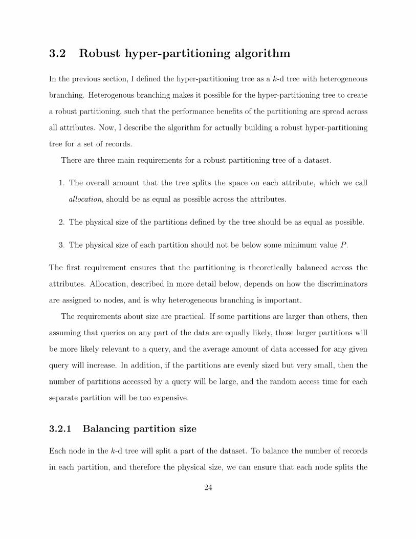
3.2 Robust hyper-partitioning algorithm

In the previous section, I defined the hyper-partitioning tree as a k-d tree with heterogeneous

branching. Heterogenous branching makes it possible for the hyper-partitioning tree to create

a robust partitioning, such that the performance benefits of the partitioning are spread across

all attributes. Now, I describe the algorithm for actually building a robust hyper-partitioning

tree for a set of records.

There are three main requirements for a robust partitioning tree of a dataset.

1. The overall amount that the tree splits the space on each attribute, which we call

allocation, should be as equal as possible across the attributes.

2. The physical size of the partitions defined by the tree should be as equal as possible.

3. The physical size of each partition should not be below some minimum value P .

The first requirement ensures that the partitioning is theoretically balanced across the

attributes. Allocation, described in more detail below, depends on how the discriminators

are assigned to nodes, and is why heterogeneous branching is important.

The requirements about size are practical. If some partitions are larger than others, then

assuming that queries on any part of the data are equally likely, those larger partitions will

be more likely relevant to a query, and the average amount of data accessed for any given

query will increase. In addition, if the partitions are evenly sized but very small, then the

number of partitions accessed by a query will be large, and the random access time for each

separate partition will be too expensive.

3.2.1 Balancing partition size

Each node in the k-d tree will split a part of the dataset. To balance the number of records

in each partition, and therefore the physical size, we can ensure that each node splits the

24

records in its space equally, and that each partition is formed from the same number of splits.

The discriminator of a node determines what dimension it splits on, and the value of a

node determines where it splits in that dimension. Assuming the discriminator has already

been decided, we choose the value of each node as the median value on the discriminator

dimension of the records located in the node’s space, so it splits the records equally.

Additionally, we want every bucket to be on the same level of the tree, so that each

partition is formed from the same number of splits. Therefore, we build the tree to be full,

meaning every node has exactly two children, except the nodes on the last level.

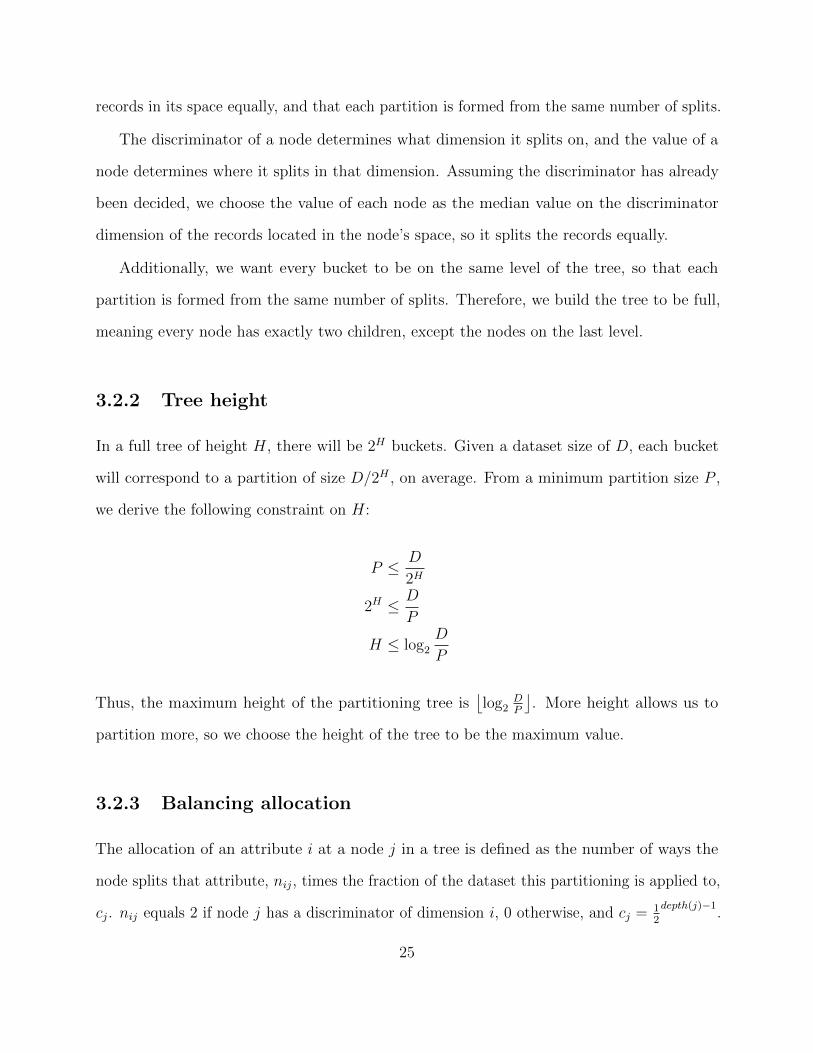
3.2.2 Tree height

In a full tree of height H, there will be 2H buckets. Given a dataset size of D, each bucket

will correspond to a partition of size D/2H , on average. From a minimum partition size P ,

we derive the following constraint on H:

P ≤ D

2H

2H ≤ D

P

H ≤ log2

D

P

Thus, the maximum height of the partitioning tree is⌊log2

DP

⌋. More height allows us to

partition more, so we choose the height of the tree to be the maximum value.

3.2.3 Balancing allocation

The allocation of an attribute i at a node j in a tree is defined as the number of ways the

node splits that attribute, nij , times the fraction of the dataset this partitioning is applied to,

cj . nij equals 2 if node j has a discriminator of dimension i, 0 otherwise, and cj = 12

depth(j)−1.

25

The allocation of an attribute, over all nodes in the tree, can be understood as the average

granularity of the partitioning on that attribute, considering both the parts of the dataset

that are partitioned on that attribute and those that are not.

For example, refer back to Figure 3.3. The total allocation of the first attribute is

2× 12

0= 2, the allocations of the second and third attributes are each 2× 1

2

1+ 2× 1

2

2= 1.5,

and the allocation of the fourth attribute is 2× 12

2+ 2× 1

2

2= 1.

The robust hyper-partitioning algorithm constructs the tree level by level, adding nodes

one at a time starting from the top. At each node, the algorithm chooses the attribute

that has the lowest allocation so far as the discriminator. Refer to [31] for more details and

pseudocode.

26

Chapter 4

Query Processing with

Hyper-Partitioning

Once a hyper-partitioning tree is built and the records are laid out in partitions accordingly,

the database system can use the hyper-partitioning structure to reduce data access costs for

queries. Our Hyper-Partitioning system can support any type of predicate-based data

access. In this chapter, I will discuss how hyper-partitioning can be used in selection and

join queries, particularly joins between two tables. Other types of queries, such as grouped

aggregates and multi-table joins, are left for future work.

4.1 Selections

A selection query retrieves records that satisfy some combination of predicates on the attributes

of the dataset. For example, possible predicates might be ‘r.id = 100’, ‘r.age > 30’, or

‘r.gender = F’.

Hyper-partitioning can be easily applied to selection queries to improve their performance.

The algorithm given previously for searching k-d trees for the partition of a specific record

27

can be generalized to search the tree for partitions that might contain records fulfilling a

given predicate. We traverse the tree’s nodes as follows, until buckets are reached. For each

node searched:

• If the node’s discriminator is not the same attribute as the predicate, then the node

does not help narrow down the search, and both of its subtrees must be searched.

• If the node’s discriminator matches the predicate, then from the tree’s search property,

we know all the records in the left subtree are less than or equal to the node’s value, and

the records in the right subtree are greater than its value. Depending on the values of

the operator and constant in the predicate, only the left subtree, only the right subtree,

or both subtrees must be searched.

The partitioning guarantees that no relevant records will be outside of the partitions

returned by the search. Using this search, the database system can skip all the partitions not

returned, reducing the data access time.

Figure 4.1 shows an example of the search for partitions that may contain records matching

a predicate.

4.2 Joins

A join query is a query that combines records from two or more tables, as specified by a join

predicate. For example, we might want to join each record from a table of orders O with

the record of the customer that placed that order, from the table of customers C. Here, the

join predicate would be ‘order.customer id = customer.id’, and the join query can be

defined as:

{(order, customer) ∈ (O × C) | order.customer id = customer.id}

28

r.3 = 48r.4 = 87 r.4 = 83 r.2 = 112

P121 P122P112P111 P211 P212 P221 P222

r.1 = 10

r.2 = 120 r.3 = 25

{r | r.1 ≤ 10, r.2 ≤ 120, r.4 ≤ 87}

{r | r.1 > 10, r.3 > 25, r.3 ≤ 48}

{r | r.1 > 10, r.3 > 25, r.3 > 48}

{r | r.1 ≤ 10, r.2 ≤ 120, r.4 > 87}

{r | r.1 ≤ 10, r.2 > 120, r.4 ≤ 83}

{r | r.1 ≤ 10, r.2 > 120, r.4 > 83}

{r | r.1 > 10, r.3 ≤ 25,

r.2 ≤ 112}

{r | r.1 > 10, r.3 ≤ 25,

r.2 > 112}

Figure 4.1: Example of searching the hyper-partitioning tree for partitions that could containrecords matching the predicate ‘r.2 > 130’. The gray nodes are those traversed by thesearch.

29

In general, many algorithms exist for executing join queries, and the choice of algorithm

depends on factors such as the size of the tables, the type of join predicate, and how the

tables are distributed or partitioned, if at all. In the rest of this section, we consider an

algorithm for the case of equijoin queries, join queries where the join predicate is an equality

relation, between two tables that are both hyper-partitioned.

4.2.1 Co-partitioning

First, I review how regular partitioning can be applied in the execution of equijoins, which

motivates our application of hyper-partitioning.

For equijoins, it can be beneficial to partition each table with the same method on

the join predicate attribute, which is called co-partitioning the tables on the join key. For

example, recall the join query between the orders and customers tables, with join predicate

‘order.customer id = customer.id’. The appropriate co-partitioning for this query would

be the orders table partitioned on customer id and the customers table partitioned on id,

using the same partition definitions. If range partitioning were being used, for instance, the

ranges of the partitions would be the same for both tables. With this co-partitioning, we

know that any customer records that may fulfill the join predicate with a record from a given

partition of orders must be located in the corresponding partition of customers, and vice

versa, so combining the joins of each pair of corresponding partitions will give the correct

overall join result.

In general, when the tables in an equijoin are co-partitioned, the pairs of corresponding

partitions from each table can be joined separately to fulfill the join query. Thus, the

appropriate co-partitioning can be beneficial in two ways. First, it enables parallelism,

significantly improving performance when multiple machines are available. Each pair of

partitions can be joined at the same time by a different machine.

Furthermore, joining the pairs of smaller partitions may be easier than joining the whole

30

tables. A simple hash join algorithm can be used to compute an equijoin when at least one

of the tables fits into memory. In this algorithm, each record of the smaller table is stored in

a hash table by its join key value. Then, each record from the second table is joined with the

matching records from the hash table. This simple algorithm can’t be used if both tables

are too large to be hashed in memory. However, if large tables are co-partitioned into small

enough partitions, their join can be easily computed by performing a hash join on each pair

of partitions instead.

Overall, computing an equijoin can be much faster if the appropriate co-partitioning for

the join predicate already exists. A pair of tables can only be co-partitioned on one attribute,

however, so only equijoins on that attribute will benefit. To execute equijoins with the tables

on other attributes, the data usually must be repartitioned.

4.2.2 Approximating co-partitioning with hyper-partitioning

We can achieve more balanced performance improvements for equijoins if tables are hyper-

partitioned on all of their attributes, rather than co-partitioned on one. The idea is that the

hyper-partitioning on each table can be used to approximate a co-partitioning on any key.

The reason co-partitioning on the join key is helpful in the execution of an equijoin is that

it allows the computation to be broken down into smaller joins. Each pair of corresponding

partitions in the co-partitioning can be joined separately. With hyper-partitioning, the data

is partially partitioned on every attribute. Intuitively, we can still break the computation into

smaller joins by grouping similar partitions together, even if the partitions do not exactly

match.

We call this grouping a rough co-partitioning. Each group in the rough co-partitioning

consists of a set of partitions from each table, such that the union of the joins of each group

will be equal to the original equijoin. The set of partitions from one table in each group must

also fit in memory, so that each group can be joined with a hash join.

31

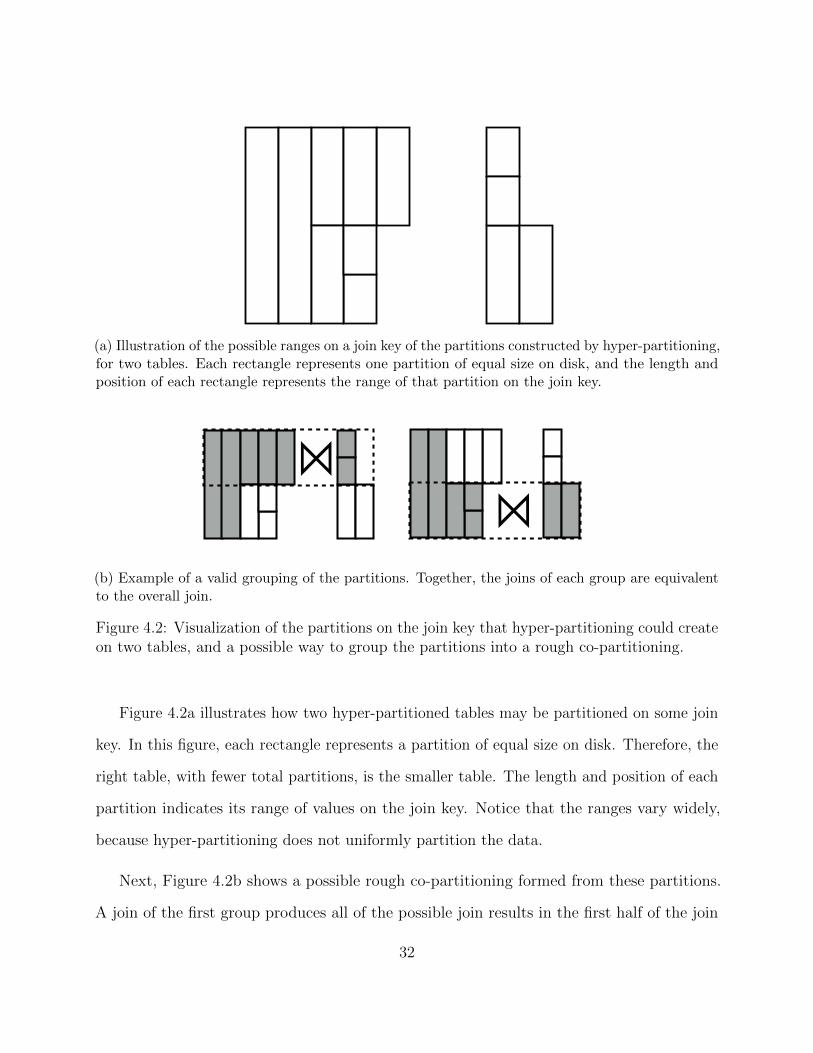
(a) Illustration of the possible ranges on a join key of the partitions constructed by hyper-partitioning,for two tables. Each rectangle represents one partition of equal size on disk, and the length andposition of each rectangle represents the range of that partition on the join key.

⋈⋈

(b) Example of a valid grouping of the partitions. Together, the joins of each group are equivalentto the overall join.

Figure 4.2: Visualization of the partitions on the join key that hyper-partitioning could createon two tables, and a possible way to group the partitions into a rough co-partitioning.

Figure 4.2a illustrates how two hyper-partitioned tables may be partitioned on some join

key. In this figure, each rectangle represents a partition of equal size on disk. Therefore, the

right table, with fewer total partitions, is the smaller table. The length and position of each

partition indicates its range of values on the join key. Notice that the ranges vary widely,

because hyper-partitioning does not uniformly partition the data.

Next, Figure 4.2b shows a possible rough co-partitioning formed from these partitions.

A join of the first group produces all of the possible join results in the first half of the join

32

key range, and a join of the second group produces all of the possible join results in the

second half. Notice that two partitions from the larger table on the left are included in both

groups. They contain records in both halves of the join key range, so they must be joined

with partitions from the other table covering both halves of the join key range.

This is just one of many possible groupings. Formally, we have two tables R and S, each

split into a set of partitions with hyper-partitioning:

R =⋃

Ri

S =⋃

Si

Given a join query between these tables with the predicate ‘r.keyR = s.keyS’, we would

like to find a set of groups {Gi}, where each group contains a subset of the partitions from

each table:

{Gi} = {(GRi, GSi)}

with

GRi ⊆ {Ri}

GSi ⊆ {Si}.

The union of the joins of these groups must be equal to the original join:

⋃i

{(r, s) ∈ (GRi ×GSi) | r.keyR = s.keyS} = {(r, s) ∈ (R× S) | r.keyR = s.keyS}

and for each pair Gi, either GRi or GSi must fit into memory.

Those constraints define all possible groupings {Gi} that will produce a correct join result.

Of these possibilities, we would like to find the one with the smallest cost. If the entire join

33

is being performed on one machine, then we want to find the grouping {Gi} that minimizes

the total input cost:

arg min{Gi}

∑Gi∈{Gi}

|Gi|

If the join is being performed in parallel on many machines, then each machine must process

some subset of the groups, and we would like to minimize the maximum work done by any

single machine.

We expect this rough co-partitioning approach to be slower than the ideal case, where an

exact co-partitioning on the join key exists, because in this approach, some partitions must

be included in more than one group. However, the exact co-partitioning can only exist for

one join key, while this approach will work for all possible join keys. As long as there are

not too many replicated partitions, this algorithm should be faster than repartitioning the

data into the appropriate co-partitioning before computing the join. Repartitioning the data

requires reading each record from each table and then writing each record to a new location,

so if the number of replicated records does not exceed two times the sum of the sizes of the

tables, using a rough co-partitioning will be advantageous.

4.2.3 Algorithms for forming rough co-partitionings

Clearly, this is a complex problem. The potential search space is huge: each group Gi in a

rough co-partitioning can consist of any non-empty subset of partitions from R and S, which

gives

|R| × 2|R|−1 × |S| × 2|S|−1

possibilities for each pair, before considering the constraints.

In this work, I present sketches of some heuristic algorithms for forming a rough co-

partitioning. Finding optimal solutions remains as future work.

34

Algorithm 1: Index Nested Loop Join

A simple solution is to split the join key domain into a set of ranges, and use these ranges to

define the groups. Each group Gi consists of the partitions that overlap with its assigned

range, found by searching the hyper-partitioning tree of each table for the range.

Figure 4.3a shows the groups formed by this algorithm with four ranges, on the same

example partitionings as before. This method is straightforward and simple to implement on

top of selection queries. However, partitions from each table that span a larger range than

the assigned ranges will be replicated many times, which can be observed in the figure. If the

tables are not partitioned with sufficient granularity, the rough co-partitioning formed by

this algorithm will have a high input cost.

Algorithm 1b: Index Nested Loops, Split

If many partitions are larger than the ranges chosen in Algorithm 1, then using a smaller

number of ranges, and thus larger ranges, may be beneficial. It will reduce the amount of

replication from both tables. The first example of rough co-partitioning, shown earlier in

Figure 4.2b, was formed by Algorithm 1 with two ranges.

With a smaller number of ranges, however, there are fewer groups, reducing the degree of

parallelism possible. To address this, the groups can be split. The set of partitions from the

larger table is distributed among the splits, while the same set of partitions from the smaller

table is added to each split. Splitting the groups increases the replication of partitions from

the smaller table, but as long as the increase in replication is not too large, the increase in

parallelism will compensate for it.

Figure 4.3b shows the groups after each group in Figure 4.2b is split once. Notice that the

total number of partitions in the groups is higher than before splitting (18, vs. 14), but the

maximum number of partitions per group is lower (5, vs. 7), so the splitting was beneficial

for parallelization.

35

⋈⋈

⋈⋈

(a) Algorithm 1: Index nested loops.

⋈ ⋈

⋈⋈

(b) Algorithm 1b: Index nested loops with larger ranges, split.

⋈⋈

⋈(c) Algorithm 2: Minimizing replication of the larger table.

Figure 4.3: Rough co-partitionings found by various algorithms.

36

In the example, this algorithm also produces a better grouping than the regular index

nested loops algorithm, with a lower overall cost and a lower maximum cost per worker. In

our experiments, we found this algorithm decreased the amount of replication as compared

to the regular index nested loops algorithm, but it may not be as effective for in all cases,

depending on the relative sizes of the tables being joined and the extent that the tables are

partitioning on the join attribute.

Algorithm 2: Minimizing Replication of the Larger Table

If the larger table is significantly larger than the smaller table, then it might make sense

to avoid replicating partitions from the larger table, even if replication of the smaller table

increases. In this algorithm, the partitions from the larger table with similar ranges on the

join key are grouped together. Then, for each of those groups, the partitions from the smaller

table whose ranges on the join key overlap partitions in that group are added.

With this approach, each partition from the larger table is contained in exactly one group,

eliminating all replication of the larger table. However, there may be heavy replication of the

smaller table because the join key ranges of the groups may be large and/or overlap with

each other. This will be detrimental if the smaller table is not much smaller than the larger

table. In addition, if the join key range of a group is large, the hash table of the overlapping

partitions from the smaller table may not fit in memory, making the grouping formed by this

algorithm infeasible in some cases.

Figure 4.3c illustrates the application of this algorithm. Observe how the presence of

some long-spanning partitions in the larger table causes the first group to include the entire

smaller table.

37

Algorithm 3: Bottom-up Grouping

The algorithsm presented above are case-specific: in some cases, they could produce a good

solution, but in other cases, the solution may be inefficient or even infeasible. This algorithm,

while still heuristic, is more general, because it uses a more principled approach for grouping

partitions together.

It is based on Ward’s method for hierarchical grouping to optimize an objective function

[38]. It is a bottom-up approach; we start out with as much replication as possible, with a

large number of groups, and then successively merge pairs of the groups to reduce the input

cost, until we reach the desired number of groups.

First, we split the join key domain into the smallest ranges that we want to consider,

based on the granularity of the partitions on the join key. Then, for each partition from the

larger table, a separate group containing that partition is created for each of the ranges that

it overlaps. Each of these groups is also assigned the set of partitions from the smaller table

that its range covers, so that the joins of these groups will produce a complete set of join

results.

Until the number of groups reaches the desired number, the following process repeats:

• Within the remaining set of groups, each possible pair of groups is considered for

merging.

– When two groups covering overlapping ranges are merged, they can share some

partitions from the smaller table, reducing replication of the smaller table.

– When two groups containing the same partition from the larger table are merged,

that partition no longer has to be replicated between those two groups, again

reducing input size.

– While merging, the constraint on maximum hash input size must be followed. In

addition, if we are optimizing for parallelism, the final groups should be fairly

38

balanced in size, which can be achieved by imposing an additional limit on the

maximum total size of a group.

• The merge that reduces the input size the most, while following the constraints, is

performed.

One disadvantage of this algorithm is runtime. Its time complexity is O(N3), where N is

the number of initial groups. While the number of candidate pairs in each iteration may be

reduced through further heuristics, and this is significantly less than the complexity of the

general hyper-partition join grouping problem, it still takes a long time for large datasets, in

practice.

39

Chapter 5

Hyper-Partitioning System

The Hyper-Partitioning system extends a general data processing software stack with

components that hyper-partition the data and make use of hyper-partitioning in the execution

of query operations.

Partitioning occurs in two stages: an upfront stage, where a robust initial hyper-

partitioning is created, and an adaptive stage, where the partitioning is adjusted. While

processing queries, our system can make use of the hyper-partitioning structure to improve

performance with custom physical operators.

This chapter provides a brief overview of the Hyper-Partitioning system, then details

the implementation of the upfront partitioner and the physical operators.

5.1 System overview

First, I describe the overall Hyper-Partitioning system. It adds support for hyper-

partitioning to a general data processing system with partitioning components, which partition

data with hyper-partitioning trees and adapt the partitionings as needed, and physical

operators, which implement algorithms designed for hyper-partitioning.

40

adaptive repartitioner

other operators

Spark

hyper-partitioning operators

upfront partitioner

HDFS

query processor

physical operators

data management

Figure 5.1: Overview of Hyper-Partitioning system, highlighting the novel components.

Figure 5.1 shows how the partitioning components and physical operators fit within the

overall system. The upfront partitioner and the adaptive repartitioner are part of the data

management layer, defining the partitions that are stored in the distributed file system.

The hyper-partitioning operators add to the set of physical operators available to the query

processor, which the query processor uses to access data.

Partitioning components

Before the system can process any queries, data must be uploaded through the upfront

data partitioner, which hyper-partitions the data across all its attributes. These partitions

are stored as data blocks in the underlying distributed file system. In our implementation,

we used HDFS for storage, but any block-based distributed storage system could be used.

Section 5.2 discusses how the data partitioner works in more detail, including important

optimizations.

41

Another component, the adaptive repartitioner, collects workload statistics and repartitions

the data during query processing if it seems beneficial. As previously mentioned, this

component of the Hyper-Partitioning system is not a focus of this work, and is discussed

in [31].

Physical operators

The new physical operators in our system implement logical operations with algorithms

optimized for the case when the data is partitioned with a hyper-partitioning tree. Currently,

we have two new operators, for predicate-based selections and equijoins, based on the

algorithms presented in Chapter 4. These supplement the general physical operators in a

data processing system, allowing the data processor to take advantage of hyper-partitioning.

Section 5.3 details how we implemented the operators for Spark.

5.2 Upfront data partitioner

The upfront data partitioner takes an input dataset and hyper-partitions it robustly, across all

the attributes. It does this in two phases. The first phase builds a robust hyper-partitioning

tree, and the second phase partitions the dataset into data blocks according to the tree.

We used two main optimizations in this process to improve performance. If the input

dataset is distributed in a cluster, the data partitioner can perform each of the phases

in parallel, significantly decreasing the time required for partitioning. In addition, if the

underlying distributed file system replicates data for fault-tolerance, the data partitioner

can use a method called heterogeneous replication to construct more fine-grained partitions,

improving future query performance.

42

5.2.1 Two-phase partitioning

Tree construction

In the tree construction phase, the data partitioner scans the dataset and uses it to build

a robust hyper-partitioning tree, with the algorithm described in Section 3.2. Briefly, the

algorithm calculates the ideal depth for the tree from the size of the dataset, and then level

by level, it assigns the values and attributes of each node. The attribute of each node is

chosen by finding the least-allocated attribute so far, to evenly distribute allocation, and the

value of each node is chosen by finding the median of the set of records that the node splits,

to ensure the resulting partitions contain equal numbers of records.

This phase is straightforward, except that finding the exact median of large datasets is

expensive. Finding the median requires at least linear time in the number of records, and

requires even more time if the dataset cannot be maintained in memory. Our implementation

of the upfront partitioner therefore constructs the tree based on a sample of the dataset,

rather than the entire dataset, and takes the sample such that it will fit in memory. As long

as the sample is representative, the sample medians will be close to the true medians, and

the resulting tree will still create fairly equal-sized partitions. In addition, sampling speeds

up the tree construction phase, because a full scan of the dataset is no longer required.

We use a block sampler, which samples blocks of records from the dataset. For each block,

the partitioner randomly decides, with probability equal to the desired sampling rate, if the

block should be included in the sample. Only sampled blocks are scanned and parsed. With

this method, we only have to read a fraction of the dataset equivalent to our sampling rate,

significantly speeding up the sampling process. Using blocks also reduces random access

time. In our implementation, we used a block size of 5KB and a sampling rate of 0.002.

Depending on the dataset’s size and distribution, these parameters may need to be tuned.

Other sampling methods, such as stratified sampling, could also be substituted.

43

Data Blocking

Once it takes the sample is taken and constructs the hyper-partitioning tree, the partitioner

partitions the data, creating the appropriate data blocks in the distributed file system. Each

record in the dataset is scanned and its partition assignment is found in the tree. It then

collects the records belonging to each partition and buffers the partitions in memory, only

writing to the file system when the buffers fill. Our current implementation writes each

partition to a different file in HDFS, but future work could integrate hyper-partitioning

within the internal block structure of HDFS files, so the dataset could still be represented as

a single file.

The resulting partition files are distributed randomly among the machines in the cluster;

we simply rely on the default random data placement policy of HDFS. The consequence of this

decision is that the relevant data for any query will likely be located throughout the cluster.

A machine can read from its local disk faster than it can fetch data from others, but when a

query accesses significant fractions of the data, as analytic queries do, it is advantageous to

have the relevant data on several machines so the data can be processed in parallel. Moreover,

due to advances in hardware and network design, fetching data across a network no longer

takes too much more time than reading from a local disk. Recent research has shown that

with typical hardware, accessing data from a remote disk in a cluster is only 8% slower [2].

5.2.2 Partitioning in parallel

Because the upfront partitioning step must be performed before queries can be executed, we

want it to be as fast as possible. Therefore, we modified the partitioning process described

above to execute in parallel, when the input dataset is distributed in a cluster.

• Tree construction: The samples can be taken from each part in parallel. Then, a

single machine collects the samples and builds the tree, writing the result to the file

44

system. There is no simple way to build the tree in parallel, but constructing the tree

is relatively fast.

• Data blocking: Each machine loads the partitioning tree and writes the records in its

portion of the input dataset to the appropriate partition files, as before, except that

each machine writes its partition files to a separate directory. Using separate directories

removes the need for any coordination to avoid writing to the same file at once. The

system is aware of these separate directories and will return all the files in a partition

when the partition is requested.

5.2.3 Heterogeneous replicas

Many distributed file systems, including HDFS, replicate data for fault tolerance. If one

copy of some data becomes unavailable, the system can still continue if other copies exist.

By default, HDFS replicates every block in a file three times. If we use this replication

mechanism, we would have three replicas of a dataset partitioned in the same way.

If replication is already being used, however, we can partition the data more thoroughly

by using another replication method, heterogeneous replication. In heterogeneous replication,

the dataset is still replicated, but the blocks in each replica are different. We partition each

replica with a different partitioning tree. This method provides fault-tolerance, but with

slower recovery; if one block becomes unavailable, an exact copy of that block does not exist.

A scan of several, or even all, of the blocks in another replica may be necessary to reconstruct

the missing block.

If slower recovery can be tolerated, the major advantage of heterogenous replication is

increased overall allocation. If there are three replicas, we can split the attributes into three

subsets, and partition each replica on one of the subsets. With fewer attributes in each

tree, each attribute can receive more allocation in its tree, resulting in more fine-grained

45

partitioning for each attribute.

Creating heterogeneous replicas requires the following modifications to the partitioning

process:

• Tree construction: After sampling, the partitioner constructs multiple partitioning trees,

rather than a single one. Each tree only considers a certain subset of the attributes for

its discriminators.

• Data blocking: For each record, the partitioner finds a partition assignment from each

tree, and maintains separate partitions in memory for each replica. With three replicas,

there are three times as many partitions to write to disk, but each partition is only

stored on one machine. Thus, writing to disk does not take much longer than the

standard case, where each partition is stored on three machines.

The system records the attributes present in each replica, so it can automatically determine

which replica to access for a given query.

5.3 Physical operators

Hyper-partitioning the data is only useful if the query processor knows how to use the hyper-

partitioning structure. Of course, because hyper-partitioning is a new partitioning strategy,

existing data processing systems do not have any physical operators that can use hyper-

partitioning. Therefore, we implemented two new physical operators, which take advantage of

hyper-partitioning for predicate-based selections and equijoins with the algorithms described

in Chapter 4.

To implement this, we wrote custom implementations of the HDFS interfaces InputFormat,

InputSplit, and RecordReader. In general, when a Spark job requests an operation on a

set of data from HDFS, the InputFormat specifies how the input data should be divided

46

into InputSplit instances for distribution to workers, and the RecordReader specifies how

records are read from each InputSplit. Usually, these classes are relatively straightforward,

used to simply handle various file formats, but we added more complex logic to optimize the

query processing when a predicate-based selection or equijoin is requested.

InputFormat

The hyper-partitioning selection and equijoin algorithms are mostly contained in two cus-

tom InputFormat implementations, SparkInputFormat and SparkJoinInputFormat. The

appropriate class is instantiated in a Spark job based on the query type.

• SparkInputFormat: When this class receives a request for splits, it searches the hyper-

partitioning index for the job’s query predicate to find the relevant partitions. Then,

rather than including all the files in the dataset, it only includes files for relevant

partitions in the returned InputSplit instances.

• SparkJoinInputFormat: Using information about the join query from the job configu-

ration, it finds a rough co-partitioning of the data. Then, for each group in the rough

co-partitionng, it returns an instance of InputSplit, containing the specified partitions

from each table.

InputSplit

Our SparkInputSplit class just adds a record iterator to each InputSplit instance, in

addition to the standard list of files. The iteratorallows us to specify additional logic on each

partition. For example, we can add a filter to the partitions, since the partitions may include

some records irrelevant to the query.

47

RecordReader

Again, we have two RecordReader implementations, one for selections and one for joins. The

appropriate InputFormat instantiates the correct type of RecordReader.

• SparkRecordReader simply uses the custom iterator provided in SparkInputSplit to

return records from the partitions.

• SparkJoinRecordReader: In this case, the SparkInputSplit contains partitions from

both tables in the join. The SparkJoinRecordReader performs a hash join and returns

the joined records.

48

Chapter 6

Evaluation

This chapter evaluates the success of the upfront hyper-partitioning algorithm. First, I

evaluate the robustness of the hyper-partitioning tree, particularly in comparison to the k-d

tree. Then, I evaluate how hyper-partitioning improves the performance of selection and join

queries.

6.1 Robustness of partitioning tree

Again, the aim of hyper-partitioning is to support ad-hoc analytics. The partitioning should

improve the performance of queries on any of the attributes in a dataset, and in the absence

of a workload, the improvements should be evenly distributed across the attributes. In this

section, I define a robustness metric for partitioning trees, and compare the robustness of the

hyper-partitioning tree to that of a conventional k-d tree, to validate the upfront partitioning

algorithm.

49

6.1.1 Definitions

Allocation

In a partitioning tree, the total allocation of an attribute is a measure of how finely the

tree will partition the dataset on that attribute. As previously defined in Section 3.1, the

allocation of an attribute i at a single node j is:

Allocationij = nij · cj

where nij is the fanout of node j on attribute i, the number of ways the node partitions on

that attribute, and cj is the coverage of node j, the fraction of the total dataset that the

node partitions. nij equals 2 if node j has a discriminator of dimension i, 0 otherwise, and cj

equals 12

depth(j)−1.

The total allocation of an attribute i is given by:

Allocationi =∑j

nij · cj.

Thus, the total allocation of an attribute in a partitioning tree represents the average fanout

of the attribute in the partitioning specified by that tree.

Robustness

In a robust partitioning, the allocations for each attribute should be both balanced, with a

low variance, and as large as possible, with a high mean. Therefore, a robust tree should

have a low coefficient of variation for the allocations for each attribute:

CV =σ

µ

50

where σ and µ are the standard deviation and mean of the allocations, respectively. We can

define robustness R as the reciprocal of CV :

R =1

CV=µ

σ

6.1.2 Comparison to k-d tree

The hyper-partitioning tree is a modification of the k-d tree intended to improve the robustness

of the partitioning, so a basic validation test for the hyper-partitioning tree is a comparison

of the robustness of partitioning trees built with the hyper-partitioning algorithm and trees

built with the conventional k-d tree algorithm. We built both types of trees on the lineitem

table in the TPC-H benchmark, for various scale factors.

Figure 6.1a shows the allocations for each attribute in the resulting trees, for scale factor 10.

We can see the k-d tree has a higher allocation for the first six attributes, but the remaining

ten attributes do not have any allocation at all. On the other hand, in the hyper-partitioning

tree, the allocation is more evenly distributed across all of the attributes. We note that one

attribute has a significantly higher allocation of 2 because the root node, which provides

allocation 2, must be assigned some attribute.

Figure 6.1b shows the robustness, as defined above, for the two types of tree across

several scale factors. As the scale factor increases, the number of nodes in the partitioning

trees, and thus the total available allocation, increases, resulting in increased robustness for

both types of trees. For all scale factors, however, we observe that the robustness of the

hyper-partitioning tree is significantly higher than the robustness of the k-d tree, and is 5

times higher for scale factor 1000.

Finally, Figure 6.1c shows the time taken to build each type of tree, after the sample has

been taken. While having much higher robustness, hyper-partitioning trees take a similar

amount of time to build as conventional k-d trees.

51

(a) Allocation per attribute, scale factor 10.

(b) Robustness for various scale factors. (c) Time to build tree for various scale factors.

Figure 6.1: Comparison of k-d tree and hyper-partitioning tree, on the TPC-H lineitem table.

52

6.2 Query performance

The previous section demonstrates the theoretical robustness of upfront hyper-partitioning.

Next, we aim to show that the upfront hyper-partitioning provides robust performance

improvements for an ad-hoc query workload, for both selections and joins.

6.2.1 Experimental setup

Our setup consists of a cluster of 10 nodes. Each node has 64 Intel Xeon E7-4830 2.13Ghz

processors, 256 GB main memory, and 11 TB of disk storage, and is running Ubuntu 12.04.

The Hyper-Partitioning system uses Hadoop version 2.6.0 as the storage system and runs

queries with Spark 1.3.1.

The following experiments were run on the TPC-H dataset with scale factor 1000, i.e.,

1TB of base data occupying 3TB on disk given a replication factor of 3 in HDFS.

6.2.2 Selections

Because the upfront hyper-partitioning partitions the dataset over all attributes, we expect

to see a performance improvement for selection queries on each attribute. To evaluate this,

we ran selection queries of the following form on each attribute A of the lineitem table L:

{l ∈ L | start < l.A ≤ end}

We chose the start and end values such that the selectivity of each query would be as close

as possible to 5%. In most cases, the selectivity was equal to 5%, but where the attribute

had a low cardinality and the minimum possible selectivity was therefore higher than 5%,

the selectivity was chosen to be as low as possible.

We compare the runtime of the selection queries with hyper-partitioning to the full scan

53

runtime, with no partitioning, and to the theoretically ideal runtime, where the fraction of

the data accessed is equal to the selectivity of the query. Note that the ideal runtime for a

given query could only be achieved if the dataset were partitioned perfectly for the attribute

of that query.

Figure 6.2 shows the runtimes of queries on each attribute of the lineitem table, scale

factor 1000. We observe two important results: first, that the hyper-partitioning runtime is a

middle ground between the full scan and the ideal runtimes, and second, that the performance

benefit from hyper-partitioning is similar across all attributes. Overall, hyper-partitioning

decreases the runtime of the queries by 40% in comparison to a full scan.

Figure 6.2 also shows the runtimes when heterogeneous replication is used, so that the

hyper-partitioning is separately constructed per replica, as described in Section 5.2.3). We

can see that per-replica hyper-partitioning improves query runtimes further, because the data

is partitioned more finely on each attribute. The average decrease in query runtime is 63%

from a full scan. We note that per-replica hyper-partitioning did not reduce the runtime of

queries on returnflag and linestatus, because those attributes have very low cardinalities

and the data could not be partitioned further on them.

Overall, we can see that upfront hyper-partitioning improves query performance for

selection queries on all attributes. Without any a priori knowledge about the query workload,

upfront hyper-partitioning can efficiently support ad-hoc analysis, which is a major result.

6.2.3 Joins

As with selection queries, we expect to see performance improvements for equijoin queries on

any join attribute, when both join tables are hyper-partitioned. Here, due to time constraints,

we only show the performance improvements for one join query, between the lineitem and part

tables, with the join predicate ‘lineitem.partkey = part.partkey’. Since the lineitem

table is equally partitioned on every attribute, we expect that equijoins between lineitem and

54

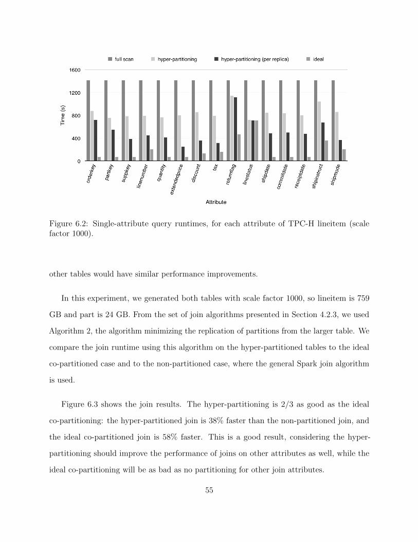
Figure 6.2: Single-attribute query runtimes, for each attribute of TPC-H lineitem (scalefactor 1000).

other tables would have similar performance improvements.

In this experiment, we generated both tables with scale factor 1000, so lineitem is 759

GB and part is 24 GB. From the set of join algorithms presented in Section 4.2.3, we used

Algorithm 2, the algorithm minimizing the replication of partitions from the larger table. We

compare the join runtime using this algorithm on the hyper-partitioned tables to the ideal

co-partitioned case and to the non-partitioned case, where the general Spark join algorithm

is used.

Figure 6.3 shows the join results. The hyper-partitioning is 2/3 as good as the ideal

co-partitioning: the hyper-partitioned join is 38% faster than the non-partitioned join, and

the ideal co-partitioned join is 58% faster. This is a good result, considering the hyper-

partitioning should improve the performance of joins on other attributes as well, while the

ideal co-partitioning will be as bad as no partitioning for other join attributes.

55

Figure 6.3: Runtimes for an equijoin query between the TPC-H lineitem and part tables,scale factor 1000, with different types of upfront partitioning on the tables.

6.3 Partitioning overhead

Finally, we consider the overhead of the upfront hyper-partitioning step, as compared to a

standard HDFS data upload with no partitioning. The upfront partitioner preserves the same

format (i.e. row, uncompressed) as standard HDFS, so the difference in time is solely due to

the difference in partitioning.

Figure 6.4 shows the time to hyper-partition the TPC-H lineitem table with scale factor

1000, as well as the time to upload lineitem into HDFS with the standard uploader. Compared

to the standard HDFS upload time, hyper-partitioning takes 2.6 times as long, and per-replica

hyper-partitioning takes 3.5 times as long. This is comparable to other workload-specific data

preparation steps, such as indexing and traditional partitioning [27, 5]. Thus, we conclude

the overhead of hyper-partitioning is reasonable.

56

Figure 6.4: Time to upload the TPC-H lineitem table (scale factor 1000) to HDFS, withdifferent partitioning techniques.

57

Chapter 7

Conclusion

This thesis showed how data can be robustly partitioned without knowledge of the query

workload to support ad-hoc analysis, using a novel multi-attribute data partitioning scheme

called hyper-partitioning. We presented the design of the hyper-partitioning tree and upfront

partitioning algorithm, as well as methods for optimizing predicate-based selection and

join queries with the hyper-partitioning structure. Our implementation of the Hyper-

Partitioning system and experimental results show that partitioning on a large number

of attributes with hyper-partitioning is a feasible and effective method for improving the

upfront performance of a varied query workload on large datasets.

58

Bibliography

[1] Sanjay Agrawal, Vivek Narasayya, and Beverly Yang. Integrating vertical and horizontalpartitioning into automated physical database design. In Proceedings of the 2004 ACMSIGMOD International Conference on Management of Data, SIGMOD ’04, pages 359–370, New York, NY, USA, 2004. ACM.

[2] Ganesh Ananthanarayanan, Ali Ghodsi, Scott Shenker, and Ion Stoica. Disk-locality indatacenter computing considered irrelevant. HotOS, 2011.

[3] Jon Louis Bentley. Multidimensional binary search trees used for associative searching.Communications of the ACM, 18(9):509–517, 1975.

[4] Carlo Curino, Evan Jones, Yang Zhang, and Sam Madden. Schism: A workload-drivenapproach to database replication and partitioning. Proceedings of the VLDB Endowment,3(1-2):48–57, September 2010.

[5] Jens Dittrich, Jorge-Arnulfo Quiane-Ruiz, Alekh Jindal, Yagiz Kargin, Vinay Setty, andJorg Schad. Hadoop++: Making a yellow elephant run like a cheetah (without it evennoticing). Proceedings of the VLDB Endowment, 3(1-2):515–529, 2010.

[6] Ahmed Eldawy and Mohamed F. Mokbel. A demonstration of spatialhadoop: Anefficient mapreduce framework for spatial data. Proceedings of the VLDB Endowment,6(12):1230–1233, 2013.

[7] Mohamed Y. Eltabakh, Yuanyuan Tian, Fatma Ozcan, Rainer Gemulla, Aljoscha Krettek,and John McPherson. Cohadoop: flexible data placement and its exploitation in hadoop.Proceedings of the VLDB Endowment, 4(9):575–585, 2011.

[8] Raphael A. Finkel and Jon Louis Bentley. Quad trees: a data structure for retrieval oncomposite keys. Acta informatica, 4(1):1–9, 1974.

[9] Shahram Ghandeharizadeh and David J. DeWitt. Magic: a multiattribute declusteringmechanism for multiprocessor database machines. Parallel and Distributed Systems,IEEE Transactions on, 5(5):509–524, 1994.

[10] Martin Grund, Jens Kruger, Hasso Plattner, Alexander Zeier, Philippe Cudre-Mauroux,and Samuel Madden. Hyrise: a main memory hybrid storage engine. Proceedings of theVLDB Endowment, 4(2):105–116, 2010.

59

[11] Antonin Guttman. R-trees: A dynamic index structure for spatial searching. SIGMODRec., 14(2):47–57, June 1984.

[12] Alexander Hall, Olaf Bachmann, Robert Bussow, Silviu Ganceanu, and Marc Nunkesser.Processing a trillion cells per mouse click. Proceedings of the VLDB Endowment,5(11):1436–1446, 2012.

[13] Stratos Idreos, Martin L. Kersten, and Stefan Manegold. Database cracking. In CIDR,volume 3, pages 1–8, 2007.

[14] Impala. http://www.cloudera.com/content/cloudera/en/products-and-services/cdh/impala.html.

[15] Alekh Jindal and Jens Dittrich. Relax and let the database do the partitioning online.In Enabling Real-Time Business Intelligence, pages 65–80. Springer, 2012.

[16] Alekh Jindal, Jorge-Arnulfo Quiane-Ruiz, and Jens Dittrich. Trojan data layouts: rightshoes for a running elephant. In Proceedings of the 2nd ACM Symposium on CloudComputing, page 21. ACM, 2011.

[17] Martin L. Kersten and Stefan Manegold. Cracking the database store. In CIDR, volume 5,pages 4–7, 2005.

[18] Sam Lightstone and Bishwaranjan Bhattacharjee. Automated design of multidimensionalclustering tables for relational databases. In Proceedings of the 30th VLDB Conference,pages 1170–1181. VLDB Endowment, 2004.

[19] Guido Moerkotte. Small materialized aggregates: A light weight index structure for datawarehousing. In Proceedings of the 24th VLDB Conference, pages 476–487, 1998.

[20] Rimma Nehme and Nicolas Bruno. Automated partitioning design in parallel databasesystems. In Proceedings of the 2011 ACM SIGMOD International Conference onManagement of Data, pages 1137–1148. ACM, 2011.

[21] Jurg Nievergelt, Hans Hinterberger, and Kenneth C. Sevcik. The grid file: An adaptable,symmetric multikey file structure. ACM Transactions on Database Systems (TODS),9(1):38–71, 1984.

[22] Shoji Nishimura, Sudipto Das, Divyakant Agrawal, and Amr El Abbadi. Md-hbase: ascalable multi-dimensional data infrastructure for location aware services. In MobileData Management (MDM), 2011 12th IEEE International Conference on, volume 1,pages 7–16. IEEE, 2011.

[23] Christopher Olston, Benjamin Reed, Utkarsh Srivastava, Ravi Kumar, and AndrewTomkins. Pig latin: a not-so-foreign language for data processing. In Proceedings of the2008 ACM SIGMOD International Conference on Management of Data, pages 1099–1110.ACM, 2008.

60

[24] Sriram Padmanabhan, Bishwaranjan Bhattacharjee, Tim Malkemus, Leslie Cranston,and Matthew Huras. Multi-dimensional clustering: a new data layout scheme in db2. InProceedings of the 2003 ACM SIGMOD International Conference on Management ofData, pages 637–641. ACM, 2003.

[25] Stratos Papadomanolakis and Anastassia Ailamaki. Autopart: Automating schemadesign for large scientific databases using data partitioning. In Scientific and StatisticalDatabase Management, 2004. Proceedings. 16th International Conference on, pages383–392. IEEE, 2004.

[26] Andrew Pavlo, Carlo Curino, and Stanley Zdonik. Skew-aware automatic databasepartitioning in shared-nothing, parallel oltp systems. In Proceedings of the 2012 ACMSIGMOD International Conference on Management of Data, pages 61–72. ACM, 2012.

[27] Andrew Pavlo, Erik Paulson, Alexander Rasin, Daniel J. Abadi, David J. DeWitt,Samuel Madden, and Michael Stonebraker. A comparison of approaches to large-scaledata analysis. In Proceedings of the 2009 ACM SIGMOD International Conference onManagement of Data, pages 165–178. ACM, 2009.

[28] Abdul Quamar, K. Ashwin Kumar, and Amol Deshpande. Sword: scalable workload-aware data placement for transactional workloads. In Proceedings of the 16th InternationalConference on Extending Database Technology, pages 430–441. ACM, 2013.

[29] Jun Rao, Chun Zhang, Nimrod Megiddo, and Guy Lohman. Automating physicaldatabase design in a parallel database. In Proceedings of the 2002 ACM SIGMODInternational Conference on Management of Data, SIGMOD ’02, pages 558–569, NewYork, NY, USA, 2002. ACM.

[30] Felix Martin Schuhknecht, Alekh Jindal, and Jens Dittrich. The uncracked pieces indatabase cracking. Proceedings of the VLDB Endowment, 7(2), 2013.

[31] Anil Shanbhag, Alekh Jindal, Qui Nguyen, Samuel Madden, Jorge-Arnulfo Quiane-Ruiz,Divyakant Agrawal, and Aaron J. Elmore. A multi-attribute partitioning scheme forad-hoc and time-varying database analytics. Submitted, 2015.

[32] Dominik Slezak, Jakub Wroblewski, Victoria Eastwood, and Piotr Synak. Brighthouse:an analytic data warehouse for ad-hoc queries. Proceedings of the VLDB Endowment,1(2):1337–1345, 2008.

[33] MySQL Subpartitioning. https://dev.mysql.com/doc/refman/5.1/en/partitioning-subpartitions.html.

[34] Oracle Subpartitioning. https://docs.oracle.com/cd/E17952 01/refman-5.5-en/partitioning-subpartitions.html.

61

[35] Young-Kyoon Suh, Ahmad Ghazal, Alain Crolotte, and Pekka Kostamaa. A new toolfor multi-level partitioning in teradata. In Proceedings of the 21st ACM InternationalConference on Information and Knowledge Management, pages 2214–2218. ACM, 2012.

[36] Liwen Sun, Michael J. Franklin, Sanjay Krishnan, and Reynold S. Xin. Fine-grainedpartitioning for aggressive data skipping. In Proceedings of the 2014 ACM SIGMODInternational Conference on Management of Data, pages 1115–1126. ACM, 2014.

[37] Ashish Thusoo, Joydeep Sen Sarma, Namit Jain, Zheng Shao, Prasad Chakka, SureshAnthony, Hao Liu, Pete Wyckoff, and Raghotham Murthy. Hive: a warehousing solutionover a map-reduce framework. Proceedings of the VLDB Endowment, 2(2):1626–1629,2009.

[38] Joe H. Ward Jr. Hierarchical grouping to optimize an objective function. Journal of theAmerican Statistical Association, 58(301):236–244, 1963.

[39] Daniel C Zilio, Jun Rao, Sam Lightstone, Guy Lohman, Adam Storm, Christian Garcia-Arellano, and Scott Fadden. Db2 design advisor: integrated automatic physical databasedesign. In Proceedings of the 30th International Conference on Very Large Data Bases,volume 30, pages 1087–1097. VLDB Endowment, 2004.

62