Density-matrix based numerical methods for discovering order and correlations in interacting systems

Density-matrix based numerical methods for discoveringorder and correlations in interacting systems

Christopher L. HenleyLaboratory of Atomic And Solid State Physics, Cornell University, Ithaca, NY 14853, USA

Hitesh J. ChanglaniDepartment of Physics, University of Illinois at Urbana-Champaign, Urbana, IL 61801, USA

Abstract. We review recently introduced numerical methods for the unbiased detection ofthe order parameter and/or dominant correlations, in many-body interacting systems, by usingreduced density matrices. Most of the paper is devoted to the “quasi-degenerate densitymatrix” (QDDM) which is rooted in Anderson’s observation that the degenerate symmetry-broken states valid in the thermodynamic limit, are manifested in finite systems as a setof low-energy “quasi-degenerate” states (in addition to the ground state). This method, itsoriginal form due to Furukawa et al. [Phys. Rev. Lett. 96, 047211 (2006)], is given a numberof improvements here, above all the extension from two-fold symmetry breaking to arbitrarycases. This is applied to two test cases (1) interacting spinless hardcore bosons on the triangularlattice and (2) a spin-1/2 antiferromagnetic system at the percolation threshold. In addition,we survey a different method called the “correlation density matrix”, which detects (possiblylong-range) correlations only from the ground state, but using the reduced density matrix froma cluster consisting of two spatially separated regions.

arX

iv:1

407.

4189

v1 [

cond

-mat

.str

-el]

16

Jul 2

014

Density-matrix based numerical methods for discovering order and correlations 2

1. Introduction

The ground state of quantum many-body strongly correlated electron, spin or bosonic systems,is characterized by a variety of order parameters and/or correlations (such as charge densitywaves, spirals, superconductivity and antiferromagnetism). Once the primary objective offinding out if the system is gapped or gapless is achieved (i.e. the presence or absence oflong range order is established), it is important to understand what kind of order (or lackof it) exists in the system. Even though “more is different” and every system is interestingin its own right, there are organizational principles that can be uncovered by defining andstudying metrics which make almost no (or minimal) assumptions of the underlying physicsof the system and do not rely on human intuition. This is especially important when theorder is exotic and has not been thought of previously. Historically, understanding the orderparameter of the system has been an art of sorts: one of the main objectives of this Articlewill be to suggest ways in which this entire procedure can be more or less automated.

Given the immense difficulty of the many-body problem and the absence of controlledanalytic approximations, utilizing numerical methods has become a standard way forunderstanding quantum systems. In particular, exact or highly accurate numerical methodssuch as exact diagonalization (ED), density matrix renormalization group (DMRG) [1, 2] andquantum Monte Carlo (QMC) [3, 4, 5, 6] have become indispensable tools for researchers inthis field. It is imperative that we maximize the potential of these methods and develop theproper tools to measure physical properties of a wide variety of systems.

In recent years, there has been a cross fertilization of ideas between condensed matter andquantum information as a result of which a new language for describing strongly correlatedsystems has emerged. In this language, the mathematical object of utmost importance is thequantum mechanical reduced density matrix for a given spatial region (other generalizations,for example to momentum space [7], have also been explored in the literature). For the presentpurpose, the term ”reduced density matrix” ρA for a spatial cluster A, with a local Hilbertspace of D states, is defined by,

ρA = TrA(|ψGS〉〈ψGS |

)(1)

where |ψGS〉 is the ground state wavefunction of the entire system and where TrA meanstrace over everything but cluster A i.e. tracing out the “environment”. Knowledge of thereduced density matrix (henceforth abbreviated as RDM) serves a very important purpose: itsD eigenvalues reflect the probability of the cluster to exist in the corresponding eigenvector,just like the thermal density matrix captures the knowledge of the energies and microstates ofa classical system in contact with a thermal bath.

While RDMs are central for all the methods covered here, for most of the paper,there is a second key ingredient: where the exact eigenstates includes a distinct family oflow-lying levels which are called quasi-degenerate (abbreviated as QD). We will presenta path (proposed initially by Furukawa et al. [8]) that combines these two ingredients todiscovering in an unbiased fashion what the order parameter is: we call this promising methodthe quasi-degenerate density matrix (QDDM) method. In our version of the method (andimplicitly in Ref. [8]), a key step is extending the RDM construction so as to mix two differentQD states, whence the name “quasi-degenerate density matrix” (formally defined in Sec. 3.)

In the rest of this paper, we first (in Sec. 2) review the original paper of Furukawa,Misguich and Oshikawa [8], which was limited to two-fold symmetry breakings with twoquasi-degenerate states. We introduce several improvements that foreshow the extensionof this method (in Sec 3) to an arbitrary number of QD states. The method is then tested


by computations for two example systems: first, in Sec. 4, order parameters for three-folddensity-wave order on a triangular lattice at 1/3 filling. Then in Sec. 5, we characterizeemergent S = 1/2 spins in a quantum antiferromagnet at the percolation threshold; thisshows that the QDDM has applications beyond symmetry breakings (the quasi-degeneracyhas a different origin in this case.) In Sec. 6, we survey some as-yet unrealized extensions ofthe QDDM method. In Sec. 7, we turn to reviewing a distinct method with a similar purpose,the Correlation Density Matrix (abbreviated as CDM). Finally Sec. 8, the conclusion, revisitsthe most important results and discusses the limitations of the various methods.

Before proceeding to the specifics, we want to place this work against the context ofmodern “entanglement” studies, a burgeoning industry based on RDMs. The typical aim ofan entanglement calculation (whether numerical or analytic) is the finite-size scaling of theentanglement entropy [9, 10, 11, 12, 13, 14, 15, 16] and/or interpreting the patterns of the“entanglement spectrum” [17, 18, 19, 20] i.e. the eigenvalues of the RDM. The aim is toreliably capture universal, long-wavelength properties of topological and/or critical states.For such a calculation the cluster should be as large as is practical, e.g. half the total systemsize (in which case the cluster and environment play equivalent roles).

Our own interest in RDMs [21, 22, 23, 24, 25, 26] had quite different motivations,(originally inspired by DMRG), eg. the discovery of the formula for the free-fermion RDMin terms of the Green’s function [21]. This led to the CDM method [25, 27], which willalso be reviewed in Section 7. These methods, and the QDDM, use RDMs constructed on thesmallest clusters that give physical results, typically a few sites.

2. Basic QDDM: Improving on Furukawa, Misguich and Oshikawa (M = 2 case)

In this section, we walk through the Quasi-degenerate Density Matrix approach in the simplestcase, that of two quasi-degenerate eigenstates, starting from the original paper by Furukawa,Misguich and Oshikawa [8], which we henceforth referred to as “FMO”. We will explainhow one can “discover” an order parameter from the RDM, in a (nearly) unbiased fashion,and expose the mathematical/computational apparatus needed. To make this concrete, oneseeks the operator Φ, defined on a cluster of sites A, which (acting as a perturbation) “moststrongly” splits the QD states.

In our retelling of FMO, we take the liberty of using our own notation. In places, werecast the FMO recipe in a mathematically equivalent but more illuminating form. Thiswill highlight the limitations of the QDDM of FMO, which may explain why the methodwas not taken up and widely applied. Along the way, we will introduce several majorimprovements we have made: a pre-processing requiring no prior assumptions; the use of L2

norms, amenable to eigenvalue analysis; and a better weighting of the answer. The greatestextension, the extension to M > 2 quasi-degenerate states, is left to the following section.

2.1. Quasi-degeneracy and order parameters

Before diving into the methods, we pause in this subsection to remind the reader of twogeneral concepts for understanding how long-range order, in the thermodynamic limit,manifests itself in finite systems: quasi-degeneracy (mentioned already in the introduction)and order parameter operators. This section applies also to the general case with M > 2.

2.1.1. Quasi-degenerate (QD) states Imagine a situation where we have exact diagonal-ization results for a system such that a subset of M eigenstates {|ψm〉} is quasi-degenerate(QD): that is, their eigenenergies are all small compared to those of all the other states. In


other words, the splittings within the quasi-degenerate states are small compared to the gapbetween them and the other states. This term “quasi-degenerate” is borrowed from the workof Lhuillier and co-workers [28, 29], who studied such states in the context of antiferromag-netic lattice models. We have willed the liberty of extending the term to cases in which thenearly-degeneracy is not due to long-range order in the thermodynamic limit.

One possible origin for quasi-degeneracy is the existence of a spontaneous symmetrybreaking. As originally understood by Anderson [30], whenever the associated orderparameter is not conserved by the Hamiltonian, the actual eigenstates are not symmetry-broken states and indeed the order parameter has zero expectation in any one of them.However, the system has a subset of quasi-degenerate states, and certain linear combinationsof these are symmetry-broken states – which are long-lived, since the quasi-degenerate statesdiffer only slightly in energy. Equivalently, one can construct a symmetry-broken basis for theQD states; the Hamiltonian in this basis has small, off-diagonal terms representing the smallamplitude for tunneling between these states, so the actual eigenstates are linear combinationswith small splittings. The energy splittings among QD states decrease rapidly with increasingsystem size.

When calling these states “quasi-degenerate”, we posited that their splitting is to somedegree accidental. In many cases, this splitting depends on details such as evenness/oddnessof the number of sites, or the aspect ratio of the finite system used, and thus may vary ina complicated fashion within a family of successively larger systems. Therefore, all of ouranalyses eventually seek to get answers invariant with respect to changes of basis among theQD states.

2.1.2. Order parameters and symmetries Now we turn to order parameters. Note first that,for any extended system, there is an infinite set of valid definitions for an order parameter.Every one of them transforms the same way under symmetry operations, and every one willgive the identical answer for the symmetry-broken states. Particular order parameters arechosen for convenience – most often, because they are local (e.g. involving one site, or twoneighboring sites).

Thus, we are free to adopt whichever definition of order parameter leads to a simplesolution. This will be controlled by our choice of the optimization criterion. In view of whatwas just said about the freedom in choosing order parameters, we should not worry if theoptimum, according to our trackable criterion, is sub optimal from the viewpoint of another,more natural, criterion. On the other hand, it is essential that some optimization is done. Thisis to ensure we pick up the fundamental order-parameter operator, and not a secondary one. ‡

There is a major constraint on a proper order-parameter: it must transform according to a(nontrivial) representation of the symmetry being broken. One basic corollary is that the orderparameter is unbiased: in the order-parameter space, the expectations from all the symmetry-broken states are distributed equally around zero. Keep in mind that, in general, we will havemulti-component order parameters, and also we have no idea (a priori) what is the nature ofthe symmetry.

A particular consequence is that the order parameter, when averaged over all the QDstates, is zero. § To translate this notion to the computational context, we define the average

‡ For example, the spin Sz is a fundamental order-parameter for an Ising model, whereas (Sz)3 − (const)Sz

would be a secondary operator.§ This follows since the family of QD states is presumed to be related to the symmetry-broken states by a unitarytransformation.


density matrix which is simply the average of the RDM as calculated from all the QD states:

ρav ≡ 1

M

M∑m=1

TrA

(|ψm〉〈ψm|

). (2)

Note that our desired order-parameter operator Φ must satisfy the condition,

Tr(ρavΦ) = 0. (3)

where the trace here is over all QD states.Roughly speaking, the average DM tells us what local configurations of the cluster are

common to all QD states; like a projection matrix, it annihilates any local states that occuronly in whole-system eigenfunctions with higher energies. We are seeking an operator thatdistinguishes these states, so this is to be found in the subspace orthogonal to ρav.

2.1.3. Invariance under change of QD basis Finally, we turn to an additional symmetry,related to the idea of quasi-equivalence. The philosophy of the present approach is to view theQD states as linear combinations of the symmetry-broken states, meaning they are idealized asbeing exactly degenerate. Therefore, we discard all the information contained in the splittingsamong the QD states. (Note that in other ways for using QD states [29], the crucial clues tothe nature of the long-range order holding in the thermodynamic limit, is precisely the patternof splittings, as correlated with lattice and spin symmetries of the states.)

It follows that any construction we use must give identical answers, independent of anyunitary transformation of the basis we use for the QD subspace of the Hilbert space,

|ψ′m′〉 ≡∑m

Um′m|ψm〉 (4)

where Um′m is an M ×M unitary matrix and |ψ′m′〉 is a transformed QD state. Evidently,the average density matrix (Eq. (2)) satisfies this condition, being invariant under suchtransformations.

Now consider the implications for the reduced density matrix itself. If we let ρ′m′

denotethe RDM constructed from |ψ′m′〉, we see

ρ′m′

=∑mn

(Um′mU∗m′n)ρmn (5)

involving a generalization of the density matrix that is off-diagonal in that it is constructedfrom two different eigenstates m and n:

ρmn ≡ TrA

(|ψm〉〈ψn|

). (6)

When, as here, ρmn is built from the QD states, we call it the quasi-degenerate density matrix(QDDM). Note that ρmn is implicitly dependent on the choice of cluster A; thus A should beconsidered as yet another index of ρmn: that has been suppressed, since the cluster A oncechosen is kept fixed through the analysis.

Off-diagonal density matrices can appear in other contexts, involving different choicesof the subspace of eigenstates entering them. In any case, the off-diagonal density matrixcontains information on any matrix element of any operator O (defined on A) between anytwo of the eigenstates:

〈ψm|O|ψn〉 = TrA

(ρmnO

)(7)

(To verify this, simply insert equation (6) in the right hand side of equation (7), and use thedefinition of the trace.)


2.2. Initial symmetry processing of QD states

FMO begin by assuming there are just M = 2 QD states, ψ1 and ψ2. The final aim is to find(1) the order-parameter operator Φ, and (2) the two linear combinations of ψ1 and ψ2 whichapproximate the symmetry-broken states, as best as possible in a system of finite-size. Thegoals are related in that Φ is the operator that splits the linear combinations of ψ1 and ψ2 asmuch as possible.

In the case of M = 2 states, we have a 22 − 1 = 3 dimensional space of operatorsorthogonal to ρav. FMO assume time-reversal and/or lattice symmetries, which allow themto find a special basis for the DM states Ψ1 and Ψ2. Then they uniquely define the operatorρdiff = ρ11− ρ22. (In the presence of either symmetry, the other two QDDM components ρ12

and ρ21 are in fact zero, making their search for an order parameter one dimensional.)The symmetry assumption unnecessarily violates our principle of using no assumptions

about the order. In fact, one can find the same special DM basis as FMO even in the absenceof symmetries. Roughly speaking, the criterion for the optimal basis vectors is to minimizethe operator norms of ρ12 and ρ21, the off-diagonal parts of the QDDM.

The above mentioned criterion is a special case of a method we will propose for generalM (the modified viewpoint) explained in Sec. 3.2. Since the details depend on using fusedindices and rely on a few more formal definitions, we will defer discussions about our methodto this later section.

2.3. Optimization criterion (M = 2 case)

FMO chose the optimization criterion,

σΦ = max||Φ||max=1

∣∣Tr(Φρdiff)∣∣ (8)

where the trace is over the M = 2 QD states and the notation ||O||max denotes a kind ofoperator norm,

||O||max ≡ max|〈v|O|v〉| (9)

where v is any normalized state vector. ‖ The solution to this optimization problem (8) isshown to be

Φ =∑j

|j〉sgn λj〈j| (10)

where λj are the eigenvalues and |j〉 are the corresponding eigenvectors of the operator ρdiff ,and sgnλj is the sign of λj . This form suffers from the deficiency that it gives an equalweight to the leading eigenvector, as it does to those with negligible eigenvalue. That will bepernicious in numerical applications, when the smaller λj’s are dominated by roundoff errors.

Instead, a much more numerically stable form is obtained, if we take a criterion using L2

norms:σΦ = max||Φ||2=1

∣∣Tr(Φρdiff)∣∣2 (11)

where,||Φ||2 ≡ Tr(Φ∗Φ) =

∑mn

|〈ψm|Φ|ψn〉|2 (12)

is the standard operator norm.

‖ This ||...||max norm is reminiscent of an L∞ norm, except that it is properly invariant with respect to changes ofbasis.


As in the FMO method, diagonalizing ρdiff (and after imposing the normalizationcondition on Φ), one obtains the solution, which is,

Φ =1√2

∑j

λj |j〉〈j| =1√2ρdiff . (13)

In this form, the subdominant eigenvectors are suppressed.

2.4. Choice of the cluster size

The cluster A should generally be the smallest one that will capture the order parameter. Thismeans that the resulting recipe for the order parameter is local, which as mentioned above(Sec. 2.1) is usually desirable. FMO illustrated this choice of cluster with the contrastingexamples of Neel order in a spin chain (requiring one site) with dimer order (requiring two).But one may choose a larger cluster that may be more symmetric with respect to the orderparameter.

This all highlights that the cluster choice is the weak link in our aim to have an unbiasedmethod: if we do not know the order parameter a priori, we cannot be sure what cluster Asuffices to capture it. We do not have a definitive answer, since we already had an expectationwhen we approached the example cases (Sections 4 and 5 in this paper). We believe this willshow up in the final stage of analyzing the resulting operators. If the cluster is too small, wewill probably find that the operators obtained are insufficient to fully split the QD manifold ofstates.

The same cluster should be used in QDDM calculations using different system sizes.The resulting order parameters should be exactly the same operators, in principle. Deviationsfrom this behavior give a measure of finite size effects and whether the results are adequatelyconverged.

The QDDM of Ref. [8] was applied not only to systems with an order parameter, but alsoto those with topological order. The analog of an order parameter must be a string operatorinvolving a set of sites forming a topologically nontrivial loop. (Here is one situation thatcalls for an extended cluster A). FMO applied this to the case of (T2) topological order. Onecould combine our generalization of our M > 2 method (in Sec. 3) to topological order, andcapture more general forms of it.

3. Extended QDDM: Recipe for many quasi-degenerate states

Now we turn to the harder task of extending the ideas of Sec. 2 to general, multi-componentorder parameters that go along with M > 2 quasi-degenerate states.

Trying to imitate the path of Sec. 2, we immediately run across two questions. The firstand easier one is, which cost function to choose? The second question is how to generalizethe “preprocessing” described in Sec 2.2. As noted already, the symmetric combination ofdensity matices ρav cannot split the QD states, so we must certainly work in the orthogonalsubspace, which evidently has dimension M2 − 1 in general. In the FMO treatment of theM = 2 case, that 3-dimensional subspace was reduced to a one dimensional subspace calledρdiff . And in fact, this was basically the final answer, since the order parameter was also onedimensional. For M > 2, we face the new task of somehow finding the right subset of thatM2 − 1-dimensional “difference” space: the sought-for order parameter space has a lowerdimension.


3.1. Fusing indices and operator singular value decomposition

As in Sec. 2 we were looking for the (normalized) operator Φ, defined within cluster A, thathas the “maximum possible” expectation, if we are allowed to make any (normalized) linearcombination of the QD states {|ψm〉}. Following the philosophy of using L2 normals, wechoose to maximize

σ2Φ =

∑mn

′ ∣∣〈ψm|Φ|ψn〉∣∣2 (14)

In other words, our criterion is to maximize the variance of the order parameter matrixelements rather than to find an operator that maximizes its magnitude acting only on a singlesymmetry broken state. (A practical drawback of the latter choice is that the action of theorder parameter on the sub-maximally split states would be underdetermined.) Instead, allstates (and all possible operators) must be treated on an equal footing.

Note that the ”∑′” symbol in Eq. (14) signifies we are using a QDDM with ρav projected

out, i.e. part of the “difference” subspace having rank M2 − 1. Then if an order parameteroperator Φ had any component of ρav, it would contribute nothing to our objective function(14). Therefore, with this criterion all components of the order parameter must indeedbe constructed from the “difference” subspace. From here on, all our work is within thatsubspace.

We now use Eq. (7), to rewrite Eq. (14) as,

σ2Φ =

∑mn

′Tr (ρmnΦ) Tr (ρmnΦ)

∗, (15)

Then, each factor in our objective function (15) can be re-expanded:

Tr (ρmnΦ) =∑aa′

〈a|ρmn|a′〉〈a′|Φ|a〉 ≡∑aa′

ρmnaa′ Φa′a (16)

where we have used a(a′) as the index for the basis state for cluster A and have defined thenotation ρmnaa′ ≡ 〈a|ρmn|a′〉.

To make progress, we can handle Eq. (15) using the tricks of grouping indices anddefining fused indices. More specifically, we think of mn as one fused index (denoting acompact index for a pair of QD states) and aa′ as another (denoting a compact index fora pair of states of the cluster Hilbert space), so that the matrix elements of the QDDM areρmn,aa′ ≡ 〈a|ρmn|a′〉. (This very same matrix element ρmn,aa′ has been written out as ρmnaa′for ease of notation.) Another way of saying this is that the QDDM is an M × M arrayof operators (as was explained in Sec. 2.1.3), each of which is a diagonal or off diagonalreduced DM, constructed from two (possibly different) eigenstates from the QD subspace. Inour language, the QDDM is a rectangular matrix of dimension M2 × D2, where D is thedimension of the Hilbert space of cluster A.

We define fused indices for the local Hilbert space indices aa′ → α and bb′ → β, andmn→ µ for the QD indices: Then we rewrite equation (16) using the fused indices; we makethe replacements

∑aa′ ρ

mnaa′ Φa′a →

∑α ρ

µαΦ∗α, where we have used the Hermiticity of Φ i.e.

Φa′a = Φ∗aa′ Hence Eq. (15) becomes,

σ2Φ =

∑µαβ

′

ρµαρµβ∗Φ∗αΦβ (17)

Note that with the adoption of fused indices, the D ×D matrix Φa′a is re-framed as a vectorΦα of size D2.


To put the objective function in equation (17) into a more illuminating form, define thecontracted matrix

Cαβ ≡∑µ

′

ρµαρµβ∗ (18)

which can easily be verified to be Hermitian. At this point we re-emphasize the importanceof the

∑′, it is crucial when computing the contracted matrix.Finally, our objective function becomes,

σ2Φ =

∑αβ

CαβΦ∗αΦβ (19)

Note that this is nothing but a vector-matrix-vector contraction.The next (and key) step is to diagonalize Cαβ , which is an example of the advertised

“operator singular value decomposition”. In the diagonal basis, the Cαβ is replaced by atransformed matrix Cjk = |λj |2δjk, where |λj |2 are the eigenvalues. We get

σ2Φ =

∑j

|λj |2ΦjΦ∗j , (20)

where Φj are the eigenvectors of the contracted matrix. Note that the coefficients ofeigenvector Φj in the α basis can be denoted as Φ

(j)α . Also, realize that we are allowed

the call the eigenvalues “|λj |2” since Cαβ is a nonnegative-definite matrix by construction; abetter reason for this notation will emerge in the next subsection.

It is clear that in (20), the best we can do is to make Φj parallel to the leading eigenvectorof Cαβ . This is our answer: the order parameter operators are the eigenvectors of Cαβ , andthe order-parameter operators have the same degeneracy as that leading eigenvector. The finalstep is to un-fuse the indices so as to write each of those eigenvectors as the D × D matrixwith the matrix elements of the sought-for optimal operator.

At this point, we note that the idea of fusing of indices is also the essence of a trickused for the Correlation Density Matrix (CDM) [25] (see section 7) but the indices fused hereare different. Thus the relation between the two density matrices is only mathematical, notphysical.

3.2. Modified viewpoint: singular-value decomposition

The focus in the processing in the previous subsection was to re-mix the state basis for thecluster. In contrast, the FMO approach for M = 2 (as well as the modification in Sec. 2.2),was based on re-mixing the QD indices. In fact, one could have adopted either focus in eithercase, so it is not at all obvious whether these alternate recipes are equivalent. We shall showthat they are, and in the process will slightly streamline the recipe.

Let us take step back to the QDDM written in fused indices as ρµα. This is a rectangularnot a square matrix. The µ index has fewer values, so the matrix rank isM2−1 after projectingout the average part.

We can perform a singular-value decomposition of the QDDM to obtain

ρµα =∑j

λjV(j)µ Φ(j)

α (21)

where Vµ are the left singular “vectors”, related to mixing between QD states, and Φα arethe right singular “vectors”, relating to mixing of the cluster’s Hilbert space. Thus, the two


different focuses used in Sec. 2.2 and in Sec. 3.1 are just two sides of the same coin: eq. (21)unifies the two approaches and shows that the recipes are equivalent. The diagonalizationin (20) is nothing more than the trick for converting a singular-value computation into aneigenvalue one. The quantity λj and Φ

(j)α are identical to those of the same name in the

previous subsection. (However, we note that performing the SVD will also yield an operatorproportional to ρav. This operator must be discarded since our desired order parameter isorthogonal to it.)

This, then, is the final version of our recipe: the un-fused version of the operators Φ(j)α

associated with the largest singular values λj . The reason for the detour through Sec. 3.1 wasthe need to relate the procedure to our objective function |σΦ|2.

3.3. Final processing of order parameters

The output of the QDDM, thus far, is a set of (possibly) degenerate, orthogonal orderparameter operators. This still does not solve the problem of identifying the nature of thesymmetry-breaking, which we now take up.

The operators extracted must form a representation of the symmetry group, andfurthermore must form an algebra. (The identity operator will be proportional to the averagedensity matrix, ρav.) Then, by multiplying the operators with each other and decomposingthe result into linear combinations of the operator set, we obtain this algebra’s rules,computationally. At this point, inspection should suffice for one to identify which of thefinite algebras this is. Of course, to the extent the operators are derived from a finite system,this algebra will not be exact: there will be an error term that is not a linear combination ofthe operators.

We could instead make the operators more transparent by a pre-preprocessing usinglattice or spin symmetries, which have not been used at all up to this point – i.e. we gotan arbitrary linear combination of the order parameter operators. In many cases, we do havea hint for the final processing of the order parameter, in the form of the known lattice or spinspin symmetries of our Hamiltonian. Then distinct components of the order parameter wouldbelong to different group representations of those symmetries.

It may happen that the QDDM states will already be nicely sorted according to thosesymmetries. In our experience, this happens when those symmetries are broken by the choiceof the system cell used for ED, or of the cluster A used to construct the reduced densitymatrices. But that cannot be relied on: since the splittings of the QD states are exponentiallyor algebraically decreasing with system size, in a sufficiently large system cell the splitting istoo small to be resolved by Lanczos diagonalization, so the QD eigenstates are random linearcombinations from the the QD subspace.

If one wanted to force the symmetries onto our states, one has the choice of doing so atdifferent stages of the construction. In effect, FMO did this at the earliest state, by rotatingthe QD states themselves. Our preference is to impose them at the end, i.e. on the orderparameters themselves, just prior to computing the operator products so as to tease out thestructure of the algebra that they form. Indeed, this is more or less the situation for both ourexamples in the following sections, where we had to merely confirm our prior suspicion as towhat symmetries are broken.


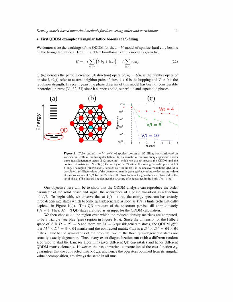
4. First QDDM example: triangular lattice bosons at 1/3 filling

We demonstrate the workings of the QDDM for the t−V model of spinless hard core bosonson the triangular lattice at 1/3 filling. The Hamiltonian of this model is given by,

H = −t∑〈i,j〉

(b†i bj + h.c.

)+ V

∑〈i,j〉

ninj (22)

b†i (bi) denotes the particle creation (destruction) operator, ni = b†i bi is the number operatoron site i, 〈i, j〉 refer to nearest neighbor pairs of sites, t > 0 is the hopping and V > 0 is therepulsion strength. In recent years, the phase diagram of this model has been of considerabletheoretical interest [31, 32, 33] since it supports solid, superfluid and supersolid phases.

QDEnerg

y

10-10

10-8

10-6

10-4

10-2

100

1 2 3 4 5 6 7 8

Eig

enva

lue

Number

V/t = 4

V/t = 6

V/t = 10

(a) (b) (c)

Figure 1. (Color online) t − V model of spinless bosons at 1/3 filling was considered onvarious unit cells of the triangular lattice. (a) Schematic of the low energy spectrum showsthree quasidegenerate states (1+2 structure), which we use to process the QDDM and thecontracted matrix (see Sec 3) (b) Geometry of the 27 site cell showing the solid phase at 1/3filling. The region (blue/shaded), denoted asA in the text, is the one over which the QDDM iscalculated. (c) Eigenvalues of the contracted matrix (arranged according to decreasing value)at various values of V/t for the 27 site cell. Two dominant eigenvalues are observed in thesolid phase. (The dashed line denotes the structure of eigenvalues in the limit V/t→∞.)

Our objective here will be to show that the QDDM analysis can reproduce the orderparameter of the solid phase and signal the occurrence of a phase transition as a functionof V/t. To begin with, we observe that at V/t → ∞, the energy spectrum has exactlythree degenerate states which become quasidegenerate as soon as V/t is finite (schematicallydepicted in Figure 1(a)). This QD structure of the spectrum persists till approximatelyV/t ≈ 4. Thus, M = 3 QD states are used as an input for the QDDM calculation.

We then choose A: the region over which the reduced density matrices are computed,to be a triangle (see blue (grey) region in Figure 1(b)). Since the dimension of the Hilbertspace of A is D = 23 = 8 and there are M = 3 quasidegenerate states, the QDDM ρmnaa′is a M2 × D2 = 9 × 64 matrix and the contracted matrix Cαβ is a D2 × D2 = 64 × 64matrix. Due to the symmetries of the problem, two of the three quasidegenerate states areactually exactly degenerate. Thus, every exact diagonalization run (with a different randomseed used to start the Lanczos algorithm) gives different QD eigenstates and hence differentQDDM matrix elements. However, the basis invariant construction of the cost function σΦ

guarantees that the contracted matrix Cαβ , and hence the operators obtained from its singularvalue decomposition, are always the same in all runs.


0

0.2

0.4

0.6

0.8

1

4 5 6 7 8 9 10

Max

imum

Eigen

value

V/t

18 (6x3)24 (8x3)

27

0

0.05

0.1

0.15

0.2

0.25

4 5 6 7 8 9 10

Offdiag

contrib

ution

V/t

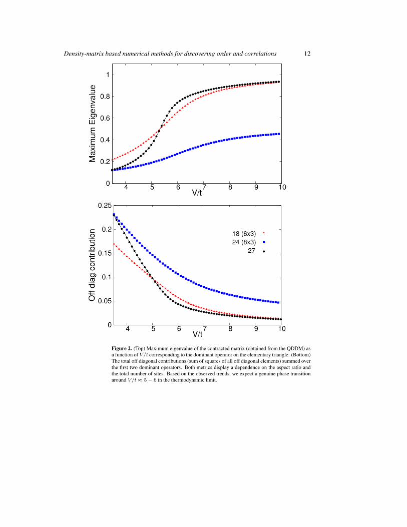
Figure 2. (Top) Maximum eigenvalue of the contracted matrix (obtained from the QDDM) asa function of V/t corresponding to the dominant operator on the elementary triangle. (Bottom)The total off diagonal contributions (sum of squares of all off diagonal elements) summed overthe first two dominant operators. Both metrics display a dependence on the aspect ratio andthe total number of sites. Based on the observed trends, we expect a genuine phase transitionaround V/t ≈ 5− 6 in the thermodynamic limit.


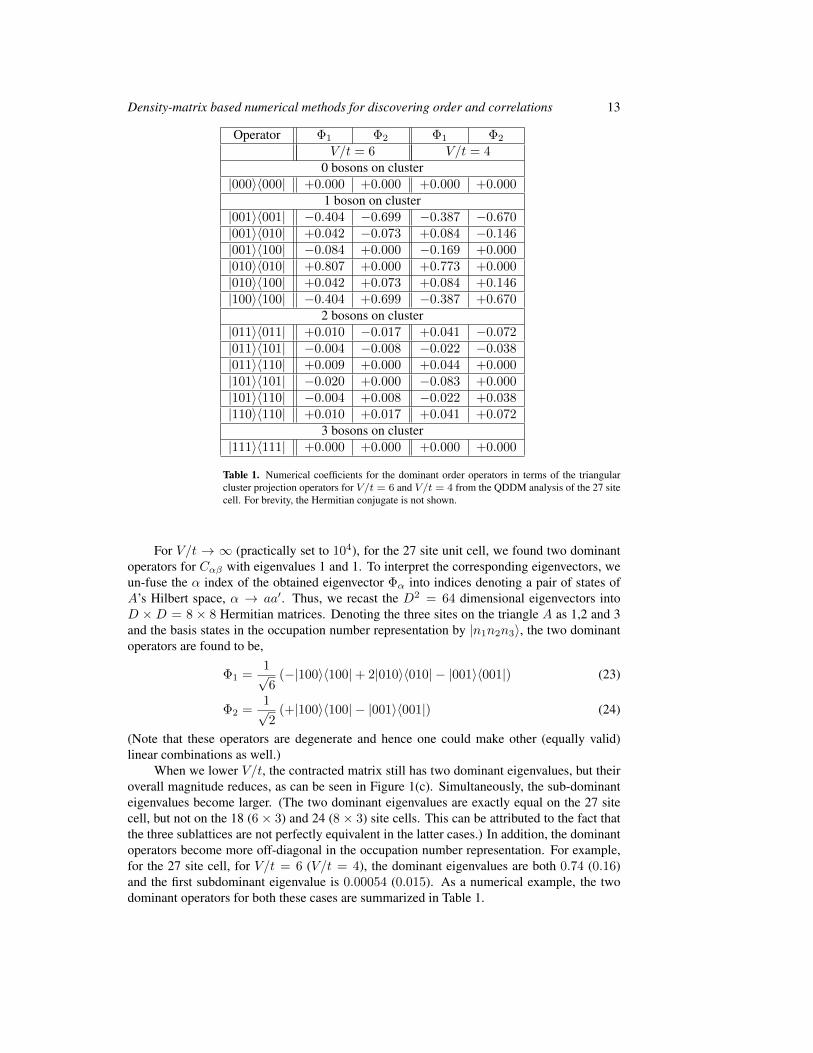
Operator Φ1 Φ2 Φ1 Φ2

V/t = 6 V/t = 40 bosons on cluster

|000〉〈000| +0.000 +0.000 +0.000 +0.0001 boson on cluster

|001〉〈001| −0.404 −0.699 −0.387 −0.670|001〉〈010| +0.042 −0.073 +0.084 −0.146|001〉〈100| −0.084 +0.000 −0.169 +0.000|010〉〈010| +0.807 +0.000 +0.773 +0.000|010〉〈100| +0.042 +0.073 +0.084 +0.146|100〉〈100| −0.404 +0.699 −0.387 +0.670

2 bosons on cluster|011〉〈011| +0.010 −0.017 +0.041 −0.072|011〉〈101| −0.004 −0.008 −0.022 −0.038|011〉〈110| +0.009 +0.000 +0.044 +0.000|101〉〈101| −0.020 +0.000 −0.083 +0.000|101〉〈110| −0.004 +0.008 −0.022 +0.038|110〉〈110| +0.010 +0.017 +0.041 +0.072

3 bosons on cluster|111〉〈111| +0.000 +0.000 +0.000 +0.000

Table 1. Numerical coefficients for the dominant order operators in terms of the triangularcluster projection operators for V/t = 6 and V/t = 4 from the QDDM analysis of the 27 sitecell. For brevity, the Hermitian conjugate is not shown.

For V/t → ∞ (practically set to 104), for the 27 site unit cell, we found two dominantoperators for Cαβ with eigenvalues 1 and 1. To interpret the corresponding eigenvectors, weun-fuse the α index of the obtained eigenvector Φα into indices denoting a pair of states ofA’s Hilbert space, α → aa′. Thus, we recast the D2 = 64 dimensional eigenvectors intoD ×D = 8 × 8 Hermitian matrices. Denoting the three sites on the triangle A as 1,2 and 3and the basis states in the occupation number representation by |n1n2n3〉, the two dominantoperators are found to be,

Φ1 =1√6

(−|100〉〈100|+ 2|010〉〈010| − |001〉〈001|) (23)

Φ2 =1√2

(+|100〉〈100| − |001〉〈001|) (24)

(Note that these operators are degenerate and hence one could make other (equally valid)linear combinations as well.)

When we lower V/t, the contracted matrix still has two dominant eigenvalues, but theiroverall magnitude reduces, as can be seen in Figure 1(c). Simultaneously, the sub-dominanteigenvalues become larger. (The two dominant eigenvalues are exactly equal on the 27 sitecell, but not on the 18 (6× 3) and 24 (8× 3) site cells. This can be attributed to the fact thatthe three sublattices are not perfectly equivalent in the latter cases.) In addition, the dominantoperators become more off-diagonal in the occupation number representation. For example,for the 27 site cell, for V/t = 6 (V/t = 4), the dominant eigenvalues are both 0.74 (0.16)and the first subdominant eigenvalue is 0.00054 (0.015). As a numerical example, the twodominant operators for both these cases are summarized in Table 1.


These notions can be put on a quantitative footing, by tracking the evolution of the mostdominant eigenvalue as a function of V/t, as is shown in the top panel of Figure 2. Therelatively rapid change in the magnitude of this dominant eigenvalue around V/t ≈ 5 − 6suggests the occurrence of a genuine phase transition. This can also be verified by observinghow the total contribution of all off diagonal elements of the two most dominant operatorschanges with V/t, as is shown in the bottom panel of Figure 2. (More precisely, this metricwas calculated by summing squares of all off diagonal coefficients over the two most dominantoperators.)

In summary, our results indicate that the solid melts into another phase (which previousnumerical studies [31, 32, 33] indicate to be a superfluid), at (V/t)c ≈ 5 − 6 i.e. (t/V )c ≈0.17− 0.20. This compares reasonably well with the Monte Carlo estimate [32] of (t/V )c =0.195 ± 0.025 and the DMFT estimate [33] of (t/V )c = 0.216. We expect that calculationsfor bigger systems and a thorough understanding of the dependence of the order parameter onthe aspect ratio of the finite systems studied will reveal a more quantitatively accurate pictureof this phase transition.

Finally, we note that a fermionic version involving a related t− V model was studied byMotrunich and Lee [34]. In this case, the solid at 1/3 filling melts into a renormalized Fermiliquid on lowering V/t. This phase transition can also be detected by a QDDM analysis [35].

5. Second QDDM example: “emergent spins” in randomly diluted antiferromagnets

We now present another situation where quasidegenerate states occur and where their physicalorigin is unrelated to spontaneous symmetry breaking. Here, the quasidegeneracy will beattributed to the formation of (and interaction between) local spin moments in the presence ofdisorder.

5.1. Previously known results for randomly diluted antiferromagnets

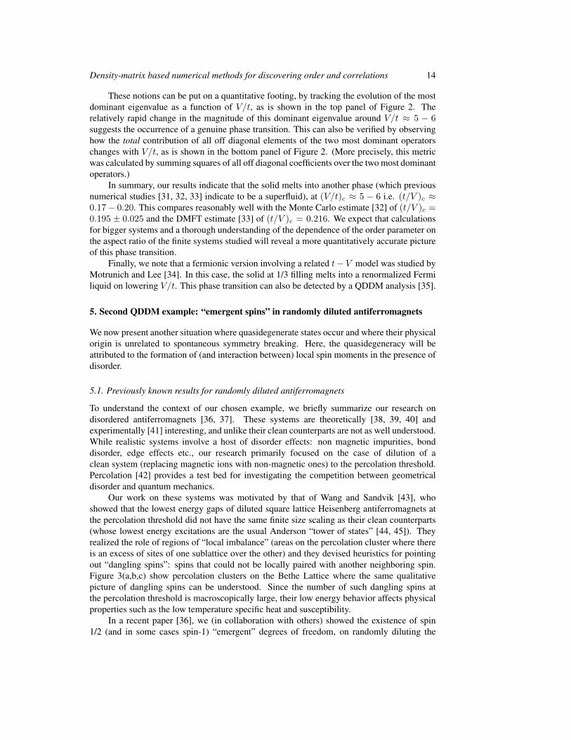
To understand the context of our chosen example, we briefly summarize our research ondisordered antiferromagnets [36, 37]. These systems are theoretically [38, 39, 40] andexperimentally [41] interesting, and unlike their clean counterparts are not as well understood.While realistic systems involve a host of disorder effects: non magnetic impurities, bonddisorder, edge effects etc., our research primarily focused on the case of dilution of aclean system (replacing magnetic ions with non-magnetic ones) to the percolation threshold.Percolation [42] provides a test bed for investigating the competition between geometricaldisorder and quantum mechanics.

Our work on these systems was motivated by that of Wang and Sandvik [43], whoshowed that the lowest energy gaps of diluted square lattice Heisenberg antiferromagnets atthe percolation threshold did not have the same finite size scaling as their clean counterparts(whose lowest energy excitations are the usual Anderson “tower of states” [44, 45]). Theyrealized the role of regions of “local imbalance” (areas on the percolation cluster where thereis an excess of sites of one sublattice over the other) and they devised heuristics for pointingout “dangling spins”: spins that could not be locally paired with another neighboring spin.Figure 3(a,b,c) show percolation clusters on the Bethe Lattice where the same qualitativepicture of dangling spins can be understood. Since the number of such dangling spins atthe percolation threshold is macroscopically large, their low energy behavior affects physicalproperties such as the low temperature specific heat and susceptibility.

In a recent paper [36], we (in collaboration with others) showed the existence of spin1/2 (and in some cases spin-1) “emergent” degrees of freedom, on randomly diluting the


unfrustrated coordination-3 Bethe lattice Heisenberg antiferromagnet. As is depicted inFigure 3(a-c), our inference was based on the observation of quasidegenerate (QD) statesseen in the many body spectrum obtained from either ED or DMRG. We also found (usingmultiple metrics), these emergent spin-excitations to be relatively localized in space. Thispicture of the low energy physics is very different from the case for clean antiferromagnetswhere the degrees of freedom are macroscopically big sublattice spins.

2 x 3 states2

Δ

Emean

2 spin 1/2

2 states2 2 states

4 1

2 spin 1/21 spin 1

Energy

4 spin 1/2

0 J

0.5 J

A

QD

A'

(a) (b) (c)

A

A'

10-5

10-4

10-3

10-2

10-1

100

1 2 3 4 5 6 7 8

SV

D e

igen

valu

e

Number

(d)

Figure 3. (a),(b),(c) show three different percolation clusters (all of the same size) on theBethe lattice, along with their respective low energy spectra. The red (dark) and green (light)circles indicate even and odd sublattice sites. The broken dashed lines show dimer coveringswhich serve as a heuristic to locate the “dangling spins” (circled with thick black lines).Energy spectra for each of the clusters show low-lying quasidegenerate (QD) states separatedfrom the continuum by an energy scale ∆QD . For purpose of the QDDM calculation inthe text, the percolation cluster (a) is chosen. Two different patches A and A′ (shown byshaded/blue circles) are chosen for two separate QDDM analyses. (d) shows the eigenvaluesof the contracted matrix calculated for patches A and A′. (Parts of this figure have beenadapted from the original by Changlani et al. [36] and modified for the present purposes.)


5.2. QDDM calculation

Having established the existence of these local moments, we then asked the question: Whatare the composite “effective” spin operators that describe the observed QD states? We wishto obtain the answer to this question in a relatively unbiased and automated way, for whichthe QDDM formalism is very apt.

To demonstrate how the QDDM method works for this system, we take as our systemthe 18-site percolation cluster of Figure 3(a), which has two dangling spins and hence (weexpect) two emergent quasispins, implying a total of 22 = 4 QD states ¶. Our patch A for theRDM + is chosen to encompass the central sites participating in one of the emergent spins:namely, three sites forming a “fork”, a geometric motif that has a local imbalance associatedwith it. The Hilbert space of this patch thus has dimension 23. ∗

Processing the QDDM with M = 4 states, (i.e. one S = 0 and three lowest S = 1states), we obtain three dominant operators. This is expected because the model is SU(2)symmetric, guaranteeing the three operators are those that correspond to the three componentsof an effective spin operator T (basically, T z , T+ and T−).

To be sure of our interpretation, we checked the commutation relations of these operators.The operator commutation algebra only approximately corresponds to that of a true spin-1/2algebra, although the approximation is very good in this case. In fact there is apriori noreason that the effective spin operator be a true spin 1/2 operator, since the transformationfrom the bare to effective spins is not a linear/unitary one. (Also note that we do not see anycontributions corresponding to the identity operator, because ρav is proportional to it. OurQDDM formalism explicitly looks for an operator orthogonal to ρav to split the QD states.)

For the three site fork (site 2 is the center of the fork and 1 and 3 its equivalent ends), ournumerically obtained operator T+ can be expressed in terms of the bare spin operators S1,S2 and S3, as

T+ ≈ 0.085(2S+

1 (1− 4S2 · S3) + 2S+3 (1− 4S1 · S2)− S+

2 (1− 4S1 · S3))

(25)

(The other operators T− and T z follow from Eq. (25) since the spin-rotation symmetry isexact at all stages of processing.)

Up to this point we have only discussed one choice of patch to process the QDDM.However, one can scan all possible local patches and process the QDDM. To show that theQDDM is not a misleading diagnostic for detecting an effective composite spin operator,we considered another patch A′ consisting of four sites (shown in Figure 3(a)) for the samepercolation cluster with two dangling spins. This patch does not have any locally unbalancedspins and is expected to be inert (i.e. not involved in the low energy physics). As can be seenin Figure 3(d), the QDDM analysis of this patch revealed that the dominant operator on A′

has an eigenvalue about 40 times smaller than that obtained for the case of patch A. Thus, theQDDM analysis confirms that patch A′ has no emergent local moments associated with it.

Finally, we remark on the application of QDDM for other percolation clusters. Forexample, the analysis of the 18-sites system in Figure 3(b), should be very similar to that

¶ We remark that multiple low lying states must be targeted in the Lanczos algorithm to ensure that one obtainsan accurate representation of the QD spectrum. (An insufficient number of Krylov vectors may lead to absence ofcertain QD states.)+ To avoid confusion in using the word “cluster” for a finite “percolation cluster” and the “cluster A” i.e. our regionof interest whose RDM is processed, we will instead refer to the latter as a local “patch” in this section.∗ In fact, as noted in [36], the emergent spins were found to be exponentially localized around the fork: thus, bytaking a larger local patch, we should obtain cleaner numerical results. The price is not only the exponentiallyincreased computational cost: if the patch is extended too far, the results may be polluted by contributions from adifferent, neighboring emergent spin.


already carried out for percolation cluster (a), although there will be M = 16 instead ofM = 4 QD states to process. On the other hand, in the case of the percolation cluster inFigure 3(c), there are local patches where the emergent spin 1/2 degrees of freedom are onthe same sublattice and are located spatially close to one another. Thus, the QDDM analysisis expected to reveal the effective spin-1 nature of this degree of freedom.

6. Extensions of the QDDM method

This section collects several ways in which the current method may be extended: the commonfactor is they have not been tried yet, and we offer them in the hopes that others may take upthe challenge. One might extract the low-lying states by means other than ED (Subsection6.1, or might apply the method to the new systems (Subsection 6.2, and 6.3), in which thequasi-degeneracy or degeneracy has an origin other than some incipient order. (One couldalso imagine modifying the optimization criterion or index-fusing methods we used to obtainthe results – but we have no specific proposals to offer here.)

6.1. Beyond Exact Diagonalization: Calculation of the QDDM with Matrix Product States

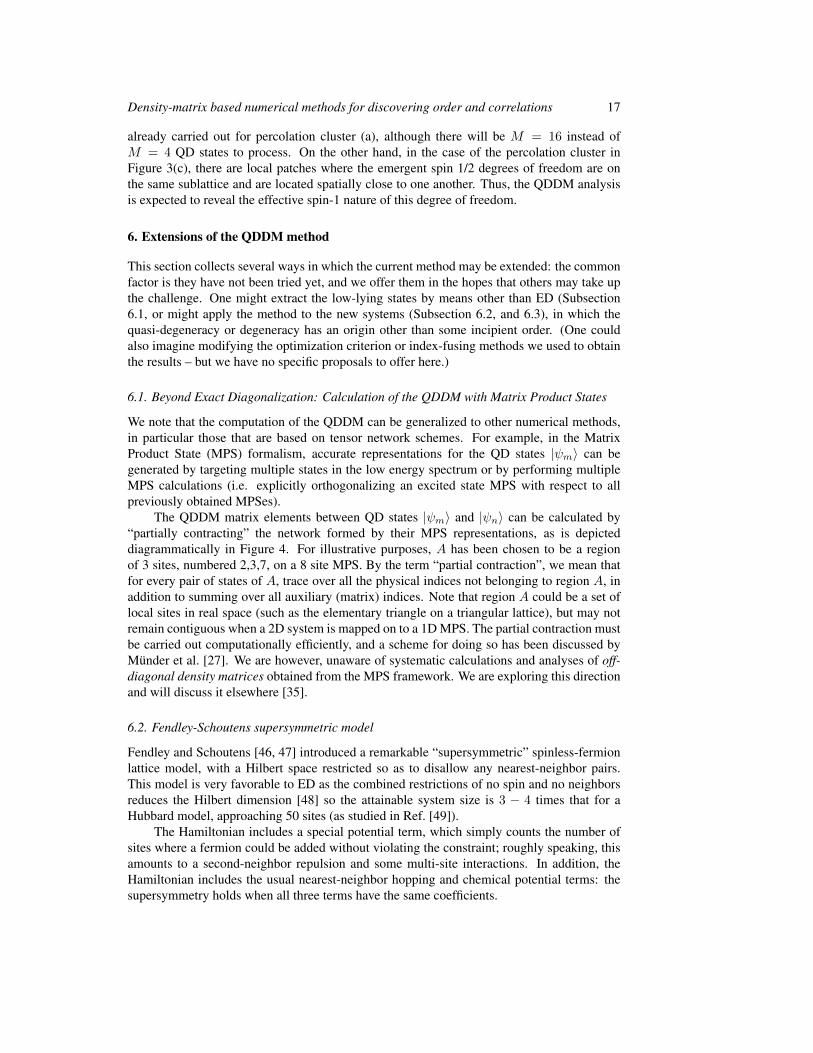
We note that the computation of the QDDM can be generalized to other numerical methods,in particular those that are based on tensor network schemes. For example, in the MatrixProduct State (MPS) formalism, accurate representations for the QD states |ψm〉 can begenerated by targeting multiple states in the low energy spectrum or by performing multipleMPS calculations (i.e. explicitly orthogonalizing an excited state MPS with respect to allpreviously obtained MPSes).

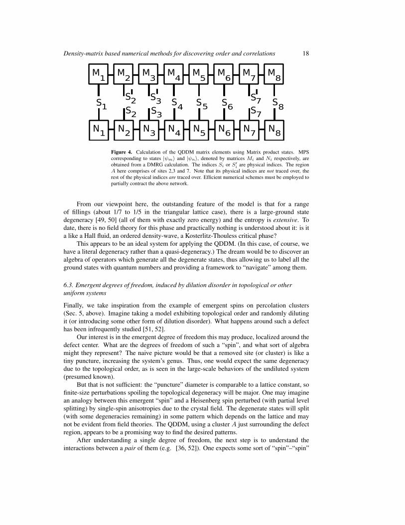
The QDDM matrix elements between QD states |ψm〉 and |ψn〉 can be calculated by“partially contracting” the network formed by their MPS representations, as is depicteddiagrammatically in Figure 4. For illustrative purposes, A has been chosen to be a regionof 3 sites, numbered 2,3,7, on a 8 site MPS. By the term “partial contraction”, we mean thatfor every pair of states of A, trace over all the physical indices not belonging to region A, inaddition to summing over all auxiliary (matrix) indices. Note that region A could be a set oflocal sites in real space (such as the elementary triangle on a triangular lattice), but may notremain contiguous when a 2D system is mapped on to a 1D MPS. The partial contraction mustbe carried out computationally efficiently, and a scheme for doing so has been discussed byMunder et al. [27]. We are however, unaware of systematic calculations and analyses of off-diagonal density matrices obtained from the MPS framework. We are exploring this directionand will discuss it elsewhere [35].

6.2. Fendley-Schoutens supersymmetric model

Fendley and Schoutens [46, 47] introduced a remarkable “supersymmetric” spinless-fermionlattice model, with a Hilbert space restricted so as to disallow any nearest-neighbor pairs.This model is very favorable to ED as the combined restrictions of no spin and no neighborsreduces the Hilbert dimension [48] so the attainable system size is 3 − 4 times that for aHubbard model, approaching 50 sites (as studied in Ref. [49]).

The Hamiltonian includes a special potential term, which simply counts the number ofsites where a fermion could be added without violating the constraint; roughly speaking, thisamounts to a second-neighbor repulsion and some multi-site interactions. In addition, theHamiltonian includes the usual nearest-neighbor hopping and chemical potential terms: thesupersymmetry holds when all three terms have the same coefficients.


S S S S S1 4 5 6 8

M1

M2

M3

M4

M5

M6

M7

M8

N1

S2S2

S3S3

S7S7

' ' '

N1 N2 N3 N5 N6 N7 N8N4

Figure 4. Calculation of the QDDM matrix elements using Matrix product states. MPScorresponding to states |ψm〉 and |ψn〉, denoted by matrices Mi and Ni respectively, areobtained from a DMRG calculation. The indices Si or S′

i are physical indices. The regionA here comprises of sites 2,3 and 7. Note that its physical indices are not traced over, therest of the physical indices are traced over. Efficient numerical schemes must be employed topartially contract the above network.

From our viewpoint here, the outstanding feature of the model is that for a rangeof fillings (about 1/7 to 1/5 in the triangular lattice case), there is a large-ground statedegeneracy [49, 50] (all of them with exactly zero energy) and the entropy is extensive. Todate, there is no field theory for this phase and practically nothing is understood about it: is ita like a Hall fluid, an ordered density-wave, a Kosterlitz-Thouless critical phase?

This appears to be an ideal system for applying the QDDM. (In this case, of course, wehave a literal degeneracy rather than a quasi-degeneracy.) The dream would be to discover analgebra of operators which generate all the degenerate states, thus allowing us to label all theground states with quantum numbers and providing a framework to “navigate” among them.

6.3. Emergent degrees of freedom, induced by dilution disorder in topological or otheruniform systems

Finally, we take inspiration from the example of emergent spins on percolation clusters(Sec. 5, above). Imagine taking a model exhibiting topological order and randomly dilutingit (or introducing some other form of dilution disorder). What happens around such a defecthas been infrequently studied [51, 52].

Our interest is in the emergent degree of freedom this may produce, localized around thedefect center. What are the degrees of freedom of such a “spin”, and what sort of algebramight they represent? The naive picture would be that a removed site (or cluster) is like atiny puncture, increasing the system’s genus. Thus, one would expect the same degeneracydue to the topological order, as is seen in the large-scale behaviors of the undiluted system(presumed known).

But that is not sufficient: the “puncture” diameter is comparable to a lattice constant, sofinite-size perturbations spoiling the topological degeneracy will be major. One may imaginean analogy between this emergent “spin” and a Heisenberg spin perturbed (with partial levelsplitting) by single-spin anisotropies due to the crystal field. The degenerate states will split(with some degeneracies remaining) in some pattern which depends on the lattice and maynot be evident from field theories. The QDDM, using a cluster A just surrounding the defectregion, appears to be a promising way to find the desired patterns.

After understanding a single degree of freedom, the next step is to understand theinteractions between a pair of them (e.g. [36, 52]). One expects some sort of “spin”–“spin”


interaction, mediated by the intervening topological fluid. The Correlation Density matrix(described in the next section) appears to be well-suited to elucidate such interactions.

An amusing possibility arises if the mediated interactions are unfrustrated. This willprobably induce long-range order of the defect sites at T = 0. The system might then exhibita mix of coexisting topological and long-range orders.

7. Correlation density matrix

In this section, we turn our attention to another kind of reduced density matrix, the correlationdensity matrix (CDM), originally proposed in Ref. [25]. The CDM is quite distinct fromthe QDDM – except insofar as both of these methods are basis-invariant, depend on densitymatrices, and may be used to detect long-range order when the order parameter is not knownin advance. Whereas the QDDM is constructed using one cluster and many eigenstates, theCDM uses two clusters and in principle one eigenstate. Whereas the QDDM detects globalorders – either global symmetry-breaking or (with an appropriate cluster) topological order,the CDM detects correlation functions. Specifically, the CDM may be used to:

B verify the absence of any kind of order (even exotic orders that no one has imagined) insystems such as the spin-1/2 kagome antiferromagnet

B verify the existence of long range order (by identifying that correlations are not decayingwith distance, even if the nature of the correlation was not recognized in advance)

B extract the scaling exponents and scaling operators of a critical system, in an extensionof the method

Critical correlations demand the RDM for a wide range of cluster separations. Groundstates for the sizes needed are not adequately accessed by Lanczos diagonalizations, even forone-dimensional chains. Instead, DMRG may be used to obtain very accurate approximationsof the ground state and the CDM can be calculated within the MPS formalism [27]. One must,however, be attentive to the usual artifacts of DMRG, such as end effects.

We first outline the basic version of the CDM, which analyzes just one particular pairof clusters at a time [25]. An extension of this analysis involves considering all possibleseparations at the same time [27]. Finally, we delineate the CDM approach from thesuperficially similar, and more familiar, mutual information approach.

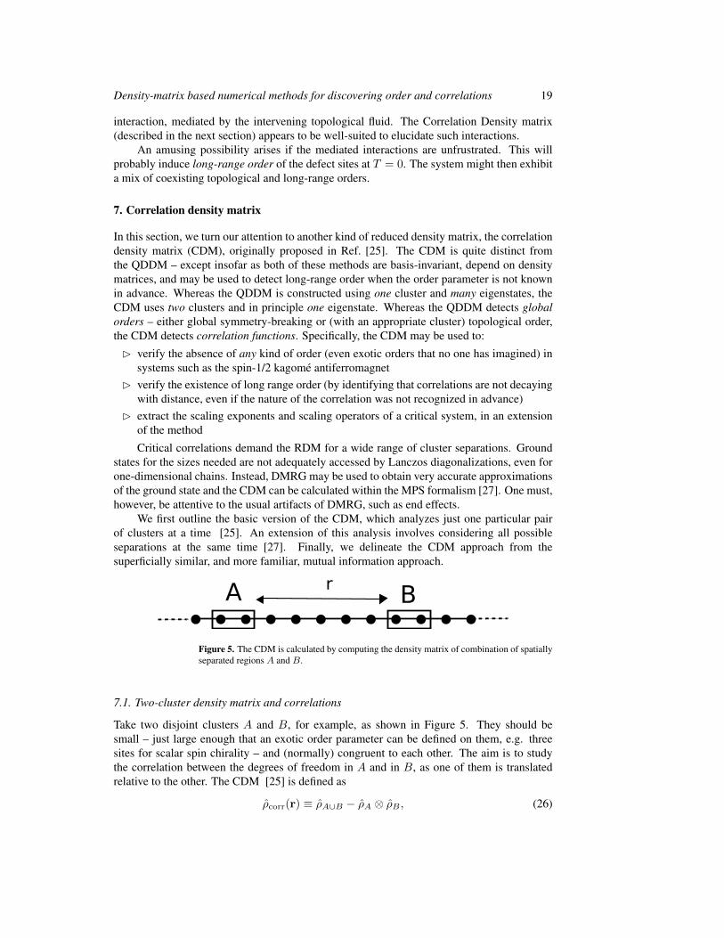
A Br

Figure 5. The CDM is calculated by computing the density matrix of combination of spatiallyseparated regions A and B.

7.1. Two-cluster density matrix and correlations

Take two disjoint clusters A and B, for example, as shown in Figure 5. They should besmall – just large enough that an exotic order parameter can be defined on them, e.g. threesites for scalar spin chirality – and (normally) congruent to each other. The aim is to studythe correlation between the degrees of freedom in A and in B, as one of them is translatedrelative to the other. The CDM [25] is defined as

ρcorr(r) ≡ ρA∪B − ρA ⊗ ρB , (26)


where ρA is the density matrix for the (small) cluster A, constructed by tracing out itsenvironment, similarly ρB and ρA∪B .

Evidently, the CDM contains all possible correlations between operator OA on A andanother operator OB on B, since the connected correlation function is given by

〈OAOB〉conn ≡ 〈OAOB〉 − 〈OA〉〈OB〉 ≡ Tr(ρcorrOAOB). (27)

Thus, the Frobenius (sum-of-squares) norm ||ρcorr|| immediately gives an absolutemeasurement of the total correlations of all kinds between the two clusters. ]

It may happen that the finite system being diagonalized has degenerate or quasi-degenerate ground states; this may simply be a consequence of the specific shape of thesystem being diagonalized. Then the recipe [23] is to restore the symmetry of the Hamiltonianby averaging over the (quasi) degenerate states in the evaluation of ρA, ρB , and ρA∪B (just aswas used to evaluate ρav in the QDDM case).

7.2. Fused indices and operator singular-value decomposition

Rather than merely condense the correlations into a single scalar that quantifies theirmagnitude, we would like an unbiased way to discover what operators are responsible for thiscorrelation. This can be done using a special singular-value decomposition, using a notion offused indices, analogous to our processing of the QDDM but using different indices.

Let a and a′ denote the “ket” and “bra” indices in block A, and similarly b and b′ inblock B. Then replace (a, a′) by the fused index α = α(a, a′), and (b, b′) by the fused indexβ = β(b, b′), write out the elements of ρcorr as a D2 × D2 matrix with components rαβ .Perform the singular value decomposition, obtaining

rαβ =∑l

σlφ(l)α φ′(l)β . (28)

where σl are the singular values. When we un-fuse the indices, the left and right singular“vectors” φ(l)

α and φ′(l)β become operators acting on clusters A and B respectively:

Φ(l) =∑aa′

φ(l)aa′ |a〉〈a

′| (29)

Φ′(l) =∑bb′

φ′(l)bb′ |b〉〈b

′|. (30)

Since the singular vectors (either right or left) are mutually orthogonal, the operators on eithercluster are also mutually orthogonal, according to the Frobenius inner product.

Finally this operator singular-value decomposition yields

ρcorr =∑l

σlΦ(l)(A)Φ′(l)(B), (31)

With this, the density matrix has been decomposed into terms representing different kinds ofcorrelation. The strengths σl reveal in an unbiased fashion, the respective strengths of theseterms; they control the strength of the output when a correlation function is computed using(27)).

] It should be noted that A. Lauchli and S. Capponi independently discovered the CDM idea up to this point.


Assuming the system has a unique ground state wavefunction, this must have the fullsymmetry of the Hamiltonian and the symmetries (those ones that act within a cluster) arecarried over to symmetries of ρcorr. It follows that the terms in (31) can be classified intosymmetry sectors: e.g. they would be labeled by net spin angular momentum in a spin-full system, and/or by the change of particle number (within the block) in a system wherethat is conserved globally. Thus one can distinguish, in an electron system, whether thesuperconducting type correlations are s, p, or d-wave, whether the charge-density-wave-likecorrelations are site-centered or bond-centered, and which of these classes is dominant for theparameters in question.

7.3. Scaling operator CDM

The method, as presented up to now, has the deficiency that one requires an independentdecomposition (31) be carried out for each possible displacement vector R between clustersA andB. Our intuition, however, suggests that only a few operators on the cluster that captureall its quantum fluctuations have long range effects. Then we invoke locality – the distantcorrelation/entanglement must be propagated via a chain of mediating sites – and it followsthat the same operators do this, independent of the location of the distant cluster.

Therefore, in the CDM analysis, the dominant operators Φ(l) and Φ(l′) on clusters Aand B should be the independent of the separation vectors R between A and B. The weightmultiplying them is σl → σl(R); it decays (and sometimes oscillates) as a function of R.

Our expectation of this algebraic form has an explicit theoretical basis, for the specialcase of a critical state. Those characteristic operators Φ(l) are the scaling operators emergingfrom the renormalization group, each corresponding to a weight function decaying as a purepower, σl ∼ 1/|R|2xl . where xl is defined to be a scaling dimension. The scaling extensionof the CDM should be able (given a sufficient range of separations) to resolve several differentscaling powers – at least, those that have different symmetries.

A technical recipe is needed for extracting a set of local operators Φ(l) thatsimultaneously work for all separations, and the functions σl(R). Variant recipes can beimagined: one might want to obtain the distance-dependent weight σl(R); but if one knowsthe correlations will be algebraic, one could build that knowledge into the analysis, so as toextract purer versions of Φl. Sec. 5 of Ref. [27] presents a recipe to combining the CDM fordifferent separations R, in the case of a critical linear chain. It involves yet more applicationsof singular-value decomposition.

Also in Ref. [27], the method was tested on the model of spinless fermions on a two-legladder with a nearest-neighbor exclusion. For certain limiting values of its parameters, weknew that this model was nontrivially equivalent to free fermions [25, 26], and is hence acritical model.

It appears this method would be well-suited for identifying the form of the slowest-decaying (but still exponential) correlations in the spin-1/2 Kagome antiferromagnet, forwhich ED on systems has been done by numerous authors, with the current limit at 42sites [53]. To date, the form of this correlation tail was analyzed only by calculating thespin-spin correlations and by visual inspections [53].

7.4. Comparison to the Mutual Information approach

Finally, we highlight the difference between using the CDM and the more modern approachof using the mutual information [54, 55, 56, 57], which is denoted by IAB , and defined to be,

IAB ≡ S(ρA∪B)− S(ρA)− S(ρB) (32)


where S(ρ) ≡ −Tr(ρ ln ρ). In addition to being very different mathematical objects (theCDM is a matrix, whereas the mutual information is a scalar), these are clearly independentquantities. The one case where an obvious functional relation exists is where ρA, ρB , andρA∪B all deviate infinitesimally from the identity matrix, which physically represents the limitof maximum disorder. A quick calculation finds the functional relation IAB ≈ 1

2 ||ρcorr||2.(Just use the Taylor expansion of S(ρ) keeping in mind that Tr(ρ) = 1 for any density matrix.)However, for the most generic case, the functional relation between the mutual informationand the CDM is not very apparent.

In case of 1D critical lattice systems, one is often interested in obtaining multiplescaling dimensions of the low energy continuum theory. The mutual information, for twoclusters separated by a finite distance, involves in general, a sum over many power laws(corresponding to all low lying operators), making it hard to resolve the various individualoperator contributions to it. While the CDM suffers from similar problems, Ref. [27] haspresented a scheme taking advantage of the operator nature of the method, to process morethan one scaling dimension and scaling operator. It would be interesting to apply this (orrelated) CDM formalism to more challenging situations, such as critical systems with centralcharge greater than one. We will leave this to future exploration.

8. Conclusion

We now summarize our findings and conclude by briefly mentioning some future directionsfor the RDM based methods discussed in this paper.

Our starting point was the appreciation that low lying quasidegenerate (QD) states, inaddition to the ground state, can play an important role in the discovery of the system’sorder parameter. The path we followed was one that was proposed by Furukawa, Misguichand Oshikawa [8] (FMO): the method of processing their “quasidegenerate density matrix”(QDDM) was reviewed in Sec 2 and its limitations were understood.

In particular, we introduce major improvements to the original QDDM formulation ofFMO:

(1) We clarified (Sec. 2.2) the pre-processing of the QD eigenstates, showing that priorassumptions about the order, are unnecessary.

(2) We used L2 norms throughout, in particular replacing the objective function of FMO;which opened the door to using the full apparatus of linear algebra, in particular the“operator singular-value decomposition”, which depend on the trick of fusing indices.(Sec. 2.3.)

(3) We extend the method to the fuller general case with more than two QD states, andsymmetry breakings other than the simplest (Z2), kinds (Sec. 3)

The technical trick of fused operators and operator singular-value decomposition [25]appeared more than once. This deals with an array of operators (thus a four-index object),by combining pairs of indices into one, then diagonalizing or constructing a singular-valuedecomposition, and finally un-fusing the indices to obtain the result. This idea appearedin the QDDM of Sec. 2 (implicitly) and is central in Sec. 3, as well (with a differentkind of grouping) for the “correlation density matrix” (CDM) of Sec. 7. It is hoped thatthis mathematical machinery will be useful to define other kinds of DMs and will simulateresearch in related directions.

To demonstrate our QDDM, we considered two example systems. In Sec. 4, we testedthe t − V model on the triangular lattice at 1/3 filling where we obtained the density wave


order parameter and studied its behavior on changing V/t. The eigenvalue corresponding tothe order parameter operator was found to be a good metric for detecting a phase transition inthis model. We also discussed another case in Sec. 5, that was motivated by our studiesof randomly diluted antiferromagnets [36], where the quasidegeneracy arose due to theemergence of local spin excitations. We explicitly obtained the form of the effective operatorof a localized spin moment in terms of the bare spins on our selected local patches.

On the technical front, even though our current calculations are restricted to Lanczosdiagonalizations, we discussed using the QDDM technique with the DMRG/MPS method inSec. 6.1. Ultimately, our hope is to see the application of our QDDM method to new problemswhere a completely unexpected order is waiting to be detected. Such examples include exactlydegenerate zero-energy states in the supersymmetric Fendley-Schoutens spinless fermionmodels [46, 47], discussed in Sec. 6.2 and other problems with dilution disorder, discussed inSec. 6.3.

Finally, we reviewed the “correlation density matrix” (CDM) in Section 7 which utilizedthe ground state density matrix of spatially separated regions. This DM shares a lot ofmathematical apparatus in common with the QDDM: however it provides complementaryinformation (such as the type of long range order in the system or lack there of, and thescaling dimensions and operators for critical systems). We have also briefly discussed themerits of the CDM with respect to approaches which use the mutual information entropy.

9. Acknowledgement

We thank Sumiran Pujari and Shivam Ghosh for early collaboration on the quasidegeneratedensity matrix and for discussions on various related topics. We acknowledge discussionsor collaborations with Siew-Ann Cheong, Stefanos Papanikolau, Jan von Delft, AndreasWeichselbaum, Garnet Chan, Shinsei Ryu, Taylor Hughes, Bryan Clark, Andreas Lauchli,Norm Tubman, W. Munder, Victor Chua and Olabode Sule. CLH acknowledges supportfrom NSF DMR-1005466. HJC was supported by grant DOE FG02-12ER46875. Numericalcalculations were performed on the Taub campus cluster at UIUC/NCSA.

References

[1] S.R. White, Phys. Rev. Lett. 69, 2863 (1992)[2] U. Schollwock, Rev. Mod. Phys. 77, 259 (2005)[3] Quantum Monte Carlo Methods in Physics and Chemistry, edited by M. P. Nightingale and C. J. Umrigar, NATO

ASI Series, Series C, Mathematical and Physical Sciences, Vol. C-525, (Kluwer Academic Publishers,Boston, 1999).

[4] N. Trivedi and D. M. Ceperley, Phys. Rev. B 41, 4552 (1990); D.M. Ceperley and M. H. Kalos in Monte CarloMethods in Statistical Physics edited by K.Binder (Springer-Verlag, Berlin, 1979);

[5] Olav F. Syljusen and Anders W. Sandvik, Phys. Rev. E 66, 046701(2002)[6] R. Blankenbecler, D. J. Scalapino, and R. L. Sugar, Phys. Rev. D 24, 2278 (1981)[7] Ian Mondragon-Shem, Mayukh Khan, and Taylor L. Hughes, Phys. Rev. Lett. 110, 046806 (2013)[8] S. Furukawa, G. Misguich, and M. Oshikawa, Phys. Rev. Lett. 96, 047211 (2006)[9] Pasquale Calabrese and John Cardy J. Stat. Mech. (2004) P06002

[10] M. B. Hastings, I. Gonzalez, A. B. Kallin, R. G. Melko, Phys. Rev. Lett. 104, 157201 (2010)[11] S. V. Isakov, M. B. Hastings, R. G. Melko, Nature Phys. 7, 772-775 (2011):[12] Y. Zhang, T. Grover, and A. Vishwanath, Phys. Rev. Lett. 107, 067202 (2011)[13] A. M. Lauchli, E. J. Bergholtz and M. Haque New J. Phys. 12 075004 (2010)[14] Eduardo Fradkin and Joel E. Moore Phys. Rev. Lett. 97, 050404 (2006)[15] J. McMinis and N. M. Tubman, Phys. Rev. B 87, 081108(R) (2013)[16] Shinsei Ryu and Tadashi Takayanagi, Phys. Rev. Lett. 96, 181602 (2006)[17] H. Li and F. D. M. Haldane, Phys. Rev. Lett. 101, 010504 (2008)[18] Andreas M. Lauchli, E. J. Bergholtz, J. Suorsa, and M. Haque Phys. Rev. Lett. 104, 156404 (2010)


[19] Pasquale Calabrese and Alexandre Lefevre, Phys. Rev. A 78, 032329 (2008)[20] Anushya Chandran, M. Hermanns, N. Regnault, and B. Andrei Bernevig, Phys. Rev. B 84, 205136 (2011)[21] Siew-Ann Cheong and Christopher L. Henley, Phys. Rev. B 69, 075111 (2004)[22] Siew-Ann Cheong and C. L. Henley, Phys. Rev. B 69, 075112 (2004)[23] S. A. Cheong and C. L. Henley, Phys. Rev. B 74, 165121 (2006)[24] S. A. Cheong, PhD thesis (Cornell University, 2006) Permanent public access at

“http://hdl.handle.net/1813/11559”.[25] S.-A. Cheong and C. L. Henley, Phys. Rev. B 79, 212402 (2009)[26] Siew-Ann Cheong and C. L. Henley, Phys. Rev. B 80, 165124 (2009) [20 pp]:[27] W. Munder, A. Weichselbaum, A. Holzner, J. von Delft, and C. L. Henley, New. J. Phys. 12, 075027 (2010)[28] B. Bernu, C. Lhuillier, and L. Pierre, Phys. Rev. Lett. 69, 2590 (1992)[29] C. Lhuillier arXiv:cond-mat/0502464v1 (unpublished)[30] P.W. Anderson, Phys. Rev. 86, 694 (1952), P.W. Anderson, Basic Notions of Condensed Matter Physics

(Benjamin, New York, 1984), see section 2D, Page 44-46.[31] see for example; R. G. Melko, A. Paramekanti, A. A. Burkov, A. Vishwanath, D. N. Sheng, and L. Balents,

Phys. Rev. Lett. 95, 127207 (2005); D. Heidarian and K. Damle, Phys. Rev. Lett. 95, 127206 (2005);[32] S. Wessel and M. Troyer, Phys. Rev. Lett. 95, 127205 (2005)[33] S. R. Hassan, L. de Medici, and A.-M. S. Tremblay, Phys. Rev. B 76, 144420 (2007)[34] O. I. Motrunich and Patrick A. Lee, Phys. Rev. B 70, 024514 (2004)[35] H. J. Changlani (unpublished)[36] H. J. Changlani, S. Ghosh, S. Pujari, C. L. Henley, Phys. Rev. Lett 111, 157201 (2013).[37] H. J. Changlani, PhD thesis (Cornell University, 2013)[38] Y.-C. Chen and A. H. Castro Neto, Phys. Rev. B 61, R3772 (2000)[39] N. Bray-Ali, J. E. Moore, T. Senthil and A. Vishwanath, Phys. Rev. B. 73, 064417 (2006)[40] A. W. Sandvik, Phys. Rev.B 66, 024418 (2002).[41] O. P. Vajk, P.K. Mang, M. Greven, P.M. Gehring and J.W. Lynn, Science 295, 1691 (2002)[42] D. Stauffer and A. Aharony, Introduction to Percolation Theory (Taylor and Francis, New York, 1992)[43] L. Wang, A. W. Sandvik, Phys. Rev. Lett. 97, 117204 (2006), L. Wang and A. W. Sandvik, Phys. Rev. B 81,

054417 (2010)[44] H. Neuberger and T. Ziman, Phys. Rev. B 39, 2608 (1989).[45] M. Gross, E. Sanchez-Velasco and E.Siggia, Phys. Rev. B 39, 2484 (1989).[46] P. Fendley, K. Schoutens, and J. de Boer, Phys. Rev. Lett. 90, 120402 (2003)[47] P. Fendley and K. Schoutens, Phys. Rev. Lett 95, 046403 (2005)[48] N.G. Zhang and C.L. Henley, Phys. Rev. B 68, 014506 (2003)[49] D. Galanakis, C. L. Henley, and S. Papanikolaou, Phys. Rev. B 86, 195105 (2012)[50] L. Huijse, D. Mehta, N. Moran, K. Schoutens, and J. Vala, New J. Phys. 14 073002 (2012)[51] G. Misguich, D. Serban and V. Pasquier, J. Phys.: Cond. Mat. 16, S823-7 (2004).[52] A. J. Willans, J. T. Chalker, and R. Moessner, Phys. Rev. Lett. 104, 237203 (2010)[53] A.M. Lauchli, J. Sudan, E.S. Sorensen Phys. Rev. B 83, 212401 (2011)[54] V. Alba, L. Tagliacozzo, P. Calabrese J. Stat. Mech. (2011) P06012[55] Shunsuke Furukawa, Vincent Pasquier, and Junichi Shiraishi, Phys. Rev. Lett. 102, 170602 (2009)[56] R. G. Melko, A. B. Kallin, and M. B. Hastings, Phys. Rev. B 82, 100409 (2010)[57] M. M. Wolf, F. Verstraete, M. B. Hastings, and J. I. Cirac, Phys. Rev. Lett. 100, 070502 (2008)

http://hdl.handle.net/1813/11559

http://arxiv.org/abs/cond-mat/0502464

Density-matrix based numerical methods for discovering order and correlations in interacting systems

Documents

Transcript of Density-matrix based numerical methods for discovering order and correlations in interacting systems