asdf

First Black Report

2011

Discovering Technicolor

Composite Higgs physics @ LHC

arX

iv:1

104.

1255

v1 [

hep-

ph]

7 A

pr 2

011

Discovering Technicolor

J.R. Andersenr O. Antipinr G. AzuelosN L. Del Debbio♣ E. Del Nobiler

S. Di Chiarar T. Hapolar M. Jarvinen� P.J. Lowdon♣ Y. Maravin♠

I. MasinaHr M. Nardecchiar C. Picar F. Sanninor

rCP3-Origins, University of Southern Denmark, Odense, DenmarkNUniversite de Montreal, Montreal, Canada and TRIUMF, Vancouver, Canada♣Tait Institute, University of Edinburgh, Edinburgh, Scotland, UK�Crete Center for Theoretical Physics, University of Crete, Heraklion, Greece♠Kansas State University, Manhattan, KS, USAHUniversita degli Studi di Ferrara and INFN Sez. di Ferrara, Italy

Abstract

We provide a pedagogical introduction to extensions of the Standard Model inwhich the Higgs is composite. These extensions are known as models of dynamicalelectroweak symmetry breaking or, in brief, Technicolor. Material covered includes:motivations for Technicolor, the construction of underlying gauge theories leadingto minimal models of Technicolor, the comparison with electroweak precision data,the low energy effective theory, the spectrum of the states common to most of theTechnicolor models, the decays of the composite particles and the experimentalsignals at the Large Hadron Collider. The level of the presentation is aimed atreaders familiar with the Standard Model but who have little or no prior exposureto Technicolor. Several extensions of the Standard Model featuring a compositeHiggs can be reduced to the effective Lagrangian introduced in the text.

We establish the relevant experimental benchmarks for Vanilla, Running, Walk-ing, and Custodial Technicolor, and a natural fourth family of leptons, by layingout the framework to discover these models at the Large Hadron Collider.

CP3-Origins-2011-13CCTP-2011-11

Contents

1 The need to go beyond 31.1 The Higgs . . . . . . . . . . . . . . . . . . . . . . . . . . . . . . . . . . . . 41.2 Riddles . . . . . . . . . . . . . . . . . . . . . . . . . . . . . . . . . . . . . . 7

2 Dynamical Electroweak Symmetry Breaking 112.1 Superconductivity versus electroweak symmetry breaking . . . . . . . . 112.2 From color to Technicolor . . . . . . . . . . . . . . . . . . . . . . . . . . . 122.3 Constraints from electroweak precision data . . . . . . . . . . . . . . . . 132.4 Standard Model fermion masses . . . . . . . . . . . . . . . . . . . . . . . 162.5 Walking . . . . . . . . . . . . . . . . . . . . . . . . . . . . . . . . . . . . . . 192.6 Ideal walking . . . . . . . . . . . . . . . . . . . . . . . . . . . . . . . . . . 21

3 Phenomenology of Minimal Technicolor 233.1 Low energy theory for MWT . . . . . . . . . . . . . . . . . . . . . . . . . 25

3.1.1 Scalar sector . . . . . . . . . . . . . . . . . . . . . . . . . . . . . . . 253.1.2 Vector bosons . . . . . . . . . . . . . . . . . . . . . . . . . . . . . . 283.1.3 Fermions and Yukawa interactions . . . . . . . . . . . . . . . . . . 303.1.4 Weinberg Sum Rules . . . . . . . . . . . . . . . . . . . . . . . . . . 313.1.5 Passing the electroweak precision tests . . . . . . . . . . . . . . . 333.1.6 The Next to Minimal Walking Technicolor Theory (NMWT) . . . 34

3.2 Beyond MWT . . . . . . . . . . . . . . . . . . . . . . . . . . . . . . . . . . 343.2.1 Partially Gauged Technicolor . . . . . . . . . . . . . . . . . . . . . 353.2.2 Split Technicolor . . . . . . . . . . . . . . . . . . . . . . . . . . . . 35

3.3 Vanilla Technicolor . . . . . . . . . . . . . . . . . . . . . . . . . . . . . . . 363.4 WW - Scattering in Technicolor and Unitarity . . . . . . . . . . . . . . . . 38

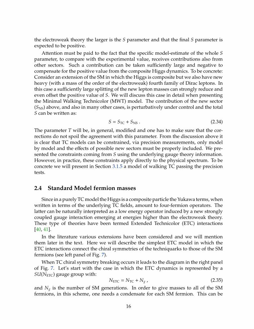
3.4.1 Spin zero + spin one . . . . . . . . . . . . . . . . . . . . . . . . . . 393.4.2 Spin zero + spin one + spin two . . . . . . . . . . . . . . . . . . . 41

4 Phenomenological benchmarks 434.1 Spin one processes: Decay widths and branching ratios . . . . . . . . . . 45

4.1.1 pp→ R→ `` . . . . . . . . . . . . . . . . . . . . . . . . . . . . . . . 514.1.2 pp→ R→WZ→ ```ν . . . . . . . . . . . . . . . . . . . . . . . . . 534.1.3 pp→ R→ `ν . . . . . . . . . . . . . . . . . . . . . . . . . . . . . . 554.1.4 pp→ R→ j j . . . . . . . . . . . . . . . . . . . . . . . . . . . . . . . 57

1

4.1.5 pp→ R→ γV and pp→ R→ ZZ . . . . . . . . . . . . . . . . . . . 574.2 Ultimate LHC reach for heavy spin resonances . . . . . . . . . . . . . . . 57

4.2.1 pp→ R→ 2`, `ν, 3`ν at 14 TeV . . . . . . . . . . . . . . . . . . . . . 574.2.2 pp→ Rjj at 14 TeV . . . . . . . . . . . . . . . . . . . . . . . . . . . 59

4.3 Composite Higgs phenomenology . . . . . . . . . . . . . . . . . . . . . . 604.3.1 pp→WH and pp→ ZH . . . . . . . . . . . . . . . . . . . . . . . . 614.3.2 Higgs vector boson fusion, pp→ Hjj . . . . . . . . . . . . . . . . . 634.3.3 H→ γγ and H→ gg . . . . . . . . . . . . . . . . . . . . . . . . . . 634.3.4 Higgs production via gluon fusion . . . . . . . . . . . . . . . . . . 70

5 A Natural fourth family of leptons at the TeV scale 705.1 The Standard Model leptons: a Mini-review . . . . . . . . . . . . . . . . . 715.2 Adding a fourth lepton family . . . . . . . . . . . . . . . . . . . . . . . . . 72

5.2.1 Heavy leptons not Mixing with Standard Model neutrinos . . . . 735.2.2 Promiscuous heavy leptons . . . . . . . . . . . . . . . . . . . . . . 74

5.3 LHC phenomenology for the natural heavy lepton family . . . . . . . . . 755.3.1 Production and decay of the new leptons . . . . . . . . . . . . . . 765.3.2 Collider signatures of heavy leptons with an exact flavor symmetry 78

5.4 Collider signatures of promiscuous heavy leptons . . . . . . . . . . . . . 81

6 Conclusion 82

A Realization of the generators for MWT and the Standard Model embedding 84

B Technicolor on Event Generators 85B.1 Ruling Technicolor with FeynRules . . . . . . . . . . . . . . . . . . . . . . 86B.2 Madding Technicolor via MadGraph/MadEvent v.4 . . . . . . . . . . . . 88B.3 Calculating Technicolor with CalcHEP . . . . . . . . . . . . . . . . . . . . 92

2

1 The need to go beyond

The energy scale at which the Large Hadron Collider experiment (LHC) operates isdetermined by the need to complete the Standard Model (SM) of particle interactionsand, in particular, to understand the origin of mass of the elementary particles. Togetherwith classical general relativity the SM constitutes one of the most successful models ofnature. We shall, however, argue that experimental results and theoretical argumentscall for a more fundamental description of nature.

In Fig. 1, we schematically represent, in green, the known forces of nature. The SMof particle physics describes the strong, weak and electromagnetic forces. The yellowregion represents the energy scale around the TeV scale and is being explored at theLHC, while the red part of the diagram is speculative.

Fermi Scale

Standard Model

Figure 1: Cartoon representing the various forces of nature. At very high energies onemay imagine that all the low-energy forces unify in a single force.

All of the known elementary particles constituting the SM fit on the postage stampshown in Fig. 2. Interactions among quarks and leptons are carried by gauge bosons.Massless gluons mediate the strong force among quarks while the massive gaugebosons, i.e. the Z and W, mediate the weak force and interact with both quarks andleptons. Finally, the massless photon, the quantum of light, interacts with all of theelectrically charged particles. The SM Higgs is introduced to provide mass to theelementary particles and in its minimal version does not feel strong interactions. Theinteractions emerge naturally by invoking a gauge principle which is intimately linked

3

to the underlying symmetries relating the various particles of the SM. The asterisk

SU(3)

SU(2)

U(1)

Figure 2: Postage stamp repre-senting all of the elementary parti-cles which constitute the SM. Theforces are mandated with the SU(3)×SU(2) ×U(1) gauge group.

Low Energy Effective Theory

SM

Figure 3: The SM can be viewed as a low-energy theory valid up to a high energy scaleΛ.

on the Higgs boson in the postage stamp indicates that it has not yet been observed.Intriguingly the Higgs is the only fundamental scalar of the SM.

The SM can be viewed as a low-energy effective theory valid up to an energy scale Λ,as schematically represented in Fig. 3. Above this scale new interactions, symmetries,extra dimensional worlds or any other extension could emerge. At sufficiently lowenergies with respect to this scale one expresses the existence of new physics viaeffective operators. The success of the SM is due to the fact that most of the correctionsto its physical observables depend only logarithmically on this scale Λ. In fact, in theSM there exists only one operator which acquires corrections quadratic in Λ. This isthe squared mass operator of the Higgs boson. Since Λ is expected to be the highestpossible scale, in four dimensions the Planck scale (assuming that we have only the SMand gravity), it is hard to explain naturally why the mass of the Higgs is of the orderof the Electroweak (EW) scale. This is the hierarchy problem. Due to the occurrenceof quadratic corrections in the cutoff this SM sector is most sensitive to the existence ofnew physics.

1.1 The Higgs

It is a fact that the Higgs allows for a direct and economical way of spontaneouslybreaking the electroweak symmetry. It generates simultaneously the masses of the

4

quarks and leptons without introducing Flavor Changing Neutral Currents (FCNC)sat the tree level. The Higgs sector of the SM possesses, when the gauge couplings areswitched off, an SU(2)L × SU(2)R symmetry. The full symmetry group can be madeexplicit when re-writing the Higgs doublet field

H =1√

2

(π2 + iπ1

σ − iπ3

)(1.1)

as the right column of the following two by two matrix:

1√

2

(σ + i~τ · ~π

)≡M . (1.2)

The first column can be identified with the column vector iτ2H∗ while the second withH. τ2 is the second Pauli matrix. The SU(2)L×SU(2)R group acts linearly on M accordingto:

M→ gLMg†R and gL/R ∈ SU(2)L/R . (1.3)

One can verify that:

M(1 − τ3)

2= (0 , H) . M

(1 + τ3)

2= (i τ2H∗ , 0) . (1.4)

The SU(2)L symmetry is gauged by introducing the weak gauge bosons Wa with a =1, 2, 3. The hypercharge generator is taken to be the third generator of SU(2)R. Theordinary covariant derivative acting on the Higgs, in the present notation, is:

DµM = ∂µM − i g WµM + i g′M Bµ , with Wµ = Waµ

τa

2, Bµ = Bµ

τ3

2. (1.5)

The Higgs Lagrangian is

L =12

Tr[DµM†DµM

]−

m2M

2Tr

[M†M

]−λ4

Tr[M†M

]2. (1.6)

At this point one assumes that the mass squared of the Higgs field is negative and thisleads to the electroweak symmetry breaking. Except for the Higgs mass term the otherSM operators have dimensionless couplings meaning that the natural scale for the SMis encoded in the Higgs mass1. We recall that the Higgs Lagrangian has a familiarform since it is identical to the linear σ Lagrangian which was introduced long ago todescribe chiral symmetry breaking in QCD with two light flavors.

1The mass of the proton is due mainly to strong interactions, however its value cannot be determinedwithin QCD since the associated renormalization group invariant scale must be fixed to an hadronicobservable.

5

At the tree level, when taking m2M negative and the self-coupling λ positive, one

determines:

〈σ〉2 ≡ v2 =|m2

M|

λand σ = v + h , (1.7)

where h is the Higgs field. The global symmetry breaks to its diagonal subgroup:

SU(2)L × SU(2)R → SU(2)V . (1.8)

To be more precise the SU(2)R symmetry is already broken explicitly by our choice ofgauging only an U(1)Y subgroup of it and hence the actual symmetry breaking patternis:

SU(2)L ×U(1)Y → U(1)Q , (1.9)

with U(1)Q the electromagnetic abelian gauge symmetry. According to the Nambu-Goldstone’s theorem three massless degrees of freedom appear, i.e. π± and π0. Inthe unitary gauge these Goldstones become the longitudinal degree of freedom of themassive elecetroweak gauge bosons. Substituting the vacuum value for σ in the HiggsLagrangian the gauge bosons quadratic terms read:

v2

8

[g2

(W1

µWµ,1 + W2µWµ,2

)+

(g W3

µ − g′ Bµ)2]. (1.10)

The Zµ and the photon Aµ gauge bosons are:

Zµ = cosθW W3µ − sinθWBµ ,

Aµ = cosθW Bµ + sinθWW3µ , (1.11)

with tanθW = g′/g while the charged massive vector bosons are W±

µ = (W1± i W2

µ)/√

2.The bosons masses M2

W = g2 v2/4 due to the custodial symmetry satisfy the tree levelrelation M2

Z = M2W/ cos2 θW. Holding fixed the EW scale v the mass squared of the

Higgs boson is 2λv2EW and hence it increases with λ.

Besides breaking the electroweak symmetry dynamically the ordinary Higgs servesalso the purpose to provide mass to all of the SM particles via the Yukawa terms of thetype:

− Yi jd Qi

LHd jR − Yi j

u QiL(iτ2H∗)u j

R + h.c. , (1.12)

where Yq is the Yukawa coupling constant, QL is the left-handed Dirac spinor of quarks,H the Higgs doublet and q the right-handed Weyl spinor for the quark and i, j the flavorindices. The SU(2)L weak and spinor indices are suppressed.

When considering quantum corrections the Higgs mass acquires large quantumcorrections proportional to the scale of the cutoff squared.

MH2ren −M2

H =kg2Λ2

16π2 . (1.13)

6

Here g is and electroweak constant and k a numerical factor depending on the specificmodel, expected to be O(1). Λ is the highest energy above which the SM is no longer avalid description of Nature and a large fine tuning of the parameters of the Lagrangianis needed to offset the effects of the cutoff. This large fine tuning is needed because thereare no symmetries protecting the Higgs mass operator from large corrections whichwould hence destabilize the Fermi scale (i.e. the electroweak scale). This problem isthe one we referred above as the hierarchy problem of the SM.

The constant value of the Higgs field evaluated on the ground state is determined bythe measured mass of the W boson. On the other hand, the value of the SM Higgs mass(MH) is constrained only indirectly by the electroweak precision data. The preferredvalue of the Higgs mass (obtained by the standard fit which excludes direct Higgssearches at LEP and Tevatron) is MH = 95.7+30.6

−24.2 GeV at 68% confidence level (CL) witha 95% CL upper limit MH < 171.5 GeV, as given by the generic fitting package Gfitter[1]. The corresponding results obtained by a fit including the direct Higgs searchesproduces MH = 120.6+17.9

−5.2 GeV at 68% confidence level (CL) with a 95% CL upper limitMH < 155.3 GeV, as reported on http://gfitter.desy.de/GSM/ by the Gfitter Group 2.

The final result of the average of all of the measures, however, has a Pearson’s chi-square (χ2) test of 17.5 for 14 degrees of freedom. A Higgs heavier than 155.3 GeV iscompatible with precision tests if we allow simultaneously new physics to compensatefor the effects of the heavier value of the mass. The precision measurements of directinterest for the Higgs sector are often reported using the S and T parameters as shownin Fig. 5. From this graph one deduces that a heavy Higgs is compatible with dataat the expense of a large value of the T parameter. Actually, even the lower directexperimental limit on the Higgs mass can be evaded with suitable extensions of the SMHiggs sector.

Many more questions need an answer if the Higgs is found at the LHC: Is it com-posite? How many Higgs fields are there in nature? Are there hidden sectors?

1.2 Riddles

Why do we expect that there is new physics awaiting to be discovered? Of course,we still have to observe the Higgs, but this cannot be everything. Even with the Higgsdiscovered, the SM has both conceptual problems and phenomenological shortcomings.In fact, theoretical arguments indicate that the SM is not the ultimate description ofnature:

• Hierarchy Problem: The Higgs sector is highly fine-tuned. We have no naturalexplanation of the large hierarchy between the Planck and the electroweak scales.

2All the plots and numerical results we use in this section are reported by the Gfitter Group and canbe found at the web-address: http://gfitter.desy.de/GSM/.

7

[GeV]HM20 40 60 80 100 120 140 160

tmbmcm

W

WM)2

Z(M(5)

had

b0Rc0RbAcA

0,bFBA

0,cFBA

)FB

(Qlepteff

2sin(SLD)lA(LEP)lA

0,lFBAlep0R

0had

Z

ZM

- 75 + 71142 - 25 + 32 99 - 24 + 31 96 - 24 + 31 96 - 34 + 75116 - 25 + 62 43 - 24 + 31 96 - 24 + 31 96 - 24 + 31 96 - 24 + 31 96 - 25 + 33 68 - 24 + 30 94 - 24 + 30 94 - 32 + 40122 - 24 + 31 92 - 26 + 32100 - 25 + 30100 - 25 + 31 97 - 25 + 32 97 - 26 + 49 61

[GeV]HM20 40 60 80 100 120 140 160

G fitter SM

Nov 10

Figure 4: Values of the Higgs massfrom the standard fit (which doesnot take into account direct Higgssearches) obtained by excluding dif-ferent electroweak observables. Thegreen band represent the 1σ errorrange around the best fit value of MH.

S-0.4 -0.3 -0.2 -0.1 0 0.1 0.2 0.3 0.4 0.5

T-0.4

-0.3

-0.2

-0.1

0

0.1

0.2

0.3

0.4

0.5

68%, 95%, 99% CL fit contours=120 GeV, U=0)

H(M

[114,1000] GeV HM 1.1 GeV± = 173.3tm

HM

preliminary

S-0.4 -0.3 -0.2 -0.1 0 0.1 0.2 0.3 0.4 0.5

T-0.4

-0.3

-0.2

-0.1

0

0.1

0.2

0.3

0.4

0.5G fitter SM

B

Aug 10

Figure 5: The 68%, 95%, and 99% CL coun-tours of the electroweak parameters S andT determined from different observables de-rived from a fit to the electroweak precisiondata. The gray area gives the SM predictionwith mt and MH varied as shown. MH = 120GeV and mt = 173.1 GeV defines the referencepoint at which all oblique parameters vanish.

• Strong CP problem: There is no natural explanation for the smallness of theelectric dipole moment of the neutron within the SM. This problem is also knownas the strong CP problem.

• Origin of patterns: The SM can fit, but cannot explain the number of mattergenerations and their mass spectrum.

• Unification of the forces: Why do we have so many different interactions? It isappealing to imagine that the SM forces could unify into a single Grand UnifiedTheory (GUT). We could imagine that at very high energy scales gravity alsobecomes part of a unified description of nature.

8

There is no doubt that the SM is incomplete since we cannot even account for a numberof basic observations:

• Neutrino physics: Only recently it has been possible to have some definite an-swers about properties of neutrinos. We now know that they have a tiny mass,which can be naturally accommodated in extensions of the SM, featuring for ex-ample a see-saw mechanism. We do not yet know if the neutrinos have a Diracor a Majorana nature.

• Origin of bright and dark mass: Leptons, quarks and the gauge bosons medi-ating the weak interactions possess a rest mass. Within the SM this mass can beaccounted for by the Higgs mechanism, which constitutes the electroweak sym-metry breaking sector of the SM. However, the associated Higgs particle has notyet been discovered. Besides, the SM cannot account for the observed large frac-tion of dark mass of the universe. What is interesting is that in the universe thedark matter is about five times more abundant than the known baryonic matter,i.e. bright matter. We do not know why the ratio of dark to bright matter is oforder unity.

• Matter-antimatter asymmetry: From our everyday experience we know thatthere is very little bright antimatter in the universe. The SM fails to predict theobserved excess of matter.

These arguments do not imply that the SM is necessarily incorrect, but it must beextended to answer any of the questions raised above. The truth is that we do not havean answer to the basic question: What lies beneath the SM?

A number of possible generalizations have been conceived (see [2, 3, 4, 5, 6, 7] forreviews). Such extensions are introduced on the base of one or more guiding principlesor prejudices. Two technical reviews are [8, 9].

In the models we will consider here the electroweak symmetry breaks via a fermionbilinear condensate. The Higgs sector of the SM becomes an effective description of amore fundamental fermionic theory. This is similar to the Ginzburg-Landau theory ofsuperconductivity. If the force underlying the fermion condensate driving electroweaksymmetry breaking is due to a strongly interacting gauge theory these models aretermed Technicolor (TC).

TC, in brief, is an additional non-abelian and strongly interacting gauge theoryaugmented with (techni)fermions transforming under a given representation of thegauge group. The Higgs Lagrangian is replaced by a suitable new fermion sectorinteracting strongly via a new gauge interaction (technicolor). Schematically:

LHiggs → −14

FµνFµν + iQγµDµQ + . . . , (1.14)

where, to be as general as possible, we have left unspecified the underlying nonabeliangauge group and the associated technifermion (Q) representation. The dots represent

9

new sectors which may even be needed to avoid, for example, anomalies introduced bythe technifermions. The intrinsic scale of the new theory is expected to be less or of theorder of a few TeV. The chiral-flavor symmetries of this theory, as for ordinary QCD,break spontaneously when the technifermion condensate QQ forms. It is possible tochoose the fermion charges in such a way that there is, at least, a weak left-handeddoublet of technifermions and the associated right-handed one which is a weak singlet.The covariant derivative contains the new gauge field as well as the electroweak ones.The condensate spontaneously breaks the electroweak symmetry down to the electro-magnetic and weak interactions. The Higgs is now interpreted as the lightest scalarfield with the same quantum numbers of the fermion-antifermion composite field. TheLagrangian part responsible for the mass-generation of the ordinary fermions will alsobe modified since the Higgs particle is no longer an elementary object.

Models of electroweak symmetry breaking via new strongly interacting theories ofTC type [10, 11] are a mature subject. The two uptodate reviews on which this work isbased are [12, 13]. For older nice reviews, updated till 2002, see [14, 15].

One of the main difficulties in constructing such extensions of the SM is the verylimited knowledge about generic strongly interacting theories. This has led theorists toconsider specific models of TC which resemble ordinary QCD and for which the largebody of experimental data at low energies can be directly exported to make predictionsat high energies. To reduce the tension with experimental constraints new stronglycoupled theories with dynamics different from the one featured by a scaled up versionof QCD are needed [16].

We will review models of dynamical electroweak symmetry breaking making use ofnew type of four dimensional gauge theories [16, 17, 18] and their low energy effectivedescription [19] useful for collider phenomenology. The phase structure of a largenumber of strongly interacting nonsupersymmetric theories, as function of number ofunderlying colors has been uncovered via traditional nonperturbative methods [20] aswell as novel ones [21, 22].

The theoretical part of this report should be integrated with earlier reviews [13, 14,15, 23, 24, 25, 26, 27, 28] on the various subjects treated here.

10

2 Dynamical Electroweak Symmetry Breaking

It is a fact that the SM does not fail, when experimentally tested, to describe all ofthe known forces to a very high degree of experimental accuracy. This is true even ifwe include gravity. Why is it so successful?

The SM is a low energy effective theory valid up to a scale Λ above which new inter-actions, symmetries, extra dimensional worlds or any possible extension can emerge.At sufficiently low energies with respect to the cutoff scale Λ one expresses the existenceof new physics via effective operators. The success of the SM is due to the fact thatmost of the corrections to its physical observable depend only logarithmically on thecutoff scale Λ.

Superrenormalizable operators are very sensitive to the cut off scale. In the SM thereexists only one operator with naive mass dimension two which acquires correctionsquadratic in Λ. This is the squared mass operator of the Higgs boson. Since Λ isexpected to be the highest possible scale, in four dimensions the Planck scale, it is hardto explain naturally why the mass of the Higgs is of the order of the electroweak scale.The Higgs is also the only particle predicted in the SM yet to be directly produced inexperiments. Due to the occurrence of quadratic corrections in the cutoff this is the SMsector highly sensitve to the existence of new physics.

In Nature we have already observed Higgs-type mechanisms. Ordinary supercon-ductivity and chiral symmetry breaking in QCD are two time-honored examples. Inboth cases the mechanism has an underlying dynamical origin with the Higgs-likeparticle being a composite object of fermionic fields.

2.1 Superconductivity versus electroweak symmetry breaking

The breaking of the electroweak theory is a relativistic screening effect. It is useful toparallel it to ordinary superconductivity which is also a screening phenomenon albeitnon-relativistic. The two phenomena happen at a temperature lower than a critical one.In the case of superconductivity one defines a density of superconductive electrons ns

and to it one associates a macroscopic wave function ψ such that its modulus squared

|ψ|2 = nC =ns

2, (2.15)

is the density of Cooper’s pairs. That we are describing a nonrelativistic system ismanifest in the fact that the macroscopic wave function squared, in natural units, hasmass dimension three while the modulus squared of the Higgs wave function evaluatedat the minimum is equal to 〈|H|2〉 = v2/2 and has mass dimension two, i.e. is a relativisticwave function. One can adjust the units by considering, instead of the wave functions,the Meissner-Mass of the photon in the superconductor which is

M2 = q2ns/(4me) , (2.16)

11

with q = −2e and 2me the charge and the mass of a Cooper pair which is constituted bytwo electrons. In the electroweak theory the Meissner-Mass of the photon is comparedwith the relativistic mass of the W gauge boson

M2W = g2v2/4 , (2.17)

with g the weak coupling constant and v the electroweak scale. In a superconductorthe relevant scale is given by the density of superconductive electrons typically of theorder of ns ∼ 4× 1028 m−3 yielding a screening length of the order of ξ = 1/M ∼ 10−6cm.In the weak interaction case we measure directly the mass of the weak gauge bosonwhich is of the order of 80 GeV yielding a weak screening length ξW = 1/MW ∼ 10−15cm.

For a superconductive system it is clear from the outset that the wave function ψ isnot a fundamental degree of freedom, however for the Higgs we are not yet sure aboutits origin. The Ginzburg-Landau effective theory in terms of ψ and the photon degreeof freedom describes the spontaneous breaking of the U(1)Q electric symmetry and it isthe equivalent of the Higgs Lagrangian.

If the Higgs is due to a macroscopic relativistic screening phenomenon we expect itto be an effective description of a more fundamental system with possibly an underlyingnew strong gauge dynamics replacing the role of the phonons in the superconductivecase. A dynamically generated Higgs system solves the problem of the quadraticdivergences by replacing the cutoff Λ with the weak energy scale itself, i.e. the scale ofcompositness. An underlying strongly coupled asymptotically free gauge theory, a laQCD, is an example.

2.2 From color to Technicolor

In fact even in complete absence of the Higgs sector in the SM the electroweaksymmetry breaks [26] due to the condensation of the following quark bilinear in QCD:

〈uLuR + dLdR〉 , 0 . (2.18)

This mechanism, however, cannot account for the whole contribution to the weak gaugebosons masses. If QCD was the only source contributing to the spontaneous breakingof the electroweak symmetry one would have

MW =gFπ2∼ 29 MeV , (2.19)

with Fπ ' 93 MeV the pion decay constant. This contribution is very small with respectto the actual value of the W mass that one typically neglects it.

According to the original idea of TC [10, 11] one augments the SM with anothergauge interaction similar to QCD but with a new dynamical scale of the order of theelectroweak one. It is sufficient that the new gauge theory is asymptotically free and hasglobal symmetry able to contain the SM SU(2)L ×U(1)Y symmetries. It is also required

12

that the new global symmetries break dynamically in such a way that the embeddedSU(2)L × U(1)Y breaks to the electromagnetic abelian charge U(1)Q . The dynamicallygenerated scale will then be fit to the electroweak one.

Note that, except in certain cases, dynamical behaviors are typically nonuniversalwhich means that different gauge groups and/or matter representations will, in general,possesses very different dynamics.

The simplest example of TC theory is the scaled up version of QCD, i.e. an SU(NTC)nonabelian gauge theory with two Dirac Fermions transforming according to the fun-damental representation or the gauge group. We need at least two Dirac flavors torealize the SU(2)L × SU(2)R symmetry of the SM discussed in the SM Higgs section.One simply chooses the scale of the theory to be such that the new pion decayingconstant is:

FTCπ = v ' 246 GeV . (2.20)

The flavor symmetries, for any NTC larger than 2 are SU(2)L × SU(2)R × U(1)V whichspontaneously break to SU(2)V × U(1)V. It is natural to embed the electroweak sym-metries within the present TC model in a way that the hypercharge corresponds tothe third generator of SU(2)R. This simple dynamical model correctly accounts for theelectroweak symmetry breaking. The new technibaryon number U(1)V can break dueto not yet specified new interactions. In order to get some indication on the dynamicsand spectrum of this theory one can use the ’t Hooft large N limit [29, 30, 31]. Forexample the intrinsic scale of the theory is related to the QCD one via:

ΛTC ∼

√3

NTC

FTCπ

FπΛQCD . (2.21)

At this point it is straightforward to use the QCD phenomenology for describing theexperimental signatures and dynamics of a composite Higgs.

2.3 Constraints from electroweak precision data

The relevant corrections due to the presence of new physics trying to modify theelectroweak breaking sector of the SM appear in the vacuum polarizations of theelectroweak gauge bosons. These can be parameterized in terms of the three quantitiesS, T, and U (the oblique parameters) [32, 33, 34, 35], and confronted with the electroweakprecision data. Recently, due to the increase precision of the measurements reportedby LEP II, the list of interesting parameters to compute has been extended [36, 37]. Weshow below also the relation with the traditional one [32]. Defining with Q2

≡ −q2

the Euclidean transferred momentum entering in a generic two point function vacuumpolarization associated to the electroweak gauge bosons, and denoting derivatives with

13

respect to −Q2 with a prime we have [37]:

S ≡ g2 Π′W3B(0) , (2.22)

T ≡g2

M2W

[ΠW3W3(0) −ΠW+W−(0)] , (2.23)

W ≡g2M2

W

2

[Π′′W3W3(0)

], (2.24)

Y ≡g′2M2

W

2

[Π′′BB(0)

], (2.25)

U ≡ −g2[Π′W3W3(0) −Π′W+W−(0)

], (2.26)

V ≡g2 M2

W

2

[Π′′W3W3(0) −Π′′W+W−(0)

], (2.27)

X ≡gg′M2

W

2Π′′W3B(0) . (2.28)

Here ΠV(Q2) with V = {W3B, W3W3, W+W−, BB} represents the self-energy of the vectorbosons. The electroweak couplings are the ones associated to the physical electroweakgauge bosons:

1g2 ≡ Π′W+W−(0) ,

1g′2≡ Π′BB(0) , (2.29)

while GF is

1√

2GF

= −4ΠW+W−(0) , (2.30)

as in [38]. S and T lend their name from the well known Peskin-Takeuchi parametersS and T which are related to the new ones via [37, 38]:

αS4s2

W

= S − Y −W , αT = T −s2

W

1 − s2W

Y . (2.31)

Here α is the electromagnetic structure constant and sW = sinθW is the weak mixingangle. Therefore in the case where W = Y = 0 we have the simple relation

S =αS4s2

W

, T = αT . (2.32)

The result of the the fit is shown in Fig. 5. If the value of the Higgs mass increases thecentral value of the S parameter moves to the left towards negative values.In TC it is easy to have a vanishing T parameter while typically S is positive. Besides,the composite Higgs is typically heavy with respect to the Fermi scale, at least for

14

-0.2 0.0 0.2 0.4-0.1

0.0

0.1

0.2

0.3

0.4

0.5

S

T

Figure 6: T versus S for SU(3) TC with one technifermion doublet (the full disc) versusprecision data for a one TeV composite Higgs mass.

technifermions in the fundamental representation of the gauge group and for a smallnumber of techniflavors. The oldest TC models featuring QCD dynamics with threetechnicolors and a doublet of electroweak gauged techniflavors deviate a few sigmafrom the current precision tests as summarized in Fig. 6. Clearly it is desirable toreduce the tension between the precision data and a possible dynamical mechanismunderlying the electroweak symmetry breaking. It is possible to imagine different waysto achieve this goal and some of the earlier attempts have been summarized in [39].

The computation of the S parameter in TC theories requires the knowledge ofnonperturbative dynamics making difficult the precise knowledge of the contributionto S. For example, it is not clear what is the exact value of the composite Higgs massrelative to the Fermi scale and, to be on the safe side, one typically takes it to be quitelarge, of the order at least of the TeV. However in certain models it may be substantiallylighter due to the intrinsic dynamics. We will discuss the electroweak parameters laterin this chapter.

It is, however, instructive to provide a simple estimate of the contribution to Swhich allows to guide model builders. Consider a one-loop exchange of ND doubletsof techniquarks transforming according to the representation RTC of the underlying TCgauge theory and with dynamically generated mass Σ(0) assumed to be larger than theweak intermediate gauge bosons masses. Indicating with d(RTC) the dimension of thetechniquark representation, and to leading order in MW/Σ(0) one finds:

Snaive = NDd(RTC)

6π. (2.33)

This naive value provides, in general, only a rough estimate of the exact value of S.However, it is clear from the formula above that, the more TC matter is gauged under

15

the electroweak theory the larger is the S parameter and that the final S parameter isexpected to be positive.

Attention must be paid to the fact that the specific model-estimate of the whole Sparameter, to compare with the experimental value, receives contributions also fromother sectors. Such a contribution can be taken sufficiently large and negative tocompensate for the positive value from the composite Higgs dynamics. To be concrete:Consider an extension of the SM in which the Higgs is composite but we also have newheavy (with a mass of the order of the electroweak) fourth family of Dirac leptons. Inthis case a sufficiently large splitting of the new lepton masses can strongly reduce andeven offset the positive value of S. We will discuss this case in detail when presentingthe Minimal Walking Technicolor (MWT) model. The contribution of the new sector(SNS) above, and also in many other cases, is perturbatively under control and the totalS can be written as:

S = STC + SNS . (2.34)

The parameter T will be, in general, modified and one has to make sure that the cor-rections do not spoil the agreement with this parameter. From the discussion above itis clear that TC models can be constrained, via precision measurements, only modelby model and the effects of possible new sectors must be properly included. We pre-sented the constraints coming from S using the underlying gauge theory information.However, in practice, these constraints apply directly to the physical spectrum. To beconcrete we will present in Section 3.1.5 a model of walking TC passing the precisiontests.

2.4 Standard Model fermion masses

Since in a purely TC model the Higgs is a composite particle the Yukawa terms, whenwritten in terms of the underlying TC fields, amount to four-fermion operators. Thelatter can be naturally interpreted as a low energy operator induced by a new stronglycoupled gauge interaction emerging at energies higher than the electroweak theory.These type of theories have been termed Extended Technicolor (ETC) interactions[40, 41].

In the literature various extensions have been considered and we will mentionthem later in the text. Here we will describe the simplest ETC model in which theETC interactions connect the chiral symmetries of the techniquarks to those of the SMfermions (see left panel of Fig. 7).

When TC chiral symmetry breaking occurs it leads to the diagram in the right panelof Fig. 7. Let’s start with the case in which the ETC dynamics is represented by aSU(NETC) gauge group with:

NETC = NTC + Ng , (2.35)

and Ng is the number of SM generations. In order to give masses to all of the SMfermions, in this scheme, one needs a condensate for each SM fermion. This can be

16

�ETC

ψL

QL

QR

ψR

�QL

QR

ETC

ψL

ψR

Figure 7: Left panel: ETC gauge boson interaction involving techniquarks and SMfermions. Right panel: Diagram contribution to the mass to the SM fermions.

achieved by using as technifermion matter a complete generation of quarks and leptons(including a neutrino right) but now gauged with respect to the TC interactions.

The ETC gauge group is assumed to spontaneously break Ng times down to SU(NTC)permitting three different mass scales, one for each SM family. This type of TC withassociated ETC is termed the one family model [42]. The heavy masses are provided bythe breaking at low energy and the light masses are provided by breaking at higherenergy scales. This model does not, per se, explain how the gauge group is brokenseveral times, neither is the breaking of weak isospin symmetry accounted for. Forexample we cannot explain why the neutrino have masses much smaller than theassociated electrons. See, however, [43] for progress on these issues. Schematicallyone has SU(NTC + 3) which breaks to SU(NTC + 2) at the scale Λ1 providing the firstgeneration of fermions with a typical mass m1 ∼ 4π(FTC

π )3/Λ21 at this point the gauge

group breaks to SU(NTC + 1) with dynamical scale Λ2 leading to a second generationmass of the order of m2 ∼ 4π(FTC

π )3/Λ22 finally the last breaking SU(NTC) at scale Λ3

leading to the last generation mass m3 ∼ 4π(FTCπ )3/Λ2

3.Without specifying an ETC one can write down the most general type of four-

fermion operators involving TC particles Q and ordinary fermionic fields ψ. Followingthe notation of Hill and Simmons [14] we write:

αabQγµTaQψγµTbψ

Λ2ETC

+ βabQγµTaQQγµTbQ

Λ2ETC

+ γabψγµTaψψγµTbψ

Λ2ETC

, (2.36)

where the Ts are unspecified ETC generators. After performing a Fierz rearrangementone has:

αabQTaQψTbψ

Λ2ETC

+ βabQTaQQTbQ

Λ2ETC

+ γabψTaψψTbψ

Λ2ETC

+ . . . , (2.37)

The coefficients parametrize the ignorance on the specific ETC physics. To be morespecific, the α-terms, after the TC particles have condensed, lead to mass terms for theSM fermions

mq ≈g2

ETC

M2ETC

〈QQ〉ETC , (2.38)

17

where mq is the mass of e.g. a SM quark, gETC is the ETC gauge coupling constantevaluated at the ETC scale, METC is the mass of an ETC gauge boson and 〈QQ〉ETC isthe TC condensate where the operator is evaluated at the ETC scale. Note that we havenot explicitly considered the different scales for the different generations of ordinaryfermions but this should be taken into account for any realistic model.

The β-terms of Eq. (2.37) provide masses for pseudo Goldstone bosons and alsoprovide masses for techniaxions [14], see Fig. 8. The last class of terms, namely theγ-terms of Eq. (2.37) induce FCNCs. For example it may generate the following terms:

1Λ2

ETC

(sγ5d)(sγ5d) +1

Λ2ETC

(µγ5e)(eγ5e) + . . . , (2.39)

where s, d, µ, e denote the strange and down quark, the muon and the electron, respec-tively. The first term is a ∆S = 2 flavor-changing neutral current interaction affectingthe KL−KS mass difference which is measured accurately. The experimental bounds onthese type of operators together with the very naive assumption that ETC will generatethese operators with γ of order one leads to a constraint on the ETC scale to be of theorder of or larger than 103 TeV [40]. This should be the lightest ETC scale which inturn puts an upper limit on how large the ordinary fermionic masses can be. The naiveestimate is that one can account up to around 100 MeV mass for a QCD-like TC theory,implying that the top quark mass value cannot be achieved.

The second term of Eq. (2.39) induces flavor changing processes in the leptonicsector such as µ→ eee, eγwhich are not observed. It is clear that, both for the precision

�ETCΠ Π

Figure 8: Leading contribution to the mass of the TC pseudo Goldstone bosons via anexchange of an ETC gauge boson.

measurements and the fermion masses, a better theory of the flavor is needed. For theETC dynamics interesting developments recently appeared in the literature [44, 45, 46,47]. We note that nonperturbative chiral gauge theories dynamics is expected to playa relevant role in models of ETC since it allows, at least in principle, the self breakingof the gauge symmetry. Recent progress on the phase diagrams of these theories hasappeared in [12].

18

In Fig. 9 we show the ordering of the relevant scales involved in the generationof the ordinary fermion masses via ETC dynamics, and the generation of the fermionmasses (for a single generation and focussing on the top quark) assuming QCD-likedynamics for TC.

mf ≈g2

ETC

Λ2ETC

< QQ >ETCΛETC

ΛTC

mf ≈g2

ETC

Λ2ETC

< QQ >ETC � mTop

Electroweak breaks

< QQ >ETC ≈< QQ >TC ∼ Λ3TC

Figure 9: Cartoon of the expected ETC dynamics starting at high energies with a morefundamental gauge interaction and the generation of the fermion masses assumingQCD-like dynamics.

2.5 Walking

To better understand in which direction one should go to modify the QCD dynamics,we analyze the TC condensate. The value of the TC condensate used when giving massto the ordinary fermions should be evaluated not at the TC scale but at the ETC one.Via the renormalization group one can relate the condensate at the two scales via:

〈QQ〉ETC = exp(∫ ΛETC

ΛTC

d(lnµ)γm(α(µ)))〈QQ〉TC , (2.40)

19

where γm is the anomalous dimension of the techniquark mass-operator. The bound-aries of the integral are at the ETC scale and the TC one. For TC theories with a runningof the coupling constant similar to the one in QCD, i.e.

α(µ) ∝1

lnµ, for µ > ΛTC , (2.41)

this implies that the anomalous dimension of the techniquark masses γm ∝ α(µ). Whencomputing the integral one gets

〈QQ〉ETC ∼ ln(ΛETC

ΛTC

)γm

〈QQ〉TC , (2.42)

which is a logarithmic enhancement of the operator. We can hence neglect this correc-tion and use directly the value of the condensate at the TC scale when estimating thegenerated fermionic mass:

mq ≈g2

ETC

M2ETC

Λ3TC , 〈QQ〉TC ∼ Λ3

TC . (2.43)

The tension between having to reduce the FCNCs and at the same time providea sufficiently large mass for the heavy fermions in the SM as well as the pseudo-Goldstones can be reduced if the dynamics of the underlying TC theory is differentfrom the one of QCD. The computation of the TC condensate at different scales showsthat if the dynamics is such that the TC coupling does not run to the UV fixed point butrather slowly reduces to zero one achieves a net enhancement of the condensate itselfwith respect to the value estimated earlier. This can be achieved if the theory has anear conformal fixed point. This kind of dynamics has been denoted as of walking type.In Fig. 10 the comparison between a running and walking behavior of the coupling isqualitatively represented.

In the walking regime:

〈QQ〉ETC ∼

(ΛETC

ΛTC

)γm(α∗)

〈QQ〉TC , (2.44)

which is a much larger contribution than in QCD dynamics [48, 49, 50, 51]. Here γm isevaluated at the would be fixed point value α∗. Walking can help resolving the problemof FCNCs in TC models since with a large enhancement of the 〈QQ〉 condensate thefour-Fermi operators involving SM fermions and technifermions and the ones involvingtechnifermions are enhanced by a factor of ΛETC/ΛTC to the γm power while the oneinvolving only SM fermions is not enhanced.

We note that walking is not a fundamental property for a successful model of theorigin of mass of the elementary fermions featuring TC. In fact several alternative ideasalready exist in the literature (see [52, 53] and references therein). However, a nearconformal theory would still be useful to reduce the contributions to the precision dataand, possibly, provide a light composite Higgs of much interest to LHC physics [17].

20

Figure 10: Top left panel: QCD-like behavior of the coupling constant as function ofthe momentum (Running). Top right panel: walking-like behavior of the couplingconstant as function of the momentum (Walking). Bottom right panel: cartoon of thebeta function associated to a generic walking theory.

2.6 Ideal walking

There are several issues associated with the original idea of walking:

• Since the number of flavors cannot be changed continuously it is not possible toget arbitrarily close to the lower end of the conformal window. This applies tothe TC theory in isolation i.e. before coupling it to the SM and without taking intoaccount the ETC interactions.

• It is hard to achieve large anomalous dimensions of the fermion mass operatoreven near the lower end of the conformal window for ordinary gauge theories.

• It is not always possible to neglect the interplay of the four fermion interactionson the TC dynamics.

In [54] it has been argued that it is possible to solve simultaneously all the problemsabove by consistently taking into account the effects of the four-fermion interactionson the phase diagram of strongly interacting theories for any matter representation asfunction of the number of colors and flavors. A positive effect is that the anomalousdimension of the mass increases beyond the unity value at the lower boundary of thenew conformal window and can get sufficiently large to yield the correct mass for thetop quark. It has also been shown that the conformal window, for any representation,shrinks with respect to the case in which the four-fermion interactions are neglected.

21

This analysis derives from the study of the gauged Nambu-Jona-Lasinio phase diagram[55].

It has been made the further unexpected discovery that when the extended TC sector,responsible for giving masses to the SM fermions, is sufficiently strongly coupled, theTC theory, in isolation, must feature an infrared fixed point in order for the full modelto be phenomenologically viable and correctly break the electroweak symmetry [56].

22

3 Phenomenology of Minimal Technicolor

The existence of a new weak doublet of technifermions amounting to, at least, aglobal SU(2)L × SU(2)R symmetry later opportunely gauged under the electroweakinteractions is the bedrock on which models of TC are built on.

It is therefore natural to construct first minimal models of TC passing precision testswhile also reducing the FCNC problem by featuring near conformal dynamics. Byminimal we mean with the smallest fermionic matter content. These models were putforward recently in[16, 17]. To be concrete we describe here the (N)MWT [13] extensionof the SM.

The extended SM gauge group is now SU(2)TC×SU(3)C×SU(2)L×U(1)Y and the fieldcontent of the TC sector is constituted by four techni-fermions and one techni-gluonall in the adjoint representation of SU(2)TC. The model features also a pair of Diracleptons, whose left-handed components are assembled in a weak doublet, necessaryto cancel the Witten anomaly [57] arising when gauging the new technifermions withrespect to the weak interactions. Summarizing, the fermionic particle content of theMWT is given explicitly by

QaL =

(Ua

Da

)L, Ua

R , DaR , a = 1, 2, 3 , (3.45)

with a being the adjoint color index of SU(2). The left handed fields are arranged inthree doublets of the SU(2)L weak interactions in the standard fashion. The condensateis 〈UU + DD〉 which correctly breaks the electroweak symmetry as already argued forordinary QCD in Eq. (2.18).

The model as described so far suffers from the Witten topological anomaly [57].However, this can easily be solved by adding a new weakly charged fermionic doubletwhich is a TC singlet [17]. Schematically:

LL =

(NE

)L, NR , ER . (3.46)

In general, the gauge anomalies cancel using the following generic hypercharge assign-ment

Y(QL) =y2, Y(UR,DR) =

(y + 1

2,

y − 12

), (3.47)

Y(LL) = − 3y2, Y(NR,ER) =

(−3y + 1

2,−3y − 1

2

), (3.48)

where the parameter y can take any real value [17]. In our notation the electric chargeis Q = T3 + Y, where T3 is the weak isospin generator. One recovers the SM hyper-charge assignment for y = 1/3. To discuss the symmetry properties of the theory it is

23

Minimal Walking Technicolor

Sannino, Tuominen ‘04; Dietrich, Sannino, Tuominen ‘05

Nextra

neutrino

Eextra

electron

UTC-up

DTC-down

GTC-gluon

U(1)Y

SU(2)L

SU(3)C

SU(2)TC

TC-fermions in the SU(2)TC ad-joint rep.: a = 1, 2, 3;

QaL =

�Ua

L

DaL

�, Ua

R, DaR

Heavy leptons to cancel Wittenanomaly

LL =

�NL

EL

�, NR, ER

S. Di Chiara Planck 2010

Figure 11: Cartoon of the Minimal Walking Technicolor Model extension of the SM.

convenient to use the Weyl basis for the fermions and arrange them in the followingvector transforming according to the fundamental representation of SU(4)

Q =

UL

DL

−iσ2U∗R−iσ2D∗R

, (3.49)

where UL and DL are the left handed techniup and technidown, respectively and UR

and DR are the corresponding right handed particles. Assuming the standard breakingto the maximal diagonal subgroup, the SU(4) symmetry spontaneously breaks to SO(4).Such a breaking is driven by the following condensate

〈Qαi Qβ

jεαβEi j〉 = −2 〈URUL + DRDL〉 , (3.50)

where the indices i, j = 1, . . . , 4 denote the components of the tetraplet of Q, and theGreek indices indicate the ordinary spin. The matrix E is a 4×4 matrix defined in termsof the 2-dimensional unit matrix as

E =

(0 1

1 0

). (3.51)

Here εαβ = −iσ2αβ and 〈Uα

LUR∗βεαβ〉 = −〈URUL〉. A similar expression holds for the

D techniquark. The above condensate is invariant under an SO(4) symmetry. This

24

leaves us with nine broken generators with associated Goldstone bosons, of whichthree become the longitudinal degrees of freedom of the weak gauge bosons.

Replacing the Higgs sector of the SM with the MWT the Lagrangian now reads:

LH → −14F

aµνF

aµν + iQLγµDµQL + iURγ

µDµUR + iDRγµDµDR

+iLLγµDµLL + iERγ

µDµER + iNRγµDµNR (3.52)

with the TC field strength F aµν = ∂µAa

ν − ∂νAaµ + gTCεabc

AbµA

cν, a, b, c = 1, . . . , 3. For the

left handed techniquarks the covariant derivative is:

DµQaL =

(δac∂µ + gTCA

bµε

abc− i

g2~Wµ · ~τδ

ac− ig′

y2

Bµδac)

QcL . (3.53)

Aµ are the techni gauge bosons, Wµ are the gauge bosons associated to SU(2)L and Bµ isthe gauge boson associated to the hypercharge. τa are the Pauli matrices and εabc is thefully antisymmetric symbol. In the case of right handed techniquarks the third termcontaining the weak interactions disappears and the hypercharge y/2 has to be replacedaccordingly to Eq. (3.47). For the left-handed leptons the second term containing theTC interactions disappears and y/2 changes to −3y/2. Only the last term is present forthe right handed leptons with an appropriate hypercharge assignment.

3.1 Low energy theory for MWT

We construct the effective theory for MWT including composite scalars and vectorbosons, their self interactions, and their interactions with the electroweak gauge fieldsand the SM fermions.

3.1.1 Scalar sector

The relevant effective theory for the Higgs sector at the electroweak scale consists,in our model, of a composite Higgs σ and its pseudoscalar partner Θ, as well as ninepseudoscalar Goldstone bosons and their scalar partners. These can be assembled inthe matrix

M =[σ + iΘ

2+√

2(iΠa + Πa) Xa]

E , (3.54)

which transforms under the full SU(4) group according to

M→ uMuT , with u ∈ SU(4) . (3.55)

The Xa’s, a = 1, . . . , 9 are the generators of the SU(4) group which do not leave theVacuum Expectation Value (VEV) of M invariant

〈M〉 =v2

E . (3.56)

25

Note that the notation used is such that σ is a scalar while the Πa’s are pseudoscalars.It is convenient to separate the fifteen generators of SU(4) into the six that leave thevacuum invariant, Sa, and the remaining nine that do not, Xa. Then the Sa generatorsof the SO(4) subgroup satisfy the relation

Sa E + E SaT = 0 , with a = 1, . . . , 6 , (3.57)

so that uEuT = E, for u ∈ SO(4). The explicit realization of the generators and theembedding of the electroweak generators in the SU(4) algebra are shown in AppendixA. With the tilde fields included, the matrix M is invariant in form under U(4) ≡SU(4)×U(1)A, rather than just SU(4). However the U(1)A axial symmetry is anomalous,and is therefore broken at the quantum level.

The connection between the composite scalars and the underlying techniquarkscan be derived from the transformation properties under SU(4), by observing that theelements of the matrix M transform like techniquark bilinears:

Mi j ∼ Qαi Qβ

jεαβ with i, j = 1 . . . 4. (3.58)

Using this expression, and the basis matrices given in Appendix A, the scalar fieldscan be related to the wavefunctions of the techniquark bound states. This gives thefollowing charge eigenstates:

v + H ≡ σ ∼ UU + DD , Θ ∼ i(Uγ5U + Dγ5D

),

A0≡ Π3

∼ UU −DD , Π0≡ Π3

∼ i(Uγ5U −Dγ5D

),

A+≡

Π1− iΠ2

√2

∼ DU , Π+≡

Π1− iΠ2

√2

∼ iDγ5U ,

A− ≡Π1 + iΠ2

√2

∼ UD , Π− ≡Π1 + iΠ2

√2

∼ iUγ5D ,

(3.59)

for the technimesons, and

ΠUU ≡Π4 + iΠ5 + Π6 + iΠ7

2∼ UTCU ,

ΠDD ≡Π4 + iΠ5

−Π6− iΠ7

2∼ DTCD ,

ΠUD ≡Π8 + iΠ9

√2

∼ UTCD ,

ΠUU ≡Π4 + iΠ5 + Π6 + iΠ7

2∼ iUTCγ5U ,

ΠDD ≡Π4 + iΠ5

− Π6− iΠ7

2∼ iDTCγ5D ,

ΠUD ≡Π8 + iΠ9

√2

∼ iUTCγ5D ,

(3.60)

26

for the technibaryons, where U ≡ (UL,UR)T and D ≡ (DL,DR)T are Dirac technifermions,and C is the charge conjugation matrix, needed to form Lorentz-invariant objects. Tothese technibaryon charge eigenstates we must add the corresponding charge conjugatestates (e.g. ΠUU → ΠUU).

Three of the nine Goldstone bosons (Π±,Π0) associated with the relative brokengenerators become the longitudinal degrees of freedom of the massive weak gaugebosons, while the extra six Goldstone bosons will acquire a mass due to ETC interactionsas well as the electroweak interactions per se. Using a bottom up approach we will notcommit to a specific ETC theory but limit ourself to introduce the minimal low energyoperators needed to construct a phenomenologically viable theory. The new HiggsLagrangian is

LHiggs =12

Tr[DµMDµM†

]−V(M) +LETC , (3.61)

where the potential reads

V(M) = −m2

M

2Tr[MM†] +

λ4

Tr[MM†

]2+ λ′Tr

[MM†MM†

]− 2λ′′

[Det(M) + Det(M†)

], (3.62)

and LETC contains all terms which are generated by the ETC interactions, and not bythe chiral symmetry breaking sector. Notice that the determinant terms (which arerenormalizable) explicitly break the U(1)A symmetry, and give mass to Θ, which wouldotherwise be a massless Goldstone boson.

In order to give masses to the remaining uneaten Goldstone boson we add this termwhich is generated in the ETC sector:

LETC ⊃m2

ETC

4Tr

[MBM†B + MM†

], (3.63)

and B ≡ 2√

2S4 is a specific generator in the SU(4) algebra.The potentialV(M) produces a VEV which parameterizes the techniquark conden-

sate, and spontaneously breaks SU(4) to SO(4). In terms of the model parameters theVEV is

v2 = 〈σ〉2 =m2

M

λ + λ′ − λ′′, (3.64)

while the Higgs mass is

M2H = 2 m2

M . (3.65)

The linear combination λ + λ′ − λ′′ corresponds to the Higgs self coupling in the SM.The three pseudoscalar mesons Π±, Π0 correspond to the three massless Goldstone

27

bosons which are absorbed by the longitudinal degrees of freedom of the W± and Zboson. The remaining six uneaten Goldstone bosons are technibaryons, and all acquiretree-level degenerate mass through the ETC interaction in (3.63):

M2ΠUU

= M2ΠUD

= M2ΠDD

= m2ETC . (3.66)

The remaining scalar and pseudoscalar masses are

M2Θ = 4v2λ′′

M2A± = M2

A0 = 2v2 (λ′ + λ′′) (3.67)

for the technimesons, and

M2ΠUU

= M2ΠUD

= M2ΠDD

= m2ETC + 2v2 (λ′ + λ′′) , (3.68)

for the technibaryons. To gain insight on some of the mass relations one can use [58].

3.1.2 Vector bosons

The composite vector bosons of a theory with a global SU(4) symmetry are conve-niently described by the four-dimensional traceless Hermitian matrix

Aµ = Aaµ Ta , (3.69)

where Ta are the SU(4) generators: Ta = Sa, for a = 1, . . . , 6, and Ta+6 = Xa, for a = 1, . . . , 9.Under an arbitrary SU(4) transformation, Aµ transforms like

Aµ→ u Aµ u† , where u ∈ SU(4) . (3.70)

Eq. (3.70), together with the tracelessness of the matrix Aµ, gives the connection withthe techniquark bilinears:

Aµ, ji ∼ Qα

i σµ

αβQβ, j−

14δ j

i Qαkσ

µ

αβQβ,k . (3.71)

Then we find the following relations between the charge eigenstates and the wavefunc-tions of the composite objects:

v0µ≡ A3µ

∼ UγµU − DγµD , a0µ≡ A9µ

∼ Uγµγ5U − Dγµγ5D

v+µ≡

A1µ− iA2µ

√2

∼ DγµU , a+µ≡

A7µ− iA8µ

√2

∼ Dγµγ5U

v−µ ≡A1µ + iA2µ

√2

∼ UγµD , a−µ ≡A7µ + iA8µ

√2

∼ Uγµγ5D

v4µ≡ A4µ

∼ UγµU + DγµD ,

(3.72)

28

for the vector mesons, and

xµUU ≡A10µ + iA11µ + A12µ + iA13µ

2∼ UTCγµγ5U ,

xµDD ≡A10µ + iA11µ

− A12µ− iA13µ

2∼ DTCγµγ5D ,

xµUD ≡A14µ + iA15µ

√2

∼ DTCγµγ5U ,

sµUD ≡A6µ− iA5µ

√2

∼ UTCγµD ,

(3.73)

for the vector baryons.There are different approaches on how to introduce vector mesons at the effective

Lagrangian level. At the tree level they are all equivalent.Based on this premise, the minimal kinetic Lagrangian is:

Lkinetic = −12

Tr[WµνWµν

]−

14

BµνBµν −12

Tr[FµνFµν

]+ m2 Tr

[CµCµ

], (3.74)

where Wµν and Bµν are the ordinary field strength tensors for the electroweak gaugefields. Strictly speaking the terms above are not only kinetic ones since the Lagrangiancontains a mass term as well as self interactions. The tilde on Wa indicates that theassociated states are not yet the SM weak triplets: in fact these states mix with thecomposite vectors to form mass eigenstates corresponding to the ordinary W and Zbosons. Fµν is the field strength tensor for the new SU(4) vector bosons,

Fµν = ∂µAν − ∂νAµ − ig[Aµ,Aν

], (3.75)

and the vector field Cµ is defined by

Cµ ≡ Aµ −gg

Gµ . (3.76)

and Gµ is given byGµ = g Wa

µ La + g′ BµY , (3.77)

where La and Y are the generators of the left-handed and hypercharge transformations,as defined in Appendix A, with Y. The parameter g represents the coupling amongthe vectors and the ratio g

g is phenomenologically very important because it sets themixing among gauge eigenstates and composite vectors eigenstates. The mass termin Eq. (3.74) is gauge invariant, and gives a degenerate mass to all composite vectorbosons, while leaving the actual gauge bosons massless. (The latter acquires mass asusual from the covariant derivative term of the scalar matrix M, after spontaneoussymmetry breaking.)

29

The Cµ fields couple with M via gauge invariant operators. Up to dimension fouroperators the Lagrangian is

LM−C = g2 r1 Tr[CµCµMM†

]+ g2 r2 Tr

[CµMCµTM†

]+ i g

r3

2Tr

[Cµ

(M(DµM)† − (DµM)M†

)]+ g2 s Tr

[CµCµ

]Tr

[MM†

].

(3.78)

The dimensionless parameters r1, r2, r3, s parameterize the strength of the interactionsbetween the composite scalars and vectors in units of g, and are therefore naturallyexpected to be of order one. However, notice that for r1 = r2 = r3 = 0 the overallLagrangian possesses two independent SU(2)L×U(1)R×U(1)V global symmetries. Onefor the terms involving M and one for the terms involving Cµ

3. The Higgs potentialonly breaks the symmetry associated with M, while leaving the symmetry in the vectorsector unbroken. This enhanced symmetry guarantees that all r-terms are still zero afterloop corrections. Moreover if one chooses r1, r2, r3 to be small the near enhancedsymmetry will protect these values against large corrections [59, 60].

3.1.3 Fermions and Yukawa interactions

The fermionic content of the effective theory consists of the SM quarks and lep-tons, the new lepton doublet L = (N,E) introduced to cure the Witten anomaly, and acomposite techniquark-technigluon doublet.

We now consider the limit according to which the SU(4) symmetry is, at first, ex-tended to ordinary quarks and leptons. Of course, we will need to break this symmetryto accommodate the SM phenomenology. We start by arranging the SU(2) doublets inSU(4) multiplets as we did for the techniquarks in Eq. (3.49). We therefore introducethe four component vectors qi and li,

qi =

ui

Ldi

L−iσ2ui

R∗

−iσ2diR∗

, li =

νi

Lei

L−iσ2νi

R∗

−iσ2eiR∗

, (3.79)

where i is the generation index. Note that such an extended SU(4) symmetry automat-ically predicts the presence of a right handed neutrino for each generation. In additionto the SM fields there is an SU(4) multiplet for the new leptons,

L =

NL

EL

−iσ2NR∗

−iσ2ER∗

, (3.80)

3The gauge fields explicitly break the original SU(4) global symmetry to SU(2)L×U(1)R×U(1)V, whereU(1)R is the T3 part of SU(2)R, in the SU(2)L × SU(2)R ×U(1)V subgroup of SU(4).

30

and a multiplet for the techniquark-technigluon bound state,

Q =

UL

DL

−iσ2U∗R−iσ2D∗R

. (3.81)

The techniquark-technigluon states, Q, being bound states of the underlying MWTmodel, have a dynamical mass.

With this arrangement, the electroweak covariant derivative for the fermion fieldscan be written

Dµ = ∂µ − i g Gµ(YV) , (3.82)

where YV = 1/3 for the quarks, YV = −1 for the leptons, YV = −3y for the new leptondoublet, and YV = y for the techniquark-technigluon bound state. Based on this mattercontent, we write the following gauge part of the fermion Lagrangian:

Lfermion = i qiασ

µ,αβDµqiβ + i l

iασ

µ,αβDµliβ + i Lασ

µ,αβDµLβ + i Qασµ,αβDµQβ

+ x Qασµ,αβCµQβ . (3.83)

We now turn to the issue of providing masses to the SM fermions. In the first chapterthe simplest ETC model has been briefly reviewed. Many extensions of TC havebeen suggested in the literature to address this problem. Some of the extensionsuse another strongly coupled gauge dynamics, others introduce fundamental scalars.Many variants of the schemes presented above exist and a review of the major modelsis the one by Hill and Simmons [14]. At the moment there is not yet a consensus onwhich is the correct ETC. In our phenomenological approach will we parameterize ourignorance about a complete ETC theory by simply coupling the fermions to our lowenergy effective Higgs throughout the ordinary effective SM Yukawa interactions andwe assume that any dangerous FCNC operator is strongly suppressed and thereforenegligible.

A discussion regarding the implications of having a natural fourth family of leptonsis presented in detail in Section 5 of this report.

3.1.4 Weinberg Sum Rules

In order to make contact with the underlying gauge theory, and discriminate be-tween different classes of models, we make use of the Weinberg Sum Rules (WSR)s. In[61] it was argued that the zeroth WSR – which is nothing but the definition of the Sparameter –

S = 4π[

F2V

M2V

−F2

A

M2A

], (3.84)

31

and the first WSR,F2

V − F2A = F2

π , (3.85)

do not receive significant contributions from the near conformal region, and are there-fore unaffected. In these equations MV (MA) and FV (FA) are mass and decay constantof the vector-vector (axial-vector) meson, respectively, in the limit of zero electroweakgauge couplings. Fπ is the decay constant of the pions: since this is a model of dynam-ical electroweak symmetry breaking, Fπ = 246 GeV. The heavy vector boson massesare:

M2V = m2 +

g2 (s − r2) v2

4,

M2A = m2 +

g2 (s + r2) v2

4, (3.86)

and

FV =

√2MV

g,

FA =

√2MA

gχ ,

F2π = (1 + 2ω) F2

V − F2A , (3.87)

where

ω ≡v2 g2

4M2V

(1 + r2 − r3) , χ ≡ 1 −v2 g2 r3

4M2A

. (3.88)

Then Eqs. (3.84) and (3.85) give

S =8πg2

(1 − χ2

), (3.89)

r2 = r3 − 1 . (3.90)

The second WSR, corresponding to a zero on the right hand side of the followingequation, does receive important contributions from the near conformal region, and ismodified to

F2VM2

V − F2AM2

A = a8π2

d(R)F4π , (3.91)

where a is expected to be positive and O(1), and d(R) is the dimension of the repre-sentation of the underlying fermions [61]. For each of these sum rules a more generalspectrum would involve a sum over all the vector and axial states.

In the effective Lagrangian we codify the walking behavior in a being positive andO(1), and the minimality of the theory in S being small. A small S is both due to thesmall number of flavors in the underlying theory and to the near conformal dynamics,which reduces the contribution to S relative to a running theory [61, 62, 63].

32

Figure 12: The ellipses represent the 90% confidence region for the S and T parameters.The ellipses, from lower to higher, are obtained for a reference Higgs mass of 117 GeV,300 GeV, and 1 TeV, respectively. The contribution from the TC sector of the MWTtheory per se and from the new leptons is expressed by the green region. The left panelhas been obtained using a SM type hypercharge assignment while the right one is fory = 1.

3.1.5 Passing the electroweak precision tests

We have studied the effects of the lepton family on the electroweak parametersin [17], we summarize here the main results in Fig. 12, where we have used the updatedexperimental values for S and T given in [64]. The ellipses represent the 90% confidenceregion for the S and T parameters. The ellipses, from lower to higher, are obtained fora reference Higgs mass of 117 GeV, 300 GeV, and 1 TeV, respectively. The contributionfrom the MWT theory per se and of the new leptons [65] is expressed by the greenregion. The left panel has been obtained using a SM type hypercharge assignmentwhile the right one is for y = 1. In both pictures the regions of overlap between thetheory and the precision contours are achieved when the upper component of the weakisospin doublet is lighter than the lower component. The opposite case leads to a totalS which is larger than the one predicted within the new strongly coupled dynamics perse. This is due to the sign of the hypercharge for the new leptons. The mass range usedin the plots is MZ 6 mE,N 6 10 MZ. The plots have been obtained assuming a Diracmass for the new neutral lepton (in the case of a SM hypercharge assignment).

The analysis for the Majorana mass case has been performed in [66] where one canagain show that it is possible to be within the 90% contours.

33

3.1.6 The Next to Minimal Walking Technicolor Theory (NMWT)

The theory with three technicolors contains an even number of electroweak dou-blets, and hence it is not subject to a Witten anomaly. The doublet of technifermions, isthen represented again as:

Q{C1,C2}

L =

(U{C1,C2}

D{C1,C2}

)L, Q{C1,C2}

R =(U{C1,C2}

R , D{C1,C2}

R

).

(3.92)

Here Ci = 1, 2, 3 is the technicolor index and QL(R) is a doublet (singlet) with respectto the weak interactions. Since the two-index symmetric representation of SU(3) iscomplex the flavor symmetry is SU(2)L×SU(2)R×U(1). Only three Goldstones emergeand are absorbed in the longitudinal components of the weak vector bosons.

Gauge anomalies are absent with the choice Y = 0 for the hypercharge of the left-handed technifermions:

Q(Q)L =

(U(+1/2)

D(−1/2)

)L. (3.93)

Consistency requires for the right-handed technifermions (isospin singlets):

Q(Q)R =

(U(+1/2)

R , D−1/2R

),

Y = +1/2, −1/2 . (3.94)

All of these states will be bound into hadrons. There is no need for an associated fourthfamily of leptons, and hence it is not expected to be observed in the experiments.

Here the low-lying technibaryons are fermions constructed with three techniquarksin the following way:

B f1, f2, f3;α = Q{C1,C2}

L;α, f1Q{C3,C4}

L;β, f2Q{C5,C6}

L;γ, f3εβγεC1C3C5εC2C4C6 . (3.95)

where fi = 1, 2 corresponds to U and D flavors, and we are not specifying the flavorsymmetrization which in any event will have to be such that the full technibaryonwave function is fully antisymmetrized in technicolor, flavor and spin. α, β, and γassume the values of one or two and represent the ordinary spin. Similarly we canconstruct different technibaryons using only right-handed fields or a mixture of left-and right-handed ones.

3.2 Beyond MWT

When going beyond MWT one finds new and interesting theories able to breakthe electroweak symmetry while featuring a walking dynamics and yet not at oddswith precision measurements, at least when comparing with the naive S parameter.A compendium of these theories can be found in [20]. Here we will review only theprincipal type of models one can construct.

34

3.2.1 Partially Gauged Technicolor

A small modification of the traditional TC approach, which neither involves addi-tional particle species nor more complicated gauge groups, allows constructing severalother viable candidates. It consists in letting only one doublet of techniquarks trans-form non-trivially under the electroweak symmetries with the rest being electroweaksinglets, as first suggested in [17] and later also used in [67]. Still, all techniquarks trans-form under the TC gauge group. Thereby only one techniquark doublet contributesdirectly4 to the oblique parameter which is thus kept to a minimum for theories whichneed more than one family of techniquarks to be quasi-conformal. It is the condensa-tion of that first electroweakly charged family that breaks the electroweak symmetry.The techniquarks which are uncharged under the electroweak gauge group are naturalbuilding blocks for components of dark matter.

3.2.2 Split Technicolor

We summarize here also another possibility [17] according to which we keep thetechnifermions gauged under the electroweak theory in the fundamental representationof the SU(N) TC group while still reducing the number of techniflavors needed to benear the conformal window. Like for the partially gauged case described above this canbe achieved by adding matter uncharged under the weak interactions. The differenceto Section 3.2.1 is that this part of matter transforms under a different representationof the TC gauge group than the part coupled directly to the electroweak sector. Forexample, for definiteness let’s choose it to be a massless Weyl fermion in the adjointrepresentation of the TC gauge group. The resulting theory has the same matter contentas N f -flavor super QCD but without the scalars; hence the name Split Technicolor. Thematter content of Split Technicolor lies between that of super QCD and QCD-like theorieswith matter in the fundamental representation. We note that a split TC-like theory hasbeen used in [69], to investigate the strong CP problem.

Split Technicolor shares some features with theories of split supersymmetry ad-vocated and studied in [70, 71] as possible extensions of the SM. Clearly, we haveintroduced Split Technicolor—differently from split supersymmetry—to address thehierarchy problem. This is why we do not expect new scalars to appear at energy scaleshigher than the one of the electroweak theory unless one tries to supersymmetrize themodel at higher energies.

In [72] one can find an explicit example of (near) conformal TC with two typesof technifermions, i.e. transforming according to two different representations of theunderlying TC gauge group [20, 73]. The model possesses a number of interestingproperties to recommend it over the earlier models of dynamical electroweak symmetrybreaking:

4Via TC interactions all of the matter content of the theory will affect physical observables associatedto the sector coupled to the electroweak symmetry.

35

• Features the lowest possible value of the naive S parameter [32, 33] while pos-sessing a dynamics which is near conformal.

• Contains, overall, the lowest possible number of fermions.

• Yields natural DM candidates.

Due to the above properties we term this model Ultra Minimal near conformal Technicolor(UMT). It is constituted by an SU(2) TC gauge group with two Dirac flavors in the fun-damental representation also carrying electroweak charges, as well as, two additionalWeyl fermions in the adjoint representation but singlets under the SM gauge groups.

By arranging the additional fermions in higher dimensional representations, it ispossible to construct models which have a particle content smaller than the one ofpartially gauged TC theories. In fact instead of considering additional fundamentalflavors we shall consider adjoint flavors. Note that for two colors there exists only onedistinct two-indexed representation.

3.3 Vanilla Technicolor

Despite the different envisioned underlying gauge dynamics it is a fact that theSM structure alone requires the extensions to contain, at least, the following chiralsymmetry breaking pattern (insisting on keeping the custodial symmetry of the SM):

SU(2)L × SU(2)R → SU(2)V . (3.96)

We will call this common sector of any TC extension of the SM, the vanilla sector.The reason for such a name is that the vanilla sector is common to old models ofTC featuring running and walking dynamics. It is worth mentioning that the vanillasector is common not only to TC extensions but to several extensions, even of extra-dimensional type, in which the Higgs sector can be viewed as composite. In fact,the effective Lagrangian we are about to introduce can be used for modeling severalextensions with a common vanilla sector respecting the same constraints spelled outin [19]. The natural candidate for a walking TC model featuring exactly this globalsymmetry is NMWT [16].

Based on the vanilla symmetry breaking pattern we describe the low energy spectrumin terms of the lightest spin one vector and axial-vector iso-triplets V±,0,A±,0 as well asthe lightest iso-singlet scalar resonance H. In QCD the equivalent states are the ρ±,0,a±,01 and the f0(600) [74]. It has been argued in [13, 58], using Large N arguments, and in[17, 20], using the saturation of the trace of the energy momentum tensor, that modelsof dynamical electroweak symmetry breaking featuring (near) conformal dynamicscontain a composite Higgs state which is light with respect to the new strongly coupledscale (4π v with v ' 246 GeV). These indications have led to the construction of modelsof TC with a naturally light composite Higgs. Recent investigations using Schwinger-Dyson [75] and gauge-gravity dualities [76] also arrived to the conclusion that the

36

composite Higgs can be light 5. The 3 technipions Π±,0 produced in the symmetrybreaking become the longitudinal components of the W and Z bosons.

The composite spin one and spin zero states and their interaction with the SM fieldsare described via the following effective Lagrangian which we developed, first forminimal models of walking TC [19, 60]:

Lboson = −12

Tr[WµνWµν

]−

14

BµνBµν −12

Tr[FLµνF

µνL + FRµνF

µνR

]+ m2 Tr

[C2

Lµ + C2Rµ

]+

12

Tr[DµMDµM†

]− g2 r2 Tr

[CLµMCµ

RM†]

−i g r3

4Tr

[CLµ

(MDµM†

−DµMM†)

+ CRµ

(M†DµM −DµM†M

)]+

g2s4

Tr[C2

Lµ + C2Rµ

]Tr

[MM†

]+µ2

2Tr

[MM†

]−λ4

Tr[MM†

]2, (3.97)

where Wµν and Bµν are the ordinary electroweak field strength tensors, FL/Rµν are thefield strength tensors associated to the vector meson fields AL/Rµ

6, and the CLµ and CRµ

fields are

CLµ ≡ ALµ −gg

Wµ , CRµ ≡ ARµ −g′

gBµ . (3.98)

The 2×2 matrix M is

M =1√

2[v + H + 2 i πa Ta] , a = 1, 2, 3 (3.99)

where πa are the Goldstone bosons produced in the chiral symmetry breaking, v =

µ/√λ is the corresponding VEV, H is the composite Higgs, and Ta = σa/2, where σa are

the Pauli matrices. The covariant derivative is

DµM = ∂µM − i g Waµ TaM + i g′ M Bµ T3 . (3.100)

When M acquires a VEV, the Lagrangian of Eq. (3.97) contains mixing matrices for thespin one fields. The mass eigenstates are the ordinary SM bosons, and two triplets ofheavy mesons, of which the lighter (heavier) ones are denoted by R±1 (R±2 ) and R0

1 (R02).

These heavy mesons are the only new particles, at low energy, relative to the SM.Now we must couple the SM fermions. The interactions with the Higgs and the

spin one mesons are mediated by an unknown ETC sector, and can be parametrized at

5The Higgs boson here is identified with the lightest 0++ state of the theory. Calling it a dilaton or ameson makes no physical difference since these two states mix at the 100% level and both couple to thetrace of the stress energy momentum tensor of the theory. In the construction of the low energy effectivetheory saturating the trace anomaly there is no way to distinguish these states.

6In [19], where the chiral symmetry is SU(4), there is an additional term whose coefficient is labeledr1. With an SU(N) × SU(N) chiral symmetry this term is just identical to the s term.

37

low energy by Yukawa terms, and mixing terms with the CL and CR fields. Assumingthat the ETC interactions preserve parity and do not generate extra flavor violationbeyond the SM like Yukawa terms, the most general form for the quark Lagrangian is 7

Lquark = qiL i /DqiL + qi

R i /DqiR

−

[qi

L (Yu) ji M

1 + τ3

2q jR + qi

L (Yd) ji M

1 − τ3

2q jR + h.c.

], (3.101)

where i and j are generation indices, i = 1, 2, 3, qiL/R are electroweak doublets, Yu andYd are 3×3 complex matrices. The covariant derivatives are the ordinary electroweakones,

/DqiL =(/∂ − i g /W

aTa− i g′ /BYL

)qiL ,

/DqiR =(/∂ − i g′ /BYR

)qiR , (3.102)

where YL = 1/6 and YR = diag(2/3,−1/3). One can exploit the global symmetries ofthe kinetic terms to reduce the number of physical parameters in the Yukawa matrices.Thus we can take

Yu = diag(yu, yc, yt) , Yd = V diag(yd, ys, yb) , (3.103)

and

qiL =

(uiL

V ji d jL

), qi

R =

(uiR

diR

), (3.104)

where V is the CKM matrix.It is possible to further reduce the number of independent couplings using the

WSRs discussed above. For example in NMWT, featuring technifermions with threetechnicolors transforming according to the two-index symmetric representation of theTC gauge group, the naive one-loop S parameter is S = 1/π ' 0.3: this is a reasonableinput for S in Eq. (3.84).

With S = 0.3 the remaining parameters are MA, g, s and MH, with s and MH havinga sizable effect in processes involving the composite Higgs 8.

3.4 WW - Scattering in Technicolor and Unitarity

The simplest argument often used to predict the existence of yet undiscoveredparticles at the TeV scale comes from unitarity of longitudinal gauge boson scattering

7The lepton sector works out in a similar way, the only difference being the possible presence ofMajorana neutrinos.

8 The information on the spectrum alone is not sufficient to constrain s, but it can be measuredstudying other physical processes.

38

amplitudes. If the electroweak symmetry breaking sector (EWSB) is weakly interacting,unitarity implies that new particle states must show up below one TeV, being these spinzero isosinglets (the Higgs boson) or spin one isotriplets (e.g. Kaluza-Klein modes). Astrongly interacting EWSB sector can however change this picture, because of the strongcoupling between the pions (eaten by the longitudinal components of the standardmodel gauge bosons) and the other bound states of the strongly interacting sector. Anilluminating example comes from QCD. In [77] it was shown that for six colors ormore, the 770 GeV ρ meson is enough to delay the onset of unitarity violation of thepion-pion scattering amplitude up to well beyond 1 GeV. Here the ’t Hooft large Nlimit was used, however an even lower number of colors is needed to reach a similardelay of unitarity violation when an alternative large N limit is used [78]. Scaling upto the electroweak scale, this translates in a 1.5 TeV technivector being able to delayunitarity violation of longitudinal gauge boson scattering amplitudes up to 4 TeV ormore. As we discussed in the previous sections such a model, however, would not berealistic for other reasons: a large contribution to the S parameter [32], and large FCNCif the ordinary fermions acquire mass via an old fashioned ETC, to mention the mostrelevant ones. It is therefore interesting to analyze the pion-pion scattering in genericmodels of Walking TC. We follow the analyses performed in [108, 107].

In the effective theory for TC the scattering amplitudes for the longitudinal SM gaugebosons approach at large energies the scattering amplitudes for the corresponding eatenpions. We mainly analyze the contribution to the ππ scattering amplitude from a spinzero isosinglet and a spin one isotriplet, and consider the case in which a spin twoisosinglet contributes as well.

3.4.1 Spin zero + spin one

The isospin invariant amplitude for the pion-pion elastic scattering is [79]:

A(s, t,u) =

(1

F2π

−3g2

Vππ

M2V

)s −

h2

M2H

s2

s −M2H

− g2Vππ

[s − u

t −M2V

+s − t

u −M2V

]. (3.105)

Note that our normalization for gVππ, which is the heavy vector to two-pions effectivecoupling, differs by a factor of

√2 from that of Ref. [79]. The scalar H contribution is

proportional to the coupling h. These couplings are simply related to the ones of theVanilla TC Lagrangian, but the specific relation is not relevant here.

The amplitude of Eq. (3.105) has an s-channel pole in the Higgs exchange. In thevicinity of this pole the propagator should be modified to include the Higgs width. Inorder to catch the essential features of the unitarization process we will take the Higgsto be a relatively narrow state, and consider values of

√s far away from MH, where the

finite width effects can be neglected. If the Higgs or any other state is not sufficientlynarrow to be treated at the tree level, it would be relevant to investigate the effectsdue to unitarity corrections using specific unitarization schemes as done for examplein [80]. In order to study unitarity of the ππ scattering the most general amplitude

39

0.5 1.0 1.5 2.0 2.5 3.0

�0.4

�0.2

0.0

0.2

0.4

s �TeV�

a 00

MV � 1 TeV

Figure 13: I = 0 J = 0 partial wave amplitude for the ππ scattering. Here a Higgs withmass MH = 200 GeV, and a spin-one vector meson with mass MV = 1 TeV contribute tothe full amplitude. The different groups of curves correspond, from top to bottom, togVππ = 2, 2.5, 3, 3.5, 4. The different curves within each group correspond, from top tobottom, to h = 0, 0.1, 0.15, 0.2. Nonzero values of gVππ and h give negative contributionsto the linear term in s in the amplitude, and may lead to a delay of unitarity violation.

40

should be expanded in its isospin I and spin J components, aIJ. However the I = 0 J = 0

component,

a00(s) =

164π

∫ 1

−1d cosθ [3A(s, t,u) + A(t, s,u) + A(u, t, s)] , (3.106)

has the worst high energy behavior, and is therefore sufficient for our analysis. Sincewe are interested in testing unitarity at few TeVs in presence of a light Higgs, we setMH = 200 GeV as a reference value, and study the regions in the (MV, gVππ) plane inwhich a0

0 is unitary up to 3 TeV, for different values of h. If the Higgs mass is largerthan 200 GeV but still smaller than or of the same size of MV, we expect our results tobe qualitatively similar, even though finite width effects might be important due to thepole in the s-channel. If the Higgs mass is much larger than MV the theory is Higgslessat low energies. This case was studied in Ref. [108], and applies also to the light Higgsscenario if H is decoupled from the pions, i.e. h = 0.

In order to study the effect of the Higgs exchange on the scattering amplitude,consider the high energy behavior of A(s, t,u),

A(s, t,u) ∼(

1F2π

−3g2

Vππ

M2V

−h2

M2H

)s . (3.107)

This shows that the Higgs exchange provides an additional negative contribution atlarge energies, which, together with the vector meson, contributes to delay unitarityviolation to higher energies. In Fig. 13 a0

0 is plotted as a function of√

s for MV = 1TeV, MH = 200 GeV, and different values of gVππ and h. The different groups of curvesfrom top to bottom correspond to gVππ = 2, 2.5, 3, 3.5, and 4. For comparison, the QCDvalue that follows from Γ(ρ → ππ) ' 150 MeV would be gVππ ' 5.6 9. Within eachgroup, the top curve corresponds to the Higgsless case, h = 0, while the remaining onescorrespond, from top to bottom, to h = 0.1, 0.15, and 0.2. For small values of gVππ thepresence of a light Higgs delays unitarity violation to higher energies: If the partialwave amplitude has a maximum near 0.5 the delay is dramatic.

For a given value of MV, the presence of a light Higgs enlarges the interval of valuesof gVππ for which the theory is unitary, provided that |h| is not too large.

3.4.2 Spin zero + spin one + spin two

In addition to spin-zero and spin-one mesons, the low energy spectrum can containspin two mesons as well [79]. The contribution of a spin-two meson F2 to the invariantamplitude is

A2(s, t,u) =g2

2

2(M2F2− s)

[−

s2

3+

t2 + u2

2

]−

g22s3

12M4F2

, (3.108)

9Fig. 13 does not reproduce a scaled up version of QCD ππ scattering. For the latter to occur, thevector resonance should be as large as (246 GeV/93 MeV)×770 MeV ' 2 TeV. However in a theory withwalking dynamics the resonances are expected to be lighter than in a running setup.

41

1 2 3 4 5 6

�0.4

�0.2

0.0

0.2

0.4

s �TeV�

a 00�spin

�two�

0.5 1.0 1.5 2.0 2.5 3.0 3.5 4.0

�0.4

�0.2

0.0

0.2

0.4

s �TeV�a 00

MV � 1 TeV, MF2 � 3 TeV, g2 � 4 TeV�1

Figure 14: Left: Contribution from the spin-two exchanges to the I = 0 J = 0 partialwave amplitude of the ππ scattering. The different groups of curves correspond, fromleft to right, to MF2 = 2, 3, 4 TeV. Within each group, the different curves correspond,from smaller to wider, to g2 = 2, 2.5, 3, 3.5, 4 TeV−1. Right: I = 0 J = 0 partial waveamplitude with all channels included (spin-zero, -one, and -two). The dashed curvesreproduce Fig. 13, with just the spin-zero and the spin-one channels included. Thesolid curves contain also the spin-two exchanges, for MF2 = 3 TeV, and g2 = 4 TeV−1.If unitarity is violated at negative values of a0

0, the spin-two exchanges may lead to adelay of unitarity violation.

where MF2 and g2 are mass and coupling with the pions, respectively. A referencevalue for g2 can be obtained from QCD: m f2 ' 1275 MeV and Γ( f2 → ππ) ' 160 MeVgive |g2| ' 13 GeV−1 so that |g2|Fπ ' 1.2. Scaling up to the eletroweak scale results in|g2| ' 4 TeV−1. The contribution of F2 to the I = 0 J = 0 partial wave amplitude is givenin Fig. 14 (left) for different values of MF2 and g2. Notice that the amplitude is initiallypositive, and then becomes negative at large values of

√s. If MF2 is large enough,

the positive contribution can balance the negative contribution from the spin-zero andspin-one channels, shown in Fig. 13. This can lead to a further delay of unitarityviolation, as shown in Fig. 14 (right). Here the curves of Fig. 13 are redrawn dashed,while the full contribution from spin-zero, spin-one, and spin-two is shown by the solidlines, for MF2 = 3 TeV and g2 = 4 TeV−1. If unitarity is violated at negative values of a0

0,then the spin-two contibution delays the violation to higher energies.

The unitarity analysis presented here is for generic Vanilla TC theories, or anyother model, featuring spin zero, one, and two resonances. The specialization torunning and walking TC is described in detail in [108, 107]. The bottom line is that itis possible to delay the onset of unitarity violation, at the effective Lagrangian level,for phenomenologically viable values of the couplings and masses of the compositespectrum.

42

4 Phenomenological benchmarks

We introduce here a natural classification of the different types of dynamical modelswhich can be constrained at the LHC. We do this by analyzing the constraints that dif-ferent types of dynamics imposes on the coefficients of the general effective Lagrangianintroduced in the earlier sections. We start with counting the number of parameters.The effective Lagrangian (3.97) contains 9 parameters:

• g and g′, the SU(2)L ×U(1)Y gauge couplings;

• µ and λ, the parameters of the scalar potential;

• g, the strength of the spin one resonances interaction;

• m2, the SU(2)L × SU(2)R invariant vector-axial mass squared;

• r2, r3, s, the couplings between the Higgs and the vector states;

Using the experimental values of GF, MZ and α we can eliminate 3 of them. Theremaining parameters can be rearranged according to the needs of the model builder.

For the Vanilla TC case, we found useful to choose as independent parametersthe vector and axial vectors masses MV, MA, since they dictate the scale of the newresonances, as well as the physical mass of the composite Higgs MH, the value of the Sparameter of the theory and the two couplings g and s.

The Lagrangian couplings r2, r3, and m can be expressed as functions of MA, MV

and the S parameter in the following way:

m2 =(M2

A + M2V − g2v2s

)/2 , (4.109)

r2 = 2(M2A −M2

V)/g2v2 , (4.110)

r3 = 4M2A

(1 ±

√1 − g2S/8π

)/g2v2 . (4.111)

The input parameters for the various models analyzed here as special cases of theVanilla TC are listed in Table 1. Under the last column we quote only the constraintsthat can be used to reduce the number of input parameters.

Briefly we comment about the different models:

• Walking TC: using the first WSR we eliminate MV from the list of input param-eters. In walking dynamics, the second WSR is modified according to [61]. Wecan use this relation as a constraint on the parameter space requiring that a > 0 in(3.91).

• Running TC: in this case both the first and the second WSRs can be used to reducethe number of input parameters. We eliminate MV and S.

43

Model Input parameters Constraints

Vanilla MH, g, MA, MV, s, SWalking MH, g, MA, s, S 1st WSRRunning MH, g, MA, s 1st and 2nd WSRNMWT MH, g, MA, s 1st WSR, S = 0.3Custodial MH, g, MA, s r2 = r3 = 0D-BESS MH, g, MA r2 = r3 = s = 0

Table 1: List of models to be used as benchmarks at the LHC. We classified them in asimple manner for the experiments to be able to easily identify the relevant parameterspace.

• NMWT: we apply the same constraints as in the case of the general Walking TC,but now we take S = 0.3 estimated knowing the underlying TC theory.

• Custodial TC: this scenario requires r2 = r3 = 0. In this case S is automatically 0and MV = MA [60, 61, 81, 82].

• D-BESS model: in this model [59] all couplings involving one or more vectorresonances and one or more scalar fields vanish. Effectively it is like the previouscase plus the condition s = 0.

As for ordinary QCD besides the simplest spin one and spin zero sectors discussedhere the underlying dynamics will produce several composite states of bosonic andfermionic nature. For example, there will be states analog to the familiar baryons ofQCD. The physics of these new states is very interesting, it will help selecting the specificunderlying gauge dynamics, and needs to be explored in much detail. However, wehave chosen to limit ourselves to the most common sectors which have been studiedextensively in the literature for an initial analysis.

We present basic processes relevant for the collider phenomenology of sensiblemodels of dynamical electroweak symmetry breaking. We have divided the processesaccording to the spin of the new relevant composite particle which can be potentiallydiscovered at collider experiments.

Before launching in the actual predictions we highlight key features of the modelwhich will help understanding the search strategy and the result presented below.When turning off the electroweak interactions some of the interesting decay modes,depending on the parameters of the effective Lagrangian, involving spin one massivevector states and composite scalars are:

V → Π Π , A→ H Π , H→ Π Π , (4.112)

with the appropriate charge assignments. We assumed in the equation above that thecomposite Higgs is lighter than the vector states, however our effective theory allows

44

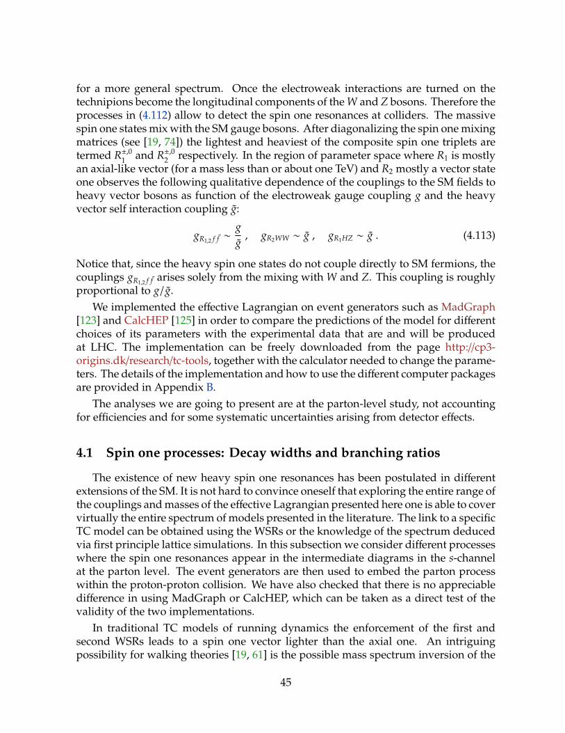
for a more general spectrum. Once the electroweak interactions are turned on thetechnipions become the longitudinal components of the W and Z bosons. Therefore theprocesses in (4.112) allow to detect the spin one resonances at colliders. The massivespin one states mix with the SM gauge bosons. After diagonalizing the spin one mixingmatrices (see [19, 74]) the lightest and heaviest of the composite spin one triplets aretermed R±,01 and R±,02 respectively. In the region of parameter space where R1 is mostlyan axial-like vector (for a mass less than or about one TeV) and R2 mostly a vector stateone observes the following qualitative dependence of the couplings to the SM fields toheavy vector bosons as function of the electroweak gauge coupling g and the heavyvector self interaction coupling g:

gR1,2 f f ∼gg, gR2WW ∼ g , gR1HZ ∼ g . (4.113)

Notice that, since the heavy spin one states do not couple directly to SM fermions, thecouplings gR1,2 f f arises solely from the mixing with W and Z. This coupling is roughlyproportional to g/g.

We implemented the effective Lagrangian on event generators such as MadGraph[123] and CalcHEP [125] in order to compare the predictions of the model for differentchoices of its parameters with the experimental data that are and will be producedat LHC. The implementation can be freely downloaded from the page http://cp3-origins.dk/research/tc-tools, together with the calculator needed to change the parame-ters. The details of the implementation and how to use the different computer packagesare provided in Appendix B.

The analyses we are going to present are at the parton-level study, not accountingfor efficiencies and for some systematic uncertainties arising from detector effects.

4.1 Spin one processes: Decay widths and branching ratios

The existence of new heavy spin one resonances has been postulated in differentextensions of the SM. It is not hard to convince oneself that exploring the entire range ofthe couplings and masses of the effective Lagrangian presented here one is able to covervirtually the entire spectrum of models presented in the literature. The link to a specificTC model can be obtained using the WSRs or the knowledge of the spectrum deducedvia first principle lattice simulations. In this subsection we consider different processeswhere the spin one resonances appear in the intermediate diagrams in the s-channelat the parton level. The event generators are then used to embed the parton processwithin the proton-proton collision. We have also checked that there is no appreciabledifference in using MadGraph or CalcHEP, which can be taken as a direct test of thevalidity of the two implementations.

In traditional TC models of running dynamics the enforcement of the first andsecond WSRs leads to a spin one vector lighter than the axial one. An intriguingpossibility for walking theories [19, 61] is the possible mass spectrum inversion of the

45

MA (TeV)

MV-

MA

(TeV

)

S=0.3

g=2,5

-0.2

-0.1

0

0.1

0.2

0.3

0.4

0.5

0.6 0.8 1 1.2 1.4 1.6 1.8 2 2.2

Mass Splitting

MR±1 (TeV)

MR± 2-M

R± 1 (TeV

)

S=0.3

g=2,5

00.05

0.10.15

0.20.25

0.30.35

0.40.45

0.5

0.6 0.8 1 1.2 1.4 1.6 1.8 2 2.2

Figure 15: Mass splittings MV −MA (left) and MR±2−MR±1

(right). The dotted lines arefor g = 5 while the solid lines are for g = 2.

vector and axial spin one mesons. This occurs since the second WSR gets modified[61]. In Fig. 15 (left) we plot MV −MA as a function of MA for two reference values of gand S = 0.3. For generic values of S the inversion occurs for

Minv =

√4πS

Fπ . (4.114)

This gives Minv' 1.6 TeV for S = 0.3, as clearly shown in the plot. Fig. 15 (right)

shows MR±2−MR±1

as a function of MR±1, where R±,01 (R±,02 ) are the lighter (heavier) vector

resonances, with tree-level electroweak corrections included. This mass difference isalways positive by definition, and the mass inversion becomes a kink in the plot. Awayfrom Minv R1 (R2) is an axial (vector) meson for MA < Minv, and a vector (axial) mesonfor MA > Minv. The mass difference in Fig. 15 is proportional to g2, and becomesrelatively small for g = 2. The effects of the electroweak corrections are larger for smallg couplings. For example, the minimum of MR±2

−MR±1is shifted from Minv

' 1.59 TeVto about 1 TeV for g = 2. To help the reader we plot in Fig. 16 the actual spectrum forthe vector boson masses versus MA. Preliminary studies on the lattice of MWT and themass inversion issue appeared in [83].

The widths of the heavy vectors are displayed in Fig. 17. The lighter meson, R1, isvery narrow. The heavier meson, R2, is very narrow for small values of g. In fact inthis case MR2 ' MR1 , forbidding decays of R2 to R1 (+anything). For large g, R2 is verynarrow for large masses, but then becomes broader when the R2 → R1,X channels openup, where X is a SM gauge boson. It becomes very broad when the R2 → 2R1 decaychannel opens up. The former are only important below the inversion point, where R1

is not too heavy. The latter is only possible when R2 is essentially a spin one vector andMR2 > 2MR1 .

46

MA (TeV)

Mas

s Sp

ectr

um (T

eV)

R±2,0

R±1,0 S=0.3

g=20.4

0.6

0.8

1

1.2

1.4

1.6

1.8

2

2.2

0.4 0.6 0.8 1 1.2 1.4 1.6 1.8 2 2.2

MA (TeV)

Mas

s Sp

ectr

um (T

eV)

R±2,0

R±1,0 S=0.3

g=50.4

0.6

0.8

1

1.2

1.4

1.6

1.8

2

2.2

0.4 0.6 0.8 1 1.2 1.4 1.6 1.8 2 2.2

Figure 16: The mass spectrum of the MR±,01,2vector mesons versus MA for g = 2 (left)

and g = 5 (right). The masses of the charged vector mesons are denoted by solid lines,while the masses of the neutral mesons are denoted by dashed lines.

Mass (TeV)

(GeV

)

R±2

R±1

S=0.3

g=2

10-1

1

10

10 2

0.6 0.8 1 1.2 1.4 1.6 1.8 2 2.2

Mass (TeV)

(GeV

)

R±2

R±1

S=0.3g=5

10-1

1

10

10 2

10 3

0.6 0.8 1 1.2 1.4 1.6 1.8 2 2.2

Mass (TeV)

(GeV

)

R02

R01

S=0.3g=2

10-1

1

10

10 2

10 3

0.6 0.8 1 1.2 1.4 1.6 1.8 2 2.2

Mass (TeV)

(GeV

)

R02

R01

S=0.3g=5

10-1

1

10

10 2

10 3

0.6 0.8 1 1.2 1.4 1.6 1.8 2 2.2

Figure 17: Decay width of the charged (first row) and neutral (second row) vectormesons for S = 0.3 and g = 2, 5. We take MH = 0.2 TeV, s = 0.

47

The narrowness of R1 (and R2, when the R2 → R1,X channels are forbidden) isessentially due to the small value of the S parameter. In fact for S = 0 the trilinearcouplings of the vector mesons to two scalar fields of the strongly interacting sectorvanish. This can be understood as follows: the trilinear couplings with a vectorresonance contain a derivative of either the Higgs or the technipion, and this can onlycome from r3 in Eq. (3.97). Since r3 = 0 implies S = 0, as Eqs. (3.89) and (3.88) showexplicitly, it follows that the decay width of R1 and R2 to two scalar fields vanishes asS → 0. As a consequence, for S = 0 the vector meson decays to the longitudinal SMbosons are highly suppressed, because the latter are nothing but the eaten technipions.(The couplings to the SM bosons do not vanish exactly because of the mixing with thespin one resonances.) A known scenario in which the widths of R1 and R2 are highlysuppressed is provided by the D-BESS model [84], where the spin one and the spin zeroresonances do not interact. Therefore, in D-BESS all couplings involving one or morevector resonances and one or more scalar fields vanish, not just the trilinear couplingwith one vector field. The former scenario requires r2 = r3 = s = 0, the latter onlyrequires r3 = 0. A somewhat intermediate scenario is provided by custodial TC, inwhich r2 = r3 = 0 but s , 0. Narrow spin one resonances seem to be a common featurein various models of dynamical electroweak symmetry breaking. (see for example[85]). Within our effective Lagrangian (3.97) this property is linked to having a small Sparameter.

The R1 branching ratios are shown in Fig. 18. The wild variations observed in theplots around 1.6 TeV reflect the mass inversion discussed earlier. Here the mixingbetween Ra

1 and Wa, with a = 0,±1, vanishes, suppressing the decay to SM fermions.The other observed structure for the decays in ZH and WH, at low masses, is due to

the opposite and competing contribution coming from the TC and electroweak sectors.This is technically possible since the coupling of the massive vectors to the longitudinalcomponent of the gauge bosons and the composite Higgs is suppressed by the smallvalue of S.

Now we consider the R2 branching ratios displayed in Fig. 19. Being R2 heavierthan R1 by definition, new channels like R2 → 2R1 and R2 → R1X show up, where Xdenotes a SM boson. Notice that there is a qualitative difference in the R2 decay modesfor small and large values of g. First, for small g the R2 − R1 mass splitting is not largeenough to allow the decays R2 → 2R1 and R2 → R1H, which are instead present forlarge g. Second, for small g there is a wide range of masses for which the decays toR1 and a SM vector boson are not possible, because of the small mass splitting. Thebranching ratios to fermions do not drop at the inversion point, because the R2 − Wmixing does not vanish.

48

Mass (TeV)

BR

(R± 1)

tb

ff

nl

W±Z

W±H

S=0.3

g=2

10-6

10-5

10-4

10-3

10-2

10-1

1

0.6 0.8 1 1.2 1.4 1.6 1.8 2 2.2

Mass (TeV)

BR

(R± 1)

tb

ff

nl

W±Z

W±H

S=0.3

g=5

10-6

10-5

10-4

10-3

10-2

10-1

1

0.6 0.8 1 1.2 1.4 1.6 1.8 2 2.2

Mass (TeV)

BR

(R0 1)

ff

llW+W

-ZH

S=0.3

g=2

10-6

10-5

10-4

10-3

10-2

10-1

1

0.6 0.8 1 1.2 1.4 1.6 1.8 2 2.2

Mass (TeV)

BR

(R0 1)

ff

ll

W+W

-

ZH

S=0.3

g=5

10-6

10-5

10-4

10-3

10-2

10-1

1

0.6 0.8 1 1.2 1.4 1.6 1.8 2 2.2

Figure 18: Branching ratios of the charged (first row) and neutral (second row) R1

resonance for S = 0.3 and g = 2, 5. We take MH = 0.2 TeV, s = 0.

49

Mass (TeV)

BR

(R± 2)

nl

tb

ff

W±Z

W±H

W± R

01

Z R±

1

S=0.3

g=2

10-6

10-5

10-4

10-3

10-2

10-1

1

0.6 0.8 1 1.2 1.4 1.6 1.8 2 2.2

Mass (TeV)

BR

(R± 2)

tb

ff

nl

W±Z

W±H

W± R

01

Z R±

1

R±

1 R01

R±

1 H

S=0.3

g=5

10-6

10-5

10-4

10-3

10-2

10-1

1

0.6 0.8 1 1.2 1.4 1.6 1.8 2 2.2

Mass (TeV)

BR

(R0 2)

ff

llW

+W

-

ZH

WR1

S=0.3

g=2

10-6

10-5

10-4

10-3

10-2

10-1

1

0.6 0.8 1 1.2 1.4 1.6 1.8 2 2.2

Mass (TeV)

BR

(R0 2)

ff

ll

W+W

-

ZH

WR1R

+1 R

-1

R01H

S=0.3

g=5

10-6

10-5

10-4

10-3

10-2

10-1

1

0.6 0.8 1 1.2 1.4 1.6 1.8 2 2.2

Figure 19: Branching ratios of the charged (first row) and neutral (second row) R2

resonance for S = 0.3 and g = 2, 5 . We take MH = 0.2 TeV, s = 0.

�R0

1,2

q

q `−

`+

Figure 20: Feynman diagram of the signal processes for the dilepton production.

50

4.1.1 pp→ R→ ``

Dilepton production was discussed also in [74], with√

s = 14 TeV and 100 fb−1

integrated luminosity. The Feynman diagram of this Drell-Yan process is shown inFig. 20. We updated that analysis for the near future LHC using the parameters

√s = 7

TeV and 10 fb−1. The signal and the background are obviously reduced compared tothe earlier studies, but in the optimal region of the parameter space signals are stillclearly visible. Increasing the effective TC coupling g quickly flattens out the signal. InFig. 21 we plot the number of events with respect to the invariant mass of the leptonpair, using g = 2, 3, 4 and MA = 0.5, 1, 1.5 TeV, where MA is the mass of axial eigenstatebefore mixing with the SM gauge bosons. We have applied cuts of |η`| < 2.5 and p`T > 15GeV on the rapidity and transverse momentum of the leptons. The peaks from the R1

and R2 clearly stand out with signal-to-background ratio S/B > 10 for several binsover the parameter space under consideration. The background is considered to bethe contribution coming from the SM gauge bosons Z and γ. In Table 2 the signal andbackground cross sections are reported, applying the cut

Table 2: pp → R1,2 → `+`−. Signal and background cross sections for g = 2, 3, 4 andestimates for required luminosity for 3σ and 5σ signals. MR1,2 are the physical massesfor the vector resonances in GeV.

g MA MR1,2 σS (fb) σB (fb) L (fb−1) for 3σ L (fb−1) for 5σ2 500 M1 = 517 194 3.43 0.012 0.0382 500 M2 = 623 118 1.34 0.019 0.0562 1000 M1 = 1027 4.57 9.17 · 10−2 0.53 1.82 1000 M2 = 1083 16.4 5.60 · 10−2 0.13 0.392 1500 M1 = 1526 0.133 5.91 · 10−3 26 672 1500 M2 = 2103 0.776 2.81 · 10−3 2.7 8.23 500 M1 = 507 93.5 3.71 0.037 0.0903 500 M2 = 715 0.447 0.649 39 813 1000 M1 = 1013 1.32 8.81 · 10−2 2.7 7.43 1000 M2 = 1097 2.94 5.15 · 10−2 0.79 2.53 1500 M1 = 1514 3.19 · 10−3 5.63 · 10−3 6300 140003 1500 M2 = 1541 0.120 3.94 · 10−3 29 684 500 M1 = 504 34.6 3.85 0.12 0.344 500 M2 = 836 0.0 0.649 - -4 1000 M1 = 1007 0.234 8.98 · 10−2 30 854 1000 M2 = 1148 0.0 5.15 · 10−2 - -4 1500 M1 = 1509 1.31 · 10−3 3.94 · 10−3 25000 570004 1500 M2 = 1533 1.43 · 10−2 3.94 · 10−3 435 1200

51

10-2

10-1

1

10

10 2

10 3

500 1000 1500

Mll(GeV)Num

ber o

f eve

nts/

20 G

eV @

10

fb-1

10-2

10-1

1

10

10 2

10 3

500 1000 1500

Mll(GeV)Num

ber o

f eve

nts/

20 G

eV @

10

fb-1

10-2

10-1

1

10

10 2

10 3

500 1000 1500

Mll(GeV)Num

ber o

f eve

nts/

20 G

eV @

10

fb-1

Figure 21: Dilepton invariant mass distribution M`` for pp → R1,2 → `+`− signal andbackground processes. We consider g = 2, 3, 4 respectively from left to right and massesMA = 0.5 TeV (purple), MA = 1 TeV (red) and MA = 1.5 TeV (green).

52

|M`` −MR| < 5 GeV (4.115)

separately for the R1 and R2 peaks. The choice of the value 5 GeV is dictated by thedilepton invariant mass resolution [86]. The invariant mass resolution drops whenthe mass of the resonance increases, in any event, we use the same cut for all of thedifferent mass values coming from the one with worst resolution. Also estimates forthe required integrated luminosity for the 3σ and 5σ discoveries are given in the Table.The significance is defined as the number of signal events divided by the square rootof the number of background events, when the number of events is large. The Poissondistribution is used for the small event samples. The dilepton final state should beclearly visible at the LHC in this particular region of the parameter space already with1 fb−1 integrated luminosity.

4.1.2 pp→ R→WZ→ ```ν

�R+(−)

1,2

W+(−)

Z

q

q

`+

`−

`+ (ν)

ν (`−)

Figure 22: Feynman diagram for the process pp→ R± →WZ± → ```ν.

The final state signature with three leptons and missing energy arises from theprocess pp → R → WZ → ```ν (see Fig. 22), where ` denotes a muon or an electronand ν denotes the corresponding neutrino. This was also studied in [74], with

√s = 14

TeV and 100 fb−1, where it was shown to be a promising signature for higher valuesof g and MA. The technivector-fermion couplings are suppressed for large g, whichmakes the dilepton final state uninteresting in that region of the parameter space. Incontrast, the technivector coupling to SM vector bosons is enhanced for large valuesg, balancing the suppression coming from the quark couplings. This can be seen fromFig. 23, where the second peak begins to go down slowly with increasing g. Following[74], we have used the transverse mass variable

(MT3`)

2 = [√

M2(```) + p2T(```) + |/pT|]

2− |~pT(```) + ~/pT|

2, (4.116)

where /pT denotes the missing transverse momentum. The cuts for the leptons areapplied as in the previous subsection and in addition we impose a cut on the missingtransverse energy /ET > 15 GeV. As a background we consider the SM processes withR±1,2 replaced by the W±.

53

10-2

10-1

1

10

400 600 800 1000 1200

MT3l(GeV)N

umbe

r of e

vent

s/20

GeV

@ 1

0 fb

-1

10-2

10-1

1

10

400 600 800 1000 1200

MT3l(GeV)N

umbe

r of e

vent

s/20

GeV

@ 1

0 fb

-1

10-2

10-1

1

10

400 600 800 1000 1200

MT3l(GeV)N

umbe

r of e

vent

s/20

GeV

@ 1

0 fb

-1

Figure 23: Transverse mass distribution MT3` for pp → R±1,2 → ZW±

→ ```ν signal andbackground processes. We consider g = 2, 3, 4 respectively from left to right and massesMA = 0.5 TeV (green), MA = 1 TeV (red).

54

In Table 3 we present the signal and background cross sections and quantify thepossible observability of the signal.

Table 3: pp→ R±1,2 → ZW±→ ```ν. Signal and background cross sections for g = 2, 3, 4

and estimates for required luminosity for 3σ and 5σ signals. Cuts are applied to takeinto account only the region of the visible peak. MR1,2 are the physical masses (GeV).

g MA MR1 MR2 σB (fb) σS (fb) L (fb−1) for 3σ L (fb−1) for 5σ2 500 512 619 1.75 1.12 16 352 1000 1012 1081 7.34 · 10−2 0.545 8.4 243 500 505 713 1.12 0.340 89 2433 1000 1009 1094 0.117 1.10 3.7 114 500 503 835 0.659 2.15 · 10−2 10000 -4 1000 1005 1145 8.92 · 10−2 0.297 21 60

4.1.3 pp→ R→ `ν

�R+(−)

1,2

q

q ν (`−)

`+ (ν)

Figure 24: Feynman diagram for the process pp→ R± → `ν.

This is the third signature, with leptons in the final state, studied in [74]. The essen-tial complication compared to the `+`− final state is that the longitudinal component ofthe neutrino momentum cannot be measured. The cuts applied for the charged leptonand on the missing energy are |η`| < 2.5, p`T > 15 GeV and /ET > 15 GeV. In Fig. 25, thenumber of events is plotted with respect to the transverse mass variable

MT` =

√2 /ET pT(`) (1 − cos ∆φ`,ν) , (4.117)

using the parameter space points g = 2, 3, 4 and MA = 0.5, 1, 1.5 TeV. This final statesignature behaves like the dilepton final state. Due to the suppression of the fermioncouplings, the signal is reduced when g is increased.

55

10-1

1

10

10 2

10 3

500 1000 1500

MTl (GeV)N

umbe

r of e

vent

s/20

GeV

@ 1

0 fb

-1

10-1

1

10

10 2

10 3

500 1000 1500

MTl (GeV)N

umbe

r of e

vent

s/20

GeV

@ 1

0 fb

-1

10-1

1

10

10 2

10 3

500 1000 1500

MTl (GeV)N

umbe

r of e

vent

s/20

GeV

@ 1

0 fb

-1

Figure 25: Transverse mass distribution MT` for pp→ R±1,2 → `ν signal and background

processes. We consider g = 2, 3, 4 respectively from left to right and masses MA = 0.5TeV (purple), MA = 1 TeV (red) and MA = 1.5 TeV (green).

56

4.1.4 pp→ R→ j j

The tree-level MWT contributions to this process is the s-channel exchange of acomposite vector boson (Drell-Yan process, Fig. 26).

�R1,2

qi

qi q f

q f

Figure 26: Feynman diagram for the Drell-Yan process pp→ R→ j j.

The quark couplings to the heavy spin one states are generated by the mixing withthe SM gauge bosons. Their value can then be expanded perturbatively in powers ofg/g, where g is the SU(2)L coupling constant, for large g. Therefore the cross sectionfor this process is reduced by, at least, a factor of g−4, respect to the SM one. Thereforethe signal drowns in the large QCD background for this process.

4.1.5 pp→ R→ γV and pp→ R→ ZZ

Up to dimension four operators, and before including operators involving theLorentz εµνρσ invariant tensor [12, 81], the photon coupling γR+

1 W− is forbidden. Thisimplies that we do not have diagrams with technivectors decaying into photon andvector boson. Higher order operators as well as operators involving the εµνρσ in acoherent manner will be investigated in the near future. The pp → R → ZZ processesare also absent in the present effective description.

4.2 Ultimate LHC reach for heavy spin resonances

We conclude this subsection summarizing the results for the ultimate reach of LHC,i.e. 14 TeV and 100 fb−1 [74]. We consider the representative parameter space pointsg = 2, 5 and MA = 0.5, 1, 1.5, 2 TeV for our plots and discussion.

4.2.1 pp→ R→ 2`, `ν, 3`ν at 14 TeV

The invariant mass and transverse mass distributions for signatures pp → R →2`, `ν, 3`ν are shown in Figs. 27-29. In the left frames of Figs. 27 and 28, correspondingto g = 2, clear signals from the leptonic decays of R0

1,2 and R±1,2 are seen even for 2 TeVresonances. Moreover Fig. 27 demonstrates that for g = 2 both peaks from R0

1 and R02

may be resolved.

57

1

10

10 2

10 3

10 4

500 1000 1500 2000

S=0.3g=2

Mll (GeV)Num

ber o

f eve

nts/

20 G

eV @

100

fb-1

1

10

10 2

10 3

10 4

500 1000 1500 2000

S=0.3g=5

Mll (GeV)Num

ber o

f eve

nts/

20 G

eV @

100

fb-1

Figure 27: Dilepton invariant mass distribution M`` for pp → R01,2 → `+`− signal and

background processes. We consider g = 2, 5 respectively and masses MA = 0.5 TeV(purple), MA = 1 TeV (red), MA = 1.5 TeV (green) and MA = 2 TeV (blue).

1

10

10 2

10 3

10 4

10 5

500 1000 1500 2000

S=0.3g=2

MTl (GeV)N

umbe

r of e

vent

s/20

GeV

@ 1

00 fb

-1

1

10

10 2

10 3

10 4

500 1000 1500 2000

S=0.3g=5

MTl (GeV)N

umbe

r of e

vent

s/20

GeV

@ 1

00 fb

-1

Figure 28: MT` mass distribution for pp→ R±1,2 → `±ν signal and background processes.

We consider g = 2, 5 respectively and masses MA = 0.5 TeV (purple), MA = 1 TeV (red),MA = 1.5 TeV (green) and MA = 2 TeV (blue).

58

10-1

1

10

10 2

500 1000 1500 2000

S=0.3g=2

MT3l (GeV)N

umbe

r of e

vent

s/20

GeV

@ 1

00 fb

-1

10-1

1

10

10 2

500 1000 1500 2000

S=0.3g=5

MT3l (GeV)N

umbe

r of e

vent

s/20

GeV

@ 1

00 fb

-1

Figure 29: MT3` mass distribution for pp → R±1,2 → ZW±

→ 3`ν signal and backgroundprocesses. We consider g = 2, 5 respectively and masses MA = 0.5 TeV (purple), MA = 1TeV (red), MA = 1.5 TeV (green) and MA = 2 TeV (blue).

Let us now turn to the case of g = 5 in the right frames of Figs. 27 and 28. Forlarge g the R f f couplings are suppressed, so observing signatures pp → R → 2` andpp → R → `ν could be problematic. However, for large g, the triple-vector couplingis enhanced, so one can observe a clear signal in the MT

3` distribution presented inFig. 29. At low masses the decays of the heavy vector mesons to SM gauge bosons aresuppressed and the signal disappears. This mass range can, however, be covered withsignatures pp→ R→ 2` and pp→ R→ 3`ν.

4.2.2 pp→ Rjj at 14 TeV

�W

Z,W

R1,2

qi

q′i

q f

q′f

Figure 30: Feynman diagram for the vector boson fusion process pp→ Rjj.

Vector Boson Fusion (VBF) is, in principle, an interesting channel for the vectormeson production (see Fig. 30), especially in theories in which the fermion couplingsof the vector resonances are suppressed. Unfortunately, as we shall see, it is notan appealing channel to explore at the LHC due to a small production rate of R±,01,2 .

59

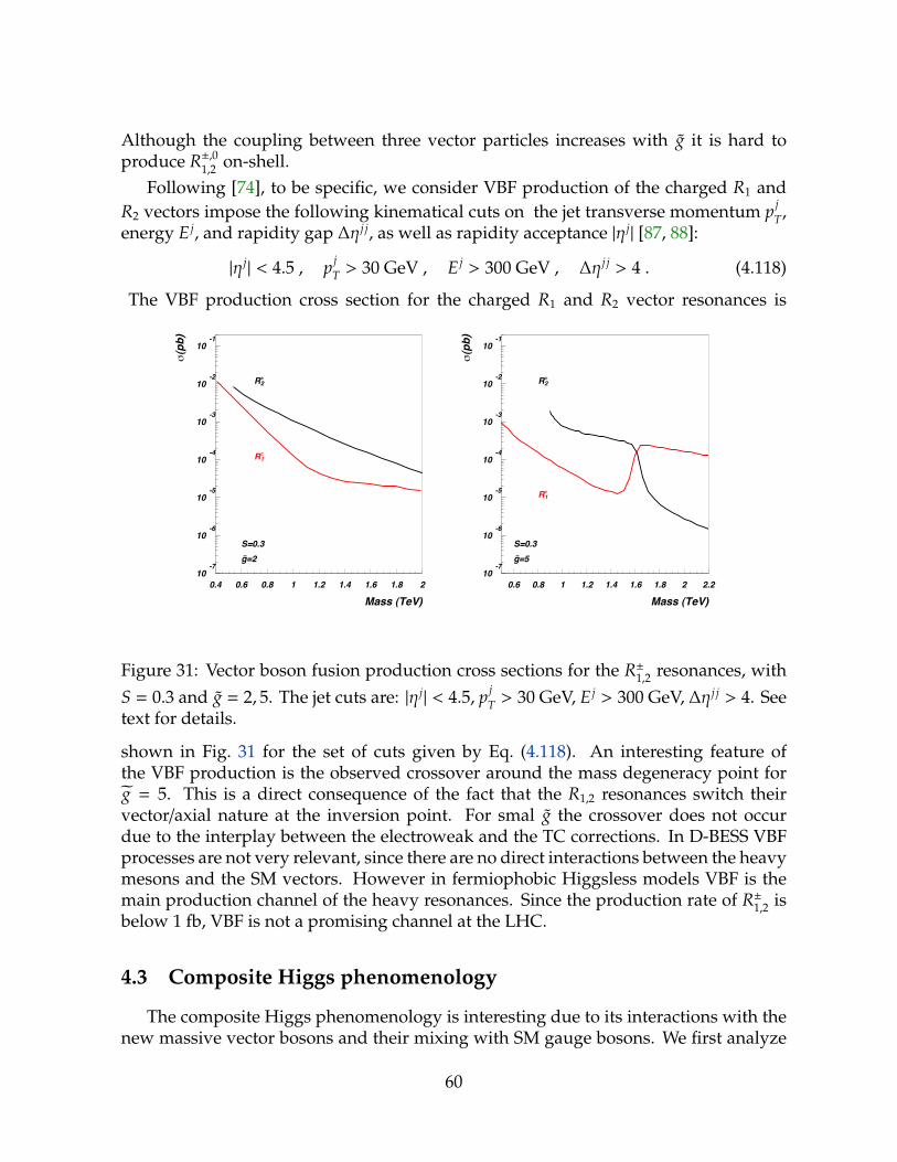
Although the coupling between three vector particles increases with g it is hard toproduce R±,01,2 on-shell.

Following [74], to be specific, we consider VBF production of the charged R1 andR2 vectors impose the following kinematical cuts on the jet transverse momentum p j

T,energy E j, and rapidity gap ∆η j j, as well as rapidity acceptance |η j

| [87, 88]:

|η j| < 4.5 , p j

T > 30 GeV , E j > 300 GeV , ∆η j j > 4 . (4.118)

The VBF production cross section for the charged R1 and R2 vector resonances is

Mass (TeV)

(pb)

R±2

R±1

S=0.3g=2

10-7

10-6

10-5

10-4

10-3

10-2

10-1

0.4 0.6 0.8 1 1.2 1.4 1.6 1.8 2

Mass (TeV)

(pb)

R±2

R±1

S=0.3g=5

10-7

10-6

10-5

10-4

10-3

10-2

10-1

0.6 0.8 1 1.2 1.4 1.6 1.8 2 2.2

Figure 31: Vector boson fusion production cross sections for the R±1,2 resonances, with

S = 0.3 and g = 2, 5. The jet cuts are: |η j| < 4.5, p j

T > 30 GeV, E j > 300 GeV, ∆η j j > 4. Seetext for details.

shown in Fig. 31 for the set of cuts given by Eq. (4.118). An interesting feature ofthe VBF production is the observed crossover around the mass degeneracy point forg = 5. This is a direct consequence of the fact that the R1,2 resonances switch theirvector/axial nature at the inversion point. For smal g the crossover does not occurdue to the interplay between the electroweak and the TC corrections. In D-BESS VBFprocesses are not very relevant, since there are no direct interactions between the heavymesons and the SM vectors. However in fermiophobic Higgsless models VBF is themain production channel of the heavy resonances. Since the production rate of R±1,2 isbelow 1 fb, VBF is not a promising channel at the LHC.

4.3 Composite Higgs phenomenology

The composite Higgs phenomenology is interesting due to its interactions with thenew massive vector bosons and their mixing with SM gauge bosons. We first analyze

60

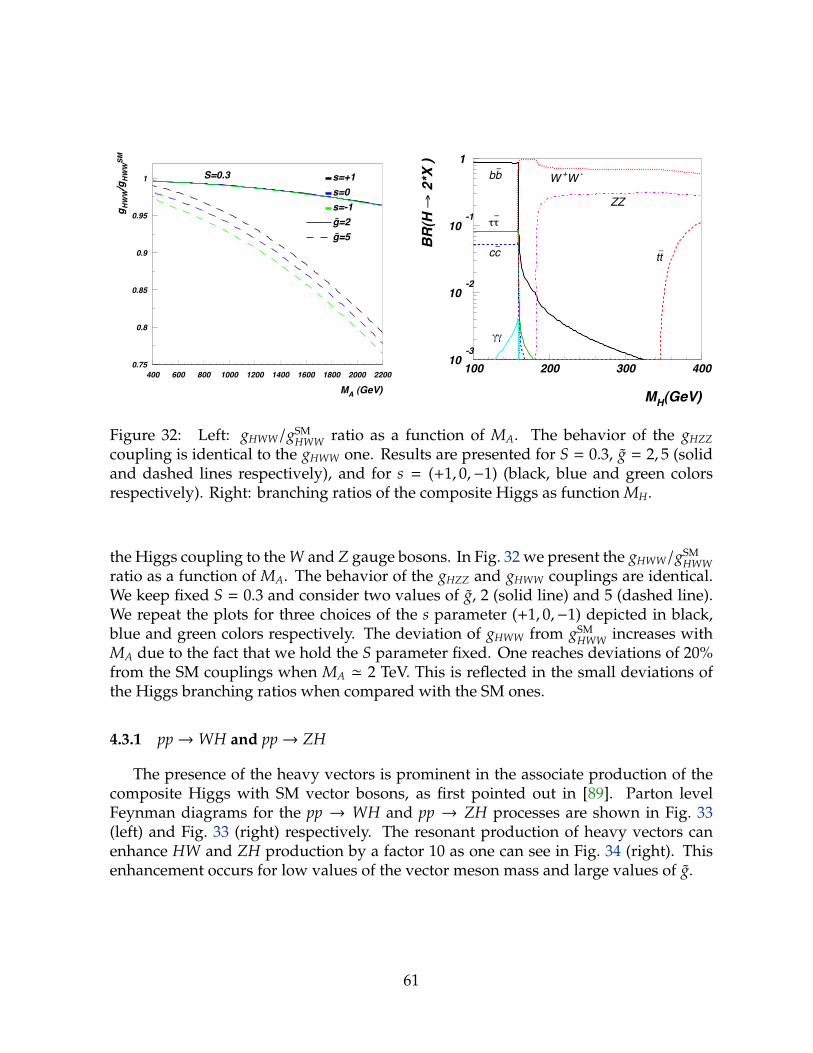
MA (GeV)

g HW

W/g

HW

WSM

S=0.3 s=+1s=0s=-1g=2g=5

0.75

0.8

0.85

0.9

0.95

1

400 600 800 1000 1200 1400 1600 1800 2000 220010

-3

10-2

10-1

1

100 200 300 400

bb–

tt–cc

–

–

W +W -

ZZ

MH(GeV)

BR

(H

2*X

)Figure 32: Left: gHWW/gSM

HWW ratio as a function of MA. The behavior of the gHZZ

coupling is identical to the gHWW one. Results are presented for S = 0.3, g = 2, 5 (solidand dashed lines respectively), and for s = (+1, 0,−1) (black, blue and green colorsrespectively). Right: branching ratios of the composite Higgs as function MH.

the Higgs coupling to the W and Z gauge bosons. In Fig. 32 we present the gHWW/gSMHWW

ratio as a function of MA. The behavior of the gHZZ and gHWW couplings are identical.We keep fixed S = 0.3 and consider two values of g, 2 (solid line) and 5 (dashed line).We repeat the plots for three choices of the s parameter (+1, 0,−1) depicted in black,blue and green colors respectively. The deviation of gHWW from gSM

HWW increases withMA due to the fact that we hold the S parameter fixed. One reaches deviations of 20%from the SM couplings when MA ' 2 TeV. This is reflected in the small deviations ofthe Higgs branching ratios when compared with the SM ones.

4.3.1 pp→WH and pp→ ZH

The presence of the heavy vectors is prominent in the associate production of thecomposite Higgs with SM vector bosons, as first pointed out in [89]. Parton levelFeynman diagrams for the pp → WH and pp → ZH processes are shown in Fig. 33(left) and Fig. 33 (right) respectively. The resonant production of heavy vectors canenhance HW and ZH production by a factor 10 as one can see in Fig. 34 (right). Thisenhancement occurs for low values of the vector meson mass and large values of g.

61

�W±,R±1,2

q

q′ W±

H

�γ,Z,R0

1,2

q

q Z

H

Figure 33: Feynman diagrams for the composite Higgs production in association withSM gauge bosons.

10-1

1

500 1000 1500 2000

MH=200 GeV, S=0.3, g~=3sms=-1s=0s=+1

MA(GeV)

(pp

WH

)(pb)

10-1

1

500 1000 1500 2000

MH=200 GeV, S=0.3, g~=6sms=-1s=0s=+1

MA(GeV)

(pp

WH

)(pb)

Figure 34: The cross section for pp → WH production at 7 TeV in the center of mass(W+H and W−H modes are summed up) versus MA for S = 0.3, s = (+1, 0, 1) and g = 3(left) and g = 6 (right). The dotted line at the bottom indicates the SM cross sectionlevel.

62

0

0.02

0.04

0.06

0.08

0.1

0.12

0.14

500 1000 1500 2000

MA (GeV)

(pp

Hjj)

(pb)

MH = 200 GeV g = 2

g = 5

SM

0

0.02

0.04

0.06

0.08

0.1

0.12

0.14

500 1000 1500 2000

MA (GeV)

(pp

Hjj)

(pb)

MH = 400 GeV g = 2

g = 5

SM

Figure 35: Composite Higgs production cross section via the VBF mechanism at 7 TeV.

4.3.2 Higgs vector boson fusion, pp→ Hjj

We have also analyzed the composite Higgs production in VBF processes pp→ Hjj.We find that it is not enhanced with respect to the corresponding process in the SM asit is clear from Fig. 35. The behavior of σ(pp→ Hjj) as function of MA traces the one ofthe Higgs-gauge bosons coupling shown in Fig. 32.

We used the same kinematic cuts as for the pp→ Rjj section except for the transversemomenta and energy of the jets that we take to be p j

T > 15 GeV and E j > 150 GeV.

4.3.3 H→ γγ and H→ gg

�H

γ, g

γ, g

Figure 36: Feynman diagram for the composite Higgs decay to γγ or gg via SM fermionloop.

The one loop Higgs decay (see Fig. 36) width to two photons for any weaklyinteracting elementary particle contributing to this process can be neatly summarizedvia the formula [90]:

63

Γ(H→ γγ) =α2GFM2

H

128√

2π3

∣∣∣∣∣∣∣∑i

ni Q2i Fi

∣∣∣∣∣∣∣2

, (4.119)

where i runs over the spins, ni is the multiplicity of each species with electric charge Qi

in units of e. The Fi functions are given by

F1 = 2 + 3τ + 3τ(2 − τ) f (τ) , F1/2 = −2τ[1 + (1 − τ) f (τ)] , F0 = τ(1 − τ f (τ)

), (4.120)

where τ =4m2

iM2

Hand

f (τ) =

(arcsin

√1τ

)2

, if τ ≥ 1

−14

(log

(1+√

1−τ1−√

1−τ

)− iπ

)2, if τ < 1

(4.121)

The lower index of the function F indicates the spin of each particle contributing to theprocess. It is clear from this formula that there can be strong interferences betweenthe different terms contributing. In particular we anticipate that there is an importantinterplay between the SM gauge bosons and the TC contribution for this process.

The contribution to the Higgs decay to two-photon process in the SM is due tothe Ws and SM fermion loops contributions (with the leading one given by the topquark). In fact it is an excellent approximation to use just the top in the fermion loop,since the ratio between the corresponding result and the one obtained including all thecontributions is around 0.98, for the reference value of the Higgs mass of MH ' 120 GeV.The approximation improves as the Higgs mass increases. We consider here the case inwhich the Higgs is a composite state constituted of some more fundamental matter asin TC. The SM Higgs sector Lagrangian is therefore interpreted simply as a low energyeffective theory. We assume the Vanilla TC theory and therefore the composite Higgs(H) effective field coincides with the SM one. It is straightforward to generalize theglobal symmetries of the TC theories to large symmetry groups.

The contribution to the sought process is modeled by re-coupling, in a minimal way,the composite Higgs to the techniquarks Q via the following operator:

LQH =√

2MQ

v

[QL

t·HDRt + QL

t· (i τ2 H∗)URt

]+ h.c. , (4.122)

where MQ is the dynamical mass of the techniquark and t = 1, . . . , d[r] is the techni-color index and d[r] the dimension of the representation under which the techniquarkstransform. This type of hybrid models have been employed many times in the QCDliterature to extra dynamical information and predictions for different phenomenolog-ically relevant processes. A close example is the σ(600) decay into two photons [91]investigated using, for example, hybrid type models in [92] and [93].

64

We assumed a single TC doublet with respect to the Weak interactions as predictedby minimal models of TC [16]. We added a new Lepton family to cure the Wittentopological anomaly (with respect to the weak interactions) [57] when the TC sectorfeatures an odd number of doublets charged under the SU(2)L Weak interactions. Thisoccurs when the dimension of the TC matter representation is an odd number. Afurther Leptonic interaction term is then added:

LLH =√

2ME

vLL ·HER +

√

2MN

vLL · (i τ2 H∗)NR + h.c. , (4.123)

with ME and MN the fermion masses expected to be of the order of the electroweakscale [94]. The detailed spectrum is partially dictated by the precision electroweakconstraints.

The techniquark dynamical mass is intrinsically linked to the technipion decayconstant Fπ via the Pagels-Stokar formula MQ ≈

2πFπ√

d[r]. To achieve the correct values of

the weak gauge bosons the decay constant is related to the electroweak scale via:

v =√

N f Fπ, with v = 246 GeV . (4.124)

We have checked that the numerical value of the contribution of the ME/N states isnegligible when the masses are of the order of the electroweak scale. We have used asa reference value for these lepton masses 500 GeV 10.

At this point we determine the contribution of the techniquarks, not carrying ordi-nary color charge, and new leptons for the diphoton process by evaluating the naiveone loop triangle diagrams in which the composite Higgs to two techniquarks, as wellas the new leptons, vertex can be read off from the Lagrangian above. The contributionat the amplitude level for each new particle is identical to the one of a massive SMfermion provided one takes into account the correct electric charge and degeneracyfactor.

Although we adopted a simple model computation we now argue that the finalgeometric dependence on the gauge structure, matter representation and number oftechniflavors of the composite theory is quite general.

We plot in Fig. 37 the intrinsic dependence on the dimension of the TC matterrepresentation d[r] raccording to the ratio:

R =ΓSM(H→ γγ) − ΓTC(H→ γγ)

ΓSM(H→ γγ). (4.125)

For any odd representation we included the lepton contribution and therefore wecould not simply join the points. Interestingly when d[r] is around 7 the contributionfrom the techniquarks adds to one of the SM fermion ones (i.e. mainly the top) andcancels the one due to the W’s leading to ΓTC ≈ 0. The techniquark matter dominatesthe process for d[r] larger than around seven. A similar behavior occurs when we

65

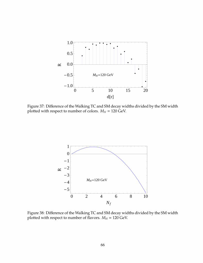
MH =120 GeV

0 5 10 15 20-1.0

-0.5

0.0

0.5

1.0

d@rD

R

Figure 37: Difference of the Walking TC and SM decay widths divided by the SM widthplotted with respect to number of colors. MH = 120 GeV.

MH =120 GeV

0 2 4 6 8 10

-5

-4

-3

-2

-1

0

1

N f

R

Figure 38: Difference of the Walking TC and SM decay widths divided by the SM widthplotted with respect to number of flavors. MH = 120 GeV.

66

increase the number of flavors as shown in Fig. 38. The dependence on the Higgs masswith d[r] = 2 and N f = 2 is shown in Fig. 39. The WW threshold is evident in the plot

120 140 160 180 200

0.25

0.30

0.35

0.40

mH

R

Figure 39: Dependence of R as function of the Higgs mass MH for a reference value ofthe techniquark matter representation d[r] = 2 and two number of Dirac techniflavors.

which shows how the ratio decreases with the Higgs mass.To illustrate our results we plot in Fig. 40 the Higgs to two-photon branching ratio

as function of the Higgs mass for the MWT model and compare it to the SM one. It is

100 120 140 160 180 200

10-1

10-2

10-3

10-4

10-5

mH

BR

HH-

>Γ

ΓL

MWT

SM

Figure 40: Higgs to two photons branching ratio in MWT as function of the compositeHiggs mass versus the SM result.

clear from the plot that we expect sizable corrections to the SM Higgs to two photonsprocess to be visible at the LHC.

10For ME/N �MH the contribution approaches a constant due to the functional form of F1/2.

67

It is interesting to estimate the impact on the digluon process coming from a poten-tially composite Higgs made by technimatter charged under QCD interactions. Thiscontribution can be estimated, as we have done for the diphoton process, by consideringthe one loop contribution of the techniquarks arriving at:

Γ(H→ gg) =α2

s GFM3H

64√

2π3

∣∣∣∣∣∣∣∑i

FSMi +

∑j

2T[r j]d[r j]FTCj

∣∣∣∣∣∣∣2

, (4.126)

where T[r j] is the index of the representation of the techniquarks under the SM colorgroup SU(3) and d[r j] is the dimension of the representation under the TC gauge group.For techniquarks transforming according to the fundamental representation of QCD

MH =120 GeV

2.0 2.5 3.0 3.5 4.0 4.5 5.00

20

40

60

80

100

120

d@rD

Rg

Figure 41: Difference of the Walking TC and SM decay widths divided by the SM widthplotted with respect to number of flavors. MH = 120 GeV.

the two gluon decay width of the Higgs is strongly enhanced. This is presented inFig. 41 where we have plotted the ratio

Rg =ΓTC(H→ gg) − ΓSM(H→ gg)

ΓSM(H→ gg). (4.127)

as a function of the dimension of the representation under the TC gauge group. Thecomposite Higgs to two-gluon decay width increases monotonically with respect tothe number of technicolors in contrast with the diphoton decay width. The differenceresides in the fact that gluons do not couple directly to the other gauge bosons of theSM.

We now estimate the viability of the models with colored techniquarks by comparingour results with the study performed in [95]. Here the authors considered the effects ofthe fourth fermion SM generation to the process σgg→H × BR(H → W+W−). The fourth

68

10

20

30

120 140 160 180 2001.0

1.2

1.4

1.6

1.8

2.0

2.2

2.4

mH

d@rD

Figure 42: Contours in the d[r] versus Higgs mass plane for fixed values of the enhance-ment of the gg → H production cross section compared to the SM one. Obviously, inpractice, the dimension of the representation cannot be taken to be continuous andthe plot simply shows that already for d[r] around 2 (which is the minimal nontrivialmatter group-theoretical dimension) the enhancement factor is around 30.

generation quarks enhances the gg → H production cross section by a factor of 9 to7.5 in the Higgs mass range MH = 110 − 300 GeV with respect to the SM result. Thisenhancement leads to a 95% confidence level exclusion of the Higgs in the mass rangeMH = 131 − 208 GeV or of the presence of a fourth generation if the Higgs turns outto be within this mass energy range. Colored techniquakrs are further penalized withrespect to the SM fourth generation of quarks since they carry also technicolor leadingto a further dramatic enhancement of this process. In Fig. 42 we have plotted contoursin the dimension of the techniquark representation versus the Higgs mass when thegg → H production cross section is enhanced by factors 10, 20 and 30 respectivelycompared to the SM one. Obviously, in practice, the dimension of the representationcannot be taken to be continuous and the plot simply shows that already for d[r]around two (which is the minimal nontrivial matter group-theoretical dimension) theenhancement factor is around 30. Thus we conclude that this process alone stronglyindicates that viable TC models should feature colorless techniquarks as it is the case ofMWT or that a light composite Higgs made of colored techniquarks is excluded by theTevatron experiment. These results are in perfect agreement with the LEP electroweakprecision data which require a small S parameter.

69

In these two last subsections we introduced a simple framework to estimate thecomposite Higgs boson coupling to two photons and gluons for generic TC extensionsof the SM. By comparing the decay rates with the SM ones for the diphoton case weshow that the corrections are typically of order one and therefore this process canbe efficiently used to disentangle a light composite Higgs from a SM one. We thenturned our attention to the composite Higgs to two gluon process and showed that theTevatron results for the gluon-gluon fusion production of the Higgs exclude either thetechniquarks to carry color charges up to the 95% confidence level or the existence of alight composite Higgs made of colored techniquarks.

4.3.4 Higgs production via gluon fusion

As we have shown above if the techniquarks do not carry color this process occursas in the SM, provided that the ETC interactions do not strongly modify the Yukawasector.

5 A Natural fourth family of leptons at the TeV scale

If the LHC discovers a new fourth family of leptons but no associated quarks, whatwould that imply? Either the associated quarks are much heavier than the electroweakscale or a new set of fermions are needed to account for the 4th family lepton inducedgauge anomalies. The new fermions could address directly the big hierarchy problemof the SM if their dynamics leads to a composite Higgs scenario. This is the setup weare going to discuss in this chapter, using as a template MWT [16, 94].

Before investigating the phenomenology of such a theory, we will first review theleptonic sector of the SM (see e.g. [96] for a recent review). Secondly, we will considera general mass structure for the fourth neutrino and both the case of mixing and nomixing with the SM neutrinos. We will also summarize the (in)direct phenomenologicalconstraints. We then analyze the interplay of the composite Higgs sector with the newlepton family at the LHC.

We will study the production and decay of the new leptons in proton - protoncollisions which is relevant to select the LHC signatures for the discovery of these newleptons. We show that the composite Higgs structure can affect and differentiate thefinal signatures with respect to the case in which the Higgs is elementary. The bottomline is that one can experimentally determine if the fourth family is associated to acomposite Higgs sector.

70

5.1 The Standard Model leptons: a Mini-review

In the SM, the three lepton families, ` = e, µ, τ, belong to the following representa-tions of the gauge group SU(3)C × SU(2)L ×U(1)Y:

L` = (ν`L `L)T∼ (1, 2,−1/2) , `R ∼ (1, 1,−1) , (5.128)

where the chirality projectors PL = (1− γ5)/2 and PR = (1 + γ5)/2 have been introducedand the relation Q = T3 + Y has been adopted in order to define the hypercharge withrespect to the electric charge. The neutral and charged current interactions of the SMleptons are then respectively accounted for by the Lagrangian terms:

LNC =g

cosθW

(12νLγ

µνL −12

¯Lγµ`L + sin2 θW ¯γµ`)

Zµ + e ¯γµ` Aµ

(5.129)

LCC =g√

2¯LγµνL W−

µ + h.c.

where ` = `L + `R and θW is the Weinberg angle.In the SM, due to the absence of gauge singlet fermions with R-chirality, it is not

possible to endow neutrinos with a Dirac-type mass term. An effective Majorana-type mass term can however be identifyed among the non-renormalizable operators ofdimension 5. Symbolically:

(LH)T(LH)Λ

(5.130)

where Λ represents the energy scale at which additional interactions and/or fields showup, which must violate total lepton number (the effective mass operator above violatesit by two units). The associated effective neutrino masses would thus be suppressedwith respect to the electroweak scale, v, by a factor O(v/Λ). Experiments on neutrinooscillations, which measure differences of squared masses and mixing angles, haveestabished that at least two of the SM neutrinos have a small mass, not larger than theeV scale [64]. This would indeed suggest a very high scale for lepton number violation,Λ ∼ 1011v.

The neutrino mass matrix is diagonalised in general by a 3 × 3 unitary matrix U,called the PMNS mixing matrix:

mν = U∗mdiagU† . (5.131)

Since U and mdiag are in general complex, neutrino masses can provide three CP vio-lating phases: the one in U (which is the analog of the CP violating phase in the CKMquark mixing matrix) plus the two phase differences in mdiag, which are denoted asMajorana phases.

Two distinct oscillation frequencies have been first measured in solar and atmo-spheric neutrino oscillations and later confirmed by experiments on earth. Two well

71

separated differences need at least three different neutrino mass eigenstates involvedin oscillations so that the three known neutrino species can be sufficient. Then at leasttwo neutrinos must be massive while, in principle, the third one could still be massless.The mass eigenstates involved in solar oscillations are m1 and m2 and, by definition,|m2| > |m1|, so that ∆m2

sun = |m2|2− |m1|

2 > 0. The atmospheric neutrino oscillationsinvolve m3: ∆m2

atm = |∆m231| with ∆m2

31 = |m3|2− |m1|

2 either positive (normal hierarchy)or negative (inverse hierarchy). The present data are still compatible with both cases.The degenerate spectrum occurs when the average absolute value of the masses ismuch larger than all mass squared differences. With the standard set of notations anddefinitions the present data are summarised by [64]

∆m2sun = (7.05 − 8.34) × 10−5eV2 , ∆m2

atm = (2.07 − 2.75) × 10−3eV2 ,

0.25 ≤ sin2 θ12 ≤ 0.37 , 0.36 ≤ sin2 θ23 ≤ 0.67 . (5.132)

In addition, sin2 θ13 < 0.035 at 90% C.L. The pattern of neutrino mixing is drasticallydifferent from the pattern of quark mixing. At present no experimental information onthe Dirac and Majorana CP violation phases in the neutrino mixing matrix is available.

Oscillation experiments do not provide information about the absolute neutrinomass scale. Limits on that are obtained from the endpoint of the tritium beta decayspectrum, from cosmology and from neutrino-less double beta decay. From tritium wehave an absolute upper limit of 2.2 eV (at 95% C.L.) on the mass of electron antineutrino,which, combined with the observed oscillation frequencies under the assumption ofthree CPT-invariant light neutrinos, also amounts to an upper bound on the masses ofthe other active neutrinos.

Oscillation experiments cannot distinguish between Dirac and Majorana neutrinos.The detection of neutrino-less double beta decay would provide direct evidence oflepton number violation, and the Majorana nature of neutrinos. It would also offera way to possibly disentangle the 3 cases of degenerate, normal or inverse hierachyneutrino spectrum. The present limit from 0νββ (with large ambiguities from nuclearmatrix elements) is about |mee| < (0.3 − 0.8) eV [96].

5.2 Adding a fourth lepton family

In the following, we will account for the light neutrino masses and mixings bymeans of an effective Majorana mass term, namely we add to the SM Lagrangian adimension-5 non-renormalizable operator.

Our aim here is to study the phenomenology of an additional heavy lepton family,with masses about the TeV scale [94]. Thus, we add a 4th-family of leptons - for whichwe introduce the ζ-flavor - composed by a lepton doublet, a charged lepton singlet anda gauge singlet:

Lζ = (νζL ζL)T∼ (1, 2,−1/2) , ζR ∼ (1, 1,−1) , νζR ∼ (1, 1, 0) . (5.133)

72

The ζ-charged lepton, ζ = ζL + ζR, will have a Dirac mass term like the other threecharged leptons of the SM, but large enough to avoid conflict with the experimentallimits. We work in the basis in which the 4× 4 charged lepton mass matrix is diagonal.

5.2.1 Heavy leptons not Mixing with Standard Model neutrinos

We forbid, in this section, the mixing between the ζ-neutrino and the three lightneutrinos of the SM. The Lagrangian can be split as L = LSM +Lζ.

The Lagrangian mass terms we take for the ζ-sector reads:

Lmassζ = −mζ ζ ζ −

12

[(νζL (νζR)c

) ( 0 mD

mD mR

) ((νζL)c

νζR

)+ h.c.

], (5.134)

Diagonalizing the neutrino mass matrix above, we obtain two independent Majoranaeigenstates, N1 and N2, with real and positive masses, M1 and M2 (for conventionM1 ≤M2),

M1 =mR

2

√

1 + 4m2

D

m2R

− 1

, M2 =mR

2

√

1 + 4m2

D

m2R

+ 1

, (5.135)

which are related to the original Dirac and Majorana masses according to M1M2 = m2D

and M2 −M1 = mR.The ζ-neutrino chiral states will be an admixture of the two Majorana eigenstates

N1 and N2:(νζL

(νζR)c

)=

(i cosθ sinθ−i sinθ cosθ

) (PLN1

PLN2

), tan 2θ =

2mD

mR. (5.136)

In the limit mD � mR the seesaw mechanism would be at work (leading to M1 ∼ m2D/mR,

M2 ∼ mR, νζL ∼ i PLN1, (νζR)c∼ PLN2). Here however we are more interested in the

situation mD ∼ mR, in which both Majorana neutrinos have a mass about the TeV scaleand hence have a large SU(2)-active component.

The neutral current interaction of the ζ-leptons in terms of the heavy neutrinoMajorana mass eigenstates reads:

LNCζ =

gcosθW

(12νζLγ

µνζL −12ζLγ

µζL + sin2 θW ζγµζ)

Zµ + e ζγµζ Aµ , (5.137)

where

νζLγµνζL = −

cos2 θ2

N1γµγ5N1 −

sin2 θ2

N2γµγ5N2 + i cosθ sinθN2γ

µN1 . (5.138)

73

The interaction of the Z with a couple of N1 or N2 is axial, while the one with twodifferent Ni is a vector interaction. As for the charged current:

LCCζ =

g√

2W−

µ ζLγµ(i cosθ PLN1 + sinθ PLN2) + h.c. .

The Dirac mass can be written in terms of the Yukawa coupling yζ and the Higgs VEVv as mD = yζ v/

√2. Hence the interaction of the new neutrinos with the Higgs field

reads:

LHζ = −

mD

v

(νζR νζL + νζL νζR

)H (5.139)

= −mD

v[cosθ sinθ

(N1N1 + N2N2

)− i cos(2θ) N1γ5N2

]H .

5.2.2 Promiscuous heavy leptons

In this section we consider the possibility that the new heavy leptons mix with theSM leptons. For clarity of presentation we assume that the heavy neutrinos mix onlywith one SM neutrino of flavor ` (` = e, µ, τ). We refer to [94] for the discussion of thegeneral case. The entries of the mass matrix are:

− L =12

( ν`L νζL (νζR)c )

O(eV) O(eV) m′

O(eV) O(eV) mD

m′ mD mR

(ν`L)c

(νζL)c

νζR

+ h.c. . (5.140)

The measured values of the light neutrino masses suggest the entries of the upper 2×2block to be of O(eV) while the remaining entries are expected to be at least of the orderof the electroweak energy scale. Given such a hierarchical structure and up to smallcorrections ofO(eV/M1,2) . 10−11, one obtains the following form for the unitary matrixwhich diagonalises (5.140): ν`L

νζL

(νζR)c

= V

PLN0

PLN1

PLN2

, V =

cosθ′ i cosθ sinθ′ sinθ sinθ′

− sinθ′ i cosθ cosθ′ sinθ cosθ′

0 −i sinθ cosθ

. (5.141)

N0,1,2 are the new (Majorana) mass eigenstates and

tanθ′ =m′

mD, tan 2θ = 2

m′DmR

, m′D2≡ m2

D + m′2 . (5.142)

The light neutrino N0 has a mass of O(eV). Up to corrections of O(eV), the heavyneutrinos N1,2 have masses given by:

M1 =mR

2

√

1 + 4m′D

2

m2R

− 1

, M2 =mR

2

√

1 + 4m′D

2

m2R

+ 1

. (5.143)

74

Notice that the smaller is mR, the more the neutrinos N1 and N2 become (the two Weylcomponents of) a Dirac state.Including the neutrino of flavor `, the neutral fermion current in Eq. (5.138) is replacedwith

ν`Lγµν`L + νζLγ

µνζL = −12

N0γµγ5N0 −

cos2 θ2

N1γµγ5N1 −

sin2 θ2

N2γµγ5N2

+ i cosθ sinθN2γµN1 , (5.144)

while the charged current terms in the Lagrangian, Eq. (5.139), become

LCCζ =

g√

2W−

µ ζLγµ(− sinθ′PLN0 + i cosθ cosθ′ PLN1 + sinθ cosθ′ PLN2) + h.c. (5.145)

and

LCC` =

g√

2W−

µ¯Lγµ(cosθ′PLN0 + i cosθ sinθ′ PLN1 + sinθ sinθ′ PLN2) + h.c. (5.146)

Notice that the neutral current remains flavor diagonal at tree-level 11, hence the heavyneutrinos couple to the SM ones only through the charged current interactions at thisorder. This is a distinctive feature of our TeV neutrino physics. The SM like Yukawainteractions lead to the following terms involving the Higgs:

LHζ = −

mD

v(1 +

m′2

m2D

) cosθ′[sinθ cosθ(N1N1 + N2N2) − i cos(2θ) N1γ5N2] H . (5.147)

The low energy effective theory we will use for determining the interesting signals forLHC phenomenology [19, 60] is the effective Lagrangian for Vanilla Technicolor.

5.3 LHC phenomenology for the natural heavy lepton family

In this section we investigate aspects of the phenomenology related to the interplaybetween the new weekly coupled sector, i.e. the heavy leptons with its mixing with theSM fermions, and the new strongly coupled sector breaking the electroweak symmetrydynamically [94]. We consider only the MWT global symmetries relevant for theelectroweak sector, i.e. the subsector SU(2) × SU(2) spontaneously breaking to SU(2).The low energy spectrum contains, besides the composite Higgs, two SU(2) tripletsof (axial-) vector spin one mesons. The effective Lagrangian has been introduced in[19, 74]. The spin one massive eigenstates are indicated with R1 and R2 and are linearcombinations of the composite vector/axial mesons of MWT and the weak gauge bosoneigenstates. We have implemented the SU(2)×SU(2) TC sector in CalcHEP [131] usingthe LanHEP module [129] to generate the Feynman rules in [74]. We have added thenew leptons to this implementation for the present study.

11The neutral current is not flavor diagonal in models with TeV scale right handed neutrinos involvedin the see-saw mechanism for the light SM neutrino masses, see e.g. [98].

75

γ,Z,R0

1,2

q

q N j, ζ∓

Ni, ζ±

W±,R±1,2

q

q′ ζ±

Ni

Figure 43: Feynman diagrams for direct production of the heavy leptons in MWT withi, j = 1, 2.

5.3.1 Production and decay of the new leptons

The heavy leptons may be directly produced through the charged- and neutralcurrent interactions:

pp → W±/R±1,2 → ζ±Ni ,

pp → Z/γ/R01,2 → ζ+ζ− , pp→ Z/R0

1,2 → NiN j , i, j = 1, 2. (5.148)

The corresponding Feynman diagrams are given in Fig. 43. The direct productioncross sections for the heavy leptons in MWT are largely independent of the parametersassociated to the TC sector: in the direct production of ζ+ζ− the only free parameter isthe mass of the charged lepton Mζ; the direct production of NiN j and ζ±Ni depends, inaddition to the masses of the leptons, on the V matrix entries of Eq. (5.141) as followsfrom Eqs. (5.144) and (5.145). Plots of the LHC cross sections for pp→ ζ+ζ−, ζ±Ni,NiNi

can be found in [94].The final state distributions arising from the direct production of the leptons depend

on the specific parameters of the TC sector. In particular R1 is a (mostly) axial-resonanceand R2 is a (mostly) vector-resonance, so R1 mixes mostly with the Z boson while R2

mixes significantly with the photon. Consequently, the invariant mass distribution ofthe heavy neutral leptons NiNi will be relatively more dominated by the R1 resonancecompared to the charged leptons ζ+ζ−. This is demonstrated in Fig. 44. The massesand widths of R1,2 as a function of MA, g and S are given in [74].

Production of the heavy leptons can also proceed via the Yukawa-type couplings tothe composite Higgs following from Eq. (5.147). We are following [19] for an effectiveway to give masses to the SM fermions in the MWT setup. The composite Higgs mayitself be produced through either gluon fusion, vector boson fusion or in associationwith a SM vector boson:

gg→ H , pp→ qq′H , pp→ HZ/HW . (5.149)

The process gg → H → NiNi → WWµµ (within the SM framework) was recentlyconsidered in [99, 100, 101] where also a 4th generation of quarks were included thatenhance the gg→ H cross section [100] (for a recent review of the scenario in which the

76

10-2

10-1

1

10

10 2

10 3

600 800 1000 1200

MWT+4, MA=750, g~=3sm+4

M( )(GeV)

Nu

mb

er o

f ev

ents

/5 G

eV @

10

fb-1

10-2

10-1

1

10

10 2

10 3

600 800 1000 1200

MWT+4, MA=750, g~=3sm+4

M(N1N1)(GeV)Nu

mb

er o

f ev

ents

/10

GeV

@ 1

0 fb

-1

Figure 44: Invariant mass distributions, M(ζ+ζ−) and M(N1N1) in pair production ofζ+ζ− (left) and N1N1 (right) in the MWT (purple/gray) and when the leptons are addedto the SM (black). The plots are for LHC at 7 TeV in the centre of mass and 10 fb−1. Forthe second plot we assumed unit mixing matrix element. In both frames the first peakcorresponds to the R1 resonance while the second corresponds to the R2 resonance.The neutral current coupling of N1N1 is axial and therefore more dominated by theR1 resonance. We take the values g = 3,MA = 750,S = 0.1 for the parameters of theTC sector. The corresponding masses and widths of R1,2 are given in [74]. sm + 4 andMWT+4 in the legend refer to respectively to the SM plus the fourth family and to theMWT with the fourth family implementation on event generators.

new leptons are accompanied by a fourth generation of quarks, see [102]). In the MWTclass of models, this channel is not expected to be enhanced compared to the SM sincethe techniquarks are not colored. The same applies for vector boson fusion productionof the composite Higgs [74].

On the other hand, the associate production of the composite Higgs can actually beenhanced in MWT models [74, 89], in particular the pp→ HZ/HW channel, due to thepresence of a light axial-vector resonance as shown in [74]. We will therefore focus onthe associate production of the Higgs.

The relevant expressions for the decay widths of the heavy leptons can be foundin [94]. Clearly, the decay patterns depend on the mass hierarchy and the mixingsbetween the leptons. Notice that, in the regime where Mζ > M1 and MH > M1, N1 coulddecay only via its mixing with SM leptons, N1 → `±W∓, whose vertex is proportional tosinθ′. The decay width and lifetime of N1 are displayed in [94]. We note that a value of

77

sinθ′ ∼ 10−6 would yield a decay length of ∼ 1 m, which is enough for a relativisticallyboosted particle to escape detection at the LHC and be considered as missing energyin the various processes [103].

5.3.2 Collider signatures of heavy leptons with an exact flavor symmetry

Let us first consider the limit in which the new leptons do not mix appreciably withthe SM ones. If Mζ > M1, then N1 constitutes a long lived neutral particle and will giverise to missing momentum /pT and missing energy /ET signals. In particular, the decaymode H→ N1N1 gives rise to an invisible partial width of the composite Higgs.

As pointed out in [74, 89], the cross-section for ZH production can be enhanced inMWT models because the axial-vector resonance can be light [19, 61]. Here the `+`−+/pTfinal state will receive contributions both from ZH and N1,N2 production, as shown inFig. 45. We therefore study the proces pp→ ZN1N1 → `+`− + /pT. We consider limiting

�γ,Z,R0

1,2

Z

H

q

q

N1

N1

`+

`−�

γ,Z,R01,2

N2 Z

q

q

N1

N1

`+

`−

Figure 45: Feynman diagrams for the `+`−+ /pT signal due to heavy leptons in the MWTmodel.

values of the parameters such that either the Higgs or the N2 state is too heavy tocontribute significantly as well as parameters where both contribute in the process.

The acceptance cuts relevant for LHC are

|η`| < 2.5 , p`T > 10 GeV , ∆R(``) > 0.4 . (5.150)

Here ` is a charged lepton, η` and p`T are the pseudo-rapidity and transverse momentumof a single lepton while ∆R measures the separation between two leptons in the detector.∆R is defined via the difference in azimuthal angle ∆φ and rapidity ∆η between twoleptons as ∆R ≡

√(∆η)2 + (∆φ)2.

The main sources of background come from di-boson production followed by lep-tonic decays [104, 105, 106]

ZZ→ `+`−νν , W+W−→ `+ν`−ν , ZW → `+`−`ν (5.151)

where in the last process the lepton from the W decay is missed.

78

We impose the additional cuts

|M`` −MZ| < 10 GeV , and ∆φ(``) < 2.5 . (5.152)

The first is meant to reduce the WW background by requiring the invariant mass ofthe lepton pair to reproduce the Z boson mass. The second cut on the azimuthal angleseparation together with taking large /pT reduces potential backgrounds such as singleZ production + jets with fake /pT [104, 105].

The results are given in Fig. 46 assuming a fully invisibly decaying Higgs. On theleft panel we show the signal and background arising from the SM featuring the newheavy leptons. On the right hand panel we show the same signal but in the MWT model.For /pT > 100 GeV where the signal could potentially be observed, the Higgs productionchannel dominates and in the MWT model a very distinct /pT distribution arises dueto the effect of the R1 resonance. While invisible decays of a SM model Higgs at mostappear as an excess of events compared to the background in e.g. /pT distributions, thepresence of a light axial-vector resonance results in a peaked distribution, differentfrom the shape of the background, making it a more striking signal. In general the peakof the R1 resonance will increase for larger values of g and decrease with the mass ofR1. In addition, due to the smallness of the S parameter, the electroweak contributionsto the ZH production cross section cancel the contribution from the TC sector for smallg at particular values of MR1 , causing a strong depletion of the signal. We show this inthe left panel in Fig. 47. However, for a light axial resonance a relatively large value ofg is favored by unitarity arguments [107, 108] and electroweak precision observables[74, 19, 82].

The true invisible branching fraction of the Higgs will depend on the mass of theN1 particle, as shown in Fig. 47. An invisible partial width of the composite Higgshas been searched for at LEP in the proces e+e− → HZ with Z decaying hadronically[109]. However, no limits were achieved for MH > 114 GeV. The same final statefrom HZ/HW production in pp collisions has been considered by several authors, alsorecently in the context of TC models (see for instance [110] and references therein). TheLHC discovery potential for an invisibly decaying Higgs in this final state at LHC hasalso been investigated at detector level [106, 111]. It was found that the HW mode isnot promising [111] while the ZH mode remains challenging. With a SM productioncross section of HZ a significance of 3.43 σwas achieved at MH = 160 GeV, dropping toa 2 σ excess at MH = 200 GeV [106].

Thanks to the possible increase in the HZ production cross section found in [74]together with the resonance like structure in the /pT distribution displayed in Fig. 46,we believe that this channel could be interesting to investigate the interplay betweennew long-lived heavy neutrinos and composite vector states at LHC.

If instead Mζ < M1, then ζ can be a long-lived CHAMP (Charged Massive Particle).Collider signatures of long lived charged leptons could either be displaced vertices or, if

79

10-2

10-1

1

10

10 2

100 200 300 400

tan 2 =0.01, M1=50 GeV tan 2 =1.5, M1=50 GeV sm

Missing pT(GeV)

Num

ber

of e

vent

s/5

GeV

@ 1

0 fb

-1

10-1

1

10

10 2

100 200 300 400

tan 2 =0.01, M1=50 GeV tan 2 =1.5, M1=50 GeV sm

Missing pT(GeV)

Num

ber

of e

vent

s/5

GeV

@ 1

0 fb

-1

Figure 46: `+`− + /pT signal from pp → ZN1N1 → `+`−N1N1 in the SM (left) and in theMWT (right). In black the full SM background. The purple/gray line corresponds toMH = 150 GeV, M1 = 50 GeV, tan 2θ=0.01 (to decouple the second neutrino we set M2 to2000 TeV); the red (bottom) line corresponds to MH = 150 GeV, M1 = 50 GeV, tan 2θ=1.5(M2 = 175 GeV).

the charged lepton decays outside the detector, a muon like signal for which the heavymass should be reconstructable. Such a long-lived CHAMP arises in several scenariosand has been studied in some detail, for a review see e.g. [112].

In [113] a Herwig based study of the LHC reach for long-lived leptonic CHAMPswas considered. With a discovery criterion of 5 pairs of reconstructed opposite chargeheavy leptons a reach of Mζ = 950 GeV at 100 fb−1 was found, reduced to 800 GeVwithout specialized triggers. We can expect this reach to be improved in our modelby searching also for single ζ production channel. Additionally, it was found thatlong-lived leptonic and scalar CHAMPS could be distinguished for masses up to 580GeV.

The discovery potential for long-lived CHAMPS has also been studied at detectorlevel for LHC. The CMS and Atlas collaboration has considered various long-livedCHAMPS [114]. From their results we infer that 3 signal events with less than onebackground event could be observed in CMS with 1 fb−1 and Mζ ∼ 300 GeV andsimilarly in Atlas. More precisely, in [114] 3 signal events could be seen in direct pairproduction of 300 GeV KK taus with a pair production cross-section of 20 fb, verysimilar to what we found. Fig. 44 shows that it is interesting to investigate the invariant

80

10-2

10-1

1

50 100 150 200 250

N1N1, tan 2 =0.01, MH=200 GeVN1N1, tan 2 =1, MH=200 GeVN1N1, tan 2 =0.01, MH=500 GeVN1N1, tan 2 =1, MH=500 GeVN1N2, tan 2 =1, MH=500 GeV

M1(GeV)

BR

(H

N1N

1(2)

)

10-7

10-6

10-5

10-4

10-3

10-2

10-1

1

600 800 1000 1200 1400

g~=2, S=0.1g~=5, S=0.1g~=2, S=0.3g~=5, S=0.3

MR01(GeV)

(pp

R0 1

ZH

)(pb)

Figure 47: The invisible branching fraction of the composite Higgs to either N1N1 orN1N2 as a function of M1 (left). The production cross-section times branching ratioσ(pp → R0

1 → ZH) as a function of MR1 for S = 0.1 (red) and S = 0.3 (black) as well asfor g = 2 (dotted lines) and g = 5 (solid lines).

mass distribution of the leptonic CHAMP.

5.4 Collider signatures of promiscuous heavy leptons

If the heavy leptons mix with the SM leptons, this will give rise to Lepton NumberViolating (LNV) processes with same sign leptons and jets in the final state, e.g.

pp → W±/R±1,2 → µ±Ni → µ±µ±W∓→ µ±µ± j j

pp → Z/R01,2 → NiN j → µ±µ±W∓W∓

→ µ±µ± j j j j , i = 1, 2, (5.153)

as in Fig. 48.The potential for observing the µ±µ± j j final state has been extensively studied

in scenarios with heavy right-handed neutrino singlets, both in the SM with 3 lightneutrinos [98, 115, 116, 117] and in the presence of additional new physics [103, 118].Same sign lepton final states have been searched for at the Tevatron in [119, 120]. Thepp → W±

→ `±Ni → `±`′± j j process in the SM with 3 light neutrinos was studied in[121] at the level of a fast detector simulation. While backgrounds for same sign leptonproduction are smaller than for opposite sign lepton production, arising in the Diraclimit, they were found to be significantly larger than previously estimated in partonlevel processes, in particular for Mi < MW.

81

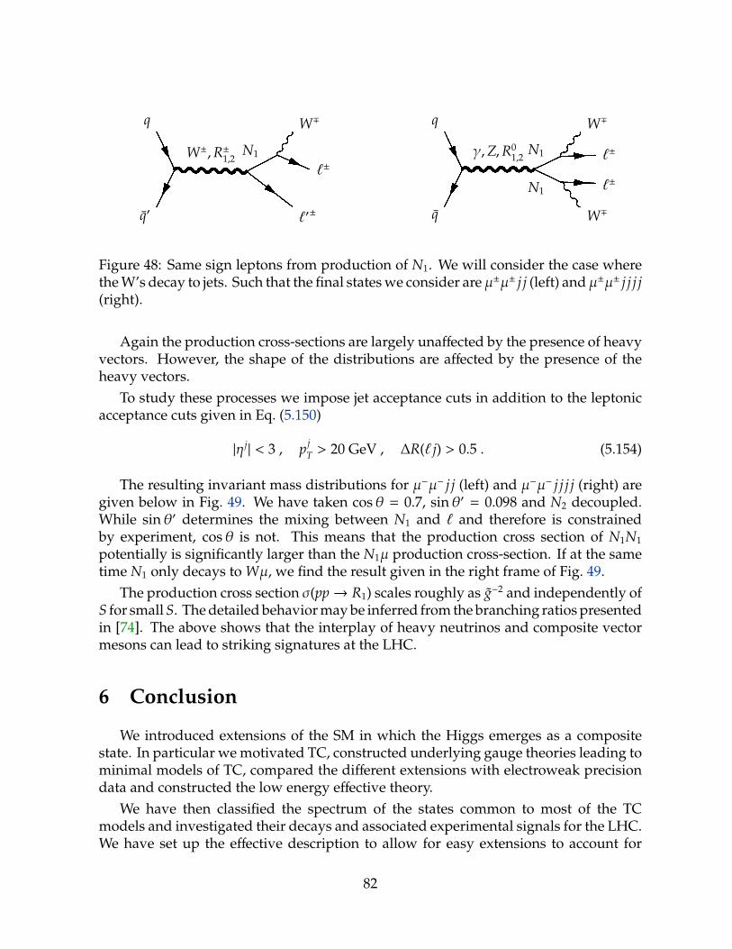
W±,R±1,2 N1

q

q′

W∓

`±

`′±�

γ,Z,R01,2

N1

N1

q

q

W∓

W∓

`±

`±

Figure 48: Same sign leptons from production of N1. We will consider the case wherethe W’s decay to jets. Such that the final states we consider areµ±µ± j j (left) andµ±µ± j j j j(right).

Again the production cross-sections are largely unaffected by the presence of heavyvectors. However, the shape of the distributions are affected by the presence of theheavy vectors.

To study these processes we impose jet acceptance cuts in addition to the leptonicacceptance cuts given in Eq. (5.150)

|η j| < 3 , p j

T > 20 GeV , ∆R(` j) > 0.5 . (5.154)

The resulting invariant mass distributions for µ−µ− j j (left) and µ−µ− j j j j (right) aregiven below in Fig. 49. We have taken cosθ = 0.7, sinθ′ = 0.098 and N2 decoupled.While sinθ′ determines the mixing between N1 and ` and therefore is constrainedby experiment, cosθ is not. This means that the production cross section of N1N1

potentially is significantly larger than the N1µ production cross-section. If at the sametime N1 only decays to Wµ, we find the result given in the right frame of Fig. 49.

The production cross section σ(pp→ R1) scales roughly as g−2 and independently ofS for small S. The detailed behavior may be inferred from the branching ratios presentedin [74]. The above shows that the interplay of heavy neutrinos and composite vectormesons can lead to striking signatures at the LHC.

6 Conclusion

We introduced extensions of the SM in which the Higgs emerges as a compositestate. In particular we motivated TC, constructed underlying gauge theories leading tominimal models of TC, compared the different extensions with electroweak precisiondata and constructed the low energy effective theory.

We have then classified the spectrum of the states common to most of the TCmodels and investigated their decays and associated experimental signals for the LHC.We have set up the effective description to allow for easy extensions to account for

82

10-4

10-3

10-2

10-1

1

10

500 600 700 800 900 1000

gt=3, MA=750 GeV, S=0.1MN1=100 GeV, MN2=1000 GeV

M(lljj)(GeV)Nu

mb

er o

f ev

ents

/5 G

eV @

100

fb

-1

10-3

10-2

10-1

1

10

600 700 800 900 1000 1100

gt=3, MA=750 GeV, S=0.1MN1=100 GeV, MN2=1000 GeV

M(lljjjj)(GeV)Nu

mb

er o

f ev

ents

/5 G

eV @

100

fb

-1

Figure 49: Invariant mass distributions for LHC at 14 TeV: pp → N1µ− → µ−µ− j j(left) and pp → N1N1 → µ−µ− j j j j (right). The parameters in the TC sector are fixedto be MA = 750 GeV, S = 0.1, g = 3 while the new lepton sector parameters areM1 = 100GeV, cosθ = 0.7, sinθ′ = 0.098. N2 is decoupled for these parameters.

specific features of given underlying gauge dynamics or for generic models in whichthe Higgs emerges as a composite state.

We have established important experimental benchmarks for Vanilla, Running,Walking and Custodial Technicolor for the potential discovery of these models at theLHC.

Acknowledgments

It is a pleasure for us to thank M. Antola, A. Belyaev, S. Catterall, D.D. Dietrich,R. Foadi, M.T. Frandsen, H. Fukano-Sakuma, M. Heikinheimo, J. Giedt, S.B. Gudnason,C. Kouvaris, A. Nisati, T.A. Ryttov, V. Sanz, J. Schechter, P. Schleper, R. Shrock andK. Tuominen for having shared part of the work on which this work is based on, longand fruitful collaborations, relevant discussions, criticism and/or careful reading of themanuscript.

83

A Realization of the generators for MWT and the Stan-dard Model embedding

It is convenient to use the following representation of SU(4)

Sa =

(A BB† −AT

), Xi =

(C DD† CT

), (A.155)

where A is hermitian, C is hermitian and traceless, B = −BT and D = DT. The S arealso a representation of the SO(4) generators, and thus leave the vacuum invariantSaE + ESaT = 0 . Explicitly, the generators read

Sa =1

2√

2

(τa 00 −τaT

), a = 1, . . . , 4 , (A.156)

where a = 1, 2, 3 are the Pauli matrices and τ4 = 1. These are the generators ofSU(2)V ×U(1)V.

Sa =1

2√

2

(0 Ba

Ba† 0

), a = 5, 6 , (A.157)

withB5 = τ2 , B6 = iτ2 . (A.158)

The rest of the generators which do not leave the vacuum invariant are

Xi =1

2√

2

(τi 00 τiT

), i = 1, 2, 3 , (A.159)

and

Xi =1

2√

2

(0 Di

Di† 0

), i = 4, . . . , 9 , (A.160)

withD4 = 1 , D6 = τ3 , D8 = τ1 ,D5 = i1 , D7 = iτ3 , D9 = iτ1 .

(A.161)

The generators are normalized as follows

Tr[SaSb

]=

12δab , ,Tr

[XiX j

]=

12δi j , Tr

[XiSa

]= 0 . (A.162)

Having set the notation, it is instructive to split the scalar matrix into four two bytwo blocks as follows:

M =

(X O

OTZ

), (A.163)

withX andZ two complex symmetric matrices accounting for six independent degreesof freedom each and O is a generic complex two by two matrix featuring eight real

84

bosonic fields. O accounts for the SM like Higgs doublet and a second copy as well asfor the three Goldstones which upon electroweak gauging will become the longitudinalcomponents of the intermediate massive vector bosons. The electroweak subgroup canbe embedded in SU(4), as explained in detail in [60]. Here SO(4) is the subgroup towhich SU(4) is maximally broken. The Sa generators, with a = 1, . . . , 4, together withthe Xa generators, with a = 1, 2, 3, generate an SU(2)L × SU(2)R ×U(1)V algebra. This iseasily seen by changing genarator basis from (Sa,Xa) to (La,Ra), where

La≡

Sa + Xa

√2

=

(τa

2 00 0

), −RaT

≡Sa− Xa

√2

=

(0 00 −

τaT

2

), (A.164)

with a = 1, 2, 3. The electroweak gauge group is then obtained by gauging SU(2)L, andthe U(1)Y subgroup of SU(2)R ×U(1)V, where

Y = −R3T+√

2 YV S4 , (A.165)

and YV is the U(1)V charge. For example, from Eq. (3.47) and Eq. (3.48) we see thatYV = y for the techniquarks, and YV = −3y for the new leptons. As SU(4) spontaneouslybreaks to SO(4), SU(2)L × SU(2)R breaks to SU(2)V. As a consequence, the electroweaksymmetry breaks to U(1)Q, where

Q =√

2 S3 +√

2 YV S4 . (A.166)

Moreover the SU(2)V group, being entirely contained in the unbroken SO(4), acts as acustodial isospin, which insures that the ρ parameter is equal to one at tree-level.

The electroweak covariant derivative for the M matrix is

DµM = ∂µM − i g[Gµ(y)M + MGT

µ(y)], (A.167)

where

g Gµ(YV) = g Waµ La + g′ Bµ Y

= g Waµ La + g′ Bµ

(−R3T

+√

2 YV S4). (A.168)

Notice that in the last equation Gµ(YV) is written for a general U(1)V charge YV, whilein Eq. (A.167) we have to take the U(1)V charge of the techniquarks, YV = y, since theseare the constituents of the matrix M, as explicitly shown in Eq. (3.58).

B Technicolor on Event Generators

We now implement the effective Lagrangian (3.97) on event generators such asMadGraph [122, 123] and CalcHEP [124, 125].

85

To implement the models on Monte Carlo event generators we used the FeynRulesMathematica package [126, 127, 128]12. FeynRules offers interfaces to several MonteCarlo generators. The interfaces to CalcHEP and MadGraph have been tested for thismodel. The implementation supports unitary gauge. The FeynRules model file andthe precompiled model files for MadGraph and CalcHEP can be downloaded here

https://feynrules.phys.ucl.ac.be/wiki/TechniColor

and here

http://cp3-origins.dk/research/tc-tools.

Unless the user wants to modify the model to include some new features, it is advisableto download the precompiled input files. These include some tweaks with respect tothe output of FeynRules which makes their use easier.

B.1 Ruling Technicolor with FeynRules

The model contains the SM fermions and gauge bosons. The naming convention ofthe particles was chosen to follow that of the SM implementation in MadGraph. As theimplementation is aimed for studying the signals from new high energy interactions,the SM Lagrangian was taken to be a very simple one. In particular, the electron, themuon, and the neutrinos, as well as the up, down and strange quarks, are taken to bemassless. This increases significantly the speed of Monte Carlo computations for someprocesses. We include only the Cabibbo mixing of the quarks. The input parameters(and their corresponding default values) of the SM sector are:

• EE = 0.313429, the electron charge;

• GF = 0.0000116637, the Fermi coupling constant (in units of GeV−2);

• MZ = 91.1876, the mass of the Z boson (in units of GeV);

• aS = 0.118, the Z pole value of the strong coupling constant αs;

• cabi = 0.227736, the Cabibbo angle;

• The masses of the heavy quarks MC = 1.3, MB = 4.2, MT = 172, and the taulepton MTA = 1.777;

• The widths of the weak gauge bosons and the top quark: wZ = 2.4952, wW =2.141, and wT = 1.508.

12The FeynRules implementation is a complete rewrite of the LanHEP [129] implementation that wasused in [74, 130].

86

The TC sector of the model implements the Vanilla Technicolor Lagrangian (3.97)with the mass of the heavy vector spin one state fixed by the first WSR, i.e. the case ofgeneric walking TC in Table 1. Thus the composite states are

• H: the composite Higgs H;

• R1N and R2N: the neutral heavy spin one states R01 and R0

2;

• R1+, R1-, R2+, and R2-: the charged heavy spin one states R±1 and R±2 .

For these states the effective theories of MWT and NMWT coincide.The input parameters of the composite TC sector are those listed already in Table 1:

• MA, the mass MA of the axial spin one states. Its allowed range is from about 500(GeV) to about 3000, depending on the values of gt and S.

• gt is the coupling strength g of the TC interactions and its allowed value rangesfrom about 1 to circa 10, depending slightly on the parameters MA and PS.

• PS indicates the S parameter of the new strongly coupled sector in isolation. Thisvalue is expected to be positive and small (much less than one). Estimates givePS ' 0.1 for MWT and PS ' 0.3 for NMWT. The full phenomenologically relevantS parameter comes from different contributions such as the one from the newlepton family.

• MH is the mass MH of the composite Higgs boson. As discussed in the main text,the Higgs is expected to be lighter than the vector mesons for walking TC models.

• rs is the parameter s that controls the coupling between the composite Higgs andthe heavy spin one states which is expected to be O(1).

An important feature of the model is that the widths of the heavy vectors and thecomposite Higgs depend strongly on the parameters MA, gt, and MH. This dependenceneeds to be included in the Monte Carlo calculations in order to obtain reliable results.The FeynRules implementation does not include the expressions for these widths, sincethey are computed in different ways, for example, in CalcHEP and in MadGraph. Itis possible to set CalcHEP to calculate and update the widths on the fly automaticallywhenever the values of the parameters are changed (see the CalcHEP manual [131]). InMadGraph, the widths can be included in the calculator program which takes care ofchanging the parameters. A calculator for the TC model, which includes the widths ofthe composite particles, can be downloaded from the same webpages of the FeynRulesmodel implementation given above.

87

B.2 Madding Technicolor via MadGraph/MadEvent v.4

MadGraph/MadEvent (just MadGraph or MG/ME in brief) is a software that allowsto generate amplitudes and events in models for particle interactions. The SM as wellas some beyond SM models are already included in the MG/ME model files and areready to be used once installed. The (N)MWT implementation can be downloadedfrom the links given at the beginning of this Section.

Here the aim is to provide a fast, practical and ready-to-go guide throughout theinstallation of MadGraph version 4 13 and its use with the MWT package; for furtherinformations and a deeper insight refer to the MadGraph manual, downloadable from

http://cp3wks05.fynu.ucl.ac.be/twiki/bin/view/.

To download the MadGraph package a registration is needed on the MG/ME websiteor one of its mirrors. To compute the matrix elements only the MadGraph StandAlonepackage is needed, while to also generate events, the entire MadGraph Developer’s kitis needed.

We refer to the MadGraph manual for installation instructions. Inside the MG/MEfolder one finds two useful directories: the Model directory is the one where the MWTmodel folder needs to be placed, while the Template directory is the one from where thesimulations are run. Here the files with the events generated by MadGraph are created.Fig. 50 shows the position of the directories and files used.

To use the new model the first step is to specify the process or the processes onewants to study. This is done by modifying the proc card.dat file inside the Template/Cardsfolder. As shown in the default file it is possible to specify more than one process at thetime, provided that the various processes are identified by an integer number followingthe character @. The names of the particles and respective antiparticles are defined inthe particles.dat file inside the specified model folder, and are case insensitive; in theSM default implementation for instance e-, mu-, ta- are the charged leptons (withantiparticles e+, mu+, ta+), ve, vm, vt the neutrinos (with antiparticles denoted by a ∼after the name), the quarks are u, d, c, s, t, b (again with antiparticles denoted by a ∼after the name), h is the Higgs boson and g, a, z, w+ and w- are the gauge bosons. Inthe MWT implementation the SM particles preserve their names, and in addition onehas the new neutral vector resonances r1, r2 plus the charged vector resonances r1+,r1-, r2+, r2-.

The process is specified listing initial and final particles separated by the character>. For example to study e+e− → µ+µ− one should type e+e->mu+mu-. At the bottom ofthis file one can set the definitions for the ‘multiparticles’, i.e. labels that are given tosets of particles rather than a single one. For instance, one can define the proton as

P uu˜dd˜g

13No modifications for MadGraph v. 5 are needed.

88

Figure 50: Graph illustrating the usage of the MWT implementation in MG/ME. Circlesrepresent directories, rectangles represent text files while hexagons are executable files.Blue arrows show placement of files and folders into the various directories, thickyellow arrows indicate input for the executable files while thick red ones indicateoutput.

89

meaning that the proton p is composed by u, u, d, d and the gluon g. The processpp>e+e-will henceforth consist of all the processes with any combination of two of thefollowing partons u, u, d, d and g in the initial state. Besides modifying the presentdefinitions, the user can provide some new ones. Note that the antiproton is not definedhere, and if one wants pp in the initial state he should just write pp: whether these areprotons and/or antiprotons it will be specified later, in the choice of the collider type inthe run card.dat file.

When specifying the process, use the form xy>z>abc to require the particle z toappear in a s-channel intermediate state, and use xy>abc/z to exclude the particle z toappear in any diagram.

Right below the process specification one can assign the maximum number of QED-and QCD-type vertices in each Feynman diagram that will be produced.

The model one wants to use for his simulations shall be specified as the name ofthe corresponding folder inside the Model directory; for example it is MWT for the MWTmodel (case insensitive).

To generate the Feynman diagrams for the processes specified, one has now to enterthe Template/bin folder and run the command ./newprocess from shell. The resultcan be seen by opening the file Template/index.html and by clicking on the link ‘ProcessInformation’; the Feynman diagrams are provided both as jpg files (click on ‘html’) aswell as ps files (click on ‘postscript’).

We can now generate events to compute different cross-sections. The result willdepend on both the Feynman diagrams that have been generated in the previous stepand the value of the couplings and parameters of the model used. To assign differentvalues to the MWT parameters it is necessary to use the calculator, downloadable fromthe webpages linked at the beginning of this Section; the readme.txt file coming alongwith it contains instructions on how to use it. Once extracted the package one has tocompile it typing make from shell; the executable file MWT calculator is then created.One can assign new values to some or all external parameters editing the param inputfile, where all the parameters that can be modified are listed. The calculator will assigna default value to all those parameters that are not requested to be modified in this file.To run the calculator, type

./MWT_Calculator parameter_input > param_card.dat

from shell, so that the file parameter input is given as input and a file named param card.datis produced. Opening this last file one can see the values of all the external parametersand all the masses of the model; the values of the other parameters will be automaticallycalculated by MadGraph. Substituting now this file to the existing one in the MWTmodel folder inside the Model directory will update the model with the new parametersvalues.

The second step before generating events is editing the Template/Cards/run card.datfile, where one can set the simulation and the collider parameters, choose the parton

90

distribution functions (PDF) and specify some cuts. The simplest entries one can editare:

• the tag name for the run, that is just one word providing a label to the run;

• the number of (unweighted) events one wants;

• the random seed; it should be always left to zero, unless the user aims to reproducea specific set of results. If left to zero, it is incremented automatically in each runso that successive runs are statistically independent;

• the collider type, that means the type of particles in each beam and their PDFs:use 1 to indicate the proton and −1 for the antiproton; setting 0, the PDFs areswitched off. The default setting is pp, as in the case of LHC;

• the beams energy;

• the PDF choice: to have the list of different possibilities, see the MG/ME manual.Note that the PDF automatically fixes also αs and its evolution;

• the cuts.

To generate events and get the cross sections of the processes, run now from insidethe directory Template/bin the command ./generate_events from shell; type 0 to runthe simulation on a single machine, and then provide the run name, i.e. a label forthe run. Depending on the number of particles and the number of Feynman diagramsinvolved the run can take from minutes to hours. The result of the simulation can beseen once again opening the file Template/index.html and clicking on the link ‘Resultsand Event Database’. The files containing the events (in the LHEF format [132]) arestored in the Template/Events folder.

Summarising:

1. Install the MadGraph/MadEvent package from the website;

2. download the MWT implementation and the calculator from

http://cp3-origins.dk/research/tc-tools,

and place the MWT model folder inside the MadGraph Models directory andcompile the calculator;

3. specify the processes you want to study and the model in the Cards/proc card.datfile;

4. run ./newprocess from the Template/bin directory to produce the Feynman dia-grams. You can check the result in the file Template/index.html;

91

5. to change the parameters of the MWT model, edit the parameter input file in thecalculator folder and then run./MWT_Calculator parameter_input > param_card.dat

to generate the param card.dat file, that has to be placed into the MWT modelfolder in the MadGraph Models directory;

6. in order to set the run parameters (collider type, beams energy, PDFs and so on)and impose cuts, edit the Template/Cards/run card.dat;

7. run ./generate_events from Template/bin to calculate the cross section and gen-erate the events;

8. check the result with the file Template/index.html; the event files are stored into theTemplate/Events folder.

B.3 Calculating Technicolor with CalcHEP

CalcHEP is a package that allows the user to go from the Lagrangian to the physicalobservables calculated at the lowest order in perturbation theory. The package can bedownloaded from the CalcHEP website, where also the manual and information aboutnew features are available. In addition users need Fortran and C compilers14 and XWindow System (X11)15 to install the program.

The current CalcHEP version 2.5.7 includes by default the SM and large extradimensional model implementations. Other models can be also downloaded from theCalcHEP web page. The (N)MWT implementation can be downloaded from the linksgiven at the beginning of this Section.

First of all one has to download the tar file that contains the source code from theCalcHEP web page, and extract the package. One has then to open the file getFlags inthe new CalcHEP folder and make sure that the names of the Fortran and C compilerscorrespond to those which are installed in the computer (and in case they do not,one has to change the names to the corresponding ones). To install the programone should move to the CalcHEP folder and run the command make. If all worksproperly the message CalcHEP is installed successfully and can be started should appear.It is convenient to create a working directory placed outside the CalcHEP folder byusing the command ./mkUsrDir ../WorkDir. At this point the program is ready touse and a Graphical User Interface (GUI) session can be launched with the command./calchep, to be entered preferably from the working directory. One can navigate

from menu to menu by using the arrow and esc keys. Instructions and help can befound pressing the F1 and F2 keys.

To install a new model in the current CalcHEP installation one should downloadthe model files and copy them to the models folder inside the CalcHEP main folder.

14For example g77 and gcc.15In some operating systems additional X11 development libraries are required.

92

Among those, the file prtcls.mdl contains description of the particles, vars.mdl definesthe model parameters, func.mdl contains additional parameters which depend on thosedefined in the previous file, and lgrng.mdl determines the interactions. To install thenew model one has to launch CalcHEP, choose from the second menu Import models,and type CALCHEP/models: in the resulting menu one can scroll the available modelsand choose the one to import.

Figure 51: Menus of the symbolic part.

CalcHEP contains two parts: a symbolic and a numerical one. Menus of the symbolicpart are presented in Fig. 51. In the second menu in Fig. 51 the user can choose thegauge (either Feynman-’t Hooft or unitary), or edit the model. Choosing Enter Processthe user can define the process. The number of initial state particles have to be eitherone or two. While the number of the final state particles is not limited in principle, theincreasing amount of time required by the simulation sets a practical limit between fourand six on that number, for a typical machine and process. It is also possible to excludesome particles from the Feynman diagrams used to calculate the process amplitude.

In the third menu the user can view the created diagrams and also save them ina separate file. Choosing Squaring techniques CalcHEP squares the diagrams. Thenumerical session can now be started directly by choosing Make&Launch n calchep or

93

Figure 52: Menus of the numerical part.

94

the user can ask CalcHEP to calculate directly the squared matrix elements by choosingSymbolic calculations. The resulting analytic expressions for the squared matrix elementscan be saved in different formats. One can then move to to the numerical session bychoosing C-compiler from the fifth menu in Fig. 51.

In numerical sessions the user can define the momentum of the initial state particlesand choose if and which parton distribution functions (PDF’s) to use. Several cuts canbe imposed and regularization of the propagators can be done before the numericalintegration. Also the model parameters can be changed at this point. CalcHEP au-tomatically re-calculates values of the related parameters if the model parameters arechanged. The structure of the menus in the numerical part is presented in Fig. 52.

CalcHEP uses Vegas to perform the numerical integrals: the user has to choose thenumber of Vegas calls and iteration steps. The actual number depends on how muchtime the user allows and how well the integrals converge. Some convergence problemscan be fixed by the a wise choice of the regularization scheme and appropriate cuts.The program can also generate plots of the differential cross section associated witha given process in function of one of the independent variables. The important partof the program is the event generator which allows to make predictions for colliderphenomenology. The method for producing the events is explained in the CalcHEPmanual.

Though intuitive, the graphical interface is not the only way to use CalcHEP: the usercan write at once all the information relative to the process to be simulated in the batchfile and then execute it in the working directory. For example, if the name of the batchfile is ee-mumu-batch one has to use the command ./calchep_batch ee-mumu-batch

to run the batch.For more information on CalcHEP usage, visit the CalcHEP homepage where the

official manual can be downloaded.

References

[1] H. Flacher, M. Goebel, J. Haller, A. Hocker, K. Monig and J. Stelzer, Eur. Phys. J.C 60, 543 (2009) [arXiv:0811.0009 [hep-ph]].

[2] J. Ellis, Nucl. Phys. A 827, 187C (2009) [arXiv:0902.0357 [hep-ph]].

[3] G. Altarelli, arXiv:0902.2797 [hep-ph].

[4] G. F. Giudice, J. Phys. Conf. Ser. 110, 012014 (2008) [arXiv:0710.3294 [hep-ph]].

[5] M. L. Mangano, Int. J. Mod. Phys. A 23, 3833 (2008) [arXiv:0802.0026 [hep-ph]].

[6] G. Altarelli, arXiv:0805.1992 [hep-ph].

[7] R. Barbieri, Nuovo Cim. B 123, 485 (2008).

95

[8] A. De Roeck et al., Eur. Phys. J. C 66, 525 (2010) [arXiv:0909.3240 [hep-ph]].

[9] E. Accomando et al., arXiv:hep-ph/0608079.

[10] S. Weinberg, Phys. Rev. D 19, 1277 (1979).

[11] L. Susskind, Phys. Rev. D 20, 2619 (1979).

[12] F. Sannino, Acta Phys. Polon. B 40, 3533 (2009) [arXiv:0911.0931 [hep-ph]].

[13] F. Sannino, arXiv:0804.0182 [hep-ph].

[14] C. T. Hill and E. H. Simmons, Phys. Rept. 381, 235 (2003) [Erratum-ibid. 390, 553(2004)] [arXiv:hep-ph/0203079].

[15] K. Lane, arXiv:hep-ph/0202255.

[16] F. Sannino and K. Tuominen, Phys. Rev. D 71, 051901 (2005) [arXiv:hep-ph/0405209].

[17] D. D. Dietrich, F. Sannino and K. Tuominen, Phys. Rev. D 72, 055001 (2005)[arXiv:hep-ph/0505059].

[18] D. D. Dietrich, F. Sannino and K. Tuominen, Phys. Rev. D 73, 037701 (2006)[arXiv:hep-ph/0510217].

[19] R. Foadi, M. T. Frandsen, T. A. Ryttov and F. Sannino, Phys. Rev. D 76, 055005(2007) [arXiv:0706.1696 [hep-ph]].

[20] D. D. Dietrich and F. Sannino, Phys. Rev. D 75, 085018 (2007) [arXiv:hep-ph/0611341].

[21] C. Pica and F. Sannino, arXiv:1011.3832 [hep-ph].

[22] T. A. Ryttov and F. Sannino, Phys. Rev. D 78, 065001 (2008) [arXiv:0711.3745[hep-th]].

[23] R. Shrock, arXiv:hep-ph/0703050.

[24] S. Sarkar, Rept. Prog. Phys. 59, 1493 (1996) [arXiv:hep-ph/9602260].

[25] M. S. Chanowitz, Ann. Rev. Nucl. Part. Sci. 38, 323 (1988).

[26] E. Farhi and L. Susskind, Phys. Rept. 74, 277 (1981).

[27] R. K. Kaul, Rev. Mod. Phys. 55, 449 (1983).

[28] R. S. Chivukula, arXiv:hep-ph/0011264.

[29] G. ’t Hooft, Nucl. Phys. B 72, 461 (1974).

96

[30] E. Witten, Nucl. Phys. B 160, 57 (1979).

[31] G. ’t Hooft, C. Itzykson, A. Jaffe, H. Lehmann, P. K. Mitter, I. M. Singer andR. Stora, New York, Usa: Plenum ( 1980) 438 P. ( Nato Advanced Study InstitutesSeries: Series B, Physics, 59)

[32] M. E. Peskin and T. Takeuchi, Phys. Rev. Lett. 65, 964 (1990).

[33] M. E. Peskin and T. Takeuchi, Phys. Rev. D 46, 381 (1992).

[34] D. C. Kennedy and P. Langacker, Phys. Rev. Lett. 65, 2967 (1990) [Erratum-ibid.66, 395 (1991)].

[35] G. Altarelli and R. Barbieri, Phys. Lett. B 253, 161 (1991).

[36] I. Maksymyk, C. P. Burgess and D. London, Phys. Rev. D 50, 529 (1994) [arXiv:hep-ph/9306267].

[37] R. Barbieri, A. Pomarol, R. Rattazzi and A. Strumia, Nucl. Phys. B 703, 127 (2004)[arXiv:hep-ph/0405040].

[38] R. S. Chivukula, E. H. Simmons, H. J. He, M. Kurachi and M. Tanabashi, Phys.Lett. B 603, 210 (2004) [arXiv:hep-ph/0408262].

[39] M. E. Peskin and J. D. Wells, Phys. Rev. D 64, 093003 (2001) [arXiv:hep-ph/0101342].

[40] E. Eichten and K. D. Lane, Phys. Lett. B 90, 125 (1980).

[41] S. Dimopoulos and L. Susskind, Nucl. Phys. B 155, 237 (1979).

[42] E. Farhi and L. Susskind, Phys. Rev. D 20, 3404 (1979).

[43] T. Appelquist, N. D. Christensen, M. Piai and R. Shrock, Phys. Rev. D 70, 093010(2004) [arXiv:hep-ph/0409035].

[44] T. A. Ryttov and R. Shrock, Phys. Rev. D 82, 055012 (2010) [arXiv:1006.5477 [hep-ph]].

[45] T. A. Ryttov and R. Shrock, Phys. Rev. D 81, 116003 (2010) [Erratum-ibid. D 82,059903 (2010)] [arXiv:1006.0421 [hep-ph]].

[46] T. A. Ryttov and R. Shrock, Eur. Phys. J. C 71, 1523 (2011) [arXiv:1005.3844 [hep-ph]].

[47] T. A. Ryttov and R. Shrock, Phys. Rev. D 81, 115013 (2010) [arXiv:1004.2075 [hep-ph]].

[48] K. Yamawaki, M. Bando and K. i. Matumoto, Phys. Rev. Lett. 56, 1335 (1986).

97

[49] B. Holdom, Phys. Lett. B 150, 301 (1985).

[50] B. Holdom, Phys. Rev. D 24, 1441 (1981).

[51] T. W. Appelquist, D. Karabali and L. C. R. Wijewardhana, Phys. Rev. Lett. 57, 957(1986).

[52] M. Antola, M. Heikinheimo, F. Sannino and K. Tuominen, JHEP 1003, 050 (2010)[arXiv:0910.3681 [hep-ph]].

[53] M. Antola, S. Di Chiara, F. Sannino and K. Tuominen, arXiv:1001.2040 [hep-ph].

[54] H. S. Fukano and F. Sannino, Phys. Rev. D 82, 035021 (2010) [arXiv:1005.3340[hep-ph]].

[55] K. Kondo, M. Tanabashi and K. Yamawaki, Mod. Phys. Lett. A 8, 2859 (1993).

[56] H. S. Fukano and F. Sannino, Int. J. Mod. Phys. A 25, 3911 (2010) [arXiv:0908.2424[hep-ph]].

[57] E. Witten, Phys. Lett. B 117, 324 (1982).

[58] D. K. Hong, S. D. H. Hsu and F. Sannino, Phys. Lett. B 597, 89 (2004) [arXiv:hep-ph/0406200].

[59] R. Casalbuoni, A. Deandrea, S. De Curtis, D. Dominici, R. Gatto and M. Grazzini,Phys. Rev. D 53, 5201 (1996) [arXiv:hep-ph/9510431].

[60] T. Appelquist, P. S. Rodrigues da Silva and F. Sannino, Phys. Rev. D 60, 116007(1999) [arXiv:hep-ph/9906555].

[61] T. Appelquist and F. Sannino, Phys. Rev. D 59, 067702 (1999) [arXiv:hep-ph/9806409].

[62] R. Sundrum and S. D. H. Hsu, Nucl. Phys. B 391, 127 (1993) [arXiv:hep-ph/9206225].

[63] M. Kurachi and R. Shrock, Phys. Rev. D 74, 056003 (2006) [arXiv:hep-ph/0607231].

[64] K. Nakamura et al. [Particle Data Group], J. Phys. G 37, 075021 (2010).

[65] H. J. He, N. Polonsky and S. f. Su, Phys. Rev. D 64, 053004 (2001) [arXiv:hep-ph/0102144].

[66] K. Kainulainen, K. Tuominen and J. Virkajarvi, Phys. Rev. D 75, 085003 (2007)[arXiv:hep-ph/0612247].

[67] N. D. Christensen and R. Shrock, Phys. Lett. B 632, 92 (2006) [arXiv:hep-ph/0509109].

98

[68] K. A. Intriligator and N. Seiberg, Nucl. Phys. Proc. Suppl. 45BC, 1 (1996)[arXiv:hep-th/9509066].

[69] S. D. H. Hsu and F. Sannino, Phys. Lett. B 605, 369 (2005) [arXiv:hep-ph/0408319].

[70] N. Arkani-Hamed and S. Dimopoulos, JHEP 0506, 073 (2005) [arXiv:hep-th/0405159].

[71] G. F. Giudice and A. Romanino, Nucl. Phys. B 699, 65 (2004) [Erratum-ibid. B 706,65 (2005)] [arXiv:hep-ph/0406088].

[72] T. A. Ryttov and F. Sannino, Phys. Rev. D 78, 115010 (2008) [arXiv:0809.0713[hep-ph]].

[73] K. D. Lane and E. Eichten, Phys. Lett. B 222, 274 (1989).

[74] A. Belyaev, R. Foadi, M. T. Frandsen, M. Jarvinen, F. Sannino and A. Pukhov,Phys. Rev. D 79, 035006 (2009) [arXiv:0809.0793 [hep-ph]].

[75] A. Doff, A. A. Natale and P. S. Rodrigues da Silva, Phys. Rev. D 77, 075012 (2008)[arXiv:0802.1898 [hep-ph]].

[76] M. Fabbrichesi, M. Piai and L. Vecchi, Phys. Rev. D 78, 045009 (2008)[arXiv:0804.0124 [hep-ph]].

[77] M. Harada, F. Sannino, J. Schechter, Phys. Rev. D69, 034005 (2004). [hep-ph/0309206].

[78] F. Sannino, J. Schechter, Phys. Rev. D76, 014014 (2007). [arXiv:0704.0602 [hep-ph]].

[79] M. Harada, F. Sannino, J. Schechter, Phys. Rev. D54, 1991-2004 (1996). [hep-ph/9511335].

[80] D. Black, A. H. Fariborz, S. Moussa, S. Nasri, J. Schechter, Phys. Rev. D64, 014031(2001). [hep-ph/0012278].

[81] Z. y. Duan, P. S. Rodrigues da Silva and F. Sannino, Nucl. Phys. B 592, 371 (2001)[arXiv:hep-ph/0001303].

[82] R. Foadi, M. T. Frandsen and F. Sannino, Phys. Rev. D 77, 097702 (2008)[arXiv:0712.1948 [hep-ph]].

[83] L. Del Debbio, A. Patella and C. Pica, Phys. Rev. D 81, 094503 (2010)[arXiv:0805.2058 [hep-lat]].

[84] R. Casalbuoni, S. De Curtis and M. Redi, Eur. Phys. J. C 18, 65 (2000) [arXiv:hep-ph/0007097].

[85] G. H. Brooijmans et al., arXiv:0802.3715 [hep-ph].

99

[86] G. L. Bayatian et al. [CMS Collaboration], CERN-LHCC-2006-001

[87] H. J. He et al., “LHC Signatures of New Gauge Bosons in Minimal HiggslessModel,” arXiv:0708.2588 [hep-ph].

[88] A. Birkedal, K. T. Matchev and M. Perelstein, “Phenomenology of Higgslessmodels at the LHC and the ILC,” In the Proceedings of 2005 International Lin-ear Collider Workshop (LCWS 2005), Stanford, California, 18-22 Mar 2005, pp 0314[arXiv:hep-ph/0508185].

[89] A. R. Zerwekh, Eur. Phys. J. C 46, 791 (2006) [arXiv:hep-ph/0512261].

[90] J. F. Gunion, H. E. Haber, G. L. Kane and S. Dawson, Front. Phys. 80, 1 (2000).

[91] M. R. Pennington, Phys. Rev. Lett. 97, 011601 (2006).

[92] F. Giacosa, T. Gutsche and V. E. Lyubovitskij, Phys. Rev. D 77, 034007 (2008)[arXiv:0710.3403 [hep-ph]].

[93] E. van Beveren, F. Kleefeld, G. Rupp and M. D. Scadron, Phys. Rev. D 79, 098501(2009) [arXiv:0811.2589 [hep-ph]].

[94] M. T. Frandsen, I. Masina and F. Sannino, Phys. Rev. D 81, 035010 (2010)[arXiv:0905.1331 [hep-ph]].

[95] T. Aaltonen et al. [CDF and D0 Collaboration], arXiv:1005.3216 [hep-ex].

[96] G. Altarelli, arXiv:1011.5342 [hep-ph].

[97] A. Semenov, Comput. Phys. Commun. 180, 431 (2009) [arXiv:0805.0555 [hep-ph]].

[98] F. del Aguila and J. A. Aguilar-Saavedra, JHEP 0505, 026 (2005) [arXiv:hep-ph/0503026].

[99] T. Cuhadar-Donszelmann, M. Karagoz, V. E. Ozcan, S. Sultansoy and G. Unel,JHEP 0810, 074 (2008) [arXiv:0806.4003 [hep-ph]].

[100] G. D. Kribs, T. Plehn, M. Spannowsky and T. M. P. Tait, Phys. Rev. D 76, 075016(2007) [arXiv:0706.3718 [hep-ph]].

[101] W. Y. Keung and P. Schwaller, arXiv:1103.3765 [hep-ph].

[102] B. Holdom, W. S. Hou, T. Hurth, M. L. Mangano, S. Sultansoy and G. Unel, PMCPhys. A 3, 4 (2009) [arXiv:0904.4698 [hep-ph]].

[103] L. Basso, A. Belyaev, S. Moretti and C. H. Shepherd-Themistocleous, Phys. Rev.D 80, 055030 (2009) [arXiv:0812.4313 [hep-ph]].

100

[104] R. M. Godbole, M. Guchait, K. Mazumdar, S. Moretti and D. P. Roy, Phys. Lett. B571, 184 (2003) [arXiv:hep-ph/0304137].

[105] H. Davoudiasl, T. Han and H. E. Logan, Phys. Rev. D 71, 115007 (2005) [arXiv:hep-ph/0412269].

[106] F. Meisel, M. Duhrssen, M.Heldmann, K. Jacobs, ATL-PHYS-PUB-2006-009,

[107] R. Foadi, M. Jarvinen and F. Sannino, Phys. Rev. D 79, 035010 (2009)[arXiv:0811.3719 [hep-ph]].

[108] R. Foadi and F. Sannino, Phys. Rev. D 78, 037701 (2008) [arXiv:0801.0663 [hep-ph]].

[109] G. Abbiendi et al. [OPAL Collaboration], Eur. Phys. J. C 49, 457 (2007) [arXiv:hep-ex/0610056].

[110] R. Foadi, M. T. Frandsen and F. Sannino, Phys. Rev. D 80, 037702 (2009)[arXiv:0812.3406 [hep-ph]].

[111] P. Gagnon, ATL-PHYS-PUB-2005-011.

[112] M. Fairbairn, A. C. Kraan, D. A. Milstead, T. Sjostrand, P. Z. Skands and T. Sloan,Phys. Rept. 438, 1 (2007) [arXiv:hep-ph/0611040].

[113] B. C. Allanach, C. M. Harris, M. A. Parker, P. Richardson and B. R. Webber, JHEP0108, 051 (2001) [arXiv:hep-ph/0108097].

[114] S. Giagu [ATLAS Collaboration and CMS Collaboration], arXiv:0810.1453 [hep-ex].

[115] F. del Aguila, J. A. Aguilar-Saavedra and R. Pittau, J. Phys. Conf. Ser. 53, 506(2006) [arXiv:hep-ph/0606198].

[116] T. Han and B. Zhang, Phys. Rev. Lett. 97, 171804 (2006) [arXiv:hep-ph/0604064].

[117] A. Atre, T. Han, S. Pascoli and B. Zhang, JHEP 0905, 030 (2009) [arXiv:0901.3589[hep-ph]].

[118] F. del Aguila and J. A. Aguilar-Saavedra, JHEP 0711, 072 (2007) [arXiv:0705.4117[hep-ph]].

[119] A. Abulencia et al. [CDF Collaboration], Phys. Rev. Lett. 98, 221803 (2007)[arXiv:hep-ex/0702051].

[120] T. Aaltonen et al. [CDF Collaboration], Phys. Rev. D 79, 011101 (2009)[arXiv:0809.3781 [hep-ex]].

[121] F. del Aguila, J. A. Aguilar-Saavedra and R. Pittau, JHEP 0710, 047 (2007)[arXiv:hep-ph/0703261].

101

[122] J. Alwall et al., JHEP 0709 (2007) 028 [arXiv:0706.2334 [hep-ph]].

[123] MadGraph/MadEvent website: http://madgraph.phys.ucl.ac.be.

[124] A. Pukhov et al., arXiv:hep-ph/9908288.

[125] CalcHEP website: http://theory.sinp.msu.ru/ pukhov/calchep.

[126] N. D. Christensen, C. Duhr, Comput. Phys. Commun. 180, 1614-1641 (2009).[arXiv:0806.4194 [hep-ph]].

[127] N. D. Christensen, P. de Aquino, C. Degrande, C. Duhr, B. Fuks, M. Herquet,F. Maltoni, S. Schumann, Eur. Phys. J. C71, 1541 (2011). [arXiv:0906.2474 [hep-ph]].

[128] FeynRules website: https://feynrules.phys.ucl.ac.be/wiki.

[129] A. Semenov, field theory. Version 3.0,” Comput. Phys. Commun. 180, 431-454(2009). [arXiv:0805.0555 [hep-ph]].

[130] M. T. Frandsen, M. Jarvinen, F. Sannino,

[arXiv:1103.3271 [hep-ph]]

[131] A. Pukhov, arXiv:hep-ph/0412191.

[132] J. Alwall et al., Comput. Phys. Commun. 176, 300 (2007) [arXiv:hep-ph/0609017].

102

asdf

•

AddressCP³-OriginsUniversity of Southern DenmarkCampusvej 55, 5230 Odense M, Denmark

Telephone: +45 6550 2316Email: cp3@cp3.sdu.dk