Discovering all most specific sentences

Discovering All Most Specific Sentences

DIMITRIOS GUNOPULOSComputer Science and Engineering Department, University of California,RiversideRONI KHARDONEECS Department, Tufts University, Medford, MAHEIKKI MANNILADepartment of Computer Science, University of Helsinki, Helsinki, FinlandSANJEEV SALUJALSI Logic, Milpitas, CAHANNU TOIVONENDepartment of Computer Science, University of Helsinki, Helsinki, FinlandandRAM SEWAK SHARMAComputer Science and Engineering Department, University of California,Riverside

Data mining can be viewed, in many instances, as the task of computing a representation of a theoryof a model or a database, in particular by finding a set of maximally specific sentences satisfyingsome property. We prove some hardness results that rule out simple approaches to solving theproblem.

The a priori algorithm is an algorithm that has been successfully applied to many instancesof the problem. We analyze this algorithm, and prove that is optimal when the maximally specificsentences are “small”. We also point out its limitations.

The work of D. Gunopulos was partially supported by National Science Foundation (NSF) CAREERAward 9984729, NSF grants IIS-9907477 and ITR 0220148, and the Department of Defense (DoD).The reseach of R. Khardon was supported by Office of Naval Research (ONR) grant N00014-95-1-0550 and ARO grant DAAL03-92-G-0115.Authors’ addresses: D. Gunopulos and R. Sewak Sharma, Computer Science and EngineeringDepartment, University of California, Riverside, Riverside, CA 92507; email: {dg;rssharma}@cs.ucr.edu; R. Khardon, EECS Department, Tufts University, Medford, MA 02155, email: [email protected]; H. Mannila, HIIT Basic Research Unit, Department of Computer Science, Uni-versity of Helsinki, Helsinki; Finland; email: [email protected]; S. Saluja, LSI Logic,MS E 192, 1551 McCarthy Blvd., Milpitas, CA 95035; email: [email protected]; H. Toivonen, De-partment of Computer Science, University of Helsinki, Helsinki, Finland; email: [email protected] to make digital or hard copies of part or all of this work for personal or classroom use isgranted without fee provided that copies are not made or distributed for profit or direct commercialadvantage and that copies show this notice on the first page or initial screen of a display alongwith the full citation. Copyrights for components of this work owned by others than ACM must behonored. Abstracting with credit is permitted. To copy otherwise, to republish, to post on servers,to redistribute to lists, or to use any component of this work in other works requires prior specificpermission and/or a fee. Permissions may be requested from Publications Dept., ACM, Inc., 1515Broadway, New York, NY 10036 USA, fax: +1 (212) 869-0481, or [email protected]© 2003 ACM 0362-5915/03/0600-0140 $5.00

ACM Transactions on Database Systems, Vol. 28, No. 2, June 2003, Pages 140–174.

Discovering All Most Specific Sentences • 141

We then present a new algorithm, the Dualize and Advance algorithm, and prove worst-casecomplexity bounds that are favorable in the general case. Our results use the concept of hypergraphtransversals. Our analysis shows that the a priori algorithm can solve the problem of enumeratingthe transversals of a hypergraph, improving on previously known results in a special case. On theother hand, using results for the general case of the hypergraph transversal enumeration problem,we can show that the Dualize and Advance algorithm has worst-case running time that is sub-exponential to the output size (i.e., the number of maximally specific sentences).

We further show that the problem of finding maximally specific sentences is closely related tothe problem of exact learning with membership queries studied in computational learning theory.

Categories and Subject Descriptors: H.3.3 [Information Storage and Retrieval]: InformationSearch and Retrieval—search process

General Terms: Algorithms, Theory

Additional Key Words and Phrases: Data mining, association rules, maximal frequent sets, learningwith membership queries, minimal keys

1. INTRODUCTION

Data mining has recently emerged as an active area of investigation and appli-cations [Fayyad et al. 1996]. The goal of data mining can briefly be stated as “de-velopment of efficient algorithms for finding useful high-level knowledge fromlarge amounts of data.” The area combines methods and tools from databases,machine learning, and statistics.

A large part of current research in data mining can be viewed as address-ing instances of the following problem: given a language, an interestingnesscriterion, and a database, find all sentences from the language that are truein the database and satisfy the interestingness criterion. Typically, this crite-rion is a frequency criterion that states that there are sufficiently many in-stances in the database satisfying the sentence. Examples of scenarios wherethis formulation works include the discovery of frequent sets, association rules,strong rules, episodes, and keys. In this article, we show how the problemsof finding frequent sets in relations and of finding minimal keys in databasescan be reduced to this formulation. Using this theory extraction formulation[Mannila 1995, 1996; Mannila and Toivonen 1997], one can formulate generalresults about the complexity of algorithms for these data mining tasks.

The specific problem we are considering is the complexity of computing themost specific interesting sentences. This problem has known lower bound re-sults, however existing algorithms have running times significantly worse thanthe best known lower-bounds. We analyze the running time of one of the mostsuccessful data mining algorithms, a priori, that has been applied to that prob-lem. We then give a new algorithm, Dualize and Advance, that is designed tofind the most specific sentences only.

Several variations of the a priori algorithm have been successfully appliedto problems of data mining [Agrawal and Srikant 1994; Agrawal et al. 1996;Mannila and Toivonen 1997; Mannila et al. 1994, 1995]. The a priori algorithmcomputes the interesting sentences by walking up in the lattice of sentences,one level at a time. Thus, it operates in a bottom-up fashion: first, the truthand frequency of the simplest, most general, sentences from the language are

ACM Transactions on Database Systems, Vol. 28, No. 2, June 2003.

142 • D. Gunopulos et al.

evaluated against the database, and then the process continues for more spe-cific sentences, one level at a time. To concentrate on its operation, we referto a priori algorithm as the level-wise algorithm. We show that as long as thenumber of levels in the search is small this algorithm is indeed optimal thusexplaining its empirical success and shedding some light on when and why it isuseful. Furthermore, we show that this algorithm can be used to efficiently solvea special case of the hypergraph transversal problem, improving on previoustheoretical results.

On the other hand, the analysis indicates that when the number of levels inthe search is large, the number of sentences of interest may become too large tohandle. An alternative method is to try to search for the most specific sentencesfrom the language that satisfy the requirements: these sentences determinethe theory uniquely. The number of interesting sentences can be exponentialto the number of most specific interesting sentences. It is therefore likely thatan algorithm that computes the most specific sentences can offer significantimprovements in computation time.

For this purpose, we present the Dualize and Advance algorithm (first intro-duced in Gunopulos et al. [1997]) for locating the most specific true sentencessatisfying the frequency criterion. We prove upper bounds on the complexity ofthe algorithm for the general case, showing that it comes close to lower boundsfor the problem. Our basic algorithm is deterministic and is sufficient to providethe worst case complexity bounds. We further apply a randomized heuristicin the algorithm that can improve its running time in practice considerably.While the algorithm is randomized, it is complete, in the sense that it returnsall most specific sentences, and the worst case bounds hold for it as well.

Briefly, the method works as follows. We apply a greedy search to locate somemaximal elements from the language. We then use the simple fact that if somemost specific sentences are known, then every unknown one must contain aminimal transversal of the complements of the known sentences. The algorithmalternates between finding most specific true sentences and finding minimaltransversals of the complements of the already discovered most specific truesentences, until no new most specific true sentences can be found.

We show that the running time of the algorithm is sub-exponential to thesize of the output. This result also shows that the complexity of the problem ofcomputing the most specific interesting sentences is lower than the complex-ity of finding all the interesting sentences, thus providing theoretical supportfor the experimental evidence that recent heuristic algorithms [Bayardo 1998;Burdick et al. 2001; Agrawal et al. 2000; Gouda and Zaki 2001], that have beendesigned to find maximal frequent sets directly, can significantly outperform apriori.

To demonstrate the utility of the algorithm, we apply it to the problem of com-puting of all minimal keys, or functional dependencies, in a relational databasein addition to the problem of computing of all maximal frequent sets of a {0, 1}matrix for a given threshold. The computation of maximal frequent sets is afundamental data mining problem which is required in discovering associationrules [Agrawal et al. 1993, 1996; Agrawal and Srikant 1994]. Computation ofminimal keys is important for semantic query optimization, which leads to fast



query processing in database systems [Mannila and Raiha 1994; Knobbe andAdriaans 1995; Bell and Brockhausen 1995; Schlimmer 1993]. Here, we referto possible keys that exist in a specific instance of a relational database andare not designed as such. In both cases, we first prove some hardness results ofrelated problems ruling out simple algorithmic approaches. We then show thatthe algorithm can be adapted to solve these problems.

The rest of this article is organized as follows: In Section 2, we present amodel of data mining that formally defines the theory extraction problem. Wealso show how this model can be used to describe the problems of computingfrequent sets and minimal keys. We also show the correspondence between thisproblem and problems studied in learning theory. In Section 3, we give hard-ness results that show that these two specific problems are difficult to solve.In Section 4, we formally define our computational model. Section 5 presentsand analyses the level-wise algorithm. Section 6 presents the Dualize andAdvance algorithm and analyses its complexity. Section 7 describes how theDualize and Advance algorithm can be adapted to compute maximal frequentsets and minimal keys. We also apply this algorithm to the problem of learn-ing Boolean monotone functions using membership queries. Section 8 presentsan incremental algorithm for computing the transversals of a hypergraph.Section 9 presents related work. In Section 10, we discuss the scope of ouralgorithms and point out some directions of further work. Preliminary versionsof the work presented here appeared previously in [Gunopulos et al. 1997a,1997b].

2. DATA MINING AS THEORY EXTRACTION

The model of knowledge discovery that we consider is the following [Mannila1995, 1996; Mannila and Toivonen 1997]. Given a database r, a language Lfor expressing properties or defining subgroups of the data, and a frequencycriterion q for evaluating whether a sentence ϕ ∈ L defines a sufficiently largesubclass of r. The computational task is to find the theory of r with respect toL and q, that is, the set Th(L, r, q) = {ϕ ∈ L | q(r, ϕ) is true}.

We are not specifying any satisfaction relation for the sentences of L in r:this task is taken care of by the frequency criterion q. For some applications,q(r, ϕ) could mean that ϕ is true or almost true in r, or that ϕ defines (in someway) a sufficiently large or otherwise interesting subgroup of r. We thereforeabstract this away by saying that ϕ is interesting when q(r, ϕ) = 1, and discussthe problem of mining for interesting sentences.

Obviously, ifL is infinite and q(r, ϕ) is satisfied for infinitely many sentences,(an explicit representation of) all of Th(L, r, q) cannot be computed feasibly.Therefore, for the above formulation to make sense, the language L has to bedefined carefully. In caseL is infinite, there are alternative ways of meaningfullydefining feasible computations in terms of dynamic output size, but we do notconcern ourselves with these scenarios. In this article, we assume that L isfinite.

As already considered by Mitchell [1982], we use a specialization/generalization relation between sentences. (See, e.g., Langley [1995] for an



overview of approaches to related problems.) A specialization relation is apartial order ¹ on the sentences in L. We say that ϕ is more general than θ , ifϕ ¹ θ ; we also say that θ is more specific than ϕ. The relation ¹ is a monotonespecialization relation with respect to q if the quality predicate q is monotonewith respect to ¹, that is, for all r and ϕ we have the following: if q(r, ϕ) andϕ′ ¹ ϕ, then q(r, ϕ′). In other words, if a sentence ϕ is interesting based onthe quality predicate q, then also all less special (i.e., more general) sentencesϕ′ ¹ ϕ are interesting. We write σ ≺ τ if σ ¹ τ and not τ ¹ σ .

Denote by rank(ψ) the rank of a sentence ψ ∈ L, defined as follows: If for noθ ∈ Lwe have θ ¹ ψ , then rank(ψ) = 0; otherwise, rank(ψ) = 1+max{rank(θ ) |θ ¹ ψ}. For T ⊂ L, let Ti denote the set of the sentences of L with rank i.

Typically, the relation ¹ is (a restriction of) the semantic implication rela-tion: if σ ¹ τ , then τ |= σ , that is, for all databases r, if r |= τ , then r |= σ .Note that if the interestingness predicate q is defined in terms of statisticalsignificance or something similar, then the semantic implication relation is nota monotone specialization relation with respect to q: a more specific statementcan be interesting, even when a general statement is not.

Given a specialization relation ¹, the set Th(L, r, q) can be represented byenumerating only its maximal elements, that is, the set

MTh(L, r, q) = {φ ∈ Th(L, r, q) | for no θ ∈ Th(L, r, q) φ ≺ θ}.Here again, one should be careful when working with infinite lattices. We

assume throughout the article that the maximal elements exist and are welldefined, and similarly for the minimal elements outside the theory Th(L, r, q).This definitely holds in finite lattices, and can be useful in more general casesas well. The problem considered in this article is therefore the following:

Problem 1 [MaxTh]. Given L, r, and q, find MTh(L, r, q).

It is easy to show ([Mannila and Toivonen 1997]) that finding frequent sets,episodes, keys, or inclusion dependencies are instances of the problem MaxTh.Especially for the problem of finding keys (or, more generally, functional depen-dencies) from relation instances the current framework has lots of connectionsto previous work.

2.1 Association Rules and Frequent Sets

To facilitate the presentation, we next discuss the problem of computing fre-quent sets that will serve to illustrate ideas in the next sections.

Given a 0/1 relation r with attributes R, an association rule is an expressionX ⇒ A, where X ⊆ R and A ∈ R. The intuitive meaning of such a rule is that,if a row has 1 in all attributes of X , then it tends also to have 1 in column A.Typically, in data mining, association rules are searched so that the set of rowshaving 1 in the attributes in X ∪ A is large enough; if we were to draw randomrows from r, it is required that such rows will be drawn with frequency at leastσ , for some fixed σ . The actual frequency is called the support of the rule. Theratio of rows including 1 in X ∪ A to those including 1 in the set X is called theconfidence of the rule.



Given the above description, a major subtask that is usually solved first isthat of computing frequent sets. Namely, given a 0/1 relation r, compute allsubsets Z such that the frequency of rows having 1 in all attributes of Z islarger than σ . Clearly, this is an instance of the problem discussed above; L isthe set of subsets of R, and q corresponds to having frequency higher than σ .The set Th(L, r, q) corresponds to the set of frequent sets, and similarly we cantalk of maximal frequent sets. This leads to the definition of the first specificinstance of the problem we are considering:

Problem 2 (Finding Maximal Frequent Sets). Given a 0/1 relation, and athreshold σ compute all maximal frequent sets.

Once the frequent sets are found, the problem of computing association rulesfrom them is straightforward. For each frequent set Z , and for each A ∈ Z , onecan test the confidence of the rule Z \A⇒ A.

2.2 Finding Minimal Keys in Databases

In this section, we discuss the problem of finding all minimal keys of a database.We begin by defining what we mean by keys and describe an application inwhich it is useful to find all minimal keys. We view a relational database r as amatrix whose columns correspond to fields and rows correspond to records.Let R denote the set of all fields (i.e., columns of the matrix). Then, a setX ⊆ R is a key of r, if no two rows of r agree on every attribute in X . Aminimal key is a key such that no proper subset of it is a key. Note that everykey must contain some minimal key and conversely every superset of a min-imal key is a key. Therefore, the collection of all minimal keys of a databaseis a succinct representation of the set of all keys of the database. Note thedistinction between our definition of key and the more standard definition of(primary) key of a database [Ullman 1988]. A (primary) key is a key (withrespect to our definition) of the database throughout the life of the databaseand is maintained so by the database manager. However, an arbitrary key, byour definition, may be so at current state of the database and may not existto be so after an update of the database. The problem we consider here is thefollowing:

Problem 3 (Finding Keys). Given a relational database, compute all mini-mal keys that exist currently.

As has been discussed in Bell [2003], the knowledge of all minimal keysexisting currently in the database can help in semantic query optimization thatis, in the process by which a database manager substitutes a computationallyexpensive query by a semantically equivalent query that can be processed muchfaster.

2.3 Relation to Learning Theory

We now show that the problem discussed above is very closely related to prob-lems in learning theory. One of the scenarios discussed in learning theory is



as follows: a Boolean function f : {0, 1}n → {0, 1} is fixed by some adversary(modeling a concept in the world). A learner is given access to some oraclegiving it partial information on the function f . The task of the learner is to finda representation for a Boolean function that is identical (or approximates) f .In particular, we consider the model of exact learning with membership queries[Angluin 1988].

A membership query oracle MQ( f ) allows the learner to ask for the value off on a certain point. That is, given x ∈ {0, 1}n, MQ( f ) returns the value f (x).The learning algorithm is given access to MQ( f ), and the algorithm is requiredto produce an expression that computes f exactly.

Definition 4. An algorithm is an exact learning algorithm with time com-plexity T (), query complexity Q(), and representation class H, for a class offunctions F , if for all f ∈ F , when given access to MQ( f ), the algorithm runsin time T (), asks MQ on at most Q() points and then outputs a representationh ∈ H for a Boolean function such that h is equivalent to f .

In the above definition, we omitted the parameters of the functions T () andQ(). Normally, the algorithm is allowed time polynomial in the number of vari-ables n, and the size of a representation for f in some representation language.

In particular, we next consider the problem of learning monotone functionswith membership queries. A function f is monotone if f (x) = 1, and y ≥x implies f ( y) = 1, where ≤ is the normal partial order on {0, 1}n. We alsoconsider the standard CNF and DNF representations for such functions. Aterm is a conjunction of literals, for example, x1x2 is a term. A DNF expressionis a disjunction of terms, for example, x1x2∨x2x3 is a DNF expression. Similarly,a CNF expression is a conjunction of disjunctions, for example, (x1∨ x2)(x2∨ x3)is a CNF expression. It is well known that monotone functions have uniqueminimum size representations in both DNF and CNF, that include all minimalterms or clauses respectively of the function. (A minimal term, called a primeimplicant, is a term that implies f and such that every subset of it does notimply f .)

In the scenario that follows, the learning algorithm is allowed time relativeto the number of attributes n, and the sum of sizes of its DNF and CNF rep-resentations. That is, we consider T (m), and Q(m) where m = n+ |DNF ( f )| +|CNF ( f )|.

The correspondence between learning monotone functions and computinginteresting sets is thus straightforward. The elements of {0, 1}n correspond tosubsets of the variables so that a value 1 implies that the corresponding at-tribute is in the set. The value of the function on an assignment corresponds tothe negation of the interestingness relation q. Since q is monotone, the functionis monotone. Membership queries now naturally correspond to Is-interestingqueries. We therefore get:

THEOREM 5. The problem of computing interesting sentences for problemsrepresentable as sets is equivalent to the problem of learning monotone functionswith membership queries, with representation class CNF (or DNF).



3. HARDNESS RESULTS ON THE COMPUTATION OF FREQUENT SETSAND MINIMAL KEYS

Computing frequent sets or maximal frequent sets is an enumeration problem.The algorithm must enumerate all sets and in the end provide proof that nomore sets exist. The results in this section indicate that it is difficult not onlyto find all maximal frequent sets and minimal keys, but it is also difficult toverify that all maximal sets or keys have already been found. The hardnessresults we present also show that it is difficult to to find the number of frequentsets or keys. As a result, algorithms that find frequent sets or keys are likelyto be worst case exponential. Consequently, we use an output-size sensitivecomplexity model to evaluate the performance of the algorithms.

3.1 Hardness Results on the Computation of Frequent Sets

We first consider the problem of counting the number of σ -frequent sets.

THEOREM 6. The problem of finding the number of σ -frequent sets of a given0− 1 relation r and a threshold σ ∈ [0, 1] is #P-hard.

PROOF. We show a polynomial time reduction from the problem of comput-ing the number of satisfying assignments of a monotone-2CNF formula to theproblem of computing the number of frequent sets, that has a simple mappingbetween the number of solutions. This suffices, since the problem of computingthe number of satisfying assignment of monotone-2CNF formulas is known tobe #P-hard [Valiant 1979].

A monotone-2CNF formula is a Boolean formula in conjunctive normal formin which every clause has at most two literals and every literal is unnegated.Given a monotone-2CNF formula f with m clauses and n variables, constructan m × n {0, 1} matrix M as follows: M j ,i is 0 if the ith variable is presentin the j th clause and 1 otherwise. An assignment of variables falsifies f , iffthe set of columns corresponding to variables with value 1 forms a frequentset of M with threshold 1

m . Therefore, the number of frequent sets of M withthreshold 1

m is (2n—the number of satisfying assignments of f ). This completesthe reduction.

Note that the above result still does not rule out the possibility of an outputpolynomial algorithm for computing all maximal frequent sets, since in contrastwith counting, for enumeration one is given time polynomial in the size of theoutput. The next theorem rules out the possibility of an efficient algorithm thatoutputs the maximal frequent sets in the decreasing order of their size.

THEOREM 7. The problem of deciding if there is a maximal σ -frequent setwith at least t attributes for a given 0− 1 relation r, and a threshold σ ∈ [0, 1],is NP-complete.

PROOF. It is easily seen that the problem is in NP. To show the NP-hardness,we show a polynomial time reduction from the Balanced Bipartite Clique prob-lem to the above problem. Since the Balanced Bipartite Clique is known to beNP-hard, the result will follow [Garey and Johnson 1979].



Given a bipartite graph G = (V1, V2, E), a balanced clique of size k is acomplete bipartite graph with exactly k vertices from each of V1 and V2. TheBalanced Bipartite Clique problem is, given a bipartite graph G and a positiveinteger k, check if there exists a balanced bipartite clique of size k.

Given a bipartite graph G and a positive integer k, let n1 and n2 be thenumber of vertices in V1 and V2 respectively. Define an n1 × n2 {0, 1}matrix Mas follows. Mi, j is 1 iff ith vertex of V1 is connected to the j th of V2. Then, thereis a bipartite clique of size k in G iff there is a frequent set of M of size at leastk with threshold k

n1.

3.2 Hardness Results for Computing Minimal Keys

THEOREM 8. The problem of finding the number of all keys of a givendatabase is #P-hard.

PROOF. We prove the result in two steps. First, we show a polynomial-timereduction from the problem of computing the number of satisfying assignmentsof a monotone-2CNF formula to the problem of computing the number of set-covers of a family of sets. Then, we show a polynomial time reduction from theproblem of computing the number of set covers of family of sets to the problemof computing the number of keys of a database. Since the reductions maintainthe same number of solutions, and the problem of computing the number ofsatisfying assignments of a monotone-2CNF formula is #P-hard [Valiant 1979],this proves the result.

Recall that, given a family of sets each of which is subset of a finite universeset, a set cover is a collection of sets from the family such that every element ofthe universe is in at least one of the sets in the collection. Given a monotone-2CNF formula with m clauses and n variables, construct a family of n setsS1, . . . , Sn each of which is a subset of the set {1, 2, . . . , m}, as follows. Theset Si contains j iff ith variable is present in j th clause. It is easily seen thata satisfying assignment of the monotone-2CNF formula corresponds to a uniqueset cover of the family of sets and vice-versa, by picking Si in the set cover iff theith variable has value 1 in the assignment. Therefore, the number of satisfyingassignments of the monotone-2CNF formula is exactly the number of set coversof the family of sets. This completes the first reduction.

We now discuss the second reduction. Given a family of sets S1, . . . , Sn eachof which is a subset of the universe set {1, 2, . . . , m}, construct a relationaldatabase as follows: The database has n fields f1, . . . , fn and m + 1 recordsr0, . . . , rm. The record r0 will have value 0 in every field. For 1 ≤ j ≤ n and1 ≤ i ≤ m, the field f j of record ri will have value i if element i is present inthe set Sj ; otherwise, it will have value 0. Note that a collection Si1 , Si2 , . . . , Sic(for some c) of sets from the family will be a set cover iff the collection of fieldsfi1 , . . . , fic is a key of the database. Therefore, the number of set covers of thegiven family of sets is the same as the number of keys of the database. Thiscompletes the second reduction and the proof of the theorem.

The following theorem shows that counting the number of minimal keys isnot easier than counting the number of all keys.



THEOREM 9. The problem of finding the number of minimal keys of a givendatabase is #P-hard.

PROOF. Once again, we show two polynomial time reductions that main-tain the same number of solutions. The first reduction is from the problem ofcomputing the number of minimal vertex covers of a graph to the problem ofcomputing the number of minimal set covers of a family of sets. The secondreduction is from the problem of computing the number of minimal set coversof a family of sets to the problem of computing the number of minimal keys ofthe database. Since the problem of computing the number of minimal vertexcovers of a graph is known to be #P hard [Valiant 1979], this implies the result.

Recall that a vertex cover of a graph G is a set of vertices of G such thatevery edge of G is incident on at least one vertex in the set. Given a graph Gwith n vertices and m edges, define a family of sets S1, . . . , Sn each of whichis a subset of the set {1, 2, . . . , m}, as follows. The set Si has element j iff thej th edge of the graph is incident on the ith vertex. Note that a collection ofsets Si1 , . . . , Sic (for some c) from the family is a minimal set cover iff the setof vertices {i1, . . . , ic} is a minimal vertex cover of G. Therefore, the number ofminimal vertex covers of G is same as the number of minimal set covers of thefamily. This completes the first reduction.

For the second reduction, we use the same reduction that was used as sec-ond reduction in the proof of Theorem 8. With respect to the reduction, notethat a collection Si1 , . . . , Sic is a minimal set cover of the family iff the set offields { fi1 , . . . , fic} is a minimal key of the database. Therefore, the number ofminimal set covers of the family is same as the number of minimal keys of thedatabase.

4. COMPLEXITY OF FINDING ALL INTERESTING SENTENCES

The hardness results we presented in the previous section show that algorithmsthat find maximal frequent sets or keys are likely to have exponential worstcase running time. Consequently, we use an output-size sensitive complexitymodel to evaluate the performance of the algorithms.

To study the complexity of the generation problem, we introduce some no-tation and basic results that appeared previously in Mannila and Toivonen[1997].

Consider a set S of sentences from L such that S is closed downwards underthe relation ¹, that is, if θ ∈ S and ϕ ¹ θ , then ϕ ∈ S. The border Bd(S) ofS consists of those sentences σ such that all generalizations of σ are in S andnone of the specializations of σ is in S. Those sentences σ in Bd(S) that are inS are called the positive border1 Bd+(S), and those sentences σ in Bd(S) thatare not in S are the negative border Bd−(S). In other words,

Bd(S) = Bd+(S) ∪ Bd−(S),

where

Bd+(S) = {σ ∈ S | for all γ such that σ ≺ γ , we have γ 6∈ S}1That is, the positive border corresponds to the set “S” of [Mitchell 1982].



and

Bd−(S) = {σ ∈ L \ S | for all γ ≺ σ, we have γ ∈ S}.

The positive border of the theory is the set of its maximal elements, that is,MTh(L, r, q) = Bd+(Th(L, r, q)). Note that Bd(S) can be small even for large S.

Above, we assumed that the set S is closed downwards. We generalize thenotation for sets S that are not closed downwards by simply defining thatBd(S) = Bd(S′) where S′ is the downward closure of S. The generalizationis similar for negative and positive borders.

Some straightforward lower bounds for the problem of finding all frequentsets are given in Agrawal et al. [1996] and Mannila et al. [1994]. Now weconsider the problem of lower bounds in a more realistic model of computation.

The main effort in finding interesting sets is in the step where the interest-ingness of subgroups are evaluated against the database. Thus, we consider thefollowing model of computation. Assume the only way of getting informationfrom the database is by asking questions of the form

Is-interesting Is the sentence ϕ interesting, that is, does q(r, ϕ) hold?

THEOREM 10 [MANNILA AND TOIVONEN 1997]. Any algorithm for computingTh(L, r, q) that accesses the data using only Is-interesting queries must use atleast |Bd(Th(L, r, q))| queries.

This result, simple as it seems, gives as a corollary a result about findingfunctional dependencies that in the more specific setting is not easy to find;cf. Mannila and Raiha [1992] and Mannila and Toivonen [1997]. Similarly, thecorresponding verification problem requires at least this number of queries.

Problem 11 (Verification). Given L, r, q, and a set S ⊆ L, verify that S =MTh(L, r, q).

COROLLARY 12 [MANNILA AND TOIVONEN 1997]. Given L, r, q, and a set S ⊆ L,determining whether S =MTh(L, r, q) requires in the worst case at least |Bd(S)|evaluations of the predicate q, and it can be solved using exactly this number ofevaluations of q.

We now show that the verification problem is closely related to computinghypergraph transversals. A collectionH of subsets of R is a (simple) hypergraph,if no element of H is empty and if X , Y ∈ H and X ⊆ Y imply X = Y . Theelements ofH are called the edges of the hypergraph, and the elements of R arethe vertices of the hypergraph. Given a simple hypergraphH on R, a transversalT of H is a subset of R intersecting all the edges of H, that is, T ∩ E 6= ∅ for allE ∈ H.

Transversals are also called hitting sets. Here we consider minimal transver-sals: a transversal T ofH is minimal if no T ′ ⊂ T is a transversal (Figure 1). Thecollection of minimal transversals of H is denoted by Tr(H). It is a hypergraphon R.

Problem 13 (HTR). Given a hypergraph H, construct Tr(H).



BA

C D

Fig. 1. The set {A, B} is a transversal of the hypergraph with edges AB, AC, AD, BD.

For more information on hypergraphs, see [Berge 1973]. The problem of com-puting transversals appears in various branches of computer science; a com-prehensive study of this problem is given by [Eiter and Gottlob 1995]. The HTRproblem also appears in several forms in databases. In particular, the problemof translating between a set of functional dependencies and their correspondingArmstrong relation [Mannila and Raiha 1986, 1992] is at least as hard as thisproblem and equivalent to it in special cases [Eiter and Gottlob 1995]. Furtherdiscussion of these issues is given by Khardon [1995] and Mannila and Raiha[1994].

Notice that, in general, the output for this problem may be exponentiallylarger than its input, and thus the question is whether it can be solved in timepolynomial in both its input size and output size. We say that an algorithm isoutput T () time algorithm for the problem if it runs in time T (I, O) where I isthe input size, and O is the corresponding output size. A more strict condition,that we use here, requires that the output transversals be enumerated, and thatthe time to compute the ith transversal will be measured against the input sizeand i. That is, an algorithm solves the problem in incremental T (I, i) time if theith transversal is computed in time T (I, i). For further discussion and othervariations, see Eiter and Gottlob [1995].

The exact complexity of the HTR problem is yet unknown. A subexponentialsolution for the problem has been recently discovered [Fredman and Khachiyan1996], and several special cases can be solved in polynomial time [Eiter andGottlob 1995; Mishra and Pitt 1997].

Now we return to the verification problem. Given S ⊆ L, we have to deter-mine whether S =MTh(L, r, q) holds using as few evaluations of the interest-ingness predicate as possible.

Definition 14 (Representing as Sets). Let L be the language, ¹ a special-ization relation, and R a set; denote by P(R) the powerset of R. A functionf : L → P(R) is a representation of L (and ¹) as sets, if f is one-to-one andsurjective, f and its inverse are computable, and for all θ and ϕ we have θ ¹ ϕif and only if f (θ ) ⊆ f (ϕ).



A B C D

AB AC AD BC BD CD

ABCD

ABC ABD ACD BCD

{}

Fig. 2. The lower shaded area represents the downward closure of S = {ABC, ABD}, S is exactlythe positive border and the negative border is the set CD.

Thus, representing as sets requires that the structure imposed on L by ¹ isisomorphic to a subset lattice. In particular, the lattice must be finite, and itssize must be a power of 2. Note that frequent sets, functional dependencies withfixed right-hand sides, and inclusion dependencies are easily representable assets; the same holds for monotone Boolean functions. However, the language ofMannila et al. [1995] used for discovering episodes in sequences does not satisfythis condition.

Given S, we can compute Bd+(S) without looking at the data r at all: sim-ply find the most special sentences in S. The negative border Bd−(S) is alsodetermined by S, but finding the most general sentences in L\S can be dif-ficult. We now show how minimal transversals can be used in the task. As-sume that ( f , R) represents L as sets, and consider the hypergraph H(S)on R containing as edges the complements of sets f (ϕ) for ϕ ∈ Bd+(S):H(S) = {R\ f (ϕ) | ϕ ∈ Bd+(S)}. Then Tr(H(S)) is a hypergraph on R, andhence we can apply f −1 to it: f −1(Tr(H(S))) = { f −1(H) | H ∈ Tr(H(S))}. Wehave the following.

THEOREM 15 [MANNILA AND TOIVONEN 1997]. f −1(Tr(H(S))) = Bd−(S).

Example 16. Consider the problem of computing frequent sets illustratedin Figure 2, with attributes R = {A, B, C, D}. Let S = {ABC, ABD}, wherewe use a shorthand notation for sets, for example, we represent {A, B, C} byABC. Then, the downward closure of S is equal to {ABC, ABD, AB, AC, AD,BC, BD, A, B, C, D}, and S includes the maximal elements. The negative border(that can be found by drawing the corresponding lattice) is Bd−(S) = {CD}.

For this problem, we already have L represented as sets and thus usethe identity mapping f (X )= X , thus H(S)={D, C}. It is easy to see thatTr({D, C})={CD}, and thus f −1 indeed yields the correct answer.



The requirement for representing as sets is quite strong. It is however nec-essary. In particular, the mapping f must be surjective, that is, cover all ofP (R). Otherwise, after computing the transversal, a set may not have an in-verse mapping to be applied in the last transformation in the theorem. This isindeed the case when we consider the problem of finding sequential patterns[Agrawal and Srikant 1995] or episodes [Mannila et al. 1995]. The a priori(level-wise) algorithm can be extended to handle sequences of attributes ratherthan sets of attributes because we can define a monotone specialization relationbetween sequences. However, it is not clear how to represent sequences of at-tributes as sets so the Dualize and Advance algorithm cannot be applied in thiscase.

5. THE LEVEL-WISE ALGORITHM

The a priori algorithm [Agrawal and Srikant 1994; Mannila and Toivonen 1997]for computing Th = Th(L, r, q) proceeds by first computing the set Th0 consist-ing of the sentences of rank 0 that are in Th. Then, assuming Thi is known, itcomputes a set of candidates: sentences ψ with rank i + 1 such that all θ withθ ≺ ψ are in Th. For each one of these candidates ψ , the algorithm calls thefunction q to check whether ψ really belongs to Th. This iterative procedure isperformed until no more sentences in Th are found.

This level-wise algorithm has been used in various forms in finding associa-tion rules, episodes, sequential rules, etc. [Agrawal and Srikant 1994, 1995;Agrawal et al. 1996; Mannila et al. 1995; Mannila and Toivonen 1997]. InGunopulos et al. [1997a], it is shown to be optimal for the computation of theset Th(L, r, q). The algorithm solves the problem MaxTh by simply finding allinteresting statements, that is, the whole theory Th(L, r, q) going bottom up.The method is as follows:

Algorithm 17. The a priori (level-wise) algorithm for finding all interesting state-ments.Input: A database r, a language L with specialization relation ¹, and a quality predi-cate q.Output: The set Th(L, r, q).Method:

1. C1 := {ϕ ∈ L | there is no ϕ′ in L such that ϕ′ ≺ ϕ};2. i := 1;3. While Ci 6= ∅ do4. Li := {ϕ ∈ Ci | q(r, ϕ)};5. Ci+1 := {ϕ ∈ L | for all ϕ′ ≺ ϕ we

have ϕ′ ∈ ⋃ j≤i L j }\⋃

j≤i Cj ;6. i := i + 1;7. Od;8. output

⋃j<i L j ;

The algorithm works iteratively, alternating between candidate generationand evaluation phases. First, in the generation phase of an iteration i, a collec-tion Ci of new candidate sentences is generated, using the information availablefrom more general sentences. Then the quality predicate is computed for these



{}

AB AC AD BC BD CD

ABCD

ABC ABD ACD BCD

A B C D

Fig. 3. The a priori algorithm operates at levels: After computing the frequent sets of size 2(L2 = {AB, AC, BC}), the only set of cardinality 3 that must be considered is ABC, which is asuperset of all the sets in L2.

candidate sentences. The collection Li will consist of the interesting sentencesin Ci. In the next iteration i + 1, candidate sentences in Ci+1 are generatedusing the information about the interesting sentences in

⋃L j (Figure 3). Note

that using the notion of border, Step 5 of the algorithm can be written asCi+1 := Bd−(

⋃j≤i L j ) \

⋃j≤i Cj .

The algorithm aims at minimizing the amount of database processing, that is,the number of evaluations of q (Step 4). Note that the computation to determinethe candidate collection does not involve the database (Step 5). For example,in Agrawal et al. [1996], when computing frequent sets Step 5 used only anegligible amount of time.

Clearly, by definition, the algorithm finds the maximal interesting sentences.Moreover, we show that under certain conditions the algorithm does not taketoo much time. The following theorem is immediate.

THEOREM 18. The level-wise algorithm computes the set of interesting sen-tences correctly, and it evaluates the predicate q

|Th(L, r, q) ∪ Bd−(Th(L, r, q))|times.

Example 19. Consider, again, the problem of computing frequent setswhere R = {A, B, C, D} and MaxTh = {ABC, BD}, that is, the situation ofFigure 2. The level-wise algorithm works its way up from the bottom. It startsby evaluating the singletons A, B, C, and D; all of these are frequent. In thesecond iteration, C2 contains pairs of attributes such that both attributes arefrequent, in this case all attribute pairs. Of them, AB, AC, BC, and BD are



frequent. C3 then contains such sets of size three all of whose subsets are fre-quent, that is, the set ABC, which is actually frequent. Notice that the negativeborder corresponds exactly to the sets that have been found not interestingalong the way, that is the sets AD and CD.

In order to further analyze the complexity, we use the following notation.First, recall the definition of rank, given in Section 2, capturing the “level” ofa sentence. Denote by dc(k) the maximal size of the downward closure of anysentence φ of rank ≤ k. Also, by width(L,¹), denote the maximal number ofimmediate successors on L and ¹. That is,

width(L,¹) = maxθ|{φ | θ ≺ φ and for no ψ, θ ≺ ψ ≺ φ}|.

THEOREM 20. Let k be the maximal rank over all interesting sentences inthe problem (L, r, q). The level-wise algorithm computes the set of interestingsentences correctly, and the number of queries it makes is bounded by

dc(k) width(L,¹) |MTh(L, r, q)|.PROOF. The number of sentences below any maximal element is bounded

by dc(k), and thus the number of elements not rejected from Ci at all stagestogether is bounded by dc(k)|MTh(L, r, q)|. Each of these sentences might createat most width(L,¹) new sentences for consideration in Ci+1 that may be rejected(i.e., they are in Bd−(Th(L, r, q))).

This result holds for any (L, r, q). For problems representable as sets one canderive more explicit bounds. In particular, in the problem of frequent sets therank corresponds to the size of the set, the width is the number of attributes,and dc(k) = 2k . A standard assumption in practical applications is that the sizeof frequent sets is bounded. In these cases the level-wise algorithm is indeedefficient:

COROLLARY 21. Let k be the size of the largest frequent set, and n the numberof attributes. The level-wise algorithm computes the set of frequent sets correctly,and the number of queries it makes is bounded by 2kn|MTh(L, r, q)|.

As a further corollary of the above, we get that if the size of frequent sets isnot too large then the size of Bd−(Th(L, r, q)) is not prohibitive and thus theproblem is feasible.

COROLLARY 22. Let k be the size of the largest frequent set, and n the numberof attributes.

(i) The size of sets in Bd−(Th(L, r, q)) is bounded by k + 1.(ii) If k = O(log n), the size of Bd−(Th(L, r, q)) is bounded by O(nO(1)|

MTh(L, r, q)|).We thus get an application for hypergraph transversals:



THEOREM 23. For k = O(log n), the problem of computing hypergraph trans-versals, where the edges of the input graph are all of size at least n−k, is solvablein input polynomial time by the level-wise algorithm.

PROOF. If the edge size is at least n− k, then the maximal sets that are nottransversals are of size at most k. Set non-transversals to be “interesting” anduse the algorithm. We get that the negative border is the required transversalhypergraph.

This improves on previous results by Eiter and Gottlob [1995] (Theorem 5.4)that show that this is possible for constant k (and uses a brute force enumer-ation algorithm using property (i) above). Notice that the level-wise algorithmdoes not use the structure of original hypergraph directly. All it does is to testwhether certain subsets are transversals of it or not.

6. THE DUALIZE AND ADVANCE ALGORITHM

The results of the previous section show that the a priori algorithm is optimal ifwe want to compute all frequent elements. It also performs very well when wewant to compute the maximal elements, and the size of the maximal elementsis small. Given this analysis, the disadvantage of the level-wise approach isclear. If there is an element in MTh whose rank is large, then all the down-ward closure of this element will be tested and this would require too muchtime.

Example 24. For example, consider the situation where there are n at-tributes, and k maximal sets of size n

k . Then, the size of the border is O(n2)(the maximal frequent sets are k, and the minimal nonfrequent sets are allpairs of attributes that belong to different maximal frequent sets), while thetotal number of frequent sets is O(nn/k). For constant k, an algorithm thatfinds the maximal frequent sets by way of computing all the frequent sets cantake exponential amount of computational time even if the size of the output ispolynomial.

Intuitively, one would want in such case to have an algorithm that goesdirectly to the maximal element instead of exploring all of its downward closurefirst. Our algorithm captures exactly this intuition with the subroutine AMSS(A Most Specific Sentence). Given an interesting sentence ϕ, AMSS finds amaximal interesting sentence θ , such that ϕ ¹ θ . Once a set of most specificsentences is found the algorithm focuses its search by computing the negativeborder of the sentences found so far (using a transversal computation), andstarting its upward search from this negative border. Clearly, if progress canbe made, it can be made from the negative border and thus the approach isguaranteed to succeed. These intuitions are formalized in the algorithm and itsanalysis that follows.

While the algorithm can be phrased for any (L,¹), our analysis only holdsfor problems representable as sets, and we thus describe it in the restrictedsetting.



AB AC AD BC BD CD

ABCD

ABC ABD ACD BCD

A B C D

{}

Fig. 4. The operation of the algorithm AMSS. The attributes are considered in the order C, A, D, Bin the example. Sets C and AC are found frequent, the set ACD is not frequent, and finally ABC isfound to be a maximal frequent set.

We first give the algorithm to compute one most specific sentence from Th.Denote ψ ≺1 θ , if ψ ≺ θ and for no ϕ we have ψ ≺ ϕ ≺ θ ; in this case, we saythat θ is an immediate specialization of ψ .

Algorithm AMSS. Given a relation r with attributes {R1, . . . Rm}, a language L withspecialization relation ¹, equivalent to the subset relation on R, and a quality predicateq, find a most specific sentence from MTh(L, r, q).

(1) Find a permutation p of the numbers 1, 2, . . .m.(2) ψ := {}.(3) For i= 1 to m do:

If q(r, ψ ∪ {Rp(i)}) holds, let ψ := ψ ∪ {Rp(i)}.(4) Output ψ .

The algorithm assumes that {} ∈ L, and proceeds to specialize it successivelyuntil a most specific sentence is found (Figure 4). In Step 2, if ψ is initializedwith an arbitrary sentence σ ∈ Th instead of “true”, then the algorithm willfind a most specific sentence s′ such that s ≤ s′.

Note that the correctness of the algorithm, and the subsequent analysis doesnot depend on the use of a specific permutation p. In order to discover a maximalfrequent set, the algorithm has to consider all attributes sequentially, but theactual order does not matter. The use of random permutations is an interestingheuristic that can allow more efficient discovery of new maximal frequent sets.

Once a collection C of most specific sentences is found, any new most specificsentence F cannot be a subset or a superset of any of the ones found so far. Itfollows that F intersects all the complements of all sets in C and therefore is atransversal of the hypergraph whose edges are the complements of all sets in C.



To discover new most specific sentences, we start with a minimal transversalof the hypergraph whose edges are the complements of sets in C, and extend itto a most specific sentence. If every minimal transversal is considered for thisextension, then every new most specific sentence will be discovered.

Denote by Algorithm AMSS(ψinit) the parameterized version of the AlgorithmAMSS, which starts by initializing ψ with the sentence ψinit.

We now give the general algorithm for finding all most specific sentences.

Algorithm All MSS. Given a relation r with attributes {R1, . . . Rm}, a languageL with specialization relation ¹, equivalent to the subset relation on R, x a qualitypredicate q, compute MTh(L, r, q).

1. i := 12. Ci = {}3. Di := {complements of sets in Ci}4. Use a subroutine to enumerate the minimal transversals of Di

5. For each transversal X enumerated:(a) if q(r, X ) holds, mark X as a counter example and quit loop

6. If, for every transversal, q(r, X ) does not hold output Ci and exit.7. For the counterexample X :

Run Algorithm AMSS(X ) to find a maximal superset Y of X such that q(r, Y ) holds8. Ci+1 = Ci ∪ {Y }9. i = i + 1

10. Go to 3.

It is useful to notice that the transversal computation does not look at thedata, only at elements ofL; if the input data is large, a complicated computationon L can still be much cheaper than just reading the data once.

Example 25. Consider the problem of computing frequent sets describedin Figure 5.

The algorithm All MSS starts with C1 = ∅, and D1 = {ABCD}. The transver-sals are Tr(D1) = {A, B, C, D}. Assume that, in Step 5, the transversal A istested first. Then, A is found interesting and the algorithm continues in Step 7to find a maximal element Y . This can be done by adding one attribute at atime, and testing whether q holds, and yields Y = ABC. In the next iterationC2 = {ABC}, D2 = {D}, and Tr(D2) = {D}. In Step 5 D, is found to be interest-ing, and, in Step 7, the algorithm finds that Y = BD is maximal interesting.We therefore have C3 = {ABC, BD}, D3 = {D, AC}, and Tr(D3) = {AD, AC}. Allthe elements of the transversal are not interesting and therefore the algorithmstops. The set C3 is exactly MTh and Tr(D3)

6.1 The Complexity of the Algorithm

We now prove an upper bound for the complexity of the algorithm. Similarbounds were previously obtained by [Bshouty et al. 1996; Bioch and Ibaraki1995] in the context of identifying Boolean functions with membership queries(see Section 2.3), for somewhat different algorithms. In order to establish cor-rectness, we start with a simple lemma:



{}

AB AC AD BC BD CD

ABCD

ABC ABD ACD BCD

A B C D

Fig. 5. The operation of the Dualize and Advance algorithm: Assume that ABC and BD are themaximal frequent sets found so far. Then any other frequent set must be a superset of eitherAC or CD. These are the transversals of the hypergraph with edges D = ABCD\ABC and AC =ABCD\BD.

LEMMA 26. For any iteration i of the algorithm, if Ci 6= MTh(L, r, q), thenat least one of the elements of Tr(Di) is interesting.

PROOF. First note that the elements of Ci are verified by the algorithm to bemaximal interesting. We therefore have Ci ⊆MTh(L, r, q). Now if there is a setc ∈ MTh(L, r, q)\Ci, then (since ¹ is monotone) there is a minimal interestingset not in Ci, that is there is an interesting set in Bd−(Ci). (Just walk down inthe lattice to find such a set).

As we saw earlier, sets of attributes are already represented as sets andthe identity mapping f (X ) = X is used. We thus get from Theorem 15 thatTr(Di) = Bd−(S) and one of these elements is interesting.

The question is how many sets X should be enumerated before finding such acounterexample on the negative border. The following example shows that thereare cases where the size of MTh(L, r, q) and its negative border are small, butin an intermediate step the size of the negative border of Ci may be large.

Example 27 [Mannila and Raiha 1986]. Consider the case where MTh =MTh(L, r, q) includes all sets of size n−2, and Bd−(MTh) thus includes all setsof size n− 1. Further consider the case where Ci is such that Di = {{x2i−1, x2i} |1 ≤ i ≤ n/2}. Then the size of Tr(Di) is 2n/2 while Bd−(MTh) is small.

LEMMA 28. For any iteration i of the algorithm, if Ci 6=MTh(L, r, q) then thenumber of sets enumerated before a counterexample set X is found is boundedby |Bd−(MTh(L, r, q))|.



PROOF. Denote Bd− = Bd−(MTh(L, r, q)). We show that each set X enumer-ated either matches an element of Bd− exactly, or is interesting. In other words,the set X cannot be both not interesting, and a strict superset of an element inBd−. It follows that at most |Bd−| elements need to be enumerated.

To prove the claim, notice that every set that is deemed interesting by theCi is indeed interesting. If X is both not interesting, and a strict superset of anelement Z in Bd−, then Z , which is not interesting, is claimed interesting byCi (since X ∈ Bd−(Ci) is minimal, and Z ⊂ X ); a contradiction.

THEOREM 29. If there is an incremental T(I, i) time algorithm for computinghypergraph transversals then MTh =MTh(L, r, q) can be computed in time poly-nomial in |MTh| and T (|MTh|, |Bd−(MTh)|), while using at most (|Bd−(MTh)|+width(L,¹)|MTh|) queries.

PROOF. The bound follows by using algorithm All MSS. By Lemma 26, eachiteration finds a new maximal set, and therefore the algorithm is correct, andthe number of iterations is |MTh|. By Lemma 28, in each iteration the algorithmruns a transversals subroutine that enumerates sets on the negative boundary.Each set is either a counterexample, or is a set of Bd−(MTh). If we keep thesets in Bd−(MTh) that we have already discovered, then, for each set X thatthe transversal subroutine enumerates, first we determine whether it is one ofthe sets we know already are in Bd−(MTh) (in which case we can ignore it),and otherwise we check if it is frequent. If not, then X is part of Bd−(MTh),but if it is frequent, we try to extend it to a maximal set. The extension of thecounterexample X into a maximal set Y requires at most rank(MTh) stageseach with one query. The total number of queries is then |Bd−(MTh)| to discoverthe negative boundary, and at most width(L,¹) to discover each maximal set(since we can use the order induced by R and avoid trying to add an attributemore than once when going up in the lattice).

Thus, we see that the connection to hypergraph transversals holds not onlyfor the verification problem but also for the generation problem. It is also impor-tant to notice that the time complexity and query complexity of the algorithmare separated. Theorem 29 shows that, while the running time depends on thetransversal enumeration and may not be polynomial, only a polynomial numberof queries is required.

Recently, Fredman and Khachiyan [1996] presented an incremental algo-rithm for the HTR problem with time complexity T (I, i) = (I + i)O(log(I+i)). Wecan therefore conclude the following:

THEOREM 30. For any problem representable as sets, MTh(L, r, q) can becomputed in time t(|MTh| + |Bd−(MTh)|), where t(n) = nO(log n), while using atmost (|Bd−(MTh)| +width(L,¹)|MTh| queries.

The theorem shows that the Dualize and Advance algorithm always takessubexponential time to the size of the output (number of maximal elements),and can in fact be exponentially faster than the a priori algorithm.



7. APPLYING THE DUALIZE AND ADVANCE ALGORITHM FOR COMPUTINGMAXIMAL FREQUENT SETS, FOR FINDING MINIMAL KEYS, AND FORLEARNING MONOTONE FUNCTIONS

In this section, we discuss how to adapt the Dualize and Advance algorithm tofind maximal frequent sets of a {0, 1}matrix and threshold value σ , for findingminimal keys in a database, and for learning monotone functions. The case offrequent sets is straightforward, and we briefly outline the approach here.

As in the general case, the following lemma guarantees the success of ourmethod.

LEMMA 31. Let C be a collection of maximal σ -frequent sets of a relation, andF be a maximal σ -frequent set not in C. Then there exists a minimal transversalT of the hypergraph defined by the complements of the sets in C such that T ⊆ F.

To apply the general algorithm (Algorithm AMSS), we use the lattice struc-ture efficiently: the process can be seen as a random walk in the lattice. GivenX , in order to select a set Y such that X ¹1 Y the only thing we have to do isto get an item A ∈ R\X and let Y = X ∪ {A}. We give the algorithm AMFS (AMaximal Frequent Set), which finds a single maximal σ -frequent set containinga given set S of attributes. This algorithm corresponds to the parameterizedversion of the algorithm AMSS.

Algorithm AMFS(S). Given a {0, 1}matrix M with attributes R = {A1, . . . , A|R|} andn tuples (rows), a threshold σ and the set S of attributes {AS1 , . . . , ASl }; find a maximalσ -frequent set F containing all the attributes in S.

(1) Find a permutation p of (1, . . . , |R|) such that for i ≤ |S|, p(i) = Si .(2) Set X = ∅.(3) For i = 1 to |R|:

(a) If X ∪ {Ap(i)} is a σ -frequent set, add Ap(i) to X .(4) Return X

The following theorem shows that the AMFS algorithm does not need to makewidth(L,¹) passes over the data, but instead can be performed efficiently bymaintaining an index per item.

THEOREM 32. Let S be a σ -frequent set of a relation r. Then the algorithmAMFS(S) finds the lexicographically first (in according with the ordering givenby p) maximal σ -frequent set containing attributes in S. Further, its time com-plexity is O(|r|).

PROOF. The basic operation of the algorithm is to add a new attribute in theσ -frequent set X . We keep the set of rows α(X , r) that support X as a vectors = (s1, . . . , sm). When attribute Ri is considered, we take the intersection ofs and the i-th column of r. This is the support of the set X ∪ Ri. This processtakes O(m) time, so the total running time of the algorithm is O(m|R|) = O(|r|),linear to the size of the relation r.

Note that with respect to a given permutation, a maximal frequent set F1 islexicographically smaller than another maximal frequent set F2, if the smallestattribute (with respect to the order of attributes defined using permutation) inthe symmetric difference of F1 and F2 is in F1.



It is clear that the output set X is a maximal σ -frequent set. Assume thatit is not the lexicographically first maximal σ -frequent set with respect to theordering p that contains S. S has to be a frequent set itself, and all the attributesof S are in the beginning of p, they will all be included in X is Step 3. Thereafter,the algorithm will add greedily into X attributes in the order given by p. LetLF = {RLF1 , . . . , RLFk } be the lexicographically first maximal σ -frequent setwith the attributes sorted according to p, and let Pi be the first attribute thatis included to LF but not X . But the set {RLF1 , . . . , Ri} is a frequent set, andtherefore the algorithm would add Pi to X when it was considered. It followsthat at the end of the algorithm F will represent the lexicographically smallestmaximal σ -frequent set containing S.

The following is a corollary of Theorems 30 and 32:

COROLLARY 33. The algorithm All MFS finds all maximal σ -frequent setsof the input matrix M in time subexponential to the number of the maximalσ -frequent sets.

7.1 Finding Minimal Keys

We now discuss our algorithm for discovering all minimal keys of a database.We first note that for the case of functional dependencies with fixed right-handside, and for keys, even simpler algorithms can be used [Mannila and Raiha1992; Khardon 1995]. In this case, one can access the database and directlycompute Bd−(MTh) (according to the appropriate representation as sets, thiscorresponds to the so called agree sets of the relation). Then a single run ofan HTR subroutine suffices. The current approach can be applied even if theaccess to the database is restricted to “Is-interesting” queries. Furthermore, aswe show, it can be implemented efficiently, and depending on the database, itcan be more efficient since it avoids the computation of the agree sets that isquadratic in the number of tuples in the database.

To keep an analogy with the problem of discovering maximal frequent sets,we use the notion of an anti-key. An anti-key in a database is a set of fieldswhich is complement of some key of the database. A maximal anti-key is ananti-key such that no proper superset of it is an anti-key. Note that a set offields is a maximal anti-key iff its complement is a minimal key. Therefore, theproblem of finding all minimal keys of a database is equivalent to the problem offinding all maximal anti-keys of the database. To keep presentation analogousto maximal frequent sets, we will henceforth in this section talk only of theproblem of finding all maximal anti-keys of a database.

We first present algorithm AMAK (A Maximal Anti-Key) for finding onemaximal anti-key containing a given set of fields.

Algorithm AMAK(S). Given a database in the form of an n×m matrix M and a setS = { fi1 , . . . , fis } of fields of the database, find a maximal anti-key which contains allthe fields in the set, provided there exists one.

1. Find a permutation p of (1, 2, . . . , m) such that for j ≤ s, p( j ) = i j .2. Set A = ∅.ACM Transactions on Database Systems, Vol. 28, No. 2, June 2003.


3. For j = 1 to m:(a) If A∪ { f p( j )} is an anti-key, add f p( j ) to A.

4. If S ⊂ A, return A.

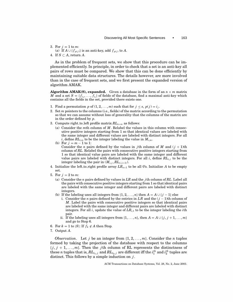
As in the problem of frequent sets, we show that this procedure can be im-plemented efficiently. In principle, in order to check that a set is an anti-key allpairs of rows must be compared. We show that this can be done efficiently bymaintaining suitable data structures. The details however, are more involvedthan in the case of frequent sets, and we first present the expanded version ofalgorithm AMAK.

Algorithm AMAK(S), expanded. Given a database in the form of an n×m matrixM and a set S = { fi1 , . . . , fis } of fields of the database, find a maximal anti-key whichcontains all the fields in the set, provided there exists one.

1. Find a permutation p of (1, 2, . . . , m) such that for j ≤ s, p( j ) = i j .2. Set m pointers to the columns (i.e., fields) of the matrix according to the permutation

so that we can assume without loss of generality that the columns of the matrix arein the order defined by p.

3. Compute right to left profile matrix RLn×m as follows:(a) Consider the mth column of M . Relabel the values in this column with consec-

utive positive integers starting from 1 so that identical values are labeled withthe same integer and different values are labeled with distinct integers. For alli, define RLi,m to be the integer labeling the value in Mi,m.

(b) For j = m− 1 to 1:Consider the n pairs defined by the values in j th column of M and ( j + 1)thcolumn of RL. Relabel the pairs with consecutive positive integers starting from1 so that identical value pairs are labeled with the same integer and differentvalue pairs are labeled with distinct integers. For all i, define RLi, j to be theinteger labeling the pair in (Mi, j , RLi,( j+1)).

4. Initialize the left to right profile array LRn×1 to be all 0’s. Initialize A to be emptyset.

5. For j = 2 to m:(a) Consider the n pairs defined by values in LR and the j th column of RL. Label all

the pairs with consecutive positive integers starting from 1 so that identical pairsare labeled with the same integer and different pairs are labeled with distinctintegers.

(b) If the labeling uses all integers from {1, 2, . . . , n} then A = A∪ { j − 1} elsei. Consider the n pairs defined by the entries in LR and the ( j − 1)th column of

M . Label the pairs with consecutive positive integers so that identical pairsare labeled with the same integer and different pairs are labeled with distinctintegers. For all i, update the value of LRi,1 to be the integer labeling the ithpair.

ii. If the labeling uses all integers from {1, . . . , n}, then A = A∪ { j , j + 1, . . . , m}and go to Step 6.

6. For k = 1 to |S|: If fk 6∈ A then Stop.7. Output A.

Observation. Let j be an integer from {1, 2, . . . , m}. Consider the n tuplesformed by taking the projection of the database with respect to the columns{ j , j + 1, . . . , m}. Then the j th column of RL represents the distinctness ofthese n tuples that is, RLi1, j and RLi2, j are different iff the ith

1 and ith2 tuples are

distinct. This follows by a simple induction on j .



Observation. At the end of the ith iteration of the for loop (just before Step 6,the array LR represents the distinctness of the n tuples formed by columns inthe set { f1, . . . , fi} \ A. This follows by a simple induction on the loop variablej . A field f j is inserted in A only if the fields before j that are not in A togetherwith the fields f j+1, . . . , fm form a key. Therefore, A is always the complementof a key.

THEOREM 34. For a given set S of fields, suppose there is an anti-key that con-tains all the fields in S. Then, the algorithm AMAK outputs the lexicographicallysmallest maximal anti-key with respect to the permutation and that contains allthe fields in S. Further, assuming that the time to access any field of any recordis constant, the running time of the algorithm is O(nm).

PROOF. The algorithm greedily inserts fields in A, under the invariant thatA remains an anti-key, and so outputs the lexicographically first maximal anti-key, with respect to permutation p. Since p has all fields in S before any otherkey, A includes all fields in S if S is an anti-key.

Note that the Step 3 makes one pass of the whole database and hence needO(nm) time. Here we are assuming the domain is prefixed and finite so thatthe assignment of names can be done in linear time using a bucket sort likemethod. Similarly Step 5 makes one pass of the database. Other steps takeO(m)or O(n) time. Therefore the total time complexity of the algorithm isO(nm).

We now give the complete algorithm for finding all maximal antikeys, whichis analogous to the algorithm for finding all maximal frequent sets. First wepoint out that an analogue of the Lemma 26 holds also for the case of maximalanti-keys.

LEMMA 35. Given a collection C of maximal anti-keys of a database, letK be a maximal anti-key not in C. Then there exists a minimal transversalT of the hypergraph defined by the complements of the sets in C such thatT ⊆ K .

In the description of the algorithm All MAK, we ignore the details of how tofind all minimal transversals of a hypergraph.

Algorithm All MAK. Given a relational database in the form of n×m matrix M, findall maximal anti-keys.

(1) C = {}(2) Run algorithm AMAK(φ) and add to C the maximal anti-key discovered.(3) While new antikeys are being found:

(a) Compute the set X of all minimal transversals of the hypergraph defined bycomplements of subsets in C.

(b) For each x ∈ X : Run algorithm AMAK(X) and add any new maximal anti-keyfound to C.

(4) Output C.

We can now claim the following corollary.



COROLLARY 36. The algorithm All MAK finds all maximal anti-keys (andhence minimal keys) of the input database.

7.2 Learning Monotone Functions

In this section, we apply the results of the previous section to the problem oflearning monotone Boolean functions using membership queries. Theorem 5shows that this problem is equivalent to the problem of finding maximal fre-quent sets.

Example 37. The problem of computing the maximal frequent sets de-scribed in Figure 4 is mapped to the problem of learning the function fwhose DNF representation is f = AD ∨ CD and whose CNF representationis f = (A ∨ C)(D). The terms of the DNF correspond to the elements of Bd−,and the clauses of the CNF are the complements of the sets in MTh.

As an immediate corollary of the results in Section 5, we get:

COROLLARY 38. The level-wise algorithm can be used to learn the class ofmonotone CNF expressions where each clause has at least n− k attributes andk = O(log n), in polynomial time, and with a polynomial number of membershipqueries.

As a corollary of Theorem 10, we get a lower bound:

COROLLARY 39. Any algorithm that learns monotone functions with mem-bership queries must use at least |DNF( f )| + |CNF( f )| queries.

While the bound is not surprising, it hinges on the lower bound given byAngluin [1988]. It is shown there that an algorithm may need to take timeexponential in the DNF size when not allowed CNF size as a parameter. Indeedthe CNF size of the function used to show the lower bound is exponential. (Thelower bound in Angluin [1988] is, however, more complex since the learner hasaccess to several additional oracles.) On the other hand, by using Theorem 29,we see that with membership queries alone one can come close to this lowerbound.

COROLLARY 40. If there is an incremental T(I,i) time algorithm for com-puting hypergraph transversals, then there is a learning algorithm for mono-tone functions with membership queries, that produces both a DNF and aCNF representation for the function. The number of MQ queries is boundedby (|DNF( f )| +n|CNF( f )|). The running time of the algorithm is polynomial inn and T (|CNF( f )|, |DNF( f )|).

As noted earlier, Bioch and Ibaraki [1995] have studied the same problemand have previously derived a similar result, as well as other related results.The result can also be derived from a more general construction in Bshouty et al.[1996] (Theorem 18), that studies the complexity of learning in the context ofNP-Oracles.

Here again, using the result of Fredman and Khachiyan [1996], we can deriveas a corollary a subexponential learning algorithm for this problem.



8. COMPUTING THE TRANSVERSALS OF THEHYPERGRAPH INCREMENTALLY

The results of Section 6 show that the efficient operation of the Dualize andAdvance algorithm depends on an incremental algorithm for computing thetransversals of a hypergraph. The general problem of finding all minimaltransversals of a hypergraph in output polynomial time is still an open problem.The algorithm by Fredman and Khachiyan [1996] generates all transversals inprovably output subexponential time, however it is difficult to implement.

In this section, we present a heuristic technique for finding the transversalsof a hypergraph. Our technique has the advantage of being easy to describeand implement, as well as being able to continue the transversal computationat each step of the Dualize and Advance algorithm from the previous one. As aresult, the transversal computation can be integrated to the algorithm insteadof starting from the beginning at each step.

Consider two consecutive steps of the algorithm All MSS, the ith and the(i + 1)th. If some new maximal frequent sets were found during step i, thenDi ⊂ Di+1. Let X be a transversal of Di. Then either X is a transversal of Di+1as well, or it can become a transversal of Di+1 if it is expanded by a set of itemsthat cover Di+1 \ Di. In fact, each such transversal can be expended to a set oftransversals of the set Di+1.

Example 41. Let Di = {{A, B}, {B, C}}, and Di+1 = {{A, B}, {B, C}, {D, E}}.Then, the set {B} is a transversal of Di, but Di+1 contains an additional edgethat is not covered by {B}. We can expand {B} by adding D or E (these coverthe new edge). In both cases we get a transversal for Di+1 ({B, D} and {B, E},respectively.

It follows that, if we have the transversals of Di, we can incrementally createthe transversals of Di+1 by expanding each of the original transversals so thatthey intersect each of the new complements of maximal elements.

In addition, if a transversal X is found to be not frequent at step i, then wedo not expand this transversal in the next step. All the transversals we can gen-erate from it have to be nonfrequent as well. This is an important improvementbecause it allows us to reduce the number of transversals we have to generateat each step.

The algorithm is given below:

Algorithm for computing transversals at Step i+ 1. Let Ti be the set of transver-sals at step i.

(1) Set Ti+1 = {}(2) For each X ∈ Ti

(a) Expand X and obtain a set X ′ of transversals of Di+1.(b) For each X ′ ∈ X ′:

i. It X ′ is not interesting, remove X ′ from X ′(c) Ti+1 = Ti+1 ∪ X ′

To complete the algorithm we need a technique to efficiently extend eachtransversal in Ti so that it intersects all the complements of the new maximal



A C D

AE C

CDE

D

ABE BC D

BC BD CD DE

BCE ABC BD CD DE

ABD CD DE

ACD BCD DE

BDEADE

BE ACD

CDEAB

ACE BD

AD BCE

BC ADE

BD ACE

CD ABE

DE ABC

MF Set Comp.

Fig. 6. To compute the transversals incrementally we use a tree structure: Assume attributesA, B, C, D, E. Let BE be the first maximal frequent set found. It’s complement is ACD, and thetransversals of the complement are A, C, and D. When a new maximal frequent set is found (AB inthe second row), the existing transversals are extended, if necessary, to intersect the complementof the new maximal frequent set (CDE). In this case, the new transversals are AE, C, D. Whena transversal is found to be non-frequent, (as is ABE in the example), the branch of the tree ispruned.

frequent sets. We use the tree-structure scheme for traversing the set oftransversals of hypergraph that was presented in Kavvadias and Stavropoulos[1999]. The operation of the algorithm is shown in Figure 6.

9. RELATED WORK

Recently, a number of algorithms have been proposed to solve the MaxTh prob-lem for frequent sets [Bayardo 1998; Lin and Kedem 1998; Burdick et al. 2001;Agrawal et al. 2000; Han et al. 2000; Gouda and Zaki 2001]. Below, we brieflydescribe the most recent and important of these algorithms and compare theirdesign approach with Dualize and Advance. We note that none of these algo-rithms has provably worst case complexity that is subexponential to the sizeof the output, as Dualize and Advance does (Theorem 30). For some of thesealgorithms [Bayardo 1998; Lin and Kedem 1998; Han et al. 2000], we give exam-ples that show that their worst-case complexity is exponential to the size of theoutput (i.e., to the number of maximal frequent sets). Therefore, in the worstcase, these algorithms are provably asymptotically slower than Dualize andAdvance. The other algorithms use heuristics and their worst case complexityis not yet known.

Pincer-Search [Lin and Kedem 1998] is similar to a priori and to Dualize-and-Advance in that it also uses the lattice method to enumerate the item sets.Pincer-Search combines a bottom-up and a top-down technique to find the max-imal frequent sets. The bottom-up technique moves through the lattice level bylevel. The bottom-up process finds frequent sets, and nonfrequent sets. The



nonfrequent sets are used by a top down process to refine a set of potentialmaximal frequent sets. For example, assume that at the beginning of the algo-rithm, a set ABCD is a potential maximal frequent set. If a set BD is found to benon-frequent, then ABCD cannot be frequent any more. It is refined to the setsABD and ABC that are potential frequent sets and their support is checked inthe next iteration of the algorithm.

The combination of a bottom-up and a top-down search can result to signif-icant improvements compared to a priori. One such case is if there exists onlyone maximal frequent set of cardinality n − 1 (where n is the number of at-tributes). In this case, Pincer-search finds this set in two database passes, andafter finding the support of its subsets of cardinality 1 and 2.

The operation of Pincer-Search has similarities to the operation of theDualize and Advance algorithm. The main difference is that Pincer-Searchtries to guess maximal frequent sets, by considering large sets that may befrequent, while Dualize and Advance starts from sets that have to be frequentand expands them to maximal frequent sets. As a result, Dualize and Advanceguarantees that new maximal sets are found in each iteration (if a maximal setis not found, then a set in the negative boundary is found) and thus is alwaysmaking progress, while Pincer-Search does not always do that.

The following example shows a case where this happens. Assume that thereare n attributes, all the sets of size at most k are frequent, and no sets ofk + 1 are frequent. For such a dataset, the performance of Pincer-Search isidentical to the performance of a priori. This is because the bottom-up searchdoes not find any non-frequent sets until the kth step, and therefore the topdown search cannot refine the candidate maximal frequent sets until that point.Therefore the number of sets for which the algorithm finds their support canbe exponential to the number of frequent sets. If for example k = n − c, forsome constant c, the number of frequent sets is O(2n), and the number of themaximal frequent sets is O(nc) (see also Example 24).

This example shows that Pincer-Search can take time that is exponential tothe size of the output because it has to find the support of a number of setsthat is exponential to the number of maximal frequent sets. In this case, theperformance of Pincer-Search is exponentially worse that the performance ofthe Dualize and Advance algorithm, in terms of the number of Is-interestingqueries executed.

FP-Growth [Han et al. 2000] uses a new data structure, the FP-tree, to rep-resent all the transactions of the database. It then uses this structure with arecursive technique to find large frequent sets. This is a very efficient techniquefor finding all frequent sets. However, although the technique does not need tocompute sets of candidate patterns, it still finds the support of all frequent setsand therefore can be less efficient than other techniques when used to find themaximal frequent sets only.

Max-Miner [Bayardo 1998] was one of the first successful practical algo-rithms for finding all maximal frequent sets. The algorithm uses Rymon’s setenumeration [Rymon 1992] to enumerate all the itemsets (Figure 7). Max-Minerreduces the search space by pruning the tree to eliminate both supersets of in-frequent sets and subsets of frequent sets. Essentially, when the algorithm



A B C D E

AB

ABC

ABCD

ABCDE

ABCE

ABD ABE

AC AD AE BC BD BE CD CE DE

ACD ACE ADE BCD BCE BDE

ABDE ACDE BCDE

Fig. 7. Rymon’s set enumeration tree.

computes the support of a set A, it also computes the support of the largest setthat appears in the subtree rooted at this set (by the design of Rymon’s tree,this is a superset of A). If this superset is frequent, then all other sets in thissubtree must be frequent too. Thus, the algorithm avoids having to computethe support of all the frequent sets, and therefore performs better than a prioriwhen the size of the maximal frequent sets is large.

Max-Miner uses a breadth-first-search technique to explore the set enumer-ation tree. It computes the support of candidate sets that are on the same levelof the tree in one database pass. An important factor in the efficiency of the algo-rithm is the use of heuristics that reorder the attributes, and therefore changethe order that the various sets appear in the tree [Burdick et al. 2001]. Experi-mentally, it has been shown that ordering the attributes in increasing supportgives the best results [Bayardo 1998]. In the best case, Max-Miner can find allmaximal frequent sets in a few database passes, and using a small number ofIs-interesting queries (linear to the number of maximal frequent sets).

In its operation, Max-Miner uses a similar approach to Dualize and Advancein looking for large frequent sets as early as possible, and in trying to pruneparts of the space that are known to be frequent. The difference is that Dualizeand Advance uses a slow procedure (the transversal computation) that guar-antees efficient pruning, while Max-Miner uses heuristics that are much moreefficient to apply but do not offer such a guarantee, as the following exampledemonstrates.

An example of a dataset that results to running time that is exponential to thesize of the output in the execution of Max-Miner is given in Figure 8. Assumethat all itemsets are frequent, except the supersets of a given set with twoattributes. Also assume that the two items in this set always have individuallythe highest support. This can happen if we take a dataset where all sets arefrequent for a given small threshold, add two new items (D and E in Figure 8),and create a new dataset as follows: For each tuple in the original dataset, wecreate two new tuples and add these in the new dataset. The original attributesremain the same, but in the first new tuple attribute E is 1 and D is 0, and inthe second new tuple E is 0 and D is 1. So the set DE is not frequent, but the



Fig. 8. A worst case for Max-Miner. Set DE and its supersets are the only nonfrequent sets. Weassume that the ordering of the attributes, A, B, C, D, E, is in ascending support.

attributes D and E have always the highest individual support. In this case,Max-Miner has to compute the support of all frequent sets because no subtreecan be eliminated. The number of Is-interesting queries evaluated is the samewith a priori, and exponential to the number of the maximal frequent sets.Assuming n attributes, the algorithm has to find the support of O(2n) sets, whilethe number of maximal frequent sets is constant. In the example of Figure 8,the attributes are A, B, C, D, E, ordered in ascending support. If the set DEand its supersets are infrequent, the only maximal frequent sets are ABCDand ABCE, yet Max-Miner has to find the support of all frequent itemsets.

Similar to Max-Miner, MAFIA [Burdick et al. 2001], DepthProject [Agrawalet al. 2000], and MaxGen [Gouda and Zaki 2001] use Rymon’s set enumerationtechnique. The design of DepthProject has been influenced by the continuousincrease in available main memory size. It assumes that the dataset fits inmain memory and does not attempt to minimize the number of dataset passes.Both MAFIA and DepthProject use a depth-first-search mechanism to enumer-ate the itemsets. All three algorithms also use efficient pruning heuristics toavoid examining some itemsets that can be determined to be frequent or non-frequent. Compared to Max-Miner, MAFIA, DepthProject and MaxGen use thesame technique to enumerate the search space (although MAFIA and Depth-Project enumerate the space in different order since they use depth-first-searchenumeration), and use a similar set of heuristics to prune the set enumerationtree, including: (i) attribute reordering, and (ii) checking the support of thelargest set in the subtree rooted at the current node. They also introduce newoptimizations; one such optimization, used by MAFIA and MaxGen checks ifcandidate sets are subsets of known maximal frequent sets before computingtheir support. However, they use different techniques for computing the sup-port, resulting to different performance characteristics. For example, MAFIAuses a very efficient vertical bitmap representation with compression, whichsignificantly improves the running time. This set of algorithms (including Max-Miner) has proven to be very efficient in practice, however their performance



crucially depends on how effective the pruning heuristics that the algorithmsemploy are in reducing the search space. The worst-case complexity of thesealgorithms is not known, and so a theoretical comparison with the Dualize andAdvance algorithm cannot be made.

10. DISCUSSION

In this article, we studied the data mining problem of searching for a set ofmaximally interesting sentences. This problem comes up in many data miningapplications, including the well known problem of computing association rules.

We present a thorough analysis of two algorithms for the problem. Thesealgorithms have complementary properties. The a priori (level-wise) algorithmis efficient as long as the rank of interesting sentences in the generalizationlattice of the language is small. The algorithm is in fact optimal if we wantto find all the interesting sentences. This result is also supported by recentexperimental comparisons between various techniques [Zheng 2001]. The level-wise algorithm is too slow, however, if there are interesting sentences of largerank.

We introduce the Dualize and Advance algorithm that is useful in the generalcase. The algorithm alternates between phases of finding maximal elements,and computing the negative boundary of these elements via a transversal com-putation.

The analysis of the algorithm shows that the complexity of finding the mostspecific interesting sequences is lower than the complexity of finding all inter-esting sequences. The number of queries the algorithm makes to the databaseis essentially optimal, while the time complexity depends on the complexity ofenumerating hypergraph transversals, for which the best known algorithm ismildly super-polynomial.

We have illustrated the application of the algorithm in two important datamining scenarios: computing all maximal σ -frequent sets of a {0, 1} relationwith threshold σ and computing all minimal keys of a database. To the best ofour knowledge, this is the only known subexponential algorithm for finding allthe maximal σ -frequent sets of a relation.

A number of issues can be explored in future work. These include exper-iments on the trade-off between performing the transversal computation forfocusing search and employing randomized search to find more most specificsentences from each seed. A particularly important issue concerns the numberof passes over the database. In the description of the algorithm, we assume thatthe data fit in memory, but in many cases this is not so in practice. In this situ-ation, an important consideration is to minimize the number of times we haveto read the entire data from the file system into the main memory. This issuecan be tackled in several ways. We can use a randomized version of algorithmAMSS (taking a random permutation p in Step 1 of algorithm AMSS) and runthis algorithm a number of times at each starting point. All the randomizedinstantiations starting from a given point can be run at the same time duringone pass over the database. Another aspect concerns the basic subroutine forgoing up in the lattice. In principle this procedure requires one round for each



attribute in the database (though it can be done on a large batch in one round).Recently, Bshouty [1996] introduced an algorithm for learning monotone func-tions in parallel that may be useful in this respect. Intuitively, the idea is thatwe have a large batch of points with which to go up; instead of going up oneattribute at a time, we will test in each round the unions of the sets we alreadyhave, and of these will choose a subset that will give us the best leap in goingup in the lattice. In this way the number of rounds is reduced considerably.

Another interesting possibility we plan to explore is to use the randomizedheuristic in combination with the level-wise algorithm. The randomized algo-rithm for maximal σ -frequent sets can be used to select the right range for σ ,as a preprocessing step to the a priori algorithm of Agrawal and Srikant [1994]and Agrawal et al. [1996].

Finally, an extension of our theoretical framework will be useful. We as-sumed throughout the paper that the algorithms can only access the data via“is-interesting” queries. Clearly, more can be done with real databases. Thequestion is whether real computational advantages can be gained by usingsuch services. Another limitation of our results is that they only apply to prob-lems representable as sets. One can easily generalize the Dualize and Advancealgorithm for arbitrary lattices, and prove its correctness. The question is whencan we take advantage of the structure so as to derive efficient algorithms usingthis method.

ACKNOWLEDGMENTS

We wish to thank Eyal Kushilevitz for pointing out the work in Bshouty et al.[1996], Roberto Bayardo, Rakesh Agrawal, and Christino Tamon for useful dis-cussions, and Jordan Gergov for comments on an earlier version of the article.

REFERENCES

AGRAWAL, R. C., AGGARWAL, C. C., AND PRASAD, V. V. V. 2000. Depth first generation of long patterns.In Knowledge Discovery and Data Mining, pp. 108–118.

AGRAWAL, R., IMIELINSKI, T., AND SWAMI, A. 1993. Mining association rules between sets of itemsin large databases. In Proceedings of ACM SIGMOD Conference on Management of Data (SIG-MOD’93) (May). ACM, New York, pp. 207–216.

AGRAWAL, R., MANNILA, H., SRIKANT, R., TOIVONEN, H., AND VERKAMO, A. I. 1996. Fast discoveryof association rules. In Advances in Knowledge Discovery and Data Mining, U. M. Fayyad,G. Piatetsky-Shapiro, P. Smyth, and R. Uthurusamy, Eds. AAAI Press, Menlo Park, Calif., pp.307–328.

AGRAWAL, R. AND SRIKANT, R. 1994. Fast algorithms for mining association rules in large databases.In Proceedings of the 20th International Conference on Very Large Data Bases (VLDB’94) (Sept.).pp. 487–499.

AGRAWAL, R. AND SRIKANT, R. 1995. Mining sequential patterns. In Proceedings of the 11th Inter-national Conference on Data Engineering (ICDE’95) (Taipei, Taiwan, Mar.). pp. 3–14.

ANGLUIN, D. 1988. Queries and concept learning. Mach. Learn. 2, 4, (Apr.), 319–342.BAYARDO, R. J. 1998. Efficiently mining long patterns from databases. In Proceedings of the ACM

SIGMOD International Conference on Management of Data. ACM, New York.BELL, S. 2003. Deciding distinctness of query results by discovered constraints. Manuscript.BELL, S. AND BROCKHAUSEN, P. 1995. Discovery of data dependencies in relational databases. Tech.

Rep. LS-8 14. Universitat Dortmund, Fachbereich Informatik, Lehrstuhl VIII, Kunstliche Intel-ligenz.



BERGE, C. 1973. Hypergraphs. Combinatorics of Finite Sets, 3rd ed. North-Holland, Amsterdam,The Netherlands.

BIOCH, J. AND IBARAKI, T. 1995. Complexity of identification and dualization of positive Booleanfunctions. Inf. Comput. 123, 1, 50–63.

BSHOUTY, N. H. 1996. The monotone theory for the pac-model. In Proceedings of the ACM Sympo-sium on Theory of Computing (STOC). ACM, New York.

BSHOUTY, N. H., CLEVE, R., GAVALDA, R., KANNAN, S., AND TAMON, C. 1996. Oracles and queries thatare sufficient for exact learning. J. Comput. Syst. Sci. 52, 421–433.

BURDICK, D., CALIMLIM, M., AND GEHRKE, J. 2001. Mafia: A maximal frequent itemset algorithm fortransactional databases. In Proceedings of the International Conference on Data Engineering.

EITER, T. AND GOTTLOB, G. 1995. Identifying the minimal transversals of a hypergraph and relatedproblems. SIAM J. Comput. 24, 6 (Dec.), 1278–1304.

FAYYAD, U. M., PIATETSKY-SHAPIRO, G., SMYTH, P., AND UTHURUSAMY, R., EDS. 1996. Advances in Knowl-edge Discovery and Data Mining. AAAI Press, Menlo Park, Calif.

FREDMAN, M. L. AND KHACHIYAN, L. 1996. On the complexity of dualization of monotone disjunctivenormal forms. J. Algorithms 21, 3 (Nov.), 618–628.

GAREY, M. AND JOHNSON, D. 1979. Computers and Intractability—A Guide to the Theory of NP-Completeness. W. H. Freeman, New York.

GOUDA, K. AND ZAKI, M. J. 2001. Efficiently mining maximal frequent itemsets. In ICDM, pp.163–170.

GUNOPULOS, D., KHARDON, R., MANNILA, H., AND TOIVONEN, H. 1997a. Data mining, hypergraphtransversals, and machine learning. In Proceedings of the 16th ACM SIGACT-SIGMOD-SIGARTSymposium on Principles of Database Systems (PODS’97). ACM, New York.

GUNOPULOS, D., MANNILA, H., AND SALUJA, S. 1997b. Discovering all most specific sentences byrandomized algorithms. In Proceedings of the International Conference on Database Theory(ICDT’97).

HAN, J., PEI, J., AND YIN, Y. 2000. Mining frequent patterns without candidate generation. InProceedings of the 2000 ACM SIGMOD International Conference on Management of Data. ACM,New York, pp. 1–12.

KAVVADIAS, D. AND STAVROPOULOS, E. C. 1999. Evaluation of an algorithm for the transversal hy-pergraph problem. In Algorithm Engineering, pp. 72–84.

KHARDON, R. 1995. Translating between Horn representations and their characteristic models. J.Artif. Intel. Res. 3, 349–372.

KNOBBE, A. J. AND ADRIAANS, P. W. 1995. Discovering foreign key relations in relational databases.In Workshop Notes of the ECML-95 Workshop on Statistics, Machine Learning, and KnowledgeDiscovery in Databases (Heraklion, Crete, Greece, Apr.). pp. 94–99.

LANGLEY, P. 1995. Elements of Machine Learning. Morgan-Kaufmann, San Mateo, Calif.LIN, D.-I. AND KEDEM, Z. M. 1998. Pincer search: A new algorithm for discovering the maximum

frequent set. In Extending Database Technology, pp. 105–119.MANNILA, H. 1995. Aspects of data mining. In Workshop Notes of the ECML-95 Workshop on

Statistics, Machine Learning, and Knowledge Discovery in Databases (Heraklion, Crete, Greece,Apr.). pp. 1–6.

MANNILA, H. 1996. Data mining: Machine learning, statistics, and databases. In Proceedings ofthe 8th International Conference on Scientific and Statistical Database Management (Stockholm,Sweden). pp, 2–9.

MANNILA, H. AND RAIHA, K.-J. 1986. Design by example: An application of Armstrong relations. J.Comput. Syst. Sci. 33, 2, 126–141.

MANNILA, H. AND RAIHA, K.-J. 1992. Design of Relational Databases. Addison-Wesley, Wokingham,U.K.

MANNILA, H. AND RAIHA, K.-J. 1994. Algorithms for inferring functional dependencies. Data Knowl.Eng. 12, 1 (Feb.), 83–99.

MANNILA, H. AND TOIVONEN, H. 1997. Levelwise search and borders of theories in knowledge dis-covery. Data Mining Knowl. Disc. 1, 3, 241–258.

MANNILA, H., TOIVONEN, H., AND VERKAMO, A. I. 1994. Efficient algorithms for discovering associa-tion rules. In Knowledge Discovery in Databases, Papers from the 1994 AAAI Workshop (KDD’94)(Seattle, Wash., July), pp. 181–192.



MANNILA, H., TOIVONEN, H., AND VERKAMO, A. I. 1995. Discovering frequent episodes in sequences.In Proceedings of the 1st International Conference on Knowledge Discovery and Data Mining(KDD’95) (Montreal, Ont., Canada, Aug.). AAAI Press, pp. 210–215.

MISHRA, N. AND PITT, L. 1997. Generating all maximal independent sets of bounded-degree hy-pergraphs. In Proceedings of the Conference on Computational Learning Theory (COLT). pp.211–217.

MITCHELL, T. M. 1982. Generalization as search. Artif. Intel. 18, 203–226.RYMON, R. 1992. Search through systematic set enumeration. In Proceedings of the International

Conference on Principles of Knowledge Representation and Reasoning.SCHLIMMER, J. 1993. Using learned dependencies to automatically construct sufficient and sensi-

ble editing views. In Knowledge Discovery in Databases, Papers from the 1993 AAAI Workshop(KDD’93) (Washington, D.C.). AAAI Press, pp. 186–196.

ULLMAN, J. D. 1988. Principles of Database and Knowledge-Base Systems, vol. I. Computer SciencePress, Rockville, Md.

VALIANT, L. G. 1979. The complexity of enumeration and reliability problems. SIAM J. Comput.8, 3, 410–421.

ZHENG, Z., KOHAVI, R., AND MASON, L. 2001. Real world performance of association rule algorithms.In Proceedings of the 7th ACM SIGKDD International Conference on Knowledge Discovery andData Mining. ACM, New York.

Received March 2001; revised April 2002, November 2002, February 2003; accepted February 2003


Discovering all most specific sentences

Documents

Transcript of Discovering all most specific sentences