"Discovering Orbits"

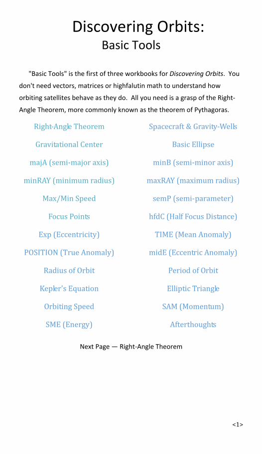
<1>

Discovering Orbits: Basic Tools

"Basic Tools" is the first of three workbooks for Discovering Orbits. You

don't need vectors, matrices or highfalutin math to understand how

orbiting satellites behave as they do. All you need is a grasp of the Right-

Angle Theorem, more commonly known as the theorem of Pythagoras.

Right-Angle Theorem Spacecraft & Gravity-Wells

Gravitational Center Basic Ellipse

majA (semi-major axis) minB (semi-minor axis)

minRAY (minimum radius) maxRAY (maximum radius)

Max/Min Speed semP (semi-parameter)

Focus Points hfdC (Half Focus Distance)

Exp (Eccentricity) TIME (Mean Anomaly)

POSITION (True Anomaly) midE (Eccentric Anomaly)

Radius of Orbit Period of Orbit

Kepler's Equation Elliptic Triangle

Orbiting Speed SAM (Momentum)

SME (Energy) Afterthoughts

Next Page — Right-Angle Theorem

<2>

Right-Angle Theorem A triangle that has one 90° corner has the following properties. The side

opposite the 90° angle is called the hypotenuse, which we'll call 'A' for

short. The shorter sides we'll call 'B' & 'C' for short. Then the A-side,

multiplied by itself, equals B-side, multiplied by itself, plus C-side multiplied

by itself.

Right-Angle Theorem: A2 = B2 + C2

Diagrams 1.00 and 1.00A

The right-angle theorem is the basis for trigonometry, since the angles

<3>

of the corners can be matched with specific ratios between any two of the

three sides. The matches are calculated using trigonometric functions

called sine (SIN), cosine (COS) and tangent (TAN). Digital calculators

perform these functions rapidly and accurately. Before the advent of

integrated circuits, engineers had to look up the matches in multipage

tables.

Diagram 1.01

Diagram 1.02

NOTE: the positive/negative dispositions of X and Y. When you use the

<4>

ARCTAN function (y/x), you will know which quadrant the angle should be

by checking the signs of X & Y.

We have introduced a new term (Radius) to mark the hypotenuse or A-

side of the triangle. Trigonometric functions are based on the unit circle

where the radius equals one. The SIN and COS functions compute ratios

between zero and one, whereas the TAN function computes ratios

between zero and infinity.

If you know the ratio, you can find the angle. If you know the angle you

can find the ratio. Very simple so far, don't you agree?

Orbital dynamics boils down to the Right-Angle Theorem and its

trigonometric functions. From these simple relationships, you can observe

and analyze an orbiting spacecraft. You use angles and side lengths like

calipers to gauge the size and shape of a spacecraft's orbit. Moreover, the

Right-Angle Theorem lets you calculate distances between any two points

on a plane. Positions in the Cartesian coordinate system are plotted as an

X-lengths and a Y-lengths away from the origin (0, 0), where the X-axis

(horizontal) and the Y-axis (vertical) form a 90° angle. Hence, the X & Y

lengths represent the short sides of a 90° triangle.

Diagram 1.03

Contents.

Next Page — Gravitational Center

<5>

Gravitational Center The most common parameters are spacecraft speed and distance away

from the gravitational center. The distance away from the gravitational

center is called the radius of orbit. Both radius and speed often change

during the course of an orbit. If you know the direction of speed with

respect to the radius line, you can describe the entire orbit, including its

shape and orientation.

Diagram 1.04

A satellite moves on a flat plane around a gravitational attractor. The

flightpath of a satellite is called an orbit or orbital path. Orbits represent a

balance between satellite speed and the inbound force of gravity.

Newton's 1st-Law of Motion describes inertia: An object at rest will

remain at rest; an object in motion will remain moving in the straight line

of its motion.

A satellite wants to keep moving in a straight line, whereas the force of

gravity keeps pulling the satellite toward its center. The two forces cause

the satellite to follow a curved path around the gravitational attractor.

<6>

Man-made satellites have very small mass compared to the masses of

planets and major moons, so the mass of a satellite can be ignored in lieu

of its orbital behavior. The equations of motion use the gravitational

parameter of the massive body around which the satellite orbits.

Gravitational parameters for the sun and most visible bodies of the solar

system have been calculated with great precision. From here on, the

acronym GP will mean the same thing as gravitational parameter.

GP = Gravitational Parameter of earth.

GP(moon) = Gravitational Parameter of the moon.

GP(sun) = Gravitational Parameter of the sun.

Contents.

Next Page — Spacecraft & Gravity-wells

<7>

Spacecraft & Gravity-Wells When a spacecraft approaches a massive body, three things may

happen.

• The spacecraft's speed is too small to reach a balance with the

gravitational attractor, so spacecraft will dive into the massive body

or burn up in the atmosphere, if any.

• The spacecraft's speed is too great for the gravitational attractor, so

the massive body can only deflect the spacecraft's flightpath. The

spacecraft may also acquire the orbiting speed and/or redirection of

the attractor, but its inherent speed with respect to the massive body

will remain unchanged from inbound to outbound.

• The speed of the spacecraft finds a balance with the attractor, and

the spacecraft will be "captured" by the massive body. As a result,

the spacecraft will form an orbit around the attractor. The flightpath

of a "captured" spacecraft is called an ellipse. The farther a satellite

orbits from its attractor, the more potential energy it has. In effect, it

occupies a higher niche in its gravity-well.

NOTE: When a spacecraft escapes earth's gravity-well and travels to

another planet, the spacecraft remains in orbit around the sun's gravity-

well.

Contents.

<8>

Next Page — Basic Ellipse

<9>

Basic Ellipse An ellipse is a stretched out circle. In the real-world very few orbits are

perfect circles. Most orbits are ellipses—or epicycles as the ancients called

planetary flightpaths. An epicycle is a graphic artist's rendition of an

ellipse. Epicyclic equations are harder to use than elliptic equations, so it

makes sense to use elliptic parameters.

Diagram 1.05

Equation 1.01

The X & Y terms are variables. The mark the satellite's position through

all phases of its orbit. The A & B terms are constants for a particular orbit.

To make a class of orbits with the same shape and orbital period, all you

need is a pair of the basic parameters. Any combination will let you

calculate the other parameters from time-tested formulas. In case you

were wondering, the period of orbit means how long it takes for a satellite

<10>

to travel once-around.

Contents.

Next Page — majA

<11>

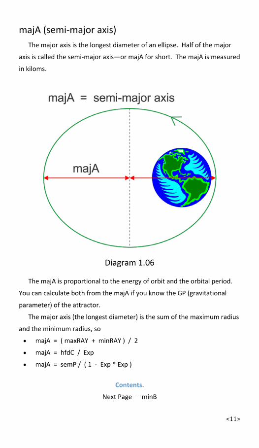
majA (semi-major axis) The major axis is the longest diameter of an ellipse. Half of the major

axis is called the semi-major axis—or majA for short. The majA is measured

in kiloms.

Diagram 1.06

The majA is proportional to the energy of orbit and the orbital period.

You can calculate both from the majA if you know the GP (gravitational

parameter) of the attractor.

The major axis (the longest diameter) is the sum of the maximum radius

and the minimum radius, so

• majA = ( maxRAY + minRAY ) / 2

• majA = hfdC / Exp

• majA = semP / ( 1 - Exp * Exp )

Contents.

Next Page — minB

<12>

minB (semi-minor axis) The minor axis is shortest diameter of an ellipse. Half of the minor axis

is called the semi-minor axis—or minB for short. The minB is measured in

kiloms.

Diagram 1.07

Equations 1.02 and 1.03

Contents.

Next Page — minRAY

<13>

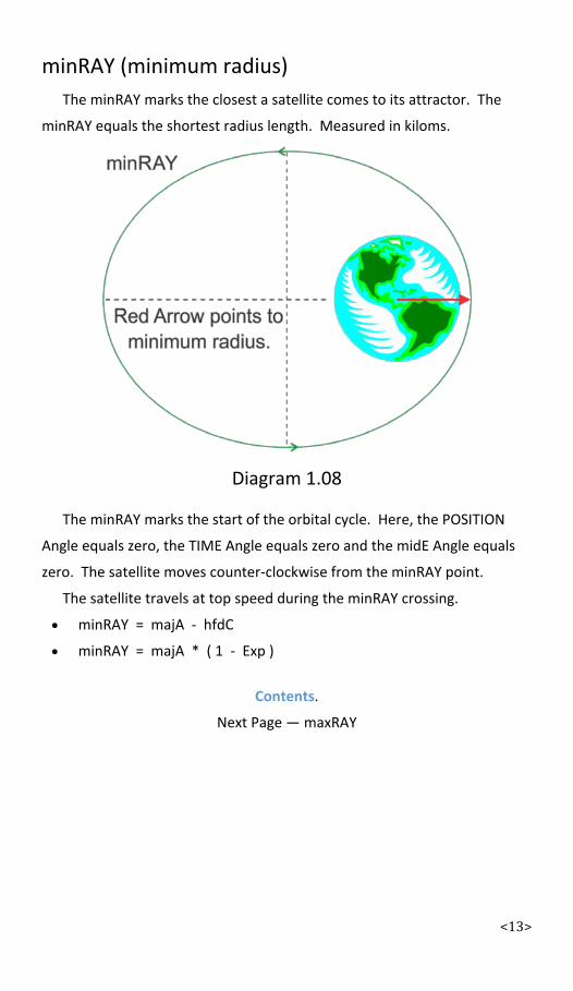
minRAY (minimum radius) The minRAY marks the closest a satellite comes to its attractor. The

minRAY equals the shortest radius length. Measured in kiloms.

Diagram 1.08

The minRAY marks the start of the orbital cycle. Here, the POSITION

Angle equals zero, the TIME Angle equals zero and the midE Angle equals

zero. The satellite moves counter-clockwise from the minRAY point.

The satellite travels at top speed during the minRAY crossing.

• minRAY = majA - hfdC

• minRAY = majA * ( 1 - Exp )

Contents.

Next Page — maxRAY

<14>

maxRAY (Maximum radius) The maxRAY marks the longest radius of the satellite in elliptic orbit.

Measured in kiloms.

Diagram 1.09

The maxRAY marks the halfway point of orbit in terms of distance and

time. The maxRAY coincides with 180° of the POSITION, midE and TIME

Angles.

The satellite travels at the lowest speed during the maxRAY crossing.

• maxRAY = majA + hfdC

• maxRAY = majA * ( 1 + Exp )

Contents.

Next Page — Max/Min Speed

<15>

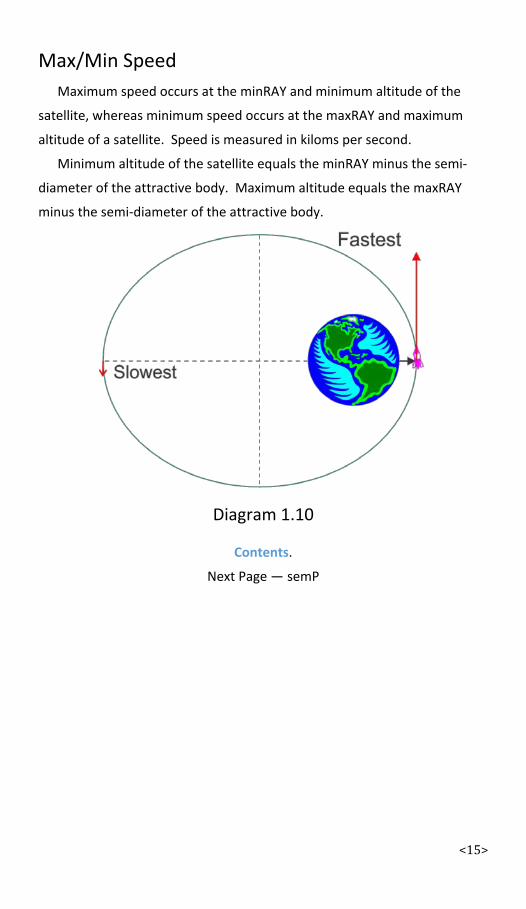
Max/Min Speed Maximum speed occurs at the minRAY and minimum altitude of the

satellite, whereas minimum speed occurs at the maxRAY and maximum

altitude of a satellite. Speed is measured in kiloms per second.

Minimum altitude of the satellite equals the minRAY minus the semi-

diameter of the attractive body. Maximum altitude equals the maxRAY

minus the semi-diameter of the attractive body.

Diagram 1.10

Contents.

Next Page — semP

<16>

semP (semi-parameter) The semP represents a vertical line drawn from the gravitational center

to a point on the orbital path. Measured in kiloms.

Diagram 1.11

• semP = majA * ( 1 - Exp * Exp )


Contents.

Next Page — Focus Points

<17>

Focus Points Elliptic orbits have two focus points.

You can make an ellipse with a pencil, a length of string, two thumb

tacks and a thick sheet of cardboard. Tie the string to each of thumb tacks.

Sink the thumb tacks in the cardboard, but make sure the distance

between thumb tacks is less than the length of string. Push the business

end of the pencil inside the string until it's stretched taut. And then draw

an ellipse around the tacks.

If the length of string is much larger than the distance between the

tacks, the ellipse will tend toward a circular shape. If the length of string is

only slightly greater than the distance between the tacks, the ellipse will

have a streamlined shape. The length of string is twice the length of the

majA, whereas the distance between focus points is twice the hfdC. Hence,

the ratio between the hfdC and the majA governs the shape of orbital path.

Diagram 1.12

The prime focus lies at the gravitational center. The 2nd-focus lies on

<18>

the major-axis at an equal and opposite distance away from the Geometric

Center (0, 0). Focus Points have (hfdC, 0 and -hfdC, 0) coordinates.

The elliptic focus points render a fascinating symmetry. The satellite's

current speed is proportional to the ratio of the lines between the satellite

and either focus point. Indeed, the current speed is proportional to line

drawn to the 2nd-focus over the line drawn to the prime focus.

• Speed ~ (2nd-Focus to orbit) / (Prime focus to orbit)

Contents.

Next Page — hfdC

<19>

hfdC (half distance between focus points) The hfdC extends along the major axis from geometric center to either

focus point. The hfdC is measured in kiloms.

Diagram 1.13

• hfdC = Exp * majA

• hfdc = ( majA — minRAY )

Contents.

Next Page — Exp

<20>

Exp (Expander or Eccentricity) The Exp is a ratio between zero and almost one for an ellipse. Exp

governs the shape of an ellipse. The Exp value of one signifies the

minimum escape speed from a gravitational attractor. The flightpath is

parabolic. The Exp value greater than one implies a hyperbolic flightpath.

The Exp has no units. Below you will see the orbits becoming stretched out

as the Exp ratio goes from zero to nearly one.

Diagram 1.14

• Exp = hfdC / majA


Contents.

Next Page — TIME Angle

<21>

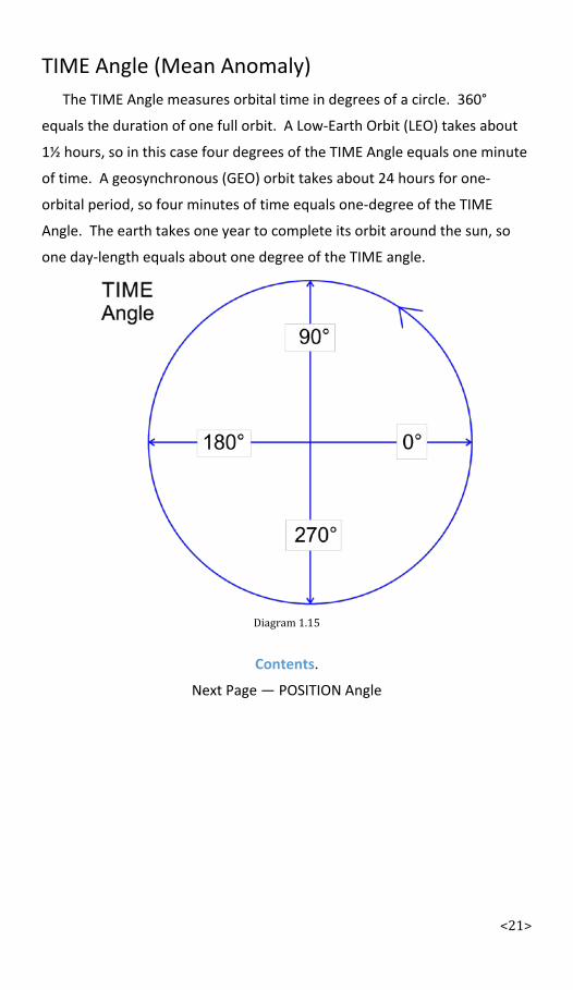
TIME Angle (Mean Anomaly) The TIME Angle measures orbital time in degrees of a circle. 360°

equals the duration of one full orbit. A Low-Earth Orbit (LEO) takes about

1½ hours, so in this case four degrees of the TIME Angle equals one minute

of time. A geosynchronous (GEO) orbit takes about 24 hours for one-

orbital period, so four minutes of time equals one-degree of the TIME

Angle. The earth takes one year to complete its orbit around the sun, so

one day-length equals about one degree of the TIME angle.

Diagram 1.15

Contents.

Next Page — POSITION Angle

<22>

POSITION (POS) Angle (True Anomaly) The POSITION Angle is the angular sweep of the satellite's current radius

as measured from the minRAY point.

Diagram 1.16

You can determine POSITION Angle if you know the satellite's position in

space via an accurate observation.

Diagram 1.16

<23>

The ARCOSINE function is the inverse of the COSINE. It works like a

watch that gives time in a.m. or p.m. Worse, the ARCOSINE doesn't

distinguish between morning and afternoon., so you have to decide

whether the satellite moves in the 1st-half or 2nd-half of its orbital trek. If

it's in the 2nd-half, then subtract the angle from 360°. If your calculator is

set to angular radians, then subtract your answer from 2π.

Equation (1.16) needs accurate positional values for X, Y and radius, and

these may not be available. In which case, the POSITION angle can be

found directly from the midE Angle.

Equation 1.09

Contents.

Next Page — midE Angle

<24>

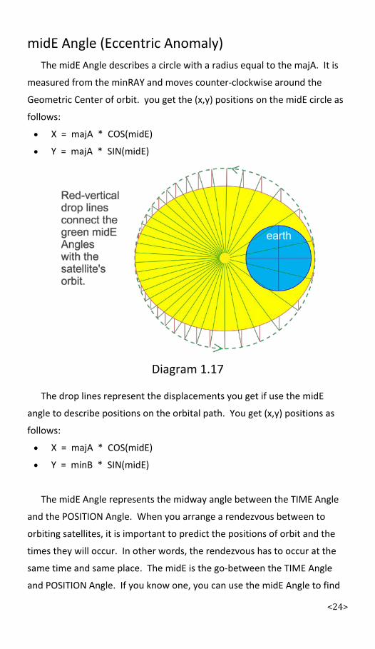
midE Angle (Eccentric Anomaly) The midE Angle describes a circle with a radius equal to the majA. It is

measured from the minRAY and moves counter-clockwise around the

Geometric Center of orbit. you get the (x,y) positions on the midE circle as

follows:

• X = majA * COS(midE)

• Y = majA * SIN(midE)

Diagram 1.17

The drop lines represent the displacements you get if use the midE

angle to describe positions on the orbital path. You get (x,y) positions as

follows:

• X = majA * COS(midE)

• Y = minB * SIN(midE)

The midE Angle represents the midway angle between the TIME Angle

and the POSITION Angle. When you arrange a rendezvous between to

orbiting satellites, it is important to predict the positions of orbit and the

times they will occur. In other words, the rendezvous has to occur at the

same time and same place. The midE is the go-between the TIME Angle

and POSITION Angle. If you know one, you can use the midE Angle to find

<25>

the other. First, the midE Angle relates to the TIME Angle through Kepler's

Equation, which will be covered in later pages. Second, the midE Angle

relates to the POSITION Angle, using the equations below:


The ARCOSINE function is the inverse of the COSINE. It works like a

watch that gives time in a.m. or p.m. Worse, the ARCOSINE doesn't

distinguish between a.m. or p.m., so you have to decide whether the

satellite should be in the 1st-half or 2nd-half of the orbital trek. If it's in the

2nd-half, then subtract the angle from 360°. If your calculator is set to

angular radians, then subtract your answer from 2π.

Contents.

Next Page — Radius

<26>

Radius of Orbit The radius describes a straight line from the Gravitational Center to the

current position of the satellite. Measured in kiloms.

Diagram 1.18


The radius can also be found from (x,y,z) coordinates in space. Because

orbital flightpaths stay on the same flat plane, the 3rd-dimension can be

ignored unless you want a visual sighting of a particular orbit. Discovering

Orbits is only concerned with examining the behavior of satellites in a

general sense. The equations and parameters will let you make a class of

orbits, all of which follow the same codes of conduct.

<27>

If you want to narrow the class of orbits to a special case, you must

specify the minRAY and three orbiting angles with literal times, sightlines

and locations. Any good astronomy textbook will show you how to do this.

In essence, it makes no difference whether you have a satellite crossing

its minRAY at 10:00 p.m. or at 11:45 p.m., whether you're looking toward

the zenith or nadir. The satellite will still move along its orbit in the same

fashion.

Thus, we can safely ignore distractions in the z-direction, which runs

perpendicular to the (x,y) plane of orbit. The radius of earth is about

6,378.15 kiloms. If ranging-finding radar determines your satellite is 300

kiloms above the surface, the effective radius is 6378.15 + 300 = 6678.15

kiloms. The X and Y distances for the satellite are measured from the

gravitational center.

Equation 1.14

• POSITION Angle = ARCTAN(Y/X)

You determine the POSITION Angle's quadrant from plus-minus signs. If

Y and X are positive, POSITION lies in the 1st-quadrant. If Y is positive and X

is negative, POSITION lies in the 2nd-quadrant. If Y and X are negative,

POSITION lies in the 3rd-quadrant. If Y is negative and X is positive,

POSITION lies in the 4th-quadrant.

Satellite in terms of polar coordinates:

• (Radius, POSITION Angle)

Contents.

Next Page — Period of Orbit

<28>

Period of Orbit Period refers to the time elapsed during one full orbit. Period is

measured in seconds of clock time.

Equation 1.15

If you want to convert the seconds of clock time to seconds of the TIME

Angle's arc, multiply by 15.

Contents.

Next Page — Kepler's Equation

<29>

Kepler's Equation Kepler's Equation links the TIME Angle with the midE Angle. The

equation relies on Kepler's 2nd-Law of elliptic motion which states the

satellite's radius migrates across equal areas in equal times.

Diagram 1.19

The satellite takes as much time going through the yellow area as the

red area. Next inscribe an ellipse inside a circle.

Diagram 1.20

<30>

Using the ratio minB/majA, we can relate areas of the ellipse to the

mirrored areas in the blue circle. Moreover, the proportionate area swept

by the radius equals the same proportionate time. All that remains is to

select point 'E' on the orbital path that lies an arbitrary distance from the

minRAY.

Diagram 1.21

Point 'E' on the ellipse relates to point 'P' on the outlying circle, since

the angle M-C-P is the midE angle. To find the 'yellow' area in terms of

midE Angle, you solve the following:

• TIME / 2π ~> area MFE (ellipse) ~> area MCP (circle)

• MCP = ½ * majA2 * midE

• Area MAE = (minB / majA) * Area MAP

Then subtracting the gray (red) triangle...

• MAP = ½majA2 * midE - ½majA * Exp * majA * SIN(midE)


Kepler's Equation easily solves for the TIME Angle when you know the

<31>

midE Angle. But what happens if you know the TIME angle and you wish to

find the midE Angle?

• midE = TIME + Exp * SIN(midE)

Because the midE Angle appears on both sides of the equation, you

have to make a smart guess. From the look of Kepler's equation, you can

expect the TIME Angle to lag behind the midE angle during the 1st-half of

the orbit. The midE Angle will lag behind the TIME Angle during the 2nd-

half. Solve the equation over and over until the left side of the equation

converges to the proposed value on the right side.

Let's say we start with midE0 as your guess. Then...

• midE1 = TIME + Exp * SIN(midE0)

Then repeat using midE1 as your new guesstimate.

• midE2 = TIME + Exp * SIN(midE1)

And repeat until the midEn and midEn-1 are nearly the same.

NOTE: Kepler's Equation only works for radian-mode angles where the

unit circle has a radius of one and circumference of 2π.

Contents.

Next Page — Elliptic Triangle

<32>

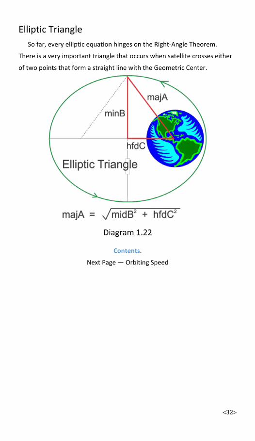
Elliptic Triangle So far, every elliptic equation hinges on the Right-Angle Theorem.

There is a very important triangle that occurs when satellite crosses either

of two points that form a straight line with the Geometric Center.

Diagram 1.22

Contents.

Next Page — Orbiting Speed

<33>

Orbiting Speed Outer space lends very little hindrance to the motion of a satellite.

There is almost no atmosphere 200 kiloms above earth's surface, so no

friction to hold the spacecraft back. In essence, a satellite exists in a

perpetual-motion system. The energy of orbit remains constant. The

Specific Angular Momentum (SAM) remains constant. And the Specific

Mechanical Energy (SME) remains constant. Nonetheless, you will observe

satellites moving at different speeds throughout their orbits. At times, they

display more kinetic energy; at other times they assume more potential

energy.

You might suppose a spacecraft's speed is inversely proportional to the

current length of its radius. However, this simple relationship doesn't

always work. Elliptic speed has direction as well as magnitude because it is

the combination of two speeds that act at 90° to each other. First, we have

the Dynamic Circular Speed (DCS), which is the speed arrow associated

with a circular orbit. Second, we have the Dynamic Stretch Speed (DSS),

which causes the circular flightpath to stretch.

The DCS lies tangent to an imaginary circle whose radius is the

gravitational center. The DCS arrow starts at the current position of the

spacecraft and points in the direction of motion. The DSS lies along the

spacecraft's radius. It points away from the gravitational center between

zero and 180° of the orbit. And it points toward the gravitation center

between 180° and 360° of the orbit.

Arrows of DCS and DSS form a 90° corner, so you rely once again on the

Right-Angle Theorem to find the speed in kiloms per second.

Equation 1.18

In essence, you obtain speed for any point in the flightpath if you know

the DCS and DSS, either of which change dynamically during the course of

an orbit. In many ways, the DCS and DSS are tougher to find than the

<34>

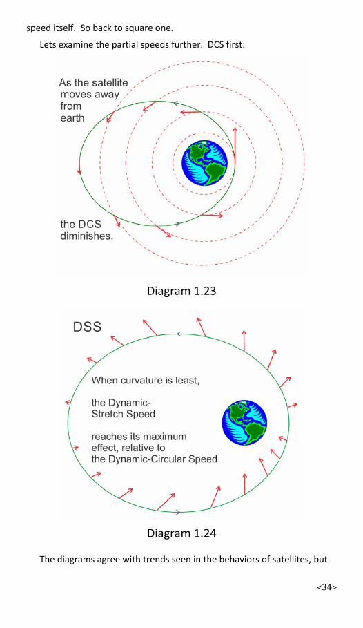
speed itself. So back to square one.

Lets examine the partial speeds further. DCS first:

Diagram 1.23

Diagram 1.24

The diagrams agree with trends seen in the behaviors of satellites, but

<35>

the pictures don't bring us closer to determining instantaneous values for

the DCS and DSS.

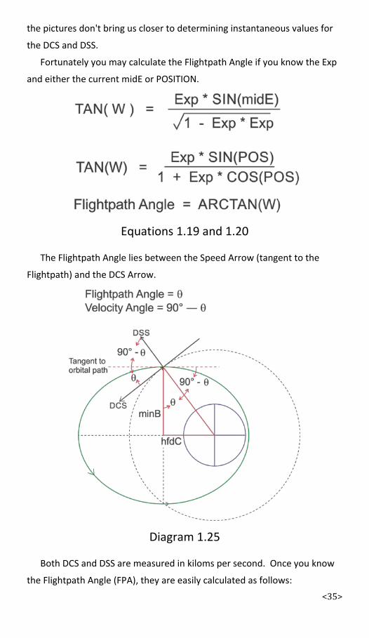
Fortunately you may calculate the Flightpath Angle if you know the Exp

and either the current midE or POSITION.


The Flightpath Angle lies between the Speed Arrow (tangent to the

Flightpath) and the DCS Arrow.

Diagram 1.25

Both DCS and DSS are measured in kiloms per second. Once you know

the Flightpath Angle (FPA), they are easily calculated as follows:

<36>

• DCS = Speed * COSINE(Flightpath Angle)

• DSS = Speed * SINE(Flightpath Angle)

Contents.

Next Page — SAM (Specific Angular Momentum)

<37>

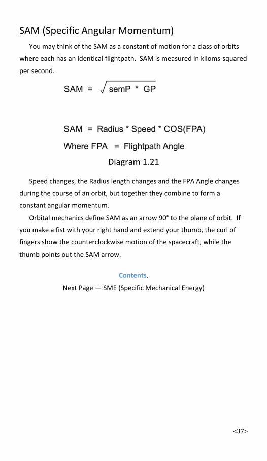
SAM (Specific Angular Momentum) You may think of the SAM as a constant of motion for a class of orbits

where each has an identical flightpath. SAM is measured in kiloms-squared

per second.

Diagram 1.21

Speed changes, the Radius length changes and the FPA Angle changes

during the course of an orbit, but together they combine to form a

constant angular momentum.

Orbital mechanics define SAM as an arrow 90° to the plane of orbit. If

you make a fist with your right hand and extend your thumb, the curl of

fingers show the counterclockwise motion of the spacecraft, while the

thumb points out the SAM arrow.

Contents.

Next Page — SME (Specific Mechanical Energy)

<38>

SME (Specific Mechanical Energy) Energy of orbit is the result of an indefinite integral. In other words,

orbital energy is the sum of all possible speeds and radius lengths that

occur after once-around the flightpath. Orbital mechanics normally ignore

the constant of integration, so SME is expressed as a negative value of all

"captured" spacecraft in elliptic orbits. The higher up the gravity-well that

a spacecraft flies, the smaller negative value of SME, which reduces to zero

if the spacecraft achieves escape speed and becomes positive if the

spacecraft exits on a hyperbolic trajectory.

Elliptic orbits with the same majA will have the same SME, as you might

suspect from the following energy equations.


The larger the majA, the greater the energy, even though satellites that

loft to higher altitudes travel at slower speeds. The higher up the gravity-

well, the more potential energy a spacecraft has. This more than makes up

for the slower speeds.

The SME is measured in kiloms-squared /over/ seconds-squared.

Contents.

Next Page — Afterthoughts

<39>

Afterthoughts Here you have the Basic Tools for Discovering Orbits. The equations are

not only useful for solving problems of orbital dynamics; you may use them

to calculate distance and trip times for bicycles, roadsters or jumbo jets.

You can use them to determine the acreage of odd-shape property lots.

Download the PDF source file. I only ask that you credit my efforts in

preparing this handy reference. Likewise, if you notice any gross errors or

omissions, please contact me at <[email protected]>

I certainly don't wish to dole out bad info and send others on wild-goose

chases.

Installments two and three of Discovering Orbits will show you how to

apply these Basic Tools for orbits around earth and moon. You will learn

how to rendezvous two spacecraft, how to transfer orbits from LEO to GEO,

how to go from earth to moon, how to arrive at the moon with the right

speed to be "captured" in its gravity-well, and so on...

Contents.

mailto:[email protected]

"Discovering Orbits"

Documents

Transcript of "Discovering Orbits"