Autonomous prediction of GPS and

GLONASS satellite orbits

Mari Seppanen*, Juha Ala-Luhtala, Robert Piche, Simo Martikainen, Simo Ali-Loytty

Tampere University of Technology

*Corresponding author: mari.j.seppanen@tut.fi

ABSTRACT

A method to predict satellite orbits in a stand-alone consumer-grade GNSS navigation device is presented. The

motivation for this work was to reduce the startup time of a navigation device without the use of network assistance.

The presented orbit prediction method works for both GPS andGLONASS, achieving median accuracies of 58 and 23

meters in satellite’s position, respectively, for prediction up to four days ahead. A simple method for prediction of the

satellite’s clock offsets is also discussed. A basic analysis indicates that the method gives a line of sight range errorof

15 meters, for both GPS and GLONASS, with most of the error dueto the clock offset prediction.

INTRODUCTION

When standalone GNSS navigation devices are turned on, there is a delay of at least 30 seconds before they begin

to provide position information. This delay occurs becauseof the time needed for signal acquisition and tracking

and after that one has to wait until the navigation data is acquired. It takes 18 seconds in GPS to send the three first

subframes [1, p. 127-128] and 8 seconds in GLONASS to send thefirst four strings [2, p. 18-19], which contain

the immediate or minimum data required for positioning. Furthermore, in both systems, this essential information

is repeated only once every 30 seconds [1; 2]. If the receiverdoes not have a direct view to the sky, for example

because of trees or buildings in the way, the signal acquisition and tracking slows down and the time until the first

positioning result can take longer, even several minutes [3]. This is annoying for typical users, and could have more

serious consequences in emergency or other special situations. Therefore there is a demand for methods which could

decrease the time from turning on a device to the first position estimate, known as the Time To First Fix (TTFF).

The minimum information needed for positioning in GNSS includes the satellite’s ephemeris parameters and the clock

correction terms, which model the difference between onboard time scale and GNSS’s system time. Because one

of the reasons for long TTFF is the time it takes to receive thesatellite’s ephemeris broadcast, alternative ways of

obtaining satellite’s position, velocity and clock information can be used to reduce it. Then the satellite would be

needed only for receiving the time of the satellites clock ora pseudorange measurement. This is faster because the

satellite sends the time stamp once every six seconds in GPS and every two seconds in GLONASS [1; 2]. In addition,

the information about satellite’s position and velocity can be used to speed up the signal acquisition in the GNSS

receiver, which is another cause of the startup delay, in twoways. First, assuming that a crude estimate about the

receiver’s location and approximate time are known, the satellite’s position coordinates can be used to identify the

visible satellites. Secondly, with the information about satellite’s velocity the range of possible Doppler frequency

shifts can be reduced. Altogether, by predicting satellite’s kinematic state i.e. position and velocity as well as clock

correction terms, it would be possible to get the first positioning result in about 5 seconds [3] after turning on the

device.

Besides reducing TTFF, satellite orbit prediction can alsowiden the capability of GNSS devices. In some navigation

cases, the user is indoors or in urban canyons where the signal is strong enough to be detected and for getting

pseudorange measurements, but too weak or fragmental for reading the whole ephemeris. Then the predicted orbit can

make it possible to both compute a position and reduce TTFF.

A widely used alternative to the navigation message broadcast by the satellite is the use of assistance data servers

that send data to the navigation device that enable the computation of satellite’s position, velocity and satellite’s clock

offset. However, there are problems associated with such assistance data: Connection to the assistance server may fail

or the user may consider the assistance data connection to betoo expensive. Furthermore, many navigation devices

are not even equipped to make a network connection. There is therefore interest in methods that can be implemented

entirely in the navigation device, without network connection.

In self-assisted GNSS the aim is to attain properties similar to assisted GNSS, without a network connection. This is

accomplished by generating within the device the information that would have been received as assistance data. In this

paper, satellite orbits are predicted using only the satellite’s broadcast data that was received the previous times the

device was in operation. This technique has been implemented in commercial products and is outlined in the literature

[3; 4], but these publications do not give a detailed description of the algorithms. We have developed a related method

and believe its accuracy is competitive compared to the other methods. In our previous paper [5] we gave a detailed

presentation of the ephemeris prediction algorithm for GPSsatellites. The aim of this paper is to present an extended

version of the algorithm that also covers the GLONASS satellites. Moreover, we present a study of satellite’s clock

offset prediction and of the positioning error that can be expected with the position and clock offset predictions.

The paper begins with a description of the satellite’s equation of motion. It includes only the forces that have the2

greatest effect on the satellite’s orbit. Then, the reference frames used in the computation are introduced and the

ephemerides’ structure and accuracy in GNSS is discussed. After these introductory sections the actual algorithm is

presented and its performance in GPS and GLONASS is evaluated. The next section discusses the prediction of the

clock offsets. Finally the errors due to the satellite’s predicted orbit and predicted clock offsets are combined in order

to consider the total error in the range measurement. The paper concludes with a short summary.

FORCE MODEL

The orbit prediction algorithm introduced in this work is based on the satellite’s equation of motion

r = a(t, r), (1)

wherer is the second time derivative of the satellite’s position vector anda is a vector valued function which gives the

satellite’s acceleration vector as a function of time and satellite’s position. Given the satellite’s position and velocity

at instantt0, sayr(t0) = r0 andv(t0) = v0, we can compute the satellite’s position at any other instant t by double-

integrating equation (1) with respect to time. Usually, in order to predict GNSS satellite orbits with very high accuracy,

a large number of different forces have to be included to the model. However, we have taken into account only the

four forces that have the greatest influence on a satellite’sorbit at GNSS satellite altitude, and write the acceleration as

a(t, r) = ag + amoon+ asun+ asrp, (2)

whereag, amoon, asun andasrp are the accelerations due to Earth gravitation (taking intoaccount the unsymmetrical

mass distribution of the Earth), lunar gravitation, solar gravitation and solar radiation pressure, respectively.

If the Earth was a uniform sphere, the gravitational acceleration would depend on the satellite’s radial distancer only,

and the gravity potentialU would be of the form

U(r) =GME

r,

whereG is the gravitational constant andME is the mass of the Earth. When the unsymmetrical mass distribution of

the Earth is taken into account, the gravity potentialU can be written in the form of the spherical harmonics expansion

3

[6, p. 57]

U(r, λ, ϕ) =GME

r

∞∑

n=0

n∑

m=0

[

(

RE

r

)n

Pnm(sinϕ)

(

Cnm cos(mλ) + Snm sin(mλ))

]

. (3)

Here the potentialU is not only a function of satellite’s radiusr, but also the longitudeλ and latitudeϕ. The constant

RE in this formula is the Earth’s radius and the termsPnm are the associated Legendre polynomials of degreen and

orderm. The coefficientsSnm andCnm in the formula are experimentally determined constants whose magnitude

decreases very fast with increasingn andm. Therefore, the potential can be approximated by taking into account only

the first few terms. At GNSS satellite altitude, the terms up to the degree and order 4 are significant [7, p. 54], but we

use terms up to the degree and order 8. The values for the geopotential coefficientsCnm andSnm are obtained from

the EGM2008 model [8].

The acceleration due to Earth gravitation can be computed asa gradient of the gravity potentialU . We have used a

recursive algorithm introduced by Cunningham [9] and laterextended by Metris et al.[10] to compute the derivatives.

The algorithm takes the partial derivatives with respect tothe Earth centered Earth fixed (ECEF) position vectorre,

which is related to the satellite’s inertial position by thetransformationre = Rr, where R is the transformation matrix.

The gradient of the potentialU gives the acceleration in ECEF coordinates, which can be transformed to the inertial

reference frame by the formula [6, p. 68]

ag(r) = R−1∇U(re). (4)

After the Earth’s gravitation the second biggest acceleration components in the satellite’s equation of motion are caused

by the gravitational forces of the Moon and the Sun. To compute the acceleration acting on the satellite because of the

gravitational force of any celestial body, one can use the form

acb = GM

(

rcb − r

‖rcb − r‖3−

rcb

‖rcb‖3

)

, (5)

whereM is the mass of the celestial body,rcb is its position in Earth centered inertial reference frame and r is the

position of the satellite in the same reference frame. Besides the Moon and the Sun this formula can be used also

for computing the planetary accelerations, but we have ignored these because their influence to the satellite’s orbit is

negligible.

The orbits of the Sun and the Moon have to be known in order to compute the gravitational acceleration with the

formula (5). In our model we use simple models presented in [6, p. 70-73] to compute the lunar and the solar4

coordinates. The coordinates are accurate to about 0.1-1% [6].

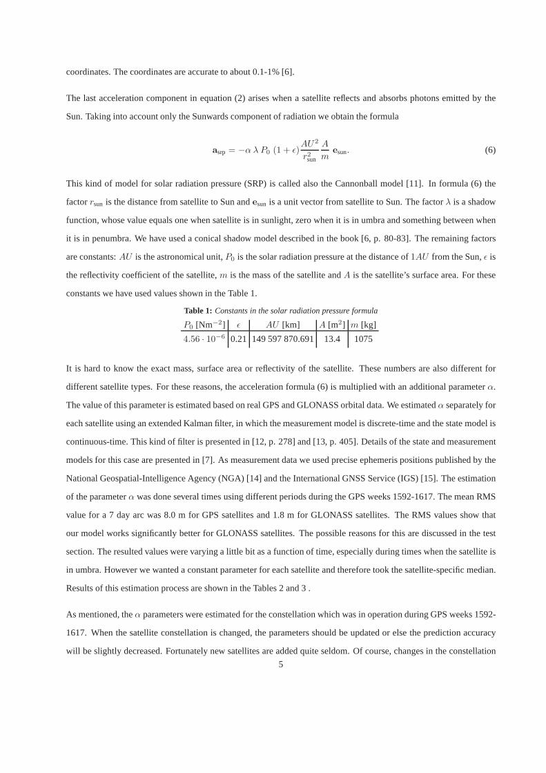
The last acceleration component in equation (2) arises whena satellite reflects and absorbs photons emitted by the

Sun. Taking into account only the Sunwards component of radiation we obtain the formula

asrp = −α λ P0 (1 + ǫ)AU2

r2sun

A

mesun. (6)

This kind of model for solar radiation pressure (SRP) is called also the Cannonball model [11]. In formula (6) the

factorrsun is the distance from satellite to Sun andesun is a unit vector from satellite to Sun. The factorλ is a shadow

function, whose value equals one when satellite is in sunlight, zero when it is in umbra and something between when

it is in penumbra. We have used a conical shadow model described in the book [6, p. 80-83]. The remaining factors

are constants:AU is the astronomical unit,P0 is the solar radiation pressure at the distance of1AU from the Sun,ǫ is

the reflectivity coefficient of the satellite,m is the mass of the satellite andA is the satellite’s surface area. For these

constants we have used values shown in the Table 1.

Table 1: Constants in the solar radiation pressure formula

P0 [Nm−2] ǫ AU [km] A [m2] m [kg]

4.56 · 10−6 0.21 149 597 870.691 13.4 1075

It is hard to know the exact mass, surface area or reflectivityof the satellite. These numbers are also different for

different satellite types. For these reasons, the acceleration formula (6) is multiplied with an additional parameterα.

The value of this parameter is estimated based on real GPS andGLONASS orbital data. We estimatedα separately for

each satellite using an extended Kalman filter, in which the measurement model is discrete-time and the state model is

continuous-time. This kind of filter is presented in [12, p. 278] and [13, p. 405]. Details of the state and measurement

models for this case are presented in [7]. As measurement data we used precise ephemeris positions published by the

National Geospatial-Intelligence Agency (NGA) [14] and the International GNSS Service (IGS) [15]. The estimation

of the parameterα was done several times using different periods during the GPS weeks 1592-1617. The mean RMS

value for a 7 day arc was 8.0 m for GPS satellites and 1.8 m for GLONASS satellites. The RMS values show that

our model works significantly better for GLONASS satellites. The possible reasons for this are discussed in the test

section. The resulted values were varying a little bit as a function of time, especially during times when the satellite is

in umbra. However we wanted a constant parameter for each satellite and therefore took the satellite-specific median.

Results of this estimation process are shown in the Tables 2 and 3 .

As mentioned, theα parameters were estimated for the constellation which was in operation during GPS weeks 1592-

1617. When the satellite constellation is changed, the parameters should be updated or else the prediction accuracy

will be slightly decreased. Fortunately new satellites areadded quite seldom. Of course, changes in the constellation

5

Table 2: Solar radiation pressure parameters for GPS satellites

PRN 1 2 3 4 5 6 7 8α 1.439 1.484 1.337 1.335 1.434 1.339 1.441 1.325

9 10 11 12 13 14 15 161.341 1.323 1.481 1.453 1.479 1.479 1.454 1.490

17 18 19 20 21 22 23 241.445 1.488 1.474 1.475 1.465 1.470 1.498 1.356

25 26 27 28 29 30 31 321.551 1.330 1.326 1.469 1.445 1.334 1.451 1.350

Table 3: Solar radiation pressure parameters for GLONASS satellites

PRN 1 2 3 4 5 6 7 8α 2.155 2.165 2.132 2.170 2.154 2.149 2.144 2.144

9 10 11 12 13 14 15 162.137 2.147 2.134 2.142 2.136 2.145 2.142 2.139

17 18 19 20 21 22 23 242.146 2.147 2.129 2.147 2.144 2.158 2.107 2.165

can be handled by updating theα parameters a few times per year, for instance, as a part of a software update.

To summarize, in this section we presented a motion model forGNSS satellites. We can now introduce a vector valued

functionϑ which, given satellite’s position and velocity at instantt0, returns the satellite’s position and velocity at

another instanttf . The definition for this kind of function is

ϑ(t0, tf , r0,v0) =

r(tf )

v(tf )

=

r(t0) +∫ tf

t0

(

v(t0) +∫ tf

t0a(t, r)dt

)

dt

v(t0) +∫ tf

t0a(t, r)dt

. (7)

We have used the Runge-Kutta-Nystrom -method [16, p. 284; 6, p. 124] to solve the equation of motion. The

algorithm is an efficient integration method for second order differential equations in which the second derivative (the

accelerationa) is independent on the first derivative (the velocity).

REFERENCE FRAMES

The International Earth Rotation and Reference Systems Service (IERS) maintains two important reference systems:

a Celestial Reference System (CRS) and a Terrestrial Reference System (TRS). CRS is a reference system whose

coordinate axes maintain their orientation with respect todistant stars. The origin of this reference frame is in the

center of the Earth and Earth is in an accelerated motion while orbiting around the sun. Therefore CRS is not precisely

inertial, but is an adequate approximation of an inertial reference frame for our purposes. TRS is an Earth fixed

reference frame. Its origin is the Earth’s centre of mass andits z-axis is the mean rotational axis of the Earth. This

mean pole of rotation was defined, because the Earth’s instantaneous rotation pole moves with respect to Earth’s crust

whereas in Earth fixed reference frame the axes must be pointing at a fixed point on the Earth’s surface. The coordinate6

transformation between these two reference systems can be written as

rTRS(t) = W(t)G(t)N(t)P(t)rCRS, (8)

where the matricesW, G, N andP describe polar motion, Earth rotation, nutation and precession, respectively. The

transformation matrices are time dependent and thus the vector rCRS, being constant in CRS, is time dependent after

transformation to TRS. We follow the book [6] and use IAU76 theory when computing the precession matrixP and

nutation theory IAU80 for matrixN, although more recent models IAU2000A and IAU2000B are available and can

be found from [17].

The third matrixG describes the rotation of the Earth. In order to compute it, we need Greenwich Mean Sidereal

Time (GMST), which can be computed as follows. Starting fromGPS time, we first compute the corresponding

Julian date as JDGPS = 2444244.5 + t/86400 s, wheret is the number of seconds elapsed since the beginning of

GPS time, 6.1.1980. We express the Julian date (JD) in Universal Time UT1 by subtracting the leap secondsτ that

have been added to Coordinated Universal Time (UTC) since the beginning of GPS time, and adding the difference

dUT1 = UT1-UTC. That is

JDUT1 = JDGPS+dUT1− τ

86400 s.

The number of leap seconds is typically known by the GPS device, because the current number of leap seconds is part

of the broadcast message and new leap seconds are added quiteseldom. However the time difference dUT1, which

is one of the Earth orientation parameters (EOP), is not necessarily known when starting the prediction. This time

difference is small (|dUT1| < 0.9 s) and it does not cause noticeable error if we neglect it.

Next JDUT1 is divided into two parts, such that the first part, JD0hUT1, is the JD at the beginning of the current day and

the second part,UT 1, is the rest of JDUT1. When computing these, one has to notice that the Julian dateinteger part

changes at noon, but0 h universal time is at midnight. Also theUT 1 must be given in seconds. Taking these facts into

account we can apportion as follows:

JD0hUT1 = ⌊JDUT1 + 0.5⌋ − 0.5

UT 1 = (JDUT1 − JD0hUT1) · 86400 s.

Now we can compute the Greenwich Mean Sidereal Time in seconds with the formula [6; 17]

GMST = 24110.54841 + 1.002737909350795 UT1+

8640184.812866 T0 + 0.093104 T2 − 6.2 · 10−6

T3, (9)

7

where the time argumentsT andT0 are

T =JDUT1 − 2451545

36525T0 =

JD0hUT1 − 2451545

36525,

i.e the number of Julian centuries of Universal Time elapsedsince 2000 Jan. 1.5 UT1 at the current time and at the

beginning of the day, respectively. Furthermore the equation of equinoxes [6; 17]

GAST = GMST+ ∆ψ cos ε+ 0. 002649 sinΩ

+ 0. 000013 cosΩ (10)

is used to compute Greenwich Apparent Sidereal Time (GAST).In this equation the parameters∆ψ, ε andΩ come

from the nutation theory and. denotes that the number is presented in arcseconds. Finally, we can compute the

transformation matrix

G(t) = Rz(GAST).

In this equationRz is a rotation around thez-axis i.e

Rz(γ) =

cos γ sin γ 0

− sinγ cos γ 0

0 0 1

. (11)

After multiplying the vectorrCRSwith precession, nutation and Earth rotation matrices, it is in a Terrestial Intermediate

Reference System (TIRS), whosez-axis points to the Celestial Ephemeris Pole (CEP). We assume that the orientation

of Earth’s rotation axis is the same as the orientation of this CEP pole. CEP is not fixed with respect to the surface of

the Earth, but performs a periodic motion around its mean position, called polar motion. The motion is small, having

a radius of under 10 m, but it is important to take it into account. The rotation matrix describing the polar motion is

W(t) = Ry(−xp)Rx(−yp).

wherexp andyp are the polar motion parameters andRx andRy are simple rotation matrices around the x- and y-axes.

Together with dUT1 they are called also Earth Orientation Parameters (EOP). The daily values for these parameters

can be found from the homepage of IERS [18].

IERS reports the observed values for EOP and quite accurate short term predictions. However the Earth orientation

parameters are not long-term predictable, which causes some problems while trying to do the prediction in a device8

without any network connection. We can not form a predictionmodel that would be valid for the life of the device i.e.

years. Neither are the EOP parameters part of the broadcast message yet, though this fact will be changed in the future

as the new L1C signal comes into use [19]. However, later in section Initial value improvement we will show how to

infer these parameters based on the collected broadcast ephemeris data.

When transforming the position vectorrCRS to the TRS one matrix at a time according to equation (8), every

intermediate step is also a reference frame. For example when multiplying with matrixP we get a mean of date (mod)

system and after multiplied also with nutation matrixN we get a true of date (tod) system. Figure 1 illustrates the

connection between CRS and TRS, as well as the intermediate reference frames between them. Next we will present

the reference frames we have used, and illustrate how the transformation matrices between them are compounded of

those four matrices connecting CRS and TRS.

Figure 1: Connection between the IERS reference systems CRS and TRS. Transformation matrices and intermediate referenceframes. The inverse of a transformation matrix is its transpose.

The broadcast position and velocity we get from broadcast ephemeris are in Earth fixed reference in the beginning. In

GPS the reference frame is WGS84, which is so close to TRS thatwe assume these two to be equivalent. In GLONASS

the received ephemeris is in Earth fixed PZ90.02 reference frame [20] but it can be transformed to WGS84 or TRS by

9

a translation of origin [21]

rWGS84 = rPZ90.02+

−0.36 m

0.08 m

0.18 m

. (12)

Now for numerical integration we need an inertial referenceframe and we choose to use the TIRS system at epocht0,

the initial epoch for the equation of motion. Before starting to predict satellite’s position according to the model (7),

we need to transform the position and velocity vectors to this inertial reference frame, denoted by subscript IN. For

the position vector, the transformation from TRS at an arbitrary timet to the TIRS system at epocht0 is

rIN = rTIRS(t0) (13)

= G(t0)N(t0)P(t0)PT (t)NT (t)GT (t)WT (t)rTRS.

However, when we start the prediction we havet = t0 and the transformation reduces to

rIN = WT (t0)rTRS(t0). (14)

For velocity the transformation from TRS to IN can be computed by differentiating equation (13) with respect to time.

When differentiating, the other matrices are treated as constants and the time dependence of the Earth rotation matrix

GT (t) is taken into account [5]. Denoting the transformation matrix from reference frame A to B asRBA, we have

RTIRSCRS = GNP andRCRS

TIRS = (RTIRSCRS)T = PT NTGT . With these notations the velocity transformation is [5]

vIN = RTIRSCRS(t0)R

CRSTIRS(t)

(

WT (t)vTRS +

ω ×(

WT (t)rTRS)

)

. (15)

whereω = [0 0 ω]T is the angular velocity vector of the Earth’s rotation.

After predicting the satellite’s position and velocity at time t in the future, we have to do the transformations the other

way around. SolvingrTRS andvTRS from equations (13) and (15) we get

rTRS = W(t)RTIRSCRS(t)RCRS

TIRS(t0)rIN (16)

vTRS = W(t)(

RTIRSCRS(t)RCRS

TIRS(t0)vIN −

ω ×(

RTIRSCRS(t)RCRS

TIRS(t0)rIN)

)

. (17)

When the satellite’s orbit is predicted, we actually do not know the exact matrixW(t). However, we might know

10

the polar motion parametersxp andyp at the beginning of the prediction and because they do not change much in a

few days long prediction, we can approximate the matrix byW(t0) = W(xp(t0), yp(t0)). Similarly the third Earth

orientation parameter dUT1 is needed to compute the rotation matricesRTIRSCRS(t0) andRTIRS

CRS(t). If we set dUT1= 0

when computing these matrices, we do two approximations: setting dUT1(t0) = 0 causes a constant offset and setting

dUT1(t) = dUT1(t0) neglects the variation of dUT1 during the prediction. The former approximation does not lead

to significant errors, but neglecting the change in dUT1 results in median error of 4.2 meters in the satellite’s position

after a 4 days long prediction. However, this approximationis necessary because the value of dUT1 may, in general, be

unknown to the device and its evolution is very difficult to predict. By making these approximations, we can introduce

a transformation functionξ, which depends both on time and the polar motion parameter values but is independent of

dUT1 which is set to zero. The transformation function transforms the state of the satellite from TRS to the inertial

reference frame IN, that is

r

v

IN

= ξ

r

v

TRS

, t,p

=

RTIRSCRS(t0)R

CRSTIRS(t)W

T (p)rTRS

RTIRSCRS(t0)R

CRSTIRS(t)

(

WT (p)vTRS + ω ×(

WT (p)rTRS)

)

.

.

Herep = [xp yp]T is the vector of polar motion parameters. The inverse transformation, from IN to TRS, is denoted

ξ−1. With these notations, we can write down the prediction function (7) in the TRS system. We end up with the

formula

ϑTRS(t0, tf , rTRS(t0),vTRS(t0),p) =

r(tf )

v(tf )

TRS

= ξ−1

ϑ

t0, tf , ξ

r(t0)

v(t0)

TRS

, t0,p

, tf ,p

. (18)

In addition to the transformationsξ andξ−1, which are done at the beginning and at the end of the prediction, we need

to do some transformations during the prediction. In the previous section it was mentioned that the satellite’s position

vector has to be represented in an Earth fixed reference frameto calculate the acceleration due to the Earth’s gravitation.

TRS is an Earth fixed reference frame, so we can do the transformation to it using equation (16). Therefore the

transformation matrixR presented in equation (4) isW(t)RTIRSCRS(t)RCRS

TIRS(t0). To speed up the numerical integration,

we approximate the matrixR. If the length of prediction is only some days, the precession and nutation matrices

remain almost unchanged. We can writePPT ≈ I andNNT ≈ I and thereby get the following approximation:

W(t)G(t)N(t)P(t)PT (t0)NT (t0)G

T (t0) ≈ W(t)G(t)GT (t0).

11

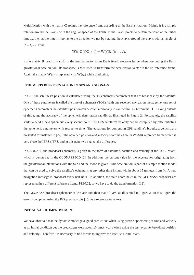
Multiplication with the matrixG rotates the reference frame according to the Earth’s rotation. Mainly it is a simple

rotation around thez-axis, with the angular speed of the Earth. If thex-axis points to certain meridian at the initial

time t0, then at the timet it points to the direction we get by rotating thex-axis around thez-axis with an angle of

(t− t0)ω. Thus

W(t)G(t)GT (t0) = W(t)Rz((t− t0)ω)

is the matrixR used to transform the inertial vector to an Earth fixed reference frame when computing the Earth

gravitational acceleration. Its transpose is then used to transform the acceleration vector to the IN reference frame.

Again, the matrixW(t) is replaced withW(t0) while predicting.

EPHEMERIS REPRESENTATION IN GPS AND GLONASS

In GPS the satellites’s position is calculated using the 16 ephemeris parameters that are broadcast by the satellite.

One of these parameters is called the time of ephemeris (TOE). With one received navigation message i.e. one set of

ephemeris parameters the satellite’s position can be calculated at any instant within±2 h from the TOE. Going outside

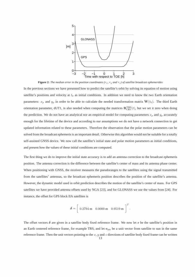
of this range the accuracy of the ephemeris deteriorates rapidly, as illustrated in Figure 2. Fortunately, the satellite

starts to send a new ephemeris every second hour. The GPS satellite’s velocity can be computed by differentiating

the ephemeris parameters with respect to time. The equations for computing GPS satellite’s broadcast velocity are

presented for instance in [22]. The obtained position and velocity coordinates are in WGS84 reference frame which is

very close the IERS’s TRS, and in this paper we neglect the difference.

In GLONASS the broadcast ephemeris is given in the form of satellite’s position and velocity at the TOE instant,

which is denotedtb in the GLONASS ICD [2]. In addition, the current value for theacceleration originating from

the gravitational interactions with the Sun and the Moon is given. This acceleration is part of a simple motion model

that can be used to solve the satellite’s ephemeris at any other time instant within about 15 minutes fromtb. A new

navigation message is broadcast every half hour. In addition, the state coordinates in the GLONASS broadcast are

represented in a different reference frame, PZ90.02, so we have to do the transformation (12).

The GLONASS broadcast ephemeris is less accurate than that of GPS, as illustrated in Figure 2. In this Figure the

error is computed using the IGS precise orbits [15] as a reference trajectory.

INITIAL VALUE IMPROVEMENT

We have observed that the dynamic model gave good predictions when using precise ephemeris position and velocity

as an initial condition but the predictions were about 10 times worse when using the less accurate broadcast position

and velocity. Therefore it is necessary to find means to improve the satellite’s initial state.12

Time with respect to TOE [h]

[m]

GLONASS

GPS

−3 −2 −1 0 1 2 30

1

2

3

4

5

Figure 2: The median error in the position coordinates (rx, ry andrz) of satellite broadcast ephemerides

In the previous sections we have presented how to predict thesatellite’s orbit by solving its equation of motion using

satellite’s positions and velocity att0 as initial conditions. In addition we need to know the two Earth orientation

parameters:xp andyp in order to be able to calculate the needed transformation matrix W(t0). The third Earth

orientation parameter, dUT1, is also needed when computingthe matricesRTIRSCRS(t), but we set it zero when doing

the prediction. We do not have an analytical nor an empiricalmodel for computing parametersxp andyp accurately

enough for the lifetime of the device and according to our assumptions we do not have a network connection to get

updated information related to these parameters. Therefore the observation that the polar motion parameters can be

solved from the broadcast ephemeris is an important detail.Otherwise this algorithm would not be suitable for a totally

self-assisted GNSS device. We now call the satellite’s initial state and polar motion parameters as initial conditions,

and present how the values of these initial conditions are computed.

The first thing we do to improve the initial state accuracy is to add an antenna correction to the broadcast ephemeris

position. The antenna correction is the difference betweenthe satellite’s center of mass and its antenna phase center.

When positioning with GNSS, the receiver measures the pseudoranges to the satellites using the signal transmitted

from the satellites’ antennas, so the broadcast ephemeris position describes the position of the satellite’s antenna.

However, the dynamic model used in orbit prediction describes the motion of the satellite’s center of mass. For GPS

satellites we have provided antenna offsets used by NGA [23], and for GLONASS we use the values from [24]. For

instance, the offset for GPS block IIA satellites is

δ =

[

0.2794 m 0.0000 m 0.9519 m

]T

.

The offset vectorsδ are given in a satellite body fixed reference frame. We now letr be the satellite’s position in

an Earth centered reference frame, for example TRS, and letesun be a unit vector from satellite to sun in the same

reference frame. Then the unit vectors pointing to thex, y andz directions of satellite body fixed frame can be written13

as

uz = −r

‖r‖, uy = −

esun× uz

‖esun× uz‖andux =

uy × uz

‖uy × uz‖

in TRS. The unit vectoruz is pointing towards the Earth,uy is chosen such that it is perpendicular to the plane

containing both the Earth and the Sun, andux is defined such that it completes the right-handed system. Using these,

the antenna offset in TRS can be written as

δ = δxux + δyuy + δzuz.

The antenna offset vectorδ gives the antenna’s position coordinates with respect to the center of mass of the satellite.

The center of massrcom is then given by

rcom = r − δ.

The opposite correction, from center of mass to antenna phase center, could be done after the prediction. However, in

our tests we do not do it, because we compare the predicted satellite positions to the precise ephemeris, which is given

in terms of the center of mass.

Like the solar radiation pressure parametersα, the antenna offset values should also be updated when a new satellite is

added to the constellation or when an old satellite is removed. This update can be done as a part of a software update.

After applying the antenna correction, the satellites’ position coordinates can be used together with the motion model

to find estimates for the satellite’s velocity and polar motion parameters by fitting them to the broadcast data. Let

t0 denote the time instant related to the latest received broadcast ephemeris. For GLONASS it is the instant of the

position and velocity coordinates in the ephemeris. For GPSthe time instant can be chosen to be anything within

±2 h from the time of ephemeris (TOE) of the latest broadcast ephemeris, because the accuracy inside this range is

uniform. For prediction, it is convenient to chooset0 to be later than TOE, for instance TOE+1.5 h. After t0 is chosen

the antenna corrected broadcast ephemeris positionr0 = r(t0) can be computed as explained above. From equation

(18) we see that in order to predict satellites’ states, we still need the satellite’s initial velocity and the polar motion

parameters at instantt0. Therefore, if there is available ephemeris data fromn satellites, the vector of unknowns is

x =

v10

...

vn0

p0

=

vall0

p0

, (19)

wherevi0 is the velocity of thei:th satellite andp0 = [xp(t0) yp(t0)]

T are the polar motion parameters.

14

We introduce a functionf which, starting from the desired initial instantt0, computes satellite’s state attk i.e.

ri(tk)

vi(tk)

= f i

k(x) = ϑTRS(t0, tk, ri0,v

i0,p0), i = 1, . . . n. (20)

HereϑTRS, defined in equation (18), is the function that predicts satellite states by integrating a nonlinear differential

equation and carrying out the required transformations between the TRS and the inertial reference frame. Therefore,

it represent the connection between a satellite’s two TRS states, for instance broadcast states. Moreover, the function

ϑTRS models the effect of the polar motion parametersp0, which are buried in the TRS state representation.

Because the initial momentt0 and antenna corrected positionr0 are assumed to be fixed, they are left out of the

arguments of the functionf . Furthermore, in the simulations of this paper we use five satellites broadcasts, which all

have the same initial instantt0. Identical instants were assumed for simplicity and that the algorithm can equally well

handle broadcasts having slightly different instantt0. Indeed, this is an important notion as in real applicationsthet0

differ from broadcast to broadcast, depending on what data the receiver has collected. However one should not use too

old, say over a week old broadcasts. This is because the polarmotion parametersp are changing with respect to time

and this is not taken into account in our algorithm.

The least square fitting needs some observation data. Assumethat there is some broadcast data available, i.e. positions

and velocities ofn satellites at the instantstk. We might have one or more observations for each satellite and the

time indexes of the observations might differ from one satellite to another. Therefore, the set of time indexesk would

actually be depending on the satellite in question. However, we again simplify a little bit and present the algorithm in

the form, where the number of observationsm and time instantsk = 1, . . . ,m related to these observations are the

same for every satellite. To conclude, we have a set of satellites’ statesyik as measurements and these can be described

as

yik = f i

k(x) + εik, i = 1, . . . , n k = 1, . . . ,m. (21)

Here the vectorsεik are the differences between the measured state at instanttk and the one which was predicted using

the nonlinear functionf ik defined in equation (20).

All the observation vectors from different satellites at different time instants can be combined into one measurement

vectory. The corresponding combined nonlinear function is denotedf and the residual vectorε. With these notations,

the nonlinear weighted least squares problem is defined as finding the statex that minimizes the quadratic loss function

εTDε = (y − f(x))T

D(y − f(x)).

15

t2 t1tk t0tm

y2

y1yk

ym

fm(x) ^ f1(x) ^

f2(x) ^

fk(x) ^

time

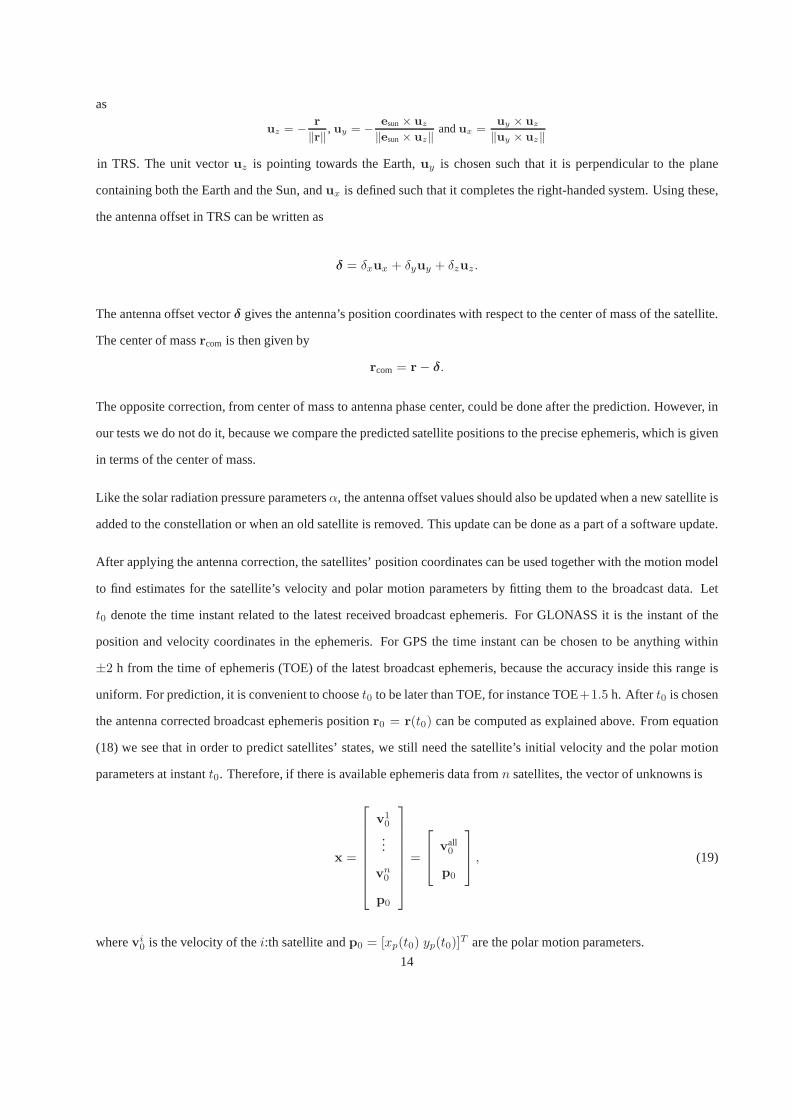
Figure 3: The nonlinear functionfk predicts or connects satellites’ states fromt0 to tk. This connection depends on the vectorx,which includes satellites’ velocities and the polar motionparameters. As measurements we have the satellites’ state vectorsyk,which are obtained from the broadcast ephemeris. Atx the predicted statesfk(x) fit the measurements best in the least squaressense.

Here the diagonal matrixD is a weight matrix that has a value of(1000)2 in those elements corresponding to

velocity components and ones elsewhere. These weights are empirical and we have found that they work well in

this case. Furthermore, to use only satellites’ positions as measurements instead of position and velocity, the weights

corresponding to the velocity components can be set to zero.

A nonlinear least squares problem (LSQ)

x = argminx

(y − f(x))T

D(y − f(x))

can be solved with the Levenberg-Marquardt method. The algorithm requires an initial iterate forx. An initial iterate

near the true value speeds up the convergence of the least squares fitting algorithm. For the initial velocitiesvall0 we use

the broadcast velocityvBE(t0). For polar motion parameters we usexp = 0.05 arcseconds andyp = 0.35 arcseconds,

which is the approximate center of the polar motion spiral during the years 2004-2008. In practice the initial iterate

for polar motion could be taken from the results of a previousLSQ solution.

From the LSQ solution we obtain estimates for the polar motion parametersp0 and for the velocitiesvall0 at the time

instantt0. The orbit prediction for future times then can be computed using the methods described in previous sections.

TESTS

For GPS satellites the least squares fitting can be done already with one received navigation message. As illustrated

in Figure 2, GPS’s broadcast ephemeris accuracy is uniform within ±2 h from the time of ephemeris. The same

holds true also for the velocity, except the accuracy of velocity deteriorates a bit earlier. Therefore, we can compute

satellite’s position and velocity at any instant inside this range, and use them as initial conditions or observations.

However, we have found that the algorithm works better if theinitial instantt0 of the prediction and the moment or

moments of observationstk are chosen apart from each other. In paper [5] we chose the initial moment of prediction

as TOE+ 1.5 h and as the measurements was the satellite’s state att1 = TOE− 1.5 h. Now in this paper, we do not

16

use the whole state, but only the position components as observations. Doing this improves the accuracy of the solved

polar motion parameters, and does not significantly affect the prediction accuracy.

Using only the position components as measurements, we needmore than one measurement instant in order to keep

the least squares problem overdetermined. As one can see from the equation (19), the number of variables is3n +

2, wheren is the number of received satellites. Therefore, one position measurement from each satellite, or3n

measurements, is not enough. However, two position measurements for each satellite is already enough to make the

system overdetermined. Therefore, in the tests of this paper we made the following choices: the initial instant is

t0 = TOE+ 1.5 h and the measurement instants aret1 = TOE andt2 = TOE− 1.5 h.

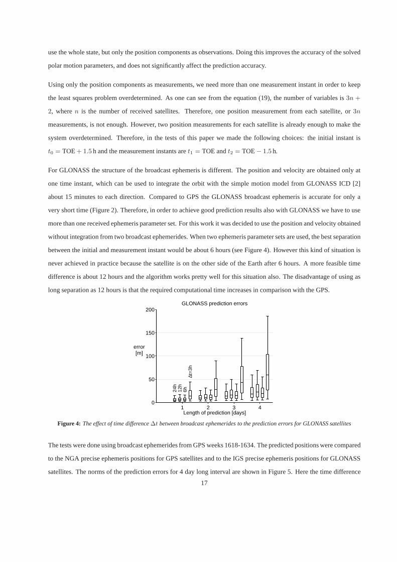
For GLONASS the structure of the broadcast ephemeris is different. The position and velocity are obtained only at

one time instant, which can be used to integrate the orbit with the simple motion model from GLONASS ICD [2]

about 15 minutes to each direction. Compared to GPS the GLONASS broadcast ephemeris is accurate for only a

very short time (Figure 2). Therefore, in order to achieve good prediction results also with GLONASS we have to use

more than one received ephemeris parameter set. For this work it was decided to use the position and velocity obtained

without integration from two broadcast ephemerides. When two ephemeris parameter sets are used, the best separation

between the initial and measurement instant would be about 6hours (see Figure 4). However this kind of situation is

never achieved in practice because the satellite is on the other side of the Earth after 6 hours. A more feasible time

difference is about 12 hours and the algorithm works pretty well for this situation also. The disadvantage of using as

long separation as 12 hours is that the required computational time increases in comparison with the GPS.

GLONASS prediction errors

Length of prediction [days]

error [m]

∆t=

3h6h12

h24

h

1 2 3 40

50

100

150

200

Figure 4: The effect of time difference∆t between broadcast ephemerides to the prediction errors forGLONASS satellites

The tests were done using broadcast ephemerides from GPS weeks 1618-1634. The predicted positions were compared

to the NGA precise ephemeris positions for GPS satellites and to the IGS precise ephemeris positions for GLONASS

satellites. The norms of the prediction errors for 4 day longinterval are shown in Figure 5. Here the time difference

17

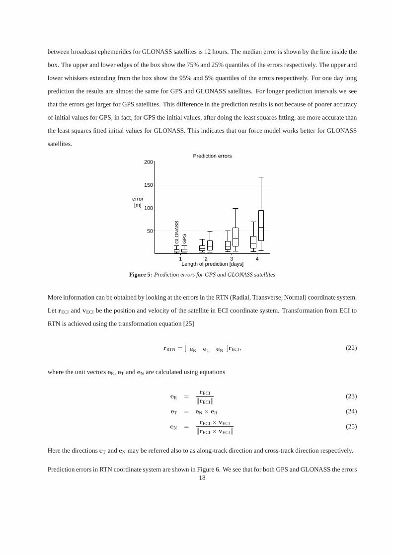
between broadcast ephemerides for GLONASS satellites is 12hours. The median error is shown by the line inside the

box. The upper and lower edges of the box show the 75% and 25% quantiles of the errors respectively. The upper and

lower whiskers extending from the box show the 95% and 5% quantiles of the errors respectively. For one day long

prediction the results are almost the same for GPS and GLONASS satellites. For longer prediction intervals we see

that the errors get larger for GPS satellites. This difference in the prediction results is not because of poorer accuracy

of initial values for GPS, in fact, for GPS the initial values, after doing the least squares fitting, are more accurate than

the least squares fitted initial values for GLONASS. This indicates that our force model works better for GLONASS

satellites.

Prediction errors

Length of prediction [days]

error [m]

GP

S

GLO

NA

SS

1 2 3 4

50

100

150

200

Figure 5: Prediction errors for GPS and GLONASS satellites

More information can be obtained by looking at the errors in the RTN (Radial, Transverse, Normal) coordinate system.

Let rECI andvECI be the position and velocity of the satellite in ECI coordinate system. Transformation from ECI to

RTN is achieved using the transformation equation [25]

rRTN = [ eR eT eN ]rECI, (22)

where the unit vectorseR, eT andeN are calculated using equations

eR =rECI

‖rECI‖(23)

eT = eN × eR (24)

eN =rECI × vECI

‖rECI × vECI‖(25)

Here the directionseT andeN may be referred also to as along-track direction and cross-track direction respectively.

Prediction errors in RTN coordinate system are shown in Figure 6. We see that for both GPS and GLONASS the errors18

are mostly in the tangential or along-track direction. Prediction errors in the radial and normal directions are small.

For positioning applications most important is the radial error, since this has the largest effect to the pseudorange error

(see next section). For four day long prediction 95% of the radial errors are under 6 meters for GPS and under 4 meters

for GLONASS.

GPS prediction errors in RTN(95% quantile)

Length of prediction [days]

error [m]

1 2 3 40

50

100

150

200RTN

GLONASS prediction errors in RTN(95% quantile)

Length of prediction [days]

error [m]

1 2 3 40

50

100

150

200RTN

Figure 6: 95% quantile of prediction errors in RTN coordinate system for (left) GPS satellites and (right) GLONASS satellites

From the prediction results it is seen that our model works better for GLONASS satellites than for GPS satellites. A

possible explanation for the results may be in the solar radiation pressure model. The solar radiation pressure model

used in this work is a simple model including acceleration only from the direct solar radiation pressure. However

studies have shown that for GPS satellites there is also an acceleration, often called y-bias, in the direction of the solar

panel axis of the satellite [11; 26]. The magnitude of the y-bias acceleration is quite small, in the order of10−9m/s2,

but for predictions over several days the effects can be significant. The exact reason for the force is unknown, but

one possible explanation is the misalignment of the solar panel axis [11]. The effect of solar radiation pressure on

GPS and GLONASS satellites has been studied by Ineichen et al. [27], who found out that the mean values for

y-bias acceleration were very close to zero for GLONASS satellites, whereas for GPS satellites the mean values of

y-bias were significantly different from zero. This suggests that including the y-bias acceleration to the solar radiation

pressure model might increase the accuracy of the prediction results for GPS satellites.

In order to estimate the computational complexity we testedthe runtime of our algorithm with Nokia N900 mobile

phone which has a 600MHz ARM Cortex-A8 CPU processor. The C-code used for testing was automatically generated

from our MATLAB implementation, using Matlab CoderTM -tool. We believe that the code could be further optimized

for real device implementation. The time needed to perform a4 days long orbit prediction for one satellite was 1.95

seconds, including the time needed to transform the predicted positions into extended Keplerian form i.e. to the

GPS ephemeris format. The time needed to fit the initial velocity of one GPS satellite was 0.36 seconds for known

19

polar motion parameters. However, when solving the polar motion parameters together with the initial velocities of 5

satellites, the computational time is 25.0 seconds. This isthe bottleneck of the whole algorithm and, as a consequence,

the parameters should be solved as seldom as possible. Instead, extrapolation based on earlier solved parameter values

should be preferred when possible.

We wish to point out that the fitting and subsequent prediction can begun immediately after the previous navigation

session is completed. Predictions can be done before the device is turned off, so that they are instantaneously available

when the device is opened again. If the device is a mobile phone, that is, the user tends to close the navigation

application but keep the phone on, the algorithm can be carried out progressively such that the positions are predicted

only slightly ahead of real time.

The time needed to integrate the GLONASS orbit is the same as for GPS, but the time needed for the fitting of initial

velocity differs, because it depends on the time differencebetween the two ephemerides used for fitting. For GPS

satellites the time difference of the furthermost states used for fitting is 3 hours and therefore each iteration of the

algorithm includes the integration of the satellites equation of motion over 3 hours long interval. As a consequence, if

the time difference of the 2 received GLONASS ephemerides is12 hours, the initial velocity fitting will take 4 times

longer than for GPS satellites i.e4 × 0.36 = 1.44 seconds.

SATELLITE CLOCK OFFSETS

In addition to the satellites’ ephemeris, GNSS satellite sends information about the satellite’s clock offsets. These

offsets, which describe the difference between the satellite’s own clock and the GNSS system time, are modeled with

a low order polynomials whose coefficients are sent in the navigation message. In GPS the offset, denotedδtgps, is

approximated with a second order polynomial and in GLONASS the offsetδtglo is approximated with a first order

polynomial, that is

δtgps(t) = af0 + af1(t− toc) + af2(t− toc)2 (26)

δtglo(t) = −τn + γn(t− tb). (27)

The polynomial coefficients are often denoted with the symbols written in the equations above. In addition to the

polynomial coefficients, the equations include two other terms toc andtb, which are the clock data reference times.

For further information about the clock offset polynomials, see the references [28] and [2].

20

When computing the user’s position in a standalone GNSS, thepseudorange measurements are of the form

ρ = ‖u− r‖ + c(tu − δt) + ε, (28)

whereu is the user’s position,r is the satellite’s position,tu is the receiver’s clock bias andδt is the satellite’s clock

offset andc is the speed of light in vacuum. Furthermore, there is an additional errorε, which among others includes

the atmospheric delays, receiver noise and multipath errors. These are sometimes referred to User Equipment Errors

(UEE). When considering the positioning calculation without reading the whole navigation message, i.e. with only

the time difference from satellite to the receiver, we need to predict the satellites’ positionsr as well as the satellite’s

clock offsetsδt in order to calculate the user’s position.

As a part of the navigation message the navigation device receives the coefficient for the clock offset models stated

in the equations (26) and (27). The simplest way to predict the offsets further is to use the same polynomial models

with the latest received coefficients. This approach workedquite well with the GPS satellites. The tests with the GPS

broadcast ephemeris data showed that the second order coefficientaf2 was zero, but the first order polynomials were

enough to model the offsets in longer term. In contrast, for GLONASS even the first order coefficient, the drift term

γn, was zero for several satellites. Nevertheless, the ephemeris prediction algorithm presented for GLONASS required

two earlier receiver broadcasts, so we can use two broadcasts when calculating the clock offsets as well. Computing

the future offset att with the model

δtglo(t) = −τn(tb) +−(τn(tb) − τn(t

∗

b))

tb − t∗b(t− tb), (29)

wheretb is the reference time of the latest received broadcast andt∗b of the another broadcast, one can obtain more

precise offsetsδtglo(t) for the GLONASS satellites. This model, where the coefficient γn is replaced with the slope

computed from two sequential−τn parameters, seems to work better than the parameterγn that is sometimes given by

the satellite.

In analogy to the tests of the previous section, the time differencetb − t∗b between the two broadcasts was chosen to

be 12 hours when testing the prediction model of the equation(29). Furthermore, the time instantstb of the chosen

test sample were equal to those used in the GLONASS ephemerisprediction tests in the previous section. The results

are shown in the Figure 7 together with the GPS offset predictions which were based on only one received broadcast.

The error in the clock offsetcδt is denoted byc∆t and it is expressed in meters. Again, the boxes show the 75%,

50% and 25% error quantiles, respectively, while the upper and lower whisker show the 95% and 5% quantiles. The

individual error|c∆t| was calculated as an absolute value between the predicted clock offset and the precise clock

21

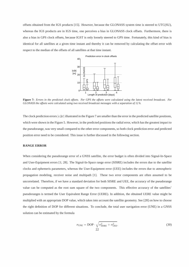
offsets obtained from the IGS products [15]. However, because the GLONASS system time is steered to UTC(SU),

whereas the IGS products are in IGS time, one perceives a biasin GLONASS clock offsets. Furthermore, there is

also a bias in GPS clock offsets, because IGST is only looselysteered to GPS time. Fortunately, this kind of bias is

identical for all satellites at a given time instant and thereby it can be removed by calculating the offset error with

respect to the median of the offsets of all satellites at thattime instant.

Length of prediction [days]

|c∆t| [m]

Prediction error in clock offsets

GLO

NA

SS

GP

S

1 2 3 40

10

20

30

40

Figure 7: Errors in the predicted clock offsets. For GPS the offsets were calculated using the latest received broadcast. ForGLONASS the offsets were calculated using two received broadcast messages with a separation of 12 h.

The clock prediction errors|c∆t| illustrated in the Figure 7 are smaller than the error in the predicted satellite positions,

which were shown in the Figure 5. However, in the predicted positions the radial error, which has the greatest impact to

the pseudorange, was very small compared to the other error components, so both clock prediction error and predicted

position error need to be considered. This issue is further discussed in the following section.

RANGE ERROR

When considering the pseudorange error of a GNSS satellite,the error budget is often divided into Signal-In-Space

and User-Equipment errors [1; 28]. The Signal-In-Space range error (SISRE) includes the errors due to the satellite

clocks and ephemeris parameters, whereas the User-Equipment error (UEE) includes the errors due to atmospheric

propagation modeling, receiver noise and multipath [1]. These two error components are often assumed to be

uncorrelated. Therefore, if we have a standard deviation for both SISRE and UEE, the accuracy of the pseudorange

value can be computed as the root sum square of the two components. This effective accuracy of the satellites’

pseudoranges is termed the User Equivalent Range Error (UERE). In addition, the obtained UERE value might be

multiplied with an appropriate DOP value, which takes into account the satellite geometry. See [28] on how to choose

the right definition of DOP for different situations. To conclude, the total user navigation error (UNE) in a GNSS

solution can be estimated by the formula

σUNE = DOP·√

σ2SISRE+ σ2

UEE, (30)

22

which was given in [29].

SISRE is the error attributed to the ephemeris parameters and clock model generated by the control segment. Because

the purpose of our prediction method is to replace exactly this information, the SISRE is a suitable quantity for

estimating the performance of our prediction method. Knowing the distribution for SISRE a person having expertise

with GNSS positioning can infer the actual positioning error in desired circumstances and application area. Therefore,

the rest of this section focuses on determining the standarddeviationσSISRE from a sample of errors in predicted

satellite positions and in predicted satellite clock offsets. The individual error components are computed with respect

to IGS precise orbit and clock offset data [15].

According to [29], the standard deviation for Signal-In-Space range error can be estimated by the formula

σSISRE =

√

σ2∆R−c∆t +

1

72(σ2

∆T + σ2∆N), (31)

where∆R, ∆T and∆N are the radial, tangential and normal error components in satellite’s predicted position,c∆t

is the range error due to the inaccurate clock offset model, and σ2X is the variance of the subscript quantity X. This

formula can be derived by writing the range measurement equation (28) in terms of the RTN components and deducing

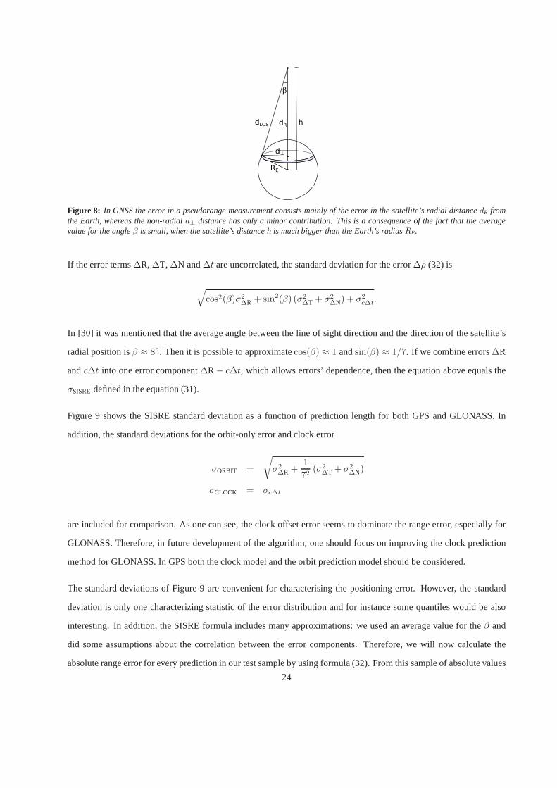
in which proportion they affect the pseudorange error if theuser’s location is restricted to the Earth’s surface. Denoting

the exact distance components from satellite to the user asdR, dT anddN, the range equation can be written as

ρ =√

d2R + d2

T + d2N − cδt =

√

d2R + d2

⊥− cδt.

Hered⊥ denotes the non-radial distance, i.e combined tangential and normal distances. The combined distanced⊥ is

introduced because the magnitude of the distancesdT anddN in the pseudorange are equal due to symmetry (Figure

8). If we now have errors∆R and∆⊥ in the two distance components and∆t is the error in the predicted clock offset,

then by 1st order Taylor approximation the total error in therangeρ is

∆ρ ≈ cos(β)∆R + sin(β)∆⊥ − c∆t. (32)

Here the trigonometric coefficientscos(β) = dR/dLOS andsin(β) = d⊥/dLOS are the partial derivatives of the function

ρ with respect to the error terms∆R and∆⊥, respectively. The variabledLOS is the Line Of Sight distance i.e. the

distance between the user and the satellite.

23

d⊥

RE

dRdLOS h

β

Figure 8: In GNSS the error in a pseudorange measurement consists mainly of the error in the satellite’s radial distancedR fromthe Earth, whereas the non-radiald⊥ distance has only a minor contribution. This is a consequence of the fact that the averagevalue for the angleβ is small, when the satellite’s distance h is much bigger thanthe Earth’s radiusRE.

If the error terms∆R, ∆T, ∆N and∆t are uncorrelated, the standard deviation for the error∆ρ (32) is

√

cos2(β)σ2∆R + sin2(β) (σ2

∆T + σ2∆N) + σ2

c∆t.

In [30] it was mentioned that the average angle between the line of sight direction and the direction of the satellite’s

radial position isβ ≈ 8. Then it is possible to approximatecos(β) ≈ 1 andsin(β) ≈ 1/7. If we combine errors∆R

andc∆t into one error component∆R− c∆t, which allows errors’ dependence, then the equation above equals the

σSISRE defined in the equation (31).

Figure 9 shows the SISRE standard deviation as a function of prediction length for both GPS and GLONASS. In

addition, the standard deviations for the orbit-only errorand clock error

σORBIT =

√

σ2∆R +

1

72(σ2

∆T + σ2∆N)

σCLOCK = σc∆t

are included for comparison. As one can see, the clock offseterror seems to dominate the range error, especially for

GLONASS. Therefore, in future development of the algorithm, one should focus on improving the clock prediction

method for GLONASS. In GPS both the clock model and the orbit prediction model should be considered.

The standard deviations of Figure 9 are convenient for characterising the positioning error. However, the standard

deviation is only one characterizing statistic of the errordistribution and for instance some quantiles would be also

interesting. In addition, the SISRE formula includes many approximations: we used an average value for theβ and

did some assumptions about the correlation between the error components. Therefore, we will now calculate the

absolute range error for every prediction in our test sampleby using formula (32). From this sample of absolute values

24

Length of prediction [days]

σ [m]

Estimated range error for GPS

0 1 2 3 40

5

10

15SISRECLOCKORBIT

Length of prediction [days]

σ [m]

Estimated range error for GLONASS

0 1 2 3 40

5

10

15SISRECLOCKORBIT

Figure 9: Error in predicted clock offsets seems to dominate the rangeerror

one can compute the 95% error quantile and median, which approximate the upper error bound and the typical error,

respectively. Earlier the angleβ was chosen to be8.21, but now we will calculate the error quantiles as a function of

the satellite’s angle of elevationφel i.e the angular height measured from the horizontal, which depends onβ through

the relation

tanβ =R sin(90 − φel)

h− Rcos(90 − φel),

where R is the radius of the Earth and h is the satellite’s distance from the Earth’s center. The 95% quantile and median

of the absolute range error|∆ρ| are plotted as a function of satellite’s elevation in Figure10. The two uppermost lines

correspond to the 4 days long predictions: the solid line shows the error for GPS and the line with the triangles for

GLONASS. Below these lines are also from three down to one daylong predictions for both systems.

0 30 60 900

10

20

30

40

50

60

Elevation angle [°]

[m]

Upper bound for |∆ρ| (95% quantile)

4 days

3 days

2 days

1 day

0 30 60 900

5

10

15

Elevation angle [°]

[m]

Median of the range error |∆ρ|

Figure 10: Upper bounds (95% quantile) and typical values (median) forthe absolute range error|∆ρ|

In GPS the longer predictions include much error in the non-radial componentd⊥ and this makes the error dependent of

the elevation angleφel. In GLONASS there is no dependence of the elevation angle, because the clock error dominates

the range error so strongly. These facts can be used when trying to improve the algorithm and could be taken into

account when calculating the user’s position: for GPS it might be worthwhile to weight the different pseudorange

measurements according to the satellite’s angle of elevation.

25

CONCLUSION

Assisted GNSS is a common way to improve the startup performance of the personal navigations devices. The aim

of this paper was to study a method with which one could attainsimilar properties to assisted GNSS in a standalone

GNSS device as well. These standalone devices do not have anynetwork connection and the broadcast ephemeris is

the only data they can receive.

In order to improve the TTFF when turning on a GNSS device, we need to know the satellites’ locations beforehand,

without reading the navigation message. Our method for predicting satellite’s position is based on solving the satellite’s

equation of motion numerically. We have included only the most significant forces: Earth gravitation, solar and lunar

gravitation and solar radiation pressure to the equation ofmotion, which we call the force model. However, before

we can use the force model we have to solve the satellite’s initial state and the polar motion parameters, which are

needed in order to know the exact rotation axis of the Earth. This is done by a nonlinear least squares fitting algorithm,

which uses earlier received broadcast ephemerides as its fitting data. For GPS satellites only one broadcast ephemeris

is needed when solving the initial values. For GLONASS satellites we have used two broadcast ephemerides to solve

the initial values.

The prediction method was tested with real broadcast ephemeris data and the prediction error was calculated using

the precise ephemeris delivered by NGA for GPS and IGS for GLONASS as a reference. For one day long prediction

95% of the prediction errors were below 18 meters for both systems. With longer prediction intervals our model

works better for GLONASS satellites than for GPS satellites. For instance, in a four day long prediction 95% of the

errors are below 100 meters for GPS and below 51 meters for GLONASS. The prediction errors were also studied in

RTN coordinate system, which gives the radial, tangential or along-track and normal or cross-track components of the

errors. The errors are largest in the tangential direction and relatively small in the radial and normal directions. This

is very desirable, because the error in the radial componenttends to have the greatest impact to the range error from

the satellite to the receiver.

For radiation pressure we used a simple Cannonball model anda scale term which is pre-estimated separately for each

satellite using precise ephemeris data. Studies conductedfor GPS satellites suggest that there is also acceleration in

the direction of the satellites’ solar panel axis, which is not observed for GLONASS satellites. This acceleration, often

called y-bias, might be the reason for the difference in the prediction errors for GPS and GLONASS.

In addition to the orbit prediction method, we have briefly investigated the validity of the GNSS satellite’s clock

offset polynomials for prediction. In our case the length ofprediction has been from one to four days, which is

notably outside the typical GNSS broadcast life span, whichis around 4 hours for GPS and about half an hour for

26

GLONASS. As a conclusion, the offset polynomial received from GPS broadcast can be used as such for up to 4 days

long prediction, if one can accept an error of 18 m (95% quantile). In contrast, for GLONASS one received offset

polynomial is not enough to reach an accuracy which would be competitive with the GPS offsets. However, if two

broadcasts are received, with a separation of 12 hours for example, we can use them to form a simple linear prediction

model. This model was able to predict the offsets with 35 m accuracy (95% quantile) for 4 days.

Finally, the navigation error related to the presented prediction method is discussed. We used the Signal-In-Space

range error formula for approximating the part of the range error that would accumulate from the error in the predicted

satellite positions and the predicted clock offsets. This formula gave standard deviations of about 15 m for the range

error for both GPS and GLONASS, when the prediction length was 4 days and no impulsive change, like NANU events,

occurred. Moreover, a comparison between the ephemeris andclock prediction errors indicated that the inaccuracy in

the clock offset predictions constrains the positioning accuracy.

ACKNOWLEDGMENTS

This research was partly funded by Nokia Inc.. Mari Seppanen also acknowledges the financial support of Tampere

Graduate School in Information Science and Engineering.

REFERENCES

[1] Misra, P. and Enge, P.,Global Positioning System: Signals, Measurements and Performance, 2nd ed. Lincoln

(MA): Ganga-Jamuna Press, 2006, 569p.

[2] Global navigation satellite system GLONASS: InterfaceControl Document (GLONASS ICD), version 5.0,

(2002), Russian Institute of Space Device Engineering/Research.

[3] Mattos, P. G., “Hotstart every time - compute the ephemeris on the mobile,” inProceedings of the 21st

International Technical Meeting of the Satellite Divisionof The Institute of Navigation (ION GNSS 2008),

Savannah, GA, September 2008, pp. 204–211.

[4] Zhang, W., Venkatasubramanian, V., Liu, H., Phatak, M.,and Han, S., “SiRF InstantFix II Technology,” in

Proceedings of the 21st International Technical Meeting ofthe Satellite Division of the Institute of Navigation

(ION GNSS 2008), Savannah, GA, September 2008, pp. 1840 – 1847.

[5] Seppanen, M., Perala, T., and Piche, R., “Autonomous satellite orbit prediction,” in 2011

International Technical Meeting, San Diego, California, January 2011. [Online]. Available:

http://www.ion.org/meetings/abstractSearch/showAbstract.cfm?key=72&t=C&s=2&collection=ITM2011Abstracts

27

[6] Montenbruck, O. and Gill, E.,Satellite Orbits, 3rd ed. Berlin Heidelberg New York: Springer, 2005, 369 p.

[7] Seppanen, M., “GPS-satelliitin radan ennustaminen,”M.Sc. Thesis, Tampere University of Technology, March

2010. [Online]. Available: http://math.tut.fi/posgroup/seppanenmscth.pdf

[8] An Earth Gravitational Model to Degree 2160: EGM2008, presented at the 2008 General

Assembly of the European Geosciences Union, Vienna, Austria, April 13-18, 2008. http://earth-

info.nima.mil/GandG/wgs84/gravitymod/egm2008/firstrelease.html.

[9] Cunningham, L., “On the computation of the spherical harmonic terms needed during the numerical integration

of the orbital motion of an artificial satellite,”Celestial Mechanics, vol. 2, pp. 207–216, 1970.

[10] Metris, G., Xu, J., and Wytrzyszczak, I., “Derivatives of the gravity potential with respect to rectangular

coordinates,”Celestial Mechanics and Dynamical Astronomy, vol. 71, no. 2, pp. 137–151, 1999.

[11] Froidevall, L. O., “A study of solar radiation pressureacting on GPS satellites,” Ph.D.

dissertation, The University of Texas at Austin, Austin TX USA, August 2009. [Online]. Available:

http://repositories.lib.utexas.edu/bitstream/handle/ 2152/6623/froidevall45515.pdf

[12] Simon, D.,Optimal state estimation. Hoboken, New Jersey and Canada: John Wiley & Sons, 2006, 526p.

[13] Jazwinski, A. H.,Stochastic Processes and Filtering Theory. New York: Academic Press, 1970, vol. 64, 378 p.

[14] NGA GPS Satellite Precise Ephemeris (PE) Center of Mass. [Online]. Available: http://earth-

info.nga.mil/GandG/sathtml/PEexe.html

[15] Dow, J., Neilan, R., and Rizos, C., “The international GNSS service in a changing landscape of Global

Navigation Satellite Systems,”Journal of Geodesy, vol. 83, pp. 689–689, 2009, 10.1007/s00190-009-0315-4.

[Online]. Available: http://dx.doi.org/10.1007/s00190-009-0315-4

[16] Hairer, E., Nrsett, S. P., and Wanner, G.,Solving Ordinary Differential Equations I: Nonstiff Problems, 2nd ed.

Berlin: Springer-Verlag, 1993, 528 p.

[17] McCarthy, D. D. and Petit., G., iERS Conventions (2003). (IERS Technical Note ; 32) Frankfurt am Main: Verlag

des Bundesamts fr Kartographie und Geodasie, 2004. 127 pp., paperback, ISBN 3-89888-884-3.

[18] IERS C04 series of the Earth orientation parameters. [Online]. Available:

http://data.iers.org/products/214/14443/orig/eopc0408 IAU2000.62-now

[19] Navstar Global Position System Interface Specification, Navstar GPS Space Segment/User Segment L1C

Interfaces Draft IS-GPS-800, CA: Arinc Engineering Service LLC, 19 Apr 2006. [Online]. Available:

http://www.navcen.uscg.gov/ gps/modernization/L1/IS-GPS-80019 DRAFT A pr06.pdf28

[20] Global navigation satellite system GLONASS: Interface Control Document (GLONASS ICD),

version 5.1, (2008), Russian Institute of Space Device Engineering/Research. [Online]. Available:

http://facility.unavco.org/data/docs/ICDGLONASS5.1 (2008)en.pdf

[21] Global navigation satellite system and global positioning system. Coordinate systems.

Methods of transformations for determinated points coordinate, 2008. [Online]. Available:

http://protect.gost.ru/document.aspx?control=7&baseC=6&page=0&month=9&year=2009&search=&id=174517

[22] Korvenoja, P. and Piche, R., “Efficient satellite orbit approximation,” in Proceedings of ION

GPS 2000, September 19-22, 2000, Salt Lake City, USA, 2000, pp. 1930–1937. [Online]. Available:

http://math.tut.fi/posgroup/korvenojapiche ion2000a.pdf

[23] NGA GPS Ephemeris/Station/Antenna Offset Documentation. [Online]. Available: http://earth-

info.nga.mil/GandG/sathtml/gpsdoc201009a.html

[24] Cai, C., “Precise point positioning using dual-frequency GPS and GLONASS measurements,”

Master’s thesis, University of Calgary, Calgary, Alberta,August 2009. [Online]. Available:

http://www.ucalgary.ca/engowebdocs/YG/09.20291ChangshengCai.pdf

[25] Tapley, B. D., Schutz, B. E., and Born, G. H.,Statistical Orbit Determination. Elsevier Academic Press, 2004.

[26] Springer, T., G.Beutler, and Rothacher, M., “A new solar radiation pressure model for GPS satellites,”GPS

Solutions, vol. 2, pp. 50–62, 1999.

[27] Ineichen, D., Springer, T., and Beutler, G., “Combinedprocessing of the IGS and the IGEX

network,” Journal of Geodesy, vol. 75, pp. 575–586, 2001, 10.1007/s001900000152. [Online]. Available:

http://dx.doi.org/10.1007/s001900000152

[28] Kaplan, E. D.,Understanding GPS: Principles and Applications. Boston/London: Artech House, 1996, 576 p.

[29] Malys, S., Larezos, M., Gottschalk, S., Mobbs, S., Winn, B., Feess, W., Menn, M., Swift, E., Merrigan, M.,

and Mathon, W., “The GPS accuracy improvement initiative,”in Proceedings of the 10th International Technical

Meeting of the Satellite Division of The Institute of Navigation (ION GPS 1997), Kansas City, MO, September

1997, pp. 375 – 384.

[30] Montenbruck, O., Gill, E., and Kroes, R., “Rapid orbit determination of LEO satellites using IGS clock

and ephemeris products,”GPS Solutions, vol. 9, pp. 226–235, 2005, 10.1007/s10291-005-0131-0. [Online].

Available: http://dx.doi.org/10.1007/s10291-005-0131-0

29