Discovering Frequent Graph Patterns Using Disjoint Paths ∗

E. Gudes, S. E. Shimony, N. Vanetikehud,shimony,orlovn@cs.bgu.ac.il

Dept. of Computer Science, Ben-Gurion University of the Negev, Beer-Sheva, Israel

Abstract

Whereas data-mining in structured data focuses on fre-quent data values, in semi-structured and graph datamining the issue is frequent labels and common spe-cific topologies. Here, the structure of the data is justas important as its content. We study the problemof discovering typical patterns of graph data, a taskmade difficult because of the complexity of requiredsub-tasks, especially sub-graph isomorphism.

In this paper, we propose a new apriori-based algo-rithm for mining graph data, where the basic buildingblocks are relatively large - disjoint paths. The algo-rithm is proven to be sound and complete. Empiricalevidence shows practical advantages of our approachfor certain categories of graphs

Keywords: H.2.8 Database Applications: H.2.8.dData mining, H.2.8.i Mining methods and algorithms,H.2.8.m Web mining, Graph mining.

1 Introduction

Due to increasing amounts of structured and unstruc-tured data collected by various companies and insti-tutions, the importance of data mining has grown sig-nificantly over the last several years. Whereas in thepast, data mining was mainly applied to structureddata and flat files, there is growing interest in miningand discovering frequent patterns in semi-structureddata such as web data ([24],[36],[2]), chemical com-pounds data [8, 28] or biological data [30]. The focusof this paper is on discovering such freqent patterns,in the form of (possibly labeled) graphs, and a newalgorithm for this difficult task.

Semistructured data appears when the source does notimpose a rigid structure on the data, such as the web,or when data is combined from several heterogeneoussources. Unlike unstructured raw data (like imageand sound), semistructured data does have some struc-ture, but unlike structured data (such as relational orobject-oriented databases), semistructured data has noabsolute schema or class fixed in advance. For exam-ple, in the movie XML database [29], some movies havemore actors than others; some fields (e.g., Award) aremissing for some movies; some actors have birthdayrecorded and some do not; etc. As a result, the struc-

∗Partially supported by the KITE consortium under contractto the Israeli Ministry of Trade and Industry, and by the PaulIvanier Center for Robotics and Production Management.

ture of objects is irregular and a query over the struc-ture is as important as a query over the data. Thisstructural irregularity, however, does not imply thatthere is no structural similarity among semistructuredobjects. On the contrary, it is common for semistruc-tured objects describing the same type of informationto have similar structures. For example, every movieobject has Title and Director labels; every Actor ob-ject has a Name label; 50% of Actor objects have aNationality label, etc. This phenomenon is commonin other types of semi-structured data as well [20].While in the field of structured data-mining frequentdata values and their common appearances are of in-terest, in mining semi-structured data, the focus is onfrequent labels and common appearances of sub-setsof such labels (in terms of XML, one would look forfrequent occurrences of structures of elements or at-tributes, disregarding the attribute values). Therefore,frequently, a common model is a graph, with labels onnodes, or on edges, or on both (the transformation be-tween these types of models is quite simple). In thispaper we assume the model of a directed or undirectedgraph (or set of graphs) with node labels, and our taskis to find frequent patterns in such a graph. For ex-ample, see Figure 1, depicting some frequent graphpatterns found by our algorithm in an XML moviedatabase [29].

movieG2

cast title filmedinset

G7 movie

movie movie

directordirector movie movie directoractor

G14

Figure 1: Pattern examples

1.1 Graph mining applications

Discovering and understanding frequent patterns thatrepresent a sufficiently large part of a semistructureddatabase can be useful in several application areas:Improving database storage and design [10, 32].Semistructured data sets (a typical example beingXML data), carry their own schema information.Though required for data exchange and integration,such schema incorporation entails considerable spaceoverhead, since the schema information is stored withthe data (e.g. element names in XML). Because of this

1

overhead, commercial DBMS often store XML data inrelational databases. Semistructured data can alwaysbe stored as a ternary relation, since the data is anedge-labeled graph, but this is no better than stor-ing the schema with the data. A ”good” mapping (interms of disk space or fragmentation) from a semistruc-tured data instance into a relational schema is desir-able. Frequent patterns discovered in the semistruc-tured data can be used for that purpose since theycan help generate the basic relations, while the non-frequent patterns would be stored as ”overflow” rela-tions (see [10]).

Efficient indexing and querying.

Querying a semistructured database is an importantand common activity. Numerous query languages wereproposed for this purpose (see [9, 3]). To speed upquery processing several indexing techniques were pro-posed for semistructured and XML data [13, 26, 14].Recently, it was realized that full indexing on all pos-sible labels and paths in a semistructured data is notpractical. The APEX indexing scheme [5] suggests in-dexing mainly on frequent paths, where the frequentpaths are found by data mining techniques. This ideaof using mining for indexing can naturally be gener-alized to general graphs, as proposed in [31], wherepaths are used for finding all occurrences of a querygraph in the database.

User preference-based and user modeling appli-cations[11, 39].

An important goal for web-page design is to pro-vide viewer-oriented personalization of web-page con-tent. Designers often strive to condition web-page con-tent and appearance on the current preferences of theviewer, and probably on some underlying structureof the web-page content. In order to optimize suchcontent, one often refers to data mining. When thesemistructured database is a collection of user traver-sal patterns , one can derive expected user behaviorfrom knowledge about frequent traversal patterns ofthe same user collected over a certain period of time.This results in useful applications, e.g. placing adver-tisements in proper places and better customer/userclassification and behavior analysis. In past work, webnavigation patterns were usually represented as pathsor trees, and for this type of problems tree and pathmining are most relevant [4]. However, if one looks atsets of related web navigation patterns, or at behaviourover time, one gets more complex patterns which canbe represented by graphs, motivating the use of graphmining. Another application related to user behaviouris the area of social networks, analysing which is animportant field in communication and in security ap-plications [12]. An example social network databasebased on e-mails is used in our study.

1.2 Categories of graph mining problems

In the past, most work done in this field dealt witheither single path patterns [2] or tree-like patterns[24, 36, 4]. However, much of the data on the webis graph-like, either cyclic or acyclic, motivating themining of general graph data. The field of graph min-ing received much attention in recent years and sev-eral well known algorithms were developed, such as:AGM [18], FSG [21], gSpan [40], CloseGraph [41], andAdiMine [35]. In this paper we present a new algo-rithm for mining frequent patterns in semi-structureddata, where the data is modeled as a labeled graph.Our algorithm handles general unrestricted graphs, di-rected or undirected.

There are two distinct problem formulations for fre-quent pattern mining in graph datasets. In the for-mer, known as the graph-transaction setting, the inputto the pattern mining algorithm is a set of (usually)relatively small graphs, and a pattern is considered fre-quent if it appears in a large number or fraction of thegraphs. Note that a pattern occurence is counted onlyonce per transaction, independent of posible multipleoccurences in the same transaction. A typical applica-tion for this formulation is finding frequent sub-graphsin molecular transactions [21].

In the alternate setting, the frequency of a pattern isbased on the number of its occurrences (i.e., embed-dings) of a pattern in all the data, counting multipleoccurences per transaction. For this setting, one canassume without loss of generality that the input is asingle graph, because one can always treat multiplegraphs as a single graph with disconnected compo-nents. For historical reasons, we refer to this formula-tion as the single-graph setting [22], although neitherthe problem formulation nor the algorithms are limitedin this manner.

Due to the inherent differences in characteristics ofthe problem formulation, algorithms developed for thegraph-transaction setting cannot handle the single-graph setting, whereas the latter algorithms can beused to solve the former problem. In recent years, anumber of efficient and scalable algorithms have beendeveloped to find patterns in the graph-transactionsetting [20, 21, 40, 19, 16, 17, 6]. These algorithms arecomplete in the sense that they are guaranteed to dis-cover all frequent subgraphs and were shown to scaleto very large graph datasets. However, developing al-gorithms that are capable of finding patterns in caseswhere each transaction is a large graph, and especiallythe single-graph setting, has received much less atten-tion, despite the fact that this problem setting is moregeneric and applicable to a wider range of datasets andapplication domains than the former problem. Otherthan our own papers [33, 34], the most recent paperdealing with the single graph setting is [22], discussedin Section 5.

2

1.3 Overview of the proposed algorithm

The algorithm presented in this paper uses breadth-first enumeration, and is based on the Apriori algo-rithm [1]. These algorithms use an admissibility prop-erty (defined below) of the support measure in orderto prune candidate patterns, without checking theirsupport directly, while ensuring completeness. Sincea pattern is considered to be frequent in a datasetgraph if its support measure is greater than a user-provided threshold, then once a pattern has supportsmaller than the threshold, all of its superpattens canbe pruned, or potentially not even be generated in thefirst place.

Let the support measure S be a function from graphpatterns and dataset graphs to real numbers (usuallyin [0, 1]). As usually the dataset graph is understood,this argument to S is omitted. S obeys the admissibil-ity constraint (also called anti-monotonicity, or down-ward closure) if every subgraph of a frequent patternis also frequent [1, 15]. Formally:

Definition (admissible support measure) A sup-port measure S is admissible if for every pattern P ,S(P ) ≥ 0 and for all patterns P1, P2 such that P1 ⊆ P2

we have S(P1) ≥ S(P2).

Apriori-based algorithms compose candidate patternsfrom building blocks that vary between algorithms. Inour algorithm, the building block is a complete path(see the next section for precise definitions) - as seenin the following (extremely simplified) outline of ouralgorithm:

1. Find all patterns composed of a single path, bydirectly counting the number of occurrences ofthese patterns in the dataset. Eliminate the non-frequent patterns.

2. Find all candidate patterns composed of two fre-quent paths, and eliminate the non-frequent pat-terns.

3. At each successive step n:

(a) Construct candidate patterns from smallerfrequent ones, which have a common “core”.Specifically, generate patterns with n + 1paths by merging two patterns with n paths,that have a common core with n − 1 paths.A simple example for n = 2, is shown inFigure 8: two graphs, each consisting of twopaths, with an identical core consisting ofone path, are merged to create a graph withthree paths. In general, this construction,the ”heart” of the algorithm, is quite com-plex.

(b) Prune candidates that are not frequent.

(c) Stop when no more frequent patterns can begenerated.

The above outline is precisely the same as for mostapriori based algorithms, the crucial difference beingthat while for itemset mining the building block is anitem, and for most graph mining algorithm (such asFSG or gSpan) the building blocks are edges or nodes,in our algorithm the building block is the (typicallymuch larger) edge-disjoint paths. Making the buildingblock larger allows for a smaller number of iterations,as well as for a smaller number of candidate patternsthat need to be tested for support - the main goal ofour scheme. Since testing support of a pattern is ex-pensive, especially for graph data, it is important toimprove pruning, even if it entails considerable over-head over the naive methods of generating and testingpatterns. Another complication is that achieving com-pleteness becomes non-trivial, and considerable spaceis devoted in this paper to how completeness can beprovably maintained.

1.4 Contributions and outline of the paper

The idea of using paths as building blocks in a graphmining algorithm was presented briefly in an earlier,conference version of this paper [33]. The operatorsused to define graph composition, that allow for effi-cient implementation of the graph merge in practice,are a new contribution of this version. A major is-sue in this respect is proving that our edge-disjointpath based algorithm is complete. This proof of cor-rectness (Section 3) is a previously unpublished, non-trivial main contribution of this paper.

In attempting to find frequently occurring subgraphpatterns within a graph, computing the frequency ofoccurrence of the pattern in the larger graph (thedatabase), and the support measure, is an intensivecomputational step. This is due to involves multiplecomputations of the sub-graph isomorphism problemwhich is a hard problem. In order to decrease the num-ber of extremely expensive support computations, wemust discard, as early as possible, as many candidatepatterns as possible. This is a general property of ouralgorithm. Minimizing the number of expensive sup-port computations is the second major contribution ofthis paper. This advantage is more prominent whenthe transaction-graphs are large, and even more so inthe “single-graph” setting, where the support compu-tation tends to be extremely hard.

To prove the feasibility of our scheme we implementedthe proposed algorithms, tested them on some XMLdatabases and synthetic graphs, and compared them toother approaches for counting graphs patterns, mainlythe naive and the FSG algorithms. Note that the al-gorithm presented here is orthogonal to the supportmeasure and therefore can be used for both cases, andis compared experimentally to FSG in both cases. Theresults show that while in the transaction setting, thetwo algorithms are comparable, in the “single-graph”setting our algorithm shows a significant reduction in

3

the number of candidates generated, and therefore inthe number of support computations. In our exper-iments we dealt with medium-size graph databases(upto 20,000 nodes) since for larger sizes the single-graph case support computation was too heavy compu-tationally for both the FSG algorithm and ours. Theexperimental evaluation of our algorithm (Section 4)is the third contribution of this paper.

The rest of this paper is organized as follows. We be-gin with revisiting some graph theoretic notation andresults (Section 2), followed by a formal definition ofour graph-mining problem, and new definitions used inspecifying the algorithm. The graph mining algorithmand its correctness proof are then presented (Section3). Empirical evaluation of our algorithm on both syn-thetic and real data is examined in Section 4. Section5 discusses related work, as well as applicability of ouralgorithm to other settings.

2 Preliminaries

We begin with revisiting standard terms from the liter-ature. A formal statement of our graph-mining prob-lem is made, followed by definition of composition op-erators essential for generating candidate graphs in thealgorithm. Important basic properties of the operatorsare stated and proved.

2.1 Paths and path covers

We begin by revisiting some graph-theoretic terms andproperties. Notation needed later on is also intro-duced.

A path is an alternating sequence of nodes and (theirincident) edges, that begins and ends with a node, andthat does not contain any edge more than once. Fordirected graphs, we require a path to respect the direc-tion of the edges, resulting in a directed path. A set Pof edge-disjoint paths covering all edges of of a graphG exactly once is called a path cover of G. A pathcover P is called minimal if it has the smallest cardi-nality of all path covers of G. Clearly, in general theminimal cover is not unique. The path number p(G) isthe cardinality of any minimal path-cover of G.

In this paper we use paths as the building blocks, inorder to create larger graphs, but are not concernedabout how to traverse the paths once they have beencreated. Henceforth, we ignore the ordering inherentto the path definition, and represent a path simplyas the set of nodes and edges in the path, i.e. as agraph. Two different paths that have the same setof nodes and edges are thus indistinguishable in ourmethod. Note that we still require that such a graph betraversable as a single path, even though the traversaldoes not have to be unique.

Removing path P from graph G, denoted by G \ P ,consists of removing all edges of P from G, followedby removing all stand-alone nodes. To compute thepath number we rely on well-known facts:

1. A connected undirected graph G = (V,E) is Eu-lerian (can be covered by a single cyclic path) ifffor every v ∈ V , d(v) is even. A connected di-graph G = (V,E) is Eulerian (can be covered bya single directed cyclic path) iff for every v ∈ V ,d+(v) = d−(v). (Throughout, we denote thein-degree of v by d+(v), and the out-degree byd−(v).)

2. For every connected undirected graph G = (V,E),p(G) = 1 if G is Eulerian,and p(G) = |v | v ∈ V, d(v) is odd| /2 otherwise.For every connected directed graph G = (V,E) ,p(G) = 1 if G is Eulerian andp(G) = (

∑v∈V |d+(v)− d−(v)|)/2 otherwise.

Observe that the path number of a graph is nevergreater than the number of edges, being in fact muchsmaller in most cases - especially for undirected graphs.Thus, paths as building blocks should decrease thenumber of iterations in the algorithm, as well as im-prove the pruning.

2.2 Problem statement

A labeled graph is a graph that has a label associatedwith each node v, denoted by label(v). We assumewithout loss of generality that the dataset (as well asthe pattern) graph is labeled (otherwise, assign to allnodes in the graph the same arbitrary label). Giventwo graphs G′ = (V ′, E′) and G′′ = (V ′′, E′′), a label-preserving isomorphism between G′ and G′′ is a graphisomorphism φ : V ′ → V ′′ such that for every v ∈ V ′label(v) = label(φ(v)). When such an isomorphismexists, denote by G′ ≈ G′′ the fact that the graphs areisomorphic. P is a graph pattern in graph G if it isisomorphic to a connected subgraph of G.

Our problem is formally defined as follows. Given adataset labeled graph G, and a support measure Sover pattern graphs, and a support threshold σ, findall pattern graphs P with support S(P ) ≥ σ in G.Recall that the input can be a set of graphs as well asa single graph w.l.o.g. throught.

2.3 Lexicographic ordering

To facilitate efficient indexing of path covers in agraph, we use a canonical representation of paths andpath sequences. The lexicographical ordering overpaths uses node labels and degrees of nodes in paths,as follows.

A path P uniquely defines the graph (V (P ), E(P )):the nodes traversed by the path, and the edges tra-versed by the path, respectively. For node v ∈ V (P )the path degrees d+

P (v) and d−P (v) are the in-degree andout degree, respectively, of v in (V (P ), E(P )). Forundirected paths, the path degree dP (v) of v is simplythe degree of v in (V (P ), E(P )).

Let P be a directed path, and let v ∈ V (P ). A nodein a path is represented by a representing tuple (see

4

Figure 2), defined as follows:

RTP (v) := (label(v), d+P (v), d−P (v))

For undirected paths, the representing tuple is likewisedefined as:

RTP (v) := (label(v), dP (v))

Assuming a natural complete ordering between labels,as well the natural complete ordering between integers,a lexicographical ordering between the node represen-tation tuples of u and v, denoted v ≺L u, is under-stood. Likewise, equality operator v =L u denotesequality of the respective representing tuples.

v2

v3

a

c

d

a

b

path P

path Q

v1

v

v

5

4

Figure 2: Representing tuples

Paths are indexed by a path descriptor, defined as fol-lows. Given a path P , sort V (P ) using the order ≺L.The resulting sorted sequence, denoted by de(P ), is thepath descriptor of P . The order ≺p between paths is alexicographic ordering between path descriptors, using≺L for element-wise comparison. When the path de-scriptors of P and Q are lexicographically equal (whichoccurs just when the sequences are equal), we writeP =p Q. If de(P ) and de(Q) are sequences of unequallength, such that the shorter sequence (let it be de(P )without loss of generality) is a prefix of the longer se-quence, we will use the convention that in this caseP ≺p Q. Note that P = Q entails P =p Q, but notvice-versa.

Figure 2 shows a path cover of size 2 of a graph,where the paths are P = v1, v2, v5, v4, v3 andQ = v1, v3, v2. The path descriptors are de(P ) =(a, 0, 1), (a, 1, 1), (b, 1, 0), (c, 1, 1), (d, 1, 1), and de(Q) =(a, 0, 1), (a, 1, 0), (b, 1, 1). Since de(Q) ≺lex de(P ) (be-cause (a, 0, 1) =lex (a, 0, 1) and (a, 1, 0) ≺lex (a, 1, 1)),we have Q ≺p P .

Observation 1: ≺p is transitive and complete (thatis, every pair of paths is comparable).

Finally, multi-sets of paths (which are used to repre-sent a decomposition of a graph into paths) are indexedby composition descriptors, defined as follows. Let Pbe a multi-set of paths. The decomposition descrip-tor of P, denoted dc(P), is the sorted sequence of the

elements of the multi-set de(P )|P ∈ P, sorted ac-cording to the ordering ≺p. The ordering ≺lex overmulti-sets of paths is defined as a lexicographic order-ing of their composition descriptors.

A minimal path cover P of a graph G is called P −minimal if there is no minimal path cover Q for whichQ ≺lex P. Observe that there may be more than oneP −minimal path cover for a given graph G, but thecomposition descriptors of all the minimal path coversof G are equal.

2.4 Properties of path covers

In our data mining algorithm, we intend to keep inthe nth frequent candidate set only graphs with pathnumber n. The path number of a graph can be com-puted in linear time, as it can be determined uniquelyfrom the multi-set of node degrees. In order to cor-rectly produce candidates with path number (n + 1),by combining graph pairs with path number n, severalbasic properties of the path covers must be shown, toguarantee completeness of our algorithm:

1. Removing a path (in a minimal path cover) from agraph reduces the path number by 1.

2. For every connected graph G and minimal pathcover of size n > 2, there are at least two paths in thecover, each of which can be subtracted from G, leavingthe resulting graph connected.

3. If path number is greater than 1, all paths in aminimal cover are non-cyclic.

These properties are stated and proved below.

Theorem 1 Let G be a graph (directed or undirected)with path number n > 1, and P be a minimal pathcover of G. Then for every path P ∈ P, the graphG′ = G \ P has path number n− 1.

Proof. Clearly, P \ P is a path cover of G \ P , andthus p(G \ P ) ≤ n − 1. Now, let P ′ be a path coverof G \ P of size n′ < n − 1. Then P ′ ∪ P is a pathcover of G of size n′ + 1 < n, a contradiction.

Theorem 2 Let G = (V,E) be a connected graph withp(G) = n ≥ 2 and (P1, ..., Pn) a minimal path de-composition (assuming any arbitrary ordering on thepaths). Then there exist 1 ≤ i < j ≤ n such thatgraphs G \ Pi and G \ Pj are connected.

Proof. Define the undirected “decomposition graph”G′ = (V ′, E′) of the decomposition, as follows: V ′ =vi|1 ≤ i ≤ n, and vi, vj ∈ E′ just when Pi, Pj haveat least one node in common. Clearly G is connected ifand only if G′ is connected. This property also holdsfor any G \ Pi and its corresponding decompositiongraph, where the latter decomposition graph is equalto G′ with node vi and its incident edges removed.Since G is connected, so is the decomposition graphG′. It is well known that every connected graph withmore than two nodes has at least two nodes, each ofwhich can be removed (together with their incidentedges), leaving the graph connected. Let vi, vj be twosuch nodes in G′ (with i 6= j). By construction, this

5

implies that G \ Pi and G \ Pj are both connectedgraphs.

Finally, a minimal path cover of a connected graphwith path number greater than 1 consists only of non-cyclic paths, i.e paths whose start and end verticesare different. That is because any cycle P can be atany point v where it intersects another path Q, andmerged into path Q - thereby reducing the size of thecover (contradicting the minimality of the path cover).Thus, we can construct all graphs with path numbern > 1 just from non-cyclic frequent paths. For undi-rected graphs, we also can show this:

Lemma 1 Let G = (V,E) be an undirected graph withminimal path cover P, with p(G) ≥ 2. Then every pathP ∈ P starts at a node v of odd degree, and ends at anode u of odd degree, and v 6= u.

Proof. From the above result, all paths in the pathcovers are non-cyclic. Let P ∈ P, and node v be thestart of P (alternately, P ends at v, but not both),implying that P has an odd number of edges incidenton v. Then, for all Q ∈ P, path Q 6= P contains aneven number of edges incident to v (because otherwiseQ either starts or ends at v, and can be merged withP into a single path, again contradicting minimalityof P). The degree of v is the sum of the number ofedges incident on v over all paths in the cover, which(being the sum of even numbers plus exactly one oddnumber) is odd.

2.5 Compositions and graph merging - nota-tion and definitions

In this section we define the basic operations used tocombine graphs with a common core, preceded by somerequired notation.

2.5.1 Notation

For sequences and tuples, we use the following stan-dard notation. Let t be a sequence of length n (orn-tuple). Then for 1 ≤ i ≤ j ≤ n we denote the ith el-ement of t by t[i], and t[i : j] denotes the subsequence(subtuple) of t starting at i and ending at j, inclusive.The above subscripting and subsequence operators arealso applied to sets of tuples. Thus, if T is a set of tu-ples, then T [i : j] = t[i : j]|t ∈ T. A set subtractionoperator inside the square brackets indicates removalof the subtracted elements from the tuple (resp. setof tuples). Thus, t[1 : n \ j] indicates an (n-1)-tupleconsisting of all the elements of t except t[j], in thesame order as in t.

We use the dot operator as a sequence (resp. tuple)concatenation operator. Applied to a simple element,we mean concatenation with the respective 1-tuple.For example, when e is a simple element, t.e denotes an(n+1)-tuple, with (t.e)[1 : n] = t, and (t.e)[n+ 1] = e.When referring to graph elements, we use ⊥ to de-note a null element. By t = ⊥ we mean that in tuplet all elements are equal to ⊥. We define a composi-

tion operator (denoted as +) between graph elementsas follows. Let a be a non-null graph element. Theoperator is defined as follows:

a+ a = a+⊥ = ⊥+ a = a

⊥+⊥ = ⊥

The composition of two different, non-null elements isundefined (as used in this paper, such a compositionis called inconsistent). The composition operator isalso applied as a vector operator, to pairs of n-tuples,denoting element-wise composition, thus: (a,⊥, b,⊥)+(a, b,⊥,⊥) = (a, b, b,⊥). A vector composition whereany of the element-wise compositions is undefined isalso undefined (inconsistent).

2.5.2 Graph compositions

As one of the steps of our algorithm, two graphs (eachcomposed of a set of paths) are merged to create alarger graph. In order to facilitate operations on suchcomposite graphs, we define the notion of compositiontuple-set (a composition for short). See Table 1 for anexample.

Definition 1 Let G be a set of graphs. A com-position tuple-set τ of width n over G is a pair(G(τ), tuples(τ)), where G(τ) is an n-tuple with eachelement designating a graph in G, and T = tuples(τ)is a set of n-tuples, where, for every tuple t ∈ T , andevery 1 ≤ i ≤ n, the element t[i] designates either anode in the graph G(T )[i] or ⊥. A tuple t is label-consistent if for all 1 ≤ i, j ≤ n for which t[i] and t[j]are non-null, the nodes designated by t[i] and t[j] havethe same label.

The number of elements in each tuple in tuples(τ) willbe denoted by width(τ). Observe that G(τ) may havemore than one element referring to the same graph.In our algorithm, the set G will always contain singlepaths, i.e. graphs that have a path number of 1, butthe notation can also be used for composition of othertypes of graph. We will henceforth assume that G isthe set of paths in our dataset graph, and thus omitreference to G. (In practice, we actually take this setto be the set of just the frequent paths, for reasons ofefficiency.) The semantics of a composition is a (com-posite) graph, called the induced graph, which has onenode for every tuple in T . In order to define the in-duced graph, we first wish to make sure that the com-position tuple-set defines an edge-disjoint compositionof subgraphs, that does not distort the subgraphs ofwhich it consists.

Definition 2 A composition τ (over G) is consistentif all the following conditions hold:

1. For every 1 ≤ i ≤ width(T ) and every node v ∈V (G(T )[i]), there exists a unique t ∈ T such thatt[i] = v. (The node consistency condition: thereis a unique representing tuple for every node.)

6

2. Every t ∈ T is non-null and label-consistent.

3. For every pair of tuples t1, t2 ∈ T , we have|i|(t1[i], t2[i]) ∈ E(G(T )[i])| ≤ 1. (The edge dis-jointness condition: each pair of (induced) verticeshas an edge in at most one of the graphs partici-pating in T .)

Two composition tuple sets are equivalent if they areequal, or one is equal to the other under a permuta-tion of the indices. (By “under a permutation” wemean any arbitrary permutation, but with the samepermutation applied to all the tuples in tuples(τ) andto G(τ).) The graph induced by a composition tuple-set τ = (G(τ), T ) is denoted by Ω(τ), and defined asfollows:

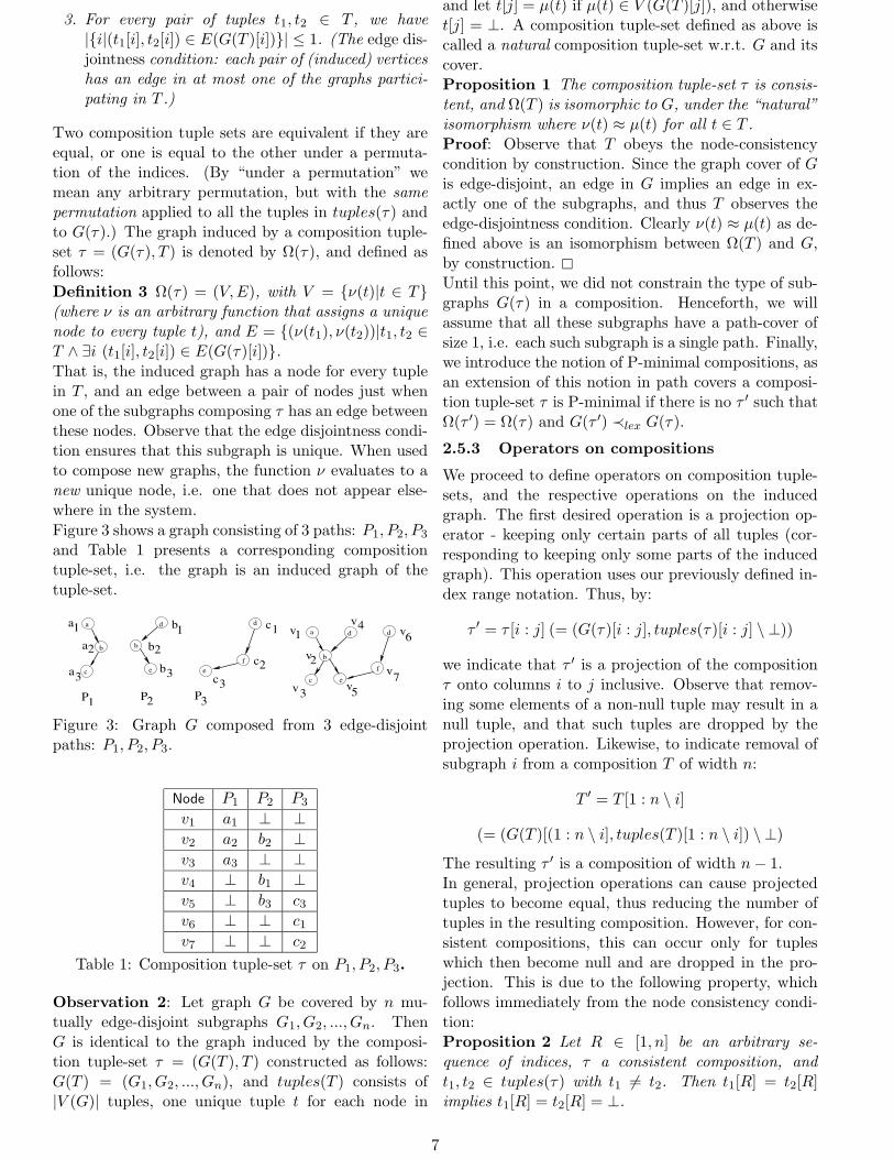
Definition 3 Ω(τ) = (V,E), with V = ν(t)|t ∈ T(where ν is an arbitrary function that assigns a uniquenode to every tuple t), and E = (ν(t1), ν(t2))|t1, t2 ∈T ∧ ∃i (t1[i], t2[i]) ∈ E(G(τ)[i]).That is, the induced graph has a node for every tuplein T , and an edge between a pair of nodes just whenone of the subgraphs composing τ has an edge betweenthese nodes. Observe that the edge disjointness condi-tion ensures that this subgraph is unique. When usedto compose new graphs, the function ν evaluates to anew unique node, i.e. one that does not appear else-where in the system.

Figure 3 shows a graph consisting of 3 paths: P1, P2, P3

and Table 1 presents a corresponding compositiontuple-set, i.e. the graph is an induced graph of thetuple-set.

v3

v2

v1v4

v5

v7

v6

P1

a1a2

a3

P2

b1b2

b3

P3

c1

c2c3

a

b

c

b

d

e e

a

b

c

d

e

d

ff

d

Figure 3: Graph G composed from 3 edge-disjointpaths: P1, P2, P3.

Node P1 P2 P3

v1 a1 ⊥ ⊥v2 a2 b2 ⊥v3 a3 ⊥ ⊥v4 ⊥ b1 ⊥v5 ⊥ b3 c3

v6 ⊥ ⊥ c1

v7 ⊥ ⊥ c2

Table 1: Composition tuple-set τ on P1, P2, P3.

Observation 2: Let graph G be covered by n mu-tually edge-disjoint subgraphs G1, G2, ..., Gn. ThenG is identical to the graph induced by the composi-tion tuple-set τ = (G(T ), T ) constructed as follows:G(T ) = (G1, G2, ..., Gn), and tuples(T ) consists of|V (G)| tuples, one unique tuple t for each node in

v ∈ G. Denote the bijection from tuples to nodes by µ,and let t[j] = µ(t) if µ(t) ∈ V (G(T )[j]), and otherwiset[j] = ⊥. A composition tuple-set defined as above iscalled a natural composition tuple-set w.r.t. G and itscover.Proposition 1 The composition tuple-set τ is consis-tent, and Ω(T ) is isomorphic to G, under the “natural”isomorphism where ν(t) ≈ µ(t) for all t ∈ T .Proof: Observe that T obeys the node-consistencycondition by construction. Since the graph cover of Gis edge-disjoint, an edge in G implies an edge in ex-actly one of the subgraphs, and thus T observes theedge-disjointness condition. Clearly ν(t) ≈ µ(t) as de-fined above is an isomorphism between Ω(T ) and G,by construction.Until this point, we did not constrain the type of sub-graphs G(τ) in a composition. Henceforth, we willassume that all these subgraphs have a path-cover ofsize 1, i.e. each such subgraph is a single path. Finally,we introduce the notion of P-minimal compositions, asan extension of this notion in path covers a composi-tion tuple-set τ is P-minimal if there is no τ ′ such thatΩ(τ ′) = Ω(τ) and G(τ ′) ≺lex G(τ).

2.5.3 Operators on compositions

We proceed to define operators on composition tuple-sets, and the respective operations on the inducedgraph. The first desired operation is a projection op-erator - keeping only certain parts of all tuples (cor-responding to keeping only some parts of the inducedgraph). This operation uses our previously defined in-dex range notation. Thus, by:

τ ′ = τ [i : j] (= (G(τ)[i : j], tuples(τ)[i : j] \ ⊥))

we indicate that τ ′ is a projection of the compositionτ onto columns i to j inclusive. Observe that remov-ing some elements of a non-null tuple may result in anull tuple, and that such tuples are dropped by theprojection operation. Likewise, to indicate removal ofsubgraph i from a composition T of width n:

T ′ = T [1 : n \ i]

(= (G(T )[(1 : n \ i], tuples(T )[1 : n \ i]) \ ⊥)

The resulting τ ′ is a composition of width n− 1.In general, projection operations can cause projectedtuples to become equal, thus reducing the number oftuples in the resulting composition. However, for con-sistent compositions, this can occur only for tupleswhich then become null and are dropped in the pro-jection. This is due to the following property, whichfollows immediately from the node consistency condi-tion:Proposition 2 Let R ∈ [1, n] be an arbitrary se-quence of indices, τ a consistent composition, andt1, t2 ∈ tuples(τ) with t1 6= t2. Then t1[R] = t2[R]implies t1[R] = t2[R] = ⊥.

7

Having defined the required notation, the main opera-tors used in our algorithm are defined below. Creatinga larger graph from two smaller graphs is done usingthe bijective sum operator, defined as follows.Definition 4 (Bijective Sum) Let τ1 = τ2 be com-positions, each of width n − 1, such that τ1[1 : (n −2)] = τ2[1 : (n − 2)]. Let T1 = tuples(τ1), andT2 = tuples(τ2). The bijective sum of τ1 and τ2, de-noted BS(τ1, τ2), is a composition τ of width n withG(τ) = G(τ1).G(τ2)[n − 1] and with tuples(τ) being(the union of) the following sets of tuples:

1. t1.t2[n − 1] | t1 ∈ T1, t2 ∈ T2, t1[1 : (n − 2)] =t2[1 : (n− 2)] 6= ⊥

2. ⊥n−2.t[n − 1].⊥ | t ∈ T1, t[1 : (n − 2)] = ⊥(where ⊥i means an all-⊥ i-tuple).

3. ⊥n−2.⊥.t[n− 1] | t ∈ T2, t[1 : (n− 2)] = ⊥The intuition for this definition is as follows, by consid-ering the induced graphs of the composition tuple-sets(see Figure 4). Now, map (and consider as the samenode) the nodes in the induced graphs standing for thetuples that include T1[1 : (n− 2)] to those induced byT2[1 : (n − 2)], basing the mapping on tuple equal-ity. Tuples in (1) correspond to nodes appearing inthe induced graphs of both τ1 and τ2. Tuples in (2)correspond to nodes that appear in the graph inducedby τ1, but do not appear in τ2. Likewise, tuples in (3)correspond to nodes that appear in the graph inducedby τ2, but do not appear in τ1. Henceforth, the con-struction (1) above will be called type 1 constructionand the respective generated tuples are called type 1tuples. Likewise for items (2) and (3) above. Observethat in some cases the result of a bijective sum may beinconsistent due to a violation of the edge disjointnesscondition. Our algorithm will discard the results ofsuch inconsistent bijective sums.The definition of bijective sum can easily be general-ized to allow for the equivalent part of τ1 and τ2 tobe any subset of indices of size n − 2, not necessarily[1 : (n− 2)], and not necessarily in sorted order. How-ever, this would make the notation exceedingly cum-bersome. Equivalently, one can view this generalizeddefinition as permuting the element positions of τ1 andτ2 in order to get τ1[1 : (n− 2)] = τ2[1 : (n− 2)], per-forming the bijective sum, and arbitrarily permutingthe positions of τ . In the description of the algorithm,we use this permutation scheme, in order to simplifythe notation.Table 2 demonstrates a bijective sum T3 = BS(T1, T2)of two composition tables T1 and T2, and Figure 4 therespective induced graphs G1 = Ω(T1), G2 = Ω(T2)and G3 = Ω(T3). Null values are shown as blanks.Observe that lifting the restriction that the width ofthe composition sets be equal results in a meaningful(as far as the induced graph is concerned) and poten-tially useful operator. But since our algorithm does

v1

v2

v3 v5

v6

v7v3

v2

v1v4

v5

v7

v6

v3

v2

v1v4

v5

v7

v6

P1 P2 P3

a1a2

a3

b1b2

b3

c1

c2c3

P4

d 1

d 2

d3

G2

v4

G1

G3 v8

v9

a

b

c

a

b

c

a

b

c

a

b

c

b

d

e

d

e

e

e

d

d

d

d

f

f

f

d

d

e

h

h

h

g

g

g

Figure 4: Induced graph of a bijective sum.not use such a generalization, we shall not discuss thisissue further.

Our algorithm also requires an operator that allowsnodes induced by tuples of types (2) to be mergedwith nodes induced by tuples of type (3) after a bi-jective sum. The merged nodes are determined by acomposition of width 2. For this purpose, we definethe splice operation, as follows (refer to Figure 5 as anexample).

Definition 5 (Splice) Let τ be a composition ofwidth n ≥ 3, and S be a composition of width 2, withG(S) = G(τ)[(n − 1) : n]. The result of splicing τby S, denoted Splice(τ, S), is a composition τ ′ withG(τ ′) = G(τ), and T ′ = tuples(τ ′) defined as follows.Denote T = tuples(τ), s = tuples(S), and let M be aset of “merged” tuples:

M = t1 + t2 | t1, t2 ∈ T,∃s ∈ s (1)

( t1[n− 1] = s[1] 6= ⊥ ∧ t2[n] = s[2] 6= ⊥∧ t1[n] + s[2] = s[2] ∧ t2[n− 1] + s[1] = s[1])

Let M ′ be the set of all tuples t1, t2 from T beingmerged above (i.e. that participate in the sum t1 +t2 inthe above definition of M). The tuples in the resultingcomposition are T ′ = M ∪ T \M ′.Observe that t1 = t2 is allowed in Equation 1. Also,note that it is possible to have S and T such that someof the t1 + t2 are undefined. In this case the splice op-eration is undefined (inconsistent). For example, Ta-ble 3 describes composition tuple-sets T1, T2 and theirsplice T3 = Splice(T1, T2). Figure 5 shows the cor-responding induced graphs G1 = Ω(T1), G2 = Ω(T2)and G3 = Ω(T3). In this figure, the paths P2 and P3

in G1 are spliced using information on nodes commonto these paths in G2.

3 The graph mining algorithm

This section presents our algorithm pseudocode formining frequent graph patterns, which works for bothdirected and undirected graphs. A proof of correctnessand a partial complexity analysis are then developed.

8

T1 T2 T3

Node P1 P2 P3 Node P1 P2 P4 Node P1 P2 P3 P4

v1 a1 u1 a1 w1 a1

v2 a2 b2 u2 a2 b2 w2 a2 b2v3 a3 u3 a3 w3 a3

v4 b1 u4 b1 d1 w4 b1 d1

v5 b3 c3 u5 b3 w5 b3 c3

v6 c1 u6 d2 w6 c1

v7 c2 u7 d3 w7 c2

w8 d2

w9 d3

Table 2: Bijective sum.

T1 T2 T3

Node P1 P2 P3 Node P2 P3 Node P1 P2 P3

v1 a1 u2 b1 c1 w1 a1

v2 a2 b2 u4 b2 w2 a2 b2v3 a3 u5 b3 c3 w3 a3

v4 b1 u6 c2 w4 b1 c1

v5 b3 c3 w5 b3 c3

v6 c1 w6 c2

v7 c2

Table 3: Splice.

G1

G2

v3

v2

v1v4

v5

v6

G3

v3

v2

v1v4

v5

v7

v6

v4

v5

v7

v2

P1

a1a2

a3

P2

b1b2

b3

P3

c1

c2c3

a

b

c

d

b

e

a

b

c

d

eef f

dd

d

e

d

e

bb

a

c

ff

Figure 5: Induced graph of a splice.

3.1 Description of the algorithm

The algorithm consists of three phases. In phase I, wefind all frequent paths (including paths with cycles),starting with frequent nodes and frequent edges. Inphase II, we find all graphs composed of two paths, inother words, we find all possible intersections betweenpairs of paths from phase I. In phase III we merge pairsof frequent graphs, each consisting of n−1 paths, suchthat the graphs have a common core of n− 2 paths, inan attempt to produce graphs with n paths. Through-out, we assume that some admissible support measureis used. In phases I and III we construct frequent graphpatterns recursively, using the Apriori approach [1].

Phase I (Algorithm 1) constructs the frequent pathsconsidering all frequent paths found in the previ-ous iteration, and potentially adding a frequent edge.Adding the edges is done using the ExpandPath func-tion. First, consider the case for directed graphs inExpandPath, which considers adding an outgoing edgefrom some nodes in the path. If the path is cyclic

b

b

aa

a

a

b

a

a

aa

a

+ =

b

b

aa

a

balanced node

unbalanced node

a

b

b

b

aa

a

+ =a

a

a

a

a

aa

a

a

a

aa

a

(a) adding edge to a non-cyclic path

(b) adding edge to a cyclic path

Figure 6: Phase I example.(not necessarily a simple cycle) we can add the out-going edge anywhere, provided the node labels match(see Figure 6b for examples). Otherwise, we can onlyadd an outgoing edge at a node that has an in-degreegreater than the out-degree - there can be only onesuch node if P is a path (Figure 6a). We use the nodeset X to denote the nodes where an edge can be added.There are now two cases: adding an additional nodeto the path (step 1, and see Figure 6 (a and b2) foran example), and adding an edge to a node alreadyon the path (step 2, see Figure 6b1 for an example)In the graph, one could add an edge at any node thathas unequal in-degree and out-degree (an unbalancednode), but it is sufficient to add just the outgoing edge,as shown in the proof of correctness later on.

Treatment of undirected graphs is practically thesame, differing only in that ExpandPath for undirected

9

Notation: Fi is a set containing frequent graphpatterns that are paths with i edges;ψ(.) is a function that creates a new node with thesame label as its argument.Ci is a candidate set for 1-path patterns with i edges.Output: L1, a sorted set containing the frequentpaths.

1. Find all frequent nodes and add them to F0.

2. Find and add to F1 all frequent edges by

scanning the data set and set k := 2.

3. Set Ck := ∅, Fk := ∅.4. For every path P = (V,E) ∈ Fk−1

and for every e ∈ F1 do:

Ck := Ck ∪ ExpandPath(P, e).

5. For every G ∈ Ck,add G to Fk if G is

frequent, and Fkcontains no graph isomorphic to G.

6. If Fk 6= ∅ set k := k + 1 and goto step 3.

7. Output L1 =⋃k−1i=1 Fi sorted according to ≺p.

Function ExpandPath(P, e) for directed graphsLet Result = ∅. Denote e by (v, u).If there is a node x ∈ V s.t. d−(x) < d+(x),let X = x.Otherwise (i.e. P is cyclic), let X = V .

1. For every x ∈ X s.t.

label(x) = label(v) add

G = (V ∪ ψ(u) , E ∪ (x, ψ(u))) to Result.

2. For every x ∈ X s.t. label(x) = label(v), and

every y ∈ V \ x s.t. label(y) = label(u) and

(x, y) /∈ E, add graph G = (V,E ∪ (x, y)) to

Result.

Function ExpandPath(P, e) for undirected graphsLet Result = ∅. Denote e by v, u.Let X be the set of nodes of odd degree in

P. If X is empty, (i.e. P is cyclic), let

X = V .

1. For every x ∈ X s.t. label(x) = label(v), add

G = (V ∪ ψ(u) , E ∪ x, ψ(u)) to Result.

2. For every x ∈ X, s.t.label(x) = label(u) add

G = (V ∪ ψ(v) , E ∪ x, ψ(v)) to Result.

3. For every x, y ∈ V , x 6= y s.t. x, y /∈ E,label(x) = label(v), label(y) = label(u)s.t. at least one of x, y is in X,

add G = (V,E ∪ x, y) to Result.

Algorithm 1: Frequent paths - Phase I

graphs considers adding an undirected edge. Here, anedge can be added anywhere if the path is cyclic, orat one of the two odd-degree nodes if the path is non-cyclic. When adding an additional node (steps 1, 2 inAlgorithm 1, ExpandPath for undirected graphs) thenew node can be at either end of the edge.

Observe that only in phase I there exists a significantdifference between directed and undirected graphs, ex-cept for code hidden in computing the number of paths

(which is a simple counting of node degrees), and inthe support measure (which is external and largely in-dependent of our algorithm).

Notation: L2 is a set that contains compositiontuple-sets of frequent graph patterns with pathnumber 2.C2 is a candidate set for the above compositiontuple-sets.

1. Let C2 = ∅, L2 = ∅.2. For every pair of paths P1, P2 ∈ L1

and every consistent composition

tuple-set τ with G(τ) = (P1, P2),s.t. Ω(τ) is connected and p(Ω(τ)) = 2, add

tuple-set τ to C2.

3. Remove from C2 all tuple-sets that

are not P-minimal.

4. For every tuple-set τ ∈ C2, if Ω(τ) is

frequent, add τ to L2.

5. Output graphs Ω(τ) | τ ∈ L2.

Algorithm 2: Frequent path pairs - Phase II

Phase II (see Algorithm 2) constructs the frequentgraphs with path number 2, by combining one-pathgraphs. The non-trivial steps are steps 2, 3 and 4,where in step 2 all possible compositions of the twopaths are considered, and in step 4 both the path num-ber and the support measure are calculated; in step3 all non-P-minimal isomorphic graphs are removed.Figure 7 shows (in terms of the lexicographic order wedefined earlier) how several different 2-path graphs areconstructed from two paths.

=+

a

b

c d

a

ordinary nodes

join nodes

a

b

c d

b

a

b

c d

a

b

c

a

b

d

Figure 7: Phase II example

Phase III (see Algorithm 3) constructs the frequentgraphs with path number n from graphs with pathnumber n − 1. The non-trivial step is step 2. In case2a the graph is constructed by finding the commonn − 1 subgraph structure and adding the remainingtwo paths P1, P2 (one from each graph), using thebijective-sum operation. Note that the specificationof an “arbitrary permutation” is just a notational con-venience, and is not actually implemented this way (itwould require an exponential number of tests). In-stead, the composition tuple-sets τi are represented insorted order of the paths in G(τi), where each path is

10

represented by its index in the sorted L1. To checkwhether two compositions can undergo bijective sum,simply compare the strings of sorted indices of pathsin G(τ1), G(τ2), allowing for up to one substitution,which can be done very efficiently. The number ofcases meeting this requirement is typically many or-ders of magnitude smaller than the number of possi-ble permutations, which are not explicitly generated1.Only after the above test passes do we need to comparethe tuples in the projected tuple-sets.

In case 2b, any combination S of the two paths P1, P2

which is frequent and isomorphic to the remainingpaths is found from L2. Although not stated in thepseudocode, this step is fast because L2 can be indexedfor fast retrieval of compositions containing specificpaths. The paths P1, P2 in the graph are combined(using Splice) with the generated candidate. This lat-ter step is needed because merging two patterns di-rectly (using bijective sum) may overlook cases wheresome nodes in the remaining paths are shared. Step3 removes redundant isomorphic graphs, while step 4checks the support of the candidates, as in phases Iand II.

An optional final step in the algorithm (not shownhere) is removing all frequent sub-graphs which arenot maximal, i.e. contained in larger frequent graphs.Figure 8 demonstrates merging two 2-path graphs thathave one path in common, into one 3-path graph.

Notation: Ln: set of composition tuple-sets of widthn.Cn is a candidate set for these compositions.

1. Set n = 3, Cn =∅, Ln =∅.2. For every pair τ1, τ2 of (arbitrarily

permuted) composition tuple-sets from Ln−1

s.t. τ1[1 : n− 2] = τ2[1 : n− 2], do:

(a) Construct τ = BS(τ1, τ2).If Ω(τ) is connected and has

path number n, add τ to Cn.

(b) For every composition tuple-set S ∈ L2,

if Ω(Splice(τ, S)) is connected and has

path number n, add Splice(τ, S) to Cn.

3. Remove from Cn all composition tuple-sets

that are not P-minimal.

4. For every τ ∈ Cn, add τ to Ln if Ω(τ) is

frequent.

5. If Ln = ∅, halt.

6. Output Ω(τ)|τ ∈ Ln, then set n := n+ 1 and

go to step 3.

Algorithm 3: Frequent graphs - Phase III

1The fact that non-isomorphic paths can have the same de-scriptor is a complication, but not a serious problem, especiallyin labeled and directed graphs, where such cases are less likelyto occur.

+ =

a

b b

a

b

c d

b

d e

b

c d

b

e

b

common path

paths that are different

a

Figure 8: Phase III example

3.2 Proof of correctness

It is obvious by construction, that our algorithm issound, since (in all phases) only frequent patterns arekept at the end of the computation. Therefore, show-ing completeness of the algorithm, i.e. that all fre-quent patterns are indeed found by the algorithm, issufficient to prove correctness. Since all phases of thealgorithm are separate (and run sequentially), com-pleteness of each will be formally stated and provedseparately.

Theorem 3 When phase I (Algorithm 1) completes,L1 contains all frequent single-path graph patterns.

Proof outline: Note that from every path with kedges an edge can be removed so that the remaininggraph is a path with k−1 edges. Using the admissibil-ity of the support measure, and the assumption thatall frequent paths with k − 1 edges were found in theprevious iteration, the theorem follows by induction.

Theorem 4 Phase II (Algorithm 2) outputs all con-nected frequent graphs patterns with path number 2.Additionally, at the end of phase II, the set L2 con-tains all P-minimal composition tuple-sets, for everyconnected frequent graph pattern with path number 2.

Proof. Let G be a frequent graph pattern withp(G) = 2. Then G can be decomposed into two edge-disjoint paths, and has a P-minimal decompositionP1, P2. Since we are using an admissible support mea-sure, P1 and P2 are frequent, and by Theorem 3 anisomorphic copy of each of them is in L1 at the end ofphase I. Denote the isomorphisms of P1, P2 by P ′1, P

′2,

respectively. During phase II, all possible consistentcomposition tuple-sets τ with G(τ) = (P ′1, P

′2) are con-

structed, including the composition τ for which Ω(τ) isisomorphic to G under the natural isomorphism. Sincethe path descriptors are invariant under isomorphism,and the decomposition of G into P1, P2 is P-minimal,then τ is also P-minimal, and thus not pruned fromC2 at step 3. Since G is frequent, τ is stored in L2 instep 4, and G is output at step 5.

Theorem 5 Phase III outputs all frequent connectedgraph patterns G with path number p(G) ≥ 3.

Proof outline: We show the invariant that at theend of each iteration n, if G is a frequent graph with

11

path number n, then there is a P-minimal compositionτ ∈ Ln such that Ω(τ) is isomorphic to G. Proofof the invariant is based on the invariant holding forgraphs with path number n − 1 at the beginning ofthe iteration, which holds for n = 2 due to Theorem4. Using the admissibility of the support measure, weshow that if G is frequent then there exist P-minimalcompositions in Ln−1 with a common core of widthn− 2. These compositions induce frequent subgraphsG1, G2 with path number n− 1, that are composed inthe iteration by using bijective sum and splice to formG.

3.3 Complexity discussion

The complexity of our algorithm is composed of twocomponents. The first component has to do with theproblem definition, and not with the specific algo-rithm. This complexity is exponential in the size ofthe pattern, and inherent to apriori-like algorithms.The complexity of Apriori is due to the fact that thenumber of frequent patterns can be exponential, andthe complexity of any graph mining algorithm is con-strained by the need to find all subgraphs of a databaseisomorphic to a given pattern in order to evaluate itssupport. The main goal of a mining algorithm shouldthus be to decrease the number of candidate patterns,and by doing so decrease the number of support com-putations. Our approach is feasible, because the num-ber of patterns remaining from one phase to the nextis reduced considerably, according to our experiments.The generation of candidate set Cn−1 in the worst case,takes time:

O(|Ln|2

2∗ n2 ∗ |L2|).

In real life cases, frequent patterns from the set Ln usu-ally have different path structure and labeling, and thenumber of candidate patterns created is much smaller.Even though the complexity is bounded by an expo-nential in n, in reality for large databases, the scan ofthe database whose complexity is n ∗N may be worse,and in these cases, the approach of apriori-TID maybe beneficial.

Support computation. The second component ofcomplexity is due to the need to find all subgraphsisomorphic to the given pattern, which is exponentialin the size of the pattern as well. While the largenumber of support computations is inherent to thebasic Apriori algorithm ([1]), complexity of a singlesupport computation is significantly higher for semi-structured databases. Such computation requires (a)finding all subgraphs of a database isomorphic to agiven graph pattern; (b) evaluating support using anadmissible support measure. Finding all subgraphs ofa database graph isomorphic to a given pattern de-pends strongly on the topology of a database graph.For a dense graph, the number of such subgraphs canbe exponential in the size of a pattern. For a com-

plete graph and an appropriate support value, everysubgraph of a complete graph can be frequent! How-ever, for a sparse graph (or the case for the real-lifesemi-structured databases) the number of instances ofa pattern is much smaller. In addition, a databasegraph with a large number of different labels is likelyto produce a smaller number of pattern instances thana similar graph with a small number of different labels.A formal complexity analysis of the entire algorithmis very difficult, and thus not pursued here. Althoughthe complexity is exponential in the worst case, theexperiments in the next section suggest that for non-dense graphs the algorithm is still reasonable for largegraphs.

4 Empirical evaluation

In the empirical evaluation, two sets of experimentswere performed. The first set of experiments comparesour algorithm to an edge-based algorithm. Two typesof databases were used: synthetic, where we can con-trol both the topology and labeling of graphs, and areal-life XML ”movies” database [29]. Only the sin-gle graph setting was tested in this set of experiments.The second set of experiments compared our algorithmto FSG for both transactions and single graph settings.This set of experiments used also two databases, onesynthetic, and a real-life social network composed ofelectronic mails. The database records emails over aperiod of a week among users of the BGU email sys-tem. Source, destination and size of the message wererecorded. The message size is used as an approximate”label” on the edge.

4.1 Experimental setting

The experimental environment is a Sun Ultra-30 work-station running at 247 MHz and 128 MB of mainmemory. The real XML file we used is a portion ofthe “movies” database. XML elements are treated asnodes, and inheritance relationships and references -as edges.

4.1.1 The support measure

The standard measure of support for transactiondatabases in the literature is as follows. The supportS for an item set I =< i1, ..., ik > in a dataset oftransactions D is:

S(I) =|t | t ∈ D,< i1, ..., ik >∈ t|

|D| (2)

However, if the application makes it necessary to countthe total number of occurences of a pattern, the abovescheme is inappropriate. An alternate definition ofsupport, taking the multiple occurences into account,must be defined, a non-trivial issue due to possibleoverlaps between instances.For example, one trivial support measure is the num-ber of instances of a frequent pattern. This measure,however, is not admissible. Figure 9 shows a database

12

that contains 3 instances of pattern A and only one in-stance of pattern B, while B ⊆ A. Another approachis to take into account all automorphisms of a pat-tern in question. Again, the database in figure 9 is acounterexample, since |Aut(B)| = 6 and |Aut(A) = 4|,making the total count of A’s instances 12 which isstill greater than 6.

B - appears once

but not independentlyA - appears 3 times,

Database graph

Figure 9: Graph pattern support

The only non-trivial provably admissible measure wecould find for the “single-graph”-setting is defined asfollows [33]. Let D be a database graph, and G be agraph pattern for which we wish to compute support.Let A1, A2, ..An be all instances of G in D. We create anew graph called the instance graph, in which each ofthe Ai is a node, and there is an edge between Ai andAj if the two sub-graphs Ai and Aj have at least onecommon edge. The maximum independent set (MIS)measure is defined as the size of the maximum inde-pendent set over the instance graph, and was shown in[33] to be admissible.Using the MIS measure, we must compute the maxi-mum independent set of the instance graph IG. The-oretically, this can take time exponential in the sizeof IG, since the independent set problem is NP-hard.However, for real-life cases of sparse database graphwith a reasonable number of labels, this task is usuallymuch easier. In our experiments, time for computingthe maximum independent set was actually negligiblecompared to the time to find the instances. There-fore, the performance of the algorithms is not stronglydependant on the specific (MIS) support measure. Inaddition, approximation techniques can be used in thiscase (see [15] for details) as a user usually does not careabout a precise support value. See further discussionon computing the MIS measure in Section 5.

4.2 The implemented algorithms

We implemented the mining algorithm for fully labeledgraphs described in Section 3, as well as the two typesof edge-based algorithms discussed below. The latterwere used in order to compare the number of gener-ated candidate patterns with our algorithm. 2 Thesame admissible MIS support measure was used for all

2The reason our comparison is done opposite simple edge-based algorithms, rather than to FSG or GSPAN, is that thelatter algorithms use the transaction-graph setting, making a di-rect comparison inapplicable. Additionally, little research existson algorithms that use the maximum independent set (MIS) sup-port measure, the only non-trivial admissible support measurewe know for the single-graph setting (see Section 5).

algorithms. Tests were conducted multiple times andtime averages were taken to eliminate factors of systemload.

The first algorithm is based on finding all frequentgraphs G with k edges, and then extending each graphG into graphs with k+ 1 edges by either adding a newnode and an edge to G frequent graph or by addingan edge between two existing nodes of G. The processis repeated until no graphs extended in this mannerare frequent. For the comparison with FSG, we haveimplemented a version of FSG for the single graph set-ting, based on [21].

4.3 Experimental results

4.3.1 First set

We investigated the behavior of the algorithms usingthe following performance parameters: (1) number ofcandidate patterns produced by an algorithm duringdata mining; (2) number of isomorphism computationsduring data mining, and overall number of supportcomputations; (3) total time spent on data mining(not CPU time) and on support computations.

Table 5 presents results for testing on synthetic treesand synthetic sparse graphs. The notation used in allthree tables is explained in Table 4. For our algorithmthe number of candidate patterns can sometimes beless than the number of frequent patterns since fre-quent nodes and edges are computed directly with-out generating candidate patterns. Our implementa-

N, E, L # of nodes, edges and labels in the database

S support threshold in %

C, FP # of candidate and frequent patterns

I, SC # of isomorphism and support computations

TT total time (seconds) spent on data mining

ST time in sec. of support computations

EA edge addition algorithm

PM Path Mining, denotes our algorithm

# serial number of a database graph

CR candidate ratio

Table 4: Notation used in results tables

tion needs to generate all appropriate subgraphs of adatabase graph, find among them all subgraphs thatare isomorphic to the pattern in question, and buildan instance graph and find its maximum independentset size. Thus, testing our algorithm on dense graphsseems to be extremely time consuming. An additionalconsideration was the fact that most real-life databasesrepresent sparse graphs rather than dense ones. There-fore, we decided to limit our tests to trees and sparsegraphs and to choose a support threshold that, on theone hand, will not limit the output to trivial graphs(nodes and edges) and on the other hand, will not makeevery connected subgraph of the database frequent.

From Table 5 we conclude that our algorithm runsfaster even though it conducts more isomorphism

13

Trees Sparse graphs

# N, L, S, FP Alg C, I, SC ST TT N, E, L, S, FP Alg C, I, SC ST TT

1 40 4 7% 15 EA 100 24 92 41 44 40 50 4 7% 14 EA 60 33 52 19 24

PM 52 47 52 12 20 PM 49 55 42 14 23

2 50 4 7% 16 EA 110 41 102 676 682 40 50 6 5% 17 EA 84 48 76 33 40

PM 45 45 42 22 29 PM 59 70 54 15 26

3 50 6 3% 37 EA 470 82 458 326 340 50 60 6 5% 28 EA 355 74 343 314 326

PM 202 239 205 68 106 PM 117 185 143 41 70

4 50 8 3% 27 EA 306 62 290 280 290 60 80 4 4% 16 EA 101 31 93 609 614

PM 119 91 111 12 39 PM 56 58 56 123 132

5 60 4 5% 15 EA 100 24 92 220 224 60 80 6 3% 27 EA 265 86 253 842 857

PM 52 47 52 56 63 PM 120 102 110 41 57

6 60 6 5% 44 EA 728 203 716 3493 3537 70 90 8 3% 27 EA 252 77 236 44 57

PM 175 868 276 238 376 PM 126 98 110 21 37

7 60 8 5% 14 EA 103 18 87 19 22 80 100 8 3% 32 EA 403 74 387 160 172

PM 41 29 26 4 9 PM 149 127 141 41 60

Table 5: Experimental results for trees and sparse graphs

checks than the edge addition algorithm. The latteroccurs because our algorithm produces fewer candi-date patterns, and thus less time is wasted on supportcomputation.Table 6 contains the number of frequent patterns foundin six different subsets of the movie database with dif-ferent support values. The structure of the database(a tree as in set #6 or a sparse graph) can be seen tohave more impact on the number of frequent patternsthan the support value.As seen from Table 6, for the same values of sup-port, the number of frequent patterns is smaller, andthus the execution time is much smaller in the moviedatabase than in the synthetic dataset. This indicatesthe feasibility of our algorithm in real-life cases. As thegraph becomes larger, the number of frequent patternsfor the same support value decreases since a largernumber of edge-disjoint instances is required for eachpattern in order to pass the support threshold. Notethat these patterns do not contain titles of movies ornames of directors, since these are present only as at-tributes and not as tags in the XML database. Relatedresearch [25] attempts to treat attributes and values ofan XML database as well.We deduce the following facts from our experiments:

1. Our algorithm produces fewer candidate patternsand therefore performs fewer support computa-tions than the edge addition algorithm.

2. Support computation is easier if the database is atree due to fewer candidate patterns.

3. Synthetic graphs are not very regular. As thenumber of distinct labels in synthetic database in-creases, the chance of finding non-trivial frequentpatterns in that database decreases drastically.

4. Large real-life graph databases are highly regularand contain complex patterns.

4.3.2 Second set - comparison with FSG

In this set of experiments, we compared FSG with ouralgorithm for both transaction setting and single graphsetting. For the transaction setting, the results werecomparable and are not shown here. For the singlegraph setting, we measured both the time and thenumber of support computations. Since the runningtime was dominated by the number of support compu-tations, we decided not to report it at all, and insteadreport the number of support computations, which isequal to the number of candidates generated. There-fore in all the tables and graphs below, the measure ofefficiency is the number of candidates generated.

Table 7 shows number of candidate and frequent pat-terns generated by both algorithms for various supportvalues on two subsets (5000 and 2000 nodes) of a Ben-Gurion university e-mail traffic database. The entiredatabase is large (over 50000 nodes) and quite dense,which makes it difficult to mine. In all tables, PMstands for Path Mining and denotes results achievedby our algorithm.

Table 8 shows numbers of candidates and frequent pat-terns generated by both algorithms for various supportvalues on random graphs with 3000 nodes, 4000 edgesand different numbers of labels: 30, 40 and 50. Theseresults show that our algorithm produces fewer candi-date patterns that FSG and therefore performs fewersupport computations.

Figure 10 shows numbers of candidates generated byboth algorithms for various support values on randomgraphs with 1000 nodes, 2000 edges and different num-bers of labels: 10 and 20 respectively. We learned fromour experiments that support computation is the fac-tor having the most impact on the computation timebecause of the need for multiple subgraph isomorphismcomputations, in both single and multiple graph set-tings. Reducing support computation is significantlymore important than computing a DFS code of a pat-

14

Data set Nodes Edges Labels S 50% 40% 30% 20% 10% 9% 8% 7% 6% 5%

#1 12656 13878 112 FP 5 6 7 8 15 16 16 18 21 22

#2 8337 9416 25 FP 3 4 5 6 12 12 12 12 13 14

#3 7027 7851 22 FP 3 4 4 5 10 10 10 10 11 11

#4 4730 4813 90 FP 5 5 8 9 11 11 12 12 12 16

#5 2757 2794 76 FP 2 2 5 6 7 7 8 9 10 11

#6 1293 1292 91 FP 21 32 34 46 79 79 84 84 86 86

Table 6: Movie DB: support vs. frequent patterns

5000 nodes 2000 nodes

S C FSG C PM FP CR S C FSG C PM FP CR

1% 54 45 9 1.2 0.1% 209 190 19 1.1

0.9% 54 45 9 1.2 0.09% 252 231 21 1.09

0.8% 65 55 10 1.18 0.08% 252 231 21 1.09

0.7% 65 55 10 1.18 0.07% 275 253 22 1.09

0.6% 65 55 10 1.18 0.06% 275 253 22 1.09

0.5% 65 55 10 1.18 0.05% 405 378 27 1.07

0.4% 77 66 11 1.17 0.04% 405 378 27 1.07

0.3% 77 66 11 1.17 0.03% 527 496 31 1.06

0.2% 119 105 14 1.13 0.02% 527 496 31 1.06

0.1% 230 210 20 1.1 0.01% 1034 990 44 1.04

Table 7: BGU e-mail database results

50 labels 40 labels 30 labels

S C FSG C PM FP S C FSG C PM FP S C FSG C PM FP

0.2 113 83 28 0.3 28 20 8 0.5 3 2 1

0.19 113 83 28 0.25 187 152 35 0.45 9 6 3

0.18 113 83 28 0.24 187 152 35 0.4 40 29 11

0.17 306 244 58 0.23 187 152 35 0.35 185 147 32

0.16 306 244 58 0.22 408 339 63 0.3 884 707 920.21 408 339 630.2 1216 1020 126

Table 8: Random graph with 3000 nodes and 4000 edges

Figure 10: Random graph with 1000 nodes and 2000edgestern or eliminating isomorphic candidates, since fre-quent patterns are not very large compared to thedatabase size.

5 Discussion and related work

This section briefly presents related work, and dis-cusses our contribution in the context of prior researchin the field. As mentioned in the introduction, mostof the work done on graph mining is comparatively re-cent. The basic work related to this subject is frequentitem-set mining in structured databases and the Apri-ori algorithm and its variations [1]. For conciseness,

reference to the significant body of existing work ontransaction database mining is omitted. Papers thatdeal with mining topologically simple patterns, such aspaths and trees, are directly related to our work andthus reviewed below.

[2] presents two algorithms for mining frequent di-rected simple path patterns in a web environment.Both algorithms are based on an algorithm called MF,that finds all maximal forward references in a set oftraversal sequences contained in the database. Thegoal of the two mining algorithms is to find frequentsequences in these paths. The main differences be-tween the algorithm of [2] and ours is that the formerhandles only linear paths, making its support measurecomputationally simple.

The simple paths mining problem is generalized in [36],which describes an algorithm for finding maximal fre-quent tree-like patterns in semi-structured documents,represented in the standard OEM model. Althoughthis algorithm searches only for tree-like patterns, itcan also handle patterns containing cycles by trans-forming them into trees. One important restriction inthis paper is that only rooted trees are considered, i.e.trees whose root is the same as the root of the entireweb database. Chi, Nijssen, Muntz and Kok handlethe problem of tree mining in a wider sense in [28].

15

Work on mining general graph patterns began in the90’s. A recent survey of graph mining, by Washioand Motoda [38], presents some of the earlier workson the subject like SUBDUE [7] and GBI [42]. It thenclassifies the mining algorithms into two major cate-gories. Greedy search algorithms which search exhaus-tively for all the frequent graph patterns, and Induc-tive (ILP) approaches which pregenerate many graphpatterns according to some logic constraints and back-ground knowledge, and then use a query language toretrieve the interesting patterns [27]. Since our paperuses the greedy approach, we do not further discussILP here.

Regarding the greedy approach, two categories of al-gorithms were mentioned in the introduction: transac-tion graphs and single graph settings. To-date, mostwork was for the transaction graph setting, with algo-rithms are divided roughly into two classes: breadth-first search (or Apriori-based) and depth-first search.

Most BFS algorithms use the basic idea employed inthe Apriori algorithm. The main difference betweenthe various algorithms of this category is in the typeof the building block used to generate the item of levelK. [18] uses vertices. An algorithm by Kuramochiand Karpis [20] uses edges as the main building block,and was extended and improved in [21] by adding sev-eral clever heuristics which make mining and supportcomputation more efficient. This latter version, calledFSG, is currently one of the best known and oftencompared to version of BFS graph mining algorithmsfor the graph-transaction setting case. FSG introducesthe definition of a canonical labeling of graphs basedon the adjacency matrix, used to eliminate isomorphiccandidates. To increase the efficiency of deriving thecanonical labels, the approach uses some graph ver-tex invariants, such as the degree of each vertex inthe graph. FSG also increases the efficiency of thecandidate frequent subgraph generation by introduc-ing the transaction ID (TID) method. Furthermore,FSG limits the class of the frequent subgraphs to con-nected graphs. Under this limitation, FSG introducesan efficient search algorithm using a “core”, which is ashared part of size k−1 in the two frequent subgraphsof the size k. FSG increases the joining efficiency bylimiting the common part of the two frequent graphsto the core. Once the candidates are obtained, theirfrequency counting is conducted by checking the cardi-nality of the intersection of both TID lists. FSG is fastdue to the introduction of numerous techniques, but itsmemory consumption is heavy (storage for TID lists ofmassive graph data). Some ideas similar to those inFSG, e.g. those related to joining of two sub-graphs,are present in this paper as well. However, the methodin this paper was derived independently, and our useof edge-disjoint paths as a building block is new.

Other works which use the BFS approach are [19, 16,17, 6]. The second approach, called gSpan [40], grows

patterns from a single graph directly, by using a depth-first search strategy. The algorithm maps each patternto a unique canonical label, and assigns each graph aunique minimum DFS code. By using these labels,a complete order relation is imposed over all possiblepatterns. This lexicographic order is also used to im-pose a tree-hierarchy order over all patterns, resultingin a hierarchical search tree. This search-tree is tra-versed in a DFS manner, pruning on the way all sub-graphs with non-minimal DFS code. This algorithmalso uses the TID approach. Since the algorithm ex-plores the search space in DFS manner, it enables useof several mining techniques which are especially ap-plicable to DFS algorithms, such as maintaining anembedding set for each frequent subgraph, like [54].[40] also presents an experimental evaluation wherethey compare gSpan with FSG and show the betterperformance of gSpan on several molecular databases.Several of the ideas of [40] were used later on in an ap-proach which is intermediate between BFS and DFS,in [18].

In summary, the ideas presented in the above papers,have influenced our work considerably. However, usingpaths as building blocks, and an efficient method formerging graphs represented as compositions of paths,are original contributions of this paper. From our ex-perimens we did not see an inherent problem of scalingup the algorithm to very large graphs, however, we en-countered memory problems with large graphs. Thesemay be handled similarly to [35].

6 Conclusion

An apriori-like algorithm for retrieving frequent graphpatterns from a given set of graphs is the central is-sue in this paper. In contrast with most existingwork, the pattern can be either a directed or an undi-rected graph, and may contain cycles. The addedfunctionality can support data mining on the increas-ing fraction of on-line documents, which consist ofblocks connected by references. Knowledge abouttypical structure of documents is helpful in analyz-ing complex repositories of semistructured data (e.g.XML databases, the web), and is potentially usefulfor querying data, indexing it and storing it efficiently.In searching for frequent patterns, candidates are con-structed using frequent paths. The scheme is evalu-ated empirically and is promising, as it shows a de-cided advantage over other algorithms. The schemeproposed here can be extended in several ways, suchas using partially labeled patterns, using more com-plex building blocks (trees), adapting the algorithmto the dynamic database model and using apriori-TIDtechnique.

Aknowledgements

Partially supported by the KITE consortium undercontract to the Israeli Ministry of Trade and Indus-

16

try, and by the Paul Ivanier Center for Robotics andProduction Management. We wish to thank MarinaLitvak for implementing a significant fraction of thecode for the experiments, and the anonymous review-ers for useful comments that contibuted to the finalversion of the manuscript.

References

[1] R. Agrawal and R. Srikant, Fast Algorithms for Mining

Association Rules, Proc. of the 20th Int’l Conf. on VLDB ,

Santiago, Chile, September 1994.

[2] M. S. Chen, J. S. Park, P. S. Yu, Efficient Data Mining for

Path Traversal Patterns, IEEE Transactions on Knowledge

and Data Engineering , 10(2), 1998: 209-221.

[3] D. Chamberlin, XQuery: A Query Language for XML,

Proceedings of SIGMOD Conference 2003

[4] Y. Chi, S. Nijssen, R. R. Muntz, and J. N. Kok. Frequent

subtree mining: an overview, Fundamenta Informaticae,

Special Issue on Graph and Tree Mining, 2005

[5] C. Chung, J. Ki Min, K. Shim: APEX: an adaptive path

index for XML data, Proceedings of SIGMOD Conference

2002: 121-132, 2002

[6] M. Cohen, E. Gudes, Diagonally Subgraphs Pattern Min-

ing , Proceedings of the 9th ACM SIGMOD Workshop on

Research Issues in Data Mining and Knowledge Discovery,

Paris, France, 2004

[7] J. Cook, L. Holder, Substructure discovery using minimum

description length and background knowledge, J. of Arti-

ficial Intell. Research, pages 231-255, 1994

[8] L. Dehaspe, H. Toivonen, and R. D. King, Finding fre-

quent substructures in chemical compounds, Proceedings

of the 4th International Conference on Knowledge Discov-

ery and Data Mining (KDD-98), pages 30-36. New York,

New York: 1998

[9] A. Deutsch , M. Fernandez , D. Florescu , A. Levy , D.

Maier , D. Suciu, Querying XML data, IEEE Data Engi-

neering Bulletin 22(3), 1999: 27-34.

[10] A. Deutsch, M. F. Fernandez, D. Suciu, Storing Semistruc-

tured Data with STORED, Proceedings of SIGMOD Con-

ference 1999: 431-442.

[11] C. Domshlak, R. Brafman and S. E. Shimony, Preference-

based Configuration of Web Page Content, Proceedings of

IJCAI , August 2001.

[12] Garton, L., Haythornthwaite, C. and Wellman, B. Studyin-

gOnline Social Networks. Journal of Computer-Mediated

Communication, 3(1), 2004

[13] R. Goldman and J. Widom, DataGuides: Enabling

Query Formulation and Optimization in Semistructured

Databases, Proc. of 23rd VLDB Conf ., Athens, Greece,

1997.

[14] R. Goldman, J. Widom, DataGuides: Enabling Query For-

mulation and Optimization in Semistructured Databases.

Proceedings of VLDB 1997: 436-445, 1997

[15] E. Gudes, S. E. Shimony, N. Vanetik, Support measures for

semistructured data. To appear in DAMI journal, 2006

[16] M. Hong, H. Zhou, W. Wang, B. Shi, An Efficient Algo-

rithm of Frequent Connected Subgraph Extraction Pro-

ceedings of PAKDD, 2003

[17] J. Huan, W. Wang, J. Prins, Efficient Mining of Frequent

Subgraphs in the Presence of Isomorphism. Proceedings of

ICDM 2003: 549-552, 2003

[18] A. Inokuchi, T. Washio, H. Motoda, An apriori based algo-

rithm for mining frequent substructures from graph data,

Proceedings of PKDD00, 2000

[19] A. Inokuchi, T. Washio, H. Motoda: Complete Mining of

Frequent Patterns from Graphs, Mining Graph Data. Ma-

chine Learning 50(3): 321-354 2003

[20] M. Kuramochi and G. Karypis, Frequent Subgraph Discov-

ery, Proceedings of IEEE ICDM, 2001.

[21] M. Kuramochi and G. Karypis, An efficient algorithm for

discovering frequent subgraphs, IEEE Trans on Knowledge

and Data Eng., Vol 16, No. 9, Sept. 2004

[22] M. Kuramochi and G. Karypis, Finding Frequent Patterns

in a Large Sparse Graph Proceedings 2004 SIAM Data

Mining Conference, Orlando, Florida, 2004

[23] V. Lipets and E. Gudes, An Efficient Algorithm for Sub-

graph Isomorphism, 4th Haifa workshop on graph theory

and algorithms, Haifa, Israel, 2004.

[24] X. Lin, Ch. Liu, Y. Zhang and X. Zhou, Efficiently Com-

puting Frequent Tree-Like Topology Patterns in a Web

Environment, Proceedings of 31st Int. Conf. on Tech. of

Object-Oriented Language and Systems, 1998.

[25] A. Meisels, M. Orlov, T. Maor, Discovering associations in

XML data, BGU Technical report , 2001.

[26] T. Milo and D. Suciu: Index Structures for Path Expres-

sions, Proceedings of ICDT 1999: 277-295D, Jerusalem,

Israel, 1999

[27] S. Muggleton, L. DeRaedt, Inductive logic programming:

Theory and methods, J. of Logic programming, 19(2),

pages 629-679, 1994

[28] Nijssen, S., J. N. Kok: Frequent graph mining and its ap-

plication to molecular databases, proceedings of IEEE Int.

Conf. on Systems, Man and Cybernatics, pp. 4571-4577,

2004

[29] Movie database, http://us.imdb.com.

[30] X. Pennec, N. Ayache, A geometric algorithm to find small

but highly similar 3D substructures in proteins, Bioinfor-

matics 14(6): 516-522 ,1998

[31] D. Shasha, J. T. L. Wang and R. Guigno, Algorithmics and

Applications of Tree and Graph Searching, Proceedings of

the 21st ACM SIGMOD-SIGACT-SIGART Symposium on

Principles of Database Systems, 2002, pp. 39-52

17

[32] F. Tian, D. DeWitt, J. Chen, and C. Zhang, The Design

and Performance Evaluation of Alternative XML Storage

Strategies, Technical report, CS Dept., University of Wis-

consin, 2000.

[33] N. Vanetik, E. Gudes, S. E. Shimony, Computing Frequent

Graph Patterns from Semistructured Data, Proceedings

ICDM 2002 : 458-465.

[34] N. Vanetik and E. Gudes, Mining Frequent Labeled and

Partially Labeled Graph Patterns, Proceedings of ICDE

2004: 91-102, Boston, MA, 2004

[35] C. Wang, W. Wang, J. Pei, Y. Zhu, B. Shi, Scalable min-

ing of large disk based graph database, Proceedings of

KDD2004, Seatle, 2004

[36] K. Wang, H. Liu, Discovering Typical Structures of Doc-

uments: A Road Map Approach, Proceedings of SIGIR

1998 : 146-154.

[37] X. Wang, J. T. Li Wang, D. Shasha, B. Shapiro, I. Rigout-

sos, K. Zhang, Finding Patterns in Three-Dimensional

Graphs: Algorithms and Applications to Scientific Data

Mining, IEEE Trans. on Knowledge and Data Eng. 14(4):

731-749, 2002

[38] T. Washio, H. Motoda, State of the art of graph-based data

mining,, SIGKDD explorations, July, 2003

[39] S. Wasserman, K. Faust, D. Iacobucci, Social Network

Analysis: Methods and Applications (Structural Analysis

in the Social Sciences S.) Cambridge university press, 1994

[40] X. Yan and J. Han, gSpan: Graph-Based Substructure Pat-

tern Mining, Proceedings of ICDM 2002 : 721-724.

[41] X. Yan and J. Han, CloseGraph: mining closed frequent

graph patterns, Proceedings of KDD03, Washington, 2003

[42] K. Yoshida, H. Motoda and N. Indurkhya, Graph-based

induction as a unified learning framework, J. of Applied

Intelligence, pages 297-328, 1994

Solomon Eyal Shimony receivedthe BSc degree in Electrical Engi-neering from the Technion in 1982,a PhD in Computer Science fromBrown University in 1991, afterwhich he joined the department ofComputer Science at Ben-Gurion

University. At present, he is a deputy head ofCS department at BGU, chair of the Paul IvanierCenter for Robotics and Production Management,and an associate editor of IEEE Systems, Man, andCybernetics, section B. His research interests are ar-tificial intelligence, probabilistic reasoning, knowledgediscovery in databases, robotics, flexible computation,and spatial data models.

Ehud Gudes recieved his Bsc andMsc from the Technion, and hisPhD in Computer and Informa-tion Science from the Ohio StateUniversity in 1976. Following hisPhd, he worked both in academia(Penn State University, Ben-GurionUniversity,), where he did researchin the areas of database systems

and data security, and in industry (Wang Laborato-ries, National Semiconductors, Elron, IBM Research),where he developed query languages, CAD software,and expert systems for planning and scheduling. Heis currently an associate professor in computer scienceat BGU, and his research interests are: knowledge anddatabases, data security and data mining, especiallygraph mining.

Natalia Vanetik received the BScdegree in mathematics and com-puter science from Ben-Gurion Uni-versity in 1996, the MSc degreein mathematics and computer sci-ence from Ben-Gurion University in2003. She is currently a PhD stu-

dent at the Department of Computer Science, Ben-Gurion University. Her research interests include com-binatorial optimization, graph theory and graph min-ing.

18