Mining Frequent Itemsets using Patricia Tries∗

Andrea Pietracaprina and Dario ZandolinDepartment of Information Engineering

University of Padovaandrea.pietracaprina@unipd.it, dzandol@tin.it

Abstract

We present a depth-first algorithm, PatriciaMine, thatdiscovers all frequent itemsets in a dataset, for a given sup-port threshold. The algorithm is main-memory based andemploys a Patricia trie to represent the dataset, which isspace efficient for both dense and sparse datasets, whereasalternative representations were adopted by previous algo-rithms for these two cases. A number of optimizations havebeen introduced in the implementation of the algorithm. Thepaper reports several experimental results on real and ar-tificial datasets, which assess the effectiveness of the im-plementation and show the better performance attained byPatriciaMine with respect to other prominent algorithms.

1. Introduction

In this work, we focus on the problem of findingall fre-quent itemsetsin a datasetD of transactions over a set ofitemsI, that is, all itemsetsX ⊆ I contained in a num-ber of transactions greater than or equal to a certain giventhreshold [2].

Several algorithms proposed in the literature to discoverall frequent itemsets follow a depth-first approach by con-sidering one item at a time and generating (recursively) allfrequent itemsets which contain that item, before proceed-ing to the next item. A prominent member of this class ofalgorithms is FP-Growth proposed in [7]. It represents thedatasetD through a standard trie (FP-tree) and, for eachfrequent itemsetX, it materializes a projectionDX of thedataset on the transactions containingX, which is used torecursively discover all frequent supersetsY ⊃ X. Thisapproach is very effective for dense datasets, where the trieachieves high compression, but becomes space inefficientwhen the dataset is sparse, and incurs high costs due to thefrequent projections.

∗This research was supported in part by MIUR of Italy under project“ALINWEB: Algorithmics for Internet and the Web”.

Improved variants of FP-Growth appeared in the litera-ture, which avoid physical projections of the dataset (Top-Down FP-Growth [14]), or employ two alternative array-based and trie-based structures to cope, respectively, withsparse and dense datasets, switching adaptively from one tothe other (H-mine [12]). The most successful ideas devel-oped in these works have been gathered and further refinedin OpportuneProject [9] which opportunistically selects thebest strategy based on the characteristics of the dataset.

In this paper, we present an algorithm, PatriciaMine,which further improves upon the aforementioned algo-rithms stemmed from FP-Growth. Our main contributionis twofold:

• We use a compressed (Patricia) trie to store the dataset,which provides a space-efficient representation forboth sparse and dense datasets, without resorting totwo alternative structures, namely array-based and trie-based, as was suggested in [12, 9]. Indeed, by featuringa smaller number of nodes than the standard trie, thePatricia trie exhibits lower space requirements, espe-cially in the case of sparse datasets, where it becomescomparable to the natural array-based representation,and reduces the amount of bookkeeping operations.Both theoretical and experimental evidence of thesefacts is given in the paper.

• A number of optimizations have been introduced inthe implementation of PatriciaMine. In particular, aheuristic has been employed to limit the number ofphysical projections of the dataset during the course ofexecution, with the intent to avoid the time and spaceoverhead incurred by projection, when not beneficial.Moreover, novel mechanisms have been developed fordirectly generating groups of itemsets supported bythe same subset of transactions, and for visiting thetrie without traversing individual nodes multiple times.The effectiveness of these optimizations is discussed inthe paper.

We coded PatriciaMine in C, and compared its perfor-mance with that of a number of prominent algorithms,

whose source/object code was made available to us, on sev-eral real and artificial datasets. The experiments provideclear evidence of the higher performance of PatriciaMinewith respect to these other algorithms on both dense andsparse datasets. It must be remarked that our focus is onmain-memory execution, in the sense PatriciaMine worksunder the assumption that the employed representation ofthe dataset fits in main memory. If this is not the case,techniques such as those suggested in [13, 9] could be em-ployed, but this is beyond the scope of this work.

The rest of the paper is organized as follows. Section 2introduces some notation and illustrates the datasets usedin the experiments. Section 3 presents the main iterativestrategy adopted by PatriciaMine, which can be regardedas a reformulation (with some modifications) of the recur-sive strategies adopted in [7, 12, 14, 9]. Sections 4 and 5describe the most relevant features of the algorithm imple-mentation, while the experimental results are reported anddiscussed in Section 6.

2. Preliminaries

LetI be a set ofitems, andD a set oftransactions, whereeach transactiont ∈ D consists of a distinct identifiertidand a subset of itemstset ⊆ I. For anitemsetX ⊆ I,its support in D, denoted by suppD(X), is defined as thenumber of transactionst ∈ D such thatX ⊆ tset. Given anabsolute support thresholdmin sup, with 0 < min sup≤|D|, an itemsetX ⊆ I is frequent w.r.t.D and minsup,if suppD(X) ≥ min sup. With a slight abuse of notation,we call an itemi ∈ I frequentif {i} is frequent, and referto suppD({i}) as the support ofi1. We study the problemof determining the set of all frequent itemsets for givenDand minsup, which we denote byF(D, min sup). For anitemsetX ⊆ I, we denote byDX the subset ofD projectedon those transactions that containX.

Let I ′ = {i1, i2, . . .} ⊆ I denote the subset of frequentitems ordered by increasing support, and assume that theitems in each frequent itemset are ordered accordingly. Asobserved in [1, 9], the setF(D, min sup) can be conve-niently represented through a standard trie [8], calledFre-quent ItemSet Tree(FIST), whose nodes are in one-to-onecorrespondence with the frequent itemsets. Specifically,each nodev is labelled with an itemi and a support valueσv, so that the itemset associated withv is given by the se-quence of items labelling the path from the root tov, andhas supportσv. The root is associated with the empty item-set and is labelled with(·, |D|). The children of every nodeare arranged right-to-left consistently with the ordering oftheir labelling items.

1When clear from the context, we will refer to frequent items or item-sets, omittingD and minsup.

TID Items1 A B D E F G H I2 B C E L3 A B D F H L4 A B C D F G L5 B G H L6 A B D F I

Figure 1. Sample dataset (items in bold arefrequent for min sup = 3)

Figure 2. FIST for the sample dataset withmin sup = 3

A sample dataset and the corresponding FIST formin sup = 3 are shown in Figures 1 and 2. Notice thata different initial ordering of the items inI ′ would pro-duce a different FIST. Most of the algorithms that computeF(D, min sup) perform either a breadth-first or a depth-firstexploration of some FIST. In particular, our algorithm per-forms a depth-first exploration of the FIST defined above.

2.1. Datasets used in the experiments

The experiments reported in this paper have been con-ducted on several real and artificially generated datasets,frequently used in previous works. We briefly describe thembelow and refer the reader to [4, 16] for more details (seealso Table 1).Pos: From Blue-Martini Software Inc., contains yearsworth of point-of-sale data form an electronics retailer.WebView1, WebView2: From Blue-Martini SoftwareInc., contain several months of clickstream data from e-commerce web sites.Pumsb, Pumsb*:derived by [4] from census data.Mushroom: It contains characteristics of various species ofmushrooms.Connect-4, Chess:are relative to the respective games.

1. DetermineI′ andD′;2. Create IL and link it toD′;

X ← ∅; h← 0; `← 0;while ( < |IL |) do

3. if (IL [`].count< min sup) then ← ` + 1;else

4. if ((h > 0) AND (IL [`].item= X[h− 1]))5. then`← ` + 1; h← h− 1;

else6. X[h]← IL [`].item;7. h← h + 1;8. Generate itemsetX;9. for i← `− 1 downto 0 do

make IL[i].ptr point to head of t-list(i,D′X);

IL [i].count← support of IL[i].item inD′X ;

`← 0;

Figure 3. Main Strategy

IBM-Artificial: a class of artificial datasets obtained usingthe generator developed in [3]. A dataset in this class is de-noted through the parameters used by the generator, namelyas Dx.Ty.Iw.Lu.Nz, wherex is the number of transactions,y the average transaction size,w the average size of max-imal potentially large itemsets,u the number of maximalpotentially large itemsets, andz the number of items.

Datasets from Blue-Martini Software Inc. and (usually)the artificial ones are regarded as sparse, while the otherones as dense.

3. The main strategy

The main strategy adopted by PatriciaMine is describedby the pseudocode in Figure 3 and is based on a depth-firstexploration of the FIST, similar to the one employed by thealgorithms in [7, 12, 14, 9]. However, it must be remarkedthat while previous algorithms were expressed in a recur-sive fashion, PatriciaMine follows an iterative explorationstrategy, which avoids the burden of managing recursion.

A first scan of the datasetD is performed to determinethe setI ′ of frequent items, and a pruned instanceD′ ofthe original dataset where non-frequent items and emptytransactions are removed (Step 1). Then, anItem List(IL)vector is created (Step 2), where each entry IL[`] consistsof three fields: IL[`].item, IL[`].count, and IL[`].ptr, whichstore, respectively, a distinct item ofI ′, its support and apointer. The entries are sorted by decreasing value of thesupport field, hence the most frequent items are positionedto the top of the IL. The IL is linked toD′ as follows. Foreach entry IL[`], the pointer IL[`].ptr points to a list thatthreads together all occurrences of IL[`].item inD′. We callsuch a list thethreaded listfor IL [`].item with respect toD′,and denote it by t-list(`,D′). The initial IL for the sample

Figure 4. Initial IL and t-lists for the sampledataset

dataset and the t-lists built on a natural representation of thedataset, are shown in Figure 4. (The actual data structureused to representD′ will be discussed in the next section.)

Then, a depth-first exploration of the FIST is started vis-iting the children of each node by decreasing support order(i.e., left-to-right with respect to Figure 2). This explorationis performed by the while-loop in the pseudocode. A vectorX and an integerh are used to store, respectively, the item-set associated with the last visited node of the FIST and itslength (initially, X is empty andh = 0, meaning that theroot has just been visited).

Let us consider the beginning of a generic iteration ofthe while-loop and letv be the last visited node of the FIST,associated with itemsetX = (a1, a2, . . . , ah), whereah isthe item labellingv, and, forj < h, aj is the item labellingthe ancestorwj of v at distanceh−j from it. For1 ≤ j ≤ h,let `j be the IL index such that IL[`j ].item = aj , and notethat `h < `h−1 < · · · < `1; also denote byXj the prefix(a1, a2, . . . , aj) of X, which is the itemset associated withwj (clearly,X = Xh).

The following invariant holds at the beginning of the it-eration. Let`′ be an arbitrary index of the IL, and sup-pose that j+1 < `′ ≤ `j , for some0 ≤ j ≤ h, settingfor convenience 0 = |IL | − 1 and `h+1 = −1. Then,IL [`′].count stores the support of item IL[`′].item inD′

Xj,

and IL[`′].ptr points to t-list(`′,D′Xj

), that threads togetherall occurrences of IL[`′].item inD′

Xj(we let X0 = ∅ and

D′X0

= D′).During the current iteration and, possibly, a number of

subsequent iterations, the nodeu which is either the firstchild of v, if any, or the first unvisited child of one ofv’sancestors is identified (Steps 3÷5). If no such node is foundthe algorithm terminates. It is easily seen that the item la-belling u is the first item IL[`].item found scanning the ILfrom the top, such that IL[`].count≥ min sup and 6= `j

for every1 ≤ j ≤ h. If nodeu is found, its correspond-ing itemset is generated (Steps 6÷8). (Note that ifu is the

Figure 5. IL and t-lists after visiting (L,4)

child of an ancestorw of v, we have that before Step 6 isexecutedX[0 . . . h − 1] correctly stores the itemset associ-ated withw.) Then, the first entries of the IL are updatedso to enforce the invariant for the next iteration (for-loopof Step 9). Figure 5 shows the IL and t-lists for the sam-ple dataset at the end of the while-loop iteration where nodeu=(L,4) is visited and itemsetX = (L) is generated. Ob-serve that while the entries for itemsG andH (respectively,IL [5] and IL[6]) are relative to the entire dataset, all otherentries are relative toD′

X .The correctness of the whole strategy is easily estab-

lished by noting that the invariant stated before holds withh = 0 at the beginning of the while-loop, i.e., at the end ofthe visit of the root of the FIST.

4. Representing the dataset as a Patricia trie

Crucial to the efficiency of the main strategy presentedin the previous section is the choice of the data structureemployed to represent the datasetD′. Some previous worksrepresented the datasetD′ through a standard trie, calledFP-tree, built on the set of transactions, with items sortedby decreasingsupport [7, 14]. The advantage of using thetrie is substantial for dense datasets because of the compres-sion achieved by merging common prefixes, but in the worstcase, when the dataset is highly sparse, the number of nodesmay be close to the sizeN of the original dataset (i.e., thesum of all transaction lengths). Since each node of the triestores an item, a count value, which indicates the numberof transactions sharing the prefix found along the path fromthe node to the root, plus other information needed for nav-igating the trie (e.g., pointers to the children and/or to thefather), the overall space taken by the trie may turn out tobeαN , whereα is a constant greater than 1.

For these reasons, it has been suggested in [12, 9] thatsparse datasets, for which the trie becomes space inefficient,be stored in a straightforward fashion as arrays of transac-tions. However, these works also encourage to switch to thetrie representation during the course of execution, for por-

Figure 6. Standard trie for the sample dataset

Figure 7. Patricia trie for the sample dataset

tions of the dataset which are estimated to be sufficientlydense. However, an effective heuristic to decide when toswitch from one structure to another is hard to find and maybe costly to implement. Moreover, even if a good heuristicwas found, the overhead incurred in the data movement mayreduce the advantages brought by the compression gained.

To avoid the need for two alternative data structures to at-tain space efficiency, our algorithm resorts to a compressedtrie, better known asPatricia trie [8]. The Patricia trie fora datasetD′ is a modification of the standard trie: namely,each maximal chain of nodesv1 → v2 → · · · → vk, whereall vi’s have the same count valuec and (except forvk) ex-actly one child, is coalesced into a single node that inher-its count valuec, vk ’s children, and stores the sequence ofitems previously stored in thevi’s. (A Patricia trie repre-sentation of a transaction dataset has been recently adoptedby [6] in an dynamic setting where the dataset evolves withtime, and on-line queries on frequencies of individual item-sets are supported.)

The standard and Patricia tries for the sample datasetare compared in Figure 6 and 7, respectively. As the fig-ure shows, a Patricia trie may still retain some single-childnodes, however these nodes identify boundaries of transac-tions that are prefixes of other transactions. The followingtheorem provides an upper bound on the overall size of the

Patricia trie.

Theorem 1 A datasetD′ consisting ofM transactions withaggregate sizeN can be represented through a Patricia trieof size at mostN + O (M).

Proof. Consider the Patricia trie described before. The triehas less than2M nodes since each node which has eitherzero or one child accounts for (one or more) distinct trans-actions, and, by standard properties of trees, all other nodesare at most one less than the number of leaves. The theoremfollows by noting that the total number of items stored atthe nodes is at mostN . �

It is important to remark that even for sparse datasets,which exhibit a moderate sharing of prefixes among trans-actions, the total number of items stored in the trie may turnout much less thanN , and if the number of transactionsis M � N , as is often the case, the Patricia trie becomesvery space efficient. To provide empirical evidence of thisfact, Table 1 compares the space requirements of the repre-sentations based on arrays, standard trie, and Patricia trie,for the datasets introduced before, on some fixed supportthresholds. For each dataset the table reports: the number oftransactions, the average transaction size (AvTS), the cho-sen support threshold (in percentage), and the sizes in bytesof the various representations (data are relative to datasetspruned of non-frequent items). An item is assumed to fitin one word (4 bytes). For the array-based representationwe considered an overhead of 1 word for each transaction,while for the standard and Patricia tries, we considered anoverhead per node of 4 and 5 words, respectively, which areneeded to store the count, the pointer to the father and otherinformation used by our algorithm (the extra word in eachPatricia trie node is used to store the number of items at thenode).

The data reported in the table show the substantial com-pression achieved by the Patricia trie with respect to thestandard trie, especially in the case of sparse datasets. Also,the space required by the Patricia trie is comparable to, andoften much less than that of the simple array-based repre-sentation. In the few cases where the former is larger, in-dicated in bold in the table, the difference between the twois rather small (and can be further reduced through a morecompact representation of the Patricia trie nodes). Further-more, it must be observed that in the execution of the algo-rithm additional space is required to store the threaded listsconnected to the IL. Initially, this space is proportional tothe overall number of items appearing in the dataset repre-sentation, which is smaller for the Patricia trie due to thesharing of prefixes among transactions.

Construction of the Patricia trie Although the Patriciatrie provides a space efficient data structure for representing

D′, its actual construction may be rather costly, thus influ-encing the overall performance of the algorithm especiallyif, as it will be discussed later, the dataset is projected anumber of times during the course of the algorithm.

A natural construction strategy starts from an initialempty trie and inserts one transaction at a time into it. To in-sert a transactiont, the current trie is traversed downwardsalong the path that corresponds to the prefix shared byt withpreviously inserted transactions, suitably updating the countat each node, until eithert is entirely covered, or a point int is reached where the shared prefix ends. In the latter case,the remaining suffix is stored into a new node added as achild of the last node visited. In order to efficiently searchthe correct child of a nodev during the downward traver-sal of the trie, we employ a hash table whose buckets storepointers to the children ofv based on the first items theycontain. (A similar idea was employed by the Apriori algo-rithm [3] in the hash tree.) The number of buckets in thehash table is chosen as a function of the number of chil-dren of the node, in order to strike a good trade-off betweenthe space taken by the table and the search time. Moreover,since during the mining of the itemsets the trie is only tra-versed upwards, the space occupied by the hash table canbe freed after the trie is build.

5. Optimizations

A number of optimizations have been introduced andtested in the implementation of the main strategy describedin Section 3. In the following subsections, we will alwaysmake reference to a generic iteration of the while-loop ofFigure 3 where a new frequent itemsetX is generated inStep 8 after adding, in Step 6, item IL[`].item. Also, wedefine aslocally frequent itemsthose items IL[j].item, withj < `, such that their support inD′

X is at least minsup.

5.1. Projection of the dataset

After frequent itemsetX has been generated, the discov-ery of all frequent supersetsY ⊃ X could proceed either ona physical projection of the dataset (i.e., a materialization ofD′

X ) and on a new IL, both restricted to the locally frequentitems, or on the original datasetD′, with D′

X is identifiedby means of the updated t-lists in the IL (in this case, a newIL or the original one can be used).

The first approach, which was followed in FP-Growth[7], is effective if the new IL andD′

X shrink considerably.On the other hand, in the second approach, employed inTop-Down FP-Growth [14], no time and space overheadsare incurred for building the projected datasets and main-taining in memory all of the projected datasets along a pathof the FIST.

Dataset Transactions AvgTS min sup % Array Trie PatriciaChess 3,196 35.53 20 467,060 678,560 250,992Connect-4 67,557 31.79 60 8,861,312 69,060 55,212Mushroom 8,124 22.90 1 776,864 532,720 380,004Pumsb 49,046 33.48 60 6,765,568 711,800 349,180Pumsb* 49,046 37.26 20 7,506,220 5,399,120 2,177,044T10.I4.D100k.N1k.L2k 100,000 10.10 0.002 4,440,908 14,294,760 5,129,212T40.I10.D100k.N1k.L2k 100,000 39.54 0.25 16,217,064 71,134,380 16,935,176T30.I16.D400k.N1k.L2k 397,487 29.30 0.5 48,175,824 163,079,980 41,023,616POS 515,597 6.51 0.01 15,497,908 32,395,740 13,993,508WebView1 59,601 2.48 0.054 831,156 1,110,960 618,292WebView2 77,512 4.62 0.004 1,742,516 4,547,380 1,998,316

Table 1. Space requirements of array-based, standard trie, and Patricia trie representations

Ideally, one should implement a hybrid strategy allow-ing for physical projections only when they are beneficial.This was attempted in OpportuneProject [9] where physicalprojections are always performed when the dataset is rep-resented as an array of transactions (and if sufficient mem-ory is available), while they are inhibited when the datasetis represented through a trie, unless sufficient compressioncan be attained. However, in this latter case, no preciseheuristic is provided to decide when physical projectionmust take place. In fact, the compression rate is rather hardto estimate without doing the actual projection, hence incur-ring high costs.

In our implementation, we experimented several heuris-tics for limiting the number of projections. Although noheuristic was found superior to all others in every experi-ment, a rather simple heuristic exhibited very good perfor-mance in most cases: namely, to allow for physical projec-tion only at the tops levels of the FIST and when the locallyfrequent items are at leastk (in the experiments,s = 3 andk = 10 seemed to work fairly well). The rationale behindthis heuristic is that the cost of projection is justified if themining of the projected dataset goes on for long enough totake full advantage of the compression it achieves. More-over, the heuristic limits the memory blowup by requiringat mosts projected datasets to coexist in memory. Exper-imental results regarding the effectiveness of the heuristic,will be presented and discussed in Section 6.1

5.2. Immediate generation of subtrees of the FIST

Suppose that at the end of the for-loop every locally fre-quent item IL[j].item, withj < `, has support IL[j].count=IL [`].count= c in D′

X . Let Z denote the set of the locallyfrequent items. Then, for everyZ ′ ⊆ Z we have thatX∪Z ′

is frequent with supportc. Therefore, we can immediatelygenerate all of these itemsets and set` = ` + 1 rather than

resetting` = 0 after the for-loop.2 Viewed on the FIST,this is equivalent to generate all nodes in the subtree rootedat the node associated withX, without actually exploringsuch a subtree.

A similar optimization was incorporated in previ-ous implementations, but limited to the case when thet-list(`,D′

X), pointed by IL[`].ptr, consists of a single node.Our condition is more general and encompasses also caseswhen t-list(`,D′

X) has more than one node.

5.3. Implementation of the for loop

Another important issue concerns the implementation ofthe for-loop (Step 9), which contributes a large fraction ofthe overall running time. By the invariant previously stated,we have that, before entering the for-loop, IL[`].ptr pointsto head of t-list(`,D′

X), that is, it threads together all of theoccurrences of IL[`].item in nodes of the trie correspondingto transactions inD′

X . Moreover, the algorithm must ensurethat the count of each such node is relative toD′

X and notto the entire dataset. LetTX denote the portion of the triewhose leaves are threaded together by t-list(`,D′

X).The for-loop determines t-list(j,D′

X) for every0 ≤ j <` − 1, and updates IL[j].count to reflect the actual sup-port of IL[j].item inD′

X . To do so, one could simply takeeach occurrence of IL[`].item threaded by t-list(`,D′

X) andwalk up the trie suitably updating the count of each nodeencountered, and the count and t-list of each item storedat the node. This is essentially, the strategy implementedby Top Down FP-growth [14] and OpportuneProject (undertrie representation) [9]. However, it has the drawback oftraversing every nodev ∈ TX multiple times, once for eachleaf in v’s subtree. It is not difficult to show an example

2This optimization is inspired by the concept ofclosed frequent itemset[11] in the sense that onlyX ∪ Z is closed and would be generated whenmining this type of itemsets.

where, with this approach, the number of node traversals isquadratic in the size ofTX .

In our implementation, we adopted an alternative strat-egy that, rather than traversing each individual leaf-rootpath inTX , performs a global traversal from the leaves tothe root guided by the entries of the IL which are being up-dated. In this fashion, each node inTX is traversed onlyonce. We refer to this strategy as theitem-guided traver-sal. Specifically, the item-guided traversal starts by walk-ing through the nodes threaded together in t-list(`,D′

X).For each such nodev, the count and t-list of each itemIL [j].item stored inv, with j < `, are updated, andvis inserted in t-list(j,D′

X) marked asvisited. Also, thecount and t-list of the last item, say IL[j′].item, stored inv’s fatheru are updated andu is inserted in t-list(j′,D′

X)marked asunvisited. After all nodes in t-list(`,D′

X) havebeen dealt with, the largest indexj < ` is found such thatt-list(j,D′

X) contains some unvisited nodes (which can beconveniently positioned at the front of the list). Then, theitem-guided traversal is iterated walking through the unvis-ited nodes in t-list(j,D′

X). It terminates when no threadedlist is found that contains unvisited nodes (i.e., the top of theIL is reached). The following theorem is easily proved.

Theorem 2 The item-guided traversal correctly visits allnodes inTX . Moreover, each such node withk direct chil-dren is touchedk times and fully traversed exactly once.

6. Experimental results

This section presents the results of several experimentswe performed on the datasets described in Section 2.1.Specifically, in Subsection 6.1 we assess the effectivenessof our implementation, while in Subsections 6.2 and 6.3 wecompare the performance of PatriciaMine with that of otherprominent algorithms. The experiments reported in the firsttwo subsections have been conducted on an IBM RS/6000SP multiprocessor, using a single 375Mhz POWER3-II pro-cessor, with 4GB main memory, and two 9.1 GB SCSIdisks under the AIX 4.3.3 operating system. On this plat-form, running times as well as other relevant quantities(e.g., cache and TLB hits/misses) have been measured withhardware counters, accessed through the HPM performancemonitor by [5]. Instead, since for OpportuneProject only theobject code for a Windows platform was made available tous by the authors, the experiments in Subsection 6.3 havebeen performed on a 1.7Ghz Pentium IV PC, with 256MBRAM, and 100GB hard disk, under Windows 2000 Pro.

6.1. Effectiveness of the heuristic for conditionalprojection

A first set of experiments was run to verify whetherallowing for physical projections of the dataset improves

performance and if the heuristic we implemented to de-cide when to physically project the dataset is effec-tive. The results of the experiments are reported in Fig-ures 8 and 9 (running times do not include the outputof the frequent itemsets). For each dataset, we com-pared the performance of PatriciaMine using the heuris-tic (line “WithProjection”) with the performance of a ver-sion of PatriciaMine where physical projection is inhib-ited (line “WithoutProjection”), on four different valuesof support, indicated in percentage. It is seen that theheuristic yields performance improvements, often verysubstantial, at low support values (e.g., see Connect-4, Pumsb*, WebView1/2, T30.I16.D400k.N1k.L2k, andT40.I10.D100k.N1k.L2k) while it has often no effect or in-curs a slight slowdown at higher supports. This can be ex-plained by the fact that at high supports the FIST is shal-low and the projection overhead cannot be easily hidden bythe subsequent computation. Note that the case of Pos isanomalous. For this dataset the heuristic, and in fact all ofthe heuristics we tested, slowed down the execution, hencesuggesting that physical projection is never beneficial. Thiscase, however, will be further investigated.

We also tested the speed-up achieved by immediatelygenerating all supersets of a certain frequent itemsetXwhen the locally frequent items have the same support asX. In particular, we observed that the novelty introducedin our implementation, that is considering also those caseswhen the threading list t-list(`,D′

X) consists of more thanone node, yielded a noticeable performance improvement(e.g., a factor 1.4 speed-up was achieved on WebView1 withsupport0.054%, and a factor 1.6 speed-up was achieved onWebView2 with support0.004%).

We finally compared the effectiveness of the implemen-tation of the for-loop of Figure 3 based on the novel item-guided traversal, with respect to the straightforward one.Although the item-guided traversal is provably superior inan asymptotic worst-case sense (e.g., see Theorem 2 and thediscussion in Section 5.3) , the experiments provided mixedresults. For all dense datasets and for Pos, the item-guidedtraversal turned out faster than the straightforward one up toa factor 1.5 (e.g., for Mushroom with support 5%), while forsparse datasets it resulted actually slower by a factor at most1.2. This can be partly explained by noting that if the tree tobe traversed is skinny (as is probably the case for the sparsedatasets, except for Pos) the item-guided traversal cannotprovide a substantial improvement while it suffers a slightoverhead for the scan of the IL. Moreover, for some sparsedatasets, we observed that while the item-guided traversalperforms a smaller number of instructions, it exhibits lesslocality (e.g., it incurs higher TLB misses) which causesthe higher running time. We conjecture that a refined imple-mentation could make the item-guided traversal competitiveeven for sparse datasets.

60% 40% 30% 20%10−1

100

101

102

Tim

e (s

)

Support

ChessWithProjectionWithoutProjection

5% 2% 1% 0.25%10−1

100

101

102

Tim

e (s

)

Support

MushroomWithProjectionWithoutProjection

90% 80% 60% 50%100

101

102

Tim

e (s

)

Support

Pumsb

WithProjectionWithoutProjection

50% 40% 30% 20%100

101

102

103

104 T

ime

(s)

Support

Pumsb*

WithProjectionWithoutProjection

70% 60% 50% 40%100

101

102

Tim

e (s

)

Support

Connect−4

WithProjectionWithoutProjection

0.5% 0.1% 0.05% 0.01%100

101

102

103

Tim

e (s

)

Support

Pos

WithProjectionWithoutProjection

Figure 8. Comparison between PatriciaMinewith and without projection on Chess, Mush-room, Pumsb, Pumsb*, Connect-4, Pos

6.2. Comparison with other algorithms

In this subsection, we compare PatriciaMine with otherprominent algorithms whose source code was made avail-able to us: namely FP-Growth [7], which has been men-tioned before, DCI [10], and Eclat [15].

DCI (Direct Count & Intersect) performs a breadth-firstexploration of the FIST, generating a set of candidate item-sets for each level, computing their support, and then de-termining the frequent ones. It employs two alternativerepresentations for the dataset, a horizontal and a verticalone, and, respectively, a count-based and intersection-basedmethod to compute the supports, switching adaptively fromone to the other based on the characteristics of the dataset.

Eclat, instead is based on a depth-first exploration strat-egy (like FP-Growth and PatriciaMine). It employs a verti-cal representation of the dataset which stores with each itemthe list of transaction IDs (TID-list) where it occurs, anddetermines an itemset’s support through TID-lists intersec-tions. The counting mechanism was successively improvedin dEclat [16] by using diffsets, that is, differences between

0.075% 0.067% 0.059% 0.054%10−1

100

101

102

103

Tim

e (s

)

Support

WebView1WithProjectionWithoutProjection

0.065% 0.052% 0.045% 0.004%10−1

100

101

102

Tim

e (s

)

Support

WebView2WithProjectionWithoutProjection

10% 5% 1% 0.5%100

101

102

103

104

Tim

e (s

)

Support

T30I16D400kWithProjectionWithoutProjection

5% 2.5% 0.5% 0.25%100

101

102

103

Tim

e (s

)

Support

T40I100D100k

WithProjectionWithoutProjection

0.050% 0.010% 0.005% 0.002%100

101

102

Tim

e (s

)

Support

T10I4D100kWithProjectionWithoutProjection

Figure 9. Comparison between PatriciaMinewith and without projection on WebView1,WebView2, and some artificial datasets

TID-lists, in order to avoid managing very long TID-lists.For FP-Growth and Eclat, we used the source code de-

veloped by Goethals3, while for DCI we obtained the sourcecode directly from the authors. The implementation of Eclatwe employed includes the use of diffsets.

The experimental results are reported in Figures 10 and11. For each dataset, a graph shows the running timesachieved by the algorithms on four support values, indicatedin percentages. (Here we included the output time since forDCI the writing on file of frequent itemsets is functionalto the algorithm’s operation.) It is easily seen that the per-formance of PatriciaMine is significantly superior to that ofEclat and FP-Growth on all datasets and supports. We alsoobserved that Eclat features higher locality than FP-Growth,exhibiting in some cases a better running time, though per-forming a larger number of instructions.

Compared to DCI, PatriciaMine is consistently and oftensubstantially faster at low values of support, while at highersupports, where execution time is in the order of a few sec-

3Available athttp://www.cs.helsinki.fi/u/goethals

onds, the two algorithms exhibit similar performance andsometimes PatriciaMine is slightly slower, probably due tothe trie construction overhead. However, it must be re-marked that small differences between DCI and Patricia atlow execution times could also be due to the different for-mat required of the initial dataset, and different input/outputfunctions employed by the two algorithms.

60% 50% 40% 35%100

101

102

103

Tim

e (s

)

Support

ChessPatriciaDCI Eclat FP−growth

15% 10% 5% 2%10−1

100

101

102

103 T

ime

(s)

Support

MushroomPatriciaDCI Eclat FP−growth

90% 80% 70% 60%100

101

102

103

104

Tim

e (s

)

Support

PumsbPatriciaDCI Eclat FP−growth

70% 60% 50% 40%100

101

102

Tim

e (s

)

Support

Pumsb*PatriciaDCI Eclat FP−growth

90% 80% 70% 60%100

101

102

103

104

Tim

e (s

)

Support

Connect−4PatriciaDCI Eclat FP−growth

1% 0.5% 0.1% 0.05%100

101

102

103

Tim

e (s

)

Support

PosPatriciaDCI Eclat FP−growth

Figure 10. Comparison of PatriciaMine, DCI,Eclat and FP-Growth on Chess, Mushroom,Pumsb, Pumsb*, Connect-4, Pos

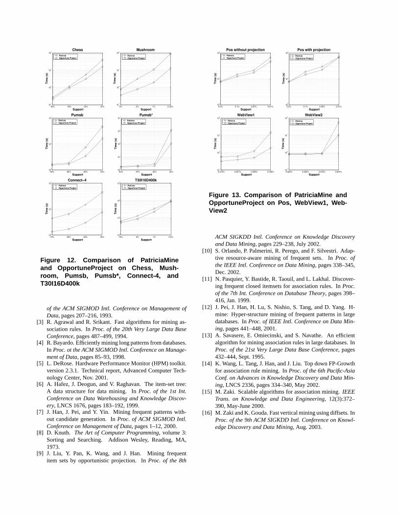
6.3. Comparison with OpportuneProject

Particularly relevant for our work is the comparison be-tween PatriciaMine and OpportuneProject [9], which, to thebest of our knowledge, represents the latest and most ad-vanced algorithm in the family stemmed from FP-Growth.For lack of space, we postpone a detailed and critical discus-sion of the strengths and weaknesses of the two algorithmsto the full version of the paper.

Figures 12 and 13, report the performances exhib-ited by PatriciaMine and OpportuneProject on the Pen-tium/Windows platform for a number of datasets and sup-ports. It can be seen that, the performance of Patrici-

0.085% 0.075% 0.067% 0.060%10−1

100

101

102

Tim

e (s

)

Support

WebView1PatriciaDCI Eclat FP−growth

0.065% 0.058% 0.052% 0.045%100

101

102

103

Tim

e (s

)

Support

WebView2PatriciaDCI Eclat FP−growth

0.05% 0.01% 0.005% 0.002%100

101

102

103

104

Tim

e (s

)

Support

T10I4D100kPatriciaDCI Eclat FP−growth

5% 2.5% 0.5% 0.25%100

101

102

103

104

Tim

e (s

)

Support

T40I100D100kPatriciaDCI Eclat FP−growth

Figure 11. Comparison of PatriciaMine, DCI,Eclat and FP-Growth on WebView1, Web-View2, and some artificial datasets

aMine is consistently superior, up to one order of magnitude(e.g., in Pumsb*). The only exception are Pos (see graphlabelled “Pos with projection”) and the artificial datasetT30.I16.D400k.N1k.L2k. For Pos, we have already ob-served that our heuristic for limiting the number of phys-ical projections does not improve the running time. In fact,it is interesting to note that by inhibiting projections, Patri-ciaMine becomes faster than OpportuneProject (see graphlabelled “Pos without projection”). This suggests that a bet-ter heuristic could eliminate this anomalous case.

As for T30.I16.D400k.N1k.L2k, some measurements weperformed revealed that the time taken by the initializationof the Patricia trie accounts for a significant fraction of therunning time at high support thresholds, and such an ini-tial overhead cannot be hidden by the subsequent miningactivity. However, at lower support thresholds, where thecomputation of the frequent itemsets dominates over the trieconstruction, PatriciaMine becomes faster than Opportune-Project.

Finally we report that on WebView1 for absolute support32 (about 0.054%), OpportuneProject ran out of memorywhile PatriciaMine successfully completed the execution.

References

[1] R. Agrawal, C. Aggarwal, and V. Prasad. A tree projectionalgorithm for generation of frequent itemsets.Journal ofParallel and Distributed Computing, 61(3):350–371, 2001.

[2] R. Agrawal, T. Imielinski, and A. Swami. Mining associa-tion rules between sets of items in large databases. InProc.

60% 40% 30% 20%10−1

100

101

102

Tim

e (s

)

Support

ChessPatricia Opportune Project

5% 2% 1% 0.25%10−1

100

101

102

Tim

e (s

)

Support

MushroomPatricia Opportune Project

90% 80% 60% 50%100

101

102

Tim

e (s

)

Support

PumsbPatricia Opportune Project

50% 40% 30% 20%100

101

102

103

104 T

ime

(s)

Support

Pumsb*Patricia Opportune Project

70% 60% 50% 40%100

101

102

Tim

e (s

)

Support

Connect−4Patricia Opportune Project

10% 5% 1% 0.5%100

101

102

103

Tim

e (s

)

Support

T30I16D400kPatricia Opportune Project

Figure 12. Comparison of PatriciaMineand OpportuneProject on Chess, Mush-room, Pumsb, Pumsb*, Connect-4, andT30I16D400k

of the ACM SIGMOD Intl. Conference on Management ofData, pages 207–216, 1993.

[3] R. Agrawal and R. Srikant. Fast algorithms for mining as-sociation rules. InProc. of the 20th Very Large Data BaseConference, pages 487–499, 1994.

[4] R. Bayardo. Efficiently mining long patterns from databases.In Proc. ot the ACM SIGMOD Intl. Conference on Manage-ment of Data, pages 85–93, 1998.

[5] L. DeRose. Hardware Performance Monitor (HPM) toolkit.version 2.3.1. Technical report, Advanced Computer Tech-nology Center, Nov. 2001.

[6] A. Hafez, J. Deogun, and V. Raghavan. The item-set tree:A data structure for data mining. InProc. of the 1st Int.Conference on Data Warehousing and Knowledge Discov-ery, LNCS 1676, pages 183–192, 1999.

[7] J. Han, J. Pei, and Y. Yin. Mining frequent patterns with-out candidate generation. InProc. of ACM SIGMOD Intl.Conference on Management of Data, pages 1–12, 2000.

[8] D. Knuth. The Art of Computer Programming, volume 3:Sorting and Searching. Addison Wesley, Reading, MA,1973.

[9] J. Liu, Y. Pan, K. Wang, and J. Han. Mining frequentitem sets by opportunistic projection. InProc. of the 8th

0.5% 0.1% 0.05% 0.01%100

101

102

Tim

e (s

)

Support

Pos without projectionPatricia Opportune Project

0.5% 0.1% 0.05% 0.01%100

101

102

Tim

e (s

)

Support

Pos with projectionPatricia Opportune Project

0.075% 0.067% 0.059% 0.055%10−1

100

101

102

Tim

e (s

)

Support

WebView1Patricia Opportune Project

0.065% 0.052% 0.045% 0.004%10−1

100

101

102

Tim

e (s

)

Support

WebView2Patricia Opportune Project

Figure 13. Comparison of PatriciaMine andOpportuneProject on Pos, WebView1, Web-View2

ACM SIGKDD Intl. Conference on Knowledge Discoveryand Data Mining, pages 229–238, July 2002.

[10] S. Orlando, P. Palmerini, R. Perego, and F. Silvestri. Adap-tive resource-aware mining of frequent sets. InProc. ofthe IEEE Intl. Conference on Data Mining, pages 338–345,Dec. 2002.

[11] N. Pasquier, Y. Bastide, R. Taouil, and L. Lakhal. Discover-ing frequent closed itemsets for association rules. InProc.of the 7th Int. Conference on Database Theory, pages 398–416, Jan. 1999.

[12] J. Pei, J. Han, H. Lu, S. Nishio, S. Tang, and D. Yang. H-mine: Hyper-structure mining of frequent patterns in largedatabases. InProc. of IEEE Intl. Conference on Data Min-ing, pages 441–448, 2001.

[13] A. Savasere, E. Omiecinski, and S. Navathe. An efficientalgorithm for mining association rules in large databases. InProc. of the 21st Very Large Data Base Conference, pages432–444, Sept. 1995.

[14] K. Wang, L. Tang, J. Han, and J. Liu. Top down FP-Growthfor association rule mining. InProc. of the 6th Pacific-AsiaConf. on Advances in Knowledge Discovery and Data Min-ing, LNCS 2336, pages 334–340, May 2002.

[15] M. Zaki. Scalable algorithms for association mining.IEEETrans. on Knowledge and Data Engineering, 12(3):372–390, May-June 2000.

[16] M. Zaki and K. Gouda. Fast vertical mining using diffsets. InProc. of the 9th ACM SIGKDD Intl. Conference on Knowl-edge Discovery and Data Mining, Aug. 2003.