IFT-UAM/CSIC-22-64

UTTG-09-2022

Membrane nucleation rates from holography

Maite Arcos,a Willy Fischler,b Juan F. Pedraza,c and Andrew Sveskoa

aDepartment of Physics and Astronomy, University College London, London, WC1E 6BT, UKbDepartment of Physics, The University of Texas at Austin, Austin, Texas 78712, USAcInstituto de Fısica Teorica UAM/CSIC, Calle Nicolas Cabrera 13-15, Madrid 28049, Spain

E-mail: maite.arcos@ucl.ac.uk, fischler@physics.utexas.edu,

j.pedraza@csic.es, a.svesko@ucl.ac.uk

Abstract: Membrane nucleation, a higher dimensional analog of the Schwinger effect, is

a useful toy model for vacuum decay. While a non-perturbative effect, the computation of

nucleation rates has only been accomplished at weak coupling in the field theory. Here we

compute the nucleation rates of spherical membranes using AdS/CFT duality, thus naturally

including the effects of strong coupling. More precisely, we consider the nucleation of spherical

membranes coupled to an antisymmetric tensor field, a process which renders the vacuum

unstable above a critical value of the field strength. We analyze membrane creation in flat and

de Sitter space using various foliations of AdS. This is accomplished via instanton methods,

where the rate of nucleation is dominated by the semi-classical on-shell Euclidean action. Our

findings generalize the holographic Schwinger effect and provide a step toward holographic

false vacuum decay mediated by Coleman-De Luccia instantons.

arX

iv:2

207.

0644

7v2

[he

p-th

] 2

1 Ju

l 202

2

Contents

1 Introduction 1

2 Set-up and review of holographic Schwinger effect 4

2.1 Gravity set-up: preliminaries 4

2.2 Schwinger effect: Euclidean instanton, decay rate and critical field 5

3 Membrane nucleation rates in flat space 10

3.1 Membranes in flat space 10

3.2 On-shell Euclidean action and nucleation rate 13

4 Membrane nucleation rates in de Sitter space 15

4.1 Membranes in de Sitter space 16

4.2 On-shell Euclidean action and nucleation rate 19

5 Conclusion 23

A Nucleation at weak coupling 25

A.1 Membranes in flat space 25

A.2 Membranes in de Sitter space 27

B De Sitter foliations of Anti de Sitter space 29

1 Introduction

Quantum tunneling, a non-perturbative phenomenon for which there is no classical coun-

terpart, plays an essential role in a number of physical processes. A famous example of

tunneling is the decay of the false vacuum due to the nucleation of bubbles of true vacuum

during first order phase transitions [1, 2]. Consequently, a curved de Sitter spacetime – an

idealized approximation of our universe in the far past and future – is possibly in a metastable

false vacuum state [3].1 Additional fundamental processes with a tunneling description range

from nuclear fusion to Hawking radiation [5], to cosmological phase transitions and structure

formation, e.g., [6–8]. A particularly interesting subclass of tunneling processes include the

nucleation of membranes in flat and curved backgrounds. As a higher dimensional analog of

Schwinger pair production [9], membrane nucleation provides a mechanism for the neutral-

ization of the cosmological constant [10, 11] (see [12–14] for a modern treatment), and acts as

1Alternatively, via the creation of false vacuum bubbles, a de Sitter-like background may undergo true

vacuum decay [4].

– 1 –

an illustrative precursor for studying the materialization of various topological defects during

cosmic inflation [15].

By now it is standard practice to describe tunneling processes using instanton techniques.

Instantons, as classical solutions to the Euclidean equations of motion obeying suitable bound-

ary conditions, are saddle points to a Euclidean path integral and therefore are the leading

order contribution to the path integral in a saddle-point approximation. The leading order

contribution to the nucleation rate Γ, or, equivalently, the exponential behavior of the tun-

neling probability, of an object is found by computing the partition function and is thereby

proportional to the exponential of the on-shell Euclidean action SE of the system of interest

(see [16] for a pedagogical review)

Γ = Ae−SE . (1.1)

Here the prefactor A is typically comprised of functional determinants generated by inte-

grating out small quantum fluctuations about the instanton stationary point, thus encoding

typically subleading 1-loop quantum corrections. For example, the Schwinger nucleation rate

of a spin-j particle-antiparticle pair of mass m in a strong electric field E is [9]

Γ =(2j + 1)E2

8π3

∞∑n=1

(−1)(n+1)(2j+1)

n2e−

πm2nE , (1.2)

which can be recovered from a sum over instanton amplitudes to tunnel through a potential

barrier [17]. Similar derivations hold for the computation of nucleation rates of strings,

membranes, and topological defects, in both flat and curved backgrounds [15, 18, 19].

Despite being non-perturbative in nature, an unfortunate limitation of each of the afore-

mentioned computations, including the rate (1.2), directly or indirectly assume the quantum

field theory is weakly coupled. Of course, weakly coupled field theories comprise only a small

class among the landscape of field theories; indeed the standard model of particle physics is an

example of a strongly coupled field theory. It is of interest then to compute nucleation rates

beyond the weak coupling regime. In this article we take steps in addressing this question

and analyze nucleation rates of spherical membranes in flat and de Sitter backgrounds using

the Anti-de Sitter space/conformal field theory (AdS/CFT) correspondence.

AdS/CFT, born from studies in string theory, is a non-perturbative candidate model of

quantum gravity, in which gravitational physics in a (bulk) d+2-dimensional AdS background

has a dual description in terms of a conformal field theory living on the d+1-dimensional con-

formal boundary of AdS. The correspondence is thus a specific realization of the holographic

principle. A striking feature of the AdS/CFT correspondence is that it is a strong-weak

coupling duality: coupling constants between the bulk and boundary theories are inversely

related, such that strongly coupled field computations on the boundary may instead be per-

formed via a gravity calculation at weak coupling. For example, the challenging task of

computing entanglement entropy of certain strongly coupled field theories can be accom-

plished by computing the area of bulk minimal surfaces obeying certain homology conditions

[20]. Further, AdS/CFT was used to predict a universal value of the shear viscosity to en-

tropy density ratio in a wide class of theories with classical gravity duals [21], in remarkable

– 2 –

agreement with the value measured experimentally for the quark-gluon plasma produced in

heavy-ion collision experiments [22]. Thus, at the very least, AdS/CFT has proven to be

a powerful tool to analyze aspects of strongly coupled field theories. Here we exploit this

feature to compute the nucleation rates of membranes at strong coupling.

Progress along these lines has already been made. In particular, the Schwinger pair pro-

duction rate of W-bosons in a supersymmetric Yang-Mills theory in Minkowski space was

computed using holographic methods, leading to a holographic generalization of Schwinger’s

pair production formula (1.2) including strong coupling effects [23]. From the bulk perspec-

tive, this amounts to evaluating the on-shell Euclidean action of a string ending on a stack of

flavor branes. The endpoints of the string are coupled to a Maxwell field with a constant elec-

tric field, and represent the particle-antiparticle Schwinger pair. The holographic Schwinger

effect has since been extended in a variety of ways, e.g., [24–28], including the study of pair

production in curved backgrounds, non-relativistic backgrounds and confining models, among

others [29–34]. In particular, the rate of production of Schwinger pairs in de Sitter space was

achieved by considering de Sitter foliations of AdS [30], extending various non-holographic

computations to the strong coupling regime [15, 19, 35–41].

In this article we move beyond the holographic Schwinger effect and use AdS/CFT to

study the nucleation of spherical membranes in flat and de Sitter backgrounds of arbitrary

spacetime dimension. More precisely, we consider the creation of spherical membranes coupled

to a higher rank antisymmetric tensor field, which can be understood as a toy model for false

vacuum decay. The nucleation rate and critical value of the field strength are computed

by evaluating the on-shell membrane action. Our results thus extend the aforementioned

holographic Schwinger effect, reducing to this case in the appropriate limit, as well as a

strong coupling generalization of conventional field theoretic constructions. Of note is the

evaluation of the on-shell Euclidean membrane action in de Sitter space which is determined

completely analytically in arbitrary dimensions.

The remainder of this article is as follows. In Section 2 we briefly review the holographic

set-up and computation of the on-shell action of a string used in the holographic Schwinger

effect. Section 3 is devoted to the analysis of membrane nucleation rates in flat space, by

computing the on-shell action for a membrane ending on a cutoff surface near the flat con-

formal boundary of AdSd+2. We find the Lorentzian continuation of the instanton describes

a spherical membrane contracting and expanding at constant proper acceleration, and relate

the rest energy of the membrane to the bulk cutoff. Similarly, in Section 4 we compute the

membrane nucleation rate in de Sitter space by considering various (d + 1)-dimensional de

Sitter space foliations of AdS. In this case and in the limit the field strength vanishes, our

results yield the spontaneous nucleation rate for defects solely due to the background infla-

tion. We summarize and provide concluding remarks in Section 5, discussing multiple future

avenues worth exploring. For the sake of completeness we include two appendices. Appendix

A reviews the computation of membrane nucleation rates using conventional quantum field

theory at weak coupling [15], and Appendix B lists multiple de Sitter foliations of AdS.

– 3 –

2 Set-up and review of holographic Schwinger effect

We begin by providing an elementary review of the holographic set-up used to study the

holographic Schwinger effect, which we analyze using instanton methods by computing the

on-shell Nambu-Goto action for a string coupled to a Maxwell field. This review will act as

a useful comparison when we consider the nucleation of spherical membranes as many of the

techniques generalize in a straightforward manner.

2.1 Gravity set-up: preliminaries

Broadly, the AdS/CFT correspondence says the following: the states of certain conformal field

theories in the large Nc limit and large ’t Hooft coupling λ = g2YMNc living on a d+ 1 dimen-

sional spacetime Md+1 are dual to solutions of supergravity theories which asymptotically

approach AdSd+2×X, where X is a compact manifold whose isometries are recognized as the

global symmetries of the field theory, and the boundary of AdSd+2 is identified with Md+1.

In its strongest form, the duality purports a full equivalence between the partition functions

between the boundary CFT and the bulk theory. However, for practical purposes it is often

discussed within a saddle-point approximation, valid at large Nc, because bulk calculations

are tractable in this regime [42, 43]. The canonical example of AdS/CFT duality relates

type IIB string theory on an AdS5 × S5 background with Nc units of Ramond-Ramond flux

through S5 to N = 4 SU(Nc) super-Yang-Mills theory, though we will not restrict ourselves

to a specific version of the correspondence.

In fact, it is often sufficient to consider a bulk spacetime Bd+2 × X for an appropriate

internal space X, where Bd+2 is a solution to Einstein’s equations with a negative cosmological

constant Λ = −d(d+1)2L2 , where L being the length scale of the asymptotic AdSd+2 spacetime.

In this context one relates the bulk (d+ 2)-dimensional Newton’s constant GN to the central

charge c of the dual CFT via

c =Ld

16πGN. (2.1)

Hence, for fixed radius L, studying holographic CFTs in the large c limit amounts to consid-

ering (classical) gravity in the GN → 0 limit, neglecting quantum gravity corrections. With

this in mind, we will consider the case when the bulk spacetime is represented by empty

AdSd+2, which in Poincare coordinates has the line element

ds2d+2 =

L2

z2

(−dt2 + d~x2 + dz2

), (2.2)

where d~x2 = dx21+dx2

2+...dx2d. According to the standard AdS/CFT dictionary, this geometry

is dual to the vacuum of a (d + 1)-dimensional CFT with central charge c (2.1). Here the

coordinate z is a bulk ‘radial’ coordinate, such that the (flat) conformal boundary is located

at z = 0. In the following two sections we will consider string and membrane solutions living

in this background subject to specific boundary conditions.

As described above, Schwinger pair production or membrane nucleation requires one to

couple to a Maxwell gauge field or a higher antisymmetric tensor field, respectively. This

– 4 –

means one needs to add fundamental matter to the field theory. Holographically this would

entail introducing a stack of Nf flavor branes in the bulk geometry. With the canonical

example in mind, when Nf Nc, the flavor branes act as probe branes, i.e., we may neglect

their backreaction effects on the background geometry and treat the geometry as given.

Furthermore, the flavor branes will be assumed to expand in all directions on the boundary,

however, only exist to finite extent in the bulk, between the boundary z = 0 and some cutoff

surface zm, where they ‘end’ (meaning that one of their internal cycles shrinks down to zero

size [44]). While this description provides a useful picture for us, we will be largely agnostic

to the precise details of the flavor branes. Rather, we will simply introduce a cutoff surface

at z = zm where the Maxwell gauge field or antisymmetric tensor field live.

A few additional comments are in order. First, it is natural to understand zm as a funda-

mental UV scale in the theory. This follows from the usual UV/IR connection in AdS/CFT,

where the bulk coordinate z maps to a length scale L ∼ z in the boundary theory such that

z = zm corresponds to a length L ≈ zm. Second, for zm 6= 0, the fundamental matter degrees

of freedom added at the boundary acquire a finite mass (or energy). This is easily understood

as the introduction of this UV scale removes high energy modes, which would provide any

excitation with infinite energy. Third, the existence of such a scale provides a non-zero thick-

ness to the membranes analyzed here. The thickness is linked to the aforementioned UV/IR

connection, and the fact that a finite zm introduces a minimal length one can resolve in the

theory. Lastly, since z = zm 6= 0 is not exactly on the boundary, non-normalizable modes

of the bulk fields, including the metric, are allowed to fluctuate on this surface. Thus, even

though in our setup we are assuming a rigid boundary metric, one may couple field theoretic

degrees of freedom (e.g., those resulting from integrating out the UV) to dynamical gravity,

reminiscent of Randall-Sundrum braneworld models [45, 46]. In such a setting one would need

to add a codimension-1 brane at the cutoff surface z = zm with induced dynamical gravity

and proper field theoretic degrees of freedom which may backreact on the classical geometry

in a consistent way (cf. [47–49]).

2.2 Schwinger effect: Euclidean instanton, decay rate and critical field

As a warmup before we analyze membrane nucleation, let us consider a string moving in one

of the spatial directions of the flat AdS background (2.2), say x1 ≡ x. In holography, the

string is dual to a Schwinger pair of particles. The string is attached to a stack of flavor

branes that lie at z = zm. Working in static gauge ξi = (t, x), and parametrizing the string

embedding as Xµ = (t, x,~0, z(t, x)), the Nambu-Goto action for the string yields

SNG = Tst

∫d2ξ√−det γij =

√λ

2π

∫Σdtdx

√1 + z′2 − z2

z2, (2.3)

where γij = ∂iXµ∂jX

νgµν is the induced metric on the string worldsheet Σ and Tst = 12πα′ =

√λ

2πL2 is the string tension, given in terms of the ’t Hooft coupling λ. One can easily verify

that the following is a solution of the equations of motion [50]:

z(t, x) =√R2 + t2 − x2 . (2.4)

– 5 –

-4 -2 2 4

-4

-2

2

4

-2 -1 1 2

-2

-1

1

2t tE

x x

Figure 1: Left: Hyperbolic trajectory of a pair of particles undergoing constant proper

acceleration. Right: Euclidean analytic continuation of the instanton describing pair creation.

Notice this solution reaches out to the AdS boundary z = 0. Indeed, evaluating the embedding

at z = 0 we can obtain the trajectory of the (as we will see, infinitely massive) particles dual

to the string,

x(t) = ±√R2 + t2 , (2.5)

i.e., the usual hyperboloid trajectory for motion with constant proper acceleration A = 1/R.

Such a trajectory can be obtained by, e.g., exerting a constant electric field upon the particles.

In Euclidean signature, the trajectory of the pair must have rotational symmetry given that

the electric field acts as a magnetic field after Wick rotation. Hence, the instanton follows

the usual cyclotron orbit,

x(tE) = ±√R2 − t2E . (2.6)

See Figure 1 for an illustration.

The above string solution reaches out to the AdS boundary z → 0, hence the dual

particles are infinitely massive. However, in order to properly analyze the Schwinger effect

one needs to consider finite mass, otherwise pair production would be suppressed. This can

be achieved by letting the flavor branes reach up to some finite radial distance zm 6= 0. The

string solution in this case is the same as (2.4) but truncated at some z = zm. It can be

written as follows [51]:

z(t, x) =√z2m +R2 + t2 − x2 , (2.7)

such that we recover (2.5) by evaluating (2.7) at z = zm.

Note that this is still the same solution, however, we have shifted R2 → R2 + z2m. The

cutoff parameter zm is a fundamental constant of the theory and is set by the position of the

flavor branes. As such, several physical observables will end up depending on this parameter.

– 6 –

For example, one can compute the (spacetime) momentum densities for a fundamental string

Πµ =∂LNG

∂Xµ= −Tst

XµX′2 −X ′µ(X ·X ′)√

(X ·X ′)2 − X2X ′2, (2.8)

and write them in terms of zm. The prototypical example is a static string hanging from the

stack of flavor branes at some x = constant. In this case, the total energy E yields the rest

mass m of the dual particle,

E =

∫ ∞zm

Πtdz = TstL2

∫ ∞zm

dz

z2=

√λ

2πzm≡ m, (2.9)

which can be inverted to obtain

zm =

√λ

2πm. (2.10)

As advertised, the mass of the particle m turns out to be inversely proportional to the cutoff

radius zm, so that m→∞ as zm → 0. We can repeat the exercise for the accelerated solution

with embedding (2.7). In this case we obtain

E =

∫ √R2+z2m+t2

zm

Πtdz =2TstL

2√R2 + z2

m

√R2 + t2

zm. (2.11)

The energy varies with time as the speed of the dual particles is changing. The rest energy

E0 ≡ E(t = 0) for this solution is

E0 =

√λ

π√R2 + z2

m

(R

zm

), (2.12)

which can also be inverted to obtain zm(E0, R).

We note that for zm R, or equivalently,√λ RE0, then zm ≈

√λ

πE0 , where we may

relate the rest energy to the mass of a pair of static particles, E0 ≈ 2m, recovering (2.10). A

couple of comments are in order. First note that, as in the static case, the rest energy E0 is

infinite in the limit zm → 0. This is due to the infinite volume of AdS near the conformal

boundary. Second, in general E0 6= 2m, rather, E0 ends up depending on R = 1/A, which is a

parameter of the specific trajectory. This is due to the fact that, for zm 6= 0, the dual particles

are no longer pointlike, but rather, are surrounded by a ‘glue cloud’ of finite size zm [52–54].

The effects of such a cloud are most directly seen from expectation values of local operators,

such as 〈TrF 2(x)〉 or 〈Tµν(x)〉, which for accelerated trajectories end up depending on not only

the relativistic boost factor γ(t), but also, the acceleration a(t) and higher order derivatives,

j(t) ≡ a(t), etc, rendering these observables anisotropic [55, 56]. For such extended objects,

thence, the total intrinsic energy E (as well as their rate of radiation) ends up depending

highly non-trivially on the trajectory x(t), even when they are instantaneously at rest.2

2See [57] for a review on the subject.

– 7 –

For all practical purposes, then, we may consider zm as a fundamental constant of the

theory which we will take as given. This parameter can be thought of as a UV scale giving

rise to the (finite) masses/energies of the various objects that the dual theory may nucleate.

Now, to enforce the accelerated motion one must include an external force which acts

upon the endpoints of the string. This can be achieved by turning on a constant electric field

with strength Ftx = E on the flavor branes. This amounts to adding to the Nambu-Goto

action (2.3) the action SA of a minimally coupled gauge field A obeying F = dA,

SA =

∫∂ΣA , A ≡ Aidxi , (2.13)

with ∂Σ being the boundary of the string worldsheet living on the surface z = zm.

It turns out this system, described by the total action S = SNG +SA, is unstable above a

certain critical value of the electric field strength. This can be seen from the nucleation rate

of the string Γ, dual to the nucleation rate of Schwinger pair production. Indeed, from the

original computation of pair creation by Schwinger [9], one can see there is a critical value

of the electric field Ec = m2/αs, with fine structure constant αs ' 1/137, at which point

the vacuum becomes unstable and decay. Further, since the critical field strength is beyond

the limit of weak field condition, Ec m2, one may expect nucleation processes to receive

relevant non-perturbative corrections. Motivated by this, the Schwinger pair production rate

(1.2) may be derived rederived using instanton techniques, specifically, from the imaginary

part of the Euclidean worldline path integral, (see e.g. [58]), where the contribution of an

instanton to the nucleation rate is of the form Γ = Ae−SE , where A is a prefactor that

comes from integrating over quantum fluctuations about the instanton solution and SE is the

on-shell Euclidean action.

Missing from this derivation, however, are effects coming from the backreaction of the

particles on the gauge fields, which are enhanced at strong coupling. To study such correc-

tions, one may use AdS/CFT to reexamine the Schwinger effect, holographically understood

as the nucleation of the string described above [23]. Thus, one moves to Euclidean signa-

ture, t→ −itE for Euclidean time tE , and looks for instanton solutions to the Euclideanized

Nambu-Goto action. In this case the instanton is given by the Wick rotated string solution

(2.7), which takes the following form:

z(tE , x) =√z2m +R2 − t2E − x2 . (2.14)

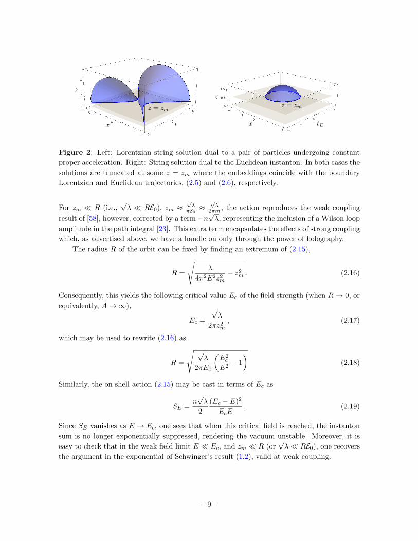
Figure 2 shows a schematic illustration of the Lorentzian and Euclidean string embeddings,

(2.7) and (2.14), respectively.

Note that at z = zm, the Euclidean solution reduces to a circle of radius R, as expected

from (2.6). Hence, an instanton of the Euclidean path integral is a cyclotron orbit which may

wrap n times in the time direction. The associated Euclidean action, SE = SNG +SA|t→−itE ,

evaluated on-shell is found to be

SE = n√λ

(√1 +

R2

z2m

− 1

)− nπR2E . (2.15)

– 8 –

tx tEx

zz

z = zmz = zm

Figure 2: Left: Lorentzian string solution dual to a pair of particles undergoing constant

proper acceleration. Right: String solution dual to the Euclidean instanton. In both cases the

solutions are truncated at some z = zm where the embeddings coincide with the boundary

Lorentzian and Euclidean trajectories, (2.5) and (2.6), respectively.

For zm R (i.e.,√λ RE0), zm ≈

√λ

πE0 ≈√λ

2πm , the action reproduces the weak coupling

result of [58], however, corrected by a term −n√λ, representing the inclusion of a Wilson loop

amplitude in the path integral [23]. This extra term encapsulates the effects of strong coupling

which, as advertised above, we have a handle on only through the power of holography.

The radius R of the orbit can be fixed by finding an extremum of (2.15),

R =

√λ

4π2E2z2m

− z2m . (2.16)

Consequently, this yields the following critical value Ec of the field strength (when R→ 0, or

equivalently, A→∞),

Ec =

√λ

2πz2m

, (2.17)

which may be used to rewrite (2.16) as

R =

√ √λ

2πEc

(E2c

E2− 1

)(2.18)

Similarly, the on-shell action (2.15) may be cast in terms of Ec as

SE =n√λ

2

(Ec − E)2

EcE. (2.19)

Since SE vanishes as E → Ec, one sees that when this critical field is reached, the instanton

sum is no longer exponentially suppressed, rendering the vacuum unstable. Moreover, it is

easy to check that in the weak field limit E Ec, and zm R (or√λ RE0), one recovers

the argument in the exponential of Schwinger’s result (1.2), valid at weak coupling.

– 9 –

As a final comment, we note that the critical field strength Ec can be easily understood

from the flavor brane point of view. Specifically, in the static gauge, the DBI Lagrangian for

a probe brane reads

√−det(gab + 2πα′Fab) ∝

√1

z4−(

2π√λFtx

)2

, (2.20)

which is real at z = zm provided Ftx ≡ E <√λ/(2πz2

m). Beyond this value, the creation of

open strings is energetically favored, such that the system becomes unstable, as E > Ec.

3 Membrane nucleation rates in flat space

Having reviewed the nucleation of strings in flat space, we generalize to the case of nucleating

spherical membranes, first in (d+ 1)-dimensional flat space, and then in (d+ 1)-dimensional

de Sitter space in Section 4.

3.1 Membranes in flat space

Let us consider a (p+ 1)-dimensional membrane embedded in pure AdSd+2, with 1 ≤ p ≤ d,

where in the limit p = 1 the system reduces to a string as reviewed in Section 2. Assuming

spherical polar coordinates along the p-spatial directions, the bulk AdSd+2 metric in Poincare

coordinates is

ds2d+2 =

L2

z2(−dt2 + dr2 + r2dΩ2

p−1 + d~x2⊥ + dz2) . (3.1)

Here ~x⊥ denotes the directions transverse to the brane; however, when p = d, there are no

extra transverse directions. As before, we imagine flavor branes extending into the bulk from

the boundary at z = 0 to some finite cutoff position z = zm. The spherical membranes are

attached to the stack of flavor branes along z = zm, such that the boundary of the membrane

worldvolume ends at z = zm. In a moment we will see how to relate the energy of various

membrane solutions the bulk cutoff position zm, analogous to the string case.

Working in static gauge, the worldvolume Σp is parametrized by coordinates ξi = (t, r, ~Ωp−1)

while the embedding functions of the membrane into AdSd+2 are Xµ = (t, r, ~Ωp−1, ~x⊥, z(t, r)).

Here ~Ωp−1 denotes the collection of spherical angular coordinates, and ~x⊥ denotes the coor-

dinates of the (p − d) transverse directions, which, without loss of generality, we may fix to

be at ~0. The Lorentzian action Sp characterizing the dynamics of the membrane is given by

the area of Σp, generalizing the Nambu-Goto action for a string:

Sp = Tp

∫Σp

dp+1ξ√−detγij . (3.2)

Here Tp denotes the tension of the membrane, such that for p = 1 we recover the tension of

the string T1 =√λ

2πL2 . With respect to the line element (3.1), it is straightforward to show

the action becomes

Sp = TpLp+1Ωp−1

∫Σp

dtdrrp−1√

1 + z′2 − z2

zp+1, (3.3)

– 10 –

x1 x1 x1x2 x2 x2

z z z

z = zmz = zmz = zm

t = 1t = 0t = − 12

Figure 3: Snapshots of the (Lorentzian) membrane solution (3.4) as it contracts and expands

in time. For the sake of the plots, we have only shown the case of a (2 + 1)-dimensional

membrane (i.e., with p = 2), but the solution is valid for arbitrary p. The p = 1 case reduces

to a string worldsheet, as depicted in Figure 2 (left).

where Ωp−1 = 2πp/2

Γ(p/2) is the volume of a (p−1)-dimensional unit sphere, and we have introduced

the shorthand notation z ≡ dzdt and z′ ≡ dz

dr .

From the action (3.3), one can easily verify the same solution z(t, r) for the string (2.7)

is a solution to the equations of motion of the membrane for any p

z(t, r) =√R2 + z2

m + t2 − r2 , (3.4)

with the change x ↔ r and where we have explicitly included the cutoff zm such that the

membrane has finite mass (energy). Thus, at the cutoff surface z = zm, the solution (3.4)

describes a massive spherical membrane which contracts and expands radially with radius

given by r(t) =√R2 + t2. Figure 3 illustrates the time evolution of this membrane solution.

As for the case of the holographic Schwinger effect, enforcing this solution requires an

external force acting on the boundary of the membrane ∂Σp. Unlike the string case, however,

this amounts to coupling the membrane to a higher antisymmetric tensor field A of rank p,

A = A[i...k]dxi ∧ ... ∧ dxk , (3.5)

on the boundary where one imagines flavor branes to extend. The action for A is

SA =

∫∂Σp

A . (3.6)

For spherically symmetric configurations, the gauge field strength F associated with A via

F = dA, will only have a single independent component, and may be expressed as

F = −Eε , (3.7)

where ε is the natural volume form of the (p+ 1)-dimensional spacetime, ε =√|g|εi...kldxi ∧

. . .∧ dxk ∧ dxl (with ε01...p = 1), and E is a constant ‘electric’ field strength. The total action

of interest is then

S = Sp + SA . (3.8)

– 11 –

Rest energy of membranes

We can compute the energy E of any membrane solution, analogous to the string case (2.9)

or (2.11), and determine its dependence on the various parameters of the theory.

It is first worthwhile to consider the energy of a static membrane that hangs at some

x1 = constant and extends to infinity in the remaining p−1 directions. In this case, the total

energy E yields the rest mass mp of the membrane, generalizing (2.9) to:

E =

∫ ∞zm

Πtdz = TpLp+1Vp−1

∫ ∞zm

dz

zp+1=Tp L

p+1Vp−1

p zpm≡ mp . (3.9)

Here Vp−1 ≡∫dx2 · · · dxp stands the p− 1 volume. If desired, we can invert (3.9) to express

zm in terms of mp, which yields

zm =

(Tp L

p+1Vp−1

pmp

)1/p

, (3.10)

which correctly reproduces (2.10) for p = 1 with T1 →√λ

2πL2 and Vp−1 → 1.

We can now consider the spherical membranes with profile given by (3.4). In this case,

the momentum densities for a given spherically symmetric solution are given by:

Πµ =∂Lp∂Xµ

= −TpΩp−1

(Lr

z

)p−1 XµX

′2 −X ′µ(X ·X ′)√(X ·X ′)2 − X2X ′2

. (3.11)

Substituting in the solution (3.4), the energy of the membrane yields,3

E =

∫ √R2+t2+z2m

zm

dzΠt =TpΩp−1L

p+1

p√R2 + z2

m

(R2 + t2)p/2

zpm. (3.12)

As expected, the energy decreases as the membrane contracts, reaches a minimum at t = 0

and then grows back to infinity as the membrane expands. The rest energy of the membrane

E0 ≡ E(t = 0) is thus

E0 =TpΩp−1L

p+1

p√R2 + z2

m

(R

zm

)p. (3.13)

As before, we assume zm to be a fundamental constant of the theory, which we take as given.

One may try to invert (3.13) to express the cutoff zm in terms of E0 and R, but the result is

lengthy and not particularly useful, hence we will refrain from doing so.

As a final comment we point out that, as for the case of the string, the truncated solution

with zm 6= 0 is expected to be dual to a membrane with a finite width proportional to zm,

thus departing from the infinitely thin shell regime. It would be interesting to investigate

this further. For example, it would be insightful to compute the expectation values of local

operators, such as 〈TrF 2(x)〉 or 〈Tµν(x)〉, e.g., following [55, 56], and determine the spatial

profiles sourced by these membranes.

.3To carry out this calculation it is easier to parametrize the worldvolume with coordinates ξi = (t, z, ~Ωp−1)

and invert (3.4) to obtain r(t, z), such that we work with the embedding Xµ = (t, r(t, z), ~Ωp−1, ~x⊥, z).

– 12 –

3.2 On-shell Euclidean action and nucleation rate

The nucleation rate Γ for membranes, analogous to Schwinger pair production, can be com-

puted using instanton methods [15], where the leading order effect is given by the on-shell

Euclidean action SE (1.1). Thus far, aside from the case of the string [30], such nucleation

rates have been carried out at weak coupling, without the employ of holography. Here we use

AdS/CFT as a general tool to compute Γ ∼ e−SE , for which the classical bulk computation

is valid, leaving aside the corrections due to quantum fluctuations. We thus Euclideanize the

total action (3.8) via Wick rotating the AdSd+2 time t→ −itE ,

SE = SEp + SEA , (3.14)

and use the fact that the field strength tensor F is unchanged under the Wick rotation (as is

the case for standard Maxwell theory).

Specifically, Euclideanizing the membrane action (3.3) leads to

SEp = TpLp+1Ωp−1

∫Σp

dtEdrrp−1√

1 + z′2 + z2

zp+1, (3.15)

where now Σp is the Euclidean worldvolume and z ≡ ∂z∂tE

. The solution (3.4) Wick rotates to

z(tE , r) =√R2 + z2

m − t2E − r2 , (3.16)

and is a solution to the Euclidean equations of motion coming from (3.15). It corresponds

to a spherical membrane, where tE now acts as an additional spatial coordinate, and can

be viewed as a higher dimensional generalization to the Euclidean string solution shown in

Figure 2 (right). In this case, the on-shell Euclidean action for the membrane yields

SEp = TpLp+1Ωp−1

√R2 + z2

m

∫Σp

dtEdrrp−1

[R2 + z2m − t2E − r2](p+2)/2

. (3.17)

To evaluate the integral we perform the following change of integration variables,

r = ρ cosφ , tE = ρ sinφ , (3.18)

where since r is taken to be non-negative, ρ ∈ [0, R] and φ ∈ [−π2 ,

π2 ], in contrast with the

string case, where x ranges over positive and negative values. Consequently, the on-shell

membrane action evaluates to

SEp =πp+12 Tp L

p+1Rp+1

Γ(p+32 )(z2

m +R2)p+12

2F1

(p+ 1

2,p+ 2

2,p+ 3

2,

R2

R2 + z2m

). (3.19)

where we have used Ωp−1 = 2πp/2

Γ(p/2) . For later convenience, we also use the following identity

of hypergeometric functions:

zpm2F1

(p+ 1

2,p+ 2

2,p+ 3

2,

R2

R2 + z2m

)= (R2 + z2

m)p2 2F1

(1

2, 1,

p+ 3

2,

R2

R2 + z2m

), (3.20)

– 13 –

to rewrite (3.19) as

SEp =πp+12 Tp L

p+1Rp+1

Γ(p+32 )zpm

√R2 + z2

m

2F1

(1

2, 1 ,

p+ 3

2,

R2

R2 + z2m

). (3.21)

Meanwhile, since the boundary of the Euclidean worldvolume Σp is closed, we may employ

Stokes’ theorem such that, on-shell, the second part of the action, SEA , may be cast as

SEA = −E∫Vp+1

ε = −EVp+1 , (3.22)

where Vp+1 denotes the Euclidean spacetime volume enclosed by the boundary of the mem-

brane, ∂Σp, a (p+ 1)-dimensional ball of radius R,

Vp+1 =πp+12 Rp+1

Γ(p+32 )

=ΩpR

p+1

(p+ 1). (3.23)

Combining (3.21) and (3.22), the total on-shell Euclidean action (3.14) for arbitrary p yields

SE =ΩpR

p+1

(p+ 1)

[Tp L

p+1

zpm√R2 + z2

m

2F1

(1

2, 1 ,

p+ 3

2,

R2

R2 + z2m

)− E

]. (3.24)

For example,

S(p=1)E =

2πL2T1

zm

(√R2 + z2

m − zm)− πR2E,

S(p=2)E =

2πL3T2

z2m

[R√R2 + z2

m − z2marctanh

(R√

R2 + z2m

)]− 4

3πR3E ,

S(p=3)E =

2π2L4T3

3z3m

√R2 + z2

m

[R2 + 2z2

m

(√z2m

R2 + z2m

− 1

)]− 1

2π2R4E ,

(3.25)

where for p = 1 we recover the on-shell string action (2.15) (for winding n = 1).

We can fix the radius R in terms of zm, Tp and E by finding the extremum dSE/dR = 0,

R =

√(Tp Lp+1

Ezpm

)2

− z2m . (3.26)

As for the string case, the entire system will become unstable for a critical value of the field

strength, denoted Ec, which occurs when A→∞ or R→ 0. Explicitly,

Ec = Tp

(L

zm

)p+1

, (3.27)

such that the radius R is

R =zmE

√E2c − E2 , (3.28)

– 14 –

and the on-shell action (3.24) becomes

SE =Ωp

(p+ 1)ERp+1

[2F1

(1

2, 1 ,

p+ 3

2,E2c − E2

E2c

)− 1

]. (3.29)

Since SE ∝ Rp+1 it is clear the on-shell action vanishes when the field strength approaches

its critical value E → Ec. Further, given the field strength dependence in R, it is easy to see

that for any integer p > 0 SE diverges in the limit E → 0. Thus, there is not a consistent

limit for which membrane creation may occur in flat space without coupling to the external

gauge field A. We will see in the next section that this need not be the case for membrane

nucleation in a de Sitter background.

Lastly, in the weak field limit E Ec, and zm R (or, equivalently, TpLp+1 RE0) we

have R ≈ ( pE0EΩp−1

)1/p, reproducing the result found using standard field theoretic methods at

weak coupling [15] (see Eq. (A.12) in Appendix A for details)

SE ≈Ωp

p(p+ 1)ERp+1 =

Ωp

(p+ 1)

[p

E

(E0

Ωp−1

)(p+1)]1/p

, (3.30)

where we used 2F1(12 , 1,

p+32 , 1) = 1 + 1/p. More generally, expanding (3.24) in the two

dimensionless parameters, one finds an infinite set of corrections in powers of E/Ec and

TpLp+1/RE0, which may be regarded as non-perturbative corrections to (3.30) due to strong

coupling and strong electric fields, and away from the infinitely thin shell regime.

4 Membrane nucleation rates in de Sitter space

Thus far we efficiently computed the nucleation rate for spherical membranes including non-

perturbative effects via AdS/CFT holography, where the conformal boundary of AdS was

taken to be Minkowski space. Importantly, the conformal boundary of AdS where the CFT

lives need not be flat, allowing one to study, at least in principle, quantum processes in curved

backgrounds. As such, here we investigate membrane nucleation rates in (d+ 1)-dimensional

de Sitter space (dSd+1) at strong coupling using the tools of AdS/CFT.

As a starting point, notice one may foliate asymptotically AdSd+2 spaces using dSd+1

slices such that the dual theory is a strongly-coupled QFT living on a fixed dSd+1 background

[59]. In particular, when the bulk geometry is pure AdSd+2, then the line element can be cast

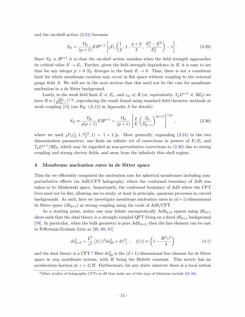
in Fefferman-Graham form as [30, 60, 61]

ds2d+2 =

L2

z2

[f(z)2ds2

dS + dz2], f(z) ≡

(1− H2z2

4

)(4.1)

and the dual theory is a CFT.4 Here ds2dS is the (d+ 1)-dimensional line element for de Sitter

space in any coordinate system, with H being the Hubble constant. This metric has an

acceleration horizon at z = 2/H. Furthermore, for any static observer there is a local notion

4Other studies of holographic CFTs in dS that make use of this type of foliations include [62–66].

– 15 –

of thermodynamics, with a temperature equal to the Gibbons-Hawking temperature of the

acceleration horizon, TdS = H2π . It is useful to redefine the bulk z coordinate by

z =2

He−2arctanh(u) =

2

H

(1− u)

(1 + u), (4.2)

such that u ∈ [0, 1], with u = 0 corresponding to the acceleration horizon (z = 2/H) and

u = 1 the conformal boundary of AdS (z = 0). Thence, the line element (4.1) becomes

ds2d+2 =

4L2

(1− u2)2

[H2u2ds2

dS + du2]. (4.3)

In Appendix B we analyze multiple such foliations of AdSd+2 due to various coordinate

representations of dSd+1. Two particular forms of the AdS2 line element (4.1) of interest

include foliations by de Sitter described in global coordinates,

ds2d+2 =

4L2

(1− u2)2

[H2u2

(−dτ2 +

cosh2(Hτ)

H2dΩ2

d

)+ du2

], (4.4)

and static patch coordinates,

ds2d+2 =

4L2

(1− u2)2

[H2u2

(−(1−H2r2)dt2 +

dr2

1−H2r2+ r2dΩ2

d−1

)+ du2

]. (4.5)

which may be transformed into one another via the coordinate change (B.9).

4.1 Membranes in de Sitter space

Let us now consider a (d+ 1)-dimensional membrane embedded in AdSd+2 foliated by dSd+1

slices in global coordinates (4.4).5 In particular, we would like to find membrane solutions

preserving the symmetries of a Sd−1. To do so, we look for embeddings depending only on

the polar angle in the line element dΩ2d = dφ2 + sin2 φdΩ2

d−1. Parametrizing the worldvolume

Σ with coordinates ξi = (τ, φ, ~Ωd−1), and choosing the embedding functions to be Xµ =

(τ, φ, ~Ωd−1, u(τ, φ)), it is a simple exercise to show the membrane action (3.2) becomes

Sd = 2d+1TdLd+1Ωd−1

∫dτdθ

ud cosd−1(Hτ) sind−1 φ√u′2 + cos2 τ(u2 − u2)

(1− u2)d+1, (4.6)

where u′ ≡ dudφ and u ≡ du

dτ . From this action one may obtain the membrane equation of

motion and solve it for u(τ, φ) subject to appropriate boundary conditions.

We are interested in obtaining membranes expanding at a constant proper acceleration.

However, since we have a non-trivial boundary metric, we need to determine the form of such

a trajectory, and then impose it as a boundary condition for the bulk membrane. Without

5For dS spacetimes, a constant ‘electric’ field is only a solution of the homogeneous gauge field equations

when p = d. Hence, in this section we specialize to (d+ 1)-dimensional bulk membranes.

– 16 –

lose of generality, we can parametrize the boundary trajectory as xµ = τ, φ(τ),Ωd−1. A

short calculation reveals that the trajectories we are looking for are of the form

φ(τ) = arccos (κ sech(Hτ)) , (4.7)

where κ is an arbitrary constant. For later convenience, we redefine this constant such that

κ = cos(α), in terms of which the norm of the acceleration vector yields

√aµaµ = H cot(α) , aµ ≡ d2xµ

dτ2+ Γµαβ

dxα

dτ

dxβ

dτ. (4.8)

The geometric meaning of α will be clear momentarily, once we move to Euclidean signature.

Imposing (4.7) as a boundary condition for the bulk membrane leads to the solution

u(τ, φ) =cosh(Hτ) cos(φ)−

√cosh2(Hτ) cos2(φ)− cos2(α)

cos(α), (4.9)

where one can check one recovers (4.7) at u → 1. It is worth noting that, similar to the

flat space case (3.4), the embedding (4.9) for a spherical membrane in dS turns out to be

independent of d.6 The solution (4.9) directly follows from solving the equations of motion

for u(τ, φ), however, the analysis is cumbersome. In the next subsection we will provide an

alternative and far simpler derivation of (4.9).

Before proceeding further, it is illustrative to translate the membrane solution to static

patch coordinates using the transformations (B.9), such that

u(t, r) =1

cos(α)

[√1−H2r2 cosh(Ht)−

√(1−H2r2) cosh2(Ht)− cos2(α)

]. (4.10)

Alternatively, in terms of the original bulk coordinate z (4.2), we obtain

z(t, r) =2

H

√√1−H2r2 cosh(Ht)−

√1−H2R2

√1−H2r2 cosh(Ht) +

√1−H2R2

, R ≡ sin(α)

H. (4.11)

Notice in the flat space limit, H → 0, we recover the solution for a spherical membrane in

flat space (3.4) (with zm = 0). Evaluating this solution at z = 0 we recover

r(t) =sech(Ht)

H

√sin2(Ht) +H2R2 , (4.12)

which describes the uniformly accelerated trajectory in the static patch of dS. From the

boundary perspective, the membrane contracts, reaches a minimum radius r = R and then

expands back at a ‘constant’ rate. However, as seen from the static observer, this rate of

expansion is redshifted; this means that for such an observer, the membrane appears to slow

down and only reach the cosmological horizon at r = 1/H as t→∞.

6This solution was derived in [30] for the case of a string (d = 1 case), though the angle θ there was taken

to be an azimuthal angle of global dS, rather than a polar angle.

– 17 –

x1 x1 x1x2 x2 x2

rH = 1 rH = 1 rH = 1z z z

z = zmz = zmz = zm

zH = 2zH = 2zH = 2

t > 0t = 0t < 0

Figure 4: Snapshots of the (Lorentzian) membrane solution (4.14) as it contracts and ex-

pands in time. The cosmological and bulk (acceleration) horizons, at r = 1/H and z = 2/H,

respectively, are depicted in red. For the sake of the plots, we have only shown the case of

a (2 + 1)-dimensional membrane (i.e., with d = 2), but the solution is valid for arbitrary d,

with the d = 1 case reducing to the string worldsheet studied in [30].

Similar to the flat space case, we now need to truncate this solution at some z = zm.

This can be achieved by redefining the constant R according to

R→√R2(4−H2z2

m)2 + 16z2m

(4 +H2z2m)

, (4.13)

so that one recovers (4.12) by evaluating the embedding at z = zm. Explicitly, after this

substitution, the truncated solution becomes

z(t, r) =2

H

√(4 +H2z2

m)√

1−H2r2 cosh(Ht)− (4−H2z2m)√

1−H2R2

(4 +H2z2m)√

1−H2r2 cosh(Ht) + (4−H2z2m)√

1−H2R2. (4.14)

Contrary to the flat space case, this solution does not preserve spherical symmetry in the

bulk, but rather, describes a membrane that is squashed along the holographic z-direction.

We can understand this as a result of the non-trivial foliation of AdS. In Figure 4 we show a

few snapshots of the Lorentzian evolution of this solution.

Rest energy of membranes

Let us now compute the energy E of some membrane solutions, as we did for a flat boundary.

First, note we can only generalize the static membranes with x1 = constant if we consider

the conformally flat patch of dS. A similar solution will not exist in global dS or the static

patch, given the lack of invariance under spatial translations. One problem, however, is that

it is only in the static patch that we have a time translation symmetry, so that energy can

be properly defined. Now, focusing on the static patch, one may be tempted to look for

static solutions that reach the boundary at some r = constant. This is indeed possible for

d = 1, as shown in [30]; however, such a solution does not generalize for higher d. Solving

perturbatively close to the boundary, one quickly learns that the embedding function becomes

imaginary, meaning that one needs to look for a more general ansatz (i.e., one that allows for

time-dependence in the bulk while keeping the radius fixed at the boundary). We will not

– 18 –

do this here. Instead, we will only consider the membrane solutions we have already derived,

dual to a boundary membrane contracting and expanding at a constant proper acceleration.

We thus consider the AdSd+2 metric foliated with dSd+1 slices in the static patch.

Parametrizing the worldvolume with coordinates ξi = (t, z, ~Ωd−1) and choosing the embedding

as Xµ = (t, r(t, z), ~Ωd−1), the membrane action becomes7

Sd = TdΩd−1

∫dzdt

(Lfr

z

)d−1√X2X ′2 − (X ·X ′)2 . (4.15)

Likewise, in this parametrization, the energy density Πt reads

Πt = TdLd+1Ωd−1

fdrd−1

zd+1

h(r) + f2r′2√h(r) + f2r′2 − r2

h(r)

, (4.16)

with h(r) ≡ 1−H2r2. The energy E then follows from integrating Πt with respect to z from

the cutoff zm to the maximum value of z (which occurs at r = 0), leading to

E = TdLd+1Ωd−1

√1−H2R2(4−H2z2

m)d+1

d√

16z2m +R2(4−H2z2

m)2

√

sinh2(Ht) +H2R2

4Hzm cosh(Ht)

d

. (4.17)

Finally, the rest energy of the membrane E0 ≡ E(t = 0) is

E0 =TdΩd−1L

d+1

d

√1−H2R2f(zm)d+1√z2m +R2f(zm)2

(R

zm

)d, (4.18)

with f(zm) = 1− H2z2m4 . Note that in the H → 0 limit, we recover the energy of a spherical

membrane in flat space (3.13). Further, as explained previously, we expect any zm 6= 0 to lead

to a boundary membrane with finite width, departing from the infinitely thin shell regime.

4.2 On-shell Euclidean action and nucleation rate

Let us now turn to the on-shell action for spherical membranes nucleating in dSd+1. Our

starting point is the Euclideanized action (3.14) including the gauge field contribution SAE .

To evaluate the Euclidean action, it is most convenient to work in coordinates where Euclidean

AdS is represented by a solid cylinder [30, 67]

ds2d+2 = L2

[dP 2

1 + P 2+ (1 + P 2)dZ2 + P 2dΩ2

d

]. (4.19)

7Note one can easily invert (4.14) to obtain r(t, z).

– 19 –

with ~Ωd = ϕ, ~Ωd−1. The coordinates (P,Z, ϕ) are related to Euclidean AdSd+2 foliated by

static patch coordinates via (see Appendix B)

P =2u

1− u2

√1− cos2 tE cos2 θ ,

Z = arccosh

(1 + u2√

(1 + u2)2 − 4u2 cos2 tE cos2 θ

),

ϕ = arccos

(cos θ sin tE√

1− cos2 tE cos2 θ

),

(4.20)

where we have Wick rotated the time t of a static observer t→ −itE/H, and where the angular

variable θ is related to the radial coordinate r via Hr = sin θ, such that the cosmological

horizon is located at θ = π/2.8 In these coordinates the conformal boundary is located at

P →∞, however, it is typically cut off by a surface at P = Pm. See Figure 5 (left).

We choose to parametrize the worldvolume Σd with coordinates ξi = (P, ~Ω), and pick

embedding functions Xµ = (P, ~Ωd, Z(P )). Consequently, the Euclidean membrane action is

SEd = TdLd+1Ωd

∫Σd

dPP d√

(1 + P 2)2Z ′2 + 1

1 + P 2. (4.21)

It is straightforward to show that Z(P ) = constant is a solution to the equations of motion

for Z. In particular, it is natural to fix

Z(P ) =1

sinα, (4.22)

such that α coincides the instanton’s angle on the Euclidean ball with respect to the axis of

symmetry.9 To see this, we transform the solution (4.22) to static patch coordinates (B.12),

u(τE , θ) =cos tE cos θ −

√cos2 tE cos2 θ − cos2 α

cosα. (4.23)

We recognize this as the analytic continuation of the Lorentzian solution (4.9). Further, we

note the parameter α has a very clear geometric meaning in this coordinate system, as the

polar angle subtended by the membrane at the conformal boundary, u → 1. See Figure 5

(right) for an illustration.

As before, we need to truncate these solution at the cutoff surface P = Pm to avoid a

diverging mass of the membrane. We may relate Pm to the original cutoff um (or, equivalently,

zm) by inverting (4.23) to express the angular variables in terms of u and α, and substitute

the result into the definition of P (4.20), yielding

Pm =2um

(1− u2m)

√1− (1 + u2

m)2

4u2m

cos2(α) , (4.24)

8The remaining angular coordinates, ~Ωd−1, remain untouched.9We will shortly truncate this solution at the surface P = Pm, which will induce a shift in α.

– 20 –

66

Z

Pϕ Pm

6 tE

u

θ

um

Figure 5: Left: Membrane solution (4.22) in the Euclidean cylinder with bulk cutoff Pm.

Right: Membrane solution (4.23) in the Euclidean ball with bulk cutoff um. The two solutions

map to each other under the bulk transformations (4.20). Furthermore, to properly account

for the finite cutoff, one needs to redefine α according to (4.26).

where the cutoffs um and zm are related via

(1 + u2m)

2um=

(4 +H2z2

m

4−H2z2m

). (4.25)

We can think of α as the polar angle on the (d+ 1)-dimensional (Euclidean) de Sitter sphere

of radius H−1, such that the radius of the membrane instanton is R = H−1 sin(α). In order

to consistently truncate the solution at the cutoff surface, we thus need to redefine this radius

according to the replacement rule (4.13). In terms of α, this amounts to replacing

cos(α)→(

4−H2z2m

4 +H2z2m

)cos(α) , (4.26)

which, via (4.2) and (4.24), implies

Pm =2um

(1− u2m)

sin(α) =

(1

Hzm− Hzm

4

)sin(α) . (4.27)

We are now ready to compute the on-shell action. Using Z ′ = 0, the Euclidean membrane

action (4.21) may be computed exactly in any number of dimensions d,

SEd = TdLd+1Ωd

∫ Pm

0dP

P d√1 + P 2

= TdLd+1Ωd

P d+1m

(d+ 1)2F1

(1

2,d+ 1

2,d+ 3

2, −P 2

m

).

(4.28)

Using (4.27), we may rewrite the result in terms of zm and R, so that

SEd =TdL

d+1Ωd

(d+ 1)

(R

zm

)d+1

f(zm)d+12F1

(1

2,d+ 1

2,d+ 3

2, −R

2

z2m

f(zm)2

). (4.29)

– 21 –

Furthermore, as in the flat space case, the on-shell Euclidean action for the external gauge

field A is given by

SEA =

∫∂Σd

A = −E∫Vd+1

ε = −EVd+1 , (4.30)

with Vd+1 being the Euclidean spacetime volume enclosed by the boundary of the membrane

with radius R = H−1 sin(α),

Vd+1 =Ωd

Hd+1

∫ α

0sind θ dθ =

Ωd

Hd+1

[√πΓ[d+1

2 ]

2Γ[d2 + 1]− cos(α)2F1

(1

2,1− d

2,3

2, cos2(α)

)]. (4.31)

Combining these two results, we obtain the total Euclidean action SE yields

SE = SEd + SEA

=TdL

d+1Ωd

(d+ 1)

(R

zm

)d+1

f(zm)d+12F1

(1

2,d+ 1

2,d+ 3

2, −R

2

z2m

f(zm)2

)− EVd+1 .

(4.32)

For example,

S(d=1)E =

√λ

√1 +

(1

Hzm− Hzm

4

)2

sin2(α)− 1

− 2πE

H2(1− cos(α)) ,

S(d=2)E = 2πL2T2

sin(α)

Hzmf(zm)

√1 +

(sin(α)

Hzm

)2

f(zm)2 − arcsinh

[sin(α)

Hzmf(zm)

]− 2πE

H3[α− cos(α) sin(α)] ,

S(d=3)E =

2π2

3L4T3

2 +

√1 +

(sin(α)

Hzm

)2

f(zm)2

[(sin(α)

Hzm

)2

f(zm)2 − 2

]− 8π2E

3H4(2 + cos(α)) sin4

(α4

),

(4.33)

where in the first line we used T1 =√λ

2πL2 , recovering the string result derived in [30]. Note

that setting sinα = HR and taking the limit H → 0, we exactly recover the on-shell action

for spherical membranes in flat space (3.25).

We can fix the radius R (or, equivalently, α) by extremizing the on-shell action (4.32)

with respect to α. A quick calculation yields

sin2(α) =(4−H2z2

m)2(d+1)(HL)2(d+1)T 2d − (4Hzm)2(d+1)E2

(4−H2z2m)2[(HL)2(d+1)T 2

d + (4Hzm)2dE2]. (4.34)

As a consistency check, notice one may recover (3.26) in the H → 0 limit. Further, the

associated critical value for the field magnitude Ec, which occurs when R→ 0, is given by

Ec = Td

(L

zm

)d+1(1− H2z2

m

4

)d+1

, (4.35)

– 22 –

which differs from the flat space result (3.27) only by an overall factor of f(zm)d+1. In terms

of Ec, the radius R is

R = H−1 sin(α) =4dzmf(zm)

√(E2

c − E2)

[(Hzm)2f(zm)−2(d+1)E2c + 42dE2]

, (4.36)

which indeed vanishes in the limit E → Ec. Since the total action SE vanishes when R (or

α) goes to zero, the action will likewise vanish in the limit E → Ec, indicating an unstable

vacuum.

It is worth emphasizing that in the E → 0 limit, i.e., when the external field A is

turned off, the on-shell action SE remains finite, unlike the flat space case, where it diverges.

This tells us that membrane nucleation occurs in de Sitter space when there is no external

gauge field present, mediated solely by the background gravitational field. This scenario

corresponds to the spontaneous nucleation of membranes or topological defects due to the

accelerated expansion present in the de Sitter background, analogous to [18, 68]. Thus, the

on-shell action (4.32) with E = 0 provides the dominant contribution to the nucleation of

defects during inflation, at strong coupling.

Finally, with some effort, in the weak field limit E Ec and zm R (or, equivalently,

E0 TdLd+1H), one exactly recovers the weakly coupled result (A.19) first uncovered in [15].

Explicitly,

SE =

√πΓ(d2

)Γ(d+1

2

) E0R√1−H2R2

− qEΩdH−(d+1)

∫ α

0dθ sind(θ) , (4.37)

where sin(α) = HR and R = (dE0/qEΩd−1)1/d. As in the flat space case, this weak coupling

result receives corrections represented by higher powers in E/E0 and TdLd+1H/E0, which

may be regarded as non-perturbative corrections due to strong coupling and strong electric

fields, and away from the infinitely thin shell regime.

5 Conclusion

In this article we computed the nucleation rates of spherical membranes in flat and de Sitter

backgrounds at strong coupling using AdS/CFT. This was accomplished using instanton tech-

niques by computing the on-shell actions describing the worldvolume of membranes ending

on a cutoff surface in the AdSd+2 bulk. In the case of nucleation rates in flat space, we consid-

ered empty AdSd+2 with a flat conformal boundary, and coupled a bulk (p+ 1)-dimensional

membrane (p ≤ d) to an antisymmetric tensor field with a field strength tensor of constant

field magnitude, a higher dimensional analog of the holographic Schwinger effect. Impor-

tantly, the cutoff surface was taken to be at a finite distance of the conformal boundary of

AdS so, via the standard UV/IR connection of AdS/CFT, the dual p-dimensional membranes

being nucleated at the boundary are thus finite width membranes. Similarly, by considering

dSd+1 foliations of AdSd+2, such that the conformal boundary of AdS was de Sitter space,

– 23 –

we analytically computed the nucleation rate of d-dimensional membranes in dSd+1.10 Via

holography, our findings are inherently at strong coupling. In either set-up, we found exact

agreement with prior nucleation rate computations in the weak coupling limit. Beyond the

weak coupling limit, we found the nucleation rates to be corrected non-perturbatively, in

which higher powers in the field strength and the coupling constant appear, analogous to the

holographic Schwinger effect at strong coupling.

There are a number of future research directions worth pursuing. Firstly, as membranes

nucleate, there will be a finite probability for these membranes to collide. Such membrane

collisions provide a toy model for bubble collisions arising during vacuum decay [69, 70], for

which there exist exact solutions, e.g., [71, 72] and may have observational signatures (cf. [73–

75]). It would be straightforward to extend our analysis to the case of spherical membrane

collisions using the solutions found in [76]. Second, it would be interesting to study the

nucleation of strings and membranes in other spacetimes, e.g., AdS black hole backgrounds,

by considering a different foliation of bulk AdSd+2, along the lines of [29, 59].

Thirdly, in this article we only focused on the exponential contribution to the nucleation

rate, Γ = Ae−SE , ignoring the details of the prefactor A. The prefactor encodes bulk quantum

fluctuations about the instantons, and follows from an evaluation of one-loop functional de-

terminants. It would be interesting to study the influence of the quantum fluctuations about

the instanton solutions in the holographic model uncovered here, for which the analysis given

in [15] would be of use. On general grounds, we expect the contributions of these quantum

fluctuations to be relevant if we depart from the strict infinite-Nc limit.

Lastly, the creation of membranes considered here may be seen as a toy model for vacuum

decay. This follows due to the fact we treated both the antisymmetric tensor field and

gravitational field as external, neglecting the effects of backreaction. It would therefore be

very interesting to consider full fledged vacuum decay, e.g., the Coleman-De Luccia mechanism

[3], in the context of AdS/CFT, where gravity is allowed to be dynamical. There have been

a plethora of previous studies on understanding false vacuum decay via AdS/CFT, e.g., [77–

89]. One way of introducing dynamical gravity is through braneworld holography,11 where one

considers a bulk AdS spacetime with a brane inside with its own induced dynamical gravity

(for a recent review see [91]). A similar set-up was analyzed in [86], where a Minkowski

false vacuum decays into AdS, where the decay geometry contains only a portion of AdS,

a Coleman-De Luccia AdS bubble. Then, via AdS/CFT, this portion of AdS is dual to a

well defined CFT with a cutoff such that the CFT lives on a domain wall, and is spiritually

similar to decays due to end of world branes [92]. Alternatively, one could consider a set-

up in which dynamical gravity exists on the conformal boundary of AdS. Such a scenario

was developed in [93, 94], where boundary counterterms in the bulk gravity action lead to

a class of boundary conditions which render the boundary metric dynamical. The boundary

gravitational dynamics is then induced by the holographic CFT. It would be interesting to

10Crucially, in dS space, a constant electric field E can be supported without charges only for p = d.11The study of the Coleman-De Luccia mechanism on a flat Randall-Sundrum braneworld without a holo-

graphic description was considered in [90].

– 24 –

push this further to study false vacuum decay a la Coleman-De Luccia. Further, a setting

with dynamical gravity would allow one to test the quantum nature of dS spacetime, e.g., the

imprint of the (possibly) finite dimensional Hilbert space of dS on nucleation rates [95–103].

Acknowledgments

We are grateful to Ruth Gregory, Tanmay Vachaspati, and George Zahariade for useful cor-

respondence. MA is supported by the Mexican National Council of Science and Technology

(CONACYT), and by EPSRC. WF is supported by the National Science Foundation un-

der Grant Number PHY-1914679. JFP is supported by the ‘Atraccion de Talento’ program

(2020-T1/TIC-20495, Comunidad de Madrid) and by the Spanish Research Agency (Agen-

cia Estatal de Investigacion) through the Grant IFT Centro de Excelencia Severo Ochoa

No. CEX2020-001007-S, funded by MCIN/AEI/10.13039/501100011033. AS is supported by

the Simons Foundation via It from Qubit: Simons Collaboration on quantum fields, gravity,

and information, EPSRC and a MAPS ECR travel grant. AS would also like to thank IFT

UAM/CSIC for hospitality while this work was being completed.

A Nucleation at weak coupling

Here we review the computation of nucleation rates of membranes in de Sitter space at weak

coupling [15] without the employ of holography. These results act as a useful consistency

check with the strong coupling calculations performed in the main text.

A.1 Membranes in flat space

It is illustrative to first consider the creation of spherical membranes in (d + 1)-dimensional

flat space. Analogous to Schwinger pair production, membranes may be created in (d + 1)-

dimensional flat or de Sitter space via an external antisymmetric tensor field A = A[µ...ρ]dxµ∧

... ∧ dxρ of rank d coupled to a d-dimensional worldvolume Σ of a charged membrane [11].

The total Lorentzian action S of the membrane is given by the sum of a generalization of the

Nambu-Goto action for a string action coupled to the external tensor field A,

S =M∫

Σddξ√

detγij + q

∫ΣA . (A.1)

Here ξi for i = 0, ..., d− 1 denote a collection of coordinates parametrizing the worldvolume,

M is a constant representing the tension of the membrane, and q is the membrane charge.

The field strength associated with A, denoted by F = dA, has only a single independent

component, such that F = −Eε, where E is the analog of the constant electric field in

Schwinger pair production, and ε is the spacetime volume form. For d = 1, the above action

simply characterizes a spinless particle of mass M and charge q interacting with a Maxwell

field A, with Σ being the particle’s worldline.

One can relate the parameter M to the (rest) energy E0 of the membrane. To see

this, we embed the worldvolume into Minkowski space with embedding coordinates Xµ =

– 25 –

(t, r(t), ~Ωd−1), where ~Ωd−1 represents the collection of angular coordinates, and parametrize

the worldvolume with coordinates ξi = (t, ~Ωd−1). The Lorentzian membrane action then is

S =MΩd−1

∫Σdtrd−1

√−gµνXµXν , (A.2)

where Xµ ≡ ∂Xµ

∂t . The momentum Πµ then is

Πµ =∂Ld∂Xµ

= −Mrd−1Ωd−1Xµ√

−gµνXµXν, (A.3)

for which the energy E

E ≡ Πt =MΩd−1rd−1

√1− r2

. (A.4)

The Lorentzian solution for a spherical membrane is given by a worldvolume of radius R

r(t) =√R2 + t2 , (A.5)

for any d. Substituting this into Πt yields the energy

E =MΩd−1

R(R2 + t2)d/2 . (A.6)

The ‘rest’ energy E0 = E(t = 0) is then

E0 =MΩd−1Rd−1 . (A.7)

Instantons

The nucleation rate Γ of these spherical membranes are described by instantons, solutions

to the Euclidean action, such that Γ ∼ e−SE , where SE is the on-shell Euclidean action.

The total Euclidean action SE of the membrane follows from Wick rotating t → −itE the

Lorentzian action12 (A.1),

SE =M∫

Σddξ√

detγij + q

∫ΣA . (A.8)

Since the membrane is closed, by Stokes’ theorem the Euclidean action (A.8) becomes

SE =M∫

Σddξ√

detγ − qE∫Vε . (A.9)

Directly from the action SE (A.9), the Euclidean equations of motion of the action (A.9)

were computed in [104, 105] and are characterized by the extrinsic curvature Kij of the

Euclidean worldvolume,

γijKij = −qEM

. (A.10)

12One also uses that the field strength F is unchanged under Wick rotation, which requires Wick rotating

the spatial components of the gauge field A.

– 26 –

Spherical worldvolumes of radius R with solution r(tE) =√R2 − t2E , where

R =dMqE

=

(dE0

qEΩd−1

)1/d

, (A.11)

follows from extremizing the Euclidean action. Upon Wick rotating back to Lorentzian signa-

ture, one recovers the solution (A.5). Consequently, the on-shell Euclidean action for spherical

membranes in (d+ 1)-dimensional flat space follows from substituting r(tE) into (A.9) where

tE ∈ [−R,R] for the integration range, leading to:

SE =MSd(R)− qEVd =ΩdMRd

(d+ 1)=

Ωd

(d+ 1)

[d

qE

(E0

Ωd−1

)(d+1)]1/d

. (A.12)

Here Sd is the surface area of Σd of radius R

Sd(R) = ΩdRd =

2π(d+1)/2

Γ(d+1

2

) Rd , (A.13)

and Vd is the (Euclidean) spacetime volume enclosed by Σd,

Vd =2π(d+1)/2

Γ(d+1

2

) Rd+1

(d+ 1). (A.14)

In particular, substituting R (A.11) into the on-shell action (A.12) we find

S(d=1)E =

M2π

qE=πE2

0

4qE,

S(d=2)E =

16M3π

3q2E2=

2

3

E3/20√πqE

,

S(d=3)E =

27M4π2

2q3E3=

(3π2

4qE

)1/3 E4/30

8.

(A.15)

When multiplied by an overall winding number n, the d = 1 Euclidean action is precisely the

factor which appears in Schwinger’s formula for the producton rate of a particle-antiparticle

pair in a constant electric field background.

A.2 Membranes in de Sitter space

We now review the nucleation of charged spherical membranes in (d + 1)-dimensional de

Sitter space analyzed in [15]. One starts with the action (A.1), however, where now it is

understood the membrane is embedded in the ambient de Sitter background. This will alter

the form of the solution and the rest energy relation to the parameter M. Specifically, the

Lorentzian solution for a spherical membrane in (d+ 1)-dimensional de Sitter space in static

patch coordinates is

r(t) =sech(Ht)

H

√sinh2(Ht) +H2R2 , (A.16)

– 27 –

such that the energy E is

E = Πt =MΩd−1rd−1

(1−H2r2

)3/2√(1−H2r2)2 − r2

. (A.17)

Consequently, the rest energy E0 is

E0 =MΩd−1Rd−1√

1−H2R2 , (A.18)

consistent with (A.7) in the flat space limit H → 0.

Upon Euclideanization, spherical worldvolumes were found to be extrema of the Euclidean

action (A.9) such that the on-shell action for spherical membranes in de Sitter space is [15]

SE =MSd(R)− qEVd(α) . (A.19)

This is nearly identical to the flat space case (A.12), however, now the worldvolume is of

radius R = H−1 sinα, with H−1 being the radius of the (d + 1)-dimensional sphere found

upon Wick rotating Lorentzian de Sitter, and α its polar angle, and, further, Vd is the volume

Vd(α) = ΩdH−(d+1)

∫ α

0dθ sind θ . (A.20)

The volume Vd may be cast in terms of hypergeometric functions for any positive integer d.

Extremizing the on-shell action (A.19) with respect to α fixes the radius R to be

R =dM√

d2H2M2 + q2E2=

(E0d

qEΩd−1

)1/d

, (A.21)

where the point out the second equality is equivalent to the flat space radius (A.11). From

the first equality it is easy to verify qE tan(α) = dMH. Further, when H → 0 one recovers

the circular worldline solution of radius R = M/qE in (1 + 1)-dimensions, which is exactly

equal to the distance between two charged particles whose electric potential energy balances

their rest mass. Substituting R (A.21) into the on-shell action (A.19) yields, for example,

S(d=1)E =

2π

H2

[√M2H2 + q2E2 − qE

],

S(d=2)E =

4π

H3

[MH − qE

2arctan

(2HMqE

)],

S(d=3)E =

2π2

3H4

[9H2M2 + 2q2E2

(9H2M2 + q2E2)1/2− 2qE

].

(A.22)

We can easily reexpress the on-shell action in terms of E0, however, it is generally more

cumbersome. For example, for d = 1, substituting (A.18) and (A.21) in for M leads to

S(d=1)E =

2π

H2

qE√1−

(E0H2qE

)2

1−

√1−

(E0H

2qE

)2 . (A.23)

– 28 –

Regardless, notice that in the flat space limit, for the screening configuration13 (q > 0), the

Euclidean action is finite, and is consistent with (A.15). Finally, in the limit E → 0, such that

the coupling to the antisymmetric tensor field is turned off and R = H−1, the on-shell action

remains finite (contrasting the flat space limit), and one recovers the instanton solutions

describing spontaneous nucleation of defects during inflation [18, 68].

B De Sitter foliations of Anti de Sitter space

Here we list several de Sitter (dSd+1) foliations of AdSd+2. Specifically, following [30, 60, 61],

we write the AdSd+2 line element as

ds2d+2 =

L2

z2

[(1− H2z2

4

)2

ds2dS + dz2

], (B.1)

where ds2dS is a (d+ 1)-dimensional line element for de Sitter in any coordinate system, with

H being the Hubble constant. Redefining the bulk z coordinate via

z =2

He−2arctanh(u) =

2

H

(1− u)

(1 + u), (B.2)

where u ∈ [0, 1], with u = 0 corresponding to the acceleration horizon (z = 2/H) and u = 1

the conformal boundary of AdS (z = 0), leads to

ds2d+2 =

4L2

(1− u2)2

[H2u2ds2

dS + du2]. (B.3)

Let us now explore such foliations of AdSd+2 due to various coordinate frames of dSd+1.

Global foliations

First consider when the AdS metric is foliated by dS in global coordinates,

ds2dS = −dτ2 +

1

H2cosh2(Hτ)dΩ2

d , (B.4)

where τ is time coordinate and dΩ2d is the line element for the d-dimensional sphere; explicitly,

dΩ2d = dφ2 + sinφ2dψ2

1 + sin2 φ sin2 ψ1dψ22 + ... = dφ2 + sin2 φdΩ2

d−1 . (B.5)

In the context of cosmology, dS in global coordinates is sometimes called the ‘closed slicing’

as it represents a closed FRW cosmology for an isotropic, homogeneous universe, with a scale

factor a(τ) = H−1 cosh(Hτ).

The Euclidean dS spacetime, which is achieved by Wick rotating τ → −iτE/H (such that

τE is dimensionless), yields

ds2dS =

1

H2dτ2E +

1

H2cos2(τE)(dφ2 + sin2 φdΩ2

d−1) . (B.6)

13The flat space limit has infinite action for the anti-screening configuration.

– 29 –

With the Euclidean coordinate system (B.6), the Euclidean AdSd+2 line element is

ds2d+2 =

4L2

(1− u2)2

(du2 + u2[dτ2

E + cos2(τE)(dφ2 + sin2 φdΩ2d−1)]

). (B.7)

This line element for Euclidean AdS is known as the Poincare ball, where the boundary is a

Sd+1 sphere, and τE is a polar angle.

Static patch foliations

In static patch coordinates, one commonly writes the dSd+1 line element as

ds2dS = −

(1−H2r2

)dt2 +

(1−H2r2

)−1dr2 + r2dΩ2

d−1 , (B.8)

for radial coordinate 0 < r < H−1. The transformation which moves us from global coordi-

nates to static patch coordinates is

τ = H−1arcsinh[−√

1−H2r2 sinh(Ht)], φ = arctan

[− Hr√

1−H2r2sech(Ht)

]. (B.9)

The static patch line element manifestly has a timelike Killing symmetry ∂t, and describes

the geometry of a single geodesic observer in causal contact with only a portion of the full de

Sitter geometry, due to the presence of a cosmological horizon r = H−1. The cosmological

horizon behaves similar to a black hole horizon, having a Gibbons-Hawking temperature

TdS = H2π . Since this foliation only covers a portion of the full spacetime geometry, such that

with respect to this foliation one only describes the hyperbolic patch of AdS2, in which the

Killing horizon z = 2/H is identified with a Rindler horizon.14

It is useful to introduce an angular coordinate θ

Hr = sin θ , (B.10)

for 0 < θ < π/2, where the cosmological horizon appears at θ = π/2. Then, the static patch

line element becomes

ds2dS = − cos2 θdt2 +

1

H2

(dθ2 + sin2 θdΩ2

d−1

). (B.11)

Wick rotating such that t → −itE/H, we have Euclidean dS in static patch coordinates

become

ds2dS =

1

H2

(cos2 θdt2E + dθ2 + sin2 θdΩ2

d−1

). (B.12)

To avoid a conical singularity at θ = π/2, one periodically identifies the Euclidean time

coordinate, tE ∼ tE + 2π, an azimuthal angle. Cast in this way, the line element is manifestly

a Sd+1 sphere in Hopf-like coordinates (cf. [107]).

14Consequently, a pure state from the point of view global AdS will appear mixed due to entanglement

between degrees of freedom inside and outside of the acceleration, providing a bulk description of thermality

in the boundary (see, e.g., [106].

– 30 –

Substituting (B.12) into the AdS metric (B.3) yields

ds2d+2 =

4L2

(1− u2)2[du2 + u2[cos2 θdt2E + dθ2 + sin2 θdΩ2

d−1] . (B.13)

Since the static patch observer in Lorentzian coordinates only has access to a portion of the

full de Sitter geometry, this should be reflected in the Euclidean geometry (B.13). Indeed, the

the topology of the Euclidean static patch is a hemisphere as opposed to the whole sphere,

such that each static patch observer has a different analytic continuation which amounts to

rotating the hemipshere around the sphere.

Poincare cylinder

Another useful set of coordinates is to express Euclidean AdS as a solid cylinder. To accom-

plish this one performs the following coordinate transformation from AdSd+2 foliated in static

patch coordinates15

P =2u

1− u2

√1− cos2 tE cos2 θ ,

Z = arccosh

(1 + u2√

(1 + u2)2 − 4u2 cos2 tE cos2 θ

),

ϕ = arccos

(cos θ sin tE√

1− cos2 tE cos2 θ

).

(B.14)

Thus, the Euclidean AdSd+2 line element (B.13) becomes

ds2d+2 = L2

[dP 2

1 + P 2+ (1 + P 2)dZ2 + P 2dΩ2

d

], (B.15)

where now

dΩ2d = dϕ2 + sin2 ϕdΩ2

d−1 . (B.16)

In these coordinates the boundary of the cylinder appears at P →∞ (u = 1), and ϕ ∈ [0, π].

References

[1] S. R. Coleman, The Fate of the False Vacuum. 1. Semiclassical Theory, Phys. Rev. D 15

(1977) 2929–2936.

[2] C. G. Callan, Jr. and S. R. Coleman, The Fate of the False Vacuum. 2. First Quantum

Corrections, Phys. Rev. D 16 (1977) 1762–1768.

[3] S. R. Coleman and F. De Luccia, Gravitational Effects on and of Vacuum Decay, Phys. Rev. D

21 (1980) 3305.

15Note that, by swapping tE ↔ θ, one attains the transformation from Euclidean AdSd+2 foliated by global

dS to the Poincare cylinder [67].

– 31 –

[4] K.-M. Lee and E. J. Weinberg, Decay of the True Vacuum in Curved Space-time, Phys. Rev. D

36 (1987) 1088.

[5] M. K. Parikh and F. Wilczek, Hawking radiation as tunneling, Phys. Rev. Lett. 85 (2000)

5042–5045, [hep-th/9907001].

[6] W. A. Hiscock, CAN BLACK HOLES NUCLEATE VACUUM PHASE TRANSITIONS?,

Phys. Rev. D 35 (1987) 1161–1170.

[7] R. Gregory, I. G. Moss and B. Withers, Black holes as bubble nucleation sites, JHEP 03

(2014) 081, [1401.0017].

[8] P. Burda, R. Gregory and I. Moss, Gravity and the stability of the Higgs vacuum, Phys. Rev.

Lett. 115 (2015) 071303, [1501.04937].

[9] J. S. Schwinger, On gauge invariance and vacuum polarization, Phys. Rev. 82 (1951) 664–679.

[10] J. D. Brown and C. Teitelboim, Dynamical Neutralization of the Cosmological Constant, Phys.

Lett. B 195 (1987) 177–182.

[11] J. D. Brown and C. Teitelboim, Neutralization of the Cosmological Constant by Membrane

Creation, Nucl. Phys. B 297 (1988) 787–836.

[12] N. Kaloper, Hidden Variables of Gravity and Geometry and the Cosmological Constant

Problem, 2202.06977.

[13] N. Kaloper, Pancosmic Relativity and Nature’s Hierarchies, 2202.08860.

[14] N. Kaloper and A. Westphal, A Quantum-Mechanical Mechanism for Reducing the

Cosmological Constant, 2204.13124.

[15] J. Garriga, Nucleation rates in flat and curved space, Phys. Rev. D 49 (1994) 6327–6342,

[hep-ph/9308280].

[16] S. Coleman, Aspects of Symmetry: Selected Erice Lectures. Cambridge University Press,

Cambridge, U.K., 1985, 10.1017/CBO9780511565045.

[17] I. K. Affleck, O. Alvarez and N. S. Manton, Pair Production at Strong Coupling in Weak

External Fields, Nucl. Phys. B 197 (1982) 509–519.

[18] R. Basu, A. H. Guth and A. Vilenkin, Quantum creation of topological defects during inflation,

Phys. Rev. D 44 (1991) 340–351.

[19] J. Garriga, Pair production by an electric field in (1+1)-dimensional de Sitter space, Phys.

Rev. D 49 (1994) 6343–6346.

[20] S. Ryu and T. Takayanagi, Holographic derivation of entanglement entropy from AdS/CFT,

Phys. Rev. Lett. 96 (2006) 181602, [hep-th/0603001].

[21] P. Kovtun, D. T. Son and A. O. Starinets, Viscosity in strongly interacting quantum field

theories from black hole physics, Phys. Rev. Lett. 94 (2005) 111601, [hep-th/0405231].

[22] M. Luzum and P. Romatschke, Conformal Relativistic Viscous Hydrodynamics: Applications

to RHIC results at s(NN)**(1/2) = 200-GeV, Phys. Rev. C 78 (2008) 034915, [0804.4015].

[23] G. W. Semenoff and K. Zarembo, Holographic Schwinger Effect, Phys. Rev. Lett. 107 (2011)

171601, [1109.2920].

– 32 –

[24] J. Ambjorn and Y. Makeenko, Remarks on Holographic Wilson Loops and the Schwinger

Effect, Phys. Rev. D 85 (2012) 061901, [1112.5606].

[25] Y. Sato and K. Yoshida, Holographic description of the Schwinger effect in electric and

magnetic fields, JHEP 04 (2013) 111, [1303.0112].

[26] Y. Sato and K. Yoshida, Potential Analysis in Holographic Schwinger Effect, JHEP 08 (2013)

002, [1304.7917].

[27] D. Kawai, Y. Sato and K. Yoshida, Schwinger pair production rate in confining theories via

holography, Phys. Rev. D 89 (2014) 101901, [1312.4341].

[28] X. Wu, Notes on holographic Schwinger effect, JHEP 09 (2015) 044, [1507.03208].

[29] Y. Sato and K. Yoshida, Universal aspects of holographic Schwinger effect in general

backgrounds, JHEP 12 (2013) 051, [1309.4629].

[30] W. Fischler, P. H. Nguyen, J. F. Pedraza and W. Tangarife, Holographic Schwinger effect in

de Sitter space, Phys. Rev. D 91 (2015) 086015, [1411.1787].

[31] K. Bitaghsir Fadafan and F. Saiedi, Holographic Schwinger effect in non-relativistic

backgrounds, Eur. Phys. J. C 75 (2015) 612, [1504.02432].

[32] D. Kawai, Y. Sato and K. Yoshida, A holographic description of the Schwinger effect in a

confining gauge theory, Int. J. Mod. Phys. A 30 (2015) 1530026, [1504.00459].

[33] M. Ghodrati, Schwinger Effect and Entanglement Entropy in Confining Geometries, Phys.

Rev. D 92 (2015) 065015, [1506.08557].

[34] L. Shahkarami, M. Dehghani and P. Dehghani, Holographic Schwinger Effect in a D-Instanton

Background, Phys. Rev. D 97 (2018) 046013, [1511.07986].

[35] V. M. Villalba, Creation of spin 1/2 particles by an electric field in de Sitter space, Phys. Rev.

D 52 (1995) 3742–3745, [hep-th/9507021].

[36] S. P. Kim and D. N. Page, Schwinger Pair Production in dS(2) and AdS(2), Phys. Rev. D 78

(2008) 103517, [0803.2555].

[37] C. Stahl, E. Strobel and S.-S. Xue, Fermionic current and Schwinger effect in de Sitter

spacetime, Phys. Rev. D 93 (2016) 025004, [1507.01686].

[38] E. Bavarsad, C. Stahl and S.-S. Xue, Scalar current of created pairs by Schwinger mechanism

in de Sitter spacetime, Phys. Rev. D 94 (2016) 104011, [1602.06556].

[39] C. Stahl and S.-S. Xue, Schwinger effect and backreaction in de Sitter spacetime, Phys. Lett. B

760 (2016) 288–292, [1603.07166].

[40] R. Sharma and S. Singh, Multifaceted Schwinger effect in de Sitter space, Phys. Rev. D 96

(2017) 025012, [1704.05076].

[41] M. Grewal and K. Parmentier, Characters, quasinormal modes, and Schwinger pairs in dS2

with flux, JHEP 03 (2022) 165, [2112.07630].

[42] S. S. Gubser, I. R. Klebanov and A. M. Polyakov, Gauge theory correlators from noncritical

string theory, Phys. Lett. B 428 (1998) 105–114, [hep-th/9802109].

[43] E. Witten, Anti-de Sitter space and holography, Adv. Theor. Math. Phys. 2 (1998) 253–291,

[hep-th/9802150].

– 33 –

[44] A. Karch and E. Katz, Adding flavor to AdS / CFT, JHEP 06 (2002) 043, [hep-th/0205236].

[45] L. Randall and R. Sundrum, An Alternative to compactification, Phys. Rev. Lett. 83 (1999)

4690–4693, [hep-th/9906064].

[46] L. Randall and R. Sundrum, A Large mass hierarchy from a small extra dimension, Phys. Rev.

Lett. 83 (1999) 3370–3373, [hep-ph/9905221].

[47] R. Emparan, A. Fabbri and N. Kaloper, Quantum black holes as holograms in AdS brane

worlds, JHEP 08 (2002) 043, [hep-th/0206155].

[48] R. Emparan, A. M. Frassino and B. Way, Quantum BTZ black hole, JHEP 11 (2020) 137,

[2007.15999].

[49] R. Emparan, J. F. Pedraza, A. Svesko, M. Tomasevic and M. R. Visser, Black holes in dS3,

2207.03302.

[50] B.-W. Xiao, On the exact solution of the accelerating string in AdS(5) space, Phys. Lett. B

665 (2008) 173–177, [0804.1343].

[51] E. Caceres, M. Chernicoff, A. Guijosa and J. F. Pedraza, Quantum Fluctuations and the Unruh

Effect in Strongly-Coupled Conformal Field Theories, JHEP 06 (2010) 078, [1003.5332].

[52] J. L. Hovdebo, M. Kruczenski, D. Mateos, R. C. Myers and D. J. Winters, Holographic

mesons: Adding flavor to the AdS/CFT duality, Int. J. Mod. Phys. A 20 (2005) 3428–3433.

[53] M. Chernicoff, J. A. Garcia and A. Guijosa, Generalized Lorentz-Dirac Equation for a

Strongly-Coupled Gauge Theory, Phys. Rev. Lett. 102 (2009) 241601, [0903.2047].

[54] M. Chernicoff, J. A. Garcia and A. Guijosa, A Tail of a Quark in N=4 SYM, JHEP 09 (2009)

080, [0906.1592].

[55] M. Chernicoff, A. Guijosa and J. F. Pedraza, The Gluonic Field of a Heavy Quark in

Conformal Field Theories at Strong Coupling, JHEP 10 (2011) 041, [1106.4059].

[56] C. A. Agon, A. Guijosa and J. F. Pedraza, Radiation and a dynamical UV/IR connection in

AdS/CFT, JHEP 06 (2014) 043, [1402.5961].

[57] M. Chernicoff, J. A. Garcia, A. Guijosa and J. F. Pedraza, Holographic Lessons for Quark

Dynamics, J. Phys. G 39 (2012) 054002, [1111.0872].

[58] T. D. Cohen and D. A. McGady, The Schwinger mechanism revisited, Phys. Rev. D 78 (2008)

036008, [0807.1117].

[59] D. Marolf, M. Rangamani and T. Wiseman, Holographic thermal field theory on curved

spacetimes, Class. Quant. Grav. 31 (2014) 063001, [1312.0612].

[60] W. Fischler, S. Kundu and J. F. Pedraza, Entanglement and out-of-equilibrium dynamics in

holographic models of de Sitter QFTs, JHEP 07 (2014) 021, [1311.5519].

[61] W. Fischler, P. H. Nguyen, J. F. Pedraza and W. Tangarife, Fluctuation and dissipation in de

Sitter space, JHEP 08 (2014) 028, [1404.0347].

[62] S.-J. Zhang, B. Wang, E. Abdalla and E. Papantonopoulos, Holographic thermalization in

Gauss-Bonnet gravity with de Sitter boundary, Phys. Rev. D 91 (2015) 106010, [1412.7073].

[63] C.-S. Chu and D. Giataganas, AdS/dS CFT Correspondence, Phys. Rev. D 94 (2016) 106013,

[1604.05452].

– 34 –

[64] C.-S. Chu and D. Giataganas, Thermal bath in de Sitter space from holography, Phys. Rev. D

96 (2017) 026023, [1608.07431].

[65] S.-J. Zhang, Subregion complexity in holographic thermalization with dS boundary, Eur. Phys.

J. C 79 (2019) 715, [1905.10605].

[66] D. S. Ageev, Butterfly velocity and chaos suppression in de Sitter space, 2105.02258.

[67] P. Krtous and A. Zelnikov, Minimal surfaces and entanglement entropy in anti-de Sitter space,

JHEP 10 (2014) 077, [1406.7659].

[68] R. Basu and A. Vilenkin, Nucleation of thick topological defects during inflation, Phys. Rev. D

46 (1992) 2345–2354.

[69] A. H. Guth and E. J. Weinberg, Could the Universe Have Recovered from a Slow First Order

Phase Transition?, Nucl. Phys. B 212 (1983) 321–364.

[70] J. Garriga, A. H. Guth and A. Vilenkin, Eternal inflation, bubble collisions, and the

persistence of memory, Phys. Rev. D 76 (2007) 123512, [hep-th/0612242].

[71] B. Freivogel, G. T. Horowitz and S. Shenker, Colliding with a crunching bubble, JHEP 05

(2007) 090, [hep-th/0703146].

[72] S. Chang, M. Kleban and T. S. Levi, When worlds collide, JCAP 04 (2008) 034, [0712.2261].

[73] A. Aguirre, M. C. Johnson and A. Shomer, Towards observable signatures of other bubble

universes, Phys. Rev. D 76 (2007) 063509, [0704.3473].

[74] A. Aguirre and M. C. Johnson, Towards observable signatures of other bubble universes. II:

Exact solutions for thin-wall bubble collisions, Phys. Rev. D 77 (2008) 123536, [0712.3038].

[75] S. Chang, M. Kleban and T. S. Levi, Watching Worlds Collide: Effects on the CMB from

Cosmological Bubble Collisions, JCAP 04 (2009) 025, [0810.5128].

[76] D. Vegh, Relativistic membrane solutions in AdS4, 2101.03143.

[77] G. L. Alberghi, D. A. Lowe and M. Trodden, Charged false vacuum bubbles and the AdS /

CFT correspondence, JHEP 07 (1999) 020, [hep-th/9906047].

[78] V. Balasubramanian and S. F. Ross, The Dual of nothing, Phys. Rev. D 66 (2002) 086002,

[hep-th/0205290].

[79] T. Banks, Heretics of the false vacuum: Gravitational effects on and of vacuum decay. 2.,

hep-th/0211160.

[80] S. F. Ross and G. Titchener, Time-dependent spacetimes in AdS/CFT: Bubble and black hole,

JHEP 02 (2005) 021, [hep-th/0411128].

[81] V. Balasubramanian, K. Larjo and J. Simon, Much ado about nothing, Class. Quant. Grav. 22

(2005) 4149–4170, [hep-th/0502111].

[82] S. de Haro, I. Papadimitriou and A. C. Petkou, Conformally Coupled Scalars, Instantons and

Vacuum Instability in AdS(4), Phys. Rev. Lett. 98 (2007) 231601, [hep-th/0611315].

[83] I. Papadimitriou, Multi-Trace Deformations in AdS/CFT: Exploring the Vacuum Structure of

the Deformed CFT, JHEP 05 (2007) 075, [hep-th/0703152].

[84] J. He and M. Rozali, On bubbles of nothing in AdS/CFT, JHEP 09 (2007) 089,

[hep-th/0703220].

– 35 –

[85] J. L. F. Barbon and E. Rabinovici, Holography of AdS vacuum bubbles, JHEP 04 (2010) 123,

[1003.4966].

[86] J. Maldacena, Vacuum decay into Anti de Sitter space, 1012.0274.

[87] J. L. F. Barbon and E. Rabinovici, AdS Crunches, CFT Falls And Cosmological

Complementarity, JHEP 04 (2011) 044, [1102.3015].

[88] J. K. Ghosh, E. Kiritsis, F. Nitti and L. T. Witkowski, Revisiting Coleman-de Luccia

transitions in the AdS regime using holography, JHEP 09 (2021) 065, [2102.11881].

[89] R. Antonelli, I. Basile and A. Bombini, AdS Vacuum Bubbles, Holography and Dual RG Flows,

Class. Quant. Grav. 36 (2019) 045004, [1806.02289].

[90] L. Cuspinera, R. Gregory, K. M. Marshall and I. G. Moss, Higgs Vacuum Decay in a

Braneworld, Int. J. Mod. Phys. D 29 (2020) 2050005, [1907.11046].

[91] H. Z. Chen, R. C. Myers, D. Neuenfeld, I. A. Reyes and J. Sandor, Quantum Extremal Islands

Made Easy, Part I: Entanglement on the Brane, JHEP 10 (2020) 166, [2006.04851].

[92] E. Witten, Instability of the Kaluza-Klein Vacuum, Nucl. Phys. B 195 (1982) 481–492.

[93] G. Compere and D. Marolf, Setting the boundary free in AdS/CFT, Class. Quant. Grav. 25

(2008) 195014, [0805.1902].

[94] C. Ecker, W. van der Schee, D. Mateos and J. Casalderrey-Solana, Holographic evolution with

dynamical boundary gravity, JHEP 03 (2022) 137, [2109.10355].

[95] T. Banks, Cosmological breaking of supersymmetry?, Int. J. Mod. Phys. A 16 (2001) 910–921,

[hep-th/0007146].

[96] R. Bousso, Positive vacuum energy and the N bound, JHEP 11 (2000) 038, [hep-th/0010252].

[97] T. Banks and W. Fischler, M theory observables for cosmological space-times,

hep-th/0102077.

[98] E. Witten, Quantum gravity in de Sitter space, in Strings 2001: International Conference, 6,

2001. hep-th/0106109.

[99] T. Banks, Some thoughts on the quantum theory of de sitter space, in The Davis Meeting on

Cosmic Inflation, 5, 2003. astro-ph/0305037.

[100] M. K. Parikh and E. P. Verlinde, De sitter space with finitely many states: A Toy story, in

10th Marcel Grossmann Meeting on Recent Developments in Theoretical and Experimental

General Relativity, Gravitation and Relativistic Field Theories (MG X MMIII),

pp. 2346–2351, 3, 2004. hep-th/0403140. DOI.

[101] L. Susskind, Black Holes Hint Towards De Sitter-Matrix Theory, 2109.01322.

[102] D. Anninos, D. A. Galante and B. Muhlmann, Finite Features of Quantum De Sitter Space,

2206.14146.

[103] E. K. Morvan, J. P. van der Schaar and M. R. Visser, On the Euclidean Action of de Sitter

Black Holes and Constrained Instantons, 2203.06155.

[104] J. Garriga and A. Vilenkin, Perturbations on domain walls and strings: A Covariant theory,

Phys. Rev. D 44 (1991) 1007–1014.

– 36 –

[105] J. Guven, Covariant perturbations of domain walls in curved space-time, Phys. Rev. D 48

(1993) 4604–4608, [gr-qc/9304032].

[106] B. D. Chowdhury and M. K. Parikh, Foliation-dependence of CFTs in Lorentzian-AdS/CFT,

Phys. Rev. D 93 (2016) 046004, [1407.4467].

[107] V. L. Martin and A. Svesko, Higher spin partition functions via the quasinormal mode method

in de Sitter quantum gravity, SciPost Phys. 9 (2020) 039, [2004.00128].

– 37 –