Parallel Formulations of Decision-TreeClassification Algorithms∗

A. Srivastava E. Han V. Kumar V. Singh

Information Technology Lab Dept. of Computer Science Information Technology Lab

Hitachi America, Ltd. Army HPC Research Center Hitachi America, Ltd.

anurags@hitachi.com University of Minnesota vsingh@hitachi.comfhan,kumarg@cs.umn.edu

Abstract

Classification decision tree algorithms are used extensively for data mining in many domains such as retail target

marketing, fraud detection, etc. Highly parallel algorithms for constructing classification decision trees are desirable

for dealing with large data sets in reasonable amount of time. Algorithms for building classification decision trees

have a natural concurrency, but are difficult to parallelize due to the inherent dynamic nature of the computation. In

this paper, we present parallel formulations of classification decision tree learning algorithm based on induction. We

describe two basic parallel formulations. One is based on Synchronous Tree Construction Approach and the other

is based on Partitioned Tree Construction Approach. We discuss the advantages and disadvantages of using these

methods and propose a hybrid method that employs the good features of these methods. We also provide the analysis

of the cost of computation and communication of the proposed hybrid method. Moreover, experimental results on an

IBM SP-2 demonstrate excellent speedups and scalability.

Keywords: Data mining, parallel processing, classification, scalability, decision trees.

∗A significant part of this work was done while Anurag Srivastava and Vineet Singh were at IBM TJ Watson Research Center. This work wassupported by NSF grant ASC-9634719, Army Research Office contract DA/DAAH04-95-1-0538, Cray Research Inc. Fellowship, and IBM partner-ship award, the content of which does not necessarily reflect the policy of the government, and no official endorsement should be inferred. Accessto computing facilities was provided by AHPCRC, Minnesota Supercomputer Institute, Cray Research Inc., and NSF grant CDA-9414015.

1 Introduction

Classification is an important data mining problem. A classification problem has an input dataset called the training

set which consists of a number of examples each having a number of attributes. The attributes are either continuous,

when the attribute values are ordered, or categorical, when the attribute values are unordered. One of the categorical

attributes is called the class label or the classifying attribute. The objective is to use the training dataset to build a

model of the class label based on the other attributes such that the model can be used to classify new data not from the

training dataset. Application domains include retail target marketing, fraud detection, and design of telecommunication

service plans. Several classification models like neural networks [Lip87], genetic algorithms [Gol89], and decision

trees [Qui93] have been proposed. Decision trees are probably the most popular since they obtain reasonable accuracy

[DMT94] and they are relatively inexpensive to compute. Most current classification algorithms such as C4.5 [Qui93],

and SLIQ [MAR96] are based on the ID3 classification decision tree algorithm [Qui93].

In the data mining domain, the data to be processed tends to be very large. Hence, it is highly desirable to design

computationally efficient as well as scalable algorithms. One way to reduce the computational complexity of building

a decision tree classifier using large training datasets is to use only a small sample of the training data. Such methods do

not yield the same classification accuracy as a decision tree classifier that uses the entire data set [WC88, Cat91, CS93a,

CS93b]. In order to get reasonable accuracy in a reasonable amount of time, parallel algorithms may be required.

Classification decision tree construction algorithms have natural concurrency, as once a node is generated, all of

its children in the classification tree can be generated concurrently. Furthermore, the computation for generating suc-

cessors of a classification tree node can also be decomposed by performing data decomposition on the training data.

Nevertheless, parallelization of the algorithms for construction the classification tree is challenging for the following

reasons. First, the shape of the tree is highly irregular and is determined only at runtime. Furthermore, the amount of

work associated with each node also varies, and is data dependent. Hence any static allocation scheme is likely to suf-

fer from major load imbalance. Second, even though the successors of a node can be processed concurrently, they all

use the training data associated with the parent node. If this data is dynamically partitioned and allocated to different

processors that perform computation for different nodes, then there is a high cost for data movements. If the data is not

partitioned appropriately, then performance can be bad due to the loss of locality.

In this paper, we present parallel formulations of classification decision tree learning algorithm based on induction.

1

We describe two basic parallel formulations. One is based on Synchronous Tree Construction Approach and the other is

based on Partitioned Tree Construction Approach. We discuss the advantages and disadvantages of using these methods

and propose a hybrid method that employs the good features of these methods. We also provide the analysis of the cost

of computation and communication of the proposed hybrid method. Moreover, experimental results on an IBM SP-2

demonstrate excellent speedups and scalability.

2 Sequential Classification Rule Learning Algorithms

Most of the existing induction–basedalgorithms like C4.5 [Qui93], CDP [AIS93], SLIQ [MAR96], and SPRINT [SAM96]

use Hunt’s method [Qui93] as the basic algorithm. Here is a recursive description of Hunt’s method for constructing a

decision tree from a set T of training cases with classes denoted fC1, C2, . . . , Ckg.

Case 1 T contains cases all belonging to a single class C j . The decision tree for T is a leaf identifying class C j .

Case 2 T contains cases that belong to a mixture of classes. A test is chosen, based on a single attribute, that has one

or more mutually exclusive outcomes fO1, O2, . . . , Ong. Note that in many implementations, n is chosen to be

2 and this leads to a binary decision tree. T is partitioned into subsets T1, T2, . . . , Tn , where Ti contains all the

cases in T that have outcome Oi of the chosen test. The decision tree for T consists of a decision node identifying

the test, and one branch for each possible outcome. The same tree building machinery is applied recursively to

each subset of training cases.

Case 3 T contains no cases. The decision tree for T is a leaf, but the class to be associated with the leaf must be

determined from information other than T . For example, C4.5 chooses this to be the most frequent class at the

parent of this node.

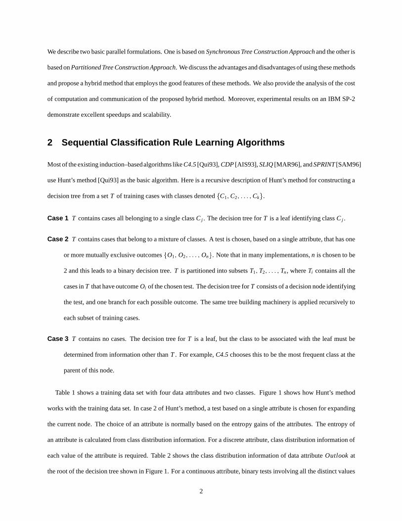
Table 1 shows a training data set with four data attributes and two classes. Figure 1 shows how Hunt’s method

works with the training data set. In case 2 of Hunt’s method, a test based on a single attribute is chosen for expanding

the current node. The choice of an attribute is normally based on the entropy gains of the attributes. The entropy of

an attribute is calculated from class distribution information. For a discrete attribute, class distribution information of

each value of the attribute is required. Table 2 shows the class distribution information of data attribute Outlook at

the root of the decision tree shown in Figure 1. For a continuous attribute, binary tests involving all the distinct values

2

Outlook Temp(F) Humidity(%) Windy? Classsunny 75 70 true Playsunny 80 90 true Don’t Playsunny 85 85 false Don’t Playsunny 72 95 false Don’t Playsunny 69 70 false Play

overcast 72 90 true Playovercast 83 78 false Playovercast 64 65 true Playovercast 81 75 false Play

rain 71 80 true Don’t Playrain 65 70 true Don’t Playrain 75 80 false Playrain 68 80 false Playrain 70 96 false Play

Table 1: A small training data set [Qui93]

PlayDont’ Play Play

Play

Play Dont’ Play Dont’ Play Play

sunnyovercast rain

Outlook

Windy

sunnyovercast

rain

<= 75 > 75 true false

Play

Outlook

Humidity

non-leaf node

expandable leaf node

non-expandable leaf node

(a) Initial Classification Tree (b) Intermediate Classification Tree (c) Final Classification Tree

Figure 1: Demonstration of Hunt’s Method

3

Attribute Value ClassPlay Don’t Play

sunny 2 3overcast 4 0

rain 3 2

Table 2: Class Distribution Information of Attribute Outlook

Attribute Value Binary Test ClassPlay Don’t Play

65 ≤ 1 0> 8 5

70 ≤ 3 1> 6 4

75 ≤ 4 1> 5 4

78 ≤ 5 1> 4 4

80 ≤ 7 2> 2 3

85 ≤ 7 3> 2 2

90 ≤ 8 4> 1 1

95 ≤ 8 5> 1 0

96 ≤ 9 5> 0 0

Table 3: Class Distribution Information of Attribute H umidi ty

of the attribute are considered. Table 3 shows the class distribution information of data attribute H umidi ty. Once the

class distribution information of all the attributes are gathered, each attribute is evaluated in terms of either entropy

[Qui93] or Gini Index [BFOS84]. The best attribute is selected as a test for the node expansion.

The C4.5 algorithm generates a classification–decision tree for the given training data set by recursively partition-

ing the data. The decision tree is grown using depth–first strategy. The algorithm considers all the possible tests that

can split the data set and selects a test that gives the best information gain. For each discrete attribute, one test with

outcomes as many as the number of distinct values of the attribute is considered. For each continuous attribute, binary

tests involving every distinct value of the attribute are considered. In order to gather the entropy gain of all these binary

tests efficiently, the training data set belonging to the node in consideration is sorted for the values of the continuous

attribute and the entropy gains of the binary cut based on each distinct values are calculated in one scan of the sorted

data. This process is repeated for each continuous attribute.

4

Recently proposed classification algorithms SLIQ [MAR96] and SPRINT [SAM96] avoid costly sorting at each node

by pre-sorting continuous attributes once in the beginning. In SPRINT, each continuous attribute is maintained in a

sorted attribute list. In this list, each entry contains a value of the attribute and its corresponding record id. Once the

best attribute to split a node in a classification tree is determined, each attribute list has to be split according to the split

decision. A hash table, of the same order as the number of training cases, has the mapping between record ids and

where each record belongs according to the split decision. Each entry in the attribute list is moved to a classification

tree node according to the information retrieved by probing the hash table. The sorted order is maintained as the entries

are moved in pre-sorted order.

Decision trees are usually built in two steps. First, an initial tree is built till the leaf nodes belong to a single class

only. Second, pruning is done to remove any overfitting to the training data. Typically, the time spent on pruning for

a large dataset is a small fraction, less than 1% of the initial tree generation. Therefore, in this paper, we focus on the

initial tree generation only and not on the pruning part of the computation.

3 Parallel Formulations

In this section, we give two basic parallel formulations for the classification decision tree construction and a hybrid

scheme that combines good features of both of these approaches. We focus our presentation for discrete attributes

only. The handling of continuous attributes is discussed in Section 3.4. In all parallel formulations, we assume that N

training cases are randomly distributed to P processors initially such that each processor has N/P cases.

3.1 Synchronous Tree Construction Approach

In this approach, all processors construct a decision tree synchronously by sending and receiving class distribution

information of local data. Major steps for the approach are shown below:

1. Select a node to expand according to a decision tree expansion strategy (eg. Depth-First or Breadth-First), andcall that node as the current node. At the beginning, root node is selected as the current node.

2. For each data attribute, collect class distribution information of the local data at the current node.

3. Exchange the local class distribution information using global reduction [KGGK94] among processors.

4. Simultaneously compute the entropy gains of each attribute at each processor and select the best attribute forchild node expansion.

5. Depending on the branching factor of the tree desired, create child nodes for the same number of partitions ofattribute values, and split training cases accordingly.

5

Proc 0

Proc 0 Proc 1 Proc 2 Proc 3

Proc 1 Proc 2 Proc 3

Class Distribution Information

Class Distribution Information

Figure 2: Synchronous Tree Construction Approach with Depth–First Expansion Strategy

6. Repeat above steps (1–5) until no more nodes are available for the expansion.

Figure 2 shows the overall picture. The root node has already been expanded and the current node is the leftmost

child of the root (as shown in the top part of the figure). All the four processors cooperate to expand this node to have

two child nodes. Next, the leftmost node of these child nodes is selected as the current node (in the bottom of the figure)

and all four processors again cooperate to expand the node.

The advantage of this approach is that it does not require any movement of the training data items. However, this

algorithm suffers from high communication cost and load imbalance. For each node in the decision tree, after collecting

the class distribution information, all the processors need to synchronize and exchange the distribution information. At

the nodes of shallow depth, the communication overhead is relatively small, because the number of training data items

to be processed is relatively large. But as the decision tree grows and deepens, the number of training set items at

the nodes decreases and as a consequence, the computation of the class distribution information for each of the nodes

decreases. If the average branching factor of the decision tree is k, then the number of data items in a child node is on the

average 1k th of the number of data items in the parent. However, the size of communication does not decrease as much,

as the number of attributes to be considered goes down only by one. Hence, as the tree deepens, the communication

overhead dominates the overall processing time.

6

The other problem is due to load imbalance. Even though each processor started out with the same number of the

training data items, the number of items belonging to the same node of the decision tree can vary substantially among

processors. For example, processor 1 might have all the data items on leaf node A and none on leaf node B, while

processor 2 might have all the data items on node B and none on node A. When node A is selected as the current node,

processor 2 does not have any work to do and similarly when node B is selected as the current node, processor 1 has

no work to do.

This load imbalance can be reduced if all the nodes on the frontier are expanded simultaneously, i.e. one pass of

all the data at each processor is used to compute the class distribution information for all nodes on the frontier. Note

that this improvement also reduces the number of times communications are done and reduces the message start–up

overhead, but it does not reduce the overall volume of communications.

In the rest of the paper, we will assume that in the synchronous tree construction algorithm, the classification tree is

expanded breadth-first manner and all the nodes at a level will be processed at the same time.

3.2 Partitioned Tree Construction Approach

In this approach, whenever feasible, different processors work on different parts of the classification tree. In particular,

if more than one processors cooperate to expand a node, then these processors are partitioned to expand the successors

of this node. Consider the case in which a group of processors Pn cooperate to expand node n. The algorithm consists

of following steps:

Step 1 Processors in Pn cooperate to expand node n using the method described in Section 3.1.

Step 2 Once the node n is expanded in to successor nodes, n1, n2, . . . , nk , then the processor group Pn is also parti-tioned, and the successor nodes are assigned to processors as follows:

Case 1: If the number of successor nodes is greater than |Pn|,

1. Partition the successor nodes into |Pn| groups such that the total number of training cases correspond-ing to each node group is roughly equal. Assign each processor to one node group.

2. Shuffle the training data such that each processor has data items that belong to the nodes it is responsiblefor.

3. Now the expansion of the subtrees rooted at a node group proceeds completely independently at eachprocessor as in the serial algorithm.

Case 2: Otherwise (if the number of successor nodes is less than |Pn|),

1. Assign a subset of processors to each node such that number of processors assigned to a node is pro-portional to the number of the training cases corresponding to the node.

2. Shuffle the training cases such that each subset of processors has training cases that belong to the nodesit is responsible for.

7

Proc 0 Proc 1 Proc 2 Proc 3

Proc 0 Proc 1 Proc 2 Proc 3

Data Item

Data Item

Proc 0 Proc 1 Proc 3Proc 2

Figure 3: Partitioned Tree Construction Approach

3. Processor subsets assigned to different nodes develop subtrees independently. Processor subsets thatcontain only one processor use the sequential algorithm to expand the part of the classification treerooted at the node assigned to them. Processor subsets that contain more than one processor proceedby following the above steps recursively.

At the beginning, all processors work together to expand the root node of the classification tree. At the end, the

whole classification tree is constructed by combining subtrees of each processor.

Figure 3 shows an example. First (at the top of the figure), all four processors cooperate to expand the root node just

like they do in the synchronous tree construction approach. Next (in the middle of the figure), the set of four processors

is partitioned in three parts. The leftmost child is assigned to processors 0 and 1, while the other nodes are assigned to

processors 2 and 3, respectively. Now these sets of processors proceed independently to expand these assigned nodes.

In particular, processors 2 and processor 3 proceed to expand their part of the tree using the serial algorithm. The group

containing processors 0 and 1 splits the leftmost child node into three nodes. These three new nodes are partitioned in

8

two parts (shown in the bottom of the figure); the leftmost node is assigned to processor 0, while the other two are

assigned to processor 1. From now on, processors 0 and 1 also independently work on their respective subtrees.

The advantage of this approach is that once a processor becomes solely responsible for a node, it can develop a

subtree of the classification tree independently without any communication overhead. However, there are a number

of disadvantages of this approach. The first disadvantage is that it requires data movement after each node expansion

until one processor becomes responsible for an entire subtree. The communication cost is particularly expensive in the

expansion of the upper part of the classification tree. (Note that once the number of nodes in the frontier exceeds the

number of processors, then the communication cost becomes zero.) The second disadvantage is poor load balancing

inherent in the algorithm. Assignment of nodes to processors is done based on the number of training cases in the

successor nodes. However, the number of training cases associated with a node does not necessarily correspond to the

amount of work needed to process the subtree rooted at the node. For example, if all training cases associated with a

node happen to have the same class label, then no further expansion is needed.

3.3 Hybrid Parallel Formulation

Our hybrid parallel formulation has elements of both schemes. The Synchronous Tree Construction Approach in Sec-

tion 3.1 incurs high communication overhead as the frontier gets larger. The Partitioned Tree Construction Approach

of Section 3.2 incurs cost of load balancing after each step. The hybrid scheme keeps continuing with the first approach

as long as the communication cost incurred by the first formulation is not too high. Once this cost becomes high, the

processors as well as the current frontier of the classification tree are parti tioned into two parts.

Our description assumes that the number of processors is a power of 2, and that these processors are connected in a

hypercube configuration. The algorithm can be appropriately modified if P is not a power of 2. Also this algorithm can

be mapped on to any parallel architecture by simply embedding a virtual hypercube in the architecture. More precisely

the hybrid formulation works as follows.

• The database of training cases is split equally among P processors. Thus, if N is the total number of trainingcases, each processor has N/P training cases locally. At the beginning, all processors are assigned to one parti-tion. The root node of the classification tree is allocated to the partition.

• All the nodes at the frontier of the tree that belong to one partition are processed together using the synchronoustree construction approach of Section 3.1.

• As the depth of the tree within a partition increases, the volume of statistics gathered at each level also increasesas discussed in Section 3.1. At some point, a level is reached when communication cost become prohibitive. At

9

this point, the processors in the partition are divided into two partitions, and the current set of frontier nodes aresplit and allocated to these partitions in such a way that the number of training cases in each partition is roughlyequal. This load balancing is done as described as follows:

– On a hypercube, each of the two partitions naturally correspond to a sub-cube. First, corresponding pro-cessors within the two sub-cubes exchange relevant training cases to be transferred to the other sub-cube.After this exchange, processors within each sub-cube collectively have all the training cases for their parti-tion, but the number of training cases at each processor can vary between 0 to 2∗N

P . Now, a load balancingstep is done within each sub-cube so that each processor has an equal number of data items.

• Now, further processing within each partition proceeds asynchronously. The above steps are now repeated ineach one of these partitions for the particular subtrees. This process is repeated until a complete classificationtree is grown.

• If a group of processors in a partition become idle, then this partition joins up with any other partition that haswork and has the same number of processors. This can be done by simply giving half of the training cases locatedat each processor in the donor partition to a processor in the receiving partition.

Computation Frontier at depth 3

Figure 4: The computation frontier during computation phase

Partition 1 Partition 2

Figure 5: Binary partitioning of the tree to reduce communication costs

A key element of the algorithm is the criterion that triggers the partitioning of the current set of processors (and

the corresponding frontier of the classification tree ). If partitioning is done too frequently, then the hybrid scheme

will approximate the partitioned tree construction approach, and thus will incur too much data movement cost. If the

partitioning is done too late, then it will suffer from high cost for communicating statistics generated for each node of

10

the frontier, like the synchronized tree construction approach. One possibility is to do splitting when the accumulated

cost of communication becomes equal to the cost of moving records around in the splitting phase. More precisely,

splitting is done when

∑(Communication Cost) ≥ MovingCost + Load Balancing

As an example of the hybrid algorithm, Figure 4 shows a classification tree frontier at depth 3. So far, no partitioning

has been done and all processors are working cooperatively on each node of the frontier. At the next frontier at depth

4, partitioning is triggered, and the nodes and processors are partitioned into two partitions as shown in Figure 5.

A detailed analysis of the hybrid algorithm is presented in Section 4.

3.4 Handling Continuous Attributes

Note that handling continuous attributes requires sorting. If each processor contains N/P training cases, then one ap-

proach for handling continuous attributes is to perform a parallel sorting step for each such attribute at each node of

the decision tree being constructed. Once this parallel sorting is completed, each processor can compute the best lo-

cal value for the split, and then a simple global communication among all processors can determine the globally best

splitting value. However, the step of parallel sorting would require substantial data exchange among processors. The

exchange of this information is of similar nature as the exchange of class distribution information, except that it is of

much higher volume. Hence even in this case, it will be useful to use a scheme similar to the hybrid approach discussed

in Section 3.3.

A more efficient way of handling continuous attributes without incurring the high cost of repeated sorting is to use

the pre-sorting technique used in algorithms SLIQ [MAR96], SPRINT [SAM96], and ScalParC [JKK98]. These al-

gorithms require only one pre-sorting step, but need to construct a hash table at each level of the classification tree.

In the parallel formulations of these algorithms, the content of this hash table needs to be available globally, requiring

communication among processors. Existing parallel formulations of these schemes [SAM96, JKK98] perform commu-

nication that is similar in nature to that of our synchronous tree construction approach discussed in Section 3.1. Once

again, communication in these formulations [SAM96, JKK98] can be reduced using the hybrid scheme of Section 3.3.

Another completely different way of handling continuous attributes is to discretize them once as a preprocessing

11

symbol definitionN Total number of training samplesP Total Number of processorsPi Number of processors cooperatively working on tree expansionAd Number of categorical attributesC Number of classesM Average number of distinct values in the discrete attributesL Present level of a decision treetc Unit computation timets Start up time of communication latency [KGGK94]tw Per–word transfer time of communication latency [KGGK94]

Table 4: Symbols used in the analysis.

step [Hon97]. In this case, the parallel formulations as presented in the previous subsections are directly applicable

without any modification.

Another approach towards discretization is to discretize at every node in the tree. There are two examples of this

approach. The first example can be found in [ARS98] where quantiles [ARS97] are used to discretize continuous at-

tributes. The second example of this approach to discretize at each node is SPEC [SSHK97] where a clustering tech-

nique is used. SPEC has been shown to be very efficient in terms of runtime and has also been shown to perform essen-

tially identical to several other widely used tree classifiers in terms of classification accuracy [SSHK97]. Parallelization

of the discretization at every node of the tree is similar in nature to the parallelization of the computation of entropy

gain for discrete attributes, because both of these methods of discretization require some global communication among

all the processors that are responsible for a node. In particular, parallel formulations of the clustering step in SPEC is

essentially identical to the parallel formulations for the discrete case discussed in the previous subsections [SSHK97].

4 Analysis of the Hybrid Algorithm

In this section, we provide the analysis of the hybrid algorithm proposed in Section 3.3. Here we give a detailed analysis

for the case when only discrete attributes are present. The analysis for the case with continuous attributes can be found

in [SSHK97]. The detailed study of the communication patterns used in this analysis can be found in [KGGK94].

Table 4 describes the symbols used in this section.

12

4.1 Assumptions

• The processors are connected in a hypercube topology. Complexity measures for other topologies can be easily

derived by using the communication complexity expressions for other topologies given in [KGGK94].

• The expression for communication and computation are written for a full binary tree with 2L leaves at depth L.

The expressions can be suitably modified when the tree is not a full binary tree without affecting the scalability

of the algorithm.

• The size of the classification tree is asymptotically independent of N for a particular data set. We assume that a

tree represents all the knowledge that can be extracted from a particular training data set and any increase in the

training set size beyond a point does not lead to a larger decision tree.

4.2 Computation and Communication Cost

For each leaf of a level, there are Ad class histogram tables that need to be communicated. The size of each of these

tables is the product of number of classes and the mean number of attribute values. Thus size of class histogram table

at each processor for each leaf is:

Class histogram size for each leaf = C ∗ Ad ∗ M

The number of leaves at level L is 2L . Thus the total size of the tables is:

Combined class histogram tables for a processor = C ∗ Ad ∗ M ∗ 2L

At level L, the local computation cost involves I/O scan of the training set, initialization and update of all the class

histogram tables for each attribute:

Local Computation cost = θ(Ad ∗ N

P+ C ∗ Ad ∗ M ∗ 2L) ∗ tc = θ(

N

P) (1)

where tc is the unit of computation cost.

At the end of local computation at each processor, a synchronization involves a global reduction of class histogram

13

values. The communication cost1 is :

Per level Communication cost = (ts + tw ∗ C ∗ Ad ∗ M ∗ 2L) ∗ log Pi ≤ θ(log P) (2)

When a processor partition is split into two, each leaf is assigned to one of the partitions in such a way that number of

training data items in the two partitions is approximately the same. In order for the two partitions to work independently

of each other, the training set has to be moved around so that all training cases for a leaf are in the assigned processor

partition. For a load balanced system, each processor in a partition must have NP training data items.

This movement is done in two steps. First, each processor in the first partition sends the relevant training data items

to the corresponding processor in the second partition. This is referred to as the “moving” phase. Each processor can

send or receive a maximum of NP data to the corresponding processor in the other partition.

Cost for moving phase ≤ 2 ∗N

P∗ tw (3)

After this, an internal load balancing phase inside a partition takes place so that every processor has an equal number of

training data items. After the moving phase and before the load balancing phase starts, each processor has training data

item count varying from 0 to 2∗NP . Each processor can send or receive a maximum of N

P training data items. Assuming

no congestion in the interconnection network, cost for load balancing is:

Cost for load balancing phase ≤ 2 ∗N

P∗ tw (4)

A detailed derivation of Equation 4 above is given in [SSHK97]. Also, the cost for load balancing assumes that there

is no network congestion. This is a reasonable assumption for networks that are bandwidth-rich as is the case with most

commercial systems. Without assuming anything about network congestion, load balancing phase can be done using

transportation primitive [SAR95] in time 2 ∗ NP ∗ tw time provided N

P ≥ O(P2)

Splitting is done when the accumulated cost of communication becomes equal to the cost of moving records around

1If the message size is large, by routing message in parts, this communication step can be done in time : (ts + tw ∗ MesgSize) ∗ k0 for a smallconstant k0. Refer to [KGGK94] section 3.7 for details.

14

in the splitting phase [KK94]. So splitting is done when:

∑(Communication Cost) ≥ Moving Cost + Load Balancing

This criterion for splitting ensures that the communication cost for this scheme will be within twice the communication

cost for an optimal scheme [KK94]. The splitting is recursive and is applied as many times as required. Once splitting

is done, the above computations are applied to each partition. When a partition of processors starts to idle, then it sends

a request to a busy partition about its idle state. This request is sent to a partition of processors of roughly the same size

as the idle partition. During the next round of splitting the idle partition is included as a part of the busy partition and

the computation proceeds as described above.

4.3 Scalability Analysis

Isoefficiency metric has been found to be a very useful metric of scalability for a large number of problems on a large

class of commercial parallel computers [KGGK94]. It is defined as follows. Let P be the number of processors and

W the problem size (in total time taken for the best sequential algorithm). If W needs to grow as fE (P) to maintain an

efficiency E, then fE (P) is defined to be the isoefficiency function for efficiency E and the plot of fE (P) with respect

to P is defined to be the isoefficiency curve for efficiency E.

We assume that the data to be classified has a tree of depth L1. This depth remains constant irrespective of the size

of data since the data “fits” this particular classification tree.

Total cost for creating new processor sub-partitions is the product of total number of partition splits and cost for each

partition split (=θ( NP )) using Equations 3 and 4. The number of partition splits that a processor participates in is less

than or equal to L1– the depth of the tree.

Cost for creating new processors partitions ≤ L1 ∗ θ(N

P) (5)

Communication cost at each level is given by Equation 2 (= θ(log P)). The combined communication cost is the

15

product of the number of levels and the communication cost at each level.

Combined communication cost for processing attributes ≤ L1 ∗ θ(log P) = θ(log P) (6)

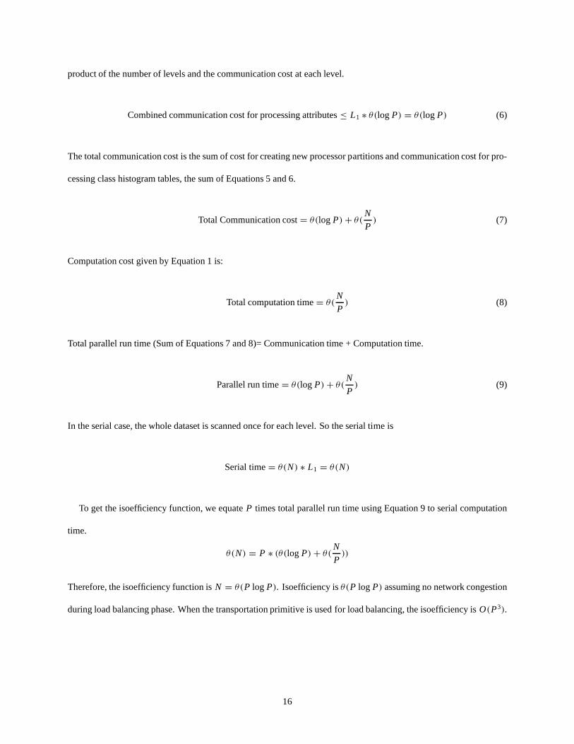
The total communication cost is the sum of cost for creating new processor partitions and communication cost for pro-

cessing class histogram tables, the sum of Equations 5 and 6.

Total Communication cost = θ(log P) + θ(N

P) (7)

Computation cost given by Equation 1 is:

Total computation time = θ(N

P) (8)

Total parallel run time (Sum of Equations 7 and 8)= Communication time + Computation time.

Parallel run time = θ(log P) + θ(N

P) (9)

In the serial case, the whole dataset is scanned once for each level. So the serial time is

Serial time = θ(N) ∗ L1 = θ(N)

To get the isoefficiency function, we equate P times total parallel run time using Equation 9 to serial computation

time.

θ(N) = P ∗ (θ(log P) + θ(N

P))

Therefore, the isoefficiency function is N = θ(P log P). Isoefficiency is θ(P log P) assuming no network congestion

during load balancing phase. When the transportation primitive is used for load balancing, the isoefficiency is O(P3).

16

5 Experimental Results

We have implemented the three parallel formulations using the MPI programming library. We use binary splitting at

each decision tree node and grow the tree in breadth first manner. For generating large datasets, we have used the widely

used synthetic dataset proposed in the SLIQ paper [MAR96] for all our experiments. Ten classification functions were

also proposed in [MAR96] for these datasets. We have used the function 2 dataset for our algorithms. In this dataset,

there are two class labels and each record consists of 9 attributes having 3 categoric and 6 continuous attributes. The

same dataset was also used by the SPRINT algorithm [SAM96] for evaluating its performance. Experiments were done

on an IBM SP2. The results for comparing speedup of the three parallel formulations are reported for parallel runs on

1, 2, 4, 8, and 16 processors. More experiments for the hybrid approach are reported for up to 128 processors. Each

processor has a clock speed of 66.7 MHz with 256 MB real memory. The operating system is AIX version 4 and the

processors communicate through a high performance switch (hps). In our implementation, we keep the “attribute lists”

on disk and use the memory only for storing program specific data structures, the class histograms and the clustering

structures.

First, we present results of our schemes in the context of discrete attributes only. We compare the performance of

the three parallel formulations on up to 16 processor IBM SP2. For these results, we discretized 6 continuous attributes

uniformly. Specifically, we discretized the continuous attribute salary to have 13, commission to have 14, age to have

6, hvalue to have 11, hyears to have 10, and loan to have 20 equal intervals. For measuring the speedups, we worked

with different sized datasets of 0.8 million training cases and 1.6 million training cases. We increased the processors

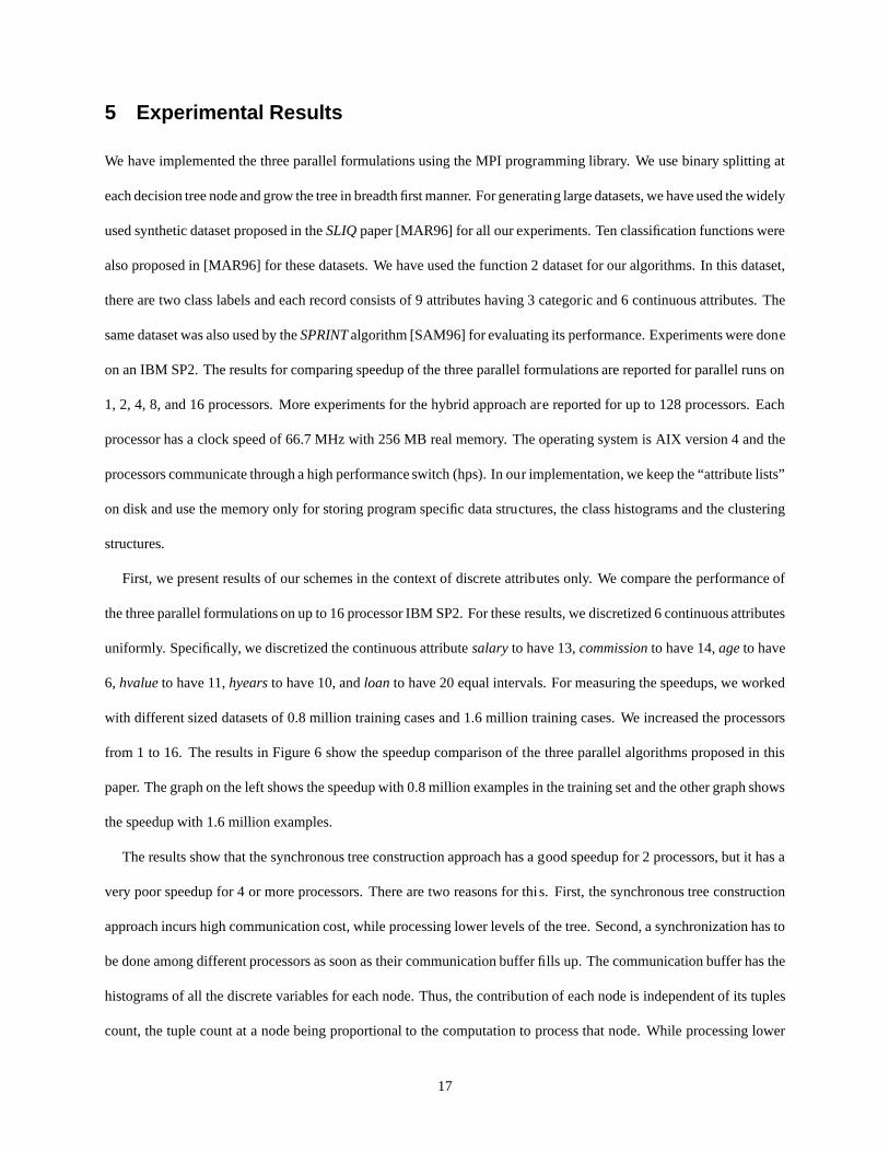
from 1 to 16. The results in Figure 6 show the speedup comparison of the three parallel algorithms proposed in this

paper. The graph on the left shows the speedup with 0.8 million examples in the training set and the other graph shows

the speedup with 1.6 million examples.

The results show that the synchronous tree construction approach has a good speedup for 2 processors, but it has a

very poor speedup for 4 or more processors. There are two reasons for thi s. First, the synchronous tree construction

approach incurs high communication cost, while processing lower levels of the tree. Second, a synchronization has to

be done among different processors as soon as their communication buffer fills up. The communication buffer has the

histograms of all the discrete variables for each node. Thus, the contribution of each node is independent of its tuples

count, the tuple count at a node being proportional to the computation to process that node. While processing lower

17

levels of the tree, this synchronization is done many times at each level (after every 100 nodes for our experiments).

The distribution of tuples for each decision tree node becomes quite different lower down in the tree. Therefore, the

processors wait for each other during synchronization, and thus, contribute to poor speedups.

The partitioned tree construction approach has a better speedup than the synchronous tree construction approach.

However, its efficiency decreases as the number of processors increases to 8 and 16. The partitioned tree construction

approach suffers from load imbalance. Even though nodes are partitioned so that each processor gets equal number of

tuples, there is no simple way of predicting the size of the subtree for that particular node. This load imbalance leads

to the runtime being determined by the most heavily loaded processor. The partitioned tree construction approach also

suffers from the high data movement during each partitioning phase, the partitioning phase taking place at higher levels

of the tree. As more processors are involved, it takes longer to reach the point where all the processors work on their

local data only. We have observed in our experiments that load imbalance and higher communication, in that order,

are the major cause for the poor performance of the partitioned tree construction approach as the number of processors

increase.

The hybrid approach has a superior speedup compared to the partitioned tree approach as its speedup keeps increas-

ing with increasing number of processors. As discussed in Section 3.3 and analyzed in Section 4, the hybrid controls

the communication cost and data movement cost by adopting the advantages of the two basic parallel formulations.

The hybrid strategy also waits long enough for splitting, until there are large number of decision tree nodes for splitting

among processors. Due to the allocation of decision tree nodes to each processor being randomized to a large extent,

good load balancing is possible. The results confirmed that the proposed hybrid approach based on these two basic

parallel formulations is effective.

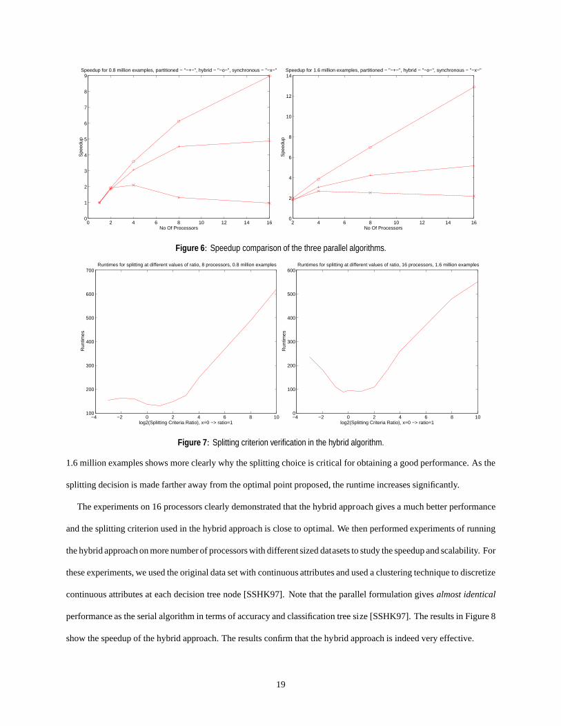
We have also performed experiments to verify our splitting criterion of the hybrid algorithm is correct. Figure 7

shows the runtime of the hybrid algorithm with different ratio of communication cost and the sum of moving cost and

load balancing cost, i.e.,

ratio =

∑(Communication Cost)

Moving Cost + Load Balancing.

The graph on the left shows the result with 0.8 million examples on 8 processors and the other graph shows the result

with 1.6 million examples on 16 processors. We proposed that splitting when this ratio is 1.0 would be the optimal time.

The results verified our hypothesis as the runtime is the lowest when the ratio is around 1.0. The graph on the right with

18

0 2 4 6 8 10 12 14 160

1

2

3

4

5

6

7

8

9

No Of Processors

Spe

edup

Speedup for 0.8 million examples, partitioned − "−+−", hybrid − "−o−", synchronous − "−x−"

2 4 6 8 10 12 14 160

2

4

6

8

10

12

14

No Of Processors

Spe

edup

Speedup for 1.6 million examples, partitioned − "−+−", hybrid − "−o−", synchronous − "−x−"

Figure 6: Speedup comparison of the three parallel algorithms.

−4 −2 0 2 4 6 8 10100

200

300

400

500

600

700

log2(Splitting Criteria Ratio), x=0 −> ratio=1

Run

times

Runtimes for splitting at different values of ratio, 8 processors, 0.8 million examples

−4 −2 0 2 4 6 8 100

100

200

300

400

500

600

log2(Splitting Criteria Ratio), x=0 −> ratio=1

Run

times

Runtimes for splitting at different values of ratio, 16 processors, 1.6 million examples

Figure 7: Splitting criterion verification in the hybrid algorithm.

1.6 million examples shows more clearly why the splitting choice is critical for obtaining a good performance. As the

splitting decision is made farther away from the optimal point proposed, the runtime increases significantly.

The experiments on 16 processors clearly demonstrated that the hybrid approach gives a much better performance

and the splitting criterion used in the hybrid approach is close to optimal. We then performed experiments of running

the hybrid approach on more number of processors with different sized datasets to study the speedup and scalability. For

these experiments, we used the original data set with continuous attributes and used a clustering technique to discretize

continuous attributes at each decision tree node [SSHK97]. Note that the parallel formulation gives almost identical

performance as the serial algorithm in terms of accuracy and classification tree size [SSHK97]. The results in Figure 8

show the speedup of the hybrid approach. The results confirm that the hybrid approach is indeed very effective.

19

0

20

40

60

80

100

0 20 40 60 80 100 120 140

Spe

edup

Number of processors

Speedup curves for different sized datasets

0.8 million examples1.6 million examples3.2 million examples6.4 million examples

12.8 million examples25.6 million examples

Figure 8: Speedup of the hybrid approach with different size datasets.

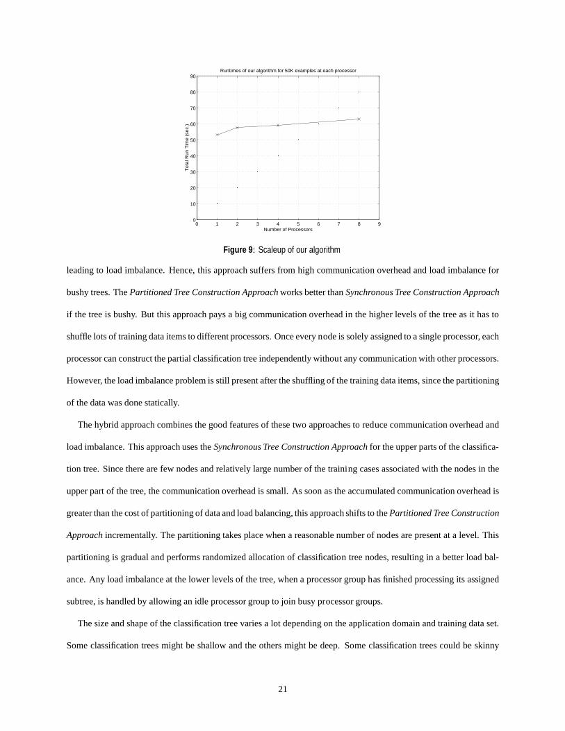
To study the scaleup behavior, we kept the dataset size at each processor constant at 50,000 examples and increased

the number of processors. Figure 9 shows the runtime on increasing number of processors. This curve is very close to

the ideal case of a horizontal line. The deviation from the ideal case is due to the fact that the isoefficiency function is

O(P log P) not O(P). Current experimental data is consistent with the derived isoefficiency function but we intend

to conduct additional validation experiments.

6 Concluding Remarks

In this paper, we proposed three parallel formulations of inductive-classification learning algorithm. The Synchronous

Tree Construction Approach performs well if the classification tree remains skinny, having few nodes at any level,

throughout. For such trees, there are relatively large number of training cases at the nodes at any level; and thus the

communication overhead is relatively small. Load imbalance is avoided by processing all nodes at a level, before syn-

chronization among the processors. However, as the tree becomes bushy, having a large number of nodes at a level, the

number of training data items at each node decrease. Frequent synchronization is done due to limited communication

buffer size, which forces communication after processing a fixed number of nodes. These nodes at lower depths of

the tree, which have few tuples assigned to them, may have highly variable distribution of tuples over the processors,

20

0 1 2 3 4 5 6 7 8 90

10

20

30

40

50

60

70

80

90

Number of Processors

Tot

al R

un T

ime

(sec

.)

Runtimes of our algorithm for 50K examples at each processor

Figure 9: Scaleup of our algorithm

leading to load imbalance. Hence, this approach suffers from high communication overhead and load imbalance for

bushy trees. The Partitioned Tree Construction Approach works better than Synchronous Tree Construction Approach

if the tree is bushy. But this approach pays a big communication overhead in the higher levels of the tree as it has to

shuffle lots of training data items to different processors. Once every node is solely assigned to a single processor, each

processor can construct the partial classification tree independently without any communication with other processors.

However, the load imbalance problem is still present after the shuffling of the training data items, since the partitioning

of the data was done statically.

The hybrid approach combines the good features of these two approaches to reduce communication overhead and

load imbalance. This approach uses the Synchronous Tree Construction Approach for the upper parts of the classifica-

tion tree. Since there are few nodes and relatively large number of the training cases associated with the nodes in the

upper part of the tree, the communication overhead is small. As soon as the accumulated communication overhead is

greater than the cost of partitioning of data and load balancing, this approach shifts to the Partitioned Tree Construction

Approach incrementally. The partitioning takes place when a reasonable number of nodes are present at a level. This

partitioning is gradual and performs randomized allocation of classification tree nodes, resulting in a better load bal-

ance. Any load imbalance at the lower levels of the tree, when a processor group has finished processing its assigned

subtree, is handled by allowing an idle processor group to join busy processor groups.

The size and shape of the classification tree varies a lot depending on the application domain and training data set.

Some classification trees might be shallow and the others might be deep. Some classification trees could be skinny

21

others could be bushy. Some classification trees might be uniform in depth while other trees might be skewed in one

part of the tree. The hybrid approach adapts well to all types of classification trees. If the decision tree is skinny, the

hybrid approach will just stay with the Synchronous Tree Construction Approach. On the other hand, it will shift to the

Partitioned Tree Construction Approach as soon as the tree becomes bushy. If the tree has a big variance in depth, the

hybrid approach will perform dynamic load balancing with processor groups to reduce processor idling.

References

[AIS93] R. Agrawal, T. Imielinski, and A. Swami. Database mining: A performance perspective. IEEE Transactions on Knowl-

edge and Data Eng., 5(6):914–925, December 1993.

[ARS97] K. Alsabti, S. Ranka, and V. Singh. A one-pass algorithm for accurately estimating quantiles for disk-resident data. In

Proc. of the 23rd VLDB Conference, 1997.

[ARS98] K. Alsabti, S. Ranka, and V. Singh. CLOUDS: Classification for large or out-of-core datasets.

http://www.cise.ufl.edu/∼ranka/dm.html, 1998.

[BFOS84] L. Breiman, J. Friedman, R. Olshen, and C. Stone. Classification and Regression Trees. Wadsworth, Monterrey, CA,

1984.

[Cat91] J. Catlett. Megainduction: Machine Learning on Very Large Databases. PhD thesis. University of Sydney, 1991.

[CS93a] Philip K. Chan and Salvatore J. Stolfo. Experiments on multistrategy learning by metalearning. In Proc. Second Intl.

Conference on Info. and Knowledge Mgmt., pages 314–323, 1993.

[CS93b] Philip K. Chan and Salvatore J. Stolfo. Metalearning for multistrategy learning and parallel learning. In Proc. Second

Intl. Conference on Multistrategy Learning, pages 150–165, 1993.

[DMT94] D.J. Spiegelhalter D. Michie and C.C. Taylor. Machine Learning, Neural and Statistical Classification. Ellis Horwood,

1994.

[Gol89] D. E. Goldberg. Genetic Algorithms in Search, Optimizations and Machine Learning. morgan-kaufman, 1989.

[Hon97] S.J. Hong. Use of contextual information for feature ranking and discretization. IEEE Transactions on Knowledge and

Data Eng., 9(5):718–730, September/October 1997.

[JKK98] M.V. Joshi, G. Karypis, and V. Kumar. ScalParC: A new scalable and efficient parallel classification alg orithm for

mining large datasets. In Proc. of the International Parallel Processing Symposium, 1998.

22

[KGGK94] Vipin Kumar, Ananth Grama, Anshul Gupta, and George Karypis. Introduction to Parallel Computing: Algorithm

Design and Analysis. Benjamin Cummings/ Addison Wesley, Redwod City, 1994.

[KK94] George Karypis and Vipin Kumar. Unstructured tree search on simd parallel computers. Journal of Parallel and Dis-

tributed Computing, 22(3):379–391, September 1994.

[Lip87] R. Lippmann. An introduction to computing with neural nets. IEEE ASSP Magazine, 4(22), April 1987.

[MAR96] M. Mehta, R. Agrawal, and J. Rissanen. SLIQ: A fast scalable classifier for data mining. In Proc. of the Fifth Int’l

Conference on Extending Database Technology, Avignon, France, 1996.

[Qui93] J. Ross Quinlan. C4.5: Programs for Machine Learning. Morgan Kaufmann, San Mateo, CA, 1993.

[SAM96] J. Shafer, R. Agrawal, and M. Mehta. SPRINT: A scalable parallel classifier for data mining. In Proc. of the 22nd

VLDB Conference, 1996.

[SAR95] R. Shankar, K. Alsabti, and S. Ranka. Many-to-many communication with bounded traffic. In Frontiers ’95, the fifth

symposium on advances in massively parallel computation, McLean, VA, February 1995.

[SSHK97] Anurag Srivastava, Vineet Singh, Eui-Hong Han, and Vipin Kumar. An efficient, scalable, parallel classifier for data

mining. Technical Report TR-97-010,http://www.cs.umn.edu/∼kumar, Department of Computer Science, University

of Minnesota, M inneapolis, 1997.

[WC88] J. Wirth and J. Catlett. Experiments on the costs and benefits of windowing in ID3. In 5th Int’l Conference on Machine

learning, 1988.

23