Expert Systems with Applications 40 (2013) 6283–6291

Contents lists available at SciVerse ScienceDirect

Expert Systems with Applications

journal homepage: www.elsevier .com/locate /eswa

Fisher’s decision tree

0957-4174/$ - see front matter � 2013 Elsevier Ltd. All rights reserved.http://dx.doi.org/10.1016/j.eswa.2013.05.044

⇑ Corresponding author. Address: Universidad Autónoma del Estado de México,Centro Universitario Zumpango. Tel.: +52 555919174140.

E-mail address: alchau@uaemex.mx (A. López-Chau).

Asdrúbal López-Chau a,⇑, Jair Cervantes b, Lourdes López-García a, Farid García Lamont b

a Centro Universitario UAEM Zumpango, Camino viejo a Jilotzingo continuación calle Rayón, Valle Hermoso. Zumpango, Estado de México C.P. 55600, Mexicob Centro Universitario UAEM Texcoco, Av. Jardn Zumpango s/n, Fracc. El Tejocote, Texcoco, México C.P. 56259, Mexico

a r t i c l e i n f o

Keywords:Oblique decision treeFisher’s linear discriminantC4.5

a b s t r a c t

Univariate decision trees are classifiers currently used in many data mining applications. This classifierdiscovers partitions in the input space via hyperplanes that are orthogonal to the axes of attributes, pro-ducing a model that can be understood by human experts. One disadvantage of univariate decision treesis that they produce complex and inaccurate models when decision boundaries are not orthogonal toaxes. In this paper we introduce the Fisher’s Tree, it is a classifier that takes advantage of dimensionalityreduction of Fisher’s linear discriminant and uses the decomposition strategy of decision trees, to comeup with an oblique decision tree. Our proposal generates an artificial attribute that is used to split thedata in a recursive way.

The Fisher’s decision tree induces oblique trees whose accuracy, size, number of leaves and trainingtime are competitive with respect to other decision trees reported in the literature. We use more thanten public available data sets to demonstrate the effectiveness of our method.

� 2013 Elsevier Ltd. All rights reserved.

1. Introduction

Classification is an important task in pattern recognition, ma-chine learning and data mining. It consists in predicting the cate-gory, class or label of previously unseen objects. Methods thatimplement this task are known as classifiers.

Decision trees (DT) are powerful classifiers widely used in manyapplications such as intrusion detection (Li, 2005), stock trading(Wu, Lin, & Lin, 2006), health (Cruz-Ramírez, Acosta-Mesa, Carril-lo-Calvet, & Barrientos-Martínez, 2009; Fan, Chang, Lin, & Hsieh,2011), fault detection of induction motors (Pomorski & Perche,2001) and online purchasing behavior of users (Xiaohu, Lele, &Nianfeng, 2012).

DT have some advantages over other methods such as to be tol-erant to noise, support missing values and be able to produce mod-els easily interpreted by human beings. In addition, the inductionof DT is not costly.

The general algorithm to induce decision trees from data worksseparating or splitting the data recursively, in such way that parti-tions are increasingly purer up to certain criterion is satisfied.

Classical DT such as CART (Breiman, Friedman, Olshen, & Stone,1984) and C4.5 (Quinlan, 1993) split the data using hyperplanesthat are orthogonal to axes, this kind of trees is known as univar-iate or axis-parallel DT. The splits are found testing every axis ateach possible splitting point.

They are two intrinsic characteristics of axis-parallel decisiontrees: (a) The separating boundaries may result in complicated orinaccurate trees if the decision boundary of data set is describedby hyperplanes not orthogonal to axes of features (Cantu-Paz & Ka-math, 2003), (b) The computational cost increases whether theattributes are of numeric type or there is a large number offeatures.

The oblique (or multivariate) trees are DT whose separatinghyperplanes are not necessarily parallel to axes, in contrast, thehyperplanes can have an arbitrary direction. The induced obliqueDT are usually smaller and in certain cases they achieve better clas-sification accuracy than univariate DT, however the characteristicto be interpretable vanishes.

Several algorithms to induce oblique DT have been proposedbefore, they can be categorized according to the technique usedto create the decision boundaries. One type uses an optimizationstep to determine separating hyperplanes (Murthy, Kasif, & Salz-berg, 1994; Shah & Sastry, 1999; Menkovski, Christou, & Efremidis,2008; Manwani & Sastry, 2009), usually these methods are costlyin terms of complexity. Other use heuristics (Iyengar, 1999) toavoid the computational cost, the accuracy achieved is comparableto univariate trees. Other methods apply genetic algorithms to pro-duce more accurate trees (Cantu-Paz & Kamath, 2003; Shali, Kang-avari, & Bina, 2007), an important remark with this approach isthat the efficiency of greedy methods to induce trees is notpreserved.

In our case we use projection on a vector that maximizes thedistance between the means, which corresponds to the vector ofFisher’s linear discriminant. Similar methods such as (Henrichon

6284 A. López-Chau et al. / Expert Systems with Applications 40 (2013) 6283–6291

& Fu, 1969; Gama, 1997, 1999) follow this approach however theyneed to add more attributes to the training set and they use thefirst principal components.

1.1. Our contribution

In this paper we present the design, implementation and evalu-ation of an oblique decision tree induction method that is designedfor binary classification problems.

The main characteristics of our method are the following: (a)The Fisher’s Linear Discriminant Tree induces oblique trees fromdata, using only one artificial attribute to split the data, recursively.(b) The test of split points is realized on the artificial attribute, sothe number of tests is equal to the number of objects at each node.(c) The supported attribute type is numeric, this common in mostoblique trees. (d) The method is designed for binary classification.

Our method is programmed using in Java programming lan-guage and based on the Weka platform. An executable jar file ofFisher’s decision tree is public available at http://www.media-fire.com/?g1meq364bsvs18l.1

The Fisher’s decision tree works as follows:

1. A vector (x) that maximizes the distance between mean of twoclasses is computed.

2. All objects in data set are projected on x.3. An hyperplane that best splits the data is computed using the

entropy gain criterion.4. A sub tree is grown in each partition.5. The steps are recursively applied.

To the best of our knowledge this is the first time that a decisiontree method is implemented as presented here and also the com-plete implementation and source code is made public available,other proposals with a similar approach are shown in the nextsection.

The rest of this paper is organized as follows. The related workis shown in the Section 2. A brief review on decision trees and Fish-er’s linear discriminant is presented in Section 3, the proposedmethod is explained in Section 4. The results of experiments anddiscussion are in Section 5, finally the conclusions and future workare in Section 6.

2. Related work

The paper presented in Henrichon and Fu (1969) is the first in-tent to induce models from data that resemble current decisiontrees. In that work authors gave ‘‘examples of indications of somemethods which may be useful for improving recognition accuracies’’,they propose to use ‘‘linear transgeneration units’’’ that can be seenas linear combinations of inputs. In Henrichon and Fu (1969) it ismentioned that observation points can be mapped into a line cor-responding to the direction of the eigenvector associated with thelargest eigenvalue of an estimated covariance matrix, which is sim-ilar to our work, however, there are some differences: first, somefeatures are added to the training set (maximum eigenvector, lin-ear discriminant a Quadratic form), in our proposal this is not nec-essary. Second, they use pre-prunning technique, whereas ourapproach use post-pruning. Third, the other method uses the firstprincipal components.

The Robust Linear Decision Trees (John, 1994) is a method thatcan induce oblique decision trees, the method is based on a soft-ened linear discriminant function to discover best split points, such

1 For obtaining the complete source code, write a mail to alchau@uaemex.mx.

function has the form (1). They iteratively solve an optimizationproblem using gradients.

gh ¼ 1=ð1þ expð�hT xÞÞ ð1Þ

Another idea to build oblique decision trees was presented in 1984in the Classification and Regression Trees methodology (Breimanet al., 1984), the method was called CART-LC (CART Linear Combi-nation). In that work the set of allowable splits was extended to in-clude all linear combinations splits, which have the form (2), thismodel is currently used in many other decision trees.

The CART-LC was reported to achieve competitive accuracywith respect to other classification methods (see Breiman et al.,1984, p. 39), however solving the set of linear combinations usingdeterministic heuristics search is computational costly.

Xm

i¼1

amxm 6 C? ð2Þ

The LMDT algorithm (Utgoff & Brodley, 1991) solves a set of R mul-ti-class linear discriminant functions at each node, they are collec-tively used to assign each instance to one of the R classes. A problemwith LMDT is that convergence can not be guaranteed, so a heuristicmust be used to determine when a node has stabilized.

The OC1 (Murthy et al., 1994) method combines hill climbingwith randomization to find good oblique separating hyperplanesat each node of a decision tree, the key idea relies on perturbingeach of the parameters of the hyperplane split rules individuallyseveral times to achieve the optimization. The OC1 computes boththe axis-parallel splits and then the separating hyperplanes to de-cide which to use.

In Setiono and Liu (1999) an artificial neural network is used tobuild an oblique decision tree as follows, the data is first used totrain a neural network having only one hidden layer. After thatthe hidden unit activation values of the network are used to builda decision tree. Then each test at the nodes of the tree is replacedby a linear combination of initial attributes.

The APDT algorithm in Shah and Sastry (1999) uses the concept‘‘degree of linear separability’’, it uses a function that minimizesnon separable patterns in children nodes. When a child node is lin-early separable, the split that puts more patterns in that child nodeis preferred, preserving linear separability.

The Linear Discriminant Trees presented in Yildiz and Alpaydin(2000) resembles our method, but it uses the K main componentsof PCA, and addition it requires to train a neural network for thesplits.

In the HOT heuristics (Iyengar, 1999) the projections on a vectorare used to create oblique splits. The vector is produced joining thecentroids of the two adjacent regions discovered by an axis-paral-lel decision tree.

The Oblique Linear Tree and Discriminant Tree were proposedin Gama (1997, 1999) respectively. The main differences withour method is that they do not use the same discriminant functionthat we apply and in their method the number of attributes canchange along the tree.

In Vadera (2005) an oblique decision tree is developed, thatalgorithm uses the linear discriminant analysis to identify obliquerelationships between (continuous) attributes and then carries outan appropriate modication to ensure that the resulting tree errorson the side of safety. Because that algorithm is oriented to optimizethe cost of misclassification it searches in every attribute, produc-ing an accurate classifier at expense of investing more time to in-duce the tree.

The LST algorithm (He, Xu, & Chen, 2008) transforms local datafrom its original attribute space to the singular vector space, it useslinear independent combinations of the original attributes to builda oblique tree. From the results in He et al. (2008), it can been

A. López-Chau et al. / Expert Systems with Applications 40 (2013) 6283–6291 6285

observed that the local singular vector space constructed by LSTdoes not necessarily lead to the better classification result.

The algorithm in Menkovski et al. (2008) is based on a combina-tion of support vector machine and C4.5 algorithm. This can be-come a bottleneck because it requires to solve quadraticprogramming problems, which computation has a complexity be-tween O(n1.5) and O(n2).

Recently, other methods to induce oblique decision trees usingevolutionary algorithms have been proposed (Vadera, 2010), see(Barros, Basgalupp, de Carvalho, & Freitas, 2011) for a survey onthese techniques. We think that comparison of greedy methodsto induce decision trees against evolutionary methods is not just,because although the reported results in Barros et al. (2011) showthat the second methods produce better trees in terms of accuracy,these methods explore the space of solutions in a different way,usually using randomly procedures that allow to scape from localoptima at expense of increasing computational cost.

3. Preliminaries

The core of proposed method is based on a combination of clas-sic univariate decision tree and the Fisher’s discriminant classifier,before presenting our method, an overview of these two topics isexposed.

3.1. Decision trees

Decision tree is a classifier method able to produce models thatcan be comprehensible by human experts (Breiman et al., 1984).Among the advantages of decision trees over other classificationmethods are (Cios, Pedrycz, Swiniarski, & Kurgan, 2007): robust-ness to noise, ability to deal with redundant attributes, generaliza-tion ability via post-pruning strategy and a low computationalcost, this last is more notorious when decision trees are trainedusing data sets with nominal attributes.

A trained decision tree is a tree structure that consists of a rootnode, links or branches, internal nodes and leaves. The root node isthe topmost node in the tree structure, the branches connect theinternal nodes (root, internal and leaves), finally the leaves are ter-minal nodes which have not further branches.

Classic decision tree algorithms such as CART, C4.5 and ID3, cre-ate or grow trees using a greedy top-down recursive partitioningstrategy. In order to explain the general training process of decisiontrees on numeric attributes, let’s represent the training data sets asin (3).

X ¼ fðxi; yiÞ; i ¼ 1; ::;M: s:t: xi 2 Rd; yi 2 fC1; . . . ;CLgg ð3Þ

With

X

Training set, xi A vector that represents an example or object in X, yi The category or class of xi, M Number of examples in training set, d Number of features, L Number of classes.

The general methodology to build a decision tree is as follows:beginning from root node (it contains X), split the data into two ormore smaller disjoint subsets, each subset should contain all ormost of its elements with the same class, however this is not nec-essary. Each subset can be considered as a leaf whether certain cri-terion is satisfied (usually a minimum number of objects withinthe node or a level of impurity), in this case the partition process

is stopped and the node is labeled according majority class in thatnode, otherwise the process is recursively applied on each subset.A branch or link is created from a node to each one of its partitions.

The data in a node is split computing the attribute that pro-duces the purer partitions. The test to determine best attribute typ-ically takes the form (4). Among all possible values, the generalheuristic is to choose the attribute that decreases the impurity asmuch as possible (Duda, Hart, & Stork, 2000).

There are different impurity measures, most common are infor-mation impurity or entropy impurity (5), variance impurity for twoclass problems (6), gini impurity (7) and miss classification impu-rity (8).

xi;j 6 xk;j? ð4Þ

withxi,j The value of jth feature (0 < j 6 d) of the ith object in X,xk,j The value of jth feature of the kth object in X,k = 1, . . . N,N the

number of elements within the node.

iðNodeÞ ¼ �XL

l¼1

Pðy ¼ clÞlog2ðPðy ¼ clÞÞ ð5Þ

with P(y = cl) the fraction of objects within the node that have classcl.

iðNodeÞ ¼ Pðy ¼ c1ÞPðy ¼ c2Þ ð6Þ

iðNodeÞ ¼XL

l¼1;m¼1;m–l

Pðy ¼ clÞPðy ¼ cmÞ ð7Þ

iðNodeÞ ¼ 1�maxclPðy ¼ clÞ ð8Þ

Once a decision tree has been growth, the general methodologysuggests to (post) prune the tree to avoid over-fitting.

3.2. Fisher’s linear discriminant

Fisher linear discriminant can be considered as a method forlinear dimensionality reduction. The method is based on minimiz-ing the projected class overlapping that maximizes the distancebetween class means while minimizing the variance within eachclass.

Considering a binary classification problem, the training dataset has same structure (3). Let’s separate X into two subsets X+

and X�.

Xþ ¼ fxi 2 X s:t: yi ¼ c1g ð9ÞX� ¼ fxi 2 X s:t: yi ¼ c2g ð10Þ

The means l+ and l� for X+ and X� respectively are computed using(11).

l� ¼ 1jX�j

XjX�j

i¼1

x; x 2 X� ð11Þ

With

X± Represent X+ or X�,

l± Represent either l+ 2 Rd or l� 2 Rd

Let be x 2 Rd a vector used to project every example in X. Themean of projections on x is given by (12).

m� ¼ 1jX�j

XjX�j

i¼1

xi; x 2 X� ð12Þ

With

xi = xTx

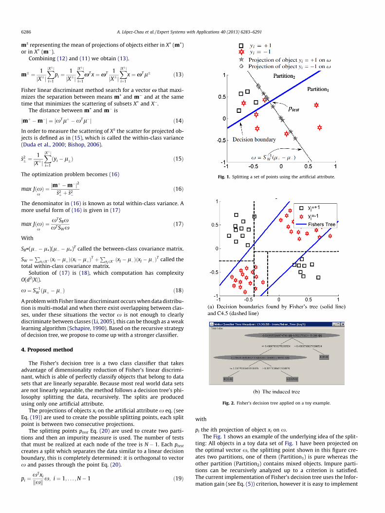
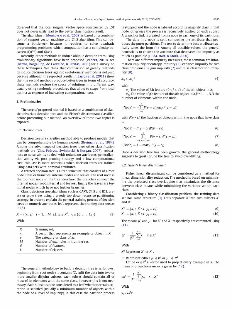
Fig. 1. Splitting a set of points using the artificial attribute.

Fig. 2. Fisher’s decision tree applied on a toy example.

6286 A. López-Chau et al. / Expert Systems with Applications 40 (2013) 6283–6291

m± representing the mean of projections of objects either in X+ (m+)or in X+ (m�).

Combining (12) and (11) we obtain (13).

m� ¼ 1jX�j

XjX�j

i¼1

pi ¼1jX�j

XjX�j

i¼1

xT x ¼ xT 1jX�j

XjX�j

i¼1

x ¼ xTl� ð13Þ

Fisher linear discriminant method search for a vector x that maxi-mizes the separation between means m+ and m� and at the sametime that minimizes the scattering of subsets X+ and X�.

The distance between m+ and m� is

jmþ �m�j ¼ jxTlþ �xTl�j ð14Þ

In order to measure the scattering of X± the scatter for projected ob-jects is defined as in (15), which is called the within-class variance(Duda et al., 2000; Bishop, 2006).

~s2� ¼

1jX�j

XjX�j

i¼1

ðyi � l�Þ ð15Þ

The optimization problem becomes (16)

max JðxÞx¼ jm

þ �m�j2~s2þ þ ~s2

�ð16Þ

The denominator in (16) is known as total within-class variance. Amore useful form of (16) is given in (17)

max JðxÞx¼ xT SBx

xT SWxð17Þ

With

SB=(l� � l+)(l� � l+)T called the between-class covariance matrix.

SW ¼P

xi2Xþ ðxi � lþÞðxi � lþÞT þ

Pxj2X� ðxj � l�Þðxj � l�Þ

T called thetotal within-class covariance matrix.

Solution of (17) is (18), which computation has complexityO(d2jXj).

x ¼ S�1W ðlþ � l�Þ ð18Þ

A problem with Fisher linear discriminant occurs when data distribu-tion is multi-modal and when there exist overlapping between clas-ses, under these situations the vector x is not enough to clearlydiscriminate between classes (Li, 2005), this can be though as a weaklearning algorithm (Schapire, 1990). Based on the recursive strategyof decision tree, we propose to come up with a stronger classifier.

4. Proposed method

The Fisher’s decision tree is a two class classifier that takesadvantage of dimensionality reduction of Fisher’s linear discrimi-nant, which is able of perfectly classify objects that belong to datasets that are linearly separable. Because most real world data setsare not linearly separable, the method follows a decision tree’s phi-losophy splitting the data, recursively. The splits are producedusing only one artificial attribute.

The projections of objects xi on the artificial attribute x eq. (seeEq. (19)) are used to create the possible splitting points, each splitpoint is between two consecutive projections.

The splitting points ptest Eq. (20) are used to create two parti-tions and then an impurity measure is used. The number of teststhat must be realized at each node of the tree is N � 1. Each ptest

creates a split which separates the data similar to a linear decisionboundary, this is completely determined: it is orthogonal to vectorx and passes through the point Eq. (20).

pi ¼xT xi

kxkx; i ¼ 1; . . . ;N � 1 ð19Þ

with

pi the ith projection of object xi on x.The Fig. 1 shows an example of the underlying idea of the split-

ting: All objects in a toy data set of Fig. 1 have been projected onthe optimal vector x, the splitting point shown in this figure cre-ates two partitions, one of them (Partition1) is pure whereas theother partition (Partition2) contains mixed objects. Impure parti-tions can be recursively analyzed up to a criterion is satisfied.The current implementation of Fisher’s decision tree uses the Infor-mation gain (see Eq. (5)) criterion, however it is easy to implement

A. López-Chau et al. / Expert Systems with Applications 40 (2013) 6283–6291 6287

the Gain ratio, Gini index or others. The maximum number of pos-sible partitions is two in the current implementation of theclassifier.

ptest ¼xTðpi þ piþ1Þ

2kxk x ð20Þ

The Fisher’s tree growing method is shown in Algorithm 1, it resem-bles to traditional decision trees, however the main difference is inhow the splits are created; instead of testing every attribute onlythe artificial attribute is used. Although it seems that Fisher’s treesuffers from repetition, which is the phenomenon that occurs whenan attribute is repeatedly tested along a given branch of the tree,this is different because there is only one attribute to split.

Algorithm 1: Fisher’s decision tree growing

Data:S: a set of objectsMinobj: Minimum number of objects per leafOutput:T: a decision treeBegin algorithmCreate a node N using Sif (all elements in N are in the same class C)

return N as leaf node, assign it class C;else if (N contains less than Minobj objects)

return N as leaf node, assign it to majority class C;elseBuild X+ and X� according to (9) and (10).Compute artificial attribute x using (18)Compute best split point (Algorithm 2)Split N according to best split point Eq. (21)for each partition do

Grow a subtree on partition (a son of N)end forreturn Fisher’s decision treeEnd algorithm

Algorithm 2: Compute split point

Data:S: a set of objectsx: Artificial attributeOutput:ptestOpt: The best split point (according to some criterion)Begin algorithmProject every object in S on xSort S in ascending order w.r.t projection//Choose the projection that produce the best split

ptestOpt worst possible impurity value//e.g. �1for each ptest (20) do

Compute impurities of partitions, use (5),(6) or (7)

if ptest is better than ptestOptthen//Update best split point (save the index and real

value)

ptestOpt ptest

end ifend forreturn ptestOpt

End algorithm

The partitions are created according to Eq. (21).

Partition1 ¼ fðxi; yiÞ 2 N; s:t: pi <¼ ptestg ð21ÞPartition2 ¼ fðxi; yiÞ 2 N; s:t: pi > ptestg

In order to efficiently split N in Algorithm 1, the Algorithm 2 actu-ally returns the index of the best split point and the real value (Eq.(22)) which is used in the prediction phase.

ptestOpt ¼xTðpi þ piþ1Þ

2kxk ð22Þ

When a node can not be split any more because it is pure or thereare not enough objects, the node becomes a leaf of the tree. The leafis assigned to the class having the highest probability.

The Fisher’s decision tree avoids to model anomalies in thetraining data due to noise or outliers by pruning the tree. Amongseveral options such as pre pruning, the use of training set to esti-mate error rates and pessimistic post pruning, Fisher’s decisiontree uses the last. We adopt an implementation similar to C4.5.

The Fig. 2 shows an example of an induced decision tree from atoy data set using the proposed method. The Fig. 2(a) shows thedecision boundaries and the Fig. 2(b) shows the tree structure.The boundaries discovered by the Fisher’s decision tree are lesscomplicated than the obtained with a univariate decision tree,the size of the tree is also smaller.

Once the tree has been induced each non terminal node con-tains the vector x and the optimal split point, the label of unseenexamples is predicted by following down the tree down to a leaf asfollows:

(1) If current node is a leaf then the label of the example is theclass associated to the leaf, stop.

(2) Otherwise, project the new example on x, and go to left orright node according to the following rule

(a) If projection is greater than split point go to right node,(b) otherwise go to left node,

(3) recursively repeat this process.

The proposed method involves the following steps to induce thetree: (a) Separate in positive and negative class, (b) compute vectorx, (c) compute split point and split a set of examples.

At each non terminal node, the step (a) runs in O(jSj) time withjSj the size of set being partitioned. The step (b) is the most costly.The vector x is computed in O(d2jSj) time, with d the number ofdimensions. The step (c) requires resorting the data at each recur-sive call, which adds O(S log(jSj)) time. An advantage of our methodwith respect to other decision trees is that it is not necessary to useany discretization either test every attribute.

5. Experiments and discussion

We study the performance of the Fisher’s decision tree using 12public available data sets.

Two experiments were conduced. In the first experiment, weexplore how the performance of our classifier is affected by chang-ing the parameters. In the second experiment we compare ourmethod against C4.5, a well known univariate decision tree Theaccuracy, size and training time of produced trees is presented.

5.1. Data sets

In order to test the effectiveness of the proposed method, it wastested on data sets commonly used for classification, the Table 1shows the main characteristics of them. Because some of the data

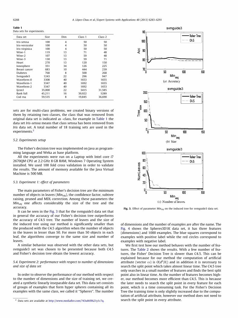
Table 1Data sets for experiments.

Data set Size Dim Class 1 Class 2

Iris-setosa 100 4 50 50Iris-versicolor 100 4 50 50Iris-virginica 100 4 50 50Wine-1 119 13 71 48Wine-2 107 13 59 48Wine-3 130 13 59 71Heart 270 13 120 150Ionosphere 351 34 126 225Breast cancer 683 10 444 239Diabetes 768 8 500 268Svmguide3 1243 22 296 947Waveform-0 3308 40 1653 1655Waveform-1 3347 40 1692 1655Waveform-2 3347 40 1692 1653Ijcnn1 35,000 22 3415 31,585Bank full 45,211 16 39,922 5289Cod rna 59,535 8 19,845 36,690

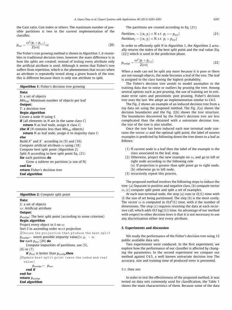
Fig. 3. Effect of parameter Minobj on the induced tree for svmguide3 data set.

6288 A. López-Chau et al. / Expert Systems with Applications 40 (2013) 6283–6291

sets are for multi-class problems, we created binary versions ofthem by retaining two classes, the class that was removed fromoriginal data set is indicated as -class, for example in Table 1 thedata set Iris-setosa means that class setosa has been removed fromIris data set. A total number of 18 training sets are used in theexperiments.2

5.2. Experiments setup

The Fisher’s decision tree was implemented on Java as program-ming language and Weka as base platform.

All the experiments were run on a Laptop with Intel core i72670QM CPU at 2.2 GHz 8 GB RAM, Windows 7 Operating Systeminstalled. We used 100 fold cross validation in order to validatethe results. The amount of memory available for the Java VirtualMachine is 500 MB.

5.3. Experiment 1: effect of parameters

The main parameters of Fisher’s decision tree are the minimumnumber of objects in leaves (Minobj), the confidence factor, subtreeraising, pruned and MDL correction. Among these parameters theMinobj one affects considerably the size of the tree and theaccuracy.

It can be seen in the Fig. 3 that for the svmguide3 data set thatin general the accuracy of our Fisher’s decision tree outperformsthe accuracy of C4.5 tree. The number of leaves and the size ofthe induced tree using our method is significantly smaller thanthe produced with the C4.5 algorithm when the number of objectsin the leaves in lesser than 50. For more than 50 objects in eachleaf, the algorithms converge to the same size and number ofleaves.

A similar behavior was observed with the other data sets, butsvmguide3 set was chosen to be presented because both C4.5and Fisher’s decision tree obtain the lowest accuracy.

5.4. Experiment 2: performance with respect to number of dimensionsand size of data set

In order to observe the performance of our method with respectto the number of dimensions and the size of training set, we cre-ated a synthetic linearly inseparable data set. This data set consistsof groups of examples that form hyper spheres containing all itsexamples with the same class, we called it ‘‘Spheres’’. The number

2 Data sets are available at http://www.mediafire.com/?43u8tl9h21y1c7q.

of dimensions and the number of examples are after the name. TheFig. 4 shows the Spheres3D1K data set, it has three features(dimensions) and 1000 examples. The blue squares correspond toexamples with positive label while the red circles correspond toexamples with negative label.

We first test how our method behaves with the number of fea-tures. The Table 2 shows the results. With a few number of fea-tures, the Fisher’ Decision Tree is slower than C4.5. This can beexplained because for our method the computation of artificialattribute (vector x) is O(d2jXj) and in addition it is necessary tosearch the split point which takes almost linear time. The C4.5 treeonly searches in a small number of features and finds the best splitpoint also in linear time. As the number of features becomes high-er, our method becomes more efficient than C4.5. This is becausethe later needs to search the split point in every feature for eachpoint, which is a time consuming task. For the Fisher’s DecisionTree the training time is only slightly increased due to the compu-tation of artificial attribute, however our method does not need tosearch the split point in every attribute.

Fig. 4. Example of synthetic data set in three dimensions.

Table 2Performance of the method with respect to number of features.

Data set/Method Minobj Treesize Time (ms) Acc (%)

Spheres2D40KFisher’s Tree 2 61 1186 90.76C4.5 2 159 690 91.07

Spheres3D40KFisher’s Tree 2 351 1790 97.95C4.5 2 283 900 98.61

Spheres4D40KFisher’s Tree 2 343 1360 98.15C4.5 2 301 1100 98.42

Spheres6D40KFisher’s Tree 2 377 1810 98.85C4.5 2 253 2130 99.49

Spheres10D40KFisher’s Tree 2 27 1005 99.96C4.5 2 47 1720 99.94

Spheres15D40KFisher’s Tree 2 75 1260 99.94C4.5 2 91 3270 99.85

Spheres20D40KFisher’s Tree 2 49 1230 99.93C4.5 2 83 5200 99.89

Spheres40D40KFisher’s Tree 2 15 1790 99.96C4.5 2 85 13,030 99.91

Table 3Performance of the method with respect to size.

Data set/Method Minobj Treesize Time (ms) Acc (%)

Spheres10D1KFisher’s Tree 2 11 10 99.30Fisher’s Tree 20 6 10 98.40C4.5 2 17 50 98.60C4.5 20 17 50 93.80

Spheres10D2KFisher’s Tree 2 29 30 99.10Fisher’s Tree 20 11 30 97.70C4.5 2 27 80 99.20C4.5 20 13 30 97.15

Spheres10D10K KFisher’s Tree 2 67 200 99.69Fisher’s Tree 2 31 120 99.14C4.5 2 37 470 99.73C4.5 2 25 330 99.30

Spheres10D40K KFisher’s Tree 2 27 1005 99.96Fisher’s Tree 20 19 900 99.93C4.5 2 47 1720 99.94C4.5 20 23 1450 99.90

Spheres10D80K KFisher’s Tree 2 99 4650 99.94Fisher’s Tree 20 57 4140 99.82C4.5 2 201 6790 99.85C4.5 20 105 4910 99.68

Table 4Values of parameters used in experiment 3.

Parameter Fisher’s Tree C4.5

Binary splits N/A trueCollapse Tree true trueConfidence factor 0.25 0.25Num Folds NA 3Subtree raising true truePruned true trueUse Laplace false falseuse MDL Correction false false

A. López-Chau et al. / Expert Systems with Applications 40 (2013) 6283–6291 6289

Now we explore how the proposed method behaves with re-spect to the size of training data set. We chose the Sphere10Dand we vary the number of examples from 1000 up to 80,000.The Table 3 shows the training times and accuracy for several sizesof the synthetic data set. It can be observed that in general the Fih-ser’s Decision Tree produces more accurate results and the trainingtime is better than the other method.

We can say that our method scales better than C4.5, with re-spect to the number of attributes. Our method scales similar tothe other method with respect to the size of training set.

5.5. Experiment 3: accuracy, tree size and training time

For the third experiment, we fixed the parameters of Fisher’sdecision tree. The values used are shown in the Table 4.

The Fisher’s decision tree is compared with C4.5 classifier, theformer produces oblique trees and the last one produces parallel-axis partitions.

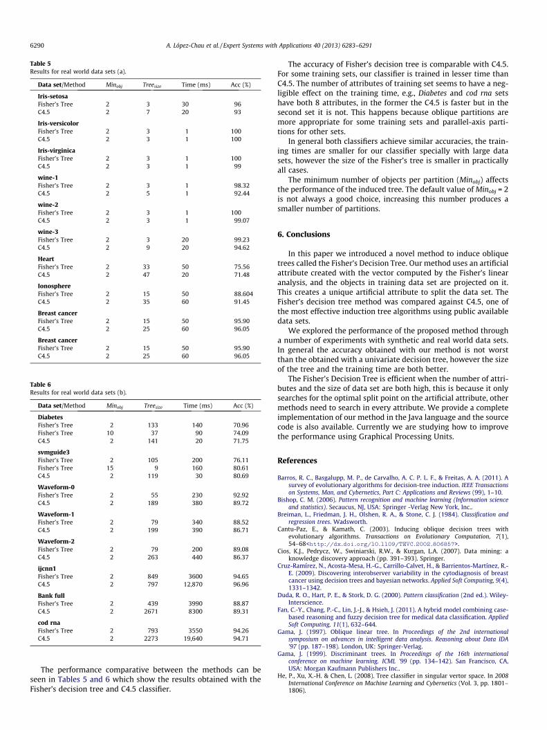
Table 5Results for real world data sets (a).

Data set/Method Minobj Treesize Time (ms) Acc (%)

Iris-setosaFisher’s Tree 2 3 30 96C4.5 2 7 20 93

Iris-versicolorFisher’s Tree 2 3 1 100C4.5 2 3 1 100

Iris-virginicaFisher’s Tree 2 3 1 100C4.5 2 3 1 99

wine-1Fisher’s Tree 2 3 1 98.32C4.5 2 5 1 92.44

wine-2Fisher’s Tree 2 3 1 100C4.5 2 3 1 99.07

wine-3Fisher’s Tree 2 3 20 99.23C4.5 2 9 20 94.62

HeartFisher’s Tree 2 33 50 75.56C4.5 2 47 20 71.48

IonosphereFisher’s Tree 2 15 50 88.604C4.5 2 35 60 91.45

Breast cancerFisher’s Tree 2 15 50 95.90C4.5 2 25 60 96.05

Breast cancerFisher’s Tree 2 15 50 95.90C4.5 2 25 60 96.05

Table 6Results for real world data sets (b).

Data set/Method Minobj Treesize Time (ms) Acc (%)

DiabetesFisher’s Tree 2 133 140 70.96Fisher’s Tree 10 37 90 74.09C4.5 2 141 20 71.75

svmguide3Fisher’s Tree 2 105 200 76.11Fisher’s Tree 15 9 160 80.61C4.5 2 119 30 80.69

Waveform-0Fisher’s Tree 2 55 230 92.92C4.5 2 189 380 89.72

Waveform-1Fisher’s Tree 2 79 340 88.52C4.5 2 199 390 86.71

Waveform-2Fisher’s Tree 2 79 200 89.08C4.5 2 263 440 86.37

ijcnn1Fisher’s Tree 2 849 3600 94.65C4.5 2 797 12,870 96.96

Bank fullFisher’s Tree 2 439 3990 88.87C4.5 2 2671 8300 89.31

cod rnaFisher’s Tree 2 793 3550 94.26C4.5 2 2273 19,640 94.71

6290 A. López-Chau et al. / Expert Systems with Applications 40 (2013) 6283–6291

The performance comparative between the methods can beseen in Tables 5 and 6 which show the results obtained with theFisher’s decision tree and C4.5 classifier.

The accuracy of Fisher’s decision tree is comparable with C4.5.For some training sets, our classifier is trained in lesser time thanC4.5. The number of attributes of training set seems to have a neg-ligible effect on the training time, e.g., Diabetes and cod rna setshave both 8 attributes, in the former the C4.5 is faster but in thesecond set it is not. This happens because oblique partitions aremore appropriate for some training sets and parallel-axis parti-tions for other sets.

In general both classifiers achieve similar accuracies, the train-ing times are smaller for our classifier specially with large datasets, however the size of the Fisher’s tree is smaller in practicallyall cases.

The minimum number of objects per partition (Minobj) affectsthe performance of the induced tree. The default value of Minobj = 2is not always a good choice, increasing this number produces asmaller number of partitions.

6. Conclusions

In this paper we introduced a novel method to induce obliquetrees called the Fisher’s Decision Tree. Our method uses an artificialattribute created with the vector computed by the Fisher’s linearanalysis, and the objects in training data set are projected on it.This creates a unique artificial attribute to split the data set. TheFisher’s decision tree method was compared against C4.5, one ofthe most effective induction tree algorithms using public availabledata sets.

We explored the performance of the proposed method througha number of experiments with synthetic and real world data sets.In general the accuracy obtained with our method is not worstthan the obtained with a univariate decision tree, however the sizeof the tree and the training time are both better.

The Fisher’s Decision Tree is efficient when the number of attri-butes and the size of data set are both high, this is because it onlysearches for the optimal split point on the artificial attribute, othermethods need to search in every attribute. We provide a completeimplementation of our method in the Java language and the sourcecode is also available. Currently we are studying how to improvethe performance using Graphical Processing Units.

References

Barros, R. C., Basgalupp, M. P., de Carvalho, A. C. P. L. F., & Freitas, A. A. (2011). Asurvey of evolutionary algorithms for decision-tree induction. IEEE Transactionson Systems, Man, and Cybernetics, Part C: Applications and Reviews (99), 1–10.

Bishop, C. M. (2006). Pattern recognition and machine learning (Information scienceand statistics). Secaucus, NJ, USA: Springer -Verlag New York, Inc..

Breiman, L., Friedman, J. H., Olshen, R. A., & Stone, C. J. (1984). Classification andregression trees. Wadsworth.

Cantu-Paz, E., & Kamath, C. (2003). Inducing oblique decision trees withevolutionary algorithms. Transactions on Evolutionary Computation, 7(1),54–68<http://dx.doi.org/10.1109/TEVC.2002.806857>.

Cios, K.J., Pedrycz, W., Swiniarski, R.W., & Kurgan, L.A. (2007). Data mining: aknowledge discovery approach (pp. 391–393). Springer.

Cruz-Ramírez, N., Acosta-Mesa, H.-G., Carrillo-Calvet, H., & Barrientos-Martínez, R.-E. (2009). Discovering interobserver variability in the cytodiagnosis of breastcancer using decision trees and bayesian networks. Applied Soft Computing, 9(4),1331–1342.

Duda, R. O., Hart, P. E., & Stork, D. G. (2000). Pattern classification (2nd ed.). Wiley-Interscience.

Fan, C.-Y., Chang, P.-C., Lin, J.-J., & Hsieh, J. (2011). A hybrid model combining case-based reasoning and fuzzy decision tree for medical data classification. AppliedSoft Computing, 11(1), 632–644.

Gama, J. (1997). Oblique linear tree. In Proceedings of the 2nd internationalsymposium on advances in intelligent data analysis. Reasoning about Data IDA’97 (pp. 187–198). London, UK: Springer-Verlag.

Gama, J. (1999). Discriminant trees. In Proceedings of the 16th internationalconference on machine learning. ICML ’99 (pp. 134–142). San Francisco, CA,USA: Morgan Kaufmann Publishers Inc..

He, P., Xu, X.-H. & Chen, L. (2008). Tree classifier in singular vertor space. In 2008International Conference on Machine Learning and Cybernetics (Vol. 3, pp. 1801–1806).

A. López-Chau et al. / Expert Systems with Applications 40 (2013) 6283–6291 6291

Henrichon, E. G., & Fu, K.-S. (1969). A nonparametric partitioning procedure forpattern classification. IEEE Transactions on Computers, 18(7), 614–624.

Iyengar, V. (1999). Hot: Heuristics for oblique trees. In Proceedings of the 11th IEEEinternational conference on tools with artificial intelligence (pp. 91–98).

John, G. H. (1994). Robust linear discriminant trees. AI& Statistics-95 (Vol. 7).Springer-Verlag [pp. 285–291].

Li, X.-B. (2005). A scalable decision tree system and its application in patternrecognition and intrusion detection. Decision Support Systems, 41(1), 112–130.

Manwani, N., & Sastry, P. (2009). A geometric algorithm for learning obliquedecision trees. In Pattern recognition and machine intelligence. In S. Chaudhury, S.Mitra, C. Murthy, P. Sastry, & S. Pal (Eds.). Lecture notes in computer science (Vol.5909, pp. 25–31). Berlin Heidelberg: Springer.

Menkovski, V., Christou, I. & Efremidis, S. (2008). Oblique decision trees usingembedded support vector machines in classifier ensembles. In 7th IEEEinternational conference on cybernetic intelligent systems CIS 2008 (pp. 1–6).

Murthy, S. K., Kasif, S., & Salzberg, S. (1994). A system for induction of obliquedecision trees. Journal of Artificial Intelligence Research, 2(1), 1–32.

Pomorski, D., & Perche, P. (2001). Inductive learning of decision trees: Application tofault isolation of an induction motor. Engineering Applications of ArtificialIntelligence, 14(2), 155–166.

Quinlan, J. R. (1993). C4.5: Programs for machine learning. San Mateo, CA: MorganKaufmann.

Schapire, R. E. (1990). The strength of weak learnability. Machine Learning, 5(2),197–227<http://dx.doi.org/10.1023/A:1022648800760>.

Setiono, R., & Liu, H. (1999). A connectionist approach to generating obliquedecision trees. IEEE Transactions on Systems, Man, and Cybernetics, Part B:Cybernetics, 29(3), 440–444.

Shah, S., & Sastry, P. (1999). New algorithms for learning and pruning obliquedecision trees. IEEE Transactions on Systems, Man, and Cybernetics, Part C:Applications and Reviews, 29(4), 494–505.

Shali, A., Kangavari, M. & Bina, B. (2007). Using genetic programming for theinduction of oblique decision trees. In 6th International conference on machinelearning and applications ICMLA 2007 (pp. 38–43).

Utgoff, P.E. & Brodley, C.E. (1991). Linear machine decision trees. Tech. rep.,Amherst, MA, USA.

Vadera, S. (2005). Inducing safer oblique trees without costs. Expert Systems, 22(4),206–221.

Vadera, S. (2010). Csnl: A cost-sensitive non-linear decision tree algorithm. ACMTransactions on Knowledge Discovery from Data, 4(2), 6:1–6:25<http://doi.acm.org/10.1145/1754428.1754429>.

Wu, M.-C., Lin, S.-Y., & Lin, C.-H. (2006). An effective application of decision tree tostock trading. Expert Systems with Applications, 31(2), 270–274.

Xiaohu, W., Lele, W., & Nianfeng, L. (2012). An application of decision tree based onid3. Physics Procedia, 25, 1017–1021.

Yildiz, O. T., & Alpaydin, E. (2000). Linear discriminant trees. In Proceedings of the17th international conference on machine learning. ICML ’00 (pp. 1175–1182). SanFrancisco, CA, USA: Morgan Kaufmann Publishers Inc.<http://dl.acm.org/citation.cfm?id=645529.657979>.