Au

Wa

b

c

d

e

a

ARRA

KADSWA

1

dba

0d

Computerized Medical Imaging and Graphics 33 (2009) 111–121

Contents lists available at ScienceDirect

Computerized Medical Imaging and Graphics

journa l homepage: www.e lsev ier .com/ locate /compmedimag

utomatic segmentation of magnetic resonance imagessing a decision tree with spatial information

en-Hung Chaoa,b, You-Yin Chena,∗, Sheng-Huang Linc, Yen-Yu I. Shihd, Siny Tsange

Department of Electrical and Control Engineering, National Chiao Tung University, No. 1001, Ta-Hsueh Rd., Hsinchu 300, Taiwan, ROCDepartment of Biomedical Engineering, Yuanpei University, No. 306, Yuanpei St., Hsinchu 300, Taiwan, ROCDepartment of Neurology, Buddhist Tzu Chi General Hospital, No. 707, Sec. 3, Chung Yang Rd., Hualien 970, Taiwan, ROCInstitute of Biomedical Sciences, Academia Sinica, No. 128, Sec. 2, Academia Rd., Taipei 115, Taiwan, ROCCollege of Criminal Justice, Sam Houston State University, Huntsville, TX 77341-2296, USA

r t i c l e i n f o

rticle history:eceived 2 December 2007eceived in revised form 21 October 2008ccepted 30 October 2008

eywords:utomatic segmentationecision treepatial informationavelet transform

ccuracy rates

a b s t r a c t

Here we proposed an automatic segmentation method based on a decision tree to classify the braintissues in magnetic resonance (MR) images. Two types of data – phantom MR images obtained fromIBSR (http://www.cma.mgh.harvard.edu/ibsr) and simulated brain MR images obtained from BrainWeb(http://www.bic.mni.mcgill.ca/brainweb) – were segmented using an automatic decision tree algorithmto obtain images with improved visual rendition. Spatial information on the general gray level (G), spatialgray level (S), and two-dimensional wavelet transform (W) was combined in-plane in two coordinatesystems (Euclidean coordinates (x, y) or polar coordinates (r, �)). The decision tree was constructed basedon a binary tree with nodes created by splitting the distribution of input features of the tree. The spatialinformation obtained from MR images with different noise levels and inhomogeneities were segmented tocompare whether the use of a decision tree improved the identification of human anatomical structures ina neuroimage. The average accuracy rates of segmentation for phantom images with a noise variation of 15gray levels were 0.9999 and 0.9973 with spatial information (G, x, y, r, �) and (S, x, y, r, �), respectively, and0.9999 and 0.9819 with spatial information (G, x, y, S, r, �) and (W, x, y, G, r, �). The average accuracy ratesof segmentation for simulated MR images with a noise level of 5% were 0.9532 and 0.9439 with spatialinformation (G, x, y, r, �) and (S, x, y, r, �), respectively, and 0.9446 and 0.9287 with spatial information(G, x, y, S, r, �) and (W, x, y, G, r, �). The accuracy rates of segmentation were highest for both simulatedphantom and brain MR images, having the lowest noise levels, from a reduction of overlapping gray levelsin the images. The accuracies of segmentation were higher when the spatial information included thegeneral gray level than when it included the spatial gray level, which in turn were higher than when it

included the wavelet transform. Furthermore, the performance of segmentation was also evaluated witha boundary detection methodology that is based on the Hausdorff distance to compare with the meancomputer to observer difference (COD) and mean interobserver difference (IOD) for gray matter (GM),white matter (WM), and all areas (ALL) from images segmented using the decision tree. The values ofmean COD are similar and around 12 mm for GM segmented using the decision tree. Our segmentationmethod based on a decision tree algorithm presented an easy way to perform automatic segmentation

ue re

ts

for both phantom and tiss

. Introduction

Magnetic resonance (MR) imaging is widely used in clinicaliagnosis. Segmentation is one of the techniques used to classify therain tissues in MR images, which is a basic problem for identifyingnatomical structures in MR image processing. Several segmen-

∗ Corresponding author. Tel.: +886 3 571 2121x54427; fax: +886 3 612 5059.E-mail address: irradiance@so-net.net.tw (Y.-Y. Chen).

tscoAsmd

895-6111/$ – see front matter © 2008 Published by Elsevier Ltd.oi:10.1016/j.compmedimag.2008.10.008

gions in brain MR images.© 2008 Published by Elsevier Ltd.

ation methods have been applied in the analysis of anatomicaltructures involving three-dimensional (3D) reconstruction, tissue-ype contour definition, clinical diagnosis [1,2], and in corticalurface segmentation, volume assessment of brain tissue, tissuelassification, tumor segmentation, and characterization of vari-

us brain diseases such as sclerosis, epilepsy, stroke, cancer, andlzheimer’s disease [3,4]. The accuracy of segmenting the corticalurface for analyzing the volumes of different tissues, such as grayatter (GM) and white matter (WM), significantly affects clinical

iagnoses. It this is made difficult by the presence of imaging noise

1 al Imaging and Graphics 33 (2009) 111–121

apamsdirITti[mAmrrotAWa

mehonatSinbsbwaisstctpw((

2

2

ayitb

e�i

Fa

tfi

S

wgsltwwli

2

12 W.-H. Chao et al. / Computerized Medic

nd inhomogeneities. Several segmentation techniques have beenroposed to improve the detection of brain structures in MR imagesnd the subsequent diagnoses. Both manual and automatic seg-entation methods are used to segment brain MR images. Manual

egmentations, such as thresholding, is a traditional method used toistinguish among different tissues in MR brain images [5–7], but it

s difficult due to a low contrast-to-noise ratio, low signal-to-noiseatio (SNR), and tissue overlapping in the gray-level distributions.t is also a very labor-intensive and time-consuming procedure [8].herefore, several studies have investigated automatic segmenta-ion methods for distinguishing brain MR images structures andmproving the efficiency of segmentation and tissue classification2,9–16]. Marroquin et al. presented an automatic segmentation

ethod based on an accurate and efficient Bayesian algorithm [17].utomatic segmentation based on a constrained Gaussian mixtureodel framework employed an expectation-maximization algo-

ithm to determine parameters and to segment both simulated andeal three-dimensional, T1-weighted noisy MR images [18]. Somef these automatic segmentation methods were used to classify theissues (GM, WM, and cerebrospinal fluid (CSF)) in brain MR images.n automatic segmentation method has also been used to segmentM lesions [19]. However, it is essential to increase accuracy in the

utomatic segmentation of the GM, WM, and CSF.Several studies have improved coil sensitivities and the perfor-

ance of transmitter devices [20–24], but it remains difficult andxpensive to reduce imaging noise and inhomogeneity throughardware improvements. The purpose of these studies was tobtain better anatomical structures of MR images. A low cost tech-ique to obtain MR brain structures is valuable to study. Thus, thebility through software improvements to discriminate differentissue characteristics of brain structures is increasingly important.patial features defined as the combination of image intensities andn-plane information in two coordinate systems (Euclidean coordi-ates (x, y) or polar coordinates (r, �)) in images have generallyeen used to extract the spatial features of MR images [18,19]. Thepatial gray information was defined in the current study by com-ining neighboring pixel intensities, as described in Section 2. Theavelet-transform spatial information obtained from each local

rea was also used. The performances of the three types of spatialnformation were compared using decision tree algorithms. Deci-ion trees are easily implemented according to the attributes of aubset in the entire data set, and provide rapid analysis. Decisionrees have been widely used in the analysis of symbolic data sets,lassifying EEG spatial patterns [25], and different regions of digi-al images sensed remotely [26]. The present study compared theerformance of segmentation based on an automatic decision treeith different types of spatial information – the general gray level

G), spatial gray level (S), and two-dimensional wavelet transformW) – to improve the accuracy of segmentation in MR images.

. Materials and methods

.1. Preprocessing for spatial information

Spatial information on the general gray level, spatial gray level,nd wavelet transform were combined in Euclidean coordinates (x,) or polar coordinates (r, �) with image preprocessing. Noise and RFnhomogeneities often reduce the quality of MR images; therefore,heir effects on the accuracy of segmentation need to be reduced

y image manipulation.

The general gray level represents the intensity of each pixelxpressed in Euclidean coordinates (x, y) or polar coordinates (r,) for MR image segmentation. The use of more spatial informationn an image improved the accuracy of image segmentation. Two

upsqw

ig. 1. Diagrams of two spatial features in the local area: (a) spatial gray local area,nd (b) wavelet transform of the neighboring area.

ypes of spatial feature information were used in this study. Therst was the spatial gray level:

(x, y) =n∑

i=1

ωigi(x, y), (1)

hich is the summation of combined weighting ωi and gray leveli(x, y) of pixel i on the neighboring area. The neighboring area washown in Fig. 1(a), where n = 5 and ωi was the weighting of the grayevel at the center pixel with the nearest four pixels. The secondype of spatial feature information used was the coefficient of theavelet transform transferred from each local area to represent theavelet spatial features of the center pixel for every location. The

ocal area consisted of every nine pixels in an MR image, as shownn Fig. 1(b).

.2. Segmentation

The proposed automatic decision tree segmentation methodsed in this study was the classification and regression tree (CART)

roposed by Breiman et al. [27] to model the prediction tree bytatistical analysis, considering outcome variables and decisionuestions to assess the prediction accuracy. The method protocolas described below.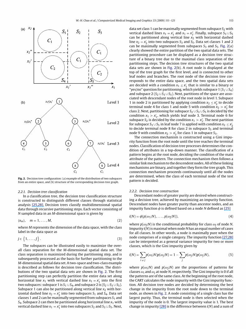

W.-H. Chao et al. / Computerized Medical Ima

Ff

2

iadN

{wl

j

acsMibphtSicSv

dvclccptpdtlra“ac1tccsftn

rndpasmcap

2

iDi

i

wIfncc

i

wcttt

ig. 2. Decision tree configuration: (a) example of the distribution of two subspacesrom an entire space, and (b) structure of the corresponding decision tree graph.

.2.1. Decision tree classificationIn a classification tree, the decision tree classification structure

s constructed to distinguish different classes through statisticalnalysis [25,28]. Decision trees classify multidimensional spatialata through recursive partitioning steps. Each vector consisting ofsampled data in an M-dimensional space is given by

xm}, m = 1, . . . , M, (2)

here M represents the dimension of the data space, with the classabel in the data space as

∈{

1, . . . , J}

. (3)

The subspaces can be illustrated easily to maximize the over-ll class separation for the M-dimensional spatial data set. Thelass separation is maximized during the partitioning step, and isubsequently processed as the basis for further partitioning to the-dimensional spatial data set. A two-space and two-class example

s described as follows for decision tree classification. The distri-utions of the two spatial data sets are shown in Fig. 2. The firstartitioning step can perfectly partition the entire data set alongorizontal line x1 with vertical dashed line x1 = x′

1 into the firstwo subspaces: subspace 1 is S1 ∪ S4, and subspace 2 is (S2 ∪ S3 ∪ S5).

ubspace 1 can also be partitioned along vertical line x2 with hor-zontal dashed line x2 = x′′

2 into two subspaces S1 and S4. Data setlasses 1 and 2 can be maximally segmented from subspaces S1 and4. Subspace 2 can then be partitioned along horizontal line x1 withertical dashed line x1 = x′′

1 into two subspaces S2 and S3 ∪ S5. Next,

cnlic

ging and Graphics 33 (2009) 111–121 113

ata set class 1 can be maximally segmented from subspace S2 withertical dashed lines x1 = x′

1 and x1 = x′′1. Finally, subspace S3 ∪ S5

an be partitioned along vertical line x2 with horizontal dashedine x2 = x′

2 into two subspaces S3 and S5. Data set classes 1 and 2an be maximally segmented from subspaces S3 and S5. Fig. 2(a)learly showed the entire partition of the two spatial data sets. Theartitioning procedure can be displayed as a decision tree struc-ure of a binary tree due to the maximal class separation of theartitioning steps. The decision tree structures of the two spatialata sets are shown in Fig. 2(b). A root node is displayed at theop of the tree graph for the first level, and is connected to othereaf nodes and branches. The root node of the decision tree cor-esponds to the entire data space, and the two spatial data setsre decided with a condition x1 ≤ x′

1 that is similar to a binary oryes/no” question for partitioning, which yields subspace 1 (S1 ∪ S4)nd subspace 2 (S2 ∪ S3 ∪ S5). Next, partitions of the space are asso-iated with descendant nodes of the root node in level 1. Subspacein node 2 is partitioned by applying condition x2 ≤ x′′

2 to decideerminal node 4 for class 1 and node 5 with condition x2 > x′′

2 forlass 2. Next, partitioning for subspace S2 ∪ S3 ∪ S5 is decided by theondition x1 > x′

1, which yields leaf node 3. Terminal node 6 forubspace S2 is decided by the condition x1 > x′′

1. The next partitionor subspace S3 ∪ S5 in leaf node 7 is applied with condition x2 ≤ x′

2o decide terminal node 8 for class 2 in subspace S5 and terminalode 9 with condition x2 > x′

2 for class 1 in subspace S3.The connection mechanism is constructed using a Gini impu-

ity function from the root node until the tree reaches the terminalodes. Classification of decision tree processes determines the con-ition of attributes in a top-down manner. The classification of aattern begins at the root node, deciding the condition of the mainttribute of the pattern. The connection mechanism then follows aimilar link mechanism to the descendent nodes. All of these linkingechanisms are binary, and together they form the tree graph. This

onnection mechanism proceeds continuously until all the nodesre determined, when the class of each terminal node of the testattern is decided.

.2.2. Decision tree constructionDescendant nodes of greater purity are desired when construct-

ng a decision tree, achieved by maximizing an impurity function.escendant nodes have greater purity than ancestor nodes, and an

mpurity function � is defined based on a node N defined as [25]

(N) = �(p(ω1|N), . . . , p(ωJ |N)), (4)

here p(ωJ|N) is the conditional probability for class ωJ of node N.mpurity i(N) is maximal when node N has an equal number of casesor all classes. In other words, a node is maximally pure when theode comprises of a single category. The impurity function [27,28]an be interpreted as a general variance impurity for two or morelasses, which is the Gini impurity given by

(N) =∑

i /= j

p(ωi|N)p(ωj|N) = 1 −∑

j

p(ωj|N)p(ωj|N), (5)

here p(ωi|N) and p(ωj|N) are the proportions of patterns forlasses ωi and ωj at node N, respectively. The Gini impurity is 0 if allhe patterns are of the same class. At the beginning of the root node,he CART calculates the node impurity with the Gini impurity func-ion. All decision tree nodes are decided by determining the best

hange in the impurity from the root node down to the terminalode, as shown in Fig. 2. A node consisting of a single class has the

argest purity. Thus, the terminal node is then selected when thempurity of the node is 0. The largest impurity value is 1. The besthange in impurity [28] is the difference between i(N) and a sum of

114 W.-H. Chao et al. / Computerized Medical Ima

FnVm

t

�

wandttinrpriocpNtb

2

tocalSaifwa

TDa

D

VVVVVV

Rsenlt

2

oagrmq

O

wtoabrkgc

uTefida

d

d

d

Ic

I

w

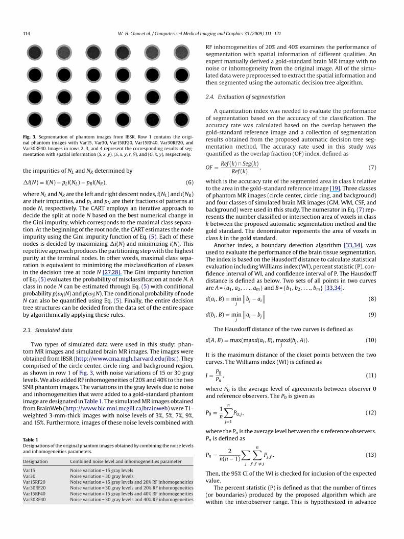
ig. 3. Segmentation of phantom images from IBSR. Row 1 contains the origi-al phantom images with Var15, Var30, Var15RF20, Var15RF40, Var30RF20, andar30RF40. Images in rows 2, 3, and 4 represent the corresponding results of seg-entation with spatial information (S, x, y), (S, x, y, r, �), and (G, x, y), respectively.

he impurities of NL and NR determined by

i(N) = i(N) − pLi(NL) − pRi(NR), (6)

here NL and NR are the left and right descent nodes, i(NL) and i(NR)re their impurities, and pL and pN are their fractions of patterns atode N, respectively. The CART employs an iterative approach toecide the split at node N based on the best numerical change inhe Gini impurity, which corresponds to the maximal class separa-ion. At the beginning of the root node, the CART estimates the nodempurity using the Gini impurity function of Eq. (5). Each of theseodes is decided by maximizing �i(N) and minimizing i(N). Thisepetitive approach produces the partitioning step with the highesturity at the terminal nodes. In other words, maximal class sepa-ation is equivalent to minimizing the misclassification of classesn the decision tree at node N [27,28]. The Gini impurity functionf Eq. (5) evaluates the probability of misclassification at node N. Alass in node N can be estimated through Eq. (5) with conditionalrobability p(ωi|N) and p(ωj|N). The conditional probability of nodecan also be quantified using Eq. (5). Finally, the entire decision

ree structures can be decided from the data set of the entire spacey algorithmically applying these rules.

.3. Simulated data

Two types of simulated data were used in this study: phan-om MR images and simulated brain MR images. The images werebtained from IBSR (http://www.cma.mgh.harvard.edu/ibsr). Theyomprised of the circle center, circle ring, and background region,s shown in row 1 of Fig. 3, with noise variations of 15 or 30 grayevels. We also added RF inhomogeneities of 20% and 40% to the twoNR phantom images. The variations in the gray levels due to noisend inhomogeneities that were added to a gold-standard phantom

mage are designated in Table 1. The simulated MR images obtainedrom BrainWeb (http://www.bic.mni.mcgill.ca/brainweb) were T1-eighted 3-mm-thick images with noise levels of 3%, 5%, 7%, 9%,

nd 15%. Furthermore, images of these noise levels combined with

able 1esignations of the original phantom images obtained by combining the noise levelsnd inhomogeneities parameters.

esignation Combined noise level and inhomogeneities parameter

ar15 Noise variation = 15 gray levelsar30 Noise variation = 30 gray levelsar15RF20 Noise variation = 15 gray levels and 20% RF inhomogeneitiesar30RF20 Noise variation = 30 gray levels and 20% RF inhomogeneitiesar15RF40 Noise variation = 15 gray levels and 40% RF inhomogeneitiesar30RF40 Noise variation = 30 gray levels and 40% RF inhomogeneities

a

P

wP

P

Tv

(w

ging and Graphics 33 (2009) 111–121

F inhomogeneities of 20% and 40% examines the performance ofegmentation with spatial information of different qualities. Anxpert manually derived a gold-standard brain MR image with nooise or inhomogeneity from the original image. All of the simu-

ated data were preprocessed to extract the spatial information andhen segmented using the automatic decision tree algorithm.

.4. Evaluation of segmentation

A quantization index was needed to evaluate the performancef segmentation based on the accuracy of the classification. Theccuracy rate was calculated based on the overlap between theold-standard reference image and a collection of segmentationesults obtained from the proposed automatic decision tree seg-entation method. The accuracy rate used in this study was

uantified as the overlap fraction (OF) index, defined as

F = Ref (k) ∩ Seg(k)Ref (k)

, (7)

hich is the accuracy rate of the segmented area in class k relativeo the area in the gold-standard reference image [19]. Three classesf phantom MR images (circle center, circle ring, and background)nd four classes of simulated brain MR images (GM, WM, CSF, andackground) were used in this study. The numerator in Eq. (7) rep-esents the number classified or intersection area of voxels in classbetween the proposed automatic segmentation method and the

old standard. The denominator represents the area of voxels inlass k in the gold standard.

Another index, a boundary detection algorithm [33,34], wassed to evaluate the performance of the brain tissue segmentation.he index is based on the Hausdorff distance to calculate statisticalvaluation including Williams index (WI), percent statistic (P), con-dence interval of WI, and confidence interval of P. The Hausdorffistance is defined as below. Two sets of all points in two curvesre A = {a1, a2, . . ., am} and B = {b1, b2, . . ., bm} [33,34].

(ai, B) = minj

∥∥bj − ai

∥∥ (8)

(bi, B) = minj

∥∥ai − bj

∥∥ (9)

The Hausdorff distance of the two curves is defined as

(A, B) = max(maxi

d{ai, B}, maxj

d{bj, A}). (10)

t is the maximum distance of the closet points between the twourves. The Williams index (WI) is defined as

= P0

Pn, (11)

here P0 is the average level of agreements between observer 0nd reference observers. The P0 is given as

0 = 1n

n∑

j=1

P0,j, (12)

here the Pn is the average level between the n reference observers.n is defined as

n = 2n(n − 1)

∑

j

n∑

j′:j′ /= j

Pj,j′ . (13)

hen, the 95% CI of the WI is checked for inclusion of the expectedalue.

The percent statistic (P) is defined as that the number of timesor boundaries) produced by the proposed algorithm which areithin the interobserver range. This is hypothesized in advance

W.-H. Chao et al. / Computerized Medical Imaging and Graphics 33 (2009) 111–121 115

Fdv

tleltoov

3

3

ms

Table 2Designations of the original simulated MR images obtained by combining the noiselevels and inhomogeneities parameters.

Designation Combined noise level and inhomogeneities parameter

T1n3 Noise level = 3%T1n5 Noise level = 5%T1n7 Noise level = 7%T1n9 Noise level = 9%T1n15 Noise level = 15%T1n3RF20 Noise level = 3% and 40% RF inhomogeneitiesT1n5RF20 Noise level = 5% and 20% RF inhomogeneitiesT1n7RF20 Noise level = 7% and 20% RF inhomogeneitiesT1n9RF20 Noise level = 9% and 20% RF inhomogeneitiesT1n15RF20 Noise level = 15% and 20% RF inhomogeneitiesT1n3RF40 Noise level = 3% and 40% RF inhomogeneitiesTTTT

�rSutgViuEuFd4t

xthose segmented with spatial information (G, x, y). Images with a

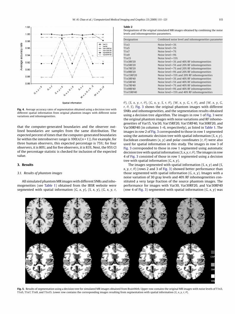
FT

ig. 4. Average accuracy rates of segmentation obtained using a decision tree withifferent spatial information from original phantom images with different noiseariations and inhomogeneities.

hat the computer-generated boundaries and the observer out-ined boundaries are samples from the same distribution. Thexpected percent of times that the computer-generated boundariesie within the interobserver range is 100(n/(n + 1)). For example, forhree human observers, this expected percentage is 75%; for fourbservers, it is 80%; and for five observers, it is 83%. Next, the 95% CIf the percentage statistic is checked for inclusion of the expectedalue.

. Results

.1. Results of phantom images

All simulated phantom MR images with different SNRs and inho-ogeneities (see Table 1) obtained from the IBSR website were

egmented with spatial information (G, x, y), (S, x, y), (G, x, y, r,

nsp(

ig. 5. Results of segmentation using a decision tree for simulated MR images obtained fro1n5, T1n7, T1n9, and T1n15. Lower row contains the corresponding images resulting fro

1n5RF40 Noise level = 5% and 40% RF inhomogeneities1n7RF40 Noise level = 7% and 40% RF inhomogeneities1n9RF40 Noise level = 9% and 40% RF inhomogeneities1n15RF40 Noise level = 15% and 40% RF inhomogeneities

), (S, x, y, r, �), (G, x, y, S, r, �), (W, x, y, G, r, �), and (W, x, y, G,, �, S). Fig. 3 shows the original phantom images with differentNRs and inhomogeneities, and the segmentation results obtainedsing a decision tree algorithm. The images in row 1 of Fig. 3 werehe original phantom images with noise variations and RF inhomo-eneities of Var15, Var30, Var15RF20, Var15RF40, Var30RF20, andar30RF40 (in columns 1–6, respectively), as listed in Table 1. The

mages in row 2 of Fig. 3 corresponded to those in row 1 segmentedsing the automatic decision tree with spatial information (S, x, y).uclidean coordinates (x, y) and polar coordinates (r, �) were alsosed for spatial information in this study. The images in row 3 ofig. 3 corresponded to those in row 1 segmented using automaticecision tree with spatial information (S, x, y, r, �). The images in rowof Fig. 3 consisted of those in row 1 segmented using a decision

ree with spatial information (G, x, y).The images segmented with spatial information (S, x, y) and (S,

, y, r, �) (rows 2 and 3 of Fig. 3) showed better performance than

oise variation of 30 gray levels and 40% RF inhomogeneities con-tituted a very large fraction of the source phantom images. Theerformance for images with Var30, Var30RF20, and Var30RF40row 4 of Fig. 3) segmented with spatial information (G, x, y) was

m BrainWeb. Upper row contains the original MR images with noise levels of T1n3,m segmentation with spatial information (G, x, y, r, �).

1 al Imaging and Graphics 33 (2009) 111–121

uVaxGagsabita(xrttrwraSepscwxax0aw

3

i

Ff

siriattwrsaCatt

FT

16 W.-H. Chao et al. / Computerized Medic

nclear. The segmentation of phantom MR images with Var15,ar30, Var15RF20, Var15RF40, Var30RF20, and Var30RF40 usingdecision tree with spatial information (G, x, y, r, �), (G, x, y), (G,

, y, r, �), (G, x, y, S, r, �), (S, x, y), (W, x, y, G, r, �), and (W, x, y,, r, �, S) produced better performance. Fig. 4 shows the averageccuracy rate of phantom images with different SNRs and inhomo-eneities segmented by a decision tree algorithm with differentpatial information. The average accuracy rates were averagedcross all phantom image regions (circle ring, circle center, andackground). They were evaluated by the OF index as described

n Section 2. The average accuracy rates of segmentation for phan-om images with Var15, Var30, Var15RF20, Var15RF40, Var30RF20,nd Var30RF40 and segmentation spatial information (G, x, y, r, �),G, x, y), (G, x, y, r, �), (G, x, y, S, r, �), (S, x, y), (W, x, y, G, r, �), and (W,, y, G, r, �, S), were shown in Fig. 4. The highest average accuracyates of segmentation are in the range of 0.9819–0.9999 for phan-om images with Var15 and Var15RF20 segmented using a decisionree for all of the used spatial information. The higher average accu-acy rates of segmentation are shown in Fig. 4 for phantom imagesith Var15RF40 for all of the used spatial information. The accuracy

ates of phantom images with Var30 and Var30RF20 segmented bydecision tree for spatial information (G, x, y, r, �), (G, x, y), (G, x, y,

, r, �), (S, x, y), (W, x, y, G, r, �), and (W, x, y, G, r, �, S) were mod-rate, ranging from 0.9164 to 0.9872. The average accuracy rates ofhantom images with Var30 and Var30RF20 segmented by a deci-ion tree for spatial information (S, x, y, r, �) and (S, x, y) were alsolose to the highest values. Segmenting images with Var30RF40ith spatial information (G, x, y, r, �), (G, x, y), (G, x, y, S, r, �), (W,

, y, G, r, �), and (W, x, y, G, r, �, S) produced the lowest averageccuracy rates, although segmentation with spatial information (S,, y, r, �) and (S, x, y) produced a higher average accuracy rate of.9461. The segmentation results shown in Fig. 3 indicated that theutomatic decision tree successfully segmented phantom imagesith different noise variations and RF inhomogeneities.

.2. Results of simulated brain MR images

All simulated MR brain images with different noise levels andnhomogeneities (see Table 2), as described in Section 2, were also

irS�r

ig. 7. Results of segmentation using a decision tree for simulated MR images. Upper row1n7RF20, T1n9RF20, and T1n15RF20. Lower row contains the corresponding images resu

ig. 6. Average accuracy rates of segmentation with different spatial informationrom the original MR images with noise levels of T1n3, T1n5, T1n7, T1n9, and T1n15.

egmented using the automatic decision tree with different spatialnformation (G, x, y), (S, x, y), (G, x, y, r, �), (S, x, y, r, �), (G, x, y, S,, �), (W, x, y, G, r, �), and (W, x, y, G, r, �, S). Fig. 5 shows the orig-nal simulated MR images obtained from BrainWeb (upper row)nd the images resulting from segmentation with spatial informa-ion (G, x, y, r, �) (lower row). The OF index was used to assesshe performance of segmentation using the automatic decision treeith different spatial information. Fig. 6 shows the average accu-

acy rates of segmentation with different spatial information forimulated MR images with noise levels of T1n3, T1n5, T1n7, T1n9,nd T1n15. All accuracy rates were calculated for the GM, WM,SF, and background of simulated brain MR images. The averageccuracy rates decreased as the noise levels increased from T1n3o T1n15 for most of the segmentations with this spatial informa-ion. Fig. 6 shows that segmenting these MR images with spatialnformation (G, x, y, r, �) produced the highest average accuracy

ates (0.9374–0.9598), with the resulting images shown in Fig. 5.egmenting these MR images with spatial information (G, x, y, S, r,) and (W, x, y, G, r, �) produced moderate and low average accu-acy rates of 0.9132–0.9626 and 0.8920–0.9297, respectively. Fig. 5

contains the original MR images with noise parameters of T1n3RF20, T1n5RF20,lting from segmentation with spatial information (G, x, y, r, �).

W.-H. Chao et al. / Computerized Medical Imaging and Graphics 33 (2009) 111–121 117

FtT

sltx

nWssrsrtmfta(yr

FtT

lss

e(tsrtrTm

FT

ig. 8. Average accuracy rates of segmentation with different spatial informa-ion from MR images with noise parameters of T1n3RF20, T1n5RF20, T1n7RF20,1n9RF20, and T1n15RF20.

hows that all of the simulated brain MR images with these noiseevels were successfully segmented with the automatic decisionree with spatial information (G, x, y, r, �), (G, x, y), (S, x, y, r, �), (G,, y, S, r, �), (S, x, y), (W, x, y, G, r, �, S), and (W, x, y, G, r, �).

Fig. 7 shows original simulated brain MR images with differentoise levels and an RF inhomogeneity of 20% obtained from Brain-eb (upper row) and the images resulting from segmentation with

patial information (G, x, y, r, �) (lower row). The segmented imageshowed better visual rendition. Fig. 8 shows the average accuracyates of segmentation with different spatial information from theimulated brain MR images shown in Fig. 7. The average accu-acy rates decreased as the noise level increased from T1n3RF20o T1n15RF20 for most of the segmentations with this spatial infor-

ation. They do not differ greatly between Figs. 6 and 8, rangingrom 0.96 to 0.89. The presence of 20% RF inhomogeneities had lit-

le effect on segmentation of these simulated brain MR images. Theverage accuracy rates of segmentation in these brain MR imagesFig. 8) with spatial information (G, x, y, r, �), (G, x, y, S, r, �), and (W, x,, G, r, �) were 0.9376–0.9587, 0.9144–0.9538, and 0.8865–0.9285,espectively. All of the simulated brain MR images with these noise

igRsy

ig. 9. Results of segmentation using a decision tree for simulated MR images. Upper row1n7RF40, T1n9RF40, and T1n15RF40. Lower row contains the corresponding images resu

ig. 10. Average accuracy rates of segmentation with different spatial informa-ion from MR images with noise parameters of T1n3RF40, T1n5RF40, T1n7RF40,1n9RF40, and T1n15RF40.

evels and inhomogeneities were successfully segmented with thispatial information for all of the accuracy rates of automatic deci-ion tree segmentation.

Fig. 9 shows original simulated brain MR images with differ-nt noise levels and an RF inhomogeneity of 40% from BrainWebupper row) and the images resulting from segmentation with spa-ial information (G, x, y, r, �) (lower row). The segmented imageshowed better visual rendition. Fig. 10 shows the average accu-acy rates of segmentation with different spatial information fromhe simulated brain MR images shown in Fig. 9. The average accu-acy rates decreased as the noise level increased from T1n3RF40 to1n15RF40 for most of the segmentations with this spatial infor-ation. They do not differ greatly between Figs. 8 and 10 except

n lower values of the range. The 40% RF inhomogeneities have a

reater effect on the segmentation than that shown for the 20%F inhomogeneities in Figs. 7 and 8. The average accuracy rates ofegmentation of these MR images with spatial information (W, x,, G, r, �) as shown in Fig. 10 changed from 0.8810 to 0.9261. They

contains the original MR images with noise parameters of T1n3RF40, T1n5RF40,lting from segmentation with spatial information (G, x, y, r, �).

118 W.-H. Chao et al. / Computerized Medical Ima

FuT(

wTmsmbswwfaT

siTfWrlctcas

wdddimsyGmigAaowto0swdaHWGisosr

4

ttocpudvegei

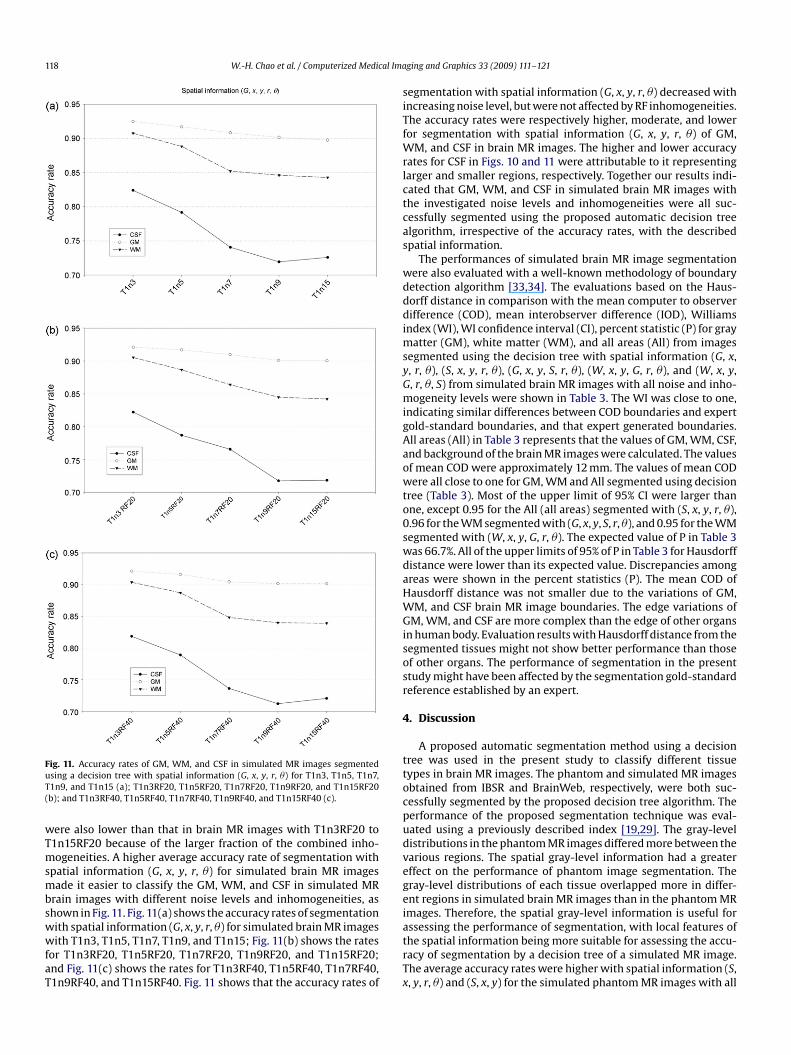
ig. 11. Accuracy rates of GM, WM, and CSF in simulated MR images segmentedsing a decision tree with spatial information (G, x, y, r, �) for T1n3, T1n5, T1n7,1n9, and T1n15 (a); T1n3RF20, T1n5RF20, T1n7RF20, T1n9RF20, and T1n15RF20b); and T1n3RF40, T1n5RF40, T1n7RF40, T1n9RF40, and T1n15RF40 (c).

ere also lower than that in brain MR images with T1n3RF20 to1n15RF20 because of the larger fraction of the combined inho-ogeneities. A higher average accuracy rate of segmentation with

patial information (G, x, y, r, �) for simulated brain MR imagesade it easier to classify the GM, WM, and CSF in simulated MR

rain images with different noise levels and inhomogeneities, ashown in Fig. 11. Fig. 11(a) shows the accuracy rates of segmentation

ith spatial information (G, x, y, r, �) for simulated brain MR imagesith T1n3, T1n5, T1n7, T1n9, and T1n15; Fig. 11(b) shows the rates

or T1n3RF20, T1n5RF20, T1n7RF20, T1n9RF20, and T1n15RF20;nd Fig. 11(c) shows the rates for T1n3RF40, T1n5RF40, T1n7RF40,1n9RF40, and T1n15RF40. Fig. 11 shows that the accuracy rates of

atrTx

ging and Graphics 33 (2009) 111–121

egmentation with spatial information (G, x, y, r, �) decreased withncreasing noise level, but were not affected by RF inhomogeneities.he accuracy rates were respectively higher, moderate, and loweror segmentation with spatial information (G, x, y, r, �) of GM,

M, and CSF in brain MR images. The higher and lower accuracyates for CSF in Figs. 10 and 11 were attributable to it representingarger and smaller regions, respectively. Together our results indi-ated that GM, WM, and CSF in simulated brain MR images withhe investigated noise levels and inhomogeneities were all suc-essfully segmented using the proposed automatic decision treelgorithm, irrespective of the accuracy rates, with the describedpatial information.

The performances of simulated brain MR image segmentationere also evaluated with a well-known methodology of boundaryetection algorithm [33,34]. The evaluations based on the Haus-orff distance in comparison with the mean computer to observerifference (COD), mean interobserver difference (IOD), Williams

ndex (WI), WI confidence interval (CI), percent statistic (P) for grayatter (GM), white matter (WM), and all areas (All) from images

egmented using the decision tree with spatial information (G, x,, r, �), (S, x, y, r, �), (G, x, y, S, r, �), (W, x, y, G, r, �), and (W, x, y,, r, �, S) from simulated brain MR images with all noise and inho-ogeneity levels were shown in Table 3. The WI was close to one,

ndicating similar differences between COD boundaries and expertold-standard boundaries, and that expert generated boundaries.ll areas (All) in Table 3 represents that the values of GM, WM, CSF,nd background of the brain MR images were calculated. The valuesf mean COD were approximately 12 mm. The values of mean CODere all close to one for GM, WM and All segmented using decision

ree (Table 3). Most of the upper limit of 95% CI were larger thanne, except 0.95 for the All (all areas) segmented with (S, x, y, r, �),.96 for the WM segmented with (G, x, y, S, r, �), and 0.95 for the WMegmented with (W, x, y, G, r, �). The expected value of P in Table 3as 66.7%. All of the upper limits of 95% of P in Table 3 for Hausdorffistance were lower than its expected value. Discrepancies amongreas were shown in the percent statistics (P). The mean COD ofausdorff distance was not smaller due to the variations of GM,M, and CSF brain MR image boundaries. The edge variations of

M, WM, and CSF are more complex than the edge of other organsn human body. Evaluation results with Hausdorff distance from theegmented tissues might not show better performance than thosef other organs. The performance of segmentation in the presenttudy might have been affected by the segmentation gold-standardeference established by an expert.

. Discussion

A proposed automatic segmentation method using a decisionree was used in the present study to classify different tissueypes in brain MR images. The phantom and simulated MR imagesbtained from IBSR and BrainWeb, respectively, were both suc-essfully segmented by the proposed decision tree algorithm. Theerformance of the proposed segmentation technique was eval-ated using a previously described index [19,29]. The gray-levelistributions in the phantom MR images differed more between thearious regions. The spatial gray-level information had a greaterffect on the performance of phantom image segmentation. Theray-level distributions of each tissue overlapped more in differ-nt regions in simulated brain MR images than in the phantom MRmages. Therefore, the spatial gray-level information is useful for

ssessing the performance of segmentation, with local features ofhe spatial information being more suitable for assessing the accu-acy of segmentation by a decision tree of a simulated MR image.he average accuracy rates were higher with spatial information (S,, y, r, �) and (S, x, y) for the simulated phantom MR images with all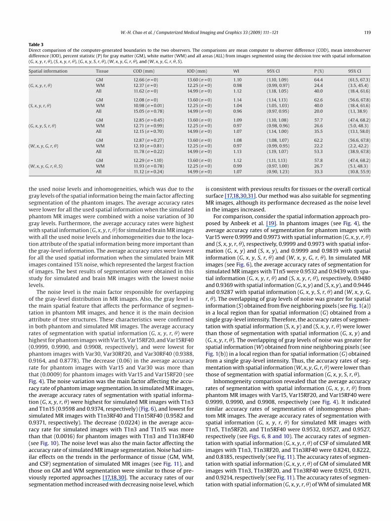

W.-H. Chao et al. / Computerized Medical Imaging and Graphics 33 (2009) 111–121 119

Table 3Direct comparison of the computer-generated boundaries to the two observers. The comparisons are mean computer to observer difference (COD), mean interobserverdifference (IOD), percent statistic (P) for gray matter (GM), white matter (WM) and all areas (ALL) from images segmented using the decision tree with spatial information(G, x, y, r, �), (S, x, y, r, �), (G, x, y, S, r, �), (W, x, y, G, r, �), and (W, x, y, G, r, �, S).

Spatial information Tissue COD (mm) IOD (mm) WI 95% CI P (%) 95% CI

(G, x, y, r, �)GM 12.66 (� = 0) 13.60 (� = 0) 1.10 (1.10, 1.09) 64.4 (61.5, 67.3)WM 12.37 (� = 0) 12.25 (� = 0) 0.98 (0.99, 0.97) 24.4 (3.5, 45.4)All 11.62 (� = 0) 14.99 (� = 0) 1.12 (1.18, 1.05) 40.0 (18.4, 61.6)

(S, x, y, r, �)GM 12.08 (� = 0) 13.60 (� = 0) 1.14 (1.14, 1.13) 62.6 (56.6, 67.8)WM 10.98 (� = 0.01) 12.25 (� = 0) 1.04 (1.05, 1.03) 40.0 (18.4, 61.6)All 15.05 (� = 0.78) 14.99 (� = 0) 0.96 (0.97, 0.95) 20.0 (1.1, 38.9)

(G, x, y, S, r, �)GM 12.85 (� = 0.45) 13.60 (� = 0) 1.09 (1.10, 1.08) 57.7 (47.4, 68.2)WM 12.71 (� = 0.99) 12.25 (� = 0) 0.97 (0.98, 0.96) 26.6 (5.0, 48.3)All 12.15 (� = 0.70) 14.99 (� = 0) 1.07 (1.14, 1.00) 35.5 (13.1, 58.0)

(W, x, y, G, r, �)GM 12.87 (� = 0.27) 13.60 (� = 0) 1.08 (1.08, 1.07) 62.2 (56.6, 67.8)WM 12.10 (� = 0.81) 12.25 (� = 0) 0.97 (0.99, 0.95) 22.2 (2.2, 42.2)All 11.78 (� = 0.22) 14.99 (� = 0) 1.13 (1.19, 1.07) 53.3 (38.9, 67.8)

(0 (� =5 (� =9 (� =

tgswpgwwttfiosl

ottairh(p0rtFrttas0rt(aiatvs

isMi

paVamiistaariistt(sFfmt

rp0stsTrti

W, x, y, G, r, �, S)GM 12.29 (� = 1.10) 13.6WM 11.93 (� = 0.78) 12.2All 11.12 (� = 0.24) 14.9

he used noise levels and inhomogeneities, which was due to theray levels of the spatial information being the main factor affectingegmentation of the phantom images. The average accuracy ratesere lower for all the used spatial information when the simulatedhantom MR images were combined with a noise variation of 30ray levels. Furthermore, the average accuracy rates were highestith spatial information (G, x, y, r, �) for simulated brain MR imagesith all the used noise levels and inhomogeneities due to the loca-

ion attribute of the spatial information being more important thanhe gray-level information. The average accuracy rates were lowestor all the used spatial information when the simulated brain MRmages contained 15% noise, which represented the largest fractionf images. The best results of segmentation were obtained in thistudy for simulated and brain MR images with the lowest noiseevels.

The noise level is the main factor responsible for overlappingf the gray-level distribution in MR images. Also, the gray level ishe main spatial feature that affects the performance of segmen-ation in phantom MR images, and hence it is the main decisionttribute of tree structures. These characteristics were confirmedn both phantom and simulated MR images. The average accuracyates of segmentation with spatial information (G, x, y, r, �) wereighest for phantom images with Var15, Var15RF20, and Var15RF400.9999, 0.9990, and 0.9908, respectively), and were lowest forhantom images with Var30, Var30RF20, and Var30RF40 (0.9388,.9164, and 0.8778). The decrease (0.06) in the average accuracyate for phantom images with Var15 and Var30 was more thanhat (0.0009) for phantom images with Var15 and Var15RF20 (seeig. 4). The noise variation was the main factor affecting the accu-acy rate of phantom image segmentation. In simulated MR images,he average accuracy rates of segmentation with spatial informa-ion (G, x, y, r, �) were highest for simulated MR images with T1n3nd T1n15 (0.9598 and 0.9374, respectively) (Fig. 6), and lowest forimulated MR images with T1n3RF40 and T1n15RF40 (0.9582 and.9371, respectively). The decrease (0.0224) in the average accu-acy rate for simulated images with T1n3 and T1n15 was morehan that (0.0016) for phantom images with T1n3 and T1n3RF40see Fig. 10). The noise level was also the main factor affecting theccuracy rate of simulated MR image segmentation. Noise had sim-

lar effects on the trends in the performance of tissue (GM, WM,nd CSF) segmentation of simulated MR images (see Fig. 11), andhose on GM and WM segmentation were similar to those of pre-iously reported approaches [17,18,30]. The accuracy rates of ouregmentation method increased with decreasing noise level, which

atiat

0) 1.12 (1.11, 1.13) 57.8 (47.4, 68.2)0) 0.99 (0.97, 1.00) 26.7 (5.1, 48.3)0) 1.07 (0.90, 1.23) 33.3 (10.8, 55.9)

s consistent with previous results for tissues or the overall corticalurface [17,18,30,31]. Our method was also suitable for segmentingR images, although its performance decreased as the noise level

n the images increased.For comparison, consider the spatial information approach pro-

osed by Anbeek et al. [19]. In phantom images (see Fig. 4), theverage accuracy rates of segmentation for phantom images withar15 were 0.9999 and 0.9973 with spatial information (G, x, y, r, �)nd (S, x, y, r, �), respectively, 0.9999 and 0.9973 with spatial infor-ation (G, x, y) and (S, x, y), and 0.9999 and 0.9819 with spatial

nformation (G, x, y, S, r, �) and (W, x, y, G, r, �). In simulated MRmages (see Fig. 6), the average accuracy rates of segmentation forimulated MR images with T1n5 were 0.9532 and 0.9439 with spa-ial information (G, x, y, r, �) and (S, x, y, r, �), respectively, 0.9480nd 0.9369 with spatial information (G, x, y) and (S, x, y), and 0.9446nd 0.9287 with spatial information (G, x, y, S, r, �) and (W, x, y, G,, �). The overlapping of gray levels of noise was greater for spatialnformation (S) obtained from five neighboring pixels (see Fig. 1(a))n a local region than for spatial information (G) obtained from aingle gray-level intensity. Therefore, the accuracy rates of segmen-ation with spatial information (S, x, y) and (S, x, y, r, �) were lowerhan those of segmentation with spatial information (G, x, y) andG, x, y, r, �). The overlapping of gray levels of noise was greater forpatial information (W) obtained from nine neighboring pixels (seeig. 1(b)) in a local region than for spatial information (G) obtainedrom a single gray-level intensity. Thus, the accuracy rates of seg-

entation with spatial information (W, x, y, G, r, �) were lower thanhose of segmentation with spatial information (G, x, y, S, r, �).

Inhomogeneity comparison revealed that the average accuracyates of segmentation with spatial information (G, x, y, r, �) fromhantom MR images with Var15, Var15RF20, and Var15RF40 were.9999, 0.9990, and 0.9908, respectively (see Fig. 4). It indicatedimilar accuracy rates of segmentation of inhomogenous phan-om MR images. The average accuracy rates of segmentation withpatial information (G, x, y, r, �) for simulated MR images with1n5, T1n5RF20, and T1n5RF40 were 0.9532, 0.9527, and 0.9527,espectively (see Figs. 6, 8 and 10). The accuracy rates of segmen-ation with spatial information (G, x, y, r, �) of CSF of simulated MRmages with T1n3, T1n3RF20, and T1n3RF40 were 0.8241, 0.8222,

nd 0.8185, respectively (see Fig. 11). The accuracy rates of segmen-ation with spatial information (G, x, y, r, �) of GM of simulated MRmages with T1n3, T1n3RF20, and T1n3RF40 were 0.9251, 0.9211,nd 0.9214, respectively (see Fig. 11). The accuracy rates of segmen-ation with spatial information (G, x, y, r, �) of WM of simulated MR

1 al Ima

iawtioiaHmsttamsa

tmipdTulTmtioM

A

atNVF

R

[

[

[

[

[

[

[

[

[

[

[

[[

[

[

[

[

[

[[

[

[

[

[

[

WiPCaHi

YthNE

20 W.-H. Chao et al. / Computerized Medic

mages with T1n3, T1n3RF20, and T1n3RF40 were 0.9077, 0.9054,nd 0.9038, respectively (see Fig. 11). These data indicated thereere no significant differences among accuracy rates of segmenta-

ion of tissues in inhomogenous MR images. Thus, the presence ofnhomogeneity in MR images might not decrease the accuracy ratesf segmentation for both phantom MR images and simulated MRmages. Furthermore, segmentation performance was also evalu-ted by a boundary detection methodology. Evaluation results withausdorff distance from the segmented tissues demonstrated thatean computer-generated and mean expert gold standard showed

imilar differences from the expert gold-stand. The percent statis-ics (P) was the largest when tissues were segmented using decisionree with spatial information (G, x, y, r, �). Other approaches couldlso be used to determine the gold-standard reference image. Aore sophisticated method [32] is to have a group of experts con-

truct the reference gold-standard image, which might improve theccuracy of segmentation.

In conclusion, our segmentation method based on a decisionree algorithm presented a useful way to perform automatic seg-

entation for both phantom and tissue (GM, WM, and CSF) regionsn brain MR images. It provided an easy method, through theartition of each spatial information (spatial feature), to form aecision tree for the brain tissues segmentation in MR images.he accuracy rates of segmentation were highest for both sim-lated phantom and brain MR images, having the lowest noise

evels, from a reduction of overlapping gray levels in the images.he accuracies of segmentation were higher when the spatial infor-ation included the general gray level (G) than when it included

he spatial gray level (S), which in turn were higher than when itncluded the wavelet transform (W). Finally, the accuracy rate ofur segmentation method was not affected by inhomogeneity inR images.

cknowledgments

The authors thank Mr. Kuan-Hung Lin for his suggestionsnd comments concerning this manuscript. This study was par-ially supported by grants NSC95-2221-E-009-171-MY3 from theational Science Council of the Republic of China and grantGHUST96-P5-19 from VGHUST Joint Research Program, Tsou’soundation, Taiwan.

eferences

[1] Zoroofi RA, Nishii T, Sato Y, Sugano N, Yoshikawa H, Tamura S. Segmentationof avascular necrosis of the femoral head using 3D MR images. Comput MedImaging Graph 2001;25:511–21.

[2] Zoroofi RA, Sato Y, Nishii T, Sugano N, Yoshikawa H, Tamura S. Automated seg-mentation of necrotic femoral head from 3D MR data. Comput Med ImagingGraph 2004;28(5):267–78.

[3] Liu J, Udupa JK, Odhner D, Hacney D, Moonis G. A system for brain tumor volumeestimation via MR imaging and fuzzy connectedness. Comput Med ImagingGraph 2005;29(1):21–34.

[4] Behrens S, Laue H, Altthias M, Boehler T, Kuemmerlan B, Hahn HK, et al. Com-puter assistance for MR based diagnosis ofbreast cancer: present and futurechallenges. Comput Med Imaging Graph 2007;31:236–47.

[5] Cline HE, Doumulin CL, Hart HR, Lorensen WE, Ludke S. 3-D reconstructionof the brain from magnetic resonance images using a connectivity algorithm.Magn Reson Imaging 1987;5:345–52.

[6] Joliot M, Majoyer BM. Three-dimensional segmentation and interpolation ofmagnetic resonance brain images. IEEE Trans Med Imag 1993;12(2):269–77.

[7] Schiemann T, Tiede U, Hohne KH. Segmentation of visible human for high qual-ity volume-based visualization. Med Imag Anal 1996;1:263–70.

[8] Shan ZY, Ji Q, Gajjar A, Reddick E. A knowledge-guided active contour methodof segmentation of cerebella on MR images of pediatric patients with medul-

loblastoma. Magn Reson Imaging 2005;21(1):1–11.

[9] Andersen AH, Zhang Z, Avison MJ, Gash DM. Automated Segmentation of mul-tispectral brain MR images. J Neurosci Methods 2002;122(1):13–23.

10] Amato U, Larobina M, Antoniadis A, Alfano B. Segmentation of magneticresonance brain images through discriminant analysis. J Neurosci Methods2003;131(1–2):65–74.

ea(

Si

ging and Graphics 33 (2009) 111–121

11] Ali AA, Dale AM, Badea A, Johnson GA. Automatic segmentation of neu-roanatomical structures in multispectral MR microscopy of the mouse brain.NeuroImage 2005;27:425–35.

12] Mohr J, Hess A, Scholz M, Obermayer K. A method for automatic segmentation ofautoradiographic image stacks and spatial normalization of functional corticalactivity patterns. J Neurosci Methods 2004;134(1):45–58.

13] Sharma J, Sanfilipo M, Benedict RH, Weinstock-Guttman B, Munschauer IIIFE, Bakshi R. Whole-brain atrophy in multiple sclerosis measured by auto-mated versus semiautomated MR imaging segmentation. Am J Neuroradiol2004;25(6):985–96.

14] Admiraal-Behloul F, Van Den Heuvel DMJ, Van Osch OMJP, Van Der Grond J,Van Buchem MA, Reiber JHC. Fully automatic segmentation of white matterhyperintensities in MR images of the elderly. NeuroImage 2005;28(3):607–17.

15] Prastawa M, Gilmore JH, Lin W, Gerig G. Automatic segmentation of MR imagesof the developing newborn brain. Med Imag Analysis 2005;9(5):457–66.

16] Xia Y, Bettinger K, Shen L, Reiss A. Automatic segmentation of thecaudate nucleus from human brain MR images. IEEE Trans Med Imag2007;26(4):509–17.

17] Marroquin JL, Vemuri BC, Botello S, Calderon F, Fernadez-Bouzas A. An accurateand efficient Bayesian method for automatic segmentation of brain MRI. IEEETrans Med Imag 2002;21(8):934–45.

18] Greenspan H, Ruf A, Goldberger J. Constrained Gaussian mixture model frame-work for automatic segmentation of MR brain images. IEEE Trans Med Imag2006;25(9):1233–45.

19] Anbeek P, Vincken KL, Van Osch MJP, Bisschops RHC, Van Der Grond J. Poob-abilistic segmentation of white matter lesions in MR imaging. NeuroImage2004;21:1037–44.

20] Lufkin RB, et al. Dynamic-range compression in surface-coil MRI. Am J Nuerora-diol 1986;147:379–82.

21] Lufkin RB. The MRI manual. California: Mosby, Inc.; 1998.22] Vokurka EA, Watson NA, Watson Y, Thacker NA, Jackson A. Improved high reso-

lution MR imaging for surface coils using automated intensity non-uniformitycorrection: feasibility study in the Orbit. J Magn Reson Imaging 2001;14:540–6.

23] Suits BH, Garroway AN. Optimizing surface coils and the self-shielded gra-diometer. J Appl Phys 2003;94(6):4170–8.

24] Gensanne D, Josse G, Lagarde JM, Vincensini D. High spatial resolution quanti-tative MR images: an experimental study of dedicated surface coils. Phys MedBiol 2006;51(11):2843–55.

25] Grajski KA, Breiman L, De Prisco GV, Freeman WJ. Classification of EEG spatialpatterns with a tree structured methodology: CART. IEEE Trans Biomed Eng1986;BME-33(12):1076–86.

26] Bittencourt HR, Clarke RT. Use of classification and regression trees (CART) toclassify remotely-sensed digital images. In: Proceedings of the IEEE interna-tional geoscience and remote sensing symposium, IGARSS 2003, vol. 6. 2003.p. 3751–3.

27] Breiman L, Friedman JH, Olshen RA, Stone CJ. Classification and regression trees.CA: Wadsworth International; 1984.

28] Duda RO, Hart PE, Stork DG. Pattern classification. New York: Wiley; 2001.29] Wang B, Saha PK, Udupa JK, Ferrante MA, Baumgardner J, Roberts DA, et al. 3D

airway segmentation via hyperpolarized 3He gas MRI by using scale-based fuzyconnectedness. Comput Med Imaging Graph 2004;28:77–86.

30] Archibald R, Chen K, Gelb A, Renaut R. Improving tissue segmentation of humanbrain MRI through preprocessing by the Gegenbauer reconstruction method.NeuroImage 2003;20(1):489–502.

31] Yu ZQ, Zhu Y, Yang J, Zhu YM. A hybrid region-boundary model for cerebral cor-tical segmentation in MRI. Comput Med Imaging Graph 2006;30(3):197–208.

32] Warefield SK, Zou KH, Wells WM. Validation of image segmentation and expertquality with an expectation-maximization algorithm. In: Proceeding of MICCAI,vol. 2488 of lecture notes in computer science. Springer; 2002. p. 298–306.

33] Chalana V, Kim Y. A methodology for evaluation of boundary detection algo-rithms on medical images. IEEE Trans Medical Imaging 1997;16(5):642–52.

34] Carlos AL, Marcos MF, Juan RA. Comments on: a methodology for evaluationof boundary detection algorithms on medical images. IEEE Trans Med Imaging2004;23(5):658–60.

en-Hung Chao Wen-Hung Chao received the M.S. degree in biomedical engineer-ng from National Cheng Kung University, Tainan, Taiwan, in 1996. He also receivedh.D. degree in the Department of Electrical and Control Engineering from Nationalhiao-Tung University, Hsinchu, Taiwan in 2008. Since August 1996, he has beenLecturer with the Department of Biomedical Engineering, Yuanpei University,sinchu, Taiwan. His current research interests are biomedical signal processing,

mage processing, fuzzy neural networks, and designing biomedical instruments.

ou-Yin Chen is an Assistant Professor of the Department of Electrical and Con-rol Engineering at National Chiao-Tung University in Hsinchu, Taiwan. He receivedis Ph.D. (2004) and M.S. (1998) degrees, respectively, in Electrical Engineering inational Taiwan University and B.S. degree (1996) in the Department of Electricalngineering from the National Chiao-Tung University. Dr. Chen’s research inter-

st is in the field of Neuroengineering. Topics of Neuroengineering include thenalysis of neuroimage, neural ensemble recordings and brain-machine interfacesBMI).

heng-Huang Lin received his M.D. degree from Kaohsiung Medical School, Taiwan,n 1992, and he obtained his M.Sc. degree in the Institute of Medical Science at Tzu Chi

al Ima

UTm

YePs

Bn

W.-H. Chao et al. / Computerized Medic

niversity, Taiwan in 2000. Currently, he is an attending neurologist in the Buddhistzu Chi General Hospital and focusing on the research of Parkinson disease and

ovement disorders.

en-Yu I. Shih received his B.S. degree in Biomedical Imaging and Radiological Sci-nces from National Yang-Ming University, Taiwan, in 2004, and he obtained hish.D. degree in the Institute of Biomedical Engineering at National Taiwan Univer-ity, Taiwan in 2007. Currently, he is a post-doctoral researcher in the Institute of

S2Sgm

ging and Graphics 33 (2009) 111–121 121

iomedical Sciences at Academia Sinica and focusing on the research of imagingociceptive responses in rodent brain using MRI and PET.

iny Tsang completed her B.S. in Agriculture from National Taiwan University in007. She is now a master student in the College of Criminal Justice at Sam Houstontate University, U.S.A. Her research interests include psychopathy, serial offenders,ender differences between offenders, and the neurological mechanism of criminalinds.