KatholiekeUniversiteitLeuven

Departement ElektrotechniekAfdeling ESAT/PSICentrum voor Beeld-en SpraakverwerkingKardinaal Mercierlaan 94B-3001 Heverlee - Belgium

TECHNISCH RAPPORT-TECHNICAL REPORT

Automatic segmentation of brain tissues andMR bias field correction using a digital brain atlas

Koen Van Leemput, Dirk Vandermeulen,Paul Suetens.

June 1998

Nr.KUL/ESAT/PSI/9806

Automatic segmentation of brain tissues and MR bias field

correction using a digital brain atlas

Koen Van Leemput, Frederik Maes∗, Dirk Vandermeulen, Paul Suetens

Katholieke Universiteit Leuven

Medical Image Computing (ESAT-Radiology)

UZ Gasthuisberg, Herestraat 49, B-3000 Leuven, Belgium

E-mail: Koen.Vanleemput@uz.kuleuven.ac.be

Abstract

This paper proposes a method for fully automatic segmentation of brain tissues and MR bias fieldcorrection using a digital brain atlas. We have extended the EM segmentation algorithm, includingan explicit parametric model of the bias field. The algorithm interleaves classification with parameterestimation, yielding better results at every iteration. The method can handle multi-channel data andslice-per-slice constant offsets, and is fully automatic due to the use of a digital brain atlas.

1 Introduction

Accurate segmentation of magnetic resonance (MR) images of the brain is of increasing interest in thestudy of many brain disorders such as schizophrenia and epilepsia. For instance, it is important toprecisely quantify the total amounts of grey matter, white matter and cerebro-spinal fluid, as well as tomeasure abnormalities of brain structures. In multiple sclerosis, accurate segmentation of white matterlesions is necessary for drug treatment assessment. Since such studies typically involve vast amounts ofdata, manual segmentation is too time consuming. Furthermore, such manual segmentations show largeinter- and intra-observer variability. Therefore, there is an increasing need for automated segmentationtools.

A major problem when segmenting MR images is the corruption with a smooth inhomogeneity biasfield. Although not always visible for a human observer, such a bias field can cause serious misclassifica-tions when intensity-based segmentation techniques are used.

Early methods for estimating and correcting bias fields used phantoms [1]. However, this approachassumes that the bias field is patient independent, which it is not. Homomorphic filtering [2] assumes thatthe frequency spectrum of the bias field and the image structures are well separated. This assumption,however, fails in the case of MR images. Other approaches use an intermediate classification or requirethat the user manually selects some reference points [3] [4].

Wells et al. [5] introduced the idea that estimation of the bias field is helped by classification andvice versa. This leads to an iterative method, interleaving classification with bias correction. In theExpectation-Maximization (EM) algorithm [6], which interleaves classification with class-conditional pa-rameter estimation, Wells et al. substituted the step for estimating the class parameters by a biasestimation step. This requires that the user manually selects representative points for each of the classesconsidered. But such user interaction is time consuming, yields subjective and unreproducible segmen-tation results, and should thus be avoided if possible.

This paper describes a new method, based on the same idea of interleaving classification with biascorrection. Rather than substituting the class-conditional parameter estimation step, as Wells et al.do, we propose an extension of the EM algorithm by including a bias field parameter estimation step.

∗Frederik Maes is Aspirant of the Belgian National Fund for Scientific Research (NFWO).

1

Furthermore, we use a digital brain atlas in the form of a priori probability maps for the location ofthe tissue classes. This method yields fully automatic classifications of brain tissues and MR bias fieldcorrection.

2 Method

2.1 The Expectation-Maximization (EM) algorithm

The EM algorithm [6] applied to segmentation interleaves a statistical classification of image voxels intoK classes with estimation of the class-conditional distribution parameters. If each class is modeled bya normal distribution, then the probability that class j has generated the voxel value yi at position iis p(yi | Γi=j, θj) = Gσj (yi − µj) with Γj ∈ {j} the tissue class at position i and θj = {µj , σj} thedistribution parameters for class j. Defining θ = {θj} as the model parameters, the overall probabilityfor yi is

p(yi | θ) =∑

j

p(yi | Γi=j, θj)p(Γi=j)

The Maximum Likelihood estimates for the parameters µj and σj can be found by maximization of thelikelihood

∏i p(yi | θ), equivalent to minimization of

∑i − log(p(yi | θ)). The expression for µj is given

by the condition that∂

∂µj

( ∑i

− log( ∑

j

p(yi | Γi=j, θj)p(Γi=j)))

= 0

Differentiating and using Bayes’ rule

p(Γi=j | yi, θ) =p(yi | Γi=j, θj)p(Γi=j)∑j p(yi | Γi=j, θj)p(Γi=j)

(1)

yields

µj =∑

i yi p(Γi=j | yi, θ)∑i p(Γi=j | yi, θ)

(2)

The same approach can be followed to find the expression for σj :

σ2j =

∑i p(Γi=j | yi, θ)(yi − µj)2∑

i p(Γi=j | yi, θ)(3)

Note that equation 1 performs a classification, whereas equation 2 and 3 are parameter estimates. To-gether they form a set of coupled equations, which can be solved by alternately iterating between classi-fication and parameter estimation.

2.2 Extension of the EM algorithm

In order to estimate the bias field, we propose to make an extension of the EM algorithm. As in the originalalgorithm, each class j is modeled by a normal distribution, but now we also add a parametric modelfor the field inhomogeneity: the bias is modeled by a polynomial

∑k Ckφk(x). Field inhomogeneities are

known to be multiplicative; we first compute the logarithmic transformation on the intensities so thatthe bias becomes additive. Our model is then

p(yi | Γi=j, θj , C) = Gσj (yi − µj −∑

k

Ckφk(xi))

andp(yi | θ, C) =

∑j

p(yi | Γi=j, θj , C)p(Γi=j)

2

with C = {Ck} the bias field parameters. In order to find the bias field, the parameters µj , σj and Ck

maximizing the likelihood∏

i p(yi | θ, C) must be searched. The Ck then allow calculating the estimatedbias field.

Following the same approach as for equations 2 and 3, the expressions for the distribution parametersµj and σj are

µj =∑

i p(Γi=j | yi, θ, C)(yi −∑

k Ckφk(xi))∑i p(Γi=j | yi, θ, C)

(4)

and

σ2j =

∑i p(Γi=j | yi, θ, C)(yi − µj −

∑k Ckφk(xi))2∑

i p(Γi=j | yi, θ, C)(5)

Equations 4 and 5 are no surprise, as they are in fact the same equations which arise in the original EMalgorithm (equations 2 and 3). The only difference is that the data is corrected for a bias field before thedistribution parameters are calculated.

Setting the partial derivate for Ck to zero yields

C1

C2

...

= (AT WA)−1AT W�r with A =

1 φ1(x1) φ2(x1) . . .1 φ1(x2) φ2(x2) . . ....

......

. . .

(6)

and with weights W and residue �r

Wmn =

{ ∑j

p(Γm=j|ym,θ,C)σ2

j

if m = n

0 otherwise�r =

y1 −∑

jp(Γ1=j|y1,θ,C)µj/σ2

j∑j

p(Γ1=j|y1,θ,C)/σ2j

y2 −∑

jp(Γ2=j|y2,θ,C)µj/σ2

j∑j

p(Γ2=j|y2,θ,C)/σ2j

...

Equation 6 is a weighted least-squares fit. From the intermediate classification and Gaussian distributionestimates, a prediction of the signal without bias is constructed and subtracted from the original data.A weight is assigned to each voxel of the resulting residue image, inversely proportional to a weightedvariance. The bias is then the weighted least-squares fit to that residue. In the special case in which eachvoxel is exclusively assigned to one single class, the predicted signal contains the mean of the class eachvoxel belongs to. The weights are then inversely proportional to the variance of that class.

Iterating between equations 1, 4, 5 and 6 interleaves classification (step 1), distribution parameterestimation (step 2) and bias estimation (step 3). This has to be compared to the original EM algorithm,where only steps 1 and 2 were used. Wells et al. [5], on the contrary, only use steps 1 and 3.

2.3 Further extensions

We have further extended the algorithm to handle multi-channel data input. Furthermore, we haveincluded a model for the background noise as well as for slice-per-slice constant offsets. We just summarizethe results here; more details can be found in [7].

Multi-channel data The algorithm is easily extended to multi-channel data by substituting the Gaus-sian distributions by multivariate normals with mean �µ and covariance matrix Σ.

Background noise Since the background signal only contains noise and is not affected by the biasfield, we have included an explicit model for the background noise. Pixels assigned to the backgroundautomatically get a zero weight for the bias estimation.

3

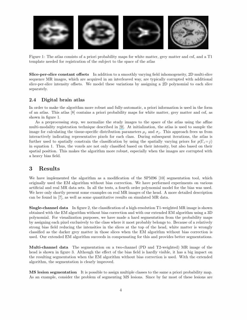
Figure 1: The atlas consists of a priori probability maps for white matter, grey matter and csf, and a T1template needed for registration of the subject to the space of the atlas

Slice-per-slice constant offsets In addition to a smoothly varying field inhomogeneity, 2D multi-slicesequence MR images, which are acquired in an interleaved way, are typically corrupted with additionalslice-per-slice intensity offsets. We model these variations by assigning a 2D polynomial to each sliceseparately.

2.4 Digital brain atlas

In order to make the algorithm more robust and fully-automatic, a priori information is used in the formof an atlas. This atlas [8] contains a priori probability maps for white matter, grey matter and csf, asshown in figure 1.

As a preprocessing step, we normalize the study images to the space of the atlas using the affinemulti-modality registration technique described in [9]. At initialization, the atlas is used to sample theimage for calculating the tissue-specific distribution parameters µj and σj . This approach frees us frominteractively indicating representative pixels for each class. During subsequent iterations, the atlas isfurther used to spatially constrain the classification by using the spatially varying priors for p(Γi=j)in equation 1. Thus, the voxels are not only classified based on their intensity, but also based on theirspatial position. This makes the algorithm more robust, especially when the images are corrupted witha heavy bias field.

3 Results

We have implemented the algorithm as a modification of the SPM96 [10] segmentation tool, whichoriginally used the EM algorithm without bias correction. We have performed experiments on variousartificial and real MR data sets. In all the tests, a fourth order polynomial model for the bias was used.We here only shortly present some examples on real MR images of the head. A more detailed descriptioncan be found in [7], as well as some quantitative results on simulated MR data.

Single-channel data In figure 2, the classification of a high-resolution T1-weighted MR image is shownobtained with the EM algorithm without bias correction and with our extended EM algorithm using a 3Dpolynomial. For visualization purposes, we have made a hard segmentation from the probability mapsby assigning each pixel exclusively to the class where it most probably belongs to. Because of a relativelystrong bias field reducing the intensities in the slices at the top of the head, white matter is wronglyclassified as the darker grey matter in those slices when the EM algorithm without bias correction isused. Our extended EM algorithm succeeds in compensating for this and provides better segmentations.

Multi-channel data The segmentation on a two-channel (PD and T2-weighted) MR image of thehead is shown in figure 3. Although the effect of the bias field is hardly visible, it has a big impact onthe resulting segmentation when the EM algorithm without bias correction is used. With the extendedalgorithm, the segmentation is clearly improved.

MS lesion segmentation It is possible to assign multiple classes to the same a priori probability map.As an example, consider the problem of segmenting MS lesions. Since by far most of these lesions are

4

located inside white matter, we have used the a priori white matter probability map for both the whitematter and MS lesion class. The result for three-channel data of an MS patient, including T1, T2 andPD-weighted images, is shown in figure 4.

Slice-per-slice constant offsets As an example of bias correction for images with slice-per-slice con-stant offsets, we have processed the image shown in figure 5. The slice-per-slice offsets can clearly be seenas an interleaved bright-dark intensity pattern in a cross-section orthogonal to the slices. The estimatedbias is also shown; it can be seen that the algorithm has found the slice-per-slice offsets.

4 Discussion

The algorithm that is proposed is based on Maximum-Likelihood parameter estimation using the EMalgorithm. The method interleaves classification with parameter estimation, increasing likelihood at eachiteration step.

The bias is estimated as a weighted least-squares fit, with the weights inversely proportional to thevariance of the class each pixel belongs to. Since white matter and, in a lesser extend, grey matter have anarrow histogram, voxels belonging to the brain automatically get a large weight compared to non-braintissues. We use a polynomial model for the bias field, which is a well-suited way for estimating bias fieldsin regions where the bias cannot be confidently estimated, i.e. regions with a low weight. The bias fieldis estimated from brain tissues and extrapolated to such regions.

At every iteration, the normal distribution parameters µj and σj for each class are updated. Incombination with the atlas which provides a good initialization, this allows the algorithm to run fullyautomatic, avoiding manual selection of pixels representative for each of the classes considered. Thisyields objective and reproducible results. Furthermore, tissues surrounding the brain are hard to trainfor manually since they consist of a combination of different tissues types. Since our algorithm re-estimatesthe class distributions at each iteration, non-brain tissues automatically get a large variance and thus alow weight for the bias estimation.

We use an atlas which provides a priori information about the expected location of white matter,grey matter and csf. This information is used for initialization, avoiding user interaction which can giveunreproducible results. Furthermore, the atlas makes the algorithm significantly more robust, since voxelsare forced to be classified correctly even if the intensities largely differ due to a heavy bias field.

5 Summary and conclusions

In this paper, we have proposed a method for fully automatic segmentation of brain tissues and MR biasfield correction using a digital brain atlas. We have extended the EM segmentation algorithm, includingan explicit parametric model of the bias field. Results were presented on MR data with importantfield inhomogeneities and slice-per-slice offsets. The algorithm is fully automatic, avoids tedious andtime-consuming user interaction and yields objective and reproducible results.

6 Acknowledgments

This research was performed within the context of the BIOMORPH project ”Development and Validationof techniques for Brain Morphometry” supported by the European Commission under contract BMH4-CT96-0845 in the BIOMED2 programme and the research grant KV/E/197 (Elastische Registratie voorMedische Toepassingen) of the FWO-Vlaanderen to Dirk Vandermeulen.

References

[1] M. Tincher, C.R. Meyer, R. Gupta, and D.M. Williams. Polynomial modeling and reduction of RFbody coil spatial inhomogeneity in MRI. IEEE transactions on medical imaging, 12(2):361–365, june1993.

5

[2] R.C. Gonzalez and R.E. Woods. Digital Image Processing. Addison-Wesley, 1993.

[3] Benoit M. Dawant, Alex P. Zijdenbos, and Richard A. Margolin. Correction of intensity varia-tions in MR images for computer-aided tissue classification. IEEE transactions on medical imaging,12(4):770–781, december 1993.

[4] C.R. Meyer, P.H. Bland, and J. Pipe. Retrospective correction of MRI amplitude inhomogeneities. InN. Ayache, editor, Proc. CVRMed ’96, Computer Vision, Virtual Reality, and Robotics in Medicine;Lecture Notes in Computer Science, pages 513–522. Berlin, Germany: Springer–Verlag, 1995.

[5] W.M. Wells, III, W.E.L. Grimson, R. Kikinis, and F.A. Jolesz. Adaptive segmentation of MRI data.IEEE transactions on medical imaging, 15(4):429–442, august 1996.

[6] A. P. Dempster, N. M. Laird, and D. B. Rubin. Maximum likelihood from incomplete data via theEM algorithm. J. Roy. Stat. Soc., 39:1–38, 1977.

[7] K. Van Leemput, D. Vandermeulen, and P. Suetens. Automatic segmentation of brain tissues and MRbias field correction using a digital brain atlas. Technical Report KUL/ESAT/PSI/9806, ESAT/PSI,june 1998.

[8] Evans A.C., Collins D.L., Mills S.R., Brown E.D., Kelly R.L., and Peters T.M. 3d statisticalneuroanatomical models from 305 MRI volumes. In Proc. IEEE Nuclear Science Symposium andMedical Imaging Conference, pages 1813–1817, 1993.

[9] F. Maes, A. Collignon, D. Vandermeulen, G. Marchal, and P. Suetens. Multi-modality image registra-tion by maximization of mutual information. IEEE transactions on medical imaging, 16(2):187–198,april 1997.

[10] John Ashburner, Karl Friston, Andrew Holmes, and Jean-Baptiste Poline. Statistical ParametricMapping. The Wellcome Department of Cognitive Neurology, University College London.

6

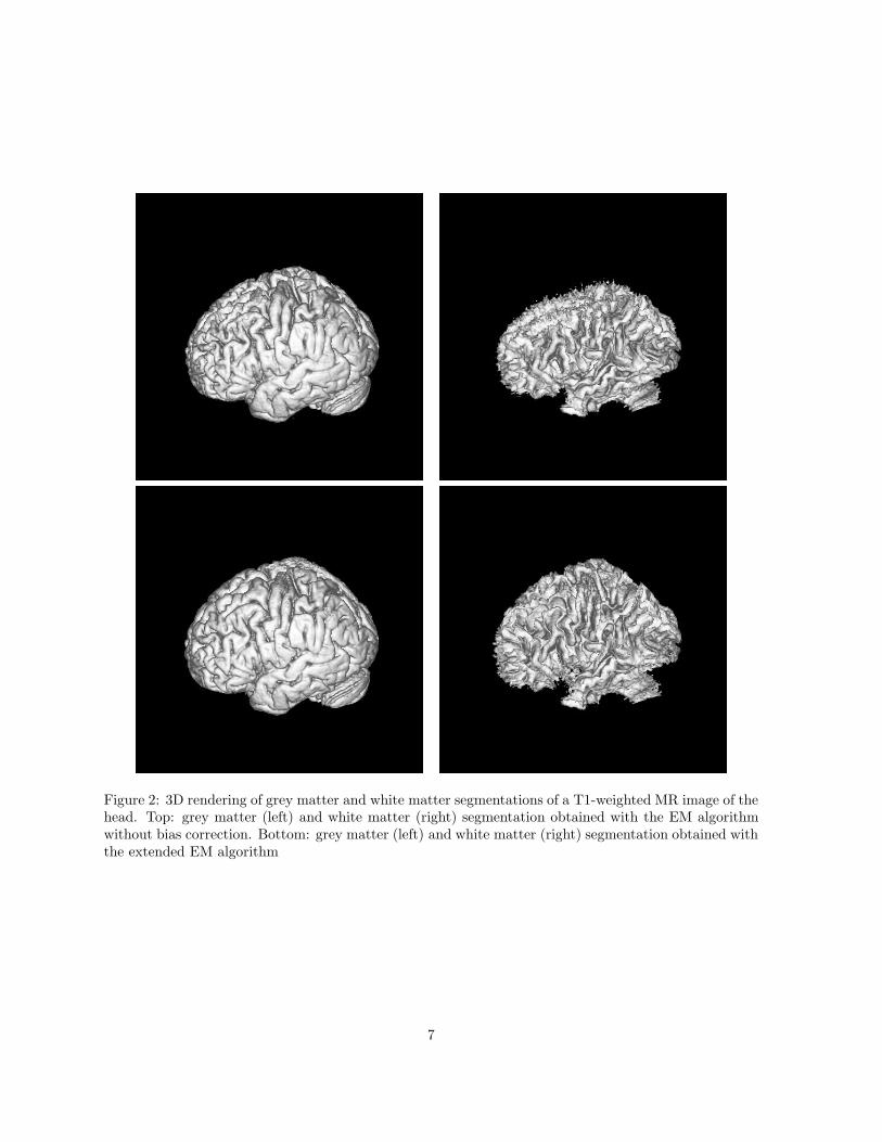
Figure 2: 3D rendering of grey matter and white matter segmentations of a T1-weighted MR image of thehead. Top: grey matter (left) and white matter (right) segmentation obtained with the EM algorithmwithout bias correction. Bottom: grey matter (left) and white matter (right) segmentation obtained withthe extended EM algorithm

7

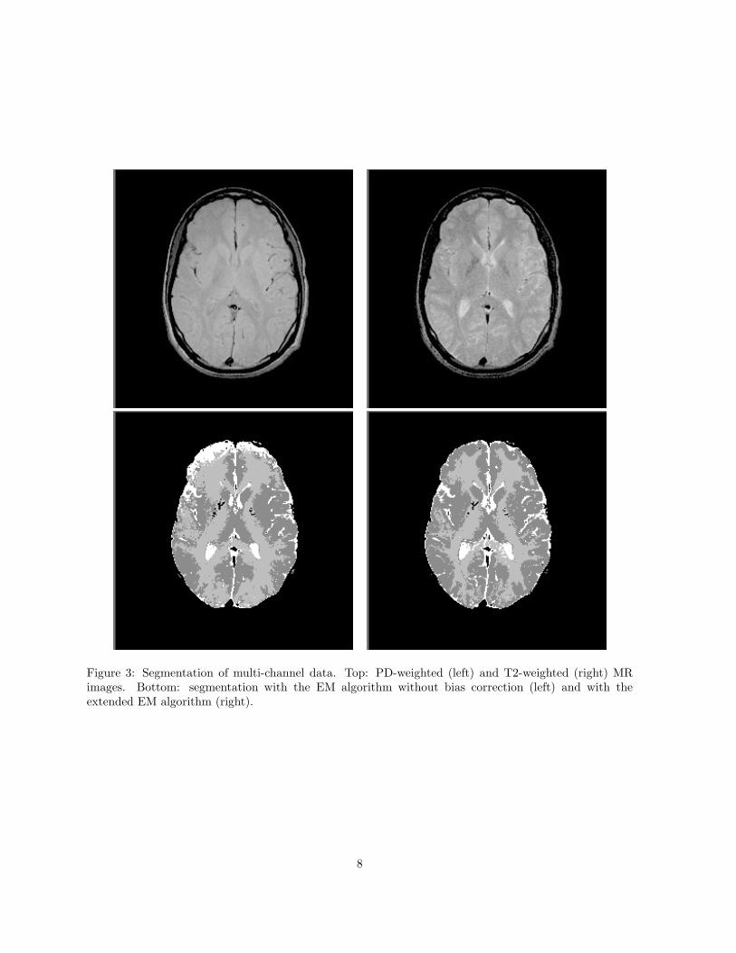
Figure 3: Segmentation of multi-channel data. Top: PD-weighted (left) and T2-weighted (right) MRimages. Bottom: segmentation with the EM algorithm without bias correction (left) and with theextended EM algorithm (right).

8

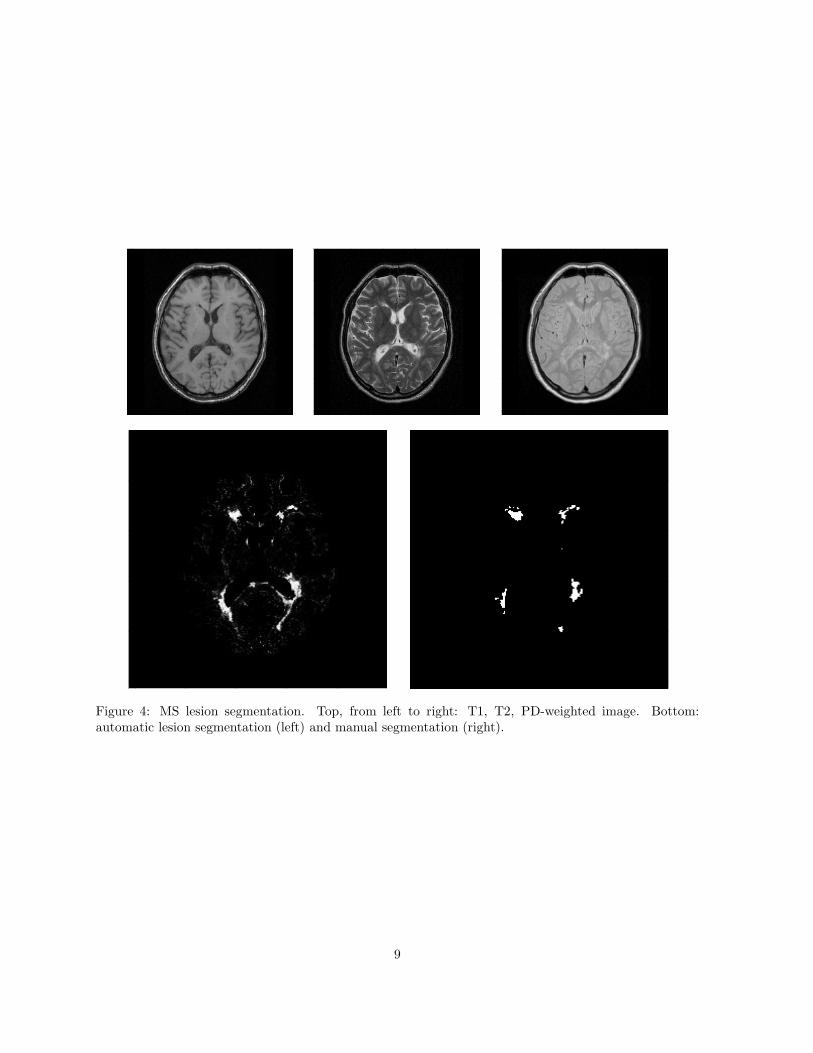
Figure 4: MS lesion segmentation. Top, from left to right: T1, T2, PD-weighted image. Bottom:automatic lesion segmentation (left) and manual segmentation (right).

9

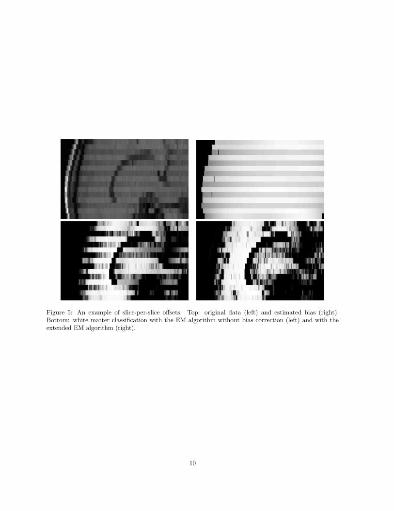
Figure 5: An example of slice-per-slice offsets. Top: original data (left) and estimated bias (right).Bottom: white matter classification with the EM algorithm without bias correction (left) and with theextended EM algorithm (right).

10