Published in Annals of Biomedical Engineering 2012, DOI: 10.1007/s10439-012-0552-1 The final version is available at www.springerlink.com

Automatic Scan Planning for Magnetic Resonance Imaging

of the Knee Joint

Stefan Bauera, Lucas E. Ritacco

b, Chris Boesch

c, Lutz-P. Nolte

a, Mauricio Reyes

a

a Institute for Surgical Technology and Biomechanics, University of Bern, Switzerland

b Virtual Planning and Navigation Unit, Hospital Italiano de Buenos Aires, Argentina

c Departments of Clinical Research and Radiology, University of Bern, Switzerland

Short title : Automatic Scan Planning for Knee MRI

Contact:

Stefan Bauer

ISTB, University of Bern

Stauffacherstr. 78 3014 Bern Switzerland

stefan.bauer@istb.unibe.ch

phone: +41 31 631 5948

fax: +41 31 631 5960

Published in Annals of Biomedical Engineering 2012, DOI: 10.1007/s10439-012-0552-1 The final version is available at www.springerlink.com

2

Abstract

Automatic scan planning for magnetic resonance imaging of the knee aims at defining an

oriented bounding box around the knee joint from sparse scout images in order to choose the

optimal field of view for the diagnostic images and limit acquisition time. We propose a fast and

fully automatic method to perform this task based on the standard clinical scout imaging

protocol. The method is based on sequential Chamfer matching of 2D scout feature images with

a three-dimensional mean model of femur and tibia. Subsequently, the joint plane separating

femur and tibia, which contains both menisci, can be automatically detected using an

information-augmented active shape model on the diagnostic images. This can assist the

clinicians in quickly defining slices with standardized and reproducible orientation, thus

increasing diagnostic accuracy and also comparability of serial examinations. The method has

been evaluated on 42 knee MR images. It has the potential to be incorporated into existing

systems because it does not change the current acquisition protocol.

Keywords: Bounding Box Detection, Automatic Alignment, Chamfer Matching, Active Shape

Model Segmentation, Anatomy Localization, Scout Imaging

Published in Annals of Biomedical Engineering 2012, DOI: 10.1007/s10439-012-0552-1 The final version is available at www.springerlink.com

3

1 Introduction

Magnetic resonance imaging (MRI) of the knee is becoming more important in daily clinical

practice because it offers the possibility not only to diagnose bone fractures but also to draw

conclusions about injuries of soft tissues such as cartilages, ligaments or the menisci 17

.

Following scout images (also called “localizer” or “locator” images), multiple diagnostic series

are acquired. The quality of these scout images is comparatively low and not sufficient for

diagnosis, but they can be acquired in a very short time and they define anatomical structures

sufficiently to prescribe the following sequences. As a standard procedure in a clinical

environment, few slices (usually 3 slices) of 2D scout images, with sparse resolution in three

orientations (axial, coronal, sagittal) are taken first, in order to determine the optimal field of

view and slice orientation for the more detailed diagnostic images.

For a thorough analysis of the knee joint, the diagnostic image must contain left and right

meniscus as well as anterior cruciate ligament (ACL) and posterior cruciate ligament (PCL),

which means the orientation of the bounding box for image acquisition should also be taken into

account. Currently, in clinical practice, the locator images are analyzed manually by a technician

who decides about the field of view for the diagnostic images. This decision is based on

alignment in parallel to the line interconnecting the lateral and medial condyles and in parallel to

the tibia plateau for the menisci. An automatic method, which is seamlessly integrated into the

clinical workflow could bring down both scan time and costs thanks to less user interaction.

Furthermore, using an automatic approach, the selection of the scan field could be standardized

and would be less variable because it does not depend on the skills and experience of the

technician. In order to automate and facilitate the task, it would be desirable to have a software

Published in Annals of Biomedical Engineering 2012, DOI: 10.1007/s10439-012-0552-1 The final version is available at www.springerlink.com

4

tool, which analyzes the locator images automatically in order to find an oriented bounding box

for the field of view of diagnostic images. As a requirement, this tool has to be fast, robust with

respect to the imaging protocol and should not include any user interaction.

1.1 Related work

Automatic scan planning (ASP) for magnetic resonance imaging has been applied to other

anatomical structures before, e.g. brain 10

, heart 11

or pelvis 16

. However, ASP for clinical

workflow integration in knee MRI is a rather new topic and to the best of our knowledge, there

are only five publications in this field so far. Bystrov et al. 4 derive anatomical landmarks by

adapting an active shape model to a 3D scout scan and use the obtained landmarks for defining

the field of view. This method has been clinically evaluated by Lecouvet et al. 15

. Jolly et al. 12

took a different approach. They did not apply a model-based technique, but employ a

combination of hidden Markov models and random walker algorithm for segmentation and

condyle detection on 3D scout images instead. Finally, Zhan et al. 19

suggest a completely

different method based on a hierarchical redundant anatomy detection framework. This work has

also been described in more detail and further evaluated in 18

. However, all the three different

methods presented so far have in common that they require a new and modified fully 3D scout

imaging protocol for alignment, whereas the current manual alignment is based on 2D scout

slices. The 3D scout image is not introduced in the clinics yet.

In a related field for automatic scan prescription, Blumenfeld et al. 1 and also Goldenstein et al.

7

propose to use image registration techniques for automatic alignment. However, these methods

are only intended to be employed for follow-up studies, and not for scan planning in general.

Published in Annals of Biomedical Engineering 2012, DOI: 10.1007/s10439-012-0552-1 The final version is available at www.springerlink.com

5

They perform alignment on the diagnostic images, not on the scout images, and their processing

times are beyond what is acceptable for standard scan planning in the clinics.

We developed a method for automatic scan planning of knee MRI exams, which is fast and can

be seamlessly integrated into the clinical workflow. In contrast to all other methods for ASP

presented so far, it can operate on the standard 2D locator images currently used in the clinics,

and it does not require a new protocol for acquisition of isotropic 3D locator images. As an

extension, we present a method to automatically define the oblique plane showing both menisci

from the diagnostic images. This can help the clinician to quickly navigate to the structure of

interest in large image datasets.

2 Materials and Methods

We use a model-based approach with Chamfer matching on the currently employed standard 2D

scout images for initial alignment and definition of the oriented bounding box (OBB). After the

diagnostic images have been acquired accordingly, the joint plane separating femur and tibia can

be detected using an information-augmented active shape modeling (ASM) method. The

workflow is illustrated in figure 1. The method has been implemented on a stand-alone system

using the Insight Toolkit for Segmentation and Registration (ITK) 9 and the Visualization Toolkit

(VTK) 13

. Both software libraries are open-source and based on C++ with an open licensing

model, which offers the possibility to integrate them into vendor systems. The method and

workflow is described in the next sections in more detail.

Figure 1

Published in Annals of Biomedical Engineering 2012, DOI: 10.1007/s10439-012-0552-1 The final version is available at www.springerlink.com

6

2.1 Definition of the Oriented Bounding Box

The oriented bounding box defining the relevant region of the knee joint, is computed based on a

Chamfer matching approach 2. An example of the 2D scout images on which it is applied, is

shown in coronal, sagittal and axial acquisition view in figure 2.

Figure 2.

Chamfer matching is a fast algorithm for alignment of a template model with a feature image.

This is achieved by convolution of the template model with the image and a search for the best

possible match. As a template for matching, we use a mean model of femur and tibia, generated

from 190 manually segmented CT images from normal volunteers (data from 14

and 3). In our

case, the feature image consists of the edges of the original image, which are obtained using a

Canny edge detector 5. This method detects edges in an image based on the maxima of the

gradient magnitude of the Gaussian-smoothed image and hysteresis thresholding. From the edge

image, a Chamfer distance map is computed, which encodes the distance of every voxel in the

image to the closest edge. The best match between the image and the template model can then be

found by sliding the template over the distance map, calculating the Chamfer distance chamferd at

each step and choosing the position with minimum distance. Using a distance map instead of

using the feature image directly speeds up the process significantly because the distance map can

serve as a lookup table. The Chamfer distance chamferd between the aligned model and the image

is computed according to equation (1), where M corresponds to the mean model, m are the

individual points of the model and I corresponds to the distance map.

Published in Annals of Biomedical Engineering 2012, DOI: 10.1007/s10439-012-0552-1 The final version is available at www.springerlink.com

7

Mm

I mM

IM )(1

),( dd chamfer (1)

So, for each point m of the model M , the distance )(mId to the closest feature point in the

image is computed using the distance map I . Taking the mean over the number of all points of

the model M , we get the average distance to the nearest edge. By sliding the model over the

distance map in different scales and with different translations and rotations, the expression for

),( IMchamferd in equation (1) should be minimized.

In our implementation, an initial alignment is based on matching the centroids of the feature

image and the model. Next, a laterality detection determines if the left or right knee is being

imaged. This is based on the location of the feature image centroid. Then a refinement cascade

for model alignment using the previously described Chamfer matching process is started, which

operates on the coronally, sagittally and axially acquired images sequentially. This is according

to the standard acquisition order of the clinical protocol. The process allows for a pipeline

operation, where the previous view can be processed while the next view is already being

acquired. First, we operate on the coronal scout images, where we perform Chamfer matching

with the mean model at three different scales and translations in x,y,z-direction. The alignment

with minimum Chamfer distance on the coronal images serves as initialization for a more refined

alignment on sagittal scout images, where translations in x,y,z-direction in a smaller range are

allowed. Finally, on the axial scout images we allow for some more small translations in x- and

y-direction, before a rotation around the z-axis is performed. The alignment of the model with

minimum Chamfer distance chamferd after scaling, translations and rotations is chosen as the best

alignment. Based on the aligned model, the oriented bounding box for acquisition of the

Published in Annals of Biomedical Engineering 2012, DOI: 10.1007/s10439-012-0552-1 The final version is available at www.springerlink.com

8

diagnostic images can be determined. The extremal points of the aligned model define the

corners of the bounding box and two distinguished points on both condyles of the aligned model

define the rotation angle. A safety margin of 6 mm is added to the bounding box in x- and y-

direction in order to be able to handle small misalignments without risking an incomplete

coverage of the knee joint.

2.2 Definition of the Joint Plane

After obtaining the diagnostic image, the joint plane separating femur and tibia can be found

using a method based on active shape modeling (ASM) 6,

8. An example of a diagnostic image,

on which the algorithm operates is depicted in figure 3.

Figure 3.

Active shape modeling uses statistical shape models (SSM) 6 of the structure of interest and

adapts them to the same structure in the patient. We build the shape model from the same 190

manually segmented CT images of femurs and tibia employed before and we use the mean shape

together with its first ten modes of variation computed by Principal Component Analysis (PCA)

(more than 90% of variation retained). The information contained in the shape model is

augmented by defining landmark points on the model, which can deform along with the model

during adaptation to the patient image. The landmarks were defined together with a clinical

expert on both femoral condyles and on the tibia plateau. The ASM search is initialized using the

laterality and coordinates for femur and tibia computed by the initial Chamfer matching process.

We use two separate SSMs for femur and tibia, whereas the femur alignment is performed first

and the tibia alignment second.

Published in Annals of Biomedical Engineering 2012, DOI: 10.1007/s10439-012-0552-1 The final version is available at www.springerlink.com

9

Active shape model alignment 6,

8 is a shape-constrained segmentation method, which requires a

sufficiently good pre-alignment. After pre-alignment based on the outcome of the Chamfer

matching process, a search along the normals of the initially aligned model for the most probable

structure of interest in the image is performed. In this case, the structure of interest is found

based on the gradient-magnitude filtered diagnostic image, in which we look for the largest

gradient along the normals of each point in the model. This is supposed to correspond to the edge

of the bone. In order to increase robustness, we set an additional tissue constraint, which ensures

that the normalized image intensities inside the model correspond to actual bone intensities.

After having found tentative points of the structure of interest, the model is adapted towards

these points in an iterative process. This is done using a similarity transformation (7 degrees of

freedom including scaling, translations and rotations 20

) and local deformations (driven by the

PCA modes of the SSM 6) to iteratively align and deform the model to the structure of interest.

The process is stopped once the changes in alignment are small or the maximum number of

iterations has been reached. Mathematically, this iterative alignment is formulated as a

minimization problem with the objective to find the parameters of the transformation matrix T

and the PCA-based deformation parameters b , which minimize the error measure e between the

points of the model and the feature points.

)(minarg ,,,

PbxTy xbT

ste (2)

In equation (2), y are the tentative feature points, which have been found in the image while

searching for the strongest gradient along the normals of the model, ,,stxT is the transformation

matrix for a similarity transform (with translation tx , scaling s and rotation ), x is the mean

Published in Annals of Biomedical Engineering 2012, DOI: 10.1007/s10439-012-0552-1 The final version is available at www.springerlink.com

10

shape of the model, P is the matrix of eigenvectors of the model originating from the PCA, and

b is a vector of deformation coefficients, which have to be determined 6. These coefficients are

constrained to lie within 3 standard deviations from the respective eigenvalues in order to allow

for plausible shapes only.

We use a multi-resolution approach 8 with 3 resolution levels. This employs a coarse-to-fine

strategy for model alignment on subsampled versions of the original image in order to increase

robustness and speed of the algorithm. In the first resolution level, an approximate alignment

with long search range along the normals of the model is done, which is further refined in the

next two levels. The statistical shape model we use has approximately 18000 points. As we are

not interested in a perfect segmentation of the bone, but only in a good general alignment we

subsample this model by a factor of 9 in order achieve a higher speed performance.

After alignment of the femur shape model, we can define the lowest femur point and the two

condyles exactly. The joint plane separating femur and tibia and containing both menisci is based

on the aligned shape model of the tibia because the menisci are embedded in the tibia plateau.

We define three points on the tibia, which are deformed along with the model. These three points

determine a plane defining the tibia plateau (see also figure 5 for an illustration of the points).

3 Results

We evaluated the algorithm on 42 MR images of knee joints. The images were acquired on a 3T

Siemens TIM-TRIO scanner (Siemens, Erlangen, Germany). The participants were specifically

recruited for this study, however acquisition was performed according to the standard imaging

Published in Annals of Biomedical Engineering 2012, DOI: 10.1007/s10439-012-0552-1 The final version is available at www.springerlink.com

11

protocols. Despite the fact that apparently healthy volunteers were recruited, one volunteer had a

ligament rupture (1 knee joint) and two volunteers exhibited bone edema (4 knee joints). IRB

approval (Kantonale Ethikkommission Bern) was obtained and the participants gave written

informed consent. One data set was obtained from the Toshiba data base, acquired on a 1.5T

Toshiba MRT200SP6 scanner (Toshiba Medical Systems, Otawara, Japan). In terms of accuracy,

the results of the method have been validated retrospectively using manual landmark definitions

by an expert and checked by an orthopedic surgeon. The manual definitions were done on 3D

volumetric MR images, which were acquired for each dataset together with the scout and

diagnostic images. These high-quality images have a resolution of less than 1mm in each

direction (imaging parameters: 3D gradient echo sequence with TR=11ms and TE=4.92ms on

Siemens machines and with TR=9.1ms and TE=3.5ms on Toshiba machines). They were acquired

for validation and visualization purposes only and were not used by the algorithm. Additionally,

we also evaluated the robustness of the method in a qualitative way by judging if the result for

the OBB and joint plane was “perfect” (manual definition would have been similar

retrospectively), “acceptable” (manual definition would have been different retrospectively, but

relevant region is fully covered and inclination is reasonable) or “bad” (relevant region is not

fully covered or inclination is wrong).

3.1 Results for the Definition of the Oriented Bounding Box

The scout images, on which the scan planning was performed, usually contained 3 slices in

coronal, sagittal and axial view (see figure 2). The images had an intra-slice resolution of 0.5-

0.7mm and an inter-slice spacing of 9-10mm (imaging parameters: 2D gradient echo sequence

with TR=7.7ms and TE=3.67ms on the Siemens system and 2D gradient echo sequence with

Published in Annals of Biomedical Engineering 2012, DOI: 10.1007/s10439-012-0552-1 The final version is available at www.springerlink.com

12

TR=9.1ms and TE=3.5ms on the Toshiba system). As it occurs in clinics, the images covered the

knee joint only partially and were sometimes shifted with respect to the center of the knee joint,

which further complicated the task.

The laterality of the knee present in the locator image was correctly identified by the algorithm in

all cases. The resulting oriented bounding box is shown for two cases in figure 4. For better

visualization it is depicted in three views on a T2-weighted high-resolution volumetric image of

the patient knee and not on the original scout image. The first row of figure 4 shows a good

alignment: the knee joint is fully covered and the box is aligned with the posterior condyles of

the femur, while the covered area is not too large. On the other hand, the image in the second

row shows one case where the alignment with the condyles is not satisfactory.

Figure 4.

Judging the robustness, 50% of the OBB were considered to be perfectly aligned, 40% were

acceptable and 10% were bad. In most cases, the non-perfect alignment was caused by

unsatisfactory orientation of the angle with the condyles (see bottom row of figure 4 for an

illustration). For the quantitative analysis, we manually defined six landmarks on the femur,

which determine the location and maximum extent of the knee joint, as well as the condyle

rotation angle. The average accuracy of the landmarks defining the bounding box was 5.3 mm

with a standard deviation of 4.3 mm and the average error of the condyle rotation angle was 6°

with a standard deviation of 5°. The individual accuracies for each point are shown in table 1.

The four cases which were judged to be “bad”, were not considered for the quantitative analysis.

In general, the cases in which the knee joint was covered only partially or shifted, were more

frequent than the cases of failure, and they did not coincide with the cases where the algorithm

Published in Annals of Biomedical Engineering 2012, DOI: 10.1007/s10439-012-0552-1 The final version is available at www.springerlink.com

13

returned bad results. The failures could neither be attributed to uncommon structures of the knee

joint nor to the pathologic cases, but a general pattern which caused unsatisfactory results could

not be identified.

Table 1.

Acquisition time for the scout image was 6 seconds per view, so 18 seconds in total.

Computation time on a 2.3 GHz quad-core processor with 3 GB of RAM was 18 seconds on

average, which means also around 6 seconds per view.

3.2 Results for the Definition of the Joint Plane

The diagnostic images for definition of the joint plane were acquired in sagittal direction

covering the knee joint completely. They had an intra-slice resolution of 0.3-0.4mm and an inter-

slice spacing of 3.6-3.9mm, with 25 slices on average (imaging parameters: 2D spin echo

sequence with TR=550ms and TE=16ms on the Siemens system and 2D spin echo sequence with

TR=540ms and TE=15ms on the Toshiba system).

The aligned models of femur and tibia after active shape modeling are shown in coronal, sagittal

and axial view in figure 5 as an overlay on the T2-weighted high-resolution volumetric image of

the patient knee (for better visualization not on the original sagittal diagnostic image). Both

models are well aligned with the bones. The red crosses indicate the landmark points on the

model used to determine both posterior condyles of the femur (two points) and the joint plane

with both menisci on the tibia (three points).

Figure 5.

Published in Annals of Biomedical Engineering 2012, DOI: 10.1007/s10439-012-0552-1 The final version is available at www.springerlink.com

14

In figure 6, the joint plane is depicted, which was automatically found from the three points

defined on the tibia model for the same case as the one shown in figure 5. On the left, the plane

is shown in coronal view and in the center in sagittal view. The right image shows the oblique

plane itself in axial view. It is obvious that both menisci can be well seen on this automatically

selected slice and it can also be seen that the position and inclination of the plane corresponds

well to the patient anatomy.

Figure 6

Figure 7 shows a comparison of the manual definition of the joint plane on the left and the

automatic definition of the joint plane in the center for one patient. It can be seen that for both

cases, the menisci are present, whereas the manual definition covers a slightly larger part of

cartilage thanks to a slightly better inclination of the plane in the volumetric image (circled area).

Additionally in the picture on the right it is illustrated that it is not sufficient to choose the best

axis-aligned slice in z-direction because without considering the inclination, only one meniscus

is partially covered in the image, while the other is missing completely (circled area).

Figure 7

All knee images were included in the analysis of the joint plane location, including those for

which the initialization by the OBB method was considered to be unsatisfactory. Judging

qualitatively, in 81% of all cases the selected plane was evaluated to be perfect, in 14% it was

acceptable and in 5% of all cases the method failed. Failure was caused by a shift of the plane

position in z-direction (due to bad initialization by the OBB method), so that the plane showed

bone instead of cartilage. Based on the high-resolution volumetric images, an expert defined the

joint plane containing both menisci manually. The outcome of the algorithm for the plane origin

Published in Annals of Biomedical Engineering 2012, DOI: 10.1007/s10439-012-0552-1 The final version is available at www.springerlink.com

15

and plane normal was compared to the result of the expert. The two cases, when the method

failed were left out for the quantitative results. The average transversal deviation of the

automatic joint plane definition from the manual definition was 1.2 mm with a standard

deviation of 0.8 mm. The average difference between the plane normals was 3.6° with a standard

deviation of 2.5°(see also table 2). It should be emphasized, that the clinician doing the manual

definition found it very difficult and time-consuming to perform the manual annotation in the

volumetric images. Therefore, when comparing the outcome of the manual and automatic

method retrospectively, in some cases the automatic method was considered to be even better.

Computation time depended on the convergence speed of the method. On average, the joint plane

was found within 21 seconds.

Table 2

4 Discussion and Conclusion

We presented a method to perform automatic scan planning for acquisition of diagnostic

magnetic resonance images of the knee joint. This method was combined with a technique to

automatically localize the joint plane containing both menisci from the diagnostic images. In

contrast to other approaches suggested so far, the method at hand can work on the currently used

2D scout imaging protocols and does not require a new volumetric scout sequence, which has a

longer acquisition time. The automatic joint plane localization can help the clinicians to analyze

the diagnostic sequences in shorter time and in an optimized fashion such that diagnostic

accuracy and reproducibility is improved. This is particularly important in serial examinations,

e.g. to follow the development of degenerative processes, healing of tendons following surgery,

cartilage repair in interventional studies, etc.

Published in Annals of Biomedical Engineering 2012, DOI: 10.1007/s10439-012-0552-1 The final version is available at www.springerlink.com

16

The approach was tested under challenging conditions with images from different machines and

sites, as well as different patient groups. The accuracy and robustness proved to be sufficient in

the majority of cases, although a further increase in robustness for the bounding box definition

would be beneficial for even less need for human intervention. The method for scan planning is

almost twice as accurate as the resolution of the scout images on which it operates (5 mm

average landmark error versus 9-10 mm slice spacing) and it can find the borders of structures

which are not present in the images at all. This can only be achieved thanks to the model-based

approach, which is able to infer for example the tip of the condyles from the alignment of the

whole model based on other parts of the femur. Computation time was sufficiently fast, so that

the method can be used in a clinical scenario. As the images are processed in the same order as

they are acquired, the previous acquisition can be analyzed while the next view is already being

acquired. This reduces overall computation time, meaning the oriented bounding box, which

defines the limits for the diagnostic acquisition, is available only 6 seconds after the acquisition

of the scout images has finished. The accuracy of the bounding box detection on the scout

images is in a similar range, although slightly lower compared to 4. It is lower compared with

18,

however both competing methods use a non-conventional 3D scout image, which contains much

more information and they do not provide a delineation of the joint plane.

The method at hand has the potential to significantly speed-up the clinical workflow for

acquisition of diagnostic knee MR images compared to the manual bounding box definition. The

speed-up can in return lead to cost-savings in hospitals because more patients can be scheduled

within the same time period and the technician is free to perform other tasks in the meantime. It

has the potential to be easily incorporated into existing systems because it does not change the

Published in Annals of Biomedical Engineering 2012, DOI: 10.1007/s10439-012-0552-1 The final version is available at www.springerlink.com

17

current acquisition protocol, it does not require any special computation hardware and is fast

enough for clinical use.

Acknowledgements

We would like to thank Karin Zwygart for helping with data acquisition. We would also like to

acknowledge Dr. Yasuo Sakurai for helpful discussions and data collection.

Supplementary Material

Please see supplementary material available online at (link to be added later) for specific

parameter settings of the image processing methods.

References

1. Blumenfeld, J., J. Carballido-Gamio, R. Krug, D. J. Blezek, I. Hancu, and S. Majumdar.

Automatic prospective registration of high-resolution trabecular bone images of the tibia.

Annals of biomedical engineering 35:1924-31, 2007.

2. Borgefors, G. Hierarchical chamfer matching: A parametric edge matching algorithm.

IEEE Transactions on pattern analysis and machine intelligence 10:849–865, 1988.

3. Bou Sleiman, H., L. E. Ritacco, L. Aponte-Tinao, D. L. Muscolo, L.-P. Nolte, and M.

Reyes. Allograft Selection for Transepiphyseal Tumor Resection Around the Knee Using

Three-Dimensional Surface Registration. Annals of biomedical engineering ,

2011.doi:10.1007/s10439-011-0282-9

4. Bystrov, D., V. Pekar, S. Young, S. P. M. Dries, H. S. Heese, and A. M. van Muiswinkel.

Automated planning of MRI scans of knee joints. Proceedings of SPIE 6509:65092Z-

65092Z-9, 2007.

Published in Annals of Biomedical Engineering 2012, DOI: 10.1007/s10439-012-0552-1 The final version is available at www.springerlink.com

18

5. Canny, J. A Computational Approach to Edge Detection. IEEE Transactions on Pattern

Analysis and Machine Intelligence PAMI-8:679-698, 1986.

6. Cootes, T. F. Active Shape Models-Their Training and Application. Computer Vision and

Image Understanding 61:38-59, 1995.

7. Goldenstein, J., J. Schooler, J. C. Crane, E. Ozhinsky, J.-B. Pialat, J. Carballido-Gamio,

and S. Majumdar. Prospective image registration for automated scan prescription of

follow-up knee images in quantitative studies. Magnetic resonance imaging 29:693-700,

2011.

8. Heimann, T., and H. P. Meinzer. Statistical shape models for 3D medical image

segmentation: A review. Medical image analysis 13:543–563, 2009.

9. Ibanez, L., W. Schroeder, L. Ng, J. Cates, and others. The ITK software guide. Citeseer:

2003.

10. Itti, L., L. Chang, and T. Ernst. Automatic scan prescription for brain MRI. Magnetic

Resonance in Medicine 45:486-494, 2001.

11. Jackson, C. E., M. D. Robson, J. M. Francis, and J. A. Noble. Computerised planning of

the acquisition of cardiac MR images. Computerized medical imaging and graphics the

official journal of the Computerized Medical Imaging Society 28:411-418, 2004.

12. Jolly, M. P., C. V. Alvino, B. L. Odry, X. Deng, J. Zheng, M. Harder, and J. Guehring.

Automatic femur segmentation and condyle line detection in 3D MR scans for alignment

of high resolution MR. , 2010.doi:10.1109/ISBI.2010.5490142

13. Kitware. VTK User’s Guide. Kitware Inc.: 2010.

14. Kozic, N., S. Weber, P. Büchler, C. Lutz, N. Reimers, M. a González Ballester, and M.

Reyes. Optimisation of orthopaedic implant design using statistical shape space analysis

based on level sets. Medical image analysis 14:265-75, 2010.

15. Lecouvet, F. E., J. Claus, P. Schmitz, V. Denolin, C. Bos, and B. C. Vande Berg. Clinical

evaluation of automated scan prescription of knee MR images. Journal of magnetic

resonance imaging : JMRI 29:141-5, 2009.

16. Lee, S.-L., P. Horkaew, A. Darzi, and G.-Z. Yang. Optimal Scan Planning with Statistical

Shape Modelling of the Levator Ani. , 2003.doi:10.1007/978-3-540-39899-8_87

17. Ostlere, S. Imaging the knee. Imaging 19:249-268, 2007.

Published in Annals of Biomedical Engineering 2012, DOI: 10.1007/s10439-012-0552-1 The final version is available at www.springerlink.com

19

18. Zhan, Y., M. Dewan, M. Harder, A. Krishnan, and X. Zhou. Robust Automatic Knee MR

Slice Positioning through Redundant and Hierarchical Anatomy Detection. IEEE

transactions on medical imaging 1-14, 2011.doi:10.1109/TMI.2011.2162634

19. Zhan, Y., M. Dewan, and X. S. Zhou. Auto-alignment of knee MR scout scans through

redundant, adaptive and hierarchical anatomy detection. , 2011.

20. Zitova, B., and J. Flusser. Image registration methods: a survey. Image and Vision

Computing 21:977-1000, 2003.

Published in Annals of Biomedical Engineering 2012, DOI: 10.1007/s10439-012-0552-1 The final version is available at www.springerlink.com

20

Figure, Table Legends

Figure Legends

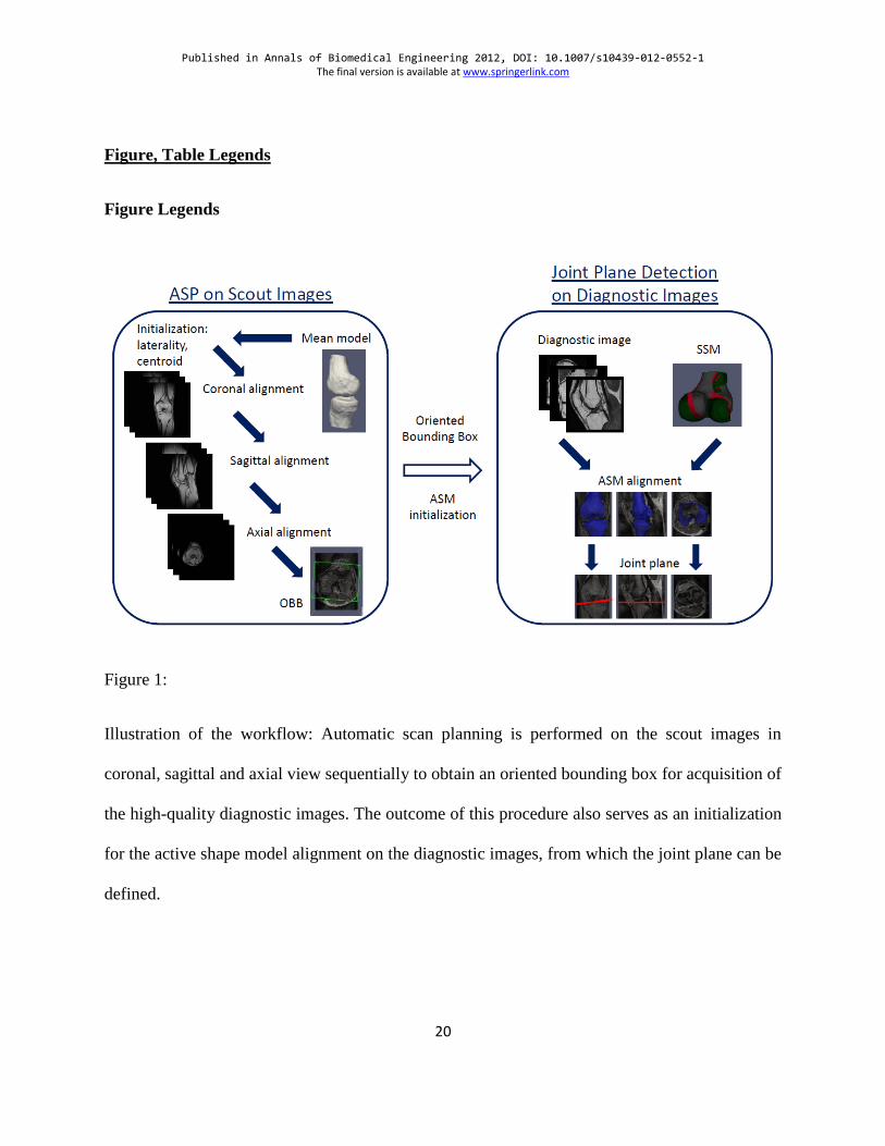
Figure 1:

Illustration of the workflow: Automatic scan planning is performed on the scout images in

coronal, sagittal and axial view sequentially to obtain an oriented bounding box for acquisition of

the high-quality diagnostic images. The outcome of this procedure also serves as an initialization

for the active shape model alignment on the diagnostic images, from which the joint plane can be

defined.

Published in Annals of Biomedical Engineering 2012, DOI: 10.1007/s10439-012-0552-1 The final version is available at www.springerlink.com

21

Figure 2:

One example for the scout images (2D gradient echo sequence, TR=7.7ms and TE=3.67ms), on

which the Chamfer matching for OBB definition is performed. Top row: the three slices in

coronal acquisition. Center row: the three slices in sagittal acquisition. Bottom row: the three

slices in axial acquisition. (9mm slice spacing in each case)

Published in Annals of Biomedical Engineering 2012, DOI: 10.1007/s10439-012-0552-1 The final version is available at www.springerlink.com

22

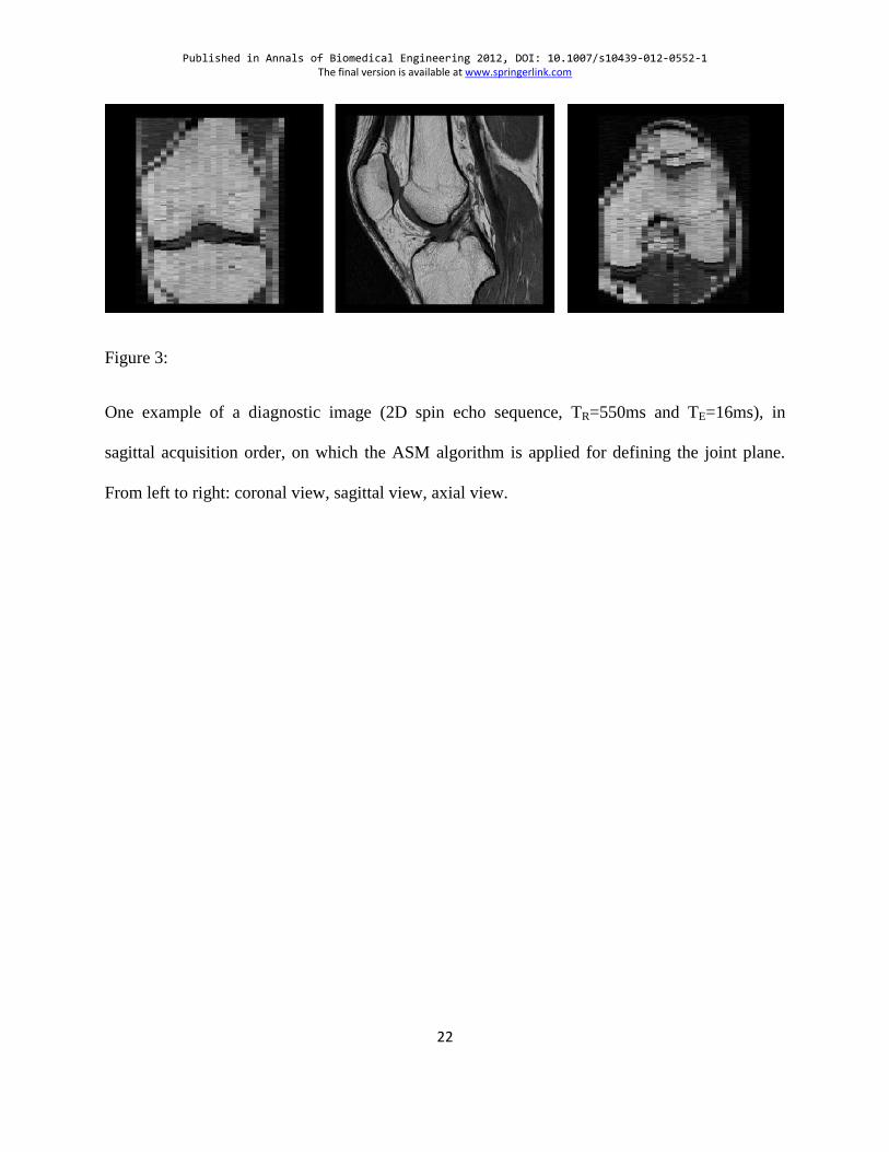
Figure 3:

One example of a diagnostic image (2D spin echo sequence, TR=550ms and TE=16ms), in

sagittal acquisition order, on which the ASM algorithm is applied for defining the joint plane.

From left to right: coronal view, sagittal view, axial view.

Published in Annals of Biomedical Engineering 2012, DOI: 10.1007/s10439-012-0552-1 The final version is available at www.springerlink.com

23

Figure 4:

The oriented bounding box, which is found after Chamfer matching on the scout images (from

left to right: coronal, sagittal and axial view). For better visual assessment, it is shown here on

the 3D high-resolution images (3D gradient echo sequence, TR=11ms and TE=4.92ms) and not

on the scout images. Top row: one case with good results, the knee joint is completely covered,

the bounding box is well aligned with the condyles and cover area is not too large. A line

interconnecting both posterior condyles is shown in dashed blue to illustrate the good orientation

of the alignment angle with the condyles. Bottom row: one case with bad results: the bounding

Published in Annals of Biomedical Engineering 2012, DOI: 10.1007/s10439-012-0552-1 The final version is available at www.springerlink.com

24

box is not well aligned with the condyles (compare to the manually drawn dashed blue line,

interconnecting both posterior condyles), the knee joint is not completely covered in the anterior

part (blue arrows) and on the lateral side the covered area is too large.

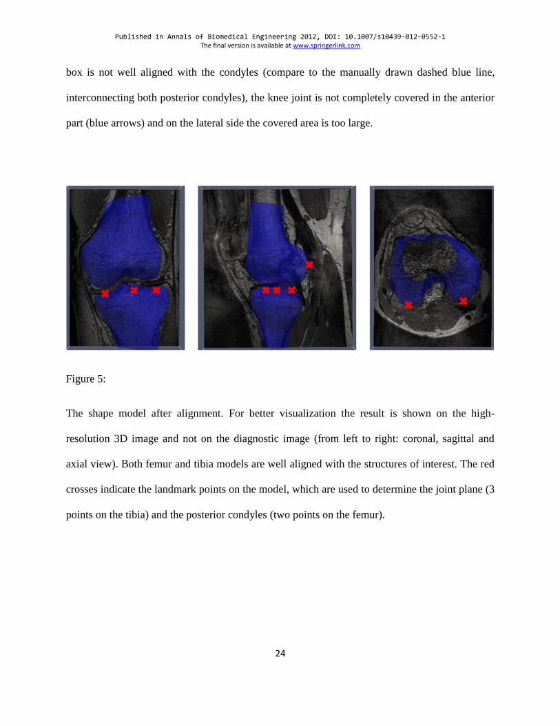
Figure 5:

The shape model after alignment. For better visualization the result is shown on the high-

resolution 3D image and not on the diagnostic image (from left to right: coronal, sagittal and

axial view). Both femur and tibia models are well aligned with the structures of interest. The red

crosses indicate the landmark points on the model, which are used to determine the joint plane (3

points on the tibia) and the posterior condyles (two points on the femur).

Published in Annals of Biomedical Engineering 2012, DOI: 10.1007/s10439-012-0552-1 The final version is available at www.springerlink.com

25

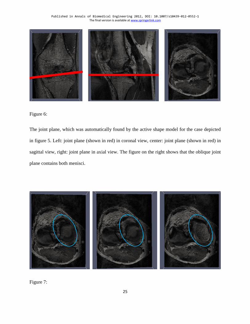
Figure 6:

The joint plane, which was automatically found by the active shape model for the case depicted

in figure 5. Left: joint plane (shown in red) in coronal view, center: joint plane (shown in red) in

sagittal view, right: joint plane in axial view. The figure on the right shows that the oblique joint

plane contains both menisci.

Figure 7:

Published in Annals of Biomedical Engineering 2012, DOI: 10.1007/s10439-012-0552-1 The final version is available at www.springerlink.com

26

Comparison of the manual definition of the joint plane on the left and automatic definition of the

joint plane in the center, shown on the same patient case as figure 5 and 6. The right image

shows the result if only the best slice in z-direction is chosen, without considering the

inclination. It can be seen that in this case only one meniscus is partially covered, while the other

is missing completely in this slice (circled area).

Published in Annals of Biomedical Engineering 2012, DOI: 10.1007/s10439-012-0552-1 The final version is available at www.springerlink.com

27

Table Legends

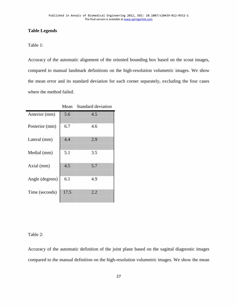
Table 1:

Accuracy of the automatic alignment of the oriented bounding box based on the scout images,

compared to manual landmark definitions on the high-resolution volumetric images. We show

the mean error and its standard deviation for each corner separately, excluding the four cases

where the method failed.

Mean Standard deviation

Anterior (mm) 5.6 4.5

Posterior (mm) 6.7 4.6

Lateral (mm) 4.4 2.9

Medial (mm) 5.1 3.5

Axial (mm) 4.5 5.7

Angle (degrees) 6.1 4.9

Time (seconds) 17.5 2.2

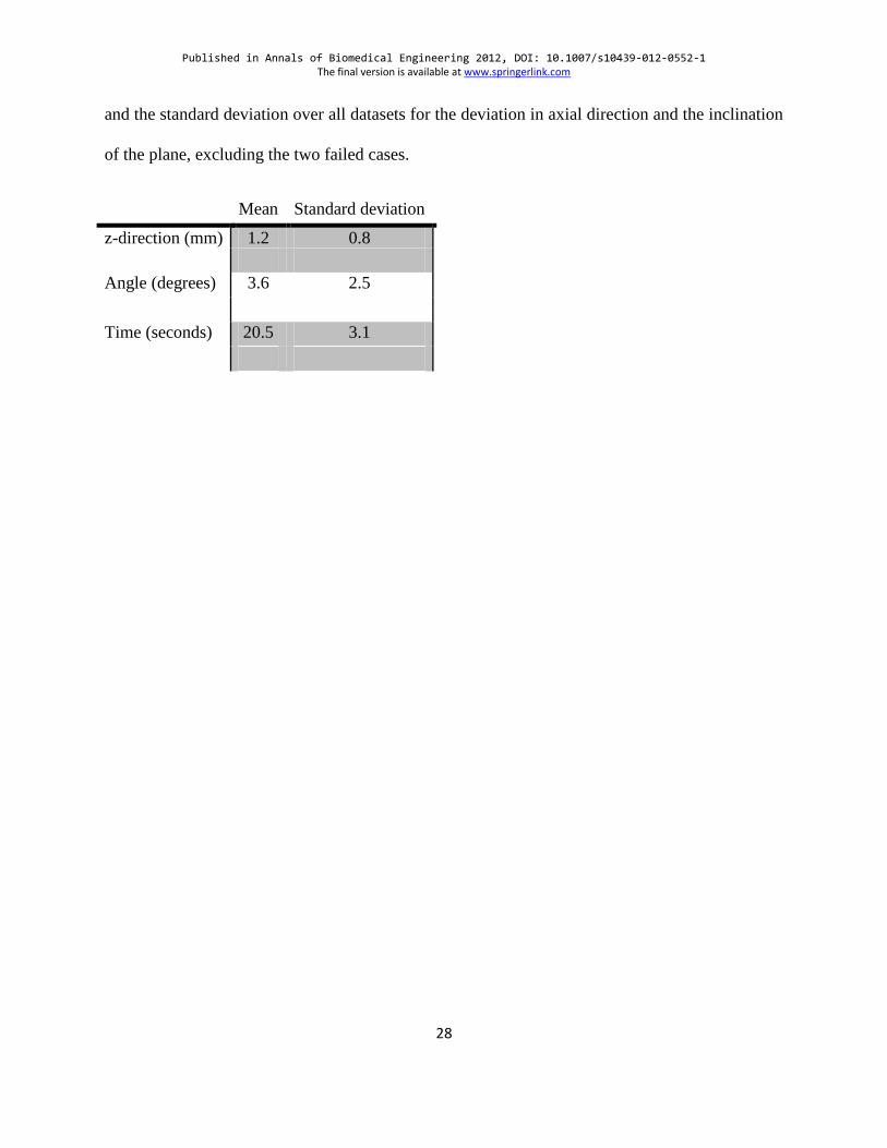
Table 2:

Accuracy of the automatic definition of the joint plane based on the sagittal diagnostic images

compared to the manual definition on the high-resolution volumetric images. We show the mean

Published in Annals of Biomedical Engineering 2012, DOI: 10.1007/s10439-012-0552-1 The final version is available at www.springerlink.com

28

and the standard deviation over all datasets for the deviation in axial direction and the inclination

of the plane, excluding the two failed cases.

Mean Standard deviation

z-direction (mm) 1.2 0.8

Angle (degrees) 3.6 2.5

Time (seconds) 20.5 3.1