Discretized Spatio-Temporal Scan Window

Seyed H. Mohammadi †‡, Vandana P. Janeja †∗, Aryya Gangopadhyay †

† Information Systems Department, University of Maryland, Baltimore County, MD, USA‡Johns Hopkins University, MD, USA

smohamm1@jhuadig.admin.jhu.edu,{vjaneja,gangopad}@umbc.edu

AbstractThe focus of this paper is the discovery of anomalousspatio-temporal windows. We propose a Discretized Spatio-Temporal Scan Window approach to address the questionof how we can treat Space and Time together withoutcompromising on the properties of each and their impacton each other. In doing so we discover anomalous Spatio-Temporal windows, identify at what point in time thewindow changes, identify the spatial patterns of change overtime and identify a spatial extent in time which is completelydeviant with respect to the rest of the anomalous spatio-temporal windows. None of the current approaches addressall these issues in combination. Subsequently we performexperiments on several real world datasets to validate ourapproach while comparing with the established approach ofdiscovering a cylindrical spatio-temporal Scan window.

1 Introduction

Spatial and Spatio-Temporal data mining provides theknowledge necessary to make informed decisions inseveral critical applications such as analyzing the datatransmitted by satellites, discovering potential diseaseoutbreaks in a region, evaluating the drinking watermonitoring data for safety, studying tumor growths, toname a few.

The ability to represent time in Geospatial Informa-tion Systems has been a major concern [1]. Similarlyability to represent space in time has also posed sev-eral challenges [21]. Many of the spatio-temporal datamining techniques consider time as another dimensionor feature of the spatial data. However the temporalelement of the spatial data presents new challenges thatneed to be addressed in a distinct manner, such that itcan evolve into another aspect of the analysis.

The focus of this paper is the discovery of Anoma-lous Spatio-Temporal windows. Before we discussSpatio-Temporal Windows we talk briefly about anoma-lous windows and more specifically Spatial windows [13]which are contiguous spatial points occurring in thedata, such as a set of contiguous counties belonging toa disease outbreak window.

A number of techniques have been proposed to ad-dress the problem of identifying anomalous windows

∗Corresponding Author

[13, 18, 20]. However, most of these techniques limit toidentifying individual unusual objects [2] (e.g., outliers),traditional partitioning (clusters) [3] or fixed size win-dows [20]. Scan statistic extends this to varying sizewindows and proposes an intuitive framework for iden-tification of unusual groupings in the data. Scan Statis-tics pertains to the testing of a point process to see if itis purely random or a cluster can be identified. A onedimensional Scan statistics identifies the largest num-ber of objects in a window of fixed or variable length ascompared to the entire distribution. This comparisonis quantified using the likelihood ratio of the scan win-dow as occurring by chance vs. occurring due to certainnon-random process.

Kulldorff proposed a spatial [13,14] (region scannedwith a circular window) and spatio temporal [15,16](re-gion scanned with a cylindrical window) scan statistic.The window with a large number of points as comparedto the points outside the window is observed and itslikelihood ratio is computed. The window with themaximum likelihood ratio over all possible windows isrecorded and compared to its distribution under the nullhypothesis of a purely random process, thus providinga significance value.

We consider anomalous Spatio-Temporal Windowsas the unusual groupings of contiguous spatio-temporalpoints in space. Thus the window comprises of a set ofspatial points across various temporal points which areunusual as compared to the rest of the data. The pro-cess of discovery of such anomalous windows across bothspace and time becomes even more critical to several ap-plications. For instance, (a) evaluating the health risksover a period of time,(b) fluctuating disease clusters andunusual death rates (tracking disease clusters), (c) un-usual rates of accidents along highways over time, (d)unusual seasonal geospatial hot-spots of plant or animalspecies and (e) a localized temporal deviant disease phe-nomenon which may not follow the general trend(e.g:bio terrorism attack).

In spatio-temporal scan statistic [15], the windowshape is cylindrical where the height represents the time

1197 Copyright © by SIAM. Unauthorized reproduction of this article is prohibited.

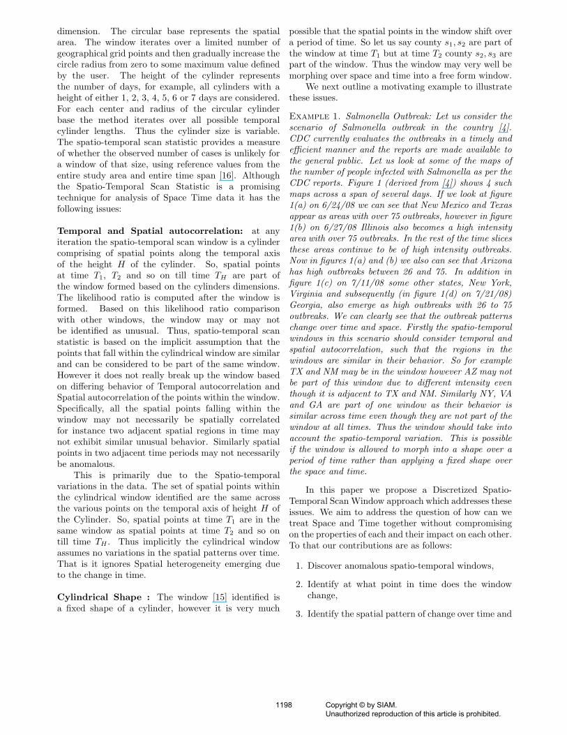
dimension. The circular base represents the spatialarea. The window iterates over a limited number ofgeographical grid points and then gradually increase thecircle radius from zero to some maximum value definedby the user. The height of the cylinder representsthe number of days, for example, all cylinders with aheight of either 1, 2, 3, 4, 5, 6 or 7 days are considered.For each center and radius of the circular cylinderbase the method iterates over all possible temporalcylinder lengths. Thus the cylinder size is variable.The spatio-temporal scan statistic provides a measureof whether the observed number of cases is unlikely fora window of that size, using reference values from theentire study area and entire time span [16]. Althoughthe Spatio-Temporal Scan Statistic is a promisingtechnique for analysis of Space Time data it has thefollowing issues:

Temporal and Spatial autocorrelation: at anyiteration the spatio-temporal scan window is a cylindercomprising of spatial points along the temporal axisof the height H of the cylinder. So, spatial pointsat time T1, T2 and so on till time TH are part ofthe window formed based on the cylinders dimensions.The likelihood ratio is computed after the window isformed. Based on this likelihood ratio comparisonwith other windows, the window may or may notbe identified as unusual. Thus, spatio-temporal scanstatistic is based on the implicit assumption that thepoints that fall within the cylindrical window are similarand can be considered to be part of the same window.However it does not really break up the window basedon differing behavior of Temporal autocorrelation andSpatial autocorrelation of the points within the window.Specifically, all the spatial points falling within thewindow may not necessarily be spatially correlatedfor instance two adjacent spatial regions in time maynot exhibit similar unusual behavior. Similarly spatialpoints in two adjacent time periods may not necessarilybe anomalous.

This is primarily due to the Spatio-temporalvariations in the data. The set of spatial points withinthe cylindrical window identified are the same acrossthe various points on the temporal axis of height H ofthe Cylinder. So, spatial points at time T1 are in thesame window as spatial points at time T2 and so ontill time TH . Thus implicitly the cylindrical windowassumes no variations in the spatial patterns over time.That is it ignores Spatial heterogeneity emerging dueto the change in time.

Cylindrical Shape : The window [15] identified isa fixed shape of a cylinder, however it is very much

possible that the spatial points in the window shift overa period of time. So let us say county s1, s2 are part ofthe window at time T1 but at time T2 county s2, s3 arepart of the window. Thus the window may very well bemorphing over space and time into a free form window.

We next outline a motivating example to illustratethese issues.

Example 1. Salmonella Outbreak: Let us consider thescenario of Salmonella outbreak in the country [4].CDC currently evaluates the outbreaks in a timely andefficient manner and the reports are made available tothe general public. Let us look at some of the maps ofthe number of people infected with Salmonella as per theCDC reports. Figure 1 (derived from [4]) shows 4 suchmaps across a span of several days. If we look at figure1(a) on 6/24/08 we can see that New Mexico and Texasappear as areas with over 75 outbreaks, however in figure1(b) on 6/27/08 Illinois also becomes a high intensityarea with over 75 outbreaks. In the rest of the time slicesthese areas continue to be of high intensity outbreaks.Now in figures 1(a) and (b) we also can see that Arizonahas high outbreaks between 26 and 75. In addition infigure 1(c) on 7/11/08 some other states, New York,Virginia and subsequently (in figure 1(d) on 7/21/08)Georgia, also emerge as high outbreaks with 26 to 75outbreaks. We can clearly see that the outbreak patternschange over time and space. Firstly the spatio-temporalwindows in this scenario should consider temporal andspatial autocorrelation, such that the regions in thewindows are similar in their behavior. So for exampleTX and NM may be in the window however AZ may notbe part of this window due to different intensity eventhough it is adjacent to TX and NM. Similarly NY, VAand GA are part of one window as their behavior issimilar across time even though they are not part of thewindow at all times. Thus the window should take intoaccount the spatio-temporal variation. This is possibleif the window is allowed to morph into a shape over aperiod of time rather than applying a fixed shape overthe space and time.

In this paper we propose a Discretized Spatio-Temporal Scan Window approach which addresses theseissues. We aim to address the question of how can wetreat Space and Time together without compromisingon the properties of each and their impact on each other.To that our contributions are as follows:

1. Discover anomalous spatio-temporal windows,

2. Identify at what point in time does the windowchange,

3. Identify the spatial pattern of change over time and

1198 Copyright © by SIAM. Unauthorized reproduction of this article is prohibited.

(a) 6/24/08 (b) 6/27/08

(c) 7/11/08 (d) 7/21/08

Figure 1: Cases infected with the outbreak strain of Salmonella Saint Paul, United States, by state [4]

4. Identify a spatial extent in time which is completelydeviant with respect to the rest of the anomalousspatio-temporal window.

It is important to note that none of the approaches[8–13, 15, 19, 20] address all of these aspects of anoma-lous spatio-temporal window detection in combination.While [19] addresses emerging space time clusters itdoes not address the discovery of the point in time whenthe change occurs and what is the spatial pattern ofchange and deviant extents. Our approach first dis-cretizes the spatio-temporal data into time steps. Sub-sequently we perform the scan statistic computation forwindows within each time step. Next we compute theComposite Likelihood for the anomalous window formedacross the bins. We then identify various propertiesof the window namely temporal change points, spa-tial pattern of change and deviant spatial extents. Wealso discuss various theoretical properties of our spatio-temporal window and for the scan statistics evaluationin general. Our experiments show promising resultsin identifying spatio-temporal windows in various realworld datasets.

The rest of the paper is organized as follows:Section 2 outlines some preliminaries for our approach.In section 3 we outline our approach, in section 4 we

discuss detailed results in several real world datasets andvarious theoretical properties for evaluating the results.In section 5 we discuss some theoretical properties of thediscretized Spatio-temporal scan Window. We concludein section 6.

2 Preliminaries

We first begin with some preliminaries to explain spatialand temporal terminologies:Spatial Nodes: A spatial region comprises of a set ofspatial locations, which we call as spatial nodes. LetS = {s1, . . . , sn} be the set of spatial nodes, where eachsi ∈ S is associated with a pair of spatial coordinates(six, siy) and a set of attributes Ai = {ai1, . . . , aim}.

Each spatial node may have associated attributesacross several temporal points. So let us say for nodesi ∈ S the attribute ai1 may have several temporalvalues such that ai1 = {a1

i1, . . . , ati1} These temporal

values could be associated with an event occurringacross various points in time.Spatial relationship: Given a set of spatial nodes S,there exists a spatial relationship sr(sp, sq) between twospatial nodes sp and sq iff there exists a topological, di-rection or distance relationship between sp and sq. Atopological relationship exists when two nodes are ad-

1199 Copyright © by SIAM. Unauthorized reproduction of this article is prohibited.

Temporal Discretization

Equal Width Binning

Spatio Temporal Window

Temporal Window

Window Detection

Spatio-Temporal Scan

Composite Likelihood

Scan Statistics

Figure 2: Overall Approach

jacent, inside, disjoint etc., direction relationship existswhen a node is in a certain direction with respect toother node such as north, south, east, west, north-eastetc., and distance relationship exists when a certain dis-tance criteria is met for the two nodes. A combinationof two or more of these relationships forms a complexspatial relationship.Temporal relationship: Given a spatial node si ∈ Swith its the temporal attribute values, there existsa temporal relationship tr(aq

i1, ari1) iff there exists a

distance relationship between aqi1, a

ri1 (values separated

by a time lag or delay, values occurring before or aftereach other). Here q, r are the two points in time wherethe attribute ai1 is measured.Spatio Temporal Scan window: A window is noth-ing but a subset of the nodes in the data. A spatiotemporal window must have spatial relationships be-tween the nodes and the temporal relationship betweenthe temporal attributes of the nodes within the window,such that it forms a contiguous set of temporal values.For instance, if we consider a cylinder shaped scan win-dow, then all nodes and their corresponding temporalattribute values falling within the cylinder are part ofthe spatio-temporal scan window such that they havespatial relationships of adjacency between the nodes inthe cylinder and temporal relationship between the at-tribute values in the cylinder. In a traditional sense thespatio-temporal scan window is defined as follows:

Definition 1. [Spatio Temporal Scan Window (STS)]Given a set of spatial nodes S, and a set of temporalattribute values T a Spatio Temporal Window st ={st1, . . . , stm}, such that st ⊂ S, T where each sti ∈ stis associated with a pair of spatial coordinates (six, siy)and a set of attributes Ai = {ai1, . . . , aim} where eachai1 may have several temporal values such that ai1 ={a1

i1, . . . , ati1} and there exists sr(sp, sq)∀sp, sq ∈ st and

there exists tr(ayi1, a

zi1) ∀y, z ∈ T

3 Discretized Spatio-Temporal Scan Window(DSTS)

3.1 Temporal Discretization If there is a spatiallink between two nodes (by virtue of two nodes having

spatial relationships), then this link can potentiallypropagate at all temporal states. However since theselinks are also impacted by the temporal process inplay, these spatial links may for the same two nodesacross time. Our goal here is to create a combinedspatio-temporal model which embodies these spatialand temporal relationships in such data. Let us say thats1, s2 are two spatial nodes that are related spatiallysuch that they can have a link between them. Thisessentially could mean that each spatial node has somepossibility (not quantified yet) to transition to a similarlink across time. However this is a purely spatialperspective. To bring in a temporal perspective webegin by performing an equal width binning to formdiscrete temporal intervals. Now if we consider thesetwo spatial nodes s1, s2 across such spatio-temporalslices of the data this linkage between them may changeand it may be possible that at some point in time thesenodes may not necessarily be similar.

A temporal interval allows for the discretizationof a continuous temporal attribute. We formally definea temporal interval [17]as follows:

Definition 2. [Temporal Interval] Given a set of tem-poral attribute values T = [t1, . . . , tn] a temporal in-terval I = {int1 . . . intτ} where each interval inti =[t1, . . . , tm] is a subpart of T such that inti ∈ Tand int1 < int2, . . . , < intτ , where each inti=<intistart, intiend > such that the size intisize = (intstart−intend).

For our illustration purposes we consider theseintervals to be approximately equal width intervals suchthat for any two intervals inti, intj ∈ I intisize = intjsize.However an unequal width interval can also be used.A temporal relationships also translates to temporalintervals. We outline an algorithm for the temporaldiscretization in 1. In the algorithm we deal with ascenario when the last bin may or may not be equalin frequency to the other bins. The complexity ofalgorithm 1 is O(B.bw), which in the worst case couldbe O(bw), where B is the number of bins and bw is thenumber of items in a bin.

3.2 Spatio Temporal Window We next performthe spatial scan [13] across each temporal interval. Soat the end of this process we get a set of circular scanwindows such that each scan window corresponds to atemporal interval. So let us say we have a set of inter-vals I, now let us consider an interval i, within this in-terval the region is scanned with a varying size window.For each window a likelihood ratio is computed. Thelikelihood value is defined by the underlying distributionused such as Poisson or Bernoulli [13]. For each interval

1200 Copyright © by SIAM. Unauthorized reproduction of this article is prohibited.

Algorithm 1 Temporal Discretization

Require: A set of spatial nodes S = {s1, . . . , sn},each si ∈ S is associated with a pair of spatialcoordinates (six, siy) and a set of attributes Ai ={ai1, . . . , aim}.

Require: A temporal attribute ai1 may have severaltemporal values such that ai1 = T = [t1, . . . , tn]

Require: Number of Bins BEnsure: Temporal Intervals I = {int1 . . . intτ}1: PROCEDURE: Temporal Discretization2: bw = Integer(n/B)3: while τ < B do4: while x ≤ bw do5: inti = append(apx)6: x + +7: end while8: τ + +9: end while

10: if (bw + n%B)! = 0 then11: bw = bw + n%B12: end if13: while x ≤ bw do14: inti = append(apx)15: x + +16: end while

we have a set of windows wi = wi1 . . . wi

z . The windowwith the maximum likelihood ratio from all wi

z windowsis selected as the window for this interval. A p-value iscomputed for this window [11], so that a significance isassociated with this window identified. Thus we iden-tify a set of interval windows W I={w1 . . . wτ}. Eachwindow wi =< Si, ti, cxi, cyi, bx1i, bx2i, λi, α > whereSi is the set of spatial nodes that are part of this win-dow, ti are all the temporal values associated with thenodes, cxi, cyi are the coordinates of the center of thewindow, bx1i, bx2i, are the border coordinates of thewindow (the end points of the diameter, incidentallywe do not need to record the y coordinate), λi is thelikelihood ratio of this window and α is the p-value forthis window. A spatio-temporal window comprises ofthese unusual windows. We next define the discretizedspatio-temporal window in the context of our approach:

Definition 3. [Discretized Spatio-Temporal ScanWindow (DSTS)] Given a set of spatial nodes S, a set oftemporal attribute values T , a set of I = {int1 . . . intτ}a Discretized Spatio-Temporal Window is the aggre-gate of all interval windows W I

sig={w1 . . . wτ |α <αthreshold}.

Traditionally αthreshold is p-values < 0.005 or signif-icant in 5% of the tests (say in 10000 Monte Carlo simu-

lations). To quantify the unusualness of the discretizedwindow, we consider something called as a CompositeLikelihood [7,22] to quantify the entire Spatio-Temporalwindow deriving from the individual intervals windows.We define the composite likelihood in the context of ourapproach as follows:

Definition 4. [Composite Likelihood] Givena Discretized Spatio-Temporal Scan WindowW I

sig = {w1 . . . wτ |α < αthreshold} where eachwi =< Si, ti, cxi, cyi, bx1i, bx2i, λi, α > we de-fine composite likelihood Cdsts as f(λi), wheref={sum, max, average} of λi associated with each wi

Due to the nature of the discretized spatio-temporalwindow we are able to not only discover anomalousSpatio-Temporal windows, but also identify at whatpoint in time does the window change, identify thespatial pattern of change over time and identify a spatialextent in time which is completely deviant with respectto the rest of the anomalous spatio-temporal window.We talk more specifically about the discovery process.

We next show that the maximum likelihood of thediscretized spatio-temporal scan window (referred to asglobal) is the sum of the likelihoods of the individualspatio-temporal scan windows (local). The lemmafollows:

Lemma 3.1. The maximum likelihood of the number ofanomalies in the aggregate spatio-temporal scan window(referred to as global) is the sum of the likelihoodsof the individual spatio-temporal scan windows (local),assuming the anomalies are Poisson distributed.

Proof. If there are n spatio-temporal scan windows andx1, . . . , xn are the number of anomalies for each localspatio-temporal scan window, the following holds forthe global spatio-temporal scan window, where λ isthe expected value (also the variance) of the numberof anomalies in the global window, which proves thelemma.:

f(x1, . . . , xn|λ) = e−λλx1

x!

1

∗ · · · ∗ e−λλxn

x!n

= e−nλ∗λ

P

xiQ

x!

i

∴ ln(f) = −nλ + ln(λ) ∗∑

xi − ln(∏

xi),

∴∂ln(f)

∂λ= −n +

P

xi

λ= 0

∴ nλ =∑

xi

3.3 Temporal Change Point Given adiscretized spatio-temporal window W I

sig =

{w1 . . . wτ |α < αthreshold} where each wi =<

1201 Copyright © by SIAM. Unauthorized reproduction of this article is prohibited.

Si, ti, cxi, cyi, bx1i, bx2i, λi, α > we are also able toidentify if the window has changed over the periodof time. For this we consider the spatial extent ofeach sub window of the dsts. For each sub windowwi =< Si, ti, cxi, cyi, bxi, byi, λi, α > we consider thespatial nodes belonging to the window such that wecan compare the for each wi if Si is the same.

Definition 5. [Temporal Change Point]Given a discretized spatio-temporal windowW I

sig = {w1 . . . wτ |α < αthreshold} where eachwi =< Si, ti, cxi, cyi, bx1i, bx2i, λi, α >, temporalchange point TCi is defined as the point in time i wherefor any two sub windows wi, wj Si 6= Sj

Each dsts can be associated with 0 to τ temporalchange points.

Algorithm 2 Discretized Spatio-Temporal Scan Statis-tics

Require: Temporal Intervals I = {int1 . . . intτ}Ensure: Discretized Spatio-Temporal Scan Window

W Isig={w1 . . . wτ |α < αthreshold}

Ensure: Cdsts

1: PROCEDURE:Discretized Spatio-Temporal ScanWindow Detection

2: for i ∈ I do3: {wi ← Circular Scan window}4: {Compute Likelihood ratio λi}5: p−valuei← Procedure: Monte Carlo Simulations6:

7: if p− valuei < Thresholdsignificance then8: W I

sig ← append(wi)9: Cdsts = Cdsts + λi

10: {Temporal Change Point}11: if (cxi! = cxi−1)&(i! = 0) then12: TCi ← append(i, si)13: end if14: {Spatial Pattern of Change}15: SCdsts ← append(cxi, cyi)16: end if17: end for18: PROCEDURE:Deviant Spatial Extent19: for q ∈W I

sig do

20: for r ∈W Isig do

21: if (bx1q! = bx1r)&(bx1q! = bx1r) then22: SEdsts ← append(sq)23: end if24: end for25: end for

3.4 Spatial pattern of change Given adiscretized spatio-temporal window W I

sig =

{w1 . . . wτ |α < αthreshold} where each wi =<Si, ti, cxi, cyi, bx1i, bx2i, λi, α > we discover the spatialpattern of change. Let us say that the spatial extentfor window wi is Si and for wj is Sj where each Si, Sj

are associated with coordinates. Then the spatialpattern of change is the trajectory following the centralcoordinates (coordinates of the center of the window)cxi, cyi and cxj , cyj .

Definition 6. [Spatial pattern of change]Given a discretized spatio-temporal windowW I

sig = {w1 . . . wτ |α < αthreshold} where eachwi =< Si, ti, cxi, cyi, bx1i, bx2i, λi, α >, Spatial patternof change SCdsts is the trajectory comprising of theset of coordinates of each window Si such that SCast

={< cxi, cyi > · · · < cxτ , cyτ >}

3.5 Deviant Spatial Extent We identify a spatialextent in time which is completely deviant with respectto the rest of the anomalous spatio-temporal window.For this we consider the discretized spatio-temporalwindow W I

sig = {w1 . . . wτ |α < αthreshold} whereeach wi =< Si, ti, cxi, cyi, bx1i, bx2i, λi, α >. We nextconsider the spatial extent for each sub window. If anyone sub window has a spatial extent entirely differentfrom the rest of the sub windows we consider this as adeviant spatial extent.

Definition 7. [Deviant Spatial Extent] Givena discretized spatio-temporal window W I

sig =

{w1 . . . wτ |α < αthreshold} where each wi =<Si, ti, cxi, cyi, bx1i, bx2i, λi, α >, Deviant SpatialExtent SEdsts is the set of spatial nodes sz of thesub window z such that the boundary coordinates< bx1z, bx2z > != < bx1i, bx2i > ∀ wi ∈W .

We outline algorithm 2 for the discovery of the dis-cretized Spatio-temporal scan window, temporal changepoint, spatial pattern of change and deviant spatial ex-tent. The procedure for the discovery of the discretizedSpatio-Temporal Scan Window is specified on lines 1-17. On lines 10-13 we identify Temporal Change pointduring the discovery of the discretized window. TheSpatial pattern of change is identified on lines 14-15.Subsequently the procedure for the discovery of deviantspatial extent is outlined on lines 18-27. The overallcomplexity of the algorithm 2 is O(I2) where I is thenumber of intervals.

4 Experimental Results

In this section, we apply the Discretized Spatio-Temporal Scan Window (DSTS) approach to threedatasets. It is important to note that these results per-tain to the algorithmic proof of concept and should not

1202 Copyright © by SIAM. Unauthorized reproduction of this article is prohibited.

in any way be construed as results for medical implica-tions of these datasets:

• New Mexico Lung Cancer [23]: this data coversa 228-month-period, beginning January 1973 andending December 1991. It contains the instancesof malignant lung cancer during this period with9,254 total cases. The population data are basedon the census and as of July of each year. Thecoordinates are measured in kilometers.

• HIV/AIDS [5]: The data is provided by state andlocal health departments and categorized by demo-graphics, location and time of diagnosis, reportedon monthly basis. The population under consider-ation is the United States population from January1981 through December 2002.

• Salmonella Outbreak [6]: This dataset is collectedby CDC in collaboration with state, local and tribalhealth department and Federal Drug and FoodAdministration (FDA). It relates to the SalmonellaSt Paul outbreak from June 24 2008 to July 21,2008. The total number of cases identified fromstart of the outbreak (about April 2008) to the end(August 2008) is 1442 cases. The United Statespopulation is the population in question.

In each of the datasets we discuss the results for

1. the discovery of the anomalous Spatio-Temporalwindows,

2. the associated Temporal Change Point,

3. the Spatial Pattern of Change and

4. the Deviant Spatial Extent.

We compare the results using the Discretized Spatio-Temporal Scan Window (W I

sig)which we refer here as(DSTS) with Kulldorff’s spatio-temporal Scan Window(STS) [15]. Note that the DSTS includes most-likelyclusters that are considered statistically significant, i.e.where P-values are less than 0.05. Thus unlike the STSour windows may have holes in them and are not acontiguous cylindrical shape as is the case in STS.Metrics Used: Subsequently we discuss some theo-retical properties of the metrics we have used namelyLLR and p-value and give a justification of why onlythe significant subwindows are selected as part of theDSTS. These properties are also discussed to show whyour metrics are indeed appropriate for the analysis.

Total # of bins

Nth bin

Counties Start End LLR P-VAL

1 1 Eddy, Lea, Chaves Jan-73 Dec-91 48.53 0.001

∑ 48.53

4 1 Eddy, Lea, Chaves Jan-73 Sep-77 10.77 0.001

4 2 Eddy, Lea, Chaves Oct-77 Jun-82 22.22 0.001

4 3Socorro, Sierra, Lincoln,

Torrance, Valencia,

Bernalillo, Sandoval

Jul-82 Mar-87 11.11 0.001

4 4Chaves, DeBaca, Eddy,

LeaApr-87 Dec-91 13.55 0.001

∑ 57.66

(a)

(b)

Figure 3: New Mexico Dataset: Results with STS,DSTS with 4-bin discretization

4.1 Results with New Mexico Lung CancerData Spatio-Temporal Windows: Figure 3 showsthe results obtained for the New Mexico lung cancer,based on the Poisson probability model, (a)using theretrospective space-time analysis over the entire timespan in STS and (b) using 4-bin discretization inDSTS.

Here each bin contains exactly 57 periods. Weobserve that the same counties (Eddy, Lea, and Chaves)appear only in 3 out of 4 bins. Furthermore, aninspection of the results shows that all 228 periodsare included in this discretization with no breaks ordiscontinuities. That is in every discrete bin we found asignificant part of the DSTS window. Finally, the loglikelihood ratios are aggregated to obtain the compositeLLR value. When we compare the composite likelihoodto the likelihood obtained by the STS we find that weare able to identify windows with higher Composite LLRas compared to STS.

In contrast to the 4-bin discretization where everybin had a significant component of the DSTS Window,in a 12-bin discretization we observed that only 8out of the 12 bins have been included; the other 4have been omitted because they are considered to bestatistically insignificant. The spatial node distributionsare of particular interest in this case. An analysis ofthe counties involved shows that areas represented indifferent windows are not homogeneous. Furthermore,unlike the 4-bin discretization, not all of the 228 timeperiods are included in the overall results and there arebreaks and discontinuities.

This also brings us to an important point that asthe number of bins increases the composite likelihoodwill not necessarily increase as more and more windows

1203 Copyright © by SIAM. Unauthorized reproduction of this article is prohibited.

(a) (b)

(c) (d)

Temporal Change Point

Figure 4: New Mexico Dataset Spatial Pattern ofchange and Temporal change Points

in the bins will start to appear as insignificant. Soalthough the composite likelihood is additive it skipsthe bins where no significant window is identified.Temporal Change Point, Spatial pattern ofchange, Deviant Extent: Figure 4 shows the win-dows for the 4-bin and 12-bin discretization. For sim-plicity and clarity, we have opted to show the windowsin two dimensions, where the vertical axis is time andthe horizontal axis is the x-coordinate in space. The un-discretized window found with STS is super-imposedfor comparative purposes in figure 4(a,c).

We also depict the temporal change point for the 4-bin discretization as shown in figure 4(b). The Temporalchange point in the 4-bin is Jul-82 when a totallynew window is introduced in the third bin. In thecase of 12-bins even though these windows have somecommon nodes, there are some that clearly fall outsideand therefore the intersection of each two windows isa temporal change point. So in case of the 12 -binsthe starting point of each new window corresponds to atemporal change point resulting in 12 temporal changepoints.

For a representation of the Spatial pattern of changewe identify the centers of each window and plot thecurve running through these points. For simplicitywe depict dotted lines in figures 4(b) and (d) showingthe trajectories for the 4 and 12-bin discretizationrespectively. This trajectory is useful to analyze theresults especially in temporally variant cases. Forexample in the case of 12-bin discretization 4 (d) we cansee that at every bin there is a temporal change pointhowever with the spatial pattern of change over time wecan see a trajectory emerging which is somewhat similarin different number of bins for example the trajectories

Total bins BIN # Location LAT LONG Radius Start End LLR p-Val

1 1 NJ, DE, CT, NY, PA, MD, DC 40.314 (74.509) 267 1/1/82 12/31/02 111633 0.001

1 Total ∑ 111633

4 1 NY 42.150 (74.938) - 1/1/81 12/31/85 5039 0.001

4 2 NY, CT, NJ 42.150 (74.938) 207 1/1/86 12/31/90 16003 0.001

4 3 NJ, DE, CT, NY, PA, MD, DC 40.314 (74.509) 267 1/1/91 12/31/95 27839 0.001

4 4 NJ, DE, CT, NY, PA, MD, DC 40.314 (74.509) 267 1/1/96 12/31/02 34498 0.001

4 Total ∑ 83380

11 1 NY 42.150 (74.938) - 1/1/81 12/31/82 625 0.001

11 2 NY 42.150 (74.938) - 1/1/83 12/31/84 2476 0.001

11 3 NY 42.150 (74.938) - 1/1/85 12/31/86 5105 0.001

11 4 NY, CT, NJ 42.150 (74.938) 207 1/1/87 12/31/88 6650 0.001

11 5 NY, CT, NJ 42.150 (74.938) 207 1/1/89 12/31/90 6743 0.001

11 6 NY 42.150 (74.938) - 1/1/91 12/31/92 7136 0.001

11 7 PA, MD, DC, DE, NJ, NY 40.577 (77.264) 261 1/1/93 12/31/94 14602 0.001

11 8 NJ, DE, CT, NY, PA, MD, DC 40.314 (74.509) 267 1/1/95 12/31/96 13809 0.001

11 9 NJ, DE, CT, NY, PA, MD, DC 40.314 (74.509) 267 1/1/97 12/31/98 12443 0.001

11 10 NJ, DE, CT, NY, PA, MD, DC, RI, MA 40.314 (74.509) 328 1/1/99 12/31/00 7600 0.001

11 11 PA, MD, DC, DE, NJ, NY 40.577 (77.264) 261 1/1/01 12/31/02 8266 0.001

11 Total ∑ 85456

Figure 5: AIDS Dataset: Results with STS, DSTS with4-bin, 11-bin discretization

in 4 (b) and (d). In addition the trajectory may reveala periodic pattern. So in essence the trajectory allowsus to view the temporal changes at a slightly highergranularity. Although it is important to note that atthis point this is a purely visual observation.

Deviant Spatial Extent in Time We can see fromfigure 3 (b) that for the 4-bin discretization the 3rdwindow is, in fact, a completely deviant spatial extentin time since it does not overlap with any other windowswithin the discretized spatio-temporal window. Thismay indicate some event that pushed the window outfrom the spatial extent entirely. That, however, is notthe case with the 12-bin discretized windows as there isno window which lies entirely outside of the aggregatedspatio-temporal window, with no overlapping nodes.

We also obtained and analyzed the results of anumber of other discretized windows (i.e. 6-bins, 19bins, 38 bins), however, the results were comparable toeither 4-bin or 12-bin discretization and hence we havenot included these results here.

4.2 Results with AIDS Data Spatio TemporalWindows: Figure 5 shows the results obtained forthe AIDS dataset for the United States, based on thePoisson probability model, (a)using the retrospectivespace-time analysis over the entire time span in STSand (b) using 4, 11 bin discretization in DSTS. Thetime period under consideration spans from 1/1/1981to 12/31/2002.

It is interesting to note that regardless of thenumber of bins in the discretization each bin resulted insome significant spatio-temporal window. However theSTS identified a window with much larger Likelihoodas compared to any of the DSTS methods.

1204 Copyright © by SIAM. Unauthorized reproduction of this article is prohibited.

Bin # nth bin State Start Date End Date LLR p-values

2 1 TX, NM, IL 06/24/08 07/07/08 3,425.003 0.001

2 2 TX, IL, NM, VA, DC, MD, NY, MA 07/07/08 07/21/08 5,527.018 0.001

∑ 8,952.021

28 1 TX, NM, IL 06/24/08 06/24/08 321.947 0.001

28 2 TX, NM, IL 06/25/08 06/25/08 368.437 0.001

28 3 TX, AZ, NM, IL 06/27/08 06/27/08 328.019 0.001

28 4 TX, IL, NM, MD, NY 06/29/08 06/29/08 346.845 0.001

28 5 TX, IL, NM, MD, NY 06/30/08 06/30/08 361.103 0.001

28 6 TX, AZ, NM, IL, MD, NY 07/01/08 07/01/08 372.094 0.001

28 7 TX, NM, IL, VA, DC, MD, NY 07/02/08 07/02/08 396.172 0.001

28 8 TX, NM, IL, VA, DC, MD, NY 07/03/08 07/03/08 407.564 0.001

28 9 TX, NM, IL, VA, DC, MD, NY 07/06/08 07/06/08 415.941 0.001

28 10 TX, NM, IL, VA, DC, MD, NY 07/07/08 07/07/08 429.092 0.001

28 11 TX, IL, NM, VA, DC, MD, NY 07/08/08 07/08/08 443.391 0.001

28 12 TX, IL, NM, VA, DC, MD, NY, MA 07/09/08 07/09/08 471.355 0.001

28 13 TX, IL, NM, VA, DC, MD, NY, MA 07/10/08 07/10/08 491.314 0.001

28 14 TX, IL, NM, VA, DC, MD, NY, MA 07/11/08 07/11/08 491.314 0.001

28 15 TX, IL, NM, VA, DC, MD, NY, MA 07/14/08 07/14/08 517.502 0.001

28 16 TX, IL, NM, VA, DC, MD, NY, GA, MA 07/15/08 07/15/08 536.290 0.001

28 17 TX, IL, NM, VA, DC, MD, NY, GA, MA 07/16/08 07/16/08 546.563 0.001

28 18 TX, IL, NM, VA, DC, MD, NY, GA, MA 07/17/08 07/17/08 558.540 0.001

28 19 TX, IL, NM, VA, DC, MD, NY, GA, MA 07/18/08 07/18/08 572.888 0.001

28 20 TX, IL, NM, VA, DC, MD, NY, GA, MA 07/21/08 07/21/08 582.992 0.001

∑ 8,959.363

ALL ALL TX, IL, NM, VA, DC, MD, NY, GA, MA 06/24/08 07/21/08 6,710.791 0.001

∑ 6,710.791

Largest Composite LLR 8,959.363

Figure 6: Salmonella Dataset: Results with STS, DSTSwith 2-bin, 28-bin discretization

Temporal Change Point, Spatial pattern ofchange, Deviant Extent: Figure 5 shows the win-dows for the 4-bin and 11-bin discretization. In termsof change points despite of the number of bins againwe see some similar patterns. In case of 11-bins onechange point occurs on 1/1/1986 where the area un-der consideration expands to include NJ and CT. Notethat even though there are 11 distinct bins, there areonly 6 temporal change points, the first one occurringon 1/1/1986 when the spatial node changes from NY toNY, NJ and CT. However in case of the 4 bins there are2 change points and the fist change point correspondsto the first change point in 11 bins. Thus again we cansee that even though the number of bins is different westill retain some of the important patterns in the data.

Unlike the NM dataset, where we were able toclearly identify a complete deviant spatial extent in timein the 4-bin discretized set, there are no deviant spatialextents related to the AIDS/HIV dataset, regardlessof which bin is examined. For example, in the 11-bindiscretized set, each window has at least one node incommon with all the other nodes.

4.3 Results with Salmonella Data Spatio Tem-poral Windows: Figure 6 shows the results obtainedfor the Salmonella dataset, (a) using the purely spatial,retrospective analysis, using the ordinal probability dis-tribution. (b) using 2, 4, 7, 14 and 28 bin discretizationin DSTS. The time period under consideration spansfrom 6/24/2008 to 07/21/2008.

Note that, unlike the lung cancer and HIV datasets,where only the most-likely clusters were used, in thisinstance both most-likely and secondary clusters havebeen taken into account. The reason for this change

is that the poisson probability distribution is used withcontinuous data whereas the ordinal distribution is usedwith discrete data. Therefore, in case where Poissondistribution is used, a continuous area is identified eventhough there may not be a spatial auto-correlation.Ordinal distribution however identifies discrete areasand lists the outcome as distinct, sorted based on theirLLR. Hence, to identify all relevant areas, we haveincluded all spatial nodes as long as there are consideredstatistically significant.

Figure 6 shows the results of the un-discretized aswell as the discretized datasets for the Salmonella SaintPaul outbreak. We experimented with five differentdiscretized datasets containing 2, 4, 7, 14 and 28 binsrespectively. We present here the results from 2 and 28bins where the start date, end date, log likelihood ra-tio (LLR), P-value and the composite LLR is presented.

Temporal Change Point, Spatial pattern ofchange, Deviant Extent: In the various discretiza-tions we found that this is a fast evolving phenomenonand several change points are detected. For instancein the 2 bin discretization also there is a change fromday one of the outbreak to day 2. Throughout the var-ious discretizations we observed several change pointsas the data was constantly being updated by the CDC.We can however see stabilizing of the trajectory in sometime periods as seen from the 12-bin discretization.

4.4 Observations: Overall we made the followingobservations:

• The different number of bins in DSTS does notloose the high level patterns in the data.

• The change in number of bins does not necessarilymask a significant window or a trajectory of spatialpattern.

• As the number of bins increases the compositelikelihood does not necessarily increase as shownin figure 7.

• the deviant spatial extent may depict some eventthat causes a sudden shift in the pattern. This isparticularly seen in the New Mexico data in figure4.

• In general we identified the windows that overlapwith STS however in some cases we identifiedthe windows with higher likelihoods and better p-values.

1205 Copyright © by SIAM. Unauthorized reproduction of this article is prohibited.

8700

8750

8800

8850

8900

8950

9000

2 4 7 14 28

LLR

# of Bins

Salmonella Outbreak

82,000

82,500

83,000

83,500

84,000

84,500

85,000

85,500

86,000

0 2 4 6 8 10 12

LLR

# of Bins

AIDS

54

56

58

60

62

64

66

68

0 10 20 30 40# of Bins

LLR

Lung Cancer

Figure 7: LLR values Vs number of bins

5 Theoretical Properties of DiscretizedSpatio-temporal Scan Window

We study the theoretical properties of three aspects ofthe results, namely, the likelihood ratio, the probabilityvalue and the relative risk associated with each cluster.This discussion essentially shows that the metrics wehave used are indeed an indication of anomalous spatio-temporal windows. In addition we also discuss somequantitative results which justify considering only sig-nificant sub windows in our discretized Spatio-temporalwindow.

5.1 Log Likelihood Ratio (LLR) vs. RelativeRisk (RR) An examination of the results reveals someinteresting relationships between the variables. Thefirst, and perhaps most obvious, is the relationshipbetween the Log Likelihood Ratio test (LLR) and theRelative Risk (RR).

It is intuitively obvious that as the likelihood of theoccurrence of an event increases, so does the relativerisk. This observation is also corroborated by theresults. For example let us consider the results from the4-bin discretized set in the NM dataset for the followingdiscussions. We start with the relationship betweenLLR and RR for only the significant clusters as shownin figure 8.

There is however one caveat: the relationship infigure 8 only holds true to the extent that the LogLikelihood Ratio (LLR) is relatively large. As the valueof LLR decreases, the relationship between LLR and RRstarts to disappear, as can be seen in figure 9, where welook at all clusters significant and non significant.

5.2 Using bins with significant P-value Now inconsidering an appropriate threshold for the significancewe would like to answer the question: At what point, orunder what circumstances does the relationship betweenLLR and RR starts to disappear? To answer thisquestion, we first examine the changes in P-value as thevalue of LLR changes and show that the two are related.Finally, we see how changes in P-values will impact therelationship between LLR and RR.

Figure 10 shows the graph of LLR vs. P-values.

Figure 1 - Relationship between LLR and RR

0

0.2

0.4

0.6

0.8

1

1.2

1.4

1.6

0 5 10 15 20 25

Log Likelihood Ratio (LLR)

Rel

ativ

e R

isk

(RR

)

Figure 8: Relationship between LLR vs. RR for ALLstatistically significant clusters for New Mexico Data(4-bin)

0

0.2

0.4

0.6

0.8

1

1.2

1.4

1.6

0 5 10 15 20 25

LLR

RR

Figure 9: LLR vs. RR for all clusters; 0 < p− val ≤ 1

1206 Copyright © by SIAM. Unauthorized reproduction of this article is prohibited.

0

0.2

0.4

0.6

0.8

1

1.2

-5 0 5 10 15 20 25

p-val

LLR

Figure 10: LLR vs. P-value for all occurrences of most-likely and secondary clusters; 0 < P − val ≤ 1

As evident from this figure, while LLR is less than 1,P-value remains at or very close to 1. P-values dropsharply as LLR increases in magnitude from 1 to 5 andthen start to level off for values greater than 5, levelingcompletely off for values greater than close to 10 andabove. In general, the larger LLR value becomes, thecloser P-value gets to zero. Note, however, that the P-value never actually equals zero; i.e. the curve is nevercrossing the x-axis.

It is important to point out that there are no re-strictions on LLR and P-values and that this relation-ship holds regardless of the magnitude of either of thesetwo metrics.

5.3 Impact of P-value Figure 9 indicates that LLRand RR are correlated, for large values of likelihoodratios (roughly, when LLR > 5). There is also arelationship between LLR and P-value, as indicated byfigure 10. Further analysis of the data and graphs,however, does not reveal direct relationship between P-values and the relative risk (RR). If however, figure 10 issuper-imposed on figure 9 an interesting pattern revealsitself which indicates when the direct relationship startsto disappear.

Figure 11 illustrates the combined result of plottingthe two graphs simultaneously. As can be inferred fromthis figure, as long as the P-value is less than 0.05, LLRand RR will be directly proportional. However, as LLRdecreases in magnitude, every small decrement resultsin increasingly steep and rapid increase in the P-value.Under these conditions, the relationship between LLRand RR will fail to hold.

Based on these experimental results, it follows thatthe smaller the probability value is, the stronger therelationship between LLR and RR tend to be; i.e. the

0

0.2

0.4

0.6

0.8

1

1.2

1.4

1.6

-5 0 5 10 15 20 25

LLR

p-v

al

- R

R

Figure 11: Super-imposed graph of LLR vs. p-val onLLR vs. RR

correlation between RR and LLR holds to the extentthat the P-values remain statistically significant.

The relationship above holds, or fails to do so, de-pending on the P-value. Therefore, in order to deter-mine the components of our spatio-temporal window,we have considered those windows in the bins which aresignificant i.e. their P-value is less than 0.05. To getthe composite likelihood we sum up all the likelihoodratios generated for all clusters in each bin as long asthe P-value is less than 0.05, irrespective of the clustertype.

The P-value is the probability of obtaining a statis-tic as different or more different that specified in thenull hypothesis. This probability is calculated based onthe assumption that the null hypothesis is true. As theP-value decreases, there is stronger support to reject thenull hypothesis. Although the P-value is user-defined,most often, the null hypothesis is rejected at a signifi-cant level less than 0.05 or .005(depending on the num-ber of Monte Carlo Simulations). Essentially p-value isset to 5% of the number of Monte Carlo Simulations toreject or not to reject the null hypotheses.

It is important to note that P-values should onlybe used to reject, or not reject the null hypothesis.P-values do not provide any evidence that the nullhypothesis should be accepted; acceptance requiresfurther examination.

Based on the results we believe the most accurateresults can be obtained by SaTScan, if the data isfirst discretized over time and then the LLR for eachdistinct set is calculated. The set with the highestlikelihood ratio, calculated based on the procedureabove, should be used. In our approach we have used anequal frequency binning, however further investigationis required to determine the optimal binning strategy

1207 Copyright © by SIAM. Unauthorized reproduction of this article is prohibited.

and optimal discrete interval points in the data. This isindeed a challenging problem which we intend to addressin our future work.

6 Conclusions and Future Work

In this paper we have proposed an approach to iden-tify anomalous windows in space and time. In iden-tifying these windows we also address certain criticalaspects namely, the discovery of the anomalous Spatio-Temporal windows, the associated Temporal ChangePoint, the Spatial Pattern of Change and the DeviantSpatial Extent. We have utilized a discretization of thetemporal data and then performed a spatial scan onthe data to identify the anomalous windows. While ourempirical results are encouraging this work can be seenas laying the foundation of the important theoreticalhypotheses that an optimal discretization can lead tothe discovery of interesting and non trivial knowledgein space and time. Thus in our future work we pro-pose to address this major challenge of identifying un-equal width optimal discretization points which shoulddemarcate the change in the temporal processes. Sub-sequently we would like to study how such a discretiza-tion technique would facilitate the discovery of the spa-tio temporal knowledge while also comparing with otherestablished discretization techniques.

References

[1] T. Abraham and J. F. Roddick. Survey of spatio-temporal databases. Geoinformatica, 3(1):61–99, 1999.

[2] V. Barnett and T. Lewis. Outliers in Statistical Data.John Wiley and Sons, 3rd edition, 1994.

[3] M. Ester, H. P. Kriegel, J. Sander, and X. Xu. Adensity-based algorithm for discovering clusters in largespatial databases. In Proc. of the 2nd Intl. Conferenceon Knowledge Discovery and Data Mining, pages 44–49, U.S.A., 1996. AAAI Press.

[4] Centers for Disease Control and Prevention. Investi-gation of outbreak of infections caused by salmonellasaintpaul, July 2008. Last Accessed, July 22.

[5] Centers for Disease Control(CDC). The aids/hivdataset.

[6] Centers for Disease Control(CDC). Salmonella st. pauloutbreak data.

[7] P. J. Heagerty and S. R. Lele. A composite likelihoodapproach to binary spatial data. Journal of the Amer-ican Statistical Association, 93(443):1099–1111, 1998.

[8] V. S. Iyengar. On detecting space-time clusters. InProc. KDD ’04, pages 587–592, NY, 2004. ACM Press.

[9] V.P. Janeja and V. Atluri. FS3: A random walk

based free-form spatial scan statistic for anomalouswindow detection. In 5th IEEE Intl. Conference onData Mining, pages 661–664, 2005.

[10] V.P. Janeja and V. Atluri. LS3: A linear semantic scan

statistic technique for detecting anomalous windows.In ACM Symposium on Applied Computing, 2005.

[11] V.P. Janeja and V. Atluri. Random walks to identifyanomalous free-form spatial scan windows. IEEETransactions on Knowledge and Data Engineering,20(10):1378–1392, 2008.

[12] V.P. Janeja and V. Atluri. Spatial outlier detection inheterogeneous neighborhoods. Intelligent Data Analy-sis, 13(1), 2008.

[13] M. Kulldorff. A spatial scan statistic. Communicationsof Statistics - Theory Meth., 26(6):1481–1496, 1997.

[14] M. Kulldorff. Spatial scan statistics: models, calcula-tions, and applications., 1999.

[15] M. Kulldorff, W. Athas, E. Feuer, B. Miller, andC. Key. Evaluating cluster alarms: A space-time scanstatistic and brain cancer in los alamos. AmericanJournal of Public Health, 88(9):1377–1380, 1998.

[16] Kulldorff M, Heffernan R, Hartman J, Assuno R, andMostashari F. A space-time permutation scan statisticfor disease outbreak detection. PLoS Medicine, 2(3),2005.

[17] M. P. McGuire, V.P. Janeja, and A. Gangopad-hyay. Spatiotemporal neighborhood discovery for sen-sor data. In Proceedings of the 2nd InternationalWorkshop on Knowledge Discovery from Sensor Data(Sensor-KDD 2007), held in conjunction with the 14thInternational Conference on Knowledge Discovery andData Mining (ACM SIG-KDD 2008), August 2008.

[18] J. Naus. The distribution of the size of the maximumcluster of points on the line. Journal of the AmericanStatistical Association 60, pages 532–538, 1965.

[19] D. B. Neill, A. W. Moore, M. Sabhnani, and K. Daniel.Detection of emerging space-time clusters. In KDD’05: Proceedings of the eleventh ACM SIGKDD in-ternational conference on Knowledge discovery in datamining, pages 218–227, New York, NY, USA, 2005.ACM.

[20] S. Openshaw. A mark 1 geographical analysis machinefor the automated analysis of point data sets. Intl.Journal of GIS, 1(4):335–358, 1987.

[21] John H. Steele Thomas M. Powell. Ecological TimeSeries. Springer, 1994.

[22] C. Varin. On composite marginal likelihoods. AStAAdvances in Statistical Analysis, 92(1):1–28, February2008.

[23] W.F.Athas and C.R.Key. Los Alamos Cancer ratestudy: Phase I, Final report, New Mexico Dep. ofHealth, 1993.

1208 Copyright © by SIAM. Unauthorized reproduction of this article is prohibited.