Efficient Multiscale Sauvola's Binarization - Archive ouverte HAL
Upload
khangminh22Category
view
0download
0
HAL Id: hal-03404542https://hal.archives-ouvertes.fr/hal-03404542
Submitted on 26 Oct 2021
HAL is a multi-disciplinary open accessarchive for the deposit and dissemination of sci-entific research documents, whether they are pub-lished or not. The documents may come fromteaching and research institutions in France orabroad, or from public or private research centers.
L’archive ouverte pluridisciplinaire HAL, estdestinée au dépôt et à la diffusion de documentsscientifiques de niveau recherche, publiés ou non,émanant des établissements d’enseignement et derecherche français ou étrangers, des laboratoirespublics ou privés.
First-order tree-to-tree functionsMikolaj Bojańczyk, Amina Doumane
To cite this version:Mikolaj Bojańczyk, Amina Doumane. First-order tree-to-tree functions. LICS, Aug 2020, Saar-brücken, Germany. �10.1145/nnnnnnn.nnnnnnn�. �hal-03404542�

First-order tree-to-tree functionsMikołaj Bojańczyk and Amina Doumane
AbstractWe study tree-to-tree transformations that can be defined infirst-order logic or monadic second-order logic. We prove adecomposition theorem, which shows that every transfor-mation can be obtained from prime transformations, suchas tree-to-tree homomorphisms or pre-order traversal, byusing combinators such as function composition.
1 IntroductionThe purpose of this paper is to decompose tree transforma-tions into simple building blocks. An important inspirationis the Krohn-Rhodes theorem [24, p. 454], which says that ev-ery string-to-string function recognised by a Mealy machinecan be decomposed into certain prime functions.
Regular functions. The transformations studied in thispaper are the regular functions.In [19, Theorem 13], Engelfriet and Hoogeboom proved
that deterministic two-way transducers recognise the samestring-to-string functions as mso transductions. Because ofthis and other properties – such as closure under composi-tion [13, Theorem 1] and decidable equivalence [22, Theorem1] – this class of functions is now called the regular string-to-string functions. Other equivalent descriptions of the regularfunctions include: string transducers of Alur and Černý [2],and several models based on combinators [4, 11, 16].There are also regular functions for trees, which can be
defined using any of the following equivalent models: msotree-to-tree transductions [7, Section 3], single use attributedtree grammars [7], macro tree transducers of linear size in-crease [18, Theorem 7.1], and streaming tree transducers [3,Theorem 4.6].
The goal of this paper is to prove a decomposition resultfor regular tree-to-tree functions. As in the Krohn-Rhodestheorem, we want to show that every such function can beobtained by combining certain prime functions.
Permission to make digital or hard copies of all or part of this work forpersonal or classroom use is granted without fee provided that copies are notmade or distributed for profit or commercial advantage and that copies bearthis notice and the full citation on the first page. Copyrights for componentsof this work owned by others than ACMmust be honored. Abstracting withcredit is permitted. To copy otherwise, or republish, to post on servers or toredistribute to lists, requires prior specific permission and/or a fee. Requestpermissions from [email protected]’17, July 2017, Washington, DC, USA© 2021 Association for Computing Machinery.ACM ISBN 978-x-xxxx-xxxx-x/YY/MM. . . $15.00https://doi.org/10.1145/nnnnnnn.nnnnnnn
First-order transductions. Although mso transductionsare the more popular model, we work mainly with the lessexpressive model of first-order transductions. Why?As we explain in Section 7, every mso tree-to-tree trans-
duction can be decomposed as: (a) first, a relabelling definedinmso, which does not change the tree structure; followed by(b) a first-order tree-to-tree transduction. In this sense, as faras transformations of the tree structure are concerned, first-order andmso transductions have the same expressive power.Another argument for the importance of first-order tree-to-tree transductions is a connection with the _-calculus. Aswe explain in Section 6, first-order tree-to-tree transductionsare expressive enough to capture evaluation of _-terms (as-suming linearity, i.e. every variable is used once), and suchevaluation turns out to be one of the core computationalsteps implicit in a tree-to-tree transduction.
Another advantage of first-order logic on trees, comparedto mso, is a better decomposition theory, in the sense of de-composing formulas into simpler ones [8, 20, 23]. For ourpaper, the most useful decomposition is a remarkable theo-rem of Schlingloff, which says that first-order logic on trees isequivalent to a certain two-way variant of ctl [26, Theorem4.5]. In contrast, there are no such results for mso.
Summing up, we believe that first-order tree transforma-tions are expressive, have a strong theory, and deserve toleave the shadow of their better known mso cousin.
Structured datatypes. We present our main decompositionresult in a formalism based on functional programming (ina combinatory variant, i.e. without variables), with struc-tured datatypes such as pairs or co-pairs. The motivationbehind this approach – which is inspired by [11] – is to avoidencoding datatypes in our constructions using syntactic an-notation such as endmarkers and separators. Thanks to thestructured datatypes, we can use established operations suchas map, and we can assign informative types to our functions,such as Σ1 × Σ2 → Σ𝑖 for projection, as opposed to sayingthat all functions input and output trees.The choice of datatypes for trees is harder than for the
string case that was studied in [11]. The difficulty is in split-ting the input into smaller pieces. A piece of a string is alsoa string, but this is no longer true for trees, where the pieceshave dangling edges (or variables). As a result, more compli-cated datatypes are needed; and our design choices lead usto functions that operate on ranked sets, where each elementhas an associated arity.This is a long paper. Given the limited space, we have
decided to prioritise explaining design choices and intuitions,with examples and many pictures. As a result, almost all ofthe proofs are in the appendix.
1

Conference’17, July 2017, Washington, DC, USA Mikołaj Bojańczyk and Amina Doumane
2 Trees and tree-to-tree functionsIn this section, we describe the trees and tree-to-tree func-tions that are discussed in this paper. A ranked set is a setwhere each element has an associated arity in {0, 1, 2, . . .}. If𝑎 of a ranked set has arity 𝑛, then elements of {1, . . . , 𝑛} arecalled ports of 𝑎. We adopt the convention that ranked setsare red, e.g. Σ or Γ, and other objects (elements of ranked sets,or unranked sets) are black. We use ranked sets as buildingblocks for trees. The following picture describes the notionof trees that we use and some terminology:
arity 2
arity 1
arity 0
a ranked alphabet a treethis node has a label of arity 2,and therefore it has 2 children
this node is child 2(children are ordered)
We use standard tree terminology, such as ancestor, de-scendant, child, parent. We write treesΣ for the (unranked)set of trees over a ranked set Σ. This paper is about tree-to-tree functions, which are functions of the type
𝑓 : treesΣ→ treesΓ.
2.1 First-order logic and transductionsTo define tree-to-tree functions and tree languages, we uselogic, mainly first-order logic and monadic second-orderlogic mso. The idea is to view a tree as a model, and touse logic to describe properties and transformations of suchmodels.
A vocabulary is defined to be a set of relation names, eachone with associated arity. We do not use function symbols inthis paper. A vocabulary can be formalised as a ranked set,which is why we use red letters like 𝜎 or 𝜏 for vocabularies.
Definition 2.1 (Tree as a model). For a tree 𝑡 over a rankedalphabet Σ, its associated model is defined as follows. Theuniverse is the nodes of the tree, and it is equipped with thefollowing relations:
𝑥 < 𝑦 𝑥 is an ancestor of 𝑦 arity 2child𝑖 (𝑥) 𝑥 is an 𝑖-th child (𝑖 ∈ {1, 2, . . .}) arity 1𝑎(𝑥) 𝑥 has label 𝑎 (𝑎 ∈ Σ) arity 1
The 𝑖-th child predicates are only needed for 𝑖 up to themaximal arity of letters in the ranked alphabet, and hencethe vocabulary in the above definition is finite. We refer tothis vocabulary as the vocabulary of trees over Σ. A sentenceof first-order logic (or mso) over this vocabulary describesa tree language, namely the set of trees whose associated
models satisfy the sentence. For example, the sentence
∀𝑥 𝑎(𝑥) ⇒ ∃𝑦 𝑥 < 𝑦 ∧ 𝑏 (𝑥)
is true in (the models associated to) trees 𝑡 where everynode with label 𝑎 has a descendant with label 𝑏. For morebackground about defining properties of trees using logic,see the survey of Thomas [32].The regular tree languages are exactly those that can be
defined in mso, which was proved by Doner [17, Corollary3.11], and also Thatcher and Wright [30, p. 74]. The treelanguages definable in first-order logic are a proper subset ofthose definable in mso, and it is an open problem whether ornot one can decide if a regular tree language can be defined infirst-order logic [9, Section 3]. This is in contrast to the caseof words, where the decidable characterisation of first-orderlogic by Schützenberger-McNaughton-Papert [25, Theorem10.5] is a cornerstone of algebraic language theory.
Tree-to-tree functions. Apart from defining tree languages,logic can also be used to define transformations on models.In the context of this paper, we are interested mainly infirst-order transductions, defined below. Roughly speaking,a first-order transduction uses first-order logic to define anew tree structure on the input tree.
Definition 2.2 (First-order tree-to-tree transduction). Atree-to-tree function is called a first-order transduction ifit can be obtained by composing any number of operations1of the following two kinds:
1. Copying. Let 𝑘 ∈ {1, 2, . . .}. Define 𝑘-copying to be theoperation which inputs a tree and outputs a tree whereevery node is preceded by a chain of 𝑘 −1 unary nodeswith a fresh label , as in the following picture:
k – 1 = 2}
After 𝑘-copying, the number of nodes grows 𝑘 times.2. Non-copying first-order transductions. This is a tree-to-
tree function which uses first-order logic to define anew tree structure over the nodes of the input tree.The syntax of such a transduction is given by:a. Input and output alphabets Σ and Γ, which are finite
ranked sets. We use the name input vocabulary forthe vocabulary of trees over the input alphabet Σ,likewise we define the output vocabulary.
b. A first-order formula over the input vocabulary, withone free variable, called the universe formula.
1There is a normal form of first-order transductions, where at two phasesare used: first item 1, then item 2. We do not need the normal form, so wedo not prove it, but it can be shown similarly to [15, Section 7.1.5].
2
First-order tree-to-tree functions Conference’17, July 2017, Washington, DC, USA
c. For each relation of the output vocabulary, of arity 𝑛,a corresponding first-order formula over the inputvocabulary with 𝑛 free variables.
The transduction inputs a tree over the input alphabet,and outputs a tree over the output alphabet where:• the nodes are those nodes of the input tree that sat-isfy the universe formula in item 2b;• the labels, descendant, and child relations are definedby the formulas in item 2c.
In order for the transduction to be well defined, theformulas in item 2c must be such that they produce atree model for every input tree.
If we allowed monadic second-order logic mso in items 2band 2c (the free variables of the formulas would still be first-order variables ranging over tree nodes), then we wouldget the mso tree-to-tree transductions of Bloem and Ensgel-friet [7, Section 3]. We discuss these in Section 7.
We conclude this section with two examples of first-ordertree-to-tree transductions.
Example 2.3. Let the input and output alphabets be:
arity 2 arity 1 arity 0
input alphabet
arity 2 arity 0
output alphabet{ {and consider the function which removes the unary nodes:
This is a non-copying first-order transduction. The universeformula selects nodes which have non-unary labels. Thedescendant relation is inherited from the input tree. To definethe child relation on the output tree, we use the descendantrelation in the input tree. A node 𝑥 satisfies the unary 𝑖-thchild predicate in the output tree if it satisfies the followingfirst-order formula in the input tree:
∃𝑦 child𝑖 (𝑦) ∧ 𝑦 ≤ 𝑥 ∧ ∀𝑧 (𝑦 ≤ 𝑧 < 𝑥 ⇒ (𝑧))︸ ︷︷ ︸𝑦 is the farthest ancestor that can be
reached from 𝑥 using only unary nodes
.
This example shows the usefulness of first-order logic withdescendant, as opposed to child only as used in [6].
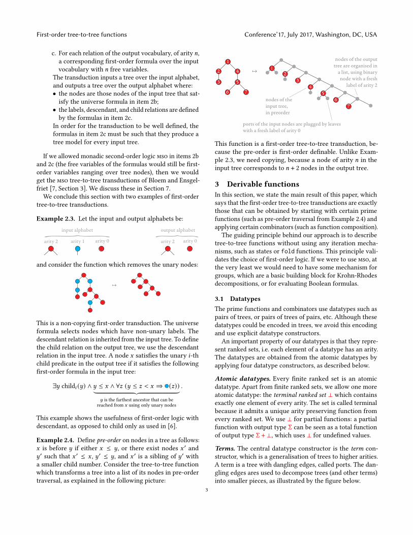
Example 2.4. Define pre-order on nodes in a tree as follows:𝑥 is before 𝑦 if either 𝑥 ≤ 𝑦, or there exist nodes 𝑥 ′ and𝑦 ′ such that 𝑥 ′ ≤ 𝑥 , 𝑦 ′ ≤ 𝑦, and 𝑥 ′ is a sibling of 𝑦 ′ witha smaller child number. Consider the tree-to-tree functionwhich transforms a tree into a list of its nodes in pre-ordertraversal, as explained in the following picture:
nodes of theinput tree,in preorder
ports of the input nodes are plugged by leaves with a fresh label of arity 0
nodes of the output tree are organised in
a list, using binary node with a fresh
label of arity 2
1
2 24
46
67
7
3 35
5
1
This function is a first-order tree-to-tree transduction, be-cause the pre-order is first-order definable. Unlike Exam-ple 2.3, we need copying, because a node of arity 𝑛 in theinput tree corresponds to 𝑛 + 2 nodes in the output tree.
3 Derivable functionsIn this section, we state the main result of this paper, whichsays that the first-order tree-to-tree transductions are exactlythose that can be obtained by starting with certain primefunctions (such as pre-order traversal from Example 2.4) andapplying certain combinators (such as function composition).
The guiding principle behind our approach is to describetree-to-tree functions without using any iteration mecha-nisms, such as states or fold functions. This principle vali-dates the choice of first-order logic. If we were to use mso, atthe very least we would need to have some mechanism forgroups, which are a basic building block for Krohn-Rhodesdecompositions, or for evaluating Boolean formulas.
3.1 DatatypesThe prime functions and combinators use datatypes such aspairs of trees, or pairs of trees of pairs, etc. Although thesedatatypes could be encoded in trees, we avoid this encodingand use explicit datatype constructors.
An important property of our datatypes is that they repre-sent ranked sets, i.e. each element of a datatype has an arity.The datatypes are obtained from the atomic datatypes byapplying four datatype constructors, as described below.
Atomic datatypes. Every finite ranked set is an atomicdatatype. Apart from finite ranked sets, we allow one moreatomic datatype: the terminal ranked set ⊥ which containsexactly one element of every arity. The set is called terminalbecause it admits a unique arity preserving function fromevery ranked set. We use ⊥ for partial functions: a partialfunction with output type Σ can be seen as a total functionof output type Σ + ⊥, which uses ⊥ for undefined values.
Terms. The central datatype constructor is the term con-structor, which is a generalisation of trees to higher arities.A term is a tree with dangling edges, called ports. The dan-gling edges ares used to decompose trees (and other terms)into smaller pieces, as illustrated by the figure below.
3

Conference’17, July 2017, Washington, DC, USA Mikołaj Bojańczyk and Amina Doumane
a tree a term with 4 ports that rep-resents part of the tree
Formally speaking, terms are defined by induction as follows.As term over a ranked set Σ is either the identity term denotedby , which consists of a port and nothing else, or otherwiseit is an expression of the form 𝑎(𝑡1, . . . , 𝑡𝑛) where 𝑎 ∈ Σ hasarity 𝑛, and 𝑡1, . . . , 𝑡𝑛 are already defined terms. The arity ofa term is the number of ports. Terms of arity zero are thesame as trees. We write TΣ for the ranked set of terms overa ranked set Σ. Because the term constructor – like otherdatatype constructors – outputs a ranked set, it makes senseto talk about terms of terms, etc.
Terms are amonad, in the category of ranked sets and aritypreserving functions2. The unit of the monad, an operationof type Σ→ TΣ, is illustrated in the following picture:
The product of the monad, an operation of type TTΣ→ TΣthat we call flattening, is illustrated in the following picture:
This monad structure will be part of our prime functions.
Products and coproducts. There are two binary datatypeconstructors
Σ1 × Σ2︸ ︷︷ ︸product
Σ1 + Σ2︸ ︷︷ ︸coproduct
.
An element of the product is a pair (𝑎1, 𝑎2) where 𝑎𝑖 ∈ Σ𝑖 .The arity of the pair is the sum of arities of its two coordinates𝑎1 and 𝑎2. An element of the coproduct is a pair (𝑖, 𝑎) where𝑖 ∈ {1, 2} and 𝑎 ∈ Σ𝑖 . The arity is inherited from 𝑎.
The set of terms can be defined in terms of products andcoproducts, as the least solution of the equation:
TΣ = { }+∐𝑎∈Σ(TΣ)arity of 𝑎
2An almost identical monad is used in [10, Section 9.2], which differs fromours in that it allows multiple uses of a single port.
where∐
denotes possibly infinite coproduct and𝑋𝑛 denotesthe 𝑛-fold product of a ranked set 𝑋 with itself.
Folding. The final – and maybe least natural – datatypeconstructor called folding. Folding has two main purposes:(1) reordering ports in a term; and (2) reducing arities bygrouping ports into groups.
Folding is not one constructor, but a family of unary con-structors F𝑘Σ, one for every 𝑘 ∈ {1, 2, 3, . . .}. An 𝑛-ary ele-ment of F𝑘Σ, which is called a 𝑘-fold, consists of an element𝑎 ∈ Σ together with an injective grouping function
𝑓 : {1, . . . , arity of 𝑎}︸ ︷︷ ︸an element of this set is
called a port of 𝑎
→ {1, . . . , 𝑛} × {1, . . . , 𝑘}︸ ︷︷ ︸these pairs are called sub-ports
We denote such an element as 𝑎/𝑓 and draw it like this:port 4
port 3, subport 1
fa
Already for 𝑘 = 1, the constructor F1 is non-trivial. Forexample, F1TΣ is a generalisation of terms where ports arenot necessarily ordered left-to-right (because the groupingfunction need not be monotone), and some ports need notappear (because the grouping function need not be total); inother words this is the same as terms in the usual sense ofuniversal algebra, with the restriction that each variable isused at most once (sometimes called linearity).When viewed as a family of datatype constructors, folds
have a monad-like structure: they are a graded monad in thesense of [21, p. 518]. The unit is the operation
of type Σ→ F1Σ, while the product (or flattening) in thegraded monad is the family of operations of type
F𝑘2F𝑘1Σ→ F𝑘1 ·𝑘2Σ,
indexed by 𝑘1, 𝑘2 ∈ {1, 2, . . .}, that is illustrated below:
More formally, the flattening of a double fold (𝑎/𝑓1)/𝑓2 hasthe grouping function defined by
𝑖 ↦→ (𝑖2, 𝜋 (𝑝1, 𝑝2)) where
{(𝑖1, 𝑝1) = 𝑓1 (𝑖)(𝑖2, 𝑝2) = 𝑓2 (𝑖1)
and 𝜋 is the natural bijection between {1, . . . , 𝑘1}×{1 . . . , 𝑘2}and {1, . . . , 𝑘1𝑘2}.
4
First-order tree-to-tree functions Conference’17, July 2017, Washington, DC, USA
• Function composition.
𝑓 ◦ 𝑔 : Σ→ Δ for 𝑓 : Σ→ Γ and 𝑔 : Γ → Δ
• Lifting of functions along datatype constructors
𝑓1 + 𝑓2 : Σ1 + Σ2 → Γ1 + Γ2 for {𝑓𝑖 : Σ𝑖 → Γ𝑖 }𝑖=1,2(𝑓1, 𝑓2) : Σ1 × Σ2 → Γ1 × Γ2 for {𝑓𝑖 : Σ𝑖 → Γ𝑖 }𝑖=1,2
F𝑘 𝑓 : F𝑘Σ→ F𝑘Γ for 𝑓 : Σ→ ΓT𝑓 : TΣ→ TΓ for 𝑓 : Σ→ Γ
Figure 1. Combinators
• Unit and product in the monad T.
unit : Σ → TΣ flat : TTΣ → TΣ
• Unit and product in the graded monad F𝑘 .
unit : Σ → F1Σ flat : F𝑘F𝑙Σ → F𝑘.𝑙Σ
• Inductive structure of terms (for finite Σ only).
TΣdecompose // { } +∐𝑎∈Σcompose
oo (TΣ)arity of 𝑎
• Remove unused fold.F𝑘Σ → Σ + ⊥(𝑎/𝑓 ) ↦→ 𝑎 if 𝑎 has arity 0, undefined otherwise
Figure 2. Prime functions for terms and fold.
This completes the list of datatype constructors.
Definition 3.1 (Datatypes). The datatypes are the least classof ranked sets which contains all finite ranked sets, the termi-nal set, and which is closed under applying the constructors
TΣ Σ1 × Σ2 Σ1 + Σ2 F𝑘Σ.
3.2 Derivable functionsWe now present the central definition of this paper.
Definition 3.2 (Derivable function). An arity preservingfunction between two datatypes is called derivable if it canbe generated, by using the combinators in Figure 1, from thefollowing prime functions:• for every Σ, the unique arity preserving function Σ→ ⊥;• all arity preserving functions with finite domain;• the prime functions in Figures 2,3 and 4;
The combinators in Figure 1 are function composition, andthe obvious liftings of functions along the datatype construc-tors. The prime functions in Figure 2 describe the monadstructure of terms and folds, and were explained in Sec-tion 3.1. The prime functions in Figure 3 are simple syntactictransformations, which are intended to have no computa-tional content. Figure 4 contains less obvious operations,whose definitions are deferred to Section 3.3.
• Co-projections.
Σ + Σ → Σ Σ𝑖]𝑖→ Σ1 + Σ2
(𝑎, 𝑖) ↦→ 𝑎 𝑎 ↦→ (𝑎, 𝑖)• Commutativity.
Σ + Γ → Γ + Σ Σ × Γ → Γ × Σ(𝑎, 1) ↦→ (𝑎, 2) (𝑎, 𝑏) ↦→ (𝑏, 𝑎)(𝑎, 2) ↦→ (𝑎, 1)
• Associativity.
(Σ + Γ) + Δ → Γ + (Σ + Δ) (Σ × Γ) × Δ → Σ × (Γ × Δ)((𝑎, 1), 1) ↦→ (𝑎, 1) ((𝑎, 𝑏), 𝑐) ↦→ (𝑎, (𝑏, 𝑐))((𝑎, 2), 1) ↦→ ((𝑎, 1), 2)(𝑎, 2) ↦→ ((𝑎, 2), 2)
• Distributivity.
(Σ1 + Σ2) × Γ → (Σ1 × Γ) + (Σ2 × Γ)((𝑎, 𝑖), 𝑏) ↦→ ((𝑎, 𝑏), 𝑖)
Figure 3. Prime functions for product and coproduct.
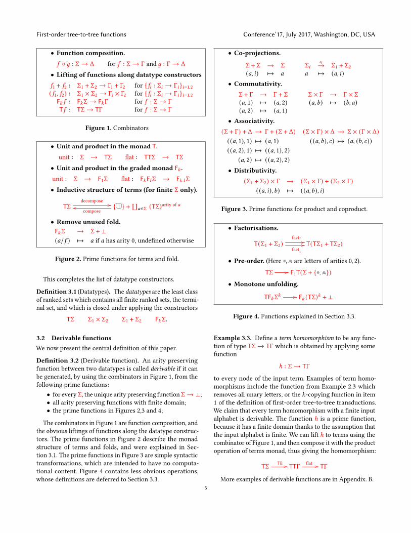
• Factorisations.
T(Σ1 + Σ2)fact↑ //fact↓// T(TΣ1 + TΣ2)
• Pre-order. (Here , are letters of arities 0, 2).
TΣ // F1T(Σ + { , })• Monotone unfolding.
TF𝑘Σ𝑘 // F𝑘 (TΣ)𝑘 + ⊥
Figure 4. Functions explained in Section 3.3.
Example 3.3. Define a term homomorphism to be any func-tion of type TΣ→ TΓ which is obtained by applying somefunction
ℎ : Σ→ TΓ
to every node of the input term. Examples of term homo-morphisms include the function from Example 2.3 whichremoves all unary letters, or the 𝑘-copying function in item1 of the definition of first-order tree-to-tree transductions.We claim that every term homomorphism with a finite inputalphabet is derivable. The function ℎ is a prime function,because it has a finite domain thanks to the assumption thatthe input alphabet is finite. We can lift ℎ to terms using thecombinator of Figure 1, and then compose it with the productoperation of terms monad, thus giving the homomorphism:
TΣ Tℎ // TTΓ flat // TΓ
More examples of derivable functions are in Appendix. B.5
Conference’17, July 2017, Washington, DC, USA Mikołaj Bojańczyk and Amina Doumane
We are now ready to state the main theorem of this paper.We say that a tree-to-tree function
𝑓 : treesΣ→ treesΓ
is derivable if it agrees on arguments that are trees with somederivable partial function
𝑓 : TΣ→ TΓ + ⊥.
The main result of this paper is the following theorem.
Theorem 3.4. A tree-to-tree function is a first-order trans-duction if and only if it is derivable.
The right-to-left implication in the above theorem is provedby a relatively straightforward induction on the derivation.The general idea is that we associate to each datatype arelational structure; for example the relational structure as-sociated to a pair (𝑎1, 𝑎2) is the disjoint union of the rela-tional structures associated to 𝑎1 and 𝑎2. In the appendix, weshow that all prime functions are first-order transductions(adapted suitably to structures other than trees); and thatthis property is preserved under applying the combinators.There is one nontrivial step in the proof, which concernsmonotone unfolding, and will be discussed below.The left-to-right implication in the theorem, which says
that every first-order transduction is derivable, is the maincontribution of this paper, and is discussed in Sections 4–6.1.
3.3 The prime functions from Figure 4In this section, we describe the prime functions from Figure 4.Each of these functions will play a key role in one of themain results of the paper.
3.3.1 FactorisationsWe begin with the two factorisation functions
fact↑, fact↓ : T(Σ1 + Σ2) → T(TΣ1 + TΣ2),
which are used to cut terms into smaller parts. Define afactorisation of a term to be any term of terms that flattens toit. An alternative view is that a factorisation is an equivalencerelation on nodes in a term, where every equivalence classis connected via the parent-child relation.Consider a term 𝑡 ∈ T(Σ1 + Σ2). We say that two nodes
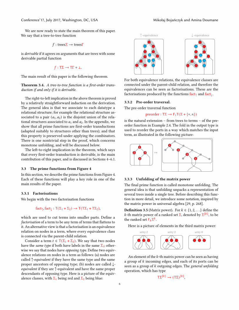
have the same type if both have labels in the same Σ𝑖 ; other-wise we say that nodes have opposing type. Define two equiv-alence relations on nodes in a term as follows: (a) nodes arecalled ↑-equivalent if they have the same type and the sameproper ancestors of opposing type; (b) nodes are called ↓-equivalent if they are ↑-equivalent and have the same properdescendants of opposing type. Here is a picture of the equiv-alence classes, with Σ1 being red and Σ2 being blue:
-equivalence -equivalence
For both equivalence relations, the equivalence classes areconnected under the parent-child relation, and therefore theequivalences can be seen as factorisations. These are thefactorisations produced by the functions fact↑ and fact↓.
3.3.2 Pre-order traversal.The pre-order traversal function
preorder : TΣ→ F1T(Σ + { , })is the natural extension – from trees to terms – of the pre-order function in Example 2.4. The fold in the output type isused to reorder the ports in a way which matches the inputterm, as illustrated in the following picture:
3
1
22
1
344
3.3.3 Unfolding of the matrix powerThe final prime function is called monotone unfolding. Thegeneral idea is that unfolding unpacks a representation ofseveral trees inside a single tree. Before describing this func-tion in more detail, we introduce some notation, inspired bythe matrix power in universal algebra [29, p. 268].Definition 3.5 (Matrix power). For 𝑘 ∈ {1, 2, . . .} define the𝑘-th matrix power of a ranked set Σ, denoted by Σ [𝑘 ] , to bethe ranked set F𝑘Σ𝑘 .Here is a picture of elements in the third matrix power:
arity 2 arity 2 arity 0
An element of the 𝑘-th matrix power can be seen as havinga group of 𝑘 incoming edges, and each of its ports can beseen as a group of 𝑘 outgoing edges. The general unfoldingoperation, which has type
TΣ [𝑘 ] → (TΣ) [𝑘 ],6

First-order tree-to-tree functions Conference’17, July 2017, Washington, DC, USA
Figure 5. Unfolding the matrix power
matches the 𝑘 incoming edges in a node with the 𝑘 outgoingedges in the parent port; it also removes the unreachablenodes. This operation is illustrated in Figure 5, and a formaldefinition is in the appendix.
Chain logic. The general unfolding operation is too power-ful to be included in the derivable functions, as we explainbelow. It does, however, admit a characterisation in terms ofa fragment of mso called chain logic, see [31, Section 2] or [8,Section 2.5.3], whose expressive power is strictly betweenfirst-order logic and mso. Chain logic is defined to be thefragment of mso where set quantification is restricted to setswhere all nodes are comparable by the descendant relation.
Theorem 3.6. The following conditions are equivalent fortree-to-tree functions:
• is derivable, as in Definition 3.2, except that generalunfold is used instead of monotone unfold;
• is a transduction, as in Definition 2.2, except that chainlogic is used instead of first-order logic.
To see why chain logic is needed to describe general un-folding, consider the following unfolding, where two coordi-nates are swapped in each node of the input tree:
For inputs with an odd number of swaps, the output of un-folding has a white leaf in the first coordinate, and for inputswith an even number of swaps, the output has a white leafin the first coordinate. Checking if a path has even lengthcan be done in chain logic, but not in first-order logic.
Monotone unfolding To avoid the problems with cyclicswaps, the unfolding function in Figure 4 imposes a mono-tonicity requirement on the matrix power, described below.
Let 𝑎 ∈ Σ [𝑘 ] be an element of the matrix power, let 𝑝, 𝑞 ∈{1, . . . , 𝑘}, and let 𝑖 be a port of 𝑎. Define the twist function ofport 𝑖 , denoted by→𝑖 , as follows: 𝑞 →𝑖 𝑝 if coordinate 𝑞 inthe 𝑖-th outgoing edge is connected to coordinate 𝑝 in root,as described in the following picture:
an element ofthe matrix power
its twist functions1 2 3
1 2 3 1 2 3
The twist function is partial. Call an element of the matrixpowermonotone if for every port, its twist functions is mono-tone (when restricted to inputs where it is defined). In thepicture above,→1 is monotone, while→2 is not. Also, theproblems with an even number of swaps discussed earlierarise from a non-monotone twist function:
1 2
1 2
The monotone unfolding operation in Figure 5 defined to bethe restriction of general unfolding, which is undefined ifthe input contains at least one label which is non-monotone,and otherwise returns the output of the general unfolding.
Is unfolding derivable? The prime functions in our maintheorem are meant to be simple syntactic rewritings. It is de-batable whether the unfolding operation – even in its mono-tone variant – is of this kind. For example, our proof that
7

Conference’17, July 2017, Washington, DC, USA Mikołaj Bojańczyk and Amina Doumane
monotone unfolding is a first-order transduction requiresan invocation of the Schützenberger-McNaughton-Paperttheorem about first-order logic on words being the same ascounter-free automata.Is it possible to break down monotone unfolding into
simpler primitives? In the appendix, we devote consider-able resources to answering this question. We propose onenew datatype and seventeen additional prime functions,which can be called syntactic rewriting without straining thereader’s patience. Then, we show that monotone unfoldingcan be derived using the new datatype and functions. Theproof of this result is one of the main technical contributionsof this paper.
4 Register tree transducersWe now begin the proof of the harder implication in Theo-rem 3.4, which says that every first-order tree-to-tree trans-duction is derivable. Our proof passes through an automatonmodel, which is roughly based on existing transducer modelsfor mso transductions from [3, 7]. The automaton uses regis-ters to store parts of the output tree. The semantics of theautomaton involves two phases: (a) mapping the input treeto an expression that uses register updates; (b) evaluatingthe expression. These phases are described in more detailbelow.
Register valuations and updates. We begin by explaininghow the registers work. The registers store terms that areused to construct the output tree. Each register has an arity:registers of arity zero store trees, registers of arity one storeunary terms, etc.Fix two finite ranked sets: the register names 𝑅 and the
output alphabet Γ. A register valuation is defined to be anyarity preserving function from the register names 𝑅 to termsTΓ. To transform register valuations, we use register updates.A register update is an operation which inputs several reg-ister valuations and outputs a single register valuation. For𝑛 ∈ {0, 1, . . .}, an 𝑛-ary register update is defined to be anyarity-preserving function
𝑢 : 𝑅→T(Γ + 𝑛𝑅),where 𝑛𝑅 stands for the disjoint union of 𝑛 copies of 𝑅. The𝑖-th copy of 𝑅 represents the register contents in the 𝑖-thargument. Here is a picture of a register update which hasarity 3 and uses two registers 𝑟 and 𝑠:
r3 r2
r1
s2 s1
register s from argument 2
register r from argument 3
register r of arity 2 register s of arity 0
An 𝑛-ary register update 𝑢 induces a operation, which in-puts 𝑛 register valuations and outputs the register valuationobtained by taking 𝑢 and replacing the 𝑖-th copy of a registername with the contents of that register in the 𝑖-th input reg-ister valuation. Register updates have arities, and thereforethe ranked set of register updates is written in red, and canbe used for labels in a tree. For such a tree
𝑡 ∈ trees(register updates),
define its evaluation to be the register valuation defined byinduction in the natural way. Note that register updates ofarity zero are the same as register valuations, which givesthe induction base.
First-order relabellings. Our automatonmodel has no states.Instead, it uses a first-order relabelling, as defined below, todirectly assign to each node of the input tree a register up-date that will be applied in that node. A similar model isused by Bloem and Engelfriet [7, Theorem 17], except thatin their case, the first phase uses mso relabellings, and thesecond phase is an attribute grammar.
Definition 4.1 (First-order relabelling). A first-order rela-belling is given by two finite ranked sets Σ and Γ, called theinput and output alphabets, and a family
{𝜑𝑎 (𝑥)}𝑎∈Γof first-order formulas over the vocabulary of trees over Σ.These formulas need to satisfy the following restriction:
(*) for every tree over the input alphabet and node in thattree, there is a unique output letter 𝑎 ∈ Γ such that𝜑𝑎 (𝑥) selects the node; furthermore, the arity of 𝑎 isthe same as the arity of (the label of) the node.
The semantics of a first-order tree relabelling is a function
treesΣ→ treesΓ,
which changes the label of every node in the input tree tothe unique letter described in (*).
A first-order tree relabelling is a very special case of a first-order tree-to-tree transduction, where only the labelling ofthe input tree is changed, while the universe as well as thechild and descendant relations are not affected.
Register transducers. Having defined registers, registerupdates, and first-order tree relabellings, we are now readyto define our automaton model.
Definition 4.2 (First-order register transducer). The syntaxof a first-order register transducer consists of:• An input alphabet Σ, which is a finite ranked set;• An output alphabet Γ, which is a finite ranked set;• A set 𝑅 of registers, which is a finite ranked set;• A total order on the registers.• A designated output register in 𝑅, of arity zero.
8

First-order tree-to-tree functions Conference’17, July 2017, Washington, DC, USA
• A transition function, which is a first-order relabelling
treesΣ→ treesΔ,
for some finite setΔ of register updates over registers𝑅and output alphabet Γ. We require all register updatesin Δ to be single-use and monotone, as defined below:1. Single-use3.An𝑛-ary register update𝑢 is called single-
use if every 𝑟 ∈ 𝑛𝑅 appears in at most one term from{𝑢 (𝑠)}𝑠∈𝑅 , and it appears at most once in that term.
2. Monotone4. This condition uses the total order onregisters. An 𝑛-ary register update 𝑢 is called mono-tone if for every 𝑖 ∈ {1, . . . , 𝑛}, the binary relation→𝑖 on register names 𝑟, 𝑠 ∈ 𝑅 defined by
𝑟 →𝑖 𝑠 if the 𝑖-th copy of 𝑟 appears in 𝑢 (𝑠),
which is a partial function from 𝑟 to 𝑠 when 𝑢 issingle-use, is monotone:
𝑟1 ≤ 𝑟2 ∧ 𝑟1 →𝑖 𝑠1 ∧ 𝑟2 →𝑖 𝑠2 ⇒ 𝑠1 ≤ 𝑠2
The semantics of the transducer is a tree-to-tree function,defined as follows. The input is a tree over the input alphabet.To this tree, apply the transition function, yielding a tree ofregister updates. Next, evaluate the tree of register updates,yielding a register valuation. The output tree is defined tobe the contents of the designated output register.The main difference of our model with respect to prior
work is that we want to capture tree transformations definedin first-order logic, as opposed to mso used in [1, 3, 7]. Thisis why we use first-order relabellings instead of mso rela-bellings. For the same reason, we require the register updatesto be monotone, see the discussion in Section 3.3.3.The main result of this section is that first-order register
transducers are expressively complete for first-order tree-to-tree transductions.
Theorem 4.3. Every first-order tree-to-tree transduction isrecognised by a first-order register transducer.
The proof, which is in Appendix E, uses the compositionmethod for logic, like similar proofs for [3, Theorem 4.6]and [7, Theorem 14]. The converse inclusion in the theoremis also true. This is can be shown directly without muchdifficulty, following the same lines as in [7, Section 5]. Theconverse inclusion also follows from other results in this pa-per: (a) we show in the following sections that every functioncomputed by the transducer is derivable; and (b) derivablefunctions are first-order tree-to-tree transductions by theeasy implication in Theorem 3.4.
3The single-use restriction is a standard feature of transducer models withlinear size increase [1, 3, 7]. It prohibits iterated duplication of registers,which would lead to exponential size outputs.4This is notion of monotonicity corresponds to the one used in Section 3.3.3,see the comments on page 11. A similar notion appears in [11, p. 7].
Proof strategy for Sections 5–6. By Theorem 4.3, to provederivability of every first-order tree-to-tree transduction,and thus finish the proof of our main theorem, it sufficesto prove derivability for first-order register transducers. Ina first-order register transducer, the computation has twosteps: a first-order relabelling, followed by evaluation of theregister updates. The first step is handled in Section 5, andthe second step is handled in Section 6.
5 First-order relabellingsIn this section we prove derivability of the first computationstep used in first-order register transducers.
Proposition 5.1. Every first-order relabelling is derivable.
To prove the proposition, we use a decomposition of first-order relabellings into simpler functions, in the style of theKrohn-Rhodes theorem. We use the name unary query for afirst-order formulawith one free variable over the vocabularyof trees. This assumes some implicit alphabet Σ. For a unaryquery, define its characteristic function, of type
treesΣ→ trees(Σ + Σ),to be the function which replaces the label of each node byits first or second copy, depending on whether the node isselected by the query. This is a special case of a first-orderrelabelling. The key to Proposition 5.1 is the following lemma,which decomposes first-order relabellings into characteristicfunctions of certain basic unary queries.
Lemma 5.2. Every first-order relabelling can be obtained bycomposing the following functions:
1. Letter-to-letter homomorphisms. For every finite Γ, Σand 𝑓 : Σ→ Γ, its tree lifting trees𝑓 : treesΣ→ treesΓ.
2. For every finite Σ and its subsets Δ, Γ ⊆ Σ, the char-acteristic functions of the following unary queries overalphabet Σ:a. Child: 𝑥 is an 𝑖-th child, for 𝑖 ∈ {1, 2, . . .}
child𝑖 (𝑥);b. Until: 𝑥 has a descendant 𝑦 with label in Δ, such that
all nodes strictly between 𝑥 and 𝑦 have label in Γ
∃𝑦 𝑦 > 𝑥 ∧ Δ(𝑦) ∧ ∀𝑧 (𝑥 < 𝑧 < 𝑦 ⇒ Γ(𝑧));c. Since: 𝑥 has an ancestor 𝑦 with label in Δ, such that
all nodes strictly between 𝑥 and 𝑦 have label in Γ
∃𝑦 𝑦 < 𝑥 ∧ Δ(𝑦) ∧ ∀𝑧 (𝑦 < 𝑧 < 𝑥 ⇒ Γ(𝑧)).
The lemma uses a theorem of Schlingloff [26, Theorem2.6], which says that all first-order definable tree propertiescan be defined using a temporal logic with operators simi-lar to the ones used in items 2 of the lemma. Note that thetemporal logic is a two-way logic, because until dependson the descendants of the node 𝑥 , while since depends onthe ancestors. In fact, there is no temporal logic which char-acterises first-order logic, uses only descendants, and has
9

Conference’17, July 2017, Washington, DC, USA Mikołaj Bojańczyk and Amina Doumane
finitely many operators [12, Theorem 5.5]. The exact reduc-tion to Schlingloff’s theorem is in Appendix D.
It remains to show that all of the functions from Lemma 5.2are derivable. The letter-to-letter homomorphisms from item 1are a special case of homomorphisms discussed in Exam-ple 3.3, and hence derivable. In Appendix D, we show thatthe functions from item 2 are also derivable. In the proof, akey role is played by the factorisation functions discussed inSection 3.3.1.
6 Evaluation of register updatesIn this section, we deal with the second computation phase ina first-order register transducer, namely evaluating registerupdates. As discussed in the end of Section 4, this completesthe proof of our main theorem.
Our proof uses the language of _-calculus. In Section 6.1,we discuss derivability of normalisation of _-terms. In Sec-tion 6.2, we reduce evaluation of register updates to unfold-ing the matrix power and normalisation of _-terms.
6.1 Normalisation of simply typed linear _-termsWe assume that the reader is familiar with the basic notionsof the simply typed _-calculus; more detailed definitions canbe found in [27]. Define simple types to be expressions gener-ated from an atomic type 𝑜 using a binary arrow constructor,as in the following examples:
𝑜 𝑜 → 𝑜 (𝑜 → 𝑜) → (𝑜 → 𝑜) · · ·
In this paper, the atomic type 𝑜 represents trees over theoutput alphabet. Let𝑋 be a set of variables, each one with anassociated simple type. A _-term is any expression that canbe built from the variables, using _-abstraction _𝑥 .𝑀 andterm application𝑀𝑁 . We say that a _-term is well-typed ifone can associate to it a simple type according to the usualtyping rules of simply typed _-calculus, see [27, Definition3.2.1]. Because the variables are typed, a _-term has eithera unique type, or is not well-typed. Here is an example of awell-typed _-term, with the type annotation in blue:
(𝑜→𝑜)→𝑜→𝑜︷ ︸︸ ︷_𝑦𝑜→𝑜 . _𝑥𝑜 . 𝑦 (𝑦𝑥).︸ ︷︷ ︸
𝑜
We use the standard notion of 𝛽-reduction for _-terms,see [27, Definition 1.2.1]. Because of normalisation and con-fluence for the simply typed _-calculus, every well-typed_-term has a unique normal form, i.e a _-term to which it 𝛽-reduces (in zero or more steps), and which cannot be further𝛽-reduced.A _-term can be seen as a tree over the ranked alphabet
arity 0︷ ︸︸ ︷{𝑥 : 𝑥 ∈ 𝑋 } ∪
arity 1︷ ︸︸ ︷{_𝑥 : 𝑥 ∈ 𝑋 } ∪
arity 2︷︸︸︷{@} (1)
where @ represents term application. Using this representa-tion, and assuming that the set of variables is finite, it makessense to view normalisation as a tree-to-tree function
_-term ↦→ its normal form,
and ask about its derivability. We show that this function isderivable, under two assumptions on the input _-term.The first assumption is that the input _-term is linear:
every bound variable is exactly once in its scope5, but freevariables are allowed to appear multiple times. The secondassumption is that the input _-term can be typed using afixed finite set of types T : it has type in T , and the same istrue for all of its sub-terms. In Appendix F.1, we explain whythe assumptions are needed.
Theorem 6.1. Let 𝑋 be a finite set of simply typed vari-ables, and let T be a finite set of simple types. The followingtree-to-tree function is derivable, assuming that _-terms arerepresented as trees:
• Input. A _-term over variables 𝑋 .• Output. Its normal form, if it is linear and can be typedusing T , and undefined otherwise.
This is one of our main technical contributions, and itsproof is in Appendix F. A key role in the proof is played bythe pre-order function.
6.2 Evaluation of register updatesEquipped with Theorem 6.1, we prove derivability of evalua-tion of register updates. Fix a first-order register transducer.From now on, when speaking about register updates or reg-ister valuations, we mean those of the fixed transducer. Ourgoal is to prove the following lemma, which completes theproof of our main theorem.
Lemma 6.2. Consider the tree-to-tree function, which inputsa tree of register updates, evaluates it, and outputs the contentsof the designated output register. This function is derivable.
Output letters in _-terms. Wewill use _-terms to representregister updates, which involve letters of the output alphabetΓ. Therefore, for the rest of Section 6.2, we use an extendednotion of _-terms, which allows building _-terms of the form
𝑎(𝑀1, . . . , 𝑀𝑛) for every 𝑎 ∈ Γ of arity 𝑛. (2)
The typing rules are extended as follows: if the arguments𝑀1, . . . , 𝑀𝑛 all have type 𝑜 (no other type is allowed for ar-guments of 𝑎), then (2) has type 𝑜 . These _-terms can berepresented as trees, as in the following picture:
λx
x
@
5This restriction could easily be relaxed to “at most once”.10

First-order tree-to-tree functions Conference’17, July 2017, Washington, DC, USA
Theorem 6.1 works without change for the extended no-tion of _-terms used in this section. Note that there is no𝛽-reduction rule for _-terms of the form (2).
_-representations of register updates. To prove Lemma 6.2,we represent register updates using a matrix power of _-terms. The idea is that the matrix power handles the parallelevaluation of registers.
Let 𝑋 be a set of variables {𝑥1 . . . , 𝑥𝑚}, all of them havingtype 𝑜 , where𝑚 is the maximal arity among registers. DefineΓ_ to be the output alphabet Γ plus the ranked alphabetdefined in (1) for tree representations of _-terms.
Recall that a register update – of arity say 𝑛 – consists ofa family of terms over alphabet Γ + 𝑛𝑅, one for each register𝑟 ∈ 𝑅. We begin by explaining the _-representation for termsin the family, which is a function of type
T(Γ + 𝑛𝑅)_-representation // TΓ_ . (3)
This function is not arity preserving, which is why it is notwritten in red. Define a placeholder to be an element of 𝑛𝑅;we write placeholders as 𝑟𝑖 with 𝑟 ∈ 𝑅 and 𝑖 ∈ {1, . . . , 𝑛}.The function (3) is explained in the following picture:
r1
r2s1
a term t withplaceholders
its λ-representation one boundvariable
for each portof t
each port of tis replaced by
a correspondingvariable
λx1
λx2
@
@
@
x1
x2
@
each placeholder of t is replaced by a port applied to its children using @
Note how the arities need not be preserved: the arity ofthe output is the number of placeholders in the input, whichneed not be the same as the number of ports in the input. Thecorrespondence of ports in the output termwith placeholdersin the input term is defined with respect to some arbitraryorder on the set 𝑛𝑅 of placeholders, say lexicographic withrespect to the order on registers and {1, . . . , 𝑛}.
Having defined the _-representation of terms with place-holders, we lift it a _-representation of register updates
register updates_-representation // (TΓ_) [𝑘 ] , (4)
where 𝑘 is the number of registers. This function is aritypreserving.
For a register update (𝑡1, . . . , 𝑡𝑘 ), where 𝑡𝑖 is the term withplaceholders used in the 𝑖-th register, its _-representation is
trees(register updates)
evaluateregisterupdates
(a)
��
trees(_-representation)(c)
// trees((TΓ_) [𝑘 ])unfoldmatrixpower
(d)��
arity 0 elements of
(TΓ_) [𝑘 ]normalise_-terms(e)
��register valuations
_-representation
(b) // arity 0 elements of
(TΓ_) [𝑘 ]
Figure 6
defined to be
(_-representation of 𝑡1, . . . , _-representation of 𝑡𝑘 )/𝑓 ,
where the grouping function 𝑓 connects a placeholder 𝑟𝑖 tothe 𝑟 -th sub-port of port 𝑖 . Here is a picture
a register valuation its λ-representation
r2r1 s2s1
x1
λx1
@ @
r1
r s
r2
r
argument 1 argument 2 s1 s2
s
The following three properties of the _-representation forregister updates will be used later in the proof:(P1) If we restrict the domain to a finite set of register up-
dates, e.g. those used in the transducer, then it is aprime function, by virtue of having finite domain.
(P2) A register update is monotone (as in Definition 4.2) ifand only if its _-representation is monotone (as definedin Section 3.3.3 for the matrix power).
(P3) Every bound variable in the _-representation is usedexactly once, and the types that appear are of the form
at most (maximal arity in Γ) times︷ ︸︸ ︷𝑜 → 𝑜 → · · · → 𝑜 → 𝑜 → 𝑜,
hence Theorem 6.1 can be applied.
Putting it all together. To finish the proof of Lemma 6.2,we observe that the semantics of a register automaton aretranslated – under the _-representation – to unfolding thematrix power and normalising a _-term. This observation isformalised by saying that the diagram in Figure 6 commutes,and it follows directly from the definitions. Instead of givinga proof, we illustrate it on an example in Figure 7.
11

Conference’17, July 2017, Washington, DC, USA Mikołaj Bojańczyk and Amina Doumane
x1
λx1
@ @r2r1 s2s1
x1
λx1
λx1
@ @
(a)
(b)
(c)
(d)
(e)
λx1 λx1
x1 x1
λx1 λx1
x1 x1
x1
Figure 7. Example for Figure 6.
We claim that all of the arrows (c), (d) and (e) on the right-down path in Figure 6 are derivable:
(c) Since we work with a fixed register transducer, there isa finite subset Δ of register updates used, and thereforeoperation (a) in the figure is derivable by property (P1).
(d) Arrow (d) represents the unfolding of thematrix power.By property (P2), the outputs of arrow (c) are mono-tone, and so we can use the monotone unfolding opera-tion, which is a prime function and therefore derivable.
(e) Finally, arrow (e) represents normalisation of _-terms.This arrow is derivable by Theorem 6.1. The assump-tions of this theorem are met by property (P3).
Since the arrows (c), (d), (e) are derivable, and the diagramcommutes, it follows that the composition of the arrows(a) and (b) is derivable. In other words, there is a deriv-able function which maps a tree of register updates to the_-representation of the resulting register valuation (whenviewing a register valuation as a special case of a register
update of arity zero). Finally, to get the contents of the out-put register, we get rid of the fold in the matrix power byusing the last function from Figure 2, and project onto thecoordinate for the output register.
This completes the proof of Lemma 6.2, and therefore alsoof the main theorem.
7 Monadic second-order transductionsWe finish the paper by discussing a variant of our maintheorem for mso tree-to-tree transductions. We simply add,as prime functions, allmso relabellings, which are defined thesame way as the first-order relabellings from Definition 4.1,except that the unary queries can use mso logic instead offirst-order logic.
Theorem 7.1. A tree-to-tree function is an mso transductionif and only if it can be derived using Definition 3.2 extendedby adding all mso relabellings as prime functions.
Proof. In [14, Corollary 1], Colcombet shows that every msoformula on trees can be replaced by a first-order formula thatruns on an mso relabelling of the input tree. Applying thatresult to transductions, we see that every mso tree-to-treetransduction can be decomposed as: (a) an mso relabelling;followed by (b) a first-order tree-to-tree transduction. Thetheorem follows. □
The solution above is not particularly subtle, and contrastsour results for first-order logic and chain logic, where wetook care to have a small number of primitives. This waspossible thanks in part to the decomposition of first-orderqueries into simpler ones that was is in Section 5, and theKrohn-Rhodes theorem that is used in the proof of Theo-rem 3.6 about chain logic. In principle, a decomposition ofmso relabellings could be possible, but proving it would likelyrequire developing a new decomposition theory for regulartree languages, in the style of the Krohn-Rhodes theorem,which we feel is beyond the scope of this paper. One wouldexpect a Krohn-Rhodes theorem for trees to yield an effectivecharacterisation of first-order logic – as it does for words– but finding such a characterisation remains a major openproblem [9, Section 3].
References[1] Rajeev Alur. Streaming String Transducers. InWorkshop on Logic, Lan-
guage, Information and Computation, WoLLIC 2011, Philadelphia, USA,volume 6642 of Lecture Notes in Computer Science, page 1. Springer,2011.
[2] Rajeev Alur and Pavol Černý. Expressiveness of streaming stringtransducers. In Foundations of Software Technology and TheoreticalComputer Science, FSTTCS 2010, Chennai, India, volume 8 of LIPIcs,pages 1–12. Schloss Dagstuhl - Leibniz-Zentrum fuer Informatik, 2010.
[3] Rajeev Alur and Loris D’Antoni. Streaming tree transducers. Journalof the ACM (JACM), 64(5):31, 2017.
[4] Rajeev Alur, Adam Freilich, and Mukund Raghothaman. Regularcombinators for string transformations. In Computer Science Logic and
12

First-order tree-to-tree functions Conference’17, July 2017, Washington, DC, USA
Logic in Computer Science, CSL-LICS 2014, Vienna, Austria,, pages 1–10.ACM, 2014.
[5] Augustin Baziramwabo, Pierre McKenzie, and Denis Thérien. Modulartemporal logic. In Logic in Computer Science LICS, Trento, Italy, pages344–351. IEEE, 1999.
[6] Michael Benedikt and Luc Segoufin. Regular tree languages definablein FO and in FOmod . ACM Trans. Comput. Log., 11(1):4:1–4:32, 2009.
[7] Roderick Bloem and Joost Engelfriet. A Comparison of Tree Trans-ductions Defined by Monadic Second Order Logic and by AttributeGrammars. Journal of Computer and System Sciences, 61(1):1–50, Au-gust 2000.
[8] Mikołaj Bojańczyk. Decidable Properties of Tree Languages. PhD Thesis,University of Warsaw, 2004.
[9] Mikołaj Bojańczyk. Some open problems in automata and logic. ACMSIGLOG News, 2(4):3–15, 2014.
[10] Mikołaj Bojańczyk. Recognisable languages over monads. CoRR,abs/1502.04898, 2015.
[11] Mikołaj Bojańczyk, Laure Daviaud, and Shankara Narayanan Krishna.Regular and First-Order List Functions. In Logic in Computer Science,LICS 2018, Oxford, UK,, pages 125–134. ACM, 2018.
[12] Mikołaj Bojańczyk, Howard Straubing, and Igor Walukiewicz. WreathProducts of Forest Algebras, with Applications to Tree Logics. LogicalMethods in Computer Science, 8(3), 2012.
[13] Michal Chytil and Vojtech Jákl. Serial Composition of 2-Way Finite-State Transducers and Simple Programs on Strings. In InternationalColloquium on Automata, Languages and Programming, ICALP, Turku,Finland, volume 52 of Lecture Notes in Computer Science, pages 135–147.Springer, 1977.
[14] Thomas Colcombet. A Combinatorial Theorem for Trees. In Interna-tional Colloquium on Automata, Languages and Programming, ICALP,Wrocław, Poland, Lecture Notes in Computer Science, pages 901–912.Springer, 2007.
[15] Bruno Courcelle. The monadic second-order logic of graphs v: onclosing the gap between definability and recognizability. TheoreticalComputer Science, 80(2):153 – 202, 1991.
[16] Vrunda Dave, Paul Gastin, and Shankara Narayanan Krishna. Reg-ular transducer expressions for regular transformations. In Logic inComputer Science, LICS 2018, Oxford, UK,, pages 315–324, 2018.
[17] John Doner. Tree acceptors and some of their applications. J. Comput.System Sci., 4:406–451, 1970.
[18] J. Engelfriet and S. Maneth. Macro Tree Translations of Linear SizeIncrease are MSO Definable. SIAM Journal on Computing, 32(4):950–1006, January 2003.
[19] Joost Engelfriet and Hendrik Jan Hoogeboom. MSO Definable StringTransductions and Two-way Finite-state Transducers. ACM Trans.Comput. Logic, 2(2):216–254, April 2001.
[20] Z. Ésik and P. Weil. On logically defined recognizable tree languages.In FSTTCS, volume 2914 of LNCS, pages 195–207, 2003.
[21] Soichiro Fujii, Shin-ya Katsumata, and Paul-André Melliès. Towards aformal theory of gradedmonads. In Foundations of Software Science andComputation Structures, FoSSaCS, Eindhoven, the Netherlands, LectureNotes in Computer Science, pages 513–530. Springer, 2016.
[22] Eitan M. Gurari. The Equivalence Problem for Deterministic Two-WaySequential Transducers is Decidable. SIAM J. Comput., 11(3):448–452,1982.
[23] Thilo Hafer and Wolfgang Thomas. Computation tree logic CTL*and path quantifiers in the monadic theory of the binary tree. InInternational Colloquium on Automata, Languages and Programming,ICALP, Turku, Finland, pages 269–279. Springer, 1987.
[24] Kenneth Krohn and John Rhodes. Algebraic theory of machines. i.prime decomposition theorem for finite semigroups and machines.Transactions of the American Mathematical Society, 116:450–450, 1965.
[25] Robert McNaughton and Seymour Papert. Counter-free automata. TheM.I.T. Press, Cambridge, Mass.-London, 1971.
[26] Bernd-Holger Schlingloff. Expressive completeness of temporal logicof trees. Journal of Applied Non-Classical Logics, 2(2):157–180, 1992.
[27] Morten Heine Sorensen and Pawel Urzyczyn. Lectures on the Curry-Howard Isomorphism. Elsevier, July 2006.
[28] Howard Straubing. Finite Automata, Formal Logic, and Circuit Com-plexity. Birkhauser. 1994.
[29] Walter Taylor. The fine spectrum of a variety. Algebra Universalis,5(1):263–303, 1975.
[30] J. W. Thatcher and J. B. Wright. Generalized finite automata the-ory with an application to a decision problem of second-order logic.Mathematical systems theory, 2(1):57–81, March 1968.
[31] Wolfgang Thomas. Infinite trees and automaton- definable relationsover 𝜔-words. Theoretical Computer Science, 103(1):143 – 159, 1992.
[32] Wolfgang Thomas. Languages, automata, and logic. In Handbook offormal languages, pages 389–455. Springer, 1997.
13
Conference’17, July 2017, Washington, DC, USA Mikołaj Bojańczyk and Amina Doumane
A Unfolding the matrix powerIn this part of the appendix, we define formally the unfoldingfunction
TΣ [𝑘 ] → (TΣ) [𝑘 ]
that was described in Section 3.3.3. We present the definitionin a slightly verbose manner, by decomposing unfolding intosimpler operations. The presentation highlights the inductivecharacter of unfolding, and the reasons why we are uneasyabout it being a prime operation.
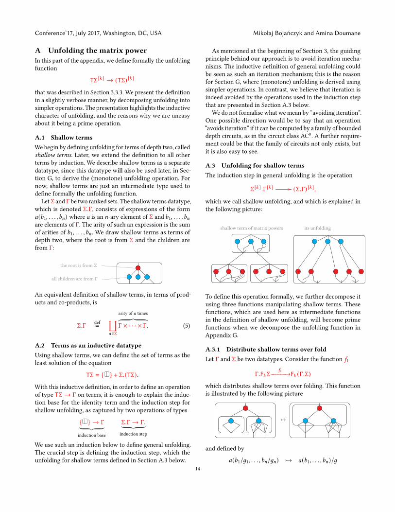
A.1 Shallow termsWe begin by defining unfolding for terms of depth two, calledshallow terms. Later, we extend the definition to all otherterms by induction. We describe shallow terms as a separatedatatype, since this datatype will also be used later, in Sec-tion G, to derive the (monotone) unfolding operation. Fornow, shallow terms are just an intermediate type used todefine formally the unfolding function.
Let Σ and Γ be two ranked sets. The shallow terms datatype,which is denoted Σ.Γ, consists of expressions of the form𝑎(𝑏1, . . . , 𝑏𝑛) where 𝑎 is an 𝑛-ary element of Σ and 𝑏1, . . . , 𝑏𝑛are elements of Γ. The arity of such an expression is the sumof arities of 𝑏1, . . . , 𝑏𝑛 . We draw shallow terms as terms ofdepth two, where the root is from Σ and the children arefrom Γ:
the root is from Σ
all children are from Γ
An equivalent definition of shallow terms, in terms of prod-ucts and co-products, is
Σ.Γdef=
∐𝑎∈Σ
arity of 𝑎 times︷ ︸︸ ︷Γ × · · · × Γ, (5)
A.2 Terms as an inductive datatypeUsing shallow terms, we can define the set of terms as theleast solution of the equation
TΣ = { } + Σ.(TΣ).
With this inductive definition, in order to define an operationof type TΣ→ Γ on terms, it is enough to explain the induc-tion base for the identity term and the induction step forshallow unfolding, as captured by two operations of types
{ } → Γ︸ ︷︷ ︸induction base
Σ.Γ → Γ.︸ ︷︷ ︸induction step
We use such an induction below to define general unfolding.The crucial step is defining the induction step, which theunfolding for shallow terms defined in Section A.3 below.
As mentioned at the beginning of Section 3, the guidingprinciple behind our approach is to avoid iteration mecha-nisms. The inductive definition of general unfolding couldbe seen as such an iteration mechanism; this is the reasonfor Section G, where (monotone) unfolding is derived usingsimpler operations. In contrast, we believe that iteration isindeed avoided by the operations used in the induction stepthat are presented in Section A.3 below.
We do not formalise what we mean by “avoiding iteration”.One possible direction would be to say that an operation“avoids iteration” if it can be computed by a family of boundeddepth circuits, as in the circuit class AC0. A further require-ment could be that the family of circuits not only exists, butit is also easy to see.
A.3 Unfolding for shallow termsThe induction step in general unfolding is the operation
Σ [𝑘 ] .Γ [𝑘 ] // (Σ.Γ) [𝑘 ],
which we call shallow unfolding, and which is explained inthe following picture:
shallow term of matrix powers its unfolding
To define this operation formally, we further decompose itusing three functions manipulating shallow terms. Thesefunctions, which are used here as intermediate functionsin the definition of shallow unfolding, will become primefunctions when we decompose the unfolding function inAppendix G.
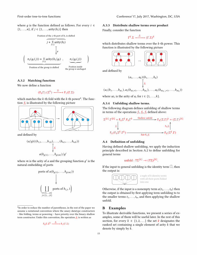
A.3.1 Distribute shallow terms over foldLet Γ and Σ be two datatypes. Consider the function 𝑓1
Γ.F𝑘Σ𝑓1−−−−−−→F𝑘 (Γ.Σ)
which distributes shallow terms over folding. This functionis illustrated by the following picture
and defined by
𝑎(𝑏1/𝑔1, . . . , 𝑏𝑛/𝑔𝑛) ↦→ 𝑎(𝑏1, . . . , 𝑏𝑛)/𝑔14
First-order tree-to-tree functions Conference’17, July 2017, Washington, DC, USA
where 𝑔 is the function defined as follows. For every 𝑖 ∈{1, . . . , 𝑛}, if 𝑗 ∈ {1, . . . , arity(𝑏𝑖 )} then
Position of the 𝑗-th port of 𝑏𝑖 is shifted︷ ︸︸ ︷𝑗 + Σ
𝑙<𝑖arity(𝑏𝑙 )_
𝑔��(
𝜋2 (𝑔𝑖 ( 𝑗)) + Σ𝑙<𝑖
arity(𝑏𝑙/𝑔𝑙 )︸ ︷︷ ︸Position of the group is shifted
, 𝜋1 (𝑔𝑖 ( 𝑗))︸ ︷︷ ︸Position inside
the group is unchaged
)
A.3.2 Matching functionWe now define a function
(F𝑘Γ).(Σ𝑘 )𝑓2−−−−−−→ F1 (Γ.Σ)
which matches the 𝑘-th fold with the 𝑘-th power6. The func-tion 𝑓2 is illustrated by the following picture
and defined by
(𝑎/𝑔) ((𝑏1,1, . . . , 𝑏1,𝑘 ), . . . , (𝑏𝑛,1, . . . , 𝑏𝑛,𝑘 ))_
𝑓2
��𝑎(𝑏𝑔 (1) , . . . , 𝑏𝑔 (𝑚) )/𝑔′
where𝑚 is the arity of 𝑎 and the grouping function 𝑔′ is thenatural embedding of ports
ports of 𝑎(𝑏𝑔 (1) , . . . , 𝑏𝑔 (𝑚) ))
��( ∐𝑖∈{1,...,𝑛}𝑗 ∈{1,...,𝑘 }
ports of 𝑏𝑖, 𝑗 , 1)
6In order to reduce the number of parentheses, in the rest of the paper weassume a notational convention where the unary datatype constructors– like folding, terms or powering – have priority over the binary shallowterm constructor. Under this convention, the operation 𝑓2 is written as
F𝑘Γ.Σ𝑘 𝑓2−−−−−−→ F1 (Γ.Σ)
A.3.3 Distribute shallow terms over productFinally, consider the function
Γ𝑘 .Σ𝑓3−−−−−−→ (Γ.Σ)𝑘
which distributes shallow terms over the 𝑘-th power. Thisfunction is illustrated by the following picture
and defined by
(𝑎1, . . . , 𝑎𝑘 ) (𝑏1, . . . , 𝑏𝑛)_
𝑓2
��(𝑎1 (𝑏1, . . . , 𝑏ar1 ), 𝑎2 (𝑏ar1+1, . . . , 𝑏ar2 ), . . . , 𝑎𝑘 (𝑏ar𝑘−1+1, . . . , 𝑏ar𝑘 ))
where ar𝑖 is the arity of 𝑎𝑖 for 𝑖 ∈ {1, . . . , 𝑘}.
A.3.4 Unfolding shallow terms.The following diagram defines unfolding of shallow termsin terms of the operations 𝑓1, 𝑓2, 𝑓3 defined above:
Σ [𝑘 ] .Γ [𝑘 ] = F𝑘Σ𝑘 .F𝑘Γ𝑘
𝑓1��
Shallow unfold // F𝑘 (Σ.Γ)𝑘 = (Σ.Γ) [𝑘 ]
F𝑘 (F𝑘Σ𝑘 .Γ𝑘 ) flat◦F𝑘 𝑓2// F𝑘 (Σ𝑘 .Γ)
F𝑘 𝑓3
OO
A.4 Definition of unfoldingHaving defined shallow unfolding, we apply the inductionprinciple described in Section A.2 to define unfolding forgeneral terms
unfold : TΣ [𝑘 ] → (TΣ) [𝑘 ] .
If the input to general unfolding is the identity term , thenthe output is:
a tuple of k identity terms with all their ports folded into one
Otherwise, if the input is a nonempty term 𝑎(𝑡1, . . . , 𝑡𝑛) thenthe output is obtained by first applying term unfolding to tothe smaller terms 𝑡1, . . . , 𝑡𝑛 , and then applying the shallowunfold.
B ExamplesTo illustrate derivable functions, we present a series of ex-amples, some of them will be useful later. In the rest of thissection, for every 𝑘 ∈ {1, 2, . . . } the set 𝑘 designates theranked set containing a single element of arity 𝑘 that wedenote by simply by 𝑘 .
15

Conference’17, July 2017, Washington, DC, USA Mikołaj Bojańczyk and Amina Doumane
Example B.1 (Parent and children). Let Γ be a finite type.We define Γ0 to be the ranked set obtained from Γ by settingthe arity of every element to 0. Consider the function:
Parent : TΓ → T(Γ × (Γ0 + 0))which adds to every node of a term in TΣ the label of itsparent if it has one, and 0 if it is the root.Let us explain how Parent can be derived. To illustrate
this construction, we use the following alphabet Γ
and the following term as a running example.
We denote by Γ1 the ranked set obtained from Γ by setting thearity of every element to 1. If 𝑎 is a element of Γ, we denoteby 𝑎1 the corresponding element of Γ1. In our example, thealphabet Γ1 is
1. First, we apply the homomorphism
Hom𝑔 : TΓ → T(Γ + Γ1 + 1)where 𝑔 is defined on the elements of Γ as follows
𝑔 : Γ→ T(Γ + Γ1 + 1)𝑎 ↦→ 𝑎(1(𝑎1 ( )), . . . , 1(𝑎1 ( )))
In our example, the action of 𝑔 on the elements of Γlooks like this
Hence, after the application of the homomorphismHom𝑔, our initial term becomes
2. We apply the factorization
fact↑ : T(Γ + Γ1 + 1) → T(T(Γ + Γ1) + T1)to separate the symbol 1 form the other symbols. Afterthis operation, each node lies in the same factor as (the
element of Γ1 representing) its parent. In our example,the obtained term is the following
3. Consider the functionℎ : T1→ T((Γ + Γ1) × (Γ0 + 0))
which is the empty term constant function. It is deriv-able by lifting the empty term constant function over1 to terms. And let 𝑘 be the function
𝑘 : T(Γ + Γ1) → T((Γ + Γ1) × (Γ0 + 0))which is the identity function, except for the followingterms in which it is defined as follows
𝑎( , . . . , ) ↦→ (𝑎, 0) ( , . . . , )𝑏1 (𝑎( , . . . , )) ↦→ (𝑎, 𝑏0) ( , . . . , )
𝑏1 ( ) ↦→We apply the function ℎ to the factors T1 and the function𝑘 to the factors T(Γ + Γ1). Doing so, we obtain a term inTT((Γ + Γ1) × (Γ0 + 0)), which we flatten, then we erase thesymbols Γ1 using the function Filter of Example 3.3 to obtainthe desired term.
If Γ is a finite ranked set, we define Γ∗ as∐𝑖≤ maximal arity in Γ
Γ × · · · × Γ︸ ︷︷ ︸𝑖 times
Now consider the functionChildren : TΓ → T(Γ × (Γ0 + 0)∗)
which tags every node of a term in TΓ by the list of itschildren symbols. When a child is a port, it is marked by 0 inthe list. The function Children can be derived using a similarconstruction as above.
Example B.2 (Root and leaves). Let Σ be a finite type and𝑓 : Σ→ Γ, 𝑔 : Σ→ Γ be derivable functions. The function
Root𝑓 ,𝑔 : TΣ→ TΓ
which applies 𝑓 to the root and 𝑔 to the rest of the tree is aderivable function. To show this, we first start by applyingthe function Parent. Doing so, the root can be distinguishedfrom the other nodes since it will be tagged by 0.
The function ℎ defined below is derivable since its domainis finite.
ℎ : Σ × (Σ0 + 0)→ Γ
(𝑎, 0) ↦→ 𝑓 (𝑎)(𝑎, 𝑏) ↦→ 𝑔(𝑎) if 𝑏 ≠ 0.
16

First-order tree-to-tree functions Conference’17, July 2017, Washington, DC, USA
We lift ℎ to terms to conclude.Similarly, the function
Leaves𝑓 ,𝑔 : TΣ→ TΓ
which applies 𝑓 to the leaves and 𝑔 to the rest of the treeis derivable. This is done using the same ideas as before,but invoking the function Children instead of the functionParent: leaves can be distinguished from the other nodessince they are tagged either by a list of 0 or the empty list.
Example B.3 (Descendants and ancestors). If Σ is a finitetype and Γ ⊆ Σ, then the functions• DescendantΓ : TΣ→ T(Σ + Σ) which replaces the la-bel of each node by its first or second copy, dependingon whether it has a descendant in Γ,• AncestorΓ : TΣ→ T(Σ + Σ) which replaces the labelof each node by its first or second copy, depending onwhether it has a descendant in Γ,
are derivable.To derive DescendantΓ , we start by applying the factor-
izationfact↓ : TΣ→ T(TΓ + T(Σ \ Γ))
which regroups the elements of Σ and the elements of Σ \ Γinto factors depending on whether they have the same an-cestors of the same type.
Obviously, all the nodes of the Γ factors have a descendantin Γ. In the Σ \ Γ factors which are not leaves in the factor-ized term, all the nodes have a Γ descendant in the originalterm. To show this, take 𝑓 to be one of these factors, andsuppose by contradiction that one of its nodes does not havea descendant in Γ. By definition of fact↑, all the elementsof 𝑓 do not have a descendant in Γ as well. Since 𝑓 is not aleaf, it has a child 𝑔. The factor 𝑔 cannot be a Γ factor as thenodes of 𝑓 would have a descendant in Γ. The factor 𝑔 is thennecessarily a Σ \ Γ factor. If a node of 𝑔 has a descendantin Γ, this would give a Γ descendant to one of the node of𝑓 . Thus all the nodes of 𝑔 are in Σ \ Γ and do not have adescendant in Γ, meaning that 𝑓 and 𝑔 are actually the samefactor, which gives a contradiction. Finally, the Σ \ Γ factorswhich are leaves do not have a descendant in Γ. With theseobservations, we can now implement DescendantΓ .Let us consider the functions
YesΓ : Γ → Σ + ΣYesΣ\Γ: Σ \ Γ → Σ + ΣNoΣ\Γ: Σ \ Γ → Σ + Σ
which replaces the label of each node by its first copy forYesΓ and YesΣ\Γ , and by its second copy for NoΣ\Γ . The threefunctions are derivable as their domains are finite. Considerthe functions
𝑓 :=TYesΓ + TNoΣ\Γ : TΓ + T(Σ \ Γ) → T(Σ + Σ)𝑔 :=TYesΓ + TYesΣ\Γ : TΓ + T(Σ \ Γ) → T(Σ + Σ)
The descendant function is obtained by applying leaves𝑓 ,𝑔followed by a flattening.To derive the function AncestorΓ , we apply first a the
factorization
fact↑ : TΣ→ T(TΓ + T(Σ \ Γ))
which regroups the elements of Σ and the elements of Σ \ Γinto factors depending on whether they have the same de-scendants of the same type. Using similar arguments as be-fore, we can conclude that:• The nodes inside Γ factors have Γ ancestors.• If a Σ \ Γ factor is the root of the factorized term, thenits nodes do not have a Γ ancestor.• If a Σ \ Γ factor is not the root of the factorized term,then its nodes do have a Γ [𝐷𝑒𝑠𝑐𝑒𝑛𝑑𝑎𝑛𝑡𝑠𝑎𝑛𝑑𝑎𝑛𝑐𝑒𝑠𝑡𝑜𝑟𝑠]ancestor.
The ancestor function is obtained by applying root𝑓 ,𝑔 fol-lowed by a flattening.
Example B.4 (Error raising.). We can think of the type ⊥ asan error type. Indeed, the following raising error functionsare derivable.
Lemma B.5. Let Σ and Γ be two datatypes. The functions
T(Σ + ⊥) → TΣ + ⊥(Σ + ⊥) × (Γ + ⊥) → Σ × Γ + ⊥(Σ + ⊥) .(Γ + ⊥) → Σ.Γ + ⊥
F𝑘 (Σ + ⊥) → F𝑘Σ + ⊥
which are defined as follows
𝑡 of arity 𝑛 ↦→{𝑡 if 𝑡 does not contain any element of ⊥,𝑛 otherwise.
are derivable.
These functions can be easily derived using Proposition 5.1and distributivity prime functions. The details of the proofare left as an exercise to the reader.
Example B.6 (Partial functions.). Thinking of ⊥ as an errordatatype, a function of type Σ→ Γ + ⊥ can be seen as apartial function from Σ to Γ. We write
Σ ⇀ Γ
as a notation for the function type Σ→ Γ + ⊥. Using theerror raising mechanisms discussed earlier, we can manipu-late transparently partial function. Indeed, all datatype con-structors can be lifted to partial functions, by composingthe liftings (1)–(4) with the error raising functions fromLemma B.5. For example, if 𝑓 : Σ ⇀ Γ is a partial function,then T𝑓 : TΣ ⇀ TΓ is defined as the composition
TΣT𝑓−−→ T(Γ + ⊥)
Error raising−−−−−−−−−→ TΓ + ⊥.
17

Conference’17, July 2017, Washington, DC, USA Mikołaj Bojańczyk and Amina Doumane
C Derivable functions can be described infirst-order logic
The goal of this section is to show the right-to-left implica-tion of Theorem 3.4, which says that derivable functions canbe implemented by first-order transductions.
As discussed in the body of the paper, we proceed by induc-tion on the derivation. During this induction, we will need toshow that every prime function is a first-order transduction.Prime functions are not tree-to-tree functions, instead theytransform dataypes into datatypes. This is the reason whywe need
• to generalize tree-to-tree transductions into transduc-tions that can transform models over arbitrary vocab-ularies (and not only the vocabulary of trees).• show how datatypes (terms, pairs, copairs and folds)can be encoded as models over a well chosen vocabu-lary.More precisely, wewill associate to every datatypeΣ a relational vocabulary that we call vocabulary of Σ.Structures over this vocabulary will be called modelsover Σ. Then we will define a function
Σ𝑥 ↦→𝑥 // models over Σ
which assigns to each element 𝑥 ∈ Σ a correspondingmodel over Σ, which is denoted by 𝑥 .
Right-to-left implication of Theorem 3.4 can be then gen-eralized to the following statement, more suited to a proofby induction:
Proposition C.1. Let Γ and Σ be two datatype. For everyderivable function 𝑓 , there is a first-order transduction 𝑔 suchthat the following diagram commutes
Σ
𝑥 ↦→𝑥
��
𝑓 // Γ
𝑥 ↦→𝑥
��models over Σ
𝑔// models over Γ
The rest of this section is organized as follows. We definefirst-order transductions transforming arbitrary models inSection C.1. In Section C.2 we define the vocabularies forthe datatypes and the model representation 𝑥 ↦→ 𝑥 . Finally,we prove Proposition C.1 which gives as a corollary theright-to-left implication of Theorem 3.4.
C.1 First-order transductionsThe following definition introduces first-order transductions,which generalizes tree-to-tree transductions given in Defini-tion 2.2 to arbitrary models.
Definition C.2 (First-order transduction). A first-ordertransduction is defined to be any composition of the followingtwo kinds of transformations on structures:
1. Copying. Fix some relational vocabulary 𝜎 and let 𝑘 ∈{1, 2, . . .}. Define 𝑘-copying to be the operation of type
models over 𝜎
��models over 𝜎 extendedwith a 𝑘-ary relation copy
which inputs a model A, and outputs 𝑘 disjoint copiesofA, where the copy relation is interpreted as the set oftuples (𝑎1, . . . , 𝑎𝑘 ) such that, for some 𝑎 ∈ A, the firstcopy of 𝑎 is 𝑎1, the second copy of 𝑎 is 𝑎2, etc. The copyrelation is not commutative, because we distinguishthe copies.
2. Non-copying first-order transduction. The syntax of anon-copying first-order transduction is given by:a. Input relational vocabulary 𝜎 and output relational
vocalbulary 𝛾 .b. A first-order universe formula 𝜑 (𝑥) over 𝜎 .c. For every relation 𝑅 in vacubulary 𝛾 , a first-order
formula 𝜑𝑅 (𝑥1, . . . , 𝑥arity(𝑅) ) over 𝜎 .The semantics of a non-copying first-order transduc-tion is a function
models over 𝜎
��models over 𝛾
defined as follows. If the input model is A, then theoutput model is defined as follows: the universe is el-ements of A which satisfy the universe formula, andeach relation 𝑅 is interpreted as those tuples that sat-isfy 𝜑𝑅 .
The notion of copying used in the above definition isslightly different from the notion of copying used for tree-to-tree transductions in Definition 2.2, which was specificallytailored to stay within the realm of trees. Nevertheless, thetwo definitions are easily seen to define the same class oftree-to-tree functions.
C.2 Datatypes as models.Let us show how to encode datatypes as relational vocabu-laries and data as models over these vocabularies.
Definition C.3 (Associated models for terms, pairs, co-pairs,folds.). To each type Σ we associate a vocabulary, called thevocabulary of Σ, and a map𝑎 ∈ Σ ↦→ 𝑎 ∈ models over the vocabulary of Σ︸ ︷︷ ︸
associated model of 𝑎
.
Furthermore, for each 𝑎 ∈ Σ we distinguish a sequence(whose length is the arity of 𝑎) of elements in 𝑎, which arecalled the ports of 𝑎. The definitions are by induction on thestructure of Σ, as given below.
18

First-order tree-to-tree functions Conference’17, July 2017, Washington, DC, USA
• Finite ranked sets. Elements of a ranked set
Σ = {𝑎1, . . . , 𝑎𝑘 }
are modelled using a vocabulary which has unary rela-tions 𝑎1, . . . , 𝑎𝑘 and 𝑃1, . . . , 𝑃𝑚 where𝑚 is the maximalarity of elements in Σ. For 𝑎 ∈ Σ of arity𝑛, the universeof 𝑎 is {0, 1, . . . , 𝑛}, with the ports being 1, . . . , 𝑛. Therelation 𝑃𝑖 is interpreted as {𝑖} when 𝑖 ∈ {1, . . . , 𝑛}and as the empty set otherwise. The relation 𝑎𝑖 is in-terpreted as {0} when 𝑎 = 𝑎𝑖 and as the empty setotherwise.• Coproduct. Elements of the coproduct Σ1 + Σ2 are mod-elled using the disjoint union of the vocabularies of Σ1and Σ2. If an element of the coproduct comes from Σ1,then its associated model is defined as for the type Σ1,with the remaining relations from the vocabulary of Σ2interpreted as empty sets. The definition is analogousfor elements from Σ2.• Product. Pairs in Σ1 × Σ2 are modelled using the dis-joint union of the vocabularies of Σ1 and Σ2. For (𝑎1, 𝑎2),the associated model is the disjoint union of models𝑎1+𝑎2, with the relations of 𝑎1 using the vocabulary ofΣ1, and the relations of 𝑎2 using the vocabulary Σ1. If𝑛1 is the arity of 𝑎1, then the first 𝑛1 ports are inheritedfrom 𝑎1 and the remaining ports are inherited from 𝑎2.• Folding. For 𝑘 ∈ {1, 2, . . .}, elements of F𝑘Σ are mod-elled using the vocabulary of Σ plus two extra binaryrelations ⊏ and 𝑅. If 𝑎 ∈ Σ has arity 𝑛𝑘 , then the modelassociated to 𝑎/𝑓 – which has arity 𝑛 – is obtainedfrom 𝑎 by adding a copy of the model below, where ⊏is the natural ordering on integers
({1, . . . , 𝑛}, ⊏),
whose elements are used as the ports, and interpretingthe binary relation 𝑅 as
{(𝑖-th port of 𝑎, 𝑓 (𝑖)) : 𝑖 ∈ {1, . . . , 𝑛𝑘}}
• Terms. Terms in TΣ are modelled using vocabulary ofΣ extended with two fresh binary relations < and ⊏.Let 𝑡 ∈ TΣ. Consider the disjoint union of models∐
𝑥 ∈non-port nodes in 𝑡
𝑎(𝑥), (6)
where 𝑎(𝑥) is the model over vocabulary of Σ that isdefined by induction assumption. In the above disjointunion, the same vocabulary, namely the vocabularyof Σ, is used for all parts of the disjoint union. Next,consider the model
({1, . . . , 𝑛}, ⊏) (7)
where ⊏ is the natural ordering on {1, . . . , 𝑛}. Themodel of 𝑡 is defined by taking the disjoint union ofthe models in (6) and (7), and defining the descendentrelation < as the set of pairs (𝑢, 𝑣) such that:
– either 𝑢 is the 𝑖-th port of 𝑎(𝑥) for some node 𝑥 of𝑎, 𝑣 is a port of 𝑎(𝑦) for some node 𝑦 which is adescendent of the 𝑖-th child of 𝑥 .
– or 𝑢 is the 𝑖-th port of 𝑎(𝑥) for some node 𝑥 of 𝑎, 𝑣 =
𝑗 ∈ {1, . . . , 𝑛} and the 𝑗-th port of 𝑎 is a descendentof the 𝑖-th child of 𝑥 .
The above definition creates a certain ambiguity for trees,because if 𝑡 is a tree over a finite ranked set Σ, then 𝑡 can beunderstood in two ways: as per Definition 2.1 for trees, oras per Definition C.3 when 𝑡 is viewed as a special case of aterm 𝑡 ∈ TΣ. Since we only use first-order transductions totransform relational structures, this ambiguity is not a prob-lem, because one can easily define first-order transductionswhich map one definition of 𝑡 to the other.
C.3 Proof of Proposition C.1The proof proceeds by induction, following the definitionof derivable functions. In the induction step, we have todeal with function composition and the lifting of functionalong the datatype constructors. First-order transductionsare closed under composition by definition, while the liftingsare immediate.
In the induction base, we need to show that all of the primefunctions are first-order transductions. All the cases are easy,and consist mainly on unfolding the definitions; this is thepoint of calling these functions prime. There is one exception,which requires some more explanation, namely monotoneunfolding. We explain below just one of the easy functions,the unit function Σ→ TΣ, and the monotone unfolding. Theother prime functions are left as an exercise.
C.3.1 A first-order transduction for the term unitIn the following, it will be convenient to use, as part of thevocabulary of Σ, a unary relation PortΣ which selects theports of the structures over the vocabulary of Σ; and a binaryrelation ⊏Σ which orders these ports. By induction on Σ,we can show that both relations are definable by first-orderformulas over the vocabulary of Σ.
Given an element 𝑥 of Σ, let us show how unit(𝑥) can beimplemented using a first-order transduction. The copyingconstant is 2, the first copy will contain the whole structure𝑥 and the second copy will select only the ports of 𝑥 whichwill serve as the ports of the structure unit(𝑥), as illustratedby the following picture
19

Conference’17, July 2017, Washington, DC, USA Mikołaj Bojańczyk and Amina Doumane
The universe formulas are then:
𝜑1 (𝑥) = True 𝜑2 (𝑥) = PortΣ (𝑥)In the first copy, the vocabulary of Σ will be interpreted asin the original structure, and as the empty set in the secondcopy. That is, for every unary relation 𝑅 and for every binaryrelation 𝑆 in the vocabulary of Σ, we set:
𝜑1𝑅 (𝑥) = 𝑅(𝑥) 𝜑
1,1𝑆(𝑥,𝑦) = 𝑆 (𝑥,𝑦)
𝜑2𝑅 (𝑥) = False 𝜑
2,2𝑆(𝑥,𝑦) = False
Let us interpret the relations < and ⊏ of the vocabulary ofTΣ. The ports of unit(𝑥) inherit the order of the ports of 𝑥 ,this is why we set:
𝜑2,2⊏ (𝑥,𝑦) = 𝑥 ⊏Σ 𝑦
The descendant relation < connects the 𝑖𝑡ℎ port of 𝑥 to the𝑖𝑡ℎ port of unit(𝑥). Since these nodes come from the samenode in the original structure, we set:
𝜑1,2< (𝑥,𝑦) = 𝑥 = 𝑦
C.3.2 A first-order transduction for monotoneunfolding
Having illustrated the syntax of first-order transductions onthe example of the unit function, we describe a first-ordertransduction for the monotone unfolding operation
TΣ [𝑘 ] → (TΣ) [𝑘 ] + ⊥.This is the only prime function whose corresponding first-order transduction is not obvious. Unlike in Section C.3.1,we focus more on the underlying conceptual difficulties thanon the syntax of first-order transductions.Recall that when defining the monotone unfolding oper-
ation, for each element 𝑎 ∈ TΣ [𝑘 ] of the matrix power, weused a family of (partial) twist functions
→𝑖 : {1, . . . , 𝑘} → {1, . . . , 𝑘},one for each port 𝑖 of 𝑎. For the reader’s convenience, werepeat a picture from Section 3.3.3, which explains the twistfunctions:
an element ofthe matrix power
its twist functions1 2 3
1 2 3 1 2 3
In this example, the twist function→1 is monotone, but→2is not. The monotone unfolding operation works in the sameway as general unfolding, except that it uses the undefinedvalue ⊥ if the input term has at least one letter which usesat least one non-monotone twist.The following lemma, whose simple proof is left to the
reader, shows that the twist functions can be defined usingfirst-order logic.
Lemma C.4. Let Σ be a datatype and let 𝑘 ∈ {1, 2, . . .}. Forevery partial function
𝜏 : {1, . . . , 𝑘} → {1, . . . , 𝑘}
there is a first-order formula𝜑𝜏 (𝑥) such that for every 𝑎 ∈ Σ [𝑘 ] ,𝑎 |= 𝜑𝜏 (𝑥)
if and only if 𝑥 represents a port with twist function 𝜏 .
By using the formulas from the above lemma, one canconstruct a first-order formula which checks if a term inTΣ [𝑘 ] uses only monotone twists, i.e. whether or not theoutput of monotone unfolding should be ⊥.
We now proceed to the more interesting part of monotoneunfolding, i.e. actually doing the unfolding for monotoneinputs. Consider an input 𝑡 ∈ TΣ [𝑘 ] to monotone unfolding.Define a sub-node of 𝑡 to be a pair (node of 𝑡 , number in{1, . . . , 𝑘}), as explained in the following picture:
sub-nodes
In the output of the monotone unfolding, which is of theform
(𝑡1, . . . , 𝑡𝑘 )/𝑓 ∈ TΣ [𝑘 ],the nodes of the output terms 𝑡1, . . . , 𝑡𝑘 will correspond tothe sub-nodes in the input 𝑡 . The sub-nodes can be producedby copying the input term 𝑘-times.
The most interesting part of the structure in the output isthe descendant relation in the terms 𝑡1, . . . , 𝑡𝑘 . This relationcan be viewed as a descendant relation on the sub-nodes.We only describe how the descendant relation on the sub-nodes can be defined in first-order logic, and the rest of thetransduction is left to the reader.
When defining the descendant relation on sub-nodes, thecrucial part is composing the twist functions. Suppose thatwe want to check the descendant relationship between twosub-nodes
(𝑥, 𝑖)?≤ (𝑦, 𝑗), (8)
where 𝑥,𝑦 are nodes on the input term and 𝑖, 𝑗 ∈ {1, . . . , 𝑘}.We will show that the descendant relationship (8) holds ifand only if 𝑥 is an ancestor of 𝑦 in the input term, and the
20

First-order tree-to-tree functions Conference’17, July 2017, Washington, DC, USA
twist functions on the path connecting 𝑥 and 𝑦 maps 𝑗 to 𝑖 ,as explained below.
Consider a path in the input term, which connects node 𝑥with 𝑦, as illustrated in the following picture
x
connecting edges
y
Each edge in the input term corresponds to a chosen port insome node, which in turn corresponds to some twist function,and therefore it makes sense to talk about the twist functionassociated to an edge in the input term. Define
𝜏𝑥𝑦 : {1, . . . , 𝑘} → {1, . . . , 𝑘}to be the partial function, which is obtained by composingall of the twist functions corresponding to edges on the pathconnecting 𝑦 to 𝑥 , starting with 𝑦 and ending with 𝑥 . Inthe example from the above picture, we compose two twistfunctions, which correspond to edges marked in yellow.
Equipped with the above definitions, we can now charac-terise the descendant ordering on sub-nodes by
(𝑥, 𝑖) ≤ (𝑦, 𝑗) iff 𝑥 ≤ 𝑦 ∧ 𝜏𝑥𝑦 ( 𝑗) = 𝑖 .
Therefore, to complete the proof, it remains to show thefollowing lemma. This is where we use the monotonicityassumption.
Lemma C.5. For every 𝑖, 𝑗 ∈ {1, . . . , 𝑘} there is a first-orderformula𝜓 𝑖
𝑗 (𝑥,𝑦) such that for every 𝑡 ∈ TΣ [𝑘 ]
𝑡 |= 𝜓 𝑖𝑗 (𝑥,𝑦) iff 𝜏𝑥𝑦 ( 𝑗) = 𝑖 .
Proof. Let 𝐹 be the set of monotone partial functions from{1, . . . , 𝑘} to itself. Define 𝐿 ⊆ 𝐹 ∗ to be the set of those words𝑓1 · · · 𝑓𝑛 such that the composition of functions 𝑓𝑛 ◦ · · · ◦ 𝑓1maps 𝑖 to 𝑗 . We will show that – thanks to the monotonicityassumption – the language 𝐿 is definable in first-order logic.To get the conclusion of the lemma, we check if the sequence
of twist functions on the path from 𝑥 to 𝑦 satisfies the first-order formula defining the language 𝐿.
The language 𝐿 is recognised by a finite automaton, whichhas states {1, . . . , 𝑘,⊥}, and which simply applies the func-tion in its input letter to the present state. We show be-low that this automaton is counter-free, in the sense of Mc-Naughton and Papert [25, p. 6], and therefore it can be de-fined in first-order logic.
Recall that a counter in an automaton is a sequence of atleast two pairwise distinct states 𝑞1, . . . , 𝑞𝑛 such that
𝑞1𝑤→ 𝑞2
𝑤→ · · · 𝑤→ 𝑞𝑛𝑤→ 𝑞1
holds for some common input string 𝑤 . In the automatonfor the language 𝐿 that we have discussed above, there is nocounter. Indeed, if we would have 𝑞1 ≤ 𝑞2, then by mono-tonicity of the function𝑤 ∈ 𝐹 we would have
𝑞1 ≤ 𝑞2 ≤ · · · ≤ 𝑞𝑛 ≤ 𝑞1
and therefore all of 𝑞1, . . . , 𝑞𝑛 would be equal, contradictingthe assumption that they are pairwise distinct. The sameargument would work when 𝑞1 ≥ 𝑞2. By [25, Theorem 10.5],if an automaton has no counter, then its language is definablein first-order logic.
□
D Appendix on first-order relabelling
The goal of this section is to show Proposition 5.1, whichsays that first-order relabeling are derivable. As discussed inthe body of the paper, the proof of this proposition is basedon an equivalence result between first-order queries on treesand a temporal logic, as stated in Lemma 5.2.While this resultis deaply inspired from a similar result of Schlingloff [26], ourframeworks are not exactly the same (he uses for ainstanceunranked trees). In the rest of this section, we provide moredetails about the reduction from Schilgloff’s result to ourlemma (Section D.1). Then we show in Section D.2 how touse it in order to prove Proposition 5.1.
D.1 Reduction to Schilgloff’s theoremLet us proceed to the proof of Lemma 5.2. Clearly the func-tions in the lemma are first-order tree relabeling, and first-order tree relabeling are easily seen to be closed under com-position, which gives the right-to-left inclusion in the lemma.The hard part is the left-to-right inclusion, which says thatevery first-order tree relabeling can be decomposed intofunctions as in items 1,2a–2c. The first step in the proofof the right-to-left inclusion is the observation that everyfirst-order tree relabeling can be decomposed as
𝑔 ◦ 𝑓1 ◦ · · · ◦ 𝑓𝑛where 𝑔 is a relabeling as in item 1 of the lemma and each𝑓𝑖 is a characteristic function of some unary query (not nec-essarily of the simple form indicated in items 2a – 2c in the
21

Conference’17, July 2017, Washington, DC, USA Mikołaj Bojańczyk and Amina Doumane
lemma). This is a simple observation: the functions 𝑓1, . . . , 𝑓𝑛annotate the tree with the truth values of the unary queriesused in the definition of the first-order relabeling, and 𝑔 usesthese truth values to select the appropriate output label. Thehard part of the lemma is showing that each 𝑓𝑖 can be furtherdecomposed into functions as indicated in the lemma. Thisis where we us the result of Schlingloff [26, Theorem 2.6],which says that all first-order definable tree properties canbe defined using a temporal logic that has operators similarto the ones used in items 2a – 2c of the lemma.
The following table summarizes our framework (first col-umn) and Schlingloff’s one (second column). The first rowdescribes the models under consideration, the second rowthe corresponding version of first-order logic, and the thirdrow the corresponding temporal logic.
Models
Trees over a finiteranked alphabet Γ:finitely branching,ranked trees, labeled
from Γ.
Models over a setof propositions 𝑃 :finitely branching,unranked trees,labeled from 2𝑃 .
First-orderlogic
Usual first-order connectives (∃,∨,¬)with the descendant predicate 𝑥 ≤ 𝑦
and the following predicates:𝑎(𝑥): 𝑥 is labeled 𝑎
(𝑎 ∈ Γ).𝑝 (𝑥): label of 𝑥
contains 𝑝 (𝑝 ∈ 𝑃 ).child𝑖 (𝑥): 𝑥 is an 𝑖-th
child.We call it Γ-fo. We call it 𝑃-fo.
Temporallogic
Usual CTL connectives (𝑆 (Since),𝑈(Until), ∨, ¬) together with:
𝑎 ∈ Γ, 𝑝 ∈ 𝑃 ,⊙𝑖𝜙 : the 𝑖-th child
satisfies 𝜙 .𝑋𝑖𝜙 : at least 𝑖
children satisfy 𝜙 .We call it 2-CTL. We call it 4-CTL.
What is named Γ-fo in the table is what we simply calledfirst-order logic along the paper. The operators of 2-CTLare those of Lemma 5.2. Using the notation of the table,Schlingloff’s theorem says that 𝑃-fo formulas are equivalentto 4-CTL formulas, and Lemma 5.2 states that Γ-fo formulasare equivalent to 2-CTL ones. To deduce the later from theformer, we will show how to translate every ranked tree 𝑡over Γ into a model [𝑡] over a well chosen set of propositions𝑃 , then we will apply the following scheme
𝜑 ∈ Γ-fo oo∀𝑡, 𝑡 |=𝜑 ↔ [𝑡 ] |=𝜓
Lemma 𝐷.1// 𝜓 ∈ 𝑃-foOO
Schlingloff’stheorem��
\ ∈ 2-CTL oo ∀𝑡, 𝑡 |=\ ↔ [𝑡 ] |=𝛿Lemma 𝐷.2
// 𝛿 ∈ 4-CTL
The translation [_] and Lemmas D.1 and D.2 are explainedbelow.
From ranked trees to Schlingloff’s models. Let us fix aranked alphabet Γ. Let 𝑃 be the following set of propositions
𝑃def= Γ ∪ {𝑖-th-child | 𝑖 ∈ [1,max arity of Γ]}
Let 𝑡 be a ranked tree over Γ. The translation [𝑡] of 𝑡 is themodel defined as follows. It has the same set of nodes and thesame descendant relation as 𝑡 . The label of a node contains𝑎 if its label in 𝑡 is 𝑎. It contains the proposition 𝑖-th-child ifit is an 𝑖-th child in 𝑡 .
First-order logic for ranked and unranked trees. Let Γand 𝑃 be as above. Let us show that Γ-fo and 𝑃-fo are equiv-alent.
Lemma D.1. For every Γ-fo formula 𝜙 , there is a 𝑃-fo for-mula𝜓 such that
∀𝑡 ∈ treesΓ, 𝑡 |= 𝜙 ↔ [𝑡] |= 𝜓
and conversely.
Proof. To show this lemma its is enough to show how totranslate the specific predicates of each formalism into theother. The predicate 𝑎(𝑥) of Γ-fo can be translated by thesame predicate in 𝑃-fo and conversely. The predicate child𝑖 (𝑥)can be translated by 𝑖-th-child(𝑥) and conversely. It is clearthat these translations preserve the semantics. □
Temporal logic for ranked and unranked trees. Let Γ and𝑃 be as above. We show that 2-CTL and 4-CTL are equivalent.
Lemma D.2. For every Γ-fo formula 𝜙 , there is a 𝑃-fo for-mula𝜓 such that
∀𝑡 ∈ treesΓ, 𝑡 |= 𝜙 ↔ [𝑡] |= 𝜓
and conversely.
Proof. Here again, it is enough to translate the specific con-nectives of each formalism into the other. The connective 𝑋𝑖
can be encoded in 2-CTL as follows, where 𝑏 is the maximalarity of Γ ∨
𝐼 ⊆[1,𝑏 ]#𝐼=𝑖
∧𝑗 ∈𝐼⊙𝑗 𝜙
Conversely, the connective ⊙𝑖 can be encoded in 4-CTL asfollows:
𝑋1 (𝑖-th-child ∧ 𝜙)□
D.2 First-order relabelling are derivableTo show Proposition 5.1, saying that first-order relabellingare derivable, we will show that each function appearingin Lemma 5.2 and corresponding to each operator of 2-CTLis derivable. This is the role of LemmasD.3–D.5 presentedbelow.
22
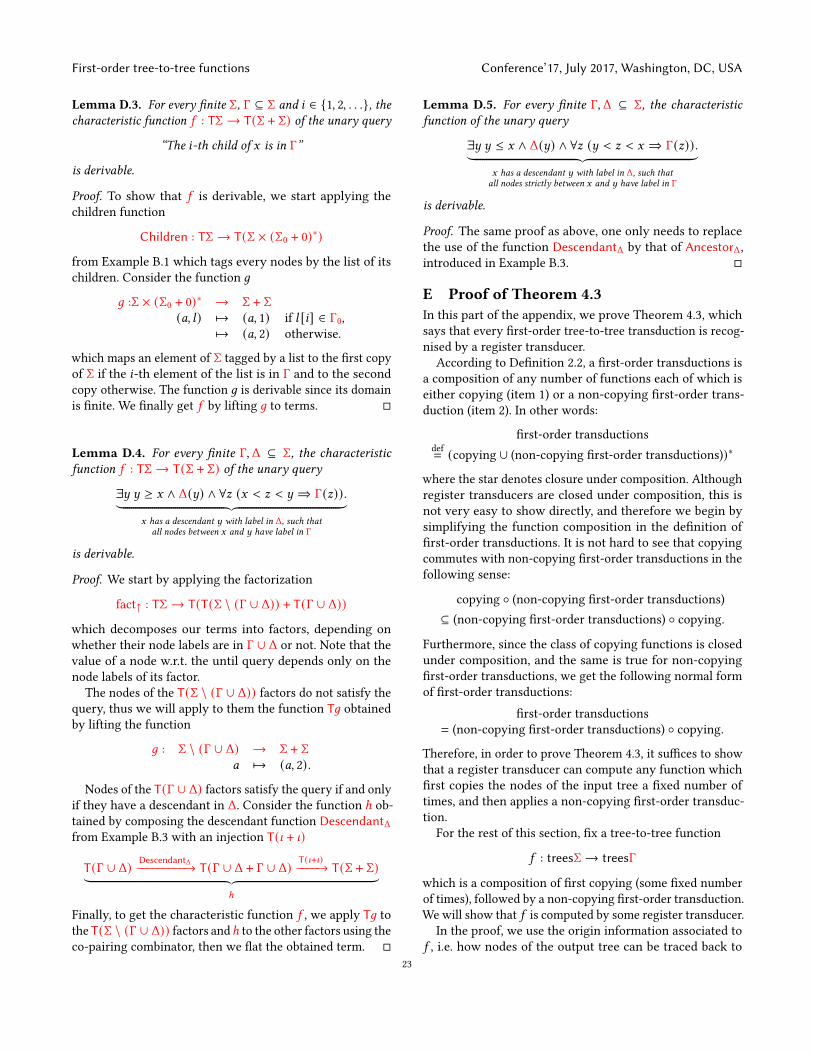
First-order tree-to-tree functions Conference’17, July 2017, Washington, DC, USA
Lemma D.3. For every finite Σ, Γ ⊆ Σ and 𝑖 ∈ {1, 2, . . .}, thecharacteristic function 𝑓 : TΣ→ T(Σ + Σ) of the unary query
“The 𝑖-th child of 𝑥 is in Γ”
is derivable.
Proof. To show that 𝑓 is derivable, we start applying thechildren function
Children : TΣ→ T(Σ × (Σ0 + 0)∗)
from Example B.1 which tags every nodes by the list of itschildren. Consider the function 𝑔
𝑔 :Σ × (Σ0 + 0)∗ → Σ + Σ(𝑎, 𝑙) ↦→ (𝑎, 1) if 𝑙 [𝑖] ∈ Γ0,
↦→ (𝑎, 2) otherwise.
which maps an element of Σ tagged by a list to the first copyof Σ if the 𝑖-th element of the list is in Γ and to the secondcopy otherwise. The function 𝑔 is derivable since its domainis finite. We finally get 𝑓 by lifting 𝑔 to terms. □
Lemma D.4. For every finite Γ,Δ ⊆ Σ, the characteristicfunction 𝑓 : TΣ→ T(Σ + Σ) of the unary query
∃𝑦 𝑦 ≥ 𝑥 ∧ Δ(𝑦) ∧ ∀𝑧 (𝑥 < 𝑧 < 𝑦 ⇒ Γ(𝑧)) .︸ ︷︷ ︸𝑥 has a descendant 𝑦 with label in Δ, such that
all nodes between 𝑥 and 𝑦 have label in Γ
is derivable.
Proof. We start by applying the factorization
fact↑ : TΣ→ T(T(Σ \ (Γ ∪ Δ)) + T(Γ ∪ Δ))
which decomposes our terms into factors, depending onwhether their node labels are in Γ ∪ Δ or not. Note that thevalue of a node w.r.t. the until query depends only on thenode labels of its factor.
The nodes of the T(Σ \ (Γ ∪ Δ)) factors do not satisfy thequery, thus we will apply to them the function T𝑔 obtainedby lifting the function
𝑔 : Σ \ (Γ ∪ Δ) → Σ + Σ𝑎 ↦→ (𝑎, 2).
Nodes of the T(Γ ∪ Δ) factors satisfy the query if and onlyif they have a descendant in Δ. Consider the function ℎ ob-tained by composing the descendant function DescendantΔfrom Example B.3 with an injection T(] + ])
T(Γ ∪ Δ) DescendantΔ−−−−−−−−−→ T(Γ ∪ Δ + Γ ∪ Δ)T(]+])−−−−→ T(Σ + Σ)︸ ︷︷ ︸
ℎ
Finally, to get the characteristic function 𝑓 , we apply T𝑔 tothe T(Σ \ (Γ ∪ Δ)) factors andℎ to the other factors using theco-pairing combinator, then we flat the obtained term. □
Lemma D.5. For every finite Γ,Δ ⊆ Σ, the characteristicfunction of the unary query
∃𝑦 𝑦 ≤ 𝑥 ∧ Δ(𝑦) ∧ ∀𝑧 (𝑦 < 𝑧 < 𝑥 ⇒ Γ(𝑧)) .︸ ︷︷ ︸𝑥 has a descendant 𝑦 with label in Δ, such thatall nodes strictly between 𝑥 and 𝑦 have label in Γ
is derivable.
Proof. The same proof as above, one only needs to replacethe use of the function DescendantΔ by that of AncestorΔ,introduced in Example B.3. □
E Proof of Theorem 4.3In this part of the appendix, we prove Theorem 4.3, whichsays that every first-order tree-to-tree transduction is recog-nised by a register transducer.
According to Definition 2.2, a first-order transductions isa composition of any number of functions each of which iseither copying (item 1) or a non-copying first-order trans-duction (item 2). In other words:
first-order transductionsdef= (copying ∪ (non-copying first-order transductions))∗
where the star denotes closure under composition. Althoughregister transducers are closed under composition, this isnot very easy to show directly, and therefore we begin bysimplifying the function composition in the definition offirst-order transductions. It is not hard to see that copyingcommutes with non-copying first-order transductions in thefollowing sense:
copying ◦ (non-copying first-order transductions)⊆ (non-copying first-order transductions) ◦ copying.
Furthermore, since the class of copying functions is closedunder composition, and the same is true for non-copyingfirst-order transductions, we get the following normal formof first-order transductions:
first-order transductions= (non-copying first-order transductions) ◦ copying.
Therefore, in order to prove Theorem 4.3, it suffices to showthat a register transducer can compute any function whichfirst copies the nodes of the input tree a fixed number oftimes, and then applies a non-copying first-order transduc-tion.
For the rest of this section, fix a tree-to-tree function
𝑓 : treesΣ→ treesΓ
which is a composition of first copying (some fixed numberof times), followed by a non-copying first-order transduction.We will show that 𝑓 is computed by some register transducer.
In the proof, we use the origin information associated to𝑓 , i.e. how nodes of the output tree can be traced back to
23
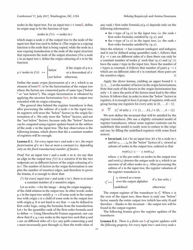
Conference’17, July 2017, Washington, DC, USA Mikołaj Bojańczyk and Amina Doumane
nodes in the input tree. For an input tree 𝑡 ∈ treesΣ, defineits origin map to be the function of type
nodes in 𝑓 (𝑡) → nodes in 𝑡
which maps a node 𝑥 of the output tree to the node of theinput tree that was used to define it. (The origin in a copyingfunction is the node that is being copied, while the node in anon-copying transduction is the node of the input structurethat represents the node of the output structure.) For a node𝑥 in an input tree 𝑡 , define the origin colouring of 𝑥 to be thefunction
𝑦 ∈ nodes in 𝑓 (𝑡) ↦→
below
if the origin of 𝑦 is 𝑥or a descendant of 𝑥
not below otherwise.
Define the name origin factorisation of 𝑥 in 𝑡 , which is anelement of treesTΓ, to be the factorisation of the output treewhere the factors are connected parts of same type (“below” or “not below”). The origin factorisation is obtained byapplying the ancestor factorisation fact↑ to the output treeextended with its origin colouring.The general idea behind the register transducer is that,
after processing the subtree of a node 𝑥 in the input tree,its registers will store the “below” factors in the origin fac-torisation of 𝑥 . We only store the “below” factors, and notthe “not below” factors, because only the “below” factorscan be computed using register updates based on the subtreeof the node 𝑥 in the input tree. The key observation is thefollowing lemma, which shows that the a constant numberof registers will be enough.
Lemma E.1. For every input tree 𝑡 and node 𝑥 in 𝑡 , the originfactorisation of 𝑥 in 𝑡 has at most a constant (i.e. dependingonly on the fixed transduction) number of factors.
Proof. For an input tree 𝑡 and a node 𝑥 in it, we say thatan edge in the output tree 𝑓 (𝑡) is 𝑥-sensitive if its the twoendpoints are in different factors of the origin colouring of 𝑥in 𝑡 . The number of factors in the origin factorisation is oneplus the number of sensitive edges, and therefore to provethe lemma, it is enough to show that:
(*) for every input tree 𝑡 and node 𝑥 in 𝑡 , there is at mosta constant number of 𝑥-sensitive edges.
Let us write→ for the image – along the origin mapping –of the child relation in the output tree. In other words, nodes𝑦, 𝑧 in the input tree satisfy𝑦 → 𝑧 if some node in the outputtree with origin 𝑧 is a child of some node in the output treewith origin 𝑦. It is not hard to see that→ can be defined infirst-order logic, using the formulas from the transduction.Let 𝑟 be the quantifier rank of the first-order formula usedto define→. Using Ehrenfeucht-Fraisse argument, one canshow that if 𝑥,𝑦, 𝑧 are nodes in the input tree such that 𝑦 and𝑧 are on different sides of 𝑥 (i.e. any path connecting 𝑦 and𝑧 must necessarily pass through 𝑥), then the truth value of
any rank 𝑟 first-order formula 𝜑 (𝑦, 𝑧) depends only on thefollowing information:• the 𝑟 -type of (𝑦, 𝑥) in the input tree, i.e. the rank 𝑟
first-order formulas satisfied by (𝑦, 𝑥); and• the 𝑟 -type of (𝑧, 𝑥) in the input tree, i.e. the rank 𝑟
first-order formulas satisfied by (𝑦, 𝑥).Since the relation→ has constant outdegree and indegree,and it can be defined using quantifier rank 𝑟 , follows thatif 𝑦 → 𝑧 are on different sides of 𝑥 then there can only bea constant number of nodes 𝑦 ′ such that (𝑦, 𝑥) and (𝑦 ′, 𝑥)have the same 𝑟 -type in the input tree. Since the number of𝑟 -types is constant, it follows that number of pairs 𝑦 → 𝑧
which are on different sides of 𝑥 is constant; these pairs arethe sensitive edges. □
Apply the above lemma, yielding an upper bound 𝑘 ∈{1, 2, . . .} on the number of factors in the origin factorisations.Note that each of the factors in the origin factorisation hasarity < 𝑘 , since the ports of the factors must lead to the otherfactors. It follows that, in order to store the “below” factors inregisters, it is enough to have 𝑘 groups of registers, with eachgroup having one registers for every arity in {0, . . . , 𝑘 − 1}:
𝑅def= {𝑟 𝑗
𝑖of arity 𝑗 : 𝑖 ∈ {1, . . . , 𝑘}, 𝑗 ∈ {0, . . . , 𝑘 − 1}}
We now define the invariant that will be satisfied by theregister transducer. (We use a slightly extended model ofregister transducers, where some register contents can beundefined; this model is easily seen to reduce to the origi-nal one, by filling the undefined registers with some fixednonces.• Invariant. Let 𝑡 be an input tree, let 𝑥 be a node in 𝑡 ,and let 𝑠1, . . . , 𝑠𝑛 be the “below” factors of 𝑥 , viewed assubsets of nodes in the output tree, ordered so that
root(𝑠1) ⪯ · · · ⪯ root(𝑠𝑛)where ⪯ is the pre-order on nodes in the output treeand root(𝑠𝑖 ) denotes the unique node in 𝑠𝑖 which is anancestor of all other nodes in 𝑠𝑖 . After processing thesubtree of 𝑥 in the input tree, the register valuation ofthe register transducer is
𝑟𝑗
𝑖↦→
𝑠𝑖 viewed as a termover the output alphabet if 𝑠𝑖 has arity 𝑗
undefined otherwise.
The output register of the transducer is 𝑟 01 . When 𝑥 isthe root of the input tree, then there is only one “below”factor, namely the entire output tree (which has arity 0) andtherefore – thanks to the invariant – the output tree will befound in the output register.The following lemma gives the register updates of the
transducer.
Lemma E.2. There is a finite set Δ of register updates withthe following property. For every input tree 𝑡 and every node 𝑥
24

First-order tree-to-tree functions Conference’17, July 2017, Washington, DC, USA
in 𝑡 , there is some 𝑢 ∈ Δ such that the register valuation of 𝑥(as defined in the invariant) is obtained by applying 𝑢 to theregister valuations of the children 𝑥1, . . . , 𝑥𝑛 of 𝑥 , in listed inleft-to-right order. Furthermore, there is a family {𝜑𝑢 (𝑥)}𝑢∈Δof unary queries over the input alphabet such that the updateassociated to a node 𝑥 is𝑢 if and only if the node satisfies𝜑𝑢 (𝑥)in the input tree.
Proof. The crucial observation is that each of the “below”factors in the origin factorisation for 𝑥 – seen as subsets ofnodes in the output tree – is a (disjoint) set union of the the“below” factors in the origin factorisations for the childrenof 𝑥 , plus the nodes in the output tree which have origin in𝑥 . Since there is at most a constant number of children andnodes with origin 𝑥 , there is a finite number – dependingonly on the transduction – of ways in which these factors canbe combined; this finite set of possible combinations is theset Δ. The “furthermore” part of the lemma, about computingthe update using first-order queries, follows from a simpleinspection of the first-order formulas used in defining thetransduction. □
The above lemma completes the definition of the registertransducer. Its register updates are Δ as in the lemma, andits transition function assigns label 𝑢 ∈ Δ to each node thatsatisfies 𝜑𝑢 (𝑥). The final part of the proof is showing that theregister updates are monotone. We use the following orderon the registers:
𝑟 01 < 𝑟 11 < · · · < 𝑟𝑘−11 < 𝑟 02 < 𝑟 12 < · · · < 𝑟𝑘−2𝑘
< 𝑟𝑘−1𝑘︸ ︷︷ ︸
lexicographic, with the lower index having priority
.
Let 𝑥 be a node in an input tree 𝑡 , and let 𝑠1, 𝑠2 be a “below”factor in the origin factorisation of 𝑥 , which are register con-tents in register valuation of 𝑥 . The registers storing 𝑠1 and𝑠2 will be ordered – according to the invariant – with respectto the pre-order on the root nodes of 𝑠1 and 𝑠2. Let 𝑥 ′ be theparent of 𝑥 . By the reasoning in the proof of Lemma E.2,there are “below” factors in the origin factorisation of 𝑥 ′which contain the factors 𝑠1 and 𝑠2; call these factors 𝑠 ′1 and𝑠 ′2 (possibly 𝑠
′1 = 𝑠 ′2). Since 𝑠
′1 contains 𝑠1 (as a set of nodes in
the output tree), and the same is true for 𝑠 ′2 and 𝑠2, we have
root(𝑠1) ⪯ root(𝑠2) implies root(𝑠 ′1) ⪯ root(𝑠 ′2)
which establishes monotonicity of the register updates.This completes the proof of Theorem 4.3.
F Normalisation of _-terms is a first-ordertransduction
In this part of the appendix, we show Theorem 6.1, whichsays that under some restrictions, normalisation of _-termsis a first-order transduction. Before proving this result in F.3,we will first explain in F.1 why these restrictions are unavoid-able. Then we show in F.2 that the set of _-terms satisfying
these restrictions form a first-order tree language. This resultwill be useful for the proof of Theorem 6.1.
F.1 Explaining the restrictionsRecall that Theorem 6.1 says that normalisation of _-termsis derivable under two assumptions: the input term shouldbe linear, and could be typed using a fixed finite set of types.If the linearity condition is removed, and because of iter-
ated duplication, the normal form of a well-typed _-term canbe exponential (or worse, see [27, Section 3.6]), as shown bythe following example.
Example F.1. Assume that we have two variables 𝑥𝑜 and𝑦𝑜→𝑜→𝑜 and consider the _-terms defined by:
𝑀0def= 𝑥𝑜 𝑀𝑛+1 = (_𝑥𝑜 .𝑦𝑜→𝑜→𝑜𝑥𝑜𝑥𝑜 )𝑀𝑛 .
The _-term𝑀𝑛 is well-typed and of type 𝑜 . It has size linearin 𝑛, but its normal form has size at least 2𝑛 .
If there was a first-order transduction normalising theseterms, it would be exponential-size increase, which is notpossible since all first-order transductions are linear-sizeincrease.
Being linear alone is not enough to normalise terms withfirst-order transductions. Another obstacle is terms that usetypes of unbounded complexity, as illustrated in the follow-ing example.
Example F.2. Consider the following _-terms, which havetypes of unbounded size:
𝑀𝑛 =
𝑛 times︷ ︸︸ ︷_𝑥𝑜 ._𝑥𝑜 . · · · _𝑥𝑜 . 𝑥𝑜
This is a well-typed affine term, whose type is
𝑜𝑛 → 𝑜def=
𝑛 + 1 arrows︷ ︸︸ ︷𝑜 → 𝑜 → · · · → 𝑜
To𝑀𝑛 , apply𝑚 arguments of type 𝑜 :
𝑀𝑛
𝑚 times︷ ︸︸ ︷𝑦𝑜 𝑦𝑜 · · ·𝑦𝑜 . (9)
We claim that the above _-term cannot be normalised usinga first-order transduction, or even a monadic second-ordertransduction. In order to normalise, a transduction wouldneed to be able to compare the numbers 𝑛 and𝑚 as follows:if𝑚 < 𝑛 the normal form contains _, if𝑚 = 𝑛 the normalform does not contain _, and if𝑚 > 𝑛 then the normal formis undefined because the _-term is not well-typed. Whetheror not a _-term (seen as a tree over a finite alphabet) contains_ is a first-order definable property, and first-order definableproperties are preserved under inverse images of first-ordertransductions. Therefore, if normalisation would be a first-order transduction, then there would be a first-order formulawhich would be true for terms of the form (9) with𝑚 > 𝑛 andwhich would be false for terms of the form (9) with𝑚 = 𝑛.
25

Conference’17, July 2017, Washington, DC, USA Mikołaj Bojańczyk and Amina Doumane
Such a formula cannot exist, which can be shown using apumping argument or Ehrenfeucht-Fraïssé games.
F.2 Restrictions of Theorem 6.1 are first-orderdefinable
In this section, we show that the restrictions of Theorem 6.1discussed above, are first-order definable, as stated in thefollowing theorem.Proposition F.3. Let 𝑋 be a finite set of simply typed vari-ables and let T be a finite set of simple types. The tree languageof linear _-terms which can be typed using T is first-order de-finable.
In the rest of this appendix, we denote by ΛT𝑋 this treelanguage. To prove Proposition F.3, we first show that for_-terms in ΛT𝑋 , checking if their type is 𝜏 , where 𝜏 is a typein T , is a fo property:Lemma F.4. For every type 𝜏 in T , there is a first-order query𝜑𝜏 such that:
∀𝑀 ∈ ΛT𝑋 𝑀,𝑢 |= 𝜑𝜏 ←→ 𝑀 |𝑢 : 𝜏where𝑀 |𝑢 is the sub-tree of𝑀 rooted in 𝑢.
Before establishing this lemma, let us see how Proposi-tion F.3 can be derived from it. Linearity can be easily seen asa first-order property. The hard part is to show that the set of_-terms which can be typed using T is first-order. Supposefor convenience that T is downward closed. For every type𝜏 in T , let 𝜑𝜏 be the formula given by Lemma F.4. In the fol-lowing, we use the binary formula Succ𝑖 (𝑢, 𝑣) which is validwhen 𝑣 is the 𝑖-th child of 𝑢, and which is easily expressiblein first-order logic.
Consider the unary formula Lambda(𝑢), which expressesthat 𝑢 is a binder node, that its type and the type of its childmatch well and both belong to T :
Lambda(𝑢) := _𝑥 (𝑢)︸︷︷︸𝑢 has label _𝑥
∧∨𝜎→𝜏 ∈T𝑥 :𝜎
𝜑𝜎→𝜏 (𝑢)︸ ︷︷ ︸𝑢 has type 𝜎 → 𝜏
∧∃𝑣 Succ1 (𝑢, 𝑣) ∧ 𝜑𝜏 (𝑣)︸ ︷︷ ︸the child of 𝑢 has type 𝜏
Similarly, consider the unary formula Application(𝑢) whichchecks that a node is an application node, that the type ofits children match well and that both belong to T :Application(𝑢) := @(𝑢)︸︷︷︸
𝑢 has label @
∧
∃𝑣,𝑤 ∨𝜎→𝜏 ∈T
Succ1 (𝑢, 𝑣) ∧ 𝜑𝜎→𝜏 (𝑣)︸ ︷︷ ︸the left child of 𝑢 has type 𝜎 → 𝜏
∧ Succ2 (𝑢,𝑤) ∧ 𝜑𝜎 (𝑤)︸ ︷︷ ︸the right child of 𝑢 has type 𝜎
Finally, consider the formula Variable(𝑢), which expressesthat 𝑢 is a variable node, whose type is in T :
Variable(𝑢) :=∨
𝑥 :𝜎 ∈T𝑥 (𝑢)︸︷︷︸
𝑢 has label 𝑥
We claim that the following (nullary) formula 𝜙 recognizesthe tree language ΛT𝑋
𝜙 = ∀𝑢. Variable(𝑢) ∨ Lambda(𝑢) ∨ Application(𝑢)If a _-term is in ΛT𝑋 , then it clearly satisfies 𝜙 . Suppose bycontradiction that there is a _-term𝑀 which is not in ΛT𝑋and yet satisfies 𝜙 . Let 𝑢 be the deepest node of 𝑀 whichis not in ΛT𝑋 (we identify in this proof a node 𝑢 and thesub-term𝑀 |𝑢 ). In particular, the descendants of 𝑢 are all inΛT𝑋 . The node 𝑢 cannot be a variable, since variable nodesare well-typed and their type is in T by the first disjunct of𝜙 . If 𝑢 was labeled by _𝑥 , where 𝑥 is of type 𝜎 , then by thesecond disjunct of 𝜙 there is a type 𝜏 such that 𝜎 → 𝜏 ∈ Tand the child 𝑣 of 𝑢 satisfies 𝜑𝜏 . Since 𝑣 is in ΛT𝑋 , its typeis 𝜏 by Lemma F.4. Hence 𝑢 is well-typed and its type is𝜎 → 𝜏 ∈ T . As a consequence 𝑢 is in ΛT𝑋 which is acontradiction. Finally, if 𝑢 was labeled by @, then by thethird disjunct of 𝜙 , its two children 𝑢1 and 𝑢2 would satisfyrespectively 𝜑𝜎→𝜏 and 𝜑𝜎 and by Lemma F.4 they are of type𝜎 → 𝜏 and 𝜎 respectively. The node 𝑢 is then well-typedand its type is 𝜏 (which is a type of T thanks to downwardcloseness). As a consequence, 𝑢 is in ΛT𝑋 , which gives acontradiction and concludes the proof.
We can go back now to the proof of Lemma F.4.
Proof of Lemma F.4. Let us show that the following unaryquery is expressible in first-order logic
”if 𝑡 is a _-term of Λ𝑠𝑋 , then its type is 𝜏 “:
For that, notice that the type of a well-typed term dependsonly on its left-most branch. In fact, the type of a term isexactly the type of its left-most branch in the following sens.Consider the (unranked) alphabet 𝑋_ := 𝑋 ∪ {@, _𝑥 |𝑥 ∈
𝑋 }. We can equip the words over 𝑋_ with the followingtyping rules:
𝑥 : 𝜎𝑢 : 𝜏
𝑢_𝑥 : 𝜎 → 𝜏
𝑢 : 𝜎 → 𝜏
𝑢@ : 𝜏where 𝑥 is of type 𝜎 and 𝜎, 𝜏 ∈ T .
We say that 𝑤 is of type 𝜏 and write 𝑤 : 𝜏 if there is atyping derivation for𝑤 : 𝜏 .
We can associate to every branch of a _-term a word over𝑋_ corresponding to the sequence of its labels read bottom-up. By induction on _-terms, we can easily show that thetype of a _-term is the type of the word corresponding to itsleftmost branch.By this last observation, we can reduce the query asking
if the type of a term is 𝜏 , to the same query but on 𝑋_ words.To show that the former is a first-order query, it is thensufficient to show that the following word language
𝑊𝜏 = {𝑤 ∈ 𝑋 .{@, _𝑥 |𝑥 ∈ 𝑋 }∗ | 𝑤 : 𝜏}is first-order definable, or equivalently that𝑊𝜏 is recognizedby a counter-free finite automaton. For that we proceed asfollows: first, we show that𝑊𝜏 is recognized by a pushdown
26

First-order tree-to-tree functions Conference’17, July 2017, Washington, DC, USA
automaton 𝑃𝜏 . Then we will show that the stack height of 𝑃𝜏is bounded, thus it can be turned into a deterministic finiteautomaton𝐷𝜏 . Finally, we show that the obtained automaton𝐷𝜏 is actually counter-free.
Consider the pushdown automaton 𝑃𝜏 whose• set of states is {𝑖, 𝑝, 𝑓 }, where 𝑖 is the initial state and𝑓 the accepting state;• input alphabet is the alphabet 𝑋_ ;• stack alphabet is the set of types T ;• and whose transition function is described as follows:– If the automaton is in the initial state 𝑖 with an emptystack, and if the symbol it reads is a variable 𝑥 oftype 𝜎1 → · · · → 𝜎𝑛 , then we go to the state 𝑝 andpush the symbols 𝜎𝑛, . . . , 𝜎1 in the stack in this order.The top-level symbol of the stack is then 𝜎1.
– If the automaton is in the state 𝑝 and it reads the sym-bol _𝑦, where 𝑦 is of type 𝜎 , then push the symbol𝜎 in the stack, and stay in the state 𝑝 .
– If the automaton is in the state 𝑝 , if it reads thesymbol @ and if the stack is non empty, then popthe top-level symbol and stay in the state 𝑝 .
– If the automaton reaches the end of the word beingin state 𝑝 , and if the stack contains the symbols𝜏1, . . . 𝜏𝑚 in this order, 𝜏1 being the top-level symbol,where 𝜏1 → · · · → 𝜏𝑚 is the type 𝜏 , then pop themall and go to the final state 𝑓 .
A word 𝑤 is accepted by 𝑃𝜏 if there is a run that reachesthe end of 𝑤 in the accepting state 𝑓 with an empty stack.We write (𝑟, 𝑠) 𝑤−→ (𝑟 ′, 𝑠 ′) if there is a run over the word 𝑤which starts in the state 𝑟 ∈ {𝑖, 𝑝, 𝑓 } and with a stack 𝑠 andends up in the state 𝑟 ′ ∈ {𝑖, 𝑝, 𝑓 } and with a stack 𝑠 ′.By induction on the length of the word𝑤 , we can easily
show that:
Lemma F.5. For every word𝑤 ∈ 𝑋 .{@, _𝑥 |𝑥 ∈ 𝑋 }∗, we havethat:
(𝑖, 𝜖) 𝑤−→ (𝑝, 𝜎𝑛 . . . 𝜎1) iff 𝑤 : 𝜎1 → · · · → 𝜎𝑛
A direct consequence of this lemma is that 𝑃𝜏 recognizes𝑊𝜏 . Another direct consequence is that the stack height of𝑃𝜏 is bounded by𝑚, the size of the longest type in T . Thus𝑃𝜏 can be turned into a DFA 𝐷𝜏 , by encoding the stack in-formation in the states. More precisely, the states of 𝐷𝜏 arepairs (𝑟, 𝑠) where 𝑟 ∈ {𝑖, 𝑝, 𝑓 } and 𝑠 is a stack of height atmost 𝑚, the initial state is (𝑖, 𝜖) and there is a transition(𝑟, 𝑠) 𝑎−→ (𝑟 ′, 𝑠 ′) where 𝑎 ∈ 𝑋_ ∪ {𝜖} if there is a corre-sponding run in 𝑃𝜏 . We show in the following that 𝐷𝜏 iscounter-free.Let us start with some observations. In the pushdown
automaton 𝑃𝜏 , the effect of a word 𝑤 on a stack 𝑠 , startingfrom the state 𝑝 is the following: it erases the first 𝑛 top levelelements of 𝑠 , and replaces them by a word 𝑢. The number 𝑛and the word 𝑢 do not depend on the stack 𝑠 but only on theword𝑤 . This is exactly what the following lemma claims.
Lemma F.6. For every word 𝑤 over 𝑋_∗, there is a naturalnumber 𝑛 and a word 𝑢 ∈ T ∗ such that if (𝑝, 𝑠) 𝑤−→ (𝑝, 𝑠 ′)then 𝑠 and 𝑠 ′ can be decomposed as follows:
𝑠 = 𝑡 .𝑣, 𝑠 ′ = 𝑡 .𝑢 and |𝑣 | = 𝑛.
The proof is an easy induction on the length of 𝑤 . As aconsequence we have that:
• If (𝑝, 𝑠1)𝑤−→ (𝑝, 𝑠2)
𝑤−→ (𝑝, 𝑠3) and |𝑠2 | > |𝑠1 | then|𝑠3 | > |𝑠2 |.• If (𝑝, 𝑠1)
𝑤−→ (𝑝, 𝑠2)𝑤−→ (𝑝, 𝑠3) and |𝑠2 | < |𝑠1 | then
|𝑠3 | < |𝑠2 |.• If (𝑝, 𝑠1)
𝑤−→ (𝑝, 𝑠2)𝑤−→ (𝑝, 𝑠3) and |𝑠2 | = |𝑠1 | then
𝑠3 = 𝑠2.Let us show that 𝐷𝜏 is counter-free. Suppose by contra-
diction that there is a word 𝑤 and pairwise distinct stacks𝑠1, . . . , 𝑠𝑛 such that
(𝑝, 𝑠1)𝑤−→ (𝑝, 𝑠2)
𝑤−→ . . . (𝑝, 𝑠𝑛)𝑤−→ (𝑝, 𝑠1).
By the first two properties above, we have necessarily that
|𝑠1 | = · · · = |𝑠𝑛 |
Thus by the third property, we have that
𝑠1 = · · · = 𝑠𝑛
which concludes the proof. □
F.3 Normalisation of _-termsThis section is dedicated to the proof of Theorem 6.1. Let usfirst introduce some terminology. In a _-term, we call redexa pattern of the following form
that is, an application node whose left child is an abstractionnode. In a well-typed _-term, we define the type of a redexto be the type of the left sub-term of its application node.In the figure above, the type of the redex is 𝜏 → 𝜎 . If theabstraction node of a redex is labeled by _𝑥 , we say that 𝑥 isthe variable of the redex and that this redex is an 𝑥-redex.
Let us go back to the proof of Theorem 6.1. Before normal-ising _-terms, the first thing to do is to discriminate those_-terms satisfying the restrictions of Theorem 6.1 from theothers. This amounts to pre-processing the normalisationprocess by the function
trees𝑋_ → trees𝑋_ + ⊥
which is the identity for inputs satisfying the restrictionsand is undefined otherwise. Let us see how this functioncan be derived. Thanks to Proposition F.3, the restrictionsof Theorem 6.1 are first-order definable, say by a first-order
27

Conference’17, July 2017, Washington, DC, USA Mikołaj Bojańczyk and Amina Doumane
query 𝜙 . By virtue of Proposition 5.1, the characteristic func-tion of 𝜙 is derivable. Now following the label’s root of theinput, we either output the input tree if the label says that itsatisfies the query 𝜙 , or outputs the undefined symbol oth-erwise. This last function can be easily derived. From nowon, we suppose that our _-terms satify the restrictions ofTheorem 6.1.
To normalise _-terms, we proceed by induction on the setof types T . The main observation is that, if the evaluation ofa redex of type 𝜎 → 𝜏 creates new redexes, then their typesare either 𝜎 or 𝜏 . They belong, in particular, to T \ {𝜎 → 𝜏}.As a consequence, we only need to show that the functionthat evaluates all the redexes of a fixed type is derivable. Aswe only create strictly smaller redexes, we need to iteratethis process only finitely many times, the bound being thesize of T .Since we have only finitely many typed variables, it is
enough to show that the function that evaluates all the re-dexes of a fixed type 𝜎 and a fixed variable 𝑥 is derivable.This will be our goal in the rest of this section.
Proposition F.7. Let 𝑋 be a finite set of simply typed vari-ables, T be a finite set of simple types, 𝑥 be a variable in 𝑋
and 𝜎 a simple type in T . The following tree-to-tree functionis derivable:
• Input. A _-term 𝑡 over variables 𝑋 .• Output. The _-term obtained by evaluating in 𝑡 allthe 𝑥-redexes of type 𝜎 , if 𝑡 is in ΛT𝑋 , and undefinedotherwise.
To show this proposition, we will factorise (via a derivablefunction) our _-terms into factors satisfying the followingproperties:(P1) All the 𝑥-redexes of type 𝜎 fall entirely into one of the
factors.(P2) Each factor have a a very specific shape called thin.
These factors are those _-terms with ports whose nor-mal form have the shape of a word (by opposition totrees, which is the general case).
By properties (P1) and (P2), it is enough to show that nor-malisation of thin _-terms (with ports) is derivable. For thispurpose, our strategy will be to prove that the word obtainedby normalising a thin _-term results from a pre-order traver-sal. Since pre-order traversal is a prime function, this impliesthat normalisation of thin _-terms is derivable.
The last ingredient to conclude the proof is to notice that𝛽-reducing the factors of (a factorisation of) a _-term, thenapplying a flattening, is the same thing as 𝛽-reducing theoriginal _-term, which follows directly from the fact that𝛽-reduction is a congruence on terms. This concludes theproof.In the rest of this section, we develop on each of the two
main steps of the proof, namely proving Properties (P1) and(P2). In Section F.3.1 we present thin _-terms with ports and
show how to normalise them. Then we show in Section F.3.2how to factorise a _-term into thin factors.
F.3.1 Normalisation of thin _-termsAs discussed earlier, we will need to normalise _-terms withports (the factors of our factorisation). In the following, wewill denote by 𝑋_ the ranked set
arity 0︷ ︸︸ ︷{𝑥 : 𝑥 ∈ 𝑋 } ∪
arity 1︷ ︸︸ ︷{_𝑥 : 𝑥 ∈ 𝑋 } ∪
arity 2︷︸︸︷{@}
With this notation, _-terms with ports are the inhabitants ofT𝑋_ . Normalisation of these terms generalizes that of usual_-terms in a straightforward way: the 𝑖-th port is replacedby a fresh variable 𝑥𝑖 , the obtained _-term (without ports) isevaluated as usual, then the variable 𝑥𝑖 is replaced back bythe port 𝑖 , as one can see in the following example.
Note that when a _-term is linear, its normal form has thesame number of ports. Note also that respecting the originalorder of ports in the normal form (which is important forcompositionality) may twist ports, as in the example above.As a consequence, normalisation of linear _-terms with portsis an arity preserving function of type:
T𝑋_ → F1T𝑋_ + ⊥
Let us present now the class of thin _-terms with ports.
Definition F.8. We say that the node of a _-term is branch-ing if its has at two distinct children which are not ports.
A thin _-term with ports is a term from T𝑋_ in which everybranching node is the application node of a redex.
In the remaining of this section we will omit the mention“with ports” if clear from the context.
Since thin _-terms branch only on redexes, the result oftheir normalisation is a “word”, in the sens that every nodehas at most one non-port child. We will show that this wordcan actually be obtained by a pre-order traversal of the origi-nal _-term. We will then use the prime preorder function toshow that normalisation of thin _-terms is derivable.
The left _-term below is linear and thin. The rednodes arethe ones which are not redexes nor the variables of theseredexes. The right _-term is its normal form: we can seethat nodes appear top-down in the pre-order of the original_-term.
28

First-order tree-to-tree functions Conference’17, July 2017, Washington, DC, USA
Proposition F.9. Let 𝑋 be a finite set of simply typed vari-ables,T be a finite set of simple types. The following tree-to-treefunction is derivable:• Input. A _-term 𝑡 over variables 𝑋 .• Output. The normal form of 𝑡 , if it is linear and thin,and undefined otherwise.
Let 𝑡 be a thin _-term and let 𝑢 be its normal form. Asnoticed before, 𝑢 has the shape of a word. Moreover, since 𝑡is linear, the nodes of 𝑢 are exactly the nodes of 𝑡 which arenot redexes, nor their variables.
Proposition F.10. Let 𝑡 be a linear thin _-term and let 𝑢 beits normal form. The order in which the inner nodes (ie. nonports) of 𝑢 appear top-down is the pre-order of 𝑡 .
Proof. To establish this proposition, we need the followinglemma.
Lemma F.11. Let 𝑡 be a linear thin _-term and let 𝑟 be one ofits redexes. Consider𝑚 to be the binder node of 𝑟 and 𝑛 to beits variable node.
The node 𝑛 is the greatest (that is the left-most) node in thesub-term 𝑡 |𝑚 w.r.t. the pre-order.
Proof. We proceed by induction on the length of the pathbetween𝑚 and 𝑛. When it is 0 the result is clear. Supposeby contradiction that it is strictly greater than 0 and thatthere is a node 𝑜 which is strictly greater than 𝑛. We take𝑜 to be the smallest node which is greater than 𝑛. Since 𝑡is thin, the least common ancestor 𝑙 between 𝑛 and 𝑜 is anapplication node of a redex. Since 𝑛 is smaller than 𝑜 , 𝑛 isthe left descendant of 𝑙 , in other words it is the descendantof the left child 𝑝 of 𝑙 , which is a binder. The node𝑚,𝑛, 𝑜 and𝑝 are illustrated below:
By induction hypothesis, the variable bound by 𝑝 is strictlygreater than 𝑛. Is is also strictly smaller than 𝑜 , which givesa contradiction and concludes the proof. □
Let us go back to the proof of our proposition. Considertwo inner nodes 𝑛,𝑚 of 𝑡 which are also nodes of𝑢, and suchthat𝑚 is smaller than 𝑛 is the pre-order of 𝑡 (we well call itsimply pre-order in the rest of the proof). We show that 𝑛 isa descendant of𝑚 in 𝑢. There is two cases to consider:• Either 𝑛 is a descendant of 𝑚 in 𝑡 , in this case wecan conclude easily since 𝛽-reduction preserves thedescendant relation. Indeed, by a small analysis of 𝛽-reduction, one can notice that a reduction step mayextend the descendant relation, but can never change(or break) the order of two comparable nodes in theoriginal _-term.• Otherwise, let us consider the lowest common ancestor𝑝 of𝑚 and 𝑛. We proceed by induction on the lengthof the path between 𝑚 and 𝑝 . By definition of thin_-terms, since 𝑝 is branching it is necessarily an appli-cation node, whose left child 𝑞 is a binder node, let ussay _𝑥 . By Lemma F.11,𝑚 is smaller w.r.t. the pre-orderthan the node 𝑟 of the variable bound by 𝑞 . We arethen left with the following two situations. The firstcase, illustrated by the left figure below, is when 𝑟 is adescendant of𝑚 in 𝑡 . In this case, after one reductionstep 𝑛 will be a descendant of of𝑚. The other case iswhen𝑚 is in the left of 𝑟 in 𝑡 , as illustrated by the rightfigure below. In this case, after one reduction step, thelowest common ancestor between𝑚 and 𝑛 will be adescendant of 𝑝 , and we can conclude by inductionhypothesis.
This concludes the proof of the first claim. □
Let us construct now a derivable function which computesthe normal form of linear thin _-terms. We illustrate thisconstruction on the term 𝑡 below which will be our runningexample in this proof.
Proof of Proposition F.9. Let 𝑡 be a linear thin _-term in T𝑋_ .1. We start by distinguishing the redexes of 𝑡 and their
variables from the other nodes. For that, we apply29

Conference’17, July 2017, Washington, DC, USA Mikołaj Bojańczyk and Amina Doumane
the characteristic function of the following first-orderquery 𝜑 :
“The node 𝑢 is a redex or a variable of a redex”This query is first-order expressible. Indeed it is thedisjunction of the following queries
@Redex(𝑢) = @(𝑢) ∧ ∃𝑣 Child1 (𝑢, 𝑣) ∧∨
𝑥 ∈𝑋 _𝑥 (𝑣)
_Redex(𝑢) = _𝑥 (𝑢) ∧ ∃𝑣 Child1 (𝑣,𝑢) ∧@(𝑣)
𝑋Redex(𝑢) = ∨𝑥 ∈𝑋 𝑥 (𝑢) ∧ ∃𝑣 _Redex(𝑣) ∧ 𝑣 binds 𝑢
where@Redex(𝑢) says that𝑢 is the application node ofa redex, _Redex(𝑢) says that it is the abstraction nodeof a redex and 𝑋Redex(𝑢) says that it is the variableof a redex. The formula 𝑢 binds 𝑣 , defined below, is abinary first-order query expressing that the node 𝑢 isan abstraction node that binds 𝑣 .∨𝑥 ∈𝑋
_𝑥 (𝑢) ∧ 𝑥 (𝑣) ∧ 𝑢 < 𝑣 ∧ ∀𝑢 < 𝑤 < 𝑣 ¬_𝑥 (𝑤)
The query 𝜑 being first-order, its characteristic func-tion is derivable thanks to Proposition 5.1.When we apply this function to 𝑡 , we get a term inT(𝑋_ + 𝑋_) term below. Below is the effect of this firststep on our running example. We colored in red thenodes belonging to the first copy of 𝑋_ , that is thenodes satisfying the query 𝜑 . These nodes are the onesthat will disappear in the normal form of 𝑡 .
2. After that, we apply the preorder function
preorder : T(𝑋_ + 𝑋_) → F1T(𝑋_ + 𝑋_ + 0 + 2)After this step, our initial term becomes
In this term, the nodes of the normal form appear inthe right order thanks to Prop. F.10. Now, we only needto get rid of the redexes and the variable nodes that
participated in the computation of the normal form(that is the ones colored in red) together with the nodesand introduced by the preorder function.
3. For this purpose, we apply the function
T(𝑋_ + 𝑋_ + 0 + 2) → T(𝑋_ + 𝑋_ + 0 + 2 + 1)
which adds the unary symbol 1 as the parent of everynode 2. This function can be easily implemented usingthe derivable homomorphism function of Example ??.Then we apply the factorisation fact↑ to separate thesymbol 1 from the others:
fact↑ : T(𝑋_ + 𝑋_ + 0 + 2 + 1) → T(T(𝑋_ + 𝑋_ + 0 + 2) + T1))
After this step, our example term becomes like this
4. Now consider the function
𝑔 : T(𝑋_ + 𝑋_ + 0 + 2) → F1T(𝑋_ + 𝑋_ + 0 + 2)
which is the identity function, except for the followingfinite set of terms for which it is defined in figure 8.The red elements are those belonging to the first copyof 𝑋_ .Now back to our term, we replace the T1 factors bythe empty term, and to the other factors we apply thefunction 𝑔. After that, we apply the function
F1F1Σ→ F1Σ
which untwists two consecutive applications of F1.Doing so, we get a term of type
F1T(𝑋_ + 𝑋_ + 0 + 2)
which is the normal form of 𝑡 . Our running examplebecomes then
30

First-order tree-to-tree functions Conference’17, July 2017, Washington, DC, USA
Figure 8. Definition of the function 𝑔.
5. Note that we obtained the desired term, but not withthe desired type. To obtain a term in F1T𝑋_ , we get ridof the labels 0 + 2 by transforming them respectivelyinto variables and application nodes. The choice ofwhich variables to choose is not important, since theonly terms that will actually have 0 + 2 in their resultsare _-terms which are not linear or not thin.
□
F.3.2 Factorising _-terms into blocks of thin _-termsIn a linear _-term, we call full redex a set of nodes containinga redex, the node of its variable, together with the set ofnodes between them, as illustrated below
Proposition F.12. For every finite set of typed variables 𝑋 ,for every finite set of types T and for every 𝑥 ∈ 𝑋 and 𝜎 ∈ T ,there is a factorisation
𝑓 : T𝑋_ → TT𝑋_ + ⊥which satisfies, for every linear _-term 𝑡 , that(1) every full 𝑥-redex of type 𝜎 in 𝑡 is entirely contained in
one of the factors of 𝑓 (𝑡);(2) the factors of 𝑓 (𝑡) are thin.
and is undefined otherwise.
Proof. We define the function 𝑓 as the composition of thefollowing three functions
T𝑋_𝑔−−→ T(𝑋_ + 1) block↑−−−−−−→ T(T𝑋_ + T1) erase−−−−−→ TT𝑋_
The function 𝑔 will indicate, using the unary symbol 1, theplaces wheres two distinct blocks of 𝑓 will be separated. Wewill describe it more precisely a bit later. The function block↑will create these blocks and finally, we erase all the factorsT1.
The function block↑ is a prime function and erase can beeasily derivable. Let us show how to derive the function 𝑔, sothat the 1-nodes it introduces creates blocks satisfying theconditions (1) and (2) of Proposition F.12 (when the input isa linear _-term).
We define 𝑔 as the composition of the characteristic func-tion of three first-order unary queries: @redex,Right andLeft, followed by a homomorphims ℎ. We define them in thefollowing:• The property @Redex checks whether a node is theapplication node of an 𝑥-redex of type 𝜎 . It can beexpressed by the following first-order formula, where𝜑𝜎 is a first-order formula which decides if the type ofa node is 𝜎 (for instance the one given by Lemma F.4):
App(𝑢) :=@(𝑢) ∧ ∃𝑣 Succ1 (𝑢, 𝑣) ∧ _𝑥 (𝑣) ∧ 𝜑𝜎 (𝑣)• The query Right (resp. Left) checks if the node is anapplication node, which lies, together with his right(resp. left) child, between the application node of an 𝑥-redex of type 𝜎 and the node it binds. Those propertiescan be easily expressed by a first-order formula.
Whenwe apply the characteristic functions of these queriesto a term in T𝑋_ , each node will be decorated by three infor-mations: whether is satisfies or not App, whether is satisfiesor not Right and whether is satisfies or not Left. Note thatfor linear _-terms, some combinations of these propertiescannot hold in the same node. For instance, a node cannot sat-isfy Right and Left simultaneously, as this would contradictlinearity.
31

Conference’17, July 2017, Washington, DC, USA Mikołaj Bojańczyk and Amina Doumane
Now we define the homomorphism ℎ, which maps the_-terms with these three informations to terms of T(𝑋_ + 1).We define the action of ℎ on each node, depending on itslabel and the three informations it contains:• If the label of the node is 𝑦 or _𝑦 for some variable𝑦 ∈ 𝑋 , or if the label is @ and satisfies App, then ℎ
returns the same node (seen as a term), forgetting theextra three informations.• If the node is an application node satisfying
¬App ∧ ¬Right ∧ ¬Leftthen ℎ adds 1 to the two children of the node.• If the node is an application node satisfying
¬App ∧ ¬Right (resp. ¬App ∧ ¬Left)then ℎ adds 1 to the left (resp. right) child of the node.
Let 𝑡 be a linear _-term. We show that the factors induced by𝑔 satisfy the two conditions of Proposition F.12. First of all,by analyzing the action of ℎ on each node, note that everyapplication node will receive 1 as one of its children, exceptwhen it is satisfies App. Thus the only branching nodes in afactor are redexes, hence the factors are thin. Now supposeby contradiction that there is some full 𝑥-redex of type 𝜎of 𝑡 which is not entirely contained in a factor. This meansthat in 𝑔(𝑡) there is a 1 between the application node ofsome 𝑥-redex of type 𝜎 and its variable. By construction ofℎ, 1 is the child of an application node (call it 𝑛). Supposew.l.o.g. that it is the right child of𝑛. The node𝑛 cannot satisfyApp because it got 1 as a child by ℎ. Is satisfies Right by thecontradiction hypothesis. Thus its satisfies ¬App ∧ ¬Right,therefore it receives also 1 as its left child by ℎ. This meansthat 𝑛 received 1 for its both children, and the only way toget that is to satisfy ¬App ∧ ¬Right ∧ ¬Left, which gives acontradiction. □
G Decomposing the unfolding functionAs discussed in the main body of the paper, the unfoldingfunction may be regarded as unsatisfactory. In this section,we will decompose it into a collection of small functionscontaining no form of iteration.
We present these new prime functions in Section G.1, andstate the main result of this section which is that term unfold-ing can be derived from these new prime functions (and theother prime functions of Section 3). To prove this result, ourstrategy is to show that term unfolding can be derived for arestricted class of terms that we call homogeneous, and thento show that every term can be factorised into homogeneousterms.The notion of homogeneous terms, and the result about
decomposing arbitrary terms into homogeneous ones, arepresented in Section G.2. Next, in Section G.3, we show howterm unfolding can be done for homogeneous inputs. Finally,in Section G.4 we prove the main result of the section bycombining the results of Sections G.2 and G.3.
• Unit.Σ ↔ Σ · 1
• Associativity.
(Σ · Γ) · Δ → Σ · (Γ · Δ)
• Terms as shallow terms.1 + Σ.TΣ ↔ TΣ
Every term is either just a port,or has a root and child subterms.
• Tensors as shallow terms.Σ𝑛 ↔ 𝑛.Σ
Figure 9. Prime functions for shallow terms.
G.1 New prime functions replacing the unfoldingIn order to decompose the unfolding function, we enrichdatatypes with the constructor of shallow terms introducedin Section A.1.We present the prime functions which will replace the
unfolding in Figures 9–12. Prime functions of Figure 9 de-scribe the behaviour of the shallow term datatype. Figure 10contains some additional laws for the fold datatype and Fig-ure 11 contains some new ditributivity laws. Prime functionsof Figure 12 are weak versions of the unfolding function,containing no form of iteration.
Note that some of these functions were already presentedin Appendix A.3 to define formally the unfolding function:distributivity of shallow terms over fold, distributivity ofshallow terms over product (Figure 11), and the matchingfunction (Figure 12). In appendix A.3, those functions wereintroduced in a very formal (hence verbose) way. In this ap-pendix, we made the opposite choice of giving only informaldefinitions trough some hopefully clear and unambiguouspictures.The main result of this section is that the unfolding can
be replaced by the more atomic functions of Figures 9–12, inpresence of the prime functions presented in Section 3, asstated in the following theorem
32

First-order tree-to-tree functions Conference’17, July 2017, Washington, DC, USA
• Unit.Σ → F𝑘Σ𝑘
• Increase fold.F𝑘Σ → F𝑘+1Σ
• Decrease fold.F𝑘+1Σ → F𝑘Σ + ⊥
• Projection of products.
Σ × Σ → F1Σ
Figure 10. Additional prime functions for folds.
Theorem G.1. The unfolding function can be derived us-ing the functions of Figures 9–12 and the prime functions ofSection 3.
In the rest of Appendix G, derivable means derivable fromthe prime functions of Figures 9–12 and the prime functionsof Section 3 except from unfolding.
G.2 Factorisation forestsThis section is devoted to stating and proving a tree versionof the Factorisation Forest Theorem of Imre Simon. Our re-sult differs from the original Factorisation Forest Theorem inthe following ways: (a) we consider trees instead of strings;(b) we use aperiodic finite monoids instead of arbitrary finitemonoids; and (c) the factorisation in the conclusion of thetheorem can be computed by a derivable function. A treegeneralisation of the Factorisation Forest Theorem was al-ready proved by Colcombet [14, Theorem 1 and Section 3.3],but Colcombet’s result is proved for monadic second-orderlogic, and therefore it does not satisfy condition (c).
Factorisation forests The idea behind factorisation forestsis to split a term into a nested factorisation, which is a termof terms of terms, and so on up to a certain depth. Define anested factorisation of depth 𝑘 ∈ {1, 2, . . .} over alphabet Σto be an element of T𝑘Σ which is defined by
T0Σ = Σ and T𝑘+1Σ = TT𝑘Σ.
• Fold over coproduct.
F𝑘 (Σ1 + Σ2) → F𝑘Σ1 + F𝑘Σ2(𝑎, 𝑖)/𝑓 ↦→ ((𝑎/𝑓 ), 𝑖)
• Shallow terms over coproduct.
(Σ1 + Σ2).Γ → (Σ1 .Γ) + (Σ2.Γ)(𝑎, 𝑖) (𝑡1, . . . , 𝑡𝑛) ↦→ (𝑎(𝑡1, . . . , 𝑡𝑛), 𝑖)
• Shallow terms over product.
(Σ1 × Σ2).Γ → (Σ1.Γ) × (Σ2.Γ)
• Fold over product.
F𝑘 (Σ1 × Σ2) → F𝑘 ((F𝑘Σ1) × (F𝑘Σ2))
• Fold over product (bis).
(F𝑘Σ1) × (F𝑘Σ2) → F𝑘 (Σ1 × Σ2)
• Shallow terms over fold.Σ.F𝑘Γ → F𝑘 (Σ.Γ)
• Fold over shallow terms.F𝑘 (Σ · Γ) → (F𝑘Σ) · Γ [𝑘 ]
Γ is a set of unary elements.
Figure 11. Additional distributivity prime functions.
Nested factorisations can be flattened to terms by using anoperation flat𝑘 : T𝑘Σ→TΣ defined by
flat1 = identity and flat𝑘+1 def= flat ◦ T(flat𝑘 ).
33

Conference’17, July 2017, Washington, DC, USA Mikołaj Bojańczyk and Amina Doumane
• Untwist.TF1Σ → F1TΣ
• External fold.TF𝑘Σ → F𝑘TF𝑘Σ
• Matching.
F𝑘Σ.Γ𝑘 → F1 (Σ.Γ)
Figure 12. Weak forms of unfolding.
An equivalent definition of flat𝑘+1 would be flat𝑘 ◦ T𝑘−1flat,the equivalence of these definitions corresponds to the factthat T is a monad.
Branches and subbranches Define a branch in a rankedset to be an element of the ranked set together with a distin-guished port. We draw branches like this:
We write BΣ for the (unranked) set of branches over a rankedset Σ. For a term, we classify its edges as internal (linking anon-port node with a non-port child) and external (linking anon-port node with a child port). Each edge in a term 𝑡 ∈ TΣcorresponds to a branch over Σ, namely the branch whichleads to the edge. Any branch obtained this way is called asubbranch of 𝑡 . Here is a picture of subbranches in the caseof a term of terms:
the subbranch corresponding to
an internal edge
the subbranch corresponding toan external edge
Branches in terms form a monoid. Using the monoid struc-ture of branches in terms, we can extend any function ℎ :BΣ→ 𝑀 , with𝑀 a monoid, to a monoid homomorphism
ℎ (𝑛) : BT𝑛Σ→ 𝑀
whichmaps a branch of a term to the product – in themonoid𝑀 – of all of its subbranches (after flattening). A more formaldefinition is that ℎ (0) is the same as ℎ, while ℎ (𝑛+1) is theunique monoid homomorphism which makes the followingdiagram commute
BT𝑛Σℎ (𝑛)
##Bunit��
BT𝑛+1Σℎ (𝑛+1)
// 𝑀
The idea behind factorisation forests, as expressed in Def-inition G.2 below, is to factorise a term into a term of termsof terms (etc.) so that the depth of nesting is bounded, andat each level all branches behave regularly with respect tosome monoid homomorphism.
DefinitionG.2 (Homogeneous factorisations). Letℎ : BΣ→𝑀 be a function into a monoid𝑀 .• We say that a factorisation 𝑡 ∈ TTΣ is homogeneouswith respect to ℎ if it either:1. it is a shallow term (which means that all internal
edges originate from the root); or2. all internal subbranches of 𝑡 have the same value
under ℎ (1) ; or3. if 𝑎, 𝑏 ∈ 𝑀 appear as values – underℎ (1) – of internal
branches in 𝑡 , then 𝑎𝑏 = 𝑎.• We say that a nested factorisation 𝑡 ∈ T𝑛Σ is hereditar-ily homogeneous with respect to ℎ if either 𝑛 = 1 and 𝑡is the unit of a letter, or 𝑛 ≥ 2 and both:1. it is homogeneous with respect to ℎ (𝑛−1) ; and2. every node has a label in T𝑛−1Σ that is hereditarily
homogeneous with respect to ℎ.
Recall that a finite monoid is aperiodic if it has only trivialsubgroups. An equivalent definition is that every element𝑚of the monoid satisfies
∃𝑛 ∈ {1, 2, . . .}𝑚𝑛 =𝑚𝑛+1 .
A famous theorem of Schützenberger, McNaughton and Pa-pert, see [28, Theorem VI.1.1] says that the languages of
34

First-order tree-to-tree functions Conference’17, July 2017, Washington, DC, USA
words recognised by homomorphisms into finite aperiodicmonoids are exactly those that can be defined in first-orderlogic. This is the reason why we consider aperiodic monoids.
Example G.3. Let 𝑘 ∈ {1, . . .} and consider the monoid ofpartial functions
{1, . . . , 𝑘} → {1, . . . , 𝑘}.This monoid is not aperiodic, because it contains the group ofall permutations of {1, . . . , 𝑘}. Consider now the restrictionof this monoid to partial functions which are monotone(this is a monoid, because such functions are closed undercomposition). This monoid is aperiodic, because if 𝑓 is apartial function, then for every 𝑖 ∈ {1, 2, . . . , 𝑘} the sequence
𝑓 1 (𝑘), 𝑓 2 (𝑘), 𝑓 3 (𝑘), . . .reaches a fixpoint (or becomes undefined) in at most 𝑘 steps.
We are now ready to state our version of the FactorisationForest Theorem.
Theorem G.4 (Factorisation Forest Theorem). Let Σ be aranked set and let ℎ : BΣ→ 𝑀 be a function into a finite ape-riodic monoid𝑀 . There is some 𝑛 ∈ {1, 2, . . .} and a function
𝑓 : TΣ→ T𝑛Σ
such that flat𝑛 ◦ 𝑓 is the identity on TΣ, and all outputs of 𝑓are hereditarily homogeneous with respect to ℎ. Furthermore,if Σ is finite7 then 𝑓 is derivable.
In the proof below, the constructions are designed so thatthey can be formalised using derivable functions, howeverwe leave the details of the “Furthermore” part to the reader.
Define a good set to be any subset 𝑋 ⊆ TΣ which admits afunction
𝑓 : TΣ→ T𝑛Σ for some 𝑛 ∈ {1, 2, . . .}such that flat𝑛 ◦ 𝑓 is the identity on TΣ, and 𝑓 restricted to 𝑋produces only hereditarily homogeneous outputs. Our goalis to show that the entire set TΣ is good. To prove this, we usea more refined result, stated below, which has a parameterthat can be used for induction. We say that a term 𝑡 ∈ TΣuses𝐴 ⊆ 𝑀 for internal subbranches if all internal subbranchhave image under ℎ (1) that belongs to 𝐴.
Lemma G.5. Let Σ be a ranked set and let ℎ : BTΣ→ 𝑀 bea monoid homomorphism into a finite aperiodic monoid 𝑀 .For every 𝐴 ⊆ 𝑀 , the terms that use 𝐴 for inner subbranchesis good.
Theorem G.4 follows immediately from the lemma, bytaking 𝐴 to be the entire monoid. The rest of Section G.2is therefore devoted to proving the lemma. The proof is byinduction on two parameters: (a) the size of 𝐴; and (b) thesize of the semigroup ⟨𝐴⟩ ⊆ 𝑀 that is generated by𝐴. These7This finiteness assumption could be relaxed by saying that Σ is possiblyinfinite but the function ℎ is derivable, in the sense that a derivable functioncan decorate the ports of an element in Σ by their values under𝑀 .
parameters are ordered lexicographically, with the size ofthe semigroup being more important.
The induction base is when 𝐴 contains only one element𝑎 of the monoid. If a term uses {𝑎} for internal subbranches,then applying Tunit leads to a factorisation that is homoge-neous according to item 2 of Definition G.2, which is alsohereditarily homogeneous because all nodes are labelled byunits. This completes the proof of the induction base.
In the proof of the induction step, we consider two cases.• The first case is when every 𝑎 ∈ 𝐴 satisfies
⟨{𝑏𝑎 : 𝑏 ∈ ⟨𝐴⟩}⟩ = ⟨𝐴⟩This means that every for every 𝑎 ∈ 𝐴, the function𝑏 ↦→ 𝑏𝑎 is a permutation of ⟨𝐴⟩. Since the monoid isaperiodic, this permutation must necessarily be theidentity. Therefore, we have 𝑎𝑏 = 𝑎 for every 𝑎, 𝑏 ∈⟨𝐴⟩. This means that if all a term uses 𝐴 for internalsubbranches, then applying Tunit gives a factorisationwhich is hereditarily homogeneous according to item 3of Definition G.2.• If the previous item does not hold, then there is some𝑎 ∈ 𝐴 such that
⟨{𝑏𝑎 : 𝑏 ∈ ⟨𝐴⟩}⟩is a proper subsemigroup of ⟨𝐴⟩. Fix some such 𝑎. De-fine a sensitive edge in a term 𝑡 ∈ TΣ to be any internaledge where the corresponding subbranch has value 𝑎under ℎ (1) . Call an internal edge post-sensitive if it isnot sensitive, but its parent edge is. Here is a picture:
external edge
sensitive internal edge
post-sensitive internal edge
internal edgethat is neithersensitive nor
post-sensitive
Define the split of a term to be the factorisation whichcuts along post-sensitive edges, as shown in the fol-lowing picture:
We only consider splits for terms which use 𝐴 for in-ternal subbranches. Roughly speaking, we will show
35

Conference’17, July 2017, Washington, DC, USA Mikołaj Bojańczyk and Amina Doumane
that all factors in the split are good, and the split itselfis good. Combining these two observations, we willsee that all termsWe begin by looking at the factors in the split (of aterm where 𝐴 is used for internal subbranches). Hereis a picture of such a factor:
If we follow a branch in an factor of the split, from rootto port, we first have a sequence of non-sensitive edgesfrom the original term, followed by a sequence of sen-sitive edges. Group the non-sensitive edges together,and group the sensitive edges together, resulting in ashallow term from TΣ.TΣ, which is illustrated in thefollowing picture:
no sensitive edges
only sensitive edges
In the resulting shallow term, the root is labelled bya term without sensitive edges (i.e. it is a term whichuses 𝐴 − {𝑎} for internal subbranches), while the chil-dren are labelled by terms where all edges are sensitive(i.e. they are terms which use {𝑎} for internal sub-branches). We can apply the induction in both cases,and combine the resulting nested factorisations usinga shallow term, as in item 1 of Definition G.2.Having established that the factors of the split aregood, we turn to the split itself. By construction, everysubbranch of the split is mapped by ℎ (1) to the smallersemigroup
⟨{𝑏𝑎 : 𝑏 ∈ ⟨𝐴⟩}⟩,We can view the split as a term over alphabet Γ = TΣ.Since all internal subbranches of the split are in thesmaller subsemigroup, we can apply the inductionassumption of the lemma (with Γ and ℎ (1) ), showingthat the split is good. More formally, the set
{split of 𝑡 : 𝑡 ∈ TΓ uses 𝐴 for internal subbranches}is good. To show now that original set of terms 𝑡 thatuse 𝐴 for internal branches is good, we first apply the
split, then compute the nested factorisation for thesplit, and finally we compute the nested factorisationsfor the factors of the split (the letters from Γ.).
G.3 Term unfolding for homogeneous inputsThe goal of this section is to show that term unfolding isderivable for homogeneous inputs. Actually, we will firstshow that unfolding is derivable for another particular caseof inputs which we call constant-twists. Then we will use thisfunction as a macro to unfold the homogeneous inputs.
G.3.1 Unfolding constant-twist functionsIn the proof of this section, it will be sometimes convenientto manipulate partial shallow terms, that is shallow termswhere some children of the root maybe ports. We will definethem more precisely, and show that unfolding matrix powerof partial shallow terms is derivable.
Partial shallow unfold If Γ and Δ are types, we defineΓ ⊙ Δ to be Γ.(Δ + {1}). We call its inhabitants the partialshallow terms. A partial shallow term looks like this, wherewe omitted to draw the element 1
We define the partial shallow unfolding function as the ex-tension of the shallow unfold function of Figure 12 to partialshallow terms. It is the function of type
F𝑘Σ ⊙ Γ𝑘 → F𝑘 (Σ ⊙ Γ)
defined as in the following picture
the partial shallow unfolding function can be derived asfollows. Consider the functions 𝑓 and 𝑔 defined as follows
𝑓 : Γ𝑘Increse-fold−−−−−−−−→ F𝑘Γ𝑘
F𝑘 (]1)𝑘−−−−−→ F𝑘 (Γ + 1)𝑘
𝑔 : 1k-Unit−−−−→ F𝑘1𝑘
F𝑘 (]2)𝑘−−−−−→ F𝑘 (Γ + 1)𝑘
We start by lifting 𝑓 and 𝑔 as follows
F𝑘Σ ⊙ Γ𝑘def= F𝑘Σ · (Γ𝑘 + 1) → F𝑘Σ · F𝑘 (Γ + 1)𝑘
We compose the obtained function with the prime functionwhich distributes the shallow product over the fold:
F𝑘Σ · F𝑘 (Γ + 1)𝑘 → F𝑘 (F𝑘Σ · (Γ + 1)𝑘 )
Now we can apply the shallow unfold function, more pre-cisely we lift it along the constructor F𝑘 . Then we compose
36

First-order tree-to-tree functions Conference’17, July 2017, Washington, DC, USA
the result with the product of the graded monad:
F𝑘 (F𝑘Σ · (Γ + 1)𝑘 )F𝑘Shallow unfold−−−−−−−−−−−−→ F𝑘F1 (Σ · (Γ + 1))
Then we compose the result with the product of the gradedmonad, to obtain the desired function
F𝑘F1 (Σ · (Γ + 1))flat−−→ F𝑘Σ · (Γ + 1)
def= F𝑘Σ ⊙ Γ
Term unfolding for constant-twist inputs We say thata term 𝑡 ∈ TΣ [𝑘 ] is a constant-twist term if each twist ofan internal branches is a constant function. Note that theinternal twists need not to be the same constant function.Here is an example of a constant-twist term
This section is devoted to proving the following lemma.
Lemma G.6. Let 𝑘 ∈ {1, 2, . . .}. There is a derivable function
𝑓 : TΣ [𝑘 ] ⇀ (TΣ) [𝑘 ]
which coincides with unfolding for all constant-twist inputs.
Proof. The function 𝑓 can be derived using the followingsteps. We use the example of the constant-twists term aboveas a running example.
1. We start by applying the external unfolding function.We get a term in F𝑘TΣ [𝑘 ] . Our example becomes likethis
2. Next, we will transform each matrix power node intoa tensor product as follows
Σ [𝑘 ] → F𝑘 (F𝑘Σ × . . . F𝑘Σ) → F1 (F𝑘Σ)𝑘
The idea here is that, since the image of each twist is asingleton, the ports of the matrix power are indepen-dent. We can then transform safely each node into atensor product. After that, we transform each tensorproduct (F𝑘Σ)𝑘 into a shallow term 𝑘.F𝑘Σ which wesee itself as a term of type T(𝑘 + F𝑘Σ). After the appli-cation of the unfolding function unfold1 followed bya flattening, and the simplification of F𝑘F1T(𝑘 + F𝑘Σ)into F𝑘T(𝑘 + F𝑘Σ) we get a term in F𝑘T(𝑘 + F𝑘Σ). Ourrunning example becomes as follows after this step
3. Now we apply the factorization
T(𝑘 + F𝑘Σ) → TT(𝑘 + F𝑘Σ)
which regroups each element F𝑘Σ with its children oftype 𝑘 in the same factor, and leaves the other nodesin isolated factors. At this point our term looks likethis
Note that this factorization have the following shape:the root is labeled by 𝑘 , and all the other nodes havelabels in (F𝑘Σ) ⊙ 𝑘 . We want to reflect this structurein the type by applying the following function
TT(𝑘 + F𝑘Σ) → 𝑘.T((F𝑘Σ) ⊙ 𝑘)
This function can be implemented easily using thedecomposition function, the functions which mapsevery type to 1 and mechanisms of raising errors.
4. In each node (F𝑘Σ) ⊙ 𝑘 , we transform 𝑘 into 1𝑘 (thisfunction is basic since its domain is finite). After that,
37

Conference’17, July 2017, Washington, DC, USA Mikołaj Bojańczyk and Amina Doumane
we apply the partial shallow unfold function, com-posed with the prime functions eliminating the 1 anddecreasing the fold:(F𝑘Σ) ⊙ 𝑘 → F𝑘 (Σ ⊙ 1) → F𝑘Σ→ F1Σ
as illustrated by the following picture
5. At this point we have a term of type F𝑘 (𝑘 · TF1Σ). Weapply the untwist function
TF1Σ→ F1TΣ
then the function which transforms shallow terms intotensor product
𝑘 · F1TΣ→ (F1TΣ)𝑘
Now our term is of type F𝑘 (F1TΣ)𝑘 . To conclude, weapply the prime function which permutes the tensorproduct with the fold, then we apply the product ofthe graded monad.
□
G.3.2 Term unfolding for 𝛼-homogeneous inputsFor a monotone function
𝛼 : {1, . . . , 𝑘} → {1, . . . , 𝑘}
we say that a term 𝑡 ∈ TΣ [𝑘 ] is 𝛼-homogeneous if all internalbranches have twist 𝛼 . This section is devoted to proving thefollowing lemma.
Lemma G.7. Let 𝑘 ∈ {1, 2, . . .} and let 𝛼 : {1, . . . , 𝑘} →{1, . . . , 𝑘} be a monotone function. There is a derivable opera-tion
𝑓 : TΣ [𝑘 ] → (TΣ) [𝑘 ]
which coincides with term unfolding for all inputs which are𝛼-homogeneous.
Proof. We proceed by induction on 𝑘 . When 𝑘 = 1, the un-folding coincides with the basic distributivity function
TF1Σ→ F1TΣ
Let us treat the inductive case. For that, we introduce a toolthat will be useful to analyze the function 𝛼 . For a function
𝛼 : {1, . . . , 𝑘} → {1, . . . , 𝑘}define its graph as the directed graph whose set of verticesis {1, . . . , 𝑘}, and which contains an edge 𝑖 → 𝑗 if 𝛼 (𝑖) = 𝑗 .Note that the out-degree of the nodes is 1.
In the proof of the inductive case, we distinguish two cases.The first one is when the graph of 𝛼 is not weakly connected.In this case, by monotonicity of 𝛼 , we can find𝑚 ∈ {1, 𝑘 − 1}such that 𝛼 ({1,𝑚}) ⊆ {1,𝑚} and 𝛼 ({𝑚 + 1, 𝑘}) ⊆ {𝑚 + 1, 𝑘}.
The idea is then to create two copies of the original term: inthe first one we keep only the first𝑚 elements of the tensorproduct of each node, and in the second one we keep the last𝑘 −𝑚 copies. Then we unfold these terms by applying theinduction hypothesis, and finally we gather them to obtainthe unfolding of the original term.Let us now implement the ideas we discussed above. We
start by unfolding the external twists, using the basic externalunfold function. This way, the domain of every external twistcannot be shared by the two disconnected components ofthe domain of 𝛼 . Then, we duplicate the input term usingthe basic function
TΣ [𝑘 ] → F2 (TΣ [𝑘 ] × TΣ [𝑘 ])To the first copy, we apply the function
𝑓1 : TΣ [𝑘 ] → (TΣ) [𝑚]
which keeps only the first𝑚 elements of the tensor product,then applies the induction hypothesis to the obtained term.To the second copy, we apply the function
𝑓2 : TΣ [𝑘 ] → (TΣ) [𝑘−𝑚]
which keeps only the last 𝑘 −𝑚 elements of the tensor prod-uct, then applies the induction hypothesis to the obtainedterm.
The function 𝑓1 can be derived using the tensor projectionfunction, the merge of folds, then reducing the fold andfinally invoking the induction hypothesis.
When we apply 𝑓1 and 𝑓2 to the two copies of the originalterm, we get a term of type
F2 ((TΣ) [𝑚] × (TΣ) [𝑘−𝑚])At this point, we are almost done, we only need to transformthe type in order to match the desired type. For that weincrease the fold by applying the following prime functions
F𝑚 (TΣ)𝑚 → F𝑘 (TΣ)𝑚 F𝑘−𝑚 (TΣ)𝑘−𝑚 → F𝑘 (TΣ)𝑘
We swap the fold with the tensor product using the corre-sponding prime function, then we decrease the fold. Thisconcludes the proof of the first case.
Now consider the case where the graph of 𝛼 is weaklyconnected. By monotonicity, we can show that either
𝛼−1 (1) = ∅ or 𝛼−1 (𝑘) = ∅
By symmetry, we suppose wlog that 𝛼−1 (𝑘) = ∅. We supposealso that 𝛼 (𝑘) = 𝑘 − 1, the general case can be treated in asimilar way. We consider as example the following function𝛼 , whose graph, drawn below, is weakly connected
38

First-order tree-to-tree functions Conference’17, July 2017, Washington, DC, USA
Consider the function
F𝑘Σ𝑘 → F2 (F𝑘−1Σ𝑘−1 × Σ)
which acts as in the following picture
If we inject both F𝑘−1Σ𝑘−1 and Σ into Δdef= F𝑘−1Σ𝑘−1 + Σ, we
get a term in the matrix power Δ [2] . Note that the twistsof such elements are the constant 1. We can then apply theunfolding function for constant-twists inputs
TΔ [2] → TΔ [2]
We can decompose the term TΔ into (TF𝑘−1Σ𝑘−1) ⊙ Σ, byanalyzing its structure. Now we can apply the inductionhypothesis to unfold TF𝑘−1Σ𝑘−1 into F𝑘−1 (TΣ)𝑘−1. By apply-ing the prime functions which permute the fold with thetensor product then increase the fold, we obtain the desiredterm. □
G.3.3 Term unfolding for homogeneous inputswe say that a term 𝑡 ∈ TΣ [𝑘 ] is homogeneous if for everytwo internal branches 𝑏1, 𝑏2 having twists 𝛼1, 𝛼2 respectivelyand such that 𝑏2 is a child of 𝑏1, we have that
𝛼1𝛼2 = 𝛼1
The rest of this section is devoted to proving the followinglemma.
LemmaG.8. Let 𝑘 ∈ {1, 2, . . .}. There is a derivable operation
𝑓 : TΣ [𝑘 ] → (TΣ) [𝑘 ]
which coincides with term unfolding for all inputs which arehomogeneous.
Lemma G.9. Let 𝛼 : [1, 𝑘] → [1, 𝑘] and 𝛽 : [1, 𝑘] → [1, 𝑘]be two monotone functions such that
𝛼𝛽 = 𝛼.
If the graph of 𝛼 is not weakly connected, then so is the graphof 𝛽 . Moreover, if𝑚 ∈ {1, . . . , 𝑘} is such that
𝛼 [1,𝑚] ⊆ [1,𝑚] and 𝛼 [𝑚 + 1, 𝑘] ⊆ [𝑚 + 1, 𝑘]
then we have also
𝛽 [1,𝑚] ⊆ [1,𝑚] and 𝛽 [𝑚 + 1, 𝑘] ⊆ [𝑚 + 1, 𝑘]
If the graphs of 𝛼 and 𝛽 are both weakly connected, then 𝛼and 𝛽 are both constant functions.
Proof of Lemma G.8. We proceed by induction on𝑘 . The basecase, ie when 𝑘 = 1 is realized by the untwist prime function.Let us treat the inductive case. First, we factorize our term insuch a way that in each factor, either all the internal twits areweakly connected, or all of them are not weakly connected.To realize this factorization, it is enough to detect the firstnodes (that is the closest to the root) where the twist becomesnot weakly connected. Indeed, by LemmaG.9, we know thatthe twits of the sub-tree rooted in such nodes are all notweakly connected. To detect these node, the following primefunction is of particular interest
If we analyze this factorization, it has the form TΣ [𝑘 ] ⊙ TΣ [𝑘 ] ,where the root contains only connected internal twists andthe leaves onlyweakly connected internal twists. By LemmaG.9,we know that the internal twists of the root are constant,and that in each leave, there is an integer𝑚 such that everyinternal twist 𝛼 satisfies
𝛼 [1,𝑚] ⊆ [1,𝑚] and 𝛼 [𝑚 + 1, 𝑘] ⊆ [𝑚 + 1, 𝑘] .To unfold the root, we apply PropositionG.6. To unfold eachleave, we proceed by induction, in the exact same way as thenon-connected case in the proof of Proposition G.7. Finally tountwist the whole term, we apply the prime shallow unfoldfunction. □
G.4 Proof of Theorem G.1In this section, we complete the proof of Theorem G.1. Wesay that a nested factorisation in T𝑛Σ [𝑘 ] is monotone if all ofthe labels from Σ [𝑘 ] that appear in it are monotone. Considerthe homomorphism which maps a branch to its correspond-ing twist, and which gives the completely undefined functionin case the twist is not monotone. The homomorphism usesan aperiodic monoid, as discussed in Example G.3. Apply theFactorisation Forest Theorem with respect to this homomor-phism, yielding a derivable function
𝑓 : TΣ [𝑘 ] → T𝑛Σ [𝑘 ]
which produces only nested factorisations that are heredi-tarily homogeneous. (Also, because monotone functions areclosed under composition, it follows that if an input to 𝑓 ismonotone, then the same is true for the output.) Therefore,Theorem G.1 follows by composing the function 𝑓 with thefunction 𝑔𝑛 from the following lemma.
LemmaG.10. For every finite ranked set Σ and 𝑛 ∈ {1, 2, . . .}there is a derivable function
𝑔𝑛 : T𝑛Σ [𝑘 ] → T[𝑘 ]Σ
39
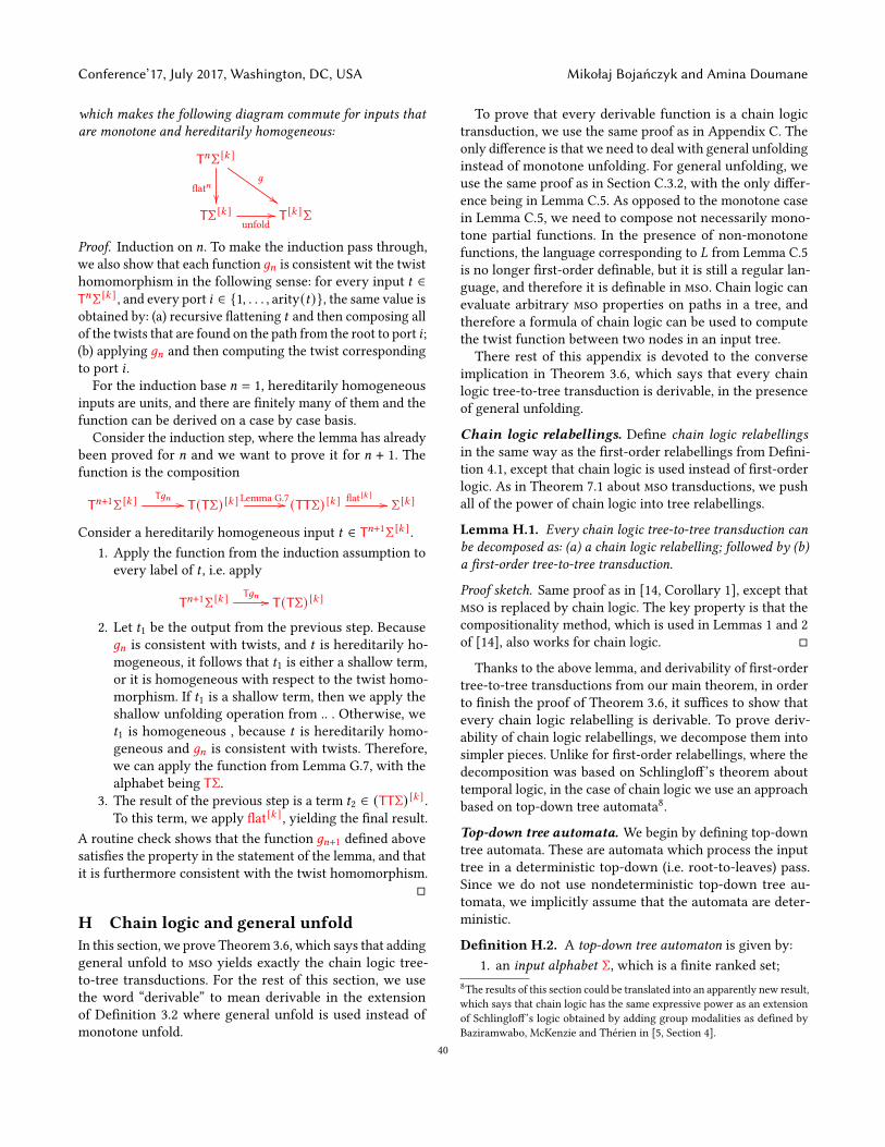
Conference’17, July 2017, Washington, DC, USA Mikołaj Bojańczyk and Amina Doumane
which makes the following diagram commute for inputs thatare monotone and hereditarily homogeneous:
T𝑛Σ [𝑘 ]
flat𝑛��
𝑔
$$TΣ [𝑘 ]
unfold// T[𝑘 ]Σ
Proof. Induction on 𝑛. To make the induction pass through,we also show that each function 𝑔𝑛 is consistent wit the twisthomomorphism in the following sense: for every input 𝑡 ∈T𝑛Σ [𝑘 ] , and every port 𝑖 ∈ {1, . . . , arity(𝑡)}, the same value isobtained by: (a) recursive flattening 𝑡 and then composing allof the twists that are found on the path from the root to port 𝑖;(b) applying 𝑔𝑛 and then computing the twist correspondingto port 𝑖 .For the induction base 𝑛 = 1, hereditarily homogeneous
inputs are units, and there are finitely many of them and thefunction can be derived on a case by case basis.
Consider the induction step, where the lemma has alreadybeen proved for 𝑛 and we want to prove it for 𝑛 + 1. Thefunction is the composition
T𝑛+1Σ [𝑘 ]T𝑔𝑛 // T(TΣ) [𝑘 ] Lemma G.7// (TTΣ) [𝑘 ] flat[𝑘 ] // Σ [𝑘 ]
Consider a hereditarily homogeneous input 𝑡 ∈ T𝑛+1Σ [𝑘 ] .1. Apply the function from the induction assumption to
every label of 𝑡 , i.e. apply
T𝑛+1Σ [𝑘 ]T𝑔𝑛 // T(TΣ) [𝑘 ]
2. Let 𝑡1 be the output from the previous step. Because𝑔𝑛 is consistent with twists, and 𝑡 is hereditarily ho-mogeneous, it follows that 𝑡1 is either a shallow term,or it is homogeneous with respect to the twist homo-morphism. If 𝑡1 is a shallow term, then we apply theshallow unfolding operation from .. . Otherwise, we𝑡1 is homogeneous , because 𝑡 is hereditarily homo-geneous and 𝑔𝑛 is consistent with twists. Therefore,we can apply the function from Lemma G.7, with thealphabet being TΣ.
3. The result of the previous step is a term 𝑡2 ∈ (TTΣ) [𝑘 ] .To this term, we apply flat[𝑘 ] , yielding the final result.
A routine check shows that the function 𝑔𝑛+1 defined abovesatisfies the property in the statement of the lemma, and thatit is furthermore consistent with the twist homomorphism.
□
H Chain logic and general unfoldIn this section, we prove Theorem 3.6, which says that addinggeneral unfold to mso yields exactly the chain logic tree-to-tree transductions. For the rest of this section, we usethe word “derivable” to mean derivable in the extensionof Definition 3.2 where general unfold is used instead ofmonotone unfold.
To prove that every derivable function is a chain logictransduction, we use the same proof as in Appendix C. Theonly difference is that we need to deal with general unfoldinginstead of monotone unfolding. For general unfolding, weuse the same proof as in Section C.3.2, with the only differ-ence being in Lemma C.5. As opposed to the monotone casein Lemma C.5, we need to compose not necessarily mono-tone partial functions. In the presence of non-monotonefunctions, the language corresponding to 𝐿 from Lemma C.5is no longer first-order definable, but it is still a regular lan-guage, and therefore it is definable in mso. Chain logic canevaluate arbitrary mso properties on paths in a tree, andtherefore a formula of chain logic can be used to computethe twist function between two nodes in an input tree.There rest of this appendix is devoted to the converse
implication in Theorem 3.6, which says that every chainlogic tree-to-tree transduction is derivable, in the presenceof general unfolding.
Chain logic relabellings. Define chain logic relabellingsin the same way as the first-order relabellings from Defini-tion 4.1, except that chain logic is used instead of first-orderlogic. As in Theorem 7.1 about mso transductions, we pushall of the power of chain logic into tree relabellings.
Lemma H.1. Every chain logic tree-to-tree transduction canbe decomposed as: (a) a chain logic relabelling; followed by (b)a first-order tree-to-tree transduction.
Proof sketch. Same proof as in [14, Corollary 1], except thatmso is replaced by chain logic. The key property is that thecompositionality method, which is used in Lemmas 1 and 2of [14], also works for chain logic. □
Thanks to the above lemma, and derivability of first-ordertree-to-tree transductions from our main theorem, in orderto finish the proof of Theorem 3.6, it suffices to show thatevery chain logic relabelling is derivable. To prove deriv-ability of chain logic relabellings, we decompose them intosimpler pieces. Unlike for first-order relabellings, where thedecomposition was based on Schlingloff’s theorem abouttemporal logic, in the case of chain logic we use an approachbased on top-down tree automata8.
Top-down tree automata. We begin by defining top-downtree automata. These are automata which process the inputtree in a deterministic top-down (i.e. root-to-leaves) pass.Since we do not use nondeterministic top-down tree au-tomata, we implicitly assume that the automata are deter-ministic.
Definition H.2. A top-down tree automaton is given by:1. an input alphabet Σ, which is a finite ranked set;
8The results of this section could be translated into an apparently new result,which says that chain logic has the same expressive power as an extensionof Schlingloff’s logic obtained by adding group modalities as defined byBaziramwabo, McKenzie and Thérien in [5, Section 4].
40

First-order tree-to-tree functions Conference’17, July 2017, Washington, DC, USA
2. a finite unranked set of states 𝑄 ;3. a designated initial state in 𝑄 ;4. for each input letter 𝑎 ∈ Σ, a transition function
𝛿𝑞 : 𝑄 → 𝑄arity of 𝑎 ;
5. an accepting set, which is a subset of
𝑄 × (input letters of arity zero).
For an input tree 𝑡 ∈ treesΣ, the run of the automatonis defined to be the labelling of the nodes by states, whichis defined as follows by induction on the distance from theroot. The state in the root is the initial state. Suppose that wehave already defined the state 𝑞 in a node 𝑥 of the input tree.Apply the transition function, corresponding to the label ofnode 𝑥 , to the state 𝑞, yielding a tuple of states 𝑞1, . . . , 𝑞𝑛 .These are the states of the run in the children of node 𝑥 .An input tree is accepted if for every leaf, the accepting setcontains the pair (state in the leaf, label of the leaf).
Definition H.3 (Tree relabellings associated to a top-downtree automaton). We associate two tree-to-tree functions toa top-down tree automaton A with input alphabet Σ. Eachof these is a special cases of a chain logic relabelling.• The ancestor relabelling, is denoted by
A↑ : treesΣ→ trees(𝑄 × Σ),where 𝑄×Σ is be the ranked set which consists of onecopy of the alphabet Σ for each state. The ancestorrelabelling simply extends the input tree with the runof the automaton. Note that the accepting set of theautomaton does not play a role in the definition of theancestors relabelling.• The descendant relabelling, denoted by
A↓ : treesΣ→ trees(Σ + Σ),is the characteristic function, in the sense of Section 5,of the query which selects nodes whose subtree is ac-cepted by A. In other words, for each node 𝑥 in theinput tree, its label is replaced by the correspondinglabel in the first copy of Σ if the subtree of 𝑥 is acceptedby A, and otherwise it is replaced by the correspond-ing label in the second copy of Σ.
The reason for notation in the above definition is that, inthe ancestor relabelling, the label of a node depends on itsancestors, while in the descendant relabelling, the label ofa node depends on its descendants. It is worth pointing outthat many different runs of the automaton are used in thedescendant relabelling, because for each node the automatonis started again with the initial state in that node.We begin with the following lemma, which states a con-
nection between chain logic and (nestings of) top-down treeautomata that was described in [8].
Lemma H.4. Every chain logic relabelling is a compositionof functions which are either:
(a) a letter-to-letter homomorphism; or(b) the descendant relabelling of a top-down tree automaton.
Proof. Adjusting for a slightly different terminology, thislemma is the same as [8, Theorem 2.5.9]. To help with the ter-minology, we note that the wordsum automata (WS) from [8]are the same as top-down tree automata here, while the cas-cade product of wordsum automata is the same as composingdescendant relabellings. □
Since letter-to-letter homomorphisms are derivable, in or-der to finish the proof of Theorem 3.6, it remains to prove thatevery function of kind (b) in the above lemma is derivable.We prove this by doing a further decomposition, which re-duces the descendant relabelling to the ancestor relabelling.
Lemma H.5. For every top-down tree automaton, its descen-dant relabelling is a composition of functions which are either:
(c) a first-order relabelling; or(d) the ancestor relabelling of a top-down tree automaton.
Proof. In this proof, we use the forward Ramseyan splits ofColcombet [14].Fix a top-down tree automaton A. For the proof of this
lemma, as well as for subsequent results, it will be convenientto use a different perspective on top-down tree automata,which uses automata on words. Recall the set of branchesBΣ that was defined in page 34: a branch is a letter togetherwith a distinguished port. Define the branch automaton ofA to be the deterministic word automaton, where the inputalphabet is BΣ, the states are the same, the initial state is thesame as in A, and the transition function is defined by
(
𝑄︷︸︸︷𝑞 ,
BΣ︷︸︸︷(𝑎, 𝑖) ) ↦→ 𝑖-th state in the tuple 𝛿𝑎 (𝑞).
The branch automaton does not have accepting states. Roughlyspeaking, the run of a top-down tree automaton correspondsto running the branch automaton on every root-to-leaf pathin the tree. This correspondence is spelled out in more detailbelow.
Consider two nodes in a tree, called the source and target,such that the source is an ancestor of the target. The sourcecan be equal to the target. The path between these two nodesis defined to be the set of edges in the tree which connectsthem. We can view the path as a word over the alphabet BΣ,as illustrated in the following picture:
tree with a pathfrom x to y
word corresponding to the path
x
y
41

Conference’17, July 2017, Washington, DC, USA Mikołaj Bojańczyk and Amina Doumane
The correspondence between the top-down tree automatonA and its branch automaton can now be phrased as follows:for a node 𝑥 , the state of the top-down tree automaton innode 𝑥 is the same as the state of the branch automaton afterreading the (word corresponding to the) path from the rootto node 𝑥 .Equipped with the above terminology, we complete the
proof of the lemma. For a path in an input tree, define itsstate transformation to be the function of type𝑄 → 𝑄 whichdescribes the state transformation of the branch automatonover the (word corresponding to the) path. By Colcombet’sresults on forward Ramseyan splits [14, Lemma 3], there isa top-down tree automaton B with input alphabet Σ and afamily of first-order formulas
{𝜑 𝑓 (𝑥,𝑦)}𝑓 :𝑄→𝑄
with the following property. For every input tree 𝑡 ∈ treesΣand nodes 𝑥 ≤ 𝑦 in that tree, the state transformation forthe path from 𝑥 to 𝑦 is equal to 𝑓 if and only if
B↑(𝑡) |= 𝜑 𝑓 (𝑥,𝑦).
The idea is that the top-down tree automatonB computes theforward Ramseyan split associated to state transformationsin the branch automaton of A. It follows that there is aformula 𝜑 (𝑥) of first-order logic such that for every 𝑡 ∈treesΣ,
B↑(𝑡) |= 𝜑 (𝑥)
holds if and only if the subtree of node 𝑥 is accepted by theautomatonA. The formula says that for all leaves 𝑦 ≤ 𝑥 , thecorresponding state transformation of the branch automatonleads to an accepting state. Therefore, the descendant rela-belling of A can be computed by first applying the ancestorrelabelling of B, and then a first-order relabelling. □
We now show that the ancestor relabellings produced bythe previous lemma can be further decomposed, so that theunderlying automata are reversible. Call a top-down tree au-tomaton reversible if the corresponding branch automaton,as defined in the proof of Lemma H.5, is reversible, whichmeans that for every input letter the corresponding transi-tion function is a permutation of the states.
Lemma H.6. For every top-down automaton, its ancestorfunction is a composition of functions which are either:
(c) a first-order relabelling; or(e) the ancestor relabelling of a reversible top-down automa-
ton.
Proof. A corollary of the original Krohn-Rhodes theorem.Define aMealy machine to be a string-to-string transducer,
which is obtained from a deterministic word automaton byadding an output function, which maps every transition toa letter of an output alphabet. The original Krohn-Rhodestheorem says that every Mealy machine is a composition of
Mealy machines where the underlying automaton is eitheraperiodic or reversible.
Take a top-down tree automaton. We can view its associ-ated branch automaton as a Mealy machine which decorateseach position in the input word by the state after reading theinput word up to and including that position. To this Mealymachine apply the Krohn-Rhodes theorem. The relabellingsfor the aperiodic Mealy machines can be computed by thefunctions of kind (c), while the relabellings for the reversibleones correspond to kind (e). □
Putting together Lemmas H.4, H.5 and H.6, we see thatevery chain logic relabelling is a composition of functionswhich have kinds (c) or (e) as in the statement of Lemma H.6.Since first-order relabellings are derivable, it remains to de-rive the functions of kind (e).
Lemma H.7. For every reversible top-down tree automaton,its ancestor relabelling is derivable (in the presence of generalunfolding).
Proof. Let the states of the automaton be 𝑄 = {𝑞1, . . . , 𝑞𝑘 }.We assume that 𝑞1 is the initial state. Consider an input letter𝑎, and its associated transition function as in item 4. Here isa picture of such a transition function, where the letter 𝑎 isbinary and the number of states is 𝑘 = 3.
q1
q2q1
q2
q2q1
q3
q3q3
In terms of the above picture, the reversibility of the automa-ton can be described as follows:
q1
q2q1
q2
q2q1
q3
q3q3
each state appearsexactly once as
a �rst child
each state appearsexactly once asa second child
We can represent the above transition function as an elementof the 𝑘-th matrix power of 𝑄 copies of the states, denotedby
𝑎 ∈ (𝑄 × Σ) [𝑘 ],
which is illustrated in the following picture:42
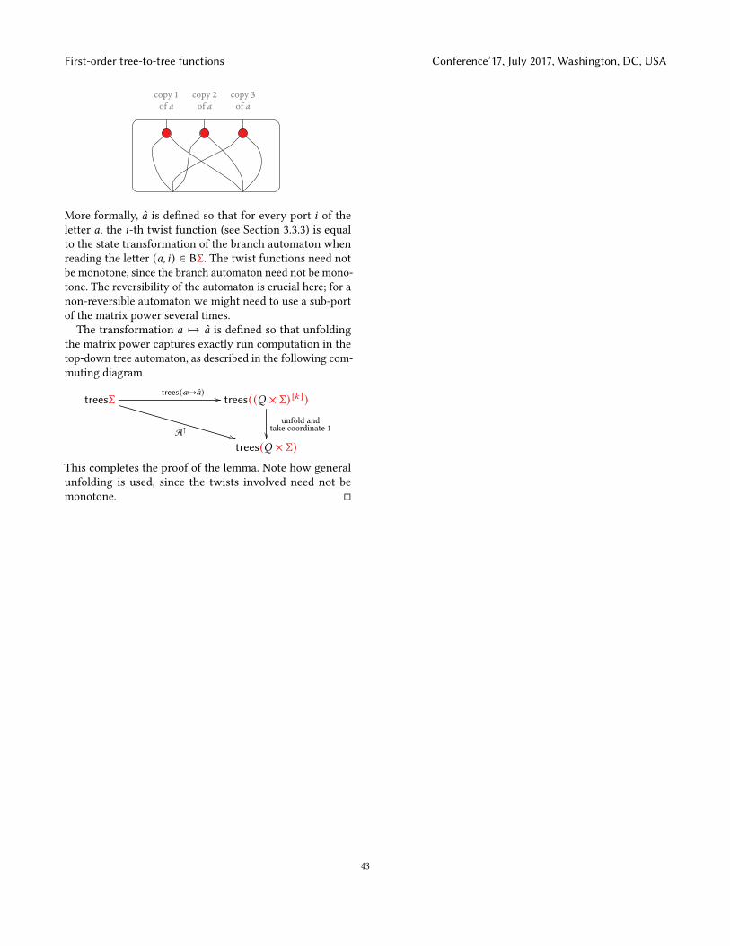
First-order tree-to-tree functions Conference’17, July 2017, Washington, DC, USA
copy 1of a
copy 2of a
copy 3of a
More formally, 𝑎 is defined so that for every port 𝑖 of theletter 𝑎, the 𝑖-th twist function (see Section 3.3.3) is equalto the state transformation of the branch automaton whenreading the letter (𝑎, 𝑖) ∈ BΣ. The twist functions need notbe monotone, since the branch automaton need not be mono-tone. The reversibility of the automaton is crucial here; for anon-reversible automaton we might need to use a sub-portof the matrix power several times.The transformation 𝑎 ↦→ 𝑎 is defined so that unfolding
the matrix power captures exactly run computation in thetop-down tree automaton, as described in the following com-muting diagram
treesΣtrees(𝑎 ↦→𝑎) //
A↑ **
trees((𝑄 × Σ) [𝑘 ])unfold and
take coordinate 1��
trees(𝑄 × Σ)This completes the proof of the lemma. Note how generalunfolding is used, since the twists involved need not bemonotone. □
43
Copyright © 2022 FDOKUMEN